On the dynamical properties of an elliptical–oval billiard with static boundary

Commun Nonlinear Sci Numer Simulat 15 (2010) 1092–1102

Contents lists available at ScienceDirect

Commun Nonlinear Sci Numer Simulat

journal homepage: www.elsevier .com/locate /cnsns

On the dynamical properties of an elliptical–oval billiard withstatic boundary

Diego F.M. Oliveira a,*, Edson D. Leonel b

a Departamento de Física, Instituto de Geociências e Ciências Exatas, Universidade Estadual Paulista, Av. 24A, 1515, Bela Vista, CEP: 13506-900, Rio Claro, SP, Brazilb Departamento de Estatística, Matemática Aplicada e Computação, Instituto de Geociências e Ciências Exatas, Universidade Estadual Paulista, Av. 24A, 1515,Bela Vista, CEP: 13506-900, Rio Claro, SP, Brazil

a r t i c l e i n f o a b s t r a c t

Article history:Received 7 May 2009Accepted 9 May 2009Available online 23 May 2009

Keywords:BilliardChaosLyapunov

1007-5704/$ - see front matter � 2009 Elsevier B.Vdoi:10.1016/j.cnsns.2009.05.044

* Corresponding author.E-mail addresses: [email protected] (D.F.M. Oliv

Some dynamical properties for a classical particle confined inside a closed region with anelliptical–oval-like shape are studied. The dynamics of the model is made by using a two-dimensional nonlinear mapping. The phase space of the system is of mixed kind and wehave found the condition that breaks the invariant spanning curves in the phase space.We have discussed also some statistical properties of the phase space and obtained thebehaviour of the positive Lyapunov exponent.

� 2009 Elsevier B.V. All rights reserved.

1. Introduction

The interest in understanding the dynamics of billiard problems becomes in earlies 1927 when Birkhoff [1] introduced asystem to describe the motion of a free particle inside a closed region with which the particle suffers elastic collisions. Ingeneral, a billiard is defined by a connected region Q � RD, with boundary @Q � RD�1 which separates Q from its complement.Inside the billiard, a point particle of mass m (commonly it is assumed to be the unity) moves freely along a straight line untilit encounters the boundary. After the collision, it is assumed that the particle is specularly reflected. It thus implies that theincidence angle must be equals to the reflection angle. It is well known that depending on the shape of the boundary as wellas on the combination of both control parameters and initial conditions, the dynamics of the particle might generate phasespaces of different kinds, including: (i) regular; (ii) ergodic; (iii) mixed. The integrability of the regular cases is generally re-lated to some kind of preservation in the dynamics, in particular the angular momentum. On the other hand, for the com-pletely ergodic billiards, only chaotic and therefore unstable periodic orbits are present in the dynamics. In order to illustratesystems that show such property, the so called Bunimovich stadium [2,3] and the Sinai billiard [4,5] consist of typical exam-ples. For these systems the time evolution of a single initial condition, for appropriated combinations of control parameters,is enough to fills up ergodically the entire phase space. Finally, there is a representative number of billiards that presentmixed phase space structure [6–12], which have control parameters with different physical significance.

Depending on the combination of both the initial conditions and control parameters, the phase space presents a very richstructure which could, in principle, contains invariant spanning curves (sometimes also called as invariant tori), Kolmogo-rov–Arnold–Moser (KAM) islands and chaotic seas. This mixed structure of the phase space is generic for non-degenerateHamiltonian systems [13] and might be observed in problems of one-dimensional time-dependent potentials [14–18], rip-pled channels [19,20] and many other different problems including tokamak [21–23].

. All rights reserved.

eira), [email protected] (E.D. Leonel).

mailto:[email protected]

mailto:[email protected]

http://www.sciencedirect.com/science/journal/10075704

http://www.elsevier.com/locate/cnsns

D.F.M. Oliveira, E.D. Leonel / Commun Nonlinear Sci Numer Simulat 15 (2010) 1092–1102 1093

In this paper, we propose a special geometry for the boundary of a classical billiard, which we call as elliptical–ovalboundary. Our main goal is to understand and describe some dynamical and moreover chaotic properties of such system.It is important to say that the shape of the boundary is controlled by three relevant control parameters. Varying such param-eters we can recover the results of the circular billiard and elliptical billiard, the oval billiard and finally we obtain totallynew results considering simultaneously variation of both control parameters, thus having an elliptical–oval billiard shape.

In the first part of this paper, we discuss all the details needed to construct the mapping that describes the dynamics ofthe model. The shape of the boundary is dependent on three control parameters and its expression in polar coordinates isgiven by Rðh; p; e; �Þ ¼ ð1� e2Þ=ð1þ e cosðhÞÞ þ � cosðphÞ, where p is an integer number, e and � are parameters that controlthe circle deformation. Inside the boundary, we consider that a classical particle of mass m is moving freely and in the totalabsence of any external field. When the particle hits the boundary it changes the direction according to a specular reflectionwithout suffering fractional loss of energy. The phase space is mixed, in the sense that, depending on both, the combinationof the control parameters and initial conditions, KAM islands usually surrounded by a chaotic sea, limited by a set of invari-ant spanning curves, can be observed. We have found a critical control parameter where no invariant spanning curves areobserved. This condition is related to the fact that the boundary may changes locally from positive curvature to negative cur-vature. After constructing the mapping, we explore some numerical results from it. For the case of e ¼ � ¼ 0, we recover theresults of the circular billiard where only regular dynamics is observed in the phase space. Considering the situation where� ¼ 0 and e – 0, then the results for the elliptical billiard are obtained. If we assume that e ¼ 0 and � – 0, we obtain the re-sults for the oval billiard. The last case is assuming that e – 0 and � – 0.

For the second part of the paper, we obtain and discuss some numerical results for the four possible cases, as discussedabove. We show that the positive Lyapunov exponent grows as the control parameters increase and it passes a regime ofmaximum then experiencing a small decay. We explain the increase in the Lyapunov exponent based on the behaviour ofthe histogram of frequency for chaotic orbits.

The paper is organized as follows: in Section 2 we give all the details needed for the construction of the nonlinear map-ping that describes the dynamics of the elliptical–oval billiard. Section 3 is devoted to discuss our numerical results anddynamical properties of the system as function of the control parameters. Finally, in Section 4 we drawn our conclusions.

2. The elliptical–oval billiard and the mapping

In this section we discuss all the details needed for the construction of a nonlinear map that describes the dynamics of theproblem. The model consists basically in consider the dynamics of a classical particle of mass m confined into a closed regionsuffering elastic and specular collisions with the border. When the particle hits the boundary it is reflected with the samevelocity. The radius of the boundary, in polar coordinates, is given by

Rðh;p; e; �Þ ¼ 1� e2

1þ e cosðhÞ

� �þ � cosðphÞ: ð1Þ

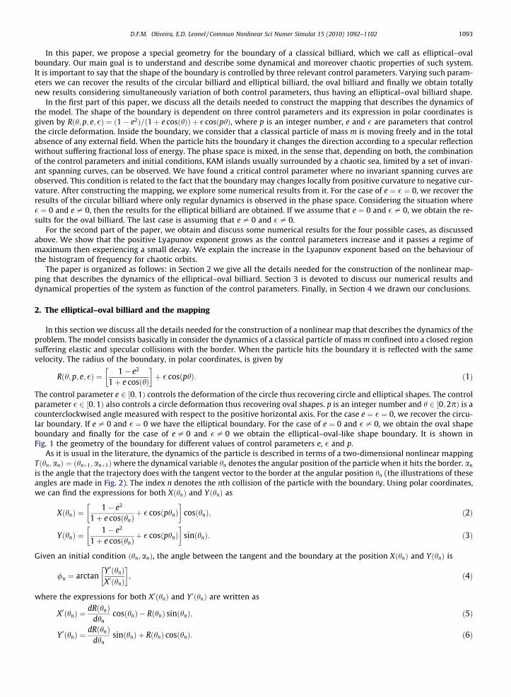
The control parameter e 2 ½0;1Þ controls the deformation of the circle thus recovering circle and elliptical shapes. The controlparameter � 2 ½0;1Þ also controls a circle deformation thus recovering oval shapes. p is an integer number and h 2 ½0;2pÞ is acounterclockwised angle measured with respect to the positive horizontal axis. For the case e ¼ � ¼ 0, we recover the circu-lar boundary. If e – 0 and � ¼ 0 we have the elliptical boundary. For the case of e ¼ 0 and � – 0, we obtain the oval shapeboundary and finally for the case of e – 0 and � – 0 we obtain the elliptical–oval-like shape boundary. It is shown inFig. 1 the geometry of the boundary for different values of control parameters e, � and p.

As it is usual in the literature, the dynamics of the particle is described in terms of a two-dimensional nonlinear mappingTðhn;anÞ ¼ ðhnþ1;anþ1Þwhere the dynamical variable hn denotes the angular position of the particle when it hits the border. an

is the angle that the trajectory does with the tangent vector to the border at the angular position hn (the illustrations of theseangles are made in Fig. 2). The index n denotes the nth collision of the particle with the boundary. Using polar coordinates,we can find the expressions for both XðhnÞ and YðhnÞ as

XðhnÞ ¼1� e2

1þ e cosðhnÞþ � cosðphnÞ

� �cosðhnÞ; ð2Þ

YðhnÞ ¼1� e2

1þ e cosðhnÞþ � cosðphnÞ

� �sinðhnÞ: ð3Þ

Given an initial condition ðhn;anÞ, the angle between the tangent and the boundary at the position XðhnÞ and YðhnÞ is

/n ¼ arctanY 0ðhnÞX0ðhnÞ

� �; ð4Þ

where the expressions for both X0ðhnÞ and Y 0ðhnÞ are written as

X0ðhnÞ ¼dRðhnÞ

dhncosðhnÞ � RðhnÞ sinðhnÞ; ð5Þ

Y 0ðhnÞ ¼dRðhnÞ

dhnsinðhnÞ þ RðhnÞ cosðhnÞ: ð6Þ

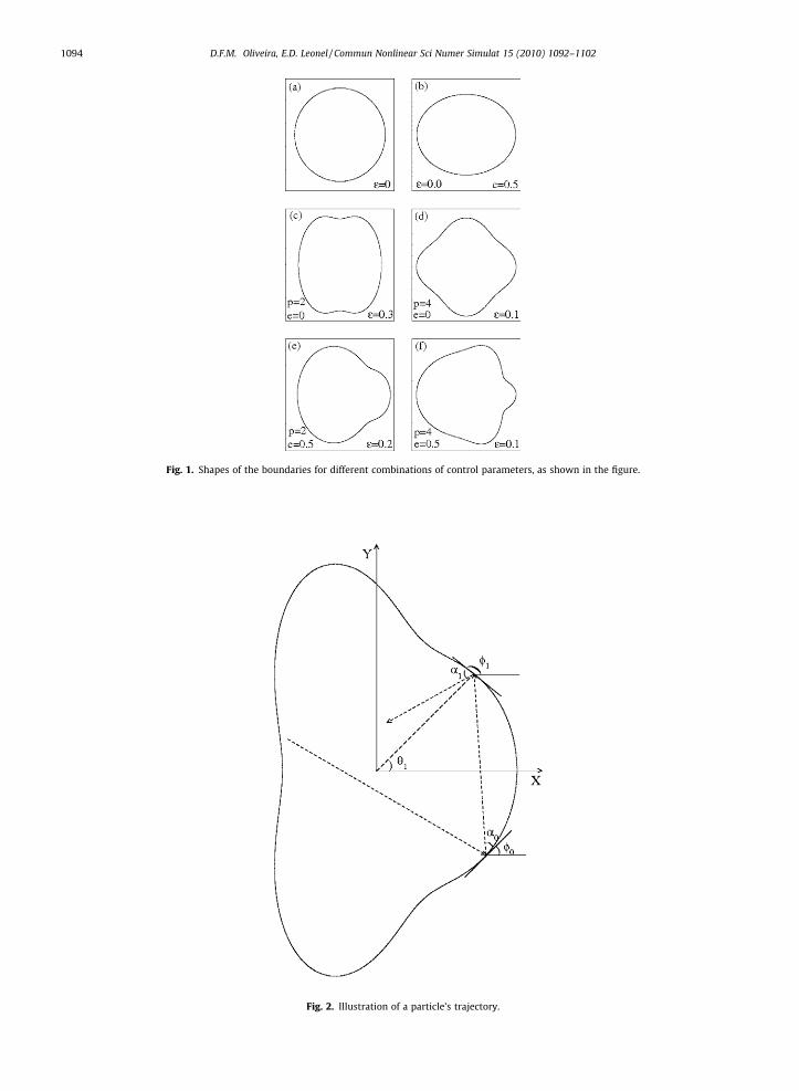
Fig. 1. Shapes of the boundaries for different combinations of control parameters, as shown in the figure.

Fig. 2. Illustration of a particle’s trajectory.

1094 D.F.M. Oliveira, E.D. Leonel / Commun Nonlinear Sci Numer Simulat 15 (2010) 1092–1102


The term dRðhnÞ=dhn is given by

Fig. 3.orbit.

dRðhnÞdhn

¼ ð1� e2Þe sinðhnÞ½1þ e cosðhnÞ�2

� �p sinðphnÞ: ð7Þ

We stress that the particle does not suffers influence of any external field upon collisions with the boundary. The particlethus travels with constant velocity along a straight line until reaches the boundary. To obtain the new angular positionfor the next hit of the particle with the border, we must solve the following equation

Yðhnþ1Þ � YðhnÞ ¼ tanðan þ /nÞ½Xðhnþ1Þ � XðhnÞ�; ð8Þ

where /n is obtained from the slope between the tangent vector and the positive horizontal axis. Xðhnþ1Þ and Yðhnþ1Þ are thenew positions of the particle at the angular position hnþ1, which is numerically obtained as solution of Eq. (8). The new anglethat the trajectory does with the tangent at hnþ1 is obtained from geometrical considerations, as can be seen in Fig. 2. It isgiven by

anþ1 ¼ /nþ1 � ðan þ /nÞ: ð9Þ

Fig. 2 illustrates geometrically all the details needed to obtain the new angle anþ1. Thus, we obtain that the map which de-scribes the dynamics of the model is given by

T :Fðhnþ1Þ ¼ Rðhnþ1Þ sinðhnþ1Þ � YðhnÞ � tanðan þ /nÞ½Rðhnþ1Þ cosðhnþ1Þ � XðhnÞ�;anþ1 ¼ /nþ1 � ðan þ /nÞ

�ð10Þ

where hnþ1 is numerically obtained as the solution of Fðhnþ1Þ ¼ 0, Rðhnþ1Þ ¼ ð1� e2Þ=ð1þ e cosðhnþ1ÞÞ þ � cosðphnþ1Þ and/nþ1 ¼ arctan½Y 0ðhnþ1Þ=X 0ðhnþ1Þ�.

3. Numerical results

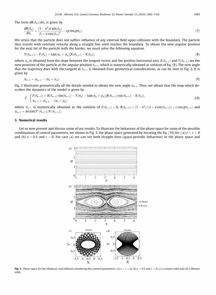
Let us now present and discuss some of our results. To illustrate the behaviour of the phase space for some of the possiblecombinations of control parameters, we shown in Fig. 3, the phase space generated by iterating the Eq. (10) for: (a) e ¼ � ¼ 0and (b) e ¼ 0:5 and � ¼ 0. For case (a) we can see both straight lines (quasi-periodic behaviour) in the phase space and

Phase space for the elliptical–oval billiard considering the control parameters: (a) e ¼ � ¼ 0, (b) e ¼ 0:5 and � ¼ 0, (c) a rotator orbit and (d) a librator


periodic orbits marked by a finite set of points in the phase portrait, as it is known from the circular billiard [6,24]. On theother hand, for (b) we can see a large double island limited by a separatrix curve and a set of invariant spanning curves, thusrecovering results of the elliptical phase space as it is well known in the literature [6,25]. In Fig. 3(b) we can observe twodifferent kinds of behaviour in the phase space separated by a separatrix, namely, rotators and librators. Librators consistof trajectories that are confined between the two focus and in the phase space are confined into the separatrix curve. Onthe other hand, rotators are trajectories near to the boundary exploring all the values of h. In the phase space they are outsideof the separatrix curve. Fig. 3(c, d) shows the behaviour of both, rotators and librators, respectively.

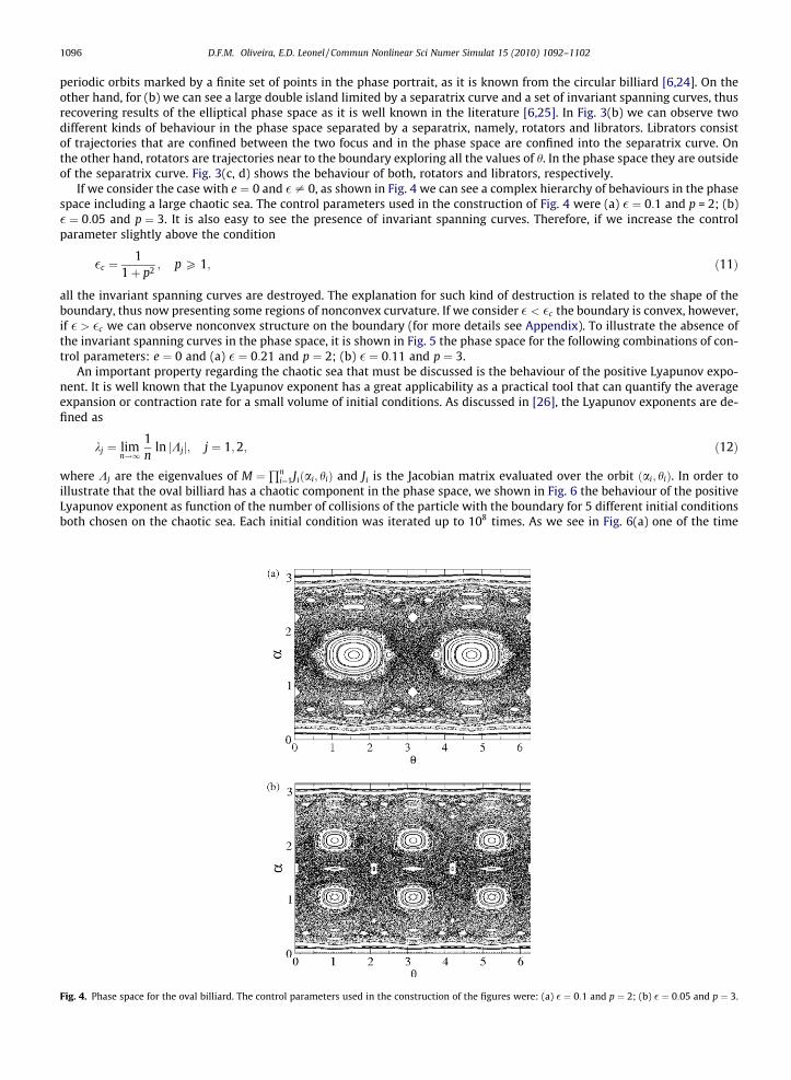
If we consider the case with e ¼ 0 and � – 0, as shown in Fig. 4 we can see a complex hierarchy of behaviours in the phasespace including a large chaotic sea. The control parameters used in the construction of Fig. 4 were (a) � ¼ 0:1 and p = 2; (b)� ¼ 0:05 and p ¼ 3. It is also easy to see the presence of invariant spanning curves. Therefore, if we increase the controlparameter slightly above the condition

Fig. 4.

�c ¼1

1þ p2 ; p P 1; ð11Þ

all the invariant spanning curves are destroyed. The explanation for such kind of destruction is related to the shape of theboundary, thus now presenting some regions of nonconvex curvature. If we consider � < �c the boundary is convex, however,if � > �c we can observe nonconvex structure on the boundary (for more details see Appendix). To illustrate the absence ofthe invariant spanning curves in the phase space, it is shown in Fig. 5 the phase space for the following combinations of con-trol parameters: e ¼ 0 and (a) � ¼ 0:21 and p ¼ 2; (b) � ¼ 0:11 and p ¼ 3.

An important property regarding the chaotic sea that must be discussed is the behaviour of the positive Lyapunov expo-nent. It is well known that the Lyapunov exponent has a great applicability as a practical tool that can quantify the averageexpansion or contraction rate for a small volume of initial conditions. As discussed in [26], the Lyapunov exponents are de-fined as

kj ¼ limn!1

1n

ln jKjj; j ¼ 1;2; ð12Þ

where Kj are the eigenvalues of M ¼Qn

i¼1Jiðai; hiÞ and Ji is the Jacobian matrix evaluated over the orbit ðai; hiÞ. In order toillustrate that the oval billiard has a chaotic component in the phase space, we shown in Fig. 6 the behaviour of the positiveLyapunov exponent as function of the number of collisions of the particle with the boundary for 5 different initial conditionsboth chosen on the chaotic sea. Each initial condition was iterated up to 108 times. As we see in Fig. 6(a) one of the time

Phase space for the oval billiard. The control parameters used in the construction of the figures were: (a) � ¼ 0:1 and p ¼ 2; (b) � ¼ 0:05 and p ¼ 3.

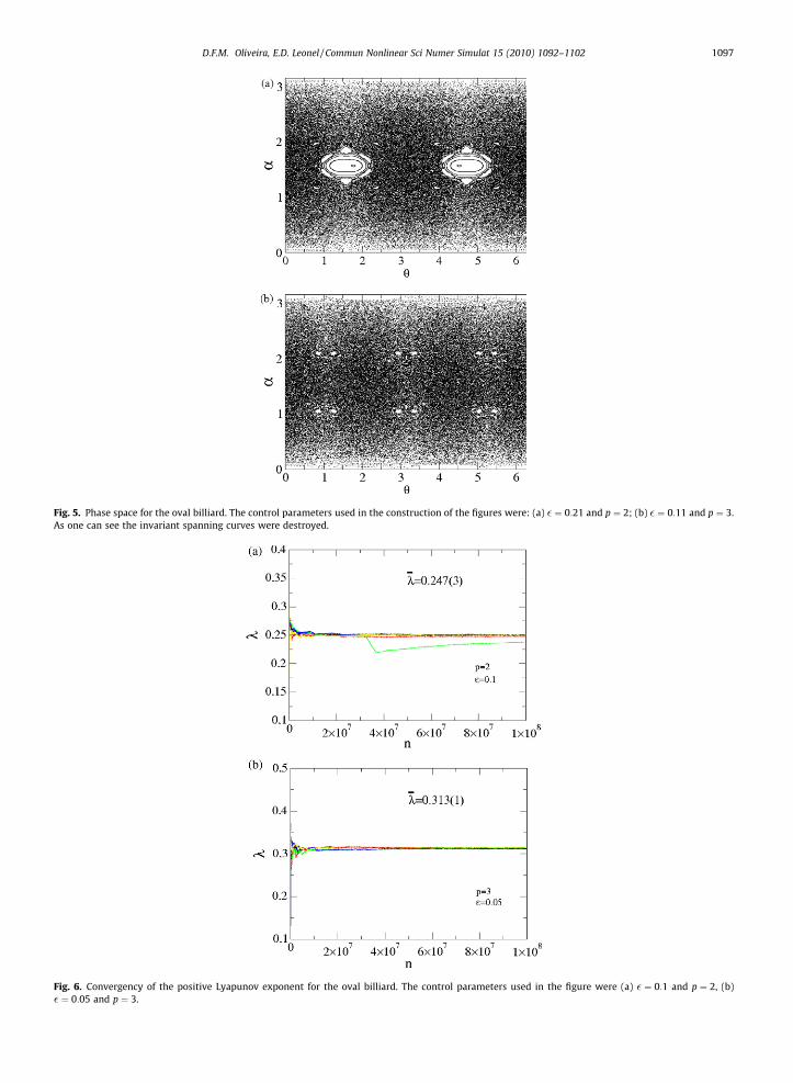
Fig. 5. Phase space for the oval billiard. The control parameters used in the construction of the figures were: (a) � ¼ 0:21 and p ¼ 2; (b) � ¼ 0:11 and p ¼ 3.As one can see the invariant spanning curves were destroyed.

Fig. 6. Convergency of the positive Lyapunov exponent for the oval billiard. The control parameters used in the figure were (a) � ¼ 0:1 and p ¼ 2, (b)� ¼ 0:05 and p ¼ 3.



series suffers a small decay for approximately 4:5� 106 collisions with the boundary. After that, the positive Lyapunov expo-nent tends towards a regime of convergency marked by a constant plateau. The short decay is due to the fact that the particlehas been confined into a sticky region by around 4:5� 106 iterations. The control parameters used in the construction ofFig. 6(a) were � ¼ 0:1 and p ¼ 2 and (b) � ¼ 0:05 and p ¼ 3. The average of the positive Lyapunov exponent for the ensembleof 5 samples furnishes (a) �k ¼ 0:247� 0:003 and (b) �k ¼ 0:313� 0:001. The values �0:003 and �0:001 correspond to thestandard deviation of the 5 samples.

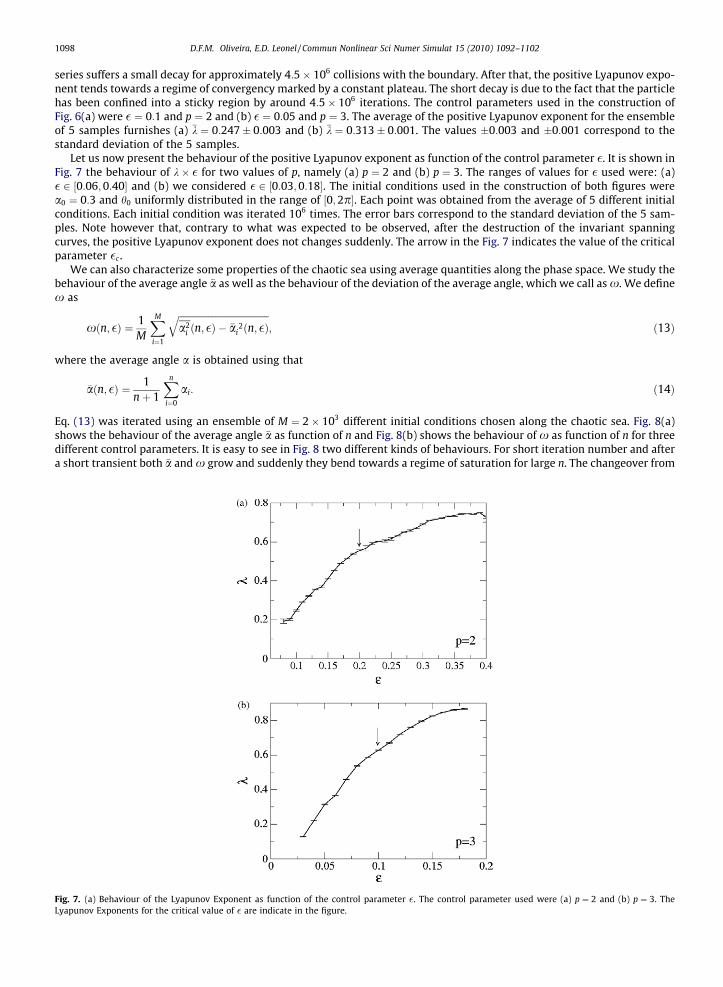
Let us now present the behaviour of the positive Lyapunov exponent as function of the control parameter �. It is shown inFig. 7 the behaviour of k� � for two values of p, namely (a) p ¼ 2 and (b) p ¼ 3. The ranges of values for � used were: (a)� 2 ½0:06;0:40� and (b) we considered � 2 ½0:03;0:18�. The initial conditions used in the construction of both figures werea0 ¼ 0:3 and h0 uniformly distributed in the range of ½0;2p�. Each point was obtained from the average of 5 different initialconditions. Each initial condition was iterated 106 times. The error bars correspond to the standard deviation of the 5 sam-ples. Note however that, contrary to what was expected to be observed, after the destruction of the invariant spanningcurves, the positive Lyapunov exponent does not changes suddenly. The arrow in the Fig. 7 indicates the value of the criticalparameter �c .

We can also characterize some properties of the chaotic sea using average quantities along the phase space. We study thebehaviour of the average angle �a as well as the behaviour of the deviation of the average angle, which we call as x. We definex as

Fig. 7.Lyapun

xðn; �Þ ¼ 1M

XM

i¼1

ffiffiffiffiffiffiffiffiffiffiffiffiffiffiffiffiffiffiffiffiffiffiffiffiffiffiffiffiffiffiffiffiffiffiffiffiffiffiffia2

i ðn; �Þ � �ai2ðn; �Þ

q; ð13Þ

where the average angle a is obtained using that

�aðn; �Þ ¼ 1nþ 1

Xn

i¼0

ai: ð14Þ

Eq. (13) was iterated using an ensemble of M ¼ 2� 103 different initial conditions chosen along the chaotic sea. Fig. 8(a)shows the behaviour of the average angle �a as function of n and Fig. 8(b) shows the behaviour of x as function of n for threedifferent control parameters. It is easy to see in Fig. 8 two different kinds of behaviours. For short iteration number and aftera short transient both �a and x grow and suddenly they bend towards a regime of saturation for large n. The changeover from

(a) Behaviour of the Lyapunov Exponent as function of the control parameter �. The control parameter used were (a) p ¼ 2 and (b) p ¼ 3. Theov Exponents for the critical value of � are indicate in the figure.

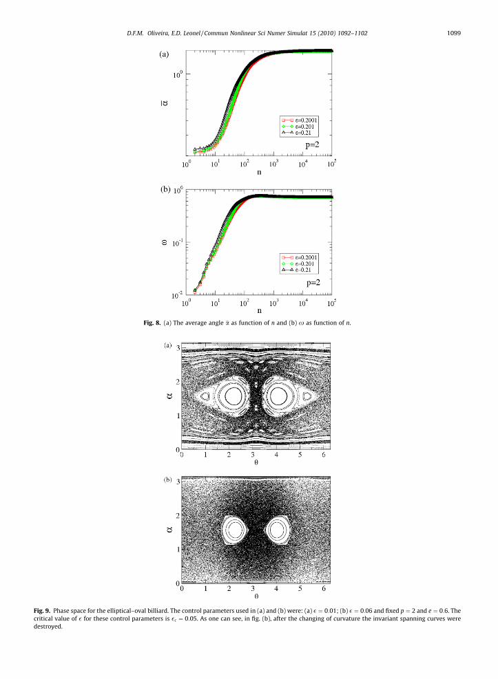
Fig. 8. (a) The average angle �a as function of n and (b) x as function of n.

Fig. 9. Phase space for the elliptical–oval billiard. The control parameters used in (a) and (b) were: (a) � ¼ 0:01; (b) � ¼ 0:06 and fixed p ¼ 2 and e ¼ 0:6. Thecritical value of � for these control parameters is �c ¼ 0:05. As one can see, in fig. (b), after the changing of curvature the invariant spanning curves weredestroyed.



growth to the saturation is marked by a crossover iteration number nx. When n� nx the deviation of the average anglegrows according to the power law

Fig. 10after th

xðn; �Þ / nb: ð15Þ

After doing some extensive simulation for the range of � 2 ½0:2001;0:21� we obtain that b ¼ 1:23� 0:02. As n increases,n� nx, x approaches a regime of saturation. However for the range of control parameters we have considered, the plateausdo not seem to depend on the control parameters. Such a property is related to the limited region of the phase space, i.e.a 2 ½0;p� as well as to the symmetry existing in the regions a 2 ½0;p=2� and a 2 ½p=2;p�.

Let us now consider the elliptical–oval case. We assume that both e – 0 and � – 0. It is shown in Fig. 9(a) the phase spacefor different values of � and considering fixed the values of e and p, as shown in the figure. We can see that the phase spaceshows a rich structure of behaviour exhibiting KAM islands surrounded by a chaotic sea and a set of invariant spanningcurves. The invariant spanning curves will be destroyed for the case of nonconvex curves. The condition that destroys theinvariant spanning curves is given by

�c ¼1� e

ð1þ eÞð1þ p2Þ ; p > 1: ð16Þ

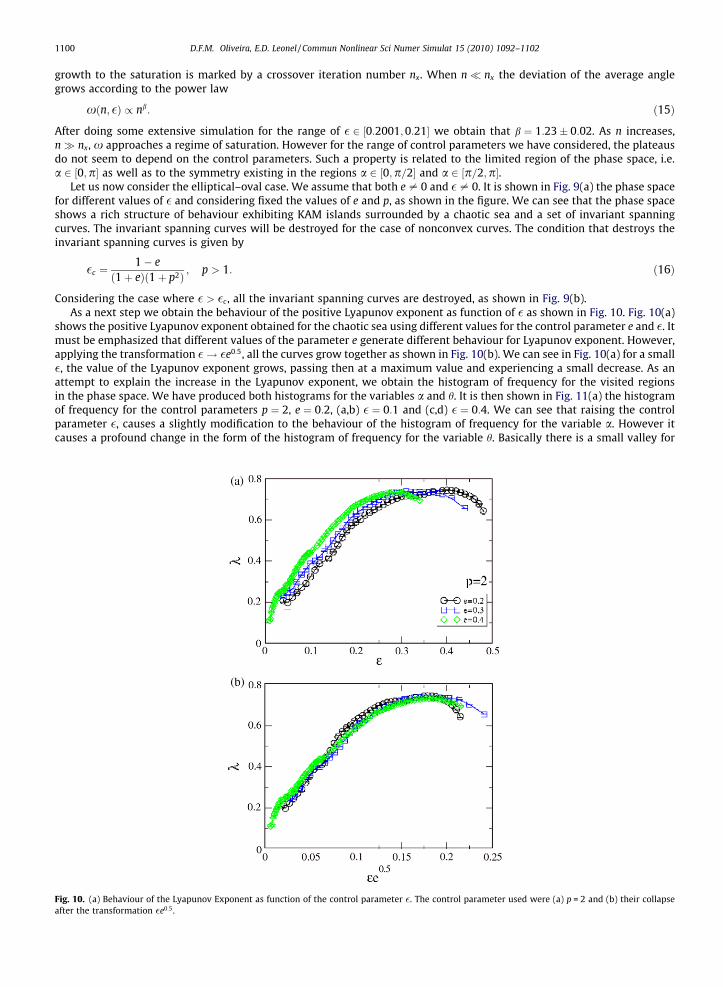
Considering the case where � > �c , all the invariant spanning curves are destroyed, as shown in Fig. 9(b).As a next step we obtain the behaviour of the positive Lyapunov exponent as function of � as shown in Fig. 10. Fig. 10(a)

shows the positive Lyapunov exponent obtained for the chaotic sea using different values for the control parameter e and �. Itmust be emphasized that different values of the parameter e generate different behaviour for Lyapunov exponent. However,applying the transformation �! �e0:5, all the curves grow together as shown in Fig. 10(b). We can see in Fig. 10(a) for a small�, the value of the Lyapunov exponent grows, passing then at a maximum value and experiencing a small decrease. As anattempt to explain the increase in the Lyapunov exponent, we obtain the histogram of frequency for the visited regionsin the phase space. We have produced both histograms for the variables a and h. It is then shown in Fig. 11(a) the histogramof frequency for the control parameters p ¼ 2, e ¼ 0:2, (a,b) � ¼ 0:1 and (c,d) � ¼ 0:4. We can see that raising the controlparameter �, causes a slightly modification to the behaviour of the histogram of frequency for the variable a. However itcauses a profound change in the form of the histogram of frequency for the variable h. Basically there is a small valley for

. (a) Behaviour of the Lyapunov Exponent as function of the control parameter �. The control parameter used were (a) p = 2 and (b) their collapsee transformation �e0:5.

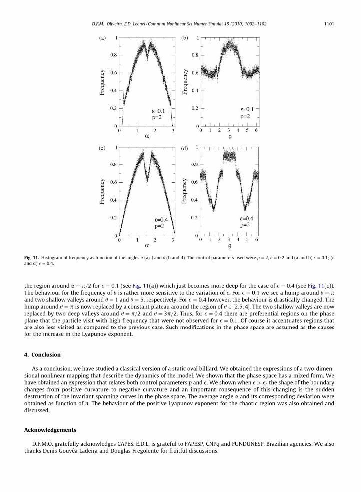
Fig. 11. Histogram of frequency as function of the angles a (a,c) and h (b and d). The control parameters used were p ¼ 2, e ¼ 0:2 and (a and b) � ¼ 0:1; (cand d) � ¼ 0:4.


the region around a ¼ p=2 for � ¼ 0:1 (see Fig. 11(a)) which just becomes more deep for the case of � ¼ 0:4 (see Fig. 11(c)).The behaviour for the frequency of h is rather more sensitive to the variation of �. For � ¼ 0:1 we see a hump around h ¼ pand two shallow valleys around h ¼ 1 and h ¼ 5, respectively. For � ¼ 0:4 however, the behaviour is drastically changed. Thehump around h ¼ p is now replaced by a constant plateau around the region of h 2 ½2:5;4�. The two shallow valleys are nowreplaced by two deep valleys around h ¼ p=2 and h ¼ 3p=2. Thus, for � ¼ 0:4 there are preferential regions on the phaseplane that the particle visit with high frequency that were not observed for � ¼ 0:1. Of course it accentuates regions thatare also less visited as compared to the previous case. Such modifications in the phase space are assumed as the causesfor the increase in the Lyapunov exponent.

4. Conclusion

As a conclusion, we have studied a classical version of a static oval billiard. We obtained the expressions of a two-dimen-sional nonlinear mapping that describe the dynamics of the model. We shown that the phase space has a mixed form. Wehave obtained an expression that relates both control parameters p and �. We shown when � > �c the shape of the boundarychanges from positive curvature to negative curvature and an important consequence of this changing is the suddendestruction of the invariant spanning curves in the phase space. The average angle a and its corresponding deviation wereobtained as function of n. The behaviour of the positive Lyapunov exponent for the chaotic region was also obtained anddiscussed.

Acknowledgements

D.F.M.O. gratefully acknowledges CAPES. E.D.L. is grateful to FAPESP, CNPq and FUNDUNESP, Brazilian agencies. We alsothanks Denis Gouvêa Ladeira and Douglas Fregolente for fruitful discussions.


Appendix

In this Appendix, we present the procedure to obtain the expression of the critical control parameter �c . When we in-crease the control parameter �, the shape of the boundary changes (see Fig. 1). We can obtain the expression for the criticalvalue �c , where the curvature of the boundary changes from positive ðj > 0Þ to negative ðj < 0Þ. Using polar coordinates theexpression for jðhÞ is given by

jðhÞ ¼ X 0ðhÞY 00ðhÞ � X00ðhÞY 0ðhÞ½X02ðhÞ þ Y 02ðhÞ�

32

: ð17Þ

For the general case, the expressions for X 0ðhÞ, Y 0ðhÞ, X00ðhÞ and Y 00ðhÞ are

X0ðhÞ ¼ dRðhÞdh

cosðhÞ � RðhÞ sinðhÞ;

Y 0ðhÞ ¼ dRðhÞdh

sinðhÞ þ RðhÞ cosðhÞ;

X00ðhÞ ¼ d2RðhÞdh2 cosðhÞ � 2

dRðhÞdh

sinðhÞ � RðhÞ cosðhÞ;

Y 00ðhÞ ¼ d2RðhÞdh2 sinðhÞ þ 2

dRðhÞdh

cosðhÞ � RðhÞ sinðhÞ; ð18Þ

where dRðhÞdh and d2RðhÞ

dh2 are given by

dRðhÞdh

¼ ð1� e2Þe sinðhÞ½1þ e cosðhÞ�2

� �p sinðphÞ;

d2RðhÞdh2 ¼ 2ð1� e2Þe2 sin2ðhÞ

½1þ e cosðhÞ�3þ ð1� e2Þe cosðhÞ½1þ e cosðhÞ�2

� �p2 cosðphÞ: ð19Þ

We obtain �c by considering the case where j0 ¼ 0. The expression for �c as function of e and p is

�c ¼1� e

ð1þ eÞð1þ p2Þ ; p > 1: ð20Þ

Thus, when � < �c the boundary is strictly convex, however, if � > �c we can observe nonconvex pieces on the boundary. Forthe case of e ¼ 0 we recover the expression for �c obtained for the oval billiard.

References

[1] Birkhoff GD. Dynamical Systems Amer. Math. Soc. Colloquium Publ. 9. Providence: American Mathematical Society; 1927.[2] Bunimovich LA. On ergodic properties of certain billiards. Funct Anal Appl 1974;8:254–5.[3] Bunimovich LA. On the ergodic properties of nowhere dispersing billiards. Commun Math Phys 1979;65:295–312.[4] Sinai YG. Dynamical systems with elastic reflections. Russ Math Surv 1970;25:137–89.[5] Sinai YG. Ergodic properties of dispersive billiards. Russ Math Surv 1970;25:141–92.[6] Berry MV. Regularity and chaos in classical mechanics, illustrated by three deformations of a circular billiard. Eur J Phys 1981;2:91–102.[7] Kamphorst SO, de Carvalho SP. Bounded gain of energy on the breathing circle billiard. Nonlinearity 1999;12:1363–71.[8] Robnik M. Classical dynamics of a family of billiards with analytic boundaries. J Phys A Math Gen 1983;16:3971–86.[9] Robnik M, Berry MV. Classical billiards in magnetic fields. J Phys A Math Gen 1985;18:1361–78.

[10] Markarian R, Kamphorst SO, de Carvalho SP. Chaotic properties of the elliptical stadium. Commun Math Phys 1996;174:661–79.[11] Lopac V, Mrkonjic I, Radic D. Chaotic dynamics and orbit stability in the parabolic oval billiard. Phys Rev E 2001;66:036202 (5pp).[12] Lopac V, Mrkonjic I, Pavin N, Radic D. Chaotic dynamics of the elliptical stadium billiard in the full parameter space. Phys D 2006;217:88–101.[13] Ozorio de Almeida AM. Hamiltonian systems: chaos and quantization. Cambridge: Cambridge University Press; 1988.[14] Leonel ED, McClintock PVE, Scaling properties for a classical particle in a time-dependent potential well. Chaos 2005;15:033701–7.[15] Mateos JL. Traversal-time distribution for a classical time-modulated barrier. Phys Lett A 1999;256:113–21.[16] Luna-Acosta GA, Orellana-Rivadeneyra G, Mendoza-Galván A, Jung C. Chaotic classical scattering and dynamics in oscillating 1-D potential wells. Chaos

Solitons Fractals 2001;12:349–63.[17] Leonel ED, McClintock PVE. Chaotic properties of a time-modulated barrier. Phys Rev E 2004;70:016214 (11pp).[18] Leonel ED, McClintock PVE. Dynamical properties of a particle in a time-dependent double-well potential. J Phys A Math Gen 2004;37:8949–68.[19] Luna-Acosta GA, Mendez-Bermudéz JA, Seba P, Pichugin KN. Classical versus quantum structure of the scattering probability matrix: chaotic

waveguides. Phys Rev E 2002;65:046605 (8pp).[20] Luna-Acosta GA, Krokhin AA, Rodriguez MA, Hernandez-Tejeda PH. Classical chaos and ballistic transport in a mesoscopic channel. Phys Rev B

1996;54:11410–6.[21] Ullmann K, Caldas IL. Symplectic mapping for the ergodic magnetic limiter and its dynamical analysis. Chaos Solitons Fractals 2000;11:2129–40.[22] Portela JSE, Viana RL, Caldas IL. Periodic orbits and global chaos in a symplectic mapping describing magnetic field line structure in tokamaks. Phys A

2003;317:411–31.[23] Da Silva EC, Caldas IL, Viana RL. Ergodic magnetic limiter for the TCABR. Braz J Phys 2002;32:39–45.[24] Toporowicza LA, Beims MW. Correlation effects of two interacting particles in a circular billiard. Phys A 2006;37:5–9.[25] Koiller J, Markarian R, Carvalho SP, Kamphorst SO. Static and time dependent perturbations of the classical elliptical stadium. J Stat Phys

1996;83:127–43.[26] Eckmann JP, Ruelle D. Ergodic theory of chaos and strange attractors. Rev Mod Phys 1985;57:617–56.

Documents

On the dynamical properties of an elliptical–oval billiard with static boundary