on the surface chemistry of some rhombohedral carbonate minerals in aqueous solutions

ON THE SURFACE CHEMISTRY OF SOME RHOMBOHEDRAL CARBONATE MINERALS

IN AQUEOUS SOLUTIONS

Adrián Villegas-Jiménez

Department of Earth & Planetary Sciences

McGill University, Montréal

October 2009

A thesis submitted to McGill University in partial fulfillment

of the requirements of the degree of Doctor of Philosophy

Adrián Villegas-Jiménez, 2009

ii

iii

ABSTRACT

Fundamental aspects of the surface chemistry of calcite, dolomite, magnesite, and

gaspeite in aqueous solutions were examined using different lines of investigation

including experimental, theoretical, and/or computer-assisted modeling approaches (i.e.,

ab initio molecular and surface complexation modeling).

A Genetic Algorithm (GA) was implemented and tested for the calibration of

surface complexation models (SCMs). The GA can successfully optimize numerous

adjustable SCM parameters without incurring convergence problems while minimizing

numerical instability problems, a notable advantage over conventional deterministic, root-

finding, and optimization techniques implemented in codes such as FITEQL. It was

routinely used throughout this thesis for the simultaneous calibration of surface

complexation parameters (e.g., intrinsic constants, capacitances) at carbonate surfaces.

The definition of reactive surface sites at hydrated rhombohedral carbonate

mineral surfaces was critically revisited. Using calcite as the model mineral, a single

generic charge-neutral surface site scheme was proposed for the formulation of surface

equilibria. The resulting molecular representation of surface equilibria is consistent with

experimental and theoretical findings and is compatible with assumptions implicit in

SCMs. Based upon the one-site scheme, new and simplified SCMs for magnesite and

dolomite were formulated. These successfully reproduced published surface charge and

electrokinetic data while yielding surface speciation predictions consistent with available

spectroscopic data.

The acid-base behavior of the gaspeite (NiCO3(s)) surface in NaCl solutions was

investigated for the first time by means of conventional titration techniques and micro-

iv

electrophoresis. Surface protonation and the electrophoretic mobility of gaspeite are

strongly affected by the background electrolyte. Acid-base surface complexation

reactions, formulated according to the one-site scheme, closely reproduced proton

adsorption data and reasonably simulated the electrokinetic behavior of gaspeite

suspensions at I ≤ 0.01 M.

The ground-state structural, energetic properties, and bonding relationships of the

hydrated (10.4) calcite surface were investigated using Roothaan-Hartree-Fock molecular

orbital methods and slab cluster models. A detailed 3D description of the hydrated calcite

surface, including the 1st and 2

nd hydration layers, was derived for the first time at the ab

initio level. Most noteworthy is the distortion of the Ca-O octahedra via the relaxation

and possible rupture of some Ca-O bonds upon hydration, leading to the weakening of the

outermost atomic calcite layer.

Finally, the quantitative characterization of the proton sorptive properties of

calcite in aqueous solutions by a novel surface titration protocol provides evidence for the

following ion-exchange equilibrium between the solution and labile exchangeable cation

sites (“exc”):

(CaCO3)2(exc) + 2 H+

Ca(HCO3)2(exc) + Ca2+

This proposed ion-exchange mechanism has far reaching implications as it directly

impacts the aqueous speciation of closed and partially open (poor CO2 ventilation)

carbonate-rock systems via the buffering of pH and calcite dissolution and CO2(g)

sequestration upon calcite precipitation.

v

RÉSUMÉ

Des aspects fondamentaux sur la chimie surfacique des minéraux carbonatés dans

des solutions aqueuses ont été examinés par des approches expérimentales et théoriques

ainsi que par des méthodes d‟optimisation numérique et de modélisation moléculaire.

Un algorithme génétique (GA, selon son sigle anglais) a été implémenté et testé

pour la calibration de modèles de complexation à la surface (SCMs, selon son sigle

anglais). Le GA peut optimiser de façon stochastique et simultanée des nombreux

paramètres tout en minimisant des problèmes de convergence ou de stabilité numérique.

Cet algorithme est très avantageux par rapport aux techniques déterministiques

conventionnelles adoptées par des codes d‟optimisation de constantes d‟équilibre tel que

FITEQL. Le GA a donc été utilisé de façon routinière dans cette étude, pour estimer les

constantes de formation des espèces chimiques se formant à la surface des minéraux

carbonatés.

En utilisant la calcite comme modèle, nous avons réévalué de façon critique la

définition de sites réactifs à la surface hydratée des minéraux carbonatés rhomboédriques.

Ceci nous a permis de définir un site d‟adsorption générique neutre pour ce type de

minéraux, qui est compatible avec les résultats d‟études théoriques et expérimentales ainsi

qu‟avec des hypothèses associées à la formulation de SCMs. Des nouvelles réactions,

basées sur un seul site générique, ont été formulées pour la magnésite et dolomite et

calibrées en utilisant des données publiées de charge surfacique et, par la suite, testées

avec des données électrocinétiques et spectroscopiques disponibles dans la littérature.

Le comportement acide-base à la surface de la gaspéite (NiCO3(s)), dans des

solutions de NaCl, à été examiné par des techniques conventionnelles de titrage

vi

surfacique et par la micro-électrophorèse. Nous avons trouvé que l‟électrolyte de support

influence, de façon substantielle, la protonation surfacique ainsi que la mobilité

électrocinétique de la gaspéite. Des réactions acide-base ont été formulées en fonction du

site d‟adsorption générique postulé dans cette étude. Celles-ci reproduisent bien les

données d‟adsorption de protons et simulent raisonnablement le comportement

électrocinétique aux forces ioniques ≤ 0.01 M.

Nous avons étudié les propriétés structurales et énergétiques à l‟état fondamental

de la surface (10.4) hydratée de la calcite ainsi que les types de liaisons établies entre les

molécules d‟eau et les atomes à la surface du minéral. À cette fin, nous avons appliqué

des méthodes basées sur la théorie quantique de l‟orbital moléculaire (Roothaan-Hartree-

Fock) en combinaison avec des modèles structuraux tridimensionnels (finis) de la calcite.

Nous proposons, par la première fois au niveau ab initio, un modèle structural détaillé de

la surface (10.4) hydratée de la calcite comprenant la première et la deuxième couche

d‟hydratation. Particulièrement remarquable est la distorsion significative des octaèdres

surfaciques de Ca-O suite à la relaxation (et possiblement rupture) de quelques liaisons

Ca-O. Ceci amène à l„affaiblissement de la couche atomique surfacique de la calcite.

Finalement, nous avons caractérisé de façon quantitative, les propriétés

d‟adsorption de protons par la calcite dans des solutions aqueuses en utilisant une

nouvelle technique de titrage surfacique développée dans la présente étude. Nous

proposons une réaction d‟échange d‟ions entre la solution et des sites cationiques

réactifs de caractère échangeable (“exc”):



vii

Ce mécanisme a des nombreuses répercussions significatives car il affecte la

spéciation en phase aqueuse des systèmes carbonatés qui sont isolés ou partiellement

isolés (faible ventilation de CO2(g)) de l‟atmosphère, via le tamponnage du pH et de la

dissolution de la calcite et par la séquestration du CO2(g) induite par la précipitation de la

calcite.

viii

ix

TABLE OF CONTENTS

Abstract iii

Résumé v

Acknowledgements xvii

Contribution of Authors xxii

Chapter 1: Introduction 1

REFERENCES 10

Preface to Chapter 2 14

Chapter 2: Estimating Intrinsic Formation Constants of Mineral Surface Species using a Genetic Algorithm 15

ABSTRACT 16

1. INTRODUCTION 18 2. IMPLEMENTATION OF THE GENETIC ALGORITHM 21

3. APPLICATION OF THE GA TO THE FORWARD PROBLEM 25

4. APPLICATION OF THE GA TO THE INVERSE PROBLEM 27

4.1 Estimation of Intrinsic Ionization Constants:

Constant Capacitance Model 27

4.2 Simultaneous Estimation of Intrinsic Ionization Constants

and Adsorption Constants: Constant Capacitance Model 33

4.3 Simultaneous Estimation of Intrinsic Ionization Constants and Adsorption Constants: Triple Layer Model 38

5. CONCLUSIONS 43

x

6. ACKNOWLEDGMENTS 44

7. REFERENCES 45

8. TABLES 51

Table 1 51

Table 2 52

9. FIGURES 53

Figure 1 53

Figure 2 54

Figure 3 55

Figure 4 56

Figure 5 57

Figure 6 58

Figure 7 59


Chapter 3: Defining Reactive Sites on Hydrated Mineral Surfaces: Rhombohedral Carbonate Minerals 61

ABSTRACT 62

1. INTRODUCTION 64

2. DEFINITION OF PRIMARY SURFACE SITES 67

2.1 Charge Assignment 67

2.2 Elemental Stoichiometry 71

3. RHOMBOHEDRAL CARBONATE MINERALS 72

3.1 Case of the (10.4) Calcite Surface 72

3.1.1 Evidence from Spectroscopic and Molecular Modeling Studies 72

3.1.2 Single Generic Primary Surface Site 75

xi

3.2 SCM Reactions: One-Site vs Two-Site Scheme 77

3.3 Mixed-Metal Carbonate Minerals 79

4. EVALUATION OF THE ONE-SITE SCHEME 81

4.1 Re-calibration of Surface Reactions for Magnesite and Dolomite 81

4.2 Intrinsic Formation Constants and Surface Speciation 91

4.3 Comparison against Spectroscopic Information 93

5. CONCLUSIONS 96 6. ACKNOWLEDGMENTS 98

7. REFERENCES 99

8. TABLES 112

Table 1 112

Table 2 113

Table 3 114

Table 4 116

9. FIGURES 118

Figure 1 118

Figure 2 119

Figure 3 120

Figure 4 121

Figure 5 122

Figure 6 123


Chapter 4: Acid-Base Behavior of the Gaspeite (NiCO3(s)) Surface in NaCl Solutions 125

ABSTRACT 126

1. INTRODUCTION 127

2. MATERIALS AND METHODS 130

xii

2.1 Preparation and Standardization of Reagents 130

2.2 Chemical Analysis 130

2.3 Gaspeite Synthesis 131

2.4 Surface Titrations 132

2.4.1. pH Electrode Calibration 132

2.4.2. Conditions of Surface Titrations 134

2.5 Computation of Proton Adsorption 136

2.6 Coagulation Experiments 138

2.7 Electrokinetic measurements 139

3. RESULTS AND DISCUSSION 141

3.1 Proton Adsorption on the Gaspeite Surface 141

3.1.1 Acidimetric Titrations 141

3.1.2 Verification of Potential Artifacts 145

3.1.3 Surface Complexation Modeling of Acidimetric Data: One-Site CCM approach 147 3.1.4 Surface Complexation Modeling of Acidimetric Data: One-Site, Multi-Site, BSM, and TLM approaches 153

3.1.5 Alkalimetric Titrations 154

3.2 Electrokinetics 157

4. CONCLUSIONS 160 5. ACKNOWLEDGMENTS 161

6. REFERENCES 162

7. TABLES 166

Table 1 166

Table 2 167

8. FIGURES 168

Figure 1 168

Figure 2 169

Figure 3 171

Figure 4 172

xiii

Figure 5 174

Figure 6 175

Figure 7 176

Figure 8 177

Figure 9 178


Chapter 5: Theoretical Insights into the Hydrated (10.4) Calcite Surface: Structure, Energetics and Bonding Relationships 181

ABSTRACT 182

1. INTRODUCTION 184 2 METHODS 187

2.1 Computational Methods and Cluster Models 187 3 RESULTS 191

3.1 Structural Details of the Hydrated Clusters 191

3.2 Energies of Adsorption 196

3.3 H2O Interlayer Penetration 198

4 DISCUSSION 200

4.1 Reliability of RHF/6-31G(d,p) Results 200

4.2 Three-D Structural Registry 201

4.3 Bonding Relationships: Geometric and Energetic Criteria 206

5 CONCLUSIONS 214 6 ACKNOWLEDGMENTS 216 7 REFERENCES 217 8 TABLES 227

Table 1 227

Table 2 228

xiv

Table 3 229

9. FIGURES 230

Figure 1 230

Figure 2 231

Figure 3 232

Figure 4 233

Figure 5 234

Figure 6 236

Figure 7 237


Chapter 6: Proton/Calcium Ion Exchange Behavior of Calcite 239

ABSTRACT 240

1. INTRODUCTION 242

2. MATERIALS AND METHODS 246

2.1 Principle of Calcite Titrations 246

2.2 Description of Reaction Vessel 247

2.3 Surface Titration Conditions 248

2.4 Computation of Sorption Data 250

3. RESULTS AND DISCUSSION 253

3.1 Qualitative Interpretation of Data 253

3.2 Possible Mechanisms of “Proton Uptake/Calcium Release” and “Apparent” Incongruent Calcite Dissolution 260

3.3 Sorption Modeling 264

3.4 Ion-Exchange vs Surface Equilibria 273

3.5 Implications of Proton/Calcium Ion Exchange 275

4. CONCLUSIONS 279

xv

5. ACKNOWLEDGMENTS 281

6. REFERENCES 282

7. TABLES 291

Table 1 291

Table 2 292

Table 3 293

8. FIGURES 294

Figure 1 294

Figure 2 295

Figure 3 296

Figure 4 297

Figure 5 299

Figure 6 300

Figure 7 301

Figure 8 303

Chapter 7: General Conclusions 305

CONTRIBUTIONS TO KNOWLEDGE 305

RECOMMENDATIONS FOR FUTURE RESEARCH 310

REFERENCES 314

Appendices: 340

I. Chapter 1: Gedanken Experiment Data 341

II. Chapter 4: Gaspeite: Acidimetric Titration Data 342

III. Chapter 4: Gaspeite: Alkalimetric Data 345

IV. Chapter 4: Gaspeite: Electrokinetic Data 346

V. Chapter 5: Optimized Small Calcite Cluster 348

VI. Chapter 5: Optimized Large Calcite Cluster 350

VII. Chapter 5: Geometrically-Optimized (CaCO3)9/4H2O cluster 354

VIII. Chapter 6: CaCO3(s) Solubility Product Data 355

IX. Chapter 6: CaCO3(s) Acidimetric Titration Data 356

xvi

X. Chapter 6: CaCO3(s) Calcium Titration Data 358

XI. Chapter 6: Methods and Calculations 359

XII. Chapter 6: Referencing of data to the ZNSRC 365

XIII. Chapter 6: Equilibrium Speciation Calculations involving Ion Exchange 367

XIV. Chapter 6: Tableau-based Formulation: CaCO3(s)-KCl-H2O System 369

XV. Chapters 2, 3, 4, and 6: Matlab© Subroutines 370

xvii

ACKNOWLEDGMENTS

I would like to express my gratitude to my Ph.D. thesis supervisor, Professor Alfonso

Mucci, for giving me the freedom to thoroughly propose, design, and conduct my

doctoral research while according me full intellectual independence to elaborate and test

my scientific hypotheses and formulate my own conclusions. His comments and

constructive criticisms as well as his guidance in anglicizing my prose have undoubtedly

added substantial value to my thesis and are sincerely acknowledged. The participation of

Professor Jeanne Paquette in commenting on crystallographic and editorial aspects of my

thesis and her guidance during my early training on carbonate crystallography is greatly

appreciated.

I acknowledge the hospitality of Dr Oleg S. Pokrovsky and Dr Jacques Schott

during my 6-month visit to their lab (LMTG-CNRS) in Toulouse, France in 2003. Their

scientific contributions to my doctoral work were critical and their financial contribution

during my stay in France is appreciated. I also recognize the invaluable technical

assistance offered by the extremely competent laboratory staff at LMTG and most

particularly by Madame Carole Causserand.

I sincerely thank Emeritus Professor Michael A. Whitehead who granted me

access to his computer facilities and provided guidance over the course of the molecular

modeling work I conducted in his laboratory. I also appreciate the two-month stipend he

provided me with in 2006.

Special recognition goes to Professor Theo van de Ven, Professor David Burns,

and Dr Luuk Koopal for critical and inspiring discussions at early stages of my Ph.D.

residency, which led to significant improvements of my research work. I would also like

xviii

to express my sincere appreciation to Dr Johannes Lützenkirchen for critically reviewing

my thesis and making important remarks on my work.

Thanks also to Dr Nora de Leeuw, Dr Paul Fenter, Dr Kate Wright, Dr Brian L.

Phillips, and Dr Michel J. Rossi who kindly provided additional information on their

published work.

Many thanks to all the staff in the Department of Earth and Planetary Sciences

who kindly offered assistance of various kinds at different stages of my research work. I

am particularly grateful to Brigitte Dionne for her guidance in computer-related issues as

well as to Glenna Keating, Sandra Lalli, and Constance Guignard for technical assistance

in laboratory analyses as well as to Carol Matthews, Kristy Thornton, and Anne

Kosowski for advice and help regarding administrative and academic issues. Critical

advice on laboratory analyses provided by Professor Tariq Ahmedali is truly appreciated.

I am sincerely grateful to Professor Hojatollah Vali for allocating me suitable

office space for nearly two years following the temporary closure of our office/laboratory

facilities in 2005. Special thanks go to Professor Theo van de Ven from the Chemistry

Department who temporarily guaranteed my supply of Milli-Q® water when it was

compromised.

I am also indebted to numerous scientists and professors who, from my early B.Sc.

years in Ensenada (Mexico) to present, have provided me with guidance, encouragement,

or simply with pure scientific inspiration. It is impossible to do justice and accord proper

recognition to all those responsible for triggering my scientific motivations and/or

participating in my training as a science professional. Particularly, wise supervision and

solid guidance from Professor André Tessier and Dr José Vinicio Macías-Zamora during

my M.Sc. and B.Sc. studies, respectively, paved a smooth way towards my Ph.D. studies.

http://www.eps.mcgill.ca/index.php?id=0&url=./People/faculty/index.php&faculty=vali

xix

My Ph.D. research was supported financially by a Graduate Student Research

Grant to A. Villegas-Jiménez from the Geological Society of America (GSA), by Natural

Sciences and Engineering Research Council of Canada (NSERC) Discovery grants to A.

Mucci, J. Paquette, and M. A. Whitehead, and by grants from the Centre National de la

Recherche Scientifique (CNRS) to J. Schott. In addition, the following institutions are

deeply acknowledged for kindly awarding me financial support either through fellowships

or by offering “on-campus” work during my Ph.D. residency at McGill:

Consejo Nacional de Ciencia y Tecnología of Mexico (CONACyT):

Excellence doctoral scholarships awarded from 2001 to 2004 (inclusive).

The GEOTOP-UQAM-McGill Research Center: Summer doctoral bursary

(2002).

McGill University: Overseas Alma Mater Student Travel Grants to attend

“The Goldschmidt Conference” held in Davos (2002) and Copenhagen (2004).

The Organizing Committees of the 2004 and 2008 “Goldschmidt Conference”

for providing partial financial support to attend their meetings held in

Copenhagen and Vancouver, respectively.

The National Science Foundation (NSF) for fully supporting my attendance to

the Water-Rock Interactions Symposium held in Saratoga in 2004.

The Department of Earth and Planetary Sciences at McGill University for

providing me with Teaching Assistantships over several years (2001-2005).

The Faculties of Science and Engineering at McGill University for offering me

invigilation work during several examination periods (2002, 2005, and 2006).

In addition, the summer research assistantships (2001-2004) and partial financial

support (2005-2006) offered by my thesis supervisor are sincerely appreciated.

The financial support I received from my parents and my two brothers, Armando

and Omar, from 2006 to 2008 was critical to bring this thesis to a successful end.

xx

This thesis is dedicated to my family, but most particularly to my dearest parents,

Rosa Elvia Jiménez-Rodríguez and Armando Villegas-Bobadilla to whom I am deeply

grateful for their unconditional support, rock-solid encouragement, and sincere

understanding during this rather challenging time of my life. Little doubt remains… they

are the best.

A special dedication goes also to all those fine scientists who, through sound

intuition, solid evidence, vigorous thinking, and pragmatic interpretations, attach

authority to scientific knowledge and do justice to what is known as: “La Force de la

Science”.

Adriano

xxi

Impose ta chance, serre ton bonheur,

et va vers ton risque. À te regarder, ils s’habitueront

René Char (1950)

xxii

CONTRIBUTION OF AUTHORS

This thesis is the outgrowth of the author‟s Ph.D. research work in the Department of

Earth and Planetary Sciences at McGill University under the supervision of Professor

Alfonso Mucci and co-supervision of Professor Jeanne Paquette. The thesis consists of

seven chapters, five of which are scientific research manuscripts whereas the remaining

two are the general introduction and conclusions. Chapter 2 was accepted for publication

by the scientific journal Mathematical Geology and currently awaits publication, Chapter

3 was published in the scientific journal Geochimica et Cosmochimica Acta, Chapter 4

will be submitted to the scientific journal Langmuir, Chapter 5 was published in the

scientific journal Langmuir. Finally, Chapter 6 was published in the scientific journal

Physical Chemistry Chemical Physics. In conformity with the format of the published

articles, all relevant supplementary material associated with each Chapter (e.g., raw data,

computer subroutines, detailed explanations, etc.) can be found in the appendices to this

thesis. With exception of Chapter 4, specifically the gaspeite titration experiment, which

was originally proposed to the author by Dr Oleg S. Pokrovsky and Dr Jacques Schott,

researchers of LMTG, UMR 5563, Université Paul-Sabatier - CNRS in Toulouse, France;

the research presented in this thesis was fully proposed by the author and initiated after

discussions with the author‟s thesis supervisor, Professor Alfonso Mucci and co-

supervisor, Professor Jeanne Paquette.

Theoretical, experimental, analytical, ab initio molecular modeling, Matlab©

computer coding, computer-assisted numerical optimization work, data acquisition as

well as interpretation, speciation calculations, and experimental protocols were entirely

designed and/or carried out by the author. Consequently, the author is responsible for the

content of the thesis and is the lead author of the five associated manuscripts. Professor

xxiii

Alfonso Mucci commented on data evaluation and interpretation, and critically reviewed

the scientific contents and style of all the material presented in this thesis, and therefore,

he co-authors the five associated manuscripts. Professor Jeanne Paquette is the fifth co-

author of Chapter 4 and third of Chapter 6. She commented on the scientific contents and

style of these manuscripts and provided references that helped improve their quality.

Dr Oleg S. Pokrovsky is the third co-author of Chapters 3 and 4. His contributions

to this work include guidance during my laboratory studies conducted at LMTG, UMR

5563, Université Paul-Sabatier - CNRS in France. He also provided constructive

comments, criticisms, and suggestions on the interpretation of experimental data and

modeling results as well as critically reviewed the scientific content and style of the two

associated manuscripts. In addition, he provided novel (unpublished) electrokinetic data

for NiCO3(s) (electrophoretic measurements, series-II) used in Chapter 4 to further

validate the Surface Complexation Model postulated for this mineral. Dr Jacques Schott

is the fourth co-author of Chapters 3 and 4. He provided constructive comments,

criticisms, and suggestions on the interpretation of experimental data and modeling

results as well as critically reviewed the scientific content and style of these two

manuscripts.

Finally, Emeritus Professor Michael Anthony Whitehead is the third co-author of

Chapter 5. He provided guidance on the molecular modeling work I conducted in his

laboratory in the Department of Chemistry at McGill University. He also provided

constructive comments and suggestions on the interpretation of the molecular modeling

results and critically reviewed the scientific content and style of Chapter 5.

1

CHAPTER 1

INTRODUCTION

Under Earth surface conditions, carbonate minerals are among the most chemically

reactive and ubiquitous minerals in the environment. They are found as suspended

particles in aquatic systems (Morse and Mackenzie, 1990) and the atmosphere (Usher et

al., 2003) and as part of the sediment and rock record (Morse et al., 2007). Calcite

(CaCO3(s)) and dolomite (CaMg(CO3)2(s)) are by far the most abundant carbonate

minerals, comprising nearly 20% by volume of Phanerozoic sedimentary rocks. In

modern sediments, aragonite and high-magnesian calcites dominate in shallow water

environments whereas low magnesium calcite (> 99% CaCO3(s)) composes almost all

deep sea carbonate-rich sediments (Morse et al., 2007). These minerals largely impact the

chemistry of aquatic systems by regulating pH and alkalinity through

dissolution/precipitation equilibria, govern the mobility and cycling of hazardous metal

contaminants and radionuclides via ion exchange, adsorption, and co-precipitation

reactions, as well as participate in the long-term biogeochemical cycling of major

elements (Van Cappellen et al., 1993). For instance, CaCO3(s) minerals represent an

important component of the inorganic carbon budget in the ocean where the balance

between continental weathering and biogenic precipitation of calcium carbonates

influence the global carbon cycle (Sarmiento and Sundquist, 1992). CaCO3(s) polymorphs

are also the building blocks of shells and skeletons of various marine invertebrates

(Morse et al., 2007) whereas, in the Earth‟s atmosphere, they constitute a reactive

component of mineral aerosols that regulate the CO2 exchange and influence the

2

chemistry of volatile inorganic and organic acids (Usher et al., 2003; Al-Hosney and

Grassian, 2005). CaCO3(s) polymorphs also have numerous industrial applications that

range from fillers for paints, plastics, rubbers, pharmaceuticals, cosmetics, optical

devices, and paper to raw material in the construction industry, agriculture, as well as in

the production of biomedical scaffolds (e.g., Vanerek et al., 2000 and Tas, 2007).

Given their environmental significance and broad industrial applications,

carbonate minerals have been the subject of extensive research in numerous experimental

and theoretical investigations. It is now well recognized that fundamental reactions at the

carbonate/water interface such as hydration, ion sorption, and development of surface

charge, play a critical role on macroscopic processes such as carbonate mineral

dissolution and growth kinetics, crystal morphology, pathways of carbonate diagenesis,

and particle coagulation (Brady et al., 1996). This realization has stimulated interest about

the surface reactivity of carbonate minerals in aqueous solutions. Accordingly, over the

last few decades, considerable efforts have focused on the experimental characterization

of the ion sorptive properties of carbonate minerals and the derivation of empirical and

semi-empirical relationships to quantitatively interpret ion partitioning between the

aqueous phase and the surface of calcite, aragonite, Mg-bearing carbonates and, to a

lesser extent, other divalent carbonate minerals (Morse and Mackenzie, 1990).

The greater reactivities (i.e., faster reaction rates and larger solubilities) of

carbonates relative to other minerals such as metal oxides, silicates, and clays and the

occurrence of stepwise and/or parallel reactions (e.g., adsorption, surface precipitation,

co-precipitation, dissolution) have made it difficult to experimentally resolve adsorption

processes (Morse, 1986). Furthermore, the interpretation of adsorption data is often

problematic as they may reflect the product of several overlapping reactions. In fact, these

3

data have most commonly been interpreted as a fast initial adsorption and subsequent

slow lattice incorporation (precipitation) of the adsorbate (e.g., Franklin and Morse, 1983;

Davis et al, 1987; Pingitore et al, 1988; Zachara et al, 1991; Tesoriero and Pankow,

1996). These two steps were further decomposed into: 1) diffusion into a hydrated

surface layer (Davis et al., 1987); 2) dehydration and formation of MeCO3 bonds on the

surface (Franklin and Morse, 1983); 3) nucleation (McBride, 1979), and the ultimate

precipitation of a solid solution layer (Lorens, 1981; Davis et al, 1987) or of a pure phase

(McBride, 1979). In addition, it has been suggested that solid-state ion diffusion may

affect the rate and extent of trace metal sorption by calcite (Stipp et al., 1992).

These findings reflect the complexity of ion sorption processes on carbonate

mineral surfaces and explains why carbonate experimentalists must conduct their

adsorption studies within relatively narrow ranges of chemical conditions (e.g., pH,

sorbate/adsorbant ratio) or employ surface-sensitive techniques (e.g., X-ray, electron

diffraction, spectroscopy, chromatography, thermogravimetry, atomic force microscopy)

to characterize the surface structure and obtain quantitative insights on the reactivity of

carbonate mineral surfaces. Nevertheless, despite these efforts, critical aspects on the

surface reactivity of carbonate minerals in aqueous solutions are still not fully understood.

For instance, the nature of the surface reactions that control the (ad)sorption behavior of

potential-determining ions such as H+, OH

-, Ca

2+, CO3

2-, and/or HCO3

- remain

controversial and subject of scientific debate. Consequently, factors that determine the pH

of isoelectric point (pHIEP) of calcite remain ambiguous (e.g., Prédali and Cases, 1973;

Foxall et al., 1979; Cicerone et al., 1992; Moulin and Roques, 2003).

It follows that the design and implementation of experimental approaches for the

rigorous evaluation of adsorption equilibria over expanded ranges of chemical conditions

4

is required. Conventional titration techniques, used in the characterization of the surface

properties of less reactive minerals such as metal oxides or clays (Huang, 1981), are not

suitable for the characterization of highly reactive carbonate minerals that rapidly

respond, via dissolution/precipitation reactions, to minute variations in the solution

chemistry. These considerations drove earlier workers to develop a novel experimental

protocol, based on the use of a fast flow-through reactor, to minimize the contribution of

dissolution and precipitation during acid-base titrations performed on two sparingly

soluble carbonates: siderite and rhodochrosite (Charlet et al., 1990). This protocol was

later used by several researchers to obtain surface charge data for siderite, rhodochrosite

(Van Cappellen et al., 1993), magnesite (Pokrovsky et al., 1999a), and dolomite

(Pokrovsky et al., 1999b; Brady et al., 1999) from which they formulated surface

complexation models (SCMs) for these minerals. Unfortunately, the application of this

approach to highly reactive carbonate minerals such as calcite or aragonite is not feasible

because their fast dissolution kinetics interferes significantly with the computation of

surface charge. Consequently, available SCMs for calcite (Van Cappellen et al., 1993)

were calibrated either to the “generally accepted” (yet ambiguous, given the strong

solution composition-dependency of this parameter) pH of isoelectric point of calcite

recorded under specific solution conditions (pHIEP = 8.2, Mishra, 1978) or against

selected electrokinetic data available in the literature (Wolthers et al., 2008).

Nevertheless, the latter authors concluded that a straightforward validation of the

postulated SCMs was not possible because of the uncertainties associated with the nature

and magnitude of potential artifacts inherent in the electrokinetic data obtained in calcite

suspensions.

5

Despite the success of these SCMs in reproducing the surface charge of FeCO3(s),

MnCO3(s), MgCO3(s), and CaMg(CO3)2(s) (Van Cappellen et al., 1993; Pokrovsky et al.,

1999a,b) and reasonably predicting the electrokinetic behavior of MgCO3(s) and

CaMg(CO3)2(s) (Pokrovsky et al., 1999a,b) in aqueous solutions, the postulated models are

not robust and represent first-order descriptions of the surface chemistry of carbonate

minerals that are amenable to refinement from a theoretical and experimental standpoint.

For instance, in all these studies, the formation constants of surface species were adjusted

simultaneously on a trial and error basis (by arbitrarily varying the values of the

formation constants) until the predicted surface speciation closely reproduced surface

charge data. Hence, the contribution of individual surface reactions (i.e., acid-base and

lattice-derived, constituent, ion adsorption) could not be resolved nor could the formation

constants of surface species be estimated accurately.

Another critical issue is the definition of the reactive sites whereupon surface

reactions are formalized. Based upon spectroscopic evidence (Stipp and Hochella, 1991;

Pokrovsky et al., 1999a; 1999b), two types of vicinal surface hydration sites were

hypothesized to form at the (10.4) surface of rhombohedral carbonate minerals (MeOH0

and CO3H0) and these were assumed to display a distinct reactivity that remained

unaffected by the presence of reacted neighbouring surface species. This scheme yields

complex SCMs defined by at least six (for single-metal carbonate minerals) or twelve (for

mixed-metal carbonate minerals) surface reactions that spawn questionable predictions of

surface speciation which, in turn, may not reflect realistic processes at the

carbonate/water interface. Clearly, to improve our understanding of carbonate surface

reactivity in aqueous solutions we need to: (i) generate representative experimental

6

adsorption data covering wide compositional ranges, (ii) revisit and refine our

quantitative interpretations of old and new data using chemically-sound and

mathematically-tractable ion partitioning models, (iii) test the validity of these models

against additional experimental data acquired by alternate investigative approaches and/or

under conditions beyond the calibration range, (iv) critically evaluate the adequacy of

available experimental and theoretical information to elucidate surface processes at the

carbonate/water interface and, (v) select suitable ion partitioning models for this type of

minerals that reflect an acceptable compromise between the quality of the experimental

data available for model calibration, the compatibility of such model with

physical/chemical constraints, the accuracy of the model predictions, and their

applicability to real-world systems. Some of these issues are addressed in this thesis.

The objectives of this thesis are: (i) to derive a realistic description of the

ionization and lattice ion surface species at the carbonate-water interface by critically

revisiting the definition of primary surface sites (“adsorption centres”) whereupon

mass-action expressions describing adsorption equilibria at hydrated (10.4)

rhombohedral carbonate mineral surfaces are formalized; (ii) to use this description

for the reformulation and calibration of SCMs for magnesite and dolomite, evaluate

their predictive power against published electrokinetic and spectroscopic data for

these two minerals, and compare their results against those of previous SCMs; (iii) to

use gaspeite (NiCO3(s)) as a surrogate carbonate mineral to investigate the acid-base

behavior of rhombohedral carbonate minerals by application of conventional titration

and electrokinetic techniques and interpret proton adsorption data within the

framework of surface complexation theory; (iv) to investigate the structure and

energetics of the 1st and 2

nd hydration layers at the cleavage (10.4) calcite surface

7

using ab initio Roothan-Hartree-Fock molecular orbital techniques and analyze the

bonding relationships between adsorbing water molecules and surface atoms; and (v)

to examine the proton sorptive properties of calcite over a relatively wide range of

chemical conditions using a novel titration protocol.

The contributions of this dissertation include, but are not limited to: (1) the

implementation of a Genetic Algorithm that allows the simultaneous optimization of

numerous adjustable parameters (i.e., intrinsic formation constants of surface species,

capacitances, site densities) for the successful calibration of SCMs; (2) a refined and

simplified formulation of surface equilibria at rhombohedral (10.4) surfaces based upon a

generic single reactive hydration site which reconciles available experimental and

theoretical information and allows reasonable surface speciation predictions; (3) the

quantitative characterization of the acid-base surface properties of gaspeite at different

ionic strengths, the discovery of the important role exerted by the background electrolyte

on the protonation and charge acquisition of the gaspeite surface, and the derivation of

reasonable SCM predictors for the simulation of surface protonation, surface charge, and

electrokinetic behavior of gaspeite at ionic strength ≤ 0.01 M; (4) an improvement of our

theoretical understanding of the structure, energetic, and bonding relationships of H2O

molecules with the (10.4) surface; most noteworthy is the fact that we obtained evidence

of the significant weakening of the outermost calcite layer upon hydration-induced

relaxation, and possible rupture, of surface Ca-O bonds (a process never postulated

before); and (5) a rigorous quantitative characterization of the proton sorptive properties

of calcite in aqueous solutions that strongly suggests the existence of a previously

unreported proton/calcium ion exchange mechanism which, in turn, may have far-

reaching implications on the control of aqueous speciation of carbonate-rock aquatic

8

environments with null (closed system) or restricted (pseudo-closed system) CO2(g)

ventilation.

Chapter 2 investigates the application of a powerful evolutionary optimization

technique, the Genetic Algorithm (GA), to estimate the intrinsic formation constants of

mineral surface species under various scenarios and SCMs. Given the power of the GA

for the simultaneous optimization of numerous adjustable parameters, it was routinely

used throughout this thesis for the calibration of surface complexation reactions at

carbonate surfaces. It was particularly useful for the calibration of multiple surface

complexation reactions for magnesite and dolomite presented in Chapter 3 where we

critically revisit the definition of reactive surface sites at hydrated rhombohedral

carbonate mineral surfaces. In Chapter 3, the formulation of surface reactions for

rhombohedral carbonate minerals based upon a single charge-neutral generic surface site,

(MeCO3)·H2O0, is derived (i.e., one-site binding scheme). Accordingly, new and

simplified SCMs for magnesite and dolomite were formulated, calibrated using published

surface charge data, and qualitatively tested against earlier electrokinetic data acquired

over a wide range of chemical conditions. Available spectroscopic evidence served to

further confirm the viability of the SCMs postulated for these minerals.

Chapter 4 examines the acid-base surface properties of the least reactive of known

naturally-occurring rhombohedral carbonate minerals, gaspeite (NiCO3(s)), in NaCl

solutions by means of conventional titration techniques and micro-electrophoresis. The

acquired proton adsorption data at I ≤ 0.01 M are suitable for the calibration of surface

complexation reactions formulated within the one-site binding scheme (described in

Chapter 3) and can reasonably simulate the electrophoretic mobility of gaspeite

9

suspensions under conditions similar to those from which the data, used for calibrating

the SCM, were acquired.

Chapters 5 and 6 focus on the surface chemistry of calcite, a very reactive

naturally-occurring rhombohedral carbonate mineral, in aqueous solution. Chapter 5

investigates the ground-state structural and energetic properties, and bonding

relationships of the hydrated (10.4) calcite surface using ab initio molecular orbital

techniques. Results of this study are compatible with the generalized one-site scheme

formulated in Chapter 3 for rhombohedral carbonate mineral surfaces. They also reveal

the weakening of the outermost atomic calcite layer following the substantial relaxation

and possible rupture of some Ca-O bonds upon hydration. Chapter 6 evaluates the proton

sorptive properties of calcite in aqueous solutions using a novel surface titration technique

and provides reliable sorption data that substantiate the following ion-exchange

equilibrium:

(CaCO3(exc))2 + 2 H+


(1)

According to our data interpretation, the postulated mechanism possibly masks

other proton and/or calcium ion sorption reactions at the calcite surface and, under certain

chemical scenarios, may lead to a net sequestration of CO2(aq) upon enhanced calcite

precipitation. Finally, a brief discussion on the role exerted by proton/calcium ion

exchange in determining the aqueous speciation of aquatic environments exhibiting poor

CO(2)(g) ventilation concludes Chapter 6.

10

REFERENCES

Al-Hosney H.A. and Grassian V.H. (2005). Water, sulfur, dioxide and nitric acid

adsorption on calcium carbonate: A transmission and ATR-FTIR study. Phys.

Chem. Chem. Phys. 7, 1266-1276.

Brady P.V., Krumhans J.L. and Papenguth, H.W. (1996) Surface complexation clues to

dolomite growth. Geochim. Cosmochim. Acta 60(4), 727-731.

Brady P.V., Papenguth H.W., Kelly J.W. (1999). Metal sorption to dolomite surfaces.

Applied Geochem. 14, 569-579.

Charlet L., Wersin P. and Stumm W. (1990) Surface charge of MnCO3 and FeCO3.

Geochim Cosmochim. Acta. 54, 2329-2336.

Cicerone D.S. Regazzoni A.E. and Blesa M.A. (1992) Electrokinetic properties of the

calcite/water interface in the presence of magnesium and organic matter. J.

Colloid Interface Sci. 154, 423-433.

Davis J.A. Fuller C.C. and Cook A.D. (1987) A model for trace metal sorption processes

at the calcite surface: Adsorption of Cd2+

and subsequent solid solution formation.

Geochim. Cosmochim. Acta 51(6), 1477-1490.

Foxall T. Peterson G.C., Rendall H.M. and Smith A.L. (1979) Charge determination at

calcium salt/aqueous solution interface. J. Chem. Soc. Farad. Trans. 175, 1034-

1039.

Franklin M.L. and Morse J.W. (1983) The interaction of manganese (II) with the surface

of calcite in dilute solutions and seawater. Mar. Chem., 12(4), 241-254

11

Huang C.P. (1981). The surface acidity of hydrous solids in: Adsorption of Inorganics at

Solid-Liquid Interfaces. M.A. Anderson and A.J. Rubin (eds.) Ann Arbor Science,

Ann Arbor, Mich., pp. 183-217.

Lorens R.B. (1981) Sr, Cd, Mn and Co distribution coefficients in calcite as a function of

calcite precipitation rate. Geochim. Cosmochim. Acta 45, 553–561.

McBride M.B. (1979) Chemisorption and precipitation of Mn2+

at CaCO3 surfaces. Soil

Sci. Soc. Am. J. 43, 693–698.

Mishra S.K. (1978) The electrokinetics of apatite and calcite in inorganic electrolyte

environment. Int. J. Miner. Process. 5, 69-83.

Morse J.W. (1986) The surface chemistry of calcium carbonate minerals in natural

waters: An overview. Mar. Chem. 20, 91-112.

Morse J.W. and Mackenzie F.T. (1990) Geochemistry of Sedimentary Carbonates;

Develop. Sedimentol., 48. Elsevier: Amsterdam, 724 p.

Morse J.W., Arvidson R.S. and Lüttge A. (2007) Calcium carbonate formation and

dissolution. Chem. Rev. 2007, 107, 342-381.

Moulin P. and Roques H. (2003) Zeta potential measurement of calcium carbonate. J.

Colloid. Inter. Sci. 261, 115-126.

Pingitore N.E. Jr., Eastman M.P., Sandidge M., Oden K. and Freiha B. (1988) The

coprecipitation of manganese (II) with calcite: an experimental study. Mar. Chem.

25(2), 107-120.

12

Pokrovsky O.S., Schott J. and Thomas F. (1999a) Processes at the magnesium-bearing

carbonates/solution interface. I. A surface speciation model for magnesite.


Pokrovsky O.S., Schott J. and Thomas F. (1999b) Dolomite surface speciation and

reactivity in aquatic systems. Geochim. Cosmochim. Acta. 63(19/20), 3133-3143.

Prédali J.-J. and Cases J.-M.J. (1973) Zeta potential of magnesian carbonates in inorganic

electrolytes. J. Colloid Interface Sci. 45(3), 449-458.

Sarmiento J.L. and Sundquist E.T. (1992) Revised budget for the oceanic uptake for

anthropogenic carbon dioxide. Nature 356, 589-593.

Stipp S.L. and Hochella M.F. Jr. (1991) Structure and bonding environments at the calcite

surface as observed with X-ray photoelectron spectroscopy (XPS) and low energy

electron diffraction (LEED). Geochim. Cosmochim. Acta 55, 1723-1736.

Stipp S.L.S., Hochella, F., Parks, G.A. and Leckie J.O. (1992) Cd2+

uptake by calcite,

solid-state diffusion, and the formation of solid-solution: Interface processes

observed with near-surface sensitive techniques (XPS, LEED, and AES).

Geochim. Cosmochim. Acta 56, 1941-1954.

Tas A.C., (2007) Porous, biphasic CaCO3-calcium phosphate biomedical cement

scaffolds from calcite (CaCO3) powder. Int. J. Appl. Ceram. Technol. 4(2), 152-

163.

Tesoriero A. and Pankow J. (1996) Solid solution partitioning of Sr2+

, Ba2+

, and Cd2+

to

calcite. Geochim. Cosmochim. Acta. 60(6), 1053-1063.

Usher C.R., Michel A.E. and Grassian V.H. (2003) Reactions on mineral dust. Chem.

Rev. 103, 4883-4939.

13

Van Cappellen P., Charlet L., Stumm W. and Wersin P. (1993) A surface complexation

model of the carbonate mineral-aqueous solution interface. Geochim. Cosmochim.

Acta 57, 3505-3518.

Vanerek A., Alince B. and van de Ven T.G.M. (2000) Interaction of calcium carbonate

fillers with pulp fibres: Effect of surface charge and cationic polyelectrolytes. J.

Pulp Paper Sci. 26(9), 317-322.

Wolthers M., Charlet L., and Van Cappellen P. (2008) The surface chemistry of divalent

metal carbonate minerals; a critical assessment of surface charge and potential

data using the charge distribution multi-site ion complexation model. Am. J. Sci.,

308, 905-941.

Zachara J.M., Cowan C.E. and Resch C.T. (1991) Sorption of divalent metals on calcite.


14

PREFACE TO CHAPTER 2

Derivative-based and simple hill-climbing root-finding numerical techniques such as the

Newton-Raphson approach, frequently implemented in forward and inverse modeling

chemical equilibrium codes such as MINEQL+, HYDRAQL, PHREEQC, MINTEQA2,

and FITEQL, are local in scope and are sometimes plagued by numerical convergence

problems that, in the best case scenario, require the implementation of back-substitution

algorithms for the adequate initialization of the iterative process. For example, FITEQL, a

derivative-based non-linear least squares optimization routine, may face convergence

problems when numerous parameters are adjusted or when extensive data sets are not

available. It follows that an alternative tool that can circumvent these limitations and

allow the simultaneous optimization of the numerous adjustable parameters implicit to

some Surface Complexation Models (SCMs) would be desirable.

This issue is addressed in the following chapter, “Estimating intrinsic formation

constants of mineral surface species using a genetic algorithm”, where we introduce and

evaluate the applicability of a powerful evolutionary programming technique, the Genetic

Algorithm (GA), for the determination of intrinsic equilibrium constants of geologically-

relevant reactions at mineral surfaces under scenarios of varying complexity. This

includes cases where FITEQL fails to converge or yields poor data fits upon convergence.

As shown in Chapter 3, the implementation of the GA approach served to

calibrate, via numerical optimization, the SCMs for magnesite and dolomite, a task that

had not been carried out before due to the lack of a suitable optimization tool for this type

of data. In addition, the GA approach is used in Chapter 4 to calibrate surface

complexation reactions describing the acid-base behavior of the gaspeite surface.

15

CHAPTER 2

ESTIMATING INTRINSIC FORMATION CONSTANTS OF MINERAL SURFACE SPECIES USING A GENETIC ALGORITHM

Adrián Villegas-Jiménez*1 and Alfonso Mucci

1

1 Earth and Planetary Sciences, McGill University, 3450 University Street

Montréal, Qc H3A 2A7, Canada.

*Corresponding Author:

E-mail: [email protected]

Accepted for publication by Mathematical Geosciences

16

ABSTRACT

The application of a powerful evolutionary optimization technique for the estimation of

intrinsic formation constants describing geologically-relevant adsorption reactions at

mineral surfaces is introduced.

We illustrate the optimization power of a simple Genetic Algorithm (GA) for

forward (aqueous chemical speciation calculations) and inverse (calibration of Surface

Complexation Models, SCMs) geochemical modeling problems of varying degrees of

complexity, including problems where conventional deterministic derivative-based root-

finding techniques such as Newton-Raphson, implemented in popular programs such as

FITEQL, fail to converge or incur notable numerical instability problems.

Subject to sound a priori physical-chemical constraints, adequate solution

encoding schemes, and simple GA operators, the GA conducts an exhaustive probabilistic

search in a broad solution space and finds a suitable solution regardless of the input

values and without requiring sophisticated GA implementations (e.g., advanced GA

operators, parallel genetic programming). The drawback of the GA approach is the large

number of iterations that must be performed to obtain a satisfactory solution.

Nevertheless, for computationally-demanding problems, the efficiency of the

optimization can be greatly improved by combining heuristic GA optimization with the

Newton-Raphson approach to exploit the power of deterministic techniques after the

evolutionary-driven set of potential solutions has reached a suitable level of numerical

viability.

Despite the computational requirements of the GA, its robustness, flexibility, and

simplicity make it a very powerful, alternative tool for the calibration of SCMs, a critical

step in the generation of a reliable thermodynamic database describing adsorption

17

reactions. This aspect is key in the forward modeling of the adsorption behavior of

minerals and geologically-based adsorbents in hydro-geological settings (e.g., aquifers,

pore waters, water basins) and/or in engineered reactors (e.g., mining, hazardous waste

disposal industries).

Keywords: Evolutionary programming, heuristic optimization, surface complexation

modeling and calibration, inverse modeling.

18

1. INTRODUCTION

The quantitative characterization of the sorptive properties of minerals and geologically-

based adsorbents is key to the understanding of natural geochemical processes (e.g.,

solute mobility/sequestration) in hydro-geological settings (e.g., aquifers, pore waters,

water basins) and to the optimization of multiple engineering processes (e.g., mining,

hazardous waste disposal) and wastewater treatment technologies. Among the approaches

devised for the quantitative description of adsorption equilibria (e.g., isotherm equations,

partition coefficients), Surface Complexation Models (SCMs) represent, at present, the

most geochemically-sound and powerful theoretical framework for the prediction of

adsorption equilibria. Detailed descriptions of SCMs can be found in most modern

aquatic chemistry/geochemistry textbooks (e.g., Morel and Hering, 1993; Stumm and

Morgan, 1996; Langmuir, 1997).

In the last few decades, a number of computer programs have been developed and

successfully validated to perform SCM-based routine calculations of adsorption equilibria

in heterogeneous systems involving aqueous and adsorbent phases (forward modeling):

MICROQL II (Westall, 1979), WATEQ (Ball et al., 1981), HYDRAQL (Papelis et al.,

1988), SOILCHEM (Sposito and Coves, 1988), MINTEQA2/PRODEFA2 (Allison et al.,

1991), MINEQL+ (Schecher and McAvoy, 1992), EQ3NR (Wolery, 1992), WHAM

(Tipping, 1994), PHREEQC (Parkhurst, 1995), GEOSURF (Sahai and Sverjensky, 1998),

CHESS (van der Lee and de Windt, 1999), and ECOSAT (Keizer and van Riemsdijk,

1999).

In general, the solution to adsorption equilibrium problems can be achieved by

two equivalent approaches: i) the Gibbs Free Energy Minimization of the system (GEM)

and ii) the application of Laws of Mass Action (LMA) and mass balance constraints

19

where chemical species concentrations are relaxed until solution of the derived set of

nonlinear equations (see Zeleznik and Gordon, 1968 for a review of both methods). This

latter approach was exploited by Morel and Morgan (1972) nearly four decades ago to

develop a derivative-based iterative numerical procedure for the solution of aqueous

chemical speciation in homogeneous and heterogeneous systems which was later

extended to the computation of adsorption equilibra (Westall, 1979). This method

typically computes a correct and unique solution, provided the geochemical equilibrium

problem is mathematically defined in terms of adequate chemical components (see for

instance the Tableau approach in Morel and Hering, 1993) and the set of values

initializing the iterative procedure is wisely chosen to prevent convergence problems

(Westall, 1979). Most forward adsorption modeling computer codes are based upon the

LMA-Tableau approach.

Similarly, computer codes may be adapted for the calibration of Surface

Complexation Model (SCM) parameters such as intrinsic formation constant(s),

capacitance(s), and/or site densities from experimental sorption (i.e.,

adsorption/desorption) data (inverse modeling). For example, FITEQL (Herbelin and

Westall, 1996) is a derivative-based non-linear least squares optimization program (also

based upon the LMA-Tableau approach) that is commonly used to obtain best estimates

of intrinsic formation constants of mineral surface species using data from batch or

titration adsorption experiments. As most geochemical equilibrium programs, FITEQL

shows few convergence problems, provided the number of adjustable parameters is not

particularly large (especially when an extensive data set is not available) and the

adjustable SCM parameters are not strongly correlated (Herbelin and Westall, 1996).

Other inverse modeling codes with similar applications either make use of deterministic

20

root-finding approaches (ECOSAT-FIT, Kinniburgh, 1999), heuristic direct search

minimization techniques (Protofit, Turner and Fein, 2006), or hybrid optimization

schemes that combine heuristic Particle Swarm Optimization with deterministic

Levenberg-Marquardt non-linear regression (ISOFIT, Matott and Rabideau, 2008). The

latter two were devised for specific inverse modeling applications: Protofit estimates

proton adsorption/desorption intrinsic (surface complexation) constants using a proton

buffering function whereas ISOFIT fits conditional constants to adsorption isotherms, in

large contrast with FITEQL and ECOSAT-FIT that can extract intrinsic constants

involving any type of sorbate(s) (in addition to protons) within the framework of surface

complexation theory.

Despite the usefulness of these computer codes, it is well known that derivative-

based and simple hill-climbing numerical techniques are local in scope and are plagued

by numerical instability and convergence problems particularly for non-differentiable,

discontinuous, and under-determined (i.e., more unknowns than data points) functions.

Furthermore, non-linear regression techniques are susceptible to excessive parameter

correlation (Essaid et al., 2003). Consequently, these techniques may provide solutions

close to the initial “guess” values, possibly a local well from which the solver may not be

able to emerge, rather than the best solution, or they may not converge at all.

Accordingly, an alternative tool that can circumvent or minimize these limitations and

provide a higher flexibility in the optimization of multiple SCM parameters (including

multi-sorbate adsorption) would be desirable.

Genetic Algorithms (GAs) are efficient and robust heuristic, evolutionary,

exhaustive sampling techniques that have been successfully used in a wide range of

applications (e.g., Holland, 1975; Goldberg, 1989; Mestres and Scuseira, 1995;

21

Michalewicz, 1996; Gen and Cheng, 1997; Sait and Youssef, 1999; Gen and Cheng,

2000). Nowadays, GAs and Simulated Annealing are the preferred stochastic

optimization algorithms (Mosegaard and Sambridge, 2002) and are particularly reliable

for small inverse problems (Mosegaard, 1998). GA optimizations are performed using

probabilistic rather than deterministic rules and, thus, are especially well-suited for ill-

conditioned, non-smooth, discontinuous problems (Fernández Alvarez et al., 2008) and

perform well irrespectively of the number of data points or the error associated with the

data. This contrasts with other conventional root-finding methods such as Newton-

Raphson and Quasi-Newton that require: i) calculation of the local gradient, ii) a

reasonably well-behaved (smooth) objective function with reasonably separated roots,

and iii) extensive data sets (Gans, 1976; Epperson, 2002).

In this paper, we examine the application of a simple GA to the solution of

adsorption equilibrium inverse problems of varying degrees of complexity. We first

verify the ability of GAs to solve several forward aqueous speciation problems subjected

to identical thermodynamic, mass and charge balance constraints to those of the inverse

problems. We then test the performance of the GA on several inverse problems requiring

the optimization of multiple SCM parameters and compare the results against those

returned by FITEQL, the most frequently-used inverse modeling speciation code for SCM

calibration.

2. IMPLEMENTATION OF THE GENETIC ALGORITHM

Matlab©

software (MathWorks, Inc.) was used to write the subroutines in which we

incorporated a modified version of the GA originally written by Ron Shaffer from the

Chemometrics Research Group of the Naval Research Laboratory (USA). Six subroutines

22

are required: (i) EQUIL reads the input file containing all the information relevant to the

definition of the sorption equilibrium problem, (ii) FITGEN defines the GA parameters,

performs the binary-string encoding (see below) and initializes iterations, (iii) FITLOG

decodes the potential set of solutions, performs all calculations defining the objective

function, and computes the weighted squared residuals corresponding to the mass and/or

charge balance equations (see later sections); finally, three additional subroutines: (iv)

EVAL_GA, (v) MUT_GA, and (vi) XOVER_GA, contain the genetic operators:

selection, mutation, and crossover, required by the evolutionary process.

The unknowns for the forward problem are the concentrations of chemical

species. They are treated as optimizing quantities whereas, for the inverse problem, the

fitting parameters are: the intrinsic formation constant(s), the capacitance(s), and the site

densities invoked by the SCM of interest. Each unknown was encoded as a binary string

within a section of the solution chromosome. The length of each section (number of bits,

nj) is proportional to the search domain and constrained to reasonable boundary values

(i.e., maximum and minimum expected values for each parameter). The length of each

section is given by:

nj = log2 · (Vj) (1)

where Vj stands for the boundary value that requires the maximum number of bits for its

encoding. For instance, in the case of the forward problem, the maximum value assigned

to the free chemical component concentrations would correspond to the total analytical

molar concentration (i.e. free plus complexed species) whereas the minimum is assigned

an arbitrary value of 10-50

M, grossly overestimating the degree of interaction with other

23

chemical components in the system. Accordingly, the search domain would be defined by

log2 (10-50

) which, in binary representation, corresponds to 166 bits. To shorten the string

length and, thus, save computational time while maintaining an acceptable numerical

precision of the adjustable parameters, Vj values were expressed as 103 times their

logarithmic values. Accordingly, the modified string length (nj-ext):

nj-ext = log2 ( log10 (Vj )· 103) ) (2)

corresponds to a chromosome section of 16 bits for each chemical component. This

operation requires that the decoded values (extended logarithmic units) be divided by a

factor of 103 at each generation (iteration) to be consistent with units of the objective

function described below. This simple encoding scheme substantially reduces round-off

and truncation error during GA optimization while keeping the chromosome size practical

for GA optimization (see below). In addition, as recognized earlier (Fernández-Alvarez et

al., 2008), logarithmic parameterization linearizes the correlation structure among model

parameters, improving the sampling efficiency by reducing the number of rejected moves

in the algorithm. All fitting parameters involved in the solution of forward and inverse

problems were encoded according to this scheme.

Simple stochastic genetic operators (Gen and Cheng, 2000) were used in all

optimization problems presented in this study. To carry out chromosome selection, the

binary tournament operator was used (Goldberg et al., 1989). Only the fittest

chromosome from each generation was preserved to exploit its entire numerical genotype

(encoded solution) in the next generation. This operation is called elitism and was used in

24

all the equilibrium problems described in this paper. All other selected chromosomes

participate in the crossover and mutation operations to generate a transient set of solutions

to the problem. In this study, we tested four crossover operators: one-cut-point, two-cut-

point, uniform (Gen and Cheng, 2000), and the randomized and/or crossover (RAOC,

Keller and Lutz, 1997). This operator is of special relevance because the robustness of

GA comes from its ability to transmit information (through crossover) and create, after a

number of generations, better fitted individuals. Hence, the search for the best individual

is not blind, as in random walk procedures, but guided (Mestres and Scuseira, 1995).

Similarly, different types of mutation techniques can be carried out (e.g., Sait and

Youssef, 1999) but only the simplest type, the so-called “uniformly distributed random

mutation”, was applied in this study. Low mutation probabilities, equal to the reciprocal

of the length of the chromosomes (Keller and Lutz, 1997), were chosen to avoid pushing

the population towards unfavorable areas of the solution space. Nevertheless, higher

probabilities (0.05, 0.1 and 0.15) were also tested but produced statistically identical

results. In all optimizations performed in this study, all other GA parameters (population

size, number of generations, and type and probability of crossover) were arbitrarily

chosen for each run and were empirically optimized for each type of problem.

In the following sections, we illustrate the application of a simple GA to a number

of forward and inverse problems defined within the LMA-Tableau approach. The fitting

strategy shown in Figure 1 applies in all cases presented here but some adaptations were

made to meet problem-specific requirements and are specified below.

25

3. APPLICATION OF THE GA TO THE FORWARD PROBLEM

In this section, we verified the performance of the GA in the solution of aqueous chemical

speciation (forward problem) which requires the optimization of adjustable parameters

(molar concentrations) varying over several orders of magnitude. We solved a number of

speciation problems and compared the GA results to those returned by commercially-

available programs (MINEQL+, HYDRAQL, WHAM). The forward problem consists of

optimizing the concentration of the chemical components which are constrained by

equilibrium constants, mass and charge balance equations. Hence, the GA searches the

solution that best minimizes the total sum of residuals (Y) between the total experimental

concentrations (free plus complexed) and those estimated from the mass balance

equations of all chemical components in the system as defined by (Herbelin and Westall,

1996):

m

j

n

i

ji Tc)j,i(vY

1

2

1

(3)

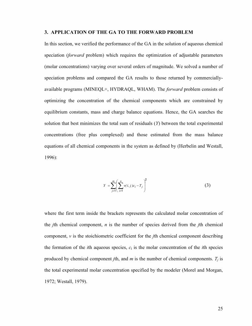
where the first term inside the brackets represents the calculated molar concentration of

the jth chemical component, n is the number of species derived from the jth chemical

component, v is the stoichiometric coefficient for the jth chemical component describing

the formation of the ith aqueous species, ci is the molar concentration of the ith species

produced by chemical component jth, and m is the number of chemical components. Tj is

the total experimental molar concentration specified by the modeler (Morel and Morgan,

1972; Westall, 1979).

26

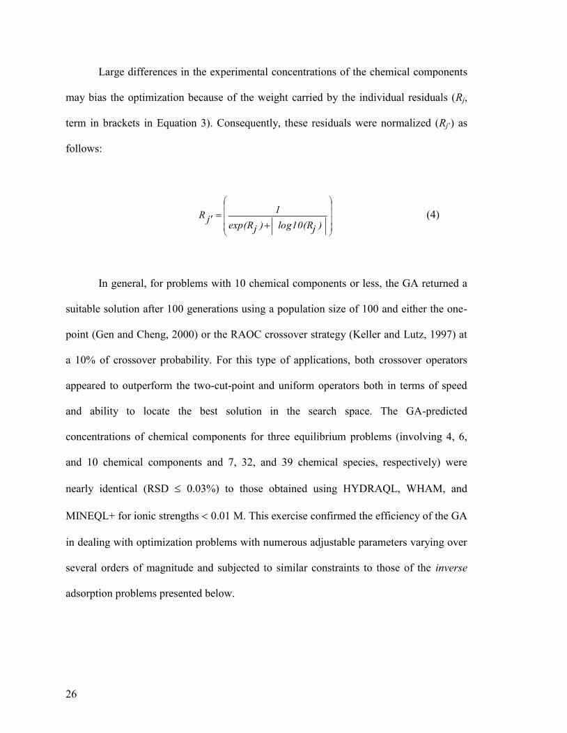
Large differences in the experimental concentrations of the chemical components

may bias the optimization because of the weight carried by the individual residuals (Rj,

term in brackets in Equation 3). Consequently, these residuals were normalized (Rj‟) as

follows:

)jlog10(R)jexp(R

1j'R (4)

In general, for problems with 10 chemical components or less, the GA returned a

suitable solution after 100 generations using a population size of 100 and either the one-

point (Gen and Cheng, 2000) or the RAOC crossover strategy (Keller and Lutz, 1997) at

a 10% of crossover probability. For this type of applications, both crossover operators

appeared to outperform the two-cut-point and uniform operators both in terms of speed

and ability to locate the best solution in the search space. The GA-predicted

concentrations of chemical components for three equilibrium problems (involving 4, 6,

and 10 chemical components and 7, 32, and 39 chemical species, respectively) were

nearly identical (RSD 0.03%) to those obtained using HYDRAQL, WHAM, and

MINEQL+ for ionic strengths 0.01 M. This exercise confirmed the efficiency of the GA

in dealing with optimization problems with numerous adjustable parameters varying over

several orders of magnitude and subjected to similar constraints to those of the inverse

adsorption problems presented below.

27

4. APPLICATION OF THE GA TO THE INVERSE PROBLEM

4.1 Estimation of Intrinsic Ionization Constants: Constant Capacitance Model

Our main objective is to implement a reliable and flexible approach to address specific

inverse problems that cannot be easily handled by conventional, deterministic, derivative-

based, root-finding techniques implemented in popular SCM calibration programs such as

FITEQL.

Because reasonable a priori knowledge is available (physical-chemical

constraints, geochemistry of the adsorbent phase, etc.), the viability of conceptual

adsorption reactions can be evaluated intuitively against specified criteria prior to

optimization, greatly reducing the number of alternative SCMs that deserve systematic

evaluation via inverse modeling. Furthermore, emphasis on conceptual and mathematical

simplicity in the formulation of SCMs is paramount and must be consistent with the

quantity and quality of available data. As emphasized in earlier studies (e.g., Herbelin and

Westall, 1996), when several SCMs fit the data equally, the most parsimonious one must

be preferred unless there is compelling evidence in support of another. Models with many

degrees of freedom incur serious risks among which: (i) fitting of inconsistent or

irrelevant „„noise‟‟ in the data records; (ii) severely diminished predictive power; (iii) the

generation of ill-defined, near-redundant parameter combinations; and (iv) masking of

geochemically-significant behavior derived from data over-fitting (Jakeman et al, 2006).

Irrespectively, the inverse problem should be well determined and, hence, contain more

data points than adjustable parameters. Finally, a posteriori physical-chemical evaluation

of the fitted SCM parameters is key to ascertain their thermodynamic relevance within the

SCM. It follows that within this scheme, the calibration of SCMs, by deterministic or

28

heuristic approaches, is properly constrained and goes well beyond a mere data fitting

exercise.

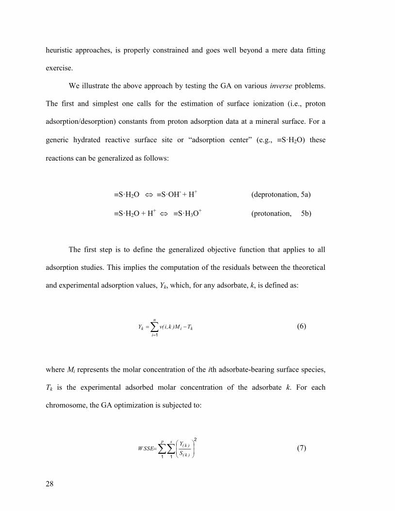
We illustrate the above approach by testing the GA on various inverse problems.

The first and simplest one calls for the estimation of surface ionization (i.e., proton

adsorption/desorption) constants from proton adsorption data at a mineral surface. For a

generic hydrated reactive surface site or “adsorption center” (e.g., S·H2O) these

reactions can be generalized as follows:

S·H2O S·OH- + H

+ (deprotonation, 5a)

S·H2O + H+ S·H3O

+ (protonation, 5b)

The first step is to define the generalized objective function that applies to all

adsorption studies. This implies the computation of the residuals between the theoretical

and experimental adsorption values, Yk, which, for any adsorbate, k, is defined as:

n

i

kik TM)k,i(vY

1

(6)

where Mi represents the molar concentration of the ith adsorbate-bearing surface species,

Tk is the experimental adsorbed molar concentration of the adsorbate k. For each

chromosome, the GA optimization is subjected to:

2

1 1

p s

)k(

)k(

S

YW SSE (7)

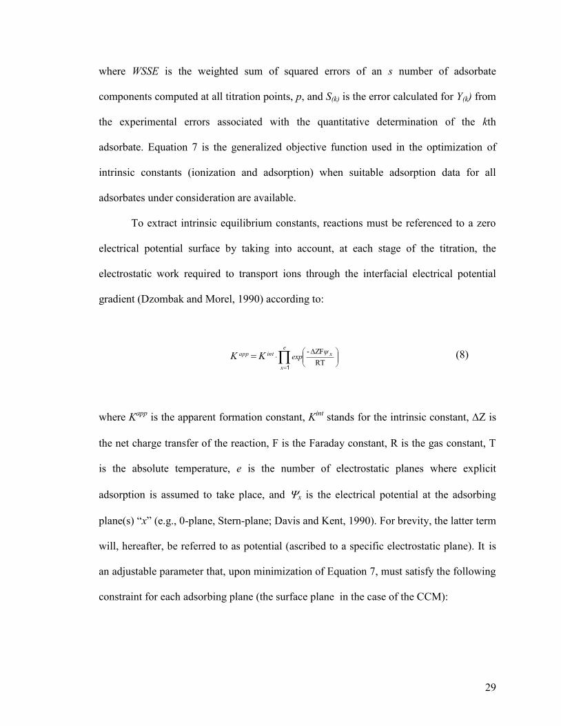
29

where WSSE is the weighted sum of squared errors of an s number of adsorbate

components computed at all titration points, p, and S(k) is the error calculated for Y(k) from

the experimental errors associated with the quantitative determination of the kth

adsorbate. Equation 7 is the generalized objective function used in the optimization of

intrinsic constants (ionization and adsorption) when suitable adsorption data for all

adsorbates under consideration are available.

To extract intrinsic equilibrium constants, reactions must be referenced to a zero

electrical potential surface by taking into account, at each stage of the titration, the

electrostatic work required to transport ions through the interfacial electrical potential

gradient (Dzombak and Morel, 1990) according to:

e

x

xintapp ψexpKK

1RT

ZF- (8)

where Kapp

is the apparent formation constant, Kint

stands for the intrinsic constant, Z is

the net charge transfer of the reaction, F is the Faraday constant, R is the gas constant, T

is the absolute temperature, e is the number of electrostatic planes where explicit

adsorption is assumed to take place, and x is the electrical potential at the adsorbing

plane(s) “x” (e.g., 0-plane, Stern-plane; Davis and Kent, 1990). For brevity, the latter term

will, hereafter, be referred to as potential (ascribed to a specific electrostatic plane). It is

an adjustable parameter that, upon minimization of Equation 7, must satisfy the following

constraint for each adsorbing plane (the surface plane in the case of the CCM):

30

electx

q

i

ii CzAS

F

1

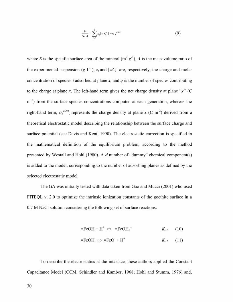
][ (9)

where S is the specific surface area of the mineral (m2 g

-1), A is the mass:volume ratio of

the experimental suspension (g L-1

), zi and [Ci] are, respectively, the charge and molar

concentration of species i adsorbed at plane x, and q is the number of species contributing

to the charge at plane x. The left-hand term gives the net charge density at plane “x” (C

m-2

) from the surface species concentrations computed at each generation, whereas the

right-hand term, xelect

, represents the charge density at plane x (C m-2

) derived from a

theoretical electrostatic model describing the relationship between the surface charge and

surface potential (see Davis and Kent, 1990). The electrostatic correction is specified in

the mathematical definition of the equilibrium problem, according to the method

presented by Westall and Hohl (1980). A d number of “dummy” chemical component(s)

is added to the model, corresponding to the number of adsorbing planes as defined by the

selected electrostatic model.

The GA was initially tested with data taken from Gao and Mucci (2001) who used

FITEQL v. 2.0 to optimize the intrinsic ionization constants of the goethite surface in a

0.7 M NaCl solution considering the following set of surface reactions:

FeOH + H+ FeOH2

+ Ka1 (10)

FeOH FeO- + H

+ Ka2 (11)

To describe the electrostatics at the interface, these authors applied the Constant

Capacitance Model (CCM, Schindler and Kamber, 1968; Hohl and Stumm, 1976) and,

31

thus, this model was implemented in the Matlab©

script to compute the value of x at

each generation according to the following expression (Stumm and Morgan, 1996):

C0

0σ

ψ (12)

where C is the specific capacitance and 0 and 0 are the charge and potential at the

surface (i.e., plane “0”). Given that only ionization reactions were considered to take

place at the surface, experimental surface charge data are available (net proton adsorption

densities are identical to surface charge densities) and, therefore, for a given capacitance

value, these data can be used to compute the surface potential at each titration point and

perform the electrostatic correction using Equations 8 and 12, respectively.

Aqueous equilibrium was solved first using either the GA or the Newton-Raphson

approach (implemented in an additional Matlab©

subroutine) to compute the

concentration of the free chemical components in solution before the intrinsic ionization

constants were optimized with the GA. In contrast to the strategy typically applied by

FITEQL users, whereby the specific capacitance is varied manually in each optimization

and the goodness of fit evaluated on the basis of the WSOS/DOF (“weighted sum of

squares divided by the degrees of freedom”) parameter (Dzombak and Morel, 1990), the

specific capacitance and the intrinsic ionization constants were optimized simultaneously

by the GA. Using the encoding rules described earlier, the capacitance can be

successfully treated as a fitting parameter and added to the chromosome encoding the

solution to the intrinsic ionization constants.

32

Like the chemical component concentrations (see preceding section), the intrinsic

constants were formulated in extended logarithmic units. Conventionally, chromosome

binary-strings represent solutions from -25000 to 25000 (i.e., 10-25

to 1025

M or 50 orders

of magnitude) that approximately cover the range of formation constants typically

reported in thermodynamic compilations (e.g., NIST, 1998). Nevertheless, for specific

adsorption reactions, such a wide range may not necessarily represent

thermodynamically-meaningful quantities and, hence, based upon physical-chemical

concepts, the modeler may select a reasonable solution space for each adjustable

parameter (as explained above), constraining the range of potential solutions and its

compatibility with the physical reality. The specific capacitance was constrained between

0.2 and 2 F/m2, covering the range of values previously reported for oxide mineral

surfaces (e.g., Hiemstra et al., 1999).

SCM parameters optimized with the GA and input values of S and A are presented

in Table 1 and compared to those reported by Gao and Mucci (2001). Because of the

probabilistic nature of the GA optimization, several GA runs were performed using

different GA parameters (e.g., population size, maximum number of generations,

mutation rates) and the associated error was calculated for each adjustable quantity. It

should be noted that this error is associated with the GA-optimization rather than to the

experiment. True uncertainties of the optimized SCM parameters must be determined

from multiple GA runs using independent replicate data sets ( 3). As shown in Table 1,

the optimized values are very reproducible, even when the population size or number of

generations varied significantly, and the mean values are close to those obtained by Gao

and Mucci (2001). Nevertheless, the ionization constants and capacitance values that best

33

describe the experimental data are slightly different than those obtained when fixed

capacitance values are used in the optimization, as in the case of FITEQL. It is

noteworthy that the GA facilitates the search of suitable intrinsic constants and

capacitance values in a single optimization run, in contrast to FITEQL and other available

inverse modeling programs (e.g., ECOSAT-FIT, Protofit). Although the difference is

small in this particular example, in other applications, relaxation of the capacitance(s) and

minimization of round-off and truncation errors via GA optimization may impact

significantly on the optimized SCM parameters. The experimental proton adsorption data

and the GA-predicted proton adsorption densities are shown in Figure 2.

4.2 Simultaneous Estimation of Intrinsic Ionization and Adsorption Constants:

Constant Capacitance Model

Typically, direct, experimental surface charge data are unavailable when adsorption of

adsorbates other than protons occurs. Consequently, surface charge must be computed

from the speciation predicted at each generation to obtain adequate estimates of the

surface potential and apply the appropriate electrostatic corrections (Eqs. 8 and 12).

Within the CCM scheme, this problem can be easily circumvented by initializing the GA

iterative process using a set of “best guess” surface charge values. This serves to pre-

adjust the constants to reasonable estimates of surface potential (related to surface charge

via an electrostatic model, Westall and Hohl, 1980) and leads the chromosome population

towards favorable regions within the solution space. After a number of generations

(iterth), the GA will calculate surface potentials from Equation 12 using the surface charge

computed from the predicted surface speciation (left-hand term in Equation 9) and will

estimate the electrostatic correction in subsequent generations. This procedure guarantees

34

fulfillment of Equation 9 from generation iterth while pushing evolution towards

successful minimization of Equation 7.

Using published phosphate adsorption data on the goethite surface in 0.7 NaCl

solutions (Gao and Mucci, 2001), we re-optimized the phosphate adsorption constants

with the GA using an identical conceptual SCM defined by the following set of surface

reactions:

FeOH + H2PO4- FePO4

2- + H

+ + H2O

(13)

FeOH + H2PO4- FePO4H

- + H2O

(14)

FeOH + H2PO4- + H

+ FePO4H2

+ H2O

(15)

For this application, assigning initial zero potentials (i.e., null electrostatic

corrections) to the surface allowed for a good performance of the GA in combination with

a rather large maximum number of iterations (maxiter 300). Several GA runs indicated

that after 50% of the pre-fixed maxiter (150), the numerical viability of the evolved

chromosome population was suitable for the computation of surface potentials from the

surface speciation and Equation 12 as well as for successful fitting of the data (Figure 3).

The success of the optimization confirms the ability of the GA to extract values of the

intrinsic adsorption constants within the CCM formalism, in the absence of surface

charge data, without explicit fitting of the surface potential.

The optimized values of the intrinsic adsorption constants are reported in Table 2

and compared to those obtained by Gao and Mucci (2001). To see the impact of the GA

optimization on the estimation of phosphate adsorption constants independently of other

35

SCM parameters, the Ka1, Ka2 and capacitance values originally proposed by Gao and

Mucci (2001) were used in this GA optimization exercise. Note that, whereas the intrinsic

constants of reactions 14 and 15 optimized by the GA are, within error, very similar to

those estimated by FITEQL, the GA-optimized intrinsic constant of reaction 13 is nearly

one order of magnitude lower. This is a clear distinction between the output returned by

FITEQL and the GA and is attributable to the better numerical stability displayed by the

latter.

To evaluate the performance of the GA with more complex optimization problems

within the CCM scheme, we optimized ionization and adsorption intrinsic constants using

synthetic data of a gedanken experiment, an acidimetric titration of a reactive mineral

(MeX(s)) displaying moderate pH-promoted dissolution. In this experiment, we considered

that dissolved, lattice-constituent divalent metal ions (Me2+

) reabsorb on the mineral

surface, competing with protons for reactive surface sites and altering surface protonation

and surface charge. The ionization and metal adsorption surface reactions, formulated in

terms of the single-site 2-pK ionization model (Lützenkirchen, 2003), are:

MeOH + H+ MeOH2

+ (16)

MeOH MeO- + H

+ (17)

MeOH + Me2+

MeOMe+

+ H+

(18)

pH, total dissolved Me2+

concentration, total adsorbed proton ([H+]Ads, data set 1), and

total adsorbed metal concentrations ([Me2+

]Ads, data set 2) compose the available data at

each titration point and were used in the minimization of Equation 7 for the optimization

36

of the intrinsic constants describing reactions 16-18. It is assumed that Me2+

does not

form ion pairs or complexes in aqueous solution (i.e., total Me2+

concentrations are equal

to free Me2+

concentrations). The chemical scenario of this gedanken experiment is

similar to classical, competitive ion adsorption studies where the pH and the aqueous

adsorbate(s) concentration are simultaneously monitored at each experimental point.

Using a population of 100 chromosomes and after 500 generations, the GA

successfully reproduces all the experimental data, as shown in Figure 4. In contrast, the

simultaneous optimization of two or three of the constants (reaction 16, 17 or 18) and the

number of available reactive surface sites with a specified capacitance (GA-optimized

value) with FITEQL v. 3.2 resulted in convergence problems and no output. When only

the constant describing reaction 16 was optimized, while the constants for reactions 17

and 18 were fixed at the GA-optimized values, FITEQL converged but gave very poor

fits to the [Me2+

]Ads, and [H+]Ads data (Figure 4), with a WSOS/DOF value of 19.5. This

reveals that, in some cases, successful convergence of FITEQL does not necessarily

return good fits to all the experimental data. In turn, this raises questions about the

validity of the recommended range of WSOS/DOF values (0.1 to 20) for the evaluation of

the goodness of fit (Westall, 1982). It appears that FITEQL converged towards a local

minimum rather than a global one and the relative contribution of reactions 16 and 17

(ionization reactions) versus 18 (divalent metal adsorption reaction) to the proton

adsorption behavior could not be resolved accurately upon fitting of data sets 1 and 2.

Conversely, the GA optimization gradually minimizes the difference between the

experimental and simulated data and, thus, the evolved generation retains critical

information for searching the global minimum. Given an adequate conceptual SCM and

sufficient high quality data, the GA will find the combination of model parameters that

37

best minimizes Equation 7 even in cases that are difficult to tackle by deterministic

approaches.

It has been stressed that an a posteriori analysis of non-uniqueness and uncertainty

of solutions to inverse problems (resolution analysis) is necessary to assess scientific

conclusions based on inverse modeling (Moosegard, 1998). Whereas this is an important

step for inverse problems involving a large number of ill-defined, poorly constrained

parameters, this is not crucial for the problems presented in our study since the selected

SCM parameters are physically-meaningful and well constrained. Hence, they do not

generally yield numerous solutions to a given problem (or selected SCM), unless the

available data are insufficient or unsuitable to quantitatively resolve the contribution of

each adsorption reaction. Nevertheless, a sensitivity analysis should be conducted to

select the best solution among the possible options (several SCMs fitting the data

reasonably well) and prevent over-interpretation of the data. This is typically done by

gradually incorporating adsorption reactions to the simplest physically-meaningful SCM

and by testing its ability to reproduce the experimental data. We performed this analysis

in a recent study (Villegas-Jiménez et al., 2009) where, based upon fundamental

chemistry concepts, several SCMs were formulated and alternatively calibrated via GA

optimization using relatively large experimental data sets for two rhombohedral carbonate

minerals: magnesite and dolomite (Pokrovsky et al., 1999a,b). Whereas more than one

SCM fitted the data within the same tolerance (as shown by ANOVA tests), only one

reasonably complied with all other a posteriori criteria (theoretical constraints and

alternate experimental data) imposed for model validation. Again, emphasis must be

placed on model parsimony.

38

4.3 Simultaneous Estimation of Intrinsic Ionization and Adsorption Constants:

Triple Layer Model

It is often necessary to adopt an electrostatic model other than the CCM to describe the

spatial distribution of charged surface species at the mineral-water interface

(Lützenkirchen, 2003). For multi-layer electrostatic models, such as the Triple Layer

Model (TLM), a specific potential must be defined at each interfacial plane (surface and

Stern planes and diffuse layer). In this case, the GA must find a suitable set of intrinsic

constants, capacitance values, and site densities (intensive variables) that, in combination

with appropriate potentials (extensive variables), minimize Equation 7 while satisfying

Equation 9. Since the surface charge displayed by the mineral varies according to the

chemical conditions of the system (i.e., pH, chemical speciation), individual potentials

must be adjusted at each titration or experimental data point, and for each electrostatic

plane. Given the large number of adjustable extensive variables, some modifications

were made to the optimization approach described earlier.

Sets of potential solutions for these extensive variables are encoded in a 3D

binary-string matrix (Matrix-A) whose dimensions are determined by: (i) the selected

population size, (ii) the number of available data points, and (iii) the number of interfacial

electrostatic planes (“dummy” components), excluding the diffuse region, required by the

selected multi-layer electrostatic model (Westall and Hohl, 1980). To define the size of

the chromosomes in Matrix-A and the solution space, realistic boundary values of surface

potential must be chosen for each electrostatic plane. For this purpose, zeta-potentials

obtained from electrokinetic measurements are useful for the selection of these

constraints (Dzombak and Morel, 1990). The structure of a generalized 3D matrix,

including the “dummy” components, is illustrated in Figure 5.

39

Another matrix (Matrix-B) encodes the solutions for the intensive variables. Its

dimensions are dictated by the selected population size and the number of adjustable

intensive variables. To improve the effectiveness of the evolutionary process, Matrix-A

and Matrix-B were dimensioned and manipulated separately throughout the GA

optimization. In other words, genetic operations are carried out independently for each

matrix, maintaining a good numerical diversity in both matrices and facilitating the search

for the best solution to the optimization problem. Whereas the evaluation of the

chromosomes in Matrix-B is subject to Equation 7, the evaluation of chromosomes in

Matrix-A is based on fulfillment of Equation 9 (for each electrostatic plane where

adsorption occurs) by minimization of:

p eElec

xCalc

xY

1 1

2 (19)

where the total sum of residuals (Y) corresponds to the difference between the charge

calculated from the speciation predicted at plane “x” (xCalc

, in C m-2

) and the charge

computed from electrostatics for plane “x” using appropriate surface-charge-potential

relationships (xElec

, in C m-2

). For the TLM, these are (Davis and Kent, 1990):

)(00

ψψElec

1C (20)

0

)(

d

Elec

ψψ2C (21)

)2/sinh(1174.0 RTZFψI d

Elec

d (22)

40

where, as before, and represent, respectively, charge and potential at each specific

interfacial plane: i) the surface (plane-0), ii) the plane where outer-sphere complexes are

located (plane-), and iii) the diffuse layer (plane-d). C1 and C2 are the integral

capacitance values of the interfacial layers, and F/RT represents the reciprocal of the

Boltzmann factor for charged molecules and ions (0.02569 V-1

). Because the TLM makes

no explicit provision of ion adsorption at the diffuse layer, the calculation of the diffuse

layer charge, d, is obtained from the charge neutrality equation (Davis and Kent, 1990):

d = - 0 - (23)

and hence, the d can be obtained directly from equation 22. In other words, only 0 and

are subjected to optimization via Equation 19, and thus, only two “dummy”

components are required in Matrix A. Additional “dummy” components will be required

by other sophisticated multi-layer electrostatic models such as the Four Layer Model

(Charmas, 1999).

One advantage of this treatment is that the “best” potential computed at each

iteration, the one that best minimizes Equation 19, can be tested against inequality

constraints defined by physically realistic boundary values for each electrostatic plane

(Dzombak and Morel, 1990; Davis and Kent, 1990). This operation serves to determine

whether the calculated potentials are realistic and, thus, can be used in the next iteration,

otherwise the old value is retained for evaluation in the next generation. The performance

of the GA is improved by interrupting the optimization of the extensive variables once the

above-mentioned constraints are achieved. In other words, hereafter, only Matrix-B will

41

be subject to evolution, via Equation 7 using the most realistic potential values (that best

minimize equation 19) to continue the iterative procedure.The strategy employed for each

matrix is schematically represented in Figure 6.

To further improve the performance (i.e., speed and computational requirements)

of the GA optimization in this type of application, an additional implementation must be

made. Given a chromosome population 100 and after a sufficient number of generations

(i.e., n > 100), the GA should have reached a suitable level of numerical viability and can

be interrupted even if the data fit is inadequate. The optimized, intensive variables are

best values and can be used to quickly verify whether they can successfully simulate the

data upon solution of the adsorption equilibrium forward problem (adjustment of

extensive variables) by a derivative-based numerical technique. The implementation of

the Newton-Raphson (NR) technique for these types of problems is straightforward and

was explained in detail elsewhere (e.g., Papelis et al., 1988). In other words, evolutionary

optimization can be switched to a subroutine that calculates the Jacobians corresponding

to all chemical component(s) and electrostatic term(s). Once the Jacobians are obtained,

the matrix is solved by the Gauss-elimination procedure (Nicholson, 1995) and the

iterative procedure carries on until the residual meets a pre-fixed tolerance level (Sahai

and Sverjensky, 1998). This strategy exploits the advantages of the GA to optimize the

intensive variables (with pre-adjusted extensive variables) which, in combination with

deterministically-derived potentials can simulate titration data. The Newton-Raphson

technique is used to fine-tune the estimation of the potentials, ensure minimization of

Equation 19 at the end of the iterative process, and reduce the computational time. If

42

required, additional GA-NR micro-iterations can be implemented to improve the quality

of the fit and further refine the intensive variable estimates.

This “hybrid” GA-NR optimization technique was successfully tested against

published surface titration data for goethite in 0.01 M NaCl solutions (Villalobos and

Leckie, 2001). The authors originally modeled their data using the TLM (Figure 7). In

this formalism, seven intensive variables must be adjusted: two ionization constants

(reactions 10 and 11), two background electrolyte adsorption constants:

FeOH + Na+ FeO

-Na

+ + H

+ (24)

FeOH + Cl- + H

+ FeOH2

+Cl

- (25)

two capacitance values (C1 and C2), and the total number of reactive surface sites.

Because FITEQL convergence is not assured when several parameters are

adjusted, particularly when interdependent reactions (reactions 10, 11, 24, and 25 are pH-

dependent) are fitted simultaneously (Hayes et al., 1991), some criteria are commonly

applied to pre-select either the ionization or electrolyte adsorption constants before

proceeding with the optimization of all other fitting parameters. Accordingly, Villalobos

and Leckie (2001) selected fixed values of the ionization constants (reactions 10 and 11)

and optimized those corresponding to reactions 24 and 25 to fit their data. In contrast, the

hybrid GA-NR technique allows for the simultaneous optimization of all fitting

parameters required by the TLM and for the successful simulation of titration data, as

shown in Figure 7.

43

5. CONCLUSIONS

A powerful evolutionary optimization technique, the genetic algorithm, was applied to the

calibration of SCMs for mineral surfaces. This technique was successfully tested for the

inverse modeling of adsorption equilibria under several scenarios of varying degrees of

complexity using published and synthetic data.

The GA performs an exhaustive probabilistic search in a broad solution space that

is constrained by physically realistic values selected by the modeler. Given suitable

combinations of geochemical (set of adsorption reactions) and electrostatic (charge

distribution at the adsorbent-water interface) models and sufficient quality experimental

data, the GA can successfully optimize numerous parameters without incurring

convergence problems while achieving good numerical stability, a notable advantage over

conventional deterministic, root-finding, and optimization techniques implemented in

popular inverse modeling codes such as FITEQL. At the modeler‟s discretion, multiple

intrinsic ionization and adsorption constants, capacitance(s), and/or reactive surface site

densities can be simultaneously fitted by the GA. Nevertheless, an a posteriori theoretical

evaluation of the fitted SCM parameters must be made to ascertain their thermodynamic

meaningfulness and confirm their relevance within the SCM. This aspect is key for the

construct of sound, yet parsimonious, SCMs.

The drawback of the GA approach is the large number of iterations that must be

performed to obtain a satisfactory solution, particularly for cases involving numerous

fitting parameters. Alternatively, the power of the GA can be more efficiently exploited

when a deterministic technique such as Newton-Raphson is incorporated once the

chromosome population has reached a suitable level of numerical viability. Consequently,

44

we propose the use of a hybrid GA-NR approach for the efficient optimization of intrinsic

constants in complex problems such as those involving the TLM.

We believe that the computational requirements of the GA to the calibration of

SCMs are greatly outweighed by its robustness, simplicity, and potential to generate a

reliable thermodynamic database describing adsorption reactions. This is a critical step to

making reliable predictions of the adsorption behavior of minerals and geologically-based

adsorbents in hydro-geological settings (e.g., aquifers, pore waters, water basins) and/or

in engineered reactors (e.g., mining and wastewater treatment industries). Future work to

test and develop more sophisticated adaptive strategies and hybrid heuristic-deterministic

optimization approaches may improve the GA performance in this type of applications.

6. ACKNOWLEDGMENTS

A.V.-J. thanks Dr. David Burns for critical discussions that inspired this investigation and

EMEA S.C. Environmental Consulting Firm for providing suitable facilities to complete

this work. This research was supported by a graduate student grant to A.V.-J. from the

Geological Society of America (GSA) and Natural Sciences and Engineering Research

Council of Canada (NSERC) Discovery grants to A.M. A.V.-J. benefited from post-

graduate scholarships from the Consejo Nacional de Ciencia y Tecnología (CONACyT)

of Mexico and additional financial support from the Department of Earth and Planetary

Sciences, McGill University and Consorcio Mexicano Flotus-Nanuk.

45

7. REFERENCES

Allison J.D., Brown D.S. and Novo-Gradac K.J. (1991) MINTEQA2/PRODEFA2, a

geochemical assessment model for environmental systems: version 3.0. User‟s

manual, Environmental Research Laboratory, Office of Research and

Development, U.S. Environmental Protection Agency, Athens, GA, 106.

Ball J.W., Jenne E.A. and Norstrom D.K. (1981) WATEQ2- A computerized chemical

model for trace and major element speciation and mineral equilibrium of natural

waters. In: E.A. Jenne (Ed.) Chemical Modeling in Aqueous Systems, Symposium

series 93, American Chemical Society, Washington, D.C. pp 815-836.

Charmas R. (1999) Four-layer complexation model for ion adsorption at energetically

heterogeneous metal oxide/electrolyte interfaces. Langmuir 15(17), 5635-5648.

Davis J.A. and Kent D.B. (1990) Surface complexation modeling in aqueous

geochemistry. In: Mineral-Water Interface Geochemistry. (ed. M.F. Hochella and

A.F. White). Rev. Mineral. 23. Mineral. Soc. Washington, DC. pp 177-260.

Dzombak D.A. and Morel F.M.M. (1990) Surface Complexation Modeling. John Wiley

and Sons, New York, NY, 393.

Epperson J.F. (2002) An Introduction to Numerical Methods and Analysis. John Wiley


Essaid H.I., Cozzarelli I.M., Eganhouse R.P., Herkelrath W.N., Bekins B.A. and Delin

G.N. (2003) Inverse modeling of BTEX dissolution and biodegradation at the

Bemidji, MN crude-oil spill site. J. Cont. Hydr. 67(1), 269-299.

Fernández Alvarez J.P., Fernández Martínez J.L. and Menéndez Pérez C.O. (2008)

Feasibility analysis of the use of binary genetic algorithms as importance samplers

Application to 1-D DC resistivity inverse problem. Math. Geosci. 40, 375-408.

46

Gans P. (1976) Numerical methods for data-fitting problems. Coord. Chem. Rev. 19, 99-

124.

Gao Y. and Mucci A. (2001) Acid base reactions, phosphate and arsenate complexation,

and their competitive adsorption at the surface of goethite in 0.7 M NaCl solution.


Gen M. and Cheng R. (1997) Genetic Algorithms and Engineering Design. John Wiley


Gen M. and Cheng R. (2000) Genetic Algorithms and Engineering Optimization. John

Wiley and Sons, New York, NY, 495 pp.

Goldberg D. (1989) Genetic Algorithms in Search, Optimization and Machine Learning.

Addison-Wesley, Reading, MA, 412.

Golberg D., Korb K. and Deb K. (1989) Messy genetic algorithms: motivation, analysis

and first results. Complex Systems 3, 493-530.

Hayes K.F., Redden G., Ela W. and Leckie J.O. (1991). Surface complexation models:

An evaluation of model parameter estimation using FITEQL and oxide mineral

titration. J. Colloid Interface Sci. 142(2), 448-469.

Herbelin A. and Westall J. (1996) FITEQL-. A computer program for determination of

chemical equilibrium constants from experimental data version 3.2: user‟s

manual. Department of Chemistry. Oregon State University, Corvallis, OR,

Report 96-01.

Hiemstra T., Yong H. and van Riemsdijk W.H. (1999) Interfacial charging phenomena of

aluminum (hydr)oxides. Langmuir 15(18), 5942-5955.

47

Hohl H. and Stumm W. (1976) Interaction of Pb2+

with hydrous -Al2O3. J. Colloid

Interface Sci. 55, 281-288.

Holland J. (1975) Adaptation in Natural and Artificial Systems. University of Michigan

Press, Ann Arbor MI, 183.

Jakeman A.J., Letcher R.A. and Norton J.P. (2006) Ten iterative steps in development

and evaluation of environmental models. Environ. Model. Software 21, 602-614.

Keizer M.G. and van Riemsdijk W.H. (1999) ECOSAT, Technical Report of the

departments of Soil Science and Plant Nutrition. Wageningen University,

Wageningen, The Netherlands.

Keller B. and Lutz R. (1997) A new crossover operator for rapid function optimization

using a genetic algorithm. Proceedings of the Eighth Ireland Conference on

Artificial Intelligence (AI-97), Vol. 2, pp. 48-57.

Kinniburgh D.G. (1999) FIT User Guide. British Geological Survey, Keyworth, UK,

WD/93/23.

Langmuir D. (1997) Aqueous Environmental Geochemistry. Prentice Hall, Upper Saddle

River, N.J., 600.

Lützenkirchen J. (2003) Surface complexation models for adsorption: A critical survey in

the context of experimental data. In: Tóth J. (Ed) Adsorption: Theory, Modeling,

and Analysis, Surfactant Science Series 107, New York, NY, Marcel Dekker Inc.,

pp. 631-710.

Matott L.S. and Rabideau A.J. (2008) ISOFIT - A program for fitting sorption isotherms

to experimental data. Environ Model Software 23: 670-676.

48

Mestres J. and Scuseira G.E. (1995) Genetic algorithms, A robust scheme for geometry

optimizations and global minimum structure problems. J. Comput. Chem. 16(6),

729-742.

Michalewicz Z. (1996) Genetic Algorithms + Data Structure = Evolution Programs, 2nd

ed. Springer-Verlag, New York, NY, 387.

Morel F.M.M. and Morgan J. (1972) A numerical method for computing equilibria in

aqueous chemical systems. Environ. Sci. Technol. 6, 58-87.

Morel F.M.M. and Hering J.G. (1993) Principles and Applications of Aquatic Chemistry.

John Wiley and Sons, New York, NY, 588.

Mosegaard K. (1998) Resolution analysis of general inverse problems through inverse

Monte Carlo sampling. Inverse Probl. 14, 405-426.

Mosegaard K. and Sambridge M. (2002) Monte Carlo Analysis of inverse problems.

Inverse Probl. 18, 29-54.

Nicholson K. (1995) Linear Algebra with Applications. PWS Pub. Co., Boston, MD, 540.

NIST (1998) Critically Selected Stability Constants of Metal Complexes, Standard

Reference Database 46, Version 5, National Institute of Standards and

Technology, US Department of Commerce, Gaithersburg, MD, USA.

Papelis C., Hayes K.F. and Leckie J.O. (1988) HYDRAQL: A program for the

computation of chemical equilibrium, composition of aqueous batch systems

including surface-complexation modeling of ion adsorption at the oxide/solution

interface. Report No. 306. Stanford University, Stanford, CA, 130.

Parkhurst D.L. (1995) User‟s guide to PHREEQC. U.S. Geological Survey, Water

Resources Investigations Report 95-4277, 212.

49





reactivity in aquatic systems. Geochim. Cosmochim. Acta 63(19/20), 3133-3143.

Sahai N. and Sverjensky D.A. (1998) GEOSURF: A computer program for modeling

adsorption on mineral surfaces from aqueous solution. Comp. Geosci. 24(9), 853-

873.

Sait S.M. and Youssef H. (1999) Iterative Computer algorithms with Applications in

Engineering Solving Combinatorial Optimization Problems. IEEE Computer

Society Los Alamitos, CA, 387.

Schecher W.D. and McAvoy D.C. (1992) MINEQL+: A software environment for

chemical equilibrium modeling. Computers, Environment and Urban Systems 16,

65-76.

Schindler P.W. and Kamber H.R. (1968) Die acidität von silanolgruppen. Helv. Chim.

Acta 51, 1781-1786.

Sposito G. and Coves J. (1988) SOILCHEM: A computer program for the calculation of

chemical speciation in soils. Keamey Found. Soil Sci., Univ. California,

Riverside.

Stumm W. and Morgan J. (1996) Aquatic Chemistry: Chemical Equilibria and Rates in

Natural Waters. John Wiley and Sons Inc., New York, 1022.

Tipping E. (1994) WHAM- A chemical equilibrium model and computer code for water,

sediments and soils incorporating a discrete site/electrostatic model of ion-binding

by humic substances. Comp. Geosci. 20, 973-1023.

50

Turner B.F. and Fein J.B. (2006) Protofit: A program for determining surface protonation

constants from titration data. Comp. Geosci. 32, 1344–1356.

van der Lee J. and de Windt L. (1999) CHESS Tutorial and cookbook. Technical report

No. LHM/RD/99/05. École des Mines de Paris. Fontainebleu, France. 77.

Villalobos M. and Leckie J.O. (2001) Surface complexation modeling and FTIR study of

carbonate adsorption to goethite. Geochim. Cosmochim. Acta 235,15-32.

Villegas-Jiménez A., Mucci A., Pokrovsky O.S. and Schott J. (2009) Defining reactive

sites at hydrated mineral surfaces: rhombohedral carbonate minerals. Geochim.

Cosmochim. Acta 73(15), 4326-4345.

Westall J.C. (1979) MICROQL II: Computation of adsorption equilibria in BASIC.

Technical Report. Swiss Federal Institute of Technology, EAWAG, 8600

Dübendorf, Switzerland.

Westall J.C. (1982) FITEQL: A computer program for determination of chemical

equilibrium constants from experimental data. Version 1.2 Report 82-01,

Department of Chemistry, Oregon State University, Corvallis, OR, USA.

Westall J. and Hohl H. (1980) A comparison of electrostatic models for the

oxide/solution interface. Adv. Colloid Int. Sci. 12, 265-294.

Wolery T.J. (1992) EQ3NR: A computer program for geochemical aqueous speciation-

solubility calculations: theoretical manual, user‟s guide and related documentation

(Version 7.0), Report No. UCRL-MA-110662-PT-III, Lawrence Livermore

National Laboratory, Livermore, CA.

Zeleznik F.J. and Gordon S. (1968) Calculation of complex chemical equilibria. Ind. Eng.

Chem. 60, 27-57.

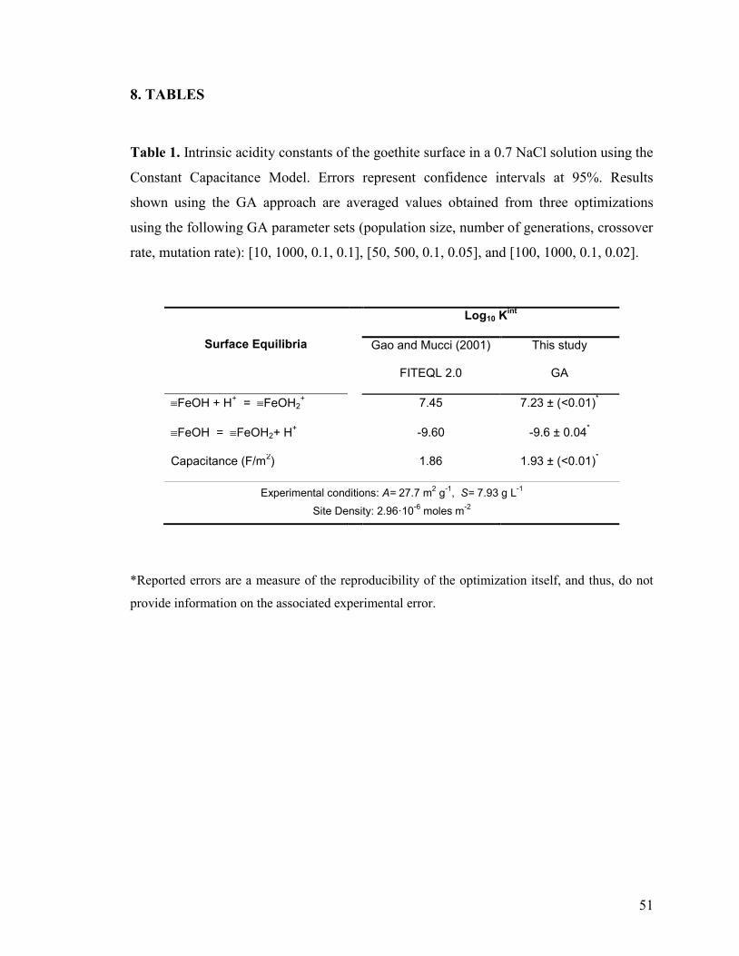
51

8. TABLES

Table 1. Intrinsic acidity constants of the goethite surface in a 0.7 NaCl solution using the

Constant Capacitance Model. Errors represent confidence intervals at 95%. Results

shown using the GA approach are averaged values obtained from three optimizations

using the following GA parameter sets (population size, number of generations, crossover

rate, mutation rate): [10, 1000, 0.1, 0.1], [50, 500, 0.1, 0.05], and [100, 1000, 0.1, 0.02].

Surface Equilibria

Log10 Kint

Gao and Mucci (2001)

FITEQL 2.0

This study

GA

FeOH + H+ = FeOH2

+ 7.45 7.23 ± (<0.01)

*

FeOH = FeOH2+ H+ -9.60 -9.6 ± 0.04

*

Capacitance (F/m2) 1.86 1.93 ± (<0.01)

*

Experimental conditions: A= 27.7 m2 g

-1, S= 7.93 g L

-1

Site Density: 2.96·10-6

moles m-2

*Reported errors are a measure of the reproducibility of the optimization itself, and thus, do not

provide information on the associated experimental error.

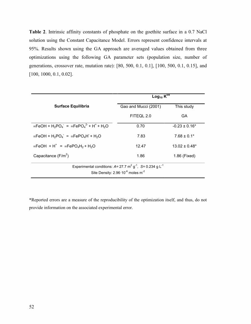
52

Table 2. Intrinsic affinity constants of phosphate on the goethite surface in a 0.7 NaCl

solution using the Constant Capacitance Model. Errors represent confidence intervals at

95%. Results shown using the GA approach are averaged values obtained from three

optimizations using the following GA parameter sets (population size, number of

generations, crossover rate, mutation rate): [80, 500, 0.1, 0.1], [100, 500, 0.1, 0.15], and

[100, 1000, 0.1, 0.02].

Surface Equilibria

Log10 Kint

Gao and Mucci (2001)

FITEQL 2.0

This study

GA

FeOH + H2PO4- = FePO4

2- + H

+ + H2O 0.70 -0.23 ± 0.16*

FeOH + H2PO4- = FePO4H

- + H2O 7.83 7.68 ± 0.1*

FeOH + H+

= FePO4H2 + H2O 12.47 13.02 ± 0.48*

Capacitance (F/m2) 1.86 1.86 (Fixed)

Experimental conditions: A= 27.7 m2 g

-1, S= 0.234 g L

-1

Site Density: 2.96·10-6

moles m-2

*Reported errors are a measure of the reproducibility of the optimization itself, and thus, do not

provide information on the associated experimental error.

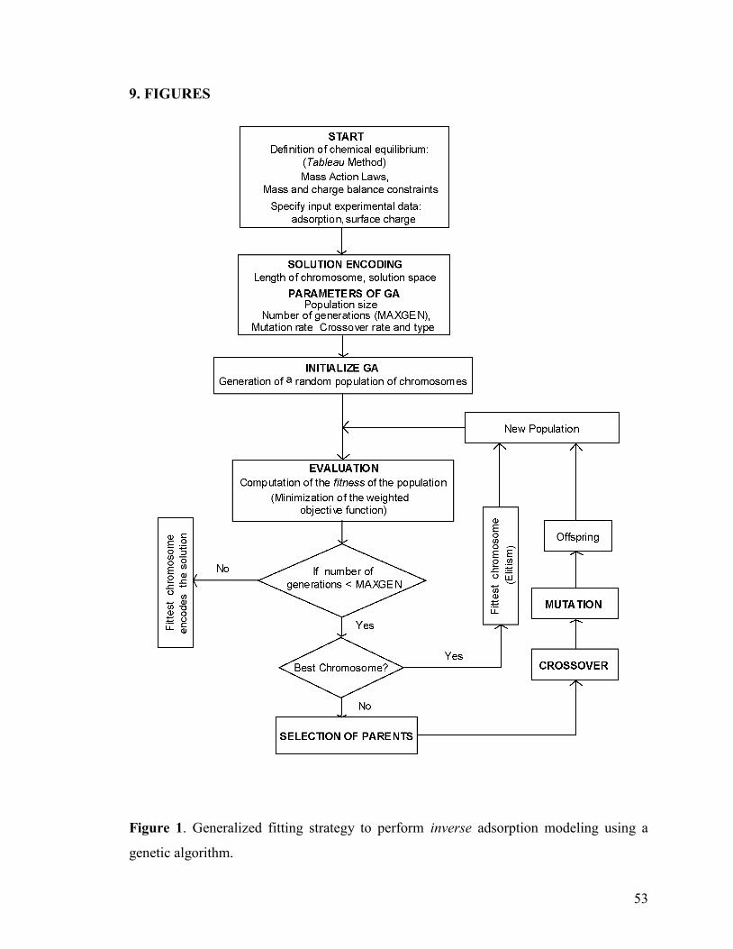
53

9. FIGURES

Figure 1. Generalized fitting strategy to perform inverse adsorption modeling using a

genetic algorithm.

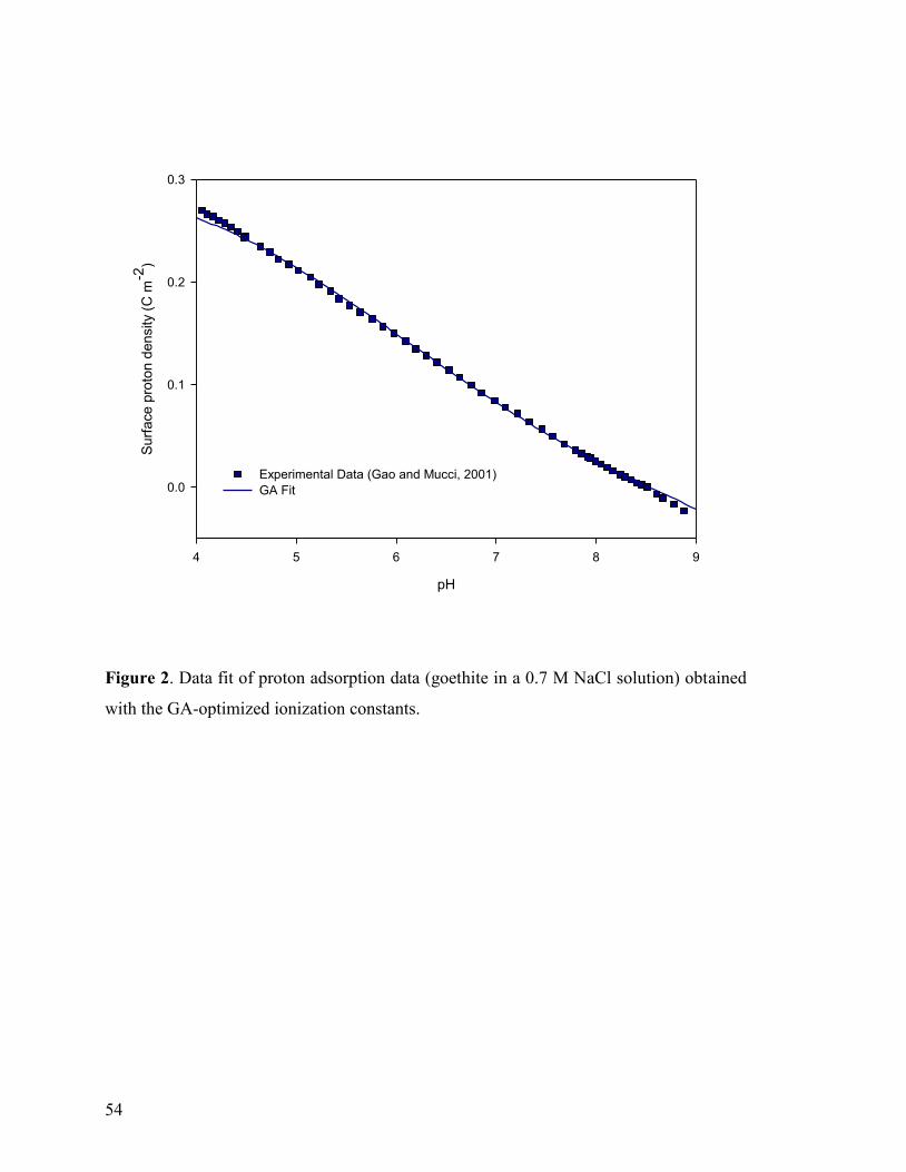
54

pH

4 5 6 7 8 9

Su

rfa

ce

pro

ton d

en

sity

(C m

-2)

0.0

0.1

0.2

0.3

Experimental Data (Gao and Mucci, 2001)

GA Fit

Figure 2. Data fit of proton adsorption data (goethite in a 0.7 M NaCl solution) obtained

with the GA-optimized ionization constants.

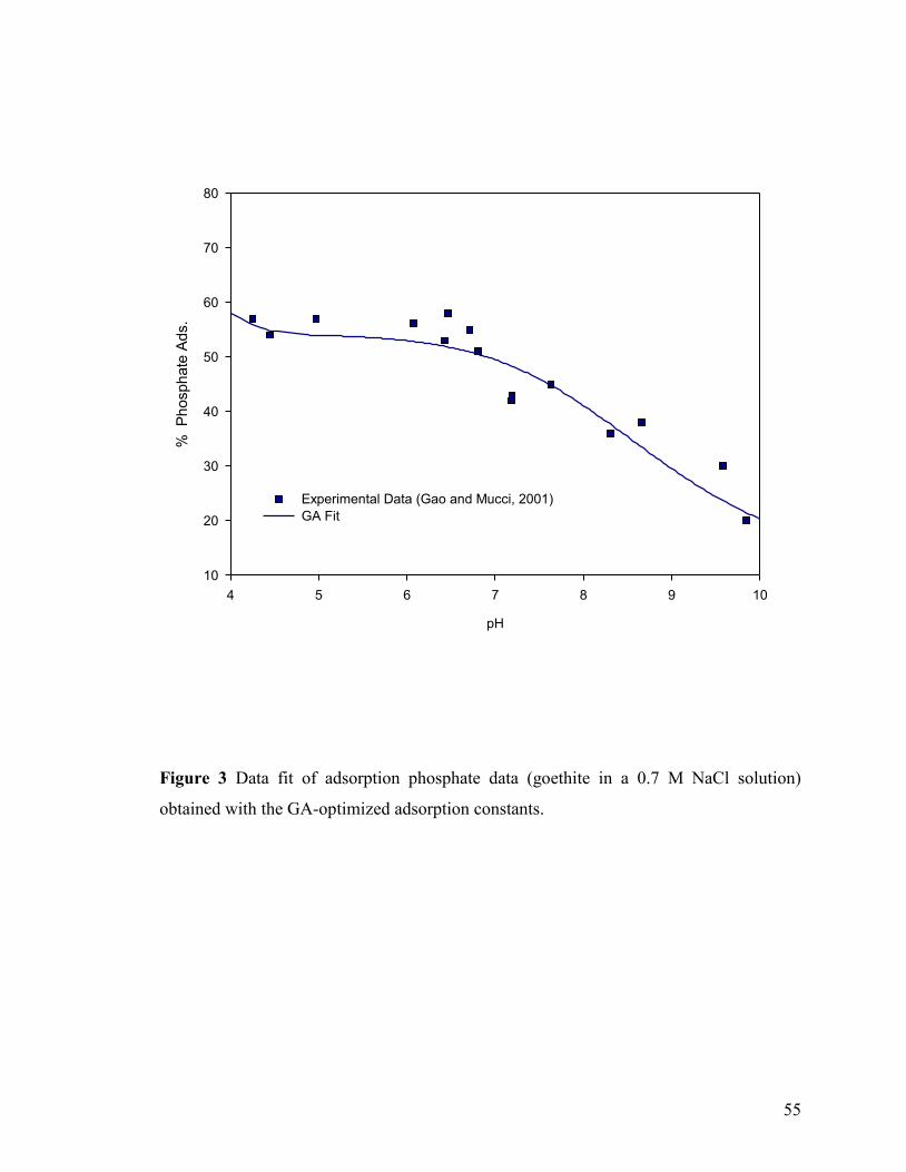
55

pH

4 5 6 7 8 9 10

% P

hosphate

Ads.

10

20

30

40

50

60

70

80

Experimental Data (Gao and Mucci, 2001)

GA Fit

Figure 3 Data fit of adsorption phosphate data (goethite in a 0.7 M NaCl solution)

obtained with the GA-optimized adsorption constants.

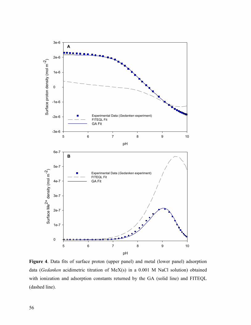
56

pH

5 6 7 8 9 10

Surf

ace M

e2+

density (

mol m

-2)

0

1e-7

2e-7

3e-7

4e-7

5e-7

6e-7

pH

5 6 7 8 9 10

Surf

ace p

roto

n d

ensity (

mol m

-2)

-3e-6

-2e-6

-1e-6

0

1e-6

2e-6

3e-6

Experimental Data (Gedanken experiment)

FITEQL Fit

GA Fit

A

B

Experimental Data (Gedanken experiment)

FITEQL Fit

GA Fit

Figure 4. Data fits of surface proton (upper panel) and metal (lower panel) adsorption

data (Gedanken acidimetric titration of MeX(s) in a 0.001 M NaCl solution) obtained

with ionization and adsorption constants returned by the GA (solid line) and FITEQL

(dashed line).

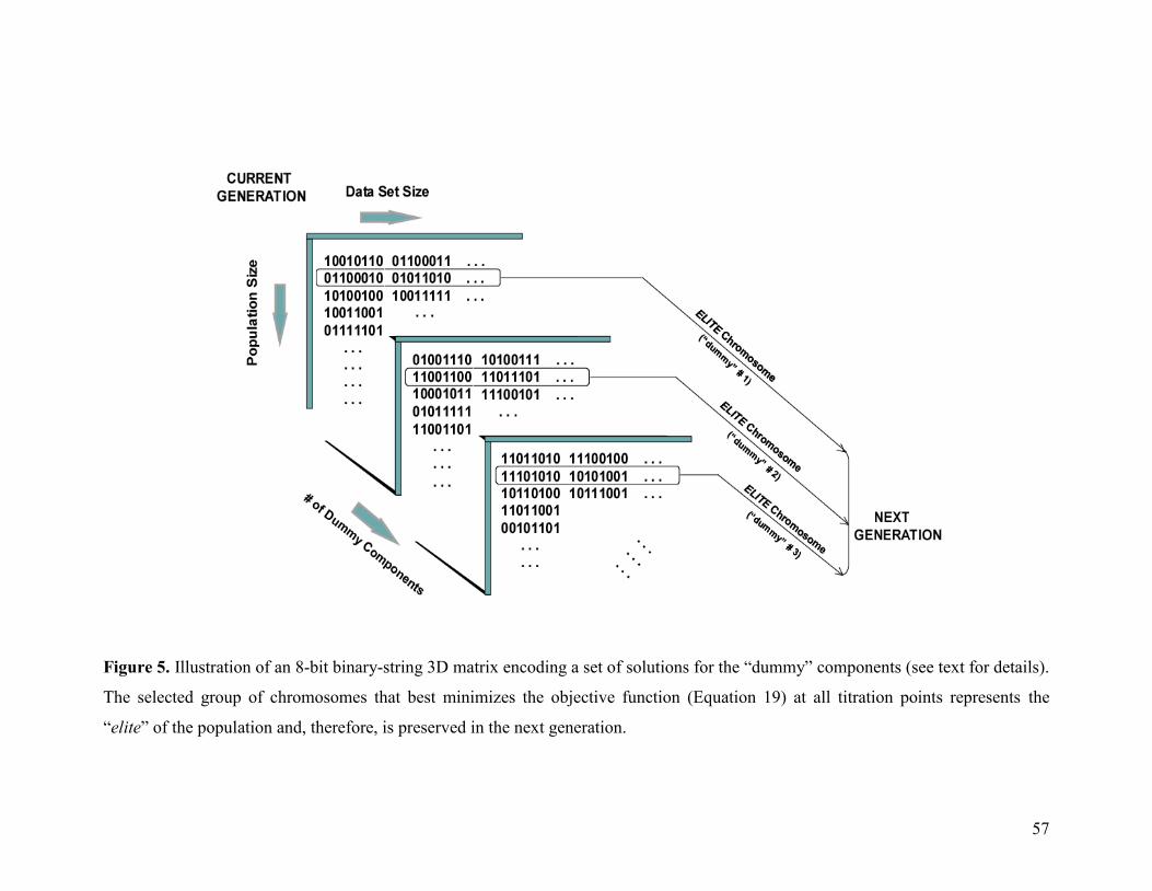
57

Figure 5. Illustration of an 8-bit binary-string 3D matrix encoding a set of solutions for the “dummy” components (see text for details).

The selected group of chromosomes that best minimizes the objective function (Equation 19) at all titration points represents the

“elite” of the population and, therefore, is preserved in the next generation.

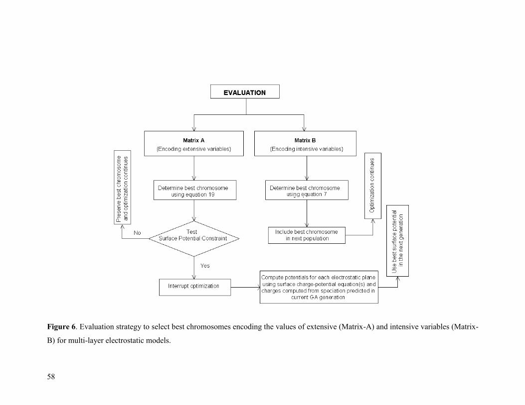
58

Figure 6. Evaluation strategy to select best chromosomes encoding the values of extensive (Matrix-A) and intensive variables (Matrix-

B) for multi-layer electrostatic models.

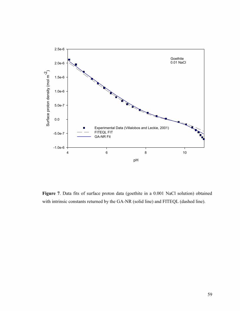
59

pH

4 6 8 10

Su

rfa

ce

pro

ton

de

nsity

(mo

l m

-2)

-1.0e-6

-5.0e-7

0.0

5.0e-7

1.0e-6

1.5e-6

2.0e-6

2.5e-6

Experimental Data (Villalobos and Leckie, 2001)

FITEQL FIT

GA-NR Fit

Goethite0.01 NaCl

Figure 7. Data fits of surface proton data (goethite in a 0.001 NaCl solution) obtained

with intrinsic constants returned by the GA-NR (solid line) and FITEQL (dashed line).

60


In the early 1990‟s, researchers designed and implemented a novel flow-through titration

reactor to perform acid-base titrations of carbonate mineral surfaces which was used to

generate surface charge data for rhodochrosite, siderite, magnesite, and dolomite. Using

these data, the first SCMs were devised for these minerals in aqueous solutions based

upon a two (siderite, rhodochrosite and magnesite) and four reactive site scheme

(dolomite). To date, these studies provide the only available surface charge data for

carbonate minerals whose quantitative interpretation in terms of surface complexation

reactions represents a first-order description of the chemistry of the carbonate/aqueous

solution interface. No significant refinements or major improvements to these SCMs have

been achieved since, from either an experimental or theoretical standpoint.

In the following chapter: “Defining Reactive Sites on Hydrated Mineral Surfaces:

Rhombohedral Carbonate Minerals”, we critically review the definition of reactive

surface sites whereupon mass-action expressions describing adsorption equilibria at the

hydrated surface of rhombohedral carbonate minerals are formulated. The analysis led to

the derivation of a single generic charge-neutral surface site scheme analogous to the one-

site 2-pKa ionization model employed in the description of the amphoteric behavior of

numerous metal oxide surfaces. This scheme allows for a simplified and generalized

representation of surface equilibria for this type of minerals and is compatible with

experimental and theoretical findings as well as with common assumptions implied by

SCMs. Via the GA approach introduced in the previous chapter, new SCMs were

calibrated, using available data for magnesite and dolomite and evaluated qualitatively

against published electrokinetic for these two minerals.

61

CHAPTER 3

DEFINING REACTIVE SITES ON HYDRATED MINERAL SURFACES: RHOMBOHEDRAL CARBONATE MINERALS

Adrián Villegas-Jiménez*1, Alfonso Mucci

1, Oleg S. Pokrovsky

2 and Jacques Schott

2



2Géochimie et Biogéochimie Expérimentale,

LMTG, UMR 5563,

Université de Toulouse – CNRS, 14, Avenue Edouard Belin 31400 Toulouse, France

*Corresponding Author


Published in Geochimica Cosmochimica Acta

Geochim. Cosmochim. Acta 73(15) 4326-4345

62

ABSTRACT

Despite the success of surface complexation models (SCMs) to interpret the adsorptive

properties of mineral surfaces, their construct is sometimes incompatible with

fundamental chemical and/or physical constraints and, thus, cast doubts on the physical-

chemical significance of the derived model parameters. In this paper, we address the

definition of primary surface sites (i.e., adsorption units) at hydrated carbonate mineral

surfaces and discuss its implications to the formulation and calibration of surface

equilibria for these minerals.

Given the abundance of experimental and theoretical information on the structural

properties of the hydrated (10.4) cleavage calcite surface, this mineral was chosen for a

detailed theoretical analysis of critical issues relevant to the definition of primary surface

sites. Accordingly, a single, generic charge-neutral surface site (CaCO3·H2O0) is defined

for this mineral whereupon mass-action expressions describing adsorption equilibria were

formulated. The one-site scheme, analogous to previously postulated descriptions of

metal oxide surfaces, allows for a simple, yet realistic, molecular representation of

surface reactions and provides a generalized reference state suitable for the calculation of

sorption equilibria for rhombohedral carbonate minerals via Law of Mass Action (LMA)

and Gibbs Energy Minimization (GEM) approaches.

The one-site scheme is extended to other rhombohedral carbonate minerals and

tested against published experimental data for magnesite and dolomite in aqueous

solutions. A simplified SCM based on this scheme can successfully reproduce surface

charge, reasonably simulate the electrokinetic behavior of these minerals, and predict

surface speciation agreeing with available spectroscopic data. According to this model, a

63

truly amphoteric behavior is displayed by these surfaces across the pH scale but at

circum-neutral pH (5.8-8.2) and relatively high CO2 ( 1 mM), proton/bicarbonate co-

adsorption becomes important and leads to the formation of a charge-neutral H2CO3-like

surface species which may largely account for the surface charge-buffering behavior and

the relatively wide range of pH values of isoelectric points (pHiep) reported in the

literature for these minerals.

Keywords: One-site surface complexation, carbonate minerals, primary surface sites,

residual charges, carbonic acid-like surface specie.

64

1. INTRODUCTION

Surface complexation models (SCMs) have been extensively applied to the interpretation

of adsorption and surface reactivity data on a large number of minerals in aqueous

solutions. Their relative simplicity and capacity to incorporate fundamental concepts of

thermodynamics, crystallography, and inorganic and colloid chemistry make them

suitable tools for the description of the adsorptive properties of minerals under a wide

range of chemical conditions.

Nevertheless, despite the success and refinements achieved by many of these

models, many shortcomings remain to be addressed before their applicability to natural

systems and their validation at the molecular level can be established (e.g., Westall and

Hohl, 1980; Goldberg, 1991; Sahai and Sverjensky, 1997; Kallay and Žalac, 2000; Zuyi

et al., 2000; Lützenkirchen, 2002). Among these, the definition of the surface sites

(hydrated adsorption units) that serve as reference species, hereafter referred to as

“primary surface sites”, for the formulation of surface reactions is at the heart of a

realistic description of adsorption processes (Healy and White, 1978; Pivovarov, 1997;

Kulik et al., 2000; Kulik, 2002). These can be formalized in terms of discrete chemical

units of given chemical composition and charge, in analogy to functional groups of ionic

and molecular aqueous species. However, they differ from their aqueous analogues

because primary surface sites have a fixed density per unit area and cannot be diluted

infinitely on the surface (Kulik, 2002). These properties affect the definition of standard

states for surface species and reflect on the values of the intrinsic formation constants

(Kint

) of surface species (Kulik, 2002; Sverjensky, 2003). Other distinctions include

stereochemical, structural and electrostatic conditions at the mineral/water interface that

65

influence the energetics of the primary surface sites (Sposito, 1989; Zachara and Westall,

1999).

Two major ions binding schemes (or models) have been postulated for the

formulation of SCMs: one-site and multi-site complexation. One-site schemes assign an

average “macroscopic” reactivity to all atoms present at the mineral surface whereas

multi-site schemes formalize the reactivities of individual surface atoms in terms of their

chemical identity, coordination environment, and hydrogen bonding arrangements

(Hiemstra et al., 1989; Barrow et al., 1993; Hiemstra et al., 1996). Despite their generic

nature, one-site schemes are simple, practical, and powerful predictive tools based upon

well established statistical mechanical grounds (Borkovec, 1997) and are, despite their

disregard of the complexities inherent to real-world sorbents (chemical heterogeneity),

the foundation of numerous electrical double-layer models that describe the charge-

potential relationship at the mineral/water interface (Sposito, 1983).

On the other hand, multi-site schemes are more realistic insofar as they reflect,

semi-quantitatively, the compositional “heterogeneity” of the predominant mineral

surfaces (Hiemstra et al., 1989; Hiemstra and van Riemsdijk, 1991; Hiemstra and van

Riemsdijk, 1996; Scheidegger and Sparks, 1996). Nevertheless, the quantitative

characterization of the reactivity of individual primary surface sites is far from trivial

because the proper calibration of these multi-site, multi-reaction models requires: (i)

uniform and/or well-characterized mineral surfaces in terms of chemical composition and

micro-topography (Barrow et al., 1993; Piasecki et al., 2001), (ii) suitable experimental

data arising from various independent sources and carrying sufficient information to

properly resolve the energetic contributions of individual surface sites (Rudziński et al.,

1992, 1998; Piasecki et al., 2001), and (iii) the application of sophisticated mathematical

66

treatments (Chandler, 1987; Jäger, 1991; Borkovec and Koper, 1994). For instance, it is

well known that, because of compensating effects, the composite adsorption (or surface

charge) isotherms obtained from titration experiments that are typically used for the

calibration of adsorption chemical models, are largely insensitive to surface energetic

heterogeneity and, therefore, additional data (e.g., potentiometric, electrokinetic,

radiometric, calorimetric) are required to properly discriminate among potential

heterogeneity models and prevent misleading over-interpretations of available data (van

Riemsdijk et al., 1987; Blesa and Kallay, 1988; Ĉerník et al., 1995; Rudziński et al.,

1992, 1998; Lützenkirchen, 2005). Furthermore, the presence of surface irregularities

(steps, kinks, and dislocations), chemical micro-heterogeneities, and multi-domain

crystal surfaces, difficult to characterize experimentally, add to the complexity of multi-

site models, so that the physical-chemical significance of the derived model parameters

and their application to natural systems is seriously questioned (Lützenkirchen, 1997). It

follows that simpler models are expected to remain prominent in the quantitative

modeling of equilibrium adsorption phenomena (Lützenkirchen, 2002) and kinetic

dissolution processes (Bandstra and Brantley, 2008).

Despite the lack of scientific consensus with regards to the application of one-site

vs multi-site schemes to describe sorption reactions, it is generally agreed that primary

surface sites must contain sufficient information about the sorbent phase for the accurate

description of its surface reactivity while allowing for a simple and realistic

representation of sorption equilibria (Kulik, 2002). Furthermore, because Law of Mass

Action (LMA)-based sorption modeling approaches (Morel and Morgan, 1972; Westall

and Hohl, 1980; Goldberg, 1995), frequently incorporated in widespread computer codes

(e.g., MINEQL, HYDRAQL, PHREEQC, FITEQL etc.), are subjected to charge and

67

mass balance constraints, the definition of primary surface sites in terms of their residual

charges and elemental stoichiometry is critical for the reliable estimation of model

parameters (i.e., intrinsic formation constants of surface species, capacitances, site

densities) and the solution of surface speciation equilibria. This issue is the focus of the

present study within the context of rhombohedral carbonate minerals.

We begin by highlighting critical aspects relevant to the definition of the residual

charges and the elemental stoichiometry of primary surface sites. Later, the discussion

focuses on the (10.4) cleavage calcite surface, as a model for all rhombohedral carbonate

minerals, to rationalize the available theoretical and experimental evidence and formalize

a realistic primary surface site for these surfaces. Accordingly, new surface equilibria are

derived, calibrated and evaluated against published experimental data (i.e., surface

charge, electrokinetic, and spectroscopic) for two common rhombohedral carbonate

minerals: magnesite and dolomite.

2. DEFINITION OF PRIMARY SURFACE SITES

2.1 Charge Assignment

Atomic charges are not physical properties that can be readily defined accurately

(Chandra and Kollman, 1984) and, hence, their assignment to primary surface sites at

mineral surfaces is problematic. Typically, either a “zero residual charge” or a “fractional

residual charge” scheme is assigned to primary surface sites in surface complexation

studies. Whereas the former is based on simple, yet realistic, chemical stability grounds

(charge dissipation upon surface hydration), the latter is based upon Bond Valence

concepts: “Pauling‟s Electrostatic Valence Principle” (Pauling, 1929) and “Bond Valence

68

Theory” (Brown, 1981). These concepts were originally developed and calibrated to bulk

structures and were later applied to idealized, unrelaxed, unreconstructed metal oxide

surfaces (displaying no bond relaxation and/or bond breaking) for the estimation of the

unsatisfied valence of surface atoms which was considered as an approximate measure of

their residual charge (Yoon et al., 1979; Hiemstra et al., 1989; Bleam, 1993; Hiemstra et

al., 1996). It should be noted that Bond Valence Theory, a semi-empirical approach based

upon central atom valences, coordination number and bond lengths, must not be confused

with Valence-Bond Theory that complements Molecular Orbital Theory and involves

fundamental quantum chemistry concepts where bonding is accounted for in terms of

atomic valences and hybridized orbitals (Gallup, 2002).

Depending on the residual charge and relative abundance of the primary surface

sites, the unreacted hydrated mineral surface will carry a neutral, positive, or negative

“reference charge density” (REF) as described by (Hiemstra and van Riemsdijk, 1996):

jjREF NzF (1)

where zj and Nj represent, respectively, the charge and density (in moles m-2

) of the j

primary surface site and F is the Faraday constant. In other words, REF represents the net

charge of the surface when only primary surface sites are present. It is the resultant of

crystal truncation (“dangling bonds”) and mineral hydration which, in turn, may lead to

the re-organization of bonds (e.g., bond relaxation, bond breaking and/or bond making) at

the mineral surface and the establishment of “unknown” residual charges at the primary

surface sites. REF contributes to the net surface charge density (0, C m-2

) as follows:

69

REFPSISH0 (2)

where H is the net proton surface charge density (F(ΓH+ - ΓOH-), ΓH+ and ΓOH- are,

respectively, the net surface H+ and OH

- adsorption densities in mol m

-2), IS is the net

charge density resulting from the total charge of ions (excluding H+ and OH

-) bound by

inner-sphere surface coordination, and PS is the net permanent structural surface charge

arising from isomorphic substitutions exhibited by some minerals (Chorover and Sposito,

1995). For simplicity, we will focus our discussion exclusively on minerals without

permanent structural charge (PS = 0) and only within the context of adsorption at the 0-

plane (surface).

The calibration of intrinsic formation constants (Kint

) by LMA approaches

(Herbelin and Westall, 1996) is constrained by proton and, if applicable, inner-sphere ion

adsorption data (HandIS, respectively) and is subjected to the following charge

equality constraint:

elect0REF0iiz

ΑS

][

F (3)

where A is the specific surface area (m2 g

-1), S is the solid to solution ratio (g L

-1), zi is

the net charge transfer of the reaction producing surface species i, [i0] is the molar

concentration of species i adsorbed at the surface (plane-0), and 0elect

represents the

electrostatically-derived net surface charge density (an a priori unknown) computed from

70

an electrostatic interfacial model (EIM), describing the surface charge-potential

relationship (Westall and Hohl, 1980), and the iteratively-optimized surface potential

(0). The left-hand term in Equation 3 represents the “net surface charge” and requires

definition of REF and computation of the “apparent surface charge” (0app

, first left-hand

term of Eq. 3) from the surface speciation predicted by the iteratively-optimized Kint

values. Because Kint

and 0elect

are interdependent (Eq. 3), their optimization is a function

of two fixed experimentally-accessible quantities (H and IS, although their

measurement may not be trivial for some minerals) and one ill-defined quantity (REF). In

addition, the latter affects the Kint

values via the estimated 0 which depends on the

adjusted 0elect

and the selected EIM. Any modification in the values of 0 is reflected in

the electrostatic correction necessary to reference apparent constants, Kapp

, to a zero

potential standard state for the calibration of Kint

values:

RT

F- 0i ψZexpKK intapp (4)

where R is the gas constant and T is the absolute temperature. The main corollary to this

discussion is that the selected REF may impact the calibration of the intrinsic formation

constants via LMA approaches, and therein lies the importance of assigning appropriate

charges to primary surface sites.

71

2.2 Elemental Stoichiometry

The selection of the elemental stoichiometry of the primary surface sites is also

critical because it influences the molecular representation of surface reactions and

participates in the mass balance constraint imposed by LMA-based approaches (total

crystallographic site density) in the modeling of sorption equilibria (Kulik, 2002).

The simplest scenario is to consider individual surface atoms (hydroxylated or

hydrated) as the primary surface sites. However, electrostatic and steric interactions

between neighboring surface species may arise and affect the energetics of the sorption

processes. For instance, vicinal surface atoms may both interact with the same sorbate

(bidentate adsorption; Ludwig and Schindler, 1995) or, upon reaction with a sorbate,

adjacent surface atoms may be inactivated (Benjamin, 2002). In both cases, two adjacent

surface atoms could be formalized as one surface site.

These premises were championed by Pivovarov (1997) who, based upon

crystallographic considerations, proposed the elemental stoichiometry of two generic

types of charge-neutral surface sites for the hydrated hematite surface, (FeOH)2(OH2)+

and (O3H)2(H2O)-, assuming that H2O molecules physically adsorbed to hydroxylated

vicinal surface metal and oxygen atoms represent a single “adsorption center”

whereupon surface reactions occur. This approach yielded surface OH group densities in

close agreement with experimental values (Morimoto et al., 1969). A similar definition of

the elemental stoichiometry of one generic surface site for all metal oxides (O0.5H) was

postulated by Kulik (2002) under the assumption that primary surface sites at mineral

surfaces comprise H2O molecules from the adsorbed water monolayer. This definition of

surface sites was influenced by results of wet chemical, spectroscopic and molecular

72

modeling studies that confirmed the presence of OH groups at metal oxide surfaces

(Morimoto et al., 1969; Davis and Kent, 1990). The proposed one-site scheme considers

the bidentate coordination of a H2O molecule to one surface metal and one surface

oxygen and yields two vicinal charge-neutral hydroxyl groups (i.e., MeOH and OH) of

which either only one is reactive (Kulik, 2002) or both participate simultaneously in the

adsorption processes and are thus conceptualized as a single site (Pivovarov, 1998). This

scenario allowed the modeling of sorption equilibria by both LMA (Pivovarov, 1998) and

Gibbs Energy Minimization (GEM, Kulik, 2002) approaches and provided a suitable

molecular representation of surface reactions at the metal oxide/H2O interface. It follows

that the application of identical criteria for the definition of elemental stoichiometries for

other mineral surfaces is warranted.

3. RHOMBOHEDRAL CARBONATE MINERALS

3.1 Case of the (10.4) Calcite Surface

3.1.1 Evidence from Spectroscopic and Molecular Modeling Studies

The (10.4) calcite surface has been extensively studied (e.g., Stipp and Hochella, 1991; de

Leeuw and Parker, 1997; Fenter et al., 2000; Wright et al., 2001; Geissbühler et al.,

2004). This surface is of great interest because it represents the most stable and

predominant crystallographic face displayed by this mineral in aqueous solutions and it

serves as a model for other rhombohedral carbonate minerals such as magnesite,

dolomite, siderite, rhodochrosite, and gaspeite. The ideal (10.4) cleavage surface

configuration displays a stoichiometric number of adjacent cations and anions that carry

an equivalent but opposite residual charge per surface unit cell and corresponds to the

73

atomic plane where strictly ionic (metal-oxygen) and no covalent bonds (carbon-oxygen)

are broken. The major stability of this atomic configuration over others was confirmed

using a simple crystal lattice truncation protocol (based upon Bond Valence concepts)

devised to determine the most stable atomic configuration of oxide mineral surfaces

according to charge and bond strength minimization criteria (Koretsky et al., 1998).

Numerous surface-sensitive instrumental techniques have been employed to

characterize the (10.4) calcite surface under wet and/or vacuum conditions such as X-Ray

Photoelectron Spectroscopy (XPS, Stipp and Hochella, 1991; Stipp, 1999), Low Energy

Electron Diffraction (LEED, Stipp and Hochella, 1991; Stipp, 1999), Time-Of-Flight

Secondary Ion Mass Spectroscopy (TOF-SIMS, Stipp, 1999), Infrared Spectroscopy (IR,

Neagle and Rochester, 1990), Fourier Transform Infrared Spectroscopy (FTIR, Kuriyavar

et al., 2000), Diffuse Reflectance Infrared Fourier Transform Spectroscopy (DRIFT,

Pokrovsky et al., 2000), Attenuated Total Reflection-Fourier Transform Infrared

Spectroscopy (ATR-FTIR, Al-Hosney and Grassian, 2005), Atomic Force Microscopy

(AFM, Rachlin et al., 1992; Stipp et al., 1994; Liang et al., 1996; Stipp, 1999), and X-

Ray Reflectivity and Scattering (SXR, Chiarello et al., 1993; Fenter et al., 2000;

Geissbühler et al., 2004). These techniques revealed that the outer-most atomic layer

relaxes and the surface undergoes a certain degree of reconstruction upon hydration. The

presence of OH groups was detected near the cleaved (10.4) calcite surface exposed to

moistened conditions (e.g., Stipp and Hochella, 1991; Fenter et al., 2000) and the

formation of a hydration monolayer was confirmed (e.g., Fenter et al., 2000). These

findings established that water constituents are chemically associated with the surface

allowing for the formation of hydrated surface species. Furthermore, “chemisorption” of

water was also demonstrated by earlier thermogravimetric studies (Morimoto et al., 1980;

74

Ahsan, 1992). Nevertheless, it is not yet possible to ascertain, by any of these analytical

techniques, whether hydration occurs through adsorption of dissociated or undissociated

water molecules because these are unable to detect hydrogen atoms and, thus, hydroxyl

ions cannot be distinguished from adsorbed H2O molecules. In other words, it is not

possible, for instance, to distinguish whether the primary surface site: Ca(H2O) or

CaOH° (or both) form at the calcite surface. Consequently, water dissociation products

cannot be ascribed to specific surface atoms. The only conclusion that can be drawn from

these data is that the internal coordinates (i.e. O-H bond lengths and H-O-H angle) of

undissociated water molecules are possibly modified upon adsorption but it is unknown to

what extent. To ascertain whether H2O dissociates to its hydrolysis products (H+

and OH-)

upon adsorption on the calcite surface, additional information is needed.

Theoretical studies provide information on the structure, energetics, and atomic

bonding relationships at the hydrated mineral surface. Computer-assisted Atomistic

simulations (de Leeuw and Parker, 1997; de Leeuw and Parker, 1998; de Leeuw et al.,

1998; Kuriyavar et al., 2000; Hwang et al., 2001; Wright et al., 2001; Kerisit et al., 2003;

Kerisit and Parker, 2004), Molecular Dynamics (Kerisit et al., 2003; Kerisit and Parker,

2004; Kerisit et al., 2005a; Perry et al., 2007), ab initio Density Functional Theory

(Parker et al., 2003; Kerisit et al., 2003; Archer, 2004; Kerisit et al., 2005b), and Roothan-

Hartree-Fock Molecular Orbital Theory (Villegas-Jiménez et al., 2009a) were used to

investigate the interactions of H2O monomers with the (10.4) calcite surface. All these

studies reveal that the internal coordinates of water monomers remain essentially

unchanged upon adsorption and, that associative adsorption of H2O on the (10.4) calcite

surface is energetically favorable (over dissociative adsorption) where one H2O monomer

75

bonds to one calcium atom and is likely hydrogen-bonded to either one (Archer, 2004;

Villegas-Jiménez et al., 2009a) or two neighboring surface oxygen atoms of carbonate

groups (de Leeuw and Parker, 1997; Wright et al., 2001; Kerisit and Parker, 2004; Perry

et al., 2007). In other words, each adsorbed H2O monomer interacts simultaneously with

one cationic and at least one anionic centre, and hence, charge and mass discretization of

hydrolysis products among individual surface atoms is problematic. Clearly, a suitable

formalism must be adopted for mass and charge assignment of water constituents among

individual surface atoms in the definition of primary surface sites.

Extension of these Atomistic simulations to other hydrated (10.4) carbonate

surfaces, such as magnesite and dolomite, reveals that H2O adsorbs associatively on these

surfaces according to a 1:1 H2O:MeCO3(surface) stoichiometry where each adsorbed H2O

molecule interacts with one metal center (Mg for magnesite and Mg or Ca for dolomite)

and at least one neighboring O surface atom (de Leeuw and Parker, 2001; de Leeuw and

Parker, 2002; Wright et al., 2001; Parker et al., 2003; Kerisit et al., 2005a; Austen et al.,

2005). This information strongly suggests that, regardless of the specific orientation of

adsorbed H2O molecules relative to the mineral surface, all (10.4) single- and mixed-

metal carbonate surfaces are subjected to similar hydration processes where water

remains undissociated upon adsorption.

3.1.2 Single Generic Primary Surface Site

Based upon the results of spectroscopic and molecular modeling studies, a generic

primary surface site for the (10.4) cleavage calcite surface can be defined as:

(CaCO3)·H2O, where the constituents in parentheses represent surface atoms. This

76

reactive surface site reflects the elemental stoichiometry of the (10.4) hydrated surface

unit cell: two neighboring surface atoms, one metal atom and one carbonate group,

interacting with one water (undissociated) molecule (Figure 1a). This scheme is

equivalent to those of Kulik (2002) and Pivovarov (1997) for metal oxides insomuch as

the adsorbed H2O molecules are considered as the reactive elemental units at the surface,

whereupon surface reactions occur.

Because a stoichiometric number of divalent cationic (Ca atoms) and anionic (CO3

groups) are present at the idealized (10.4) cleavage calcite surface (and of all

rhombohedral carbonate minerals to that matter), and regardless of the residual charge

displayed by individual surface atoms (following bond re-organization on hydration),

charge-neutrality should be preserved at the idealized stoichiometric unit, (CaCO3), and

maintained upon adsorption of neutral H2O monomers. Accordingly, a neutral charge can

be assigned to the newly defined primary surface site: (CaCO3)·H2O0.

In contrast to earlier multi-site SCMs that assume the formation of primary surface

sites of type MeOH

and CO3H, (δ = residual charge), the one-site scheme

circumvents the problem of mass and charge discretization allowing for a generic, yet

realistic, mass and charge localization at the primary surface site, rather than at individual

surface atoms. This yields a REF=0, identical to that of earlier multi-site SCMs for single-

and mixed-metal rhombohedral carbonate surfaces (Van Cappellen et al., 1993;

Pokrovsky et al., 1999a,b; Pokrovsky and Schott, 2002; Wolthers et al., 2008) and

consistent with the reference level of zero proton charge typically adopted by 2-pK

models (Sposito, 1998). Detailed structural information of hydrated (relaxed) carbonate

surfaces from independent studies (e.g., molecular modeling, Fitts et al., 2005; Kubicki et

77

al., 2008) is required to determine realistic bond lengths, coordination environments and

hydrogen bonding arrangements of surface atoms as well as derive more accurate δ values

(and REF), as emphasized by earlier workers (Bickmore, 2004; Villegas-Jiménez et al.,

2005; Wolthers et al., 2008).

3.2. SCM Reactions: One-Site vs Two-Site Scheme

The one-site scheme is analogous to the one describing non-overlapping bidentate

adsorption, where pairs of specific neighboring surface sites (rather than pairs of random

neighboring surface sites as for overlapping bidentate adsorption) react with a given

sorbate to produce a bidentate surface complex (Benjamin, 2002), and thus, two

neighboring sites are inactivated for further reaction (see Figure 1b). For carbonate

minerals, polydentate adsorption is well-exemplified by the interaction of aspartate with

calcium ions on the calcite surface (Teng and Dove, 1997), leading to a large perturbation

of the local molecular surface geometry, significant steric effects and the inactivation of

adjacent sites (see also the “Umbrella effect”, Kovačević et al., 1998). This contrasts with

the two-site scheme where, with the exception of synergistic effects related the

development of the macroscopic electrical potential, each site is independent and, thus, it

is assumed that adsorption at one site does not affect the macroscopic reactivity of any of

its neighbors.

Earlier workers described the charging behavior of single-metal carbonate

minerals with six generic reactions (ionization and constituent-ion adsorption reactions)

based upon a two-site (Van Cappellen et al., 1993; Pokrovsky et al., 1999a; Pokrovsky

and Schott, 2002) or a multi-site scheme (Pokrovsky et al., 1999b; Wolthers et al., 2008).

Similarly, analogous reactions can be derived for the one-site scheme (see Table 1).

78

Although reactions are equivalent in terms of charge and mass transfer, the participating

individual species in both schemes carry a distinct stoichiometry and different

“conceptual” mechanisms are implied in each case. Figure 2 illustrates ionization

reactions conceptualized at the molecular-level for the one-site scheme.

The main distinction between the one-site and two-site models is revealed upon

reaction of the primary surface sites. In the case of the protonation reaction for calcite

(reactions 3a and 3b, Table 1), the one-site model conceptually involves the participation

of both CO3H0

and CaOH0 sites to produce the protonated positively-charged specie:

(CaCO3)·H3O+. In contrast, according to the two-site scheme, only one cationic site

reacts to produce the protonated positively-charged specie: CaOH2+ while leaving one

anionic site, CO3H0, available for further reaction. In other words, in both cases, one

positive charge is transferred to the surface per mole of primary surface site reacted but,

whereas only one primary surface site is available for further reaction in the one-site

model, (CaCO3)·H2O0 (on a surface unit cell basis), three sites remain available

according to the two-site model, one CaOH0 and two CO3H

0. Once surface equilibrium

is established, the charge density of the surface unit cell will depend on whether

additional reactions take place at the surface (e.g., constituent ion adsorption). Clearly,

multi-site schemes allow for a multitude of reactions that can lead to surface charge

acquisition and may equally reproduce experimental surface charge data, at the expense

of a larger number of unknown parameters (that must be adjusted or arbitrarily selected,

see below) than for the one-site scheme. This has important consequences in the

calibration of intrinsic formation constants and directly reflects on surface speciation

predictions, as discussed in section 4.2. In Figure 3, the availability of “unreacted”

79

primary surface sites at a generic single-metal (10.4) carbonate surface is illustrated as a

function of the proton occupancy for acid-base reactions formulated for the one-site

(reactions 1a to 3a, Table 1) and two-site (reactions 1b to 3b, Table 1) schemes.

3.3 Mixed-Metal Carbonate Minerals

In mixed-metal rhombohedral carbonate minerals, two different types of constituent

cations (i.e. Me1 and Me2) alternate along the (10.4) surface. Thus, for the one-site

scheme, two types of generic primary surface sites, (Me1CO3)·H2O0 and

(Me2CO3)·H2O0 would be required to formulate equivalent surface reactions to those of

the earlier four-site SCM model for dolomite that requires twelve surface reactions

(Pokrovsky et al., 1999b). The Kint

values describing these reactions, however, would be

difficult to calibrate without a combination of suitable experimental data (e.g., titration,

calorimetric, radiometric, electrokinetic) acquired over a wide range of solution

compositions and use of suitable mathematical strategies that would allow resolution of

the contribution of individual surface reactions (through their intrinsic formation

constants) to the development of surface charge (see Introduction). Unfortunately,

because of their reactivity (fast dissolution/precipitation kinetics, Pokrovsky and Schott,

2002), the experimental characterization of the sorptive properties of carbonate minerals

is typically constrained to a relatively narrow range of solution compositions (pH, Me

and/or CO2, solid:solution ratios) which complicates the quantitative evaluation of these

constants. This type of calibration would be even more problematic within the Charge

Distribution MultiSite Ion Complexation (CD-MUSIC) approach as it requires the fitting

and/or arbitrary selection of a larger number of parameters (Wolthers et al., 2008). Other

80

approaches, such as molecular modeling techniques (Rustad et al., 1996; Wasserman et

al., 1999), may be required to establish critical theoretical constraints for the accurate

evaluation of the individual reactivity of multiple primary surface sites at carbonate

surfaces.

An alternate treatment for mixed carbonate minerals is to formulate surface

reactions in terms of a single charge-neutral surface site that reflects half the

stoichiometry of the hydrated (10.4) surface unit cell: (MeCO3)·H2O0 where MeCO3

represents generically Me1 or Me2 (e.g., Ca or Mg for dolomite). Under this scheme, the

number of adjustable intrinsic formation constants is reduced by at least a factor of two

with respect to previous multi-site models (i.e., dolomite: Pokrovsky et al., 1999b;

Wolthers et al., 2008), which renders the model more mathematically tractable. This

formalism is justified by the inadequacy of the available experimental data for the proper

calibration of multiple surface reactions and largely disregards the attribution of too much

mechanistic meaning (e.g., surface site heterogeneity) to composite charging curves or

adsorption isotherms (see Lützenkirchen, 1997). The newly-formulated surface reactions

can be generalized for single- and mixed-metal carbonate minerals as shown in Table 1,

the only difference being that, for mixed-metal carbonate minerals, one additional cation

adsorption reaction (reaction 4a, Table 1) is required to express the individual affinity of

Me1 and Me2 towards (MeCO3)·H2O0. One corollary to this single charge-neutral

surface site formalism is that an average reactivity is assigned to the generic surface site,

and hence, whether surface reactions formally take place at (Me1CO3)·H2O

or

(Me2CO3)·H2O remains undefined. In other words, the individual reactivities of these

sites are averaged out during model calibration and expressed in terms of the formation

81

constant, a reasonable approximation considering that the individual site reactivities in

mixed-metal carbonate minerals are hard to decouple experimentally. That Ca2+

and Mg2+

ions adsorb in near-stoichiometric ratios on dolomite surfaces over a wide range of pH,

Ca/Mg, ionic strength, and pCO2 (Brätter et al., 1972; Brady et al., 1996) suggests that

both primary surface sites exhibit similar reactivities.

4. EVALUATION OF THE ONE-SITE SCHEME

4.1. Re-Calibration of Surface Reactions for Magnesite and Dolomite

Despite all the arguments provided in favor of the one-site scheme, it is important to test

the relevance of the derived reactions against experimental data. To this end, the

calibration of one-site-based SCMs for magnesite and dolomite was performed using

experimental surface charge data from Pokrovsky et al. (1999a,b). These data were

obtained using a modified limited residence time (LRT) reactor where the pH was varied

by additions of NaOH or HCl. Given the experimental difficulties involved in the

experimental protocol, only a limited number of data points could be obtained for each

acid-base titration ( 13) under a range of chemical conditions selected at the beginning

of each experiment (i.e. magnesite: g = 0.8 to 7 mM and CO2 = 0.9 to 29 mM;

dolomite: g = 0.07 to 3.8 mM, Ca = 0.03 to 5.7 mM; CO2 = 0.6 to 13 mM).

Unfortunately, the one-site scheme cannot be tested for calcite because of the dearth or

lack of reliable data characterizing the proton and constituent ion sorptive properties of

this highly reactive carbonate mineral (see Villegas-Jiménez et al., 2009b).

In earlier multi-site SCMs models for carbonate minerals, (Van Cappellen et al.,

1993; Pokrovsky et al., 1999a,b; Pokrovsky and Schott, 2002) a single set of surface

82

reactions (involving reactions 1b-6b) was used in model calibration. Additional reactions

were considered in a recent SCM to account for the reactivity of primary surface sites at

terraces, corners and edges and consider the formation of a new surface species: ≡CO3H2+

(Wolthers et al., 2008). Given the nature of the available experimental data (composite

surface charge or electrokinetic data rather than adsorption data) and because of the large

number of adjustable parameters (Kint

‟s, capacitances, etc.), numerical optimization using

commercially-available computer codes such as FITEQL (Herbelin and Westall, 1996)

was not attempted by earlier workers (Van Cappellen et al., 1993; Pokrovsky et al.,

1999a,b; Pokrovsky and Schott, 2002; Wolthers et al., 2008). In the present study, we

tested the one-site scheme for both minerals against different sets of reactions (Models)

which were calibrated via stochastic numerical optimization using an in-house Matlab©

subroutine. The latter incorporates a powerful search and optimization stochastic

technique, the genetic algorithm (GA), that can perform the simultaneous optimization of

a large number of parameters within a pre-established solution space and allows tackling

complex optimization problems (Gen and Cheng, 2000). The application of GAs to

estimate intrinsic formation constants of surface species has been described and

successfully tested on a number of cases of varying degrees of complexity where

adsorption data and/or surface charge data are used for calibrating the SCM (Villegas-

Jiménez and Mucci, 2009, see Chapter 2 of this thesis). Because of the stochastic nature

of GA optimizations, the GA parameters (i.e., population size, number of generations,

type and probability of crossover and mutation probability) must be carefully selected and

the optimization repeated to verify the reproducibility of the adjusted quantities. If poor

reproducibility in the optimized values is observed upon multiple optimizations, the

adopted model is incorrect and/or the data are inadequate for model calibration. All GA

83

optimizations described below were run in triplicate with the following GA parameters:

population of 500 chromosomes, 100 generations, a single-point crossover probability of

0.25, and a mutation probability of 0.02. All associated Matlab©

subroutines can be found

in the appendices to this thesis.

The predictive power of each model (selected set of surface reactions) was

evaluated on the basis of three criteria: i) its ability to reproduce surface charge (used to

perform the model calibration), ii) its capacity to simulate, at a semi-quantitative level,

published electrokinetic data acquired over a wide range of solution conditions, and iii)

the compatibility of the predicted surface speciation with available spectroscopic

information. The latter two are a posteriori SCM validation criteria independent of model

calibration, an important step in inverse modeling. Our starting point was to calibrate the

ionization reactions (generic reactions 1a-3a, Table 1) independently (Model I). To this

end and for each mineral, surface charge data obtained from independent titrations at

identical ionic strengths (I = 0.01M for dolomite and I = 0.1 M for magnesite) and

moderatively low CO2 and Me concentrations (magnesite: CO2 < 1.7 mM, Mg < 1

mM; dolomite: CO2 < 1 mM, Ca < 0.5 mM, and Mg < 0.8 mM) were combined into

a single data set for each mineral and used in model calibration. In these data sets, pH was

the master variable controlling the chemical speciation (covering the range: 5 pH 10

for both minerals) while CO2 and Mg were kept at relatively low concentrations

minimizing the influence of constituent ions on surface charge development. This allowed

us to examine the influence of ionization reactions on surface charge development and

obtain initial estimates of their corresponding Kint

values (reactions 1a-3a, Table 1).

84

Following the procedure applied in earlier studies (Van Cappellen et al., 1993;

Pokrovsky et al., 1999a,b; Pokrovsky and Schott, 2002), we used the Constant

Capacitance Model (CCM) to describe the surface charge-potential relationship, where

the surface is assumed to behave as a flat capacitor with the potential varying linearly

away from the surface (Sposito, 1984, Goldberg, 1993):

C0

0σ

ψ (5)

where C is the specific integral capacitance (F m-2

) of the electrified interfacial layer

(EIL). In this model, the capacitance is a function of the ionic strength and was described

earlier by Van Cappellen et al. (1993):

α

I1/2

C (6)

where I is the ionic strength and is an adjustable parameter related to the physical

properties of the EIL that reconciles working units (m2

· mol½

· V · C-1

). In the CCM

formulation, all surface species are assumed to adsorb chemically at the surface plane (0-

plane), allowing for the formation of inner-sphere surface complexes. This is compatible

with the premises implied by the limited residence time (LRT) experimental protocol (or

Flow-through reactor technique originally developed by Charlet et al., 1990) that

allocates ion charge imbalances recorded in solution (excluding the background

electrolyte) at each titration point to the 0-plane (charge imbalance in filtered

85

solution=surface charge). Surface species are treated in mol kg-1

units referenced to the 1

molal standard state whereas aqueous species are given in molar concentrations under the

constant ionic medium convention (Sposito, 1984). Ion pair formation and aqueous

complexation were considered in model calibration and surface complexation using the

formation constants listed in Table 2. Note that because the LRT technique produces

composite adsorption data (it involves protons, hydroxyls and constituents ions), the

computation of net sorption densities upon referencing of apparent sorption densities to

the Point of Zero Net Proton Charge (PZNPC), as recommended by some authors (e.g.,

Chorover and Sposito, 1995; Sposito, 1998), is not applicable to the data used in our

study (Pokrovsky et al., 1999a,b). Unfortunately, to date, no method can unambiguously

characterize the surface charge of a mineral suspension prior to titration (electrokinetic

measurements yield potentials at the shear plane which can only be related to surface

charge by an electrostatic model). Thus, the common assumption is to assign a “zero”

surface charge to the carbonate mineral surface (REF=0, Equation 2) prior to titration,

rendering apparent surface charge densities identical to net surface charge densities (e.g.,

Charlet et al., 1990; Van Cappellen et al., 1993; Pokvrosky et al., 1999a,b). This is based

on the assumption that once a MeCO3 suspension in pure water has reached equilibrium,

the mineral surface must approach the Point of Zero Net Charge, (PZNC, Charlet et al.,

1990).

Intrinsic constants were referenced to a zero potential standard state by performing

the electrostatic correction to the mass law expression as defined by Equation. 4. We

fixed the site densities of both minerals to their respective crystallographic values (9.8·10-

6 for magnesite and 8.9·10

-6 moles m

-2 for dolomite). In all cases, the value of was

86

adjusted simultaneously for capacitance values comprised between 0.1 to 100 F m-2

. In

contrast, a large solution space was chosen for all log10 Kint

values (-25 to 25) to perform

an exhaustive search for the set of Kint

values that best reproduced the experimental data.

All attempts to fit magnesite and dolomite data with the simplest electrostatic model, the

generalized double-layer model (DLM, Davis and Kent, 1990) were unsuccessful. After

the DLM, the CCM is the simplest electrostatic model describing the surface charge-

potential relationship and is, hence, a reasonable framework to rationalize adsorption data

acquired by the LRT experimental protocol. There is little point in testing more

sophisticated electrostatic models (e.g., Basic Stern Model, Triple Layer Model; Davis

and Kent, 1990) and add complexity to our interpretation without having at our disposal

individual, self-consistent sets of proton and constituent ion adsorption data at different

ionic strengths that would serve to better define the affinity and type of interaction (inner-

sphere vs outer-sphere) of constituent and background electrolyte ions with the surface.

Additional surface-sensitive spectroscopic data such as that of Pokrovsky et al. (2000)

will be also key in distinguishing between these types of interaction.

Upon calibration, Model I provided reasonable fits of surface charge data for both

minerals but the optimised Kint

values of magnesite could not simulate the zeta potential

measurements of Pokrovsky et al. (1999a), particularly at high CO2 (> 0.01 M). This

was expected given that Model I does not account for carbonate adsorption. Furthermore,

the pH of isoelectric point (pHiep) of dolomite and magnesite, reported to range from pH 6

to 8.8 and 6.8 to 8.5, respectively (Prédali and Cases, 1973; Pokrovsky et al., 1999a,b;

Chen and Tao, 2004; Gence and Ozbay, 2006), were poorly predicted by the optimized

87

model parameters. These observations led us to perform further calibrations whereupon

additional reactions (i.e., ionization and constituent ion adsorption) were considered.

Given the known dependency of zeta potential values on CO2, and Me

(Pokrovsky et al., 1999a,b), we tested, individually, the influence of constituent ion (Me2+

and CO32-

) adsorption on the development of surface charge. To this end, specific sets of

surface reactions for both minerals and selected data points for each mineral were used in

subsequent optimizations. For the calibration of ionization and constituent anion

adsorption reactions (Model II, reactions 1a-3a, 5a and 6a, Table 1), only data points with

relative low Me concentrations (i.e., Mg < 3 mM for magnesite; Mg and Ca < 1.5

mM for dolomite) were used in the calibration. In contrast, constituent cation adsorption

and ionization reactions (Model III, reactions 1a-4a) were calibrated using data with

moderate to low CO2 concentrations (i.e., < 3.6 mM for magnesite and < 2.7 mM for

dolomite) and the highest Me concentrations available. Although optimized SCM

parameters are different among models (see Tables 3 and 4), all models reasonably

reproduced the titration data of Pokrovsky et al. (1999a,b). One-way Analysis of Variance

(ANOVA) tests (95% confidence) confirmed that all model fits are statistically identical.

A final calibration (using all available surface charge data) including ionization and

constituent ion adsorption reactions (reactions 1a-6a) was performed for comparison

(Model IV).

For both minerals, the estimated Kint

values for the constituent cation adsorption

reactions (Model III and IV) are very small and carry large uncertainties (suggesting that

these are unnecessary to describe the data, see Tables 3 and 4) whereas the uncertainties

of the Kint

values of the ionization reactions are low. In contrast, constituent anion

88

adsorption constants, optimized within Model II, carry relatively low uncertainties and

are therefore believed to be relevant in the description of the data. This suggests that the

available experimental data are adequate to derive reliable Kint

values for ionization and

constituent anion adsorption reactions but may be insufficient to properly calibrate the

Kint

values of constituent cation adsorption reactions and, thus, additional experimental

data (batch adsorption or LRT-based titrations experiments covering higher constituent

cation concentrations) are required to accurately resolve their affinity for these surfaces.

We recognize that at high metal concentrations, adsorption of constituent metals will

affect surface charge development on carbonate minerals but, in the absence of pertinent

data to calibrate this reaction, its inclusion in the model is premature and, in fact,

unnecessary to fit our data.

In all cases and for both minerals, rather high specific capacitances ( 31.6 F m-2

for magnesite and 18.2 to 31.6 F m-2

for dolomite) are needed to reproduce the

experimental surface charge. High capacitance values (30 to 100 F m-2

) were also

required in previous studies to simulate the surface charge and/or the electrokinetic

behavior of these and other divalent carbonate minerals using either monolayer (CCM,

Van Cappellen et al., 1993; Pokrovsky et al., 1999a,b; Pokrovsky and Schott, 2002) or

multi-layer EIMs (Wolthers et al., 2008). All attempts to fit the data with smaller

capacitance values, by further restricting the GA-optimization range of the adjustable

parameter α, significantly decreased the quality of the fit. Although the estimated

capacitance values for both minerals (except from Model IV for dolomite) are lower than

those derived in earlier studies (Pokrovsky et al., 1999a,b; Pokrovsky and Schott, 2002;

Wolthers et al., 2008) and are in better agreement with physical constraints (i.e., thickness

89

of EIL), they lie outside the range typically assigned to metal oxides (0.1 to 2 F · m-2

).

High capacitances at carbonate surfaces were explained by the presence of a thin, highly

structured, non-diffuse EIL by earlier workers (Van Cappellen et al., 1993; Pokrovsky et

al., 1999a,b; Wolthers et al., 2008) but its strict physical interpretation would require a

very high and unrealistic dielectric constant of the interfacial water (Hayes et al., 1991).

Alternatively, they could be interpreted as being related to the large experimental surface

charge densities rather than to the absence/presence of multiple electrostatic layers, and

hence, we prefer to assign a purely operational character to the capacitance. Accordingly,

in conformity with premises of the CCM, all derived model parameters are considered as

reasonable surface speciation predictors (i.e., model fit parameters), applicable only to the

chemical conditions of model calibration (pH, I, etc.).

Surface charge simulations for magnesite, performed at fixed solution conditions

(Mg = 0.002M and CO2 = 0.003 M.) using Models I and II and the two-site SCM of

Pokrovsky and coworkers (1999a), are shown in Figure 4 and compared against

experimental data. It is noteworthy that at pH 8.5, the large range of measured surface

charge cannot be reproduced by any of the models. Under strongly alkaline conditions,

slight differences in CO2 concentrations may induce significant changes in surface

charge via carbonate adsorption which are not properly described at the selected solution

conditions of our simulations. Consideration of the experimental CO2 and Mg

conditions (the latter influencing the aqueous carbonate ion activities upon ion pair

formation) at each titration point is required to improve the agreement between

experimental data displayed in Figure 4 and surface charge predictions of our one-site-

based Model II (or the two-site-based model of Pokrovsky et al., 1999a). In contrast,

90

surface charge predictions of Model I would remain unchanged because no provision for

carbonate and/or metal ion adsorption is made by this Model.

Because the presence of a shear-plane is ill-defined in the CCM, predicted surface

potentials (the potential at the 0-plane) were compared with zeta potentials (-potentials,

measured at the shear-plane), but only at a semi-quantitative level. We found that Model

II is the only one that provides reasonable predictions of surface potential for a range of

chemical conditions (i.e. it follows the trend displayed by zeta potentials) and best

reproduces the pHiep values measured for both minerals (see Figure 5). The predicted

surface potentials are in reasonable agreement with -potentials measured at pHs < 8.5

but, at pH above 9, Model II consistently predicts more negative surface potentials for

both minerals at all CO2 of our SCM simulations (see conditions in Figure 5). This

observation is, nonetheless, compatible with the premise that the absolute potential

measured at the shear-plane must be lower than the surface potential (Davis and Kent,

1990).

Based upon the selected criteria for evaluating the predictive power of our

Models, we believe that the calibrated model parameters for Model II are good predictors

of the surface charge and the electrokinetic behavior and surface speciation (see sections

4.2 and 4.3) of magnesite and dolomite surfaces in chemical systems whose composition

(i.e., pH, ionic strength, Me and CO2) is similar to those under which the experimental

data used for model calibration were acquired. Nevertheless, the optimized parameters

should be used with caution for predictive purposes since adsorption reactions involving

constituent cations may be significant under specific chemical conditions (e.g., high Me)

and may influence the development of charge at the surfaces of some carbonate minerals

91

such as calcite (e.g., Siffert and Fimbel, 1984; Huang et al., 1991; Cicerone et al., 1992).

Further experimental work (e.g., batch constituent ion adsorption experiments) is needed

to verify the self-consistency of these parameters under different chemical conditions and

to carefully evaluate the relevance of other surface reactions (e.g., constituent cation and

background electrolyte adsorption) that may contribute to the development of the surface

charge and the formation of a more sophisticated EIL than envisioned by the CCM.

4.2. Intrinsic Formation Constants and Surface Speciation

Our selected set of log10 Kint

values are significantly different from those derived from

earlier surface complexation models for both minerals (Tables 3 and 4). This divergence

is explained by the application of the one-site scheme in the formulation of surface

equilibra and the different strategies employed in each study to estimate the intrinsic

formation constants. In earlier studies, Kint

values were calibrated manually against

surface charge or electrokinetic data on a trial and error basis using equilibrium constants

of analogous reactions in aqueous solution as their starting point (Van Cappellen et al.,

1993; Pokrovsky et al., 1999a,b; Pokrovsky and Schott, 2002) or by using theoretical

schemes originally developed for metal oxides (Wolthers et al., 2008). It is noteworthy

that the latter authors report Kint

values for a “hybrid” SCM where ionization reactions

were calibrated according to the CD-MUSIC-Triple-Plane approach whereas the Kint

values of constituent ion adsorption reactions were those of earlier CCM-based SCMs

(Van Cappellen et al., 1993; Pokrovsky et al., 1999a,b). Clearly, comparisons between

these Kint

values and those derived in the present study are unwarranted.

92

Interestingly, the one-site-based log10 Kint

values obtained for the one-step

protolysis reaction for both minerals (reaction 1a, Table 1) are in reasonable agreement

with those of analogous reactions in aqueous solutions (NIST, 1998):

CaHCO3 CaCO3 + H+

log10 K = -8.40 (7)

MgHCO3 MgCO3 + H+

log10 K = -8.42 (8)

In Figure 6 we present the surface speciation predicted by Model II for magnesite

and dolomite for the following chemical conditions: ΣCO2 = ΣMe =1 mM, which largely

contrasts with that predicted by multi-site-based SCMs for these minerals (Pokrovsky et

al, 1999a,b; Wolthers et al., 2008). For instance, whereas the one-site scheme predicts the

predominance of protonated and deprotonated species under very different pH regimes

(acid and alkaline, respectively) as it would be expected for a truly amphoteric surface

(analogous to a polyprotic acid in solution), multi-site SCMs predict the simultaneous

predominance of a double-protonated (MeOH2+ for the CCM or MeOH2

+1/3 for terraces

for the CD-MUSIC) and a deprotonated species (CO3- for the CCM and CO3

-1/3 for

terraces for the CD-MUSIC) over a wide pH range (~ 5 to 9). In other words, according to

multi-site SCMs, protonation and deprotonation reactions (1b and 3b, see Table 1)

simultaneously occur over a wide pH range, suggesting that a large number (n) of these

double-protonated species must be neighboring an approximately equal number (m) of

deprotonated species. This is intuitively unrealistic because such a molecular scenario

(i.e., n MeOH2+ m CO3

-) would most likely result in the re-establishment of the

global stoichiometry and charge of primary surface sites (MeOH2+ + CO3

- =

93

MeCO3·H2O0), implying that a negligible net protonation or deprotonation (hence, a

negligible net charge transfer) occurs at the mineral surface under these chemical

conditions. Furthermore, it would be difficult to explain why the anionic primary surface

site, CO3H0 strongly deprotonates at pH ~ 5 whereas the cationic primary surface site,

MeOH0, readily undergoes protonation under identical pH conditions. This is a direct

consequence of assigning individual reactivities (e.g., acidities) to neighboring cationic

and anionic surface sites and performing a simultaneous (unconstrained) adjustment of

their corresponding intrinsic ionization constants. This contrasts with the one-site scheme

that, by assigning an average reactivity to the cationic-anionic primary surface site, allows

for a realistic description of the amphoteric behavior of the carbonate surface, and hence,

yields intuitively reasonable predictions of surface speciation.

According to Model II, the predominance of the charge-neutral H2CO3-bearing

surface species, ≡(MeCO3)·H2CO30, and, to a lesser extent, of the “unreacted” primary

surface site, ≡(MeCO3)·H2O0, at conditions similar to those under which carbonate

mineral studies are typically conducted: ΣCO2 ΣMe 1 mM; pH 5.5-8.5, accounts for

the charge-buffering behavior displayed by magnesite and dolomite surfaces and may

explain the relatively wide range of pHiep values reported in the literature for these

minerals (Prédali and Cases, 1973; Pokrovsky et al., 1999a; Chen and Tao, 2004; Gence

and Ozbay, 2006).

4.3. Comparison against Spectroscopic Information

According to the one-site scheme (Model II), surface speciation and charge acquisition is

dominated only by the protonated species at low pH (< 5) whereas, at circum-neutral pH

(5.8-8.2), the charge-neutral H2CO3-bearing surface species is predominant for both

94

minerals. This is in agreement with results of DRIFT spectroscopic studies (Pokrovsky et

al., 2000) and Knudsen flow reactor-based CO2(g) adsorption studies (Santschi and Rossi,

2006) that revealed the presence of carbonate-bearing species at the dolomite and calcite

surface at pH 5 and CO2 10-3

M (Pokrovsky et al., 2000), and at hydrated calcite

surfaces exposed to CO2(g) atmospheres (Santschi and Rossi, 2006). These findings

dismiss the viability of models that make no provision for carbonate ion adsorption

(Models I and III). Similarly, because of the low Kint

values returned from the

optimization of carbonate adsorption (generic reactions 5a and 6a, Table 1) in Model IV,

this model predicts negligible concentrations of carbonate-bearing species at the above

conditions, in conflict with available spectroscopic information.

Using X-ray Reflectivity, Fenter et al. (2000) investigated the surface speciation

of calcite, under three different chemical scenarios (Ca, CO2, I, pH) which, according

to SCM predictions (Van Cappellen et al., 1993), represented either: i) a “calcium-

terminated” surface (Ca 1.4 M, CO2 = 0.34 mM, pH = 6.83), ii) a “water-terminated”

surface (Ca 0.5 mM, CO2 = 1.33 mM, pH = 8.25) or iii) a “carbonate-terminated”

surface (Ca 0.012 mM, CO2 = 2.27 mM, pH = 12.1). Among these, the solution

composition generating the “water-terminated” scenario most closely reflects the

chemical conditions (Ca = CO2 = 10-3

M) under which our speciation predictions

(Figure 6) were conducted and, thus, is best suited for comparisons. According to our

one-site-based SCM calculations (Figure 6), at a pH ≤ 8.2, the surface speciation of

magnesite and dolomite is dominated by H3O+-, H2O-bearing and/or a carbonate-bearing

species. The abundance of the former and the latter species abruptly drops as pH

increases and, thus, the H2O-bearing and/or the OH-bearing species predominate at

95

slightly higher pH. These two species are undistinguishable from each other given that

protons are not detected by X-ray Reflectivity and thus, under these pH conditions, the

surface speciation predicted by Model II is consistent with Fenter and coworker‟s

conclusion that X-ray Reflectivity data and the implied surface speciation at the three

above-mentioned regimes could be explained solely by protonation/deprotonation

reactions (generic reactions 1a-3a and 1b-3b). In other words, at pH > 8.2, the calcite

surface is essentially dominated by hydroxyl-bearing surface species (be it as OH, OH2

and/or OH3), and at very high pH, by deprotonated species, ≡(MeCO3)·O2-

, which, within

the multi-site scheme, can be interpreted as ≡CO3. Note that the latter is not considered

as an adsorbed carbonate-bearing species but rather as a deprotonated primary surface

site.

According to our one-site SCM calculations (Model II), neither the “carbonate-

terminated” nor the “calcium-terminated” scenario examined by Fenter and coworkers

(2000) are adequate to evaluate carbonate adsorption because the very high pH in the

former (beyond the range of carbonate-bearing surface species) and the very high Ca in

the latter (which substantially decreases CO32-

activities in solution upon ion-pair

formation) are unfavorable to the development of carbonate-bearing surface species.

Hence, under both scenarios, surface speciation would be dominated by H3O+-, H2O-,

and/or OH-bearing species, in agreement with Fenter and coworker‟s results. It should be

noted, however, that the above comparisons should be revised when X-ray Reflectivity-

based surface speciation studies are extended to magnesite and dolomite surfaces.

96

5. CONCLUSIONS

The definition of primary surface sites in terms of their elemental stoichiometry and

residual charge plays a critical role on the molecular representation of reactions at mineral

surfaces and the calibration of surface complexation models via LMA approaches.

Given the abundance of experimental and theoretical information for the (10.4)

cleavage calcite surface, this surface was selected as a case study to revisit the definition

of reactive surface sites on divalent rhombohedral carbonate minerals. A single primary

surface site is proposed for calcite which is compatible with available spectroscopic data

and molecular modeling results as well as with assumptions frequently implied in the

construct of SCMs. In addition, it circumvents the problem of charge and mass

discretization associated with earlier multi-site schemes.

The one-site scheme was extended to the surface of magnesite and dolomite and

published surface charge data for both minerals were used in the calibration of the newly

defined surface reactions. Several sets of one-site-based surface reactions, including

ionization and/or constituent ion adsorption reactions can successfully simulate surface

charge but only one can qualitatively simulate the electrokinetic behavior displayed by

both minerals while yielding intuitively reasonable predictions of surface speciation,

agreeing with available spectroscopic data, and reflecting the behavior of a truly

amphoteric surface. The simplified model for both minerals, involving bicarbonate ion

adsorption and proton/bicarbonate ion co-adsorption reactions (in addition to ionization

reactions), accounts for the surface charge-buffering behavior displayed by these minerals

under circum-neutral conditions and offers a possible explanation to the relatively wide

range of pHiep values typically reported in the literature. This is achieved with a reduced

number of parameters (five log10 Kint

values and one capacitance) which contrasts with

97

more sophisticated multi-site schemes (such as the CD-MUSIC model) that require many

more parameters that must be manually adjusted on a trial and error basis (as borrowed

from earlier CCM-based SCMs) and/or arbitrarily selected on the basis of multiple

theoretical assumptions originally derived for metal oxides. Admittedly, as in earlier

SCMs for carbonate minerals calibrated within single (CCM) or multiple (Triple Plane)

electrostatic layer schemes, the physical interpretation of the adjusted capacitances is

problematic, and hence, we prefer to consider all model parameters as reasonable surface

speciation predictors (i.e., model fit parameters), applicable to the chemical conditions of

model calibration (pH, I, etc.).

Given its simplicity and compatibility with available experimental data, we

propose that the one-site scheme is a convenient approach to use in the construct of SCMs

for other rhombohedral carbonate minerals. As more experimental data of different

sources (adsorption isotherms, calorimetric, radiometric, electrokinetic, etc.) become

available, it might be possible to fine-tune these models and reliably incorporate multi-

layer and multi-site adsorption concepts without the necessity to expand upon numerous

assumptions. Additional theoretical constraints obtained from molecular modeling

techniques and fundamental crystal and colloid chemistry will be key for the proper

calibration of such sophisticated models.

98

6. ACKNOWLEDGMENTS

A.V.-J. thanks Dr. Luuk Koopal for critical discussions that inspired this investigation.

We acknowledge the insightful reviews of Dimitri Sverjensky, Phillipe Van Cappellen,

Mariëtte Wolthers, and two anonymous reviewers. This research was supported by a

graduate student grant to A.V.-J. from the Geological Society of America (GSA) and

Natural Sciences and Engineering Research Council of Canada (NSERC) Discovery

grants to A.M. A.V.-J. also benefited from post-graduate scholarships from the Consejo

Nacional de Ciencia y Tecnología (CONACyT) of Mexico and additional financial

support from the Department of Earth and Planetary Sciences, McGill University and

from Consorcio Mexicano Flotus-Nanuk.

99

7. REFERENCES

Ahsan T. (1992) The surface properties of pure and modified precipitated calcium

carbonate by adsorption of nitrogen and water vapour. Colloids Surf. 64, 167-176.

Al-Hosney H.A. and Grassian V.H. (2005) Water, sulfur dioxide and nitric acid


Chem. Chem. Phys. 7, 1266-1276.

Archer T.D. (2004) Computer simulations of calcite. Ph.D. Thesis, University of

Cambridge. UK 162 p.

Austen K.T., Wright K., Slater B. and Gale J.D. (2005) The interaction of dolomite

surfaces with metal impurities: a computer simulation study. Phys. Chem. Chem.

Phys. 7, 4150-4156.

Bandstra J.Z. and Brantley S.L. (2008) Surface evolution of dissolving minerals

investigated with a kinetic ising model. Geochim. Cosmochim. Acta 72:11, 2587-

2600.

Barrow N.J., Brümer G.W. and Strauss R.G. (1993) Effects of surface heterogeneity on

ion adsorption by metal oxides and by soils. Langmuir. 9, 2606-2611.

Benjamin M. (2002) Modeling the mass-action expression for bidentate adsorption.

Environ. Sci. Technol. 36, 307-313.

Bickmore B.R., Tadanier C.J., Rosso K.M., Monn W.D. and Egget D.L. (2004). Bond-

Valence methods for pKa prediction: critical reanalysis and a new approach.

Geochim. Cosmochim. Acta. 68(9), 2025-2042.

Bleam W.F. (1993) On the modeling proton affinity at the oxide/water interface. J.

Colloid Interface. Sci. 159, 312-318.

100

Blesa M.A. and Kallay N. (1988) The metal oxide-electrolyte solution interface revisited.

Adv. Colloid Interface Sci. 28, 111-134.

Borkovec M. (1997) Origin of 1-pK and 2-pK models for ionizable water-solid interfaces.

Langmuir 13, 2608-2613.

Borkovec M. and Koper G.J.M. (1994) Ising models of polyprotic acids and bases. J.

Phys. Chem. 98, 6038-6045.

Brady P.V., Krumhansl J.L. and Papenguth H.W. (1996) Surface complexation clues to

dolomite growth. Geochim. Cosmochim. Acta 60:4, 727-731.

Brätter P, Möller P. and Rösick U. (1972) On the equilibrium of coexisting sedimentary

carbonates. Earth Planet. Sci. Lett. 14, 50-54.

Brown I.D. (1981) The bond-valence method: an empirical approach to chemical

structure and bonding. In: Structure and Bonding in Crystals. (eds. M. O'Keeffe,

and A. Navrotsky). Academic Press, New York, Vol 2, pp. 1-30.

Cerník M., Borkovec M. and Westall J.C. (1995) Regularized least-squares methods for

the calculation of discrete and continuous affinity distributions for heterogeneous

sorbents. Environ. Sci. Technol. 29, 413-425.

Chandler D. (1987) Introduction to Modern Statistical Mechanics. Oxford University

Press, New York, 288 p.

Chandra S. W. and Kollman P. (1984) An approach to computing electrostatic charges for

molecules. J. Comput. Chem. 5(2), 129-145.



101

Chen G. and Tao D. (2004) Effect of solution chemistry on flotability of magnesite and

dolomite. Int. J. Min. Process. 74, 343–357.

Chiarello R.P., Wogelius R.A. and Sturchio N. (1993) In-situ synchrotron X-ray

reflectivity measurements at the calcite-water interface. Geochim. Cosmochim.

Acta 57(16), 4103-4110.

Chorover J. and Sposito G. (1995) Surface charge characteristics of kaolinitic tropical

soils. Geochim. Cosmochim. Acta 59(5), 875-884.

Cicerone D.S., Regazzoni A.E. and Blesa M.A. (1992) Electrokinetic properties of the



Davis J.A. and Kent D.B. (1990) Surface complexation modeling in aqueous

geochemistry. In Mineral-Water Interface Geochemistry. (ed. M.F. Hochella and

A.F. White). Rev. Mineral. 23. Mineral. Soc. Washington, DC. pp 177-260.

de Leeuw N.H. and Parker S.C. (1997) Atomistic simulation of the effect of molecular

adsorption of water on the surface structure and energies of calcite surfaces. J.

Chem. Soc., Faraday Trans. 93(3), 467-475.

de Leeuw N.H. and Parker S.C. (1998) Surface structure and morphology of calcium

carbonate polymorphs calcite, aragonite, and vaterite: an atomistic approach. J.

Phys. Chem. B. 102, 2914-2922.

de Leeuw N.H. and Parker S.C. (2001) Surface-water interactions in the dolomite

problem. Phys. Chem. Chem. Phys. 3, 3217-3221.

102

de Leeuw N.H. and Parker S.C. (2002) Surface structures, stabilities, and growth of

magnesian calcites: a computational investigation from the perspective of

dolomite formation. Am. Mineral., 87, 679-689.

de Leeuw N.H., Parker S.C., and Hanumantha Rao K. (1998) Modeling the competitive

adsorption of water and methanoic acid on calcite and fluorite surfaces. Langmuir

14, 5900-5906.

Fenter P., Geissbühler P., DiMasi E., Srajer G., Sorensen B. and Sturchio N.C. (2000)

Surface speciation of calcite observed in situ by high-resolution X-ray reflectivity.


Fitts J.P., Machesky M.L., Wesolowski D.J., Shang X., Kubicki J.D., Flynn G.W., Heinz

T.F. and Eisenthal K.B. (2005) Second-harmonic generation and theoretical

studies of protonation at the water/α TiO2 (110) interface. Chem. Phys. Letters

411, 399-403.

Gallup G.A. (2002) Valence bond methods: Theory and applications. Cambridge

University Press, New York, 238 p.

Geissbühler P., Fenter P., DiMasi E., Sorensen L.B. and Sturchio N.C. (2004) Three-

dimensional structure of the calcite–water interface by surface X-ray scattering.

Surf. Sci. 573, 191-203.

Gen M. and Cheng R. (2000) Genetic algorithms and engineering optimization. John

Wiley and Sons, New York, NY, 495 p.

Gence N. and Ozbay N. (2006) pH dependence of electrokinetic behaviour of dolomite

and magnesite in aqueous electrolyte solutions. Appl. Surface Sci. 252, 8057-

8061.

103

Goldberg S. (1991) Sensitivity of surface complexation modeling to the surface site

density parameter. J. Colloid Interface Sci. 145:1, 1-9.

Goldberg S. (1993) Constant capacitance model: Chemical surface complexation model

for describing adsorption of toxic trace elements on soil minerals. Am. Chem. Soc.

Symp. Ser. 518: 278-307.

Golderg S. (1995) Adsorption models incorporated into chemical equilibrium models. In:

Chemical Equilibrium and Reaction Models. (ed. R. Loeppert, A.P. Schwab and

S. Goldberg), Soil. Sci. Soc. Am. Special Publication 42, 75-95.

Hayes K.F., Redden G., Ela W. and Leckie J.O. (1991) Surface complexation models: an

evaluation of model parameter estimation using FITEQL and oxide mineral

titration data. J. Colloid Interface Sci. 142:2, 448-469.

Healy T.W. and White L.R. (1978) Ionizable surface groups models of aqueous

interfaces. Adv. Colloid Interface Sci. 9, 303-345.

Herbelin A. and Westall J. (1996) FITEQL- A computer program for determination of

chemical equilibrium constants from experimental data; version 3.2: user‟s


Report 96-01.

Hiemstra T., van Riemsdijk W.H. and Bolt G.H. (1989) Multi-site proton adsorption

modeling at the solid/solution interface of (hydr)oxides: A new approach. J.

Colloid Interface Sci. 133(1), 91-104.

Hiemstra T. and van Riemsdijk W.H. (1991) Physical chemical interpretation of primary

charging behaviour of metal (hydr)oxides. Colloids Surfaces 59, 7-25.

104

Hiemstra T. and van Riemsdijk W.H. (1996) A surface structural approach to ion

adsorption: The charge distribution (CD) model. J. Colloid Interface Sci. 179,

488-508.

Hiemstra T., Venema P. and van Riemsdijk W.H. (1996) Intrinsic proton affinity of

reactive surface groups of metal (hydr)oxides: The bond valence principle. J.


Huang Y.C., Fowkes F.M., Lloyd T.B. and Sanders, N.D. (1991) Adsorption of calcium

ions from calcium chloride solutions onto calcium carbonate particles. Langmuir,

7, 1742-1748.

Hwang S., Blanco M. and Goddard W.A. III (2001) Atomistic simulations of corrosion

inhibitors adsorbed on calcite surfaces I. Force field parameters for calcite. J.

Phys. Chem. B. 105, 10746-10752.

Jäger I. (1991) Adsorption of pairwise interacting atoms on the derivation of the

interaction parameters between first and second neighbours from experimental

data. Surf. Sci. 254, 300-308.

Kallay N. and Žalac S. (2000) Charged surfaces and interfacial ions. J. Colloid Interface

Sci. 230(1), 1-11.

Kerisit S. and Parker S.C. (2004) Free energy of adsorption of water and metal ions on

the (10.4) calcite surface. J. Am. Chem. Soc. 126, 10152-10161.

Kerisit S., Parker S.C. and Harding J.H. (2003) Atomistic simulation of the dissociative

adsorption of water on calcite surfaces. J. Phys. Chem. B. 107, 7676-7682.

105

Kerisit S., Cooke D.J., Spagnoli D. and Parker S.C. (2005a) Molecular dynamics

simulations of the interactions between water and inorganic solids. J. Mater.

Chem. 15, 1454-1462.

Kerisit S., Marmier A. and Parker S.C. (2005b) Ab initio surface phase diagram of the

(10.4) calcite surface. J. Phys. Chem. B, 109:39, 18211-18213.

Koretsky C.M., Sverjensky D.A. and Sahai N. (1998) A model of surface sites types on

oxide and silicate minerals based on crystal chemistry: Implications for site types

and densities, multi-site adsorption, surface infrared spectroscopy and dissolution

kinetics. Am. J. Sci. 298, 349-438.

Kovačević D., Kobal I. and Kallay N. (1998) Adsorption of organic acids on metal

oxides. The umbrella effect. Croat. Chim. Acta 71(4), 1139-1153.

Kubicki J.D., Paul K.W. and Sparks D.L. (2008) Periodic density functional theory of

bulk and the (010) surface of goethite. Geochem. Trans. 9:4.

Kulik D. A. (2002) Gibbs energy minimization approach to modeling sorption equilibria

at the mineral-water interface: Thermodynamic relations for multi-site-surface

complexation. Am. J. Sci. 302, 227-279.

Kulik D.A., Aja S.U., Sinitsyn V.A. and Wood S.A. (2000) Acid–base surface chemistry

and sorption of some lanthanides on K1-saturated Marblehead illite: II. A

multisite–surface complexation modeling. Geochim. Cosmochim. Acta 64:2, 195-

213.

Kuriyavar S.I., Vetrivel R., Hegde S.G., Ramaswamy A.V., Chakrabarty D. and

Mahapatra S. (2000) Insights into the formation of hydroxyl ions in calcium

carbonate: temperature dependent FTIR and molecular modeling studies. J. Mater.

Chem. 10, 1835-1840.

106

Liang Y., Lea A.S., Baer D.R. and Engelhard M.H. (1996) Structure of the cleaved

CaCO3 (104) surface in an aqueous environment. Surf. Sci. 351, 172-182.

Ludwig C. and Schindler P.W. (1995) Surface complexation on TiO2. I Adsorption of

H+and Cu

2+ ions onto TiO2 (anatase). J. Interface Colloid Sci. 169, 284-290.

Lützenkirchen J. (1997) Ionic strength effects on cation sorption to oxides: macroscopic

observations and their significance in microscopic interpretation. J. Colloid


Lützenkirchen J. (2002) Surface complexation models of adsorption: a critical survey in

the context of experimental data In: Adsorption. Theory, Modeling and Analysis

(ed. Tóth J.), Marcel Dekker Inc., New York. pp 631-710.

Lützenkirchen J. (2005) On derivatives of surface charge of carbonate minerals. J.


Morel F. and Morgan J. (1972) A numerical method for computing equilibria in aqueous

chemical systems. Environ. Sci. Technol. 6, 58-87.

Morimoto T., Nagao M. and Tokuda F. (1969) Relation between the amounts of

chemisorbed and physisorbed water on metal oxides. J. Phys. Chem., 73(1), 243-

248.

Morimoto T., Kishi J., Okada O. and Kadota T. (1980) Interaction of water with the

surface of calcite. Bull. Chem. Soc. Jpn. 53(7), 1918-1921.

Neagle W. and Rochester C.H. (1990) Infrared study of the adsorption of water and

ammonia on calcium carbonate. J. Chem. Soc., Faraday Trans. 86(1), 181-183.

107




Parker S.C., Kerisit S., Marmier A., Grigoleit S. and Watson G.W. (2003) Modeling

inorganic solids and their interfaces: A combined approach of atomistic and

electronic structure simulation techniques. Faraday Discuss. 124, 155–170.

Pauling L.J. (1929) The principle determining the structure of complex ionic crystals. Am.

Chem. Soc. 51, 1010-1026.

Perry T.D., Cygan R.T. and Mitchell R. (2007) Molecular models of a hydrated calcite

mineral surface. Geochim. Cosmochim. Acta 71, 5876–5887

Piasecki W, Rudziński W. and Charmas R. (2001) 1-pK and 2-pK protonation models in

the theoretical description of simple ion adsorption at the oxide/electrolyte

interface: a comparative study of the behaviour of the surface charge, the

individual isotherms of ions, and the accompanying electrokinetic effects. J. Phys.

Chem. B 105, 9755-9771.

Pivovarov S. (1997) Surface structure and site density of the oxide-solution interface. J.


Pivovarov S. (1998) Acid–base properties and heavy and alkaline earth metal adsorption

on the oxide–solution interface: Non-electrostatic model. J. Colloid Interface Sci.

206, 122-130.


carbonate/solution interface. I. A surface speciation model for magnesite.


108



Pokrovsky O.S., Mielczarski J.A., Barres O. and Schott J. (2000) Surface speciation

models of calcite and dolomite/aqueous solution interfaces and their spectroscopic

investigation. Langmuir 16, 2677-2688.

Pokrovsky O.S. and Schott J. (2002) Surface chemistry and dissolution of divalent metal

carbonates. Environ. Sci. Technol. 36(3), 426-432.



Rachlin A.L., Henderson G.S. and Goh M.C. (1992) An atomic force microscope (AFM)

study of the calcite cleavage plane; image averaging in Fourier space. Am.

Mineral. 77(9/10), 904-910.

Rudziński W., Charmas R., Partyka S., Thomas F. and Bottero J.Y. (1992) On the nature

of the energetic surface heterogeneity in ion adsorption at a water/oxide interface:

the behaviour of potentiometric, electrokinetic, and radiometric data. Langmuir 8,

1154-1164.

Rudziński W., Charmas R, Piasecki W., Thomas F., Villieras F., Prelot B. and Cases J.

M. (1998) Calorimetric effects accompanying ion adsorption at the charged metal

oxide/electrolyte interfaces: effects of oxide surface energetic heterogeneity.

Langmuir 14, 5210-5225.

Rustad J.R., Felmy A R. and Hay B.P. (1996) Molecular statics calculations of proton

binding to goethite surfaces: A new approach to estimation of stability constants

for multisite surface complexation models. Geochem. Cosmochim. Acta 60(9),

1563-1576.

109

Sahai N. and Sverjensky D.A. (1997) Evaluation of internally consistent parameters for

the triple-layer model by the systematic analysis of oxide surface titration data.


Santschi Ch. and Rossi M.J. (2006) Uptake of CO2, SO2, HNO3 and HCl on calcite

(CaCO3) at 300 K: Mechanism and the role of adsorbed water. J. Phys. Chem. A

110, 6789-6802.

Scheidegger A.M., and Sparks D.L. (1996) A critical assessment of sorption-desorption

mechanisms at the soil mineral/water interface. Soil Sci. 161, 813-831.

Siffert B. and Fimbel, P. (1984) Parameters affecting the sign and the magnitude of the

electrokinetic potential of calcite. Colloids Surf., 1984, 11, 377-389.

Sposito G. (1983) On the surface complexation model of the oxide-aqueous solution

interface. J. Colloid Interface Sci. 91(2), 329-340.

Sposito G. (1984) The Surface Chemistry of Soils. Oxford University Press, New York,

234 p.

Sposito G. (1989) Surface reactions in natural aqueous colloidal systems. Chimia 43, 169-

176.

Sposito G. (1998) On points of zero charge. Environ. Sci. Technol. 32(19), 2815-2819.

Stipp S. L. (1999) Toward a conceptual model the calcite surface: hydration, hydrolysis,

and surface potential. Geochim. Cosmochim. Acta 63(19/20), 3121-3131.

Stipp S. L. and Hochella M.F. Jr. (1991) Structure and bonding environments at the

calcite surface as observed with X-ray photoelectron spectroscopy (XPS) and low

energy electron diffraction (LEED). Geochim. Cosmochim. Acta 55, 1723-1736.

110

Stipp S.L.S., Eggleston C.M. and Nielsen B.S. (1994) Calcite surface structure observed

at microtopographic and molecular scales with atomic force microscopy (AFM).


Stumm W. and Morgan J. (1996) Aquatic Chemistry: Chemical Equilibria and Rates in

Natural Waters. John Wiley and Sons Inc., 3rd

Edition New York, 1022 p.

Sverjensky D.A. (2003) Standard states for the activities of mineral surface sites and

species. Geochim. Cosmochim. Acta 67, 17–28.

Teng H.H. and Dove P.M. (1997) Surface site-specific interactions of aspartate with

calcite during dissolution: Implications for biomineralization. Am. Mineral. 82,

878-887.



Acta 57, 3505-3518.

van Riemsdijk W.H., De Wit J.C.M., Koopal L.K and Bolt G.H. (1987) Metal ion

adsorption on heterogeneous surfaces: Adsorption models. J. Colloid Interface

Sci. 116(2), 511-522.

Villegas-Jiménez A. and Mucci A. (2009) Estimating intrinsic formation constants of

mineral surface species using a genetic algorithm. Math. Geosci. (accepted).

Villegas-Jiménez A., Mucci A. and Whitehead M.A. (2005) Ab initio molecular orbital

investigation of the chemical interactions of water with the (10.4) calcite surface.

Proceedings of the First Applied Pulp and Paper Molecular Modeling Symposium.

Montréal, Canada, 227-244.

111

Villegas-Jiménez A., Mucci A. and Whitehead M.A. (2009a) Theoretical insights into the

hydrated (10.4) calcite surface: structure, energetics and bonding relationships.

Langmuir 25(12), 6813-6824.

Villegas-Jiménez A., Mucci A., Paquette, J. (2009b) Proton/calcium ion exchange

behavior of calcite. Phys. Chem. Chem. Phys 39(11), 8895-8912.

Wasserman E., Rustad J.R. and Felmy A.R. (1999) Molecular modeling of surface

charging of hematite: I. The calculation of proton affinities and acidities on a

surface. Surf. Sci. 424, 19-27.

Westall J. and Hohl H. (1980) A comparison of electrostatic models for the oxide/solution

interface. Adv. Colloid Int. Sci. 12, 265-294.

Wolthers M., Charlet L., and Van Cappellen P.V. (2008) The surface chemistry of

divalent metal carbonate minerals; A critical assessment of surface charge and

potential data using the charge distribution multi-site ion complexation model.

Am. J. Sci. 308, 905-941.

Wright K., Cygan R. T. and Slater B. (2001) Structure of the (10.4) surfaces of calcite,

dolomite and magnesite under wet and dry conditions. Phys. Chem. Chem. Phys.

3, 839-844.

Yoon R. H., Salman T. and Donnay G. (1979) Predicting points of zero charge of oxides

and hydroxides. J. Colloid Interface Sci. 70(3), 483-493.

Zachara, J. M. and Westall, J.C. (1999) Chemical modeling of ion adsorption in soils, In

Soil Physical Chemistry, 2nd ed. (ed. D. L. Sparks), CRC Press LLC, Boca Raton,

FL, pp 47–95.

Zuyi T., Taiwei C. and Weijuan L. (2000) On the application of surface complexation

models to ionic adsorption. J. Colloid Interface Sci. 232(1), 174-177.

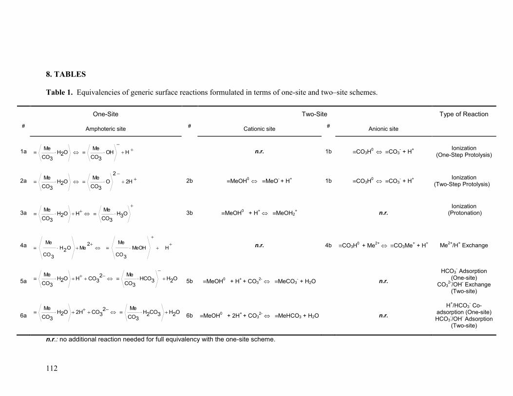
112

8. TABLES

Table 1. Equivalencies of generic surface reactions formulated in terms of one-site and two–site schemes.

One-Site

Two-Site Type of Reaction

# Amphoteric site

# Cationic site

# Anionic site

1a

H OH

3CO

Me O2H

3CO

Me n.r. 1b CO3H

0 CO3

- + H

+

Ionization (One-Step Protolysis)

2a

H2

2

O

3CO

Me O2H

3CO

Me 2b MeOH

0 MeO

- + H

+ 1b CO3H

0 CO3

- + H

+

Ionization (Two-Step Protolysis)

3a O3H

3CO

Me H O2H

3CO

Me

3b MeOH0 + H

+ MeOH2

+

n.r. Ionization

(Protonation)

4a

H MeOH

3CO

Me

2Me O2H

3CO

Me

n.r. 4b CO3H

0 + Me

2+ CO3Me

+ + H

+ Me

2+/H

+ Exchange

5a O2H3HCO

3CO

Me

23COH O2H

3CO

Me

5b MeOH0 + H

+ + CO3

2- MeCO3

- + H2O n.r.

HCO3- Adsorption

(One-site) CO3

2-/OH

- Exchange

(Two-site)

6a O2H3CO2H

3CO

Me

23CO2H O2H

3CO

Me

6b MeOH0 + 2H

+ + CO3

2- MeHCO3 + H2O

n.r.

H+/HCO3

- Co-

adsorption (One-site) HCO3

-/OH

- Adsorption

(Two-site)

n.r.: no additional reaction needed for full equivalency with the one-site scheme.

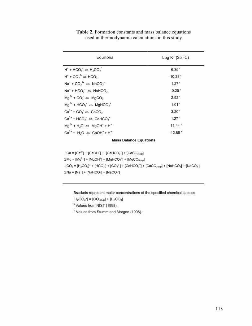
113

Table 2. Formation constants and mass balance equations

used in thermodynamic calculations in this study

Equilibria Log K (25 C)

H

+ + HCO3

- H2CO3

* 6.35 a

H+ + CO3

2- HCO3 10.33 a

Na+ + CO3

2- NaCO3

- 1.27 a

Na+ + HCO3

- NaHCO3 -0.25 a

Mg2+

+ CO3- MgCO3 2.92 a

Mg2+

+ HCO3- MgHCO3

+ 1.01 a

Ca2+

+ CO3- CaCO3 3.20 a

Ca2+

+ HCO3- CaHCO3

+ 1.27 a

Mg2+

+ H2O MgOH+ + H

+ -11.44 b

Ca2+

+ H2O CaOH+

+ H+ -12.85 b

Mass Balance Equations

Ca = [Ca2+] + [CaOH+] + [CaHCO3+] + [CaCO3(aq)]

Mg = [Mg2+] + [MgOH+] + [MgHCO3+] + [MgCO3(aq)]

CO2 = [H2CO3]* + [HCO3-] + [CO3

2-] + [CaHCO3+] + [CaCO3(aq)] + [NaHCO3] + [NaCO3

-]

Na = [Na+] + [NaHCO3] + [NaCO3-]

Brackets represent molar concentrations of the specified chemical species

[H2CO3*] = [CO2(aq)] + [H2CO3]

a Values from NIST (1998).

b Values from Stumm and Morgan (1996).

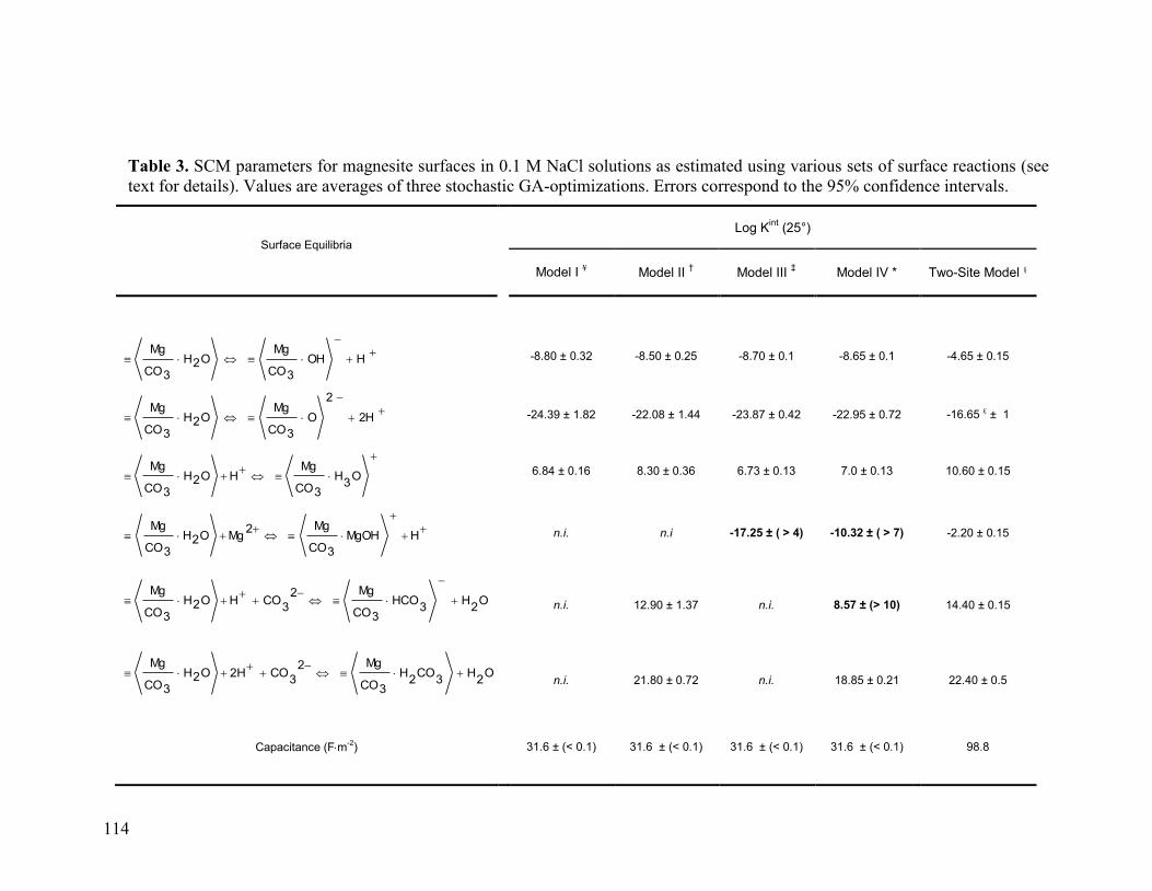
114

Table 3. SCM parameters for magnesite surfaces in 0.1 M NaCl solutions as estimated using various sets of surface reactions (see

text for details). Values are averages of three stochastic GA-optimizations. Errors correspond to the 95% confidence intervals.

Surface Equilibria

Log Kint

(25°)

Model I ¥

Model II

† Model III

‡ Model IV * Two-Site Model §

H OH

3CO

Mg O2H

3CO

Mg

-8.80 ± 0.32 -8.50 ± 0.25 -8.70 ± 0.1 -8.65 ± 0.1 -4.65 ± 0.15

H2

2

O

3CO

Mg O2H

3CO

Mg

-24.39 ± 1.82 -22.08 ± 1.44 -23.87 ± 0.42 -22.95 ± 0.72 -16.65 £ ± 1

O3

H

3CO

Mg H O2H

3CO

Mg

6.84 ± 0.16 8.30 ± 0.36 6.73 ± 0.13 7.0 ± 0.13 10.60 ± 0.15

H MgOH

3CO

Mg

2Mg O2H

3CO

Mg

n.i. n.i -17.25 ± ( > 4) -10.32 ± ( > 7) -2.20 ± 0.15

O2

H3

HCO

3CO

Mg

2

3COH O2H

3CO

Mg

n.i. 12.90 ± 1.37 n.i. 8.57 ± (> 10) 14.40 ± 0.15

O2

H3

CO2

H

3CO

Mg

2

3CO2H O2H

3CO

Mg

n.i. 21.80 ± 0.72 n.i. 18.85 ± 0.21 22.40 ± 0.5

Capacitance (Fm-2)

31.6 ± (< 0.1) 31.6 ± (< 0.1) 31.6 ± (< 0.1) 31.6 ± (< 0.1) 98.8

115

(Footnote of Table 3)

Intrinsic constants with large uncertainties in bold (see text for details). Optimization performed using data set at following conditions:

(¥)CO2 < 1.7 mM, Mg < 1 mM; (†) 1 < CO2 < 10 mM and 1.2 < Mg < 3 mM (optimization subsequently repeated with full data

set); (‡) 0.9 < CO2 < 3.6 mM and 1 < Mg < 7 mM; (*) Full data set. (§) Log10 Kint values for two-site-based equivalent reactions

taken from Pokrovsky et al., 1999a. (£) Value reflects full surface protolysis (cationic + anionic site). n.i. = reaction not included in the

model. Bold-type identify Log10 Kint with large uncertainties. Note that these values cannot be directly compared with those of

Wolthers et al. (2008) because their Log10 Kint values correspond to a „„hybrid” CCM-CD-MUSIC model. These authors only calibrated

ionization constants (generic reaction 1a–3a, plus a novel reaction involving the doubled-protonated carbonate corner site: >CO3H2+)

according to the CD-MUSIC-Triple-Plane model, whereas all constituent ion adsorption reactions (generic reaction 4a–6a) were taken

from Pokrovsky et al. (1999a), CCM approach) without further adjustment.

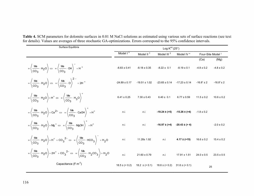
116

Table 4. SCM parameters for dolomite surfaces in 0.01 M NaCl solutions as estimated using various sets of surface reactions (see text

for details). Values are averages of three stochastic GA-optimizations. Errors correspond to the 95% confidence intervals.

Surface Equilibria

Log Kint

(25°)

Model I ¥

Model II

† Model III

‡ Model IV * Four-Site Model §

(Ca) (Mg)

H OH

3CO

Me O2H

3CO

Me

-8.83 ± 0.41 -8.18 ± 0.35 -8.22 ± 0.1 -8.19 ± 0.1 -4.8 ± 0.2 -4.8 ± 0.2

H2

2

O

3CO

Me O2H

3CO

Me

-24.89 ± 0.17 -19.51 ± 1.02 -23.65 ± 0.14 -17.23 ± 0.14 -16.8£ ± 2 -16.8£ ± 2

O3

H

3CO

Me H O2H

3CO

Me

6.41 ± 0.25 7.30 ± 0.43 6.40 ± 0.1 6.77 ± 0.59 11.5 ± 0.2 10.6 ± 0.2

H CaOH

3CO

Me

2Ca O2H

3CO

Me

n.i. n.i. -19.24 ± (>5) -15.26 ± (>4) -1.8 ± 0.2

H MgOH

3CO

Me Mg O2H

3CO

Me

n.i. n.i. -16.97 ± (>4) -20.43 ± (> 4) -2.0 ± 0.2

O2

H3

HCO

3CO

Me

2

3COH O2H

3CO

Me

n.i. 11.28± 1.92 n.i. 4.17 ± (>15) 16.6 ± 0.2 15.4 ± 0.2

O2

H3

CO2

H

3CO

Me

2

3CO2H O2H

3CO

Me

n.i. 21.60 ± 0.79 n.i. 17.91 ± 1.51 24.0 ± 0.5 23.5 ± 0.5

Capacitance (Fm-2

)

18.5 ± (< 0.2) 18.2 ± (< 0.1) 18.6 ± (< 0.2) 31.6 ± (< 0.1)

25

117

(Footnote of Table 4)

Intrinsic constants with large uncertainties in bold (see text for details). “Me” represents generically either Ca2+or Mg2+. Optimization

performed using data set at following conditions: (¥) CO2 < 1 mM, Ca < 0.5 mM, and Mg < 0.8 mM; (†) 0.6 < CO2 < 3 mM, 0.18

< Mg < 1.5 mM, and 0.06 < Ca < 1.5 mM (optimization subsequently repeated with full data set); (‡) 2< CO2 < 2.7 mM, 1.1 < Mg

< 2.7 mM, and 1.1 < Ca < 2.7 mM; (*) Full data set. (§) Log10 Kint values for four-site-based equivalent reactions taken from

Pokrovsky et al., 1999b. (£) Value reflects full surface protolysis (cationic + anionic site). n.i. = reaction not included in the model.

Bold-type identify Log10 Kint with large uncertainties. Note that these values cannot be directly compared with those of Wolthers et al.

(2008) because their Log10 Kint values correspond to a „„hybrid” CCM-CD-MUSIC model. These authors only calibrated ionization

constants (generic reaction 1a–3a, plus a novel reaction involving the doubled-protonated carbonate corner site: >CO3H2+) according

to the CD-MUSIC-Triple-Plane model, whereas all constituent ion adsorption reactions (generic reaction 4a–6a) were taken from

Pokrovsky et al. (1999b), CCM approach) without further adjustment.

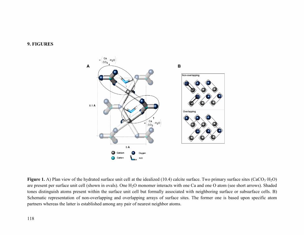
118

9. FIGURES

Figure 1. A) Plan view of the hydrated surface unit cell at the idealized (10.4) calcite surface. Two primary surface sites (CaCO3·H2O)

are present per surface unit cell (shown in ovals). One H2O monomer interacts with one Ca and one O atom (see short arrows). Shaded

tones distinguish atoms present within the surface unit cell but formally associated with neighboring surface or subsurface cells. B)

Schematic representation of non-overlapping and overlapping arrays of surface sites. The former one is based upon specific atom

partners whereas the latter is established among any pair of nearest neighbor atoms.

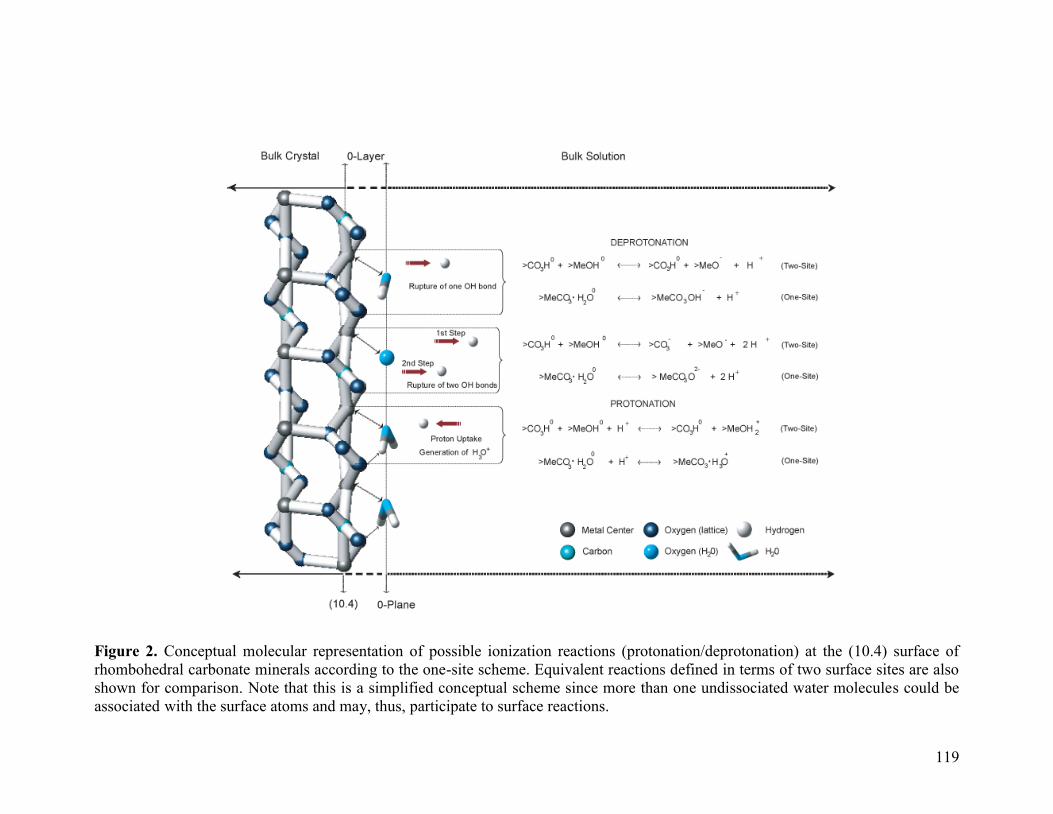
119

Figure 2. Conceptual molecular representation of possible ionization reactions (protonation/deprotonation) at the (10.4) surface of

rhombohedral carbonate minerals according to the one-site scheme. Equivalent reactions defined in terms of two surface sites are also

shown for comparison. Note that this is a simplified conceptual scheme since more than one undissociated water molecules could be

associated with the surface atoms and may, thus, participate to surface reactions.

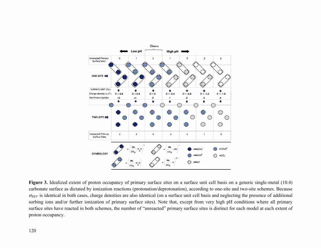
120

Figure 3. Idealized extent of proton occupancy of primary surface sites on a surface unit cell basis on a generic single-metal (10.4)

carbonate surface as dictated by ionization reactions (protonation/deprotonation), according to one-site and two-site schemes. Because

REF is identical in both cases, charge densities are also identical (on a surface unit cell basis and neglecting the presence of additional

sorbing ions and/or further ionization of primary surface sites). Note that, except from very high pH conditions where all primary

surface sites have reacted in both schemes, the number of “unreacted” primary surface sites is distinct for each model at each extent of

proton occupancy.

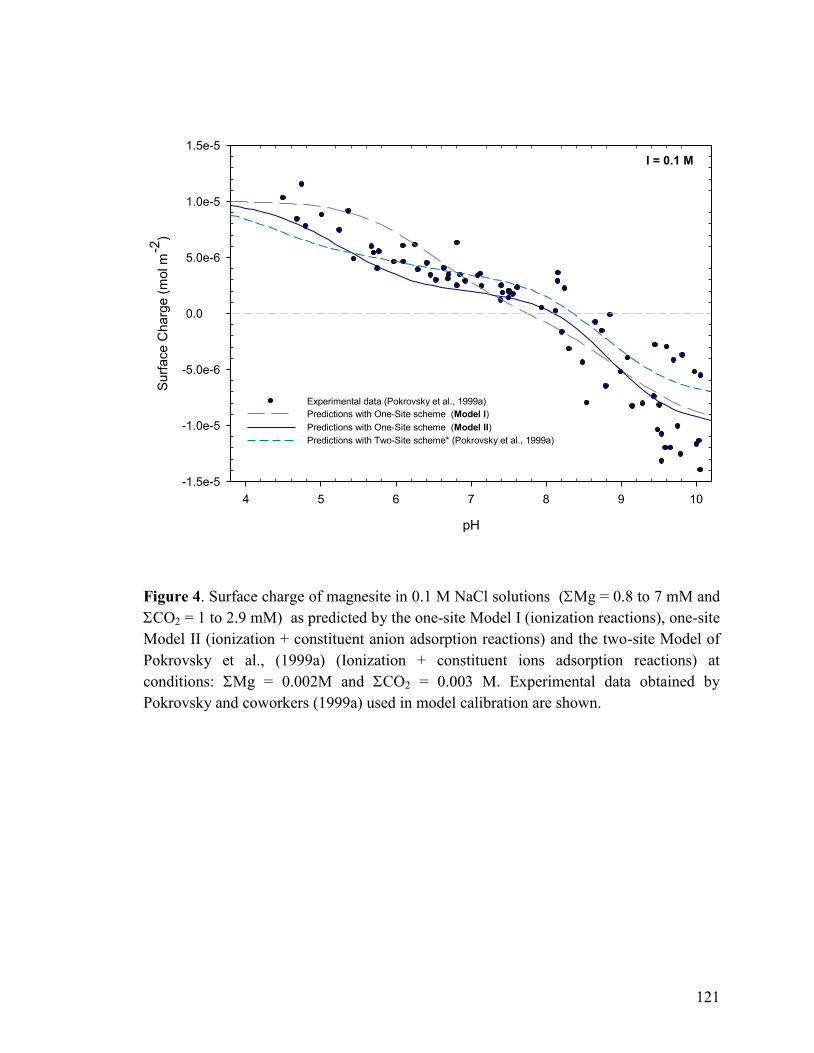
121

pH

4 5 6 7 8 9 10

Surf

ace C

harg

e (

mol m

-2)

-1.5e-5

-1.0e-5

-5.0e-6

0.0

5.0e-6

1.0e-5

1.5e-5

Experimental data (Pokrovsky et al., 1999a)

Predictions with One-Site scheme (Model I)

Predictions with One-Site scheme (Model II)

Predictions with Two-Site scheme* (Pokrovsky et al., 1999a)

I = 0.1 M

Figure 4. Surface charge of magnesite in 0.1 M NaCl solutions (Mg = 0.8 to 7 mM and

CO2 = 1 to 2.9 mM) as predicted by the one-site Model I (ionization reactions), one-site

Model II (ionization + constituent anion adsorption reactions) and the two-site Model of

Pokrovsky et al., (1999a) (Ionization + constituent ions adsorption reactions) at

conditions: Mg = 0.002M and CO2 = 0.003 M. Experimental data obtained by

Pokrovsky and coworkers (1999a) used in model calibration are shown.

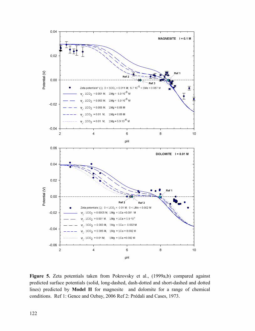
122

Figure 5. Zeta potentials taken from Pokrovsky et al., (1999a,b) compared against

predicted surface potentials (solid, long-dashed, dash-dotted and short-dashed and dotted

lines) predicted by Model II for magnesite and dolomite for a range of chemical

conditions. Ref 1: Gence and Ozbay, 2006 Ref 2: Prédali and Cases, 1973.

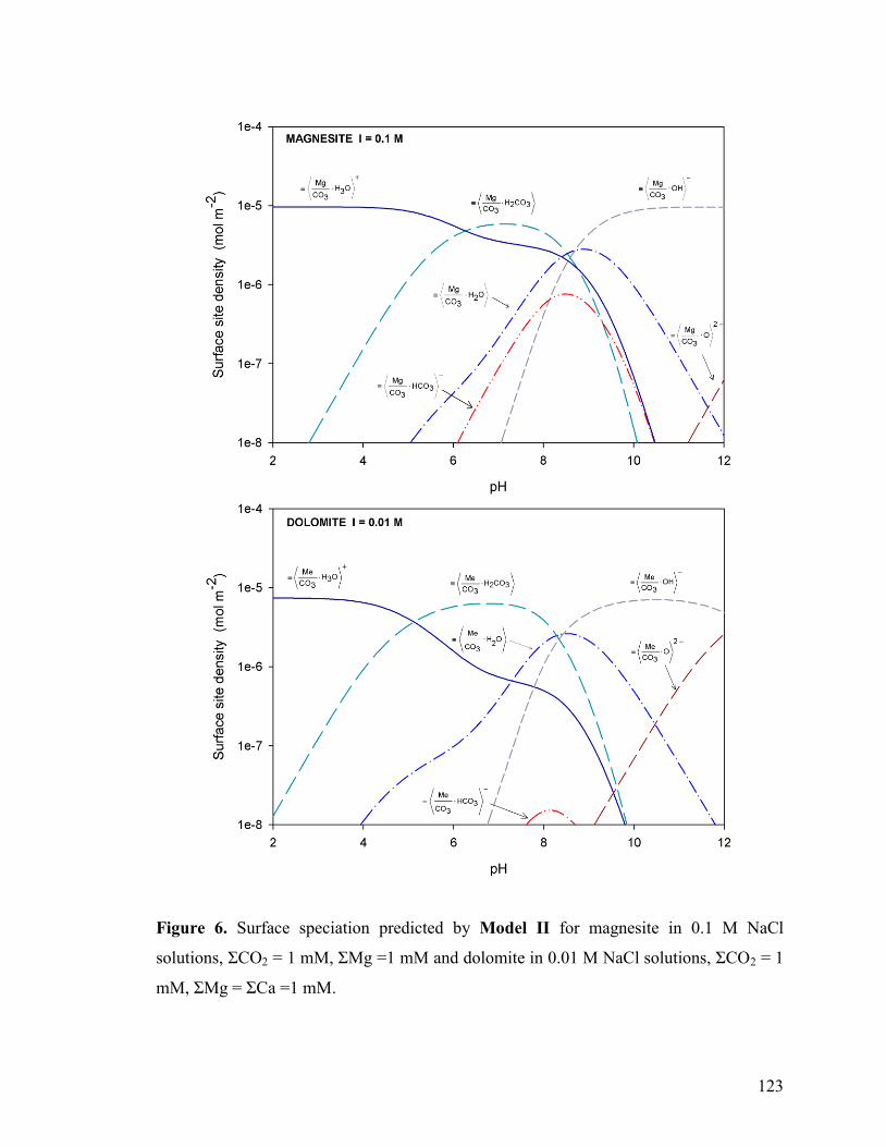
123

Figure 6. Surface speciation predicted by Model II for magnesite in 0.1 M NaCl

solutions, ΣCO2 = 1 mM, ΣMg =1 mM and dolomite in 0.01 M NaCl solutions, ΣCO2 = 1

mM, ΣMg = ΣCa =1 mM.

124


Having developed and successfully tested the single surface site formalism for magnesite

and dolomite, this scheme was tested on other rhombohedral carbonate minerals to

generalize its application to the construct of SCMs for this type of minerals. This aspect is

addressed in the following chapter, “Acid-Base Behavior of the NiCO3(s) Surface in NaCl

Solutions”.

Because NiCO3(s) (gaspeite) is the least reactive of known naturally-occurring

rhombohedral carbonate minerals in aqueous solutions, it was selected as a surrogate to

obtain additional experimental information on the surface reactivity of calcite-type

minerals in NaCl solutions by means of conventional titration techniques and micro-

electrophoresis. In this study we found that surface protonation of NiCO3(s) is strongly

affected by the background electrolyte beyond what is typically observed in most mineral

surfaces such as metal oxides, silicates and clay surfaces.

A simple one-site-based SCM is postulated that successfully simulates proton

adsorption and electrokinetic data acquired at I ≤ 0.01 M and outperforms the predictive

power of more sophisticated SCMs tested in this study. The most important insights

obtained in this study is that the background electrolyte affects the properties of the

gaspeite surface (surface protonation and the development of surface charge) possibly

through modification of the structure of the electrified interfacial layer, perturbation of

the solvent structure dynamics and the affinity of water molecules and adsorbing ions

towards the mineral surface. These observations challenge earlier conceptions on

carbonate mineral surfaces that traditionally considered surface charge acquisition

processes on these minerals as chemically indifferent to background electrolyte ions.

125

CHAPTER 4

ACID-BASE BEHAVIOR OF THE GASPEITE (NiCO3(S)) SURFACE IN NaCl SOLUTIONS


1, Oleg S. Pokrovsky

2, Jacques Schott

2 and

Jeanne Paquette1



2Géochimie et Biogéochimie Expérimentale,

LMTG, UMR 5563,

Université de Toulouse – CNRS, 14, Avenue Edouard Belin 31400 Toulouse, France



To be submitted to: Langmuir

126

ABSTRACT

The acid-base properties of the gaspeite surface in NaCl solutions were investigated at

nearly-ambient conditions (25 3 C and 1 atm) by means of conventional acidimetric

and alkalimetric titration techniques and microelectrophoresis. Dissolution-corrected

proton adsorption densitites and electrokinetic data were obtained over a pH range of 5 to

10 under CO2-free conditions at three ionic strengths (0.001, 0.01 and 0.1 M). Over the

entire pH range investigated in this study, surface protonation and electrokinetic mobility

are strongly affected by the backgrund electrolyte leading to a significant shift in the pH

of Zero Net Proton Charge (pHznpc) and the pH of isoelectric point (pHiep) towards lower

pH with increasing ionic strength. This is conceptually explained by the role exerted by

the background electrolyte which affects in more than one way the properties of the

gaspeite surface (surface protonation and the development of surface charge) possibly

through modification of the structure of the electrified interfacial layer, perturbation of

the solvent structure dynamics, and the affinity of water molecules and adsorbing ions

towards the mineral surface. These observations challenge earlier conceptions that

traditionally considered surface charge acquisition processes on carbonate minerals as

chemically indifferent to background electrolyte ions. Although no self-consistent

interpretation was found to explain all data, a simple SCM involving ionization reactions

closely simulates proton adsorption data and reasonably predicts the electrokinetic

behavior of gaspeite supensions at low (I=0.001 M) and intermediate (I=0.01 M) ionic

strengths. Nevertheless, the influence of the background electrolyte on the development

of surface charge and surface protonation must be further investigated.

Keywords: Nickel carbonate, gaspeite acid-base behavior, surface ionization, sodium

adsorption

127

1. INTRODUCTION

Carbonate minerals are of considerable environmental significance due to their ubiquity

and high chemical reactivity in natural aquatic systems. In aqueous solutions, their

macroscopic properties are controlled by multiple homogeneous and heterogeneous

equilibria among which, surface reactions (i.e. ionization and adsorption) are recognized

to play a critical role (Van Capellen et al., 1993). This realization has stimulated

numerous scientific studies on the surface reactivity of hydrated carbonate surfaces

(Pokrovsky et al., 1999a,b; Brady et al., 1999; Pokrovsky and Schott, 2002; Jordan et al.,

2001; Duckworth and Martin, 2003; Kendall and Martin, 2005). Particular attention has

been paid to the derivation of empirical and semi-empirical relationships to represent ion

partitioning between the aqueous phase and the surface of calcite, aragonite, magnesium-

bearing carbonates and, to a lesser extent, other divalent carbonate minerals (Morse and

Mackenzie, 1990).

Despite these efforts, the quantitative characterization of most carbonate surfaces

has lagged behind that of other mineral surfaces such as metal oxides and silicates (Davis

and Kent, 1990). This task is a sizable challenge because of the higher reactivities (i.e.,

faster reaction rates and greater solubilities) of carbonates relative to other minerals, and

the occurrence of stepwise and/or parallel reactions (e.g., adsorption, surface

precipitation, co-precipitation, dissolution) that are difficult to resolve experimentally

(Morse, 1986). Dissolution and precipitation reactions, in particular, interfere with the

characterization of surface equilibria. These considerations drove earlier workers to

develop a novel experimental protocol, based upon the use of a fast flow-through reactor,

to minimize the contribution of dissolution and precipitation, during acid-base titrations

128

performed on some sparingly soluble carbonates (Charlet et al., 1990). This protocol was

used by several researchers to obtain surface charge data for siderite, rhodochrosite

(Charlet et al., 1990; Van Capellen et al., 1993), magnesite (Pokrovsky et al., 1999a) and

dolomite (Pokrovsky et al., 1999b; Brady et al., 1999). On the basis of their results, they

proposed surface complexation models (SCMs) for these minerals that include ionization

and lattice constituents adsorption reactions in analogy to acid-base and complexation

equilibria in solution for the CO2(s)-H2O system. Unfortunately, the application of this

approach to highly reactive carbonate minerals such as calcite or aragonite is not feasible

because their fast dissolution kinetics interferes significantly with the computation of

surface charge (Van Cappellen et al., 1993).

Conversely, gaspeite, a nickel-bearing carbonate with a calcite-type structure

displays the slowest dissolution kinetics of all naturally-occurring rhombohedral

carbonate minerals in aqueous solutions (Pokrovsky and Schott, 2002), and thus, it is

amenable to investigations by experimental protocols commonly applied to metals oxides

but unsuitable for other carbonate minerals. Natural gaspeite specimens typically contain

intermediate to high amounts of magnesium which closely reflect the physical properties

of the hypothetical solid solution: Ni0.5Mg0.5(CO3)2 (Kohls and Rodda, 1966). In contrast,

only a small degree of Ca2+

substitution by Ni 2+

ions in the calcite structure has been

experimentally confirmed (Hoffmann and Stipp, 2001), which may explain why a NiCO3-

CaCO3 solid solution series has not be found in nature.

Regardless of their purity, NiCO3(s)-bearing specimens display a rhombohedral

structure predominantly bounded by the (10.4) domain (Bermanec et al., 2000), a

common feature of other carbonate isomorphs such as calcite, magnesite and dolomite

(Reeder, 1990). This characteristic makes nickel carbonate a suitable surrogate to obtain

129

information on the surface reactivity of calcite-type minerals. Although the formation of

hydrated NiCO3(s) phases, NiCO32Ni(HO)2 and NiCO34H2O, is possible at room

temperature (Hoffmann and Stipp, 2001), pure hydrothermally-synthesized gaspeite

rhombohedral crystals are thermodynamically stable at room temperature and, are

therefore, suitable for experimental investigations at ambient conditions.

To our knowledge, a single investigation of the surface reactivity of gaspeite has

been carried out to date (Pokrovsky and Schott, 2002), which included a study of its

electrokinetic behavior in aqueous solutions over a range of pH (6 to 9) and a fairly

constant aqueous composition (CO2 = 510–3

M, 10–6

Ni 210–6

and I = 0.005 M).

No systematic investigation on the acid-base properties of this mineral, however, has been

conducted under a wide range of chemical conditions.

In this study, a series of acidimetric and alkalimetric titrations are performed on

NiCO3(s) suspensions at three ionic strengths within a wide pH range (5 to 10) where

dissolution effects can be quantitatively accounted for in the computation of proton

adsorption. In addition, numerous electrophoretic measurements are performed under a

wide range of solution conditions (pH and ionic strength). These data are used to calibrate

and test surface complexation reactions for gaspeite formulated according to the one-site

scheme previously introduced for the hydrated (10.4) calcite surface (Villegas-Jiménez et

al., 2009a) and successfully extended to other rhombohedral carbonate minerals as

discussed in Chapter 3 of this thesis.

130

2. MATERIALS AND METHODS

2.1 Preparation and Standardization of Reagents

All solutions were prepared using analytical grade reagents and high purity deionized

(MilliQ, ~ 18 Mohm cm-1

) water. Hydrochloric acid solutions were prepared from 32%

HCl and standardized using gravimetrically prepared tris(hydroxymethyl)methylamine

(TRIS) solutions that were kept refrigerated. NaOH solutions were prepared every two to

three days from NaOH pellets using MilliQ water from which CO2 had been removed by

boiling and bubbling of ultrapure N2 for at least three hours. These solutions were titrated

against standardized HCl solutions before use and were kept under a N2 atmosphere to

minimize CO2 absorption. The ionic strength of the solutions was adjusted (i.e., 0.001,

0.01 or 0.1 M) using a 1 M NaCl solution.

2.2 Chemical Analyses

Alkalinity measurements were carried out using a Radiometer TTT85 titration system

using standardized HCl. The end-point of the titration was identified by the first-

derivative method (APHA-AWWA-WPCF, 1998). The precision of the analysis was ±

0.05 % and the limit of detection was 0.6 mmol kg-1

. Nickel concentrations were

measured by Graphite Furnace Atomic Absorption Spectrophotometry (GFAAS,

AAnalystTM

800 Perkin Elmer) using external standards (i.e., diluted from a 1000 ppm

Certified Standard). The detection limit of this analysis was 0.8 μg L-1

with a

reproducibility of ± 4 %. Free carbonate ion concentrations were determined using a

combination ELIT Ion 8091 ion selective electrode calibrated against NaHCO3 standards

covering a relatively wide range of CO32-

ion concentrations (5 M to 1 mM), as

calculated from thermodynamic equilibrium calculations performed iteratively using the

131

Newton-Raphson method implemented in an in-house computer Matlab©

routine using

alkalinity and pH measurements as input. Equilibrium constants and mass balance

equations used in all the thermodynamic calculations of this study are given in Table 1.

2.3 Gaspeite Synthesis

Gaspeite was hydrothermally synthesized during 2 months at 250 °C in titanium reactors

from analytical reagent grade hydrous nickel carbonate. Synthesis was performed in

solutions of pH (25 °C) ~ 4 and pCO2 of about 40 atm, achieved by addition of ~10 grams

of solid CO2 per 200 mL of distilled water in the reactor before the synthesis.

The precipitated powder was oven-dried at 50°C, dry-sieved, and the 0.1-50 m

size fraction isolated for the surface titrations. Its mineralogy and crystallinity was

confirmed by X-ray diffraction analysis using a G3000 INEL diffractometer. All major

peaks of gaspeite were revealed, and no trace of other phases or impurities were found.

The specific surface area of the < 50 m size fraction, obtained by sieving, was

determined by the multiple-point Ar-BET method (Brunauer et al., 1938) before and after

the titrations to check for variations resulting from the dissolution of the smaller particles.

Note that to minimize the surface irregularities, no grinding of synthetic powder was

performed. The surface area of freshly prepared powder was of 0.38 m2

g-1

; but after the

first titration, it decreased to 0.30 m2 g

-1, probably due to complete dissolution of ultrafine

particles. After repeated titrations (more than two) of the same powder, the specific

surface area remained constant: 0.23 m2 g

-1 within the uncertainty of the measurements (±

0.005 m2 g

-1). For the sake of consistency and considering the limited amount of available

gaspeite powder, only data obtained from surface titrations using recycled powders (n >

2) were used in the computation of proton adsorption. After each titration, the powder

132

was extensively rinsed with Milli-Q® water to remove surface impurities arising from

previous titrations (i.e. adsorbed protons, nickel or background electrolyte ions), filtered,

and oven-dried at 70°C before being re-used. The excellent reproducibility of titration

data acquired at all ionic strengths examined in this study (see below) confirms the

absence of significant amounts of recalcitrant contaminants in the recycled powder (in

contrast to what it is sometimes observed for metal oxide surfaces) and justifies its re-use

in the experiments presented in this study.

2.4 Surface Titrations

2.4.1 pH Electrode Calibration

Surface titrations were conducted with a Radiometer Titralab 865 titrator equipped with a

Schott N6980 pH electrode, suitable for pH measurements in concentrated suspensions,

and a Teflon-coated suspended stir bar to minimize grinding of the powder. The

Nernstian behavior of the electrode was checked before and after each experiment against

four NIST-traceable pH buffers (4, 7, 10 and 11) at 25 0.5°C and it was, in all cases,

very similar ( 0.8 mV) to the theoretical value at 25°C (i.e. 59.2 mV).

The pH electrode was calibrated on the total proton molar concentration scale

according to:

j

0 E EE

][H log

F

RT 2.303 (1)

where E and E° are the observed and the standard potential values for a given ionic

strength, F is the Faraday Constant, R is the universal gas constant, T is the absolute

temperature, [H+] is the total proton molar concentration and Ej is the junction potential.

133

For accurate pH determinations, the effect of the background electrolyte must be

properly accounted for in the calibration of the pH electrode (Wiesner et al., 2006). To

this end, we followed the method described by Pehrsson et al (1976). Briefly, this method

consists of estimating the junction potential which is defined by: Ej = jH [H+] for the

acidic regime (pH < 7) and by: Ej = jOH [OH-] for the alkaline regime (pH > 7). The

coefficients jH and jOH are characteristic of the electrode and the ionic medium. They were

estimated independently by titration of 1 mM HCl solutions with standardized equimolar

NaOH (acidic regime) or of 1 mM NaOH solutions with standardized equimolar HCl

(alkaline regime). In all cases, the ionic strength of the solutions was fixed with NaCl at

the values of interest (i.e. 0.001, 0.01 and 0.1 M). The coefficients jH and jOH were readily

obtained from a linear regression between E – 59.2 log [H+] against [H

+] (or [OH

-] for the

alkaline regime) which yielded jH (or jOH) as the slope and E° as the intercept. Using these

coefficients and Equation 1, a more accurate estimate of E° was computed from blank

titrations of the background electrolyte in the absence of solids conducted at both, the

acid and the alkaline regimes under identical conditions as for the suspension titrations

(i.e. pH range, ionic strength). For each pH regime and ionic strength, the mean of

multiple E° determinations were adopted for pH determination. As the same reaction

vessel was used for both blank and suspension titrations, wall effects (i.e. proton

adsorption) are implicitly considered in the estimation of E0. For a given set of E

0, jH and

jOH values, the proton molar concentration was calculated numerically via Equation 1

using the Newton-Raphson iterative method incorporated in an in-house Matlab©

subroutine (available in the appendices to this thesis). The Davies equation was used to

estimate activity coefficients and compute the pH from the calculated molar

concentrations (Stumm and Morgan, 1996).

134

2.4.2 Conditions of Surface Titrations

Preliminary titrations revealed that highly concentrated gaspeite suspensions are required

to resolve the contribution of adsorption reactions in determining the bulk solution

equilibria. Consequently, all titrations were conducted at a solid/solution ratio of 50 g L-1

.

The stability criterion of the automatic titrator for the pH electrode was set at 0.3 mV min-

1 to minimize the duration of the titration (and minimize dissolution effects and electrode

drift) and to maintain an acceptable accuracy. Two different types of titrations were

conducted at three ionic strengths (0.001, 0.01, 0.10 M NaCl). Type-I experiments, run in

triplicate to verify their reproducibility, were acidimetric titrations performed within the

pH range of 5 to 10. The suspensions were first prepared in CO2-free Milli-Q

water (as

described in section 2.1) and allowed to equilibrate for about 10 minutes before the pH

was adjusted by the addition of a known amount of the standardized NaOH solution and

the titration initiated shortly after. A short pre-equilibration time is critical to allow for the

hydration of the surface while keeping dissolution to a minimum. The duration of these

titrations varied from 8 to 10 hours.

The dissolved nickel concentration was monitored throughout these experiments

in order to determine the consumption of protons due to gaspeite dissolution, as described

by the following reaction:

NiCO3(s) + 2 H+ Ni

2+ + H2O + CO2 (g) (2)

This was achieved by carrying out numerous additional titrations (n > 10), under

the same experimental conditions (i.e., pH range, ionic strength, duration of titration, etc),

that were interrupted at critical pH values along the titration curve. Aliquots of the

135

decanted solution were withdrawn and syringe-filtered through a 0.45 m Milipore HA-

type filter into HDPE bottles. The solutions were acidified with a 1% equivalent volume

of concentrated HCl and stored for later nickel analysis by GFAAS. These data were fit to

logarithmic expressions that served to interpolate nickel concentrations at given pH

values.

Type-II experiments were alkalimetric titrations of gaspeite suspensions prepared

in CO2–free Milli-Q

water with no pre-addition of NaOH and a pre-equilibration time of

less than 10 minutes. Given the enhanced dissolution kinetics of gaspeite at low pH

(Pokrovsky and Schott, 2002), these experiments were initiated at circumneutral pH and

ended at a pH of about 10. The duration of these titrations was between 3 to 4 hours.

To prevent carbonate adsorption reactions from competing with the acid-base

equilibria at reactive adsorption sites, suspensions were maintained CO2-free by bubbling

ultrapure N2 in the suspensions throughout the titrations. In preliminary experiments, the

absence of significant amounts of inorganic carbon in the system was verified by

alkalinity determinations and by direct measurements of the carbonate ion concentration

using the carbonate ion selective electrode at pre-determined points along the titration

curve. Evaporation of the experimental solution was minimized by keeping a positive

pressure of H2O vapor-saturated N2 in the headspace overlying the reaction vessel. In all

cases, the extent of evaporation was determined gravimetrically to be less than 1% over

the course of whole titrations (up to 10 hours).

136

2.5 Computation of Proton Adsorption

In contrast to minerals containing protons and/or hydroxyls groups within their lattices

(e.g., kaolinite, goethite, lepidocrocite, hydroxylapatite), pure divalent metal carbonate

minerals (MeCO3(s)) do not contain protons or hydroxyls groups within their lattices, and

hence, no proton imbalance develops at their dry surfaces. In other words, no proton

excess (or deficit) is introduced into the mineral-H2O system upon MeCO3(s) immersion

in water. Thus, in the case of gaspeite, and provided CO2(g) exchange with the atmosphere

(affecting the proton and carbon balance in solution upon H2CO3(aq) formation) is

prevented or properly accounted for (as in our study, see below), net proton adsorption

densities, HNet

, can be computed by subtracting the experimentally-measured proton

balance in solution from the theoretical proton balance following incremental acid and/or

base additions:

H - OH = (1/AS) · (CA – CB – [H+] + [OH

-] – [H

+]diss) (3)

where H and OH are the calculated adsorption densities of H+ and OH

-

(mol m-2

), CA and CB are the total molar concentrations of the added acid and base, [H+]

and [OH-] are the estimated molar concentrations obtained from pH measurements, A is

the specific surface area (m2 g

-1), S is the solid concentration (g L

-1), and [H

+]diss

represents the net concentration of protons consumed by the dissolution of gaspeite.

Because, for gaspeite, HNet

data are directly obtained with Equation 3, no referencing to

the Point of Zero Net Proton Charge (PZNPC) is required, in contrast to H- and/or OH-

containing minerals that require a pre-determination of the PZNPC by suitable

137

approaches to compute net proton adsorption densities from apparent proton adsorption

data, Happ

(Anderson and Sposito, 1992, Chorover and Sposito, 1995). It follows that the

PZNPC determined across the pH scale for a given ionic strength (i.e., pHpznpc,I) can be

directly obtained from adequate analysis of HNet

data vs pH plots (see below).

According to reaction 2, two protons are needed for the release of one Ni2+

ion

which, in turn, can form a number of hydroxo-complexes depending on the pH of the

solution. Upon the formation of these complexes, protons will be released to the solution,

and thus, will contribute to the computed proton balance. This can be accounted for by

the following expressions:

1

)(

3

321

)(

2

211

3

2

2

22

2

)()()(1

OHNiH

Ni

OHNiH

Ni

NiOHH

Ni

a

KKK

a

KK

a

KNi

(4)

NiOHH

NiNi

a

KNiOH

22 1 (5)

2

2

)(

2

2

)( OHNiH

NiOHNiOH

a

KNiOH

(6)

3

22

3

)(

3

)(3

)(OHNiH

OHNiNiOH

a

KNiOH

(7)

where i and i represent, respectively, the ionization factors and the activity coefficients

of the aqueous species identified by the subscripts, K1-K3 are the thermodynamic stability

constants of the nickel hydroxo-complexes (see Table 1), and aH+ stands for the proton

activity. Thus, the net contribution of dissolution to the observed proton balance can be

computed from:

138

)NiOHNiOHNi

32diss (2 ]2[Ni ][H (8)

where [Ni2+

] is the total nickel molar concentration interpolated from the logarithmic fit

for a given pH and ionic strength (see preceding section).

Consideration of carbonate equilibria is, in principle, not necessary in the

computation of proton adsorption since our experimental set-up should allow for the

removal of most inorganic carbon evolved from gaspeite dissolution while preventing

contamination from atmospheric CO2(g). Nevertheless, the influence of undetected levels

of dissolved carbonate species (below the detection limits of alkalinity and CO32-

ion

selective electrode measurements) on the computation of proton adsorption is discussed

later.

Under the conditions of our titrations, the formation of freshly precipitated

Ni(OH)2(s), potentially affecting the proton and Ni2+

ion concentrations in solution, is not

expected to occur. Thermodynamic calculations using stability constants listed in Table 1

reveal that, in all cases, the experimental systems were kept below saturation with respect

to Ni(OH)2 throughout the titrations (saturation indices < 0.29).

2.6 Coagulation Experiments

To check whether electrolyte-induced coagulation occurred during our titrations and

could affect (upon reduction of the number of available reactive surface sites) the

computation of proton adsorption, we performed a semi-quantitative coagulation test. A

series of polypropylene centrifuge tubes containing aqueous gaspeite suspensions at

solid:solution ratios identical to those of the titrations (i.e. 50 g L-1

) were prepared at

139

varying concentrations of NaCl, which ranged from 100 μM to 1 M, including those

selected in our titrations. This test was run in duplicate. Tubes were shaken vigorously for

15 minutes using a Wrist Action Shaker (Burrell Model 75) followed by a settling period

of 2 minutes, a second stirring of 10 minutes and allowed to stand for 2 hours. A blank

(containing NiCO3(s) but no NaCl) was also tested for comparison (Hunter, 2001). A

slight coagulation effect (<1%) was observed for particles with a radius 0.6 μM

(representing less than 0.5% of the particle population) at ionic strengths equal or higher

than 0.01M, based on the turbidity of the supernatant of these suspensions measured by

UV spectrophotometry (Spectronic 601, Milton Roy Company). The packing volume of

the settled particles at all ionic strengths was nearly identical suggesting that no

significant aggregation of the larger particles took place (loose particles display larger

packing volume (Huang et al., 1991). Consequently, it is considered that the surface area

available for reaction was not significantly reduced by coagulation in any of the systems

investigated in this study.

2.7 Electrokinetic Measurements

The electrophoretic mobility of gaspeite particles in aqueous suspensions was measured

with a micro-electrophoremeter (Zeta-phoremeter IV 4000, CAD Instrumentation) at 25

4 °C under a range of conditions (i.e. pH, CO2, Ni and I). The NiCO3(s) suspensions

were prepared using the 0.5-1 m size fraction of the synthesized powder. According to

Stokes‟ law, this size fraction corresponds to the particle population remaining in

suspension after at least 12 (but less than 48 hours) of decantation in a 1 L Nalgene bottle.

Two series of electrokinetic experiments were carried out: Series-I consisted of individual

-potential measurements acquired in systems of variable composition where the pH was

140

varied with NaOH, CO2 was controlled with additions of NaHCO3 or Na2CO3 solutions

and Ni was varied by additions of supernatant from pre-equilibrated gaspeite

suspensions. In Series-II experiments, -potential measurements were performed in

systems of similar composition as those of the surface titrations, and therefore, only pH

and ionic strength were varied. To this end, several gaspeite suspensions were prepared in

CO2-free solutions at three ionic strengths (0.001, 0.01 and 0.1 M, prepared with NaCl)

and the pH of each suspension was varied by additions of HCl or NaOH. The -potentials

were measured for each selected pH value. Throughout these experiments, N2(g) was

constantly bubbled through the suspensions to prevent contamination from atmospheric

CO2(g).

The measurements were performed in triplicate on new suspensions in a quartz

cell connecting two Pd electrode chambers. The suspended particles were illuminated by

a 2 mW He/Ne laser and an electric field of 80 V (DC) cm-1

was applied. The particle

trajectories were followed by a CCD camera and data transmitted to a computer. The

electrophoretic mobility was derived from a time-lapsed image analysis and the

potentials were estimated using the Smoluchowski equation. This equation is applicable

to the ionic strengths and range of particle size used in this study (Hunter, 2001).

The pH of the suspensions was measured for each replicate using a Schott

Blueline 18 pH combination glass electrode. Aliquots of the supernatant were withdrawn

with a syringe immediately after the electrokinetic measurements, filtered through 0.45

m Millipore HA-type membranes and stored in HDPE bottles for later nickel and

alkalinity analyses (see section 2.2).

141

3. RESULTS AND DISCUSSION

3.1 Proton Adsorption on the Gaspeite Surface

3.1.1 Acidimetric Titrations

To illustrate the influence of NiCO3(s) dissolution on the computation of proton adsorption

for the acidimetric titrations, corrected (see section 2.5) and uncorrected surface proton

density measurements acquired at I = 0.01 M are presented in Figure 1. At low pH (pH <

6.5), dissolution significantly affects the proton balance in solution and the computation

of proton adsorption. Consequently, only corrected data computed from Equation 3 are

presented in the following discussion and were used to construct HNet

data vs pH plots at

each ionic strength, HNet

(pH, I), from which the pHpznpc,I values were obtained by fitting

the complete HNet

(pH, I) dataset to a polynomial function of pH and the resultant

function solved for pH at the condition H=0 (Chorover and Sposito, 1995).

The corrected proton adsorption curves generated at the three ionic strengths

investigated in this study are shown in Figure 2. Results from three titrations conducted at

each ionic strength are shown and highlight the good reproducibility of the

measurements. Inspection of these curves reveals four major common features: i) a clear

asymmetry across the pHznpc,I ii) a distinct “surface-charge buffer” region, within a pH

range of 6.5 to 9, for each ionic strength, iii) a strong dependency on the ionic strength

(i.e., position of the pHznpc,I), and iv) a lower number of maximum protonated and

deprotonated adsorption sites per square meter than the theoretical Ni or CO3 site density

predicted by crystallography (9.99 mol·m-2

). In addition, titration curves at the

intermediate and high ionic strengths (0.01M and 0.1 M) show a much larger maximum

142

number of negatively-charged sites at high pH than the maximum number of positively-

charged sites registered at low pH.

To account for the observed features of the titration curves, and in conformity with

the formalism adopted for the calcite surface (Villegas-Jiménez et al., 2009a), we elected

to explain surface protonation on the basis of surface reactions formulated on the basis of

a single primary surface site, (NiCO3)H2O0. Accordingly, ionization reactions were

postulated as follows:

O)3(H3CO

Ni H O2H

3CO

Ni (9)

H OH3CO

Ni O2H

3CO

Ni (10)

2H

2

O3CO

Ni O2H

3CO

Ni (11)

Reactions 10 and 11 describe, respectively, the step-wise and global deprotonation

reactions of the adsorbed H2O monomer(s). Whereas these reactions may account for the

asymmetry across the pHznpc,I, because two protons may be released at alkaline conditions

and only one proton is adsorbed under acidic conditions, they cannot explain the observed

ionic strength dependency.

Our data show that the background electrolyte has a strong effect on the gaspeite

surface as reflected by the shifting position of the pHznpc,I values and the extent of surface

143

protonation registered at each ionic strength (Figure 2). This effect is more than could be

generated by purely electrostatic interactions between background electrolyte ions and the

charged mineral surface as postulated by the Stern and the Triple-Layer models (Davis

and Kent, 1990). These models postulate that electrolyte ions are adsorbed via

electrostatics at a given distance from the mineral surface (-plane) increasing the extent

of surface protonation or deprotonation (away from the pHznpc) as a result of surface

charge neutralization. In other words, electrolyte adsorption decreases the electrostatic

work required to move protons through the electrified interfacial layer (EIL) affecting the

overall sorption processes:

elecint0 ΔGΔGΔG [12]

where ΔG0 is the Gibbs free energy of adsorption, ΔG

int is the intrinsic free-energy term:

ΔGint

= RT ln Kint

(where Kint

representing the intrinsic formation constant), and ΔGelec

is

the electrostatic work: ΔGelec

=ZFx, a function of the net charge transfer (ΔZ)

associated with the adsorption reaction, the Faraday constant, and the potential recorded

at the adsorbing plane “x” (x).

According to the Stern and the Triple-Layer models, in the absence of the

electrostatic effect (null charge), the electric potential vanishes, and thus, proton titration

curves must intersect at a certain pH commonly referred to as the common point of

intersection (CIP) or the point of zero salt effect (pHpzse). In contrast, our titration curves

do not yield a CIP as they do not intersect at their respective pHznpc,I. To reconcile this

observation, we propose that sodium ions compete with protons for available adsorption

144

sites, possibly adsorbing at the surface plane via chemical interactions and modifying the

extent of protonation of the gaspeite surface.

There is, in fact, some evidence that at high NaCl concentrations, the surface

reactivity of some carbonate minerals is severely affected. For instance, surface charge,

zeta potential, and dissolution kinetics of magnesite are also affected by NaCl (Pokrovsky

et al., 1999a; Gence and Ozbay, 2006) whereas Na+ ions significantly affect the extent of

Ca and Mg ion adsorption on dolomite at high ionic strengths (Brady et al., 1999).

Furthermore, specific adsorption of Na+ was proposed to account for the ionic

strength-dependency of the surface charge on wollastonite (Xie and Walther, 1994)

whereas unequal adsorption affinity of Na+ and Cl

- ions was postulated to explain the

electrokinetic behavior of gibbsite (Rowdlands et al., 1997). In addition, it was recently

shown that NaI background electrolyte concentrations exceeding 0.1 mol L-1

induce a

shift in the pHiep values of hematite and rutile towards higher pH than the “pristine” pHiep

values of these minerals measured at low ionic strengths. Hence, this behavior was

explained in terms of specific adsorption of sodium ions on the mineral surfaces

(Kosmulski et al., 2002). It follows that similar mechanisms may operate at the gaspeite

surface affecting proton adsorption equilibria.

If background electrolyte sodium ions adsorb specifically at the gaspeite surface

(0-plane) according to:

H NaOH3CO

Ni Na O2H

3CO

Ni (13)

145

then surface protolysis would be further promoted at high pH and high ionic strengths,

this may, at least qualitatively, explain why the extent of surface protonation decreases

upon an increase in the ionic strength.

3.1.2 Verification of Potential Artifacts

Before calibration of the model, it is important to evaluate some potential artefacts

associated with our experimental protocols and experimental conditions that may have

affected the computation of proton adsorption data (via Equation 3) and may account, to

some extent, for the atypical acid-base behavior observed at all ionic strengths. For

instance, the presence of undetected amounts of carbonate species (< 5M) could affect

the free proton concentrations and activities in solution upon the formation of protonated

carbonate species (see Table 1). Similarly, the formation of surface carbonate species may

impact the proton concentration in solution as well as the availability of primary surface

sites according to the following equilibria which is analogous to that previously

postulated by earlier workers for the gaspeite surface (Pokrovsky and Schott, 2002):

O2H3HCO

3CO

Ni

23CO H O2H

3CO

3NiCO

(14)

O2H3CO2H

3CO

Ni

23CO 2H O2H

3CO

3NiCO

(15)

To test this, we considered the presence of hypothetical concentrations of total

inorganic carbon (CO2) in solution in proportions relative to the total nickel

concentrations predicted at each titration point (see section 2.4.2). In other words, we

146

assumed that a fraction of inorganic carbon in solution arising from the dissolution of

NiCO3(s) is not completely purged from the system upon bubbling of N2 and remains

undetected upon alkalinity and carbonate ion activity measurements. This may be

particularly true for alkaline conditions where CO2(aq) and H2CO3(aq) are not the

predominant carbonate species, and thus, carbon evacuation from the system via CO2(g)

purging could be difficult (see Equation 3).

To account for the proton consumption/release in solution by carbonate equilibria

in the computation of proton adsorption, the following correction, [H+]CO2, was added to

Equation 3:

[H+]CO2 = f ·[Ni

2+] ·(2 CO3 + HCO3 + NaHCO3 + NiCO3) (16)

where i represent the ionization factors (analogous to Eqs. 4-7) of the carbonate species

identified by the subscripts, brackets represent molar concentrations and f stands for the

hypothetical fraction of CO2 arising from gaspeite dissolution (see reaction 2) that is

assumed to remain in solution despite constant purging with N2(g). All reactions

associated with the dissolution products of gaspeite and their contributions to proton

balance in solution are illustrated in Figure 3.

In Figure 4, we illustrate the effect of aqueous carbonate equilibria on the

computed proton adsorption density for the following values of f : 0.1, 0.25, 0.5, 0.75 and

1. At all ionic strengths, increasingly positive proton adsorption densities are observed in

the pH range between about 6 to 8.5 following a rise in dissolved CO2. This provides an

idea of the potential error carried by the computed surface proton density values used for

147

model calibration (see Figure 2). Clearly, this error is only significant within a relatively

narrow pH range (6.5 to 7.5) and at CO2 / [Ni]T ratios greater than 0.75. The pHznpc.I

values are shifted towards higher pH upon an increase of CO2. This shift is greater at I =

0.1 M because the pHznpc lies within the pH range (6.5 to 7) where the CO2 effect is

greatest.

In addition, using the intrinsic formation constants of the following reactions

(equivalent to reactions 14 and 15) originally proposed by Pokrvosky and Schott (2002):

NiOH + H+ + CO3

2- NiCO3

- + H2O log10 K

int = 14 (17)

NiOH + 2 H+ + CO3

2- NiHCO3 + H2O log10 K

int = 19.5 (18)

we confirmed that carbonate adsorption on gaspeite is negligible at all hypothetical

inorganic carbon concentrations (0.1< f > 1) and experimental conditions of our titrations.

Hence, we can confidently ascertain that whereas residual inorganic carbon in solution

could have slightly affected the computation of proton adsorption via the formation of

aqueous carbonate species, it cannot account for the peculiar surface protonation behavior

of NiCO3(s) observed at different ionic strengths.

3.1.3 Surface Complexation Modeling of Acidimetric Data: One-Site CCM Approach

The optimization of the intrinsic constants was achieved with an in-house Matlab©

subroutine which is provided in the appendices to this thesis. The code uses a powerful

search and optimization stochastic technique, the genetic algorithm (GA), which has

proved efficient in tackling complex optimization problems including a large number of

parameters within a pre-established solution space (Gen and Cheng, 2000) and is

148

described in detail for this type of applications in Chapter 2 of this thesis (see Villegas-

Jiménez and Mucci, 2009). All GA optimizations described below were run in triplicate

using the dissolution-corrected proton adsorption data sets with the following GA

parameters: population of 500 chromosomes, 100 generations, a single-point crossover

probability of 0.25, and a mutation probability of 0.02. The reproducibility of the

optimization is reflected in the error associated with the log Kint

values (see details in Gen

and Cheng, 2000).

Intrinsic constants are referenced to a zero potential standard state by taking into

account the coulombic contribution to the apparent formation constant, Kapp

:

RT

ZF-

exp0ψ

intKappK (19)

where Kapp

is the apparent constant, Kint

stands for the intrinsic constant.

Following the track of earlier workers (Van Cappellen et al., 1993; Pokrovsky et

al., 199a,b; Pokovsky and Schott, 2002) and in consistency with our previous work on

magnesite and dolomite (presented in Chapter 3 of this thesis), our first step was to use

the Constant Capacitance Model (CCM) to describe the surface charge-potential

relationship but other, more sophisticated electrostatic models (i.e., Basic Stern and Triple

Layer, see below) were also tested under the one-site and multi-site scheme scenarios.

In the CCM, the surface is assumed to behave as a flat capacitor with the potential

varying linearly away from the surface (Sposito, 1984):

149

C0

0σ

ψ (20)

where 0 is the experimental surface charge density (C m-2

) and C is the specific integral

capacitance (Farad m-2

) of the EIL. In this model, the capacitance is a function of the

ionic strength as described by:

α

I1/2

C (21)

where I is the ionic strength and is an adjustable parameter related to the physical

properties of the EIL that reconciles working units (m2

· mol½

· V · C-1

). In the CCM

formulation, surface species are treated in mol kg-1

units referenced to the 1 molal

standard state whereas aqueous species are given in molar concentrations under the

constant ionic medium convention (Sposito, 1984). Note that although this definition of

the standard state yields intrinsic constants that depend on the properties of the solid

sorbent such as the site density and surface area, available analytical relationships

between the standard states, on the basis of site occupancy and the usual standard state

definition, allows simple conversion of equilibrium constants from one standard state to

the other (Sverjensky, 2003).

Multiple combinations of reactions 9-11 and 13 (Models) were used in a series of

GA optimizations for the simulation of the titration data at all ionic strengths investigated

in this study. Given that the computed HNet

values reflect a varying number of maximum

charged sites, the total number of adsorption sites was treated as an adjustable parameter.

150

Attempts to fit the data using the theoretical crystallographic number of sites (or

theoretical lattice site density), 9.99 mol m-2

, were unsuccessful for all chemical models

at all ionic strengths investigated in this study. The GA approach allows for all unknowns

quantities (intrinsic constants, capacitance and site densities) to be optimized

simultaneously. Accordingly, the value of was adjusted simultaneously for capacitance

values comprised between 0.1 to 15 F · m2, site densities were adjusted within the range

from 2 to 10 mol m-2

, whereas a large solution space was chosen (-25 to 25) to perform

an exhaustive search for the set of log10 Kint

values that best reproduced the experimental

data.

We found that ionization reactions (9-11) can closely simulate titration data at

ionic strengths of 0.001 and 0.01M (Model I) with capacitances ranging from 10 to 12.5 F

m-2

(Figure 2). Consideration of sodium adsorption (reaction 13), in addition to

ionization reactions (Model II), did not improve the quality of the fits and resulted in

small variations of the estimated log Kint

, capacitance and site density values (see Table

2). Modification of the GA parameters (1000 chromosomes, 200 generations) to extend

the search space of the optimization of this particular data set provided statistically

identical results. In contrast, titration data at high ionic strength (I = 0.1 M) could not be

reproduced with any combination of these reactions. To fit these data, it was necessary to

consider the specific adsorption of nickel ion on the NiCO3(s) surface:

HNiOH3CO

Ni 2Ni O2H

3CO

3NiCO (22)

151

Nickel arising from NiCO3(s) dissolution may re-adsorb on the surface and modify

the extent of surface protonation. According to reaction 22, nickel adsorption promotes

surface protolysis and results in a net increase of the surface charge. Optimization of this

constant was constrained by the predicted activity of Ni2+

and the pH measured at each

titration point (see section 2.4.2). Consideration of this reaction and ionization reactions

(Model III) for the description of data at ionic strengths of 0.001 and 0.01 M did not

improve the quality of the fit, did not significantly affect the values of the ionization

constants and yielded a very low Ni2+

adsorption constant (log10 Kint

= 7) indicating that

reaction 22 is unnecessary to successfully simulate the data at these ionic strengths. In

contrast, a rather high, rather unrealistic, constant for reaction 22 (log10 Kint

= 1.5) was

required, in combination with ionization reactions and a very high capacitance value (

73 F · m-2

), for simulation of data at I = 0.1 M. That data at I 0.1 M did not require

consideration of reaction 22 for the succesful fitting of the data casts serious doubts on

the validity of the estimated log10 Kint

values. Consequently, Model III can be dimissed

and will not be discussed any further.

It is noteworthy that the calibration of this constant is constrained by the pH-

dependency of the reaction (22) and the free nickel ion concentration in solution rather

than by nickel adsorption data. Thus, rigorously speaking, batch nickel adsorption

experiments are needed to properly calibrate this constant. Furthermore, that titration data

at low and intermediate ionic strengths could be fitted using solely the ionization

reactions casts doubt on the reliability of the optimized constant describing Ni2+

adsorption at high ionic strength. Inclusion of this reaction in the modeling of these data

is required because of the additional positive charge that is brought to the surface upon

152

Ni2+

adsorption that influences the electrostatics of the adsorption process. In other words,

the estimated log10 Kint

value for reaction 22, in combination with a high capacitance, are

possibly a mathematical artefact imposed by the GA, via the electrostatic factor (Equation

19), on all mass action laws along the titration curve to modulate surface charge and

successfully fit the data at I = 0.1 M.

Optimized model parameters for Model I and Model II are presented in Table 2.

Although the intrinsic formation constants yielded by Models I and II are very similar,

within their respective uncertainties, they display a clear ionic strength dependency,

consistent with the premises of the CCM: the estimated model parameters are considered

as reasonable surface speciation predictors (i.e., model fit parameters), rather than

thermodynamic quantities, applicable only to the chemical conditions of model

calibration (pH, I, etc.).

The log10 Kint

values for reaction 13 (Model II) are consistently small and, are

thus, clearly not required to successfully fit the data. Furthermore, the optimized intrinsic

constants for this reaction are somewhat questionable because, as in the case of reaction

22, adsorption data are unavailable, and thus, the calibration of this constant is only

constrained indirectly via its pH-dependency. Consequently, the derived constants must

be considered only as first-order estimates of the sodium affinity towards the gaspeite

surface. Additional experimental work such as batch sodium adsorption experiments is

needed to obtain reliable estimates of this constant.

The surface speciation, surface charge and surface protonation as predicted by

Model I and Model II for systems at ionic strengths of 0.001 and 0.01 M are presented in

Figures 5 and 6 respectively. A slight discrepancy of the predicted speciation is observed

153

between models for each ionic strength. It results from different intrinsic constants for

reactions 9 and 10 and capacitance values optimized from each data set.

Model II predicts identical surface charge and surface protonation densities for

systems at 0.001 and 0.01 M from pH=5 until pH values of about 8.2 and 7.5

respectively. Beyond these values, surface charge densities become more positive than

surface protonation densities following a gradual increase of the relative abundance of the

neutral sodium-bearing species over the singly-deprotonated species forming from

reaction 10. Thus, sodium specific adsorption would result in a slight buffering of the

surface charge (more significant at higher ionic strength) and a small shift of the Point of

Zero Net Charge (pHpznc) towards higher pH values. In contrast, Model I, postulates that

pHpznpc is identical to pHpznc for NiCO3(s)-NaCl systems at I 0.01 M.

3.1.4 Surface Complexation Modeling of Acidimetric Data: One-Site, Multi-Site, BSM,

and TLM Approaches

In an attempt to offer a better interpretation to our data, we considered more sophisticated

descriptions of the EIL than envisioned by the CCM. To this end, we applied the Basic

Stern Model (BSM) and the Triple Layer Model (TLM, Davis and Kent, 1990) to the

calibration of multiple sets of reactions (Models or SCMs) which included: i) acid-base

(ionization) reactions (analogous to reactions 9-11), ii) inner-sphere and/or outer-sphere

cation and anion electrolyte binding reactions (e.g., Davis and Kent, 1990, Villalobos and

Leckie, 2001) and, iii) nickel adsorption reactions (analogous to reaction 13). Within the

BSM and/or the TLM, numerous combinations of these reactions (Models), initially

formulated within the one-site scheme, were subjected to numerical optimization using

proton adsorption data generated in our acidimetric titrations. Exhaustive modeling work

154

using these Models, revealed that none of them could yield a self-consistent set of

parameters that could succesfully fit data at all ionic strengths. In addition, fits of data at

I=0.1 M were consistently unsatisfactory. These aspects violate the premises under which

the BSM and TLM are grounded since model parameters must be independent of the

composition of the system, and hence, must remain constant at different ionic strengths.

Reformulation of these reactions within a multi-site scheme (i.e., multiple generic

primary surface sites of type: NiCO3H2O0 but exhibiting distinct reactivities) generated

additional, more complex Models that could not offer a better interpretation to the data

upon calibration.

It follows that one-site-based Models formulated within the CCM described in

section 3.1.3) are the simplest models that can reasonably account for most data without

the necessity to invoke numerous adjustable parameters. With these considerations in

mind, the validity of these models can be better assessed qualitatively against

electrokinetic data as discussed in section 3.2.

3.1.5 Alkalimetric Titrations

Our nickel analyses indicate that a certain amount of nickel is removed from the solution

as the titration proceeds to higher pH (Figure 7) that, according to our calculations, cannot

be attributed to gaspeite precipitation. For this reason, we believe that nickel adsorption

takes place during the titrations (acidimetric and alkalimetric) but is only revealed in the

alkalimetric titrations. This is because proton-promoted dissolution of gaspeite

(Pokrovsky and Schott, 2002), at the beginning of the alkalimetric titrations (around

circumneutral pH), allows for relatively high levels of Ni2+

( 10-6

M) which, in

combination with decreasing proton activities in solution (reaction 22), favor the

155

formation of Ni-bearing surface species possibly revealing the role exerted by the mineral

surface on the Nickel concentrations in solution. In contrast, during acidimetric titrations,

NiCO3(s) dissolution is promoted as the titration proceeds (reaction 2) whereas adsorption

is unfavorable. In other words, in acidimetric titration experiments dissolution controls

the nickel concentrations in solution largely masking the effects of adsorption.

If nickel adsorption is governed by reaction 22, the amount of protons consumed

in this reaction affects the computation of proton adsorption and must be added to

Equation 3 as follows:

H - OH = (1/AS) [CA – CB – [H+] + [OH

-] – [H

+]diss+ [Ni

2+]ads] (23)

where [Ni2+

]ads stands for the amount of nickel removed from the solution and is

equivalent to the amount of protons released upon adsorption. Semi-quantitative estimates

of nickel adsorption were obtained by subtracting the measured nickel concentrations at a

given pH (> 7) from the maximum total nickel concentration recorded at a pH of about

8.5 (slightly higher than the measured Ni at the beginning of the titration because of the

time elapsed) where adsorption is expected to start taking over dissolution (Figure 7).

Log normal fits of these data, also shown in Figure 7, served to predict the amount of

nickel adsorbed at a given pH and revealed that Ni2+

adsorption becomes significant (>

0.5 M) at pH values above 9.

Proton adsorption densities computed for all ionic strengths using Equation 23 are

presented in Figure 8. The adsorption behavior is similar to the one observed from the

acidimetric titrations. Although the alkalimetric titrations cover only the proton-deficient

156

end of the curves, the ionic strength dependency observed in the acidimetric titrations is

reproduced in the alkalimetric plots. There is a small discrepancy between the acidimetric

and alkalimetric titrations with respect to the number of negatively-charged sites recorded

at the alkaline (systems at I = 0.001 M and I = 0.1 M) or acid end (systems at I = 0.01 and

I = 0.1 M) of the titration. This discrepancy is higher for systems at I=0.01 and 0.1 M (~

14 %, at high pH, and ~ 60 % at circumneutral pH) than for systems at I=0.001 M (~ 3 %

at high pH and ~ 30 % at circumneutral pH). The observed discrepancy cannot be easily

explained because of the absence of a clear trend in the data. As stated earlier, Ni2+

adsorption is unaccounted for in the computation of proton adsorption data from

acidimetric titrations, and hence, according to Eq. 23, proton adsorption may be slightly

underestimated data at the alkaline end. Whereas this could explain why higher densities

are computed for alkalimetric data at I=0.1 M in this pH range, it does not explain results

at lower ionic strengths. Reaction kinetics hysteresis, in both directions of the titration, is

possible and could affect the pH measurements acquired under identical instrumental

stability criteria (see above) which may, in turn, partly account for the observed

discrepancies.

Surface complexation modeling of the alkalimetric data using identical sets of

reactions to those used for acidimetric data were tested within the CCM. Intrinsic

constants derived from Model I for reactions 10 and 11 are in good agreement (< 6 %

discrepancy within their respective uncertainties) with those optimized from the

acidimetric data at I=0.001 M and 0.01 M. Whereas good fits to the data acquired at the

low and intermediate ionic strengths were achieved with Model I, no Model tested

allowed a reasonable fit to the high ionic strength data.

157

Alkalimetric data comprise about half of the pH range covered by the acidimetric

titrations, and thus, reflect conditions where surface protolysis dominates. It is unlikely

that these data can fully resolve the contribution of reaction 9 on proton adsorption

densities as in the acidimetric data. To test this, we performed a final optimization with

data at I = 0.001 M, that included reactions 10 and 11 only. As expected, the data could

be reproduced equally well as with Model I, but with small (~ 8 %) discrepancies of the

optimized intrinsic constants, which proves that proton uptake is not predominant within

this pH range. These result suggest that acidimetric data is best suited to calibrate the set

of surface complexation reactions postulated in this study.

3.2 Electrokinetics

Firstly, it is important to point out that none of the Models calibrated within either the

BSM or the TLM that succesfully reproduced proton adsorption data at I 0.1 M, could

also reasonably simulate the electrokinetic behavior of gaspeite suspensions at identical

ionic strengths. In other words, predictions returned by these Models were not consistent

with both types of data. This contrasts with the one-site CCM Models presented in section

3.1.3. that show reasonable consistency with proton adsorption and electrokinetic data for

systems at I 0.1 M.

Unlike sophisticated electrostatic models, the CCM neglects the existence of a

diffuse layer at the EIL (Davis and Kent, 1990). Consequently, no direct relationship can

be established between zeta-potentials and surface potentials. Nevertheless, electrokinetic

data are useful to test, qualitatively, the predictive power of the calibrated SCM. In

Figure 9 we compare the -potential values measured in this study (raw data and solution

conditions for data of Series-I and Series-II are given in the appendices to this thesis) as

158

well as those measured by Pokrovsky and Schott (2002) against the surface potentials

predicted by Model I and Model II (I = 0.001 and I = 0.01 M). For the chemical

conditions selected by the latter authors (pH=6.08-9.26, [Ni2+

]T = 1·10-6

to 2·10-6

,

CO2=5·10-3

M, I=0.005 M), the -potentials follow the trend displayed by surface

potential predictions (I=0.01 M) but the former are consistently more negative than the

surface potentials predicted by both Models. This could be explained by the rather high

CO2 (510-3

M) characterizing this data set which would favor carbonate ion adsoprtion

(reactions 14 and 15) shifting the -potentials towards more negative values.

In contrast, some electrokinetic data for Series-I at pH > 9 (data points 9-14) are

consistently more positive than the predicted surface potentials. Other reactions (e.g.

lattice constituents adsorption), unaccounted for by Model I, may affect the -potential at

the alkaline end. For instance, as noted earlier, nickel adsorption may be important at

these pH values and the additional positive charge brought to the surface by this reaction

(reaction 22) may explain why -potentials shift towards more positive values than

surface potentials. Conversely, the agreement between -potentials and predicted surface

potentials at I=0.01 M significantly improves at pH < 9 (data points 1 to 8) for this

electrokinetic data set.

On the other hand, Series-II experiments confirm the ionic strength-dependency of

surface protonation observed in our titration experiments. Whereas -potentials at I=0.001

and 0.01 M are in very good agreement with the surface potentials predicted by Model I,

data at I=0.1 M could not be simulated becasuse of the lack of a suitable Model

describing surface protonation at this ionic strength. It is noteworthy, however, that -

potentials measured at all ionic strengths (including I=0.1 M) reasonably follow the trend

159

displayed by proton adsorption data at circum-neutral and low pH where surface

protonation and surface potential decrease with increasing ionic strength. In addition, the

pH of isoelectric point (pHiep) shifts towards lower pH as a function of ionic strength

(from 8.9 at I=0.001 to 6.2 at 0.1 M), an identical behavior to that shown by the pHpznpc

(from 8.8 at I=0.001 to 6.6 at 0.1 M).

Admittedly, other mechanisms than those envisioned by Models I and II must be

considered to properly describe the surface protonation and electrokinetic behavior of

NiCO3(s) suspensions at high ionic strengths. For instance, ionic strengthpromoted

dissolution effects, observed for other carbonate minerals (Pokrovsky and Schott, 1999;

Gence and Ozbay, 2006), may explain the decreasing number of charged sites with

increasing ionic strength at low pH whereas, at alkaline conditions, sodium adsorption

may explain the observed differential extent of surface protolysis at different ionic

strengths. However, we think that additional mechanisms, unaccounted for by traditional

SCMs, must also exert a role on the development of surface charge and the electrokinetic

behavior of gaspeite, an effect that is likely accentuated at high ionic strength. Despite

these considerations, the model parameters postulated by Model I at intermediate and low

ionic strengths (I=0.001 and 0.001 M) can be considered, as reasonable predictors of the

surface charge and the electrokinetic behavior of gaspeite for systems at conditions

similar to those of model calibration.

160

4. CONCLUSIONS

The acid-base behavior of gaspeite was examined using titration techniques never applied

before in the study of the surface properties of carbonate minerals. After consideration of

dissolution and potential artefacts, reliable proton adsorption data were obtained within a

pH range of 5 to 10.

Surface protonation is strongly affected by NaCl over the entire pH range

investigated in this study. The background electrolyte plays a critical role in determining

the extent of surface protonation and leads to a shift of the pHpznpc and the pHiep towards

lower pH values with increasing ionic strength. The protonation and electrokinetic

behavior observed at different ionic strength conditions contrasts with what is typically

observed for other mineral-solution interactions. No self-consistent interpretation to this

has been found in terms of background electrolyte binding to the gaspeite surface (inner-

sphere or outer-sphere binding), and thus, we believe that the background electrolyte

affects in more than one way the surface properties of the gaspeite surface (surface

protonation and the development of surface charge) possibly through modification of the

structure of the electrified interfacial layer, perturbation of the solvent structure dynamics

and the affinity of water molecules and adsorbing ions towards the mineral surface. These

observations challenge earlier conceptions on carbonate mineral surfaces that traditionally

considered these minerals as being chemically inert to background electrolyte ions. These

effects should be carefully examined in future studies through alternative experimental

approaches and/or using different background electrolytes.

Ionization reactions formulated in terms of the one-site scheme (Model I) and

calibrated within the Constant Capacitance Model can reproduce titration data at low and

intermediate ionic strengths (0.001 and 0.01 M) but simulation of data at I=0.1 M was

161

unsuccessful probably because of the enhanced ionic strength artifacts that are not fully

accounted for by SCMs. Qualitative agreement with electrokinetic data lends support to

Model I as a useful conditional predictor (i.e., applicable to specific chemical conditions)

of the surface charge of gaspeite for ionic strengths 0.01 M and a pH range from 5 to

10. Model I parameters calibrated at I=0.001 M are likely to best represent the intrinsic

acid-base chemistry of the gaspeite surface because the influence of the electrolyte is low.

Nevertheless, the self-consistency of these values must be verified beyond the calibration

conditions and the effect of the background electrolyte and dissolved lattice ions on the

development of surface charge and surface protonation must be quantified separately.

5. ACKNOWLEDGEMENTS

A.V.-J. thanks the hospitality of Dr Oleg S. Pokrovsky and Dr Jacques Schott during his

visit to LMTG. This research was supported by a student grant to A.V.-J. from the

Geological Society of America (GSA), by Natural Sciences and Engineering Research

Council of Canada (NSERC) Discovery grants to A.M. and by the Centre National de la

Recherche Scientifique (CNRS). A.V.J. acknowledges Consejo Nacional de Ciencia y

Tecnología of Mexico (CONACyT) by the post-graduate scholarships received during his

Ph.D. tenure. A.V.-J. also benefited from additional financial support from the

Department of Earth and Planetary Sciences, McGill University and from Consorcio

Mexicano Flotus-Nanuk.

162

6. REFERENCES

Anderson S.J. and Sposito G. (1992) Proton surface-charge density in soils with structural

and pH-dependent charge. Soil Sci. Soc. Am. J. 56, 1437- 1443.

APHA-AWWA-WPCF (1998). Standard Methods for the Examination of Water and

Wastewater. 20th ed., American Public Health Association, 1015 Fifteenth Street, N.W.,

Washington, D.C., USA, 981 p.

Bermanec V., Sijarić, Kniewald G. and Mandarino J.A. (2000). Gaspeite and associated

Ni-rich minerals from veins in altered ultrabasic rocks from Duboštica, Bosnia

and Herzegovina. Can. Mineral. 38, 1371-1376.



Brunauer S., Emmet P.H. and Teller E. (1938) Adsorption of gases in multimolecular

layers. J. Phys. Chem. 60, 309-316.

Charlet L., Wersin P. and Stumm W. (1990). Surface charge of MnCO3 and FeCO3.

Geochim. Cosmochim. Acta. 54, 2329-2336.

Chorover J. and Sposito G. (1995). Surface charge characteristics of kaolinitic tropical

soils. Geochim. Cosmochim. Acta 59(5), 875-884.

Davis J.A. and Kent D.B. (1990). Surface complexation modeling in aqueous

geochemistry. In: Mineral-Water Interface Geochemistry. (ed. M.F. Hochella and

A.F. White). Rev. Mineral. 23. Mineral. Society of America. Washington, DC. pp

177-260.

163

Duckworth O.W. and Martin S.T. (2003). Connections between surface complexation and

geometric models of mineral dissolution investigated for rhodochrosite. Geochim.

Cosmochim. Acta 67, 1787-1801.


Wiley and Sons, New York, NY, 495 p.

Gence N. and Ozbay N. (2006). pH dependence of electrokinetic behavior of dolomite

and magnesite in aqueous electrolyte solutions. Appl. Surf. Sci. 252, 8057-8061.

Jordan G., Higgins S.R., Eggleston C.M., Knauss K.G. and Schmahl, W.W. (2001).

Dissolution kinetics of magnesite in acidic aqueous solution, a hydrothermal

atomic force microscopy (HAFM) study: Step orientation and kink dynamics.

Geochim. Cosmochim. Acta. 65, 4257-4266

Hoffmann U. and Stipp S.L.S. (2001). The behavior of Ni2+

on calcite surfaces. Geochim.

Cosmochim. Acta 65(22), 4131-4139.

Huang Y.C., Fowkes F.M., Lloyd T.B. and Sanders, N.D. (1991) Adsorption of calcium

ions from calcium chloride solutions onto calcium carbonate particles. Langmuir

7, 1742-1748.

Hunter R.J. (2001). Foundations of Colloid Science. Oxford University, Oxford, 806 p.

Kendall T.A. and Martin S.T. (2005) Mobile ions on carbonate surfaces. Geochim.

Cosmochim. Acta. 69, 3257-3263.

Kohls D.W. and Rodda J.L. (1966). Gaspeite, (Ni, Mg, Fe) (CO3), a new carbonate from

the Gaspé peninsula, Québec. Am. Mineral. 51, 677-684.

164

Kosmulski M., Maczka E. and Rosenholm J.B. (2002). Isoelectric points of metal oxides

at high ionic strengths. J. Phys. Chem. B 106, 2918-2921.

Morse J. W. (1986). The surface chemistry of calcium carbonate minerals in natural



Develop. Sedimentol., 48. Elsevier: Amsterdam, 707 p.




Pehrsson L., Ingman F. and Johanssson A. (1976). Acid-Base titrations by stepwise

additions of equal volumes of titrant with special reference to automatic titrations-

I. Theory, discussion of the Gran functions, the Hofstee method and two proposed

methods for calculating equivalence volumes. Talanta. 23, 769-780.

Pokrovsky O.S. and Schott J. (2002). Surface chemistry and dissolution of divalent metal


Pokrovsky O.S., Schott J. and Thomas F. (1999a). Processes at the magnesium-bearing



Pokrovsky O.S., Schott J. and Thomas F. (1999b). Dolomite surface speciation and


Stumm W. and Morgan J. (1996). Aquatic Chemistry: Chemical Equilibria and Rates in





165

Van Cappellen P., Charlet L., Stumm W. and Wersin P. (1993). A surface complexation


Acta. 57, 3505-3518.

Villalobos M. and Leckie J.O. (2001) Surface complexation modeling and FTIR study of

carbonate adsorption to goethite. Geochim. Cosmochim. Acta 235,15-32.


mineral surface species using a genetic algorithm. Math. Geosci. (accepted).

Villegas-Jiménez A., Mucci A., Pokrovsky O.S. and Schott J. (2009a) Defining reactive


Cosmochim. Acta 73(15), 4326-4345.

Wiesner A.D, Katz L.E. and Chen C. (2006) The impact of ionic strength and background

electrolyte on pH measurements in metal ion adsorption experiments. J. Colloid


Xie Z. and Walther J. (1994) Dissolution stoichiometry of alkali and alkaline earth

elements to the acid-reacted wollastonite surface at 25ºC. Geochim. Cosmochim.

Acta. 58, 2587-2598.

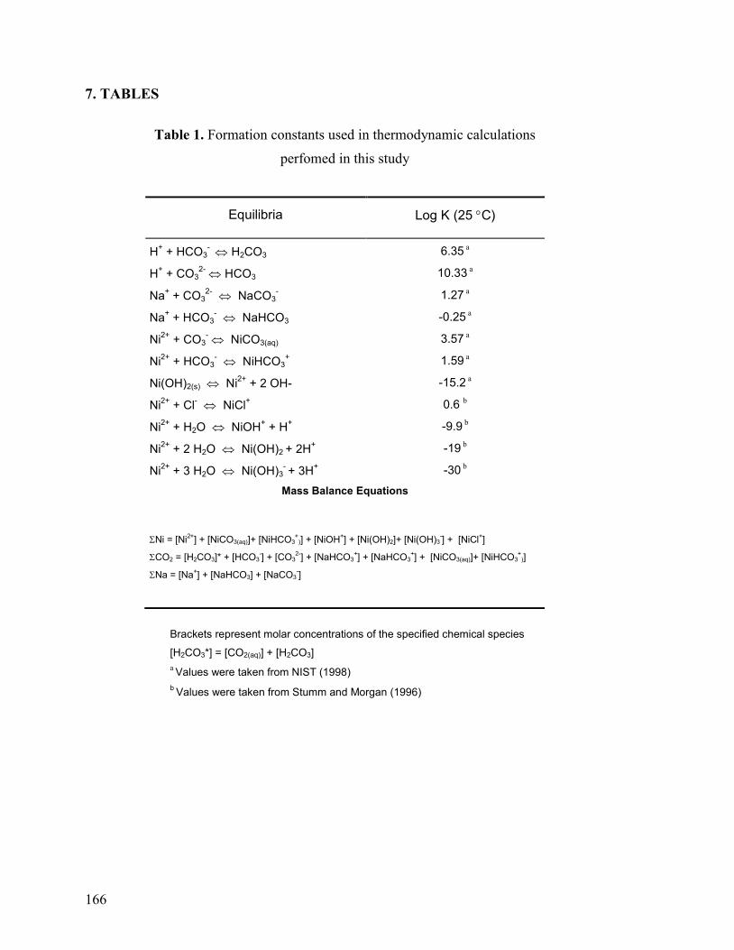
166

7. TABLES

Table 1. Formation constants used in thermodynamic calculations

perfomed in this study

Equilibria Log K (25 C)

H

+ + HCO3

- H2CO3 6.35 a

H+ + CO3

2- HCO3 10.33 a

Na+ + CO3

2- NaCO3

- 1.27 a

Na+ + HCO3

- NaHCO3 -0.25 a

Ni2+

+ CO3- NiCO3(aq) 3.57 a

Ni2+

+ HCO3- NiHCO3

+ 1.59 a

Ni(OH)2(s) Ni2+

+ 2 OH- -15.2 a

Ni2+

+ Cl- NiCl

+ 0.6 b

Ni2+

+ H2O NiOH+ + H

+ -9.9 b

Ni2+

+ 2 H2O Ni(OH)2 + 2H+ -19 b

Ni2+

+ 3 H2O Ni(OH)3- + 3H

+ -30 b


Ni = [Ni2+

] + [NiCO3(aq)]+ [NiHCO3+

)] + [NiOH+] + [Ni(OH)2]+ [Ni(OH)3

-] + [NiCl

+]

CO2 = [H2CO3]* + [HCO3-] + [CO3

2-] + [NaHCO3

+] + [NaHCO3

+] + [NiCO3(aq)]+ [NiHCO3

+)]

Na = [Na+] + [NaHCO3] + [NaCO3

-]

Brackets represent molar concentrations of the specified chemical species

[H2CO3*] = [CO2(aq)] + [H2CO3]

a Values were taken from NIST (1998)

b Values were taken from Stumm and Morgan (1996)

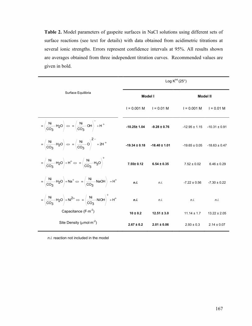
167

Table 2. Model parameters of gaspeite surfaces in NaCl solutions using different sets of

surface reactions (see text for details) with data obtained from acidimetric titrations at

several ionic strengths. Errors represent confidence intervals at 95%. All results shown

are averages obtained from three independent titration curves. Recommended values are

given in bold.

Surface Equilibria

Log K

int (25°)

Model I

Model II

I = 0.001 M I = 0.01 M I = 0.001 M I = 0.01 M

H OH

3CO

Ni O2H

3CO

Ni

-10.25± 1.04 -9.28 ± 0.76 -12.95 ± 1.15 -10.31 ± 0.91

H2

2

O

3CO

Ni O2H

3CO

Ni

-19.34 ± 0.18 -18.40 ± 1.01 -19.65 ± 0.05 -18.63 ± 0.47

O3H

3CO

Ni H O2H

3CO

Ni

7.55± 0.12 6.54 ± 0.35 7.52 ± 0.02 6.46 ± 0.29

H NaOH

3CO

Ni Na O2H

3CO

Ni

n.i. n.i. -7.22 ± 0.56 -7.30 ± 0.22

H NiOH

3CO

Ni

2Ni O2H

3CO

Ni

n.i. n.i. n.i. n.i.

Capacitance (Fm-2

)

10 ± 0.2 12.51 ± 3.0 11.14 ± 1.7 13.22 ± 2.05

Site Density (molm-2

)

2.67 ± 0.2 2.01 ± 0.06 2.93 ± 0.3 2.14 ± 0.07

n.i. reaction not included in the model

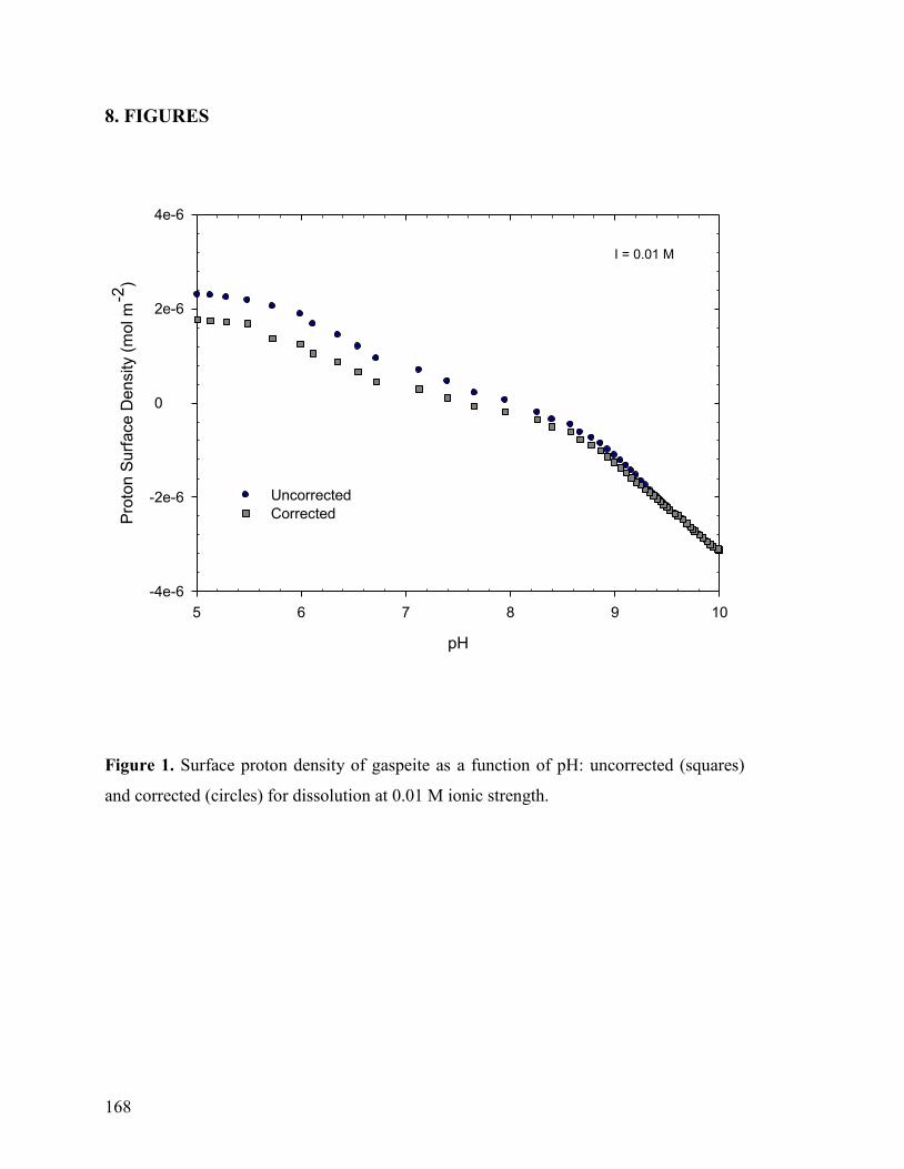
168

8. FIGURES

pH

5 6 7 8 9 10

Pro

ton S

urf

ace D

ensity (

mol m

-2)

-4e-6

-2e-6

0

2e-6

4e-6

Uncorrected

Corrected

I = 0.01 M

Figure 1. Surface proton density of gaspeite as a function of pH: uncorrected (squares)

and corrected (circles) for dissolution at 0.01 M ionic strength.

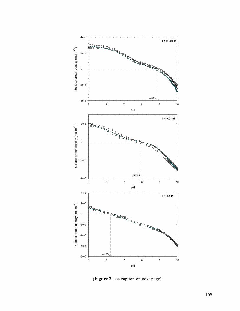
169

I=0.001M

pH

5 6 7 8 9 10

Su

rfa

ce

pro

ton

de

nsity (

mo

l m

-2)

-4e-6

-2e-6

0

2e-6

4e-6

I = 0.001 M

I=0.001M

pH

5 6 7 8 9 10

Su

rfa

ce

pro

ton

de

nsity (

mo

l m

-2)

-4e-6

-2e-6

0

2e-6

I = 0.01 M

Col 1 vs Col 2

Col 1 vs Col 3

Col 1 vs Col 4

Col 1 vs Col 11

I=0.001M

pH

5 6 7 8 9 10

Su

rfa

ce

pro

ton

de

nsity (

mo

l m

-2)

-8e-6

-6e-6

-4e-6

-2e-6

0

2e-6

4e-6I = 0.1 M

pznpc

pznpc

pznpc

(Figure 2, see caption on next page)

170

Figure 2. Corrected surface proton density of gaspeite derived from acidimetric titrations

carried out at three ionic strengths (0.001 M, 0.01 M , 0.1 M). Three independent

titrations (are shown at each ionic strength. Solid lines represent predictions by Model I

for the I = 0.001M and I = 0.01M regimes.

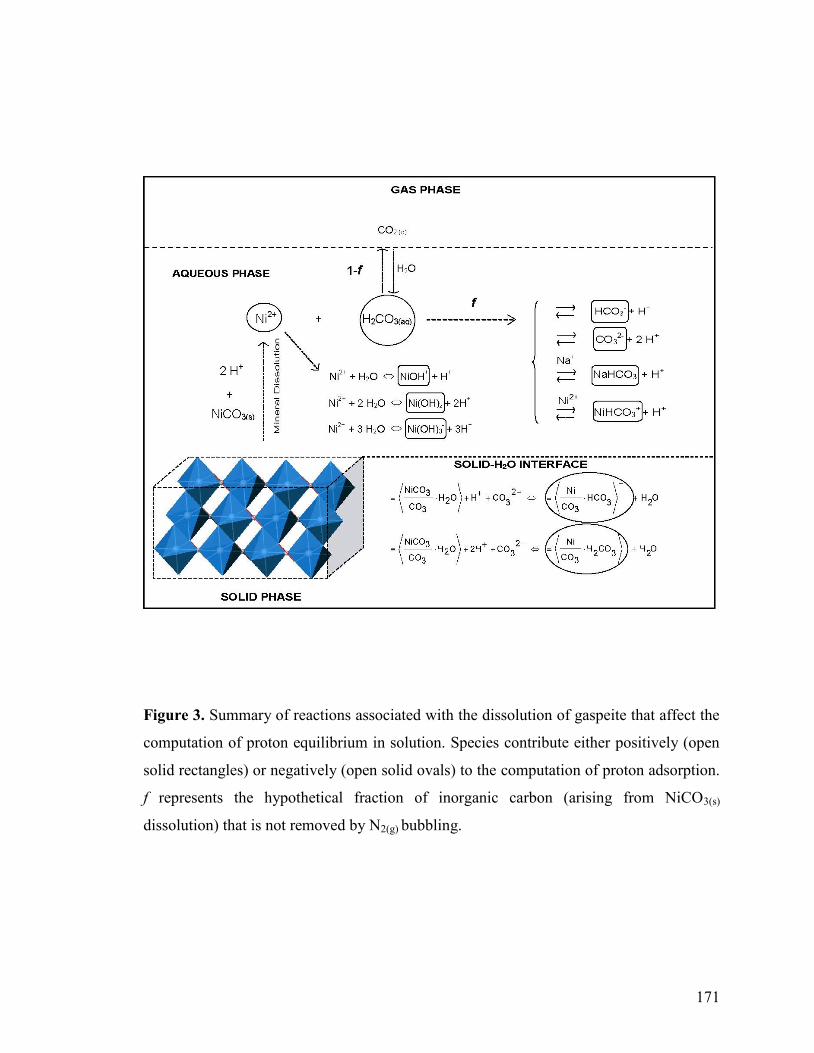
171

Figure 3. Summary of reactions associated with the dissolution of gaspeite that affect the

computation of proton equilibrium in solution. Species contribute either positively (open

solid rectangles) or negatively (open solid ovals) to the computation of proton adsorption.

f represents the hypothetical fraction of inorganic carbon (arising from NiCO3(s)

dissolution) that is not removed by N2(g) bubbling.

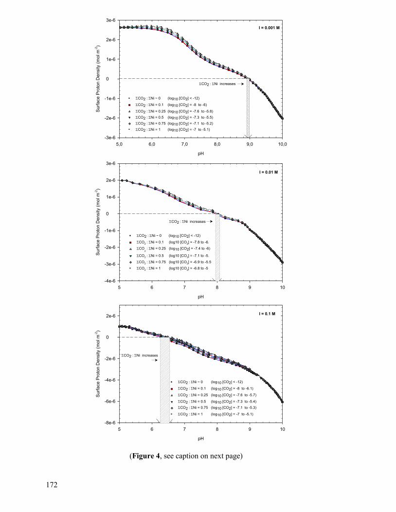
172

(Figure 4, see caption on next page)

I=0.001 M

pH

5 6 7 8 9 10

Su

rfa

ce

Pro

ton D

ensity (

mo

l m

-2)

-8e-6

-6e-6

-4e-6

-2e-6

0

2e-6

CO2 : Ni ~ 0 (log10 [CO2] < -12)

CO2 : Ni = 0.1 (log10 [CO2] = -8 to -6.1)

CO2 : Ni = 0.25 (log10 [CO2] = -7.6 to -5.7)

CO2 : Ni = 0.5 (log10 [CO2] = -7.3 to -5.4)

CO2 : Ni = 0.75 (log10 [CO2] = -7.1 to -5.3)

CO2 : Ni = 1 (log10 [CO2] = -7 to -5.1)

pH

5 6 7 8 9 10

Su

rfa

ce

Pro

ton D

ensity (

mo

l m

-2)

-4e-6

-3e-6

-2e-6

-1e-6

0

1e-6

2e-6

3e-6

CO2 : Ni ~ 0 (log10 [CO2] < -12)

CO2 : Ni = 0.1 (log10 [CO

2] = -7.8 to -6.

CO2

: Ni = 0.25 (log10 [CO2] = -7.4 to -6)

CO2 : Ni = 0.5 (log10 [CO

2] = -7.1 to -5.

CO2 : Ni = 0.75 (log10 [CO

2] = -6.9 to -5.5

CO2 : Ni = 1 (log10 [CO

2] = -6.8 to -5

I = 0.01 M

I = 0.1 M

pH

5,0 6,0 7,0 8,0 9,0 10,0

Su

rfa

ce

Pro

ton D

ensity (

mo

l m

-2)

-3e-6

-2e-6

-1e-6

0

1e-6

2e-6

3e-6

CO2 : Ni ~ 0 (log10 [CO2] < -12)

CO2 : Ni = 0.1 (log10 [CO2] = -8 to -6)

CO2 : Ni = 0.25 (log10 [CO2] = -7.6 to -5.8)

CO2 : Ni = 0.5 (log10 [CO2] = -7.3 to -5.5)

CO2 : Ni = 0.75 (log10 [CO2] = -7.1 to -5.2)

CO2 : Ni = 1 (log10 [CO2] = -7 to -5.1)

I = 0.001 M

CO2 : Ni increases

CO2 : Ni increases

CO2 : Ni increases

173

Figure 4. Surface proton density plots computed with equation 3 plus additional

corrections to account for the presence of protonated carbonate species in solution

(equation 16) at various concentrations. The shaded area indicate the pH range where the

point of net zero proton charge would appear depending on the concentration of total

inorganic carbon in solution.

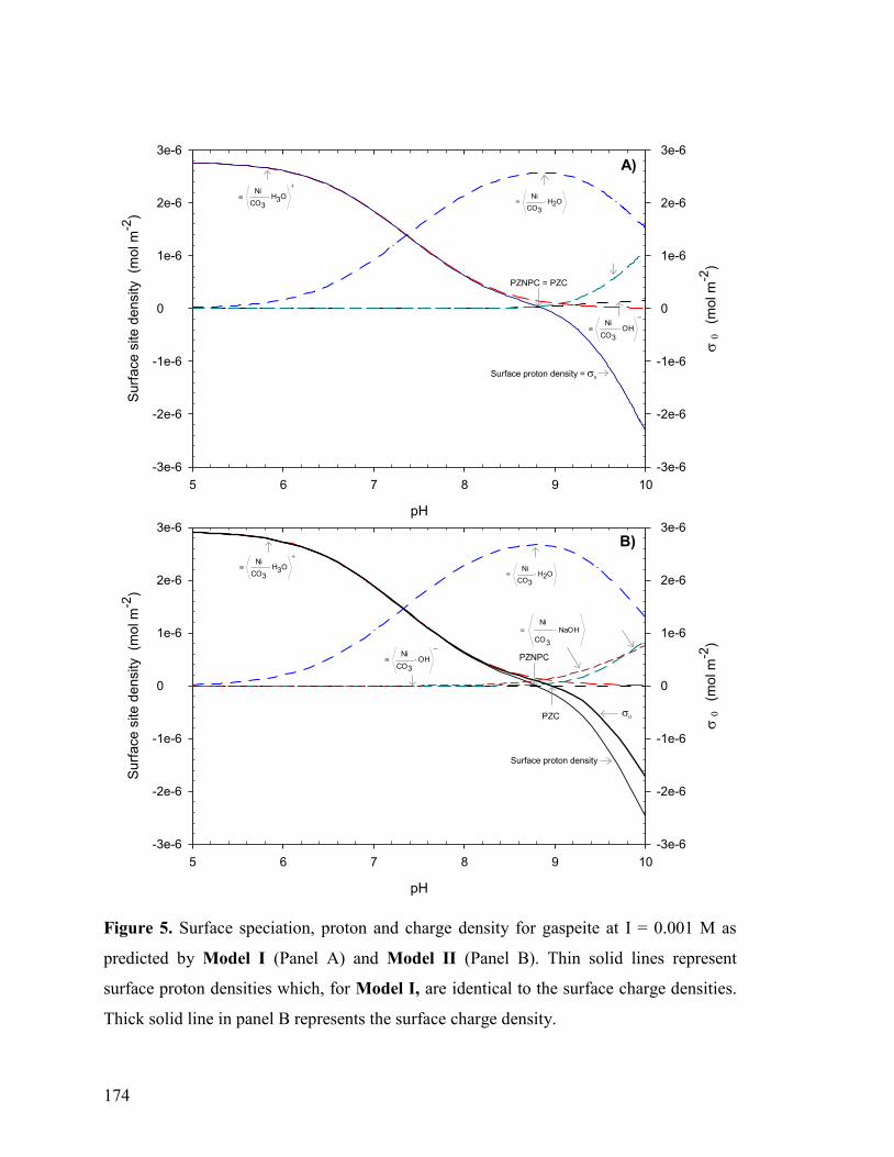
174

pH

5 6 7 8 9 10

Surf

ace s

ite d

ensity

(mol m

-2)

-3e-6

-2e-6

-1e-6

0

1e-6

2e-6

3e-6

(

mol m

-2)

-3e-6

-2e-6

-1e-6

0

1e-6

2e-6

3e-6

A)

pH

5 6 7 8 9 10

Surf

ace s

ite d

ensity

(mol m

-2)

-3e-6

-2e-6

-1e-6

0

1e-6

2e-6

3e-6

(

mol m

-2)

-3e-6

-2e-6

-1e-6

0

1e-6

2e-6

3e-6

Surface proton density

Surface proton density =

B)

PZNPC = PZC

PZNPC

PZC

2

O

3CO

Ni

NaOH

3CO

Ni

O2H

3CO

Ni

O3H

3CO

Ni

OH

3CO

Ni

O3H

3CO

Ni

O2H

3CO

Ni

2

O

3CO

Ni

OH

3CO

Ni

Figure 5. Surface speciation, proton and charge density for gaspeite at I = 0.001 M as

predicted by Model I (Panel A) and Model II (Panel B). Thin solid lines represent

surface proton densities which, for Model I, are identical to the surface charge densities.

Thick solid line in panel B represents the surface charge density.

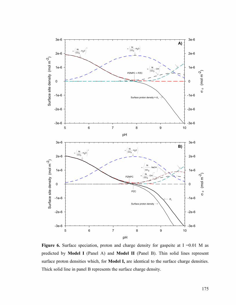
175

pH

5 6 7 8 9 10

Surf

ace s

ite

den

sity

(mol m

-2)

-3e-6

-2e-6

-1e-6

0

1e-6

2e-6

3e-6

(

mol m

-2)

-3e-6

-2e-6

-1e-6

0

1e-6

2e-6

3e-6

Surface proton density =

A)

O3H

3CO

Ni

O2H

3CO

Ni

OH

3CO

Ni

PZNPC = PZC

pH

5 6 7 8 9 10

Surf

ace s

ite

den

sity

(mol m

-2)

-3e-6

-2e-6

-1e-6

0

1e-6

2e-6

3e-6

(

mol m

-2)

-3e-6

-2e-6

-1e-6

0

1e-6

2e-6

3e-6

Surface proton density

B)

PZNPC

PZC

2

O

3CO

Ni

NaOH

3CO

Ni

O2H

3CO

Ni

2

O

3CO

Ni

O3H

3CO

Ni

OH

3CO

Ni

Figure 6. Surface speciation, proton and charge density for gaspeite at I =0.01 M as

predicted by Model I (Panel A) and Model II (Panel B). Thin solid lines represent

surface proton densities which, for Model I, are identical to the surface charge densities.

Thick solid line in panel B represents the surface charge density.

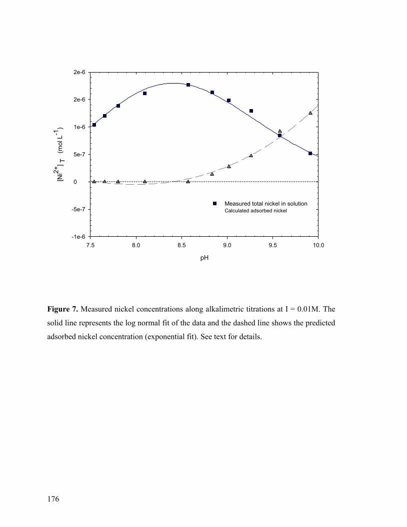
176

pH

7.5 8.0 8.5 9.0 9.5 10.0

[Ni2

+] T

(

mol L

-1)

-1e-6

-5e-7

0

5e-7

1e-6

2e-6

2e-6

Measured total nickel in solutionCalculated adsorbed nickel

Figure 7. Measured nickel concentrations along alkalimetric titrations at I = 0.01M. The

solid line represents the log normal fit of the data and the dashed line shows the predicted

adsorbed nickel concentration (exponential fit). See text for details.

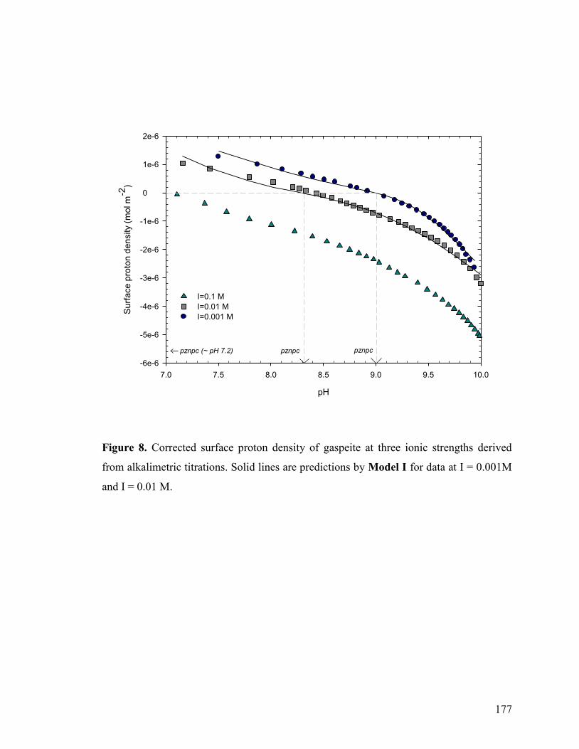
177

pH

7.0 7.5 8.0 8.5 9.0 9.5 10.0

Surf

ace p

roto

n d

ensity

(mol m

-2)

-6e-6

-5e-6

-4e-6

-3e-6

-2e-6

-1e-6

0

1e-6

2e-6

I=0.1 M

I=0.01 M

I=0.001 M

pznpc pznpcpznpc (~ pH 7.2)

Figure 8. Corrected surface proton density of gaspeite at three ionic strengths derived

from alkalimetric titrations. Solid lines are predictions by Model I for data at I = 0.001M

and I = 0.01 M.

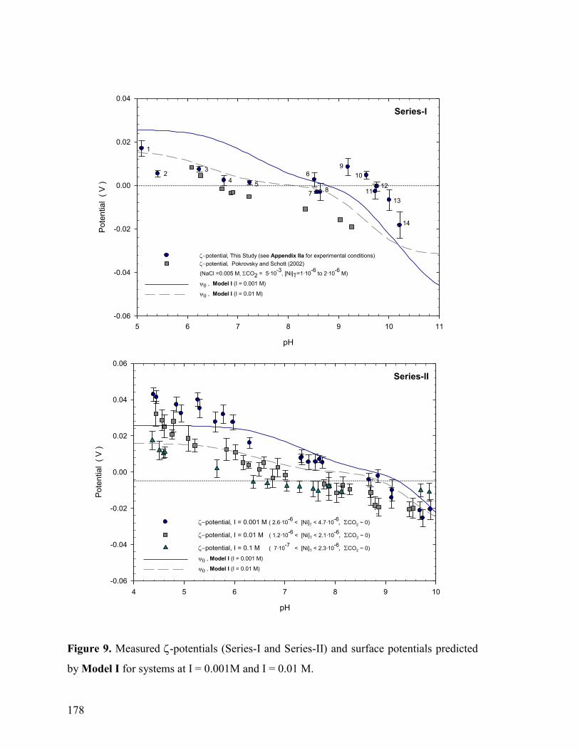
178

pH

5 6 7 8 9 10 11

Po

ten

tia

l (

V )

-0.06

-0.04

-0.02

0.00

0.02

0.04

potential This Study (see Appendix IIa for experimental conditions)

potential Pokrovsky and Schott (2002)

(NaCl =0.005 M, CO2 = 5·10-3

, [Ni]T=1·10-6

to 2·10-6

M)

, Model I (I = 0.001 M)

, Model I (I = 0.01 M)

1

23

45

6

78

9

10

1112

13

14

Series-I

pH

4 5 6 7 8 9 10

Po

ten

tia

l (

V )

-0.06

-0.04

-0.02

0.00

0.02

0.04

0.06

potential I = 0.001 M ( 2.6·10-6

< [Ni]T < 4.7·10-6CO2 ~ 0)

potential, I = 0.01 M ( 1.2·10-6

< [Ni]T < 2.1·10-6CO2 ~ 0)

potential, I = 0.1 M ( 7·10-7

< [Ni]T < 2.3·10-6CO2 ~ 0)

, Model I (I = 0.001 M)

, Model I (I = 0.01 M)

Series-II

Figure 9. Measured -potentials (Series-I and Series-II) and surface potentials predicted

by Model I for systems at I = 0.001M and I = 0.01 M.

179

180


In contrast to gaspeite, calcite is one of the most reactive naturally-occurring

rhombohedral carbonate minerals in aqueous solution and, by far, the most ubiquitous

in aquatic systems. Accordingly, numerous studies have focused on the

characterization of the calcite surface reactivity in aqueous solutions. Among these,

molecular modeling studies have pressed forward because of the experimental

difficulties inherent in the characterization of the surface reactivity of this mineral. In

most of these studies, atomistic and Molecular Dynamics force-field-based methods

and, to a lesser extent, Density Functional Theory (DFT) techniques were applied and

provided important insights on the structural registry of dry and wet calcite surfaces.

Nevertheless, despite all these efforts, no systematic ab initio molecular orbital study

on the ground-state structural and electronic properties of the first and second

hydration layers at the (10.4) calcite surface has been conducted. In the following

chapter, “Theoretical Insights into the Hydrated (10.4) Calcite Surface: Structure,

Energetics and Bonding Relationships” we exploit ab initio molecular orbital methods

using cluster models to represent the idealized (10.4) calcite surface, obtain a detailed

description of its 3D structural registry and elucidate the bonding relationships

governing the hydration process. Results of this study are in reasonable agreement

with earlier findings and further support the single-site scheme postulated for

rhombohedral carbonate mineral surfaces in Chapter 3 and subsequently used in

Chapter 4. This study revealed a significant Ca-O bonding reorganization at the

mineral surface leading to the weakening of the topmost atomic layer with respect to

the bulk.

181

CHAPTER 5

THEORETICAL INSIGHTS INTO THE HYDRATED (10.4) CALCITE SURFACE: STRUCTURE, ENERGETICS, AND BONDING RELATIONSHIPS


1 and Michael Anthony Whitehead

2



2 Chemistry, McGill University, 801 Sherbrooke Street W. Montréal, Qc Canada



“Reproduced with permission from the American Chemical Society:

Adrián Villegas-Jiménez, Alfonso Mucci, and Michael Anthony Whitehead (2009) Theoretical Insights into the

Hydrated (10.4) Calcite Surface: Structure, Energetics, and Bonding Relationships Langmuir 25(12) 6813-6824

Copyright 2009 American Chemical Society."

182

ABSTRACT

Roothaan-Hartree-Fock molecular orbital methods were applied to investigate the

ground-state structural, energetic properties, and bonding relationships of the hydrated

(10.4) calcite surface. The adsorption of water molecules was modelled at the 6-31G(d, p)

level of theory using Can(CO3)n slab cluster models (4 n 18), with a varying number

of H2O monomers (2 (H2O)n 6) interacting with the surface. Modelling results add

fresh insights into the detailed 3D structural registry of the 1st and 2

nd hydration layers

and the reconstructed (10.4) calcite surface, complementary to the information acquired

from earlier Atomistic, Density Functional, X-ray Scattering and Grazing Incidence X-

Ray Diffraction studies. Both the modelled energies and geometries agree best with

results of earlier Density Functional calculations, supporting the associative character of

adsorbed water molecules. Two adsorption configurations are postulated: i) H2O

molecules interacting with surface Ca through ionic bonding and by Hydrogen Bonding

to a surface O with their dipole slightly oblique above the surface (1st hydration layer)

and, ii) H2O molecules that Hydrogen Bond to surface O and to H2O molecules in the 1st

hydration layer with their dipole nearly parallel to the surface (2nd

hydration layer). These

interactions are consistent with the “chemisorption” and “physisorption” of H2O on

calcite surfaces, proposed on the basis of previous thermogravimetric and Fourier-

Transformed Infrared studies. Most significant is the distortion of the surface Ca-O

octahedra caused by the relaxation (and possibly rupture) of some Ca-O bonds upon

hydration, weakening the topmost atomic layer. These findings are consistent with

interpretations of X-ray Photoelectron Spectroscopy, Density Functional Theory and

Electrokinetic studies that suggest the preferential release of surface Ca atoms over

183

surface CO3 groups upon hydration of the cleavage surface. These insights will help to

elucidate mechanisms of carbonate mineral dissolution, the rearrangement of surface

layers, ion replacement, charge development and solute transport through subsurface

lattice layers.

Keywords: Molecular Orbital theory; surface hydration; calcite clusters; Ca-O bond

stretching, Ca-O octahedron distortion.

184

1. INTRODUCTION

Among CaCO3 polymorphs, calcite is the most abundant and ubiquitous form in natural

aquatic environments, where it plays a critical role on the regulation of pH, alkalinity, and

heavy metal transport/mobility through exchange and co-precipitation reactions (Morse

and Mackenzie, 1990). Calcite finds numerous industrial applications that range from the

production of paper, paints, plastics, pharmaceuticals and cosmetics to raw material in the

construction industry and agriculture (Vanerek et al., 2000; Usher et al., 2003).

Given its environmental significance and broad industrial applications, calcite has

been the subject of extensive experimental studies (Morimoto et al., 1980; Ahsan, 1992;

Davis et al., 1987; Zachara et al., 1991) which revealed the critical role that its surface

properties play on the macroscopic chemical behaviour of this mineral in aqueous

suspensions. These properties result from the interplay of intermolecular and surface

forces, such as hydrogen bonding, van der Waals interactions and solvation at the mineral

surface-water interface (Sposito, 1990; Israelachvili, 1992). Hydration is the most

fundamental phenomenon to which dry mineral surfaces are subjected when immersed in

aqueous solution. Surface forces modify the structure and properties of adsorbed and

interfacial water, relative to the bulk solution, by breaking down water clusters and

limiting the ability of H2O molecules to reorient their dipoles (Israelachvili, 1992) which

affects the properties of the mineral surface.

Surface-sensitive, non-invasive, X-ray, Electron Diffraction and spectroscopic

techniques as well as Atomic Force microscopic methods were used to investigate the

structural properties of the calcite mineral-water interface (Neagle and Rochester, 1990;

Stipp and Hochella, 1991; Chiarello et al, 1993; Stipp et al., 1994; Liang et al., 1996;

Stipp, 1999; Pokrovsky et al., 2000; Fenter et al., 2000; Geissbühler et al., 2004;

185

Magdans et al., 2006). They provided direct characterization of the molecular structure of

the hydrated calcite surface, revealing a degree of surface reconstruction upon hydration.

In addition, recent X-ray Scattering (Geissbühler et al., 2004) and Grazing Incidence X-

ray Diffraction (Magdans et al., 2006) studies unveiled, for the first time, 3D structural

details (interlayer spacing, inter-atomic distances and lateral registry) of the hydrated

(10.4) calcite surface.

Similarly, molecular modelling techniques are powerful tools to investigate the

energy and structure of hydrated CaCO3 surfaces. Several computer-assisted Atomistic

simulations (Force-Field-based) of the H2O interactions with calcite and magnesium-

bearing calcite surfaces were performed by numerous research groups (de Leeuw and

Parker, 1997; de Leeuw and Parker, 1998; de Leeuw et al., 1998; Stöckelmann and

Hentschke, 1999; de Leeuw and Parker, 2000; Kuriyavar et al., 2000; de Leeuw and

Parker, 2002; Hwang et al., 2001; Wright et al., 2001; Parker et al., 2003; Kerisit et al.,

2003; Kerisit and Parker, 2004; Kerisit et al., 2005a; Perry et al., 2007). Despite small

discrepancies in the estimated inter-atomic distances between surface atoms and H2O

molecules, results of most studies suggested the formation of a monolayer of

associatively adsorbed H2O in a nearly-flat arrangement, relative to the surface, adopting

a herringbone pattern (de Leeuw and Parker, 1997; de Leeuw and Parker, 1998; Parker et

al., 2003; Kerisit et al., 2003). A slight vertical displacement of surface Ca atoms and

rotation of the surface CO3 groups were also reported in these studies.

Electronic structure studies, based on Density Functional Theory (DFT),

investigated the hydration of the (10.4) calcite surface (Parker et al., 2003; Kerisit et al.,

2003; Archer, 2004; Kerisit et al., 2005b) and examined its surface composition upon

contact with a gaseous phase containing H2O and CO2(g) (Kerisit et al., 2005b). Whereas

186

some of these calculations (Parker et al., 2003; Kerisit et al., 2003) predict a similar

configuration of the associatively adsorbed H2O molecules to those of the Atomistic

studies (de Leeuw et al., 1997; de Leeuw and Parker, 1998; Kerisit et al., 2003), the latter

consistently overestimated the energies of dry and wet calcite surfaces because do not

contain explicit chemical information and lack the full electronic relaxation offered by

DFT techniques (Parker et al., 2003).

Ab initio Molecular Orbital methods have also been used to investigate the

ground-state properties of CaCO3 polymers and clusters. Roothaan-Hartree-Fock (RHF)

techniques were applied to i) investigate the bonding and charge distribution in CaCO3

monomers (Thackeray and Siders, 1998), ii) study protonation and H2O attachment to

CaCO3 monomers and dimers (Mao and Siders, 1997), and iii) evaluate the performance

of different protocols to stabilize Can(CO3)n clusters of different size (4 n 22)

expressing the (001) surface (Ruuska et al., 1999). It was concluded that H2O surrounding

the calcite clusters, simulating hydration, stabilize the clusters while decreasing the time

required to achieve the Self-Consistent-Field (SCF) convergence. Finally, partial

geometric optimisations of Can(CO3)n clusters (n 21), where only the geometries of the

adsorbates were optimised, were carried out to investigate the interactions of anionic

collectors, oleate and oleoyl sarcosine anions, with the calcite surface with RHF/3-21G

(Hirva and Tikka, 2002). This study confirmed that moderately large Can(CO3)n cluster

models (n ≥ 14) are adequate surrogate models to correctly describe the effect of

neighbouring surface atoms, model the infinite calcite surface and investigate adsorption

reactions.

187

Despite all these efforts, no systematic ab initio Molecular Orbital study of the

structure and energy of the hydration layers at the (10.4) calcite surface has been

conducted. The present investigation is an extension of earlier studies, based on the

application of RHF techniques, to exploit the power of Roothan-Hartree-Fock methods

using moderately large cluster models (n = 18), to properly represent the idealized

stoichiometric (10.4) calcite surface and accurately describe hydrogen bonding (Tossel

and Vaughan, 1992). The results from earlier Atomistic simulations and DFT calculations

were used to select reasonable geometric constraints on the clusters and assign an initial

configuration to the H2O molecules. A series of RHF/6-31G(d,p) partial geometric

optimisations, involving specific “reactive” atoms at the (10.4) calcite surface and a

varying number of H2O molecules, were performed to obtain information on the structure,

the energy and the bonding relationships governing the hydration process.

2. METHODS

2.1 Computational Methods and Cluster Models

Gaussian 03 software

(Frisch et al., 2003) was used to perform the geometric

optimisations of finite charge-neutral slabs (clusters) taken from the bulk calcite structure

(Graf, 1961). The ideal stoichiometric (10.4) cleavage plane was represented in the slab

and adopted as the molecular model of the calcite surface as in earlier studies (de Leeuw,

and Parker, 1997; Wright et al., 2001; Hirva and Tikka, 2002; Parker et al., 2003; Kerisit

et al., 2003; Kerisit and Parker, 2004). The validity of this representation was confirmed

using a standard protocol devised to determine the most stable surface atomic

configuration of oxide minerals according to residual charge and bond strength

minimization criteria (Koretsky et al., 1998).

188

Cluster models have been commonly used to study the electronic structure of

carbonate (Mao and Siders, 1997; Thackeray and Siders, 1998; Ruuska et al., 1999; Hirva

and Tikka, 2002) and metal oxide minerals (Xiao and Lasaga,, 1994; Kubicki and Bleam,

2003). Specifically, clusters models were found suitable for investigations of adsorption

reactions on CaCO3 surfaces (Mao and Siders, 1997; Thackeray and Siders, 1998; Ruuska

et al., 1999; Hirva and Tikka, 2002). Therefore, this approach was adopted throughout

this study. The absence of periodic boundary conditions in cluster models requires a

formalism to treat crystal structure terminations and prevent “edge effects”. Hydrogen

atoms are commonly used as terminators of covalent compounds (Xiao and Lasaga, 1994)

and oxide minerals (Tossel and Vaughan, 1992; Xiao and Lasaga, 1994; Kubicki and

Bleam, 2003) but this approach is not suitable for systems in which hydrogen bonding is

involved, as for H2O adsorption (Tossel and Vaughan, 1992). In addition, for semi-ionic

minerals such as CaCO3, the use of standard point embedding techniques can be

problematic because of possible polarization of cations near the borders of the cluster and

because they cannot prevent unrealistic delocalisation of the cluster wave function arising

from the neglect of Pauli’s exclusion effects (Stefanovich and Truong, 1997).

Furthermore, the embedded point charges depend on the geometry and charge relaxation

of the crystal surface and, therefore, the results must be subjected to validation against

multiple point embedding models, a process that is both tedious and time-consuming

(Ruuska et al., 1999). Alternatively, stabilisation of CaCO3 surfaces can be improved by

placing H2O molecules in the vicinity of the exposed surfaces (Ruuska et al., 1999).

Consequently, the use of sufficiently large charge-neutral cluster models, in

combination with appropriate geometric constraints, is considered an adequate alternative

to simulate semi-infinite calcium carbonate surfaces and minimize edge effects (Ruuska

189

et al., 1999; Hirva and Tikka, 2002). The selected cluster must realistically represent the

mineral surface and the underlying bulk crystal to accurately describe local and long-

range interactions while keeping the cluster size practical for ab initio calculations

(Rosso, 2001).

In this study, the Can(CO3)n cluster size ranged from 4 n 18 with a varying

number of H2O monomers, 0 (H2O)n 6. The Ca9(CO3)9 and Ca18(CO3)18 clusters were

used to represent one and two full surface unit cells, respectively. The surface atomic

layer of the Ca9(CO3)9 cluster was composed of 3 Ca atoms and 6 CO3 groups, whereas

the subatomic layer contained 3 CO3 groups and 6 Ca atoms (Fig. 1). In contrast, the

composition of the surface and subsurface atomic layers of the Ca18(CO3)18 cluster were

identical: 9 CaCO3 units in each layer (Fig. 2). Most of our calculations were performed

using these two clusters which will hereafter be referred to, respectively, as the small and

large cluster models. The selected density of H2O molecules per surface area unit

composing the 1st hydration layer (4.9 nm-

2) is consistent with the density of

exchangeable surface Ca atoms (5 nm-2

), measured experimentally (Möller and Sastri,

1974) and reflects a 1:1 H2O:Ca stoichiometry.

Preliminary all-atom RHF/6-31G(d,p) optimisations of smaller clusters,

Ca4(CO3)4 and Ca5(CO3)5, were carried out for comparison with the geometry of the bulk

crystal. These calculations revealed that, when all atom positions are allowed to relax, the

cluster geometry is significantly distorted, particularly at the edges, and unrealistic

interactions are obtained, such as several Ca atoms bonding directly to C atoms or to an

unreasonable number of O atoms. Consequently, before performing further optimisations,

criteria were developed to select the atoms whose positions could be restricted to those of

190

the bulk structure. This step is critical to prevent the generation of unrealistic interactions

between neighbouring atoms and minimize computational time. To impose some control

on the 3D symmetry of the selected cluster and mimic the bulk crystal, all the atoms

present in the second atomic layer, the subsurface atoms, were fixed and the computed

geometry was examined for modifications in the coordination environment of both the

surface and subsurface atoms. This condition was slightly modified later as explained

below.

In adsorption studies, it is common practice to fully optimise the internal

coordinates of the adsorbates while the surface atom positions are kept frozen (Hirva and

Tikka, 2002). However, this approach does not exploit the full potential of electronic

relaxation offered by ab initio methods. It is more realistic to unlock some surface atoms,

such as those that participate directly in the adsorption process, which will be referred to

as “reactive” surface atoms throughout this paper. A careful selection of these geometric

constraints will allow a more realistic description of the configuration of the hydrated

surface layer and account for the interactions between the surface and the adsorbate

(water) while controlling the 2D symmetry of the mineral surface and minimizing edge

effects. The number of surface atoms allowed to relax must be selected on the basis of the

adsorption reaction of interest, the cluster size and the available computational

capabilities.

Earlier theoretical studies (de Leeuw and Parker, 1997; Wright et al., 2001; Parker

et al., 2003; Kerisit et al., 2003; Archer, 2004; Perry et al., 2007) showed that each

adsorbed H2O, in the 1st hydration layer, interacts with one Ca and one or two O atoms at

the (10.4) calcite surface. These “reactive” atoms are well represented in our cluster

models (Figs. 1 and 2) and were allowed to relax during the cluster geometry

191

optimisations. For the Ca9(CO3)9/2H2O and Ca9(CO3)9/3H2O clusters, all other surface

atoms were frozen in their original crystallographic positions.

To optimise computational time and prevent edge effects, water molecules were

only allowed to interact with surface atoms within a full surface unit cell at the centre of

the large cluster surface. The initial position of the H2O molecules in the 1st hydration

layer were chosen to reflect results common to earlier studies: i) herringbone adsorption

pattern (de Leeuw and Parker, 1997; Parker et al., 2003), ii) flat alignment of H2O

molecules (de Leeuw and Parker, 1997; Parker et al., 2003; Kerisit et al., 2003) with

respect to the surface and, iii) H2O oxygen atoms located at a distance of approximately

2.37 Å with respect to the surface calcium atoms (de Leeuw and Parker, 1997; Kerisit et

al., 2003). Based on results of Molecular Dynamics (Kerisit and Parker, 2004) and X-ray

Scattering (Geissbühler., 2004), H2O molecules in the 2nd

hydration layer, formally

ascribed to the 1st hydration layer in earlier studies (Geissbühler., 2004; Kerisit and

Parker, 2004; Magdans et al., 2006) were initially placed at a greater distance from the

surface (~3.3 Å), with a larger x-y displacement from the surface Ca (~3.9 Å) and

according to a 2:1 Ca:H2O stoichiometry (Fig. 2).

3. RESULTS

3.1 Structural Details of the Hydrated Clusters

Preliminary cluster geometry optimisations of the small cluster models were performed

using the STO3G and 3-21G basis sets for a quick comparison against the highest level of

theory selected in this study, 6-31G(d,p). Very similar configurations of associatively

adsorbed H2O molecules were obtained with the 3-21G and the 6-31G(d,p) basis sets,

with the inter-atomic distances between H2O and the surface “reactive atoms” differing

192

by less than 16%. In contrast, the STO-3G basis set predicted the dissociation of H2O

upon adsorption whereas the position of H2O constituents differed by up to 31% with

respect to results generated by the 6-31G(d,p) basis set. Both the 3-21G and 6-31G(d,p)

basis set simulations revealed that H2O molecules do not lie flat on the mineral surface

but are tilted with one of their H atoms pointing towards one of the “reactive” surface O

atoms and the other pointing away from the surface. In other words, only one hydrogen

bond can form between each H2O monomer and the surface (see discussion below).

As in an earlier study (Kerisit et al., 2003), to further confirm the associative

adsorption character of H2O, the adsorption of the H2O constituents, H+ and OH

-, on the

calcite surface was simulated at the RFH/6-31G(d,p) level of theory using the small

cluster. H+ were initially bonded to surface O at 1 Å and OH

- were bonded to surface Ca

at the bulk crystal Ca-O bond length of 2.37 Å. The optimised structure revealed that the

H+

and OH- spontaneously associated to H2O with an identical configuration and SCF

energy as when undissociated H2O was considered as the initial configuration. That the 6-

31G(d,p) basis sets predicts associative adsorption of H2O from both initially dissociated

and undissociated H2O and yields identical Ca(surface)-O(water) inter-atomic distances further

supports its use in the optimisation of larger CaCO3 clusters.

The optimised inter-atomic distances of the Ca-O octahedra imply the substantial

relaxation of the Ca-O bonds between the surface Ca and the subsurface O. The surface

Ca atoms shift out from the surface, increasing their inter-atomic distances to subsurface

O to the extent that the bond is substantially weakened (average Ca(surface)-O(subsurface) bond

length of 2.5 Å). To confirm this observation, we performed: i) a geometric optimisation

of the Ca9(CO3)9/2H2O cluster for which the subsurface O bonded to the surface Ca was

unlocked and, ii) a geometric optimisation of a three atomic layer cluster, Ca12(CO3)12+

193

2H2O, for which the entire CO3 group in the second atomic layer associated with the

surface Ca was unlocked (Fig. 3) and the third layer was frozen to impose the bulk

symmetry of the cluster. Both calculations confirmed the substantial relaxation of at least

one Ca-O bond per surface Ca-O octahedron and yielded nearly identical structural results

to those of the first RHF/6-31G(d, p) calculation.

The optimised Ca12(CO3)12/2H2O cluster shows that the Ca atoms move out of the

surface whereas the subsurface O atoms move away from the Ca both horizontally (x-y

directions) and vertically (z-direction). As subsurface CO3 groups relax, they rotate

towards the subsurface plane (-1 layer in Fig. 3) resulting in the stretching of more

surface Ca-O bonds than in the small cluster without significantly affecting the average

structure of the reconstructed surface. This observation validates the criteria we selected

to impose geometric constraints and supports our premise that at least one Ca-O bond per

surface Ca-O octahedron is significantly weakened, and approaches rupture, upon

hydration. A thorough discussion on this issue is given below.

Having ascertained the self-consistency of our results using different cluster

thicknesses, we can confidently focus on the results of the large clusters,

Ca18(CO3)18/4H2O and Ca18(CO3)18/6H2O, which provide a reasonable representation of

the infinite calcite surface. Although the calcite surface undergoes some reconstruction

upon hydration, the average 2D dimensions of the (10.4) surface unit cell increase only by

approximately 1% along the x direction while they remain unchanged along the y

direction (Fig. 2). Table 1 summarizes the structural details of the reconstructed hydrated

calcite surface for the Ca18(CO3)18/6H2O cluster. They, respectively, reflect the average

Cartesian and internal coordinates of the relaxed surface atoms and the H2O. It is

noteworthy that the Ca and C atoms are displaced differently along the three Cartesian

194

coordinates. Their differential displacement along the z- direction, normal to the surface,

determines the height of the reconstructed surface layer, relative to the subsurface atomic

layer, and yields the extent of surface relaxation. Conventionally, as in previous studies

(Geissbühler, 2004), the averaged, relaxed positions of the Ca atoms were selected to

define the reconstructed surface atomic layer and reference the position of H2O in the

hydration layer.

Using the reconstructed lattice spacing, d12, the average surface relaxation, 12, can

be expressed as a percentage of the perfect lattice spacing, d, according to (Markmann et

al., 2006):

100δ

d

dd12

12 (1)

An average surface relaxation of 5.6% relative to surface Ca was observed. The

extent of surface corrugation is given by the surface rumpling parameter (z) which

represents the difference between the z-coordinates of surface anions (Zanion

) and cations

(Zcation

) with respect to the ideal lattice spacing (Markmann et al., 2006):

100d

zzz

cationanion (2)

At the ideal (10.4) unreconstructed calcite surface, one O of each surface CO3 lies

0.8 Å above the surface Ca and C atoms. Thus, the intrinsic rumpling (z) of the surface

is 26.4% which, upon reconstruction, decreases to 24%. If the z-displacement of the

195

central C of each CO3, rather than the surface O, is considered relative to the surface Ca,

the surface rumpling would go from zero for the unreconstructed surface, to 4.9% in the

reconstructed surface. On reconstruction, the glide symmetry at the surface is slightly

broken because of the differential displacement, along the z- direction, of the surface Ca

and the alternatively oriented CO3 groups (Config-1 and Config-2 in Fig. 4).

Upon hydration, surface Ca-O octahedra are distorted following changes in the

Ca-O bond lengths. The average surface Ca-O bond length is stretched by ~ 4 % (2.46 Å),

35% of the relaxed Ca-O bonds are stretched by less than 4.5% and one Ca-O bond per

surface Ca-O octahedra stretches by at least 10% whereas Ca-O bond contraction up to

5% is also observed in some Ca-O octahedra. Conversely, the CO3 groups are not

significantly distorted from their original trigonal planar geometry, although rigorously

speaking, their D3h symmetry is lost as a result of the differential displacement of the

three O atoms along the z-axis (Fig. 4). The average change in the CO3 dihedral angle (O-

C-O-O) is only 1.8º, which reflects the small out-of-plane distortion of the CO3 group.

The C-O bond lengths are only slightly shortened ( 0.8%) whereas the average O-C-O

angle remains unchanged. CO3 groups are tilted towards the plane of the relaxed surface

Ca atoms by an average of 4.1° but their atomic positions along the x-y directions are

significantly modified (Table 1). Because of the relative rigidity of the CO3 groups, their

average x-y displacement is expressed in terms of the optimised x-y coordinates of the

central C atom, the CO3 centre of mass, rather than relative to the surface O.

The associative character of adsorbed H2O in the 1st and 2

nd hydration layers is

confirmed in the large cluster, Ca18(CO3)18/6H2O. H2O molecules in the 1st hydration

layer (Mode-I) are slightly oblique to the surface with one H oriented towards one surface

O and the other towards H2O in the 2nd

hydration layer. H2O molecules in the 2nd

196

hydration layer align their dipole nearly parallel to the surface (Mode-II). The average O-

H-O angle of H2O in the 2nd

hydration layer is smaller than that of H2O in the 1st

hydration layer whereas the average O-H bond length of H2O in both layers is identical,

0.95 Å. Nevertheless, H2O in the 2nd

hydration layer display a short (0.94 Å) and a long

O-H bond (0.97 Å), the longer being oriented towards surface O following hydrogen

bonding (see below) and the shorter one pointing away from the surface. Structural details

of the reconstructed calcite surface, including the two hydration layers modelled in this

study, are illustrated in Figure 5.

3.2 Energies of Adsorption

The energy of interaction between H2O molecules and the calcite surface, Eads, can be

computed from (Cao and Chen, 2006):

Eads = Eslab/water n

– ( Eslab + n·Ewater ) (3)

where Eslab/watern represents the energy of the optimised cluster covered with n H2O

molecules (n = 2, 4 or 6, depending on the cluster model) at their adsorption

configurations, Eslab is the single-point energy of the cluster model with no H2O attached

(dry cluster model) and Ewater is the energy of a single H2O in the gas phase. The

adsorption energy of n H2O attached to the cluster is equal to –172.8 and –306 kJ mol-1

for the small (n=2) and large (n=4) clusters respectively. Upon normalization to the

number of attached H2O monomers, their respective energies become –86.4 and –76.5 kJ

mol-1, corresponding to the binding energy of a single H2O monomer at the cluster

197

surface. The adsorption energy of the 2nd

hydration layer, Eads-2nd, to the hydrated surface

is given by:

Eads-2nd = Eslab/water 6-(Eslab/1st+2·Ewater) (4)

where Eslab/1st is the total energy of the large cluster with the four 1st layer H2O monomers

attached. Once normalized to the total number of adsorbed H2O, Eads-2nd is –106.1 kJ mol-

1. To calculate the interaction energy between H2O and the dry surface with no other

adsorbates attached, the adsorption energy must be corrected by the average interaction

energy, Einter, among H2O in the 1st and 2

nd hydration layers (Cao and Chen, 2006):

Einter = Ewater/1st/2nd – (6·EH2O) (5)

where Ewater/1st/2nd is the single-point energy of the H2O of the 1st and 2

nd hydration layers

of the large hydrated cluster at their adsorbed configurations. To estimate Einter for H2O

molecules constituting the 1st hydration layer, we subtracted the gas phase single-point

energy of 4 H2O molecules from the single-point energy of the 4 H2O molecules in the 1st

hydration layer at their adsorbed configurations. In both cases, the estimated Einter values

per H2O molecule are nearly equal (–11.9 kJ mol-1

for n= 6 and –12 kJ mol-1

for n=4)

and are in excellent agreement with the Einter estimated by DFT calculations (–12.5 kJ

mol-1

after Basis Set Superposition Error, BSSE, correction; Archer, 2004). The

agreement between the two independent energy estimates strongly supports the suitability

of RHF methods, in combination with cluster models, to investigate hydration reactions at

198

CaCO3 surfaces, making computationally-expensive periodic boundary condition

calculations unnecessary.

Finally, the following energy decomposition:

interE - layer-adsE = slab-layerE (6)

provides the individual interaction energy of H2O in the 1st and 2

nd hydration layer with

the dry surface (Elayer-slab), where Eads-layer corresponds to the interaction energy of a

single H2O molecule of either the first (Eads-1st-layer) or second (Eads-2nd-layer) hydration layer

and Einter corresponds to the estimated interaction energy at each hydration layer.

Equation 6 yields energies of –64.5 kJ mol-1

and –94.2 kJ mol-1

per adsorbed H2O

molecule for the 1st and 2

nd hydration layers, respectively.

3.3 H2O Interlayer Penetration

The surface reconstruction and weakening of the surface atomic layer that result from the

relaxation of Ca-O bonds upon hydration may allow H2O to penetrate the subsurface

layers as it is the case in other minerals such as scheelite (CaWO4, de Leeuw and Cooper,

2003). To model this effect, two additional H2O were placed in the interlayer of the

RHF/6-31G(d,p) optimised Ca9(CO3)9/2H2O cluster and a geometric optimisation of the

Ca9(CO3)9/4H2O cluster, with identical geometric constraints (i.e., freezing of subsurface

lattice atoms and unlocking of “reactive” surface atoms and H2O molecules) to those used

for the small cluster, was performed. This optimisation revealed that one of the H2O

remains un-dissociated and lies at the centre of the subsurface interlayer with its dipole

199

paralel to the surface whereas the second H2O is repelled and migrates towards one end of

the cluster, dissociates and interacts with atoms at the cluster edge forming Ca-OH(water)

and O-H(water) bonds (see Supporting Information). The interlayer H2O significantly

stretches one Ca(surface)-O(surface) bond (3.06Å) whereas the average Ca-O bond stretching is

of 6 % (2.52 Å). In addition to the Ca-O octahedra distortion induced upon hydration of

the surface, following Ca(surface)-O(subsurface) bond stretching, the subsurface H2O further

weakens the topmost atomic layer. The energy of H2O incorporation from the bulk gas-

phase to the subsurface interlayer, Einc, is computed from:

Einc= Etot - Eads2 (7)

where, Eads2 is the energy of adsorption of two H2O to the surface calculated with

Equation 3, whereas ETot is the total energy of H2O adsorption and interlayer

incorporation as given for the Ca9(CO3)9/4H2O cluster model by:

Etot = Eslab/water4

- (Eslab +4·EH2O) (8)

Equation 7 yields a value of Einc equal to –4.8 kJ mol-1

. Because of the vastly

different configurations that H2O molecules adopt upon incorporation into the calcite

lattice, this value was not normalized to the number of H2O molecules and, hence, it

reflects the energy of incorporation of two H2O molecules.

200

4. DISCUSSION

4.1 Reliability of RHF/6-31G(d,p) Results

Proper evaluation of the accuracy of our theoretical predictions must be ultimately made

against reliable experimental data. The only available experimental data describing the

3D structure of the hydrated calcite surface was obtained via X-ray Scattering and

GIXRD techniques (Geissbühler et al., 2004; Magdans et al., 2006). Nevertheless, the

uniqueness of a structural model derived from these techniques largely depends on their

ability to resolve discrete, model-independent, structural features and to correct for

systematic errors in the raw data exceeding the expected statistical error, issues difficult

to address in practice (Fenter and Sturchio, 2004). More specifically, bond lengths derived

from these X-ray measurements might incur systematic errors and should be treated with

caution (Fenter and Sturchio, 2004). This is well illustrated by the differences between the

structural models constructed from X-ray Scattering and GIXRD data (e.g., equilibrium

positions of surface atoms, inter-atomic distances) which makes it difficult to adopt one

data set as “benchmark” for evaluating the accuracy of our theoretical results.

Alternatively, the accuracy of our RHF calculations, uncorrected by BSSE and

Zero Point Vibrational Energy (ZPVE) effects, can be estimated by comparing published

data acquired at different levels of theory ranging from uncorrelated RHF methods to

higher levels of theory, accounting for electron correlation, BSSE and ZPVE effects.

Numerous first- and second-row element-containing polyatomic models have been

studied at different levels of theory including RHF, DFT and Møller-Plesset perturbation

methods (MP2) (deFrees and McLean, 1985; Saebø et al., 1993; Scott and Radom, 1996;

Maheshwary et al., 2001; Zhou et al., 2004; Rozmanov et al., 2004). These studies

revealed that, for moderate basis sets coupled with suitable polarization functions, e.g. 6-

201

31G(d,p), MP2 approaches do not offer any substantial improvement over the less

demanding uncorrelated, BSSE- and ZPVE-uncorrected RHF methods for the calculation

of Zeroth-order (e.g., structure, association and stabilization energies; Saebø et al., 1993;

Maheshwary et al., 2001; Zhou et al., 2004; Rozmanov et al., 2004) or Second-order (e.g.,

harmonic frequencies, entropies and enthalpies; deFrees and McLean, 1985; Scott and

Radom, 1996; Rozmanov et al., 2004) chemical properties. In fact, in some cases (e.g.,

thermochemical quantities; Scott and Radom, 1996; Rozmanov et al., 2004), uncorrelated

RHF and correlated DFT methods performed better than MP2 suggesting an intrinsic

compensation of electron correlation, BSSE and ZPVE effects. Based on these

considerations and considering the excellent agreement of our results with those obtained

with BSSE-corrected correlated DFT techniques (see above), we estimated the

uncertainty of our RHF/6-31G(d,p) calculations to be 5%, what we believe to be an

excellent compromise between accuracy and computational cost for the investigation of

surface reactions at the ab initio level.

4.2 Three-D Structural Registry

Our results show that the hydrated calcite surface undergoes significant reconstruction

upon hydration, including: bond relaxation, differential displacement of surface atoms

along the x-, y- and z- directions and rupture of Ca-O bonds. This partly contrasts,

qualitatively and/or quantitatively, with the results of some previous theoretical (de

Leeuw and Parker, 1997; Hwang et al., 2001; Wright et al., 2001; Parker et al., 2003;

Kerisit et al., 2003) and experimental studies (Geissbühler et al., 2004; Magdans, 2006).

Associative adsorption of H2O is observed under various adsorption scenarios,

consistent with earlier results of Atomistic studies (de Leeuw and Parker, 1997; Hwang et

202

al., 2001; Wright et al., 2001; Parker et al., 2003; Kerisit et al., 2003), Molecular

Dynamic simulations (Stöckelmann and Hentschke, 1999; Kerisit and Parker, 2004; Perry

et al., 2007) and DFT (Kerisit et al., 2003; Archer, 2004) calculations. These common

findings challenge the traditional idea that water hydrolysis products are attached to

individual surface atoms upon dissociative H2O adsorption (Stipp and Hochella, 1991;

Van Cappellen et al., 1993). Within the context of adsorption and surface complexation

theory, the present results have fundamental implications to the definition of reactive

surface sites, including charge and mass assignment that reflect on the formulation of

mass action laws and the calibration of surface reactions as discussed in Chapter 3 of this

thesis (see Villegas-Jiménez et al., 2009a).

The configuration of adsorbed H2O computed in this study is not flat relative to

the surface (de Leeuw and Parker, 1997; Parker et al., 2003; Kerisit et al., 2003) nor does

it display a herringbone pattern (de Leeuw and Parker, 1997; Parker et al., 2003). The

H2O dipole in the 1st hydration layer lies slightly oblique to the surface. To minimize

electrostatic repulsion between neighbouring H2O molecules, one of the H of adsorbed

H2O in the 1st hydration layer is oriented towards an O of the adjacent H2O (H2Oadj) in the

2nd

hydration layer whereas the other H is oriented towards a surface O. This

configuration is intermediate between those predicted by Atomistic and Molecular

Dynamics studies: i) flat-orientation (de Leeuw and Parker, 1997; Parker et al., 2003;

Kerisit et al., 2003), ii) aligned near the surface with both H pointing to the surface

(Wright et al., 2001; Kerisit et al., 2005b; Perry et al., 2007), and iii) slightly angled

above the surface with the two H pointing away from the surface (Hwang et al., 2001).

The discrepancy reflects the chemical information contained in the RHF/6-31G(d,p)

technique which contrasts with the non-chemically informative Force Field-based

203

calculations mentioned above. As expected, based upon the superior performance of

electronic structure methods for the modelling of structural and energetic properties of

minerals (Parker et al., 2003), the RHF/6-31G(d,p) simulations agree best with results of

the BSSE-corrected DFT calculations (Archer, 2004) which also showed one H2O

hydrogen pointing to one surface O and the other H away from the surface.

The predicted average distance between surface Ca and O(water) atoms in the 1st

hydration layer (2.48 Å), is in excellent agreement with values of earlier studies:

Atomistic simulations (2.35 to 2.73 Å) and Density Functional Theory (2.37 to 2.42 Å),

but contrasts with X-ray specular and Non-specular Scattering and Grazing Incidence X-

ray Diffraction data that yield inter-atomic distances of 2.97 Å and 2.1 Å, respectively. In

the former case, the large Ca- O(water) distance was explained by a significant lateral

displacement of H2O relative to surface Ca along the x- and y- directions whereas, in the

latter, no explanation was provided to explain such a short Ca-O(water) distance.

Estimated distances between the H atoms of H2O in the 1st hydration layer and

surface O atoms differ from earlier theoretical investigations. Results of the RHF/6-

31G(d, p) simulations show that one of the water H points towards a surface O at a

distance of 2.01 Å, suggesting hydrogen bonding, whereas the other H points away from

the surface at an average distance of 3.3 Å from the nearest surface O, precluding

hydrogen bonding with the surface (see next section). These results agree with DFT

results (based upon the Generalized Gradient Approximation, GGA; Parker et al., 2003;

Kerisit et al., 2003) insomuch as the formation of one hydrogen bond per adsorbed H2O

(H(water)-O (surface) distance of 2.42 Å) but they differ with respect to the other H(water)-

O(surface) inter-atomic distance (1.66 Å) which was assumed to reflect a second H-Bond

204

in that study. A much better agreement is obtained with BSSE-corrected DFT calculations

that predict the formation of only one hydrogen bond and only slightly different H(water)-

O(surface) distances (1.81 Å and 3 Å; Archer, 2004). These discrepancies must reflect the

absence of Self Interaction Corrections in DFT (Suba and Whitehead, 1995) and improper

treatment by the DFT functionals of the van der Waals (dispersion) attractive forces,

arising from the long-range correlations of electronic density fluctuations (Ireta et al.,

2004; Santra et al., 2007; Santra et al., 2008), which makes this technique less accurate

than RHF/6-31G(d,p) in predicting hydrogen bonding and bridging.

Furthermore,

whereas DFT-GGA yields varying C–O bond lengths in CO3 (1.29 to 1.37 Å; Parker et

al., 2003), the RHF/6-31G(d,p) optimised C-O bond lengths agree with the bulk calcite

bond lengths to within 1%. The lack of explicit chemical information in Atomistic

calculations can explain why they predict the formation of two hydrogen bonds rather

than the single one found in the present study and in an earlier DFT investigation (Archer,

2004). Unfortunately, because of the weak X-ray Scattering power of the H atoms, the

structural models produced from least-squares fitting of X-ray Scattering (Geissbühler et

al., 2004) or GIXRD (Magdans, 2006) data are not sensitive enough to reliably determine

the orientation of adsorbed water (no rotational degrees of freedom), and therefore,

comparisons of the internal coordinates of H2O and H atoms positions against our results

are unwarranted.

According to our RHF calculations, the H2O molecules in the 1st hydration layer

lie 2.36 Å from the surface, along the z-plane, in agreement with results of Molecular

Dynamics (2.2 Å and 2.3 Å) and X-ray Scattering (2.3 Å) studies. The H2O molecules in

the 2nd

hydration layer sit 0.93 Å above the 1st hydration layer and 3.3 Å from the calcite

205

surface, also in good agreement with Molecular Dynamics (3.2 Å and 3.0 Å) and X-ray

Scattering (3.45 Å) results.

Upon hydration and relaxation of the calcite surface, Atomistic simulations

(Wright et al., 2001) and X-ray Scattering (Geissbühler, 2004) studies yield negative

displacements of the Ca and C along the z -direction. In contrast, results of this study

predict a positive outward displacement of 0.17 Å, in good agreement with a recent

Molecular Dynamics study (0.12 Å; Perry et al., 2007). Our simulations revealed a x-y

displacement of H2O molecules with respect to surface Ca atoms of 0.57 Å, much smaller

than the one derived from X-ray Scattering (1.9 Å) but is in excellent agreement with

results of Molecular Dynamics studies (0.6 Å; Kerisit et al., 2005a; Parker, private

communication in Geissbühler, 2004) which also consider the presence of multiple

hydration layers near the surface to better represent solvent effects. It is noteworthy that

these additional H2O (or solvent) layers have been shown to have little effect on the

bonded H2O (Whitehead et al., 2004). This further justifies our application of RHF

techniques on sufficiently large Can(CO3)n clusters (n 18) with a reduced number of

H2O (≥ 6) to adequately model the semi-infinite hydrated calcite surface, as usually

represented in periodic DFT studies.

Disruption of the glide symmetry observed in our study (by 0.11 Å) arises from

the differential displacement of Ca surface atoms along the z- direction and contrasts with

X-ray reflectivity (Geissbühler, 2004) and GIXRD

(Magdans, 2006) data that show no

evidence of such reconstruction and assume that the glide symmetry of the calcite surface

is passed on to the hydration layer. The observed loss of symmetry in our study is,

however, compatible with results of Atomic Force Microscopy (AFM) studies (Stipp et

al., 1994; Liang et al., 1996) that imply a vertical relaxation of approximately 0.35 Å

206

(Stipp et al., 1994) of the two alternatively oriented CO3 groups within the surface unit

cell (Fig. 4) and agrees well with Atomistic simulations of partially hydrated surfaces (de

Leeuw and Parker, 1997) that predict a differential displacement of the two CO3 groups

by 0.05 Å along the z-axis. Because AFM is believed to be plagued by technical artefacts

(surface deformation by interaction with the probe tip), which may significantly

overestimate the vertical relaxation of surface atoms (Stipp et al., 1994), a more subtle

loss of symmetry, such as that suggested by the present results, is thought to be more

realistic. Interestingly, in a more recent Atomistic study (Rohl et al., 2003), a (2x1)

reconstruction of the calcite surface (with rotation of half of the surface CO3 groups) was

predicted and it was concluded that the extent of reconstruction largely depends on the

experimental conditions which, in turn, may explain why surface reconstruction went

undetected in some of the above-mentioned studies.

4.3 Bonding Relationships: Geometric and Energetic Criteria

On thermodynamic grounds, the formation of the 1st and 2

nd hydration layers is

favourable, in agreement with earlier theoretical (de Leeuw and Parker, 1997; Wright et

al., 2001; Parker et al., 2003) and experimental findings (Liang et al., 1996) that indicate

an increasing stabilization of the (10.4) calcite surface following the adsorption of H2O

layers. At identical H2O adsorption densities (2 H2O molecules per unit cell in the 1st

hydration layer), the estimated adsorption or hydration energy per H2O molecule in the 1st

hydration layer, corrected for H2O-H2O interactions (-64.5 kJ mol-1

), lies within the range

of values reported in earlier Atomistic studies (de Leeuw and Parker, 1998; de Leeuw et

al., 1998; Wright et al., 2001; Kerisit et al., 2003), -53.9 to -93.9 kJ mol

-1, and is in

excellent agreement (3%) with the one estimated by BSSE-corrected DFT calculations

207

also corrected for H2O-H2O interactions (-62.7 kJ mol-1

, Archer, 2004). This suggests that

the BSSE associated to our RHF/6-31G(d,p) calculations is either very small or is largely

cancelled out by other effects (e.g., correlation effects, ZPVE) not accounted for in our

calculations (note that our Einter differs by less than 5% from the BSSE-corrected DFT

value (Archer, 2004, see above). Unfortunately, the energy of adsorption of H2O in the

2nd

hydration layer predicted in our study (–94.2 kJ mol-1

, corrected for H2O-H2O

interactions) cannot be evaluated against experimental or other theoretical approaches

since this information is not available in any previous study.

The relaxation of surface atoms following hydration results in a significant

weakening of some Ca-O bonds and of the topmost atomic layer of the calcite mineral

with respect to the bulk. Because of steric hindrance, H2O can only approach the mineral

surface to within approximately 2.37 Å, the ideal Ca-O bond length in the bulk crystal

structure. In response to their affinity for H2O, Ca surface atoms are vertically displaced,

increasing the inter-atomic distances of Ca to adjacent surface or subsurface CO3 groups

and relaxing and possibly breaking some Ca-O bonds. This can be analysed in terms of

Bond Valence Theory (Brown, 1981), an empirical approach based upon Pauling‟s

Valence Sum Principle (Pauling, 1929) and parameterised on the basis of bulk crystal

inter-atomic distances. Although the applicability of Bond Valence concepts to surface

structures subjected to external stresses is controversial (Bickmore et al., 2004), the

progressive convergence of this theory with molecular-orbital models of chemical

bonding (Burdett and Hawthorne, 1993) makes it a very promising approach to rationalise

bond orders at reconstructed surfaces in terms of inter-atomic distances.

Using the RHF/6-31G(d,p) optimised Ca-O inter-atomic distances, we computed

their respective Bond Valences from (Brown, 1981):

208

B

rrS

ijo

ij exp (9)

where Sij is the bond strength for a given cation-anion pair (i,j) in valence units, v.u., r0 is

an empirical parameter specific to that pair of atoms (r0 = 1.967 Å for Ca-O), rij represents

the experimental bond length and B is a fitted parameter equal to 0.37 (Brown, 1981). For

all bonds formed by a given central atom, the Valence Sum Principle must be satisfied

(Pauling, 1929; Brown, 1981):

j

iji Sv (10)

where vi is the formal valence of the central atom i and the right-hand term is the

calculated Bond Valence, vCalc

. Any deviations from vi are typically considered to

represent the unsatisfied or residual valence exhibited by atom i (Bickmore et al., 2004).

Nevertheless, it has been recently proposed that electronic and steric effects may generate

substantial deviations from integer stoichiometric valences, vStoich

, for some atoms and

specific crystal structures (Wang and Liebau, 2009). This might be the case of bulk

lattice Ca atoms which are shown to exhibit a net increase in charge of ~ 0.24 electrons,

per atom slightly decreasing the divalent stoichiometric valence (vStoich

=2) typically

ascribed to the Ca cation in calcite which, in turn, should give a structural valence

(vStruct

) of 1.76 (Skinner et al., 1994). Application of Eq. 9 and 10 using the average

optimised RHF/6-31G(d,p) Ca-O bond lengths (Table 2) yielded a vCalc

of 1.62 for the

209

surface Ca atoms, significantly smaller than vStoich

. In other words, in terms of Bond

Valence and vStoich

, it would seem that contraction of some Ca-O bonds do not fully

compensate for the stretching of others and, hence, a net positive unsatisfied valence of

approximately 0.4 v.u. per surface Ca atom is predicted. However, this unsatisfied

valence would reduce to 0.14 v.u. if the structural valence predicted for Ca atoms in the

bulk calcite lattice (vStruct

=1.76; Skinner et al., 1994) applies to the surface as well.

Alternatively, an hypothetical error of 4% in the r0 value (for Ca-O interactions) would

suffice to fulfil the Valence Sum Principle, vCalc

vStoich

. Such an error would be

compatible with the accuracy of the Bond Valence method for ionic compounds (5-7%;

Brown and Shannon, 1973) and would fall within the variability of r0 values designated

for H-O ( 25%; Yu et al., 2006), OH (15%; Yu et al., 2006) and lanthanide-O

interactions (1-4%; Zocchi, 2007) which show a dependency on the type or Coordination

Number of the specific compounds used in r0 calibration.

Regardless of the accuracy of the computed vCalc

values, the estimated Sij values

undoubtedly represent useful estimates of bond strengths which can be used as bond order

indexes. Hence, as a rule, Ca-O Bond Valences reduced to 50% (0.17 v.u.) of their

bulk calcite value were considered to reflect very weak Ca-O bonds approaching rupture

which are hereafter referred to as “significantly-weakened bonds” (SWBs). This

reduction in Bond Valence corresponds to a cut-off bond length 2.6 Å which is

equivalent to approximately 10% of bond stretching. Application of Emri‟s equation of

bond orders (Emri, 2003) shows that the selected cut-off bond length corresponds to a

bond order of 0.5 which is half of that in the bulk calcite lattice. This supports our

premise that at distances 2.6 Å, the Ca-O bond strength weakens to at least 50% of its

210

value in the bulk crystal and substantiates our hypothesis that some Ca-O bonds may

break upon hydration. Future Extended X-ray Absorption Fine Structure (EXAFS)

investigations designed to resolve the coordination number, CN, of surface Ca atoms at

hydrated cleavage calcite surfaces will be instrumental in ascertaining whether the SWBs

are part of the coordination shell of the central Ca atoms.

In Table 2, we show the average individual Ca-O bond lengths predicted in this

study for wet conditions (n= 6 H2O) as well as those obtained by an earlier GIXRD

investigation (Magdans, 2006). It is noteworthy that although the distortion of the Ca-O

octahedron is observed in the dry and wet scenarios, the Ca-O stretching is more subtle in

the former. For both scenarios, the ranges of Ca-O inter-atomic distances postulated by

GIXRD data are broader (dry: 1.9-2.5 Å; wet: 2.1-3 Å) than in our study (dry: 2.3-2.4 Å;

wet: 2.32-2.63 Å). Our predicted Ca-O bond lengths agree better with those estimated by

an earlier Atomistic study (dry: 2.3-2.7 Å; wet: unspecified bond lengths; Wright et al.,

2001). It follows that the disruption of the bulk crystal periodicity at the calcite surface

leads per se to a detectable distortion of Ca-O octahedra which increases upon interaction

of the water layer with the calcite surface. Although earlier X-ray Scattering data

(Geissbühler et al., 2004) also suggested a distortion of the surface Ca-O octahedra upon

contraction of the in-plane Ca–O bond lengths and expansion of the Ca(surface)-O(water) bond

length, the Ca-O bond lengths are not specified in such study and comparisons are not

possible.

The above considerations show that in addition to the stabilizing effect of H2O on

the calcite surface, H2O also plays an important role in the reorganization of Ca-O bonds.

The significant relaxation of at least one Ca-O bond per surface Ca atom reflects the

strong affinity of Ca for H2O and must therefore be a precursory step to the eventual

211

release of surface Ca atoms to the bulk solution which, in turn, may lead to a provisional

non-stoichiometric calcite dissolution regime. It is worth noting that earlier findings could

also be taken as indirect evidence of the preferential dissolution of Ca atoms over CO32-

ions by H2O following the stabilization of the hydrated mineral surface. For instance,

DFT calculations (Kerisit et al., 2005b), revealed that, at 100% relative humidity, a non-

stoichiometric, calcium-deficient surface may predominate over the ideal (10.4)

stoichiometric termination whereas XPS data showed a slight depletion in both O and Ca

relative to C atoms in the surface of dissolving calcite samples (Stipp and Hochella,

1991). Furthermore, interpretations of the electrokinetic behaviour of calcite in aqueous

suspensions suggest the greater tendency of Ca2+

than CO32-

ions to pass into solution

(Douglas and Walker, 1950). Finally, recent acid-base surface titrations of calcite

suspensions revealed that Ca2+

is released in exchange for H+ under circum-neutral and

alkaline conditions, reflecting the strong susceptibility of Ca atoms to leave the surface

(Villegas-Jiménez et al., 2009b).

It has also been hypothesized that Ca-O bonds may break upon attachment of

protons to the calcite surface (via bonding to surface O atoms) under acidic conditions

(Sjöberg, 1978), but the substantial weakening or rupture of Ca-O bonds following the

adsorption of H2O has not been postulated before. Furthermore, our results show that H2O

in the 1st hydration layer may diffuse to the subsurface interlayer further weakening the

topmost layer by rupture of additional Ca-O bonds. We did not thoroughly examine the

effect of H2O interlayer incorporation on the stability of the calcite surface but we believe

that this mechanism deserves further investigation as it possibly plays a key role on

mineral dissolution, rearrangement of surface layers, ion replacement and solute transport

through subsurface lattice layers in aqueous solutions.

mailto:H@O

212

The similarity in the bond lengths between surface Ca and H2O (2.48 Å) with Ca-

O bonds in the bulk lattice (2.36 Å) and the strong interaction between a single H2O and

the calcite surface (Eads-1st-layer= -64.5 kJ mol-1

) suggests similarities between the character

of binding of the Ca(surface)-O(water) and the Ca(surface)-O(calcite) bonds. Although the latter has

been traditionally considered ionic, there is some theoretical evidence that the 3p orbital

of Ca may hybridise slightly with the 2s and 2p orbitals of C and O and, therefore,

contribute to the electron density on the C-O bond in CO3, implying some covalent

character (Archer, 2004). In contrast, the Bond Valence scale only ascribes a covalent

character to bonds with Bond Valences 0.6 (Altermatt and Brown, 1985) which is not

the case of the Ca-O interactions observed in our study. Regardless of whether the

Ca(surface)-O(water) interaction is purely ionic or not, our findings are consistent with

experimental results confirming the chemisorption of H2O molecules in direct contact

with the calcite surface (Morimoto et al., 1980).

H2O-calcite surface interactions are illustrated by the Delocalised Molecular

Orbitals, DLMO-198 and DLMO-309, in Figure 6. DLMO-198 shows a local interaction

between H2O in the 1st hydration layer and a surface Ca, whereas in DLMO-309, the

interaction involves Ca, C and O surface atoms and H2O molecules in the 1st and 2

nd

hydration layers. They show that, in the 1st layer, H2O is directly bonded to the surface Ca

while interacting, through hydrogen bonding, with surface O and adjacent H2O in the 2nd

hydration layer.

The formation of hydrogen bonds between water and surface atoms and between

pairs of adjacent adsorbed water monomers can be discussed within the context of the

geometry of the hydrogen bond, as previously done for liquid water (Mezei and

Beverdige, 1981) and a large number of aqueous mixtures (Ferrario et al., 1990; Luzar

213

and Chandler, 1993; Chowdhuri and Chandra, 2002). Under this scheme, the hydrogen

bond is defined by geometric criteria and maximum internal coordinates (Luzar and

Chandler, 1993). These coordinates are illustrated in Fig. 7 for the calcite surface-H2O

and H2O-H2O interactions. Let RO represent either the oxygen in the CO3 group or in the

H2O molecule, then ROO represents the inter-atomic distance between the oxygen of the

bridging H2O molecule and RO, H is the angle between the H-O bond of H2O and RO, and

ROH is the length of the hydrogen bond.

The cut-off values are those specified earlier for H2O-H2O interactions

(Chowdhuri and Chandra, 2002): ROO ≤ 3.5 Å, ROH ≤ 2.45Å and H ≤ 30°. This geometric

approach is convenient since it applies to discretely H-bonded molecules and can be

generalized directly to systems other than water and water-like systems (Mezei and

Beverdige, 1981). On the basis of these criteria (Table 3), one hydrogen bond is formed

between H2O in the 1st hydration layer and a surface O (O

2-H

2 in Fig. 7) and, in

agreement with Atomistic studies (de Leeuw and Parker, 1997; Wright et al., 2001), there

is no hydrogen bond between adjacent H2O in the 1st hydration layer. In addition, H2O of

the 2nd

hydration layer are hydrogen-bonded to a surface O atom and to one adjacent H2O

in the 1st hydration layer (Fig. 5).

In agreement with earlier findings (de Leeuw and Parker, 1997), the hydrogen

bond network within the 1st hydration layer is disrupted by its strong interaction with the

surface. Ordering of the 2nd

hydration layer cannot be properly evaluated with this model

because only two H2O monomers are used to model this layer and the influence exerted

by adjacent multiple H2O layers is neglected. However, as emphasized earlier, solvent

effects are most likely negligible (Whitehead et al., 2004), and therefore, the present

214

results are considered as reliable first-order descriptors of the 2nd

hydration layer registry

obtained, for the first time, at the ab initio level.

The different nature of the interaction established by H2O in the 2nd

layer

(hydrogen bonding) and by H2O in the 1st layer (ionic bond and hidrogen bonding) with

the surface is consistent with thermogravimetric (Morimoto et al., 1980; Ahsan, 1992)

and Fourier-Transformed Infrared data (Ahsan, 1992) revealing the presence of strongly

adsorbed H2O, “chemisorbed”, and weakly adsorbed H2O, “physisorbed”, at hydrated

calcite surfaces.

5. CONCLUSIONS

The power of ab initio RHF Molecular Orbital methods, coupled to moderately large

cluster models and adequate basis sets, was exploited to investigate the ground-state

structural, energetic properties, and bonding relationships of the hydrated (10.4) calcite

surface. Fresh insights into the 3D structural registry and adsorption energetics of the 1st

and 2nd

hydration layers at the reconstructed (10.4) calcite surface complement the

information derived from earlier Atomistic and X-ray Scattering and GIXRD studies.

Whereas small discrepancies in the configuration of adsorbed H2O molecules and

their lateral registry are observed with respect to results of Atomistic and Molecular

Dynamic studies, in general, there is a good agreement with earlier DFT calculations,

especially with those corrected to the BSSE. The extent of surface reconstruction upon

hydration is more important than previously suggested. This includes bond stretching and

the differential 3D displacement of surface atoms which results in surface relaxation (5.6

%) and a decrease in the intrinsic surface rumpling (2.4 %) following the rotation of CO3

groups towards the surface.

215

The stabilizing effect of associatively adsorbed water on the (10.4) calcite surface,

previously postulated by Atomistic and DFT studies, was confirmed at the RHF/6-

31G(d,p) level of theory. The formation of two ordered hydration layers is

thermodynamically favourable where each H2O in the 1st hydration layer is bonded to a

single surface Ca by ionic bonding and to a surface O by a hydrogen bond. There is

therefore “chemisorption” of H2O to the calcite surface, as shown by experiment.

According to geometric criteria, the strong H2O-surface interaction disrupts the hydrogen

bond network of H2O in the bulk solution which prevents hydrogen bonding between

adjacent H2O in the 1st

layer. H2O in the 2nd

layer hydrogen bonds with a surface O and

with adjacent H2O in the 1st layer, reflecting a weaker interaction with the surface relative

to H2O in the 1st layer. This interaction is interpreted as H2O “physisorption”, in

agreement with earlier experimental data.

Most noteworthy is the role that H2O plays in the reorganization of Ca-O bonds at

the calcite surface. In agreement with X-ray Scattering and GIXRD results, surface Ca-O

octahedra undergo substantial distortion upon H2O binding to Ca, but in contrast to earlier

suggestions, the six-fold coordination shell of surface Ca atoms is probably not restored

because of the relaxation of surface atoms. This significantly weakens at least one Ca-O

bond per surface Ca atom and possibly leads to bond rupture. Alternate methods such as

EXAFS techniques must be applied in future studies to determine the CN of surface Ca

atoms and confidently ascertain whether the SWBs at the hydrated (10.4) calcite surface

reflect bond breaking or not. We conclude that, to stabilize the hydrated surface, H2O

may provisionally dissolve surface Ca preferentially over CO3 groups. This observation is

critical in the understanding of molecular mechanisms of mineral dissolution,

rearrangement of surface layers, ion replacement, charge development and solute

transport through subsurface lattice layers.

216

6. ACKNOWLEDGMENTS

A.V.-J. thanks Prof. Theo G. M. van de Ven for critical discussions at earlier stages of

this investigation as well as Dr. Nora de Leeuw, Dr. Kate Wright and Dr Paul Fenter

for providing additional information on their results. The constructive comments

provided by two anonymous reviewers have substantially improved the quality of our

work. This research was supported by a student grant to A.V.-J. from the Geological

Society of America (GSA) and by the Natural Sciences and Engineering Research

Council of Canada (NSERC) Discovery through Discovery grants to M.A.W. and

A.M. A.V.-J. also received post-graduate scholarships from Consejo Nacional de

Ciencia y Tecnología of Mexico and benefited from additional financial support from

Consorcio Mexicano Flotus-Nanuk, the Department of Earth and Planetary Sciences

of McGill University and the GEOTOP-McGill-UQAM Research Centre.

217

7. REFERENCES

Ahsan T. (1992) The surface properties of pure and modified precipitated calcium

carbonate by adsorption of nitrogen and water vapor. Colloids Surf. 64, 167.

Altermatt D. and Brown I.D. (1985) The automatic searching for chemical bonds in

inorganic crystal structures. Acta Cryst. B41, 240-244.

Archer T.D., Computer Simulations of Calcite. Ph. D. Thesis, University of Cambridge,

2004.

Bickmore B.R., Tadanier C.J., Rosso K.M., Monn W.D. and Egget D.L. (2004). Bond-

Valence methods for pKa prediction: critical reanalysis and a new approach.


Brown I.D. and Shannon R.D. (1973) Empirical bond-strength-bond-length curves for

oxides. Acta Cryst. A29(3), 266-282.

Brown I.D. (1981) In Structure and Bonding in Crystals.; Vol. 2, O'Keeffe, M.,

Navrotsky, A. Eds.; Academic Press: New York USA,1981; pp. 1-30.

Burdett J.K. and Hawthorne F.C. (1993) An orbital approach to the theory of bond

valence. Am. Mineral. 78, 884-892.

Cao Y. and Chen Z.-X. (2006) Theoretical studies on the adsorption and decomposition

of H2O on Pd(111) surface. Surf. Sci. 600(19), 4572-4583.



Acta 57(16), 4103-4110.

218

Chowdhuri S. and Chandra A. (2002) Hydrogen bonds in aqueous electrolyte solutions:

statistics and dynamics based on both geometric and energetic criteria. Physical

Rev. E. 66, 041203-1-7.

Davis J.A., Fuller C.C. and Cook A.D. (1987) A model for trace metal sorption processes




deFrees D.J. and McLean A.D. (1985) Molecular orbital predictions of the vibrational

frequencies of some molecular ions J. Chem. Phys., 82(1), 333-341.

de Leeuw N.H. and Parker S.C. (1997) Atomistic simulation of the effect of molecular


Chem. Soc.,Faraday Trans. 93(3), 467-475.

de Leeuw N.H. and Parker S.C. (1998) Surface structure and morphology of calcium


Phys. Chem. B. 102, 2914-2922.

de Leeuw N.H. and Parker S.C. (2000) Modeling absorption and segregation of

magnesium and cadmium ions to calcite surfaces: Introducing MgCO3 and CdCO3

potential models. J. Chem. Phys. 112(9), 4326.

de Leeuw N.H. and Parker S.C. (2002) Surface structures, stabilities, and growth of


dolomite formation. Am. Mineral. 87, 679-689.

de Leeuw N.H. and Cooper T.J. (2003) The layering effect of water on the structure of

scheelite. Phys. Chem. Chem. Phys., 5, 433-436.

219

de Leeuw N.H., Parker S.C., and Hanumantha Rao K. (1998) Modeling the competitive

adsorption of water and methanoic acid on calcite and fluorite surfaces. Langmuir

14, 5900-5906.

Douglas H.W. and Walker R.A. (1950) The electrokinetic behavior of iceland spar

against aqueous electrolyte solution. Trans. Faraday Soc. 46, 559-568.

Emri J. (2003) Using a novel relationship between bond length and bond order to

calculate accurate bond orders for carbon-carbon bonds. J. Mol. Struct.

(Theochem), 620, 283-290.

Fenter P., Geissbühler P., DiMasi E, Srajer G, Sorensen B and Sturchio N.C. (2000)



Fenter P. and Sturchio N.C. (2004) Mineral-water interfacial structures revealed by

synchrotron X-ray scattering . Progress Surf. Sci. 77, 171–258.

Ferrario M., Haughney M., McDonald I.R. and Klein M. (1990) Molecular-dynamics

simulation of aqueous mixtures: Methanol, acetone, and ammonia. J. Chem. Phys.

93(7), 5156-5166.

Frisch, M. J. ; Trucks, G. W.; Schlegel, H. B.; Scuseria, G. E.; Robb, M. A.; Cheeseman,

J. R.; Zakrzewski, V. G.; Montgomery, J. A.; Stratmann, R. E.; Burant, J. C.;

Dapprich, S.; Millam, J. M.; Daniels, A. D.; Kudin, K. N.; Strain, M. C.; Farkas,

O.; Tomasi, J.; Barone, V.; Cossi, M.; Cammi, R.; Mennucci, B.; Pomelli, C.;

Adamo, C.; Clifford, S.; Ochterski, J.; Petersson, G. A.; Ayala, P. Y.; Cui, Q.;

Morokuma, K.; Malick, D. K.; Rabuck, A. D.; Raghavachari, K.; Foresman, J. B.;

Cioslowski, J.; Ortiz, J. V.; Baboul, A. G.; Stefanov, B. B.; Liu, G.; Liashenko,

A.; Piskorz, P.; Komaromi, I.; Gomperts, R.; Martin, R. L.; Fox, D. J.; Keith, T.;

Al-Laham, M. A.; Peng, C. Y.; Nanayakkara, A.; Gonzalez, C.; Challacombe, M.;

220

Gill, P. M. W.; Johnson, B. G.; Chen, W. M.; Wong, W.; Andres, J. L.; Head-

Gordon, M.; Replogle, E. S.; Pople, J. A. Gaussian 03W, Revision B.02,

Gaussian, Inc.: Pittsburgh, PA, 2003.

Geissbühler P, Fenter P, DiMasi E., Sorensen, L.B. and Sturchio N.C. (2004) Three-

dimensional structure of the calcite–water interface by surface X-ray scattering.

Surf. Sci. 573, 191-203.

Graf D.L. (1961) Crystallographic tables for the rhombohedral carbonates. Am. Mineral.

46, 1283-1316.

Hirva P. and Tikka H.-K. (2002) Ab initio study on the interaction of anionic collectors

with calcite and dolomite surfaces. Langmuir 8, 5002-5006.

Hwang S., Blanco M. and Goddard W.A. III (2001) Atomistic simulations of corrosion


Phys. Chem. B. 105, 10746-10752.

Ireta J., Neugebauer J. and Scheffler M. (2004) On the accuracy of DFT for describing

hydrogen bonds: dependence on the bond directionality. J. Phys. Chem. A,

108(26), 5692-5698.

Israelachvili J. (1992) Intermolecular and Surface Forces, Academic Press, 2nd

Edition,

San Diego CA, 450 p.

Kerisit S. and Parker S.C. (2004) Free energy of adsorption of water and metal ions on


Kerisit S., Parker S.C. and Harding J. H. (2003) Atomistic simulation of the dissociative

adsorption of water on calcite surfaces J. Phys. Chem. B. 107, 7676-7682.

221

Kerisit S., Cooke D.J., Spagnoli D. and Parker S.C. (2005a) Molecular dynamics


Chem. 15, 1454-1462.

Kerisit S., Marmier A., Parker S.C. (2005b) Ab initio surface phase diagram of the (10.4)

calcite surface. J. Phys. Chem. B 109:39, 18211-18213.

Koretsky C.M., Sverjensky D.A. and Sahai N. (1998) A model of surface sites types on




Kubicki J.D. and Bleam W.F. (2003) Molecular Modeling of Clays and Mineral Surfaces,

The Clay Mineral Society CMS Workshop Lectures, Vol 12, 2003, pp 229.

Kuriyavar S.I., Vetrivel R., Hegde S.G., Ramaswamy A.V., Chakrabarty D. and

Mahapatra S. (2000) Insights into the formation of hydroxyl ions in calcium


Chem. 10, 1835-1840.

Liang Y., Lea A.S., Baer D.R. and Engelhard M.H. (1996) Structure of the cleaved

CaCO3 (104) surface in an aqueous environment. Surface Sci. 351, 172-182.

Luzar A. and Chandler D. (1993) Structure and hydrogen bond dynamics of water–

dimethyl sulfoxide mixtures by computer simulations. J. Chem. Phys., 98(10),

8160-8173.

Magdans U., Gies H., Torrelles X. and Rius J. (2006) Investigation of the {104} surface

of calcite under dry and humid atmospheric conditions with grazing incidence X-

ray diffraction (GIXRD). Eur. J. Mineral. 18, 83-92.

222

Maheshwary S., Patel N., Sathyamurthy N., Kulkarni A.D. and Gadre S.R. (2001)

Structure and stability of water clusters (H2O)n, n=8-20: An ab initio investigation.

J. Phys. Chem. A, 105:46, 10525-10537.

Mao Y. and Siders P.D. (1997) Molecular Hartree–Fock model of calcium carbonate.

Journal of Mol. Struct. (Theochem) 419, 173-184.

Markmann A., Gavartin J.L. and Shluger A. L. (2006) Chemisorption of HCl to the

MgO(001) surface: A DFT study. Phys. Chem. Chem. Phys. 8, 4359.

Mezei M. and Beverdige D.L. (1981) Theoretical studies of hydrogen bonding in liquid

water and dilute aqueous solutions. J. Chem. Phys. 74(1), 622-632.

Möller P. and Sastri C. S. (1974) Estimation of the number of surface layers of calcite

involved in Ca45

Ca istotopic exchange with solution. Zeit. Physik. Chem. Neue.

Folg. 89, 80-87.

Morimoto T., Kishi J., Okada O. and Kadota T. (1980) Interaction of water with the

surface of calcite. Bull. Chem. Soc. Jpn. 53(7), 1918-1921.

Morse J.W. and Mackenzie F.T. (1990) Geochemistry of Sedimentary Carbonates,

Develop. in Sedimentol. 48. Elsevier Science Pubs., Amsterdam, pp 707.



Parker S.C., private communications in Geissbühler et al., 2004.

Parker S.C., Kerisit S., Marmier A., Grigoleit S. and Watson G.W. (2003) Modeling

inorganic solids and their interfaces: A combined approach of atomistic and

electronic structure simulation techniques. Faraday Discuss. 124, 155–170.

http://www.rsc.org/Publishing/Journals/CP/article.asp?doi=b608719a



223

Pauling L.J. (1929) The principles determining the structures of complex ionic crystals. J.

Am. Chem. Soc. 51, 1010-1026.

Pokrovsky O.S., Mielczarski J.A., Barres O., and Schott J. (2000) Surface speciation



Rohl A.L., Wright K. and Gale J.D. (2003) Evidence for the (2x1) reconstruction of the

(104) surface of calcite from computer simulation. Am. Mineral. 88, 921-925.

Rosso K.M. (2001) in: Molecular Modeling Theory: Application in the Geosciences, (ed.

R. T. Cygan and J. D. Kubicki), Mineralogical Society of America, Rev. Mineral.

Geochem. Vol 42, Washington, DC., 2001, pp 199.

Rozmanov D.A., Sizova O.S., Burkov K.A. (2004) Ab initio studies of the beryllium

aquahydrocomplexes. J. Mol. Struct. Theochem. 712(1), 123-130.

Ruuska H., Hirva P. and Pakkanen T.A. (1999) Cluster models for calcite surfaces: Ab

initio quantum chemical studies. J. Phys. Chem. B 1999, 103(32), 6734-6740.

Saebø S., Tong W. and Pulay P. (1993) Efficient elimination of basis set superposition

errors by the local correlation method: Accurate ab initio studies of the water

dimer. J. Chem. Phys., 98:3, 2170-2175.

Santra B., Michaelides A., Fuchs M., Tkatchenko A., Filippi C. and Scheffler M. (2007)

On the accuracy of density-functional theory exchange-correlation functionals for

H bonds in small water clusters: Benchmarks approaching the complete basis set

limit. J. Phys. Chem. 127,184104.



224

H bonds in small water clusters. II. The water hexamer and van der Waals

interactions. J. Phys. Chem. 129, 194111.

Scott A.P. and Radom L. (1996) Harmonic vibrational frequencies – An evaluation of

Hartree-Fock, Moller-Plesset, Quadratic configuration interaction, Density

functional theory, and Semiempirical scale factors. J. Phys. Chem. 100, 16502-

16513.

Sjöberg E.L. (1978) Kinetics and mechanism of calcite dissolution in aqueous solutions at

low temperatures. Stockholm Contrib. Geol., 1978, 32(1), 1-92.

Skinner A.J., LaFemina J.P. and Jansen H.J.F. (1994) Structure and bonding of calcite: A

theoretical study. Am. Min. 1994, 79, 205-214.

Sposito G. (1990) in: Mineral-Water Interface Geochemistry, ed. M F. Hochella Jr. and

A. F. White, Mineralogical Society of America, Rev. Mineral. Vol 23, 261 p.

Stefanovich E.V. and Truong T.N. (1997) A theoretical approach for modeling reactivity

at solid–liquid interfaces. J.Chem. Phys. 106, 7700.

Stipp S.L. (1999) Toward a conceptual model the calcite surface: hydration, hydrolysis,








225

Stöckelmann, E.; Hentschke, R. (1999) Adsorption isotherms of water vapor on calcite :

A molecular dynamics-Monte Carlo hybrid simulation using a polarizable water

model. Langmuir, 15, 5141-5149.

Suba S. and Whitehead M.A. In Recent Advances in Computational Chemistry- Vol. 1,

Recent Advances in Density Functional Methods Part 1, Chong, D. P. Ed.; World

Scientific: New Jersey, USA, 1995; pp 53-78.

Thackeray D. and Siders P.D. (1998) Molecular-orbital and empirical-potential

descriptions of CaCO3. J. Chem. Soc., Faraday Trans. 94, 2653-2661.

Tossel J.A. and Vaughan D.J. (1992) Theoretical Geochemistry: Applications of Quantum

Mechanics in the Earth and Mineral Sciences, Oxford University Press, New

York, pp 514.

Usher C.R., Michel A.E. and Grassian V. H. (2003) Reactions on mineral dust. Chem.

Rev. 103, 4883-4939.



Acta 57, 3505-3518.

Vanerek A., Alince B. and van de Ven T.G.M. (2000). Interaction of calcium carbonate


Pulp Paper Sci. 26:9, 317-322.

Villegas-Jiménez A., Mucci A., Pokrovsky O.S. and Schott J. (2009a) Defining reactive

sites at hydrated mineral surfaces: Rhombohedral carbonate minerals. Geochim.

Cosmochim. Acta 73(15), 4326-4345.

http://www.rsc.org/Publishing/Journals/FT/article.asp?doi=a804260h

http://www.rsc.org/Publishing/Journals/FT/article.asp?doi=a804260h

226

Villegas-Jiménez A., Mucci, A., Paquette, J. (2009b) Proton/calcium ion exchange

behavior of calcite. Phys. Chem. Chem. Phys 39(11), 8895-8912.

Wang X. and Liebau F. (2009) On the optimization of bond-valence parameters: Artifacts

conceal chemical effects. Acta Cryst. Struct. Sci. B65, 96-98.

Whitehead M.A., van de Ven T.G.M. and Malardier-Jugroot C. (2004) Study of the water

conformation around hydrophilic and hydrophobic parts of stryene-maleic

anhydride J. Mol. Struct. (Theochem) 679, 171-177.

Wright K., Cygan R.T. and Slater B. (2001) Structure of the (10.4) surfaces of calcite,

dolomite and magnesite under wet and dry conditions. Phys. Chem. Chem. Phys.,

3, 839-844.

Xiao Y. and Lasaga A.C. (1994) Ab initio quantum mechanical studies of the kinetics and

mechanism of silicate dissolution: H+(H3O

+) catalysis. Geochim. Cosmochim.

Acta, 58(24), 5379-5400.

Yu D., Xue D. and Ratajczak H. (2006) Bond-valence parameters for characterizing O–

H O hydrogen bonds in hydrated borates. J. Mol. Struct. 792-793, 280-285.


Geochim. Cosmochim. Acta, 55, 1549-1562.

Zhou Z., Shi Y. and Zhou X. (2004) Theoretical studies on the hydrogen bonding

interaction of complexes of formic acid with water. J. Phys. Chem. A, 108(5),

813-822.

Zocchi F. (2007) Accurate bond valence parameters for lanthanide-oxygen bonds. J. Mol.

Struct. (Theochem) 805, 73-78.

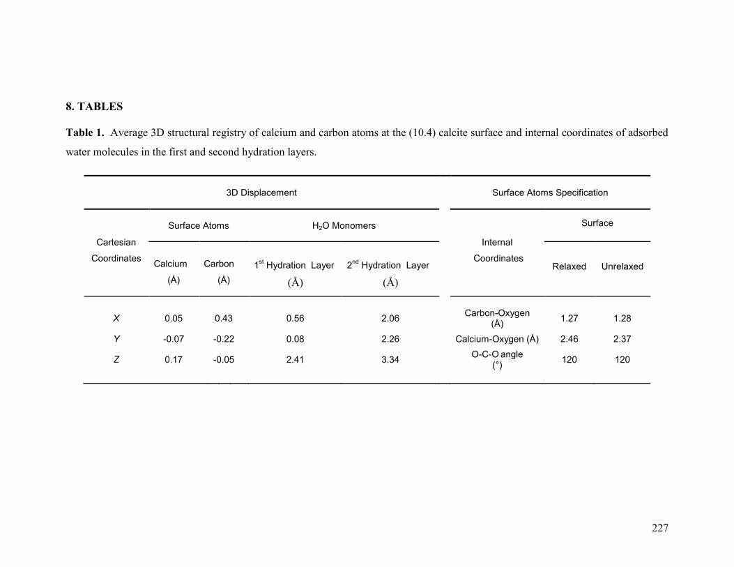
227

8. TABLES

Table 1. Average 3D structural registry of calcium and carbon atoms at the (10.4) calcite surface and internal coordinates of adsorbed

water molecules in the first and second hydration layers.

3D Displacement

Surface Atoms Specification

Cartesian

Coordinates

Surface Atoms H2O Monomers

Internal

Coordinates

Surface

Calcium

(Å)

Carbon

(Å)

1st Hydration Layer

(Å)

2nd

Hydration Layer

(Å)

Relaxed Unrelaxed

X 0.05 0.43 0.56 2.06 Carbon-Oxygen

(Å) 1.27 1.28

Y -0.07 -0.22 0.08 2.26 Calcium-Oxygen (Å) 2.46 2.37

Z 0.17 -0.05 2.41 3.34 O-C-O angle

(°) 120 120

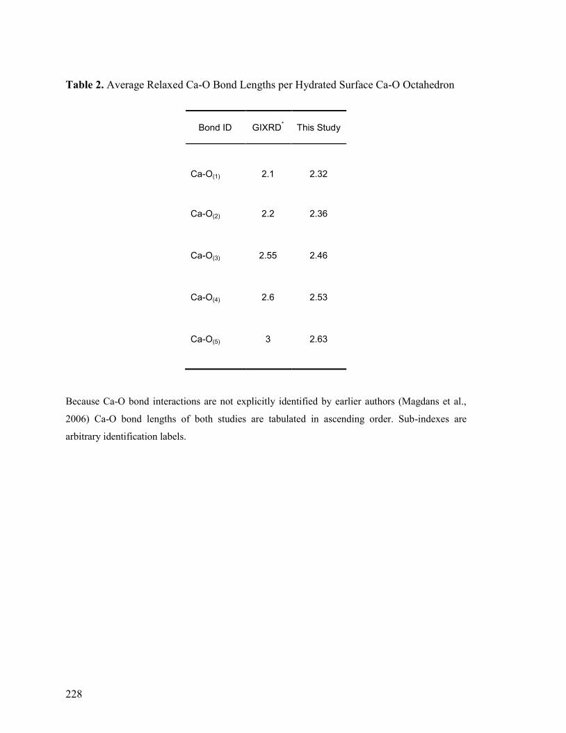
228

Table 2. Average Relaxed Ca-O Bond Lengths per Hydrated Surface Ca-O Octahedron

Bond ID

GIXRD*

This Study

Ca-O(1) 2.1 2.32

Ca-O(2) 2.2 2.36

Ca-O(3) 2.55 2.46

Ca-O(4) 2.6 2.53

Ca-O(5) 3 2.63

Because Ca-O bond interactions are not explicitly identified by earlier authors (Magdans et al.,

2006) Ca-O bond lengths of both studies are tabulated in ascending order. Sub-indexes are

arbitrary identification labels.

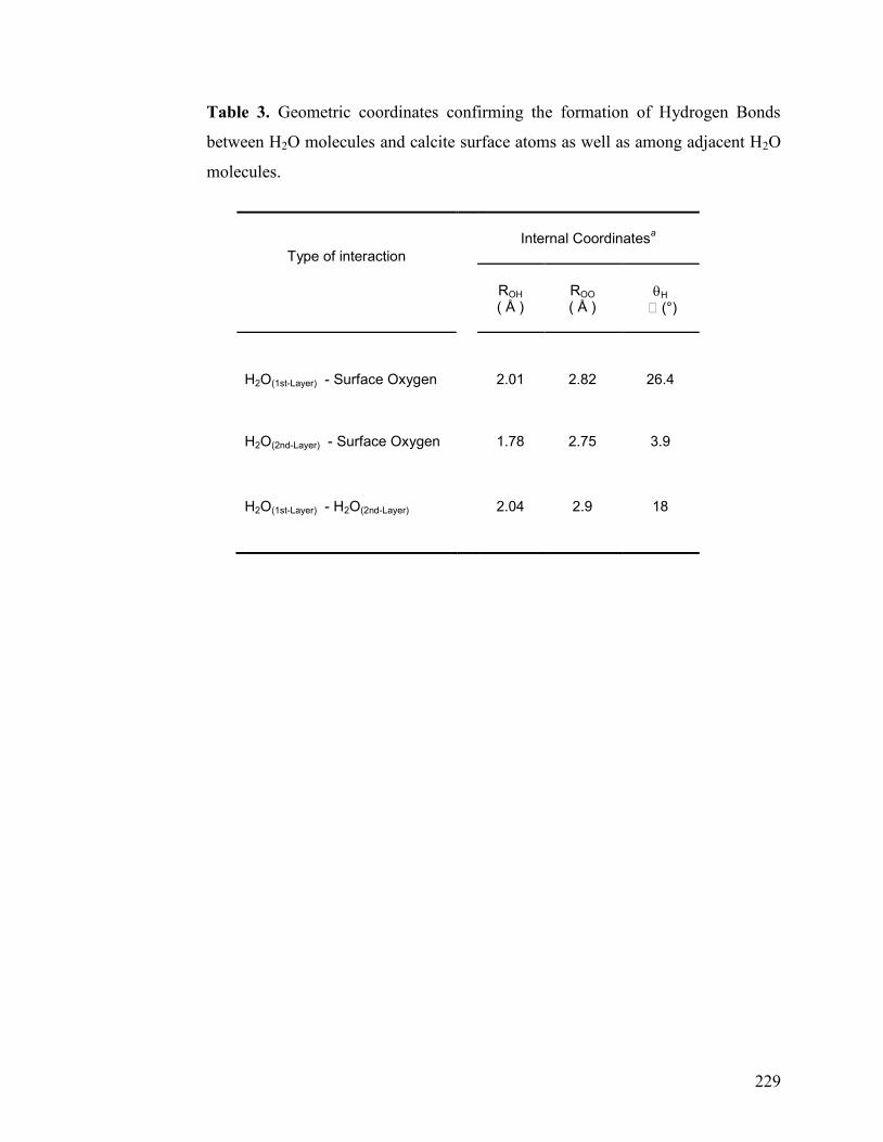
229

Table 3. Geometric coordinates confirming the formation of Hydrogen Bonds

between H2O molecules and calcite surface atoms as well as among adjacent H2O

molecules.

Type of interaction

Internal Coordinatesa

ROH ( Å )

ROO

( Å )

H (°)

H2O(1st-Layer) - Surface Oxygen 2.01 2.82 26.4

H2O(2nd-Layer) - Surface Oxygen 1.78 2.75 3.9

H2O(1st-Layer) - H2O(2nd-Layer) 2.04 2.9 18

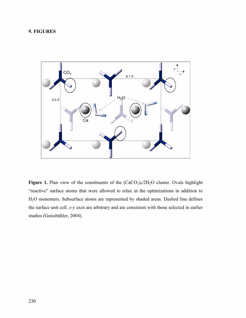
230

9. FIGURES

Figure 1. Plan view of the constituents of the (CaCO3)9/2H2O cluster. Ovals highlight

“reactive” surface atoms that were allowed to relax in the optimizations in addition to

H2O monomers. Subsurface atoms are represented by shaded areas. Dashed line defines

the surface unit cell. x-y axes are arbitrary and are consistent with those selected in earlier

studies (Geissbühler, 2004).

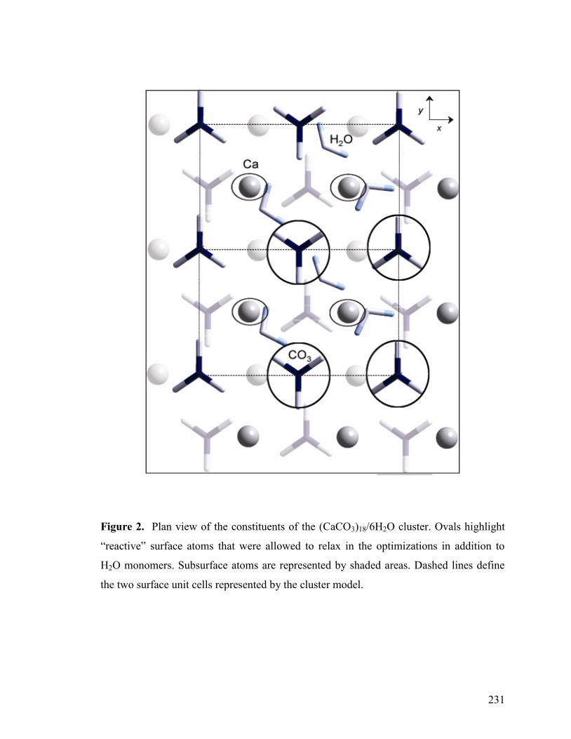
231

Figure 2. Plan view of the constituents of the (CaCO3)18/6H2O cluster. Ovals highlight

“reactive” surface atoms that were allowed to relax in the optimizations in addition to

H2O monomers. Subsurface atoms are represented by shaded areas. Dashed lines define

the two surface unit cells represented by the cluster model.

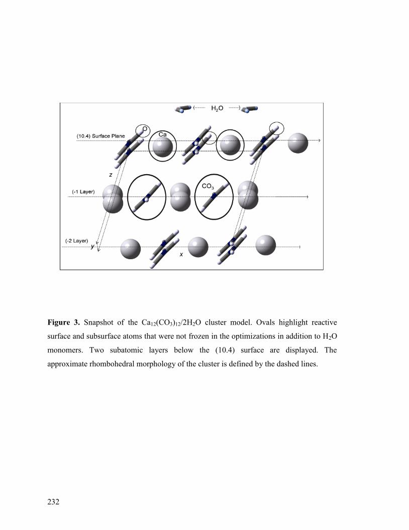
232

Figure 3. Snapshot of the Ca12(CO3)12/2H2O cluster model. Ovals highlight reactive

surface and subsurface atoms that were not frozen in the optimizations in addition to H2O

monomers. Two subatomic layers below the (10.4) surface are displayed. The

approximate rhombohedral morphology of the cluster is defined by the dashed lines.

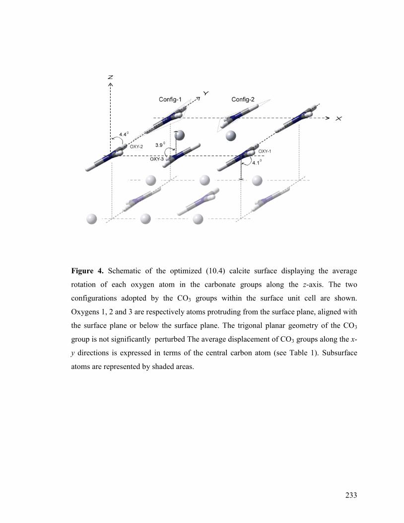
233

Figure 4. Schematic of the optimized (10.4) calcite surface displaying the average

rotation of each oxygen atom in the carbonate groups along the z-axis. The two

configurations adopted by the CO3 groups within the surface unit cell are shown.

Oxygens 1, 2 and 3 are respectively atoms protruding from the surface plane, aligned with

the surface plane or below the surface plane. The trigonal planar geometry of the CO3

group is not significantly perturbed The average displacement of CO3 groups along the x-

y directions is expressed in terms of the central carbon atom (see Table 1). Subsurface

atoms are represented by shaded areas.

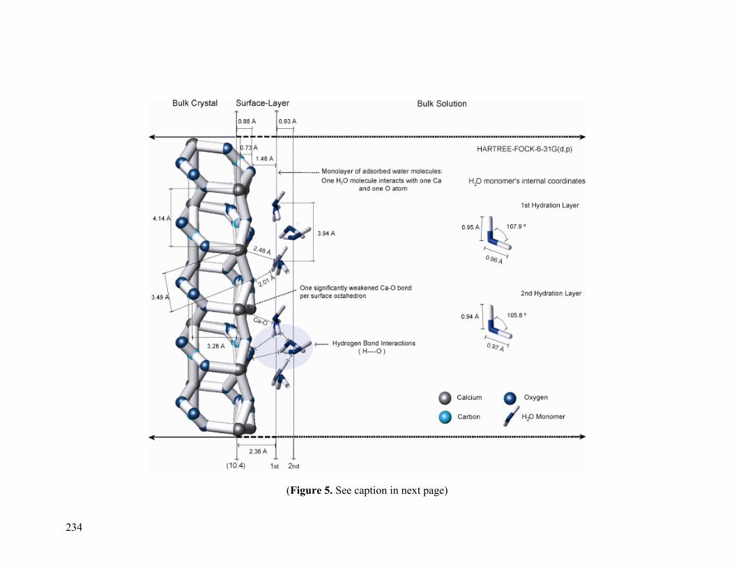
234

(Figure 5. See caption in next page)

235

Figure 5. Lateral view of the (10.4) reconstructed calcite surface as predicted at the HF-6-31G(d.p) level of theory. Structural details

of the first and second hydration layers are given. The average internal coordinates of the adsorbed water monomers are specified. Ca-

O and Hydrogen-bond interactions are shown.

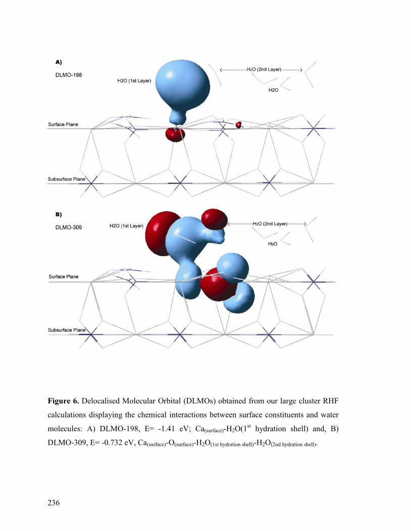
236

Figure 6. Delocalised Molecular Orbital (DLMOs) obtained from our large cluster RHF

calculations displaying the chemical interactions between surface constituents and water

molecules: A) DLMO-198, E= -1.41 eV; Ca(surface)-H2O(1st hydration shell) and, B)

DLMO-309, E= -0.732 eV, Ca(surface)-O(surface)-H2O(1st hydration shell)-H2O(2nd hydration shell).

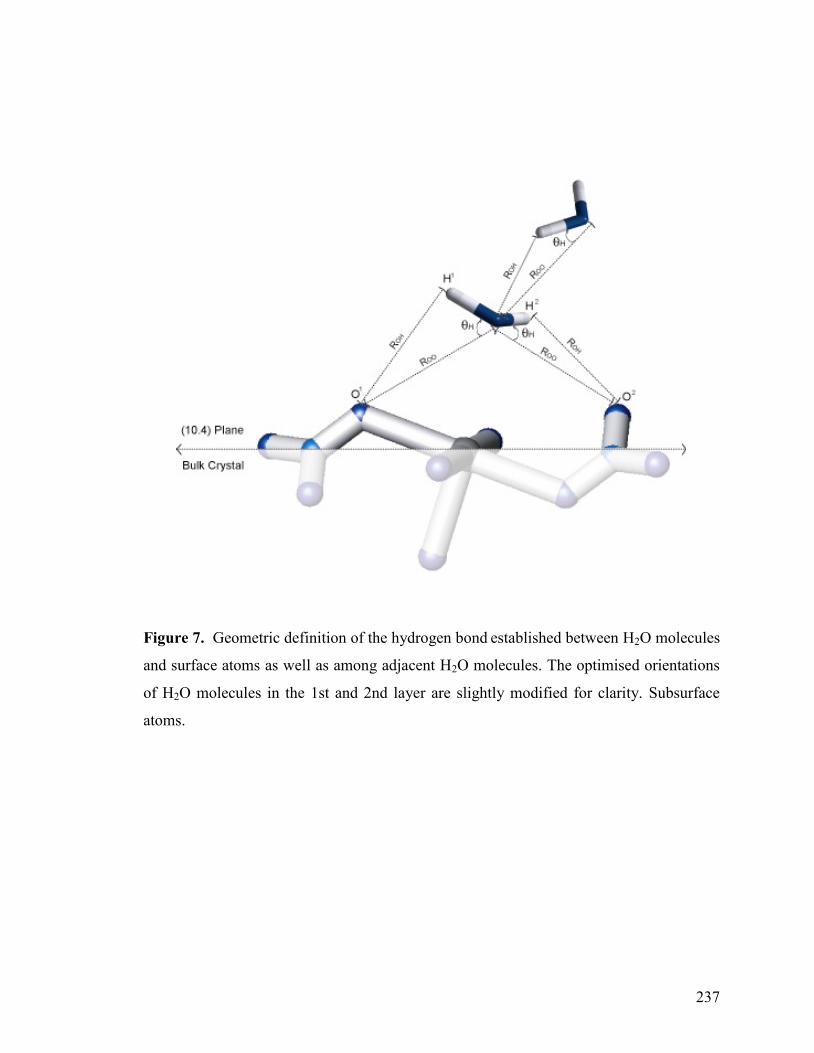
237

Figure 7. Geometric definition of the hydrogen bond established between H2O molecules

and surface atoms as well as among adjacent H2O molecules. The optimised orientations

of H2O molecules in the 1st and 2nd layer are slightly modified for clarity. Subsurface

atoms.

238


Despite the usefulness of molecular modeling techniques in the investigation of the

structural and energetic properties of the calcite surface, experimental data are required to

validate these results and further improve our understanding of the surface properties of

this mineral in aqueous solutions. Given the lack of suitable experimental protocols, the

quantitative characterization of some of the more fundamental sorptive properties of

calcite (e.g., proton, calcium) are still poorly known because sorption reactions at

carbonate surfaces are typically: i) characterized over relatively narrow ranges of

chemical composition (e.g., batch adsorption experiments, thermogravimetry,

chromatography), ii) qualitatively evaluated with surface sensitive instrumental

techniques (e.g., X-ray, Electron Diffraction, Spectroscopy), or iii) semi-quantitatively

inferred from electrokinetic studies. It follows that the acquisition of adsorption data over

expanded compositional ranges is a critical step for probing of sorption phenomena at the

calcite surface. In the following chapter, “Proton/Calcium Ion Exchange Behavior of

Calcite”, we address this issue by introducing a novel surface titration protocol that

allows, for the first time, the rigorous quantitative characterization of the proton sorptive

properties of calcite in aqueous solutions over a relatively wide range of chemical

conditions. In contrast to other rhombohedral carbonate minerals (magnesite, dolomite,

gaspeite) whose proton sorptive properties could be rationalized in terms of surface

complexation reactions, our calcite data led us to postulate on the existence of a

proton/calcium ion exchange reaction involving subsurface calcite layers. This reaction,

never postulated before, significantly impacts the aqueous speciation of closed carbonate-

rock systems and open environments with poor CO2 ventilation, via pH and calcite

dissolution buffering and CO2(g) sequestration upon ion exchange-induced calcite

precipitation.

239

CHAPTER 6

PROTON/CALCIUM ION EXCHANGE BEHAVIOR

OF CALCITE


1 and Jeanne Paquette

1





“Reproduced by permission of the PCCP Owner Societies: Phys. Chem. Chem. Phys. 39(11) 8895-8912”

http://dx.doi.org./10.1039/B815198A

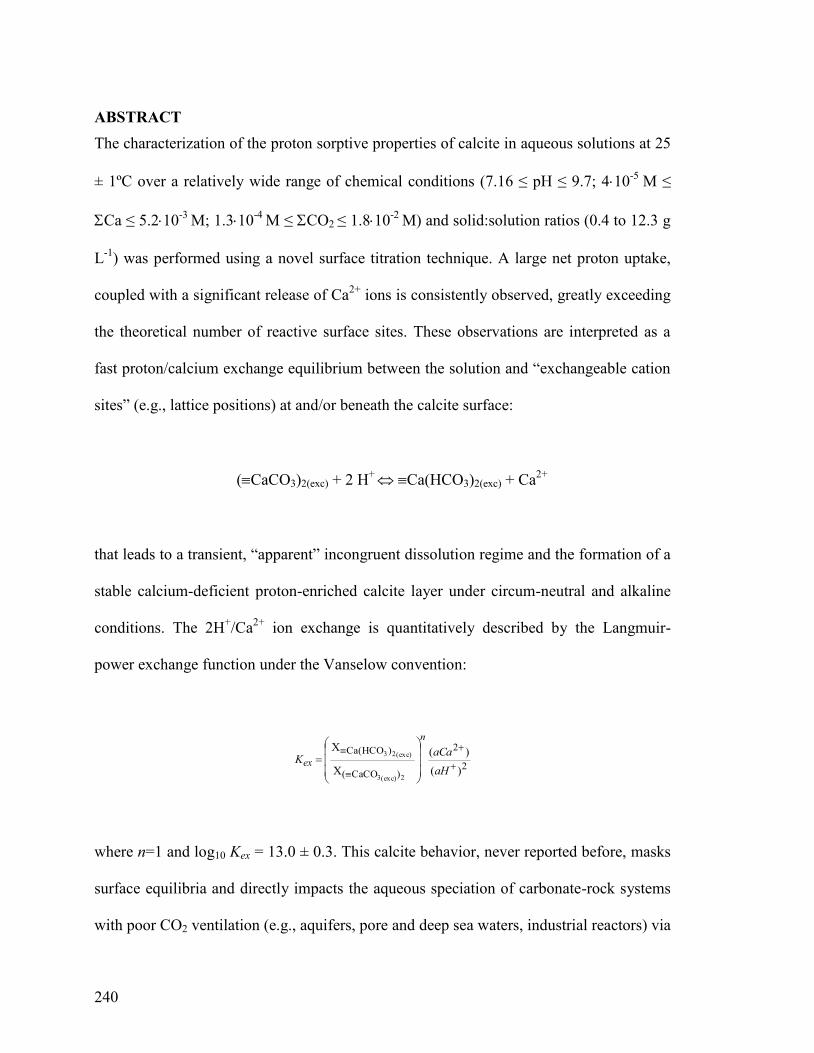
240

ABSTRACT

The characterization of the proton sorptive properties of calcite in aqueous solutions at 25

± 1ºC over a relatively wide range of chemical conditions (7.16 ≤ pH ≤ 9.7; 410-5

M ≤

Ca ≤ 5.210-3

M; 1.310-4

M ≤ CO2 ≤ 1.810-2

M) and solid:solution ratios (0.4 to 12.3 g

L-1

) was performed using a novel surface titration technique. A large net proton uptake,

coupled with a significant release of Ca2+

ions is consistently observed, greatly exceeding

the theoretical number of reactive surface sites. These observations are interpreted as a

fast proton/calcium exchange equilibrium between the solution and “exchangeable cation

sites” (e.g., lattice positions) at and/or beneath the calcite surface:



that leads to a transient, “apparent” incongruent dissolution regime and the formation of a

stable calcium-deficient proton-enriched calcite layer under circum-neutral and alkaline

conditions. The 2H+/Ca

2+ ion exchange is quantitatively described by the Langmuir-

power exchange function under the Vanselow convention:

2

2

)CaCO(

)HCO(Ca

)(

)(

X

X

2(exc)3

(exc)23

aH

aCaK

n

ex

where n=1 and log10 Kex = 13.0 ± 0.3. This calcite behavior, never reported before, masks

surface equilibria and directly impacts the aqueous speciation of carbonate-rock systems

with poor CO2 ventilation (e.g., aquifers, pore and deep sea waters, industrial reactors) via

241

the buffering of pH and calcite dissolution. In contrast, at fixed pCO2 conditions, aqueous

speciation remains unaffected upon CO2(g) sequestration resulting from ion exchange-

induced calcite precipitation:

(CaCO3)2(exc) + CO2(g)+ H2O Ca(HCO3)2(exc) + CaCO3(s)

Accordingly, reliable predictions of aqueous speciation in natural or engineered calcite-

containing systems at variable CO2(g) conditions must consider this exchange reaction and

associated Kex. The postulated proton/calcium exchange may have far-reaching

implications on the interpretation of kinetic and equilibrium data, and can partly explain

the anomalous solution chemistry observed in some field and laboratory carbonate

studies.

Keywords: Calcite titrations, proton sorptive properties, bicarbonate lattice species,

“apparent” incongruent calcite dissolution, calcium-deficient proton-enriched leached

layer.

242

1. INTRODUCTION

The most stable calcium carbonate polymorphs (calcite and aragonite) are highly reactive

minerals and ubiquitous in the environment. They are found: in aquatic systems as

suspended particles and carbonate-rich sediments whose occurrence range from tropical

environments (Morse and MacKenzie, 1990) to glacial settings (McGillen and Fairchild,

2005), in biological systems as the building blocks of shells and skeletons (MacKenzie et

al., 1990), and in the Earth‟s troposphere as mineral aerosols (Usher et al., 2003). They

also have numerous engineered applications, from fillers for paints, plastics, rubbers,

pharmaceuticals, cosmetics, optical devices, and paper (Vanerek et al., 2000) to raw

material in the construction industry, agriculture, as well as in the production of

biomedical scaffolds (Tas, 2007). In aqueous systems, they largely impact the solution

chemistry by regulating pH and alkalinity through their dissolution and precipitation, and

govern the mobility and bioavailability of trace and major elements via ion exchange

(Zachara et al., 1991) and sorption reactions (Martin-Garin, 2003). In the atmosphere,

these minerals regulate the CO2 exchange (Robbins and Fabry, 1994) and influence the

chemistry of volatile inorganic and organic acids (Usher et al., 2003; Al-Hosney and

Grassian, 2005).

Despite their environmental significance and broad industrial applications, critical

aspects of the reactivity of these minerals in aqueous solutions are still not fully

understood. Bulk phase CaCO3(s)-H2O equilibria are fairly well characterized

thermodynamically (Morse and MacKenzie, 1990) but surface properties, including the

pH of the isoelectric point (pHIEP) of calcite (Douglas and Walker, 1950; Prédali and

Cases, 1973; Mishra, 1978; Foxall et al., 1979; Siffert and Fimbel, 1984; Thompson and

Pownall, 1989; Huang et al., 1991; Cicerone et al., 1992; Moulin and Roques, 2003) and

243

the sorption behavior of potential-determining ions such as hydrolysis products, H+, OH

-

(Prédali and Cases, 1973; Mishra, 1978; Foxall et al., 1979), and lattice-derived

(constituent) ions, Ca2+

, CO32-

and HCO3- (Douglas and Walker, 1950; Siffert and Fimbel,

1984; Thompson and Pownall, 1989; Huang et al., 1991; Cicerone et al., 1992; Moulin

and Roques, 2003), that reflect on the macroscopic behavior of these minerals (e.g.,

coagulation, dissolution, etc.), remain poorly described. This is because proton and

constituent ion sorption equilibria are often difficult to resolve experimentally from the

dissolution/precipitation reactions that rapidly respond to minute variations in the solution

chemistry. This is particularly problematic when the experimental solution can exchange

CO2 with a gas phase, impacting the proton and carbon balance in solution to an unknown

extent, and hence, prohibiting the use of conventional titration techniques commonly

applied to the characterization of the ion sorptive properties of less reactive minerals such

as metal oxides (Huang, 1981) and sparingly reactive carbonates (Charlet et al., 1990).

The first attempt to quantitatively describe the surface reactivity of calcite in

aqueous solutions in terms of acid-base and constituent ion adsorption reactions was

provided by Van Cappellen and coworkers (1993) in the form of a surface complexation

model (SCM). In that study, formation constants of surface species were adjusted

manually until the predicted surface speciation closely reproduced the pHIEP (8.2)

recorded by electrokinetic measurements under specific solution conditions (Mishra,

1978). This procedure is useful but not rigorous because of the limited amount of

experimental data used in model calibration (a single data point: the pHIEP) which renders

the system an undetermined one: the number of adjustable model parameters (model

degrees of freedom) largely exceeds the number of data points used in parameter

calibration. Furthermore, in contrast to adsorption data, electrokinetically-derived data

244

(i.e., zeta potentials) are often obtained at conditions far from thermodynamic equilibrium

and do not allow direct probing of sorption reactions (an arbitrarily-selected electrostatic

model is required to relate zeta potentials to charge data which can, in turn, be used for

the calibration of sorption reactions, Westall and Hohl, 1980). Consequently, the

contribution of individual surface reactions to the development of surface charge cannot

be resolved nor can the formation constants of surface species be estimated accurately by

the above procedure. Recently, a multi-site ion complexation approach was applied to the

calibration of proton and constitutent ion surface complexation reactions for calcite using

selected electrokinetic data from the literature (Wolthers et al., 2008). It was concluded

that a straightforward validation of the postulated multi-site SCM was not possible

because of the uncertainties associated with the nature and magnitude of potential

artifacts inherent to the electrokinetic data. Clearly, reliable proton and constituent ion

adsorption data, acquired over a wide range of chemical conditions, are required for the

proper calibration of acid-base and constituent ion adsorption reactions at the calcite

surface.

Fast surface acid-base titration techniques were successfully applied to

determine ion sorption and/or surface charge development on sparingly reactive

carbonate minerals such as siderite and rhodochrosite (Charlet et al., 1990; Van

Cappellen et al., 1993), magnesite (Pokrovsky et al., 1999a) and dolomite (Pokrovsky

et al., 1999b; Brady et al., 1996; Brady et al., 1999). However, application of these

and more conventional

titration techniques (Huang, 1981) is unsuitable to the

characterization of the acid-base properties of highly reactive carbonate minerals such

as calcite and its polymorphs because their fast dissolution and precipitation kinetics

largely impacts the sorbate molar balance in solution, and hence, affects the

245

computation of surface charge (Van Cappellen et al., 1993; Wolthers et al., 2008).

Despite these considerations, conventional acidimetric surface titration techniques

were recently used in an attempt to estimate proton adsorption on calcite in aqueous

suspensions at different ionic strengths (Eriksson et al., 2007, 2008). Unfortunately,

the experimental protocol adopted in these studies suffers from serious deficiencies

among which: i) calcite dissolution was neglected in the computation of proton

adsorption data; ii) CO2(g) exchange with the atmosphere was neither prevented nor

monitored during the titrations thus affecting the CO2 and proton mass balance in

solution; and iii) the time intervals selected for the acquisition of serial experimental

data throughout the titrations were ill-defined (presumably very short) and reflect, at

best, partial restoration of bulk CaCO3(s)-CO2(g)-H2O thermodynamic equilibrium.

Consequently, the acquired proton sorption data are unsuitable for the calibration of

proton sorption reactions, as previously suggested (Wolthers et al., 2008).

To date, no reliable proton or carbonate adsorption data for the calcite surface

are available. To our knowledge, only one systematic constituent cation adsorption

study (Huang et al., 1991), conducted under a narrow range of solution conditions (9.3

≤ pH ≤ 9.9; 210-5

M ≤ CO2 ≤ 1.210-4

M; 10-5

M ≤ Ca ≤ 10

-2 M; solid:solution ratio:

250 g L-1

, equivalent to a surface area:solution ratio of 2160 m2 L

-1),

provides

quantitative calcium adsorption data suitable for the calibration of calcium adsorption

reaction(s) on the calcite surface.

It follows that the design of appropriate

experimental protocols for the acquisition of quantitative proton and constituent ion

adsorption data over a wide compositional range is a critical step for the quantitative

characterization of sorption equilibria of CaCO3(s) polymorphs (e.g., surface

246

complexation, ion exchange, etc.) and its interpretation within a self-consistent

theoretical framework.

In this paper, we address this issue by introducing a novel titration technique

that allows us, for the first time, to perform acidimetric and calcium ion titrations in

calcite suspensions, resolve sorption processes from bulk calcite

dissolution/precipitation reactions and, obtain reliable proton sorption and calcium

desorption data over a wide range of solution compositions. These are then interpreted

quantitatively on the basis of binary ion exchange equilibria established between the

solution and “exchangeable cation sites” (e.g., lattice positions).

2. MATERIALS AND METHODS

2.1 Principle of Calcite Titrations

In contrast to previous surface titration protocols where dissolution/precipitation

reactions are either circumvented or minimized (e.g., Huang, 1981; Charlet et al.,

1990) the high reactivity of calcite is exploited in the new technique. The

characterization of ion sorption is based on the following premises: i) an accurate

mass balance registry of all chemical components is maintained throughout the

titrations and ii) bulk-phase thermodynamic equilibrium is fully re-established upon

each titrant addition. The latter aspect contrasts with fast titration techniques (Charlet

et al., 1990; Van Cappellen, et al., 1993; Pokrovsky et al., 1999a; Pokrovsky et al.,

1999a; Brady et al., 1996; Brady et al., 1999) that are premised on the establishment

of surface rather than bulk equilibrium. Briefly, the titration is conducted over a

suitable range of chemical conditions in a closed-system in the absence of a gas phase

(i.e., headspace, dead volume) where known amounts of titrant are added

247

incrementally to a pre-equilibrated CaCO3(s) suspension. Under this scenario, no

CO2(g) is transferred from or to the suspension throughout the experiment (total

inorganic carbon, CO2, and proton mass conservation conditions). The solution

chemistry of the suspension is fully characterized before and after each titrant addition

(upon restoration of bulk equilibrium) without perturbing the experimental system

which permits the computation of sorption densities after consideration of

dissolution/precipitation reactions via thermodynamic speciation calculations. The

faster the system reacts to restore equilibrium, the shorter the duration of the titration.

Detailed explanations on the computation of sorption data are given below.

2.2 Description of the Reaction Vessel

A gas-tight glass reaction vessel was constructed specifically for this study (Fig. 1).

The reaction vessel is composed of two pieces joined by an O-ring and firmly held

together with a Plexiglas®

clamp. The top part of the reaction vessel is equipped with

threaded glass ports through which three ion selective electrodes (ISEs) and one

titrant dispenser tube are inserted. The ISEs and the titrant dispenser were secured to

the vessel with gas-tight, plastic threaded stoppers. The ISEs were used to monitor H+,

Ca2+

and CO32-

ion activities at each titration point and allow the full chemical

characterization of the system via the aqueous equilibra given in Table 1 and the

Davies Equation (Morel and Hering, 1993). Note that whereas the three ISEs were

used in most preliminary titration experiments, only the pCa and pH ISEs were used

in subsequent acidimetric and calcium titration experiments (see appendices). To

exclude the presence of a gas phase (i.e., headspace), the reaction vessel was

248

completely filled with the calcite suspension whereas, to accommodate the added

titrant, a 5 or 10 mL high density polyethylene (HDPE) syringe was fitted on a

protruding glass inlet at the top of the reaction vessel and carefully sealed with

Teflon®

tape and Parafilm®

. A gas-tight, two-way polyethylene stopcock was mounted

on the top of the reaction vessel to evacuate excess solution and/or adventitious air

bubbles before initiating the titration. To minimize grinding of the calcite powder, the

suspension was stirred with a Teflon-coated, suspended stir bar positioned at the

bottom of the reaction vessel. The total dead volume of the fully-assembled reaction

vessel, including all components displayed in Figure 1, was determined

gravimetrically using Milli-Q®

water at 25C. A suitable correction was made to

account for the volume of the calcite powder present in each titration experiment.

Details on chemical analyses, preparation and standardization of titrant solutions,

characterization and pre-treatment of the calcite powder, calibration of ISEs, and

preliminary titrations are given in the appendices to this thesis.

2.3 Surface Titration Conditions

Preliminary thermodynamic calculations revealed that highly concentrated calcite

suspensions are required to properly resolve the contribution of potential sorption

reactions from dissolution/precipitation equilibria. However, exceedingly high

solid:solution ratios must be avoided to ensure that crystals remain in suspension,

prevent possible interferences of CaCO3 particles with the ISEs, and circumvent

electrolyte-induced coagulation. Accordingly, titrations were performed at

solid:solution ratios ranging from 0.4 to 12.3 g L-1

(surface area:solution ratios of 0.2

249

to 5.7 m2/L) which proved to be effective for the acquisition of sorption data. The

ionic strength of the CaCO3 suspensions was adjusted to ~ 0.02 M with a 3 M KCl

solution. Two types of experiments were conducted at 1 atm and 25 1C:

acidimetric and calcium surface titrations. These were performed with a Radiometer

Titralab 865 titrator to which the pH electrode and the titrant dispenser tube (Fig. 1)

were connected. An Elite Ion Analyzer multichannel potentiometer, interfaced to a PC

computer, was used to monitor the Ca2+

and CO32-

ISE responses, although, as

mentioned earlier, the latter was used only in the preliminary titrations (see

appendices to this thesis). Because of the differential response times of the ISEs, the

titrations could not readily be pre-programmed to perform automatic incremental

titrant additions through the selection of a universal electrode stability criterion (e.g.,

mV/time). Alternatively, discrete titrant additions were performed manually at pre-

determined time intervals. The selection of these time intervals for each type of

titration is critical in the acquisition of reliable sorption data because the length of the

titration must be kept to a minimum to limit electrode drift or titrant leaks by diffusion

through the dispenser tube, while maximizing the number of titration points that

reflect complete restoration of bulk equilibrium. In addition, detectable changes in the

solution chemistry must be generated throughout the titration. To this end, preliminary

equilibrium speciation calculations were performed to select suitable initial chemical

conditions for our titration experiments (Table 2) and titrant concentrations.

Prior to titrations, a few mg of calcite were pre-equilibrated for at least 14 days

in the solutions described in Table 2 using stoppered 1 L Pyrex®

glass bottles (with

minimum headspace) before use (first equilibration). After standardization of the

250

titrant solutions and calibration of the ISEs, the supernatant of the pre-equilibrated

and decanted calcite suspension (accompanied by a few calcite particles to preserve

saturation) was transferred to the reaction vessel (containing known amounts of dry,

un-reacted, non-titrated, calcite powder) which was immediately assembled, closed,

and sealed to minimize CO2 exchange with the atmosphere. After full assembly of the

titration system (Fig. 1), the suspension was allowed to re-equilibrate for a minimum

of 24 hours under vigorous stirring before starting the titrations. Throughout this

second equilibration period, pH and pCa were continuously monitored to verify the

re-establishment of equilibrium conditions. The presence of adventitious air bubbles

inside the reaction vessel was monitored before and during the surface titrations. As a

rule, if bubbles were detected at the end of the second equilibration period, these

were evacuated, the reaction vessel was replenished with the supernatant remaining

from the first equilibration and the reaction vessel closed, sealed, and allowed to re-

equilibrate for another 24 hrs before initiating the titrations (third equilibration). If

recalcitrant bubbles (e.g., infiltrated air, evolved CO2(g)) were detected after the third

equilibration period or during the titration, the experiment was interrupted and all

data discarded. Details on the validation of our titration system and of our titration

experiments are given in the appendices to this thesis. Unless otherwise specified,

MINEQL+ v.4.6 software was used in all equilibrium calculations in this paper.

2.4 Computation of Sorption Data

All relevant definitions, mass and mole balance equations as well as associated

nomenclature for the Tableau-based aqueous phase definition of the CaCO3(s)-KCl-

H2O chemical equilibrium (Morel and Hering, 1993)1

and the computation of sorption

251

data are provided in Table 3. Apparent proton and calcium sorption densities (Happ

and Caapp

, respectively) are computed from:

Happ

= (1/A·S)·(TOTH*Theo - TOTH*Exp) (1)

Caapp

=(1/A·S)·(Ca*Theo – Ca*Exp) (2)

where A is the specific surface area (m2

g-1

) and S is the solid:solution ratio (g L-1

).

In contrast to proton- and OH-bearing minerals such as metal oxides (goethite,

lepidocrocite etc.), pure calcite powders do not display a net proton imbalance at their dry

terminal surfaces (no protons or hydroxyl groups within their lattices or at their surfaces),

and hence, no excess or deficit in protons is introduced to the mineral-H2O system (in

addition to CA-CB, see Table 3) upon calcite immersion in water. Thus, assuming CO2(g) is

not exchanged with a gas-phase (as in our experiment), net proton densities, Hnet

, of the

calcite surface, at the beginning and throughout the titration, can be obtained directly

from pH and pCa measurements, the amounts of CA and CB added, and application of Eq.

1. This yields the condition: Happ

=Hnet

. This contrasts with proton- and OH-bearing

minerals that require a pre-determination of the Point of Zero Net Proton Charge

(PZNPC) before Hnet

can be computed (Sposito, 1998). Similarly, potential calcium

imbalances (with respect to a stoichiometric number of CO3 groups) at the calcite surface,

possibly arising from differential constituent ion re-adsorption or transient non-

stoichiometric calcite dissolution before titration (Douglas and Walker, 1950; Stipp and

Hochella, 1991; Villegas-Jiménez et al., 2009), can be estimated from pH and pCa

252

measurements, the initial amounts of Ca and CO2 in the system, and Eq. 2. This yields

the condition: Caapp

= Canet

where the latter term represents net calcium densities.

The simplest way to verify that the above conditions are met is to compute Happ

and Caapp

from the solution chemistry measured in the simplest possible CaCO3(s)-H2O

scenario: an equilibrated suspension of calcite (≥ 99% purity) in pure water (Milli-Q®, ~

18 Mohm cm, without CO2(g) exchange with a gas phase) which should correspond to

the solution condition: TOTH0=TOTCa

0=0. Under this condition, if no significant proton

or calcium adsorption/desorption occurs (i.e., Happ

= Caapp

=0), the pH and pCa

measured at 25 ± 1ºC must be nearly identical to those predicted thermodynamically. The

excellent agreement between the measured and theoretical pH and pCa values (>99% and

>97%, respectively) under these chemical conditions confirmed the validity of the

assumption that sorbateapp

=sorbatenet

=0 where the subscript “sorbate” represents proton or

calcium ions This chemical scenario will be referred to as the zero net sorption reference

condition (ZNSRC) This is a common assumption in carbonate mineral surface studies

(Charlet et al., 1990; Van Cappellen, et al., 1993; Pokrovsky et al., 1999a, b), even though

it is rarely defined explicitly (Charlet et al., 1990) or verified experimentally.

Whereas the ZNSRC prevails at the beginning of Experiments TH-I, TH-III, TH-

IV and TH-VI, it does not necessarily hold for titrations conducted under the following

initial chemical conditions: TOTH0 and/or TOTCa

0 0 (Experiments: TH-II, TH-V, TCa-

I-TCa-IV), because the proton and/or constituent ion imbalance in solution may induce

ion sorption and modify the chemistry of the solution (TOTH0

Exp TOTH0

Theo and/or

Ca0Exp

Ca

0Theo) and the calcite surface (H

0 and/or Ca

0 0) during the first and

second equilibration periods and prior to titration. Consequently, to correctly compute

253

the net sorption densities, sorbatenet

, in these experiments, new TOTH0

Theo and Ca0

Theo

values must be “experimentally” determined from the pH and pCa measured in the

supernatant at the end of the first equilibration period and before exposure to additional

calcite (i.e., the powder subjected to titration). Once transferred to the reaction vessel, a

new sorption equilibrium with the un-reacted calcite powder is established, and thus, Hnet

and Canet

can be estimated using the new TOTH0

Theo and Ca0

Theo values, pH and pCa

measurements, and Eqs. 1 and 2. Alternatively, once the pre-equilibrated supernatant

(first equilibration) is transferred to the reaction vessel and after the second

equilibration period, one can determine TOTH0

and Ca0 (total calcium concentration

before titration) from the measured pH and pCa values and the definitions given in Table

3, substitute these in Eqs. 1 and 2 respectively (as the TOTH*

Theo and Ca*Theo values

prior to titration: TOTH0

Theo and Ca0

Theo, and compute the initial extent of proton

occupancy of the calcite sample (subsequently subjected to acidimetric or calcium

titrations) via a suitable mathematical relationship. This relationship, derived from

experiments initiated at the ZNSRC, is described in the “sorption modeling section”,

whereas detailed explanations on the computation of sorbatenet

values for titrations

initiated away from the ZNSRC are given in the appendices to this thesis.

3. RESULTS AND DISCUSSION

3.1 Qualitative Interpretation of Data

Before proceeding to the quantitative interpretation of the sorption data, some

preliminary discussion is required. Firstly, the Happ

values computed via Eq. 1 in all

our acidimetric and calcium titrations (Hnet

>> 0), largely exceed the theoretical

254

number of reactive surface sites at the (10.4) calcite surface (8.2 moles m-2

) which is a

striking result, particularly in the case of calcium titrations considering that no HCl

was added in these experiments. Secondly, the Caapp

values computed in all titration

experiments by Eq. 2 reflect a substantial calcium release (Canet

<< 0). In other

words, Ca*Exp values were consistently much larger than Ca*Theo reflecting a large

excess of Ca over CO2 in solution (TOTCa*

Exp >> 0). Because stoichiometric

calcite dissolution should not affect the Ca:CO2 ratios, the registered TOTCa*

Exp

values are unexpected in all cases (including experiment TH-V initiated at TOTCa*

Exp

> 0), but most particularly, in experiments initiated at TOTCa0

Exp = 0 (TH-I, TH-III,

TH-IV, TH-VI, in which no calcium addition was made) and at TOTCa0

<< 0 (TCa-I-

TCa-IV). These results are counterintuitive since, under the conditions of our calcium

titration experiments (stepwise additions of CaCl2 rather than HCl), a net calcium

removal from solution via calcite precipitation and calcium adsorption (Huang et al.,

1991) was expected, possibly coupled with a net proton release (rather than a net

proton uptake) induced by calcium/proton exchange surface reactions as those

postulated earlier (Van Cappellen et al., 1993; Wolthers et al., 2008). Keeping in mind

that precipitation/dissolution reactions are accounted for in the determination of the

Ca0

Theo values, it is clear that other mechanism(s) must be called upon to explain the

“anomalous” TOTH*

Exp, Ca0

Exp, and TOTCa*

Exp values registered in our acidimetric

and calcium titrations.

Whereas contamination of our suspensions by impurities carried-over from

previous experiments can be dismissed (see precautions described in the appendices to

this thesis), neither can the observed Ca*Exp and TOTCa*Exp values be explained by

255

the desorption of Ca2+

ions (potentially pre-adsorbed on the calcite surface) because

the release of several hypothetically “Ca-enriched” atomic layers (up to 16 layers,

according to the maximum proton uptake and calcium release observed in our

experiments at a pH of 7.2, see below) would be required to account for the high

Ca values measured at the end of the titrations. This is clearly an unrealistic

scenario. Similarly, the “non-stoichiometric” release of Ca2+

over CO32-

ions from the

calcite outmost surface layer (Douglas and Walker, 1950; Stipp and Hochella, 1991;

Villegas-Jimenez et al., 2009)

and/or the preferential detachment of Ca2+

from

subsurface atomic layers are either insufficient to account for our observations or

would generate an unreasonable number of ion vacancies and negative charges within

the lattice. Likewise, the extent of carbonate adsorption required to increase

TOTCa*Exp to the observed levels largely exceeds the theoretical number of reactive

surface sites available in our experimental systems (7.5·10-7

-2.4·10-5

moles, as

computed from the theoretical site density, the specific surface area, the mass:volume

ratio, and the total volume of the suspensions). Finally, incongruent calcite dissolution

upon the formation of a secondary solid phase (e.g., calcium hydroxide) is

thermodynamically unfavorable and could not account for either proton uptake or

calcium release. Consequently, we propose that a proton/calcium ion exchange takes

place between calcite and the solution according to the following reaction:

(CaCO3)2(exc) + 2 H+ Ca(HCO3)2(exc) + Ca

2+ (3)

256

where species identified with the subscript “exc” correspond to reactive units at and/or

beneath the calcite surface which we will refer to hereafter as “exchangeable cation

sites”. Reaction 3 describes the non-stoichiometric release of one Ca2+

ion, with

respect to CO32-

ions (“apparent” incongruent dissolution), upon substitution by two

protons at exchangeable cation sites, which preserves charge-neutrality within the

mineral lattice. Alternatively, reaction 3 could be equally formulated as:

CaCO3(exc) + 2 H+ H2CO3(exc) + Ca

2+ (4)

which only contrasts with reaction 3 in the nature of the resultant exchangeable cation

species.

A representative example of the mirror-image displayed by the net proton and

calcium densities is shown in Figure 2. Although the computed average Hnet

:Canet

ratio (~1.5) differs from the ideal stoichiometry (2.0) of reactions 3 and 4, the

discrepancy is ascribed to cumulative and systematic errors associated to the

computation of TOTH*Exp and TOTCa*Exp. For instance, calculations using our

sorption data, the Ca2+

ISE calibration curves, and the chemical definitions given in

Table 3 reveal that a systematic decrease in the Ca2+

ISE signal by 1-3%, consistent

with the estimated electrode drift (see appendices to this thesis), would lead to a net

increase in the TOTH*Exp and a concomitant net decrease in Ca*Exp by 2-6%

depending on the pH range. Whereas errors of this magnitude would not impact

significantly on the quantitative interpretation of the sorption data (see below), they

would account for most of the discrepancy between the observed and ideal Hnet

:Canet

257

ratios (R) suggested by reactions 3 and 4. Furthermore, propagation of error analysis

based on the experimental uncertainties of our experimental protocol (ISE readings,

titrant concentrations, volumetric titrant additions, etc.) adds up to a 10% random

error in the estimated Happ

and Caapp

values which, in turn, yields a random error of

14% in the computed R values. This translates into R values ranging from 1.3 to 1.7,

in close agreement with the variability of the experimental R values (1.25-1.8). In

brief, a combination of random and systematic errors inherent to our experimental

protocol likely accounts for the discrepancy between the observed and “ideal” R

values.

Alternatively, a Hnet

:Canet

ratio of 1, dictated by the stoichiometry of the

proton/calcium ion exchange reaction involving the background electrolyte cation in

our experimental system (K+):

CaCO3 (exc) + H+

+ K+ KHCO3 (exc) + Ca

2+ (5)

could only be obtained if the pCa values derived from Ca2+

ISE readings carried much

larger systematic errors (~ 12-18%, depending on the pH) than those required to achieve a

Hnet

:Canet ratio of 2, an unlikely scenario given the maximum Ca

2+ ISE drift (3 %, see

appendices to this thesis). In addition, experimental studies reveal that potassium defects

in natural calcite samples (incorporated during early mineral crystallization) are highly

unstable under Earth‟s surface conditions and potassium ions tend to migrate

spontaneously out of the lattice and accumulate in crystallites at the calcite surface (Stipp

et al., 1997; Stipp et al., 1998). These observations strongly argue against the stability of

258

the KHCO3 (exc) species and the viability of reaction 5, a premise that was further

confirmed by our sorption modeling work described below. Because no other potentially

exchangeable cation is present in the system, the last possibility to the observed R values

is that the proton/calcium exchange is not governed by a reaction with an integer 2:1

stoichiometry (reactions 3 and 4) but rather, by a reaction involving a fractional

stoichiometry which would lead to a large net negative charge buildup within the calcite

lattice (because more positive charges are leaving the calcite lattice than are incorporated

via proton uptake), a largely speculative hypothesis that would be difficult to explain

thermodynamically. It follows that cation exchange reactions 3 and 4 are the most viable

mechanisms for the quantitative interpretation of our sorption data.

If we consider that, upon HCl additions to the suspensions, calcite will dissolve

according to:

CaCO3(s) + 2 H+

Ca2+

+ H2CO3* (6)

combining reactions 3 and 6 yields:

(CaCO3)2(exc) + CaCO3(s) + 4 H+

Ca(HCO3)2(exc) + 2 Ca2+

+ H2CO3* (7)

Estimated values of TOTCa*Exp as a function of the deficit in CO2 with respect to the

amount expected from calcite dissolution (i.e., CO2* = CO2*Theo - CO2*Exp; see

Table 3), obtained in all the acidimetric titrations, are compiled in Figure 3. Note that

259

to properly account for TOTCa*Exp arising solely from reactions between the bulk

solution and calcite at conditions: TOTCa0 0 (Experiments TH-II and TH-V),

TOTCa0 was subtracted from the corresponding TOTCa*Exp values and the corrected

values reported in Figure 3. A linear regression of these data yields a slope of 2.1, in

excellent agreement with the Ca:C stoichiometry dictated by reaction 7. The CO2*

values are explained by the net decrease in calcite dissolution following proton uptake

and Ca2+

release to the solution. In other words, upon HCl additions, proton/calcium

ion buffers the pH, increases the Ca2+

ion activity (yielding higher TOTCa*Exp) in

solution which, in turn, buffers the calcite saturation state, limits calcite dissolution,

and progressively decreases CO2*

Exp (i.e. increases CO2

*). This is consistent with

the non-stoichiometric release of Ca2+

over CO32-

ions postulated by reaction 3 upon

strong acid additions.

On the other hand, upon incremental additions of CaCl2 to the experimental

suspensions containing large concentrations of HCO3- ions (Experiments TCa-I to

TCa-IV), calcite precipitation occurs and generates increasing levels of H2CO3*

according to:

Ca2+

+ 2 HCO3- CaCO3(s) + H2CO3

* (8)

Hence, for this scenario, we can illustrate the 2H+/Ca

2+ exchange mechanism by

combining reactions 3, 8 and the following equilibrium:

2 H2CO3* 2 H

+ + 2 HCO3

- (9)

260

to yield:

(CaCO3)2(exc) + H2CO3*

Ca(HCO3)2(exc) + CaCO3(s) (10)

Reaction 10 suggests that carbonic acid, generated by CaCO3(s) precipitation upon

CaCl2 additions, can be removed from solution upon 2H+/Ca

2+ ion exchange-induced

calcite precipitation.

To summarize, under all chemical scenarios examined in our study (see Table

2) we observe that: i) proton removal from solution (i.e., TOTH*Exp << TOTH*

Theo)

largely exceeds the theoretical number of reactive surface sites (by up to ~32-fold,

according to the maximum proton uptake and calcium release observed in our

experiments at a pH of 7.2 and assuming a 1:1 sorbate:surface site stoichiometry,

see below) and ii) a significant TOTCa*Exp increase is generated throughout the

titrations that cannot be explained by the desorption of potentially pre-adsorbed Ca2+

ions on the calcite surface. Both observations (eventually confirmed by Hnet

and

Canet

data) can only be explained by invoking the presence of reactive sites other than

those conventionally defined at the calcite surface (e.g., exchangeable cation sites at

and/or beneath the calcite surface). This is the basis of the postulated 2H+/Ca

2+ ion

exchange mechanism proposed by reactions 3 and 4.

3.2 Possible Mechanisms of “Proton Uptake/Calcium Release” and “Apparent”

Incongruent Calcite Dissolution

Several mechanisms could equally account for the stoichiometry of reactions 3 and 4,

including mechanisms that might involve possible OH-bearing defects (e.g.,

261

CaCO3nH2O(s) and/or Ca(OH)2(s)) homogeneously embedded within the calcite

lattice (i.e., subsurface layers) prior to titration, and subsequently released to the

solution via co-dissolution, ion migration along micro-fractures and/or rapid physical

rearrangement of the near-surface layers (see Figure 4). In mechanism A, n H2O

molecules are presumably embedded in the calcite lattice through interactions with

CaCO3 lattice units whereas in mechanism B, 2n hydroxyl groups replace nCO32-

lattice units preserving charge neutrality in the bulk crystal. Under these scenarios,

lattice OH- groups and Ca

2+ ions are released either by: i) co-dissolution of n

Ca(OH)2(s) / n CaCO3(s) units, leading to a hypothetical substitution of

(CaCO3H2O)x “hypothetical” defects by CaCO3(x-n)H2Ox-2n and (CO3H2)n lattice

units, or ii) coupled Ca2+

/OH- ion migration outwards from the crystal. Both

mechanisms would lead to a net decrease of TOTH*Exp (upon proton neutralization by

releasing OH- ions) and a net increase of TOTCa*Exp in solution. Nevertheless, these

mechanisms are unlikely under our experimental conditions. Firstly, although H2O

and/or OH-bearing defects have been observed within the lattice of Mg-rich biogenic

calcites (Gaffey, 1995), precursor metastable amorphous CaCO3 phases (Elfil and

Roques, 2001), and aragonite (B. Phillips, personal communication); available NMR

evidence is still inconclusive to confirm their presence in synthetic Mg-free calcite

samples as the one used in this study (B. Phillips, personal communication; Feng et

al., 2006). Furthermore, the aging pre-treatment, to which our calcite powder was

subjected (see calcite specimen section in the appendices to this thesis), would have

removed most of these “hypothetical” OH- and/or H2O-bearing defects. In turn, this

would have affected the solution chemistry recorded in individual titration

262

experiments, yielding inconsistent results between experiments. Secondly, mechanism

A would be expected to occur only under a dissolution regime (acidimetric tirations),

and hence, would not explain results obtained in the calcium titration experiments

where precipitation takes place. Conversely, mechanism B would be independent of

dissolution/precipitation processes but would generate numerous lattice vacancies that

would destabilize the crystal lattice, an aspect difficult to explain thermodynamically.

Finally, because solid-state ion diffusion is unlikely within the time-scale of our

experiments (Fisler and Cygan, 1999),

an unrealistic number of micro-fractures

serving as ion conduits would have to pervade the calcite crystals used in all titrations.

Consequently, we believe that the most plausible mechanism involves a fast

2H+/Ca

2+ ion exchange (mechanism C in Fig. 4) between the solution and the solid,

following the dynamic rearrangement of the near-surface calcite layers (i.e.,

spontaneous recrystallisation, Hoffmann and Stipp, 2001). The latter would lead to a

renewal of the adsorption sites, a net increase in proton uptake capacity, and the

generation of a proton-enriched, calcium-deficient layer, analogous to the chemically

and structurally altered “leached” layers developed by some chain-silicate minerals

(e.g., wollastonite, diopside, albite, labradorite) following their incongruent

dissolution under acidic regimes (Casey et al., 1993; Green and Lüttge, 2006). In fact,

rearrangement of the calcite surface has been shown to extend over at least 10 atomic

layers upon exposure to air at 30% relative humidity or more (Stipp et al., 1997) and

is consistent with mechanisms of fast ion incorporation into the calcite lattice (i.e.,

lattice penetration or surface recrystallization) postulated by other researchers

(Zachara et al., 1988; Zachara et al., 1991; Stipp et al., 1992; Stipp et al., 1996;

Hoffmann and Stipp, 2001; Curti et al., 2005). These observations have led to the

263

suggestion of the presence of an “interfacial region” conceptualized either as a

hydrated CaCO3(s) “gel-like” phase (Somasundaran and Agar, 1967), a porous

membrane composed of adsorbed and surface layers (Mucci et al., 1985), or as a

hydrated “multi-atomic disordered CaCO3(s) layer” (Davis et al., 1987) through which

ions presumably diffuse, segregate, and dehydrate before incorporation in the bulk

lattice. These conceptualizations of the hydrated calcite interface would provide a

suitable environment for the fast proton incorporation and calcium release postulated

by mechanism C. Unlike mechanisms A and B, mechanism C does not require an

homogeneous distribution (most likely unrealistic) of hydroxyl-bearing defects

(CaCO3nH2O(s) and/or Ca(OH)2(s)) over the calcite lattice prior to titration nor does

it lead to the generation of lattice vacancies that could destabilize the crystal.

Results of a recent Nuclear Magnetic Resonance (NMR) spectroscopy study

(Feng et al., 2006) reveal the presence of stable bicarbonate species within the bulk

lattice of organic defect-free synthetic calcite samples whereas Knudsen flow reactor-

based adsorption experiments suggest the presence of bicarbonate-bearing species at

hydrated calcite surfaces after their exposure to CO2(g) (Santschi and Rossi, 2006),

consistent with the formation of the bicarbonate species postulated by reaction 3.

Similarly, recent theoretical (Tossel, 2006) and experimental studies (Usher et al.,

2003, Al-Hosney and Grassian, 2005) suggest that H2CO3 might be stable in solid

phase either in some oligomeric form (Tossel, 2006) or as an adsorbed species at acid-

treated carbonate mineral surfaces (Usher et al., 2003, Al-Hosney and Grassian,

2005), supporting the formation of H2CO3–like species such as produced by reaction

4. Whether HCO3- or H2CO3-bearing species form or not within the calcite lattice is

264

beyond the scope of the present study but we believe that the formation of

≡Ca(HCO3)2(exc) is more likely to explain proton stabilization within the calcite lattice

than the presence of ≡H2CO3(exc) species. Accordingly, the following discussion will

focus on reaction 3. Nevertheless, as explained below, the quantitative treatment

performed on our sorption data is equivalent whether based on reactions 3 or 4.

3.3 Sorption Modeling

As discussed above, the chemical conditions selected in this study induce

proton/calcium exchange and are thus suitable for the quantitative description of

reaction 3. Given the inter-dependency of Ca2+

and H+ activities under equilibrium

conditions, sorption isotherms calibrated to specific pH values are not useful for the

interpretation of sorption data. Instead, the pH-dependency of this reaction allows the

simultaneous quantitative interpretation of sorption data acquired at different pH

values, as is commonly done in surface complexation modeling studies.

The mass action law describing the binary exchange (reaction 3) can be

represented by the selectivity constant (Kex) defined by the classical Langmuir-power

exchange function based upon the Vanselow convention:

2

2

)CaCO(

)HCO(Ca

)(

)(

X

X

2(exc)3

(exc)23

aH

aCaK

n

ex (11)

which is defined in terms of the mole fractions (X) of the

exchangeable cation sites, the activities (a) of the aqueous species and an empirical

265

exponent (n) that accounts for deviations from ideal cation mixing (n1) arising from

steric and electrostatic effects (i.e., local electrostatic balance) within the crystal

lattice. The activity of solid component i, ai, is given by:

ai = i Xi (12)

where i is the corresponding solid activity coefficient and depends on the

composition of the system (Stoessell, 1998). Hence, if mole fractions realistically

reflect the activities of exchange sites (=1) and local electrostatic balance is fully

achieved (n=1), then Kex corresponds to the conditional equilibrium constant

describing the 2H+/Ca

2+ exchange,

cKex (Stoessell, 1998).

We assume that only a small fraction of the calcite lattice participates to

proton/calcium exchange which, hereafter, we will refer to as the “exchangeable

cation site density” (ECSD). According to reactions 3 and 4, the ECSD represents half

of the proton uptake capacity (PUC) of calcite. Both parameters are expressed in mol

m-2

units for consistency with adsorption data normalized to the experimental BET

specific surface area. Nevertheless, it must be emphasized that because proton uptake

appears to extend beneath the topmost surface atomic layer, the PUC is unlikely a

surface property, and instead, presumably reflects the intrinsic ability of calcite to

develop a partial solid solution of the type: Ca(1-x)H2xCO3 under specific chemical

conditions. In addition, one must note that, although the specific BET-surface area of

the titrated calcite sample was not significantly different from that of the non-titrated

material, BET measurements on reacted, rinsed, and dried powders would not reveal

266

the presence of features (e.g., gels, channels, crystallographic re-arrangements) that

may have developed upon proton/calcium exchange (and possibly affected the

available reactive surface area) since they may only be persistent in solution.

The concentration of the so-called “cation-specific surface sites”, presumably

corresponding to the concentration of exchangeable Ca at the topmost surface layer(s)

of calcite crystals, was previously estimated, using 45

Ca isotopic exchange

experiments, at 3.6·10-6

moles g-1

(or 0.72·10-6

moles m-2

; Zachara et al., 1991). This

value, however, is too low to successfully model our sorption data using equation 11.

Attempts to model our data, using the experimental total CaCO3(s) molar concentration

(0.004-0.12 M) to estimate molar fractions, without optimization of the ECSD, were

also unsuccessful. Consequently, Kex and ECSD were estimated via numerical

optimization using FITEQL v.3.2 (Herbelin and Westall, 1996), in analogy to the

procedures commonly adopted to estimate intrinsic formation constants and the total

surface site density within the framework of surface complexation theory (Dzombak

and Morel, 1990). Preliminary estimates of Kex and ECSD were obtained using net

proton sorption data from experiments initiated at the ZNSRC (experiments TH-I, TH-

III, TH-IV and TH-VI). Since successful convergence was achieved with n=1 (ideal

cation mixing) for all selected data sets, this value was used in subsequent

optimization runs. An average log10 Kex of 13.1 0.4 and an average ECSD of 12

(3.7) ·10-5

moles m-2

, corresponding to ~ 0.7 % of the total CaCO3 in the system and

equivalent to 32 calcite monolayers (according to reaction 3), were obtained. Since

most solid solutions behave ideally when the mole fraction of the solvent crystal

approaches unity, we can confidently assume that the solid solution Ca (1-x)H2xCO3

267

(where x < 0.01) satisfies the same criterion over the compositional range of study,

and hence, the activities of exchange species can be equated to their mole fractions in

equation 11. This shows that the constant returned by FITEQL optimization of

reaction 3 represents indeed cKex, and thus, we will refer as such hereafter.

As mentioned earlier, apparent proton sorption densities derived from

experiments TH-II and TH-V were referenced to the ZNSRC to account for the extent

of proton occupancy at the beginning of these titrations and compute the

corresponding net sorption densities. The latter were used in subsequent optimizations

of cKex and ECSD (see appendices to this thesis). An average log10

cKex of 13.1 0.4

and an average ECSD of 13 ( 3.1) ·10-5

moles m-2

were obtained upon optimization

of these data, values statistically identical to those obtained in our previous

optimizations.

Net proton sorption densities computed from all our acidimetric titrations are

displayed in Figure 5. The good reproducibility of the data obtained under different

chemical conditions confirms that the experimental protocol can quantitatively resolve

sorption or ion exchange reactions from bulk dissolution equilibria. It is noteworthy

that, although the initial conditions of Experiments TH-II and TH-V differ

significantly from others (including a lower initial pH), the net proton densities

derived from these are consistent with results of other titrations and extend the

investigational pH range to circum-neutral pH values. In all cases, proton uptake

increases smoothly from pH 10 to about 8.5 and displays a significant increase at pH

< 8.5. The solid curve in Figure 5 shows the net proton densities predicted by

speciation calculations including reaction 3, the optimized cKex, and ECSD values for

268

a solid:solution ratio of 9.61 g L-1

(surface area: solution ratio of 4.42 m2 L

-1). Clearly,

reaction 3 successfully simulates data over a wide range of chemical conditions with

small deviations at pH > 8.5 where proton sorption values are relatively low.

Similarly, because all calcium titrations were performed at TOTH0 > 0 and

TOTCa0

< 0, proton sorption densities computed from these experiments using Eqs. 1

and 2 were corrected and referenced to the ZNSRC (see appendices to this thesis). As

calcium was added incrementally to the solution, the calcite saturation state increased,

triggering its precipitation and the concomitant formation of H2CO3* (reaction 8).

Thus, intuitively, either positive or null calcium sorption densities (Canet

≥ 0) are

expected but, as stated earlier, the opposite behavior (i.e., Ca releaseCanet

<< 0,) was

observed accompanied by a substantial proton uptake. These results can be explained

by the net removal of H2CO3* from solution upon proton/calcium ion exchange,

following calcite precipitation, resulting in a net proton uptake and net Ca release

(reaction 10). Consequently, the computed amounts of calcium released to the solution

(i.e., “calcium desorption data”) were used to fit Kex and ECSD. To this end, and

according to the stoichiometry of reaction 3, the amount of Ca released to the solution

(in absolute molar units: |Canet

|·S·A) was subtracted from the total molar

concentration of exchangeable cation sites, (CaCO3)2(exc), available in each

experiment (Experiments TCa-I to TCa-III: 6.0·10-4

mol L-1

, Experiment TCa-IV:

2.4·10-5

mol L-1

). The latter was computed from the product of the solid:solution ratio

in each experiment, the specific surface area, and the average ECSD value previously

optimized with acidimetric titration data (13·10-5

moles m-2

). This subtraction yields

the apparent molar concentration of unreacted exchangeable cation sites,

269

(CaCO3)2(exc)*, at each titration point. The molar concentration of exchangeable

cation sites initially occupied by protons, Ca(HCO3)2(exc)o, after the second

equilibration and prior to titration (see appendices to this thesis), was then subtracted

from (CaCO3)2(exc)* to normalize data to the ZNRSC and obtain the net unreacted

(available) exchangeable cation site concentration, (CaCO3)2(exc)*net

, which was

subsequently used in the FITEQL optimizations. The net molar densities of unreacted

exchangeable cation sites (i.e., ECSD-Hnet

) and the model predictions are shown in

Figure 6. The data from experiment TCa-III could not be fitted with FITEQL and

show significant deviations from the model predictions. The inability of our model to

fit these data is explained by the high CO2 in this experiment ( 0.023 M) promoting

calcite precipitation (i.e., reaction 8 was favored), largely masking calcium

desorption, and affecting the accuracy of the estimated (CaCO3)2(exc)* used in

FITEQL optimizations. In Figure 6, the experimental H2CO3(aq)* values are also

displayed for each titration experiment. Note that, for a given H2CO3(aq)* value

(dictated by the pH and the pCa), an identical fraction of unreacted exchangeable

cation sites is generated, regardless of the TOTH0

Theo and TOTCa0

Theo values, as

observed in experiments TCa-I, TCa-II and TCa-IV, in conformity with reaction 10.

The average conditional equilibrium constant derived from the calcium

titration data, log10 cKex = 12.9 ± 0.2 (with n=1 as well), is in excellent agreement

with the value computed from the acidimetric titrations (13.1 0.3). Averaging all the

optimized cKex values yields a log10

cKex of 13.0 ± 0.3, the conditional equilibrium

constant for reaction 3 over the compositional range of this study. Combining this

value, the calcite solubility product (Kºsp), the product of the dissociation constants of

270

carbonic acid (K°H2CO3* K°HCO3, Table 1), and their associated uncertainties (Plummer

and Busenberg, 1982), we obtain a log10 cKex2 of 4.8 ± 0.4 for the following mass

action law describing reaction 10:

n

)*COaH((

(

exKc

322

2(exc)3

(exc)23

)CaCOX

)HCOCaX

(13)

With the exception of data from experiment TCa-III, the model predictions fit

experimental data reasonably well and confirm the validity of reaction 3 beyond the

chemical conditions under which the acidimetric titrations were conducted. The

uncertainty of our sorption data (~ 10%) and of the optimized log10 cKex value (± 0.3)

describing reaction 3 confirm that the maximum errors potentially associated to the

computation of TOTCa*Exp and TOTH*Exp (see above) do not affect significantly the

optimization of cKex. Note that modification of the solid:solution ratios resulting from

calcite dissolution (acidimetric titrations, Eq. 7) or precipitation (calcium titrations,

Eq. 10) do not affect the cKex value because the concentration units of the

exchangeable species, (CaCO3)2(exc) and Ca(HCO3)2(exc), in reaction 3 cancel each

other, and thus, eliminate their mass and surface area dependency. All attempts to fit

sorption data to reaction 5 with FITEQL were unsuccessful, further dismissing the

viability of this ion exchange mechanism as explained above.

In view of the successful model results provided by reaction 3, we believe that

the estimated cKex and ECSD values are reliable predictors to model proton/calcium

exchange over a circum-neutral and alkaline pH regime (preponderant in calcite-

271

containing systems) but we have yet to establish if these values vary significantly with

the properties of the calcite substrate (e.g., purity, pre-treatment, specific surface area)

or the solution chemistry, particularly under acidic conditions where the proton-

enriched, calcium-deficient leached layer might be destabilized upon enhanced calcite

dissolution. Because of the formalism adopted in reactions 3 and 4 to define the

exchangeable lattice species, Ca(HCO3)2(exc) and H2CO3(exc), the calibrated cKex and

ECSD values apply to both reactions. The only distinction is that, because lattice

species in reaction 3 involve full unit cells (i.e., 2 CaCO3 units), the corresponding

ECSD represents 32 calcite monolayers, whereas for reaction 4 only half this value

is involved. Application of Nuclear Magentic Resonance techniques (Feng et al.,

2006), Raman Spectroscopy (Casey et al.,1993), Ion Beam Analyses (Casey et al.,

1993; Petit et al., 1987; Bureau et al., 2009) to acid-reacted single calcite crystals

should shed light on the identity of the lattice species and the extent of proton

penetration within the calcite lattice. This information will be key in ascertaining the

mechanisms accounting for the 2H+/Ca

2+ ion exchange behavior of calcite and in the

characterization of the proton-enriched, calcium-deficient leached layer postulated in

this study.

As suggested by our model predictions in Figure 5, under circum-neutral and

slightly acidic conditions, exchangeable cation sites may become fully saturated by

protons, and thus, provided no calcium is added to the system, proton/calcium ion

exchange will likely be interrupted; unless additional exchangeable cation sites (i.e.,

higher PUC), not revealed in our study, are available in calcite. Under the former

scenario, a progressive decrease of pH, following incremental additions of a strong

272

acid (HA), should lead to the dissolution of the calcium-deficient, proton-enriched

layer (presumably located near the topmost surface layer) as well as of some of the

underlying bulk CaCO3(s) layers. This may allow the system to restore the TOTH*Theo,

TOTCa*Theo and Ca/CO2 values predicted by thermodynamic calculations without

consideration of proton/calcium exchange.

The predicted behavior of TOTH*Theo, TOTCa*Theo and Ca/CO2 upon HA

additions with and without consideration of proton/calcium exchange at different

solid:solution ratios is displayed in Figure 7. As a result of 2H+/Ca

2+ exchange,

TOTH*Theo decreases with increasing solid concentration whereas TOTCa*Theo and

Ca/CO2 increase upon the non-stoichiometric Ca2+

release over CO32-

ions. The

salient feature in Figure 7 is that, once the exchangeable cation sites are fully titrated,

the slopes (m) of TOTH*Theo and TOTCa*Theo become equal to those predicted in the

absence of ion exchange (m=1), reflecting the prevalent role of calcite dissolution

(over ion exchange) in dictating the solution chemistry behavior under these chemical

conditions. The curves do not overlap at this point because the solution chemistry is

affected differentially (depending on the amount of calcite) by the chemical

composition of the calcium-deficient, proton-enriched leached layer developed in the

ion exchange scenario. Nevertheless, all curves will overlap if the leached layer

constituents are fully released to the solution, following a destabilization of the

calcium-deficient, proton-enriched layer, a phenomenon not observed in our

experiments and neglected in our modeling but potentially important in studies

conducted under acidic conditions or at other PVT conditions not investigated in our

study.

273

3.4 Ion Exchange vs Surface Equilibria

The postulated proton/calcium ion exchange mechanism is consistent with the fast

incorporation of some divalent metals within the calcite lattice (Stipp et al., 1992;

Stipp et al., 1997; Hoffmann and Stipp, 2001), possibly coupled with proton

incorporation (Curti et al., 2005), and reveals that ion sorption likely extends over

several subsurface calcite layers within the so-called “gel-like” interfacial region

(Somasundaran and Agar, 1967).

Results of numerous sorption (Davis et al., 1987; Huang et al., 1991; Stipp et

al., 1992; Zhong an Mucci, 1995; Hoffmann and Stipp, 2001; Eriksson et al., 2007,

2008) ion exchange (Zachara et al., 1988, 1991; Curti et al., 2005) and surface

complexation (Comans and Middelburg 1987; Van Cappellen et al., 1993; Pokrovsky

et al., 2000; Martin-Garin et al., 2003; Wolthers et al., 2008) studies of metal ions at

the calcite surface can be found in the literature but none was designed for the

quantitative evaluation of the proton/cation exchange equilibria. For example, Huang

et al (1991) obtained calcium adsorption data that were interpreted in terms of a

Langmuir-type isotherm over a very limited pH range (9.3-9.9) but the authors could

not observe 2H+/Ca

2+ ion exchange because their experimental conditions (i.e.,

TOTHTheo=0 and TOTCaTheo 0) did not promote proton/calcium exchange. In other

words, the driving force (TOTHTheo > 0 and/or TOTCaTheo< 0) necessary to induce

proton/calcium ion exchange in pure calcite samples was absent. Similarly, earlier

proton adsorption data, obtained from acidimetric titrations of calcite suspensions

conducted in open reaction vessels (Eriksson et al., 2007, 2008) are not useful for the

evaluation of 2H+/Ca

2+ exchange because an accurate mass balance registry of H (or

274

TOTH, see Table 3), CO2 and Ca cannot be obtained by the employed methods.

Consequently, neither adsorption nor ion exchange reactions can be properly

evaluated with these data.

In fact, it is possible that, under most experimental conditions, proton surface

equilibria and proton/calcium exchange are intrinsically coupled in calcite, the former

dictating the surface speciation and the development of surface charge while the latter

affects the composition of the solution and the speciation of exchangeable cation sites.

If so, the experimental decoupling of these two processes is not trivial (if possible at

all) since ion exchange may affect proton adsorption by modifying the chemical

composition of the near-surface calcite layers which, in turn, should reflect on its

surface properties (e.g., ion affinity). Similarly, it is possible that additional

adsorption reactions involving other metals (e.g. Mg2+

) or large adsorbates (e.g.,

phosphate, sulfate, organics) interfere with ion exchange equilibria by blocking

reactive surface sites and/or inhibiting the rearrangement of the calcite surface which,

in turn, may affect ion transport to or from the exchangeable cation sites. The complex

interplay of these equilibria must exert a key role on determining the surface

properties of calcite and its macroscopic behavior in aqueous solutions (e.g.,

coagulation, dissolution, pHIEP). Consequently, quantitative interpretations of its

surface reactivity, including its surface charge, electrokinetic behavior (Huang et al.,

1991; Cicerone et al., 1992; Van Cappellen et al., 1993; Wolthers et al., 2008) and

dissolution kinetics (Sjöberg and Rickard, 1984; Van Cappellen et al., 1993; Arakaki

and Mucci, 1995) based upon surface reactions calibrated against data acquired under

275

proton/calcium exchange inducing conditions

will likely be more intricate than

previously considered.

3.5 Implications of Proton/Calcium Ion Exchange

Proton/calcium ion exchange has numerous and important implications with respect to

the interpretation of experimental and field data. The best way to illustrate this is by

comparing speciation calculations performed with and without consideration of

proton/calcium exchange. Because MINEQL+ v.4.6, as well as many other

equilibrium speciation computer codes, does not allow the user to decouple the mass

action law and the mass balance matrices necessary to properly define the ion

exchange equilibrium problem, these calculations were performed using an in-house

Matlab subroutine specifically adapted for this purpose. Nevertheless, identical

calculations can be performed within any equilibrium speciation code in which

suitable modifications can be implemented to decouple the mass action law and the

mass balance matrices. Detailed explanations on these calculations are provided in the

appendices to this thesis.

Figure 8 shows the speciation predicted in a closed CaCO3(s)-H2O system upon

additions of a strong acid (HA) without (Scenario I) and with (Scenario II)

consideration of ion exchange at a high solid:solution ratio (100 g L-1

or 46 m2 L

-1) to

magnify the impact of ion exchange on the solution chemistry. For equivalent strong

acid additions, the values of Ca, H2CO3* and Total Alkalinity (TA) predicted in

Scenario I are consistently higher whereas pH displays the opposite behavior. As a

result of ion exchange, solution pH is significantly buffered, decreasing the extent of

276

calcite dissolution which, in turn, shifts the equilibrium towards lower Ca,

H2CO3*, and TA values. Note that, although reactions 6 (calcite dissolution

scenario, acidimetric titrations) and 8 (calcite precipitation scenario, calcium

titrations) predict increasing levels of H2CO3*, proton/calcium exchange results in a

lowered H2CO3*. This is because in the dissolution scenario, less H2CO3* is

produced upon ion exchange since more protons are required for H2CO3* generation

than when ion exchange is neglected (see the differential H+:H2CO3* stoichiometries

of reactions 6 and 7). Similarly, a net H2CO3* consumption takes place in the

precipitation scenario upon ion exchange (reaction 10), in contrast with what is

predicted when ion exchange is not considered (reaction 8). For a given pH, Ca

values are higher and H2CO3* and TA are lower in Scenario II than in Scenario I

because more strong acid equivalents (CA) are needed in Scenario II to reach an

identical pH because of the pH buffering induced by ion exchange. Additions of CA

favor 2H+/Ca

2+ exchange and increase Ca but decrease the amount of carbonate

equivalents that must be dissolved to restore saturation, as manifested by the lower

H2CO3* and TA values. The difference in CA equivalents required to achieve a given

pH increases at lower pH, reflecting the enhanced pH-buffering capacity of calcite

induced by proton/calcium ion exchange under these solution conditions.

In contrast to closed-systems, in open carbonate systems where the pCO2 is

fixed or at steady-state, the aqueous speciation is identical for Scenarios I and II

whereas the relative concentrations of exchangeable cation species, (Ca(HCO3)2(exc)

and (CaCO3(exc))2), are solely dictated by the pCO2 and cKex, and thus, remain fixed

throughout the entire pH scale in Scenario II (see reaction 10). Hence, in open

277

systems, provided enough exchangeable cation sites are available for proton uptake,

net non-stoichiometric Ca2+

ion release (over CO3-2

) will be observed upon addition of

CO2(g) to aquatic carbonate-rock systems, as defined by (reaction 10 minus reaction

8):

(CaCO3)2(exc) + 2 H2CO3* Ca(HCO3)2(exc) + Ca2+

+ 2 HCO3- (14)

It follows that model predictions of the response of carbonate-rich (sediments,

suspended particles) aquatic environments to rising atmospheric pCO2 (i.e., enhanced

[H2CO3]*) must consider the role of proton/calcium exchange on the carbonate

mineral equilibria as the reaction will buffer pH and the calcite saturation state of the

waters, partly mitigating the postulated negative effects (e.g., decalcification of

calcifying organisms, deleterious development of coral reefs; Andersson et al., 2003,

2006) of anthropogenic CO2(g) invasion in marine shelf waters. Interestingly, this

geochemically-driven ion exchange mechanism is similar to the physiologically-

driven 2H+/Ca

2+ ion exchange exhibited by some calcifying marine species

(McConnaughey, 1991; McConnaughey and Falk, 1991; Al-Horani et al., 2003). The

calcification of some marine algae and coral species is believed to be promoted by

extra-cellular transport of Ca2+

ions to calcification sites and removal of protons

through ATP-driven 2H+/Ca

2+ ion exchange which induces aragonite supersaturation

within the calcifying environment (McConnaughey, 1991; McConnaughey and Falk,

1991; Al-Horani et al., 2003). It follows that the quantitative decoupling of these two,

278

possibly overlapping proton/calcium exchange mechanisms, represents a new

scientific challenge to carbonate marine geochemists.

Clearly, quantitative interpretations of field or laboratory data that rely on

speciation calculations of the CaCO3(s)-H2O system should consider reaction 3 when

experiments are conducted under conditions favorable for proton/calcium exchange

such as: i) when pCO2 is variable, ii) when strong acid is added to a calcite suspension

and/or iii) when calcite powder is subjected to chemical pre-treatments (such as dilute

HCl leaching) before use in order to remove potential impurities or reduce surface

roughness (Zachara et al., 1991; Elzinga et al., 2006; Ahmed et al., 2008). For instance,

some researchers have reported anomalously high Ca equilibrium concentrations

upon HCl additions to highly concentrated calcite suspensions (Eriksson et al., 2007).

Similarly, field data reveal large Ca and TA anomalies in water column samples in

equilibrium with CaCO3(s) collected from the deep ocean that reflect an apparent

excess of calcium (or TA deficit) over that predicted from stoichiometric calcite

dissolution (Brewer et al., 1975). These findings could be, a priori, interpreted as the

incongruent dissolution of calcite whereas they more likely reflect the non-

stoichiometric release of Ca2+

over CO32-

ions induced by proton/calcium exchange.

The observed “apparent” incongruent dissolution regime is presumably a transient

stage of the overall dissolution process that remains active until saturation of available

exchangeable cation sites and might be eventually masked by a possible

destabilization of the calcium-deficient, proton-enriched leached layer under acidic

conditions (or at other PVT conditions) and the re-establishment of the congruent

dissolution regime. A detailed quantitative discussion of the role of proton/calcium

279

ion exchange in dictating aqueous speciation in carbonate-rock aquatic systems under

different chemical scenarios and its implications for the in-situ, long-term geological

storage of atmospheric CO2(g) and on the responses of marine carbonate-rich shelf

sediments to rising atmospheric pCO2 will be the subject of future work.

4. CONCLUSIONS

A novel experimental protocol was developed to quantitatively characterize the proton

sorptive properties of calcite in aqueous suspensions. Sorption data were acquired via

acidimetric and CaCl2 titrations conducted over a relatively wide range of chemical

conditions (pH, Ca, CO2 and solid:solution ratios). In contrast to expectations, a

large net proton uptake, coupled with a significant release of Ca2+

ions is consistently

observed. Because proton uptake greatly exceeds the theoretical number of available

reactive surface sites at the calcite surface, sorption data cannot be quantitatively

interpreted by adsorption or surface complexation reactions. Alternatively, these data

were interpreted on the basis of a proton/calcium ion exchange reaction, a possible

analogue of the physiologically-driven 2H+/Ca

2+ ion exchange behavior exhibited by

some calcifying marine organisms. The postulated 2H+/Ca

2+ ion exchange would

occur by a fast, chemically-driven equilibrium mechanism between the solution and

“exchangeable cation sites” (e.g., lattice positions) at and/or beneath the calcite

surface following the dynamic rearrangement of the near-surface calcite layers. The

latter would lead to a renewal of the adsorption sites, a net increase in proton uptake

capacity and the generation of a calcium-deficient, proton-enriched layer, under

circum-neutral and alkaline conditions, analogous to the leached layer developed by

280

chain-silicate minerals under acidic conditions. The application of NMR, Ion Beam

Analysis, and Raman Spectroscopy techniques is required for a detailed chemical

characterization of this layer and for determining the depth of proton penetration

within the calcite lattice.

This newly postulated proton/calcium exchange behavior of calcite largely

masks surface equilibria and directly impacts the solution chemistry of carbonate-rock

systems isolated from the atmosphere (closed-system) or where CO2 ventilation is

restricted (e.g., aquifers, pore and deep sea waters, industrial reactors) via pH and

calcite dissolution buffering. In contrast, in systems exposed to fixed pCO2 conditions

(e.g., open-systems), aqueous speciation remains unaffected because of CO2(g)

sequestration arising from 2H+/Ca

2+ ion exchange-induced calcite precipitation. The

postulated mechanism may partly explain the anomalous solution chemistry observed

in some field and laboratory studies. Accordingly, quantitative interpretations of

experimental data acquired at proton/calcium exchange inducing conditions (i.e.,

TOTH0 > 0 and/or TOTCa

0 < 0) require consideration of this reaction via the

cKex and

the ECSD values calibrated in this study. For instance, dissolution kinetics data

acquired following the incremental addition of a strong (e.g., HCl) or a weak acid

(i.e., CO2(g)) without full characterization of the solution chemistry may require a re-

evaluation since these may partly reflect the transient, non-stochiometric release of

Ca2+

and CO32-

ions to the solution upon ion exchange (i.e., “apparent” incongruent

dissolution), with the concomitant formation of a leached layer, rather than the

progressive destruction of the 3D crystallographic framework (i.e., congruent calcite

dissolution). Similarly, accurate predictions of the response of carbonate-rich shelf

sediments to rising atmospheric pCO2 must consider the pH and calcite saturation state

281

buffering capacity imparted by the proton/calcium exchange behavior of calcite and

possibly other carbonate minerals that make up the sediment assemblage.

Finally, the titration protocol introduced in this study is recommended for the

quantitative characterization of ion exchange and/or sorption reactions between calcite

(or its polymorphs: aragonite and vaterite) and other potential sorbates whose

activities can be measured with available Ion Selective Electrodes.

5. ACKNOWLEDGMENTS

A.V.-J. is grateful to Mrs. Rosy J.-R. for offering a stimulating environment

throughout the preparation of this paper. Special thanks go to Dr. Brian Phillips and

Dr Michel Rossi for providing additional information on their results. The insightful

comments of two anonymous reviewers are greatly appreciated. This research was

supported by a graduate student grant to A.V.-J. from the Geological Society of

America (GSA) and Natural Sciences and Engineering Research Council of Canada

(NSERC) Discovery grants to A.M. and J.P. A.V.-J. also benefited from post-graduate

scholarships from the Consejo Nacional de Ciencia y Tecnología (CONACyT) of

Mexico as well as financial support from the Department of Earth and Planetary

Sciences, McGill University and Consorcio Mexicano Flotus-Nanuk.

282

6. REFERENCES

Ahmed I.A.M., Crout N.M.J. and Young S.D. (2008) Kinetics of Cd sorption, desorption

and fixation by calcite: A long-term radiotracer study. Geochim. Cosmochim. Acta

72, 1498-1512.

Al-Horani F.A., Al-Moghrabi S.M., de Beer D. (2003) The mechanism of calcification

and its relation to photosynthesis and respiration in the scleractinian coral Galaxea

fascicularis. Mar. Biol. 142, 419-426.



Chem. Chem. Phys. 7, 1266-1276.

Andersson A.J., Mackenzie F.T., Ver L.M. (2003) Solution of shallow-water carbonates:

An insignificant buffer against rising atmospheric. CO2. Geology 31(6), 513-516.

Andersson A.J., Mackenzie F.T., Lerman A. (2006) Coastal ocean CO2–carbonic acid–

carbonate sediment system of the Anthropocene. Global Biogeochem. Cycles

20:GB1S92, 1-13.

Arakaki T. and Mucci A. (1995) A continouous and mechanistic representation of calcite

reaction-controlled kinetics in dilute solutions at 25° and 1 atm total pressure.

Aquatic Geochem. 1, 105-130.



Brady P.V., Papenguth, H.W. and Kelly J.W. (1999) Metal sorption to dolomite surfaces.

Applied Geochem. 14(5), 569-579.

http://www.rsc.org/Publishing/Journals/CP/article.asp?doi=b417872f



283

Brewer P.G., Wong G.T.F., Bacon M.P. and Spencer D.W. (1975) An oceanic calcium

problem? Earth Planet. Sci. Lett. 26, 81-87.

Bureau H., Raepsaet C., Khodja H., Carraro A. and Aubaud C. (2009) Determination of

hydrogen content in geological samples using elastic recoil detection analysis

(ERDA). Geochim. Cosmochim. Acta 73(11), 3311-3322.

Casey W.H., Westrich H.R., Banfield J.F., Ferruzi G. and Arnold G.W. (1993) Leaching

and reconstruction at surfaces of dissolving chain-silicate minerals. Nature 366,

253-256.



Cicerone D.S., Regazzoni A.E. and Blesa M.A. (1992) Electrokinetic properties of the



Comans R.N.J. and Middelburg J.J. (1987) Sorption of trace metals on calcite:

Applicability of the surface precipitation model. Geochem. Cosmochim. Acta 51,

2587-2591.

Curti E., Kulik D.A. and Tits J. (2005) Solid solutions of trace Eu(III) in calcite:

Thermodynamic evaluation of experimental data over a wide range of pH and

pCO2. Geochim. Cosmochim. Acta 69(7), 1721-1737.





284

Douglas H.W. and Walker R.A. (1950) The electrokinetic behavior of iceland spar



and Sons Inc.: New York, NY, Chapters 1-3.

Elfil H. and Roques H. (2001) Role of hydrate phases of calcium carbonate on the scaling

phenomenon. Desalination, 137, 177-186.

Elzinga E.J., Rouff A.A. and Reeder R.J. (2006) The long-term fate of Cu2+

, Zn2+

, and

Pb2+

adsorption complexes at the calcite surface: An X-ray absorption

spectroscopic study. Geochim. Cosmochim. Acta, 70, 2715-2725.

Eriksson R., Merta J. and Rosenholm J.B. (2007) The calcite/water interface I. Surface

charge in indifferent electrolyte media and the influence of low-molecular-weight

polyelectrolyte. J. Colloid Interface Sci. 313, 184-193.

Eriksson R., Merta J. and Rosenholm J.B. (2008) The calcite/water interface II. Effect of

added lattice ions on the charge properties and adsorption of sodium polyacrylate.

J. Colloid Interface Sci., 2008, 326, 396-402.

Felmy A.R., Dixon D.A., Rustad J.R., Mason M.J. and Onishi L.M. (1998) The

hydrolysis and carbonate complexation of strontium and calcium in aqueous

solution. Use of molecular modeling calculations in the development of aqueous

thermodynamic models. J. Chem. Thermodynamics 30, 1103-1120.

Feng J., Lee Y.J., Reeder R.J. and Phillips B.L. (2006) Observation of bicarbonate in

calcite by NMR spectroscopy. Am. Mineral. 91, 957-960.

Fisler D.K. and Cygan R.T. (1999) Diffusion of Ca and Mg in calcite. Am. Mineral. 84,

1392-1399.

285

Foxall T., Peterson G.C., Rendall H.M. and Smith A. L. (1979) Charge determination at


1039.

Gaffey S.J. (1995) H2O and OH in echinoid calcite: A spectroscopic study. Am. Mineral.

80, 947-959.

Green E. and Lüttge A. (2006) Incongruent dissolution of wollastonite measured with

vertical scanning interferometry. Am. Mineral. 91, 430-434.

Herbelin A. and Westall, J. (1996) FITEQL- A computer program for determination of

chemical equilibrium constants from experimental data; version 3.2: user‟s


Report 96-01.



Cosmochim. Acta 65(22), 4131-4139.




Huang, Y.C., Fowkes F.M., Lloyd, T.B. and Sanders, N.D. (1991) Adsorption of calcium


7, 1742-1748.

Mackenzie F.T., Bischoff W. D., Bishop F. C., Loijens M., Schoonmaker J. and Wollast,

R. In Carbonates: Mineralogy and chemistry; Reeder, R.J., Eds.; Rev. Mineral.

Mineralogical Society of America: Michigan, 1990; Vol 11, pp 97-144.

286

Martin-Garin A; Van Cappellen P. and Charlet, L. (2003) Aqueous cadmium uptake by

calcite: A stirred flow-through reactor study. Geochim. Cosmochim. Acta 67(15),

2763-2774.

McConnaughey T.A. (1991) Calcification in Chara corallina: CO2, hydroxylation

generates protons for bicarbonate assimilation. Limnol. Oceanogr. 36(4), 619-628.

McConnaughey T.A. and Falk R.H., (1991) Calcium-proton exchange during algal

calcification. Biol. Bull. 180, 185-195.

McGillen M.R. and Fairchild, I.J. (2005) An experimental study of incongruent

dissolution of CaCO3 under analogue glacial conditions. J. Glaciol. 51(174), 383-

390.



Morel F.M.M. and Hering, J. G. Principles and Applications of Aquatic Chemistry; John

Wiley and Sons Inc.: New York, NY, 1993; Chapters 1-6..


Develop. Sedimentol., 48. Elsevier: Amsterdam, Chapter 1.



Mucci A., Morse J.W. and Kaminsky M.S. (1985) Auger spectroscopy analysis of

magnesian calcite overgrowths precipitated from seawater and solutions of similar

composition Am. J. Sci. 285, 289-305.

287




Petit J.-C., Delia Mea G., Drand J.-C., Schott J. and Berner R.A. (1987) Mechanism of

diopside dissolution from hydrogen depth profiling. Nature, 325, 705-707.

Plummer L.N. and Busenberg E. (1982) The solubilities of calcite, aragonite and vaterite

in CO2-H2O solutions between 0 and 90°C, and an evaluation of the aqueous

model for the system CaCO3-CO2-H2O. Geochim. Cosmochim. Acta 46(6), 1011-

1040.









Robbins L. L. and Fabry V. J. (1994) In Carbon Dioxide Chemistry: Environmental

Issues; Paul, J., Pradier, C., Eds.; The Royal Society of Chemistry: Cambridge,

U.K., pp 301-304.



110, 6789-6802.

288


electrokinetic potential of calcite. Colloids Surf. 11, 377-389.

Somasundaran P. and Agar G.E. (1967) The zero point of charge of calcite. J. Colloid







uptake by calcite,




Stipp S.L.S., Gutmannsbauer W. and Lehmann, T. (1996) The dynamic nature of calcite

surfaces in air. Am. Mineral. 81,1-8.

Stipp, S.L.S., Kulik A.J., Franzreb K., Benoit W. and Mathieu H.J. A (1997) Combination

of SFM and TOF-SIMS imaging for observing local inhomogenieties in

morphology and composition: Aged calcite surfaces. Surf. Interface Analysis 25,

959-965.

Stipp S.L.S., Konnerup-Madsen K., Franzreb K., Kulik A. and Mathieu H.J. (1998)

Spontaneous movement of ions through calcite at standard temperature and

pressure. Nature 396, 356-359.

Stoessell R.K. (1998) Binary cation exchange reactions. Clays Clay Miner. 46(2), 215-

218.

289

Tas C.A. (2007) Porous, biphasic CaCO3-calcium phosphate biomedical cement scaffolds

from calcite (caco3) powder Int. J. Appl. Ceram. Technol, 4(2), 152-163.

Thompson D.W. and Pownall P.G. (1989) Surface electrical properties of calcite. J.


Tossel J.A. (2006) H2CO3 and its oligomers: Structures, stabilities, vibrational and NMR

spectra, and acidities. Inorg. Chem., 45, 5961-5970.

Usher C.R., Michel A.E. and Grassian V.H. (2003) Reactions on mineral dust. Chem.

Rev. 103, 4883-4939.



Acta 57, 3505-3518.

Vanerek A., Alince B. and van de Ven T. G. M. (2000) Interaction of calcium carbonate


Pulp Paper Sci. 26:9, 317-322

Villegas-Jiménez A., Mucci A. and Whitehead M.A. (2009) Theoretical insights into the

hydrated (10.4) calcite surface: structure, energetic, and bonding relationships.

Langmuir 25(12), 6813-6824.

Westall J. and Hohl H. (1980) A comparison of electrostatic models for the oxide/solution

interface. Adv. Colloid Int. Sci. 12, 265-294.

Wolthers M., Charlet L., and Van Cappellen P.V. (2008) The surface chemistry of

divalent metal carbonate minerals; A critical assessment of surface charge and

potential data using the charge distribution multi-site ion complexation model.

Am. J. Sci. 308, 905-941.

290

Zachara J.M., Kittrick, J.A., Harsh J.B. (1988) The mechanism of Zn2+

adsorption on

calcite. Geochim. Cosmochim. Acta 52, 2281-2291.



Zhong S. and Mucci A. (1995) Partitioning of rare earth elements (REEs) between calcite

and seawater solutions at 25°C and 1 atm and high dissolved REE concentrations.

Geochem. Cosmochim. Acta 59, 443-453.

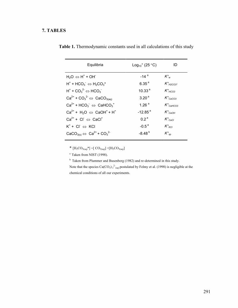
291

7. TABLES

Table 1. Thermodynamic constants used in all calculations of this study

Equilibria Log10° (25 C) ID

H2O

H

+ + OH

- -14

a K°w

H+ + HCO3

- H2CO3* 6.35

a K°H2CO3*

H+ + CO3

2- HCO3

- 10.33

a K°HCO3

Ca2+

+ CO32-

CaCO3(aq) 3.20 a K°CaCO3

Ca2+

+ HCO3- CaHCO3

+ 1.26

a K°CaHCO3

Ca2+

+ H2O CaOH+

+ H+ -12.85

a K°CaOH

Ca2+

+ Cl- CaCl

+ 0.2

a K°CaCl

K+ + Cl

- KCl -0.5

a K°KCl

CaCO3(s) Ca2+

+ CO32-

-8.48 b K°sp

* [H2CO3(aq)*] =[ CO2(aq)] +[H2CO3(aq)]

a Taken from NIST (1998).

b Taken from Plummer and Busenberg (1982) and re-determined in this study.

Note that the species Ca(CO3) 22-

(aq) postulated by Felmy et al. (1998) is negligible at the

chemical conditions of all our experiments.

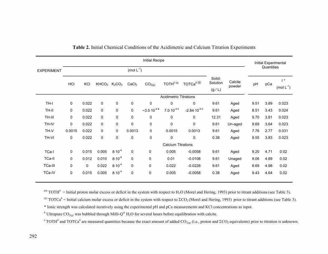
292

Table 2. Initial Chemical Conditions of the Acidimetric and Calcium Titration Experiments

EXPERIMENT

Initial Recipe Initial Experimental

Quantities (mol L

-1)

HCl KCl KHCO3 K2CO3 CaCl2 CO2(g) TOTH0 (†) TOTCa

0 (§)

Solid: Solution

(g / L)

Calcite powder

pH pCa I *

(mol L-1

)

Acidimetric Titrations

TH-I 0 0.022 0 0 0 0 0 0 9.61 Aged 9.51 3.89 0.023

TH-II 0 0.022 0 0 0 ~3.510-4 ¥

7.010-4 £

-2.8410-5 £

9.61 Aged 8.51 3.43 0.024

TH-III 0 0.022 0 0 0 0 0 0 12.31 Aged 9.70 3.81 0.023

TH-IV 0 0.022 0 0 0 0 0 0 9.61 Un-aged 9.69 3.64 0.023

TH-V 0.0015 0.022 0 0 0.0013 0 0.0015 0.0013 9.61 Aged 7.76 2.77 0.031

TH-VI 0 0.022 0 0 0 0 0 0 0.38 Aged 9.55 3.83 0.023

Calcium Titrations

TCa-I 0 0.015 0.005 810-4

0 0 0.005 -0.0058 9.61 Aged 9.20 4.71 0.02

TCa-II 0 0.012 0.010 810-4

0 0 0.01 -0.0108 9.61 Unaged 9.06 4.89 0.02

TCa-III 0 0 0.022 810-4

0 0 0.022 -0.0228 9.61 Aged 8.69 4.98 0.02

TCa-IV 0 0.015 0.005 810-4

0 0 0.005 -0.0058 0.38 Aged 9.43 4.64 0.02

(†) TOTH

0 = Initial proton molar excess or deficit in the system with respect to H2O (Morel and Hering, 1993) prior to titrant additions

(see Table 3).

(§)

TOTCa0 = Initial calcium molar excess or deficit in the system with respect to CO2 (Morel and Hering, 1993)

prior to titrant additions (see Table 3).

* Ionic strength was calculated iteratively using the experimental pH and pCa measurements and KCl concentrations as input.

¥ Ultrapure CO2(g) was bubbled through Milli-Q

® H2O for several hours before equilibration with calcite.

£ TOTH

0 and TOTCa

0 are measured quantities because the exact amount of added CO2(g) (i.e., proton and CO2 equivalents) prior to titration is unknown.

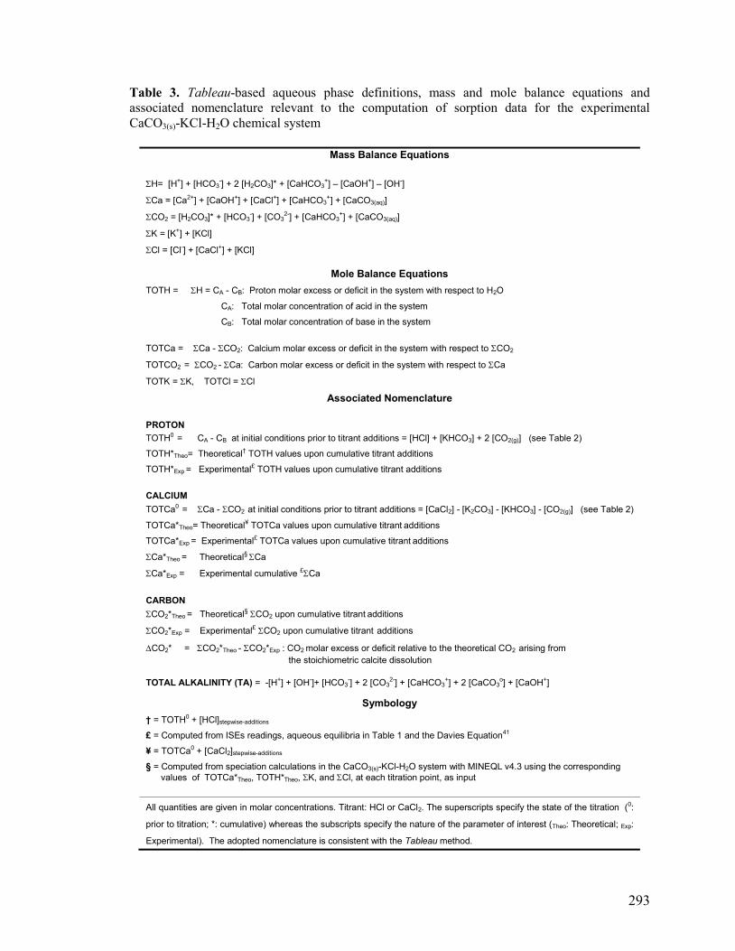
293

Table 3. Tableau-based aqueous phase definitions, mass and mole balance equations and

associated nomenclature relevant to the computation of sorption data for the experimental

CaCO3(s)-KCl-H2O chemical system


H= [H+] + [HCO3-] + 2 [H2CO3]* + [CaHCO3

+] – [CaOH+] – [OH-]

Ca = [Ca2+] + [CaOH+] + [CaCl+] + [CaHCO3+] + [CaCO3(aq)]

CO2 = [H2CO3]* + [HCO3-] + [CO3

2-] + [CaHCO3+] + [CaCO3(aq)]

K = [K+] + [KCl]

Cl = [Cl-] + [CaCl+] + [KCl]

Mole Balance Equations

TOTH = H = CA - CB: Proton molar excess or deficit in the system with respect to H2O

CA: Total molar concentration of acid in the system

CB: Total molar concentration of base in the system

TOTCa = Ca - CO2: Calcium molar excess or deficit in the system with respect to CO2

TOTCO2 = CO2 - Ca: Carbon molar excess or deficit in the system with respect to Ca

TOTK = K, TOTCl = Cl

Associated Nomenclature

PROTON

TOTH0 = CA - CB at initial conditions prior to titrant additions = [HCl] + [KHCO3] + 2 [CO2(g)] (see Table 2)

TOTH*Theo= Theoretical† TOTH values upon cumulative titrant additions

TOTH*Exp = Experimental£ TOTH values upon cumulative titrant additions

CALCIUM

TOTCa0 = Ca - CO2 at initial conditions prior to titrant additions = [CaCl2] - [K2CO3] - [KHCO3] - [CO2(g)] (see Table 2)

TOTCa*Theo= Theoretical¥ TOTCa values upon cumulative titrant additions

TOTCa*Exp = Experimental£ TOTCa values upon cumulative titrant additions

Ca*Theo = Theoretical§ Ca

Ca*Exp = Experimental cumulative £Ca

CARBON

CO2*Theo = Theoretical§ CO2 upon cumulative titrant additions

CO2*Exp = Experimental£ CO2 upon cumulative titrant additions

CO2* = CO2*Theo - CO2*Exp : CO2 molar excess or deficit relative to the theoretical CO2 arising from

the stoichiometric calcite dissolution

TOTAL ALKALINITY (TA) = -[H+] + [OH-]+ [HCO3

-] + 2 [CO32-] + [CaHCO3

+] + 2 [CaCO3o] + [CaOH+]

Symbology

† = TOTH0 + [HCl]stepwise-additions

£ = Computed from ISEs readings, aqueous equilibria in Table 1 and the Davies Equation41

¥ = TOTCa0 + [CaCl2]stepwise-additions

§ = Computed from speciation calculations in the CaCO3(s)-KCl-H2O system with MINEQL v4.3 using the corresponding

values of TOTCa*Theo, TOTH*Theo, K, and Cl, at each titration point, as input

All quantities are given in molar concentrations. Titrant: HCl or CaCl2. The superscripts specify the state of the titration (0:

prior to titration; *: cumulative) whereas the subscripts specify the nature of the parameter of interest (Theo: Theoretical; Exp:

Experimental). The adopted nomenclature is consistent with the Tableau method.

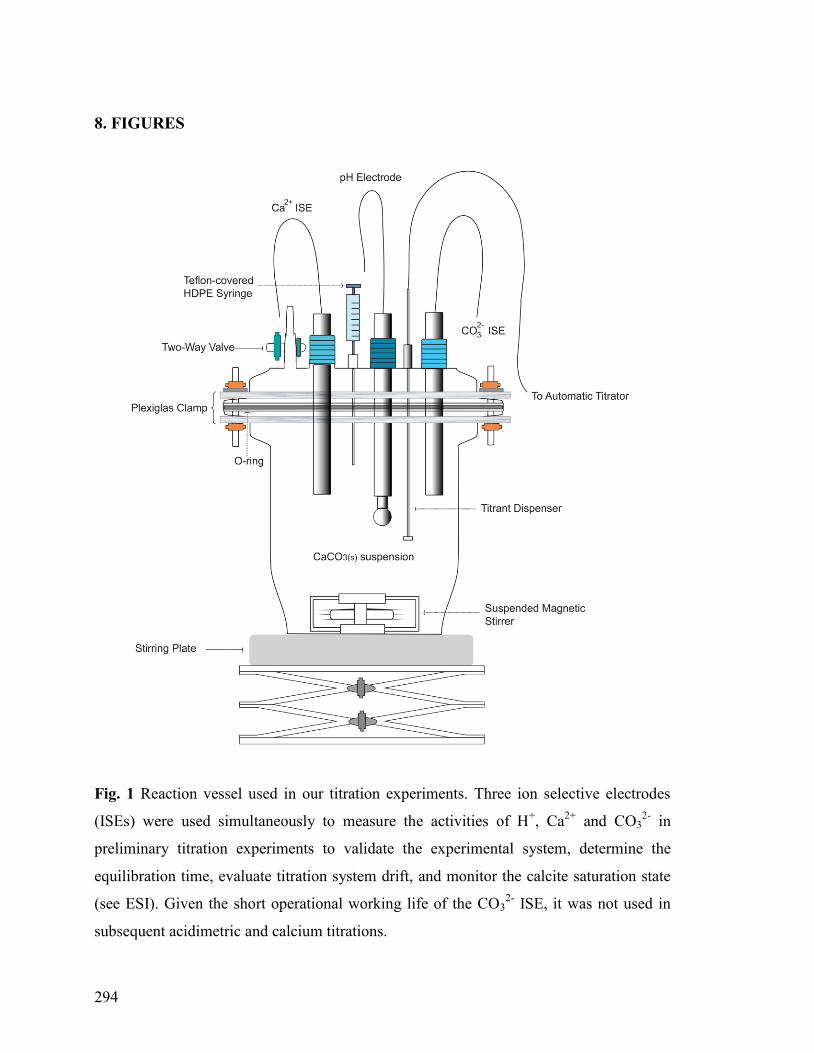
294

8. FIGURES

Fig. 1 Reaction vessel used in our titration experiments. Three ion selective electrodes

(ISEs) were used simultaneously to measure the activities of H+, Ca

2+ and CO3

2- in

preliminary titration experiments to validate the experimental system, determine the

equilibration time, evaluate titration system drift, and monitor the calcite saturation state

(see ESI). Given the short operational working life of the CO32-

ISE, it was not used in

subsequent acidimetric and calcium titrations.

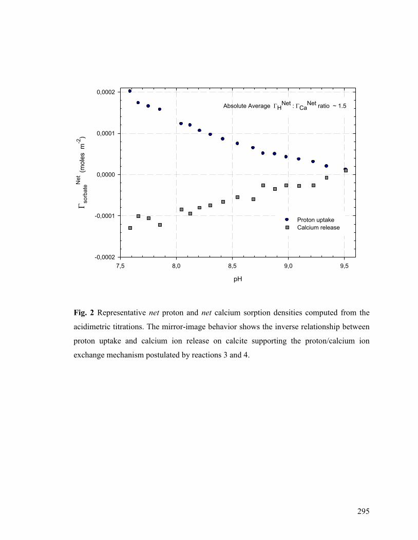
295

pH

7,5 8,0 8,5 9,0 9,5

sorb

ate

Net (m

ole

s m

-2)

-0,0002

-0,0001

0,0000

0,0001

0,0002

Proton uptake

Calcium release

Absolute Average HNet : Ca

Net ratio ~ 1.5

Fig. 2 Representative net proton and net calcium sorption densities computed from the

acidimetric titrations. The mirror-image behavior shows the inverse relationship between

proton uptake and calcium ion release on calcite supporting the proton/calcium ion

exchange mechanism postulated by reactions 3 and 4.

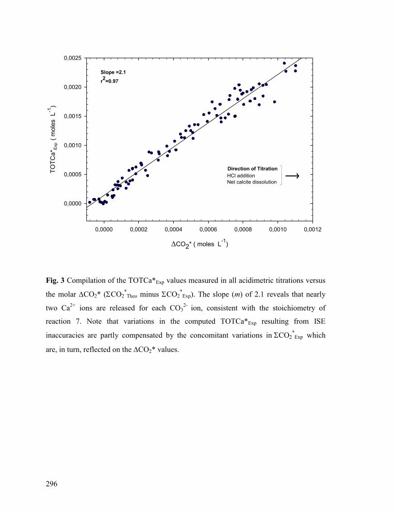
296

Slope =2.1

r2

=0.97

CO2* ( moles L-1

)

0,0000 0,0002 0,0004 0,0006 0,0008 0,0010 0,0012

TO

TC

a* E

xp

(

mole

s L

-1)

0,0000

0,0005

0,0010

0,0015

0,0020

0,0025

Direction of Titration

HCl addition

Net calcite dissolution

Fig. 3 Compilation of the TOTCa*Exp values measured in all acidimetric titrations versus

the molar CO2* (CO2*Theo minus CO2

*Exp). The slope (m) of 2.1 reveals that nearly

two Ca2+

ions are released for each CO32-

ion, consistent with the stoichiometry of

reaction 7. Note that variations in the computed TOTCa*Exp resulting from ISE

inaccuracies are partly compensated by the concomitant variations inCO2*Expwhich

are, in turn, reflected on the CO2* values.

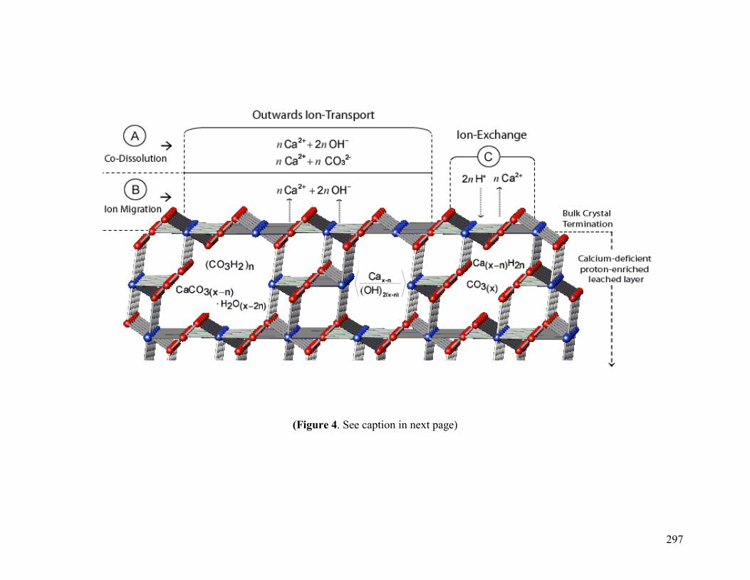
297


298

Fig. 4 Schematic representation of three equivalent mechanisms accounting for the pH and pCa behavior observed in the acidimetric

and calcium titrations. Panels A and B consider the hypothetical presence of hydroxyl-bearing species (CaCO3nH2O(s) and/or

Ca(OH)2(s)) embedded within the calcite lattice prior to titrations. If co-dissolution of Ca(OH)2(s) and CaCO3(s) species occurs

(Panel A), no lattice vacancy is generated. In contrast, if Ca2+

and OH- ions are removed from their lattice positions by ion migration

along surface features such as micro-fractures, lattice vacancies might be generated (Panel B). Panel C schematizes the substitution of

Ca2+

lattice ions by protons via a chemically-driven 2H+/Ca

2+ ion exchange mechanism between the bulk solution and a “labile”,

possibly hydrated, interfacial region following the dynamic rearrangement of the calcite topmost atomic layers. In scenario C, no

lattice vacancies are generated because protons occupy lattice sites formerly occupied by Ca2+

ions at exchangeable cation sites and

yield Ca(HCO3)2(exc) and/or H2CO3(exc) lattice species as defined respectively by reactions 3 and 4.

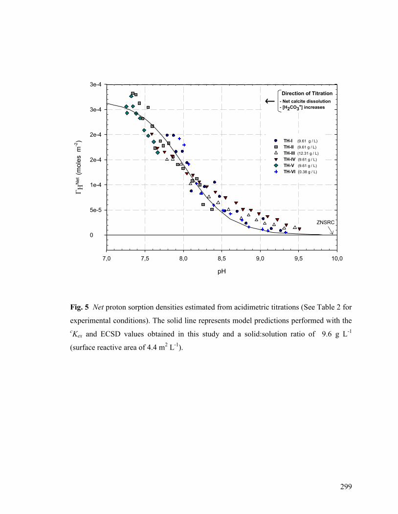
299

pH

7,0 7,5 8,0 8,5 9,0 9,5 10,0

Net (m

ole

s m

-2)

0

5e-5

1e-4

2e-4

2e-4

3e-4

3e-4

TH-I (9.61 g / L)

TH-II (9.61 g / L)

TH-III (12.31 g / L)

TH-IV (9.61 g / L)

TH-V (9.61 g / L)

TH-VI (0.38 g / L)


- Net calcite dissolution

- [H2CO3*] increases

ZNSRC

Fig. 5 Net proton sorption densities estimated from acidimetric titrations (See Table 2 for

experimental conditions). The solid line represents model predictions performed with the

cKex and ECSD values obtained in this study and a solid:solution ratio of 9.6 g L

-1

(surface reactive area of 4.4 m2 L

-1).

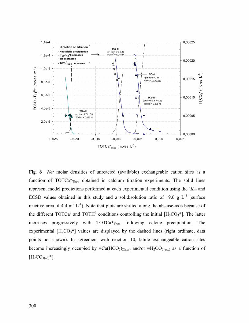
300

TOTCa*Theo (moles L-1

)

-0,025 -0,020 -0,015 -0,010 -0,005 0,000 0,005

EC

SD

-

Net (m

ole

s m

-2)

2,0e-5

4,0e-5

6,0e-5

8,0e-5

1,0e-4

1,2e-4

1,4e-4

H2C

O3*

(mo

les L

-1)

0,00000

0,00005

0,00010

0,00015

0,00020

0,00025


- Net calcite precipitation

- [H2CO3*] increases

- pH decreases

- TOTH*Exp decreases

TCa-I

(pH from 9.2 to 7)

TOTH0 = 0.005 M

TCa-II

(pH from 9 to 7.4)

TOTH0 = 0.010 M

TCa-IV(pH from 9.4 to 7.5)

TOTH0 = 0.005 M

TCa-III (pH from 8.7 to 7.5)

TOTH0 = 0.022 M

Fig. 6 Net molar densities of unreacted (available) exchangeable cation sites as a

function of TOTCa*Theo obtained in calcium titration experiments. The solid lines

represent model predictions performed at each experimental condition using the cKex and

ECSD values obtained in this study and a solid:solution ratio of 9.6 g L-1

(surface

reactive area of 4.4 m2 L

-1). Note that plots are shifted along the abscise-axis because of

the different TOTCa0 and TOTH

0 conditions controlling the initial [H2CO3*]. The latter

increases progressively with TOTCa*Theo following calcite precipitation. The

experimental [H2CO3*] values are displayed by the dashed lines (right ordinate, data

points not shown). In agreement with reaction 10, labile exchangeable cation sites

become increasingly occupied by Ca(HCO3)2(exc) and/or H2CO3(exc) as a function of

[H2CO3(aq)*].

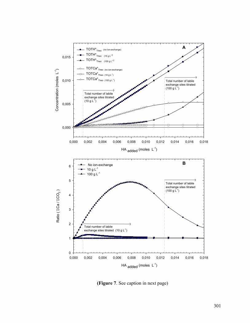
301

HA added (moles L-1

)

0,000 0,002 0,004 0,006 0,008 0,010 0,012 0,014 0,016 0,018

Concentr

ation (

mole

s L

-1)

0,000

0,005

0,010

0,015

TOTH*Theo

(no ion-exchange)

TOTH*Theo (10 g L

-1)

TOTH*Theo (100 g L

-1)

TOTCa*Theo (no ion-exchange)

TOTCa*Theo (10 g L

-1)

TOTCa*Theo (100 g L

-1)

A

Total number of labile

exchange sites titrated

(10 g L-1)



(100 g L-1)

HA added (moles L-1

)

0,000 0,002 0,004 0,006 0,008 0,010 0,012 0,014 0,016 0,018

Ratio (

C

a /

CO

2 )

0

1

2

3

4

5

6 No ion-exchange

10 g L-1

100 g L-1

B


exchange sites titrated (10 g L-1)



(100 g L-1)


302

Fig. 7 Predicted TOTH*Theo and TOTCa*Theo values (Panel A) and Ca:CO2 ratios

(Panel B) upon a hypothetical acidimetric titration (HA: strong acid) conducted in a

closed CaCO3(s)-H2O system (at TOTH0 and TOTCa

0=0), with and without consideration

of proton/calcium ion exchange and at different solid:solution ratios using log10 cKex = 13

and the average ECSD value obtained in this study (13.5·10-5

moles m-2

or 6.2·10-5

moles

g-1

).

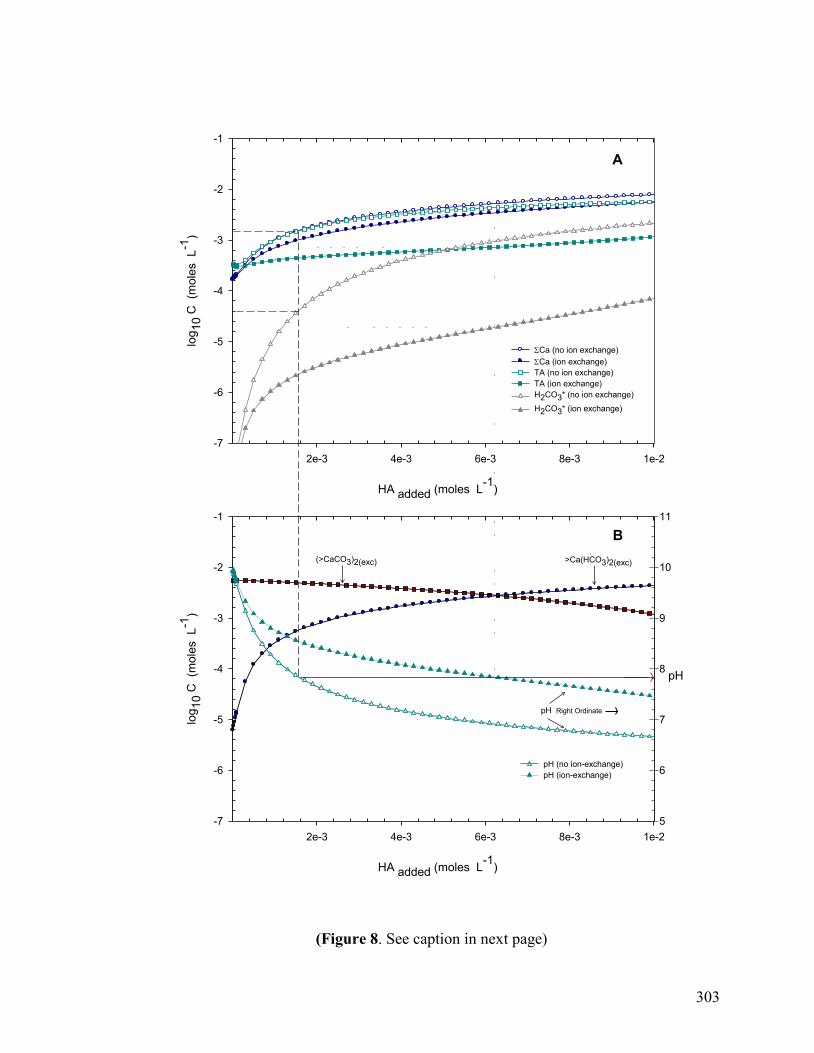
303

HA added (moles L-1

)

2e-3 4e-3 6e-3 8e-3 1e-2

log10

C (m

ole

s L

-1)

-7

-6

-5

-4

-3

-2

-1

HA added (moles L-1

)

2e-3 4e-3 6e-3 8e-3 1e-2

pH

log10

C (m

ole

s L

-1)

-7

-6

-5

-4

-3

-2

-1

5

6

7

8

9

10

11

>Ca(HCO3)2(exc)(>CaCO3)2(exc)

pH Right Ordinate

Ca (no ion exchange)

Ca (ion exchange)

TA (no ion exchange)

TA (ion exchange)

H2CO3* (no ion exchange)

H2CO3* (ion exchange)

pH (no ion-exchange)

pH (ion-exchange)

A

B


304

Fig. 8 Predicted Ca, Total Alkalinity (TA), [H2CO3*] (Panel A), pH and speciation of

labile exchangeable cation sites (Panel B) upon a hypothetical acidimetric titration (HA:

strong acid) in a closed CaCO3(s)-H2O system with (solid symbols) and without (open

symbols) consideration of proton/calcium ion exchange. Ion exchange speciation

predictions were performed at a fixed solid:solution ratio of 100 g L-1

(reactive surface

area of 0.46 m2 L

-1) using log10

cKex = 13 and the average ECSD value obtained in this

study (13.5·10-5

moles m-2

or 6.2·10-5

moles g-1

). Under these conditions, equimolar

concentrations of protonated and non-protonated (“unreacted”) labile exchangeable sites

are registered at a pH of 7.8. Drop dotted lines intersecting panels A and B are

references to facilitate comparison of Ca, TA and [H2CO3*] values predicted with and

without consideration of ion proton/calcium exchange at pH=7.8.

305

CHAPTER 7

GENERAL CONCLUSIONS

CONTRIBUTIONS TO KNOWLEDGE

Despite significant scientific efforts focused on carbonate minerals, some fundamental

aspects of the surface reactivity of these minerals in aqueous solutions, such as ion

sorption processes, remain poorly characterized. Because of the higher reactivities of

carbonates relative to other minerals such as metal oxides, silicates, and clays, and the

occurrence of stepwise and/or parallel reactions, the experimental characterization of

these processes represents a sizable challenge. This explains why the systematic

acquisition of experimental data and the elaboration, calibration, and validation of

empirical, semi-empirical, and/or theoretical models describing sorption phenomena on

carbonate minerals have lagged behind those of less reactive minerals. Consequently, the

combination of multiple investigative approaches represents a suitable strategy to

improve our understanding of the sorptive properties of these minerals. In addition, the

development of novel experimental protocols extending the range of experimental

conditions under which the sorptive properties of carbonate minerals can be investigated

would be desirable. In this dissertation, we combined theoretical, experimental, computer-

assisted molecular modeling, and numerical simulation approaches to investigate sorption

phenomena at carbonate surfaces in aqueous solutions under ambient conditions. In doing

so, we introduced several elements of novelty that allowed new interpretations and fresh

insights into the reactivity of these surfaces.

We implemented a powerful evolutionary programming technique, the Genetic

Algorithm (GA) that allowed, for the first time, the rigorous calibration of SCMs for

306

magnesite and dolomite via stochastic numerical optimization. The GA is simple,

flexible, and robust and possesses important advantages over conventional numerical

techniques used in commercially-available programs with inverse modeling applications

such as FITEQL. The GA is a powerful tool to estimate intrinsic formation constants of

mineral surface species, a critical step in the generation of a reliable thermodynamic

database. Given the ability of our GA-based optimization code to simultaneous fit

intrinsic ionization and affinity constants, capacitance(s), and/or site densities, we

strongly recommend its use for the calibration of sophisticated Surface Complexation

Models (SCMs), particularly those that invoke numerous adjustable parameters or when

extensive data sets are not available for model calibration. A future user-friendly version

will help generalize its use among SCM practitioners and modelers.

Despite the success of earlier SCMs to simulate the surface charge behavior of

rhombohedral carbonate mineral surfaces, a critical analysis of the definition of surface

sites revealed that the postulated reactions may not necessarily reflect realistic processes

at the carbonate/water interface and may yield questionable predictions of surface

speciation. Consequently, we formulated, calibrated, and tested chemically-sound and

simplified SCMs for two representative rhombohedral carbonate minerals: MgCO3(s)

(magnesite) and CaMg(CO3)2(s) (dolomite). The models include proton/bicarbonate ion

co-adsorption as one of the fundamental mechanisms to explain the surface charge-

buffering behavior and the relatively wide range of pH values of isoelectric point (pHiep)

displayed by these minerals in aqueous solutions. In analogy to the one-site 2-pKa

ionization model frequently adopted for metal oxides, our SCMs are formalized in terms

of a single-site that renders them more mathematically-tractable than earlier multi-site

complexation models that require numerous reactions to reproduce experimental data.

307

Although, we recognize that, under specific chemical conditions, multi-site complexation

may occur at carbonate surfaces, its relevance for the quantitative description of available

experimental data is debatable because it is well known that surface irregularities (e.g.,

steps, kinks and dislocations), chemical micro-heterogeneities, and the existence of multi-

domain crystal surfaces, presumably allowing for the presence of multiple reactive sites,

are properties that are difficult to assess quantitatively. Accordingly, the applicability of

the multi-site approach is limited to well-characterized surfaces and to high quality

experimental data suitable for the proper calibration of the multi-site-based surface

reaction(s) of interest. Because the simplified SCMs are a fair compromise between the

quality of the experimental data available for model calibration, the compatibility of the

models with physical/chemical constraints, and the viability of the SCM predictions, it is

a convenient and realistic approach to use in the construct of SCMs for other

rhombohedral carbonate minerals and represents an important advance in the

rationalization/interpretation of available experimental surface charge data for this type of

minerals.

The applicability of the one-site scheme was extended to other rhombohedral

carbonate minerals using the least reactive of known naturally-occurring rhombohedral

carbonate minerals in aqueous solutions, gaspeite (NiCO3(s)), as a surrogate of calcite-type

minerals. Conventional surface titrations applied to gaspeite allowed us to obtain

quantitative proton adsorption data for the calibration of a SCM for this mineral. To this

end, we employed conventional titration techniques, never applied before to carbonate

minerals, and generated abundant electrokinetic data to qualitatively evaluate the

predictive power of the derived SCM. The most important insights obtained in this study

is that the background electrolyte (NaCl) affects the properties of the gaspeite surface

308

(surface protonation and the development of surface charge) possibly through

modification of the structure of the electrified interfacial layer, perturbation of the solvent

structure dynamics and the affinity of water molecules and adsorbing ions towards the

mineral surface. These observations challenge earlier conceptions on carbonate mineral

surfaces that traditionally considered these minerals as chemically inert to background

electrolyte ions. Clearly, carbonate surfaces behave differently than most metal oxides,

silicates, and clay surfaces in aqueous solutions and, hence, electrolyte effects should be

carefully examined in future studies through alternative experimental approaches and/or

using different background electrolytes. This should help fine tune the postulated SCMs

and extend their applicability to solution conditions beyond those of model calibration.

Regardless of the physical significance of the calibrated SCM parameters, those obtained

at low and intermediate ionic strengths (I=0.001 and 0.01 M) can be considered as useful

operational quantities that can yield reasonable predictions of the surface protonation and

the electrokinetic behavior of gaspeite over compositional ranges similar to those

investigated in our study.

Our other line of investigation involved the study of the interactions between

one of the most reactive naturally-occurring rhombohedral carbonate minerals in

aqueous solution, calcite, and H2O and/or H2O constituents using molecular modeling

and experimental techniques. Quantitative insights into the energetics of H2O

adsorption on the (10.4) calcite surface and on the 3D structural registry of the 1st and

2nd

hydration layers were obtained using ab initio molecular orbital methods and

cluster models. This theoretical approach had never been applied before to

characterize the structure of the hydrated calcite surface and elucidate the bonding

relationships governing the hydration process. The results are in reasonable agreement

309

with earlier findings of force-field-based and Density Functional Theory studies and

show that H2O molecules in the 1st hydration layer adsorb associatively to the surface

through ionic bonding with calcium atoms and hydrogen bonding with one surface

oxygen atom. This scenario is consistent with the generalized single primary surface

site scheme postulated in this study for rhombohedral carbonate mineral surfaces. In

addition, our ab initio study revealed a significant reorganization of the mineral

surface, specifically Ca-O bond relaxation and possible bond rupture leading to the

weakening of the topmost atomic layer with respect to the bulk. This new insight may

have important implications with respect to the elucidation of mechanisms of mineral

dissolution, rearrangement of surface layers and, possibly, solute transport through

subsurface lattice layers.

Finally, we developed a novel titration protocol that allowed, for the first time,

the rigorous quantitative characterization of the proton sorptive (or hydroxyl ion

desorptive) properties of calcite in aqueous solutions over a relatively wide range of

chemical conditions. Using this approach we generated data that lead us to postulate

the existence of a dynamic proton/calcium ion exchange reaction that extends beneath

the topmost surface calcite layer. This process may significantly impact the aqueous

speciation of closed (e.g., aquifers, pore waters) and open aquatic environments with

poor CO2 ventilation (e.g., deep sea waters, industrial reactions), via pH buffering and

CO2(g) sequestration upon ion exchange-induced calcite precipitation. Although the

observed fast proton/calcium ion exchange cannot be ascribed to any specific

transport mechanism such as ion physical entrapment, “solid-state” ion diffusion, or

ion migration through micro-fractures, it certainly reflects the highly dynamic nature

of the topmost surface calcite layers and lends support to earlier ideas that

310

conceptualize the interface between the bulk calcite crystal and the bulk solution as a

porous membrane of adsorbed or surface layers (or as a hydrated “gel-like” region)

through which processes such as site competition, dehydration, segregation, and/or ion

diffusion occur. In turn, these ideas are compatible conceptually with the weakening

of the topmost atomic layer as suggested by our ab initio molecular orbital study. The

observed proton/calcium ion exchange reaction could be directly involved in the

physiologically-driven 2H+/Ca

2+ exchange behavior exhibited by some calcifying

marine organisms, may have far-reaching implications on the interpretation of field

and laboratory data as well as on on the predicted responses of carbonate-rich shelf

sediments to rising atmospheric pCO2 and ocean acidification. Finally, although our

results cannot support or challenge earlier ideas on the origin of surface charge, the

electrokinetic behavior of calcite and/or potential mechanisms of calcite dissolution, it

raises serious questions on the validity of quantitative interpretations of adsorption,

electrokinetic, and dissolution kinetic data based upon surface speciation concepts and

suggest that these may require revision.

RECOMMENDATIONS FOR FUTURE RESEARCH

Despite the valuable scientific insights obtained in this thesis, numerous issues about the

reactivity of carbonate surfaces in aqueous solutions remain to be tackled. The best way

to address these is through a combination of multiple investigative approaches and a

careful acquisition and interpretation of novel data.

Because of their high reactivity, carbonate surfaces are not as “investigator-

friendly” as most metal oxides, a serious limitation to experimentalists wishing to apply

311

conventional experimental techniques. The corollary to this is straightforward. Either

novel experimental protocols must be developed, alternate investigative approaches (e.g.,

theoretical) must be used, or a combination of both must be adopted to obtain further

insight into processes at these mineral surfaces.

In doing so, it is critical to remember that, within specific time-scales, not all

carbonate minerals will react similarly as it was clearly demonstrated by our acidimetric

titration experiments conducted on: (i) the least reactive of known naturally-occurring

rhombohedral carbonate minerals in aqueous solutions: gaspeite and, (ii) one of the most

reactive ones: calcite. It follows that, whereas some fundamental concepts may be

common to all carbonate surfaces (e.g., hydration), others may not (e.g., proton uptake)

and therein lies the importance of compiling self-consistent and well-characterised data

sets (in terms of time scale, solution chemistry, nature, and history of mineral specimen,

etc.) for a specific carbonate mineral. Statistically- and geochemically-sound data

treatment is critical for the reliable description of the surface reactivity of these minerals.

Another important consideration is that the high reactivity of carbonate minerals

can be sometimes exploited to the experimentalist‟s advantage (as was demonstrated in

our calcite titration experiments) as it may allow the characterization of surface and near-

surface processes (e.g., ion exchange, surface rearrangement, solute transport through

lattice layers), a task that would be difficult or prohibitive for other minerals displaying

slow dissolution/equilibrium kinetics.

It is critical to carefully test and validate the experimental protocols and avoid

using these beyond the operational conditions at which they were validated. For instance,

in this study, by simulating a strict closed carbonate mineral system, we were able to

investigate the proton sorption behavior of calcite over an alkaline pH regime of interest

312

for many environmental applications. Because the nature of the carbonate system

(substantial evolution of CO2(g)) precludes extension of this protocol to acidic regimes (to

further examine the sorptive properties of calcite), the implementation of a novel

experimental protocol would be required. A feasible alternative would be to implement a

closed-system titration protocol, involving the presence of a confined gas phase in contact

with a calcite suspension, where the solution chemistry (pH and pCa) and the pCO2(g) in

the headspace are constantly monitored. Such a protocol would be analogous to that

implemented by Villalobos and Leckie (2000) for the evaluation of carbonate adsorption

at the goethite surface.

Clearly, a multitude of research projects could be designed to gain further insight

into the surface reactivity of carbonate minerals but they cannot be all enumerated here. It

suffices to say that, regardless of the specific carbonate surface of interest, emphasis must

be placed on the following aspects:

Implementing novel experimental protocols for the characterization of the sorptive

properties of carbonate minerals.

Generating well-constrained, well-characterised, self-consistent experimental data

sets for a specific carbonate mineral by multiple approaches (such as batch and

automatised titrations, calorimetric, radiometric and electrokinetic techniques). A

critical evaluation of the suitability of these composite data sets to describe

specific surface processes is warranted.

Examining the role of different background electrolytes on the sorptive properties

and reactivity of the carbonate mineral of interest (particularly important for

environmental applications such as saline brines and oceans).

313

Studying the proton sorptive properties of aragonite and natural magnesian

calcites (predominant in marine environments) using either the titration protocol

described in this thesis or analogous titration protocols.

Investigating the role of protons and water molecules on carbonate dissolution by

ab initio methods and/or molecular dynamics techniques.

Describing the nature of the postulated “proton-enriched, calcium-deficient

leached calcite layer” by spectroscopic and ab initio molecular modeling

techniques.

Developing novel semi-empirical or theoretical schemes to investigate and/or

interpret ion sorption at carbonate surfaces.

Finally, it would also be useful to fine tune the GA technique presented in this

study for the optimization of intrinsic constants (e.g., test other GA operators). A

combination of the GA with other powerful global search algorithms (e.g., Particle

Swarm or Differential Evolution) may render it more efficient for this type of application.

Clearly, a user-friendly version of the Matlab

-based GA optimization subroutines

(preferably written in Fortran or C++ languages) would be of interest to surface

complexation modelers and practitioners.

314

REFERENCES

Ahmed I.A.M., Crout N.M.J. and Young S.D. (2008) Kinetics of Cd sorption, desorption

and fixation by calcite: A long-term radiotracer study. Geochim. Cosmochim. Acta

72, 1498-1512.

Al-Horani F.A., Al-Moghrabi S.M., de Beer D. (2003) The mechanism of calcification

and its relation to photosynthesis and respiration in the scleractinian coral Galaxea

fascicularis. Mar. Biol. 142, 419-426.



Chem. Chem. Phys. 7, 1266-1276.

Allison J. D., Brown D.S. and Novo-Gradac, K.J. (1991) MINTEQA2/PRODEFA2, a

geochemical assessment model for environmental systems: version 3.0. User‟s

manual, Environmental Research Laboratory, Office of Research and

Development, U.S. Environmental Protection Agency, Athens, GA, 106 pp.

Andersson A.J., Mackenzie F.T., Ver L.M. (2003) Solution of shallow-water carbonates:

An insignificant buffer against rising atmospheric CO2. Geology 31(6), 513-516.

Andersson A.J., Mackenzie F.T., Lerman A. (2006) Coastal ocean CO2–carbonic acid–

carbonate sediment system of the Anthropocene. Global Biogeochem. Cycles

20:GB1S92, 1-13.

APHA-AWWA-WPCF (1998). Standard Methods for the Examination of Water and

Wastewater Sewage and Industrial Wastes. Washington, D.C.

Arakaki T. and Mucci A. (1995) A continouous and mechanistic representation of calcite

reaction-controlled kinetics in dilute solutions at 25° and 1 atm total pressure.

Aquatic Geochem 1, 105-130.

315

Archer T. D. (2004) Computer Simulations of Calcite. Ph.D. Thesis, University of

Cambridge. UK.

Austen K. T., Wright K., Slater B and Gale J.D. (2005) The interaction of dolomite

surfaces with metal impurities: a computer simulation study. Phys. Chem. Chem.

Phys. 7, 4150-4156.

Ball J. W., Jenne E. A. and Norstrom D. K. (1981) WATEQ2- A computerized chemical

model for trace and major element speciation and mineral equilibrium of natural

waters. In: E. A. Jenne (Ed.) Chemical Modeling in Aqueous Systems, Symposium

series 93, American Chemical Society, Washington, D.C. p. 815-836.

Bandstra J.Z. and Brantley S.L. (2008) Surface evolution of dissolving minerals

investigated with a kinetic ising model. Geochim. Cosmochim. Acta 72:11, 2587-

2600.

Barrow N. J., Brümer G. W. and Strauss R. g (1993) Effects of surface heterogeneity on

ion adsorption by metal oxides and by soils. Langmuir. 9, 2606-2611.

Benjamin M. (2002) Modeling the mass-action expression for bidentate adsorption.

Environ. Sci. Technol. 36, 307-313.

Bermanec V., Sijarić, Kniewald G. and Mandarino J.A. (2000). Gaspeite and associated

Ni-rich minerals from veins in altered ultrabasic rocks from Duboštica, Bosnia

and Herzegovina. Can. Mineral. 38, 1371-1376.

Berner, R. A. and Morse, J. W. (1974) Dissolution kinetics of calcium carbonate in

seawater; IV, Theory of calcite dissolution. Am. J. Sci. 274, 108-134.

316

Bureau H., Raepsaet C., Khodja H., Carraro A. and Aubaud C. (2009) Determination of

hydrogen content in geological samples using elastic recoil detection analysis

(ERDA). Geochim. Cosmochim. Acta 73(11), 3311-3322.

Bickmore B. R., Rosso K. M., Tadanier C. J., Bylaska E. J. and Doud D. (2006). Bond-

Valence methods for pKa prediction: Bond-valence, electrostatic, molecular

geometry and solvation effects. Geochim. Cosmochim. Acta. 70, 4057-4071.

Bleam W. F. (1993) On the modeling proton affinity at the oxide/water interface. J.


Blesa M.A. and Kallay N. (1988) The metal oxide-electrolyte solution interface revisited.

Adv. Colloid Interface Sci. 28, 111-134.





Brewer P.G., Wong G.T.F., Bacon M.P. and Spencer D. W. (1975) An oceanic calcium

problem? Earth Planet. Sci. Lett. 26, 81-87.

Borkovec M. (1997). Origin of 1-pK and 2-pK models for ionizable water-solid

interfaces. Langmuir. 13, 2608-2613.

Borkovec M. and Koper G. J. M. (1994). Ising models of polyprotic acids and bases. J.

Phys. Chem. 98, 6038-6045.

Bruanuer S., Emmet P.H. and Teller E. (1938) Adsorption of gases in multimolecular

layers. J. Phys. Chem. 60, 309-316.

317

Casey W.H., Westrich H.R., Banfield J.F., Ferruzi G. and Arnold G.W. (1993) Leaching

and reconstruction at surfaces of dissolving chain-silicate minerals. Nature 366,

253-256.

Ĉerník M., Borkovec M. and Westall J. C. (1995). Regularized least-squares methods for

the calculation of discrete and continuous affinity distributions for heterogeneous

sorbents. Environ. Sci. Technol. 29, 413-425.

Chandler D. (1987) Introduction to Modern Statistical Mechanics. Oxford University

Press, New York, 288 p.

Chandra S.W. and Kollman P. (1984) An approach to computing electrostatic charges for

molecules. J. Comput. Chem. 5(2), 129-145.

Charlet L., Wersin P. and Stumm W. (1990). Surface charge of MnCO3 and FeCO3.

Geochim Cosmochim. Acta. 54, 2329-2336.

Charmas R. (1999) Four-layer complexation model for ion adsorption at energetically

heterogeneous metal oxide/electrolyte interfaces. Langmuir 15(17), 5635-5648.



Acta. 57(16), 4103-4110.

Chou L., Garrels R.M. and Wollast R. (1989) Comparative study of the kinetics and

mechanisms of dissolution of carbonate minerals. Chem. Geol. 78, 269–282.

Cicerone D.S., Regazzoni A.E. and Blesa M. A. (1992) Electrokinetic properties of the



318

Comans R.N.J. and Middelburg J.J. (1987) Sorption of trace metals on calcite:

Applicability of the surface precipitation model. Geochem. Cosmochim. Acta 51,

2587-2591.

Compton R.G. and Unwin P.R. (1990) The dissolution of calcite in aqueous solution at

pH less 4: kinetics and mechanism. R. Phil. Trans. R. Soc. Lond. A. 330, 1-45.

Compton R.G. and Pritchard K.L. (1990) The dissolution of calcite at pH > 7: kinetics

and mechanism. R. Phil. Trans. R. Soc. Lond. A. 330, 47-70.

Culberson C. and Pytkowicz R.M. (1968) Effect of pressure on carbonic acid, boric acid

and the pH in seawater. Limnol. Oceanogr. 13(3), 403-417.

Curti E., Kulik D.A. and Tits J. (2005) Solid solutions of trace Eu(III) in calcite:

Thermodynamic evaluation of experimental data over a wide range of pH and

pCO2. Geochim. Cosmochim. Acta 69(7), 1721-1737.

Davis J.A. and Kent D.B. (1990). Surface complexation modeling in aqueous

geochemistry. In Mineral-Water Interface Geochemistry. (ed. M.F. Hochella and

A.F. White). Rev. Mineral. 23. Mineral. Soc. Washington, DC. p. 177-260.





Douglas, H.W. and Walker, R. A. (1950) The electrokinetic behavior of iceland spar


Duckworth O.W. and Martin S.T. (2003). Connections between surface complexation and

geometric models of mineral dissolution investigated for rhodochrosite. Geochim.

Cosmochim. Acta 67, 1787-1801

319


and Sons Inc.: New York, NY, Chapters 1-3.

de Leeuw N. H. and Parker S. C. (1997). Atomistic simulation of the effect of molecular


Chem. Soc., Faraday Trans., 93(3), 467-475.

de Leeuw N. H. and Parker S. C. (1998). Surface structure and morphology of calcium


Phys. Chem. B., 102, 2914-2922.

de Leeuw N. H. and Parker S.C. (2001). Surface-water interactions in the dolomite

problem. Phys. Chem. Chem. Phys., 3, 3217-3221.

de Leeuw N. H. and Parker S.C. (2002). Surface structures, stabilities, and growth of


dolomite formation. Am. Mineral., 87, 679-689.

de Leeuw N. H., Parker S.C., and Hanumantha Rao K. (1998). Modeling the competitive

adsorption of water and methanoic acid on calcite and fluorite surfaces. Langmuir,

14, 5900-5906.

Elfil H. and Roques H. (2001) Role of hydrate phases of calcium carbonate on the scaling

phenomenon. Desalination, 137, 177-186.

Elzinga E.J., Rouff A.A. and Reeder R.J. (2006) The long-term fate of Cu2+

, Zn2+

, and

Pb2+

adsorption complexes at the calcite surface: An X-ray absorption

spectroscopic study. Geochim. Cosmochim. Acta, 70, 2715-2725.

Epperson J. F. (2002) An Introduction to Numerical Methods and Analysis. John Wiley

and Sons, New York, NY, 556 pp.

320

Eriksson R., Merta J. and Rosenholm J.B. (2007) The calcite/water interface I. Surface

charge in indifferent electrolyte media and the influence of low-molecular-weight

polyelectrolyte. J. Colloid Interface Sci. 313, 184-193.

Eriksson R., Merta J. and Rosenholm J.B. (2008) The calcite/water interface II. Effect of

added lattice ions on the charge properties and adsorption of sodium polyacrylate.

J. Colloid Interface Sci., 2008, 326, 396-402.

Essaid H.I., Cozzarelli I.M., Eganhouse R.P., Herkelrath W.N., Bekins B.A. and Delin

G.N. (2003) Inverse modeling of BTEX dissolution and biodegradation at the

Bemidji, MN crude-oil spill site. J. Cont. Hydr. 67(1), 269-299.

Felmy A.R., Dixon D.A., Rustad J.R., Mason M.J. and Onishi L.M. (1998) The

hydrolysis and carbonate complexation of strontium and calcium in aqueous

solution. Use of molecular modeling calculations in the development of aqueous

thermodynamic models. J. Chem. Thermodynamics 30, 1103-1120.

Feng J., Lee Y.J., Reeder R.J. and Phillips B.L. (2006) Observation of bicarbonate in

calcite by NMR spectroscopy. Am. Mineral. 91, 957-960.

Fenter P., Geissbühler P., DiMasi E, Srajer G, Sorensen B and Sturchio N.C. (2000)



Fernández Alvarez J.P., Fernández Martínez J.L. and Menéndez Pérez C.O. (2008)

Feasibility analysis of the use of binary genetic algorithms as importance samplers

Application to 1-D DC resistivity inverse problem. Math. Geosci. 40, 375-408.

Foxall T., Peterson G.C., Rendall H.M. and Smith A. L. (1979) Charge determination at


1039.

321

Franklin M.L. and Morse J.W. (1983) The interaction of manganese(II) with the surface

of calcite in dilute solutions and seawater. Mar. Chem., 12(4), 241-254.

Gaffey S.J. (1995) H2O and OH in echinoid calcite: A spectroscopic study. Am. Mineral.

80, 947-959.

Gans P. (1976) Numerical methods for data-fitting problems. Coord. Chem. Rev. 19, 99-

124.

Gao Y. and Mucci A. (2001) Acid base reactions, phosphate and arsenate complexation,

and their competitive adsorption at the surface of goethite in 0.7 M NaCl solution.

Geochim. Cosmochim. Acta. 65, 2361-2378.

Geissbühler P, Fenter P, DiMasi E., Sorensen, L.B. and Sturchio N.C. (2004). Three-

dimensional structure of the calcite–water interface by surface X-ray scattering .

Surf. Sci. 573, 191-203.

Gen M. and Cheng R. (1997) Genetic Algorithms and Engineering Design. John Wiley

and Sons, New York, NY, 411 pp.


Wiley and Sons, New York, NY, 495 pp.Goldberg D. (1989) Genetic Algorithms

in Search, Optimization and Machine Learning. Addison-Wesley, Reading, MA,

412 pp.

Gence N. and Ozbay N. (2006) pH dependence of electrokinetic behavior of dolomite and

magnesite in aqueous electrolyte solutions. Appl. Surface Sci. 252, 8057-8061.

Gieskes J. M. Alkalinity, pH, Mg, Ca, Si, PO4 and NH4: Interstitial water studies, Leg

15: Initial Repts. Deep-Sea Drilling Proj., v. 15, 1974, p. 63-79.

http://www.sciencedirect.com/science?_ob=ArticleURL&_udi=B6VC2-489RJTB-2S&_user=10&_coverDate=04%2F30%2F1983&_alid=762832370&_rdoc=1&_fmt=high&_orig=search&_cdi=5942&_sort=d&_docanchor=&view=c&_ct=1&_acct=C000050221&_version=1&_urlVersion=0&_userid=10&md5=bba22a9efd22d853c57bd6ea91a81f90



322

Golberg D., Korb K. and Deb K. (1989) Messy genetic algorithms: motivation, analysis

and first results. Complex Systems 3, 493-530.

Goldberg S. (1991) Sensitivity of surface complexation modeling to the surface site

density parameter. J. Colloid Interface Sci. 145:1, 1-9.

Goldberg S. (1993) Constant capacitance model: Chemical surface complexation model

for describing adsorption of toxic trace elements on soil minerals. Am. Chem. Soc.

Symp. Ser. 518: 278-307.

Golderg S. (1995) Adsorption models incorporated into chemical equilibrium models. In:

Chemical Equilibrium and Reaction Models. (ed. R. Loeppert, A.P. Schwab and

S. Goldberg), Soil. Sci. Soc. Am. Special Publication 42, 75-95.

Green E. and Luttge A. (2006) Incongruent dissolution of wollastonite measured with

vertical scanning interferometry. Am. Mineral. 91, 430-434.

Hayes K.F., Redden G., ELA W. and Leckie J.O. (1991). Surface complexation models:

An evaluation of model parameter estimation using FITEQL and oxide mineral

titration. J. Colloid Interface Sci. 142(2), 448-469.

Healy T. W. and White L. R. (1978) Ionizable surface groups models of aqueous

interfaces. Adv. Colloid Interface Sci. 9, 303-345.

Herbelin A. and Westall J. (1996) FITEQL-. A computer program for determination of

chemical equilibrium constants from experimental data version 3.2: user‟s


Report 96-01.

Hiemstra T. and van Riemsdijk W. H. (1991). Physical chemical interpretation of primary

charging behavior of metal (hydr)oxides. Colloids and Surfaces 59, 7-25.

323

Hiemstra T. and van Riemsdijk W. H. (1996). A surface structural approach to ion

adsorption: The charge distribution (CD) model. J. Colloid Interface Sci. 179,

488-508.

Hiemstra T. Yong, H. and van Riemsdijk W.H. (1999) Interfacial charging phenomena of

aluminum (hydr)oxides. Langmuir 15(18), 5942-5955.

Hiemstra T., van Riemsdijk W. H. and Bolt G. H. (1989). Multi-site proton adsorption

modeling at the solid/solution interface of (hydr)oxides: A new approach. Journal

J. Colloid Interface Sci. 133(1), 91-104.

Hiemstra T., Venema P. and van Riemsdijk W. H. (1996). Intrinsic proton affinity of

reactive surface groups of metal (hydr)oxides: The bond valence principle. J.




Cosmochim. Acta 65(22), 4131-4139.

Hohl H. and Stumm W. (1976) Interaction of Pb2+

with hydrous -Al2O3. J. Colloid

Interface Sci. 55, 281-288

Holland J. (1975) Adaptation in Natural and Artificial Systems. University of Michigan

Press, Ann Arbor MI, 183 pp.




Huang, Y.C., Fowkes F.M., Lloyd, T.B. and Sanders, N.D. (1991) Adsorption of calcium


7, 1742-1748.

324

Hunter R.J. (2001). Foundations of Colloid Science. Oxford University, Oxford, 806 p.

Hwang S., Blanco M. and Goddard W.A. III (2001). Atomistic simulations of corrosion


Phys. Chem. B. 105, 10746-10752.

Jäger I. (1991). Adsorption of pairwise interacting atoms on the derivation of the

interaction parameters between first and second neighbors from experimental data.

Surf. Sci. 254, 300-308.

Jakeman A.J., Letcher R.A. and Norton J.P. (2006) Ten iterative steps in development

and evaluation of environmental models. Environ. Model. Software 21, 602-614.

Jordan, G., Higgins, S.R., Eggleston, C.M., Knauss, K.G. and Schmahl, W.W., 2001.

Dissolution kinetics of magnesite in acidic aqueous solution, a hydrothermal

atomic force microscopy (HAFM) study: Step orientation and kink dynamics.

Geochim. Cosmochim. Acta. 65, 4257-4266

Kallay N. and Žalac S. (2000). Charged surfaces and interfacial ions. J. Colloid Interface

Sci. 230(1), 1-11.

Keizer M. G. and van Riemsdijk W. H. (1999) ECOSAT, Technical Report of the

departments of Soil Science and Plant Nutrition. Wageningen University,

Wageningen, The Netherlands.

Keller B and R. Lutz (1997) A new crossover operator for rapid function optimization

using a genetic algorithm, Proceedings of the Eighth Ireland Conference on

Artificial Intelligence (AI-97), Vol. 2, p. 48-57.

Kendall T.A. and Martin S.T. (2005) Mobile ions on carbonate surfaces. Geochim.

Cosmochim. Acta. 69, 3257-3263.

325

Kerisit S. and Parker S. C. (2004). Free energy of adsorption of water and metal ions on


Kerisit S., Parker S. C. and Harding J. H. (2003). Atomistic simulation of the dissociative

adsorption of water on calcite surfaces J. Phys. Chem. B. 107, 7676-7682.

Kerisit S., Cooke D.J., Spagnoli D. and Parker S.C. (2005a). Molecular dynamics


Chem. 15, 1454-1462.

Kerisit S., Marmier A., Parker S.C. (2005b) Ab initio surface phase diagram of the (10.4)

calcite surface. J. Phys. Chem. B, 109:39, 18211-18213.

Kohls D.W. and Rodda J.L. (1966). Gaspeite, (Ni, Mg, Fe) (CO3), A new carbonate from

the Gaspé peninsula, Québec. Am. Mineral. 51, 677-684.

Koretsky C. M. Sverjensky D. A. and Sahai N. (1998) A model of surface sites types on




Kosmulski M., Maczka E. and Rosenholm J. B. (2002). Isoelectric points of metal oxides

at high ionic strengths. J. Phys. Chem. B 106, 2918-2921.

Kovačević D., Kobal I. and Kallay N. (1998) Adsorption of organic acids on metal

oxides. The umbrella effect. Croat. Chim. Acta 71(4), 1139-1153.

Kulik D.A. (2002) Gibbs energy minimization approach to modeling sorption equilibria

at the mineral-water interface: Thermodynamic relations for multi-site-surface

complexation. Am. J. Sci. 302, 227-279.

326

Kulik D. A., Aja S. U., Sinitsyn V. A. and Wood S. A. (2000) Acid–base surface

chemistry and sorption of some lanthanides on K1-saturated Marblehead illite: II.

A multisite–surface complexation modeling. Geochim. Cosmochim. Acta. 64:2,

195-213.

Kuriyavar S. I., Vetrivel R., Hegde S. G., Ramaswamy A.V., Chakrabarty D. and

Mahapatra S. (2000). Insights into the formation of hydroxyl ions in calcium


Chem. 10, 1835-1840.

Langmuir D. (1997) Aqueous Environmental Geochemistry. Prentice Hall, Upper Saddle

River, N.J., 600.

Liang Y., Lea A.S., Baer D.R. and Engelhard M.H. (1996). Structure of the cleaved

CaCO3 (104) surface in an aqueous environment. Surface Sci. 351, 172-182.

Lorens R. B. (1981) Sr, Cd, Mn and Co distribution coefficients in calcite as a function of

calcite precipitation rate. Geochim. Cosmochim. Acta 45, 553–561.

Ludwig C. and Schindler P. W. (1995). Surface complexation on TiO2. I Adsorption of

H+and Cu

2+ ions onto TiO2 (anatase). J. Interface Colloid Sci. 169, 284-290.

Lützenkirchen J. (1997). Ionic strength effects on cation sorption to oxides: macroscopic

observations and their significance in microscopic interpretation. J. Colloid


Lützenkirchen J. Surface Complexation Models of Adsorption: A Critical Survey in the

Context of Experimental Data In: Tóth J. (2002). Adsorption. Theory, Modeling

and Analysis, Marcel Dekker Inc., New York. pp 631-710.

327

Lützenkirchen J. (2003) Surface complexation models for adsorption: A critical survey in

the context of experimental data. In: Tóth J. (Ed) Adsorption: Theory, Modeling,

and Analysis, Surfactant Science Series 107, New York, NY, Marcel Dekker Inc.,

p. 631-710.

Lützenkirchen J. (2005). On derivatives of surface charge of carbonate minerals. J.


Mackenzie, F.T., Bischoff, W. D., Bishop, F. C., Loijens, M., Schoonmaker, J. and

Wollast, R. In Carbonates: Mineralogy and Chemistry; Reeder, R.J., Eds.; Rev.

Mineral. Mineralogical Society of America: Michigan, 1990; Vol 11, pp 97-144.

Martin-Garin A; Van Cappellen P. and Charlet, L. (2003) Aqueous cadmium uptake by

calcite: A stirred flow-through reactor study. Geochim. Cosmochim. Acta 67(15),

2763-2774.

Matott L.S. and Rabideau A.J. (2008) ISOFIT - A program for fitting sorption isotherms

to experimental data. Environ Model Software 23: 670-676.

McConnaughey T.A. (1991) Calcification in Chara coralline: CO2, hydroxylation

generates protons for bicarbonate assimilation. Limnol. Oceanogr. 36(4), 619-628.

McConnaughey T.A. and Falk R.H., (1991) Calcium-proton exchange during algal

calcification. Biol. Bull. 180, 185-195.

McGillen, M.R. and Fairchild, I.J. (2005) An experimental study of incongruent

dissolution of CaCO3 under analogue glacial conditions. J. Glaciol. 51(174), 383-

390.

328

Mestres J. and Scuseira G.E. (1995) Genetic algorithms, A robust scheme for geometry

optimizations and global minimum structure problems. J. Comput. Chem. 16(6),

729-742.

Michalewicz Z. (1996) Genetic Algorithms + Data Structure = Evolution Programs, 2nd

ed. Springer-Verlag, New York, NY, 387 pp.



Möller P. and Sastri C.S. (1974) Estimation of the number of surface layers of calcite

involved in Ca45

Ca istotopic exchange with solution. Zeit. Physik. Chem. Neue.

Folg. 89, 80-87.

Morel F. and Morgan J. (1972) A numerical method for computing equilibria in aqueous

chemical systems. Environ. Sci. Technol. 6, 58-87.

Morel F.M.M. and Hering, J. G. (1993) Principles and Applications of Aquatic

Chemistry; John Wiley and Sons Inc.: New York, NY, Chapters 1, 2 and 5.

Morse J.W. (1986) The surface chemistry of calcium carbonate minerals in natural


Morse J.W. and Berner R.A. (1972) Dissolution kinetics of calcium carbonate in sea

water; I, A kinetic origin for the lysocline. Am. J. Sci. 272, 840–851.

Morse J.W. and Mackenzie F.T. (1990). Geochemistry of Sedimentary Carbonates.

Develop. in Sedimentol. 48. Elsevier Science Pubs. Amsterdam, 707 p.

Morse J.W., Arvidson R.S. and Lüttge A. (2007) Calcium carbonate formation and

dissolution. Chem. Rev. 2007, 107, 342-381.

329

Mosegaard K. (1998) Resolution analysis of general inverse problems through inverse

Monte Carlo sampling. Inverse Probl. 14, 405-426.

Mosegaard K. and Sambridge M. (2002) Monte Carlo Analysis of inverse problems.

Inverse Probl. 18, 29-54.



Mucci A., Morse J.W. and Kaminsky M.S. (1985) Auger spectroscopy analysis of

magnesian calcite overgrowths precipitated from seawater and solutions of similar

composition. Am. J. Sci. 285, 289-305.



Nicholson K. (1995) Linear Algebra with Applications. PWS Pub. Co., Boston, MD, 540

pp.




Papelis C., Hayes K. F. and Leckie J.O. (1988) HYDRAQL: A program for the

computation of chemical equilibrium, composition of aqueous batch systems

including surface-complexation modeling of ion adsorption at the oxide/solution

interface. Report No. 306. Stanford University, Stanford, CA, 130 pp.

Parkhurst D. L. (1995) User‟s guide to PHREEQC. U.S. Geological Survey, Water

Resources Investigations Report 95-4277, 212 pp.

330

Pehrsson L, Ingman F and Johanssson A. (1976). Acid-Base titrations by stepwise

additions of equal volumes of titrant with special reference to automatic titrations-

I. Theory, discussion of the Gran functions, the Hofstee method and two proposed

methods for calculating equivalence volumes. Talanta. 23, 769-780.

Pingitore N.E. Jr., Eastman M.P., Sandidge M., Oden K. and Freiha B. (1988) The

coprecipitation of manganese(II) with calcite: an experimental study. Mar. Chem.

25(2), 107-120.

Plummer L.N. and Busenberg E. (1982) The solubilities of calcite, aragonite and vaterite

in CO2-H2O solutions between 0 and 90°C, and an evaluation of the aqueous

model for the system CaC03-CO2-H20. Geochim. Cosmochim. Acta 46(6), 1011-

1040.

Pokrovsky O.S. and Schott J. (2002). Surface chemistry and dissolution of divalent metal












http://www.sciencedirect.com/science?_ob=ArticleURL&_udi=B6VC2-489SSXN-8N&_user=10&_coverDate=10%2F31%2F1988&_alid=762832391&_rdoc=1&_fmt=high&_orig=search&_cdi=5942&_sort=d&_docanchor=&view=c&_ct=1&_acct=C000050221&_version=1&_urlVersion=0&_userid=10&md5=0aef38ad7be1cc84bd4222a16472ea28



331

Robbins L. L. and Fabry V. J. (1994) In Carbon Dioxide Chemistry: Environmental

Issues; Paul, J., Pradier, C., Eds.; The Royal Society of Chemistry: Cambridge,

U.K., pp 301-304.

Saebø S., Tong W. and Pulay P. (1993) Efficient elimination of basis set superposition

errors by the local correlation method: Accurate ab initio studies of the water

dimer. J. Chem. Phys., 98:3, 2170-2175.

Sahai N. and Sverjensky D.A. (1997). Evaluation of internally consistent parameters for

the triple-layer model by the systematic analysis of oxide surface titration data.


Sahai N. and Sverjensky D. A. (1998) GEOSURF: A computer program for modeling

adsorption on mineral surfaces from aqueous solution. Comp. Geosc. 24(9), 853-

873.

Sait S. M. and Youssef H. (1999) Iterative Computer algorithms with Applications in

Engineering Solving Combinatorial Optimization Problems. IEEE Computer

Society Los Alamitos, CA, 387 pp.



H bonds in small water clusters: Benchmarks approaching the complete basis set

limit. J. Phys. Chem. 127,184104.



H bonds in small water clusters. II. The water hexamer and van der Waals

interactions. J. Phys. Chem. 129, 194111.

332



110, 6789-6802.

Sarmiento J.L. and Sundquist E.T. (1992) Revised budget for the oceanic uptake for

anthropogenic carbon dioxide. Nature 356, 589-593.

Schecher W.D. and McAvoy D.C. (1992) MINEQL+: A software environment for

chemical equilibrium modeling. Computers, Environment and Urban Systems 16,

65-76.

Scheidegger A. M., and Sparks D. L. (1996). A critical assessment of sorption-desorption

mechanisms at the soil mineral/water interface. Soil Sci. 161, 813-831.

Schindler P.W. and Kamber H.R. (1968) Die acidität von silanolgruppen. Helv. Chim.

Acta 51, 1781-1786.

Scott A.P. and Radom L. (1996) Harmonic vibrational frequencies – An evaluation of

Hartree-Fock, Moller-Plesset, Quadratic configuration interaction, Density

functional theory, and Semiempirical scale factors. J. Phys. Chem. 100, 16502-

16513.


electrokinetic potential of calcite. Colloids Surf. 11, 377-389.

Sjöberg E.L. and Rickard D.T. (1984) Calcite dissolution kinetics: surface speciation and

the origin of the variable pH dependence. Chem. Geol. 42, 119-136.

Skinner A.J., LaFemina J.P. and Jansen H.J.F. (1994) Structure and bonding of calcite: A

theoretical study. Am. Min. 1994, 79, 205-214.

333

Somasundaran P. and Agar G.E. (1967) The zero point of charge of calcite. J. Colloid


Sposito G. (1983). On the surface complexation model of the oxide-aqueous solution

interface. J. Colloid Interface Sci. 91(2), 329-340.

Sposito G. (1984). The Surface Chemistry of Soils. Oxford University Press, New York,

234 p.

Sposito G. (1989). Surface reactions in natural aqueous colloidal systems. Chimia 43,

169-176.

Sposito G. (1990) in: Mineral-Water Interface Geochemistry, ed. M F. Hochella Jr. and

A. F. White, Mineralogical Society of America, Rev. Mineral. Vol 23, 261 p.


Sposito G. and Coves J. (1988) SOILCHEM: A computer program for the calculation of

chemical speciation in soils. Keamey Found. Soil Sci., Univ. California,

Riverside.

Stefanovich E.V. and Truong T.N. (1997) A theoretical approach for modeling reactivity

at solid–liquid interfaces. J.Chem. Phys. 106, 7700.

Stipp S.L.S. (1999) Toward a conceptual model the calcite surface: hydration, hydrolysis,





334


uptake by calcite,







Stipp S.L.S., Gutmannsbauer W. and Lehmann, T. (1996) The dynamic nature of calcite

surfaces in air. Am. Mineral. 81,1-8.

Stipp, S.L.S., Kulik A.J., Franzreb K., Benoit W. and Mathieu H.J. A (1997) Combination

of SFM and TOF-SIMS imaging for observing local inhomogenieties in

morphology and composition: Aged calcite surfaces. Surf. Interface Analysis 25,

959-965.

Stipp S.L.S., Konnerup-Madsen K., Franzreb K., Kulik A. and Mathieu H.J. (1998)

Spontaneous movement of ions through calcite at standard temperature and

pressure. Nature 396, 356-359.

Stoessell R.K. (1998) Binary cation exchange reactions. Clays Clay Miner. 46(2), 215-

218.

Stumm W. and Morgan J. (1996). Aquatic Chemistry: Chemical Equilibria and Rates in





335

Tas C.A. (2007) Porous, biphasic caco3-calcium phosphate biomedical cement scaffolds

from calcite (CaCO3) powder. Int. J. Appl. Ceram. Technol, 4(2), 152-163.

Teng H.H. and Dove P.M. (1997) Surface site-specific interactions of aspartate with

calcite during dissolution: Implications for biomineralization. Am. Mineral. 82,

878-887.

Tesoriero A. and Pankow J. (1996) Solid solution partitioning of Sr2+

, Ba2+

, and Cd2+

to

calcite. Geochim. Cosmochim. Acta. 60(6), 1053-1063.

Thompson D.W. and Pownall P.G. (1989) Surface electrical properties of calcite. J.


Tipping E. (1994) WHAM- A chemical equilibrium model and computer code for water,

sediments and soils incorporating a discrete site/electrostatic model of ion-binding

by humic substances. Comp. Geosci. 20, 973-1023.

Tossel J.A. (2006) H2CO3 and its oligomers: Structures, stabilities, vibrational and NMR

spectra, and acidities. Inorg. Chem., 45, 5961-5970.

Tossel J.A. and Vaughan D.J. (1992) Theoretical Geochemistry: Applications of Quantum

Mechanics in the Earth and Mineral Sciences, Oxford University Press, New

York, pp 514.

Turner B.F. and Fein J.B. (2006) Protofit: A program for determining surface protonation

constants from titration data. Comp. Geosci. 32, 1344–1356.

Usher C. R., Michel A. E. and Grassian V. H. (2003) Reactions on mineral dust. Chem.

Rev. 103, 4883-4939.

http://www.sciencedirect.com/science?_ob=ArticleURL&_udi=B6V66-3Y0RSBR-2S&_user=10&_coverDate=03%2F31%2F1996&_alid=762828816&_rdoc=1&_fmt=high&_orig=search&_cdi=5806&_sort=d&_docanchor=&view=c&_ct=1&_acct=C000050221&_version=1&_urlVersion=0&_userid=10&md5=e47cbaa0c64c137d8754a4b10f9ace17

http://www.sciencedirect.com/science?_ob=ArticleURL&_udi=B6V66-3Y0RSBR-2S&_user=10&_coverDate=03%2F31%2F1996&_alid=762828816&_rdoc=1&_fmt=high&_orig=search&_cdi=5806&_sort=d&_docanchor=&view=c&_ct=1&_acct=C000050221&_version=1&_urlVersion=0&_userid=10&md5=e47cbaa0c64c137d8754a4b10f9ace17

336

Vanerek A., Alince B. and van de Ven T. G. M. (2000) Interaction of calcium carbonate


Pulp Paper Sci. 26:9, 317-322



Acta. 57, 3505-3518.

van der Lee J. and de Windt L. (1999) CHESS Tutorial and cookbook. Technical report

No. LHM/RD/99/05. École des Mines de Paris. Fontainebleu, France. 77.

Van Riemsdijk W. H., De Wit J. C.M., Koopal L. K and Bolt G.H. (1987). Metal ion

adsorption on heterogeneous surfaces: Adsorption models. J. Colloid Interface

Sci. 116(2), 511-522.

Villalobos M. and Leckie J. O. (2000) Carbonate adsorption on goethite under closed and

open CO2 conditions. Geochim. Cosmochim. Acta 64(22), 3787–3802.

Villalobos M. and Leckie J. O. (2001). Surface complexation modeling and FTIR study

of carbonate adsorption to goethite. Geochim. Cosmochim. Acta. 235, 15-32.

Villegas-Jiménez A., Mucci A. and Whitehead M.A. (2005). Ab initio molecular orbital

investigation of the chemical interactions of water with the (10.4) calcite surface.

Proceeding of the First Applied Pulp and Paper Molecular Modeling Symposium.

Montréal, Canada. pp. 227-244.


mineral surface species using a genetic algorithm. Math. Geosci. (Accepted).

337

Villegas-Jiménez A., Mucci A. and Whitehead M.A. (2009) Theoretical insights into the

hydrated (10.4) calcite surface: structure, energetic, and bonding relationships.

Langmuir 25(12), 6813-6824.

Villegas-Jiménez A., Mucci A., Paquette J. (2009) Proton/calcium ion exchange behavior

of calcite. Phys. Chem. Chem. Phys. 39(11), 8895-8912.

Villegas-Jiménez A., Mucci A., Pokrovsky O.S. and Schott J. (2009) Defining reactive


Cosmochim. Acta 73(15), 4326-4345.

Wasserman E., Rustad J. R., Felmy A. R. (1999) Molecular modeling of surface charging

of hematite: I. The calculation of proton affinities and acidities on a surface. Surf.

Sci. 424, 19-27.

Westall J.C. (1979) MICROQL II: Computation of adsorption equilibria in BASIC.

Technical Report. Swiss Federal Institute of Technology, EAWAG, 8600

Dübendorf, Switzerland.

Westall J.C. (1982) FITEQL: A computer program for determination of chemical

equilibrium constants from experimental data. Version 1.2 Report 82-01,

Department of Chemistry, Oregon State University, Corvallis, OR, USA.

Westall J. and Hohl H. (1980) A comparison of electrostatic models for the

oxide/solution interface. Adv. Colloid Int. Sci. 12, 265-294.

Wolery T.J. (1992) EQ3NR: A computer program for geochemical aqueous speciation-

solubility calculations: theoretical manual, user‟s guide and related documentation

(Version 7.0), Report No. UCRL-MA-110662-PT-III, Lawrence Livermore

National Laboratory, Livermore, CA.

338

Wiesner A.D, Katz L.E. and Chen C. (2006) The impact of ionic strength and background

electrolyte on pH measurements in metal ion adsorption experiments. J. Colloid


Wright K., Cygan R.T. and Slater B. (2001) Structure of the (10.4) surfaces of calcite,

dolomite and magnesite under wet and dry conditions. Phys. Chem. Chem. Phys.

3, 839-844.

Xiao Y. and Lasaga A.C. (1994) Ab initio quantum mechanical studies of the kinetics and

mechanism of silicate dissolution: H+(H3O

+) catalysis. Geochim. Cosmochim.

Acta, 58(24), 5379-5400.

Xie Z. and Walther J. (1994) Dissolution stoichiometry of alkali and alkaline earth

elements to the acid-reacted wollastonite surface at 25ºC. Geochim. Cosmochim.

Acta. 58, 2587-2598.

Yoon R. H., Salman T. and Donnay G. (1979) Predicting points of zero charge of oxides

and hydroxides. J. Colloid Interface Sci. 70(3), 483-493.

Yu D., Xue D. and Ratajczak H. (2006) Bond-valence parameters for characterizing O–

H O hydrogen bonds in hydrated borates. J. Mol. Struct. 792-793, 280-285.

Zachara, J. M. and Westall, J. C. (1999) Chemical modeling of ion adsorption in soils, In

Soil Physical Chemistry, 2nd ed. (ed. D. L. Sparks), CRC Press LLC, Boca Raton,

FL, 47–95.

Zachara J.M., Kittrick, J.A., Harsh J.B. (1988) The mechanism of Zn2+

adsorption on

calcite. Geochim. Cosmochim. Acta 52, 2281-2291.



339

Zeleznik F.J. and Gordon S. (1968) Calculation of complex chemical equilibria. Ind. Eng.

Chem. 60, 27-57.

Zhong S. and Mucci A. (1995) Partitioning of rare earth elements (REEs) between calcite

and seawater solutions at 25°C and 1 atm and high dissolved REE concentrations

Geochem. Cosmochim. Acta 59, 443-453.

Zhou Z., Shi Y. and Zhou X. (2004) Theoretical studies on the hydrogen bonding

interaction of complexes of formic acid with water. J. Phys. Chem. A, 108(5),

813-822.

Zocchi F. (2007) Accurate bond valence parameters for lanthanide-oxygen bonds. J. Mol.

Struct. (Theochem) 805, 73-78.

Zuyi T., Taiwei C. and Weijuan L. (2000) On the application of surface complexation

models to ionic adsorption. J. Colloid Interface Sci. 232(1), 174-177.

340

APPENDICES

XVI. Chapter 1: Gedanken Experiment Data

XVII. Chapter 4: Gaspeite: Acidimetric Titration Data

XVIII. Chapter 4: Gaspeite: Alkalimetric Data

XIX. Chapter 4: Gaspeite: Electrokinetic Data

XX. Chapter 5: Optimised Small Calcite Cluster

XXI. Chapter 5: Optimised Large Calcite Cluster

XXII. Chapter 5: Geometrically-optimized (CaCO3)9/4H2O cluster

XXIII. Chapter 6: CaCO3(s) Solubility Product Data

XXIV. Chapter 6: CaCO3(s) Acidimetric Titration Data

XXV. Chapter 6: CaCO3(s) Calcium Titration Data

XXVI. Chapter 6: Methods and Calculations

XXVII. Chapter 6: Referencing of data to the ZNSRC

XXVIII. Chapter 6: Equilibrium Speciation Calculations involving Ion Exchange

XXIX. Chapter 6: Tableau-based Formulation : CaCO3(s)-KCl-H2O System

XXX. Chapters 2, 3, 4 and 6: Matlab© Subroutines

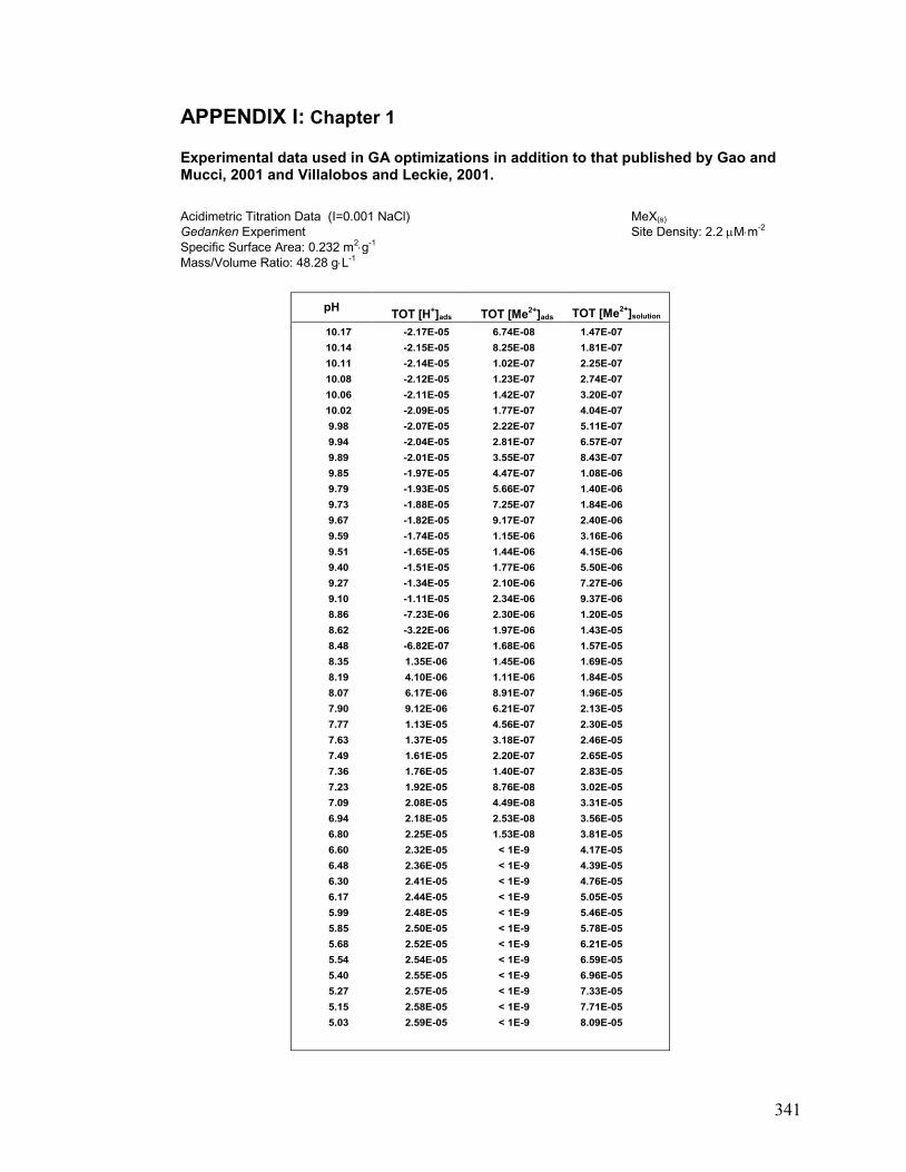
341

APPENDIX I: Chapter 1

Experimental data used in GA optimizations in addition to that published by Gao and Mucci, 2001 and Villalobos and Leckie, 2001.

Acidimetric Titration Data (I=0.001 NaCl) MeX(s)

Gedanken Experiment Site Density: 2.2 Mm-2

Specific Surface Area: 0.232 m2g-1

Mass/Volume Ratio: 48.28 gL-1

pH

TOT [H+]ads

(mol · L

-1)

TOT [Me

2+]ads

(mol · L

-1)

TOT [Me

2+]solution

(mol · L

-1)

10.17 -2.17E-05 6.74E-08 1.47E-07

10.14 -2.15E-05 8.25E-08 1.81E-07

10.11 -2.14E-05 1.02E-07 2.25E-07

10.08 -2.12E-05 1.23E-07 2.74E-07

10.06 -2.11E-05 1.42E-07 3.20E-07

10.02 -2.09E-05 1.77E-07 4.04E-07

9.98 -2.07E-05 2.22E-07 5.11E-07

9.94 -2.04E-05 2.81E-07 6.57E-07

9.89 -2.01E-05 3.55E-07 8.43E-07

9.85 -1.97E-05 4.47E-07 1.08E-06

9.79 -1.93E-05 5.66E-07 1.40E-06

9.73 -1.88E-05 7.25E-07 1.84E-06

9.67 -1.82E-05 9.17E-07 2.40E-06

9.59 -1.74E-05 1.15E-06 3.16E-06

9.51 -1.65E-05 1.44E-06 4.15E-06

9.40 -1.51E-05 1.77E-06 5.50E-06

9.27 -1.34E-05 2.10E-06 7.27E-06

9.10 -1.11E-05 2.34E-06 9.37E-06

8.86 -7.23E-06 2.30E-06 1.20E-05

8.62 -3.22E-06 1.97E-06 1.43E-05

8.48 -6.82E-07 1.68E-06 1.57E-05

8.35 1.35E-06 1.45E-06 1.69E-05

8.19 4.10E-06 1.11E-06 1.84E-05

8.07 6.17E-06 8.91E-07 1.96E-05

7.90 9.12E-06 6.21E-07 2.13E-05

7.77 1.13E-05 4.56E-07 2.30E-05

7.63 1.37E-05 3.18E-07 2.46E-05

7.49 1.61E-05 2.20E-07 2.65E-05

7.36 1.76E-05 1.40E-07 2.83E-05

7.23 1.92E-05 8.76E-08 3.02E-05

7.09 2.08E-05 4.49E-08 3.31E-05

6.94 2.18E-05 2.53E-08 3.56E-05

6.80 2.25E-05 1.53E-08 3.81E-05

6.60 2.32E-05 < 1E-9 4.17E-05

6.48 2.36E-05 < 1E-9 4.39E-05

6.30 2.41E-05 < 1E-9 4.76E-05

6.17 2.44E-05 < 1E-9 5.05E-05

5.99 2.48E-05 < 1E-9 5.46E-05

5.85 2.50E-05 < 1E-9 5.78E-05

5.68 2.52E-05 < 1E-9 6.21E-05

5.54 2.54E-05 < 1E-9 6.59E-05

5.40 2.55E-05 < 1E-9 6.96E-05

5.27 2.57E-05 < 1E-9 7.33E-05

5.15 2.58E-05 < 1E-9 7.71E-05

5.03 2.59E-05 < 1E-9 8.09E-05

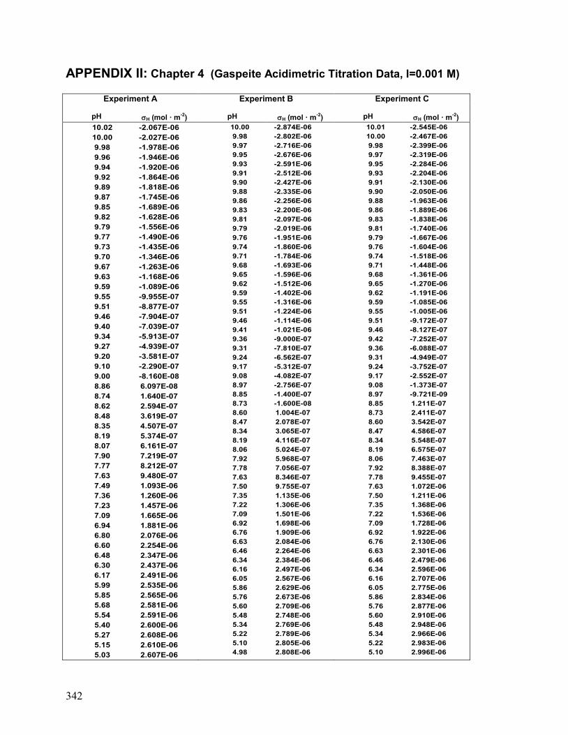
342

APPENDIX II: Chapter 4 (Gaspeite Acidimetric Titration Data, I=0.001 M)

Experiment A Experiment B Experiment C

pH

H (mol · m-2)

pH

H (mol · m-2)

pH

H (mol · m-2)

10.02 -2.067E-06

10.00 -2.027E-06

9.98 -1.978E-06

9.96 -1.946E-06

9.94 -1.920E-06

9.92 -1.864E-06

9.89 -1.818E-06

9.87 -1.745E-06

9.85 -1.689E-06

9.82 -1.628E-06

9.79 -1.556E-06

9.77 -1.490E-06

9.73 -1.435E-06

9.70 -1.346E-06

9.67 -1.263E-06

9.63 -1.168E-06

9.59 -1.089E-06

9.55 -9.955E-07

9.51 -8.877E-07

9.46 -7.904E-07

9.40 -7.039E-07

9.34 -5.913E-07

9.27 -4.939E-07

9.20 -3.581E-07

9.10 -2.290E-07

9.00 -8.160E-08

8.86 6.097E-08

8.74 1.640E-07

8.62 2.594E-07

8.48 3.619E-07

8.35 4.507E-07

8.19 5.374E-07

8.07 6.161E-07

7.90 7.219E-07

7.77 8.212E-07

7.63 9.480E-07

7.49 1.093E-06

7.36 1.260E-06

7.23 1.457E-06

7.09 1.665E-06

6.94 1.881E-06

6.80 2.076E-06

6.60 2.254E-06

6.48 2.347E-06

6.30 2.437E-06

6.17 2.491E-06

5.99 2.535E-06

5.85 2.565E-06

5.68 2.581E-06

5.54 2.591E-06

5.40 2.600E-06

5.27 2.608E-06

5.15 2.610E-06

5.03 2.607E-06

10.00 -2.874E-06

9.98 -2.802E-06

9.97 -2.716E-06

9.95 -2.676E-06

9.93 -2.591E-06

9.91 -2.512E-06

9.90 -2.427E-06

9.88 -2.335E-06

9.86 -2.256E-06

9.83 -2.200E-06

9.81 -2.097E-06

9.79 -2.019E-06

9.76 -1.951E-06

9.74 -1.860E-06

9.71 -1.784E-06

9.68 -1.693E-06

9.65 -1.596E-06

9.62 -1.512E-06

9.59 -1.402E-06

9.55 -1.316E-06

9.51 -1.224E-06

9.46 -1.114E-06

9.41 -1.021E-06

9.36 -9.000E-07

9.31 -7.810E-07

9.24 -6.562E-07

9.17 -5.312E-07

9.08 -4.082E-07

8.97 -2.756E-07

8.85 -1.400E-07

8.73 -1.600E-08

8.60 1.004E-07

8.47 2.078E-07

8.34 3.065E-07

8.19 4.116E-07

8.06 5.024E-07

7.92 5.968E-07

7.78 7.056E-07

7.63 8.346E-07

7.50 9.755E-07

7.35 1.135E-06

7.22 1.306E-06

7.09 1.501E-06

6.92 1.698E-06

6.76 1.909E-06

6.63 2.084E-06

6.46 2.264E-06

6.34 2.384E-06

6.16 2.497E-06

6.05 2.567E-06

5.86 2.629E-06

5.76 2.673E-06

5.60 2.709E-06

5.48 2.748E-06

5.34 2.769E-06

5.22 2.789E-06

5.10 2.805E-06

4.98 2.808E-06

10.01 -2.545E-06

10.00 -2.467E-06

9.98 -2.399E-06

9.97 -2.319E-06

9.95 -2.284E-06

9.93 -2.204E-06

9.91 -2.130E-06

9.90 -2.050E-06

9.88 -1.963E-06

9.86 -1.889E-06

9.83 -1.838E-06

9.81 -1.740E-06

9.79 -1.667E-06

9.76 -1.604E-06

9.74 -1.518E-06

9.71 -1.448E-06

9.68 -1.361E-06

9.65 -1.270E-06

9.62 -1.191E-06

9.59 -1.085E-06

9.55 -1.005E-06

9.51 -9.172E-07

9.46 -8.127E-07

9.42 -7.252E-07

9.36 -6.088E-07

9.31 -4.949E-07

9.24 -3.752E-07

9.17 -2.552E-07

9.08 -1.373E-07

8.97 -9.721E-09

8.85 1.211E-07

8.73 2.411E-07

8.60 3.542E-07

8.47 4.586E-07

8.34 5.548E-07

8.19 6.575E-07

8.06 7.463E-07

7.92 8.388E-07

7.78 9.455E-07

7.63 1.072E-06

7.50 1.211E-06

7.35 1.368E-06

7.22 1.536E-06

7.09 1.728E-06

6.92 1.922E-06

6.76 2.130E-06

6.63 2.301E-06

6.46 2.479E-06

6.34 2.596E-06

6.16 2.707E-06

6.05 2.775E-06

5.86 2.834E-06

5.76 2.877E-06

5.60 2.910E-06

5.48 2.948E-06

5.34 2.966E-06

5.22 2.983E-06

5.10 2.996E-06

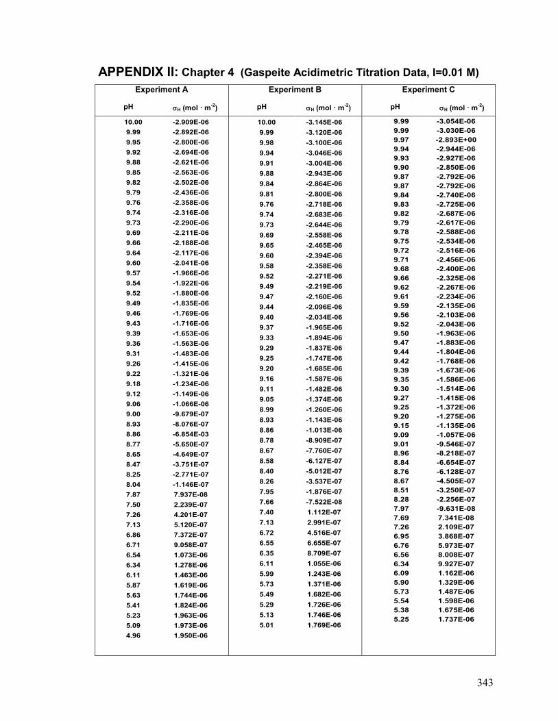
343



pH

H (mol · m-2)

pH

H (mol · m-2)

pH

H (mol · m-2)

10.00 -2.909E-06

9.99 -2.892E-06

9.95 -2.800E-06

9.92 -2.694E-06

9.88 -2.621E-06

9.85 -2.563E-06

9.82 -2.502E-06

9.79 -2.436E-06

9.76 -2.358E-06

9.74 -2.316E-06

9.73 -2.290E-06

9.69 -2.211E-06

9.66 -2.188E-06

9.64 -2.117E-06

9.60 -2.041E-06

9.57 -1.966E-06

9.54 -1.922E-06

9.52 -1.880E-06

9.49 -1.835E-06

9.46 -1.769E-06

9.43 -1.716E-06

9.39 -1.653E-06

9.36 -1.563E-06

9.31 -1.483E-06

9.26 -1.415E-06

9.22 -1.321E-06

9.18 -1.234E-06

9.12 -1.149E-06

9.06 -1.066E-06

9.00 -9.679E-07

8.93 -8.076E-07

8.86 -6.854E-03

8.77 -5.650E-07

8.65 -4.649E-07

8.47 -3.751E-07

8.25 -2.771E-07

8.04 -1.146E-07

7.87 7.937E-08

7.50 2.239E-07

7.26 4.201E-07

7.13 5.120E-07

6.86 7.372E-07

6.71 9.058E-07

6.54 1.073E-06

6.34 1.278E-06

6.11 1.463E-06

5.87 1.619E-06

5.63 1.744E-06

5.41 1.824E-06

5.23 1.963E-06

5.09 1.973E-06

4.96 1.950E-06

10.00 -3.145E-06

9.99 -3.120E-06

9.98 -3.100E-06

9.94 -3.046E-06

9.91 -3.004E-06

9.88 -2.943E-06

9.84 -2.864E-06

9.81 -2.800E-06

9.76 -2.718E-06

9.74 -2.683E-06

9.73 -2.644E-06

9.69 -2.558E-06

9.65 -2.465E-06

9.60 -2.394E-06

9.58 -2.358E-06

9.52 -2.271E-06

9.49 -2.219E-06

9.47 -2.160E-06

9.44 -2.096E-06

9.40 -2.034E-06

9.37 -1.965E-06

9.33 -1.894E-06

9.29 -1.837E-06

9.25 -1.747E-06

9.20 -1.685E-06

9.16 -1.587E-06

9.11 -1.482E-06

9.05 -1.374E-06

8.99 -1.260E-06

8.93 -1.143E-06

8.86 -1.013E-06

8.78 -8.909E-07

8.67 -7.760E-07

8.58 -6.127E-07

8.40 -5.012E-07

8.26 -3.537E-07

7.95 -1.876E-07

7.66 -7.522E-08

7.40 1.112E-07

7.13 2.991E-07

6.72 4.516E-07

6.55 6.655E-07

6.35 8.709E-07

6.11 1.055E-06

5.99 1.243E-06

5.73 1.371E-06

5.49 1.682E-06

5.29 1.726E-06

5.13 1.746E-06

5.01 1.769E-06

9.99 -3.054E-06

9.99 -3.030E-06

9.97 -2.893E+00

9.94 -2.944E-06

9.93 -2.927E-06

9.90 -2.850E-06

9.87 -2.792E-06

9.87 -2.792E-06

9.84 -2.740E-06

9.83 -2.725E-06

9.82 -2.687E-06

9.79 -2.617E-06

9.78 -2.588E-06

9.75 -2.534E-06

9.72 -2.516E-06

9.71 -2.456E-06

9.68 -2.400E-06

9.66 -2.325E-06

9.62 -2.267E-06

9.61 -2.234E-06

9.59 -2.135E-06

9.56 -2.103E-06

9.52 -2.043E-06

9.50 -1.963E-06

9.47 -1.883E-06

9.44 -1.804E-06

9.42 -1.768E-06

9.39 -1.673E-06

9.35 -1.586E-06

9.30 -1.514E-06

9.27 -1.415E-06

9.25 -1.372E-06

9.20 -1.275E-06

9.15 -1.135E-06

9.09 -1.057E-06

9.01 -9.546E-07

8.96 -8.218E-07

8.84 -6.654E-07

8.76 -6.128E-07

8.67 -4.505E-07

8.51 -3.250E-07

8.28 -2.256E-07

7.97 -9.631E-08

7.69 7.341E-08

7.26 2.109E-07

6.95 3.868E-07

6.76 5.973E-07

6.56 8.008E-07

6.34 9.927E-07

6.09 1.162E-06

5.90 1.329E-06

5.73 1.487E-06

5.54 1.598E-06

5.38 1.675E-06

5.25 1.737E-06

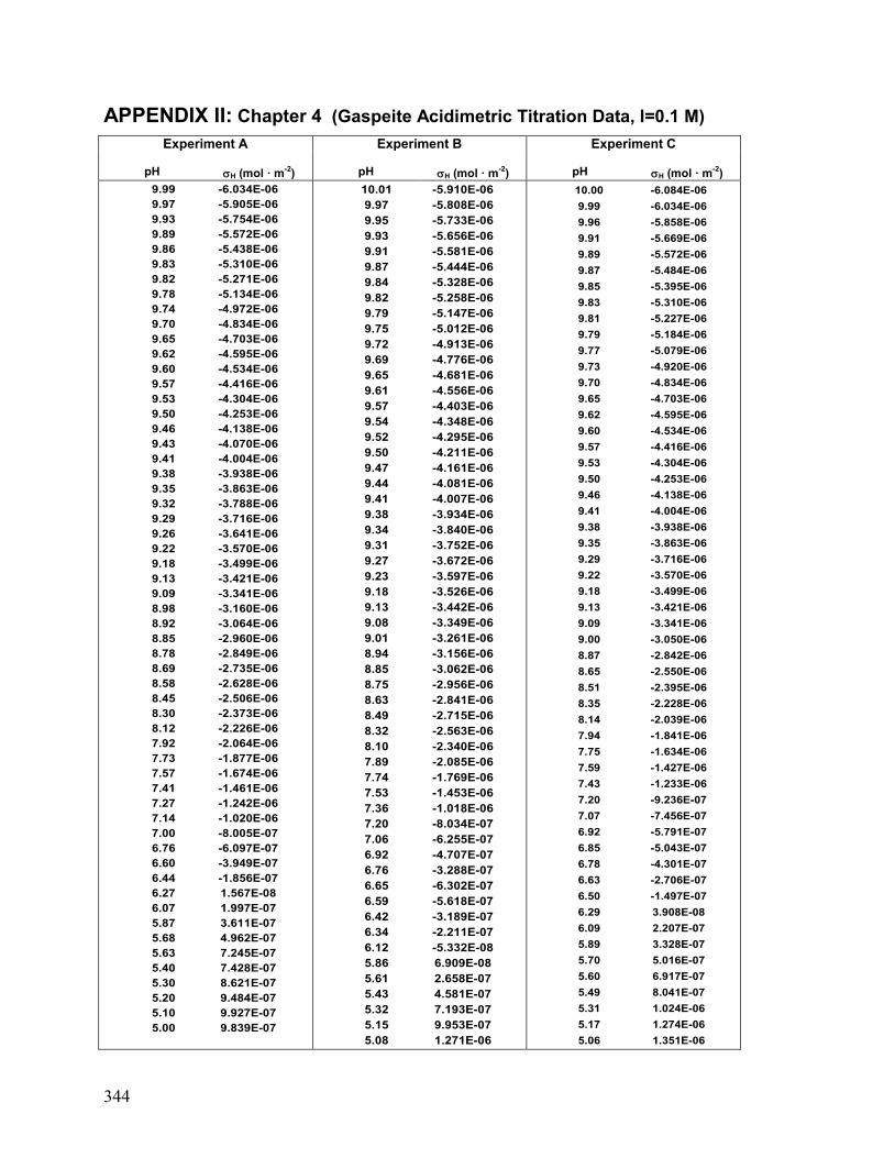
344



pH

H (mol · m-2)

pH

H (mol · m-2)

pH

H (mol · m-2)

9.99 -6.034E-06

9.97 -5.905E-06

9.93 -5.754E-06

9.89 -5.572E-06

9.86 -5.438E-06

9.83 -5.310E-06

9.82 -5.271E-06

9.78 -5.134E-06

9.74 -4.972E-06

9.70 -4.834E-06

9.65 -4.703E-06

9.62 -4.595E-06

9.60 -4.534E-06

9.57 -4.416E-06

9.53 -4.304E-06

9.50 -4.253E-06

9.46 -4.138E-06

9.43 -4.070E-06

9.41 -4.004E-06

9.38 -3.938E-06

9.35 -3.863E-06

9.32 -3.788E-06

9.29 -3.716E-06

9.26 -3.641E-06

9.22 -3.570E-06

9.18 -3.499E-06

9.13 -3.421E-06

9.09 -3.341E-06

8.98 -3.160E-06

8.92 -3.064E-06

8.85 -2.960E-06

8.78 -2.849E-06

8.69 -2.735E-06

8.58 -2.628E-06

8.45 -2.506E-06

8.30 -2.373E-06

8.12 -2.226E-06

7.92 -2.064E-06

7.73 -1.877E-06

7.57 -1.674E-06

7.41 -1.461E-06

7.27 -1.242E-06

7.14 -1.020E-06

7.00 -8.005E-07

6.76 -6.097E-07

6.60 -3.949E-07

6.44 -1.856E-07

6.27 1.567E-08

6.07 1.997E-07

5.87 3.611E-07

5.68 4.962E-07

5.63 7.245E-07

5.40 7.428E-07

5.30 8.621E-07

5.20 9.484E-07

5.10 9.927E-07

5.00 9.839E-07

10.01 -5.910E-06

9.97 -5.808E-06

9.95 -5.733E-06

9.93 -5.656E-06

9.91 -5.581E-06

9.87 -5.444E-06

9.84 -5.328E-06

9.82 -5.258E-06

9.79 -5.147E-06

9.75 -5.012E-06

9.72 -4.913E-06

9.69 -4.776E-06

9.65 -4.681E-06

9.61 -4.556E-06

9.57 -4.403E-06

9.54 -4.348E-06

9.52 -4.295E-06

9.50 -4.211E-06

9.47 -4.161E-06

9.44 -4.081E-06

9.41 -4.007E-06

9.38 -3.934E-06

9.34 -3.840E-06

9.31 -3.752E-06

9.27 -3.672E-06

9.23 -3.597E-06

9.18 -3.526E-06

9.13 -3.442E-06

9.08 -3.349E-06

9.01 -3.261E-06

8.94 -3.156E-06

8.85 -3.062E-06

8.75 -2.956E-06

8.63 -2.841E-06

8.49 -2.715E-06

8.32 -2.563E-06

8.10 -2.340E-06

7.89 -2.085E-06

7.74 -1.769E-06

7.53 -1.453E-06

7.36 -1.018E-06

7.20 -8.034E-07

7.06 -6.255E-07

6.92 -4.707E-07

6.76 -3.288E-07

6.65 -6.302E-07

6.59 -5.618E-07

6.42 -3.189E-07

6.34 -2.211E-07

6.12 -5.332E-08

5.86 6.909E-08

5.61 2.658E-07

5.43 4.581E-07

5.32 7.193E-07

5.15 9.953E-07

5.08 1.271E-06

10.00 -6.084E-06

9.99 -6.034E-06

9.96 -5.858E-06

9.91 -5.669E-06

9.89 -5.572E-06

9.87 -5.484E-06

9.85 -5.395E-06

9.83 -5.310E-06

9.81 -5.227E-06

9.79 -5.184E-06

9.77 -5.079E-06

9.73 -4.920E-06

9.70 -4.834E-06

9.65 -4.703E-06

9.62 -4.595E-06

9.60 -4.534E-06

9.57 -4.416E-06

9.53 -4.304E-06

9.50 -4.253E-06

9.46 -4.138E-06

9.41 -4.004E-06

9.38 -3.938E-06

9.35 -3.863E-06

9.29 -3.716E-06

9.22 -3.570E-06

9.18 -3.499E-06

9.13 -3.421E-06

9.09 -3.341E-06

9.00 -3.050E-06

8.87 -2.842E-06

8.65 -2.550E-06

8.51 -2.395E-06

8.35 -2.228E-06

8.14 -2.039E-06

7.94 -1.841E-06

7.75 -1.634E-06

7.59 -1.427E-06

7.43 -1.233E-06

7.20 -9.236E-07

7.07 -7.456E-07

6.92 -5.791E-07

6.85 -5.043E-07

6.78 -4.301E-07

6.63 -2.706E-07

6.50 -1.497E-07

6.29 3.908E-08

6.09 2.207E-07

5.89 3.328E-07

5.70 5.016E-07

5.60 6.917E-07

5.49 8.041E-07

5.31 1.024E-06

5.17 1.274E-06

5.06 1.351E-06

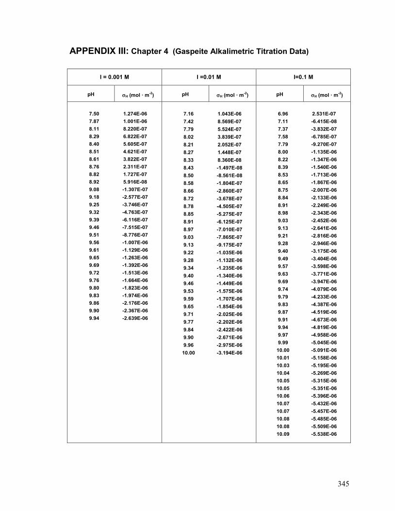
345

APPENDIX III: Chapter 4 (Gaspeite Alkalimetric Titration Data)

I = 0.001 M I =0.01 M I=0.1 M

pH

H (mol · m-2)

pH

H (mol · m-2)

pH

H (mol · m-2)

7.50 1.274E-06

7.87 1.001E-06

8.11 8.220E-07

8.29 6.822E-07

8.40 5.605E-07

8.51 4.621E-07

8.61 3.822E-07

8.76 2.311E-07

8.82 1.727E-07

8.92 5.916E-08

9.08 -1.307E-07

9.18 -2.577E-07

9.25 -3.746E-07

9.32 -4.763E-07

9.39 -6.116E-07

9.46 -7.515E-07

9.51 -8.776E-07

9.56 -1.007E-06

9.61 -1.129E-06

9.65 -1.263E-06

9.69 -1.392E-06

9.72 -1.513E-06

9.76 -1.664E-06

9.80 -1.823E-06

9.83 -1.974E-06

9.86 -2.176E-06

9.90 -2.367E-06

9.94 -2.639E-06

7.16 1.043E-06

7.42 8.569E-07

7.79 5.524E-07

8.02 3.839E-07

8.21 2.052E-07

8.27 1.448E-07

8.33 8.360E-08

8.43 -1.497E-08

8.50 -8.561E-08

8.58 -1.804E-07

8.66 -2.860E-07

8.72 -3.678E-07

8.78 -4.505E-07

8.85 -5.275E-07

8.91 -6.125E-07

8.97 -7.010E-07

9.03 -7.865E-07

9.13 -9.175E-07

9.22 -1.035E-06

9.28 -1.132E-06

9.34 -1.235E-06

9.40 -1.340E-06

9.46 -1.449E-06

9.53 -1.575E-06

9.59 -1.707E-06

9.65 -1.854E-06

9.71 -2.025E-06

9.77 -2.202E-06

9.84 -2.422E-06

9.90 -2.671E-06

9.96 -2.975E-06

10.00 -3.194E-06

6.96 2.531E-07

7.11 -6.415E-08

7.37 -3.832E-07

7.58 -6.785E-07

7.79 -9.270E-07

8.00 -1.135E-06

8.22 -1.347E-06

8.39 -1.540E-06

8.53 -1.713E-06

8.65 -1.867E-06

8.75 -2.007E-06

8.84 -2.133E-06

8.91 -2.249E-06

8.98 -2.343E-06

9.03 -2.452E-06

9.13 -2.641E-06

9.21 -2.816E-06

9.28 -2.946E-06

9.40 -3.175E-06

9.49 -3.404E-06

9.57 -3.598E-06

9.63 -3.771E-06

9.69 -3.947E-06

9.74 -4.079E-06

9.79 -4.233E-06

9.83 -4.387E-06

9.87 -4.519E-06

9.91 -4.673E-06

9.94 -4.819E-06

9.97 -4.958E-06

9.99 -5.045E-06

10.00 -5.091E-06

10.01 -5.158E-06

10.03 -5.195E-06

10.04 -5.269E-06

10.05 -5.315E-06

10.05 -5.351E-06

10.06 -5.396E-06

10.07 -5.432E-06

10.07 -5.457E-06

10.08 -5.485E-06

10.08 -5.509E-06

10.09 -5.538E-06

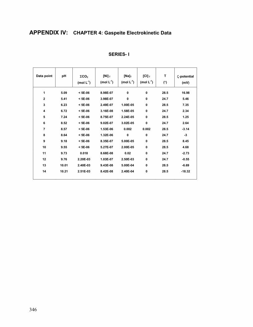
346

APPENDIX IV: CHAPTER 4: Gaspeite Electrokinetic Data

SERIES- I

Data point

pH

CO2

(mol L-1)

[Ni] T

(mol L-1)

[Na]T

(mol L-1)

[Cl] T

(mol L-1)

T

(°)

-potential

(mV)

1 5.09 < 5E-06 8.98E-07 0 0 28.5 16.98

2 5.41 < 5E-06 3.98E-07 0 0 24.7 5.46

3 6.23 < 5E-06 2.49E-07 1.00E-05 0 28.5 7.35

4 6.72 < 5E-06 3.16E-08 1.58E-05 0 24.7 2.34

5 7.24 < 5E-06 8.75E-07 2.24E-05 0 28.5 1.25

6 8.52 < 5E-06 9.02E-07 3.02E-05 0 24.7 2.64

7 8.57 < 5E-06 1.53E-06 0.002 0.002 28.5 -3.14

8 8.64 < 5E-06 1.32E-06 0 0 24.7 -3

9 9.18 < 5E-06 8.35E-07 5.00E-05 0 28.5 8.45

10 9.55 < 5E-06 5.27E-07 2.00E-05 0 28.5 4.68

11 9.73 0.018 8.68E-08 0.02 0 24.7 -2.73

12 9.76 2.20E-03 1.03E-07 2.50E-03 0 24.7 -0.55

13 10.01 2.40E-03 9.43E-08 5.00E-04 0 28.5 -6.69

14 10.21 2.51E-03 8.42E-08 2.40E-04 0 28.5 -18.32

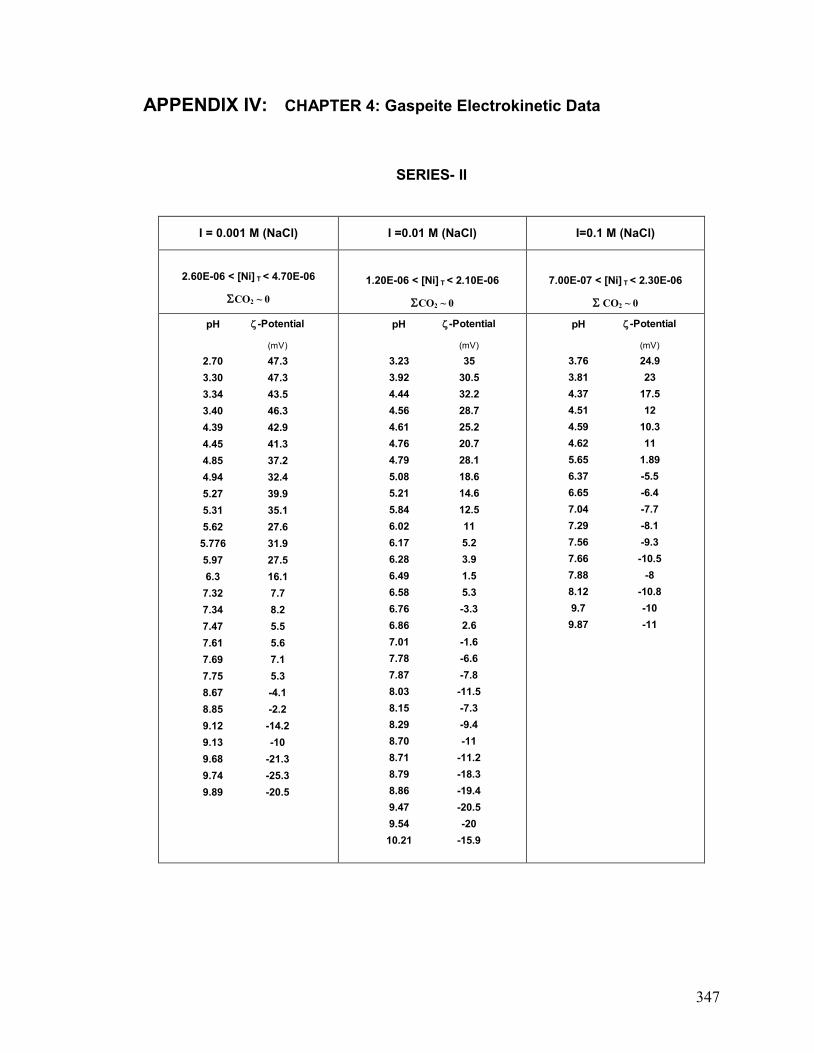
347

APPENDIX IV: CHAPTER 4: Gaspeite Electrokinetic Data

SERIES- II

I = 0.001 M (NaCl) I =0.01 M (NaCl) I=0.1 M (NaCl)

2.60E-06 < [Ni] T < 4.70E-06

CO2 ~ 0

1.20E-06 < [Ni] T < 2.10E-06

CO2 ~ 0

7.00E-07 < [Ni] T < 2.30E-06

CO2 ~ 0

pH -Potential

(mV)

2.70 47.3

3.30 47.3

3.34 43.5

3.40 46.3

4.39 42.9

4.45 41.3

4.85 37.2

4.94 32.4

5.27 39.9

5.31 35.1

5.62 27.6

5.776 31.9

5.97 27.5

6.3 16.1

7.32 7.7

7.34 8.2

7.47 5.5

7.61 5.6

7.69 7.1

7.75 5.3

8.67 -4.1

8.85 -2.2

9.12 -14.2

9.13 -10

9.68 -21.3

9.74 -25.3

9.89 -20.5

pH -Potential

(mV)

3.23 35

3.92 30.5

4.44 32.2

4.56 28.7

4.61 25.2

4.76 20.7

4.79 28.1

5.08 18.6

5.21 14.6

5.84 12.5

6.02 11

6.17 5.2

6.28 3.9

6.49 1.5

6.58 5.3

6.76 -3.3

6.86 2.6

7.01 -1.6

7.78 -6.6

7.87 -7.8

8.03 -11.5

8.15 -7.3

8.29 -9.4

8.70 -11

8.71 -11.2

8.79 -18.3

8.86 -19.4

9.47 -20.5

9.54 -20

10.21 -15.9

pH -Potential

(mV)

3.76 24.9

3.81 23

4.37 17.5

4.51 12

4.59 10.3

4.62 11

5.65 1.89

6.37 -5.5

6.65 -6.4

7.04 -7.7

7.29 -8.1

7.56 -9.3

7.66 -10.5

7.88 -8

8.12 -10.8

9.7 -10

9.87 -11

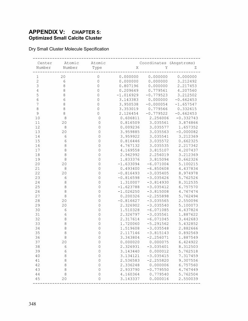
348

APPENDIX V: CHAPTER 5:

Optimized Small Calcite Cluster Dry Small Cluster Molecule Specification

---------------------------------------------------------------------

Center Atomic Atomic Coordinates (Angstroms)

Number Number Type X Y Z

---------------------------------------------------------------------

1 20 0 0.000000 0.000000 0.000000

2 6 0 0.000000 0.000000 3.212492

3 8 0 0.807196 0.000000 2.217453

4 8 0 0.209649 0.779561 4.207560

5 8 0 -1.016929 -0.779523 3.212502

6 6 0 3.143383 0.000000 -0.662453

7 8 0 3.950538 -0.000054 -1.657547

8 8 0 3.353019 0.779566 0.332615

9 8 0 2.126454 -0.779522 -0.662453

10 8 0 0.606811 2.256006 -0.332743

11 20 0 0.816509 3.035561 3.874866

12 8 0 0.009236 3.035577 1.657352

13 20 0 3.959885 3.035563 -0.000082

14 6 0 3.959922 3.035541 3.212369

15 6 0 0.816446 3.035572 0.662325

16 8 0 4.767132 3.035535 2.217342

17 8 0 4.169558 3.815107 4.207437

18 8 0 2.942992 2.256019 3.212369

19 8 0 1.833376 3.815094 0.662326

20 20 0 -1.633094 -6.071004 5.100215

21 8 0 0.493400 -6.850608 4.437834

22 20 0 -0.816493 -3.035405 8.974978

23 6 0 -0.816598 -3.035426 5.762526

24 8 0 1.310007 -3.814930 8.312535

25 8 0 -1.623788 -3.035412 6.757570

26 8 0 -1.026250 -3.815008 4.767474

27 8 0 0.200326 -2.255898 5.762494

28 20 0 -0.816627 -3.035565 2.550096

29 20 0 2.326902 -3.035540 5.100073

30 6 0 1.510328 -6.071085 4.437824

31 6 0 2.326797 -3.035561 1.887622

32 8 0 2.317614 -6.071045 3.442683

33 8 0 1.720060 -5.291562 5.432852

34 8 0 1.519608 -3.035548 2.882666

35 8 0 2.117146 -3.815143 0.892569

36 8 0 3.343804 -2.256071 1.887549

37 20 0 0.000020 0.000075 6.424922

38 6 0 2.326931 -3.035401 8.312503

39 6 0 3.143440 0.000012 5.762518

40 8 0 3.134121 -3.035415 7.317459

41 8 0 2.536583 -2.255820 9.307556

42 8 0 2.336248 0.000006 6.757560

43 8 0 2.933790 -0.779550 4.767449

44 8 0 4.160364 0.779540 5.762504

45 20 0 3.143337 0.000016 2.550039

---------------------------------------------------------------------

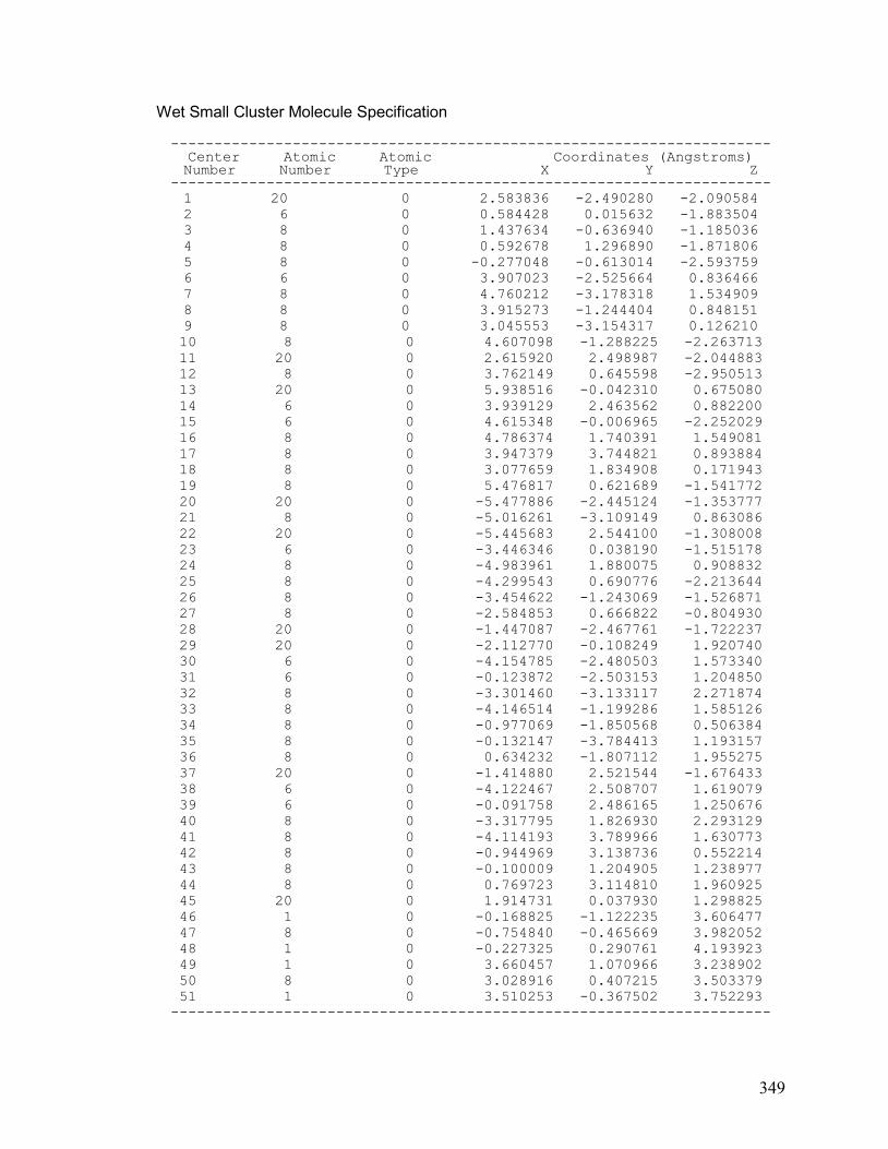
349

Wet Small Cluster Molecule Specification

--------------------------------------------------------------------- Center Atomic Atomic Coordinates (Angstroms) Number Number Type X Y Z

---------------------------------------------------------------------

1 20 0 2.583836 -2.490280 -2.090584

2 6 0 0.584428 0.015632 -1.883504

3 8 0 1.437634 -0.636940 -1.185036

4 8 0 0.592678 1.296890 -1.871806

5 8 0 -0.277048 -0.613014 -2.593759

6 6 0 3.907023 -2.525664 0.836466

7 8 0 4.760212 -3.178318 1.534909

8 8 0 3.915273 -1.244404 0.848151

9 8 0 3.045553 -3.154317 0.126210

10 8 0 4.607098 -1.288225 -2.263713

11 20 0 2.615920 2.498987 -2.044883

12 8 0 3.762149 0.645598 -2.950513

13 20 0 5.938516 -0.042310 0.675080

14 6 0 3.939129 2.463562 0.882200

15 6 0 4.615348 -0.006965 -2.252029

16 8 0 4.786374 1.740391 1.549081

17 8 0 3.947379 3.744821 0.893884

18 8 0 3.077659 1.834908 0.171943

19 8 0 5.476817 0.621689 -1.541772

20 20 0 -5.477886 -2.445124 -1.353777

21 8 0 -5.016261 -3.109149 0.863086

22 20 0 -5.445683 2.544100 -1.308008

23 6 0 -3.446346 0.038190 -1.515178

24 8 0 -4.983961 1.880075 0.908832

25 8 0 -4.299543 0.690776 -2.213644

26 8 0 -3.454622 -1.243069 -1.526871

27 8 0 -2.584853 0.666822 -0.804930

28 20 0 -1.447087 -2.467761 -1.722237

29 20 0 -2.112770 -0.108249 1.920740

30 6 0 -4.154785 -2.480503 1.573340

31 6 0 -0.123872 -2.503153 1.204850

32 8 0 -3.301460 -3.133117 2.271874

33 8 0 -4.146514 -1.199286 1.585126

34 8 0 -0.977069 -1.850568 0.506384

35 8 0 -0.132147 -3.784413 1.193157

36 8 0 0.634232 -1.807112 1.955275

37 20 0 -1.414880 2.521544 -1.676433

38 6 0 -4.122467 2.508707 1.619079

39 6 0 -0.091758 2.486165 1.250676

40 8 0 -3.317795 1.826930 2.293129

41 8 0 -4.114193 3.789966 1.630773

42 8 0 -0.944969 3.138736 0.552214

43 8 0 -0.100009 1.204905 1.238977

44 8 0 0.769723 3.114810 1.960925

45 20 0 1.914731 0.037930 1.298825

46 1 0 -0.168825 -1.122235 3.606477

47 8 0 -0.754840 -0.465669 3.982052

48 1 0 -0.227325 0.290761 4.193923

49 1 0 3.660457 1.070966 3.238902

50 8 0 3.028916 0.407215 3.503379

51 1 0 3.510253 -0.367502 3.752293

---------------------------------------------------------------------

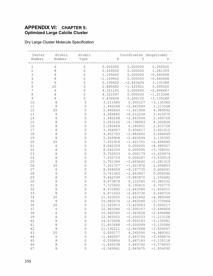
350

APPENDIX VI: CHAPTER 5:

Optimized Large Calcite Cluster Dry Large Cluster Molecule Specification

---------------------------------------------------------------------



---------------------------------------------------------------------

1 6 0 0.000000 0.000000 0.000000

2 8 0 0.000000 0.000000 1.281359

3 8 0 1.109660 0.000000 -0.640608

4 8 0 -1.109660 0.000055 -0.640668

5 8 0 0.330620 -2.843624 3.135388

6 20 0 2.880682 -1.421821 0.000020

7 6 0 4.321125 0.000065 -2.494667

8 8 0 4.321097 0.000030 -1.213308

9 8 0 5.430894 0.000120 -3.135268

10 8 0 3.211480 0.000127 -3.135360

11 8 0 1.440248 -2.843544 1.213368

12 20 0 2.880643 -1.421958 4.989592

13 6 0 4.586882 -0.012234 3.415070

14 6 0 1.440248 -2.843544 2.494728

15 8 0 5.063126 -0.798083 4.300836

16 8 0 5.282409 0.280951 2.415728

17 8 0 3.364907 0.406617 3.601012

18 8 0 4.651703 -2.843642 0.640649

19 8 0 2.549908 -2.843599 3.135395

20 20 0 7.201916 -1.421701 -2.494640

21 6 0 8.642359 0.000205 -4.989327

22 8 0 8.642330 0.000095 -3.708051

23 8 0 9.752033 0.000179 -5.629974

24 8 0 7.532714 0.000267 -5.630019

25 8 0 5.761364 -2.843642 -1.281319

26 20 0 7.201727 -1.421976 2.494853

27 6 0 8.948459 -0.167735 0.606041

28 6 0 5.761363 -2.843647 0.000040

29 8 0 9.442599 -0.883870 1.550682

30 8 0 9.673878 0.122565 -0.382532

31 8 0 7.723932 0.190415 0.702775

32 8 0 8.972892 -2.843580 -1.854011

33 8 0 6.871023 -2.843736 0.640714

34 20 0 11.523055 -1.421642 -4.989346

35 8 0 10.082576 -2.843580 -3.775964

36 20 0 11.522913 -1.422063 0.000217

37 6 0 12.963340 -0.000157 -2.494404

38 6 0 10.082560 -2.843628 -2.494688

39 8 0 12.963322 -0.000233 -1.213128

40 8 0 14.073008 -0.000183 -3.135081

41 8 0 11.853688 -0.000099 -3.135086

42 8 0 11.192211 -2.843668 -1.854007

43 20 0 0.000177 4.265590 -4.989361

44 6 0 -1.440267 2.843704 -2.494674

45 8 0 0.330856 5.687183 -3.135118

46 8 0 -1.440238 2.843740 -3.776033

47 8 0 -2.549941 2.843675 -1.854090

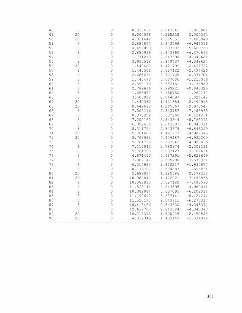
351

48 8 0 -0.330621 2.843643 -1.853981

49 20 0 0.000058 4.265235 0.000262

50 20 0 4.321442 4.265651 -7.483949

51 6 0 2.880873 2.843798 -4.989316

52 8 0 4.652090 5.687303 -5.629758

53 8 0 2.880996 2.843860 -6.270693

54 8 0 1.771230 2.843690 -4.348681

55 8 0 3.990518 2.843737 -4.348624

56 20 0 1.440400 1.421799 -2.494762

57 6 0 1.440501 5.687122 -2.494426

58 6 0 2.685631 2.761765 0.371704

59 8 0 1.440473 5.687086 -1.213066

60 8 0 2.550176 5.687151 -3.134989

61 8 0 2.789616 2.999221 -0.848325

62 8 0 1.653977 3.188750 1.062132

63 8 0 3.505912 2.064097 1.026148

64 20 0 1.440362 1.421654 2.494915

65 20 0 8.642613 4.265667 -9.978547

66 6 0 7.202116 2.843757 -7.483968

67 8 0 8.973292 5.687260 -8.124294

68 8 0 7.202160 2.843844 -8.765243

69 8 0 6.092436 2.843803 -6.843314

70 8 0 8.311754 2.843679 -6.843259

71 20 0 5.761600 1.421977 -4.989346

72 20 0 8.703963 4.454187 -4.925209

73 6 0 5.761736 5.687242 -4.989066

74 6 0 7.115945 2.783874 -2.308131

75 8 0 5.761738 5.687127 -3.707654

76 8 0 6.871410 5.687291 -5.629649

77 8 0 7.082147 2.885490 -3.579351

78 8 0 6.014683 2.910217 -1.635677

79 8 0 8.176797 2.534887 -1.695424

80 20 0 5.689914 1.385686 0.178253

81 20 0 10.082847 1.422021 -7.483935

82 6 0 10.082930 5.687182 -7.483590

83 6 0 11.523141 2.843595 -4.989041

84 8 0 10.082884 5.687095 -6.202314

85 8 0 11.192612 5.687141 -8.124244

86 8 0 11.523175 2.843711 -6.270317

87 8 0 10.413466 2.843620 -4.348374

88 8 0 12.632785 2.843524 -4.348348

89 20 0 10.215315 1.500425 -2.452555

90 20 0 4.312349 4.402449 -2.534072

---------------------------------------------------------------------

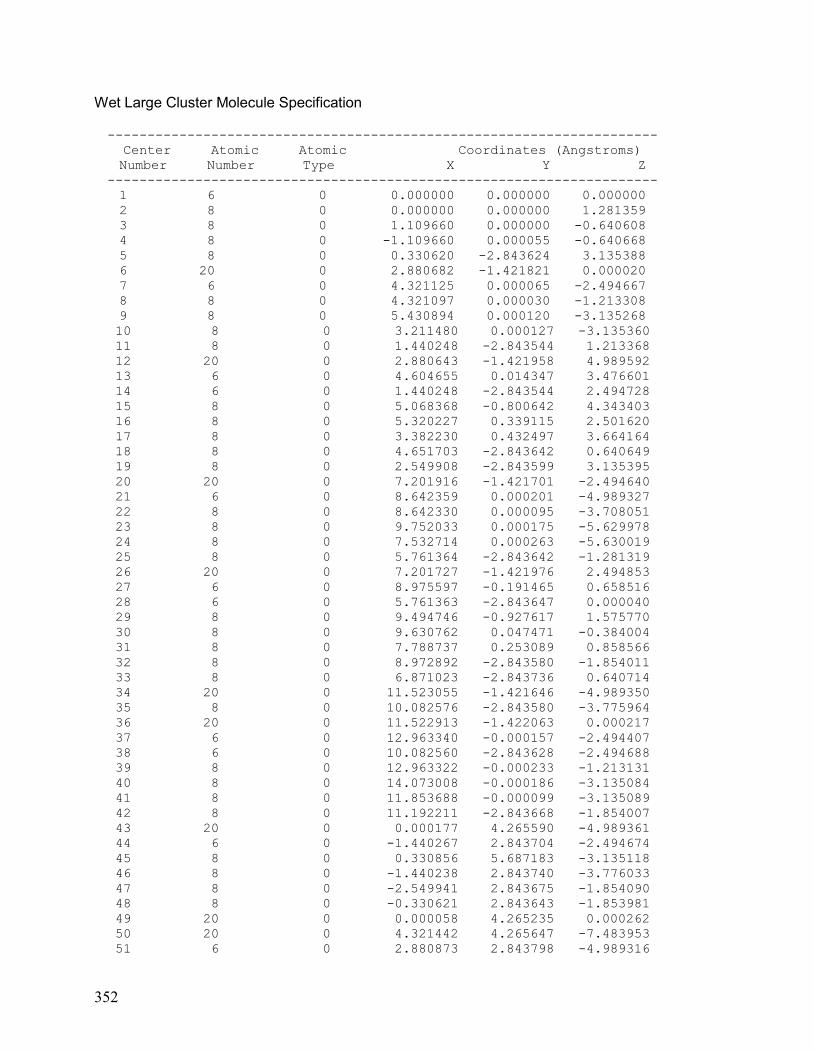
352

Wet Large Cluster Molecule Specification ---------------------------------------------------------------------



---------------------------------------------------------------------

1 6 0 0.000000 0.000000 0.000000

2 8 0 0.000000 0.000000 1.281359

3 8 0 1.109660 0.000000 -0.640608

4 8 0 -1.109660 0.000055 -0.640668

5 8 0 0.330620 -2.843624 3.135388

6 20 0 2.880682 -1.421821 0.000020

7 6 0 4.321125 0.000065 -2.494667

8 8 0 4.321097 0.000030 -1.213308

9 8 0 5.430894 0.000120 -3.135268

10 8 0 3.211480 0.000127 -3.135360

11 8 0 1.440248 -2.843544 1.213368

12 20 0 2.880643 -1.421958 4.989592

13 6 0 4.604655 0.014347 3.476601

14 6 0 1.440248 -2.843544 2.494728

15 8 0 5.068368 -0.800642 4.343403

16 8 0 5.320227 0.339115 2.501620

17 8 0 3.382230 0.432497 3.664164

18 8 0 4.651703 -2.843642 0.640649

19 8 0 2.549908 -2.843599 3.135395

20 20 0 7.201916 -1.421701 -2.494640

21 6 0 8.642359 0.000201 -4.989327

22 8 0 8.642330 0.000095 -3.708051

23 8 0 9.752033 0.000175 -5.629978

24 8 0 7.532714 0.000263 -5.630019

25 8 0 5.761364 -2.843642 -1.281319

26 20 0 7.201727 -1.421976 2.494853

27 6 0 8.975597 -0.191465 0.658516

28 6 0 5.761363 -2.843647 0.000040

29 8 0 9.494746 -0.927617 1.575770

30 8 0 9.630762 0.047471 -0.384004

31 8 0 7.788737 0.253089 0.858566

32 8 0 8.972892 -2.843580 -1.854011

33 8 0 6.871023 -2.843736 0.640714

34 20 0 11.523055 -1.421646 -4.989350

35 8 0 10.082576 -2.843580 -3.775964

36 20 0 11.522913 -1.422063 0.000217

37 6 0 12.963340 -0.000157 -2.494407

38 6 0 10.082560 -2.843628 -2.494688

39 8 0 12.963322 -0.000233 -1.213131

40 8 0 14.073008 -0.000186 -3.135084

41 8 0 11.853688 -0.000099 -3.135089

42 8 0 11.192211 -2.843668 -1.854007

43 20 0 0.000177 4.265590 -4.989361

44 6 0 -1.440267 2.843704 -2.494674

45 8 0 0.330856 5.687183 -3.135118

46 8 0 -1.440238 2.843740 -3.776033

47 8 0 -2.549941 2.843675 -1.854090

48 8 0 -0.330621 2.843643 -1.853981

49 20 0 0.000058 4.265235 0.000262

50 20 0 4.321442 4.265647 -7.483953

51 6 0 2.880873 2.843798 -4.989316

353

52 8 0 4.652090 5.687303 -5.629762

53 8 0 2.880996 2.843860 -6.270693

54 8 0 1.771230 2.843690 -4.348681

55 8 0 3.990518 2.843737 -4.348624

56 20 0 1.440400 1.421799 -2.494762

57 6 0 1.440501 5.687122 -2.494426

58 6 0 2.624743 2.734907 0.395448

59 8 0 1.440473 5.687086 -1.213066

60 8 0 2.550176 5.687151 -3.134993

61 8 0 2.714486 2.967435 -0.821638

62 8 0 1.636567 3.221194 1.112711

63 8 0 3.405815 1.972883 1.033582

64 20 0 1.440362 1.421654 2.494915

65 20 0 8.642613 4.265663 -9.978549

66 6 0 7.202116 2.843753 -7.483968

67 8 0 8.973292 5.687256 -8.124298

68 8 0 7.202160 2.843840 -8.765243

69 8 0 6.092436 2.843799 -6.843314

70 8 0 8.311754 2.843675 -6.843259

71 20 0 5.761597 1.421973 -4.989346

72 20 0 8.715971 4.547224 -4.798165

73 6 0 5.761736 5.687242 -4.989070

74 6 0 7.060296 2.684957 -2.344034

75 8 0 5.761738 5.687127 -3.707658

76 8 0 6.871410 5.687287 -5.629653

77 8 0 7.189152 2.782233 -3.600004

78 8 0 5.901690 2.776652 -1.801008

79 8 0 8.049922 2.470265 -1.588306

80 20 0 5.632710 1.483148 0.172931

81 20 0 10.082845 1.422017 -7.483939

82 6 0 10.082930 5.687178 -7.483594

83 6 0 11.523140 2.843595 -4.989045

84 8 0 10.082884 5.687091 -6.202318

85 8 0 11.192612 5.687136 -8.124248

86 8 0 11.523173 2.843707 -6.270321

87 8 0 10.413466 2.843620 -4.348378

88 8 0 12.632785 2.843524 -4.348352

89 20 0 10.137314 1.546532 -2.401857

90 8 0 5.133493 5.442819 -0.321180

91 1 0 6.089056 5.450648 -0.302737

92 1 0 4.828074 6.326240 -0.185179

93 1 0 6.680104 2.638194 2.679882

94 8 0 7.053362 2.796457 1.826888

95 1 0 7.741044 2.150173 1.703085

96 1 0 9.301588 5.734964 -1.886283

97 8 0 9.647984 5.296011 -2.647326

98 1 0 10.599582 5.229323 -2.569447

99 1 0 12.177248 3.319319 -1.162930

100 8 0 11.782595 2.521463 -0.818036

101 1 0 12.449912 1.834806 -0.825848

102 1 0 8.091095 4.191689 -0.636802

103 8 0 7.968290 5.007258 -0.154820

104 1 0 8.057777 4.765604 0.753669

105 1 0 13.084608 5.363889 -2.650458

106 8 0 12.433860 4.700834 -2.485661

107 1 0 12.550864 4.032377 -3.195608

108 20 0 4.309359 4.446754 -2.457821

354

APPENDIX VII: CHAPTER 5:

Geometrically-optimized (CaCO3)9/4H2O cluster H2O PENETRATION INTO THE CALCITE INTERLAYER

Optimized Structure

DLMO-101 E=-1.406 eV

355

APPENDIX VIII: CHAPTER 6

CaCO3(s) Solubility Product Data

ID pH

Ca

(mol L-1

)

Alkalinity (mol L

-1)

I

(mol L-1

)

Log 10 K°sp

Ksp-1 9.87 1.1610

-4 2.5110

-4 3.810

-4 -8.49

Ksp-2 9.75 1.2310-4

2.3710-4

3.810-4

-8.52

Ksp-3 9.75 1.3310-4

2.5410-4

4.110-4

-8.45

Ksp-4 9.78 1.3910-4

2.2610-4

4.010-4

-8.49

Ksp-5 9.73 1.3410-4

2.5710-4

4.110-4

-8.45

Ksp-6 9.60 1.3910-4

2.4310-4

4.110-4

-8.52

Ksp-7 9.63 1.4510-4

2.3810-4

4.210-4

-8.50

Ksp-8 9.68 1.4010-4

2.5910-4

4.210-4

-8.45

Ksp-9 9.67 1.4310-4

2.5710-4

4.310-4

-8.45

Ksp-10 9.84 1.1010-4

2.5710-4

3.710-4

-8.50

Ksp-11 9.70 1.0310-4

2.6810-4

3.610-4

-8.54

Ksp-12 9.72 1.3110-4

2.6310-4

4.110-4

-8.45

Ksp-13 9.71 1.3710-4

2.4510-4

4.110-4

-8.47

Ksp-14 9.76 1.2710-4

2.4210-4

3.910-4

-8.49

Ksp-15 9.78 1.2210-4

2.4710-4

3.810-4

-8.49

Ksp-16 9.61 1.3510-4

2.3710-4

4.010-4

-8.53

Ksp-17 9.75 1.3110-4

2.7110-4

4.110-4

-8.42

Ksp-18 9.71 1.3710-4

2.810-4

4.310-4

-8.40

Ksp-19 9.70 1.3410-4

2.64e-4 4.210-4

-8.45

Ksp-20 9.70 1.3110-4

2.41e-4 4.010-4

-8.50

-8.48 0.04

356

APPENDIX IX: CHAPTER 6

CaCO3(s) Acidimetric Titrations Data

ID pH pCa Log10 [K+] Log10 [Cl

-]

TOTH*Theo (mol L

-1)

I¥

(mol L -1

) ID pH pCa Log10 [K

+] Log10 [Cl

-]

TOTH* Theo (mol L

-1)

I¥

(mol L -1

)

(PART I)

TH-I TH-II

TH-I-1 9.27 3.70 -1.66 -1.66 2.3510-4

0.023 TH-II-1 8.37 3.36 -1.66 -1.66 8.3210-4

0.024

TH-I-2 9.15 3.66 -1.66 -1.66 3.1010-4

0.023 TH-II-2 8.26 3.28 -1.66 -1.66 9.4310-4

0.024

TH-I-3 9.04 3.54 -1.66 -1.65 3.8510-4

0.023 TH-II-3 8.22 3.04 -1.66 -1.66 1.0110-3

0.026

TH-I-4 8.82 3.46 -1.66 -1.65 4.5910-4

0.023 TH-II-4 8.18 3.01 -1.66 -1.66 1.0810-3

0.026

TH-I-5 8.70 3.37 -1.66 -1.65 5.8410-4

0.024 TH-II-5 8.12 3.01 -1.66 -1.66 1.1410-3

0.026

TH-I-6 8.54 3.32 -1.66 -1.65 7.0810-4

0.024 TH-II-6 8.00 2.93 -1.66 -1.66 1.3410-3

0.027

TH-I-7 8.48 3.27 -1.66 -1.65 8.5610-4

0.024 TH-II-7 7.93 2.91 -1.66 -1.66 1.4710-3

0.027

TH-I-8 8.41 3.16 -1.66 -1.65 9.3010-4

0.024 TH-II-8 7.86 2.88 -1.66 -1.66 1.6010-3

0.028

TH-I-9 8.28 3.11 -1.66 -1.65 1.0010-3

0.025 TH-II-9 7.81 2.82 -1.66 -1.66 1.7310-3

0.028

TH-I-10 8.11 3.06 -1.66 -1.64 1.1510-3

0.025 TH-II-10 7.74 2.81 -1.66 -1.66 1.8610-3

0.029

TH-I-11 8.05 3.00 -1.66 -1.64 1.4010-3

0.025 TH-II-11 7.70 2.81 -1.66 -1.66 2.0010-3

0.029

TH-I-12 7.99 2.95 -1.66 -1.64 1.5210-3

0.026 TH-II-12 7.63 2.80 -1.66 -1.66 2.1310-3

0.029

TH-I-13 7.91 2.93 -1.66 -1.64 1.6410-3

0.026 TH-II-13 7.60 2.77 -1.66 -1.66 2.3410-3

0.030

TH-I-14 7.88 2.88 -1.66 -1.64 1.7610-3

0.027 TH-II-14 7.54 2.72 -1.66 -1.66 2.5610-3

0.031

TH-I-15 7.79 2.85 -1.66 -1.63 1.8910-3

0.027 TH-II-15 7.47 2.73 -1.66 -1.66 2.7710-3

0.031

TH-II-16 7.43 2.70 -1.66 -1.66 2.9910-3

0.031

TH-II-17 7.38 2.68 -1.66 -1.66 3.2010-3

0.032

TH-II-18 7.34 2.67 -1.66 -1.66 3.4110-3

0.032

TH-III TH-IV

TH-III-1 9.45 3.57 -1.66 -1.65 1.5810-4

0.023 TH-IV-1 9.51 3.62 -1.66 -1.65 1.2310-4

0.023

TH-III-2 9.31 3.63 -1.66 -1.65 2.2510-4

0.023 TH-IV-2 9.34 3.51 -1.66 -1.65 1.8510-4

0.023

TH-III-3 9.18 3.55 -1.66 -1.65 2.9110-4

0.023 TH-IV-3 9.22 3.42 -1.66 -1.65 2.4810-4

0.023

TH-III-4 9.06 3.52 -1.66 -1.65 3.5810-4

0.023 TH-IV-4 9.10 3.38 -1.66 -1.65 3.1010-4

0.023

TH-III-5 8.95 3.46 -1.66 -1.65 4.2410-4

0.023 TH-IV-5 8.98 3.35 -1.66 -1.65 3.7210-4

0.023

TH-III-6 8.85 3.37 -1.66 -1.65 4.9010-4

0.024 TH-IV-6 8.88 3.31 -1.66 -1.65 4.3510-4

0.024

TH-III-7 8.76 3.41 -1.66 -1.65 5.5610-4

0.024 TH-IV-7 8.78 3.29 -1.66 -1.65 4.9710-4

0.024

TH-III-8 8.59 3.28 -1.66 -1.65 6.8810-4

0.024 TH-IV-8 8.69 3.21 -1.66 -1.65 5.5910-4

0.024

TH-III-9 8.45 3.19 -1.66 -1.64 8.2010-4

0.025 TH-IV-9 8.55 3.17 -1.66 -1.64 6.8310-4

0.025

TH-III-10 8.33 3.12 -1.66 -1.64 9.5110-4

0.025 TH-IV-10 8.42 3.12 -1.66 -1.64 8.0610-4

0.025

TH-III-11 8.23 3.09 -1.66 -1.64 1.0810-3

0.026 TH-IV-11 8.30 3.08 -1.66 -1.64 9.3010-4

0.026

TH-III-12 8.09 3.02 -1.66 -1.64 1.3010-3

0.026 TH-IV-12 8.21 3.04 -1.66 -1.64 1.0510-3

0.026

TH-III-13 7.97 2.89 -1.66 -1.63 1.5210-3

0.028 TH-IV-13 8.12 3.00 -1.66 -1.64 1.1810-3

0.028

TH-III-14 7.86 2.86 -1.66 -1.63 1.7310-3

0.028 TH-IV-14 8.05 2.99 -1.66 -1.64 1.3010-3

0.028

TH-III-15 7.79 2.88 -1.66 -1.63 1.9510-3

0.028 TH-IV-15 7.85 2.89 -1.66 -1.63 1.6610-3

0.028

TH-IV-16 7.75 2.87 -1.66 -1.63 1.9110-3

0.028

TH-IV-17 7.66 2.84 -1.66 -1.62 2.1510-3

0.028

TH-IV-18 7.59 2.80 -1.66 -1.62 2.3910-3

0.028

(Part II, see next page)

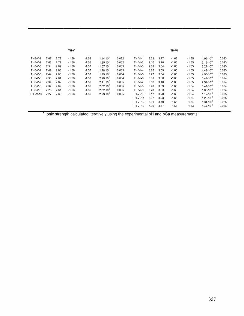
357

TH-V TH-VI

TH5-V-1 7.67 2.73 -1.66 -1.58 1.1410-3

0.032 TH-VI-1 9.33 3.77 -1.66 -1.65 1.9910-4

0.023

TH5-V-2 7.62 2.72 -1.66 -1.58 1.3510-3

0.032 TH-VI-2 9.10 3.70 -1.66 -1.65 3.1210-4

0.023

TH5-V-3 7.54 2.69 -1.66 -1.57 1.5710-3

0.033 TH-VI-3 9.03 3.64 -1.66 -1.65 3.2710-4

0.023

TH5-V-4 7.49 2.68 -1.66 -1.57 1.7810-3

0.033 TH-VI-4 8.85 3.59 -1.66 -1.65 4.4810-4

0.023

TH5-V-5 7.44 2.65 -1.66 -1.57 1.9910-3

0.034 TH-VI-5 8.77 3.54 -1.66 -1.65 4.9510-4

0.023

TH5-V-6 7.38 2.64 -1.66 -1.57 2.2010-3

0.034 TH-VI-6 8.61 3.50 -1.66 -1.65 6.4410-4

0.024

TH5-V-7 7.34 2.62 -1.66 -1.56 2.4110-3

0.035 TH-VI-7 8.52 3.46 -1.66 -1.65 7.3410-4

0.024

TH5-V-8 7.32 2.62 -1.66 -1.56 2.6210-3

0.035 TH-VI-8 8.40 3.39 -1.66 -1.64 8.4110-3

0.024

TH5-V-9 7.26 2.61 -1.66 -1.56 2.8210-3

0.035 TH-VI-9 8.23 3.33 -1.66 -1.64 1.0810-3

0.024

TH5-V-10 7.27 2.65 -1.66 -1.56 2.9310-3

0.035 TH-VI-10 8.17 3.28 -1.66 -1.64 1.1210-3

0.025

TH-VI-11 8.07 3.23 -1.66 -1.64 1.2910-3

0.025

TH-VI-12 8.01 3.19 -1.66 -1.64 1.3410-3

0.025

TH-VI-13 7.95 3.17 -1.66 -1.63 1.4710-3

0.026

¥ Ionic strength calculated iteratively using the experimental pH and pCa measurements

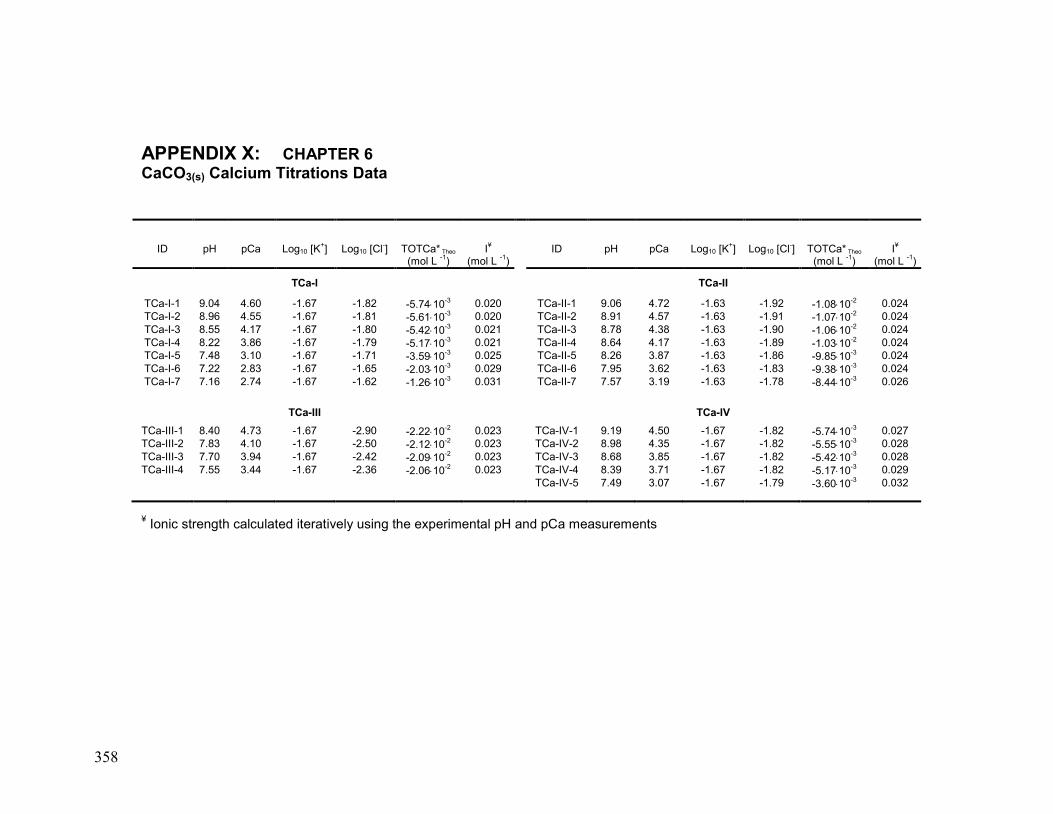
358

APPENDIX X: CHAPTER 6 CaCO3(s) Calcium Titrations Data


-] TOTCa* Theo

(mol L -1)

I¥

(mol L -1)


-] TOTCa* Theo

(mol L -1)

I¥

(mol L -1)

TCa-I TCa-II

TCa-I-1 9.04 4.60 -1.67 -1.82 -5.7410-3 0.020 TCa-II-1 9.06 4.72 -1.63 -1.92 -1.0810

-2 0.024

TCa-I-2 8.96 4.55 -1.67 -1.81 -5.6110-3 0.020 TCa-II-2 8.91 4.57 -1.63 -1.91 -1.0710

-2 0.024

TCa-I-3 8.55 4.17 -1.67 -1.80 -5.4210-3 0.021 TCa-II-3 8.78 4.38 -1.63 -1.90 -1.0610

-2 0.024

TCa-I-4 8.22 3.86 -1.67 -1.79 -5.1710-3 0.021 TCa-II-4 8.64 4.17 -1.63 -1.89 -1.0310

-2 0.024

TCa-I-5 7.48 3.10 -1.67 -1.71 -3.5910-3 0.025 TCa-II-5 8.26 3.87 -1.63 -1.86 -9.8510

-3 0.024

TCa-I-6 7.22 2.83 -1.67 -1.65 -2.0310-3 0.029 TCa-II-6 7.95 3.62 -1.63 -1.83 -9.3810

-3 0.024

TCa-I-7 7.16 2.74 -1.67 -1.62 -1.2610-3 0.031 TCa-II-7 7.57 3.19 -1.63 -1.78 -8.4410

-3 0.026

TCa-III TCa-IV

TCa-III-1 8.40 4.73 -1.67 -2.90 -2.2210-2 0.023 TCa-IV-1 9.19 4.50 -1.67 -1.82 -5.7410

-3 0.027

TCa-III-2 7.83 4.10 -1.67 -2.50 -2.1210-2 0.023 TCa-IV-2 8.98 4.35 -1.67 -1.82 -5.5510

-3 0.028

TCa-III-3 7.70 3.94 -1.67 -2.42 -2.0910-2 0.023 TCa-IV-3 8.68 3.85 -1.67 -1.82 -5.4210

-3 0.028

TCa-III-4 7.55 3.44 -1.67 -2.36 -2.0610-2 0.023 TCa-IV-4 8.39 3.71 -1.67 -1.82 -5.1710

-3 0.029

TCa-IV-5 7.49 3.07 -1.67 -1.79 -3.6010-3 0.032

¥ Ionic strength calculated iteratively using the experimental pH and pCa measurements

359

APPENDIX XI: CHAPTER 6

Methods and Calculations Preparation and standardization of titrant solutions

All solutions were prepared using analytical grade reagents and high purity deionized

(Milli-Q®

, ~ 18 Mohm cm) water. Hydrochloric acid solutions were prepared from

32% HCl and standardized using three gravimetrically prepared

tris(hydroxymethyl)methylamine (TRIS) solutions that were kept refrigerated. The

precision of this standardization was better than 0.1 %. The calcium titrant stock

solutions and calcium standards were prepared from CaCl2H2O crystals and kept

refrigerated before use. These solutions were standardized by volumetric titration with

EGTA. The EGTA titrant solution was standardized using Copenhagen IAPSO

standard seawater. The precision of this determination was better than 0.4 %.

Chemical analyses of CaCO3 suspensions

Alkalinity measurements were carried out using a Radiometer TTT85 titration system

with standardized HCl. The end-point of the titration was identified by the first-

derivative method. The precision of the analysis was better than ± 0.4% and the limit

of detection was of 0.6 mmol kg-1

. Total calcium concentrations were measured by

Flame Atomic Absorption Spectrophotometry (FAAS, AAnalyst 100TM

800 Perkin

Elmer) using external standards (i.e., diluted from a 1000 ppm Certified Standard).

The detection limit of this analysis was 3 μg L-1

with a reproducibility of ± 5%. pH

measurements were performed with a Schott N6980 pH combination electrode,

suitable for concentrated suspensions, and calibrated against four NIST-traceable pH

buffer solutions (4.01, 7.00, 10.00 and 11.00) at 25 0.5°C with a precision of ±

0.002 pH units. Its Nernstian behavior was always very similar (59.2 1.1 mV/log10

aH+) to the theoretical value at 25°C. Calcium ion activities were measured with a

combination Orion 97-20 ionplus® ion selective electrode calibrated with CaCl2

standards (5∙10-6

to 0.015 M) prepared in 0.02 M KCl solutions following the

manufacturer‟s recommendation to achieve a precision of ± 4% at 25 ± 1°C.

Carbonate ion activities were determined using a combination ELIT Ion 8091 ion

selective electrode initially calibrated by two methods: A) against NaHCO3 standards,

360

prepared in 0.02 M KCl solutions, covering a relatively wide range of CO32-

ion

concentrations (3∙10-6

to 0.012 M) and B) against pre-equilibrated calcite suspensions

prepared in 0.02 KCl at different initial Ca:HCO3-:CO3

2- ratios (achieved with

additions of CaCl2, KHCO3 and/or K2CO3) to cover a range of carbonate ion

concentrations similar to the one of method A (2∙10-6

to 0.008 M). In method A, CO32-

ion activities in the standards were estimated from thermodynamic equilibrium

calculations performed iteratively using the Newton-Raphson method implemented in

an in-house Matlab©

subroutine using alkalinity and pH measurements as input. In

contrast, in method B, CO32-

ion activities were estimated using the Ca2+

ion activities

measured with the ISE in the equilibrated calcite suspensions, just before the

calibration of the CO32-

ISE, and application of the solubility product relationship:

where a represent the activity of the specified ion and K°sp stands for the

thermodynamic solubility product of calcite at 25°C. Method B provided better

(Nernstian) and more reproducible calibration slopes and was, therefore, adopted for

the routine calibration of the CO32-

ISE. Thermodynamic constants used in all

calculations of this study are given in Table 1 in the main text. The optimum

operational pH, temperature and analyte concentration ranges were respected for the

three ISEs. Nevertheless, it must be noted that the CO32-

ISE only performed to

specifications in a few preliminary titrations (see below). We suspect that the presence

of CaCO3(s) particles in our experiments may significantly decrease the operational

life expectancy of this ISE. Consequently, this ISE was only used in preliminary

titrations to validate the experimental protocol described below, estimate the re-

equilibration time required after discrete titrant additions, evaluate titration system

drift, and monitor the calcite saturation state. In all other experiments, CO32-

ion

activities were derived from the Ca2+

ISE activities and application of Equation R1 (in

analogy to the CO32-

ISE calibration by method B).

2

02

3aCa

spKaCO

(R1)

361

Calcite specimen

All titrations were carried out with Baker “Instra-analyzed flux reagent” grade

calcium carbonate powder that was size-separated by settling through a 3 m x 0.1 m

Plexiglas®

tube filled with Millli-Q®

water. The middle third portion of the settled

CaCO3 was freeze-dried and used for all experiments reported in this paper. The

average grain size was estimated at 3-7 m based on Stoke‟s Law and corroborated by

numerous Scanning Electron Microscopy (SEM) images. X-ray diffraction and SEM

analyses of this material confirmed that the powder was composed of at least 99%

calcite. The specific surface area of the size-separated fraction was of 0.46 (± 0.02) m2

g-1

,

as determined by the multiple-point N2-BET method

with an Autosorbed-1

Physisorption Analyzer. This parameter was determined before and after one

acidimetric and one calcium titration to check for variations resulting from the

dissolution of the finest particles and/or possible calcite re-precipitation. The specific

surface area of the titrated solids was, within the uncertainty of our measurements,

identical to the starting material, and therefore, the original value was used in further

calculations. To minimize possible surface irregularities (such as step edges and

kinks), a fraction of the calcite powder was aged in Milli-Q®

water for about one year.

This is a common procedure used in sorption studies to “heal” carbonate mineral

surface defects (e.g., steps, dislocations and point defects) and minimize the

heterogeneity of surface site energies upon re-crystallisation. Furthermore, this pre-

treatment, through Ostwald ripening, allows the dissolution of smaller CaCO3

particles and precipitation onto larger particles, and hence, a narrowing of the particle

size distribution. Before use in surface titrations, the calcite powder was exhaustively

rinsed with Milli-Q®

water to remove adsorbed impurities, oven-dried at 70C, and

kept in a desiccator. For the sake of accuracy, the solubility product of our calcite

substrate was verified by equilibrating a series of calcite suspensions in Milli -Q®

water in centrifuge tubes under constant stirring for 10 days. After this time, pH,

alkalinity and the total calcium concentration (Ca, determined by AAS) were

measured and the Ca2+

and CO32-

activities calculated with MINEQL+ v.4.6 software.

The measured log10 Kºsp was –8.48 0.04, in excellent agreement with the value

selected by the National Institute of Standards and Technology.

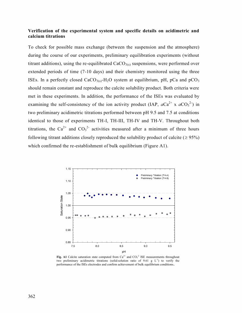
362

Verification of the experimental system and specific details on acidimetric and

calcium titrations

To check for possible mass exchange (between the suspension and the atmosphere)

during the course of our experiments, preliminary equilibration experiments (without

titrant additions), using the re-equilibrated CaCO3(s) suspensions, were performed over

extended periods of time (7-10 days) and their chemistry monitored using the three

ISEs. In a perfectly closed CaCO3(s)-H2O system at equilibrium, pH, pCa and pCO3

should remain constant and reproduce the calcite solubility product. Both criteria were

met in these experiments. In addition, the performance of the ISEs was evaluated by

examining the self-consistency of the ion activity product (IAP, aCa2+

x aCO32-

) in

two preliminary acidimetric titrations performed between pH 9.5 and 7.5 at conditions

identical to those of experiments TH-I, TH-III, TH-IV and TH-V. Throughout both

titrations, the Ca2+

and CO32-

activities measured after a minimum of three hours

following titrant additions closely reproduced the solubility product of calcite ( 95%)

which confirmed the re-establishment of bulk equilibrium (Figure A1).

Fig. A1 Calcite saturation state computed from Ca2+ and CO3

2- ISE measurements throughout

two preliminary acidimetric titrations (solid:solution ratio of 9.61 g L-1) to verify the

performance of the ISEs electrodes and confirm achievement of bulk equilibrium conditions.

363

Upon confirmation of the performance of the experimental system, acidimetric

titrations were conducted by stepwise addition of varying volumes (0.3 to 1.2 mL) of

standardized 0.1 M HCl solutions to pre-equilibrated calcite suspensions prepared at

different initial chemical conditions (Table 2 in main text). The ISE measurements

were recorded at least three hours after each titrant addition but longer time intervals

(up to 12 hours) were also investigated to confirm full restoration of bulk equilibr ium.

Complete titrations required from 4 to 5 days. Similarly, calcium titrations were

conducted by stepwise additions of varying volumes (0.05 to 2 mL) of a standardized

0.4 M CaCl2 solution to pre-equilibrated calcite suspensions prepared at different

initial chemical conditions (Table 2 in main text). The initial conditions for these

titration were carefully chosen to allow for detectable changes in Ca2+

activities upon

CaCl2 additions and to expand the range of total calcium concentration (Ca) covered

by each titration experiment. To this end, the initial composition of the suspensions

was varied by additions of HCl, KHCO3 and/or Na2CO3 solutions to set their

respective initial pH, Ca and CO2 before the first equilibration period (Table 2).

Preliminary calcium titrations revealed that a period of at least 18 hours is necessary

to obtain stable ISE readings after each discrete CaCl2 addition. Hence, data for these

experiments were acquired after at least 24 hours of equilibration following each

CaCl2 addition. Complete titrations required between 5 and 8 days.

Additional titrations were conducted using dilute calcite suspensions (0.2 g L-1

equivalent to 0.9 m2 L

-1) prepared in a 0.02 M KCl solution (Experiments TH-VI and

TCa-IV, respectively) under conditions identical to at least one acidimetric and one

calcium surface titration experiment. They served to: i) evaluate “mass effects”

influencing sorption behavior by properly accounting for dissolution (acidimetric

titrations) and precipitation (calcium titrations) while the surface available for

adsorption reactions is low (i.e., bulk reactions dominate over surface interactions),

and ii) detect possible “background effects” (e.g., adsorption) associated to the

titration system. Since the bulk kinetics of dissolution and precipitation are

proportional to the reactive surface area of the mineral, equilibration times for the

“blank” runs were longer than for equivalent titrations performed at higher

solid:solution ratios, and therefore, data were only recorded once stable ISEs readings

364

were obtained (after 7 hours for acidimetric and 30 hours for calcium titrations).

After each titration experiment, the ISEs were re-calibrated to verify their

performance and evaluate the electrode drift. In all cases, electrode drift was < 3%,

and thus, considered acceptable. To prevent carry-over contamination from preceding

experiments, the reaction vessel and its components were acid-washed (with 5% v/v

HCl solutions) and rinsed with Milli-Q®

water before each titration and the pH and

pCa of the Milli-Q®

water stored in the fully-assembled reaction vessel were

monitored for several hours to confirm the absence of contaminants (i.e., H+, Ca

2+)

possibly adhering to components of the reaction vessel. Low pH and relatively high

CO2 conditions allowing for moderate to high carbonic acid concentrations in the

experimental system were avoided to prevent the formation of CO2(g) nuclei inside the

reaction vessel and ensure that the CO2 an proton mass conservation conditions

required by our titration protocol were met (see main text). For instance, CO2 bubble

nucleation was observed in some titrations carried out to a pH of approximately 6.7. A

judicious selection of initial pH, Ca and CO2 conditions (Table 2 in main text)

guaranteed that sufficiently low levels of carbonic acid were maintained throughout

our titrations to prevent CO2(g) bubble formation while covering a pH range from 7.1

to 9.7. The maximum concentrations of H2CO3* registered at the end of our

experiments was ~ 410-4

M.

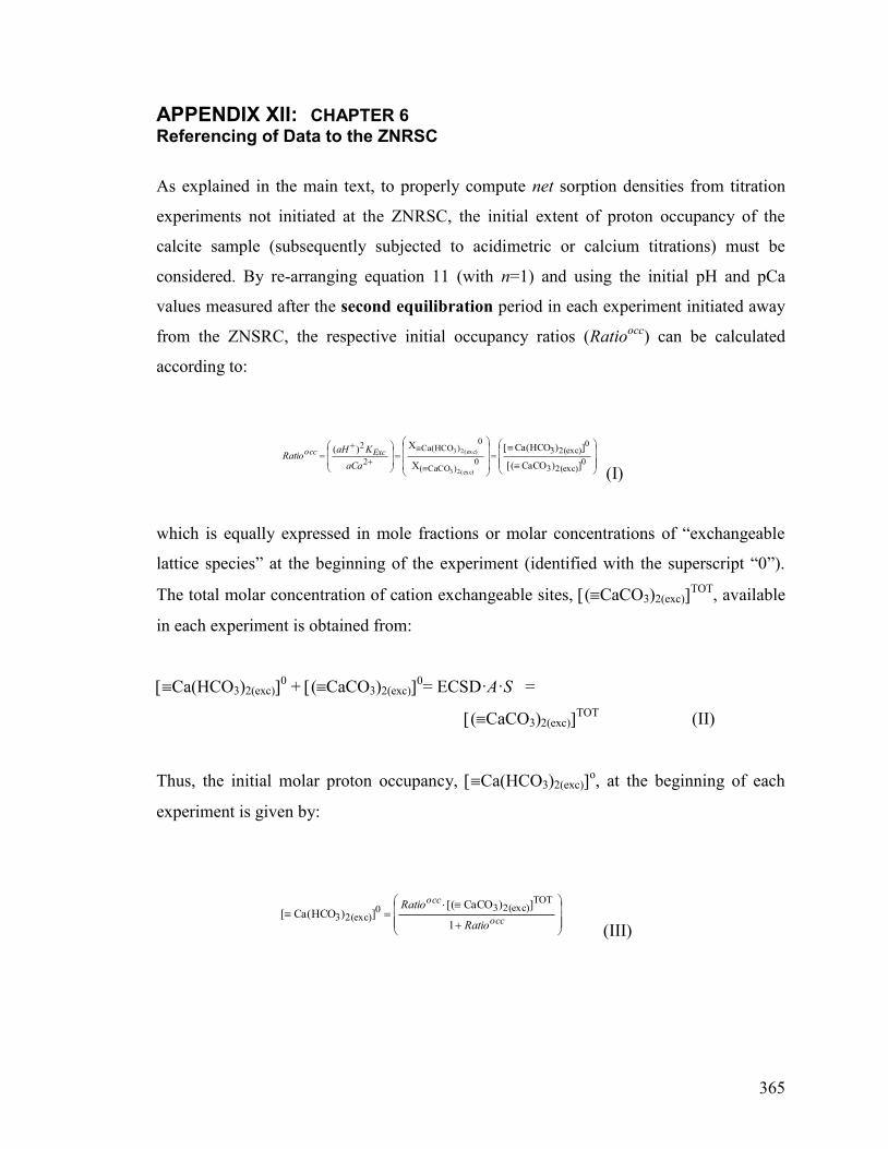
365

APPENDIX XII: CHAPTER 6

Referencing of Data to the ZNRSC

As explained in the main text, to properly compute net sorption densities from titration

experiments not initiated at the ZNRSC, the initial extent of proton occupancy of the

calcite sample (subsequently subjected to acidimetric or calcium titrations) must be

considered. By re-arranging equation 11 (with n=1) and using the initial pH and pCa

values measured after the second equilibration period in each experiment initiated away

from the ZNSRC, the respective initial occupancy ratios (Ratioocc

) can be calculated

according to:

which is equally expressed in mole fractions or molar concentrations of “exchangeable

lattice species” at the beginning of the experiment (identified with the superscript “0”).

The total molar concentration of cation exchangeable sites, (CaCO3)2(exc)TOT

, available

in each experiment is obtained from:

Ca(HCO3)2(exc)0 + (CaCO3)2(exc)

0= ECSD·A·S =

(CaCO3)2(exc)TOT

(II)

Thus, the initial molar proton occupancy, Ca(HCO3)2(exc)o, at the beginning of each

experiment is given by:

occ

occ

Ratio

Ratio

1

])CaCO[(])Ca(HCO[

TOT2(exc)30

2(exc)3

(III)

02(exc)3

02(exc)3

0)CaCO(

0)HCO(Ca

2

2

)CaCO(

)Ca(HCO

X

X)(

(exc)23

(exc)23

aCa

KaHRatio Excocc

(I)

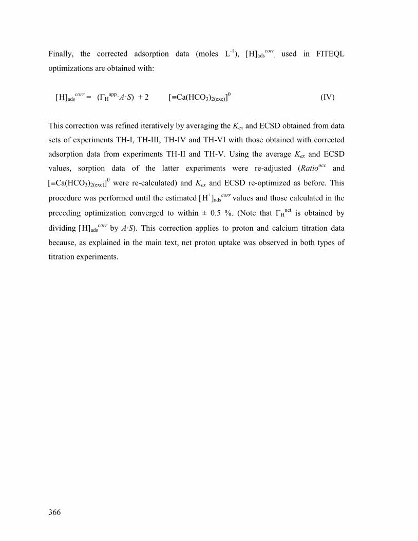
366

Finally, the corrected adsorption data (moles L-1

), Hadscorr

, used in FITEQL

optimizations are obtained with:

Hadscorr

= (app

·A·S) + 2 Ca(HCO3)2(exc)0 (IV)

This correction was refined iteratively by averaging the Kex and ECSD obtained from data

sets of experiments TH-I, TH-III, TH-IV and TH-VI with those obtained with corrected

adsorption data from experiments TH-II and TH-V. Using the average Kex and ECSD

values, sorption data of the latter experiments were re-adjusted (Ratioocc

and

Ca(HCO3)2(exc)0 were re-calculated) and Kex and ECSD re-optimized as before. This

procedure was performed until the estimated H+ads

corr values and those calculated in the

preceding optimization converged to within ± 0.5 %. (Note that Hnet

is obtained by

dividing Hadscorr

by A·S). This correction applies to proton and calcium titration data

because, as explained in the main text, net proton uptake was observed in both types of

titration experiments.

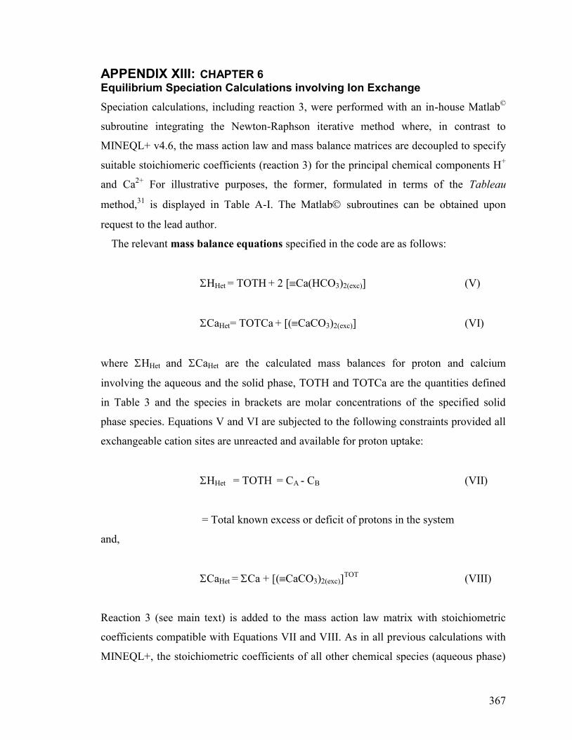
367

APPENDIX XIII: CHAPTER 6

Equilibrium Speciation Calculations involving Ion Exchange

Speciation calculations, including reaction 3, were performed with an in-house Matlab©

subroutine integrating the Newton-Raphson iterative method where, in contrast to

MINEQL+ v4.6, the mass action law and mass balance matrices are decoupled to specify

suitable stoichiomeric coefficients (reaction 3) for the principal chemical components H+

and Ca2+

For illustrative purposes, the former, formulated in terms of the Tableau

method,31

is displayed in Table A-I. The Matlab subroutines can be obtained upon

request to the lead author.

The relevant mass balance equations specified in the code are as follows:

HHet = TOTH + 2 [Ca(HCO3)2(exc)] (V)

CaHet= TOTCa + [(CaCO3)2(exc)] (VI)

where HHet and CaHet are the calculated mass balances for proton and calcium

involving the aqueous and the solid phase, TOTH and TOTCa are the quantities defined

in Table 3 and the species in brackets are molar concentrations of the specified solid

phase species. Equations V and VI are subjected to the following constraints provided all

exchangeable cation sites are unreacted and available for proton uptake:

HHet = TOTH = CA - CB (VII)

= Total known excess or deficit of protons in the system

and,

CaHet = Ca + [(CaCO3)2(exc)]TOT

(VIII)

Reaction 3 (see main text) is added to the mass action law matrix with stoichiometric

coefficients compatible with Equations VII and VIII. As in all previous calculations with

MINEQL+, the stoichiometric coefficients of all other chemical species (aqueous phase)

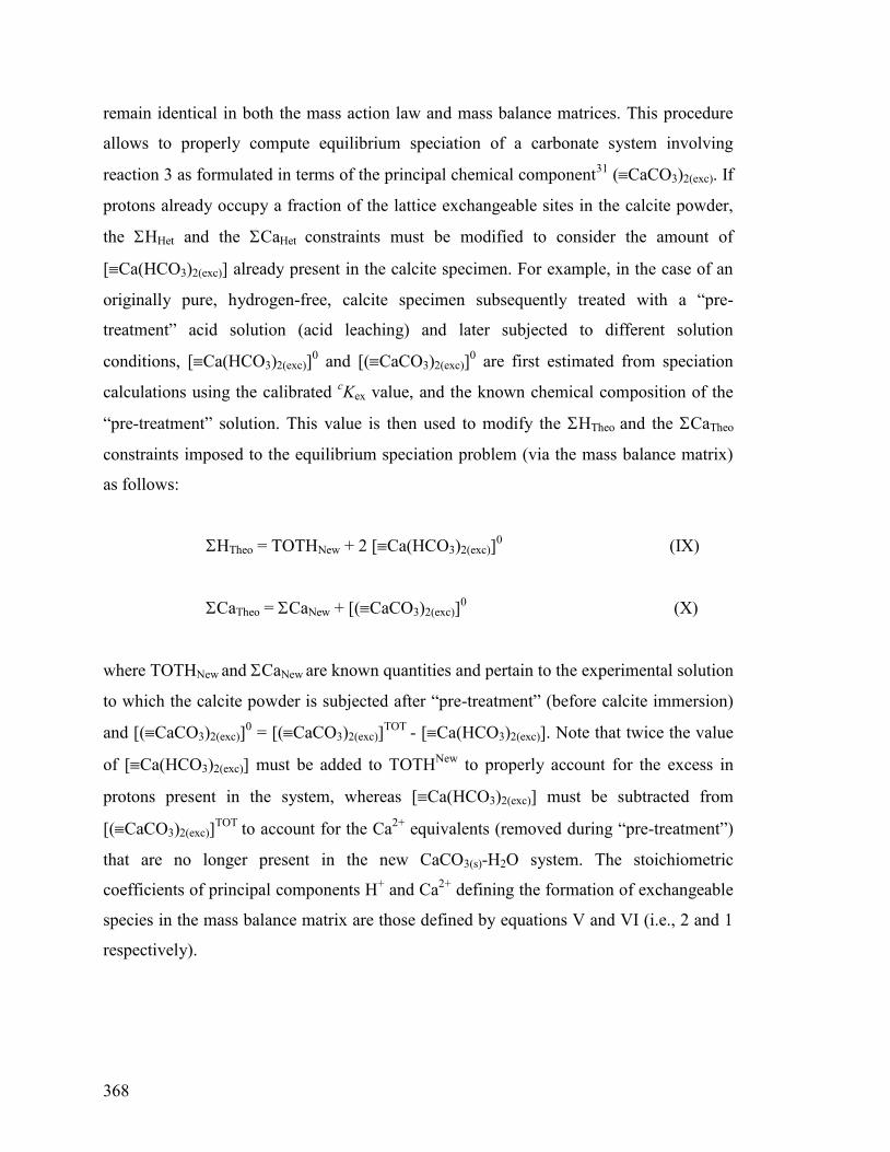
368

remain identical in both the mass action law and mass balance matrices. This procedure

allows to properly compute equilibrium speciation of a carbonate system involving

reaction 3 as formulated in terms of the principal chemical component31

(CaCO3)2(exc). If

protons already occupy a fraction of the lattice exchangeable sites in the calcite powder,

the HHet and the CaHet constraints must be modified to consider the amount of

[Ca(HCO3)2(exc)] already present in the calcite specimen. For example, in the case of an

originally pure, hydrogen-free, calcite specimen subsequently treated with a “pre-

treatment” acid solution (acid leaching) and later subjected to different solution

conditions, [Ca(HCO3)2(exc)]0 and [(CaCO3)2(exc)]

0 are first estimated from speciation

calculations using the calibrated cKex value, and the known chemical composition of the

“pre-treatment” solution. This value is then used to modify the HTheo and the CaTheo

constraints imposed to the equilibrium speciation problem (via the mass balance matrix)

as follows:

HTheo = TOTHNew + 2 [Ca(HCO3)2(exc)]0 (IX)

CaTheo = CaNew + [(CaCO3)2(exc)]0 (X)

where TOTHNew and CaNew are known quantities and pertain to the experimental solution

to which the calcite powder is subjected after “pre-treatment” (before calcite immersion)

and [(CaCO3)2(exc)]0 = [(CaCO3)2(exc)]

TOT - [Ca(HCO3)2(exc)]. Note that twice the value

of [Ca(HCO3)2(exc)] must be added to TOTHNew

to properly account for the excess in

protons present in the system, whereas [Ca(HCO3)2(exc)] must be subtracted from

[(CaCO3)2(exc)]TOT

to account for the Ca2+

equivalents (removed during “pre-treatment”)

that are no longer present in the new CaCO3(s)-H2O system. The stoichiometric

coefficients of principal components H+ and Ca

2+ defining the formation of exchangeable

species in the mass balance matrix are those defined by equations V and VI (i.e., 2 and 1

respectively).

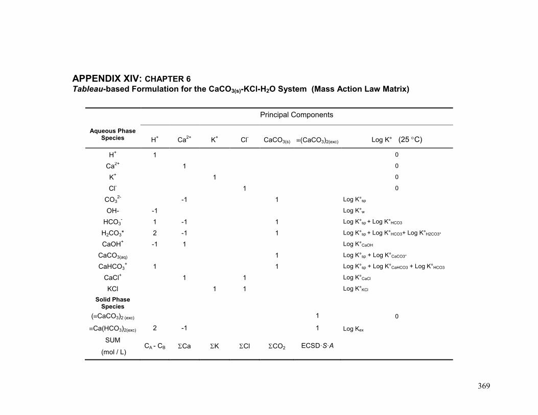
369

APPENDIX XIV: CHAPTER 6

Tableau-based Formulation for the CaCO3(s)-KCl-H2O System (Mass Action Law Matrix)

Principal Components

Aqueous Phase Species H

+ Ca

2+ K

+ Cl

- CaCO3(s) (CaCO3)2(exc) Log K° (25 C)

H+ 1 0

Ca2+

1 0

K+ 1 0

Cl- 1 0

CO32-

-1 1 Log K°sp

OH- -1 Log K°w

HCO3- 1 -1 1 Log K°sp + Log K°HCO3

H2CO3* 2 -1 1 Log K°sp + Log K°HCO3+ Log K°H2CO3*

CaOH+ -1 1 Log K°CaOH

CaCO3(aq) 1 Log K°sp + Log K°CaCO3°

CaHCO3+ 1 1 Log K°sp + Log K°CaHCO3 + Log K°HCO3

CaCl+ 1 1 Log K°CaCl

KCl 1 1 Log K°KCl

Solid Phase Species

(CaCO3)2 (exc) 1 0

Ca(HCO3)2(exc) 2 -1 1 Log Kex

SUM

(mol / L) CA - CB Ca K Cl CO2 ECSD·S·A

APPENDIX XV:

Matlab SUBROUTINES

(CHAPTERS 2, 3, 4, and 6)

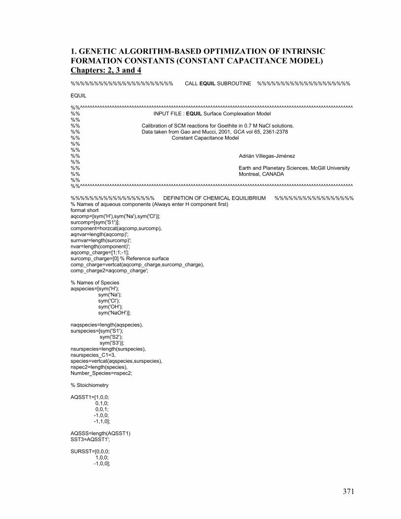
371

1. GENETIC ALGORITHM-BASED OPTIMIZATION OF INTRINSIC

FORMATION CONSTANTS (CONSTANT CAPACITANCE MODEL)

Chapters: 2, 3 and 4 %%%%%%%%%%%%%%%%%%%%%% CALL EQUIL SUBROUTINE %%%%%%%%%%%%%%%%%%%% EQUIL %%^^^^^^^^^^^^^^^^^^^^^^^^^^^^^^^^^^^^^^^^^^^^^^^^^^^^^^^^^^^^^^^^^^^^^^^^^^^^^^^^^^^^^^^^^^^^^^^^^^^^^^^^^^^^^^^ %% INPUT FILE : EQUIL Surface Complexation Model %% %% Calibration of SCM reactions for Goethite in 0.7 M NaCl solutions. %% Data taken from Gao and Mucci, 2001, GCA vol 65, 2361-2378 %% Constant Capacitance Model %% %% %% Adrián Villegas-Jiménez %% %% Earth and Planetary Sciences, McGill University %% Montreal, CANADA %% %%^^^^^^^^^^^^^^^^^^^^^^^^^^^^^^^^^^^^^^^^^^^^^^^^^^^^^^^^^^^^^^^^^^^^^^^^^^^^^^^^^^^^^^^^^^^^^^^^^^^^^^^^^^^^^^^ %%%%%%%%%%%%%%%%%% DEFINITION OF CHEMICAL EQUILIBRIUM %%%%%%%%%%%%%%%%% % Names of aqueous components (Always enter H component first) format short aqcomp=[sym('H'),sym('Na'),sym('Cl')]; surcomp=[sym('S1')]; component=horzcat(aqcomp,surcomp), aqnvar=length(aqcomp)'; surnvar=length(surcomp)'; nvar=length(component)'; aqcomp_charge=[1;1;-1]; surcomp_charge=[0] % Reference surface comp_charge=vertcat(aqcomp_charge,surcomp_charge), comp_charge2=aqcomp_charge'; % Names of Species aqspecies=[sym('H'); sym('Na'); sym('Cl'); sym('OH'); sym('NaOH')]; naqspecies=length(aqspecies), surspecies=[sym('S1'); sym('S2'); sym('S3')]; nsurspecies=length(surspecies), nsurspecies_C1=3, species=vertcat(aqspecies,surspecies), nspec2=length(species), Number_Species=nspec2; % Stoichiometry AQSST1=[1,0,0; 0,1,0; 0,0,1; -1,0,0; -1,1,0]; AQSSS=length(AQSST1) SST3=AQSST1'; SURSST=[0,0,0; 1,0,0; -1,0,0];

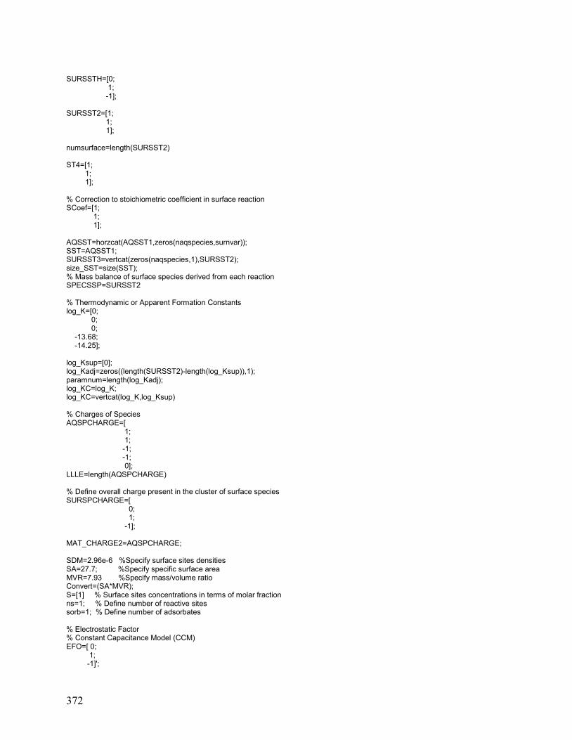
372

SURSSTH=[0; 1; -1]; SURSST2=[1; 1; 1]; numsurface=length(SURSST2) ST4=[1; 1; 1]; % Correction to stoichiometric coefficient in surface reaction SCoef=[1; 1; 1]; AQSST=horzcat(AQSST1,zeros(naqspecies,surnvar)); SST=AQSST1; SURSST3=vertcat(zeros(naqspecies,1),SURSST2); size_SST=size(SST); % Mass balance of surface species derived from each reaction SPECSSP=SURSST2 % Thermodynamic or Apparent Formation Constants log_K=[0; 0; 0; -13.68; -14.25]; log_Ksup=[0]; log_Kadj=zeros((length(SURSST2)-length(log_Ksup)),1); paramnum=length(log_Kadj); log_KC=log_K; log_KC=vertcat(log_K,log_Ksup) % Charges of Species AQSPCHARGE=[ 1; 1; -1; -1; 0]; LLLE=length(AQSPCHARGE) % Define overall charge present in the cluster of surface species SURSPCHARGE=[ 0; 1; -1]; MAT_CHARGE2=AQSPCHARGE; SDM=2.96e-6 %Specify surface sites densities SA=27.7; %Specify specific surface area MVR=7.93 %Specify mass/volume ratio Convert=(SA*MVR); S=[1] % Surface sites concentrations in terms of molar fraction ns=1; % Define number of reactive sites sorb=1; % Define number of adsorbates % Electrostatic Factor % Constant Capacitance Model (CCM) EFO=[ 0; 1; -1]';

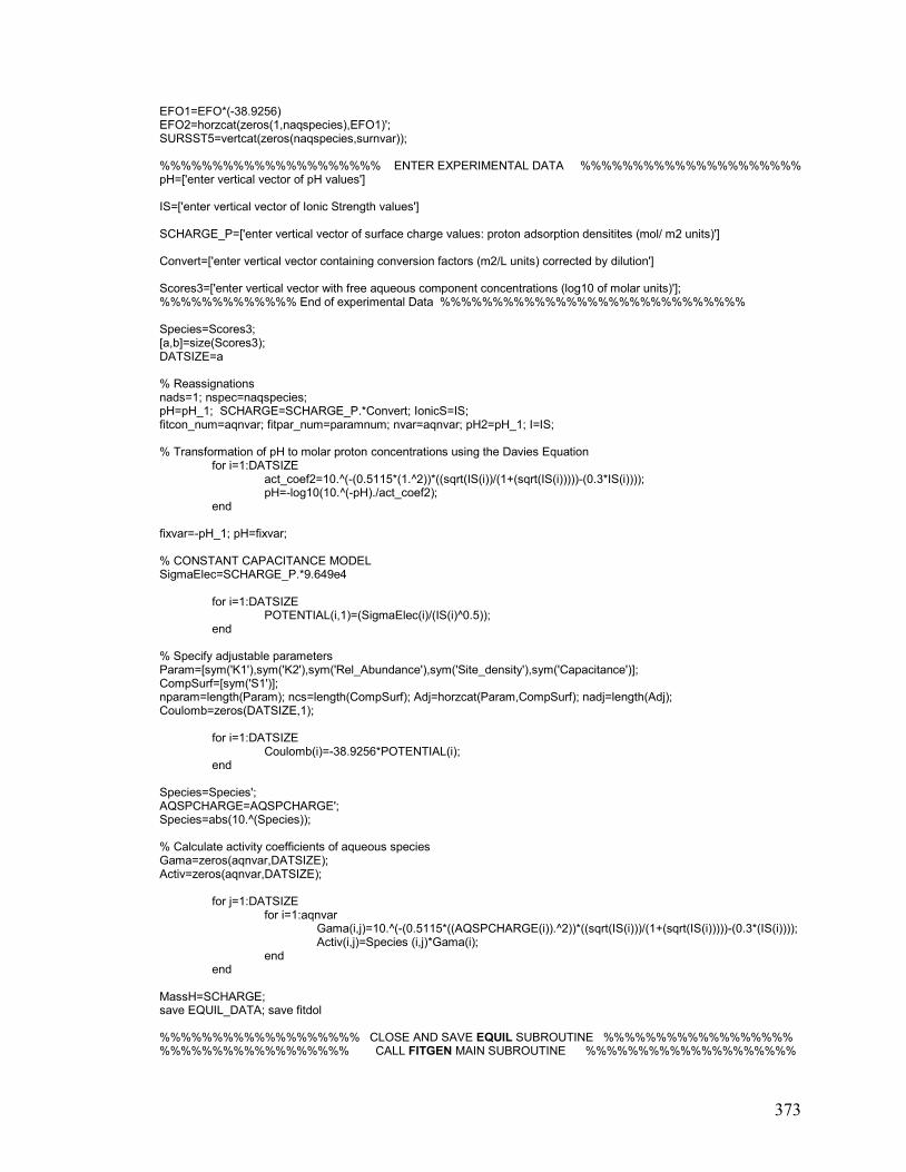
373

EFO1=EFO*(-38.9256) EFO2=horzcat(zeros(1,naqspecies),EFO1)'; SURSST5=vertcat(zeros(naqspecies,surnvar)); %%%%%%%%%%%%%%%%%%%%% ENTER EXPERIMENTAL DATA %%%%%%%%%%%%%%%%%%%%% pH=['enter vertical vector of pH values'] IS=['enter vertical vector of Ionic Strength values'] SCHARGE_P=['enter vertical vector of surface charge values: proton adsorption densitites (mol/ m2 units)'] Convert=['enter vertical vector containing conversion factors (m2/L units) corrected by dilution'] Scores3=['enter vertical vector with free aqueous component concentrations (log10 of molar units)']; %%%%%%%%%%%%% End of experimental Data %%%%%%%%%%%%%%%%%%%%%%%%%%%%% Species=Scores3; [a,b]=size(Scores3); DATSIZE=a % Reassignations nads=1; nspec=naqspecies; pH=pH_1; SCHARGE=SCHARGE_P.*Convert; IonicS=IS; fitcon_num=aqnvar; fitpar_num=paramnum; nvar=aqnvar; pH2=pH_1; I=IS; % Transformation of pH to molar proton concentrations using the Davies Equation

for i=1:DATSIZE act_coef2=10.^(-(0.5115*(1.^2))*((sqrt(IS(i))/(1+(sqrt(IS(i)))))-(0.3*IS(i)))); pH=-log10(10.^(-pH)./act_coef2);

end fixvar=-pH_1; pH=fixvar; % CONSTANT CAPACITANCE MODEL SigmaElec=SCHARGE_P.*9.649e4

for i=1:DATSIZE POTENTIAL(i,1)=(SigmaElec(i)/(IS(i)^0.5));

end % Specify adjustable parameters Param=[sym('K1'),sym('K2'),sym('Rel_Abundance'),sym('Site_density'),sym('Capacitance')]; CompSurf=[sym('S1')]; nparam=length(Param); ncs=length(CompSurf); Adj=horzcat(Param,CompSurf); nadj=length(Adj); Coulomb=zeros(DATSIZE,1);

for i=1:DATSIZE Coulomb(i)=-38.9256*POTENTIAL(i);

end Species=Species'; AQSPCHARGE=AQSPCHARGE'; Species=abs(10.^(Species)); % Calculate activity coefficients of aqueous species Gama=zeros(aqnvar,DATSIZE); Activ=zeros(aqnvar,DATSIZE);

for j=1:DATSIZE for i=1:aqnvar Gama(i,j)=10.^(-(0.5115*((AQSPCHARGE(i)).^2))*((sqrt(IS(i)))/(1+(sqrt(IS(i)))))-(0.3*(IS(i)))); Activ(i,j)=Species (i,j)*Gama(i); end

end

MassH=SCHARGE; save EQUIL_DATA; save fitdol %%%%%%%%%%%%%%%%%%% CLOSE AND SAVE EQUIL SUBROUTINE %%%%%%%%%%%%%%%%%% %%%%%%%%%%%%%%%%%% CALL FITGEN MAIN SUBROUTINE %%%%%%%%%%%%%%%%%%%%

374

function [stats,pop,elitechrome,Constants] =FITGEN %^^^^^^^^^^^^^^^^^^^^^^^^^^^^^^^^^^^^^^^^^^^^^^^^^^^^^^^^^^^^^^^^^^^^^^^^^^^^^^^^^^^^^^^^^^^^^^^^^^^^^^^^^^^^^^^^^ % % FITGEN is the main subroutine to perform stochastic optimizations of Surface Complexation Model parameters % based on a %% genetic algorithm % It defines the GA parameters, solution space, number and length of chromosomes and calls all required % subroutines % % 10/04/02 Earth and Planetary Sciences, McGill University % Adrián Villegas-Jiménez % %^^^^^^^^^^^^^^^^^^^^^^^^^^^^^^^^^^^^^^^^^^^^^^^^^^^^^^^^^^^^^^^^^^^^^^^^^^^^^^^^^^^^^^^^^^^^^^^^^^^^^^^^^^^^^^^^^ t=cputime; for k=1:1 % Set number of GA optimization of a single data set (up to 3) contador=k; load EQUIL_DATA load fitdol; save Electrostatics fitval=[]; resid2=1e100; Ecart2=1e56; OPTIM=1; save check resid2 OPTIM save check2 Ecart2 save output2 fitval varchrome=[]; minval=[]; maxval=[]; fprintf('PRESS ANY KEY TO CONTINUE \n'); pause clc home % fprintf('xxxxxxxxxxxxxxxxxxxxxxxxxxxxxxxxxxxxxxxxxxxxxxxxxxxxxxxxxxxxxxxxxxxxxxxxxxxxxxxxxxxxxxxxxxxxxxxx \n'); fprintf('\n'); fprintf(' \t \t \tFITGEN A computer routine for the calculation of intrinsic surface parameters from experimental data \n'); fprintf('\n'); fprintf('xxxxxxxxxxxxxxxxxxxxxxxxxxxxxxxxxxxxxxxxxxxxxxxxxxxxxxxxxxxxxxxxxxxxxxxxxxxxxxxxxxxxxxxxxxxxxxxx \n'); % fprintf(' Default chromosome length calculated from analytical concentrations \n'); fprintf('\n'); nvar=input('Specify the number of parameters to be optimized in the objective function >'); cc=input('Specify chromosome length and assign lower and upper limits for each parameter? (1 for YES, 2 for NO) >'); cc=2

if cc==1 for j=1:nadj Parameter=Adj(j) fprintf('\n'); VC=input('Enter now the size of the chromosome for the given parameter >'); fprintf('\n'); varchrome=horzcat(varchrome,VC); minv=input('Enter now the minimum value for the value of the given parameter >'); minval=horzcat(minval,minv); maxv=input('Enter now the maximum value for the value of the given parameter >'); maxval=horzcat(maxval,maxv); end else %1st GA Run minval=[-25000,-25000,...... Number of adjustable parameter] % Define minimum boundary value maxval=[25000,25000,........ Number of adjustable parameter] % Define maximum boundary value sizevec=[15,15,10,....] % Define number of bits required by each section of the chromosome (adjustable parameter)

if contador==2

%2nd GA Run minval=[-25000,-25000,...... Number of adjustable parameter] % Define minimum boundary value maxval=[25000,25000,........ Number of adjustable parameter] % Define maximum boundary value sizevec=[15,15,10,....] % Define number of bits required by each section of the chromosome (adjustable parameter) else end

if contador==3 %3rd GA Run

375

minval=[-25000,-25000,...... Number of adjustable parameter] % Define minimum boundary value maxval=[25000,25000,........ Number of adjustable parameter] % Define maximum boundary value sizevec=[15,15,10,....] % Define number of bits required by each section of the chromosome (adjustable parameter)

else end

end fprintf('\n'); fprintf('\n'); fprintf(' \t General Parameters of the Genetic Algorithm \n') fprintf(' \t PRESS ANY KEY TO CONTINUE\n'); pause fprintf(' \t Parameters must be entered as follows:\n') fprintf('\t [population size, number of generations\n') fprintf(' \t mutation rate, crossover rate,\n') fprintf(' \t type of crossover (1=single point 2=two points, 3=three points)\n') fprintf('\n'); fprintf('\n'); Conf=input('Enter the GA parameters now e.g. [10,1000,0.01,0.25,1] ) >'); prnlevel=1; ffunc=1; gray=1; popsize=Conf(1); popsize1=popsize; numgen=Conf(2); pm=Conf(3); px=Conf(4); xtype=Conf(5); ndim=sum(varchrome); ndim2=sum(varchromeb); % set GA configuration clc home elite = 2; gray = 1; numxover = 0; nummut = 0; nstat = 7; test = rem(popsize,2); if elite == 1 if (test == 0) popsize = popsize + 1; end else if (test ~= 0) popsize = popsize + 1; end end % Initialize population randomly pop = [(rand(popsize,ndim)<0.5)]; % % Optimize for a given number of generations tnumgen =numgen; SS=1; cgn=0; child=0; childcount=0; Fuse=1; for cgn = 1:tnumgen % % Compute fitness function for each member of the population % cgn=cgn+1; %%%%%%%%%%%%%%%%%%%% CALL FITLOG SUBROUTINE %%%%%%%%%%%%%%%%%%

376

[SS,SB,scores,Residual,vars1,Constants,resid,poss] = FITLOG(pop,numgen,ffunc,varchrome,varchromeb,maxval,maxvalb,minval,minvalb,nvar,cgn,childcount,child,xtype,Fuse,contador); function [SS,SB,scores,Residual,vars1,Constants,resid,poss] = FITLOG(pop,numgen,ffunc,varchrome,varchromeb,maxval,maxvalb,minval,minvalb,nvar,cgn,childcount,child,xtype,Fuse,contador) %^^^^^^^^^^^^^^^^^^^^^^^^^^^^^^^^^^^^^^^^^^^^^^^^^^^^^^^^^^^^^^^^^^^^^^^^^^^^^^^^^^^^^^^^^^^^^^^^^^^^^^^^^^^^^^^^^ % % FITLOG computes fitness scores and performs all calculations required by the objective function % It decodes binary-strings and splits chromosome into predetermined sections for each variable % % Subroutine designed for the optimization of multiple SCM parameters from surface protonation and adsorption data % Data fits for one or two adsorbates can be fitted within the Constant Capacitance Model % % The chromosome has to be splitted into nvar sections (one section for each master specie or principal component) % the corresponding lengths can be either be calculated in the input file or can be specified directly by the user % Solution is coded in nominal values and tested in logarithmic units % % 10/04/02 Earth and Planetary Sciences, McGill University % Adrián Villegas-Jiménez % %^^^^^^^^^^^^^^^^^^^^^^^^^^^^^^^^^^^^^^^^^^^^^^^^^^^^^^^^^^^^^^^^^^^^^^^^^^^^^^^^^^^^^^^^^^^^^^^^^^^^^^^^^^^^^^^^^ global Data Plothandle load fitdol load check load check2 load Electrostatics [popsize,ndim] = size(pop); var=[]; gray=1;

if xtype ==5 if cgn >1 gray=2 vars=child'; end

end % Optimizing intrinsic parameters

if gray == 1 count=1; fin=0; start=1; maxval=maxval;

for j=1:nparam varchrome2=(varchrome(j)); minval2=(minval(j)); maxval2=(maxval(j)); pow_two = 2.^(0:varchrome2); maxintval = ((2^varchrome2)-1); range =maxval2-minval2; start = start+fin; fin= fin + varchrome2;

for i = 1:popsize tvars(1:varchrome2) = pop(i,start:fin); % % now decode binary number to real number (scale maxval to minval) %

real = 0;

for k = 1:varchrome2 real = real + pow_two(k)*tvars(varchrome2-k+1); end % % Takes integer value and converts to a real number (genotype to phenotype transformation)

377

% vars1(i,j) = (range*(real/maxintval)) + minval2; end start=1; end else end vars1=10.^(vars1./1000); format long E np=nparam; alpha=vars1(:,nparam)'; guess=zeros(aqnvar,DATSIZE);

for j=1:DATSIZE for i=1:aqnvar guess(i,j)=Activ(i,j); end

end quihubo=guess; act=ones(surnvar,DATSIZE); guess=(vertcat(guess,act))'; guess=log10(guess); unito=(ones(1,DATSIZE))'; guess=horzcat(guess,unito); Konstants1=zeros(popsize,np);

for i=1:popsize for j=1:np Konstants1(i,j)=vars1(i,j); end

end % Express constants in terms of an operational reference state as suggested by Dr D. Sverjensky % Konstants=Konstants1*(1/stdstate); Ksurcomp=ones(popsize,surnvar); Konstants=log10(horzcat(Ksurcomp,Konstants1))‟; % Estimating free concentrations of surface components icc=0; surconc=zeros(DATSIZE,surnvar); static=zeros(nsurspecies,1); EFO2=EFO';

for j=1:popsize jcc=np; icc=icc+1;

for i=1:DATSIZE

Electro=Coulomb(i,1); alpha=vars1(icc,jcc); UF=vars1(icc,jcc-1); UF=vars1(icc,jcc-1)*Convert(i,1); FRACT(1,1)=abs(vars1(icc,jcc-2)); FRACT(1,2)=1-FRACT(1,1); FF2=Konstants(1:nsurspecies,j);

for k=1:nsurspecies static(k,1)=log10(exp(Electro*alpha*EFO2(k,1))); end FF=FF2+static; SURSST3=horzcat(SURSST,FF); adivina=guess(i,(1:nvar+(ns+1)))'; adivina2=(10.^((SURSST3*adivina)./SCoef))'; surface=adivina2*SURSST4; unos=ones(1,surnvar); surface2=surface; FRACT(1,1:ns);

378

surconc(i,1:surnvar,icc)=(UF*FRACT(1,1:ns))./surface2; end

end

consur=surconc; icc=0; quihubo=quihubo'; M=zeros(DATSIZE,nvar+2,popsize); anexo=ones(DATSIZE,1);

for k=1:popsize MB1=log10(horzcat(quihubo,surconc(1:DATSIZE,1:surnvar,k))); MB1=horzcat(MB1,anexo); M(1:DATSIZE,1:(nvar+(ns+1)),k)=MB1(1:DATSIZE,1:(nvar+(ns+1)),1);

End

MB1=M; MB2=zeros(DATSIZE,popsize); MB7=zeros(DATSIZE,surnvar,popsize); MB6=zeros(surnvar,popsize); CB3=zeros(DATSIZE,popsize); CB4=zeros(DATSIZE,popsize); SB_residual=zeros(surnvar,popsize); adivina5=zeros(DATSIZE,popsize,nsurspecies);

if surnvar>1 SURFACE=zeros(DATSIZE,surnvar,popsize);

else SURFACE=zeros(DATSIZE,popsize);

end %loop for calculating surface species concentrations vale=[];

for j=1:popsize jcc=np; icc=icc+1;

for i=1:DATSIZE Electro=Coulomb(i,1); alpha=vars1(icc,jcc); FF2=Konstants(1:nsurspecies,j);

for k=1:nsurspecies static(k,1)=log10(exp(Electro*alpha*EFO2(k,1))); end

FF=FF2+static; SURSST3=horzcat(SURSST,FF); adivina=MB1(i,(1:nvar+ns+1),icc)'; adivina2=((SURSST3*adivina)./SCoef)'; % estimate concentration of surface species adivina4=10.^(adivina2); adivina5(i,icc,1:nsurspecies)=adivina4; surface2=(adivina4*SURSST4); MB7(i,1:surnvar,icc)=surface2; % Mass balance for the xth chromosome CB=adivina4*SURSPCHARGE; MH=adivina4*SURSSTH; MBH(i,icc)=MH; Up_Charge(i,icc)=CB/Convert(i,1); % Charge balance for the xth chromosome CB4(i,icc)=MBH(i,icc)/Convert(i,1);

if sorb > 1 GUESS_ADS(i,icc)=(adivina4*SURADS); else end end

end

for j = 1:popsize

379

for i=1:DATSIZE

if sorb == 1 % %Compute proton component residuals % scores_proton(i,j)=(MBH(i,j)-MassH(i))^2; scores(i,j)=(scores_proton(i,j)); else %

%Compute individual residuals % scores_proton(i,j)=(MBH(i,j)-MassH(i))^2; scores_ads(i,j)=(GUESS_ADS(i,j)-TOTADS(i))^2; % % Normalize residuals %

perc1=1/((exp(scores_proton(i,j)))+abs(log10(scores_proton(i,j)))); perc2=1/((exp(scores_ads(i,j)))+abs(log10(scores_ads(i,j)))); scores1(i,j)=perc1+perc2; % cumulative residual scores2(i,j)=perc1+perc2; % cumulative residual end

end

end

Sum_Scores1=(sum(scores1)); Sum_Scores2=(sum(scores2)); [min1,poss1]=min(Sum_Scores1); [min2,poss2]=min(Sum_Scores2); resid=min1; Residual=resid; poss=poss2; poss1=poss2; sitios=adivina5(1:DATSIZE,poss1,1:nsurspecies);

for i=1:DATSIZE site(1:DATSIZE,1:surnvar)=MB7(i,1:surnvar,poss1)./Convert(i,1);

end scores1=MBH(1:DATSIZE,poss1); scores=Sum_Scores1; KK=vars1'; Update=Up_Charge(:,poss1).*9.649e4; % Select "best" surface charge (C/m2) superficie=adivina5(1:DATSIZE,poss1,1:nsurspecies);

for i=1:DATSIZE super(i,1:nsurspecies)=superficie(i,1,1:nsurspecies);

end super_balance=sum(super');

if surnvar>1 Site_balance=(SURFACE(1:DATSIZE,1:surnvar,poss1));

else Site_balance=(SURFACE(1:DATSIZE,poss1))./Convert;

end

for i=1:DATSIZE super(i,1:nsurspecies)=superficie(i,1,1:nsurspecies);

end super_balance=sum(super'); Constants=KK(:,poss1); KONSTANTES=log10(Constants); Coulomb2=Coulomb; % Update surface charge from surface speciation %

if cgn >=0.5*numgen

380

for i=1:DATSIZE

POTENTIAL(i,1)=(Update(i,1)/(IonicS(i,1)^0.5)); end Coulomb=zeros(DATSIZE,1);

for i=1:DATSIZE Coulomb(i)=-38.9256*POTENTIAL(i); end save Electrostatics Coulomb

end

if resid <= resid2 results=CB4(:,poss1); OPTIM=results; generation=cgn resid2=resid; Ks=log10(Constants) SUMA_SB=sum(Site_balance)/DATSIZE; Site_balance=sum(site); if contador==1

save output Ks resid2 scores1 results site generation OPTIM Update Coulomb POTENTIAL Site_balance poss cgn scores1 Site_balance adivina2 MB6 SUMA_SB sitios

else end if contador==2

save output3 Ks resid2 scores1 results site OPTIM Update Coulomb Ads POTENTIAL Site_balance poss cgn scores1 Site_balance adivina2 MB6 SUMA_SB sitios

else end

if contador==3 save output4 Ks resid2 scores1 results site OPTIM Update Coulomb Ads POTENTIAL Site_balance poss cgn scores1 Site_balance adivina2 MB6 SUMA_SB sitios

else end

save check resid2 SCHARGE_P=SCHARGE_P(1:DATSIZE) pH2=pH_1(1:DATSIZE);

drawnow plot(pH2,SCHARGE_P,pH2,SCHARGE_P,'o',pH2,results,pH2,results,'*') xlabel ('pH') ylabel ('Surface Charge Density (moles/m2)') title ('Surface Complexation Model for Goethite')

else end %%%%%%%%%%%%%%%%%%%%% END FITLOG SUBROUTINE %%%%%%%%%%%%%%%%%%%% SS=SS'; SS=scores; [minva,possmb]=min(SS); [topfit,topi] = min(SS); ms = mean(SS); sd = std(SS); fprintf('%i \t %8.2f \t %8.2f \t %8.10f \n',cgn,ms,sd,topfit); elitechrome = pop(poss,:); fittest=elitechrome; %%%%%%%%%%%%%%%% %%%%% CALL EVAL_GA SUBROUTINE %%%%%%%%%%%%%%%%%%%% mate = EVAL_GA(pop,scores,elite); function mateset = EVAL_GA(pop,scores,elite)

381

%^^^^^^^^^^^^^^^^^^^^^^^^^^^^^^^^^^^^^^^^^^^^^^^^^^^^^^^^^^^^^^^^^^^^^^^^^^^^^^^^^^^^^^^^^^^^^^^^^^^^^^^^^^^^^^^^^ % % Select most fit members of population for mating subset % using tournament selection and eliteist strategy (if turned on) % scores % % function mateset = EVAL_GA(pop,scores,elite) % EVAL_GA performs selection of chromsomes (by stochastic tournament) % Version 1.1 5/5/2005 Adrián Villegas-Jiménez % Earth and Planetary Sciences, McGill University % Modified from the original “MUTATE “ Matlab subroutine Version 1.0 by Ron Shaffer 1/23/96 % TSELECT tournament mating selection % %^^^^^^^^^^^^^^^^^^^^^^^^^^^^^^^^^^^^^^^^^^^^^^^^^^^^^^^^^^^^^^^^^^^^^^^^^^^^^^^^^^^^^^^^^^^^^^^^^^^^^^^^^^^^^^^^^ % set constants % [popsize,ndim] = size(pop) % % With elistist strategy on you only need to choose a mating set with popsize - 1 % members in it b/c the last spot is save for the elite chromosome % %if elite == 1 % popsize = popsize - 2; %end % % % compute vector of random integers % randlist = [round(rand((popsize*2),1)*popsize+0.5)]; % % Begin tournament selection % count = 0; for i = 1:popsize count = count + 2; cmo = count - 1; % % 2 randomly chosen chromosomes from population will compete for inclusion % in mating subset according to the fitness values obtained from the mass % balance equation (minimization) % if scores(randlist(count)) < scores(randlist(cmo)) mateset(i,1:ndim) = pop(randlist(count),1:ndim); else mateset(i,1:ndim) = pop(randlist(cmo),1:ndim); end end %%%%%%%%%%%%%%%%%%% END EVAL_GA SUBROUTINE %%%%%%%%%%%%%%%%%%% % perform crossover if required % %%%%%%%%%%%%%%%%%%% CALL XOVER_GA SUBROUTINE %%%%%%%%%%%%%%%%%%% [new,xcount] = XOVER_GA(old,px,xtype,Residual,scores1,vars1,nvar) function [new,xcount] = XOVER_GA (old,px,xtype,Residual,scores1,vars1,nvar)

382

%^^^^^^^^^^^^^^^^^^^^^^^^^^^^^^^^^^^^^^^^^^^^^^^^^^^^^^^^^^^^^^^^^^^^^^^^^^^^^^^^^^^^^^^^^^^^^^^^^^^^^^^^^^^^^^^^^ % % XOVER_GA: Performs crossover operations of Genetic Algorithm-Based Fitting of Surface Complexation Model (SCM) % Parameters % Version 1.1 5/5/2005 Adrián Villegas-Jiménez % Earth and Planetary Sciences, McGill University % % Modified from the original “XOVER” Matlab subroutine by Ron Shaffer % Version 1.0 1/23/96 Ron Shaffer % Version 1.1 2/27/96 Ron Shaffer % added options for two-point and uniform crossover % Version 1.2 6/24/96 Ron Shaffer % fixed bug in 2-point crossover discovered by % Mr. Radovan Cemes ([email protected]). Crossover % points are now sorted before swapping is performed. % % new -- new population of chromosomes % xcount-- # of times crossover was performed % old -- input population of chromosomes % px -- crossover probability % xtype -- type of crossover % % Several types of xover can be performed according to an inequality constraint % determined by the residual value as suggested by Gen et al, 1996. % % Residual--Difference between estimated values and total concentrations % of components excepting H % -- 1) 1-point crossover % -- 2) 2-point crossover % -- 3) Uniform crossover % -- 4) Randomised and/or crossover as suggested by Bill Keller from University of Sussex % -- 5) Direction based crossover as suggested by Michalewicz et al, 1994 % %^^^^^^^^^^^^^^^^^^^^^^^^^^^^^^^^^^^^^^^^^^^^^^^^^^^^^^^^^^^^^^^^^^^^^^^^^^^^^^^^^^^^^^^^^^^^^^^^^^^^^^^^^^^^^^^^^ % set constants % [popsize,ndim] = size(old); halfpop = floor(popsize/2); xcount = 0; % % loop through chromosomes determining whether xover should be performed % and if so performing single-point crossover. % if xtype == 1 randlist = rand((halfpop),1); for i = 1:halfpop x = (i*2) - 1; xpo = x + 1; new(x,1:ndim) = old(x,1:ndim); new(xpo,1:ndim) = old(xpo,1:ndim); if (randlist(i) < px) xcount = xcount + 1; xpoint = round((rand * ndim)+0.5); new(xpo,1:xpoint)=old(x,1:xpoint); new(x,1:xpoint) = old(xpo,1:xpoint); end end end % % two-point crossover % if xtype == 2 randlist = rand((halfpop),1); for i = 1:halfpop x = (i*2)-1; xpo = x+1;

383

new(x,1:ndim) = old(x,1:ndim); new(xpo,1:ndim) = old(xpo,1:ndim); if (randlist(i) < px) xcount = xcount + 1; [xpoint] = sort(round((rand(1,2) * ndim)+0.5)); new(xpo,xpoint(1):xpoint(2)) = old(x,xpoint(1):xpoint(2)); new(x,xpoint(1):xpoint(2)) = old(xpo,xpoint(1):xpoint(2)); end end end % % uniform crossover % if xtype == 3 for i = 1:halfpop x = (i*2)-1; xpo = x+1; new(x,1:ndim) = old(x,1:ndim); new(xpo,1:ndim) = old(xpo,1:ndim); for j = 1:ndim test = rand; if test < px xcount = xcount + 1; new(xpo,j) = old(x,j); new(x,j) = old(xpo,j); end end end end % Randomised and/or crossover if xtype == 4 for i = 1:halfpop x = (i*2)-1; xpo = x+1; new(x,1:ndim) = old(x,1:ndim); new(xpo,1:ndim) = old(xpo,1:ndim); for j = 1:ndim test = rand; if test <= px xcount = xcount + 1; if old(x,j)==1 new(x,j) = 1; new(xpo,j) = 1; else new(x,j) = 0; new(xpo,j) = 1; end else if old(xpo,j)==1 new(x,j) = 0; new(xpo,j) = 1; else new(x,j) = 0; new(xpo,j) = 0; end end end

xcount = xcount + 1;

if old(x,j)==1 if old(xpo,j)==1; new(x,j) = 1; new(xpo,j) = 1; else new(x,j) = 1; new(xpo,j) = 0; end

384

else if old(xpo,j)==1 new(x,j) = 1; new(xpo,j) = 0; else new(x,j) = 0; new(xpo,j) = 0; end end end else end % Direction based xover. It uses the values of the objective function in determining the direction of genetic search. It distinguishes between the binary and the numeric representations scores1=scores1; vars1=vars1;

if xtype == 5 new = zeros(nvar,popsize);

for i = 1:nvar for j = 1:popsize test = rand; if j==popsize if scores1(i,popsize) <= scores1(i,1) xcount = xcount + 1; new(i,j)=abs((test*(vars1(i,j)-vars1(i,1)))+ vars1(i,j)); else xcount = xcount + 1; new(i,j)=abs((test*(vars1(i,1)-vars1(i,j)))+ vars1(i,1)); end else

if scores1(i,j) <= scores1(i,(j+1)) xcount = xcount + 1; new(i,j)=abs((test*(vars1(i,j)-vars1(i,(j+1))))+ vars1(i,j)); else xcount = xcount + 1; new(i,j)=abs((test*(vars1(i,(j+1))-vars1(i,j)))+ vars1(i,(j+1))); end end end end

else end %%%%%%%%%%%%%%%%%%% END XOVER_GA SUBROUTINE %%%%%%%%%%%%%%%%%% numxover = numxover + txnum; child=child; % perform mutation % %%%%%%%%%%%%% %%%%%%% CALL MUT_GA SUBROUTINE %%%%%%%%%%%%%%%%%%% [new,nmut] = MUT_GA(pop,pm,Residual)

385

function [new,nmut] = MUT_GA(pop,pm,Residual) %^^^^^^^^^^^^^^^^^^^^^^^^^^^^^^^^^^^^^^^^^^^^^^^^^^^^^^^^^^^^^^^^^^^^^^^^^^^^^^^^^^^^^^^^^^^^^^^^^^^^^^^^^^^^^^^^^ % % MUT_GA: performs mutation on population of chromsomes % Version 1.1 5/5/2005 Adrián Villegas-Jiménez % Earth and Planetary Sciences, McGill University % % Modified from the original MUTATE Matlab subroutine by Ron Shaffer % version: 1.0 % date: 1/23/96 % %^^^^^^^^^^^^^^^^^^^^^^^^^^^^^^^^^^^^^^^^^^^^^^^^^^^^^^^^^^^^^^^^^^^^^^^^^^^^^^^^^^^^^^^^^^^^^^^^^^^^^^^^^^^^^^^^^ % set constants % %if Error2 <=0.5 % pm = 0.01 %end [popsize,ndim] = size(pop); nmut = 0; % % loop through population testing whether to mutate % for i = 1:popsize for j = 1:ndim test = rand; if test < pm pop(i,j) = abs(pop(i,j)-1); nmut = nmut + 1; end end end % % return new population % new = pop; % % Children + elite chromosome (if elitism turned on) form the new generation % %%%%%%%%%%%%%%%%%%% END MUT_GA SUBROUTINE %%%%%%%%%%%%%%%%%%% nummut = nummut + tnmut; pop = child; if elite == 2 pop=vertcat(pop,fittest); else end [t,s]=size(pop); Population_Size=t end end %%%%%%%%%%%%%%%%%%% END FITGEN MAIN SUBROUTINE %%%%%%%%%%%%%%%%%%

386

2. GENETIC ALGORITHM-BASED OPTIMIZATION OF INTRINSIC

FORMATION CONSTANTS (TRIPLE LAYER MODEL)

Chapter 2 %%%%%%%%%%%%%%%%%%%%%% CALL EQUIL SUBROUTINE %%%%%%%%%%%%%%%%%%%% EQUIL %%^^^^^^^^^^^^^^^^^^^^^^^^^^^^^^^^^^^^^^^^^^^^^^^^^^^^^^^^^^^^^^^^^^^^^^^^^^^^^^^^^^^^^^^^^^^^^^^^^^^^^^^^^^^^^^^ %% Input file : EQUIL Surface Complexation Model %% %% Calibration of SCM reactions for Goethite in 0.01 M NaCl solutions. %% Data taken from Villalobos and Leckie, 2001, GCA, vol 235, 15-32 %% Triple Layer Model %% %% Adrián Villegas-Jiménez %% Earth and Planetary Sciences, McGill University %% Montreal, CANADA %% %%^^^^^^^^^^^^^^^^^^^^^^^^^^^^^^^^^^^^^^^^^^^^^^^^^^^^^^^^^^^^^^^^^^^^^^^^^^^^^^^^^^^^^^^^^^^^^^^^^^^^^^^^^^^^^^^ %%%%%%%%%%%%%%% DEFINITION OF CHEMICAL EQUILIBRIUM %%%%%%%%%%%%%%%%%%% %Names of aqueous components (Always enter H component first) format short aqcomp=[sym('H'),sym('Na'),sym('Cl')]; surcomp=[sym('S1')]; aqcomp_charge=[1;1;-1]; surcomp_charge=[0] aqspecies=[sym('H'); sym('Na'); sym('Cl'); sym('OH')]; surspecies=[sym('S1'); sym('S2'); sym('S3'); sym('S4'); sym('S5')]; component=horzcat(aqcomp,surcomp); aqnvar=length(aqcomp)'; surnvar=length(surcomp)'; ncs=surnvar; nvar=length(component)'; naqspecies=length(aqspecies); comp_charge=vertcat(aqcomp_charge,surcomp_charge); comp_charge2=aqcomp_charge'; nsurspecies=length(surspecies); species=vertcat(aqspecies,surspecies); nspec2=length(species); Number_Species=nspec2; % % Stoichiometry % AQSST1=[1,0,0; 0,1,0; 0,0,1; -1,0,0]; AQSSS=length(AQSST1); SST3=AQSST1'; SURSST=[0,0,0,1; -1,0,0,1; 1,0,0,1; -1,1,0,1; 1,0,1,1];

387

logSup=[0; 0; 0; 0]; SURSST2=[1; 1; 1; 1; 1]; numsurface=length(SURSST2) SURADSST=[0,0,0; -1,0,0; 1,0,0; -1,0,0; 1,0,0]; ST4=[1; 1; 1; 1; 1]; SCoef=ST4; %Matrix to define stoichiometry of adsorbed species SURSST7 = [0,0,0,1; -1,0,0,1; 1,0,0,1; -1,1,0,1; 1,0,1,1]; AQSST=horzcat(AQSST1,zeros(naqspecies,surnvar)); SST=AQSST1; SURSST3=vertcat(zeros(naqspecies,ncs),SURSST2); size_SST=size(SST); % Mass balance of surface species derived from each reaction SPECSSP=SURSST2 layers=3; nads=1 % %Thermodynamic Formation Constants % log_K=[0; 0; 0; -14]; log_Ksup=[0]; log_Kadj=zeros((length(SURSST2)-length(log_Ksup)),1); paramnum=length(log_Kadj); log_KC=log_K; log_KC=vertcat(log_K,log_Ksup) % %Charges of Species % AQSPCHARGE=[1; 1; -1; -1]; LLLE=length(AQSPCHARGE) %Define overall charge associated with each electrostatic plane by the adsorbed species N_Planes=3

388

% Matrix is defined as follows rows represent surfacespecies and columns are surface reactive sites % SURCHARGE contains charges directly associated with the surface whereas STERNCHARGE contains those present at % the Stern Layer SURCHARGE= [0; -1; 1; -1; 1]; STERNCHARGE=[0; 0; 0; 1; -1]; DUMMY= [0,0,0; -1,0,0; 1,0,0; -1,1,0; 1,-1,0]; dummy=2; SURSPCHARGE=horzcat(SURCHARGE,STERNCHARGE); Stoichiometry=horzcat(SURADSST,SURSPCHARGE); % Merge Charge Vectors MAT_CHARGE2=AQSPCHARGE; % %Surface sites densities (mol/m2) SDM=3.819E-06 %2.3 sites/nm2 SDM2=1.6603E-05 %10 sites/nm2 SA=70; % Specify specific surface area (m2/g) MVR=12.6 % Specify mass/volume ratio (g/L) DIEL=78.5; % Dielectric constant of solvent (water) S=[1] % Surface sites concentrations in terms of molar fraction %Capacitance=2; % Electrostatic Factor EFO=SURSPCHARGE*(-38.9256); SURSST5=vertcat(zeros(naqspecies,surnvar)); %%%%%%%%%%%% ENTER EXPERIMENTAL DATA %%%%%%%%%%%%%%%%%%%%%%%%%%%%% pH=['enter vertical vector of pH values'] IS=['enter vertical vector of Ionic Strength values'] SCHARGE_P=['enter vertical vector of surface charge values: proton adsorption densitites (mol/ m2 units)'] Convert=['enter vertical vector containing conversion factors (m2/L units) corrected by dilution'] Scores3=['enter vertical vector with free aqueous component concentrations (log10 of molar units)']; %%%%%%%%%%%%% END OF EXPERIMENTAL DATA %%%%%%%%%%%%%%%%%%%%%%%%%%%%% fixed=pH; pH_Fix=1; S1=length(pH); I=0.01; varnum=1; a=length(pH); UF=[SDM*SA*MVR]; DATSIZE=a;

for i=1:DATSIZE MADS_C1(i)=SCHARGE_P(i)*(SA*MVR); end TOT_ADS=horzcat(MADS_C1',(zeros(23,2))); Charge_initial=SADS_C1;

389

for i=1:DATSIZE Convert(i)=(SA*MVR); end

for i=1:DATSIZE if SADS_C1(i,1)<=0 psi(i)=0; else psi(i)=1; end end SADS2=SADS_C1; nads=1;pH_1=pH; nspec=naqspecies Z=1; %Specify valence of symmetric electrolyte (NaCl) % Transformation of pH to molar proton concentrations

for i=1:DATSIZE act_coef2=10.^(-(0.5115*(1.^2))*((sqrt(IS(i))/(1+(sqrt(IS(i)))))-(0.3*IS(i)))); %Davis Equation pH(i,1)=log10((10.^(-pH(i,1)))./act_coef2)

end format long % INPUT Background symmetric electrolyte: NaCl BGND=0.01; Species_Conc=zeros(aqnvar-1,DATSIZE); for j=1:DATSIZE Species_Conc(1:aqnvar-1,j)=BGND; end Species_Conc=Species_Conc'; Species_Conc=horzcat(pH,log10(Species_Conc)); pH2=pH; %Calculate activity coefficients of aqueous species for i=1:DATSIZE IEq(i,1)=I; end Activ=zeros(aqnvar,DATSIZE); Gama2=zeros(aqnvar,DATSIZE); for j=1:DATSIZE for i=1:aqnvar Gama2(i,1)=(-(0.5115*((aqcomp_charge(i)).^2))*((sqrt(IS(j))/(1+(sqrt(IS(j)))))-(0.3*IS(j)))); Activ(i,j)=10.^(Species_Conc(j,i)+Gama2(i,1)); end end EM=3; Activ=abs(Activ); Species_Conc; save fitdol save EQUIL_DATA %%%%%%%%%%%%%%%%%%% CLOSE AND SAVE EQUIL SUBROUTINE %%%%%%%%%%%%%%%%%% %%%%%%%%%%%%%%%%%%%% CALL FITGEN MAIN SUBROUTINE %%%%%%%%%%%%%%%%%%

390

function [stats,pop,elitechrome,Constants] =FITGEN %^^^^^^^^^^^^^^^^^^^^^^^^^^^^^^^^^^^^^^^^^^^^^^^^^^^^^^^^^^^^^^^^^^^^^^^^^^^^^^^^^^^^^^^^^^^^^^^^^^^^^^^^^^^^^^^^^ % % FITGEN is the main subroutine to perform stochastic optimizations, via a genetic algorithm, of Surface % Complexation Model parameters coupled with multi-layer electrostatic models % It defines the GA parameters, solution space, number and length of chromosomes and calls all required % subroutines % % 05/05/04 Earth and Planetary Sciences, McGill University % Adrián Villegas-Jiménez % %^^^^^^^^^^^^^^^^^^^^^^^^^^^^^^^^^^^^^^^^^^^^^^^^^^^^^^^^^^^^^^^^^^^^^^^^^^^^^^^^^^^^^^^^^^^^^^^^^^^^^^^^^^^^^^^^^ clear save optimized t=cputime; load EQUIL_DATA % Specify file containing the definition of the geochemical equilibrium and aqueous speciation load results% Specify file containing aqueous speciation results ncs=1; %Specify number of surface sites dummy=1; fitval=[]; resid2=1e100; Ecart2=1e56; save check resid2; save check2 Ecart2; save output2 fitval; save update Ecart2 varchrome=[]; minval=[]; maxval=[]; fprintf('PRESS ANY KEY TO CONTINUE \n'); clc home fprintf('xxxxxxxxxxxxxxxxxxxxxxxxxxxxxxxxxxxxxxxxxxxxxxxxxxxxxxxxxxxxxxxxxxxxxxxxxxxxxxxxxxxxxxxxxxxxxxxxxxxxxx \n'); fprintf('\n'); fprintf(' \t \t \tFITGEN A computer pseudocode for the calculation of intrinsic surface parameters from experimental data \n'); fprintf('\n'); fprintf('xxxxxxxxxxxxxxxxxxxxxxxxxxxxxxxxxxxxxxxxxxxxxxxxxxxxxxxxxxxxxxxxxxxxxxxxxxxxxxxxxxxxxxxxxxxxxxxxx \n'); % fprintf(' Default chromosome length calculated from analytical concentrations \n'); fprintf('\n'); fprintf(' \t General Parameters of the Genetic Algorithm \n') fprintf(' \t PRESS ANY KEY TO CONTINUE\n'); pause fprintf(' \t Parameters must be entered as follows:\n') fprintf('\t [population size, number of generations\n') fprintf(' \t mutation rate, crossover rate,\n') fprintf(' \t type of crossover (1=single point 2=two points, 3=three points)\n') fprintf('\n'); fprintf('\n'); Conf=[100,100,0.02,0.25,1]; prnlevel=1; ffunc=1; gray=1; popsize=Conf(1); popsize1=popsize; numgen=Conf(2); pm1=Conf(3); pm2=pm1; pm3=pm1; px1=Conf(4); px2=pm1; px3=px1; xtype=Conf(5); % % set GA configuration % clc home elite = 2; gray = 1; numxover = 0; nummut = 0; nstat = 7; test = rem(popsize,2);

if elite == 2 if (test == 0)

391

popsize = popsize + 1; end

else if (test ~= 0) popsize = popsize + 1; end

end % % % Initialize population randomly % fprintf('\n');

switch EM % Specify number of electrostatic planes

case 1 %Constant Capacitance Model N_Planes=1; fprintf('\n'); SCA=input('Experimental surface charge data available? (1=YES 2=NO >'); fprintf('\n');

if SCA ==1 MAT_Vari=1;

% %Define interval of intensive variables (log K's) in Matrix A minval=[-25000,-25000,...... Number of adjustable parameters] % Minimum

%boundary value maxval=[25000,25000,........ Number of adjustable parameter] % Define maximum

%boundary value sizevec=[15,15,10,....] % Define number of bits required by each section of the

%chromosome (adjustable parameter) nparam=length(sizevec); np=nparam; varchrome=sizevec; ndim=sum(varchrome); pop = [(rand(popsize,ndim)<0.5)]; else MAT_Vari=1; % % Define interval of intensive variables (log K's) in Matrix A minval=[-25000,-25000,...... Number of adjustable parameters] % Define minimum

%boundary value maxval=[25000,25000,........ Number of adjustable parameters] % Define

%maximum boundary value sizevec=[15,15,10,....] % Define number of bits required by each section of the chromosome (adjustable parameter)

nparam=length(sizevec); np=nparam; varchrome=sizevec; ndim=sum(varchrome); pm=1/ndim; %Define initial values for electrostatic components exp(zFY/RT) in Matrix C logef=[-1];

for i=1:DATSIZE MAT_C(i,1)=logef(1); end

pop = [(rand(popsize,ndim)<0.5)]; end

case 2 % Basic Stern Model N_Planes=2; MAT_Vari=2; %Define interval of intensive variables (log K's) in Matrix B minval=[-2000,-2000,-2000,-2000,-2000,-2000]; maxval=[2000,2000,2000,2000,2000,2000]; sizevec=[11,11,11,11,11,11]; nparam=length(sizevec); np=nparam; varchrome1=sizevec; ndim=sum(varchrome1); %Define interval of intensive variables (Capacitances) in Matrix B minval2=[20,20];

maxval2=[4000,4000];

392

sizevec2=[12,12]; nparam2=length(sizevec2); np2=nparam2; varchrome2=sizevec2; ndim2=sum(varchrome2); pm=1/ndim; pm2=1/ndim2; np2=nparam2; N_Cap=nparam2;

%Define initial values for electrostatic components exp(-zFY/RT) in Matrix A logef=[-1,-0.5,-0.2];

for i=1:DATSIZE

MAT_C(i,1:3)=logef(1:3); end

pop = [(rand(popsize,ndim)<0.5)]; pop2 = [(rand(popsize,ndim2)<0.5)];

case 3 % Triple Layer Model N_Planes=3; MAT_Vari=2; % Define interval of intensive variables (log K's) in Matrix B minval=[-25000,-25000,...... Number of adjustable parameter] % Define minimum boundary

%value maxval=[25000,25000,........ Number of adjustable parameter] % Define maximum boundary

%value sizevec=[15,15,10,....] % Define number of bits required by each section of the chromosome

%(adjustable parameter)

np=length(maxval); sizevec=[20,20,15,15,1,1];

paramnum=length(minval); nparam=length(sizevec); np=nparam; varchrome1=sizevec; lenchrome=sum(varchrome1); % Define interval of intensive variables (Capacitances) in Matrix C minval2=[-10,-800]; maxval2=[200,-500]; sizevec2=[10,10]; varchrome2=sizevec2; lenchrome2=sum(varchrome2);

% Define interval of extensive variables (Capacitances) in Matrix A minval3=[-4000,-2000,-1000]; maxval3=[4000,2000,1000]; sizevec3=[12,11,10]; varchrome3=sizevec3; lengthchrome3=sum(varchrome3); ndim3=sum(varchrome3); nparam2=length(sizevec2); np2=nparam2; N_Cap=nparam2; pm=1/lenchrome; pm2=1/lenchrome2; ndim1=sum(varchrome1); ndim2=sum(varchrome2); ndim=ndim1+ndim2; for k=1:DATSIZE pop4(1:popsize,1:ndim3,k)= [(rand(popsize,ndim3)<0.5)]; end

pop1=[(rand(popsize,ndim1)<0.5)]; pop2=[(rand(popsize,ndim2)<0.5)];

otherwise error('UNDEFINED ELECTROSTATIC MODEL (Re-initialize FITGEN)'); end % % Optimize for a given number of generations % tnumgen =numgen; SS=1; cgn=0; child=0; childcount=0; Fuse=1; varza10=0; dummy=2; varchrome=varchrome2';

393

varchromeb=varchrome1'; minvalb=minval; maxvalb=maxval; pop=pop1; [popsize,ndim] = size(pop); var=[]; gray=1; % if xtype ==5 if cgn >1 gray=2 vars=child'; end end for cgn = 1:tnumgen if cgn~=1 & MAT_Vari~=1 vars=vars1; else end

MAT_B=zeros(popsize,(N_Planes-1)); gener=cgn; %% BUILT-IN SUBROUTINE %%^^^^^^^^^^^^^^^^^^^^^^^^^^^^^^^^^^^^^^^^^^^^^^^^^^^^^^^^^^^^^^^^^^^^^^^^^^^^^^^^^^^^^^^^^^^^^^^^^^^^^^^^^^^^^^^ %% Binary encoding of adjustable parameters (Matrix A and Matrix B) %% %% Compute fitness function for each member of the population %% %% Computes fitness scores for Genetic Algorithm %% Splits chromosome into predetermined sections for each variable %% %% 05/05/04 Earth and Planetary Sciences, McGill University %% Adrián Villegas-Jiménez %% %% The chromosome has to be splitted into nvar sections (one section for each master specie or principal component) %% the corresponding lengths can be either be calculated in the input file or can be specified directly by the user %% Solution is coded in nominal values but tested in logarithmic units %%^^^^^^^^^^^^^^^^^^^^^^^^^^^^^^^^^^^^^^^^^^^^^^^^^^^^^^^^^^^^^^^^^^^^^^^^^^^^^^^^^^^^^^^^^^^^^^^^^^^^^^^^^^^^^^^ %%% Optimizing master variables concentrations %%%

for i=1:MAT_Vari if i==1 varchrome4=varchrome1; nparam4=np; minval4=minval; maxval4=maxval; vars=0; tvars=0; pop3=pop1; else varchrome4=varchrome2; nparam4=np2; minval4=minval2; maxval4=maxval2; vars1=vars; vars=0; tvars=0; pop3=pop2; end

if gray == 1 count=1; fin=0; start=1;

for j=1:nparam4

varchrome_op=(varchrome4(j)); minval_op=(minval4(j)); maxval_op=(maxval4(j)); pow_two = 2.^(0:varchrome_op);

maxintval_op = ((2^varchrome_op)-1);

394

range =maxval_op-minval_op; start = start+fin;

fin= fin + varchrome_op;

for i = 1:popsize tvars(1:varchrome_op) = pop3(i,start:fin); % % now decode binary number to real number (scale maxval to minval) % real = 0;

for k = 1:varchrome_op real = real + pow_two(k)*tvars(varchrome_op-k+1); end % % Takes integer value and converts to a real number (genotype to

% phenotype transformation) % vars(i,j) = (range*(real/maxintval_op)) + minval_op; end start=1; end else end

end format long E vars1=(vars1./1000); vars2=10.^(vars./1000); MAT_A=vars1; %Matrix encoding log K values MAT_B=vars2; %Matrix encoding capacitance values % vars2=zeros(popsize,dummy,DATSIZE); for h=1:DATSIZE

if gray == 1 count=1;

fin=0; start=1;

for j=1:dummy+1 varchrome33=(varchrome3(j)); minval33=(minval3(j)); maxval33=(maxval3(j)); pow_two = 2.^(0:varchrome33); maxintval = ((2^varchrome33)-1); range =maxval33-minval33; start = start+fin; fin= fin + varchrome33;

for i = 1:popsize tvars(1:varchrome33) = pop4(i,start:fin,h); %

% now decode binary number to real number (scale maxval to minval) % real = 0;

for k = 1:varchrome33 real = real + pow_two(k)*tvars(varchrome33-k+1); end % % Takes integer value and converts to a real number (genotype to phenotype

%transformation) % vars33(i,j,h) = ((range*(real/maxintval)) + minval33); end start=1; end

else end end

395

vars33=(vars33./1000); MAT_C=vars33; format long E vars=zeros(popsize,nparam,DATSIZE); static=zeros(popsize,DATSIZE,nsurspecies); [%%%%%%%%%%%%%%%%%%%% CALL FITLOG SUBROUTINE %%%%%%%%%%%%%%%%%%% scores,scoress,minss1,poss1,poss2] = FITLOG(MAT_A,MAT_B,MAT_C,EM,N_Cap,popsize,numgen,nparam,np,np2,gener,N_Planes,ncs,cgn,tnumgen); function [scores,scoress,minss1,poss1,poss2] = FITLOG(MAT_A,MAT_B,MAT_C,EM,N_Cap,popsize,numgen,nparam,np,np2,gener,N_Planes,ncs,cgn,tnumgen); %^^^^^^^^^^^^^^^^^^^^^^^^^^^^^^^^^^^^^^^^^^^^^^^^^^^^^^^^^^^^^^^^^^^^^^^^^^^^^^^^^^^^^^^^^^^^^^^^^^^^^^^^^^^^^^^^^ % % FITLOG computes fitness scores and performs all calculations required by the objective function % % Subroutine designed for the optimization of multiple SCM parameters from surface protonation and adsorption data % Data fits for one or two adsorbates is fitted within the scope of multi-layer electrostatic models % % The chromosome has to be splitted into nvar sections (one section for each master specie or principal component) % the corresponding lengths can be either be calculated in the input file or can be specified directly by the user % Solution is coded in nominal values but tested in logarithmic units % % 1/12/07 Earth and Planetary Sciences, McGill University % Adrián Villegas-Jiménez % %^^^^^^^^^^^^^^^^^^^^^^^^^^^^^^^^^^^^^^^^^^^^^^^^^^^^^^^^^^^^^^^^^^^^^^^^^^^^^^^^^^^^^^^^^^^^^^^^^^^^^^^^^^^^^^^^^ load EQUIL_DATA load check load optimized load update % -------------------------------------------------------------- Section 1 --------------------------------------------------------------------------------- % Compute Charges from Electrostatics % ----------------------------------------- --------------------------------------------------------------------------------------------------------------------- for i=1:popsize for h=1:DATSIZE for j=1:N_Planes % Number of electrostatic layers MAT_C2(h,j,i)=-log(10^(MAT_C(i,j,h)))*0.02569; end end end MAT_D=MAT_C2; % COMPUTE MULTI-LAYER CHARGES ACCORDING TO ELECTROSTATICS switch EM % Specify type of electrostatic model

case 1 % Constant Capacitance Model for i=1:popsize Charge_Elec_O(1:DATSIZE,j)=MAT_C2(1:DATSIZE,j)*MAT_B(i,1); end case 2 % Basic Stern Model for i=1:popsize Charge_Elec_O(1:DATSIZE,i)=(MAT_C2(1:DATSIZE,1)-MAT_C2(1:DATSIZE,2))*MAT_B(i,1); Charge_Elec_D(1:DATSIZE,i)=MAT_B(i,2)*(MAT_C2(1:DATSIZE,3)-MAT_C2(1:DATSIZE,2)) ; Charge_Elec_B(1:DATSIZE,i)=-Charge_Elec_O(1:DATSIZE,1)-Charge_Elec_D(1:DATSIZE,1);

end case 3 % Triple Layer Model (Charge calculated in molar units) for i=1:popsize for j=1:DATSIZE Charge_Elec_O(j,i)=(MAT_C2(j,1)-MAT_C2(j,2))*MAT_B(i,1)*(Convert(j,1)/9.649e4);

% Gouy-Chapman Equation at 25 Celsius Charge_Elec_D(j,i)=(-0.1174*(IEq(j,1))^0.5)*(sinh(Z*19.46*MAT_C2(j,3))) *(Convert(j,1)/9.649e4);

396

Charge_Elec_B(j,i)=(((MAT_C2(j,2)-MAT_C2(j,3))*MAT_B(i,2))-Charge_Elec_O(j,i)) *(Convert(j,1)/9.649e4);

end end otherwise end load update Capaci=MAT_B(1,1:N_Planes-1); % minimize with respect to residuals of the B-Layer if EM~= 1

for i=1:DATSIZE %Diffuse Potential in Volts MAT_D(i,3)=(asinh ((Charge_Elec_D(i,1)*(9.649e4/Convert(j,1))) /(-0.1174*(IEq(i,1)^0.5))))/19.4635; MAT_D(i,2)=(((Charge_Elec_O(i,1)*(9.649e4/Convert(i)))+(Charge_Elec_B(i,1)*(9.649e4/Convert(i))))/Capaci(1,2))+MAT_D(i,3);

MAT_D(i,1)=((Charge_Elec_O(i,1)*(9.649e4/Convert(i)))/Capaci(1,1))+MAT_D(i,2); %Surface Potential in Volts

end else end % Compute charge associated with each electrostatic plane guess=zeros(aqnvar,DATSIZE); for j=1:DATSIZE

for i=1:aqnvar guess(i,j)=Activ(i,j); end end quihubo=guess; act=ones(surnvar,DATSIZE); guess=(vertcat(guess,act))'; guess=log10(guess); unito=(ones(1,DATSIZE))'; for i=1:N_Planes-1

guess=horzcat(guess,unito); end Konstants1=zeros(popsize,np); for i=1:popsize

for j=1:np Konstants1(i,j)=10^(MAT_A(i,j)); end end %Express constants in terms of the 1 Molar reference state as suggested by Dr D. Sverjensky %Konstants=Konstants1*(1/stdstate); Ksurcomp=ones(popsize,surnvar); Konstants2=log10(Konstants1)'; for j=1:popsize

log_K1(1:nsurspecies,j)=vertcat(log_Ksup,Konstants2(1:paramnum,j)); end %Estimating free concentrations of surface components icc=0; surconc=zeros(DATSIZE,surnvar); % --------------------------------------------------------------------------------------------------------------------------------------------------------------- % ---------------------------------- Loop for calculating the free surface components concentrations -------------------------------------- % --------------------------------------------------------------------------------------------------------------------------------------------------------------- statica=zeros(nsurspecies,N_Planes-1); for j=1:popsize

jcc=np; icc=icc+1;

for i=1:DATSIZE

UF=10^(MAT_A(icc,jcc)); UF=10^(MAT_A(icc,jcc))*Convert(i,1);

FRACT(1,1)=abs(10^(MAT_A(icc,jcc-1)));

397

FRACT(1,2)=1-FRACT(1,1); FF2=log_K1(1:nsurspecies,j);

for nsite=1:ncs switch nsite

case 1 x=1; y=1;

case 2 x=nsurspecies+1;

y=2; case 3 x=(2*nsurspecies)+1; y=3; case 4 x=(3*nsurspecies)+1; y=4; otherwise end

kk=0;

for k=x:((nsurspecies+x)-1) kk=kk+1;

for nplane=1:N_Planes-1 statica(kk,nplane,icc)=log10(exp(MAT_D(i,nplane,icc)*EFO(k,nplane))); end end

statica2(1:nsurspecies,i)=sum(statica(1:nsurspecies,1:N_Planes-1,j)')'; end

FF=FF2+statica2(1:nsurspecies,i); SURSST3=horzcat(SURSST,FF); adivina=guess(i,(1:nvar+ncs))'; adivina2=10.^((SURSST3*adivina))'; surface=adivina2*SURSST2; surface2=surface; surconc(i,1:surnvar,icc)=(UF*FRACT(1,1:ncs))./surface2;

end end consur=surconc; quihubo=quihubo'; M=zeros(DATSIZE,nvar+2,popsize); anexo=ones(DATSIZE,1); for k=1:popsize MB1=horzcat((log10(quihubo)),log10(surconc(1:DATSIZE,1:surnvar,k))); MB1=horzcat(MB1,anexo); M(1:DATSIZE,1:nvar+1,k)=MB1(1:DATSIZE,1:nvar+1,1); end SB_residual=zeros(surnvar,popsize); if surnvar>1

SURFACE=zeros(DATSIZE,surnvar,popsize); else

SURFACE=zeros(DATSIZE,popsize); end MB1=M; % --------------------------------------------------------------------------------------------------------------------------------------------------------------- % ---------------------------------- Loop for calculating the surface species concentrations -------------------------------------------------- % --------------------------------------------------------------------------------------------------------------------------------------------------------------- icc=0; static=zeros(nsurspecies,N_Planes-1);

398

for j=1:popsize jcc=np;

icc=icc+1;

for i=1:DATSIZE FF2=log_K1(1:nsurspecies,j);

for nsite=1:ncs switch nsite

case 1 x=1; y=1; case 2 x=nsurspecies+1; y=2; case 3 x=(2*nsurspecies)+1; y=3; case 4 x=(3*nsurspecies)+1; y=4; otherwise end

kk=0;

for k=x:((nsurspecies+x)-1) kk=kk+1;

for nplane=1:N_Planes-1

static(kk,nplane)=log10(exp(MAT_D(i,nplane,icc)*EFO(k,nplane))); end end static2(1:nsurspecies,i)=sum(static(1:nsurspecies,1:N_Planes-1)')'; end FF=FF2+static2(1:nsurspecies,i); SURSST3=horzcat(SURSST,FF);

adivina=MB1(i,(1:nvar+1),icc)'; % log adivina2=(SURSST3*adivina)'; %estimate concentration of surface species adivina4=10.^(adivina2);% Nominal concentration of surface species Stoi=Stoichiometry'; adivina5=adivina4'; ADSB(i,1:aqnvar+dummy)=(Stoi*adivina5)'; sitios(i,1:surnvar,icc)=adivina4*ST4; CB(i,1:N_Planes-1)=(adivina4*SURSPCHARGE); SUR_SPEC(i,1:nsurspecies,icc)=adivina2(1:nsurspecies); % Compute charges CHARGE_MAT(i,1:N_Planes-1,j)=(adivina4*SURSPCHARGE); CB4_0(i,j)=abs(CB(i,1)-(Charge_Elec_O(i,j))); % Charge density balance for the xth chromosome

if EM ~=1 CHARGE_DIFFUSE(i,j)=((-0.1174*(IEq(i,1)).^0.5)*(sinh(Z*19.46*MAT_C2(1,3)))

*(Convert(i)/9.649e4)); CB4_B(i,j)=abs(CB(i,2)-(Charge_Elec_B(i,j))); % Charge density balance for the

%xth chromosome CB4_D(i,j)=abs(CHARGE_DIFFUSE(i,j)-Charge_Elec_D(i,j)); else end

if EM ~=1 CHARGE_MAT(i,N_Planes-2,j)=CB(i,1); CHARGE_MAT(i,N_Planes-1,j)=CB(i,2); CHARGE_MAT(i,N_Planes,j)=(-CB(i,1)-CB(i,2)); % Compute charge in diffuse

%layer else end modelled(i,1:nads,j)=ADSB(i,1:nads)/Convert(i,1); for h=1:nads TOT1=horzcat(TOT_ADS(i,1:aqnvar),Charge_Elec_O(i,j)); TOT2=horzcat(TOT1,Charge_Elec_B(i,j));

MB7(i,1:aqnvar,j)=(ADSB(i,1:aqnvar)-TOT_ADS(i,1:aqnvar)).^2; % Mass Balance

399

TOTT1=horzcat(Charge_Elec_O(i,j),Charge_Elec_B(i,j)); % Electrostatics MB8(i,1:dummy,j)=(ADSB(i,aqnvar+1:aqnvar+dummy)-TOTT1).^2; % end end

end % --------------------------------------------------------------------------------------------------------------------------------------------------------------- % ---------------------------------- Microloop to compute scores and select best chromosome ------------------------------------------ % ---------------------------------------------------------------------------------------------------------------------------------------------------------------

SKOR1=MB7; %Mass Balance Adsorbed Species SKOR2=MB8;

for i=1:popsize

for j=1:DATSIZE RESIDUAL(j,i)=sum(SKOR1(j,1:aqnvar,i)); RESIDUAL2(j,i)=sum(SKOR2(j,1:N_Planes-1,i)); end

end

if layers==0 scores1=RESIDUAL; scores2=RESIDUAL2;

else

for j=1:popsize for i=1:DATSIZE perc1=1/((exp(RESIDUAL(i,j)))+abs(log10(RESIDUAL(i,j)))); perc2=1/((exp(RESIDUAL2(i,j)))+abs(log10(RESIDUAL2(i,j)))); scores1(i,j)=perc1+perc2; scores2(i,j)=perc2; end

end scores1=sum(scores1); scores2=sum(scores2); scores3=scores1+scores2; end Sum_Scores=scores; [minss1,poss1]=min(scores1); %Find best chromosome for the intensive variables scores=scores1; resid=minss1; [minss2,poss2]=min(scores2); % Find best chromosome for the extensive variables scoress=scores2; residual=minss2; RES_1=CB4_0(1:DATSIZE,poss1); RES_2=CB4_B(1:DATSIZE,poss1); RES_3=CB4_D(1:DATSIZE,poss1); MB11=MB1(1:DATSIZE,(1:nvar+1),poss1); RES2=horzcat(RES_1,RES_2)'; RES2=abs(horzcat(RES2',RES_3)'); Sp_Conc5=10.^(SUR_SPEC(1:DATSIZE,1:nsurspecies,poss1)); %molar concentration mod=modelled(1:DATSIZE,1:nads,poss1); % molar density Capaci=MAT_B(poss1,1:N_Planes-1); % minimize with respect to residuals of the B-Layer for m=1:popsize

Charge_0calc(1:DATSIZE,m)=(CHARGE_MAT(1:DATSIZE,1,poss1)).*(9.649e4./Convert); %Coulombs/m2 Charge_Bcalc(1:DATSIZE,m)=(CHARGE_MAT(1:DATSIZE,2,poss1)).*(9.649e4./Convert); %Coulombs/m2 Charge_Dcalc(1:DATSIZE,m)=(CHARGE_MAT(1:DATSIZE,3,poss1)).*(9.649e4./Convert); %Coulombs/m2 end % --------------------------------------------------------------------------------------------------------------------------------------------------------------- % ------------------------------ Compute potentials from electrostatics and computed charges ---------------------------------------- % --------------------------------------------------------------------------------------------------------------------------------------------------------------- if cgn > numgen

for i=1:DATSIZE Charge_Elec_O(i,1:popsize)=Charge_0calc(i,1:popsize); %Coulombs/m2

Charge_Elec_B(i,1:popsize)=Charge_Bcalc(i,1:popsize); %Coulombs/m2

400

Charge_Elec_D(i,1:popsize)=Charge_Dcalc(i,1:popsize); %Coulombs/m2 end

MAT_D=MAT_C2; save update MAT_D

for j=1:popsize

for i=1:DATSIZE MAT_D(i,3,j)=(asinh(Charge_Dcalc(i,j)/(-0.1174*(IEq(i,1)^0.5))))/19.4635;%Diffuse

%Potential in Volts MAT_D(i,2,j)=(-Charge_Dcalc(i,j)/Capaci(1,2))+MAT_D(i,3,j);%Stern Potential in

%Volts MAT_D(i,1,j)=(Charge_0calc(i,j)/Capaci(1,1))+MAT_D(i,2,j); %Surface Potential in

%Volts POT_D(i,j)=(asinh(Charge_Dcalc(i,poss1)/(-0.1174*(IEq(i,1)^0.5))))/19.4635;

%Diffuse Potential in Volts

POT_B(i,j)=(-Charge_Dcalc(i,poss1)/Capaci(1,2))+POT_D(i,1); %Stern Potential in Volts

POT_0(i,j)=(Charge_0calc(i,poss1)/Capaci(1,1))+POT_B(i,1); %Surface Potential in Volts

end end

MAT_C1=horzcat(POT_0(1:DATSIZE,poss1),POT_B(1:DATSIZE,poss1)); results2=horzcat(MAT_C1,POT_D(1:DATSIZE,poss1)) MATEO=log10(exp(-38.9256*results2)) MAT_C=zeros(popsize,3,DATSIZE);

for i=1:popsize

for k=1:DATSIZE MAT_C(i,1:3,k)=MATEO(k,1:3); end

end

save update MAT_C else

results2(DATSIZE,1:3)=MAT_C(poss1,1:3,DATSIZE) end for i=1:DATSIZE

site(1:DATSIZE,1:surnvar)=sitios(i,1:surnvar,poss1)./Convert(i,1); end mod=modelled(1:DATSIZE,1,poss1); K=log_K1(1:nsurspecies,poss1); if resid <= resid2 iternum=cgn; volts=MAT_C2(1:DATSIZE,1:N_Planes,poss1) capaci=MAT_B(poss1,1:2) resid2=resid; save output K resid2 site mod volts capaci iternum save check resid2 drawnow plot(pH_1,SADS_C1,pH_1,SADS_C1,'o',pH_1,mod(1:DATSIZE,1),pH_1,mod(1:DATSIZE,1),'*') xlabel ('pH') ylabel ('Surface Charge Density (moles/m2)') title ('Surface Complexation Model for Goethite') else end if cgn == numgen results=MAT_C2; %Matrix containing initial potential values results=results2 results2=log10(exp(-38.9256*potential)); MAT_C22=(exp(-38.9256*results));%Calculate electrostatic factors MAT_C2=MAT_C22; MATT=MAT_C22'; optim_old=MATT(1:N_Planes,1:DATSIZE); PSII=results; %nominal values of electrostatic potential MAT_C=log10(MAT_C2); %Log of electrostatic factor

401

KK_1=log_K1(1:nsurspecies,poss1); save optimized MAT_C KK_1 Sp_Conc6=Sp_Conc5'; quihubo2=quihubo; MAT_C3=zeros(DATSIZE,N_Planes); Charge_0=zeros(DATSIZE,1); Charge_B=zeros(DATSIZE,1); Charge_D=zeros(DATSIZE,1); save microdata Charge_Elec_O; Charge_Elec_B; Charge_Elec_D; Charge_0calc; Charge_Bcalc; Charge_Dcalc; % Switch to Newton-Raphson microiterations %%%%%%%%%%%%%%%%%%%%% END FITLOG SUBROUTINE %%%%%%%%%%%%%%%%%%%% % fprintf('%i \t %8.2f \t %8.2f \t %8.10f \n',cgn,minss1)

if elite == 2 elitechrome1 = pop1(poss1,:); elitechrome2 = pop2(poss1,:); for i=1:DATSIZE elitechrome3(1,1:ndim3,i)=pop4(poss2,1:ndim3,i); end else end % select most fit members of population for mating subset % using tournament selection and eliteist strategy (if turned on) %%%%%%%%%%%%%%%% %%%%% CALL EVAL_GA SUBROUTINE %%%%%%%%%%%%%%%%%%%% [mateset1, mateset2,mateset3] = EVAL_GA(pop1,pop2,pop4,scores,scoress,elite); function [mateset1,mateset2,mateset3] = EVAL_GA(pop1,pop2,pop4,scores,scoress,elite); %^^^^^^^^^^^^^^^^^^^^^^^^^^^^^^^^^^^^^^^^^^^^^^^^^^^^^^^^^^^^^^^^^^^^^^^^^^^^^^^^^^^^^^^^^^^^^^^^^^^^^^^^^^^^^^^^^ % % Select most fit members of population for mating subset % using tournament selection and eliteist strategy (if turned on) % scores % % function mateset = EVAL_GA(pop,scores,elite) % EVAL_GA performs selection of chromsomes (by stochastic tournament) % Version 1.1 5/5/2005 Adrián Villegas-Jiménez % Earth and Planetary Sciences, McGill University % Modified from the original “MUTATE “ Matlab subroutine Version 1.0 by Ron Shaffer 1/23/96 % TSELECT tournament mating selection % %^^^^^^^^^^^^^^^^^^^^^^^^^^^^^^^^^^^^^^^^^^^^^^^^^^^^^^^^^^^^^^^^^^^^^^^^^^^^^^^^^^^^^^^^^^^^^^^^^^^^^^^^^^^^^^^^^ % set constants % [popsize,ndim1] = size(pop1); [popsize,ndim2] = size(pop2); [popsize,ndim3,DATSIZE] = size(pop4); % % With elistist strategy on you only need to choose a mating set with popsize - 1 % members in it b/c the last spot is save for the elite chromosome % if elite == 2 popsize1 = popsize - 1; popsize2 = popsize - 1;

402

popsize3 = popsize - 1; end % % compute vector of random integers % randlist1 = [round(rand((popsize1*2),1)*popsize2+0.5)]; randlist2 = [round(rand((popsize2*2),1)*popsize2+0.5)]; randlist3 = [round(rand((popsize3*2),1)*popsize3+0.5)]; %. % Begin tournament selection % count = 0; for i = 1:popsize1 count = count + 2; cmo = count - 1; % % 2 randomly chosen chromosomes from population % will compete for inclusion in mating subset % if scores(randlist1(count)) > scores(randlist1(cmo)) mateset1(i,1:ndim1) = pop1(randlist1(count),1:ndim1); else mateset1(i,1:ndim1) = pop1(randlist1(cmo),1:ndim1); end if scores(randlist2(count)) > scores(randlist2(cmo)) mateset2(i,1:ndim2) = pop2(randlist2(count),1:ndim2); else mateset2(i,1:ndim2) = pop2(randlist2(cmo),1:ndim2); end for k=1:DATSIZE if scoress(randlist3(count)) < scoress(randlist3(cmo)) mateset3(i,1:ndim3,k) = pop4(randlist3(count),1:ndim3,k); else mateset3(i,1:ndim3,k) = pop4(randlist3(cmo),1:ndim3,k); end end end %%%%%%%%%%%%%%%%%%% END EVAL_GA SUBROUTINE %%%%%%%%%%%%%%%%%%% % perform crossover if required % %%%%%%%%%%%%%%%%%%%%%%% CALL XOVER_GA SUBROUTINE %%%%%%%%%%%%%%% [child1, child2, child3, xcount] = XOVER_GA(mateset1,mateset2,mateset3,px1,px2,px3,xtype);

403

function [child1, child2, child3, xcount] = XOVER_GA(mateset1,mateset2,mateset3,px1,px2,px3,xtype); %^^^^^^^^^^^^^^^^^^^^^^^^^^^^^^^^^^^^^^^^^^^^^^^^^^^^^^^^^^^^^^^^^^^^^^^^^^^^^^^^^^^^^^^^^^^^^^^^^^^^^^^^^^^^^^^^^ % % XOVER_GA: Performs crossover operations of Genetic Algorithm-Based Fitting of Surface Complexation Model (SCM) % Parameters % Version 1.1 5/5/2005 Adrián Villegas-Jiménez % Earth and Planetary Sciences, McGill University % % Modified from the original “XOVER” Matlab subroutine by Ron Shaffer % Version 1.0 1/23/96 Ron Shaffer % Version 1.1 2/27/96 Ron Shaffer % added options for two-point and uniform crossover % Version 1.2 6/24/96 Ron Shaffer % fixed bug in 2-point crossover discovered by % Mr. Radovan Cemes ([email protected]). Crossover % points are now sorted before swapping is performed. % % new -- new population of chromosomes % xcount-- # of times crossover was performed % old -- input population of chromosomes % px -- crossover probability % xtype -- type of crossover % % Several types of xover can be performed according to an inequality constraint % determined by the residual value as suggested by Gen et al, 1996. % % Residual--Difference between estimated values and total concentrations % of components excepting H % -- 1) 1-point crossover % -- 2) 2-point crossover % -- 3) Uniform crossover % -- 4) Randomised and/or crossover as suggested by Bill Keller from University of Sussex % -- 5) Direction based crossover as suggested by Michalewicz et al, 1994 % %^^^^^^^^^^^^^^^^^^^^^^^^^^^^^^^^^^^^^^^^^^^^^^^^^^^^^^^^^^^^^^^^^^^^^^^^^^^^^^^^^^^^^^^^^^^^^^^^^^^^^^^^^^^^^^^^^ % set constants % old1=mateset1; old2=mateset2; old3=mateset3; [popsize1,ndim1] = size(old1); [popsize2,ndim2] = size(old2); [popsize3,ndim3,DATSIZE] = size(old3); halfpop1 = popsize1/2; halfpop2 = popsize2/2; halfpop3 = popsize3/2; xcount = 0; px=px1; if xtype == 1 randlist = rand((halfpop1),1); for i = 1:halfpop1 x = (i*2) - 1; xpo = x + 1; new1(x,1:ndim1) = old1(x,1:ndim1); new1(xpo,1:ndim1) = old1(xpo,1:ndim1); if (randlist(i) < px1) xcount = xcount + 1; xpoint = round((rand * ndim1)+0.5); new1(xpo,1:xpoint)=old1(x,1:xpoint); new1(x,1:xpoint) = old1(xpo,1:xpoint); end end end child1=new1; if xtype == 1 randlist = rand((halfpop2),1);

404

for i = 1:halfpop2 x = (i*2) - 1; xpo = x + 1; new2(x,1:ndim2) = old2(x,1:ndim2); new2(xpo,1:ndim2) = old2(xpo,1:ndim2); if (randlist(i) < px) xcount = xcount + 1; xpoint = round((rand * ndim2)+0.5); new2(xpo,1:xpoint)=old2(x,1:xpoint); new2(x,1:xpoint) = old2(xpo,1:xpoint); end end end child2=new2; if xtype == 1 randlist = rand((halfpop3),1); for k=1:DATSIZE for i = 1:halfpop3 x= (i*2) - 1; xpo = x + 1; new3(x,1:ndim3,k) = old3(x,1:ndim3,k); new3(xpo,1:ndim3,k) = old3(xpo,1:ndim3,k); if (randlist(i) < px3) xcount = xcount + 1; xpoint = round((rand * ndim3)+0.5); new3(xpo,1:xpoint,k)=old3(x,1:xpoint,k); new3(x,1:xpoint,k) = old3(xpo,1:xpoint,k); end end end end child3=new3; % % two-point crossover % if xtype == 2 randlist = rand((halfpop),1); for i = 1:halfpop x = (i*2)-1; xpo = x+1; new(x,1:ndim) = old(x,1:ndim); new(xpo,1:ndim) = old(xpo,1:ndim); if (randlist(i) < px) xcount = xcount + 1; [xpoint] = sort(round((rand(1,2) * ndim)+0.5)); new(xpo,xpoint(1):xpoint(2)) = old(x,xpoint(1):xpoint(2)); new(x,xpoint(1):xpoint(2)) = old(xpo,xpoint(1):xpoint(2)); end end end % % uniform crossover % if xtype == 3 for i = 1:halfpop x = (i*2)-1; xpo = x+1; new(x,1:ndim) = old(x,1:ndim); new(xpo,1:ndim) = old(xpo,1:ndim); for j = 1:ndim test = rand; if test < px xcount = xcount + 1; new(xpo,j) = old(x,j); new(x,j) = old(xpo,j);

405

end end end end % Randomised and/or crossover if xtype == 4 for i = 1:halfpop x = (i*2)-1; xpo = x+1; new(x,1:ndim) = old(x,1:ndim); new(xpo,1:ndim) = old(xpo,1:ndim); for j = 1:ndim test = rand; if test <= px xcount = xcount + 1; if old(x,j)==1 if old(xpo,j)==1 new(x,j) = 1; new(xpo,j) = 1; else new(x,j) = 0; new(xpo,j) = 1; end else if old(xpo,j)==1 new(x,j) = 0; new(xpo,j) = 1; else new(x,j) = 0; new(xpo,j) = 0; end end else xcount = xcount + 1; if old(x,j)==1 if old(xpo,j)==1; new(x,j) = 1; new(xpo,j) = 1; else new(x,j) = 1; new(xpo,j) = 0; end else if old(xpo,j)==1 new(x,j) = 1; new(xpo,j) = 0; else new(x,j) = 0; new(xpo,j) = 0; end end end end end end %%%%%%%%%%%%%%%%%%% END XOVER_GA SUBROUTINE %%%%%%%%%%%%%%%%%% % % perform mutation % %%%%%%%%%%%%% %%%%%%% CALL MUT_GA SUBROUTINE %%%%%%%%%%%%%%%%%%% [newmut1, newmut2, newmut3, tnmut] = MUT_GA(child1, child2, child3, pm1, pm2, pm3); nummut = nummut + tnmut;

406

function [newmut1, newmut2, newmut3, nmut] = MUT_GA(pop1, pop2, pop4, pm1, pm2, pm3) %^^^^^^^^^^^^^^^^^^^^^^^^^^^^^^^^^^^^^^^^^^^^^^^^^^^^^^^^^^^^^^^^^^^^^^^^^^^^^^^^^^^^^^^^^^^^^^^^^^^^^^^^^^^^^^^^^ % % MUT_GA: performs mutation on population of chromsomes % Version 1.1 5/5/2005 Adrián Villegas-Jiménez % Earth and Planetary Sciences, McGill University % % Modified from the original MUTATE Matlab subroutine by Ron Shaffer % version: 1.0 % date: 1/23/96 % %^^^^^^^^^^^^^^^^^^^^^^^^^^^^^^^^^^^^^^^^^^^^^^^^^^^^^^^^^^^^^^^^^^^^^^^^^^^^^^^^^^^^^^^^^^^^^^^^^^^^^^^^^^^^^^^^^ [popsize1,ndim1,DATSIZE] = size(pop1); [popsize2,ndim2,DATSIZE] = size(pop2); [popsize3,ndim3,DATSIZE] = size(pop4); nmut = 0; % % loop through population testing whether to mutate % for i = 1:popsize1 for j = 1:ndim1 test = rand; if test < pm1 pop1(i,j) = abs(pop1(i,j)-1); nmut = nmut + 1; end end end for i = 1:popsize2 for j = 1:ndim2 test = rand; if test < pm2 pop2(i,j) = abs(pop2(i,j)-1); nmut = nmut + 1; end end end for k=1:DATSIZE for i = 1:popsize3 for j = 1:ndim3 test = rand; if test < pm3 pop4(i,j,k) = abs(pop4(i,j,k)-1); nmut = nmut + 1; end end end end % return new population % newmut1=pop1; newmut2=pop2; newmut3 = pop4; %%%%%%%%%%%%%%%%%%% END MUT_GA SUBROUTINE %%%%%%%%%%%%%%%%%%% % Children + elite chromosome (if elitism turned on) form the new generation % pop1 = newmut1; pop2 = newmut2; pop4 = newmut3;

407

if elite == 2 popi=popsize; pop1(popi,:) = elitechrome1; pop2(popi,:) = elitechrome2; for k=1:DATSIZE pop4(popi,1:ndim3,k)=elitechrome3(1,1:ndim3,k); end else end end %%%%%%%%%%%%%%%%%% END FITGEN MAIN SUBROUTINE %%%%%%%%%%%%%%%%%%%

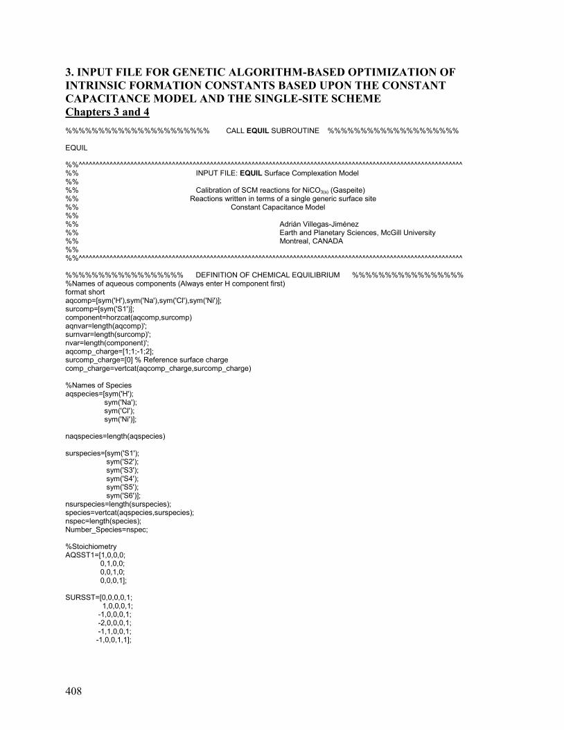
408

3. INPUT FILE FOR GENETIC ALGORITHM-BASED OPTIMIZATION OF

INTRINSIC FORMATION CONSTANTS BASED UPON THE CONSTANT

CAPACITANCE MODEL AND THE SINGLE-SITE SCHEME

Chapters 3 and 4 %%%%%%%%%%%%%%%%%%%%%% CALL EQUIL SUBROUTINE %%%%%%%%%%%%%%%%%%%% EQUIL %%^^^^^^^^^^^^^^^^^^^^^^^^^^^^^^^^^^^^^^^^^^^^^^^^^^^^^^^^^^^^^^^^^^^^^^^^^^^^^^^^^^^^^^^^^^^^^^^^^^^^^^^^^^^^^^^ %% INPUT FILE: EQUIL Surface Complexation Model %% %% Calibration of SCM reactions for NiCO3(s) (Gaspeite) %% Reactions written in terms of a single generic surface site %% Constant Capacitance Model %% %% Adrián Villegas-Jiménez %% Earth and Planetary Sciences, McGill University %% Montreal, CANADA %% %%^^^^^^^^^^^^^^^^^^^^^^^^^^^^^^^^^^^^^^^^^^^^^^^^^^^^^^^^^^^^^^^^^^^^^^^^^^^^^^^^^^^^^^^^^^^^^^^^^^^^^^^^^^^^^^^ %%%%%%%%%%%%%%%%%% DEFINITION OF CHEMICAL EQUILIBRIUM %%%%%%%%%%%%%%%%% %Names of aqueous components (Always enter H component first) format short aqcomp=[sym('H'),sym('Na'),sym('Cl'),sym('Ni')]; surcomp=[sym('S1')]; component=horzcat(aqcomp,surcomp) aqnvar=length(aqcomp)'; surnvar=length(surcomp)'; nvar=length(component)'; aqcomp_charge=[1;1;-1;2]; surcomp_charge=[0] % Reference surface charge comp_charge=vertcat(aqcomp_charge,surcomp_charge) %Names of Species aqspecies=[sym('H'); sym('Na'); sym('Cl'); sym('Ni')]; naqspecies=length(aqspecies) surspecies=[sym('S1'); sym('S2'); sym('S3'); sym('S4'); sym('S5'); sym('S6')]; nsurspecies=length(surspecies); species=vertcat(aqspecies,surspecies); nspec=length(species); Number_Species=nspec; %Stoichiometry AQSST1=[1,0,0,0; 0,1,0,0; 0,0,1,0; 0,0,0,1]; SURSST=[0,0,0,0,1; 1,0,0,0,1; -1,0,0,0,1; -2,0,0,0,1; -1,1,0,0,1; -1,0,0,1,1];

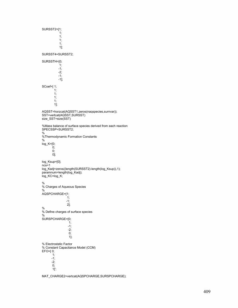
409

SURSST2=[1; 1; 1; 1; 1; 1]; SURSST4=SURSST2; SURSSTH=[0; 1; -1; -2; -1; -1]; SCoef=[ 1; 1; 1; 1; 1; 1]; AQSST=horzcat(AQSST1,zeros(naqspecies,surnvar)); SST=vertcat(AQSST,SURSST) size_SST=size(SST) %Mass balance of surface species derived from each reaction SPECSSP=SURSST2; % %Thermodynamic Formation Constants % log_K=[0; 0; 0; 0]; log_Ksup=[0]; ncs=1 log_Kadj=zeros((length(SURSST2)-length(log_Ksup)),1); paramnum=length(log_Kadj); log_KC=log_K; % % Charges of Aqueous Species % AQSPCHARGE=[1; 1; -1; 2]; % % Define charges of surface species % SURSPCHARGE=[0; 1; -1; -2; 0; 1]; % Electrostatic Factor % Constant Capacitance Model (CCM) EFO=[ 0; 1; -1; -2; 0; 1]'; MAT_CHARGE2=vertcat(AQSPCHARGE,SURSPCHARGE);

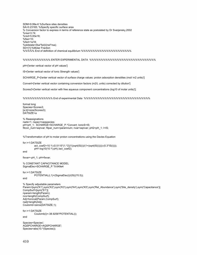
410

SDM=9.99e-6 %Surface sites densities SA=0.23165; %Specify specific surface area % Conversion factor to express in terms of reference state as postulated by Dr Sverjensky,2002 %rsa=3.74; %rsd=5.83e18; %fsa=10; %fsd=1e18; %stdstate=(fsa*fsd)/(rsd*rsa); SD=[1];%Molar Fraction %%%%% End of definition of chemical equilibrium %%%%%%%%%%%%%%%%%%%%%% %%%%%%%%%%%% ENTER EXPERIMENTAL DATA %%%%%%%%%%%%%%%%%%%%%%%%%%%%% pH=['enter vertical vector of pH values'] IS=['enter vertical vector of Ionic Strength values'] SCHARGE_P=['enter vertical vector of surface charge values: proton adsorption densitites (mol/ m2 units)'] Convert=['enter vertical vector containing conversion factors (m2/L units) corrected by dilution'] Scores3=['enter vertical vector with free aqueous component concentrations (log10 of molar units)']; %%%%%%%%%%%%% End of experimental Data %%%%%%%%%%%%%%%%%%%%%%%%%%%%% format long Species=Scores3; [a,b]=size(Scores3); DATSIZE=a % Reassignations nads=1; nspec=naqspecies; pH=pH_1; SCHARGE=SCHARGE_P.*Convert; IonicS=IS; fitcon_num=aqnvar; fitpar_num=paramnum; nvar=aqnvar; pH2=pH_1; I=IS; %Transformation of pH to molar proton concentrations using the Davies Equation for i=1:DATSIZE

act_coef2=10.^(-(0.5115*(1.^2))*((sqrt(IS(i))/(1+(sqrt(IS(i)))))-(0.3*IS(i)))); pH=-log10(10.^(-pH)./act_coef2); end fixvar=-pH_1; pH=fixvar; % CONSTANT CAPACITANCE MODEL SigmaElec=SCHARGE_P.*9.649e4 for i=1:DATSIZE

POTENTIAL(i,1)=(SigmaElec(i)/(IS(i)^0.5)); end % Specify adjustable parameters Param=[sym('K1'),sym('K2'),sym('K3'),sym('K4'),sym('K5'),sym('Rel_Abundance'),sym('Site_density'),sym('Capacitance')]; CompSurf=[sym('S1')]; nparam=length(Param); ncs=length(CompSurf); Adj=horzcat(Param,CompSurf); nadj=length(Adj); Coulomb=zeros(DATSIZE,1); for i=1:DATSIZE

Coulomb(i)=-38.9256*POTENTIAL(i); end Species=Species'; AQSPCHARGE=AQSPCHARGE'; Species=abs(10.^(Species));

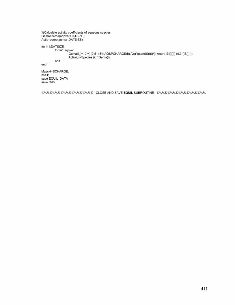
411

%Calculate activity coefficients of aqueous species Gama=zeros(aqnvar,DATSIZE); Activ=zeros(aqnvar,DATSIZE); for j=1:DATSIZE

for i=1:aqnvar Gama(i,j)=10.^(-(0.5115*((AQSPCHARGE(i)).^2))*((sqrt(IS(i)))/(1+(sqrt(IS(i)))))-(0.3*(IS(i)))); Activ(i,j)=Species (i,j)*Gama(i); end end MassH=SCHARGE; ns=1; save EQUIL_DATA save fitdol %%%%%%%%%%%%%%%%%%% CLOSE AND SAVE EQUIL SUBROUTINE %%%%%%%%%%%%%%%%%%

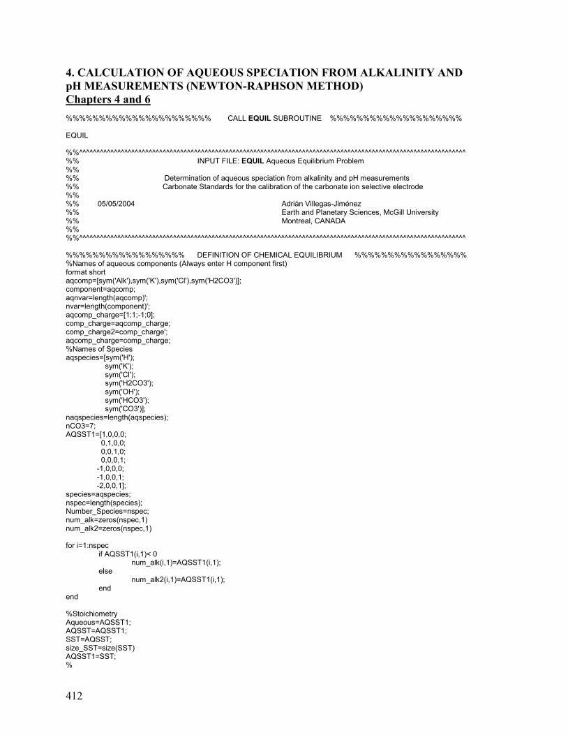
412

4. CALCULATION OF AQUEOUS SPECIATION FROM ALKALINITY AND

pH MEASUREMENTS (NEWTON-RAPHSON METHOD)

Chapters 4 and 6 %%%%%%%%%%%%%%%%%%%%%% CALL EQUIL SUBROUTINE %%%%%%%%%%%%%%%%%%%% EQUIL %%^^^^^^^^^^^^^^^^^^^^^^^^^^^^^^^^^^^^^^^^^^^^^^^^^^^^^^^^^^^^^^^^^^^^^^^^^^^^^^^^^^^^^^^^^^^^^^^^^^^^^^^^^^^^^^^ %% INPUT FILE: EQUIL Aqueous Equilibrium Problem %% %% Determination of aqueous speciation from alkalinity and pH measurements %% Carbonate Standards for the calibration of the carbonate ion selective electrode %% %% 05/05/2004 Adrián Villegas-Jiménez %% Earth and Planetary Sciences, McGill University %% Montreal, CANADA %% %%^^^^^^^^^^^^^^^^^^^^^^^^^^^^^^^^^^^^^^^^^^^^^^^^^^^^^^^^^^^^^^^^^^^^^^^^^^^^^^^^^^^^^^^^^^^^^^^^^^^^^^^^^^^^^^^ %%%%%%%%%%%%%%%%%% DEFINITION OF CHEMICAL EQUILIBRIUM %%%%%%%%%%%%%%%%% %Names of aqueous components (Always enter H component first) format short aqcomp=[sym('Alk'),sym('K'),sym('Cl'),sym('H2CO3')]; component=aqcomp; aqnvar=length(aqcomp)'; nvar=length(component)'; aqcomp_charge=[1;1;-1;0]; comp_charge=aqcomp_charge; comp_charge2=comp_charge'; aqcomp_charge=comp_charge; %Names of Species aqspecies=[sym('H'); sym('K'); sym('Cl'); sym('H2CO3'); sym('OH'); sym('HCO3'); sym('CO3')]; naqspecies=length(aqspecies); nCO3=7; AQSST1=[1,0,0,0; 0,1,0,0; 0,0,1,0; 0,0,0,1; -1,0,0,0; -1,0,0,1; -2,0,0,1]; species=aqspecies; nspec=length(species); Number_Species=nspec; num_alk=zeros(nspec,1) num_alk2=zeros(nspec,1) for i=1:nspec if AQSST1(i,1)< 0 num_alk(i,1)=AQSST1(i,1); else num_alk2(i,1)=AQSST1(i,1); end end %Stoichiometry Aqueous=AQSST1; AQSST=AQSST1; SST=AQSST; size_SST=size(SST) AQSST1=SST; %

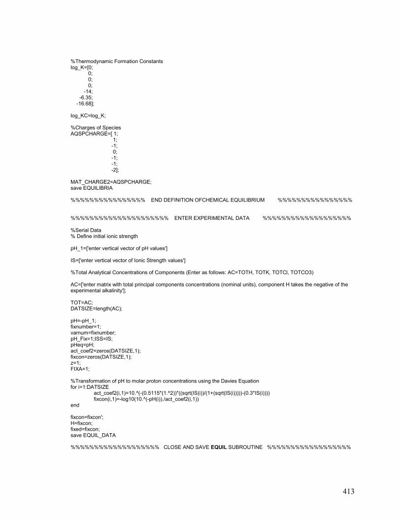
413

%Thermodynamic Formation Constants log_K=[0; 0; 0; 0; -14; -6.35; -16.68]; log_KC=log_K; %Charges of Species AQSPCHARGE=[ 1; 1; -1; 0; -1; -1; -2]; MAT_CHARGE2=AQSPCHARGE; save EQUILIBRIA %%%%%%%%%%%%%%%% END DEFINITION OFCHEMICAL EQUILIBRIUM %%%%%%%%%%%%%%%% %%%%%%%%%%%%%%%%%%%%% ENTER EXPERIMENTAL DATA %%%%%%%%%%%%%%%%%%% %Serial Data % Define initial ionic strength pH_1=['enter vertical vector of pH values'] IS=['enter vertical vector of Ionic Strength values'] %Total Analytical Concentrations of Components (Enter as follows: AC=TOTH, TOTK, TOTCl, TOTCO3) AC=['enter matrix with total principal components concentrations (nominal units), component H takes the negative of the experimental alkalinity']; TOT=AC; DATSIZE=length(AC); pH=-pH_1; fixnumber=1; varnum=fixnumber; pH_Fix=1;ISS=IS; pHeq=pH; act_coef2=zeros(DATSIZE,1); fixcon=zeros(DATSIZE,1); z=1; FIXA=1; %Transformation of pH to molar proton concentrations using the Davies Equation for i=1:DATSIZE

act_coef2(i,1)=10.^(-(0.5115*(1.^2))*((sqrt(IS(i))/(1+(sqrt(IS(i)))))-(0.3*IS(i)))) fixcon(i,1)=-log10(10.^(-pH(i))./act_coef2(i,1)) end fixcon=fixcon'; H=fixcon; fixed=fixcon; save EQUIL_DATA %%%%%%%%%%%%%%%%%%% CLOSE AND SAVE EQUIL SUBROUTINE %%%%%%%%%%%%%%%%%%

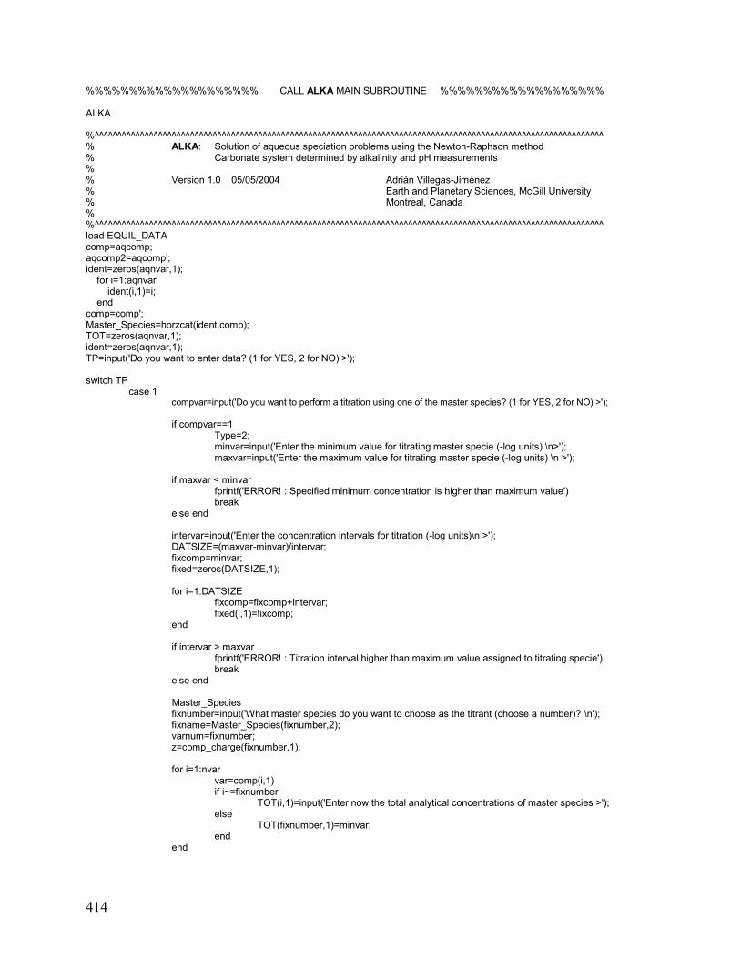
414

%%%%%%%%%%%%%%%%%%%% CALL ALKA MAIN SUBROUTINE %%%%%%%%%%%%%%%%%%% ALKA %^^^^^^^^^^^^^^^^^^^^^^^^^^^^^^^^^^^^^^^^^^^^^^^^^^^^^^^^^^^^^^^^^^^^^^^^^^^^^^^^^^^^^^^^^^^^^^^^^^^^^^^^^^^^^^^^ % ALKA: Solution of aqueous speciation problems using the Newton-Raphson method % Carbonate system determined by alkalinity and pH measurements % % Version 1.0 05/05/2004 Adrián Villegas-Jiménez % Earth and Planetary Sciences, McGill University % Montreal, Canada % %^^^^^^^^^^^^^^^^^^^^^^^^^^^^^^^^^^^^^^^^^^^^^^^^^^^^^^^^^^^^^^^^^^^^^^^^^^^^^^^^^^^^^^^^^^^^^^^^^^^^^^^^^^^^^^^^ load EQUIL_DATA comp=aqcomp; aqcomp2=aqcomp'; ident=zeros(aqnvar,1); for i=1:aqnvar ident(i,1)=i; end comp=comp'; Master_Species=horzcat(ident,comp); TOT=zeros(aqnvar,1); ident=zeros(aqnvar,1); TP=input('Do you want to enter data? (1 for YES, 2 for NO) >'); switch TP

case 1 compvar=input('Do you want to perform a titration using one of the master species? (1 for YES, 2 for NO) >');

if compvar==1

Type=2; minvar=input('Enter the minimum value for titrating master specie (-log units) \n>'); maxvar=input('Enter the maximum value for titrating master specie (-log units) \n >');

if maxvar < minvar fprintf('ERROR! : Specified minimum concentration is higher than maximum value') break else end

intervar=input('Enter the concentration intervals for titration (-log units)\n >'); DATSIZE=(maxvar-minvar)/intervar; fixcomp=minvar; fixed=zeros(DATSIZE,1);

for i=1:DATSIZE fixcomp=fixcomp+intervar; fixed(i,1)=fixcomp; end

if intervar > maxvar fprintf('ERROR! : Titration interval higher than maximum value assigned to titrating specie') break else end

Master_Species fixnumber=input('What master species do you want to choose as the titrant (choose a number)? \n'); fixname=Master_Species(fixnumber,2); varnum=fixnumber; z=comp_charge(fixnumber,1); for i=1:nvar var=comp(i,1) if i~=fixnumber TOT(i,1)=input('Enter now the total analytical concentrations of master species >'); else TOT(fixnumber,1)=minvar; end end

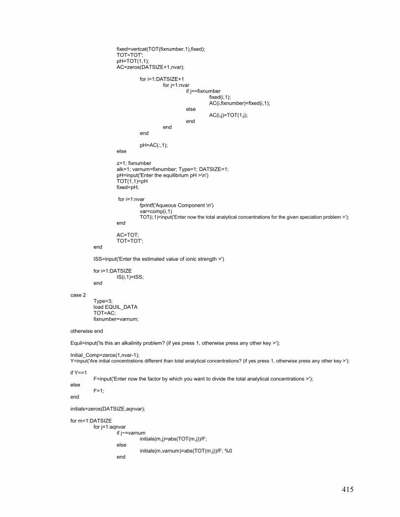
415

fixed=vertcat(TOT(fixnumber,1),fixed); TOT=TOT';

pH=TOT(1,1); AC=zeros(DATSIZE+1,nvar);

for i=1:DATSIZE+1 for j=1:nvar if j==fixnumber fixed(i,1);

AC(i,fixnumber)=fixed(i,1); else

AC(i,j)=TOT(1,j); end

end end

pH=AC(:,1);

else

z=1; fixnumber alk=1; varnum=fixnumber; Type=1; DATSIZE=1; pH=input('Enter the equilibrium pH >\n') TOT(1,1)=pH fixed=pH;

for i=1:nvar fprintf('Aqueous Component \n') var=comp(i,1) TOT(i,1)=input('Enter now the total analytical concentrations for the given speciation problem >');

end

AC=TOT; TOT=TOT';

end

ISS=input('Enter the estimated value of ionic strength >')

for i=1:DATSIZE IS(i,1)=ISS; end case 2

Type=3; load EQUIL_DATA TOT=AC; fixnumber=varnum; otherwise end Equil=input('Is this an alkalinity problem? (if yes press 1, otherwise press any other key >'); Initial_Comp=zeros(1,nvar-1); Y=input('Are initial concentrations different than total analytical concentrations? (if yes press 1, otherwise press any other key >');

if Y==1

F=input('Enter now the factor by which you want to divide the total analytical concentrations >'); else F=1; end initials=zeros(DATSIZE,aqnvar); for m=1:DATSIZE for j=1:aqnvar

if j~=varnum initials(m,j)=abs(TOT(m,j))/F; else initials(m,varnum)=abs(TOT(m,j))/F; %0

end

416

if initials(m,j)==0 initials(m,j)=1e-4;

else end end

if FIXA==3 & Calcite==1

initials(m,varnum)=1; else end end Scores3=zeros(DATSIZE,nvar); Residuals=zeros(DATSIZE,nvar); Species=zeros(DATSIZE,nspec); IonicS=zeros(DATSIZE,1); fixcon=zeros(DATSIZE,1); fixa=input('Fixed activities of at least 1 component? (if yes press 1, otherwise press any other key >'); I_Corr=input('Include ionic strength corrections? (if yes press 1, otherwise press any other key >'); %Transformation of pH or master variable's acitvity to molar proton concentrations using the Davies Equation AI=input('Known activities but no total concentrations? (if yes press 1, otherwise press any other key >'); if AI==1

Act_Fix=1; else

Act_Fix=2; end if I_Corr==1

for i=1:DATSIZE z=aqcomp_charge(varnum,1); act_coef2(i,1)=10.^(-(0.5115*(z.^2))*((sqrt(IS(i)))/(1+(sqrt(IS(i))))-(0.3*IS(i))));

if TP==1 & Type==2 break else fixcon(i,varnum)=-log10(10.^(-fixed(i))./act_coef2(i,1)); end end else end Spc=zeros(DATSIZE,naqspecies); AC2=zeros(aqnvar,DATSIZE); for i=1:DATSIZE

for j=1:aqnvar if j~=varnum AC2(j,i)=initials(i,j); else AC2(varnum,i)=10^(-fixcon(i,1)); end end

Spc(i,1:naqspecies)=10.^((SST*log10(AC2(1:aqnvar,i)))+log_K)'; FI(i,1)=0.5*(Spc(i,1:naqspecies)*(MAT_CHARGE2.^2)); Ratio(i,1)=FI(i,1)/0.5; end for i=DATSIZE

[F]=min(TOT(i,1)); end OPTIONS(1) = 0; OPTIONS(2) = 1e-5; OPTIONS(3) = 1e-10; num_iter=0; if Act_Fix==1

optimum=raphson2(initials,fixcon,fixnumber,fixa,num_iter,FI,varnum,AC2,Equil,Ratio,I_Corr); else %%%%%%%%%%%%%%%%%%% CALL ALKALINITY SUBROUTINE %%%%%%%%%%%%%%%%%%% optimum=alkalinity(initials,fixcon,fixnumber,fixa,num_iter,FI,varnum,AC2,Equil,Ratio,I_Corr);

417

function [optima] =alkalinity(initials,fixcon,fixnumber,fixa,num_iter,FI,varnum,AC2,Equil,Ratio,I_Corr); %^^^^^^^^^^^^^^^^^^^^^^^^^^^^^^^^^^^^^^^^^^^^^^^^^^^^^^^^^^^^^^^^^^^^^^^^^^^^^^^^^^^^^^^^^^^^^^^^^^^^^^^^^^^^^^^^ % Alkalinity computes jacobians based on the Newton-Raphson and Gauss-Elimination method % Input data includes carbonate alkalinity and pH measurements % % Version 1.0 05/05/2004 Adrián Villegas-Jiménez % Earth and Planetary Sciences, McGill University % Montreal, Canada % %^^^^^^^^^^^^^^^^^^^^^^^^^^^^^^^^^^^^^^^^^^^^^^^^^^^^^^^^^^^^^^^^^^^^^^^^^^^^^^^^^^^^^^^^^^^^^^^^^^^^^^^^^^^^^^^^ load EQUIL_DATA format long if num_iter==0

results=initials; else end num_iter=num_iter+1; Ratio=FI(1,1)/0.5; %---------------------------------------------------------------------------------------------------------------------------------------------------------------- %------------------------------------------- Call Newton-Raphson after a given number of generations ------------------------------------ %---------------------------------------------------------------------------------------------------------------------------------------------------------------- maxiter=100; % Vector with initial concentrations for M=1:DATSIZE

niter=0; h=0;

for i=1:aqnvar h=h+1; optim_old(i,1)=results(M,i); h=h-1; end

counter=0; xtol = 1000*eps; ftol = 1e6*eps; error = 2*xtol; ISS=IS;

if num_iter==1 & pH==1

IEq=zeros(a,1); Activ=zeros(nvar,a); Species=zeros(nspec,a); else end

xtol = 1000000*eps; xtol = eps; ftol = 1e6*eps; error = 2*xtol; ISS=ISS(M,1);

while niter<=maxiter

counter=0+1; niter=niter+1 % Transformation of molar concentrations to activities using the Davies Equation gamma=zeros(nspec,nvar);

for k=1:nspec for j=1:aqnvar z=comp_charge2(1,j); act_coef2=(-(0.5115*(z^2))*((sqrt(ISS))/(1+(sqrt(ISS)))-(0.3*ISS))); gamma(k,j)=(act_coef2*SST(k,j)); end end

418

if I_Corr==1 if pH_Fix==1 z=1; act_coef_H=10.^(-(0.5115*(z^2))*((sqrt(ISS)/(1+(sqrt(ISS))))-(0.3*ISS))); fixvar=((10^(pH(M,1)))./act_coef_H) else end

for i=1:nspec for j=1:nvar if gamma(i,j)==1 gamma(i,j)=0; else end end end

Korr1=(sum(gamma'))'; Korr2=zeros(nspec,1);

if I_Corr==1

for i=1:nspec if MAT_CHARGE2(i,1)~=0 Korr2(i,1)=(-(0.5115*(MAT_CHARGE2(i,1)^2))

%*((sqrt(ISS)/(1+(sqrt(ISS))))-(0.3*ISS))); else end end else end

log_K1=(log_K+Korr1)-Korr2; %corrected log K for ionic strength else fixvar=10^(pH(M,1)); log_K1=log_K; end optim_old2=optim_old; % Mass Balance Equations (Minimum Energy Condition) if pH_Fix==1

optim_old(varnum,1)=fixvar; else end

optim_old3=log10(optim_old) Sp_Conc2=(SST*optim_old3)

for i=1:nspec Sp_Conc5(i,1)=10.^(Sp_Conc2(i,1)+log_K1(i)); end

%Estimate ionic strength Sp_Conc4=(Sp_Conc5'); ISS3=0.5*(Sp_Conc4*(MAT_CHARGE2.^2)); % update ionic strength ISS2=ISS; Ionic_Strength=ISS2(1,1);

%if ISS2 <= 1.1(Ratio) & I_Corr==1 if niter < 0.5*maxiter ISS=ISS3; Ratio=ISS2/0.5; else end

MB=(Sp_Conc4*SST); Mass=MB;

%Definition of Charge Balance (Electroneutrality Condition) Electro_Neut2=(Sp_Conc4*MAT_CHARGE2);

%---------------------------------------------------------------------------------------------------------------------------------------------------------------- %----------------------------------------------------- Calculate Jacobian Matrix ----------------------------------------------------------- %----------------------------------------------------------------------------------------------------------------------------------------------------------------

419

switch FIXA case 1

for pivote=2:aqnvar for i=1:nspec for j=2:aqnvar if j==pivote k=pivote; else k=j; end Jacob(i,j-1)=(Sp_Conc5(i,1)*SST(i,pivote)*SST(i,k))/(Sp_Conc5(k,1)); end end Deriva(pivote-1,1:nvar-1)=sum(Jacob); end case 2 for pivote=1:nvar for i=1:nspec for j=1:nvar if j==pivote k=pivote; Jacob(i,j)=(Sp_Conc5(i,1)*SST(i,pivote)

*SST(i,k))/(Sp_Conc5(k,1)); else k=j;

Jacob(i,j)=(Sp_Conc5(i,1)*SST(i,pivote) *SST(i,k))/(Sp_Conc5(k,1));

end end end Deriva(pivote,1:nvar)=sum(Jacob); end case 3 for pivote=1:aqnvar-1 for i=1:nspec for j=1:aqnvar-1 if j==pivote k=pivote; else k=j; end Jacob(i,j)=(Sp_Conc5(i,1)*SST(i,pivote)*SST(i,k))/(Sp_Conc5(k,1)); end end Deriva(pivote,1:aqnvar-1)=sum(Jacob); end otherwise end Der=Deriva; optim_old=10.^(optim_old3); Calculo=Mass(1:aqnvar); Fixed=AC(M,1:aqnvar);

if FIXA~=3 Fixed(1,varnum)=Calculo(1,varnum); else end switch FIXA

case 1 residuos=(Mass(2:aqnvar) - AC(M,2:aqnvar)); case 2 residuos=(Mass - AC(M,1:aqnvar)); case 3 a=Mass(1:aqnvar-1) b=AC(M,1:aqnvar-1) residuos=(Mass(1:aqnvar-1) - AC(M,1:aqnvar-1)); otherwise end % solves the system of linear equations (Gauss-Elimination Method)

420

residuos=residuos'; factor=Der \ residuos; % computes total inorganic concentration if Equil==1 H=sum((Sp_Conc5(1:nspec)).*(-num_alk2)) TOTCO2=sum((Sp_Conc5(1:nspec)).*(num_alk)) H2CO3=(AC(M,1)+H)/(TOTCO2/Sp_Conc5(nvar)); optima=optim_old; optima(aqnvar)=H2CO3; optima=log10(optima); Sp_Conc6=(SST*optima);

for i=1:nspec Sp_Conc7(i,1)=10.^(Sp_Conc6(i,1)+log_K1(i)); end CO3=Sp_Conc7(nCO3,1); TOTCO2=sum(Sp_Conc7.*(SST(1:nspec,aqnvar))); AC(M,aqnvar)=TOTCO2; else end switch FIXA

case 1 optim_new=(optim_old(2:aqnvar) - factor); optima=optim_new;

for i=1:aqnvar-1 if optim_new(i,1)==0 optima(i,1)=(optim_old2(i,1)); else end if optim_new(i,1) < 0 optima(i,1)=(optim_old2(i,1)/10); else end if optim_new(i,1) > 0 optima(i,1)=(optim_new(i,1)); else end end

case 2 optim_new=(optim_old - factor);

for i=1:aqnvar if optim_new(i,1)==0 optima(i,1)=optim_new(i,1); else end if optim_new(i,1) < 0 optima(i,1)=optim_old(i,1)/10; else end if optim_new(i,1) > 0 optima(i,1)=optim_new(i,1); else end end case 3 optim_new=(optim_old(1:aqnvar-1) - factor);

for i=1:aqnvar-1 if optim_new(i,1)==0 optima(i,1)=(optim_new(i,1)); else end if optim_new(i,1) < 0 optima(i,1)=(optim_old(i,1)/10); else end if optim_new(i,1) > 0 optima(i,1)=(optim_new(i,1)); else end end

otherwise end

optim_old2=optima; optim_new=zeros(aqnvar,1);

421

switch FIXA

case 1 optim_old2 optim_new(2:aqnvar,1)=optim_old2; optim_new(varnum,1)=(fixvar); case 2 optim_new(1:aqnvar,1)=optim_old2; case 3 optim_new(1:aqnvar-1,1)=optim_old2 optim_new(aqnvar,1)=1;

otherwise end

error= norm(optim_new - optim_old) optim_old=optim_new; optim_old2=optim_old(1:aqnvar); optim_old=optim_old2; IEq(M,1)=ISS; Calc(M,1:aqnvar)=Calculo; Fix(M,1:aqnvar)=Fixed; ERR(M,1)=error; Kons(1:nspec,M)=log_K1; Optimum(1:aqnvar,M)=optim_old; Num(M,1)=niter; ICal(M,1)=ISS3;

if FIXA==3

Species=(SST*log10(optim_old)); else

Species=(SST*log10(optim_old)); end

for i=1:nspec

Spec(i,1)=10.^(Species(i,1)+log_K1(i)); end

zet=zeros(nspec,1); gamma=zeros(nspec,nvar);

for k=1:nspec

zet(k,1)=AQSPCHARGE(k,1)'; act_coef2(k,M)=10^(-(0.5115*(zet(k,1)^2))*((sqrt(IEq(M,1)))/(1+(sqrt(IEq(M,1))))- (0.3*IEq(M,1)))); end

Activ(1:nspec,M)=act_coef2(1:nspec,M).*Spec(1:nspec,1);

if Equil==1 CO2(M,1)=TOTCO2;

Car(M,1)=CO3; else

Car=0; CO2=0;

end

save results IEq Calc Fix ERR CO2 Kons Car Optimum Num Activ ICal end

end %%%%%%%%%%%%%%%%%%% END ALKALINITY SUBROUTINE %%%%%%%%%%%%%%%%%%%% end %%%%%%%%%%%%%%%%%%%% END ALKA MAIN SUBROUTINE %%%%%%%%%%%%%%%%%%%%

422

5. CALCULATION OF pH FROM E0, JH AND JOH VALUES (NEWTON-

RAPHSON METHOD)

Chapter 4 pH %%%%%%%%%%%%%%%%%%%% CALL pH MAIN SUBROUTINE %%%%%%%%%%%%%%%%%%%% %%^^^^^^^^^^^^^^^^^^^^^^^^^^^^^^^^^^^^^^^^^^^^^^^^^^^^^^^^^^^^^^^^^^^^^^^^^^^^^^^^^^^^^^^^^^^^^^^^^^^^^^^^^^^^^^^ %% %% pH function: Computes the pH values by the Newton-Raphson method using the Nerstian equation %% with accurately-calibrated electrode parameters (standard electromotive force, %% junction potential coefficients) as input %% %% 05/05/2005 Adrián Villegas-Jiménez %% Earth and Planetary Sciences, McGill University %% Montreal, CANADA %% %%^^^^^^^^^^^^^^^^^^^^^^^^^^^^^^^^^^^^^^^^^^^^^^^^^^^^^^^^^^^^^^^^^^^^^^^^^^^^^^^^^^^^^^^^^^^^^^^^^^^^^^^^^^^^^^^ function [results] =pH % %% Enter Experimental Data and Activity Coefficients E=['enter vertical vector of EMF values']; acoef=['enter vertical vector of activity coefficients for the H+ ion']; DATSIZE2=length(E); %%% Enter Parameters for the Combination pH glass electrode EM1='enter alkaline-end EMF' joh='enter alkaline-end EMF' EM2='enter acid-end EMF' jh='enter acid-end EMF' % Define maximum number of iterations MAXiter='enter maximum number of iterations'; range='enter number pH values to be determined with the alkaline-end electrode parameters'; % Evaluate function and compute derivatives for i=1:DATSIZE

activ=acoef(i); H=1e-13; % Guess free proton concentration (initial value) old=H; res=10; if i<range EM=EM1; else EM=EM2; end for k=1:MAXiter Y=-E(i,1)+(EM+(59.2*log10(H))+(jh*H)+(joh*(1e-14/(H*(activ^2))))); Y2=59.2*(1/(H*2.30258509299405))+jh+joh; Z(i,1)=(EM+(59.2*log10(H))+(jh*H)+(joh*(1e-14/(H*(activ^2))))); factor=(Y / Y2); new=(old - factor); old=new; H=new; results(i)=new; error(i,1)=Y; end end pH=-log10(results'.*acoef); save results pH error Z %%%%%%%%%%%%%%%%%%%%% END pH MAIN SUBROUTINE %%%%%%%%%%%%%%%%%%%

423

6. CHEMICAL EQUILIBRIUM SPECIATION INVOLVING ION-

EXCHANGE REACTIONS (NEWTON-RAPHSON METHOD)

Chapter 6 %%%%%%%%%%%%%%%%%%%%%% CALL EQUIL SUBROUTINE %%%%%%%%%%%%%%%%%%%% EQUIL %%^^^^^^^^^^^^^^^^^^^^^^^^^^^^^^^^^^^^^^^^^^^^^^^^^^^^^^^^^^^^^^^^^^^^^^^^^^^^^^^^^^^^^^^^^^^^^^^^^^^^^^^^^^^^^^^ %% INPUT FILE: EQUIL Aqueous Equilibrium Problem %% %% Definition of chemical equilibrium of the CaCO3(s)-KCl-H2O system %% %% %% 10/07/2007 Adrián Villegas-Jiménez %% Earth and Planetary Sciences, McGill University %% Montreal, CANADA %% %%^^^^^^^^^^^^^^^^^^^^^^^^^^^^^^^^^^^^^^^^^^^^^^^^^^^^^^^^^^^^^^^^^^^^^^^^^^^^^^^^^^^^^^^^^^^^^^^^^^^^^^^^^^^^^^^ %%%%%%%%%%%%%%%%%% DEFINITION OF CHEMICAL EQUILIBRIUM %%%%%%%%%%%%%%%%% %Names of components format short aqcomp=[sym('H'),sym('Ca'),sym('K'),sym('Cl'),sym('CaCO3surf'),sym('CaCO3s')]; component=aqcomp; aqnvar=length(aqcomp)'; nvar=length(component)'; aqcomp_charge=[1;2;1;-1;0;0]; comp_charge=aqcomp_charge; comp_charge2=comp_charge'; aqcomp_charge=comp_charge; %Names of Species aqspecies=[sym('H'); sym('Ca'); sym('K'); sym('Cl'); sym('CO3'); sym('OH'); sym('H2CO3'); sym('HCO3'); sym('CaCO3'); sym('CaHCO3'); sym('CaOH'); sym('CaCl'); sym('KCl'); sym('CaCO3surf'); sym('H2CO3surf')]; naqspecies=length(aqspecies); AQSST1=[1,0,0,0,0,0; 0,1,0,0,0,0; 0,0,1,0,0,0; 0,0,0,1,0,0; 0,-1,0,0,0,1; -1,0,0,0,0,0; 2,-1,0,0,0,1; 1,-1,0,0,0,1; 0,0,0,0,0,1; 1,0,0,0,0,1; -1,1,0,0,0,0; 0,1,0,1,0,0; 0,0,1,1,0,0; 0,0,0,0,1,0; 2,-1,0,0,1,0];

424

SST2=[ 1,0,0,0,0,0; 0,1,0,0,0,0; 0,0,1,0,0,0; 0,0,0,1,0,0; 0,-1,0,0,0,1; -1,0,0,0,0,0; 2,-1,0,0,0,1; 1,-1,0,0,0,1; 0,0,0,0,0,1; 1,0,0,0,0,1; -1,1,0,0,0,0; 0,1,0,1,0,0; 0,0,1,1,0,0; 0,1,0,0,1,0; 2,0,0,0,1,0]; [taille]=length(SST2); Ca_Diss=zeros(taille); CO2_MBSTT=zeros(taille); species=aqspecies; nspec=length(species); Number_Species=nspec; num_alk=zeros(nspec,1) num_alk2=zeros(nspec,1) for i=1:nspec if AQSST1(i,1)< 0 num_alk(i,1)=AQSST1(i,1); else num_alk2(i,1)=AQSST1(i,1); end end %Stoichiometry Aqueous=AQSST1; AQSST=AQSST1; SST=AQSST; size_SST=size(SST) AQSST1=SST; % Thermodynamic or Apparent Formation Constants % log_K=[0; 0; 0; 0; -8.48; -14; 8.2; 1.85; -5.28; 3.11; -12.85; 0.2; -0.5; 0; „enter log10(Kexc)‟]; % Solid phases Kps=-8.48; Fix_solid=1; Solid_Act=1; log_KC=log_K;

425

%Charges of Species AQSPCHARGE=[ 1; 2; 1; -1; -2; -1; 0; -1; 0; 1; 1; 1; 0; 0; 0]; MAT_CHARGE2=AQSPCHARGE; save EQUILIBRIA % Total Analytical Concentrations of Components (Enter as follows: AC=TOTH, TOTK, TOTCl, TOTCO3) and specify a % value of “1” for the last component in all cases. % aqcomp=[sym('H'),sym('Ca'),sym('K'),sym('Cl'),sym('CaCO3surf'),sym('CaCO3s')] AC=[„enter experimental data either as a vertical vector or as a matrix for serial data„]; TOT=AC; DATSIZE=length(AC); varnum=5; FIXA=2; %Serial Data % Define initial ionic strength IS=[„enter ionic strength either as a vertical vector or as a matrix for serial data„]; ISS=IS; %Define fixed variable values (if applicable) pH_1=[„enter pH data as a vertical vector or as a matrix for serial data„]; Ca_Fix=pH_1; Calcium=1; CO3_Fix=Ca_Fix; nfix=2; fixact=horzcat(pH_1,Ca_Fix); pH_1=log10(pH_1); Ca_Fix=log10(Ca_Fix); CO3_Fix=log10(CO3_Fix); fixvar=5; pH=-pH_1; fixnumber=1; varnum2=2; varnum3=5; pH_Fix=2; pHeq=pH; act_coef2=zeros(DATSIZE,1); fixcon=zeros(DATSIZE,1); z=1; %Transformation of pH to molar proton concentrations using the Davies Equation for i=1:DATSIZE act_coef2(i,1)=10.^(-(0.5115*(1.^2))*((sqrt(IS(i))/(1+(sqrt(IS(i)))))-(0.3*IS(i)))); fixcon(i,1)=-log10(10.^(-pH(i))./act_coef2(i,1)); end fixcon=fixcon'; H=fixcon; fixed=fixcon; varnum=5; fixvariables=1 %fixnow fixvariables=2 %TOT Calcite=1; save EQUIL_DATA %%%%%%%%%%%%%%%%%%% CLOSE AND SAVE EQUIL SUBROUTINE %%%%%%%%%%%%%%%%%%

426

%%%%%%%%%%%%%%%%%%%% CALL ION_SPEC SUBROUTINE %%%%%%%%%%%%%%%%%%%% ION_SPEC %%^^^^^^^^^^^^^^^^^^^^^^^^^^^^^^^^^^^^^^^^^^^^^^^^^^^^^^^^^^^^^^^^^^^^^^^^^^^^^^^^^^^^^^^^^^^^^^^^^^^^^^^^^^^^^^^ %% INPUT FILE: ION_SPEC Aqueous Equilibrium Problem %% %% File "ION_SPEC" uses the function "TOT" to estimate the equilibrium %% concentrations of dissolved and surface species %% %% 10/07/2007 Adrián Villegas-Jiménez %% Earth and Planetary Sciences, McGill University %% Montreal, CANADA %% %%^^^^^^^^^^^^^^^^^^^^^^^^^^^^^^^^^^^^^^^^^^^^^^^^^^^^^^^^^^^^^^^^^^^^^^^^^^^^^^^^^^^^^^^^^^^^^^^^^^^^^^^^^^^^^^^ load EQUIL_DATA comp=aqcomp; aqcomp2=aqcomp'; ident=zeros(aqnvar,1);

for i=1:aqnvar ident(i,1)=i;

end comp=comp'; Master_Species=horzcat(ident,comp); TOT=zeros(aqnvar,1); ident=zeros(aqnvar,1); TP=input('Do you want to enter data? (1 for YES, 2 for NO) >'); switch TP

case 1 compvar=input('Do you want to perform a titration using one of the master species? (1 for YES, 2 for NO) >');

if compvar==1 Type=2;

minvar=input('Enter the minimum value for titrating master specie (-log units) \n>'); maxvar=input('Enter the maximum value for titrating master specie (-log units) \n >');

if maxvar < minvar fprintf('ERROR! : Specified minimum concentration is higher than maximum value')

break else end

intervar=input('Enter the concentration intervals for titration (-log units)\n >');

DATSIZE=(maxvar-minvar)/intervar; fixcomp=minvar; fixed=zeros(DATSIZE,1);

for i=1:DATSIZE fixcomp=fixcomp+intervar; fixed(i,1)=fixcomp; end

if intervar > maxvar fprintf('ERROR! : Titration interval higher than maximum value assigned to titrating

%specie')

break else end fixnumber=input('What master species do you want to choose as the titrant (choose a

%number)? \n'); fixname=Master_Species(fixnumber,2); varnum=fixnumber; z=comp_charge(fixnumber,1);

for i=1:nvar var=comp(i,1)

if i~=fixnumber

427

TOT(i,1)=input('Enter now the total analytical concentrations of master species >');

else TOT(fixnumber,1)=minvar;

end end

fixed=vertcat(TOT(fixnumber,1),fixed); TOT=TOT'; pH=TOT(1,1); AC=zeros(DATSIZE+1,nvar);

for i=1:DATSIZE+1

for j=1:nvar if j==fixnumber fixed(i,1); AC(i,fixnumber)=fixed(i,1); else AC(i,j)=TOT(1,j); end end

end pH=AC(:,1);

else

z=1; fixnumber alk=1; varnum=fixnumber; Type=1; DATSIZE=1; pH=input('Enter the equilibrium pH >\n') TOT(1,1)=pH fixed=pH;

for i=1:nvar fprintf('Aqueous Component \n') var=comp(i,1) TOT(i,1)=input('Enter now the total analytical concentrations for the given speciation

problem >');

end

AC=TOT; TOT=TOT';

end

ISS=input('Enter the estimated value of ionic strength >')

for i=1:DATSIZE IS(i,1)=ISS; end

case 2 Type=3; load EQUIL_DATA TOT=AC; fixnumber=varnum; otherwise end Equil=input('Is this an alkalinity problem? (if yes press 1, otherwise press any other key >'); if Eq==1 Equil=1; else Equil=2; end Initial_Comp=zeros(1,nvar-1); Y=input('Are initial concentrations different than total analytical concentrations? (if yes press 1, otherwise press any other key >'); if Y==1 F=input('Enter now the factor by which you want to divide the total analytical concentrations >'); else F=1; end

428

initials=zeros(1,nvar-1); if Equil~=1

initials=zeros(DATSIZE,nvar-1); for m=1:DATSIZE for j=1:nvar-1 if j==1

k=2; else end

initials(m,j)=TOT(m,k)/F; k=k+1; end end else end initials=zeros(DATSIZE,aqnvar); for m=1:DATSIZE for j=1:aqnvar if j~=varnum initials(m,j)=abs(TOT(m,j))/F; else initials(m,varnum)=abs(TOT(m,j))/F; %0 end if initials(m,j)==0 initials(m,j)=1e-4; else end end end Scores3=zeros(DATSIZE,nvar); Residuals=zeros(DATSIZE,nvar); Species=zeros(DATSIZE,nspec); IonicS=zeros(DATSIZE,1); fixcon=zeros(DATSIZE,1); fixa=input('Fixed activities of at least 1 component? (if yes press 1, otherwise press any other key >'); I_Corr=input('Include ionic strength corrections? (if yes press 1, otherwise press any other key >'); %Transformation of pH or master variable's acitvity to molar proton concentrations using the Davies Equation AI=input('Known activities press 1 known total concentrations press any other key >'); if AI==1 Act_Fix=1; else Act_Fix=2; end initials=zeros(DATSIZE,aqnvar); size(initials); for m=1:DATSIZE for j=1:aqnvar if j~=varnum initials(m,j)=abs(TOT(m,j))/F; else initials(m,varnum)=abs(TOT(m,j))/F; end

if initials(m,j)==0 initials(m,j)=1e-4; else end

end end Scores3=zeros(DATSIZE,nvar); Residuals=zeros(DATSIZE,nvar); Species=zeros(DATSIZE,nspec); IonicS=zeros(DATSIZE,1); fixcon=zeros(DATSIZE,1);

429

if I_Corr==1 for i=1:DATSIZE

z=aqcomp_charge(varnum,1); act_coef2(i,1)=10.^(-(0.5115*(z.^2))*((sqrt(IS(i)))/(1+(sqrt(IS(i))))-(0.3*IS(i))));

if TP==1 & Type==2 break else

fixcon(i,varnum)=-log10(10.^(-fixed(i))./act_coef2(i,1)); end end else end Spc=0; AC2=zeros(aqnvar,DATSIZE); for i=1:DATSIZE for j=1:aqnvar if j~=varnum AC2(j,i)=initials(i,j); else AC2(varnum,i)=10^(-fixcon(i,1)); end end Spc(1,1:naqspecies)=10.^((SST*log10(AC2(1:aqnvar,i)))+log_K)'; FI(i,1)=0.5*(Spc(1,1:naqspecies)*(MAT_CHARGE2.^2)); Ratio(i,1)=FI(i,1)/0.5; end for i=DATSIZE

[F]=min(TOT(i,1)); end OPTIONS(1) = 0; OPTIONS(2) = 1e-5; OPTIONS(3) = 1e-10; num_iter=0; %%%%%%%%%%%%%%%%%%%% CALL TOT SUBROUTINE %%%%%%%%%%%%%%%%%%%% if Act_Fix==1

optimum=raphson2(initials,fixcon,fixnumber,fixa,num_iter,FI,varnum,AC2,Equil,Ratio,I_Corr); else optimum=tot(initials,fixcon,fixnumber,fixa,num_iter,FI,varnum,AC2,Equil,Ratio,I_Corr); function [optima] =tot(initials,fixcon,fixnumber,fixa,num_iter,FI,varnum,AC2,Equil,Ratio,I_Corr); %%^^^^^^^^^^^^^^^^^^^^^^^^^^^^^^^^^^^^^^^^^^^^^^^^^^^^^^^^^^^^^^^^^^^^^^^^^^^^^^^^^^^^^^^^^^^^^^^^^^^^^^^^^^^^^^^ %% %% TOT computes jacobians based on the Newton-Raphson and Gauss-Elimination method %% %% %% 10/07/2007 Adrián Villegas-Jiménez %% Earth and Planetary Sciences, McGill University %% Montreal, CANADA %% %%^^^^^^^^^^^^^^^^^^^^^^^^^^^^^^^^^^^^^^^^^^^^^^^^^^^^^^^^^^^^^^^^^^^^^^^^^^^^^^^^^^^^^^^^^^^^^^^^^^^^^^^^^^^^^^^ load EQUIL_DATA format long

if num_iter==0 results=initials;

else end num_iter=num_iter+1; Ratio=FI(1,1)/0.5; for M=1:DATSIZE

430

maxiter=10; niter=0; h=0; for i=1:aqnvar

h=h+1; optim_old(i,1)=results(M,i); h=h-1;

end counter=0; xtol = 1000*eps; ftol = 1e6*eps; error = 2*xtol; ISS=IS; if num_iter==1 & pH==1

IEq=zeros(a,1); Activ=zeros(nvar,a); Species=zeros(nspec,a); else end xtol = 10*eps; ftol = 1e6*eps; error = 1e10; ISS=ISS(M,1); while error>1e-14

counter=0+1; niter=niter+1; % Transformation of molar concentrations to activities using the Davies Equation gamma=zeros(nspec,nvar);

for k=1:nspec for j=1:aqnvar z=comp_charge2(1,j); act_coef2=(-(0.5115*(z^2))*((sqrt(ISS))/(1+(sqrt(ISS)))-(0.3*ISS))); gamma(k,j)=(act_coef2*SST(k,j)); end end if I_Corr==1 if FIXA==3 act_coef_H=10.^(-(0.5115*(z^2))*((sqrt(ISS)/(1+(sqrt(ISS))))-(0.3*ISS))); fixvar=((10^(pH_1(M,1)))./act_coef_H); else end for i=1:nspec for j=1:nvar if gamma(i,j)==1 gamma(i,j)=0; else end end end Korr1=(sum(gamma'))'; Korr2=zeros(nspec,1); for i=1:nspec if MAT_CHARGE2(i,1)~=0 Korr2(i,1)=(-(0.5115*(MAT_CHARGE2(i,1)^2))*((sqrt(ISS)/(1+(sqrt(ISS))))-(0.3*ISS))); else end end

log_K1=(log_K+Korr1)-Korr2; %corrected log K for ionic strength

431

else fixvar=10^(pH(M,1));

log_K1=log_K; end optim_old2=optim_old;

% Mass Balance Equations (Minimum Energy Condition) optim_old3=log10(optim_old); Sp_Conc2=(SST*optim_old3); for i=1:nspec

Sp_Conc5(i,1)=10.^(Sp_Conc2(i,1)+log_K1(i)); end

% Estimate ionic strength Sp_Conc4=(Sp_Conc5');

if niter<0.9*maxiter

ISS2=ISS; ISS=ISS2;

else ISS2=0.5*(Sp_Conc4*(MAT_CHARGE2.^2)); % update ionic strength Ionic_Strength=ISS2; ISS=ISS2;

end MB=(Sp_Conc4*SST); Mass=MB; Spec=Sp_Conc4';

%Definition of Charge Balance (Electroneutrality Condition) Electro_Neut2=(Sp_Conc4*MAT_CHARGE2);

% --------------------------------------------------------------------------------------------------------------------------------------------------------------- % ----------------------------------------------------- Calculate Jacobian Matrix ---------------------------------------------------------- % --------------------------------------------------------------------------------------------------------------------------------------------------------------- switch FIXA

case 1 for pivote=2:aqnvar for i=1:nspec for j=2:aqnvar if j==pivote k=pivote; Jacob(i,j-1)=(Sp_Conc5(i,1)*SST(i,pivote)*SST(i,k))/(Sp_Conc5(k,1)); else k=j; end Jacob(i,j-1)=(Sp_Conc5(i,1)*SST(i,pivote)*SST(i,k))/(Sp_Conc5(k,1)); end end

Deriva(pivote-1,1:nvar-1)=sum(Jacob); end

case 2

for pivote=1:nvar-1 for i=1:nspec

for j=1:nvar-1

if j==pivote k=pivote; Jacob(i,j)=(Sp_Conc5(i,1)*SST(i,pivote)*SST(i,k))/(Sp_Conc5(k,1)); else

432

k=j; Jacob(i,j)=(Sp_Conc5(i,1)*SST(i,pivote)*SST(i,k))/(Sp_Conc5(k,1)); end end end Deriva(pivote,1:nvar-1)=sum(Jacob); end

case 3 for pivote=2:aqnvar-1 for i=1:nspec for j=2:aqnvar-1 if j==pivote k=pivote; else k=j; end Jacob(i,j-1)=(Sp_Conc5(i,1)*SST(i,pivote)*SST(i,k))/(Sp_Conc5(k,1)); end end

Deriva(pivote-1,1:aqnvar-2)=sum(Jacob); end otherwise end % solves the system of linear equations (Gauss-Elimination Method) Der=Deriva; optim_old=10.^(optim_old3); Calculo=Mass(1:aqnvar); Fixed=AC(M,1:aqnvar); if FIXA~=3 Fixed(1,varnum)=Calculo(1,varnum); else Fixed(varnum,1)=Calculo(varnum,1); end switch FIXA case 1 residuos=(Mass(2:aqnvar) - AC(M,2:aqnvar)); case 2 BB=(Mass(1:aqnvar-1)) AA=AC(M,1:aqnvar-1) residuos=(Mass(1:aqnvar-1) - AC(M,1:aqnvar-1)); case 3 residuos=(Mass(2:aqnvar-1) - AC(M,2:aqnvar-1)); otherwise end residuos=residuos'; factor=Der / residuos;

if Equil==2 H=sum((Sp_Conc5(1:nspec)).*(-num_alk2)); TOTCO2=sum((Sp_Conc5(1:nspec)).*(num_alk)); H2CO3=(AC(M,1)+H)/(TOTCO2/Sp_Conc5(nvar)); optima=optim_old; optima(aqnvar)=H2CO3; optima=log10(optima);

433

Sp_Conc6=(SST*optima);

for i=1:nspec Sp_Conc7(i,1)=10.^(Sp_Conc6(i,1)+log_K1(i)); end CO3=Sp_Conc7(nspec,1); TOTCO2=sum(Sp_Conc7.*(SST(1:nspec,aqnvar))); AC(M,aqnvar)=TOTCO2; else end switch FIXA case 1 optim_new=(optim_old(2:aqnvar) - factor);

for i=1:aqnvar-1

if optim_new(i,1)==0 optima(i,1)=log10(AC(i+1,num_iter)); else end

if optim_new(i,1) < 0 optima(i,1)=log10(optim_old2(i,1)/10); else end

if optim_new(i,1) > 0 optima(i,1)=log10(optim_new(i,1)); else end end case 2 optim_old4=optim_old; optim_new=(optim_old(1:aqnvar-1) - factor);

for i=1:aqnvar-1 if optim_new(i,1)==0 optim_old4(i,1)=optim_new(i,1);

else end if optim_new(i,1) < 0 optim_old4(i,1)=optim_old(i,1)/10; else end

if optim_new(i,1) > 0 optim_old4(i,1)=optim_new(i,1); else end end

case 3

optim_old4=optim_old; optim_new=(optim_old(2:aqnvar-1) - factor)

for i=2:aqnvar-1 if optim_new(i-1,1)==0 optim_old4(i,1)=(optim_new(i-1,1)); else end

if optim_new(i-1,1) < 0 optim_old4(i,1)=(optim_old(i-1,1)/10); else end

if optim_new(i-1,1) > 0

optim_old4(i,1)=(optim_new(i-1,1)); else end

end otherwise end optim_old2=optim_old4; optim_new=zeros(aqnvar,1); optim_new=optim_old2;

434

error= norm(optim_new - optim_old); optim_old=optim_new; TOTCO2=sum(Spec.*CO2_MBSTT); optim_old2=optim_old(1:aqnvar); optim_old=optim_old2; TOTCa=sum(Sp_Conc5.*CaDiss); TOTCO2=sum(Spec.*CaDiss); IEq(M,1)=ISS; TOTCal(M,1)=TOTCa; TOTCar(M,1)=TOTCO2; Calc(M,1:aqnvar)=Calculo; Fix(M,1:aqnvar)=Fixed; ERR(M,1)=error; Kons(1:nspec,M)=log_K1; Optimum(1:aqnvar,M)=optim_old; Num(M,1)=niter;

if FIXA==3 Species=(SST*log10(optim_old));

else Species=(SST*log10(optim_old));

end

for i=1:nspec Spec(i,1)=10.^(Species(i,1)+log_K1(i));

end

zet=zeros(nspec,1); gamma=zeros(nspec,nvar);

for k=1:nspec zet(k,1)=AQSPCHARGE(k,1)'; act_coef2(k,M)=10^(-(0.5115*(zet(k,1)^2))*((sqrt(IEq(M,1)))/(1+(sqrt(IEq(M,1))))-(0.3*IEq(M,1))));

end

Activ(1:nspec,M)=act_coef2(1:nspec,M).*Spec(1:nspec,1); Conc(1:nspec,M)=log10(Spec(1:nspec,1)); Especies=Spec(1:nspec,1)'; Car=0; CO2=0;

save results IEq Calc Fix ERR CO2 Kons Conc Car Optimum Num Activ TOTCal TOTCar

end end end %%%%%%%%%%%%%%%%%%%%%% END TOT SUBROUTINE %%%%%%%%%%%%%%%%%%%%%%

fprintf('\n'); fprintf(' \t \t \tPROBLEM CONVERGED! Type: "load results" to see output data \n'); fprintf('\n'); %%%%%%%%%%%%%%%%%%%% END ION_SPEC SUBROUTINE %%%%%%%%%%%%%%%%%%%%

Documents

on the surface chemistry of some rhombohedral carbonate minerals in aqueous solutions