Louisiana State UniversityLSU Digital Commons

LSU Master's Theses Graduate School

2016

Optimal Configuration of Inspection and ReworkStations in a Multistage Flexible FlowlineMd. Shahriar Jahan HossainLouisiana State University and Agricultural and Mechanical College, mhoss25@lsu.edu

Follow this and additional works at: https://digitalcommons.lsu.edu/gradschool_theses

Part of the Mechanical Engineering Commons

This Thesis is brought to you for free and open access by the Graduate School at LSU Digital Commons. It has been accepted for inclusion in LSUMaster's Theses by an authorized graduate school editor of LSU Digital Commons. For more information, please contact gradetd@lsu.edu.

Recommended CitationHossain, Md. Shahriar Jahan, "Optimal Configuration of Inspection and Rework Stations in a Multistage Flexible Flowline" (2016).LSU Master's Theses. 3072.https://digitalcommons.lsu.edu/gradschool_theses/3072

OPTIMAL CONFIGURATION OF INSPECTION AND REWORK STATIONS

IN A MULTISTAGE FLEXIBLE FLOWLINE

A Thesis

Submitted to the Graduate Faculty of the

Louisiana State University and

Agricultural and Mechanical College

in partial fulfillment of the

requirement for the degree of

Master of Science in Industrial Engineering

in

The Department of Mechanical and Industrial Engineering

by

Md. Shahriar Jahan Hossain

B.Sc.Engg. (IPE), Bangladesh University of Engineering & Technology, Dhaka, 2009

M.Sc. (IPE), Bangladesh University of Engineering & Technology, Dhaka, 2012

May 2016

ii

ACKNOWLEDGEMENTS

At first and foremost I would like to express my sincere respect and gratitude to my advisor

and committee chair, Professor Bhaba R. Sarker, for his thoughtful suggestions, indispensable

advice, consistent guidance and encouragement throughout the progress of this research work. I

am grateful to him for showing me a complete way of doing good research which will be beneficial

for my future career.

My special thanks are to Professor Muhammad A. Wahab and Professor T. Warren Liao

for serving on my committee. They provided their constructive remarks and valuable suggestions

during evaluation of this research. I especially thank to Professor T. Warren Liao for what I have

learned from his course on Metaheuristics and this learning helped me to develop a part of a

heuristic. My gratitude is also extended to Professors Brian D. Marx and Charles J. Monlezun of

Department of Experimental Statistics and Professor Hongchao Zhang of Department of

Mathematics from whom I learned several techniques that have been used in this research.

This research is completed under the fellowship award 2014-2018 funded by Louisiana

Economic Development Assistantship (EDA) program, Louisiana State University at Baton

Rouge, LA.

With a very special recognition, I would like to thank my dearest wife Jannatun Naim, my

father Md. Akram Hossain and my mother Salma Jahan who provided their continuous inspiration

and support that encouraged me to complete the research work successfully.

iii

TABLE OF CONTENTS

ACKNOWLEDGEMENTS…………………………………………………………………... ii

LIST OF TABLES………………………………………………………………………........ vi

LIST OF FIGURES…………………………………………………………………………… vii

ABSTRACT………………………………………………………………………………….. viii

CHAPTER 1 INTRODUCTION……………………………………………………………... 1

1.1 Literature Survey……………………………………………………………......... 2

1.1.1 Line efficiency………………………………………………………….. 2

1.1.2 Quality inspection policy optimization………………………………….. 3

1.1.3 Quality defect and rework issues…………………………………….….. 3

1.1.4 Inspection station assignment……………………………………….….. 5

1.1.5 Material flow………………………………………………………...….. 5

1.1.6 Garments production flow line………………………………………….. 6

1.2 Limitations of the Previous Research and Problem Identification…………….….. 7

CHAPTER 2 RESEARCH GOAL AND OBJECTIVES…………………………………….. 10

2.1 Research Goals………………………………………………………………..….. 10

2.2 Research Objectives…………………………………………………………..….. 11

2.3 Scope.………………………………………………………………………….…. 15

2.4 Motivating Factors of the Research……………………………………………….. 15

2.4.1 Economic importance……………………………………………….….. 16

2.4.2 Technical importance………………………………………………..….. 17

2.4.3 Industrial importance: garments industry……………………………….. 17

2.5 Methodology…………………………………………………………………..….. 18

CHAPTER 3 END-OF-LINE INSPECTION STATION……………………………………. 20

3.1 Assumptions…………………………………………………………………..….. 21

3.2 Model Formulation……………………………………………………………….. 22

3.3 Transformation of Fractional Nonlinear Program…………………………….….. 28

3.4 Throughput Analysis………………………………………………………….….. 33

3.5 A Case Study in Garments Industry…………………………………………..….. 35

3.5.1 RMG manufacturing industry producing T-shirts…………………..….. 36

3.5.2 Empirical test for large problem sets………………………………..….. 42

3.6 Conclusion of the ELI Problem……………………………………………….….. 45

CHAPTER 4 MULTISTAGE INSPECTION STATIONS……………………………….….. 47

4.1 The Multistage Inspection (MSI) Problem……………………………………….. 48

4.2 Mathematical Structure of the MSI Problem………………………………….….. 49

4.3 Model Formulation……………………………………………………………….. 50

4.3.1 Formulation of the objective function………………………………….. 52

iv

4.3.2 Formulation of the constraints………………………………………….. 56

4.3.3 Complete formulation of MSI problem……………………………..….. 59

4.4 Solution Methodology………………………………………………………...….. 60

4.4.1 Specialization to ELI problem………………………………………….. 61

4.5 Case Study…………………………………………………………………….….. 65

4.5.1 Special case………………………………………………………….….. 71

4.6 Sensitivity Analysis………………………………………………………….…… 72

4.7 Conclusion of the MSI Problem……………………………………………….….. 75

CHAPTER 5 INSPECTION STATION ASSIGNMENT (ISA): A CONTRUCTION

HEURISTIC……………………………………………………………….…..

77

5.1 Multistage Inspection Station: Extraction of the General Characteristics…….….. 78

5.1.1 Characterization of performance measures: impact of system

parameters………………………………………………………….…..

80

5.2 Development of Heuristic Method..…………………………………………...….. 86

5.2.1 Inspection Station Assignment (ISA): A construction heuristic…….….. 86

5.2.2 Solving a 15-workstation problem with ISA………………………..….. 92

CHAPTER 6 EMPIRICAL TESTS AND COMPUTATIONAL RESULTS…………….….. 97

6.1 Ant Colony Optimization for Real Numbers (ACOR)………………………...….. 97

6.1.1 ACOR and ISA+ACOR application approach………………………..….. 99

6.2 Tests Design and Analysis of the Results……………………………………..….. 101

6.2.1 Computational results………………………………………………..….. 101

6.2.2 Statistical significance of the heuristics……………………………..….. 104

6.3 Lower Bound of Unit Production Cost………………………………………..….. 109

6.4 Comparing the Results………………………………………………………….… 110

6.5 Long Production Lines: Modular Design……………………………………...….. 113

6.6 Conclusion of the Empirical Study……………………………………………….. 114

CHAPTER 7 CONCLUDING REMARKS………………………………………………….. 116

7.1 Summary……………………………………………………………………....….. 116

7.2 Conclusions…………………………………………………………………..…... 117

7.3 Significance of the Research…………………………………………………..….. 119

7.3.1 Applications to garments and modular manufacturing industries………. 119

7.3.2 Implications to other discrete product manufacturing………………..…. 120

7.4 Limitations………………………………………………………………………... 121

7.5 Future Research…………………………………………………………………... 122

REFERENCES……………………………………………………………………………….. 125

APPENDIX A. BRANCH AND BOUND RESULTS (4-WORKSTATION PROBLEM)…. 134

APPENDIX B. RANDOMLY GENERATED DATA SETS………………………………… 135

Appendix B.1. Data set for empirical tests………………..………………………….. 135

Appendix B.2. Dataset for the Workstation 5, Production line 1 [Example 4.1]…….. 136

v

APPENDIX C. MSI PROBLEM RESULTS…………………………………………………. 137

Appendix C.1. Multistage inspection problem results (u) obtained from ISA+ACOR.. 137

Appendix C.2. Multistage inspection problem results (u) obtained from ACOR…….. 138

Appendix C.3. Number of functional evaluation (nfe) for solving multistage

inspection station problem with ISA+ACOR………………………….

139

Appendix C.4. Number of functional evaluation (nfe) for solving multistage

inspection problem with ACOR……………………………………….

140

Appendix C.5. CPU time for solving multistage inspection problem with

ISA+ACOR……………………………………………………………. 141

Appendix C.6. CPU time for solving multistage inspection problem with ACOR…… 142

VITA………………………………………………………………………………………….. 143

vi

LIST OF TABLES

Table 1.1 Previous works on inspection and rework station location problem………………. 9

Table 3.1 Fixed and variable costs involved with different operations………………………. 37

Table 3.2 Decisions made on defective T-shirts produced at 10 different production lines…. 40

Table 3.3 Empirical test results for large problem sets………………………………………. 44

Table 4.1 Cost and time data used in processing, rework and inspection……………………. 67

Table 4.2 Proportion of defects ( kp ) in ten different production lines……………………….. 68

Table 4.3 Rework policy for six alternatives of iN ( 1,2i ) for Production line 1 …………. 69

Table 4.4 m-inspection station location in production line 1 (optimum rework policy)…...... 69

Table 4.5 Optimum results for ten identical production lines of branded T-shirt……………. 71

Table 5.1 Empirical test results for 15 workstation example, using exhaustive search

algorithm…………………………………………………………………………..

79

Table 5.2 Empirical test results for large problem sets using exhaustive search algorithm…. 85

Table 5.3 Solution steps of Algorithm 5.1 (ISA Heuristic) to solve a 15-workstation

problem…………………………………………………………………………….

94

Table 5.4 Computational Results of ISA Heuristic for MSI Problem……………………....... 96

Table 6.1 Comparison of optimum, ISA, ACOR and ISA+ACOR heuristics results and

performances (30-run summary) ………………………………………………….

103

Table 6.2 Testing the difference between ACOR and ISA+ACOR results in terms of bestu …. 106

Table 6.3 Testing the difference between ACOR and ISA+ACOR results in terms of CPU

time………………………………………………………………………...............

107

Table 6.4 Testing the difference between ACOR and ISA+ACOR results in terms of nfe .. 108

Table 6.5 Comparison between heuristic, lower bound and optimum solutions……………… 112

vii

LIST OF FIGURES

Figure 2.1 An N-station production flowline with single inspection station………………… 13

Figure 2.2 A flowline with m inspection stations…………………………………………… 14

Figure 3.1 An N-stage flowline with end-of-line inspection………………………………… 20

Figure 3.2 A 2-dimensional depiction of the constraint, 0k kx y on a 0-1 binary coordinate 24

Figure 3.3 Seven different operations on the T-shirt………………………………………… 36

Figure 3.4 A branded T-shirt production line with 7 different workstations………………... 36

Figure 3.5 Branch and bound algorithm result for 4-workstation problem…………………. 39

Figure 3.6 A branded T-shirt production line with 7 different workstations

(Refer to: Example 3.2, Table 3.2, Production line 1) ………………………….

42

Figure 3.7 (a) Average node searched (b) Average CPU time vs number of workstations... 45

Figure 4.1 A flowline with m inspection stations……………………………………………. 49

Figure 4.2 A two-stage in-line inspection line………………………………………………. 53

Figure 4.3 A three-stage in-line inspection line……………………………………………... 54

Figure 4.4 Exhaustive search algorithm for optimal solution of MSI problem………………. 65

Figure 4.5 Optimum configuration of Production line-2 (Example 4.1, Table 4.5)………….. 70

Figure 4.6 Sensitivity of *u with respect to (a)

5

Rt , (b) IC and (c) 5

rc ………………………. 74

Figure 5.1 Impact of m on *  u in a 15-workstation line……………………………………... 81

Figure 5.2 CPU time versus m curve for the 15-workstation line…………………………… 81

Figure 5.3 Throughput Rate ( ThR ) versus m curve for the line with 15 workstations……….. 83

Figure 5.4 u* versus *

iN curves for the line with 15 workstations…………………………. 84

Figure 5.5 A segment of a flowline with two inspection station…………………………….. 87

Figure 5.6 Inspection Station Assignment (ISA) heuristic for obtaining sub-optimal solution. 91

Figure 6.1 Convergence profile of 20-workstation example using ISA, ACOR, ISA+ACOR 104

Figure 6.2 Comparison between heuristics ( u versus N )……………………………… 111

viii

ABSTRACT

Inspection and rework are two important issues of quality control. In this research, an N-

stage flowline is considered to make decisions on these two issues. When defective items are

detected at the inspection station the items are either scrapped or reworked. A reworkable item

may be repaired at the regular defect-creating workstation or at a dedicated off-line rework station.

Two problems (end-of-line and multistage inspections) are considered here to deal with this

situation. The end-of-line inspection (ELI) problem considers an inspection station located at the

end of the line while the multistage inspection (MSI) problem deals with multiple in-line

inspection stations that partition the flowline into multiple flexible lines. Models for unit cost of

production are developed for both problems. The ELI problem is formulated for determining the

best decision among alternative policies for dealing with defective items. For an MSI problem a

unit cost function is developed for determining the number and locations of in-line inspection

stations along with the alternative decisions on each type of defects. Both of the problems are

formulated as fractional mixed-integer nonlinear programming (f-MINLP) to minimize the unit

cost of production. After several transformations the f-MINLP becomes a mixed-integer linear

programming (MILP) problem. A construction heuristic, coined as Inspection Station Assignment

(ISA) heuristic is developed to determine a sub-optimal location of inspection and rework stations

in order to achieve minimum unit cost of production. A hybrid of Ant-Colony Optimization-based

metaheuristic (ACOR) and ISA is devised to efficiently solve large instances of MSI problems.

Numerical examples are presented to show the solution procedure of ELI problems with branch

and bound (B&B) method. Empirical studies on a production line with large number of

workstations are presented to show the quality and efficiency of the solution processes involved

in both ELI and MSI problems. Computational results present that the hybrid heuristic ISA+ACOR

shows better performance in terms of solution quality and efficiency. These approaches are

applicable to many discrete product manufacturing systems including garments industry.

1

CHAPTER 1

INTRODUCTION

Quality control and cost reduction are vital tasks of any manufacturing industry. Number

of defective items reduces production rate and increases unit production cost. Eliminating

nonproductive time and controlling material waste eventually minimize production cost but may

lead to increase quality cost. Various costs are involved in quality—there can be internal costs

such as the cost of inspection, repair or rework and external costs, connected to the defective units

that reach to the customer. Consumers always seek such products which satisfy their requirements

or exceed their expectation. If nonconforming items reach to the customer then manufacturer’s

goodwill may drastically go down, and that is why, nonconforming items are tried to be prevented

from reaching any consumer. Maintaining the product quality is essential to ensure customer

satisfaction.

From the manufacturer’s point of view, good quality of product minimizes not only waste

of raw materials but also the productive time of the workers. For maintaining the goodwill in the

market and enhancing the throughput rate, the manufacturers like garments industries (flowlines)

inspects their products before leaving the production floor. Identified defective products are

supposed to be repaired if possible. Repair works are traditionally done in-line where the defect

was initiated; this strategy eventually disrupts regular flow of production. On the other hand off-

line repair involves extra investments. Sometimes repair cost is considerably high enough to

influence the manager for scrapping the defective products, instead of repair. Thus it becomes an

important research question to decide on the treatment (repair or scrap) of defective items, and in

case of repair, the locations of off-line repair stations need to be determined. Again, the location

of inspection station also affects the total cost and throughput rate. While in-line inspection is done

to identify defects on work-in-process, the defective items can be repaired before going through

2

further processing, which can save some productive time and materials as well. At the same time

multiple in-line inspection may increase the inspection cost. So the optimal number and location

of inspection stations is necessary to be determined in addition to the optimal rework-policy.

A lot of works has been done to improve the productivity, line efficiency, inspection

policies, rework issues and eventually to reduce the cost of production of production flow and

assembly lines. A brief literature survey is now conducted to identify the past research activities

in this area and to find the current status of the related research issues and avenues to improve the

inspection and rework policy.

1.1 Literature Survey

In industries quality inspections are done in order to identify nonconformities. After

inspection, defective items are supposed to be scrapped or repaired. Finding the number and

location of inspection and off-line rework stations as well as the proper treatment (scrap or repair)

on defective items, are important issues for decision making. Keeping this general scope of the

production process this research focuses on the existing literature to extend them to capture the

idea of this research.

1.1.1 Line efficiency

Many investigations have been done to increase the efficiency of a flowline. Sarker and

Shanthikumar (1983) developed a generalized approach for serial and parallel line balancing

techniques for a production line with high demand of product where task time was higher than the

production cycle time. Following this, Sarker (1984) studied the line efficiency and general

throughput of line production system with and without buffer. Bahadir (2011) discussed the design

and performance of assembly line balancing by simulation it in the context of garments industry.

Islam et al. (2014) presented a case study for obtaining an optimal layout design in an apparel

3

industry by appropriately balancing a line. None of these study discusses about offline rework

facilities for defective items.

1.1.2 Quality inspection policy optimization

Several research are found on optimizing quality inspection policies for reducing cost of

quality or increasing the net profit. Anily and Grosfeld-Nir (2006) designed a production and

inspection policy that guarantees a zero defective delivery in minimum expected total cost.

Carcano and Staudacher (2006) focused on inspection policy design into assembly-line balancing.

With their proposed model it is possible to balance the manufacturing line by minimizing total cost

of quality concurrently defining which tests to use and the position where they have to be

performed. Duffuaa and Khan (2008) proposed a new inspection plan for multi-characteristic

critical components. They developed a mathematical model that determines an optimal inspection

plan. Raviv (2013) presented an algorithm for maximizing the expected profit from an unreliable

flowline in which nonconforming items are sent back for rework after going through the inspection

stations. Yang and Cho (2014) dealt with an optimization problem for minimizing the cost of

inspections and reworks performed throughout an imperfect inspection system. Qin et al. (2015)

proposed a nonlinear integer program to determine an optimal plan of zero-defect, single-sampling

by attributes for inspecting incoming parts in an assembly line. Azadeh et al. (2015) used a particle

swarm algorithm for optimizing inspection policies in a production flow process with uncertain

inspection costs. Mohammadi et al. (2015) developed a mathematical model of a robust inspection

process plan using Taguchi and Monte Carlo methods.

1.1.3 Quality defect and rework issues

In many other research, quality defects and rework issues have been introduced. Lee (1992)

modelled a lot sizing problem in an imperfect production process where the model could deal with

corrective actions after detection of the out-of-control shifts, and the fixed setup and variable

4

processing times of reworks. Wein (1992) worked in a make-to-order marketing environment for

rework and scrap decisions in a multistage production process where a Markov decision process

model is developed and solved using dynamic programming techniques. So and Tang (1995)

presented a model of a bottleneck facility that performs regular operations as well as rework. The

goal of that analysis was to obtain an optimal operating policy for the bottleneck with a minimum

expected operating cost. Jamal et al. (2004) proposed an economic batch quantity model that

addressed reworking of defective items in a single-stage production system to minimize the total

cost. Ojha et al. (2007) also developed mathematical models considering three different scenarios,

in order to determine the optimal ordering policy for an imperfect production system with quality

assurance and rework such that the total cost for the system is minimized. Sarker et al. (2008)

extended this model to a multi-stage production system with rework option. Biswas and Sarker

(2008) developed lot sizing models a lean production system with in-cycle rework and scrap.

Parveen and Rao (2009) investigated improvement of product quality and rework for an imperfect

production system with inspection. Jeang and Lin (2014) determined process parameters for

product quality and cost. Castillo-Villar and Herbert-Acero (2014) included quality defects and

rework issues; they incorporated prevention, inspection, rework, failure and opportunity costs in

their model. Two meta-heuristic solution procedures, based on the Simulated Annealing and

genetic algorithm were proposed in that research for identifying near-optimal solutions. Ullah and

Kang (2014) presented an approach for modelling of optimum lot size and total cost; they focused

on work-in-process inventory and incorporated the effect of rework, rejects and inspection on

work-in-process inventory. Yang and Cho (2015) proposed a practical algorithm for

simultaneously determining an optimal frequency and an optimal sequence of inspection stations,

which gives a target average outgoing quality.

5

1.1.4 Inspection station assignment

Some research deal with inspection stations allocation. Eppen and Hurst (1974)

investigated the optimal location of inspection stations in a multistage production process where

each stage is comprised of basically a single station—no multiple workstations were considered

within the stage such that an inspection station could be installed between stations. Kang et al.

(1990) determined the optimal location of inspection stations using a rule-based methodology. Rau

et al. (2005) developed a mathematical model and a heuristic algorithm for solving inspection

allocation problem for re-entrant production systems with a consideration of layer manufacturing.

Rau and Chu (2005) developed mathematical models for two types of workstations at the same

time for production flow systems as well to solve the inspection allocation planning problem. The

model also deals with special concern that the work unit of rework can be sent back to any

workstation after inspection. Shi and Sandborn (2006) optimized the location(s) of rework

facilities in an electronic system assembly plant. Studies of Giannakis et al. (2010) presented the

optimization problems for flow of items with distinct rework loops in production lines. Queuing

network formulas were combined to optimally allocate inspection stations and determine the

inventory control policy. Other uncertainty issues were also addressed by Denardo and Lee (1996),

and Kim and Makis (2013).

1.1.5 Material flow

Some of the researches deal with material flow in the production line. Sarker and Xu (2000)

proposed material flow control system based on operations sequence in designing multi-product

lines. Sarker (2003) showed the effect of material flow and workload on the performance of

machine location in a bi-directional flowline. Following these works, Jamal et al. (2004) and

Biswas and Sarker (2008) determined batch size with rework process in a single-stage production

6

system and for a lean production system with in-cycle rework and scrap. Sarker, et al. (2008)

further improved batch sizing models for a multi-stage production systems with rework.

1.1.6 Garments production flow line

The research problems presented in this thesis evolves from some real life situations in

large volume readymade garments industries. The garments production is highly labor intensive

as it mostly involves manual operations. The production lines of a garments industry is generally

arranged as a flexible flowline that deals with processing, inspection and reworks. An efficient

arrangement of workstations is always a prime concern for the manufacturers as it contributes both

technically and economically to the system. The work on these flowlines are affected by frequent

changes in style, fluctuating seasonal demand and production lead times (Mok et al. 2013).

Some practical implications of line balancing algorithms in garments production are

reported in recent years. Guner et al. (2013) analyzed five different methods in balancing

production lines of T-shirts. They found the same efficiency values for five different methods

because of having fewer operational steps. However, Unal (2013) applied six different line

balancing algorithms in a suit manufacturing line which involves many operational steps and

presented the difference among the outcomes. Kayar and Akyalcin (2014) also applied five

different heuristic methods, and a classical method for T-shirt production line balancing and

presented their comparison. On the other hand, Gungor and Agac (2014) extensively studied the

problems of assembly line balancing in a company which produces men's shirts, and analyzed the

collected data via an intuitive and meta-intuitive algorithm in order to balance the assembly lines

with required quality and productivity at the lowest possible cost.

Dundar et al. (2012) solved the problem of modular line balancing by means of the

mathematical approach and graph theory for garments production. However, Gursoy (2012) also

formulated a sewing line balancing problem as an integer programming for finding the minimum

7

idle time per operator. He designed a new heuristic that can adapt to solve problems with

immediate market demand changes; this heuristic which finds the minimum number of operators

has polynomial complexity. Gursoy et al. (2015) also considered flexibility constraints of

operations in the line balancing problem in a sewing department and solved with integer

mathematical programming and genetic algorithm. Alagas et al. (2013) proposed a new algorithm

which gives optimum solution using constrained programming and queuing network for optimum

task assignment to minimize the cycle time where task times are distributed according to a

statistical distribution. Besides these, Mok et al. (2013) presented some planning algorithms for

automatic job allocations based on group technology and genetic algorithm. Chang and Lin (2015)

addressed the reliability analysis for an apparel manufacturing system by using fuzzy mathematics.

Though the balancing of workstations in a garments production line (especially sewing

line) is studied in several works, the location of inspection stations and rework stations in the line

as well as rework policies are not specifically addressed in available researches. Thus, this research

is intended to present an elaborate implication of current research in garments production line.

1.2 Limitations of the Previous Research and Problem Identification

Related literature review reveals that several attempts were made regarding rework issues

in an imperfect production system. Some of these researches (Lee 1992, Jamal et al. 2004, Ojha et

al. 2007, Sarker et al. 2008, Biswas and Sarker 2008, Ullah and Kang 2014) dealt with different

process parameters to obtain optimum lot size and some other researchers (So and Tang 1995,

Castillo-Villar and Herbert-Acero 2014) investigated the operating policies to minimize the cost

of production while considering rework issues. None of these researches investigated the

configuration of separately dedicated rework facilities.

Some researchers only worked with different quality inspection policies (Anily and

Grosfeld-Nir 2006, Carcano and Staudacher 2006, Duffuaa and Khan 2008, Azadeh et al. 2015,

8

Mohammadi et al. 2015) which are nothing but a tool for identifying the source and intensity of

non-conformities. Some other researches (Sarker and Shanthikumar 1983, Bahadir 2011, Islam et

al. 2014) discussed on-line efficiency enhancement through different line balancing techniques.

All of these focused different dimensions of research related to inspection and/or rework, but none

of them configured the location of inspection and/or rework stations.

Eppen and Hurst (1974), Rau et al. (2005), Rau and Chu (2005), Kang et al. (1990),

Giannakis et al. (2010) were concerned to find the optimum location of inspection stations and

rework stations (Shi and Sandborn 2006) on the line(s). The scope and the limitations of these

researches are summarized in Table 1.1. None of these research indicated in this table provides the

optimal decision on rework or scrap of the defective items. Though Wein (1992) presented some

works for rework and scrap decisions in a multistage batch manufacturing process (but not

necessarily in production flow), his research outcome did not provide the appropriate methodology

to locate rework or inspection stations. Only Shi and Sandborn (2006) investigated the optimal

location of both inspection and rework station, but in their research rework operation is considered

to happen immediately after the inspection. They did not consider the possibility of separate

inspection and rework station, and did not give rework-scrap decision. Above all, the throughput

enhancement is not discussed in any of the above mentioned literatures. Alagas et al. (2013)

worked with garments production line and minimized the cycle time that eventually maximizes

throughput rate, but they did not address the issues relating to optimal assignment of inspection or

rework station(s) in the line.

9

Table 1.1 Previous works on inspection and rework station location problem

Author Objective

Rework /

scrap

decision

Inspection

Location

Rework

Location Throughput

Line

configuration Comments

Eppen and

Hurst (1974)

Cost

minimization No Yes No Unknown Multistage

Multiple

workstations were

not considered

within a stage

Kang et al.

(1990)

Cost

minimization No Yes No Unknown Serial line

Cannot handle

many process

parameters

Wein (1992) Cost

minimization Yes No No Unknown Multistage

Does not optimize

the inspection or

rework location

Rau et al.

(2005), Rau

and Chu

(2005)

Profit

maximization No Yes No Unknown

Re-entrant

layer

manufacturing

Does not locate

rework facilities.

Shi and

Sandborn

(2006)

Yielded cost

minimization No Yes Yes Unknown

Serial

Assembly line

Rework is

assumed

immediately after

inspection

Giannakis

et al. (2010)

Profit

maximization No Yes No Unknown

Serial

CONWIP line

No dedicated

rework station

Alagas et al.

(2013)

Cycle time

minimization No No No Enhancement

Serial line for

garments

production

Rework /

inspection station

not addressed

Current

research

Unit cost

minimization Yes Yes Yes Enhancement

Flexible

Flowline

Overcomes

above mentioned

limitations of

previous

research

Policy for dealing with different nonconforming items can affect production cost, rate of

production and consumer satisfaction. It is noticed that, identifying the optimal treatment policy

(on-line rework, off-line rework and scrapping) is not specifically addressed in any of the available

research. A complete mathematical model for optimizing the repair policy in addition to location

of inspection station(s) to minimize the unit cost of production still needs careful attention of

extensive research. Considering this fact, this research focuses on developing a model to find

suitable number and location of in-line inspection stations and off-line rework stations and

appropriate rework policy to minimize unit cost of production and enhance the throughput rate.

10

CHAPTER 2

RESEARCH GOAL AND OBJECTIVES

Building a suitable framework for taking operational decision on dedicated rework stations

still requires extensive research as this involves conflicting objectives. For example, increasing the

number of rework stations may increase the line efficiency and reduce overall non-conforming

units but also increase the production cost. Considering this fact this research focuses in developing

a model to minimize unit cost of production through finding suitable number and location of

inspection stations and dedicated off-line rework stations.

2.1 Research Goals

In a flowline, the quality inspectors are supposed to identify defective items and separate

them from defect-free products. Defective items can be repaired at different costs depending on

labor, utility and materials. Some defect may not be repairable at all, indicating infinite repair cost.

If defective items are repaired then number of conforming items increases. Again if the defective

items are sent back to the regular on-line workstation for repair, the regular production may be

hampered. The problem thus is to decide whether the defective item should be sent back to original

workstation for repair or there should be some dedicated off-line rework-stations so that regular

production is not interrupted, or the defective item should be scrapped instead of repair. In addition

to this, the location of inspection stations affect the optimal decisions as well. While work-in-

process items are inspected and defects are identified before going through further processing, the

productive time and material wastes can be minimized. On the other hand, multiple in-line

inspection times involve extra investments and variable costs. Thus, the primary goal of this

research problem is to configure a multi-stage line production system to make an optimal decision

on the location(s) of inspections and rework stations to minimize the unit cost of production as

well as to enhance the throughput of the system. The term ‘stage’ used here refers to one or a series

11

of workstation(s) immediately followed by an inspection station. In other words, a stage consists

of one or a group of sequentially arranged workstation(s) whose services are to be inspected by

one operator or an inspection facility immediately following it.

In this research, two line configuration problems for minimizing the unit cost of production

will be studied: (1) The first problem deals with end-of-line inspection problem, in which the

number and locations of off-line rework stations and treatment policy (scrap or repair) for each

type of the defects will be determined to minimize the unit cost of production and enhance

throughput rate simultaneously. (2) The second problem deals with multiple inspection stations

for a similar large production line in which the number and locations of inspection stations in

addition to rework stations and treatment policy (i.e., scrap or repair) for the defective items will

be determined for obtaining the minimize unit cost of production. The outcomes of this research

will provide an easily executable framework to determine the required inspection and rework

facilities for dealing with non-conforming items in a flowline.

2.2 Research Objectives

There are many types of production flow or assembly lines in manufacturing industries

(Wild 1972). Given different perspectives of the prevailing situation, let a production line have N

sequentially arranged workstations (performing a complete sequence of operations needed to get

the final product) and m inspection station(s). Each workstation may perform different types of

operations, completing at least one operation at a station. A defective item identified at the

inspection station may consists of defects from single or multiple operations. In reality a product

may have multiple independent defects created at different workstations. A product with multiple

defects needs to be fedback to the corresponding workstation(s) or off-line rework-station(s) for

repair. This multiple feedbacks to different workstations will cost both manpower and productive

time of those workers and machines, disturbing the normal flow of other products. Hence, a

12

product is classified as defective corresponding to the major source (workstation k) of defect. This

major defect creating workstation (or corresponding offline rework station) repairs all other minor

defects in that product. Defect types are classified according to the origin of defects, and thus N

workstations can produce at most N types of defects. Different types of defects have different

probabilities 0kp for (1,2, , )k N . Proportion of each type of defective items are estimated

from historical data or experiences. Some workstation may not produce any defects at all and the

probability of defect kp for that workstation k is assumed to be zero.

One of three alternative options for defective items, (scrapping, repairing on-line or off-

line facilities) is opted for each rework. Depending on the number of inspection stations (m) the

line is partitioned into m stages in each of which the number of workstations depends on the several

factors such as rationale division or segmentation of the line, complexity of operations (hidden or

covered, complicated process, etc.), length of the segmentation or stage (too many workstations

usually not allowed), and probability of generating defectives at different workstations. The

general objective of the research is to configure an N-workstation production line in which m

inspection stations are to be optimally positioned, one of three rework options for each of the

workstations is to be prescribed, and off-line rework stations are to be optimally located such that

the unit cost of production is minimized and the throughput rate is enhanced. The specific

objectives of this research are now stated as follows:

(a) End-of-line Inspection:

For a simplistic line, an inspection station is located at the end of the production line as shown

in Figure 2.1. This inspection station identifies and separates non-conforming items based on the

type and source of the defect(s). There could be three alternative actions taken on each type of

defective items; scrapping, repair at defect-creating workstation or repair at separate off-line

rework facilities, so, while N distinct operations are performed in different work stations to

13

produce a finished product, there could be 3N possible options or solutions to deal with all type of

defects. For example, in a 30-workstation flowline this problem has more than 2×1014 (≤330)

feasible solutions. Among these huge number of solutions the best solution which eventually

ensures minimum cost of production per unit has to be determined.

Here, the cost of production depends on fixed and variable production cost, repair cost,

probability of defects in different workstations and fixed cost for setting dedicated off-line repair

facilities. Since the line length is fixed, the probabilities of generating defectives at different

workstations are known, and the position of the inspection station is fixed at the end of line for

such a system, the problem is to prescribe the optimal rework option (scrapping, on-line or off-

line rework) to configure the rework strategy as to which workstation will have on-line or off-line

rework facility.

(b) Multistage Inspection:

Considering that the production line is now divided into m-stage flexible flowline with

one end-of-stage inspection station for each stage. If stage i consists of iN ( i = 1, 2,…, m)

workstations, then1

m

iiN N

[see Figure 2.2]. Each stage is a reflection of Problem (a) excepting

that the number of workstations iN ( i = 1, 2,…, m) in each stage is unknown beforehand and it

needs to be determined. The best way to arrange or locate the inspection stations has to be chosen

from 1

N N

mmC

alternatives that leads to minimum unit production cost. Thus, the problem is to

determine the optimal number of inspection stations m, the values of iN ( i = 1, 2,…, m) such that

Figure 2.1 An N-station production flowline with single inspection station

1 Raw

Material 2 N End of line

inspection

14

1

m

iiN N

and the prescription of scrapping decisions and on-line or off-line rework stations for

all workstations, (1,2,  , )ij N i = 1, 2,…, m such that the throughput is enhanced and the unit

cost of production is minimized.

Figure 2.2 A flowline with m inspection stations

In order to deal with these fundamental problems the following general phases of activities

will be explored in this research:

(a) Mathematical structure of the problem: To determine production cost per unit as a

function of cycle time, proportion of defects, fixed cost and variable cost, which are

eventually dependent on the location of off-line rework and inspection stations with

respect to the source of nonconformance.

(b) Solution methodology and decision strategy: To find the optimum treatment policy (scrap

or rework) for all types of defective items and the number and location of off-line rework

and inspection station(s) that minimizes the production cost per unit.

This research outcome can help to minimize the waste of productive time and material as

well as reduce unit cost of production. The end-of-line inspection (ELI) and multistage inspections

(MSI) form the two major facets of this research. Before these problems are addressed in detailed

IS-1 1 Raw

Material 2 N1

IS-2 1 2 N2

IS-m 1 2 Nm

Finished

Goods Stage 2

Stage 1

Stage m

15

for optimal solution, scope and motivating factors of the problem are now discussed to highlight

its importance in today’s technical development and manufacturing operations.

2.3 Scope

The concept presented in this thesis is applicable to many engineering production areas

that involves high volume production or assembly operations in a flowline. Though the research

apparently appears to ensue from a garment industry, the research issues have wide scope in

engineering and electronics industry equally. The problem is of more importance to industries

which produces high volume small products on long production lines such as garments and apparel

industries, assembly lines (electronic products, appliances, telephones, etc.). This research is

relevant to high volume product lines where the product specifications change frequently to adapt

to the market demand; in other words, it can dynamically adjust to the flexibility of the production

line. Also in terms of economic value, such research entails in savings of millions of dollars in

both revenue and national economy.

2.4 Motivating Factors of the Research

The research issue raised in the thesis has significant merit in intellectual exercises that is

of utmost importance for technological enhancement and national economy. The economic

importance of this research involves, minimization of unit cost of production, and hence, results

in an opportunity for price reduction, enhancing customers’ purchasing power and overall increase

of sales. Moreover, the outcomes of the research intending to frame such an optimization model

that can also enrich the flexibility of production line, enhance throughput rate, ensure higher

product quality, and hence, increase customer satisfaction and manufacturers’ overall business

goodwill through a noticeable technological advancement.

16

2.4.1 Economic importance

The presented research on designing the line configuration, inspection station allocation

and rework policy for the manufacturers at home or abroad is essentially beneficial to the

manufacturer itself to reduce the unit cost of production, as well as to the importer and seller by

facilitating lower price to capture better market, increased revenue and profit, and above all to the

government through higher collection of taxes. This research outcome is beneficial and

implementable to many engineering production systems, especially in discrete production systems.

Manufacturers like apparels, electronics, furniture industrials, as well as their suppliers and buyers

will be beneficial from the outcome of this research. The production cost of these industries would

be minimized by implementing the optimization model presented in this thesis. Reduced unit cost

of production would increase the profit margin or create opportunity to lower the price of the

product. Consumers’ buying behavior largely depends on product’s price. Lowered price imposes

positive influence on consumers’ purchasing power indeed. As consumers’ purchasing power

increases, scope of expanding the market emerges towards new set of consumer which eventually

increases the sales as well as revenue.

Due to potential impact of globalization, the market economy of a nation is affected by any

ups and down of international markets today. Since the engineering industries involve billions of

dollars of revenue and sales, a small improvement in those systems will likewise impact the sectors

with huge financial benefit to the management and consumers. A small savings in one industrial

sector has an astronomical influence on global market of the product. Minimizing the production

cost of a single product line can change the scenario of whole economic environment of the

ancillary industries and competing products, which will eventually affect the economy of the

nation.

17

2.4.2 Technical importance

In this research, not only a mathematical model for minimizing unit cost of production will

be developed but also an efficient way to solve the problem will be investigated. In traditional

manufacturing systems, production/assembly lines are usually fixed and any changes in design

used to be an expensive undertaking. Because of the constant advancement in technological

innovation and invention, the product patterns and designs change with time, customer’s choice

and options, and local culture as is seen most commonly in garments and electronics industries.

Production line configurations are also changing with demand and technology. The manufacturers

thus have to adapt to the new changes to cope with the pace of this advancement. As a results,

production lines are now becoming more flexible so that they can easily adopt or adjust to the new

technology.

The present research work deals with a production line employing some inspection and

rework policy and essentially focuses on the flexibility of the line configuration. Product quality

enhancement is the prime concern of this research while confirming the minimum unit cost of

production. The outcomes of the research will prescribe some new line configuration policy that

would eventually increase the throughput. The rate of production—expressed in terms of

conforming products will also be enhanced, through appropriate mathematical formulation and

solution procedures. The rate of production as well as product quality affects the business goodwill

of a manufacturer. In this research the product quality (proportion of conforming items) has been

considered to enrich—as a result the business goodwill can be boosted up and conserved.

2.4.3 Industrial importance: garments industry

Readymade garments industry is one of the largest industrial sector in the world today.

This type of manufacturing systems are highly human labor oriented because of difficulty in

automating the sewing operations on fabrics. This is a quite new dimension of industrial sector in

18

terms of large volume or mass production. As a result, the unavailability of expert workers is a

common problem in garments industry. Thus, the quality defects in sewing operations is

unavoidable due to human limitations. A common practice in any garments industries is to inspect

the quality of the final products and to do rework on some repairable defective items. This common

practice of rework is often found to be disrupting for a smooth flow of the line. A distinct research

on garments manufacturing system is insufficient to deal with many important problems regarding

inspection and rework. However, for facing an ever increasing global demand for quality clothing,

the production line design changes constantly with the consumers’ choices and fashion, for which

the manufacturers have to adjust the production system always for the best locations of inspection

and rework stations to efficiently manage the system. The current research ensued from this

practical problem in garments industry and presents a useful approach to obtain the best solutions

to this problem.

2.5 Methodology

The methodology to solve this line configuration, inspection and rework policy in

manufacturing industry emerges from the general concept of time value, manpower cost,

productive and unproductive time of the production facilities, monitory investment in technology

and fixed facilities. Since many of such system parameters and variables are of binary nature, the

problem involves integer programming problems, the optimal solutions to which are sometime

computationally prohibitive for large instances suggesting some pragmatic solutions through some

heuristics. Depending on the problem structure, each of the problems is addressed from their

formulation stand points of view.

In the following Chapter 3 the first problem for ELI station has been discussed. The

mathematical structure of this problem has been formulated as a unit cost function and represented

as a Fractional Mixed Integer Non-Linear Programming (f-MINLP). After several transformation

19

it is then solved optimally using branch and bound (B&B) method (Land and Doig 1960). Some

numerical examples related to ELI problem are also presented in Chapter 3 [see Hossain and Sarker

2015, 2016]. The MSI problem is presented in Chapter 4 along with the problem formulation and

solution methodologies. The MSI problem is also formulated as an f-MINLP problem and then

transformed into an MILP structure. This problem is solved with an exhaustive search algorithm

for small size problems. Solution strategies of MSI problem for large instances are presented in

Chapter 5, where MSI problems are solved with a construction heuristic (named as Inspection

Station Assignment (ISA) heuristic), a real version of Ant Colony Optimization (ACOR), and their

hybrid (ISA+ACOR). The performance of these three heuristics are also evaluated and compared

in terms of solution quality and computational time. Some extensive empirical tests are conducted

in Chapter 6 while Chapter 7 provides the summary, conclusions, research significance, limitations

and the future work.

20

CHAPTER 3

END-OF-LINE INSPECTION STATION

In order to identify the nonconforming items produced in a production system some sort

of quality inspections is done in a production floor. Different types of non-conformities require

different level of repair or rework operations. Defective items which are detected at the inspection

station(s) are traditionally sent back to the line for repair. This traditional in-line rework provision

disrupts regular production flow of the line and hence reduces throughput rate; at the same time if

defective items are repaired then the total number of good items increases. On the other hand,

dedicated off-line repair facilities may increase the production cost but enhances the total good

product throughput rate. In addition to this, some repair works are very costly and/or are not at all

repairable, and hence, the items are completely scrapped instead of repair.

Figure 3.1 A N-stage flowline with an end-of-line inspection

Consider a (readymade garments) manufacturing industry produces a certain product (a

brand of shirts) in a flowline. Such a production line is shown in Figure 3.1. In this production line

N workstations are arranged sequentially to perform a complete sequence of operations needed to

complete the product. Each workstation performs separate distinct operations. So there are at least

N operations on the material to produce final product. A quality inspection station is located at the

end of the production line. This inspection station identifies and separates non-conforming items

based on the major source (workstation) or operation of the defect(s). Each type of defects are

independent of each other. Only the inspection station can identify the defects.

21

If there is enough space for setting extra rework-station in the production floor, decisions

are needed to be made on each type of defective items, whether they should be repaired at a regular

on-line workstation(s) or at dedicated off-line rework-station(s) or the defective items should be

scrapped, in order to ensure minimum cost of production and enhancement of throughput.

3.1 Assumptions

The problem described here is a specific situation which can be formulated based on some

clear assumptions. These important assumptions are needed to be kept in mind in order to better

understand the problem. These assumptions includes

(a) A balanced flowline with no parallel workstation is considered.

(b) The line is equipped with an inspection station located at the end of the line with

negligible inspection error.

(c) Any particular defective item that holds multiple types of nonconformities at a time, is

classified as defective corresponding to the major source of defect; this major defect

creating workstation (or corresponding offline rework station) repairs all other minor

defects in that product.

(d) Any kind of nonconformity can be repaired and repaired items assumed to be

conforming products.

(e) Repair cost is constant for a particular defect repaired in a particular workstation.

(f) Since the salvage value is negligible, the scrapped items are disposed free of cost to

the interested party.

(g) There is no space limitation in the shop floor.

These specific assumptions make the problem more clear and concrete. These are used in

the following Section to formulate the described problem.

22

3.2 Model Formulation

There could be three different options to deal with the nonconforming products; it can be

repaired at a regular workstation or at dedicated off-line rework-station or the defective item can

be scrapped. These three options are needed to be analyzed in terms of monetary value. The

cheapest option should be selected for dealing with a particular nonconformity. Before getting into

the model formulation some notations and variables need to be defined.

(a) System parameters

FC Fixed cost for the production line ($/hour)

F

kC Fixed cost for regular workstation k ($/hour)

f

kC Fixed cost added for a dedicated off-line rework station for operation k ($/hour)

c Variable cost of production for a finished item if no item is repaired ($/unit)

d

kc Variable cost of repairing at dedicated off-line rework station k ($/unit)

r

kc Variable cost of repairing at regular on-line workstation k ($/unit)

K Total number of defects, K ≤ N

N Total number of workstations

kp Proportion of defectives of at workstation k

P

kt Processing time of operation at regular workstation k (hours)

R

kt Repair time of defective item at regular workstation k (hours)

T Cycle time when no repair work is done (hours)

(b) Intermediate Variables

R

kT Total repair time of an item at regular workstation k (hours)

TC Total cost ($/hour)

23

(c) Decision Variables

effT Effective cycle time when repair works are done (hours)

kx (0,1), the number of dedicated off-line rework stations for operation k

ky 0-1 binary variable indicting decision on scrapping (0) or repair (1) for a defect

produced at workstation k .

(d) Performance Measures

ThR Throughput rate (units/ hour)

u Unit production cost ($/unit)

Cost of production can be classified into variable and fixed costs. Variable costs includes

material costs which depend on number of items produced. Fixed cost includes machine, facilities

and labor costs which are time dependent. All of the items are inspected at the end-of-line

inspection station. All defective items are not useful; as a result, the ultimate productivity reduces.

To make the defective products useable some repair actions are taken on those defective items. As

repair work is done the number of good item increases but the production cost increases as well.

Again, if repair works are done at a regular workstation the cycle time may increase eventually

reducing the production rate. The production cost per unit of good item has to be reduced, which

is the prime objective of this research.

There is a total of K type of defects being produced on the line where K N by assumption.

Each type of defects are produced at different workstations. So, ( )N K workstations do not

produce any defects. To generalize, it can be considered that, of the N workstations, the

probabilities of defects at these ( )N K workstations are zeros, that is, 0, kp (1,2, , )k N .

24

On the other hand, some defects may not be repairable for which it can be generalized by simply

considering the repair cost to be infinite.

Solution space: Now, if defective items is repaired at workstation k then 1ky , otherwise

0ky . Again if the defective item is repaired at the same regular on-line workstation then 0,kx

but if those are repaired at separate dedicated off-line workstation, then 1kx . Thus ( , )k kx y are 0-

1 binary integer variables. When defective items at workstation k are not repaired, 0.ky In this

case there is no need to have a separate repair station for off-line repair work for that defect

produced at workstation k, which means 0kx . Thus, 1kx if and only if 1ky . So, ( , )k kx y =

{(1,1),(0,0),(0,1)}are feasible solutions but ( , )k kx y = (1,0) is infeasible for any workstation k. This

condition can be definited by the half-space constraints, 0,k kx y (1,2, , )k N on a 0-1

binary plane as presented in Figure 3.2. The feasible and infeasible regions are separated by the

line 0k kx y , where the upper half-space represents the feasible (0, 1) binary solution space.

Figure 3.2: A 2-dimensional depiction of the constraint, 0k kx y on a 0-1 binary coordinate

Thus, at any workstation k, ( , )k kx y solutions may have three possible meanings: ( , )k kx y =

(0,0) indicates defects produced at workstation k are not repaired, ( , )k kx y = (0,1) means defective

25

items are repaired at the same regular workstation k and ( , )k kx y = (1,1) informs that the defective

items are repaired at separate off-line dedicated rework station. Now, it is needed to find the values

of ( , )k kx y for all k such that the cost of production remains at a minimum level.

Effective cycle time: When no repair work is done then cycle time is considered as T hours.

Now, if defects produced at workstation k is repaired at a separate dedicated rework station, the

main stream of production on the line will not be affected, but if there is no dedicated rework-

station, nonconforming products will be sent back to the regular on-line workstation where the

nonconformity was initiated. In that case line balancing might be interrupted and the cycle time

may increase up to effective cycle time effT hours, where effT T , and eventually production rate

would be reduced. If operation time and repair time for an item at workstation k are P

kt andR

kt ,

respectively, then the following theorem is true given that repair work is done once at this regular

workstation.

Theorem 3.1: For no more than one repair at any workstation, max P R

eff k k kk

T t p t , where

0 1kp .

Proof: The cycle time, max P

kk

T t for any flowline. If a product is fed back to workstation k for

a repair, it takes an extra R

kt time units. Since the workstation produces kp percentage

defective products, the average time taken at station k is P R

k k kt p t , which effectively

determines the effective production time at that workstation. Hence, the effective cycle

time effT is max P R

k k kk

t p t . □

Corollary 3.1.1: For line with no defect, 0,kp k , then max P

eff kk

T t .

26

Corollary 3.1.2: If 1,kp k , (i.e. 100 percent defective), then max( )P R

eff k kk

T t t .

Now, when repair work is done at regular workstation k then ( , )k kx y = (0,1), which gives

1 1k ky x . For all other cases like, ( , )k kx y ={(1,1),(0,0)} and (1 ) 0k ky x . So the condition

can be generalized as ( ) (1 )P R

eff k k k k kT t p t y x , (1,2, , )k N .

Problem formulation: The variable cost involves the repair costs since the repair time

affects the output rate of the production system. If defective items are repaired at regular

workstation k then variable cost per unit ( c ) will increase by (1 )r

k k k kc p y x , or if the repair works

are done at separate dedicated off-line rework station, then c will increase byd

k k kc p x . Thus the

total variable cost for a final product will be 1 1

1N Nd r

k k k k k k kk kc c p x c p y x

. Cycle time

may increase due to repair works, and eventually the production rate will reduce to1 effT per hour.

So, the variable cost for1 effT unit of final products will be

1 1[ (1 )]

N Nd r

k k k k k k k effk kc c p x c p y x T

.

Fixed cost involved in separate dedicated rework stations corresponding to the station k is

denoted by, f

kC ($/hour) and the fixed cost for the production line is FC ($/hour). The total fixed

cost becomes1

NF f

k kkC C x

. So, the total cost per hour is given by

1 1 1

1N N N

F f d r

k k k k k k k k k eff

k k k

TC C C x c c p x c p y x T

(3.1)

When a repair work is done, the proportion of good item increases by1

N

k kkp y

; so the

number of conforming (or good) products becomes 1 1

[1 ] /N N

k k k effk kp p y T

units per hour.

27

So, finally from Eq. (3.1), the unit cost of production u is shown in Eq. (3.2) in problem f

MINLPZ .

Thus the optimization problem can be formulated as fractional mixed-integer nonlinear program

as written below.

Problem f

MINLPZ

1 1 1

1 1

( ) (1 )

1

N N NF f d r

k k eff k k k k k k k

k k k

N N

k k k

k k

C C x T c c p x c p y x

Min u

p p y

(3.2)

Subject to 1,2,...,k N

0k kx y (3.2a)

1 0P R

eff k k k k kT t p t y x (3.2b)

, 0,1 , 0,1eff k kT T x y (3.2c)

Problem f

MINLPZ in eq. (3.2) is a fractional mixed-integer nonlinear programming problem

(MINLP) for which the solution is not immediate. Exhaustive search procedure can be followed

to find the optimum solution, but it will be difficult to search when there are large number of

operations. For 30 machines there will be 303 feasible points. The solution of factional linear and

nonlinear problems have been addressed by many authors including Gaubert et al. (2012), and

Emam et al. (2015) which are two most recent works, but limited literatures are available on

addressing the issues dealing with fractional MINLPs. In most cases, the problems are configured

from the system boundaries rather than addressing from generalization. Since the current problem

f

MINLPZ cannot fit to an existing problem, a series of transformations as amenable to the requirement

is done here to achieve the solution goal.

28

3.3 Transformation of Fractional Nonlinear Program

Several transformations of the initial problem f

MINLPZ is needed to find an equivalent linear

programming problemMILPZ so that it can be solved by an available solution technique. First, the

fractional MINLP is transformed to a mixed integer non-linear programming problemMINLPZ ; then

the problem MINLPZ is transformed to a mixed-integer linear programming problem

MILPZ . The final

version of the problem 2

MILPZ can be solved by branch and bound or some other suitable methods.

In order to transform the initial problem f

MINLPZ , let

1 1

1,

1

a

N N

k k kk k

wp p y

1≤ 1

11

Na

kkw p

(3.3)

and P R

k k k kt t p t , then the original fractional mixed-integer nonlinear problem f

MINLPZ in Eq. (3.2)

transforms to a MINLP as

Problem 1

MINLPZ :

1 1 1 1

N N N NF a a f a d a r a r a

eff eff k k k k k k k k k k k k

k k k k

Min u C T w T w C x cw c p x w c p y w c p y x w

(3.4)

Subject to 1 11 1

N Na a

k k kk kp w p y w

(3.4a)

and 1,2,...,k N

0k kx y (3.4b)

0eff k k k k kT t y t x y (3.4c)

1

1,1 1

Na

eff kkT T w p

, 0,1 , 0,1k kx y (3.4d)

For transforming Problem 1

MINLPZ to a linear programming problem, it is necessary to write

the following axiom.

29

Axiom 3.1: If 0,1kx and 0,1ky , then m

k kx x , n

k ky y and m n

k k k kx y x y for any integer

indices m and n.

Now, using Axiom 1 and letting a b

effT w w , b c

k kx w w , a d

k kx w w , a e

k ky w w and a f

k k kx y w w

Problem 1

MINLPZ transforms as

Problem 2

MINLPZ :

1 1 1 1

N N N NF b f c a d d r e r f

k k k k k k k k k k

k k k k

Min u C w C w cw c p w c p w c p w

(3.5)

Subject to 1 11 1

N Na e

k k kk kp w p w

(3.5a)

and 1,2,...,k N

0k kx y (3.5b)

0b e f

k k k kw t w t w (3.5c)

0a bTw w (3.5d)

b c

k kx w w , a d

k kx w w , a e

k ky w w , a f

k k kx y w w (3.5e)

1

11 1

Na

kkw p

,

bw T , 0,1 , 0,1k kx y (3.5f)

Note that ( )a

kw f y , ( , )b

k kw f x y , ( , )c

k kw f x y , ( , )d

k kw f x y , ( )e

kw f y and

( , )f

k kw f x y are nonlinear functions which need to be transformed to equivalent linear

constraints. Also, all these functional structures fall into a category where , ,, , ,i i a bw c d e is a

product of one 0-1 binary and one non-binary variables, and fw is a function of two binary and

one non-binary variables.

30

Mixed-product (product of one binary and one non-binary variable):

In constraints b c

k kx w w , a d

k kx w w , a e

k ky w w and a f

k k kx y w w , kx and ky are binary,

and aw and

bw are non-binary variables. The following proposition, based on Li (1994) and Chang

(2001), is useful to transform the nonlinear constraints to a complete set of linear constraints, and

its proof is available therein.

Proposition 1: A polynomial mixed 0-1 term in i

jj Jw x

with 0,1jx j J can be replaced

by a continuous variable iz subject to the following linear inequalities:

i i

j i jJ JM x J w z M J x w and 0 i jz Mx ,

where M is large positive number, iw is a non-binary positive number and J is the

cardinality of set J.

Thus, following Proposition 1, the nonlinear constraints b c

k kx w w , a d

k kx w w , a e

k ky w w

and a f

k k kx y w w can be transformed into the following four sets of linear inequalities, respectively,

as

1 1b c b

k k kw x M w w x M and 0 c

k kw Mx (3.6a)

1 1a d a

k k kw x M w w x M and 0 d

k kw Mx (3.6b)

1 1a e a

k k kw y M w w y M and 0 e

k kw My (3.6c)

2 2a f a

k k k k kw x y M w w x y M , f

k kw Mx and 0 f

k kw My (3.6d)

So replacing constraints in (3.5e) by constraints (3.6a) through (3.6d), Problem 2

MINLPZ is

transformed to a mixed-integer linear programming problem (MILP) as

31

Problem 1

MILPZ :

1 1 1 1

N N N Na F b f c d d r e r f

k k k k k k k k k k

k k k k

Min u cw C w C w c p w c p w c p w

(3.7)

Subject to 1 11 1

N Na e

k k kk kp w p w

(3.7a)

and 1,2,...,k N

0k kx y (3.7b)

0b e f

k k k kw t w t w (3.7c)

0a bTw w (3.7d)

1 1b c b

k k kw x M w w x M and 0 c

k kw Mx (3.7e)

1 1a d a

k k kw x M w w x M and 0 d

k kw Mx (3.7f)

1 1a e a

k k kw y M w w y M and 0 e

k kw My (3.7g)

2 2a f a

k k k k kw x y M w w x y M , f

k kw Mx and 0 f

k kw My (3.7h)

1

11 1 ,

Na b

kkw p w T

, 0,1 , 0,1k kx y (3.7i)

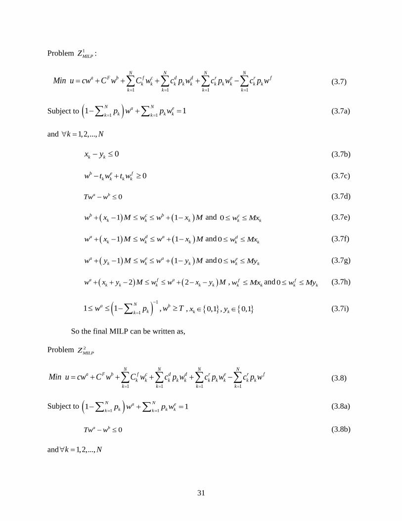
So the final MILP can be written as,

Problem 2

MILPZ

1 1 1 1

N N N Na F b f c d d r e r f

k k k k k k k k k k

k k k k

Min u cw C w C w c p w c p w c p w

(3.8)

Subject to 1 11 1

N Na e

k k kk kp w p w

(3.8a)

0a bTw w (3.8b)

and 1,2,...,k N

32

0k kx y (3.8c)

0b e f

k k k kw t w t w (3.8d)

b c

k kMx w w M (3.8e)

b c

k kMx w w M (3.8f)

0c

k kMx w (3.8g)

a d

k kMx w w M (3.8h)

a d

k kMx w w M (3.8i)

0d

k kMx w (3.8j)

a e

k kMy w w M (3.8k)

a e

k kMy w w M (3.8l)

0e

k kMy w (3.8m)

2a f

k k kMx My w w M (3.8n)

2a f

k k kMx My w w M (3.8o)

0f

k kMx w (3.8p)

0f

k kMy w (3.8q)

1

11 1 ,

Na b

kkw p w T

(3.8r)

0, 0, 0, 0c d e f

k k k kw w w w 0,1 , 0,1k kx y (3.8s)

The final version of problem 2

MILPZ has a total of 2+6N variables for N workstations, (when

N = K), among which ,k kx y are 0-1 binary integers, and , , , , ,a b c d e f

k k k kw w w w w w are positive values.

The constraints (3.8c) to (3.8q) has to be satisfied for all 1,2,...,k N , so there are total 15N

constraints are presented by the inequalities (3.8c) to (3.8q). The total number of constraints in

33

problem 2

MILPZ is 5+15N, including constraints (3.8a), (3.8b), and (3.8r). Given T, FC , c , f

kC , d

kc ,

r

kc , kp , P

kt and R

kt the problem 2

MILPZ can be solved by a mixed-integer branch and bound method.

3.4 Throughput Analysis

Given the processing time P

kt and repair time R

kt for an item at workstation k are known,

the following theorem estimates the throughput rate of the production line. The boundary

conditions extracted from Theorem 3.1, thus, leads to the following theorem and corollaries with

regard to the output performance of the production line with or without defects.

Theorem 3.2: The total time R

kT taken to repair an item at a workstation k through n recycled

reworks (feedbacks) is(1 )

(1 )

n R

k k kR

k

k

p p t

pT

.

Proof: The probability of repairing an item n times at station k is n

kp . So, the total time R

kT taken

to repair an item n times is 2 ( 1)... n n

k k k

R

kkp tp p p = (1 ) / (1 )n R

k k k kp p t p . Hence,

the result. □

Corollary 3.2.1 If the rework process at workstation k also creates defect with the same probability

kp the total time to repair it to a defect-free product is R

kT = / (1 )R

k k kp t p .

Proof: A workstation k has the probability kp to produce a defective item, which is true for rework

operation as well. For some instances, a defective item may be repaired to as good as a non-

defective item in a single repair; but each repair, on the average, has a probability kp of

creating further defect in itself. So, the probability of second repair of the same item is2

kp

(i.e. n = 2) and thus the probability of n repairs on the same item is n

kp . So, the workstation

34

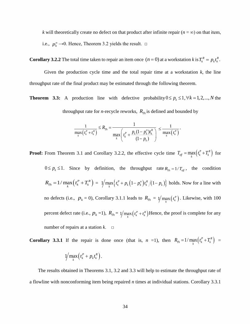
k will theoretically create no defect on that product after infinite repair (n = ∞) on that item,

i.e., n

kp →0. Hence, Theorem 3.2 yields the result. □

Corollary 3.2.2 The total time taken to repair an item once ( 0)n at a workstation k is .R

k

R

k kpT t

Given the production cycle time and the total repair time at a workstation k, the line

throughput rate of the final product may be estimated through the following theorem.

Theorem 3.3: A production line with defective probability0 1kp , 1,2,...,k N the

throughput rate for n-recycle reworks, ThR is defined and bounded by

1

max P R

k kk

t t

1

(1 )max

(1 )

n RP k k kk

T

kk

hp p

t

Rt

p

1

max P

kk

t .

Proof: From Theorem 3.1 and Corollary 3.2.2, the effective cycle time max P R

eff k kk

T t T for

0 1kp . Since by definition, the throughput rate 1/Th effR T , the condition

1/ max P R

Th k kk

R t T = 1 max 1 1P n R

k k k k kk

t p p t p holds. Now for a line with

no defects (i.e., kp = 0), Corollary 3.1.1 leads to ThR = 1 max P

kk

t . Likewise, with 100

percent defect rate (i.e., kp =1), ThR = 1 max P R

k kk

t t Hence, the proof is complete for any

number of repairs at a station k. □

Corollary 3.3.1 If the repair is done once (that is, n =1), then 1/ max P R

Th k kk

R t T =

1 max P R

k k kk

t p t .

The results obtained in Theorems 3.1, 3.2 and 3.3 will help to estimate the throughput rate of

a flowline with nonconforming item being repaired n times at individual stations. Corollary 3.3.1

35

directly estimates the throughput rate of a production line where a nonconforming item is repaired

no more than once at a particular station—which is the case of current study. In the subsequent

Section a case study is presented to solve a configuration problem of some garments production

line and elucidate performance measures of different facets of the line configuration problem.

3.5 A Case Study in Garments Industry

Despite the global ups and down in different industries, the global apparel industry

continues to grow at a healthy rate. The apparel industry is of great importance to the economy in

terms of trade, employment, investment and revenue all over the world. This particular industry

which encompasses clothing, textiles, footwear, garments, and luxury goods has a short product

life cycles, vast product differentiation and is characterized by great pace of demand changes in a

business of $2,560 trillion in 2010 and is expected to generate $3,180 billion only in garments in

2015 with a yearly growth rate in excess of 4% (Huang 2012, Bodimeade 2013). Competition from

garments manufacturing bases in very low-cost nations in Africa, South-east Asia and South

America is intense while most of the developed countries such as USA, Canada and European

conglomerates where the labor cost is high are beneficiaries of the low-cost imported garments.

Thus this labor intensive modern apparel industry is moving up the industrial chain by fostering

manufacturing that requires greater skills, better technology and more investment in advanced

equipment and manufacturing systems design.

On experiencing such an endeavor in a garments industry, a 7-workstation production line is

considered that manufactures T-shirts. The end-product is inspected by a quality inspector at the

end the production line. The company is exploring different options of repairing the defective

items either at the on-line workstation or at an off-line station or totally scrapping the product to

minimize the unit cost of the product (a branded T-short) to compete in the world market.

36

3.5.1 RMG manufacturing industry producing T-shirts

A readymade garments (RMG) manufacturing industry produces a certain design of

branded expensive T-shirt in 10 different 7-workstation flowlines, each of the workstation is doing

separate distinct operations: shoulder joint, right-side seam, left-side seam, collar joint, sleeve

joint, sleeve hem, and bottom hem, as shown in Figure 3.3.

Figure 3.3 Seven different operations on the T-shirt

The operations follow a sequence as shown in Figure 3.4. At the end of a production line

there is a quality control station that inspects all items. Inspection error is negligible. No

workstation is perfect, so each workstation may produce some defects. Defects are independent

and can be identified at the inspection station only. After inspection, defective items are supposed

to be sent back to the workstation from where the defect was initiated.

Main flow of materials Inspection

Station

1

Shoulder

joint

2

R-Side

seam

3

L-Side

seam

4

Collar

joint

5

Sleeve

joint

6

Sleeve

hem

Raw

Material

7

Bottom

hem

Figure 3.4 A branded T-shirt production line with 7 different workstations.

37

There is enough space for setting extra rework-station in the production floor. So,

management wants to decide on each type of defective items whether they should be repaired at a

regular on-line workstation(s) or at dedicated off-line rework-station(s) or the defective items

should be scrapped, in order to ensure minimum cost of production.

The production cycle time is recorded as 90 seconds for this case meaning one item is

produced every 90 seconds at the end of production line. The factory bears a fixed cost of

production $300 per hour for a production line that includes capital, labor and fixed utility costs.

Variable cost of production that includes material and variable utility costs is listed as $12 for an

item no matter whether the item is defective or not. This variable cost includes defective items as

well. All other necessary variable costs and fixed costs involved with each workstation (k =

1,2,…,7) in the first production line are estimated from existing data and listed in Table 3.1. This

problem is formulated as 2

MILPZ in order to solve with branch and bound method (Also see Hillier

and Lieberman 2010, pp. 491-521 for detiled methods). As summarized in the Section 3.3, for a

7-workstation problem there are 5+15(7) = 110 constraints and 2+6(7) = 44 variables among which

14 variables are 0-1 binary integers. Thus there are 142 =16,384 nodes to be explored to find the

optimum result, which is a big problem indeed to elaborately demonstrate.

Table 3.1 Fixed and variable costs involved with different operations

Workstation

k Operation name

f

kC

($/hour)

d

kc

($/unit)

r

kc

($/unit)

Probability of

defects kp

P

kt

(sec/unit)

R

kt

(sec/unit)

1 Shoulder joint 17.00 0.70 4.40 0.0150 65 40

2 R-Side seam 10.50 0.45 3.40 0.0750 88 150

3 L-Side seam 12.50 0.60 6.60 0.0090 87 200

4 Neck joint 7.50 0.95 26.00 0.0027 65 80

5 Sleeve joint 20.00 0.35 4.40 0.0130 90 20

6 Sleeve hem 10.00 0.25 13.20 0.0210 86 160

7 Bottom hem 25.00 1.60 0.84 0.0015 75 120

38

Example 3.1: A four-station production line:

In order to explain the solution procedure, a 4-workstation production line is considered

with an inspection station located at the end of line for demonstrative purposes. Let CF = $300/hour

and c = $12/shirt. Also, as given in Table 3.1, f

kC = {17.00, 10.50, 12.50, 7.50} dollars/shirt, d

kc

= {0.70, 0.45, 0.60, 0.95} dollars/shirt, r

kc = {4.40, 3.40, 6.60, 26.00} dollars/shirt, kp = {0.015,

0.075, 0.009, 0.0027}, P

kt = {65, 88, 87, 65}/3600 hour/shirt, R

kt = {40, 150, 200, 80}/3600

hour/shirt and T=88/3600 hour/shirt.

A branch and bound method is applied on this 4-workstation T-shirt line and illustrated in

Figure 3.5. A total of 59 nodes were explored. Detailed results of each of the nodes are listed in

Appendix A. The optimum result is found at node 46 with (x*, y*) = {(0,1), (1,1), (0,1), (0,0)} and

the minimum unit cost, *u = $19.87/shirt. Here, 1 1( , )x y = (0,1) indicates that the defective items

produced at first workstation should be repaired at the regular on-line workstation 1. Similarly,

2 2( , )x y = (1,1) indicates that defective items produced at second workstation should be repaired

at separate dedicated off-line rework station. Thus in third workstation the repair work has to be

done at the regular workstation 3 and defective items produced (with low probability) at fourth

workstation where the repair of neck-joint is expensive ($26.00/shirt) have to be scrapped. In

reality, usable scrapped products are most often salvaged through discounted sale.

39

Figure 3.5 Branch and bound algorithm result for 4-workstation problem

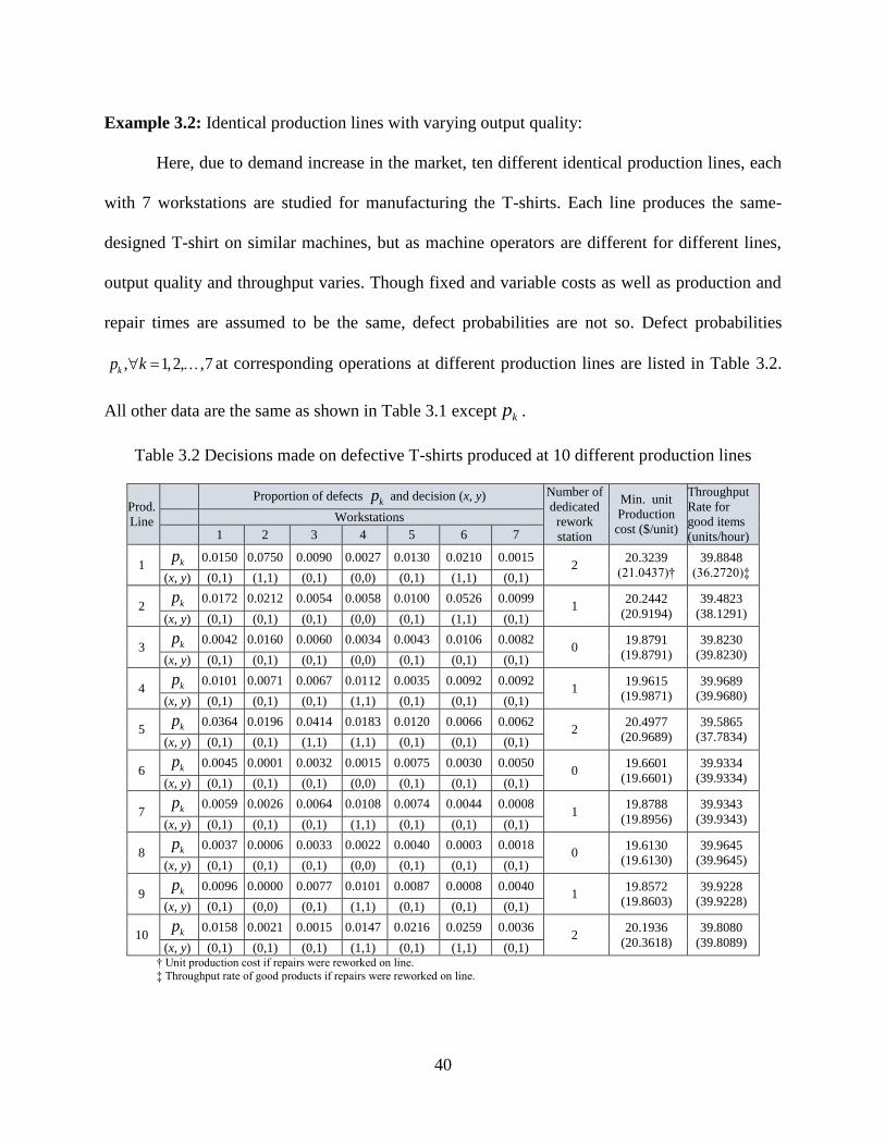
40

Example 3.2: Identical production lines with varying output quality:

Here, due to demand increase in the market, ten different identical production lines, each

with 7 workstations are studied for manufacturing the T-shirts. Each line produces the same-

designed T-shirt on similar machines, but as machine operators are different for different lines,

output quality and throughput varies. Though fixed and variable costs as well as production and

repair times are assumed to be the same, defect probabilities are not so. Defect probabilities

    1,2, , 7,kp k at corresponding operations at different production lines are listed in Table 3.2.

All other data are the same as shown in Table 3.1 except kp .

Table 3.2 Decisions made on defective T-shirts produced at 10 different production lines

† Unit production cost if repairs were reworked on line.

‡ Throughput rate of good products if repairs were reworked on line.

Prod.

Line

Proportion of defects kp and decision (x, y) Number of

dedicated

rework

station

Min. unit

Production

cost ($/unit)

Throughput

Rate for

good items

(units/hour)

Workstations

1 2 3 4 5 6 7

1 kp 0.0150 0.0750 0.0090 0.0027 0.0130 0.0210 0.0015 2

20.3239

(21.0437)†

39.8848

(36.2720)‡ (x, y) (0,1) (1,1) (0,1) (0,0) (0,1) (1,1) (0,1)

2 kp 0.0172 0.0212 0.0054 0.0058 0.0100 0.0526 0.0099 1

20.2442

(20.9194)

39.4823

(38.1291) (x, y) (0,1) (0,1) (0,1) (0,0) (0,1) (1,1) (0,1)

3 kp 0.0042 0.0160 0.0060 0.0034 0.0043 0.0106 0.0082 0

19.8791

(19.8791)

39.8230

(39.8230) (x, y) (0,1) (0,1) (0,1) (0,0) (0,1) (0,1) (0,1)

4 kp 0.0101 0.0071 0.0067 0.0112 0.0035 0.0092 0.0092 1

19.9615

(19.9871)

39.9689

(39.9680) (x, y) (0,1) (0,1) (0,1) (1,1) (0,1) (0,1) (0,1)

5 kp 0.0364 0.0196 0.0414 0.0183 0.0120 0.0066 0.0062 2

20.4977

(20.9689)

39.5865

(37.7834) (x, y) (0,1) (0,1) (1,1) (1,1) (0,1) (0,1) (0,1)

6 kp 0.0045 0.0001 0.0032 0.0015 0.0075 0.0030 0.0050 0

19.6601

(19.6601)

39.9334

(39.9334) (x, y) (0,1) (0,1) (0,1) (0,0) (0,1) (0,1) (0,1)

7 kp 0.0059 0.0026 0.0064 0.0108 0.0074 0.0044 0.0008 1

19.8788

(19.8956)

39.9343

(39.9343) (x, y) (0,1) (0,1) (0,1) (1,1) (0,1) (0,1) (0,1)

8 kp 0.0037 0.0006 0.0033 0.0022 0.0040 0.0003 0.0018 0

19.6130

(19.6130)

39.9645

(39.9645) (x, y) (0,1) (0,1) (0,1) (0,0) (0,1) (0,1) (0,1)

9 kp 0.0096 0.0000 0.0077 0.0101 0.0087 0.0008 0.0040 1

19.8572

(19.8603)

39.9228

(39.9228) (x, y) (0,1) (0,0) (0,1) (1,1) (0,1) (0,1) (0,1)

10 kp 0.0158 0.0021 0.0015 0.0147 0.0216 0.0259 0.0036 2

20.1936

(20.3618)

39.8080

(39.8089) (x, y) (0,1) (0,1) (0,1) (1,1) (0,1) (1,1) (0,1)

41

The branch and bound (B&B) method is also applied here for solving the ten problems to

find the optimum policy of reworking with minimum unit cost of production. Results have been

summarized also in Table 3.2, for all of the 10 production lines where the same-designed of T-

shirt is being manufactured. Here (x, y) in Table 3.2 indicates the prescribed optimal solutions with

number of off-line rework stations, unit production cost and throughput rate for good items in the

last three columns, respectively. For production lines allowing no offline repair have been analyzed

as well. In this case calculations are done by considering very large values for fixed costs of offline

repair stations (i.e. ,d

kc k ) in the existing problem setup such that the possibility of selecting

a dedicated repair workstation is automatically neglected. The unit cost of production and

corresponding throughput rates for good items are calculated from this problem setup (i.e., no

offline repair) and noted in parenthesis in Table 3.2 along with other optimum results. It may be

noted that dedicated offline repair workstation provides cost no more than that obtained under no-

offline repair policy. This offline repair policy advantageously provide no less throughput rate than

that yielded from the online repair system. Though all the system parametric data in Table 3.1

remains unchanged for this problem except kp , various optimal results are not the same due to the

variation in kp . For example, there is no dedicated rework station required for production lines 3,

6 and 8, whereas the number of dedicated off-line rework station required in production lines 1, 5

and 10 is 2 and other production lines require one for each of them.

Figure 3.6 illustrates the prescribed configuration of the T-shirt production line as listed in

Table 3.2. From the results it can be concluded that this production line 1 is needed to facilitate

with two dedicated off-line rework stations, one for the repair works on the defective items

produced at workstation 2 and another for doing so at workstation 6. The defective items produced

at workstation 4 is prescribed to be scrapped, and other type of defects are needed to be sent back

to the regular work stations for doing the corresponding repair works.

42

3.5.2 Empirical test for large problem sets

In order to see how a large problem can be solved using the formulated mixed integer linear

programming problem 2

MILPZ an example has been set for a 40-workstation production line. Data

are randomly generated following uniform distribution within certain range and listed in Appendix

B.1. The regular workstations are engaged in their regular processing operations on the jobs and

also perform some rework operations on the defective items, if necessary. As a result, regular

workstations are mostly facilitated with valuable machines and expert workers. On the other hand,

the off-line dedicated rework stations are devised only for rework operations that do not require

expert workers or costly machines. In some cases the repair costs (fixed and/or variable) at

dedicated rework station become higher due to some costs involved in extra material handling,

frequent machine startup, maintaining additional supply of repair materials, additional fixtures,

complexity in repair, etc. These cost might be unavoidable for the off-line dedicated rework station

but might not be common in corresponding regular workstation. Thus, the costs for repair works

in regular workstation is not necessarily same as the corresponding dedicated rework station.

Keeping these facts in mind, some certain data ranges have been considered during random data

generation.

Scrapping

Off-line rework

Main flow of materials Inspection

Station

1

Shoulder

joint

2

R-Side

seam

3

L-Side

seam

4

Collar

joint

5

Sleeve

joint

6

Sleeve

hem

Raw

Material

7

Bottom

hem

Figure 3.6 A branded T-shirt production line with 7 different workstations.

(Refer to: Example 3.2, Table 3.2, Production line 1)

Rework

station 6

Rework

station 2

On-line rework

43

Fixed cost for the production line is $1,000/hour. This $1,000 is distributed randomly

among 40 workstations. So if first n workstations are considered then fixed cost would be

1

nF F

kkC C

, where F

kC is fixed cost for regular workstation k . Again fixed cost for dedicated

rework stations f

kC are uniformly distributed from $0 to $10 per hour. Similarly, variable cost for

repair at dedicated rework station d

kc and at regular workstation r

kc are uniformly distributed

within $0 to $1 and $0 to $3 per unit, respectively. Proportion of defects kp at the regular

workstations are uniformly distributed within 0 to 0.0175, whereas processing times P

kt are

uniformly distributed with 100 to 120 seconds per unit and repair times R

kt are randomly distributed

within 90 to 600 seconds per unit. Variable cost is c = 6 $/unit. Now 7 distinct problems are tested

assuming that the inspection station is located at the end of each production line comprising of 10,

15, 20, 25, 30, 35 and 40 workstations. For the first instance, first 10 data sets are chosen from

Appendix B.1. Similarly, other examples are set for the first 15, 20, 25, 30, 35 and 40 data sets,

respectively, from Appendix B.1. Calculations are done by “intlinprog” toolbox in Matlab-2014b

on a desktop computer with processor Intel® Core™ i5-2300 CPU 2.8 GHz, RAM 16 GB and

operating system Windows 7 (64-bit). Optimum results are summarized in Table 3.3 along with,

minimum unit cost of production, CPU time and number of nodes searched.

In order to estimate the CPU time and number of node searched (&B BN ) for the empirical

test, data for this 40-workstation line have been randomly generated 10 times within the same

range and following uniform distribution as specified earlier. Although only the first set of data

are provided in Appendix B and it’s optimum results in Table 3.3, the minimum and maximum

CPU time and number of node searched from the ten sets of data are summarized in Table 3.3 as

well. The minimum and maximum values of CPU times and number of nodes searched listed

within the parenthesis were obtained from the 10 datasets including the dataset in Appendix B.1.

44

Table 3.3 Empirical test results for large problem sets

Problem

Number of

workstations

N

Optimum Solutions Average % nodes searched,

2

& 00/ 2 1 %N

B BN (x*, y*)

No. of off-line

rework station

(x, y) = (1,1) MILPu (in $)

CPU (sec)

(min, max)

Nodes Searched, &B BN

min max

& &,B B B BN N

1 10 (0,1), (0,1), (0,1), (0,1), (0,1),

(0,1), (0,0), (0,1), (0,1), (0,1) 0 13.9096

0.59

(0.50, 1.13)

46

(24, 210) 6.072

2 15

(0,1), (0,1), (0,1), (0,1), (0,1),

(0,1), (0,0), (0,1), (0,1), (0,1),

(0,1), (0,1), (0,0), (0,1), (0,0)

0 18.7487 0.78

(0.44, 1.13)

1342

(106, 1342) 1.227

3 20

(0,1), (0,1), (0,1), (0,1), (0,1),

(0,1), (0,0), (0,1), (0,1), (0,1),

(0,1), (0,1), (1,1), (0,1), (0,0),

(0,1), (0,1), (0,1), (1,1), (0,1)

2 23.5337 2.13

(0.56, 2.13)

4858

(230, 4858) 0.0923

4 25

(0,1), (0,1), (0,1), (0,1), (0,1),

(0,1), (0,0), (0,1), (0,1), (0,1),

(0,1), (0,1), (1,1), (0,1), (0,0),

(0,1), (0,1), (0,1), (1,1), (0,1),

(0,1), (1,1), (0,1), (0,1), (0,1)

3 27.0314 9.14

(1.22, 10.30)

27971

(1134, 27971) 0.0193

5 30

(0,1), (0,1), (0,1), (0,1), (0,1),

(0,1), (0,0), (0,1), (0,1), (0,1),

(0,1), (0,1), (1,1), (0,1), (1,1),

(0,1), (0,1), (0,1), (1,1), (0,1),

(0,1), (1,1), (0,1), (0,1), (0,1),

(1,1), (0,1), (0,1), (0,1), (0,1)

5 31.2266 25.80

(6.22, 27.06)

71389

(16490, 71389) 0.0034

6 35

(0,1), (0,1), (0,1), (0,1), (0,1),

(0,1), (0,0), (0,1), (0,1), (0,1),

(0,1), (0,1), (1,1), (0,1), (1,1),

(0,1), (0,1), (0,1), (1,1), (0,1),

(0,1), (1,1), (0,1), (0,1), (0,1),

(1,1), (0,1), (0,1), (0,1), (0,1),

(0,1), (1,1), (0,1), (0,1), (0,1)

6 36.2656 209.55

(8.98, 211.72)

496628

(21664, 496628) 0.00062

7 40

(0,1), (0,1), (0,1), (0,1), (0,1),

(0,1), (0,0), (0,1), (0,1), (0,1),

(0,1), (0,1), (1,1), (0,1), (1,1),

(0,1), (0,1), (0,1), (1,1), (0,1),

(0,1), (1,1), (0,1), (0,1), (0,1),

(1,1), (0,1), (0,1), (0,1), (0,1),

(0,1), (1,1), (0,1), (0,1), (0,1),

(0,1), (0,1), (0,1), (0,1), (0,1)

6 41.4081 220.45

(220.5, 1471)

481238

(481238, 3300002) 0.000139

45

Average number of node searched and average CPU time (in a 10 based logarithmic scale)

are plotted against the problem size. From the Figures 3.7 (a) and 3.7 (b) it is apparently seems

that as problem size increases number of node searched increases exponentially and CPU time

follows a polynomial function of problem size, N.

Figure 3.7 (a) Average node searched (b) Average CPU time vs number of workstations

Total number of possible nodes for this binary integer programming problem could be22 N

, but

all of the nodes were not searched for the branch and bound method. The last column of Table

3.3 presents average percentage of average nodes searched compared to maximum possible

number of nodes22 N

. Percentage of nodes which are not needed to be explored indirectly

represents the efficiency of the optimization process. Lower percentage of nodes searched

indicates higher efficiency of the optimization process. Average percentage of node searched

decreases with the increase of problem size.

3.6 Conclusion of the ELI Problem

Deciding, whether the defective items should be repaired on-line at regular workstation(s)

or off-line at separate dedicated rework station(s) or should be scrapped instead of repair, is an

important concern for making the operational decision in a line production system. This research

dealt with locating rework station on or off the production line wherein the inspection is stationed

at the end of the line. The problem is formulated as a fractional MINLP in order to find the

46

minimum unit production cost optimally. To simplify the solution procedure the f-MINLP is

transformed into an MILP problem. The final version of MILP is solved by a B&B algorithm.

Readymade garments industries are the world’s third largest industrial sector. In an

apparel industry, many garment products are produced. To describe the implication of the

prescribed model a case of a branded T-shirt production line is presented here. The model

presented can effectively make the decision on a defective item whether it should be repaired at

regular on-line workstation or at a separate dedicated off-line rework-station or should be

scrapped. It is observed that, in general, the optimum unit cost of production is lower and

throughput rate for good items is higher for the cases where separate off-line repair station is

prescribed. An empirical study is also presented for large instances. Computational results

indicate that number of node searched by B&B method increases exponentially as problem size

increases and CPU time follows polynomial function in problem size (Hossain and Sarker 2015,

2016). An efficient heuristic is recommended for solving large problems.

In this research a flowline with end-of-line inspection station, is considered. Possibility

of detecting nonconformities within the production line and the multistage inspection facilities

can be considered to remedy other pitfalls (early detection of defects, workload balancing for

quality inspection stations, reducing material wastes etc.) that was not specifically addressed in

the end-of-line inspection problem.

47

CHAPTER 4

MULTISTAGE INSPECTION STATIONS

Many products like large volume garments and electronics or many other engineering parts

and components are produced or assembled in flowlines. In order to ensure product quality that

satisfies the customers’ specifications and demand, the production lines are usually facilitated with

one or more inspection stations. The inspection station identifies defective items and separates

them from defect-free products. The end-of-line inspection (ELI) problem described in Chapter 3

decides whether the defective items should be sent back to original workstation for repair or they

should be re-worked at some off-line rework stations so that regular production is not interrupted,

or they should be scrapped completely instead of repairing. All of the operations need to be

inspected to ensure defect free production. In Chapter 3 the inspection station is not treated as an

inherent part of the production line as it is located at the end of the line. The inspection time does

not affect the regular flow of production in case of ELI. In case of in-line inspection the inspection

time may persist and it is no longer negligible, instead, this should be considered as an affecting

parameter for the cycle time when the total in-line inspection station time becomes higher than the

cycle time of that line. A real difficult problem arises in balancing the line and inspecting the

products when a bottleneck is created due to the higher inspection time at a workstation than the

cycle time. In case of ELI a bottleneck is created at the inspection station if total inspection time

is higher than the cycle time of the line. Therefore, more than one inspection station should be

planned to be located in the line, in some of which case multiple inspectors may be stationed at a

bottlenecked or at other appropriate location(s) to resolve this issue.

The problem becomes more complicated when line length (number of workstations)

increases, and the number and locations of multiple inspection stations are considered as decision

variables. The objective of this chapter is to determine the appropriate decisions on the variables

48

regarding the number and location of in-line inspection stations as well as the repair policies (on-

line/off-line rework or scrap) to keep the production cost per unit of the product at a minimum

level for a large flowline.

4.1 The Multistage Inspection (MSI) Problem

While only one inspection station is located at the end of the line and an item is identified

as ‘defective’ at the end, the repair of it may be costly (or even it could be too late to repair) than

identifying it on line and repairing when it is in process. Some flow production lines could be

considerably large, and hence, it is difficult to be handled by a single inspection station. Thus,

multiple inspection facilities become a necessary part of the problem in which case some

inspection stations are located appropriately between regular workstations in the line. Obviously,

multiple inspection stations facilitated in the line increases the cost. At the same time, defective

items could be repaired before going to the following workstation(s) effectively reducing the waste

of productive time as well as waste of material. So, in-line inspection stations are to be located

optimally that ensures minimum total cost of production. It may be worth mentioning that an

inspection facility could be a person or an equipment that does digital, optical, and magnetic or

other high-tech based inspection.

Consider an m-inspection station production line which is now divided into m stages (or

segments); each stage has  iN ( 1,2, ,  )i m stations in the line consists of one end-of-line

inspection station. If the first stage of the line consists of N1 workstations (i.e., first inspection

station is located after N1 workstations in the line), second stage of the line consists of N2

workstations starting from workstation (N1+1) to workstation (N1+N2), and so on for all m stages.

Thus, the total number of workstations would be N = N1 + N2 + N3 + … + Nm. Figure 4.1 describes

this structure of the production line.

49

Figure 4.1 A flowline with m inspection stations

For a two-workstation (N = 2) flowline, m = 1 or 2. If m = 1, there will be only one

inspection station located at the end of 2-workstation line or at the middle of the line, and for m =

2, each workstation will be followed by an inspection station. Again, if N = 3, the values of m

could be 1, 2, or 3. If m = 2, there could be 3C2 = 3 options for locating 2 inspection stations. For

m = 1 and m = 3 there are 2 other ways to arrange the inspection stations. Thus, for N workstations

arranged sequentially in series there could be 1

N N

mmC

possible ways to arrange the inspection

stations in the line. When N is large, the number of ways to arrange/locate the inspection stations

becomes huge. Moreover, each of the arrangements can generate 3N possible options (on-line, off-

line rework or scrap) or solutions to deal with defective items. The best way to arrange the

inspection stations has to be chosen from among these alternatives that leads to minimum unit

production cost. In this extended problem the number of inspection stations m and each of the

values of   1,2, ,( )iN i m for determining the location of all inspection stations, have to be

determined optimally, in addition to the number and location of off-line rework stations and

scrapping decisions.

4.2 Mathematical Structure of the MSI Problem

In this case, instead of single inspection station, multiple inspection stations are planned to

setup in between regular workstations for in-line inspection of the work-in-processes. Hence, the

IS-1 1 Raw

Material 2 N1

IS-2 1 2 N2

IS-m 1 2 Nm

Finished

Goods Stage 2

Stage 1

Stage m

50

research problem includes new set of objectives as explained previously. In this problem,

  1,2, ,( )iN i m itself is a variable where m is another variable to be determined. Hence, there are

(m+1) new variables in addition to ( , )k kx y in f

MINLPZ in Equation (3.2). The problem has also some

other dimensions in formulating the model with several other constraints such as1

m

iiN N

and

cycle time restriction for multi-stage problems in addition to the existing constraints as explained

in Chapter 3 for the single-stage line. As indicated earlier, the best way to arrange or locate the

inspection stations is to choose from 1

N N

mmC

alternatives that leads to the minimum unit

production cost. So, the total number of feasible solutions to this MSI problem including rework

policy optimization is1

3NN N

mmC

. For a small instance, an existing or a modified search

technique can be applied to solve it optimally, but for a large instance, an efficient heuristic

approach needs to be devised to find a sub-optimal solution.

4.3 Model Formulation

The necessary tasks to accomplish the stated objectives involve identifying the

mathematical structure of the problems, development of solution strategies and solution

methodology, and experimentation with the numerical examples. This section presents the

mathematical formulation of the MSI problem. Some parameters and variables are exclusively

used for formulating this problem only, which are listed below.

(a) System parameters

c Variable cost of production for a finished item if no item is repaired ($/unit)

FC Fixed cost for the production line ($/hour)

F

kC Fixed cost for regular workstation k ($/hour)

51

f

kC Fixed cost for an off-line rework station for operation k ($/hour)

IC Fixed cost for an inspection station ($/hour)

d

kc Variable cost of repairing at dedicated off-line rework station k ($/unit)

I

kc Variable cost of inspection for the operation performed at station k ($/unit)

r

kc Variable cost of repairing at regular on-line workstation k ($/unit)

K Total number of defects, K ≤ N

N Total number of workstations in the line

kp Proportion of defectives of at workstation k

P

kt Processing time of operation at regular workstation k (hours)

R

kt Repair time of defective item at regular workstation k (hours)

I

kt Inspection time for the operation performed at station k (hours)

T Cycle time when no repair work is done (hours)

(b) Intermediate Variables

R

kT Total repair time of an item at regular workstation k (hours)

TC Total cost ($/hour)

(c) Decision Variables

m Number of inspection stations

iN Number of workstations in line segment or stage-i, {1,2,..., }i m

effT Effective cycle time for optimally configured line (hours)

kx (0,1), the number of dedicated off-line rework stations for operation k

52

ky 0-1 binary variable indicting decision on scrapping (0) or repair (1) for a defect

produced at workstation k

(d) Performance Measures

ThR Throughput rate (units/hour)

u Unit production cost ($/unit)

4.3.1 Formulation of the objective function

As discussed in Chapter 3, if the defective items are reworked at the regular workstation k

where the major defects were originated then variable cost per unit ( c ) will increase by

(1 )r

k k k kc p y x , or if the reworks are done at separate dedicated off-line rework station, then c

will increase by d

k k kc p x . Unlike the ELI station problem as in Chapter 3, an MSI problem considers

the inspection costs since the decision on the inspection policy and the configuration of the line

depends on the inspection costs. Some inspection costs are variable that depend on number of

operations inspected. Some operations are complex and they incur relatively high costs and more

time to inspect. Thus, variable inspection costs are operation dependent, while we assumed that

different workstation performs different operations. Variable inspection cost for inspecting an

operation per item is defined as, I

kc ($/unit). Thus, the variable cost for a final product becomes

1

1 .N d r I

k k k k k k k kkc c p x c p y x c

The cycle time of the final product may increase due to

bottleneck at inspection stations or due to the on-line repair works. This updated cycle time (while

considering the optimal line configuration being implemented) is termed as the effective cycle

time ( effT ) for a final product. A flowline with no parallel feeding has a cycle time larger than or

equal to the maximum processing time among all the stations in the line. When no rework

operation is done on-line and/or no in-line inspection station takes longer time than the processing

53

time at any workstations, the cycle time will only depend on the processing time at any

workstation—this scenario may change, if any in-line inspection station takes longer time, or any

on-line rework operation plus processing time becomes longer than the maximum processing time

(excluding rework) among all workstations in the line. In general, the optimal line configuration

may include some on-line rework and/or in-line inspection stations. Thus, the optimally configured

production line may have different cycle time that depends not only on the processing times alone,

but also on the in-line inspection station times and on-line rework times. This updated cycle time

(namely, effective cycle time effT ) could be equal or longer than that of the regular production line

with no in-line inspection or on-line rework options. Eventually the production rate becomes 1/ effT

per hour. So, the variable cost for 1/ effT unit of final products will be

1

1 .N d r I

k k k k k k k k effkc c p x c p y x c T

This variable cost is formulated for a fixed size of line

segment and considering only one inspection station at the end of line.

Now, let us consider that the flowline is divided into two segments as shown in Figure 4.2.

Two inspection station are facilitated, one of them are located following the 1

thN workstation and

the second one is located at the end of the line.

Figure 4.2 A two-stage in-line inspection line

So, for this two-stage inspection, the variable cost for 1 effT units of final product will

become 1 1 2

11 11 1

N N Nd r I d r I

k k k k k k k k k k k k k k k k effk k Nc c p x c p y x c c p x c p y x c T

, which can

IS-1 1 Raw

Material 2 N1

IS-2 N1+1 N1+2 N1+N2

Finished

Goods

Stage 2

Stage 1

54

be written as 1

1

2

11

/ 1i i

i

N N d r I

eff k k k k k k k k effk Ni

c T c p x c p y x c T

, where 0 0N . Again, in case of

a three-stage in-line inspection [see Figure 4.3], the third stage starts from the workstation

1 2 1k N N and ends with the end of the line (i.e., at the workstation, 1 32 k N N N N ). In

general, for a flowline with m stages of inspections, thethi stage of the line consists of iN

workstations starting from 1

0 1+

i

jjk N

to

0

i

jjk N

.

Figure 4.3 A three-stage in-line inspection line.

So, for a m-stage flowline, the total variable cost for1 effT units of final product per hour

can be written as, 0

1

0k=1+

1

/ 1i

jj

i

jj

md r I

eff k k k k k k k k ff

i

N

N ec T c p x c p y x c T

.

The fixed costs involved in offline dedicated rework stations corresponding to the station

k is denoted by, f

kC ($/hour). If the workstation k is facilitated with separate offline rework station

the objective variable kx would have a value of 1kx . As a result, the total fixed cost for offline

rework stations would be0

1

0k=1

1+

i

jj

i

jj

mf

k k

N

iN

C x

. Again, If there are a total of m inspection stations

configured inline and each inspection station has a fixed cost of IC ($/hour) including inspectors’

salary, utilities and other associated costs, then the total fixed cost for dealing with all inspection

IS-1 1 Raw

Material 2 N1

IS-2 1+N1 2+N1 N1+N2

IS-3 N1+N2+1 N1+N2+2 N

Finished

Goods Stage 2

Stage 1

Stage 3

55

stations can be taken as .ImC On the other hand, the fixed cost for the production line, excluding

dedicated rework stations and inspection stations is denoted as FC ($/hour). So, the fixed cost per

hour becomes 0

1

0k=1+

1

i

jj

i

jj

mF I f

k k

i

N

NC mC C x

. Thus, the total cost per hour is given by

0 0

1 1

0 0k=1+ k=1+

1 1

/ 1i i

j jj j

i i

j jj j

m md r I F I f

eff k k k k k k k k eff k k

i

N

N Ni

N

TC c T c p x c p y x c T C mC C x

which can be rearranged as

0 0

1 1

0 0

1 1 1

11

i i

j jj j

i i

j jj j

N Nm

F I f d r I

k k k k k k k k k k

ieff effk N k N

cTC C mC C x c p x c p y x c

T T

. (4.1)

The proportion of defective items originated at workstation k is denoted as kp . While

no repair work is done the proportion of conforming items is given by 1

1N

kkp

. When a repair

work is successfully completed at workstation k (i.e., 1ky ), the proportion of good item increases

by k kp y . So the total increase in the proportion of good items is 1

N

k kkp y

. Thus, completing all

reworks on defective items, the number of conforming (or good) product becomes

1 1[1 ] /

N N

k k k effk kp p y T

units per hour. So, from Eq. (4.1), the unit cost of production, u

($/unit) becomes

0 0

1 1

0 0

1 1 1

1 1

11

[1 ] /

i i

j jj j

i i

j jj j

N Nm

F I f d r I

k k k k k k k k k k

ieff effk N k N

N N

k k k effk k

cC mC C x c p x c p y x c

T T

up p y T

.

which simplifies to

56

0 0

1 1

0 0

1 1 1

1 1

1

[1 ]

i i

j jj j

i i

j jj j

N Nm

F I f d r I

eff eff k k k k k k k k k k

i k N k N

N N

k k kk k

T C mC c T C x c p x c p y x c

up p y

. (4.2)

The unit cost of production, u , presented in Eq. (4.2) is a nonlinear function. The main

objective of the stated problem is to minimize this u . In addition to this unit cost function in Eq.

(4.2), the MSI problem involves some constraints involving effective cycle time effT , rework

stations and inspection stations. Therefore, some boundary conditions need to be constructed on

the objective function and variables for the feasible solution of the problem.

4.3.2 Formulation of the constraints

The objective function and variables are restricted by the system parameters and technical

constraints which practically defines the feasible region of the problem. These constraints are

mathematically interconnected to each other through these system parameters and some boundary

conditions. All of the constraints and their mathematical formulations are discussed in the

following subsections.

(a) Rework policy constraints:

The first constraints that pertain to decision making are the rework policies. This constraint

can be easily interpreted using the physical meaning of the variables, kx and ky . The decision

variables ( , )k kx y corresponds to 0-1 binary integer numbers. If the defective items are repaired

while the prominent defect is originated at workstation k then 1.ky On the other hand, when the

defective items are scrapped instead of repairing, the value of ky becomes 0ky . Again, if the

defective items are reworked at the same regular on-line workstation where the defect generated

then 0kx ; whereas, if the defective items are reworked at a separate dedicated off-line rework

57

station, then 1kx . So, when 0ky , there is no need to have a rework station for off-line repair

works for that defect produced at workstation k, which means 0kx . Thus, 1kx is feasible only

if 1ky . So, ,k kx y ={(1,1),(0,0),(0,1)}are feasible solutions while ( , )k kx y = (1,0) is infeasible

for any k. This conditions can be expressed by the rework policy constraints as

0,k kx y (1,2, , )k N and (0,1)kx , (0,1)ky (4.3)

(b) Inspection station constraint:

It is considered that m inspection stations are placed in the line by partitioning the line into

m stages and locating inspection stations at the end of each stage [see Figure 4.1]. If an inspection

station i is installed in order to inspect iN ( 1,2, , )i m workstations, in other words, if stage i of

the line consists of iN workstations, then the total number of workstation N is given by

1 2 3

1

...m

m i

i

N N N N N N

. (4.4)

(c) Cycle time constraints:

The next two constraints deal with the effective cycle time .effT This research deals with a

flowline with no parallel processing station. All the machines or workers doing the same

processing operation(s) are considered as a single workstation. So the cycle time of the line have

to be greater than or equal to the maximum processing station time (represented in the inequality

4.5) as well as the inspection station time (represented in inequality 4.6). The processing time at

workstation k is denoted as P

kt hours/unit, and the repair time at that workstation k is R

kt

hours/unit. The proportion of defectives at workstation k is kp . If the defective item is repaired

online at the same workstation k , then the effective cycle time might be affected if ( )P R

k k kt p t T

where T is the cycle time of the line with no online rework. The value of (1 )k ky x indicates

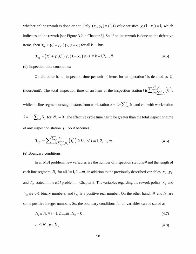
58

whether online rework is done or not. Only ( , )k kx y = (0,1) value satisfies (1 ) 1,k ky x which

indicates online rework [see Figure 3.2 in Chapter 3]. So, if online rework is done on the defective

items, then ( ) (1 )P R

eff k k k k kT t p t y x for all k . Thus,

1 0P R

eff k k k k kT t p t y x , 1,2,..., .k N (4.5)

(d) Inspection time constraints:

On the other hand, inspection time per unit of items for an operation k is denoted as I

kt

(hours/unit). The total inspection time of an item at the inspection station i is 0

1

01

i

jj

i

jj

N I

kk Nt

,

while the line segment or stage i starts from workstation 1

0 1+

i

jjk N

and end with workstation

1 1+

i

jjk N

for 0 0N . The effective cycle time has to be greater than the total inspection time

of any inspection station i . So it becomes

1

1

01

0i

jj

i

jj

N I

eff kk NT t

, 1,2,...,i m . (4.6)

(e) Boundary conditions:

In an MSI problem, new variables are the number of inspection stations m and the length of

each line segment iN for all 1,2,...i m , in addition to the previously described variables kx , ky

and effT stated in the ELI problem in Chapter 3. The variables regarding the rework policy kx and

ky are 0-1 binary numbers, and effT is a positive real number. On the other hand, m and iN are

some positive integer numbers. So, the boundary conditions for all variables can be stated as

, 1,2,...,iN i m , 0 0N , (4.7)

m N , m , (4.8)

59

, 0,1 , 0,1eff k kT T x y (4.9)

The symbol indicates the set of natural numbers such that 1,2,{ 3, }.

4.3.3 Complete formulation of MSI problem

Now, the unit cost function in Eq. (4.2) along with the constraints from Equations (4.3) to

(4.9) constructs a fractional mixed-integer non-linear programming problem, f

MINLPY [as opposed to

f

MINLPZ in Equation (3.2) in ELI problem in Chapter 3]. So the MSI problem can be summarized as

Problem f

MINLPY

Min

0 0

1 1

0 0

1 1 1

1 1

1

[1 ]

i i

j jj j

i i

j jj j

N Nm

F I f d r I

eff eff k k k k k k k k k k

i k N k N

N N

k k kk k

T C mC c T C x c p x c p y x c

up p y

(4.10)

Subject to,

0,k kx y (1,2, , )k N (4.10a)

1 2 3

1

...m

m i

i

N N N N N N

(4.10b)

1 0P R

eff k k k k kT t p t y x , 1,2,...,k N (4.10c)

1

1

01

0i

jj

i

jj

N I

eff kk NT t

, 1,2,...,i m (4.10d)

iN , 1,2,...,i m , 0 0N (4.10e)

m N , m (4.10f)

, 0,1 , 0,1eff k kT T x y ( 1,2,..., ).k N (4.10g)

Finding a solution to Problem f

MINLPY is not trivial since it involves multiple independent and

dependent variables that are intrinsically related. Hence, a transformation is needed to make this

60

problem compatible with an available optimization technique, such as linear programming and

B&B method (Land and Doig 1960) that may have the capability solve an instance of somewhat

practical sizes.

4.4 Solution Methodology

There could be several ways to optimally solve Problemf

MINLPY . An exhaustive search

strategy can be applied for small instances. Another way of finding optimum solution is to

transform Problemf

MINLPY into a form like f

MINLPZ [see Chapter 3]. Then the transformed version of

f

MINLPY can be translated in a form that fits to mixed-integer linear programming (MILP) problem,

that can be solved by B&B method described in Chapter 3. This solution approach needs to adopt

or develop some appropriate exact algorithm for solving large instances, especially an efficient

approach at least to compare with exhaustive search. Moreover, this approach can provide

optimum solution within a reasonable time, as it is experienced for end of line inspection problem

[see Chapter 3]. In order to transform f

MINLPY into a form likef

MINLPZ the following result (Theorem

4.1) will be useful.

Theorem 4.1: 0

1

01

1 1

( )i

jj

i

jj

m NN

k Ni k

f k f k

, where1

m

iiN N

, N0 = 0,

iN , 1,2,...,i m and m N for m .

Proof: Define 0

1

01

1

( )i

jj

i

jj

mN

k Ni

S f k

. Then for 1m and N0= 0,0 1

01 1( ) ( )

N N N

k N kS f k f k

.

Again, for 2m , 0 1 0 1 2 1 2

0 0 11 1 1 1

( ) ( )N N N N N N N N

k N k N N k k

S f k f k f k f k

.

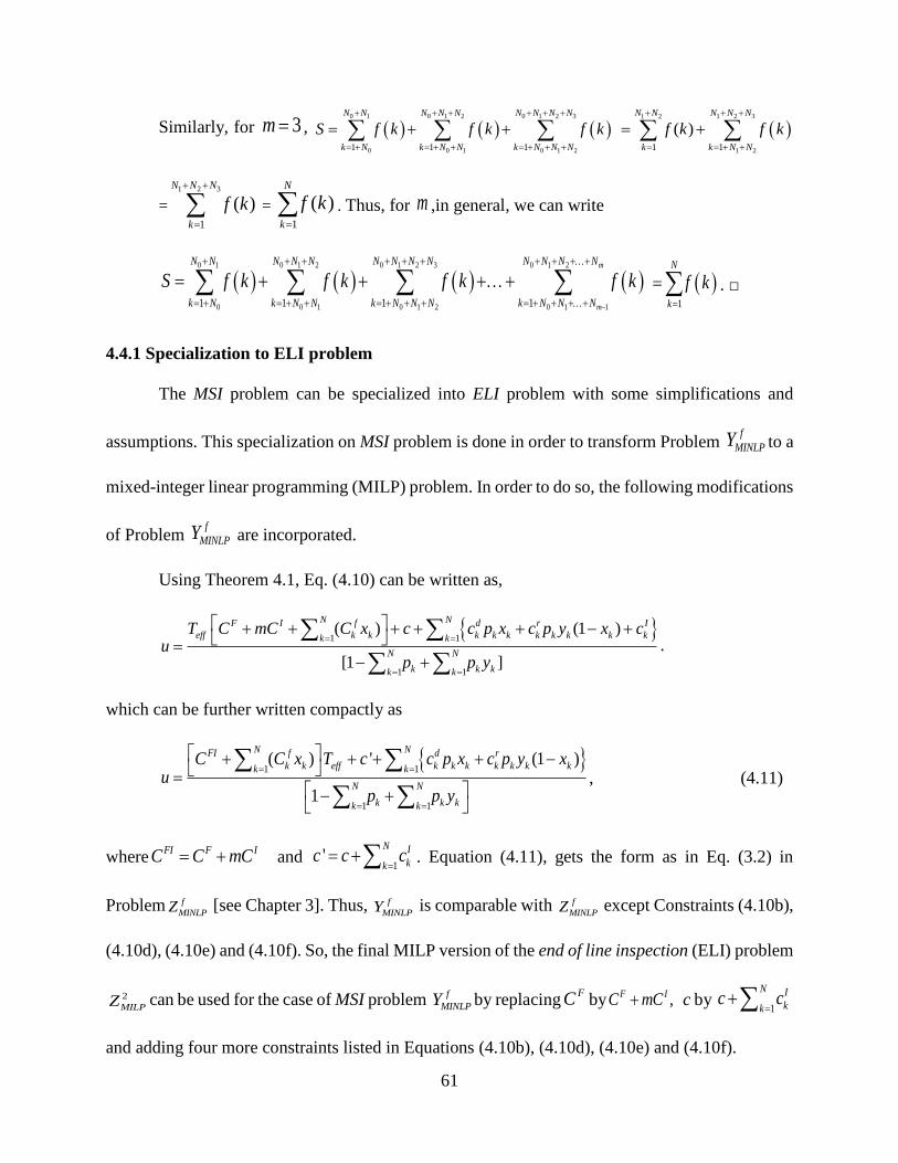
61

Similarly, for 3m , 0 1 0 1 2 0 1 2 3

0 0 1 0 1 21 1 1

N N N N N N N N N

k N k N N k N N N

S f k f k f k

1 2 31 2

1 21 1

( )N N NN N

k k N N

f k f k

=

1 2 3

1

( )N N N

k

f k

= 1

( )N

k

f k

. Thus, for m ,in general, we can write

0 1 0 1 2 0 1 2 3 0 1 2

0 0 1 0 1 2 0 1 11 1 1 1

m

m

N N N N N N N N N N N N N

k N k N N k N N N k N N N

S f k f k f k f k

1

N

k

f k

. □

4.4.1 Specialization to ELI problem

The MSI problem can be specialized into ELI problem with some simplifications and

assumptions. This specialization on MSI problem is done in order to transform Problem f

MINLPY to a

mixed-integer linear programming (MILP) problem. In order to do so, the following modifications

of Problem f

MINLPY are incorporated.

Using Theorem 4.1, Eq. (4.10) can be written as,

1 1

1 1

( ) (1 )

[1 ]

N NF I f d r I

eff k k k k k k k k k kk k

N N

k k kk k

T C mC C x c c p x c p y x cu

p p y

.

which can be further written compactly as

1 1

1 1

( ) (1 )

1

'N NFI f d r

k k eff k k k k k k kk k

N N

k k kk k

C C x T c c p x c p y xu

p p y

, (4.11)

whereFI F IC C mC and

1'

N I

kkc c c

. Equation (4.11), gets the form as in Eq. (3.2) in

Problem f

MINLPZ [see Chapter 3]. Thus, f

MINLPY is comparable with f

MINLPZ except Constraints (4.10b),

(4.10d), (4.10e) and (4.10f). So, the final MILP version of the end of line inspection (ELI) problem

2

MILPZ can be used for the case of MSI problem f

MINLPY by replacingFC by ,F IC mC c by

1

N I

kkc c

and adding four more constraints listed in Equations (4.10b), (4.10d), (4.10e) and (4.10f).

62

In Chapter 3, it is assumed that a b

effT w w . From where, replacing effT by /b aw w and

letting1

01

i

i jjN N

and

0

i

i jjN N

, the constraints in Eq. (4.10d) can be transformed to

''

'/ 0

Nb a I

kk Nw w t

, or

''

'0

Na I b

kk Nw t w

( 1,2,..., )i m .

Now,1

01

i

i j i ijN N N N

0

1i

j ijN N

.1 i iN N So, 1i i iN N N .

Thus, the constraints in Eq. (4.10d) can be replaced by two additional constraints as,

1

'0

i i

i

N Na I b

kk Nw t w

, ( 1,2,..., )i m (4.12)

and 1

01

i

i jjN N

( 1,2,..., )i m . (4.13)

Based on the above discussion, replacingFC by

F IC mC and c by1

N I

kkc c

in to ELI

problem 2 ,MILPZ and including constraints (4.10b), (4.10e), (4.10f), (4.12) and (4.13) the final

transformed MILP version of MSI problemf

MINLPY becomes

Problem MILPY

Min. 1 1 1 11

N N N Na b f c d d r e r f

k k k k k k k k k k

k

NI F I

k

k k k k

u w w C w c p w c p w c p wc c C mC

(4.14)

Subject to 1 11 1

N Na e

k k kk kp w p w

(4.14a)

0a bTw w (4.14b)

1,2,...,k N

0k kx y (4.14c)

0b e f

k k k kw t w t w (4.14d)

b c

k kMx w w M (4.14e)

63

b c

k kMx w w M (4.14f)

0c

k kMx w (4.14g)

a d

k kMx w w M (4.14h)

a d

k kMx w w M (4.14i)

0d

k kMx w (4.14j)

a e

k kMy w w M (4.14k)

a e

k kMy w w M (4.14l)

0e

k kMy w (4.14m)

2a f

k k kMx My w w M (4.14n)

2a f

k k kMx My w w M (4.14o)

0f

k kMx w (4.14p)

0f

k kMy w (4.14q)

1

11 1 ,

Na b

kkw p w T

(4.14r)

0, 0, 0, 0c d e f

k k k kw w w w 0,1 , 0,1k kx y (4.14s)

and 1 2 3

1

...m

m i

i

N N N N N N

(4.14t)

1,2,...,i m

10

i i

i

N Na I b

kk Nw t w

(4.14u)

1

01

i

i jjN N

(4.14v)

iN , 0 0N , m N , m (4.14w)

64

In this problem, m itself is a variable which can be varied from 1 to N. For a given m there

could be N

mC possible combinations of iN . If at least one inspection station is located at the end

of the line, in order to ensure all operations to be inspected, then total number of possible

combinations would be 1

1

N

mC

instead of N

mC . Now, for a given value of m and given combination

of iN , that satisfy Constraints (4.14t), (4.14v) and (4.14w), an optimum result can be obtained

using a B&B method.

Similarly different solutions (minimum u, and ,k kx y ) can be obtained from the problem

setup as ,( 1,2,..., )iN i m without considering Constraints (4.14t), (4.14v) and (4.14w) while the

value of m and Ni are generated such that these satisfy Constraints (4.14t), (4.14v) and (4.14w).

Storing the solutions for all possible values of m and iN starting from 1,m and comparing

among the corresponding u, the optimum solution can be obtained. For obtaining the optimum

solution through this approach, an exhaustive search algorithm presented in Algorithm 4.1 (also

see Figure 4.4) can be followed to solve reasonable sized problem instances.

Algorithm 4.1: Exhaustive Search Algorithm for MSI Problem

Step 0: Initialize m =0

Step 1: Set m = m+1, count j = 0.

Step 2: Generate 1

1

N

mC

combinations of ,( 1,2,..., )iN i m , such that1

m

iiN N

.

Step 3: Calculate, 1

01

i

i jjN N

and

1i i

i

N N I

kk Nt

.

Solve MILPY for ( ), k kx y and /b a

effT w w .

Store resultsju ,

jm , j

iN , , j

k kx y , j

effT .

Step 4: Set 1j j . If 1

1

N

mC j

go to Step 3.

Step 5: If m N go to Step 1.

Step 6: Return, * ) ( ju min u and corresponding

*m , *

iN , *

, k kx y , *

effT .

Step 7: Stop.

65

Figure 4.4 Exhaustive search algorithm for optimal solution of MSI problem

4.5 Case Study

In Chapter 3, two different sets of examples have been discussed. One set of examples

deals with 10 identical garments production lines with varying defect proportions [see Example

3.2, Chapter 3] and another set of empirical test problems [Example 3.3] presented in Chapter 3,

is solved using a B&B algorithm for a mixed-integer linear programming problem. In each of these

Store results , , , ,

Calculate, and

Return, and ,

, ,

Initialize m =0

Yes

No

Set, count j =0

Generate possible combinations of

, such that

No

Yes

Solve for and

66

sets of examples, the objective was to find the rework policy (on-line/off-line rework or scrap),

considering only one inspection station at the end of the line.

It is noticeable that, the end of line inspection station does not affect the regular production

flow of line, and hence, in the examples in Chapter 3 the inspection time at the inspection station

was not considered assuming that the total inspection time is less as compared to the cycle time of

the line. The complicated problem arises when total inspection time is either greater than at least

one station time or more than the cycle time. This problem creates a bottleneck problem on the

smooth flow of the production of the line or creates a “blocking phenomenon” causing an induced

stoppage of the production line. In this chapter, the same examples are presented along with the

considerable length of inspection times for each operations and a new set of variables, the number

and location of multiple inspection stations.

Example 4.1: Production lines with multiple inspection stations and varying defect proportions:

A garments product (branded T-shirt) is being produced in ten identical production lines.

Seven operations are performed at seven different workstations in each of the T-shirts. Though the

corresponding machines are identical in ten production lines the manpower requirements are not

the same. Garments production are highly human-labor oriented. Hence, the defect proportion

varies in different production lines. The fixed and variable costs as well as the unit times (which

are same in corresponding stations in each of the ten production lines) involved in processing

stations and rework stations are considered to be the same as those in Example 3.2, Chapter 3.

The problem is to determine the optimum number and location of inspection stations as

well as the rework policy (on-line/off-line rework or scrap) for each type of processing defects,

which eventually minimizes the unit cost of production given that the fixed cost for the line is FC

67

=$300 per hour (which includes the fixed cost for the ELI station). Each additional inspection

station will add IC (=$30 per hour) to the fixed cost of the line.

Table 4.1 Cost and time data used in processing, rework and inspection

Workstation

k

Operation

name

f

kC

($/hour)

d

kc

($/unit)

r

kc

($/unit)

P

kt

(sec/unit)

R

kt

(sec/unit)

I

kt

(sec/unit)

1 Shoulder joint 17.00 0.70 4.40 65 40 35.28

2 R-Side seam 10.50 0.45 3.40 88 150 14.4

3 L-Side seam 12.50 0.60 6.60 87 200 22.32

4 Neck joint 7.50 0.95 26.00 65 80 5.4

5 Sleeve joint 20.00 0.35 4.40 90 20 13.68

6 Sleeve hem 10.00 0.25 13.20 86 160 5.76

7 Bottom hem 25.00 1.60 0.84 75 120 27.36

So, in this example, the fixed cost for the line becomes ( 1) .F IC m C Again, the variable

inspection cost, i.e., the inspection cost ( )I

kc per T-shirt for all operation k, are summed up and

included in the variable production cost. Thus,1

N I

kkc c

= $12/shirt, as recorded. Other costs

and times are listed in Table 4.1. The defect proportions for each of the seven operations in ten

different production lines are listed in Table 4.2. Now, following the approach of exhaustive search

algorithm presented in Figure 4.4, the optimum results are obtained. For 1m , there will be only

one inspection station which is supposed to be located at the end of the line. So there is only one

option for locating the inspection station in case of 1.m

Again for 2m , there would be 6 different options—one inspection station locating at the

end of the line and another inspection station locating at 6 other locations in the line. Thus, iN

( 1,2)i that corresponds to the location of inspection station has possible combinations of (1, 6),

(2,5), (3,4), (4,3), (5,2) and (6,1) for 2m , where the first number in the parentheses indicate the

number of workstation before the 1st inspection station and the second number indicate the number

68

of workstation before the 2nd inspection station, that satisfy constraints (4.14t), (4.14v) and

(4.14w).

Table 4.2 Proportion of defects ( kp ) in ten different production lines

The alternative combinations of iN ( 1,2i ), gives different results as listed in Table 4.3.

Among these 6 alternative combinations, 1 1N and 2 6N gives minimum cost of production

per unit of T-shirt ($21.075/shirt). The corresponding rework policies represented by ( , )k kx y are

(0,1), (1,1), (0,1), (0,0), (0,1), (1,1) and (0,1); number of off-line rework station is 2; and

throughput rate is 39.88 shirts/hour. The total CPU time for evaluating all alternatives (when

2)m is 0.577 seconds.

Similarly, for 1,2,...,7m the minimum unit production cost (u) and corresponding results

are listed in Table 4.4. Among seven alternatives of m (1,2,…,7), 2m gives the minimum unit

production cost, which is highlighted in Table 4.4, wherein the optimum solution for the

production line-1 is obtained as, 2m , 1 1N , 2 6N , and ( , )k kx y are (0,1), (1,1), (0,1), (0,0),

(0,1), (1,1) and (0,1), respectively, for 1,2,...,7k .

Production

line

Workstations

1 2 3 4 5 6 7

1 0.0150 0.0750 0.0090 0.0027 0.0130 0.0210 0.0015

2 0.0172 0.0212 0.0054 0.0058 0.0100 0.0526 0.0099

3 0.0042 0.0160 0.0060 0.0034 0.0043 0.0106 0.0082

4 0.0101 0.0071 0.0067 0.0112 0.0035 0.0092 0.0092

5 0.0364 0.0196 0.0414 0.0183 0.0120 0.0066 0.0062

6 0.0045 0.0001 0.0032 0.0015 0.0075 0.0030 0.0050

7 0.0059 0.0026 0.0064 0.0108 0.0074 0.0044 0.0008

8 0.0037 0.0006 0.0033 0.0022 0.0040 0.0003 0.0018

9 0.0096 0.0000 0.0077 0.0101 0.0087 0.0008 0.0040

10 0.0158 0.0021 0.0015 0.0147 0.0216 0.0259 0.0036

69

Table 4.3 Rework policy for six alternatives of iN ( 1,2i ) for Production line 1

iN

1,2i

Rework policy ( ,x y ) for

workstations:

Number of

off-line

rework

station

Min. unit

Production

cost ($/unit)

Throughput

Rate for

good items

(units/hour)

CPU time

(sec.) 1 2 3 4 5 6 7

1,6 x 0 1 0 0 0 1 0

2 21.0752 39.885 0.6864 y 1 1 1 0 1 1 1

2,5 x 0 1 0 0 0 1 0

2 21.0767 39.885 0.2340 y 1 1 1 0 1 1 1

3,4 x 0 1 0 0 0 1 0

2 21.0767 39.885 0.3588 y 1 1 1 0 1 1 1

4,3 x 0 1 0 0 0 1 0

2 21.0767 39.885 0.2496 y 1 1 1 0 1 1 1

5,2 x 0 1 0 0 0 1 0

2 21.1567 39.526 0.2496 y 1 1 1 0 1 1 1

6,1 x 0 1 0 0 0 0 0

1 21.7121 37.175 0.1872 y 1 1 1 0 1 1 1

Note:iN n means there are n workstations in the line segment i

Table 4.4 m-inspection station location in Production line 1 (optimum rework policy)

The optimum solution is interpreted here in terms of the physical meaning of the variables.

To obtain minimum unit cost of production there should be two (as 2m ) inspection station in the

m iN

1,2,...,i m

Rework policy

( ,x y ) for workstations

Number of

dedicated

rework

stations

Minimum

unit

Production

cost ($/unit)

Throughput

Rate for good

items

(shirts/hour)

CPU

time

(sec.)

1 2 3 4 5 6 7

1 7 x 0 0 0 0 0 0 0

0 23.128 28.986 0.468 y 1 1 1 0 1 1 1

2 1, 6 x 0 1 0 0 0 1 0

2 21.075 39.885 0.577 y 1 1 1 0 1 1 1

3 1, 1, 5 x 0 1 0 0 0 1 0

2 21.829 39.885 1.217 y 1 1 1 0 1 1 1

4 1, 1, 1, 4 x 0 1 0 0 0 1 0

2 22.585 39.885 1.591 y 1 1 1 0 1 1 1

5 1, 1, 1, 1, 3 x 0 1 0 0 0 1 0

2 23.338 39.885 1.170 y 1 1 1 0 1 1 1

6 1, 1, 1, 1, 1, 2 x 0 1 0 0 0 1 0

2 24.092 39.885 0.484 y 1 1 1 0 1 1 1

7 1, 1, 1, 1, 1, 1, 1 x 0 1 0 0 0 1 0

2 24.846 39.885 0.094 y 1 1 1 0 1 1 1

70

line; the first inspection station needs to be located after the first work station (as 1 1N ) and second

one should be located at the end of the line. The values of ( , )k kx y represents the rework policies.

Here, ( , )k kx y =(0,1) corresponding to 1,3,5k and 7 indicates the on-line rework of the major

defects generated at workstations 1,3,5 and 7, whereas ( , )k kx y = (1,1) corresponding to k 2 and

6 indicates the off-line rework of the major defects produced at workstation 2 and 6. Further,

4 4( , )x y = (0,0) corresponding to 4k means that the major defects produced at workstation 4 need

to be scrapped instead of being reworked.

In a similar way, the optimum results for ten different production lines are obtained and

listed in Table 4.5. These results are calculated by following the exhaustive search algorithm

presented in Figure 4.4, as well. Though the costs and station times are assumed to be the same in

ten different production lines, the results differs due to the variation in defect proportions.

The optimum rework policy (on-line/off-line rework, scrapping) as well as the number of

off-line rework stations, and the location of rework and inspection station vary in different

production lines. For illustrating the solution, the optimum configuration of Production line 2 is

presented in Figure 4.5. In production line 2, the optimum configuration consists of only one

offline rework station corresponding to sixth workstation that does sleeve hem operation, and of

Scrapping

Off-line rework

Main flow of materials IS-2

1

Shoulder

joint

2

R-Side

seam

3

L-Side

seam

4

Collar

joint

5

Sleeve

joint

6

Sleeve

hem

Raw

Material

7

Bottom

hem

Figure 4.5 Optimum configuration of Production line 2 (Example 4.1, Table 4.5)

Rework

station 6

On-line rework

IS 1

IS Inspection Station

71

the two inspection stations, the first one inspects shoulder joint and right-side seam operations,

and the second one inspects rest of the operations.

Table 4.5 Optimum results for ten identical production lines of branded T-shirt

*End of line inspection (when 1m ) problem solution.

4.5.1 Special case

This identical production lines problem converges to the same problem and provides the

same result as in Example 3.2 in Chapter 3, when two conditions are satisfied: (a) only one

inspection station is allowed, which is located at the end of the line (i.e., 1m ), and (b) total

inspection time is less than the effective cycle time (i.e., 1

N I

k effkt T

. The first condition is

obvious, because Chapter 3 deals with end of line inspections only. The second condition can be

proved as in Theorem 4.2.

Prod.

line m iN

Rework policy ( ,x y )

for workstations:

Number of

dedicated

rework station

Minimum unit

Production

cost ($/unit)

Throughput Rate for

good items

(units/hour) 1 2 3 4 5 6 7

1 2 1, 6 x 0 1 0 0 0 1 0

2 21.075

(23.129)*

39.885

(28.986)* y 1 1 1 0 1 1 1

2 2 2, 5 x 0 0 0 0 0 1 0

1 21.006

(23.102)

39.482

(28.985) y 1 1 1 0 1 1 1

3 2 2, 5 x 0 0 0 0 0 0 0

0 20.635

(22.705)

39.823

(28.986) y 1 1 1 0 1 1 1

4 2 1, 6 x 0 0 0 1 0 0 0

1 20.712

(22.863)

39.969

(28.986) y 1 1 1 1 1 1 1

5 2 2, 5 x 0 0 1 1 0 0 0

2 21.250

(23.271)

39.587

(28.986) y 1 1 1 1 1 1 1

6 2 1, 6 x 0 0 0 0 0 0 0

0 20.399

(22.502)

40.000

(28.986) y 1 1 1 0 1 1 1

7 2 1, 6 x 0 0 0 1 0 0 0

1 20.630

(22.815)

39.934

(28.986) y 1 1 1 1 1 1 1

8 2 2, 5 x 0 0 0 0 0 0 0

0 20.365

(22.463)

39.964

(28.986) y 1 1 1 0 1 1 1

9 2 1, 6 x 0 0 0 1 0 0 0

1 20.608

(22.725)

39.923

(28.986) y 1 0 1 1 1 1 1

10 2 1, 6 x 0 0 0 1 0 1 0

2 20.945

(23.149)

39.809

(28.986) y 1 1 1 1 1 1 1

72

Theorem 4.2: For MSI problem, f

MINLPY converges to f

MINLPZ in ELI problem if 1

N I

k effkt T

,

given that 1N N (i.e., ELI only).

Proof: When one inspection station is allowed, 1m , and 1N N ; hence, the constraints in

Equations (4.10b), (4.10e) and (4.10f) are satisfied. Now, the condition

1

1

01

0i

jj

i

jj

N I

eff kk NT t

in Equation (4.10d) reduces to, 1

0N I

eff kkT t

for

1i , where1

11 jjN N N

, and

1 1

000jj

N N

. Thus it becomes

1

N I

k effkt T

, which also leads to satisfy Equation (4.10d). Thus Problem

f

MINLPY

becomes the same as Problemf

MINLPZ . □

This research deals with a flowline, so the effective cycle time indicates the maximum

station time (includes processing, inspection and rework time) among all stations in the line. None

of the ten production lines in Example 4.1 satisfy Equation (4.10d), even when 1m , and 1N N

are satisfied. As a result, when 1m , the bottleneck is generated at the end of line inspection

station, in other words, the cycle time effT are dominated by the inspection time. Hence, the

minimum unit costs of production are higher, and corresponding throughput rates are lower than

the results presented in Example 3.2 [see in Chapter 3].

4.6 Sensitivity Analysis

The primary objective of this research is to determine the optimum number and locations

of rework and inspection stations that minimize the unit cost of production (u). It is observed from

Eq. (4.10) that the unit cost of production, u is directly related to the inspection and rework costs

as well as time. From Equations (4.10c), (4.10d) and (4.10g) the effective cycle time effT can be

73

written as, 1

1

01

max ,( ) (1 ), ( )i

jj

i

jj

NP R I

eff k k k k k kk NT T t p t y x t

, 1,2,...,k N , which is

directly related to inspection time, I

kt and rework time R

kt . Again Eq. (4.10) can be written as

1 1 1

1 1

( ) ( ) (1 )

[1 ]

N N NF I f I d r

eff k k k k k k k k k kk k k

N N

k k kk k

T C mC C x c c c p x c p y xu

p p y

,

which clarifies a joint interacting effect of effT and the fixed cost of inspection station, IC , as well

as effT and the fixed cost of off-line rework stations, f

kC . The expression of u further illustrates a

linear dependency of u on variable costs of off-line reworks ( d

kc ), on-line reworks ( r

kc ) and

inspections ( I

kc ).

In order to investigate the sensitivity of u with respect to the inspection and rework

parameters (cost and time) a sensitivity analysis is done on the production line 1 in Example 4.1.

For doing so, the rework and inspection related parameters (5

fC , 5

dc , 5

rc , 5

Rt , 5

It andIC ) involved in

workstation 5 (arbitrarily chosen workstation) in the first production line [see Example 4.1] is

varied with 15 randomly generated data points for each parameter [data presented in Appendix

B.2] and the problem MILPY is solved for minimum unit cost of production *( )u . Each time only

one parameter of workstation 5 is changed, keeping the other parameters fixed at the original point

as presented in Table 4.1, Example 4.1.

Thus, for each parameter of the set (5

fC , 5

dc , 5

rc , 5

Rt , 5

It andIC ), 15 different solutions of the

Problem MILPY were found corresponding to each individual parameters involved with workstation

5. This results show a strong linear relationship of 5

Rt and IC with

*u , as shown in Figures 4.6(a)

and 4.6(b). The minimum unit production cost, *u shows a third degree polynomial relationship

74

with 5

rc [see Figure 4.6 (c)]. Sensitivity of *u with respect to

5

fC , 5

dc , 5

It is not found to be

prominent for the instance.

(a)

(b)

(c)

Figure 4.6 Sensitivity of *u with respect to (a) 5

Rt , (b) IC and (c) 5

rc

75

4.7 Conclusion of the MSI Problem

This Chapter deals with a multistage inspection (MSI) problem, where multiple inspection

stations are allowed to be located in-line to inspect the quality defects of work-in-progress. The

primary objective of the present research is to determine the optimum number and location of

inspection stations in addition to find out the optimal rework policies (on-line/off-line rework or

scrap) for each type of quality defects.

The problem is formulated as a fractional mixed integer non-linear programming problem

( )f

MINLPY . Then, Problem f

MINLPY is transformed into a mixed integer linear programming problem

( )MILPY . An algorithm for solving Problem MILPY is presented, that obtains the optimum number and

locations of inspection stations by an exhaustive search approach and finds the optimum rework

policies by linear programming and B&B method. An example for ten production lines with seven-

workstations (in each line) is solved optimally with this approach.

From the results, it is observed that the optimum solution *( )u is highly sensitive to the

repair time ( )R

kt and the variable cost of repair ( )r

kc at a station; and it is also sensitive to the fixed

cost of inspection stations ( )IC . The relationship of *u with

R

kt and IC are found to be linear for the

instance, whereas, *u and 5

rc follows a polynomial relationship.

The ELI problem becomes a special case of MSI problem, when if only one inspection

station is allocated at the end of line and total inspection time is lower than the effective cycle time

of the line. Thus, the results of Example 4.1 (Multistage inspection) coincides with the results of

Example 3.2 (End-of-line inspection) when these two conditions are satisfied. However, the

inspection times presented in Example 4.1 does not satisfy the second condition, as a results the

optimum solution for unit production cost, *u is found to be higher while only one inspection station

76

is allocated (at the end of the line). Thus, multistage inspection stations reduce the unit production

cost more as compared to the ELI solution when total inspection time is higher than the effective

cycle time of the line.

The exhaustive search approach presented in this Chapter can find the optimal solution to

MSI problem, but this approach is inefficient for solving an instance with a large line. The

exhaustive search algorithm solves MILP problems with B&B method, and the number of MILP

solutions, as well as the number of node searched in B&B method (see Chapter 3, Section 3.5.2)

increases exponentially with the increase of number of workstations. Thus an efficient heuristic is

needed to solve the MSI problem for large instances.

77

CHAPTER 5

INSPECTION STATION ASSIGNMENT (ISA): A CONTRUCTION HEURISTIC

In Chapter 3, an end-of-line inspection (ELI) problem was modeled and investigated with

certain set of problem instances, especially with an implied application to garments industry. This

problem reflected a typical, traditional flowline problem with a single inspector checking the end-

product, as an application to many small manufacturing systems, and passing its quality

specifications as to the acceptance, rework or rejection of the products.

Further, more complicated issues ensue from such a production line when the line length

becomes quite long as in garments industry, electronic assembly systems, automobile production

and many other large discrete manufacturing systems. Different facets (cost of production,

throughput rate, inspection station assignment, stage configuration, rework policies, computational

time, etc.) of the problems also surface out when multiple inspectors are to be deployed in the line

to check on the quality conformation of the products. Decisions become a function of convoluted

issues of the assignment of inspectors on the line, partitioning the whole line to multiple stages so

as to optimally and judiciously determine the stage size (number of workstations) and ascribing

the configuration of the inspection whether the inspected products should be scrapped or reworked

in-line or off-line. These issues have been addressed theoretically in Chapter 4.

The solution approach presented in Algorithm 4.1 (exhaustive search algorithm) is tested

for the multistage inspection (MSI) problem with the data set used in Example 3.3. Here, the

objective of the MSI problem is to find the rework policy (on/off-line inspection or scrapping) as

well as location of in-line inspection stations. One inspection station has to be located at the end

of the line for the final inspection and other inspection stations are to be located in-line judiciously.

As indicated in previous chapters, finding an optimal solution for a long flowline problem

is not a trivial task since the computational time increases exponentially. Thus, an efficient

78

heuristic, if devised considering the general nature of the problem, may give encouraging results

in terms both performance and computational time. In this chapter, an Inspection Station

Assignment (ISA) heuristic which generates a construction solution, is developed. The assignment

strategy that will employ combinatorial approach partly to determine the multistage size of the line

will try to minimize the unit cost of production. Before devising the heuristic few discussions are

needed to isolate the general characteristics of the MSI problem.

5.1 Multistage Inspection Station: Extraction of the General Characteristics

The general characteristics of the problems are based on the system parameters and general

system mechanism. Thus a few system data are necessary to define here and elucidate the behavior

of the system through some specific numerical study.

Consider a 40-workstation flowline for which the data are extracted from Appendix B.1

which has data for 40 workstations. The times (I

kt ) for inspecting the operations done in each

workstations ( 1,2,...,40)k are listed in Appendix B.1, along with other necessary data for each

individual workstations k , including ,F

kC the fixed costs for workstations ($/hour); ,f

kC the fixed

costs for off-line rework stations ($/hour); ,d

kc the variable costs for off-line repairs ($/unit); ,r

kc

the variable cost for regular on-line repair ($/unit); ,kp the defect proportions; ,P

kt the processing

times (hours/unit) and ,R

kt the repair times (hours/unit). In addition, each inspection station adds

extra cost IC ($50 per hour) to the fixed cost of the line. Variable cost that includes variable

inspection costs, is c ($6/unit). Tweenty seven problems are generated from the dataset presented

in Appendix B.1, with a varying number of workstations (i.e., the length of the production line),

starting from 1N to 25N , 30N and 35N . There is no space limitation in the line, so any

number of inspection and rework station can be allocated for the line.

79

Table 5.1 Empirical test results for 15 workstation example, using exhaustive search algorithm

m iN , ( 1,2, ,i m ) * *( , )x y MILPu

($) CPU (sec)

ThR

(units/ hour)

1 15

(0,1), (0,1), (0,1), (0,1), (0,1),

(0,1), (0,0), (0,1), (0,1), (0,1),

(0,1), (0,1), (0,1), (0,1), (0,1)

42.806 0.468 11.223

2 6,9

(0,1), (0,1), (0,1), (0,1), (0,1),

(0,1), (0,0), (0,1), (0,1), (0,1),

(0,1), (0,1), (0,1), (0,1), (0,1)

28.612 2.605 20.576

3ϯ 4,4,7

(0,1), (0,1), (0,1), (0,1), (0,1),

(0,1), (0,0), (0,1), (0,1), (0,1),

(0,1), (0,1), (1,1), (0,1), (0,0) 23.864 15.709 29.715

4 1,5,2,7

(0,1), (0,1), (0,1), (0,1), (0,1),

(0,1), (0,0), (0,1), (0,1), (0,1),

(0,1), (0,1), (1,1), (0,1), (0,0)

25.563 77.938 29.715

5 1,1,5,6,2

(0,1), (0,1), (0,1), (0,1), (0,1),

(0,1), (0,0), (0,1), (0,1), (0,1),

(0,1), (0,1), (1,1), (0,1), (0,0)

27.262 283.469 29.715

6 1,1,1,2,4,6

(0,1), (0,1), (0,1), (0,1), (0,1),

(0,1), (0,0), (0,1), (0,1), (0,1),

(0,1), (0,1), (1,1), (0,1), (0,0)

28.950 633.598 29.715

7 1,1,1,1,1,4,6

(0,1), (0,1), (0,1), (0,1), (0,1),

(0,1), (0,0), (0,1), (0,1), (0,1),

(0,1), (0,1), (1,1), (0,1), (1,1)

30.633 1016.269 29.715

8 1,1,1,1,1,1,3,6

(0,1), (0,1), (0,1), (0,1), (0,1),

(0,1), (0,0), (0,1), (0,1), (0,1),

(0,1), (0,1), (1,1), (0,1), (1,1)

32.315 1314.745 29.715

9 1,1,1,1,4,1,1,1,4

(0,1), (0,1), (0,1), (0,1), (0,1),

(0,1), (0,0), (0,1), (0,1), (0,1),

(0,1), (0,1), (1,1), (0,1), (1,1)

33.998 1022.696 29.715

10 1,1,1,1,4,1,1,1,1,3

(0,1), (0,1), (0,1), (0,1), (0,1),

(0,1), (0,0), (0,1), (0,1), (0,1),

(0,1), (0,1), (1,1), (0,1), (1,1)

35.681 598.233 29.715

11 1,1,1,1,1,1,1,1,1,1,5

(0,1), (0,1), (0,1), (0,1), (0,1),

(0,1), (0,0), (0,1), (0,1), (0,1),

(0,1), (0,1), (1,1), (0,1), (1,1)

37.363 351.267 29.715

12 1,1,1,1,1,1,1,1,1,1,1,4

(0,1), (0,1), (0,1), (0,1), (0,1),

(0,1), (0,0), (0,1), (0,1), (0,1),

(0,1), (0,1), (1,1), (0,1), (1,1)

39.046 131.524 29.715

13 1,1,1,1,1,1,1,1,1,1,1,1,3

(0,1), (0,1), (0,1), (0,1), (0,1),

(0,1), (0,0), (0,1), (0,1), (0,1),

(0,1), (0,1), (1,1), (0,1), (1,1)

40.729 35.303 29.715

14 1,1,1,1,1,1,1,1,1,1,1,1,1,2

(0,1), (0,1), (0,1), (0,1), (0,1),

(0,1), (0,0), (0,1), (0,1), (0,1),

(0,1), (0,1), (1,1), (0,1), (1,1)

42.411 5.429 29.715

15 1,1,1,1,1,1,1,1,1,1,1,1,1,1,1

(0,1), (0,1), (0,1), (0,1), (0,1),

(0,1), (0,0), (0,1), (0,1), (0,1),

(0,1), (0,1), (1,1), (0,1), (1,1)

44.094 0.390 29.715

Total CPU time= 5489.643

ϯ Optimum solution ( 1 4,N 2 5N and 3 6N for 3m )

80

At first, the solution for a 15-workstation flowline is presented in details. As indicated, the

variable cost of production is assumed as 6c $/unit and fixed cost for an inspection station is

IC =$50/hour. Other parameters ,F

kC ,f

kC ,d

kc ,r

kc ,kp ,P

kt R

kt and I

kt ( 1,2,...,15)k are adopted

from the first 15 rows of Appendix B.1, (i.e., from 1-15 rows).

Now, for all possible values of m ( 1,2,...,15)m , the best MILPY solutions for all

alternative combinations of iN ( 1,2,..., )i m are listed in Table 5.1. Among all of the MILPY

solutions, 3m and (4,4,7)iN for 1,2i and 3, respectively, gives the minimum MILPu which is

$23.86/unit. Hence, this is the optimum solution with corresponding throughput rate of 29.715

units/hour. This exhaustive search on m inspectors and iN stations (for i = 1, 2 and 3) took about

5490 seconds (i.e., 91.5 minutes).

5.1.1 Characterization of performance measures: impact of system parameters

Some important relationships of minimum unit cost (*u ), CPU time and throughput rate

( 1/ )Th effR T with the number of inspection station ( m ), and also the unit cost (*u ) with the location

of inspection stations are observed here. These relationship will elucidate several points that are

pertinent to the design issues of the MSI problem.

(a) Minimum unit cost:

The minimum unit cost (*u )obtained from MILPY solution varies with respect to the number

of inspection station ( m ) [see Figure 5.1]. At the beginning, the value of *u decreases as a convex

function with the increase of m , but after a certain value ( 3m ) it starts increasing more or less

linearly from 4.m

81

Figure 5.1 Impact of m on *  u in a 15-workstation line

(b) CPU time:

CPU time shows a bell-shape relationship with respect to m which seems symmetric

against the midpoint of the domain of m [see Figure 5.2]. This indicates that the maximum CPU

time is taken by the computation when number of inspection station is 8m , that is, half the line

length. CPU time is directly related to the number of searches. Theorem 5.1 determines the number

of searches for all possible m and , 1,2,...,iN i m as well as the estimates of total CPU time.

Figure 5.2 CPU time versus m curve for the 15-workstation line

82

Theorem 5.1: If the expected CPU time for solving one MILPY problem of size N is NCPU , then the

total CPU time for searching all possible m and ,( 1,2,..., )iN i m in MILPY problem,

is ( 1)2 .Total N

N NCPU CPU (5.1)

Proof: The total number of alternative options for arranging m inspection stations in the line of N

workstations is given by1

1

N

mC

, where the last inspection station is fixed at the end of the

line. Thus total number of functional evaluation for MILPY is also1

1

N

mC

. If the expected

time for each run of MILPY for a problem of size N, is NCPU then total time for the

exhaustive search becomes 1

1

N

N mCPU C

for a given m. Hence, from the total CPU time

for searching all possible m, is given by

1

11

NTotal N

N N mmCPU CPU C

1

( 1)!

( )!( 1)!

N

N m

NCPU

N m m

. (5.2)

Now, according to the Binomial theorem, for any three numbers a, b and n (integer)

0( )

n n jn n n

jja b C a b

. (5.3)

If , ,a b n and j are replaced by 1,1,( 1)N and ( 1)m , respectively, then Equation (5.3)

becomes,

1 1 1

112

N N N

mmC

. (5.4)

Replacing 1 1

11

N N

mmC

in Equation (5.2) by 12N

, Equation (5.1) is evident. □

For example, when N = 15, (15 1)

15 152 16384(0.323)TotalCPU CPU = 5292.032 secs =1.47 hours.

(c) Throughput Rate:

The value of throughput rate ( 1/Th effR T ) increases with the increase of number of

inspection stations m up to a certain threshold value, after which the throughput rate becomes

83

constant with respect to m [see Figure 5.3]. It is also evident that low throughput rate occurs for

the lower values of m because of bottleneck at the inspection station(s).

Throughput rate (ThR ) is the inverse of cycle time; as a result, when cycle time increases

ThR decreases. If time at any inspection station is higher than the cycle time of the line then

effective cycle time (effT ) increase, and

ThR decreases. The total inspection time is distributed

among the inspection stations. When the number of inspection station (m) is low, effT is affected

by the inspection station times. So, as m increases, individual inspection station time reduces and

its impact oneffT decreases. After a threshold value of m, individual inspection station time

becomes lower than the cycle time, and it imposes no effect oneffT . Thus, after a certain threshold

value of ,m throughout rate ThR becomes flat (horizontal). So, Figure 5.3 indicates that there is no

visible influence of the number of inspection stations on the throughput rate beyond 4.m

Figure 5.3 Throughput Rate ( ThR ) versus m curve for the line with 15 workstations

84

(d) Location of inspection station:

While one inspection station is fixed at the end of the line, other inspection station(s) are

located in-line. So, when 2m , the first inspection station (IS) can be located at one of 1N

locations in the line. Now, it is observed in Figure 5.4 that the minimum unit cost (*u ) changes

with respect to the location of inspection stations (IS). When I/S-1 is moved from workstation 1

towards the next workstations, the value of *u reduces for 6k , after which

*u starts increasing.

So, I/S-1 can be located after workstation 6; hence, 1 6N and 2 15 6 9N is a good choice of

iN when 2m . Again, if 3m , then I/S-2 can be located in between I/S-1 and I/S-3. Facilitating

three inspection stations eventually reduces*u compared to m = 2, 1 6N , 2 6N , and 3 3N .

This is a better combination of iN ’s, but this is still not the optimum solution. The computation

indicates that addition of another inspection station does not show a better result.

Figure 5.4 u* versus *

iN curves for the line with 15 workstations

85

Table 5.2 Empirical test results for large problem sets using exhaustive search algorithm

N

Optimum Solution CPU

time

(sec)

nfe *m *

iN * *( , )x y

opt

MILPu

($/unit)

ThR

(units/ hour)

1 1 1 (0,1) 8.0451 29.841 0.936 1

2 1 2 (0,1),(0,1) 8.8247 29.715 0.515 2

3 1 3 (0,1),(0,1),(0,1) 10.4188 29.715 0.874 4

4 1 4 (0,1),(1,1),(0,1),(0,1) 11.7447 29.841 1.232 8

5 1 5 (0,1),(0,1),(0,1),(0,1),(0,1) 12.7691 28.653 2.293 16

6 1 6 (0,1),(0,1),(0,1),(0,1),(0,1),(0,1) 14.4991 24.691 4.118 32

7 2 2, 5 (0,1),(1,1),(0,1),(0,1),(0,1),(0,1),(0,0),(0,1) 14.8443 29.841 8.752 64

8 2 4, 4 (0,1),(0,1),(0,1),(0,1),(0,1),(0,1),(0,0),(0,1) 16.1039 29.715 17.035 128

9 2 4, 5 (0,1),(0,1),(0,1),(0,1),(0,1),(0,1),(0,0),(0,1),

(0,1) 16.9411 29.715 41.325 256

10 2 5, 5 (0,1),(0,1),(0,1),(0,1),(0,1),(0,1),(0,0),(0,1),

(0,1), (0,1) 17.6871 28.653 63.010 512

11 2 5,6 (0,1),(0,1),(0,1),(0,1),(0,1),(0,1),(0,0),(0,1),

(0,1),(0,1),(0,1) 18.4253 28.653 238.56 1024

12 3 2,5,5 (0,1),(0,1),(0,1),(0,1),(0,1),(0,1),(0,0),(0,1),

(0,1),(0,1),(0,1),(0,1) 19.9506 29.715 520.97 2048

13 3 4,4,5 (0,1),(0,1),(0,1),(0,1),(0,1),(0,1),(0,0),(0,1),

(0,1),(0,1),(0,1),(0,1),(1,1) 21.4477 29.715 1337.1 4096

14 3 4,4,6 (0,1),(0,1),(0,1),(0,1),(0,1),(0,1),(0,0),(0,1),

(0,1),(0,1),(0,1),(0,1),(1,1),(0,1) 22.0858 29.715 3095.6 8192

15 3 4,4,7 (0,1),(0,1),(0,1),(0,1),(0,1),(0,1),(0,0),(0,1),

(0,1),(0,1),(0,1),(0,1),(1,1),(0,1),(0,0) 23.8640 29.715 5489.6 16384

16 3 4,5,7 (0,1),(0,1),(0,1),(0,1),(0,1),(0,1),(0,0),(0,1),

(0,1),(0,1),(0,1),(0,1),(1,1),(0,1),(0,0),(0,1) 23.8973 29.715 13573 32768

17 3 5,6,6

(0,1),(0,1),(0,1),(0,1),(0,1),(0,1),(0,0),(0,1),

(0,1),(0,1),(0,1),(0,1),(0,1),(0,1),(0,1),(0,1),

(0,1)

25.7399 28.360 31216 65536

18 3 5,6,7

(0,1),(0,1),(0,1),(0,1),(0,1),(0,1),(0,0),(0,1),

(0,1),(0,1),(0,1),(0,1),(0,1),(0,1),(0,1),(0,1),

(0,1),(0,1)

26.8590 28.329 68078 131072

19 4 4,4,7,4

(0,1),(0,1),(0,1),(0,1),(0,1),(0,1),(0,0),(0,1),

(0,1),(0,1),(0,1),(0,1),(1,1),(0,1),(1,1),(0,1),

(0,1),(0,1),(1,1)

29.2231 29.715 205660 262144

20 4 5,5,8,2

(0,1),(0,1),(0,1),(0,1),(0,1),(0,1),(0,0),(0,1),

(0,1),(0,1),(0,1),(0,1),(0,1),(0,1),(0,1),(0,1),

(0,1),(0,1),(0,1),(0,1)

30.9024 28.131 375570

524288

21 4 5,6,6,4

(0,1),(0,1),(0,1),(0,1),(0,1),(0,1),(0,0),(0,1),

(0,1),(0,1),(0,1),(0,1),(0,1),(0,1),(0,1),(0,1),

(0,1),(0,1),(0,1),(0,1),(0,1)

32.1761 28.131 1024500 1048576

22 4 5,5,8,4

(0,1),(0,1),(0,1),(0,1),(0,1),(0,1),(0,0),(0,1),

(0,1),(0,1),(0,1),(0,1),(0,1),(0,1),(0,1),(0,1),

(0,1),(0,1),(0,1),(0,1),(0,1),(0,1)

32.3574 28.131 2553400 2097152

86

The exhaustive search algorithm in Figure 4.5 is attempted to apply for getting the optimal

solutions of the empirical test problems of different line length, starting from N = 1. As problem

size increases, the CPU time and number of functional evaluations (nfe) of MILPY increase

exponentially [see Table 5.2]. After the problem of size N = 22, the CPU time becomes extremely

high. As a result, for a long production line, the exhaustive search algorithm in Figure 4.4, no

longer remains useful. Thus, an efficient heuristic is necessary to develop for obtaining at least a

sub-optimal solution.

5.2 Development of Heuristic Method

Theorem 5.1 indicates that when problem size increases (i.e., in case of a long production

line) the computation time increases exponentially. The memory requirement for computational

facilities also increases with the increase of problem size. The exhaustive search algorithm takes

very long time when solving large problems (N > 22), which exceeds the computer memory

capacity (capacity overflow) also. As a result, the exhaustive search algorithm in Figure 4.4

remains no longer helpful for solving the rework/inspection optimization problem for a long

flowline. However, the gathered experience and observations during implementation of the

exhaustive search algorithm helped develop an efficient construction heuristic for solving large

problems, which is coined as Inspection Station Assignment (ISA) heuristic and is presented in

Figure 5.6 in a form of a flow chart. In addition to this constructive heuristic, a popular

metaheuristic called Ant Colony Optimization (for real numbers) ACOR and a hybrid algorithm by

combining ISA and ACOR together are presented here to compare their relative performances.

5.2.1 Inspection Station Assignment (ISA): A construction heuristic

There are two type of heuristics for solving an optimization problem: construction heuristic

and improvement heuristic. The construction heuristic generates a solution to a problem from the

87

properties of the problem structure (without an initial solution), whereas an improvement heuristic

needs an initial solution to improve the current solution. Based on the general behavior of the

problem, a construction heuristic is developed here for allocation of inspection stations in a line.

The Inspection Station Assignment (ISA) heuristic is based on the relationship of number

( )m and location ( , 1,2,..., )iN i m of inspection station with the minimum unit cost obtained from

corresponding MILPY solutions. This heuristic logically develops a feasible solution for m and iN

combinations, then uses that m and combination of iN to obtain solutions from MILPY . ISA is

developed based on the general behavior of the problem structure. One of the general property of

the problem f

MINLPY is the quasi-convexity of effT with respect to the location of inspection station.

This quasi-convex behavior of effT results an indirect convexity of the objective function u in

Problemf

MINLPY with respect to the location of inspection stations. Theorem 5.2 illustrates this

convexity of objective function.

Theorem 5.2: effT for a 2-inspection station MSI line is a quasi-convex function of 1N (the location

of first inspection station).

Proof: Consider a segment of a flowline starting from workstation 1w , up to nw (where 2n ),

which consists of two inspection stations (IS). One inspection station (IS-2) is fixed at the

end of the line, and another (IS-1) is located at random position within that line segment

[see Figure 5.5].

Figure 5.5 A segment of a flowline with two inspection stations

IS-2 IS-1

88

Now the line segment is divided into two sub-segments. The first sub-segment

consists of j workstations, 1w to jw and the second segment consists of ( )n j workstation,

1jw to nw . Thus, the first inspection station (IS-1) is responsible for inspecting operations

completed in workstations 1w through jw , and total inspection time at IS-1 is

1

1,

k

j I

j wkt

where

k

I

wt is the inspection time for the operation completed at

workstation .kw Similarly, total inspection time at IS-2 is 2

1.

k

N I

j wk jt

The values of

1

j and 2

j depends on j , that determines the location of IS-1.

So, 1

1

1 ,I

wt 1 2

1

2 ,I I

w wt t …, 1 2 1

1

1 ...n

I I I

n w w wt t t ,

whereas 2 3

2

1 ... ,n

I I I

w w wt t t 3 4

2

2 ... ,n

I I I

w w wt t t …,2

1 .n

I

n wt Thus,

1 1 1

1 2 1... n and 2 2 2

1 2 1... n . It shows that 1

j is non-decreasing and 2

j is non-

increasing in j . Now, Equation (4.10d) [in Chapter 4] yields, 1

0jw I

eff kk wT t

and

1

0n

j

w I

eff kk wT t

, which can be written as,

1

eff jT and 2

eff jT , or

1 2max( , )eff j jT , which means effT is the greatest lower bound or infimum of inspection

station times (1

j ,2

j ). As, 1

j is non-decreasing and 2

j is non-increasing in j ( j determines

the location of IS-1), effT is quasi-convex with respect to the location of IS-1. □

Theorem 5.3: u in Problemf

MINLPY is quasi-convex ineffT and ( 1,2,..., ).iN i m

Proof: From Equation (4.11) the unit cost function in f

MINLPY can be written as,

1

1 1

( )

1

NFI f

k kkeffN N

k k kk k

C C xu T

p p y

1

1 1

(' 1 )

1

N d r

k k k k k k kk

N N

k k kk k

c c p x c p y x

p p y

.

89

Thus, u is linearly related with effT . According to Theorem 5.2, effT is quasi-convex in iN ,

the location of inspection stations. Hence, u is also quasi-convex in iN . □

The Inspection Station Assignment (ISA) heuristic is inspired by the quasi-convex property

of the objective function u discussed in Theorem 5.2 and Theorem 5.3. Several steps are followed

in dealing with this heuristic. ISA is presented in Algorithm 5.1 which is supposed to produce sub-

optimal solution for large problem and optimal solution for relatively smaller problem. This is also

presented as a flow chart in Figure 5.6.

Algorithm 5.1: Inspection Station Assignment (ISA) heuristic

Step 0: Variables initialization:

Initialize—a local search controller 2cl , a local search indicator 0s , and an update

indicator 0up . Set, 1m , 1N N , solve MILPY and store results (candidate solution) in

, , ,( , ) ,cnd cnd cnd cnd

i k ku m N x y 1,2,...,i m and 1,2,...,k N .

Step 1: Obtaining initial solution for an inspection station:

If m N , set 1m m

If 1 1mN , set 1 1mN and 1

1.

m

m iiN N N

Solve MILPY . Store results in

1 1 1 1, , ,( , )i k ku m N x y and 1

effT .

Else go to Step 4.

Else go to Step 5.

Step 2: Obtaining updated solution for subsequent locations of an inspection station:

If 1mN , set 1 1 1m mN N and 1

1.

m

m iiN N N

Solve MILPY . Store results in

2 2 2 2, , ,( , )i k ku m N x y .

If 1 2u u , go to Step 3.

Else, replace old solution (1 1 1 1, , ,( , )i k ku m N x y ) by the new one

2 2 2 2( , , ,( , ) )i k ku m N x y and repeat Step 2.

90

Step 3: Updating candidate solution:

If 1 cndu u ,

If 1,s set 1.up

Replace the candidate solution ( , , ,( , ) )cnd cnd cnd cnd

i k ku m N x y by 1 1 1 1( , , ,( , ) )i k ku m N x y . Go to Step 1.

Step 4: Tracking and updating search parameters:

If 1& 0 & cnd

cs up l m , set 1c cl l and cnd

i iN N , 1,2,..., ( 2)ci l

Step 5: Initializing local search:

If 1& & 1c

cnd

c c ll m l N N , set cm l , 1s , 1 1 1c c

cnd

l lN N

0up and1

1.

c

m

l i iN N N

Go to Step 1.

Step 6: Return best solution:

Returnbest cndu u and corresponding

bestm , best

iN , , k k

bestx y and

best

effT .

Step 7. Stop. □

Algorithm 5.1 starts with the initialization of the search parameters that includes a local

search controller 2cl , a local search indicator 0s , and an update indicator 0up . The function

of these three parameters is to track and control a local search. After the preliminary search the

local search indicator hold a value s = 1, which is an indication of running a local search. Again

if a local search provides improved solution it becomes 1up . On the other hand cl is increased

by 1 while an unsuccessful local search is found. An ELI solution is generated in Step 0.

In Step 1, a solution is generated by locating an inspection station i, following one

workstation (i.e., 1iN ). The next step generates subsequent solutions by moving that inspection

station ( )iN one step forward. Step 3 updates candidate solution. Step 4 deals updates local search

parameters and updates local search controller cl . Step 5 initializes and controls the local search.

At the end of the algorithm, Step 6 returns the undated candidate solution as the best solution.

91

Figure 5.6 Inspection Station Assignment (ISA) heuristic for obtaining sub-optimal solution

92

5.2.2 Solving a 15-workstation problem with ISA

To illustrate the Inspection Station Assignment (ISA) heuristic 15-workstation problem is

solved using Algorithm 5.1 as follows and the detail results are reported in Table 5.3.

Step 0: The values of 2cl , 0s , and 0up are initialized. Now setting 1m and 1 15N , MILPY

is solved and result is stored as, 42.80555cndu , 1cndm , 1 15cndN and

( , ) { 0,1), 0,1), 0,1), 0,1), 0,1), 0,1), 0,0), 0,1), 0,1), 0,1)( ( ( ( ( ( ( ( ( ( ( ( (, 0,1), 0,1), 0,1), 0,1), 0,1( ( }) .cnd

k kx y

Step 1: Here, 1 15m , so m is increased by 1, and thus it becomes 2m . Now, 2 1 1 15 1N N

, so 1 1N and 2 15 1 14.N Solving MILPY , the result is stored as, 1 42.1493u .

Step 2: Again,2 14 1N , so now, 1 1 1 2N and 2 15 2 13.N Then MILPY is solved and result is

stored as 2 37.2223u . Here 1 2u u , so

1u is replaced by 2u . Thus, now

1 37.2223.u

Step 2 is repeated until 1mN . Finally, results obtained as 1 28.6115u for 1 2{ , } 9} {6,N N

and 2=28.8878u for 1 2{ , } 8} {7,N N . So

1u is not updated by2u , further.

Step 3: A1 28.6115 42.805= 55cndu u and 1s , the candidate solution

cndu is directly replaced

by 1u . Then Steps 1, 2 and 3 are repeated. After repetition the candidate solution becomes

=26.9067cndu (for 1 6cndN , 2 6cndN and 3 3cndN ). Repeating Steps 1, 2 and 3 for third

time does not improve the candidate solution anymore.

Step 4: Here, 1s , so Step 5 if followed.

Step 5: Here, 2 12 3 & 2 15 & 6 1cnd

c cl m l N N , so it is taken 2cm l and 1s .

Now, it becomes 1 2 1 1 6 1 5cndN N , 0up and2 1

2 115 5 10,

i iN N N

Step 1 is started again.

93

After repeating Step 1, 2 and 3, the candidate solution is updated as =24.2324cndu

for1 5,cndN 2 4,cndN and 3 6,cndN ; and local search update indicator becomes 1.up

Then it goes to Step 1 again and then follows Step 2 and Step 3. There is no improvement

found in this repetition, so it goes to Step 4, and as 0up , it directly jumps to Step 5 again.

Conditions in Step 5 is satisfied, so it updates all parameters as

1 2 1 1 5 1 4,cndN N 0up and2 1

2 115 4 11,

i iN N N

then Step 1, 2 and

3, are repeated again. After repetition the candidate solution is updated as =23.863983cndu

for 1 4,cndN

2 5cndN , 3 6cndN , and it results 1.up

Then Step 1, 2 and 3 are repeated for searching any further improvements of

candidate solution. No improvement found, so if goes to Step 4 and at Step 4 the condition

is not satisfied as 0up , but the conditions at Step 5 is satisfied (as, 2 3cnd

cl m and

2 15cl N and 2 1 4 1N ), so at Step 5 it yields 1 2 1 1 4 1 3,cndN N 0up and

2 1

2 115 3 12.

i iN N N

Then Step 1,2 and 3 are repeated. This time the candidate

solution does not improve, so the local search update indicator remains as 0.up

Now, as all conditions in Step 4 are satisfied, then it yields 2 1 3cl and

1 1 4.cndN N Then Step 5, 1, 2 and 3 are repeated respectively, but this repetition does not

improve the candidate solution. Then in Step 4, the local search controller is updated as

3 1 4,cl which eventually does not satisfy the condition in Step 5, as 4 3,cnd

cl m

so it goes to Step 6.

Step 6: This step returns the best solution, 23.863983cndu , 3cndm , {4,5,6}cnd

iN for 1,2i

and 3, , d

k

n

k

cx y and cnd

effT .

94

Table 5.3 Solution steps of Algorithm 5.1 (ISA Heuristic) to solve a 15-workstation problem

Step m Work Station k

1u 2u

cndu cl s up 1 2 3 4 5 6 7 8 9 10 11 12 13 14 15

0 1 N1=15 42.8056 2 0 0

1

2

N1=1 N2=14 42.1493

2

N1=2 N2=13 37.2223 37.2223

N1=3 N2=12 36.8539 36.8539

N1=4 N2=11

34.4134 34.4134

N1=5 N2=10

31.1901 31.1901

N1=6 N2=9

28.6115 28.6115

N1=7 N2=8

28.8878

3 N1=6

N2=9 28.6115 28.6115

1

3

N1=6 N2=1

N3=8 26.9067

2

N1=6 N2=2

N3=7 26.9067 26.9067

N1=6 N2=3

N3=6 26.9067 26.9067

N1=6 N2=4

N3=5 26.9067 26.9067

N1=6 N2=5

N3=4 26.9067 26.9067

N1=6 N2=6

N3=3 26.9067 26.9067

N1=6 N2=7

N3=2 27.7745

3 N1=6 N2=6

N3=1 26.9067 26.9067

1 4

N1=6 N2=6

N3=1

N3=2 28.9317

2 N1=6 N2=6

N3=2

N4=1 28.9317 28.9317

5 2 N1=5 N2=10

1 0

1

3

N1=5 N2=1

N3=9 31.0415

2

N1=5 N2=2

N3=8 26.6004 26.6004

N1=5 N2=3

N3=7 24.2324 24.2324

N1=5 N2=4

N3=6 24.2324 24.2324

N1=5 N2=5

N3=5 24.2324

3 N1=5 N2=4

N3=6 24.2324 24.2324 1

1

4

N1=5 N2=4

N3=1

N4=5 25.9954

2

N1=5 N2=4

N3=2 N4=4

25.9954 25.9954

N1=5 N2=4

N3=3 N4=3

25.9954 25.9954

N1=5 N2=4 N3=4 N4=2 25.9954 25.9954

N1=5 N2=4 N3=5

N4=1 25.9954 25.9954

5 2 N1=4 N2=11

1 0

1

3

N1=4 N2=1 N3=10 33.9001

2

N1=4 N2=2 N3=9 31.0415 31.0415

N1=4 N2=3 N3=8 26.6004 26.6004

N1=4 N2=4 N3=7 23.8640 23.8640

N1=4 N2=5 N3=6 23.8640 23.8640

N1=4 N2=6 N3=5 26.2941

3 N1=4 N2=5 N3=6 23.8640 23.8640 1

1 4 N1=4 N2=5 N3=1 N4=5 25.5629

2 N1=4 N2=5 N3=2 N4=4 25.5629 25.5629

N1=4 N2=5 N3=3 N4=3 25.5629 25.5629

95

Step m Work Station k

1u 2u

cndu cl s up 1 2 3 4 5 6 7 8 9 10 11 12 13 14 15

N1=4 N2=5 N3=4 N4=2 25.5629 25.5629

N1=4 N2=5 N3=5

N4=1 25.5629 25.5629

5 2 N1=3

N2=12 1 0

1 3

N1=3

N2=1 N3=11 37.4734

2

N1=3

N2=2

N3=10 33.9001 33.9001

N1=3 N2=3 N3=9 31.0415 31.0415

N1=3 N2=4 N3=8 26.6004 26.6004

N1=3 N2=5 N3=7 24.2324 24.2324

N1=3 N2=6 N3=6 26.0900

4 N1=4 3

5 3 N1=4 N2=4 N3=7 1 0

1

4

N1=4 N2=4 N3=1 N4=6 25.5629

2

N1=4 N2=4 N3=2 N4=5 25.5629 25.5629

N1=4 N2=4 N3=3 N4=4 25.5629 25.5629

N1=4 N2=4 N3=4 N4=3 25.5629 25.5629

N1=4 N2=4 N3=5

N4=2 25.5629 25.5629

N1=4 N2=4 N3=6 N4=1 25.5629 25.5629

4 N1=4 N2=5 4

6 3 1 4bestN 2 5bestN

3 6bestN 23.8640

The solution obtained by Algorithm 5.1 is presented in Table 5.3. It is observed that the

solution found with ISA heuristic for 15-workstation problem is the optimum. It may be further

noted that the exhaustive search approach evaluated MILPY for 1 142 2 16384N times to obtain

the optimal solution whereas Algorithm 5.1 performed only 50 evaluations of MILPY to attain the

some objective value, which indicates the efficiency of the ISA heuristic.

The Inspection Station Assignment (ISA) heuristic can optimally solve smaller problems

easily in reasonable time, but it requires higher computational time to solve similar problems with

large number of workstations. Table 5.2 presents optimal solutions for the production lines with

varying number (from N = 1 to N = 22) of work stations. The same problems (for N = 1 to N = 22)

are solved using ISA and corresponding results are compared with the optimal solutions [see Table

5.4]. For the problems with size 1N to 18,N ISA can find the optimal solutions successfully,

(Table 5.3 Continued)

96

whereas, for the problems with size 19N to 22N , ISA could reach very close to the optimal

solutions. Though the solutions from ISA for the higher dimension problems are not optimum, the

computational time and number of evaluation of MILPY reduces drastically compared to exhaustive

search algorithm [in Figure 4.4]. Thus ISA heuristic becomes useful for both lower and higher

dimension problems.

Table 5.4 Computational results of ISA heuristic for MSI problem

N

Optimum Inspection Station Assignment (ISA)

optu CPU (sec) nfe ISAu CPU (sec)

nfe Success Mean SD

1 8.0451 0.936 1 8.0451 0.103 0.200 1 30

2 8.8247 0.515 2 8.8247 0.117 0.029 2 30

3 10.4188 0.874 4 10.4188 0.237 0.112 3 30

4 11.7447 1.232 8 11.7447 0.229 0.077 4 30

5 12.7691 2.293 16 12.7691 0.362 0.109 5 30

6 14.4991 4.118 32 14.4991 0.494 0.105 6 30

7 14.8443 8.752 64 14.8443 0.806 0.121 11 30

8 16.1039 17.035 128 16.1039 0.964 0.082 13 30

9 16.9411 41.325 256 16.9411 1.192 0.120 12 30

10 17.6871 63.010 512 17.6871 1.488 0.225 16 30

11 18.4253 238.56 1024 18.4253 1.415 0.141 14 30

12 19.9506 520.97 2048 19.9506 3.825 0.247 35 30

13 21.4477 1337.1 4096 21.4477 5.856 0.144 38 30

14 22.0858 3095.6 8192 22.0858 7.125 0.166 42 30

15 23.8640 5489.6 16384 23.8640 10.96 1.275 50 30

16 23.8973 13573 32768 23.8973 12.52 1.296 48 30

17 25.7399 31216 65536 25.7399 11.02 0.628 45 30

18 26.8590 68078 131072 26.8590 12.20 0.117 45 30

19 29.2231 2.1×106 262144 30.9965 14.25 0.162 47 0

20 30.9024 3.8×105 524288 34.2823 20.47 0.723 61 0

21 32.1761 1.0×106 1048576 36.3151 27.58 0.807 61 0

22 32.3574 2.6×106 2097152 51.0342 8.452 0.348 18 0

23 35.6183‡ 41.999 49.62 0.676 72 0

24 35.6455‡ 42.037 67.79 0.531 84 0

25 36.1684‡ 45.225 105.5 0.839 102 0

30 46.3677† 67.067 514.9 1.716 104 0

35 58.8117† 87.719 6050 4.289 151 0

Total success 540

† Best known solution obtained from ACOR

‡ Best known solution obtained from ISA+ACOR

97

CHAPTER 6

EMPIRICAL TESTS AND COMPUTATIONAL RESULTS

The previous chapters have developed at several different methods, complete enumeration

method and B&B method for exact solution, and ISA heuristic for optimal/sub-optimal solutions,

and their performances were tested on a limited set of data. In this chapter, empirical tests are

conducted on wide range of data to study the effects and performance of these heuristics under

different scenarios of MSI problems as applicable to more realistic situations. The main goal of

this analysis is to extract the general conclusion out of these empirical tests as to the characteristics

and performance of different existing and newly developed methods, systems parameters and other

design issues relating to the general MSI problem, in all of which cases, the primary goal were to

minimize the unit cost of the product and indirectly improves the throughput of the flowline.

Before proceeding to the empirical test and evaluating the performances of the methods

developed, some existing related optimization methods need to be explored—these will suffice the

acquaintance with these methods as well as introducing them to the readers in relation to the current

problem.

6.1 Ant Colony Optimization for Real Numbers (ACOR)

Ant Colony Optimization (ACO) algorithm is a probabilistic technique for solving

complex optimization problems that mimics the natural behavior (of seeking a path between their

colony and a source of food) of a little social creature—ant. This is one of the several metaheuristic

algorithms which is classified as a swarm intelligence method. Initially ACO was proposed by

Marco Dorigo in 1992 in his PhD thesis (Dorigo 1992). During the last two decades this idea is

utilized to develop several efficient metaheuristic algorithms to solve a wider class of optimization

problems. Ant colony algorithms became popular and still getting prime focus of researchers

98

because of their dynamic behavior, efficiency and versatility of application. Some of the recent

research of application of ACO in production line related problems are summarized here.

Kucukkoc and Zhang (2016) have shown an application of a hybrid agent-based ant colony

optimization-genetic algorithm approach for the solution of mixed model parallel two-sided

assembly line balancing and sequencing problem. Akpinar and Bayhan (2014) evaluated four

ACO-based approaches on the mixed-model assembly line balancing problem in terms of

computational time and solution quality. On the other hand, Celik et al. (2014) defined U-line

rebalancing problem with stochastic task times and proposes a solution procedure based on ant

colony optimization. Zha and Yu (2014) also presented a hybrid ant colony optimization algorithm

to solve the U-line rebalancing problem to minimize the moving cost of machines and labor cost.

Osman and Baki (2014) investigated a transfer line balancing problem using ant colony

optimization techniques, in order to find the line configuration that minimizes the non-productive

times. Thus, several applications of ACO algorithms in production line related problems are found

which includes combinatorial optimization problem as well. Rada-Vilela et al. (2013) presented a

comparative study of eight different Multi-Objective Ant Colony Optimization algorithms and

compared their performance on the time and space assembly line balancing problem, which is a

hard combinatorial optimization problem.

As a part to the vast field of nature inspired optimization heuristics, the rework-inspection

optimization problem presented in this chapter is also solved with a real-number version of the

Ant Colony Optimization (ACOR) technique. The main idea of ACOR, developed by Socha &

Dorigo (2008), is to use a continuous gaussian kernel probability density function. Liao et al.

(2012) proposed a method for handling discrete variables while developing three ACOR based

hybrid heuristics for discrete-continuous optimization problems and found that hybrid heuristics

are more effective and efficient in finding global optima than original ACOR. ACOR technique is

99

an improvement heuristic and thus requires an initial solution to start the computation whereas

ISA heuristic developed in Chapter 5 is a construction heuristic, and thus, by its principle,

generates a new solution. So, in this study, the original ACOR is modified by embedding the

results of ISA heuristic with ACOR to enhance the solution quality faster. The hybrid version of

ISA+ACOR is developed by introducing the results from ISA to ACOR as an initial solution

(termed as “seed solution”).

The outcomes from ACOR and ISA+ACOR are compared with original ISA solutions for

varying number of production lines ranging from 1N to N = 35 [see Table 6.1]. Each of the three

algorithms were run 30 times; the mean and standard deviation of the objective function value

( ),u number of MILPY evaluations (nfe) and the computational time (CPU) are recorded in Table

6.1 as well for different problem sizes. The solutions by exhaustive search algorithm (that provided

optimum solutions up to 22N ) are shown at the beginning of Table 6.1. All of the three

heuristics (ISA, ACOR, ISA+ACOR) continue running until a preset value of nfe is reached. The

preset value of nfe was maxnfe = 500, because the computational time and the memory capacity

of the available computers overflow this capacity value.

6.1.1 ACOR and ISA+ACOR application approach

In ACOR approach presented in this chapter starts running from 1m and evaluates MILPY

with 1m and 1N N , which is the starting solution of ACOR. Then it increases m by 1, and

original ACOR is run for maxnfe time to find the best solution of Ni for that specified value of .m

Increasing the value of m (by 1) and running ACOR (maxnfe times in each case) using that

updated m , continues till the objective function value continues decreasing.

100

Random locations of inspection stations:

To generate a solution for Ni , some non-integer random numbers Ri ( 1,2,..., 1)i m are

uniformly generated from /i i oR z m , where iz is a linear congruential generator (LCG) such that

1( )modi i oz az c m where a and c are prime numbers, om (not related to m in anyway) is

an integer and oz is a non-negetive integer seed value, introduced by Lehmer in 1951 [also see Law

and Kelton, 1982, pp. 219-239]. In order to get an integer random number to reflect the location

of an inspection station in a N-station flowline, let 1 2 1( 1)i iX n n n R , where Xi is a random

integer number within the range [ 1 2,n n ]. For the specific case of N-station flowline, 1 1n and

2 1n N . Here, Xi indicates a position of an in-line inspection station (i.e., excluding the ELI

station) immediately following the Xith workstation on a line. These positions are used to find the

length of each stage, 0

i

i i jjN X N

, where i=1,2,…,m-1 and 0N = 0. The length of last stage Nm

is calculated as, 1m mN N X . However, this approach may generate some infeasible solution to

Ni when Ni = 0 for some i , due to integerization (floor operator) of iX . To handle this situation

[that is, to avoid these infeasible solution(s)], the whole process of generating a solution for Ni

presented above is repeated until all Ni becomes feasible (i.e., Ni ≥ 1).

The parameters of ACOR are tuned based on some preliminary runs of 15-workstation

problem, and they are set as: the number of ants = 50, size of the archive 5( 1)ars m , parameter

for controlling intensification vs. diversification 0.7q , and the scaling parameter that controls

the convergence speed 0.7 (also used by Liao et al. 2012). The same parameters and strategies

are used in ISA+ACOR, except the starting solution. The ISA+ACOR starts with the initial seed

solution obtained from ISA.

101

6.2 Tests Design and Analysis of the Results

Using the empirical data set presented in Appendix B.1, three heuristics namely, ISA,

ACOR and ISA+ACOR are run for different problem sizes starting from 1N to 25N , 30N

and 35. Each of the heuristics for each problem size is run 30 times and results obtained from each

run are recorded. The mean of 30 runs of the unit cost function values ( )u , the number of functional

evaluation of MILPY ( )nfe and the computational time ( )CPU are recorded in Table 6.1.

6.2.1 Computational results

The MSI problem with different size ( )N of production lines are solved with three

heuristic approaches. The mean of the objective function ( )u , the number of MILPY evaluations ( )nfe

and the CPU time are computed for each of the heuristics. These results are summarized in Table

6.1 along with the corresponding optimum results ( )optu from exhaustive search algorithm (up to

22N ) or the global best known solution, *u (for 22N ) from the heuristics. Detail results of all

30 runs are listed in Appendix C. Each heuristics are compared with each other, as well as with

optu or *u (if optimum is not available) in terms of u , nfe ,CPU and the number of success. The

frequency of successes among 30 runs for each of the instances are listed in Table 6.1. The number

of success indicates the number of reaching to the optimum or global best known solution among

30 runs. Total success of ISA+ACOR is found 632, whereas total success of ACOR is 357. This

result shows that hybrid heuristic ISA+ACOR could reach to the optu or

*u almost twice, compare

to ACOR.

For this empirical example it is observed that, ISA solution reaches to the optimum result

in every run, for some lower dimension problems ( 18).N For higher dimension problems it

cannot reach to the optimum, and as problem size increases the deviation from the optimum also

102

increases. In case of ACOR, this deviation is sometime lower (in case of N = 20, 21, 22, 23, 25, 30

and 35) compared to ISA solutions, but sometimes ACOR cannot reach to the optimum solutions

even in some lower dimension (for 7)N problems, which means the number of success is lower.

On an average, the CPU time for running ACOR and the number of functional evaluation of MILPY

is high compared to ISA. Whereas, every times the hybrid heuristic ISA+ACOR could reach to the

corresponding optimum results for some lower dimension problems (when 18)N ; even it could

provide better solutions for some higher dimension ( 18)N problems that reaches nearer to optu or

*u . Though the ACO parameters for ACOR and ISA+ACOR are same, the success frequency is

higher in the hybrid heuristic (ISA+ACOR). The corresponding CPU times and nfe are lower in

the hybrid heuristic compared to independent ACOR. This difference is statistically tested in the

following section.

The convergence profiles of ISA, ACOR and ISA+ACOR for the 15-worstation problem is

shown in Figure 6.1. It shows that, at the beginning ISA converges faster than ACOR, but ISA

stops converging after a certain nfe. The hybrid heuristic, ISA+ACOR starts running from a better

solution point where ISA ends converging. As a results, ISA+ ACOR shows a short convergence

profile that remains below the convergence profile of ACOR. The hybrid heuristic reaches to the

optimum solution faster than ACOR.

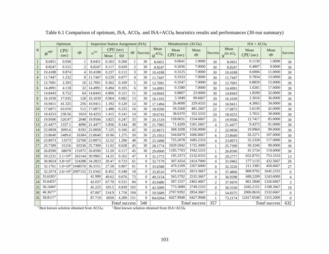
103

Table 6.1 Comparison of optimum, ISA, ACOR and ISA+ACOR heuristics results and performances (30-run summary)

N

Optimum Inspection Station Assignment (ISA) Metaheuristic (ACOR) ISA + ACOR

optu CPU(sec)

nfe ISAu CPU (sec)

nfe Success Mean

RACOu

Mean

CPU (sec)

Mean

nfe Success Mean

RISA ACOu

Mean

CPU (sec)

Mean

nfe Success Mean SD

1 8.0451 0.936 1 8.0451 0.103 0.200 1 30 8.0451 0.0641 1.0000 30 8.0451 0.1130 1.0000 30

2 8.8247 0.515 2 8.8247 0.117 0.029 2 30 8.8247 0.2656 7.0000 30 8.8247 0.4807 9.0000 30

3 10.4188 0.874 4 10.4188 0.237 0.112 3 30 10.4188 0.3125 7.0000 30 10.4188 0.6906 11.0000 30

4 11.7447 1.232 8 11.7447 0.229 0.077 4 30 11.7447 0.3333 7.0000 30 11.7447 0.7854 13.0000 30

5 12.7691 2.293 16 12.7691 0.362 0.109 5 30 12.7691 0.3547 7.0000 30 12.7691 0.8859 15.0000 30

6 14.4991 4.118 32 14.4991 0.494 0.105 6 30 14.4991 0.3380 7.0000 30 14.4991 1.0281 17.0000 30

7 14.8443 8.752 64 14.8443 0.806 0.121 11 30 14.8443 0.8807 23.0000 30 14.8443 1.8599 32.0000 30

8 16.1039 17.035 128 16.1039 0.964 0.082 13 30 16.1162 3.1849 89.6667 29 16.1039 2.3016 36.0000 30

9 16.9411 41.325 256 16.9411 1.192 0.120 12 30 17.1494 26.4698 329.4333 24 16.9411 4.3063 34.0000 30

10 17.6871 63.010 512 17.6871 1.488 0.225 16 30 18.0260 39.3568 481.2667 22 17.6872 5.6130 42.0000 30

11 18.4253 238.56 1024 18.4253 1.415 0.141 14 30 18.6742 38.6370 352.5333 24 18.4253 5.7021 38.0000 30

12 19.9506 520.97 2048 19.9506 3.825 0.247 35 30 20.1519 158.0031 1554.6667 21 19.9506 12.7417 85.0000 30

13 21.4477 1337.1 4096 21.4477 5.856 0.144 38 30 21.7985 71.4209 1501.5667 4 21.4477 9.4375 91.0000 30

14 22.0858 3095.6 8192 22.0858 7.125 0.166 42 30 22.8672 368.3208 1556.0000 2 22.0858 19.9964 99.0000 30

15 23.8640 5489.6 16384 23.8640 10.96 1.275 50 30 25.1953 544.8479 1666.8667 6 23.8640 26.2271 107.0000 30

16 23.8973 13573 32768 23.8973 12.52 1.296 48 30 25.3498 725.2078 1685.2333 4 23.8973 32.2328 117.0000 30

17 25.7399 31216 65536 25.7399 11.02 0.628 45 30 28.1774 1029.5042 1725.3000 1 25.7399 30.3240 99.0000 30

18 26.8590 68078 131072 26.8590 12.20 0.117 45 30 29.0000 1185.7703 1942.5333 1 26.8590 41.5734 119.0000 30

19 29.2231 2.1×106 262144 30.9965 14.25 0.162 47 0 31.1773 195.3373 2132.0333 0 29.2777 652.8755 753.3333 13

20 30.9024 3.8×105 524288 34.2823 20.47 0.723 61 0 32.7179 307.4354 2414.7000 4 31.0462 177.1135 432.5667 26

21 32.1761 1.0×106 1048576 36.3151 27.58 0.807 61 0 35.6588 479.2109 2267.6000 0 32.3226 211.3385 450.6667 27

22 32.3574 2.6×106 2097152 51.0342 8.452 0.348 18 0 35.8510 476.4333 2813.3667 0 37.4866 808.9792 1645.2333 0

23 35.6183‡ 41.999 49.62 0.676 72 0 40.5154 565.5792 2535.3667 0 36.9298 688.2209 1243.6000 4

24 35.6455‡ 42.037 67.79 0.531 84 0 43.0480 587.1557 2402.4667 2 37.9470 861.5848 1326.6667 3

25 36.1684‡ 45.225 105.5 0.839 102 0 42.5099 773.3089 2749.2333 0 36.5530 2445.2152 1198.3667 19

30 46.3677† 67.067 514.9 1.716 104 0 59.5689 2767.9392 2854.3667 2 54.8375 2006.8616 1532.6667 0

35 58.8117† 87.719 6050 4.289 151 0 84.0264 6427.9948 6427.9948 1 73.2174 12417.0548 1315.2000 0

Total success 540 Total success 357 Total success 632 † Best known solution obtained from ACOR; ‡ Best known solution obtained from ISA+ACOR

104

Figure 6.1 Convergence profile of 20-workstation example using ISA, ACOR, ISA+ACOR

6.2.2 Statistical significance of the heuristics

From Table 6.1 it is shown that, in terms of mean results, most of the cases the hybrid

heuristic ISA+ACOR provides better solutions as compared to ACOR. This observation is tested

by a statistical analysis for each of the instances. Assuming RACO and RIAH ACO to be the means

of the population of the best solutions of u of ACOR and ISA+ACOR, the null 0( )H and the

alternate 1( )H hypotheses for this analysis are given by

0 : 0R RACO ISA ACOH and

1 : 0R RACO ISA ACOH ,

respectively. The null hypothesis states that there is no difference between the mean values of best

solution obtained from ACOR ( RACO ) and ISA+ACOR ( )RISA ACO , whereas the alternate

105

hypothesis states that RACO is higher than RISA ACO . Empirical tests indicates that the population

data (bestu ) are distributed normally. Thus, a two-sample t-test is performed for testing this

hypothesis. The test statistics is given by,

*

2 /

R RACO ISA ACO

p

u ut

s n

for

2 2

1 2( )

2p

s ss

,

where ps is pooled standard deviation with

RACOn =RISA ACOn = n = 30, and

RACOn +RISA ACOn -2=

58 degrees of freedom, when population variances are equal; and

*

2 2

1 2

R RACO ISA ACOu ut

s s n

,

with 29 degrees of freedom, when population variances are not equal. Here, 1s and 2s are standard

deviations, and RACOu and RISA ACOu

are means of the best solutions obtained from ACOR and

ISA+ACOR, respectively.

As, the test statistics for t-test depends on the equality of population variances, it is needed

to test the equality of variance of the solutions obtained from ACOR and ISA+ACOR. An F-test is

performed for each problem, for testing equality of variances. Then the results of F-test is used for

selecting appropriate test statistics for t-test. The hypothesis for F-test are

2 2

0 1 2: 0H and 2 2

1 1 2: 0H ,

where, 1 and 2 are the respective population standard deviations of the best solutions obtained

from ACOR and ISA+ACOR. The test statistics of F-test is given by * 2 2

1 2F s s , with 29 and 29

degrees of freedom. The purpose of the test statistics are to find corresponding p-values

(probability of type-I error) from F-table and t-table. For both tests (F-test and t-test) a low p-value

(p-value<0.05, for 5% level of significance) provides sufficient evidence for rejecting 0H and

106

concluding that 1H is true. This conclusion leads to determine the better algorithm. The statistical

test results for best solutions ( )bestu are summarized in Table 6.2.

Table 6.2 Testing the difference between ACOR and ISA+ACOR results in terms of bestu

N

ACOR ISA+ACOR p-value

Better

Algorithm Mean SD Minimum Mean SD Minimum F-test

Two

sample t-

test

1 8.0451 0.0000 8.0451 8.0451 0.0000 8.0451 1.0000 1.0000 -

2 8.8247 0.0000 8.8247 8.8247 0.0000 8.8247 1.0000 1.0000 -

3 10.4188 0.0000 10.4188 10.4188 0.0000 10.4188 1.0000 1.0000 -

4 11.7447 0.0000 11.7447 11.7447 0.0000 11.7447 1.0000 1.0000 -

5 12.7691 0.0000 12.7691 12.7691 0.0000 12.7691 1.0000 1.0000 -

6 14.4991 0.0000 14.4991 14.4991 0.0000 14.4991 1.0000 1.0000 -

7 14.8443 0.0000 14.8443 14.8443 0.0000 14.8443 1.0000 1.0000 -

8 16.1162 0.0674 16.1039 16.1039 0.0000 16.1039 0.0000 0.3256 -

9 17.1494 0.5144 16.9411 16.9411 0.0000 16.9411 0.0000 0.0346 ISA+ACOR

10 18.0260 0.5714 17.6872 17.6872 0.0000 17.6872 0.0000 0.0029 ISA+ACOR

11 18.6742 0.5063 18.4253 18.4253 0.0000 18.4253 0.0000 0.0117 ISA+ACOR

12 20.1519 0.3738 19.9506 19.9506 0.0000 19.9506 0.0000 0.0062 ISA+ACOR

13 21.7985 0.5649 21.4477 21.4477 0.0000 21.4493 0.0000 0.0020 ISA+ACOR

14 22.8672 0.6210 22.0858 22.0858 0.0000 22.0858 0.0000 0.0000 ISA+ACOR

15 25.1953 1.5255 23.8640 23.8640 0.0000 23.8640 0.0000 0.0000 ISA+ACOR

16 25.3498 1.6121 23.8973 23.8973 0.0000 23.8973 0.0000 0.0000 ISA+ACOR

17 28.1774 1.8861 25.7399 25.7399 0.0000 25.7399 0.0000 0.0000 ISA+ACOR

18 29.0000 2.0634 26.8590 26.8590 0.0000 26.8590 0.0000 0.0000 ISA+ACOR

19 31.1773 2.8063 29.2254 29.2777 0.1634 29.2231 0.0000 0.0009 ISA+ACOR

20 32.7179 1.4808 30.9024 31.0462 0.6185 30.9024 0.0000 0.0000 ISA+ACOR

21 35.6588 3.9053 33.0122 32.3226 0.5309 32.1761 0.0000 0.0001 ISA+ACOR

22 35.8510 3.1724 33.4620 37.4866 2.7056 33.4620 0.3964 0.0359 ACOR

23 40.5154 5.2249 35.6767 36.9298 0.8991 35.6183 0.0000 0.0008 ISA+ACOR

24 43.0480 8.0094 35.6455 37.9470 1.1694 35.6455 0.0000 0.0017 ISA+ACOR

25 42.5099 5.7059 36.6153 36.5530 0.6520 36.1684 0.0000 0.0000 ISA+ACOR

30 59.5689 12.1065 46.3677 54.8375 2.8404 49.9430 0.0000 0.0452 ISA+ACOR

35 84.0264 22.2426 58.8117 73.2174 2.4773 68.6168 0.0000 0.0102 ISA+ACOR

The summary of the statistical significance tests presented in Table 6.2 illustrate that, for

most of the instances, the mean of the best results obtained from hybrid heuristic ISA+ACOR

( )RISA ACOu are better than what is obtained from ACOR.

107

Table 6.3 Testing the difference between ACOR and ISA+ACOR results in terms of CPU time

N

ACOR ISA+ACOR p-value

Better

Algorithm Mean SD Mean SD F-test

Two

sample t-

test

1 0.0641 0.1108 0.1130 0.1105 0.9893 0.0920 -

2 0.2656 0.0362 0.4807 0.0362 0.9913 0.0000 ACOR

3 0.3125 0.0315 0.6906 0.0490 0.0206 0.0000 ACOR

4 0.3333 0.0302 0.7854 0.0374 0.2607 0.0000 ACOR

5 0.3547 0.0307 0.8859 0.0564 0.0016 0.0000 ACOR

6 0.3380 0.0324 1.0281 0.0507 0.0191 0.0000 ACOR

7 0.8807 0.0366 1.8599 0.0631 0.0045 0.0000 ACOR

8 3.1849 5.4576 2.3016 0.0897 0.0000 0.3827 -

9 26.4698 36.6533 4.3063 0.1617 0.0000 0.0025 ISA+ACOR

10 39.3568 48.8684 5.6130 0.1150 0.0000 0.0007 ISA+ACOR

11 38.6370 61.5843 5.7021 0.1270 0.0000 0.0066 ISA+ACOR

12 158.0031 11.1078 12.7417 0.2474 0.0000 0.0000 ISA+ACOR

13 71.4209 2.7364 9.4375 0.5602 0.0000 0.0000 ISA+ACOR

14 368.3208 31.9072 19.9964 0.3610 0.0000 0.0000 ISA+ACOR

15 544.8479 63.4223 26.2271 0.4861 0.0000 0.0000 ISA+ACOR

16 725.2078 65.1710 32.2328 0.5365 0.0000 0.0000 ISA+ACOR

17 1029.5042 62.0223 30.3240 0.9389 0.0000 0.0000 ISA+ACOR

18 1185.7703 56.8798 41.5734 1.4183 0.0000 0.0000 ISA+ACOR

19 195.3373 38.0065 652.8755 517.0761 0.0000 0.0000 ACOR

20 307.4354 60.3572 177.1135 100.5690 0.0076 0.0000 ISA+ACOR

21 479.2109 71.5477 211.3385 112.3736 0.0177 0.0000 ISA+ACOR

22 476.4333 107.9987 808.9792 69.7749 0.0216 0.0000 ACOR

23 565.5792 114.1149 688.2209 224.1393 0.0005 0.0106 ACOR

24 587.1557 141.3804 861.5848 258.5001 0.0017 0.0000 ACOR

25 773.3089 131.3007 2445.2152 1545.4630 0.0000 0.0000 ACOR

30 2767.9392 1717.3639 2006.8616 651.7168 0.0000 0.0291 ISA+ACOR

35 6427.9948 1599.6337 12417.0548 3574.7526 0.0001 0.0000 ACOR

Similar statistical tests are performed for CPU time [see Table 6.3] and nfe [see Table 6.4]

as well. Low values of both CPU time and/or number of functional evaluation, nfe indicate the

higher efficiency of a heuristic or an algorithm. These tests also present similar conclusion in favor

of ISA+ACOR heuristic. It should be noted that, for a particular problem, the measure of CPU time

depends on several factors including the configuration of computer processor and memory. It also

depends on work load of the processor while the heuristic was running and some ambient

conditions of the computer. As a result the comparison with respect to nfe is more reliable than

that with CPU time.

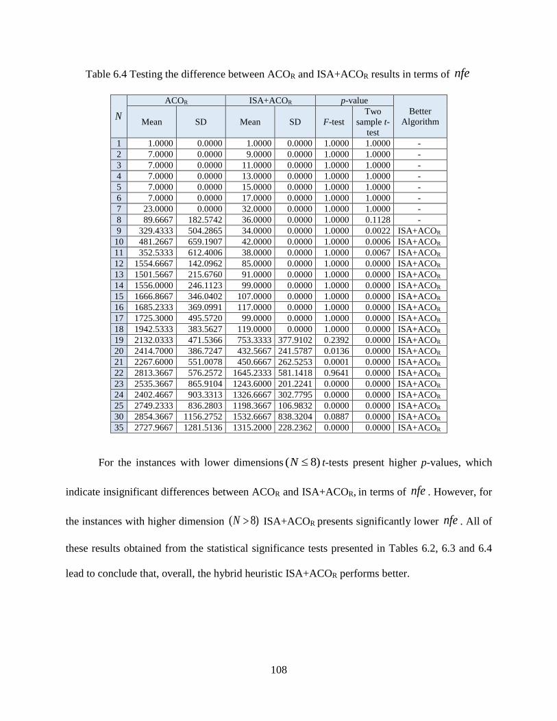
108

Table 6.4 Testing the difference between ACOR and ISA+ACOR results in terms of nfe

N

ACOR ISA+ACOR p-value

Better

Algorithm Mean SD Mean SD F-test

Two

sample t-

test

1 1.0000 0.0000 1.0000 0.0000 1.0000 1.0000 -

2 7.0000 0.0000 9.0000 0.0000 1.0000 1.0000 -

3 7.0000 0.0000 11.0000 0.0000 1.0000 1.0000 -

4 7.0000 0.0000 13.0000 0.0000 1.0000 1.0000 -

5 7.0000 0.0000 15.0000 0.0000 1.0000 1.0000 -

6 7.0000 0.0000 17.0000 0.0000 1.0000 1.0000 -

7 23.0000 0.0000 32.0000 0.0000 1.0000 1.0000 -

8 89.6667 182.5742 36.0000 0.0000 1.0000 0.1128 -

9 329.4333 504.2865 34.0000 0.0000 1.0000 0.0022 ISA+ACOR

10 481.2667 659.1907 42.0000 0.0000 1.0000 0.0006 ISA+ACOR

11 352.5333 612.4006 38.0000 0.0000 1.0000 0.0067 ISA+ACOR

12 1554.6667 142.0962 85.0000 0.0000 1.0000 0.0000 ISA+ACOR

13 1501.5667 215.6760 91.0000 0.0000 1.0000 0.0000 ISA+ACOR

14 1556.0000 246.1123 99.0000 0.0000 1.0000 0.0000 ISA+ACOR

15 1666.8667 346.0402 107.0000 0.0000 1.0000 0.0000 ISA+ACOR

16 1685.2333 369.0991 117.0000 0.0000 1.0000 0.0000 ISA+ACOR

17 1725.3000 495.5720 99.0000 0.0000 1.0000 0.0000 ISA+ACOR

18 1942.5333 383.5627 119.0000 0.0000 1.0000 0.0000 ISA+ACOR

19 2132.0333 471.5366 753.3333 377.9102 0.2392 0.0000 ISA+ACOR

20 2414.7000 386.7247 432.5667 241.5787 0.0136 0.0000 ISA+ACOR

21 2267.6000 551.0078 450.6667 262.5253 0.0001 0.0000 ISA+ACOR

22 2813.3667 576.2572 1645.2333 581.1418 0.9641 0.0000 ISA+ACOR

23 2535.3667 865.9104 1243.6000 201.2241 0.0000 0.0000 ISA+ACOR

24 2402.4667 903.3313 1326.6667 302.7795 0.0000 0.0000 ISA+ACOR

25 2749.2333 836.2803 1198.3667 106.9832 0.0000 0.0000 ISA+ACOR

30 2854.3667 1156.2752 1532.6667 838.3204 0.0887 0.0000 ISA+ACOR

35 2727.9667 1281.5136 1315.2000 228.2362 0.0000 0.0000 ISA+ACOR

For the instances with lower dimensions ( 8)N t-tests present higher p-values, which

indicate insignificant differences between ACOR and ISA+ACOR, in terms of nfe . However, for

the instances with higher dimension ( 8)N ISA+ACOR presents significantly lower nfe . All of

these results obtained from the statistical significance tests presented in Tables 6.2, 6.3 and 6.4

lead to conclude that, overall, the hybrid heuristic ISA+ACOR performs better.

109

6.3 Lower Bound of Unit Production Cost

While a lower bound presents a base or reference for evaluating the performance of an

existing or a new heuristic, an optimum or global best known solution determines the quality of

both lower bound and heuristic solutions as well. A lower bound of the objective function is

developed here based on the parametric characterization of the system. The following results helps

to find a lower bound for the MSI problem.

Theorem 6.1: The lower bound LBu to Problem f

MINLPY is given by

LBu = 1

1

01

1

max ,i

jj

i

jj

NNF I I I

k kk Nk

C mC T t c c

.

Proof: The denominator in Equation (4.10) can be written as 1 1

[1 ]N N

k k kk kp p y

=

1[1 (1 )]

N

k kkp y

. Thus, when

11

N

kkp

,

1[1 (1 )]

N

k kkp y

≤ 1 if (0,1)ky ,

which makes the objective functional value u (unit cost) in Equation (4.10) increase, and

it is maximized when kp = 1. In other words, the unit cost u is minimized when kp = 0

for all k =1, 2, …, N. Again, by definition, when kp = 0 (no defect at station k), then ky =

0 (no rework at station k) and consequently kx = 0 (no off-line rework station). So the

conditions kp = 0, ky = 0 and kx = 0 for all 1,2, ,k N leads to a conclusion that the

line produces defect-free products implying zero rework time at all stations. This situation

minimizes u by incurring no cost for rework and no fixed cost for rework station. Thus,

the objective functional value in Equation (4.10) becomes the lowest possible value for u

, calling it lower bound (LB) such that LBu =0, 0, 0k k kp y x

u u

.

110

Thus, for kp = 0, the variables ky = 0 and kx = 0 for all 1,2, , .k N So, Equation

(4.10) reduces to

LBu = 0

1

011

i

jj

i

jj

N I

kk N

mF I

eff

i

C m cC T c

.

By Theorem 4.1, 0

1

01

1 1

i

jj

i

jj

m NN I I

k kk Ni k

c c

. Hence, LBu =

1

F I

eff

NI

k

k

C mC T c c

; but

the conditions in (4.10c), (4.10d) and (4.10g) leads to conclude that effT =

0

1

01

max ,i

jj

i

jj

N I

kk NT t

. Thus, LBu = 0

1

01

1

max ,i

jj

i

jj

NNF I I I

k kk Nk

C mC t cT c

.

Hence, the proof is complete. □

The lower bound of u always falls below the optimum results, as MILPY is a minimization

problem. At the same time, a heuristic solution falls above or coincides with the optimum solution.

Thus, the difference between a lower bound ( )LBu and a heuristic solution gives an indirect

indication of the performance of that heuristic. The lower bound is useful for evaluating a heuristic

when the optimum solution is not found.

6.4 Comparing the Results

The empirical example for MSI problem presented in this chapter is solved optimally up

to N = 22. The optimum solutions for higher dimensional instances (N > 22) are not available due

to computational prohibitiveness. Thus the lower bound for u acts as a basis for evaluating the

performance of the heuristics ISA, ACOR and ISA+ACOR.

The heuristic solutions (u) obtained from ISA, ACOR and ISA+ACOR along with optimum

points and lower bounds are plotted against the problem dimension (N) [see Figure 6.2]. The figure

illustrates that for the lower dimensional instances all of the heuristics provide optimum solutions

111

or a solution which is quite closed to the optimum solution. The gap, as defined by many

optimization literatures, indicates the absolute difference between two comparing solutions, but in

the current situation, the gap between the lower bound and the heuristic and/or optimal solution

indicates the performance of the heuristic or lower bound. So the smaller the gap is the better the

performance of the heuristic or lower bound is. In the current study, the distance between lower

bound and the optimum solution is relatively very low at the lower dimensions. When problem

dimension increases, the deviation of a heuristic solution from corresponding optimum point

increases; and the deviation of an optimum solution from corresponding lower bound also

increases. Table 6.1 shows only the best known solutions (may not be the optimal) for N = 25, 30

and 35. In Figure 6.2 the optimal curve is continued beyond N = 22 with the available best known

solutions. Observing the general performance of the lower bound and the optimal solution for N ≤

22, the gap between these two measures might be expected to be less, concluding that the lower

bound performs well.

Figure 6.2 Comparison between heuristics ( u versus N )

112

The hybrid heuristic ISA+ACOR provides closer solutions to the lower bounds and

optimum solutions as compared to ISA or ACOR. An exception is observed for the instance with

22N only because this result is highly influenced by the exceptional (comparatively lower than

the adjacent workstations) value of inspection time 22( )It for Workstation 22.

A comparative ratio analysis for different heuristic solutions are presented in Table 6.5

which includes the lower bound ( )LBu of objective function of MSI problem, calculated using

Theorem 6.1. The heuristic and optimum (or global best known) solutions are compared with

respect to LBu .

Table 6.5 Comparison between heuristic, lower bound and optimum solutions

N LBu optu ISAu 0k

ISA

pu RACOu RISA ACOu

opt

LB

u

u

ISA

LB

u

u

0k

ISA

p

LB

u

u

RACO

LB

u

u

RISA ACO

LB

u

u

1 7.9555 8.0450 8.0450 7.9555 8.0451 8.0451 1.0113 1.0113 1.0000 1.0113 1.0113

2 8.7702 8.8250 8.8250 8.7702 8.8247 8.8247 1.0062 1.0062 1.0000 1.0062 1.0062

3 10.3297 10.4190 10.4190 10.3297 10.4188 10.4188 1.0086 1.0086 1.0000 1.0086 1.0086

4 11.6150 11.7450 11.7450 11.6150 11.7447 11.7447 1.0112 1.0112 1.0000 1.0112 1.0112

5 12.6554 12.7690 12.7690 12.6554 12.7691 12.7691 1.0090 1.0090 1.0000 1.0090 1.0090

6 14.3831 14.4990 14.4990 14.3831 14.4991 14.4991 1.0081 1.0081 1.0000 1.0081 1.0081

7 14.6540 14.8440 14.8440 14.6540 14.8443 14.8443 1.0130 1.0130 1.0000 1.0130 1.0130

8 15.8595 16.1040 16.1040 15.8595 16.1162 16.1039 1.0154 1.0154 1.0000 1.0162 1.0154

9 16.7802 16.9410 16.9410 16.7802 17.1494 16.9411 1.0096 1.0096 1.0000 1.0220 1.0096

10 17.5383 17.6870 17.6870 17.5383 18.0260 17.6872 1.0085 1.0085 1.0000 1.0278 1.0085

11 18.2667 18.4250 18.4250 18.2667 18.6742 18.4253 1.0087 1.0087 1.0000 1.0223 1.0087

12 19.6437 19.9510 19.9510 19.6437 20.1519 19.9506 1.0156 1.0156 1.0000 1.0259 1.0156

13 20.8668 21.4477 21.4477 20.8668 21.7985 21.4477 1.0278 1.0278 1.0000 1.0446 1.0278

14 21.4662 22.0860 22.0860 21.4662 22.8672 22.0858 1.0222 1.0222 1.0000 1.0584 1.0222

15 22.9987 23.8640 23.8640 22.9987 25.1953 23.8640 1.0308 1.0308 1.0000 1.0883 1.0308

16 23.1800 23.8970 23.8970 23.1800 25.3498 23.8973 1.0309 1.0309 1.0000 1.0936 1.0309

17 25.2585 25.7400 25.7400 25.2585 28.1774 25.7399 1.0191 1.0191 1.0000 1.1156 1.0191

18 26.5601 26.8590 26.8590 26.5601 29.0000 26.8590 1.0113 1.0113 1.0000 1.0919 1.0113

19 27.9367 29.2230 30.9960 30.6548 31.1773 29.2777 1.0460 1.1095 1.0973 1.1160 1.0480

20 30.5142 30.9020 34.2820 33.9275 32.7179 31.0462 1.0127 1.1235 1.1119 1.0722 1.0174

21 31.3388 32.1760 36.3150 35.9486 35.6588 32.3226 1.0267 1.1588 1.1471 1.1378 1.0314

22 31.9384 32.3570 51.0340 50.6507 35.8510 37.4866 1.0131 1.5979 1.5859 1.1225 1.1737

23 34.7415 35.6180 41.9990 41.5982 40.5154 36.9298 1.0252 1.2089 1.1974 1.1662 1.0630

24 34.7660 36.0770 42.0370 41.6326 43.0480 37.9470 1.0377 1.2091 1.1975 1.2382 1.0915

25 35.2678 36.1680 45.2250 44.8001 42.5099 36.5530 1.0255 1.2823 1.2703 1.2053 1.0364

30 44.4788 51.8450 67.0670 66.5708 59.5689 54.8375 1.1656 1.5078 1.4967 1.3393 1.2329

35 58.2358 72.7090 87.7190 87.1431 84.6959 73.2174 1.2485 1.5063 1.4964 1.4544 1.2573

113

In general, the ISA solution is obtained with 0,kp k to reflect the practical instances in

industry. Now when kp is set to 0 for all k, the ISA gives the lowest solution for the same instance.

So, an ISA solution with 0kp for any k will be always greater than or equal to the lower bound. To

test this hypothesis, a set of special ISA solutions is generated with 0,kp k and these solutions

validate the lower bounds. It is also observed from the ratio /opt

LBu u in Table 6.5 that optu falls

within 0.62% to 4.6% higher than the lower bound, which indicates effectiveness of the lower

bound.

The ratio analysis presented in Table 6.5 indicates that ISAu falls within 0.62% to 59.79%

and RACOu falls within 0.62% to 45.44% higher than the lower bound ( LBu ) whereas RISA ACOu

falls

within 1.0062% to 25.73% above LBu . Although the performances of the heuristics indicate high

percentage deviation from the lower bound, actually most of the problems resulted in lower

percentage deviation—only a few instances at higher dimensions performed worst. Furthermore,

the runs of the heuristics were terminated after 500 functional evaluations of the objective function

for any specific m; as a result, sometimes the computation ended prematurely without giving the

optimal or near optimal solutions. Since a comparative study of the heuristics demanded many

instances with higher dimensions to be solved, the computer was programed to run the heuristics

with this boundary condition to accommodate more results for comparison. This situation

contributed heavily to reflect the performances of the heuristics.

6.5 Long Production Lines: Modular Design

In many large scale manufecturing systems (for example, automobile and electrical

assembly including garments production flowlines) a very long (N > 35) production line is not

uncommon. In this case, the solution procedure for a MSI problem presented in this chapter

114

becomes computationally prohabiutive. However, this procedure can still be implementable for

large production lines, by following a modular design of the line. A logical partition of the line

can be made where a part of the final product is produced or assembled. These partitions or

segments of the line is a module and can be individually solved as an MSI problem. Simillar

partitions can be drawn for any parallel feeding branches of the line. A branch of a line suppling a

part or doing some operations on a part can be considered as a feeder or an independent production

line of that part and can be solved for the MSI problem independently.

Another potential approach of solving MSI problem for a long production line is by

hypothetically clustering some adjacent operations in one workstation. For computational purpose,

each cluster of operations can be treated as a single clustered workstation. Thus, the total number

of workstations in the line can be reduced (for example, N ≤ 35) line which eventually reduces the

computational time for solving the MSI problem; and the ISA+ACOR heuristic or some other

suitable heuristic or exact (optimal seeking) method may be applied. Though, none of these two

approaches guarantee an optimum solution, these approaches can provide some better solution

than arbitrarily assigning inspection or rework.

6.6 Conclusion of the Empirical Study

This chapter presents computational results of some heuristic approaches for solving large

instances of multistage inspection (MSI) problem. A construction heuristic, namely, Inspection

Station Assignment (ISA) is presented for solving the MSI problem. An Ant Colony Optimization

(ACOR) based metaheuristic algorithm and a hybrid heuristic ISA+ACOR are also presented for

solving large instances. A close observation of the computational result shows better performance

of the hybrid heuristic ISA+ACOR, in terms of efficiency and solution quality. A lower bound is

constructed for the MSI problem, which helps to investigate the performance of the heuristics for

115

large instances. The optimum solutions lie within 0.62% to 4.6% of the lower bound above it,

which is acceptable for many practical problems.

Overall, the outcome of these empirical tests presents the performance (solution quality

and computational efficiency) of ACOR, ISA and ISA+ACOR heuristics. The hybrid heuristic

ISA+ACOR is devised using the best performing characteristics of ACOR and ISA. As a results,

the hybrid version of the heuristic obviously performed better. A lower bound developed from the

general characteristics of the MSI problems also performed well.

116

CHAPTER 7

CONCLUDING REMARKS

Quantity inspection which is, in general, done in the production line is a major and

important step of manufacturing operations. A common practice for a short production line is to

conduct a quality inspection at the end of the line. Defective items detected at the inspection station

are often repaired on-line or scrapped. This research deals with the policy for dealing with the

quality defects and inspection station(s) location. The main objective of this research is to find the

optimum rework policy (on/off-line rework or scrapping) and to find optimum number and

locations of inspection stations that minimize unit cost of production.

7.1 Summary

The research is conducted in two phases. The first phase of the research dealt with an end-

of-line inspection (ELI) problem. The objective of ELI problem was to make decisions on each

type of defects—whether the defective item should be repaired on-line or off-line or should be

scrapped instead of repair. Off-line repair required additional investment for the dedicated repair

station to avoid any interruption of regular material flow of the line by inspection activity. On the

other hand, on-line rework avoids extra investment for off-line rework stations but disrupts regular

flow of the line. A scrapping decision reduces overall throughput rate. Thus, an appropriate rework

policy is needed to be decided, in order to handle the defective items efficiently. In the first phase

of the research, this ELI problem was formulated as a fractional mixed-integer non-linear

programming (f-MINLP) problem. Then the f-MINLP was transformed into a MILP problem to

solve it with a B&B method.

The second phase of the research deals with a multistage inspection (MSI) problem. The

objective of this phase of research was to find optimum number and location of the inspection

117

stations in addition to the optimal rework policy. This problem was also formulated as a f-MINLP

and transformed into MILP problem. The MSI problem is a combinatorial problem with varying

number of variables. A B&B method was not directly applicable to this MSI problem since its

formulation involved several constraints that were not amenable to linearization immediately. As

a result, an exhaustive search algorithm was first presented to solve some problem instances with

smaller dimension. For solving large instances, some heuristic algorithms were presented for

finding the number and location of inspection stations while the rework policy was still optimized

with B&B method in each iteration of the heuristic. An efficient construction heuristic, namely,

Inspection Station Assignment (ISA) heuristic was devised to solve the MSI problem and the

solution quality of it was quite high—it produced optimal solutions to the problems with line length

of up to 18 workstations in reasonable time. Later, ISA was hybridized with an Ant colony-based

metaheuristic (ACOR) resulting into ISA+ACOR, an enriched method with stipulated seed value

from the ISA heuristic. Computational results from an empirical study indicated much better

performance of ISA+ACOR in terms of solution quality and computational efficiency with respect

to other stated heuristics.

7.2 Conclusions

As indicated earlier, the basic theme of this research was to configure a flowline as to how

many inspection stations and where they should be located along the line with a prescription of

whether a defective item produced at a station should be scrapped or reworked online or off-line

so as to minimize the unit cost of the product. Obviously, these issues cast a complex problem and

call for different aspects of optimization. The general problem has been addressed in two different

phases.

118

In the first phase of this research, the end-of-line inspection (ELI) problem is formulated

as a fractional mixed-integer nonlinear programming problem and solved optimally the linearly

transformed version of it with B&B method. This solution approach is applicable for large

dimension problems as well. On the other hand, in the second phase, transformed version of the

multistage inspection (MSI) problem is solved optimally by exhaustive search approach combined

with B&B method. This problem is further solved with Inspection Station Assignment (ISA)

heuristic, Ant Colony Optimization (ACOR) based metaheuristic and a hybrid of these two

(ISA+ACOR), for obtaining a sub-optimal solutions of large instances. The hybrid algorithm

ISA+ACOR is found to be an efficient heuristic for solving large instances. The solution quality,

i.e., the objective function values are found better for most of the instances.

The theoretical studies and empirical tests of large data sets reveal some general findings

of this research that are helpful in many industrial situations. When a bottleneck situation occurs

at any station (inspection station and/or workstation) due to non-optimized assignment of

inspection and/or rework, the product quality is not maintained properly resulting in waste of

products and higher unit cost. The unit cost of the product is always low when the fraction defective

ratios are low as well, and the lower bound (uLB) of the MSI problem serves as the minimum unit

cost of product under perfect production environment (i.e., with no defects). Also, the unit

production cost u found to be highly sensitive to fixed-cost for an inspection station, repair and

inspection time at any station and rework time of a defective item at any station.

It is further observed that the location of the inspection station(s) directly influences the

unit cost of production while the inspection station time varies with respect to its location. In fact,

this general characteristic of the line configuration was exploited as a basis for developing the ISA

heuristic which performed well for relatively smaller instances (N <19).

119

As the problem dimension increases the number of functional evaluations (nfe) for ACOR and

ISA+ACOR also increases. Thus, for instances with higher dimension, the allowable maximum nfe

should be increased to get better solutions. However, for a same nfe, ISA+ACOR provided better

solution as compared to ACOR. The computational time by any heuristic for a problem increases

slowly for lower dimensional problems when it grows exponentially for higher dimensions.

7.3 Significance of the Research

A small amount of cost savings per unit of a product leads to a huge amount savings to a

manufacturer if the order size is large, especially in garments and other high-volume production

systems. For example, in the second production line of Example 3.2 (refer Table 3.2), the unit cost

reduction (from $20.9194 to $20.2442 per unit) for allowing a prescribed off-line repair facility

(i.e., a rework station) is $0.6752/unit as compared to traditional on-line repair cost, $20.9194.

This means, even for a small order size of 10,000 garments, the total savings would be $6,752

which is a huge savings for a small lot indeed. Translating it to local economy, this amounts to a

total wage of 100 workers a month in some source country in Southeast Asia like Bangladesh,

India, Nepal, Philippines and Vietnam where the gross labor-wage is only $67.50 per month (Labor

Wage, 2013). In many cases a single lot size exceeds millions of garments products for which the

savings could be astronomical. Thus, a little improvement over an existing system for high volume

production line will impact the economy of manufacturers, wholesale buyers and/or consumers

significantly.

7.3.1 Applications to garments and modular manufacturing industries

According to American Apparel and Footwear Association (AAFA, 2012), apparel and

textile industries are the world’s third largest industry sector after auto industries, and are good

examples of imperfect flowlines. Due to high labor cost most low-cost garments in America,

120

Australia or European countries are imported from the countries like China, India, Bangladesh or

Vietnam where human labor is available with comparatively very low cost. AAFA (2012) reported

that the USA imported apparel products from different countries that worth $71,398 million and

$77,659 million in 2010 and 2011, respectively. Even though garments products are mostly

imported in the United States, the production cost at the source will eventually decrease import

cost as well as price of the products. Also, garments quality is a vital factor to capture a new market

and employing better and effective inspection policy leads to enhance the factor favorably.

Construction of a quality garments production line requires a great deal of know-how, and

a lot of coordination and schedule management. Clothing manufacturing consists of a variety of

product categories, materials and styling, making it constantly difficult to adapt to changing styles

and consumer demands. Furthermore, to adapt automation for the clothing system is also hard

because, beside the complex structure, it is also labor intensive. Therefore, garments production

needs properly rationalized manufacturing technology, management and planning (Bahadir 2011,

Glock and Kunz 1995).

7.3.2 Implications to other discrete product manufacturing

Most mass production industries experience similar problems to compete in the world

markets. This problem is scalable to many other large repetitive manufacturing product lines

including electronics, mechanical products, multi-operational consumer items, and many other

products to mention a few. Sometimes a product line may need to change in a short notice in

response to customer’s change in order verities, specifications and demand. These production lines

are supposed to considerably flexible (for example in electronic assembly lines, the movable

soldering fixtures, dies, cutters, etc.) and inexpensive to reconfigure. The outcomes of the research

provide a scientific guideline to appropriate alterations in a production line that will not only

121

reduce the unit cost of production but also will enhance the throughput rate of the line. The

management will be able to quickly adjust to change the line configuration and inspection stations

and setup their rework policy. Judicious configuration of production lines not only increases the

throughput rate of good products but also minimizes the unit cost of production and indirectly

boost the customer demand and hence, the higher revenue.

7.4 Limitations

The ELI problem was finally formulated as a mixed-integer linear programming problem

which is solved by B&B method. The number of node search increases exponentially as the

problem dimension increase. MSI problem is basically a cluster of ELI problems superimposed

one after another in a contiguous, juxtaposition form. Thus, for a large dimensional problem it

becomes computationally prohibitive for both MSI and ELI problems even though an efficient

heuristic is applied.

A hybrid of construction heuristic ISA and metaheuristic ACOR was presented for solving

the MSI problems. It is observed that a heuristic does not necessarily guarantee an optimal solution.

Though, ISA+ACOR could provide optimum solutions for some instances with lower dimension,

as problem dimension increases the deviations of the heuristic solution increases from the

optimum. Thus, a more efficient approach of finding optimum solution of MSI problem still needs

to be explored.

While pursuing the single-step backward local search in the ISA heuristic, the program

stopped when the unit product cost u started increasing, but sometimes simultaneous backward

local search for multiple inspection station locations could have resulted in a better solution.

The computational time taken to reach a solution for a particular problem was influenced by

several factors such as configuration of computer processors and memory, workload of the

122

processor, ambient conditions of the computer, computational precision. Obviously, overcome of

these factors will lead to a better and efficient solution for higher dimensional problems.

7.5 Future Research

Based on the results obtained and gathered knowledge from the outcomes of this research,

some potential issues for future research can be considered. The potential research issues may

include configuration rework/inspection stations for parallel production lines, batch inspection and

station time variability. The approach of solving the inspection and rework station optimization

problem is extendable for parallel production lines by considering each segment of the parallel line

as an independent flowline. This problem can be further extended to continuous production

systems and/or with probabilistic station times.

1. Batch production system: In a practical situation, item-by-item inspection may lead to a

significant amount of idle time for each of the inspection facilities. If the inspection time

of an inspection station is It per unit, and cycle time is T per unit, then for a batch of B

items, the idle time for the inspector is ( )IT t B per batch. So the inspector will be able to

serve at other stations (instead of employing multiple inspectors) for ( )IT t B time units.

Thus, batch inspection can reduce the idle time of the quality inspectors whose productive

time could be invested to work on other stations. Hence, batch inspection will reduce

inspection cost and the batch sizes, Bi ( i =1, 2,…,m) for all m inspection stations will affect

the total production cost. Thus, a complete formulation and solution of the problem to

decide on the optimal size of each inspection batch Bi ( i =1, 2,…,m) can be good choice of

future research.

2. Probabilistic station times: On the other hand, in reality, the production times, repair times and

inspection times are usually probabilistic in nature with some known distribution

123

function(s). The variability in production, repair and inspection time will increase the

complexity of the problem since they involve multiple variables. This research issue will

involve dependent properties of probabilistic variables causing it as a convoluted problem.

These probabilistic times can be intertwined into the multistage inspection problem

keeping the same objectives that will intrinsically bring computational difficulty. A

simulation approach or a decomposition approach as applied in reliability analysis

(Ramakumar 1993, pp. 352-361) may be applied in dealing with these probabilistic station

times.

3. Bowl phenomenon: It has been researched (Hillier and Boiling 1966, Rao 1976) that application

of the principle of bowl phenomenon may be applied to increase the throughput rate of a

discrete production system. This phenomenon says that the throughput rate can be

increased by allocating progressively more task times to stations further away from the

central station. Thus, this principle may be applied as well in the current study to improve

the throughput rate of the line, and hence, to reduce the unit cost of production.

4. Parametric control: Though, ISA+ACOR could provide optimum solutions for some instances

with lower dimension as problem dimension increases, the deviations of the heuristic

solution increases from the optimum. Thus, a more efficient approach of finding optimum

solution of MSI problem still needs to be explored. Since the lower bound of the MSI

problem is constructed based on no-defect probability of product, a closer look on

combining the properties of LB and the objective function may be investigated. First, a

sensitivity of the system parameters needs to be performed on the lower bound, identifying

the most sensitive parameter in LB contribution. A mechanism in manipulating the related

variables with these parameters in the objective function may improve the solution further.

124

5. Modular production line: The proposed solution approach of MSI problem can be extended to

solve large production line by using modular production line concept. Two alternative

approaches can be followed to deal with MSI problem for such production lines. The first

approach is to make an imaginary partition on the line where (a) the length of each

partitioned segment of the line is within a suitable range, which is indenependently

solvable with ISA+ACOR or other heuristics within an acceptable computational time,

and (b) parforms a sequence of operations on a specific part, independent of other parts

of the product. Then, each partitioned segment of the line can be solved separately using

some suitable techniques. The second approach can be, clastering some adjacent

operations on a part in hypothetical workstations and thus, making the line shorter to

avoid comultational prohavitaiveness.

A complete guide to deal with these types of conguration problems in flowlines is unknown

in literature. Other variants to this configuration problems in flowlines may also exist in many

industrial situations. Obtaining the optimal solutions to these problems will not only provide with

efficient system configurataions but the complexities of obtaining such solutions will also increase

as the problem sizes and decision variables increase. Overall, the outcome of this research is

applicable to many discrete manufacturing flowlines. The research results and solution approaches

obtained here will be beneficial to both the manufacturers and the buyers from both economic and

technical perspectives.

125

REFERENCES

1. AAFA (2012) “U.S. Apparel Imports - 2002 – 2011,” American Apparel & Footwear

Association, 1601 North Kent Street, Suite 1200, Arlington, VA 22209.

2. Akpinar, S. and Bayhan, G.M. (2014) “Performance evaluation of ant colony

optimization-based solution strategies on the mixed-model assembly line balancing

problem,” Engineering Optimization 46(6): 842-862.

3. Alagas, H.M., Yuzukirmizi, M., and Turker, A.K. (2013) “Balancing stochastic assembly

lines using constraint programming and queueing networks,” Journal of the Faculty

of Engineering and Architecture, Gazi University 28(2): 231-240.

4. Anily, S. and Grosfeld-Nir, A. (2006), “An optimal lot-sizing and offline inspection policy

in the case of nonrigid demand,” Operations Research, 54(2): 311-323.

5. Azadeh, A., Sangari, M.S., Sangari, E. and Fatehi, S. (2015) “A particle swarm algorithm

for optimizing inspection policies in serial multistage production processes with

uncertain inspection costs,” International Journal of Computer Integrated

Manufacturing, 28(7): 766-780.

6. Bahadir, S. K. (2011), “Assembly line balancing in garment production by simulation,”

Chapter 4 (pp. 67-82) in Assembly Line-Theory and Practice, edited by Waldemar

Grzechca, ISBN: 978-953-307-995-0, published by InTech, Janeza Trdine 9, 51000

Rijeka, Croatia.

7. Biswas, P. and Sarker, B. R. (2008), “Optimal batch quantity models for a lean production

system with in-cycle rework and scrap,” International Journal of Production

Research, 46(23): 6585-6610.

8. Bodimeade, M. (2013) “Global Apparel Industry,” Companiesandmarket.com Report,

June 27, 2013.

9. Bouslah, B., Gharbi, A. and Pellerin, R. (2014) “Joint production and quality control of

unreliable batch manufacturing systems with rectifying inspection,” International

Journal of Production Research, 52(14): 4103-4117.

10. Carcano, O. E. and Staudacher, A.P. (2006), “Integrating inspection-policy design in

assembly-line balancing,” International Journal of Production Research, 44(18–

19): 4081–4103.

11. Castillo-Villar, K.K. and Herbert-Acero, J.F. (2014), “A metaheuristic-based approach

for the capacitated supply chain network design problem including

imperfect quality and rework,” IEEE Computational Intelligence Magazine, 9(4):

31-45.

126

12. Celik, E., Kara, Y. and Atasagun, Y. (2014) “A new approach for rebalancing of U-lines

with stochastic task times using ant colony optimisation algorithm,” International

Journal of Production Research 52(24): 7262-7275.

13. Chang, C.T. (2001) “On the polynomial mixed 0-1 fractional programming problems,”

European Journal of Operational Research, 131(1): 224-227.

14. Chang, P.C. and Lin, Y.K. (2015) “Reliability analysis for an apparel manufacturing

system applying fuzzy multistate network,” Computers & Industrial Engineering

88:458-469.

15. Chiu, S.G.W., Lee, C.H., Chiu, Y.S.P. and Cheng, F.T. (2013) “Intra-supply chain system

with multiple sales locations and quality assurance,” Expert Systems with

Applications, 40(7): 2669-2676.

16. Choudhary, A., Agnihotri, A., Paitandy, A. and Dhawan, N. (2008) “Operation

Breakdown of a T-shirt,” Project paper presented for Garment Manufacturing

Technology, National Institute of Fashion Technology, Mumbai, India, November,

2008.

17. Deliman, N.C. and Feldman, R.M. (1996) “Optimization of process improvement and

inspection location for serial manufacturing,” International Journal of Production

Research, 34(2): 395-405.

18. Denardo, E.V. and Lee, T.Y.S (1996), “Managing uncertainty in a production flowline,”

Operations Research, 44(2): 382-392.

19. Diponegoro, A. and Sarker, B. R. (2003a), “Flow distance reduction for a multi-product

flowline with sets of identical machines,” European Journal of Operational

Research, 147(3): 591-612.

20. Diponegoro, A. and Sarker, B. R. (2003b), “Machine assignment problems for a multi-

product flowline,” Journal of the Operational Research Society, 54(4): 472-489.

21. Dorigo M. (1992) “Optimization, Learning and Natural Algorithms,” PhD thesis,

Politecnico di Milano, Italy.

22. Duffuaa, S.O., Khan, M. (2008), “A general repeat inspection plan for dependent

multicharacteristic critical components,” European Journal of Operational

Research, 191(2): 374–385.

23. Dundar, P., Guner, M. and Colakoglu, O. (2012) “An approach to the modular line

balancing problem for an apparel product with graph theory,” Tekstil Ve

Konfeksiyon 22(4): 369-374.

24. Emam, O.E., Abdo, A. and Ibrahim, N.H. (2015) “Taylor series approach for solving

multi-level large scale fractional programming problem with stochastic parameters

in constraints,” British Journal of Mathematics & Computer Science, 6(2): 79-90.

127

25. Eppen, GD. and Hurst, E.G. (1974) “Optimal location of inspection stations in a

multistage production process,” Management Science Series B-Application, 20(8):

1194-1200.

26. Fernandez-Stark, K . , Frederick, S. and Gereffi, G. (2011), The Apparel Global

Value Chain, Duke University, Center on Globalization, Governance &

Competitiveness, November 2011, pp. 7-16, http://www.cggc.duke.edu/pdfs/

2011-11-11_CGGC_Apparel-Global-Value-Chain.pdf

27. Gaubert, S., Katz, R.D. and Sergeev, S. (2012) “Tropical linear-fractional programming

and parametric mean payoff games,” Journal of Symbolic Computation, 47(12):

1447–1478.

28. Geren, N. (2003) “Determination and comparison of surface mount component rework

cycle times of manual and fully automated robotic rework stations for rework

technology selection,” IEEE Transactions on Electronics Packaging

Manufacturing 26(2): 123-132. http://stat.wto.org/Home/WSDBHome.aspx?

Language=E.

29. Giannakis, G., Kouikoglou, V. S. and Nikitas, S. (2010), “Workflow analysis of

production lines with complete inspection and rework loops,” International Journal

of Production Research, 48(24): 7321–7336.

30. Glock, R. E. and Kunz, G. I. (1995), Apparel Manufacturing-Sewn Product Analysis,

Prentice Hall, New Jersey, p. 4.

31. Guner, M., Yucel, O. and Unal, C. (2013) “Applicability of different line balancing

methods in the production of apparel,” Tekstil Ve Konfeksiyon 23(1): 77-84.

32. Gungor, M. and Agac, S. (2014) “Resource-constrained mixed model assembly line

balancing in an apparel company,” Tekstil Ve Konfeksiyon 24(4): 405-412.

33. Gursoy, A. (2012) “An integer model and a heuristic algorithm for the flexible line

balancing problem,” Tekstil Ve Konfeksiyon 22(1): 58-63.

34. Gursoy, A. and Gursoy, N.K. (2015) “On the flexibility constrained line balancing

problem in lean manufacturing,” Tekstil Ve Konfeksiyon 25(4): 345-351.

35. Hillier, F. S. and Boling R. W, (1996) The effect of some design factors on the efficiency

of production lines with variable operation times,” Journal of Industrial

Engineering (new title: IIE Transactions), 17(12): 651-658.

36. Hillier, F. S. and Lieberman, G.J., (2010), Introduction to Operations Research, 9th editor,

McGraw-Hill New York, NY 10020.

128

37. Hossain, M.S.J. and Sarker, B.R. (2015) “Optimal location of rework stations in a serial

production line:a case in garments industry,” Paper # 5, Proceedings of the 1st

International Conference on Materials and Manufacturing Engineering (ICMME

2015), IUT, Tongi, Dhaka (Bangladesh), December 25-27, 2015.

38. Hossain, M.S.J. and Sarker, B.R. (2016) “Optimal locations of on-line and off-line rework

stations in a serial production system,” International Journal of Production

Research, 2016, Vol. 54, No. x, pp. xx-xx.

http://dx.doi.org/10.1080/00207543.2015.1117676 (Published Online: November

27, 2015).

39. Huang, N. (2012), Industry insight: Global textile and apparel industries,” Global Apparel

Industry Report, December 6, 2012.

40. ILO (2014), “Wages and working hours in the textiles, clothing, leather and footwear

industries,” Report # GDFTCLI/2014; International Labor Organization Office,

Geneva, September 23-25, 2014, pp. 16-18.

41. Inman, R.R., Blumenfeld, D.E., Huang, N.J., Li, J.S. and Li, J. (2013) “Survey of recent

advances on the interface between production system design and quality,” IIE

Transactions, 45(6): 557-574.

42. Ioannidis, S. (2013) “Joint production and quality control in production systems with two

customer classes and lost sales,” IIE Transactions, 45(6): 605-616.

43. Iravani, S.M.R., Duenyas, I. and Olsen, T.L. (2000), “A production/inventory system

subject to failure with limited repair capacity,” Operations Research, 48(6): 951-

964.

44. Islam, M.M., Mohiuddin, H.M., Mehidi, S.H. and Sakib, N. (2014), “An optimal layout

design in an apparel industry by appropriate line balancing: A case study,” Global

Journal of Researches in Engineering, 14(5.1): 35-43.

45. Jamal, A.M.M., Sarker, B.R., and Mondal, S. (2004), “Optimal manufacturing batch size

with rework process at a single-stage production system,” Computer & Industrial

Engineering, 47(1): 77-89.

46. Jeang, A. and Lin, Y.K. (2014) “Product and process parameters determination for quality

and cost,” International Journal of Systems Science, 45(10): 2042-2054.

47. Jun, H.B., Lee, D.H., Kim, J.G. and Kiritsis, D. (2010) “Heuristic algorithms for

minimizing total recovery cost of end-of-life products under quality constraints,”

International Journal of Production Research, 50(19): 5330-5347.

48. Kallioras, N.A., Lagaros, N.D. and Karlaftis, M.G. (2014) “An improved harmony search

algorithm for emergency inspection scheduling,” Engineering Optimization, 46(11)

1570-1592.

129

49. Kang, K.S., Ebeling, K.A. and La, S.H. (1990) “The optimal location of inspection

stations using a rule-based methodology,” Computers & Industrial Engineering,

19(1-4): 272-275.

50. Kayar, M. and Akyalcin, O.C. (2014) “Applying different heuristic assembly line

balancing methods in the apparel industry and their comparison,” Fibres & Textiles

in Eastern Europe 22(6): 8-19.

51. Kim, M.J. and Makis, V. (2013) “Joint Optimization of Sampling and Control of Partially

Observable Failing Systems,” Operations Research, 61(3): 777-790.

52. Ko, J., Nazarian, E., Wang, H. and Abell, J. (2013) “An assembly decomposition model

for subassembly planning considering imperfect inspection to reduce assembly

defect rates,” Journal of Manufacturing Systems, 32(3): 412-416.

53. Koksal, G., Taseli, A., Dolgun, L.E. and Batmaz, I. (2013) “The effect of inspection error

on quality and producer losses: the case of nominal-the-best type quality

characteristic and rework,” European Journal of Industrial Engineering, 7(4): 497-

528.

54. Kucukkoc, I. and Zhang, D.Z. (2016) “Integrating ant colony and genetic algorithms in

the balancing and scheduling of complex assembly lines,” International Journal of

Advanced Manufacturing Technology 82(1-4): 265-285.

55. Kuo, C.F., Hsu, C.T.M., Fang, C.H., Chao, S.M. and Lin, Y.D. (2013) “Automatic defect

inspection system of color filters using Taguchi-based neural network,”

International Journal of Production Research, 51(5): 1464-1476.

56. Labor Wage (2013), Bangladesh Gazettes #SRO-369-Labour-05 Dec_2013, Ministry of

Labor and Employment, Bangladesh Government Press, Page: 10303-10313.

57. Land, A. H. and Doig, A. G. (1960). "An automatic method of solving discrete

programming problems". Econometrica, 28 (3): 497–520.

58. Law, A.M. and Kelton, W.D. (1982), Simulation Modeling and Analysis, McGraw-Hill,

Inc. New York, NY.

59. Lee, H.L. (1992), “Lot sizing to reduce capacity utilization in a production process with

defective items, process corrections, and rework,” Management Science, 38(9):

1314-1328.

60. Lehmer, D.H. (1951), “Mathemetical Methods in Large-Scale Computering Units,”

Annals of the Computation Laboratory [Harvard University], 26: 141-146.

61. Li, H.L. (1994) “A global approach for general 0-1 fractional programming,” European

Journal of Operational Research, 73(3): 590-596.

130

62. Liao, T.W., Chang, P.C., Kuo, R.J. and Liao, C.J. (2014) “A Comparison of Five Hybrid

Metaheuristic Algorithms for Unrelated Parallel-Machine Scheduling and Inbound

Trucks Sequencing in Multi-door Cross Docking Systems,” Applied Soft

Computing 21(August):180-193.

63. Liao, T.W., Kuo, R.J. and Hu, J.T.L. (2012) “Hybrid ant colony optimization algorithms

for mixed discrete–continuous optimization problems,” Applied Mathematics and

Computation 219(6): 3241-3252

64. Lim, C., Sherali, H.D. and Glickman, T.S. (2015) “Cost-of-Quality Optimization via

Zero-One Polynomial Programming,” IIE Transactions, 47(3): 258-273.

65. Mohammadi, M., Siadat, A., Dantan, J.Y. and Tavakkoli-Moghaddam, R. (2015)

“Mathematical modelling of a robust inspection process plan: Taguchi and Monte

Carlo methods,” International Journal of Production Research, 53(7): 2202-2224.

66. Mok, P.Y., Cheung, T.Y., Wong, W.K., Leung, S.Y.S. and Fan, J.T. (2013) “Intelligent

production planning for complex garment manufacturing,” Journal of Intelligent

Manufacturing 24(1): 133-145.

67. Ojha, D., Sarker, B.R. and Biswas, P. (2007), “An optimal batch size for an imperfect

production system with quality assurance and rework,” International Journal of

Production Research, 45(14): 3191–3214.

68. Osman, H. and Baki, M.F. (2014) “Balancing transfer lines using Benders decomposition

and ant colony optimization techniques,” International Journal of Production

Research 52(5): 1334-1350.

69. OTEXA (2015), “TRADE DATA, U.S. Textiles and Apparel Imports by Country,” U.S.

Department of Commerce, Washington, DC 20230.

70. Ouyang, L.Y., Chen, L.Y. and Yang, C.T. (2013) “Impacts of collaborative investment

and inspection policies on the integrated inventory model with defective items,”

International Journal of Production Research, 51(19): 5789-5802.

71. Pan, J.N., Li, C.I. and Ou, S.C. (2015) “Determining the optimal allocation of parameters

for multivariate measurement system analysis,” Expert Systems with Applications,

42(20): 7036-7045.

72. Parveen, M. and Rao, T.V.V.L.N. (2009) “Optimal batch sizing, quality improvement and

rework for an imperfect production system with inspection and restoration,”

European Journal of Industrial Engineering, 3(3): 305-335.

73. Platzer, M.D. (2014), U.S. Textile manufacturing and Trans-Pacific Partnership

Negotiations, A Congregational Research Service Report #R42772, prepared by

Members and Committees of Congress, August 28, 2014, Washington, DC.

131

74. Qin, R., Cudney, E.A. and Hamzic, Z. (2015) “An optimal plan of zero-defect single-

sampling by attributes for incoming inspections in assembly lines,” European

Journal of Operational Research 246(3): 907–915.

75. Rada-Vilela, J., Chica, M., Cordon, O. and Damas, S. (2013) “A comparative study of

Multi-Objective Ant Colony Optimization algorithms for the Time and Space

Assembly Line Balancing Problem,” Applied Soft Computing 13(11): 4370-4382.

76. Ramakumar, R., (1993), Engineering Reliability: Fundamentals and Applications,

Prentice Hall, Inc., Englewood Cliffs, NJ 07632.

77. Rao, N. P. (1976), “A generalization of the ‘bowl phenomenon’ in series production

systems,” International Journal of Production Research 14(4): 437-443.

78. Rau, H. and Chu, Y.H. (2005), “Inspection allocation planning with two types of

workstation: WVD and WAD,” International Journal of Advanced Manufacturing

Technology, 25(9): 947–953.

79. Rau, H., Chu, Y.H. and Cho, K.H. (2005), “Layer modelling for the inspection allocation

problem in re-entrant production systems,” International Journal of Production

Research, 43(17): 3633–3655.

80. Raviv, T. (2013), “An efficient algorithm for maximizing the expected profit from a

production flowline with inspection stations and rework,” OR Spectrum, 35(3): 609–

638.

81. Sarker, B. R. (1984), “Some comparative and design aspects of series production

systems,” IIE Transactions, 16(3): 229-239.

82. Sarker, B. R. (2003), “The effect of material flow and workload on the performance of

machine location heuristics,” European Journal of Operational Research, 148(1):

166-191.

83. Sarker, B. R. and Shanthikumar, J. G. (1983), “A generalized approach for serial or

parallel line balancing, International Journal of Production Research, 21(1):

109-133.

84. Sarker, B. R. and Xu, Y. (2000), “Designing multi-product lines in cellular manufacturing:

Material flow control based on operation sequences,” IIE Transactions, 32(3): 219-

235

85. Sarker, B. R., Jamal, A. M. M and Mondal, S. (2008), “Optimal batch sizing in a multi-

stage production systems with rework consideration” European Journal of

Operational Research, 184 (3): 915-929.

86. Shi, Z. and Sandborn, P. (2006) “Optimization of test/diagnosis/rework location(s) and

characteristics in electronic system assembly,” Journal of Electronic Testing-Theory

and Applications, 22(1): 49-60.

132

87. So, K.C. and Tang, C.S. (1995), “Optimal operating policy for a bottleneck with random

rework,” Management Science, 41(4): 620-636.

88. Socha, K. and Dorigo, M. (2008) “Ant colony optimization for continuous domains,”

European Journal of Operational Research 185: 1155-1173.

89. Sodhi, M. S. and Sarker, B. R. (2003), “Configuring Flexible Flowlines,” International

Journal of Production Research, 41(8): 1689-1706.

90. Tian, G.D., Ke, H., Chen, X.W. (2014) “Fuzzy cost-profit tradeoff model for locating a

vehicle inspection station considering regional constraints,” Journal of Zhejiang

University-Science C-Computers & Electronics, 15(12): 1138-1146.

91. Tian, G.D., Zhou, M.C., Chu, J.W., Qiang, T.G. and Hu, H.S. (2015) “Stochastic Cost-

Profit Tradeoff Model for Locating an Automotive Service Enterprise,” IEEE

Transactions on Automation Science and Engineering, 12(2): 580-587.

92. Ullah, M. and Kang, C.W. (2014), “Effect of rework, rejects and inspection on lot size

with work-in-process inventory,” International Journal of Production Research,

52(8): 2448-2460.

93. Unal, C. (2013) “A new line balancing algorithm for manufacturing cell transformation

in apparel industry,” Industria Textila 64(3): 155-162.

94. Wang, W.B., Zhao, F. and Peng, R. (2014) “A preventive maintenance model with a two-

level inspection policy based on a three-stage failure process,” Reliability

Engineering & System Safety, 121: 207-220.

95. Wein, A.S. (1992) “Random yield, rework and scrap in a multistage batch manufacturing

environment,” Operations Research, 40(3): 551-563.

96. Wild, R. (1972), Mass Production Management: The Design and Operation of Production

Flowline Systems, ISBN-13: 978-0471944058, John-Wiley and Sons Ltd.,

Englewood, NJ.

97. Wong, W.K., Mok, P.Y., and Leung, S.Y.S. (2013), Optimizing apparel production

systems using genetic algorithms, in Optimizing Decision Making in the Apparel

Supply Chain Using Artificial Intelligence (AI): From Production to Retail, (Ed.)

Woodhead Publishing Ltd. Cambridge, UK, Chapter 8, pp. 153-166.

98. WTO, (2014), International Trade Statistics 2013, World Trade Organization

Database, August 5, 2014,

99. Wu, C.W., Wu, T.H. and Chen, T. (2015) “Developing a variables repetitive group

sampling scheme by considering process yield and quality loss,” International

Journal of Production Research, 53(7): 2239-2251.

133

100. Yang, M.H. and Cho, J.H. (2014) “Minimisation of inspection and rework cost in a BLU

factory considering imperfect inspection,” International Journal of Production

Research 52(2): 384–396.

101. Yang, M.H. and Cho, J.H. (2015) “A nonpolynomial optimal algorithm for sequencing

inspectors in a repeat inspection system with rework,” Mathematical Problems in

Engineering (2015): Article ID 601029, 9 pages.

102. Yu, J. and Sarker, B. R. (2003), “Directional decomposition heuristic for a linear machine-

cell location problem,” European Journal of Operational Research, 149(1): 142-

184.

103. Zha, J. and Yu, J.J. (2014) “A hybrid ant colony algorithm for U-line balancing and

rebalancing in just-in-time production environment,” Journal of Manufacturing

Systems 33(1): 93-102.

104. Zhang, N.L. and Yang, Q.Y. (2015) “Optimal maintenance planning for repairable multi-

component systems subject to dependent competing risks,” IIE Transactions 47(5):

521-532.

134

APPENDIX A. BRANCH AND BOUND RESULTS (4-WORKSTATION PROBLEM)

Node # x1 x2 x3 x4 y1 y2 y3 y4 u

0 0.7 0.7 0.7 0.7 0.7 0.7 0.7 0.7 16.52

1 0 0.7 0.7 0.7 0.5091 0.7 0.7 0.7 16.99

2 1 0.7 0.7 0.7 1 0.7 0.7 0.7 17.36

3 0 0 0.7 0.7 0.5350 0.5294 0.7 0.7 18.84

4 0 1 0.7 0.7 0.5414 1 0.7 0.7 18.85

5 0 0 0 0.7002 0.5343 0.5281 0.5275 0.7002 19.34

6 0 0 1 0.7002 0.5401 0.5340 1 0.7002 19.59

7 0 0 0 0 0.4897 0.4915 0.4825 0.4567 19.83

8 0 0 0 1 0.5142 0.5084 0.5060 1 19.96

9 0 0 0 0 0 0.4956 0.4909 0.4633 20.15

10 0 0 0 0 1 0.4910 0.4843 0.4543 19.91

11 0 0 0 0 1 0 0.4895 0.4574 21.10

12 0 0 0 0 1 1 0.5048 0.4818 20.69

13 0 0 0 0 1 1 0 0.4552 20.84

14 0 0 0 0 1 1 1 0.4544 20.71

151 0 0 0 0 1 1 1 0 20.71

16 0 0 0 0 1 1 1 1 20.72

17 0 0 0 0 0 0 0.4960 0.4653 21.38

18 0 0 0 0 0 1 0.4881 0.4631 20.94

19 0 0 0 1 0 1 0.4824 1 21.10

20 0 0 0 1 1 0.4894 0.4847 1 20.04

21 0 0 0 1 1 0 0.5024 1 21.24

22 0 0 0 1 1 1 0.4868 1 20.86

23 0 0 1 0 0.5074 0.5014 1 0.4747 20.08

24 0 0 1 1 0.4938 0.4895 1 1 20.21

25 0 0 1 0 0 0.4951 1 0.4663 20.41

26 0 0 1 0 1 0.4885 1 0.4565 20.16

27 0 0 1 0 1 0 1 0.4659 21.37

28 0 0 1 0 1 1 1 0.4593 21.00

29 0 0 1 0 0 0 1 0.4680 21.65

30 0 0 1 0 0 1 1 0.4641 21.25

31 0 0 1 1 0 0.4917 1 1 20.54

32 0 0 1 1 1 0.5271 1 1 20.29

33 0 0 1 1 1 0 1 1 21.51

34 0 0 1 1 1 1 1 1 21.15

35 0 0 1 1 0 0 1 1 21.79

36 0 0 1 1 0 1 1 1 21.41

37 0 1 0 0.7 0.5405 1 0.5282 0.7 19.26

38 0 1 1 0.7 0.5365 1 1 0.7 19.52

39 0 1 0 0 0.5066 1 0.4883 0.4656 19.76

40 0 1 0 1 0.4941 1 0.4670 1 19.92

41 0 1 0 0 0 1 0.4907 0.4644 20.04

42 0 1 0 0 1 1 0.4821 0.4562 19.80

43 0 1 0 0 1 1 0.4895 0.4643 19.80

44 0 1 0 0 1 1 0 0.4493 19.92

45 0 1 0 0 1 1 1 0.4534 19.87

46* 0 1 0 0 1 1 1 0 19.87

47 0 1 0 0 1 1 1 1 19.89

48 0 1 1 0 0.4869 1 1 0.4538 20.01

49 0 1 1 1 0.4773 1 1 1 20.19

50 1 0 0.7 0.7 1 0.5345 0.7 0.7 19.21

51 1 1 0.7 0.7 1 1 0.7 0.7 19.22

52 1 0 0 0.7004 1 0.5342 0.5331 0.7004 19.78

53 1 0 1 0.7004 1 0.5340 1 0.7004 20.03

54 1 0 0 0 1 0.4980 0.4949 0.4699 20.27

55 1 0 0 1 1 0.4891 0.4834 1 20.41

56 1 1 0 0.7001 1 1 0.5343 0.7001 19.67

57 1 1 1 0.7001 1 1 1 0.7001 19.92

58 1 1 0 0 1 1 0.4814 0.4561 20.16

59 1 1 0 1 1 1 0.5158 1 20.30

1Incumbent solution 1, *Optimum solution.

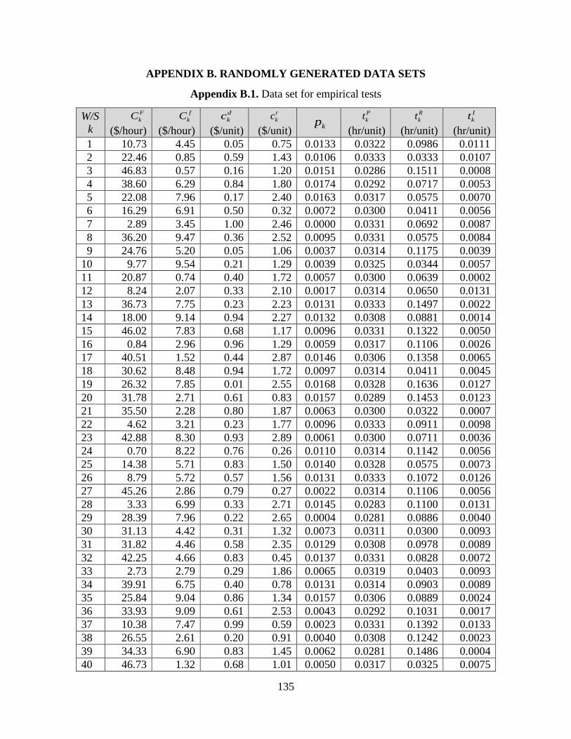
135

APPENDIX B. RANDOMLY GENERATED DATA SETS

Appendix B.1. Data set for empirical tests

W/S

k

F

kC

($/hour)

f

kC

($/hour)

d

kc

($/unit)

r

kc

($/unit) kp

P

kt

(hr/unit)

R

kt

(hr/unit)

I

kt

(hr/unit)

1 10.73 4.45 0.05 0.75 0.0133 0.0322 0.0986 0.0111

2 22.46 0.85 0.59 1.43 0.0106 0.0333 0.0333 0.0107

3 46.83 0.57 0.16 1.20 0.0151 0.0286 0.1511 0.0008

4 38.60 6.29 0.84 1.80 0.0174 0.0292 0.0717 0.0053

5 22.08 7.96 0.17 2.40 0.0163 0.0317 0.0575 0.0070

6 16.29 6.91 0.50 0.32 0.0072 0.0300 0.0411 0.0056

7 2.89 3.45 1.00 2.46 0.0000 0.0331 0.0692 0.0087

8 36.20 9.47 0.36 2.52 0.0095 0.0331 0.0575 0.0084

9 24.76 5.20 0.05 1.06 0.0037 0.0314 0.1175 0.0039

10 9.77 9.54 0.21 1.29 0.0039 0.0325 0.0344 0.0057

11 20.87 0.74 0.40 1.72 0.0057 0.0300 0.0639 0.0002

12 8.24 2.07 0.33 2.10 0.0017 0.0314 0.0650 0.0131

13 36.73 7.75 0.23 2.23 0.0131 0.0333 0.1497 0.0022

14 18.00 9.14 0.94 2.27 0.0132 0.0308 0.0881 0.0014

15 46.02 7.83 0.68 1.17 0.0096 0.0331 0.1322 0.0050

16 0.84 2.96 0.96 1.29 0.0059 0.0317 0.1106 0.0026

17 40.51 1.52 0.44 2.87 0.0146 0.0306 0.1358 0.0065

18 30.62 8.48 0.94 1.72 0.0097 0.0314 0.0411 0.0045

19 26.32 7.85 0.01 2.55 0.0168 0.0328 0.1636 0.0127

20 31.78 2.71 0.61 0.83 0.0157 0.0289 0.1453 0.0123

21 35.50 2.28 0.80 1.87 0.0063 0.0300 0.0322 0.0007

22 4.62 3.21 0.23 1.77 0.0096 0.0333 0.0911 0.0098

23 42.88 8.30 0.93 2.89 0.0061 0.0300 0.0711 0.0036

24 0.70 8.22 0.76 0.26 0.0110 0.0314 0.1142 0.0056

25 14.38 5.71 0.83 1.50 0.0140 0.0328 0.0575 0.0073

26 8.79 5.72 0.57 1.56 0.0131 0.0333 0.1072 0.0126

27 45.26 2.86 0.79 0.27 0.0022 0.0314 0.1106 0.0056

28 3.33 6.99 0.33 2.71 0.0145 0.0283 0.1100 0.0131

29 28.39 7.96 0.22 2.65 0.0004 0.0281 0.0886 0.0040

30 31.13 4.42 0.31 1.32 0.0073 0.0311 0.0300 0.0093

31 31.82 4.46 0.58 2.35 0.0129 0.0308 0.0978 0.0089

32 42.25 4.66 0.83 0.45 0.0137 0.0331 0.0828 0.0072

33 2.73 2.79 0.29 1.86 0.0065 0.0319 0.0403 0.0093

34 39.91 6.75 0.40 0.78 0.0131 0.0314 0.0903 0.0089

35 25.84 9.04 0.86 1.34 0.0157 0.0306 0.0889 0.0024

36 33.93 9.09 0.61 2.53 0.0043 0.0292 0.1031 0.0017

37 10.38 7.47 0.99 0.59 0.0023 0.0331 0.1392 0.0133

38 26.55 2.61 0.20 0.91 0.0040 0.0308 0.1242 0.0023

39 34.33 6.90 0.83 1.45 0.0062 0.0281 0.1486 0.0004

40 46.73 1.32 0.68 1.01 0.0050 0.0317 0.0325 0.0075

136

Appendix B.2. Dataset for the Workstation 5, Production line 1 [Example 4.1]

Data set 5

fC 5

dc 5

rc 5

Rt 5

It IC

1 20.00 0.35 4.40 20.16 13.68 30.00

2 9.81 1.44 16.01 175.68 7.20 23.56

3 16.72 1.47 20.42 70.20 16.56 19.60

4 15.89 1.47 24.36 147.60 27.72 23.44

5 21.99 0.98 10.05 116.28 14.04 12.73

6 9.66 0.90 23.46 41.76 22.32 11.68

7 8.84 1.28 12.33 146.16 22.32 36.49

8 15.68 0.53 2.55 75.60 25.56 38.60

9 16.04 0.97 24.39 41.40 12.60 48.81

10 20.81 1.08 10.98 109.44 24.84 13.58

11 14.32 1.32 5.35 183.24 31.68 11.48

12 24.96 0.99 22.82 198.00 33.12 23.51

13 7.74 0.82 24.05 105.48 20.16 49.28

14 24.87 0.92 11.56 55.08 30.24 43.16

15 17.16 0.62 15.63 29.52 25.92 26.25

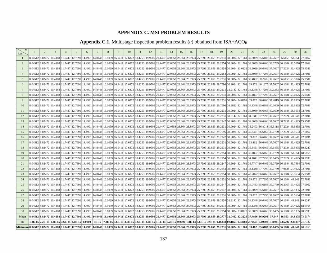
137

APPENDIX C. MSI PROBLEM RESULTS

Appendix C.1. Multistage inspection problem results (u) obtained from ISA+ACOR N

Run 1 2 3 4 5 6 7 8 9 10 11 12 13 14 15 16 17 18 19 20 21 22 23 24 25 30 35

1 8.04512 8.82472 10.4188 11.7447 12.7691 14.4991 14.8443 16.1039 16.9411 17.6872 18.4253 19.9506 21.4477 22.0858 23.864 23.8973 25.7399 26.859 29.2231 30.9024 32.1761 39.8039 35.6183 37.7607 36.6153 58.654 77.0062

2 8.04512 8.82472 10.4188 11.7447 12.7691 14.4991 14.8443 16.1039 16.9411 17.6872 18.4253 19.9506 21.4477 22.0858 23.864 23.8973 25.7399 26.859 29.2254 30.9024 32.1761 39.8039 36.6466 39.0769 36.1684 53.5076 77.0062

3 8.04512 8.82472 10.4188 11.7447 12.7691 14.4991 14.8443 16.1039 16.9411 17.6872 18.4253 19.9506 21.4477 22.0858 23.864 23.8973 25.7399 26.859 29.2254 30.9024 33.0122 39.8039 36.6466 37.7607 37.2024 53.4925 75.9581

4 8.04512 8.82472 10.4188 11.7447 12.7691 14.4991 14.8443 16.1039 16.9411 17.6872 18.4253 19.9506 21.4477 22.0858 23.864 23.8973 25.7399 26.859 29.2254 30.9024 32.1761 39.8039 37.7295 37.7607 36.1684 53.4925 72.7091

5 8.04512 8.82472 10.4188 11.7447 12.7691 14.4991 14.8443 16.1039 16.9411 17.6872 18.4253 19.9506 21.4477 22.0858 23.864 23.8973 25.7399 26.859 29.2231 30.9024 32.1761 36.4867 36.956 37.7607 36.6153 53.5076 75.9581

6 8.04512 8.82472 10.4188 11.7447 12.7691 14.4991 14.8443 16.1039 16.9411 17.6872 18.4253 19.9506 21.4477 22.0858 23.864 23.8973 25.7399 26.859 29.7596 30.9024 32.1761 39.872 40.1275 37.7607 36.1684 53.4925 72.7091

7 8.04512 8.82472 10.4188 11.7447 12.7691 14.4991 14.8443 16.1039 16.9411 17.6872 18.4253 19.9506 21.4477 22.0858 23.864 23.8973 25.7399 26.859 29.2231 31.2142 32.1761 34.1348 37.7295 39.1263 36.1684 53.4925 72.7091

8 8.04512 8.82472 10.4188 11.7447 12.7691 14.4991 14.8443 16.1039 16.9411 17.6872 18.4253 19.9506 21.4477 22.0858 23.864 23.8973 25.7399 26.859 29.2231 30.9024 32.1761 36.4867 37.7295 37.7607 36.1684 53.4925 75.9581

9 8.04512 8.82472 10.4188 11.7447 12.7691 14.4991 14.8443 16.1039 16.9411 17.6872 18.4253 19.9506 21.4477 22.0858 23.864 23.8973 25.7399 26.859 29.2231 30.9024 34.8999 39.872 36.6466 37.4819 36.1684 56.9335 72.7091

10 8.04512 8.82472 10.4188 11.7447 12.7691 14.4991 14.8443 16.1039 16.9411 17.6872 18.4253 19.9506 21.4477 22.0858 23.864 23.8973 25.7399 26.859 29.7596 34.2823 32.1761 34.1348 35.6183 40.1609 36.1684 56.9335 72.7091

11 8.04512 8.82472 10.4188 11.7447 12.7691 14.4991 14.8443 16.1039 16.9411 17.6872 18.4253 19.9506 21.4477 22.0858 23.864 23.8973 25.7399 26.859 29.2231 30.9024 32.1761 39.8039 36.6466 40.1609 36.1684 58.5634 72.7091

12 8.04512 8.82472 10.4188 11.7447 12.7691 14.4991 14.8443 16.1039 16.9411 17.6872 18.4253 19.9506 21.4477 22.0858 23.864 23.8973 25.7399 26.859 29.2231 31.2142 32.1761 34.3311 37.7295 37.7607 37.2024 49.943 72.7091

13 8.04512 8.82472 10.4188 11.7447 12.7691 14.4991 14.8443 16.1039 16.9411 17.6872 18.4253 19.9506 21.4477 22.0858 23.864 23.8973 25.7399 26.859 29.2247 30.9024 32.1761 39.8039 36.6466 37.7607 38.7957 53.4925 75.9581

14 8.04512 8.82472 10.4188 11.7447 12.7691 14.4991 14.8443 16.1039 16.9411 17.6872 18.4253 19.9506 21.4477 22.0858 23.864 23.8973 25.7399 26.859 29.2231 30.9024 32.1761 38.2403 36.8013 35.9118 37.2024 56.9335 72.7091

15 8.04512 8.82472 10.4188 11.7447 12.7691 14.4991 14.8443 16.1039 16.9411 17.6872 18.4253 19.9506 21.4477 22.0858 23.864 23.8973 25.7399 26.859 29.7596 30.9024 32.1761 35.8491 36.6466 39.0769 37.2024 58.5634 77.0062

16 8.04512 8.82472 10.4188 11.7447 12.7691 14.4991 14.8443 16.1039 16.9411 17.6872 18.4253 19.9506 21.4477 22.0858 23.864 23.8973 25.7399 26.859 29.2247 30.9024 32.1761 39.872 36.6466 37.7607 36.1684 49.943 72.7091

17 8.04512 8.82472 10.4188 11.7447 12.7691 14.4991 14.8443 16.1039 16.9411 17.6872 18.4253 19.9506 21.4477 22.0858 23.864 23.8973 25.7399 26.859 29.2231 30.9024 32.1761 33.462 36.6466 37.7607 36.1684 53.4925 72.7091

18 8.04512 8.82472 10.4188 11.7447 12.7691 14.4991 14.8443 16.1039 16.9411 17.6872 18.4253 19.9506 21.4477 22.0858 23.864 23.8973 25.7399 26.859 29.2231 30.9024 32.1761 35.8491 36.6466 35.6455 37.2024 56.9335 69.8247

19 8.04512 8.82472 10.4188 11.7447 12.7691 14.4991 14.8443 16.1039 16.9411 17.6872 18.4253 19.9506 21.4477 22.0858 23.864 23.8973 25.7399 26.859 29.2254 30.9024 32.1761 36.4867 36.6466 39.0769 36.1684 58.654 68.6168

20 8.04512 8.82472 10.4188 11.7447 12.7691 14.4991 14.8443 16.1039 16.9411 17.6872 18.4253 19.9506 21.4477 22.0858 23.864 23.8973 25.7399 26.859 29.2254 30.9024 32.1761 34.1041 37.7295 35.6455 37.2024 53.4925 70.5933

21 8.04512 8.82472 10.4188 11.7447 12.7691 14.4991 14.8443 16.1039 16.9411 17.6872 18.4253 19.9506 21.4477 22.0858 23.864 23.8973 25.7399 26.859 29.2247 30.9024 32.1761 39.7747 36.6466 39.0769 36.1684 56.7564 72.7091

22 8.04512 8.82472 10.4188 11.7447 12.7691 14.4991 14.8443 16.1039 16.9411 17.6872 18.4253 19.9506 21.4477 22.0858 23.864 23.8973 25.7399 26.859 29.2254 30.9024 32.1761 34.1348 37.7295 39.0769 37.9134 53.4925 72.7091

23 8.04512 8.82472 10.4188 11.7447 12.7691 14.4991 14.8443 16.1039 16.9411 17.6872 18.4253 19.9506 21.4477 22.0858 23.864 23.8973 25.7399 26.859 29.2254 30.9024 32.1761 43.2072 36.6466 37.7607 36.1684 58.5634 75.9581

24 8.04512 8.82472 10.4188 11.7447 12.7691 14.4991 14.8443 16.1039 16.9411 17.6872 18.4253 19.9506 21.4477 22.0858 23.864 23.8973 25.7399 26.859 29.2231 30.9024 32.1761 39.872 37.7295 37.7607 36.1684 49.943 72.7091

25 8.04512 8.82472 10.4188 11.7447 12.7691 14.4991 14.8443 16.1039 16.9411 17.6872 18.4253 19.9506 21.4477 22.0858 23.864 23.8973 25.7399 26.859 29.2247 30.9024 32.1761 36.0483 35.6183 39.0769 36.2367 53.4925 77.0062

26 8.04512 8.82472 10.4188 11.7447 12.7691 14.4991 14.8443 16.1039 16.9411 17.6872 18.4253 19.9506 21.4477 22.0858 23.864 23.8973 25.7399 26.859 29.2247 30.9024 32.1761 35.6099 35.6183 37.7607 36.1684 56.9335 72.7091

27 8.04512 8.82472 10.4188 11.7447 12.7691 14.4991 14.8443 16.1039 16.9411 17.6872 18.4253 19.9506 21.4477 22.0858 23.864 23.8973 25.7399 26.859 29.2231 30.9024 32.1761 39.872 37.7295 37.7607 36.1684 58.5634 72.7091

28 8.04512 8.82472 10.4188 11.7447 12.7691 14.4991 14.8443 16.1039 16.9411 17.6872 18.4253 19.9506 21.4477 22.0858 23.864 23.8973 25.7399 26.859 29.2254 31.2142 32.1761 34.1348 36.6466 37.7607 36.1684 49.943 69.8247

29 8.04512 8.82472 10.4188 11.7447 12.7691 14.4991 14.8443 16.1039 16.9411 17.6872 18.4253 19.9506 21.4477 22.0858 23.864 23.8973 25.7399 26.859 29.2231 30.9024 32.1761 34.1348 36.6466 37.7607 36.1684 53.4925 68.6168

30 8.04512 8.82472 10.4188 11.7447 12.7691 14.4991 14.8443 16.1039 16.9411 17.6872 18.4253 19.9506 21.4477 22.0858 23.864 23.8973 25.7399 26.859 29.2254 30.9024 33.0122 39.8039 36.6466 35.6455 36.1684 56.9335 70.5933

Mean 8.04512 8.82472 10.4188 11.7447 12.7691 14.4991 14.8443 16.1039 16.9411 17.6872 18.4253 19.9506 21.4477 22.0858 23.864 23.8973 25.7399 26.859 29.2777 31.0462 32.3226 37.4866 36.9298 37.947 36.553 54.8375 73.2174

SD 1.8E-15 7.2E-15 1.8E-15 3.6E-15 3.6E-15 0.0000 9E-15 7.2E-15 3.6E-15 3.6E-15 3.6E-15 3.6E-15 1.1E-14 7.2E-15 0.0000 1.8E-14 3.6E-15 3.6E-15 0.16338 0.61853 0.53088 2.70561 0.89908 1.16941 0.65202 2.84037 2.47732

Minimum 8.04512 8.82472 10.4188 11.7447 12.7691 14.4991 14.8443 16.1039 16.9411 17.6872 18.4253 19.9506 21.4477 22.0858 23.864 23.8973 25.7399 26.859 29.2231 30.9024 32.1761 33.462 35.6183 35.6455 36.1684 49.943 68.6168

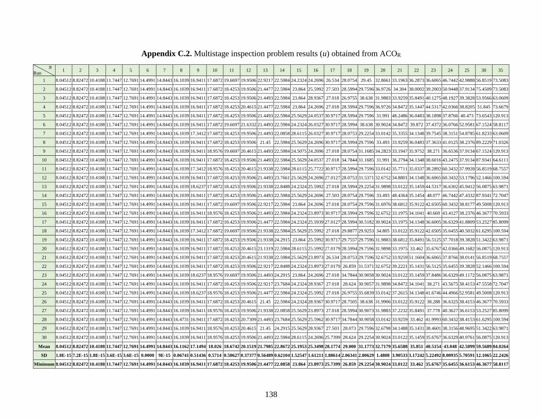
138

Appendix C.2. Multistage inspection problem results (u) obtained from ACOR N

Run 1 2 3 4 5 6 7 8 9 10 11 12 13 14 15 16 17 18 19 20 21 22 23 24 25 30 35

1 8.04512 8.82472 10.4188 11.7447 12.7691 14.4991 14.8443 16.1039 16.9411 17.6872 19.6697 19.9506 22.9217 22.5984 24.2324 24.2696 26.534 28.0754 29.45 32.8661 33.1963 36.2873 36.6065 46.7442 42.9888 56.8519 73.5083

2 8.04512 8.82472 10.4188 11.7447 12.7691 14.4991 14.8443 16.1039 16.9411 17.6872 18.4253 19.9506 21.4477 22.5984 23.864 25.5992 27.503 28.5994 29.7596 36.9726 34.304 38.0002 39.2003 50.9448 37.9134 75.4509 73.5083

3 8.04512 8.82472 10.4188 11.7447 12.7691 14.4991 14.8443 16.1039 16.9411 17.6872 18.4253 19.9506 21.4493 22.5984 23.864 28.9367 27.018 26.9755 38.638 31.9883 33.9259 35.8491 40.1275 48.1927 39.3828 53.9566 63.0609

4 8.04512 8.82472 10.4188 11.7447 12.7691 14.4991 14.8443 16.1039 16.9411 17.6872 18.4253 20.4615 21.4477 22.5984 23.864 24.2696 27.018 28.5994 29.7596 36.9726 34.8472 35.1447 44.5317 42.0366 38.8205 51.845 73.6679

5 8.04512 8.82472 10.4188 11.7447 12.7691 14.4991 14.8443 16.1039 16.9411 17.6872 18.4253 19.9506 21.4493 22.5984 25.5629 24.0537 30.9717 28.5994 29.7596 31.991 48.2486 36.0483 38.1898 37.8766 40.473 73.6543 120.913

6 8.04512 8.82472 10.4188 11.7447 12.7691 14.4991 14.8443 16.1039 16.9411 17.6872 19.6697 21.6332 21.4493 22.5984 24.2324 26.0327 30.9717 28.5994 38.638 30.9024 34.8472 39.872 37.4372 36.0766 52.9581 67.1524 58.8117

7 8.04512 8.82472 10.4188 11.7447 12.7691 14.4991 14.8443 16.1039 17.3412 17.6872 18.4253 19.9506 21.4493 22.0858 28.6115 26.0327 30.9717 28.0753 29.2254 33.0142 35.3355 34.1348 39.7545 38.3151 54.8785 61.8233 63.0609

8 8.04512 8.82472 10.4188 11.7447 12.7691 14.4991 14.8443 16.1039 16.9411 17.6872 18.4253 19.9506 21.45 22.5984 25.5629 24.2696 30.9717 28.5994 29.7596 33.493 33.9259 36.0483 37.3633 41.0125 38.2376 89.2229 71.0326

9 8.04512 8.82472 10.4188 11.7447 12.7691 14.4991 14.8443 16.1039 16.9411 18.9576 19.6697 20.4615 21.4493 22.5984 24.5075 24.2696 27.018 28.0754 31.1685 34.2823 33.1947 35.9752 38.271 36.6536 37.9134 67.1524 120.913

10 8.04512 8.82472 10.4188 11.7447 12.7691 14.4991 14.8443 16.1039 16.9411 17.6872 18.4253 19.9506 21.4493 22.5984 25.5629 24.0537 27.018 34.7844 31.1685 31.991 36.2794 34.1348 38.6016 43.2475 37.9134 87.9341 64.6111

11 8.04512 8.82472 10.4188 11.7447 12.7691 14.4991 14.8443 16.1039 17.3412 18.9576 18.4253 20.4615 21.9338 22.5984 28.6115 25.7722 30.9717 28.5994 29.7596 33.0142 35.7711 35.0337 38.2892 60.3432 37.9928 56.8519 68.7557

12 8.04512 8.82472 10.4188 11.7447 12.7691 14.4991 14.8443 16.1039 16.9411 17.6872 18.4253 19.9506 21.4493 23.7661 25.5629 24.2696 27.0127 28.0753 31.5371 32.6752 34.8801 34.1348 36.6065 60.3432 53.1796 52.1466 100.594

13 8.04512 8.82472 10.4188 11.7447 12.7691 14.4991 14.8443 16.1039 18.6237 17.6872 18.4253 19.9506 21.9338 22.8488 24.2324 25.5992 27.018 28.5994 29.2254 31.9898 33.0122 35.1459 44.5317 36.6302 45.9412 56.0875 63.9871

14 8.04512 8.82472 10.4188 11.7447 12.7691 14.4991 14.8443 16.1039 16.9411 17.6872 18.4253 19.9506 21.4493 22.5984 25.5629 24.2696 27.503 28.0754 29.7596 33.493 48.4364 35.1454 48.077 46.7442 47.4332 87.9341 72.7047

15 8.04512 8.82472 10.4188 11.7447 12.7691 14.4991 14.8443 16.1039 16.9411 17.6872 19.6697 19.9506 22.9217 22.5984 23.864 24.2696 27.018 28.0754 29.7596 31.6976 38.6812 35.9122 42.6505 60.3432 38.8177 49.5008 120.913

16 8.04512 8.82472 10.4188 11.7447 12.7691 14.4991 14.8443 16.1039 16.9411 18.9576 18.4253 19.9506 21.4493 22.5984 24.2324 23.8973 30.9717 28.5994 29.7596 32.6752 33.1975 34.1041 40.669 43.4127 38.2376 46.3677 70.5933

17 8.04512 8.82472 10.4188 11.7447 12.7691 14.4991 14.8443 16.1039 16.9411 17.6872 18.4253 19.9506 21.4477 22.5984 24.2324 25.5939 27.0127 28.5994 30.5182 30.9024 33.1975 34.1348 36.6005 36.6329 41.8809 53.2527 85.8099

18 8.04512 8.82472 10.4188 11.7447 12.7691 14.4991 14.8443 16.1039 17.3412 17.6872 19.6697 19.9506 21.9338 22.5984 25.5629 25.5992 27.018 29.8877 29.9253 34.805 33.0122 35.9122 42.6505 35.6455 40.5032 61.6295 100.594

19 8.04512 8.82472 10.4188 11.7447 12.7691 14.4991 14.8443 16.1039 16.9411 17.6872 18.4253 19.9506 21.9338 24.2915 23.864 25.5992 30.9717 29.7557 29.7596 31.9883 38.6812 35.8491 56.5125 37.7018 39.3828 51.3422 63.9871

20 8.04512 8.82472 10.4188 11.7447 12.7691 14.4991 14.8443 16.1039 16.9411 17.6872 18.4253 20.4615 23.1319 22.5984 28.6115 25.5992 27.0179 28.5994 29.7596 31.9898 33.1975 33.462 35.6767 42.0366 49.1682 56.0875 120.913

21 8.04512 8.82472 10.4188 11.7447 12.7691 14.4991 14.8443 16.1039 16.9411 17.6872 18.4253 20.4615 21.9338 22.5984 25.5629 23.8973 26.534 28.0753 29.7596 32.6752 33.9259 51.1604 36.6065 37.8766 38.0141 56.8519 68.7557

22 8.04512 8.82472 10.4188 11.7447 12.7691 14.4991 14.8443 16.1039 16.9411 17.6872 18.4253 19.9506 22.9217 22.8488 24.2324 23.8973 27.0179 26.859 31.5371 32.6752 39.2221 35.1431 56.5125 35.6455 39.3828 52.1466 100.594

23 8.04512 8.82472 10.4188 11.7447 12.7691 14.4991 14.8443 16.1039 18.6237 18.9576 19.6697 19.9506 21.4493 24.2915 23.864 24.2696 27.018 34.7844 30.9058 30.9024 33.0122 35.1459 37.8486 36.6329 49.1172 56.0875 63.9871

24 8.04512 8.82472 10.4188 11.7447 12.7691 14.4991 14.8443 16.1039 16.9411 17.6872 18.4253 19.9506 22.9217 23.7684 24.2324 28.9367 27.018 28.624 30.9057 31.9898 34.8472 34.1041 38.271 43.5675 38.4153 47.5558 72.7047

25 8.04512 8.82472 10.4188 11.7447 12.7691 14.4991 14.8443 16.1039 18.6237 18.9576 18.4253 19.9506 21.4477 22.5984 24.2324 25.5992 27.018 26.9755 35.6839 33.0142 37.2615 34.1348 41.6746 44.4966 52.9581 49.5008 120.913

26 8.04512 8.82472 10.4188 11.7447 12.7691 14.4991 14.8443 16.1039 16.9411 17.6872 18.4253 20.4615 21.45 22.5984 24.2324 28.9367 30.9717 28.7505 38.638 31.9906 33.0122 35.9122 38.288 36.6325 38.4153 46.3677 70.5933

27 8.04512 8.82472 10.4188 11.7447 12.7691 14.4991 14.8443 16.1039 16.9411 18.9576 18.4253 19.9506 21.9338 22.0858 25.5629 23.8973 27.018 28.5994 30.9073 31.9883 37.2232 35.8491 37.778 40.3627 36.6153 53.2527 85.8099

28 8.04512 8.82472 10.4188 11.7447 12.7691 14.4991 14.8443 16.4731 16.9411 17.6872 18.4253 20.7309 21.4493 23.7684 25.5629 25.5962 30.9717 34.7844 30.9058 33.0142 33.9259 33.462 41.9993 60.3432 38.4153 61.6295 100.594

29 8.04512 8.82472 10.4188 11.7447 12.7691 14.4991 14.8443 16.1039 16.9411 18.9576 18.4253 20.4615 21.45 24.2915 25.5629 28.9367 27.503 28.073 29.7596 32.6798 34.1488 35.1431 38.4601 38.3156 48.9695 51.3422 63.9871

30 8.04512 8.82472 10.4188 11.7447 12.7691 14.4991 14.8443 16.1039 16.9411 18.9576 18.4253 19.9506 21.4493 22.5984 28.6115 24.2696 25.7399 28.624 29.2254 30.9024 33.0122 35.1459 35.6767 36.6329 40.9761 56.0875 120.913

Mean 8.04512 8.82472 10.4188 11.7447 12.7691 14.4991 14.8443 16.1162 17.1494 18.026 18.6742 20.1519 21.7985 22.8672 25.1953 25.3498 28.1774 29.000 31.1773 32.7179 35.6588 35.851 40.5154 43.048 42.5099 59.5689 84.0264

SD 1.8E-15 7.2E-15 1.8E-15 3.6E-15 3.6E-15 0.0000 9E-15 0.06741 0.51436 0.5714 0.50627 0.37377 0.56489 0.62104 1.52547 1.61211 1.88614 2.06341 2.80629 1.4808 3.90533 3.17242 5.22492 8.00935 5.70591 12.1065 22.2426

Minimum 8.04512 8.82472 10.4188 11.7447 12.7691 14.4991 14.8443 16.1039 16.9411 17.6872 18.4253 19.9506 21.4477 22.0858 23.864 23.8973 25.7399 26.859 29.2254 30.9024 33.0122 33.462 35.6767 35.6455 36.6153 46.3677 58.8117

139

Appendix C.3. Number of functional evaluation (nfe) for solving multistage inspection problem with ISA+ACOR

N

Run 1 2 3 4 5 6 7 8 9 10 11 12 13 14 15 16 17 18 19 20 21 22 23 24 25 30 35

1 1 9 11 13 15 17 32 36 34 42 38 85 91 99 107 117 99 119 370 324 324 1089 1748 1202 1171 1162 1203

2 1 9 11 13 15 17 32 36 34 42 38 85 91 99 107 117 99 119 1070 324 324 1089 1166 1202 1171 1726 1203

3 1 9 11 13 15 17 32 36 34 42 38 85 91 99 107 117 99 119 1070 324 1124 1089 1166 1202 1171 1162 1203

4 1 9 11 13 15 17 32 36 34 42 38 85 91 99 107 117 99 119 1070 324 324 1089 1166 1202 1171 1150 1203

5 1 9 11 13 15 17 32 36 34 42 38 85 91 99 107 117 99 119 370 424 324 1652 1166 1202 1171 1710 1203

6 1 9 11 13 15 17 32 36 34 42 38 85 91 99 107 117 99 119 1070 424 324 1089 1166 1202 1171 1150 1203

7 1 9 11 13 15 17 32 36 34 42 38 85 91 99 107 117 99 119 470 1124 324 2240 1166 1796 1171 1150 1203

8 1 9 11 13 15 17 32 36 34 42 38 85 91 99 107 117 99 119 270 324 324 1652 1166 1202 1171 1150 1203

9 1 9 11 13 15 17 32 36 34 42 38 85 91 99 107 117 99 119 670 324 1124 1089 1166 2420 1171 1150 1203

10 1 9 11 13 15 17 32 36 34 42 38 85 91 99 107 117 99 119 1070 581 324 2240 1748 1202 1171 1150 1203

11 1 9 11 13 15 17 32 36 34 42 38 85 91 99 107 117 99 119 470 324 324 1089 1166 1181 1183 1150 1203

12 1 9 11 13 15 17 32 36 34 42 38 85 91 99 107 117 99 119 270 1124 424 2240 1166 1181 1183 3590 1203

13 1 9 11 13 15 17 32 36 34 42 38 85 91 99 107 117 99 119 1070 324 324 1089 1166 1181 1183 1150 1203

14 1 9 11 13 15 17 32 36 34 42 38 85 91 99 107 117 99 119 270 324 324 1652 1166 1768 1183 1150 1203

15 1 9 11 13 15 17 32 36 34 42 38 85 91 99 107 117 99 119 1070 424 1024 2858 1166 1181 1183 1150 1203

16 1 9 11 13 15 17 32 36 34 42 38 85 91 99 107 117 99 119 1070 324 324 1089 1166 1181 1183 3590 1203

17 1 9 11 13 15 17 32 36 34 42 38 85 91 99 107 117 99 119 270 324 424 2240 1166 1181 1183 1150 1203

18 1 9 11 13 15 17 32 36 34 42 38 85 91 99 107 117 99 119 270 324 324 2858 1166 1768 1183 1150 1764

19 1 9 11 13 15 17 32 36 34 42 38 85 91 99 107 117 99 119 1070 424 324 1652 1166 1181 1183 1150 1764

20 1 9 11 13 15 17 32 36 34 42 38 85 91 99 107 117 99 119 1070 324 324 2240 1166 1768 1183 1150 1764

21 1 9 11 13 15 17 32 36 34 42 38 85 91 99 107 117 99 119 1070 324 424 1652 1166 1181 1183 1710 1203

22 1 9 11 13 15 17 32 36 34 42 38 85 91 99 107 117 99 119 1070 324 424 2240 1166 1181 1764 1150 1203

23 1 9 11 13 15 17 32 36 34 42 38 85 91 99 107 117 99 119 1070 324 324 1089 1166 1181 1183 1150 1203

24 1 9 11 13 15 17 32 36 34 42 38 85 91 99 107 117 99 119 170 324 324 1089 1166 1181 1183 3590 1203

25 1 9 11 13 15 17 32 36 34 42 38 85 91 99 107 117 99 119 1070 324 424 1652 1748 1181 1183 1150 1203

26 1 9 11 13 15 17 32 36 34 42 38 85 91 99 107 117 99 119 1070 424 324 1652 1748 1181 1183 1150 1203

27 1 9 11 13 15 17 32 36 34 42 38 85 91 99 107 117 99 119 270 424 324 1089 1166 1181 1183 1150 1203

28 1 9 11 13 15 17 32 36 34 42 38 85 91 99 107 117 99 119 1070 1124 424 2240 1166 1181 1183 3590 1764

29 1 9 11 13 15 17 32 36 34 42 38 85 91 99 107 117 99 119 270 324 424 2240 1166 1181 1183 1150 1764

30 1 9 11 13 15 17 32 36 34 42 38 85 91 99 107 117 99 119 1070 324 1124 1089 1166 1768 1183 1150 1764

Mean 1 9 11 13 15 17 32 36 34 42 38 85 91 99 107 117 99 119 753.33 432.57 450.67 1645.2 1243.6 1326.7 1198.4 1532.7 1315.2

SD 0 0 0 0 0 0 0 0 0 0 0 0 0 0 0 0 0 0 377.91 241.58 262.53 581.14 201.22 302.78 106.98 838.32 228.24

140

Appendix C.4. Number of functional evaluation (nfe) for solving multistage inspection problem with ACOR

N

Run 1 2 3 4 5 6 7 8 9 10 11 12 13 14 15 16 17 18 19 20 21 22 23 24 25 30 35

1 1 7 7 7 7 7 23 123 123 23 1554 1554 1023 1554 1554 1554 1554 2105 2105 2681 2681 3287 3287 1554 2681 2681 3287

2 1 7 7 7 7 7 23 23 23 123 123 1554 1554 1554 1554 2105 2105 2105 2105 1554 2681 2681 3928 1554 3287 1554 3287

3 1 7 7 7 7 7 23 23 123 123 123 1554 1554 1554 1554 1023 2105 1554 1023 2681 2681 3287 2105 1554 2681 3287 3287

4 1 7 7 7 7 7 23 23 123 123 23 1554 1554 1554 1554 1554 2105 2105 2105 1554 2681 3287 1554 1554 3928 3287 2681

5 1 7 7 7 7 7 23 23 123 123 123 1554 1554 1554 2105 1554 1023 2105 2105 2681 1023 2105 2681 3287 2681 1554 1023

6 1 7 7 7 7 7 23 23 123 23 1554 2105 1554 1554 1554 2105 1023 2105 1023 2105 2681 1554 3287 2681 1554 1554 3928

7 1 7 7 7 7 7 23 123 1023 123 123 1554 1554 1554 1023 2105 1023 2105 2105 2681 2105 2681 2681 3928 1554 2105 3287

8 1 7 7 7 7 7 23 23 123 123 23 1554 1554 1554 2105 1554 1023 2105 2105 2105 2681 2105 3287 2105 3287 1023 2681

9 1 7 7 7 7 7 23 23 123 1554 1554 1554 1554 1554 1554 1554 2105 2105 2681 1554 2681 2105 2105 2681 3287 1554 1023

10 1 7 7 7 7 7 23 123 23 123 23 1554 1554 1554 2105 1554 2105 1023 2681 2681 2105 2681 2681 2681 3287 1023 4609

11 1 7 7 7 7 7 23 23 1023 1554 23 1554 1554 1554 1023 2105 1023 2105 2105 2681 2105 2681 3928 1023 3287 2681 3928

12 1 7 7 7 7 7 23 123 123 23 23 1554 1554 2105 2105 1554 2105 2105 2681 2681 3287 2681 3287 1023 1554 3287 1554

13 1 7 7 7 7 7 23 23 1554 23 23 1554 1554 1554 1554 2105 2105 2105 2105 2681 2105 3287 1554 3287 1554 2681 4609

14 1 7 7 7 7 7 23 123 23 123 123 1554 1554 1554 2105 1554 2105 2105 2105 2105 1023 3287 1554 1554 2105 1023 3287

15 1 7 7 7 7 7 23 23 123 123 1554 1554 1023 1554 1554 1554 2105 2105 2105 2105 1554 3287 1554 1023 3928 4609 1023

16 1 7 7 7 7 7 23 23 23 1554 23 1554 1554 1554 1554 1554 1023 2105 2105 2681 2681 2681 2105 2105 3287 5335 2681

17 1 7 7 7 7 7 23 123 123 23 23 1554 1554 1554 1554 2105 2105 2105 2105 2105 2681 2681 3287 3287 3287 3287 2105

18 1 7 7 7 7 7 23 23 1023 123 1554 1554 1554 1554 2105 2105 2105 1554 2105 2105 2105 3287 1554 2681 4609 2681 1554

19 1 7 7 7 7 7 23 23 123 23 23 1554 1554 1023 1554 2105 1023 2681 2105 2681 1554 3287 1023 3287 2681 3287 4609

20 1 7 7 7 7 7 23 23 123 123 23 1554 2105 1554 1023 2105 2105 2105 2105 2681 2681 2681 2681 1554 2105 2681 1023

21 1 7 7 7 7 7 23 23 123 123 23 1554 1554 1554 2105 1554 1554 2105 2105 2681 2681 1023 3287 3287 3287 2681 3928

22 1 7 7 7 7 7 23 123 123 123 123 1554 1023 1554 1554 1554 2105 1554 2681 2681 1554 3287 1023 2681 2681 3287 1554

23 1 7 7 7 7 7 23 123 1554 1554 1554 1554 1554 1023 1554 1554 2105 1023 2681 2105 2105 3287 3287 3287 1554 2681 4609

24 1 7 7 7 7 7 23 23 23 123 23 1554 1023 2105 1554 1023 2105 2105 2681 2681 2681 2681 2105 2105 3287 3928 3287

25 1 7 7 7 7 7 23 123 1554 1554 23 1554 1554 1554 1554 2105 2105 1554 1554 2681 1554 2681 2105 2105 1554 4609 1023

26 1 7 7 7 7 7 23 23 23 23 23 1554 1554 1554 1554 1023 1023 2105 1023 2681 2105 3287 3928 3287 3287 5335 2681

27 1 7 7 7 7 7 23 23 123 1554 23 1554 1554 1554 2105 1554 2105 2105 2681 2681 2105 3287 2681 2681 2681 3287 2105

28 1 7 7 7 7 7 23 1023 23 123 23 1023 1554 2105 2105 2105 1023 1023 2681 2681 2681 2681 1554 1023 3287 2681 1554

29 1 7 7 7 7 7 23 23 123 1554 123 1554 1554 1023 2105 1023 2105 2105 2105 2681 2681 3287 3287 3928 1554 3287 4609

30 1 7 7 7 7 7 23 123 23 1554 23 1554 1554 1554 1023 1554 1554 2105 2105 2105 2105 3287 2681 3287 2681 2681 1023

Mean 1 7 7 7 7 7 23 89.667 329.43 481.27 352.53 1554.7 1501.6 1556 1666.9 1685.2 1725.3 1942.5 2132 2414.7 2267.6 2813.4 2535.4 2402.5 2749.2 2854.4 2728

SD 0 0 0 0 0 0 0 182.57 504.29 659.19 612.4 142.1 215.68 246.11 346.04 369.1 495.57 383.56 471.54 386.72 551.01 576.26 865.91 903.33 836.28 1156.3 1281.5

141

Appendix C.5. CPU time for solving multistage inspection problem with ISA+ACOR N

Run 1 2 3 4 5 6 7 8 9 10 11 12 13 14 15 16 17 18 19 20 21 22 23 24 25 30 35

1 0.68750 0.54688 0.65625 0.78125 0.89063 1.03125 1.84375 2.34375 4.15625 5.60938 5.71875 12.1406 11.4817 19.3281 25.5156 32.3281 29.4063 41.4219 176.547 119.437 146.563 743.75 439.47 475.912 663.425 1617.79 13254.7

2 0.10938 0.53125 0.71875 0.79688 0.96875 1.10938 1.8125 2.25000 4.17188 5.57813 5.71875 12.5000 9.68766 19.4375 26.4688 32.5000 29.2656 40.5781 907.547 124.125 145.641 751.922 358.771 467.66 4172.04 2358.58 12603.5

3 0.09375 0.48438 0.60938 0.76563 0.92188 0.92188 2.01563 2.15625 4.29688 5.64063 5.67188 12.5156 9.62526 19.4844 25.5000 31.6563 29.8594 40.4531 1839.27 142.656 469.328 758.797 354.278 438.285 650.945 1807.26 10525.1

4 0.09375 0.46875 0.73438 0.78125 0.84375 1.07813 1.73438 2.25000 4.43750 5.35938 5.51563 12.5938 10.1089 19.5938 25.375 32.1406 30.4063 40.7344 947.812 117.344 152.156 755.437 318.226 447.192 3205.23 1475.78 14662.6

5 0.0625 0.45313 0.67188 0.75000 0.9375 1.0625 1.84375 2.29688 4.37500 5.60938 5.79688 12.6563 10.0309 19.4844 25.5000 31.2344 30.5000 40.2500 214.438 169.453 147.172 773.531 409.518 450.000 632.225 1823.48 10660.2

6 0.12500 0.54688 0.6875 0.84375 0.92188 1.04688 1.87500 2.14063 4.45313 5.45313 5.65625 12.5938 9.46926 20.0469 25.7344 32.4063 29.3438 41.3125 743.484 162.016 143.875 705.594 411.609 440.999 1340.75 1396.33 12653.9

7 0.06250 0.50000 0.79688 0.75000 0.82813 1.07813 1.84375 2.20313 4.17188 5.59375 5.59375 12.4375 10.3429 19.6719 26.2344 31.8125 33.1406 40.5000 289.312 390.297 148.016 715.219 388.614 601.462 4127.1 1531.38 12631.9

8 0.09375 0.48438 0.6875 0.82813 0.92188 1.01563 1.79688 2.3125 4.34375 5.46875 5.71875 12.5313 9.21966 19.8594 25.8125 31.2813 29.8125 41.000 123.187 127.359 147.047 755.234 379.441 498.985 2940.31 1915.19 10820.3

9 0.10938 0.50000 0.78125 0.73438 0.84375 1.03125 1.89063 2.21875 4.28125 5.73438 5.5000 12.5781 9.81246 19.4219 26.1094 32.2031 29.2813 41.0313 482.187 135.25 515.063 692.813 371.189 682.473 2235.49 2483.7 10594.3

10 0.07813 0.46875 0.6875 0.8125 0.87500 1.09375 1.82813 2.29688 4.39063 5.53125 5.46875 12.4219 9.32886 19.6563 26.6406 32.1406 30.1094 40.7031 532.844 418.266 181.375 798.016 395.884 637.560 1801.86 2999.13 10859.8

11 0.06250 0.42188 0.625 0.73438 1.06250 0.95313 1.93750 2.39063 4.35938 5.51563 5.73438 12.9219 9.21966 20.2656 26.3125 32.6719 29.6094 40.5938 283.047 127.094 151.078 785.297 810.797 997.969 4449.97 1214.98 12447.8

12 0.09375 0.46875 0.73438 0.73438 0.90625 1.12500 1.93750 2.25000 4.42188 5.60938 5.62500 13.0000 9.64086 19.8125 26.1875 33.2188 30.6875 40.4688 133.484 474.734 204.359 887.438 788.141 992.078 1233.5 2472.77 12802.1

13 0.07813 0.45313 0.64063 0.75000 0.87500 1.01563 1.84375 2.29688 4.43750 5.57813 5.84375 12.5469 9.64086 20.1250 25.6094 31.9844 30.000 43.7969 1055.73 121.312 151.391 793.234 776.781 991.984 1334.17 1483.92 9237.45

14 0.09375 0.53125 0.71875 0.79688 0.81250 1.00000 1.89063 2.26563 4.31250 5.67188 5.65625 13.0156 8.81406 19.8594 26.2969 32.2969 29.4844 41.0313 140.703 130.984 152.203 823.266 862.922 1045.02 1289.77 3005.73 10091.7

15 0.0625 0.45313 0.65625 0.79688 0.89063 1.07813 1.87500 2.40625 4.43750 5.5625 5.76563 12.7188 9.28206 20.1406 26.4375 32.1406 29.7656 41.5625 565.672 175.516 438.719 959.578 752.297 1069.33 1225.17 1175.70 9929.42

16 0.09375 0.42188 0.64063 0.8125 0.8125 1.06250 1.8125 2.21875 4.37500 5.3125 5.8125 12.7969 9.62526 19.9531 26.4531 31.6875 29.5625 41.0625 981.563 128.969 143.500 751.578 792.109 991.844 1673.45 2427.48 10320.5

17 0.07813 0.45313 0.6875 0.78125 0.98438 1.00000 1.85938 2.25000 4.32813 5.64063 5.54688 12.5000 8.82966 19.9844 26.5313 31.6406 30.7656 40.7656 104.734 123.422 249.672 898.641 836.219 987.937 2191.55 1459.03 12598.6

18 0.10938 0.48438 0.79688 0.78125 0.87500 1.06250 1.76563 2.32813 4.35938 5.73438 5.87500 12.7500 9.50046 20.5000 26.1563 31.7813 29.7344 47.0625 137.500 131.094 151.016 791.578 831.156 1063.66 1365.98 2965.88 12729.9

19 0.07813 0.43750 0.64063 0.73438 0.82813 1.03125 1.81250 2.23438 4.39063 5.67188 5.68750 12.5781 9.34446 20.0156 25.8594 32.6719 31.6719 40.8438 901.625 168.234 153.609 841.406 873.641 1092.16 1778.88 2251.34 24609.4

20 0.12500 0.50000 0.71875 0.84375 0.87500 1.00000 1.76563 2.21875 4.40625 5.70313 5.89063 12.8281 9.34446 20.1563 26.4375 32.0938 29.8594 41.4063 950.109 138.594 156.172 904.625 975.719 1044.06 1197.52 1483.13 11931.1

21 0.07813 0.48438 0.67188 0.79688 0.87500 1.00000 1.82813 2.40625 4.46875 5.54688 5.51563 12.8281 9.34446 19.8594 26.2188 32.4531 30.6563 44.5625 1054.78 126.922 207.359 804.875 824.344 1064.59 2544.66 2928.95 12442.7

22 0.10938 0.46875 0.67188 0.76563 0.81250 0.96875 1.90625 2.29688 4.34375 5.60938 5.53125 12.8750 9.06366 20.1719 26.4063 32.1563 30.3594 43.1875 977.234 128.141 219.828 890.969 842.000 1072.64 1390.86 1530.44 12788.5

23 0.07813 0.45313 0.67188 0.8125 0.82813 1.01563 1.92188 2.32813 4.40625 5.59375 5.73438 12.8594 8.90766 20.3281 26.5625 32.0469 30.1094 41.4688 923.016 133.187 153.531 804.875 831.344 1001.42 5908.31 1224.69 9225.65

24 0.09375 0.46875 0.67188 0.75000 0.92188 0.95313 1.9375 2.35938 4.40625 5.73438 5.92188 13.2344 8.86086 20.2656 26.5469 32.2813 29.9219 41.5625 71.2031 129.938 154.891 786.875 853.484 983.469 4104.69 2488.30 10081.7

25 0.07813 0.46875 0.67188 0.84375 0.92188 1.00000 1.84375 2.42188 3.95313 5.71875 5.82813 12.8594 8.93886 20.4063 26.0313 33.1719 30.8438 41.6563 669.219 135.875 201.25 875.391 874.984 1069.2 1323.92 1490.78 9916.56

26 0.12500 0.5625 0.73438 0.84375 0.87500 1.03125 1.87500 2.45313 3.78125 5.6875 5.73438 12.9375 9.00126 20.2969 25.8594 32.2344 32.625 41.5469 1058.89 175.672 149.516 809.703 917.609 1007.28 5621.25 3014.27 10308.2

27 0.14063 0.50000 0.60938 0.73438 0.90625 1.01563 1.92188 2.46875 3.96875 5.85938 5.89063 12.9688 8.97006 20.4844 27.0938 31.9375 29.9844 41.2813 110.828 175.781 149.313 796.187 861.906 1016.81 5142.75 1209.89 12582.7

28 0.12500 0.4375 0.71875 0.78125 0.85938 0.98438 1.8125 2.1875 4.29688 5.70313 5.78125 13.1875 9.26646 20.4063 26.9688 32.1406 31.0781 41.7188 961.641 411.188 235.766 782.734 845.016 1009.2 2223.38 2474.34 12714.0

29 0.07813 0.50000 0.70313 0.78125 0.82813 0.96875 1.95313 2.45313 4.39063 5.65625 5.62500 12.8438 8.72046 20.5625 26.5938 33.3438 31.5781 42.1406 131.672 131.734 219.469 961.266 827.078 1006.92 4042.77 1486.66 24567.4

30 0.09375 0.46875 0.70313 0.84375 0.87500 1.10938 1.81250 2.34375 4.26563 5.70313 5.70313 13.0313 9.70326 20.3125 27.3594 33.3281 30.2969 41.5000 2116.98 138.812 501.281 869.547 842.078 1199.44 1544.55 3008.95 11920.0

Mean 0.11302 0.48073 0.69063 0.78542 0.88594 1.02813 1.8599 2.30156 4.30625 5.61302 5.70208 12.7417 9.43754 19.9964 26.2271 32.2328 30.324 41.5734 652.876 177.114 211.339 808.979 688.221 861.585 2445.22 2006.86 12417.1

SD 0.11054 0.03617 0.04897 0.03737 0.05643 0.05066 0.0631 0.08973 0.16168 0.11502 0.12700 0.24738 0.56023 0.36097 0.48613 0.53646 0.93894 1.41833 517.076 100.569 112.374 69.7749 224.139 258.500 1545.46 651.717 3574.75

142

Appendix C.6. CPU time for solving multistage inspection problem with ACOR N

Run 1 2 3 4 5 6 7 8 9 10 11 12 13 14 15 16 17 18 19 20 21 22 23 24 25 30 35

1 0.64063 0.35938 0.3125 0.3125 0.29688 0.34375 0.92188 4.18750 10.8906 3.21875 130.297 142.703 72.9617 316.141 460.719 650.906 991.854 1066.61 154.067 234.172 437.516 522.50 553.203 324.188 615.031 2380.84 5808.66

2 0.03125 0.32813 0.29688 0.32813 0.34375 0.375 0.8125 1.01560 2.46875 13.2500 17.9219 141.922 74.0693 321.719 449.984 673.719 1145.36 1130.31 158.169 198.578 400.344 468.078 547.625 391.594 671.859 1852.91 5797.3

3 0.03125 0.29688 0.28125 0.34375 0.39063 0.34375 0.84375 0.98438 10.8437 13.3750 18.1563 142.969 74.0381 324.172 461.547 654.062 1092.01 1124.88 132.882 245.766 408.859 543.547 433.25 390.141 748.719 2539.25 9720.27

4 0.04688 0.28125 0.34375 0.32813 0.32813 0.35938 0.84375 0.98438 10.7188 13.0469 4.34375 144.109 77.8289 342.844 478.922 585.313 1139.90 1127.69 154.503 204.438 396.938 415.953 304.469 515.734 1074.14 2462.14 6434.47

5 0.03125 0.23438 0.28125 0.29688 0.34375 0.32813 0.87500 0.98438 10.875 13.5781 17.6094 143.625 74.1473 318.797 493.813 682.422 974.070 1095.8 148.763 255.922 364.313 456.797 467.547 473.719 764.109 6823.61 5136.05

6 0.04688 0.25000 0.34375 0.34375 0.34375 0.39063 0.93750 0.96876 10.5000 3.42188 158.641 166.859 71.6981 329.891 469.562 731.688 971.730 1195.5 131.914 217.797 432.609 444.250 504.906 449.313 489.719 2137.17 10592.5

7 0.03125 0.23438 0.32813 0.34375 0.34375 0.37500 0.82813 4.37500 84.1562 13.5625 18.625 151.984 73.3205 336.75 482.078 725.531 966.894 1176.47 174.082 254.406 391.500 480.250 385.703 568.688 705.109 1035.59 7611.58

8 0.03125 0.28125 0.29688 0.35938 0.35938 0.34375 0.81250 1.14060 11.2344 13.8437 4.5000 160.406 74.6465 359.719 503.656 675.203 898.297 1144.36 152.257 224.906 347.469 453.375 570.047 427.047 698.656 1903.08 5897.2

9 0.04688 0.26563 0.29688 0.3125 0.34375 0.35938 0.87500 1.06250 11.3750 99.5937 172.188 148.687 70.4501 365.187 492.703 723.266 991.875 1212.36 252.144 215.719 476.25 464.844 459.281 476.984 730.719 2232.7 4288.63

10 0.03125 0.32813 0.3125 0.26563 0.37500 0.39063 0.92188 4.28125 2.71875 13.9219 4.45312 150.813 71.2613 361.188 514.828 728.531 1004.73 1076.2 169.245 317.516 403.109 378.078 454.719 465.672 838.109 2144.84 6620.17

11 0.06205 0.29688 0.29688 0.35938 0.34375 0.3125 0.85938 1.03125 86.5781 117.016 4.28125 149.609 70.8245 343.375 484.594 705.391 947.234 1142.19 176.484 320.984 490.750 520.500 805.047 514.984 760.219 2328.78 7403.45

12 0.01563 0.28125 0.32813 0.3125 0.39063 0.32813 0.92188 4.21875 11.5469 3.21875 4.5000 151.437 70.9493 385.984 523.938 694.328 989.875 1229.22 193.75 320.766 639.297 637.906 703.391 523.438 690.234 2492.23 6884.14

13 0.04688 0.23438 0.3125 0.32813 0.40625 0.34375 0.89063 1.00000 103.312 3.34375 4.71875 151.609 72.1817 345.484 613.687 755.359 993.438 1205.83 239.375 310.625 492.859 614.141 442.219 784.703 693.516 952.688 9247.38

14 0.01563 0.20313 0.29688 0.34375 0.39063 0.3125 0.92188 4.59375 2.92187 13.9844 19.5469 156.438 69.9508 376.781 536.703 725.531 1022.42 1172.86 181.203 283.859 428.031 717.438 495.594 544.125 731.188 2200.69 6563.98

15 0.0625 0.23438 0.34375 0.29688 0.39063 0.34375 0.90625 1.09375 11.5937 14.1094 139.984 156.906 69.7792 364.375 610.984 734.281 1020.97 1177.88 189.141 288.609 486.531 559.516 533.844 530.625 1032.25 7604.05 4635.92

16 0.01563 0.21875 0.28125 0.3125 0.34375 0.32813 0.85938 1.04687 2.8750 115.234 4.45312 158.094 70.7465 363.375 524.031 757.953 974.125 1205.88 182.406 321.703 568.484 660.922 556.547 576.594 834.094 4238.47 4963.08

17 0.04688 0.25000 0.28125 0.35938 0.32813 0.32813 0.87500 4.46875 11.9063 3.42188 4.57812 155.531 70.8557 373.172 532.109 768.766 1044.97 1204.72 189.391 325.172 515.594 274.563 674.359 789.438 807.594 2529.44 5104.56

18 0.04688 0.29688 0.35938 0.34375 0.35938 0.40625 0.85938 1.00000 91.7500 14.1250 172.375 160.531 69.6388 368.156 654.500 778.125 1050.72 1171.94 191.078 298.984 511.609 402.109 540.906 645.500 1131.58 2399.72 5442.20

19 0.03125 0.29688 0.4375 0.34375 0.37500 0.34375 0.87500 1.12500 11.9063 3.50000 4.62500 157.078 70.3721 356.266 546.531 775.984 958.844 1280.98 199.906 363.234 447.563 485.516 532.234 678.297 781.656 2617.42 6986.44

20 0.04688 0.25000 0.3125 0.35938 0.3750 0.29688 0.82813 1.23437 12.1719 14.3594 4.82812 157.047 73.7729 400.937 540.094 705.109 1005.84 1186.77 202.844 374.344 511.594 449.813 598.922 573.813 755.328 1257.14 5368.52

21 0.09375 0.26563 0.3125 0.4375 0.29688 0.35938 0.92188 1.12500 12.0156 14.5156 4.67188 159.281 68.3752 384.00 583.281 606.016 1028.42 1250.73 199.188 345.734 508.516 241.109 708.203 662.266 826.25 2338.67 7367.89

22 0.03125 0.29688 0.28125 0.34375 0.35938 0.35938 0.87500 4.64062 12.2188 14.3594 19.1094 184.203 65.6296 374.859 556.469 678.984 1154.59 1193.75 230.734 363.281 514.203 572.391 547.344 667.859 788.453 2497.20 6849.95

23 0.04688 0.25000 0.32813 0.35938 0.34375 0.28125 0.84375 4.42187 107.359 121.156 175.625 161.109 68.5936 379.063 571.297 772.234 1060.83 1162.14 237.719 327.656 396.734 442.094 638.797 833.719 737.656 931.563 9208.08

24 0.06250 0.23438 0.3125 0.34375 0.32813 0.29688 0.89063 1.04687 2.96875 14.8438 4.90625 161.406 66.9556 407.313 563.000 741.531 1077.70 1255.89 259.422 358.453 520.828 461.266 589.031 619.484 843.359 2631.78 6530.47

25 0.01563 0.26563 0.3125 0.32813 0.32813 0.34375 0.89063 4.68750 112.031 123.000 4.70313 163.75 75.4577 395.234 577.359 810.469 1058.59 1163.22 196.281 362.563 530.500 274.688 590.75 623.75 629.594 7565.36 4607.70

26 0.07813 0.28125 0.29688 0.29688 0.4375 0.26563 0.90625 1.06250 2.96875 3.76563 4.92188 168.609 69.748 431.313 570.984 795.453 1016.78 1259.78 195.438 372.125 587.531 403.406 817.719 758.422 642.547 4188.77 4932.20

27 0.04688 0.23438 0.29688 0.3125 0.35938 0.3125 0.93750 1.04687 12.8125 127.062 4.70313 168.844 69.8104 381.766 703.75 629.859 1108.22 1261.94 226.313 367.984 547.906 484.578 622.469 661.266 833.688 2488.53 5082.39

28 0.06250 0.25000 0.29688 0.32813 0.34375 0.34375 0.89063 30.7656 3.04688 15.0781 5.01562 165.094 75.8321 415.422 628.531 846.828 1039.00 1187.23 281.594 370.453 521.984 448.203 584.063 490.359 855.25 2368.08 5416.2

29 0.03125 0.21875 0.29688 0.3125 0.34375 0.31250 0.87500 1.12500 13.1875 130.188 20.0625 185.312 68.9056 389.391 633.219 795.609 1100.73 1279.39 225.766 394.922 533.938 571.688 668.438 866.953 713.703 2628.97 6979.89

30 0.09375 0.25000 0.29688 0.34375 0.32813 0.31250 0.92188 4.82812 3.14062 113.609 4.76562 174.125 69.826 436.953 582.563 847.781 1055.09 1230.61 234.063 382.391 562.969 443.484 636.750 786.000 774.937 1266.48 5358.53

Mean 0.06406 0.26563 0.3125 0.33333 0.35469 0.33802 0.88073 3.1849 26.4698 39.3568 38.637 158.003 71.4209 368.321 544.848 725.208 1029.50 1185.77 195.337 307.435 479.211 476.433 565.579 587.156 773.309 2767.94 6427.99

SD 0.11082 0.03624 0.03152 0.03025 0.03075 0.03244 0.03658 5.45757 36.6533 48.8684 61.5843 11.1078 2.7364 31.9072 63.4223 65.171 62.0223 56.8798 38.0065 60.3572 71.5477 107.999 114.115 141.38 131.301 1717.36 1599.63

143

VITA

Md. Shahriar Jahan Hossain was born in Natore, Bangladesh in 1986. He received his

Bachelor of Science degree in 2009 and Masters of Science degree in 2012, both in Industrial and

Production Engineering from Bangladesh University of Engineering and Technology, Dhaka. He

worked as an Assistant Professor at the same institution before starting his PhD study at Louisiana

State University in 2014. In addition, he also worked with Impress-Newtex Composite Textiles

Ltd., Tangail, Bangladesh, and served on the faculty of several universities including Rajshahi

University of Engineering and Technology (RUET) and Military Institute of Science and

Technology (MIST) in Bangladesh.

Currently Mr. Hossain has been pursuing a PhD degree in Engineering Science, with home

affiliation in the Department of Mechanical & Industrial Engineering, Louisiana State University

at Baton Rouge, LA under a Fellowship program (Throughput and Yield Enhancement for Steel

Pipe Manufacturing for Oil and Gas Transport) funded by Louisiana Economic Development

Assistantship (EDA) Program.

Recently, one of his articles on rework policy optimization co-authored with Dr. Bhaba

Sarker has been published in International Journal of Production Research and one paper is

presented and published in the Proceedings of the 1st International Conference on Materials and

Manufacturing Engineering (ICMME 2015). Two of his articles on inventory management are

currently under review by refereed journals. Besides these, he has co-authored several journal and

conference articles on operations research, ergonomics, industrial environment, product design

and artificial intelligence.

Mr. Hossain’s current research interest includes Supply Chain Management, Operations

Research, Production Planning and Control, Lean Manufacturing Systems, Industrial

Management, Inventory Control, Manufacturing Process Optimization and Regression analysis.

He is a member of Institute of Industrial and Systems Engineers, Decision Sciences Institute, and

Institute for Operations Research and the Management Sciences.