Page 0 of 35

Optimization of paper pulp production using Artificial Neural

Networks and Simulated Annealing

Bachelor thesis by Filip Sandkvist

Thesis advisor: Mattias Ohlsson

Department of Theoretical Physics, Lund University, Sweden, 2013

Abstract: The purpose of this paper is to investigate the possibilities of optimizing the production of paper

pulp in a Conical Disc (CD) refiner for different production rates, taking into account the variables that are

thought to be the most important for the production. These include three separate dilution waters, conical

disc gap and flat gap. Another task is to compare the values of these variables after optimization for

different production rates in order to see if there is a pattern between these to be found. These two tasks

are solved using Artificial Neural Networks (ANN:s) and Simulated Annealing. Data consists of

measurements made on a CD70 refiner, and is provided by Jan Hill at QualTech Jan Hill AB. ANN:s

seems to be a possible tool for calculating refiner-specific parameters needed to predict the long fiber

content and dewatering capability of the pulp. Simulated Annealing was used in an attempt to show that

there exists a relationship between variable values that gives maximum freeness for a fixed long fiber

content of 45 %.

Keywords: CD refiner, Artificial Neural Network, hard/soft limit function, Simulated Annealing, paper

pulp, Canadian Standard Freeness.

Page 1 of 34

Contents

1. Introduction………………………………………………………………….. 2

2. The CD refiner………………………………………………………………. 2

3. Effects of changes in variables……………………………………………… 5

4. Project aims………………………………………………………………….. 6

5. Outline……………………………………………………………………….. 6

6. Data…………………………………………………………………………... 7

7. Evaluation of paper quality…………………………………………………. 7

8. Artificial Neural Networks………………………………………………….. 8

9. Simulated Annealing………………………………………………………… 16

10. Procedure and results……………………………………………………… 17

11. Discussion and conclusions…………...……………………………………. 30

12. Outlook and personal reflection…………………………………………… 33

13. Acknowledgements…………………………………………………………. 33

References……………………………………………………………………….. 34

Page 2 of 34

1. Introduction

Sweden is to this date the second largest exporter of wood industry products in the world. About 85% of

the Swedish pulp and paper production is exported (Ref.1). The wood industry is also one of the most

energy demanding industries in Sweden, summing up to 23 TWh per year (Ref.2). Because of this, it is an

important issue to make the production of paper pulp as energy efficient as possible. This project has the

Conical Disc refiner in focus, which uses the Thermo Mechanical Pulping (TMP) process. Running a

refiner with the wrong settings wastes energy (Ref.3, p.1), and that makes it important to have a model

that can predict the properties of the pulp based on the settings of the machine. In this thesis two

properties will be considered - long fiber content and freeness. (This will be further explained in section

7.)

2. The CD refiner

The TMP process is one of the main processes to refine wood. The CD refiner is an example of a machine

that uses this technique which is based on separating wood fibers from one another with mechanical forces

under high temperatures (Ref.4). An advantage of the TMP process is that it requires no chemicals, but it

can on the other hand only deliver low-cost products such as cardboard and newspaper. The CD refiner is

split into two interconnected parts, the primary refiner and the secondary refiner. The task of the CD

refiner is to turn chips of wood into paper pulp. Wood is mainly made of fibers and lignin, which is the

substance that makes wood fibers stick together. The treatment in the refiner, defiberization, makes the

lignin lose some of its binding properties. During the refining process wood fibers are separated, reduced

in length, increased in flexibility and parts of the fibers are split into finer fragments called fines. This

project focuses on the primary refiner, where the roughest part of the refining process is done.

The refining process

First wood is chopped up into centimeter thick chips, which are steamed before entering the primary

refiner through a ribbon feeder connected to a motor. The production rate is adjusted by varying the motor

load of the motor connected to the ribbon feeder in order to increase its rotational frequency. The wood

chips are fed into an approximately millimeter wide zone together with inlet dilution water. This volume

lies between one rotating and one static disc. The distance between the assumed parallel surfaces of the

rotating and the static discs will from now on be referred to as the flat gap. The pressure here is

approximately a few bars, which helps to separate the wood chips into tinier bits. The temperature in this

region is high due to friction, and that makes the water vaporize. The rotating disc is connected to a motor

(but not the same motor as the ribbon feeder). This creates a centrifugal force that pushes the wood in the

radial direction of the plate. On its way to the periphery of the discs the wood meets a disc section that has

a system of millimeter-sized bars on the surfaces of both the rotating and the static disc. The bars exert a

Page 3 of 34

sheer force on the fibers attached to each other to tear them apart. Closer to the periphery of the disc the

bars are finer. This volume, between the static and the rotating disc along the part of the radius which has

bars, is called the refining zone (Fig.1). At the edge of the rotating disc the wood fibers leave the disc and

are pushed through a volume that is at an angle compared to the flat gap. This is called the conical gap,

and the length of this gap is adjusted to provide a uniform feed of wood fibers out from the refiner. The

flat and the conical gap can be adjusted independent of each other (Fig.2). There is a flow of dilution

water to the inlet, the flat and the CD gap. There is also a hydraulic pressure on the outside of the discs

directed inwards to adjust the width of the gaps (Fig.3). An important property of the refined pulp is the

concentration (%), c, which is the mass percentage of fiber in the pulp:

The concentration is measured by taking a sample of pulp that has left the refiner. The sample is weighed,

and after drying the sample so that only fiber is left it is weighed again.

Fig.1 (Ref.4, p.51): The inside of the refiner.

Left side: The inlet mixing point is the volume where pulp and water is fed into the refiner by the ribbon

feeder. The centrifugal force from the rotor pushes the pulp in the radial direction. and marks the

beginning and the end of the refining zone, where the pulp is treated by the bars at the surfaces of the

discs (not in picture). The perpendicular distance between the discs at the narrow part of the refining zone

is the flat gap.

Right side: A temperature profile of the inside of the refiner. The temperature is the highest in the

beginning of the narrow part of the refining zone.

Page 4 of 34

Fig.2 (Ref.5, p.6): The CD gap (at the top and bottom of the two pictures) is also adjusted by a hydraulic

pressure in the same way as the flat gap. As can be seen in the picture above the flat and the CD gap can

be adjusted independently of one another. Important but missing in the picture is the three separate flows

of dilution water to the inlet (at the center), the flat gap and the conical gap.

Fig.3 (Ref.3, p.3): The disc on the left is the static disc, and the one on the right is the rotating disc

(compare with Fig.1). The hydraulic pressure (later referred to as housing pressure), denoted by H in

Fig.3, keeps the distance between the discs, i.e. the width of the refining zone, adjusted. At the top the

direction of the pulp and steam is shown (pulp and steam also exits the refiner at the bottom), where it

enters the CD gap.

Page 5 of 34

3. Effects of changes in variables

The properties of the produced paper pulp vary depending on a number of factors. Increased production

rate e.g. starts a chain of events.

An increase in production rate (which means an increased rotational frequency of the ribbon feeder)

increases the load on the motor connected to the rotating disc. This causes temperature in the refining zone

to go up due to friction. This also makes water in this region vaporize to a larger extent, causing

1) the wood fibers to soften

2) the pressure in the refining zone to go up. The refining zone has an opening through which the pulp and

steam can pass - the conical gap. This is narrow, approximately millimeter wide, and limits the flow of

steam out from the refining zone as pressure due to an increase in steam builds up.

Increased pressure due to a rise in temperature also affects the gap widths. If the hydraulic pressure from

the outside is kept constant, the flat gap becomes wider as production increases. This leaves the wooden

fibers passing through the refining zone on average less affected by the bars at the surfaces of the discs.

The increased rotational frequency of the rotating disc also exerts a greater centrifugal force on the wood

in the refining zone, which decreases the residence time (the time that wooden fibers spend in the refiner).

A larger hydraulic pressure on the discs pushes the gaps together. Because of that the motor needs to

deliver a higher power to maintain the same production rate, which increases the heat in the refining zone.

In this thesis, though, hydraulic pressure is assumed to be constant.

Less dilution water means that concentration goes up. That gives a rising temperature in the refining zone

outside the temperature maximum in the radial direction (Fig.1). Since the temperature is not evenly

distributed along the radial direction, it is hard to say how this affects the refining process.

To sum up so far – a change in any of the variables above (production rate, pressure, flat gap, conical gap

and dilution water flow to inlet, flat gap and conical gap) affect the properties of the pulp in unobvious

ways.

Several attempts to model these changes have been made before, and it is thought that an Artificial Neural

Network (ANN), in this case a function fitting network, can be used to predict the behavior of the refiner.

The goal is to find a relationship, expressed as a function, between the inputs – production rate, flat gap,

conical gap and dilution waters - to predict the output changes in long fiber content and freeness.

Page 6 of 34

4. Project aims

The questions formulated for this thesis are:

For a CD refiner with

1) constant pressures in and out

2) production rates in the interval 9-11 tonnes/h

which theoretical values for flat gap, conical gap, and the three dilution waters (to the inlet, flat gap, and

conical gap) gives a paper pulp with a predecided mass content of long fibers and maximum freeness for

each and every of the production rates in the given interval?

When different production rates are compared to one another, is there a theoretical relationship between

gaps and water flows that gives the preferred long fiber content along with the maximum freeness?

To solve these problems two methods from the Matlab environment have been used - ANN:s and

Simulated Annealing.

Why should one use an ANN to solve this problem?

ANN:s are a possible solution to this optimization problem, because they have previously been used to

find solutions to similar types of problems. An ANN needs a set of training data to ‘learn’ from, and can

make predictions based on the relationships previously found in the training set. The training data consist

of inputs and outputs. The inputs in this case are experimentally measured values of the different

variables, and the outputs are the experimental values for freeness and long fiber content. Predictions

become more accurate the more training data that is available.

5. Outline

First, we take a look at the data used in this thesis. Then it will be explained how quality of paper pulp is

measured, and a basic explanation of ANN:s and Simulated Annealing will be provided. After that the

procedure that has been followed will be presented, along with the results.

Page 7 of 34

6. Data

The data evaluated in this thesis consist of in total 124 different measurements over time of a CD70

refiner for three different production rates of pulp - 8.5, 9.5 and 10.5 dry tonnes/h. The data was collected

over a number of different test runs, and not all measurements have values for every variable. The

measurements important for this project are mostly available for all measurements. Exceptions to this are

values for specific energy and power. These were available simultaneously for 49 data points. Since power

is specific energy times production rate, this was initially used to fill in the missing values for power.

Experimental measurements of pressure are also unavailable to a large extent, but pressure is assumed to

be constant. Inlet pressure is about 1.3 bar, and housing pressure approximately 3.6 bar. Inlet pressure is

the pressure at which the pulp/water mixture enters the refiner. The housing pressure is the hydraulic

pressure on the discs.

7. Evaluation of the paper quality

The quality of paper is in this thesis evaluated by two measurable qualities:

1) Long fiber content

2) Canadian Standard Freeness (from now on called ‘freeness’, see Ref.6)

Long fiber content is the amount of fibers compared to the total amount of fibers which have a length

greater than 3 mm. This is related to the stiffness of the paper. A pulp of high long fiber content is suitable

for products that require strong paper, e.g. paper for printers. Pulp of low long fiber content is used to

make e.g. newspapers.

Freeness is a measure of how fast the refined fibers dewater. This might (which is not proven) depend on

the surface area/volume ratio, and can be seen as a measure of the fibers’ average size. The square-cube

law states that the surface area compared to the volume is larger for a smaller object compared to an

equally shaped larger one. Smaller fibers give a greater surface area/volume, which perhaps makes water

bound to fibers run off easier.

For this thesis, the aim is to find a way to produce a paper with a long fiber content of 45 % along with the

maximum possible freeness. This long fiber content was chosen because it is the typical value for paper

pulp that is used to make newspapers.

Page 8 of 34

8. Artificial Neural Networks

The ANN is a construction that resembles the way a biological neural network (Fig.4), e.g. the human

brain, works (Ref.7, section 6). The brain consists of a large number of interconnected neurons (nerve

cells). The neurons exchange information via synapses as electrical impulses. Neurons consist of a cell

body, and attached fibers called dendrites. There is also an axon, which connects the soma to other

neurons. As we learn, chemical signals are released from the synapses, changing the electrical potential of

the cell body. Above a certain threshold, an electrical signal is sent through the axon to a connected

neuron and its synapses. This makes the synapses change their potential by an amount decided by the

connection strength between the involved neurons. The reason we can learn at all is that the biological

neural network is plastical, which means that the connection strength between neurons are adaptable. A

connection that is used often is strengthened, and a connection that is used seldom will deteriorate (e.g. a

memory is lost).

Instead of somas, dendrites, axons and synapses the ANN has neurons, inputs, outputs, and adjustable

weights (Fig.5). By letting the ANN practice on training data, the network learns the relationship between

inputs and outputs (assuming that such a relationship exists) by adjusting its weights and thresholds so that

the inputs of the training data set matches the corresponding outputs. When new input data is presented,

the networks can predict outputs.

Network Architecture

The ANN is made of three different kinds of neuron layers that are often fully connected (which is the

case for every ANN in this project), i.e. connections exist from every neuron in a layer to every neuron of

the closest neighboring layer (Ref.7, section 6.4):

1) The input layer

2) The hidden layer(s)

3) The output layer

An ANN can have one or more hidden layers. An ANN with one hidden layer, which is the case for the

network used for this assignment, has two activation functions. The first is in the hidden layer and the

second in the output layer. ANN:s does not necessarily need to have a hidden layer at all. The simplest

form of an ANN, the perceptron, is a single neuron with an input layer, adjustable weights and a transfer

function (Fig.6).

Page 9 of 34

Fig.4 (Ref.7, p.185):

A biological neural network

Fig.5 (Ref.7, p.196):

An Artificial Neural Network

Page 10 of 34

Fig.6 (Ref.7, p.170): A perceptron with a hard limit transfer function, usually used for classification tasks.

The outputs can only take two values depending on the weights and values of inputs. The transfer function

can also be linear, which is a soft limit transfer function. In this case the perceptron can be used for

approximating linear functions.

The input layer

This layer consists of the input neurons. The number of neurons in this layer is equal to the number of

network inputs. Usually every input neuron has a numerical value, and is seldom represented by a

function.

The hidden layer

This layer is ‘hidden’ because it resembles a black box to some extent - the desired outputs of this layer

cannot be known. This is set by the hidden layer itself, and cannot be predicted from input-output

behavior. For classification tasks, the number of hidden neurons sets the limit for how many classes that

can be separated. This follows from the fact that every hidden neuron contains a threshold value that is

described as a linear equation with as many unknowns as the number of inputs from the input layer to the

hidden neuron. This equation is the sum of the inputs to a hidden neuron times the respective weight

between each input neuron and the hidden neuron. For e.g. two unknowns the solution - the threshold

value - lies along a line, and for three unknowns along a plane (see Fig.7). For more than three unknowns

the solution to this equation can be represented by a hyperplane. In any of these cases different points can

be divided into classes – those points that are on one side of the line/surface and those that are on the other

side of it. In some cases one such line/surface is enough to separate classes. In other cases more are

needed to tell one class from another. That means that more hidden neurons are needed.

Page 11 of 34

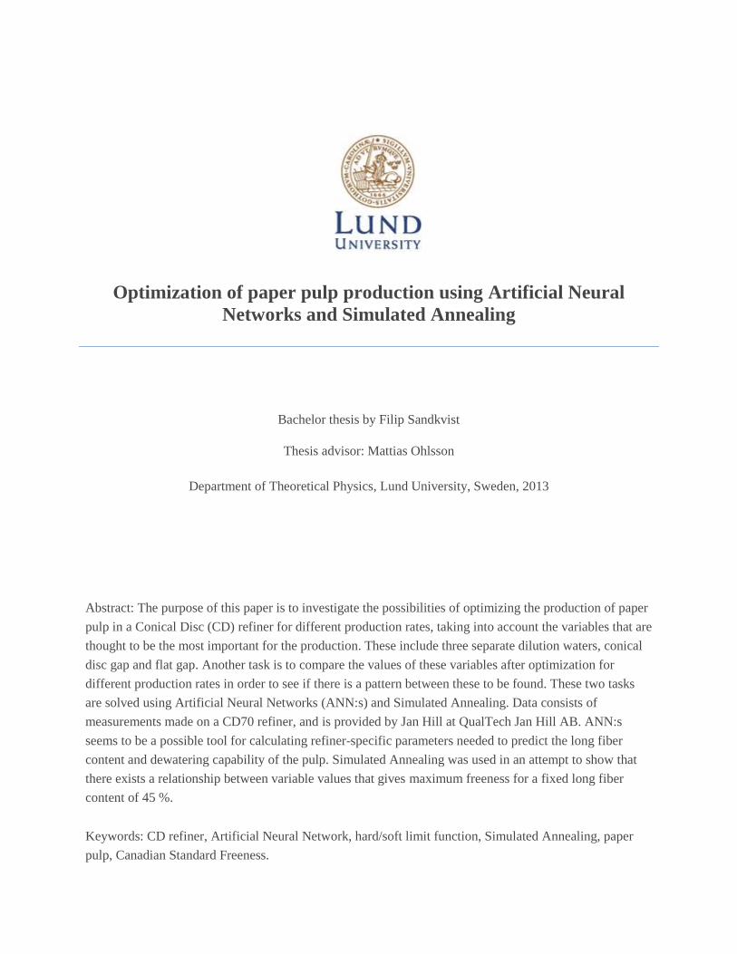
Fig.7 (Ref.7, p.171): An example of the separating surface

g that the hidden layer threshold puts up. In this case it is

g along a plane because there are three input neurons.

The transfer function for the hidden neuron j (in this case a logarithmic sigmoid transfer function) depends

on which task the network needs to solve. The value of the transfer function depends on the value of the

previously mentioned sum of inputs times the respective weights (it is assumed that the input and the

hidden layer is fully connected).

The input to hidden neuron j at iteration z is

∑

where m is the number of input neurons. The output from hidden neuron j is given by the transfer

function g

( )

so that lies in the interval [0, 1]. A sigmoid transfer function is preferred because it is convenient to

keep limited to a small interval. This helps the network error converge since it will keep the variance of

the network outputs smaller than if would have no limit.

The output layer

This layer has the second transfer function, in our case a linear function, and gives an output

depending on from the hidden layer. The quantity is in the general case calculated from the output

layer neurons from a e.g. linear function f of the sum of all values h from the hidden layer times the

respective weight to the output neuron, subtracting the output layer threshold . There is only one output

layer neuron for the networks used in this thesis, so can in this special case be expressed as

Page 12 of 34

∑

where n is the number of hidden neurons. This process is repeated for every data point. After the network

output of data point p at iteration z has been decided, is compared to the desired output ,

and an error is calculated as

[1]

where is the error for data point p. The desired output, , is a value set before training the network.

The goal of training the network is to make the output, , equal the desired output, . The Mean

Squared Error, MSE, of the network outputs from the corresponding value from the training data set is

(see eq. [1])

∑

[2]

where t is number of data points.

Updating the weights

The goal of the network is to make the MSE (see eq. [2]) converge towards 0. After the error has been

calculated for a data point, the error is propagated back through the network.

From the MSE a weight correction is calculated to adjust the weights between the hidden layer and the

output layer, which is then propagated back through the network to adjust the weights between the input

layer and the hidden layer. This is repeated for every data point before proceeding to the next training

cycle. For simplicity we will not consider this fact, and we will look at the updating procedure of the

network weights for one data point (t=1). In eq. [3] below, is the weight between hidden neuron

j from the hidden layer and the output neuron from the output layer at training cycle z. Note that this is not

the general case, in which the number of output neurons is not limited to one. This means, in the general

case, that the weights to be updated at every training cycle z between the hidden layer and the output layer,

consists of all the weights between every hidden neuron and every output neuron they are connected to. In

this thesis only fully connected ANN:s are considered, but not all ANN:s are of this type. The weights

from the hidden layer to the output layer are updated through the relationship

Page 13 of 34

where α, which is a constant in the interval [0,1], is the learning rate of the ANN and is called the error

gradient. In the special case just above, equals e (see eq. [1]). The weight between input neuron i from

the input layer and hidden neuron j from the hidden layer at training cycle z, , are updated according

to

( )

The calculation of and follows the idea behind gradient descent, which we will return to later.

Because the error gradient of the output layer decreases linearly with a decreasing error, also

decreases linearly with a decreasing error. The error gradient depends on , so so does (see eq.

[4]). As the Mean Squared Error approaches 0, and also goes to 0. The thresholds are

updated in a similar way as the weights.

With the new weights, a new network output and error is calculated, and the procedure above is repeated

until the error is sufficiently small.

Evaluation of results

The method for evaluating the network´s results after iteration z during training is the MSE (see eq. [2]) of

the training data set. An ANN takes many iteration cycles to learn, and it is not possible to know if the

best solution has been reached. Even if the MSE is small, the network might be overtrained. The risk of

overtraining (overfitting) increases if the number of hidden neurons is too large. This means that the

network tries to fit against fluctuations during training that does not have to do with the actual relationship

between inputs and outputs. This makes the network worse at generalizing. A usual sign of overtraining is

that the error for the training data has become smaller, but that the network performs worse when tested

against a new set of data.

A method for minimizing the risk of overtraining is to divide the data between a training, validation and

test set. The training set is the data used to adjust weights and thresholds of the network. This is usually a

majority of the data used. The validation set is used to prevent overtraining during training. It does not

change weights or thresholds, but the network uses the validation set to investigate if a decrease in error

for the training set leads to decrease in error for a new dataset. If the error stays the same or increases after

a number of iterations the training is stopped. When the training is completed the network is tested against

the test set as a final evaluation of the networks accuracy.

Page 14 of 34

Network settings

Matlab offers numerous different training algorithms for ANN:s. In this thesis a gradient descent training

algorithm with adaptive learning rate and a momentum term was used, which will be further explained

below.

Gradient descent

The idea behind gradient descent is to find the minimum of a given differentiable function that only has

one extreme point which is a minimum. Let us in the following example consider the function f(x). In

search of the x-value that gives the minimum of the function f(x), x takes the following value at updating

cycle s

[5]

where is the step size that decides the change in x between iteration s and s+1.

The minimum of the function is the x-value where the derivative of this function is 0. In this way it is

known for a given point x in what direction to look for the minimum value of f(x). A positive value of f’(x)

means that the solution lies in the negative direction, and vice versa. Because f’(x) gets smaller as a

solution is approached, the steps with which x is updated becomes smaller.

The principles behind gradient descent are used to update the network weights through a change in weight

from one training cycle to the next. This is called backpropagation. The learning rate parameter α of the

ANN from eq. [3] and [4] directly corresponds to the parameter ξ from eq. [5]. With the learning rate

parameter properly adjusted, the network error should converge towards 0.

In this thesis the just mentioned function f is not just a function of only one variable, but of several

variables representing the settings of the CD refiner (see ‘The refining process’, section 2).

Adaptive learning rate

The learning rate parameter α (see eq. 3 and eq. 4) is adjustable in the interval [0, 1]. If α is close to 0 the

network will need many iterations to set the weights and thresholds so that the error gradients from

eq. 3 and from eq. 4 becomes sufficiently small. If on the other hand the learning parameter is set

too high, the network error will start to oscillate and will not converge. To make the network converge in

as few iteration cycles as possible, an adaptive learning rate can be used. The idea behind this is two

heuristics (Ref.8):

1) If the change of the sum of squared errors has the same algebraic sign for several consecutive

epochs, then the learning rate parameter should be increased.

2) If the algebraic sign of the change of the sum of squared errors alternates for several consecutive

epochs, then the learning rate parameter should be decreased.

Page 15 of 34

The momentum term

The purpose of the momentum term is to help the ANN from getting trapped in a local minimum and

stabilize training. Adding a momentum term β to eq. [3] gives us (Ref.7, p.204)

The weight change Δw includes a term that is a part of the previous weight change. This means that the

weight change speeds up when several steps in the same direction towards a minimum is made. When the

direction alternates, variations will instead be smoothened out.

Weight decay

During network training, small weights are preferred because large weights increase the variance of the

outputs (Ref.9). A regularization term including a parameter γ in the interval [0, 1] is added to eq. [2] to

keep the weights small.

∑

As can be seen - the larger the weight is, the larger the penalty gets compared to the total error, .

Another way to change the performance of the ANN is to adjust the number of hidden nodes. The most

appropriate number of hidden neurons depends on the problem, but should be kept as low as possible.

Many hidden nodes on the one hand make it easier for the network to adjust the weights in such a way that

the error becomes sufficiently small, but on the other hand overtraining might become an issue. If the

number of hidden nodes is too small though, the network will not be able to solve the fitting problem

(underfitting). To get a picture of how many hidden neurons that is the most suitable, the number of

hidden neurons can be plotted against the performance from the validation data sets. The results become

better until a certain point where they start becoming worse again. The approximate number of hidden

neurons that gives the best results for this validation data set is to be preferred.

Page 16 of 34

9. Simulated Annealing

Simulated Annealing is a minimization method, aimed at finding a global minimum of a function. It

simulates a method in metallurgy called annealing, which is a process in which a metal is heated and then

slowly cooled to allow for misplaced atoms to find the place where they belong. The strength of Simulated

Annealing is that the probability of getting stuck at a local minimum is low. The idea is this: In the search

for an optimum value, an initial starting point is chosen. From there, two things can happen when

searching the space for an optimum value:

1) The new function value found is better (lower) than or equal to the currently best (lowest) value

2) The new function value is worse than the currently best value

In case 1) that data point is always saved as the new best value.

In case 2) the data point is accepted with a certain probability for the current ‘temperature’ T and a change

in ‘energy’ ΔE

[6]

where R is a random number in the interval [0, 1], E is the ’energy’ of the best current solution, and

is the ’energy’ of the new solution. The change in energy ΔE is a measure of how much worse a new

solution is compared to the best solution so far. If is larger than R, the new data point is accepted.

Finding the minimum ‘energy’ of the function corresponds to finding the smallest function value.

From eq. [6] follows that high temperatures T leads to (and always smaller than 1, because

ΔE<0). In this case a new solution is often accepted. Beginning at a high temperature T, slowly letting the

temperature drop, means that many data points of the space will be searched. Thus entrapment in a local

minimum is avoided with a very high probability. As , , and the probability of accepting

a worse solution also drops to 0. In this way it is possible to find a global minimum without getting stuck

at a local minimum.

Page 17 of 34

10. Procedure and results

During this project, different attempts were made to estimate what machine settings that would result

in maximum freeness and a long fiber content of 45 %. One idea, consisting of three steps as

illustrated below, was considered one possible procedure:

The first step of the three steps was to use an ANN to describe long fiber content as a function of the

variables production rate, pressure, flat gap, CD gap and the water flows to the inlet, flat gap and the CD

gap.

The next step was to use a similar procedure to describe freeness as a function of the same variables as in

the first step.

The final step was to once again use an ANN in order to express freeness as a function of long fiber

content.

The three step procedure above was carried out in the following way:

Data was arranged after production rate, and then the values for dilution waters (to the inlet, the flat gap

and the conical gap), pressure, conical gap and flat gap was used as network inputs, and corresponding

values for long fiber content as outputs. This would be done three times, one network per production rate.

If the network could deliver results with a low error without being overtrained, the next step would be to

compare if there is a relation between long fiber content and input values for different production rates.

The theoretical value of long fiber content 45 % was expected to be reached using the trained network that

predicts long fiber content (same weights and thresholds). Instead of predicting long fiber content from

production rate, pressure, dilution water flows and gap widths the opposite would be done. i.e. choosing

the long fiber content 45 % as the target value, and then letting the network present what values of

production rate, pressure, dilution water flows and gap widths that would correspond to that (hopefully

with one or few possible solutions, and with a clear relationship between different production rates). Then

the highest possible freeness values for the given production rates and long fiber content 45% would be

calculated.

If the attempt above would be successful, the next step would be to use the predicted values that give the

long fiber content 45% to see what value for freeness this would give. For this to work, one needs to find

some relationship between the experimental measurements of production rate, pressure, dilution water

flows, gap widths and the experimental values for freeness.

The final step would then be to find a relationship between the experimentally measured long fiber content

and experimentally measured freeness.

1) ANN: Function approximation of f(prod. rate, pressure, gap widths, water flows) long fiber content

2) ANN: Function approximation of f(prod. rate, pressure, gap widths, water flows) freeness

3) ANN: Function approximation of f(long fiber content) freeness

Page 18 of 34

Prediction of long fiber content using an ANN

Since there were measured values for long fiber content and the variables listed earlier (see section 10

above) it seemed possible that an ANN could find a relationship between these variables and the long fiber

content. The network weights of the ANN after training would then be a measure of the influence from

each variable on the long fiber content. An ANN with three layers was used, and results where compared

for up to 10 hidden neurons and different regularization parameters. The smallest error of the validation

data set was found when using 7 hidden neurons and a regularization parameter of 0.2. Unfortunately, the

ANN did not find a small enough error to predict the long fiber content in this way (see Fig.8). For low

long fiber contents predictions were poor, but for high contents the experimental values were closer to the

predicted values.

Fig.8: ANN prediction of long fiber content compared to experimental values (validation set).

Because this attempt was not successful an alternative procedure was tried. This alternative plan consisted

of four steps as illustrated below:

1) Linear regression: Function approximation of f(prod. rate, spec. E) freeness

2) ANN:Function approximation of f(prod. rate, flat gap, conical gap,

concentration) power

3) Function approximation of f(long fiber content) freeness

4) Simulated Annealing: Maximum freeness for the long fiber content 45 %

Page 19 of 34

The first step was to use linear regression (a method that uses the fitting of a straight line to a set of points

such that the sum of the squared errors becomes as small as possible) in order to approximate a function

that describes the relationship between freeness, production rate and specific energy. This was expected to

be possible since freeness almost always has a linear relationship to the specific energy. The next step was

to use a perceptron, the simplest version of an ANN, to find an expression for power of the CD refiner as

a function of the variables production rate, flat gap, conical gap and concentration. Since actual production

rate varies with density of wood flowing into the refiner, one can instead estimate the actual production

rate from motor power and specific energy (which we will return to later). This is the reason that one

would need an expression for power. The third step was to find a relationship between long fiber content

and freeness (this will also be explained in more detail later). The third step was necessary in order to do

the fourth and final step – finding which production rate, concentration, flat and CD gap width that would

give the highest possible freeness for the long fiber content 45%.

Prediction of freeness using linear regression

As already mentioned, freeness almost always has a linear relationship to specific energy. This makes it

reasonable to believe that such a relationship can be found through linear regression. By using linear

regression, an approximation to this relationship was obtained (Fig.9).

Fig.9: The relationship between experimental values of specific energy and freeness.

Page 20 of 34

According to the results of the linear regression, the predicted freeness, , can be expressed as a

function of the specific energy, , as follows

[7]

A ≈ 733 ml

B ≈ 309 ml tonne/MWh

Mean Squared Error ≈ 35

Prediction of power using a perceptron

An equation to be published (Ref. 12) can be used to predict the power from given inputs

An equation to be published (Ref. 12) can be used to estimate the power from given inputs

[8]

where

motor power

production rate

housing pressure - inlet pressure

flat gap - min. flat gap

conical gap - min. conical gap

concentration - max. concentration

and are parameters.

The goal with this step was to find the parameters and l from eq. [8] by using a perceptron

and comparing the theoretical power to the experimental.

Using experimental values of v, p, f, k, c and , the parameters, which are refiner-specific, can be found.

The reasoning behind this equation is that the power can be approximated as a Taylor expansion for values

of power close to the average power needed to run the CD refiner during operation. The terms for

production rate, flat gap and CD gap are of the first order, because terms of higher orders are not

We will now take a look at a way to approximate the motor power. An expression for power together with a

measured value of the specific energy is necessary in order to estimate what the actual production rate is, which

will be needed later. The production rate of paper pulp for a CD refiner cannot be exactly controlled, because the

density of the wood entering the refiner varies.

Page 21 of 34

statistically significant with respect to measurement errors and spread of the results (see Ref.10 and

Ref.11). For concentration, on the other hand, a term of the second order is used.

Eq. [8] can be used for an interval of ‘normal’ production rates for a CD refiner, like the interval this

thesis focuses on. More terms need to be added to the equation for higher or lower production rates than

this. According to eq. [8] dilution waters do not need to be treated separately. Instead the concentration

can be used as a measure of the water flow. There is also a known error in this equation that grows as the

gaps are pushed closer to their respective minimum values.

Since eq. [8] is on the same form as the linear equation for the threshold value of a perceptron, a

perceptron can be used as a linear function approximation tool to find an expression for power. This can

also be solved with linear regression, but a perceptron was chosen for the task. The values of the weights

after training correspond to the values of the parameters k, and the value of the threshold to the parameter

l. Since pressure was assumed constant, it was not used as an input. The pressure term was instead

included in l.

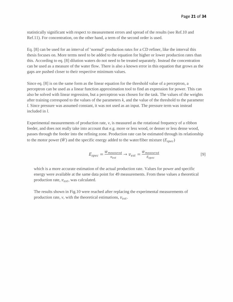
Experimental measurements of production rate, v, is measured as the rotational frequency of a ribbon

feeder, and does not really take into account that e.g. more or less wood, or denser or less dense wood,

passes through the feeder into the refining zone. Production rate can be estimated through its relationship

to the motor power ( ) and the specific energy added to the water/fiber mixture ( )

[9]

which is a more accurate estimation of the actual production rate. Values for power and specific

energy were available at the same data point for 49 measurements. From these values a theoretical

production rate, , was calculated.

The results shown in Fig.10 were reached after replacing the experimental measurements of

production rate, v, with the theoretical estimations, .

Page 22 of 34

Fig.10: Experimental power compared to theoretical power based on eq. [8].

Below are the values of the parameters and l (see eq. 8), calculated by the perceptron (these

parameters will be needed later as part of an expression for predicted freeness).

[10]

[11]

[12]

[13]

[14]

Mean Squared Error ≈ 0.11

Page 23 of 34

The relationship between long fiber content and freeness

The next step was to define a requirement so that every solution, when using an optimization method in

search of the maximum theoretical freeness, would need to have the theoretical long fiber content 45 %.

The plan was to start off with experimental measurements of the variables production rate, flat gap,

conical gap, concentration and long fiber content L. Since long fiber content was not fixed to a value of

45% in the measurements, the experimental value was extrapolated with an amount through theoretical

changes in flat gap, conical gap, concentration and production rate ( , respectively, see eq.

15 below). In order to predict how the long fiber content is affected by a change in production rate, flat

gap, conical gap and concentration, the already known experimentally approximated rates of change in

long fiber content for these variables (see and under eq. 15 below) was used. The task was

thus to find which physically possible proportions of change in these variables that gives the highest

possible freeness.

One possibility to solve this optimization problem is using an ANN, by putting long fiber content 45% as

a desired output, and after training let the network present what inputs that corresponded to the preferred

output. The problem with this method of solution is that it is not known how to get the solution that gives

the highest freeness without exhausting all possibilities of relationships between inputs that gives the

desired long fiber content. There are many (perhaps even an infinite number of) solutions that fulfill the

requirement of a theoretical long fiber content of 45%, and these solutions correspond to different values

of predicted freeness. For this reason an ANN is not to be preferred for this specific task. Other possible

methods of solution involved either a grid search or Simulated Annealing. Here Simulated Annealing was

chosen.

Since long fiber content depends on flat gap, conical gap, concentration and production rate, the following

is assumed to be true: The long fiber content after optimization using Simulated Annealing can be

written as

where is the theoretical change from an experimental measurement L,

[15]

Here the α:s are the approximate rates of change of the long fiber content, when theoretically changing the

experimental values of the variables f, k , c and the calculated with an amount Δf, Δk, Δc and Δ

(Ref.12):

whereas f, k and c are the variables from eq. [8], and is calculated from eq. [9].

The task is to make reach 45 % in such a way that freeness is maximized. In order to calculate the

Page 24 of 34

corresponding freeness it was assumed that eq. [7] could be used with the specific energy, (see eq.

[9]), using the theoretical power, (see eq. [8]), with changes , Δf, Δk and Δc in the values of ,

f, k and c obtained from the solution to eq. [15]. When calculating the theoretical power, the parameter

(see eq. [12]) was used together with because the rate of change in power for is not expected to

have a different value compared to v.

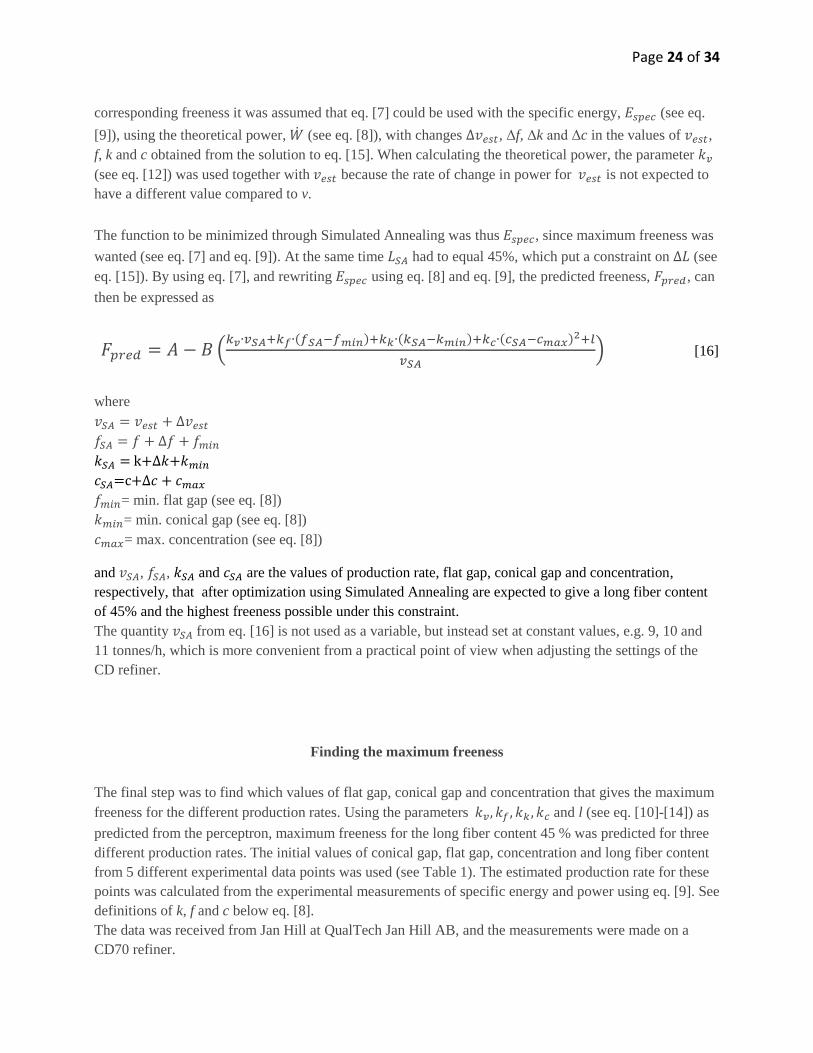
The function to be minimized through Simulated Annealing was thus , since maximum freeness was

wanted (see eq. [7] and eq. [9]). At the same time had to equal 45%, which put a constraint on (see

eq. [15]). By using eq. [7], and rewriting using eq. [8] and eq. [9], the predicted freeness, , can

then be expressed as

(

) [16]

where

k+

=c+

= min. flat gap (see eq. [8])

= min. conical gap (see eq. [8])

= max. concentration (see eq. [8])

and , , and are the values of production rate, flat gap, conical gap and concentration,

respectively, that after optimization using Simulated Annealing are expected to give a long fiber content

of 45% and the highest freeness possible under this constraint.

The quantity from eq. [16] is not used as a variable, but instead set at constant values, e.g. 9, 10 and

11 tonnes/h, which is more convenient from a practical point of view when adjusting the settings of the

CD refiner.

Finding the maximum freeness

The final step was to find which values of flat gap, conical gap and concentration that gives the maximum

freeness for the different production rates. Using the parameters and l (see eq. [10]-[14]) as

predicted from the perceptron, maximum freeness for the long fiber content 45 % was predicted for three

different production rates. The initial values of conical gap, flat gap, concentration and long fiber content

from 5 different experimental data points was used (see Table 1). The estimated production rate for these

points was calculated from the experimental measurements of specific energy and power using eq. [9]. See

definitions of k, f and c below eq. [8].

The data was received from Jan Hill at QualTech Jan Hill AB, and the measurements were made on a

CD70 refiner.

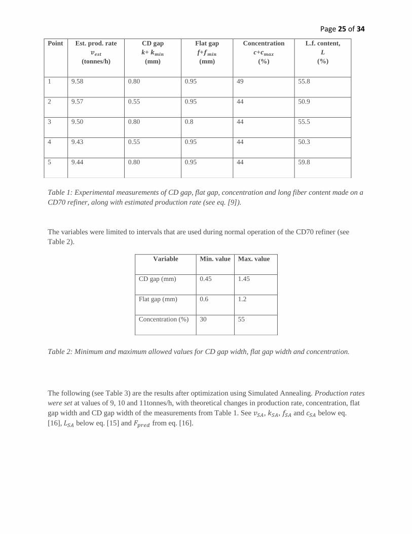
Page 25 of 34

Table 1: Experimental measurements of CD gap, flat gap, concentration and long fiber content made on a

CD70 refiner, along with estimated production rate (see eq. [9]).

The variables were limited to intervals that are used during normal operation of the CD70 refiner (see

Table 2).

Table 2: Minimum and maximum allowed values for CD gap width, flat gap width and concentration.

The following (see Table 3) are the results after optimization using Simulated Annealing. Production rates

were set at values of 9, 10 and 11tonnes/h, with theoretical changes in production rate, concentration, flat

gap width and CD gap width of the measurements from Table 1. See , , and below eq.

[16], below eq. [15] and from eq. [16].

Point Est. prod. rate

(tonnes/h)

CD gap

k+

(mm)

Flat gap

f+

(mm)

Concentration

c+

(%)

L.f. content,

L

(%)

1 9.58 0.80 0.95 49 55.8

2 9.57 0.55 0.95 44 50.9

3 9.50 0.80 0.8 44 55.5

4 9.43 0.55 0.95 44 50.3

5 9.44 0.80 0.95 44 59.8

Variable Min. value Max. value

CD gap (mm) 0.45 1.45

Flat gap (mm) 0.6 1.2

Concentration (%) 30 55

Page 26 of 34

Table 3: Values of production rate, CD gap width, flat gap width and concentration for a set predicted

long fiber content of 45% and the predicted freeness after optimization with Simulated Annealing.

The data points are colored in different colors in Fig. 11-13 below.

Point Color

(tonnes/h)

(mm)

(mm)

(%)

(%)

(ml· )

1 Yellow 9 0.5469 0.6110 50.33 45 -0.4489

2 Red 9 0.5144 0.6002 35.70 45 -1.250

3 Blue 9 0.4612 0.6024 53.84 45 0.2520

4 Green 9 0.6930 0.6276 47.41 45 -1.688

5 Black 9 0.7815 0.6188 53.54 45 0.2148

1 Yellow 10 0.6586 0.6717 51.30 45 -0.1236

2 Red 10 0.6740 0.6090 33.76 45 -13.62

3 Blue 10 0.5927 0.6287 51.98 45 0.01700

4 Green 10 0.5607 0.7339 35.78 45 -11.10

5 Black 10 0.4535 0.9393 54.00 45 0.2878

1 Yellow 11 0.8669 0.6109 44.32 45 -2.900

2 Red 11 0.4510 0.9925 49.97 45 -0.3671

3 Blue 11 0.7272 0.6375 48.17 45 -1.001

4 Green 11 0.7873 0.6967 33.12 45 -13.09

5 Black 11 0.4565 0.9172 36.46 45 -9.305

Page 27 of 34

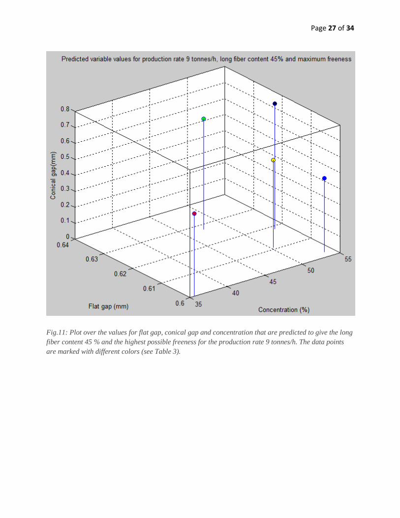
Fig.11: Plot over the values for flat gap, conical gap and concentration that are predicted to give the long

fiber content 45 % and the highest possible freeness for the production rate 9 tonnes/h. The data points

are marked with different colors (see Table 3).

Page 28 of 34

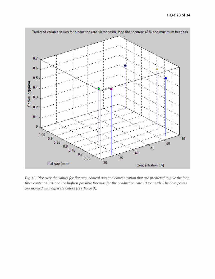
Fig.12: Plot over the values for flat gap, conical gap and concentration that are predicted to give the long

fiber content 45 % and the highest possible freeness for the production rate 10 tonnes/h. The data points

are marked with different colors (see Table 3).

Page 29 of 34

Fig.13: Plot over the values for flat gap, conical gap and concentration that are predicted to give the long

fiber content 45 % and the highest possible freeness for the production rate 11 tonnes/h. The data points

are marked with different colors (see Table 3).

Page 30 of 34

11. Discussion and conclusions

During this project different ideas have been tested to find an answer to the question of which settings

of the CD refiner that gives a paper pulp of maximum freeness and the long fiber content 45 %. First it

was tested whether an ANN could be used to solve this problem, but this attempt was not fully

successful. For a large data set it would perhaps have been possible. It can be understood that

experimental measurements of a machine such as the CD refiner, which has narrow gaps and a flow of

wood with continuously changing density and moisture, are not that easy to do accurately. The flat

gap and the conical gap are approximately millimeter wide, and a tiny change in width results in a

large change in the properties of the paper pulp. It cannot be fully concluded how large the

contributions from the different error sources are, such as how much the pulp density varies over time,

differences between measured and actual gap widths and measured water flows and actual water

flows. But it can be concluded that small errors are enough to make accurate predictions of the quality

of the pulp, in this case decided from the long fiber content and freeness, difficult.

Predictions were based on an already existing refiner specific model for theoretical power (see eq.

[8]). From this model it is possible to calculate a theoretical motor power of the CD refiner from given

values for production rate, steam pressure, width of the flat and the CD gap and concentration of the

pulp. A perceptron could be used as a function approximation tool to find the parameters for this

model with seemingly fair accuracy, since the theoretical values of motor power are close to the

measured values of motor power (see Fig.10). This was an important step because the power was used

to predict both long fiber content and freeness.

For the next part of the project, i.e. deciding which changes in variables that would result in maximum

freeness and the desired long fiber content of 45 %, Simulated Annealing was used. The reason for

this is that this problem could be expressed as two functions to be minimized, and no obvious idea as

to how an ANN could solve this task quickly and efficiently was at hand (as discussed in section 10

under ‘The relationship between long fiber content and freeness’). The results of the Simulated

Annealing are doubtful, since the predicted freeness (which is the dewatering ability of moist pulp), is

negative in most cases. In reality freeness often has a value of a few hundred, and this value is, of

course, always positive (since pulp is not expected to suck up water while it is being dewatered). The

obviously huge error in freeness probably originates to a large extent from an error in concentration.

Freeness is, according to eq. [8], proportional to the square of the difference between measured and

maximum allowed concentration of paper pulp flowing through the CD refiner. Maximum

concentration is an approximate quantity, and an error can thus become large. On the other hand, the

fact that the theoretical freeness is completely wrong does not necessarily mean that the predicted

values for gaps and concentration that gives the maximum freeness is also wrong. One explanation

could be that the measurements and/or methods resulting in eq. [7] (the expression for freeness) are in

need of improvements.

On the other hand, the allowed values during optimization for the variables flat gap, CD gap and

concentration were limited to intervals that are most often used for the CD refiner, but still allows for

them to have the wrong relationship to one another in the solution that gives the maximum theoretical

freeness.

Page 31 of 34

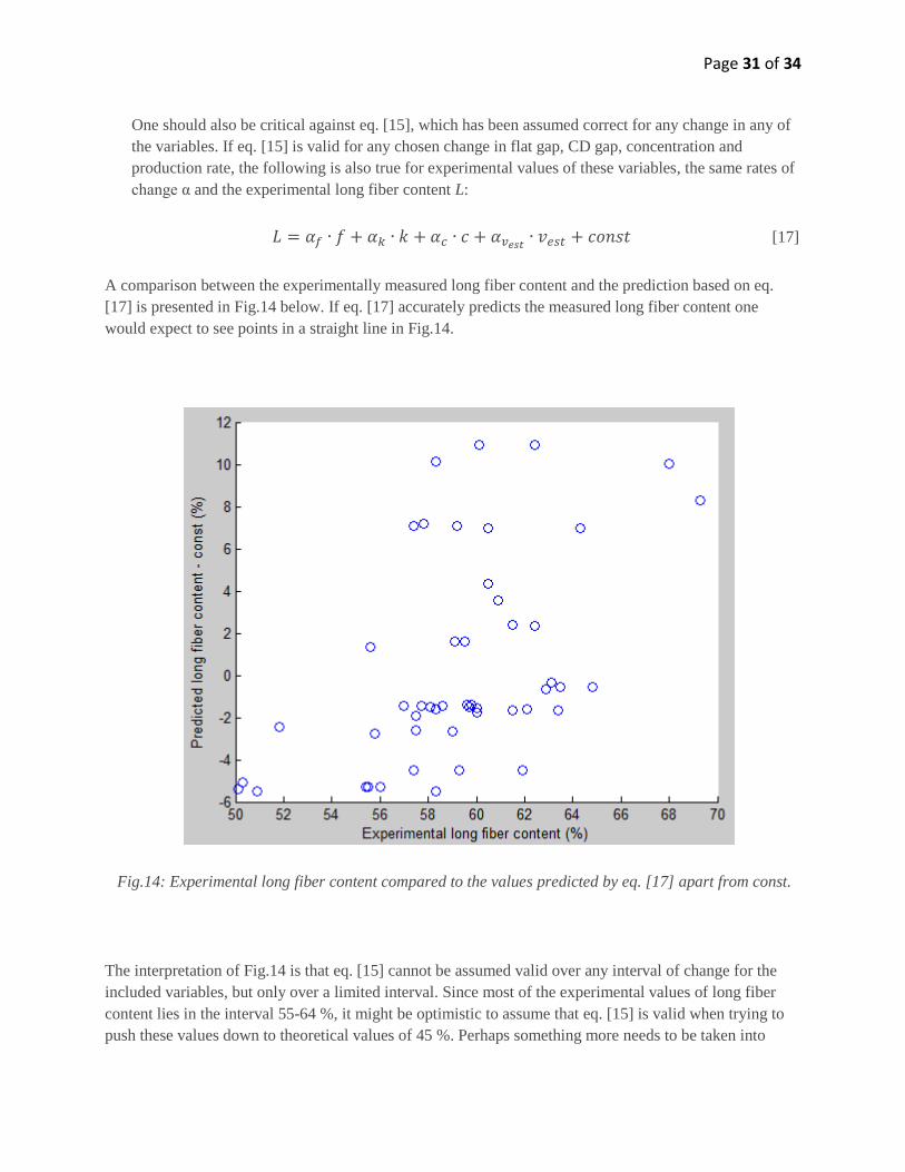
One should also be critical against eq. [15], which has been assumed correct for any change in any of

the variables. If eq. [15] is valid for any chosen change in flat gap, CD gap, concentration and

production rate, the following is also true for experimental values of these variables, the same rates of

change α and the experimental long fiber content L:

[17]

A comparison between the experimentally measured long fiber content and the prediction based on eq.

[17] is presented in Fig.14 below. If eq. [17] accurately predicts the measured long fiber content one

would expect to see points in a straight line in Fig.14.

Fig.14: Experimental long fiber content compared to the values predicted by eq. [17] apart from const.

The interpretation of Fig.14 is that eq. [15] cannot be assumed valid over any interval of change for the

included variables, but only over a limited interval. Since most of the experimental values of long fiber

content lies in the interval 55-64 %, it might be optimistic to assume that eq. [15] is valid when trying to

push these values down to theoretical values of 45 %. Perhaps something more needs to be taken into

Page 32 of 34

account than the included variables. This can also explain why the predictions seen in Fig.8 are not close

to the measured values for low long fiber contents.

Judging from Fig.11-13 there does not seem to be a pattern between those values of variables that gives

the highest freeness. Comparing the different data points to one another for different production rates,

there does not seem to be an apparent pattern (e.g. that they are points on the same plane). In addition, the

points have a large spread. Assuming that there is a pattern between the data points when comparing

different production rates, the large spread can be explained in two ways. Either the predictions are

inaccurate (since one could expect the different data points to be close to one another if one set of variable

values is clearly better than the rest) or there are many solutions that are almost equally good.

So to answer the two questions that were expected to be answered from this thesis (see ‘Project aims’,

section 4):

Theoretical values for the flat gap, conical gap and concentration (which is a measure of the dilution water

flow rate if the production rate is given) that gives the highest possible freeness and the long fiber content

45 %, for different production rates in the interval 9-11 dry tonnes/h is presented in Fig.11-13. The

interpretation of these results, when comparing different production rates that results in maximum freeness

and the long fiber content 45%, is that it cannot be concluded that there is a relationship between the

theoretical values for flat gap, conical gap and concentration.

Page 33 of 34

12. Outlook and personal reflection

The results of this thesis, which usually is the case, can be improved by making more experimental

measurements. At the current point, it cannot be proved that the best solutions have been reached because

evidence simply is not strong enough. Also, when using ANN:s and Simulated Annealing as optimization

methods it cannot be known for certain that the best solution has been reached.

The period of time that I have been spent working on this thesis has been fun and giving. I feel that I have

learned a lot about optimization methods, which is both an important and an interesting field. I believe that

many things in our surroundings can become better, more efficient, cheaper and more environmentally

friendly if such methods can be used in a clever way.

I also feel that working on this thesis has given me more practical knowledge about how to get a project

done. I have learnt that some tasks consume more time and energy than expected. Getting to understand

how something works in theory is one thing, getting it to work practically is another.

13. Acknowledgements

I would like to give my warmest thanks to my supervisor Mattias, with whom I have had interesting and

giving discussions. Your great insight and your inputs about how and what needed to be done to solve

tasks I found difficult has been of big help, and I have felt that you always took the time to help out

whenever I dropped by.

Also great thanks to Jan Hill, who was the man that presented the problem that constitutes the basis for

this thesis. Without you there would not have been a project to work on in the first place! You have

provided me with valuable inputs and tips, and also a good story now and then.

I would like to thank Patrik Edén for helping out with practical necessities, and for the helpful ideas

during the early stages of this project.

Last, thanks to Bjarni Birgisson for making me realize that I was stuck in a loop.

Page 34 of 34

References

1) http://www.skogsindustrierna.org/branschen/sverige-tar-matchen (2013-05-26)

2) http://www.skogsindustrierna.org/vi_tycker/energi_2 (2013-05-26)

3) Berg, Daniel (2005). A comprehensive Approach to Modeling and Control of Thermomechanical

Pulping Processes. Department of Signals and Systems, Chalmers University of Technology.

4) Eriksson, Karin (2005). An Entropy-Based Modelling Approach to Internally Interconnected TMP

Refining Processes. Department of Signals and Systems, Chalmers University of Technology.

5) Johansson, Ola; Hogan, Dan; Blakenship, Dale; Snow, Eddie; More, Wyllys; Qualls, Ronnie;

Pugh, Keith; Wanderer, Mike (2001). Inproved process optimization through adjustable refiner

plates. International Mechanical Pulping Conference, Helsinki.

6) http://ifbholz.ethz.ch/natureofwood/pc/gloss/c13.html (2013-05-26)

7) Negnevitsky, Michael (2005). Artificial Intelligence: A Guide to Intelligent Systems (2nd

ed).

Addison-Wesley.

8) Jacobs, Robert A. (1988). Increased rates of convergence through learning rate adaptation.

University of Massachusetts.

9) Geman, Stuart; Bienenstock, Elie; Doursat, Rene (1992). Neural Networks and the Bias/Variance

Dilemma. Neural Computation,4:1--58.

10) Hill, J.; Saarinen, K.; Stenros,R. (1991). On the control of chip refining systems. Preprint

International Mechanical Pulping Conference.

11) Hill, Jan (1993). Process understanding profits from sensor and control developments. Preprint

International Mechanical Pulping Conference.

12) Private communication with Jan Hill from QualTech Jan Hill AB.