Embed Size (px)
Citation preview

APPLICATION OF FPGA TOREAL-TIME MACHINE LEARNING:
HARDWARE RESERVOIR COMPUTERSAND SOFTWARE IMAGE PROCESSING
PIOTR ANTONIK
PHD THESIS
1

Universite libre de BruxellesFaculte des Sciences
Departement de Physique
Application of FPGA to real-timemachine learning: hardware reservoir
computers and software image processing
Piotr Antonik
Directed bySerge Massar and Marc Haelterman
Laboratoire d’Information Quantiqueand
Service OPERA-Photonique
PhD Thesis
September 2017


To my Dad,
let this be the memorial you never wanted


Jury composition
Prof. Gilles De Lentdecker, presidentInteruniversity Institute for High EnergiesUniversite libre de Bruxelles
Prof. Mustapha Tlidi, secretaryOptique non-lineaire theoriqueUniversite libre de Bruxelles
Prof. Serge Massar, promotorLaboratoire d’Information QuantiqueUniversite libre de Bruxelles
Prof. Marc Haelterman, copromotorOPERA-PhotoniqueUniversite libre de Bruxelles
Prof. Guy Van der SandeApplied Physics Research GroupVrije Universiteit Brussel
Dr. Daniel BrunnerDepartement d’OptiqueInstitut FEMTO-ST
Prof. Thomas MilnerBiomedical EngineeringUniversity of Texas at Austin
Cover image by Ahkam (freeiconspng.com)
vii


Preface
CONFIDENTIALITY NOTICE
The chapter VI of the present thesis contains confidential information.The Reader agrees:
(1) not to use the confidential information except as for the pur-pose of evaluation of the present thesis;
(2) not to disclose any confidential information to any thirdparty(ies);
(3) not to make any copies of the confidential information;(4) never to use the confidential information for commercial pur-
poses or any other purposes than the evaluation of the presentthesis.
This dissertation contains the full story of the four years of my PhD. Thestructure of the document is quite simple. The first chapter explains the the-oretical and experimental basics. Throughout my thesis, I worked on fourdistinctive experiments. Some of them were my own projects, others were col-laborations with other researchers in our group. They will be described in fourseparate chapters (Ch. II to Ch. V). By the end of my PhD, I took a five-month internship at the University of Texas at Austin, that will be coveredin Ch. V.6. Finally, Ch. VII concludes the story with a few ideas for futureresearch.
Before writing this thesis, I had to make a crucial choice: either spend threeto five months writing an original dissertation from scratch, or fill the thesiswith my publications and spend the remaining time on another experiment.Without much hesitation, I chose the second option. In other words, this thesisis not so original. In fact, it is a compilation of my journal papers, properly“glued” together to form a continuous story. This is a somewhat lazy approach– I do not deny it. But I believe the importance of a thesis consists of itsscientific value. And those extra five months allowed me to complete anotherinteresting project, thus increasing the significance of my work.
Another word of warning should be written concerning the style of thepresent thesis. Scientific English is a very clear and concise communicationtool, but may seem somewhat boring. And after writing a few journal papersand a dozen of conference proceedings, I wanted to add some colours to thefinal publication of my PhD. Therefore, while its tone remains scientific mostof the time, I allowed myself a few minor digressions. The reader will noticethat from the very first lines of the first chapter.
ix

x PREFACE
Final remark, most chapters contain a “bonus” section, describing the chal-lenges encountered during the realisation of a particular project. These sectionscontain the back story of each experiment. In most fields of science, positiveresults are published, and the negative remain in the shadows. However, know-ing what has been tried but did not work may save time in some cases, or eveninspire new ideas. For this reason, I decided to include in this dissertation somefacts that did not make it to the journal papers.
Acknowledgements
It is an immense pleasure to thank the numerous people who made thisthesis possible.
First and foremost, it is difficult to overstate my gratitude to my PhDsupervisor, Prof. Serge Massar. There are two things I long for the most –freedom and support – and Serge gave me both. While freedom gives birthto that spark that ignites new ideas, support is the fuel that turns ideas intoprojects and, ultimately, results and publications. So thank you, Serge, forbeing the best supervisor I could ever wish for. This paragraph would bedramatically incomplete without a big thanks to Prof. Marc Haelterman, myco-supervisor, for his everlasting support.
The next hat tip goes to the team of awesome postdocs I had a greatpleasure of working with. I could never complete this thesis alone, and theseare the people who took direct part in some of my projects. Starting withDr. Francois Duport, who took me under his wing right from the start, beforeI even started as a PhD student, and taught me everything I needed to workindependently in the lab, and even more. Greeting Francois in the office asearly as 7 a.m. and regularly seeing him in the lab after 9 p.m. constantlyreminded me that the only time success come before work, is in the dictionary1.Following with Dr. Anteo Smerieri, who “basically” guided me through thecomplex theory of reservoir computing and learning methods. Few people canspeak of intricate algorithms with simple words, and even less could turn it intoan enjoyable show, with particularly well-placed jokes – as was demonstratedon numerous occasions. Last (chronologically) but not least, comes Dr. MichielHermans, from whom I acquired a much deeper understanding of the machinelearning field in general, and reservoir computing in particular. And on top ofthat, the idea of taking an internship abroad was inspired by Michiel, whichultimately led to an amazing experience in Texas (more on that in Ch. V.6).Thank you very much for that!
I am particularly grateful to Prof. Thomas Milner for offering me the life-changing opportunity to join his research team at the University of Texas.Working with Prof. Milner was a very inspiring experience, and I appreciatehow much I could learn in so little time about various aspects of scientific life.
I would like to thank all the Jury members for their valuable commentson the present thesis and, in particular, Dr. Daniel Brunner for his in-depthproof-reading of the manuscript and the long list of questions and comments,that made this work more accurate and complete.
1Quote credited to Stubby Currence by Quote Investigator.
xi
xii Acknowledgements
Debuting in electronics, and especially in FPGA design, is all but an easytask. Fortunately, I could benefit from valuable help from several people well-skilled in this art. Thus, I would like to express my very great appreciationto Benoit Denegre for providing a solid starting point, as well as Colin Fera,Matthew Luscher, Ashkan Ashrafi and Arnaud from 4DSP for providing pre-cious documentation and technical support.
The working environment is only as good as the people who surroundyou. In that sense, OPERA-Photonique is the second best thing that hap-pened to me on this journey. Never before could I imagine that scientific re-search could be accompanied by numerous fun parties, uncountable pies, videogames and movie nights. Therefore, an enormous shout-out goes to my co-workers, in alphabetical order: Akram Akrout, Marc Bauduin, Serena Bolis,Arno Bouwens, Thomas Bury, Ali Chichebor, Charles Ciret, Robin De Gernier,Rima Dadoune, Evangelia Dimitriadou, Evdokia Dremetsika, Michael Fita Co-dina, Simon-Pierre Gorza, Wosen Kassa, Pascal Kockaert, Virginie Lecocq,Francois Leo, Anh-Dung Nguyen, Laurent Olislager, Nicolas Poulvellarie, MaıteSwaelens, Guillaume Tilleman and Quentin Vinckier. Very special thanks toProf. Philippe Emplit for creating and maintaining such a productive envi-ronment, and to our awesome secretaries, Ibtissame Malouli and AlexandraPeereboom, who just took care of everything.
And when I could not stand the guys from OPERA anymore (just kid-ding), I could always join my always welcoming colleagues at LIQ, again inalphabetical order: Cedric Bamps, Olmo Nieto Sileras, Jonathan Silman, TomVan Himbeeck and Erik Woodhead. And again, warm thanks to the secre-taries, Sabrina Serrano Alvarez and David Houssart, for handling my orders,travel documents, and, most importantly, reimbursing me for all my expensiveconference trips.
The one thing I benefited the most from scientific conferences – besidesthe chance to travel to some exotic places on the globe – is the opportunityto interact with scholars and industry experts, absorbing as much knowledgefrom them as possible. My first ICONIP conference in Istanbul, and longdiscussions with Prof. Joao Paulo P. Gomes was a particular revelation. I wishto acknowledge here their valuable help.
Most of the first chapter of this thesis, as well as one or two papers werewritten in various hospitals, clinics and medical centres. I very much appreciatethe efforts of the staff who made the task of writing in waiting halls quite acomfortable exercise.
I have composed quite a long list so far, but still I have the impression thatI missed someone. To those people I offer my sincere apologies – for my poormemory, and my gratitude – for their valuable help.
I would like to conclude with people who made a rather indirect contribu-tion to this work. My big thanks go to my school teachers for letting me dowhat I really wanted (that is, solving mathematical, and later, physical prob-lems) and not paying much attention in class, my school and university buddiesfor helping me get through the education process with that much fun, my closefriends Nicolas De Groote, Livio Filippin, Jonathan Bloch and Anton Leonov

xiii
for their support and inspiration. And of course, many sweet thanks go to mydear Luda, and her sister Sveta, for taking such good care of my new hairstyle.
Most appreciation and gratitude usually goes to people for their positivecontributions. However, as an old saying goes – there can be no evil withoutgood – I would like to make an exception and express my gratitude to all peoplewho managed to hurt me, deeply or not, intentionally or not. Thank you formaking me that much stronger!
Family is a true masterpiece of nature, and undoubtedly the most precioustreasure one gets to cherish. And while most of my family lives abroad andquite far away, I felt a very positive lift every time I went to visit them. Thankyou for filling me with confidence, love and kindness! And what a person wouldI be if I failed to mention my beloved sister Maria for her artistic touch and avery special character. You rock!
And as the best is usually saved for the end, my warmest thanks go tomy parents. This is where words begin to fall short, but I will try my bestanyway. To my mum, thank you for being such a positive, dynamic, kind,caring and forgiving person. Few grown-ups think twice before leaving theirparent’s home these days, but somehow, you made me think and rethink agazillion times. And to my dad, thank you for being a model to me for somany years, a friend and guide I could follow anytime with my eyes closed.Thank you for introducing me to arithmetic and basic algebra at the age ofsix, and for directing me straight into my current scientific life. There are fewthings one has the luxury of being certain of. But for me, not for a second didI doubt that one day I would be here, preparing the defence of my PhD thesis.And although I can no longer learn from you as I used to, I can still follow thatbright star on the night sky you turned into.

Author’s publications
Through the course of my PhD, we published the following titles.
Journal papers
One full-length journal paper was issued for each one of the four experi-ments I worked on. The only exception is the paper [3] that is an extendedversion of the conference paper [11], published in a special issue of NeuralProcessing Letters covering the ICONIP 2016 conference.
[1] Piotr Antonik, Franois Duport, Michiel Hermans, Anteo Smerieri, MarcHaelterman, and Serge Massar. “Online Training of an Opto-ElectronicReservoir Computer Applied to Real-Time Channel Equalization”. In:IEEE Transactions on Neural Networks and Learning Systems PP.99(2016), pp. 1–13.
[2] Michiel Hermans, Piotr Antonik, Marc Haelterman, and Serge Mas-sar. “Embodiment of Learning in Electro-Optical Signal Processors”.In: Phys. Rev. Lett. 117 (12 2016), p. 128301.
[3] Piotr Antonik, Michiel Hermans, Marc Haelterman, and Serge Massar.“Random Pattern and Frequency Generation Using a Photonic Reser-voir Computer with Output Feedback”. In: Neural Processing Letters(2017), pp. 1–14.
[4] Piotr Antonik, Marc Haelterman, and Serge Massar. “Online Trainingfor High-Performance Analogue Readout Layers in Photonic ReservoirComputers”. In: Cognitive Computation 9 (2017), pp. 297–306.
[5] Piotr Antonik, Marc Haelterman, and Serge Massar. “Brain-InspiredPhotonic Signal Processor for Generating Periodic Patterns and Emu-lating Chaotic Systems”. In: Phys. Rev. Applied 7 (2017), p. 054014.
Conference papers
Most of my conference papers were presented at machine learning venues,with submissions ranging from 8 half-size pages up to 6 double-column journal-like pages. This is more than enough to present several results without goinginto much detail about the theoretical and experimental aspects. In general,we presented numerical and preliminary experimental results in conference pro-ceedings, before submitting the whole story to a journal.
xv
xvi Author’s publications
[6] Piotr Antonik, Anteo Smerieri, Francois Duport, Marc Haelterman, andSerge Massar. “FPGA implementation of reservoir computing with on-line learning”. In: 24th Belgian-Dutch Conference on Machine Learning.http://homepage.tudelft.nl/19j49/benelearn/papers/Paper_
Antonik.pdf. 2015.[7] Piotr Antonik, Francois Duport, Anteo Smerieri, Michiel Hermans, Marc
Haelterman, and Serge Massar. “Online training of an opto-electronicreservoir computer”. In: APNNA’s 22th International Conference onNeural Information Processing. Vol. 9490. LNCS. 2015, pp. 233–240.
[8] Piotr Antonik, Francois Duport, Anteo Smerieri, Michiel Hermans, MarcHaelterman, and Serge Massar. “Improving performance of opto-electro-nic reservoir computers with online learning”. In: 20th Annual Sympo-sium of the IEEE Photonics Society Benelux Chapter. 2015.
[9] Piotr Antonik, Michiel Hermans, Francois Duport, Marc Haelterman,and Serge Massar. “Towards pattern generation and chaotic series pre-diction with photonic reservoir computers”. In: SPIE’s 2016 Laser Tech-nology and Industrial Laser Conference. Vol. 9732. 2016, 97320B.
[10] Piotr Antonik, Michiel Hermans, Marc Haelterman, and Serge Massar.“Towards adjustable signal generation with photonic reservoir comput-ers”. In: 25th International Conference on Artificial Neural Networks.Vol. 9886. 2016.
[11] Piotr Antonik, Michiel Hermans, Marc Haelterman, and Serge Mas-sar. “Pattern and frequency generation using an opto-electronic reser-voir computer with output feedback”. In: APNNS’s 23th InternationalConference on Neural Information Processing. Vol. 9948. LNCS. 2016,pp. 318–325.
[12] Akram Akrout, Piotr Antonik, Marc Haelterman, and Serge Massar.“Towards autonomous photonic reservoir computer based on frequencyparallelism of neurons”. In: Proc. SPIE. Vol. 10089. 2017, 100890S–100890S–7.
[13] Piotr Antonik, Michiel Hermans, Marc Haelterman, and Serge Massar.“Photonic Reservoir Computer With Output Feedback for Chaotic TimeSeries Prediction”. In: 2017 International Joint Conference on NeuralNetworks. 2017.
Conference abstracts
We also published a few abstracts – short versions of existing journal ofconference papers. They were presented at conferences that allow such submis-sions with the intent of advertising our work.
[14] Piotr Antonik, Marc Haelterman, and Serge Massar. “Improving Perfor-mance of Analogue Readout Layers for Photonic Reservoir Computerswith Online Learning”. In: AAAI Conference on Artificial Intelligence.2017.

.0. Conference abstracts xvii
[15] Piotr Antonik, Michiel Hermans, Marc Haelterman, and Serge Massar.“Chaotic Time Series Prediction Using a Photonic Reservoir Computerwith Output Feedback”. In: AAAI Conference on Artificial Intelligence.2017.
[16] Piotr Antonik, Marc Haelterman, and Serge Massar. “Predicting chaotictime series using a photonic reservoir computer with output feedback”.In: 26th Belgian-Dutch Conference on Machine Learning. 2017.
[17] Piotr Antonik, Marc Haelterman, and Serge Massar. “Towards high-performance analogue readout layers for photonic reservoir computers”.In: 26th Belgian-Dutch Conference on Machine Learning. 2017.

Contents
Jury composition vii
Preface ix
Acknowledgements xi
Author’s publications xv
Chapter I. Introduction 1I.1. From machine learning to reservoir computing 1I.1.1. Machine learning algorithms 1I.1.2. Artificial neural networks 4I.1.3. Reservoir computing 7I.1.4. Benchmark tasks 12I.2. Hardware implementations : opto-electronic delay systems 14I.2.1. Time-multiplexing 15I.2.2. Conceptual setup 16I.2.3. Desynchronisation 18I.2.4. Experimental setup 18I.3. Field-Programmable Gate Arrays 23I.3.1. History 23I.3.2. Market and applications 26I.3.3. Xilinx Virtex 6 : architecture and operation 27I.3.4. Design flow and implementation tools 28
Chapter II. Online training of a photonic reservoir computer 33II.1. Introduction 33II.2. Equalisation of non-stationary channels 34II.2.1. Influence of channel model parameters on equaliser performance 35II.2.2. Slowly drifting channel 35II.2.3. Switching channel 35II.3. Online training 36II.3.1. Gradient descent algorithm 37II.4. Experimental setup 38II.4.1. Input and readout 39II.4.2. Experimental parameters 40II.4.3. Experiment automation 40II.5. FPGA design 41II.6. Results 44
xix
xx Contents
II.6.1. Improved equalisation error rate 44II.6.2. Simplified training algorithm 45II.6.3. Equalisation of a slowly drifting channel 45II.6.4. Equalisation of a switching channel 49II.6.5. Influence of channel model parameters on equaliser performance 51II.7. Challenges and solutions 51II.8. Conclusion 53
Chapter III. Backpropagation with photonics 55III.1. Introduction 55III.2. Backpropagation through time 56III.2.1. General idea and new notations 57III.2.2. Setting up the problem 58III.2.3. Output mask gradient 60III.2.4. Input mask gradient 61III.2.5. Multiple inputs/outputs 63III.3. Experimental setup 63III.3.1. Online multiplication using cascaded MZMs 65III.3.2. Mask parametrisation 67III.4. FPGA design 68III.5. Results 70III.5.1. Tasks 70III.5.2. NARMA10 and VARDEL5 71III.5.3. TIMIT 72III.5.4. Gradient descent 74III.5.5. Robustness 75III.6. Challenges and solutions 76III.7. Conclusion 77
Chapter IV. Photonic reservoir computer with output feedback 79IV.1. Introduction 79IV.2. Reservoir computing with output feedback 81IV.3. Time series generation tasks 82IV.3.1. Frequency generation 82IV.3.2. Random pattern generation 83IV.3.3. Mackey-Glass chaotic series prediction 83IV.3.4. Lorenz chaotic series prediction 84IV.4. Experimental setup 84IV.5. FPGA design 86IV.6. Numerical simulations 88IV.7. Results 88IV.7.1. Noisy reservoir 89IV.7.2. Frequency generation 89IV.7.3. Random pattern generation 91IV.7.4. Mackey-Glass series prediction 96IV.7.5. Lorenz series prediction 99IV.8. Challenges and solutions 104IV.9. Conclusion 105
xxi
Chapter V. Towards online-trained analogue readout layer 109V.1. Introduction 109V.2. Methods 111V.3. Proposed experimental setup 111V.3.1. Analogue readout layer 111V.3.2. FPGA board 113V.4. Numerical simulations 113V.5. Results 115V.5.1. Linear readout: RC circuit 115V.5.2. Nonlinear readout 118V.6. Conclusion 118
Chapter VI. Real-time automated tissue characterisation for intravascularOCT scans 121
VI.1. Introduction 121VI.2. Feature extraction 127VI.2.1. GLCM features 127VI.2.2. Methods 130VI.2.3. Operation principle 131VI.2.4. FPGA design 132VI.2.5. Results 134VI.2.6. Perspectives 134VI.3. Artificial neural network 135VI.3.1. Network structure 135VI.3.2. Methods 138VI.3.3. Operation principle 140VI.3.4. FPGA design 140VI.3.5. Results 142VI.4. Conclusion 142
Chapter VII. Conclusion and perspectives 145
Bibliography 151


CHAPTER I
Introduction
In this chapter we will address three questions: (1) What is reservoir com-puting? (2) What does it have to do with optics and electronics? (3) What areFPGAs? That is a lot of information to cover, so let us get started right away!
I.1. From machine learning to reservoir computing
Reservoir computing – what a peculiar concept! Are we talking about abucket of water performing computations? The idea may seem weird, but. . . itis actually not far from reality! In fact, there has been an experiment carriedout in a water tank, where ripples on the surface of water were sampled and usedto process information [18]. But this is not exactly what reservoir computingis all about. Attributed to the machine learning (ML) field – a subfield ofcomputer science that studies data processing algorithms capable of learningfrom the data itself – reservoir computing is not an algorithm per se, but rathera set of ideas that significantly simplify another algorithm and make it moresuitable for practical applications. This other algorithm, or, rather, a classof algorithms, is called artificial neural networks. To understand the wholestory, we need a general overview of the said machine learning field.1 The goalof this section is thus to present to the reader the bigger picture, following atop-down approach. We will start with an overview of machine learning, withsome basic ideas and several examples. Then, we will dive into artificial neuralnetworks, again leaving aside most of unnecessary technical details. Finally,within neural networks we will finally introduce the RC paradigm, now withall mathematical details needed to understand how it works.
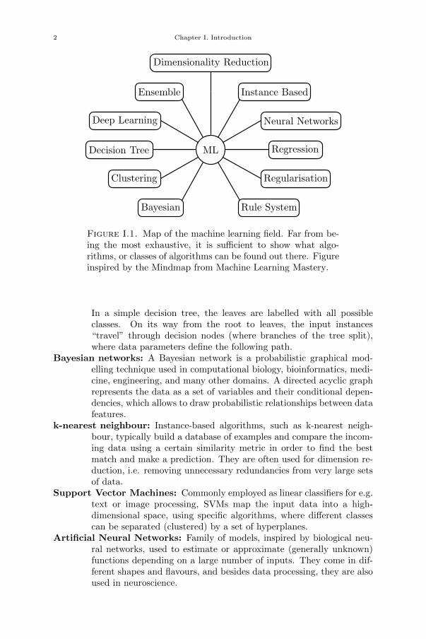
I.1.1. Machine learning algorithms. ML enjoys a fast evolution inthese days, as people are desperately looking for methods to efficiently pro-cess the huge amounts of data coming from everywhere, and ML offers severalvery promising solutions. Fig. I.1 draws a more or less complete picture ofthe machine learning field. Here we will overview a few of these methods (themost popular ones) with their basic properties and applications, obviously sim-plifying the details to the bare minimum. The goal here is not to review themachine learning field, but to give the reader a broad view of the algorithmsthat can be found there.
Decision trees: Commonly used in statistics and data mining, decision treesare predictive models for data classification based on its properties.
1This is obviously a debatable point. But it did work for me – my true revelation onreservoir computing, how and why it works, happened when I saw what is around – so I am
going to stick to this plan.
1
2 Chapter I. Introduction
ML
Bayesian
Clustering
Decision Tree
Deep Learning
Ensemble
Dimensionality Reduction
Instance Based
Neural Networks
Regression
Regularisation
Rule System
Figure I.1. Map of the machine learning field. Far from be-ing the most exhaustive, it is sufficient to show what algo-rithms, or classes of algorithms can be found out there. Figureinspired by the Mindmap from Machine Learning Mastery.
In a simple decision tree, the leaves are labelled with all possibleclasses. On its way from the root to leaves, the input instances“travel” through decision nodes (where branches of the tree split),where data parameters define the following path.
Bayesian networks: A Bayesian network is a probabilistic graphical mod-elling technique used in computational biology, bioinformatics, medi-cine, engineering, and many other domains. A directed acyclic graphrepresents the data as a set of variables and their conditional depen-dencies, which allows to draw probabilistic relationships between datafeatures.
k-nearest neighbour: Instance-based algorithms, such as k-nearest neigh-bour, typically build a database of examples and compare the incom-ing data using a certain similarity metric in order to find the bestmatch and make a prediction. They are often used for dimension re-duction, i.e. removing unnecessary redundancies from very large setsof data.
Support Vector Machines: Commonly employed as linear classifiers for e.g.text or image processing, SVMs map the input data into a high-dimensional space, using specific algorithms, where different classescan be separated (clustered) by a set of hyperplanes.
Artificial Neural Networks: Family of models, inspired by biological neu-ral networks, used to estimate or approximate (generally unknown)functions depending on a large number of inputs. They come in dif-ferent shapes and flavours, and besides data processing, they are alsoused in neuroscience.
I.1. From machine learning to reservoir computing 3
Deep learning: A class of ML algorithms that cascade multiple informationprocessing layers, each successive layer receiving the output of theprevious one as input. The layers learn multiple levels of data repre-sentation, that correspond to different levels of abstraction, and formtogether an hierarchy of concepts. The most successful deep learn-ing methods involve neural networks and have shown breathtakingresults in speech and image recognition, natural language processing,drug discovery and recommendation systems. Other less known deeparchitectures exist, such as multilayer kernel machines.
To process data, these algorithms need to be trained – in other words,taught what to do with the data. Remember, ML algorithms are not designedto perform well on a particular dataset, but rather to execute a certain versatiletask. The training serves to fine-tune the algorithm for better performance onthe dataset of interest. The training can be done using various techniques,commonly grouped into categories, based on their action principle.
Supervised learning: The algorithm is presented with a labelled dataset,that is, where the output is known for each input, such as spam/not-spam classification or a set of tagged images. During the trainingprocess, the model is tuned to correctly classify all the inputs, andthen tested on a new set of data, that was not used for training. Thisprocess is carried on until a desired level of accuracy is achieved onthe test set.
Reinforcement learning: Inspired by behavioural psychology, this methodsis employed when the corrects outputs or labels are unavailable. In-stead, the algorithm is supplied with a reward (or error) function andthen optimised to maximise (or minimise) it. Such approach is com-monly used in robotics, where exact movement patterns of differentmotors or actuators are unknown, and the robot is trained to optimisethe reward function, given by e.g. the distance travelled.
Unsupervised learning: As the name suggests, here the algorithm does notuse any labelled dataset nor reward function. It is presented with thedata alone and is supposed to find an underlying structure or somehidden insights. This case is the hardest to understand, as it lookslike some kind of dark magic. Since I have never used such methods,we shall leave the details aside. A typical example of unsupervisedlearning is clustering, that is, the task of grouping a set of objects bysimilarity.
Other approaches exist, such as semi-supervised learning, but they lie be-yond the scope of this introductory overview.
To sum up this section, numerous machine learning algorithms exist, basedon various approaches and suited for different tasks. To process data, they needto be trained first, and this can also be done in various ways, depending on thetask and the type of data available. Among all the methods lies the family ofartificial neural networks. And since reservoir computing has something to dowith neural networks, let us discuss them in detail in the next section.
4 Chapter I. Introduction
I.1.2. Artificial neural networks. The first model of artificial neuralnetworks (ANN), introduced in 1943 [19] split the research in two distinct ap-proaches: the study of actual biological processes in the brain on one side, andapplication of neural networks to machine learning. The research stagnatedafter the discovery of a fatal flaw: basic neural networks (also known as per-ceptrons – we will introduce them very soon) were incapable of processing thebasic exclusive-or (XOR) circuit! [20]. On top of that computers did not haveenough power to handle large networks on the long run. Later on, the CMOStechnology (that lead to an explosion of computational speed) and the novelbackpropagation algorithm [21, 22] allowed to efficiently train large multi-layernetworks. Recent advances in GPU-based implementations and the emergenceof highly complex, deep neural networks made this approach very popular andbrought breathtaking results in e.g. speech or text recognition and novel drugdiscovery.
Let us take a look inside those networks. They are composed of elementarycomputation units – neurons. A biological neuron is a cell capable of producinga rapid train of electric spikes. Its complex internal dynamics can be describedby the well-known Hodgkin-Huxley model [23] that takes into account the exactthree-dimensional morphology of the cell. Simulating such a precise model isextremely demanding in computational power, and so is, although of greatinterest for brain research, impractical for real-world applications. For thisreason, artificial neurons have been introduced, keeping the spiking behaviourbut greatly simplifying the internal dynamics. A plethora of models have beenproposed to emulate artificial neurons (see e.g. [24–27]). All of them encodeinformation into spike trains, just as we think biological neurons do. But onecan simplify the neuron one step further and remove the spikes at all by definingthe average spiking frequency a. Such neurons are called analogue neurons andtheir behaviour is described by the following simple equation
a = f(∑
wisi
), (I.1)
where a is the output of the neuron (that can also be referred to as the currentstate of the neuron, or the activation), si are the inputs coming from theneighbour neurons in the network, wi are the weights of these connections (thusmaking it possible to create weak or strong connections between neurons), andf is the activation function, that describes how the neuron reacts to its inputs.Crucially, this simplification removes the complex temporal dynamics of theneurons and make discrete-time computations possible. This, in turn, allowsto simulate large numbers of neurons with relatively low computational power.
The neurons are gathered in network-like structures with three main char-acteristics.
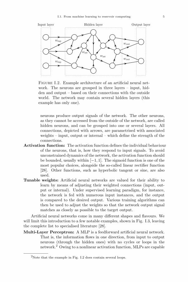
Architecture: It defines the size of the network and the connections betweenthe nodes, which in turn defines how they exchange information. Anexample neural network is sketched in Fig. I.2. The circles denotethe nodes, or the neurons, and the arrows show the connections fromthe output of a neuron to the input of another. The neurons are com-monly categorised into three layers, based on their role in the network.The input layer nodes receive signals from outside and output layer
I.1. From machine learning to reservoir computing 5
Input layer Hidden layer Output layer
winp
winp
wint
wintwout
wout
Figure I.2. Example architecture of an artificial neural net-work. The neurons are grouped in three layers – input, hid-den and output – based on their connections with the outsideworld. The network may contain several hidden layers (thisexample has only one).
neurons produce output signals of the network. The other neurons,as they cannot be accessed from the outside of the network, are calledhidden neurons, and can be grouped into one or several layers. Allconnections, depicted with arrows, are parametrised with associatedweights – input, output or internal – which define the strength of theconnections.
Activation function: The activation function defines the individual behaviourof the neurons, that is, how they respond to input signals. To avoidunconstrained dynamics of the network, the activation function shouldbe bounded, usually within [−1, 1]. The sigmoid function is one of themost popular choices, alongside the so-called linear rectifier function[28]. Other functions, such as hyperbolic tangent or sine, are alsoused.
Tunable weights: Artificial neural networks are valued for their ability tolearn by means of adjusting their weighted connections (input, out-put or internal). Under supervised learning paradigm, for instance,the network is fed with numerous input instances, and the outputis compared to the desired output. Various training algorithms canthen be used to adjust the weights so that the network output signalmatches as closely as possible to the target output.
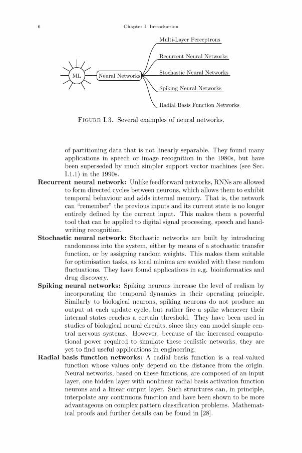
Artificial neural networks come in many different shapes and flavours. Wewill limit this introduction to a few notable examples, shown in Fig. I.3, leavingthe complete list to specialised literature [28].
Multi-Layer Perceptron: A MLP is a feedforward artificial neural network.That is, the information flows in one direction, from input to outputneurons (through the hidden ones) with no cycles or loops in thenetwork.2 Owing to a nonlinear activation function, MLPs are capable
2Note that the example in Fig. I.2 does contain several loops.
6 Chapter I. Introduction
ML Neural Networks
Multi-Layer Perceptrons
Recurrent Neural Networks
Stochastic Neural Networks
Spiking Neural Networks
Radial Basis Function Networks
Figure I.3. Several examples of neural networks.
of partitioning data that is not linearly separable. They found manyapplications in speech or image recognition in the 1980s, but havebeen superseded by much simpler support vector machines (see Sec.I.1.1) in the 1990s.
Recurrent neural network: Unlike feedforward networks, RNNs are allowedto form directed cycles between neurons, which allows them to exhibittemporal behaviour and adds internal memory. That is, the networkcan “remember” the previous inputs and its current state is no longerentirely defined by the current input. This makes them a powerfultool that can be applied to digital signal processing, speech and hand-writing recognition.
Stochastic neural network: Stochastic networks are built by introducingrandomness into the system, either by means of a stochastic transferfunction, or by assigning random weights. This makes them suitablefor optimisation tasks, as local minima are avoided with these randomfluctuations. They have found applications in e.g. bioinformatics anddrug discovery.
Spiking neural networks: Spiking neurons increase the level of realism byincorporating the temporal dynamics in their operating principle.Similarly to biological neurons, spiking neurons do not produce anoutput at each update cycle, but rather fire a spike whenever theirinternal states reaches a certain threshold. They have been used instudies of biological neural circuits, since they can model simple cen-tral nervous systems. However, because of the increased computa-tional power required to simulate these realistic networks, they areyet to find useful applications in engineering.
Radial basis function networks: A radial basis function is a real-valuedfunction whose values only depend on the distance from the origin.Neural networks, based on these functions, are composed of an inputlayer, one hidden layer with nonlinear radial basis activation functionneurons and a linear output layer. Such structures can, in principle,interpolate any continuous function and have been shown to be moreadvantageous on complex pattern classification problems. Mathemat-ical proofs and further details can be found in [28].
I.1. From machine learning to reservoir computing 7
This concludes our brief overview of machine learning and artificial neuralnetworks. Let me say again that the purpose of this introduction was not toturn the reader into expert in machine learning, but merely show the generalcontext of this work. In the next section we will focus on the main topic ofinterest – reservoir computing – with much more in-depth discussions.
I.1.3. Reservoir computing. Reservoir Computing (RC) is a set of ma-chine learning methods for designing and training artificial neural networks,introduced independently in [29] and in [30]. The idea behind these techniquesis that one can exploit the dynamics of a recurrent nonlinear network to pro-cess time series without training the network itself, but simply adding a generallinear readout layer and only training the latter. This results in a system thatis significantly easier to train (since one only needs to optimise the readoutweights), yet powerful enough to match other algorithms on a series of bench-mark tasks.
These ideas can be applied to both recurrent and spiking recurrent neuralnetworks, which gave birth to two concepts called Echo State Networks (ESN)[31] and Liquid State Machines (LSM) [30], that are grouped under the reservoircomputing paradigm. An ESN is a sparsely connected, fixed RNN with randominput and internal connections. The neurons of the hidden layer, commonlyreferred to as the reservoir, exhibit nonlinear response to the input signal dueto a nonlinear activation function (hyperbolic tangent seems to be the mostcommon choice). Liquid state machines rely on the same concept, but thereservoir consists of a “soup” of spiking neurons. The name “liquid” comesfrom an analogy to ripples on the surface of a liquid created by a falling object.Interestingly, this concept has actually been implemented in hardware, that is,as the name suggests. . . in a tank full of water! [18]
For hardware reasons, as will become clear in Sec. I.2, in this work wewill only deal with analogue neurons, leaving the spiking models aside. Fromnow on, to simplify the ideas, I will make no distinction between Echo StateNetworks and Reservoir Computing.
It is now time to introduce the math used describe the dynamics of areservoir computer. Let us denote the neurons (also called nodes, or internalvariables of the reservoir) xi. As they are analogue neurons (see Sec. I.1.2),we may consider that they evolve in discrete time n ∈ Z, so we note themxi(n). The index i goes from 0 to N−1, with N being the reservoir size, or thenumber of neurons in the network. To fix the ideas, let us consider N = 50,since this is a value commonly used in experiments. Remember equation I.1giving the output of an analogue neuron? The evolution equation of a reservoirnode is fairly similar and given by
xi(n+ 1) = f
N−1∑
j=0
aijxj(n) + biu(n)
, (I.2)
where f remains the nonlinear activation function, u(n) is the external inputsignal that is injected into the system, and aij and bi are time-independentcoefficients that determine the dynamics of the reservoir. Specifically, aij iscalled the interconnection matrix, since it defines the strengths of connections
8 Chapter I. Introduction
between all the neurons within the reservoir, with 1 being the strongest connec-tion, and 0 meaning no connection. The vector bi contains the input weightsand defines how strong is the input to each neuron. These coefficients are usu-ally drawn from a random distribution with zero mean. As an alternative pointof view, this equation can be expressed as follows
Future stateof the i-thneuron
=Nonlinearfunction of
(Previous states ofconnected neurons
+Weighted in-put signal
).
This form emphasises the two major contributions to the reservoir dynamics:the feedback, that is, the previous values of the neighbour neurons and theinput signal. This feedback is the recurrent part of the neural network thatgives it internal memory, essential for some tasks (as will be discussed later inSec. I.1.4).
The concept of an Echo State Network suggests that (a) the connectionsbetween the neurons, given by the matrix aij should be sparse (that is, arelatively low number of connections should be present within the network)and (b) the exact topology (or connection pattern) does not really matter.This is a considerable loss from the point of view of general RNNs, as allthese connections “that do not matter” could be trained instead to betterfine-tune the network. But from the point of view of ESNs, and especiallytheir hardware implementations, this is a massive relief. It allows one to pickany simple topology or even manually design a specific one that would suita potential implementation. And since the present work relies on photonicimplementations of reservoir computing, this is an important point to keep inmind.
For the rest of this work, we will consider reservoirs with ring-like topology,as depicted in Fig. I.4. The reason for this choice will be given later, in Sec.I.2, where we will introduce the experimental setup and time-multiplexing.It will then become clear that such architecture corresponds naturally to adelay system. It has been shown in [32] that the performance of such a simpleand deterministically constructed reservoir is actually comparable to a regularrandom echo state network.
A possible interconnection matrix aij corresponding to a ring like topologyis
aij = α
0 1 0 0 · · · 00 0 1 0 · · · 00 0 0 1 · · · 0...
......
.... . .
...0 0 0 0 · · · 11 0 0 0 · · · 0
, (I.3)
where α is a global scale factor. The physical system we will use correspondsto a slightly different set of equations, which can be written as
x0(n+ 1) = f (αxN−1(n− 1) + βM0u(n)) , (I.4a)
xi(n+ 1) = f (αxi−1(n) + βMiu(n)) . (I.4b)
I.1. From machine learning to reservoir computing 9
The difference with I.3 corresponds to what the node x0(n+1) is connected to:in I.3 it is connected to xN−1(n) while in I.4 it is connected to xN−1(n−1). Notethat the structure of the aij matrix is reflected by the dependence of xi(n+ 1)on xi−1(n), while the matrix itself was replaced by a simple coefficient α. Asit defines the strength of the recurrent part of the network, or feedback, weshall from now on call it feedback gain or feedback attenuation, depending onwhether it is superior or inferior to 1, respectively. In a similar way, we havereplaced the bi vector by a global scale factor β and a vector Mi, drawn froma uniform distribution over the interval [−1,+1]. The Mi vector is commonlycalled input mask, or input weights, as it defines the strengths of the inputsignal u(n) received by each individual neuron xi. The global scale parameterβ is therefore called input gain.
The nonlinear function f can be virtually any bounded function. Un-bounded functions may work as well, such as the softmax and hardmax func-tions currently used in deep learning. At the moment of writing these lines,I could not find any systematic study of reservoir performance with differentnonlinear functions. A common choice is the hyperbolic function y = tanh(x)[31]. With hardware implementations, however, the choice of f is rather dic-tated by the choice of a device with a certain nonlinear transfer function. Itcould be, for instance, a saturation curve of an optical amplifier [33] or a sat-urable element [34]. As will be explained later in Sec. I.2, in this work we willbe using exclusively a component with a sine transfer function.
With a sine activation function f(x) = sin(x), Eqs. I.4 become
x0(n+ 1) = sin (αxN−1(n− 1) + βM0u(n)) , (I.5a)
xi(n+ 1) = sin (αxi−1(n) + βMiu(n)) . (I.5b)
These equations describe the behaviour of the system we will discuss later inthis work (see Sec. I.2). It does not get any more complicated than that!
The output of the network is obtained by a simple linear readout layer,that is, by computing a linear combination of the reservoir states xi(n) and thereadout weights wi as follows
y(n) =
N−1∑
i=0
wixi(n), (I.6)
where y(n) is the temporal output signal. Fig. I.4 gives a graphical overviewof the reservoir computer we have just described.
Let us now discuss how the reservoir does what we want it to do. Itreceives a discrete-time temporal signal u(n) as input, and produces in responseanother discrete-time temporal signal y(n). With random readout weights wi,this output signal can be anything, and will most likely be something useless.However, the goal is to perform a specific function on the input signal u(n) thatwould turn it into a desired signal d(n) (examples of such target signals willbe given in Sec. I.1.4). Let us assume that the desired output d(n) is knownfor several values of input u(n), for instance, u(1 . . . 1000) and d(1 . . . 1000) areknown. These time series can be used to adjust the readout weights of thesystem to produce the correct output, i.e. to emulate the specific functionwe want to execute. Remember the different training approaches we discussed
10 Chapter I. Introduction
x0
x1 x2
x5 x4
x3
Miu(n)∑
wixi(n)
Input signal u(n) Output
signal y(n)
Input layer Reservoir Output layer
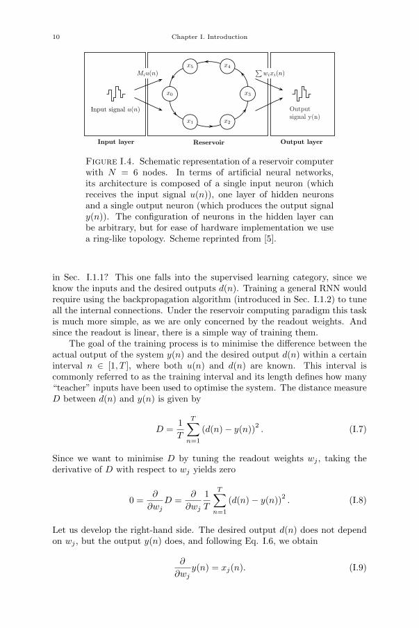
Figure I.4. Schematic representation of a reservoir computerwith N = 6 nodes. In terms of artificial neural networks,its architecture is composed of a single input neuron (whichreceives the input signal u(n)), one layer of hidden neuronsand a single output neuron (which produces the output signaly(n)). The configuration of neurons in the hidden layer canbe arbitrary, but for ease of hardware implementation we usea ring-like topology. Scheme reprinted from [5].
in Sec. I.1.1? This one falls into the supervised learning category, since weknow the inputs and the desired outputs d(n). Training a general RNN wouldrequire using the backpropagation algorithm (introduced in Sec. I.1.2) to tuneall the internal connections. Under the reservoir computing paradigm this taskis much more simple, as we are only concerned by the readout weights. Andsince the readout is linear, there is a simple way of training them.
The goal of the training process is to minimise the difference between theactual output of the system y(n) and the desired output d(n) within a certaininterval n ∈ [1, T ], where both u(n) and d(n) are known. This interval iscommonly referred to as the training interval and its length defines how many“teacher” inputs have been used to optimise the system. The distance measureD between d(n) and y(n) is given by
D =1
T
T∑
n=1
(d(n)− y(n))2. (I.7)
Since we want to minimise D by tuning the readout weights wj , taking thederivative of D with respect to wj yields zero
0 =∂
∂wjD =
∂
∂wj
1
T
T∑
n=1
(d(n)− y(n))2. (I.8)
Let us develop the right-hand side. The desired output d(n) does not dependon wj , but the output y(n) does, and following Eq. I.6, we obtain
∂
∂wjy(n) = xj(n). (I.9)
I.1. From machine learning to reservoir computing 11
Inserting Eq. I.9 into Eq. I.8 and expanding the parenthesis gives
0 =∂
∂wj
1
T
T∑
n=1
(d2(n)− 2d(n)y(n) + y2(n)
), (I.10a)
=1
T
T∑
n=1
(−2d(n)xj(n) + 2xj(n)y(n)) , (I.10b)
=1
T
T∑
n=1
(N−1∑
i=0
wixi(n)xj(n)− xj(n)d(n)
). (I.10c)
And here we obtain a system of linear equations
Rij · wi − Pj = 0 (I.11)
for the readout weights wi, where
Rij =1
T
T∑
n=1
xi(n)xj(n) (I.12)
is the correlation matrix, and
Pj =1
T
T∑
n=1
xj(n)d(n) (I.13)
is the cross-correlation vector. The solution of this system is given by
wi =
N−1∑
j=0
R−1ij Pj (I.14)
and thus, the training of the reservoir computers boils down to the inversionof the correlation matrix Rij .
The above problem – minimsation of the distance D (Eq. I.7) with respectto the unknowns w – can be viewed as minimisation of a problem of the form
‖Ax− b‖2, (I.15)
where A is a matrix, x, b are vectors and ‖ · ‖ is the Euclidean norm. SolvingEq. I.15 is equivalent to finding a solution to a linear system of the kind
Ax = b. (I.16)
The standard approach to solving such a system is to invert A using the ordi-nary least squares algorithm [35]. However, in some cases, the problem Ax = bis ill-posed. That is, no x satisfies the equation, or more than one x does, or thesolution x has very large values, which makes it unstable with respect to smallvariations of A or b. All these problems arise when the matrix A has small orvanishing eigenvalues. In such cases, using ordinary least squares leads to anoverdetermined (over-fitted) or underdetermined (under-fitted) solution. Themost common method for regularisation of ill-posed problems is the Tikhonovregularisation [36], also known as ridge regression or weight decay in the ma-chine learning field. The method consists in adding a regularisation term
‖Ax− b‖2 + ‖Γx‖2, (I.17)
12 Chapter I. Introduction
where Γ is a suitably chosen Tikhonov matrix. In many cases, it is chosen as amultiple of the identity matrix Γ = αI, with a fixed coefficient α. The solutionis now x = (A + αI)−1b, which is better posed than the original problem.That is, such regularisation gives preference to solutions with smaller norms.It is mostly used in simulations, as experimental noise already does a goodjob of preventing overfitting in physical implementations. Typically, we setα ∈ [10−9, 10−1], depending on the reservoir size and the task.
I.1.4. Benchmark tasks. We have just shown that the training of areservoir computer requires the knowledge of the target signal d(n). In simplewords, it is the output we want the system to produce. And this output dependson the task we want the system to perform. This section presents two of themost popular benchmark tasks used to test experimental reservoir computers.Many other tasks can be found in the the literature, but they are out of scopeof this thesis, simply because I did not consider them in my experiments. Moreadvanced tasks, such as VARDEL [37] and chaotic time series prediction willbe introduced in Ch. III and Ch. IV, respectively, as they require importantimprovements of the Reservoir Computer scheme in order to be solved.
I.1.4.1. Wireless channel equalisation. This task is based on a real-life situ-ation, depicted in Fig. I.5. Consider a wireless transmission between an emitterand a receiver. These could be, for instance, a message sent from a broadcastsatellite to a ground station, or from a ground station to a personal mobiledevice. The message arrives to its destination altered by noise and variousdistortions. The possible causes are (a) interference between different echosof the message, propagating through different paths and thus arriving at thereceiver at different moments, (b) imperfect behaviour of the hardware and (c)noise, captured at any stage of the transmission. For this reason, an equaliser isplaced at the receiving end to recover the original message. Multiple digital al-gorithms have been implemented to perform this task. However, the increasingdemand for higher bandwidths requires very fast Analogue-to-Digital Convert-ers (ADCs) that have to follow the high bandwidth of the channel with sufficientresolution to sample correctly the distorted signal [38]. Current manufactur-ing techniques allow producing fast ADCs with low resolution, or slow oneswith high resolution, obtaining both being very costly. This is where analogueequalisers, such as an opto-electronic reservoir computer, become interesting,as they could equalise the signal before the ADC and significantly reduce therequired resolution of the converters, thus potentially cutting costs and powerconsumption [39–41]. Moreover, optical devices may outperform digital devicesin terms of processing speed [39, 42]. It can for instance be shown that reservoircomputing implementations can reach comparable performance to other digi-tal algorithms (namely, the Volterra filter [43]) for equalisation of a nonlinearsatellite communication channel [44].
To emulate a wireless transmission, one starts by generating a message,usually composed of random symbols. The message is then fed through amodel of the channel that adds the alterations, caused by transmission, andnoise, thus producing a signal that would have been captured at the receiverend. Since the goal of the task is to recover the clean message from the distortedone, the former becomes the target signal d(n) for the reservoir computer, while
I.1. From machine learning to reservoir computing 13
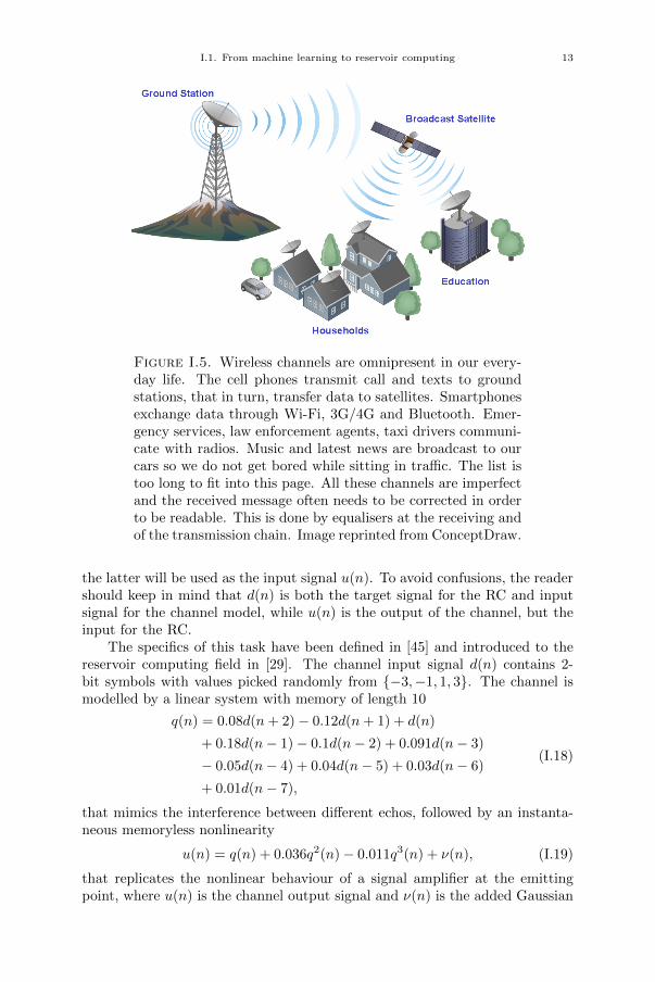
Figure I.5. Wireless channels are omnipresent in our every-day life. The cell phones transmit call and texts to groundstations, that in turn, transfer data to satellites. Smartphonesexchange data through Wi-Fi, 3G/4G and Bluetooth. Emer-gency services, law enforcement agents, taxi drivers communi-cate with radios. Music and latest news are broadcast to ourcars so we do not get bored while sitting in traffic. The list istoo long to fit into this page. All these channels are imperfectand the received message often needs to be corrected in orderto be readable. This is done by equalisers at the receiving andof the transmission chain. Image reprinted from ConceptDraw.
the latter will be used as the input signal u(n). To avoid confusions, the readershould keep in mind that d(n) is both the target signal for the RC and inputsignal for the channel model, while u(n) is the output of the channel, but theinput for the RC.
The specifics of this task have been defined in [45] and introduced to thereservoir computing field in [29]. The channel input signal d(n) contains 2-bit symbols with values picked randomly from −3,−1, 1, 3. The channel ismodelled by a linear system with memory of length 10
q(n) = 0.08d(n+ 2)− 0.12d(n+ 1) + d(n)
+ 0.18d(n− 1)− 0.1d(n− 2) + 0.091d(n− 3)
− 0.05d(n− 4) + 0.04d(n− 5) + 0.03d(n− 6)
+ 0.01d(n− 7),
(I.18)
that mimics the interference between different echos, followed by an instanta-neous memoryless nonlinearity
u(n) = q(n) + 0.036q2(n)− 0.011q3(n) + ν(n), (I.19)
that replicates the nonlinear behaviour of a signal amplifier at the emittingpoint, where u(n) is the channel output signal and ν(n) is the added Gaussian
14 Chapter I. Introduction
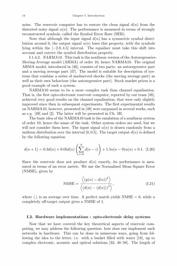
noise. The reservoir computer has to restore the clean signal d(n) from thedistorted noisy signal u(n). The performance is measured in terms of wronglyreconstructed symbols, called the Symbol Error Rate (SER).
Note that although the input signal d(n) has a symmetric symbol distri-bution around 0, the output signal u(n) loses this property, with the symbolslying within the [−2.8, 4.5] interval. The equaliser must take this shift intoaccount and correct the symbol distribution properly.
I.1.4.2. NARMA10. This task is the nonlinear version of the Autoregressive-Moving-Average model (ARMA) of order 10, hence NARMA10. The originalARMA model, introduced in [46], consists of two parts: an autoregressive partand a moving average part [47]. The model is suitable for description of sys-tems that combine a series of unobserved shocks (the moving average part) aswell as their own behaviour (the autoregressive part). Stock market prices is agood example of such a system.
NARMA10 seems to be a more complex task than channel equalisation.That is, the first opto-electronic reservoir computer, reported by our team [48],achieved very good results on the channel equalisation, that were only slightlyimproved since then in subsequent experiments. The first experimental resultson NARMA10, however, presented in [48] were surpassed in several works, suchas e.g. [49] and [2]. The latter will be presented in Ch. III.
The basic idea of the NARMA10 task is the emulation of a nonlinear systemof order 10, hence the name of the task. Other system orders are used, but wewill not consider them here. The input signal u(n) is drawn randomly from auniform distribution over the interval [0, 0.5]. The target output d(n) is definedby the following equation
d(n+ 1) = 0.3d(n) + 0.05d(n)
(9∑
i=0
d(n− i))
+ 1.5u(n− 9)u(n) + 0.1. (I.20)
Since the reservoir does not produce d(n) exactly, its performance is mea-sured in terms of an error metric. We use the Normalised Mean Square Error(NMSE), given by
NMSE =
⟨(y(n)− d(n))
2⟩
⟨(d(n)− 〈d(n)〉)2
⟩ , (I.21)
where 〈.〉 is an average over time. A perfect match yields NMSE = 0, while acompletely off-target output gives a NMSE of 1.
I.2. Hardware implementations : opto-electronic delay systems
Now that we have covered the key theoretical aspects of reservoir com-puting, we may address the following question: how does one implement suchnetworks in hardware. This can be done in numerous ways, going from fol-lowing the idea to the letter, i.e. with a bucket filled with water [18], up tocomplex electronic, acoustic and optical solutions [33, 48–58]. The length of
I.2. Hardware implementations : opto-electronic delay systems 15
the list shows the abundant interest that RC has received from experimentalresearchers.3
In this work, however, we will focus in particular on one such implemen-tation: the first opto-electronic reservoir reported by the OPERA-Photoniquegroup. It combines optics and electronics for a high-speed system. All myexperiments were based on this setup, with several add-ons. Therefore, a goodexplanation of its working principle would not be a luxury. In this section wediscuss every component of the setup, how they work all together and how itcan be used to process information under the RC paradigm.
I.2.1. Time-multiplexing. As have been explained in Sec. I.1.3, a reser-voir is a network of neurons. Each neuron evolves in time following the activa-tion function. In hardware implementations, this function could be processedby a device, or a dedicated component of the setup: an array of transistors,for instance, or a sequence of operations performed by a microprocessor. Somedevices can be made to update multiple neurons in parallel, that is, their oper-ating principle allows for multiple physical or virtual inputs and outputs (e.g.the parallel frequency-multiplexed scheme proposed in [59]). Others, such asthe light intensity modulator, used in this thesis (it will be presented in Sec.I.2.4), can only process one neuron at a time. This means that, in principle,one needs N such modulators, one for each neuron. And since these devicesare not cheap, the price of the setup becomes a big problem.
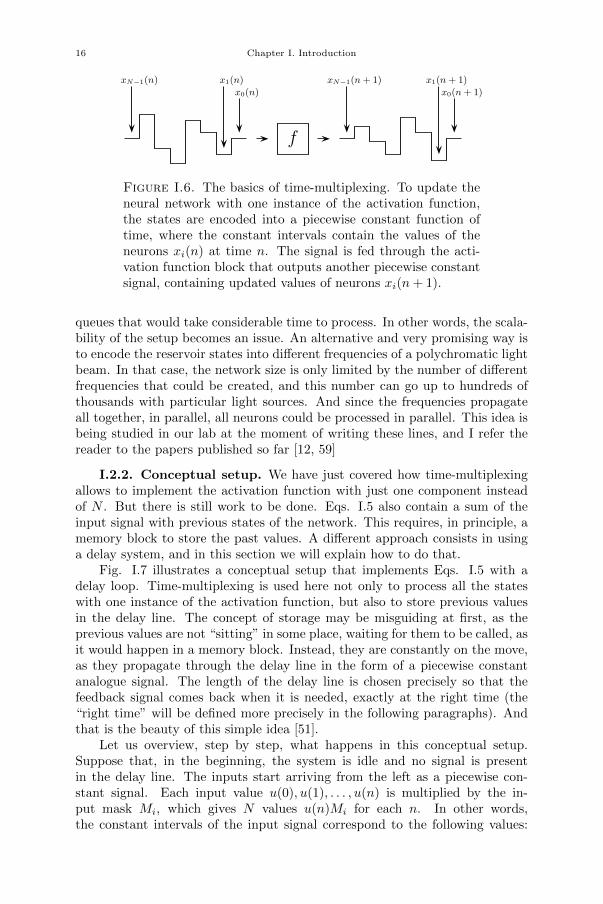
The solution to this issue relies in a careful analysis of Eqs. I.5. In fact,one may notice that neurons xi do not need to be updated simultaneously.Since each neuron xi only depends on one neighbour xi−1, they can be up-dated in a ordered way, that is, one after another. This simple idea allows toreplace N activation function components by just one, that would process thequeue of neurons x0, . . . , xN at each timestep n. Such procedure is commonlycalled time-multiplexing, as instead of processing all neurons simultaneously,in parallel, they are stacked in a queue, or in other words, time-multiplexed.
Fig. I.6 illustrates the above idea. In order to update the states of all theneurons using only one instance of the activation function, the neurons need tobe stacked in a queue. This can be achieved by defining a piecewise constantfunction of time, with each constant interval corresponding to the value of acertain neuron xi(n) of the network at time n. The output of the function givesthe updated states of the neurons at the next timestep n + 1, in the form ofa new piecewise constant function. To avoid misunderstanding, care should betaken not to confuse the physical time of the piecewise signal, and the discretetime n. While the latter is indeed called time for convenience, it is no morethan a basic index.
Time-multiplexing thus allows to significantly simplify experimental im-plementations of reservoir computing. However, this is not the only way toproceed, and the idea itself is far from being flawless. The processing speedof the activation function component defines how fast it can update each neu-ron. This means that implementing large reservoirs would results in very long
3Although I cannot guarantee the completeness of this list, I did my best to cite all
experimental setups known at the moment of writing these lines.
16 Chapter I. Introduction
f
x0(n)
x1(n)xN−1(n)
x0(n+ 1)
x1(n+ 1)xN−1(n+ 1)
Figure I.6. The basics of time-multiplexing. To update theneural network with one instance of the activation function,the states are encoded into a piecewise constant function oftime, where the constant intervals contain the values of theneurons xi(n) at time n. The signal is fed through the acti-vation function block that outputs another piecewise constantsignal, containing updated values of neurons xi(n+ 1).
queues that would take considerable time to process. In other words, the scala-bility of the setup becomes an issue. An alternative and very promising way isto encode the reservoir states into different frequencies of a polychromatic lightbeam. In that case, the network size is only limited by the number of differentfrequencies that could be created, and this number can go up to hundreds ofthousands with particular light sources. And since the frequencies propagateall together, in parallel, all neurons could be processed in parallel. This idea isbeing studied in our lab at the moment of writing these lines, and I refer thereader to the papers published so far [12, 59]
I.2.2. Conceptual setup. We have just covered how time-multiplexingallows to implement the activation function with just one component insteadof N . But there is still work to be done. Eqs. I.5 also contain a sum of theinput signal with previous states of the network. This requires, in principle, amemory block to store the past values. A different approach consists in usinga delay system, and in this section we will explain how to do that.
Fig. I.7 illustrates a conceptual setup that implements Eqs. I.5 with adelay loop. Time-multiplexing is used here not only to process all the stateswith one instance of the activation function, but also to store previous valuesin the delay line. The concept of storage may be misguiding at first, as theprevious values are not “sitting” in some place, waiting for them to be called, asit would happen in a memory block. Instead, they are constantly on the move,as they propagate through the delay line in the form of a piecewise constantanalogue signal. The length of the delay line is chosen precisely so that thefeedback signal comes back when it is needed, exactly at the right time (the“right time” will be defined more precisely in the following paragraphs). Andthat is the beauty of this simple idea [51].
Let us overview, step by step, what happens in this conceptual setup.Suppose that, in the beginning, the system is idle and no signal is presentin the delay line. The inputs start arriving from the left as a piecewise con-stant signal. Each input value u(0), u(1), . . . , u(n) is multiplied by the in-put mask Mi, which gives N values u(n)Mi for each n. In other words,the constant intervals of the input signal correspond to the following values:
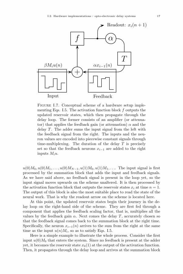
I.2. Hardware implementations : opto-electronic delay systems 17
Input
βMiu(n)
+
f b
Readout: xi(n+ 1)
α
T
Feedback
αxi−1(n)
Figure I.7. Conceptual scheme of a hardware setup imple-menting Eqs. I.5. The activation function block f outputs theupdated reservoir states, which then propagate through thedelay loop. The former consists of an amplifier (or attenua-tor) that applies the feedback gain (or attenuation) α and thedelay T . The adder sums the input signal from the left withthe feedback signal from the right. The inputs and the neu-ron values are encoded into piecewise constant signals throughtime-multiplexing. The duration of the delay T is preciselyset so that the feedback neurons xi−1 are added to the rightinputs Miu.
u(0)M0, u(0)M1, . . . , u(0)MN−1, u(1)M0, u(1)M1, . . .. The input signal is firstprocessed by the summation block that adds the input and feedback signals.As we have said above, no feedback signal is present in the loop yet, so theinput signal moves upwards on the scheme unaltered. It is then processed bythe activation function block that outputs the reservoir states xi at time n = 1.The output of this block is also the most suitable place to read the state of theneural work. That is why the readout arrow on the scheme is located here.
At this point, the updated reservoir states begin their journey in the de-lay loop on the right-hand side of the scheme. They are first fed through acomponent that applies the feedback scaling factor, that is, multiplies all thevalues by the feedback gain α. Next comes the delay T , accurately chosen sothat the feedback signal comes back to the summation block at the right time.Specifically, the neuron xi−1(n) arrives to the sum from the right at the sametime as the input u(n)Mi, so as to satisfy Eqs. I.5.
Here is a simple example to illustrate the whole process. Consider the firstinput u(0)M0 that enters the system. Since no feedback is present at the adderyet, it becomes the reservoir state x0(1) at the output of the activation function.Then, it propagates through the delay loop and arrives at the summation block
18 Chapter I. Introduction
from the right precisely at the moment when the input u(1)M1 enters thesystem from the left.
I.2.3. Desynchronisation. Before we move to the actual experimentalsetup, let me say a few words on the principle of desynchronisation, that weused in the above process without actually naming it. From what was explainedabove, a reservoir state xi−1(n) is summed up with an input value u(n)Mi. Thismay seem counter-intuitive, as one may want to combine it with u(n)Mi−1 tomatch the indexes. However, there are a few reasons to mismatch them (and,by the way, this is why this approach is called desynchronisation). First, thisis done to satisfy Eqs. I.5. One may argue that this is not the actual reason,as these equation were derived from the ring-like topology that we createdartificially. The genuine reason for desynchronising the system is to createinteraction between the neurons.
Imagine that, with synchronous indexes, input Miu(n) is summed with thefeedback xi(n). That means that the neuron xi(n), through the course of itsevolution from timestep 0 to timestep n, has only seen input values u(n)Mi withindex i, and only its own previous values xi(n − 1), . . . , xi(0). Such a systemis no longer a network of neurons, but a mere set of independent variables. Animportant property of a neural network is the ability of the neurons to exchangeinformation between them.
To wrap up, desynchronisation is a way to interconnect the neurons withinthe network. It is important to note that this is not the only approach. In [52],practically the same delay system is run synchronously. The interconnectionsare created by an added low-pass filter that links the reservoir states together,as its output depends on current and past input values.
I.2.4. Experimental setup. We can now make the final step towardsthe experimental setup, schematised in Fig. I.8. Although this setup is thecore part of all of my experiments, it is not the novelty of my work, as it hasbeen designed before I joined the lab [48]. For this reason, I present it here,in the introductory chapter, alongside all other concepts that were well knownand established before I started my research.
This experiment is often qualified as opto-electronic, electro-optic, or pho-tonic4. In Fig. I.8, electrical cables and components are drawn in black, andgrey lines correspond to optical components and fibre. Remember that thereservoir states are encoded into piecewise constant temporal signals. In thissetup, these signals are generated in two different mediums – light and electric-ity. Thus, several components serve to either generate one of the two mediumsor convert the signal from one medium to another.
At first sight, the setup in Fig. I.8 is quite different from the conceptualdesign depicted in Fig. I.7. Let us first go through all the components involvedhere, and then explain how they do the same thing as the conceptual model.The photonic reservoir computer is composed of the following devices.
4Photonics is quite a tricky term. I am yet to find an established and precise definitionand, in my experience, various scientists interpret this concept differently. In the present
work, for simplicity, I make no distinction between these three terms.
I.2. Hardware implementations : opto-electronic delay systems 19
1©
2©
3©
4©
5©
6©
7©
8©9©
SLD
MZ90/10
Att
Amp Comb
Pf
Spool
Pr
Mi × u(n)
xi(n+ 1)
Input
Readout
Figure I.8. Schematic representation of the photonic reser-voir, introduced in [48]. It contains a light source (SLD), aMach-Zehnder intensity modulator (MZ), a 90/10 beam split-ter, an optical attenuator (Att), a fibre spool (Spool), twophotodiodes (Pr and Pf), a resistive combiner (Comb) andan amplifier (Amp). Optical and electronic components areshown in grey and black, respectively.
1 An optical experiment starts with a light source: a SLD (superlu-miniscent diode) producing broadband light at the standard telecom-munication wavelength 1550 nm.
2 The light intensity is modulated by the Mach-Zehnder intensity mod-ulator (MZ) that shapes it proportional to the input electrical voltage.In other words, it serves to transfer information from an electrical sig-nal into an optical one.
3 Following the light path in optical fibre, next comes a 90/10 splitter.As its name suggests, it splits the light beam in two fractions withthe given ratio.
4 A photodetector, or photodiode (Pr) produces an electrical signalproportional to the input optical signal. Its function may been as theopposite of the intensity modulator – to transfer information from anoptical signal into an electrical one.
5 The function of the optical attenuator (Att) is given explicitly by itsname – it attenuates the light intensity by a fixed factor, nothingmore.
6 The fibre spool (Spool) is a big reel of optical fibre. Its purpose is todelay the signal between the optical attenuator (Att) and the followingphotodiode (Pf). As the speed of light in the standard optical fibre is,roughly, 2 × 10⁸ m/s, one kilometre of fibre creates a delay of about5 µs. As will be shown below, this order of magnitude is sufficient forthis setup.
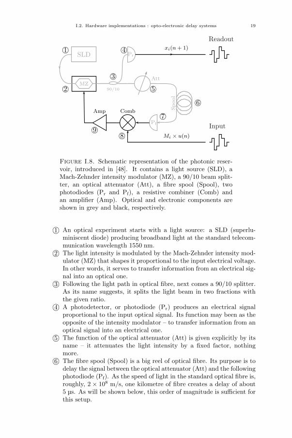
20 Chapter I. Introduction
Component Main characteristicsLight source Thorlabs SLD1550P-A40
- centre wavelength: 1550 nm- FWHM: 33 nm- maximum output power: 40 mW
Intensity modulator EOSPACE AX-2X2-0MSS-12- bandwidth: > 10 GHz- Vπ (at 1 GHz): 4.5 V
Photodiodes TTI TIA-525I- bandwidth: DC to 35 MHz or DC to 125 MHz(switchable)- maximum output voltage: 2 Vp-p
- maximum linear input: 1.2 mWOptical attenuator Agilent 81571A
- attenuation range: 0− 60 dB- resolution: 0.001 dB
Fibre spool Standard SMF-28e fibre- length: approx. 1.5 km
Resistive combiner Home-made star format power splitter- resistors (3x): 16.7 Ω
Amplifier Mini Circuits ZHL-32A+- gain: 25 dB- bandwidth: 0.05− 130 MHz- maximum input: 2 Vp-p at 50 Ω
Table I.1. Main components of the opto-electronic reservoir,schematised in Fig. I.8.
7 A second photodiode (Pf), identical to (Pr), converts the delayedoptical signal into voltage.
8 This voltage is added up with an external electrical signal, containingthe inputs to the system.
9 Finally, the newly produced voltage is amplified by an electrical ampli-fier (Amp), as the Mach-Zehnder modulator “expects” input voltagesmuch larger than the photodiode Pf can generate.
Tab. I.1 lists the exact device models used for this setup with their maincharacteristics.
The key element of the setup is the Mach-Zehnder intensity modulator,since it carries out the activation function of the neurons. The light intensityat its output is given by [48]
I(t) =I02
+I02
sin
(πV (t)
Vπ+ φ
), (I.22)
where I0 is the input light intensity and V (t) is the time-dependent voltagedriving the modulator. The bias φ can be adjusted by applying a DC voltageVφ to the modulator. The constant voltage Vπ is an intrinsic characteristic ofthe modulator, that corresponds to the voltage needed to go from a maximum
I.2. Hardware implementations : opto-electronic delay systems 21
to the next minimum of light intensity at the output of the modulator (in ourcase, Vπ ≈ 4.5 V). The transfer function of the modulator is the reason whywe use a sine activation function, as have been mentioned previously.
The reservoir states xi(n) can be both positive and negative. Hence, thevoltage V (t), driving the modulator, consists of positive and negative values.However, the Mach-Zehnder outputs a modulated light intensity that only holdspositive values. Therefore, the output voltage of the feedback photodiode Pf isstrictly positive. It can be broken down into a DC voltage VDC, proportional tothe light intensity I0/2, and an AC voltage VRF, proportional to the intensityfluctuations around the mean value. The DC voltage is cut off by the high-pass filter of the amplifier, so that only VRF is amplified and used to drivethe modulator V (t) ∼ VRF. The filter thus allows both positive and negativereservoir states, despite the fact that they are encoded into strictly positivelight intensity. More details on this aspect can be found in the SupplementaryMaterial of [48].
We will now discuss the operating principle of the entire setup. We willproceed in the same manner as we did with the conceptual setup, so as tohighlight the similarity between the schemes. To start, let us suppose that theexperiment is idle (that is, no signals are present at any point) at the momentwhen the first input comes into the reservoir.
The inputs arrive into the system as an electrical signal (the bottom rightcorner on the scheme). This signal is the same piecewise constant functioncontaining the input signal u(n), multiplied by the input mask Mi. The resis-tive combiner (Comb) sums the input and feedback signals. Since the latter isnull5 , the input signal alone is amplified (Amp) and applied to the intensitymodulator (MZ), that shapes the light intensity into the same piecewise con-stant function, proportional to the sine of the input electrical signal. In otherwords, the input signal Miu(n) is passed through the modulator transfer func-tion (here, sin(x)) and transferred from voltage to light intensity, so that theoptical output contains values sin(Miu(n)). This optical signal is then split intwo. 10% are sent to the readout photodiode Pr. Similar to the readout arrowin the conceptual setup, the readout photodiode allows to capture the reservoirstates, as it produces an electrical signal proportional to xi(n + 1). At thispoint, n = 0 and xi(1) = sin(Miu(0)) since there is no feedback signal yet inthe reservoir. The 90% of the optical signal make their way into the opticalattenuator (Att), where the feedback attenuation (α in Eqs. I.5) is applied.The resulting feedback signal then propagates through the delay line6. Finally,the feedback neurons are transferred back from light intensity into voltage bythe feedback photodiode (Pf). To illustrate the process in motion, consider theN + 1-st input M0u(1) passing through the combiner. No feedback is addedto this input, as xN−1(0) is null. However, moments later, as the next (N + 2-st) input M1u(1) enters the combiner, it is being added to the first feedback
5Technically, it is not null: the SLD is emitting light, hence the DC voltage VDC ∼ I0/2is present. But we can ignore it, since it is filtered by the amplifier.
6Note that the delay T is the total propagation time from the MZ optical output to itselectric input, that is, the full loop. In other words, fibre patch cords and electrical cables
also add up to the delay, but their contribution is relatively small.
22 Chapter I. Introduction
value x0(1) = sin(M0u(0)), obtained from the first input M0u(0) to the reser-voir. Note the mismatch of indexes because of the desynchronisation of thereservoir, as was explained in I.2.3.
Accurate choice of delay T is key for precise combination of the inputwith the feedback. This can be done in two ways. Cutting optical fibre atthe desired lengths is very unpractical, so instead of adjusting T , we tune theduration of the intervals in the piecewise constant signals. This can be easilyachieved with signal generation and acquisition devices. In practice, we startby building a reservoir computer with a certain fibre spool, then measure thedelay time T by sending in a spike and estimating the time between its echoson a scope. A basic scope with 60 MHz bandwidth allows to measure T withenough precision. From the number of neurons N that we want to fit into thereservoir, we define the duration of one neuron θ = T/N . In other words, θ isthe duration of each constant step of the piecewise signal. For instance, with1 km of fibre and T = 5 µs we can fit N = 50 neurons by setting θ = 100 ns.This corresponds to a frequency of 10 MHz. The signals can be generatedand recorded by arbitrary waveform generators (AWG) and data acquisitioncards, respectively. To get rid of the transients, induced by finite bandwidthsof physical devices, the acquired signal can be sampled at a higher frequency,e.g. 200 MHz, and then averaged over 20 samples.
To conclude this section, I list several typical characteristics of the exper-imental setup. These values are presented for readers willing to accuratelyreproduce our experiment.
- All electronic inputs and outputs are impedance-matched to 50 Ω.- The SLD pump current is set to 250 − 350 mA, so that the opti-
cal power at the readout photodiode does not exceed 1 mW (linearresponse threshold).
- The input gain is usually set between 0.1 and 0.5 (dimensionless valuesused in simulations). This roughly corresponds to signals rangingfrom 25 mVp-p to 125 mVp-p.
- With input voltages of 120 mVp-p and higher, the output of the am-plifier spans the Vπ interval [−4.5 V,+4.5 V].
- The feedback attenuations are typically tuned between 4.5 dB and6 dB – lower values would put the cavity in a regime where it oscillatesspontaneously, which decreases its performance as a reservoir, whilehigher values would not provide enough feedback to the reservoir;
- The photodiodes (TTI TIA-525I) carry two amplification stages, withselectable coupling (DC or AC). To avoid saturation of the secondamplification stage, both photodiodes are set to AC coupling. Thecutoff frequency (100 Hz) is sufficiently low to keep the signal dis-tortion minimal. We also select the minimum 1x gain and maximumbandwidth of 135 MHz.
- The fibre spool of approx. 1.5 km yields a (measured) delay of 7.94 µs.To fit 50 neurons into the reservoir, we set the sampling frequency at128.4635 MHz (with θ = 155.7 ns) and average the reservoir statesover 20 samples.
I.3. Field-Programmable Gate Arrays 23
I.3. Field-Programmable Gate Arrays
So far we have discussed the theory behind reservoir computing (Sec. I.1),and how it could be implemented physically in an opto-electronic experiment(Sec. I.2). What follows deviates completely from those two topics. Thissection introduces the true novelty of my work – an amazing device that Ihad a chance to play with for four years – a FPGA chip. Its outstandingproperties, such as high computational speed and intrinsic parallelism, werecrucial in most of the experiments presented in this thesis. Therefore, it isnatural to devote a section to thoroughly introduce the FPGAs. After a shorthistory lesson, we will discuss the internal structure of the specific FPGA chip Iwas using, together with the software tools required to program and operate it.The contents of the historical introduction is inspired by [60] with additionalinformation taken from [61] and [62]. The rest of the section is mostly original,with some facts from [63].
I.3.1. History.I.3.1.1. From transistors to integrated circuits. Our story begins in 1947 at
Bell Labs, when John Bardeen, William Shockley and Walter Brittain inventedthe first transistor. . . at least according to Bell Labs legal documents. The firstpatents on field-effect transistors were issued in 1925 in Canada to Julius EdgarLilienfeld and in 1939 in Germany to Oskar Heil, although there is no directevidence that these devices were actually built. Anyways, the 1956 Nobel Prizein Physics for the discovery of the transistor effect was awarded to Shockley,Bardeen and Brattain.
Many consider the transistor to be one of the greatest inventions of the 20thcentury. Its main applications are amplification and switching of electronicsignals, and it plays the role of the main building block of the whole modernelectronic industry. But how did we get there?
The first junction transistors were bulky, consumed a lot of power andsuffered from various performance issues, such as trapping or scattering of car-riers. Operating multiple transistors together in an electronic circuit did notseem possible at that time. However, several technological advances changedthe situation completely. In 1959, Dawon Kahng and Martin M. Atalla atBell Labs invented the metal-oxide-semiconductor field-effect transistor (MOS-FET). With a design fundamentally different from the previous bipolar junctiontransistor, the MOSFET was composed of an insulating layer of silicon diox-ide on the surface of a semiconductor (crystalline silicone), with a metallic gateelectrode on top. The subsequent progress of clean rooms, reducing contamina-tion to unprecedented levels, and the evolution of photolithography contributedto the development of the Si–SiO2 technology, thus making the MOSFET themost widely used type of transistor in integrated circuits. Let us explore thereasons of such a massive success.
There are two main types of MOSFETs: pFETs and nFETs. They eitherblock or open the current flow depending on what value they receive, 0 or 1.The CMOS (complementary metal-oxide semiconductor) technology, patentedin 1963 by Frank Wanlass, took the MOS transistors to the next level. PairingpFETs with nFETs during the fabrication process of the integrated circuit, so

24 Chapter I. Introduction
R1
R1
R2
A
B
NAND(A,B)
+VCC
Figure I.9. Logic NAND gate built with two transistors.
that one in each pair is always off, allowed to significantly cut power consump-tion and heat dissipation, as the current only flows when the transistors areactually switched.
Several transistors can be combined on a protoboard to obtain a logicgate, e.g. a NAND gate, illustrated in Fig. I.9. An array of several logicgates, composed of junction transistors, would result in a quite bulky setup.The MOSFET and CMOS technologies allowed to significantly scale the thingsdown by printing large amounts of transistors on relatively small areas of silicon.Such printed boards, called Integrated Circuits (IC), first appeared in 1961. Asthe transistor printing technology improved further, allowing to fit more andmore units on smaller areas, the famous Moore’s Law was announced in 1965.It predicts the number of transistors in IC to double every year. It is used forgoal setting in industry and research. However, it is doomed to break downvery soon. In fact, current photolithography process allows to create chipswith features of just 14 nm. Even with improved techniques, it is unclear howmuch further scaling is possible. At 2 nm, transistors would be just 10 atomswide, and it is unlikely that they would operate reliably at such a small scale.Moreover, as the transistors are packed ever tighter, dissipating the energy thatthey use becomes much harder [64, 65].
A simple integrated circuit may consist of several logic gates or a singlemultiplexer. Modern high-end chips, on the other hand, can contain up to25 million transistors per square millimetre. The design of such complex ICsis a costly and time-demanding process, with expenses up to multiple tens ofmillions of dollars. In fact, the circuit has to be conceived to suit all requiredspecifications before being placed on a silicon substrate. This often requiresadjusting individual transistors manually, which is virtually impossible for largecircuits. Therefore, automatic design software tools play an important role inthis design process, that still requires a couple of months of work to get from thedesign to production. Given the high production costs, this approach is onlyviable for large orders of chips, such as microprocessors for consumer markets.Smaller projects obviously require a fundamentally different solution to designand test integrated circuits. This is where field-programmable devices – thatare alterable by the user himself, not solely in the factory – appear on the stage.
I.3. Field-Programmable Gate Arrays 25
Programmable logic devices. A Programmable Logic Device (PLD) is a re-configurable integrated circuit. Before PLDs were introduced, read-only mem-ory (ROM) was used to perform arbitrary logic functions. However, mem-ory blocks operate much slower than dedicated logic circuits, consume morepower and are more expensive in production. In 1970, Texas Instruments de-veloped the first Programmable Logic Array (PLA): the random-access memory(RAM) based device was programmed by altering the metal layer during theproduction of the IC. In 1978, MMI introduced a Programmable Array Logic(PAL)7, a device similar to PLA, but instead of two programmable planes, ithad one Programmable Read-Only Memory (PROM) array, a fixed OR planeand a programmable AND plane, thus allowing to compute sum of productslogic equations with feedback from the outputs. A significant improvementwas made by Lattice Semiconductor in 1985 with their Generic Logic Array(GAL), that could be programmed and reprogrammed. It combined CMOStechnology with electrically erasable gate technology, making it a high-speedand low-power logic device.
The first logic arrays (PALs and GALs) were only available in small for-mats of few hundreds of logic gates. Complex Programmable Logic Devices(CPLDs) were introduced for bigger logic circuits by linking several PALs withprogrammable interconnections. In parallel to the logic arrays, a different typeof devices based on gate arrays was being developed, and gave birth to Field-Programmable Gate Arrays (FPGAs). The main difference between a CPLDand a FPGA lies in the architecture. Basically, a logic cell in a CPLD can onlybe connected to its neighbours, while in a FPGA it can be linked (routed) toany other cell across the chip through programmable interconnections. In otherwords, a CPLD has programmable logic with stiff connections between cells,while a FPGA offers programmable logic and programmable interconnections.Both CPLDs and FPGAs coexist nowadays – the former are limited in size andcapabilities and thus used for simpler designs, while the latter are employed forthe most complex applications.
How do these devices retain their configuration? A PLD can be seen as acombination of logic and memory units. The former perform individual logicoperations and the latter store the connectivity pattern between the cells, givento the device during the configuration process. Different methods have beenused through history. The simplest is a silicon antifuse, which works in oppositeway to a normal fuse, creating a connection upon destruction, when a voltageis applied. Obviously, such method is indeed field-programmable, but canonly be done once. A significant step forward was made with the arrival ofelectronic memory. At first, Programmable Read-Only Memory (PROM) wasused in 1970 – it allowed to program the chip fairly easily, but it still wasnot reprogrammable – once the memory was set, the chip configuration waspermanent. Erasable PROM (EPROM) appeared one year later, and broughtthe valuable advantage of being reprogrammable after erasing its contents withUV-light. Not the most practical solution though, as the EPROM had to be
7It seems that the engineers ran out of inspiration when they named their devices! Donot worry if you get lost in all these acronyms, though – we will not use them past this
section.

26 Chapter I. Introduction
removed from the circuit to be erased. The major improvement was made in1983 with the invention of EEPROM – Electrically Erasable PROM – thatallowed data to be read, erased and rewritten. Still not perfect yet, as it couldonly be reprogrammed a limited number of times. For this reason, modernFPGAs store their configuration in volatile Static RAM (SRAM), which canbe rewritten an unlimited number of times.
To sum up, the need for a simple and inexpensive solution for fast devel-opment of integrated electronic circuits – more efficient than placing individualcomponents on a protoboard, and less expensive than following the entire pro-cess of IC manufacturing – brought to life several families of programmablelogic devices, among which the FPGA – a large array of logic gates (up to twomillions), combined with SRAM blocks to store the internal connections.
I.3.2. Market and applications. Nowadays, FPGA market is domi-nated by two players: Xilinx and Altera. Together, they hold 90% of the mar-ket share. Other companies, such as Lattice Semiconductor, Actel, Achronixand Tabula provide more specialised chips with unique features.
Xilinx offers several FPGA families with a wide range of applications. TheArtix family holds the entry level chips with lowest cost and power consumptionand small form-factor packaging8. The Spartan family targets cost-sensitiveand high-volume requests. The Kintex family is optimised for the best price-performance. Virtex is the top-level family, with the highest system perfor-mance and capacity. Several generations of devices exist within each family.The most recent devices, at the moment of writing those lines, are Family 7chips. In this work I used a Family 6 device, since it was the latest device onthe market in 2013, when it was purchased.
Altera also offers several FPGA families, based on application needs. Stra-tix devices offer the highest performance and density, Arria is a family of mid-range FPGAs, and Cyclone series are the company’s lowest cost, lowest powerchips.
At first, FPGAs were mainly used to connect electronic components to-gether, such as bus controllers or processors. As they became larger and faster,with lower cost per logic gate, their application landscape changed dramati-cally. Modern FPGAs are capable of replacing ASIC chips and are more andmore frequently found in consumer electronic devices. Gone are the days whenthey were too expensive for high-volume productions. Furthermore, FPGAchips became reliable enough for critical applications in space, military andmedical fields. They are now commonly used for high-performance signal pro-cessing, replacing multiple dedicated DSP processors. The latest trend is theSystem on Chip (SoC) platforms, consisting of multi-core processors and high-capacity logic devices, all on a single chip. The idea is to benefit from the highcomputational power of the FPGA without the complex design process. Theuser would only interacts with the processor, while the latter could call theFPGA for support, for instance, to increase its performance on specific tasksby delegating highly repetitive routines to the FPGA.
8An Artix evaluation board can be purchased for as low as $100.
I.3. Field-Programmable Gate Arrays 27
I.3.3. Xilinx Virtex 6 : architecture and operation. With the his-torical background set, let us take a closer look inside a FPGA chip. Thissection is aimed at users with high interest in FPGA technology. If you are notone of them, you can skip this part – you will miss a lot of interesting facts,but this will not prevent you from understanding the experiments described inthe next chapters.
At this point, describing a “general” chip makes no sense, as each manu-facturer, be it Altera or Xilinx, designs its chips in different ways with differentarchitectures. We will thus focus on the FPGA chip I have been using through-out my thesis: the Xilinx Virtex 6. Some parts of this section remain valid forall FPGAs, but others are unique features only present on Xilinx devices. Thecontents of this section was inspired from [63].
Up to now, we simplified the internal structure of a FPGA to (a) a largenumber of logic gates and (b) blocks of memory to store the interconnections.Modern FPGAs are much more complex than that and contain numerous ad-ditional components. This is what we are going to overview here.
Logic blocks. The primary function of a FPGA is to perform logic opera-tions, such as AND, OR, NOT, NAND, NOR, XOR, XNOR and more complexcombinations of these. Instead of replicating thousands of individual logicgates, FPGA manufacturers make use of a more advanced logic block, calledLook-Up Table, or LUT. A general LUT, with n inputs and one output, canencode any n-input Boolean function by modelling it as a truth table. Thatway, several individual logic gates can be replaced by a single logic block. AVirtex 6 LUT has 6 inputs. The output of a LUT may be stored in a register(a simple circuit acting as a one-bit memory) in order to implement sequentiallogic. Four such LUTs are grouped in a Slice, that also contains eight regis-ters, multiplexers (used to select inputs) and arithmetic carry logic (used toperform arithmetical operations). Two slices form a Configurable Logic Block,or CLB – a feature-rich circuit capable of implementing various logic functions.A FPGA chip from Virtex-6 family may contain from 104 up to 105 CLBs [66].Obviously, each CLB contains more features than may be required. During theimplementation process, mapping tools select which components of each CLBare used, and the others are bypassed or left unconnected from the circuit.
Routing resources. The thousands of CLBs (and other components, de-scribed below) of a FPGA can be connected in various ways by the user.Therefore, a sufficient number of routing channels (or paths) should be presenton the chip in order to make any connectivity pattern possible. Surprisingly,these routing resources occupy most of the physical space on the silicon plate!In fact, the logic blocks can be pictured as small islands floating in a vast sea ofrouting resources. The channels are arranged in vertical and horizontal grids.As they are printed very densely on the chip, they may resemble a fabric. Thatis why the combination of FPGA logic and routing resources is frequently calledFPGA fabric.
Clocking resources. To ensure consistent and predictable outcomes, mostsequential logic is synchronous (or clocked), thus requiring a clock signal drivingthe registers. Reliable clock generation and distribution across the distantcorners of the chip is a challenge of extreme importance. No matter how

28 Chapter I. Introduction
efficient the logic is, if different elements are not synchronised properly, thecircuit is doomed to fail. This potential issue is addressed by a dedicatednetwork, used solely for clock distribution. The complex network consists offive parallel lanes used for different purposes, such as local or global clockdistribution. These lanes are designed to drive multiple logic blocks at once,with the shortest propagation delay, thus limiting desynchronisation betweendistant components.
A FPGA chip does not have a built-in clock generator, it has to be clockedfrom a external oscillator. On the other hand, it accommodates specific cir-cuitry capable of altering the phase and frequency of an incoming clock. Suchblocks, called Mixed-Mode Clock Managers (MMCMs), can be used as clockdividers or multipliers.
Memory. Virtex-6 FPGAs typically have several hundreds of small blocksof RAM spread across the chip, each containing up to 36 kilobits of memory.An interesting feature of Xilinx devices is another type of memory, called dis-tributed RAM. The data can be stored in the LUTs of CLBs, each LUT beingcapable of holding 64 bits. Between 25% and 50% of all slices can be usedas distributed memory. This allows to keep small amounts of data for directaccess.
DSP Slices. FPGA applications to digital signal processing (DSP) mayrequire fast and efficient execution of a series of arithmetical operations, such asmultiplication. Addition and subtraction operations can be implemented fairlyeasily with bit-logic, but this is far more complex with multiplication. Basically,a multiplication is nothing more than a sequence of additions, but the mainconcern is that it grows quickly with the sizes of multiplicands. For instance,multiplying two 16-bit numbers requires 16 16-bit adders. To perform theseoperations more efficiently, Virtex-6 devices are built with several hundreds(768 in our particular chip) dedicated DSP slices. Each one of them containsa full 25-bit by 18-bit multiplier, with several additional features, such as pre-adders and accumulators [67]. A DSP slice does not compute faster than regularlogic. However, it allows to perform multiplication with a single component,saving logic and routing resources for other purposes.
Xilinx ML605 evaluation board. For convenience, end-users are offered theoption to purchase a FPGA chip that is mounted on a motherboard-like elec-tronic circuit, called evaluation board. That way, the chip comes powered,clocked and ready to use. Moreover, the evaluation board adds useful featuresand expands the connectivity of the FPGA. Our Virtex 6 came along with aML605 evaluation board, depicted in Fig. I.10. It includes switches, LEDs,pushbuttons, a small LCD display, a DDR3 RAM bar, as well as many connec-tion ports, such as PCI Express, DVI, USB, UART and FMC. Some of thesefeatures were extensively used in our experiments and will be discussed later.
I.3.4. Design flow and implementation tools. The creation of a work-ing hardware implementation is a lengthy process. In this section I will outlinethe most important steps.
Coding: First, one has to write down (or code) the idea in a specific hard-ware description language (HDL). There are two choices here: VHDL
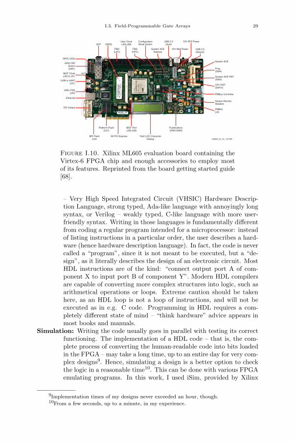
I.3. Field-Programmable Gate Arrays 29
10 www.xilinx.com Virtex-6 Getting Started GuideUG533 (v1.5) October 20, 2011
Getting Started with the Flash Demonstration
Board FeaturesThe ML605 board features are shown in Figure 1-1. The default switch and jumper settings are shown in Figure 1-2.
X-Ref Target - Figure 1-1
Figure 1-1: Virtex-6 FGPA ML605 Board Features
SFP DDR3
FMC(LPC)
FMC(HPC)
ConfigurationMode Switch
USB 2.0(Host)
12V Wall Power
12V ATX Power
USB 2.0(Device)
Pushbuttons(SW5-SW9)
16x2 LCD CharacterDisplay
MGT Port(J26-J29)
X8 PCI Express
Platform Flash(U27)
System ACE
Prog(SW4)
System ACE RST(SW3)
CPU RST(SW10)
PMBus Controller
System MonitorHeaders
PMBus(J3)
GPIO DIPSwitch(SW1)
USB to UART(J21)
MGT Clock(J30 & J31)
USB JTAG(J22)
Ethernet
DVI Output
User Clock(J55-J58)
BPI Flash(U4)
System ACEAddress
GPIO LEDs
UG533_01_01_121709
X-Ref Target - Figure 1-2
Figure 1-2: Default Jumper and Switches Settings
J69J18
J65
J42
J66J67J68
J54
J19
J35
SW1
S2 S1
UG533_01_02_121709
J66: Shunt over 1–2J67: Shunt over 1–2J68: No jumper
J54: Shunt over 1–2 (Full BW)J65: Shunt over 1–2 (SFP Enable)
S1: 4 ON (SysACE Mode = 1)3 OFF (SysACE Addr 2 = 0)2 OFF (SysACE Addr 1 = 0)1 OFF (SysACE Addr 0 = 0)
S2: 6 OFF (FLASH_A23 = 0)5 OFF (M2 = 0)4 ON (M1 = 1)3 OFF (M0 = 0)2 ON (CS_SEL = 1)1 OFF (EXT_CCLK = 0)
SW1: 8 OFF7 OFF6 OFF5 OFF4 OFF3 OFF2 OFF1 OFF
J42: Shunt over 1–2
J69: Shunt over 1–2
J19: Shunt over 1–2J35: Shunt over 9–11 and shunt over 10–12
J18: Shunt over 1–2 (Bypass FMC LPC)J17: Shunt over 1–2 (Bypass FMC HPC)Note: These are the JTAG chain bypasses for the FMC LPC and FMC HPC connectors.
Ethernet GMII
FMC Bypass
System Monitor
SFP
PCIe Lane Size Select
System ACE CF Error LED
J17
Figure I.10. Xilinx ML605 evaluation board containing theVirtex-6 FPGA chip and enough accessories to employ mostof its features. Reprinted from the board getting started guide[68].
– Very High Speed Integrated Circuit (VHSIC) Hardware Descrip-tion Language, strong typed, Ada-like language with annoyingly longsyntax, or Verilog – weakly typed, C-like language with more user-friendly syntax. Writing in those languages is fundamentally differentfrom coding a regular program intended for a microprocessor: insteadof listing instructions in a particular order, the user describes a hard-ware (hence hardware description language). In fact, the code is nevercalled a “program”, since it is not meant to be executed, but a “de-sign”, as it literally describes the design of an electronic circuit. MostHDL instructions are of the kind: “connect output port A of com-ponent X to input port B of component Y”. Modern HDL compilersare capable of converting more complex structures into logic, such asarithmetical operations or loops. Extreme caution should be takenhere, as an HDL loop is not a loop of instructions, and will not beexecuted as in e.g. C code. Programming in HDL requires a com-pletely different state of mind – “think hardware” advice appears inmost books and manuals.
Simulation: Writing the code usually goes in parallel with testing its correctfunctioning. The implementation of a HDL code – that is, the com-plete process of converting the human-readable code into bits loadedin the FPGA – may take a long time, up to an entire day for very com-plex designs9. Hence, simulating a design is a better option to checkthe logic in a reasonable time10. This can be done with various FPGAemulating programs. In this work, I used iSim, provided by Xilinx
9Implementation times of my designs never exceeded an hour, though.10From a few seconds, up to a minute, in my experience.

30 Chapter I. Introduction
Figure I.11. Example of schematic produced at the synthe-sis stage. The VHDL design has been converted into FPGAprimitives, such as input and output buffers, shown here. Thebasic design illustrated here creates two clocks (200 MHz and10 MHz) from the input system clock.
with the evaluation board. It allows to generate input and clock sig-nals, and visualise the design behaviour as a time trace of all internalsignals. This is particularly handy to verify that all arithmetic andlogic operations are executed correctly.
When the simulation results are satisfactory and the design behaves asexpected, it is passed to a series of software tools that turn the HDL code intoa bitstream that will be loaded into the FPGA. Xilinx Family 6 devices comewith ISE Design Suite, a software package containing all the compilers requiredfor implementation. The stages of the process are the following:
Synthesis: The first stage converts the HDL code into a theoretical circuit,using standard components (called primitives) available on the tar-get FPGA chip. The result can be visualised as a Resistor-TransistorLogic (RTL) diagram, illustrated in Fig. I.11, but cannot be imple-mented on a physical chip yet.
Translate: The shortest process of all, it merges the synthesised design withthe input and output ports, as well as timing and placement con-straints. In short, it gathers all design files together before the actualimplementation takes place.
Map: The core process that last the longest. It takes into account the speci-ficities of the chip and maps the theoretical design to physical logicblocks of the FPGA. Several algorithms are run to simplify and opti-mise the mapping. The total FPGA resources utilisation is displayedat the end of the process, that tells how many e.g. CLBs or memoryblocks have been used to implement the design.
Place and Route: Although called Place and Route (PAR), this process doesnot place anything, since it has already been done during the Mapprocess. It only routes the design. In other words, it takes the listof components generated by Map and connects them together, usingFPGA routing resources. This is an easy task for small designs, butbecomes quite challenging, and takes a while, for large designs. Verylarge designs may fail at this stage if there is not enough routing paths
I.3. Field-Programmable Gate Arrays 31
on the chip to connect the components in the desired manner. Afterrouting, PAR checks the timing closure.
Timing closure: Electrical signals travel at finite speed within the FPGA.Despite the propagation delays being very short, a couple nanosec-onds at most, they have to be taken into account for a synchronousdesign to function properly. And the faster the clock is, the morecritical these delays become. Simulation ignores these delays, theyare only considered during the hardware implementation stage. Max-imum delays are specified by the user, and commonly called “tim-ing constraints”. In practice, a specific file lists the clocks used todrive the chip, together with their frequencies. This information al-lows PAR to check whether the design meets the so-called “timingclosure”. If it does, and the logic has been checked thoroughly in sim-ulations, then the circuit should work as expected. If it does not, andthis happens quite often – the real struggle begins. There is no provenmethod for meeting time closure. Expert designers can resolve smalldelay issues using in-depth knowledge of hardware characteristics andimplementation software. More complex problems can only be solvedby using a slower clock or re-designing the circuit.
Generate bitstream: At last, the design is synthesised, placed, routed, andthe timing closure is met. The last stage is the generation of a bit-stream, the data that will be loaded into FPGA SRAMs and set itsconfiguration.
A Virtex chip can be configured in various ways. The bitstream can beloaded, for instance, from an on-board non-volatile memory. This consists inloading the bitstream into a specific PROM attached to the evaluation boardand set up the FPGA to load its configuration from this memory chip. It canalso be programmed by an external microprocessor. In this case, the bitstreamis loaded from a e.g. personal computer through the Joint Test Action Group(JTAG) interface – a standard first introduced for debugging of electronic cir-cuits, that is now widely used for loading the configuration file into the devicememory. The configuration of the Virtex-6 chip takes about 20 seconds. Oncecompleted, the FPGA is ready to go.
This concludes the introductory chapter of my thesis. We have coveredmost theoretical, experimental, and FPGA-related topics required for under-standing the experiments described in the following chapters. A few remainingpoints, related to particular experiments, will be discussed en route.

CHAPTER II
Online training of a photonic reservoircomputer
This chapter presents the first experiment I performed during my PhD.1
It took me almost a year and half to get going, and six more months to gainfull control of the experiment and obtain publishable results. The reason forsuch a slow start is, without any doubt, the immense complexity of FPGAprogramming. But let us not focus on the difficulties (we will get to themlater, in Sec. II.7) but rather on the achievements. And as you will find out bythe end of this chapter, this first experiment produced some very interestingresults, that inspired and shaped my following research projects. But first, letme outline what motivated this research, and what we expected to achieve inthe first place.
II.1. Introduction
The performance of a reservoir computer greatly relies on the trainingtechnique used to compute the readout weights. Offline learning methods, in-troduced in Sec. I.1.3 and used up to now in experimental implementations[33, 34, 48, 51–55, 69], provide very good results. However, they start to causeproblems in real-time applications, as they require large amounts of data to betransferred from the experiment to the post-processing computer. This opera-tion may take longer than the time it takes the reservoir to process the input se-quence [33, 34, 48]. Moreover, offline training only works on time-independenttasks, which is not always the case in real-life applications. The alternative(and more biologically plausible2) approach is to progressively adjust the read-out weights using various online learning algorithms such as gradient descent[70], recursive least squares [71] or reward-modulated Hebbian learning [72].Such procedures require minimal data storage and have the advantage of being
1The contents of this chapter is based on the journal paper reporting this very experi-ment [1]. The reader familiar with our work may recognise the same structure, figures and
tables. We wrote an extensive paper about this work and, quite frankly, there is not so muchto add here. The only new part is Sec. II.7, where I devote a few lines to the challenges
encountered during this project (mostly FPGA-related) and how they were solved. But therest of this chapter is a duplicate of our paper [1].
2Here is a simple example to illustrate the idea: an average language student needs
to encounter a new word seven times to memorise it. At each such occurrence, the brainadjusts the connections between neurons, somewhere, and by the seventh time the connectionbecomes strong enough for the student to quickly remember the not-so-new-anymore word.
The same approach can be applied to artificial neural networks, and that is what onlinelearning is all about.
33
34 Chapter II. Online training of a photonic reservoir computer
able to deal with a variable task: should any parameters of the task be alteredduring the training phase, the reservoir computer would still be able to producegood results by properly adjusting the readout weights. And as will be shownin Ch. V, online learning allows training complex (and even slightly nonlin-ear) analogue layers without the challenging task of modelling the underlyingstructure.
The basic idea of this experiment is to apply this online learning approachto an opto-electronic reservoir computer and show that such an implementationwould be well suited for real-time data processing. The use of a FPGA boardis inevitable here, as the system needs to be trained in real time, that is, inparallel with the opto-electronic experiment. Such a system could, in principle,be applied to any kind of signal processing tasks, in particular to those thatdepend on time. A good example of such a task is the wireless channel equali-sation, already investigated in previous experiments by our lab (see e.g. [33, 48,49, 73]), and introduced in Sec. I.1.4.1. In addition to its potential real-life ap-plications, it can be easily extendable from stationary to time-dependent. Thishas not been done before, so that is another minor novelty of this experiment.More on that in Sec. II.2.
Wireless communications is by far the fastest growing segment of the com-munications industry. The increasing demand for higher bandwidths requirespushing the signal amplifiers close to the saturation point which, in turn, addssignificant nonlinear distortions into the channel. These have to be compen-sated by a digital equaliser on the receiver side [74]. The main bottleneck lies inthe Analogue-to-Digital Converters (ADCs) that have to follow the high band-width of the channel with sufficient resolution to sample correctly the distortedsignal [38]. Current manufacturing techniques allow producing fast ADCs withlow resolution, or slow ones with high resolution, obtaining both being verycostly. This is where analogue equalisers become interesting, as they couldequalise the signal before the ADC and significantly reduce the required reso-lution of the converters, thus potentially cutting costs and power consumption[39–41]. Moreover, optical devices may outperform digital devices in terms ofprocessing speed [39, 42]. It can for instance be shown that reservoir computingimplementations can reach comparable performance to other digital algorithms(namely, the Volterra filter [43]) for equalisation of a nonlinear satellite com-munication channel [44].
To sum up, the primary goal of this experiment was to investigate thepossibility of online training of an opto-electronic RC with a FPGA board.Should this idea work, we then intended to evaluate the performance of thesetup on time-dependent wireless channels. As has been said above, and willbe shown in detail in Sec. II.6, not only we accomplished both parts of theproject, but we also discovered unexpected possibilities of the FPGA, that gavebirth to the experiment described in Ch. IV.
II.2. Equalisation of non-stationary channels
The standard version of the channel equalisation task has been introducedin Sec. I.1.4.1. However, in that version, the task is static, and is thus of littleinterest for the demonstration of an online-trained system. For that reason, we
II.2. Equalisation of non-stationary channels 35
had to tweak it a little bit. And since the task arises from a real-world problem,making it non-stationary requires almost no effort. One has but to think of themost common every day situations, like emitters and receivers on the move, orobstacles suddenly appearing in the way of the signal. Secs. (II.2.2 and II.2.3)will outline what add-ons we came up with to make the channel equalisationtask time-dependent. The next section II.2.1 discusses an additional study ofthe parameters of the channel model [45] that we performed in order to betterunderstand its internal mechanism.
II.2.1. Influence of channel model parameters on equaliser per-formance. Eqs. I.18 and I.19 model a particular channel with certain amountsof symbol interference and nonlinear distortion, defined by the numerical valuesof the coefficients employed. To obtain a better understanding of this particu-lar channel model, and to show which stages of input signal distortion are themost difficult to equalise, we introduce a more general channel model, given by
q(n) = (0.08 +m)d(n+ 2)− (0.12 +m)d(n+ 1)
+ d(n) + (0.18 +m)d(n− 1)
− (0.1 +m)d(n− 2) + (0.091 +m)d(n− 3)
− (0.05 +m)d(n− 4) + (0.04 +m)d(n− 5)
+ (0.03 +m)d(n− 6) + (0.01 +m)d(n− 7),
(II.1)
u(n) = p1q(n) + p2q2(n) + p3q
3(n), (II.2)
and we investigate the equalisation performance for different values of param-eters pi and m. To preserve the general shape of the channel impulse responsewe keep the coefficient of d(n) fixed at 1 in Eq. II.1. Fig. II.1 shows theresulting impulse responses, given by Eq. II.1, for several values of m. Theresults of these investigations are presented in Sec. II.6.5.
II.2.2. Slowly drifting channel. The model given by Eqs. I.18 and I.19describes an idealistic stationary noisy wireless communication channel, thatis, the channel remains the same during the transmission. However, in wirelesscommunications, the environment has a great impact on the received signal.Given its highly variable nature, the properties of the channel may be subjectto important changes in real time.
To investigate this scenario, we performed a series of experiments with a“drifting” channel model, where parameters pi or m were varying in real timeduring the signal transmission. These variations occurred at slow rates, muchslower than the time required to train the reservoir computer. We studied twovariation patterns: a monotonic increase (or decrease) and slow oscillationsbetween two fixed values. Sec. II.6.3 shows the results we obtained with ourimplementation.
II.2.3. Switching channel. In addition to slowly drifting parameters,the channel properties may be subject to abrupt variations due to suddenchanges of the environment. For better practical equalisation performance,it is crucial to be able to detect significant channel variations and adjust theRC readout weights in real time. We consider here the case of a “switching”
36 Chapter II. Online training of a photonic reservoir computer
−0.4
−0.2
0
0.2
0.4
0.6
0.8
1
d(n+ 2) d(n) d(n− 2) d(n− 4) d(n− 6)
Ch
ann
elco
effici
ents
Channel memory terms
m = 0m = 0.05m = 0.1
Figure II.1. Various channel impulse responses, given by Eq.II.1, for different values of m. Note that the d(n) coefficient iskept fixed at 1. Dotted curve shows the default shape definedby Eq. I.18.
channel, where the channel model switches instantaneously. An example of sucha scenario in real life would be, for instance, a cellular phone disconnecting fromone base station and connecting to another, with a different signal amplifier.The reservoir computer has to detect such changes and automatically trigger anew training phase, so that the readout weights get adapted for the equalisationof the new channel.
Specifically, instead of a constant channel, given by Eqs. I.18 and I.19, weintroduce three channels differing in nonlinearity
u1(n) = 1.00q(n) + 0.036q2(n)− 0.011q3(n), (II.3a)
u2(n) = 0.80q(n) + 0.036q2(n)− 0.011q3(n), (II.3b)
u3(n) = 0.60q(n) + 0.036q2(n)− 0.011q3(n), (II.3c)
and switch regularly from one channel to another, keeping Eq. I.18 unchanged.The results of this experiment are presented in Sec. II.6.4.
II.3. Online training
The online training approach can be realised through numerous differentalgorithms. Since we could not try them all, for obvious reasons, we had topick one for this experiment. Before I got into this project, Anteo Smerierihad already tested in numerical simulations three online training algorithms:simple gradient descent [70], recursive least squares (RLS) [71] and reward-modulated Hebbian learning [72]. The choice was basically dictated by theease of implementation on the FPGA. While the gradient descent algorithm
II.3. Online training 37
can be expressed with two very simple equations
wi(n+ 1) = wi(n) + λ (d(n)− y(n))xi(n),
λ(m+ 1) = λmin + γ (λ(m)− λmin) ,
where wi are the readout weights and λ is an update rate (we will explain themath in the following section, the equations are given here merely to illustratethe complexity of the algorithms), the RLS algorithm, in its compact version,looks like this
k(n) =ν−1Γ(n− 1)x(n)
1 + ν−1xTΓ(n− 1)x(n),
w(n) = w(n− 1) + k(n) (d(n)− y(n)) ,
Γ(n) = ν−1Γ(n− 1)− ν−1k(n)xT (n)Γ(n− 1),
where k(n), x(n) and w(n) are vectors and Γ(n) is the estimate of the inverseof the correlation matrix (see Sec. I.1.3), that is, a 50 × 50 matrix for a 50-neuron reservoir. One does not need to understand the precise meaning ofthese equations to get convinced that the second algorithms is more complexthan the simple gradient descent and is, hence, much more complicated toimplement in hardware. The two main complications are matrix operations,requiring significant amounts of memory, and division – one of the toughestoperations to translate into binary operations (divisions by a power of two beingan exception). And despite several non-negligible advantages in performanceand convergence speed of RLS, simple gradient descent was the lucky winner.Still, implementing RLS remains an interesting step forward, that would mostlikely require a certain development period, but the reward will be a muchfaster convergence to optimal readout weights.
II.3.1. Gradient descent algorithm. Without further ado, let us in-troduce the basic principle of the simple gradient descent. Furthermore, inthis work we also developed two new variants of the algorithm, that we testedtogether with the original version. These alternative version are going to bethe topic of Secs. II.3.1.2 and II.3.1.3.
The gradient, or steepest, descent method is an algorithm for finding a localminimum of a function using its gradient [75]. For the channel equalisation taskconsidered here, the rule for updating the readout weights is given by [70]
wi(n+ 1) = wi(n) + λ (d(n)− y(n))xi(n), (II.4)
where λ is the step size, used to control the learning rate. The origin of thisprocedure is the following: since the error at time n is given by (d(n)− y(n))2
(see Sec. I.1.3), the derivative of the error with respect to wi gives (d(n) −y(n))xi(n), i.e. the right-hand side of Eq. II.4. At high values of λ, theweights get close to the optimal values very quickly (in a few steps), but keeposcillating around these values. At low values, the weights converge slowly tothe optimal values. In practice, we start with a high value λ = λ0, and thengradually decrease it during the training phase until a minimum value λmin isreached, according to the equation
λ(m+ 1) = λmin + γ (λ(m)− λmin) , (II.5)
38 Chapter II. Online training of a photonic reservoir computer
with λ(0) = λ0 and m = bn/kc, where γ < 1 is the decay rate and k is theupdate rate for the parameter λ.
The gradient descent algorithm suffers from a relatively slow convergencetowards the global minimum, but its simplicity, with few simple computationalsteps, and flexibility, as the convergence rate and the resulting performance canbe improved by tuning the parameters λ and γ, make it a reasonable choice fora first implementation on a FPGA chip.
II.3.1.1. Full version. The step size parameter λ is used to control thelearning rate, and can also be employed to switch the training on or off. Thatis, setting λ to zero stops the training process. This is how experiments ona stationary channel are performed: λ is programmed to decay from λ0 to 0during a defined period, and then the reservoir computer performance is testedover a sequence of symbols, with constant readout weights.
II.3.1.2. Non-stationary version. When equalising a drifting channel, thereservoir should be able to follow the variations and adjust the readout weightsaccordingly. This can be achieved by setting λmin > 0 and thus letting thetraining process continue during the drift of the channel parameters. Thisprocedure was used for experiments described in Sec. II.6.3.
II.3.1.3. Simplified version. As mentioned in the previous paragraph, theequalisation of a non-stationary channel requires keeping λmin > 0. However,this worsens the equalisation performance, as the readout weights keep oscil-lating around the optimal values. This can be seen from Eq. II.4, that definesthe update rule for the readout weights: at each time step n, a small correction∆wi = λ(n)(d(n)− y(n))xi(n) is added to every weight wi. These correctionsare gradually reduced by decreasing the learning rate λ(n), so that the weightsconverge to their asymptotic values. In the case of a constant λ, the corrections∆wi are only damped by the error d(n)−y(n), which stops decreasing at somepoint, leaving the wi oscillating around the optimal values.
To check the impact of a constant λ on the equalisation performance weperformed several experiments with a simplified version of the training algo-rithm by setting γ = 0, and hence λ(n) = λ0 for all n. Although this methodwill increase the error slightly, it has several advantages. With λ constant,there is no need to search for an optimal decay rate k, which results in fewerexperimental parameters to scan and thus shorter overall experiment runtime.Keeping λ at a constant, non-zero value would also allow the equaliser to followa drifting channel, as described in Sec. II.2.2. The results obtained with thissimplified version of the algorithm are shown in Sec. II.6.2.
II.4. Experimental setup
Our experimental setup is depicted in Fig. II.2. It contains three distinctivecomponents: the opto-electronic reservoir, the FPGA board implementing theinput and the readout layers and the computer used to setup the devices andrecord the results. The reader should already be familiar with the reservoir part– it has been thoroughly discussed in Sec. I.2.4. Thus, in the following sectionswe will focus on the new components: the FPGA board (Sec. II.4.1) and thecomputer (Sec. II.4.3). Additionally, Sec. II.4.2 outlines the experimentalparameters, tuned to obtain the best results.

II.4. Experimental setup 39
Optoelectronic reservoir Input & Readout
SLED
MZ90/10
Att
Amp Comb
Pf
1.6
km
Pr
ML605FMC151
DAC
ADC
Gen
Mask
Train
PCClock
u(n)
d(n)
Mi
xi(n)
SER
Mi × u(n)
xi(n)
Figure II.2. Schematic representation of the experimentalsetup. The opto-electronic reservoir is highlighted in brownand has been introduced in Sec. I.2.4. The FPGA boardimplements both the input and output layers, generating theinput symbols and training the readout weights. The computercontrols the devices and records the results.
Figure II.3. Xilinx ML605 board with Virtex 6 FPGA chipand 4DSP FMC150 daughter card (FMC150 and FMC151cards look practically the same). Image reprinted with per-mission from www.fpgadeveloper.com
II.4.1. Input and readout. For our implementation, we use the XilinxML605 evaluation board (see Fig. II.3), powered by the Virtex 6 XC6VLX240TFPGA chip. The board is equipped with a JTAG port, used to load the FPGAdesign onto the chip, and a UART port, that we use to communicate with theboard (as described in Sec. II.5). The LPC (Low Pin Count) FMC (FPGAMezzanine Card) connector is used to attach the 4DSP FMC151 daughter card,containing one two-channel ADC (Analogue-to-Digital converter) and one two-channel DAC (Digital-to-Analogue converter). The ADC’s maximum samplingfrequency is 250 MHz with 14-bit resolution, while the DAC can sample at upto 800 MHz with 16-bit precision.
40 Chapter II. Online training of a photonic reservoir computer
Table II.1. Gradient descent algorithm parameters
λ0 λmin γ k0.4 0 0.999 10 – 50
The synchronisation of the FPGA board with the reservoir delay loop iscrucial for the performance of the experiment. For proper acquisition of reser-voir states, the ADC has to output an integer number of samples per roundtriptime. The daughter card contains a flexible clock tree, that can drive the con-verters either from the internal clock source, or an external clock signal. Asthe former is limited to the fixed frequencies of the onboard oscillator, we em-ploy the latter option. The clock signal is generated by a Hewlett Packard8648A signal generator. With a reservoir of N = 51 neurons (one neuron isadded to desynchronise the inputs from the reservoir, as has been discussed inSec. I.2.3) and a roundtrip time of 7.94 µs, the sampling frequency is set to128.4635 MHz, thus producing 20 samples per reservoir state. To get rid of thetransients, induced mainly by the finite bandwidths of the ADC and DAC, the6 first and 6 last samples are discarded, and the neuron value is averaged overthe remaining 8 samples.
The potentials of the electric signals to and from the mezzanine card need tobe adjusted in order to achieve the most efficient interface without damaging thehardware. The DAC output voltage of 2 Vp-p is sufficient for this experiment,as typical voltages of the input signal range between 100 mV and 200 mV. TheADC is also limited to 2 Vp-p input voltage. With settings described in theprevious section, the output voltage of the readout photodiode does not exceed1 Vp-p.
II.4.2. Experimental parameters. To achieve the best performance,we scan the most influential parameters, which are: the input gain β, thedecay rate k, the channel signal-to-noise ratio and the feedback attenuation,that corresponds to the feedback gain parameter α in Eqs. I.5. The first threeparameters are set on the FPGA board, while the last one is tuned on theoptical attenuator. The input gain β is stored as a 18-bit precision real in[0, 1[ and was scanned in the [0.1, 0.3] interval. The decay rate k is an integer,typically scanned from 10 up to 50 in a few wide steps. The noise ratios wereset to several pre-defined values, in order to compare our results with previousreports. The feedback attenuation was scanned finely between 4.5 dB and6 dB. Lower values would allow cavity oscillations to disturb the reservoirstates, while higher values would not provide enough feedback to the reservoir.Table II.1 contains the values of parameters we used for the gradient descentalgorithm (defined in Sec. II.3.1).
II.4.3. Experiment automation. The experiment is fully automatedand controlled by a Matlab script, running on a computer. It is designed torun the experiment multiple times over a set of predefined values of parametersof interest and select the combination that yields the best results. For statisticalpurposes, each set of parameters is tested several times with different randominput masks (see Sec. I.1.3).
II.5. FPGA design 41
At launch, connections to the optical attenuator and the FPGA board areestablished, and the parameters on the devices are set to default values. Aftergenerating a set of random input masks, the experiment is run once and theelapsed time is measured. The duration of one run depends on the lengthsof train and test sequences and varies from 6 s to 12 s. This is considerablyshorter than the offline-trained implementation [48], that required about 30 s.The script runs through all combinations of scanned parameters. For each com-bination, the values of the parameters are sent to the devices, the experimentis run several times with different input masks and the resulting error rates(see Sec. II.5) are stored in the Matlab workspace. Once all the combinationsare tested, the connections to the devices are closed and all collected data issaved to a file.
II.5. FPGA design
Rejoice, here comes my favourite section of this chapter, that describesthe FPGA design – the part of the experiment on which I spent the majorityof the time. Ironically, most readers will probably want to skip, or merelyoverlook this section, since it is, I admit, quite technical and not so crucial forunderstanding of the results in Sec. II.6. But I could not omit it, since thisis the heart of my work, the part I put most energy and time in. Therefore,I welcome any interested reader to venture in the following paragraphs, butremind once again that you will not miss any key points if you just go aheadto the next section.
The FPGA design is written in standard IEEE 1076-1993 VHDL language[76, 77] and compiled with Xilinx ISE Design Suite 14.7, provided with theboard. We also used Xilinx ChipScope Pro Analyser to monitor signals on theboard, mostly for debugging and testing.
The simplified schematics of our design is depicted in Fig. II.4. Colouredboxes represent modules (i.e. entities) and the lines stand for data connectionsbetween them. As discussed in Sec. II.4.1, the FPGA board implements boththe input and the readout layers of the reservoir computer. Modules involvedin each of these two functions are highlighted in blue and red, respectively. Theboard has a digital connection to a computer (running a Matlab script) andan analogue one to the experimental setup. The former, realised through aUART port bridged to a standard COM port, is used to load parameters (e.g.λ0, γ, . . .) into the board and read the experiment results (i.e. symbol errorrate) from the board. The latter consists of three analogue connections: anoutput signal to the reservoir, containing the masked inputs Mi×u(n), a clocksignal clk from the HP signal generator and an input signal from the readoutphotodiode, containing reservoir states xi(n).
The operation of the FPGA board is controlled from the computer. Apredefined set of 4-byte commands can be transmitted through the JTAG port,such as write a specific parameter value into the appropriate register or togglethe board state from reset to running, and vice versa. The commands arereceived and executed by the UART module. In addition, when the FPGA isrunning, the module regularly transmits the value of the SER signal to thecomputer. In order to prevent collisions in the UART channel, commands
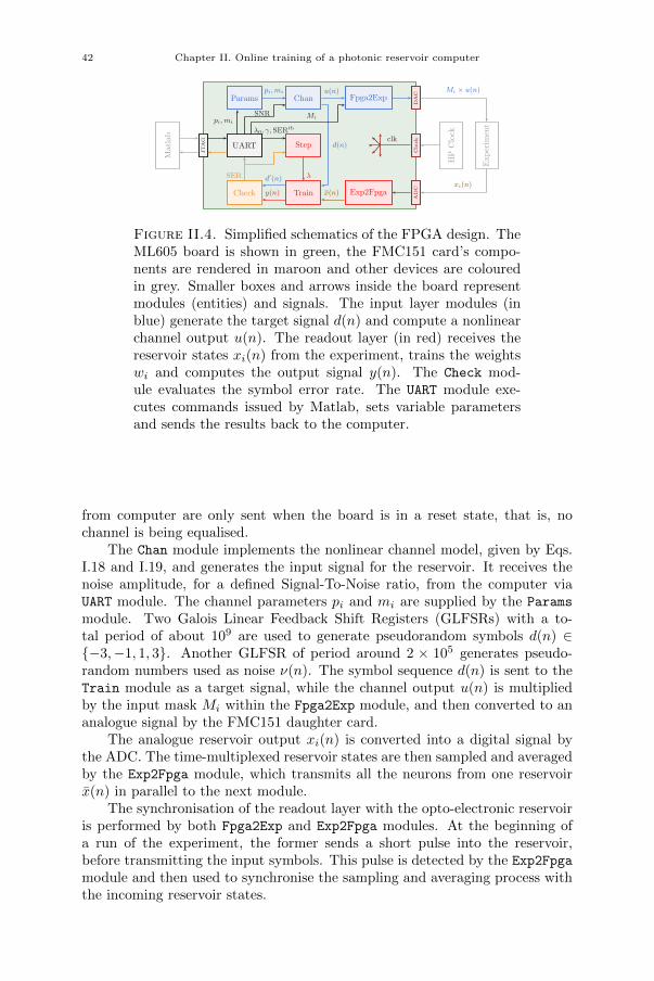
42 Chapter II. Online training of a photonic reservoir computer
Matlab
JTAG
Params
UART
Check
Chan
Step
Train
Fpga2Exp
Exp2Fpga
DAC
Clock
ADC
HP
Clock
Experim
ent
d′(n)
y(n)
λ0, γ, SERth
x(n)
u(n)
clk
pi,mi
SER λ
pi,mi
d(n)
Mi × u(n)
xi(n)
MiSNR
Figure II.4. Simplified schematics of the FPGA design. TheML605 board is shown in green, the FMC151 card’s compo-nents are rendered in maroon and other devices are colouredin grey. Smaller boxes and arrows inside the board representmodules (entities) and signals. The input layer modules (inblue) generate the target signal d(n) and compute a nonlinearchannel output u(n). The readout layer (in red) receives thereservoir states xi(n) from the experiment, trains the weightswi and computes the output signal y(n). The Check mod-ule evaluates the symbol error rate. The UART module exe-cutes commands issued by Matlab, sets variable parametersand sends the results back to the computer.
from computer are only sent when the board is in a reset state, that is, nochannel is being equalised.
The Chan module implements the nonlinear channel model, given by Eqs.I.18 and I.19, and generates the input signal for the reservoir. It receives thenoise amplitude, for a defined Signal-To-Noise ratio, from the computer viaUART module. The channel parameters pi and mi are supplied by the Params
module. Two Galois Linear Feedback Shift Registers (GLFSRs) with a to-tal period of about 109 are used to generate pseudorandom symbols d(n) ∈−3,−1, 1, 3. Another GLFSR of period around 2 × 10⁵ generates pseudo-random numbers used as noise ν(n). The symbol sequence d(n) is sent to theTrain module as a target signal, while the channel output u(n) is multipliedby the input mask Mi within the Fpga2Exp module, and then converted to ananalogue signal by the FMC151 daughter card.
The analogue reservoir output xi(n) is converted into a digital signal bythe ADC. The time-multiplexed reservoir states are then sampled and averagedby the Exp2Fpga module, which transmits all the neurons from one reservoirx(n) in parallel to the next module.
The synchronisation of the readout layer with the opto-electronic reservoiris performed by both Fpga2Exp and Exp2Fpga modules. At the beginning ofa run of the experiment, the former sends a short pulse into the reservoir,before transmitting the input symbols. This pulse is detected by the Exp2Fpga
module and then used to synchronise the sampling and averaging process withthe incoming reservoir states.
II.5. FPGA design 43
The Train module implements the simple gradient descent algorithm. Itreceives the neurons x(n), the target signal d(n) and the gradient step λ, com-putes the reservoir output y(n) with its error from the target signal, and adjuststhe readout weights wi following Eq. II.4. The input target signal d(n) is de-layed by several periods T to compensate the propagation time of the informa-tion through the input layer, the opto-electronic reservoir and the Exp2Fpga
module. The reservoir output y(n) is then rounded up to the closest chan-nel symbol y(n) −3,−1, 1, 3 and compared to the delayed target signald′(n) by the Check module, that counts misclassified symbols and outputs theresulting Symbol Error Rate.
The evolution of the learning rate λ is governed by a separate module Step,which implements the Eq. II.5, with initial value λ0 and decay rate γ set onthe computer and transferred to the board through the UART connection. Themodule also monitors the performance of the reservoir computer and resets λ toits initial value λ0 when the Symbol Error Rate exceeds a predefined thresholdvalue SERth. This feature is used for the switching channel (see Secs. II.2.3and II.6.4 ) and allows to improve the performance of the system by adjustingthe readout weights to the new channel parameters.
The gradient descent algorithm is relatively simple, with only few additionand multiplication operations involved in Eqs. II.4 and II.5. While an addercan easily be built with a small amount of logic gates, multiplication is morecomplicated to implement and requires lots of resources. Moreover, as all read-out weights are computed in parallel, the size of the design grows quickly withthe number of neurons N . This results in slow implementation process andvery low chances of generating a design that functions correctly. The solutionresides in the use of special DSP48E slices, designed and optimised to performa predefined set of arithmetic operations [67]. With proper settings, this dedi-cated microprocessor is capable of performing a 25 bit × 18 bit multiplicationin less than 6 ns. While the speed gain compared to standard logic blocksis minimal, the implementation of the FPGA design is greatly simplified, ashundreds of logic gates and registers get replaced by just one component.
The arithmetic operations mentioned above are performed on real num-bers. However, a FPGA is a logic device, designed to operate with bits. Theperformance of the design thus highly depends on the bit-representation of realnumbers, i.e. the precision. The main limitation comes from the DSP48Eslices, as these are designed to multiply a 25-bit integer by another 18-bit inte-ger. To meet these requirements, our design uses a fixed-point representationwith different bit array lengths for different variables. Parameters and signalsthat stay within the ]−1, 1[ interval are represented by 18-bit vectors, with 1bit for the sign and 17 for the decimal part. These are the learning algorithmparameters λ, λ0 and γ, the input mask elements Mi and the reservoir statesxi(n), extended from the 14-bit ADC output. Other variables, such as reser-voir output y(n) and readout weights wi span a wider [−16, 16] interval andare represented as 25-bit vectors, with 1 sign bit, 4 bits for the integer part and20 bits for the decimal part.
Table II.2 reports total FPGA resource usage of our implementation. Thedesign requires relatively few registers and Lookup Tables (LUTs). Most of the
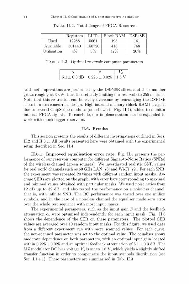
44 Chapter II. Online training of a photonic reservoir computer
Table II.2. Total Usage of FPGA Resources
Registers LUTs Block RAM DSP48EUsed 12288 5661 198 161
Available 301440 150720 416 768Utilisation 4% 3% 47% 20%
Table II.3. Optimal reservoir computer parameters
α β Vφ5.1± 0.3 dB 0.225± 0.025 1.6 V
arithmetic operations are performed by the DSP48E slices, and their numbergrows roughly as 3×N , thus theoretically limiting our reservoir to 255 neurons.Note that this restriction can be easily overcome by rearranging the DSP48Eslices in a less concurrent design. High internal memory (block RAM) usage isdue to several ChipScope modules (not shown in Fig. II.4), added to monitorinternal FPGA signals. To conclude, our implementation can be expanded towork with much bigger reservoirs.
II.6. Results
This section presents the results of different investigations outlined in Secs.II.2 and II.3.1. All results presented here were obtained with the experimentalsetup described in Sec. II.4.
II.6.1. Improved equalisation error rate. Fig. II.5 presents the per-formance of our reservoir computer for different Signal-to-Noise Ratios (SNRs)of the wireless channel (green squares). We investigated realistic SNR valuesfor real world channels such as 60 GHz LAN [78] and Wi-Fi [79]. For each SNR,the experiment was repeated 20 times with different random input masks. Av-erage SERs are plotted on the graph, with error bars corresponding to maximaland minimal values obtained with particular masks. We used noise ratios from12 dB up to 32 dB, and also tested the performance on a noiseless channel,that is, with infinite SNR. The RC performance was tested over one millionsymbols, and in the case of a noiseless channel the equaliser made zero errorover the whole test sequence with most input masks.
The experimental parameters, such as the input gain β and the feedbackattenuation α, were optimised independently for each input mask. Fig. II.6shows the dependence of the SER on these parameters. The plotted SERvalues are averaged over 10 random input masks. For this figure, we used datafrom a different experiment run with more scanned values. For each curve,the non-scanned parameter was set to the optimal value. The equaliser showsmoderate dependence on both parameters, with an optimal input gain locatedwithin 0.225± 0.025 and an optimal feedback attenuation of 5.1± 0.3 dB. TheMZ modulator DC bias voltage Vφ is set to 1.6 V, which yields a slightly shiftedtransfer function in order to compensate the input symbols distribution (seeSec. I.1.4.1). These parameters are summarised in Tab. II.3
II.6. Results 45
We compare our results to those reported in [48], obtained with the sameopto-electronic reservoir, trained offline (blue dots). For high noise levels(SNR ≤ 20 dB) our results are similar to those in [48]. For low noise lev-els (SNR ≥ 24 dB) the performance of our implementation is significantlybetter. Note that the previously reported results are only rough estimations ofthe equaliser’s performance as the input sequence was limited by hardware to6000 symbols [48]. In our experiment the SER is estimated more precisely overone million input symbols. For the lowest noise level (SER = 32 dB) an SER of1.3× 10−4 was reported in [48], while we obtained an error rate of 5.71× 10⁻⁶
with our setup. One should remember that common error detection schemes,used in real-life applications, require the SER to be lower than 10−3 in orderto be efficient. Digital equalisation algorithms, based on bilinear decision feed-back equalisers [45] and ESNs with random reservoirs [29], report error ratesof 10−3 and 10−5, respectively. These values are only provided for illustration,as it makes little sense to compare numerical algorithms and physical systems.
To the best of our knowledge, the results presented here (at 32 dB SNR) arethe lowest error rates ever obtained with a standalone experimental reservoircomputer. SERs around 10−4 have been reported in [33, 34, 48] and a passivecavity based setup [49] achieved a 1.66 × 10⁻⁵ rate (this values is limited bythe use of a 60000-symbol test sequence), but no results below 10−5 have beenpublished so far. However, this is not the main achievement of this experiment.Indeed, had it been possible to test [48] on a longer sequence, it is possible thatcomparable SERs would have been obtained. The strength of this setup residesin the adaptability to changing environment, as will be shown in the followingsections.
II.6.2. Simplified training algorithm. The performance of the simpli-fied training algorithm is shown in Fig. II.5 (brown dots). The equaliser wastested with 10 random input masks and one million input symbols, the train-ing was performed over 100000 symbols. Only three parameters were scannedduring these experiments: the input gain β, the feedback attenuation α andthe signal-to-noise ratio. The learning rate λ was set to 0.01. The overallexperimental runtime was significantly shorter: while an experiment with fulltraining algorithm would last for about 50 hours, these results were obtain inapproximately 10 hours (which is due to five different values of k tested in theformer case).
For high noise levels the results of the two algorithms are close and forlow noise levels the simplified version yields slightly worse error rates. Theperformance is much worse in the noiseless case and strongly depends on theinput mask: we notice a difference of almost two orders of magnitude betweenthe best and the worst result. This performance loss is the price to pay for thesimplified algorithm and shorter experimental runtime.
II.6.3. Equalisation of a slowly drifting channel. Besides the envi-ronmental conditions, the relative positions of the emitter and the receiver canhave a significant impact on the properties of a wireless channel. A simple ex-ample is a receiver moving away from the transmitter, causing the channel todrift more or less slowly, depending on the relative speed of the receiver. Here
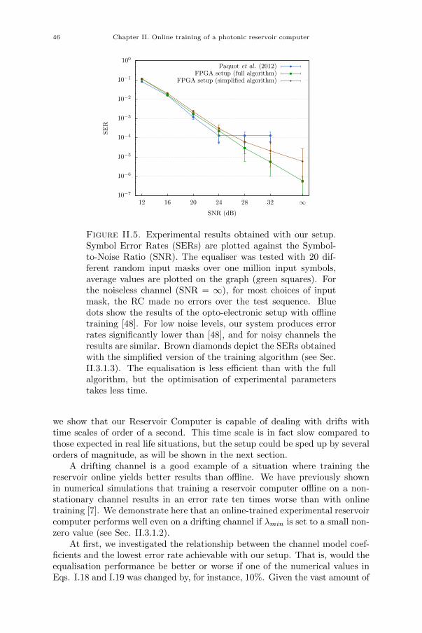
46 Chapter II. Online training of a photonic reservoir computer
10−7
10−6
10−5
10−4
10−3
10−2
10−1
100
12 16 20 24 28 32 ∞
SE
R
SNR (dB)
Paquot et al. (2012)FPGA setup (full algorithm)
FPGA setup (simplified algorithm)
Figure II.5. Experimental results obtained with our setup.Symbol Error Rates (SERs) are plotted against the Symbol-to-Noise Ratio (SNR). The equaliser was tested with 20 dif-ferent random input masks over one million input symbols,average values are plotted on the graph (green squares). Forthe noiseless channel (SNR = ∞), for most choices of inputmask, the RC made no errors over the test sequence. Bluedots show the results of the opto-electronic setup with offlinetraining [48]. For low noise levels, our system produces errorrates significantly lower than [48], and for noisy channels theresults are similar. Brown diamonds depict the SERs obtainedwith the simplified version of the training algorithm (see Sec.II.3.1.3). The equalisation is less efficient than with the fullalgorithm, but the optimisation of experimental parameterstakes less time.
we show that our Reservoir Computer is capable of dealing with drifts withtime scales of order of a second. This time scale is in fact slow compared tothose expected in real life situations, but the setup could be sped up by severalorders of magnitude, as will be shown in the next section.
A drifting channel is a good example of a situation where training thereservoir online yields better results than offline. We have previously shownin numerical simulations that training a reservoir computer offline on a non-stationary channel results in an error rate ten times worse than with onlinetraining [7]. We demonstrate here that an online-trained experimental reservoircomputer performs well even on a drifting channel if λmin is set to a small non-zero value (see Sec. II.3.1.2).
At first, we investigated the relationship between the channel model coef-ficients and the lowest error rate achievable with our setup. That is, would theequalisation performance be better or worse if one of the numerical values inEqs. I.18 and I.19 was changed by, for instance, 10%. Given the vast amount of
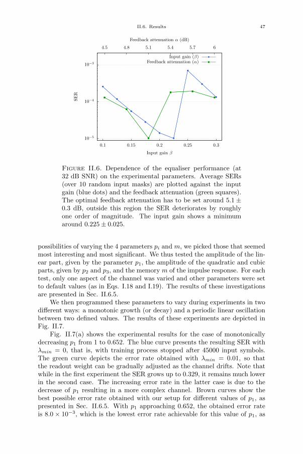
II.6. Results 47
10−5
10−4
10−3
0.1 0.15 0.2 0.25 0.3
4.5 4.8 5.1 5.4 5.7 6
SE
R
Input gain β
Feedback attenuation α (dB)
Input gain (β)Feedback attenuation (α)
Figure II.6. Dependence of the equaliser performance (at32 dB SNR) on the experimental parameters. Average SERs(over 10 random input masks) are plotted against the inputgain (blue dots) and the feedback attenuation (green squares).The optimal feedback attenuation has to be set around 5.1 ±0.3 dB, outside this region the SER deteriorates by roughlyone order of magnitude. The input gain shows a minimumaround 0.225± 0.025.
possibilities of varying the 4 parameters pi and m, we picked those that seemedmost interesting and most significant. We thus tested the amplitude of the lin-ear part, given by the parameter p1, the amplitude of the quadratic and cubicparts, given by p2 and p3, and the memory m of the impulse response. For eachtest, only one aspect of the channel was varied and other parameters were setto default values (as in Eqs. I.18 and I.19). The results of these investigationsare presented in Sec. II.6.5.
We then programmed these parameters to vary during experiments in twodifferent ways: a monotonic growth (or decay) and a periodic linear oscillationbetween two defined values. The results of these experiments are depicted inFig. II.7.
Fig. II.7(a) shows the experimental results for the case of monotonicallydecreasing p1 from 1 to 0.652. The blue curve presents the resulting SER withλmin = 0, that is, with training process stopped after 45000 input symbols.The green curve depicts the error rate obtained with λmin = 0.01, so thatthe readout weight can be gradually adjusted as the channel drifts. Note thatwhile in the first experiment the SER grows up to 0.329, it remains much lowerin the second case. The increasing error rate in the latter case is due to thedecrease of p1 resulting in a more complex channel. Brown curves show thebest possible error rate obtained with our setup for different values of p1, aspresented in Sec. II.6.5. With p1 approaching 0.652, the obtained error rateis 8.0 × 10⁻³, which is the lowest error rate achievable for this value of p1, as
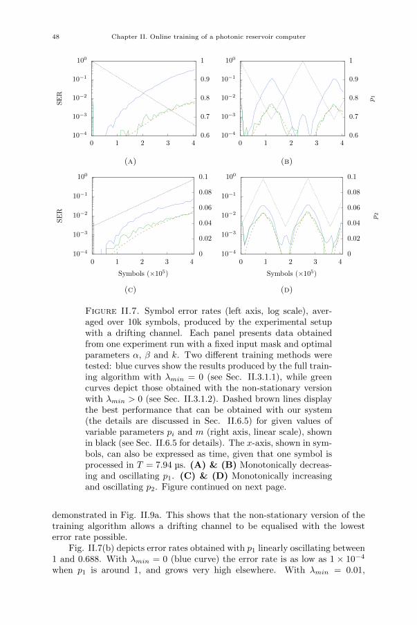
48 Chapter II. Online training of a photonic reservoir computer
10−4
10−3
10−2
10−1
100
0 1 2 3 40.6
0.7
0.8
0.9
1S
ER
(a)
10−4
10−3
10−2
10−1
100
0 1 2 3 40.6
0.7
0.8
0.9
1
p1
(b)
10−4
10−3
10−2
10−1
100
0 1 2 3 40
0.02
0.04
0.06
0.08
0.1
SE
R
Symbols (×105)
(c)
10−4
10−3
10−2
10−1
100
0 1 2 3 40
0.02
0.04
0.06
0.08
0.1
p2
Symbols (×105)
(d)
Figure II.7. Symbol error rates (left axis, log scale), aver-aged over 10k symbols, produced by the experimental setupwith a drifting channel. Each panel presents data obtainedfrom one experiment run with a fixed input mask and optimalparameters α, β and k. Two different training methods weretested: blue curves show the results produced by the full train-ing algorithm with λmin = 0 (see Sec. II.3.1.1), while greencurves depict those obtained with the non-stationary versionwith λmin > 0 (see Sec. II.3.1.2). Dashed brown lines displaythe best performance that can be obtained with our system(the details are discussed in Sec. II.6.5) for given values ofvariable parameters pi and m (right axis, linear scale), shownin black (see Sec. II.6.5 for details). The x-axis, shown in sym-bols, can also be expressed as time, given that one symbol isprocessed in T = 7.94 µs. (A) & (B) Monotonically decreas-ing and oscillating p1. (C) & (D) Monotonically increasingand oscillating p2. Figure continued on next page.
demonstrated in Fig. II.9a. This shows that the non-stationary version of thetraining algorithm allows a drifting channel to be equalised with the lowesterror rate possible.
Fig. II.7(b) depicts error rates obtained with p1 linearly oscillating between1 and 0.688. With λmin = 0 (blue curve) the error rate is as low as 1 × 10⁻⁴
when p1 is around 1, and grows very high elsewhere. With λmin = 0.01,
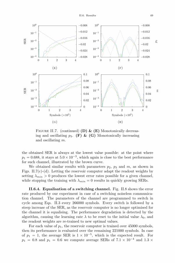
II.6. Results 49
10−4
10−3
10−2
10−1
100
0 1 2 3 4−0.028
−0.024
−0.02
−0.016
−0.012
−0.008S
ER
(e)
10−4
10−3
10−2
10−1
100
0 1 2 3 4−0.028
−0.024
−0.02
−0.016
−0.012
−0.008
p3
(f)
10−4
10−3
10−2
10−1
100
0 1 2 3 40
0.02
0.04
0.06
0.08
0.1
SE
R
Symbols (×105)
(g)
10−4
10−3
10−2
10−1
100
0 1 2 3 40
0.02
0.04
0.06
0.08
0.1
m
Symbols (×105)
(h)
Figure II.7. (continued) (D) & (E) Monotonically decreas-ing and oscillating p3. (F) & (G) Monotonically increasingand oscillating m.
the obtained SER is always at the lowest value possible: at the point wherep1 = 0.688, it stays at 5.0× 10⁻³, which again is close to the best performancefor such channel, illustrated by the brown curve.
We obtained similar results with parameters p2, p3 and m, as shown inFigs. II.7(c)-(d). Letting the reservoir computer adapt the readout weights bysetting λmin > 0 produces the lowest error rates possible for a given channel,while stopping the training with λmin = 0 results in quickly growing SERs.
II.6.4. Equalisation of a switching channel. Fig. II.8 shows the errorrate produced by our experiment in case of a switching noiseless communica-tion channel. The parameters of the channel are programmed to switch incycle among Eqs. II.3 every 266000 symbols. Every switch is followed by asteep increase of the SER, as the reservoir computer is no longer optimised forthe channel it is equalising. The performance degradation is detected by thealgorithm, causing the learning rate λ to be reset to the initial value λ0, andthe readout weights are re-trained to new optimal values.
For each value of p1, the reservoir computer is trained over 45000 symbols,then its performance is evaluated over the remaining 221000 symbols. In caseof p1 = 1, the average SER is 1 × 10⁻⁵, which is the expected result. Forp1 = 0.8 and p1 = 0.6 we compute average SERs of 7.1 × 10⁻⁴ and 1.3 ×
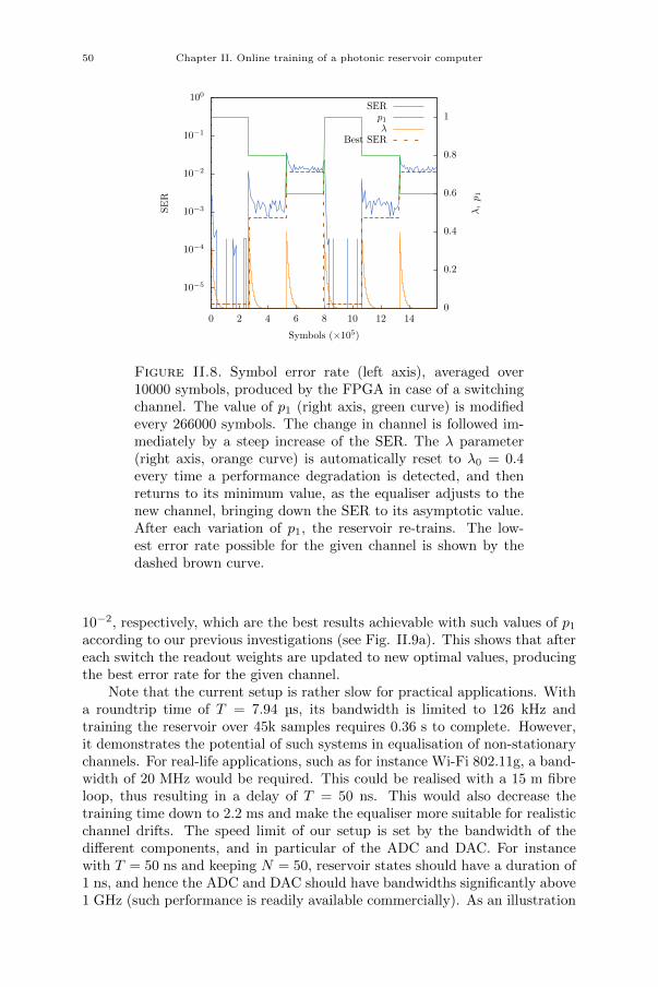
50 Chapter II. Online training of a photonic reservoir computer
10−5
10−4
10−3
10−2
10−1
100
0 2 4 6 8 10 12 140
0.2
0.4
0.6
0.8
1
SE
R
λ,p
1
Symbols (×105)
SERp1
λBest SER
Figure II.8. Symbol error rate (left axis), averaged over10000 symbols, produced by the FPGA in case of a switchingchannel. The value of p1 (right axis, green curve) is modifiedevery 266000 symbols. The change in channel is followed im-mediately by a steep increase of the SER. The λ parameter(right axis, orange curve) is automatically reset to λ0 = 0.4every time a performance degradation is detected, and thenreturns to its minimum value, as the equaliser adjusts to thenew channel, bringing down the SER to its asymptotic value.After each variation of p1, the reservoir re-trains. The low-est error rate possible for the given channel is shown by thedashed brown curve.
10−2, respectively, which are the best results achievable with such values of p1
according to our previous investigations (see Fig. II.9a). This shows that aftereach switch the readout weights are updated to new optimal values, producingthe best error rate for the given channel.
Note that the current setup is rather slow for practical applications. Witha roundtrip time of T = 7.94 µs, its bandwidth is limited to 126 kHz andtraining the reservoir over 45k samples requires 0.36 s to complete. However,it demonstrates the potential of such systems in equalisation of non-stationarychannels. For real-life applications, such as for instance Wi-Fi 802.11g, a band-width of 20 MHz would be required. This could be realised with a 15 m fibreloop, thus resulting in a delay of T = 50 ns. This would also decrease thetraining time down to 2.2 ms and make the equaliser more suitable for realisticchannel drifts. The speed limit of our setup is set by the bandwidth of thedifferent components, and in particular of the ADC and DAC. For instancewith T = 50 ns and keeping N = 50, reservoir states should have a duration of1 ns, and hence the ADC and DAC should have bandwidths significantly above1 GHz (such performance is readily available commercially). As an illustration
II.7. Challenges and solutions 51
of how a fast system would operate, we refer to the optical experiment [54] inwhich information was injected into a reservoir at rates beyond 1 GHz.
II.6.5. Influence of channel model parameters on equaliser per-formance. This section presents the results obtained after in-depth investiga-tion of the channel model (Eqs. I.18 and I.19) and its parameters, as discussedin Sec. II.2.1.
Figure II.9a shows the equalisation results for different values of p1. Wetested each value over 10 random input masks, with independent experimentalparameters optimisation for each run. Average values are presented on theplot, with error bars depicting best and worst results obtained among differentmasks. The equaliser performance was tested on a sequence of one millioninputs, and in several cases we obtained zero misclassified symbols. Note thatthe observed increase of the SER with reduction of p1 is natural as the linearpart contains the signal to be extracted. When decreasing p1, not only theuseful signal gets weaker, but the nonlinear distortion also becomes relativelymore important.
Figures II.9b and II.9c present the dependence of the SER on parametersp2 and p3, respectively. These parameters define the amplitude of the nonlineardistortion of the signal, and as they grow, the channel becomes more nonlinearand thus more difficult to equalise. The results of equalisation with differentvalues of m are shown in figure II.9d, higher values of m increase the temporalsymbol mixing of the channel, hence worse results.
II.7. Challenges and solutions
The previous Sec. II.6 listed all the successful results we obtained with thisproject. The present section is devoted to the other side of the coin, that is, thechallenges and problems we encountered in this work. Such a presentation is oflittle interest for a scientific paper, where only final results matter, but couldinterest a reader trying to replicate this experiment, partially or in full, whoseeks to find out how we actually managed to make the setup work. And sincethe real new part of this experiment if the FPGA board (the opto-electronicreservoir was already a well-known and functioning system when I started thisproject), the FPGA design was the main source of troubles. Here they are, andhow I managed to solve them.
The first thing that comes to mind is the very steep learning curve of FPGAprogramming and a completely wrong approach adopted by myself, mostly be-cause of lack of knowledge. Unlike most other programming languages, learningas you go is a very bad idea. There is so much to learn and understand aboutFPGA internals and mechanisms before even thinking of going somewhere.Well, certainly, very basic, academic designs could be completed while learn-ing, but not a complex one, such as the one described in Sec. II.5, involvingnon-trivial logic, several clock domains, multi-cycle paths and complex timingconstraints. This is, probably, the reason for such a slow start of my thesis.
Completing a FPGA design is a very long task. The implementation time,that is, the compilation process, from the VHDL code all the way down tothe FPGA bitstream, of a very basic design takes a couple of minutes on my
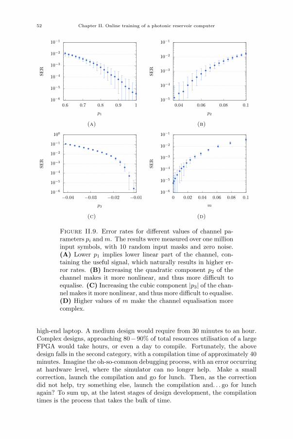
52 Chapter II. Online training of a photonic reservoir computer
10−6
10−5
10−4
10−3
10−2
10−1
0.6 0.7 0.8 0.9 1
SE
R
p1
(a)
10−5
10−4
10−3
10−2
10−1
0.04 0.06 0.08 0.1
SE
R
p2
(b)
10−6
10−5
10−4
10−3
10−2
10−1
100
−0.04 −0.03 −0.02 −0.01
SE
R
p3
(c)
10−6
10−5
10−4
10−3
10−2
10−1
0 0.02 0.04 0.06 0.08 0.1
SE
R
m
(d)
Figure II.9. Error rates for different values of channel pa-rameters pi and m. The results were measured over one millioninput symbols, with 10 random input masks and zero noise.(A) Lower p1 implies lower linear part of the channel, con-taining the useful signal, which naturally results in higher er-ror rates. (B) Increasing the quadratic component p2 of thechannel makes it more nonlinear, and thus more difficult toequalise. (C) Increasing the cubic component |p3| of the chan-nel makes it more nonlinear, and thus more difficult to equalise.(D) Higher values of m make the channel equalisation morecomplex.
high-end laptop. A medium design would require from 30 minutes to an hour.Complex designs, approaching 80− 90% of total resources utilisation of a largeFPGA would take hours, or even a day to compile. Fortunately, the abovedesign falls in the second category, with a compilation time of approximately 40minutes. Imagine the oh-so-common debugging process, with an error occurringat hardware level, where the simulator can no longer help. Make a smallcorrection, launch the compilation and go for lunch. Then, as the correctiondid not help, try something else, launch the compilation and. . . go for lunchagain? To sum up, at the latest stages of design development, the compilationtimes is the process that takes the bulk of time.
II.8. Conclusion 53
Programming usually comes with errors – humans have this sad tendency.The most harmful and deceptive problem I have encountered during the de-velopment of this project, that caused a few broken objects and lots of facialhair torn, is the well-known overflow. All numbers in the design are allocated astrict number of bits (usually 18 or 25, see Sec. II.5) and if the scale is chosenpoorly, a summation or multiplication of these numbers may result in a numbertoo big for such an amount of bits. Which results in the exceeding part beingcut off, and the calculation is performed normally. But the result is, obviously,incorrect. And such errors are not easy to detect. Moreover, such an overflowmay occur outside the trial case, that is, when the design has to deal with num-bers it has not been tested on. In other words, the designer thinks that thecode works, but, in fact, it does not. Such unexpected overflow was the reasonof relatively poor equalisation performance of the experiment, published in apreliminary conference paper [7]. The reservoir was actually equalising a morecomplex channel, and some of the symbols in the training and test sequenceswere simply wrong. Once this problem was discovered and corrected, we couldobtain the results shown in Fig. II.5.
Lastly, let me say a few words about the DSP48 slices. At first, I hatedthem – Xilinx software infers them automatically by default and activates alltheir internal registers, that cause a mess in the timing of the design. I wasvery pleased when I found the option to disable them. All multiplicationswere performed using slice logic at that stage and the compilation was takinga few hours for a 50-neuron design. This strategy did not seem viable, so Iinvested some time into understanding the DSP48 slices. Now, I love them.They are very complex, but they have so much to offer! And instead of usinghundreds of logic gates and registers, only one DSP slice is required to perform amultiplication. Much to my joy, the implementation time was greatly reduced.
II.8. Conclusion
In this chapter we covered the first experiment realised for my PhD. In thiswork we applied the online learning approach to training an opto-electronicreservoir computer. We programmed the simple gradient descent algorithmon a FPGA chip and tested our system on the nonlinear channel equalisationtask. We obtained error rates up to two orders of magnitude lower than pre-viously reported RC implementations on the channel equalisation task, whilesignificantly reducing the experimental runtime. We also demonstrated thatour system is well-suited for non-stationary tasks by equalising a drifting anda switching channel. In both cases, we obtained the lowest error rates possiblewith our setup.
So far, so good; what’s next? From our team’s point of view, this exper-iment was a first step – we employed a FPGA board for the first time andwanted to see what it was capable of and whether it was worth investigatingthis direction further. And this work has shown that, in fact, it definitely is.Using the FPGA to drive the opto-electronic reservoir allows to perform moreintricate operations on the experiment, such as compute the output in real timeor, as will be shown in Ch. IV, feed the output back as input. This, in turn,allows to investigate several novel features. These findings greatly influenced

54 Chapter II. Online training of a photonic reservoir computer
the further plans for my thesis, as I was focused on implementing these novelfeatures.
In our journal paper [1], we proposed two ideas for future work. At themoment of writing these lines, we have realised them both. First, a FPGA-driven photonic reservoir computer could implement a full optimisation of thereadout weights and the input mask, as suggested in [80, 81]. With MichielHermans, we performed that experiment right afterwards. We will talk about itin Ch. III. Second, the real-time training makes it possible to feed the outputsignal back into the reservoir. This additional feedback would highly enrichthe dynamics of the system, allowing one to tackle new tasks such as patterngeneration or chaotic series prediction [9]. And we have demonstrated thatexperimentally in early 2016. Ch. IV is devoted to this work.
To conclude, I believe that this experiment is the key achievement of myPhD, that made all subsequent results much easier. Therefore, it was two yearswell spent.
CHAPTER III
Backpropagation with photonics
This chapter presents an experiment that was not originally planned as partof my thesis. The project was set up when Michiel Hermans joined our teamin 2015 with an idea of implementing the backpropagation training algorithm(more on that in Sec. III.2) in hardware, using our opto-electronic reservoircomputer (see Sec. I.2.4) with one slight modification. After a couple of brain-stormings, we decided that the idea would be easier to realise with a FPGAin the setup. I was thus set to assist Michiel Hermans with this experiment,that we successfully completed in March 2016. Michiel Hermans designed thesetup and performed most of the measurements, while I built the experimentand programmed the FPGA.
The content of this chapter is based on our paper [2]. The paper itself,being a Letter, is quite succinct, but the Supplementary Material covers mostof the theoretical and experimental aspects of this work. The only part notcovered in the paper – the FPGA design – is presented in this thesis in Sec.III.4.
III.1. Introduction
One of the main difficulties when using nonlinear dynamical systems, suchas neural networks, is to train their internal parameters. The backpropagation(BP) algorithm [82, 83] is one of the most important algorithms in this area,and is behind the remarkable successes achieved in the field of deep learning inthe last decade [84]. The simple idea behind the BP algorithm is to compute thederivative (or gradient) of a cost function in the parameter space of the system.The gradient is then subtracted from the parameters themselves in order toreduce the cost function. This process is repeated until the cost function nolonger reduces. We will cover BP much more in detail in Sec. III.2.
In hardware implementations of neural networks the training of internalparameters is also key and the use of the BP algorithm is highly beneficial inorder to improve performance [80, 81]. However implementing the BP algo-rithm in hardware systems can be difficult because of the need of an accuratemodel to compute the gradient and because of the resources necessary to runthe BP algorithm. Remarkably, in certain cases it can be implemented phys-ically on the system it is optimising [85]. The basic idea behind this advanceis to use a slightly modified version of the system for propagating error signalsbackwards, i.e. for running the BP algorithm. Such self-learning computingsystems could be highly advantageous, as any gain in terms of processing speed
55
56 Chapter III. Backpropagation with photonics
or limited power consumption will also apply to the training phase. Further-more having the same hardware computing the BP algorithm eliminates, toa large extent, the need for an accurate model of the system. This idea mayconceivably also have implications for biological neural networks, as these arephysical system that – using mechanisms that are not yet well understood –can both compute and carry out their own training process. A proof of conceptexperiment in which physical BP was tested on a simple task was reported in[85]. However, it left open the question of whether the algorithm, with all theimperfections inherent in an experiment, can provide the same improvement inperformance as numerical approaches [80, 81].
In this experiment we implemented the BP algorithm physically on theslightly modified opto-electronic reservoir computer, introduced in Sec. I.2.4.The key innovation is to modify the system by adding a photonic componentcapable of implementing both the nonlinearity and its derivative, so that it canbe used both as signal processor and to perform the BP algorithm. We testedour system on several tasks considered hard in the machine learning community,including a real world phoneme recognition task, obtaining state of the artresults when the BP algorithm is used. This experiment thus demonstratesthe full potential of physical BP. It constitutes an important step towards self-learning hardware, with potential applications towards ultra-fast, low energyconsumption, computing systems.
III.2. Backpropagation through time
Backpropagation through time, or simply backpropagation, is a time-hon-oured method for training recurrent neural networks [82, 83]. Essentially, onedefines a cost function based on the desired network output and, using thechain rule, determines the gradient of this cost function with respect to the in-ternal parameters of the system (weights). The term “backpropagation” stemsfrom the fact that, due to the recursion in RNNs, computing the gradient in-volves propagating an error signal backward through the system updates, i.e.,backward in time [80].
In simple words, the algorithm works as follows. The RNN is fed with aninput I, that propagates through the network, from input to output neurons,in a certain number of timesteps (updates). Using a set of readout weights, theoutput O is computed. It is then compared with the target output T and anerror E is computed. At this point, the network is inverted, figuratively. Theerror signal E is propagated backwards through the linearised network, fromoutput to input neurons, in the same manner as the initial input signal I waspropagated in the forward direction. That is, output neurons act as inputs andinput neurons are considered as system outputs. This allows to compute theerror on each neuron, i.e. how its value should be changed (to first order inthe error) in order to get closer to the desired value T . Obviously, the neuronsstates cannot be “corrected”, but the weights can be. These errors are thusused to compute corrections for the input, internal and readout weights, sothat that the system output O for a given input I gets closer to the target T .The (usually small) corrections are applied iteratively until the error betweenO ant T can no longer be decreased.
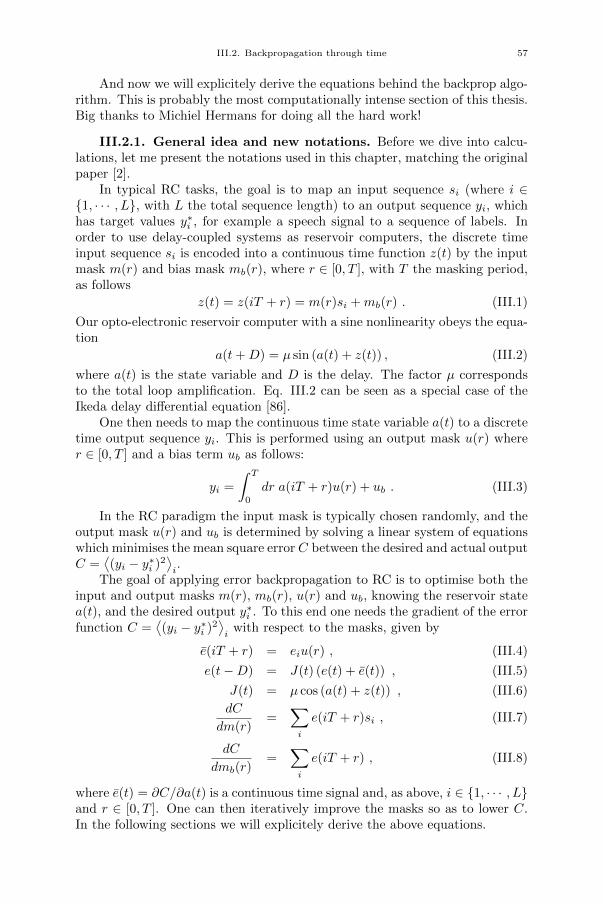
III.2. Backpropagation through time 57
And now we will explicitely derive the equations behind the backprop algo-rithm. This is probably the most computationally intense section of this thesis.Big thanks to Michiel Hermans for doing all the hard work!
III.2.1. General idea and new notations. Before we dive into calcu-lations, let me present the notations used in this chapter, matching the originalpaper [2].
In typical RC tasks, the goal is to map an input sequence si (where i ∈1, · · · , L, with L the total sequence length) to an output sequence yi, whichhas target values y∗i , for example a speech signal to a sequence of labels. Inorder to use delay-coupled systems as reservoir computers, the discrete timeinput sequence si is encoded into a continuous time function z(t) by the inputmask m(r) and bias mask mb(r), where r ∈ [0, T ], with T the masking period,as follows
z(t) = z(iT + r) = m(r)si +mb(r) . (III.1)
Our opto-electronic reservoir computer with a sine nonlinearity obeys the equa-tion
a(t+D) = µ sin (a(t) + z(t)) , (III.2)
where a(t) is the state variable and D is the delay. The factor µ correspondsto the total loop amplification. Eq. III.2 can be seen as a special case of theIkeda delay differential equation [86].
One then needs to map the continuous time state variable a(t) to a discretetime output sequence yi. This is performed using an output mask u(r) wherer ∈ [0, T ] and a bias term ub as follows:
yi =
∫ T
0
dr a(iT + r)u(r) + ub . (III.3)
In the RC paradigm the input mask is typically chosen randomly, and theoutput mask u(r) and ub is determined by solving a linear system of equationswhich minimises the mean square error C between the desired and actual outputC =
⟨(yi − y∗i )2
⟩i.
The goal of applying error backpropagation to RC is to optimise both theinput and output masks m(r), mb(r), u(r) and ub, knowing the reservoir statea(t), and the desired output y∗i . To this end one needs the gradient of the errorfunction C =
⟨(yi − y∗i )2
⟩i
with respect to the masks, given by
e(iT + r) = eiu(r) , (III.4)
e(t−D) = J(t) (e(t) + e(t)) , (III.5)
J(t) = µ cos (a(t) + z(t)) , (III.6)
dC
dm(r)=
∑
i
e(iT + r)si , (III.7)
dC
dmb(r)=
∑
i
e(iT + r) , (III.8)
where e(t) = ∂C/∂a(t) is a continuous time signal and, as above, i ∈ 1, · · · , Land r ∈ [0, T ]. One can then iteratively improve the masks so as to lower C.In the following sections we will explicitely derive the above equations.
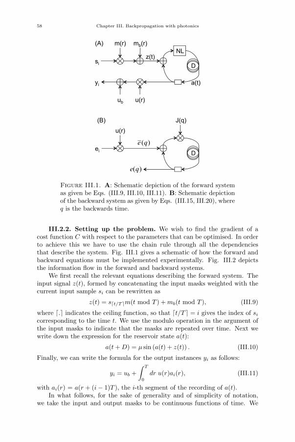
58 Chapter III. Backpropagation with photonics
si
m(r) mb(r)
NL
yi
ub u(r)
a(t)
D
z(t)
ei
u(r)
D
J(q)
e (q)
e(q)
(A)
(B)
Figure III.1. A: Schematic depiction of the forward systemas given be Eqs. (III.9, III.10, III.11). B: Schematic depictionof the backward system as given by Eqs. (III.15, III.20), whereq is the backwards time.
III.2.2. Setting up the problem. We wish to find the gradient of acost function C with respect to the parameters that can be optimised. In orderto achieve this we have to use the chain rule through all the dependenciesthat describe the system. Fig. III.1 gives a schematic of how the forward andbackward equations must be implemented experimentally. Fig. III.2 depictsthe information flow in the forward and backward systems.
We first recall the relevant equations describing the forward system. Theinput signal z(t), formed by concatenating the input masks weighted with thecurrent input sample si can be rewritten as
z(t) = sdt/Tem(t mod T ) +mb(t mod T ), (III.9)
where d.e indicates the ceiling function, so that dt/T e = i gives the index of sicorresponding to the time t. We use the modulo operation in the argument ofthe input masks to indicate that the masks are repeated over time. Next wewrite down the expression for the reservoir state a(t):
a(t+D) = µ sin (a(t) + z(t)) . (III.10)
Finally, we can write the formula for the output instances yi as follows:
yi = ub +
∫ T
0
dr u(r)ai(r), (III.11)
with ai(r) = a(r + (i− 1)T ), the i-th segment of the recording of a(t).In what follows, for the sake of generality and of simplicity of notation,
we take the input and output masks to be continuous functions of time. We
III.2. Backpropagation through time 59
Figure III.2. A: Schematic depiction of information flowwhen the system is used in the forward direction. On thebottom, the input sequence si is converted to a continuous-time signal z(t) (with time running from left to right). Eachinstance in the sequence is multiplied with the finite-lengthmasking signal m(t) and added to mb(t). These sequences arethen concatenated in time to form z(t), the input to the for-ward system. The output a(t) of the forward system is thenconverted into an output sequence yi by segmenting a(t) intime, and multiplying the segments with the output masksu(t), and integrating over each of them. B: Schematic depic-tion of the information flow in the “backwards” mode. Thederivatives ∂C/∂yi are used as an input sequence. They aremultiplied by u(t) which now plays the role of input mask.This yields the signal e(t) that serves as input for the back-ward system. The output of the backward system is e(t).
denote functional derivatives with respect to time dependent functions as ordi-nary derivatives. The case, relevant to practical implementations, in which themasks depend on a finite number of parameters, is discussed in Sec. III.3.2.For simplicity in the derivations we will assume, unless indicated otherwise,that all variables, both in continuous time t and discrete time i, are definedfor i and t going from −∞ to ∞. If we have a specific finite input sequencesi with i ∈ 1, · · · , L, we simply extend this beyond these bounds assuming

60 Chapter III. Backpropagation with photonics
that all extra si are equal to zero. Similarly, we assume that z(t) is zero ifdt/T e /∈ 1, · · · , L. Subsequently, if we sum or integrate over i or t withoutindicating limits, this indicates a summation or integration from −∞ to ∞. Inpractice it turns out that if we only have a finite sequence, we only need tocompute states over its corresponding time span. Similarly, when performingbackpropagation, we only need to compute backwards over the same time span.All states outside of this interval do not influence the gradient computation,which means there are no problems in considering only finite intervals. Thismatters, as in realistic training scenarios we typically train on relatively shortsequences (in the case of the present paper of length 100).
III.2.3. Output mask gradient. For the output masks we can write
dC
du(r)=∑
i
∂C
∂yi
dyidu(r)
. (III.12)
For example, if the cost function we wish to minimise is the squared error overthe interval of the input sequence
C =
L∑
i=1
(yi − y∗i )2,
ei =∂C
∂yi= 2(yi − y∗i ) for i ∈ 1, · · · , L.
∂C
∂yi= 0 for i /∈ 1, · · · , L.
The second factor in Eq. (III.12) we can get from Eq. III.11:
dyidu(r)
= ai(r),
such that the gradient for the output mask u(t) is simply given by
dC
du(r)=∑
i
∂C
∂yiai(r),
or, given the fact that ∂C/∂yi = 0 outside the interval in which the sequenceis defined
dC
du(r)=
L∑
i=1
∂C
∂yiai(r). (III.13)
Similarly we find that
dC
dub=
L∑
i=1
∂C
∂yi.
III.2. Backpropagation through time 61
III.2.4. Input mask gradient. The case of the input masks is moreinvolved. Working out the chain rule we find
dC
dm(r)=
∑
i
∂C
∂yi
dyidm(r)
.
=∑
i
∂C
∂yi
∫dt′
∂yi∂a(t′)
da(t′)
dm(r).
=
∫dt′ e(t′)
da(t′)
dm(r), (III.14)
where we have used
e(t′) =∂C
∂a(t′)=∑
i
∂C
∂yi
∂yi∂a(t′)
.
From Eq. III.11 we can obtain (using a modulo function in the argument ofu(r))
∂yi∂a(t′)
= δi,dt′/Teu(t′ mod T ),
i.e., equal to zero when t′ did not fall in the segment of time used to produceyi, and equal to the output mask otherwise. This yields
e(t′) = u(t′ mod T )∂C
∂ydt′/Te
= u(r)ei (III.15)
where r = t′ mod T and i = dt′/T e. In other words, e(t) is produced bymasking the sequence ∂C/∂yi with the output mask u(r).
The second factor in Eq. III.14 we work out as follows. Using the chainrule we get
da(t′)
dm(t)=
∫dt′′
da(t′)
dz(t′′)
dz(t′′)
dm(t). (III.16)
andda(t′)
dz(t′′)=∂a(t′)
∂z(t′′)+
∫dt′′′
∂a(t′)
∂a(t′′′)
da(t′′′)
dz(t′′).
From Eq. III.10 we obtain the partial derivatives
∂a(t′)
∂z(t′′)=
∂a(t′)
∂a(t′′)
= µδ(t′ − t′′ −D) cos(a(t′ −D) + z(t′ −D)),
Or, more compactly,
∂a(t′)
∂z(t′′)= δ(t′ − t′′ −D)J(t′),
with
J(t′) = µ cos(a(t′ −D) + z(t′ −D)).
This yieldsda(t′)
dz(t′′)= J(t′)
[δ(t′ − t′′ −D) +
da(t′ −D)
dz(t′′)
].
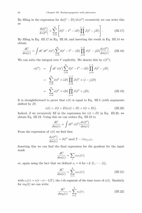
62 Chapter III. Backpropagation with photonics
By filling in the expression for da(t′ −D)/dz(t′′) recursively we can write thisas
da(t′)
dz(t′′)=
∞∑
i=0
δ(t′ − t′′ − iD)
i−1∏
j=0
J(t′ − jD)
. (III.17)
By filling in Eq. III.17 in Eq. III.16, and inserting the result in Eq. III.14 weobtain
dC
dm(r)=
∫dt′ dt′′ e(t′)
∞∑
i=0
δ(t′ − t′′ − iD)
i−1∏
j=0
J(t′ − jD)dz(t′′)
dm(r). (III.18)
We can solve the integral over t′ explicitly. We denote this by e(t′′):
e(t′′) =
∫dt′ e(t′)
∞∑
i=0
δ(t′ − t′′ − iD)
i−1∏
j=0
J(t′ − jD)
=
∞∑
i=0
e(t′′ + iD)
i−1∏
j=0
J(t′′ + (i− j)D)
=
∞∑
i=0
e(t′′ + iD)
i∏
j=1
J(t′′ + jD). (III.19)
It is straightforward to prove that e(t) is equal to Eq. III.5 (with argumentsshifted by D)
e(t) = J(t+D)(e(t+D) + e(t+D)). (III.20)
Indeed, if we recursively fill in the expression for e(t + D) in Eq. III.20, weobtain Eq. III.19. Using this we can reduce Eq. III.18 to
dC
dm(r)=
∫dt′′ e(t′′)
dz(t′′)
dm(r).
From the expression of z(t) we find that
dz(t′′)
dm(r)= δ(t′′ mod T − r)sdt/Te.
Inserting this we can find the final expression for the gradient for the inputmask
dC
dm(r)=∑
i
siei(r),
or, again using the fact that we defined si = 0 for i /∈ 1, · · · , L,
dC
dm(r)=
L∑
i=1
siei(r), (III.21)
with ei(r) = e(r−(i−1)T ), the i-th segment of the time trace of e(t). Similarlyfor m0(t) we can write
dC
dmb(r)=
L∑
i=1
ei(r). (III.22)
III.3. Experimental setup 63
III.2.5. Multiple inputs/outputs. The above explanation is easily ex-tended to multiple input and output dimensions. Suppose that we have amultivariate time series si, where the k-th element at time step i is denotedby si[k]. We can then easily construct z(t) by defining as many input masksmk(t) as there are input dimensions and adding them all up
z(t) =∑
k
sdt/Te[k]mk(t mod T ) +mb(t mod T ),
The desired output can similarly exist of a multivariate time series with ele-ments y∗i [l]. To produce an output yi[l] we simply define an output mask ul(t)and bias u0
l for each output channel
yi[l] = u0l +
∫ T
0
dtul(r)ai(r).
The same procedure can now be used to determine the gradients withrespect to the multivariate input and output masks. We find
dC
dul(r)=
L∑
i=1
dC
dyi[l]ai(r), (III.23)
and
dC
du0l
=
L∑
i=1
dC
dyi[l]. (III.24)
The source of the BP equation is now
e(t′) =∑
l
ul(t′ mod T )
dC
dydt′/Te[l], (III.25)
the recurrence for the error e(t), eq. (III.20), is unchanged, and one has
dC
dmk(r)=
L∑
i=1
si[k]ei(r) .
III.3. Experimental setup
In order to use the same hardware for both the signal processing and itsown training, one exploits the very close analogy between Eqs. III.1 and III.4– both are formed in the same way from a discrete time sequence, multipliedby a periodic mask – as well as the very close analogy between Eqs. III.2 andIII.5 – both are delay systems. However the equation for e(t) depends on futurevalues, so it needs to be solved backwards in time. In practice one time-invertse(t) and J(t) before computing e(t) to obtain a linear delayed equation
e(q +D) = J(q) (e(q) + e(q)) , (III.26)
where we use q instead of t to remind oneself that we are dealing with time-inverted signals. We also note that J(t), the derivative of the nonlinear func-tion, is a cosine, which can also be implemented using the intensity modulator.Although this property of the sine function is key for this experiment, othertypes of nonlinearity can be implemented in analogue hardware (see Sec. III.7).
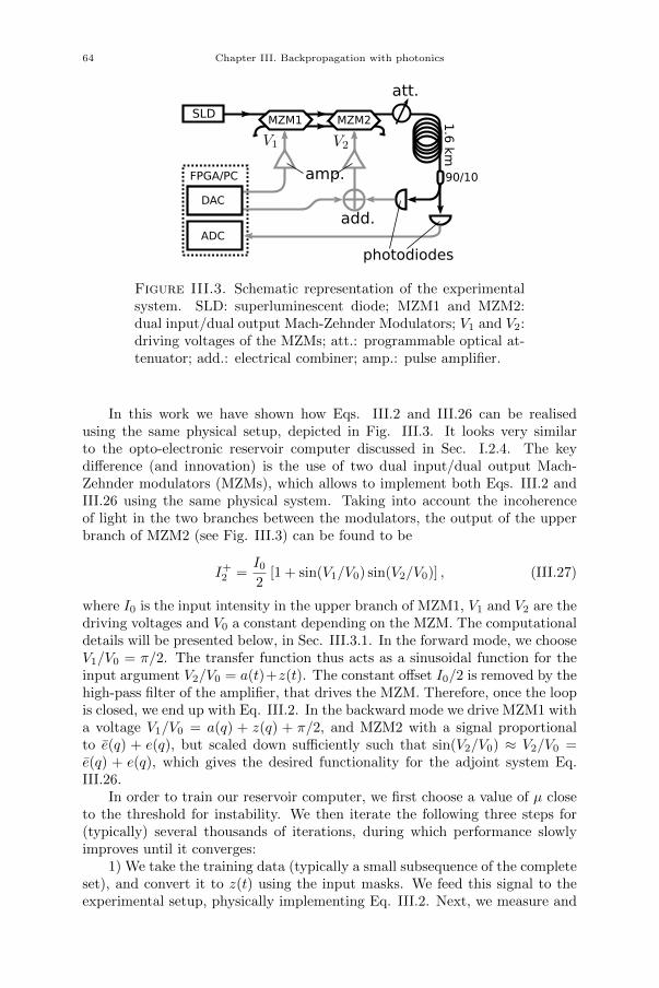
64 Chapter III. Backpropagation with photonics
SLDMZM1 MZM2
90/10
1.6
km
att.
amp.
photodiodes
DAC
ADC
FPGA/PC
add.
Figure III.3. Schematic representation of the experimentalsystem. SLD: superluminescent diode; MZM1 and MZM2:dual input/dual output Mach-Zehnder Modulators; V1 and V2:driving voltages of the MZMs; att.: programmable optical at-tenuator; add.: electrical combiner; amp.: pulse amplifier.
In this work we have shown how Eqs. III.2 and III.26 can be realisedusing the same physical setup, depicted in Fig. III.3. It looks very similarto the opto-electronic reservoir computer discussed in Sec. I.2.4. The keydifference (and innovation) is the use of two dual input/dual output Mach-Zehnder modulators (MZMs), which allows to implement both Eqs. III.2 andIII.26 using the same physical system. Taking into account the incoherenceof light in the two branches between the modulators, the output of the upperbranch of MZM2 (see Fig. III.3) can be found to be
I+2 =
I02
[1 + sin(V1/V0) sin(V2/V0)] , (III.27)
where I0 is the input intensity in the upper branch of MZM1, V1 and V2 are thedriving voltages and V0 a constant depending on the MZM. The computationaldetails will be presented below, in Sec. III.3.1. In the forward mode, we chooseV1/V0 = π/2. The transfer function thus acts as a sinusoidal function for theinput argument V2/V0 = a(t)+z(t). The constant offset I0/2 is removed by thehigh-pass filter of the amplifier, that drives the MZM. Therefore, once the loopis closed, we end up with Eq. III.2. In the backward mode we drive MZM1 witha voltage V1/V0 = a(q) + z(q) + π/2, and MZM2 with a signal proportionalto e(q) + e(q), but scaled down sufficiently such that sin(V2/V0) ≈ V2/V0 =e(q) + e(q), which gives the desired functionality for the adjoint system Eq.III.26.
In order to train our reservoir computer, we first choose a value of µ closeto the threshold for instability. We then iterate the following three steps for(typically) several thousands of iterations, during which performance slowlyimproves until it converges:
1) We take the training data (typically a small subsequence of the completeset), and convert it to z(t) using the input masks. We feed this signal to theexperimental setup, physically implementing Eq. III.2. Next, we measure and
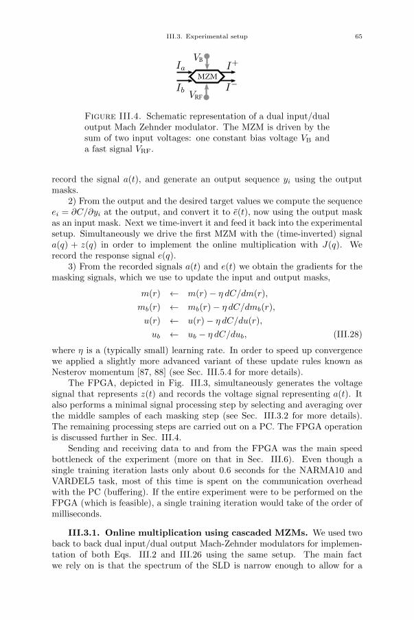
III.3. Experimental setup 65
MZM
RF
B
Figure III.4. Schematic representation of a dual input/dualoutput Mach Zehnder modulator. The MZM is driven by thesum of two input voltages: one constant bias voltage VB anda fast signal VRF.
record the signal a(t), and generate an output sequence yi using the outputmasks.
2) From the output and the desired target values we compute the sequenceei = ∂C/∂yi at the output, and convert it to e(t), now using the output maskas an input mask. Next we time-invert it and feed it back into the experimentalsetup. Simultaneously we drive the first MZM with the (time-inverted) signala(q) + z(q) in order to implement the online multiplication with J(q). Werecord the response signal e(q).
3) From the recorded signals a(t) and e(t) we obtain the gradients for themasking signals, which we use to update the input and output masks,
m(r) ← m(r)− η dC/dm(r),
mb(r) ← mb(r)− η dC/dmb(r),
u(r) ← u(r)− η dC/du(r),
ub ← ub − η dC/dub, (III.28)
where η is a (typically small) learning rate. In order to speed up convergencewe applied a slightly more advanced variant of these update rules known asNesterov momentum [87, 88] (see Sec. III.5.4 for more details).
The FPGA, depicted in Fig. III.3, simultaneously generates the voltagesignal that represents z(t) and records the voltage signal representing a(t). Italso performs a minimal signal processing step by selecting and averaging overthe middle samples of each masking step (see Sec. III.3.2 for more details).The remaining processing steps are carried out on a PC. The FPGA operationis discussed further in Sec. III.4.
Sending and receiving data to and from the FPGA was the main speedbottleneck of the experiment (more on that in Sec. III.6). Even though asingle training iteration lasts only about 0.6 seconds for the NARMA10 andVARDEL5 task, most of this time is spent on the communication overheadwith the PC (buffering). If the entire experiment were to be performed on theFPGA (which is feasible), a single training iteration would take of the order ofmilliseconds.
III.3.1. Online multiplication using cascaded MZMs. We used twoback to back dual input/dual output Mach-Zehnder modulators for implemen-tation of both Eqs. III.2 and III.26 using the same setup. The main factwe rely on is that the spectrum of the SLD is narrow enough to allow for a
66 Chapter III. Backpropagation with photonics
large extinction ratio by the MZMs, but is broad enough that the light in thetwo branches entering MZM2 from MZM1 can be considered incoherent. Inthe present experiment, the coherence length of the light from the SLD is ofthe order of a few hundreds of micrometers, which means that a very smalldifference in path length for the connections in between MZM1 and MZM2 issufficient to make the two signals incoherent.
Consider the operation of a single MZM, schematised in Fig. III.4. Theintensities of the incoming light sources are denoted by Ia and Ib, and the MZMis driven by a voltage V , which is the sum of a constant bias voltage VB anda fast voltage signal VRF. The bias voltage was omitted in the main text toavoid confusion. Taking into account the incoherence between the two inputsignals, the intensities of the output branches (I+ and I−) are given by
I+ = Ia1 + sin(V/V0)
2+ Ib
1− sin(V/V0)
2,
I− = Ia1− sin(V/V0)
2+ Ib
1 + sin(V/V0)
2, (III.29)
with V0 a constant depending on the MZM.It is now easy to model the output of the two cascaded MZMs. Suppose
the source has an intensity I0, and no light enters the second input of MZM1.And suppose MZM1 and MZM2 receive voltages V1 and V2, respectively. Theoutput intensities I+
1 and I−1 of MZM1 are given by
I+1 = I0
1 + sin(V1/V0)
2,
I−1 = I01− sin(V1/V0)
2. (III.30)
The intensity I+2 at the first output branch of MZM2 is then
I+2 = I0
(1 + sin(V1/V0))(1 + sin(V2/V0))
4(III.31)
+I0(1− sin(V1/V0))(1− sin(V2/V0))
4(III.32)
=I02
[1 + sin(V1/V0) sin(V2/V0)] . (III.33)
In the experiment MZM1 receives a constant bias signal on top of an RFdriving signal, such that V1/V0 = π/2 +V ′1/V0, with V ′1 the RF signal. We canthus write:
I+2 =
I02
[1 + cos(V ′1/V0) sin(V2/V0)] .
We use the setup in two modes. In the forward mode, V ′1 = 0, so that thecascaded MZMs behave as
I+2 =
I02
[1 + sin(V2/V0)] ,
i.e., the transfer function acts as a sinusoidal function for the input argumentV2/V0, which is equal to the sum of the input signal z(t) and the system statea(t). Note that a constant offset I0/2 is added to the output. We use, however,amplifiers with a high-pass filter to drive the MZMs, which remove the DC
III.3. Experimental setup 67
offset. Therefore, once the loop is closed, this constant bias is removed, and weeffectively end up with Eq. III.2.
In the backwards mode, we drive MZM1 with a voltage V ′1 proportional toa(q−D) + z(q−D). MZM2 is driven with a signal proportional to e(q) + e(q),but scaled down sufficiently such that sin(V2/V0) ≈ V2/V0 = e(q) + e(q). Thismeans that in the backwards mode we can write
I+2 =
I02
[1 + cos (a(q +D) + z(q +D)) (e(q) + e(q)] ,
which is (up to the constant bias, and the factor µ which is imposed later bythe optical attenuator) the desired functionality for the adjoint system (givenby Eq. III.26).
III.3.2. Mask parametrisation. While the BP theory, discussed in Sec.III.2, is generally valid for continuous-time signals, an experimental setup islimited by the finite bandwidth of the DAC/ADC, and the analogue electronicparts. To make sure that these effects play a limited role, we parametrisethe input and output masks as piecewise constant functions, which has beencommon practice for reservoirs of this type [48]. To this end we divide thedelay D into an integer number ND of equal time segments, called maskingsteps. Next, we ensure that the masking period T has a total duration thatalso contains an integer number NT of masking steps, in our case one less thanthe delay: NT = ND − 1. This allows for the mixing of the states over time,as detailed in [48].
The input and output masks are picked to be constant for the durationof each masking step. This implies that z(t) is piecewise constant. The factthat both T and D are an integer number of masking steps makes that changesin a(t) only occur in between the masking steps, i.e., they are synchronisedwith the masking steps, and this is valid for the backwards pass too. In short,a(t), e(t) and e(t) are all piecewise constant signals, with values that remainconstant during each masking step.
In practice this allows us to reduce effects of noise by averaging the signalsrepresenting a(t) and e(t) over several measuring samples during a single mask-ing step. Typically we pick a set of samples from the middle of each maskingstep, and discard those at the beginning and the end as they may contain arte-facts caused by the limited bandwidth of the ADC. More importantly, it allowsus to make a discrete time approximation of the entire system. For example,let us consider equation III.11. The mask u(t) is made up of NT constant seg-ments of equal length, with values during the segments denoted uk. Similarly,each segment ai(r) = a (t− (i− 1)T ) is piecewise constant, with values we canfor example denote with aik. The integral reduces to
yi = ub +
NT∑
k=1
aikuk,
(where we absorbed the factor T that emerges from the integration into thevalues uk). Each particular value aik can be interpreted as the state of thek-th “neuron” or “node” state during the i-th instance of the input sequence.We can still use the expressions for the gradients in Eqs. III.13, III.21 and

68 Chapter III. Backpropagation with photonics
III.22. Indeed, by construction, the gradient for the output mask u(t) for theduration of a single masking step is a constant (as a(t) remains constant overthe segment). The same holds for the gradients for the input masks. Thisimplies that u(t) and m(t) remain piecewise constant during training, and wecan in practice describe them simply as lists of values instead of a continuous-time functions.
Note that the choice of dealing with bandwidth limitations by using piece-wise constant functions is not the only possible avenue. One alternative wouldbe to impose bandwidth constraints on m(t) and u(t), such that the finite signalgenerator bandwidth and sampling rates form no obstacle in treating the setupas a continuous-time setup. We chose the piecewise-constant constraint as itis more directly related to existing implementations of delay-coupled electro-optical signal processors, and it allows to identify a specific number of “virtualnodes” (the number of segments within the masking period T ). In other words,the choice of NT determines the “complexity”, or the number of degrees of free-dom of the system.
III.4. FPGA design
The FPGA design is my key contribution to this project. As will be shownbelow, it allowed to significantly speed up the experiment, which is crucial foriterative algorithms. The design itself is much simpler than the previous one(see Sec. II.5): it performs no computations and only basic signal processingon the acquired data. The main novelty is the Ethernet interface with thecomputer, that took me some time to develop (more on that in Sec. III.6). Italows a much faster data transfer than the archaic UART, used previously.
The simplified schematics of the design is depicted in Fig. III.5. Rect-angular boxes represent modules (entities), and rounded rectangles stand forelectronic components: the FMC151 daughtercard, the Marvell Alaska PHYdevice (88E1111) for Ethernet communications (ETH), the Hewlett Packard8648A clock generator, the PC, running Matlab, and the opto-electronic ex-periment.
The operation of the FPGA is controlled from Matlab through a GbitEthernet connection. Data and various commands, such as memory read/writeor state change, are encapsulated into standard UDP packages. The Ethernet
module interfaces the Marvell Ethernet PHY chip with the rest of the design,receives the UDP packets (frames) and decodes the commands and the data.It also ensures data transmission from the FPGA to the computer.
The UDP packets are read at the PHY level on the FPGA (see [89] for areference on the OSI model). For simplicity, the board does not have a MACnor an IP address. Matlab sends the packets to a random address, since thecable only connects two devices. The design discards the PHY, TCP and UDPheaders from the received packet and only reads the data. It also ignores thechecksum at the end of the frame. The first bytes are interpreted as commandsand the following, if any, are considered as data and written in the FPGAmemory.

III.4. FPGA design 69
Matlab
ML605
BRAM si OR ei
1 OR J
Ethernet
si, ei J,m, u
Fpga2Exp
Exp2Fpgaa OR e
FMC151
ADC
CLK
DAC si OR ei (to add.)
1 OR J (to MZM1)
HP Experiment
a OR e (from photodiode)
Figure III.5. Simplified schematics of the FPGA design.Modules (entities) are represented by rectangular boxes, elec-tronic components are shown with rounded rectangles. Ex-ternal hardware, such as the computer, running Matlab, theopto-electronic reservoir and the external clock generator areshown in grey. During the forward pass, the FPGA sends theinputs si to the electrical combiner (labelled “add.” in Fig.III.3), drives the MZM1 with a constant signal equal to 1 tokeep it transparent, and records the reservoir states a from thereadout photodiode. During the backward pass, the MZM1 isdriven by the Jacobian J , the combiner is fed with the errorsei and the error signal e is recorded.
Blocks of Random-Access Memory (BRAM) are used to store data, suchas the inputs si and ei for the forward and backward runs, respectively, theJacobian J , as well as the input and output masks u and m.
Sending packets to the computer is a more challenging process, as theaddresses (MAC, IP and port number) must match the computer settings forthe data to reach Matlab. Moreover, a 32-bit Cyclic Redundancy Check (alsoknown as the checksum) must be appended to the frame for the computer toaccept the packet (and not drop it as a corrupt frame). I assigned an arbitraryIP to the computer and used the default UDP port in Matlab. These addressesare hard-coded in the FPGA design, and the CRC is computed inside theEthernet module.
The FMC151 daughtercard outputs two 14-bit signals from the ADCs andreceives two 16-bit signals for the DACs. It is also used to deliver a clocksignal from an external clock generator, that produces a high-precision signal,allowing to synchronise the FPGA with the delay loop of the experimentalsetup. This clock signal was generated by the Hewlett Packard 8648A signalgenerator.
The Fpga2Exp module controls the two signals sent to the opto-electronicreservoir through the dual-channel DAC. During the forward pass, it generatesthe masked input signal m × si by multiplying the inputs si by the mask m,both being read from the BRAM. During the backward pass, it outputs u× eithrough one channel, and J through the other.
The reservoir states a(t), as well as the error signal e(q) from the experimentare sampled and averaged by the Exp2Fpga module. The number of samplesdepends on the task and the reservoir size, as will be discussed in Sec. III.5.The data is buffered in blocks of RAM (not shown here) and then encapsulated
70 Chapter III. Backpropagation with photonics
into UDP packages in the Ethernet module and transfered to the computerthrought Ethernet.
Since the FPGA performs minimal calculations in this experiment, a legit-imate question comes to mind: do we need a FPGA at all? And the answeris yes, we do. Since BP is an iterative process, the experiment needs to berepeated a large number of times for the training to be completed. As will beshown in Sec. III.5, this number varies from 104 for NARMA and VARDELup to 106 for TIMIT tasks. Without the FPGA, as in [48], the opto-electronicexperiment can be run in approximately 30 s. That is, one training cycle forthe NARMA task would have taken about 4 days. With the FPGA, one runtakes 0.6 s, cutting the duration of a training cycle to a more manageable timeof 2 hours.
III.5. Results
We validated the experimental setup on three time series processing task.
III.5.1. Tasks. We consider first of all the NARMA10 task, introducedin Sec. I.1.4.2. The second task we will call VARDEL5 (from variable delay).Here, the input sequence consists of independent and identically distributeddigits drawn from the set 1, 2, 3, 4, 5. The desired output is then given byy∗i = si−si , i.e., the goal is to retrieve the input instance delayed with thenumber of time steps given by the current input. As a performance metricfor NARMA10 and VARDEL5 we use the normalised root mean square error(NRMSE), which is given by
NRMSE =
√〈(yi − y∗i )2〉i〈(y∗i )2〉i
.
The NRMSE varies between 0 (perfect match), and 1 (no relation betweenoutput and target).
The third task is a frame-wise phoneme labelling task. We use the TIMITdataset [90], a speech dataset in which each time step has been labelled with oneof 39 phonemes. The input data is high-dimensional (consisting of 39 frequencychannels), and the desired output is one of (coincidentally) 39 possible outputclasses. The goal is to label each frame in a separate test set. Consequently,the performance metric is now the classification error rate, i.e., the fractionof misclassified phonemes in the test set. Note that the masking scheme andBP algorithm is easily extended to multidimensional in – and output sequences(see Sec. III.2.5). The TIMIT task has been studied before in the context ofRC, which has shown it to be challenging, typically requiring extremely largereservoirs to obtain competitive performance [91, 92].
For all these tasks we compared performance of the fully trained systemto traditional RC, where we kept the input and bias masks fixed and random,and only optimised their global scaling and the feedback strength parameterµ. The results are shown in Fig. III.6. The experimental setup is successfulin performing both useful computations, and implementing its own trainingprocess. The fully trained system consistently outperforms the RC approachin all tasks considered.
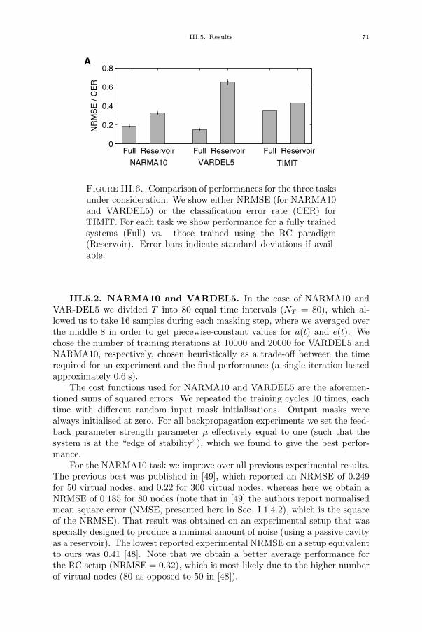
III.5. Results 71
Full Reservoir Full Reservoir Full Reservoir0
0.2
0.4
0.6
0.8
NR
MS
E /
CE
R
NARMA10 VARDEL5 TIMIT
A
B
A
Figure III.6. Comparison of performances for the three tasksunder consideration. We show either NRMSE (for NARMA10and VARDEL5) or the classification error rate (CER) forTIMIT. For each task we show performance for a fully trainedsystems (Full) vs. those trained using the RC paradigm(Reservoir). Error bars indicate standard deviations if avail-able.
III.5.2. NARMA10 and VARDEL5. In the case of NARMA10 andVAR-DEL5 we divided T into 80 equal time intervals (NT = 80), which al-lowed us to take 16 samples during each masking step, where we averaged overthe middle 8 in order to get piecewise-constant values for a(t) and e(t). Wechose the number of training iterations at 10000 and 20000 for VARDEL5 andNARMA10, respectively, chosen heuristically as a trade-off between the timerequired for an experiment and the final performance (a single iteration lastedapproximately 0.6 s).
The cost functions used for NARMA10 and VARDEL5 are the aforemen-tioned sums of squared errors. We repeated the training cycles 10 times, eachtime with different random input mask initialisations. Output masks werealways initialised at zero. For all backpropagation experiments we set the feed-back parameter strength parameter µ effectively equal to one (such that thesystem is at the “edge of stability”), which we found to give the best perfor-mance.
For the NARMA10 task we improve over all previous experimental results.The previous best was published in [49], which reported an NRMSE of 0.249for 50 virtual nodes, and 0.22 for 300 virtual nodes, whereas here we obtain aNRMSE of 0.185 for 80 nodes (note that in [49] the authors report normalisedmean square error (NMSE, presented here in Sec. I.1.4.2), which is the squareof the NRMSE). That result was obtained on an experimental setup that wasspecially designed to produce a minimal amount of noise (using a passive cavityas a reservoir). The lowest reported experimental NRMSE on a setup equivalentto ours was 0.41 [48]. Note that we obtain a better average performance forthe RC setup (NRMSE = 0.32), which is most likely due to the higher numberof virtual nodes (80 as opposed to 50 in [48]).
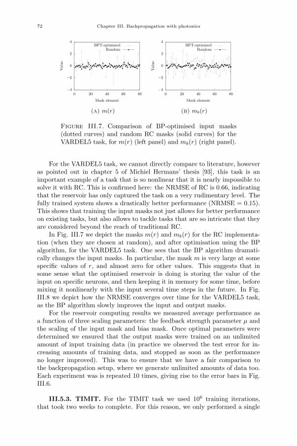
72 Chapter III. Backpropagation with photonics
−4
−2
0
2
4
0 20 40 60 80
Val
ue
Mask element
BPT-optimisedRandom
(a) m(r)
−4
−2
0
2
4
0 20 40 60 80
Val
ue
Mask element
BPT-optimisedRandom
(b) mb(r)
Figure III.7. Comparison of BP-optimised input masks(dotted curves) and random RC masks (solid curves) for theVARDEL5 task, for m(r) (left panel) and mb(r) (right panel).
For the VARDEL5 task, we cannot directly compare to literature, howeveras pointed out in chapter 5 of Michiel Hermans’ thesis [93], this task is animportant example of a task that is so nonlinear that it is nearly impossible tosolve it with RC. This is confirmed here: the NRMSE of RC is 0.66, indicatingthat the reservoir has only captured the task on a very rudimentary level. Thefully trained system shows a drastically better performance (NRMSE = 0.15).This shows that training the input masks not just allows for better performanceon existing tasks, but also allows to tackle tasks that are so intricate that theyare considered beyond the reach of traditional RC.
In Fig. III.7 we depict the masks m(r) and mb(r) for the RC implementa-tion (when they are chosen at random), and after optimisation using the BPalgorithm, for the VARDEL5 task. One sees that the BP algorithm dramati-cally changes the input masks. In particular, the mask m is very large at somespecific values of r, and almost zero for other values. This suggests that insome sense what the optimised reservoir is doing is storing the value of theinput on specific neurons, and then keeping it in memory for some time, beforemixing it nonlinearly with the input several time steps in the future. In Fig.III.8 we depict how the NRMSE converges over time for the VARDEL5 task,as the BP algorithm slowly improves the input and output masks.
For the reservoir computing results we measured average performance asa function of three scaling parameters: the feedback strength parameter µ andthe scaling of the input mask and bias mask. Once optimal parameters weredetermined we ensured that the output masks were trained on an unlimitedamount of input training data (in practice we observed the test error for in-creasing amounts of training data, and stopped as soon as the performanceno longer improved). This was to ensure that we have a fair comparison tothe backpropagation setup, where we generate unlimited amounts of data too.Each experiment was is repeated 10 times, giving rise to the error bars in Fig.III.6.
III.5.3. TIMIT. For the TIMIT task we used 106 training iterations,that took two weeks to complete. For this reason, we only performed a single
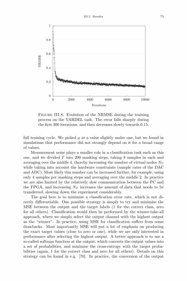
III.5. Results 73
0
0.2
0.4
0.6
0.8
1
0 2000 4000 6000 8000 10000
NRMSE
Iterations
Figure III.8. Evolution of the NRMSE during the trainingprocess on the VARDEL task. The error falls sharply duringthe first 300 iterations, and then decreases slowly towards 0.15.
full training cycle. We picked µ at a value slightly under one, but we found insimulations that performance did not strongly depend on it for a broad rangeof values.
Measurement noise plays a smaller role in a classification task such as thisone, and we divided T into 200 masking steps, taking 8 samples in each andaveraging over the middle 4, thereby increasing the number of virtual nodes NTwhile taking into account the hardware constraints (sample rates of the DACand ADC). Most likely this number can be increased further, for example, usingonly 4 samples per masking steps and averaging over the middle 2. In practicewe are also limited by the relatively slow communication between the PC andthe FPGA, and increasing NT increases the amount of data that needs to betransferred, slowing down the experiment considerably.
The goal here is to minimise a classification error rate, which is not di-rectly differentiable. One possible strategy is simply to try and minimise theMSE between the output and the target labels (1 for the correct class, zerofor all others). Classification would then be performed by the winner-take-allapproach, where we simply select the output channel with the highest outputas the “winner”. In practice, using MSE for classification suffers from somedrawbacks. Most importantly MSE will put a lot of emphasis on producingthe exact target values (close to zero or one), while we are only interested inperformance after selecting the highest output. A better approach is to use aso-called softmax function at the output, which converts the output values intoa set of probabilities, and minimise the cross-entropy with the target proba-bilities (again, 1 for the correct class and zero for all others). Details on thisstrategy can be found in e.g. [70]. In practice, the conversion of the output
74 Chapter III. Backpropagation with photonics
yi[k] into probabilities is performed using the softmax function
pi[k] =exp(yi[k])∑l exp(yi[l])
.
The cost function is the cross-entropy
C = −L∑
i=1
∑
k
ti[k] ln pi[k],
where we denote the target outputs as ti[k]. It can then be shown that
dC
dyi[k]= pi[k]− ti[k],
(and again zero if i /∈ 1, · · · , L). This means that the error we have at theoutput takes on virtually the same form as before, only this time there is theintermediary step of the softmax function. Gradients for the output masks arealmost the same as before, except for equations III.23 and III.24 where we usepi[k] − ti[k] instead of yi[k] − y∗i [k]. As far as the rest of the BP algorithmgoes, we now simply have to mask these “output errors” to produce e(q), andthe rest plays out exactly as before.
For the RC approach, optimising the parameters (input scaling, bias scalingand feedback gain) on the hardware would be too costly in terms of time.Therefore we optimised them on a PC using a simulation of the physical setup.Once we decided on the parameters, we ran all the TIMIT data through thephysical setup and recorded all the responses. Next we trained output weights,again using gradient descent with the above cross-entropy loss.
We obtained a classification error rate of 34.8% for fully trained systems,vs. 42.9% for the standard RC approach. These results are only slightly worsethan similar experimental results presented in [81], (33.2% for fully trainedsystems and 40.5% for the RC approach) where 600 virtual nodes were used asopposed as 200 in our case.
III.5.4. Gradient descent. We used stochastic gradient descent to trainthe masks. For each iteration, we drew a 100 time step sequence to deter-mine a gradient. This sequence was either generated on the fly (in the case ofVARDEL5 and NARMA10), or drawn randomly from a training set (TIMIT).Note that as the BP equation is linear, we are in principle free to rescale e aswe wish. In practice, in order to keep MZM2 in the linear regime, we scaled theinput error signal e(t) by dividing it by its standard deviation and multiplyingwith a factor 0.1. The learning rate η we choose equal to 0.25 at the start of thetraining process, after which it drops linearly to zero throughout the course ofthe experiment. On top of that we use Nesterov momentum with a momentumfactor 0.9 to speed up convergence [87, 88]. Nesterov momentum is a heuristicmethod that finds widespread use in speeding up convergence of stochastic gra-dient descent. The idea of momentum in gradient descent is to give parameterupdates a certain inertia, meaning that previous parameter updates still countin the current one, which helps with overcoming local minima and speeds upconvergence. Nesterov momentum is a simple variation of this principle, where
III.5. Results 75
the algorithm measures the gradient one update step ahead in order to changeits momentum “ahead of time”.
III.5.5. Robustness. Our work shows that physical BP is robust againstimperfections of the physical setup, as illustrated by the following imperfectionswe were confronted with.
The first imperfection was the high-pass filtering operation of the amplifiersused to drive the MZMs, with a cut-off frequency of 20 kHz. While the high-pass filter is a desirable property (to get rid of voltage bias), this correspondsto a typical time scale of about 8 µs, which is about the same as the loop delayand therefore not negligible. The current experimental setup does not take thisfiltering operation into account explicitly.
The second imperfection was an imbalance in losses between the two fibresconnecting MZM1 with MZM2.
The third imperfection was that the system was not perfectly linear duringthe backwards pass, since MZM2 is never a perfectly linear system. There isalso an important trade-off here. One can reduce the residual nonlinearity byreducing the amplitude of the incoming voltage signal that represents e(t). Butin turn this also reduces the signal-to-noise ratio of the measurement duringthe backpropagation phase, such that one needs to find a good balance betweenthese two effects.
All these effects are imperfections inherent to the physically implementedbackpropagation phase, but both in simulation and in the actual experimentswe found that they only had a very minor impact on the training process andthe overall performance.
One parameter that turned out to be crucial was the bias voltage of MZM2.The reason is that even a small offset from an effectively zero level introduces asystematic error in the backpropagation process, such that the measured signal(denoted as ec(t) to indicate that it is corrupted) becomes
ec(t−D) = J(t)(ec(t) + e(t) + e),
with e a constant offset caused by an incorrectly set voltage bias of MZM2. Itturned out that, in the experiments, keeping this bias level effectively equal tozero was difficult: very slight drifts on the effective working point of the MZMoccurred over the course of minutes/hours. Luckily, the backpropagation is alinear process. This means that we can recover e(t) by performing a secondmeasurement right after measuring ec(t)
er(t−D) = J(t)(er(t) + e),
and
e(t) = ec(t)− er(t).In other words we simply need to perform two measurements after each other,where in the second one we send a “zero” input error, and subtract this fromthe first measurement in order to remove the influence of the offset of MZM2.This turned out to solve the problem.
76 Chapter III. Backpropagation with photonics
III.6. Challenges and solutions
We had to face two big challenges while working on this project. Thefirst one is FPGA-related and it had an immense impact on the speed of theexperiment. The first design I created used the archaic UART interface totransfer data to and from the computer, as in my first experiment (see Ch.II), with a maximum transfer rate of 128 kbit/s. In this case, one run of theexperiment lasted 16 seconds, with more than 99% of the time spent on datatransfer.
Obviously, a faster connection was required. Two options were available atthis stage: Gbit Ethernet or PCI Express, both widely used in modern com-puters. Since the latter is more complex to implement on hardware level, Ipicked the Ethernet. Although I did manage to make it work in a reasonabletime, this was a poor choice on the long run. Ethernet, by its definition, is notsuitable for connections between a PC and its periferals. In short, Ethernetis an intrinsically unreliable protocol – the hardware is designed to drop data(sent by chunks called packets or frames) when it is not capable of processingit in time. Therefore, upper-layer protocols, such as TCP/IP, incorporate ac-knowledgement of received data and requests to retransmit packets that didnot make it to the destination. These protocols are usually implemented insoftware, and designing them in hardware would have taken a lot of time. SoI simply skipped them, and hoped for the best.
A good proof of Ethernet’s unreliability was found during the first full-length experiments. We discovered that, sometimes, the data received fromthe FPGA was wrong. The error, spotted after a couple of long and desperatenights, was hard to believe in at first: some packets did not arrive in thesame order to the computer as they were sent, meaning that the flow of time-multiplexed data, transmitted by the FPGA, was broken. And this is actuallynormal for an Ethernet card to switch the order of packets, whenever it choosesto, for. . . reasons.
A few problems were encountered on the way to a well-working two-wayEthernet connection. In principle, Xilinx offers ready-to-use plug-and-playblocks, called IP cores, that can handle various features of the FPGA. Onesuch core provides the Ethernet connectivity. Sadly, it simply did not work.The source files were missing important pin connections, including the clocksignal to the Ethernet PHY chip. Fortunately, after hours of Googling, I foundthe solution in Satnam Singh’s MSDN Blog [94]. Still, the Xilinx IP was toocomplex for my needs, so I decided to rip off all that was not necessary andonly leave the basic interface with Ethernet PHY chip.
Sending data from the computer to the FPGA was easy, as the latter wasprogrammed to disregard addresses and port numbers, and only read the data.That is, the computer could send the data to a random address, it would stillbe received by the FPGA. The other way around was different, as the computerand Matlab ruthlessly filter out all packets that are not explicitely addressed tothem. That means that the FPGA had to set the headers just right. Moreover,IP protocol requires a valid checksum, that is, a cyclic redundancy check, ap-pended at the end of the packet, so that the receiving hardware can verify thatthe data is not corrupted. If the checksum does not pass the test, the packet
III.7. Conclusion 77
is dropped. That is, the FPGA design had to compute the CRC-32 for eachdata frame. All these problems were resolved, but required a certain effort.
At 1 Gbit/s Ethernet data transfer rate, sending the acquired signal fromthe FPGA to the computer requires a fraction of a millisecond. However,Matlab needs a minimal 0.6 s delay to process this data. I could not find thereasons for such slow buffering, and we had no choice but to live with it. Butit is important to note that, should this Matlab problem be resolved, eachiteration of the experiment could, in principle, run several orders of magnitudefaster.
The second big challenge, encountered and solved by Michiel Hermans, wasalready described in Sec. III.5.5. At first, the error rate, similar to the oneplotted in Fig. III.8, did not want to decrease below 0.2. We fought with thesettings of the intensity modulator for a couple of days, trying to make it assymmetric as possible, untill Michiel Hermans came up with a much bettersolution. Adding a third “blanc” pass increased the experiment runtime by33%, but allowed us to achieve much better results with the setup.
III.7. Conclusion
Our work confirms the results anticipated in [80, 81]: the performanceof delay-based reservoir computers can be drastically improved by optimisingboth input and output masks. Furthermore, following the proposal of [85], weshowed that the underlying hardware is capable of running a large part of itsown optimisation process. We performed our demonstrations on a fast electro-optical system (whose speed could be readily improved by several orders ofmagnitude, see, e.g. [54]), and on tasks considered hard in the RC community.Importantly, our work has revealed that the BP algorithm is robust againstvarious experimental imperfections, as the performance gains we obtained onall three tasks were similar to those predicted by numerical simulations.
Although our experiment relies on the sine nonlinearity and its cosine de-rivative, other nonlinear functions can also be successfully realised in hardwarewith their derivatives. For instance, the so-called linear rectifier function, whichtruncates the input signal below a certain threshold, is a popular activationfunction in neural architectures [95]. Its derivative is a simple binary functionwhich can be easily implemented using an analogue switch, as in [85]. In [96]it is shown how to implement a sigmoid nonlinearity and its derivative. Andin [49, 55] the nonlinearity is quadratic, and therefore the derivative, which islinear, should also be easy to implement. Furthermore, the BP algorithm is ro-bust against imperfect implementation of the derivative, as shown here in Sec.III.5.5 and also in the Supplementary Material of [85] (see Supplementary Note4). Therefore we expect that physical implementation of the BP algorithm willbe possible in a wide variety of physical systems.
Our setup still requires some slow digital processing to perform the mask-ing and to compute gradients from the recorded signals. Performing maskingoperations in analogue hardware, however, is actively being researched: severalreadout schemes have been proposed [73, 97, 98] and a few have been realisedexperimentally [73, 97]. Moreover, Ch. V of this thesis presents a numericalexperiment demonstrating how to improve analogue readout layers with online

78 Chapter III. Backpropagation with photonics
learning. These approaches could be used to speed up the present setup. An-other limitation is the large amount of data transfered between the FPGA andthe computer. Implementing the full training algorithm on the FPGA woulddrastically increase the speed of the experiment.
Nowadays, there is an increased interest in unconventional, neuromorphiccomputing, as this could allow for energy efficient computing, and may providea solution to the predicted end of Moore’s law [64]. These novel approaches tocomputing will likely be made with components that exhibit strong element-to-element variability, or whose characteristics evolve slowly with time. Self-learning hardware may be the solution that enables these systems to fulfil theirpotential. The results in [85] and in this work therefore constitute an importantstep towards this goal.
Contrary to my first experiment, this project was completed in a coupleof months. Sadly, we could not develop this research direction any further asMichiel Hermans left the team shortly after our paper [2] was written.

CHAPTER IV
Photonic reservoir computer with outputfeedback
This chapter presents, arguably, the most important experiment of myPhD. Not because I worked on it for a long time, but because it brought themost interesting, novel and even unexpected results.
Somewhat similar to Ch. III, this project – as it is – was not part of mythesis. The original plan was to build an analogue output layer (see Ch. V)and then feed the output signal back into the reservoir and see what it does.But how often do things go as planned, if ever? After the very good resultsobtained in the online training project (see Ch. II), we decided to shortcutthe analogue part of the experiment, for two reasons. First, an analogue layerwould be more complex and we had no guarantee it would work sufficiently well.It is one thing to be able to compute the output of the system, but another toobtain a high-quality output signal that could be fed back as input. Second,analogue layers have already been researched [73, 97, 98], while nobody hasever reported an experimental reservoir computer with output feedback so far,neither digital, nor analogue. Therefore, the experimental demonstration of thenovel features of such a system seemed a much more attractive and innovativeidea.
The content of this chapter is based on our paper [5]. It is relatively long– we tested the setup on four new tasks (not yet considered by our lab) andperformed an in-depth study of the reservoir output properties – and so is thischapter. Some additional results from our paper [3] are also included.
IV.1. Introduction
Forecasting is one of the central problems in science: how can we predictthe future from the past? Over the past few decades, artificial neural networkshave gained a significant popularity in the time series forecasting community.Compared to previously employed statistics-based techniques, they are bothdata driven and non-linear, more flexible and do not require an explicit modelof the underlying process. A review of artificial neural networks models fortime series forecasting can be found in [99]. Reservoir computing can be di-rectly applied to short-term prediction tasks, that focus on generating a fewfuture timesteps. As for long-horizon forecasting, that involves predicting thetime series for as long as possible, it is possible with a small modification ofthe architecture, namely by feeding the RC output signal back into the reser-voir. This additional feedback significantly enriches the internal dynamics ofthe system, enabling it to generate time series autonomously, that is without
79
80 Chapter IV. Photonic reservoir computer with output feedback
receiving any input signal. With this modification, reservoir computing canbe used for long-term prediction of chaotic series [9, 29, 100–102]. In fact,this approach holds, to the best of our knowledge, the record for such chaotictime series prediction [29, 102]. A reservoir computer with output feedbackcan also achieve the easier task of generating periodic signals [103–105], and ofproducing a tunable frequency [10, 106, 107].
The aim of the present work is to explore these novel applications exper-imentally. Indeed, they have been widely studied numerically, but no experi-mental implementation has been reported so far. There are multiple motiva-tions for this investigation. First of all, reservoir computing is a biologicallyinspired algorithm. Indeed one of the main motivations of the seminal paper[30] was to propose how microcircuits in the neocortex could process informa-tion. More recently it has been realised that the cerebellum has a structurevery similar to that of a reservoir computer [108, 109]. Generating time se-ries with specific attributes is an important property of biological neural andchemical circuits (for e.g. movement control, biological rhythms, etc). Are bi-ological circuits similar to reservoir computers used to generate trainable timeseries? Investigating this process experimentally can shed light on this tanta-lising question, for instance by clarifying which kinds of time series, and whattraining processes are robust to experimental imperfections.
Second, generation of time series with specific properties is an importanttask in signal generation and processing. Given the possibility that photonicreservoir computing could carry out ultra-fast and low energy optical signalprocessing, this is an important area to explore, again with the aim of under-standing which tasks are robust to experimental imperfections.
Finally, this investigation raises a new fundamental question in nonlineardynamics: given a system that emulates a known chaotic time series, how doesone quantify the quality of the emulation. Answering this question becomesvital in case of experimental implementations, as physical systems are affectedby noise, and thus cannot output anything better than an approximate, noisyemulation of the target chaotic time series. The comparison techniques previ-ously used in numerical investigations fail in such situations, and one needs todevelop new evaluation metrics.
Experimental implementation of these ideas requires, in principle, a fastreadout layer capable of generating and feeding back the output signal in real-time. Several analogue solutions have been under investigation recently [73,97, 98], but none are as yet capable of realising this application. In fact, tosuccessfully train an analogue readout layer with offline learning methods, usedin most experimental RC setups up to now, a very precise model of the readoutsetup is required, which is hardly achievable experimentally, as shown in [73]:it is virtually impossible to characterise each hardware component of the setupwith sufficient level of accuracy. The reason for this sensitivity is that theoutput is a weighted sum with positive and negative coefficients of the internalstates of the reservoir. Therefore errors in the coefficients quickly build up andbecome comparable to the value of the desired output. For this reason, wechose the approach of a fast real-time digital readout layer implemented on aFPGA chip. The use of high-speed dedicated electronics makes it possible to
IV.2. Reservoir computing with output feedback 81
compute the output signal in real time, as has been demonstrated in Ch. II,and feed it back into the reservoir. In order to keep the experiment simple,we used as reservoir the opto-electronic delay system introduced in [48, 51, 52]and discussed in Sec. I.2.4, that has shown state-of-the-art results on severalbenchmark tasks and is fairly easy to operate.
Our experiments show that the system successfully solves two periodictime series generation tasks: frequency and random pattern generation, thathave been previously investigated numerically [10, 104, 106]. The first taskallows to demonstrate different timescales within the neural network, and thesecond can be used as a memory metric. The photonic computer manages togenerate both sine waves and random patterns with high stability (verified onthe timescale of several days). Furthermore, we apply the RC to emulationof two chaotic attractors: Mackey-Glass [110] and Lorenz [111] systems. Inthe literature, the performance on these tasks is quantified by computing theprediction horizon, i.e. the duration for which the RC can accurately followa given trajectory on the chaotic attractor [29]. However, this method failsin the presence of a relatively high level of experimental noise, with a Signal-to-Noise Ratio (SNR) of roughly 40 dB, as will be discussed in Sec. IV.7.1.This noise was not problematic in previous experiments using the same opto-electronic reservoir [1, 48], but turns out to be intolerable for a system withoutput feedback. This raises the question of how to evaluate a system thatemulates a known chaotic time series in the presence of noise. In this study, weintroduce several new approaches, such as frequency spectrum comparison andrandomness tests. These approaches are based on well-known signal analysistechniques, but they are employed for the first time here for the evaluationof a chaotic signal generated by a reservoir computer. Our results show that,although the RC struggles at following the target trajectory on the chaoticattractor, its output accurately reproduces the core characteristics of the targettime series.
IV.2. Reservoir computing with output feedback
The introduction of the output feedback requires a minor change of nota-tions, used in Sec. I.1.3. Since the RC can now receive two different signalsas input, we shall denote I(n) the input signal, which can be either the ex-ternal input signal I(n) = u(n), or its own output, delayed by one timestepI(n) = y(n− 1).
The reservoir computer is operated in two stages, depicted in Fig. IV.1: atraining phase and an autonomous run. During the training phase, the reservoircomputer is driven by a time-multiplexed teacher signal I(n) = u(n), and theresulting states of the internal variables xi(n) are recorded. The teacher signaldepends on the task under investigation (which will be introduced in Sec. IV.3).The system is trained to predict the next value of the teacher time series fromthe current one, that is, the readout weights wi are optimised so as to get asclose as possible to y(n) = u(n + 1). Then, the reservoir input is switchedfrom the teacher sequence to the reservoir output signal I(n) = y(n− 1), andthe system is left running autonomously. The reservoir output y(n) is used toevaluate the performance of the experiment.
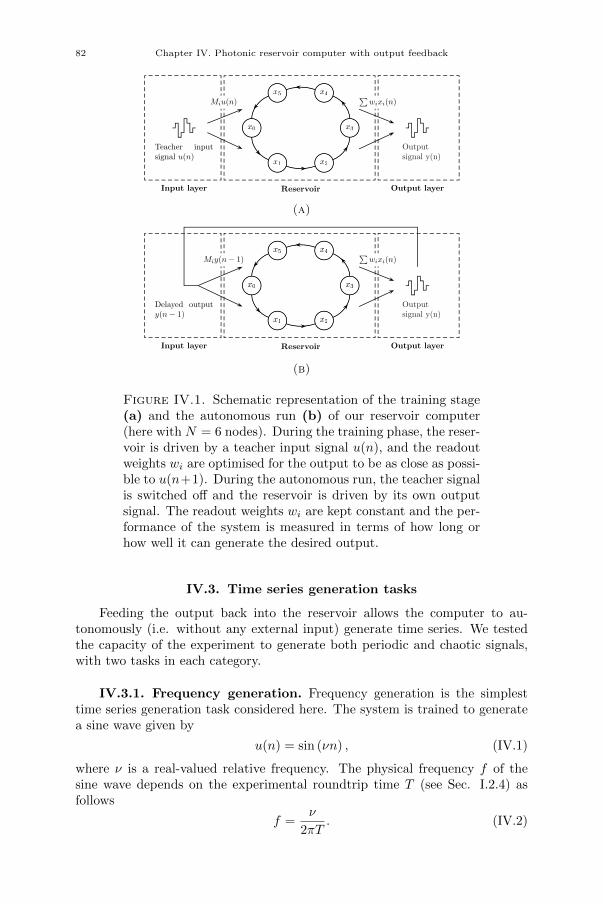
82 Chapter IV. Photonic reservoir computer with output feedback
x0
x1 x2
x5 x4
x3x0
x1 x2
x5 x4
x3
Miu(n)∑
wixi(n)
Teacher inputsignal u(n)
Outputsignal y(n)
Input layer Reservoir Output layer
(a)
x0
x1 x2
x5 x4
x3x0
x1 x2
x5 x4
x3
Miy(n− 1)∑
wixi(n)
Delayed outputy(n− 1)
Outputsignal y(n)
Input layer Reservoir Output layer
(b)
Figure IV.1. Schematic representation of the training stage(a) and the autonomous run (b) of our reservoir computer(here with N = 6 nodes). During the training phase, the reser-voir is driven by a teacher input signal u(n), and the readoutweights wi are optimised for the output to be as close as possi-ble to u(n+1). During the autonomous run, the teacher signalis switched off and the reservoir is driven by its own outputsignal. The readout weights wi are kept constant and the per-formance of the system is measured in terms of how long orhow well it can generate the desired output.
IV.3. Time series generation tasks
Feeding the output back into the reservoir allows the computer to au-tonomously (i.e. without any external input) generate time series. We testedthe capacity of the experiment to generate both periodic and chaotic signals,with two tasks in each category.
IV.3.1. Frequency generation. Frequency generation is the simplesttime series generation task considered here. The system is trained to generatea sine wave given by
u(n) = sin (νn) , (IV.1)
where ν is a real-valued relative frequency. The physical frequency f of thesine wave depends on the experimental roundtrip time T (see Sec. I.2.4) asfollows
f =ν
2πT. (IV.2)
IV.3. Time series generation tasks 83
This task allows to measure the bandwidth of the system and investigate dif-ferent timescales within the neural network.
IV.3.2. Random pattern generation. Random pattern generation isa natural step forward from the frequency generation task to a more complexproblem – instead of a regularly-shaped continuous function, the system istrained to generate an arbitrarily-shaped discontinuous function (that remainsperiodic, though). Specifically, a pattern is a short sequence of L randomlychosen real numbers (here within the interval [−0.5, 0.5]) that is repeated peri-odically to form an infinite time series [9]. Similarly to the physical frequencyin Sec. IV.3.1, the physical period of the pattern is given by τpattern = L · T .The aim is to obtain a stable pattern generator, that reproduces precisely thepattern and does not deviate to another periodic behaviour. To evaluate theperformance of the generator, we compute the MSE between the reservoir out-put signal and the target pattern signal during the training phase and theautonomous run, with a maximal threshold set to 10−3. This value is some-what arbitrary, and one could have picked a different threshold. As will beillustrated in Figs. IV.12 and IV.16 in Sec. IV.7, the 10−3 level correspondsto the point where the RC strongly deviates from the starting trajectory onthe chaotic attractor. For consistency, we have used this threshold in all ourexperiments, for all tasks. If the error does not grow above the threshold dur-ing the autonomous run, the system is considered to accurately generate thetarget pattern. We also tested the long-term stability on several patterns byrunning the system for several hours, as will be described in Sec. IV.7.
IV.3.3. Mackey-Glass chaotic series prediction. The Mackey-Glassdelay differential equation
dx
dt= β
x(t− τ)
1 + xn(t− τ)− γx, (IV.3)
with τ , γ, β, n > 0 was introduced to illustrate the appearance of complexdynamics in physiological control systems [110]. To obtain chaotic dynamics,we set the parameters as in [29]: β = 0.2, γ = 0.1, τ = 17 and n = 10. Withthese characteristics, the Kaplan-Yorke dimension of the chaotic attractor is2.1 [112].
The equation was solved using the Runge-Kutta 4 method with a stepsizeof 1.0. To avoid unnecessary computations and save time, both in simulationsand experiments, we pre-generated a sequence of 106 samples that we used forall numerical and experimental investigations.
During autonomous run, without the correct teacher signal, the systemslowly deviates from the desired trajectory. The MSE is used to evaluate boththe training phase and the autonomous run. We then compute the number ofcorrect prediction steps, i.e. steps for which the MSE stays below the 10−3
threshold (see Sec. IV.3.2), during the autonomous run and use this figure toevaluate the performance of the system.
84 Chapter IV. Photonic reservoir computer with output feedback
IV.3.4. Lorenz chaotic series prediction. The Lorenz equations, asystem of three ordinary differential equations
dx
dt= σ (y − x) , (IV.4a)
dy
dt= −xz + rx− y, (IV.4b)
dz
dt= xy − bz, (IV.4c)
with σ, r, b > 0, was introduced as a simple model for atmospheric convection[111]. The system exhibits chaotic behaviour for σ = 10, b = 8/3 and r = 28[113], that we used in this study. This yields a chaotic attractor with thehighest Lyapunov exponent of λ = 0.906 [29]. The system was solved usingMatlab’s ode45 solver and a stepsize of 0.02, as in [29]. We used all computedpoints, meaning that one timestep of the reservoir computer corresponds toa step of 0.02 in the Lorenz time scale. To avoid unnecessary computationsand save time we pre-generated a sequence of 105 samples that we used forall numerical and experimental investigations. Following [29], we used the x-coordinate trajectory for training and testing, that we scaled by a factor of0.01.
IV.4. Experimental setup
Our experimental setup, schematised in Fig. IV.2, consists of two maincomponents: the opto-electronic reservoir and the FPGA board. The structureand operation of the opto-electronic reservoir have been discussed in Sec. I.2.4.In this section we will focus on a few particular aspects of this experiment. Thefunctioning of the FPGA will be presented in Sec. IV.5.
As the neurons are time-multiplexed, the maximal reservoir size dependson the delay from the fibre spool (Spool) and the sampling frequency of theAnalogue-to-Digital converter (ADC). While increasing the latter involves rel-atively high costs, one can lengthen the delay line fairly easily. In this work,we used two spools of single mode fibre of lengths 1.6 km and 10 km, approx-imately. The first produced a delay of 7.93 µs and allowed to fit N = 100neurons into the reservoir. The second spool was used to increase the delay upto 49.2 µs and the reservoir size up to N = 600. In both cases, the reservoirstates were sampled at approximately 200 MHz (the precise frequency, givenin Sec. IV.5, depends on the delay loop) and each state was averaged over 16samples in order to decrease the noise and remove the transients induced bythe finite bandwidth of the Digital-to-Analogue converter (DAC).
The experiment is operated as follows. First, the input mask Mi and theteacher signal u(n), generated in Matlab, are uploaded on the FPGA board,which then generates the masked input signalMi×u(n), sent to the reservoir viathe DAC. The resulting reservoir states xi(n) are sampled and averaged by theFPGA, and then sent to the computer in real time. That is, the design allows tocapture the reservoir states for any desired time interval. After training of thereservoir, the optimal readout weights wi are uploaded on the board. Becauseof the relatively long delay needed for the offline training, the reservoir needs
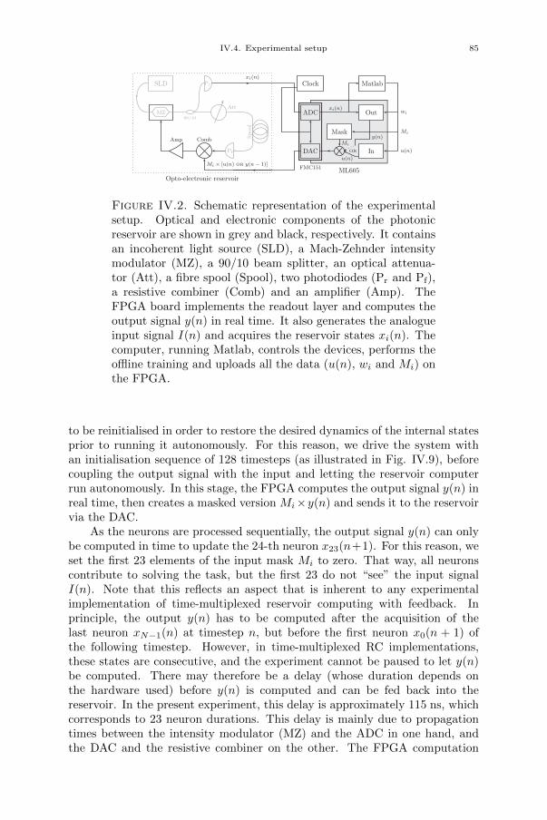
IV.4. Experimental setup 85
Opto-electronic reservoir
SLD
MZ90/10
Att
Amp Comb
Pf
Spool
Pr
ML605FMC151
DAC
ADC
In
Mask
Out
MatlabClock
u(n)
Mi
OR
xi(n)
y(n)
Mi × [u(n) OR y(n− 1)]
xi(n)
wi
Mi
u(n)
Figure IV.2. Schematic representation of the experimentalsetup. Optical and electronic components of the photonicreservoir are shown in grey and black, respectively. It containsan incoherent light source (SLD), a Mach-Zehnder intensitymodulator (MZ), a 90/10 beam splitter, an optical attenua-tor (Att), a fibre spool (Spool), two photodiodes (Pr and Pf),a resistive combiner (Comb) and an amplifier (Amp). TheFPGA board implements the readout layer and computes theoutput signal y(n) in real time. It also generates the analogueinput signal I(n) and acquires the reservoir states xi(n). Thecomputer, running Matlab, controls the devices, performs theoffline training and uploads all the data (u(n), wi and Mi) onthe FPGA.
to be reinitialised in order to restore the desired dynamics of the internal statesprior to running it autonomously. For this reason, we drive the system withan initialisation sequence of 128 timesteps (as illustrated in Fig. IV.9), beforecoupling the output signal with the input and letting the reservoir computerrun autonomously. In this stage, the FPGA computes the output signal y(n) inreal time, then creates a masked version Mi×y(n) and sends it to the reservoirvia the DAC.
As the neurons are processed sequentially, the output signal y(n) can onlybe computed in time to update the 24-th neuron x23(n+1). For this reason, weset the first 23 elements of the input mask Mi to zero. That way, all neuronscontribute to solving the task, but the first 23 do not “see” the input signalI(n). Note that this reflects an aspect that is inherent to any experimentalimplementation of time-multiplexed reservoir computing with feedback. Inprinciple, the output y(n) has to be computed after the acquisition of thelast neuron xN−1(n) at timestep n, but before the first neuron x0(n + 1) ofthe following timestep. However, in time-multiplexed RC implementations,these states are consecutive, and the experiment cannot be paused to let y(n)be computed. There may therefore be a delay (whose duration depends onthe hardware used) before y(n) is computed and can be fed back into thereservoir. In the present experiment, this delay is approximately 115 ns, whichcorresponds to 23 neuron durations. This delay is mainly due to propagationtimes between the intensity modulator (MZ) and the ADC in one hand, andthe DAC and the resistive combiner on the other. The FPGA computation

86 Chapter IV. Photonic reservoir computer with output feedback
Clock Gen
Experiment
xi(n)
Matlab
ML605FMC151
CLK expclk
ADC
DACMi × I(n)
ETH
ethclk
fmc151
etherphy
exp2fpga
xi(n)
fpga2exp
etherctrl
bramRec
comprcout
y(n)
bram2ether
bramWts
wi
bramMsk
Mi
bramInp
u(n)BRAMs
Figure IV.3. Simplified schematics of the FPGA design.Modules (entities) are represented by rectangular boxes, on-board electronic components are shown with rounded rectan-gles. External hardware, such as the computer, running Mat-lab, the opto-electronic reservoir and the external clock gen-erator are shown in grey. The design is driven by two clocks:the experimental clock expclk and the Ethernet clock ethclk.Signals from these two clock domains are drawn in solid anddashed lines, respectively.
time also plays a role here, but it does not exceed 20 ns. As we will see belowthis delay has an impact on system performance.
IV.5. FPGA design
The same Xilinx ML605 evaluation board (see Sec. I.3.3) is used in this ex-periment, paired with a 4DSP FMC151 daughtercard. The simplified schemat-ics of the design is depicted in Fig. IV.3. Rectangular boxes represent mod-ules (entities), and rounded rectangles stand for electronic components on theML605 board, namely the FMC151 daughtercard and the onboard MarvellAlaska PHY device (88E1111) for Ethernet communications (ETH).
The operation of the FPGA is controlled from the computer, running Mat-lab, via a simple custom protocol through a Gbit Ethernet connection. Dataand various commands, such as memory read/write, or state change, are en-capsulated into standard UDP packages. The etherphy module interfaces theFPGA design with the Marvell Ethernet PHY chip, and the etherctrl modulereceives the UDP packets (frames) and decodes the commands and the data.It also creates the frames for sending data from FPGA to the computer.
Blocks of Random-Access Memory (BRAM) are used to store data, such asteacher inputs u(n), input masks Mi and readout weights wi, that are generatedon the computer and uploaded on the FPGA. Each type of data is assigned aspecific module, since they vary in size (e.g. 600 values for the input mask andup to 3000 for the teacher signal) and resolution, as will be explained below.The bramRec is a buffer-like module, designed to transfer the signal recordedfrom the experiment directly to the computer through Ethernet, without per-manently storing it in memory. It consists of two blocks of RAM of 2048 byteseach, that are used as follows: while the recorded signal is written into the firstblock, bram2ether reads the contents of the second, that is then encapsulated
IV.5. FPGA design 87
into four UDP frames sent to the computer. When the first block is full, theblocks are switched and the process continues.
The FMC151 daughtercard is interfaced with the rest of the design throughthe fmc151 module, that outputs two 14-bit signals from the ADCs and receivestwo 16-bit signals from the DACs. The FMC151 card is also used to deliver aclock signal from an external clock generator, that produces a high-precisionsignal, allowing to synchronise the FPGA with the delay loop of the experimen-tal setup. This clock signal was generated by the Hewlett Packard 8648A signalgenerator. As our experiment has two delay loops (see Sec. IV.4), these needto be precisely synchronised. To this end, we fine-tuned the clock frequency soas to fit 16 samples per neuron into the roundtrip time T . Specifically, for thelarge spool with N = 600 reservoir states, we sampled at 195.4472 MHz, whilefor the small spool with N = 100 neurons we sampled at 203.7831 MHz.
The fpga2exp module controls the signal sent to the opto-electronic reser-voir through the DAC. During the training phase, it generates the masked inputsignal Mi × u(n) by multiplying the inputs u(n) by the mask Mi, both beingread from the BRAMs. During the autonomous run, it receives the reservoiroutput signal y(n), computed by the comprcout module, masks it and transfersto the DAC.
The neuron states xi(n) from the photonic reservoir are sampled and aver-aged by the exp2fpga module. During the training phase, these are buffered inbramRec, then processed by the bram2ether module and sent to the computer.During the autonomous run, the reservoir states are used by the comprcout, to-gether with the readout weights wi, read from the bramWts memory, to computethe reservoir output y(n). It is then injected back into the reservoir throughthe fpga2exp, and also transferred to the computer through the bramRec andbram2ether modules.
The design is driven by two clocks: the experimental clock expclk (around200 MHz, depending on the loop delay T , see above) that operates data ac-quisition and generation modules and allows to synchronise the FPGA withthe experiment, and the 125 MHz Ethernet clock ethclk. Both clocks have tobe managed properly within the design, as several signals, such as inputs orweights, coexist in both clock domains. That is, data to BRAMs comes fromthe Ethernet modules, and is thus driven by the ethclk clock. On the otherhand, this same data is used by the fpga2exp module, and has to appear inthe expclk clock domain. To this end, we exploit the dual-port capability ofXilinx block RAMs. That is, data is written into memory blocks through portA at clock ethclk and read from port B at clock expclk (and vice versa for thebramRec). This allows for smooth transition of data between clock domains.The two clock domains are depicted in Fig. IV.3 as follows: signals running atexpclk are shown in solid lines, and those clocking at ethclk are drawn withdashed lines.
The arithmetic operations computed by the FPGA are performed on realnumbers. However, the chip is a logic device, designed to operate bits. Theperformance of the design thus highly depends on the bit-representation of realnumbers, i.e. the precision. The main constraint comes from the ADC andDAC, limited to 14 and 16 bits, respectively. Numerical simulations, reported in
88 Chapter IV. Photonic reservoir computer with output feedback
[9], show that such precision is sufficient for all tasks studied in this work. It wasalso shown in [9] that the precision of the readout weights wi has a significantimpact on the performance of the system. For this reason we designed theexperiment for optimal utilisation of the resolution available. The reservoirstates were tuned to lie within a ]−1,+1[ interval. They are thus represented as16-bit integers, with 1 bit for the sign and 15 bits for the decimal part. Anotherlimitation comes from DSP48E slices, used to multiply the states xi(n) by thereadout weights wi. These blocks are designed to multiply a 25-bit integer bya 18-bit integer. To meet these requirements, we also keep the readout weightswi within the ]−1, 1[ interval and represent them as 25-bit integers, with 1 signbit and 24 decimal bits. To ensure that wi ∈]− 1, 1[, we amplify the reservoirstates digitally inside the FPGA. That is, the xi(n) are multiplied by 8 afteracquisition, prior to computing the output signal y(n).
IV.6. Numerical simulations
In addition to the physical experiments, we investigated the proposed setupin numerical simulations, to have a point of comparison and identify possiblemalfunctions. To this end, we developed three models that simulate the exper-iment to different degrees of accuracy. Our custom Matlab scripts are basedon [9, 48].
Idealised model: It incorporates the core characteristics of our reservoir com-puter, i.e. the ring-like architecture, the sine nonlinearity and thelinear readout layer (as described by equations I.5 and I.6), disre-garding all experimental considerations. We use this model to definethe maximal performance achievable in each configuration.
Noiseless experimental model: This model emulates the most influentialfeatures of the experimental setup, such as the high-pass filter of theamplifier, the finite resolution of the ADC and DAC, and precise inputand feedback gains. This model allows to cross-check the experimentalresults and to easily identify the problematic points.
Noisy experimental model: Contrary to the noiseless numerical models in-troduced above, our experimental implementation is noisy, which, aswill be explained below, has a significant impact on performance. Inorder to compare our experimental results to a more realistic model,we estimated the level of noise present in the experimental system(see Sec. IV.7.1), and incorporated this noise into the noisy versionof the experimental model.
IV.7. Results
In this section we present the experimental results, compare them to nu-merical simulations and discuss the performance of the reservoir computer oneach task introduced in Sec. IV.3.
The two periodic signal generation tasks were solved using a small reservoirwith N = 100 and a fibre spool of approximately 1.6 km. The chaotic signalgeneration tasks, being more complex, required a large reservoir of N = 600for decent results, that we fit in a delay line of roughly 10 km.
IV.7. Results 89
IV.7.1. Noisy reservoir. For most tasks studied here, we found the ex-perimental noise to be the major source of performance degradation in com-parison to numerical investigations. In fact, previously reported simulations[9] considered an ideal noiseless reservoir, while our experiment is noisy. Thisnoise can come from the active and even passive components of the setup: theamplifier, which has a relatively high gain and is therefore very sensitive tosmall parasitic signals (e.g. from the power source), the DAC, the photodiodesand the optical attenuator (shot noise). In-depth experimental investigationshave shown that, in fact, each component contributes more or less equally tothe overall noise level. Thus, it cannot be reduced by replacing one “faulty”component. Neither can it be averaged out, as the output value has to becomputed at each timestep. This noise was found to have a significant impacton the results, as will be shown in the following sections. For this reason weestimated the level of noise present in the experimental system and incorpo-rated it to the numerical models. This allows us to “switch off” the noise insimulations, which is impossible experimentally.
Fig. IV.4 shows numerical and experimental reservoir states of a 100-neuron reservoir, as received by the readout photodiode. That is, the curvesdepict the time-multiplexed neurons: each point represents a reservoir statex0...99(n) at times n = 1 and n = 2. The system does not receive any inputsignal I(n) = 0. The experimental signal is plotted with a solid grey line.We use it to compute the experimental noise level by taking the standarddeviation of the signal, which gives 2×10⁻³. We then employed this noise levelin the noisy experimental model to compare experimental results to numericalsimulations. The dotted black curve in Fig. IV.4 shows the response of thenoisy experimental model, with the same amount of Gaussian noise (standarddeviation of 2.0× 10⁻³) as in the experiment. The choice of a Gaussian noisedistribution was validated by experimental measurements.
The level of the experimental noise can also be characterised by the Signal-to-Noise Ratio (SNR), defined as [114]
SNR = 10 log10
(RMS2
signal
RMS2noise
),
where RMS is the Root Mean Square value, given by
RMS(xi) =
√√√√ 1
N
N∑
i=1
x2i .
We measured RMSsignal = 0.2468 and RMSnoise = 0.0023, so the SNR is equalto approximately 40 dB in this case. Note that this figure is given as anindicator of order of magnitude only as the RMS of the reservoir states dependson the gain parameters (α and β in Eqs. I.5) and varies from one experimentto another.
IV.7.2. Frequency generation. We found the frequency generation taskto be the only one not affected by noise. That is, our experimental resultsmatched accurately the numerical predictions reported in [10]. Concretely, weexpected a bandwidth of ν ∈ [0.06, π] with a 100-neuron reservoir. The upper
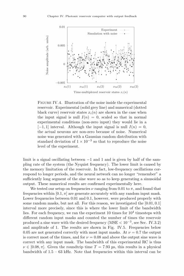
90 Chapter IV. Photonic reservoir computer with output feedback
−0.005
0
0.005
0.01
x0(1) x50(1) x0(2) x50(2) x99(2)
Noiseamplitude(arb.units)
Time-multiplexed reservoir states xi(n)
ExperimentSimulation with noise
Figure IV.4. Illustration of the noise inside the experimentalreservoir. Experimental (solid grey line) and numerical (dottedblack curve) reservoir states xi(n) are shown in the case whenthe input signal is null I(n) = 0, scaled so that in normalexperimental conditions (non-zero input) they would lie in a[−1, 1] interval. Although the input signal is null I(n) = 0,the actual neurons are non-zero because of noise. Numericalnoise was generated with a Gaussian random distribution withstandard deviation of 1× 10⁻³ so that to reproduce the noiselevel of the experiment.
limit is a signal oscillating between −1 and 1 and is given by half of the sam-pling rate of the system (the Nyquist frequency). The lower limit is caused bythe memory limitation of the reservoir. In fact, low-frequency oscillations cor-respond to longer periods, and the neural network can no longer “remember” asufficiently long segment of the sine wave so as to keep generating a sinusoidaloutput. These numerical results are confirmed experimentally here.
We tested our setup on frequencies ν ranging from 0.01 to π, and found thatfrequencies within [0.1, π] are generate accurately with any random input mask.Lower frequencies between 0.01 and 0.1, however, were produced properly withsome random masks, but not all. For this reason, we investigated the [0.01, 0.1]interval more precisely, since this is where the lower limit of the bandwidthlies. For each frequency, we ran the experiment 10 times for 104 timesteps withdifferent random input masks and counted the number of times the reservoirproduced a sine wave with the desired frequency (MSE < 10−3, see Sec. IV.3.2)and amplitude of 1. The results are shown in Fig. IV.5. Frequencies below0.05 are not generated correctly with most input masks. At ν = 0.7 the outputis correct most of the times, and for ν = 0.08 and above the output sine wave iscorrect with any input mask. The bandwidth of this experimental RC is thusν ∈ [0.08, π]. Given the roundtrip time T = 7.93 µs, this results in a physicalbandwidth of 1.5 – 63 kHz. Note that frequencies within this interval can be
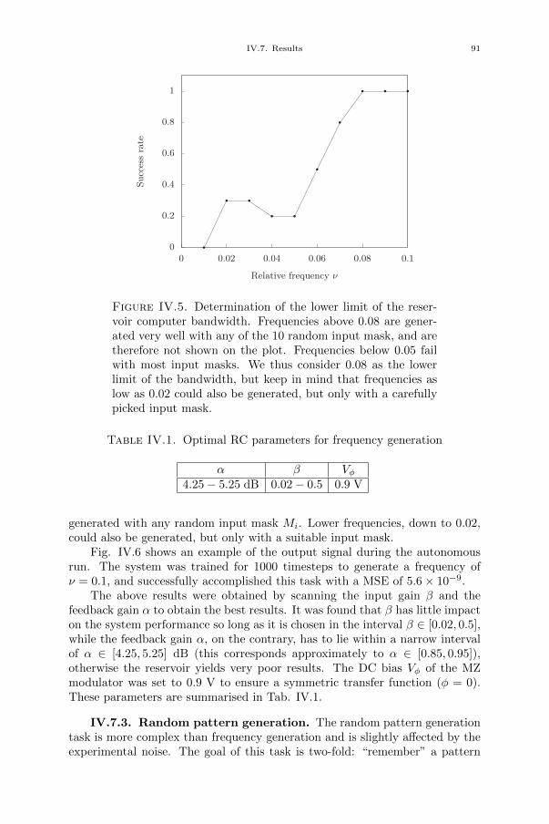
IV.7. Results 91
0
0.2
0.4
0.6
0.8
1
0 0.02 0.04 0.06 0.08 0.1
Successrate
Relative frequency ν
Figure IV.5. Determination of the lower limit of the reser-voir computer bandwidth. Frequencies above 0.08 are gener-ated very well with any of the 10 random input mask, and aretherefore not shown on the plot. Frequencies below 0.05 failwith most input masks. We thus consider 0.08 as the lowerlimit of the bandwidth, but keep in mind that frequencies aslow as 0.02 could also be generated, but only with a carefullypicked input mask.
Table IV.1. Optimal RC parameters for frequency generation
α β Vφ4.25− 5.25 dB 0.02− 0.5 0.9 V
generated with any random input mask Mi. Lower frequencies, down to 0.02,could also be generated, but only with a suitable input mask.
Fig. IV.6 shows an example of the output signal during the autonomousrun. The system was trained for 1000 timesteps to generate a frequency ofν = 0.1, and successfully accomplished this task with a MSE of 5.6× 10⁻⁹.
The above results were obtained by scanning the input gain β and thefeedback gain α to obtain the best results. It was found that β has little impacton the system performance so long as it is chosen in the interval β ∈ [0.02, 0.5],while the feedback gain α, on the contrary, has to lie within a narrow intervalof α ∈ [4.25, 5.25] dB (this corresponds approximately to α ∈ [0.85, 0.95]),otherwise the reservoir yields very poor results. The DC bias Vφ of the MZmodulator was set to 0.9 V to ensure a symmetric transfer function (φ = 0).These parameters are summarised in Tab. IV.1.
IV.7.3. Random pattern generation. The random pattern generationtask is more complex than frequency generation and is slightly affected by theexperimental noise. The goal of this task is two-fold: “remember” a pattern
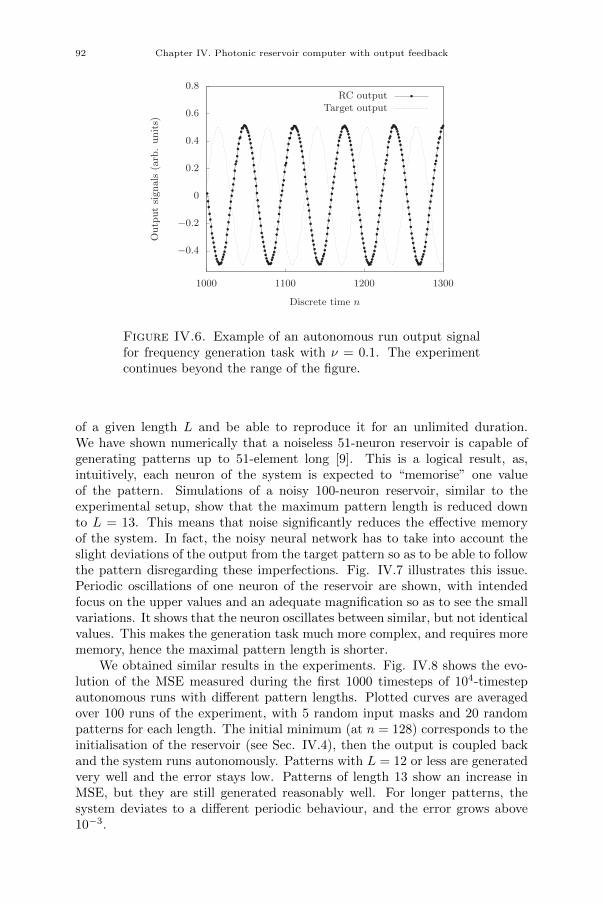
92 Chapter IV. Photonic reservoir computer with output feedback
−0.4
−0.2
0
0.2
0.4
0.6
0.8
1000 1100 1200 1300
Outputsignals
(arb.units)
Discrete time n
RC outputTarget output
Figure IV.6. Example of an autonomous run output signalfor frequency generation task with ν = 0.1. The experimentcontinues beyond the range of the figure.
of a given length L and be able to reproduce it for an unlimited duration.We have shown numerically that a noiseless 51-neuron reservoir is capable ofgenerating patterns up to 51-element long [9]. This is a logical result, as,intuitively, each neuron of the system is expected to “memorise” one valueof the pattern. Simulations of a noisy 100-neuron reservoir, similar to theexperimental setup, show that the maximum pattern length is reduced downto L = 13. This means that noise significantly reduces the effective memoryof the system. In fact, the noisy neural network has to take into account theslight deviations of the output from the target pattern so as to be able to followthe pattern disregarding these imperfections. Fig. IV.7 illustrates this issue.Periodic oscillations of one neuron of the reservoir are shown, with intendedfocus on the upper values and an adequate magnification so as to see the smallvariations. It shows that the neuron oscillates between similar, but not identicalvalues. This makes the generation task much more complex, and requires morememory, hence the maximal pattern length is shorter.
We obtained similar results in the experiments. Fig. IV.8 shows the evo-lution of the MSE measured during the first 1000 timesteps of 104-timestepautonomous runs with different pattern lengths. Plotted curves are averagedover 100 runs of the experiment, with 5 random input masks and 20 randompatterns for each length. The initial minimum (at n = 128) corresponds to theinitialisation of the reservoir (see Sec. IV.4), then the output is coupled backand the system runs autonomously. Patterns with L = 12 or less are generatedvery well and the error stays low. Patterns of length 13 show an increase inMSE, but they are still generated reasonably well. For longer patterns, thesystem deviates to a different periodic behaviour, and the error grows above10−3.
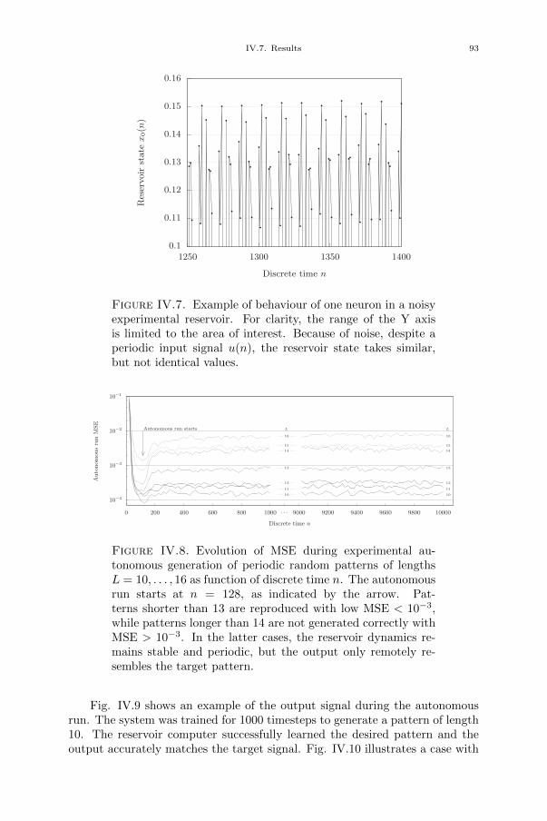
IV.7. Results 93
0.1
0.11
0.12
0.13
0.14
0.15
0.16
1250 1300 1350 1400
Reservoir
state
x0(n
)
Discrete time n
Figure IV.7. Example of behaviour of one neuron in a noisyexperimental reservoir. For clarity, the range of the Y axisis limited to the area of interest. Because of noise, despite aperiodic input signal u(n), the reservoir state takes similar,but not identical values.
10−4
10−3
10−2
10−1
0 200 400 600 800 1000 · · · 9000 9200 9400 9600 9800 10000
Autonomous run starts
· · · 10 · · ·· · · 11 · · ·· · · 12 · · ·
· · · 13 · · ·
· · · 14 · · ·· · · 15 · · ·
· · · 16 · · ·
L
10
11
12
13
14
15
16
L
AutonomousrunMSE
Discrete time n
Figure IV.8. Evolution of MSE during experimental au-tonomous generation of periodic random patterns of lengthsL = 10, . . . , 16 as function of discrete time n. The autonomousrun starts at n = 128, as indicated by the arrow. Pat-terns shorter than 13 are reproduced with low MSE < 10−3,while patterns longer than 14 are not generated correctly withMSE > 10−3. In the latter cases, the reservoir dynamics re-mains stable and periodic, but the output only remotely re-sembles the target pattern.
Fig. IV.9 shows an example of the output signal during the autonomousrun. The system was trained for 1000 timesteps to generate a pattern of length10. The reservoir computer successfully learned the desired pattern and theoutput accurately matches the target signal. Fig. IV.10 illustrates a case with
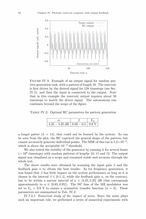
94 Chapter IV. Photonic reservoir computer with output feedback
−0.6
−0.3
0
0.3
0.6
0.9
50 100 150
Autonomous run starts
Outputsignals
(arb.units)
Discrete time n
Target outputRC output
Figure IV.9. Example of an output signal for random pat-tern generation task, with a pattern of length 10. The reservoiris first driven by the desired signal for 128 timesteps (see Sec.IV.5), and then the input is connected to the output. Notethat in this example the reservoir output requires about 50timesteps to match the driver signal. The autonomous runcontinues beyond the scope of the figure.
Table IV.2. Optimal RC parameters for pattern generation
α β Vφ4.25− 5.25 dB 0.02− 0.5 0.9 V
a longer patter (L = 14), that could not be learned by the system. As canbe seen from the plot, the RC captured the general shape of the pattern, butcannot accurately generate individual points. The MSE of this run is 5.2×10⁻³,which is above the acceptable 10−3 threshold.
We also tested the stability of the generator by running it for several hours(∼ 109 timesteps) with random patterns of lengths 10, 11 and 12. The outputsignal was visualised on a scope and remained stable and accurate through thewhole test.
The above results were obtained by scanning the input gain β and thefeedback gain α to obtain the best results. As for frequency generation, itwas found that β has little impact on the system performance so long as it ischosen in the interval β ∈ [0.1, 1], while the feedback gain α, on the contrary,has to lie within a narrow interval of α ∈ [4.25, 5.25] dB (this correspondsapproximately to α ∈ [0.85, 0.95]). The DC bias of the MZ modulator wasset to Vφ = 0.9 V to ensure a symmetric transfer function (φ = 0). Theseparameters are summarised in Tab. IV.2.
IV.7.3.1. Numerical study of the impact of noise. Since the noise playssuch an important role, we performed a series of numerical experiments with
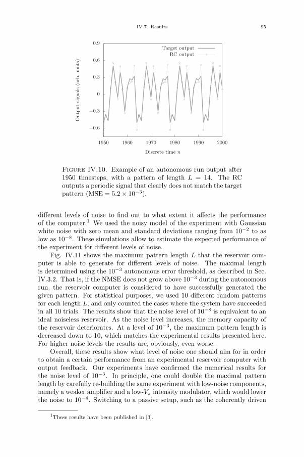
IV.7. Results 95
−0.6
−0.3
0
0.3
0.6
0.9
1950 1960 1970 1980 1990 2000
Outputsignals
(arb.units)
Discrete time n
Target outputRC output
Figure IV.10. Example of an autonomous run output after1950 timesteps, with a pattern of length L = 14. The RCoutputs a periodic signal that clearly does not match the targetpattern (MSE = 5.2× 10⁻³).
different levels of noise to find out to what extent it affects the performanceof the computer.1 We used the noisy model of the experiment with Gaussianwhite noise with zero mean and standard deviations ranging from 10−2 to aslow as 10−8. These simulations allow to estimate the expected performance ofthe experiment for different levels of noise.
Fig. IV.11 shows the maximum pattern length L that the reservoir com-puter is able to generate for different levels of noise. The maximal lengthis determined using the 10−3 autonomous error threshold, as described in Sec.IV.3.2. That is, if the NMSE does not grow above 10−3 during the autonomousrun, the reservoir computer is considered to have successfully generated thegiven pattern. For statistical purposes, we used 10 different random patternsfor each length L, and only counted the cases where the system have succeededin all 10 trials. The results show that the noise level of 10−8 is equivalent to anideal noiseless reservoir. As the noise level increases, the memory capacity ofthe reservoir deteriorates. At a level of 10−3, the maximum pattern length isdecreased down to 10, which matches the experimental results presented here.For higher noise levels the results are, obviously, even worse.
Overall, these results show what level of noise one should aim for in orderto obtain a certain performance from an experimental reservoir computer withoutput feedback. Our experiments have confirmed the numerical results forthe noise level of 10−3. In principle, one could double the maximal patternlength by carefully re-building the same experiment with low-noise components,namely a weaker amplifier and a low-Vπ intensity modulator, which would lowerthe noise to 10−4. Switching to a passive setup, such as the coherently driven
1These results have been published in [3].
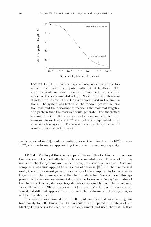
96 Chapter IV. Photonic reservoir computer with output feedback
0
20
40
60
80
100
10−8 10−7 10−6 10−5 10−4 10−3 10−2
Theoretical maximum
Our experiment
Max
imal
patt
ern
length
(L)
Noise level (standard deviation)
Figure IV.11. Impact of experimental noise on the perfor-mance of a reservoir computer with output feedback. Thegraph presents numerical results obtained with an accuratemodel of the experimental setup. Noise levels are shown asstandard deviations of the Gaussian noise used in the simula-tions. The system was tested on the random pattern genera-tion task and the performance metric is the maximal length Lof a pattern that the reservoir could generate. The theoreticalmaximum is L = 100, since we used a reservoir with N = 100neurons. Noise levels of 10−8 and below are equivalent to anideal noiseless system. The arrow indicates the experimentalresults presented in this work.
cavity reported in [49], could potentially lower the noise down to 10−5 or even10−6, with performance approaching the maximum memory capacity.
IV.7.4. Mackey-Glass series prediction. Chaotic time series genera-tion tasks were the most affected by the experimental noise. This is not surpris-ing, since chaotic systems are, by definition, very sensitive to noise. Reservoircomputing was first applied to this class of tasks in [29]. In their numericalwork, the authors investigated the capacity of the computer to follow a giventrajectory in the phase space of the chaotic attractor. We also tried this ap-proach, but since our experimental system performs as a “noisy” emulator ofthe chaotic attractor, its trajectory deviates very quickly from the target one,especially with a SNR as low as 40 dB (see Sec. IV.7.1). For this reason, weconsidered different approaches to evaluate the performance of the system, aswill be described below.
The system was trained over 1500 input samples and was running au-tonomously for 600 timesteps. In particular, we prepared 2100 steps of theMackey-Glass series for each run of the experiment and used the first 1500 as
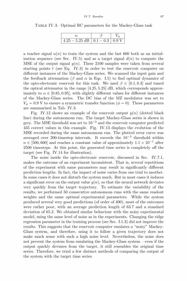
IV.7. Results 97
Table IV.3. Optimal RC parameters for the Mackey-Glass task
α β Vφ4.25− 5.25 dB 0.1− 0.3 0.9 V
a teacher signal u(n) to train the system and the last 600 both as an initial-isation sequence (see Sec. IV.5) and as a target signal d(n) to compute theMSE of the output signal y(n). These 2100 samples were taken from severalstarting points t (see Eq. IV.3) in order to test the reservoir computer ondifferent instances of the Mackey-Glass series. We scanned the input gain andthe feedback attenuation (β and α in Eqs. I.5) to find optimal dynamics ofthe opto-electronic reservoir for this task. We used β ∈ [0.1, 0.3] and tunedthe optical attenuator in the range [4.25, 5.25] dB, which corresponds approx-imately to α ∈ [0.85, 0.95], with slightly different values for different instancesof the Mackey-Glass series. The DC bias of the MZ modulator was set toVφ = 0.9 V to ensure a symmetric transfer function (φ = 0). These parametersare summarised in Tab. IV.3.
Fig. IV.12 shows an example of the reservoir output y(n) (dotted blackline) during the autonomous run. The target Mackey-Glass series is shown ingrey. The MSE threshold was set to 10−3 and the reservoir computer predicted435 correct values in this example. Fig. IV.13 displays the evolution of theMSE recorded during the same autonomous run. The plotted error curve wasaveraged over 200-timestep intervals. It exceeds the 10−3 threshold withinn ∈ [500, 600] and reaches a constant value of approximately 1.1 × 10⁻¹ after2500 timesteps. At this point, the generated time series is completely off thetarget (see Fig. IV.14 for illustration).
The noise inside the opto-electronic reservoir, discussed in Sec. IV.7.1,makes the outcome of an experiment inconsistent. That is, several repetitionsof the experiment with same parameters may result in significantly differentprediction lengths. In fact, the impact of noise varies from one trial to another.In some cases it does not disturb the system much. But in most cases it inducesa significant error on the output value y(n), so that the neural network deviatesvery quickly from the target trajectory. To estimate the variability of theresults, we performed 50 consecutive autonomous runs with the same readoutweights and the same optimal experimental parameters. While the systemproduced several very good predictions (of order of 400), most of the outcomeswere rather poor, with an average prediction length of 63.7 and a standarddeviation of 65.2. We obtained similar behaviour with the noisy experimentalmodel, using the same level of noise as in the experiments. Changing the ridgeregression parameter in the training process (see Sec. I.1.3) did not improve theresults. This suggests that the reservoir computer emulates a “noisy” Mackey-Glass system, and therefore, using it to follow a given trajectory does notmake much sense with such a high noise level. Nevertheless, the noise doesnot prevent the system from emulating the Mackey-Glass system – even if theoutput quickly deviates from the target, it still resembles the original timeseries. Therefore, we tried a few distinct methods of comparing the output ofthe system with the target time series.
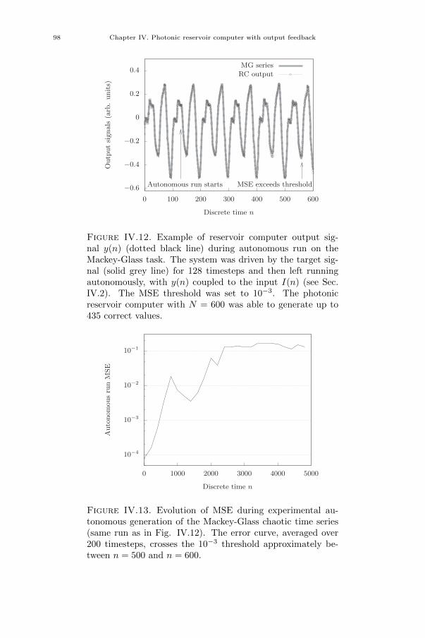
98 Chapter IV. Photonic reservoir computer with output feedback
−0.6
−0.4
−0.2
0
0.2
0.4
0 100 200 300 400 500 600
Autonomous run starts MSE exceeds threshold
Outputsignals
(arb.units)
Discrete time n
MG seriesRC output
Figure IV.12. Example of reservoir computer output sig-nal y(n) (dotted black line) during autonomous run on theMackey-Glass task. The system was driven by the target sig-nal (solid grey line) for 128 timesteps and then left runningautonomously, with y(n) coupled to the input I(n) (see Sec.IV.2). The MSE threshold was set to 10−3. The photonicreservoir computer with N = 600 was able to generate up to435 correct values.
10−4
10−3
10−2
10−1
0 1000 2000 3000 4000 5000
AutonomousrunMSE
Discrete time n
Figure IV.13. Evolution of MSE during experimental au-tonomous generation of the Mackey-Glass chaotic time series(same run as in Fig. IV.12). The error curve, averaged over200 timesteps, crosses the 10−3 threshold approximately be-tween n = 500 and n = 600.
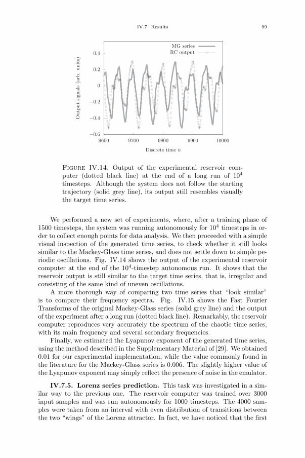
IV.7. Results 99
−0.6
−0.4
−0.2
0
0.2
0.4
9600 9700 9800 9900 10000
Outputsignals
(arb.units)
Discrete time n
MG seriesRC output
Figure IV.14. Output of the experimental reservoir com-puter (dotted black line) at the end of a long run of 104
timesteps. Although the system does not follow the startingtrajectory (solid grey line), its output still resembles visuallythe target time series.
We performed a new set of experiments, where, after a training phase of1500 timesteps, the system was running autonomously for 104 timesteps in or-der to collect enough points for data analysis. We then proceeded with a simplevisual inspection of the generated time series, to check whether it still lookssimilar to the Mackey-Glass time series, and does not settle down to simple pe-riodic oscillations. Fig. IV.14 shows the output of the experimental reservoircomputer at the end of the 104-timestep autonomous run. It shows that thereservoir output is still similar to the target time series, that is, irregular andconsisting of the same kind of uneven oscillations.
A more thorough way of comparing two time series that “look similar”is to compare their frequency spectra. Fig. IV.15 shows the Fast FourierTransforms of the original Mackey-Glass series (solid grey line) and the outputof the experiment after a long run (dotted black line). Remarkably, the reservoircomputer reproduces very accurately the spectrum of the chaotic time series,with its main frequency and several secondary frequencies.
Finally, we estimated the Lyapunov exponent of the generated time series,using the method described in the Supplementary Material of [29]. We obtained0.01 for our experimental implementation, while the value commonly found inthe literature for the Mackey-Glass series is 0.006. The slightly higher value ofthe Lyapunov exponent may simply reflect the presence of noise in the emulator.
IV.7.5. Lorenz series prediction. This task was investigated in a sim-ilar way to the previous one. The reservoir computer was trained over 3000input samples and was run autonomously for 1000 timesteps. The 4000 sam-ples were taken from an interval with even distribution of transitions betweenthe two “wings” of the Lorenz attractor. In fact, we have noticed that the first
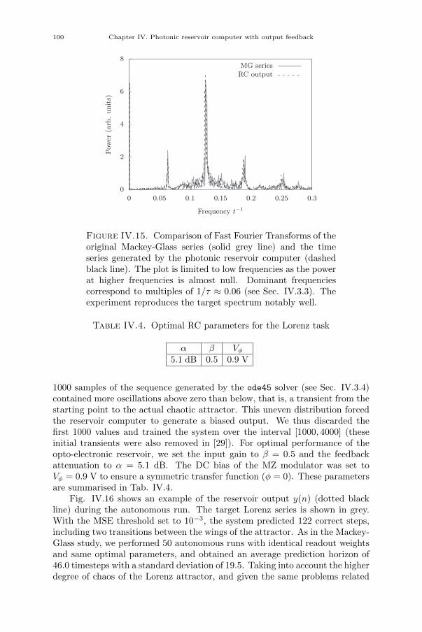
100 Chapter IV. Photonic reservoir computer with output feedback
0
2
4
6
8
0 0.05 0.1 0.15 0.2 0.25 0.3
Pow
er(arb.units)
Frequency t−1
MG seriesRC output
Figure IV.15. Comparison of Fast Fourier Transforms of theoriginal Mackey-Glass series (solid grey line) and the timeseries generated by the photonic reservoir computer (dashedblack line). The plot is limited to low frequencies as the powerat higher frequencies is almost null. Dominant frequenciescorrespond to multiples of 1/τ ≈ 0.06 (see Sec. IV.3.3). Theexperiment reproduces the target spectrum notably well.
Table IV.4. Optimal RC parameters for the Lorenz task
α β Vφ5.1 dB 0.5 0.9 V
1000 samples of the sequence generated by the ode45 solver (see Sec. IV.3.4)contained more oscillations above zero than below, that is, a transient from thestarting point to the actual chaotic attractor. This uneven distribution forcedthe reservoir computer to generate a biased output. We thus discarded thefirst 1000 values and trained the system over the interval [1000, 4000] (theseinitial transients were also removed in [29]). For optimal performance of theopto-electronic reservoir, we set the input gain to β = 0.5 and the feedbackattenuation to α = 5.1 dB. The DC bias of the MZ modulator was set toVφ = 0.9 V to ensure a symmetric transfer function (φ = 0). These parametersare summarised in Tab. IV.4.
Fig. IV.16 shows an example of the reservoir output y(n) (dotted blackline) during the autonomous run. The target Lorenz series is shown in grey.With the MSE threshold set to 10−3, the system predicted 122 correct steps,including two transitions between the wings of the attractor. As in the Mackey-Glass study, we performed 50 autonomous runs with identical readout weightsand same optimal parameters, and obtained an average prediction horizon of46.0 timesteps with a standard deviation of 19.5. Taking into account the higherdegree of chaos of the Lorenz attractor, and given the same problems related
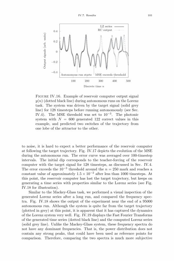
IV.7. Results 101
−0.4
−0.2
0
0.2
0.4
100 200 300 400 500
Autonomous run starts MSE exceeds threshold
Outputsignals
(arb.units)
Discrete time n
LZ seriesRC output
Figure IV.16. Example of reservoir computer output signaly(n) (dotted black line) during autonomous runs on the Lorenztask. The system was driven by the target signal (solid greyline) for 128 timesteps before running autonomously (see Sec.IV.4). The MSE threshold was set to 10−3. The photonicsystem with N = 600 generated 122 correct values in thisexample, and predicted two switches of the trajectory fromone lobe of the attractor to the other.
to noise, it is hard to expect a better performance of the reservoir computerat following the target trajectory. Fig. IV.17 depicts the evolution of the MSEduring the autonomous run. The error curve was averaged over 100-timestepintervals. The initial dip corresponds to the teacher-forcing of the reservoircomputer with the target signal for 128 timesteps, as discussed in Sec. IV.4.The error exceeds the 10−3 threshold around the n = 250 mark and reaches aconstant value of approximately 1.5× 10⁻² after less than 1000 timesteps. Atthis point, the reservoir computer has lost the target trajectory, but keeps ongenerating a time series with properties similar to the Lorenz series (see Fig.IV.18 for illustration).
Similar to the Mackey-Glass task, we performed a visual inspection of thegenerated Lorenz series after a long run, and compared the frequency spec-tra. Fig. IV.18 shows the output of the experiment near the end of a 95000autonomous run. Although the system is quite far from the target trajectory(plotted in grey) at this point, it is apparent that it has captured the dynamicsof the Lorenz system very well. Fig. IV.19 displays the Fast Fourier Transformsof the generated time series (dotted black line) and the computed Lorenz series(solid grey line). Unlike the Mackey-Glass system, these frequency spectra donot have any dominant frequencies. That is, the power distribution does notcontain any strong peaks, that could have been used as reference points forcomparison. Therefore, comparing the two spectra is much more subjective
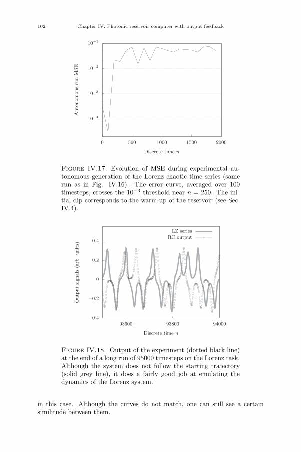
102 Chapter IV. Photonic reservoir computer with output feedback
10−4
10−3
10−2
10−1
0 500 1000 1500 2000
AutonomousrunMSE
Discrete time n
Figure IV.17. Evolution of MSE during experimental au-tonomous generation of the Lorenz chaotic time series (samerun as in Fig. IV.16). The error curve, averaged over 100timesteps, crosses the 10−3 threshold near n = 250. The ini-tial dip corresponds to the warm-up of the reservoir (see Sec.IV.4).
−0.4
−0.2
0
0.2
0.4
93600 93800 94000
Outputsignals
(arb.units)
Discrete time n
LZ seriesRC output
Figure IV.18. Output of the experiment (dotted black line)at the end of a long run of 95000 timesteps on the Lorenz task.Although the system does not follow the starting trajectory(solid grey line), it does a fairly good job at emulating thedynamics of the Lorenz system.
in this case. Although the curves do not match, one can still see a certainsimilitude between them.
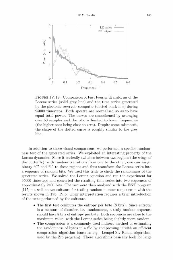
IV.7. Results 103
0
1
2
3
4
0 0.1 0.2 0.3 0.4 0.5 0.6
Pow
er(arb.units)
Frequency t−1
LZ seriesRC output
Figure IV.19. Comparison of Fast Fourier Transforms of theLorenz series (solid grey line) and the time series generatedby the photonic reservoir computer (dotted black line) during95000 timesteps. Both spectra are normalised so as to haveequal total power. The curves are smoothened by averagingover 50 samples and the plot is limited to lower frequencies(the higher ones being close to zero). Despite some mismatch,the shape of the dotted curve is roughly similar to the greyline.
In addition to those visual comparisons, we performed a specific random-ness test of the generated series. We exploited an interesting property of theLorenz dynamics. Since it basically switches between two regions (the wings ofthe butterfly), with random transitions from one to the other, one can assignbinary “0” and “1” to these regions and thus transform the Lorenz series intoa sequence of random bits. We used this trick to check the randomness of thegenerated series. We solved the Lorenz equation and ran the experiment for95000 timesteps and converted the resulting time series into two sequences ofapproximately 2400 bits. The two were then analysed with the ENT program[115] – a well known software for testing random number sequences – with theresults shown in Tab. IV.5. Their interpretation requires a brief introductionof the tests performed by the software.
• The first test computes the entropy per byte (8 bits). Since entropyis a measure of disorder, i.e. randomness, a truly random sequenceshould have 8 bits of entropy per byte. Both sequences are close to themaximum value, with the Lorenz series being slightly more random.• The compression is a commonly used indirect method of estimating
the randomness of bytes in a file by compressing it with an efficientcompression algorithm (such as e.g. Lempel-Ziv-Renau algorithm,used by the Zip program). These algorithms basically look for large
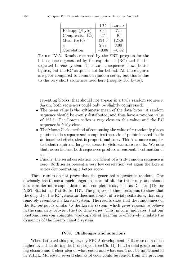
104 Chapter IV. Photonic reservoir computer with output feedback
RC LorenzEntropy (/byte) 6.6 7.1Compression (%) 17 10Mean (byte) 134.3 125.8π 2.88 3.00Correlation −0.08 −0.02
Table IV.5. Results returned by the ENT program for thebit sequences generated by the experiment (RC) and the in-tegrated Lorenz system. The Lorenz sequence shows betterfigures, but the RC output is not far behind. All these figuresare poor compared to common random series, but this is dueto the very short sequences used here (roughly 300 bytes).
repeating blocks, that should not appear in a truly random sequence.Again, both sequences could only be slightly compressed.• The mean value is the arithmetic mean of the data bytes. A random
sequence should be evenly distributed, and thus have a random valueof 127.5. The Lorenz series is very close to this value, and the RCsequence is fairly close.• The Monte Carlo method of computing the value of π randomly places
points inside a square and computes the ratio of points located insidean inscribed circle, that is proportional to π. This is a more complextest that requires a large sequence to yield accurate results. We notethat, nevertheless, both sequences produce a reasonable estimation ofπ.• Finally, the serial correlation coefficient of a truly random sequence is
zero. Both series present a very low correlation, yet again the Lorenzseries demonstrating a better score.
These results do not prove that the generated sequence is random. Oneobviously has to use a much longer sequence of bits for this study, and shouldalso consider more sophisticated and complete tests, such as Diehard [116] orNIST Statistical Test Suite [117]. The purpose of these tests was to show thatthe output of the RC generator does not consist of trivial oscillations, that onlyremotely resemble the Lorenz system. The results show that the randomness ofthe RC output is similar to the Lorenz system, which gives reasons to believein the similarity between the two time series. This, in turn, indicates, that ourphotonic reservoir computer was capable of learning to effectively emulate thedynamics of the Lorenz chaotic system.
IV.8. Challenges and solutions
When I started this project, my FPGA development skills were on a muchhigher level than during the first project (see Ch. II). I had a solid grasp on tim-ing closure and a clear idea of what could and what could not be implementedin VHDL. Moreover, several chunks of code could be reused from the previous
IV.9. Conclusion 105
projects, such as the Ethernet connection modules and the FMC151 daughter-card interface. But this time the FPGA had to be connected very tightly to theexperiment, making the synchronisation of all the module a crucial aspect. Infact, not only the reservoir states had to be sampled at the right moment, butthe output signal had to be computed and generated in a very tight timeframe.And since there is no easy way of simulating the opto-electronic reservoir inXilinx software, the development of the design was mostly done in hardware,which was very time-consuming.
Sooner or later, the FPGA design was operational and the first good resultsstarted to come. Sine waves were generated very nicely, and random patternswere stable for hours and even days. The maximum pattern length was signif-icantly lower than expected, though, but I did not pay much attention to thisdetail at first – I was happy that the experiment generated something stable atall. We then moved on to the Mackey-Glass task and this is where the prob-lems began. I managed to record several very good prediction lengths from theexperiment, but the results were very inconsistent. We know now that this isdue to the experimental noise, but we did not have that luxury at the time,and I passed a lot of time analysing the setup, trying to figure out what waswrong.
In my previous experiments, unstable outcomes indicated timing problemswith the FPGA chip. I double- (even triple-) checked the design and its be-haviour only to find that it was functioning flawlessly. Refusing to give up, Ideveloped a very precise numerical model of the opto-electronic reservoir, tak-ing into account all known characteristics of the hardware, up to the high-passfilter – but again, everything except the noise.
The ultimate revelation came when I was comparing individual reservoirstates from two different runs and noticed a significant difference between thevalues. A statistical analysis of ten identical runs of the experiment then showedeven higher deviations. Only then I though of adding these deviations to thesimulation model and – at last – the inconsistent outcomes of the experimentcould be reproduced numerically.
Once we acknowledged the noise as an inevitable “feature” of the experi-ment, a new question arose – how to evaluate the RC performance on chaoticsignals, since it was very bad at following a given trajectory? From observa-tions of the output signal, we could see that it is far from being trivial – buthow to show this quantitatively? Since these interrogations were new to ourteam, we tried to improvise a few simple solutions. The most interesting, inmy opinion, was the ENT test for the Lorenz attractor. Far from being a solidproof, it gave us some valuable numbers to quantify the properties of the RCoutput. I wish we could find something similar for the Mackey-Glass series,though. . .
IV.9. Conclusion
The present work demonstrates the potential of output feedback in hard-ware reservoir computing and constitutes an important step towards autono-mous photonic implementations of recurrent neural networks. Specifically, wepresented a photonic reservoir computer that is capable of generating both
106 Chapter IV. Photonic reservoir computer with output feedback
sine waves of different frequencies and short random patterns with substan-tial stability. Moreover, it could emulate the Mackey-Glass time series with aremarkably similar frequency spectrum, and a fairly close highest Lyapunov ex-ponent. Finally, it could efficiently capture the dynamics of the Lorenz systemand generate a time series with similar randomness properties. To the best ofour knowledge, this is the first report of these task being implemented on anexperimental reservoir computer.
The readout of the reservoir computer is carried out in real time on afast FPGA chip. This results in a digital output layer in an analogue device,that nevertheless allows one to investigate many of the issues that will affect asystem with purely analogue feedback. The latter is a much more complicatedexperiment. Indeed the only analogue output layers implemented so far onexperimental reservoir computers were reported in [73, 97, 98]. Using them foroutput feedback would require adding an additional electronic circuit consistingof a sample and hold circuit, amplification, and multiplication by the inputmask. The present experiment allows one to investigate the benefits that outputfeedback has to offer to experimental reservoir computing, while anticipatingthe difficulties and limitations that will affect a fully analogue implementation.Such a two-step procedure, in which part of the experiment is analogue andpart digital, is natural, and parallels the development of experimental reservoircomputers in which some of the first experiments were only partially analogue,see e.g. [51, 53].
This work allowed to highlight a critical limitation of the present opto-electronic setup, namely the relatively high level of noise generated by thecomponents. While this was not a concern in previous experiments with offlinereadout [48, 73], it becomes critical in this study of the output feedback. Sincethis noise cannot be averaged out, it propagates back into the system with out-put feedback and considerably deteriorates the reservoir states. This problemdoes not have a simple solution. One could rethink the entire experimentalsetup and rebuild it with new, less noisy components. One could also switch toa different experimental system, such as the low-noise passive cavity reportedin [49]. In any case, it will probably be difficult to increase the SNR above60 dB. There may also be algorithmic solutions, such as using conceptors [118,119].
The high level of experimental noise quickly pushed the reservoir computer,emulating a chaotic system, away from a given trajectory, which initiated thesearch for quantitative methods for the evaluation of the experiment perfor-mance. In this work, we introduced a few simple techniques, based on stan-dard signal analysis methods, such as statistics of the prediction length andvisual comparison of the time series and their frequency spectra after a longautonomous run. We have also proposed case-specific methods, such as therandomness test, that could only be applied to the Lorenz time series. Overall,these are only the first steps towards the answer to a very general question:given a noisy emulator of a known chaotic system, how best to evaluate itsperformance? It will be interesting to understand the relationship between theperformance obtained on the estimators above, and the properties of the cha-otic system, such as the Lyapunov exponents or the dimension and geometry

IV.9. Conclusion 107
of the chaotic attractor. These questions should lead to a rich new direction ofenquiry in the theory of nonlinear dynamics and complex systems.
Adding output feedback to experimental reservoir computers allows themto solve considerably more complex tasks than without output feedback. Futurework could address nonlinear computations that depend on past informationand that require persistent memory [120], FORCE training [121] (which how-ever requires that the learning time scale be short compared to the reservoirtime scale) and applications such as frequency modulation [106], or implemen-tation of conceptors [118, 119]. Ideally, an entirely analogue feedback shouldbe implemented, like in e.g. [4] (see also Ch. V), rather than the digital feed-back demonstrated here. The present work is therefore just a first step towardsrealising these additional applications.
Finally, going back to the question of biological implementation, our workshows that the biologically plausible structure of reservoir computing [30, 108,109] can be trained to generate highly complex temporal patterns, both periodicand chaotic, even in the presence of moderate levels of noise. Whether nature infact implements this mechanism remains to be seen, and will depend amongstother aspects on the amount of noise present in biological implementationsof reservoir computing, and whether there exist biologically plausible trainingmechanisms for this kind of signal generation.

CHAPTER V
Towards online-trained analogue readout layer
This chapter presents the last project that I started with the OPERA-Photoni-que group (the next and last Ch. V.6 will cover my internship at theUniversity of Texas at Austin, USA). At the moment of writing these lines, wepublished some interesting results, but they are based on numerical simulationsonly.
Ironically, building an improved analogue readout layer should have beenthe corner stone of my thesis: this was stated in my funding application, andthis probably was the main reason why the lab purchased a FPGA in the firstplace.
How comes that this project was not completed? I can see two explana-tions. First, we found an easier way to achieve the ultimate goal. In fact, oneof the key motivations for an efficient analogue readout was the possibility offeeding the output signal back into the reservoir. Chapter IV shows how thiscan be done with a much more simple digital layer, and what new features canbe obtained out of it. The second reason is a purely personal one. I had theaspiration to explore new research environments and when such an occasionappeared, I gladly took it. But I am getting ahead of myself – more on that inthe next chapter (Ch. V.6).
In fine, I believe we replaced my original thesis project with an even betterplan. Instead of investing time into the development of an analogue readoutlayer – a direction than has already been explored to some degree [73, 97, 98],we focused on the in-depth study of an experimental reservoir computer withoutput feedback (although digital) – a truly novel direction, that nobody hasinvestigated so far. But the story of the analogue readout layer is not over yet.Although the present thesis will only contain numerical results of this work, Istill have a couple of month in front of me to do more.
This chapter, based on our paper [4], is much shorter than the previousones: it does not contain sections on the FPGA design or on challenges andsolutions, since it does not present an actual physical experiment.
V.1. Introduction
The major drawback in experimental implementations of reservoir com-puting, listed in Sec. I.2, is the absence of efficient readout mechanisms: thestates of the neurons are collected and post-processed on a computer, severelyreducing the processing speeds and thus limiting the applicability. An ana-logue readout would resolve this issue, as suggested in [122]. This researchdirection has already been investigated experimentally in [73, 97, 98], but all
109
110 Chapter V. Towards online-trained analogue readout layer
these implementations suffered from significant performance degradation dueto the complex structure of the readout layer. Indeed the approach used inthese works was to characterise with high accuracy the linear output layer,whereupon it was possible to compute offline the output weights. However it isvirtually impossible to characterise each hardware component of the setup withsufficient level of accuracy. Furthermore the components in the output layermay have a slight nonlinear behaviour. It follows that this approach does notwork satisfactorily, as is apparent from the performance degradation reportedin [73].
In this work we address the above issues with the same online learningapproach we discussed in Ch. II. Online training has attracted much attentionin the machine learning community because it allows to optimise the systemgradually, as the input data becomes available. As we have shown in Ch. II,it can also easily cope with non-stationary input signal, whose characteristicschange with time, as the online approach can keep the model updated accordingto variations in the input. Finally, in the case of hardware systems, onlinetraining can easily cope with drifts in the hardware, as the system will adaptto gradual changes in the hardware components [72, 123].
In the context of reservoir computing, the online training implements agradient descent: it gradually changes the output layer to adapt to the task.More precisely the output layer is characterised by a series of parameters (thereadout weights), and in online training these weights are adjusted in smallincrements, so that the output of the system gets closer to the target signal.The important point in the present context is that, compared to previously usedoffline methods, in online training based on gradient descent no assumption isnecessary about how these weights contribute to the output signal. That is, it isnot necessary to model the output layer. Furthermore, the transfer function ofthe readout layer could in principle be nonlinear. Here we show, using realisticnumerical simulations, how these features could be highly advantageous fortraining hardware reservoir computers.
For concreteness, we consider in simulations the “same old” opto-electronicreservoir computing setup, introduced in Sec. I.2.4. We add to this setupan analogue layer that is now trained online by an FPGA chip processing thesimple gradient descent algorithm in real time, as in [1] and Ch. II. The readoutlayer consists of a simple Resistor-Capacitor (RC) circuit (as in [97]), instead ofa more complicated RLC circuit (consisting of a resistor R, an inductor L anda capacitor C) that was used to increase the amplitude of the output signal in[73].
We investigate the performance of this setup through numerical simulationson two benchmark tasks and show that previously encountered difficulties arealmost entirely alleviated by the online training approach. In other words,with a relatively simple analogue readout layer, trained online, and withoutany modelling of the underlying processes, we obtain results similar to thoseproduced by a digital layer, trained offline. We also explore a special case with anonlinear readout function and show that this complication does not decreasemuch the performance of the system. This work thus brings an interestingsolution to an important problem in the hardware reservoir computing field.
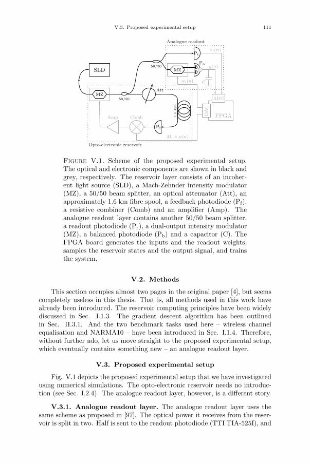
V.3. Proposed experimental setup 111
SLD
MZ50/50
50/50
Att
Amp Comb
Pf
1.6
km
Prxi(n)
MZ
Pb
-y(n)
C
FPGADAC
ADC
Mi × u(n)
wi(n)
Opto-electronic reservoir
Analogue readout
Figure V.1. Scheme of the proposed experimental setup.The optical and electronic components are shown in black andgrey, respectively. The reservoir layer consists of an incoher-ent light source (SLD), a Mach-Zehnder intensity modulator(MZ), a 50/50 beam splitter, an optical attenuator (Att), anapproximately 1.6 km fibre spool, a feedback photodiode (Pf),a resistive combiner (Comb) and an amplifier (Amp). Theanalogue readout layer contains another 50/50 beam splitter,a readout photodiode (Pr), a dual-output intensity modulator(MZ), a balanced photodiode (Pb) and a capacitor (C). TheFPGA board generates the inputs and the readout weights,samples the reservoir states and the output signal, and trainsthe system.
V.2. Methods
This section occupies almost two pages in the original paper [4], but seemscompletely useless in this thesis. That is, all methods used in this work havealready been introduced. The reservoir computing principles have been widelydiscussed in Sec. I.1.3. The gradient descent algorithm has been outlinedin Sec. II.3.1. And the two benchmark tasks used here – wireless channelequalisation and NARMA10 – have been introduced in Sec. I.1.4. Therefore,without further ado, let us move straight to the proposed experimental setup,which eventually contains something new – an analogue readout layer.
V.3. Proposed experimental setup
Fig. V.1 depicts the proposed experimental setup that we have investigatedusing numerical simulations. The opto-electronic reservoir needs no introduc-tion (see Sec. I.2.4). The analogue readout layer, however, is a different story.
V.3.1. Analogue readout layer. The analogue readout layer uses thesame scheme as proposed in [97]. The optical power it receives from the reser-voir is split in two. Half is sent to the readout photodiode (TTI TIA-525I), and
112 Chapter V. Towards online-trained analogue readout layer
the resulting voltage signal, containing the reservoir states xi(n), is recordedby the FPGA for the training process (see Eq. II.4). The other half is modu-lated by a dual-output Mach-Zehnder modulator (EOSPACE AX-2X2-0MSS-12) which applies the readout weights wi, generated by the DAC of the FPGA.The outputs of the modulator are connected to a balanced photodiode (TTITIA-527), which produces a voltage level proportional to difference of the lightintensities received at its two inputs. This allows to multiply the reservoir statesby both positive and negative weights [97]. The summation of the weightedstates is performed by a low-pass RC filter. The resistance R of the filter, notshown on the scheme, is the 50 Ω output impedance of the balanced photodi-ode. The resulting output signal, proportional to y(n), is also recorded by theFPGA, for training and performance evaluation.
Let us compute explicitly the output of the analogue readout layer. Thecapacitor integrates the output of the balanced photodiode with an exponentialkernel and a time constant τ . The impulse response of the RC filter is given in[114]
h(t) =1
RCe−tRC =
1
τe−tτ , (V.1)
the voltage Q(t) on the capacitor is then given by
Q(t) =
∫ t
−∞X(s)W (s)h(t− s)ds, (V.2)
where X(t) is the continuous signal, containing the reservoir states, and W (t)are the readout weights, applied to the dual-output intensity modulator. Theoutput y(n) is given by the charge on the capacitor at the discrete times t = nT :
y(n) = Q(nT ). (V.3)
Since X(t) and W (t) are piecewise functions X(t) = xi(n) and W (t) = wifor t ∈ [θ(i − 1), θi], where θ = T/N is the duration of one neuron, we canapproximate the integration by a discrete summation to obtain
y(n) = θ
N∑
i=1
wi
( ∞∑
k=0
xi(n− k)h(N − i−Nk)
)
=θ
τ
N∑
i=1
wi
( ∞∑
k=0
xi(n− k)e−ρ(N−i−Nk)
), (V.4)
where we have introduced the RC integrator ratio ρ = θ/τ .The readout layer output y(t) = Q(t) is thus a linear combination of the
reservoir states xi, weighted by wi and by the exponential kernel of the RCfilter. Note that contrary to usual reservoir computer outputs (see e.g. Eq.I.6), in Eq. V.4 the output at time n depends not only on the current statesxi(n), but also on the states at previous times xi(n− k).
In the previous experimental investigation of the analogue readout [73],the readout weights wi were computed using ridge regression [36] (see also Sec.I.1.3), assuming an output signal given by Eq. I.6. But since the experimentproduced an output similar to Eq. V.4 instead, the readout weights neededto be corrected appropriately. For more details, we refer to the original paper[73]. In the present work, the weights wi are adjusted gradually to match
V.4. Numerical simulations 113
the reservoir output signal y(n) with the target output d(n) (see Sec. II.3.1),without any assumptions about how these weights actually contribute to theoutput signal y(n). This is a much easier tasks, which allows to obtain betterexperimental results, as will be shown in Sec. V.5.
V.3.2. FPGA board. Similar to my previous experiments, the reservoircomputer is operated by a FPGA chip. We envision using the same XilinxML605 evaluation board, paired with the 4DSP FMC151 daughter card. Forthis experiment, we will need both ADCs and both DACs.
The FPGA generates the input signal Mi×u(n) and sends it into the opto-electronic reservoir. After recording the resulting reservoir states xi(n) fromone delay loop, it executes the simple gradient descent algorithm in order toupdate the readout weights wi(n+ 1). These are sent to the readout layer andused to generate the output signal y(n), also recorded by the FPGA.
V.4. Numerical simulations
All numerical experiments were performed in Matlab. We used a custommodel of our reservoir computer, based on previous investigations [1, 5, 48](see also Secs. II.6.3 and IV.6), that has been shown to emulate very well thedynamics of the real system. The simulations were performed in discrete time,and took into account the internal structure of the reservoir computer describedabove, such as the ring-like topology, the sine nonlinearity and the analoguereadout layer with an RC filter. The simulations allow to try out differentconfigurations and to scan various experimental parameters, including valuesthat are impossible to achieve experimentally or imposed by the hardware. Allsimulations were performed on a dedicated high-performance workstation with12-core CPU and 64 Gb RAM. Since the convergence of the gradient descentalgorithm is quite slow, we limited our investigations to a fast update ratek = 10 (see Eq. II.5), so that each simulation lasted about 24 hours.
The principal goal of the simulations was to check how the online learn-ing approach would cope with experimental difficulties encountered in previousworks [73, 97]. To that end, we gathered a list of possible issues and scannedthe corresponding experimental parameters in order to check the system per-formance. In particular, we investigated the following parameters:
• The RC integrator ratio ρ. This is the most important parameter ofthe analogue readout layer. While its accurate measure is not requiredin our setup – since we do not correct the readout weights wi – itdefines the integration span of the filter, and thus the reservoir statesthat contribute to the output signal. It can thus significantly influencethe results. Another question of importance is how dependent thesystem performance is on the exact value of ρ.• The MZ modulator bias. Mach-Zehnder modulators need to be ap-
plied a constant voltage to maintain their transfer function symmetricaround zero. The devices we were using up to now are subject to slightdrifts over time, often resulting in a non-perfectly symmetric response.We thus checked in simulations whether such an offset would impactthe results.
114 Chapter V. Towards online-trained analogue readout layer
• The DAC resolution. The precision of the DACs on the FMC151daughtercard is limited to 16 bits. Numerical investigations haveshown that the precision of readout weights has a significant impacton the performance, see e.g. [9, 124, 125]. We thus checked whetherthe resolution available is enough for this experiment.
Besides these potentially problematic parameters, we also scanned the inputand feedback gain parameters (denoted by β and α in Eqs. I.5) in order to findthe optimal dynamics of the reservoir for each task.
In a separate set of simulations, we investigated the applicability of theproposed method to nonlinear readout layers. That is, we checked whether thesimple gradient descent method would still work with a nonlinear response ofthe analogue readout layer with respect to the reservoir states xi(n) (see Eq.V.4). We picked two “saturation” functions of sigmoid shape. This choice arisesfrom the transfer function of common light detectors that are linear at lowerintensities and become nonlinear at higher intensities. We used the followingfunctions: a logistic function, given by
glg(x) =2
1 + e−2x− 1, (V.5)
and the hyperbolic tangent function, given by
ght(x) = 0.6 tanh (1.8x) . (V.6)
These functions, glg and ght, do not model any particular photodiode, but aretwo simple examples that allow us to address the above question. Both func-tions are plotted in Fig. V.4b, together with a linear response, for comparison.
We investigated two possible nonlinearities in the output layer. In the firstcase, the readout photodiode (Pr in Fig. V.1) produces a nonlinear response,while the balanced photodiode (Pb in Fig. V.1) remains linear. This scenario,that we shall refer to as “nonlinear readout”, allows one to investigate whathappens when the reservoir states xi used to compute the output signal y(n)(see Eq. I.6) differ from those employed to update the readout weights (seeEq. II.4). Thus, in this case the update rule (Eq. II.4) for the output weightsbecomes
wi(n+ 1) = wi(n) + λ (d(n)− y(n)) g(xi(n)), (V.7)
where g is given by either Eq. V.5 or Eq. V.6, while the output layer is givenby Eq. V.4.
In the second case, called “nonlinear output”, the readout photodiode islinear, but the balanced photodiode exhibits a saturable behaviour. In this casethe update rule Eq. II.4 for the output weights is unchanged, but the outputlayer Eq. V.4 becomes
y(n) =θ
τ
N∑
i=1
wi
( ∞∑
k=0
g(xi(n− k))e−ρ(N−i−Nk)
). (V.8)
Note that we have only considered cases with just one nonlinear photodiode, soas to check whether the difference between the reservoir states used for trainingand those to compute the readout (see Eqs. II.4 and I.6, respectively) would
V.5. Results 115
degrade the performance of the system. The scenario with both nonlinear pho-todiodes is hence more simple, as the reservoir states are the same in bothequations. One could consider the case with two photodiodes exhibiting differ-ent nonlinear behaviours. In that situation, similar to the results we will showin Sec. V.5, we expect the algorithm to cope with the difference up to a certainpoint, before running into troubles. For this reason, we leave that scenario forfuture investigations.
V.5. Results
For clarity, the results are split in two sections. First, we discuss theinfluence of the key parameters, listed in Sec. V.4, in the case of a linearreadout layer. Then, we consider the two nonlinear scenarios described above.
V.5.1. Linear readout: RC circuit. For each of the two tasks con-sidered here, we performed three kinds of simulations: we scanned the RCintegrator ratio ρ = θ/τ in the first simulation, the MZ bias in the second, andthe resolution of the DAC in the third. Furthermore, since different values ofthese parameters may work better with different dynamics of the reservoir, wealso scanned the input gain β and the feedback gain α in all three simulationsindependently, and applied the optimal values in each case.
For both tasks, we used a network withN = 50 neurons, as in most previousexperimental works [33, 48, 49, 73]. The reservoir was trained on 83000 inputs,with an update rate k = 10, and then tested over 105 symbols for the channelequalisation task and 104 inputs for NARMA10 task. For statistical purposes,we ran each simulation 10 times, with different random input masks. In thefollowing figures, averaged results over the masks are plotted, while the errorbars give the standard deviation over the different input masks. Results relatedto the channel equalisation task are plotted with solid lines, while dashed linescorrespond to those for NARMA10.
For the channel equalisation task, our system yields SERs between 10−4
and 10−3 depending on the input mask, as summarised in Tab. V.1 (firstline). This is comparable to previous experiments with the same opto-electronicreservoir: error rates of order of 10−4 were reported in [48] using a digitalreadout and in [73] with an analogue readout, using an RLC filter. The firstexperimental analogue system, using a simple RC circuit, as we did in thiswork, performed significantly worse, with SER of order of 10−2 [97]. Thatis, online learning does not outperform other methods, but allows to obtainsignificantly better results with a simpler setup.
As for the NARMA10 task, we obtain a NMSE of 0.20 ± 0.02. Previousexperiments with a digital readout layer produced 0.168±0.015 [48] and 0.107±0.012 [49]. With an analogue readout layer, the best NMSE reported was0.230±0.023 [73]. Our system thus slightly outperforms the analogue approach,and gets close to the digital one, except for the very good result obtained witha different reservoir, based on a passive cavity [49]. Again, our results wereobtained with a simple setup and no modelling of the readout, contrary to [73].
Furthermore, the error rates obtained here can be significantly loweredwith more training, as has been demonstrated numerically and experimentally
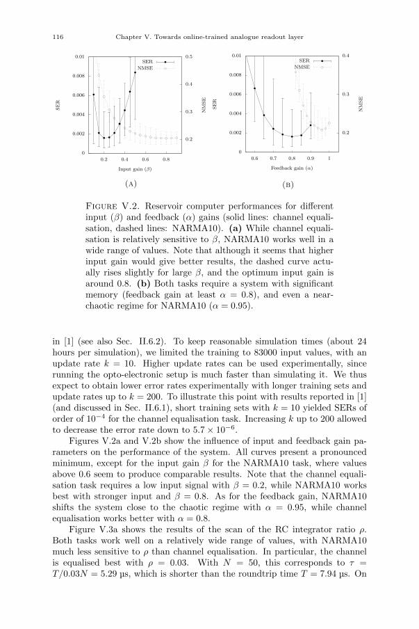
116 Chapter V. Towards online-trained analogue readout layer
0
0.002
0.004
0.006
0.008
0.01
0.2 0.4 0.6 0.8
0.2
0.3
0.4
0.5SER
NMSE
Input gain (β)
SER
NMSE
(a)
0
0.002
0.004
0.006
0.008
0.01
0.6 0.7 0.8 0.9 1
0.2
0.3
0.4
SER
NMSE
Feedback gain (α)
SER
NMSE
(b)
Figure V.2. Reservoir computer performances for differentinput (β) and feedback (α) gains (solid lines: channel equali-sation, dashed lines: NARMA10). (a) While channel equali-sation is relatively sensitive to β, NARMA10 works well in awide range of values. Note that although it seems that higherinput gain would give better results, the dashed curve actu-ally rises slightly for large β, and the optimum input gain isaround 0.8. (b) Both tasks require a system with significantmemory (feedback gain at least α = 0.8), and even a near-chaotic regime for NARMA10 (α = 0.95).
in [1] (see also Sec. II.6.2). To keep reasonable simulation times (about 24hours per simulation), we limited the training to 83000 input values, with anupdate rate k = 10. Higher update rates can be used experimentally, sincerunning the opto-electronic setup is much faster than simulating it. We thusexpect to obtain lower error rates experimentally with longer training sets andupdate rates up to k = 200. To illustrate this point with results reported in [1](and discussed in Sec. II.6.1), short training sets with k = 10 yielded SERs oforder of 10−4 for the channel equalisation task. Increasing k up to 200 allowedto decrease the error rate down to 5.7× 10⁻⁶.
Figures V.2a and V.2b show the influence of input and feedback gain pa-rameters on the performance of the system. All curves present a pronouncedminimum, except for the input gain β for the NARMA10 task, where valuesabove 0.6 seem to produce comparable results. Note that the channel equali-sation task requires a low input signal with β = 0.2, while NARMA10 worksbest with stronger input and β = 0.8. As for the feedback gain, NARMA10shifts the system close to the chaotic regime with α = 0.95, while channelequalisation works better with α = 0.8.
Figure V.3a shows the results of the scan of the RC integrator ratio ρ.Both tasks work well on a relatively wide range of values, with NARMA10much less sensitive to ρ than channel equalisation. In particular, the channelis equalised best with ρ = 0.03. With N = 50, this corresponds to τ =T/0.03N = 5.29 µs, which is shorter than the roundtrip time T = 7.94 µs. On
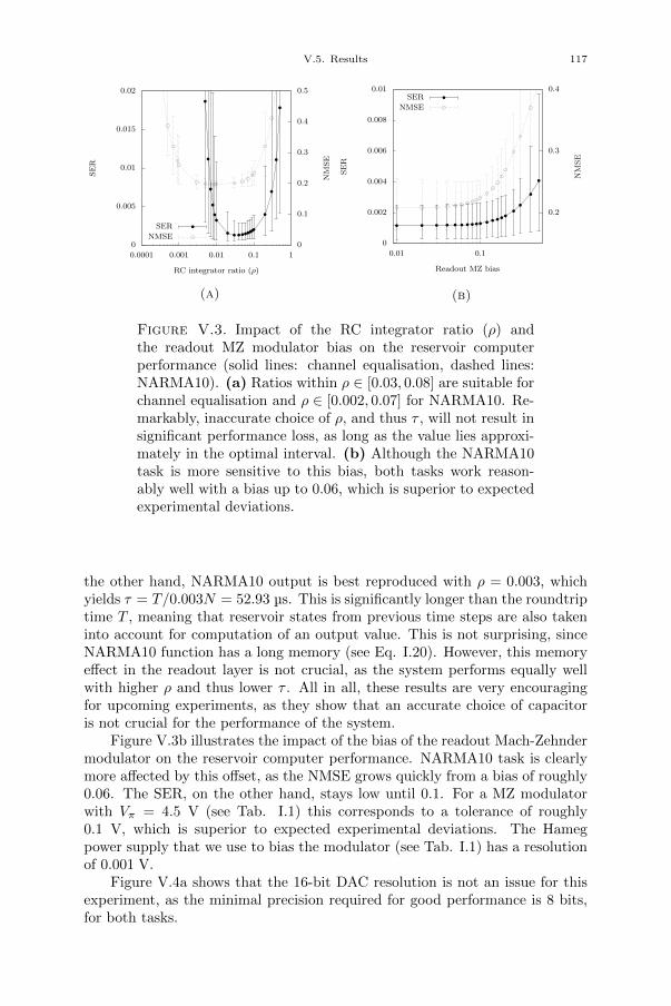
V.5. Results 117
0
0.005
0.01
0.015
0.02
0.0001 0.001 0.01 0.1 1
0
0.1
0.2
0.3
0.4
0.5SER
NMSE
RC integrator ratio (ρ)
SER
NMSE
(a)
0
0.002
0.004
0.006
0.008
0.01
0.01 0.1
0.2
0.3
0.4
SER
NMSE
Readout MZ bias
SER
NMSE
(b)
Figure V.3. Impact of the RC integrator ratio (ρ) andthe readout MZ modulator bias on the reservoir computerperformance (solid lines: channel equalisation, dashed lines:NARMA10). (a) Ratios within ρ ∈ [0.03, 0.08] are suitable forchannel equalisation and ρ ∈ [0.002, 0.07] for NARMA10. Re-markably, inaccurate choice of ρ, and thus τ , will not result insignificant performance loss, as long as the value lies approxi-mately in the optimal interval. (b) Although the NARMA10task is more sensitive to this bias, both tasks work reason-ably well with a bias up to 0.06, which is superior to expectedexperimental deviations.
the other hand, NARMA10 output is best reproduced with ρ = 0.003, whichyields τ = T/0.003N = 52.93 µs. This is significantly longer than the roundtriptime T , meaning that reservoir states from previous time steps are also takeninto account for computation of an output value. This is not surprising, sinceNARMA10 function has a long memory (see Eq. I.20). However, this memoryeffect in the readout layer is not crucial, as the system performs equally wellwith higher ρ and thus lower τ . All in all, these results are very encouragingfor upcoming experiments, as they show that an accurate choice of capacitoris not crucial for the performance of the system.
Figure V.3b illustrates the impact of the bias of the readout Mach-Zehndermodulator on the reservoir computer performance. NARMA10 task is clearlymore affected by this offset, as the NMSE grows quickly from a bias of roughly0.06. The SER, on the other hand, stays low until 0.1. For a MZ modulatorwith Vπ = 4.5 V (see Tab. I.1) this corresponds to a tolerance of roughly0.1 V, which is superior to expected experimental deviations. The Hamegpower supply that we use to bias the modulator (see Tab. I.1) has a resolutionof 0.001 V.
Figure V.4a shows that the 16-bit DAC resolution is not an issue for thisexperiment, as the minimal precision required for good performance is 8 bits,for both tasks.
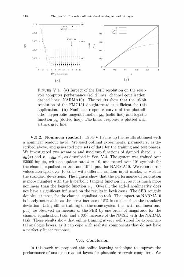
118 Chapter V. Towards online-trained analogue readout layer
0
0.002
0.004
0.006
0.008
0.01
0 2 4 6 8 10 12 14 16 18 20
0.2
0.3
0.4
FMC151
SER
NMSE
DAC Resolution
SER
NMSE
(a)
0
0.2
0.4
0.6
0.8
1
0 0.2 0.4 0.6 0.8 1
f(x
)
x
x
flg(x)
fht(x)
(b)
Figure V.4. (a) Impact of the DAC resolution on the reser-voir computer performance (solid lines: channel equalisation,dashed lines: NARMA10). The results show that the 16-bitresolution of the FMC151 daughtercard is sufficient for thisapplication. (b) Nonlinear response curves of the photodi-odes: hyperbolic tangent function ght (solid line) and logisticfunction glg (dotted line). The linear response is plotted witha thick grey line.
V.5.2. Nonlinear readout. Table V.1 sums up the results obtained witha nonlinear readout layer. We used optimal experimental parameters, as de-scribed above, and generated new sets of data for the training and test phases.We investigated two scenarios and used two functions of sigmoid shape, x →glg(x) and x→ ght(x), as described in Sec. V.4. The system was trained over83000 inputs, with an update rate k = 10, and tested over 105 symbols forthe channel equalisation task and 104 inputs for NARMA10. We report errorvalues averaged over 10 trials with different random input masks, as well asthe standard deviations. The figures show that the performance deteriorationis more manifest with the hyperbolic tangent function ght, as it is much morenonlinear than the logistic function glg. Overall, the added nonlinearity doesnot have a significant influence on the results in both cases. The SER roughlydoubles, at most, for the channel equalisation task. The impact on NARMA10is barely noticeable, as the error increase of 5% is smaller than the standarddeviation. Using offline training on the same system (i.e. with nonlinear out-put) we observed an increase of the SER by one order of magnitude for thechannel equalisation task, and a 30% increase of the NMSE with the NARMAtask. These results show that online training is very well suited for experimen-tal analogue layers, as it can cope with realistic components that do not havea perfectly linear response.
V.6. Conclusion
In this work we proposed the online learning technique to improve theperformance of analogue readout layers for photonic reservoir computers. We
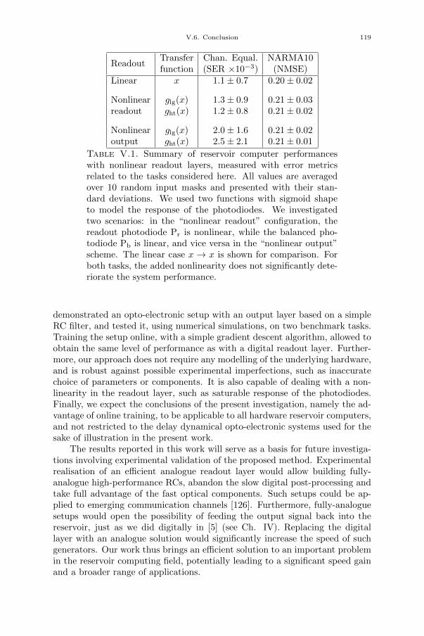
V.6. Conclusion 119
ReadoutTransfer Chan. Equal. NARMA10function (SER ×10−3) (NMSE)
Linear x 1.1± 0.7 0.20± 0.02
Nonlinear glg(x) 1.3± 0.9 0.21± 0.03readout ght(x) 1.2± 0.8 0.21± 0.02
Nonlinear glg(x) 2.0± 1.6 0.21± 0.02output ght(x) 2.5± 2.1 0.21± 0.01
Table V.1. Summary of reservoir computer performanceswith nonlinear readout layers, measured with error metricsrelated to the tasks considered here. All values are averagedover 10 random input masks and presented with their stan-dard deviations. We used two functions with sigmoid shapeto model the response of the photodiodes. We investigatedtwo scenarios: in the “nonlinear readout” configuration, thereadout photodiode Pr is nonlinear, while the balanced pho-todiode Pb is linear, and vice versa in the “nonlinear output”scheme. The linear case x → x is shown for comparison. Forboth tasks, the added nonlinearity does not significantly dete-riorate the system performance.
demonstrated an opto-electronic setup with an output layer based on a simpleRC filter, and tested it, using numerical simulations, on two benchmark tasks.Training the setup online, with a simple gradient descent algorithm, allowed toobtain the same level of performance as with a digital readout layer. Further-more, our approach does not require any modelling of the underlying hardware,and is robust against possible experimental imperfections, such as inaccuratechoice of parameters or components. It is also capable of dealing with a non-linearity in the readout layer, such as saturable response of the photodiodes.Finally, we expect the conclusions of the present investigation, namely the ad-vantage of online training, to be applicable to all hardware reservoir computers,and not restricted to the delay dynamical opto-electronic systems used for thesake of illustration in the present work.
The results reported in this work will serve as a basis for future investiga-tions involving experimental validation of the proposed method. Experimentalrealisation of an efficient analogue readout layer would allow building fully-analogue high-performance RCs, abandon the slow digital post-processing andtake full advantage of the fast optical components. Such setups could be ap-plied to emerging communication channels [126]. Furthermore, fully-analoguesetups would open the possibility of feeding the output signal back into thereservoir, just as we did digitally in [5] (see Ch. IV). Replacing the digitallayer with an analogue solution would significantly increase the speed of suchgenerators. Our work thus brings an efficient solution to an important problemin the reservoir computing field, potentially leading to a significant speed gainand a broader range of applications.


CHAPTER VII
Conclusion and perspectives
Everything happened by chance,as planned.
Life humour
The story of my PhD slowly but inevitably comes to an end. For almostfour years I have been working in a fusion of machine learning, FPGA design,optics and electronics. There was absolutely no way to be bored with such avariety, and I could not be more happy about it. To be completely honest, Igenuinely loved what I was doing and I feel very thankful towards the past mefor making the right choices that brought me here. Speaking of the past, nowis a good time to draw a short personal conclusion and compare what has beenand what it had become. The whole picture looks very pleasing – so much haschanged where it needed to, while the core values remained true. Some saythat after graduating from a university in science, the best and practically theonly skill one keeps is the ability to learn. For 5 years I have been practisingand mastering this skill, and thoroughly applied it through the 4 years of thePhD. And I must recognise that ULB did a very good job, now that I can seehow little I knew back then in 2013, and how comfortable I feel now in a fieldthat used to look so scary. . . Not to be misunderstood, I most certainly realisethat I have merely sampled the very tip of the iceberg, and there is still somuch more to learn. But now that the method has been acquired, the onlything that remains is but to keep on rolling.
Enough personal comments for now, let us get back to the main topicand actually conclude this thesis. Prior to my work, experiments on analoguereservoir computing had mostly investigated the reservoir layer, i.e differentnonlinear nodes, multiplexing schemes or coding techniques (see e.g. [33, 49],or [146] for a more complete review). The optimisation of the readout weightsand the computation of the output, on the other hand, was done using (some-what rudimentary) offline training. One notable advance beyond these minimalsystems was the implementation of analogue input and output layers [73, 97].However, the latter experiments failed to achieve state-of-the-art results due toincompatibility of offline training with complex and nonlinear readout layers.Recent trends in neural networks, together with several ideas coming from howthe brain functions suggest that there are many additional ways in which areservoir computer can be used, and in particular, different ways in which itcan be trained. When I started my thesis the time was ripe to explore thesemore advanced applications of analogue reservoir computing. By interfacing
145
146 Chapter VII. Conclusion and perspectives
a photonic reservoir computer with a FPGA we could address some of thesechallenges.
We performed three full experiments, with a fourth in progress. First, wetrained the opto-electronic reservoir online (see Ch. II). This provided shorterexperimental runtimes and more accurate (and significantly lower) error ratesthan in previous experiments, and more importantly the online-trained sys-tem could equalise drifting and switching channels. Second, with a fast GbitEthernet interface between the FPGA and a PC, we could implement the er-ror backpropagation algorithm in hardware (see Ch. III). As a consequence wecould significantly improve performance on three hard tasks in reasonable time.One of the fascinating aspects of this experiment is that it showed that a com-plex training method (error backpropagation) could at least partially be donein hardware. Third, exploiting the fast computational capability of the FPGA,we realised a RC with a output feedback and thereby demonstrated a systemcapable of solving completely new kinds of tasks, such as generating periodicand chaotic time series (see Ch. IV). Finally, combining the advantages ofonline training with the aspiration for an efficient analogue readout, we starteddesigning an online-trained analogue readout layer and reported very promisingpreliminary numerical results (see Ch. V). We chose to delay the developmentof the experiment to accommodate an additional and very interesting project(see Ch. V.6).
These experiments open many new avenues of research, some short-term,which are rather simple extensions of the work already realised, others longer-term which would require much more investment.
Advanced online learning. Our first experiment with the FPGA board(see Ch. II) showed that a photonic reservoir computer could be trained on-line, and that the idea worked quite well. Now that the feasibility has beendemonstrated, one can think of improving the realisation. Most importantly,we used a basic and very slow training algorithm that requires several secondsto converge on a setup that runs on the microsecond timescale. As has beendiscussed in Ch. II, Anteo Smerieri investigated two much more efficient algo-rithms: recursive least squares and reward-modulated Hebbian learning. Wedid not implement them back then because I was only starting with the FPGAdesigns and did not have the necessary skills. The task seems feasible now, andthe time investment should be substantially rewarded. In short, the weightswould converge 1000 times faster (roughly, 103 updates instead of 106). Severalless crucial but still important improvements could also be added to the FPGAdesign, with a more efficient resource utilisation and a faster communicationscheme between the computer and the FPGA.
In a much longer-term perspective, one could imagine a system in whichthe online training is done in hardware. That is, one could conceive an ana-logue system that implements the output layer (including multiplication by thereadout weights), but also an analogue system that computes an error signaland uses it to optimise the readout weights following the update equation (suchas Eq. II.4).
Fully-hardware backprop. The backpropagation experiment by Michiel Her-mans (see Ch. III) demonstrated the advantage of training the input mask.
147
While it is now more challenging to improve the actual RC performance, onecan further increase the efficiency of the experiment. As explained in Ch. III,most of the computations were performed on the computer. The FPGA chipshould take care of that instead for a much faster setup. As a reminder, oneof the limiting factors in our experiments was the slow convergence rate. Thiswas especially problematic with the experiment on the TIMIT task, that tooktwo weeks to complete. Optimising the input mask on the FPGA would resolvethis bottleneck.
A longer term challenge is to figure out how to implement the error back-propagation algorithm in other systems than the one we used. And an evenlonger term challenge would be to implement it entirely in the analogue domain,without using any digital help.
Output feedback. The story of the reservoir computer with output feedbackis a different one. We spent a significant amount of time on this experimentbut could not find a simple way of improving the results due to the noise floorof our experimental system. This, however, does not mean that the situation ishopeless. There are several ideas we could try. The most conservative one is tokeep the opto-electronic reservoir scheme, but build an entirely new experimen-tal setup with low-noise components. This requires in-depth knowledge of theelectronics and optics market and a significant financial investment. A moreliberal idea is to get rid of the opto-electronic reservoir and switch to a differentexperiment. My fellow PhD colleague, Quentin Vinckier, developed a new op-tical reservoir computer with a passive cavity [49], with very low level of noise,since there are now active components inside the delay loop. The challengehere is first to master the anything-but-trivial experiment, much more complexthan the opto-electronic reservoir, and only then to build a new interface forthe FPGA. Several other ideas have been proposed in our paper [5], such asthe use of conceptors [118, 119], but we did not have the time to implementthem.
Another challenge would be to realise a fully analogue reservoir computerwith output feedback. For instance, one could consider using the analogueoutput presented in [73], and feed this back into the reservoir. Implementingthis is a major challenge.
Online-trained analogue readout. The online training of an analogue read-out layer is probably the most promising short-term goal. In fact, we havepaved most of the the road. Therefore, the plan of action is very simple here:just do it, now experimentally.
Ultra-fast systems. Another challenge would be to implement the sameexperiments I have reported in my thesis, but using much faster systems. Ex-perimental reservoir computers based on delay dynamical systems can be muchfaster than the experiment I implemented, see e.g. [54, 58]. Can online train-ing, physical error backpropagation or output feedback be implemented usingthese reservoirs? A major challenge here is that FPGAs themselves may nolonger be able to follow the speed of the reservoir.
Besides the experiments discussed above, during the last year of my the-sis, I took an amazing opportunity to spend five months in the sunny Texas,
148 Chapter VII. Conclusion and perspectives
applying my FPGA skills and machine learning knowledge to the field of coro-nary imaging. Exploiting the parallel computational capacities of the FPGA,we could reduce the runtime of the automated plaque characterisation algo-rithm, based on artificial neural networks and developed at UTexas prior tomy arrival, from days to tens of seconds (see Ch. V.6). This speedup bringsthe method much closer to potential clinical use. Future investigations, with apossible collaboration between ULB and UTexas, may see the neural networkreplaced by an optical reservoir computer, tightly linked to the OCT deviceused for artery imaging. This also opens several directions for future research.
Real-time plaque characterisation on FPGA. The continuation of my projectwith UTexas seems a very exciting research direction. That is, the two maindesign blocks have been developed, and all that remains is to connect them to-gether, with some hardware optimisation. However, there are situations whereone should take things slowly, and this is one of them. Dr. Milner’s teamhad already came to realisation that, while the neural network classifier withfeature extraction is a functioning approach, it may not be the simplest or themost optimal one. A few quick tests on my own, not presented in this thesis,have suggested that the neural network could be simplified, and that not allof the 300 features are necessary. The details are yet to be confirmed, but thegeneral idea sounds promising. Which brings us to the next point.
Efficient plaque classification algorithm. The neural network classifier forplaque characterisation allowed to achieve state-of-the-art results in terms ofsensitivity and specificity. No one could possibly deny that it is a good classifier.But it may not be the best one. After some analysis of the network structureand its core characteristics, it should be possible to understand what exactlymakes it a good classifier and how complex it should be. Again, this is aninvestigation that we have already started in Austin, but it is too soon to drawany conclusions.
Novel applications of RC. During the summer of 2016, I supervised an in-tern who was working on applications of reservoir computing to various patternrecognition tasks. Although we obtained some promising preliminary results,the idea requires to be further investigated. The motivation arises from mypersonal point of view. While reservoir computing is a very elegant model, itseems to me that its optical implementations are being investigated as a “toy”,and they are yet to find a “killer” application. This is why, I believe, findingthe perfect problem to solve with optical reservoir computing is an interestingavenue of research. And it turns out that my internship in Texas might justhave brought a candidate for such an application. Consider the following sce-nario. On the one hand, there is the optical coherence tomography for scanningthe arteries. On the other – a neural network classifier in charge of analysingthe OCT images and characterising different tissue types. Would it be possi-ble to replace the neural network with an optical reservoir computer and fit itnicely alongside OCT? Such an application would exploit all the main benefitsof photonic RC – high-speed optical processing, low energy consumption, easeof training the reservoir – and most certainly attract the key players in the$500 million coronary imaging market [136].
149
In conclusion, there are many directions in which the results presentedin the present thesis could be extended. Some are relatively simple and easyto follow, others are more ambitious and challenging. But the key point isthe following. When I joined OPERA-Photonique four years ago, photonicreservoir computing had been demonstrated in its simplest versions, and theteam had an FPGA board and an idea of what to do with it. Four yearslater, several advanced information processing tasks have been demonstratedby interfacing the FPGA with the experiment, opening up many perspectivesfor future research. Thus today the lab still possesses the same FPGA, butnow with half-a-dozen new ideas. Therefore, while it is time for me to bow out,the story of FPGA-enhanced photonic reservoir computing is only beginning!
On a final note, let us take another quick peek into the future. I have pre-sented several posters at machine learning conferences, with audiences expertin neural networks, but relatively new to optical implementations of reser-voir computing. Quite often, participants were curious about the future andpractical applications of our experiments. In particular, at my last Benelearnconference in June 2017, a dutch scholar, fascinated by our work, asked whetheroptical reservoir computing would be “the future”. While I definitely admirethe simplicity of the concept and the processing speeds that can be achievedwith fast optical setups, I think that this is an overstatement. So what couldwe actually expect from optical RC in the near future?
As Michiel Hermans often told us, the computational power of a machinelearning algorithm depends on the number of trainable parameters. In reser-voir computing, this number is significantly reduced, which favours the sim-plicity of the system but deteriorates its performance on complex tasks. Forcomparison, experimental reservoir computers typically count at most a fewhundred of trainable parameters, while deep learning, that currently domi-nates the machine learning world, totals millions of them. Therefore, I donot expect reservoir computers to become ubiquitous – they are too simple todeal with challenging tasks, such as image processing. But I believe there isa niche where reservoir computing will prevail over the competition. A nichethat requires, for instance, moderately complex processing of optical signals atvery high speeds, with low energy consumption. In that case, all of the mainadvantages of optical RC could be exploited.
A realistic commercial application of optical RC does not seem possiblewithout a fast and robust device, probably integrated on a chip. This endeav-our would probably require joining the efforts of several research group acrossEurope: the integrated reservoir [55] from UGent, the high-speed systems [54,58] from IFISC and FEMTO-ST, and the low-energy passive coherent cavity[49] from our group. It is virtually impossible to tell how much time sucha large-scale collaboration would take, but the resulting system could attractmultiple clients from the industry. For instance, it could be used in opticalcommunications for routing the packets without converting them to digital do-main, thus increasing processing speed and cutting costs on analogue-to-digitalconverters. Furthermore, as my internship in Texas has recently suggested,medical imaging, such as intravascular OCT, could also benefit from embed-ded optical computing for image pre-processing or analysis. To conclude, I do

150 Chapter VII. Conclusion and perspectives
not think that optical reservoir computing is the future, but I believe it willmost certainly be part of it.
Bibliography
[18] Chrisantha Fernando and Sampsa Sojakka. “Pattern recognition in abucket”. In: European Conference on Artificial Life. Springer. 2003,pp. 588–597.
[19] Warren S McCulloch and Walter Pitts. “A logical calculus of the ideasimmanent in nervous activity”. In: The bulletin of mathematical bio-physics 5.4 (1943), pp. 115–133.
[20] Marvin Minsky and Seymour Papert. Perceptrons: Anlntroduction toComputational Geometry. MIT Press, Cambridge, Mass, 1969.
[21] Paul Werbos. Beyond regression: New tools for prediction and analysisin the behavioral sciences. 1974.
[22] Paul J Werbos. “Backpropagation through time: what it does and howto do it”. In: Proceedings of the IEEE 78.10 (1990), pp. 1550–1560.
[23] Alan L Hodgkin and Andrew F Huxley. “A quantitative description ofmembrane current and its application to conduction and excitation innerve”. In: The Journal of physiology 117.4 (1952), p. 500.
[24] Richard FitzHugh. “Mathematical models of threshold phenomena inthe nerve membrane”. In: The bulletin of mathematical biophysics 17(1955), pp. 257–278.
[25] Wulfram Gerstner. “A framework for spiking neuron models: The spikeresponse model”. In: Handbook of Biological Physics 4 (2001), pp. 469–516.
[26] Wulfram Gerstner and Werner M Kistler. Spiking neuron models: Singleneurons, populations, plasticity. Cambridge university press, 2002.
[27] Eugene M Izhikevich. “Which model to use for cortical spiking neu-rons?” In: IEEE transactions on neural networks 15.5 (2004), pp. 1063–1070.
[28] Simon Haykin. Neural networks: a comprehensive foundation. PrenticeHall, 1998.
[29] Herbert Jaeger and Harald Haas. “Harnessing nonlinearity: Predictingchaotic systems and saving energy in wireless communication”. In: Sci-ence 304 (2004), pp. 78–80.
[30] Wolfgang Maass, Thomas Natschlager, and Henry Markram. “Real-timecomputing without stable states: A new framework for neural computa-tion based on perturbations”. In: Neural comput. 14 (2002), pp. 2531–2560.
[31] Herbert Jaeger. “The “echo state” approach to analysing and trainingrecurrent neural networks - with an Erratum note”. In: GMD Report148 (2001).
151
152 BIBLIOGRAPHY
[32] Ali Rodan and Peter Tino. “Minimum complexity echo state network”.In: IEEE Trans. Neural Netw. 22 (2011), pp. 131–144.
[33] Francois Duport, Bendix Schneider, Anteo Smerieri, Marc Haelterman,and Serge Massar. “All-optical reservoir computing”. In: Opt. Express20 (2012), pp. 22783–22795.
[34] Antoine Dejonckheere, Francois Duport, Anteo Smerieri, Li Fang, Jean-Louis Oudar, Marc Haelterman, and Serge Massar. “All-optical reservoircomputer based on saturation of absorption”. In: Opt. Express 22 (2014),pp. 10868–10881.
[35] Takeshi Amemiya. Advanced econometrics. Harvard University Press,1985.
[36] Andrei Nikolaevich Tikhonov, AV Goncharsky, VV Stepanov, and Ana-toly G Yagola. Numerical methods for the solution of ill-posed problems.Vol. 328. Springer Netherlands, 1995.
[37] Michiel Hermans. “Expanding the theoretical framework of reservoircomputing”. PhD thesis. Ghent University, 2012.
[38] Jaspreet Singh, Sandeep Ponnuru, and Upamanyu Madhow. “Multi-gigabit communication: the ADC bottleneck”. In: Ultra-Wideband, 2009.ICUWB 2009. IEEE International Conference on. IEEE. 2009, pp. 22–27.
[39] David Amory Sobel and Robert W Brodersen. “A 1 Gb/s mixed-signalbaseband analog front-end for a 60 GHz wireless receiver”. In: Solid-State Circuits, IEEE Journal of 44.4 (2009), pp. 1281–1289.
[40] Xiaodong Feng, Guanghui He, and Jun Ma. “A new approach to reducethe resolution requirement of the ADC for high data rate wireless re-ceivers”. In: Signal Processing (ICSP), 2010 IEEE 10th InternationalConference on. IEEE. 2010, pp. 1565–1568.
[41] Su-Khiong Yong, Pengfei Xia, and Alberto Valdes-Garcia. 60 GHz Tech-nology for Gbps WLAN and WPAN: from Theory to Practice. John Wi-ley & Sons, 2011.
[42] Khursheed Hassan, Theodore S Rappaport, and Jeffrey G Andrews.“Analog equalization for low power 60 GHz receivers in realistic mul-tipath channels”. In: Global Telecommunications Conference (GLOBE-COM 2010), 2010 IEEE. IEEE. 2010, pp. 1–5.
[43] Jerry Malone and Mark A Wickert. “Practical volterra equalizers forwideband satellite communications with twta nonlinearities”. In: Digi-tal Signal Processing Workshop and IEEE Signal Processing EducationWorkshop (DSP/SPE), 2011 IEEE. IEEE. 2011, pp. 48–53.
[44] Marc Bauduin, Anteo Smerieri, Serge Massar, and Francois Horlin. “Equal-ization of the non-linear satellite communication channel with an echostate network”. In: Vehicular Technology Conference (VTC Spring),2015 IEEE 81st. IEEE. 2015, pp. 1–5.
[45] V John Mathews and Junghsi Lee. “Adaptive algorithms for bilinearfiltering”. In: SPIE’s 1994 International Symposium on Optics, Imaging,and Instrumentation. International Society for Optics and Photonics.1994, pp. 317–327.
BIBLIOGRAPHY 153
[46] Peter Whitle. Hypothesis testing in time series analysis. Vol. 4. Almqvist& Wiksells, 1951.
[47] Edward James Hannan. Multiple time series. Vol. 38. John Wiley &Sons, 2009.
[48] Yvan Paquot, Francois Duport, Anteo Smerieri, Joni Dambre, BenjaminSchrauwen, Marc Haelterman, and Serge Massar. “Optoelectronic reser-voir computing”. In: Sci. Rep. 2 (2012), p. 287.
[49] Quentin Vinckier, Francois Duport, Anteo Smerieri, Kristof Vandoorne,Peter Bienstman, Marc Haelterman, and Serge Massar. “High-perfor-mance photonic reservoir computer based on a coherently driven passivecavity”. In: Optica 2.5 (2015), pp. 438–446.
[50] Felix Schurmann, Karlheinz Meier, and Johannes Schemmel. “Edge ofChaos Computation in Mixed-Mode VLSI-A Hard Liquid.” In: NIPS.2004, pp. 1201–1208.
[51] Lennert Appeltant, Miguel Cornelles Soriano, Guy Van der Sande, JanDanckaert, Serge Massar, Joni Dambre, Benjamin Schrauwen, ClaudioR Mirasso, and Ingo Fischer. “Information processing using a singledynamical node as complex system”. In: Nat. Commun. 2 (2011), p. 468.
[52] Laurent Larger, MC Soriano, Daniel Brunner, L Appeltant, Jose MGutierrez, Luis Pesquera, Claudio R Mirasso, and Ingo Fischer. “Pho-tonic information processing beyond Turing: an optoelectronic imple-mentation of reservoir computing”. In: Opt. Express 20 (2012), pp. 3241–3249.
[53] Romain Martinenghi, Sergei Rybalko, Maxime Jacquot, Yanne Kouo-mou Chembo, and Laurent Larger. “Photonic nonlinear transient com-puting with multiple-delay wavelength dynamics”. In: Phys. Rev. Let.108 (2012), p. 244101.
[54] Daniel Brunner, Miguel C Soriano, Claudio R Mirasso, and Ingo Fis-cher. “Parallel photonic information processing at gigabyte per seconddata rates using transient states”. In: Nature communications 4 (2013),p. 1364.
[55] Kristof Vandoorne, Pauline Mechet, Thomas Van Vaerenbergh, MartinFiers, Geert Morthier, David Verstraeten, Benjamin Schrauwen, JoniDambre, and Peter Bienstman. “Experimental demonstration of reser-voir computing on a silicon photonics chip”. In: Nat. Commun. 5 (2014),p. 3541.
[56] Nicholas D Haynes, Miguel C Soriano, David P Rosin, Ingo Fischer, andDaniel J Gauthier. “Reservoir computing with a single time-delay au-tonomous Boolean node”. In: Physical Review E 91.2 (2015), p. 020801.
[57] Jacob Torrejon, Mathieu Riou, Flavio Abreu Araujo, Sumito Tsunegi,Guru Khalsa, Damien Querlioz, Paolo Bortolotti, Vincent Cros, AkioFukushima, Hitoshi Kubota, et al. “Neuromorphic computing with nano-scale spintronic oscillators”. In: arXiv preprint arXiv:1701.07715 (2017).
[58] Laurent Larger, Antonio Baylon-Fuentes, Romain Martinenghi, VladimirS. Udaltsov, Yanne K. Chembo, and Maxime Jacquot. “High-SpeedPhotonic Reservoir Computing Using a Time-Delay-Based Architecture:
154 BIBLIOGRAPHY
Million Words per Second Classification”. In: Phys. Rev. X 7 (1 2017),p. 011015.
[59] Akram Akrout, Arno Bouwens, Francois Duport, Quentin Vinckier, MarcHaelterman, and Serge Massar. “Parallel photonic reservoir computingusing frequency multiplexing of neurons”. In: arXiv:1612.08606 (2016).
[60] Edin Kadric. “An FPGA Implementation for a High-Speed Optical Linkwith a PCIe Interface”. PhD thesis. 2011.
[61] Kaitlyn Franz. History of the FPGA. (2015). url: http : / / blog .
digilentinc.com/history-of-the-fpga/.[62] Wikipedia. Transistor. 2017. url: http://en.wikipedia.org/wiki/
Transistor.[63] Evgeni Stavinov. 100 Power Tips for FPGA Designers. CreateSpace
Independent Publishing Platform, 2011.[64] M. Mitchell Waldrop. “The chips are down for Moore’s law”. In: Nature
530 (2016), pp. 144–147.[65] Peter Bright. Moores law really is dead this time. 2016. url: https:
//arstechnica.com/information-technology/2016/02/moores-
law-really-is-dead-this-time/.[66] Virtex-6 Family Overview. DS150 (v2.4). Xilinx Inc. 2012.[67] Virtex-6 FPGA DSP48E1 Slice. UG369. Xilinx Inc. 2011.[68] Getting Started with the Xilinx Virtex-6 FPGA ML605 Evaluation Kit.
UG533 (v1.5). Xilinx Inc. 2011.[69] Kristof Vandoorne, Wouter Dierckx, Benjamin Schrauwen, David Ver-
straeten, Roel Baets, Peter Bienstman, and Jan Van Campenhout. “To-ward optical signal processing using photonic reservoir computing”. In:Optics Express 16 (2008), pp. 11182–11192.
[70] Christopher M Bishop. Pattern recognition and machine learning. Springer,2006.
[71] Simon Haykin. Adaptive filter theory. Prentice-Hall, Upper Saddle River,New Jersey, 2000.
[72] Leon Bottou. “Online Algorithms and Stochastic Approximations”. In:Online Learning and Neural Networks. Cambridge University Press,1998.
[73] Francois Duport, Anteo Smerieri, Akram Akrout, Marc Haelterman,and Serge Massar. “Fully analogue photonic reservoir computer”. In:Sci. Rep. 6 (2016), p. 22381.
[74] Sergio Benedetto and Ezio Biglieri. Principles of digital transmission:with wireless applications. Springer Science & Business Media, 1999.
[75] George B Arfken. “Mathematical methods for physicists”. In: OrlandoFL: Academic Press, 1985.
[76] “IEEE Standard VHDL Language Reference Manual.” In: ANSI/IEEEStd 1076-1993 (1994).
[77] Volnei A. Pedroni. Circuit Design with VHDL. MIT Press, 2004.[78] Jingjing Wang, Hao Zhang, Tingting Lv, and T Aaron Gulliver. “Ca-
pacity of 60 GHz wireless communication systems over fading channels”.In: Journal of Networks 7.1 (2012), pp. 203–209.
BIBLIOGRAPHY 155
[79] Melissa Duarte, Ashutosh Sabharwal, Vaneet Aggarwal, Rittwik Jana,KK Ramakrishnan, Christopher W Rice, and NK Shankaranarayanan.“Design and characterization of a full-duplex multiantenna system forWiFi networks”. In: Vehicular Technology, IEEE Transactions on 63.3(2014), pp. 1160–1177.
[80] Michiel Hermans, Joni Dambre, and Peter Bienstman. “OptoelectronicSystems Trained With Backpropagation Through Time”. In: IEEE Trans-actions on Neural Networks and Learning Systems 26.7 (2015), pp. 1545–1550.
[81] Michiel Hermans, Miguel Soriano, Joni Dambre, Peter Bienstman, andIngo Fischer. “Photonic Delay Systems as Machine Learning Implemen-tations”. In: JMLR 16 (2015), pp. 2081–2097.
[82] David E. Rumelhart, James L. McClelland, and PDP Research Group.“Parallel Distributed Processing: Explorations in the Microstructureof Cognition, Vol. 1”. In: Cambridge, MA, USA: MIT Press, 1986.Chap. Learning Internal Representations by Error Propagation, pp. 318–362.
[83] Paul J Werbos. “Generalization of backpropagation with application toa recurrent gas market model”. In: Neural networks 1.4 (1988), pp. 339–356.
[84] Yann LeCun, Yoshua Bengio, and Geoffrey Hinton. “Deep learning”. In:Nature 521.7553 (2015), pp. 436–444.
[85] Michiel Hermans, Michael Burm, Thomas Van Vaerenbergh, Joni Dambre,and Peter Bienstman. “Trainable hardware for dynamical computingusing error backpropagation through physical media”. In: Nature com-munications 6 (2015), p. 6729.
[86] Kensuke Ikeda and Kenji Matsumoto. “High-dimensional chaotic behav-ior in systems with time-delayed feedback”. In: Physica D: NonlinearPhenomena 29.1 (1987), pp. 223–235.
[87] Yurii Nesterov. “A method of solving a convex programming problemwith convergence rate O (1/k2)”. In: Soviet Mathematics Doklady 27.2(1983), pp. 372–376.
[88] Ilya Sutskever, James Martens, George Dahl, and Geoffrey Hinton. “Onthe importance of initialization and momentum in deep learning”. In:Proceedings of the 30th international conference on machine learning(ICML-13). 2013, pp. 1139–1147.
[89] Hubert Zimmermann. “OSI Reference Model - The ISO Model of Ar-chitecture for Open Systems Interconnection”. In: IEEE Transactionson Communications 28.4 (1980), pp. 425–432.
[90] John S. Garofolo and NIST. TIMIT Acoustic-phonetic Continuous SpeechCorpus. Linguistic Data Consortium, 1993.
[91] Fabian Triefenbach, Azarakhsh Jalalvand, Benjamin Schrauwen, andJean-Pierre Martens. “Phoneme recognition with large hierarchical reser-voirs”. In: Adv. Neural Inf. Process. Syst. 23 (2010), pp. 2307–2315.
[92] Fabian Triefenbach, Kris Demuynck, and Jean-Pierre Martens. “Largevocabulary continuous speech recognition with reservoir-based acousticmodels”. In: IEEE Signal Processing Letters 21.3 (2014), pp. 311–315.
156 BIBLIOGRAPHY
[93] Michiel Hermans and Benjamin Schrauwen. “Infinite sparse thresholdunit networks”. In: Proceedings of the International Conference on Ar-tificial Neural Networks. 2012, pp. 612–619.
[94] Satnam Singh. Using the Virtex-6 Embedded Tri-Mode Ethernet MACWrapper v1.4 with the ML605 Board. 2011. url: http://blogs.msdn.microsoft.com/satnam_singh/2011/02/11/using- the- virtex-
6-embedded-tri-mode-ethernet-mac-wrapper-v1-4-with-the-
ml605-board/.[95] Xavier Glorot, Antoine Bordes, and Yoshua Bengio. “Deep Sparse Rec-
tifier Neural Networks.” In: 14th International Conference on ArtificialIntelligence and Statistics. Vol. 15. 106. 2011, p. 275.
[96] Bingxue Shi and Chun Lu. Generator of neuron transfer function andits derivative. US Patent 6429699. 2002.
[97] Anteo Smerieri, Francois Duport, Yvan Paquot, Benjamin Schrauwen,Marc Haelterman, and Serge Massar. “Analog readout for optical reser-voir computers”. In: Advances in Neural Information Processing Sys-tems. 2012, pp. 944–952.
[98] Quentin Vinckier, Arno Bouwens, Marc Haelterman, and Serge Massar.“Autonomous all-photonic processor based on reservoir computing par-adigm”. In: Conference on Lasers and Electro-Optics. Optical Societyof America. 2016, SF1F.1.
[99] G. Peter Zhang. “Neural Networks for Time-Series Forecasting”. In:Handbook of Natural Computing. Ed. by Grzegorz Rozenberg, ThomasBack, and Joost N. Kok. Berlin, Heidelberg: Springer Berlin Heidelberg,2012, pp. 461–477.
[100] Francis wyffels and Benjamin Schrauwen. “A comparative study of Reser-voir Computing strategies for monthly time series prediction”. In: Neu-rocomputing 73.1012 (2010), pp. 1958 –1964.
[101] Meiling Xu, Min Han, and Shunshoku Kanae. “L1/2 Norm RegularizedEcho State Network for Chaotic Time Series Prediction”. In: APNNS’s23th International Conference on Neural Information Processing (ICO-NIP). Vol. 9886. LNCS. 2016, pp. 12–19.
[102] The 2006/07 Forecasting Competition for Neural Networks & Computa-tional Intelligence. http://www.neural-forecasting-competition.com/NN3/. 2006.
[103] Francis wyffels, Benjamin Schrauwen, and Dirk Stroobandt. “Stableoutput feedback in reservoir computing using ridge regression”. In: In-ternational Conference on Artificial Neural Networks. Springer. 2008,pp. 808–817.
[104] Ken Caluwaerts, Michiel D’Haene, David Verstraeten, and BenjaminSchrauwen. “Locomotion Without a Brain: Physical Reservoir Comput-ing in Tensegrity Structures”. In: Artificial Life 19.1 (2013), pp. 35 –66.
[105] Ren Felix Reinhart and Jochen Jakob Steil. “Regularization and stabil-ity in reservoir networks with output feedback”. In: Neurocomputing 90(2012), pp. 96 –105.
BIBLIOGRAPHY 157
[106] Francis wyffels, Jiwen Li, Tim Waegeman, Benjamin Schrauwen, andHerbert Jaeger. “Frequency modulation of large oscillatory neural net-works”. In: Biological Cybernetics 108.2 (2014), pp. 145–157.
[107] Herbert Jaeger. “Echo state network”. In: Scholarpedia 2.9 (2007), p. 2330.[108] Tadashi Yamazaki and Shigeru Tanaka. “The cerebellum as a liquid
state machine”. In: Neural Networks 20.3 (2007), pp. 290 –297.[109] Christian Rossert, Paul Dean, and John Porrill. “At the Edge of Chaos:
How Cerebellar Granular Layer Network Dynamics Can Provide the Ba-sis for Temporal Filters”. In: PLOS Computational Biology 11.10 (Oct.2015), pp. 1–28.
[110] Michael C Mackey and Leon Glass. “Oscillation and chaos in physiolog-ical control systems”. In: Science 197.4300 (1977), pp. 287–289.
[111] Edward N Lorenz. “Deterministic nonperiodic flow”. In: Journal of theatmospheric sciences 20.2 (1963), pp. 130–141.
[112] J Doyne Farmer. “Chaotic attractors of an infinite-dimensional dynam-ical system”. In: Physica D: Nonlinear Phenomena 4.3 (1982), pp. 366–393.
[113] Morris W Hirsch, Stephen Smale, and Robert L Devaney. Differentialequations, dynamical systems, and an introduction to chaos. Academicpress, Boston, MA, 2003.
[114] Paul Horowitz and Winfield Hill. The art of electronics. Cambridge Uni-versity Press, 1980.
[115] John Walker. ENT Program. http://www.fourmilab.ch/random/.[116] George Marsaglia. The Marsaglia Random Number CDROM including
the Diehard Battery of Tests of Randomness. http://stat.fsu.edu/pub/diehard/.
[117] Andrew Rukhin, Juan Soto, James Nechvatal, Miles Smid, and ElaineBarker. A statistical test suite for random and pseudorandom numbergenerators for cryptographic applications. Tech. rep. National Instituteof Standards and Technology, 2001.
[118] Herbert Jaeger. “Conceptors: an easy introduction”. In: CoRR abs/1406.2671 (2014).
[119] Herbert Jaeger. “Controlling Recurrent Neural Networks by Concep-tors”. In: CoRR abs/1403.3369 (2014).
[120] Andr David Kovac, Maximilian Koall, Gordon Pipa, and Hazem Toutounji.“Persistent Memory in Single Node Delay-Coupled Reservoir Comput-ing”. In: PLOS ONE 11.10 (Oct. 2016), pp. 1–15.
[121] David Sussillo and L.F. Abbott. “Generating Coherent Patterns of Ac-tivity from Chaotic Neural Networks”. In: Neuron 63.4 (2009), pp. 544–557.
[122] Damien Woods and Thomas J Naughton. “Optical computing: Photonicneural networks”. In: Nature Physics 8.4 (2012), pp. 257–259.
[123] Shai Shalev-Shwartz. “Online Learning and Online Convex Optimiza-tion”. In: Foundations and Trends in Machine Learning 4.2 (2012),pp. 107–194.
158 BIBLIOGRAPHY
[124] Miguel C Soriano, Silvia Ortın, Daniel Brunner, Laurent Larger, CR Mi-rasso, Ingo Fischer, and Luıs Pesquera. “Optoelectronic reservoir com-puting: tackling noise-induced performance degradation”. In: Optics ex-press 21.1 (2013), pp. 12–20.
[125] Miguel C Soriano, Silvia Ortın, Lars Keuninckx, Lennert Appeltant,Jan Danckaert, Luis Pesquera, and Guy Van der Sande. “Delay-basedreservoir computing: noise effects in a combined analog and digital im-plementation”. In: IEEE transactions on neural networks and learningsystems 26.2 (2015), pp. 388–393.
[126] Marc Bauduin, Quentin Vinckier, Serge Massar, and Francois Horlin.“High performance bio-inspired analog equalizer for DVB-S2 non-linearcommunication channel”. In: Signal Processing Advances in WirelessCommunications (SPAWC), 2016 IEEE 17th International Workshopon. IEEE. 2016, pp. 1–5.
[127] Aldons J. Lusis. “Atherosclerosis”. In: Nature 407.6801 (2000), pp. 233–241. issn: 0028-0836.
[128] Frank D Kolodgie, Allen P Burke, Andrew Farb, Herman K Gold, Jun-ying Yuan, Jagat Narula, Aloke V Finn, and Renu Virmani. “The thin-cap fibroatheroma: a type of vulnerable plaque: the major precursorlesion to acute coronary syndromes”. In: Current opinion in cardiology16.5 (2001), pp. 285–292.
[129] Hiroshi Yabushita, Brett E. Bouma, Stuart L. Houser, H. Thomas Aretz,Ik-Kyung Jang, Kelly H. Schlendorf, Christopher R. Kauffman, MilenShishkov, Dong-Heon Kang, Elkan F. Halpern, and Guillermo J. Tear-ney. “Characterization of Human Atherosclerosis by Optical CoherenceTomography”. In: Circulation 106.13 (2002), pp. 1640–1645. issn: 0009-7322.
[130] Brett E. Bouma, Martin Villiger, Kenichiro Otsuka, and Wang-Yuhl Oh.“Intravascular optical coherence tomography (Invited)”. In: Biomed.Opt. Express 8.5 (2017), pp. 2660–2686.
[131] John Noble, Harry Lemoine Greene, and Fred F Ferri. Textbook of pri-mary care medicine. Mosby, 2001.
[132] Daniel Chamie, Zhao Wang, Hiram Bezerra, Andrew M. Rollins, andMarco A. Costa. “Optical Coherence Tomography and Fibrous CapCharacterization”. In: Curr Cardiovasc Imaging Rep 4.4 (2011). 9090[PII],pp. 276–283. issn: 1941-9066.
[133] Wikipedia. Atherosclerosis. 2017. url: http://en.wikipedia.org/wiki/Atherosclerosis.
[134] Fabio Tavora, Nathaniel Cresswell, Ling Li, David Fowler, and AllenBurke. “Frequency of acute plaque ruptures and thin cap atheromas atsites of maximal stenosis”. pt. In: Arquivos Brasileiros de Cardiologia94 (2010), pp. 153–159.
[135] Hector M Garcia-Garcia, Ik-Kyung Jang, Patrick W Serruys, Jason CKovacic, Jagat Narula, and Zahi A Fayad. “Imaging plaques to predictand better manage patients with acute coronary events”. In: Circulationresearch 114.12 (2014), pp. 1904–1917.
BIBLIOGRAPHY 159
[136] Barbara G. Goode. “Optical Coherence Tomography/Cardiology: To-tally tubular: Cardiovascular OCT goes prime time”. In: BioOpticsWorld (2010). url: http://www.bioopticsworld.com/articles/
print/volume-3/issue-4/features/optical-coherence.html.[137] Milosz Jaguszewski and Ulf Landmesser. “Optical Coherence Tomogra-
phy Imaging: Novel Insights into the Vascular Response After CoronaryStent Implantation”. In: Current Cardiovascular Imaging Reports 5.4(2012), pp. 231–238.
[138] Vikram L Baruah, Aydin Zahedivash, Taylor B Hoyt, Deborah Vela, L.Maximilian Buja, Thomas E Milner, and Marc D Feldman. “Abstract19246: Histology-Validated Neural Networks Enable Accurate PlaqueTissue and Thin-Capped Fibroatheroma Characterization Through In-travascular Optical Coherence Tomography”. In: Circulation 134.Suppl1 (2016), A19246–A19246. issn: 0009-7322.
[139] Vikram Baruah, Aydin Zahedivash, Hoyt Taylor, Austin McElroy, Deb-orah Vela, L. M. Buja, Thomas Milner, and Marc Feldman. “TCT-570Histology-Validated Neural Networks Enable Plaque Tissue and Thin-Capped Fibroatheroma Characterization Through Intravascular OpticalCoherence Tomography Based Virtual Histology”. English. In: Journalof the American College of Cardiology 68.18 (2016).
[140] Vikram Baruah, Aydin Zahedivash, Taylor Hoyt, Austin McElroy, Deb-orah Vela, L. Maximilion Buja, Marc Feldman, and Thomas Milner.“Automated Coronary Plaque Characterization Using Intravascular Op-tical Coherence Tomography and a Smart-Algorithm Approach - Vir-tual Histology OCT”. In: Journal of the American College of Cardiology:Cardiovascular Imaging (). (manuscript in progress).
[141] Robert M Haralick, Karthikeyan Shanmugam, et al. “Textural featuresfor image classification”. In: IEEE Transactions on systems, man, andcybernetics 3.6 (1973), pp. 610–621.
[142] Xiaofeng Yang, Srini Tridandapani, Jonathan J Beitler, David S Yu,Emi J Yoshida, Walter J Curran, and Tian Liu. “Ultrasound GLCMtexture analysis of radiation-induced parotid-gland injury in head-and-neck cancer radiotherapy: An in vivo study of late toxicity”. In: Medicalphysics 39.9 (2012), pp. 5732–5739.
[143] Mryka Hall-Beyer. A Grey Level Co-occurrence Matrix tutorial. 2007.url: http://www.fp.ucalgary.ca/mhallbey/tutorial.htm.
[144] MathWorks Benelux. Hyperbolic tangent sigmoid transfer function. 2017.url: http://nl.mathworks.com/help/nnet/ref/tansig.html.
[145] MathWorks Benelux. Log-sigmoid transfer function. 2017. url: http://nl.mathworks.com/help/nnet/ref/logsig.html.
[146] Guy Van der Sande, Daniel Brunner, and Miguel C Soriano. “Advancesin photonic reservoir computing”. In: Nanophotonics 6.3 (2017), pp. 561–576.