Part III

DYNAMICS OF THE MID-CONTINENT POPULATION OFLESSER SNOW GEESE - PROJECTED IMPACTS OFREDUCTIONS IN SURVIVAL AND FERTILITY ONPOPULATION GROWTH RATES

ROBERT ROCKWELL , Ornithology Department, American Museum of Natural History, New York, NY1

10024

EVAN COOCH, Biology Department, Simon Fraser University, Burnaby, BC V5A 1S6

SOLANGE BRAULT, Biology Department, University of Massachusetts, Boston, MA 02125

INTRODUCTION

Our primary task was to generate a set of scenarios involving decreases in survival and reproductivesuccess that reduce the annual growth rate of the mid-continent population of lesser snow geese. Byimplementing management actions corresponding to those scenarios, the numbers of lesser snow geese in the mid-continent population should decline. Once the population reaches a size that prevents further damage and allowsrecovery of damaged areas, management actions can be changed to use scenarios that hold the population sizenear that new level.

One of the problems modeling or monitoring the system is knowing how many geese there really are.Our best current estimates are from the mid-winter surveys. These serve as indices since the sample counts maymiss some individuals (and groups) and may include some more than once. If we assume that the surveys areperformed consistently (even if biased) and assume that annual changes in the indices are representative ofchanges in the entire mid-continent population, then annual growth rates based on the indices (indexed growthrates) can be taken as an unbiased estimate of the annual growth rate (8 = N / N ) of the mid-continentt+1 t

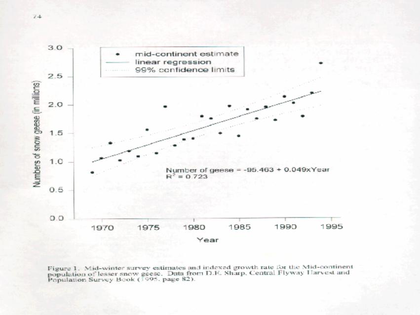
population. The current indexed growth rate is 8 = 1.049 (Figure 1) and is used both as an initial point ofreference for our modeling and for monitoring purposes.

In this report, we develop scenarios that lead to growth rates over the range 8 = 1.05, ..., 0.5. To providesome feel for the impact of instituting management plans corresponding to those growth rates, we modeled thedynamics of hypothetical populations of lesser snow geese that began at either 3,000,000 or 5,000,000individuals (Figure 2a,b). The underlying model ( N = N ×8 ) assumes no density dependence. This assumptiont 0

t

is legitimate in the case of a population that has increased its numbers due to an increase in carrying capacity ofthe environment. We have indicated the Central and Mississippi Flyway Councils Regulatory Threshold valueof 1,500,000 as a point of reference. Please note that there is no a priori reason to suppose that this is thepopulation size that prevents further damage and allows recovery of damaged areas of the arcticecosystem.

__________________________________ Comments should be addressed to this author. They can also be e-mailed to rfr@amnh.org.1

Obviously, the lower the growth rate is below 1.0, the faster the population declines. It must be kept in mind,however, that habitat monitoring is a key component to this program and implementation may take 3 to 5 years.As such, it might be judicious to avoid extremely quick reductions (such as those achieved with values as low as8 = 0.5 or 0.6) since we might not have monitoring in place before the population was reduced substantially.Growth rates within the range of 8 = 0.7 to 0.9 would seem more appropriate, at least for a population of3,000,000.

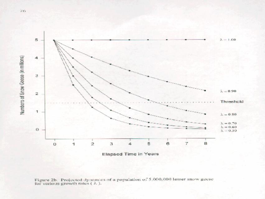
In a more general fashion, it is possible to calculate the time it would take to reduce a population ofunknown size by a specified proportion. We generated a set of such times for a range of reductions over a seriesof different growth rates (8<1) and summarized them in Table 1. Again, allowing for time to get habitatmonitoring in place, growth rates in the range of 8=0.7 to 0.9 may be the most reasonable.

MODEL

The annual cycle of lesser snow geese is illustrated in Figure 3. We evaluated annual population growthdynamics and developed our scenarios with a birth-pulse matrix projection model that coincides with thesynchronous breeding pattern of the birds. Given what we know about age-specific differences in reproductivesuccess, we used a 5 stage model of age classes i = 1, 2, 3, 4, 5+ that correspond to ages 0-1, 1-2, 2-3, 3-4, >4.We assumed a post-breeding census that begins accruing annual mortality immediately after each individualadvances 1 age class and reproduces. We equated fledging with “birth” and used it as a point of reference forreproductive output. Finally, we collapsed seasonal mortalities into a single annual product.

The annual cycle can be reduced to the simple life cycle graph depicted in Figure 4. The 9 transitionpaths are estimated as:

F = BP × (TCL / 2) × (1-TNF ) × P1 × P2 × (1-TBF ) × P3 × s for i = 1,2,ÿ,5 (1)i i i i i i i i a

P = s (2)1 0

P = s for i > 1 (3)i a

where for age class i: BP is breeding propensity, TCL is clutch size, TNF is total nest failure, P1 is egg survival,P2 is hatching success, TBF is total brood failure, P3 is gosling survival and s and s are the annual survival0 a

probabilities for juveniles (age = 0-1) and adults (age > 1) respectively. Additional technical details regardingthese variables are found in Table 2. We reduced clutch size by ½ to focus on females only.

A '

0 F2 F3 F4 F5

P1 0 0 0 0

0 P2 0 0 0

0 0 P3 0 0

0 0 0 P4 P5

n '

n1

n2

n3

n4

n5

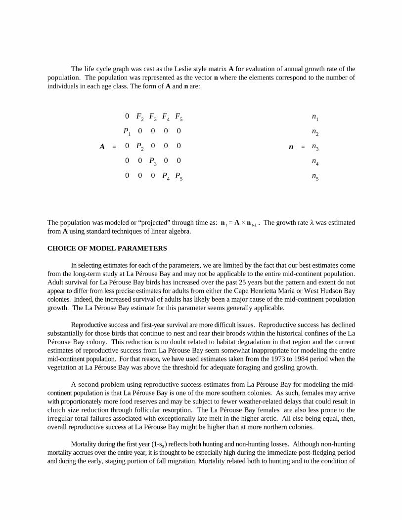
The life cycle graph was cast as the Leslie style matrix A for evaluation of annual growth rate of thepopulation. The population was represented as the vector n where the elements correspond to the number ofindividuals in each age class. The form of A and n are:

The population was modeled or “projected” through time as: n = A × n . The growth rate 8 was estimated t t-1

from A using standard techniques of linear algebra.

CHOICE OF MODEL PARAMETERS

In selecting estimates for each of the parameters, we are limited by the fact that our best estimates comefrom the long-term study at La Pérouse Bay and may not be applicable to the entire mid-continent population.Adult survival for La Pérouse Bay birds has increased over the past 25 years but the pattern and extent do notappear to differ from less precise estimates for adults from either the Cape Henrietta Maria or West Hudson Baycolonies. Indeed, the increased survival of adults has likely been a major cause of the mid-continent populationgrowth. The La Pérouse Bay estimate for this parameter seems generally applicable.

Reproductive success and first-year survival are more difficult issues. Reproductive success has declinedsubstantially for those birds that continue to nest and rear their broods within the historical confines of the LaPérouse Bay colony. This reduction is no doubt related to habitat degradation in that region and the currentestimates of reproductive success from La Pérouse Bay seem somewhat inappropriate for modeling the entiremid-continent population. For that reason, we have used estimates taken from the 1973 to 1984 period when thevegetation at La Pérouse Bay was above the threshold for adequate foraging and gosling growth.

A second problem using reproductive success estimates from La Pérouse Bay for modeling the mid-continent population is that La Pérouse Bay is one of the more southern colonies. As such, females may arrivewith proportionately more food reserves and may be subject to fewer weather-related delays that could result inclutch size reduction through follicular resorption. The La Pérouse Bay females are also less prone to theirregular total failures associated with exceptionally late melt in the higher arctic. All else being equal, then,overall reproductive success at La Pérouse Bay might be higher than at more northern colonies.

Mortality during the first year (1-s ) reflects both hunting and non-hunting losses. Although non-hunting0

mortality accrues over the entire year, it is thought to be especially high during the immediate post-fledging periodand during the early, staging portion of fall migration. Mortality related both to hunting and to the condition of

staging habitat, where birds from several colonies mix, should have the same impact on most juveniles, regardlessof their colony of origin. In contrast, local habitat conditions may have a major impact on immediate post-fledging losses and this component of first-year mortality may be colony specific. Recent estimates of first yearsurvival from La Pérouse Bay may be too low for modeling the mid-continent population since local habitat isseverely degraded. However, values from the mid to late 1980's may provide a reasonable estimate since theypredate severe degradation at La Pérouse Bay but include the more global impacts of hunting and the general 1to 2 decade decline in the condition of common staging habitat in lower Hudson and James Bays.

The reproductive and survival parameter estimates from La Pérouse Bay for the period before habitatdegradation began severely impacting local success are summarized in Table 2. The values of the associatedLeslie matrix are illustrated in the life cycle graph given in Figure 5. The population growth rate based on theseestimates is 8 = 1.107 which is higher than the indexed estimate of 8 = 1.049 (with 1.037-1.061 as the 95%confidence interval).

As explained above, it is possible that components of reproductive success estimated before severehabitat degradation at La Pérouse Bay could be higher than those for more northern colonies (which make upmost of the mid-continent population). If that is the case and if we assume the indexed rate is correct, it seemsreasonable to modify the estimates in Table 1 to generate a set of data more appropriate to modeling the entiremid-continent population. We changed adult survival to 0.88, the most recent (1987) value available from theanalyses of the La Pérouse Bay band recovery data. We changed juvenile survival to 0.30, the correspondingvalue for that same year. The population growth rate incorporating only those two changes is 8 = 1.081 whichis still above the indexed estimate.

If we retain those more recent survival estimates and reduce our estimate of overall reproductive successby 18.6% - a value consistent with 1 complete failure every 9 years or a reduction in each reproductive componentof 3%, we arrive at values for the Leslie matrix illustrated in the life cycle graph given in Figure 6. The growthrate for this set of estimates is 8 = 1.052.

Since the true values for the fecundity components of the entire mid-continent population are not known,we proceeded using the two sets of estimates illustrated in Figures 5 and 6. We will refer to them as the LaPérouse Bay and mid-continent data sets, respectively. As will become clear in the following section onelasticity analyses, conclusions regarding management options and scenarios for reducing growth rate of the mid-continent population are largely independent of which of these sets is finally chosen.

ELASTICITY ANALYSES

The elasticity of any element in a Leslie matrix is its proportionate contribution to the growth rate of thepopulation (they sum to 1). Each elasticity can also be viewed as the proportional change one would expect inthe growth rate given a proportionate change in that element. Changing those elements with higher elasticity willalter the growth rate more than changing those with lower elasticities.

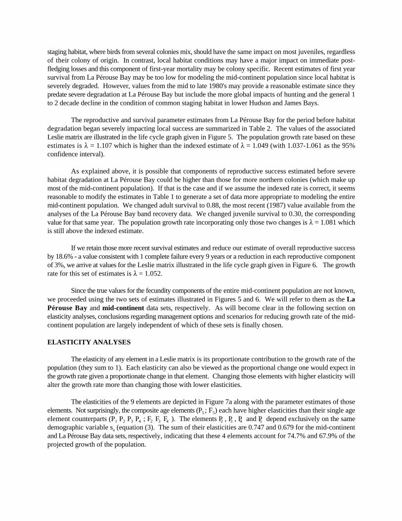
The elasticities of the 9 elements are depicted in Figure 7a along with the parameter estimates of thoseelements. Not surprisingly, the composite age elements (P ; F ) each have higher elasticities than their single age5 5

element counterparts (P P P P ; F F F ). The elements P , P , P and P depend exclusively on the same1 2 3 4 2 3 4 2 3 4 5

demographic variable s (equation (3). The sum of their elasticities are 0.747 and 0.679 for the mid-continenta

and La Pérouse Bay data sets, respectively, indicating that these 4 elements account for 74.7% and 67.9% of theprojected growth of the population.

To examine the generality of the latter result, we estimated elasticities for three example sets of estimatesthat cover a range of survivals, fertilities and growth rates (Figure 7a). In all cases, these 4 adult survivalcomponents account for more than 65% of the elasticity and are thus the primary determinant of populationgrowth. As such, it is apparent that minor adjustments to the estimates of reproductive success, such as thoseto account for inter-colony differences, will have little impact on the overall dynamics or growth rate of the mid-continent population.

Adult survival (s ) actually contributes more to the control of 8 than pooling the elasticities of thea

elements P , P , P and P indicates. Since we used a post-breeding census model, s also contributes to the2 3 4 5 a

elements F , F , F and F (equation 1) and a portion of the elasticities of those matrix elements “belongs” to s2 3 4 5 a

. Similarly, life cycle parameters such as clutch size, nesting success, etc. contribute to more than one elementin the matrix (i.e., F , F , F and F - equation 1). We estimated the contributions of each of the life cycle2 3 4 5

parameters (Table 2) to the elasticity of 8 by partial differentiation. Those contributions, depicted in Figure 7bfor the mid-continent and La Pérouse Bay data sets, are termed “lower level elasticities”. While they do not sumto 1 (as do the higher level elasticities), they do provide a relative measure of the impact of a proportionate changein each parameter on 8.

Adult survival clearly makes the highest relative contribution to the growth rate of the mid-continentpopulation. It is also the variable that offers the greatest numerical potential for altering that growth rate. Forexample, a 10% reduction in adult survival would result in more than a 5-fold greater reduction in 8 than woulda 10% reduction in any contributor to reproductive success. It must be kept in mind, however, that themanagement utility of such high elasticity variables also depends on whether they can be altered to the levelsrequired to effect desired changes in growth rate. In some cases, it may be politically or economically morefeasible to institute management actions that combine changes in both high and low elasticity variables.

SCENARIOS

Increasing Adult Mortality

We examined the effect of increasing adult mortality on population growth rate by decreasing adultsurvival from its initial estimate s = 0.88 (mid-continent) and s = 0.86 (La Pérouse Bay) to 50% of that initiala a

estimate in 5% increments. (The series was s , .95×s , .90×s ,ÿ, .50×s .) This resulted in reducing 8 from 1.052a a a a

to 0.583 for the mid-continent data set (Figure 8a - adults only) and from 8 = 1.107 to 0.629 for the La PérouseBay data set (Figure 8b - adults only).

Joint Harvest of Adults and Juveniles

Although one might attempt to selectively increase only adult mortality through harvest, it is likely thathunters would increase their direct harvest of juveniles at the same time. We investigated this for both data setsby decreasing both adult and juvenile survival at the same time. It is widely believed that part of the differencein adult and juvenile survival reflects an increased relative vulnerability of juveniles to hunting mortality.Unfortunately, it is not known whether that increased relative vulnerability itself depends on the level of adultmortality or harvest pressure.

To gain some insight into both effects, we performed two sets of simulations. In the first, we assumedthat increased juvenile relative vulnerability was independent of the level of adult mortality. That is, we assumedthe ratio of juvenile survival to adult survival (s / s ) did not change as adult mortality increased (Figure 9 -0 a

constant vulnerability). The decreasing survival series used in the simulations was: s , .95×s , .90×s , ÿ, .50×sa a a a

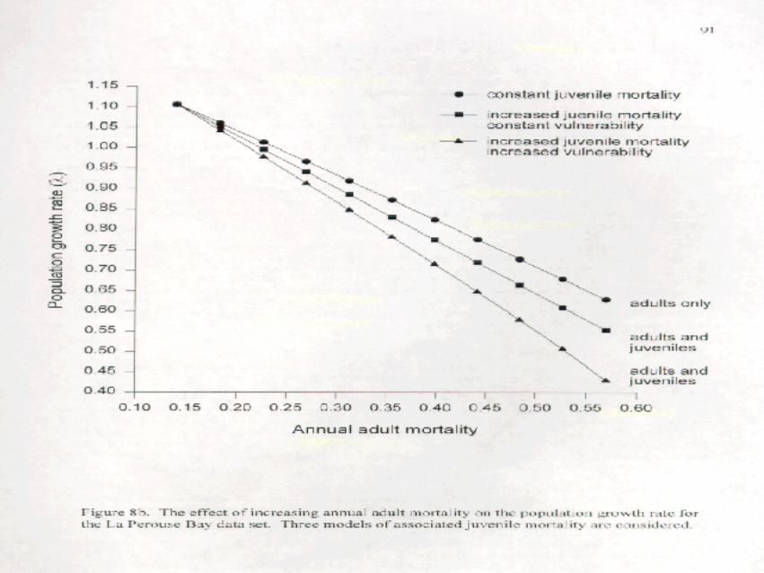
for adults and s , .95×s , .90×s , ÿ, .50×s for juveniles. The joint effects of these reductions are indicated by0 0 0 0

the “adult and juvenile - increased juvenile mortality constant vulnerability” plots on Figures 8a and b. Theimpact of increasing the mortality of both adults and juveniles (through harvest) is to lower 8 at a faster rate.

In the second simulation, we increased the relative vulnerability of juveniles as adult mortality increasedsuch that the ratio of juvenile survival to adult survival (s / s ) declined to 0 over the range of increased adult0 a

mortalities examined (Figure 9 - increasing vulnerability). We used this extreme rate of increase in vulnerability(juvenile survival reaches 0% of its initial value when adult survival reaches 50% of its initial value) in hopes ofdefining the extreme limit of such an effect. The decreasing series used was: s , .95×s , .90×s ,ÿ, .50×s fora a a a

adults and s , .90×s , .80×s , ÿ, .00×s for juveniles. The joint effects are indicated by the “adult and juvenile -0 0 0 0

increased juvenile mortality increased vulnerability” plots on Figures 8a and b. The impact of increasing adultmortality and both the mortality and relative vulnerability of juveniles at the same time is higher than the otherscenarios. Since we used an extreme pattern of relative vulnerability, it is likely that reality lies between the two“adults and juveniles” curves on Figures 8a and b.

It is possible that increases in adult harvest could reduce juvenile survival independently of increases injuvenile harvest. If one or both parents are required to successfully shepard their young through their firstmigration south, their first winter and/or their return north the following spring, then increased adult harvest couldincrease non-hunting mortality of juveniles. If this were the only source of increased juvenile survival, then therelation of 8 to increased adult mortality would be identical to the joint harvest situation with constantvulnerability in Figures 8a and b. If the increase in adult harvest results in this “parental care” effect as well asan increase in juvenile harvest, then again, reality likely lies between the two “adults and juveniles” curves onFigures 8a and b.

Egg Harvest

Harvesting eggs from the nests of laying and incubating females reduces the reproductive success ofthose individuals. From the perspective of our model, such egging can be viewed as a reduction in clutch size(TCL), an increase in nest failure (TNF) or a reduction in egg survival (P1). Since our projections of populationgrowth rate use the product of these (and other) variables as a composite fertility (F in Figure 4 and equation (1)),i

we examined the potential impact of egging on population growth rate simply by decrementing overall fertility.The decreasing fertility series used was: F , .95×F , .90×F , ÿ, .50×F with the reductions applied equally overi i i i

the age classes. The effects of decreasing fertility on the population growth rate 8 is depicted in Figures 10a and10b for the mid-continent and La Pérouse Bay data sets, respectively. For reference, we included the effect on8 of reducing adult survival by the same proportionate amounts (s , .95×s , .90×s , ÿ, .50×s ).a a a a

Consistent with the elasticity analyses, reductions in fertility do not have nearly as great an impact on8 as do equally proportionate reductions in adult survival. For the mid-continent data set, for example, it takesa 5.7% reduction in current adult survival (to .943×s ) to make the population decline (8 = 0.9999). By contrast,a

it requires a 35.8% reduction in fertility (to .642×F ) to achieve the same thing. To appreciate the magnitude ofi

the latter action, assume that there are 2,500,000 nesting females in the mid-continent population and that theentire fertility reduction is to be accomplished by egging which we will view as a decrease in nesting success.Our current estimate for nesting success in the mid-continent data set is (1-TNF) = 0.7448, obtained by applyingthe entire 18.6% reduction in the La Pérouse Bay data set to nesting success (see above.) Reducing the currentlevel of nesting success by 35.8% to 0.4782 (.642×.7448), we find that 1,304,500 (=2,500,000 × (1 - 0.4782))nests would have to fail totally to force 8 just below 1.0. This is an increase of 666,500 nests over the 638,000nests currently expected to fail totally (=2,500,000 × (1 - 0.7448)). Assuming a modal clutch size of 4 eggs(averaged over the age classes), it would require the collection of 2,666,000 eggs from the additionally harvestednests to force the mid-continent population’s growth to a level just below 8 < 1.0.

As a last bench mark, reducing fertility by 5.7% (to .943 × F ) reduces 8 from 1.052 to 1.044 rather thani

to 8 < 1 as was the case when adult survival was reduced by this proportion (above). If that fertility reductionwere again achieved solely through egging, it would require the collection of 142,000 eggs.

APPLICATIONS

The overall strategy of the Habitat Working Group is to: 1) decrease the growth rate of the mid-continent population to some 88<1 using a management program of reduced survival and reproductive successand monitor the population to see that the appropriate decrease and reductions are achieved; 2) monitor the arcticcoastal ecosystem and when the population size is at a level that is causing no further damage, change themanagement program to one that allows the population to stabilize with a growth rate of 88..1.0. The size of thatstabilized population should become the new Regulatory Threshold.

We presented a set of scenarios that relate 8 to decreasing adult mortality, decreasing adult and juvenilemortality and decreasing fertility. Before choosing one or more of them, an appropriate initial value for thereduced 8 must be selected after several factors are considered. These include both the size of the current mid-continent population and the time frame over which it should be reduced. The latter, of course, depends on thenew regulatory threshold size - a value we can not really know in advance.

The simulations depicted in Figures 2a and 2b and the values in Table 1 provide some guidance. If weaccept that it will take 3 to 5 years to get an ecosystem and goose monitoring program in place and begincollecting relevant data and if we use the current regulatory threshold of 1,500,000 as a first approximation ofa new stabilized target, then 8< 0.8 seems too severe, even for a current population of 5,000,000. If the currentpopulation is closer to 3,000,000, then a growth rate closer to 8=0.9 would seem more appropriate. In thefollowing example, we assume the current population is between these estimates and we set the initial reducedgrowth rate at 8=0.85.

Given the elasticities of the parameters, it is tempting next to appeal solely to adult survival and makeit the focus of our management efforts. As mentioned above, this is not always best and our view is that anapproach combining reductions in survival with reductions in fertility through increased harvest of eggs is areasonable overall course of action to lower 8. It is also our view, however, that the elasticity of fertility is suchthat even a substantial increase in egg harvest will be insufficient to appreciably alter reduction scenarios basedon adult mortality. As such, we will focus the rest of this section on increasing adult and juvenile mortality andcalculating associated harvest estimates.

We center on the 3 models that consider joint harvest of adults and juveniles and only on the mid-continent data set. To that end, we have recast Figure 8a as Figure 11, adding a horizontal that corresponds to8=0.85 and dropping perpendiculars from the intersections of the horizontal with the 3 models. Thoseperpendiculars intersect the x-axis at points that give the adult mortality needed to achieve 8=0.85 under eachof the models. For the “adult only” model, an annual adult mortality of 0.312 is required to achieve 8=0.85. Thismodel assumes that there is no increase in the harvest of juveniles in the face of increased adult harvest and doesnot seem too realistic. It was included primarily as a point of reference.

It is more reasonable to assume that there will be an increase in the harvest (or at least mortality) ofjuveniles associated with any increase in adult harvest. What is not clear is whether that increase will beproportional to the increased harvest of adults (Figure 8 - constant vulnerability) or whether juvenile mortalitywill increase disproportionately with increased adult harvest. The latter could result from increased vulnerability

(Figure 8a) and/or decreased parental care. Reality likely lies between these two models, indicated on Figure 11by the 2 adults and juveniles lines. This gives us a range of adult mortalities from 0.27 to 0.29 that would leadto 8=0.85. It should be recalled that associated increases in juvenile mortality are built into the models and donot need to be expressly calculated.

We assume that increasing adult mortality from its current level of 0.12 (1-s ) to a new level betweena

0.27 and 0.29 will be achieved with hunting mortality. As such, the final translation of increased adult mortalitiesinto a management plan must consider the relative contributions of hunting and non-hunting sources to adultmortality. The approach we have taken is based on recoveries of banded individuals and the data we have usedcomes from the banding program at La Pérouse Bay.

By way of review, let:

f = recovery rate (probability that a banded bird is shot, retrieved, and has the band reported)

H = harvest rate (probability that a bird is shot and retrieved)

N = reporting rate (probability that the band is reported from a banded, harvested bird)

K = hunting mortality rate (probability that a bird is lethally shot)

c = retrieval rate (probability that a lethally shot bird is retrieved)

K is the value we seek and it can be found from the relationships: H = f / N and K = H / c so that K = f / N / c.

Although recoveries of birds banded at La Pérouse Bay declined over the 20 year period from 1968 to1988, there was little decline after 1980. We used the unweighted mean of the 1980-1988 estimates as anestimate of direct recovery rate f = 0.0254. Using traditional estimates from mallard duck banding studies of N= 0.38 and a retrieval rate of c = 0.80, we find that K = 0.0836. If we define E as non-hunting mortality rate andassume additive mortality of the instantaneous rates, we find that annual adult survival rate s = (1-K) × (1-E).a

Given our estimates of s = 0.88 and K = 0.0836, we find E = 0.0398.a

We then find the K’s associated with our new mortality rates of m = 0.27 and m = 0.29 as: low high

K = 1 - (.73/.9602) = 0.2397low

K = 1 - (.71/.9602) = 0.2605 high

To achieve 8 = 0.85, then, we will have to increase the current hunting mortality rate K=0.0836 by a factorbetween 2.87 and 3.11.

The most recent average estimate of actual harvest, based on hunter surveys and the parts inventory, isapproximately 305,000. If we assume that this estimate, like the mid-winter inventory, is a representative indexof true harvest rather than the actual total harvest and if we assume that the retrieval rate remains the same, thento achieve a reduction in growth rate to 8=0.85, this harvest index will have to increase approximately 3-fold to915,000 birds.

Once the population size begins going down, the actual total harvest required to sustain an adult mortality

between 0.27 and 0.29 will necessarily decrease. The latter stems from the relationship of hunting mortality rateto total harvest number and population size. If we let G be the total number of geese harvested and G/.8 be thetotal number killed by hunters, then the hunting mortality rate at time t can be estimated as K = (G/.8) / N wheret t

N is the population size at time t. If G/.8 remains the same each year and N declines, then K must increase andt t t

so must the adult mortality rate. As the adult mortality rate increases, the population growth rate declines below8=0.85 and the population will decline at an ever-increasing rate. While overshooting the annual mortality ratefor a few years may not stress this population, the practice should not be continued indefinitely.

To avoid the situation, total number of geese harvested should be reduced as the population declines tohold adult mortality constant. If we view the actual harvest estimate as an index, then regulations must beadjusted annually so that it remains at approximately 3 times the current estimate. If we view it as the actual totalharvest, then regulations must be adjusted annually so that it decreases at a rate that maintains adult mortalitybetween .27 and .29.

As an alternative, comparative example, assume that we seek an initial reduction in the populationgrowth rate that is less severe so that our initial 8 = 0.95. From Figure 11, we can find m = 0.20 and m =low high

0.21. Following procedures outlined above, we then calculate K = .1668 and K = 0.1773. Referring to thelow high

current hunting mortality rate K = 0.0836, we find that to attain 8 = 0.95 we will have to increase current huntingmortality rate by a factor of 1.99 to 2.12.

CONCLUSIONS

Our modeling is based on a strategy that seeks to reduce population growth rate to some sustained levelwith 8 < 1.0 until a target population size can be achieved and stabilized by altering that strategy so that 8 . 1.0.The estimates for mortality and harvest reached in the above examples are based on our assumptions regardingcurrent population size, time span for reduction and a rough, first approximation of the stabilized targetpopulation that is approximately 50% of the current population size. Different assumptions will lead tosomewhat different values under this type of strategy but will likely require that a harvest index be increased toa level 2 to 3 times the current values for several years. Such an increase in harvest will lead to a growth rate ofbetween 8 = 0.85 and 8 = 0.95 and require 3 to 7 years to reduce the mid-continent population to 50% of itscurrent level (Table 1). It is not known whether the coastal tundra can support a population of that reduced sizewithout suffering further damage.

ACKNOWLEDGMENTS

We appreciate the advice of Jim Nichols and John Young on a variety of issues covered in this report.Alex Dzubin, Art Brazda and Dave Sharp continue to provide us with limitless data and insights.