Pcie Variability

8/8/2019 Pcie Variability

http://slidepdf.com/reader/full/pcie-variability 1/14

Journal of Agricultural and Applied Economics, 30,1(July 1998):21–33

0 1998 Souther nAgricultura lEconomic sAssociation

E st im a t in g P r ice Va r ia b ili t y in Agr icu lt u r e :Im p lica t ion s for Dec is ion Ma k er s

Daryll E . Ray, J ames W. Richardson, Daniel G. De La Terre

Ugarte, and Kelly H. Tiller

ABSTRACT

Using a stochastic version of the POLYSYS modeling framework, an examination of pro-

jected variability in agricultural prices, supply, demand, stocks, and incomes is conducted

for corn, wheat, soybeans, and cotton during the 1998–2006 period. Increased planting

flexibility introduced in the 1996 farm bill results in projections of significantly higher

planted acreage variability compared to recent historical levels. Variability of ending stocks

and stock-to-use ratios is projected to be higher for com and soybeans and lower for wheat

and cotton compared to the 1986-96 period. Significantly higher variability is projected

for corn prices, with wheat and soybean prices also being more variable. No significant

change in cotton price variability is projected.

Key Wor ds: POLYSYS model, price variability, stochastic simulation.

The economic well-being of product ion agr i-

cu lture and agr ibusiness is influenced by a

number of forces beyond the cont rol of eco-

n om ic a gen ts in a gr icu lt ur e. P rodu cer s a nd a n-

a lyst s ca n formu la te r ea son able expect at ion s

about the influences of some of t hese exoge-

n ou s fa ct or s, su ch a s popu la tion , per ca pit a in -com es, t ech nology, a nd cu rr en t gover nmen t

policies a nd pr ogr ams, wh en makin g produ c-

t ion pla ns. Ot her exogen ou s fa ct or s can not be

exp res sly in cor por a ted in t o t h e decis ion -mak -

ing pr ocess, bu t st ron gly in fluen ce domest ic

a nd globa l a gr icu lt ur al su pplies—in clu din g

r an dom effect s of wea th er , biologica l ph en om -

Ray is BlasingameChairof Excellenceprofessor,Uni-versityof Tenn esseeAgricultu ra lPolicy AnalysisCen-ter,Richar dsonis a professorin the Departmentof Ag-riculturalEconomics, Texas A&M University.De LaTerr eUgart eis a resea rchass ista ntprofessor,andTilleris a post-doctoralresearchassociate,both with the Uni-versityof Tenn esseeAgricultu ra lPolicy AnalysisCen-ter.

en s, ch an ges in in st it ut ion al st ru ct ur es amon g

t ra din g pa rt n er s, a n d n at ur al ph en omen a.

A la rge por tion of t he h ist or ica l va ria bilit y

in a gr icu lt ur al pr ices, s upp lies, exp or ts, a nd r e-

turns can be at t r ibu ted to factors over which

in dividu al pr odu cer s h ave n eit her con tr ol n or

r elia ble pr edict ive a bilit y. F or m or e t ha n a h alfcen t ur y, va riou s gover nmen t p rogr am s specif-

ica lly design ed in pa rt t o r ed uce t he va ria bilit y

of agr icu ltura l pr ices, supplies, expor ts, and

fa rm in com es h ave a ffect ed U.S. agr icu lt ur e.

Since passage of the Federa l Agricu lture Im-

provement and Reform (FAIR) Act in 1996, a

dismant ling of government supply cont rols

a nd pr ice st abilizin g pr ogr am s h as begu n, wit h

movem en t t owa rd fr eer a gr icult ur al pr odu c-

t ion and markets. Now that government sup-

ply cont rols and pr ice stabilizing tools a re no

lon ger a va ila ble, it h as becom e even mor e cr it -

ica l th at producers, policy makers, and oth er

agr icu lt ura l decision ma ker s a re cogn izan t of

the sou rces and magnitude of var iability

a rou nd a gr icu lt ur al yields a nd expor ts, a nd on



22 Journal of Agricultural and Applied Economics, July 1998

decision-m aking va ria bles such a s pr ices a nd

net retu rns. Also of considerable in terest is

whether price and net return variabilityy are

less or greater in the South than for the U.S.

a s a whole.A number of determin ist ic, la rge-sca le

models of the U.S. agr icultura l sector have

pr oven t o be u sefu l t ools for pr oject in g pr ices

and incomes with an “average sta te” of

wea ther , unchanged in t erna tiona l in st it u tiona l

st r uctur es, a nd other exogenous condit ions. ]

But producers, policy makers, agricultura l

lender s, a gr ibu sin esses, a nd ot h er s a r e in cr ea s-

ingly in terested in the range and rela t ive fre-

quencies of pr ices given the var ia bility a sso-ciated with yields and expor t s. Stochast ic

simulat ion techniques allow est imat ion of

pr oba bilit y dist ribu tion s for en dogen ou s va ri-

ables such as prices and net returns, given

pr oba bility dist r ibut ions for uncert ain va ri-

ables in the system. Uncer ta inty in the agri-

cultura l system may be in the form of proba-

bility dist r ibut ions on the r andom va riables,

such as yields and expor ts, or on the distur -

ba nce t erms for pa rt icu la r equ at ion s. St och as-

t ic simula t ion of such a model results in an

est imat e of t he pr oba bilit y dist ribu tion s on t he

endogenous var iables, and thus provides an

im por ta nt dim ension to the inform at ion base

for decision maker s.

Th is a dded dimen sion of va ria bilit y a rou nd

key indica t or s of agr icu lt ur a l per formance will

be esp ecia lly impor t an t for examin ing agr icu l-

tural sector impacts of the FAIR Act . This pa-per r epr esen t s an in it ia l examin at ion of supply,

dem and, pr ice, a nd income var ia bility using a

stocha st ic sim ulat ion model of th e U.S. agr i-

cultura l sect or , ba sed on the P olicy An alysis

Syst em (POLYSYS) n at ion al simula tion mod-

el (Ra y et a l. 1997). A 10-yea r st och ast ic ba se-

lin e simula tion is per formed u sin g t he Novem-

ber 1997 Food and Agriculture Policy

Resea rch In st it ut e (FAPRI) a gr icu lt ur e ba se-

lin e. All of t he ba selin e a ssumpt ion s r ega rdin g

1Examples of large-scale deterministic structuralmodels that are often used for policy analysis includemodels such as AGMOD (Ferris), COMGEM (Pensonand Chen), FAPRI (Devadoss et al.), AGSIM (Taylor1993), and CARD LP (English et al.).

agr icu lt ur a l policies, domest ic and globa l eco-

nomic condit ions, wea ther , technologica l

ch an ge, a nd ot her in flu en ces a lso ch ar act er ize

t he st och ast ic ba selin e simula tion , except t ha t

stochast ic yield and expor t shocks are int ro-

duced. Examinat ion of the result s focuses on

crops of pr imary importance to southern ag-

r iculture, including cor n, soybea ns, cot ton ,

and whea t . For s elect ed commodit ies, st a tist ics

on va ria bilit y a re pr esen ted for h ar vest ed a cr e-

a ge, yield, su pply, feed u se, expor t u se, en din g

stocks, season average pr ice, and net returns

per a cr e. Th e pr oba bilit y dist ribu tion s a ssoci-

a ted wit h t he 10- yea r simula tion a re compa red

to t he historica l va ria tion of cr op pr ices, sup-plies, demands, and returns to allow an ex-

amin at ion of t he ch an ge in pr oject ed va ria bil-

ity in agr iculture compared to observed

va ria bilit y in r ecen t yea rs.

Methodology

The POLYSYS nat ion al agr icu lt ur e simula tion

model is anchored to a nat ional baseline of

pr oject ion s for a gr icu lt ur e. Ba selin e pr ojec-

t ions for cr op a cr ea ges, pr ices, a nd expendi-

t ur es a re r et ailor ed for 305 pr odu ct ion r egion s

corr espondin g t o Agr icultur al Sta tist ic Dis-

t nict s (ASDS). Ch an ges t o t he ba selin e t hen a re

int roduced exogenously, and the model est i-

mates the impact s of changes to the baseline

for r egion al cr op su pply, na tion al cr op pr ices

and demand, livestock supply and demand,

a nd agr icultur al income. En dogenou s modelcrops include corn, soybeans, cot ton, gra in

sor ghum, ba rley, oa ts, wheat , a nd rice. Seven

livestock commodit ies also are included as a

complement to the feed dem an d componen t of

the crop sector . The calculat ion of most na-

t ional var iables in POLYSYS is dr iven by de-

via tion s fr om a ba selin e a nd ela st icit y pa ram-

eters. POLYSYS incorpora tes 305 regional

linear pr ogr amming cr op supply m odels a nd a

cr op deman d a nd pr ice simult an eou s block forthe est im at ion of en dogenous cr op var ia bles.

Th e r egion al cr op su pply models a re design ed

to alloca te margina l changes in acreage over

the ba seline cr op a crea ge within ea ch r egion,

subject to a 15% acreage shift constra int in

any simulat ion year . Thus, a POLYSYS sim-



Ray et al.: Estimating Price Variability in Agriculture 23

u la tion yields a dyn am ic per forma nce pa th for

cr op a nd livestock supply, dem and, pr ice, a nd

agr icu lt u ra l income var iables .

An implicit a ssumpt ion ch ar act er izin g r e-

su lt s from determinist ic simula t ion models

like POLYSYS is t ha t simula tion r esu lt s differ

from the baseline only to the extent tha t

ch an ges a re in tr odu ced t o defin e a simula tion .

Th us, det ermin ist ic models gener ally a re lim -

it ed to providing point est imates of endoge-

nous variables. It is possible to use a deter -

minist ic model to examine the impact s of

ch an ges fr om t he ba selin e for model va ria bles

character ized by high levels of uncer ta inty.

For example, the sensit ivity of agr icultura lvariables to baseline expor t project ions has

been the subject of several POLYSYS simu-

la tion a na lyses (e.g., Ra y a nd Tiller ; Ra y; Ra y

et al. 1995). But unless specific cha nges to the

ba selin e expor t pr oject ion s a re simula ted, t he

en dogen ou s va ria bles a re est im at ed u nder t he

assumpt ion that there is no range of values

a ssocia ted wit h ba selin e expor t pr oject ion s.

While a determinist ic model cou ld be used to

perform mult iple simula tions t ha t int roducer andomness to desir ed va ria bles, stocha st ic

t ech niqu es pr ovide a st at ist ica l fr am ewor k t o

per form a ser ies of simula tion s in a n efficien t

a nd syst emat ic man ner (Ta ylor 1994; Rich ar d-

son a nd Nixon ).

A POLYSYS stochast ic baseline simula-

t ion is developed by in tr odu cin g va ria bilit y in

(a) nat ional crop export project ions, and (b)

yield est im at es for ea ch of t he 305 r egion s in to

t he POLYSYS ba selin e simula tion . St och ast icexpor t s for eight crops were simula ted from a

mult iva ria te empir ica l (MVE ) dist ribu tion of

devia tion s fr om a t ren d. Th e MVE dist ribu tion

for expor ts wa s est im at ed u sin g da ta for 1982–

96. Historica l values of crop expor t s over the

1982–96 per iod wer e r egr essed on a t im e t ren d

for each of the eight model crops to obta in the

er ror t erms (va ria bilit y) fr om h ist or ica l t ren d

expect a tion s.z The per cen t age devia t ion s fr om

2Export data are available prior to 1982, but evi-dence of a structural change in U.S. exports around1982 exists. An alternative to truncating historical ex-ports at 1982 would be inclusion of additional histor-ical export data with an estimation of structural change

included in the regression of historical exports on atime trend.

the t rend for each crop were used to specify

empir ica l pr obabilit y dist r ibu t ion s for cr op ex-

por t devia tions. A corr ela tion ma tr ix of cr op

export deviat ions for eight crops was calcu-

la ted and used in con junct ion with the h istor -

ical percen ta ge devia tions fr om t rend t o sim-

u la te cor rela ted r an dom devia tes t o t he a nn ua l

ba selin e expor t va lu es in t he st och ast ic simu-

lation.

A mult iva ria te empirica l dist ribut ion for

crop yields was not used to genera te random

yields due to the sheer size of the correlat ion

mat r ix for simulat ing eight crops in each of

305 regions. The histor ica l variability of re-

gional crop yields, 1972–96, was used to de-velop empir ica l dist ribu tion s for pr odu ct ion

for each crop in each region. Percentage de-

viat ion st r uctur es a re preser ved by year t o r e-

flect cor rela tion a cr oss cr ops a nd r egion s. Cor -

rela ted yields were simply simula ted by

randomly select ing rows from the matr ix of

a nn ua l per cen ta ge yield devia tion s for t he 305

regions and eight crops. Once a row in the

mat r ix (year ) was selected randomly, the de-

via tion s wer e a pplied t o t heir r espect ive ba se-

lin e va lu es t o ca lcu la te t he st och ast ic yield.3

In the fir st yea r of a POLYSYS simula tion,

the model randomly selects a percentage de-

viat ion for init ial export sh ocks for ea ch cr op

and applies it to the baseline value for crop

expor ts in t ha t year . Simila rly, a r andom year

is chosen from 1972 through 1996, and the

yield percentage devia t ions for each of eight

crops in each of 305 regions for that year area pplied t o t he ba selin e yield pr oject ion s. Sim -

ilar random draws of export shocks and yield

percentage devia t ions are made in each suc-

cessive year of the simulat ion. In a 10-year

simula tion , 10 r an dom a nn ua l dr aws of expor t

shocks and yield percentage devia t ions are

m ade a nd a pplied to their respect ive baseline

va lu es. Th e model solves t he 10-yea r h or izon

3Historical crop yields were regressed on a timetrend to calculate the annual percentage deviationsfrom trend. The regional nature of the crop supply sec-tor of the model requires complete historical yield dataat the county level, which were not available electron-ically prior to 1972. Thus, historical data available for

estimation of yield deviations from a trend are limitedto 25 years.



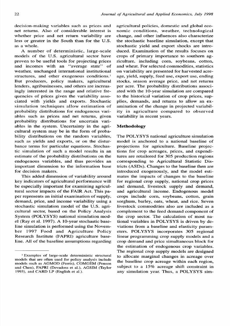
24 Journal of Agricultural and Applied Economics, July

(q-& “:’Expected NetRetarns Income

Price PricesExpectations

~

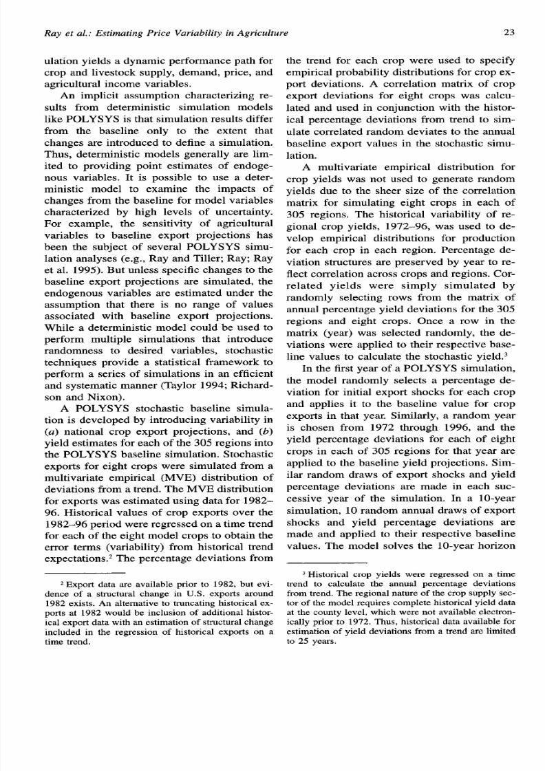
Figure 1. Sch emat ic dia gr am of s toch ast ic POLYSYS met hodology

in a recu rsive fa sh ion u sin g t he r an dom yields

and export s as the changes from the baseline

that lead to changes in quant it ies supplied,pr ices, quant it ies demanded, ending stocks,

and expected pr ices in the next year tha t lead

t o a cr ea ge ch an ges.

A 10-year simula t ion of the model with

random annua l expor t shocks and yield devi-

a t ions compr ises one itera t ion of the model.

The 10-year simulat ion sequence is repea ted

100 t imes t o allow est ima tion of a probabilit y

dist ribu tion for en dogen ou s model var iables

for each of the 10 simula t ion years. Figure 1illu st ra t es t he in ter act ion of var ia bility in ex-

por ts a nd yields over t he sim ula tion per iod a nd

across itera t ions. In the fir st yea r of the fir st

it er at ion , t he model dr aws a n export per cen t-

age devia t ion for each crop and applies it to

the baseline expor t value to in t roduce one re-

a liza tion of a st och ast ic sh ock t o expor ts.

1998

Th e

model also draws a year and applies the cor-

r espon din g per cen ta ge yield devia tion s for a lleight crops in a ll 305 regions to in t roduce one

r ea liza tion of s toch ast ic yields. Th e st och ast ic

yields dir ect ly in flu en ce cr op su pplies, wh ich

in t ur n in flu en ce a gr icu lt ur al pr ices , in comes,

stocks, and demands. The random expor t

sh ocks in flu en ce cr op dem an ds, wh ich a re r e-

flected in tota l demand, and thus the deter -

minat ion of crop pr ices. Therefore, the var i-

abilit y of bot h yields an d expor ts con tr ibu te t o

t he det ermin at ion of a gr icu lt ur al pr ices.Effects of t he expor t and yield devia t ions

fr om t he ba selin e pr oject in g a re t ra nsfer red t o

su bsequ en t sim ula tion yea rs t hr ou gh t heir in i-

t ia l in flu en ce on pr ices, wh ich a re u sed t o form

pr ice expect at ion s for fu tu re pr odu ct ion deci-

sions, an d through t heir influence on crop de-




mands and ending stocks. In the second sim-

ula t ion year , another set of random yield and

export devia tion s is a pplied t o baselin e yield

and export va lues, and the simulat ion is re-

peated. The same process follows in each ofthe remaining eight simulat ion years unt il a

10-year simulat ion sequence is completed.

This 10-yea r simu lat ion sequ en ce compr ises

on e it er at ion of t he st och ast ic m odel. On e h un -

d red it er at ion s a re per formed, dr awin g r an dom

expor t a nd yield per cen ta ge devia tion s in ea ch

of the 10 simulat ion years that compr ise one

it er a tion . The r esult in g s tocha st ic ba selin e p ro-

vides 100 est imates of each var iable in each

simulat ion year , providing an est imate of thepr oba bilit y dist ribu tion for ea ch va ria ble. Th e

st och ast ic ba selin e r epr esen ts a 10-yea r for e-

cast of supply and demand and income var i-

ables, with probability dist r ibu t ions a round

ea ch endogenou s va r ia ble.

Results

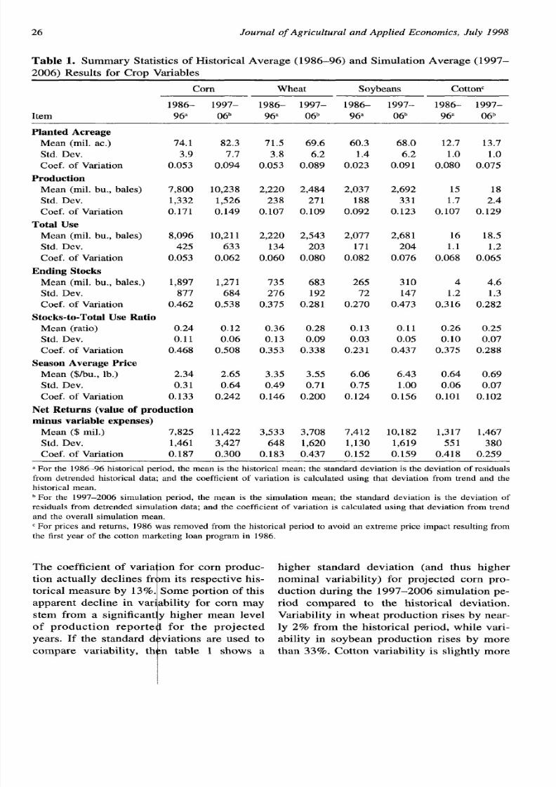
The simula ted summary sta t ist ic va lues for

key output var iables in POLYSYS—such as

plan ted acres, product ion , tota l use, ending

st ocks, a nd prices—a re summar ized in t able 1

for cr ops of m ajor impor tan ce t o sou th east er n

a gr icu lt ur e, in clu din g cor n, wh ea t, soybea ns,

a nd cot ton . Hist or ical m ean s for t he 1986–96

per iod a lso are repor ted. The 11 years of h is-

tor ical dat a were det ren ded, and standard de-

via tion s fr om t he h ist or ica l t ren d a re r epor ted

in table 1 to avoid oversta t ing the var ia t ion in

t hese da ta . Th e coefficien ts of va ria tion for t he

histor ical dat a are calcula ted using standard

deviat ion s ba sed on deviat ion s from t ren d a nd

t he h ist or ica l m ea ns. Th e fir st column for ea ch

crop in table 1 repor ts the histor ica l mean, the

st an da rd deviat ion fr om t he t ren d, an d t his de-

via t ion a s a per cen ta ge of t he h ist or ical mea n,

a s a pr oxy for t he coefficien t of var ia t ion. Th e

secon d column r epor ts sim ila r descr ipt ion s of

the da ta over the 10-year simula t ion per iod,1997–2006, wh er e t he m ea ns for ea ch va ria ble

are means over all 10 simula t ion years an d all

100 ten -yea r it er a t ions ; the s t anda rd devia t ions

a re t he a ver age devia tion s fr om t he det ren ded

sim ula tion da ta ; a nd t he coefficien ts of va ria -

t ion are the det rended st andard deviat ions as

a percent age of the overall simulat ion mean.

For each crop, the two columns provide one

way to compare var iable per formance in the

histor ical per iod to var iable performance in

the simulat ion per iod, It should be noted thatwhile these measu res provide one method of

in ter -per iod compa rison ( 1986–96 compa red

to 1997–2006), they remain a comparison of

on e obser ved pat h (amon g t he n um erou s pa th s

that could have occur red during tha t t ime) to

100 potent ia l pa ths of outcomes for the sim-

ula t ion per iod .

Planted Acreage

The 1996 farm bill provides farmers with

nea rly complet e flexibilit y in det ermin ing t h eir

crop mixes, leading to the expecta t ion that

plan ted acreage aft er 1996 will be more var i-

able than pr ior to 1996. P lan ted corn acreage

over the 1997–2006 simulat ion per iod is pro-

jected to be more than 8 million acres grea ter

than the 1986-96 average (table 1). Plan t ing

flexibilit y is pr oject ed t o in cr ea se t he r ela tive

var iability of plan ted corn acres from 0.053

dur ing 1986–96 to 0.094 for the 1997–2006

per iod, a n in cr ea se of 77.49io.

Wheat plan ted acreage declines slight ly

from the histor ical average of 71.5 million

a cr es (t able 1). Th e coefficien t of va ria tion for

whea t acreage r ises from 0.053 during 1986–

96 to 0.089 (6870 higher) dur ing the 1997–

2006 per iod. F or soybean s, 1997–2006 pla nt -

ed acreage project ions are 7.7 million acres

gr ea ter t ha n t he h ist or ica l a ver age. Va ria bilit y

over the simulat ion per iod r ises 296% from

t he h ist or ica l coefficien t of va ria tion of 0.023.

Cot ton pla nt ed a cr ea ge is pr oject ed t o in cr ea se

by 1 million acres dur ing the 1997–2006 pe-

r iod, with average var iability over the ent ire

simu lat ion per iod project ed t o be 6$%0lower

than over the histor ical per iod, as fa rmers in

margina l cot ton a reas swit ch t o ot her crops.

Production

Avera ge a nn ual pr odu ct ion for t he four cr ops

increases throughout the project ion per iod,

largely in response to acreage ga ins and

t rend-adjusted mean crop yields (table 1).




Table 1. Summar y St at ist ics of H ist or ica l Aver age (1986–96) a nd Sim ula tion Aver age ( 1997–

2006) Resu lt s for Cr op Va ria bles

corn Wheat Soybeans Cottonc

1986- 1997– 1986– 1997– 1986– 1997– 1986- 1997-

Item 9&l 06b 96 oeb 96a ofjb 9tP oeb

Plant ed Acreage

Mean (rnil. at.) 74.1

Std. Dev. 3.9

Coef. of Variation 0.053

Production

Mean (roil. bu., bales) 7,800

Std. Dev. 1,332


Total Use

Mean (roil. bu., bales) 8,096

Std. Dev. 425


Endin g Stocks

Mean (roil. bu., bales.) 1,897

Std. Dev. 877


Stocks-to-Total Use Ratio

Mean (ratio) 0.24

Std. Dev. 0.11

Coef. of Variation 0.468Season Average Price

Mean ($/bu., lb.) 2.34

Std. Dev. 0.31


Net Retur ns (value of pr odu ction

minus va riable expen ses)

Mean ($ rnil.) 7,825

Std. Dev. 1,461


82.3

7.7

0.094

10,238

1,526

0.149

10,211

633

0.062

1,271

684

0.538

0.12

0.06

0.508

2.65

0.64

0.242

11,422

3,427

0.300

71.5 69.6

3.8 6.2

0.053 0.089

2,220 2,484

238 271

0.107 0.109

2,220 2,543

134 203

0.060 0.080

735 683

276 192

0.375 0.281

0.36 0.28

0.13 0.09

0.353 0.338

3.35 3.55

0.49 0.71

0.146 0.200

3,533 3,708

648 1,620

0.183 0.437

60,3

1.4

0,023

2,037

188

0.092

2,077

171

0.082

265

72

0.270

0.13

0.03

0.231

6.06

0.75

0.124

7,412

1,130

0.152

68.0

6.2

0.091

2,692

331

0.123

2,681

204

0.076

310

147

0.473

0.11

0.05

0.437

6.43

1.00

0.156

10,182

1,619

0.159

12.7

1.0

0.080

15

1.7

0.107

16

1.1

0.068

4

1.2

0.316

0.26

0.10

0.375

0.64

0.06

0.101

1,317

551

0.418

13.7

1.0

0.075

18

2.4

0.129

18.5

1.2

0.065

4.6

1.3

0.282

0.25

0.07

0.288

0.69

0.07

0.102

1,467

380

0.259

‘ For the 1986–96 historical period, the mean is the historical mean; the standard deviation is the deviation of residualsfrom detrended historical data; and the coefficient of variation is calculated using that deviation from trend and thehistorical mean.bFor the 1997–2006 simulation period, the mean is the simulation mean; the standard deviation is the deviation of

residuals from detrended simulation data; and the coefficient of variation is calculated using that deviation from trend

and the overall simulation mean.

c For prices and returns, 1986 was removed from the historical period to avoid an extreme price impact resulting from

the first year of the cotton marketing loan program in 1986.

The coefficien t of var ia ion for corn produc-

1

t ion actua lly declines fr m its respect ive his-

tor ical measure by 13%. Some port ion of th is

apparent decline in var”ability for corn may

stem from a significan t y higher mean level

of product ion repor t e for the projected

years. If the standard d viat ions are used to

compare var iability, th n table 1 shows a

higher standard devia t ion (and thus higher

nominal var iability) for project ed corn pro-

du ct ion du rin g t he 1997–2006 simu lat ion pe-

r iod compared to the histor ical devia t ion .

Va riabilit y in wh ea t pr odu ct ion r ises by n ear -

ly 2% from the histor ical per iod, while var i-

ability in soybean product ion r ises by more

t ha n 33~0. Cot ton var iabilit y is sligh tly m ore



Rayet al.: Estimating Price Variabilip in Agriculture 27

Table 2. Probability of Exper iencing Selected Corn, Whea t , Soybeans, and Cotton Ending

Stock Levels . 1998–2006

Crop I Range 1998 1999

Cor n (r oil. bu .)

< 1,000 0.34 0.301,000–2,000 0.46 0.49

>2,000 0.20 0.21

Whea t (r oil. bu.)

<600 0.21 0.39

600–1,000 0.66 0.51

> 1,000 0.13 0.10

Soybea ns (r oil. bu .)

<200 0.34 0.34

200–500 0.49 0.39

>500 0.17 0.27Cot ton (r oil. ba les)

<3 0.06 0.09

3–6 0.73 0.71

>6 0.21 0.20

2000 2001 2002 2003 2004 2005 2006

0.36 0.41 0.41 0.38 0.380.43 0.47 0.39 0.50 0.44

0.21 0.12 0.20 0.12 0.18

0.42 0.45 0.47 0.44 0.46

0.48 0.48 0.39 0.47 0.46

0.10 0.07 0.14 0.09 0.08

0.32 0.28 0.42 0.32 0.27

0.53 0.54 0.45 0.55 0.56

0.15 0.18 0.13 0.13 0.17

0.11 0.09 0.11 0.21 0.16

0.72 0.77 0.73 0.64 0.71

0,17 0.14 0.16 0.15 0.13

0.410.44

0.15

0.46

0.47

0.07

0.29

0.53

0.18

0,13

0.77

0.10

0.410<40

0.19

0.51

0.42

0.07

0.38

0.49

0.13

0.21

0.65

0.14

t ha n 20?40a bove t he 1986–96 level (O. 107) for

t he 1997–2006 per iod.

Total Use

As with pr odu ct ion , t ot al u se of th e four crops

is pr oject ed t o be h igh er du rin g t he sim ula tion

per iod, com pa red t o t he h ist or ica l a ver age (t a-

ble 1). Cor n u se, in pa rt icu la r, r ises 26.1% du r-

ing the simulat ion per iod from the histor ical

level of 8.1 billion bushels. This increase in

corn use is a direct reflect ion of the FAPRI

ba selin e, wh ich a ssumes sign ifica nt in cr ea ses

in gr ain expor ts over t he sim ula tion per iod.

Variability in tota l use for the project ion

yea rs is gr ea ter t ha n t he h ist or ica l va ria bilit y

for corn and wheat , but lower for soybeans

an d cot ton . Wheat tot al u se sh ows t he great est

increase in var iability, while soybeans tota l

u se sh ows t he gr ea test decr ea se in va ria bilit y.

Whea t va ria bilit y is 33.390 above t h e h is tor ica l

coefficien t of 0.060 in the simulat ion, while

corn var iabilit y is 1770 h igher . Soybean tot al

use var iability declines by 7,3 Yo during the

sim ula tion per iod, com pa red t o t he h ist or ica l

per iod. Cot ton tota l use exper iences similar

va ria bilit y r esu lt s, wit h lower va ria bilit y over

t he 1997–2006 per iod.

Stocks

Aver age en din g st ock levels gen er ally a re pr o-jected to decrease in absolu te terms for corn

and wheat and as a percentage of tota l use for

all four crops over the 1997–2006 per iod (ta -

ble 1). The coefficien ts of var ia t ion for corn

a nd soybea n en din g st ocks a nd st ock s-t o-u se

rat ios increase dur ing the simulat ion per iod

compar ed t o t he h ist or ical per iod, wh ile t hey

decrease for wheat and cot ton. Variability in

soybea n st ocks, a r eflect ion of t he va ria bilit y

in soybean acreage, increases by more than

75% in th e simu lat ion compa red t o t he h ist or -

ical per iod, as it becomes the prefer red flex

crop under the 1996 fa rm bill. Var iability in

cot ton stocks as measured by the simulat ion

coefficien t of va ria tion 0.282 is lower t ha n t he

h ist or ica l coefficien t of va ria tion 0.316.

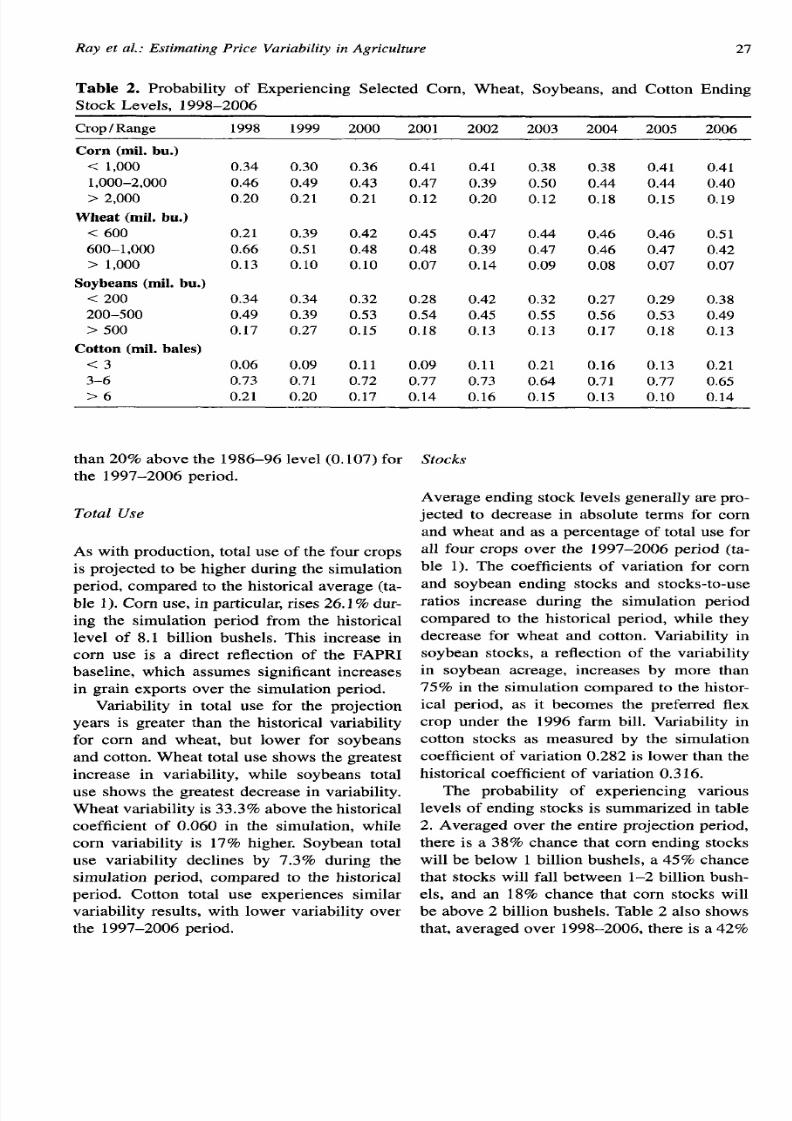
The probability of exper iencing var ious

levels of en din g st ocks is summarized in t able

2. Aver aged over t he en tir e pr oject ion per iod,

there is a 38% chance tha t corn ending stocks

will be below 1 billion bu sh els, a 4590 chan ce

t hat st ocks will fa ll bet ween 1–2 billion bu sh -

els, and an 18% chance tha t corn stocks will

be above 2 billion bush els. Table 2 also sh ows

t ha t, a ver aged over 1998–2006, t her e is a 42%




Table 3. Summary St at ist ics a nd P roba bilit y Dist ribu tion s of Sea son Aver age P rices for Cor n,

Whea t. Sovbea ns. a nd Cot ton . 1998–2006

Crop Season

AVE. Price 1998 1999 2000 2001 2002 2003 2004 2005 2006

Corn ($/bu .)Mean ($)

Std. Dev.

Coef. of Variation

Min. Observ. ($)

Max. Observ. ($)

Probability < ($)

10%

zs~o

33~o

50%

66%

‘75~o

90~o

Whea t ($/bu .)

Mean ($)

Std. Dev.

Coef. of Variation

Min. Observ. ($)

Max. Observ. ($)

Probability ~ ($)

10%zs~o

33~o

50%

66%

75%

90~o

Soybeans ($/bu.)

Mean ($)

Std. Dev.

Coef. of VariationMin. Observ. ($)

Max, Observ. ($)

Probability s ($)

10%

25%

33%

50%

66%

75~o

9070

2.48 2.42

0.65 0.57

0.261 0.236

1.35 1.29

3.99 4.26

1.79 1.76

1.96 1.99

2.05 2.14

2.30 2.29

2.59 2.54

2.95 2.76

3.38 3.11

3.05 3.41

0.65 0.76

0.214 0.224

1.52 1.91

5.15 5.19

2.27 2.392.68 2.92

2.76 3.03

2.90 3.33

3.22 3.65

3.36 3.89

3.79 4.42

6.30 6.04

1.22 1.21

0.193 0.2004.18 4.27

9.98 9.25

4.86 4.76

5.37 5.03

5.65 5.29

6.16 5.63

6.63 6.50

6.95 6.75

7.82 7.80

2.48

0.66

0.265

1.46

4.76

1.68

1.97

2.10

2.32

2.70

2.93

3.30

3.52

0.81

0.230

1.61

5.83

2.512.95

3.12

3.47

3.74

4.07

4.41

6.18

1.11

0.1793.88

9.82

4.91

5.39

5.58

6.02

6.44

6.84

7.38

2.59

0.58

0.222

1.38

4.07

1.92

2.14

2.18

2.45

2,84

2.98

3.30

3.60

0.76

0.211

2.04

5.72

2.633.04

3.18

3.57

3.89

4.07

4.43

6.20

1.15

0.1854.21

9.41

4,90

5.34

5.56

6.03

6.51

6.86

7.66

2.65

0.70

0.266

1,46

4.47

2.71

0.66

0.243

1.49

4.42

2.65

0.66

0.249

1.51

4.50

2.92

0.80

0.273

1.67

5.08

2.86

0.82

0.287

1.61

5.52

1.86

2.08

2.13

2.52

2.89

3.18

3.47

1.94

2.25

2.34

2.59

2.85

3.18

3.64

1.85

2.13

2.21

2.55

2.90

3.06

3.49

2.01

2.38

2.52

2.72

3.01

3.30

4.13

2.00

2.19

2.27

2.67

3.02

3.37

4.06

3.71

0.95

0.258

1.62

6.06

3.57

0.83

0.234

1.61

5.79

3.72

0.88

0.235

1.56

6.12

3.65

0.82

0.225

1.96

5.95

3.67

0.84

0.229

2.03

5.91

2.493.01

3.32

3.67

4.01

4.29

4.93

2.583.04

3.15

3.54

3.82

4.02

4.62

2.523.19

3.35

3.60

4.02

4.20

4.77

2.613,13

3.33

3,60

3.85

4.02

4.63

2.552.99

3.28

3.71

4.02

4.14

4.40

6.48

1.11

0.1724.24

9.87

6.47

1.06

0.1634.31

9.42

6.45

1.19

0.1844.49

10.52

6.61

1.10

0.1664.26

10.74

6.92

1.23

0.1784.77

10.43

5.11

5.77

5.89

6.38

6.82

7.03

7.92

5.21

5.64

5.85

6.35

6.87

7.22

7.78

5.19

5.59

5.84

6.11

6.64

6.94

7.88

5.33

5.75

5.97

6.54

6.91

7.28

7.73

5.40

6.03

6.25

6.73

7.29

7.54

8.44




Table 3. (Continued)

Crop Season

Avg. Pr ice 1998 1999 2000 2001 2002 2003 2004 2005 2006

Cotton ($/lb.)

Mean ($) 0.67 0.67 0.68 0.70 0.69 0.71 0,70 0.70 0.71Std. Dev. 0.07 0.08 0.08 0.08 0.08 0.09 0.07 0.08 0.09

Coef. of Variation 0.108 0.121 0.117 0.108 0.119 0.129 0.106 0.118 0.133

Min. Observ. ($) 0.47 0.50 0.53 0.48 0.51 0.56 0.54 0.53 0.51

Max. Observ. ($) 0.83 0.89 0.94 0.91 0.97 0.99 0.88 1.04 1.02

Probability ~ ($)

109ZO 0.58 0.58 0.57 0.60 0.58 0.60 0.60 0.61 0.60

25% 0.62 0.61 0.62 0.65 0.64 0.63 0.64 0.65 0.65

33% 0.64 0.63 0.64 0.67 0.66 0.66 0.66 0.67 0.66

50% 0.67 0.66 0,66 0.70 0.70 0.70 0.71 0.70 0.69

66%0.70 0.70 0.70 0.73 0.72 0.75 0.74 0.74 0.75

7570 0.72 0.72 0.72 0.74 0.74 0.76 0.76 0.75 0.76

90% 0.76 0.78 0.78 0.78 0.78 0.82 0.79 0.79 0.83

chance that wheat ending stocks will fall be-

low 600 million bushels, a 33% chance that

soybea n en din g st ocks will fa ll below 200 m il-

lion bushels, and a 13% chance that cot ton

ending stocks will fall below 3 million ba les.

The probability of achieving very high stock

levels averaged over the simula t ion per iod is

17?Z0 for soybea ns (stocks over 500 million

bushels), 16% for cot ton (stocks grea ter than

6 m illion ba les), a nd 9.4’%0 for wh ea t (st ocks

over 1 billion bu sh els). In lookin g a t in ter tem -

por a l ch anges in ending s tock s, t he probabilit y

of exper ien cin g ver y low st ock s in cr ea ses con -

sider ably over t he simula tion per iod for wh ea t,

cot ton , and corn, with the probability dist r i-

but ion for soybean ending stocks remaining

r ela tively con st an t over t ime.

Season Average Price

Season average annual prices during the

1997–2006 period are projected to increase

over the historical period for a ll fou r cr ops (t a-

ble 1). Corn pr ices are projected to average

$2.65 per bushel over the 1997–2006 per iodwith a coefficient of varia t ion of 0.242, indi-

ca tin g t ha t sea son a ver age cor n pr ices a re pr o-

jected to be 82% more var iable over the 10-

yea r study horizon tha n dur ing the hist orica l

per iod. The coefficient of var ia tion for whea t

pr ices over the 1997–2006 per iod indica tes

that wheat prices will be 4090 more variable

t ha n du rin g t he 1986–96 per iod. Soybea n pr ic-

es are projected to have 25,890 more rela t ive

var ia bility t ha n during t he histor ical per iod.

By con tr ast , cot ton pr ices have the lowest av-

er age compa r at ive in cr ea se in va riabilit y (1%)

du rin g t he simula tion per iod ver su s t he 1986–

96 per iod .

An nu al summar y st at ist ics a nd pr oba bili-

t ies for crop pr ices are provided in table 3.

Th er e is a 10’%och an ce t ha t t he 1998 com pr ice

will be less than $1.79 per bushel, and a 25 Yo

cha nce tha t the 1998 pr ice will be below $1.96

per bushel. On the other end of the dist r ibu-

t ion, the 1998 corn price has only a 109ochance of exceeding $3.38 per bushel. Gen-

erally, the dist r ibut ion of crop pr ices within

each simula t ion year is skewed leftward, as

in dica ted by a n a nn ua l m ea n pr ice gr ea ter t ha n

the median pr ice ( “50Y0 probability s” in ta-

ble 3). Thus, producers have a higher proba-

bility of exper iencing pr ices below the ex-

pected value of price and are less likely to

exper ien ce pr ices a t or a bove t he expect ed va l-ue of pr ice.

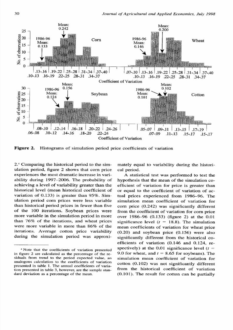
Histograms of crop pr ice coefficients of

va r ia tion aver aged over t h e 10-yea r simu la t ion

per iod sh ow t he pr oba bilit ies of exper ien cin g

alt erna tive levels of pr ice var iability dur ing

the simula t ion period, as presented in figure




25

a020“:

~ 15

% 10h

;5

zo

.10-.13 .16-.19 22-.25 28-.31 .34-.37 ,10-.13 .16-.19 22-.25 .28-.31 .34-,37

Coefficient of VariationMean: Mean:

30

~ 25

‘~ 20

j 15

; 10

05z

o

.06-.08 .10-.12 .14-.16 .18-,20 .22-.24 .07-.09 .11-.13 .15-.17 .15-.17

Coefficient of Variation

Figure 2. H ist ogr am s of sim ula tion per iod pr ice coefficien ts of va ria tion

2.4 Comparing the historical period to the sim-

ulation period, figure 2 shows that corn price

experiences the most dramatic increase in vari-

ability during 1997–2006. The probability of

achieving a level of variability greater than the

historical level (mean historical coefficient of

variation of O.133) is greater than 95%. Sim-ulation period corn prices were less variable

than historical period prices in fewer than five

of the 100 iterations. Soybean prices were

more variable in the simulation period in more

than 76% of the iterations, and wheat prices

were more variable in more than 86% of the

iterations. Average cotton price variability

during the simulation period was approxi-

4 Note that the coefficients of variation presented

in figure 2 are calculated as the percentage of the re-

siduals from trend to the period expected value, an

analogous calculation to the coefficients of variation

presented in table 1. The annual coefficients of varia-tion presented in table 3, however, are the sample stan-dard deviation as a percentage of the mean,

mately equal to variability during the histori-

cal period.

A statistical test was performed to test the

hypothesis that the mean of the simulation co-

efficient of variation for price is greater than

or equal to the coefficient of variation of ac-

tual prices experienced from 1986–96. The

simulation mean coefficient of variation for

corn price (0.242) was significantly different

from the coefficient of variation for corn price

over 1986–96 (O. 133) (figure 2) at the 0.01

significance level (t = 18.8). The simulation

mean coefficients of variation for wheat price

(0.20) and soybean price (O. 156) were also

significantly different from the historical co-

efficients of variation (O. 146 and 0.124, re-spectively) at the 0.01 significance level (t =

9.0 for wheat, and t= 8.65 for soybeans). The

simulation mean coefficient of variation for

cotton (O. 102) was not significantly different

from the historical coefficient of variation

(O. 101). The result for cotton can be partially




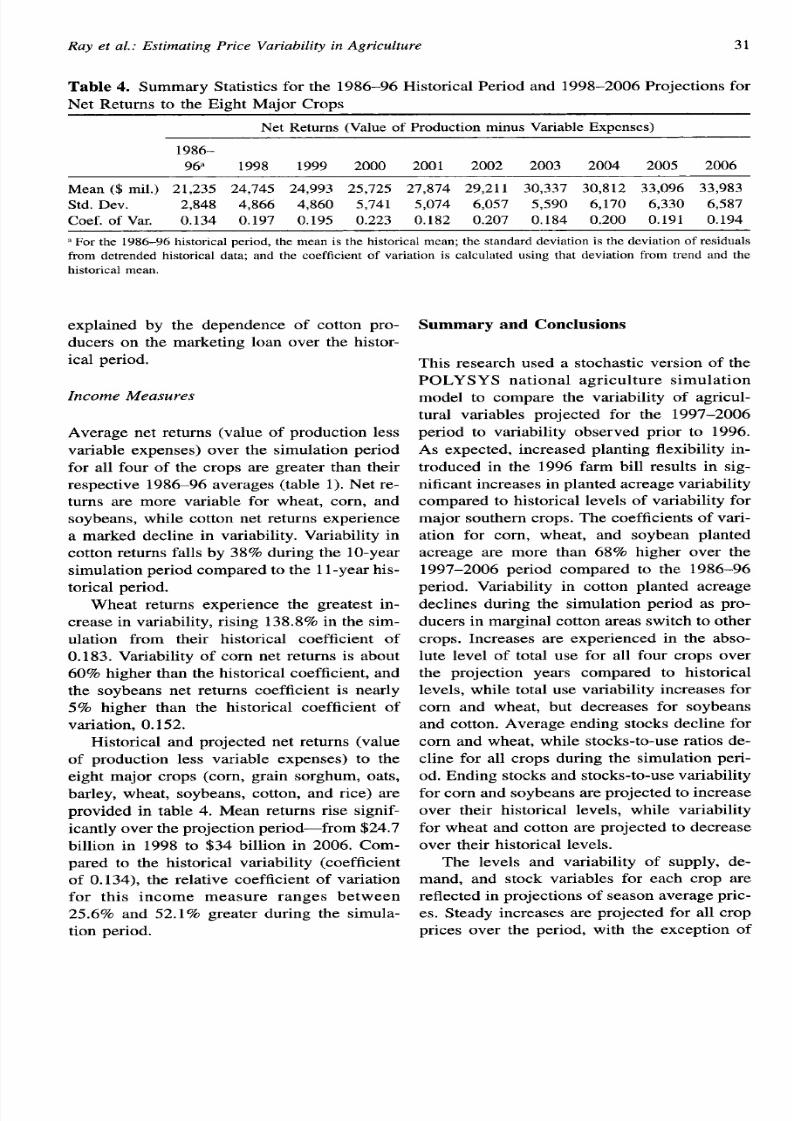
Table 4. Summar y St at ist ics for t he 1986–96 H ist or ica l P er iod a nd 1998–2006 P roject ion s for

Net Returns to the Eight Major Crops

Net Returns (Value of Production minus Variable Expenses)

1986–

96 1998 1999 2000 2001 2002 2003 2004 2005 2006

Mean ($ rnil.) 21,235 24,745 24,993 25,725 27,874 29,211 30,337 30,812 33,096 33,983

Std. Dev. 2,848 4,866 4,860 5,741 5,074 6,057 5,590 6,170 6,330 6,587

Coef. of Var. 0.134 0.197 0.195 0.223 0.182 0.207 0.184 0.200 0.191 0.194

‘ For the 1986–96 historical period, the mean is the historical mean; the standard deviation is the deviation of residuals

from detrended historical data; and the coefficient of variation is calculated using that deviation from trend and the

historical mean.

explained by the dependence of cot ton pro-ducers on the market ing loan over the histor-

ica l per iod .

Income Measures

Average net returns (va lue of product ion less

va ria ble expen ses) over t he sim ula tion per iod

for a ll four of the crops a re grea ter than their

r espect ive 1986-96 a ver ages (t able 1). Net r e-

turns a re more var iable for whea t , corn , and

soybea ns, wh ile cot ton n et r et ur ns exper ien ce

a ma rked declin e in var iabilit y. Var iabilit y in

cot ton ret ur ns fa lls by 38% du rin g t he 10-yea r

sim ula tion per iod compa red t o t he 11-yea r h is-

tor ica l per iod .

Whea t ret urns exper ience the greatest in-

cr ea se in va ria bilit y, r isin g 138.896 in t he sim -

ula t ion from their h istor ical coefficien t of

0.183. Var iability of com net returns is about60% h igh er t ha n t he h ist or ica l coefficien t, a nd

t he soybeans net returns coefficien t is near ly

5% higher than the histor ical coefficien t of

var ia t ion , 0 .152 .

H ist or ica l a nd pr oject ed n et r et ur ns (va lu e

of product ion less var iable expenses) to the

eight major crops (corn , grain sorghum, oat s,

bar ley, wheat , soybeans, cot ton , and r ice) a re

provided in table 4. Mean ret urns r ise signif-

ica nt ly over t h e pr oject ion per iod—fr om $24.7billion in 1998 to $34 billion in 2006. Com-

pa red t o t h e h ist or ica l va ria bilit y (coefficien t

of O.134), t he r ela tive coefficien t of va ria tion

for th is income measu re ranges between

25.69Z0 a n d 52.1 Yo gr ea ter du rin g t he sim ula -

t ion per iod .

Summary and Conclusions

This research used a stochastic version of the

POLYSYS national agriculture simulation

model to compare the variability of agricul-

tural variables projected for the 1997–2006

period to variability observed prior to 1996.

As expected, increased planting flexibility in-

troduced in the 1996 farm bill results in sig-

nificant increases in planted acreage variability

compared to historical levels of variability for

major southern crops. The coefficients of vari-

ation for corn, wheat, and soybean planted

acreage are more than 6896 higher over the

1997–2006 period compared to the 1986–96

period. Variability in cotton planted acreage

declines during the simulation period as pro-

ducers in marginal cotton areas switch to other

crops. Increases are experienced in the abso-

lute level of total use for all four crops overthe projection years compared to historical

levels, while total use variability increases for

corn and wheat, but decreases for soybeans

and cotton. Average ending stocks decline for

corn and wheat, while stocks-to-use ratios de-

cline for all crops during the simulation peri-

od. Ending stocks and stocks-to-use variability

for corn and soybeans are projected to increase

over their historical levels, while variability

for wheat and cotton are projected to decreaseover their historical levels.

The levels and variability of supply, de-

mand, and stock variables for each crop are

reflected in projections of season average pric-

es. Steady increases are projected for all crop

prices over the period, with the exception of




an early downturn in wheat price followed by

recovery and gains. Comparing the average

coefficient of variation for the historical period

to that for the simulation period (calculated as

deviations from a trend as a percentage of the

period expected value), com prices average

82% more variable during the 1997–2006 pe-

riod than during the historical period. Vari-

ability of wheat and soybean prices is 40?Z0

and 25.8% higher, respectively, than variabil-

ityy observed during the 1986–96 period. In

contrast, cotton prices are only 1?40more vari-

able during the simulation period. The increas-

es in price variability and production variabil-

ity are also transmitted to increases in thevariability associated with net returns to each

crop.

While price variability is clearly projected

to increase over the period, it is not possible

to use the data presented to determine precise-

ly what portion of increased price variability

may be attributed to government program and

policy changes instituted in the 1996 farm bill.

Average stocks tended to be relatively low at

the outset of the 1996 farm bill period and are

projected to remain low. Definitive statements

regarding price variability since the 1996 farm

bill should be tempered with recognition that

low stocks are generally manifest in greater

price variability, irrespective of policy set-

tings. For example, had com stocks not been

above 4 billion bushels in 1988, when average

com yield fell from 120 bushels per acre to

85 bushels per acre, a very different com price

path may have been observed during the his-

torical period. Further assessment of price

variability attributable to the 1996 farm bill

will await times of higher stock-to-use ratios.

Among the crops considered, cotton is

most unique to the South and experiences the

least variability during the simulation period,

with price variability very near recent histor-

ical levels and a decrease in variability of net

returns compared to the 1986–96 period. Inthe case of soybeans, another important crop

in the South, while mean simulation price and

net returns variability are greater than histor-

ical variability, soybeans exhibit substantially

less variability than corn and wheat. Hence,

price and net return variability for Midwestern

corn and Great Plains wheat may be larger

than for southern cotton.

References

Devadoss, S., 1? Westhoff, M. Helmar, E. Grund-

meier, K.E. Skold, W.H. Meyers, and S.R. John-

son. “The FAPRI Modeling System: A Docu-

mentation Summary.” In Agricultural Sector

Models for the United States: Description and

Selected Policy Applications, eds., C.R, Taylor,

S .R. Johnson, and K.H. Reichelderfer, Chap. 7.

Ames IA: Iowa State University Press, 1993.

English, B.C., E.G. Smith, J.D. Atwood, S,R. John-

son, and G.E. Oamek, “The CARD LP Model:

A Documentation Summary. ” In AgriculturalSector Models for the United States: Descrip-

tion and Selected Policy Applications, eds., C.R,

Taylor, S .R. Johnson, and K.H. Reichelderfer,

Chap. 5. Ames IA: Iowa State University Press,

1993.

Ferris, J.N. ‘‘AGMOD: An Econometric Model of

U.S. and World Agriculture. ” In Agricultural

Sector Models for the United States: Descrip-

tion and Selected Policy Applications, eds., C.R.

Taylor, S.R. Johnson, and K.H. Reichelderfer,

Chap. 4. Ames IA: Iowa State University Press,1993.

Food and Agricultural Policy Research Institute

(FAPRI). November 1997 U.S. Agricultural

Outlook. FAPRI, University of Missouri, Co-

lumbia, December 1997.

Penson, J. B., and D.T. Chen. “General Design of

COMGEM: A Macroeconomic Model Empha-

sizing Agriculture. ” In Agricultural Sector

Models for the United States: Description and

Selected Policy Applications, eds., C.R. Taylor,

S,R. Johnson, and K.H. Reichelderfer, Chap. 8.

Ames IA: Iowa State University Press, 1993.

Ray, D.E. “The 1996 Farm Bill: Implications for

Farmers, Families, Consumers, and Rural Com-

munities. ” Paper presented at the National Pub-

lic Policy Education Conference, Providence

RI, September 1996.

Ray, D.E., D.G. De La Terre Ugarte, M.R. Dicks,

and K.H. Tiller. “The POLYSYS Modeling

Framework: A Documentation. ” Work. Pap.,

Agricultural Policy Analysis Center, University

of Tennessee, Knoxville, November 1997.

Ray, D,E., D.G, De La Terre Ugarte, M.R, Dicks,

and R.L. White. Farm Bill Series. Agricultural

Policy Analysis Center, University of Tennes-

see, Knoxville. Various selections, Issue Nos.

1–8, 1995.

Ray, D.E., and K.H. Tiller. “U.S. Agricuhund Ex-




ports: projected Changes Under FAKRand Poten-

tial Unanticipated Changes.” Paper presented at

the Western Agricultural Economics Association

Annual Meetings, Reno NV, July 1997.

Richardson, J.W., and C.J. Nixon. “Description of

FLIPSIM V A General Firm-Level Policy Sim-ulation Model. ” Bull. No. B-1528, Texas Agr.

Exp. Sta., College Station, 1986.

Taylor, C.R. “AGSIM: An Econometric-Simulation

Model of Regional Crop and National Livestock

Production in the United States. ” In Agricultur-

al Sector Models for the United States: Descrip-

tion and Selected Policy Applications, eds., C.R.

Taylor, S.R. Johnson, and K.H. Reichelderfer,

Chap. 3. Ames IA: Iowa State University Press,

1993.—. “Deterministic versus Stochastic Evalua-

tion of the Aggregate Economic Effects of Price

Support Programs. ” Agr. Systems 44(1994):

461–73.



Documents

Pcie Variability