Embed Size (px)
Citation preview
Preferential trading arrangementsand industrial location*
Diego PugaCentre for Economic Performance,
London School of Economics
Anthony J. VenablesLondon School of Economics
and Centre for Economic Policy Research
CENTRE for ECONOMIC PERFORMANCEDiscussion Paper No. 267, October 1995
ABSTRACT: This paper considers the locational effects ofgeographically discriminatory trade policy. A preferential movetowards a free trade area pulls industry into the integratingcountries. Input-output links between imperfectly competitivefirms amplify this effect and, when trade barriers fall below somecritical level, may lead to agglomeration with some membercountries gaining industry at the expense of others. A hub-and-spoke arrangement favours location in the hub, with betterreciprocal access to spoke nations than these have to each other.Further liberalisation induces agglomeration in the hub and maytrigger disparities between the spokes.
* This paper was produced as part of the Programme on International Economic Performance at theUK Economic and Social Research Council funded Centre for Economic Performance, London Schoolof Economics. Financial support from the Banco de España (Puga) and the British Taiwan CulturalInstitute (Venables) is gratefully acknowledged.
KEY WORDS: integration, free trade area, hub-and-spoke, agglomeration.JEL CLASSIFICATION: F12, F15, R12.
Correspondence address:
Diego PugaCentre for Economic PerformanceLondon School of EconomicsHoughton StreetLondon WC2A 2AE, UK
http://dpuga.lse.ac.uk
1. Introduction
In recent years, Canada, the United States (US), and Mexico have liberalised trade
between themselves significantly more than they have with the rest of the world. The
member states of the European Union (EU) made earlier moves in the same direction
and have taken integration further with the Single European Act. Trade within the
North American Free Trade Agreement (NAFTA) already accounts for a third of the
total trade of Canada, the United States, and Mexico. Similarly, over two-thirds of EU
trade takes place within the Union. And regional trade in these two areas alone
represents more than one half of world trade.
The NAFTA and the EU are the largest of more than seventy preferential trading
arrangements (PTAs) notified to meet article XXIV of the General Agreement on Tariffs
and Trade. Yet internal disputes sometimes overshadow the achievements of regional
integration in these and other geographical areas. One of the main concerns in the
countries engaged in a preferential trade liberalisation is that it may trigger a
relocation of industry, perhaps of catastrophic proportions.[1]
Our objectives in this paper are to study the effects of PTAs on the location of
industry and the consequent effects on welfare. We look at two different forms of PTA,
free trade areas and hub-and-spoke arrangements, and analyse two issues.[2] First,
how does industry relocate between countries inside and outside the PTA? Is industry
drawn into the PTA, and if so is it the case that gains for the integrating region come
partly at the expense of those left outside (perhaps because a more integrated region
can attract industry from other countries, as firms find it advantageous to sell to
member countries from inside the PTA)? Second, how do firms relocate between
member countries of the PTA? We show that formation of a PTA does not necessarily
cause convergence of the production structures and welfare levels of member nations.
It may trigger agglomeration of activity, causing divergence of structure and income
levels across member states.
1 Recall the row between the French and British governments over the decision by Hoover toconcentrate its vacuum cleaner production in Glasgow and to eliminate 600 jobs at its plant in Dijon,or Ross Perot’s prediction of a ‘giant sucking sound’ of firms and jobs leaving the United States toMexico following the NAFTA (The Economist, 6 February 1993 and 18 September 1993 respectively).
2 The analysis is conducted in quite general form and other multi-country trade policy reformexperiments can be analysed using equations given in the appendix.
Our approach to these issues is to focus on the location of firms operating in an
imperfectly competitive environment. What essential ingredients do we need to use
in order to develop a formal model that addresses these concerns about industrial
relocation? The first important element is the conjunction of increasing returns to scale
(which induce firms to concentrate their production) and positive trade barriers
(which make their choice of location important). Krugman’s (1980) model of trade
with Dixit and Stiglitz (1977)–type monopolistic competition is the basis for
formalising this.
Second, as geographers and development economists have long noted, firms tend
to cluster together drawn by the availability of a large base of suppliers, which in turn
is due to the concentration of demand. To capture this circularity we consider, as
Krugman and Venables (1995) do, an imperfectly competitive industrial sector that
produces goods that are demanded for final consumption and also used as
intermediate inputs. That creates forward (cost) and backward (demand) linkages
between firms, and a tendency for agglomeration.
The third essential ingredient of the model is a trading system with more than two
potential locations for firms, in order to make geographically discriminatory trade
policy possible. We develop the general framework for any number M of countries,
and then particularise it when expositional clarity so requires.
To put all these features together in a tractable model we rely on some familiar
tricks, namely symmetry between firms and consumers, which enables us to talk in
terms of representative agents, and particular functional forms. Despite the loss of
generality, we believe that the results are quite suggestive and illustrative of the
tendencies, if not of the magnitudes, that one would learn if able to solve a more
realistic model.
The remainder of the paper is structured as follows. The next section sets up the
formal model, which is based on Krugman and Venables (1995). Section 3 illustrates
how differences in production structures across countries can arise, even without
differences in technology, endowments, or trade policy. Section 4 develops the
comparative statics analysis of a PTA, in the absence of agglomeration. It shows that
a preferential move towards a free trade area pulls industry into the integrating
countries. Similarly, a hub-and-spoke arrangement favours location in the hub, which
2
has better reciprocal access to spoke nations than these have to each other. Section 5
looks at the stability of the equilibrium as trade policy changes, and shows how
agglomeration may be triggered during a PTA. In the free trade area case, integration
beyond some critical level can open up differences in production in the integrating
countries. However, if these are associated with wage divergence, further integration
may close the gap. In the hub-and-spoke case, liberalisation shifts industry into the
hub region, and when a critical level of integration is reached the relocation process
may accelerate suddenly. If different employment levels induce divergence in wages,
further integration may also trigger disparities between the spoke countries. A
concluding section includes a discussion of empirical evidence on the effects analysed
in the paper.
2. A formal model
Consider a trading system with M countries. Country i is endowed with Li units of
labour, the only primary factor of production. There are two production sectors. The
commodity sector is perfectly competitive. It produces under constant returns to scale,
using one unit of labour per unit of output, a homogeneous commodity that is
costlessly tradeable and will serve as numéraire.
The industrial sector has imperfectly competitive firms, producing differentiated
goods under increasing returns to scale. Following Dixit and Stiglitz (1977),
production of a quantity xi(k) of any variety k in any country i requires the same fixed
(α) and variable (βxi(k)) quantities of the production input. As in Venables (1996), that
production input is a Cobb-Douglas composite of labour and an aggregate of the
differentiated industrial goods. Following Ethier (1982), all varieties enter
symmetrically into this constant elasticity of substitution (CES) intermediate aggregate.
The cost function of a firm producing variety k in country i is
(1)Ci(k) q
iµ w
i(1 µ) α β x
i(k) ,
where wi is the wage, and qi is the price index of the aggregate, defined by
3
The price index in each country depends on the local prices of individual varieties,
(2)qi
≡
M
j 1⌡⌠
h∈Nj
pj, i
(h)τj, i
(1 σ)dh
1 (1 σ)
.
which in turn are a function of the free on board (FOB) prices and trade barriers. The
elasticity of substitution between varieties, σ > 1, is assumed to be the same in all
countries. Nj is the set of varieties produced in location j, and pj,i(h) is the FOB price
of variety h shipped from country j to country i. Trade barriers for the industrial
goods take Samuelson’s ‘iceberg’ form: τj,i units have to be shipped from country j so
that one unit arrives in i. Given this cost function, proportions µ and (1 – µ) of costs
are spent on intermediates and labour respectively.
The representative consumer in each nation has Cobb-Douglas preferences over the
commodity and a CES aggregate of the industrial goods. For convenience, we assume
it is the same CES aggregate that enters firms’ technology. Therefore, each firm is both
an upstream supplier of intermediate inputs to other firms and a downstream
producer for final consumer demand. The indirect utility of the representative
consumer in country i is
(3)Vi
qi
γ 1 (1 γ ) mi
,
where mi is income, γ is the share of industrial goods, and (1 – γ) is the share of the
numéraire.
The division of consumers’ and producers’ expenditure on industrial goods
between individual varieties can be found by using Roy’s identity on the indirect
utility function and Shephard’s lemma on the cost function. The demand faced in
market i by a firm producing variety k in country j, denoted xj,i(k), is
(4)xj, i
(k) pj, i
(k) σ
τj, i
qi
(1 σ)
γ mi
µ ⌡⌠
h∈Ni
Ci(h)dh ,
where the term in square brackets is the value of country i consumers’ plus
intermediate expenditures on industrial goods, amounting to fractions γ of income
and µ of industrial costs.
4
Firms sell in each country, and perceive a constant own price demand elasticity of
σ in every market. All firms producing in any particular location have the same profit
maximising FOB price, which is a constant relative mark-up over marginal cost,
(5)pi
σ βσ 1
qiµ w
i(1 µ) .
If firms enter and exit in response to positive and negative profits, at equilibrium
industrial sector profits will be exhausted in every country. There is a unique level
of output that gives firms zero profits,
(6)xα (σ 1)
β.
All firms in a particular location are symmetric, and we shall define the mass of
varieties produced in location i by ni ≡ #Ni (and generally refer to it as the number
of firms in location i), and the output of each by xi. At equilibrium,
(7)(xi
x )ni
0 , xi
≤ x , ni
≥ 0 .
Turning to the labour market, the commodity sector demands labour perfectly
elastically at wage 1, so market clearing wages are higher than unity only in those
countries specialised in the production of industrial goods. Since the value of
industrial labour demand is (1 – µ) ni Ci, this gives equilibrium wage
(8)w
imax
1,(1 µ) n
iC
i
Li
max
1, qi
(1 µ) niα σ
Li
1 µ
,
where the second equation uses both the definition of costs (1) and the zero profit
condition, (6) and (7). At equilibrium the only source of consumer income is the wage,
so
(9)mi
wiL
i.
5
This completes the description of equilibrium. There are four locational forces
which together determine the equilibrium distribution of firms across locations.
Product and labour market competition tend to make firms located in markets with
relatively many firms less profitable, thereby encouraging the geographical dispersion
of industry. Product market competition is stronger in locations where more varieties
are produced locally in the sense that the price index of industrial goods is lower
—expression (2)— so that, for a given price and level of expenditure, local demand
for each industrial good is smaller —expression (4). Stronger labour market
competition in industrialised regions appears in expression (8): if a country becomes
specialised in industrial production local wages will be higher, this increasing firms’
costs.
Pushing in the opposite direction there are what Hirschman (1958) calls ‘forward
and backward linkages’. In this model, forward linkages come from the assumption
that firms use the output of other firms as an input (µ > 0). A larger number of locally
produced varieties, other things being equal, implies a lower price index of industrial
goods, and therefore lower total and marginal costs of production —expression (1).
Backward linkages arise as an increase in the number of local firms raises local
expenditure on intermediates —expression (4). Forward and backward linkages tend
to increase the profitability of locations with a larger number of firms. When they are
strong enough they can overturn product market and labour market competition
thereby making dispersed outcomes unstable and triggering industrial agglomeration.
In order to proceed analytically, it is useful to rewrite the equilibrium conditions
in vector form. Let n, q, and L denote (M-column) vectors with representative
elements ni, qi, and Li, respectively. Superscript T denotes transpose; and superscript
^ denotes a diagonal matrix with the ith element of the corresponding vector in
position (i,i), and zeros off the diagonal. Ι is the identity matrix, and ι denotes the
(column) vector of ones. Let us also introduce matrix θ, with representative element
(10)θi, j
≡ τ (1 σ)i, j
.
Here and in the next two sections we focus on equilibria where some quantity of
the numéraire is produced in every nation, so wages are constant and equal to unity.
6
Let us choose units for α = 1/σ and β = (σ – 1)/σ. Using (1), (4), (5), (6) and (9) in (7)
gives the zero profit condition as
(11)0 θ γ L q (σ 1) µ q (µ σ 1) n qσ µ ≡ π (n,q,θ) ,
Expression (11) gives M equations in the numbers of firms (vector n) and the price
indices of industrial goods (vector q) in the M countries, given parameters γ, µ, σ, and
the matrix of trade barriers θ. The definition of the M price indices of expression (2),
once we substitute in the pricing equation (5), gives the remaining M equations
necessary to solve the system:
(12)0 θT qµ(1 σ) n q(1 σ) ≡ Q(n,q,θ) ,
where the functions π and Q are convenient ways to carry the analysis.
Equilibrium values of the number of firms and the price index of industrial goods
in each of the M countries are a simultaneous solution to (11) and (12). Let us focus
on symmetric changes in trading arrangements, characterised by a matrix dθ (= dθT)
of changes in the trade policy matrix θ. Totally differentiating (11) and (12) and
rearranging gives the following comparative statics:
(13)dn πn
πqQ 1
n
1dθ π θ π
qQ 1
qdθ Qθ ,
(14)dq Q 1q
Qn
πn
πqQ 1
n
1dθ π θ π
nQ 1
ndθ Qθ ,
where πn, πq, Qn, Qq are matrices of partial derivatives, and πθ, Qθ are vectors of
partial derivatives. Explicit forms for all these are given in the appendix.
In the following sections we shall use (13) and (14) to establish the location and
price effects of a trade policy change dθ. These effects depend on the matrix
[πn – πq Qq–1Qn], which is related to the stability of the system in the following way.
Under myopic entry/exit adjustment, the location dynamics can be written as
(15)n F π (n,q,θ) ,
7
where n denotes the vector of changes (with respect to time) of the number of firms
in the M countries, and function F is such that F’ > 0 and F(0) = 0. Linearising this
system of differential equations around equilibrium, and using (11) and (12), gives:
(16)(1/F ) n πn
πqQ 1
ndn .
The local stability of the system depends on the eigenvalues of its Jacobian matrix,
[πn – πq Qq–1Qn], evaluated at equilibrium. This matrix is symmetric, so if all its
eigenvalues are negative the equilibrium is a stable node, and if all its eigenvalues are
positive then the equilibrium is an unstable node. If some eigenvalues are positive
and some are negative then the corresponding equilibrium is a saddle point —and
therefore unstable, as there are no ‘jump’ variables.
We now proceed in three steps. First (section 3), we look at the stability of a
symmetric equilibrium where all countries are the same size, face the same trade
barriers, and have the same number of firms. We do this by investigating the
eigenvalues of the Jacobian matrix of the system defined by (15). Second (section 4),
we look at the comparative statics of different trade policy experiments dθ, using
expressions (13) and (14). Finally (section 5), we pull together the comparative statics
and stability analysis to investigate the possibility that PTAs may lead to
agglomeration. In principle, this implies looking at the eigenvalues of [πn – πq Qq–1Qn]
for non-symmetric cases. In practice, we only do so for particular parameter values.
3. Global integration
Before analysing PTAs, let us look at the benchmark case where all firms, regardless
of their location, have equal access to any foreign market. That is, τi,j = τ for all i ≠ j.
By letting τ fall we can capture a process of global integration.[3]
Suppose that initially trade barriers between all countries are very high. Each
nation is then essentially self-sufficient, with domestically oriented production in both
sectors. If there are no differences in labour endowments, a symmetric equilibrium
3 This trade policy experiment is a multi-country generalisation of Krugman and Venables (1995).
8
exists where all countries have identical values for all endogenous variables, and
therefore the same number of firms.
Now think of a global reduction in trade barriers. The symmetric equilibrium still
exists, but now involves some intraindustry trade. At high global trade barriers, the
need to be close to final consumer demand dominates linkages. However, at low
enough global trade barriers, forward and backward linkages give higher profits to
firms located in countries with a larger industry, and when trade barriers fall below
a critical level the symmetric equilibrium ceases to be stable. To show this we need
to look at the Jacobian matrix of the system defined by (16), [πn – πq Qq–1Qn], in the
neighbourhood of the symmetric equilibrium. It is shown in the appendix that the
Jacobian matrix passes from being negative definite to indefinite as trade barriers fall
below the critical value
(17)τ
1Mµ(2σ 1)
(1 µ) σ (1 µ) 1
1/(σ 1)
.
Therefore, for values of trade barriers higher than this the symmetric equilibrium is
a stable node. As trade barriers fall below τ*, the symmetric equilibrium becomes
saddle point unstable. The critical value is higher, and therefore agglomeration takes
place earlier during global integration, the larger are the input-output links and scale
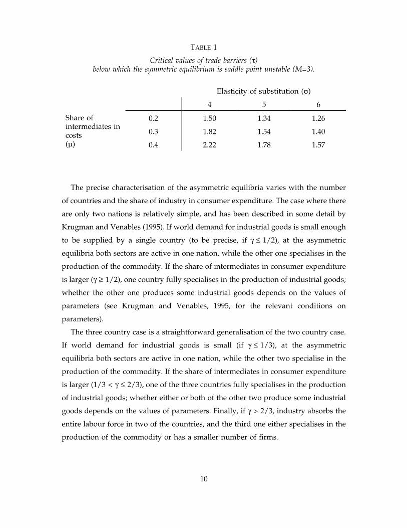
economies.[4] Table 1 illustrates this dependence when M = 3, for values of µ and σ
specified in rows and columns respectively.
When global trade barriers fall below the critical level of expression (17), and the
symmetric equilibrium becomes unstable, there are multiple stable asymmetric
equilibria where some countries have a larger share of industry than others.[5]
However, since all nations are ex ante identical, which countries gain and which lose
industry with respect to the symmetric equilibrium is indeterminate.
4 If economies of scale and input-output links between firms are very large (to the point thatσ(1 – µ) < 1), the symmetric equilibrium may be unstable for any level of τ.
5 Asymmetric equilibria exist below a value of trade barriers higher than the critical value ofexpression (17), so for some intermediate range of trade barriers there are multiple stable equilibria.
9
The precise characterisation of the asymmetric equilibria varies with the number
TABLE 1
Critical values of trade barriers (τ)below which the symmetric equilibrium is saddle point unstable (M=3).
Elasticity of substitution (σ)
4 5 6
Share ofintermediates incosts(µ)
0.2 1.50 1.34 1.26
0.3 1.82 1.54 1.40
0.4 2.22 1.78 1.57
of countries and the share of industry in consumer expenditure. The case where there
are only two nations is relatively simple, and has been described in some detail by
Krugman and Venables (1995). If world demand for industrial goods is small enough
to be supplied by a single country (to be precise, if γ ≤ 1/2), at the asymmetric
equilibria both sectors are active in one nation, while the other one specialises in the
production of the commodity. If the share of intermediates in consumer expenditure
is larger (γ ≥ 1/2), one country fully specialises in the production of industrial goods;
whether the other one produces some industrial goods depends on the values of
parameters (see Krugman and Venables, 1995, for the relevant conditions on
parameters).
The three country case is a straightforward generalisation of the two country case.
If world demand for industrial goods is small (if γ ≤ 1/3), at the asymmetric
equilibria both sectors are active in one nation, while the other two specialise in the
production of the commodity. If the share of intermediates in consumer expenditure
is larger (1/3 < γ ≤ 2/3), one of the three countries fully specialises in the production
of industrial goods; whether either or both of the other two produce some industrial
goods depends on the values of parameters. Finally, if γ > 2/3, industry absorbs the
entire labour force in two of the countries, and the third one either specialises in the
production of the commodity or has a smaller number of firms.
10
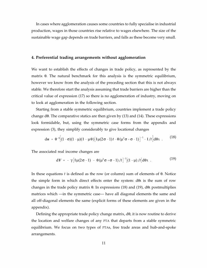
In cases where agglomeration causes some countries to fully specialise in industrial
production, wages in those countries rise relative to wages elsewhere. The size of the
sustainable wage gap depends on trade barriers, and falls as these become very small.
4. Preferential trading arrangements without agglomeration
We want to establish the effects of changes in trade policy, as represented by the
matrix θ. The natural benchmark for this analysis is the symmetric equilibrium,
however we know from the analysis of the preceding section that this is not always
stable. We therefore start the analysis assuming that trade barriers are higher than the
critical value of expression (17) so there is no agglomeration of industry, moving on
to look at agglomeration in the following section.
Starting from a stable symmetric equilibrium, countries implement a trade policy
change dθ. The comparative statics are then given by (13) and (14). These expressions
look formidable, but, using the symmetric case forms from the appendix and
expression (3), they simplify considerably to give locational changes
(18)dn θ 1 (1 σ)(1 µ)( Ι µθ ) Ιµ(2σ 1) t θ (µ2 σ σ 1) 1 Ι/t dθ ι .
The associated real income changes are
(19)dV γ Ιµ(2σ 1) θ (µ2 σ σ 1)/t 1 (1 µ)/t dθ ι .
In these equations t is defined as the row (or column) sum of elements of θ. Notice
the simple form in which direct effects enter the system: dθι is the sum of row
changes in the trade policy matrix θ. In expressions (18) and (19), dθι postmultiplies
matrices which —in the symmetric case— have all diagonal elements the same and
all off-diagonal elements the same (explicit forms of these elements are given in the
appendix).
Defining the appropriate trade policy change matrix, dθ, it is now routine to derive
the location and welfare changes of any PTA that departs from a stable symmetric
equilibrium. We focus on two types of PTAs, free trade areas and hub-and-spoke
arrangements.
11
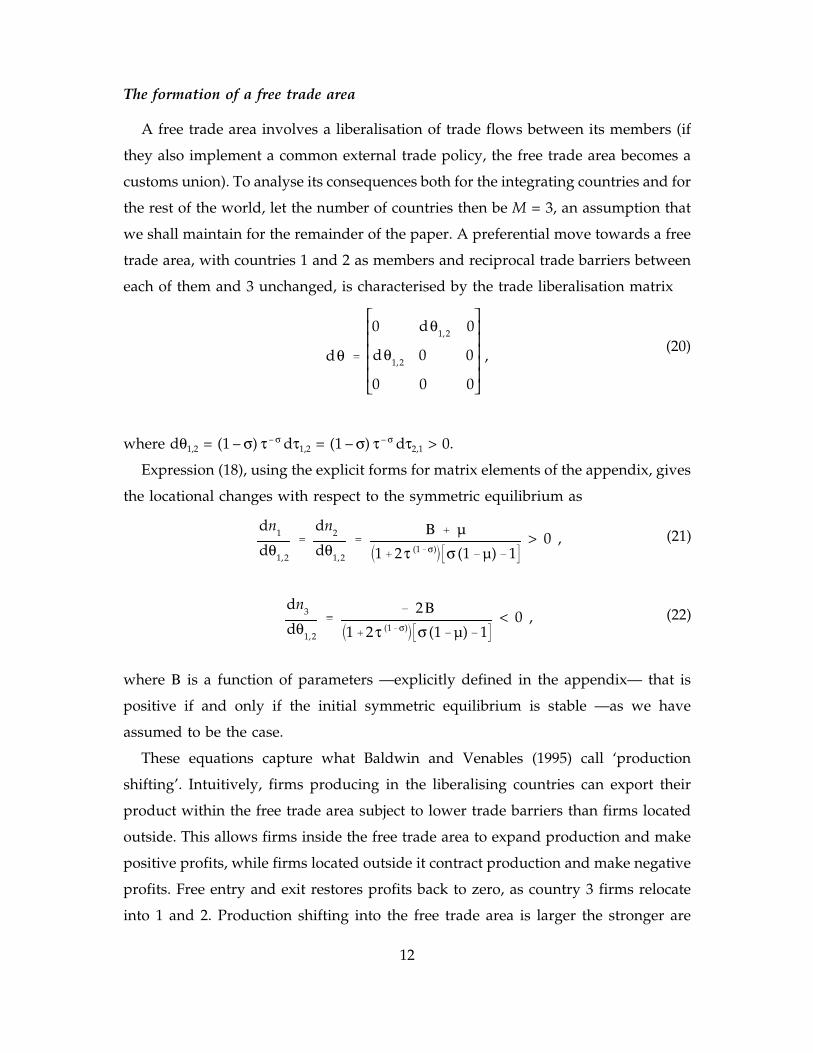
The formation of a free trade area
A free trade area involves a liberalisation of trade flows between its members (if
they also implement a common external trade policy, the free trade area becomes a
customs union). To analyse its consequences both for the integrating countries and for
the rest of the world, let the number of countries then be M = 3, an assumption that
we shall maintain for the remainder of the paper. A preferential move towards a free
trade area, with countries 1 and 2 as members and reciprocal trade barriers between
each of them and 3 unchanged, is characterised by the trade liberalisation matrix
(20)dθ
0 dθ1,2
0
dθ1,2
0 0
0 0 0
,
where dθ1,2 = (1 – σ) τ – σ dτ1,2 = (1 – σ) τ – σ dτ2,1 > 0.
Expression (18), using the explicit forms for matrix elements of the appendix, gives
the locational changes with respect to the symmetric equilibrium as
(21)dn
1
dθ1,2
dn2
dθ1,2
Β µ
1 2τ (1 σ) σ (1 µ) 1> 0 ,
(22)dn
3
dθ1,2
2Β1 2τ (1 σ) σ (1 µ) 1
< 0 ,
where Β is a function of parameters —explicitly defined in the appendix— that is
positive if and only if the initial symmetric equilibrium is stable —as we have
assumed to be the case.
These equations capture what Baldwin and Venables (1995) call ‘production
shifting’. Intuitively, firms producing in the liberalising countries can export their
product within the free trade area subject to lower trade barriers than firms located
outside. This allows firms inside the free trade area to expand production and make
positive profits, while firms located outside it contract production and make negative
profits. Free entry and exit restores profits back to zero, as country 3 firms relocate
into 1 and 2. Production shifting into the free trade area is larger the stronger are
12
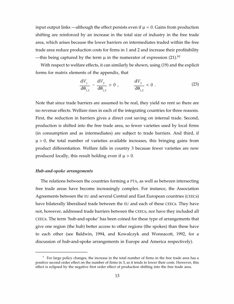
input output links —although the effect persists even if µ = 0. Gains from production
shifting are reinforced by an increase in the total size of industry in the free trade
area, which arises because the lower barriers on intermediates traded within the free
trade area reduce production costs for firms in 1 and 2 and increase their profitability
—this being captured by the term µ in the numerator of expression (21).[6]
With respect to welfare effects, it can similarly be shown, using (19) and the explicit
forms for matrix elements of the appendix, that
(23)dV
1
dθ1,2
dV2
dθ1,2
> 0 ,dV
3
dθ1,2
< 0 .
Note that since trade barriers are assumed to be real, they yield no rent so there are
no revenue effects. Welfare rises in each of the integrating countries for three reasons.
First, the reduction in barriers gives a direct cost saving on internal trade. Second,
production is shifted into the free trade area, so fewer varieties used by local firms
(in consumption and as intermediates) are subject to trade barriers. And third, if
µ > 0, the total number of varieties available increases, this bringing gains from
product differentiation. Welfare falls in country 3 because fewer varieties are now
produced locally, this result holding even if µ > 0.
Hub-and-spoke arrangements
The relations between the countries forming a PTA, as well as between intersecting
free trade areas have become increasingly complex. For instance, the Association
Agreements between the EU and several Central and East European countries (CEECs)
have bilaterally liberalised trade between the EU and each of these CEECs. They have
not, however, addressed trade barriers between the CEECs, nor have they included all
CEECs. The term ‘hub-and-spoke’ has been coined for these type of arrangements that
give one region (the hub) better access to other regions (the spokes) than these have
to each other (see Baldwin, 1994, and Kowalczyk and Wonnacott, 1992, for a
discussion of hub-and-spoke arrangements in Europe and America respectively).
6 For large policy changes, the increase in the total number of firms in the free trade area has apositive second order effect on the number of firms in 3, as it tends to lower their costs. However, thiseffect is eclipsed by the negative first order effect of production shifting into the free trade area.
13
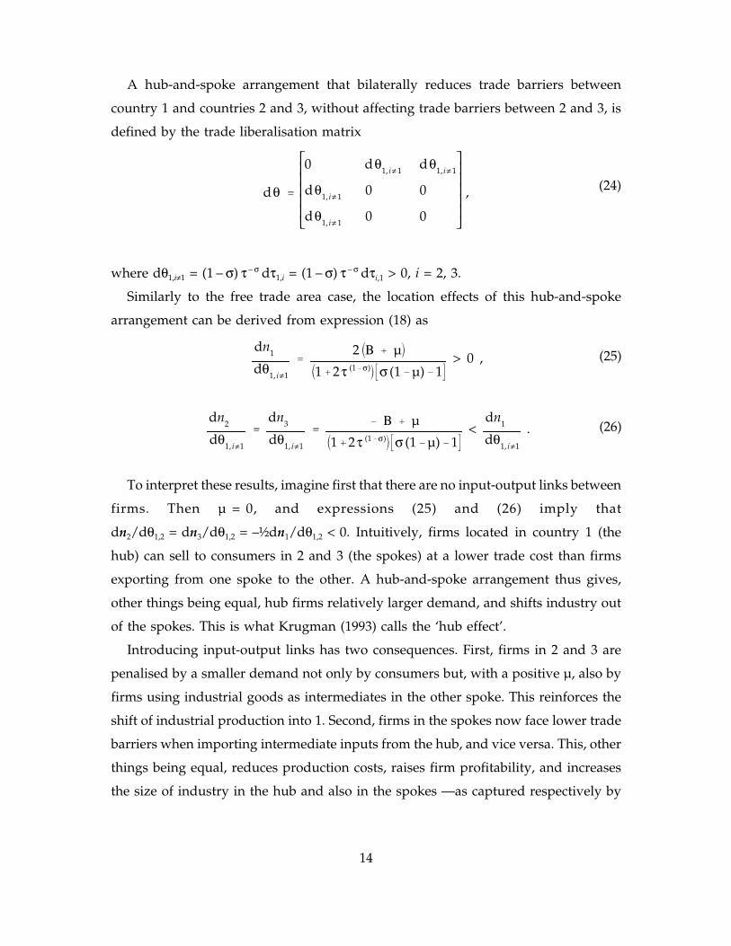
A hub-and-spoke arrangement that bilaterally reduces trade barriers between
country 1 and countries 2 and 3, without affecting trade barriers between 2 and 3, is
defined by the trade liberalisation matrix
(24)dθ
0 dθ1, i≠ 1
dθ1, i≠ 1
dθ1, i≠ 1
0 0
dθ1, i≠ 1
0 0
,
where dθ1,i≠1 = (1 – σ) τ – σ dτ1,i = (1 – σ) τ – σ dτi,1 > 0, i = 2, 3.
Similarly to the free trade area case, the location effects of this hub-and-spoke
arrangement can be derived from expression (18) as
(25)dn
1
dθ1, i≠1
2 Β µ
1 2τ (1 σ) σ (1 µ) 1> 0 ,
(26)dn
2
dθ1, i≠1
dn3
dθ1, i≠1
Β µ
1 2τ (1 σ) σ (1 µ) 1<
dn1
dθ1, i≠1
.
To interpret these results, imagine first that there are no input-output links between
firms. Then µ = 0, and expressions (25) and (26) imply that
dn2/dθ1,2 = dn3/dθ1,2 = –½dn1/dθ1,2 < 0. Intuitively, firms located in country 1 (the
hub) can sell to consumers in 2 and 3 (the spokes) at a lower trade cost than firms
exporting from one spoke to the other. A hub-and-spoke arrangement thus gives,
other things being equal, hub firms relatively larger demand, and shifts industry out
of the spokes. This is what Krugman (1993) calls the ‘hub effect’.
Introducing input-output links has two consequences. First, firms in 2 and 3 are
penalised by a smaller demand not only by consumers but, with a positive µ, also by
firms using industrial goods as intermediates in the other spoke. This reinforces the
shift of industrial production into 1. Second, firms in the spokes now face lower trade
barriers when importing intermediate inputs from the hub, and vice versa. This, other
things being equal, reduces production costs, raises firm profitability, and increases
the size of industry in the hub and also in the spokes —as captured respectively by
14
the term 2µ in the numerator of expression (25) and the term µ in the numerator of
(26).
Welfare effects can be also calculated from (19), which gives
(27)dV
1
dθ1, i≠1
> 0 ,dV
2
dθ1, i≠1
dV3
dθ1, i≠1
<dV
1
dθ1, i≠1
.
Overall, a hub-and-spoke arrangement unambiguously increases the number of firms
and welfare in the hub. In spoke nations the number of firms and welfare certainly
increases by less than in the hub and may fall, the latter being more likely the lower
are initial trade barriers.
5. Regional asymmetries and agglomeration
Regional disparities during the formation of a free trade area
Section 4 looked at the effects of trade policy when parameters are such that the initial
symmetric equilibrium is stable and agglomeration does not occur. We now look at
cases where the PTA triggers agglomeration, and address three questions. First, when
does agglomeration take place? Second, what are the characteristics of the ensuing
equilibrium? And finally, what are the welfare consequences for each country?
Suppose integration starts at a stable symmetric equilibrium, where the Jacobian
matrix of the system, [πn – πq Qq–1Qn], is locally negative definite. Agglomeration takes
place as τ1,2 (= τ2,1) falls below the critical value at which matrix [πn – πq Qq–1Qn],
valued at the relevant equilibrium (with n and q solutions to Q(n, q, θ) = 0 and
π(n, q, θ) = 0), becomes indefinite. At that point the equilibrium where both
integrating countries have the same number of firms switches from being a stable
node to an unstable saddle point. Whereas in section 3 we were able to derive a
closed form solution for the critical value of trade costs at which the symmetric
equilibrium becomes stable, now —because of the asymmetry created by the PTA—
we are forced to use numerical methods. We thus produce table 2 (analogous to
table 1 —and with which it shares one critical point: τi,j = 1.57, for all i ≠ j). Given
linkages and external trade barriers in each row and column respectively, and σ = 6,
15
bifurcation occurs as internal trade barriers fall below the specified critical level. A
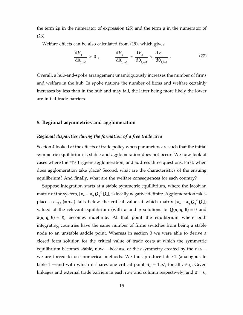
TABLE 2
Critical values of internal trade barriers (τ1,2 = τ2,1)below which the equilibrium where both countries forming a free trade area
have the same number of firms is saddle point unstable
External trade cost(τ1,3 = τ3,1 = τ2,3 = τ3,2)
1.57 1.85 2
Share ofintermediates incosts(µ)
0.2 1.22 1.21 1.20
0.3 1.37 1.34 1.33
0.4 1.57 1.51 1.49
higher µ, which represents stronger linkages, makes bifurcation take place earlier
during the formation of a free trade area. So do lower external trade barriers, which
make industry more footloose.
What happens to the share of industry in each country once internal trade barriers
fall below the critical value? At the ensuing equilibrium one of the countries in the
free trade area (we shall assume 1) gains firms, the other one (in this case 2) loses
firms, while the effect on the size of industry in country 3 is ambiguous. Let us look
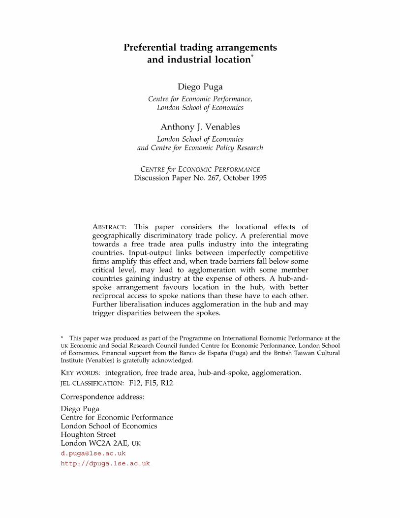
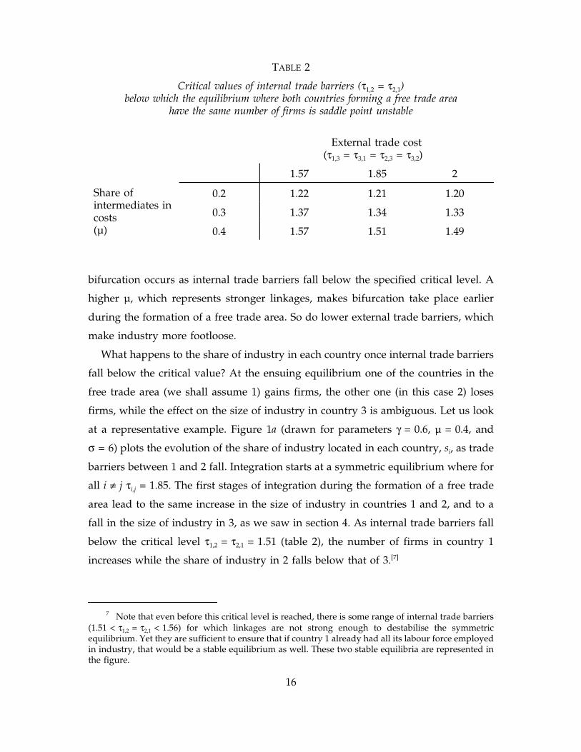
at a representative example. Figure 1a (drawn for parameters γ = 0.6, µ = 0.4, and
σ = 6) plots the evolution of the share of industry located in each country, si, as trade
barriers between 1 and 2 fall. Integration starts at a symmetric equilibrium where for
all i ≠ j τi,j = 1.85. The first stages of integration during the formation of a free trade
area lead to the same increase in the size of industry in countries 1 and 2, and to a
fall in the size of industry in 3, as we saw in section 4. As internal trade barriers fall
below the critical level τ1,2 = τ2,1 = 1.51 (table 2), the number of firms in country 1
increases while the share of industry in 2 falls below that of 3.[7]
7 Note that even before this critical level is reached, there is some range of internal trade barriers(1.51 < τ1,2 = τ2,1 < 1.56) for which linkages are not strong enough to destabilise the symmetricequilibrium. Yet they are sufficient to ensure that if country 1 already had all its labour force employedin industry, that would be a stable equilibrium as well. These two stable equilibria are represented inthe figure.
16
1 1.17 1.34 1.51 1.68 1.850
0.2
0.4
0.6
τ = τ
Ind
ustr
y sh
are
s2
s3
s1
s3
=s1 s2
1, 2 2, 1
FIGURE 1aThe formation of a free trade area: Share of industry in each country
1 1.17 1.34 1.51 1.68 1.85
0.9
1
1.1
1.2
τ = τ
Wel
fare
V1
V2
V3
V3
=V1 V2
1, 2 2, 1
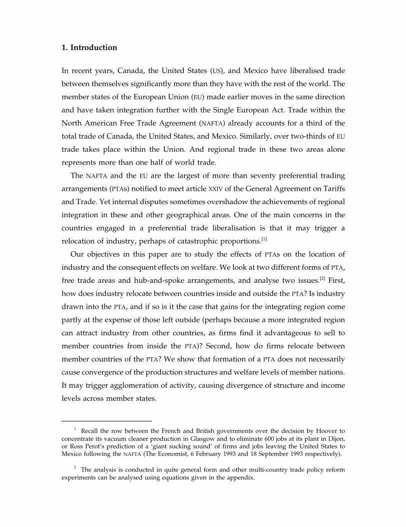
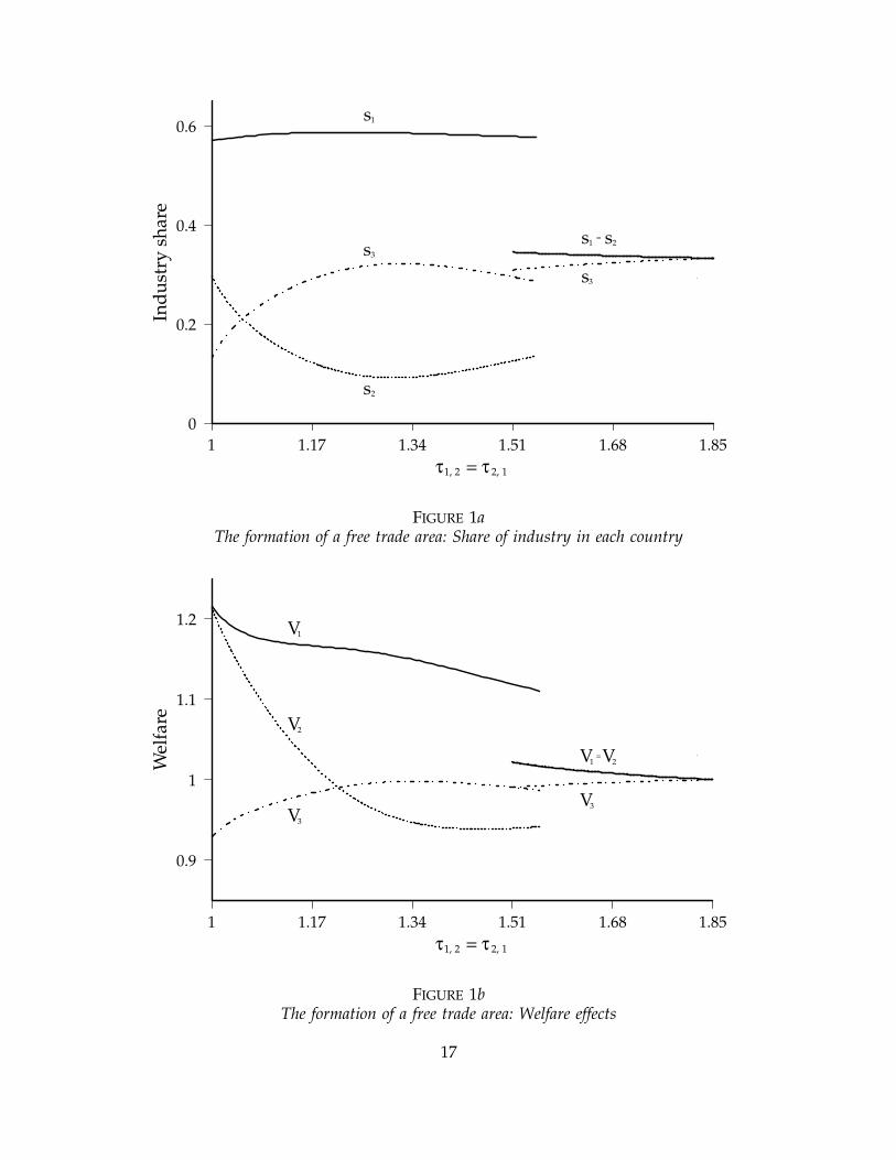
FIGURE 1bThe formation of a free trade area: Welfare effects
17
Further integration beyond the critical level makes markets with larger expenditure
more attractive locations. That has the effect of increasing industrial employment in
3 at the expense of 2. In 1, with all its labour already employed by industry, the larger
labour demand translates into higher wages instead. However, as internal trade
barriers continue to fall, location becomes increasingly sensitive to differences in
production costs. At low enough internal barriers (τ1,2 = τ2,1 = 1.3), country 2 starts
reattracting firms because of its increasingly good access to country 1 and its low
labour costs, despite having a smaller local base of suppliers. Country 3
simultaneously begins to lose firms. As τ1,2 (= τ2,1) approaches unity, the share of
industry in country 2 gets closer to that of 1, reducing differences in wages between
the two countries.
Figure 1b plots the evolution of welfare corresponding to figure 1a. Although
welfare effects are not directly caused by the evolution in country shares of industry
they are closely related with it. Countries with more industry have higher labour
demand and have to import fewer varieties subject to trade barriers, both effects
supporting the real income differences in figure 1b. Until agglomeration takes place
welfare changes are driven by members of the free trade area incurring lower trade
barriers on their usage of manufacturing, and changes in the total number of varieties
available. The formation of a free trade area between countries 1 and 2 initially
increases their welfare levels as industry shifts into them, while welfare decreases in
3. The additional feature giving rise to the large welfare differentials in figure 1b is
the fact that when internal trade barriers fall below the critical level τ1,2 = τ2,1 = 1.51,
country 1 specialises in manufacturing and the wage in this country rises above wages
elsewhere. Because a larger share of goods are produced locally instead of being
imported, the price index drops in 1, raising welfare further. In 2 welfare falls instead
following firm exit —in the figure, below the welfare level of country 3. However, as
internal trade barriers continue to fall so there is relocation of production from
country 1 to country 2, and the wage gap between 1 and 2 narrows, with internal
factor price equalisation achieved in the limit.[8]
8 Countries are identical in technology and endowments, so at perfectly free trade the locationof production within the free trade area is indeterminate.
18
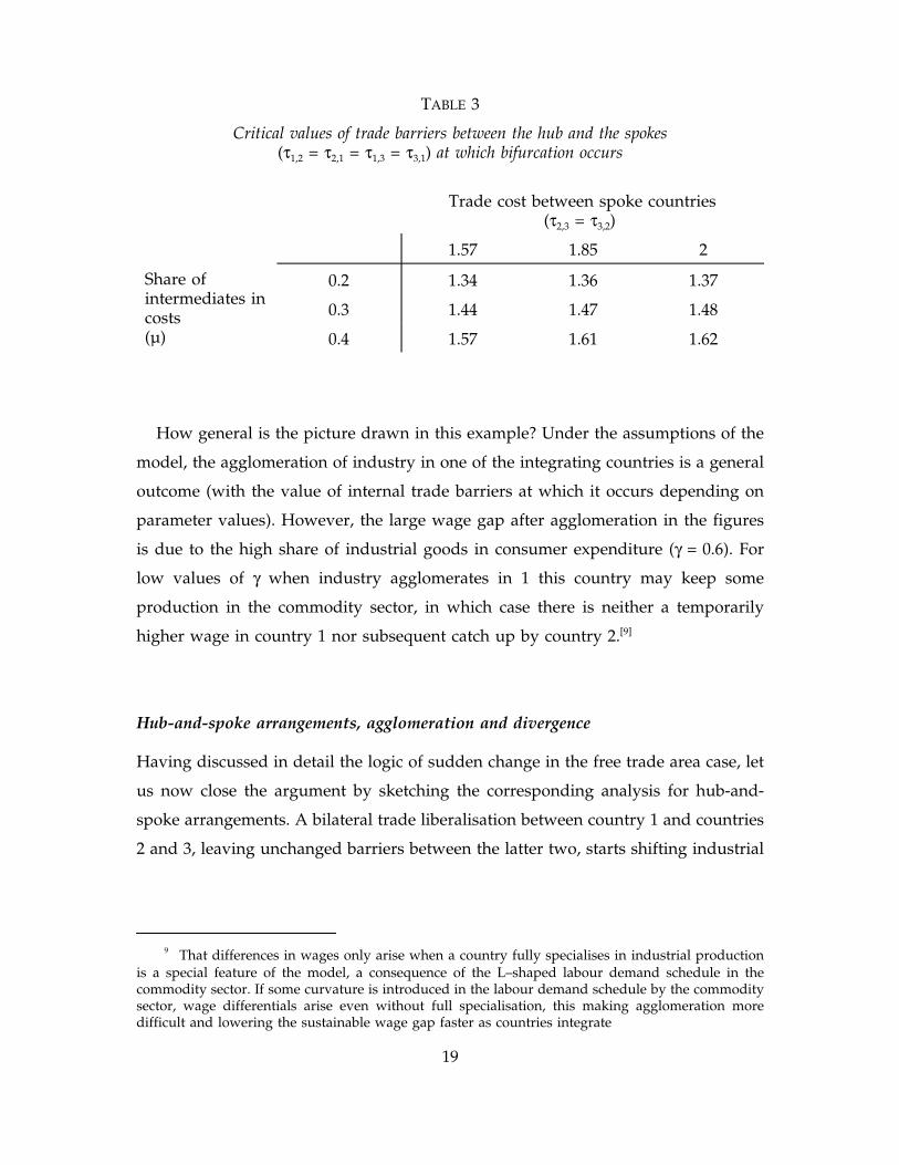
How general is the picture drawn in this example? Under the assumptions of the
TABLE 3
Critical values of trade barriers between the hub and the spokes(τ1,2 = τ2,1 = τ1,3 = τ3,1) at which bifurcation occurs
Trade cost between spoke countries(τ2,3 = τ3,2)
1.57 1.85 2
Share ofintermediates incosts(µ)
0.2 1.34 1.36 1.37
0.3 1.44 1.47 1.48
0.4 1.57 1.61 1.62
model, the agglomeration of industry in one of the integrating countries is a general
outcome (with the value of internal trade barriers at which it occurs depending on
parameter values). However, the large wage gap after agglomeration in the figures
is due to the high share of industrial goods in consumer expenditure (γ = 0.6). For
low values of γ when industry agglomerates in 1 this country may keep some
production in the commodity sector, in which case there is neither a temporarily
higher wage in country 1 nor subsequent catch up by country 2.[9]
Hub-and-spoke arrangements, agglomeration and divergence
Having discussed in detail the logic of sudden change in the free trade area case, let
us now close the argument by sketching the corresponding analysis for hub-and-
spoke arrangements. A bilateral trade liberalisation between country 1 and countries
2 and 3, leaving unchanged barriers between the latter two, starts shifting industrial
9 That differences in wages only arise when a country fully specialises in industrial productionis a special feature of the model, a consequence of the L–shaped labour demand schedule in thecommodity sector. If some curvature is introduced in the labour demand schedule by the commoditysector, wage differentials arise even without full specialisation, this making agglomeration moredifficult and lowering the sustainable wage gap faster as countries integrate
19
1 1.17 1.34 1.51 1.68 1.850
0.2
0.4
0.6
τ = τ = τ = τ
Ind
ustr
y sh
are
s2
s3
s1
=s2 s3
s1
=s2 s3
s1
1, 2 2, 1 1, 3 3, 1
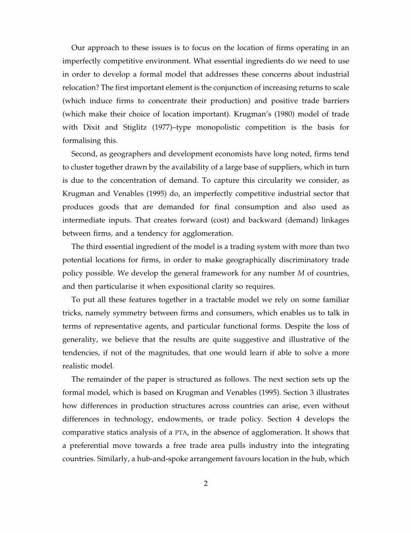
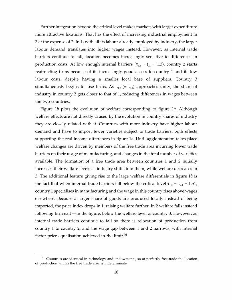
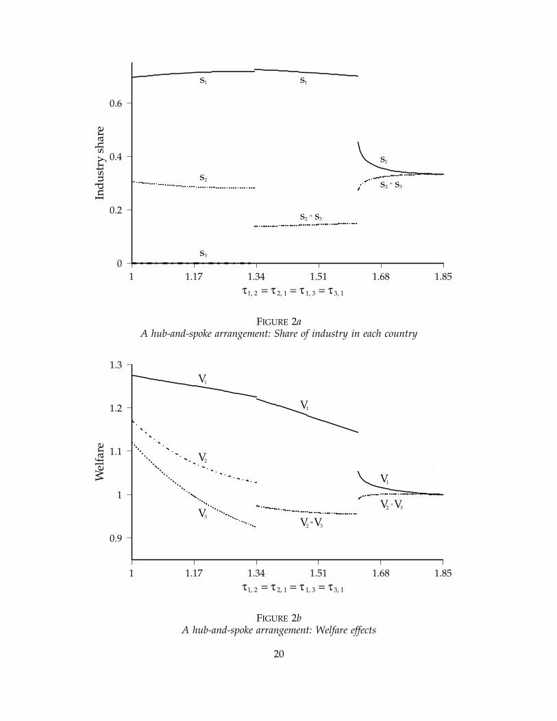
FIGURE 2aA hub-and-spoke arrangement: Share of industry in each country
1 1.17 1.34 1.51 1.68 1.85
0.9
1
1.1
1.2
1.3
τ = τ = τ = τ
Wel
fare
1, 2 2, 1 1, 3 3, 1
V1
V2
V3
=V2 V3
=V2 V3
V1
V1
FIGURE 2bA hub-and-spoke arrangement: Welfare effects
20
production into 1 gradually. However, when a critical level of integration is reached,
agglomeration in the hub takes place suddenly.
Table 3 gives the level of bilateral trade barriers at which the matrix [πn – πq Qq–1Qn]
ceases to be locally negative definite and bifurcation occurs. Linkages are given in
each row, and trade barriers between the spokes in each column, while σ = 6
throughout. Higher trade barriers between the spokes and stronger linkages bring
sudden change earlier during a gradual hub-and-spoke trade liberalisation.
Figure 2a plots the evolution of industrial location (for parameters γ = 0.5, µ = 0.4,
σ = 6, and τ2,3 = τ3,2 = 1.85). When bilateral trade barriers fall below the critical level
τ1,2 = τ2,1 = τ1,3 = τ3,1 = 1.61 (table 3), country 1 becomes fully specialised in industrial
production. Hub wages then rise above those paid in the spokes. As hub-and-spoke
trade liberalisation goes further, location becomes increasingly sensitive to cost
differences.[10]
At low enough bilateral trade barriers (τ1,2 = τ2,1 = τ1,3 = τ3,1 = 1.34), the equilibrium
where 2 and 3 have the same number of firms becomes unstable and a second
bifurcation occurs. If one of the spokes (country 2 in figure 2a) has a larger share of
industry than the other, its firms can buy intermediates at a lower cost and reduce
prices. That lowers demand for firms producing in other markets. In country 1 the
market-clearing wage consistent with zero profits falls, leaving industrial employment
unaffected. In 3 any wage cut leads industrial workers to seek employment in the
commodity sector, and firms exit as industry expands in 2. Figure 2b plots the
evolution of welfare corresponding to figure 2a. Hub-and-spoke integration, if pushed
far enough, can raise welfare in all countries involved. Yet it is a way of opening up
trade that not only favours the hub, but can also end up triggering divergence
between the spokes.
10 If agglomeration in the hub does not lead to wage divergence, as hub-and-spoke integrationgoes on beyond this critical level, industry keeps growing in country 1 and shrinking in 2 and 3.
21
6. Summary and conclusions
The analysis of the paper draws a stylised picture of how industrial location may
change in response to preferential trading arrangements (PTAs). A move towards a
free trade area lets imperfectly competitive firms in the integrating countries sell their
output to (and import intermediates from) other member countries at lower trade
barriers, as compared to firms outside the free trade area. That raises the profitability
of firms located in the liberalising nations, and shifts industry into them.
Input-output links create a tendency for firms to cluster together in markets with
a larger base of suppliers, which in turn is due to the concentration of demand.
During the initial stages of integration, high internal trade barriers provide an
incentive to supply national markets locally. All member states of the free trade area
then benefit identically from integration, while industry size and welfare fall outside
the liberalising regions.
As integration proceeds, the incentive for self-sufficiency weakens. And when
internal trade barriers fall below some critical level, the circular process of
agglomeration created by input-output links endogenously produces a core-periphery
structure, as some regions in the free trade area gain industry at the expense of
others. As a result, while the formation of a free trade area benefits the integrating
region as a whole, during the intermediate stages of integration some member
countries may have lower welfare levels than countries outside the arrangement.
Further integration initially leads to wider divergence. But if changing industrial
employment has an impact on wages, then there is a point beyond which less
industrialised countries inside the free trade area are able to reattract a share of
industry. They do so on the basis of good access to the internal market and low
labour costs, despite lacking a large local base of suppliers. Therefore, a firm and
credible commitment to full integration may convince peripheral regions to put up
with harder times during the intermediate stages of trade liberalisation. So will
transfers from the core regions, which redistribute the aggregate gains that the free
trade area achieves during the whole integration process.
Turning to hub-and-spoke arrangements, firms located in the spoke countries are
penalised by a lower demand by both consumers and firms in the other spokes, as
22
compared to that enjoyed by hub firms. Spoke firms also have larger costs, as they
face higher barriers than hub firms when importing intermediates from the other
spokes. A hub-and-spoke arrangement thus shifts industrial production into the hub.
It has been argued (see Baldwin, 1994) that, although the Association Agreements are
better than no trade liberalisation at all, they will marginalise Central and East
European countries (CEECs) by turning them into the spokes of the European Union
hub. Similarly, Kowalczyk and Wonnacott (1992) have argued that Canada will benefit
more from a free trade area with the United States and Mexico than from a hub-and-
spoke system centred on the US, although a hub-and-spoke liberalisation would have
been better for Canada than giving up its free trade area with the US. Our results
formally corroborate this argument. They also establish that cumulative causation in
the location decision of firms may make production shifting more rapid and dramatic
than expected. Integration beyond some critical level may accelerate agglomeration
in the hub suddenly. Moreover, if higher industrial employment in the hub induces
divergence in wages, further integration may also trigger disparities between the
spoke countries. Differences between the CEECs were one of the reasons argued
against a multilateral rather than bilateral approach to trade liberalisation in the first
place. If hub-and-spoke arrangements widen regional divergences, they may become
increasingly difficult to replace.
How much evidence is there to support that PTAs cause such changes in the
production structure of nations? Hanson (1994), using data on Mexico, finds support
for the hypothesis that agglomeration is associated with increasing returns. He also
shows (Hanson, forthcoming) that integration with the US has had strong effects on
industry location in Mexico. Industry has shifted towards states with good access to
the US market. At the same time, employment growth has been higher in regions that
have larger agglomerations of industries with buyer/supplier relationships. With
respect to Europe, Brülhart and Torstensson (1996) show that scale intensive
industries in the EU tend to be highly concentrated in space, and located close to the
geographical core of the EU. Using regional EU data, they also find some support for
the U-shaped relationship between the degree of regional integration and spatial
agglomeration that our model predicts: activities with larger scale economies were
23
more concentrated in regions close to the geographical core of the EU during the early
stages of European integration, while concentration in the core has fallen in the 1980s.
While these examples provide some support for our findings, more work is clearly
needed in this area. We hope that the clear predictions arising from this framework
will help encourage much needed empirical testing on the location effects of
preferential trading arrangements.
Appendix
Explicit forms for vectors and matrices of partial derivatives. At the symmetric equilibrium
we choose units for L such that q = ι, and hence n = ι/t, where
(A 1)t ≡ 1 (M 1)τ (1 σ) .
The partial derivatives of the text are given in the following set of equations, in each
of which the first expression gives the general form, and the second evaluates this at
the symmetric equilibrium.
(A 2)Qn
θT qµ(1 σ) θ ,
(A 3)Qq
θT nµ(1 σ) q [µ(1 σ) 1] (1 σ) q σ (1 σ) θ (µ/t) Ι ,
(A 4)πn
θ µ q (µ σ 1) θ µ ,
(A 5)π
qθ γ L (σ 1) q (σ 2) θ µ(µ σ 1) q (µ σ 2) n σµ q (σ µ 1)
θ (µ2 σ σ 1)/t Ισ µ,
(A 6)Qθ qµ(1 σ) n ι /t ,
(A 7)π θ γ L q (σ 1) µ q (µ σ 1) n ι /t .
24
Derivation of the critical value in the symmetric case. The Jacobian matrix of the system,
[πn – πq Qq–1Qn], valued at the symmetric equilibrium, has identical diagonal elements
(A 8)τ (1 σ) (µ2σ σ 1)(1 τ (1 σ)) 1 (M 1)τ (1 σ) σ (1 µ) 1 (1 τ (1 σ))Α
(σ 1) (1 µ) (M 1) µ τ (1 σ)
,
where
(A 9)Α ≡ (1 τ (1 σ))(1 µ) σ (1 µ) 1 τ (1 σ) Mµ(2σ 1) ,
and identical off-diagonal elements
(A 10)τ (1 σ) (µ2σ σ 1)(1 τ (1 σ)) 1 (M 1)τ (1 σ) σ (1 µ) 1
(σ 1) (1 µ) (M 1) µ τ (1 σ)
.
Provided that σ(1 – µ) > 1, the Jacobian matrix is negative definite if and only if Α > 0,
which is the case if and only if τ is larger than the critical value of equation (17) in
the text.
Location and welfare changes. The matrix
(A 11)θ 1 (1 σ)(1 µ)( Ι µθ ) Ιµ(2σ 1) t θ (µ2 σ σ 1) 1 Ι/t ,
which, when postmultiplied by dθι, as in expression (18), gives the location effects
of a trade policy change dθ in the neighbourhood of the symmetric equilibrium, has
identical diagonal elements
(A 12)(M 1)Β µ
1 (M 1)τ (1 σ) σ (1 µ) 1,
and identical off-diagonal elements
(A 13)Β1 (M 1)τ (1 σ) σ (1 µ) 1
,
where
25
Matrix(A 14)
Β ≡ τ (1 σ)(σ 1)(µ2σ σ 1) 1 (M 1)τ (1 σ) µ(1 τ (1 σ)) µσ τ (1 σ) Α(1 τ (1 σ))Α
.
(A 15)γ Ιµ(2σ 1) θ (µ2 σ σ 1)/t 1 (1 µ)/t ,
which, when postmultiplied by dθι, as in expression (19), gives the welfare effects
of a trade policy change dθ in the neighbourhood of the symmetric equilibrium, has
identical diagonal elements
(A 16)γ (M 1)τ (1 σ)(µ2σ σ 1) Α1 (M 1)τ (1 σ) σ (1 µ) 1 Α
,
and identical off-diagonal elements
(A 17)γ (µ2σ σ 1)τ (1 σ)
1 (M 1)τ (1 σ) σ (1 µ) 1 Α.
If the symmetric equilibrium is stable, Α > 0, and Β > 0, and both the matrix of
expression (A 11) and the matrix of expression (A 15) have positive diagonal elements
and negative off-diagonal elements, with the former larger in absolute value than the
latter.
References
Baldwin, Richard E. 1994. Towards an Integrated Europe. London: Centre for EconomicPolicy Research.
Baldwin, Richard E. and Anthony J. Venables. 1995. ‘Regional economic integration.’In Gene M. Grossman and Kenneth Rogoff (eds.). Handbook of InternationalEconomics, 3, Amsterdam: North-Holland: 1597-1644.
Dixit, Avinash K. and Joseph E. Stiglitz. 1977. ‘Monopolistic competition and optimumproduct diversity.’ American Economic Review, 67: 297–308.
Brülhart, Marius and Johan Torstensson. 1996. ‘Regional integration, scale economiesand industry location.’ Discussion Paper No. 1.435, Centre for Economic PolicyResearch.
26
Ethier, Wilfred J. 1982. ‘National and international returns to scale in the moderntheory of international trade.’ American Economic Review, 72: 389–405.
Hanson, Gordon H. 1994. ‘Regional adjustment to trade liberalisation.’ Working PaperNo. 4713, National Bureau of Economic Research.
Hanson, Gordon H. Forthcoming. ‘Increasing returns, trade, and the regional structureof wages.’ Economic Journal.
Hirschman, Albert O. 1958. The Strategy of Economic Development. New Haven,Connecticut: Yale University Press.
Kowalczyk, Carsten and Ronald J. Wonnacott. 1992. ‘Hubs and spokes, and free tradein the Americas.’ Working Paper No. 4198, National Bureau of Economic Research.
Krugman, Paul R. 1980 ‘Scale economies, product differentiation, and the pattern oftrade.’ American Economic Review, 70: 950–959.
Krugman, Paul R. 1993 ‘The hub effect: or, threeness in interregional trade.’ In WilfredJ. Ethier, Elhanan Helpman, and J. Peter Neary (eds.). Theory, Policy and Dynamicsin International Trade. Cambridge: Cambridge University Press: 29–37.
Krugman, Paul R. and Anthony J. Venables. 1995. ‘Globalization and the inequalityof nations.’ Quarterly Journal of Economics, 110: 857-880.
Venables, Anthony J. 1996. ‘Equilibrium locations of vertically linked industries.’International Economic Review, 37: 341-359.
27