Embed Size (px)
Citation preview
Applied Mathematics and Computation 168 (2005) 342–353
www.elsevier.com/locate/amc
Project scheduling problem withstochastic activity duration times
Hua Ke *, Baoding Liu
Uncertainty Theory Laboratory, Department of Mathematical Sciences, Tsinghua University,
Beijing 100084, China
Abstract
Project scheduling problem is to determine the schedule of allocating resources so as
to balance the total cost and the completion time. This paper considers project schedul-
ing problem with stochastic activity duration times, which has the objective of minimiz-
ing the total cost under some completion time limits. Three types of stochastic models
will be built to solve the problem according to different management requirements.
Moreover, stochastic simulation and genetic algorithm will be integrated to design a
hybrid intelligent algorithm to solve the above models. Finally, some numerical exam-
ples are illustrated to show the effectiveness of the algorithm.
� 2004 Elsevier Inc. All rights reserved.
Keywords: Project scheduling; Stochastic programming; Stochastic simulation; Genetic algorithm
0096-3003/$ - see front matter � 2004 Elsevier Inc. All rights reserved.
doi:10.1016/j.amc.2004.09.002
* Corresponding author.
E-mail addresses: [email protected] (H. Ke), [email protected] (B. Liu).

H. Ke, B. Liu / Appl. Math. Comput. 168 (2005) 342–353 343
1. Introduction
Project scheduling problem, which has been widely studied since early
1960�s, is to determine the schedule of allocating resources so as to balance
the total cost and the completion time.
Uncertainty always exists in project scheduling problem, due to the vague-ness of project activity duration times. Generally, the uncertainty of activity
duration times in project scheduling problem was assumed to be stochastic.
Freeman [8,9] first introduced probability theory into project scheduling prob-
lem in 1960. Charnes and Cooper [3,4] and Charnes et al. [5] studied project
scheduling problem via chance constrained programming in early 1960�s. Gol-
enko-Ginzburg and Gonik [10] established an expected value model in solving
a type of project scheduling problem. The reader may also refer to Elmaghraby
[7], Kotiah and Wallace [13], Loostma [19], MacCrimmon and Ryavec [20],and Parks and Ramsing [23] to see how different probability distributions were
employed to depict stochastic activity duration times in studying project sched-
uling problem. Nevertheless, all papers concerning project scheduling problem
with stochastic activity duration times just resolved problems concentrating on
optimizing completion time under resource or cost limits.
Many other researchers have studied project scheduling problem in another
way as minimizing the total cost under some time limits. Kelley [11] first pre-
sented function relationship between project cost and activity duration times,establishing the mathematical fundamental for project scheduling problem in
1961. Then in 1963, Kelley [12] originally formulated an approach to a type
of project scheduling problem with the objective of cost minimization. Since
then, many other researchers, such as Burgess and Killebrew [1], Demeuleme-
ester [6], Maniezzo and Mingozzi [21] and Mohring [22] have studied various
types of project scheduling problem in optimizing project cost with different
types of time limits. However, all these researchers just took certain activity
duration times into account when studying this type of project schedulingproblem, and no research papers have considered project scheduling problem
with stochastic activity duration times in minimizing the total cost.
In this paper, we will discuss project scheduling problem with stochastic
activity duration times, which is in attempt to minimize the total cost. And
the influence of the interest and the limit of the completion time are taken into
account in the problem.
We will design a hybrid intelligent algorithm integrating stochastic simula-
tion and genetic algorithm (GA) to settle project scheduling problem withstochastic time constraints. We may reveal that the algorithm is effective in
solving project scheduling problem.
This paper is organized as follows: Section 2 describes the project scheduling
problem in detail and Section 3 builds three kinds of stochastic models. In Sec-
tion 4, a hybrid intelligent algorithm integrating stochastic simulation and GA
344 H. Ke, B. Liu / Appl. Math. Comput. 168 (2005) 342–353
is designed. Then in order to reveal the effectiveness of the hybrid intelligent
algorithm, Section 5 give some numerical examples. Finally some conclusions
are drawn in Section 6.
2. Problem description
Before we begin to study project scheduling problem with stochastic activity
duration times, we first make some assumptions as: (a) each activity can be
processed only if the loan needed is allocated and all the foregoing activities
are finished; (b) each activity should be processed without interruption; (c)
all of the costs needed are obtained via loans with some given interest rate;
and (d) all activity duration times are assumed to be stochastic.
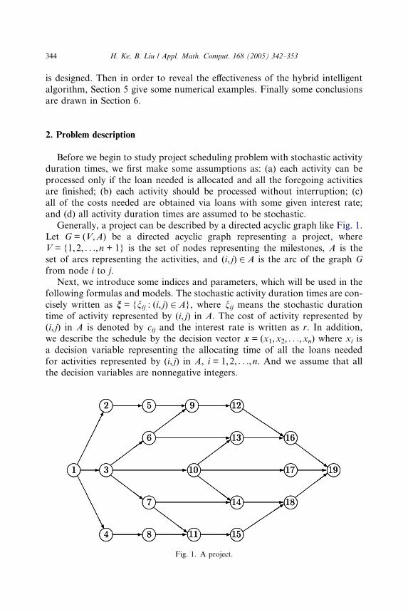
Generally, a project can be described by a directed acyclic graph like Fig. 1.Let G = (V,A) be a directed acyclic graph representing a project, where
V = {1,2, . . .,n + 1} is the set of nodes representing the milestones, A is the
set of arcs representing the activities, and (i, j) 2 A is the arc of the graph G
from node i to j.
Next, we introduce some indices and parameters, which will be used in the
following formulas and models. The stochastic activity duration times are con-
cisely written as n = {nij : (i, j) 2 A}, where nij means the stochastic duration
time of activity represented by (i, j) in A. The cost of activity represented by(i, j) in A is denoted by cij and the interest rate is written as r. In addition,
we describe the schedule by the decision vector x = (x1,x2, . . .,xn) where xi is
a decision variable representing the allocating time of all the loans needed
for activities represented by (i, j) in A, i = 1,2, . . .,n. And we assume that all
the decision variables are nonnegative integers.
Fig. 1. A project.
H. Ke, B. Liu / Appl. Math. Comput. 168 (2005) 342–353 345
We denote Ti(x,n) as the starting time of all activities represented by (i, j) in
A. According to the assumption (a), we have Ti(x,n) P xi and
T iðx; nÞP maxðk;iÞ2A
fT kðx; nÞ þ nkig:
Hence, the starting time of the total project can be known as T1(x,n) = x1, thestarting time of activities represented by (i, j) in A, i = 2, . . .,n, can be decided by
T iðx; nÞ ¼ xi _ maxðk;iÞ2A
fT kðx; nÞ þ nkig
and the completion time of the total project can be calculated by
T ðx; nÞ ¼ maxðk;nþ1Þ2A
fT kðx; nÞ þ nk;nþ1g: ð1Þ
According to the assumption (c), the total cost of the project can be written as
Cðx; nÞ ¼Xði;jÞ2A
cijð1þ rÞdðT ðx;nÞ�xiÞe; ð2Þ
where d(T(x,n) � xi)emeans the minimal integer larger than or equal to
T(x,n) � xi.
3. Stochastic models of project scheduling problem
3.1. Expected cost model
Expected value model (EVM) is widely used for solving various types of
practical problems. And in practice, many decision-makers desire to make deci-
sions with the minimum expected cost under expected time constraints for the
project. In order to satisfy this type of demand, in project scheduling problem,
we can build an expected cost model to minimize the expected cost of the pro-
ject under the expected project completion time constraint:
min E½Cðx; nÞ�subject to : E½T ðx; nÞ� 6 T 0;
x P 0; integer vector;
8><>:
where T0 is the due date of the project, and T(x,n) and C(x,n) are defined by (1)
and (2), respectively.
3.2. a-Cost model
Chance-constrained programming (CCP) was initialized by Charnes and
Cooper [2], in which management goals are obtained in condition of satisfying
some chance constraints with at least some given confidence levels. After that,CCP was developed by many researchers. This paper will use the latest version
346 H. Ke, B. Liu / Appl. Math. Comput. 168 (2005) 342–353
provided by Liu [16,18]. In this subsection, to model the project scheduling
problem, we will establish an a-cost model based on stochastic CCP.
Definition 1. The a-cost of a project is defined as minfCjPrfCðx; nÞ 6CgP ag, where a is a predetermined confidence level.
In our problem, we tend to minimize the a-cost of the project under the com-
pletion time chance constraint with a predetermined confidence level. Follow-
ing the idea of stochastic CCP, we can present the a-cost model as follows:
min C
subject to : PrfCðx; nÞ 6 CgP a;
PrfT ðx; nÞ 6 T 0gP b;
x P 0; integer vector;
8>>><>>>:
where a and b are predetermined confidence levels, T0 is the due date of the
project, and T(x,n) and C(x,n) are defined by (1) and (2), respectively.
3.3. Probability maximization model
We know that when some management targets are given, we can use
dependent-chance programming (DCP) introduced by Liu [14] to solve the pro-
ject scheduling problem. The reader who is interested in DCP may refer to Liu
and Iwamura [15] and Liu [16–18]. In this paper, the goal is given in advance as
that the probability of the total cost not overrunning the budget should be as
large as possible. And the constraint is that the probability of finishing the pro-ject before the due date should be larger than or equal to a predetermined con-
fidence level a. Hence, we can build the following probability maximization
model:
max PrfCðx; nÞ 6 C0gsubject to : PrfT ðx; nÞ 6 T 0gP a;
x P 0; integer vector;
8><>:
where a is a predetermined confidence level, T0 is the due date of the project, C0
is the budget, and T(x,n) and C(x,n) are defined by (1) and (2), respectively.
4. Hybrid intelligent algorithm
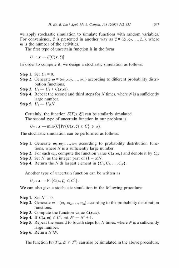
4.1. Stochastic simulations
In this paper, a hybrid intelligent algorithm integrating stochastic simulation
and GA is designed to solve the above three types of stochastic models. Firstly,
H. Ke, B. Liu / Appl. Math. Comput. 168 (2005) 342–353 347
we apply stochastic simulation to simulate functions with random variables.
For convenience, n is presented in another way as n = (n1,n2, . . .,nm), wherem is the number of the activities.
The first type of uncertain function is in the form
U 1 : x! E½Cðx; nÞ�:In order to compute it, we design a stochastic simulation as follows:
Step 1. Set U1 = 0.
Step 2. Generate x = (x1,x2, . . .,xm) according to different probability distri-
bution functions.
Step 3. U1 U1 + C(x,x).Step 4. Repeat the second and third steps for N times, where N is a sufficiently
large number.
Step 5. U1 U1/N.
Certainly, the function E[T(x,n)] can be similarly simulated.
The second type of uncertain function in our problem is
U 2 : x! minfCjPrfCðx; nÞ 6 CgP ag:The stochastic simulation can be performed as follows:
Step 1. Generate x1,x2, . . .,xN according to probability distribution func-
tions, where N is a sufficiently large number.
Step 2. For each xk, compute the function value C(x,xk) and denote it by Ck.
Step 3. Set N 0 as the integer part of (1 � a)N.
Step 4. Return the N 0th largest element in {C1,C2, . . .,CN}.
Another type of uncertain function can be written as
U 3 : x! PrfCðx; nÞ 6 C0g:We can also give a stochastic simulation in the following procedure:
Step 1. Set N 0 = 0.
Step 2. Generate x = (x1,x2, . . .,xm) according to the probability distributionfunctions.
Step 3. Compute the function value C(x,x).Step 4. If C(x,x) 6 C0, set N 0 N 0 + 1.
Step 5. Repeat the second to fourth steps for N times, where N is a sufficiently
large number.
Step 6. Return N 0/N.
The function Pr{T(x,n) 6 T0} can also be simulated in the above procedure.
348 H. Ke, B. Liu / Appl. Math. Comput. 168 (2005) 342–353
4.2. Hybrid intelligent algorithm
In this subsection, we embed the stochastic simulation, which can simulate
the above three types of uncertain functions, into GA to design a hybrid intel-
ligent algorithm. The procedure can be summarized generally as follows:
Firstly, we initialize pop_size chromosomes, in which the genes represent thedifferent allocating times of loans for different activities. The next step is to up-
date the chromosomes by crossover and mutation operations. In the third step
we calculate the objective values for all chromosomes and according to the
objective values we compute the fitness of each chromosome. Then we select
the chromosomes by spinning the roulette wheel according to the different fit-
ness values. And after a given number of generations, we report the best chro-
mosome as the optimal solution. In the above steps, stochastic simulation is
applied to check the feasibility of chromosomes and calculate the objectivevalues.
5. Numerical examples
Now let us consider a project scheduling problem shown in Fig. 1. The dura-
tion times and the costs needed for the relevant activities in the project are pre-
sented in Table 1, respectively, and the monthly interest rate is given as 0.6%according to some practical project cases. Note that the activity duration times
are assumed as random variables with normal distributions denoted by
Nða; bÞ.In the hybrid intelligent algorithm for the next three numerical examples,
there exist three parameters given in advance: the population size of one gen-
eration pop_size, the probability of crossover Pc, and the probability of muta-
tion Pm. To demonstrate the effectiveness of the hybrid intelligent algorithm,
Table 1
Stochastic duration times and costs of activities
Arc Duration
time (month)
Cost Arc Duration
time (month)
Cost Arc Duration
time (month)
Cost
(1,2) Nð9; 2Þ 1500 (1,3) Nð6; 3Þ 1800 (1,4) Nð9; 1Þ 430
(2,5) Nð7; 2Þ 1600 (3,6) Nð8; 1Þ 100 (3,7) Nð8; 2Þ 340
(3,10) Nð10; 3Þ 1200 (4,8) Nð7; 1Þ 6200 (5,9) Nð8; 2Þ 450
(6,9) Nð7; 1Þ 2100 (6,13) Nð7; 2Þ 2800 (7,11) Nð10; 3Þ 60
(7,14) Nð12; 1Þ 5200 (8,11) Nð6; 1Þ 450 (9,12) Nð7; 2Þ 2000
(10,13) Nð9; 2Þ 1700 (10,14) Nð11; 2Þ 300 (10,17) Nð10; 1Þ 150
(11,15) Nð7; 2Þ 210 (12,16) Nð11; 2Þ 250 (13,16) Nð6; 1Þ 200
(14,18) Nð10; 2Þ 300 (15,18) Nð10; 2Þ 1100 (16,19) Nð10; 1Þ 550
(17,19) Nð5; 2Þ 530 (18,19) Nð11; 2Þ 630
H. Ke, B. Liu / Appl. Math. Comput. 168 (2005) 342–353 349
the above three parameters will be given in several values and different optimal
results are compared and evaluated in some way.
5.1. Expected cost model
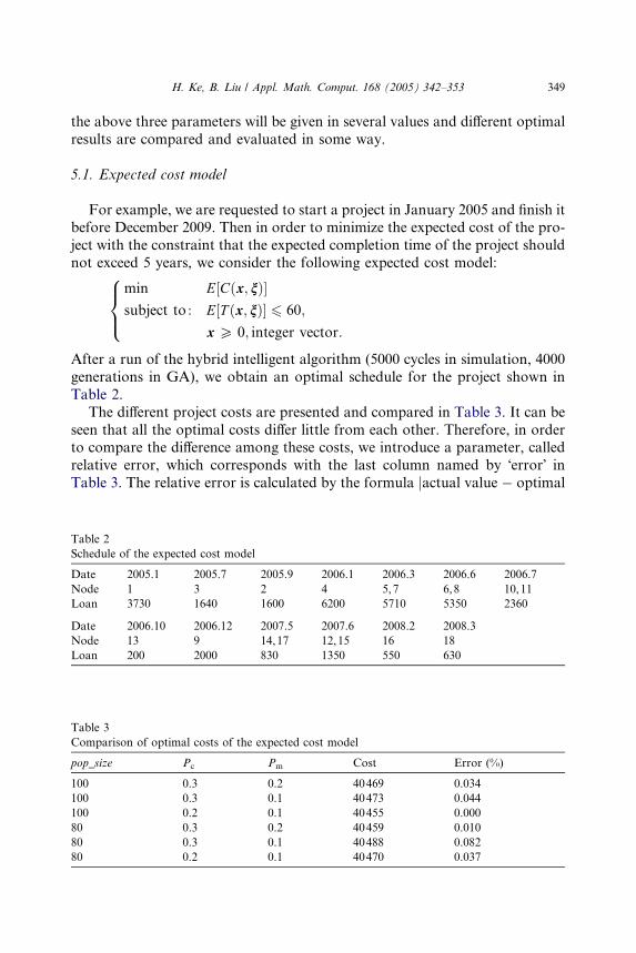
For example, we are requested to start a project in January 2005 and finish itbefore December 2009. Then in order to minimize the expected cost of the pro-
ject with the constraint that the expected completion time of the project should
not exceed 5 years, we consider the following expected cost model:
min E½Cðx; nÞ�subject to : E½T ðx; nÞ� 6 60;
x P 0; integer vector:
8><>:
After a run of the hybrid intelligent algorithm (5000 cycles in simulation, 4000
generations in GA), we obtain an optimal schedule for the project shown in
Table 2.
The different project costs are presented and compared in Table 3. It can be
seen that all the optimal costs differ little from each other. Therefore, in orderto compare the difference among these costs, we introduce a parameter, called
relative error, which corresponds with the last column named by �error� inTable 3. The relative error is calculated by the formula jactual value � optimal
Table 2
Schedule of the expected cost model
Date 2005.1 2005.7 2005.9 2006.1 2006.3 2006.6 2006.7
Node 1 3 2 4 5,7 6,8 10,11
Loan 3730 1640 1600 6200 5710 5350 2360
Date 2006.10 2006.12 2007.5 2007.6 2008.2 2008.3
Node 13 9 14,17 12,15 16 18
Loan 200 2000 830 1350 550 630
Table 3
Comparison of optimal costs of the expected cost model
pop_size Pc Pm Cost Error (%)
100 0.3 0.2 40469 0.034
100 0.3 0.1 40473 0.044
100 0.2 0.1 40455 0.000
80 0.3 0.2 40459 0.010
80 0.3 0.1 40488 0.082
80 0.2 0.1 40470 0.037

350 H. Ke, B. Liu / Appl. Math. Comput. 168 (2005) 342–353
valuej/optimal value · 100%, where the optimal value means the minimal one
of all the six costs in Table 3. It follows from Table 3 that the relative error
does not exceed 0.082% when different parameters are selected, which actually
implies that the hybrid intelligent algorithm is effective to solve the above ex-
pected cost model.
5.2. a-Cost model
We then apply the hybrid intelligent algorithm to solve the a-cost model of
the project scheduling problem. In this case, we are required to minimize the
0.90-cost of the project while the project should be finished in 6 years with
the confidence level 0.90. Hence, we have the following 0.90-cost model:
min C
subject to : PrfCðx; nÞ 6 CgP 0:90;
PrfT ðx; nÞ 6 72gP 0:90;
x P 0; integer vector:
8>>><>>>:
An optimal schedule to the model is presented in Table 4.
Similar to the analysis of the expected cost model, we compare the various
costs in Table 5. As can be seen from Table 5, among all the error values the
Table 4
Schedule of the 0.90-cost model
Date 2005.1 2005.7 2005.9 2006.2 2006.3 2006.4 2006.5 2006.7
Node 1 3 2 4 5 7 8 6
Loan 3730 1640 1600 6200 450 5260 450 4900
Date 2006.9 2006.12 2007.1 2007.3 2007.4 2007.8 2007.10 2008.7
Node 10 9 11 13 14 15 12,16,17 18
Loan 2150 2000 210 200 300 1100 1330 630
Table 5
Comparison of optimal costs of the 0.90-cost model
pop_size Pc Pm Cost Error (%)
100 0.3 0.2 41064 0.054
100 0.3 0.1 41049 0.017
100 0.2 0.1 41053 0.027
80 0.3 0.2 41042 0.000
80 0.3 0.1 41044 0.005
80 0.2 0.1 41053 0.027
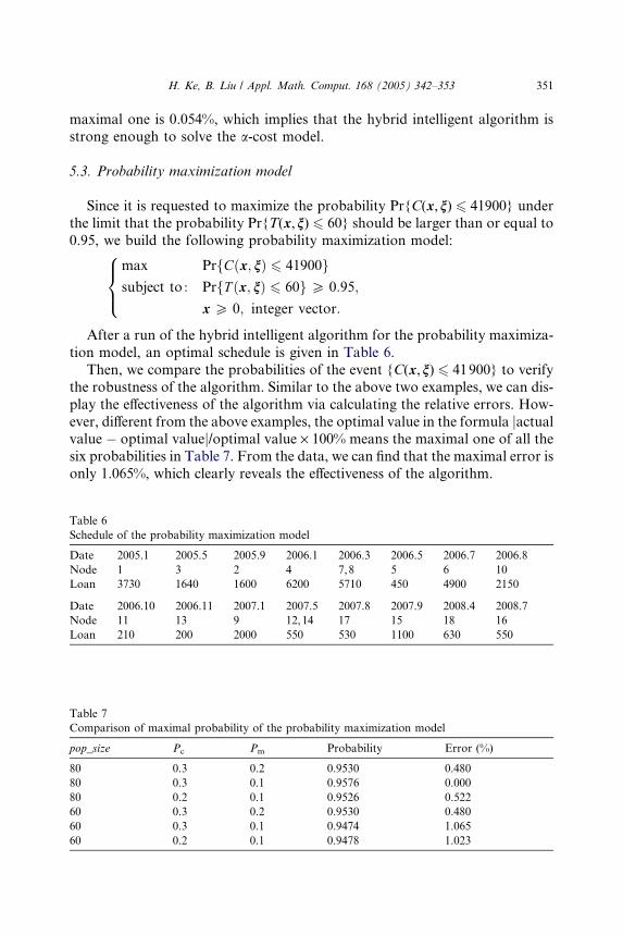
H. Ke, B. Liu / Appl. Math. Comput. 168 (2005) 342–353 351
maximal one is 0.054%, which implies that the hybrid intelligent algorithm is
strong enough to solve the a-cost model.
5.3. Probability maximization model
Since it is requested to maximize the probability Pr{C(x,n) 6 41900} underthe limit that the probability Pr{T(x,n) 6 60} should be larger than or equal to
0.95, we build the following probability maximization model:
max PrfCðx; nÞ 6 41900gsubject to : PrfT ðx; nÞ 6 60gP 0:95;
x P 0; integer vector:
8><>:
After a run of the hybrid intelligent algorithm for the probability maximiza-
tion model, an optimal schedule is given in Table 6.
Then, we compare the probabilities of the event {C(x,n) 6 41900} to verify
the robustness of the algorithm. Similar to the above two examples, we can dis-
play the effectiveness of the algorithm via calculating the relative errors. How-
ever, different from the above examples, the optimal value in the formula jactualvalue � optimal valuej/optimal value · 100% means the maximal one of all the
six probabilities in Table 7. From the data, we can find that the maximal error is
only 1.065%, which clearly reveals the effectiveness of the algorithm.
Table 6
Schedule of the probability maximization model
Date 2005.1 2005.5 2005.9 2006.1 2006.3 2006.5 2006.7 2006.8
Node 1 3 2 4 7,8 5 6 10
Loan 3730 1640 1600 6200 5710 450 4900 2150
Date 2006.10 2006.11 2007.1 2007.5 2007.8 2007.9 2008.4 2008.7
Node 11 13 9 12,14 17 15 18 16
Loan 210 200 2000 550 530 1100 630 550
Table 7
Comparison of maximal probability of the probability maximization model
pop_size Pc Pm Probability Error (%)
80 0.3 0.2 0.9530 0.480
80 0.3 0.1 0.9576 0.000
80 0.2 0.1 0.9526 0.522
60 0.3 0.2 0.9530 0.480
60 0.3 0.1 0.9474 1.065
60 0.2 0.1 0.9478 1.023
352 H. Ke, B. Liu / Appl. Math. Comput. 168 (2005) 342–353
6. Conclusion
In this paper, we attempted to solve the project scheduling problem with
stochastic activity duration times, which is to minimize the total cost under
some completion time limits and has not been studied ever before. Three types
of stochastic models, including the expected cost model, the a-cost model andthe probability maximization model, were built to satisfy the different manage-
ment goals. Then stochastic simulation and GA were proposed and integrated
to design a hybrid intelligent algorithm to solve some numerical examples.
From the numerical results, we could clearly see that the hybrid intelligent
algorithm could effectively solve the project scheduling problem.
Acknowledgments
This work was supported by National Natural Science Foundation of China
(No. 60174049), and Specialized Research Fund for the Doctoral Program of
Higher Education (No. 20020003009).
References
[1] A.R. Burgess, J.B. Killebrew, Variation in activity level on a cyclical arrow diagram, Journal
of Industrial Engineering 13 (2) (1962) 76–83.
[2] A. Charnes, W.W. Cooper, Chance-constrained programming, Management Science 6 (1)
(1959) 73–79.
[3] A. Charnes, W.W. Cooper, A network interpretation and a direct sub-dual algorithm for
critical path scheduling, Journal of Industrial Engineering 13 (1962) 213–219.
[4] A. Charnes, W.W. Cooper, Deterministic equivalents for optimizing and satisficing under
chance constraints, Operational Research 11 (1963) 18–39.
[5] A. Charnes, W.W. Cooper, G.L. Thompson, Critical path analysis via chance constrained and
stochastic programming, Operational Research 12 (1964) 460–470.
[6] E. Demeulemeester, Minimizing resource availability costs in time-limited project networks,
Management Science 41 (10) (1995) 1590–1598.
[7] S.E. Elmaghraby, On the expected duration of PERT type network, Management Science 13
(5) (1967) 299–306.
[8] R.J. Freeman, A generalized PERT, Operations Research 8 (2) (1960) 281.
[9] R.J. Freeman, A generalized network approach to project activity sequencing, IRE
Transactions on Engineering Management 7 (3) (1960) 103–107.
[10] D. Golenko-Ginzburg, A. Gonik, Stochastic network project scheduling with non-consumable
limited resources, International Journal of Production Economics 48 (1) (1997) 29–37.
[11] J.E. Kelley Jr., Critical path planning and scheduling, mathematical basis, Operations
Research 9 (3) (1961) 296–320.
[12] J.E. Kelley Jr., The critical path method: resources planning and scheduling, in: Muth,
Thompson (Eds.), Industrial Scheduling, Prentice-Hall, Englewood Cliffs, NJ, 1963 (Chapter
21).
H. Ke, B. Liu / Appl. Math. Comput. 168 (2005) 342–353 353
[13] T.C.T. Kotiah, N.D. Wallace, Another look at the PERT assumptions, Management Science
20 (1) (1973) 44–49.
[14] B. Liu, Dependent-chance programming: a class of stochastic programming, Computers and
Mathematics with Applications 34 (12) (1997) 89–104.
[15] B. Liu, K. Iwamura, Modelling stochastic decision systems using dependent-chance
programming, European Journal of Operational Research 101 (1) (1997) 193–203.
[16] B. Liu, Uncertain Programming, Wiley, New York, 1999.
[17] B. Liu, Uncertain programming: A unifying optimization theory in various uncertain
environments, Applied Mathematics and Computation 120 (1–3) (2001) 227–234.
[18] B. Liu, Theory and Practice of Uncertain Programming, Physica-Verlag, Heidelberg, 2002.
[19] F.A. Loostma, Network planning with stochastic activity durations, an evaluation of PERT,
Statistica Neerlandica 20 (1966) 43–69.
[20] K.R. MacCrimmon, C.A. Ryavec, An analytical study of PERT assumptions, Operations
Research 12 (1) (1964) 16–37.
[21] V. Maniezzo, A. Mingozzi, The project scheduling problem with irregular starting time costs,
Operations Research Letters 25 (4) (1999) 175–182.
[22] R.H. Mohring, Minimizing costs of resource requirements in project networks subject to a
fixed completion time, Operations Research 32 (1) (1984) 89–120.
[23] W.H. Parks, K.D. Ramsing, The use of the compound Poisson in PERT, Management Science
15 (8) (1969) B-397–B-402.