Embed Size (px)
DESCRIPTION
earth quake modelling using Geoslope 2012
Citation preview
Dynamic Modeling
With QUAKE/W
An Engineering Methodology
June 2013 Edition
GEO-SLOPE International Ltd.

Copyright © 2004-2013 by GEO-SLOPE International, Ltd.
All rights reserved. No part of this work may be reproduced or transmitted in any form or by any means, electronic or mechanical, including photocopying, recording, or by any information storage or retrieval system, without the prior written permission of GEO-SLOPE International, Ltd.
Trademarks: GEO-SLOPE, GeoStudio, SLOPE/W, SEEP/W, SIGMA/W, QUAKE/W, CTRAN/W, TEMP/W, AIR/W and VADOSE/W are trademarks or registered trademarks of GEO-SLOPE International Ltd. in Canada and other countries. Other trademarks are the property of their respective owners.
GEO-SLOPE International Ltd
1400, 633 – 6th Ave SW
Calgary, Alberta, Canada T2P 2Y5
E-mail: [email protected]
Web: http://www.geo-slope.com

QUAKE/W Table of Contents
Page i
Table of Contents
1 Introduction ......................................................................................... 1
1.1 Key issues ........................................................................................................................... 1
1.2 Inertial forces ....................................................................................................................... 2
1.3 Behavior of fine sand .......................................................................................................... 3
Loose contractive sand ................................................................................................. 3
Dense dilative soils ....................................................................................................... 5
1.4 Permanent deformation ...................................................................................................... 7
1.5 Concluding remarks ............................................................................................................ 8
2 Numerical Modeling: What, Why and How ......................................... 9
2.1 Introduction ......................................................................................................................... 9
2.2 What is a numerical model? ................................................................................................ 9
2.3 Modeling in geotechnical engineering ............................................................................... 11
2.4 Why model? ...................................................................................................................... 13
Quantitative predictions .............................................................................................. 13
Compare alternatives ................................................................................................. 15
Identify governing parameters .................................................................................... 16
Understand physical process - train our thinking ....................................................... 17
2.5 How to model .................................................................................................................... 20
Make a guess ............................................................................................................. 20
Simplify geometry ....................................................................................................... 21
Start simple ................................................................................................................. 22
Do numerical experiments .......................................................................................... 23
Model only essential components .............................................................................. 24
Start with estimated material properties ..................................................................... 25
Interrogate the results ................................................................................................. 26
Evaluate results in the context of expected results .................................................... 26
Remember the real world ........................................................................................... 26
2.6 How not to model .............................................................................................................. 27
2.7 Closing remarks ................................................................................................................ 28
3 Geometry and Meshing .................................................................... 29
3.1 Introduction ....................................................................................................................... 29
3.2 Geometry Objects in GeoStudio ....................................................................................... 30
Soil Regions, Points and Lines ................................................................................... 31
Free Points ................................................................................................................. 33
Table of Contents QUAKE/W
Page ii
Free Lines ................................................................................................................... 33
Interface Elements on Lines ....................................................................................... 34
Circular Openings ....................................................................................................... 36
3.3 Mesh Generation ............................................................................................................... 37
Structured mesh ......................................................................................................... 38
Unstructured quad and triangle mesh ........................................................................ 38
Unstructured triangular mesh ..................................................................................... 38
Triangular grid regions ................................................................................................ 39
Rectangular grid of quads .......................................................................................... 40
3.4 Surface layers ................................................................................................................... 40
3.5 Joining regions .................................................................................................................. 43
3.6 Meshing for transient analyses ......................................................................................... 44
3.7 Finite Elements ................................................................................................................. 45
3.8 Element fundamentals ...................................................................................................... 46
Element nodes ............................................................................................................ 46
Field variable distribution ............................................................................................ 46
Element and mesh compatibility ................................................................................. 47
Numerical integration .................................................................................................. 49
Secondary variables ................................................................................................... 50
3.9 General guidelines for meshing ........................................................................................ 50
Number of elements ................................................................................................... 51
Effect of drawing scale ............................................................................................... 51
Mesh purpose ............................................................................................................. 52
Simplified geometry .................................................................................................... 53
4 Material Properties ............................................................................ 55
4.1 Introduction ....................................................................................................................... 55
4.2 Soil behavior models ......................................................................................................... 55
Linear-elastic model ................................................................................................... 56
Equivalent linear model .............................................................................................. 56
Non-Linear model ....................................................................................................... 57
4.3 Shear modulus .................................................................................................................. 59
Granular soils ............................................................................................................. 60
Cohesive soils ............................................................................................................ 61
4.4 G-reduction function .......................................................................................................... 62
4.5 Damping ratio .................................................................................................................... 64
4.6 Equivalent cyclic stresses ................................................................................................. 65
QUAKE/W Table of Contents
Page iii
4.7 Excess pore-pressures from CSR .................................................................................... 67
Pore-pressure Ratio (ru) Function ............................................................................... 67
Cyclic number function ............................................................................................... 68
Overburden correction function, Ks ............................................................................ 70
Shear stress correction function, Ka ........................................................................... 71
Commentary on correction factors ............................................................................. 73
4.8 MFS (Martin Finn Seed) pore-pressure model ................................................................. 73
Recoverable modulus ................................................................................................. 73
MFS pore-pressure function ....................................................................................... 75
4.9 Collapse surface and steady-state strength ..................................................................... 77
Commentary on the use of the collapse surface ........................................................ 80
4.10 Structural elements ........................................................................................................... 80
4.11 Closing remarks ................................................................................................................ 80
5 Boundary Conditions ........................................................................ 83
5.1 Introduction ....................................................................................................................... 83
5.2 Earthquake records ........................................................................................................... 83
Data file header .......................................................................................................... 83
Time-acceleration data pairs ...................................................................................... 84
Acceleration only data files ......................................................................................... 84
Spreadsheet data ....................................................................................................... 85
Data modification ........................................................................................................ 86
Baseline correction ..................................................................................................... 86
Outcrop records .......................................................................................................... 87
5.3 Boundary condition basics ................................................................................................ 88
5.4 Boundary condition locations ............................................................................................ 89
5.5 Nodal force boundary conditions ...................................................................................... 90
5.6 Nodal displacement boundary conditions ......................................................................... 90
5.7 Stress boundary conditions ............................................................................................... 91
5.8 Spring boundary conditions .............................................................................................. 93
5.9 Dynamic boundaries ......................................................................................................... 93
5.10 Structural elements ........................................................................................................... 95
6 Analysis Types .................................................................................. 97
6.1 Introduction ....................................................................................................................... 97
6.2 Initial in-situ stresses ......................................................................................................... 97
Pore-water pressures ................................................................................................. 97
Example ...................................................................................................................... 98
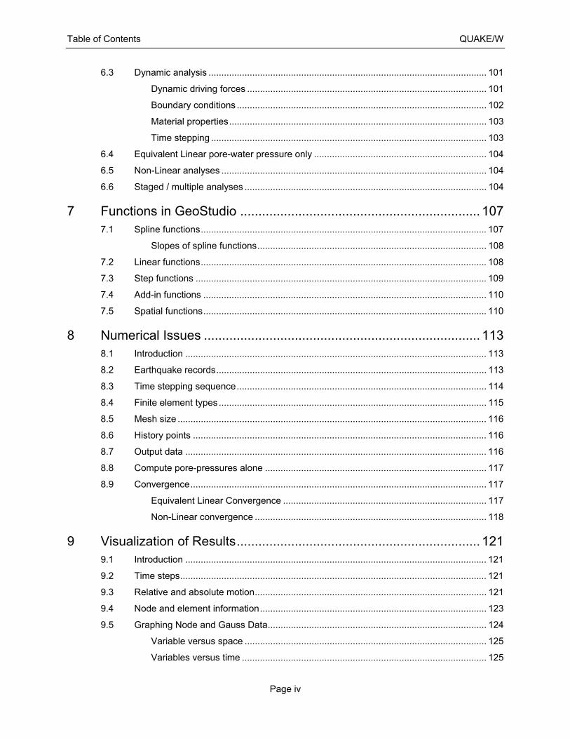
Table of Contents QUAKE/W
Page iv
6.3 Dynamic analysis ............................................................................................................ 101
Dynamic driving forces ............................................................................................. 101
Boundary conditions ................................................................................................. 102
Material properties .................................................................................................... 103
Time stepping ........................................................................................................... 103
6.4 Equivalent Linear pore-water pressure only ................................................................... 104
6.5 Non-Linear analyses ....................................................................................................... 104
6.6 Staged / multiple analyses .............................................................................................. 104
7 Functions in GeoStudio .................................................................. 107
7.1 Spline functions ............................................................................................................... 107
Slopes of spline functions ......................................................................................... 108
7.2 Linear functions ............................................................................................................... 108
7.3 Step functions ................................................................................................................. 109
7.4 Add-in functions .............................................................................................................. 110
7.5 Spatial functions .............................................................................................................. 110
8 Numerical Issues ............................................................................ 113
8.1 Introduction ..................................................................................................................... 113
8.2 Earthquake records ......................................................................................................... 113
8.3 Time stepping sequence ................................................................................................. 114
8.4 Finite element types ........................................................................................................ 115
8.5 Mesh size ........................................................................................................................ 116
8.6 History points .................................................................................................................. 116
8.7 Output data ..................................................................................................................... 116
8.8 Compute pore-pressures alone ...................................................................................... 117
8.9 Convergence ................................................................................................................... 117
Equivalent Linear Convergence ............................................................................... 117
Non-Linear convergence .......................................................................................... 118
9 Visualization of Results ................................................................... 121
9.1 Introduction ..................................................................................................................... 121
9.2 Time steps ....................................................................................................................... 121
9.3 Relative and absolute motion .......................................................................................... 121
9.4 Node and element information ........................................................................................ 123
9.5 Graphing Node and Gauss Data ..................................................................................... 124
Variable versus space .............................................................................................. 125
Variables versus time ............................................................................................... 125
QUAKE/W Table of Contents
Page v
Variables versus specific parameters ....................................................................... 126
Graphing peak values ............................................................................................... 126
Cut and paste graph data ......................................................................................... 128
Nodal history ............................................................................................................. 128
Spectral response ..................................................................................................... 129
Cyclic stress ratio (CSR) .......................................................................................... 130
Structural data .......................................................................................................... 130
9.6 “None” values .................................................................................................................. 130
9.7 Isolines ............................................................................................................................ 131
9.8 Mohr circles ..................................................................................................................... 131
9.9 Animation of motion ........................................................................................................ 132
9.10 Viewing displacements ................................................................................................... 132
9.11 Acceleration and velocity vectors .................................................................................... 133
9.12 Contours .......................................................................................................................... 133
10 Illustrative and Verification Examples ............................................. 137
11 Theory ............................................................................................. 139
11.1 Introduction ..................................................................................................................... 139
11.2 Finite element equations ................................................................................................. 139
Motion equation ........................................................................................................ 139
11.3 Mass matrix ..................................................................................................................... 140
11.4 Damping matrix ............................................................................................................... 140
11.5 Stiffness matrix ................................................................................................................ 140
11.6 Strain-displacement matrix ............................................................................................. 141
Elastic constitutive relationship ................................................................................ 141
Body forces ............................................................................................................... 142
Forces due to boundary stresses ............................................................................. 142
Forces due to earthquake load ................................................................................. 144
11.7 Numerical integration ...................................................................................................... 145
11.8 Temporal integration ....................................................................................................... 147
11.9 Equation solver ............................................................................................................... 148
11.10 Element stresses ............................................................................................................. 149
11.11 Linear elastic model ........................................................................................................ 149
12 Appendix A: Interpolating Functions ............................................... 151
12.1 Interpolating functions ..................................................................................................... 153
12.2 Field variable model ........................................................................................................ 154

Table of Contents QUAKE/W
Page vi
12.3 Derivatives of interpolating functions .............................................................................. 154
References ............................................................................................... 159
Index 163

QUAKE/W Chapter 1: Introduction
Page 1
1 Introduction
QUAKE/W is a geotechnical finite element software product used for the dynamic analysis of earth structures subjected to earthquake shaking and other sudden impact loading such as, for example, dynamiting or pile driving.
QUAKE/W is part of GeoStudio and is, consequently, fully integrated with the other components such SLOPE/W, SEEP/W, SIGMA/W for example. In this sense, QUAKE/W is unique. The integration of QUAKE/W and other products within GeoStudio greatly expands the type and range of problems that can be analyzed beyond what can be done with other geotechnical dynamic analysis software. QUAKE/W can be used as a stand-alone product, but one of its main attractions is the integration with the other GeoStudio products.
The purpose of this document is to highlight concepts, features and capabilities, and to provide some guidelines on dynamic numerical modeling. The purpose is not to explain the software interface commands. This type of information is provided in the on-line help.
The remainder of this chapter provides a brief overview of the main geotechnical issues related to the response of earth structures subjected to seismic loading and how QUAKE/W is positioned to address these issues. The intent here is not to provide an exhaustive review of the state-of-the-art of geotechnical earthquake engineering. The intent is more to provide an indication of the thinking behind the QUAKE/W development.
The textbook, Geotechnical Earthquake Engineering, by Steven Kramer (1996) provides an excellent summary of the concepts, theories and procedures in geotechnical earthquake engineering. This book was used extensively as a background reference source in the development of QUAKE/W and is referenced extensively throughout this document. QUAKE/W users should ideally have a copy of this book and use it in conjunction with this documentation. It provides significantly more details on many topics in this document.
1.1 Key issues
The response and behavior of earth structures subjected to earthquake shaking is highly complex and multifaceted. Generally, there are the issues of:
the motion, movement and inertial forces that occur during the shaking,
the generation of excess pore-water pressures,
the potential reduction of the soil shear strength,
the effect on stability created by the inertial forces, excess pore-water pressures and possible shear strength loses, and
the redistribution of excess pore-water pressures and possible strain softening of the soil after the shaking has stopped.
Not all these issues can be addressed in a single analysis, nor is it possible to address all the issues in the current version of QUAKE/W. Effects such as strain softening and re-distribution of excess pore-pressures will be perhaps dealt with in future version. The point here is that there are many issues and to use QUAKE/W effectively it is important to at least be aware of the multifaceted nature of the problem.
Chapter 1: Introduction QUAKE/W
Page 2
1.2 Inertial forces
Earthquake shaking creates inertial forces; that is, mass times acceleration forces. These forces cause the stresses in the ground to oscillate. Along a potential slip surface, the mobilized shear strength decreases and increases in response to the inertial forces. There may be moments during the shaking that the mobilized shear strength exceeds the available shear resistance, which causes a temporary loss of stability. During these moments when the factor of safety is less than unity, the ground may experience some displacement. An accumulation of these movement spurts may manifest itself as permanent displacement.
Figure 1-1 illustrates how the factor of safety may change during an earthquake. Note that the factor of safety falls below 1.0 five times during the earthquake. Subtracting the QUAKE/W computed stresses from the initial static stresses gives the additional shear stresses arising from the inertial forces. This information together with the Newmark Sliding Block concepts can be used to estimate the permanent deformation. In GeoStudio, SLOPE/W uses the QUAKE/W results to perform these calculations.
Figure 1-1 Factor of safety as a function of time during an earthquake
As discussed in more detail later in this book, examining the potential permanent deformations resulting from the dynamic inertial forces is applicable only to certain situations. It is only one aspect of earthquake engineering and does not provided answers to all to issues.
In the late 1990’s an embankment was constructed in Peru at a mine site to control temporary flooding (Swaisgood and Oliveros, 2003). The embankment was constructed from mine waste with a concrete blanket on the upstream face to control seepage through the embankment. The embankment was very wide with 4:1 side slopes and a crest width of 130 m. The embankment materials were expected to remain essentially dry (unsaturated) most of the time since water would be ponded up against the dam only for short durations after heavy rainfalls. On June 23, 2001, a Magnitude 8.3 earthquake struck the southern portion of Peru. The newly constructed dam was heavily shaken by the tremors. The dam, however, endured the shaking without much damage. The downstream crest settled only about 50 mm.
The Peru Dam is a case that lends itself well to a Newmark-type permanent deformation analysis arising from the earthquake inertial forces. The unsaturated coarse material meant that there was no generation of excess pore-pressure and very little change, if any, in the shear strength of the fill, conditions essential to an analysis like this.
Fa
cto
r o
f S
afe
ty
Time
0.8
0.9
1.0
1.1
1.2
1.3
1.4
0 2 4 6 8 10
QUAKE/W Chapter 1: Introduction
Page 3
1.3 Behavior of fine sand
Loose contractive sand
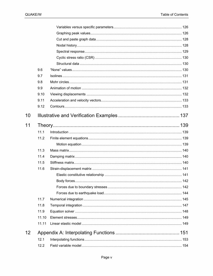
As is well known, loose sandy soils are susceptible to liquefaction. There are many variables besides grain size distributions that influence the potential for the soil to liquefy. Two of the more prominent are the density or void ratio, and the stress state. Different starting stress states can have a profound effect on the soil behavior when subjected to monotonic or cyclic loading. The behavior can best be described in the context of a q-p΄ plot (shear stress versus mean normal stress).
Consider the diagram in Figure 1-2. If a sample is isotropically consolidated (Point A), the effective stress path under undrained monotonic loading will follow the curve in Figure 1-2. Initially, the shear stress will rise, but then curve over to the left and reach a maximum at which point the soil-grain structure collapses. After the collapse there is a sudden increase in pore-pressure and the strength falls rapidly to the steady-state strength.
Another way of describing this is that liquefaction is initiated at the collapse point.
Figure 1-2 Effective stress path for loose sand under monotonic loading
Figure 1-3 presents the picture for a series of tests on triaxial specimens at the same initial void ratio, but consolidated under different confining pressures. A straight line can be drawn from the steady state strength point through the peaks or collapse points. Sladen, D’Hollander and Krahn (1985) called this line a Collapse Surface. Similar work by Hanzawa et al. (1979) and by Vaid and Chern (1983) suggests that the line through the collapse points passes through the plot origin (zero shear stress, zero mean stress) as opposed to the steady-state strength point. They called the line a Flow Liquefaction Surface.
q
p'A
Collapse point
Steady-statestrength
Chapter 1: Introduction QUAKE/W
Page 4
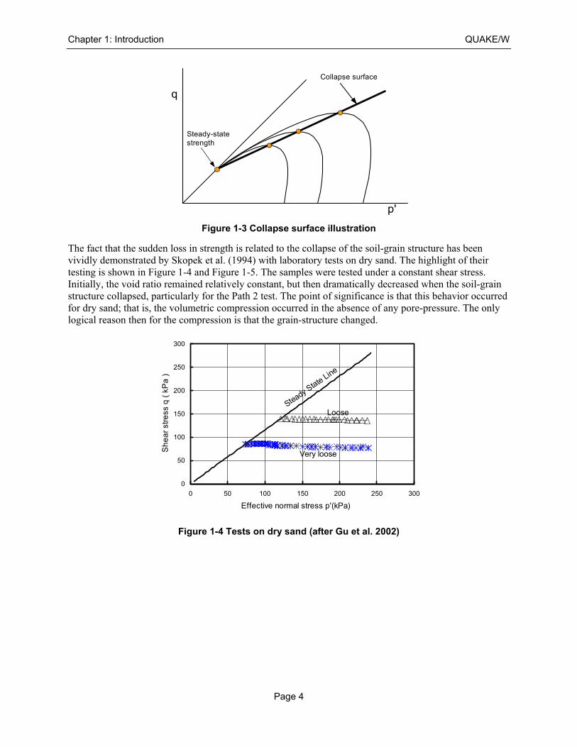
Figure 1-3 Collapse surface illustration
The fact that the sudden loss in strength is related to the collapse of the soil-grain structure has been vividly demonstrated by Skopek et al. (1994) with laboratory tests on dry sand. The highlight of their testing is shown in Figure 1-4 and Figure 1-5. The samples were tested under a constant shear stress. Initially, the void ratio remained relatively constant, but then dramatically decreased when the soil-grain structure collapsed, particularly for the Path 2 test. The point of significance is that this behavior occurred for dry sand; that is, the volumetric compression occurred in the absence of any pore-pressure. The only logical reason then for the compression is that the grain-structure changed.
Figure 1-4 Tests on dry sand (after Gu et al. 2002)
q
p'
Steady-statestrength
Collapse surface
0
50
100
150
200
250
300
0 50 100 150 200 250 300
Effective normal stress p'(kPa)
Sh
ea
r st
ress
q (
kP
a )
Loose
Very loose
Steady State Line
QUAKE/W Chapter 1: Introduction
Page 5
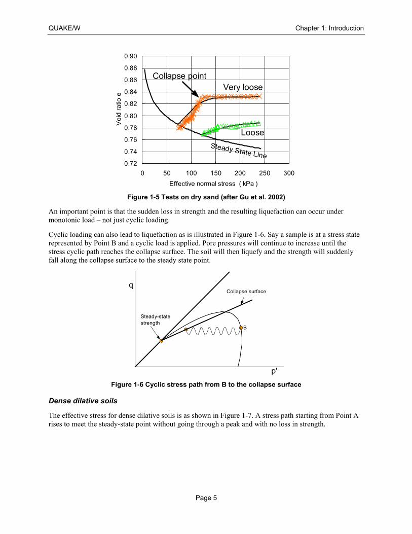
Figure 1-5 Tests on dry sand (after Gu et al. 2002)
An important point is that the sudden loss in strength and the resulting liquefaction can occur under monotonic load – not just cyclic loading.
Cyclic loading can also lead to liquefaction as is illustrated in Figure 1-6. Say a sample is at a stress state represented by Point B and a cyclic load is applied. Pore pressures will continue to increase until the stress cyclic path reaches the collapse surface. The soil will then liquefy and the strength will suddenly fall along the collapse surface to the steady state point.
Figure 1-6 Cyclic stress path from B to the collapse surface
Dense dilative soils
The effective stress for dense dilative soils is as shown in Figure 1-7. A stress path starting from Point A rises to meet the steady-state point without going through a peak and with no loss in strength.
0.72
0.74
0.76
0.78
0.80
0.82
0.84
0.86
0.88
0.90
0 50 100 150 200 250 300
Effective normal stress ( kPa )
Vo
id r
atio
e
Very loose
Loose
Collapse point
Steady State Line
q
p'
B
Collapse surface
Steady-statestrength
Chapter 1: Introduction QUAKE/W
Page 6
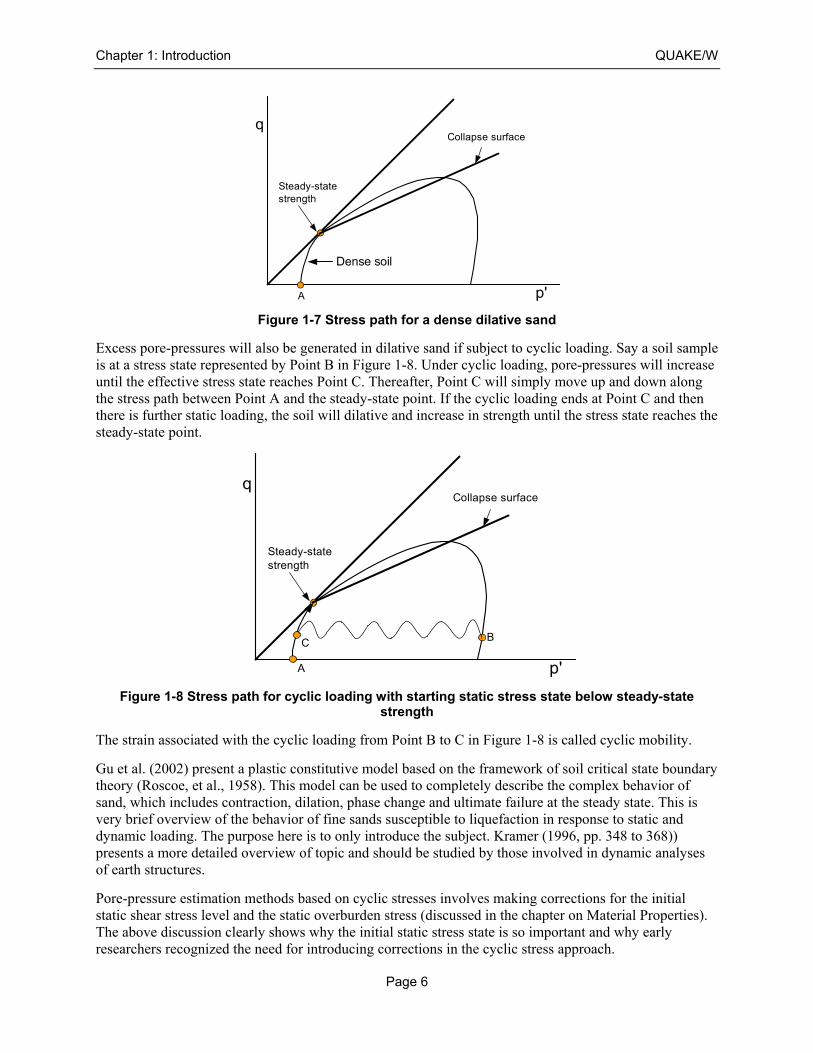
Figure 1-7 Stress path for a dense dilative sand
Excess pore-pressures will also be generated in dilative sand if subject to cyclic loading. Say a soil sample is at a stress state represented by Point B in Figure 1-8. Under cyclic loading, pore-pressures will increase until the effective stress state reaches Point C. Thereafter, Point C will simply move up and down along the stress path between Point A and the steady-state point. If the cyclic loading ends at Point C and then there is further static loading, the soil will dilative and increase in strength until the stress state reaches the steady-state point.
Figure 1-8 Stress path for cyclic loading with starting static stress state below steady-state strength
The strain associated with the cyclic loading from Point B to C in Figure 1-8 is called cyclic mobility.
Gu et al. (2002) present a plastic constitutive model based on the framework of soil critical state boundary theory (Roscoe, et al., 1958). This model can be used to completely describe the complex behavior of sand, which includes contraction, dilation, phase change and ultimate failure at the steady state. This is very brief overview of the behavior of fine sands susceptible to liquefaction in response to static and dynamic loading. The purpose here is to only introduce the subject. Kramer (1996, pp. 348 to 368)) presents a more detailed overview of topic and should be studied by those involved in dynamic analyses of earth structures.
Pore-pressure estimation methods based on cyclic stresses involves making corrections for the initial static shear stress level and the static overburden stress (discussed in the chapter on Material Properties). The above discussion clearly shows why the initial static stress state is so important and why early researchers recognized the need for introducing corrections in the cyclic stress approach.
q
p'A
Collapse surface
Steady-statestrength
Dense soil
q
p'
B
Collapse surface
Steady-statestrength
C
A

QUAKE/W Chapter 1: Introduction
Page 7
1.4 Permanent deformation
When there is a zone of soil in a soil structure that has experienced a sudden strength loss, there will be some stress adjustment and re-distribution. Zones that have lost their strength will share their excess load with regions that have not undergone the strength loss. The stress re-distribution will continue until the structure has once again reached a point of equilibrium. If the strength loss is so great that the earth structure cannot re-establish equilibrium, the entire structure will collapse, often with catastrophic consequences. If, however, the structure can find a new point of equilibrium, the stress re-distribution will be accompanied by permanent deformations. The chief engineering issue then becomes to determine how the permanent deformation affects the serviceability of the structure. The question is whether the structure is still functional or can it be repaired to again be functional or is the deformation so severe that the structure can no longer be used for its intended purpose?
There is considerable field evidence as summarized by Gu et al. (1993) that much of the stress re-distribution and the accompanying permanent deformation takes place after the earthquake shaking has stopped. If there is a failure, the failure is delayed by minutes or even hours and for this reason the associated deformation is referred to as post-earthquake deformation.
An extremely important implication of the delayed movement and failure is that the deformations are actually driven by static forces – not dynamic forces. The dynamic forces cause the generation of the excess pore-pressures, but the damaging deformations are driven by static gravitational forces. This has important numerical modeling implications. This being the case, a QUAKE/W dynamic analysis can be used to estimate the generation of excess pore-pressures, but a QUAKE/W analysis is not required to estimate the permanent deformation. The permanent deformation can be modeled with a static software product like SIGMA/W.
Modeling the stress re-distribution should ideally include a strain-softening constitutive relationship to simulate the strength loss. These types of numerical algorithms have been developed and used to study the post-earthquake re-distribution. Gu (1992), for example, developed a strain-softening model as part of his Ph.D. dissertation for analyzing the post-earthquake stress re-distribution and was successful in obtaining good agreement between the model predictions and the observed field behavior at two sites. One was the post-earthquake deformation analysis of the Wildlife Site in California (Gu et al. 1994) and the other was the analysis of the progressive failure that occurred at the Lower San Fernando Dam in California (Gu et al. 1993).
SIGMA/W has a stress re-distribution algorithm which can be used in conjunction with QUAKE/W results. The SIGMA/W method uses an elastic-plastic constitutive model and simply re-distributes the excess stress where the stress state exceeds the soil strength. The procedure can be quite effective even though it does not follow a prescribed strain-softening path. The premise is that somehow there was a strength loss and consequently there is a need to re-distribute the stresses. Stated another way, the SIGMA/W procedure gives the correct end point but not necessarily the correct path to the end point.
The analyses of the San Fernando Dams described in the QUAKE/W detailed examples demonstrate that the SIGMA/W approach together with the QUAKE/W results can be effective in investigating the post-earthquake deformation that may be associated with liquefaction even though it is not a completely rigorous approach.
In version 7.1, SIGMA/W also has a “dynamic deformation” analysis that will consider incremental stresses between saved QUAKE/W time steps as a driving force for permanent deformation if the chosen constitutive model allows for some plastic deformation based on stress-redistribution.

Chapter 1: Introduction QUAKE/W
Page 8
1.5 Concluding remarks
Conceptually, the issues as they relate to dynamic analyses, liquefaction, cyclic mobility and permanent deformation are now fairly well understood. GeoStudio now has all the components to examine all these aspects. Good illustrations of this are available in the QUAKE/W detailed examples. The San Fernando Dam Case Histories, for example, involve seepage analyses with SEEP/W, stability analyses with SLOPE/W, dynamic analyses with QUAKE/W and post-earthquake deformation analyses with SIGMA/W.
QUAKE/W Chapter 2: Numerical Modeling
Page 9
2 Numerical Modeling: What, Why and How
2.1 Introduction
The unprecedented computing power now available has resulted in advanced software products for engineering and scientific analysis. The ready availability and ease-of-use of these products makes it possible to use powerful techniques such as a finite element analysis in engineering practice. These analytical methods have now moved from being research tools to application tools. This has opened a whole new world of numerical modeling.
Software tools such as GeoStudio do not inherently lead to good results. While the software is an extremely powerful calculator, obtaining useful and meaningful results from this useful tool depends on the guidance provided by the user. It is the user’s understanding of the input and their ability to interpret the results that make it such a powerful tool. In summary, the software does not do the modeling, the user does the modeling. The software only provides the ability to do highly complex computations that are not otherwise humanly possible. In a similar manner, modern day spreadsheet software programs can be immensely powerful as well, but obtaining useful results from a spreadsheet depends on the user. It is the user’s ability to guide the analysis process that makes it a powerful tool. The spreadsheet can do all the mathematics, but it is the user’s ability to take advantage of the computing capability that leads to something meaningful and useful. The same is true with finite element analysis software such as GeoStudio.
Numerical modeling is a skill that is acquired with time and experience. Simply acquiring a software product does not immediately make a person a proficient modeler. Time and practice are required to understand the techniques involved and learn how to interpret the results.
Numerical modeling as a field of practice is relatively new in geotechnical engineering and, consequently, there is a lack of understanding about what numerical modeling is, how modeling should be approached and what to expect from it. A good understanding of these basic issues is fundamental to conducting effective modeling. Basic questions such as, What is the main objective of the analysis?, What is the main engineering question that needs to answered? and, What is the anticipated result?, need to be decided before starting to use the software. Using the software is only part of the modeling exercise. The associated mental analysis is as important as clicking the buttons in the software.
This chapter discusses the “what”, “why” and “how” of the numerical modeling process and presents guidelines on the procedures that should be followed in good numerical modeling practice.
This chapter discusses modeling in general terms and not specifically in the context of dynamic analyses. Many of the illustrations and examples come from other GeoStudio products, but the principles apply equally to QUAKE/W. The one exception perhaps is the admonition of making a preliminary guess or estimate as to what modeling results will look like. In a dynamic analysis, it is nearly impossible to make a hand-calculated guess as to a likely dynamic response of an earth structure. This makes it all the more important to start a dynamic analysis with a problem that is as simple and basic as possible so as to gain a preliminary understanding of the possible dynamic response before moving onto more advanced analyses.
2.2 What is a numerical model?
A numerical model is a mathematical simulation of a real physical process. SEEP/W is a numerical model that can mathematically simulate the real physical process of water flowing through a particulate medium. Numerical modeling is purely mathematical and in this sense is very different than scaled physical modeling in the laboratory or full-scaled field modeling.
Chapter 2: Numerical Modeling QUAKE/W
Page 10
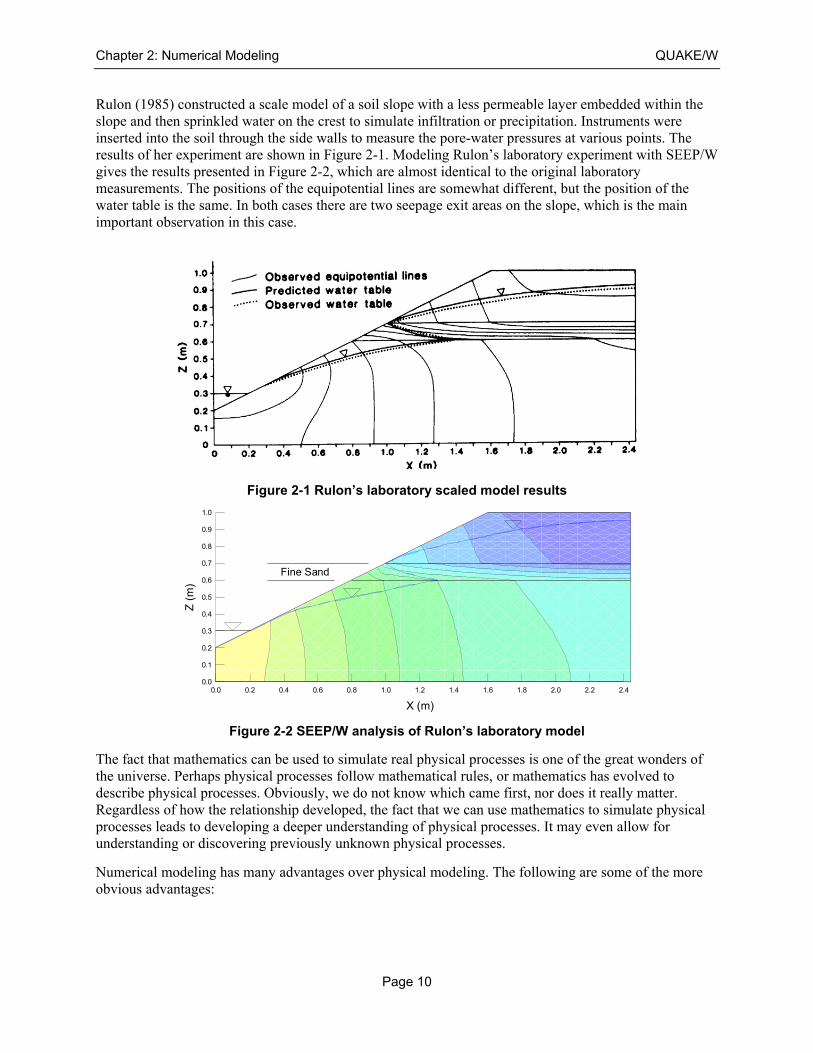
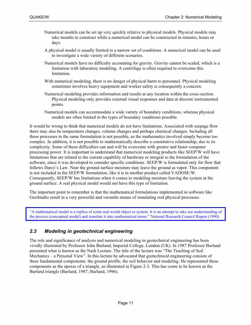
Rulon (1985) constructed a scale model of a soil slope with a less permeable layer embedded within the slope and then sprinkled water on the crest to simulate infiltration or precipitation. Instruments were inserted into the soil through the side walls to measure the pore-water pressures at various points. The results of her experiment are shown in Figure 2-1. Modeling Rulon’s laboratory experiment with SEEP/W gives the results presented in Figure 2-2, which are almost identical to the original laboratory measurements. The positions of the equipotential lines are somewhat different, but the position of the water table is the same. In both cases there are two seepage exit areas on the slope, which is the main important observation in this case.
Figure 2-1 Rulon’s laboratory scaled model results
Figure 2-2 SEEP/W analysis of Rulon’s laboratory model
The fact that mathematics can be used to simulate real physical processes is one of the great wonders of the universe. Perhaps physical processes follow mathematical rules, or mathematics has evolved to describe physical processes. Obviously, we do not know which came first, nor does it really matter. Regardless of how the relationship developed, the fact that we can use mathematics to simulate physical processes leads to developing a deeper understanding of physical processes. It may even allow for understanding or discovering previously unknown physical processes.
Numerical modeling has many advantages over physical modeling. The following are some of the more obvious advantages:
Fine Sand
X (m)
0.0 0.2 0.4 0.6 0.8 1.0 1.2 1.4 1.6 1.8 2.0 2.2 2.4
Z (
m)
0.0
0.1
0.2
0.3
0.4
0.5
0.6
0.7
0.8
0.9
1.0
QUAKE/W Chapter 2: Numerical Modeling
Page 11
Numerical models can be set up very quickly relative to physical models. Physical models may take months to construct while a numerical model can be constructed in minutes, hours or days.
A physical model is usually limited to a narrow set of conditions. A numerical model can be used to investigate a wide variety of different scenarios.
Numerical models have no difficulty accounting for gravity. Gravity cannot be scaled, which is a limitation with laboratory modeling. A centrifuge is often required to overcome this limitation.
With numerical modeling, there is no danger of physical harm to personnel. Physical modeling sometimes involves heavy equipment and worker safety is consequently a concern.
Numerical modeling provides information and results at any location within the cross-section. Physical modeling only provides external visual responses and data at discrete instrumented points.
Numerical models can accommodate a wide variety of boundary conditions, whereas physical models are often limited in the types of boundary conditions possible.
It would be wrong to think that numerical models do not have limitations. Associated with seepage flow there may also be temperature changes, volume changes and perhaps chemical changes. Including all these processes in the same formulation is not possible, as the mathematics involved simply become too complex. In addition, it is not possible to mathematically describe a constitutive relationship, due to its complexity. Some of these difficulties can and will be overcome with greater and faster computer processing power. It is important to understand that numerical modeling products like SEEP/W will have limitations that are related to the current capability of hardware or integral to the formulation of the software, since it was developed to consider specific conditions. SEEP/W is formulated only for flow that follows Darcy’s Law. Near the ground surface moisture may leave the ground as vapor. This component is not included in the SEEP/W formulation, like it is in another product called VADOSE/W. Consequently, SEEP/W has limitations when it comes to modeling moisture leaving the system at the ground surface. A real physical model would not have this type of limitation.
The important point to remember is that the mathematical formulations implemented in software like GeoStudio result in a very powerful and versatile means of simulating real physical processes.
“A mathematical model is a replica of some real-world object or system. It is an attempt to take our understanding of the process (conceptual model) and translate it into mathematical terms.” National Research Council Report (1990).
2.3 Modeling in geotechnical engineering
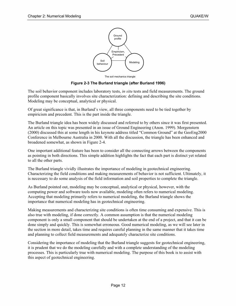
The role and significance of analysis and numerical modeling in geotechnical engineering has been vividly illustrated by Professor John Burland, Imperial College, London (UK). In 1987 Professor Burland presented what is known as the Nash Lecture. The title of the lecture was “The Teaching of Soil Mechanics – a Personal View”. In this lecture he advocated that geotechnical engineering consists of three fundamental components: the ground profile, the soil behavior and modeling. He represented these components as the apexes of a triangle, as illustrated in Figure 2-3. This has come to be known as the Burland triangle (Burland, 1987; Burland, 1996).
Chapter 2: Numerical Modeling QUAKE/W
Page 12
Figure 2-3 The Burland triangle (after Burland 1996)
The soil behavior component includes laboratory tests, in situ tests and field measurements. The ground profile component basically involves site characterization: defining and describing the site conditions. Modeling may be conceptual, analytical or physical.
Of great significance is that, in Burland’s view, all three components need to be tied together by empiricism and precedent. This is the part inside the triangle.
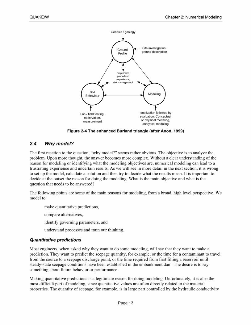
The Burland triangle idea has been widely discussed and referred to by others since it was first presented. An article on this topic was presented in an issue of Ground Engineering (Anon. 1999). Morgenstern (2000) discussed this at some length in his keynote address titled “Common Ground” at the GeoEng2000 Conference in Melbourne Australia in 2000. With all the discussion, the triangle has been enhanced and broadened somewhat, as shown in Figure 2-4.
One important additional feature has been to consider all the connecting arrows between the components as pointing in both directions. This simple addition highlights the fact that each part is distinct yet related to all the other parts.
The Burland triangle vividly illustrates the importance of modeling in geotechnical engineering. Characterizing the field conditions and making measurements of behavior is not sufficient. Ultimately, it is necessary to do some analysis of the field information and soil properties to complete the triangle.
As Burland pointed out, modeling may be conceptual, analytical or physical, however, with the computing power and software tools now available, modeling often refers to numerical modeling. Accepting that modeling primarily refers to numerical modeling, the Burland triangle shows the importance that numerical modeling has in geotechnical engineering.
Making measurements and characterizing site conditions is often time consuming and expensive. This is also true with modeling, if done correctly. A common assumption is that the numerical modeling component is only a small component that should be undertaken at the end of a project, and that it can be done simply and quickly. This is somewhat erroneous. Good numerical modeling, as we will see later in the section in more detail, takes time and requires careful planning in the same manner that it takes time and planning to collect field measurements and adequately characterize site conditions.
Considering the importance of modeling that the Burland triangle suggests for geotechnical engineering, it is prudent that we do the modeling carefully and with a complete understanding of the modeling processes. This is particularly true with numerical modeling. The purpose of this book is to assist with this aspect of geotechnical engineering.
Groundprofile
ModelingSoil
behaviour
Empiricism,Precedent
The soil mechanics triangle
QUAKE/W Chapter 2: Numerical Modeling
Page 13
Figure 2-4 The enhanced Burland triangle (after Anon. 1999)
2.4 Why model?
The first reaction to the question, “why model?” seems rather obvious. The objective is to analyze the problem. Upon more thought, the answer becomes more complex. Without a clear understanding of the reason for modeling or identifying what the modeling objectives are, numerical modeling can lead to a frustrating experience and uncertain results. As we will see in more detail in the next section, it is wrong to set up the model, calculate a solution and then try to decide what the results mean. It is important to decide at the outset the reason for doing the modeling. What is the main objective and what is the question that needs to be answered?
The following points are some of the main reasons for modeling, from a broad, high level perspective. We model to:
make quantitative predictions,
compare alternatives,
identify governing parameters, and
understand processes and train our thinking.
Quantitative predictions
Most engineers, when asked why they want to do some modeling, will say that they want to make a prediction. They want to predict the seepage quantity, for example, or the time for a contaminant to travel from the source to a seepage discharge point, or the time required from first filling a reservoir until steady-state seepage conditions have been established in the embankment dam. The desire is to say something about future behavior or performance.
Making quantitative predictions is a legitimate reason for doing modeling. Unfortunately, it is also the most difficult part of modeling, since quantitative values are often directly related to the material properties. The quantity of seepage, for example, is in large part controlled by the hydraulic conductivity
GroundProfile
ModelingSoil
Behaviour
Empiricism,precedent,experience,
risk management
Genesis / geology
Site investigation,ground description
Lab / field testing,observation,
measurement
Idealization followed byevaluation. Conceptualor physical modeling,analytical modeling
Chapter 2: Numerical Modeling QUAKE/W
Page 14
and, as a result, changing the hydraulic conductivity by an order of magnitude will usually change the computed seepage quantity by an order of magnitude. The accuracy of quantitative prediction is directly related to the accuracy of the hydraulic conductivity specified. Unfortunately, for a heterogeneous profile, there is not a large amount of confidence about how precisely the hydraulic conductivity can be specified. Sometimes defining the hydraulic conductivity within an order of magnitude is considered reasonable. The confidence you have defining the hydraulic conductivity depends on many factors, but the general difficulty of defining this soil parameter highlights the difficulty of undertaking modeling to make quantitative predictions.
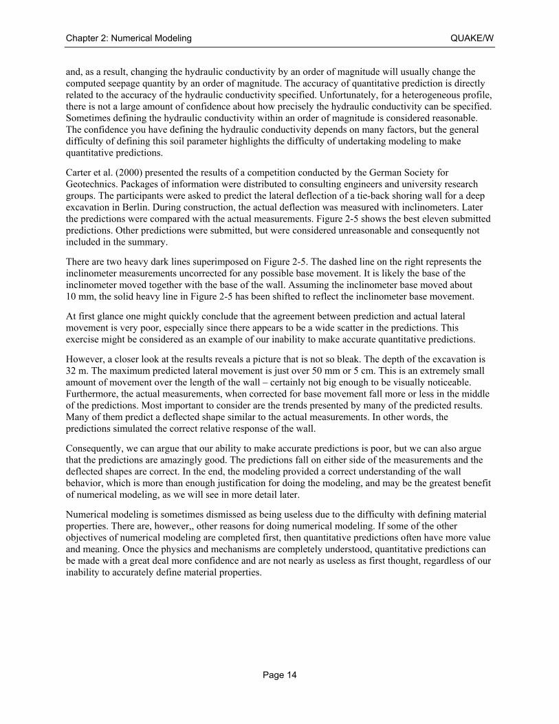
Carter et al. (2000) presented the results of a competition conducted by the German Society for Geotechnics. Packages of information were distributed to consulting engineers and university research groups. The participants were asked to predict the lateral deflection of a tie-back shoring wall for a deep excavation in Berlin. During construction, the actual deflection was measured with inclinometers. Later the predictions were compared with the actual measurements. Figure 2-5 shows the best eleven submitted predictions. Other predictions were submitted, but were considered unreasonable and consequently not included in the summary.
There are two heavy dark lines superimposed on Figure 2-5. The dashed line on the right represents the inclinometer measurements uncorrected for any possible base movement. It is likely the base of the inclinometer moved together with the base of the wall. Assuming the inclinometer base moved about 10 mm, the solid heavy line in Figure 2-5 has been shifted to reflect the inclinometer base movement.
At first glance one might quickly conclude that the agreement between prediction and actual lateral movement is very poor, especially since there appears to be a wide scatter in the predictions. This exercise might be considered as an example of our inability to make accurate quantitative predictions.
However, a closer look at the results reveals a picture that is not so bleak. The depth of the excavation is 32 m. The maximum predicted lateral movement is just over 50 mm or 5 cm. This is an extremely small amount of movement over the length of the wall – certainly not big enough to be visually noticeable. Furthermore, the actual measurements, when corrected for base movement fall more or less in the middle of the predictions. Most important to consider are the trends presented by many of the predicted results. Many of them predict a deflected shape similar to the actual measurements. In other words, the predictions simulated the correct relative response of the wall.
Consequently, we can argue that our ability to make accurate predictions is poor, but we can also argue that the predictions are amazingly good. The predictions fall on either side of the measurements and the deflected shapes are correct. In the end, the modeling provided a correct understanding of the wall behavior, which is more than enough justification for doing the modeling, and may be the greatest benefit of numerical modeling, as we will see in more detail later.
Numerical modeling is sometimes dismissed as being useless due to the difficulty with defining material properties. There are, however,, other reasons for doing numerical modeling. If some of the other objectives of numerical modeling are completed first, then quantitative predictions often have more value and meaning. Once the physics and mechanisms are completely understood, quantitative predictions can be made with a great deal more confidence and are not nearly as useless as first thought, regardless of our inability to accurately define material properties.
QUAKE/W Chapter 2: Numerical Modeling
Page 15
Figure 2-5 Comparison of predicted and measured lateral movements of a shoring wall (after Carter et al, 2000)
Compare alternatives
Numerical modeling is useful for comparing alternatives. Keeping everything else the same and changing a single parameter makes it a powerful tool to evaluate the significance of individual parameters. For modeling alternatives and conducting sensitivity studies it is not all that important to accurately define some material properties. All that is of interest is the change between simulations.
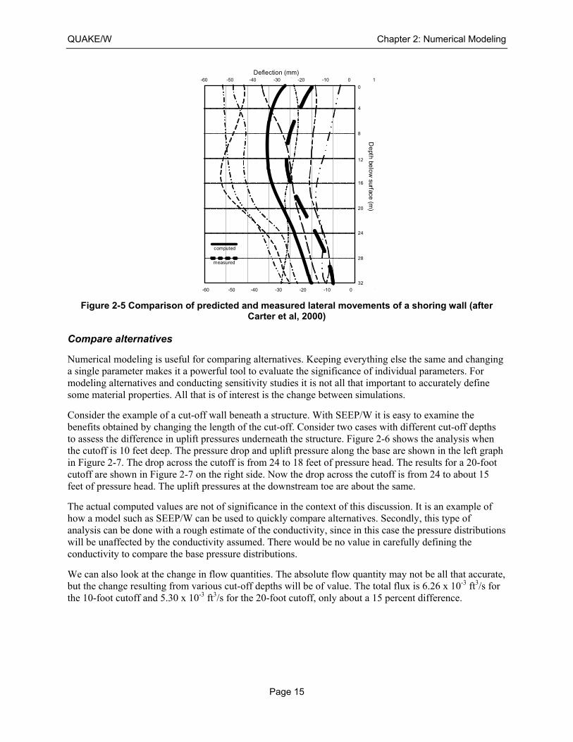
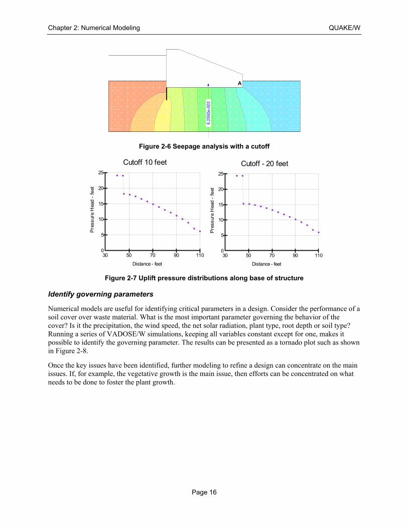
Consider the example of a cut-off wall beneath a structure. With SEEP/W it is easy to examine the benefits obtained by changing the length of the cut-off. Consider two cases with different cut-off depths to assess the difference in uplift pressures underneath the structure. Figure 2-6 shows the analysis when the cutoff is 10 feet deep. The pressure drop and uplift pressure along the base are shown in the left graph in Figure 2-7. The drop across the cutoff is from 24 to 18 feet of pressure head. The results for a 20-foot cutoff are shown in Figure 2-7 on the right side. Now the drop across the cutoff is from 24 to about 15 feet of pressure head. The uplift pressures at the downstream toe are about the same.
The actual computed values are not of significance in the context of this discussion. It is an example of how a model such as SEEP/W can be used to quickly compare alternatives. Secondly, this type of analysis can be done with a rough estimate of the conductivity, since in this case the pressure distributions will be unaffected by the conductivity assumed. There would be no value in carefully defining the conductivity to compare the base pressure distributions.
We can also look at the change in flow quantities. The absolute flow quantity may not be all that accurate, but the change resulting from various cut-off depths will be of value. The total flux is 6.26 x 10⁻³ ft3/s for the 10-foot cutoff and 5.30 x 10⁻³ ft3/s for the 20-foot cutoff, only about a 15 percent difference.
-60 -50 -40 -30 -20 -10 0 1
0
4
8
12
16
20
24
28
32
De
pth belo
w surface
(m)
Deflection (mm)
-60 -50 -40 -30 -20 -10 0 1
measured
computed
Chapter 2: Numerical Modeling QUAKE/W
Page 16
Figure 2-6 Seepage analysis with a cutoff
Figure 2-7 Uplift pressure distributions along base of structure
Identify governing parameters
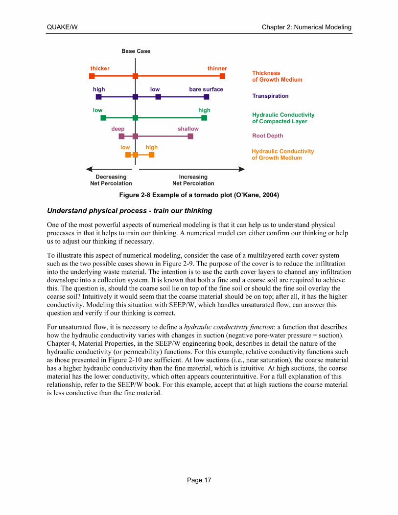
Numerical models are useful for identifying critical parameters in a design. Consider the performance of a soil cover over waste material. What is the most important parameter governing the behavior of the cover? Is it the precipitation, the wind speed, the net solar radiation, plant type, root depth or soil type? Running a series of VADOSE/W simulations, keeping all variables constant except for one, makes it possible to identify the governing parameter. The results can be presented as a tornado plot such as shown in Figure 2-8.
Once the key issues have been identified, further modeling to refine a design can concentrate on the main issues. If, for example, the vegetative growth is the main issue, then efforts can be concentrated on what needs to be done to foster the plant growth.
AA
6.2
592e
-003
Cutoff 10 feet
Pre
ssur
e H
ead
- fe
et
Distance - feet
0
5
10
15
20
25
30 50 70 90 110
Cutoff - 20 feet
Pre
ssur
e H
ead
- f
eet
Distance - feet
0
5
10
15
20
25
30 50 70 90 110
QUAKE/W Chapter 2: Numerical Modeling
Page 17
Figure 2-8 Example of a tornado plot (O’Kane, 2004)
Understand physical process - train our thinking
One of the most powerful aspects of numerical modeling is that it can help us to understand physical processes in that it helps to train our thinking. A numerical model can either confirm our thinking or help us to adjust our thinking if necessary.
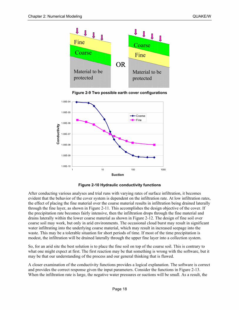
To illustrate this aspect of numerical modeling, consider the case of a multilayered earth cover system such as the two possible cases shown in Figure 2-9. The purpose of the cover is to reduce the infiltration into the underlying waste material. The intention is to use the earth cover layers to channel any infiltration downslope into a collection system. It is known that both a fine and a coarse soil are required to achieve this. The question is, should the coarse soil lie on top of the fine soil or should the fine soil overlay the coarse soil? Intuitively it would seem that the coarse material should be on top; after all, it has the higher conductivity. Modeling this situation with SEEP/W, which handles unsaturated flow, can answer this question and verify if our thinking is correct.
For unsaturated flow, it is necessary to define a hydraulic conductivity function: a function that describes how the hydraulic conductivity varies with changes in suction (negative pore-water pressure = suction). Chapter 4, Material Properties, in the SEEP/W engineering book, describes in detail the nature of the hydraulic conductivity (or permeability) functions. For this example, relative conductivity functions such as those presented in Figure 2-10 are sufficient. At low suctions (i.e., near saturation), the coarse material has a higher hydraulic conductivity than the fine material, which is intuitive. At high suctions, the coarse material has the lower conductivity, which often appears counterintuitive. For a full explanation of this relationship, refer to the SEEP/W book. For this example, accept that at high suctions the coarse material is less conductive than the fine material.
thinner
deep shallow
low high
high bare surfacelow
low high
Thicknessof Growth Medium
Transpiration
Hydraulic Conductivityof Compacted Layer
Root Depth
Hydraulic Conductivityof Growth Medium
Base Case
DecreasingNet Percolation
IncreasingNet Percolation
Chapter 2: Numerical Modeling QUAKE/W
Page 18
Figure 2-9 Two possible earth cover configurations
Figure 2-10 Hydraulic conductivity functions
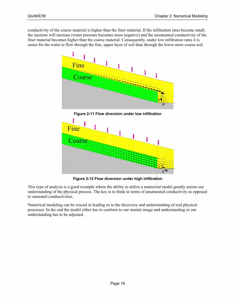
After conducting various analyses and trial runs with varying rates of surface infiltration, it becomes evident that the behavior of the cover system is dependent on the infiltration rate. At low infiltration rates, the effect of placing the fine material over the coarse material results in infiltration being drained laterally through the fine layer, as shown in Figure 2-11. This accomplishes the design objective of the cover. If the precipitation rate becomes fairly intensive, then the infiltration drops through the fine material and drains laterally within the lower coarse material as shown in Figure 2-12. The design of fine soil over coarse soil may work, but only in arid environments. The occasional cloud burst may result in significant water infiltrating into the underlying coarse material, which may result in increased seepage into the waste. This may be a tolerable situation for short periods of time. If most of the time precipitation is modest, the infiltration will be drained laterally through the upper fine layer into a collection system.
So, for an arid site the best solution is to place the fine soil on top of the coarse soil. This is contrary to what one might expect at first. The first reaction may be that something is wrong with the software, but it may be that our understanding of the process and our general thinking that is flawed.
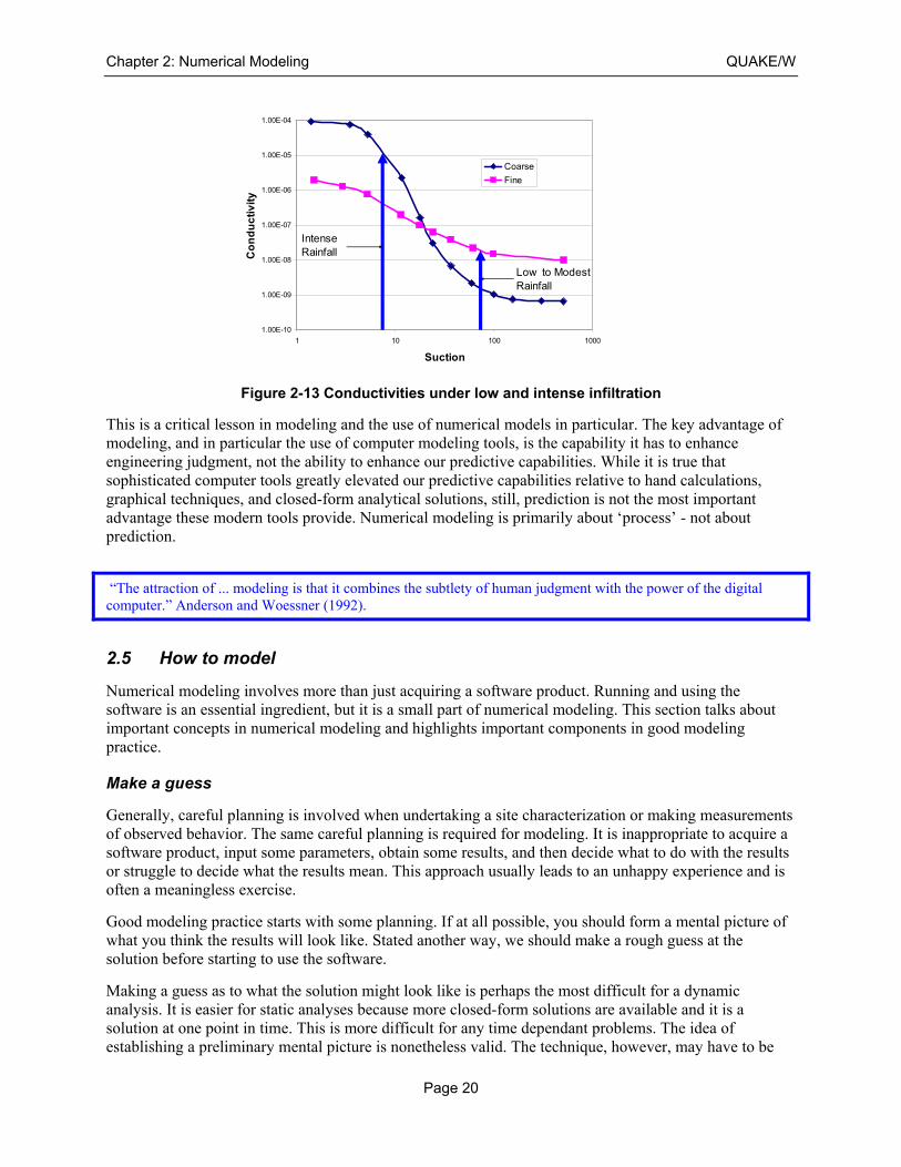
A closer examination of the conductivity functions provides a logical explanation. The software is correct and provides the correct response given the input parameters. Consider the functions in Figure 2-13. When the infiltration rate is large, the negative water pressures or suctions will be small. As a result, the
Material to beprotected
Fine
CoarseCoarse
Fine
Material to be protected
ORMaterial to beprotected
Fine
CoarseCoarse
Fine
Material to be protected
OR
1.00E-10
1.00E-09
1.00E-08
1.00E-07
1.00E-06
1.00E-05
1.00E-04
1 10 100 1000
Suction
Co
nd
uc
tiv
ity
Coarse
Fine
QUAKE/W Chapter 2: Numerical Modeling
Page 19
conductivity of the coarse material is higher than the finer material. If the infiltration rates become small, the suctions will increase (water pressure becomes more negative) and the unsaturated conductivity of the finer material becomes higher than the coarse material. Consequently, under low infiltration rates it is easier for the water to flow through the fine, upper layer of soil than through the lower more coarse soil.
Figure 2-11 Flow diversion under low infiltration
Figure 2-12 Flow diversion under high infiltration
This type of analysis is a good example where the ability to utilize a numerical model greatly assists our understanding of the physical process. The key is to think in terms of unsaturated conductivity as opposed to saturated conductivities.
Numerical modeling can be crucial in leading us to the discovery and understanding of real physical processes. In the end the model either has to conform to our mental image and understanding or our understanding has to be adjusted.
Fine
Coarse
Low to modest rainfall rates
Fine
Coarse
Intense rainfall rates
Chapter 2: Numerical Modeling QUAKE/W
Page 20
Figure 2-13 Conductivities under low and intense infiltration
This is a critical lesson in modeling and the use of numerical models in particular. The key advantage of modeling, and in particular the use of computer modeling tools, is the capability it has to enhance engineering judgment, not the ability to enhance our predictive capabilities. While it is true that sophisticated computer tools greatly elevated our predictive capabilities relative to hand calculations, graphical techniques, and closed-form analytical solutions, still, prediction is not the most important advantage these modern tools provide. Numerical modeling is primarily about ‘process’ - not about prediction.
“The attraction of ... modeling is that it combines the subtlety of human judgment with the power of the digital computer.” Anderson and Woessner (1992).
2.5 How to model
Numerical modeling involves more than just acquiring a software product. Running and using the software is an essential ingredient, but it is a small part of numerical modeling. This section talks about important concepts in numerical modeling and highlights important components in good modeling practice.
Make a guess
Generally, careful planning is involved when undertaking a site characterization or making measurements of observed behavior. The same careful planning is required for modeling. It is inappropriate to acquire a software product, input some parameters, obtain some results, and then decide what to do with the results or struggle to decide what the results mean. This approach usually leads to an unhappy experience and is often a meaningless exercise.
Good modeling practice starts with some planning. If at all possible, you should form a mental picture of what you think the results will look like. Stated another way, we should make a rough guess at the solution before starting to use the software.
Making a guess as to what the solution might look like is perhaps the most difficult for a dynamic analysis. It is easier for static analyses because more closed-form solutions are available and it is a solution at one point in time. This is more difficult for any time dependant problems. The idea of establishing a preliminary mental picture is nonetheless valid. The technique, however, may have to be
1.00E-10
1.00E-09
1.00E-08
1.00E-07
1.00E-06
1.00E-05
1.00E-04
1 10 100 1000
Suction
Co
nd
uc
tiv
ity
Coarse
Fine
IntenseRainfall
Low to ModestRainfall
QUAKE/W Chapter 2: Numerical Modeling
Page 21
different. For static analyses we can often use hand calculations which is not possible dynamic analyses. We can, however, do simple, small problem analyses to help us with a preliminary mental picture. Perhaps we can do a simple 1D or a small 2D analysis before moving on to a large field scale problem.
Another extremely important part of modeling is to clearly define at the outset, the primary question to be answered by the modeling process. Is the main question the generation of excess pore-water pressures or is it the dynamic response of the structure? If the main objective is to only establish the dynamic response the structure, then there is no need to spend a lot of time on establishing the pore-pressure functions. If, on the other hand, your main objective is to estimate the generation of excess pore-pressures, then great care is needed to establish the pore-pressure functions.
Sometimes modelers say “I have no idea what the solution should look like - that is why I am doing the modeling”. The question then arises, why can you not form a mental picture of what the solution should resemble? Maybe it is a lack of understanding of the fundamental processes or physics, maybe it is a lack of experience, or maybe the system is too complex. A lack of understanding of the fundamentals can possibly be overcome by discussing the problem with more experienced engineers or scientists, or by conducting a study of published literature. If the system is too complex to make a preliminary estimate then it is good practice to simplify the problem so you can make a guess and then add complexity in stages so that at each modeling interval you can understand the significance of the increased complexity. If you were dealing with a very heterogenic system, you could start by defining a homogenous cross-section, obtaining a reasonable solution and then adding heterogeneity in stages. This approach is discussed in further detail in a subsequent section.
If you cannot form a mental picture of what the solution should look like prior to using the software, then you may need to discover or learn about a new physical process as discussed in the previous section.
Effective numerical modeling starts with making a guess of what the solution should look like.
Other prominent engineers support this concept. Carter (2000) in his keynote address at the GeoEng2000 Conference in Melbourne, Australia when talking about rules for modeling stated verbally that modeling should “start with an estimate.” Prof. John Burland made a presentation at the same conference on his work with righting the Leaning Tower of Pisa. Part of the presentation was on the modeling that was done to evaluate alternatives and while talking about modeling he too stressed the need to “start with a guess”.
Simplify geometry
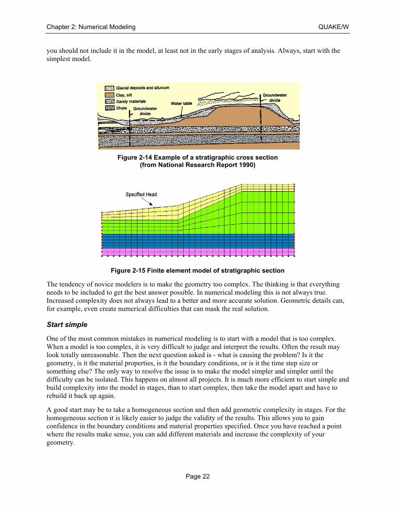
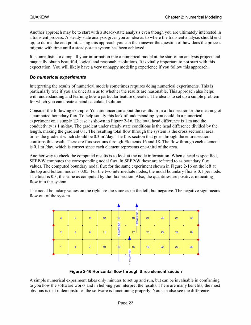
Numerical models need to be a simplified abstraction of the actual field conditions. In the field the stratigraphy may be fairly complex and boundaries may be irregular. In a numerical model the boundaries need to become straight lines and the stratigraphy needs to be simplified so that it is possible to obtain an understandable solution. Remember, it is a “model”, not the actual conditions. Generally, a numerical model cannot and should not include all the details that exist in the field. If attempts are made at including all the minute details, the model can become so complex that it is difficult and sometimes even impossible to interpret or even obtain results.
Figure 2-14 shows a stratigraphic cross section (National Research Council Report 1990). A suitable numerical model for simulating the flow regime between the groundwater divides is something like the one shown in Figure 2-15. The stratigraphic boundaries are considerably simplified for the finite element analysis.
As a general rule, a model should be designed to answer specific questions. You need to constantly ask yourself while designing a model, if this feature will significantly affect the results? If you have doubts,
Chapter 2: Numerical Modeling QUAKE/W
Page 22
you should not include it in the model, at least not in the early stages of analysis. Always, start with the simplest model.
Figure 2-14 Example of a stratigraphic cross section (from National Research Report 1990)
Figure 2-15 Finite element model of stratigraphic section
The tendency of novice modelers is to make the geometry too complex. The thinking is that everything needs to be included to get the best answer possible. In numerical modeling this is not always true. Increased complexity does not always lead to a better and more accurate solution. Geometric details can, for example, even create numerical difficulties that can mask the real solution.
Start simple
One of the most common mistakes in numerical modeling is to start with a model that is too complex. When a model is too complex, it is very difficult to judge and interpret the results. Often the result may look totally unreasonable. Then the next question asked is - what is causing the problem? Is it the geometry, is it the material properties, is it the boundary conditions, or is it the time step size or something else? The only way to resolve the issue is to make the model simpler and simpler until the difficulty can be isolated. This happens on almost all projects. It is much more efficient to start simple and build complexity into the model in stages, than to start complex, then take the model apart and have to rebuild it back up again.
A good start may be to take a homogeneous section and then add geometric complexity in stages. For the homogeneous section it is likely easier to judge the validity of the results. This allows you to gain confidence in the boundary conditions and material properties specified. Once you have reached a point where the results make sense, you can add different materials and increase the complexity of your geometry.
QUAKE/W Chapter 2: Numerical Modeling
Page 23
Another approach may be to start with a steady-state analysis even though you are ultimately interested in a transient process. A steady-state analysis gives you an idea as to where the transient analysis should end up; to define the end point. Using this approach you can then answer the question of how does the process migrate with time until a steady-state system has been achieved.
It is unrealistic to dump all your information into a numerical model at the start of an analysis project and magically obtain beautiful, logical and reasonable solutions. It is vitally important to not start with this expectation. You will likely have a very unhappy modeling experience if you follow this approach.
Do numerical experiments
Interpreting the results of numerical models sometimes requires doing numerical experiments. This is particularly true if you are uncertain as to whether the results are reasonable. This approach also helps with understanding and learning how a particular feature operates. The idea is to set up a simple problem for which you can create a hand calculated solution.
Consider the following example. You are uncertain about the results from a flux section or the meaning of a computed boundary flux. To help satisfy this lack of understanding, you could do a numerical experiment on a simple 1D case as shown in Figure 2-16. The total head difference is 1 m and the conductivity is 1 m/day. The gradient under steady state conditions is the head difference divided by the length, making the gradient 0.1. The resulting total flow through the system is the cross sectional area times the gradient which should be 0.3 m3/day. The flux section that goes through the entire section confirms this result. There are flux sections through Elements 16 and 18. The flow through each element is 0.1 m3/day, which is correct since each element represents one-third of the area.
Another way to check the computed results is to look at the node information. When a head is specified, SEEP/W computes the corresponding nodal flux. In SEEP/W these are referred to as boundary flux values. The computed boundary nodal flux for the same experiment shown in Figure 2-16 on the left at the top and bottom nodes is 0.05. For the two intermediate nodes, the nodal boundary flux is 0.1 per node. The total is 0.3, the same as computed by the flux section. Also, the quantities are positive, indicating flow into the system.
The nodal boundary values on the right are the same as on the left, but negative. The negative sign means flow out of the system.
Figure 2-16 Horizontal flow through three element section
A simple numerical experiment takes only minutes to set up and run, but can be invaluable in confirming to you how the software works and in helping you interpret the results. There are many benefits; the most obvious is that it demonstrates the software is functioning properly. You can also see the difference
1
2
3
4
5
6
7
8
9
10
11
12
13
14
15
16
17
18
19
20
21
22
23
24
25
26
27
28
29
30
3.0
000e
-001
1.0
000e
-001
1.0
000e
-001
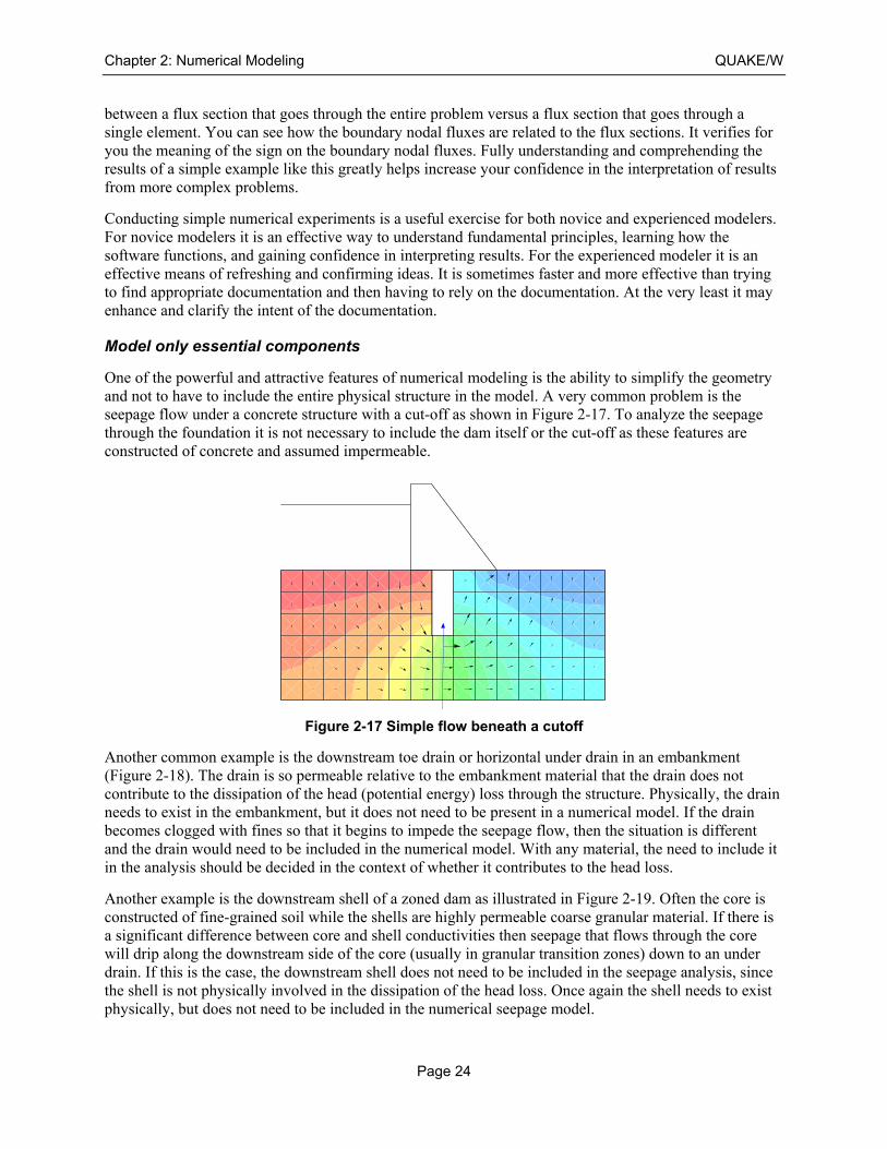
Chapter 2: Numerical Modeling QUAKE/W
Page 24
between a flux section that goes through the entire problem versus a flux section that goes through a single element. You can see how the boundary nodal fluxes are related to the flux sections. It verifies for you the meaning of the sign on the boundary nodal fluxes. Fully understanding and comprehending the results of a simple example like this greatly helps increase your confidence in the interpretation of results from more complex problems.
Conducting simple numerical experiments is a useful exercise for both novice and experienced modelers. For novice modelers it is an effective way to understand fundamental principles, learning how the software functions, and gaining confidence in interpreting results. For the experienced modeler it is an effective means of refreshing and confirming ideas. It is sometimes faster and more effective than trying to find appropriate documentation and then having to rely on the documentation. At the very least it may enhance and clarify the intent of the documentation.
Model only essential components
One of the powerful and attractive features of numerical modeling is the ability to simplify the geometry and not to have to include the entire physical structure in the model. A very common problem is the seepage flow under a concrete structure with a cut-off as shown in Figure 2-17. To analyze the seepage through the foundation it is not necessary to include the dam itself or the cut-off as these features are constructed of concrete and assumed impermeable.
Figure 2-17 Simple flow beneath a cutoff
Another common example is the downstream toe drain or horizontal under drain in an embankment (Figure 2-18). The drain is so permeable relative to the embankment material that the drain does not contribute to the dissipation of the head (potential energy) loss through the structure. Physically, the drain needs to exist in the embankment, but it does not need to be present in a numerical model. If the drain becomes clogged with fines so that it begins to impede the seepage flow, then the situation is different and the drain would need to be included in the numerical model. With any material, the need to include it in the analysis should be decided in the context of whether it contributes to the head loss.
Another example is the downstream shell of a zoned dam as illustrated in Figure 2-19. Often the core is constructed of fine-grained soil while the shells are highly permeable coarse granular material. If there is a significant difference between core and shell conductivities then seepage that flows through the core will drip along the downstream side of the core (usually in granular transition zones) down to an under drain. If this is the case, the downstream shell does not need to be included in the seepage analysis, since the shell is not physically involved in the dissipation of the head loss. Once again the shell needs to exist physically, but does not need to be included in the numerical seepage model.
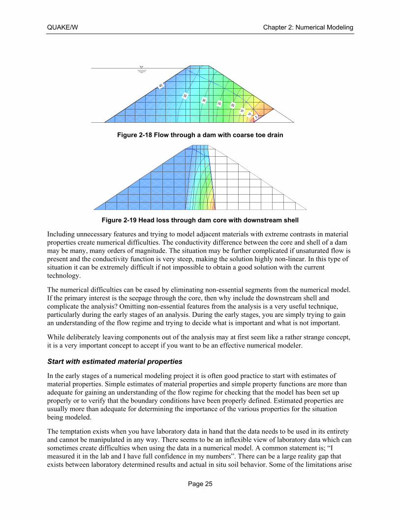
QUAKE/W Chapter 2: Numerical Modeling
Page 25
Figure 2-18 Flow through a dam with coarse toe drain
Figure 2-19 Head loss through dam core with downstream shell
Including unnecessary features and trying to model adjacent materials with extreme contrasts in material properties create numerical difficulties. The conductivity difference between the core and shell of a dam may be many, many orders of magnitude. The situation may be further complicated if unsaturated flow is present and the conductivity function is very steep, making the solution highly non-linear. In this type of situation it can be extremely difficult if not impossible to obtain a good solution with the current technology.
The numerical difficulties can be eased by eliminating non-essential segments from the numerical model. If the primary interest is the seepage through the core, then why include the downstream shell and complicate the analysis? Omitting non-essential features from the analysis is a very useful technique, particularly during the early stages of an analysis. During the early stages, you are simply trying to gain an understanding of the flow regime and trying to decide what is important and what is not important.
While deliberately leaving components out of the analysis may at first seem like a rather strange concept, it is a very important concept to accept if you want to be an effective numerical modeler.
Start with estimated material properties
In the early stages of a numerical modeling project it is often good practice to start with estimates of material properties. Simple estimates of material properties and simple property functions are more than adequate for gaining an understanding of the flow regime for checking that the model has been set up properly or to verify that the boundary conditions have been properly defined. Estimated properties are usually more than adequate for determining the importance of the various properties for the situation being modeled.
The temptation exists when you have laboratory data in hand that the data needs to be used in its entirety and cannot be manipulated in any way. There seems to be an inflexible view of laboratory data which can sometimes create difficulties when using the data in a numerical model. A common statement is; “I measured it in the lab and I have full confidence in my numbers”. There can be a large reality gap that exists between laboratory determined results and actual in situ soil behavior. Some of the limitations arise
5 10
15
20
25
30
35
40

Chapter 2: Numerical Modeling QUAKE/W
Page 26
because of how the material was collected, how it was sampled and ultimately quantified in the lab. Was the sample collected by the shovelful, by collecting cuttings or by utilizing a core sampler? What was the size and number of samples collected and can they be considered representative of the entire profile? Was the sample oven-dried, sieved and then slurried prior to the test being performed? Were the large particles removed so the sample could be trimmed into the measuring device? Some of these common laboratory techniques can result in unrealistic property functions. Perhaps the amount of data collected in the laboratory is more than is actually required in the model. Because money has been spent collecting and measuring the data, it makes modelers reticent to experiment with making changes to the data to see what effect it has on the analysis.
It is good modeling practice to first obtain understandable and reasonable solutions using estimate material properties and then later refine the analysis once you know what the critical properties are going to be. It can even be more cost effective to determine ahead of time what material properties control the analysis and decide where it is appropriate to spend money obtaining laboratory data.
Interrogate the results
Powerful numerical models such as QUAKE/W need very careful guidance from the user. It is easy to inadvertently and unintentionally specify inappropriate boundary conditions or incorrect material properties. Consequently, it is vitally important to conduct spot checks on the results to ensure the constraints and material properties are consistent with what you intended to define and the results make sense. It is important to check, for example that the boundary condition that appears in the results is the same as what you thought was specified defining the model. Is the intended property function being applied to the correct soil? Or, are the initial conditions as you assumed?
QUAKE/W has many tools to inspect or interrogate the results. You can view node or element details and there are a wide range of parameters that can be graphed for the purpose of spot checking the results.
Inspecting and spot checking your results is an important and vital component in numerical modeling. It greatly helps to increase your confidence in a solution that is understandable and definable.
Evaluate results in the context of expected results
The fundamental question that should be asked during modeling is; “Do the results conform to the initial mental picture?” If they do not, then your mental picture needs to be fixed, there is something wrong with the model or both the model and your concept of the problem need to be adjusted until they agree. The numerical modeling process needs to be repeated over and over until the solution makes perfect sense and you are able to look at the results and feel confident that you understand the processes involved.
Remember the real world
While doing numerical modeling it is important to occasionally ask yourself how much you really know about the input compared to the complexity of the analysis. The following cartoon portrays an extreme situation, but underscores a problem that exists when uneducated or inexperienced users try to use powerful software tools.
QUAKE/W Chapter 2: Numerical Modeling
Page 27
Note: origins of this figure are unknown at time of printing.
2.6 How not to model
As mentioned earlier in this chapter, it is completely unrealistic to expect to set up a complex model at the start of a project and immediately obtain realistic, understandable and meaningful results. There are far too many parameters and issues which can influence the results, so if this is your expectation, then modeling is going to lead to major disappointments.
For novice modelers, the initial reaction when faced with incomprehensible results is that something must be wrong with the software. It must be a limitation of the software that the solution is inappropriate or completely senseless. It is important to remember that the software is very powerful; it can keep track of millions of pieces of information and do repetitive computations which are far beyond the capability of the human mind. Without the software it would not be possible to make these types of analyses. The software by itself is extremely powerful numerically speaking, but essentially unintelligent. Conversely, the human mind has the capability of logic and reasoning, but has significant limitations retaining large amounts of digital data. It is the combination of the human mind together with the capability of a computer that makes numerical modeling so immensely powerful. Nether can do the task in isolation. The software can only be used effectively under the careful guidance and direction of the modeler.
Sometimes it is suggested that due to a time limitation, it is not possible to start simple and then progress slowly to a more complex analysis. A solution is needed quickly and since the budget is limited, it is necessary to immediately start with the ultimate simulation. This approach is seldom, if ever, successful. Usually this leads to a lot of frustration and the need to retreat to a simpler model until the solution is understandable and then build it up again in stages. Not following the above “how to” modeling procedures generally leads to requiring more time and financial resources than if you follow the recommended modeling concepts.
“Put another shovelfull in Pat! It is full-cores they’re wanting!”
“If we can incorporate boundaryelements rather than simple finiteelephants, enhance the statisticalevaluation of parameter generationand stick with the fuzzy sets, I amconfident that accuracy will beincreased to at least the fourthdecimal place.”

Chapter 2: Numerical Modeling QUAKE/W
Page 28
Remember, the software is only as good as your ability to guide and direct it. The intention of this document is to assist you in providing this guidance and direction so that you can take full advantages of the power the software can offer.
2.7 Closing remarks
As noted in the introduction, numerical modeling is a relatively new area of practice. Most university educational curricula do not include courses on how to approach numerical modeling and, consequently, the skill is often self-taught. As software tools such as GeoStudio become increasingly available at educational institutions and educators become comfortable with these types of tools, classes and instruction should improve with respect to numerical modeling.
When the numerical analysis software tool, GeoStudio, is effectively utilized as it was intended to be used, it becomes an immensely powerful tool, making it possible to do highly complex analyses. It can even lead to new understandings about actual physical process.
The process of modeling is a journey of discovery, a way of learning something new about the complex behavior of our physical world. It is a process that can help us understand highly complex, real physical process so that we can exercise our engineering judgment with increased confidence.
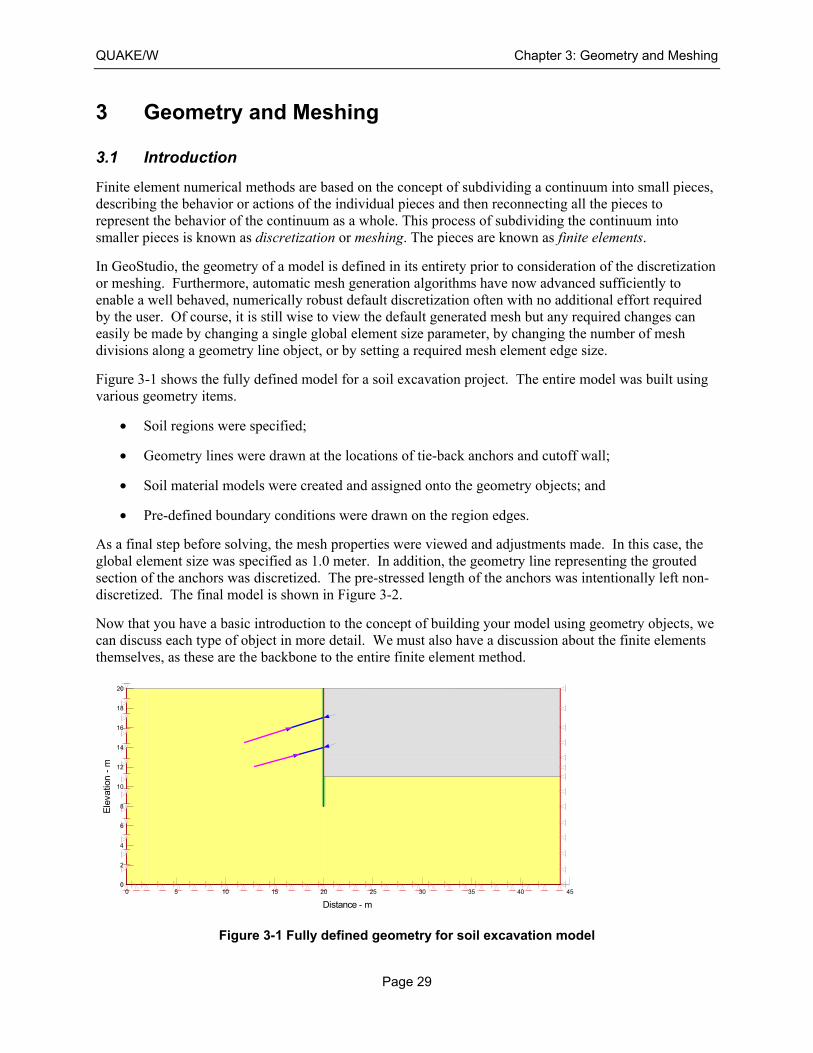
QUAKE/W Chapter 3: Geometry and Meshing
Page 29
3 Geometry and Meshing
3.1 Introduction
Finite element numerical methods are based on the concept of subdividing a continuum into small pieces, describing the behavior or actions of the individual pieces and then reconnecting all the pieces to represent the behavior of the continuum as a whole. This process of subdividing the continuum into smaller pieces is known as discretization or meshing. The pieces are known as finite elements.
In GeoStudio, the geometry of a model is defined in its entirety prior to consideration of the discretization or meshing. Furthermore, automatic mesh generation algorithms have now advanced sufficiently to enable a well behaved, numerically robust default discretization often with no additional effort required by the user. Of course, it is still wise to view the default generated mesh but any required changes can easily be made by changing a single global element size parameter, by changing the number of mesh divisions along a geometry line object, or by setting a required mesh element edge size.
Figure 3-1 shows the fully defined model for a soil excavation project. The entire model was built using various geometry items.
• Soil regions were specified;
• Geometry lines were drawn at the locations of tie-back anchors and cutoff wall;
• Soil material models were created and assigned onto the geometry objects; and
• Pre-defined boundary conditions were drawn on the region edges.
As a final step before solving, the mesh properties were viewed and adjustments made. In this case, the global element size was specified as 1.0 meter. In addition, the geometry line representing the grouted section of the anchors was discretized. The pre-stressed length of the anchors was intentionally left non-discretized. The final model is shown in Figure 3-2.
Now that you have a basic introduction to the concept of building your model using geometry objects, we can discuss each type of object in more detail. We must also have a discussion about the finite elements themselves, as these are the backbone to the entire finite element method.
Figure 3-1 Fully defined geometry for soil excavation model
Distance - m
0 5 10 15 20 25 30 35 40 45
Ele
vatio
n -
m
0
2
4
6
8
10
12
14
16
18
20
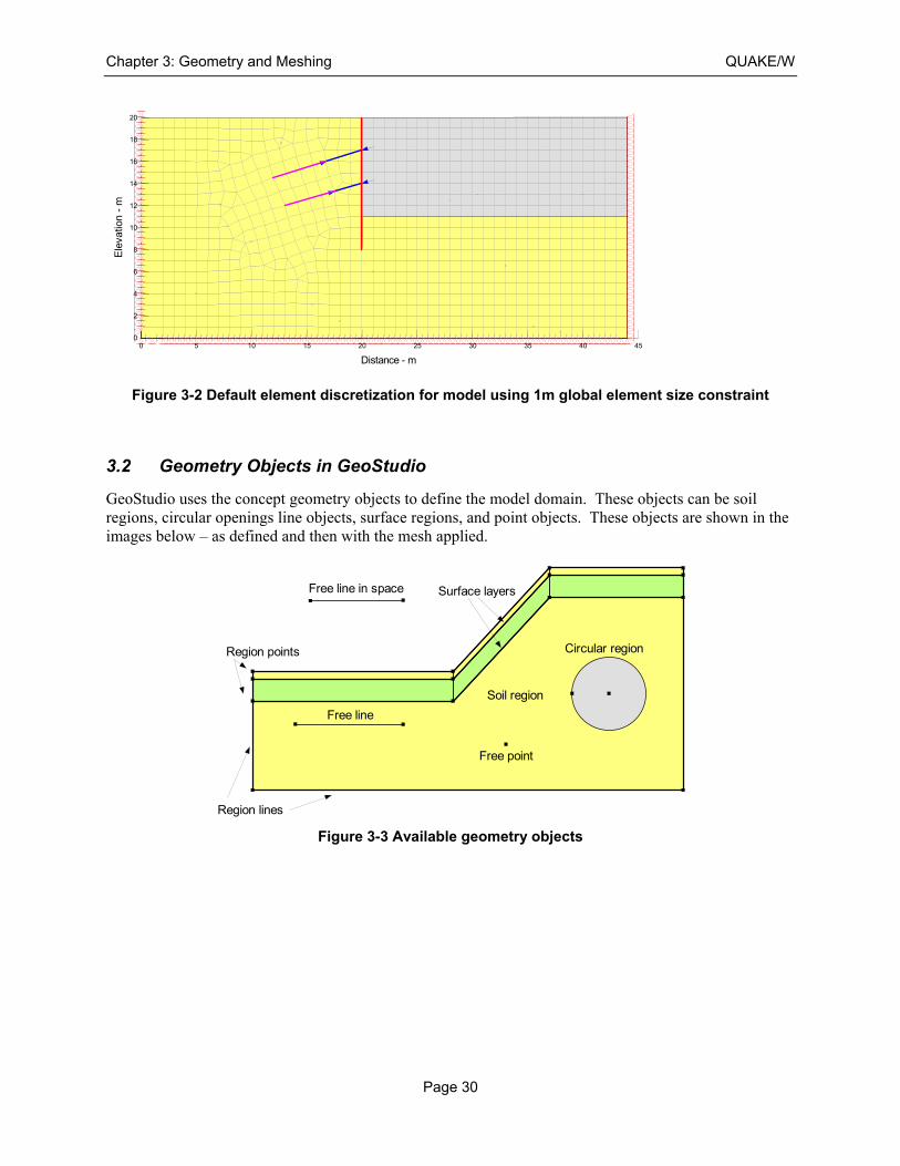
Chapter 3: Geometry and Meshing QUAKE/W
Page 30
Figure 3-2 Default element discretization for model using 1m global element size constraint
3.2 Geometry Objects in GeoStudio
GeoStudio uses the concept geometry objects to define the model domain. These objects can be soil regions, circular openings line objects, surface regions, and point objects. These objects are shown in the images below – as defined and then with the mesh applied.
Figure 3-3 Available geometry objects
Distance - m
0 5 10 15 20 25 30 35 40 45
Ele
vatio
n -
m
0
2
4
6
8
10
12
14
16
18
20
Soil region
Surface layers
Circular region
Region lines
Free line
Free point
Region points
Free line in space
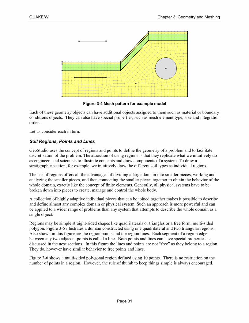
QUAKE/W Chapter 3: Geometry and Meshing
Page 31
Figure 3-4 Mesh pattern for example model
Each of these geometry objects can have additional objects assigned to them such as material or boundary conditions objects. They can also have special properties, such as mesh element type, size and integration order.
Let us consider each in turn.
Soil Regions, Points and Lines
GeoStudio uses the concept of regions and points to define the geometry of a problem and to facilitate discretization of the problem. The attraction of using regions is that they replicate what we intuitively do as engineers and scientists to illustrate concepts and draw components of a system. To draw a stratigraphic section, for example, we intuitively draw the different soil types as individual regions.
The use of regions offers all the advantages of dividing a large domain into smaller pieces, working and analyzing the smaller pieces, and then connecting the smaller pieces together to obtain the behavior of the whole domain, exactly like the concept of finite elements. Generally, all physical systems have to be broken down into pieces to create, manage and control the whole body.
A collection of highly adaptive individual pieces that can be joined together makes it possible to describe and define almost any complex domain or physical system. Such an approach is more powerful and can be applied to a wider range of problems than any system that attempts to describe the whole domain as a single object.
Regions may be simple straight-sided shapes like quadrilaterals or triangles or a free form, multi-sided polygon. Figure 3-5 illustrates a domain constructed using one quadrilateral and two triangular regions. Also shown in this figure are the region points and the region lines. Each segment of a region edge between any two adjacent points is called a line. Both points and lines can have special properties as discussed in the next sections. In this figure the lines and points are not “free” as they belong to a region. They do, however have similar behavior to free points and lines.
Figure 3-6 shows a multi-sided polygonal region defined using 10 points. There is no restriction on the number of points in a region. However, the rule of thumb to keep things simple is always encouraged.
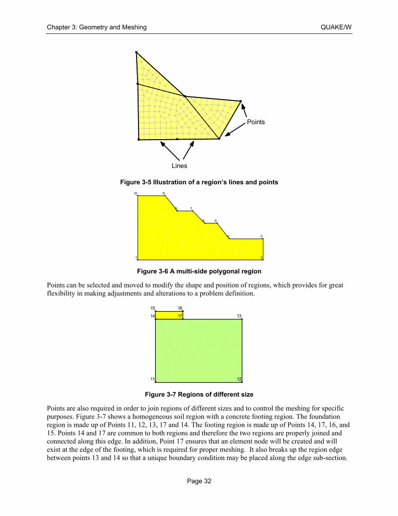
Chapter 3: Geometry and Meshing QUAKE/W
Page 32
Figure 3-5 Illustration of a region’s lines and points
Figure 3-6 A multi-side polygonal region
Points can be selected and moved to modify the shape and position of regions, which provides for great flexibility in making adjustments and alterations to a problem definition.
Figure 3-7 Regions of different size
Points are also required in order to join regions of different sizes and to control the meshing for specific purposes. Figure 3-7 shows a homogeneous soil region with a concrete footing region. The foundation region is made up of Points 11, 12, 13, 17 and 14. The footing region is made up of Points 14, 17, 16, and 15. Points 14 and 17 are common to both regions and therefore the two regions are properly joined and connected along this edge. In addition, Point 17 ensures that an element node will be created and will exist at the edge of the footing, which is required for proper meshing. It also breaks up the region edge between points 13 and 14 so that a unique boundary condition may be placed along the edge sub-section.
Points
Lines
1 2
34
56
78
910
11 12
1314
15 16
17
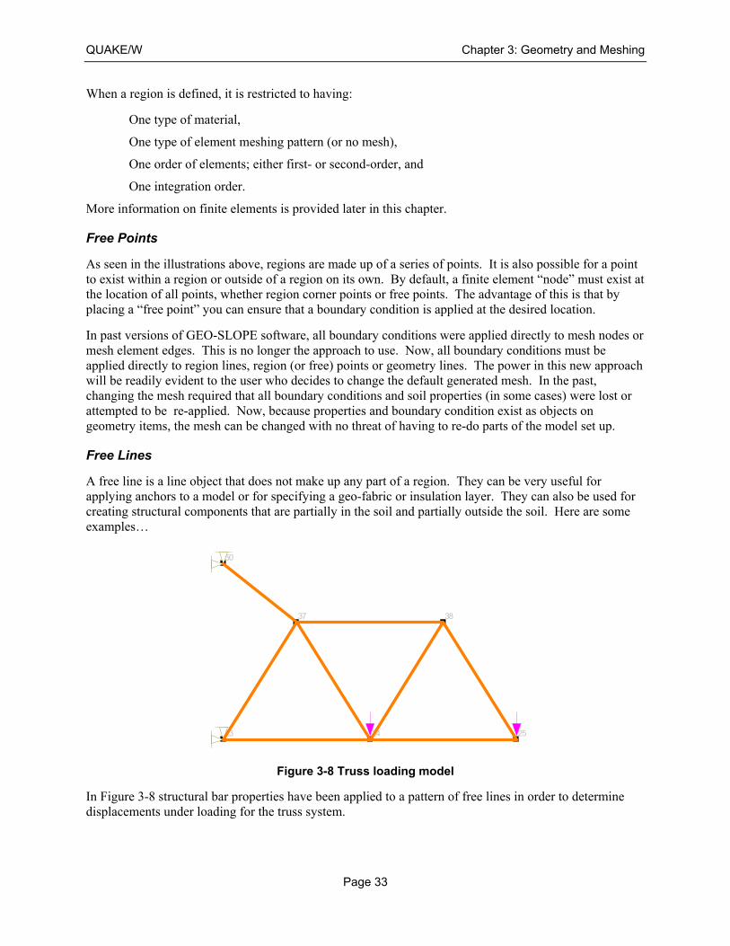
QUAKE/W Chapter 3: Geometry and Meshing
Page 33
When a region is defined, it is restricted to having:
One type of material,
One type of element meshing pattern (or no mesh),
One order of elements; either first- or second-order, and
One integration order.
More information on finite elements is provided later in this chapter.
Free Points
As seen in the illustrations above, regions are made up of a series of points. It is also possible for a point to exist within a region or outside of a region on its own. By default, a finite element “node” must exist at the location of all points, whether region corner points or free points. The advantage of this is that by placing a “free point” you can ensure that a boundary condition is applied at the desired location.
In past versions of GEO-SLOPE software, all boundary conditions were applied directly to mesh nodes or mesh element edges. This is no longer the approach to use. Now, all boundary conditions must be applied directly to region lines, region (or free) points or geometry lines. The power in this new approach will be readily evident to the user who decides to change the default generated mesh. In the past, changing the mesh required that all boundary conditions and soil properties (in some cases) were lost or attempted to be re-applied. Now, because properties and boundary condition exist as objects on geometry items, the mesh can be changed with no threat of having to re-do parts of the model set up.
Free Lines
A free line is a line object that does not make up any part of a region. They can be very useful for applying anchors to a model or for specifying a geo-fabric or insulation layer. They can also be used for creating structural components that are partially in the soil and partially outside the soil. Here are some examples…
Figure 3-8 Truss loading model
In Figure 3-8 structural bar properties have been applied to a pattern of free lines in order to determine displacements under loading for the truss system.
23 24 25
37 38
50
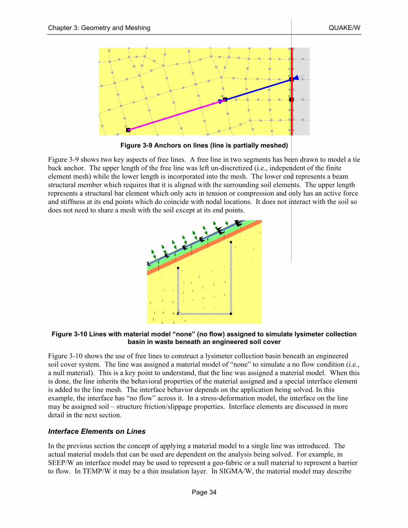
Chapter 3: Geometry and Meshing QUAKE/W
Page 34
Figure 3-9 Anchors on lines (line is partially meshed)
Figure 3-9 shows two key aspects of free lines. A free line in two segments has been drawn to model a tie back anchor. The upper length of the free line was left un-discretized (i.e., independent of the finite element mesh) while the lower length is incorporated into the mesh. The lower end represents a beam structural member which requires that it is aligned with the surrounding soil elements. The upper length represents a structural bar element which only acts in tension or compression and only has an active force and stiffness at its end points which do coincide with nodal locations. It does not interact with the soil so does not need to share a mesh with the soil except at its end points.
Figure 3-10 Lines with material model “none” (no flow) assigned to simulate lysimeter collection basin in waste beneath an engineered soil cover
Figure 3-10 shows the use of free lines to construct a lysimeter collection basin beneath an engineered soil cover system. The line was assigned a material model of “none” to simulate a no flow condition (i.e., a null material). This is a key point to understand, that the line was assigned a material model. When this is done, the line inherits the behavioral properties of the material assigned and a special interface element is added to the line mesh. The interface behavior depends on the application being solved. In this example, the interface has “no flow” across it. In a stress-deformation model, the interface on the line may be assigned soil – structure friction/slippage properties. Interface elements are discussed in more detail in the next section.
Interface Elements on Lines
In the previous section the concept of applying a material model to a single line was introduced. The actual material models that can be used are dependent on the analysis being solved. For example, in SEEP/W an interface model may be used to represent a geo-fabric or a null material to represent a barrier to flow. In TEMP/W it may be a thin insulation layer. In SIGMA/W, the material model may describe
4
5
17
18
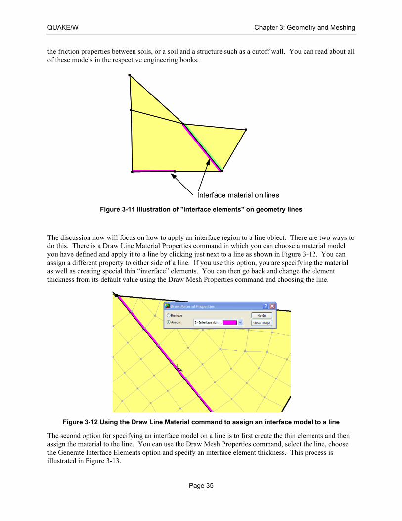
QUAKE/W Chapter 3: Geometry and Meshing
Page 35
the friction properties between soils, or a soil and a structure such as a cutoff wall. You can read about all of these models in the respective engineering books.
Figure 3-11 Illustration of "interface elements" on geometry lines
The discussion now will focus on how to apply an interface region to a line object. There are two ways to do this. There is a Draw Line Material Properties command in which you can choose a material model you have defined and apply it to a line by clicking just next to a line as shown in Figure 3-12. You can assign a different property to either side of a line. If you use this option, you are specifying the material as well as creating special thin “interface” elements. You can then go back and change the element thickness from its default value using the Draw Mesh Properties command and choosing the line.
Figure 3-12 Using the Draw Line Material command to assign an interface model to a line
The second option for specifying an interface model on a line is to first create the thin elements and then assign the material to the line. You can use the Draw Mesh Properties command, select the line, choose the Generate Interface Elements option and specify an interface element thickness. This process is illustrated in Figure 3-13.
Interface material on lines
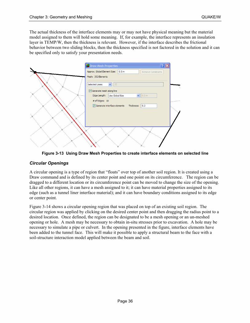
Chapter 3: Geometry and Meshing QUAKE/W
Page 36
The actual thickness of the interface elements may or may not have physical meaning but the material model assigned to them will hold some meaning. If, for example, the interface represents an insulation layer in TEMP/W, then the thickness is relevant. However, if the interface describes the frictional behavior between two sliding blocks, then the thickness specified is not factored in the solution and it can be specified only to satisfy your presentation needs.
Figure 3-13 Using Draw Mesh Properties to create interface elements on selected line
Circular Openings
A circular opening is a type of region that “floats” over top of another soil region. It is created using a Draw command and is defined by its center point and one point on its circumference. The region can be dragged to a different location or its circumference point can be moved to change the size of the opening. Like all other regions, it can have a mesh assigned to it; it can have material properties assigned to its edge (such as a tunnel liner interface material); and it can have boundary conditions assigned to its edge or center point.
Figure 3-14 shows a circular opening region that was placed on top of an existing soil region. The circular region was applied by clicking on the desired center point and then dragging the radius point to a desired location. Once defined, the region can be designated to be a mesh opening or an un-meshed opening or hole. A mesh may be necessary to obtain in-situ stresses prior to excavation. A hole may be necessary to simulate a pipe or culvert. In the opening presented in the figure, interface elements have been added to the tunnel face. This will make it possible to apply a structural beam to the face with a soil-structure interaction model applied between the beam and soil.
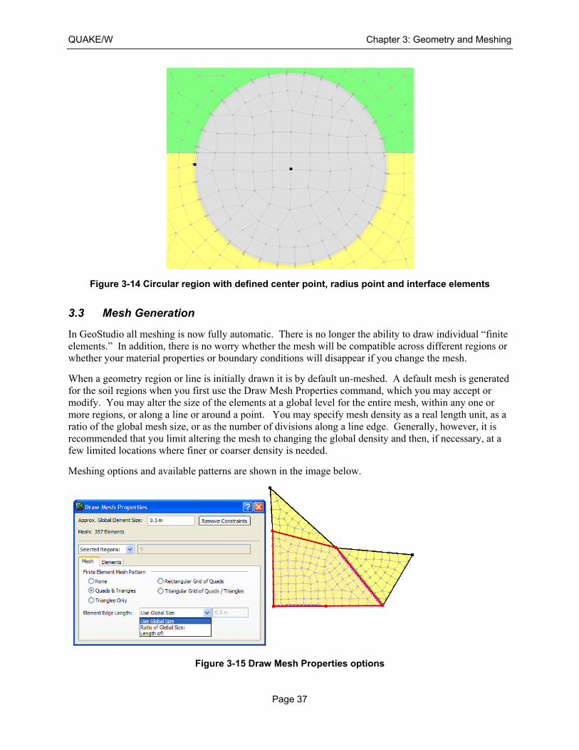
QUAKE/W Chapter 3: Geometry and Meshing
Page 37
Figure 3-14 Circular region with defined center point, radius point and interface elements
3.3 Mesh Generation
In GeoStudio all meshing is now fully automatic. There is no longer the ability to draw individual “finite elements.” In addition, there is no worry whether the mesh will be compatible across different regions or whether your material properties or boundary conditions will disappear if you change the mesh.
When a geometry region or line is initially drawn it is by default un-meshed. A default mesh is generated for the soil regions when you first use the Draw Mesh Properties command, which you may accept or modify. You may alter the size of the elements at a global level for the entire mesh, within any one or more regions, or along a line or around a point. You may specify mesh density as a real length unit, as a ratio of the global mesh size, or as the number of divisions along a line edge. Generally, however, it is recommended that you limit altering the mesh to changing the global density and then, if necessary, at a few limited locations where finer or coarser density is needed.
Meshing options and available patterns are shown in the image below.
Figure 3-15 Draw Mesh Properties options
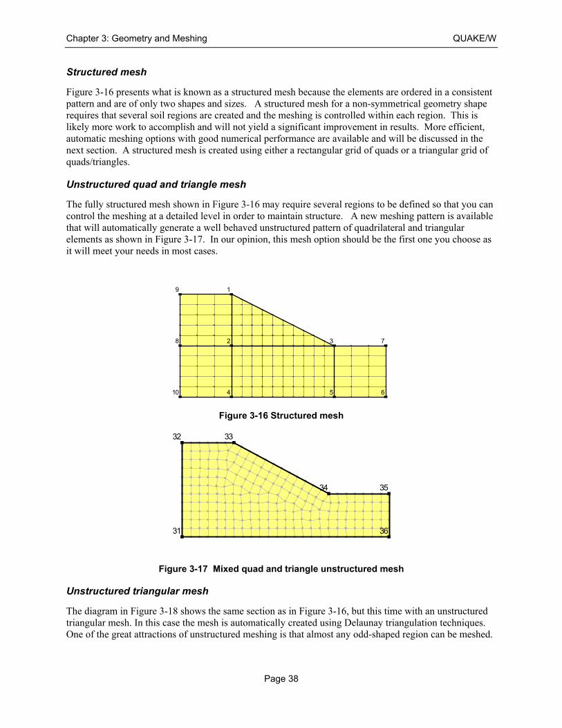
Chapter 3: Geometry and Meshing QUAKE/W
Page 38
Structured mesh
Figure 3-16 presents what is known as a structured mesh because the elements are ordered in a consistent pattern and are of only two shapes and sizes. A structured mesh for a non-symmetrical geometry shape requires that several soil regions are created and the meshing is controlled within each region. This is likely more work to accomplish and will not yield a significant improvement in results. More efficient, automatic meshing options with good numerical performance are available and will be discussed in the next section. A structured mesh is created using either a rectangular grid of quads or a triangular grid of quads/triangles.
Unstructured quad and triangle mesh
The fully structured mesh shown in Figure 3-16 may require several regions to be defined so that you can control the meshing at a detailed level in order to maintain structure. A new meshing pattern is available that will automatically generate a well behaved unstructured pattern of quadrilateral and triangular elements as shown in Figure 3-17. In our opinion, this mesh option should be the first one you choose as it will meet your needs in most cases.
Figure 3-16 Structured mesh
Figure 3-17 Mixed quad and triangle unstructured mesh
Unstructured triangular mesh
The diagram in Figure 3-18 shows the same section as in Figure 3-16, but this time with an unstructured triangular mesh. In this case the mesh is automatically created using Delaunay triangulation techniques. One of the great attractions of unstructured meshing is that almost any odd-shaped region can be meshed.
1
2 3
4 5 6
78
9
10
31
32 33
34 35
36
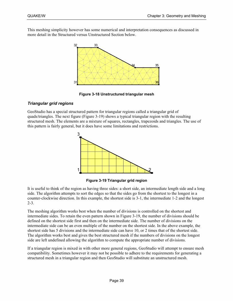
QUAKE/W Chapter 3: Geometry and Meshing
Page 39
This meshing simplicity however has some numerical and interpretation consequences as discussed in more detail in the Structured versus Unstructured Section below.
Figure 3-18 Unstructured triangular mesh
Triangular grid regions
GeoStudio has a special structured pattern for triangular regions called a triangular grid of quads/triangles. The next figure (Figure 3-19) shows a typical triangular region with the resulting structured mesh. The elements are a mixture of squares, rectangles, trapezoids and triangles. The use of this pattern is fairly general, but it does have some limitations and restrictions.
Figure 3-19 Triangular grid region
It is useful to think of the region as having three sides: a short side, an intermediate length side and a long side. The algorithm attempts to sort the edges so that the sides go from the shortest to the longest in a counter-clockwise direction. In this example, the shortest side is 3-1, the intermediate 1-2 and the longest 2-3.
The meshing algorithm works best when the number of divisions is controlled on the shortest and intermediate sides. To retain the even pattern shown in Figure 3-19, the number of divisions should be defined on the shortest side first and then on the intermediate side. The number of divisions on the intermediate side can be an even multiple of the number on the shortest side. In the above example, the shortest side has 5 divisions and the intermediate side can have 10, or 2 times that of the shortest side. The algorithm works best and gives the best structured mesh if the numbers of divisions on the longest side are left undefined allowing the algorithm to compute the appropriate number of divisions.
If a triangular region is mixed in with other more general regions, GeoStudio will attempt to ensure mesh compatibility. Sometimes however it may not be possible to adhere to the requirements for generating a structured mesh in a triangular region and then GeoStudio will substitute an unstructured mesh.
31
32 33
34 35
36
1 2
3
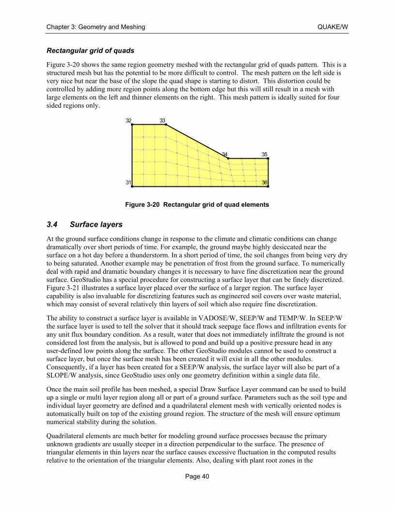
Chapter 3: Geometry and Meshing QUAKE/W
Page 40
Rectangular grid of quads
Figure 3-20 shows the same region geometry meshed with the rectangular grid of quads pattern. This is a structured mesh but has the potential to be more difficult to control. The mesh pattern on the left side is very nice but near the base of the slope the quad shape is starting to distort. This distortion could be controlled by adding more region points along the bottom edge but this will still result in a mesh with large elements on the left and thinner elements on the right. This mesh pattern is ideally suited for four sided regions only.
Figure 3-20 Rectangular grid of quad elements
3.4 Surface layers
At the ground surface conditions change in response to the climate and climatic conditions can change dramatically over short periods of time. For example, the ground maybe highly desiccated near the surface on a hot day before a thunderstorm. In a short period of time, the soil changes from being very dry to being saturated. Another example may be penetration of frost from the ground surface. To numerically deal with rapid and dramatic boundary changes it is necessary to have fine discretization near the ground surface. GeoStudio has a special procedure for constructing a surface layer that can be finely discretized. Figure 3-21 illustrates a surface layer placed over the surface of a larger region. The surface layer capability is also invaluable for discretizing features such as engineered soil covers over waste material, which may consist of several relatively thin layers of soil which also require fine discretization.
The ability to construct a surface layer is available in VADOSE/W, SEEP/W and TEMP/W. In SEEP/W the surface layer is used to tell the solver that it should track seepage face flows and infiltration events for any unit flux boundary condition. As a result, water that does not immediately infiltrate the ground is not considered lost from the analysis, but is allowed to pond and build up a positive pressure head in any user-defined low points along the surface. The other GeoStudio modules cannot be used to construct a surface layer, but once the surface mesh has been created it will exist in all the other modules. Consequently, if a layer has been created for a SEEP/W analysis, the surface layer will also be part of a SLOPE/W analysis, since GeoStudio uses only one geometry definition within a single data file.
Once the main soil profile has been meshed, a special Draw Surface Layer command can be used to build up a single or multi layer region along all or part of a ground surface. Parameters such as the soil type and individual layer geometry are defined and a quadrilateral element mesh with vertically oriented nodes is automatically built on top of the existing ground region. The structure of the mesh will ensure optimum numerical stability during the solution.
Quadrilateral elements are much better for modeling ground surface processes because the primary unknown gradients are usually steeper in a direction perpendicular to the surface. The presence of triangular elements in thin layers near the surface causes excessive fluctuation in the computed results relative to the orientation of the triangular elements. Also, dealing with plant root zones in the
31
32 33
34 35
36
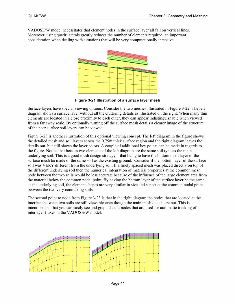
QUAKE/W Chapter 3: Geometry and Meshing
Page 41
VADOSE/W model necessitates that element nodes in the surface layer all fall on vertical lines. Moreover, using quadrilaterals greatly reduces the number of elements required, an important consideration when dealing with situations that will be very computationally intensive.
Figure 3-21 Illustration of a surface layer mesh
Surface layers have special viewing options. Consider the two meshes illustrated in Figure 3-22. The left diagram shows a surface layer without all the cluttering details as illustrated on the right. When many thin elements are located in a close proximity to each other, they can appear indistinguishable when viewed from a far away scale. By optionally turning off the surface mesh details a clearer image of the structure of the near surface soil layers can be viewed.
Figure 3-23 is another illustration of this optional viewing concept. The left diagram in the figure shows the detailed mesh and soil layers across the 0.75m thick surface region and the right diagram leaves the details out, but still shows the layer colors. A couple of additional key points can be made in regards to the figure. Notice that bottom two elements of the left diagram are the same soil type as the main underlying soil. This is a good mesh design strategy – that being to have the bottom most layer of the surface mesh be made of the same soil as the existing ground. Consider if the bottom layer of the surface soil was VERY different from the underlying soil. If a finely spaced mesh was placed directly on top of the different underlying soil then the numerical integration of material properties at the common mesh node between the two soils would be less accurate because of the influence of the large element area from the material below the common nodal point. By having the bottom layer of the surface layer be the same as the underlying soil, the element shapes are very similar in size and aspect at the common nodal point between the two very contrasting soils.
The second point to node from Figure 3-23 is that in the right diagram the nodes that are located at the interface between two soils are still viewable even though the main mesh details are not. This is intentional so that you can easily see and graph data at nodes that are used for automatic tracking of interlayer fluxes in the VADOSE/W model.
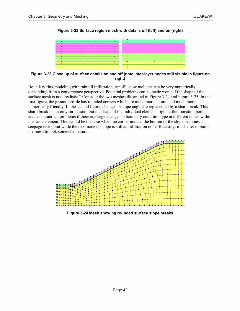
Chapter 3: Geometry and Meshing QUAKE/W
Page 42
Figure 3-22 Surface region mesh with details off (left) and on (right)
Figure 3-23 Close up of surface details on and off (note inter-layer nodes still visible in figure on right)
Boundary flux modeling with rainfall infiltration, runoff, snow melt etc. can be very numerically demanding from a convergence perspective. Potential problems can be made worse if the shape of the surface mesh is not “realistic.” Consider the two meshes illustrated in Figure 3-24 and Figure 3-25. In the first figure, the ground profile has rounded corners which are much more natural and much more numerically friendly. In the second figure, changes in slope angle are represented by a sharp break. This sharp break is not only un-natural, but the shape of the individual elements right at the transition points creates numerical problems if there are large changes in boundary condition type at different nodes within the same element. This would be the case when the corner node at the bottom of the slope becomes a seepage face point while the next node up slope is still an infiltration node. Basically, it is better to build the mesh to look somewhat natural.
Figure 3-24 Mesh showing rounded surface slope breaks
g
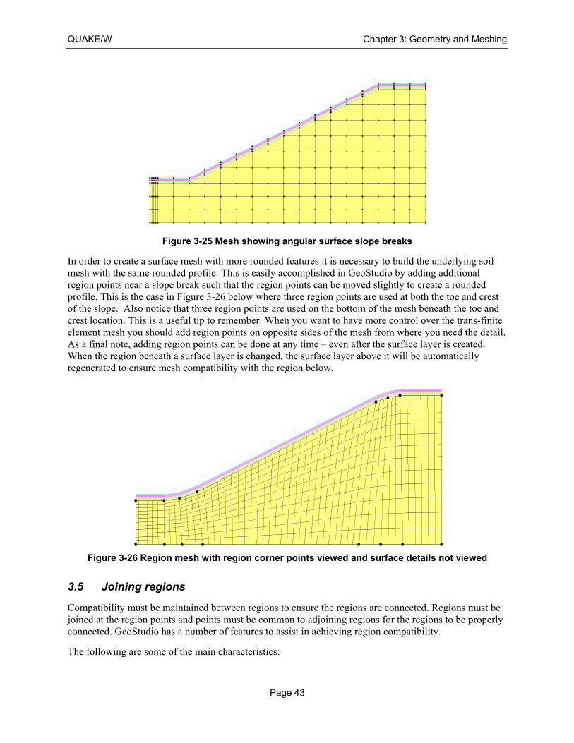
QUAKE/W Chapter 3: Geometry and Meshing
Page 43
Figure 3-25 Mesh showing angular surface slope breaks
In order to create a surface mesh with more rounded features it is necessary to build the underlying soil mesh with the same rounded profile. This is easily accomplished in GeoStudio by adding additional region points near a slope break such that the region points can be moved slightly to create a rounded profile. This is the case in Figure 3-26 below where three region points are used at both the toe and crest of the slope. Also notice that three region points are used on the bottom of the mesh beneath the toe and crest location. This is a useful tip to remember. When you want to have more control over the trans-finite element mesh you should add region points on opposite sides of the mesh from where you need the detail. As a final note, adding region points can be done at any time – even after the surface layer is created. When the region beneath a surface layer is changed, the surface layer above it will be automatically regenerated to ensure mesh compatibility with the region below.
Figure 3-26 Region mesh with region corner points viewed and surface details not viewed
3.5 Joining regions
Compatibility must be maintained between regions to ensure the regions are connected. Regions must be joined at the region points and points must be common to adjoining regions for the regions to be properly connected. GeoStudio has a number of features to assist in achieving region compatibility.
The following are some of the main characteristics:
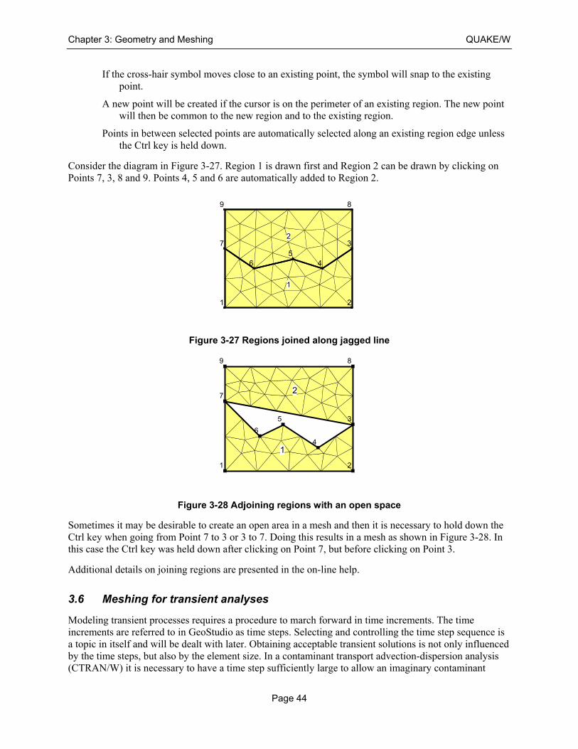
Chapter 3: Geometry and Meshing QUAKE/W
Page 44
If the cross-hair symbol moves close to an existing point, the symbol will snap to the existing point.
A new point will be created if the cursor is on the perimeter of an existing region. The new point will then be common to the new region and to the existing region.
Points in between selected points are automatically selected along an existing region edge unless the Ctrl key is held down.
Consider the diagram in Figure 3-27. Region 1 is drawn first and Region 2 can be drawn by clicking on Points 7, 3, 8 and 9. Points 4, 5 and 6 are automatically added to Region 2.
Figure 3-27 Regions joined along jagged line
Figure 3-28 Adjoining regions with an open space
Sometimes it may be desirable to create an open area in a mesh and then it is necessary to hold down the Ctrl key when going from Point 7 to 3 or 3 to 7. Doing this results in a mesh as shown in Figure 3-28. In this case the Ctrl key was held down after clicking on Point 7, but before clicking on Point 3.
Additional details on joining regions are presented in the on-line help.
3.6 Meshing for transient analyses
Modeling transient processes requires a procedure to march forward in time increments. The time increments are referred to in GeoStudio as time steps. Selecting and controlling the time step sequence is a topic in itself and will be dealt with later. Obtaining acceptable transient solutions is not only influenced by the time steps, but also by the element size. In a contaminant transport advection-dispersion analysis (CTRAN/W) it is necessary to have a time step sufficiently large to allow an imaginary contaminant
1
2
1 2
3
45
6
7
89
1
2
1 2
3
4
5
6
7
89
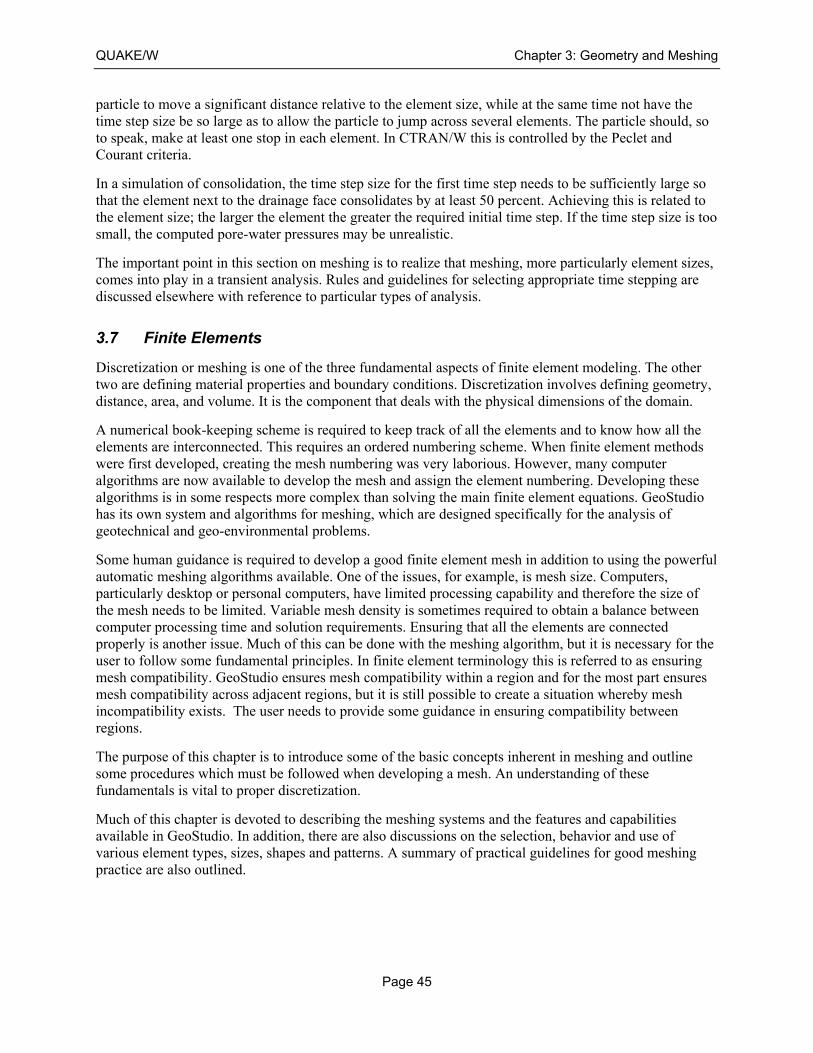
QUAKE/W Chapter 3: Geometry and Meshing
Page 45
particle to move a significant distance relative to the element size, while at the same time not have the time step size be so large as to allow the particle to jump across several elements. The particle should, so to speak, make at least one stop in each element. In CTRAN/W this is controlled by the Peclet and Courant criteria.
In a simulation of consolidation, the time step size for the first time step needs to be sufficiently large so that the element next to the drainage face consolidates by at least 50 percent. Achieving this is related to the element size; the larger the element the greater the required initial time step. If the time step size is too small, the computed pore-water pressures may be unrealistic.
The important point in this section on meshing is to realize that meshing, more particularly element sizes, comes into play in a transient analysis. Rules and guidelines for selecting appropriate time stepping are discussed elsewhere with reference to particular types of analysis.
3.7 Finite Elements
Discretization or meshing is one of the three fundamental aspects of finite element modeling. The other two are defining material properties and boundary conditions. Discretization involves defining geometry, distance, area, and volume. It is the component that deals with the physical dimensions of the domain.
A numerical book-keeping scheme is required to keep track of all the elements and to know how all the elements are interconnected. This requires an ordered numbering scheme. When finite element methods were first developed, creating the mesh numbering was very laborious. However, many computer algorithms are now available to develop the mesh and assign the element numbering. Developing these algorithms is in some respects more complex than solving the main finite element equations. GeoStudio has its own system and algorithms for meshing, which are designed specifically for the analysis of geotechnical and geo-environmental problems.
Some human guidance is required to develop a good finite element mesh in addition to using the powerful automatic meshing algorithms available. One of the issues, for example, is mesh size. Computers, particularly desktop or personal computers, have limited processing capability and therefore the size of the mesh needs to be limited. Variable mesh density is sometimes required to obtain a balance between computer processing time and solution requirements. Ensuring that all the elements are connected properly is another issue. Much of this can be done with the meshing algorithm, but it is necessary for the user to follow some fundamental principles. In finite element terminology this is referred to as ensuring mesh compatibility. GeoStudio ensures mesh compatibility within a region and for the most part ensures mesh compatibility across adjacent regions, but it is still possible to create a situation whereby mesh incompatibility exists. The user needs to provide some guidance in ensuring compatibility between regions.
The purpose of this chapter is to introduce some of the basic concepts inherent in meshing and outline some procedures which must be followed when developing a mesh. An understanding of these fundamentals is vital to proper discretization.
Much of this chapter is devoted to describing the meshing systems and the features and capabilities available in GeoStudio. In addition, there are also discussions on the selection, behavior and use of various element types, sizes, shapes and patterns. A summary of practical guidelines for good meshing practice are also outlined.

Chapter 3: Geometry and Meshing QUAKE/W
Page 46
3.8 Element fundamentals
Element nodes
One of the main features of a finite element are the nodes. Nodes exist at the corners of the elements or along the edges of the elements. Figure 3-29 and Figure 3-30 show the nodes, represented as black dots.
The nodes are required and used for the following purposes:
The positions of the nodes in a coordinate system are used to compute the geometric characteristics of the element – such as length, area or volume.
The nodes are used to describe the distribution of the primary unknowns within the element. In the SEEP/W formulation, the primary field variable is the hydraulic head or pore-water pressure.
The nodes are used to connect or join all the elements within a domain. All elements with a common node are connected at that node. It is the common nodes between elements that ensure compatibility, which is discussed in further detail below.
All finite element equations are formed at the nodes. All elements common to a single node contribute to the characteristics and coefficients that exist in the equation at that node, but it is the equation at the node that is used to compute the primary unknown at that node. In other words, the seepage equation is developed for each node and the material properties which are used within the equations are contributed from the surrounding elements.
There can be multiple finite element equations developed at each node depending on the degrees of freedom. In seepage analysis there is only one degree of freedom at each node, which is the head or pore-water pressure. The number of finite element equations to be solved is equal to the number of nodes used to define the mesh. In a 2D stress-deformation analysis, there are two degrees of freedom at each node – displacement x and displacement y. Consequently, the number of equations for the whole domain is equal to two times the number of nodes. In a coupled consolidation analysis there are three degrees of freedom at each node – displacement x, displacement y and pore-water pressure. For a coupled consolidation analysis the total number of equations required to solve the problem is three times the number of nodes.
Since the number of finite element equations is related to the number of nodes, the number of nodes in a problem is one of the main factors in the computing time required to solve for the primary unknowns.
Field variable distribution
In a finite element formulation it is necessary to adopt a model describing the distribution of the primary variable within the element (e.g., total head). The distribution could be linear or curved.
For a linear distribution of the primary unknown, nodes are required only at the element corners. The two nodes (points) along an edge are sufficient to form a linear equation. Figure 3-29 illustrates this situation. Elements with nodes existing at the corners are referred to as first-order elements.
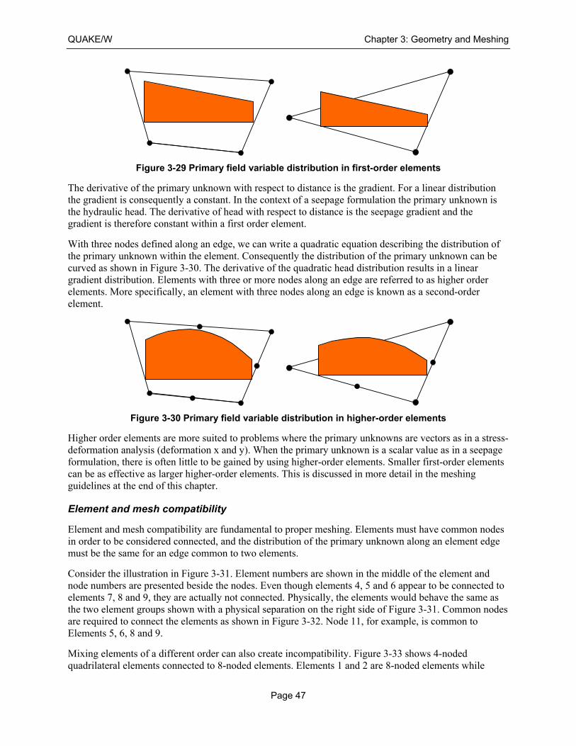
QUAKE/W Chapter 3: Geometry and Meshing
Page 47
Figure 3-29 Primary field variable distribution in first-order elements
The derivative of the primary unknown with respect to distance is the gradient. For a linear distribution the gradient is consequently a constant. In the context of a seepage formulation the primary unknown is the hydraulic head. The derivative of head with respect to distance is the seepage gradient and the gradient is therefore constant within a first order element.
With three nodes defined along an edge, we can write a quadratic equation describing the distribution of the primary unknown within the element. Consequently the distribution of the primary unknown can be curved as shown in Figure 3-30. The derivative of the quadratic head distribution results in a linear gradient distribution. Elements with three or more nodes along an edge are referred to as higher order elements. More specifically, an element with three nodes along an edge is known as a second-order element.
Figure 3-30 Primary field variable distribution in higher-order elements
Higher order elements are more suited to problems where the primary unknowns are vectors as in a stress-deformation analysis (deformation x and y). When the primary unknown is a scalar value as in a seepage formulation, there is often little to be gained by using higher-order elements. Smaller first-order elements can be as effective as larger higher-order elements. This is discussed in more detail in the meshing guidelines at the end of this chapter.
Element and mesh compatibility
Element and mesh compatibility are fundamental to proper meshing. Elements must have common nodes in order to be considered connected, and the distribution of the primary unknown along an element edge must be the same for an edge common to two elements.
Consider the illustration in Figure 3-31. Element numbers are shown in the middle of the element and node numbers are presented beside the nodes. Even though elements 4, 5 and 6 appear to be connected to elements 7, 8 and 9, they are actually not connected. Physically, the elements would behave the same as the two element groups shown with a physical separation on the right side of Figure 3-31. Common nodes are required to connect the elements as shown in Figure 3-32. Node 11, for example, is common to Elements 5, 6, 8 and 9.
Mixing elements of a different order can also create incompatibility. Figure 3-33 shows 4-noded quadrilateral elements connected to 8-noded elements. Elements 1 and 2 are 8-noded elements while
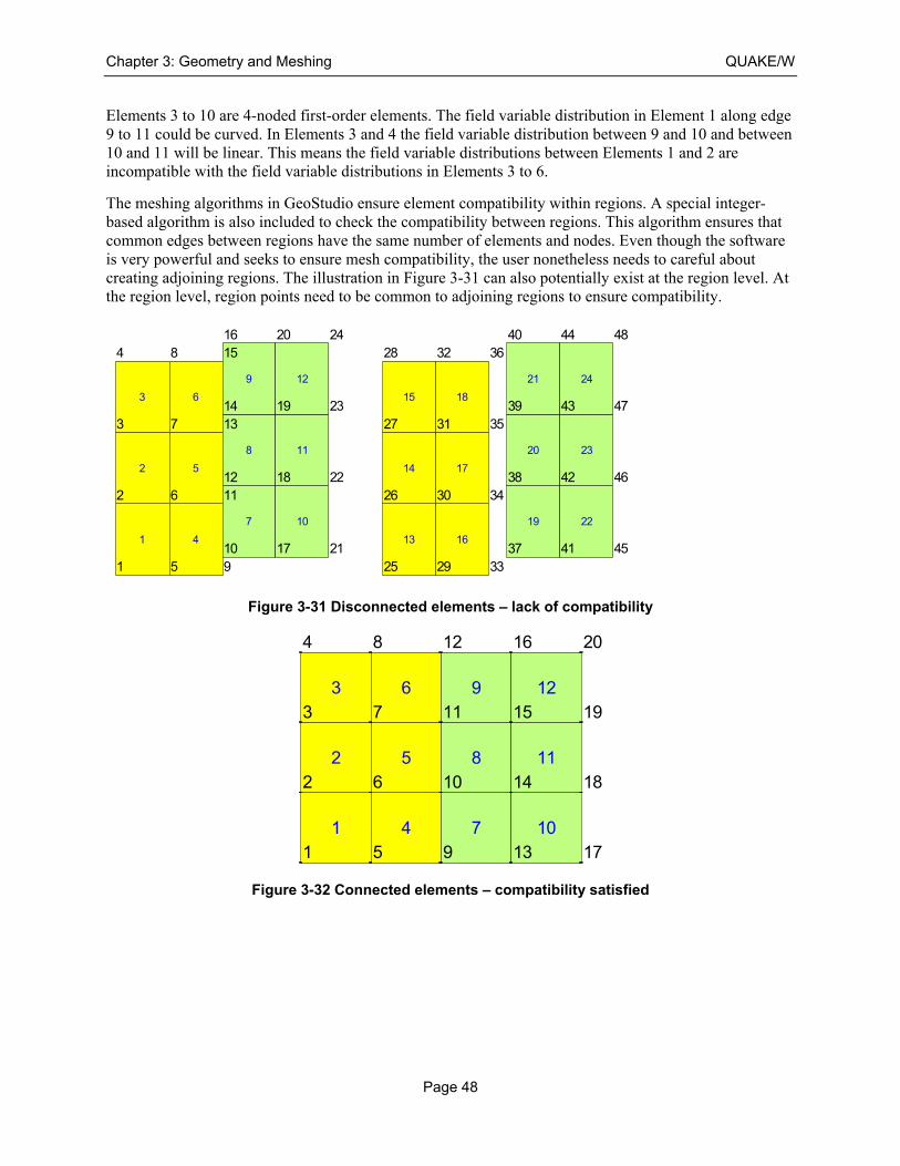
Chapter 3: Geometry and Meshing QUAKE/W
Page 48
Elements 3 to 10 are 4-noded first-order elements. The field variable distribution in Element 1 along edge 9 to 11 could be curved. In Elements 3 and 4 the field variable distribution between 9 and 10 and between 10 and 11 will be linear. This means the field variable distributions between Elements 1 and 2 are incompatible with the field variable distributions in Elements 3 to 6.
The meshing algorithms in GeoStudio ensure element compatibility within regions. A special integer-based algorithm is also included to check the compatibility between regions. This algorithm ensures that common edges between regions have the same number of elements and nodes. Even though the software is very powerful and seeks to ensure mesh compatibility, the user nonetheless needs to careful about creating adjoining regions. The illustration in Figure 3-31 can also potentially exist at the region level. At the region level, region points need to be common to adjoining regions to ensure compatibility.
Figure 3-31 Disconnected elements – lack of compatibility
Figure 3-32 Connected elements – compatibility satisfied
1
2
3
4
5
6
7
8
9
10
11
12
13
14
15
16
17
18
19
20
21
22
23
24
1
2
3
4
5
6
7
8
910
1112
1314
1516
17
18
19
20
21
22
23
24
25
26
27
28
29
30
31
32
33
34
35
36
37
38
39
40
41
42
43
44
45
46
47
48
1
2
3
4
5
6
7
8
9
10
11
12
1
2
3
4
5
6
7
8
9
10
11
12
13
14
15
16
17
18
19
20
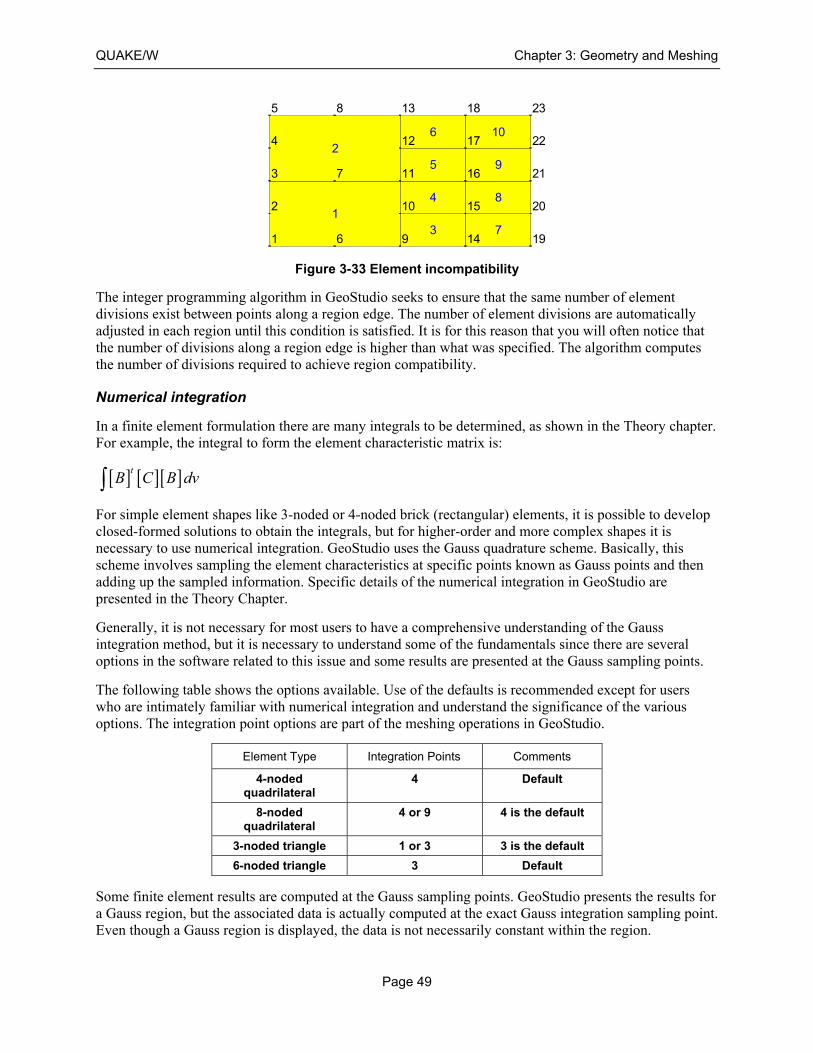
QUAKE/W Chapter 3: Geometry and Meshing
Page 49
Figure 3-33 Element incompatibility
The integer programming algorithm in GeoStudio seeks to ensure that the same number of element divisions exist between points along a region edge. The number of element divisions are automatically adjusted in each region until this condition is satisfied. It is for this reason that you will often notice that the number of divisions along a region edge is higher than what was specified. The algorithm computes the number of divisions required to achieve region compatibility.
Numerical integration
In a finite element formulation there are many integrals to be determined, as shown in the Theory chapter. For example, the integral to form the element characteristic matrix is:
For simple element shapes like 3-noded or 4-noded brick (rectangular) elements, it is possible to develop closed-formed solutions to obtain the integrals, but for higher-order and more complex shapes it is necessary to use numerical integration. GeoStudio uses the Gauss quadrature scheme. Basically, this scheme involves sampling the element characteristics at specific points known as Gauss points and then adding up the sampled information. Specific details of the numerical integration in GeoStudio are presented in the Theory Chapter.
Generally, it is not necessary for most users to have a comprehensive understanding of the Gauss integration method, but it is necessary to understand some of the fundamentals since there are several options in the software related to this issue and some results are presented at the Gauss sampling points.
The following table shows the options available. Use of the defaults is recommended except for users who are intimately familiar with numerical integration and understand the significance of the various options. The integration point options are part of the meshing operations in GeoStudio.
Element Type Integration Points Comments
4-noded quadrilateral
4 Default
8-noded quadrilateral
4 or 9 4 is the default
3-noded triangle 1 or 3 3 is the default
6-noded triangle 3 Default
Some finite element results are computed at the Gauss sampling points. GeoStudio presents the results for a Gauss region, but the associated data is actually computed at the exact Gauss integration sampling point. Even though a Gauss region is displayed, the data is not necessarily constant within the region.
1
2
3
4
5
6
7
8
9
10
1
2
3
4
5
6
7
8
9
10
11
12
13
14
15
16
17
18
19
20
21
22
23
[ ] [ ][ ]tB C B dv
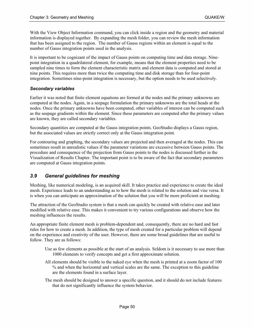
Chapter 3: Geometry and Meshing QUAKE/W
Page 50
With the View Object Information command, you can click inside a region and the geometry and material information is displayed together. By expanding the mesh folder, you can review the mesh information that has been assigned to the region. The number of Gauss regions within an element is equal to the number of Gauss integration points used in the analysis.
It is important to be cognizant of the impact of Gauss points on computing time and data storage. Nine-point integration in a quadrilateral element, for example, means that the element properties need to be sampled nine times to form the element characteristic matrix and element data is computed and stored at nine points. This requires more than twice the computing time and disk storage than for four-point integration. Sometimes nine-point integration is necessary, but the option needs to be used selectively.
Secondary variables
Earlier it was noted that finite element equations are formed at the nodes and the primary unknowns are computed at the nodes. Again, in a seepage formulation the primary unknowns are the total heads at the nodes. Once the primary unknowns have been computed, other variables of interest can be computed such as the seepage gradients within the element. Since these parameters are computed after the primary values are known, they are called secondary variables.
Secondary quantities are computed at the Gauss integration points. GeoStudio displays a Gauss region, but the associated values are strictly correct only at the Gauss integration point.
For contouring and graphing, the secondary values are projected and then averaged at the nodes. This can sometimes result in unrealistic values if the parameter variations are excessive between Gauss points. The procedure and consequence of the projection from Gauss points to the nodes is discussed further in the Visualization of Results Chapter. The important point is to be aware of the fact that secondary parameters are computed at Gauss integration points.
3.9 General guidelines for meshing
Meshing, like numerical modeling, is an acquired skill. It takes practice and experience to create the ideal mesh. Experience leads to an understanding as to how the mesh is related to the solution and vise versa. It is when you can anticipate an approximation of the solution that you will be more proficient at meshing.
The attraction of the GeoStudio system is that a mesh can quickly be created with relative ease and later modified with relative ease. This makes it convenient to try various configurations and observe how the meshing influences the results.
An appropriate finite element mesh is problem-dependent and, consequently, there are no hard and fast rules for how to create a mesh. In addition, the type of mesh created for a particular problem will depend on the experience and creativity of the user. However, there are some broad guidelines that are useful to follow. They are as follows:
Use as few elements as possible at the start of an analysis. Seldom is it necessary to use more than 1000 elements to verify concepts and get a first approximate solution.
All elements should be visible to the naked eye when the mesh is printed at a zoom factor of 100 % and when the horizontal and vertical scales are the same. The exception to this guideline are the elements found in a surface layer.
The mesh should be designed to answer a specific question, and it should do not include features that do not significantly influence the system behavior.

QUAKE/W Chapter 3: Geometry and Meshing
Page 51
The mesh should represent a simplified abstraction of the actual complex geometric field configuration.
Number of elements
Based on many years of responding to GEO-SLOPE user support questions, most users start with a mesh that is too complex, containing too many elements for the objective of the analysis. The thinking when users first start doing finite element analyses seems to be the more elements, the better; that a large number of elements will somehow improve the accuracy of the solution. This is not necessarily true. If the mesh is too large, the time required to obtain a solution can become unattainable. Sometimes it also becomes very difficult to interpret the results, particularly if the solutions appear to be unreasonable. The effort required to determine the reason for an unreasonable solution increases dramatically with mesh size.
We highly recommend that you try and create a mesh with less than 1000 elements, particularly at the start of an analysis. Our experience is that most geotechnical problems can be modeled with 1000 elements or less. Obviously there are exceptions, but this number is a good goal to strive for. Later, once you have a good first understanding of the critical mechanisms in your problem, you can increase the mesh density to refine the analysis.
Effect of drawing scale
Another good guideline is that all elements should be visible to the naked eye when the mesh is printed or viewed at a 100% zoom factor. Groups of elements that appear as a solid or nearly solid black smudge on the drawing are too small. This means a suitable element size is related to the drawing scale. A drawing at a scale of 1:100 can have much smaller elements than a drawing at a scale of 1:2000. In other words, if it is necessary to zoom in on an area of the drawing to distinguish the elements, the elements may be unnecessarily small.
All elements should be readily distinguishable when a drawing is viewed when the vertical scale is equal to the horizontal scale. It is possible to draw a nice looking mesh at a vertical exaggerated scale, but when viewed at a true vertical scale the mesh appears as a wide black line. This effect is illustrated in Figure 3-34. The top part of the figure shows a nice mesh at 10V:100H, a 10 times vertical exaggeration. The same mesh at a scale of 100V:100H appears at the bottom of Figure 3-34. At an exaggerated scale the elements appear suitable, but at a true scale they are not appropriate.
It is important to remember that the main processor which solves the finite element equations sees the elements only at the true scale. The vertical exaggeration is used only in DEFINE and CONTOUR for presentation purposes.
A good rule to follow is to always view the mesh at a true scale before solving the problem to check that the mesh is reasonable for the purpose of the analysis.
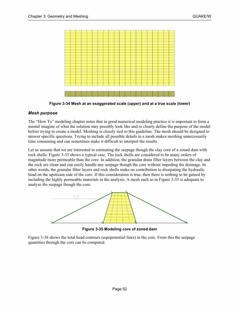
Chapter 3: Geometry and Meshing QUAKE/W
Page 52
Figure 3-34 Mesh at an exaggerated scale (upper) and at a true scale (lower)
Mesh purpose
The “How To” modeling chapter notes that in good numerical modeling practice it is important to form a mental imagine of what the solution may possibly look like and to clearly define the purpose of the model before trying to create a model. Meshing is closely tied to this guideline. The mesh should be designed to answer specific questions. Trying to include all possible details in a mesh makes meshing unnecessarily time consuming and can sometimes make it difficult to interpret the results.
Let us assume that we are interested in estimating the seepage though the clay core of a zoned dam with rock shells. Figure 3-35 shows a typical case. The rock shells are considered to be many orders of magnitude more permeable than the core. In addition, the granular drain filter layers between the clay and the rock are clean and can easily handle any seepage though the core without impeding the drainage. In other words, the granular filter layers and rock shells make no contribution to dissipating the hydraulic head on the upstream side of the core. If this consideration is true, then there is nothing to be gained by including the highly permeable materials in the analysis. A mesh such as in Figure 3-35 is adequate to analyze the seepage though the core.
Figure 3-35 Modeling core of zoned dam
Figure 3-36 shows the total head contours (equipotential lines) in the core. From this the seepage quantities through the core can be computed.
1
2 3
4
5 6
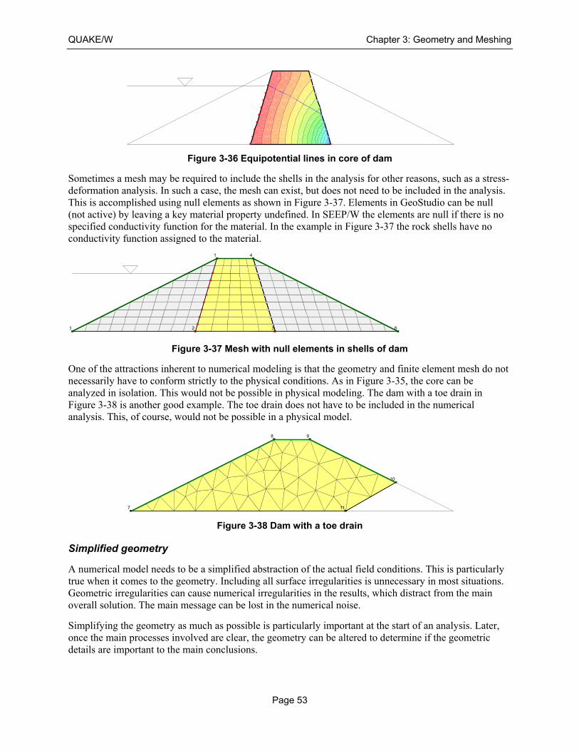
QUAKE/W Chapter 3: Geometry and Meshing
Page 53
Figure 3-36 Equipotential lines in core of dam
Sometimes a mesh may be required to include the shells in the analysis for other reasons, such as a stress-deformation analysis. In such a case, the mesh can exist, but does not need to be included in the analysis. This is accomplished using null elements as shown in Figure 3-37. Elements in GeoStudio can be null (not active) by leaving a key material property undefined. In SEEP/W the elements are null if there is no specified conductivity function for the material. In the example in Figure 3-37 the rock shells have no conductivity function assigned to the material.
Figure 3-37 Mesh with null elements in shells of dam
One of the attractions inherent to numerical modeling is that the geometry and finite element mesh do not necessarily have to conform strictly to the physical conditions. As in Figure 3-35, the core can be analyzed in isolation. This would not be possible in physical modeling. The dam with a toe drain in Figure 3-38 is another good example. The toe drain does not have to be included in the numerical analysis. This, of course, would not be possible in a physical model.
Figure 3-38 Dam with a toe drain
Simplified geometry
A numerical model needs to be a simplified abstraction of the actual field conditions. This is particularly true when it comes to the geometry. Including all surface irregularities is unnecessary in most situations. Geometric irregularities can cause numerical irregularities in the results, which distract from the main overall solution. The main message can be lost in the numerical noise.
Simplifying the geometry as much as possible is particularly important at the start of an analysis. Later, once the main processes involved are clear, the geometry can be altered to determine if the geometric details are important to the main conclusions.
1
2 3
4
5 6
7
8 9
10
11

Chapter 3: Geometry and Meshing QUAKE/W
Page 54
The situation is different if the main objective of the analysis is to study the effects of surface irregularities. Then the irregularities of course need to be included. So, once again, the degree of geometric complexity depends on the objectives of the analysis.
Also, the level of geometric detail that needs to be included in the problem must be evaluated in light of the certainty with which other factors such as the boundary conditions and material properties are known. There is little to be gained by defining a very detailed geometry if the material properties are just a rough estimate. A simplified geometry is more than adequate if the material properties are rough estimates. There needs to be a balance in complexity between all the aspects of a finite element analysis, including the geometry.
Over-complicating the geometry is a tendency when users first get into numerical modeling. Then as modelers gain more experience they tend to use more simple geometries. This obviously comes from understanding how the mesh can influence the results and what level of complexity is required. The situation should be the reverse. It is the modelers with limited experience who should use simplified geometries.
The main message to remember when starting to model is to keep the problem as simple as possible until the main engineering issues are well understood.
QUAKE/W Chapter 4: Material Properties
Page 55
4 Material Properties
4.1 Introduction
This chapter discusses the properties that can be used in QUAKE/W to describe the soil. Generally, there are two groups of properties; one is related to the soil stiffness and the other group is related to the generation of excess pore-pressures.
The most common soil property in a dynamic analysis is the shear modulus G. There are a couple of ways in QUAKE/W to specify G and how G is affected by cyclic stresses. Closely related to the soil stiffness is the soil’s ability to dissipate energy associated with seismic waves. This property is called damping.
Many of the properties related to the generation of excess pore-pressures are not constants, but they are functions. Each of the functions is described here together with explanations of how they are used in QUAKE/W.
4.2 Soil behavior models
There are four different material models to choose from when using QUAKE/W. A summary of these models and the required soil properties are given below and a discussion of the individual parameters and functions are provided in the next section.
None (used to removed part of a model in an analysis)
Linear elastic model
Unit weight, Poisson’s ratio, Damping ratio
Pore-water pressure function
Ka and Ks functions
Cyclic number function
Gmax constant or function
Equivalent linear model
Unit weight, Poisson’s ratio, c΄ and Ø΄
Damping ratio constant or function
Ka and Ks functions
Pore-water pressure function
G reduction function
Gmax constant or function
Steady state strength and collapse surface angle (for liquefied zones)
Non-linear model
Unit weight, Poisson’s ratio, C’ and Phi’
Damping ratio and Max damping ratio
MFS pore-water pressure function
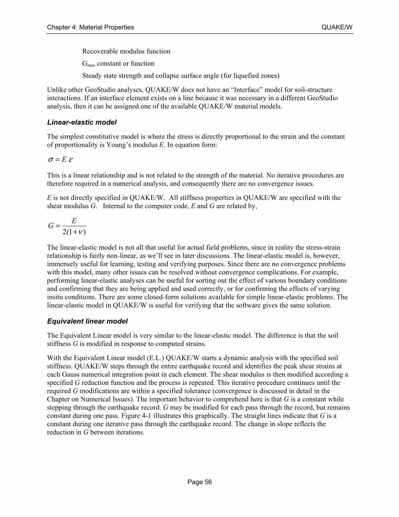
Chapter 4: Material Properties QUAKE/W
Page 56
Recoverable modulus function
Gmax constant or function
Steady state strength and collapse surface angle (for liquefied zones)
Unlike other GeoStudio analyses, QUAKE/W does not have an “Interface” model for soil-structure interactions. If an interface element exists on a line because it was necessary in a different GeoStudio analysis, then it can be assigned one of the available QUAKE/W material models.
Linear-elastic model
The simplest constitutive model is where the stress is directly proportional to the strain and the constant of proportionality is Young’s modulus E. In equation form:
Eσ ε=
This is a linear relationship and is not related to the strength of the material. No iterative procedures are therefore required in a numerical analysis, and consequently there are no convergence issues.
E is not directly specified in QUAKE/W. All stiffness properties in QUAKE/W are specified with the shear modulus G. Internal to the computer code, E and G are related by,
2(1 )
EG
ν=
+
The linear-elastic model is not all that useful for actual field problems, since in reality the stress-strain relationship is fairly non-linear, as we’ll see in later discussions. The linear-elastic model is, however, immensely useful for learning, testing and verifying purposes. Since there are no convergence problems with this model, many other issues can be resolved without convergence complications. For example, performing linear-elastic analyses can be useful for sorting out the effect of various boundary conditions and confirming that they are being applied and used correctly, or for confirming the effects of varying insitu conditions. There are some closed-form solutions available for simple linear-elastic problems. The linear-elastic model in QUAKE/W is useful for verifying that the software gives the same solution.
Equivalent linear model
The Equivalent Linear model is very similar to the linear-elastic model. The difference is that the soil stiffness G is modified in response to computed strains.
With the Equivalent Linear model (E.L.) QUAKE/W starts a dynamic analysis with the specified soil stiffness. QUAKE/W steps through the entire earthquake record and identifies the peak shear strains at each Gauss numerical integration point in each element. The shear modulus is then modified according a specified G reduction function and the process is repeated. This iterative procedure continues until the required G modifications are within a specified tolerance (convergence is discussed in detail in the Chapter on Numerical Issues). The important behavior to comprehend here is that G is a constant while stepping through the earthquake record. G may be modified for each pass through the record, but remains constant during one pass. Figure 4-1 illustrates this graphically. The straight lines indicate that G is a constant during one iterative pass through the earthquake record. The change in slope reflects the reduction in G between iterations.
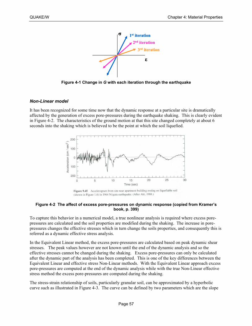
QUAKE/W Chapter 4: Material Properties
Page 57
Figure 4-1 Change in G with each iteration through the earthquake
Non-Linear model
It has been recognized for some time now that the dynamic response at a particular site is dramatically affected by the generation of excess pore-pressures during the earthquake shaking. This is clearly evident in Figure 4-2. The characteristics of the ground motion at that this site changed completely at about 6 seconds into the shaking which is believed to be the point at which the soil liquefied.
Figure 4-2 The affect of excess pore-pressures on dynamic response (copied from Kramer’s book, p. 399)
To capture this behavior in a numerical model, a true nonlinear analysis is required where excess pore-pressures are calculated and the soil properties are modified during the shaking. The increase in pore-pressures changes the effective stresses which in turn change the soils properties, and consequently this is referred as a dynamic effective stress analysis.
In the Equivalent Linear method, the excess pore-pressures are calculated based on peak dynamic shear stresses. The peak values however are not known until the end of the dynamic analysis and so the effective stresses cannot be changed during the shaking. Excess pore-pressures can only be calculated after the dynamic part of the analysis has been completed. This is one of the key differences between the Equivalent Linear and effective stress Non-Linear methods. With the Equivalent Linear approach excess pore-pressures are computed at the end of the dynamic analysis while with the true Non-Linear effective stress method the excess pore-pressures are computed during the shaking.
The stress-strain relationship of soils, particularly granular soil, can be approximated by a hyperbolic curve such as illustrated in Figure 4-3. The curve can be defined by two parameters which are the slope
σ
ε
1st iteration2nd iteration
3rd iteration
σ
ε
1st iteration2nd iteration
3rd iteration
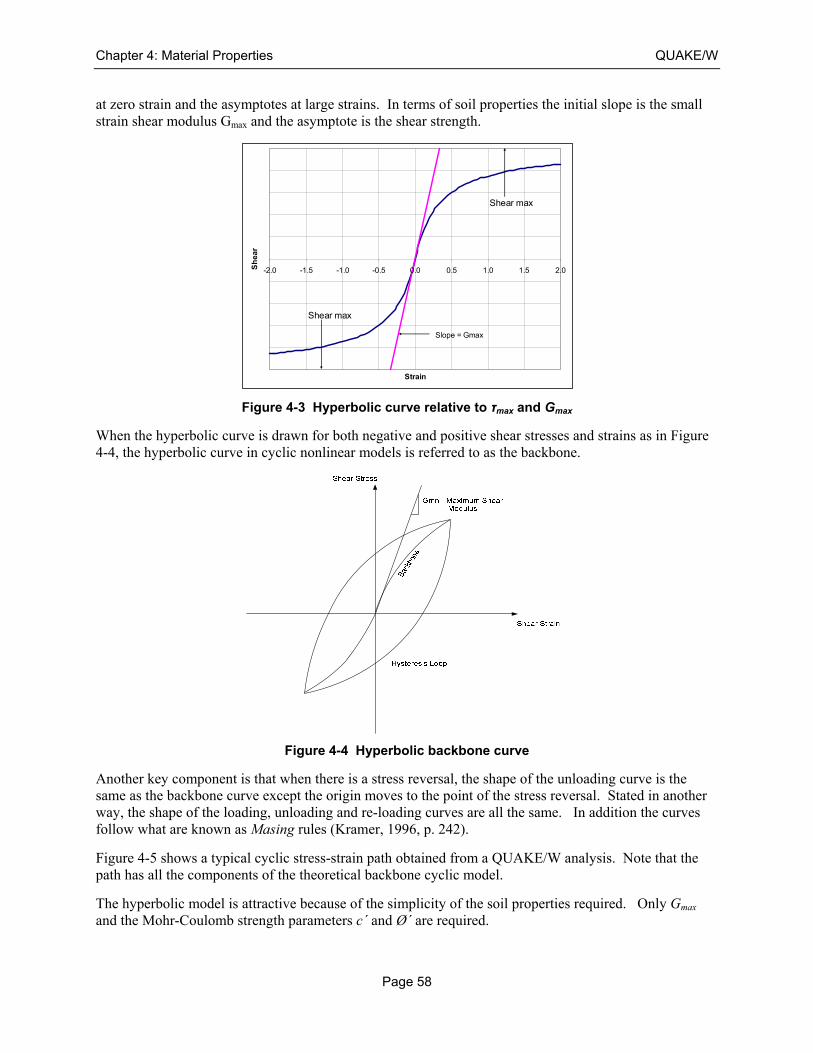
Chapter 4: Material Properties QUAKE/W
Page 58
at zero strain and the asymptotes at large strains. In terms of soil properties the initial slope is the small strain shear modulus Gmax and the asymptote is the shear strength.
Figure 4-3 Hyperbolic curve relative to τmax and Gmax
When the hyperbolic curve is drawn for both negative and positive shear stresses and strains as in Figure 4-4, the hyperbolic curve in cyclic nonlinear models is referred to as the backbone.
Figure 4-4 Hyperbolic backbone curve
Another key component is that when there is a stress reversal, the shape of the unloading curve is the same as the backbone curve except the origin moves to the point of the stress reversal. Stated in another way, the shape of the loading, unloading and re-loading curves are all the same. In addition the curves follow what are known as Masing rules (Kramer, 1996, p. 242).
Figure 4-5 shows a typical cyclic stress-strain path obtained from a QUAKE/W analysis. Note that the path has all the components of the theoretical backbone cyclic model.
The hyperbolic model is attractive because of the simplicity of the soil properties required. Only Gmax and the Mohr-Coulomb strength parameters c΄ and Ø΄ are required.
-2.0 -1.5 -1.0 -0.5 0.0 0.5 1.0 1.5 2.0
Strain
Sh
ea
r
Slope = Gmax
Shear max
Shear max
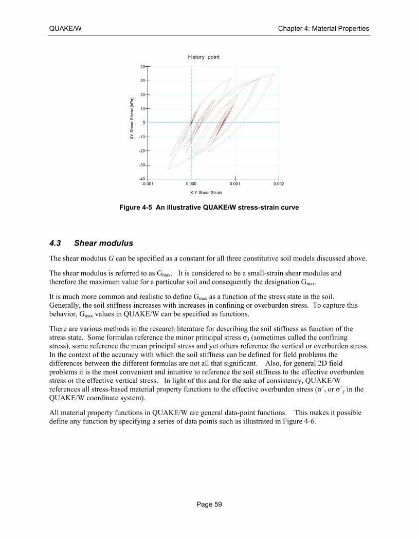
QUAKE/W Chapter 4: Material Properties
Page 59
Figure 4-5 An illustrative QUAKE/W stress-strain curve
4.3 Shear modulus
The shear modulus G can be specified as a constant for all three constitutive soil models discussed above.
The shear modulus is referred to as Gmax. It is considered to be a small-strain shear modulus and therefore the maximum value for a particular soil and consequently the designation Gmax.
It is much more common and realistic to define Gmax as a function of the stress state in the soil. Generally, the soil stiffness increases with increases in confining or overburden stress. To capture this behavior, Gmax values in QUAKE/W can be specified as functions.
There are various methods in the research literature for describing the soil stiffness as function of the stress state. Some formulas reference the minor principal stress σ3 (sometimes called the confining stress), some reference the mean principal stress and yet others reference the vertical or overburden stress. In the context of the accuracy with which the soil stiffness can be defined for field problems the differences between the different formulas are not all that significant. Also, for general 2D field problems it is the most convenient and intuitive to reference the soil stiffness to the effective overburden stress or the effective vertical stress. In light of this and for the sake of consistency, QUAKE/W references all stress-based material property functions to the effective overburden stress (σ΄v or σ΄y in the QUAKE/W coordinate system).
All material property functions in QUAKE/W are general data-point functions. This makes it possible define any function by specifying a series of data points such as illustrated in Figure 4-6.
History point
XY
-Sh
ear
Str
ess
(kP
a)
X-Y Shear Strain
-10
-20
-30
-40
0
10
20
30
40
-0.001 0.000 0.001 0.002
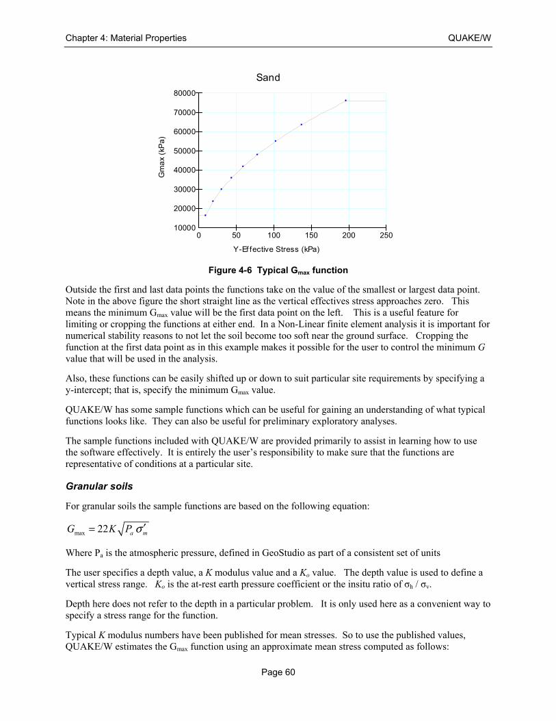
Chapter 4: Material Properties QUAKE/W
Page 60
Figure 4-6 Typical Gmax function
Outside the first and last data points the functions take on the value of the smallest or largest data point. Note in the above figure the short straight line as the vertical effectives stress approaches zero. This means the minimum Gmax value will be the first data point on the left. This is a useful feature for limiting or cropping the functions at either end. In a Non-Linear finite element analysis it is important for numerical stability reasons to not let the soil become too soft near the ground surface. Cropping the function at the first data point as in this example makes it possible for the user to control the minimum G value that will be used in the analysis.
Also, these functions can be easily shifted up or down to suit particular site requirements by specifying a y-intercept; that is, specify the minimum Gmax value.
QUAKE/W has some sample functions which can be useful for gaining an understanding of what typical functions looks like. They can also be useful for preliminary exploratory analyses.
The sample functions included with QUAKE/W are provided primarily to assist in learning how to use the software effectively. It is entirely the user’s responsibility to make sure that the functions are representative of conditions at a particular site.
Granular soils
For granular soils the sample functions are based on the following equation:
max 22 a mG K P σ ′=
Where Pa is the atmospheric pressure, defined in GeoStudio as part of a consistent set of units
The user specifies a depth value, a K modulus value and a Ko value. The depth value is used to define a vertical stress range. Ko is the at-rest earth pressure coefficient or the insitu ratio of σh / σv.
Depth here does not refer to the depth in a particular problem. It is only used here as a convenient way to specify a stress range for the function.
Typical K modulus numbers have been published for mean stresses. So to use the published values, QUAKE/W estimates the Gmax function using an approximate mean stress computed as follows:
Sand
Gm
ax
(kP
a)
Y-Ef fective Stress (kPa)
10000
20000
30000
40000
50000
60000
70000
80000
0 50 100 150 200 250
QUAKE/W Chapter 4: Material Properties
Page 61
3v o v o v
m
K Kσ σ σσ + +=
where σv is the depth times the unit weight of the soil (overburden).
The Gmax formula has been normalized in terms of Pa (atmospheric pressure) so that the same K modulus number can be used in the English and SI system of units. If Pa is in kPa then Gmax is in kPa and if Pa is in psf then Gmax is in psf. The K modulus value consequently is dimensionless.
The above empirical equation for Gmax was originally presented as (Kramer, 1996, p.233):
( )0.5
max 1000 mG K σ ′= . This equation is only directly applicable if the mean stress is in units of lb/ft2.
To make the equation workable with all sets of units and yet have the same K value, we have recast the equation as:
max
max
1000 1000
2116
22
m m
a
a m
G K Pa K PaP psf
G K P
σ σ
σ
′ ′= =
′=
QUAKE/W provides sample K values for:
Loose sand - 30
Medium dense sand - 50
Dense sand - 70
Loose gravel - 80
Medium dense gravel - 130
Dense gravel – 180
These values are based on work by Seed and Idriss (1970) and discussions by Kramer (1996, p. 233).
Once again, these K modulus numbers are provided only as a guide to gain an appreciation for typical values for preliminary exploratory analyses. Any K value can be specified that is deemed to be appropriate for a particular material.
Cohesive soils
Based on the work by Hardin & Drnevich (1972), Hardin (1978) and Mayne & Rix (1993), the Gmax of cohesive soils can be estimated from,
max 2
1625 ( )
(0.3 0.7 )k
a mG OCR Pe
σ ′= +
where e is the void ratio, OCR the over-consolidation ratio and k an exponent related to the soil plasticity index PI.
The k exponent is computed from,
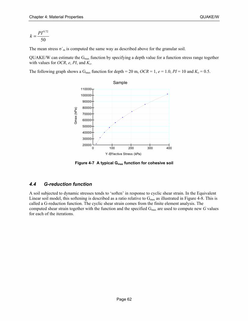
Chapter 4: Material Properties QUAKE/W
Page 62
0.72
50
PIk =
The mean stress σ΄m is computed the same way as described above for the granular soil.
QUAKE/W can estimate the Gmax function by specifying a depth value for a function stress range together with values for OCR, e, PI, and Ko.
The following graph shows a Gmax function for depth = 20 m, OCR = 1, e = 1.0, PI = 10 and Ko = 0.5.
Figure 4-7 A typical Gmax function for cohesive soil
4.4 G-reduction function
A soil subjected to dynamic stresses tends to ‘soften’ in response to cyclic shear strain. In the Equivalent Linear soil model, this softening is described as a ratio relative to Gmax as illustrated in Figure 4-8. This is called a G-reduction function. The cyclic shear strain comes from the finite element analysis. The computed shear strain together with the function and the specified Gmax are used to compute new G values for each of the iterations.
Sample
Gm
ax
(kP
a)
Y-Ef fective Stress (kPa)
20000
30000
40000
50000
60000
70000
80000
90000
100000
110000
0 100 200 300 400
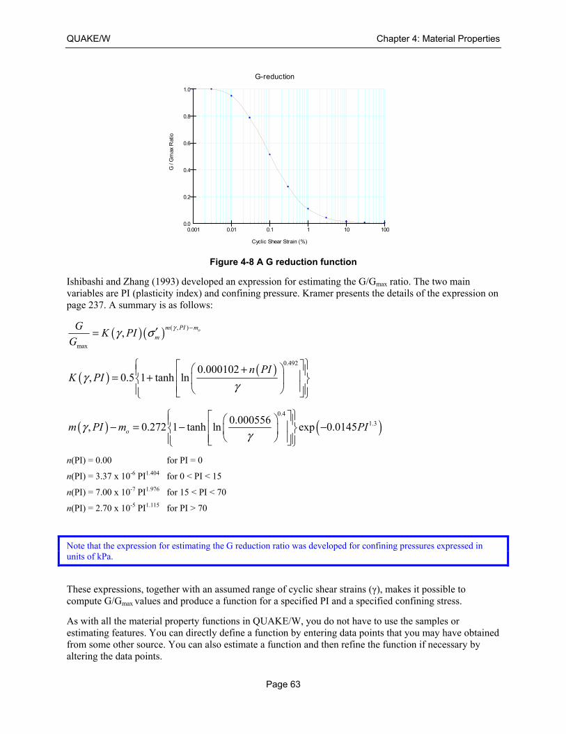
QUAKE/W Chapter 4: Material Properties
Page 63
Figure 4-8 A G reduction function
Ishibashi and Zhang (1993) developed an expression for estimating the G/Gmax ratio. The two main variables are PI (plasticity index) and confining pressure. Kramer presents the details of the expression on page 237. A summary is as follows:
( )( ) ( , )
max
, om PI m
m
GK PI
G
γγ σ −′=
( ) ( ) 0.4920.000102
, 0.5 1 tanh lnn PI
K PIγγ
+ = +
( ) ( )0.4
1.30.000556, 0.272 1 tanh ln exp 0.0145om PI m PIγ
γ
− = − −
n(PI) = 0.00 for PI = 0
n(PI) = 3.37 x 10⁻⁶ PI1.404 for 0 < PI < 15
n(PI) = 7.00 x 10⁻⁷ PI1.976 for 15 < PI < 70
n(PI) = 2.70 x 10⁻⁵ PI1.115 for PI > 70
Note that the expression for estimating the G reduction ratio was developed for confining pressures expressed in units of kPa.
These expressions, together with an assumed range of cyclic shear strains (γ), makes it possible to compute G/Gmax values and produce a function for a specified PI and a specified confining stress.
As with all the material property functions in QUAKE/W, you do not have to use the samples or estimating features. You can directly define a function by entering data points that you may have obtained from some other source. You can also estimate a function and then refine the function if necessary by altering the data points.
G-reduction
G /
Gm
ax R
atio
Cyclic Shear Strain (%)
0.0
0.2
0.4
0.6
0.8
1.0
0.001 1000.01 0.1 1 10
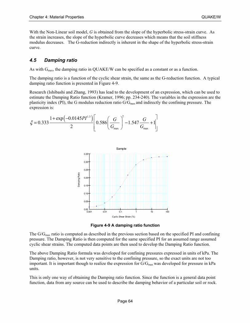
Chapter 4: Material Properties QUAKE/W
Page 64
With the Non-Linear soil model, G is obtained from the slope of the hyperbolic stress-strain curve. As the strain increases, the slope of the hyperbolic curve decreases which means that the soil stiffness modulus decreases. The G-reduction indirectly is inherent in the shape of the hyperbolic stress-strain curve.
4.5 Damping ratio
As with Gmax, the damping ratio in QUAKE/W can be specified as a constant or as a function.
The damping ratio is a function of the cyclic shear strain, the same as the G-reduction function. A typical damping ratio function is presented in Figure 4-9.
Research (Ishibashi and Zhang, 1993) has lead to the development of an expression, which can be used to estimate the Damping Ratio function (Kramer, 1996; pp. 234-240). The variables in the expression are the plasticity index (PI), the G modulus reduction ratio G/Gmax and indirectly the confining pressure. The expression is:
( ) 21.3
max max
1 exp 0.01450.333 0.586 1.547 1
2
PI G G
G Gξ
+ − = − +
Figure 4-9 A damping ratio function
The G/Gmax ratio is computed as described in the previous section based on the specified PI and confining pressure. The Damping Ratio is then computed for the same specified PI for an assumed range assumed cyclic shear strains. The computed data points are then used to develop the Damping Ratio function.
The above Damping Ratio formula was developed for confining pressures expressed in units of kPa. The Damping ratio, however, is not very sensitive to the confining pressure, so the exact units are not too important. It is important though to realize the expression for G/Gmax was developed for pressure in kPa units.
This is only one way of obtaining the Damping ratio function. Since the function is a general data point function, data from any source can be used to describe the damping behavior of a particular soil or rock.
Sample
Dam
ping
Rat
io
Cyclic Shear Strain (%)
0.00
0.05
0.10
0.15
0.20
0.25
0.30
0.35
0.001 1000.01 0.1 1 10
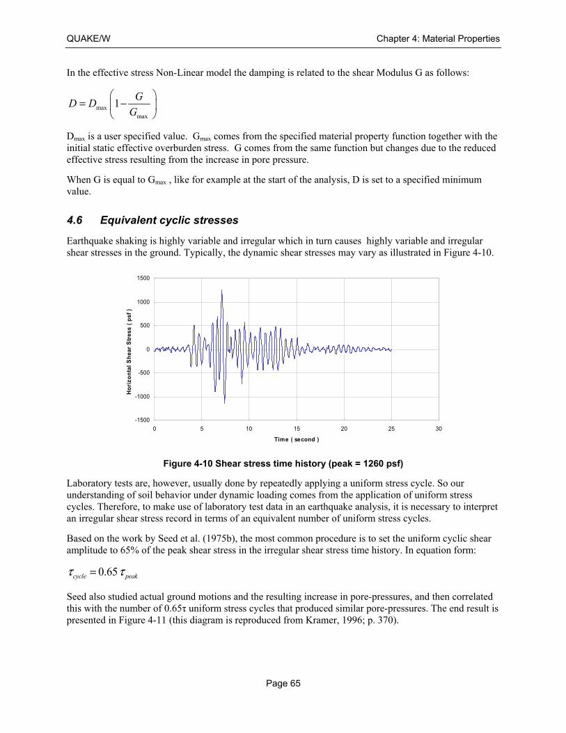
QUAKE/W Chapter 4: Material Properties
Page 65
In the effective stress Non-Linear model the damping is related to the shear Modulus G as follows:
maxmax
1G
D DG
= −
Dmax is a user specified value. Gmax comes from the specified material property function together with the initial static effective overburden stress. G comes from the same function but changes due to the reduced effective stress resulting from the increase in pore pressure.
When G is equal to Gmax , like for example at the start of the analysis, D is set to a specified minimum value.
4.6 Equivalent cyclic stresses
Earthquake shaking is highly variable and irregular which in turn causes highly variable and irregular shear stresses in the ground. Typically, the dynamic shear stresses may vary as illustrated in Figure 4-10.
Figure 4-10 Shear stress time history (peak = 1260 psf)
Laboratory tests are, however, usually done by repeatedly applying a uniform stress cycle. So our understanding of soil behavior under dynamic loading comes from the application of uniform stress cycles. Therefore, to make use of laboratory test data in an earthquake analysis, it is necessary to interpret an irregular shear stress record in terms of an equivalent number of uniform stress cycles.
Based on the work by Seed et al. (1975b), the most common procedure is to set the uniform cyclic shear amplitude to 65% of the peak shear stress in the irregular shear stress time history. In equation form:
0.65cycle peakτ τ=
Seed also studied actual ground motions and the resulting increase in pore-pressures, and then correlated this with the number of 0.65τ uniform stress cycles that produced similar pore-pressures. The end result is presented in Figure 4-11 (this diagram is reproduced from Kramer, 1996; p. 370).
-1500
-1000
-500
0
500
1000
1500
0 5 10 15 20 25 30
Time ( second )
Ho
rizo
nta
l S
hea
r S
tres
s (
psf
)
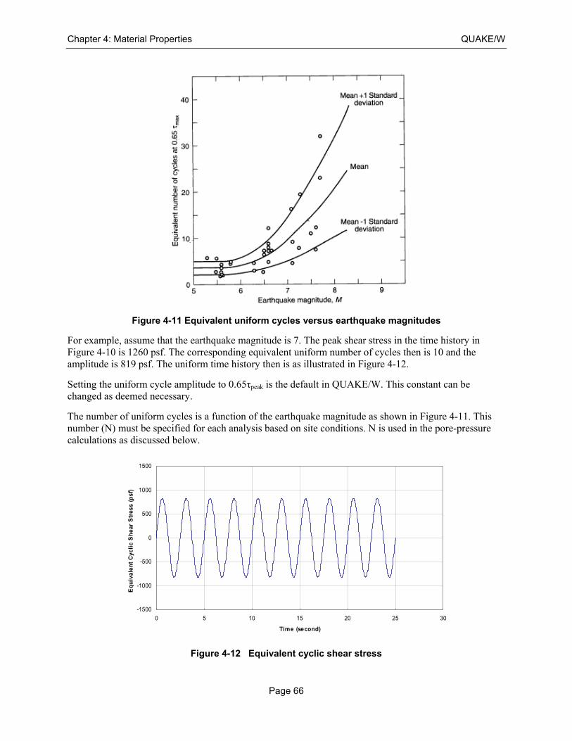
Chapter 4: Material Properties QUAKE/W
Page 66
Figure 4-11 Equivalent uniform cycles versus earthquake magnitudes
For example, assume that the earthquake magnitude is 7. The peak shear stress in the time history in Figure 4-10 is 1260 psf. The corresponding equivalent uniform number of cycles then is 10 and the amplitude is 819 psf. The uniform time history then is as illustrated in Figure 4-12.
Setting the uniform cycle amplitude to 0.65τpeak is the default in QUAKE/W. This constant can be changed as deemed necessary.
The number of uniform cycles is a function of the earthquake magnitude as shown in Figure 4-11. This number (N) must be specified for each analysis based on site conditions. N is used in the pore-pressure calculations as discussed below.
Figure 4-12 Equivalent cyclic shear stress
-1500
-1000
-500
0
500
1000
1500
0 5 10 15 20 25 30
Time (second)
Eq
uiv
alen
t C
ycli
c S
hea
r S
tres
s (p
sf)
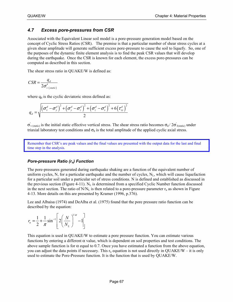
QUAKE/W Chapter 4: Material Properties
Page 67
4.7 Excess pore-pressures from CSR
Associated with the Equivalent Linear soil model is a pore-pressure generation model based on the concept of Cyclic Stress Ratios (CSR). The premise is that a particular number of shear stress cycles at a given shear amplitude will generate sufficient excess pore-pressure to cause the soil to liquefy. So, one of the purposes of the dynamic finite element analysis is to find the peak CSR values that will develop during the earthquake. Once the CSR is known for each element, the excess pore-pressures can be computed as described in this section.
The shear stress ratio in QUAKE/W is defined as:
( )2d
v static
qCSR
σ=
′
where qd is the cyclic deviatoric stress defined as:
( ) ( ) ( ) ( )2 2 2 2
6
2
d d d d d d dx y y z z x xy
dqσ σ σ σ σ σ τ− + − + − +
=
σ'v (static) is the initial static effective vertical stress. The shear stress ratio becomes σd / 2σ'
3(static) under triaxial laboratory test conditions and σd is the total amplitude of the applied cyclic axial stress.
Remember that CSR’s are peak values and the final values are presented with the output data for the last and final time step in the analysis.
Pore-pressure Ratio (ru) Function
The pore-pressures generated during earthquake shaking are a function of the equivalent number of uniform cycles, N, for a particular earthquake and the number of cycles, NL, which will cause liquefaction for a particular soil under a particular set of stress conditions. N is defined and established as discussed in the previous section (Figure 4-11). NL is determined from a specified Cyclic Number function discussed in the next section. The ratio of N/NL is then related to a pore-pressure parameter ru as shown in Figure 4-13. More details on this are presented by Kramer (1996, p.376).
Lee and Albaisa (1974) and DeAlba et al. (1975) found that the pore pressure ratio function can be described by the equation:
1/
11 1sin 2 1
2uL
Nr
N
α
π− = + −
This equation is used in QUAKE/W to estimate a pore pressure function. You can estimate various functions by entering a different α value, which is dependent on soil properties and test conditions. The above sample function is for α equal to 0.7. Once you have estimated a function from the above equation, you can adjust the data points if necessary. This ru equation is not used directly in QUAKE/W – it is only used to estimate the Pore-Pressure function. It is the function that is used by QUAKE/W.
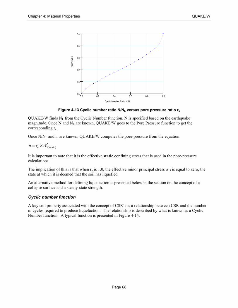
Chapter 4: Material Properties QUAKE/W
Page 68
Figure 4-13 Cyclic number ratio N/NL versus pore pressure ratio ru
QUAKE/W finds NL from the Cyclic Number function. N is specified based on the earthquake magnitude. Once N and NL are known, QUAKE/W goes to the Pore Pressure function to get the corresponding ru.
Once N/NL and ru are known, QUAKE/W computes the pore-pressure from the equation:
3( )u staticu r σ ′= ×
It is important to note that it is the effective static confining stress that is used in the pore-pressure calculations.
The implication of this is that when ru is 1.0, the effective minor principal stress σ΄3 is equal to zero, the state at which it is deemed that the soil has liquefied.
An alternative method for defining liquefaction is presented below in the section on the concept of a collapse surface and a steady-state strength.
Cyclic number function
A key soil property associated with the concept of CSR’s is a relationship between CSR and the number of cycles required to produce liquefaction. The relationship is described by what is known as a Cyclic Number function. A typical function is presented in Figure 4-14.
PW
P R
atio
Cyclic Number Ratio N/NL
0.0
0.2
0.4
0.6
0.8
1.0
0.0 0.2 0.4 0.6 0.8 1.0
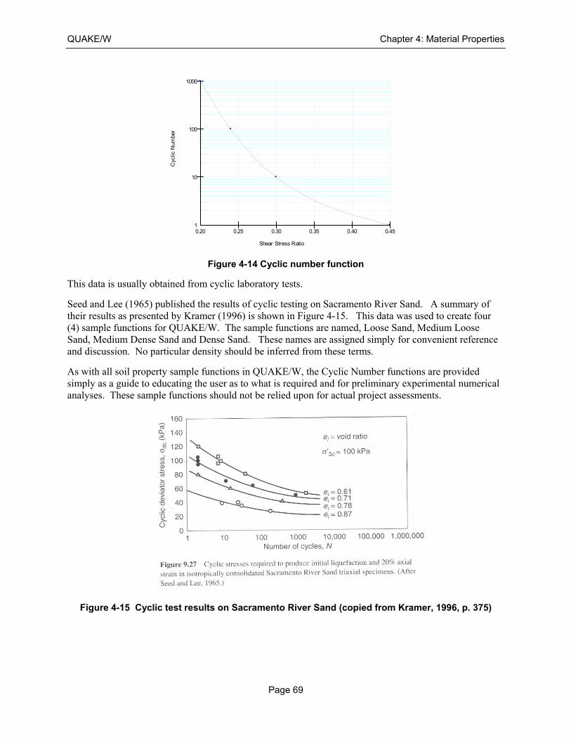
QUAKE/W Chapter 4: Material Properties
Page 69
Figure 4-14 Cyclic number function
This data is usually obtained from cyclic laboratory tests.
Seed and Lee (1965) published the results of cyclic testing on Sacramento River Sand. A summary of their results as presented by Kramer (1996) is shown in Figure 4-15. This data was used to create four (4) sample functions for QUAKE/W. The sample functions are named, Loose Sand, Medium Loose Sand, Medium Dense Sand and Dense Sand. These names are assigned simply for convenient reference and discussion. No particular density should be inferred from these terms.
As with all soil property sample functions in QUAKE/W, the Cyclic Number functions are provided simply as a guide to educating the user as to what is required and for preliminary experimental numerical analyses. These sample functions should not be relied upon for actual project assessments.
Figure 4-15 Cyclic test results on Sacramento River Sand (copied from Kramer, 1996, p. 375)
Cyc
lic N
umbe
r
Shear Stress Ratio
1
1000
10
100
0.20 0.25 0.30 0.35 0.40 0.45
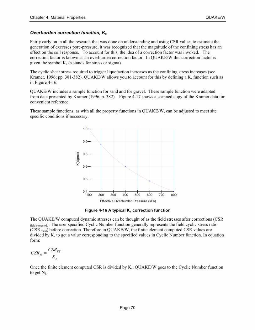
Chapter 4: Material Properties QUAKE/W
Page 70
Overburden correction function, Ks
Fairly early on in all the research that was done on understanding and using CSR values to estimate the generation of excesses pore-pressure, it was recognized that the magnitude of the confining stress has an effect on the soil response. To account for this, the idea of a correction factor was invoked. The correction factor is known as an overburden correction factor. In QUAKE/W this correction factor is given the symbol Ks (s stands for stress or sigma).
The cyclic shear stress required to trigger liquefaction increases as the confining stress increases (see Kramer, 1996; pp. 381-382). QUAKE/W allows you to account for this by defining a Ks function such as in Figure 4-16.
QUAKE/W includes a sample function for sand and for gravel. These sample function were adapted from data presented by Kramer (1996, p. 382). Figure 4-17 shows a scanned copy of the Kramer data for convenient reference.
These sample functions, as with all the property functions in QUAKE/W, can be adjusted to meet site specific conditions if necessary.
Figure 4-16 A typical Ks correction function
The QUAKE/W computed dynamic stresses can be thought of as the field stresses after corrections (CSR field corrected). The user specified Cyclic Number function generally represents the field cyclic stress ratio (CSR field) before correction. Therefore in QUAKE/W, the finite element computed CSR values are divided by Ks to get a value corresponding to the specified values in Cyclic Number function. In equation form:
FEfn
s
CSRCSR
K=
Once the finite element computed CSR is divided by Ks, QUAKE/W goes to the Cyclic Number function to get NL.
K(s
igm
a)
Ef fective Overburden Pressure (kPa)
0.4
0.5
0.6
0.8
0.9
1.0
100 200 300 400 500 600 700 800
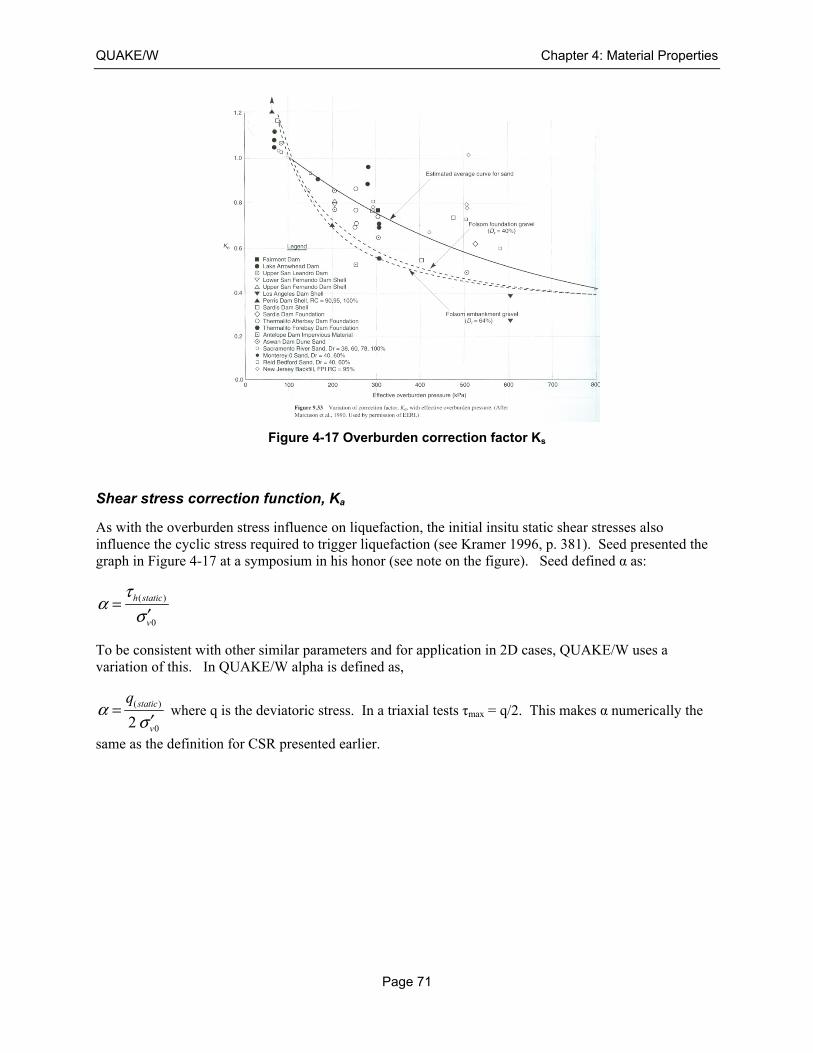
QUAKE/W Chapter 4: Material Properties
Page 71
Figure 4-17 Overburden correction factor Ks
Shear stress correction function, Ka
As with the overburden stress influence on liquefaction, the initial insitu static shear stresses also influence the cyclic stress required to trigger liquefaction (see Kramer 1996, p. 381). Seed presented the graph in Figure 4-17 at a symposium in his honor (see note on the figure). Seed defined α as:
( )
0
h static
v
τα
σ=
′
To be consistent with other similar parameters and for application in 2D cases, QUAKE/W uses a variation of this. In QUAKE/W alpha is defined as,
( )
02static
v
qα
σ=
′ where q is the deviatoric stress. In a triaxial tests τmax = q/2. This makes α numerically the
same as the definition for CSR presented earlier.
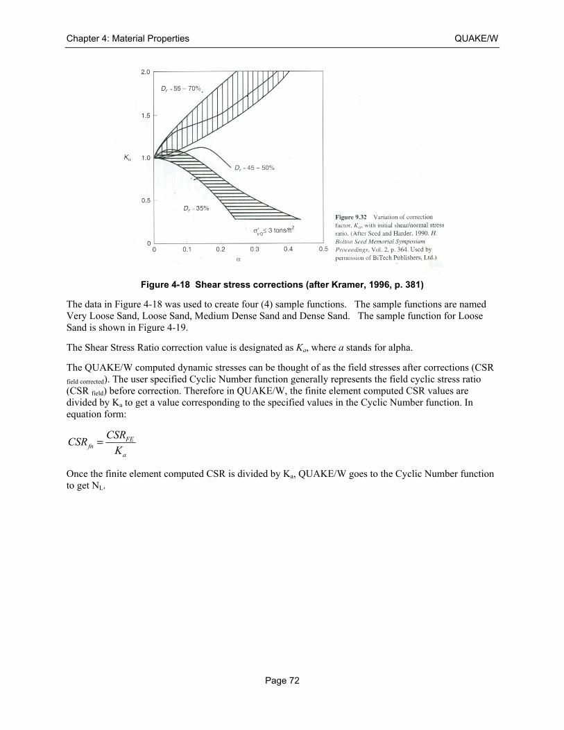
Chapter 4: Material Properties QUAKE/W
Page 72
Figure 4-18 Shear stress corrections (after Kramer, 1996, p. 381)
The data in Figure 4-18 was used to create four (4) sample functions. The sample functions are named Very Loose Sand, Loose Sand, Medium Dense Sand and Dense Sand. The sample function for Loose Sand is shown in Figure 4-19.
The Shear Stress Ratio correction value is designated as Ka, where a stands for alpha.
The QUAKE/W computed dynamic stresses can be thought of as the field stresses after corrections (CSR field corrected). The user specified Cyclic Number function generally represents the field cyclic stress ratio (CSR field) before correction. Therefore in QUAKE/W, the finite element computed CSR values are divided by Ka to get a value corresponding to the specified values in the Cyclic Number function. In equation form:
FEfn
a
CSRCSR
K=
Once the finite element computed CSR is divided by Ka, QUAKE/W goes to the Cyclic Number function to get NL.
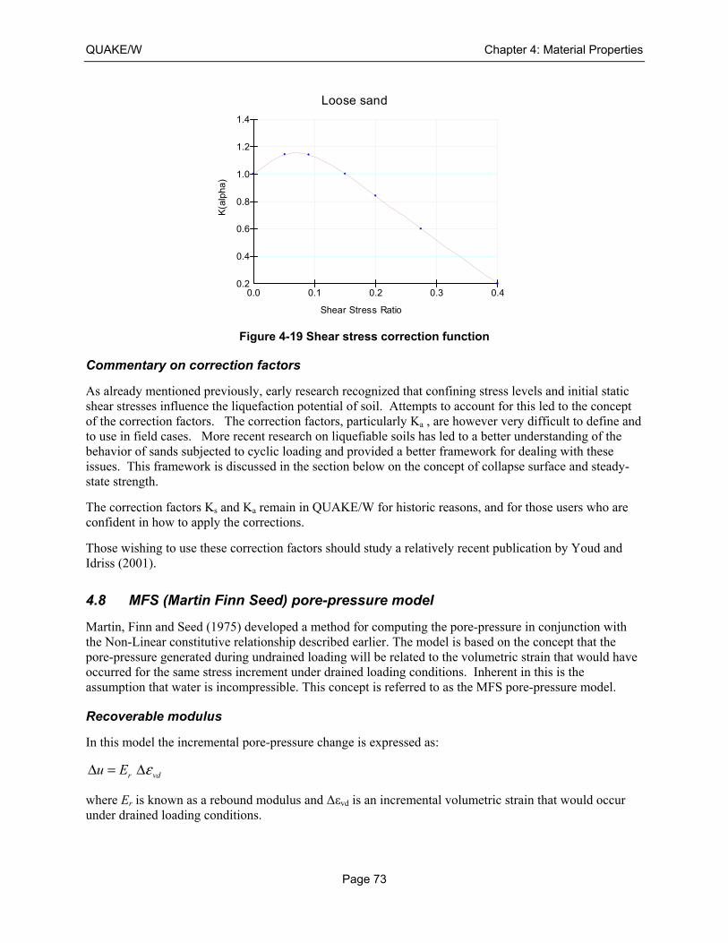
QUAKE/W Chapter 4: Material Properties
Page 73
Figure 4-19 Shear stress correction function
Commentary on correction factors
As already mentioned previously, early research recognized that confining stress levels and initial static shear stresses influence the liquefaction potential of soil. Attempts to account for this led to the concept of the correction factors. The correction factors, particularly Ka , are however very difficult to define and to use in field cases. More recent research on liquefiable soils has led to a better understanding of the behavior of sands subjected to cyclic loading and provided a better framework for dealing with these issues. This framework is discussed in the section below on the concept of collapse surface and steady-state strength.
The correction factors Ks and Ka remain in QUAKE/W for historic reasons, and for those users who are confident in how to apply the corrections.
Those wishing to use these correction factors should study a relatively recent publication by Youd and Idriss (2001).
4.8 MFS (Martin Finn Seed) pore-pressure model
Martin, Finn and Seed (1975) developed a method for computing the pore-pressure in conjunction with the Non-Linear constitutive relationship described earlier. The model is based on the concept that the pore-pressure generated during undrained loading will be related to the volumetric strain that would have occurred for the same stress increment under drained loading conditions. Inherent in this is the assumption that water is incompressible. This concept is referred to as the MFS pore-pressure model.
Recoverable modulus
In this model the incremental pore-pressure change is expressed as:
r vdu E εΔ = Δ
where Er is known as a rebound modulus and Δεvd is an incremental volumetric strain that would occur under drained loading conditions.
Loose sand
K(a
lph
a)
Shear Stress Ratio
0.2
0.4
0.6
0.8
1.0
1.2
1.4
0.0 0.1 0.2 0.3 0.4
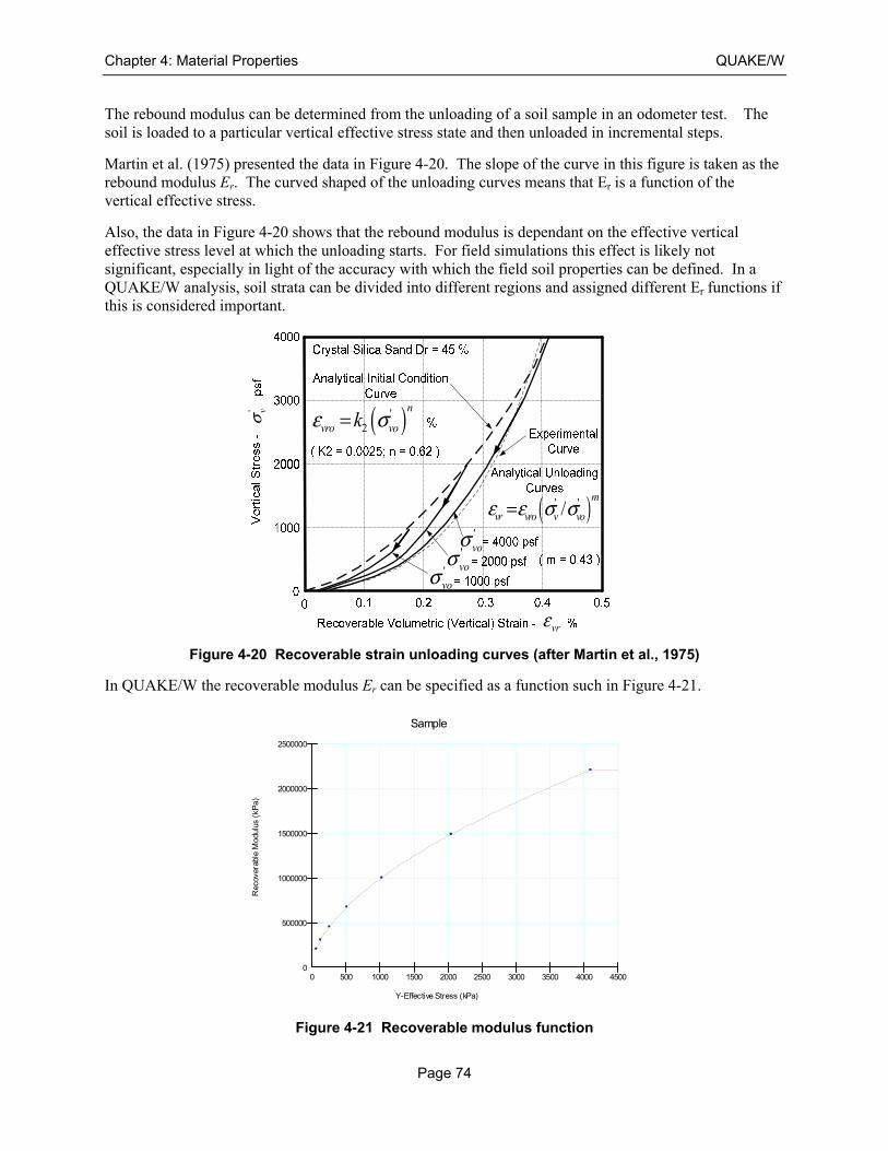
Chapter 4: Material Properties QUAKE/W
Page 74
The rebound modulus can be determined from the unloading of a soil sample in an odometer test. The soil is loaded to a particular vertical effective stress state and then unloaded in incremental steps.
Martin et al. (1975) presented the data in Figure 4-20. The slope of the curve in this figure is taken as the rebound modulus Er. The curved shaped of the unloading curves means that Er is a function of the vertical effective stress.
Also, the data in Figure 4-20 shows that the rebound modulus is dependant on the effective vertical effective stress level at which the unloading starts. For field simulations this effect is likely not significant, especially in light of the accuracy with which the field soil properties can be defined. In a QUAKE/W analysis, soil strata can be divided into different regions and assigned different Er functions if this is considered important.
Figure 4-20 Recoverable strain unloading curves (after Martin et al., 1975)
In QUAKE/W the recoverable modulus Er can be specified as a function such in Figure 4-21.
Figure 4-21 Recoverable modulus function
vrε
' vσ ( )'
2
n
vro vokε σ=
( )' '/m
vr vro v voε ε σ σ=
'voσ
'voσ
'voσ
Sample
Rec
over
able
Mod
ulus
(kP
a)
Y-Effective Stress (kPa)
0
500000
1000000
1500000
2000000
2500000
0 500 1000 1500 2000 2500 3000 3500 4000 4500
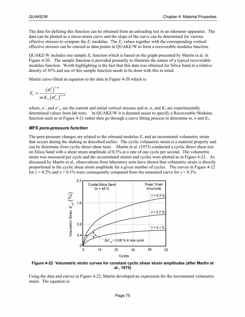
QUAKE/W Chapter 4: Material Properties
Page 75
The data for defining this function can be obtained from an unloading test in an odometer apparatus. The data can be plotted as a stress-strain curve and the slope of the curve can be determined for various effective stresses to compute the Er modulus. The Er values together with the corresponding vertical effective stresses can be entered as data points in QUAKE/W to form a recoverable modulus function.
QUAKE/W includes one sample Er function which is based on the graph presented by Martin et al. in Figure 4-20. The sample function is provided primarily to illustrate the nature of a typical recoverable modulus function. Worth highlighting is the fact that this data was obtained for Silica Sand at a relative density of 45% and use of this sample function needs to be done with this in mind.
Martin curve-fitted an equation to the data in Figure 4-20 which is:
( )( )
1
2
m
vr n m
vo
Em K
σσ
−
−
′=
′
where, σ΄v and σ΄vo are the current and initial vertical stresses and m, n, and K2 are experimentally determined values from lab tests. In QUAKE/W it is deemed easier to specify a Recoverable Modulus function such as in Figure 4-21 rather then go through a curve fitting process to determine m, n and K2.
MFS pore-pressure function
The pore-pressure changes are related to the rebound modulus Er and an incremental volumetric strain that occurs during the shaking as described earlier. The cyclic volumetric strain is a material property and can be determine from cyclic direct shear tests. Martin et al. (1975) conducted a cyclic direct shear test on Silica Sand with a shear strain amplitude of 0.3% at a rate of one cycle per second. The volumetric strain was measured per cycle and the accumulated strains and cycles were plotted as in Figure 4-22. As discussed by Martin et al., observations from laboratory tests have shown that volumetric strain is directly proportional to the cyclic shear strain amplitude for a given number of cycles. The curves in Figure 4-22 for γ = 0.2% and γ = 0.1% were consequently computed from the measured curve for γ = 0.3%.
Figure 4-22 Volumetric strain curves for constant cyclic shear strain amplitudes (after Martin et al., 1975)
Using the data and curves in Figure 4-22, Martin developed an expression for the incremental volumetric strain. The equation is:
()
%vdε
vdεΔ
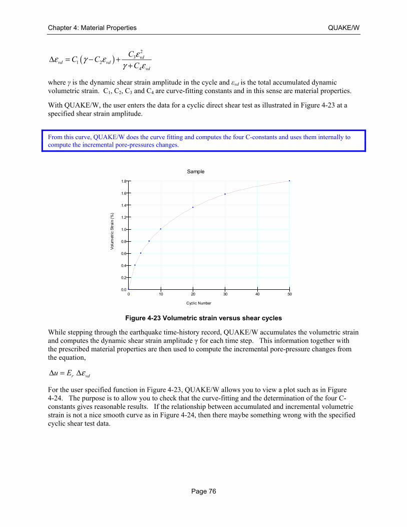
Chapter 4: Material Properties QUAKE/W
Page 76
( )2
31 2
4
vdvd vd
vd
CC C
C
εε γ εγ ε
Δ = − ++
where γ is the dynamic shear strain amplitude in the cycle and εvd is the total accumulated dynamic volumetric strain. C1, C2, C3 and C4 are curve-fitting constants and in this sense are material properties.
With QUAKE/W, the user enters the data for a cyclic direct shear test as illustrated in Figure 4-23 at a specified shear strain amplitude.
From this curve, QUAKE/W does the curve fitting and computes the four C-constants and uses them internally to compute the incremental pore-pressures changes.
Figure 4-23 Volumetric strain versus shear cycles
While stepping through the earthquake time-history record, QUAKE/W accumulates the volumetric strain and computes the dynamic shear strain amplitude γ for each time step. This information together with the prescribed material properties are then used to compute the incremental pore-pressure changes from the equation,
r vdu E εΔ = Δ
For the user specified function in Figure 4-23, QUAKE/W allows you to view a plot such as in Figure 4-24. The purpose is to allow you to check that the curve-fitting and the determination of the four C-constants gives reasonable results. If the relationship between accumulated and incremental volumetric strain is not a nice smooth curve as in Figure 4-24, then there maybe something wrong with the specified cyclic shear test data.
Sample
Vol
umet
ric
Str
ain
(%)
Cyclic Number
0.0
0.2
0.4
0.6
0.8
1.0
1.2
1.4
1.6
1.8
0 10 20 30 40 50
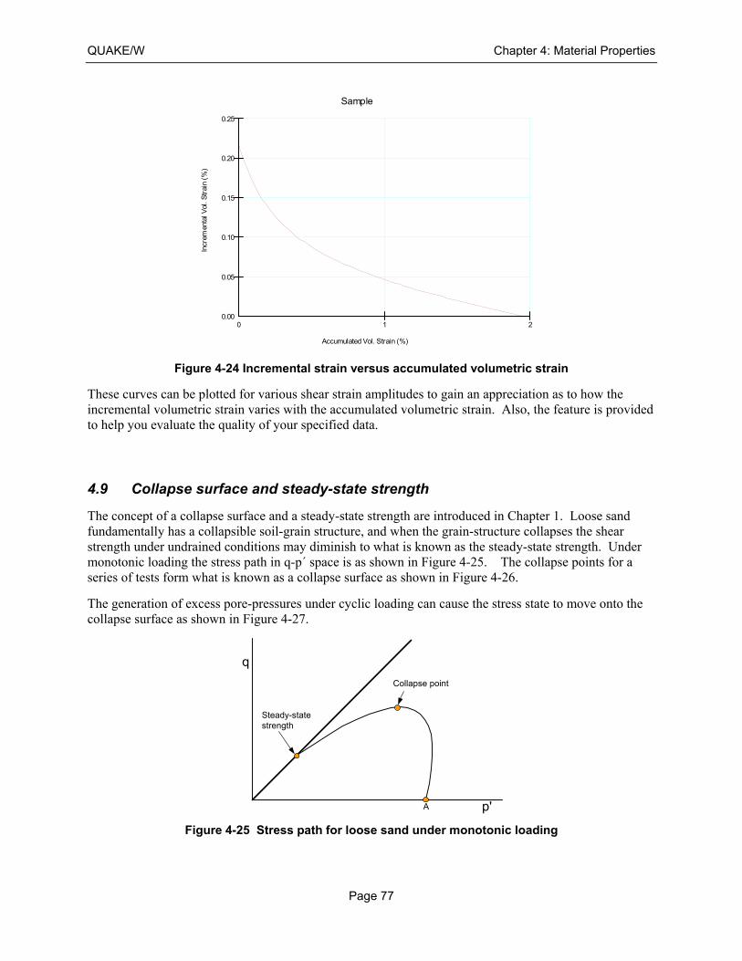
QUAKE/W Chapter 4: Material Properties
Page 77
Figure 4-24 Incremental strain versus accumulated volumetric strain
These curves can be plotted for various shear strain amplitudes to gain an appreciation as to how the incremental volumetric strain varies with the accumulated volumetric strain. Also, the feature is provided to help you evaluate the quality of your specified data.
4.9 Collapse surface and steady-state strength
The concept of a collapse surface and a steady-state strength are introduced in Chapter 1. Loose sand fundamentally has a collapsible soil-grain structure, and when the grain-structure collapses the shear strength under undrained conditions may diminish to what is known as the steady-state strength. Under monotonic loading the stress path in q-p΄ space is as shown in Figure 4-25. The collapse points for a series of tests form what is known as a collapse surface as shown in Figure 4-26.
The generation of excess pore-pressures under cyclic loading can cause the stress state to move onto the collapse surface as shown in Figure 4-27.
Figure 4-25 Stress path for loose sand under monotonic loading
Sample
Incr
emen
tal V
ol. S
trai
n (%
)
Accumulated Vol. Strain (%)
0.00
0.05
0.10
0.15
0.20
0.25
0 1 2
q
p'A
Collapse point
Steady-statestrength
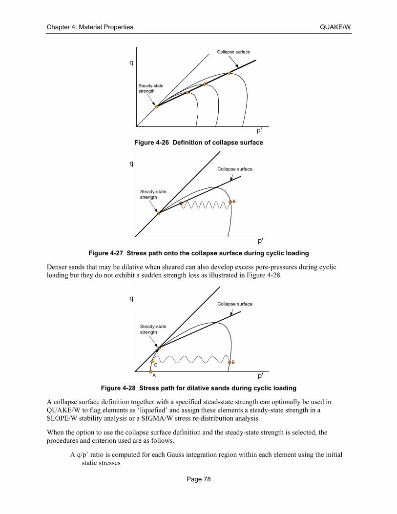
Chapter 4: Material Properties QUAKE/W
Page 78
Figure 4-26 Definition of collapse surface
Figure 4-27 Stress path onto the collapse surface during cyclic loading
Denser sands that may be dilative when sheared can also develop excess pore-pressures during cyclic loading but they do not exhibit a sudden strength loss as illustrated in Figure 4-28.
Figure 4-28 Stress path for dilative sands during cyclic loading
A collapse surface definition together with a specified stead-state strength can optionally be used in QUAKE/W to flag elements as ‘liquefied’ and assign these elements a steady-state strength in a SLOPE/W stability analysis or a SIGMA/W stress re-distribution analysis.
When the option to use the collapse surface definition and the steady-state strength is selected, the procedures and criterion used are as follows.
A q/p΄ ratio is computed for each Gauss integration region within each element using the initial static stresses
q
p'
Steady-statestrength
Collapse surface
q
p'
B
Collapse surface
Steady-statestrength
q
p'
B
Collapse surface
Steady-statestrength
C
A
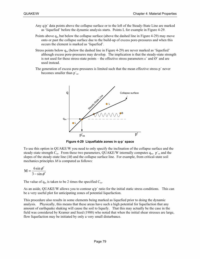
QUAKE/W Chapter 4: Material Properties
Page 79
Any q/p΄ data points above the collapse surface or to the left of the Steady-State Line are marked as ‘liquefied’ before the dynamic analysis starts. Points L for example in Figure 4-29.
Points above qss but below the collapse surface (above the dashed line in Figure 4-29) may move onto or past the collapse surface due to the build-up of excess pore-pressures and when this occurs the element is marked as ‘liquefied’.
Stress points below qss (below the dashed line in Figure 4-29) are never marked as ‘liquefied’ although excess pore-pressures may develop. The implication is that the steady-state strength is not used for these stress-state points – the effective stress parameters c΄ and Ø΄ and are used instead.
The generation of excess pore-pressures is limited such that the mean effective stress p΄ never becomes smaller than p΄ss.
Figure 4-29 Liquefiable zones in q-p΄ space
To use this option in QUAKE/W you need to only specify the inclination of the collapse surface and the steady-state strength Css. From these two parameters, QUAKE/W internally computes qss, p΄ss and the slopes of the steady-state line (M) and the collapse surface line. For example, from critical-state soil mechanics principles M is computed as follows:
6sin
3 sin
φφ′
Μ =′−
The value of qss is taken to be 2 times the specified Css.
As an aside, QUAKE/W allows you to contour q/p΄ ratio for the initial static stress conditions. This can be a very useful plot for anticipating zones of potential liquefaction.
This procedure also results in some elements being marked as liquefied prior to doing the dynamic analysis. Physically, this means that these areas have such a high potential for liquefaction that any amount of earthquake shaking will cause the soil to liquefy. That this may actually be the case in the field was considered by Kramer and Seed (1988) who noted that when the initial shear stresses are large, flow liquefaction may be initiated by only a very small disturbance.
q
p'
B
Collapse surface
qss
L
L
Stead
y-Sta
te L
ine
p'ss
Chapter 4: Material Properties QUAKE/W
Page 80
Commentary on the use of the collapse surface
Little published data is available on the inclination of the collapse surface. However, as Kramer (1996) points out the slope is often about two-thirds of Ø΄ for clean sand. This is a reasonable estimate if no data is available. Moreover, the collapse surface slope is usually not all that critical to obtaining reasonable solutions – the solutions are much more sensitive to the steady-state strength.
The collapse surface approach accounts for the initial overburden (confining) stress state and the initial static shear in a much clearer and more logical manner than do the Ks and Ka correction factors.
The collapse surface ideas have been successfully used in analyzing the Lower and Upper San Fernando Case Histories as described in detail in the related examples included with the QUAKE/W software.
QUAKE/W does not follow the path down the collapse surface to the steady-state strength once a stress point is on the surface as others like Gu et al. (1993, 1994) have done. In this sense QUAKE/W is not yet complete. The collapse surface and steady-sate strength are only used to mark elements where the steady-sate strength should be used in a SLOPE/W stability analysis or in a SIGMA/W stress re-distribution analysis.
4.10 Structural elements
Structural elements can be used to model structural components such as, for example, sheet pile walls or piles. Such structural components affect the system stiffness and therefore the dynamic response to seismic and cyclic loading.
The properties of structural elements are:
E - Young’s Modulus
I – the moment of inertia, and
A – the cross sectional area.
The moment of inertia is about the bending axis.
If the moment of inertia (I) is set to zero, the structural element has axial stiffness, but no flexural stiffness. This can be useful for simulating geo-fabrics for example.
The mass of the structural elements is not included in QUAKE/W. This is not that unrealistic for buried structures since the mass of the structural components is usually insignificant relative to the mass of soil in the analysis. Stated another way, the structural elements add stiffness to the system, but not mass.
The mass of structural elements is ignored in a QUAKE/W analysis.
4.11 Closing remarks
As is evident from the above discussion, defining material properties for a QUAKE/W dynamic analysis is not trivial. It helps a little with knowing what needs to be defined if you recognize that:
Only the soil stiffness and damping properties are required for a dynamic response analysis. Damping is defined as a constant or as a function. The shear modulus G (soil stiffness) is defined as a constant or a function of the effective overburden stress.

QUAKE/W Chapter 4: Material Properties
Page 81
All the other properties are related to estimating the generation of excess pore-pressures that may arise from the shaking. The pore-pressure related properties are only required if estimating the excess pore-pressures is part of the analysis objectives.
It is also important to recognize that the pore-pressures computed are sensitive to the specified material properties. Small changes in pore-pressure related material properties can result in significantly different pore-pressure responses. Moreover, there are many factors involved in the soil’s response, such as stress state, density, initial void ratio, grain size distribution and so forth. The reliability and accuracy of the computed pore-pressures must be viewed and interpreted in light of this.

Chapter 4: Material Properties QUAKE/W
Page 82

QUAKE/W Chapter 5: Boundary Conditions
Page 83
5 Boundary Conditions
5.1 Introduction
QUAKE/W, like all other finite element products in GeoStudio, is a boundary valued analysis; that is, the problem consists only of a small portion of the real domain and consequently it is necessary to specify conditions along the boundaries where the analysis section has been lifted out of the actual field domain.
In addition, it is necessary to specify the excitation forces acting on the body of the problem; that is, forces such as gravity and inertial forces associated with earthquake shaking.
This chapter describes the various boundary conditions available in QUAKE/W and provides discussions on the use and the applicability of the boundary conditions.
5.2 Earthquake records
Earthquake shaking creates inertial forces which are related to the mass in motion and the associated accelerations. In equation form, the inertial forces are:
F ma=
where m is mass and a is acceleration.
The acceleration is the key input parameter for a QUAKE/W analysis and is determined from ground motion measurements during an earthquake.
Earthquake records are stored and maintained by many agencies throughout the world. A typical example is the US Geological Survey. Many of these agencies now make the records available through the internet. The US Geological Survey website is:
http://nsmp.wr.usgs.gov/
Unfortunately there is no one standard digital format for these ground motion records. Some are presented in terms of a percentage of the gravitational constant g while others are in terms of length per time squared (L/t2) – for example, cm/sec2. Furthermore, the data is in time-acceleration pairs or just acceleration at an implied constant time interval. QUAKE/W can accommodate only two types of formats. Due to the lack of a universal standard, it is often necessary to make some modifications to the raw data files for importing them into QUAKE/W.
Data file header
QUAKE/W looks for a header in the textural data file that consists of two rows of equal signs (=) separated by one line of text as follows:
========================================== 2 1 ==========================================
The acceleration data has to start immediately after the second row of equal signs.
Any other identifying text can be in the data file above the top row of equal signs. It is ignored by QUAKE/W. The file needs to end with the last row of acceleration data.

Chapter 5: Boundary Conditions QUAKE/W
Page 84
The header needs to be added to almost all records so QUAKE/W can read and interpret the data. This can be done with any text editor such as Notepad or WordPad, which are included with the Windows Operating System.
Time-acceleration data pairs
The one format supported by QUAKE/W is where the data is in time-acceleration pairs. Table 5-1 below illustrates this format. Each line consists of a time value followed by an acceleration value. In this example, each line consists of five time-acceleration pairs. The number of pairs on a line can vary. QUAKE/W attempts to interpret all non-blank digits and the digits are delimited by spaces.
Table 5-1 Example of time-acceleration data pairs
Between the two rows of equal signs are digits that have meaning. These are:
The first digit (2 in this example) indicates the data is in a time-acceleration pair format.
The second digit (1 in this example) identifies the units. One means cm/sec2, 2 means meters/sec2, 3 means feet/sec2 and 4 means in/sec2.
Acceleration only data files
The other format supported by QUAKE is where the record has only acceleration values, as illustrated in Table 5-2, and the values represent a constant time interval.

QUAKE/W Chapter 5: Boundary Conditions
Page 85
Table 5-2 Example of a data file with only accelerations
In this case, each row consists of 8 acceleration values at an even time interval of 0.005 sec. The data can also be in a single column in the text file.
The meaning of the digits between the rows of equal signs (=) are:
First digit (1 in this example) indicates the data is in an acceleration data format at an even time interval.
The second digit (1 in this example) identifies the units. One means cm/sec2, 2 means meters/sec2, 3 means feet/sec2 and 4 means in/sec2. The second digit being 1 in this example means the data is in cm/sec2.
The third digit between the rows of equal signs is the time interval. In this example, the time interval is 0.005 sec.
The length unit (centimeters, meters, inches, etc.) of the accelerations is actually not all that important since QUAKE/W interprets the earthquake record in terms of g. As discussed in the next section, once the record has been imported into QUAKE/W, the record can be scaled to the desired peak percentage of g regardless of the actual dimensions of the raw data.
Spreadsheet data
Data can also be pasted directly into the QUAKE/W earthquake dialog box. Say for example, you have some acceleration data in a spreadsheet that represents some kind of cyclic motion. Such data can be cut from the spread sheet and pasted into QUAKE/W.
This is powerful and flexible since you can manipulate the data as deemed desirable before bring it into QUAKE/W. Alternatively, the spreadsheet data can be altered to fit one of the formats acceptable for importing into QUAKE/W and then saving the spreadsheet data in a text file.
A spreadsheet can also be used to create artificial cyclic data, for example which can then be used in QUAKE/W to simulate tests or to compare QUAKE/W results with closed form solution.

Chapter 5: Boundary Conditions QUAKE/W
Page 86
Data modification
Once the data has been imported into QUAKE/W, the data can be modified to suit the needs of a particular site or analysis. The desired peak acceleration and duration can be specified. The record is then scaled to these specified values. Say for example, the imported data has a peak acceleration of 0.34842g. If the peak acceleration is then specified as 0.2g the entire record is scaled so that the peak is 0.2g. The form of the record remains the same, only the amplitudes are adjusted. In a similar way, the duration of the record can also be modified.
Often earthquake records have extraneous data at the start and end of the record. This data can be deleted in QUAKE/W as deemed necessary. As discussed in the Numerical Issues chapter, from a numerical performance point of view it is best to remove such extraneous data.
Figure 5-1 A 0.348g peak record scaled to a peak of 0.2g
Baseline correction
Earthquake records often have some drift in the data as illustrated Table 5-2. This does not have a great effect on the dynamic response analysis of a structure, but it does lead to an unrealistic picture of the displacement computed from double integration of the acceleration record. QUAKE/W can make baseline correction to remove this drift. With this correction, the record in Figure 5-2 appears as in Figure 5-3.
The QUAKE/W baseline correction is based on a simple linear regression. The objective is to ensure that area under the curve is the same above and below the zero acceleration axes (that is, the slope of the modified linear regression line is zero). This does not necessarily ensure that a double integration displacement curve will return to zero at the end of the record. There may nonetheless be some cumulative displacement in the curve. The simple linear regression correction, however, helps to minimize the zero displacement offset at the end of the record.
Undesirable displacement offsets can be further diminished by removing as much as possible any extraneous data from the start and end of the records.
Ac
cele
ratio
n (
g )
Time (sec)
-0.1
-0.2
-0.3
0.0
0.1
0.2
0.3
0.4
0 2 4 6 8 10
Ac
cele
ratio
n (
g )
Time (sec)
-0.05
-0.10
-0.15
-0.20
0.00
0.05
0.10
0.15
0.20
0 2 4 6 8 10
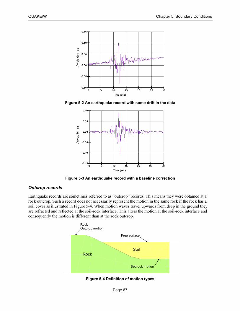
QUAKE/W Chapter 5: Boundary Conditions
Page 87
Figure 5-2 An earthquake record with some drift in the data
Figure 5-3 An earthquake record with a baseline correction
Outcrop records
Earthquake records are sometimes referred to as “outcrop” records. This means they were obtained at a rock outcrop. Such a record does not necessarily represent the motion in the same rock if the rock has a soil cover as illustrated in Figure 5-4. When motion waves travel upwards from deep in the ground they are refracted and reflected at the soil-rock interface. This alters the motion at the soil-rock interface and consequently the motion is different than at the rock outcrop.
Figure 5-4 Definition of motion types
RockSoil
RockOutcrop motion
Free surface
Bedrock motion

Chapter 5: Boundary Conditions QUAKE/W
Page 88
One-dimensional ground response analyses based on what are known as transfer functions have been developed which consider this soil-rock interaction (Kramer 1996, pp. 254-280). The software packages SHAKE and ProShake, discussed in the Verification chapter, have an “outcrop” option which addresses this effect. The earthquake motion can optionally be applied at the ground surface as opposed to at the soil-rock interface. Applying the motion at the ground surface makes it possible to estimate the motion at the soil rock interface. The computed soil-rock interface motion can then be used at other similar sites and conditions.
Similar transfer functions are not available for a two-dimensional dynamic analysis such as in QUAKE/W. In QUAKE/W the ground motion is in essence always applied at the lower boundary of the problem. Sufficient bedrock can be included in the analysis so that the “outcrop” motion is for all practical purposes the same as in the rock at the base of the problem. The soil-rock interface and the effect it has on the dynamic response is then directly included in the analysis.
Generally, it is not appropriate to use a free surface record directly in a QUAKE/W analysis. Such a record would have to be modified through trial and error for a QUAKE/W analysis until the computed results are similar to the free surface measurements. Such an analysis could provide a reasonable picture of the internal dynamic stresses and strains in the ground, however, as Kramer (1996, p. 275) has pointed out, such deconvolution from a free surface motion record should be preformed with great care and the results should be evaluated carefully.
The issue of an “outcrop” record can create considerable confusion when comparing the results from a QUAKE/W analysis with the results from a 1D SHAKE or ProShake analysis. The “outcrop” option in SHAKE and ProShake has to be unselected for such a comparison. This is discussed in more detail later in the Verification chapter.
5.3 Boundary condition basics
The finite element motion equation for a dynamic analysis is:
[ ]{ } [ ]{ } [ ]{ } { }K d D v M a F+ + =
where d is displacement, v is velocity and a is acceleration. [K] is the element characteristic matrix, [D] is the damping matrix, [M] is the mass matrix and {F} is the nodal forcing vector. The primary unknown is d (displacement) and to compute d, the equation ultimately reduces to:
[ ]{ } { }K d F=
To solve this equation it is necessary to specify d somewhere in the domain; that is, a displacement boundary condition must exist at some nodes in the problem. Usually the displacement is specified as zero somewhere along the boundary and the motion is then computed relative to this specified displacement boundary condition.
Another point of significance here is that all boundary conditions eventually reduce down to one of two types, either displacement or force. It is useful to always keep this in mind when specifying boundary conditions. The choice is limited to one of only two options.
There are other options available in QUAKE/W, as discussed in the following sections, but they are only convenient mechanisms for specifying either displacement or force.
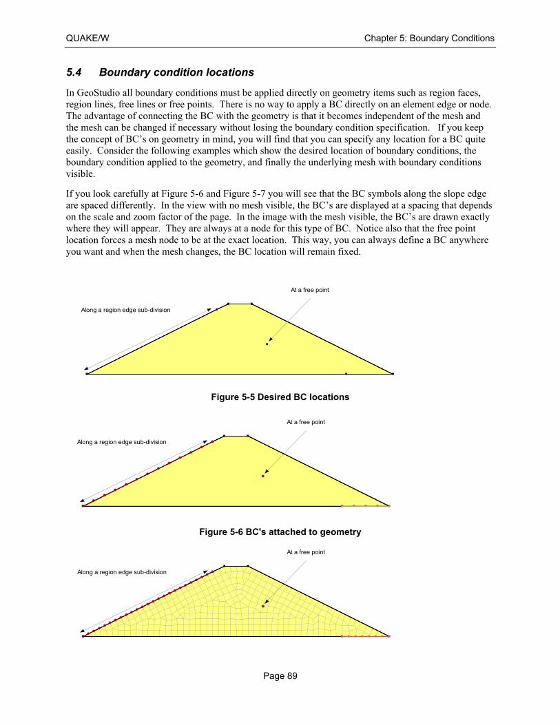
QUAKE/W Chapter 5: Boundary Conditions
Page 89
5.4 Boundary condition locations
In GeoStudio all boundary conditions must be applied directly on geometry items such as region faces, region lines, free lines or free points. There is no way to apply a BC directly on an element edge or node. The advantage of connecting the BC with the geometry is that it becomes independent of the mesh and the mesh can be changed if necessary without losing the boundary condition specification. If you keep the concept of BC’s on geometry in mind, you will find that you can specify any location for a BC quite easily. Consider the following examples which show the desired location of boundary conditions, the boundary condition applied to the geometry, and finally the underlying mesh with boundary conditions visible.
If you look carefully at Figure 5-6 and Figure 5-7 you will see that the BC symbols along the slope edge are spaced differently. In the view with no mesh visible, the BC’s are displayed at a spacing that depends on the scale and zoom factor of the page. In the image with the mesh visible, the BC’s are drawn exactly where they will appear. They are always at a node for this type of BC. Notice also that the free point location forces a mesh node to be at the exact location. This way, you can always define a BC anywhere you want and when the mesh changes, the BC location will remain fixed.
Figure 5-5 Desired BC locations
Figure 5-6 BC's attached to geometry
Along a region edge sub-division
At a free point
Along a region edge sub-division
At a free point
Along a region edge sub-division
At a free point
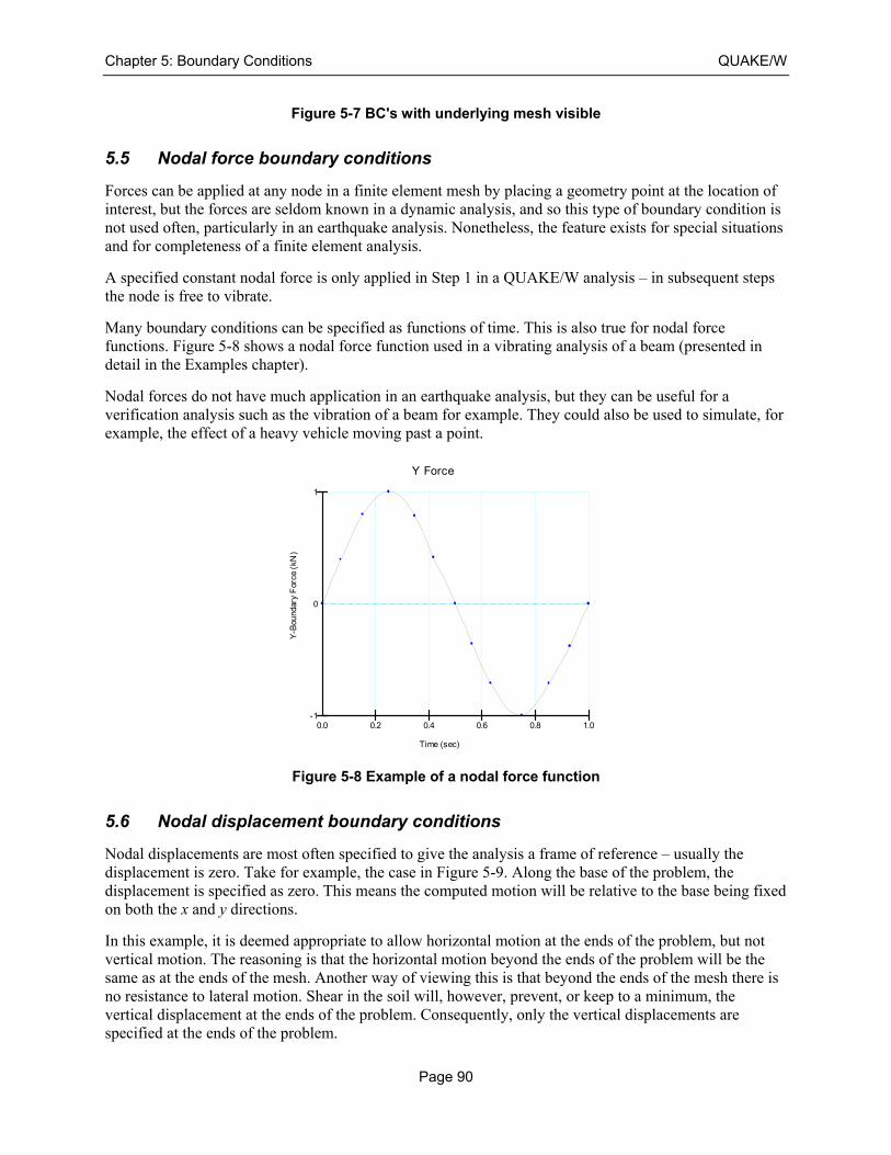
Chapter 5: Boundary Conditions QUAKE/W
Page 90
Figure 5-7 BC's with underlying mesh visible
5.5 Nodal force boundary conditions
Forces can be applied at any node in a finite element mesh by placing a geometry point at the location of interest, but the forces are seldom known in a dynamic analysis, and so this type of boundary condition is not used often, particularly in an earthquake analysis. Nonetheless, the feature exists for special situations and for completeness of a finite element analysis.
A specified constant nodal force is only applied in Step 1 in a QUAKE/W analysis – in subsequent steps the node is free to vibrate.
Many boundary conditions can be specified as functions of time. This is also true for nodal force functions. Figure 5-8 shows a nodal force function used in a vibrating analysis of a beam (presented in detail in the Examples chapter).
Nodal forces do not have much application in an earthquake analysis, but they can be useful for a verification analysis such as the vibration of a beam for example. They could also be used to simulate, for example, the effect of a heavy vehicle moving past a point.
Figure 5-8 Example of a nodal force function
5.6 Nodal displacement boundary conditions
Nodal displacements are most often specified to give the analysis a frame of reference – usually the displacement is zero. Take for example, the case in Figure 5-9. Along the base of the problem, the displacement is specified as zero. This means the computed motion will be relative to the base being fixed on both the x and y directions.
In this example, it is deemed appropriate to allow horizontal motion at the ends of the problem, but not vertical motion. The reasoning is that the horizontal motion beyond the ends of the problem will be the same as at the ends of the mesh. Another way of viewing this is that beyond the ends of the mesh there is no resistance to lateral motion. Shear in the soil will, however, prevent, or keep to a minimum, the vertical displacement at the ends of the problem. Consequently, only the vertical displacements are specified at the ends of the problem.
Y Force
Y-B
ound
ary
For
ce (
kN)
Time (sec)
-1
0
1
0.0 0.2 0.4 0.6 0.8 1.0
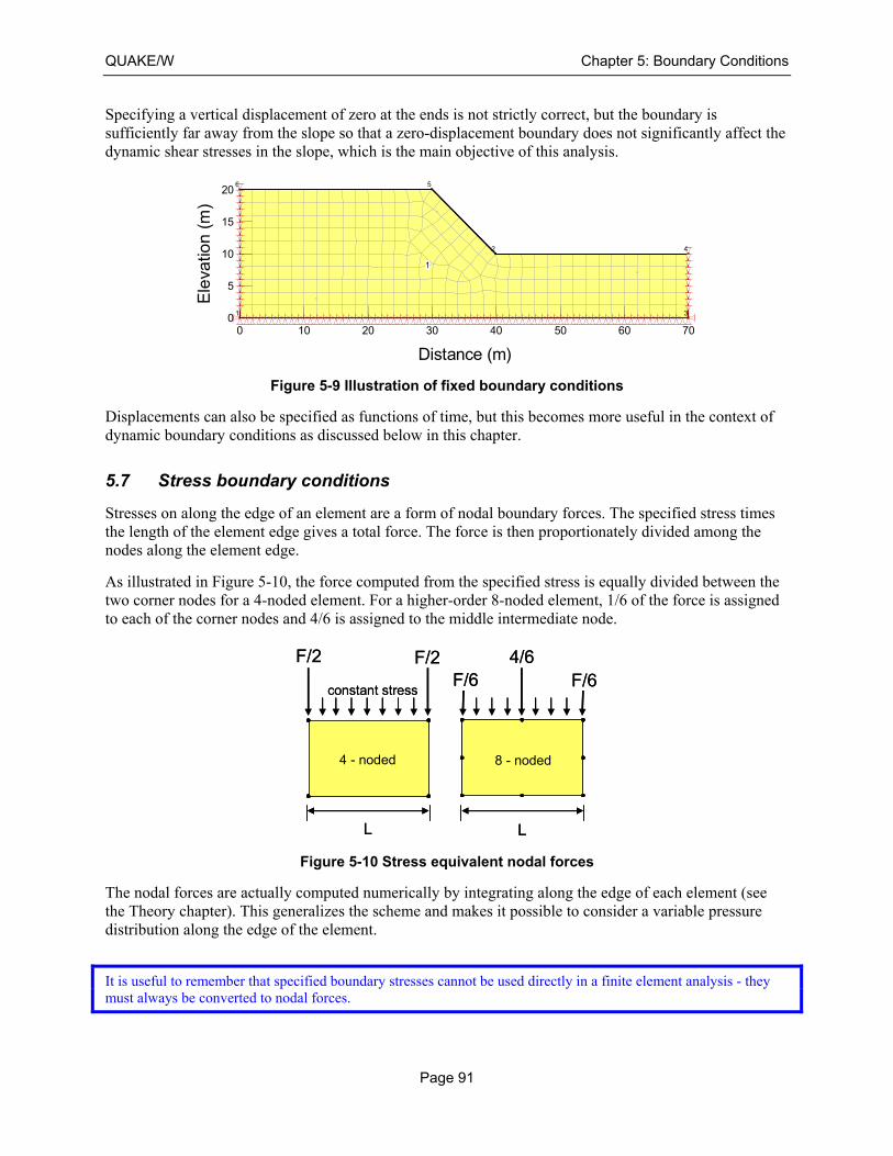
QUAKE/W Chapter 5: Boundary Conditions
Page 91
Specifying a vertical displacement of zero at the ends is not strictly correct, but the boundary is sufficiently far away from the slope so that a zero-displacement boundary does not significantly affect the dynamic shear stresses in the slope, which is the main objective of this analysis.
Figure 5-9 Illustration of fixed boundary conditions
Displacements can also be specified as functions of time, but this becomes more useful in the context of dynamic boundary conditions as discussed below in this chapter.
5.7 Stress boundary conditions
Stresses on along the edge of an element are a form of nodal boundary forces. The specified stress times the length of the element edge gives a total force. The force is then proportionately divided among the nodes along the element edge.
As illustrated in Figure 5-10, the force computed from the specified stress is equally divided between the two corner nodes for a 4-noded element. For a higher-order 8-noded element, 1/6 of the force is assigned to each of the corner nodes and 4/6 is assigned to the middle intermediate node.
Figure 5-10 Stress equivalent nodal forces
The nodal forces are actually computed numerically by integrating along the edge of each element (see the Theory chapter). This generalizes the scheme and makes it possible to consider a variable pressure distribution along the edge of the element.
It is useful to remember that specified boundary stresses cannot be used directly in a finite element analysis - they must always be converted to nodal forces.
1
1
2
3
4
56
Distance (m)
0 10 20 30 40 50 60 70
Ele
vatio
n (
m)
0
5
10
15
20
L L
4 - noded 8 - noded
F/2 F/2F/6 F/6
4/6
constant stress
L L
4 - noded 8 - noded
F/2 F/2F/6 F/6
4/6
constant stress
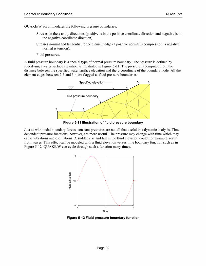
Chapter 5: Boundary Conditions QUAKE/W
Page 92
QUAKE/W accommodates the following pressure boundaries:
Stresses in the x and y directions (positive is in the positive coordinate direction and negative is in the negative coordinate direction).
Stresses normal and tangential to the element edge (a positive normal is compression; a negative normal is tension).
Fluid pressures.
A fluid pressure boundary is a special type of normal pressure boundary. The pressure is defined by specifying a water surface elevation as illustrated in Figure 5-11. The pressure is computed from the distance between the specified water surface elevation and the y-coordinate of the boundary node. All the element edges between 2-3 and 3-4 are flagged as fluid pressure boundaries.
Figure 5-11 Illustration of fluid pressure boundary
Just as with nodal boundary forces, constant pressures are not all that useful in a dynamic analysis. Time dependent pressure functions, however, are more useful. The pressure may change with time which may cause vibrations and oscillations. A sudden rise and fall in the fluid elevation could, for example, result from waves. This effect can be modeled with a fluid elevation versus time boundary function such as in Figure 5-12. QUAKE/W can cycle through such a function many times.
Figure 5-12 Fluid pressure boundary function
2 3
4
5 6
Fluid pressure boundary
Specified elevation
Time
0 1 2
Flu
id E
leva
tion
90
100
110
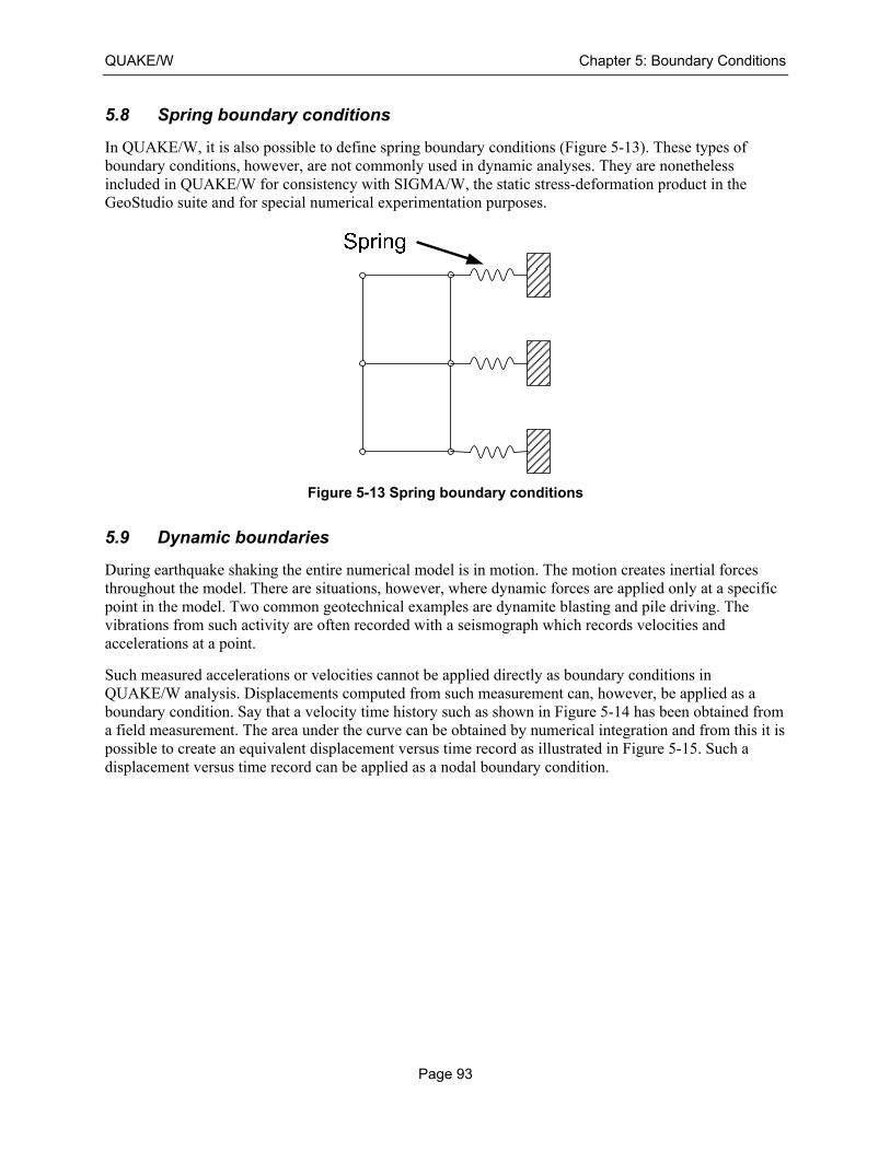
QUAKE/W Chapter 5: Boundary Conditions
Page 93
5.8 Spring boundary conditions
In QUAKE/W, it is also possible to define spring boundary conditions (Figure 5-13). These types of boundary conditions, however, are not commonly used in dynamic analyses. They are nonetheless included in QUAKE/W for consistency with SIGMA/W, the static stress-deformation product in the GeoStudio suite and for special numerical experimentation purposes.
Figure 5-13 Spring boundary conditions
5.9 Dynamic boundaries
During earthquake shaking the entire numerical model is in motion. The motion creates inertial forces throughout the model. There are situations, however, where dynamic forces are applied only at a specific point in the model. Two common geotechnical examples are dynamite blasting and pile driving. The vibrations from such activity are often recorded with a seismograph which records velocities and accelerations at a point.
Such measured accelerations or velocities cannot be applied directly as boundary conditions in QUAKE/W analysis. Displacements computed from such measurement can, however, be applied as a boundary condition. Say that a velocity time history such as shown in Figure 5-14 has been obtained from a field measurement. The area under the curve can be obtained by numerical integration and from this it is possible to create an equivalent displacement versus time record as illustrated in Figure 5-15. Such a displacement versus time record can be applied as a nodal boundary condition.
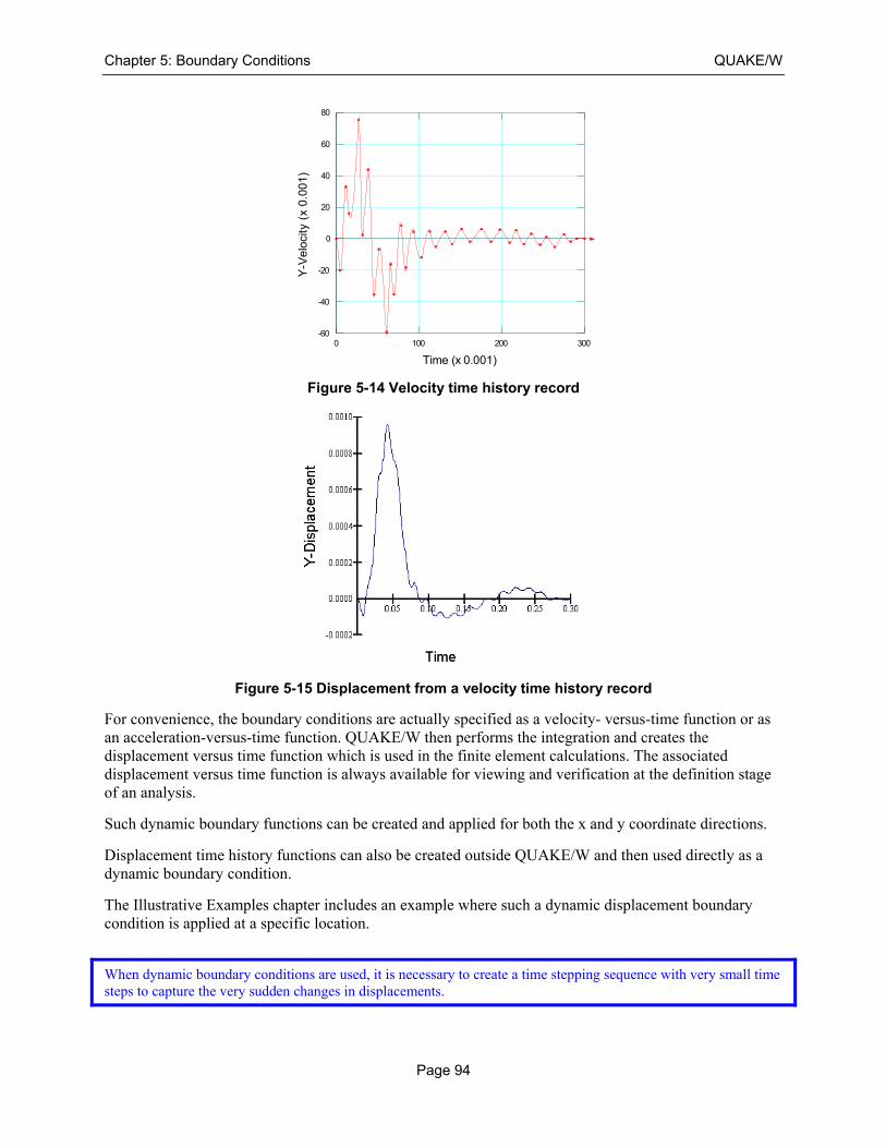
Chapter 5: Boundary Conditions QUAKE/W
Page 94
Figure 5-14 Velocity time history record
Figure 5-15 Displacement from a velocity time history record
For convenience, the boundary conditions are actually specified as a velocity- versus-time function or as an acceleration-versus-time function. QUAKE/W then performs the integration and creates the displacement versus time function which is used in the finite element calculations. The associated displacement versus time function is always available for viewing and verification at the definition stage of an analysis.
Such dynamic boundary functions can be created and applied for both the x and y coordinate directions.
Displacement time history functions can also be created outside QUAKE/W and then used directly as a dynamic boundary condition.
The Illustrative Examples chapter includes an example where such a dynamic displacement boundary condition is applied at a specific location.
When dynamic boundary conditions are used, it is necessary to create a time stepping sequence with very small time steps to capture the very sudden changes in displacements.
Time (x 0.001)
0 100 200 300
Y-V
elo
city
(x
0.0
01)
-60
-40
-20
0
20
40
60
80

QUAKE/W Chapter 5: Boundary Conditions
Page 95
5.10 Structural elements
QUAKE/W can accommodate structural elements. These elements can act as a beam or a bar. These elements are useful for simulating structural components such as a sheet pile wall for example. Such elements have a significant effect on the system stiffness and can consequently significantly affect the dynamic response of a structure.
The boundary conditions for structural elements are either a specified rotation or a specified moment. The specified values are usually zero. A zero rotation simulates a cantilever connection. A zero moment simulates a hinge.

Chapter 5: Boundary Conditions QUAKE/W
Page 96

QUAKE/W Chapter 6: Analysis Types
Page 97
6 Analysis Types
6.1 Introduction
There are basically four types of analyses available in QUAKE/W. They are:
Initial Static
Equivalent Linear Dynamic
Equivalent Linear PWP Only
Nonlinear Dynamic
This chapter discusses and describes these different types of analyses.
6.2 Initial in-situ stresses
A QUAKE/W dynamic analysis cannot be solved without first establishing the initial stresses. Material properties like the Shear Modulus (G), for example, are usually a function of the effective stresses in the ground. Other variables like the Cyclic Stress Ratio are based on the initial effective stresses. Consequently, it is essential to know the initial state of stress in the ground before starting the dynamic analysis.
QUAKE/W has a special type of analysis called ‘Initial Static’ that is formulated specifically for establishing the initial stresses. Alternatively, the initial stresses can be obtained from a SIGMA/W analysis. The Initial Static method is identical to the SIGMA/W Insitu method.
QUAKE/W, like SIGMA/W, has the option to compute the initial stresses using the Ko procedure for problems involving: a) a horizontal ground surface; b) a horizontal phreatic surface (that is, hydrostatic pore-water pressures); and c) spatially continuous and horizontal stratigraphic units.
The Initial Static (‘Insitu’) and Ko procedures, along with their limitations, are described in detail in the book: Stress and Deformation Modeling with SIGMA/W. Note that the QUAKE/W Initial Static analysis sets the stresses within structural element to zero. If the initial stresses come from a SIGMA/W analysis, then the structural elements could possibly have some initial stresses and forces.
Pore-water pressures
Initial pore-water pressures can be specified by a) drawing an initial water table; b) using the results of another finite element analysis (e.g. a SEEP/W or SIGMA/W analysis); or, c) using a spatial function. Options b) or c) should be used if the groundwater conditions differ significantly from the hydrostatic condition.
Initial water table
An initial water table requires the user to: a) specify the maximum negative pressure head (i.e. the capillary rise); and b) to Draw | Initial Water Table as a series of points that are automatically connected to form the water table. The ability to draw an initial water table is actually available to all analysis types.
The initial pore-water pressures are calculated by assuming a linear relationship between the pore-water pressure, unit weight of water wγ , and the distance above or below the water table iz :
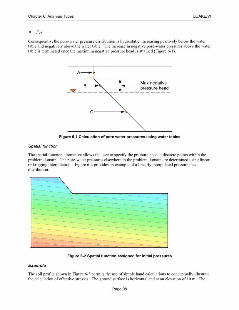
Chapter 6: Analysis Types QUAKE/W
Page 98
w iu zγ=
Consequently, the pore-water pressure distribution is hydrostatic, increasing positively below the water table and negatively above the water table. The increase in negative pore-water pressures above the water table is terminated once the maximum negative pressure head is attained (Figure 6-1).
Figure 6-1 Calculation of pore water pressures using water tables
Spatial function
The spatial function alternative allows the user to specify the pressure head at discrete points within the problem domain. The pore-water pressures elsewhere in the problem domain are determined using linear or krigging interpolation. Figure 6-2 provides an example of a linearly interpolated pressure head distribution.
Figure 6-2 Spatial function assigned for initial pressures
Example
The soil profile shown in Figure 6-3 permits the use of simple hand calculations to conceptually illustrate the calculation of effective stresses. The ground surface is horizontal and at an elevation of 10 m. The
A
B
C
Max negativepressure head
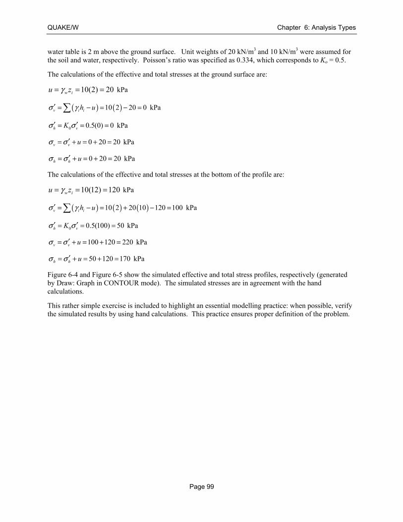
QUAKE/W Chapter 6: Analysis Types
Page 99
water table is 2 m above the ground surface. Unit weights of 20 kN/m3 and 10 kN/m3 were assumed for the soil and water, respectively. Poisson’s ratio was specified as 0.334, which corresponds to Ko = 0.5.
The calculations of the effective and total stresses at the ground surface are:
10(2) 20w iu zγ= = = kPa
( ) ( )10 2 20 0v i ih uσ γ′ = − = − = kPa
0 0.5(0) 0h vKσ σ′ ′= = = kPa
0 20 20v v uσ σ ′= + = + = kPa
0 20 20h h uσ σ ′= + = + = kPa
The calculations of the effective and total stresses at the bottom of the profile are:
10(12) 120w iu zγ= = = kPa
( ) ( ) ( )10 2 20 10 120 100v i ih uσ γ′ = − = + − = kPa
0 0.5(100) 50h vKσ σ′ ′= = = kPa
100 120 220v v uσ σ ′= + = + = kPa
50 120 170h h uσ σ ′= + = + = kPa
Figure 6-4 and Figure 6-5 show the simulated effective and total stress profiles, respectively (generated by Draw: Graph in CONTOUR mode). The simulated stresses are in agreement with the hand calculations.
This rather simple exercise is included to highlight an essential modelling practice: when possible, verify the simulated results by using hand calculations. This practice ensures proper definition of the problem.
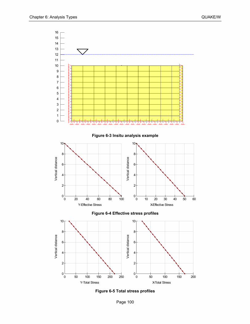
Chapter 6: Analysis Types QUAKE/W
Page 100
Figure 6-3 Insitu analysis example
Figure 6-4 Effective stress profiles
Figure 6-5 Total stress profiles
0
1
2
3
4
5
6
7
8
9
10
11
12
13
14
15
16
Ver
tical
dis
tanc
e
Y-Effective Stress
0
2
4
6
8
10
0 20 40 60 80 100
Ver
tical
dis
tanc
e
X-Effective Stress
0
2
4
6
8
10
0 10 20 30 40 50 60
Ver
tical
dis
tanc
e
Y-Total Stress
0
2
4
6
8
10
0 50 100 150 200 250
Ver
tical
dis
tanc
e
X-Total Stress
0
2
4
6
8
10
0 50 100 150 200
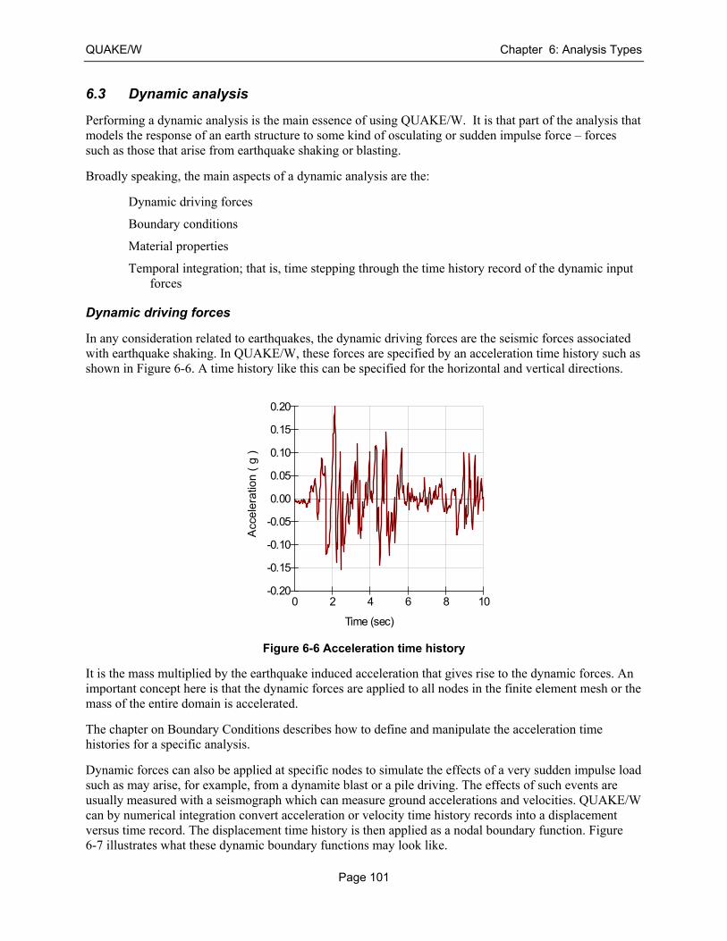
QUAKE/W Chapter 6: Analysis Types
Page 101
6.3 Dynamic analysis
Performing a dynamic analysis is the main essence of using QUAKE/W. It is that part of the analysis that models the response of an earth structure to some kind of osculating or sudden impulse force – forces such as those that arise from earthquake shaking or blasting.
Broadly speaking, the main aspects of a dynamic analysis are the:
Dynamic driving forces
Boundary conditions
Material properties
Temporal integration; that is, time stepping through the time history record of the dynamic input forces
Dynamic driving forces
In any consideration related to earthquakes, the dynamic driving forces are the seismic forces associated with earthquake shaking. In QUAKE/W, these forces are specified by an acceleration time history such as shown in Figure 6-6. A time history like this can be specified for the horizontal and vertical directions.
Figure 6-6 Acceleration time history
It is the mass multiplied by the earthquake induced acceleration that gives rise to the dynamic forces. An important concept here is that the dynamic forces are applied to all nodes in the finite element mesh or the mass of the entire domain is accelerated.
The chapter on Boundary Conditions describes how to define and manipulate the acceleration time histories for a specific analysis.
Dynamic forces can also be applied at specific nodes to simulate the effects of a very sudden impulse load such as may arise, for example, from a dynamite blast or a pile driving. The effects of such events are usually measured with a seismograph which can measure ground accelerations and velocities. QUAKE/W can by numerical integration convert acceleration or velocity time history records into a displacement versus time record. The displacement time history is then applied as a nodal boundary function. Figure 6-7 illustrates what these dynamic boundary functions may look like.
Acc
eler
atio
n (
g )
Time (sec)
-0.05
-0.10
-0.15
-0.20
0.00
0.05
0.10
0.15
0.20
0 2 4 6 8 10
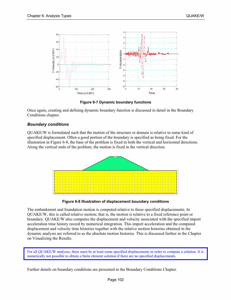
Chapter 6: Analysis Types QUAKE/W
Page 102
Figure 6-7 Dynamic boundary functions
Once again, creating and defining dynamic boundary function is discussed in detail in the Boundary Conditions chapter.
Boundary conditions
QUAKE/W is formulated such that the motion of the structure or domain is relative to some kind of specified displacement. Often a good portion of the boundary is specified as being fixed. For the illustration in Figure 6-8, the base of the problem is fixed in both the vertical and horizontal directions. Along the vertical ends of the problem, the motion is fixed in the vertical direction.
Figure 6-8 Illustration of displacement boundary conditions
The embankment and foundation motion is computed relative to these specified displacements. In QUAKE/W, this is called relative motion; that is, the motion is relative to a fixed reference point or boundary. QUAKE/W also computes the displacement and velocity associated with the specified import acceleration time history record by numerical integration. This import acceleration and the computed displacement and velocity time histories together with the relative motion histories obtained in the dynamic analysis are referred to as the absolute motion histories. This is discussed further in the Chapter on Visualizing the Results.
For all QUAKE/W analyses, there must be at least some specified displacements in order to compute a solution. It is numerically not possible to obtain a finite element solution if there are no specified displacements.
Further details on boundary conditions are presented in the Boundary Conditions Chapter.
Time (x 0.001)
0 100 200 300
Y-V
elo
city
(x
0.0
01
)
-60
-40
-20
0
20
40
60
80
Time
0 10 20 30 40
Y-A
cce
lera
tion
-6
-5
-4
-3
-2
-1
0
1
2
3
4

QUAKE/W Chapter 6: Analysis Types
Page 103
Material properties
Whether the materials behave in a linear or non-linear manner during a dynamic analysis is controlled by the type of Material Model selected. This is specified as part of the material properties. The details on specifying material properties are presented in the Material Properties Chapter.
Linear-elastic material properties generally do not produce realistic dynamic responses for actual field problems. Treating the soils as linear-elastic usually results in amplifications that are too high. While linear-elastic properties are not all that useful for a dynamic analysis, dynamic linear-elastic analyses are, however, useful for testing and verifying concepts. As noted earlier in this chapter, there are no convergence issues associated with a linear-elastic analysis. This makes it possible, for example, to experiment with the effect of various boundary conditions to discover and confirm their effects on the solution. Stated another way, linear-elastic analyses are useful for doing numerical experiments to become familiar with the intricacies of a QUAKE/W dynamic analysis. Furthermore, linear-elastic analyses are useful for the analysis of simple structures for which closed form solutions are available. This makes it possible to verify that the algorithm has been coded correctly.
Non-linear analyses, using either the E.L or true Non-Linear formulation, are required to obtain meaningful responses from a dynamic analysis of actual field problems.
Time stepping
Stepping through the acceleration time history is inherent to the direct integration method used in the QUAKE/W formulation. Due to the dramatic, very sudden changes in motion it is necessary to step though the time history in small steps. Earthquake shaking often only lasts a matter of seconds and to capture all the characteristics of the motion, the time steps must be fractions of a second. A typical value is two hundredths (0.02) of a second. This consequently results in a large number of time steps. Say the acceleration time history duration is 10 seconds. A total of 500 time steps are then required if the time steps are to be in increments of 0.02 seconds. This is the reason that a QUAKE/W analysis is so computationally intensive.
Smaller time steps are more accurate, but require considerably more computing time and can also produce substantially more data. As with all numerical analyses, it necessary to try to maintain a balance between numerical objectives and practical consequences such as computing time and the volume of data created.
There are no firm rules on selecting time step sizes. Conceptually, the time steps should be such that most of the peaks and sudden changes are approximately captured. Also, for projects where dynamic behavior is a critical issue, it may be necessary to repeat an analysis for several different time step sizes to determine the effect of time steps on the solution.
When simulating the effects of earthquakes, the specified Δt time integration should be no larger than the Δt interval in the earthquake record. For example, if the acceleration data is available at an interval of 0.02 seconds then the Δt time integration should be no greater than 0.02 seconds. The Δt time integration step size may be smaller but should not be larger.
To assists with setting up an appropriate time integration sequence, QUAKE/W has a feature that makes it possible to develop the time integration scheme from the earthquake record. This is very useful features and the recommended procedure unless there is some other compelling reason to develop an alternate time stepping sequence.
The Chapter on Numerical Issues provides further discussions on specifying the integration time step sequence and discusses things that can be done to mitigate the computing time and computer output storage requirements.
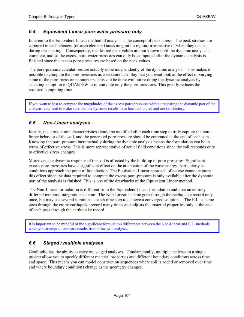
Chapter 6: Analysis Types QUAKE/W
Page 104
6.4 Equivalent Linear pore-water pressure only
Inherent to the Equivalent Linear method of analysis is the concept of peak stress. The peak stresses are captured in each element (or each element Gauss integration region) irrespective of when they occur during the shaking. Consequently, the desired peak values are not known until the dynamic analysis is complete, and so the excess pore-water pressures can only be computed after the dynamic analysis is finished since the excess pore-pressures are based on the peak values.
The pore-pressure calculations are actually done independently of the dynamic analysis. This makes it possible to compute the pore-pressures as a separate task. Say that you want look at the effect of varying some of the pore-pressure parameters. This can be done without re-doing the dynamic analysis by selecting an option in QUAKE/W to re-compute only the pore-pressures. This greatly reduces the required computing time.
If you want to just re-compute the magnitudes of the excess pore-pressures without repeating the dynamic part of the analysis, you need to make sure that the dynamic results have been computed and are satisfactory.
6.5 Non-Linear analyses
Ideally, the stress-strain characteristics should be modified after each time step to truly capture the non-linear behavior of the soil, and the generated pore-pressure should be computed at the end of each step. Knowing the pore-pressure incrementally during the dynamic analysis means the formulation can be in terms of effective stress. This is more representative of actual field conditions since the soil responds only to effective stress changes.
Moreover, the dynamic response of the soil is affected by the build-up of pore-pressures. Significant excess pore-pressures have a significant effect on the attenuation of the wave energy, particularly as conditions approach the point of liquefaction. The Equivalent Linear approach of course cannot capture this effect since the data required to compute the excess pore-pressure is only available after the dynamic part of the analysis is finished. This is one of the drawbacks of the Equivalent Linear method.
The Non-Linear formulation is different from the Equivalent Linear formulation and uses an entirely different temporal integration scheme. The Non-Linear scheme goes through the earthquake record only once, but may use several iterations at each time step to achieve a converged solution. The E.L. scheme goes through the entire earthquake record many times and adjusts the material properties only at the end of each pass through the earthquake record.
It is important to be mindful of the significant formulation differences between the Non-Linear and E.L. methods when you attempt to compare results from these two analyses.
6.6 Staged / multiple analyses
GeoStudio has the ability to carry out staged analyses. Fundamentally, multiple analyses in a single project allow you to specify different material properties and different boundary conditions across time and space. This means you can model construction sequences where soil is added or removed over time and where boundary conditions change as the geometry changes.
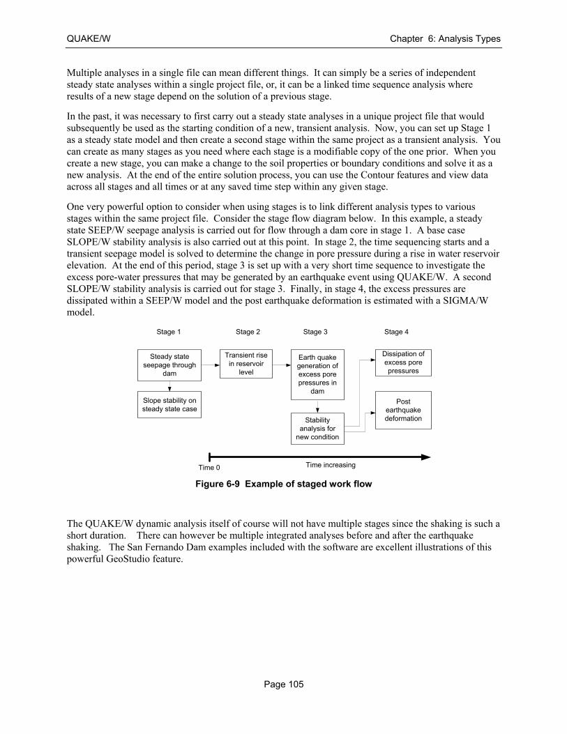
QUAKE/W Chapter 6: Analysis Types
Page 105
Multiple analyses in a single file can mean different things. It can simply be a series of independent steady state analyses within a single project file, or, it can be a linked time sequence analysis where results of a new stage depend on the solution of a previous stage.
In the past, it was necessary to first carry out a steady state analyses in a unique project file that would subsequently be used as the starting condition of a new, transient analysis. Now, you can set up Stage 1 as a steady state model and then create a second stage within the same project as a transient analysis. You can create as many stages as you need where each stage is a modifiable copy of the one prior. When you create a new stage, you can make a change to the soil properties or boundary conditions and solve it as a new analysis. At the end of the entire solution process, you can use the Contour features and view data across all stages and all times or at any saved time step within any given stage.
One very powerful option to consider when using stages is to link different analysis types to various stages within the same project file. Consider the stage flow diagram below. In this example, a steady state SEEP/W seepage analysis is carried out for flow through a dam core in stage 1. A base case SLOPE/W stability analysis is also carried out at this point. In stage 2, the time sequencing starts and a transient seepage model is solved to determine the change in pore pressure during a rise in water reservoir elevation. At the end of this period, stage 3 is set up with a very short time sequence to investigate the excess pore-water pressures that may be generated by an earthquake event using QUAKE/W. A second SLOPE/W stability analysis is carried out for stage 3. Finally, in stage 4, the excess pressures are dissipated within a SEEP/W model and the post earthquake deformation is estimated with a SIGMA/W model.
Figure 6-9 Example of staged work flow
The QUAKE/W dynamic analysis itself of course will not have multiple stages since the shaking is such a short duration. There can however be multiple integrated analyses before and after the earthquake shaking. The San Fernando Dam examples included with the software are excellent illustrations of this powerful GeoStudio feature.
Steady stateseepage through
dam
Slope stability onsteady state case
Transient risein reservoir
level
Stabilityanalysis for
new condition
Earth quakegeneration ofexcess porepressures in
dam
Dissipation ofexcess porepressures
Postearthquakedeformation
Stage 1 Stage 2 Stage 3 Stage 4
Time 0 Time increasing

Chapter 6: Analysis Types QUAKE/W
Page 106
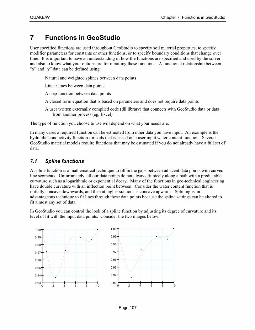
QUAKE/W Chapter 7: Functions in GeoStudio
Page 107
7 Functions in GeoStudio
User specified functions are used throughout GeoStudio to specify soil material properties, to specify modifier parameters for constants or other functions, or to specify boundary conditions that change over time. It is important to have an understanding of how the functions are specified and used by the solver and also to know what your options are for inputting these functions. A functional relationship between “x” and “y” data can be defined using:
Natural and weighted splines between data points
Linear lines between data points
A step function between data points
A closed form equation that is based on parameters and does not require data points
A user written externally complied code (dll library) that connects with GeoStudio data or data from another process (eg, Excel)
The type of function you choose to use will depend on what your needs are.
In many cases a required function can be estimated from other data you have input. An example is the hydraulic conductivity function for soils that is based on a user input water content function. Several GeoStudio material models require functions that may be estimated if you do not already have a full set of data.
7.1 Spline functions
A spline function is a mathematical technique to fill in the gaps between adjacent data points with curved line segments. Unfortunately, all our data points do not always fit nicely along a path with a predictable curvature such as a logarithmic or exponential decay. Many of the functions in geo-technical engineering have double curvature with an inflection point between. Consider the water content function that is initially concave downwards, and then at higher suctions is concave upwards. Splining is an advantageous technique to fit lines through these data points because the spline settings can be altered to fit almost any set of data.
In GeoStudio you can control the look of a spline function by adjusting its degree of curvature and its level of fit with the input data points. Consider the two images below.
0.93
0.94
0.95
0.96
0.97
0.98
0.99
1.00
0 2 4 6 8 100.93
0.94
0.95
0.96
0.97
0.98
0.99
1.00
0 2 4 6 8 10
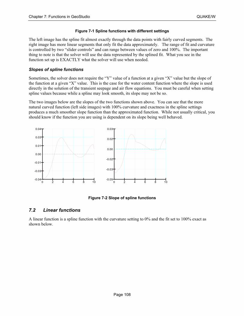
Chapter 7: Functions in GeoStudio QUAKE/W
Page 108
Figure 7-1 Spline functions with different settings
The left image has the spline fit almost exactly through the data points with fairly curved segments. The right image has more linear segments that only fit the data approximately. The range of fit and curvature is controlled by two “slider controls” and can range between values of zero and 100%. The important thing to note is that the solver will use the data represented by the splined fit. What you see in the function set up is EXACTLY what the solver will use when needed.
Slopes of spline functions
Sometimes, the solver does not require the “Y” value of a function at a given “X” value but the slope of the function at a given “X” value. This is the case for the water content function where the slope is used directly in the solution of the transient seepage and air flow equations. You must be careful when setting spline values because while a spline may look smooth, its slope may not be so.
The two images below are the slopes of the two functions shown above. You can see that the more natural curved function (left side images) with 100% curvature and exactness in the spline settings produces a much smoother slope function than the approximated function. While not usually critical, you should know if the function you are using is dependent on its slope being well behaved.
Figure 7-2 Slope of spline functions
7.2 Linear functions
A linear function is a spline function with the curvature setting to 0% and the fit set to 100% exact as shown below.
-0.01
-0.03
-0.04
0.00
0.01
0.03
0.04
0 2 4 6 8 10
-0.02
-0.03
-0.05
0.00
0.02
0.03
0 2 4 6 8 10
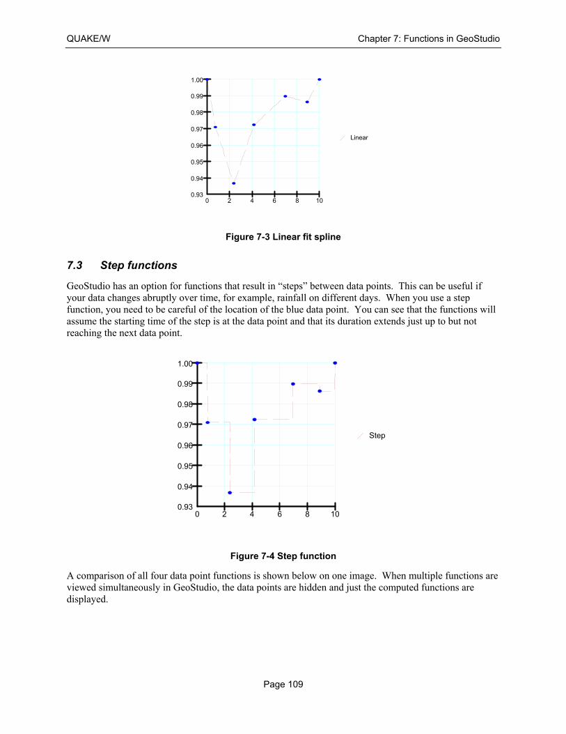
QUAKE/W Chapter 7: Functions in GeoStudio
Page 109
Figure 7-3 Linear fit spline
7.3 Step functions
GeoStudio has an option for functions that result in “steps” between data points. This can be useful if your data changes abruptly over time, for example, rainfall on different days. When you use a step function, you need to be careful of the location of the blue data point. You can see that the functions will assume the starting time of the step is at the data point and that its duration extends just up to but not reaching the next data point.
Figure 7-4 Step function
A comparison of all four data point functions is shown below on one image. When multiple functions are viewed simultaneously in GeoStudio, the data points are hidden and just the computed functions are displayed.
Linear
0.93
0.94
0.95
0.96
0.97
0.98
0.99
1.00
0 2 4 6 8 10
Step
0.93
0.94
0.95
0.96
0.97
0.98
0.99
1.00
0 2 4 6 8 10
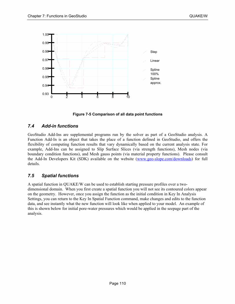
Chapter 7: Functions in GeoStudio QUAKE/W
Page 110
Figure 7-5 Comparison of all data point functions
7.4 Add-in functions
GeoStudio Add-Ins are supplemental programs run by the solver as part of a GeoStudio analysis. A Function Add-In is an object that takes the place of a function defined in GeoStudio, and offers the flexibility of computing function results that vary dynamically based on the current analysis state. For example, Add-Ins can be assigned to Slip Surface Slices (via strength functions), Mesh nodes (via boundary condition functions), and Mesh gauss points (via material property functions). Please consult the Add-In Developers Kit (SDK) available on the website (www.geo-slope.com/downloads) for full details.
7.5 Spatial functions
A spatial function in QUAKE/W can be used to establish starting pressure profiles over a two-dimensional domain. When you first create a spatial function you will not see its contoured colors appear on the geometry. However, once you assign the function as the initial condition in Key In Analysis Settings, you can return to the Key In Spatial Function command, make changes and edits to the function data, and see instantly what the new function will look like when applied to your model. An example of this is shown below for initial pore-water pressures which would be applied in the seepage part of the analysis.
Step
Linear
Spline100%
Splineapprox.
0.93
0.94
0.95
0.96
0.97
0.98
0.99
1.00
0 2 4 6 8 10
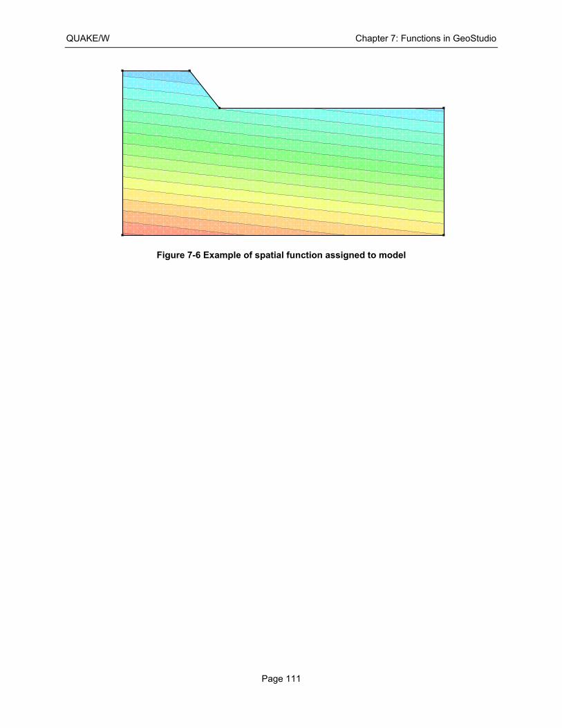
QUAKE/W Chapter 7: Functions in GeoStudio
Page 111
Figure 7-6 Example of spatial function assigned to model

QUAKE/W Chapter 8: Numerical Issues
Page 113
8 Numerical Issues
8.1 Introduction
The computations involved with a QUAKE/W dynamic analysis are highly intensive. Finite element analyses in and of themselves are computationally intensive and QUAKE/W compounds the computing required because of the necessity to step through the input motion in small time steps. Time stepping through a 10 second motion record at an interval of 0.01 seconds requires a 1000 time steps. This is like performing 1000 static analyses. In addition, the problem is non-linear and consequently an iterative procedure is required to obtain a solution. As a result, the 1000 steps may have to be performed several times.
Furthermore, large amounts of output data are created as with all finite element analyses. Again, the problem is compounded by the need to store data for multiple time steps.
Some thought, care and planning is required to keep the processing time and data storage at a manageable level.
This chapter discusses features available in QUAKE/W to mitigate the computing time and data storage requirements, and provides some suggestions on finite element meshing that can help with diminishing the practical computing problems associated with a QUAKE/W analysis.
8.2 Earthquake records
Earthquake records often have some vibrating noise at the start of the record and at the end of the record. The record shown in Figure 8-1 exhibits this. Relatively, there is very little motion between 20 and 40 seconds. Removing the last 20 seconds from the data makes the record appear as in Figure 8-2. Making this change would cut the processing time in half since there would be half the number of time steps.
Altering the input motion record to the bare minimum is effective in mitigating the required computing time, especially during the early stages of a project. Later, once the response is fairly well understood, the analysis can be repeated with the entire record to refine the analysis. Care is, however, required to ensure that the additional motion record does not simply introduce numerical noise.
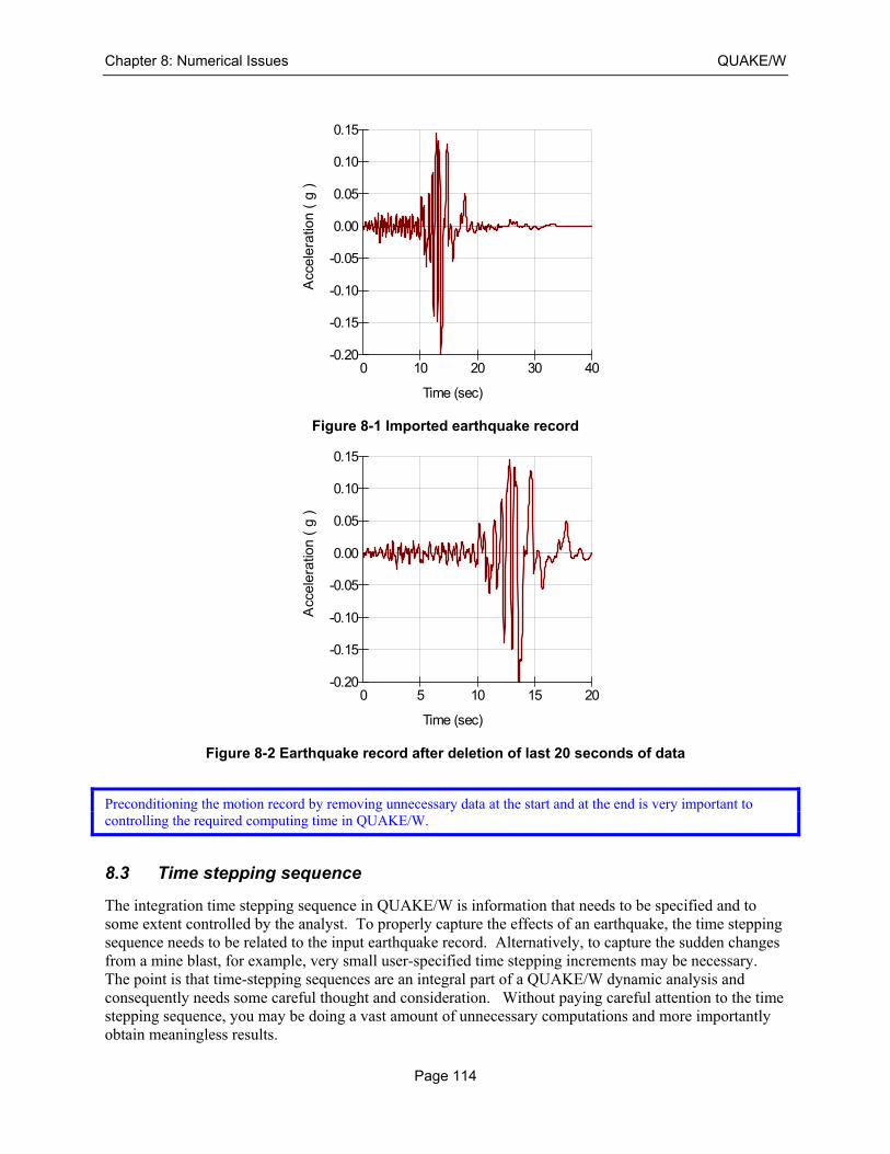
Chapter 8: Numerical Issues QUAKE/W
Page 114
Figure 8-1 Imported earthquake record
Figure 8-2 Earthquake record after deletion of last 20 seconds of data
Preconditioning the motion record by removing unnecessary data at the start and at the end is very important to controlling the required computing time in QUAKE/W.
8.3 Time stepping sequence
The integration time stepping sequence in QUAKE/W is information that needs to be specified and to some extent controlled by the analyst. To properly capture the effects of an earthquake, the time stepping sequence needs to be related to the input earthquake record. Alternatively, to capture the sudden changes from a mine blast, for example, very small user-specified time stepping increments may be necessary. The point is that time-stepping sequences are an integral part of a QUAKE/W dynamic analysis and consequently needs some careful thought and consideration. Without paying careful attention to the time stepping sequence, you may be doing a vast amount of unnecessary computations and more importantly obtain meaningless results.
Acc
eler
atio
n (
g )
Time (sec)
-0.05
-0.10
-0.15
-0.20
0.00
0.05
0.10
0.15
0 10 20 30 40
Acc
ele
ratio
n (
g )
Time (sec)
-0.05
-0.10
-0.15
-0.20
0.00
0.05
0.10
0.15
0 5 10 15 20
QUAKE/W Chapter 8: Numerical Issues
Page 115
When simulating the effects of earthquakes, the specified Δt time integration should be no larger than the Δt interval in the earthquake record. For example, if the acceleration data is available at an interval of 0.02 seconds then the Δt time integration should be no greater than 0.02 seconds. The Δt time integration step size may be smaller but should not be larger.
To assists with setting up an appropriate time integration sequence, QUAKE/W has a feature that makes it possible to develop the time integration scheme from the earthquake record. This is very useful features and the recommended procedure unless there is some other compelling reason to develop an alternate time stepping sequence.
The Δt time integration interval in QUAKE/W is controlled by, (1) the specified duration of the shaking, and (2) by the specified total number of time steps. The Δt is then computed by dividing the duration by the total number of steps.
8.4 Finite element types
QUAKE/W accommodates first-order elements such as 4-noded quadrilaterals and 3-noded triangles as well as higher order 8-noded quadrilaterals and 6-noded triangles. The quadrilateral elements can actually have 4, 5, 6, 7, or 8 nodes and the triangles can have 3, 4, 5 or 6 nodes. Secondary nodes can exist individually along any of the element edges.
The first order elements are treated as constant gradient elements; that is the stress and strain is constant in the elements. The stresses and strains are actually not constant at the Gauss integration points but the Gauss values are averaged and only one value is maintained for the first-order elements. All quadrilateral elements with less than 8 nodes and all triangular elements with less than six nodes are treated as quadrilateral elements.
Six-noded triangular and eight-noded quadrilateral elements allow for stress and strain variation within the elements. This allows for a stress distribution within the element which is obviously closer to reality.
The higher order elements generally are better for stress analyses than the first-order constant gradient elements, but they also require considerably more computing time and data storage. Secondary nodes along each of the element edges significantly increase the number of nodes in a problem, and substantially more storage is consequently required since output is created for each node. Also, the number of finite element equations in a problem is proportional to the number of nodes.
Theoretically, higher-order quadrilateral elements should have nine (3 x 3) Gauss integration points. It is, however, common to use what is known as “under integration” and still get acceptable results. So 4-point (2 x 2) integration is acceptable. While 9-point integration is theoretically better, it at the same time requires more than twice the amount data that is stored for each Gauss point (9 points versus 4 points). Furthermore, computing the element characteristic matrix based on 9 integration points takes more computing time than for 4 integration points.
As in all finite element analyses, a balance is required between numerical accuracy and practical considerations such as computing time and hardware requirements.
In the early stages of a modeling project it is generally better to start with first-order constant gradient elements with 4-point integration for quadrilateral elements and 3-point integration for triangular elements. Later when response of the system is well understood it is often advisable to switch to higher-order elements to refine the analysis.
The element order selection is obviously also a function of the mesh size. For smaller meshes it is really not an issue. Higher order elements can be used without being concerned about time and data storage. It is
Chapter 8: Numerical Issues QUAKE/W
Page 116
for larger meshes that more care is required in the element order selection and when it is necessary to start simple and then later migrate to more complexity.
8.5 Mesh size
QUAKE/W modeling and analysis can become unmanageable if the mesh gets too large. There is not a specific limit in QUAKE/W on mesh size, but for practical reasons meshes generally should not be much greater than about a 1000 elements, particularly higher-order elements. A mesh with 2000 elements is approaching the upper practical limit even with the best desktop computers currently available.
Most users tend to start a modeling project with an unnecessarily large mesh. It is much better modeling practice to start with a mesh with as few elements as possible. This is particularly true for a multi-time step dynamic analysis.
8.6 History points
QUAKE/W has what are called “history points”. Region points can be placed on the geometry to define nodes at a specific location. The region points can then be marked for extra and more complete output as history points. As discussed in the next section, output data is usually only stored for every 10th time step, for example, to reduce the data storage requirements. A complete response record is, however, sometimes required at isolated key points. A typical point may be the crest of en embankment for example. Such points can be flagged as “history points.” This assists with obtaining critical data without having to output and store all the data at all the nodes. It is another feature available to manage the large amount of data.
A maximum of 10 history points can be drawn on the domain.
8.7 Output data
As already noted in the previous section, output data can be stored at a selected interval in the time stepping sequence. Typically the output may be stored every 5th or 10th or 50th or 100th time step for example.
In addition, specific individual time steps can be flagged for output if necessary. Perhaps it is a few extra time steps near the peak input motion.
The downside of not storing output for every time step is that the data stored may not contain the absolute peak values. Graphs and contour plots of the results may not always present the absolute maximums. The trends, however, are usually well represented even if the output is only saved at some time stepping interval.
Saving the data for all time steps simply becomes unmanageable except for perhaps smaller meshes for a one-dimensional analysis.
When the time-stepping sequence is connected to the earthquake record, QUAKE/W automatically saves data at the time steps that represent the 20 highest peaks in the earthquake record. The peak responses of the structure may not necessarily occur exactly at theses time steps, but will be in the proximity of the time steps.
QUAKE/W always saves data for the last time step.
QUAKE/W Chapter 8: Numerical Issues
Page 117
8.8 Compute pore-pressures alone
Another feature available to reduce the computing time required is to compute only the pore-pressures without repeating the dynamic analysis when doing an Equivalent Linear analysis. As discussed earlier in this book, the generated pore-pressures are computed after the dynamic part of the analysis is finished. The pore-pressures are related to the peak cyclic stresses which are only known at the end of the dynamic analysis.
Sometimes it is desirable to examine the effect of making changes to the input data related to calculating the excess pores-pressures generated. This can be done by selecting the analysis which does only the pore-pressure calculations which is much faster than also repeating the dynamic analysis each time.
8.9 Convergence
QUAKE/W, like all the other GeoStudio finite element products, uses the comparison of the primary unknowns from two successive iterations to control the iterative convergence procedure. In QUAKE/W the primary unknown is the computed nodal displacement. The Equivalent Linear analysis type is an exception to this general scheme for finite analyses as described in the next section.
Equivalent Linear Convergence
The Equivalent Linear analysis basically cycles through the entire earthquake record in an attempt to establish the correct the soil stiffness (G). During each pass through the earthquake record the peak cyclic shear strains are noted in each element. The soil stiffness (G) is then modified based on the peak cyclic shear strains. Once G has been adjusted, the entire process is repeated.
Generally, five (5) passes (iterations) through the earthquake record is adequate to establish appropriate G values for each element.
The number of iterations can be controlled with a user specified parameter. The default in QUAKE/W is set to five.
There are no hard and fast rules as to the optimum number of iterations. The only thing that can be done to refine this user-specified value is to inspect the differences in the results of key parameters by experimenting with different number of iterations. For example, if the number of iterations is of concern, then you may want to try 4, 6, and 8 and see if the extra iterations significantly alter the results. Due to the computational time required to do this experimenting, you will likely only want to do this at the beginning of an analysis project. Once the required or desired number of iterations has been establish, subsequent analyses can use the established number of iterations.
Using a value as low as possible is obviously desirable since each pass through the earthquake record is computationally expensive.
The number of iterations used in an E.L. analysis also needs to be judged in light of the confidence and accuracy with which the material properties can be specified. There is no value in spending a lot of computing time on a high number of passes (iterations) through the earthquake record if the material properties are at best rough estimates.
We at GEO-SLOPE have found that five iterations is usually a reasonable number.
As noted previously several times, the excess pore-pressure is only computed after the iteration process is complete.
Chapter 8: Numerical Issues QUAKE/W
Page 118
Non-Linear convergence
The Non-Linear formulation is an incremental displacement formulation just like SIGMA/W. This means that each time-step computes an incremental displacement and the final displacement is the algebraic summation of all the incremental displacements. So if there are 1500 time steps there will be 1500 incremental displacements and the final displacement will be the summation of the 1500 increments.
With the Non-Linear formulation, an iterative scheme is required for each time step. The number of iterations required to reach the specified tolerance may vary for each time step.
With this formulation, QUAKE/W compares the displacements at each node from two successive iterations. A solution is deemed to have converged when the displacements from two successive iterations are within the specified tolerance.
From a mathematically perspective, this means making a comparison of two floating numbers. GeoStudio uses two criteria to make this comparison. They are:
• Significant figures or digits
• Minimum difference
Significant figures
Significant figures of a number are those digits that carry meaning as to the precision of the number. Leading and trailing zeros simply provide a reference as to the scale of the number. Consider a number like 5123.789. If we say that the number is precise to two significant figures its precision is 5.1 x 10³; if it is three significant figures then its precision is 5.12 x 10³, and if it is four significant figures then its precision is 5.124 x 10³.
In GeoStudio, the user is allowed to specify the desired significant figures or digits for comparison of the primary unknowns from the finite element solution. Specifying a criterion of two significant digits means that when the displacements from two successive iterations are the same to a precision of two significant figures, they are deemed to be the same or they are said to have converged.
Minimum difference
Computer computations inherently carry with them some numerical noise, or stated another way, digits that have no physical meaning. So when comparing floating point numbers it is necessary to filter out the meaningless digits.
GeoStudio does this with a user specified minimum-difference value. If the difference between two successive displacements at a node is less than this minimum specified value, the two displacements are deemed to be the same, or again the two displacements are said to have converged.
In QUAKE/W, a minimum difference specified as 0.001 means a minimum difference in displacement of 0.001 m or 1 mm; a value set to 0.005 means a displacement difference of 0.005 m or 5 mm and so forth.
Consider two numbers such as 1.23 x 10⁻⁶ and 1.23 x 10⁻⁷. These two numbers have the same number of significant digits but the difference (1.11 x 10⁻⁶) is very small and has no physical meaning in terms of a QUAKE/W analysis. The two numbers are consequently deemed to be the same or converged.
Maximum number of iterations
In any iterative scheme it is necessary to ultimately limit the number of iterations if it is not possible to meet the convergence criteria. The maximum number of iterations is a user-specified value.

QUAKE/W Chapter 8: Numerical Issues
Page 119
Viewing convergence data
For each time step that the results are saved, it is possible to make a graph of the number of unconverged nodes versus the iteration count. The objective is to go through the iterative process until all nodes have converged, or until there are no unconverged nodes.
It is also possible to make a graph of the number of iterations required (or used) for each time step in the entire earthquake record. Generally, a higher number of iterations will be required at the strong motion points in the earthquake record.

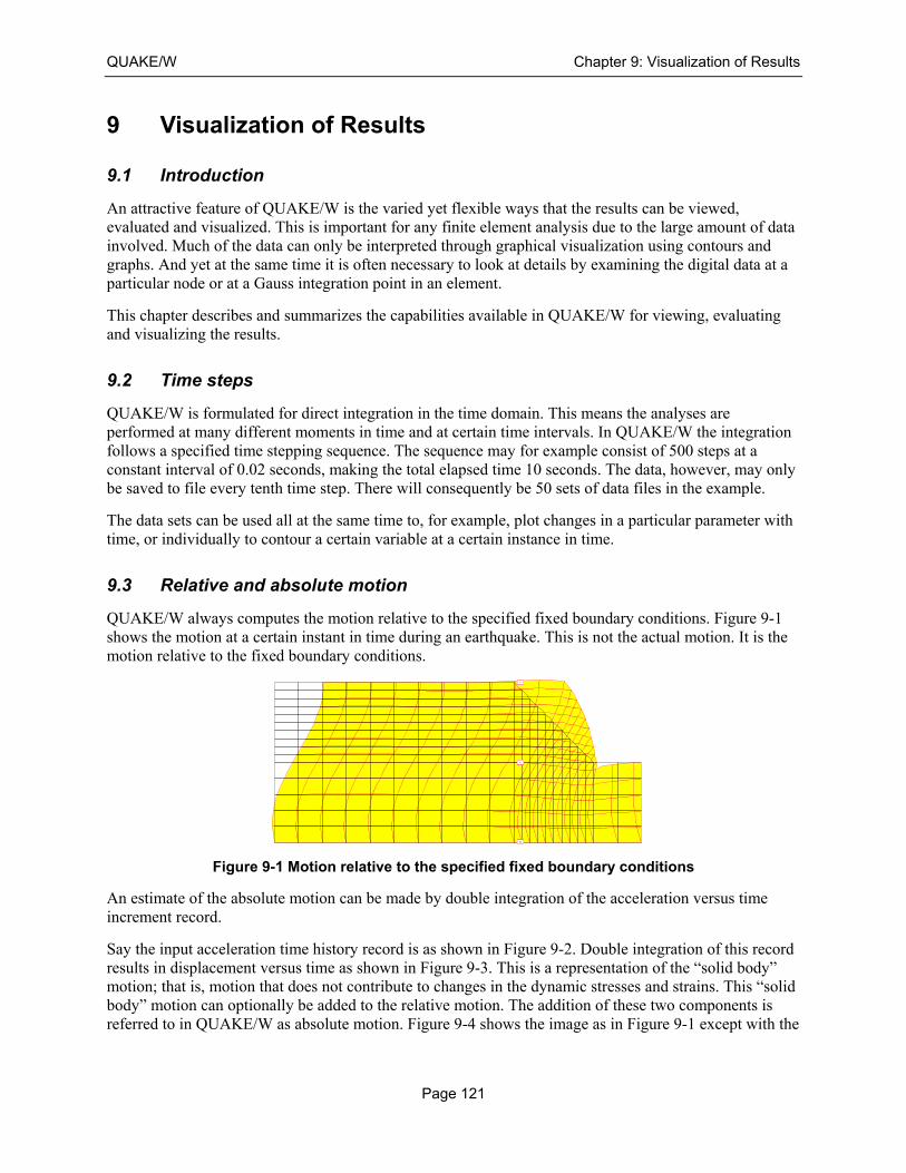
QUAKE/W Chapter 9: Visualization of Results
Page 121
9 Visualization of Results
9.1 Introduction
An attractive feature of QUAKE/W is the varied yet flexible ways that the results can be viewed, evaluated and visualized. This is important for any finite element analysis due to the large amount of data involved. Much of the data can only be interpreted through graphical visualization using contours and graphs. And yet at the same time it is often necessary to look at details by examining the digital data at a particular node or at a Gauss integration point in an element.
This chapter describes and summarizes the capabilities available in QUAKE/W for viewing, evaluating and visualizing the results.
9.2 Time steps
QUAKE/W is formulated for direct integration in the time domain. This means the analyses are performed at many different moments in time and at certain time intervals. In QUAKE/W the integration follows a specified time stepping sequence. The sequence may for example consist of 500 steps at a constant interval of 0.02 seconds, making the total elapsed time 10 seconds. The data, however, may only be saved to file every tenth time step. There will consequently be 50 sets of data files in the example.
The data sets can be used all at the same time to, for example, plot changes in a particular parameter with time, or individually to contour a certain variable at a certain instance in time.
9.3 Relative and absolute motion
QUAKE/W always computes the motion relative to the specified fixed boundary conditions. Figure 9-1 shows the motion at a certain instant in time during an earthquake. This is not the actual motion. It is the motion relative to the fixed boundary conditions.
Figure 9-1 Motion relative to the specified fixed boundary conditions
An estimate of the absolute motion can be made by double integration of the acceleration versus time increment record.
Say the input acceleration time history record is as shown in Figure 9-2. Double integration of this record results in displacement versus time as shown in Figure 9-3. This is a representation of the “solid body” motion; that is, motion that does not contribute to changes in the dynamic stresses and strains. This “solid body” motion can optionally be added to the relative motion. The addition of these two components is referred to in QUAKE/W as absolute motion. Figure 9-4 shows the image as in Figure 9-1 except with the
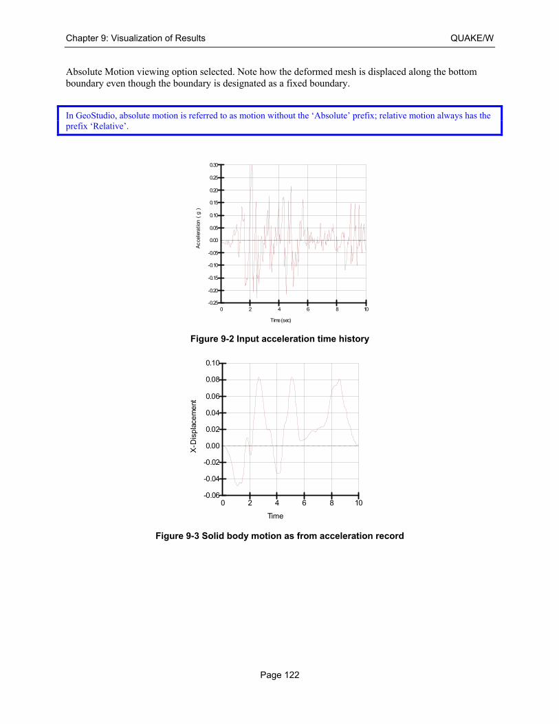
Chapter 9: Visualization of Results QUAKE/W
Page 122
Absolute Motion viewing option selected. Note how the deformed mesh is displaced along the bottom boundary even though the boundary is designated as a fixed boundary.
In GeoStudio, absolute motion is referred to as motion without the ‘Absolute’ prefix; relative motion always has the prefix ‘Relative’.
Figure 9-2 Input acceleration time history
Figure 9-3 Solid body motion as from acceleration record
Ac
cele
rati
on (
g )
Time (sec)
-0.05
-0.10
-0.15
-0.20
-0.25
0.00
0.05
0.10
0.15
0.20
0.25
0.30
0 2 4 6 8 10
X-D
ispl
ace
men
t
Time
-0.02
-0.04
-0.06
0.00
0.02
0.04
0.06
0.08
0.10
0 2 4 6 8 10

QUAKE/W Chapter 9: Visualization of Results
Page 123
Figure 9-4 Absolute motion plus relative motion
It is important to remember when using the Relative and Absolute motion option that only relative motion creates dynamic stresses – solid body motion does not contribute to dynamic stresses.
9.4 Node and element information
In order to understand what type of information can be viewed as results, it helps a bit to know how the data is obtained. So, to recap, you set up the problem geometry, define material properties, and apply boundary conditions. The solver assembles the soil property and geometry information for every Gauss point in every element and applies it to the deformation equation that is written for every node. Therefore, at each node we have applied boundary data, interpolated soil property data and geometry data. The solver then computes the unknown value in the equation for each node – the unknown value being either force or displacement. It is the Gauss point data that is used to set up the nodal equations, so the Gauss point data written to the output file is the actual data used in the solver.
In GeoStudio, all output data for nodes and gauss points anywhere in the model is accessible using the View Results Information command. With the command selected, you can click the mouse on any single node to view the output at the node. You can also hold down the shift key to multi-select many points. If you click beside a node and within the element itself, you will get the Gauss point data at that location. You can multi-select Gauss point to see a table of data.
Figure 9-5 is an illustration of the type of information that can be viewed for each node in the finite element mesh. The data types are grouped by category with each category containing various related data options. There is also a summary of the position of the node within the problem domain. In effect, the node information is a summary of the problem geometry, the soil material properties, and the boundary conditions – the three main parts of any finite element analysis.
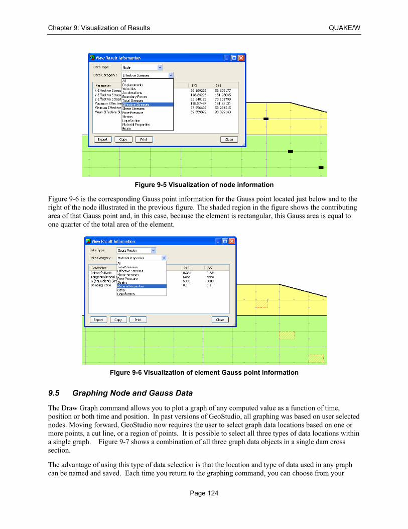
Chapter 9: Visualization of Results QUAKE/W
Page 124
Figure 9-5 Visualization of node information
Figure 9-6 is the corresponding Gauss point information for the Gauss point located just below and to the right of the node illustrated in the previous figure. The shaded region in the figure shows the contributing area of that Gauss point and, in this case, because the element is rectangular, this Gauss area is equal to one quarter of the total area of the element.
Figure 9-6 Visualization of element Gauss point information
9.5 Graphing Node and Gauss Data
The Draw Graph command allows you to plot a graph of any computed value as a function of time, position or both time and position. In past versions of GeoStudio, all graphing was based on user selected nodes. Moving forward, GeoStudio now requires the user to select graph data locations based on one or more points, a cut line, or a region of points. It is possible to select all three types of data locations within a single graph. Figure 9-7 shows a combination of all three graph data objects in a single dam cross section.
The advantage of using this type of data selection is that the location and type of data used in any graph can be named and saved. Each time you return to the graphing command, you can choose from your
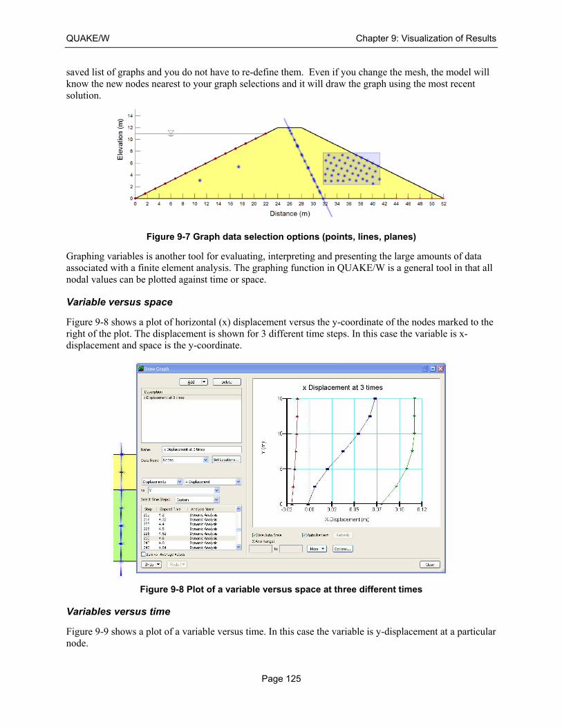
QUAKE/W Chapter 9: Visualization of Results
Page 125
saved list of graphs and you do not have to re-define them. Even if you change the mesh, the model will know the new nodes nearest to your graph selections and it will draw the graph using the most recent solution.
Figure 9-7 Graph data selection options (points, lines, planes)
Graphing variables is another tool for evaluating, interpreting and presenting the large amounts of data associated with a finite element analysis. The graphing function in QUAKE/W is a general tool in that all nodal values can be plotted against time or space.
Variable versus space
Figure 9-8 shows a plot of horizontal (x) displacement versus the y-coordinate of the nodes marked to the right of the plot. The displacement is shown for 3 different time steps. In this case the variable is x-displacement and space is the y-coordinate.
Figure 9-8 Plot of a variable versus space at three different times
Variables versus time
Figure 9-9 shows a plot of a variable versus time. In this case the variable is y-displacement at a particular node.
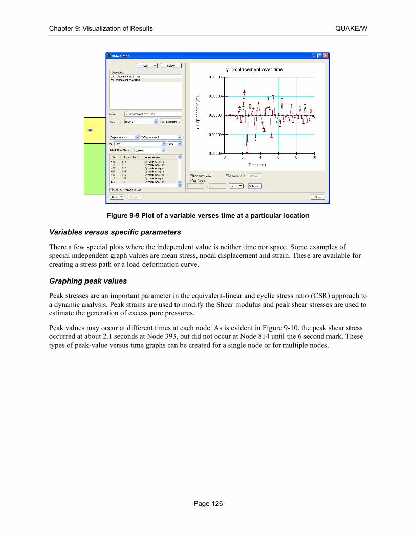
Chapter 9: Visualization of Results QUAKE/W
Page 126
Figure 9-9 Plot of a variable verses time at a particular location
Variables versus specific parameters
There a few special plots where the independent value is neither time nor space. Some examples of special independent graph values are mean stress, nodal displacement and strain. These are available for creating a stress path or a load-deformation curve.
Graphing peak values
Peak stresses are an important parameter in the equivalent-linear and cyclic stress ratio (CSR) approach to a dynamic analysis. Peak strains are used to modify the Shear modulus and peak shear stresses are used to estimate the generation of excess pore pressures.
Peak values may occur at different times at each node. As is evident in Figure 9-10, the peak shear stress occurred at about 2.1 seconds at Node 393, but did not occur at Node 814 until the 6 second mark. These types of peak-value versus time graphs can be created for a single node or for multiple nodes.
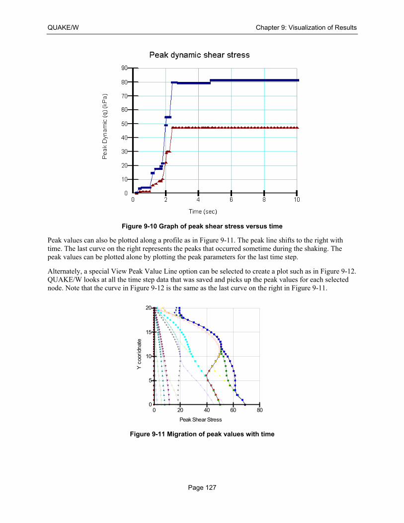
QUAKE/W Chapter 9: Visualization of Results
Page 127
Figure 9-10 Graph of peak shear stress versus time
Peak values can also be plotted along a profile as in Figure 9-11. The peak line shifts to the right with time. The last curve on the right represents the peaks that occurred sometime during the shaking. The peak values can be plotted alone by plotting the peak parameters for the last time step.
Alternately, a special View Peak Value Line option can be selected to create a plot such as in Figure 9-12. QUAKE/W looks at all the time step data that was saved and picks up the peak values for each selected node. Note that the curve in Figure 9-12 is the same as the last curve on the right in Figure 9-11.
Figure 9-11 Migration of peak values with time
Y c
oori
dnat
e
Peak Shear Stress
0
5
10
15
20
0 20 40 60 80
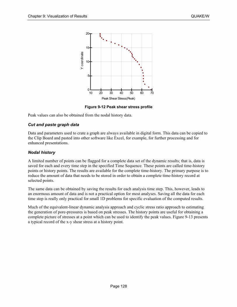
Chapter 9: Visualization of Results QUAKE/W
Page 128
Figure 9-12 Peak shear stress profile
Peak values can also be obtained from the nodal history data.
Cut and paste graph data
Data and parameters used to crate a graph are always available in digital form. This data can be copied to the Clip Board and pasted into other software like Excel, for example, for further processing and for enhanced presentations.
Nodal history
A limited number of points can be flagged for a complete data set of the dynamic results; that is, data is saved for each and every time step in the specified Time Sequence. These points are called time-history points or history points. The results are available for the complete time-history. The primary purpose is to reduce the amount of data that needs to be stored in order to obtain a complete time-history record at selected points.
The same data can be obtained by saving the results for each analysis time step. This, however, leads to an enormous amount of data and is not a practical option for most analyses. Saving all the data for each time step is really only practical for small 1D problems for specific evaluation of the computed results.
Much of the equivalent-linear dynamic analysis approach and cyclic stress ratio approach to estimating the generation of pore-pressures is based on peak stresses. The history points are useful for obtaining a complete picture of stresses at a point which can be used to identify the peak values. Figure 9-13 presents a typical record of the x-y shear stress at a history point.
Y c
oord
inat
e
Peak Shear Stress(Peak)
0
5
10
15
20
10 20 30 40 50 60 70
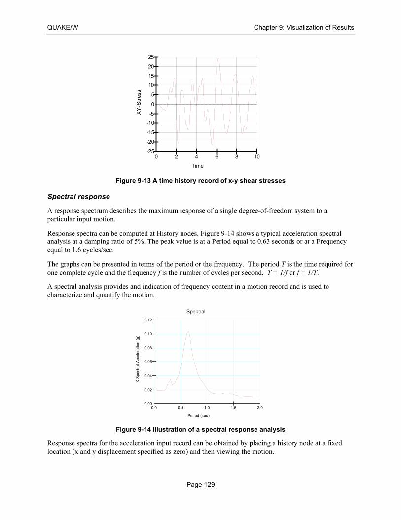
QUAKE/W Chapter 9: Visualization of Results
Page 129
Figure 9-13 A time history record of x-y shear stresses
Spectral response
A response spectrum describes the maximum response of a single degree-of-freedom system to a particular input motion.
Response spectra can be computed at History nodes. Figure 9-14 shows a typical acceleration spectral analysis at a damping ratio of 5%. The peak value is at a Period equal to 0.63 seconds or at a Frequency equal to 1.6 cycles/sec.
The graphs can be presented in terms of the period or the frequency. The period T is the time required for one complete cycle and the frequency f is the number of cycles per second. T = 1/f or f = 1/T.
A spectral analysis provides and indication of frequency content in a motion record and is used to characterize and quantify the motion.
Figure 9-14 Illustration of a spectral response analysis
Response spectra for the acceleration input record can be obtained by placing a history node at a fixed location (x and y displacement specified as zero) and then viewing the motion.
XY
-Str
ess
Time
-5
-10
-15
-20
-25
0
5
10
15
20
25
0 2 4 6 8 10
Spectral
X-S
pect
ral A
ccel
erat
ion
(g)
Period (sec)
0.00
0.02
0.04
0.06
0.08
0.10
0.12
0.0 0.5 1.0 1.5 2.0
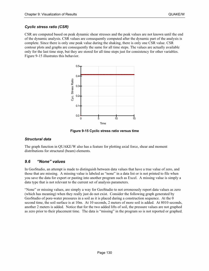
Chapter 9: Visualization of Results QUAKE/W
Page 130
Cyclic stress ratio (CSR)
CSR are computed based on peak dynamic shear stresses and the peak values are not known until the end of the dynamic analysis. CSR values are consequently computed after the dynamic part of the analysis is complete. Since there is only one peak value during the shaking, there is only one CSR value. CSR contour plots and graphs are consequently the same for all time steps. The values are actually available only for the last time step, but they are stored for all time steps just for consistency for other variables. Figure 9-15 illustrates this behavior.
Figure 9-15 Cyclic stress ratio versus time
Structural data
The graph function in QUAKE/W also has a feature for plotting axial force, shear and moment distributions for structural (beam) elements.
9.6 “None” values
In GeoStudio, an attempt is made to distinguish between data values that have a true value of zero, and those that are missing. A missing value is labeled as “none” in a data list or is not printed to file when you save the data for export or pasting into another program such as Excel. A missing value is simply a data type that is not relevant to the current set of analysis parameters.
“None” or missing values, are simply a way for GeoStudio to not erroneously report data values as zero (which has meaning) when they really just do not exist. Consider the following graph generated by GeoStudio of pore-water pressures in a soil as it is placed during a construction sequence. At the 0 second time, the soil surface is at 10m. At 10 seconds, 2 meters of more soil is added. At 8010 seconds, another 2 meters is added. Notice that for the two added lifts of soil, the pressure values are not graphed as zero prior to their placement time. The data is “missing” in the program so is not reported or graphed.
Cyc
. S
tres
s R
atio
Time
0.0
0.1
0.2
0.3
0.4
0.5
0 5 10 15

QUAKE/W Chapter 9: Visualization of Results
Page 131
Figure 9-16 Graph showing how missing data is excluded and not printed as zero
9.7 Isolines
You can use the Draw Isolines command to choose either a pore-pressure or displacement category and the parameter under each category that you want to show. For example, selecting the pore-pressure category allows for a selection of either a head or pore-water pressure isoline. Selecting displacement allows you to draw an isoline of either x or y displacements. You can also choose to draw an isoline contour at an instance in time or over multiple times. If you draw an isoline at multiple time steps then you can not also view contour shading as it only exists for any instance in time. The isolines are a way to track a single value of a parameter as it changes over time.
9.8 Mohr circles
A complete picture of the stress state at a point can be viewed with a Mohr circle diagram such as in Figure 9-17.
Figure 9-17 Mohr circle of stresses in an element
Effective Stress at Node 655
Normal
20 30 40 50 60 70 80 90 100
Sh
ea
r
-40
-30
-20
-10
0
10
20
30
40
sx
sy
36.421
-24.559
85.488
26.241
95.668
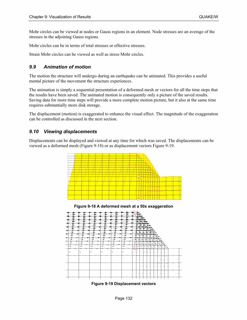
Chapter 9: Visualization of Results QUAKE/W
Page 132
Mohr circles can be viewed at nodes or Gauss regions in an element. Node stresses are an average of the stresses in the adjoining Gauss regions.
Mohr circles can be in terms of total stresses or effective stresses.
Strain Mohr circles can be viewed as well as stress Mohr circles.
9.9 Animation of motion
The motion the structure will undergo during an earthquake can be animated. This provides a useful mental picture of the movement the structure experiences.
The animation is simply a sequential presentation of a deformed mesh or vectors for all the time steps that the results have been saved. The animated motion is consequently only a picture of the saved results. Saving data for more time steps will provide a more complete motion picture, but it also at the same time requires substantially more disk storage.
The displacement (motion) is exaggerated to enhance the visual effect. The magnitude of the exaggeration can be controlled as discussed in the next section.
9.10 Viewing displacements
Displacements can be displayed and viewed at any time for which was saved. The displacements can be viewed as a deformed mesh (Figure 9-18) or as displacement vectors Figure 9-19.
Figure 9-18 A deformed mesh at a 50x exaggeration
Figure 9-19 Displacement vectors
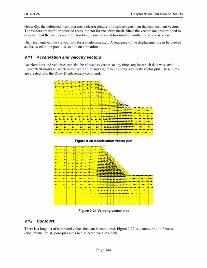
QUAKE/W Chapter 9: Visualization of Results
Page 133
Generally, the deformed mesh presents a clearer picture of displacements than the displacement vectors. The vectors are useful in selected areas, but not for the entire mesh. Since the vectors are proportioned to displacement the vectors are often too long in one area and too small in another area or vise versa.
Displacements can be viewed only for a single time step. A sequence of the displacements can be viewed as discussed in the previous section on animation.
9.11 Acceleration and velocity vectors
Accelerations and velocities can also be viewed as vectors at any time step for which data was saved. Figure 9-20 shows an acceleration vector plot and Figure 9-21 shows a velocity vector plot. These plots are created with the Draw Displacement command.
Figure 9-20 Acceleration vector plot
Figure 9-21 Velocity vector plot
9.12 Contours
There is a long list of computed values that can be contoured. Figure 9-22 is a contour plot of excess (final minus initial) pore-pressures in a selected zone in a dam.

Chapter 9: Visualization of Results QUAKE/W
Page 134
Figure 9-22 Contours of excess pore-pressure
The contour dialog box shows the data range for the selected parameter as illustrated in Figure 9-23. In this example, the pore-pressure range is -28 to 147.6 kPa. From this, QUAKE/W computes a starting contour value, a contour interval and the number of contours. These are default values. Seldom do these default contour parameters give a nice picture. The reason for irregularity in the contour is numeric noise in the data at the extremities of the data range. Usually the contour parameters need some adjustment to produce meaningful and publishable contour plots. The default values are good for a quick glance at the results, but not adequate for presentation purposes.
It usually takes several iterations to obtain a contour plot that is meaningful and presents the intended message. Once done, you can name and save the settings for easy display without having to redefine ranges etc.
Contours are always created from values at the nodes. Certain values are, however, computed and stored at the element Gauss integration; for example, all stresses are computed and stored at the element Gauss integration points. For contouring purposes, the Gauss-location values are projected to the element nodes using the interpreting functions that were adopted for the finite element formulation (see Theory chapter). After the element Gauss values have been project to the nodes, the values from all elements common to a node are average. It is this average nodal value that is used for contouring.
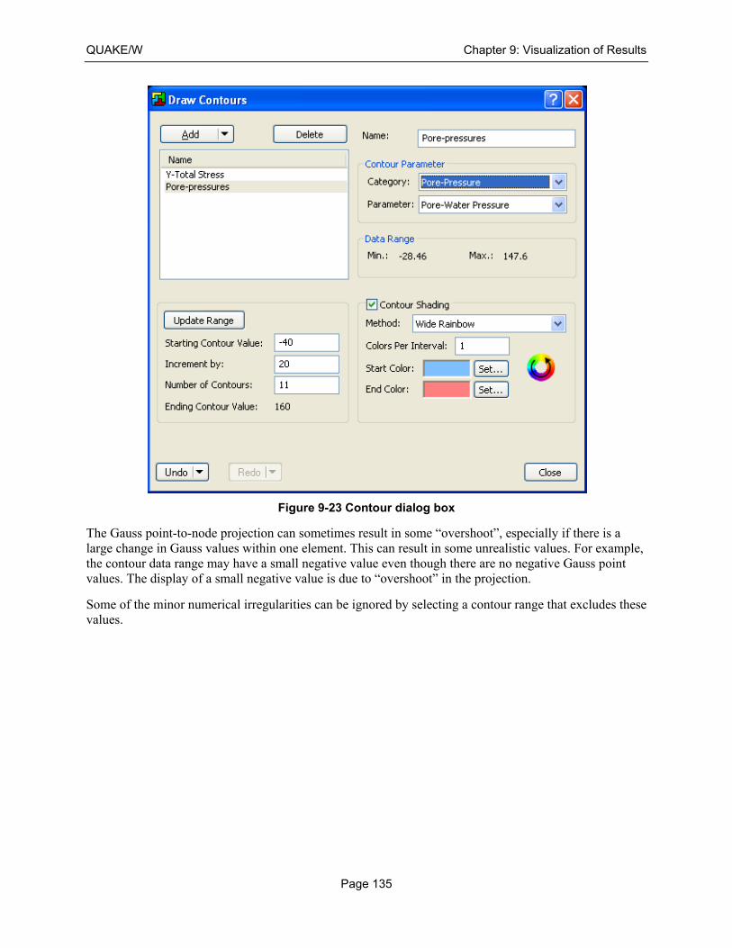
QUAKE/W Chapter 9: Visualization of Results
Page 135
Figure 9-23 Contour dialog box
The Gauss point-to-node projection can sometimes result in some “overshoot”, especially if there is a large change in Gauss values within one element. This can result in some unrealistic values. For example, the contour data range may have a small negative value even though there are no negative Gauss point values. The display of a small negative value is due to “overshoot” in the projection.
Some of the minor numerical irregularities can be ignored by selecting a contour range that excludes these values.

Chapter 9: Visualization of Results QUAKE/W
Page 136

QUAKE/W Chapter 10: Illustrative and Verification Examples
Page 137
10 Illustrative and Verification Examples
A variety of verification and illustrative examples has been developed and are available with the software. These examples can be useful for learning how to model various problems, particularly in the selection and application of boundary conditions. Each example comes with a PDF document that provides explanations on the problem setup, comments on modeling techniques and a commentary on interpreting the results. Verification examples are discussed in terms of closed-form solutions, published information and/or laboratory measurements.
All of the examples can be downloaded and installed from GEO-SLOPE’s web site (www.geo-slope.com). Once installed, it is possible to search for a particular type of analysis on the GeoStudio desktop. Conversely, the search feature is available directly on the website. It should be noted that a product-specific search is possible (e.g. search for TEMP/W or SIGMA/W).
The GeoStudio example files can be reviewed using the free GeoStudio Viewer license.

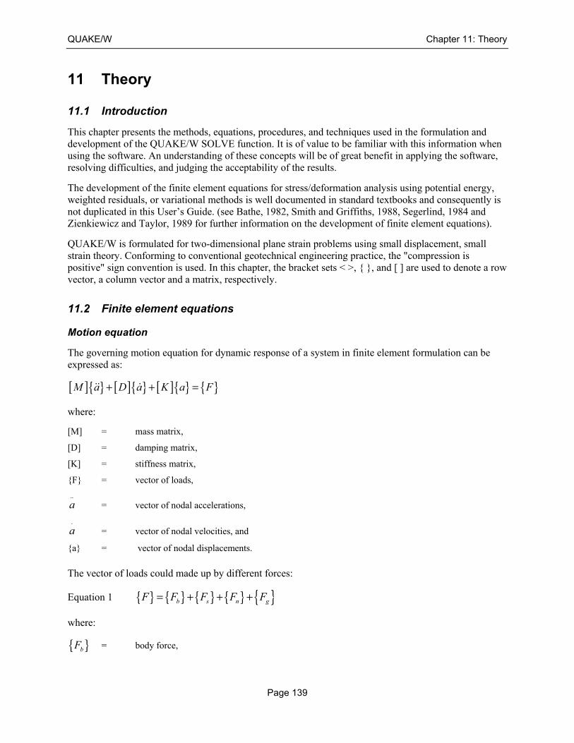
QUAKE/W Chapter 11: Theory
Page 139
11 Theory
11.1 Introduction
This chapter presents the methods, equations, procedures, and techniques used in the formulation and development of the QUAKE/W SOLVE function. It is of value to be familiar with this information when using the software. An understanding of these concepts will be of great benefit in applying the software, resolving difficulties, and judging the acceptability of the results.
The development of the finite element equations for stress/deformation analysis using potential energy, weighted residuals, or variational methods is well documented in standard textbooks and consequently is not duplicated in this User’s Guide. (see Bathe, 1982, Smith and Griffiths, 1988, Segerlind, 1984 and Zienkiewicz and Taylor, 1989 for further information on the development of finite element equations).
QUAKE/W is formulated for two-dimensional plane strain problems using small displacement, small strain theory. Conforming to conventional geotechnical engineering practice, the "compression is positive" sign convention is used. In this chapter, the bracket sets < >, { }, and [ ] are used to denote a row vector, a column vector and a matrix, respectively.
11.2 Finite element equations
Motion equation
The governing motion equation for dynamic response of a system in finite element formulation can be expressed as:
[ ]{ } [ ]{ } [ ]{ } { }M a D a K a F+ + =
where:
[M] = mass matrix,
[D] = damping matrix,
[K] = stiffness matrix,
{F} = vector of loads,
..
a = vector of nodal accelerations,
.
a = vector of nodal velocities, and
{a} = vector of nodal displacements.
The vector of loads could made up by different forces:
Equation 1 { } { } { } { } { }b s n gF F F F F= + + +
where:
{ }bF = body force,
Chapter 11: Theory QUAKE/W
Page 140
{ }sF = force due to surface boundary pressures,
{ }nF = concentrated nodal force, and
{ }gF = force due to earthquake load.
11.3 Mass matrix
The mass matrix can be a consistent mass matrix or a lumped mass matrix. The consistent mass matrix:
[ ] T
vM N N dvρ=
The lumped mass matrix:
[ ] [ ]v
M dvρ ψ=
where:
ρ = mass density,
N = row vector of interpolating functions, and
[ ]ψ = a diagonal matrix of mass distribution factors.
QUAKE/W uses a lumped mass matrix.
11.4 Damping matrix
It is common practice to assume the damping matrix to be a linear combination of mass matrix and stiffness matrix:
[ ] [ ] [ ]D M Kα β= +
where α and β are scalars and called Rayleigh damping coefficients. They can be related to a damping
ratio η by:
2
2
α βωηω
+=
where ω is the particular frequency of vibration for the system.
QUAKE/W computes the Rayleigh damping coefficients by using the lowest and the second lowest system frequencies and a constant damping ratio.
11.5 Stiffness matrix
The stiffness matrix is:
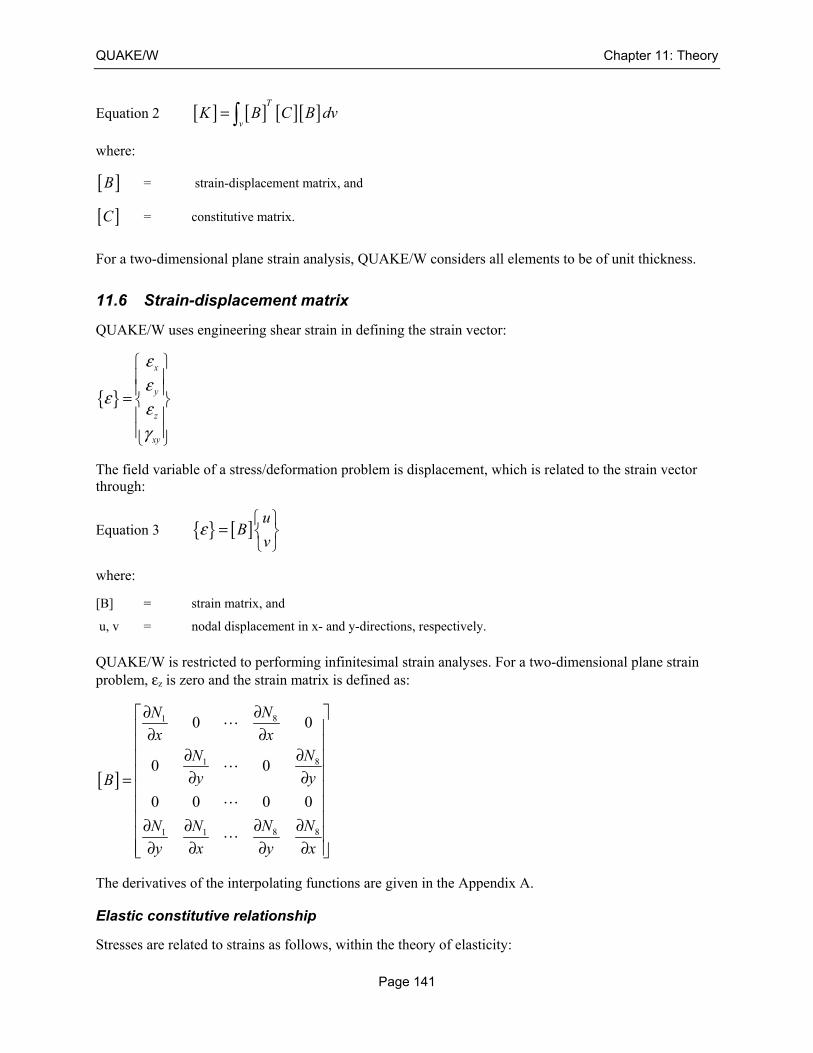
QUAKE/W Chapter 11: Theory
Page 141
Equation 2 [ ] [ ] [ ][ ]T
vK B C B dv=
where:
[ ]B = strain-displacement matrix, and
[ ]C = constitutive matrix.
For a two-dimensional plane strain analysis, QUAKE/W considers all elements to be of unit thickness.
11.6 Strain-displacement matrix
QUAKE/W uses engineering shear strain in defining the strain vector:
{ }x
y
z
xy
εε
εεγ
=
The field variable of a stress/deformation problem is displacement, which is related to the strain vector through:
Equation 3 { } [ ] uB
vε
=
where:
[B] = strain matrix, and
u, v = nodal displacement in x- and y-directions, respectively.
QUAKE/W is restricted to performing infinitesimal strain analyses. For a two-dimensional plane strain problem, εz is zero and the strain matrix is defined as:
[ ]
81
81
8 81 1
0 0
0 0
0 0 0 0
NN
x xNN
y yB
N NN N
y x y x
∂∂ ∂ ∂
∂∂ ∂ ∂= ∂ ∂∂ ∂
∂ ∂ ∂ ∂
The derivatives of the interpolating functions are given in the Appendix A.
Elastic constitutive relationship
Stresses are related to strains as follows, within the theory of elasticity:
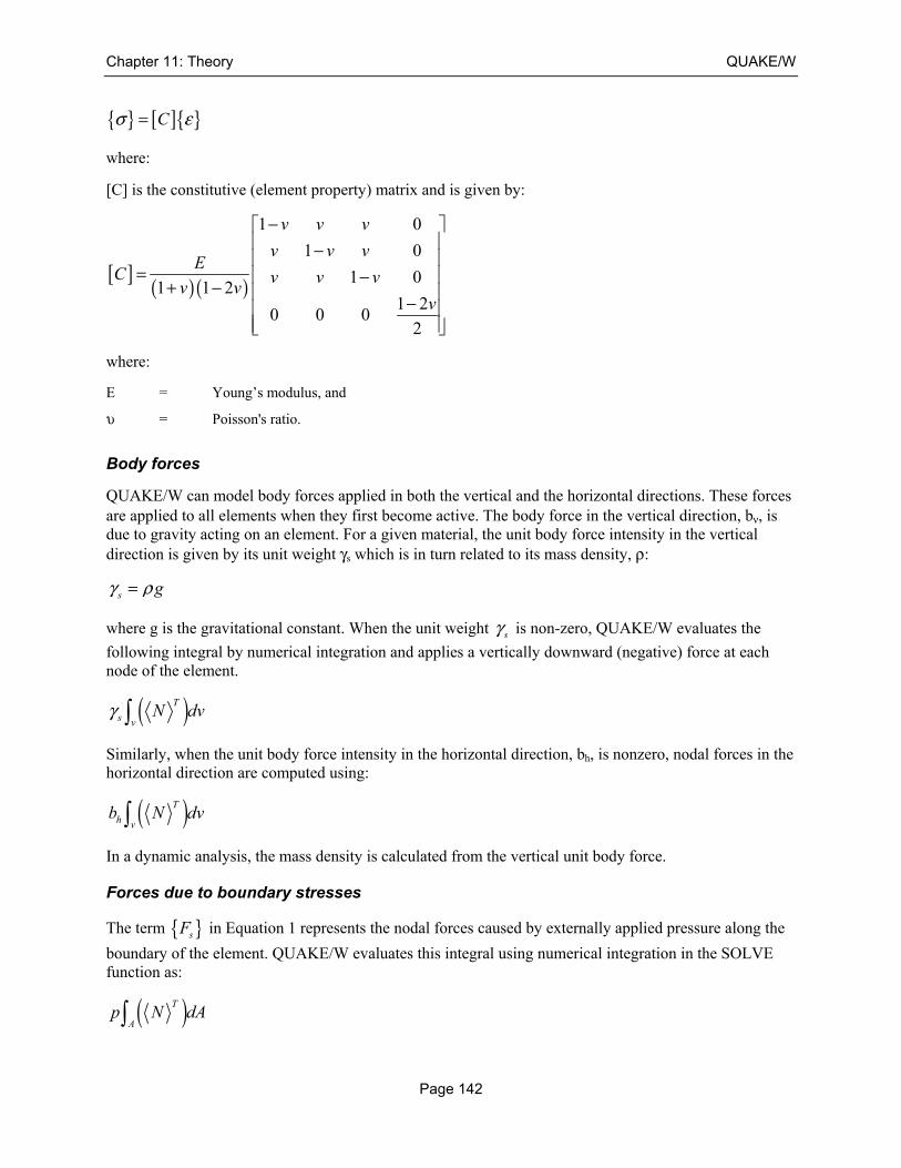
Chapter 11: Theory QUAKE/W
Page 142
{ } [ ]{ }Cσ ε=
where:
[C] is the constitutive (element property) matrix and is given by:
[ ] ( )( )
1 0
1 0
1 01 1 2
1 20 0 0
2
v v v
v v vE
C v v vv v
v
− −
= −+ − −
where:
E = Young’s modulus, and
υ = Poisson's ratio.
Body forces
QUAKE/W can model body forces applied in both the vertical and the horizontal directions. These forces are applied to all elements when they first become active. The body force in the vertical direction, bν, is due to gravity acting on an element. For a given material, the unit body force intensity in the vertical direction is given by its unit weight γs which is in turn related to its mass density, ρ:
s gγ ρ=
where g is the gravitational constant. When the unit weight sγ is non-zero, QUAKE/W evaluates the
following integral by numerical integration and applies a vertically downward (negative) force at each node of the element.
( )T
s vN dvγ
Similarly, when the unit body force intensity in the horizontal direction, bh, is nonzero, nodal forces in the horizontal direction are computed using:
( )T
h vb N dv
In a dynamic analysis, the mass density is calculated from the vertical unit body force.
Forces due to boundary stresses
The term { }sF in Equation 1 represents the nodal forces caused by externally applied pressure along the
boundary of the element. QUAKE/W evaluates this integral using numerical integration in the SOLVE function as:
( )T
Ap N dA
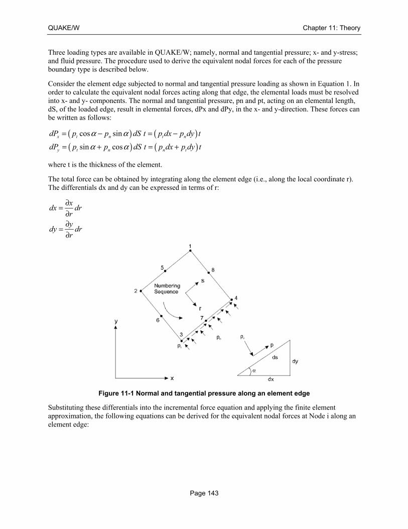
QUAKE/W Chapter 11: Theory
Page 143
Three loading types are available in QUAKE/W; namely, normal and tangential pressure; x- and y-stress; and fluid pressure. The procedure used to derive the equivalent nodal forces for each of the pressure boundary type is described below.
Consider the element edge subjected to normal and tangential pressure loading as shown in Equation 1. In order to calculate the equivalent nodal forces acting along that edge, the elemental loads must be resolved into x- and y- components. The normal and tangential pressure, pn and pt, acting on an elemental length, dS, of the loaded edge, result in elemental forces, dPx and dPy, in the x- and y-direction. These forces can be written as follows:
( ) ( )( ) ( )
cos sin
sin cos
x t n t n
y t n n t
dP p p dS t p dx p dy t
dP p p dS t p dx p dy t
α αα α
= − = −
= + = +
where t is the thickness of the element.
The total force can be obtained by integrating along the element edge (i.e., along the local coordinate r). The differentials dx and dy can be expressed in terms of r:
xdx dr
ry
dy drr
∂=∂∂=∂
Figure 11-1 Normal and tangential pressure along an element edge
Substituting these differentials into the incremental force equation and applying the finite element approximation, the following equations can be derived for the equivalent nodal forces at Node i along an element edge:
Chapter 11: Theory QUAKE/W
Page 144
xi i t n
S
yi i n t
S
x yP N t p p dr
r r
x yP N t p p dr
r r
∂ ∂ = − ∂ ∂
∂ ∂ = + ∂ ∂
The integration is carried out numerically in QUAKE/W SOLVE using Gaussian quadrature. The number of integration points used corresponds to the number of nodes along this element edge.
Resolution of elemental forces will not be necessary when x- and y-stresses being applied along an edge of the element. The equations for the equivalent nodal forces become:
xi i x
S
yi i y
S
xP N t p dr
r
xP N t p dr
r
∂ = ∂
∂ = ∂
The fluid pressure boundary is as a particular case of normal and tangential case in which no tangential pressure is applied. During numerical integration, fluid pressure is evaluated at each integration point, say the i-th integration point, using:
( )ni f f iP y yγ= − , ( ) 0f iy y− >
where:
fγ = the self-weight of the fluid,
fy = the elevation of the fluid, and,
iy = the y-coordinate at the integration point.
The fluid pressure is only computed when the fluid elevation exceeds the y-coordinate of an integration point.
Forces due to earthquake load
Earthquake loading can be expressed as:
{ } [ ]{ }g gF M a=
where:
[ ]M is the mass matrix ,
{ }ga is the applied nodal accelerations.
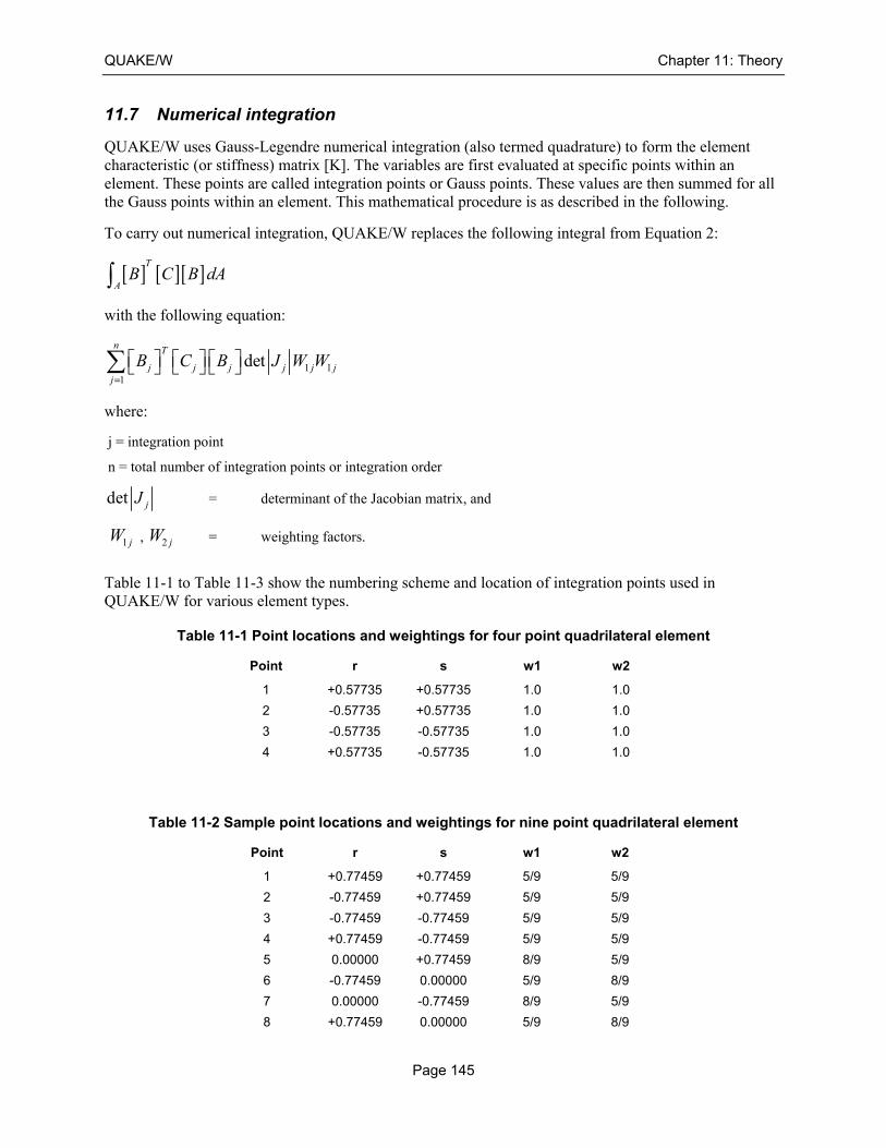
QUAKE/W Chapter 11: Theory
Page 145
11.7 Numerical integration
QUAKE/W uses Gauss-Legendre numerical integration (also termed quadrature) to form the element characteristic (or stiffness) matrix [K]. The variables are first evaluated at specific points within an element. These points are called integration points or Gauss points. These values are then summed for all the Gauss points within an element. This mathematical procedure is as described in the following.
To carry out numerical integration, QUAKE/W replaces the following integral from Equation 2:
[ ] [ ][ ]T
AB C B dA
with the following equation:
1 11
detn T
j j j j j jj
B C B J W W=
where:
j = integration point
n = total number of integration points or integration order
det jJ = determinant of the Jacobian matrix, and
1 jW , 2 jW = weighting factors.
Table 11-1 to Table 11-3 show the numbering scheme and location of integration points used in QUAKE/W for various element types.
Table 11-1 Point locations and weightings for four point quadrilateral element
Point r s w1 w2
1 +0.57735 +0.57735 1.0 1.0
2 -0.57735 +0.57735 1.0 1.0
3 -0.57735 -0.57735 1.0 1.0
4 +0.57735 -0.57735 1.0 1.0
Table 11-2 Sample point locations and weightings for nine point quadrilateral element
Point r s w1 w2
1 +0.77459 +0.77459 5/9 5/9
2 -0.77459 +0.77459 5/9 5/9
3 -0.77459 -0.77459 5/9 5/9
4 +0.77459 -0.77459 5/9 5/9
5 0.00000 +0.77459 8/9 5/9
6 -0.77459 0.00000 5/9 8/9
7 0.00000 -0.77459 8/9 5/9
8 +0.77459 0.00000 5/9 8/9
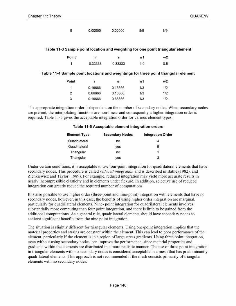
Chapter 11: Theory QUAKE/W
Page 146
9 0.00000 0.00000 8/9 8/9
Table 11-3 Sample point location and weighting for one point triangular element
Point r s w1 w2
1 0.33333 0.33333 1.0 0.5
Table 11-4 Sample point locations and weightings for three point triangular element
Point r s w1 w2
1 0.16666 0.16666 1/3 1/2
2 0.66666 0.16666 1/3 1/2
3 0.16666 0.66666 1/3 1/2
The appropriate integration order is dependent on the number of secondary nodes. When secondary nodes are present, the interpolating functions are non-linear and consequently a higher integration order is required. Table 11-5 gives the acceptable integration order for various element types.
Table 11-5 Acceptable element integration orders
Element Type Secondary Nodes Integration Order
Quadrilateral no 4
Quadrilateral yes 9
Triangular no 1
Triangular yes 3
Under certain conditions, it is acceptable to use four-point integration for quadrilateral elements that have secondary nodes. This procedure is called reduced integration and is described in Bathe (1982), and Zienkiewicz and Taylor (1989). For example, reduced integration may yield more accurate results in nearly incompressible elasticity and in elements under flexure. In addition, selective use of reduced integration can greatly reduce the required number of computations.
It is also possible to use higher order (three-point and nine-point) integration with elements that have no secondary nodes, however, in this case, the benefits of using higher order integration are marginal, particularly for quadrilateral elements. Nine- point integration for quadrilateral elements involves substantially more computing than four point integration, and there is little to be gained from the additional computations. As a general rule, quadrilateral elements should have secondary nodes to achieve significant benefits from the nine point integration.
The situation is slightly different for triangular elements. Using one-point integration implies that the material properties and strains are constant within the element. This can lead to poor performance of the element, particularly if the element is in a region of large stress gradients. Using three point integration, even without using secondary nodes, can improve the performance, since material properties and gradients within the elements are distributed in a more realistic manner. The use of three point integration in triangular elements with no secondary nodes is considered acceptable in a mesh that has predominantly quadrilateral elements. This approach is not recommended if the mesh consists primarily of triangular elements with no secondary nodes.
QUAKE/W Chapter 11: Theory
Page 147
11.8 Temporal integration
The motion equation is a second-order propagation type of equation. This equation can be solved in either frequency domain or time domain. Solution in time domain is preferred when material property may change with time. There are many methods for advancing the solution in time domain. QUAKE/W uses Wilson-θ methods to perform the time domain integration of the motion equation. The Wilson-θ method can be expressed as follows:
Assuming the displacement, velocity and acceleration at time t are known: at, a-t, a--t, the acceleration is assumed to be linear from time t to time t+θΔt, where θ >=1.0, then the acceleration at any time t+τ between t and t+θΔt, can be expressed as:
Equation 4 ( )t t t t ta a a at
τ θτθ
+ + Δ= + −Δ
The velocity and displacement at any time t+τ between t and t+θΔt, can be obtained by integration as follows:
Equation 5 2
0( )
2t t t t t t t ta a a d a a a a
t
ττ τ θττ τθ
+ + + Δ= + = + + −Δ
Equation 6 2 3
0( )
2 6t t t t t t t t ta a a d a a a a a
t
ττ τ θτ ττ τθ
+ + + Δ= + = + + + −Δ
By integrating the above equations from time t to t+θΔt, the above equations become:
( )2
t t t t t tta a a aθ θθ+ + ΔΔ= + +
2 2
( 2 )6
t t t t t t tta a ta a aθ θθθ+ Δ + ΔΔ= + Δ + +
Solving the above equations, get the acceleration and velocity at time t+θΔt in terms of displacement at time t+θΔt, we have:
Equation 7 2 2
6 6( ) 2t t t t t t ta a a a a
t tθ θ
θ θ+ Δ + Δ= − − −
Δ Δ
Equation 8 3
( ) 22
t t t t t t tta a a a a
tθ θ θ
θ+ Δ + Δ Δ= − − −
Δ
Substituting the above equations into the motion equation at time t+θΔt:
[ ]{ } [ ]{ } [ ]{ } { }t t t t t t t tM a C a K a F
θ θ θ θ+ Δ + Δ + Δ + Δ+ + =
Let:
[ ] [ ] [ ]2 2
6 3K M C K
t tθ θ = + + Δ Δ

Chapter 11: Theory QUAKE/W
Page 148
{ } { } [ ] { } { } { }
[ ] { } { } { }
2 2
6 6( 2 )
3( 2 )
2
t t t t t t t
t t t
F F M a a at t
tC a a a
t
θ θ
θ θθ
θ
+ Δ + Δ= + + + +Δ Δ
Δ+ + +Δ
Then, we have:
{ } { }t tt tK a F
θθ + Δ+ Δ =
Solving this equation and using equation Equation 7 and Equation 8 to get t ta θ+ Δ and t ta θ+ Δ , and let τ = Δt in Equation 4 to Equation 6, then we can get the displacement, velocity and acceleration at time t+Δt.
{ } { } { } { }1( )
t t t t t ta a a a
θ
θ+Δ + Δ= + −
{ } { } { } { }( )2
t t t t t tta a a a
+Δ +ΔΔ= + +
{ } { } { } { } { }2 2
3 6t t t t t t tt t
a a t a a a+Δ +ΔΔ Δ= + Δ + +
Repeat these steps to get a solution at each time step.
11.9 Equation solver
QUAKE/W uses Cholesky Factorization technique to solve the finite element equations. This technique is closely related to the Gauss elimination method. For Cholesky factorization, the stiffness matrix is decomposed by a triangular matrix as follows:
[ ] [ ][ ]TK L L=
where: [L] is a triangular matrix.
A generalized finite element equation can be expressed as:
[ ]{ } { }K a F=
By Cholesky factorization, it becomes:
[ ][ ] { } { }TL L a F=
Assuming a new vector {b} that satisfy following triangular equations and solve the {b}:
[ ]{ } { }L b F=
The final solution {a} can be obtained by back substitution of {b} into the following equations:
[ ] { } { }TL a b=
QUAKE/W Chapter 11: Theory
Page 149
The Cholesky factorization is suitable for the solution of positive definite systems. In a positive definite system, all diagonal terms in the stiffness matrix are positive.
11.10 Element stresses
QUAKE/W computes the stresses and strains at each integration point within each element once the nodal displacements have been obtained. Strains are computed from nodal displacements using Equation 3. Stresses are computed at each Gauss point using the constitutive matrix [C] in the following manner:
[ ]x x
y y
z z
xy xy
C
σ εσ εσ ετ γ
=
11.11 Linear elastic model
The simplest QUAKE/W soil model is the linear elastic model for which stresses are directly proportional to the strains. The proportionality constants are Young's Modulus, E, and Poisson's Ratio, v. The stresses and strain are related by the equation:
( )( )
1 0
1 0
1 01 1 2
1 20 0 0
2
x x
y y
z z
xy xy
v v v
v v vE
v v vv v
v
σ εσ εσ ετ γ
− − = −+ − −
For a two-dimensional plane strain analysis, εz is zero.
It is noteworthy that when v approaches 0.5, the term (1-2v)/2 approaches zero and the term (1-v) approaches v. This means that the stresses and strains are directly related by a constant, which is representative of pure volumetric strain. Furthermore, the term E/[(1+v)(1-2v)] tends towards infinity as (1-2v) approaches zero. Physically, this means that the volumetric strain tends towards zero as Poisson’s ratio approaches 0.5.
For computation purposes, v can never be 0.5; even values greater than 0.49 can cause numerical problems. Consequently, QUAKE/W limits the maximum value for Poisson’s ratio to 0.49.

Chapter 11: Theory QUAKE/W
Page 150

QUAKE/W Appendix A: Interpolating Functions
Page 151
12 Appendix A: Interpolating Functions
The global coordinate system used in the formulation of QUAKE/W is the first quadrant of a conventional x y Cartesian system.
The local coordinate system used in the formulation of element matrices is presented in Figure 12-1. Presented as well in Figure 12-1 is the local element node numbering system. The local coordinates for each of the nodes are given in Table 12-1.
Table 12-1 Local element node numbering system
Element Type Node r s
Quadrilateral 1 +1 +1
2 -1 +1
3 -1 -1
4 +1 -1
5 0 +1
6 -1 0
7 0 -1
8 1 0
Triangular 1 0 0
2 1 0
3 1 1
4 – –
5 ½ 0
6 ½ ½
7 0 ½
8 – –
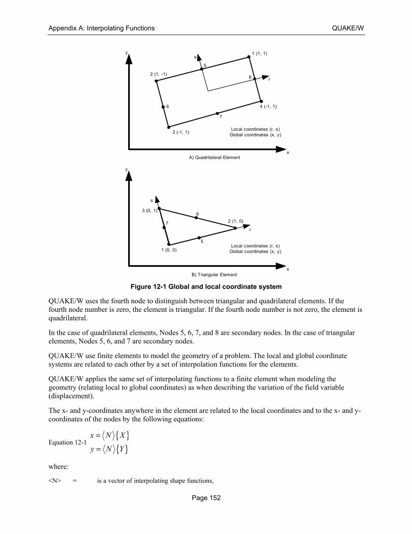
Appendix A: Interpolating Functions QUAKE/W
Page 152
Figure 12-1 Global and local coordinate system
QUAKE/W uses the fourth node to distinguish between triangular and quadrilateral elements. If the fourth node number is zero, the element is triangular. If the fourth node number is not zero, the element is quadrilateral.
In the case of quadrilateral elements, Nodes 5, 6, 7, and 8 are secondary nodes. In the case of triangular elements, Nodes 5, 6, and 7 are secondary nodes.
QUAKE/W use finite elements to model the geometry of a problem. The local and global coordinate systems are related to each other by a set of interpolation functions for the elements.
QUAKE/W applies the same set of interpolating functions to a finite element when modeling the geometry (relating local to global coordinates) as when describing the variation of the field variable (displacement).
The x- and y-coordinates anywhere in the element are related to the local coordinates and to the x- and y-coordinates of the nodes by the following equations:
Equation 12-1 { }{ }
x N X
y N Y
=
=
where:
<N> = is a vector of interpolating shape functions,
2 (1, -1)
1 (1, 1)
3 (-1, 1)
4 (-1, 1)6
5
8
7
Local coordinates (r, s)Global coordinates (x, y)
y
x
r
s
A) Quadrilateral Element
2 (1, 0)
1 (0, 0)
7
5Local coordinates (r, s)
Global coordinates (x, y)
y
x
r
s
B) Triangular Element
3 (0, 1)6

QUAKE/W Appendix A: Interpolating Functions
Page 153
{X} = the global x-coordinates of the element nodes, and
{Y} = the global y-coordinates of the element node.
The interpolating functions are expressed in terms of local coordinates. Therefore, once a set of local coordinates (r,s) have been specified, the corresponding global coordinates can be determined by Equation 12-1.
12.1 Interpolating functions
QUAKE/W uses a general set of interpolating functions presented by Bathe (1982). These general functions are suitable for elements which have none, some, or all of the secondary nodes defined. This allows for considerable versatility in the types of elements that can be used.
The interpolating functions in terms of local coordinate’s r and s for quadrilateral and triangular elements are given in Table 12-2 and Table 12-3, respectively.
The functions represent a linear equation when the secondary nodes are missing, and a quadratic (nonlinear) equation when the secondary nodes are included.
Table 12-2 Interpolation functions for quadrilateral elements
Function Include in function if node is present
5 6 7 8
N1 = ¼(1+r)(1+s) -½N5 – – -½N8
N2 = ¼(1-r)(1+s) -½N5 -½N6 – –
N3 = ¼(1-r)(1-s) – -½N6 -½N7 –
N4 = ¼(1+r)(1-s) – – -½N7 -½N8
N5 = ½(1-r2)(1+s) – – – –
N6 = ½(1-s2)(1-r) – – – –
N6 = ½(1-s2)(1-r) – – – –
N7 = ½(1-r2)(1-s) – – – –
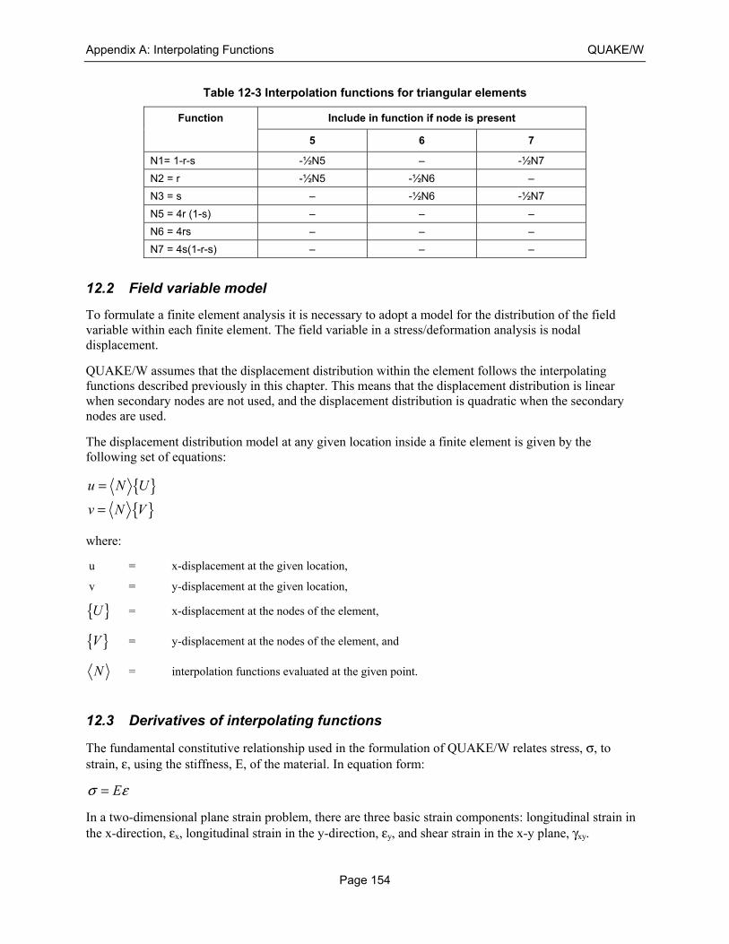
Appendix A: Interpolating Functions QUAKE/W
Page 154
Table 12-3 Interpolation functions for triangular elements
Function Include in function if node is present
5 6 7
N1= 1-r-s -½N5 – -½N7
N2 = r -½N5 -½N6 –
N3 = s – -½N6 -½N7
N5 = 4r (1-s) – – –
N6 = 4rs – – –
N7 = 4s(1-r-s) – – –
12.2 Field variable model
To formulate a finite element analysis it is necessary to adopt a model for the distribution of the field variable within each finite element. The field variable in a stress/deformation analysis is nodal displacement.
QUAKE/W assumes that the displacement distribution within the element follows the interpolating functions described previously in this chapter. This means that the displacement distribution is linear when secondary nodes are not used, and the displacement distribution is quadratic when the secondary nodes are used.
The displacement distribution model at any given location inside a finite element is given by the following set of equations:
{ }{ }
u N U
v N V
=
=
where:
u = x-displacement at the given location,
v = y-displacement at the given location,
{ }U = x-displacement at the nodes of the element,
{ }V = y-displacement at the nodes of the element, and
N = interpolation functions evaluated at the given point.
12.3 Derivatives of interpolating functions
The fundamental constitutive relationship used in the formulation of QUAKE/W relates stress, σ, to strain, ε, using the stiffness, E, of the material. In equation form:
Eσ ε=
In a two-dimensional plane strain problem, there are three basic strain components: longitudinal strain in the x-direction, εx, longitudinal strain in the y-direction, εy, and shear strain in the x-y plane, γxy.
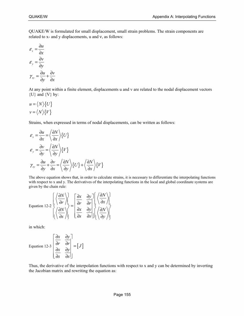
QUAKE/W Appendix A: Interpolating Functions
Page 155
QUAKE/W is formulated for small displacement, small strain problems. The strain components are related to x- and y displacements, u and ν, as follows:
x
y
xy
u
xv
y
u v
y x
ε
ε
γ
∂=∂∂=∂∂ ∂= +∂ ∂
At any point within a finite element, displacements u and v are related to the nodal displacement vectors {U} and {V} by:
{ }{ }
u N U
v N V
=
=
Strains, when expressed in terms of nodal displacements, can be written as follows:
The above equation shows that, in order to calculate strains, it is necessary to differentiate the interpolating functions with respect to x and y. The derivatives of the interpolating functions in the local and global coordinate systems are given by the chain rule:
Equation 12-2
NN x yxr r r
x yN Ns ss y
∂ ∂ ∂ ∂ ∂∂ ∂ ∂= ∂ ∂∂ ∂ ∂ ∂ ∂ ∂
in which:
Equation 12-3 [ ]x y
r r Jx y
s s
∂ ∂ ∂ ∂ = ∂ ∂ ∂ ∂
Thus, the derivative of the interpolation functions with respect to x and y can be determined by inverting the Jacobian matrix and rewriting the equation as:
{ }
{ }
{ } { }
x
y
xy
u NU
x x
v NV
y y
u v N NU V
y x y x
ε
ε
γ
∂ ∂= =∂ ∂
∂ ∂= =∂ ∂
∂ ∂ ∂ ∂= + = +∂ ∂ ∂ ∂
Appendix A: Interpolating Functions QUAKE/W
Page 156
where [ ] 1J
− is the inverse of the Jacobian.
The Jacobian matrix can be obtained by substituting Equation 12-1 into Equation 12-3 as follows:
[ ]1 181 2
2 2
81 2
8 8
...
...
X YNN NX Yr r rJ
NN N
s s s X Y
∂∂ ∂ ∂ ∂ ∂ = ∂∂ ∂ ∂ ∂ ∂
As can be seen from Equation 12-2 and Equation 12-1, derivatives of the interpolating functions are also required for calculating strains and the Jacobian.
The derivatives of the interpolation functions with respect to r and s used by QUAKE/W for quadrilateral and triangular elements are given in Table 12-4 and Table 12-5 respectively.
The following notation has been used in the preceding tables to represent the derivative of a given function Ni with respect to variable r:
,i
i r
NN
r
∂=∂
[ ] 1
N Nx r
JN N
y s
−
∂ ∂ ∂ ∂ =
∂ ∂ ∂ ∂
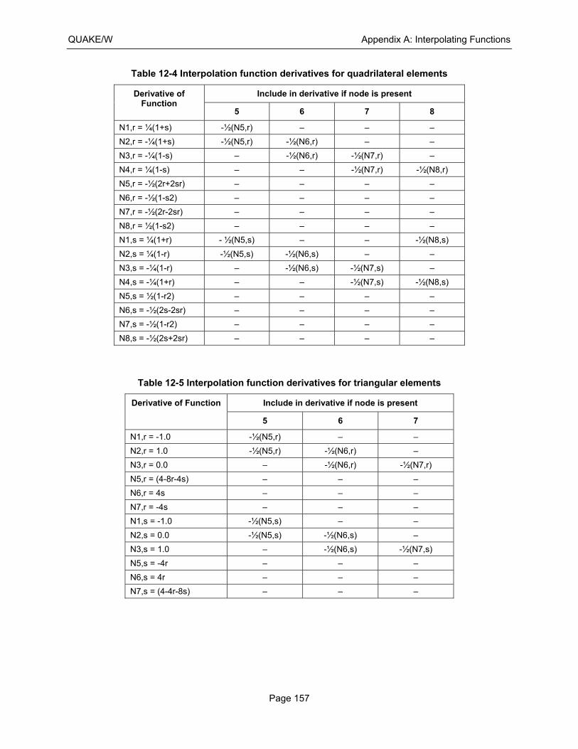
QUAKE/W Appendix A: Interpolating Functions
Page 157
Table 12-4 Interpolation function derivatives for quadrilateral elements
Derivative of Function
Include in derivative if node is present
5 6 7 8
N1,r = ¼(1+s) -½(N5,r) – – –
N2,r = -¼(1+s) -½(N5,r) -½(N6,r) – –
N3,r = -¼(1-s) – -½(N6,r) -½(N7,r) –
N4,r = ¼(1-s) – – -½(N7,r) -½(N8,r)
N5,r = -½(2r+2sr) – – – –
N6,r = -½(1-s2) – – – –
N7,r = -½(2r-2sr) – – – –
N8,r = ½(1-s2) – – – –
N1,s = ¼(1+r) - ½(N5,s) – – -½(N8,s)
N2,s = ¼(1-r) -½(N5,s) -½(N6,s) – –
N3,s = -¼(1-r) – -½(N6,s) -½(N7,s) –
N4,s = -¼(1+r) – – -½(N7,s) -½(N8,s)
N5,s = ½(1-r2) – – – –
N6,s = -½(2s-2sr) – – – –
N7,s = -½(1-r2) – – – –
N8,s = -½(2s+2sr) – – – –
Table 12-5 Interpolation function derivatives for triangular elements
Derivative of Function Include in derivative if node is present
5 6 7
N1,r = -1.0 -½(N5,r) – –
N2,r = 1.0 -½(N5,r) -½(N6,r) –
N3,r = 0.0 – -½(N6,r) -½(N7,r)
N5,r = (4-8r-4s) – – –
N6,r = 4s – – –
N7,r = -4s – – –
N1,s = -1.0 -½(N5,s) – –
N2,s = 0.0 -½(N5,s) -½(N6,s) –
N3,s = 1.0 – -½(N6,s) -½(N7,s)
N5,s = -4r – – –
N6,s = 4r – – –
N7,s = (4-4r-8s) – – –

Appendix A: Interpolating Functions QUAKE/W
Page 158

QUAKE/W References
Page 159
References
Anonymous. 1999. Definition of Geotechnical Engineering, Ground Engineering Magazine, Vol. 32, No. 11, p. 39.
Bathe, K-J., 1982. Finite Element Procedures in Engineering Analysis. Prentice-Hall.
Beakley, G.C. and Leach, H.W., 1977, Engineering An Introduction To A Creative Profession, Third Edition, Macmillan Publishing Co., Inc.(New York) and Collier Macmillan Publishers(London).
Burland, J.B. 1987. Nash Lecture: The Teaching of Soil Mechanics – a Personal View. Proceedings, 9th ECSMFE, Dublin, Vol. 3, pp 1427-1447.
Burland J.B. 1996. Closing Session Discussions, Proceedings of the First International Conference on Unsaturated Soils Conference, Paris, Vol. 3, p. 1562. (Proceedings published by A.A. Balkema; Editors, E.E, Alonso and P. Delage).
Carter, J.P., Desai, C.S, Potts, D.M., Schweiger, H.F, and Sloan, S.W. 2000. Computing and Computer Modeling in Geotechnical Engineering, Invited Paper, Conference Proceedings, GeoEng2000, Melbourne, Australia.
Chen, W.F. and Zhang, H., 1991. Structural Plasticity: Theory, Problems, and CAE Software. Springer-Verlag.
DeAlba, P., Chan, C.K., and Seed, H.B., 1975, Determination of Soil Liquefaction Characteristics By Large-Scale Laboratory Tests, Report EERC 75-14, Earthquake Engineering Research Center, University of California, Berkeley.
Duncan, J.M. and Chang, C.Y., 1970. Nonlinear analysis of stress and strain in soils. Journal of the Soil Mechanics and Foundations Division, ASCE, vol. 96, no. SM5, pp. 1629-1654.
Gu, W.H. and Krahn, J., (2002). A Model For Soil Structure Mobility and Collapse, 15th ASCE Engineering Mechanics Conference, June 2-5, 2002, Columbia University, New York, NY.
Gu, W.H., Morgenstern, N.R., and Robertson, P.K. (1993). Progressive Failure of Lower San Fernando Dam, ASCE Journal of Geotechnical Engineering, Vol.119, No.2, pp. 333-349.
Gu, W.H., Morgenstern, N.R., and Robertson, P.K. (1994). Post Earthquake Deformation Analysis of Wildlife Site, ASCE Journal of Geotechnical Engineering, Vol.120, No.2, pp. 333-349.
Gu, W.H. (1992). Post-earthquake Deformation Analysis, Ph.D. Dissertation, Department of Civil Engineering, University of Alberta, Edmonton, Alberta, Canada.
Hardin, B.O. and Vincent, P. D., 1972, Shear Modulus and Damping In Soils: Design Equations and Curves, Journal of the Soil Mechanics and Foundations Division, ASCE, SM7, pp667-691.
Hinton, E. and Owen, D.R.J., 1979 An Introduction to Finite Element Computations, Pineridge Press Ltd., U.K.
Hunson, M., Idriss, I.M. and Beikae, M., 1994, User's Manual for QUAD4M A Computer Program To Evaluate The Seismic Response of Soil Structures Using Finite Element Procedures and
References QUAKE/W
Page 160
Incorporating a Compliant Base, Department of Civil & Environmental Engineering, University of California Davis.
Idriss, I.M. and Sun, J., 1992, User's Manual for SHAKE91 A Computer Program For Conducting Equivalent Linear Seismic Response Analyses of Horizontally Layered Soil Deposits, Department of Civil & Environmental Engineering, University of California Davis.
Ishibashi, I., and Zhang, X., 1993, Unified Dynamic Shear Moduli and Damping Ratios of Sand and Clay, Soils and Foundations, Vol.33, No.1, pp. 182-191.
Kramer, S.L. and Seed, H.B. 1988. Initiation of Soil Liquefaction under Static Loading Conditions, ASCE Journal of Geotechnical Engineering, Vol. 114, No. 4, pp.412-430.
Kramer, S.L., 1996. Geotechnical Earthquake Engineering, Prentice Hall.
Lambe, T.W. and Whitman, R.V., 1969. Soil Mechanics. John Wiley and Sons, Inc.
Lambe, T.W. and Whitman, R.V., 1979. Soil Mechanics, SI Version. John Wiley and Sons, Inc.
Lancaster, P. and Salkauskas, K., 1986. Curve and Surface Fitting: An Introduction. Academic Press. pp.101-106.
Lee, K.L., and Albaisa, A., 1974, Earthquake Induced Settlements In Saturated Sands, Journal of The Soil Mechanics and Foundations Division, ASCE, Vol.100, No. GT4.
Lee, K.L., Seed, H.B, Idriss, I.M. and Makdisi, F. I., 1975, Properties of Soil In The San Fernando Hydraulic Fill Dams, Journal of The Geotechnical Engineering Division, ASCE, GT8, pp801- 821.
Lysmer, J. and Kuhlemeyer, R.L., 1969, Finite Dynamic Model For Infinite Media, Journal of the Engineering Mechanics Division, ASCE, EM4, pp859-877.
Lysmer, J., Udaka, T., Tsai, C.F. and Seed, H.B., 1975, FLUSH A Computer Program For Approximate 3-D Analysis of Soil-Structure Interaction Problems, Report No. EERC 75-30, College of Engineering, University of California Berkeley.
Martin, G.R., Finn, W.D.L. and Seed, H.B., 1975, Fundamentals of Liquefaction Under Cyclic Loading, Journal of The Geotechnical Engineering Division, ASCE, GT5, pp423-438.
Morgenstern , N.R. 2000. Common Ground, Invited Paper, Conference Proceedings, GeoEng2000, Melbourne, Australia.
National Research Council, 1990. Groundwater Models: Scientific and regulatory applications. Water Science and Technology Board, Committee on Ground Water Modelling Assessment. Commission on Physical Sciences, Mathematics and Resources. National Research Council, National Academy Press, Washington, D.C.
O’Kane Consultants Inc. 2004. Personal communication.
Roscoe, K. H., Schofield, A. N. and Wroth, C.P. 1958, On the Yielding of Sands, Geotechnique, Vol. 8, pp22-53.
QUAKE/W References
Page 161
Salkauskas, K., 1974. C´ splines for interpolation of rapidly varying data. Rocky Mountain Journal of Mathematics, Vol. 14, No. 1, pp.239-250.
Scott, R.F., 1973, The Calculation of Horizontal Accelerations From Seismoscope Records, Bulletin of The Seismological Society of America, Vol. 63, No.5, pp1637-1661.
Seed, H.B. and Peacock, W.H., 1971, Test Procedures For Measuring Soil Liquefaction Characteristics, Journal of the Soil Mechanics and Foundations Division, ASCE, SM8, pp1099-1119.
Seed, H.B., Idriss, I.M., Lee, K.L. and Makdisi, F.I., 1975, Dynamic Analysis of The Slide In The Lower San Fernando Dam During The Earthquake of February 9, 1971, Journal of The Geotechnical Engineering Division, ASCE, GT9, pp889-911.
Seed, H.B., Mori, K., and Chan, C.K., 1975, Influence of Seismic History On The Liquefaction Characteristics of Sands, Report EERC 75-25, Earthquake Engineering Research Center, University of California, Berkeley, 21pp.
Seed, H.B., Martin, P.P. and Lysmer, J., 1976, Pore-Water Pressure Changes During Soil Liquefaction, Journal of The Geotechnical Engineering Division, ASCE, GT4, pp323-345.
Seed, H.B., 1979, Considerations In the Earthquake-resistant Design of Earth and Rockfill Dams, Geotechnique, Vol.29, No.3, pp215-263.
Segerlind, L.J., 1984. Applied Finite Element Analysis, 2nd Ed. John Wiley and Sons, Inc.
Skopek, P, Morgenstern, N.R., Robertson, P.K. and Sego, D.C., 1994. Collapse of Dry Sand, Canadian Geotechnical Journal, Vol. 31, pp 1008-1014.
Sladen, J.A., D’Hollander, R.D. and Krahn, J., 1985. The liquefaction of sands, a collapse surface approach, Canadian Geotechnical Journal Vol.22, pp.564-578.
Smith, G.D., 1971. Numerical Solution of Partial Differential Equations, Oxford University Press, Oxford.
Smith, I.M. and Griffiths, D.V., 1988. Programming the Finite Element Method, 2nd Ed. John Wiley and Sons Ltd.
Swaisgood, J.R. and Oliveros, U.G., 2003. Unusual Mine Waste Dam Shakes off Magnitude 8.3 Earthquake, Proceeding: Tailing and Mine Waste Conference, Vail, Colorado, USA; A.A. Balkema Publishers, p. 519.
Terzaghi, K., 1943. Theoretical Soil Mechanics, John Wiley and Sons Ltd.
Vaid, Y.P. and Chern, J.C. 1983. Effect of static shear on resistance of liquefaction, Soils and Foundations, Vol.23, No.1, pp.47-60.
Weaver, W., Timoshenko, S. P., and Yong, D.H., 1990, Vibration Problems in Engineering, John Wiley & Sons Ltd.
Youd, T.L. and Idriss, I.M. 2001. Liquefaction Resistance of Soils: Summary Report from the 1996 NCEER and 1998 NCEER/NSF Workshop on Evaluation of Liquefaction Resistance of Soils. ASCE Journal of Geotechnical and Environmental Engineering, Vol. 127, No. 4, pp. 287-313.

References QUAKE/W
Page 162
Zienkiewicz, O.C. and Taylor, R.L., 1989. The Finite Element Method, 4th Ed., Vol. 1. McGraw-Hill.
Zienkiewicz, O.C., Chan, A.H.C., Pastor, M., Schrefler, B.A. and Shiomi, T., 1999, Computational Geomechanics with Special Reference To Earthquake Engineering,, John Wiley & Sons Ltd.

QUAKE/W Index
Page 163
Index
Absolute motion .......................... 121
Analysis Types .............................. 97
Animation .................................... 132
Baseline Correction ....................... 86
Boundary conditions
dynamic ..................................... 93
edge pressure ............................. 91
nodal displacements ................... 90
nodal force ................................. 90
spring ......................................... 93
Boundary Conditions ..................... 83
Burland triangle ............................. 12
Clip Board .................................... 128
Compare alternatives ..................... 15
Contours ....................................... 133
Cut and Paste ............................... 128
Cyclic stress ratio ......................... 130
Do numerical experiments ............. 23
Draw
initial water table ....................... 97
Earthquake Records ....................... 83
Element and mesh compatibility ... 47
Element fundamentals ................... 46
Element nodes ................................ 46
Evaluate results in the context of expected results .......................... 26
Field variable distribution .............. 46
General guidelines for meshing ..... 50
Graphing ...................................... 124
History nodes ............................... 128
How not to model .......................... 27
How to model ................................ 20
Identify governing parameters ....... 16
Illustrative Examples ................... 137
Interpolating functions ................. 151
Interrogate the results .................... 26
Joining regions ............................... 43
Material Properties ........................ 55
Meshing ......................................... 29
Meshing for transient analyses ...... 44
Model only essential components .. 24
Mohr Circles ................................ 131
Nodal history ............................... 128
Node and element information .... 123
Index QUAKE/W
Page 164
Numerical integration .................... 49
Numerical Issues .......................... 113
Numerical modeling ........................ 9
Outcrop Records ............................ 87
Peak values .................................. 126
Quantitative predictions ................. 13
Relative motion ............................ 121
Secondary variables ....................... 50
Simplify geometry ......................... 21
Spatial functions .......................... 110
Spectral Response ........................ 129
Start simple .................................... 22
Start with estimated material properties .................................... 25
Structural data .............................. 130
Structural Elements ........................ 95
Structured mesh ............................. 38
Surface mesh .................................. 40
Theory .......................................... 139
Time Steps ................................... 121
Triangular regions .......................... 39
understand physical process .......... 17
Unstructured mesh ......................... 38
Vectors
acceleration and velocity ......... 133
Viewing
dispalcements ........................... 132
Visualization of Results ............... 121
Why model? ................................... 13

Page 165
A consistent set of units
Property Units Metric Imperial
Geometry L meters feet
Unit Weight of Water F/L3 kN/m3 pcf
Soil Unit Weight F/L3 kN/m3 pcf
Cohesion F/L2 kPa pcf
Pressure F/L2 kPa psf
Force F kN lbs
E (modulus) F/L2 kPa psf