QUALITY INFORMATION DOCUMENT For IBI reanalysis …cmems-resources.cls.fr/documents/QUID/CMEMS-IBI-QUID-005-002.pdf · For IBI reanalysis Product IBI_REANALYSIS_PHYS_005_002 Issue:

QUALITY INFORMATION DOCUMENT

For IBI reanalysis Product

IBI_REANALYSIS_PHYS_005_002

Issue: 2.0

Contributors: Bruno Levier, Marcos Sotillo, Guillaume Reffray, Roland Aznar

Approval Date by Quality Assurance Review Group : under review

QUID for IBI reanalysis Product


Ref: CMEMS-IBI-QUID-005-002

Date : 14 December 2015

Issue : 2.0

© EU Copernicus Marine Service – Public Page 2/ 56

CHANGE RECORD

Issue Date § Description of Change Author Validated By

0.0

06/05/2014

All

Creation of the document

Bruno Levier, Marcos Sotillo, Guillaume Reffray

0.1 07/05/2014

All Update with High-Frequency CLASS2 metrics from the validation with data from PdE moorings

Marcos G Sotillo, Roland Aznar

1.0 12/05/2014

All Minor changes. Bruno Levier, Marcos G Sotillo

Enrique Alvarez

1.1 May 1 2015

all Change format to fit CMEMS graphical rules

L. Crosnier





Issue : 2.0


2.0 14/12/2015

all Inclusion of new metrics considering temporal extension: 2012-2014.

Bruno Levier / Marcos Sotillo

Enrique Álvarez Fanjul

TABLE OF CONTENTS

I Executive summary ....................................................................................................................................... 5

I.1 Products covered by this document ........................................................................................................... 5

I.2 Summary of the results ............................................................................................................................... 5

I.2.1 Temperature ...................................................................................................................................... 5

I.2.2 Salinity .............................................................................................................................................. 6

I.2.3 Ocean currents ................................................................................................................................... 6

I.2.4 Sea level ............................................................................................................................................ 6

I.2.5 Transports .......................................................................................................................................... 6

I.2.6 Other.................................................................................................................................................. 7

I.3 Estimated Accuracy Numbers .................................................................................................................... 7

II Production Subsystem description ................................................................................................................ 9

Reanalysis Configuration: the IBI-REA System ..................................................................................... 9

II.1 The IBI-REA ocean model: NEMO2.3 .................................................................................................... 9

II.2 Data assimilation method ........................................................................................................................ 10

III Validation framework ............................................................................................................................. 15

IV Validation results ......................................................................................................................................... 19

IV.1 Temperature ........................................................................................................................................... 19

IV.1.1 T-CLASS1-T3D-MEAN............................................................................................................. 19

IV.1.2 T-CLASS1-SST-MEAN ............................................................................................................. 20

IV.1.3 T-CLASS1-SST-TREND ........................................................................................................... 20

IV.1.4 T-CLASS2-MOORINGS ............................................................................................................ 20

IV.1.5 T-CLASS3-SST-QNET-2DMEAN ............................................................................................ 21

IV.1.6 T-CLASS3-HC_LAYER ............................................................................................................ 21





Issue : 2.0


IV.1.7 T-CLASS3-IC_CHANGE .......................................................................................................... 23

IV.1.8 T-CLASS4-LAYER .................................................................................................................... 23

IV.1.9 T-DA-INNO-STAT .................................................................................................................... 24

IV.2 Salinity ..................................................................................................................................................... 25

IV.2.1 S-CLASS1-S3D_MEAN ............................................................................................................ 25

IV.2.2 S-CLASS1-SSS-TREND ............................................................................................................ 26

IV.2.3 S-CLASS2-MOORINGS ............................................................................................................ 26

IV.2.4 S-CLASS2-SSS-SWF_2DMEAN .............................................................................................. 27

IV.2.5 S-CLASS3-SC-LAYER .............................................................................................................. 27

IV.2.6 S-CLASS3-IC_CHANGE........................................................................................................... 28

IV.2.7 S-CLASS4-LAYER .................................................................................................................... 29

IV.2.8 S-DA-INNO_STAT .................................................................................................................... 30

IV.3 Currents .................................................................................................................................................. 30

IV.3.1 UV-CLASS1-15m_MEAN ......................................................................................................... 30

IV.3.2 UV-CLASS2-MOORINGS ........................................................................................................ 31

IV.3.3 UV-CLASS2-MKE_1000m ........................................................................................................ 32

IV.4 Sea level ................................................................................................................................................... 32

IV.4.1 SL-CLASS1-TREND_2D........................................................................................................... 32

IV.4.2 SL-CLASS2-TIDE_GAUGE ...................................................................................................... 33

IV.4.3 SL-CLASS3-2DMEAN .............................................................................................................. 33

IV.4.4 SL-DA-INNO_STAT ................................................................................................................. 34

IV.5 Transports ............................................................................................................................................... 34

IV.6 Other monthly metrics ........................................................................................................................... 35

IV.6.1 OTH-CLASS1-MLD_CLIM_SEASON ..................................................................................... 35

IV.7 High frequency IBI Reanalysis validation with moorings .................................................................. 35

IV.7.1 SST-CLASS2-HF-MOORINGS ................................................................................................. 38

IV.7.2 UV-CLASS2-HF-MOORINGS .................................................................................................. 45

IV.7.3 SSS-CLASS2-HF-MOORINGS ................................................................................................. 49

IV.7.4 Other combined CLASS2-HF-MOORINGS metrics .................................................................. 52

V Quality changes since previous version ...................................................................................................... 55

VI References .................................................................................................................................................... 56





Issue : 2.0


I EXECUTIVE SUMMARY

I.1 Products covered by this document

The products assessed in this document are referenced as IBI_REANALYSIS_PHYS_005_002. This product contains the following 4 datasets:

These dataset includes monthly, daily and hourly mean fields on a regular lon/lat grid and on the native ORCA grid, all of them with a horizontal resolution of 1/12° (0.0833° lat x 0.0833° lon) with 75 levels from surface to bottom, for the following variables:

- sea_surface_height_above_sea_level

- sea_water_salinity

- sea_water_potential_temperature

- eastward_sea_water_velocity

- northward_sea_water_velocity

- eastward_sea_barotropic_velocity

- northward_sea_barotropic_velocity

- Sea_water_potential_temperature_at_sea_floor

- ocean_mixed_layer_thickness_defined_by_sigma_theta

The period covered is 02/2002-12/2014. . It should be noted that what is delivered in this IBI reanalysis product as bottom or sea floor temperature variable is referring to the temperature obtained at the deepest model level available for each grid point. The reanalysis, called IBIRYSV1R1 at internal CMEMS IBI MFC production level, is referenced as IBI-REA in this document. However, the name IBIRYSV1R1 still remains in some figures.

I.2 Summary of the results

The quality of the IBI-REA reanalysis has been mainly assessed validating reanalysed monthly fields with observational sources and comparing the IBI reanalysis products with the global GLORYS reanalysis ones (GLOBAL-REANALYSIS-PHYS-001-009). Furthermore, a specific evaluation of higher frequency IBI-REA outputs has been performed, by means of comparing reanalysis outputs with 10-yr hourly frequency observational data from 14 Puertos del Estado buoys, moored along the Iberian (Atlantic and Mediterranean) Spanish coasts and the Canary Island area. The headline results for each of the variables assessed are as follows:

I.2.1 Temperature





Issue : 2.0


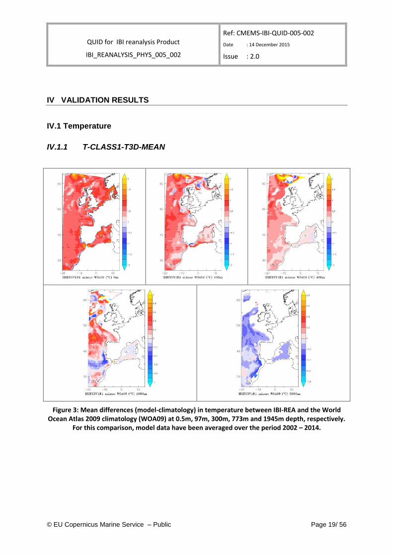
The IBI-REA reanalysis has a warm bias between surface and 1000m depth compared to Levitus 2009 climatology (except at 1000m depth in the pathway of the Mediterranean water, where the bias is cold). The bias is negative at 2000m depth. At surface, the warm bias can be greater than 1°C over the shelf, and the bias is cold along all the western coasts.

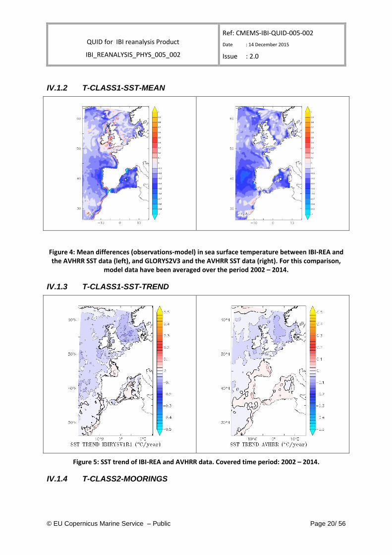
The mean SST is close to the observations with a misfit less than 0.5°C, except in shelf areas: the reanalysis is warmer than the observations along the French and Spanish coasts, and in the Gulf of Lions. The reanalysis is colder than the observations in the Irish and Celtic sea and in the English channel.

The trend is consistent with AVHRR data, negative in the northern part of the domain, and positive all around the Iberian Peninsula and along the Moroccan coast.

Compared to in-situ profiles, the bias of the IBI-REA reanalysis is weak (less than 0.1°C except near the surface), and the RMS error generally weaker than the GLORYS one (less than 0.5°C except near the surface).

I.2.2 Salinity

Compared to the WOA 2009 climatology, the IBI-REA reanalysis is generally saltier between the surface and 1000m depth. At the surface, IBI-REA is less salty along the European coasts, in the Irish sea and in the Mediterranean sea (especially at 100m depth in the Algerian current).

The bias is weak compared to in-situ profiles (maximum at the surface, decreasing towards the bottom). The RMS in average is 0.2 psu in the 5-200m layer, less than 0.1 psu below 200m. IBI-REA performs slightly better than GLORYS.

I.2.3 Ocean currents

IBI-REA reproduces well the main ocean currents and is coherent with the AOML surface drifter climatology. However, when compared to fixed moorings measurements, the near-surface currents are poorly correlated to the observations (generally between 0.2 and 0.5). MKE at 1000m is higher in IBI-REA than in ANDRO Argo drift data base (which seems to underestimate the MKE in the IBI area).

I.2.4 Sea level

IBI-REA reanalysis is very close to altimetric observations and has a good ability to describe the sea level variability. The globally averaged RMSE of the analysed sea level is about 6~7cm. Correlations with observations at tide gauges are generally higher than 0.7 and better than GLORYS2V3 reanalysis (not shown). However, the sea level trend is not in agreement with observations.

I.2.5 Transports

The transport through the Gibraltar strait is over-estimated in the surface layer and under-estimated in the bottom layer compared to published values.





Issue : 2.0


The transport through the south Portugal section is under-estimated compared to published values, but the standard deviation of the reanalysis is high.

The transport through the Biscay section is different than published estimations.

I.2.6 Other

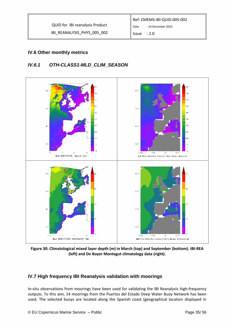
The mixed layer depth of IBI-REA reanalysis exhibits similar patterns with those in De Boyer Montegut climatology data. There is an overestimation in the north-western part of the domain.

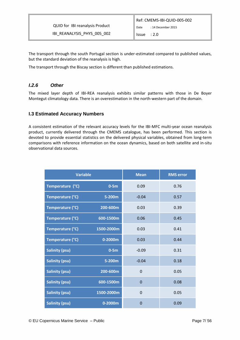
I.3 Estimated Accuracy Numbers

A consistent estimation of the relevant accuracy levels for the IBI-MFC multi-year ocean reanalysis product, currently delivered through the CMEMS catalogue, has been performed. This section is devoted to provide essential statistics on the delivered physical variables, obtained from long-term comparisons with reference information on the ocean dynamics, based on both satellite and in-situ observational data sources.

Variable Mean RMS error

Temperature (°C) 0-5m 0.09 0.76

Temperature (°C) 5-200m -0.04 0.57

Temperature (°C) 200-600m 0.03 0.39

Temperature (°C) 600-1500m 0.06 0.45

Temperature (°C) 1500-2000m 0.03 0.41

Temperature (°C) 0-2000m 0.03 0.44

Salinity (psu) 0-5m -0.09 0.31

Salinity (psu) 5-200m -0.04 0.18

Salinity (psu) 200-600m 0 0.05

Salinity (psu) 600-1500m 0 0.08

Salinity (psu) 1500-2000m 0 0.05

Salinity (psu) 0-2000m 0 0.09





Issue : 2.0






Issue : 2.0


II PRODUCTION SUBSYSTEM DESCRIPTION

Production Center: IBI MFC

Production Unit: Mercator Ocean

Dissemination Unit: Puertos del Estado

Scientific Validation Expertise: Mercator Ocean & Puertos del Estado

Reanalysis Configuration: the IBI-REA System

The present IBI MFC multi-year reanalysis product has been derived from the IBI-REA reanalysis outputs. This reanalysis system relies on the following two main components:

1. the ocean model (including the surface atmospheric boundary condition)

2. the data assimilation method and the assimilated observations

II.1 The IBI-REA ocean model: NEMO2.3

The ocean model is based on the version 2.3 of NEMO (Madec, 2008) and the configuration is NEATL12.The horizontal grid is a subset of the global 1/12° ORCA tripolar grid (367 x 638 grid points).

The original bathymetry is derived from the 30 arc-second resolution GEBCO 08 dataset (Becker et al., 2009) merged with several local databases (F. Lyard, personal communication, 2010). At open boundaries within 10-point-wide relaxation areas, bathymetry is exactly set to the parent grid model bathymetry and progressively merged with the interpolated dataset described above.

A bi-harmonic viscosity and diffusivity for the lateral dissipation of momentum and tracer are used. The diffusion coefficients are respectively -1.25e10 and -1.25e9 m

4s

-1.

The advection scheme for the momentum is written in vector form and respects the energy–entropy conservation (Barnier et al. 2006). For the tracer advection (both physical and biogeochemical variables), a 3

rd order QUICKEST scheme is used (Leonard, 1979) with the limiter of Zalezak (1979).

The vertical grid has 75 levels, with a resolution of 1 meter near the surface and 200 meters in the deep ocean. Partial bottom cell representation of the bathymetry allows an accurate representation of the steep slopes characteristic of the area.

Vertical mixing is parameterized according to a k-ε model implemented in the generic form proposed by Umlauf and Burchard (2003) including surface wave breaking induced mixing, while tracers and momentum subgrid lateral mixing is parameterized according to bilaplacian operators. Solar penetration is parameterized according to a two-band exponential scheme with monthly climatological attenuation coefficients built from Seawif satellite ocean colour imagery and IFREMER climatology.

- Surface forcing fields / corrections:

The surface boundary conditions are prescribed to the model using the CORE bulk formulation. Forcing fields are provided from ERA-Interim reanalysis products (Simons et al., 2007), interpolated on ORCA025 native grid using an Akima interpolation algorithm. The data set includes 4 turbulent variables (u10, v10, t2, q2) and the atmospheric pressure given every 3 hours and 3 fluxes: 2 downward radiative variables (radsw, radlw) and the precipitation rate given as daily average.

The ERAinterim radiative fluxes (both long wave and short wave) exhibit some unacceptable biases. Therefore a specific correction, based on GEWEX satellites fluxes products, has been implemented by





Issue : 2.0


Garric and Verbrugge (2010) in order to improve those fluxes. Basically, the idea is to apply a 2D scaling coefficient to the large scale features of the radiative fluxes. Original fields are band-pass filtered to separate large scale and small scale, using an iterative Shapiro filter. The correction is applied to the large scale and then the small scale is added to produce the radiative flux for the model.

Similar to the radiative fluxes, ERAInterim rainfall fluxes present large biases and a correction, based on GPCPV2.1 rainfalls flux, allows a more realistic SSS spatial distribution.

Due to the high vertical resolution near the surface, we implement a parameterization of the diurnal cycle on the solar flux. Input is the daily mean flux, which is spread over the day according to the time, and geographical position on the earth. This parameterization aims at better representing the night-time convection which takes place in the upper most layer of the ocean (Bernie, 2007).

Rivering inputs are implemented as lateral point sources with flow rates based on monthly climatological data taken from GRDC (http://www.bafg.de/GRDC), French “Banque Hydro” dataset (http://www.hydro.eaufrance.fr/) and simulations from SMHI.

- Lateral boundaries: Lateral open boundary data (temperature, salinity, velocities and sea level) are interpolated from the daily outputs from the MyO2 global reanalysis GLORYS2V3. These are complemented by 11 tidal harmonics (M2, S2, N2, K1, O1, Q1, M4, K2, P1, Mf, Mm) built from FES2004 (Lyard et al., 2006) and TPXO7.1 (Egbert and Erofeeva, 2002) tidal models solutions. Atmospheric pressure component, missing in the large scale parent system sea level outputs, is added hypothesing pure isostatic response at open boundaries (inverse barometer approximation).

- Initial Conditions:

The simulation started at rest, with initial temperature, salinity, velocity components and sea surface height provided by the MYO2 global reanalysis GLORYS2V3. The date of start is 2

nd January 2002.

- Time step: A baroclinic time step of 450s is used. No data were assimilated during the first four weeks.

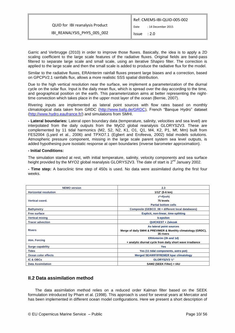
NEMO version 2.3

Horizontal resolution 1/12° (5-6 km)

Vertical coord.

z*=f(ssh)

75 levels

Partial bottom cells

Bathymetry Composite (GEBCO_08 + different local databases)

Free surface Explicit, non-linear, time-splitting

Vertical mixing k-epsilon

Tracer advection QUICKEST + Zalezak

Rivers

As lateral point sources

Merge of daily SMHI & PREVIMER & Monthly climatology (GRDC), 35 rivers

Atm. Forcing ERAinterim (3h and 1d)

+ analytic diurnal cycle from daily short wave irradiance

Surge capability Yes

Tides Yes (11 tidal components, astro pot)

Ocean color effects Merged SEAWIF/IFREMER kpar climatology

IC & OBCs GLORYS2V3 ¼°

Data Assimilation SAM2 (SEEK Filter) + IAU

II.2 Data assimilation method

The data assimilation method relies on a reduced order Kalman filter based on the SEEK formulation introduced by Pham et al. (1998). This approach is used for several years at Mercator and has been implemented in different ocean model configurations. Here we present a short description of

http://www.bafg.de/GRDC

http://www.hydro.eaufrance.fr/





Issue : 2.0


this system we then called SAM2 (Système d’Assimilation Mercator version 2) which includes the variant of the SEEK filter developed at Mercator and the model initialization procedure. For this IBI reanalysis (IBI-REA), we use the same version of the assimilation system used of GLORYS2V3 reanalysis with some differences. We use assimilation cycles of 5 days instead of 7 days usually used in Mercator systems. The objective is to use information in the past and in the future and provide the best estimate of the ocean centered in time. Using such an approach, the analysis has a smoother like feature. For technical reasons, this could not be done exactly at time=2.5 days so it has been slightly shifted at time=3days. We describe here the different aspects of the SAM2 configuration used in IBI-REA.

A. Forecast error covariance

The forecast and observation error covariances are essential parameters of an assimilation system as they define the relative weight of the background and observation field with respect to the analysis increment. These covariances are also important as they define the multivariate property of the system. Here we will focus on the model forecast error covariance. The choice of the observation error will be detailed in the “assimilated observations” section.

The SEEK formulation requires knowledge of the forecast error covariance of the control vector. In our system (REAIBI12), this vector is composed of large-scale surface temperature, sea level, the 2D barotropic height, the 3D temperature, salinity, zonal and meridional velocity fields. The forecast error covariance is based on the statistics of a collection of 3D ocean state anomalies (typically a few hundred) and is seasonally variable (i.e. fixed basis, seasonally variable). This approach comes from the concept of statistical ensembles where an ensemble of anomalies is representative of the error covariances (ergodic theory). With this approach the truncation does not take place any more, thus it is only necessary to generate the appropriate number of anomalies. This approach is similar to the Ensemble optimal interpolation (EnOI) developed by Oke et al., (2008) which is an approximation to the EnKF that uses a stationary ensemble to define background error covariances. In our case, the

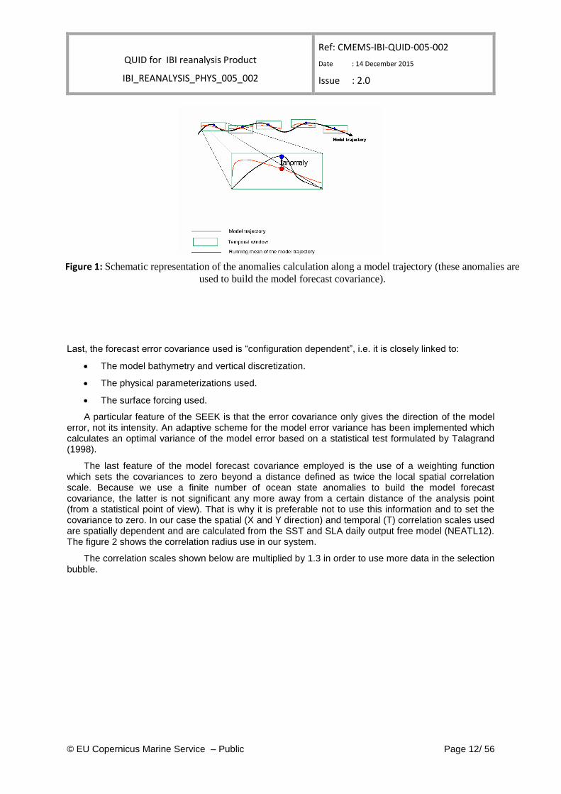
anomalies are high pass filtered ocean states (Hanning filter, length cut-off frequency = 1/30 days-1) available over the 2002-2009 time period every 1 day. These ocean states come from a reference simulation (free simulation from 01/01/2002 to 31/12/2009) carried out with the same ocean model configuration and same atmospheric forcing. The details described in the “free simulation” section. The main characteristic of the anomaly calculations is to filter out temporal scales at low frequencies in order to keep high frequencies for which the period is lower than the assimilation cycle. The Figure 1 is a schematic representation of the anomalies calculation.

For an analysis at date T, a subset of anomalies corresponding to the current season (a given number of days before and after T) is selected. From one analysis cycle to the other only a small part of the subset of anomalies changes. This method implies that at each analysis step a different sub-set of anomalies is used that improves the dynamical dependency. The error covariance continuity is kept by connecting the ensemble of anomalies with a same part of anomalies at every analysis steps.

For an assimilation cycle centered on the Nth day of year YYYY, ocean state anomalies falling in

the window [N-Δn; N+ Δn] of each year of reference run are gathered and define the covariance of the model forecast error. In REAIBI12, we tested several windows length, we chose Δn equal to 176 days with an anomaly of 8. The means use anomalies selected over all year length windows centred on the

Nth day of each year of NEATL12 simulation. However, in order to decrease the number of ocean states, only one state each two is retained over the 2002-2009. For each analysis, we use 350 ocean state anomalies. It should also be noted that the analysis increment is a linear combination of these error modes and depends on the model innovation (observation-model misfit) and on the specified observation errors (see assimilated observations section). The analysis is performed on a reduced horizontal grid (1 point every 3 in both directions) in order to reduce the computational cost.





Issue : 2.0


Last, the forecast error covariance used is “configuration dependent”, i.e. it is closely linked to:

The model bathymetry and vertical discretization.

The physical parameterizations used.

The surface forcing used.

A particular feature of the SEEK is that the error covariance only gives the direction of the model error, not its intensity. An adaptive scheme for the model error variance has been implemented which calculates an optimal variance of the model error based on a statistical test formulated by Talagrand (1998).

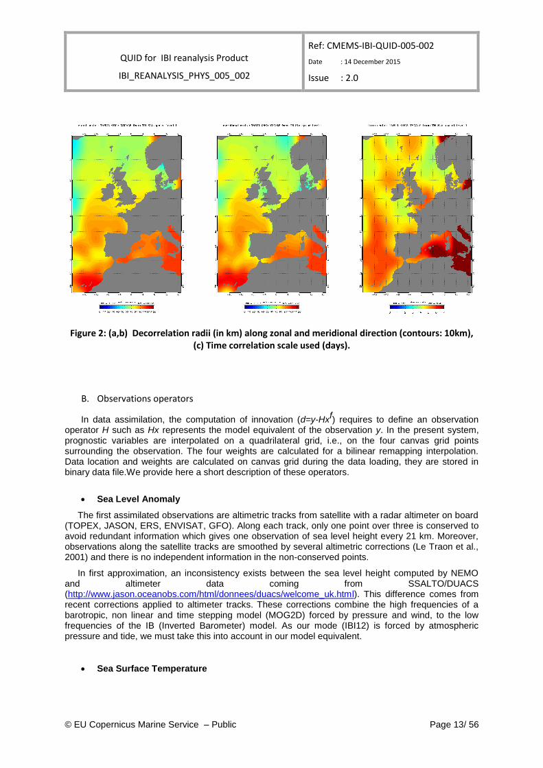
The last feature of the model forecast covariance employed is the use of a weighting function which sets the covariances to zero beyond a distance defined as twice the local spatial correlation scale. Because we use a finite number of ocean state anomalies to build the model forecast covariance, the latter is not significant any more away from a certain distance of the analysis point (from a statistical point of view). That is why it is preferable not to use this information and to set the covariance to zero. In our case the spatial (X and Y direction) and temporal (T) correlation scales used are spatially dependent and are calculated from the SST and SLA daily output free model (NEATL12). The figure 2 shows the correlation radius use in our system.

The correlation scales shown below are multiplied by 1.3 in order to use more data in the selection bubble.

Figure 1: Schematic representation of the anomalies calculation along a model trajectory (these anomalies are

used to build the model forecast covariance).





Issue : 2.0


Figure 2: (a,b) Decorrelation radii (in km) along zonal and meridional direction (contours: 10km), (c) Time correlation scale used (days).

B. Observations operators

In data assimilation, the computation of innovation (d=y-Hxf) requires to define an observation operator H such as Hx represents the model equivalent of the observation y. In the present system, prognostic variables are interpolated on a quadrilateral grid, i.e., on the four canvas grid points surrounding the observation. The four weights are calculated for a bilinear remapping interpolation. Data location and weights are calculated on canvas grid during the data loading, they are stored in binary data file.We provide here a short description of these operators.

Sea Level Anomaly

The first assimilated observations are altimetric tracks from satellite with a radar altimeter on board (TOPEX, JASON, ERS, ENVISAT, GFO). Along each track, only one point over three is conserved to avoid redundant information which gives one observation of sea level height every 21 km. Moreover, observations along the satellite tracks are smoothed by several altimetric corrections (Le Traon et al., 2001) and there is no independent information in the non-conserved points.

In first approximation, an inconsistency exists between the sea level height computed by NEMO and altimeter data coming from SSALTO/DUACS (http://www.jason.oceanobs.com/html/donnees/duacs/welcome_uk.html). This difference comes from recent corrections applied to altimeter tracks. These corrections combine the high frequencies of a barotropic, non linear and time stepping model (MOG2D) forced by pressure and wind, to the low frequencies of the IB (Inverted Barometer) model. As our mode (IBI12) is forced by atmospheric pressure and tide, we must take this into account in our model equivalent.

Sea Surface Temperature





Issue : 2.0


The SST maps that are assimilated result from an objective analysis of various satellite data sets. Reynolds 1/4° product is distributed on a 0,25 x 0,25° geographical grid but the SST does not contain signals with spatial scales shorter than ~1°. As the model grid is 1/12°, we have to slightly “smooth” the model SST in order to get an appropriate model equivalent for the AVHRR-only SST field. The observation operator in that case is a horizontal smoother applied on the model first level temperature field. The smoother consists of an iterative (60 iterations) Shapiro filter α=1/2) applied to the model SST.

In situ Temperature and Salinity

In this case, the observed profiles are interpolated on model levels by using a spline function. If the distance between two consecutive data depths is less than the model level thickness, the spline interpolation on the model level is not used. No extrapolation is performed at the top or at the bottom of the profile.





Issue : 2.0


III VALIDATION FRAMEWORK

The validation period is 1st February 2002 – 27 December 2014 (the period spanned by the reanalysis). The times series are based on monthly fields except for innovation diagnostics (see T-DA_INNO_STAT, S-DA_INNO_STAT, SL-DA-INNO_STAT, SI-CONC-DA-INNO_STAT sections), and the specific High-frequency IBI-Reanalysis validation performed with independent in-situ observational data (in hourly frequency basis) from the Puertos del Estado moorings located along the Spanish coast.

The validation methodology defined and used to validate the ocean reanalysis products is compliant with the WP18 validation plan. It consists in a series of diagnostics defined in common by all ocean reanalysis / reference forced simulation producers. The list of metrics applied following the common guidelines for Reanalysis validation (based on monthly output data) are:

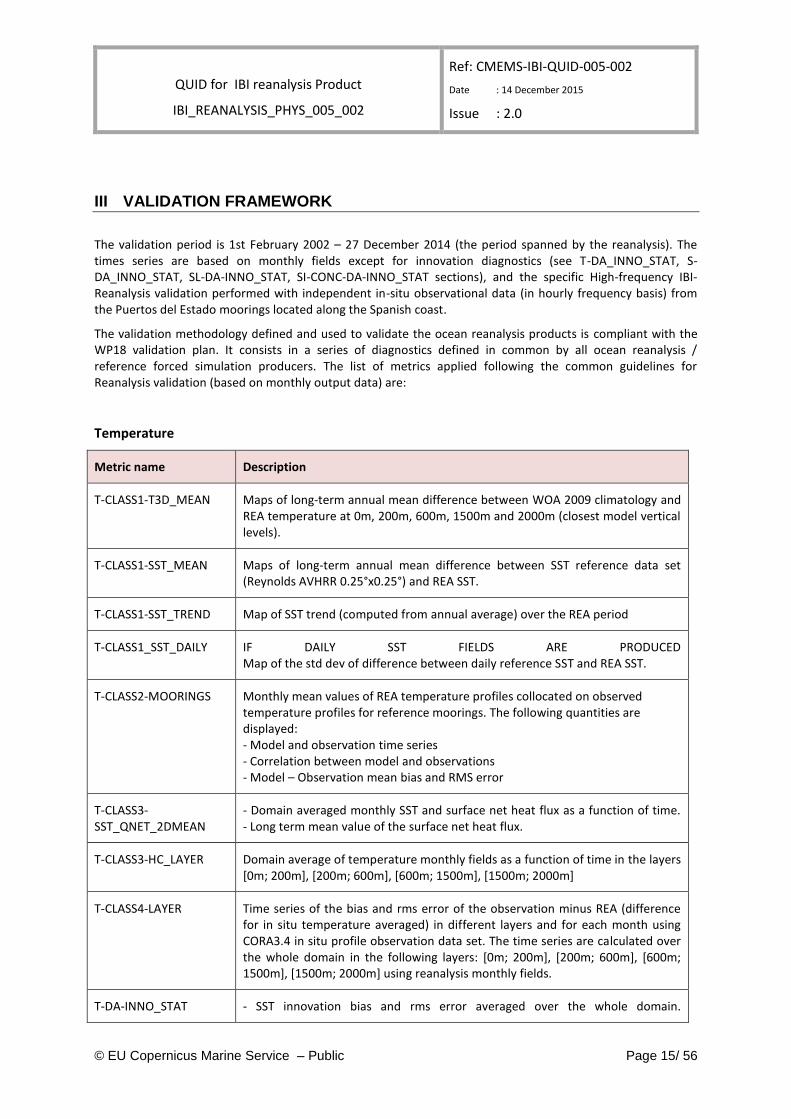
Temperature

Metric name Description

T-CLASS1-T3D_MEAN Maps of long-term annual mean difference between WOA 2009 climatology and REA temperature at 0m, 200m, 600m, 1500m and 2000m (closest model vertical levels).

T-CLASS1-SST_MEAN Maps of long-term annual mean difference between SST reference data set (Reynolds AVHRR 0.25°x0.25°) and REA SST.

T-CLASS1-SST_TREND Map of SST trend (computed from annual average) over the REA period

T-CLASS1_SST_DAILY IF DAILY SST FIELDS ARE PRODUCED Map of the std dev of difference between daily reference SST and REA SST.

T-CLASS2-MOORINGS Monthly mean values of REA temperature profiles collocated on observed temperature profiles for reference moorings. The following quantities are displayed: - Model and observation time series - Correlation between model and observations - Model – Observation mean bias and RMS error

T-CLASS3-SST_QNET_2DMEAN

- Domain averaged monthly SST and surface net heat flux as a function of time. - Long term mean value of the surface net heat flux.

T-CLASS3-HC_LAYER Domain average of temperature monthly fields as a function of time in the layers [0m; 200m], [200m; 600m], [600m; 1500m], [1500m; 2000m]

T-CLASS4-LAYER Time series of the bias and rms error of the observation minus REA (difference for in situ temperature averaged) in different layers and for each month using CORA3.4 in situ profile observation data set. The time series are calculated over the whole domain in the following layers: [0m; 200m], [200m; 600m], [600m; 1500m], [1500m; 2000m] using reanalysis monthly fields.

T-DA-INNO_STAT - SST innovation bias and rms error averaged over the whole domain.





Issue : 2.0


- In situ temperature innovation bias and rms error averaged over the whole domain as a function of time.

Table 1 Description of the metrics used for temperature in the IBI-Rea validation.

Salinity


S-CLASS1-S3D_MEAN Maps of long-term annual mean difference between WOA 2009 climatology and REA salinity at 0m, 200m, 600m, 1500m and 2000m (closest model vertical levels).

S-CLASS1-SSS_TREND Map of SSS trend (computed from annual average) over the REA period

S-CLASS2-MOORINGS Monthly mean values of REA temperature profiles collocated on observed temperature profiles for reference moorings. The following quantities are displayed: - Model and observation time series - Correlation between model and observations - Model – Observation mean bias and RMS error

S-CLASS3-SSS_SFW_2DMEAN

- Domain averaged monthly SSS and surface net fresh water flux as a function of time. - Long term mean value of the net surface fresh water flux.

S-CLASS3-SC_LAYER Domain average of salinity monthly fields as a function of time in the layers [0m; 200m], [200m; 600m], [600m; 1500m], [1500m; 2000m]

S-CLASS3-IC_CHANGE Domain average salinity change with respect to initial condition as a function of depth and time.

S-CLASS4-LAYER Time series of the bias and rms error of the observation minus REA (difference for in situ salinity averaged) in different layers and for each month using CORA3.4 in situ profile observation data set. The time series are calculated over the whole domain in the following layers: [0m; 200m], [200m; 600m], [600m; 1500m], [1500m; 2000m] using reanalysis monthly fields.

S-DA-INNO_STAT - In situ salinity innovation bias and std dev averaged over the whole domain as a function of time.

Table 2 Description of the metrics used for salinity in the IBI-Rea validation.

Currents


UV-CLASS1-15m_MEAN NOAA AOML drifter-derived climatology for total current, including Ekman component (see http://www.aoml.noaa.gov/phod/dac/drifter_climatology.html)

UV-CLASS2-MOORINGS Monthly mean values of REA temperature profiles collocated on observed

http://www.aoml.noaa.gov/phod/dac/drifter_climatology.html





Issue : 2.0


temperature profiles for reference moorings. The following quantities are displayed: - Model and observation time series - Correlation between model and observations - Model – Observation mean bias and RMS error

UV-CLASS2-MKE_1000m Mean value of kinetic energy (KE=0,5x(U2+V

2)) at 1000m depth estimated from ANDRO

Argo drift data base (http://wwz.ifremer.fr/lpo/Produits/ANDRO ) over the years 2002-2009. To be consistent, the averaging period for the reanalysis will also be 2002-2009.

Table 3: Description of the metrics used for currents in the IBI-Rea validation.

Sea level


SL-CLASS1-TREND_2D Map of sea level trend as estimated from MyOcean altimetry delayed time L4 product. Same time period as the reanalysis to be fully consistent.

SL-CLASS2-TIDE_GAUGE Monthly mean values of sea level at tide gauges locations. The following quantities are displayed on a map at tide gauge location: - REA sea level minus observation std dev, - correlation, - percentage of explained variance (100x(1-variance(model-obs)/variance(obs) ))

SL-CLASS3-2DMEAN Domain averaged sea level monthly mean time series.

SL-DA-INNO_STAT Sea level innovation bias and rms error averaged over the whole domain as a function of time.

Table 4 Description of the metrics used for sea level in the IBI-Rea validation.

Transport


UV-CLASS3-VOL_TRANSP

Volume transport through sections: long term mean value and STD from monthly means. Published estimation for Gibraltar, South Portugal and Bay of Biscay.

Table 5 Description of the metrics used for transport in the IBI-Rea validation.

High Frequency IBI reanalysis validation: List of metrics.

The high frequency validation performed with the IBI reanalysis outputs that come to complement the previous described validation framework (focused on monthly scales), is based on the following metric lists.





Issue : 2.0



SST-CLASS2-HF-MOORINGS

IBI-RE Hourly mean SST values collocated at buoy mooring positions are compared with hourly measured SST data from 16 PdE moorings.

Following statistics and metrics are computed and displayed:

IBI-RE & OBS time series (both for absolute values and anomalies)

Bias, RMS error, time correlation index and scatter index

Quantile-quantile plots and Taylor diagram are generated.

UV-CLASS2-HF-MOORINGS

U- and V- current components from IBI-RE hourly outputs collocated at buoy mooring positions are compared with hourly zonal and meridional current components observed at the 16 PdE moorings.


IBI-RE & OBS time series.

Current distribution by direction (current roses plots)

Bias, RMS error, time correlation index and scatter index.

Quantile-quantile plots and Taylor diagram generated.

Progressive vector diagrams displayed

Subinertial currents computed and displayed.

SSS-CLASS2-HF-MOORINGS

IBI-RE Hourly mean Sea surface salinity values collocated at buoy mooring positions are compared with hourly measured SSS data from 16 PdE moorings.


IBI-RE & OBS time series (both for absolute values and anomalies)

Bias, RMS error, time correlation index and scatter index

Quantile-quantile plots and Taylor diagram are generated.

SSS values together with the SST ones are depicted in T/S diagrams allowing characterization of main surface water masses occurred at each location.

Table 6: Description of the CLASS2 metrics used in the IBI-Rea validation with the Puertos del Estado moorings.

Other

Comparison to Mixed Layer Depth climatology.





Issue : 2.0


IV VALIDATION RESULTS

IV.1 Temperature

IV.1.1 T-CLASS1-T3D-MEAN

Figure 3: Mean differences (model-climatology) in temperature between IBI-REA and the World Ocean Atlas 2009 climatology (WOA09) at 0.5m, 97m, 300m, 773m and 1945m depth, respectively.

For this comparison, model data have been averaged over the period 2002 – 2014.





Issue : 2.0


IV.1.2 T-CLASS1-SST-MEAN

Figure 4: Mean differences (observations-model) in sea surface temperature between IBI-REA and the AVHRR SST data (left), and GLORYS2V3 and the AVHRR SST data (right). For this comparison,

model data have been averaged over the period 2002 – 2014.

IV.1.3 T-CLASS1-SST-TREND

Figure 5: SST trend of IBI-REA and AVHRR data. Covered time period: 2002 – 2014.

IV.1.4 T-CLASS2-MOORINGS





Issue : 2.0


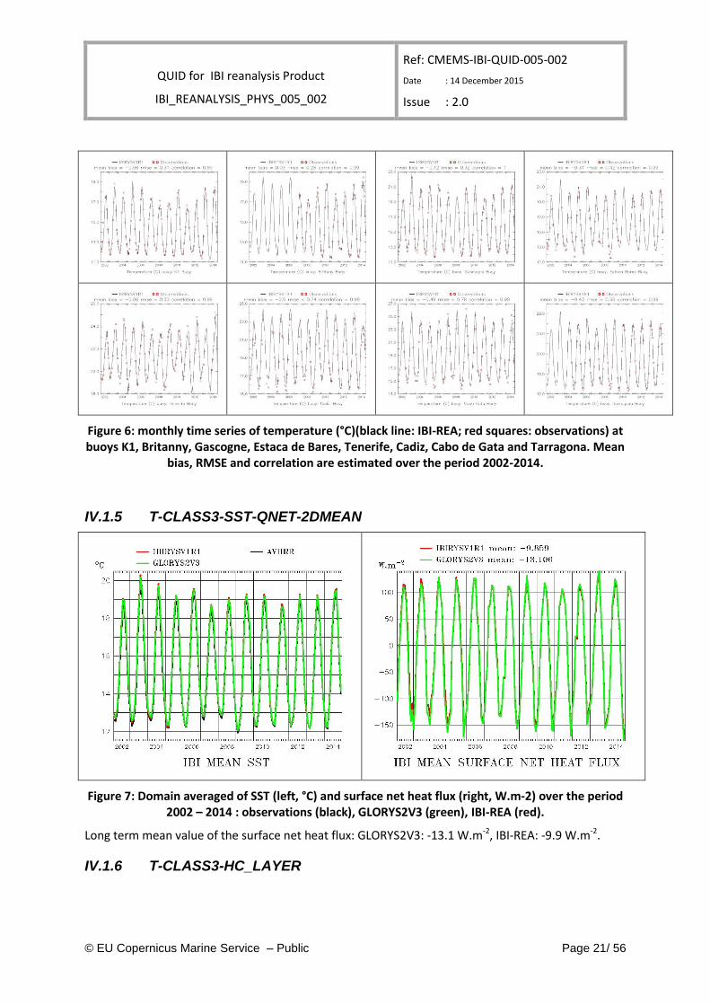
Figure 6: monthly time series of temperature (°C)(black line: IBI-REA; red squares: observations) at buoys K1, Britanny, Gascogne, Estaca de Bares, Tenerife, Cadiz, Cabo de Gata and Tarragona. Mean

bias, RMSE and correlation are estimated over the period 2002-2014.

IV.1.5 T-CLASS3-SST-QNET-2DMEAN

Figure 7: Domain averaged of SST (left, °C) and surface net heat flux (right, W.m-2) over the period 2002 – 2014 : observations (black), GLORYS2V3 (green), IBI-REA (red).

Long term mean value of the surface net heat flux: GLORYS2V3: -13.1 W.m-2, IBI-REA: -9.9 W.m-2.

IV.1.6 T-CLASS3-HC_LAYER





Issue : 2.0


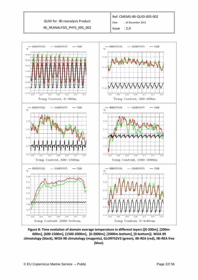
Figure 8: Time evolution of domain average temperature in different layers ([0-200m], [200m-600m], [600-1500m], [1500-2000m], [0-2000m], [2000m-bottom], [0-bottom]). WOA 09

climatology (black), WOA 98 climatology (magenta), GLORYS2V3 (green), IBI-REA (red), IBI-REA free (blue).





Issue : 2.0


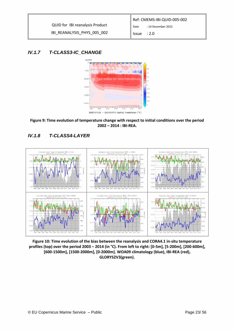
IV.1.7 T-CLASS3-IC_CHANGE

Figure 9: Time evolution of temperature change with respect to initial conditions over the period 2002 – 2014 : IBI-REA.

IV.1.8 T-CLASS4-LAYER

Figure 10: Time evolution of the bias between the reanalysis and CORA4.1 in-situ temperature profiles (top) over the period 2003 – 2014 (in °C). From left to right: [0-5m], [5-200m], [200-600m],

[600-1500m], [1500-2000m], [0-2000m]. WOA09 climatology (blue), IBI-REA (red), GLORYS2V3(green).





Issue : 2.0


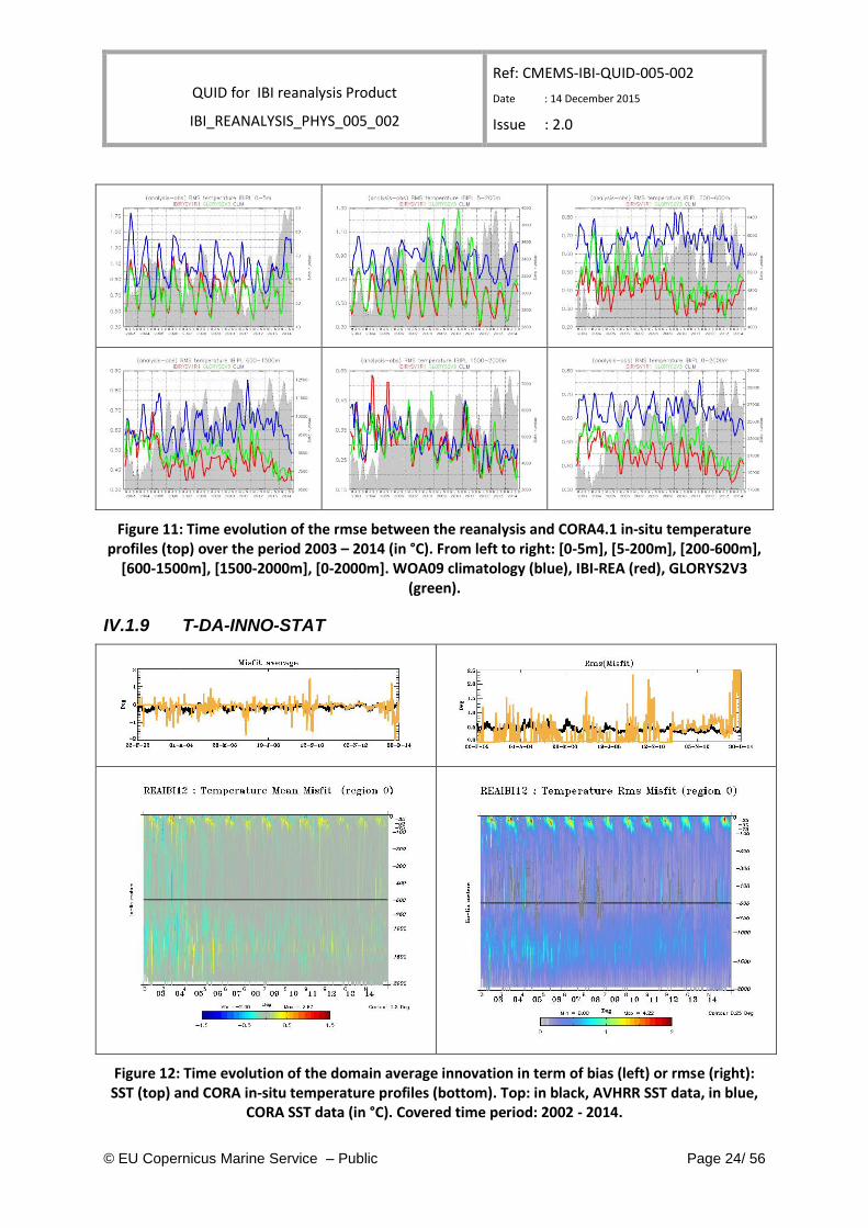
Figure 11: Time evolution of the rmse between the reanalysis and CORA4.1 in-situ temperature profiles (top) over the period 2003 – 2014 (in °C). From left to right: [0-5m], [5-200m], [200-600m],

[600-1500m], [1500-2000m], [0-2000m]. WOA09 climatology (blue), IBI-REA (red), GLORYS2V3 (green).

IV.1.9 T-DA-INNO-STAT

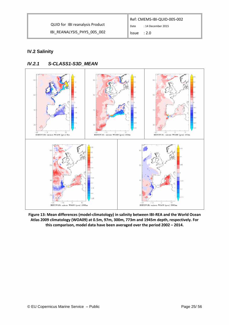
Figure 12: Time evolution of the domain average innovation in term of bias (left) or rmse (right): SST (top) and CORA in-situ temperature profiles (bottom). Top: in black, AVHRR SST data, in blue,

CORA SST data (in °C). Covered time period: 2002 - 2014.





Issue : 2.0


IV.2 Salinity

IV.2.1 S-CLASS1-S3D_MEAN

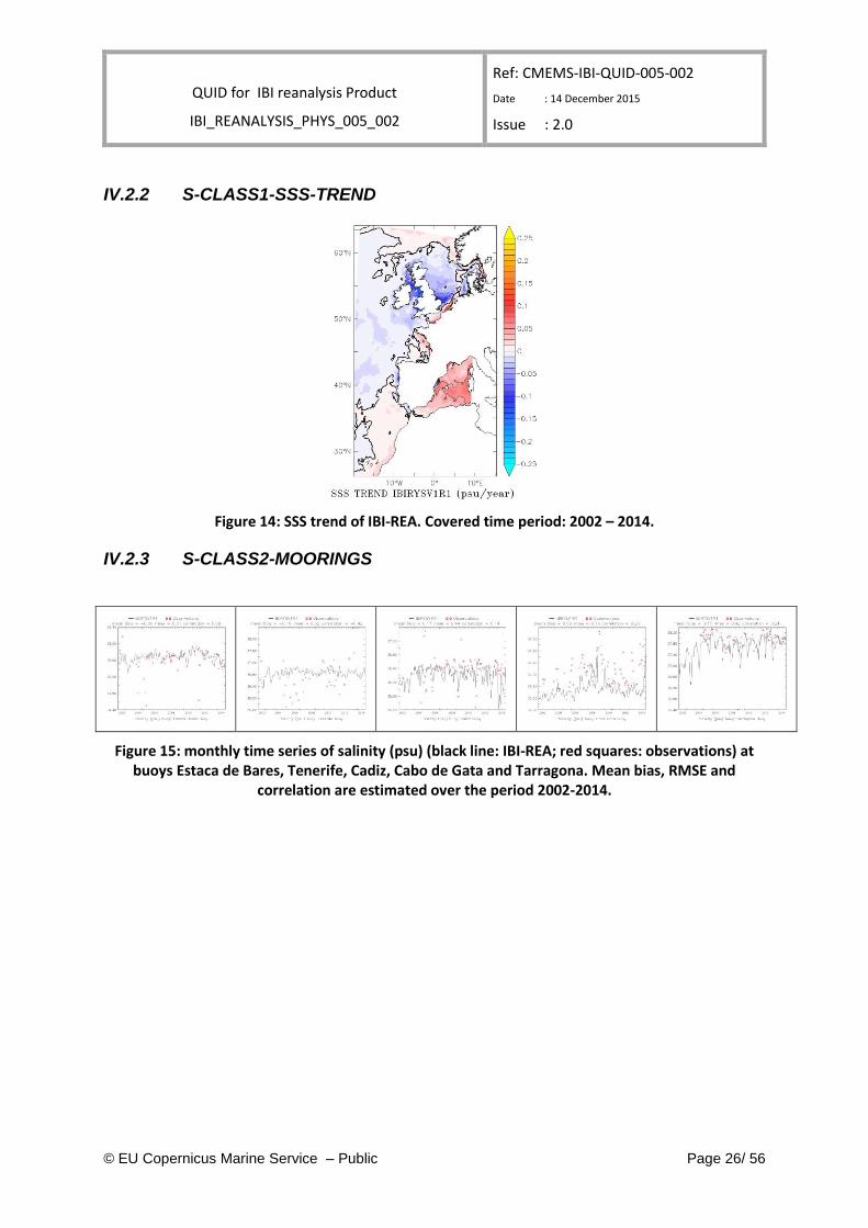
Figure 13: Mean differences (model-climatology) in salinity between IBI-REA and the World Ocean Atlas 2009 climatology (WOA09) at 0.5m, 97m, 300m, 773m and 1945m depth, respectively. For

this comparison, model data have been averaged over the period 2002 – 2014.





Issue : 2.0


IV.2.2 S-CLASS1-SSS-TREND

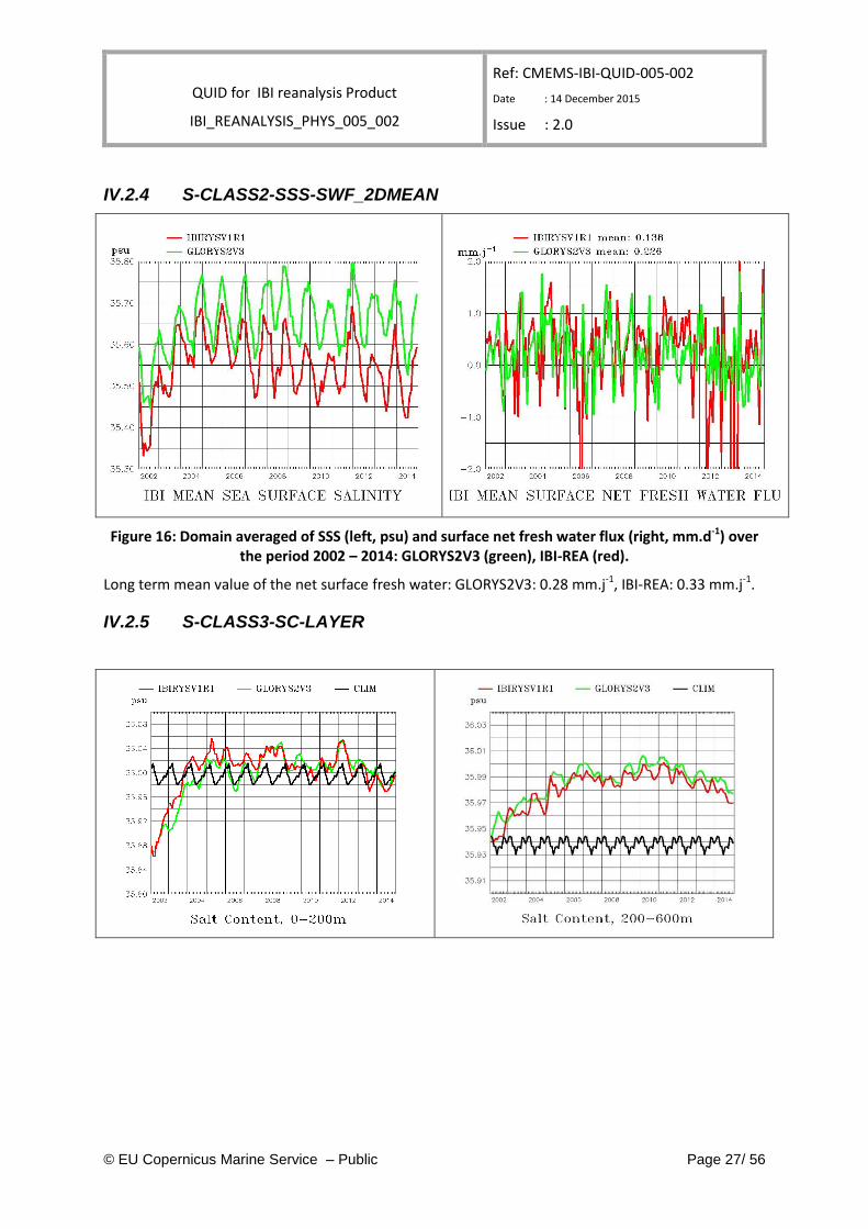
Figure 14: SSS trend of IBI-REA. Covered time period: 2002 – 2014.

IV.2.3 S-CLASS2-MOORINGS

Figure 15: monthly time series of salinity (psu) (black line: IBI-REA; red squares: observations) at buoys Estaca de Bares, Tenerife, Cadiz, Cabo de Gata and Tarragona. Mean bias, RMSE and

correlation are estimated over the period 2002-2014.





Issue : 2.0


IV.2.4 S-CLASS2-SSS-SWF_2DMEAN

Figure 16: Domain averaged of SSS (left, psu) and surface net fresh water flux (right, mm.d-1) over the period 2002 – 2014: GLORYS2V3 (green), IBI-REA (red).

Long term mean value of the net surface fresh water: GLORYS2V3: 0.28 mm.j-1, IBI-REA: 0.33 mm.j-1.

IV.2.5 S-CLASS3-SC-LAYER





Issue : 2.0


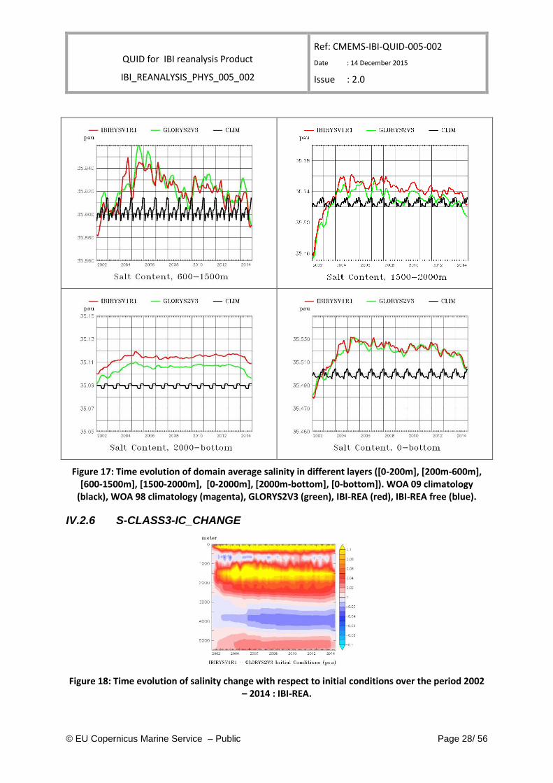
Figure 17: Time evolution of domain average salinity in different layers ([0-200m], [200m-600m], [600-1500m], [1500-2000m], [0-2000m], [2000m-bottom], [0-bottom]). WOA 09 climatology

(black), WOA 98 climatology (magenta), GLORYS2V3 (green), IBI-REA (red), IBI-REA free (blue).

IV.2.6 S-CLASS3-IC_CHANGE

Figure 18: Time evolution of salinity change with respect to initial conditions over the period 2002 – 2014 : IBI-REA.





Issue : 2.0


IV.2.7 S-CLASS4-LAYER

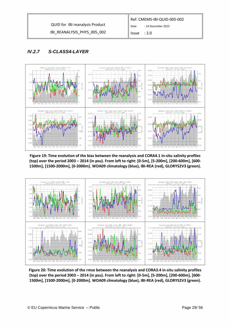
Figure 19: Time evolution of the bias between the reanalysis and CORA4.1 in-situ salinity profiles (top) over the period 2003 – 2014 (in psu). From left to right: [0-5m], [5-200m], [200-600m], [600-1500m], [1500-2000m], [0-2000m]. WOA09 climatology (blue), IBI-REA (red), GLORYS2V3 (green).

Figure 20: Time evolution of the rmse between the reanalysis and CORA3.4 in-situ salinity profiles (top) over the period 2003 – 2014 (in psu). From left to right: [0-5m], [5-200m], [200-600m], [600-1500m], [1500-2000m], [0-2000m]. WOA09 climatology (blue), IBI-REA (red), GLORYS2V3 (green).





Issue : 2.0


IV.2.8 S-DA-INNO_STAT

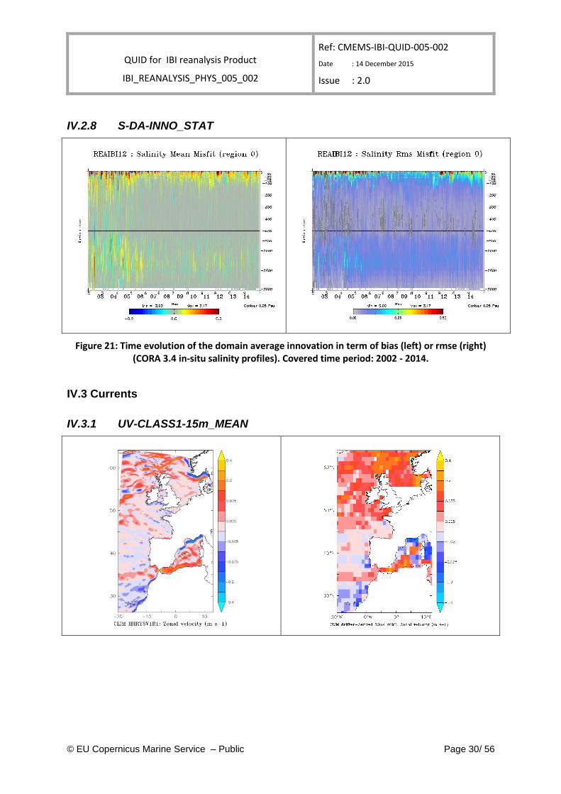
Figure 21: Time evolution of the domain average innovation in term of bias (left) or rmse (right) (CORA 3.4 in-situ salinity profiles). Covered time period: 2002 - 2014.

IV.3 Currents

IV.3.1 UV-CLASS1-15m_MEAN





Issue : 2.0


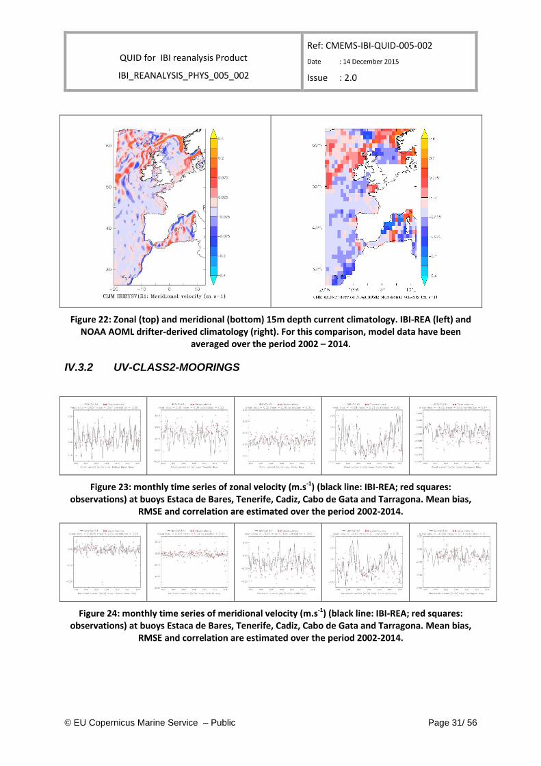
Figure 22: Zonal (top) and meridional (bottom) 15m depth current climatology. IBI-REA (left) and NOAA AOML drifter-derived climatology (right). For this comparison, model data have been

averaged over the period 2002 – 2014.

IV.3.2 UV-CLASS2-MOORINGS

Figure 23: monthly time series of zonal velocity (m.s-1) (black line: IBI-REA; red squares: observations) at buoys Estaca de Bares, Tenerife, Cadiz, Cabo de Gata and Tarragona. Mean bias,

RMSE and correlation are estimated over the period 2002-2014.

Figure 24: monthly time series of meridional velocity (m.s-1) (black line: IBI-REA; red squares: observations) at buoys Estaca de Bares, Tenerife, Cadiz, Cabo de Gata and Tarragona. Mean bias,

RMSE and correlation are estimated over the period 2002-2014.





Issue : 2.0


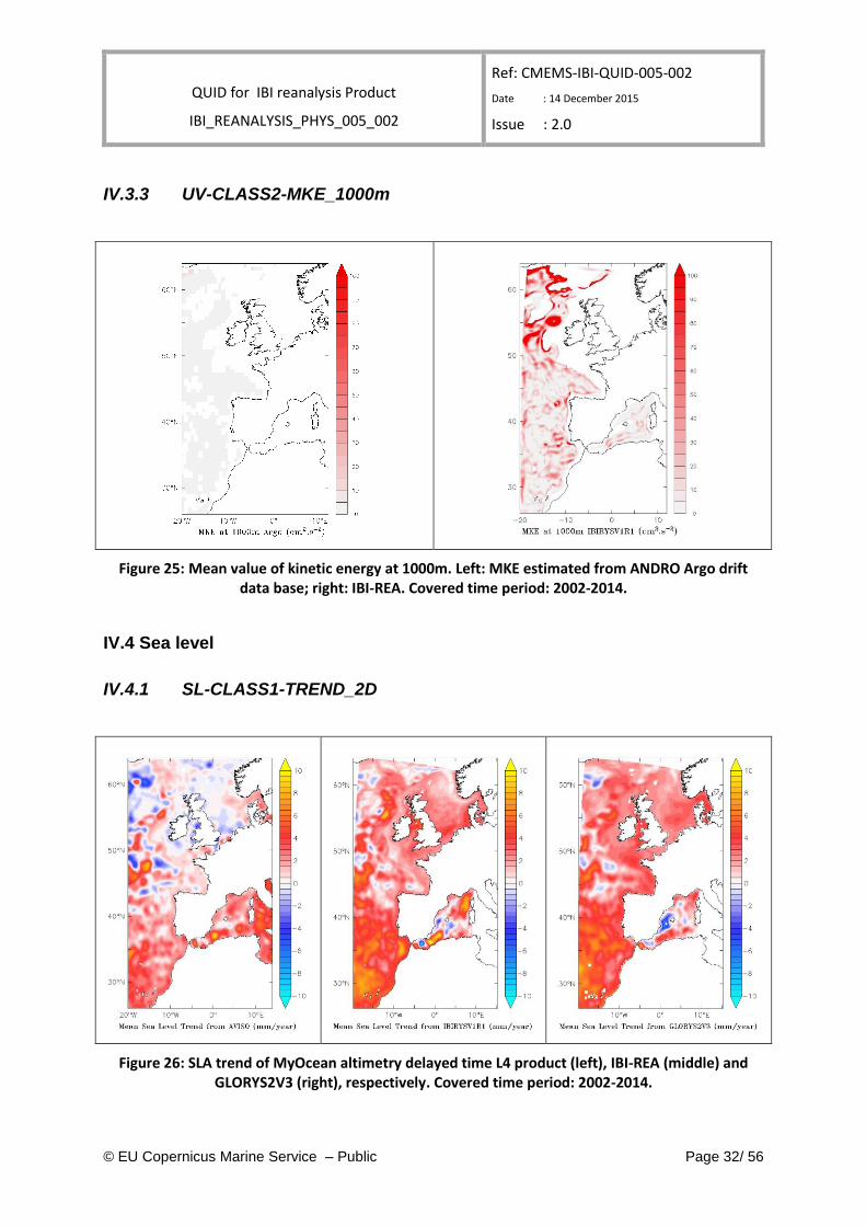
IV.3.3 UV-CLASS2-MKE_1000m

Figure 25: Mean value of kinetic energy at 1000m. Left: MKE estimated from ANDRO Argo drift data base; right: IBI-REA. Covered time period: 2002-2014.

IV.4 Sea level

IV.4.1 SL-CLASS1-TREND_2D

Figure 26: SLA trend of MyOcean altimetry delayed time L4 product (left), IBI-REA (middle) and GLORYS2V3 (right), respectively. Covered time period: 2002-2014.





Issue : 2.0


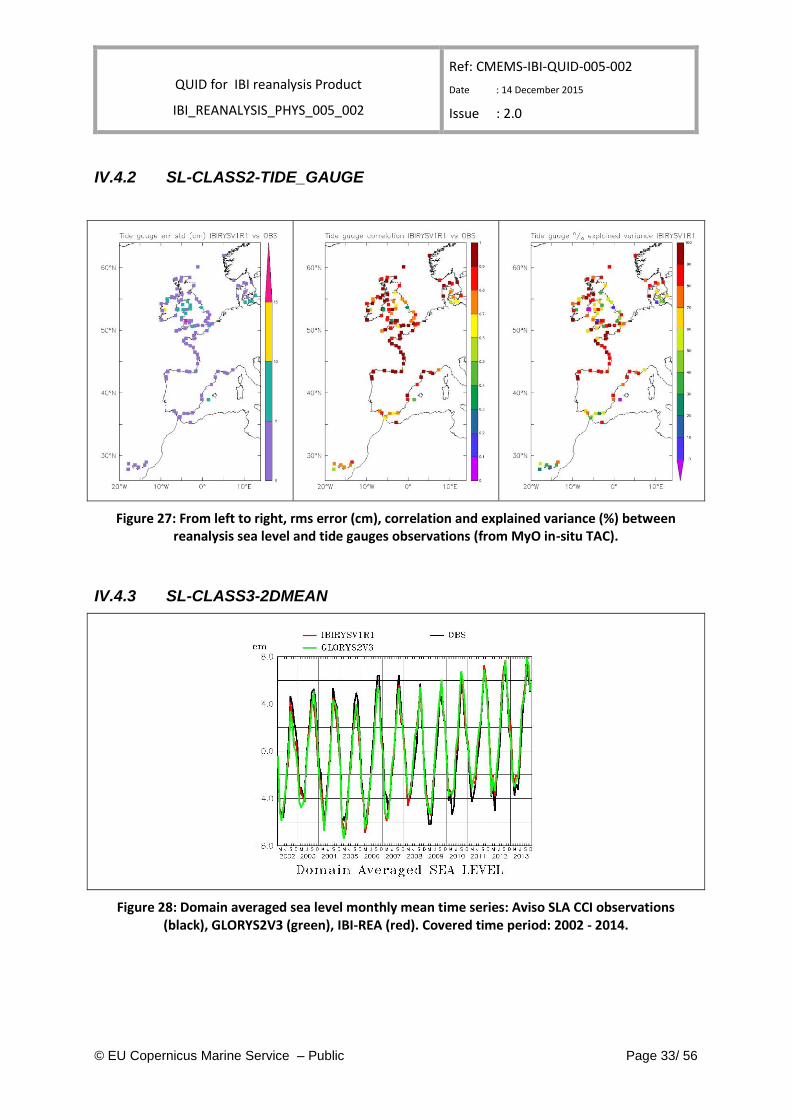
IV.4.2 SL-CLASS2-TIDE_GAUGE

Figure 27: From left to right, rms error (cm), correlation and explained variance (%) between reanalysis sea level and tide gauges observations (from MyO in-situ TAC).

IV.4.3 SL-CLASS3-2DMEAN

Figure 28: Domain averaged sea level monthly mean time series: Aviso SLA CCI observations (black), GLORYS2V3 (green), IBI-REA (red). Covered time period: 2002 - 2014.





Issue : 2.0


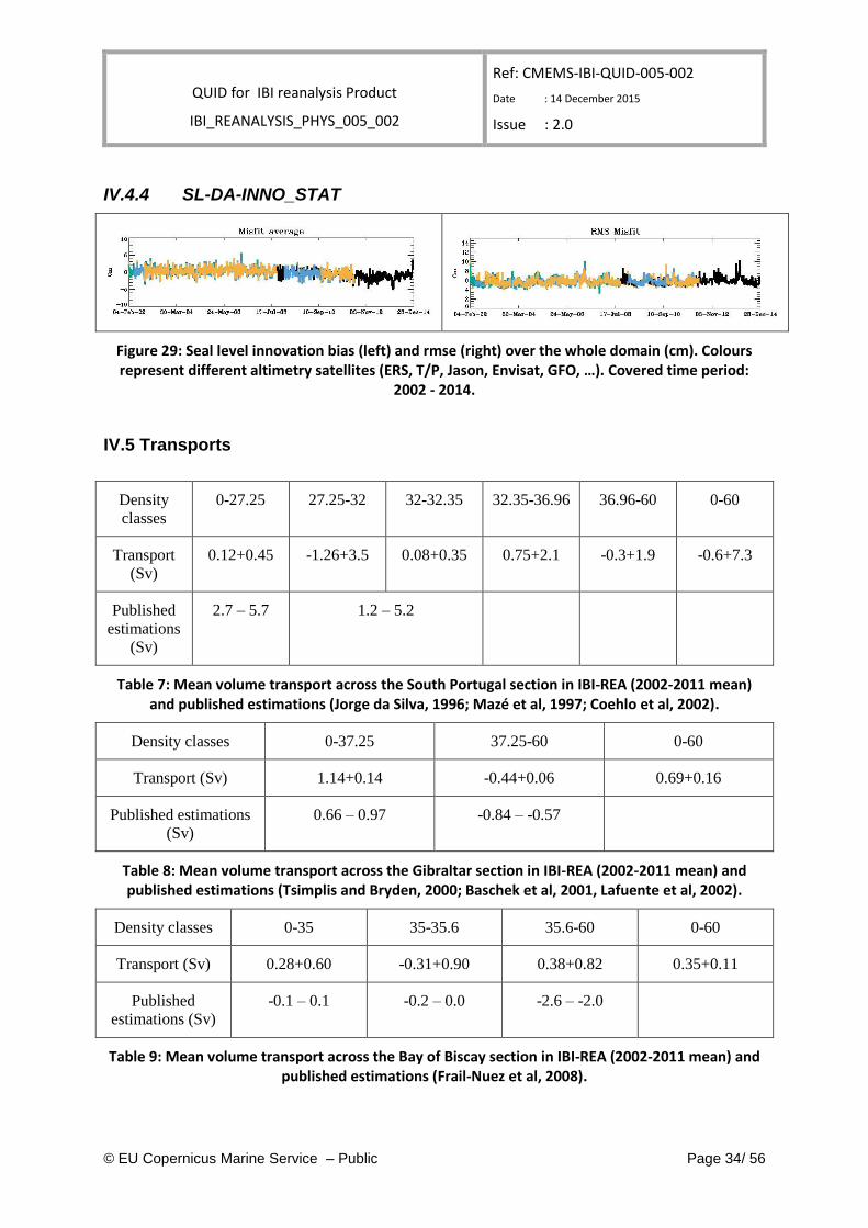
IV.4.4 SL-DA-INNO_STAT

Figure 29: Seal level innovation bias (left) and rmse (right) over the whole domain (cm). Colours represent different altimetry satellites (ERS, T/P, Jason, Envisat, GFO, …). Covered time period:

2002 - 2014.

IV.5 Transports

Density

classes

0-27.25 27.25-32 32-32.35 32.35-36.96 36.96-60 0-60

Transport

(Sv)

0.12+0.45 -1.26+3.5 0.08+0.35 0.75+2.1 -0.3+1.9 -0.6+7.3

Published

estimations

(Sv)

2.7 – 5.7 1.2 – 5.2

Table 7: Mean volume transport across the South Portugal section in IBI-REA (2002-2011 mean) and published estimations (Jorge da Silva, 1996; Mazé et al, 1997; Coehlo et al, 2002).

Density classes 0-37.25 37.25-60 0-60

Transport (Sv) 1.14+0.14 -0.44+0.06 0.69+0.16

Published estimations

(Sv)

0.66 – 0.97 -0.84 – -0.57

Table 8: Mean volume transport across the Gibraltar section in IBI-REA (2002-2011 mean) and published estimations (Tsimplis and Bryden, 2000; Baschek et al, 2001, Lafuente et al, 2002).

Density classes 0-35 35-35.6 35.6-60 0-60

Transport (Sv) 0.28+0.60 -0.31+0.90 0.38+0.82 0.35+0.11

Published

estimations (Sv)

-0.1 – 0.1 -0.2 – 0.0 -2.6 – -2.0

Table 9: Mean volume transport across the Bay of Biscay section in IBI-REA (2002-2011 mean) and published estimations (Frail-Nuez et al, 2008).





Issue : 2.0


IV.6 Other monthly metrics

IV.6.1 OTH-CLASS1-MLD_CLIM_SEASON

Figure 30: Climatological mixed layer depth (m) in March (top) and September (bottom). IBI-REA (left) and De Boyer Montegut climatology data (right).

IV.7 High frequency IBI Reanalysis validation with moorings

In-situ observations from moorings have been used for validating the IBI Reanalysis high-frequency outputs. To this aim, 14 moorings from the Puertos del Estado Deep Water Buoy Network has been used. The selected buoys are located along the Spanish coast (geographical location displayed in





Issue : 2.0


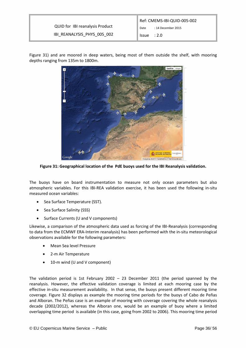
Figure 31) and are moored in deep waters, being most of them outside the shelf, with mooring depths ranging from 135m to 1800m.

Figure 31: Geographical location of the PdE buoys used for the IBI Reanalysis validation.

The buoys have on board instrumentation to measure not only ocean parameters but also atmospheric variables. For this IBI-REA validation exercise, it has been used the following in-situ measured ocean variables:

Sea Surface Temperature (SST).

Sea Surface Salinity (SSS)

Surface Currents (U and V components)

Likewise, a comparison of the atmospheric data used as forcing of the IBI-Reanalysis (corresponding to data from the ECMWF ERA-Interim reanalysis) has been performed with the in-situ meteorological observations available for the following parameters:

Mean Sea level Pressure

2-m Air Temperature

10-m wind (U and V component)

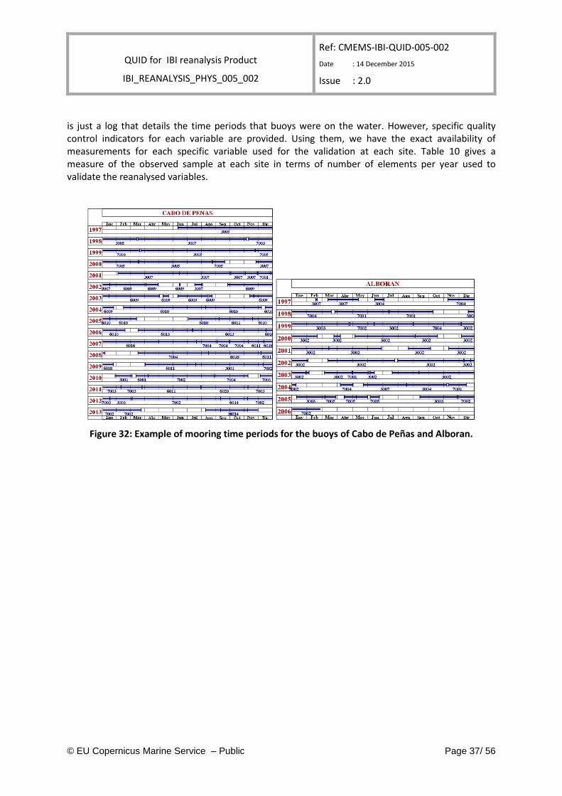
The validation period is 1st February 2002 – 23 December 2011 (the period spanned by the reanalysis. However, the effective validation coverage is limited at each mooring case by the effective in-situ measurement availability. In that sense, the buoys present different mooring time coverage. Figure 32 displays as example the mooring time periods for the buoys of Cabo de Peñas and Alboran. The Peñas case is an example of mooring with coverage covering the whole reanalysis decade (2002/2012), whereas the Alboran one, would be an example of buoy where a limited overlapping time period is available (in this case, going from 2002 to 2006). This mooring time period





Issue : 2.0


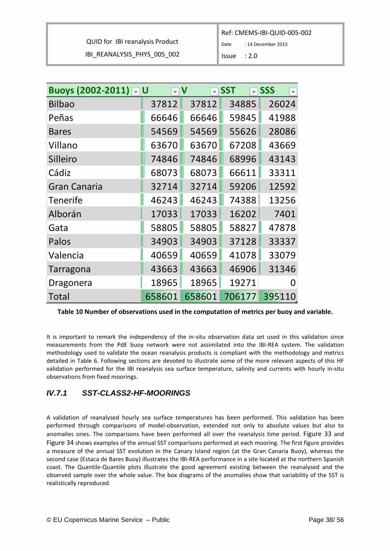
is just a log that details the time periods that buoys were on the water. However, specific quality control indicators for each variable are provided. Using them, we have the exact availability of measurements for each specific variable used for the validation at each site. Table 10 gives a measure of the observed sample at each site in terms of number of elements per year used to validate the reanalysed variables.

Figure 32: Example of mooring time periods for the buoys of Cabo de Peñas and Alboran.





Issue : 2.0


Buoys (2002-2011) U V SST SSS

Bilbao 37812 37812 34885 26024

Peñas 66646 66646 59845 41988

Bares 54569 54569 55626 28086

Villano 63670 63670 67208 43669

Silleiro 74846 74846 68996 43143

Cádiz 68073 68073 66611 33311

Gran Canaria 32714 32714 59206 12592

Tenerife 46243 46243 74388 13256

Alborán 17033 17033 16202 7401

Gata 58805 58805 58827 47878

Palos 34903 34903 37128 33337

Valencia 40659 40659 41078 33079

Tarragona 43663 43663 46906 31346

Dragonera 18965 18965 19271 0

Total 658601 658601 706177 395110

Table 10 Number of observations used in the computation of metrics per buoy and variable.

It is important to remark the independency of the in-situ observation data set used in this validation since measurements from the PdE buoy network were not assimilated into the IBI-REA system. The validation methodology used to validate the ocean reanalysis products is compliant with the methodology and metrics detailed in Table 6. Following sections are devoted to illustrate some of the more relevant aspects of this HF validation performed for the IBI reanalysis sea surface temperature, salinity and currents with hourly in-situ observations from fixed moorings.

IV.7.1 SST-CLASS2-HF-MOORINGS

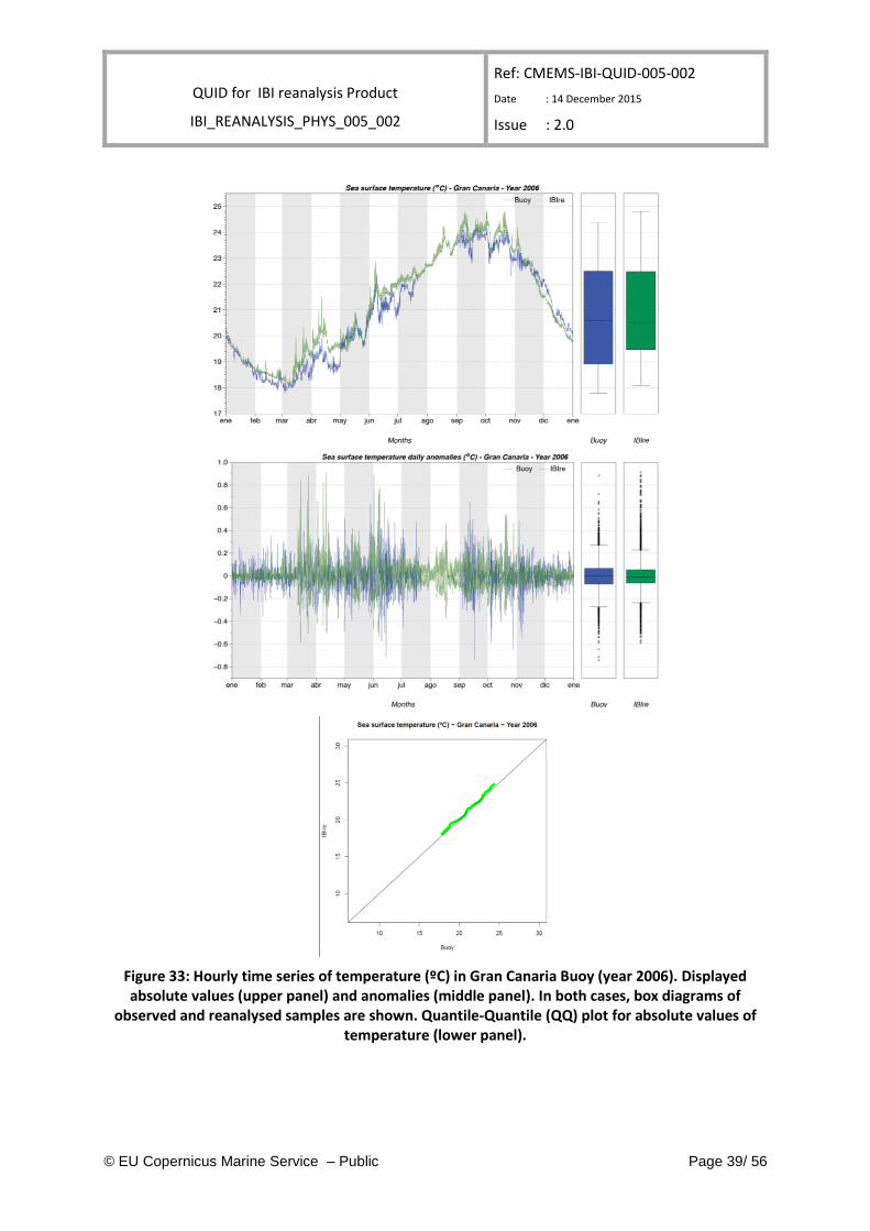
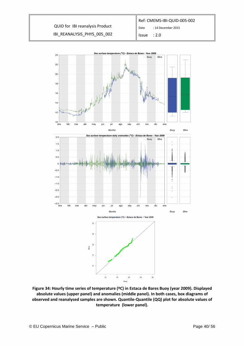
A validation of reanalysed hourly sea surface temperatures has been performed. This validation has been performed through comparisons of model-observation, extended not only to absolute values but also to

anomalies ones. The comparisons have been performed all over the reanalysis time period. Figure 33 and

Figure 34 shows examples of the annual SST comparisons performed at each mooring. The first figure provides

a measure of the annual SST evolution in the Canary Island region (at the Gran Canaria Buoy), whereas the second case (Estaca de Bares Buoy) illustrates the IBI-REA performance in a site located at the northern Spanish coast. The Quantile-Quantile plots illustrate the good agreement existing between the reanalysed and the observed sample over the whole value. The box diagrams of the anomalies show that variability of the SST is realistically reproduced.





Issue : 2.0


Figure 33: Hourly time series of temperature (ºC) in Gran Canaria Buoy (year 2006). Displayed absolute values (upper panel) and anomalies (middle panel). In both cases, box diagrams of

observed and reanalysed samples are shown. Quantile-Quantile (QQ) plot for absolute values of temperature (lower panel).





Issue : 2.0


Figure 34: Hourly time series of temperature (ºC) in Estaca de Bares Buoy (year 2009). Displayed absolute values (upper panel) and anomalies (middle panel). In both cases, box diagrams of

observed and reanalysed samples are shown. Quantile-Quantile (QQ) plot for absolute values of temperature (lower panel).





Issue : 2.0


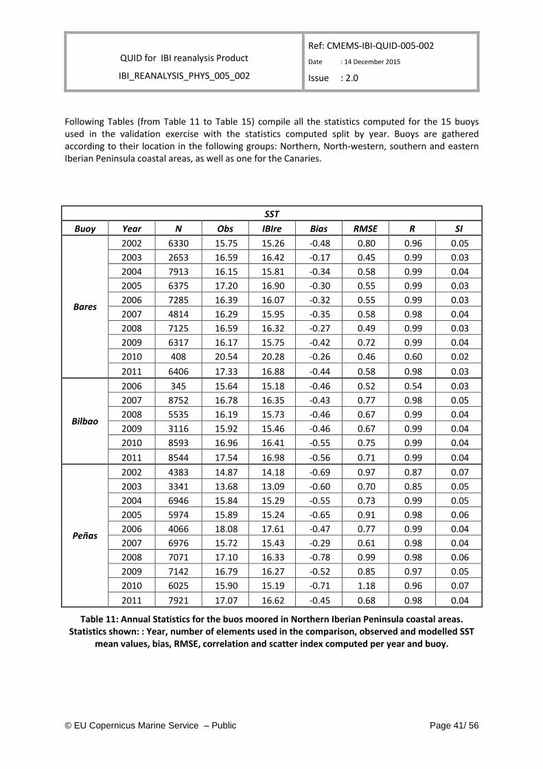
Following Tables (from Table 11 to Table 15) compile all the statistics computed for the 15 buoys used in the validation exercise with the statistics computed split by year. Buoys are gathered according to their location in the following groups: Northern, North-western, southern and eastern Iberian Peninsula coastal areas, as well as one for the Canaries.

SST

Buoy Year N Obs IBIre Bias RMSE R SI

Bares

2002 6330 15.75 15.26 -0.48 0.80 0.96 0.05

2003 2653 16.59 16.42 -0.17 0.45 0.99 0.03

2004 7913 16.15 15.81 -0.34 0.58 0.99 0.04

2005 6375 17.20 16.90 -0.30 0.55 0.99 0.03

2006 7285 16.39 16.07 -0.32 0.55 0.99 0.03

2007 4814 16.29 15.95 -0.35 0.58 0.98 0.04

2008 7125 16.59 16.32 -0.27 0.49 0.99 0.03

2009 6317 16.17 15.75 -0.42 0.72 0.99 0.04

2010 408 20.54 20.28 -0.26 0.46 0.60 0.02

2011 6406 17.33 16.88 -0.44 0.58 0.98 0.03

Bilbao

2006 345 15.64 15.18 -0.46 0.52 0.54 0.03

2007 8752 16.78 16.35 -0.43 0.77 0.98 0.05

2008 5535 16.19 15.73 -0.46 0.67 0.99 0.04

2009 3116 15.92 15.46 -0.46 0.67 0.99 0.04

2010 8593 16.96 16.41 -0.55 0.75 0.99 0.04

2011 8544 17.54 16.98 -0.56 0.71 0.99 0.04

Peñas

2002 4383 14.87 14.18 -0.69 0.97 0.87 0.07

2003 3341 13.68 13.09 -0.60 0.70 0.85 0.05

2004 6946 15.84 15.29 -0.55 0.73 0.99 0.05

2005 5974 15.89 15.24 -0.65 0.91 0.98 0.06

2006 4066 18.08 17.61 -0.47 0.77 0.99 0.04

2007 6976 15.72 15.43 -0.29 0.61 0.98 0.04

2008 7071 17.10 16.33 -0.78 0.99 0.98 0.06

2009 7142 16.79 16.27 -0.52 0.85 0.97 0.05

2010 6025 15.90 15.19 -0.71 1.18 0.96 0.07

2011 7921 17.07 16.62 -0.45 0.68 0.98 0.04

Table 11: Annual Statistics for the buos moored in Northern Iberian Peninsula coastal areas. Statistics shown: : Year, number of elements used in the comparison, observed and modelled SST

mean values, bias, RMSE, correlation and scatter index computed per year and buoy.





Issue : 2.0


SST


Silleiro

2002 5646 15.79 15.19 -0.60 0.80 0.94 0.05

2003 8618 16.60 15.59 -1.02 1.32 0.95 0.08

2004 8022 16.88 15.91 -0.97 1.25 0.96 0.07

2005 7626 16.32 15.26 -1.06 1.53 0.93 0.09

2006 8732 17.14 16.13 -1.01 1.37 0.93 0.08

2007 7850 16.39 15.62 -0.77 1.04 0.92 0.06

2008 7778 16.64 15.94 -0.70 0.98 0.95 0.06

2009 1548 14.15 13.71 -0.43 0.50 0.97 0.04

2010 5019 16.38 15.92 -0.46 0.72 0.95 0.04

2011 8157 16.55 16.16 -0.39 0.69 0.95 0.04

Villano

2002 3577 17.14 16.08 -1.06 1.41 0.91 0.08

2003 8375 16.15 15.47 -0.68 0.92 0.97 0.06

2004 8116 15.90 15.27 -0.62 0.98 0.95 0.06

2005 8707 15.62 14.75 -0.86 1.31 0.91 0.08

2006 6582 15.40 14.79 -0.61 0.81 0.97 0.05

2007 6109 15.99 15.27 -0.72 1.17 0.86 0.07

2008 6654 16.01 15.57 -0.45 0.74 0.97 0.05

2009 3955 13.80 13.44 -0.36 0.49 0.98 0.04

2010 6574 15.74 15.16 -0.59 0.94 0.96 0.06

2011 8559 16.14 15.54 -0.60 0.93 0.94 0.06

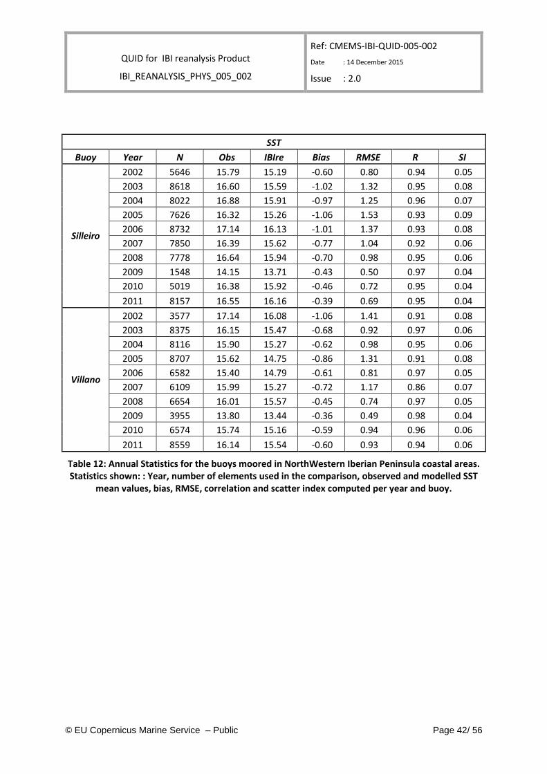
Table 12: Annual Statistics for the buoys moored in NorthWestern Iberian Peninsula coastal areas. Statistics shown: : Year, number of elements used in the comparison, observed and modelled SST






Issue : 2.0


SST


Alborán

2002 6369 20.04 17.30 -2.73 3.39 0.71 0.17

2003 2154 17.47 16.33 -1.14 1.40 0.96 0.08

2004 641 17.09 15.70 -1.38 1.43 0.48 0.08

2005 5696 17.17 16.11 -1.06 1.54 0.88 0.09

2006 1342 15.21 15.07 -0.14 0.35 0.39 0.02

2009 8735 21.00 21.12 0.12 0.49 0.98 0.02

Cádiz

2002 4618 19.99 19.32 -0.67 1.46 0.86 0.07

2003 6083 19.56 18.66 -0.90 1.32 0.97 0.07

2004 5452 20.03 19.30 -0.74 1.23 0.93 0.06

2005 7095 20.07 19.53 -0.54 0.72 0.98 0.04

2006 6954 19.65 18.92 -0.73 0.89 0.99 0.05

2007 7474 19.00 18.55 -0.45 0.77 0.97 0.04

2008 7675 19.17 18.62 -0.55 0.87 0.96 0.05

2009 7735 20.02 19.62 -0.40 0.76 0.97 0.04

2010 4957 20.32 20.10 -0.22 0.56 0.97 0.03

2011 8568 20.18 19.74 -0.43 0.76 0.97 0.04

Gata

2002 3583 21.99 21.14 -0.85 1.57 0.83 0.07

2003 4993 20.47 19.91 -0.56 1.23 0.95 0.06

2004 6709 19.50 18.72 -0.78 1.15 0.98 0.06

2005 5935 20.03 19.36 -0.67 1.23 0.96 0.06

2006 4609 17.17 16.31 -0.87 1.17 0.97 0.07

2007 8639 19.25 19.21 -0.05 0.75 0.98 0.04

2008 4928 18.61 17.85 -0.76 1.12 0.97 0.06

2009 8566 21.35 21.21 -0.14 0.45 0.98 0.02

2010 6090 20.82 20.02 -0.79 1.19 0.96 0.06

2011 5636 19.51 19.14 -0.37 0.94 0.96 0.05

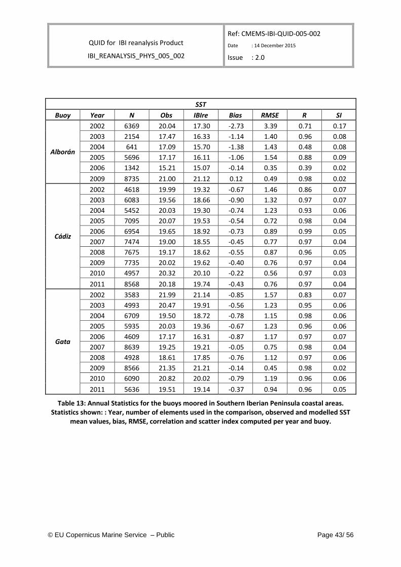
Table 13: Annual Statistics for the buoys moored in Southern Iberian Peninsula coastal areas. Statistics shown: : Year, number of elements used in the comparison, observed and modelled SST






Issue : 2.0


SST


Dragonera

2009 3355 22.35 21.78 -0.57 0.73 0.99 0.03

2010 8719 19.67 19.35 -0.32 0.71 0.99 0.04

2011 7197 21.13 20.79 -0.34 0.70 0.99 0.03

Palos

2006 3997 22.41 22.47 0.06 0.85 0.98 0.04

2007 8069 19.86 19.82 -0.04 0.61 0.99 0.03

2008 8768 19.69 19.24 -0.45 0.64 0.99 0.03

2009 8711 20.06 19.65 -0.42 0.63 1.00 0.03

2010 7812 19.70 19.59 -0.10 0.72 0.99 0.04

2011 7840 20.11 19.82 -0.29 0.70 0.99 0.03

Tarragona

2004 3198 20.97 20.70 -0.27 0.63 0.99 0.03

2005 8275 19.53 19.03 -0.50 0.91 0.99 0.05

2006 8755 19.58 19.04 -0.54 0.80 0.99 0.04

2007 8752 19.13 18.66 -0.46 0.87 0.98 0.05

2008 7477 17.98 17.83 -0.15 0.91 0.98 0.05

2009 5658 18.63 17.91 -0.71 0.90 0.99 0.05

2010 4975 21.52 21.08 -0.44 0.85 0.99 0.04

2011 8568 19.65 19.04 -0.61 0.90 0.99 0.05

Valencia

2005 2296 20.64 20.20 -0.44 0.67 0.99 0.03

2006 6336 19.75 19.05 -0.70 0.87 0.99 0.04

2007 5918 20.14 19.87 -0.27 0.47 1.00 0.02

2008 8531 19.88 19.27 -0.60 0.80 0.99 0.04

2009 7381 21.01 20.52 -0.49 0.84 0.99 0.04

2010 7967 19.71 19.12 -0.59 0.86 0.99 0.04

2011 8567 20.11 19.73 -0.38 0.65 0.99 0.03

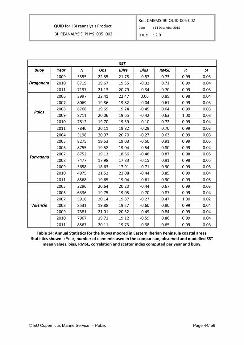
Table 14: Annual Statistics for the buoys moored in Eastern Iberian Peninsula coastal areas. Statistics shown: : Year, number of elements used in the comparison, observed and modelled SST






Issue : 2.0


SST


Gran Canaria

2002 7683 20.61 20.89 0.28 0.47 0.97 0.02

2003 8046 21.22 21.47 0.24 0.57 0.97 0.03

2004 2487 22.93 23.10 0.17 0.36 0.94 0.02

2005 1580 21.97 21.81 -0.16 0.30 0.98 0.01

2006 7783 21.03 20.78 -0.25 0.46 0.98 0.02

2007 1883 20.15 20.21 0.06 0.30 0.95 0.02

2008 7428 20.53 20.48 -0.05 0.26 0.98 0.01

2009 8735 21.00 21.12 0.12 0.49 0.98 0.02

2010 7950 21.43 21.43 0.00 0.32 0.97 0.02

2011 5631 21.99 21.87 -0.12 0.35 0.96 0.02

Tenerife

2002 7910 21.13 21.07 -0.06 0.32 0.98 0.02

2003 8254 21.48 21.48 0.00 0.44 0.97 0.02

2004 4080 22.52 22.64 0.12 0.28 0.99 0.01

2005 5616 22.16 21.90 -0.25 0.42 0.98 0.02

2006 8665 21.60 21.45 -0.15 0.47 0.97 0.02

2007 7349 21.29 21.51 0.21 0.45 0.97 0.02

2008 8365 21.26 21.09 -0.17 0.37 0.98 0.02

2009 8566 21.35 21.21 -0.14 0.45 0.98 0.02

2010 8702 21.78 21.61 -0.17 0.39 0.96 0.02

2011 6881 21.10 21.03 -0.07 0.38 0.96 0.02

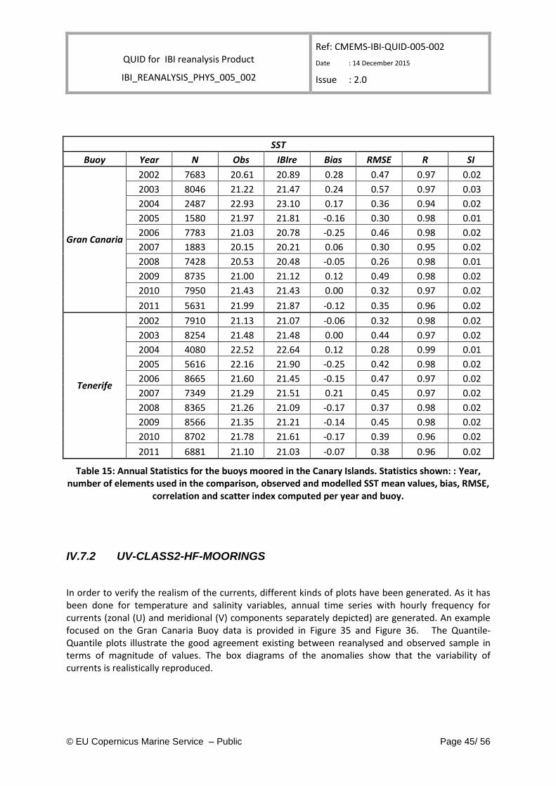
Table 15: Annual Statistics for the buoys moored in the Canary Islands. Statistics shown: : Year, number of elements used in the comparison, observed and modelled SST mean values, bias, RMSE,

correlation and scatter index computed per year and buoy.

IV.7.2 UV-CLASS2-HF-MOORINGS

In order to verify the realism of the currents, different kinds of plots have been generated. As it has been done for temperature and salinity variables, annual time series with hourly frequency for currents (zonal (U) and meridional (V) components separately depicted) are generated. An example focused on the Gran Canaria Buoy data is provided in Figure 35 and Figure 36. The Quantile-Quantile plots illustrate the good agreement existing between reanalysed and observed sample in terms of magnitude of values. The box diagrams of the anomalies show that the variability of currents is realistically reproduced.





Issue : 2.0


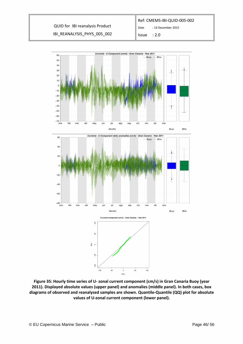
Figure 35: Hourly time series of U- zonal current component (cm/s) in Gran Canaria Buoy (year 2011). Displayed absolute values (upper panel) and anomalies (middle panel). In both cases, box

diagrams of observed and reanalysed samples are shown. Quantile-Quantile (QQ) plot for absolute values of U-zonal current component (lower panel).





Issue : 2.0


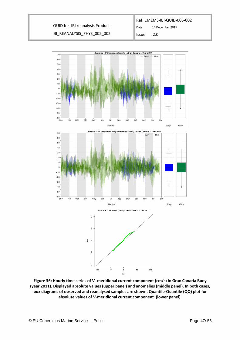
Figure 36: Hourly time series of V- meridional current component (cm/s) in Gran Canaria Buoy (year 2011). Displayed absolute values (upper panel) and anomalies (middle panel). In both cases,

box diagrams of observed and reanalysed samples are shown. Quantile-Quantile (QQ) plot for absolute values of V-meridional current component (lower panel).





Issue : 2.0


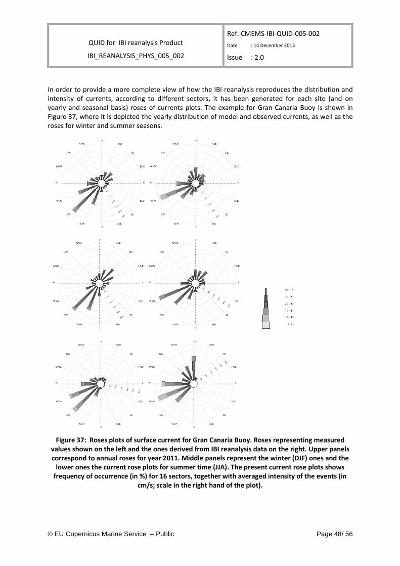
In order to provide a more complete view of how the IBI reanalysis reproduces the distribution and intensity of currents, according to different sectors, it has been generated for each site (and on yearly and seasonal basis) roses of currents plots. The example for Gran Canaria Buoy is shown in Figure 37, where it is depicted the yearly distribution of model and observed currents, as well as the roses for winter and summer seasons.

Figure 37: Roses plots of surface current for Gran Canaria Buoy. Roses representing measured values shown on the left and the ones derived from IBI reanalysis data on the right. Upper panels correspond to annual roses for year 2011. Middle panels represent the winter (DJF) ones and the

lower ones the current rose plots for summer time (JJA). The present current rose plots shows frequency of occurrence (in %) for 16 sectors, together with averaged intensity of the events (in

cm/s; scale in the right hand of the plot).





Issue : 2.0


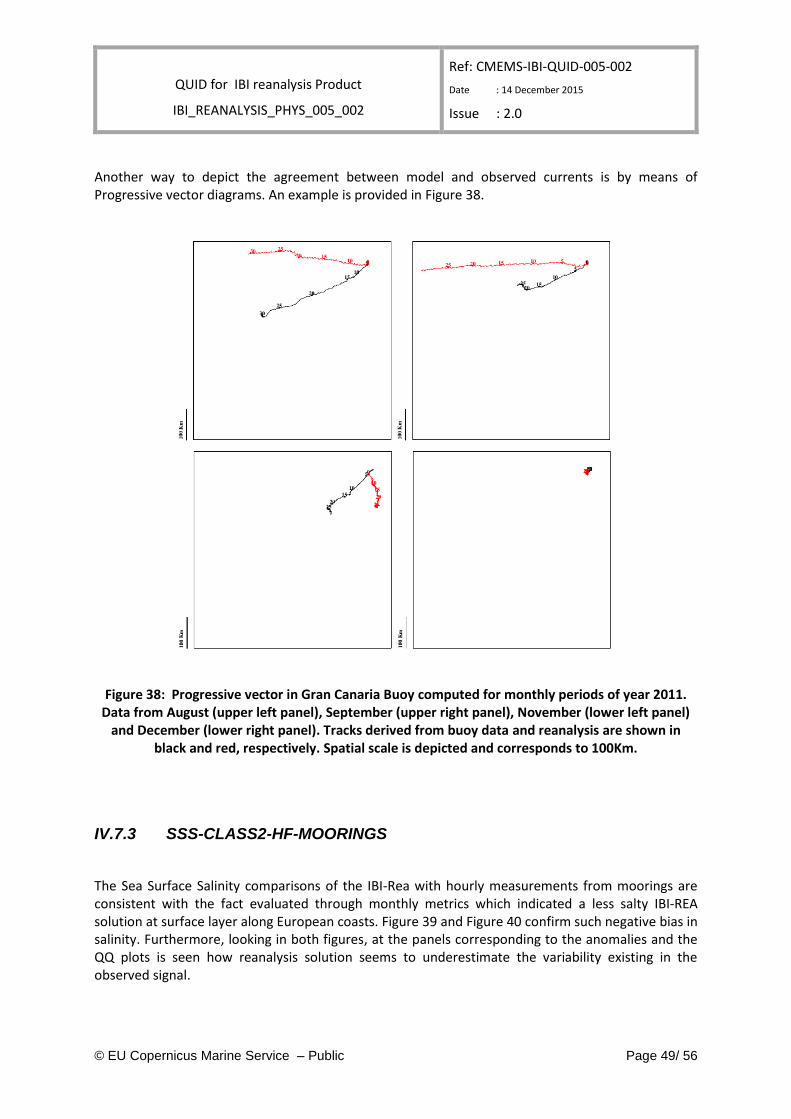
Another way to depict the agreement between model and observed currents is by means of Progressive vector diagrams. An example is provided in Figure 38.

Figure 38: Progressive vector in Gran Canaria Buoy computed for monthly periods of year 2011. Data from August (upper left panel), September (upper right panel), November (lower left panel)

and December (lower right panel). Tracks derived from buoy data and reanalysis are shown in black and red, respectively. Spatial scale is depicted and corresponds to 100Km.

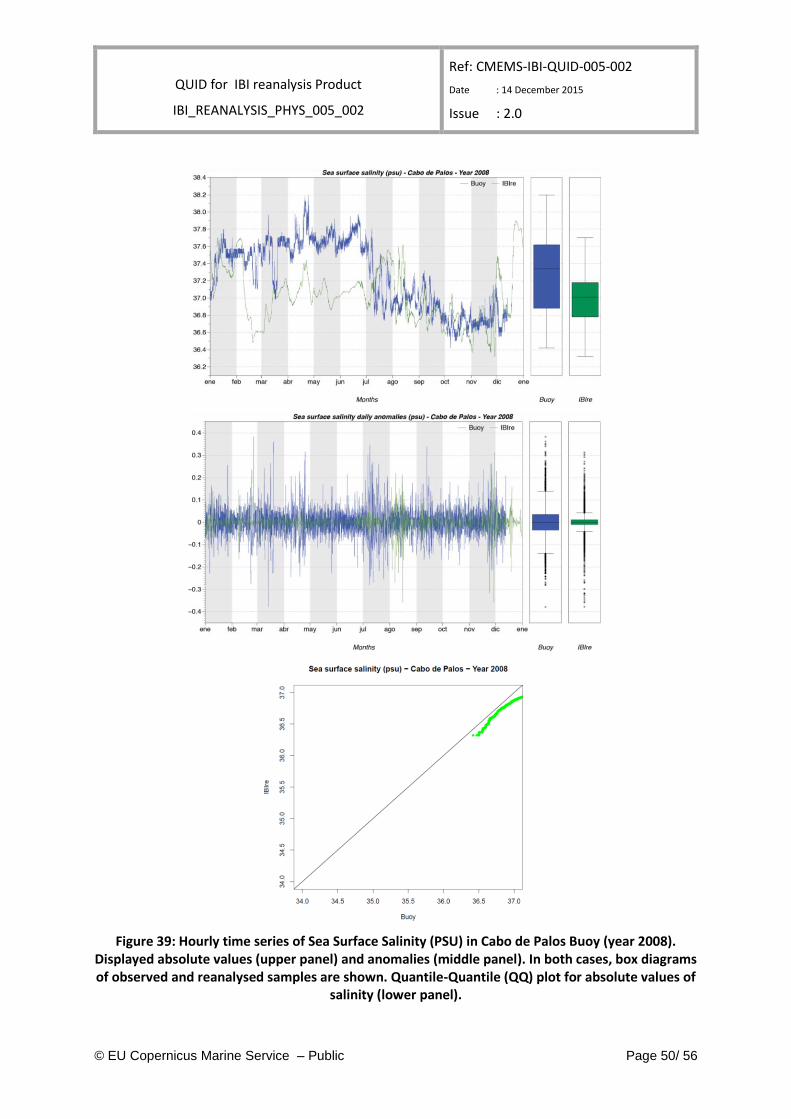
IV.7.3 SSS-CLASS2-HF-MOORINGS

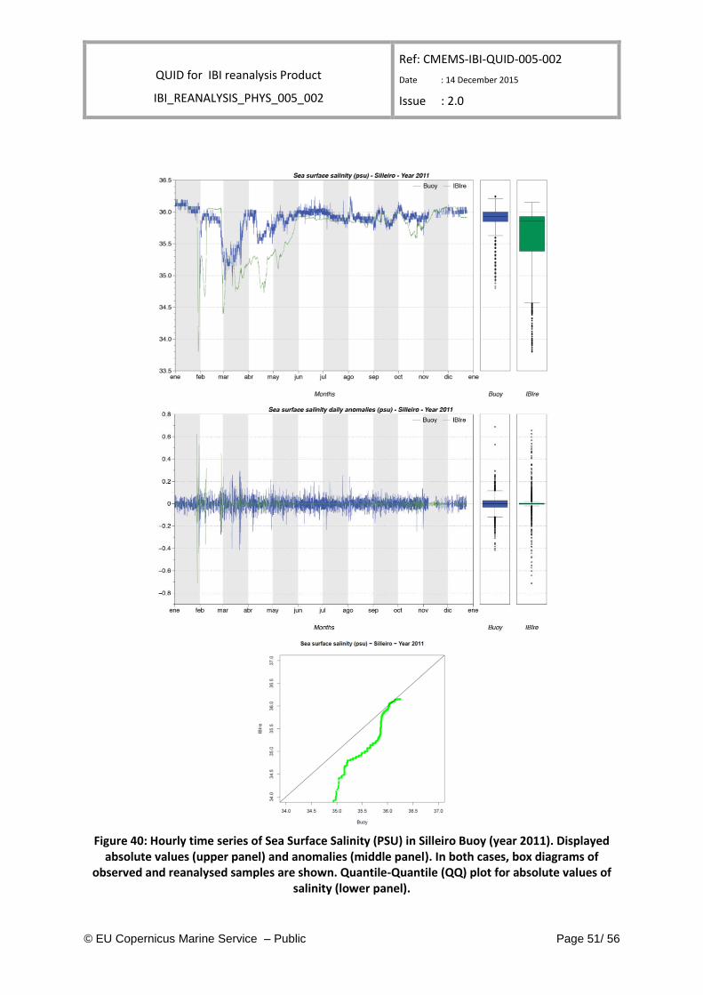
The Sea Surface Salinity comparisons of the IBI-Rea with hourly measurements from moorings are consistent with the fact evaluated through monthly metrics which indicated a less salty IBI-REA solution at surface layer along European coasts. Figure 39 and Figure 40 confirm such negative bias in salinity. Furthermore, looking in both figures, at the panels corresponding to the anomalies and the QQ plots is seen how reanalysis solution seems to underestimate the variability existing in the observed signal.





Issue : 2.0


Figure 39: Hourly time series of Sea Surface Salinity (PSU) in Cabo de Palos Buoy (year 2008). Displayed absolute values (upper panel) and anomalies (middle panel). In both cases, box diagrams of observed and reanalysed samples are shown. Quantile-Quantile (QQ) plot for absolute values of

salinity (lower panel).





Issue : 2.0


Figure 40: Hourly time series of Sea Surface Salinity (PSU) in Silleiro Buoy (year 2011). Displayed absolute values (upper panel) and anomalies (middle panel). In both cases, box diagrams of

observed and reanalysed samples are shown. Quantile-Quantile (QQ) plot for absolute values of salinity (lower panel).





Issue : 2.0


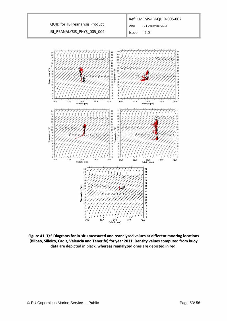
IV.7.4 Other combined CLASS2-HF-MOORINGS metrics

The following plots combine different variables. Some T/S diagrams have been generated using yearly data. These plots allow us to identify if the reanalysis is able to reproduce the surface water masses characterized through in-situ measurements. Figure 41 shows an example for buoys representing each of the geographical clusters. Likewise, Taylor diagrams have been generated for each station. These plots are quite useful for model validation purposes since they summarize different statistics (standard deviation, root mean squared errors and correlations), giving an idea of simulation realism by means of a distance metric (the closer to the reference point, the more similar are the two datasets). In these Taylor diagram, different variables, both ocean (temp, salinity and U- and V current component) and atmospheric (surface pressure, temperature and wind components), have been included in each plot. An example for one station from each geographical area is depicted in Figure 42.





Issue : 2.0


Figure 41: T/S Diagrams for in-situ measured and reanalysed values at different mooring locations (Bilbao, Silleiro, Cadiz, Valencia and Tenerife) for year 2011. Density values computed from buoy

data are depicted in black, whereas reanalyzed ones are depicted in red.





Issue : 2.0


Figure 42: Taylor diagrams of reanalysed variables at different mooring locations (Estaca de Bares, Silleiro, Cadiz, Cabo de Palos and Gran Canaria buoys). Different variables are represented at each

plot. Oceanographic ones: SST (T), surface salinity (S), and current components (U & V). Atmospheric variables: surface pressure (p), temperature (t), and u and v wind components (u &

v). Data from a 1-year time period used in each case.





Issue : 2.0


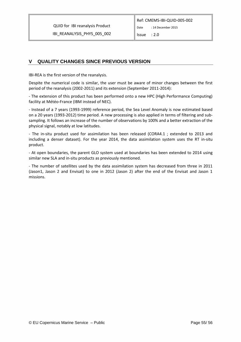
V QUALITY CHANGES SINCE PREVIOUS VERSION

IBI-REA is the first version of the reanalysis.

Despite the numerical code is similar, the user must be aware of minor changes between the first period of the reanalysis (2002-2011) and its extension (September 2011-2014):

- The extension of this product has been performed onto a new HPC (High Performance Computing) facility at Météo-France (IBM instead of NEC).

- Instead of a 7 years (1993-1999) reference period, the Sea Level Anomaly is now estimated based on a 20 years (1993-2012) time period. A new processing is also applied in terms of filtering and sub-sampling. It follows an increase of the number of observations by 100% and a better extraction of the physical signal, notably at low latitudes.

- The in-situ product used for assimilation has been released (CORA4.1 ; extended to 2013 and including a denser dataset). For the year 2014, the data assimilation system uses the RT in-situ product.

- At open boundaries, the parent GLO system used at boundaries has been extended to 2014 using similar new SLA and in-situ products as previously mentioned.

- The number of satellites used by the data assimilation system has decreased from three in 2011 (Jason1, Jason 2 and Envisat) to one in 2012 (Jason 2) after the end of the Envisat and Jason 1 missions.





Issue : 2.0


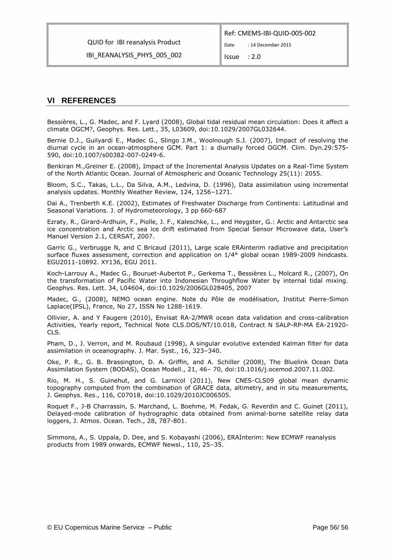
VI REFERENCES

Bessières, L., G. Madec, and F. Lyard (2008), Global tidal residual mean circulation: Does it affect a climate OGCM?, Geophys. Res. Lett., 35, L03609, doi:10.1029/2007GL032644.

Bernie D.J., Guilyardi E., Madec G., Slingo J.M., Woolnough S.J. (2007), Impact of resolving the diurnal cycle in an ocean-atmosphere GCM. Part 1: a diurnally forced OGCM. Clim. Dyn.29:575-

590, doi:10.1007/s00382-007-0249-6.

Benkiran M.,Greiner E. (2008), Impact of the Incremental Analysis Updates on a Real-Time System of the North Atlantic Ocean. Journal of Atmospheric and Oceanic Technology 25(11): 2055.

Bloom, S.C., Takas, L.L., Da Silva, A.M., Ledvina, D. (1996), Data assimilation using incremental analysis updates. Monthly Weather Review, 124, 1256–1271.

Dai A., Trenberth K.E. (2002), Estimates of Freshwater Discharge from Continents: Latitudinal and Seasonal Variations. J. of Hydrometeorology, 3 pp 660-687

Ezraty, R., Girard-Ardhuin, F., Piolle, J. F., Kaleschke, L., and Heygster, G.: Arctic and Antarctic sea ice concentration and Arctic sea ice drift estimated from Special Sensor Microwave data, User’s Manuel Version 2.1, CERSAT, 2007.

Garric G., Verbrugge N, and C Bricaud (2011), Large scale ERAinterim radiative and precipitation surface fluxes assessment, correction and application on 1/4° global ocean 1989-2009 hindcasts. EGU2011-10892. XY136, EGU 2011.

Koch-Larrouy A., Madec G., Bouruet-Aubertot P., Gerkema T., Bessières L., Molcard R., (2007), On the transformation of Pacific Water into Indonesian Throughflow Water by internal tidal mixing. Geophys. Res. Lett. 34, L04604, doi:10.1029/2006GL028405, 2007

Madec, G., (2008), NEMO ocean engine. Note du Pôle de modélisation, Institut Pierre-Simon

Laplace(IPSL), France, No 27, ISSN No 1288-1619.

Ollivier, A. and Y Faugere (2010), Envisat RA-2/MWR ocean data validation and cross-calibration Activities, Yearly report, Technical Note CLS.DOS/NT/10.018, Contract N SALP-RP-MA EA-21920-

CLS.

Pham, D., J. Verron, and M. Roubaud (1998), A singular evolutive extended Kalman filter for data assimilation in oceanography. J. Mar. Syst., 16, 323–340.

Oke, P. R., G. B. Brassington, D. A. Griffin, and A. Schiller (2008), The Bluelink Ocean Data Assimilation System (BODAS), Ocean Modell., 21, 46– 70, doi:10.1016/j.ocemod.2007.11.002.

Rio, M. H., S. Guinehut, and G. Larnicol (2011), New CNES-CLS09 global mean dynamic topography computed from the combination of GRACE data, altimetry, and in situ measurements,

J. Geophys. Res., 116, C07018, doi:10.1029/2010JC006505.

Roquet F., J-B Charrassin, S. Marchand, L. Boehme, M. Fedak, G. Reverdin and C. Guinet (2011), Delayed-mode calibration of hydrographic data obtained from animal-borne satellite relay data loggers, J. Atmos. Ocean. Tech., 28, 787-801.

Simmons, A., S. Uppala, D. Dee, and S. Kobayashi (2006), ERAInterim: New ECMWF reanalysis products from 1989 onwards, ECMWF Newsl., 110, 25–35.

Documents

QUALITY INFORMATION DOCUMENT For IBI reanalysis …cmems-resources.cls.fr/documents/QUID/CMEMS-IBI-QUID-005-002.pdf · For IBI reanalysis Product IBI_REANALYSIS_PHYS_005_002 Issue: