DI

SC

US

SI

ON

P

AP

ER

S

ER

IE

S

Forschungsinstitut zur Zukunft der ArbeitInstitute for the Study of Labor

Reducing Binge Drinking?The Effect of a Ban on Late-Night Off-Premise Alcohol Sales on Alcohol-Related Hospital Stays in Germany

IZA DP No. 8763

January 2015

Jan MarcusThomas Siedler

Reducing Binge Drinking? The Effect of a

Ban on Late-Night Off-Premise Alcohol Sales on Alcohol-Related Hospital Stays

in Germany

Jan Marcus DIW Berlin

Thomas Siedler

Universität Hamburg and IZA

Discussion Paper No. 8763 January 2015

IZA

P.O. Box 7240 53072 Bonn

Germany

Phone: +49-228-3894-0 Fax: +49-228-3894-180

E-mail: iza@iza.org

Any opinions expressed here are those of the author(s) and not those of IZA. Research published in this series may include views on policy, but the institute itself takes no institutional policy positions. The IZA research network is committed to the IZA Guiding Principles of Research Integrity. The Institute for the Study of Labor (IZA) in Bonn is a local and virtual international research center and a place of communication between science, politics and business. IZA is an independent nonprofit organization supported by Deutsche Post Foundation. The center is associated with the University of Bonn and offers a stimulating research environment through its international network, workshops and conferences, data service, project support, research visits and doctoral program. IZA engages in (i) original and internationally competitive research in all fields of labor economics, (ii) development of policy concepts, and (iii) dissemination of research results and concepts to the interested public. IZA Discussion Papers often represent preliminary work and are circulated to encourage discussion. Citation of such a paper should account for its provisional character. A revised version may be available directly from the author.

IZA Discussion Paper No. 8763 January 2015

ABSTRACT

Reducing Binge Drinking? The Effect of a Ban on Late-Night Off-Premise Alcohol Sales on Alcohol-Related Hospital Stays in Germany

Excessive alcohol consumption among young people is a major public health concern. On March 1, 2010, the German state of Baden-Württemberg banned the sale of alcoholic beverages between 10pm and 5am at off-premise outlets (e.g., gas stations, kiosks, supermarkets). We use rich monthly administrative data from a 70 percent random sample of all hospitalizations during the years 2007-2011 in Germany in order to evaluate the short-term impact of this policy on alcohol-related hospitalizations. Applying difference-in-differences methods, we find that the policy change reduces alcohol-related hospitalizations among adolescents and young adults by about seven percent. There is also evidence of a decrease in the number of hospitalizations due to violent assault as a result of the ban. JEL Classification: I12, I18, D04 Keywords: binge drinking, drinking hours, alcohol control policies, difference-in-differences,

hospital diagnosis statistics, alcohol Corresponding author: Thomas Siedler Universität Hamburg Von-Melle-Park 5 20146 Hamburg Germany E-mail: Thomas.Siedler@wiso.uni-hamburg.de

I. Introduction

According to the World Health Organization (2014), excessive alcohol consumption is re-sponsible for around 3.3 million preventable deaths worldwide in 2012, and the harmfuluse of alcohol accounts for 5.1 percent of the global burden of disease and injury. Inparticular, excessive consumption of alcohol by young people is a major public healthconcern. The Centers for Disease Control and Prevention reports that in 2010, amongU.S. adults aged 18 years and older, binge drinking prevalence and intensity was highestamong those aged 18-24 years (Kanny et al. 2012). Since drinking is habit-forming (seee.g. Enoch 2006), early drinking onset might have long-lasting adverse consequences. In-deed, a large body of literature documents a significant relationship between (extensive)alcohol consumption in young people and various negative outcomes, such as crime (Car-penter 2005a), risky sexual behavior and teenage pregnancy (Sen 2003; Carpenter 2005b),suicide (Birckmayer and Hemenway 1999; O’Connell and Lawlor 2005), lower academicperformance (Carrell et al. 2011), lower employment and higher risk of unemployment(Mullahy and Sindelar 1996), adverse health effects such as mortality and hospitalization(Chaloupka and Xu 2011; Kim et al. 2012), and motor vehicle fatalities (Ruhm 1996; Dee1999).

High-risk drinking has been increasing in the last years among young people in theUnited States (White et al. 2011) and across much of Europe, including Germany (DHS2008). Figure 1 reports trends in alcohol-related hospitalization rates among adolescentsand young adults in Germany, a country where young people can legally buy beer andwine starting with the age of 16. Panel a) displays trends in the annual number ofalcohol-related hospitalizations per 100,000 inhabitants of the same age between 2002and 2011. Panel b) displays the corresponding growth rates. The figure shows that thealcohol-related hospitalization rates doubled in the age groups 15-19, 20-24, and 25-29.The German Federal Statistical Office reports that in 2011, 41,959 individuals between15 and 29 received hospital treatment due to excessive alcohol consumption, compared to18,391 in 2002.1

In March 2010, the German state of Baden-Württemberg2 banned the sale of alcoholicbeverages between 10pm and 5am at off-premise outlets (e.g., gas stations, supermarkets,kiosks). One of the law’s main objectives was to reduce binge drinking among youngpeople. This study presents first evidence on the short-term effects of this late-night

1https://www.destatis.de/EN/FactsFigures/SocietyState/Health/Hospitals/Tables/DiagnosisAlcoholAgYears.html. Note that the numbers of alcohol-related hospitalizations inFigure 1 are taken from the same source. Accessed on July 16, 2014.

2Baden-Württemberg is located in southwestern Germany and is the third-largest German state bypopulation (10.5 million in 2011).

1

alcohol sales ban on alcohol-related hospitalizations. We exploit rich monthly data froma 70 percent random sample of the German hospital diagnosis statistics for the 2007-2011period. This nationwide hospitalization data set contains information about all inpatientsat all German hospitals. We study the short-term effect of the reform on alcohol-relatedhospitalizations in general and specifically for young people, as there are various reasonsto assume that the reform impacts youth in particular. Using an additional data setfrom one large hospital in the comparison group, we also document that the majorityof alcohol-related hospital admissions among young people takes place in late eveningand during the night. Hence, the late-night alcohol ban is likely to be most binding foradolescents and young adults.

Indeed, we find that the policy change reduces alcohol-related hospitalizations amongadolescents (ages 15-19) and young adults (ages 20-24) by about seven percent. For olderindividuals, there is no empirical evidence of a significant reduction. Our findings are ro-bust to alternative definitions of the control group (e.g., only states in western Germany,only the southern states of Bavaria and Hesse, a synthetic control group), different restric-tions of the sample, the addition of further control variables (e.g., county-specific timetrends) and various estimation issues (e.g., estimation in logs, Tobit model). We provideevidence that the ban impacts both male and female adolescents/young adults, thoughthe effect is stronger for males. Furthermore, we find empirical evidence that the late-night off-premise alcohol sales ban reduces overall hospitalizations due to diagnoses thatare often related to violent assaults. However, we do not find evidence of complementaryeffects on illicit drug use, as the ban does not decrease drug-related hospitalizations.

Overall, our empirical results suggest that the late-night off-premise alcohol ban is aneffective policy strategy for reducing excessive alcohol consumption among adolescentsand young adults. Hence, the ban can work as a measure against negative externalitiesof excessive alcohol consumption, such as violence, traffic accidents, and noise (Parry etal. 2009) and as a commitment device for individuals with time-inconsistent preferences(Hinnosaar 2012). The empirical findings contribute to the literature on whether and howpolicies can influence problematic drinking behaviors. The results are also informativefor policy makers in other countries who are considering or planning to implement similarlate-night alcohol sales bans: the investigated ban can be considered to be a fairly “lighttouch” regulation compared to other alcohol control policies, as it restricts the sale ofalcoholic beverages only at a specific time of the day (10pm to 5am) and only for aspecific type of outlet (off-premise outlets).

The outline of the paper is as follows. Section II discusses the literature on relatedalcohol control policies, Section III provides background information on the late-nightban and other relevant alcohol policies in Germany, and Section IV describes the data.

2

Section V discusses the empirical approach, and the main results are presented in SectionVI. Section VII probes the robustness of the findings and Section VIII reports furtherresults (e.g., effect heterogeneity, evolution of the treatment effect, length of hospital stay,and other diagnoses). Section IX concludes.

II. Related literature

Proponents of alcohol control policies often point out that excessive alcohol consumptionis a negative externality as it can compromise others either directly (as, e.g., in the case ofcrime, traffic accidents, and noise) or indirectly (e.g., through higher costs for the healthcare system). Additionally, alcohol control policies are often justified with reference totime-inconsistent preferences of alcohol consumers (Hinnosaar 2012). For instance, inthe morning, individuals with time-inconsistent preferences may plan to drink less or noalcohol that evening, but when evening comes, they find themselves unable to resist theurge for a drink. Therefore, a ban on late-night alcohol sales can be seen as a kind ofcommitment device for individuals with time-inconsistent preferences (Bryan et al. 2010):during the day they plan to consume fewer beverages in the night and therefore purchaseless alcohol during the day, but when the night arrives, they go to the shop again tobuy more alcohol (for a formalized version of this argument, see Hinnosaar 2012). Thelate-night ban on alcohol sales can prevent this additional shopping trip.

In general, one can distinguish among several regulatory strategies for restricting accessto alcohol: (i) regulating temporal access (e.g., hours and days of sale); (ii) regulatingthe economic access (e.g., price policies and alcohol taxes);3 (iii) regulating demographicaccess (e.g., minimum legal drinking ages, drunk driving laws)4 and (iv) regulating thelocations where alcohol is sold (e.g., on- versus off-premise outlets, public events).5

The literature most closely related to ours investigates restrictions in temporal accessto alcohol. These studies analyze how changes in the hours and days of alcohol salesaffect consumption, hospitalizations, traffic fatalities, and crime (Norström and Skog 2005;Vingilis et al. 2005; Chikritzhs and Stockwell 2006; McMillan and Lapham 2006; Vingilis2007; Middleton et al. 2010). Vingilis (2007), Popova et al. (2009) and Middleton et al.

3Overall, the literature on regulating economic access to alcohol finds that alcohol consumption de-creases with rising prices and that raising alcohol taxes is effective in preventing alcohol-related problems(Grossman et al. 1993; Manning et al. 1995; Ruhm 1996; Dee 1999; Cook and Moore 2000, 2002; Youngand Bielinska-Kwapisz 2006; Carpenter et al. 2007; Wagenaar et al. 2009, 2010; Chaloupka and Xu 2011).

4Most of the research on policies that restrict demographic access to alcohol focuses on minimum legaldrinking ages in the United States (Carpenter et al. 2007; Lovenheim and Slemrod 2010; Carrell et al.2011). The general consensus in this literature is that the introduction of the minimum legal drinking ageof 21 was effective in reducing the prevalence and intensity of drinking (Wagenaar and Toomey (2002),Carpenter et al. (2007) and references therein).

5See, for example, Scribner et al. (1995) and Speer et al. (1998).

3

(2010) provide recent surveys on the effects of changes in hours and/or days of alcoholsales on alcohol consumption and alcohol-related harm. Newton et al. (2007) examine theimpact of the UK licensing law that came into effect in November 2005 and that madethe opening hours for licensed premises more flexible. Using data from March 2005 andMarch 2006 from one emergency hospital in London, the study finds that the proportionof alcohol-related assaults resulting in overnight hospitalization increased by roughly onepercentage point, alcohol-related hospital admission rates by nearly two percentage points,and alcohol-related injuries by 2.5 percentage points. Norström and Skog (2005) study theimpact of Saturday openings of alcohol retail shops in Sweden on alcohol sales, assaults,and drunk driving. The authors exploit both time and regional variation in Saturdayopenings of alcohol retail shops. First, in February 2000, a trial phase started duringwhich six counties implemented Saturday openings, followed by an extension across thewhole of Sweden in July 2001. The authors report that alcohol sales increased by nearlyfour percent due to this change in trading days, but they find no effects on various assaultindicators and mixed effects for drunk driving. Vingilis et al. (2005) study the LiquorLicence Act in Ontario, Canada, that extended on-premise alcohol sales from 1am to 2amin Ontario. Their findings suggest that the slight extension in opening hours contributedto a slight increase in drinking-related problems in some areas of Ontario.

Closely related to our study is an analysis by Wicki and Gmel (2011). The authorsexamine a similar ban on late-night alcohol sales in the Swiss canton of Geneva, butwere unable to disentangle the effects of the late-night alcohol sales ban from those ofa general ban on alcohol sales in gas stations and video stores, which came into effectat the same time. They found major decreases in alcohol-related hospitalizations in thecanton of Geneva due to the joint effect of these reforms (e.g., a reduction of 40 percentin alcohol-related hospitalizations among teenagers). Yet, it remains unclear whether thislarge decrease is due to the late-night alcohol sales ban, to the general ban on alcoholsales at gas stations and video stores, or to both bans.

To date, there exists inconclusive evidence in the literature on the effectiveness oflimiting the hours of off-premise alcoholic sales. Indeed the Task Force on CommunityPreventive Services in the United States concludes: “The Task Force found insufficientevidence to determine the effectiveness of increasing existing limits on hours of sale at off-premise outlets, because no studies were found that assessed such evidence” (Task Forceon Community Preventive Services 2010: 606). Our study aims at filling this gap in theliterature by studying a recent legislative change in hours of alcohol sales in Germany.

4

III. Institutional background

The policy change that we analyze bans the sale of alcoholic beverages between 10pmand 5am at off-premise outlets (e.g., gas stations, supermarkets, kiosks) in the Germanstate of Baden-Württemberg. The law has two main intentions: to reduce binge drinking(especially among young people) and to reduce alcohol-related violence and harm. Thedraft bill was submitted on July 21, 2009 (Landtag von Baden-Württemberg 2009b), anddiscussed for the first time in the state parliament on July 30, 2009 (Landtag von Baden-Württemberg 2009c). During these consultations, Heribert Rech, Minister of the Interiorin Baden-Württemberg, explained the aims of the law as follows: “The aim is clear:With this law, we want to combat alcohol-related crime at night, and we want to protectadolescents and young people in particular from alcohol-induced health risks. These risksare especially high when they are able to consume alcohol at night” (Landtag von Baden-Württemberg 2009c: 5258). The law was approved by the state parliament on November4, 2009, and went into effect on March 1, 2010 (Landtag von Baden-Württemberg 2009a).

Violating the ban results in a fine of up to 5,000 euros. There are reasons to assumethat the police immediately began enforcing the ban given that this was their preferredpolicy (see Landtag von Baden-Württemberg 2009b). Furthermore, when reviewing news-papers published around the time of the ban’s introduction, we found little evidence ofcomplaints about a lack of enforcement.

Before the ban came into effect, it was theoretically possible to buy alcoholic beverages24 hours a day at off-premise outlets. Gas stations were the main place that people couldbuy alcohol around the clock. Therefore, both the public debate on the law and thereasoning for its introduction focused primarily on gas stations (Landtag von Baden-Württemberg 2009b). Since the ban applied solely to off-premise sales, bars, restaurants,and other on-premise outlets were not affected.

The ban on late-night off-premise alcohol sales can be considered as a fairly “lighttouch” regulation compared to other alcohol control policies. Unlike a general prohibition,the ban only regulates the purchase, not the consumption of alcohol. In contrast to alcoholtaxes, it is easy to legally avoid the ban, e.g., by buying the alcohol before 10pm (i.e.,pre-stocking). Moreover, unlike minimum legal drinking age regulations, the ban doesnot exclude entire demographic groups from the legal consumption of alcohol. Comparedto other policies regulating the temporal access to alcohol, the ban neither prohibits theoff-premise sale of alcohol for entire days nor does it regulate the purchase of alcoholicbeverages on-premise.

The basic argument why the ban might nevertheless be effective is that it suppressesthe spontaneous purchase of alcohol at off-premise outlets. It functions by complicating

5

access to alcoholic beverages in situations when those who have already begun consumingalcohol might otherwise continue to do so in an abusive and unhealthy way (Landtagvon Baden-Württemberg 2009b: 11, 13-14).6 In such situations, the ban can be seen asan interruption in the alcohol supply chain as it increases the effort needed to consumemore alcohol. The ban can be also considered as a commitment device for individualswith time-inconsistent preferences. As such, the law might be very effective in curbingbinge drinking, as it restricts access to alcohol at a crucial time of the day when theoverwhelming majority of excessive drinking takes place.

Figure 2 displays the distribution of hours of alcohol-related hospitalizations by agegroups.7 The histograms for individuals aged 15-19 and 20-24 show that the majority ofalcohol-related hospital admissions in these age groups occur in the late evening and atnight. Among adolescents (ages 15-19), around 70 percent of all alcohol-related hospital-izations take place between 10pm and 4am. Similarly, among young adults (ages 20-24),nearly one in two admissions happens during these hours. For other age groups, however,there is no similar peak between 10pm and 4am. In contrast, the histogram for all in-dividuals (Panel a) in Figure 2) shows that many admissions take place in the morninghours, which is mainly driven by individuals aged 30 and above (Panel e). For example,among those aged 30 and above, those who are admitted to hospital between 8am and11am are more likely to be male (82 percent compared to 78 percent), to be older (56years vs. 51 years), to stay longer in hospital, to be operated, and to be admitted tohospital during the week.8

The study by Bouthoorn et al. (2011) also reports that the majority of alcohol-relatedhospitalizations among adolescents in the Netherlands happen in the late evening and atnight. These findings suggest that banning late-night off-premise alcohol sales could bemore effective at curbing binge drinking and preventing alcohol-related harms, especiallyamong young people, than limiting alcohol sales to certain days of the week, for instance,through Sunday liquor laws (Stehr 2010; Heaton 2012).

We expect the ban to have a particularly strong impact on young individuals for severalreasons. First, the ban is likely to be most binding for youth and young adults, as mostof their excessive drinking takes place in the evening and during the night. Second, youngpeople might be less likely to buy alcohol ahead of time and store it for later consumption.

6This argument is based on the assumption of alcohol being a (harmful) addictive good: the marginalutility of current consumption rises with the amount of past consumption (reinforcement), the amountof past consumption lowers utility (tolerance), and current consumption is associated with a positivemarginal utility (withdrawal) (see e.g. Becker and Murphy 1988; Cawley and Ruhm 2012).

7The data come from one large hospital in the control group (i.e., outside of Baden-Württemberg)and contain more than 14,000 alcohol-related hospitalizations in the period 2007-2013.

8Doctors working in emergency rooms in hospitals told us that a high proportion of alcohol-relatedhospital admissions in the morning hours are elderly homeless people, who are often alcoholics.

6

Often young people do not have their own apartments or other personal spaces where theycould safely store alcohol. Third, the ban was justified by arguments that young peopleoften use gas stations as gathering points and to buy alcohol for “predrinking” (Landtagvon Baden-Württemberg 2009b: 8,11). Fourth, young individuals might be less likelyto go to bars, where alcohol is more expensive. This may be particularly salient foryoung individuals with their limited budgets. Furthermore, the German Law for theProtection of the Youth (Jugendschutzgesetz) regulates the hours during which childrenand adolescents are allowed to enter bars and pubs: children below the age of 16 can visitbars and pubs only accompanied by a parent or legal guardian; young people aged 16 or 17must leave at midnight unless accompanied by a parent or legal guardian. Additionally,minimum legal drinking ages are more tightly enforced in bars and pubs (Landtag vonBaden-Württemberg 2009b).

The reasoning for why the ban should be effective in reducing excessive alcohol con-sumption is based on the assumption that alcohol purchased at night tends to be consumedrelatively shortly after its purchase. Several arguments can be made in favor of this as-sumption. First, the ban primarily affected gas stations as not all supermarkets in thetreatment state are open after 10pm and alcohol is considerably more expensive at gasstations than at supermarkets. Hence, if young people were planning to consume the alco-hol later−for example, the next day−they could simply wait and buy the alcoholic drinksat a lower price at the supermarket. Second, evidence has been reported in newspaperarticles that many young people tend to consume alcohol immediately or shortly afterpurchasing it (Hoffmann 2009; Hoischen and Eppelsheim 2009).9

The advantage of the German setting for a clean analysis of the reform’s effect isthat many of the other regulations that might impact alcohol-related hospitalizations arefederal laws and thus constant across states. Examples include drunk driving laws, alcoholtaxes, and youth protection laws. Also minimum legal drinking ages do not differ betweenthe states. Germany has relatively nonrestrictive laws regulating alcohol purchases andconsumption, with three different legal minimum drinking ages.10 Children under the ageof 14 are not allowed to consume or purchase alcohol. Children aged 14-16 are allowedto consume undistilled alcoholic beverages, such as beer and wine, if they are in thecompany of a parent or legal guardian. Youth aged 16-18 are allowed to drink beer andwine without parental consent and without being accompanied by a legal guardian, butno hard liquor or spirits. As soon as young people turn 18, they are allowed to drink all

9For example, an article in the daily newspaper Der Tagesspiegel with the title “Pre-drinking at thegas station” (Vorglühen an der Tankstelle) describes the problem that young people drink excessively infront of gas stations (Hoffmann 2009).

10Drinking ages are regulated by §9 of the German Law for the Protection of the Youth (Jugend-schutzgesetz).

7

alcohol beverages.There are, however, a few potentially relevant laws that differ between states and over

time. A large-scale reform of the German federal system in 2006 (FöderalismusreformI ) transferred legislative competence for shopping hours from the federal to the statelevel. Following this reform all of the states (except Bavaria) enacted their own lawson shopping hours that went into effect between November 2006 and July 2007.11 Allchanges in opening hours took place about three years before the late-night alcohol salesban that we analyze here. However, in order to rule out potential effects of these policychanges, we include a set of dummy variables capturing the effect of different shoppinghour regimes. In the robustness section, we also restrict our analysis to a period withoutchanges in the shopping hours of any state.

Furthermore, bar hours differ between states. There is more variation within thanbetween states, however, as most states leave it up to the municipalities to regulate barhours. On January 1, 2010, Baden-Württemberg changed the general legal closing timeof bars, clubs, and restaurants from 2am to 3am on weekdays and from 3am to 5am onweekends. Municipalities were still allowed to extend or reduce the general closing hours.As there is some evidence in the literature (e.g., Newton et al. 2007; Vingilis 2007) thatextended bar hours might slightly increase extensive alcohol consumption, we might beunderestimating the effect of the late-night ban on off-premise alcohol sales, which cameinto force two months after the extension of the legal bar hours.12

We also checked for other potentially relevant alcohol-related initiatives that mightdiffer between states. However, these campaigns were either implemented in the wholeof Germany and/or implemented clearly before the introduction of the ban or after theperiod of our analysis (e.g., “Don’t drink too much - Stay Gold”, “HaLT - Hart am Limit”,“Null Alkohol - Voll Power”). For example, “Don’t drink too much - Stay Gold” wasinitiated nationwide in 2008 and aims at tackling excessive alcohol consumption amongyoung people with informational videos and posters.13 Similarly, “HaLT” is a nationwideinitiative aimed at preventing alcohol addiction implemented across all states. It offerschildren and adolescents who have experienced alcohol-related hospitalizations counselingand group discussions. Today, there are around 170 local HaLT initiatives throughoutGermany.14 Overall, it is unlikely that these various alcohol campaigns bias our results.

11Most states have extended shopping hours to 24 hours a day six days a week (except Sundays). Somestates, however, limited weekday opening hours to 6am to 8pm (Saarland, Bavaria) or 6am to 10pm(Saxony, Rhineland-Palatinate).

12We discuss this issue in more detail in the robustness section.13See http://www.staygold.eu/. Accessed on June 2, 2014.14See http://www.halt-projekt.de for further information. Accessed on June 2, 2014.

8

IV. Data

We use data from the German hospital diagnosis statistics for the years 2007-2011 (FDZ2014). These nationwide hospitalization statistics are a very rich source of data providinginformation about all inpatients in all German hospitals (excluding police hospitals andhospitals of the penal system). Inpatients in the German context also include individualswho receive treatment in the emergency department but do not stay overnight.15 Dueto data confidentiality regulations, we work with a 70 percent random subsample of allhospitalizations.

This data set has three main strengths. First, the sample size is extremely large (e.g.,about 13 million hospitalizations are recorded in our 70 percent subsample for the year2011). Second, as the data are not self-reported, we do not have to worry about panelattrition, social desirability bias, and the like. Third, while other data sets on alcoholconsumption provide information only on an annual basis, this data set allows us toidentify the relevant outcome on a monthly basis. This is crucial as the ban did not startat the beginning of a year. Furthermore, the monthly basis allows us to distinguish theeffect of the ban on alcohol sales from other changes that took place in the same year(but not in the same month).

The data set has some shortcomings, as well. First, for each patient, it only includesinformation about the main diagnosis and a few demographic variables (age, gender,county of residence), but no socio-economic variables. This is not a major concern for thepresent analysis, which focuses on the average effect of the reform. Yet it prevents us fromanalyzing whether the reform had differential effects on specific socio-economic groups.Second, because the data contain only the main diagnosis for each patient, the numberof alcohol-related hospitalizations may be underestimated. For instance, an individualwho suffered a physical injury (e.g., laceration) due to excessive alcohol consumptionmight not be classified based on alcohol intoxication but based on the injury (Stolle etal. 2010).16 This kind of misclassification might result in an underestimate of the policyreform’s effect.17 Third, the latest available hospitalization information is from December2011 because the data collection process is quite complex: the data are submitted bythe individual hospitals, checked by the statistical offices of the German states, and dis-tributed by the German Federal Statistical Office. Hence, we can only analyze short-termconsequences of the reform (with 22 months of post-policy information).

15In contrast to the United States, emergency rooms outside of hospitals do not exist in Germany.16Stolle et al. (2010) also provide some empirical evidence that the German hospital diagnosis statistics

underestimate the alcohol-related hospitalizations of children and adolescents.17However, when we express the reform’s effect as percentage changes in the overall level of alcohol-

related hospitalizations, we might estimate these percentage changes consistently if the share of misclas-sified hospitalizations is constant.

9

To define alcohol-related hospitalizations (ARH), we follow Wicki and Gmel (2011) inrelying on the codes F10 (“Mental and behavioral disorders due to alcohol use”) and T51(“Toxic effect of alcohol”) of the 3-digital ICD-10 classification (“International StatisticalClassification of Diseases and Related Health Problems”) constructed by the WHO.18

We aggregate the number of alcohol-related hospitalizations by month of admissionand inpatient’s county of residence. Hence, we construct a balanced panel of the 402German counties as of January 2011 (44 of them are in Baden-Württemberg) covering aperiod of 60 months. This gives rise to 24,120 county-month observations. In order tomake the ARH numbers comparable across counties with different population sizes, wecalculate hospitalization rates per 100,000 inhabitants.19 For this purpose, we combinethe hospital diagnosis statistics with county population data from the German FederalStatistical Office. In addition, we map further information at the county level into thehospital diagnosis statistics for the construction of control variables: the county’s popu-lation density, the general unemployment rate, the youth unemployment rate (defined asunemployment rate among individuals below 25), and the county’s GDP.20

In our analysis, we study the effect of the reform on alcohol-related hospitalizationrates for the entire population and for specific age groups. We focus on young people asthere are several reasons to assume that the reform impacts young individuals in particular(see section III). We study potential effects of the ban for different age groups of youngpeople divided into five-year age brackets: ages 15-19, 20-24, and 25-29.21 We also analyzeall individuals aged 30 and older. In Section A, we further differentiate the age groups.

Figure 3 displays average monthly alcohol-related hospitalizations per 100,000 inhab-itants of the same age and gender in 2009, the year prior to the ban. One can see thatthere are not many alcohol-related hospitalizations prior to age 13. Moreover, amongindividuals aged 14 and younger, gender differences are not large (ARH rates are slightlyhigher among females aged 13 and 14). Starting at 15, male ARH rates always exceedfemale ARH rates and are about twice as high.22 Among males, ARH rates peak at theage of 16, the minimum legal drinking age, then decrease, and remain at a relativelyconstant level after age 20. Similarly, female ARH rates peak at 15/16 years of age andlevel off after age 20.

18In section VII, we show that our results are robust to only using the code F10, which accounts forabout 98 percent of the cases that we classify as alcohol-related hospitalizations.

19We reweight the number of alcohol-related hospitalizations by the inverse of 0.7, in order to take intoaccount that we are only provided with a 70 percent random sample.

20These annual data are publicly available from https://www.regionalstatistik.de/genesis/online/data.

21These age brackets are also used in publications of the Federal Statistical Office on ARH among theyouth.

22The magnitude of this gender difference is in line with findings from self-reported binge drinkingrates (BZgA 2012).

10

In addition to the German hospital diagnosis statistics, we use data from one largehospital outside of Baden-Württemberg to provide additional descriptive evidence.23 Thisdata set comprises more than 14,000 alcohol-related hospital admissions for the years2007-2013. Consistent with the national statistics, these data show an increase in thenumber of alcohol-related hospitalizations over time and significantly higher admissionrates among men than among women. The main advantage of these hospital data isdetailed information on the timing of admissions and releases (e.g., hours and day ofadmission), the number of procedures carried out by the hospital, the number of additionaldiagnoses, and whether the patient was operated on, admitted to intensive care, or givenartificial respiration. This hospital data shows that the majority of alcohol-related hospitaladmissions among adolescents and young adults occur in the late evening and at night(Figure 2) and on weekends (Figure A.1 in the Appendix).

V. Empirical strategy

We estimate basic difference-in-differences (DiD) models and regression difference-in-differences models with various control variables in order to inspect the effect of thelate-night alcohol sales ban on alcohol-related hospitalization rates. The basic DiD modeltakes on the form:

ARHcst = α0 + β · banst + α1 · postt + α2 ·BaWus + εcst, (1)

where ARHcst refers to the alcohol-related hospitalization rate in county c in state s inmonth t. banst denotes our prime variable of interest, a binary variable that equals one ifthe late-night alcohol sales ban is in force in state s in month t and zero otherwise (i.e.,the interaction term of postt and BaWus). The other two regressors in the basic DiDmodel are binary variables for the post-treatment period (postt) and the treatment stateBaden-Württemberg (BaWus). εcst is the error term, which might be correlated withinstates. Therefore, we cluster standard errors on the state level.24 We estimate equation(1) for hospitalization rates in different age groups.

In the regression difference-in-differences models with various control variables, we23Due to data confidentiality we are not allowed to provide the name of the hospital or the state in

which it is located.24There is a discussion in the literature on the appropriateness of clustered standard errors when the

number of clusters is small (Donald and Lang 2007). In the robustness section, we also report wild clusterbootstrap procedures (Cameron et al. 2008). Additionally, we perform analyses using panel-correctedstandard errors.

11

refine and supplement equation (1) and estimate equations of the following form:

ARHcst = α0 + β · banst + γc + δt +X ′cstλ+ κs,season + εcst. (2)

Instead of the BaWus indicator in the basic DiD model, we include a set of countyfixed effects, γc, accounting for time-invariant differences in the level of alcohol-relatedhospitalizations between the counties (and, hence, also between the German states). Wereplace the indicator for the post-treatment period, postt, with a maximum set of time(month-year) dummy variables, δt, controlling for time shocks that commonly influencealcohol-related hospitalizations in the German states (e.g., federal drunk driving laws).25

Xcst denotes a set of time-varying control variables at the county and state levels. Itincludes the state’s share in total German GDP, the county’s general unemploymentrate, and the county’s youth unemployment rate as measures of the economic situation.Furthermore, in order to monitor changes in the population composition, Xcst includes thepopulation density of the county and the number of individuals of the analyzed age in thecounty as a share of the its total population. Additionally, Xcst includes a set of dummyvariables for different shopping hour regimes to address the issue of changes in the lawon opening hours of supermarkets (see section III).26 κs,season is a set of season-specificstate dummies capturing seasonal differences between states.27 There may be seasonaldifferences in ARH rates between states due to variations in celebrations. For example,Baden-Württemberg is famous for its Carnival celebration, which takes place in February.

In section VI we start with the basic DiD models and then gradually incorporate thecontrol variables from equation (2). We estimate equations (1) and (2) by weighted leastsquares, where the weights are given by the county’s population of the analyzed age inorder to obtain the accurate overall effect for Baden-Württemberg. Draca et al. (2011)and Kelly and Rasul (2014) apply similar weighting procedures on their aggregated data.

VI. Main results

A. Basic difference-in-differences results

Table 1 reports the results from basic difference-in-differences models. The first panel ofthe table shows the results for all age groups combined. The lower panels display the

25Since we replace the post-treatment period and the treatment state indicators with time and countyfixed effects, our regression DiD can also be regarded as a two-way fixed effects regression.

26More specifically, this set includes three indicator variables: (i) shopping is allowed around theclock except Sundays; (ii) shopping is allowed around the clock except Saturdays and Sundays; and (iii)shopping is allowed until 10pm during the week and on Saturdays. Shopping allowed until 8pm duringthe week and on Saturdays (i.e., the federal regulation prior to 2007) constitutes the reference category.

27Seasons are defined as January-March, April-June, July-September, and October-December.

12

results of separate models by age groups (ages 15-19, 20-24, 25-29, 30 and older), sincerisky drinking behavior varies considerably by age and the impact of the law is morelikely to affect young people. Figures in the first column of the table display averages inthe monthly number of alcohol-related hospitalizations per 100,000 inhabitants prior tothe implementation of the ban on March 1, 2010. Figures in the second column show thecorresponding averages for the period March 2010 to December 2011. The basic difference-in-differences approach estimates the impact of the law by comparing the difference inthe hospitalization rates between Baden-Württemberg (treatment) and all other Germanstates (control) before and after the introduction of the late-night alcohol sales ban.

The figures in the first row show that in Baden-Württemberg the hospitalization ratefor all age groups combined remain very stable over time, with 35 monthly alcohol-relatedhospitalizations per 100,000 inhabitants before and 35.14 after the implementation of thealcohol ban. In contrast, the rate of alcohol-related hospitalizations increases by 0.39 inthe other states, resulting in an estimated overall reduction of 0.25 alcohol-related hos-pitalizations per 100,000 inhabitants due to the late-night alcohol ban. The reduction of0.25 hospitalizations corresponds to an overall decrease in alcohol-related hospitalizationsby 0.7 percent (= 0.25/(0.25 + 35.14)).28

The separate estimates for the four different age groups show striking results. First, thealcohol-related hospitalization rate of adolescents (ages 15-19) decreases by seven percentdue to the ban. Similarly, for young adults (ages 20-24) there is a drop in alcohol-relatedhospitalizations of around six percent. The effect for adolescents and young adults isdriven by a considerably smaller increase in the ARH rate in the treatment state comparedto the control states. In contrast, for individuals aged 25 to 29, the increase in the ARHrate in the treatment state is slightly larger than the increase in the comparison group.The last panel indicates that the reform involved also no reduction in alcohol-relatedhospitalizations for individuals aged 30 and older. This finding suggests that the overallreform effect found in Panel A is basically driven by young individuals.

B. Regression difference-in-differences

Taking the basic, unconditional DiD estimates from Table 1 as a starting point, Table2 reports estimated coefficients and standard errors from several difference-in-differencesregressions. Each coefficient represents an estimate from a separate regression, with stan-dard errors clustered on the state level. Column 1 replicates the results from the basicdifference-in-differences models. The other columns gradually include further control vari-ables as indicated by the column headings.

28Without the reform, we estimate that there would be 35.39 (= 0.25 + 35.14) hospitalizations permonth.

13

One can see that two of the five point estimates in the first column are significantly dif-ferent from zero at conventional significance levels. The second column reports difference-in-differences estimates, including fixed effects for the 402 counties and the 60 months. Theestimates in the second column are very similar in magnitude to the basic difference-in-differences estimates. In the third column, we also add time-varying county characteristics(general and youth unemployment rate, county’s share in total German GDP, county’spopulation density, share of individuals of the analyzed age, dummy variables for differentshopping hour regimes). The inclusion of these additional explanatory variables changesthe estimated coefficients slightly. For adolescents (aged 15-19) and young adults (aged20-24) as well as for the overall population, the impact of the ban becomes somewhatstronger (more negative). As a result of the larger effect (and a narrower confidence in-terval), the overall decline in hospitalizations (Panel A) is now significant at at the onepercent level.

The last column adds state-specific seasonal dummy variables to control for potentialdifferential seasonal influences across states. This is our preferred specification. Theinclusion of these additional control variables shows relatively little effect on the estimatedcoefficients for young people aged 15-19 and 20-24. The estimated coefficients of -3.35and -1.98 for these two age groups suggest that the alcohol-related hospitalizations amongadolescents and young adults decrease by around seven percent. The effects for those aged25-29 as well as aged 30 and older are not significant in any of the specifications in thistable.

Overall, the estimates in Table 2 point to two important findings. First, the resultssuggest that the late-night alcohol ban significantly reduces alcohol-related hospitaliza-tions among adolescents and young adults. Second, alcohol-related hospitalization ratesamong adults older than 25 do not change significantly with the introduction of the late-night alcohol ban. The significant overall reform effect is basically driven by adolescentsand young adults, as their alcohol-related hospitalizations decrease by around seven per-cent. Is this a small or rather large reduction? While we are not aware of other papersexamining interventions to curb alcohol-related hospitalizations in Germany, a compari-son of our results with those of Hwang et al. (2005) might be informative. The authorsstudy the relationship between neighborhood income levels (quintiles) and alcohol-relatedhospitalizations among residents of Toronto.29 Among men aged 20-39, alcohol-relatedhospitalizations are found to be 13 percent higher in the lowest compared to the high-est income quintile. As such, a seven percent reduction is roughly equivalent to halfthe difference in alcohol-related hospitalization rates between the poorest and the richest

29A comparison with this study is interesting, since, similar to Germany, Canada has a universal healthinsurance and hospitalizations are registered in a single administrative data set.

14

neighborhoods in their study.In order to assess the magnitude of the effects further, we can also compare the re-

duction brought about by the ban with changes in ARH rates over time. For instance,among adolescents, ARH rates in Baden-Württemberg increased from 305 hospitaliza-tions in 2003 to 577 per 100,000 inhabitants in 2009. This corresponds to an averageannual increase of about 45 alcohol-related hospitalizations per 100,000 inhabitants priorto the implementation of the ban. According to our point estimate for adolescents, theban reduces ARH by around 40 hospitalizations per 100,000 inhabitants on average peryear. Hence, the ban is estimated to reduce ARH rates by about the same magnitude asthe average annual secular increase in ARH in the pre-ban period.30 These comparisonshighlight that the impact of the ban can be interpreted as a sizable effect. However, theeffect size is considerably smaller than the reduction in ARH rates due to the joint effectsof a general ban on alcohol sales in gas stations and video stores and a ban on late-nightalcohol sales reported by Wicki and Gmel (2011) for Switzerland.

Why is it that mainly adolescents and young adults are affected by the late-nightalcohol ban, but those aged 30 and older are not? One explanation might be differencesin the frequency and location of alcohol consumption, or differences in purchasing andstoring behavior. For example, those aged 30 and older might be more likely to consumealcohol with dinner or in the evening at home rather than outside the home. As a result,they might be less likely to be affected by the late-night off-premise alcohol sales banas they are more likely to buy alcohol ahead of time and store it for later consumption.Supporting descriptive evidence for this explanation comes from the representative Epi-demiological Addiction Survey. In 2006, this cross-sectional survey interviewed nearly8,000 respondents aged 18-65 in Germany about their frequency of alcohol consumptionduring the last 12 months in certain situations such as (a) in the evening at home, (b)with lunch or dinner at home; (c) at parties, celebrations, or festivities. Answers to thesequestions suggest that young people aged 18-24 are considerably less likely to consumealcohol at home compared to those aged 30 and older. In stark contrast, they are morelikely to drink alcohol at parties or festivities. For example, 28 percent of those aged 18-24report that they consume alcohol one to two times per week at parties, celebrations, orfestivities compared to only three percent among those aged 30 and older. These figuressuggest that young adults are considerably less likely to consume alcohol at home, andmore likely to drink outside the home, where the ban is likely to have more of an effect.

30Similarly, for young adults in Baden-Württemberg aged 20-24, we observe an average annual increaseof about 19 ARH per 100,000 people between 2003-2009. Again, this roughly corresponds to 24 fewerannual alcohol-related hospitalizations per 100,000 people due to the ban.

15

VII. Robustness checks

This section presents various robustness tests. The first part investigates the sensitivityof the results to different control groups, and the second part provides robustness testswith respect to various sample restrictions, estimation issues, as well as different controlvariables. The third part discusses further robustness issues.

A. Different control groups

The key assumption for our identification strategy is that in the absence of the ban,alcohol-related hospitalization rates in Baden-Württemberg (the treatment state) wouldfollow the same trend as in the control group. We cannot test this assumption directly, butan inspection of the trends before the ban came into effect might yield valuable insightsregarding the plausibility of this identification assumption. Figure 4 displays the trendsin ARH rates for Baden-Württemberg and the rest of Germany, separately for the five agegroups. For the overall population (Panel a) as well as for individuals aged 30 and older(Panel e), the two lines follow very similar trends, with Baden-Württemberg exhibitingslightly lower ARH rates than the rest of Germany. A strong seasonal pattern in ARHrates is apparent, with higher rates in summer and lower rates in winter. The graphicalinspections in Panels a) and e) in Figure 4 support the findings from the regression analysisthat there is no effect of the ban on ARH rates in the overall population and among thoseaged 30 and older. For adolescents (Panel b) the two lines follow a somewhat similartrend, but they are clearly not as close as those in Panels a) and e). While for adolescentsthe ARH rates in Baden-Württemberg annually peak in January/February, for the restof Germany the highest annual ARH rates can be mainly found in May/June. Note thatin the regression analysis, these seasonal differences in ARH rates should be mitigatedby the inclusion of state-specific seasonal indicator variables. For individuals aged 20-24(Panel c) and aged 25-29 (Panel d), the trends in ARH rates seem somewhat more similarthan the trends in ARH rates for adolescents in the treatment and control groups.31 Theban’s effect for individuals aged 20-24 can also be seen in this graph: before the ban, theline for Baden-Württemberg was mostly above the line for the rest of Germany, whereasafter the introduction of the ban, this was basically the reverse.

In summary, the graphs in Figure 4 show that the trends in ARH rates are fairlysimilar between Baden-Württemberg and the rest of Germany. However, particularly forthe age groups that show significant decreases in ARH rates after the introduction of

31In Panel c), the trends are quite different in the year 2007. We exclude this year in a robustnesscheck. In another robustness exercise, we exclude January and February 2010 as these months seem toexhibit particular peaks in some of the graphs.

16

the alcohol ban, the pre-treatment trends look slightly less similar. Some of the trenddifferences will be mitigated by our control variables. Nevertheless, in order to investigatewhether our estimates are sensitive to the selection of the control group, we also workwith different control groups.

The first alternative control group comprises only counties in western Germany, andthe second control group includes only counties in the southern German states of Bavariaand Hesse. Bavaria and Hesse are most similar to Baden-Württemberg in terms of loca-tion, the political orientation of the government during the period under analysis (center-right), and economic performance (e.g., GDP per capita and unemployment rate). Theyalso have similar overall ARH rates before the ban. The last control group constitutes asynthetic control group. The counties in the synthetic control group are reweighted suchthat the ARH rates follow exactly the same trend as the treatment counties before theintroduction of the ban. This means that the fourth control group exhibits the same av-erage hospitalization rate as in Baden-Württemberg in every month in the pre-ban periodJanuary 2007 through February 2010. We construct this synthetic control group applyingthe matching/reweighting technique “entropy balancing” (Hainmueller 2012). We rely ona separate synthetic control group for every age group.

Figure A.2 in the Appendix presents the trends in ARH rates for Baden-Württembergand the alternative control groups separately for the five age groups. In general, noneof the “natural” control groups (i.e., western Germany, Hesse and Bavaria only) seemssuperior to our main control group with respect to the similarity in pre-treatment trends.However, it is also evident from this figure that for each age group−by construction−thesynthetic control group follows exactly the same trend before the treatment as in Baden-Württemberg. As another way to inspect the similarities in pre-treatment trends, we alsocompute correlations (ρ) of the pre-treatment ARH rates in Baden-Württemberg withthe ARH rates in the various control groups. All correlation coefficients are statisticallysignificant from zero at the one percent level. In general, the correlation in pre-treatmentARH rates is highest for the overall sample and for the sample of individuals aged 30and older (ρ = 0.9), while for the younger age groups the correlation is lower (e.g. ρ isbetween 0.67 and 0.77 for adolescents and between 0.54 and 0.57 for young adults). Byconstruction the correlation is 1.00 for the synthetic control group for all age groups.

Table 3 reports the difference-in-differences estimates for the four control groups. Over-all, the results confirm the findings from the main specification. No matter which controlgroup is used, the ban is estimated to reduce ARH rates for adolescents and young adults,but not for older adults. The table indicates that our main results based on all Germanstates are rather conservative, as all alternative estimates for young people are larger inmagnitude. When relying on Hesse and Bavaria (southern states) as a comparison, the

17

ban is estimated to reduce alcohol-related hospitalizations among adolescents and youngadults by 10-11 percent, compared to seven percent when using all states or only westernGerman states.32 Similarly, the DiD estimates from the synthetic control group suggesta reduction of eight percent for young people aged 15-24.

B. Sample restrictions, estimation issues, and additional controls

The first set of robustness exercises in this subsection consists of applying different samplerestrictions (temporal, regional, individual). The second set deals with various estimationissues, and the third set includes additional control variables. Table 4 reports the resultsfor these additional robustness checks.

First, we restrict the period of analysis to the years 2008-2011. In this period, therewere no changes in shopping hours in any state. Second, we exclude January and Febru-ary 2010 from the sample as these months showed some peculiarities in the graphicalinspections (see Figure 4). Next, we perform regional sample restrictions and excludecounties in the treatment state that neighbor on other German states (Bavaria, Hesse,Rhineland-Palatinate) in order to examine potential effects of cross-border shopping (Ta-ble 4, column 3).33 Fourth, in order to check the sensitivity of our estimates to outliers inthe treatment group, we exclude the five percent of the treated counties with the highestincrease in alcohol-related hospitalizations and the five percent with the highest decreasefrom before to after the ban. Fifth, we restrict the sample on the individual level andonly use the diagnosis F10 (“Mental and behavioral disorders due to alcohol use”) inorder to construct ARH rates, as press releases and government reports on youth bingedrinking often only consider hospitalizations with this diagnosis. Sixth, we only considerindividuals who were released from hospital in the same year that they were admitted.This is done in order to eliminate any potential bias from the fact that we do not observecases in our data that were hospitalized in or before 2011 but released after 2011.34

The next set of robustness tests relates to various estimation issues. A weak pointof the difference-in-differences approach in general is that the validity of the identifica-tion assumption depends on the outcome’s scale of measurement (see e.g. Lechner 2010).Therefore, in column 7, we analyze the sensitivity of our results to a transformation of

32When relying on only Hesse and Bavaria as the control group, the effect on adolescents becomesinsignificant. This imprecision is not surprising given that−also for this specification with three states−standard errors are clustered on the state level. When we cluster on the county level or on the state-yearlevel, the coefficient becomes statistically significant at the five percent level.

33We also investigated whether the ban affects ARH rates in counties that neighbor Baden-Württemberg, where young people may live closer to off-premise outlets in Baden-Württemberg thanto outlets in their own state. We found no evidence for significant spillover effects of the ban.

34This restriction mainly drops cases that were admitted in December of one year and released inJanuary of the following year.

18

the outcome variable by taking the logarithm of the ARH rate as the dependent variable.This transformation has the advantage that the estimated coefficients can be interpretedas approximate percentage changes. Column 8 in Table 4 applies an alternative method toestimate equation (2), the Tobit model, as the ARH rates are censored at zero. Column 9uses states as the unit of analysis, as the ban was introduced at the state level. However,this specification does not allow us to include information on the county level. The nextcolumn of Table 4 presents results from a placebo regression by pretending that the banin Baden-Württemberg took place one year earlier (i.e., on 1 March, 2009). For this pur-pose, we estimate equation (2) with two modifications: we construct a pseudo-treatmentindicator using the placebo policy change and delete those time periods when the actualban was in effect from the sample, i.e., we drop the months from March 2010 throughDecember 2011.

The third set of robustness checks deals with the inclusion of further control variables.First, we include state-specific linear time trends as our estimates might be confounded bynatural time trends in ARH rates, which might differ between states (column 11 in Table4). Similarly, in column 12 we include linear time trends for each of the 402 counties. Thenext specification replaces the state-specific seasonal dummies by state-specific monthdummies, i.e., by interactions of the 16 states with the 12 months. This replacementmight be more accurate, but it increases the number of control variables considerably.The final column in Table 4 investigates whether the findings are robust to the inclusionof an indicator variable capturing the extension of the general legal bar hours in Baden-Württemberg in January 2010 (see section III).35

The results in Table 4 show that the estimates from the main specification are strik-ingly robust: among those aged 15-19 and 20-24, the decreases in ARH rates due to theban are significant in all specifications (except of the placebo regression). In contrast,among those aged 25-29 as well as among those aged 30 and older, the ban only exhibitsa significant reduction of ARH rates in two out of 28 regressions. For individuals aged15-19, the effect size varies between 5.1 percent and nine percent, whereas for youngadults, the effect size basically varies between 4.9 percent and ten percent depending onthe specification used. Moreover, the results of the placebo regressions in column ten ofTable 4 show that the placebo policy change in March 2009 has no significant effects onARH rates. These findings add further credibility to the identification assumption andindicate that the estimated effects of the actual ban are unlikely to be driven by volatilityin the ARH rates over time.

35This indicator variable takes on the value one for all observations in Baden-Württemberg startingin January 2010 and is zero otherwise. Hence, this indicator variable differs from our main treatmentindicator only with respect to the classification of January and February 2010.

19

One notable finding in Table 4 is the point estimate on the effect of the late-nightalcohol ban among those aged 20-24 in column 14, suggesting a reduction in alcohol-related hospitalizations of around 20 percent. This specification includes an additionaldummy variable that captures the effect of the new law extending bar hours in Baden-Württemberg starting in January 2010.36 To investigate this issue further, we also studythe impact of an extension of bar hours that took place in Bavaria on January 1, 2005.While Baden-Württemberg extended bar hours by one hour during the week, the extensionwas more substantial in Bavaria: closing time was extended from 2am to 5am on weekdaysand from 3am to 5am on weekends. This institutional change helps us to shed additionallight on whether ARH rates are likely to be influenced by the extension of bar hours. TableA.1 in the Appendix reports the estimated effects on extending bar hours in Bavaria forthe years 2003-2005.37 During this period, no other state in Germany changed the barhours. Similar to Table 2, we report DiD estimates from four different specifications(columns 1-4), starting with the basic DiD results in column 1. In addition, column 5 inTable A.1 reports the estimated coefficients when also controlling for state-specific lineartime trends.

Strikingly, none of the estimated coefficients in Table A.1 on extending the legal barhours in Bavaria is of sizable magnitude or statistically significant for adolescents andyoung adults.38 This suggests that the extension of the bar hours in Bavaria had noimpact on alcohol-related hospitalizations among adolescents and young adults. Amongthose aged 25 and older, the extension of bar hours in Bavaria seems to have reduced ARHby around 4-8 percent (columns 1-4 in Table A.1). However, these estimates reverse theirsign, drop to near zero, and are no longer statistically significant once we also control forstate-specific linear time trends (column 5).

These results for Bavaria on a more substantive extension of bar hours suggest thatwe should not trust the very large effect of the extension of the bar hours in Baden-Württemberg and, hence, also not the large effect of the late-night ban on alcohol salesin column 14 of Table 4. It also seems implausible that the bar hour extension in Baden-Württemberg should have such a large effect for individuals in the 20-24 age group, while itaffects neither the 15-19 nor the 25-29 age group. Further, it is important to point out that

36The estimated coefficient on the dummy variable capturing the change in the extension of the barhours is 5.69, and is precisely estimated at the one percent significance level. However, none of thecorresponding estimates in the other age groups suggests a large and significant increase in ARH dueto the extension in the legal bar hours in Baden-Württemberg. The other effect sizes are 0.26 (overall),-0.61 (ages 15-19), 0.06 (ages 25-29), and -0.19 (age 30 and older).

37The sample for this specification is based on 388 counties covering the years 2003-2005, i.e., 13,968county-month observations. We had to discard observations from Saxony-Anhalt due to a reform thatredrew county lines within the state.

38These findings are robust to various sensitivity checks with respect to the sample period and theinclusion of additional control variables.

20

municipalities did not have to follow the state regulation strictly: they were still allowedto pass municipal laws extending or reducing the bar hours. Hence, changes in bar hourswere less binding than the late-night ban on off-premise alcohol sales. Moreover, as theeffect of the extended bar hours is identified by only two months, January and February2010, it cannot be ruled out that the effect is driven by time-series volatility and/or byspecific events that only occurred in January/February 2010 in Baden-Württemberg.39

For all these reasons, specification 14 of Table 4 is not our preferred specification. Ourpreferred specification provides a more conservative−but in our view− more reliable effectsize of the late-night alcohol sales ban.

Finally, as there is a discussion in the literature on the appropriateness of clusteredstandard errors when the number of clusters is small (Donald and Lang 2007), we alsoapply wild cluster bootstrap procedures (Cameron et al. 2008). Table A.2 in the Ap-pendix displays p-values based on clustered standard errors and p-values based on wildcluster bootstrap procedures for our preferred specification. The table shows that the con-clusions do not change when applying wild cluster bootstrap procedures as the p-valuesare very similar to p-values based on conventional clustering. Further, the results arealso robust when estimating panel-corrected standard errors with and without first-orderautocorrelation (columns 4-5 in Table A.2).

C. Discussion

A potential concern with the present findings is reverse causation bias, if, for example,Baden-Württemberg had decided to implement the law as a result of a short-term increasein alcohol-related problems or alcohol-related hospital admissions prior to the ban. Whilewe cannot completely rule out this possibility, Figure 4 shows that there were no consid-erable differences in alcohol-related admissions in Baden-Württemberg prior to the bancompared to other states. Additionally, in Table 3 we only consider the states Bavariaand Hesse for the control group. This comparison is appealing since these three states aremost similar in terms of economic performance and political orientation of the government(center-right). Hence, reverse causality is likely to be less of an issue in these estimatesas there are no obvious reasons why the conservative government in Baden-Württembergdecided to implement the late-night alcohol ban while those in Bavaria and Hesse didnot. It is also important to point out that the ban was not implemented as a result of astate referendum. Moreover, the governing party in Baden-Württemberg, the ChristianDemocratic Union (CDU), which was mainly responsible for enacting the law, did not

39This concern is corroborated by the fact that we also obtain a significant effect of the ban for childrenyounger than 15 in this specification (results not shown). Children of this age should not be affected bythe extension of bar hours as they are forbidden by law from being in bars at that time of day.

21

mention a late-night off-premise alcohol sales ban in its electoral program for the previousstate election in 2006 (CDU Baden-Württemberg 2006). Overall, this suggests that re-verse causality is unlikely to be major concern: the people of Baden-Württemberg couldnot vote on the ban through a referendum. Also, they could not influence it indirectlyby voting for the CDU because at the time of the election an alcohol ban was not part ofthe party’s electoral program.

Another potential problem with the present estimates might be that the late-nightalcohol sales ban affects alcohol-related hospitalizations but does not actually impact onpeople’s patterns of alcohol consumption. For example, it might be that young people inthe treatment area are less likely to be brought to the hospital after the implementationof the ban because they binge drink more at home. To shed some light on this possibility,we complement the analysis with descriptive evidence from a representative survey con-ducted by the Federal Center for Health Education (Bundeszentrale für gesundheitlicheAufklärung, BZgA). Between June and August 2010, the BZgA interviewed young peoplein Germany, asking whether they had (binge) drunk alcohol in the last 30 days. Respon-dents were also asked: “If you drink larger quantities of alcohol, and by larger quantitiesI mean five drinks or more, where do you mainly drink?” Figure A.3 shows that−shortlyafter the introduction of the late-night alcohol sales ban−only six percent of heavy alco-hol consumers aged 15-19 who live in Baden-Württemberg report binge drinking at home,compared to around eight percent in the comparison group. Among those aged 20-24, onlyaround one in ten heavy alcohol consumers reports binge drinking mainly at home, withno considerable differences between individuals in the treatment and comparison states.The lower proportion of adolescents binge drinking at home might be due to strongersupervision by parents at home. We interpret these figures as suggestive evidence thatit is rather unlikely that the late-night ban makes young people in Baden-Württembergmore likely to drink excessively at home.40

VIII. Further results

The first part of this section investigates whether the effect of the ban differs by individualcharacteristics (e.g., gender, smaller age ranges). Subsection B analyzes the (short-run)development of the ban’s impact over time, subsection C studies potential effects of theban on the length of stay for alcohol-related hospitalizations, while subsection D examineseffects on illicit drug-related hospitalizations, hospitalizations due to diagnoses related toviolent assaults, and placebo outcomes.

40Note that we cannot estimate DiD estimates for the outcome variable “binge drinking at home” sincethe BZgA only asked this information after the implementation of the ban.

22

A. Heterogeneity of the treatment effect

There are considerable differences in alcohol consumption, binge drinking behavior, andARH rates between men and women. In order to analyze whether the ban affects menand women differentially, we estimate separate models by gender. Table 5 reports theresults using the main specification (as in the last column of Table 2). The table showsthat the ban reduces ARH for female and male adolescents and young adults, while thereduction is stronger among males. For neither men nor women do we find significantnegative effects of the ban for the other age groups.41

In Figure 5, we break up the specific age groups of young people used in the previoussections in order to investigate whether the grouping hides differences in the ban’s effectwithin age groups. More specifically, we estimate the ban’s effect and the corresponding95-percent confidence interval for each age separately. Figure 5 shows that the ban’s effectis estimated to reduce ARH rates for nearly all ages between 13 and 25. However, thereduction is only statistically significant for the ages 15, 17-18 and 22-24.

Outside this age ranges, we do not find that the ban lead to any significant reductionsin young people’s ARH rates. This gives us confidence that the age categories used inthe previous section cover the relevant ages quite well. We find the largest reduction inARH rates for individuals aged 18−that is, when young people reach adulthood and canlegally consume or purchase hard liquor and remain in bars and clubs until closing time.Figure A.4 in the Appendix displays the ban’s effect for further age groups. It shows thatbreaking the age group of individuals aged 30 and older into 10-year age groups confirmsthat the ban has no effect on ARH rates of older individuals.

B. Evolution of the treatment effect

This subsection investigates how the effect of the late-night alcohol ban evolves over time.Analyzing the dynamic of the treatment effect is important: it might be that the impactof the ban eventually converges to zero due to improved avoidance strategies on both thedemand side for alcohol and the supply side. For instance, owners of gas stations mightopen restaurants or bars nearby to legally avoid the late-night off-premise alcohol ban.On the demand side, individuals might improve their pre-stocking opportunities (e.g.,by finding hideouts) or start their pre-drinking behavior at even earlier hours. Also, ablack market for off-premise sales of alcoholic beverages might take some time to develop.However, it is difficult to distinguish consequences of improved avoidance strategies fromdifferential seasonal effects of the ban. For instance, the ban might be more effective in

41Surprisingly, the late-night ban seems to increase the number of alcohol-related hospital admissionsamong women aged 25-29, with the point estimate being significant at the five percent level. However,this effect is not robust once we also control for state-specific or county-specific linear time trends.

23

summertime, when people are more likely to drink outside. The ban might also havedifferential effects during school vacations (when every day is like a weekend).

Table 6 presents how the treatment effect evolves over time. The underlying regressionequation resembles the main specification, i.e., equation (2), with the difference that,instead of a single treatment indicator combining the 22 months from March 2010 toDecember 2011, there are eleven mutually exclusive treatment indicators, each depictingthe treatment effect for two subsequent months.42 Furthermore, we include indicators fora few sets of months prior to the ban (i.e., interactions between the treatment state andthe months November/December 2009 and January/February 2010). This can be seenas a kind of placebo test (similar to the estimates in column 10 in Table 4) and−giventhe volatility in our time series−the placebo treatments facilitate to assess whether thesize of the actual treatment effects is exceptionally large compared to volatility-induceddifferences in the pre-treatment period.43 Additionally, for the specification in Table 6, wereplace the state-specific seasonal dummies from equation (2) with state-specific monthdummies (see specification 13 in Table 4) as the treatment effects are estimated for setsof two months.

The table shows that for both adolescents and young adults, the ban’s overall effect isnot driven by single months (and, hence, not by single events) since we obtain negativepoint estimates for most of the post-treatment period. For instance, for adolescents (PanelB), ten of the eleven bimonthly treatment indicators show a negative sign (six of them arestatistically different from zero). For this age group, we obtain the largest treatment effectsin the months following the implementation and also at the very end of our observationperiod (September-December 2011). Hence, the ban’s effect does not seem to fade outover time.44 Further, there is no evidence that in this age group the ban is more effectivein summer or winter. This is different for young adults (Panel C). Here, we find thelargest effects of the ban in the warmer months May to August in both years, whereasin November/December the ban does not seem to be effective in reducing alcohol-relatedhospitalizations. Therefore, we do not interpret the two positive coefficients at the endof our observation period as evidence that the ban’s effect is fading out over time for this

42Similar pictures emerge when we group more months together, e.g., three, four or six, and when welook at each month separately. The more months we group together, the less volatile the point estimatesbecome. Grouping two months together seems to be the best trade-off between reducing volatility andbeing able to analyze the evolution of the treatment effect in a detailed manner.

43The eleven treatment indicators in Table 6 do not change notably when we exclude the placebotreatments.

44In an alternative specification to investigate the evolution of the treatment effect, we complementedequation (2) by a linear post-treatment time trend for the treatment state (i.e., an interaction termbetween the treatment effect and the number of months since the implementation of the ban). Thislinear post-treatment time trend was small and insignificant for adolescents, supporting the notion thatthe effect is not declining over time.

24

age group.Why is it that the effect of the ban shows a rather cyclical pattern for young adults but

not for adolescents? One answer may lie in differing ARH patterns of these two age groupsover the year. Figure 4 shows that in the pre-treatment period in Baden-Württemberg,the ARH rates annually peak in May-September for young adults, while for adolescents,a clear seasonal pattern is not observable. It seems that for young adults the ban is mosteffective in the months when most excessive alcohol consumption usually takes place.

Table 6 also provides some indication that the ban might affect individuals in theage range of 25 to 29 as well. For this age group, strong and significant reductions inARH rates can be observed for July/August and September/October 2010. However,for March/April 2010, the ban is estimated to significantly increase ARH rates. Thisis consistent with the graphical evidence in Figure 4. The two opposing effects roughlycancel each other out and, therefore, we do not find an overall effect of the ban on ARHrates for this age group. A potential explanation might be defiance: individuals in this agegroup might react to the implementation of the unpopular late-night ban by increasingtheir excessive alcohol consumption initially, but then stop this defiant behavior later.Another explanation is that the findings might be driven by time series volatility as themonthly ARH rates of young people are rather volatile (see Figure 4).

To further assess whether our results might be driven by time series volatility, welook at the effects of the placebo treatment indicators for November/December 2009 andJanuary/February 2010. Taking all age groups together, nine out of the ten placebotreatment effects are small and statistically insignificant, suggesting that our results arenot driven simply by volatility in the data. However, for the age group 20-24, the effect forJanuary/February 2010 is large, statistically significant, and positive. This point estimateis not very surprising given the spike in ARH rates in January/February 2010 (see PanelC of Figure 4) and the strong effect of the bar-hour reform in the previous section thatwas only identified by January and February 2010.

Does this constitute a problem for our identification strategy? We do not think so.First, note that the effect is not negative. If the effect were negative we might havesuspected that the decrease in the ARH rates in the treatment state already startedbefore the ban and, hence, might have been unrelated to the ban. Further, the bancannot be the result of the increase in ARH rates among young adults in the first monthsof 2010, as the law was already passed long before. Second, note that the increase inARH in January/February 2010 is not a general phenomenon, as one only observes thisincrease for those aged 20-24 (Panel C). Third, our results are not sensitive to excludingJanuary and February 2010 (see column 2 in Table 4). Generally, this finding highlightsthat there is volatility in the data, particularly for young people, and that, hence, single

25

coefficient estimates in Table 6 should not be given too much weight.

C. Effects on the length of hospital stay

So far, we have examined the ban’s effect on alcohol-related hospitalizations at the exten-sive margin. This subsection takes into account the intensive margin by investigating theban’s effect on the length of stay. Due to higher health care costs associated with longerhospitalizations this is of direct policy relevance. The length of stay can be also inter-preted as an indicator for the severity of hospitalization. The additional data set from onelarge hospital in the control group reveals a strong and positive correlation between thelength of stay for alcohol-related hospitalizations and the number of additional diagnoses,the number of medical procedures, and whether artificial respiration was administered oran operation took place.45 In the hospital diagnosis statistics, length of stay is definedas the difference between the day of release and the day of admission. Correspondingly,individuals who enter and leave hospital on the same calendar day are counted as havingspent zero days in the hospital.

A priori, it is not clear whether we should expect the ban to decrease or to increase thelength of stay. Hospitalizations can be expected to be shorter if, for some individuals, theban only limits the excessive consumption of alcohol without fully preventing the excess.However, it might also be that the ban prevents hospitalizations only in borderline casesand that the behavior of the more extreme cases is left unchanged by the ban. In thiscase, we would expect the average length of hospital stay to increase, as only the moresevere cases are admitted. Furthermore, the length of stay might also increase becauseindividuals buy the alcohol before 10pm, i.e., during legal hours of sale, and shift theirexcessive alcohol consumption to earlier in the day. In this case, it might be that moreindividuals enter the hospital before midnight and are counted in the hospital statistics ashaving spent one more day in the hospital than those who were admitted after midnight.Unfortunately, we do not observe the time of admission directly in our data. However, itis possible to investigate whether the ban decreases the probability of entering and leavingthe hospital on the same day.

The first column of Table 7 presents the results of a specification similar to equation(2), which, however, deviates in the outcome (number of days in hospital) and the esti-mation method (negative binomial regression). Furthermore, the analysis is performed onthe individual level to take into account the skewed distribution of the duration of stay.46

45The correlation coefficients between the length of stay in days and the number of medical proceduresor number of additional diagnoses, respectively, are 0.79 and 0.71. The correlation coefficients with thedummy variables operation and artificial respiration are 0.36 and 0.43, respectively.

46For instance, while the mean hospitalization time for excessive alcohol consumption is 1.4 days forindividuals aged 15-19, 90 percent of cases in this age group do not stay in the hospital longer than one

26

Additionally, we include a full set of age dummies for both genders.47

While we find a small but significant increase in the length of hospitalization foradolescents, we obtain no significant effect on the length of stay for individuals aged20-24. In contrast, for individuals aged 25-29 we find a reduction of the length of stay,being significant at the one percent level. These results do not change qualitatively whenconsidering only cases with fewer than 30 days of hospitalization or when estimating anOLS-specification with the outcome in logs (results not shown).

Columns two and three of that table further investigate which margins contribute tothe estimated effects on the length of stay. The second column presents the results of alinear probability model, where the outcome is a binary variable that indicates whether anARH stay is longer than one day, i.e., two or more days. The variables on the right-handside are the same as in the previous specification. For young adults (Panel C), the bandecreases the probability of staying in the hospital for more than one day. However, foradolescents (Panel B), the previously significantly positive effect becomes negative andinsignificant.

The outcome in the third column indicates whether an individual stayed one or moredays in the hospital (compared to individuals who entered and left on the same day).Hence, columns two and three differ only with respect to the classification of individualswith a length of stay of exactly one day. For individuals aged 15-19, the probability ofstaying at least one day increases by about two percentage points. In other words, for ado-lescents, the ban decreases the probability of leaving the hospital on the day of admission.This finding is in line with the idea that more adolescents are admitted to hospital beforemidnight as they shift their excessive consumption of alcohol to earlier hours. For youngadults, we observe a similar pattern. Yet, the coefficient is not statistically significant.

D. Effects on other diagnoses

This subsection analyzes whether the late-night ban on the sale of alcoholic beveragesalso affects other hospitalizations, such as hospitalizations due to head and neck injuries,excessive consumption of illicit drugs, and, as a placebo outcome, lower respiratory dis-eases. All regressions in this subsection are based on equation (2). The only difference

day. This also includes individuals who enter and leave hospital on the same day. Mean ARH durationis 3.1 for individuals aged 20-24, while 75 percent of these cases do not stay longer than one day. Therespective numbers are 6.6 and 51 percent for individuals aged 25-29 and 10 and 25 percent for individualsaged 30 and above. The figures in this footnote relate to the situation in Baden-Württemberg in thepre-treatment period.

47Note that due to data confidentiality regulations, the length of stay variable is capped at 85 daysin the hospital diagnosis data. However, the degree of censoring is very small (about 1 in 500 cases).Excluding these observations or estimating censored count data models (which due to the large samplesize is only computationally possible for Panels B, C and D) produces very similar results.

27

is that here, the outcome is defined as the monthly number of hospitalizations with therespective diagnoses per 100,000 inhabitants of the same age in that county.

First, we consider whether the ban also influences hospitalizations due to diseases ofthe lower respiratory system.48 We use this outcome for another placebo test. The fourthcolumn of Table 7 demonstrates that the ban has no significant effects on hospitalizationsdue to diseases of the lower respiratory system.

Next, we investigate whether the ban has also consequences for drug-related hos-pitalizations. There is a discussion in the literature whether illicit drugs and alcoholare substitutes or complements (see e.g. Williams et al. 2004; Crost and Guerrero 2012;Conover and Scrimgeour 2013; Kelly and Rasul 2014). Our estimates might provide ad-ditional insights into this debate as the ban can be regarded as an exogenous reductionin excessive alcohol consumption for adolescents and young adults. If alcohol and drugsare substitutes, it might be that the ban on late-night alcohol sales has the unintendedconsequence of increasing drug-related hospitalizations. However, if alcohol and drugsare complements, we would expect fewer drug-related hospitalizations due to the ban.49

The fifth column of Table 7 does not provide evidence that the late-night ban on alcoholsales decreases drug-related hospitalizations in the general population. In fact, there is noempirical evidence in any age group that drug-related hospitalizations decrease after theban. For adolescents and adults aged 25-29, we obtain a positive sign of the estimatedeffect. Note, however, that this effect is only significant for adolescents at the ten percentlevel and both effects disappear once we control for county-specific time-trends (not shownin the table). Therefore, we do not want to overinterpret this result.

The last column of Table 7 contributes to our understanding of whether the ban mightalso result in fewer head and neck injuries.50 These injuries are often related to violent as-saults (Grundel and Blättner 2010), and the relationship between alcohol and the propen-sity to being involved in violent assaults (both as offender and as victim) is uncontested.As other age groups might be victims of violent assaults under the influence of alcohol aswell, we might also expect reductions in hospitalizations due to head and neck injuries forage groups in which we do not find significant reductions in ARH rates. However, we donot know the exact reason for the head or neck injury. Some cases might be unrelated to

48This relates to the ICD-10 codes J09-J22 and J40-J47 and includes influenza, pneumonia, and bron-chitis, among others.

49In order to code drug-related hospitalizations, we follow Kelly and Rasul (2014) in relying on thecodes for mental and behavioral disorders due to using opioids (F11), cannabinoids (F12), cocaine (F14),and hallucinogens (F16), as well as on the code for poisoning by narcotics and psychodysleptics (T40).The codes X42, X62 and Y12 do not appear in our data set.

50We rely on the ICD-10 codes S00-S19 since Grundel and Blättner (2010: 17) report that these codes(injuries of head and neck) are the most common physical consequences of violent assaults. Head injuriesare by far more common than neck injuries in our hospitalization data and the results are robust to onlyconsidering head injuries.

28

violent assaults but related to alcohol, e.g., head injuries after bicycle accidents under theinfluence of alcohol. Nevertheless, this category might include numerous cases that havenothing to do with violent assaults or alcohol, thereby increasing the measurement errorin the outcome variable. When considering all age groups together (Panel A) or lookingat the age groups 20-24 or 30 and older, we obtain a statistically significant reduction ofhead and neck injuries following the ban.51 We interpret this as an indication that theban might have other beneficial effects on top of reducing alcohol-related hospitalizations.However, this preliminary conclusion requires further investigation as our hospital datado not include detailed information about the reason for the injury.

IX. Conclusion

The question of how to effectively reduce binge drinking among young people is of peren-nial importance given the increasing numbers of alcohol-related hospitalizations amongadolescents and young adults in many industrialized countries. This study exploits theintroduction of a ban on late-night off-premise alcohol sales and estimates its impact onalcohol-related hospitalizations.

We find that the policy change in the German state of Baden-Württemberg reducesalcohol-related hospitalizations among adolescents and young adults in the short termby about seven percent. This corresponds to a reduction of 3.35 hospital admissions inadolescents (ages 15-19) and 1.98 in young adults (ages 20-24) per month and 100,000same-aged individuals. Regardless of whether we compare alcohol-related hospital ad-missions in Baden-Württemberg to admissions in all other states, in the western Germanstates, in the southern states of Bavaria or Hesse, or in a synthetic control group, we findthat the implementation of the late-night off-premise alcohol ban significantly reducesalcohol-related hospital admissions among young people. Moreover, we present estimatesfor several alternative specifications to probe the robustness of our findings. All of theserobustness exercises confirm a significant decline in alcohol-related hospitalizations amongadolescents and young adults. Furthermore, we provide evidence that the estimated ef-fects are not driven by single events or single months. There is no evidence, however,that the ban reduces alcohol-related hospitalization rates among individuals in older agegroups. We show that the ban impacts both male and female adolescents and youngadults, though the effect on males is stronger. There is also evidence of a decrease in thenumber of hospitalizations due to violent assault as a result of the ban. However, we donot find evidence that the ban reduces drug-related hospitalizations.

51These results are robust to various changes in the model specification, e.g. a shorter analysis period,the inclusion of county-specific time trends, and the exclusion of the time-varying control variables.

29

According to our estimates, the ban prevented alcohol-related hospitalizations forabout 444 adolescents and 288 young adults in the 22 months after its enactment inMarch 2010. The Techniker Krankenkasse, a large German health insurer, estimates thaton average each alcohol-related hospitalization of an adolescent costs about 540 euros.52

Taking the 540 euros at face value, our estimates indicate that the German statutoryhealth insurance system saved about 396,000 euros as a result of the ban. This representsa lower bound of the total health costs for various reasons. First, the amount of 540 eurosper hospital stay includes only the direct short-run costs incurred by the health insurer.It does not include the cost of any subsequent treatments. Second, we only observe themain diagnosis in our hospitalization data. However, the ban might also reduce hospital-izations where alcohol is only a secondary diagnosis and hospitalizations that are moreindirectly related to alcohol (e.g., hospitalization due to head and neck injuries). Third,the calculated amount does not include any short-run and long-run costs borne by theindividuals themselves. Fourth, we are only looking at an extreme form of binge drink-ing, namely the kind that ends up at hospitals. It might be that health costs are beingreduced further if the ban reduces other forms of binge drinking as well. Additionally, theamount of 396,000 euros does not include any non-health costs (e.g., potential reductionsin alcohol-related crime, sick leave, and traffic accidents).

The main finding of this paper is that the late-night off-premise alcohol sales ban iseffective at reducing alcohol-related hospitalizations among adolescents and young adultsin the short term. This finding is important since there is a large literature documentingadverse health effects of excessive alcohol consumption. Furthermore, adolescence andyoung adulthood are often seen as key ages for the prevention of alcoholism (Enoch 2006).The findings are likely to be informative for policy debates in a number of jurisdictions inGermany and in other countries that are thinking about implementing late-night alcoholsales bans.53 This study provides evidence of the benefits of such a ban. However, thesebenefits have to be weighed against the potential losses to owners of off-premise outletsand especially against the encroachment upon individual liberties. Although the ban is arather “light touch” regulation (as it is easy to avoid legally by buying the alcohol before10pm or by going to bars), it is still an incursion into the private sphere. This trade-off cannot be resolved by researchers: policy-makers and, hence, voters are ultimatelyresponsible for this decision.

52See http://www.welt.de/2108614, accessed July 22, 2014. The health insurer bases its calculationson an average hospital stay of about 1.2 days, which fits the average length of hospital stays among theadolescents and young adults in our data.

53Indeed, several other German states are considering the implementation of similar policies (see http://www.faz.net/-gpg-15w1k, accessed July 23, 2014).

30

AcknowledgementWe would like to thank Silke Anger, Michael Bahrs, Deborah Anne Bowen, Jörg Breitung, Mirko Draca,Jan Göbel, Maia Güell, Dan Hamermesh, Timo Hener, Adam Lederer, Sandra McNally, Johannes Möller,Petra Persson, Frauke Peter, Erik Plug, Max Podstawski, Imran Rasul, Claudia Schaefer, Tobias Schmidt,and Conny Wunsch for helpful comments and suggestions. Further thanks go to participants in variousconferences and seminars. The hospital diagnosis statistics were provided by the statistical offices of the16 Länder and the Federal Statistical Office of Germany. We thank the team of the Research Data Centerof the Statistical Office of Berlin and Brandenburg for helpful comments regarding these data. ThomasApolke, Andreas Deneke and Jakob Simonsen contributed valuable research assistance.

31

Figure 1: Trends in alcohol-related hospitalizations

(a) (b)

Note: The figure displays trends in alcohol-related hospitalization rates in various age groups of youngpeople (15-19, 20-24, 25-29) between 2002 and 2011. Panel (a) provides the annual number of alcohol-related hospitalizations per 100,000 inhabitants of the same age. Panel (b) shows growth rates of thesealcohol-related hospitalizations compared to the base year 2002. Source: German Federal StatisticalOffice 2014.

32

Figure 2: Hours of admission of alcohol-related hospitalizations

(a) Overall (b) Age 15-19

(c) Age 20-24 (d) Age 25-29

(e) Age 30+

Note: The figure shows the distribution of admission times of alcohol-related hospitalizations. Source:Data are from one large hospital in the control group, pooled over the years 2007-2013.

33

Figure 3: Alcohol-related youth hospitalizations in 2009 by age and gender

Note: The figure displays gender-specific alcohol-related hospitalization rates for various ages in Germany,i.e., the average monthly number of alcohol-related hospitalizations in 2009 per 100,000 inhabitants ofthe same age and gender.

34

Figure 4: Trends in alcohol-related hospitalizations - treatment and control group

(a) Overall (b) Age 15-19

(c) Age 20-24 (d) Age 25-29

(e) Age 30+

Note: The figure presents trends in the number of monthly alcohol-related hospitalizations per 100,000same-aged inhabitants for treatment and control group, averaged over two months. The continuousvertical line indicates the introduction of the late-night ban on alcohol sales in the treatment state onMarch 1, 2010.

35

Figure 5: Treatment effect by ages

Note: The figure displays the estimated impact of the ban for single age years and the correspondingconfidence bands. The vertical axis displays the effect of the ban in terms of monthly alcohol-relatedhospitalization rates per 100,000 inhabitants of the same age.

36

Table 1: Basic difference-in-differences results

Before After Difference %-changePanel A: Overall

Treatment 35.00 35.14 0.14Control 36.84 37.22 0.39Difference -1.84 -2.08 -0.25 -0.70

Panel B: Age 15-19Treatment 45.87 46.09 0.22Control 44.20 48.05 3.84Difference 1.66 -1.96 -3.62 -7.29

Panel C: Age 20-24Treatment 26.25 26.67 0.43Control 25.03 27.13 2.11Difference 1.22 -0.46 -1.68 -5.92

Panel D: Age 25-29Treatment 24.06 26.73 2.67Control 23.92 26.35 2.44Difference 0.15 0.38 0.23 0.87

Panel E: Age 30+Treatment 35.85 35.77 -0.08Control 38.44 38.29 -0.15Difference -2.59 -2.52 0.07 0.19

Note: Average monthly alcohol-related hospitalizations per 100,000 inhabitants in the respective agegroup before and after the policy change for treatment (Baden-Württemberg) and control group (allother states). The last column indicates percentage changes in alcohol-related hospitalizations due to thereform.

37

Table 2: The ban’s effect on alcohol-related hospitalizations - main results

+ time/county + state-spec.Basic DiD dummies + controls seasonal eff.

Panel A: OverallEffect −0.25 −0.31 −0.69∗∗∗ −0.56∗∗∗

(0.21) (0.20) (0.10) (0.11)%-change −0.70 −0.86 −1.92 −1.57

Panel B: Age 15-19Effect −3.62∗∗∗ −3.44∗∗∗ −3.79∗∗∗ −3.35 ∗ ∗

(1.01) (0.98) (1.09) (1.15)%-change −7.29 −6.94 −7.61 −6.77

Panel C: Age 20-24Effect −1.68 ∗ ∗ −1.76 ∗ ∗ −2.16∗∗∗ −1.98∗∗∗

(0.65) (0.61) (0.60) (0.60)%-change −5.92 −6.19 −7.49 −6.89

Panel D: Age 25-29Effect 0.23 0.13 0.18 0.20

(0.54) (0.55) (0.60) (0.61)%-change 0.88 0.48 0.68 0.75

Panel E: Age 30+Effect 0.07 0.03 −0.25 −0.14

(0.25) (0.25) (0.15) (0.16)%-change 0.19 0.07 −0.69 −0.39

Note: The table displays the reform’s effect on the monthly number of alcohol-related hospitalizationsper 100,000 inhabitants for various age groups, together with its standard error clustered on the statelevel (in parentheses). The last line in each panel indicates the percentage change in alcohol-relatedhospitalizations due to the reform. All regressions are weighted by the population of the respective agegroup in the county, and based on 24,120 county-month observations. The first column repeats the resultsof the basic difference-in-differences results from Table 1, the second column includes fixed effects for the402 counties as well as for the 60 months. Additionally, the third column includes time-varying controlvariables on the county and state level. The last column adds state-specific seasonal dummies. * p < 0.1;** p < 0.05; *** p < 0.01.

38

Table 3: The ban’s effect on alcohol-related hospitalizations - different control groups

All Western Southern Syntheticstates states states control group

Panel A: OverallEffect −0.56∗∗∗ −0.48 ∗ ∗ −0.69 −0.64 ∗ ∗

(0.11) (0.15) (0.40) (0.30)%-change −1.57 −1.36 −1.92 −1.80

Panel B: Age 15-19Effect −3.35 ∗ ∗ −3.62∗∗∗ −5.75 −4.23∗∗∗

(1.15) (1.09) (2.17) (0.98)%-change −6.77 −7.28 −11.09 −8.40

Panel C: Age 20-24Effect −1.98∗∗∗ −2.00∗∗∗ −2.98∗ −2.44 ∗ ∗

(0.60) (0.57) (0.80) (0.94)%-change −6.89 −6.98 −10.04 −8.39

Panel D: Age 25-29Effect 0.20 0.06 0.24 0.32

(0.61) (0.59) (1.36) (0.73)%-change 0.75 0.21 0.91 1.22

Panel E: Age 30+Effect −0.14 −0.17 −0.17 0.10

(0.16) (0.23) (0.13) (0.27)%-change −0.39 −0.48 −0.47 0.28N 24,120 19,500 10,560 24,120

Note: All specifications are based on the specification in the last column of Table 2. See also the notebelow that table. The synthetic control group in the last column is built on a reweighted control groupthat follows exactly the same trend as the treatment group prior to the introduction of the ban. * p < 0.1;** p < 0.05; *** p < 0.01.

39

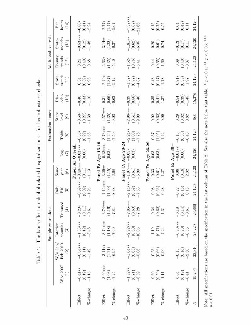
Table4:

The

ban’seff

ecton

alcoho

l-related

hospita

lizations

-further

robu

stness

checks

Samplerestric

tions

Estim

ationiss

ues

Add

ition

alcontrols

W/o

Jan/

Interio

rOnly

Same

State

Pla-

State

Cou

nty

State-

Bar

W/o

2007

Feb2010

coun

ties

Trim

med

F10

year

Log

Tobit

level

cebo

trends

trends

mon

ths

hours

(1)

(2)

(3)

(4)

(5)

(6)

(7)

(8)

(9)

(10)

(11)

(12)

(13)

(14)

Pan

elA

:O

vera

llEff

ect

−0.

41∗∗

−0.

54∗∗∗−

1.33∗∗∗−

0.20∗

−0.

69∗∗∗−

0.40∗∗∗−

0.03∗∗∗−

0.56∗−

0.50∗−

0.40

0.34

0.24

−0.

53∗∗∗−

0.80∗

(0.1

9)(0.1

1)(0.1

2)(0.1

1)(0.0

9)(0.1

1)(0.0

0)(0.2

9)(0.2

7)(0.3

3)(0.3

9)(0.4

0)(0.1

2)(0.4

1)%-cha

nge−

1.15

−1.

49−

3.48

−0.

61−

1.95

−1.

13−

1.58

−1.

39−

1.10

0.98

0.68

−1.

48−

2.24

Pan

elB

:A

ge15

-19

Effect

−3.

60∗∗∗

−3.

41∗∗

−3.

74∗∗∗−

3.74∗∗∗−

4.12∗∗∗−

3.29∗∗−

0.13∗∗∗−

3.73∗∗∗−

4.57∗∗∗−

0.31

−2.

49∗−

2.63∗−

3.14∗∗−

2.77∗

(1.0

3)(1.2

1)(1.1

8)(1.1

6)(1.0

0)(1.1

5)(0.0

3)(1.2

6)(1.3

5)(0.6

6)(1.3

7)(1.3

5)(1.2

2)(1.4

7)%-cha

nge−

7.24

−6.

95−

7.60

−7.

81−

8.38

−6.

68−

7.50

−9.

03−

0.63

−5.

12−

5.40

−6.

37−

5.67

Pan

elC

:A

ge20

-24

Effect

−1.

82∗∗

−1.

64∗∗

−2.

92∗∗∗−

2.05∗∗∗−

2.14∗∗∗−

1.97∗∗∗−

0.05∗−

2.24∗∗−

2.96∗∗∗−

0.39

−1.

37∗−

1.52∗−

1.81∗∗−

7.37∗∗∗

(0.7

1)(0.6

3)(0.6

0)(0.6

0)(0.6

2)(0.6

1)(0.0

3)(1.0

0)(0.5

1)(0.5

6)(0.7

7)(0.7

6)(0.6

2)(0.8

7)%-cha

nge−

6.39

−5.

86−

10.0

5−

7.28

−7.

53−

6.90

−7.

76−

9.99

−1.

40−

4.87

−5.

41−

6.35

−21.6

6

Pan

elD

:A

ge25

-29

Effect

−0.

300.

23−

1.19

0.34

0.08

0.33

0.03

0.37

0.02

0.35

−0.

48−

0.44

0.20

0.15

(0.5

9)(0.6

6)(0.7

1)(0.6

2)(0.6

3)(0.6

1)(0.0

3)(1.0

5)(0.6

2)(0.4

1)(0.4

7)(0.6

5)(0.6

1)(0.7

5)%-cha

nge−

1.11

0.90

−4.

241.

310.

281.

271.

420.

091.

37−

1.78

−1.

600.

740.

55

Pan

elE

:A

ge30

+Eff

ect

0.04

−0.

15−

0.90∗∗∗−

0.18

−0.

220.

06−

0.01∗∗−

0.16

0.29

−0.

540.

81∗

0.69

−0.

130.

04(0.1

9)(0.1

6)(0.2

0)(0.1

4)(0.1

6)(0.1

6)(0.0

0)(0.3

3)(0.3

2)(0.3

9)(0.3

8)(0.4

0)(0.1

7)(0.4

2)%-cha

nge−

0.41

−2.

30−

0.55

−0.

610.

182.

32−

0.43

0.82

−1.

451.

97−

0.37

0.11

0.11

N19,296

23,316

23,220

23,880

24,120

24,120

24,120

24,120

960

15,276

24,120

24,120

24,120

24,120

Note:

Allspecificatio

nsareba

sedon

thespecificatio

nin

thelast

columnof

Table2.

Seealso

theno

tebe

low

that

table.

*p<

0.1;

**p<

0.05

;***

p<

0.01

.

40

Table 5: Differential effects of the ban for men and women

Females MalesPanel A: Overall

Effect −0.35∗∗∗ −0.83∗∗∗(0.12) (0.23)

%-change −1.79 −1.58

Panel B: Age 15-19Effect −1.97∗ −4.74∗∗∗

(1.03) (1.44)%-change −5.62 −7.50

Panel C: Age 20-24Effect −1.76∗∗∗ −2.18∗

(0.45) (1.05)%-change −9.74 −5.62

Panel D: Age 25-29Effect 1.35 ∗ ∗ −0.79

(0.51) (0.83)%-change 11.23 −1.94

Panel E: Age 30+Effect −0.23 −0.08

(0.19) (0.23)%-change −1.20 −0.16

Note: All specifications are based on the specification in the last column of Table 2. See also the notebelow that table. * p < 0.1; ** p < 0.05; *** p < 0.01.

41

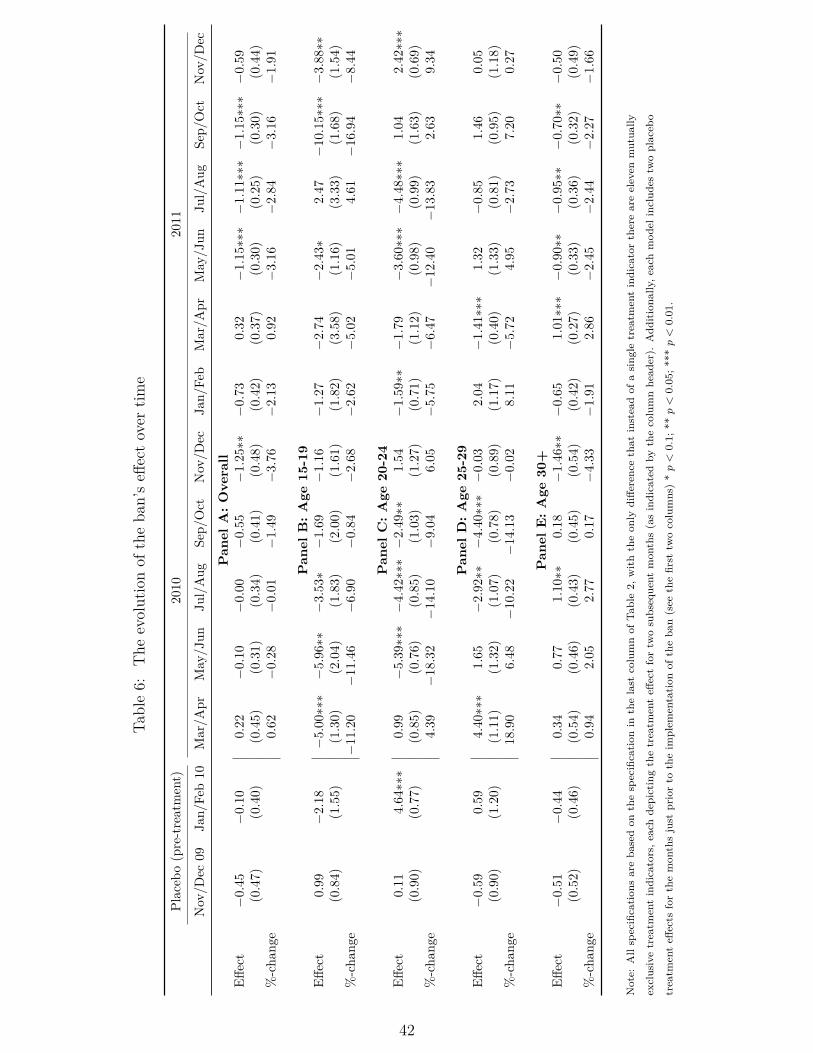
Table6:

The

evolutionof

theba

n’seff

ectover

time

Placeb

o(pre-treatment)

2010

2011

Nov/D

ec09

Jan/

Feb10

Mar/A

prMay/J

unJu

l/Aug

Sep/

Oct

Nov

/Dec

Jan/

Feb

Mar/A

prMay/J

unJu

l/Aug

Sep/

Oct

Nov/D

ec

Pan

elA

:O

vera

llEff

ect

−0.

45−

0.10

0.22

−0.

10−

0.00

−0.

55−

1.25∗∗

−0.

730.

32−

1.15∗∗∗−

1.11∗∗∗−

1.15∗∗∗−

0.59

(0.4

7)(0.4

0)(0.4

5)(0.3

1)(0.3

4)(0.4

1)(0.4

8)(0.4

2)(0.3

7)(0.3

0)(0.2

5)(0.3

0)(0.4

4)%-cha

nge

0.62

−0.

28−

0.01

−1.

49−

3.76

−2.

130.

92−

3.16

−2.

84−

3.16

−1.

91

Pan

elB

:A

ge15

-19

Effect

0.99

−2.

18−

5.00∗∗∗−

5.96∗∗

−3.

53∗

−1.

69−

1.16

−1.

27−

2.74

−2.

43∗

2.47

−10.1

5∗∗∗−

3.88∗∗

(0.8

4)(1.5

5)(1.3

0)(2.0

4)(1.8

3)(2.0

0)(1.6

1)(1.8

2)(3.5

8)(1.1

6)(3.3

3)(1.6

8)(1.5

4)%-cha

nge

−11.2

0−

11.4

6−

6.90

−0.

84−

2.68

−2.

62−

5.02

−5.

014.

61−

16.9

4−

8.44

Pan

elC

:A

ge20

-24

Effect

0.11

4.64∗∗∗

0.99

−5.

39∗∗∗−

4.42∗∗∗−

2.49∗∗

1.54

−1.

59∗∗

−1.

79−

3.60∗∗∗−

4.48∗∗∗

1.04

2.42∗∗∗

(0.9

0)(0.7

7)(0.8

5)(0.7

6)(0.8

5)(1.0

3)(1.2

7)(0.7

1)(1.1

2)(0.9

8)(0.9

9)(1.6

3)(0.6

9)%-cha

nge

4.39

−18.3

2−

14.1

0−

9.04

6.05

−5.

75−

6.47

−12.4

0−

13.8

32.

639.

34

Pan

elD

:A

ge25

-29

Effect

−0.

590.

594.

40∗∗∗

1.65

−2.

92∗∗

−4.

40∗∗∗−

0.03

2.04

−1.

41∗∗∗

1.32

−0.

851.

460.

05(0.9

0)(1.2

0)(1.1

1)(1.3

2)(1.0

7)(0.7

8)(0.8

9)(1.1

7)(0.4

0)(1.3

3)(0.8

1)(0.9

5)(1.1

8)%-cha

nge

18.9

06.

48−

10.2

2−

14.1

3−

0.02

8.11

−5.

724.

95−

2.73

7.20

0.27

Pan

elE

:A

ge30

+Eff

ect

−0.

51−

0.44

0.34

0.77

1.10∗∗

0.18

−1.

46∗∗

−0.

651.

01∗∗∗−

0.90∗∗

−0.

95∗∗

−0.

70∗∗

−0.

50(0.5

2)(0.4

6)(0.5

4)(0.4

6)(0.4

3)(0.4

5)(0.5

4)(0.4

2)(0.2

7)(0.3

3)(0.3

6)(0.3

2)(0.4

9)%-cha

nge

0.94

2.05

2.77

0.17

−4.

33−

1.91

2.86

−2.

45−

2.44

−2.

27−

1.66

Note:

Allspecification

sareba

sedon

thespecification

inthelast

columnof

Table2,

withtheon

lydiffe

rencethat

insteadof

asing

letreatm

entindicatorthereareeleven

mutua

lly

exclusivetreatm

entindicators,e

achdepictingthetreatm

enteff

ectfortw

osubsequent

mon

ths(asindicatedby

thecolumnhead

er).

Add

itiona

lly,e

achmod

elinclud

estw

oplaceb

o

treatm

enteff

ects

forthemon

thsjust

priorto

theim

plem

entation

oftheba

n(see

thefirst

twocolumns)*p<

0.1;

**p<

0.05;*

**p<

0.01.

42

Table 7: Other outcomes

Length Prob. Prob. Respiratory Headof stay stay>1 day stay≥1 day system Drugs injuries(1) (2) (3) (4) (5) (6)

Panel A: OverallEffect −0.008 0.012∗∗∗ 0.008∗∗∗ −0.40 0.25 −0.92 ∗ ∗

(0.041) (0.002) (0.001) (0.79) (0.19) (0.35)%-change −0.10 1.83 0.94 −0.88 6.17 −2.96N 1,080,954 1,080,954 1,080,954 24,120 24,120 24,120

Panel B: Age 15-19Effect 0.072∗∗∗ −0.005 0.019∗∗∗ 0.38 0.55∗ −0.72

(0.012) (0.004) (0.005) (0.43) (0.26) (1.13)%-change 4.32 −4.80 4.31 3.94 10.20 −1.26N 82,954 82,954 82,954 24,120 24,120 24,120

Panel C: Age 20-24Effect −0.005 −0.014∗ 0.010 −0.18 0.04 −1.64 ∗ ∗

(0.064) (0.007) (0.005) (0.23) (0.50) (0.57)%-change −0.18 −6.56 2.42 −2.42 0.37 −3.70N 53,585 53,585 53,585 24,120 24,120 24,120

Panel D: Age 25-29Effect −0.219∗∗∗ −0.000 −0.005 0.15 2.02 ∗ ∗ 0.33

(0.082) (0.006) (0.007) (0.24) (0.92) (0.42)%-change −3.44 −0.10 −0.71 1.93 18.01 1.26N 51,917 51,917 51,917 24,120 24,120 24,120

Panel E: Age 30+Effect −0.042 0.015∗∗∗ 0.006∗∗∗ −0.54 0.09 −0.74 ∗ ∗

(0.050) (0.002) (0.001) (0.99) (0.12) (0.32)%-change −0.44 2.04 0.67 −0.98 3.37 −2.66N 892,498 892,498 892,498 24,120 24,120 24,120

Note: The first three columns show marginal effects of the ban on different measures of length of stayfor alcohol-related hospitalizations. Unit of analysis is the individual hospitalization. The first columndisplays marginal effects from negative binomial regressions for the ban’s effect on the number of daysin hospital. The outcomes in the second and third column are binary variables indicating whetheran individual stayed more than one day in hospital (column 2) or at least one day (column 3). Thenext three columns refer to the ban’s effect on various other outcomes. Each outcome is defined as themonthly number of hospitalizations with the respective diagnoses per 100,000 inhabitants of the same age:hospitalizations due to diseases of the lower respiratory system (column 4), drug-related hospitalizations(column 5), and hospital stays due to head and neck injuries (column 6). * p < 0.1; ** p < 0.05; ***p < 0.01.

43

A. Appendix

44

Figure A.1: Day of alcohol-related admission to hospital

(a) Overall (b) Age 15-19

(c) Age 20-24 (d) Age 25-29

(e) Age 30+

Note: The figure shows the distribution of days of admission of alcohol-related hospitalizations. Source:Data are from one large hospital in the control group, pooled over the years 2007-2013.

45

Table A.1: The effect of the Bavarian bar hour extension

+ time/county + state-spec. + stateBasic DiD dummies + controls seasonal eff. trends

Panel A: OverallEffect −0.89∗∗∗ −0.90∗∗∗ −1.23∗∗∗ −1.23∗∗∗ 0.32

(0.25) (0.25) (0.40) (0.39) (0.43)%-change −2.67 −2.71 −3.67 −3.67 1.00

Panel B: Age 15-19Effect −0.21 −0.09 0.46 0.46 −0.41

(0.68) (0.68) (0.98) (0.96) (0.78)%-change −0.53 −0.24 1.19 1.19 −1.05

Panel C: Age 20-24Effect 0.35 0.29 0.18 0.18 −0.23

(0.37) (0.38) (0.39) (0.39) (0.63)%-change 1.46 1.22 0.73 0.73 −0.92

Panel D: Age 25-29Effect −0.81 ∗ ∗ −0.94∗∗∗ −1.98∗∗∗ −1.98∗∗∗ 0.09

(0.28) (0.27) (0.47) (0.46) (0.76)%-change −3.46 −3.98 −8.04 −8.04 0.39

Panel E: Age 30+Effect −1.08∗∗∗ −1.05∗∗∗ −1.38∗∗∗ −1.38∗∗∗ 0.43

(0.26) (0.26) (0.45) (0.44) (0.49)%-change −3.14 −3.07 −4.00 −4.00 1.32

Note: The table displays the effect of the Bavarian bar hour extension on January 1, 2005, on the monthlynumber of alcohol-related hospitalizations per 100,000 inhabitants for various age groups, together withits standard error clustered on the state level (in parentheses). The sample is based on information of 388counties covering the years 2003-2005, i.e. 13,968 county-month observations. The last line in each panelindicates the percentage change in alcohol-related hospitalizations due to the reform. All regressions areweighted by the population of the respective age group in the county. The first column displays theresults of a basic difference-in-differences specification, the second column includes county and time fixedeffects. Additionally, the third column includes time-varying control variables on the county and statelevel. The forth column adds state-specific seasonal dummies and the last column includes county-specificlinear time trends. * p < 0.1; ** p < 0.05; *** p < 0.01.

46

Table A.2: p-values according to different procedures

Age Clustering Wild cluster bootstrap Panel correctedMammen weights Rademacher weights Independent AR(1)

Overall 0.000 0.000 0.000 0.048 0.10415-19 0.011 0.022 0.000 0.022 0.02620-24 0.005 0.000 0.000 0.012 0.01525-29 0.748 0.772 0.806 0.778 0.77930+ 0.391 0.392 0.326 0.630 0.709

Note: The table displays p-values for the preferred specification (Table 2, last column) according todifferent computation procedures. The first column shows p-values based on clustered standard errors,which is the default option in this study. The second and third column display p-values based on wildcluster bootstrap-t procedures (1,000 replications, estimated under H1) as described in Cameron et al.(2008). The two columns differ only with respect to the weights that are used to compute the residuals:The second column relies on Mammen weights and the third column on Rademacher weights (see Cameronet al. (2008) for the details). The last two columns show p-values based on panel-corrected standard errors:the fourth column assumes that standard errors are heteroskedastic and contemporaneously correlatedacross counties but not autocorrelated, while the fifths column allows for a first-order autocorrelationprocess that all counties have in common.

47

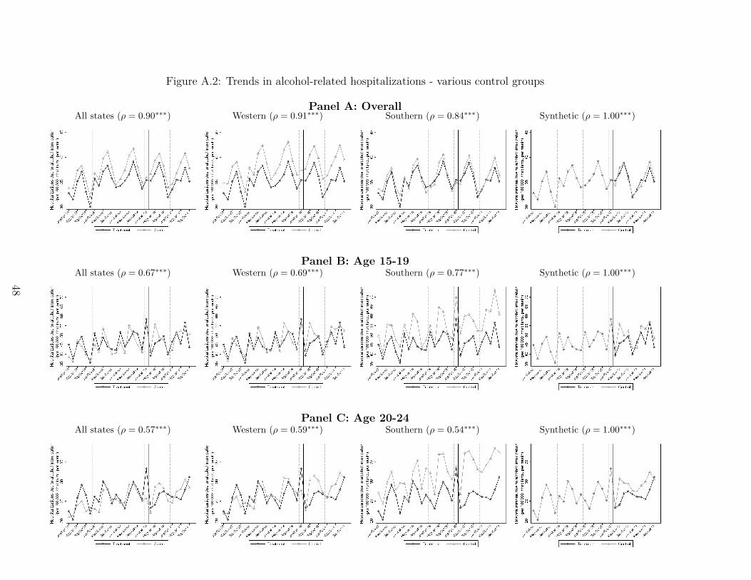
Figure A.2: Trends in alcohol-related hospitalizations - various control groups

Panel A: OverallAll states (ρ = 0.90∗∗∗) Western (ρ = 0.91∗∗∗) Southern (ρ = 0.84∗∗∗) Synthetic (ρ = 1.00∗∗∗)

Panel B: Age 15-19All states (ρ = 0.67∗∗∗) Western (ρ = 0.69∗∗∗) Southern (ρ = 0.77∗∗∗) Synthetic (ρ = 1.00∗∗∗)

Panel C: Age 20-24All states (ρ = 0.57∗∗∗) Western (ρ = 0.59∗∗∗) Southern (ρ = 0.54∗∗∗) Synthetic (ρ = 1.00∗∗∗)

48

Figure A.2: Trends in alcohol-related hospitalizations - various control groups

Panel D: Age 25-29All states (ρ = 0.68∗∗∗) Western (ρ = 0.62∗∗∗) Southern (ρ = 0.45∗∗∗) Synthetic (ρ = 1.00∗∗∗)

Panel E: Age 30+All states (ρ = 0.92∗∗∗) Western (ρ = 0.93∗∗∗) Southern (ρ = 0.85∗∗∗) Synthetic (ρ = 1.00∗∗∗)

Note: The figure presents trends in the number of monthly alcohol-related hospitalizations per 100,000 same-aged inhabitants for the treatment group and various control groups

(all states, western states, southern states, synthetic control), averaged over two months. The continuous vertical line shows the onset of the late-night ban on alcohol sales in

the treatment state on March 01, 2010. ρ indicates the pre-treatment correlation between the ARH-rates in the treatment group and the respective control group. * p < 0.1; **

p < 0.05; *** p < 0.01.

49

Figure A.3: Proportion of young people binge drinking at home

The figure displays the share of heavy alcohol consumers who state that they mainly binge drink athome. Source: Bundeszentrale für Gesundheitliche Aufklärung (BZgA). Representative survey amongyouth and young adults aged 12-25 in 2010. Interviews were conducted between June and August 2010.In this survey, young people were asked whether they were drinking alcohol in the last 30 days. Incase they say yes, respondents were also asked the following question: “In case you drink more alcohol,with more I mean five drinks or more, where do you mainly drink?”. Among the answer categories,respondents could name the location “at home”.

50

Figure A.4: The ban’s effect on ARH rates - further ages

Note: The figure displays the ban’s effect on alcohol-related hospitalization rates for 10-year age groups(see specification four of Table 2).

51

References

Becker, Gary S. and Kevin M. Murphy, “A theory of rational addiction,” Journalof Political Economy, 1988, 96 (4), 675–700.

Birckmayer, J. and D. Hemenway, “Minimum-age drinking laws and youth suicide,1970-1990,” American Journal of Public Health, 1999, 89 (9), 1365–1368.

Bouthoorn, Selma H., Joris J. van Hoof, and Nicolaas van der Lely, “Adolescentalcohol intoxication in Dutch hospital centers of pediatrics: Characteristics and genderdifferences.,” European Journal of Pediatrics, August 2011, 170 (8), 1023–1030.

Bryan, Gharad, Dean Karlan, and Scott Nelson, “Commitment devices,” AnnualReview of Economics, September 2010, 2 (1), 671–698.

BZgA, Die Drogenaffinität Jugendlicher in der Bundesrepublik Deutschland 2011, Köln:Bundeszentrale für gesundheitliche Aufklärung [German Federal Centre for Health Ed-ucation], 2012.

Cameron, Colin, Jonah B. Gelbach, and Douglas L. Miller, “Bootstrap-basedimprovements for inference with clustered errors,” Review of Economics and Statistics,August 2008, 90 (3), 414–427.

Carpenter, Christopher S., “Heavy alcohol use and the commission of nuisance crime:Evidence from underage drunk driving laws,” American Economic Review, 2005, 95 (2),267–272.

, “Youth alcohol use and risky sexual behavior: Evidence from underage drunk drivinglaws,” Journal of Health Economics, May 2005, 24 (3), 613–628.

, Deborah D. Kloska, Patrick O’Malley, and Lloyd Johnston, “Alcohol controlpolicies and youth alcohol consumption: Evidence from 28 years of Monitoring theFuture,” B.E. Journal of Economic Analysis & Policy, January 2007, 7 (1).

Carrell, Scott E., Mark Hoekstra, and James E. West, “Does drinking impaircollege performance? Evidence from a regression discontinuity approach,” Journal ofPublic Economics, February 2011, 95 (1-2), 54–62.

Cawley, John and Christopher J Ruhm, The economics of risky health behaviors,Vol. 2, Elsevier, 2012.

CDU Baden-Württemberg, “In der Tat besser. Regierungsprogramm der CDU Baden-Württemberg 2006-2011,” 2006, pp. 1–87.

52

Chaloupka, Frank J. and Xin Xu, “The effects of prices on alcohol use and itsconsequences,” Alcohol Research and Health, 2011, 34 (2), 236–245.

Chikritzhs, Tanya and Tim Stockwell, “The impact of later trading hours for hotelson levels of impaired driver road crashes and driver breath alcohol levels,” Addiction,2006, 101 (9), 1254–1264.

Conover, Emily and Dean Scrimgeour, “Health consequences of easier access toalcohol: New Zealand evidence,” Journal of Health Economics, May 2013, 32 (3), 570–585.

Cook, Philip J. and Michael J. Moore, “Alcohol,” in Anthony Culyer and JosephNewhouse, eds., Handbook of Health Economics, Vol. 1, Amsterdam: Elsevier, 2000,pp. 1631–1673.

and , “The economics of alcohol abuse and alcohol-control policies,” Health Affairs,2002, 21 (2), 120–133.

Crost, Benjamin and Santiago Guerrero, “The effect of alcohol availability on mar-ijuana use: Evidence from the minimum legal drinking age,” Journal of Health Eco-nomics, January 2012, 31 (1), 112–121.

Dee, Thomas S., “State alcohol policies, teen drinking and traffic fatalities,” Journal ofPublic Economics, May 1999, 72 (2), 289–315.

DHS, Binge drinking and Europe, Hamm: Deutsche Hauptstelle für Suchtfragen e.V.(DHS), January 2008.

Donald, Stephen G. and Kevin Lang, “Inference with difference-in-differences andother panel data,” Review of Economics and Statistics, May 2007, 89 (2), 221–233.

Draca, Mirko, Stephen Machin, and Robert Witt, “Panic on the streets of London:Police, crime, and the July 2005 terror attacks,” American Economic Review, August2011, 101 (5), 2157–2181.

Enoch, Mary-Anne, “Genetic and environmental influences on the development of al-coholism: Resilience vs. risk.,” Annals of the New York Academy of Sciences, December2006, 1094, 193–201.

FDZ, Krankenhausdiagnosestatistik, Erhebungsjahre 2007-2011, FDZ der StatistischenÄmter des Bundes und der Länder, 2014.

53

Grossman, Michael, Jody L. Sindelar, John Mullahy, and Richard Anderson,“Policy watch: Alcohol and cigarette taxes,” Journal of Economic Perspectives, 1993,7 (4), 211–222.

Grundel, Anna and Beate Blättner, Entschädigung von Opfern interpersonellerGewalt im Raum Fulda. Studie zum Opferentschädigungsgesetz (OEG) und der Ver-fahrenspraxis in der Opferentschädigung, Fulda: University of Applied Science Fulda,2010.

Hainmueller, Jens, “Entropy balancing for causal effects: A multivariate reweightingmethod to produce balanced samples in observational studies,” Political Analysis, Oc-tober 2012, 20 (1), 25–46.

Heaton, Paul, “Sunday liquor laws and crime,” Journal of Public Economics, February2012, 96 (1-2), 42–52.

Hinnosaar, Marit, “Time inconsistency and alcohol sales restrictions,” Technical Re-port, mimeo, Northwestern University 2012.

Hoffmann, Kevin, “Vorglühen an der Tankstelle,” Der Tagesspiegel, 2009, 5 March2009.

Hoischen, Oliver and Philip Eppelsheim, “Alkoholverbot an Tankstellen: Einmalvolltanken, bitte!,” Frankfurter Allgemeine Zeitung, 2009, 8 June 2009.

Hwang, Stephen W., Mohammad M. Agha, Maria I. Creatore, and Richard H.Glazier, “Age- and sex-specific income gradients in alcohol-related hospitalization ratesin an urban area,” Annals of Epidemiology, January 2005, 15 (1), 56–63.

Kanny, Dafna, Yong Liu, Robert D. Brewer, William S. Garvin, and LinaBalluz, “Vital signs: Binge drinking prevalence, frequency, and intensity among adults- United States, 2010,” Morbidity and Mortality Weekly Report (MMWR), 2012, 61 (1),14–19.

Kelly, Elaine and Imran Rasul, “Policing cannabis and drug related hospital admis-sions: Evidence from administrative records,” Journal of Public Economics, April 2014,112, 89–114.

Kim, Jason Y., Sumeet K. Asrani, Nilay D. Shah, W. Ray Kim, and Terry D.Schneekloth, “Hospitalization for underage drinkers in the United States,” Journal ofAdolescent Health, 2012, 50 (6), 648–650.

54

Landtag von Baden-Württemberg, “Gesetzbeschluss der Landesregierung. Gesetzzur Abwehr alkoholbeeinflusster Störungen der öffentlichen Sicherheit und Ord-nung während der Nachtzeit und zum Schutz vor alkoholbedingten Gesundheitsge-fahren (Alkoholverkaufsverbotsgesetz),” Technical Report, State Parliamant of Baden-Württemberg, Drucksache [printed matter] 14 / 5413, 2009.

, “Gesetzentwurf der Landesregierung. Gesetz zur Abwehr alkoholbeeinflusster Störun-gen der öffentlichen Sicherheit und Ordnung während der Nachtzeit und zum Schutzvor alkoholbedingten Gesundheitsgefahren (Alkoholverkaufsverbotsgesetz),” TechnicalReport, State Parliamant of Baden-Württemberg, Drucksache [printed matter] 14 /4850, 2009.

, “Plenarprotokoll 14 / 73, 30.07.2009,” Technical Report, State Parliamant of Baden-Württemberg, 14. Wahlperiode, 73. Sitzung, 2009.

Lechner, Michael, “The estimation of causal effects by difference-in-difference meth-ods,” University of St. Gallen Department of Economics Working Paper Series, 2010,28.

Lovenheim, Michael F. and Joel Slemrod, “The fatal toll of driving to drink: Theeffect of minimum legal drinking age evasion on traffic fatalities,” Journal of HealthEconomics, January 2010, 29 (1), 62–77.

Manning, Willard G., Linda Blumberg, and Lawrence H. Moulton, “The de-mand for alcohol: The differential response to price,” Journal of Health Economics,1995, 14 (2), 123–148.

McMillan, Garnett P. and Sandra Lapham, “Effectiveness of bans and laws inreducing traffic deaths: Legalized Sunday packaged alcohol sales and alcohol-relatedtraffic crashes and crash fatalities in New Mexico,” American Journal of Public Health,November 2006, 96 (11), 1944–8.

Middleton, Jennifer Cook, Robert A. Hahn, Jennifer L. Kuzara, Randy El-der, Robert D. Brewer, Sajal Chattopadhyay, Jonathan Fielding, Timothy S.Naimi, Traci L. Toomey, and Briana Lawrence, “Effectiveness of policies main-taining or restricting days of alcohol sales on excessive alcohol consumption and relatedharms,” American Journal of Preventive Medicine, December 2010, 39 (6), 575–589.

Mullahy, John and Jody L. Sindelar, “Employment, unemployment, and problemdrinking,” Journal of Health Economics, August 1996, 15 (4), 409–34.

55

Newton, Alastair, Shah Jalal Sarker, Gurjinderpal S. Pahal, Eric van denBergh, and Charles Young, “Impact of the new UK licensing law on emergencyhospital attendances: A cohort study,” Emergency Medical Journal, August 2007, 24(8), 532–534.

Norström, Thor and Ole-Jørgen Skog, “Saturday opening of alcohol retail shops inSweden: An experiment in two phases,” Addiction, June 2005, 100 (6), 767–776.

O’Connell, H. and B. A. Lawlor, “Recent alcohol intake and suicidality - A neu-ropsychological perspective,” Irish Journal of Medical Science, December 2005, 174(4), 51–54.

Parry, Ian W. H., Sarah E. West, and Ramanan Laxminarayan, “Fiscal andexternality rationales for alcohol policies,” The B.E. Journal of Economic Analysis &Policy, January 2009, 9 (1).

Popova, Svetlana, Norman Giesbrecht, Dennis Bekmuradov, and JayadeepPatra, “Hours and days of sale and density of alcohol outlets: Impacts on alcoholconsumption and damage - A systematic review,” Alcohol and Alcoholism, 2009, 44 (5),500–516.

Ruhm, Christopher J., “Alcohol policies and highway vehicle fatalities,” Journal ofHealth Economics, August 1996, 15 (4), 435–454.

Scribner, R., D. Mackinnon, and J. Dwyer, “The risk of assaultive violence andalcohol availability in Los Angeles county,” American Journal of Public Health, 1995,85 (3), 335–340.

Sen, Bisakha, “Can beer taxes affect teen pregnancy? Evidence based on teen abortionrates and birth rates,” Southern Economic Journal, 2003, 70 (2), 328–343.

Speer, P., D. Gorman, E. Labouvie, and M. Ontkush, “Violent crime and alcoholavailability: Relationships in an urban community,” Journal of Public Health Policy,1998, 19 (3), 303–318.

Stehr, Mark F., “The effect of Sunday sales of alcohol on highway crash fatalities,” B.E.Journal of Economic Analysis & Policy, January 2010, 10 (1).

Stolle, Martin, Peter-Michael Sack, H. Spieles, and Rainer Thomasius, “Alko-holintoxikierte Kinder und Jugendliche in der Notfallversorgung Hamburger Kranken-häuser [Acute ethanol intoxication among children and adolescents in Hamburg, Ger-

56

many],” Bundesgesundheitsblatt, Gesundheitsforschung, Gesundheitsschutz, September2010, 53 (9), 910–916.

Task Force on Community Preventive Services, “Recommendations on maintaininglimits on days and hours of sale of alcoholic beverages to prevent excessive alcoholconsumption and related harms,” American Journal of Preventive Medicine, December2010, 39 (6), 605–606.

Vingilis, Evelyn, “Limits of hours of sales and service: Effects on traffic society,” Trans-portation Research Circular, 2007, E-C123, 120–129.

, A. I. McLeod, J. Seeley, R. E. Mann, D. Beirness, and C. P. Compton,“Road safety impact of extended drinking hours in Ontario,” Accident Analysis andPrevention, May 2005, 37 (3), 549–556.

Wagenaar, Alexander C., Amy L. Tobler, and Kelli A. Komro, “Effects of alcoholtax and price policies on morbidity and mortality: A systematic review,” AmericanJournal of Public Health, November 2010, 100 (11), 2270–2278.

and Traci L. Toomey, “Effects of minimum drinking age laws: Review and analysesof the literature from 1960 to 2000,” Journal of Studies on Alcohol and Drugs, 2002,14, 206–225.

, M. M. Maldonado-Molina, and Bradley H. Wagenaar, “Effects of alcohol taxincreases on alcohol-related disease mortality in Alaska: Time-series analyses from 1976to 2004,” American Journal of Public Health, 2009, 99 (8), 1464–1470.

White, Aaron M., Ralph W. Hingson, I-Jen Pan, and Hsiao-Ye Yi, “Hospi-talizations for alcohol and drug overdoses in young adults ages 18 - 24 in the UnitedStates, 1999 - 2008: Results from the nationwide inpatient sample,” Journal of Studieson Alcohol and Drugs, September 2011, 72 (5), 774–86.

Wicki, Matthias and Gerhard Gmel, “Hospital admission rates for alcoholic intox-ication after policy changes in the canton of Geneva, Switzerland,” Drug and AlcoholDependence, November 2011, 118 (2-3), 209–215.

Williams, J., Rosalie Liccardo Pacula, Frank J. Chaloupka, and Henry Wech-sler, “Alcohol and marijuana use among college students: Economic complements orsubstitutes?,” Health Economics, September 2004, 13 (9), 825–843.

World Health Organization, Global status report on alcohol and health 2014, Geneva:World Health Organization, 2014.

57

Young, Douglas J. and Agnieszka Bielinska-Kwapisz, “Alcohol prices, consump-tion, and traffic fatalities,” Southern Economic Journal, 2006, 72 (3), 690–703.

58