Embed Size (px)
Citation preview
University of South CarolinaScholar Commons
Theses and Dissertations
5-2017
Representing the Relationships Between FieldCollected Carbon Exchanges and SurfaceReflectance Using Geospatial and Satellite-BasedTechniquesAlexandria G. McCombsUniversity of South Carolina
Follow this and additional works at: https://scholarcommons.sc.edu/etd
Part of the Arts and Humanities Commons, and the Geography Commons
This Open Access Dissertation is brought to you by Scholar Commons. It has been accepted for inclusion in Theses and Dissertations by an authorizedadministrator of Scholar Commons. For more information, please contact [email protected].
Recommended CitationMcCombs, A. G.(2017). Representing the Relationships Between Field Collected Carbon Exchanges and Surface Reflectance UsingGeospatial and Satellite-Based Techniques. (Doctoral dissertation). Retrieved from https://scholarcommons.sc.edu/etd/4103
REPRESENTING THE RELATIONSHIPS BETWEEN FIELD COLLECTED CARBON EXCHANGES AND SURFACE REFLECTANCE
USING GEOSPATIAL AND SATELLITE-BASED TECHNIQUES
by
Alexandria G. McCombs
Bachelor of Science University of Oklahoma, 2008
Master of Science
University of Oklahoma, 2013
Submitted in Partial Fulfillment of the Requirements
For the Degree of Doctor of Philosophy in
Geography
College of Arts and Sciences
University of South Carolina
2017
Accepted by:
April Hiscox, Major Professor
Cuizhen Wang, Committee Member
Gregory Carbone, Committee Member
Ankur Desai, Committee Member
Cheryl L. Addy, Vice Provost and Dean of the Graduate School

ii
© Copyright by Alexandria G. McCombs, 2017 All Rights Reserved.

iii
DEDICATION
This dissertation is dedicated to my husband, Devin, who’s unfaltering support, and
unconditional love were always what gave me motivation and drive to succeed during my
doctoral studies. Thank you for the sacrifices you have made over the last four years, and
for always believing in me.

iv
ACKNOWLEDGEMENTS
I would like to thank the undergraduate research assistants, Benjamin Marosites and
Jenna Lew for their assistance preparing and processing remote sensing data.
This work was partially supported by a SPARC Graduate Research Grant from the Office
of the Vice President for Research at the University of South Carolina.
This work used data acquired and shared by the FLUXNET community. The FLUXNET
eddy covariance data processing and harmonization was carried out by the ICOS
Ecosystem Thematic Center, AmeriFlux Management Project and Fluxdata project of
FLUXNET, with the support of CDIAC, and the OzFlux, ChinaFlux and AsiaFlux
offices.
Landsat Surface Reflectance products courtesy of the U.S. Geological Survey Earth
Resources Observation and Science Center. The Terra/MODIS Surface Reflectance 8-
Day L3 Global 500m and Terra/MODIS Land Surface Temperature and Emissivity 8-
Day L3 Global 1km CMG datasets were acquired from the Level-1 & Atmosphere
Archive and Distribution System (LAADS) Distributed Active Archive Center (DAAC),
located in the Goddard Space Flight Center in Greenbelt, Maryland
(http://ladsweb.nascom.nasa.gov).

v
ABSTRACT
Carbon exchanges between the atmosphere and the land surface vary in space and
time, and are highly dependent on land cover type. It is important to quantify these
exchanges to understand how landscapes affect the carbon budget, which will have a
significant impact on future climate change and will inform climate change projections.
However, how do you represent regional carbon exchanges from a single meteorological
station? A single observing station will represent a limited area around the station, but
each individual observation will sample a different physical land area in time due to
varying wind speeds, wind direction, and atmospheric stability. The methods and
techniques presented address the challenges, limitations, and future work that is needed to
properly scale and model carbon exchanges in four dimensions for varying agricultural
and transitioning ecotones. Seasonal variability of carbon exchanges can be modeled in
agricultural land covers using satellite-based techniques, but due to physiological
differences in crop types the values must be modeled by crop species. The spatially
varying atmospheric conditions must also be considered when modeling carbon
exchanges from a single point in the spatial realm because of the dependency of carbon
exchange on temperature and humidity conditions. In summary, field-based carbon
exchange observations are used to quantify whether a specific land cover in a region is a
carbon source to carbon sink to the atmosphere, however, it is important to consider the
spatially varying variables that limit the ability of a single point measurement to represent
carbon exchanges of an entire region.
vi
TABLE OF CONTENTS
DEDICATION ................................................................................................................... iii
ACKNOWLEDGEMENTS ............................................................................................... iv
ABSTRACT .........................................................................................................................v
LIST OF TABLES ........................................................................................................... viii
LIST OF FIGURES ........................................................................................................... ix
LIST OF ABBREVIATIONS ............................................................................................ xi
CHAPTER 1: INTRODUCTION ....................................................................................... 1
CHAPTER 2: LITERATURE REVIEW ............................................................................ 2
CHAPTER 3: CARBON FLUX PHENOLOGY FROM THE SKY: EVALUATION FOR MAIZE AND SOYBEAN .................................................................................................. 7
3.1 INTRODUCTION .......................................................................................... 8
3.2 DATASETS AND PREPROCESSING ........................................................ 11
3.3 METHODS ................................................................................................... 15
3.4 RESULTS ..................................................................................................... 18
3.5 DISCUSSION ............................................................................................... 24
3.6 CONCLUSIONS........................................................................................... 29
CHAPTER 4¨ AN EMPIRICAL MODELING APPROACH TO ESTIMATING REGIONAL SCALE NET ECOSYSTEM EXCHANGE IN MAIZE AND SOYBEAN FIELDS IN THE US CORN BELT .................................................................................. 37
4.1 INTRODUCTION ........................................................................................ 38
4.2 DATA SOURCES ........................................................................................ 41
4.3 MODEL DEVELOPMENT AND CALIBRATION .................................... 45

vii
4.4 MODEL EVALUATION ............................................................................. 50
4.5 RESULTS ..................................................................................................... 52
4.6 DISCUSSION ............................................................................................... 56
4.7 CONCLUSIONS........................................................................................... 61
CHAPTER 5: POINT TO GRID CONVERSION IN FLUX FOOTPRINTS: IMPLICATIONS OF METHOD CHOICE AND SPATIAL RESOLUTION FOR REGIONAL SCALE STUDIES ....................................................................................... 74
5.1 INTRODUCTION ........................................................................................ 75
5.2 EDDY COVARIANCE DATA INPUTS ..................................................... 79
5.3 MATERIALS AND METHODS .................................................................. 79
5.4 RESULTS ..................................................................................................... 87
5.5 DISCUSSIONS ............................................................................................. 93
5.6 CONCLUSIONS........................................................................................... 96
CHAPTER 6: CONCLUSIONS ..................................................................................... 107
REFERENCES ............................................................................................................... 111
APPENDIX A – MEAN SIGNED DIFFERENCE FOR CFP METRICS ..................... 131

viii
LIST OF TABLES
Table 3.1. Chapter 3 station datasets. ............................................................................... 31
Table 3.2. Vegetation indices evaluated. .......................................................................... 34
Table 4.1. Station datasets used. ....................................................................................... 63
Table 4.2.Best spectral bands. ........................................................................................... 64
Table 4.3. Significant surface reflectance bands .............................................................. 69
Table 4.4. Empirical model statistics for each period within the growing season ............ 70
Table 5.1. Station data used .............................................................................................. 98

ix
LIST OF FIGURES
Figure 3.1. Processing methodology ................................................................................. 32
Figure 3.2. Daytime footprint climatology ...................................................................... 33
Figure 3.3. Carbon flux phenology metrics ...................................................................... 35
Figure 3.4. Scatter plot of carbon flux phenology metrics ............................................... 36
Figure 3.5. Total NEE during the carbon uptake period. .................................................. 36
Figure 4.1. Footprint climatology for 2005 ...................................................................... 65
Figure 4.2. Transitions points in carbon flux phenology .................................................. 66
Figure 4.3. Scatterplot of surface reflectance vs. ground observed NEE. ........................ 67
Figure 4.4. Flow chart of the methodology....................................................................... 68
Figure 4.5. Grid plot of significant surface reflectance bands and climate variables ....... 71
Figure 4.6. Comparison of footprint scaled NEE. ............................................................ 72
Figure 4.7. Estimated NEE compared to gap-filled NEE values. ..................................... 73
Figure 5.1. Boundary layer sensitivity flux footprint. ...................................................... 98
Figure 5.2. Methods for projecting a continuous footprint. .............................................. 99
Figure 5.3. Upscaling methodology of 2D flux footprint ............................................... 100

x
Figure 5.4. Percent information loss of 1D footprint function ....................................... 101
Figure 5.5.Integration overestimation ............................................................................. 102
Figure 5.6. Information loss using the 2D area integration ............................................ 103
Figure 5.7.Equal interval sampling peak mismatch ........................................................ 104
Figure 5.8. Peak flux footprint migration ....................................................................... 105
Figure 5.9. Annual footprint climatology total area increase ......................................... 106

xi
LIST OF ABBREVIATIONS
1D ................................................................................................................... 1-Dimensional
2D ................................................................................................................... 2-Dimensional
EOS ................................................................................................................ End of Season
FFP ..................................................................................... Flux Footprint Parameterization
GPP .............................................................................................. Gross Primary Production
H2000 ......................................................... 1D Flux Footprint model by Hsieh et al. (2000)
K2015 ........................................................ 2D Flux Footprint Model by Kljun et al. (2015)
NEE ............................................................................................... Net Ecosystem Exchange
NIR ...................................................................................................................Near-Infrared
POS ............................................................................................................... Peak of Season
SOS ............................................................................................................... Start of Season
SWIR.......................................................................................................Shortwave Infrared
1
CHAPTER 1
INTRODUCTION
Ground-based flux measurements are routinely measured over varying land covers, land
management, vegetation types, and climate regimes. To understand carbon dynamics at
the regional scale ground-based carbon flux measurements must be up-scaled to represent
a broader spatial scale. In agricultural regions this is particularly challenging because
they are human managed landscapes that can occur in small patches. Therefore, the
dissertation presented here is a collection of three manuscripts that discuss the challenges
of upscaling carbon flux measurements to represent regional scales in agricultural fields
using geospatial and satellite-based remote sensing techniques. The first of the three
manuscripts (Chapter 3) discusses how to remotely identify the key transition points,
called carbon flux phenology metrics, where crops transition between vegetative stages
and reproductive stages using vegetation indices. In the second manuscript (Chapter 4) an
empirical model was developed to estimate carbon exchange values at 8-day temporal
resolution for specific agricultural crops (maize and soybean) using satellite-based
reflectance values. The final manuscript (Chapter 5) discusses the methodologies for
upscaling a continuous flux footprint function to a gridded dataset and the sensitivity of
this process to the cell size. Finally, this document will make some concluding remarks
on the findings of all three manuscripts.
2
CHAPTER 2
LITERATURE REVIEW
A growing global population will cause urbanization and additional lands to be used for
agricultural purposes. These land covers and land cover changes will have significant
influences on atmospheric variables. Many studies have evaluated the effect of land cover
changes, such as urbanization and agricultural practices, on air temperature and
precipitation (e.g., Hale et al., 2008; Jones et al., 1990; Mahmood et al., 2010, 2006;
Pitman, 2004; Vose et al., 2004). In many locations urbanization has been linked to the
warming of local air temperature (Basara, Hall, Schroeder, Illston, & Nemunaitis, 2008;
Chow, Brennan, & Brazel, 2011; Jones et al., 1990). In contrast, there has been little
research on the changes of atmospheric variables due to less drastic land cover and land
management changes in rural areas. Several studies have found that air temperature is
cooled due to irrigation on warm days (Bonfils and Lobell, 2007). Wind patterns have
been found to change over time with changes in land cover, and minimum air
temperatures are highly sensitive to changes in climatic forcing (Fiebrich, Morgan,
McCombs, Hall, & McPherson, 2010; Rezaul Mahmood et al., 2010). Still, the effects of
specific agricultural land management techniques and crops are not well represented in
climate and meteorological models (Rezaul Mahmood et al., 2010).
While changes in temperature and precipitation are important meteorologically, at
the climate timescale the sources and sinks of greenhouse gases such as carbon dioxide
3
are equally important. One way to quantify these changes is by measuring carbon flux.
Carbon flux is the movement of carbon through an ecosystem and atmosphere, and can
be measured using the eddy covariance technique (Aubinet, Vesala, & Papale, 2012).
Carbon fluxes can have significant spatial and temporal variation at the local scale
because they are land cover dependent and a function of temperature and moisture
availability which also varies in space and time (Bonan, 2008; Leclerc & Foken, 2014).
Land cover type can also play a significant role in the carbon budget because variables
such as soil moisture, solar radiation, precipitation, air temperature, plant functional type,
and land management drive the release of CO2 into the atmosphere (e.g., Gebremedhin et
al., 2012; Raich and Schlesinger, 1992).
A major source of error in climate change projections is agricultural land
management; currently it is not considered in models (Le Quéré et al., 2015). It is
difficult to understand the contribution of agricultural land management at a global scale
if there is not a good understanding at a regional scale. Agricultural land management
practices often include crop rotation, surface manipulation (i.e., tilling), and crop
irrigation. When a land cover is tilled annually the carbon that is sequestered during the
growing season is released into the atmosphere (Kort, Collins, & Ditsch, 1998). Irrigation
will result in higher gross primary production (GPP), and in turn increases net ecosystem
exchange of carbon (Verma et al., 2005). There are also known differences in carbon flux
between different crop types based on the plant physiology. In the case of maize and
soybean crops, maize is a C4 photosynthetic pathway, while soybeans have a C3
photosynthetic pathway. C3 and C4 are two different processes that plants use to conduct
photosynthesis. These processes make use of different enzymes and have different leaf
4
physiology. C4 photosynthetic process is very productive in hot, dry climates and are
more photosynthetically productive than plants making use of the C3 photosynthetic
pathway (Bonan, 2008; Monson & Baldocchi, 2014). Maize has a larger amount of
biomass and a higher leaf area index compared to soybean, which has been correlated
with larger carbon uptake (Suyker, Verma, Burba, & Arkebauer, 2005).
Despite these known differences in carbon flux between varying crops and
agricultural land management techniques, many regional carbon flux models represent
agriculture as one subgroup within the modeling framework. One of the reasons for this
is the complexity of representing a human managed landscape in a model (Cai et al.,
2014; Dong et al., 2015; Fu et al., 2014; Wylie et al., 2007a). There is also a spatial and
temporal mismatch between the carbon flux models and ground-based flux
measurements, which makes the direct comparison of ground-based measurements to
gridded datasets complicated. The ground-based flux measurements in agricultural fields
provide ecosystem-atmosphere gas exchanges and meteorological and climatic variables
for a finer spatial scale (less than 500m), with significant changes occurring on time-
scales as short as one hour. However, the spatial resolution of many carbon flux models
can be too coarse (e.g., 500m, 1km) to accurately represent the spatial scales that can
occur in agricultural environments (Chen et al., 2011; Kim et al., 2006a; Nicolini et al.,
2015; Schmid & Lloyd, 1999). While finer scale remote sensing datasets are available,
the coarse temporal resolution makes this impractical (i.e., Landsat which has a 30m
spatial resolution and 16-day revisit time), this easily misses changes which can occur at
a daily or hourly time scale.
5
The dissertation research presented here addresses the limitations in the literature
when modeling and spatially representing carbon flux values in agricultural regions,
where observations tend to be fetch limited (Nicolini et al., 2015). These methodologies
will provide better understanding of varying carbon flux values at the regional scale,
which have not been well quantified, and are a limitation in many climate change
projections (Le Quéré et al., 2015). These regional estimates will become more important
in the future as global population increases. Population growth will result in a greater
amount of land converted to agriculture, while the intensity of cultivation will increase to
keep up with the increasing food demand. This increase in cultivation could result in an
initial release of carbon to the atmosphere, but it will also be important to understand how
the carbon cycle will change over time (West & Marland, 2003).
There are increasing efforts to understand the contributions of agricultural crops
at regional scales to carbon sequestration because of emission trading programs, which
are currently operational in Europe, New Zealand, California (USA), and select provinces
in Canada. These programs put a monetary value on carbon sequestration which could
financially benefit farmers in these regions. As the program becomes more popular
globally, it will be important to quantify agricultural sequestration more precisely. There
are some efforts to integrate agroforestry into the program in California (Daniels, 2010).
Generally these programs do not consider varying yield or climate conditions, which will
change carbon sequestration values annually. These efforts are important as our changing
climate will affect the growing season length, water availability, and temperature
extremes, which could increase carbon sequestration that will occur over a single

6
growing season (Bonan, 2008; Garrity et al., 2011; Gebremedhin et al., 2012; Verma et
al., 2005).

7
CHAPTER 3
CARBON FLUX PHENOLOGY FROM THE SKY: EVALUATION
FOR MAIZE AND SOYBEAN1
1McCombs, A.G., A.L. Hiscox, C. Wang, A. Desai, A. Suyker, and S. Biraud. Submitted
to Journal of Atmospheric and Oceanic Technology, 01/24/2017.
8
3.1 INTRODUCTION
Human managed landscapes have a significant impact on the carbon flux dynamics
between terrestrial ecosystems and the atmosphere, and therefore are a major factor in
climate change. Responses of the global carbon cycle to agricultural landscapes are a
significant source of uncertainty in future climate projections (Le Quéré et al., 2015).
Limited ground-based carbon flux observations make it difficult to scale the total
contribution of agricultural land management to the carbon budget. For example, land
surfaces are often tilled thus releasing some of the carbon that is sequestered in soils and
affecting the long-term carbon storage in soil (Kort et al., 1998). The vegetation
phenology in agricultural systems will not always follow the same time-resolved
signatures even within the same climatic conditions because of human management
(Walker, de Beurs, Wynne, & Gao, 2012). This makes the regional prediction of
ecosystem-atmosphere energy and gas exchange particularly challenging in agricultural
lands. Here, we investigate alternative formulations of crop-based carbon flux phenology
from satellite remote sensing to improve these models of energy and gas exchange.
Multiple methods exist to remotely estimate carbon flux phenology, but they have
rarely been compared. Trends in phenological metrics are key to identifying changes in
growing season and their climatic consequences (Zhang et al., 2003). Seasonal changes in
crops are linked to the cycle of carbon dioxide (CO2) exchange between an ecosystem and
the atmosphere. The leaf emergence, development, and senescence of the canopy are
highly correlated to carbon flux phenology (CFP), where CFP identifies five recurring
transition periods that occur annually in net ecosystem exchange (NEE) measurements
(Balzarolo et al., 2016; Garrity et al., 2011; Viña, Gitelson, Nguy-Robertson, & Peng,
9
2011). Wu et al. (2012) demonstrated the importance of identifying the true length of the
carbon uptake period by showing the strong correlation between carbon uptake period
and net ecosystem production. When the carbon uptake period is delayed by one day,
there can be a reduction of 16.1 gCm-2 in non-forested land covers (Wu et al. 2012).
One challenge is that most of these remote sensing models group all agricultural
lands into a single land cover category, ignoring the phenology variations of different
crop types and management practices (e.g., Fu et al. 2014; Dong et al. 2015; Xiao et al.
2011, and others). This is known to be inaccurate, as field based studies have found that
gas exchange between different crop types and land management procedures are not
uniform (e.g., Gebremedhin et al. 2012; Frank and Dugas 2001; Cicuéndez et al. 2015,
and others).
Phenology metrics from Landsat and the MODIS observations have been
previously used for identifying vegetation type. More recently, work by Wang et al.
(2011) made use of satellite remote sensing for differentiating between grass types (i.e.,
C3 or C4 grasses) and row crops. Their work uses the 500m 8-day MODIS Normalized
Difference Vegetation Index (NDVI) time series to examine the crop and grassland
phenology and gives several statistics that can successfully delineate a variety of grass
types as well as major row crops grown. Wang et al. (2011) showed there are differences
in the phenological signals of different crop types and grass types, emphasizing that these
metrics are useful for CO2 exchanges.
Though CFP can be directly derived from field based measurements of NEE (e.g.,
Noormets et al. 2009), remote sensing is required for spatial scaling. Ground-based
measurements provide ecosystem-atmosphere gas exchanges and meteorological
10
variables for a small spatial scale (typically < 10 km2) and show significant changes
occurring on time-scales as short as 30 minutes. While it is desirable to have a remote
measure, the two most accessible datasets, MODIS and Landsat, do not provide
comparable spatial and temporal coverage. The daily and weekly 500m spatial resolution
of MODIS is too coarse over a heterogeneous landscape to accurately represent small
scale flux environments, while the 16-day return period of the finer spatial resolution
Landsat is spaced too far in time to capture the daily changes that can occur in
agricultural environments. Zhu et al. (2010) developed methods to address this by fusing
the datasets to create a time series of Landsat and MODIS using the Enhanced Spatial
and Temporal Adaptive Reflectance Fusion Model (daily) (ESTARFM). This
methodology can be used to maintain the temporal resolution of MODIS and the spatial
resolution of Landsat (30m pixels) to create a Landsat-like spatial time series of
vegetation indices for aiding in the identification of carbon flux phenology metrics and
discrimination of vegetation type (Guo, Price, & Stiles, 2003; Price, Guo, & Stiles, 2002;
Wang et al., 2011a).
The work presented here evaluates the ability of various vegetation indices to
identify CFP metrics derived from downscaled MODIS and Landsat observations.
Comparison with ground-observed CFP transition periods from eddy covariance flux
tower observations of NEE is used to determine quantity of the satellite derived metrics.
We hypothesize that the most effective remotely sensed vegetation indices for
determining CFP metrics will vary based on crop types due to the variation in biomass
that can be observed in the field of view, life cycle of the crop, and the variation in leaf
area index from crop to crop. We present here an evaluation of the effectiveness of 10
11
vegetation indices in maize (C4 Photosynthetic pathway) and soybean (C3 Photosynthetic
pathway) agricultural fields, as well as present a method for comparison of these spatially
disparate measures.
3.2 DATASETS AND PREPROCESSING
3.2.1 NET ECOSYSTEM EXCHANGE
Tower-based carbon flux observations are used as the ground-truth control data points for
vegetation indices discussed below. These observations come from FluxNet, a
confederation of regional networks of flux towers (Running et al., 1999; Wylie et al.,
2007a). One data provider to FluxNet is AmeriFlux, which is a network of PI-managed
sites measuring carbon, water and energy fluxes within the Americas. These sites include
the most continuous and reliable observations of carbon flux data available in the United
States. We focus here on five sites located in the US Great Plains with multi-year data
availability from 2002 to 2011. The five stations selected are located on fields growing
maize, maize/soybean rotation, or maize/soybean/wheat rotation. There were 15 site
years for soybean and 27 site years of maize. Table 3.1 provides a summary of the
stations and their data availability.
Since CFP is a direct function of net carbon exchange, NEE was the primary
variable used in this analysis. The goal of this analysis was to estimate the five phenology
metrics (start of season (SOS), end of season (EOS), peak of season (POS), SINK, and
SOURCE) for soybean and maize fields. NEE is directly measured using the eddy
covariance technique and averaged at 30-minute or 60-minute intervals. The eddy
covariance system makes use of a 3D sonic anemometer as well as an open or closed-
path CO2 and H2O gas analyzer that is co-located with the sonic anemometer. Since each
12
station is individually managed, the specific instrumentation (manufacturer, model, etc.)
varies. However, all data are collected and quality controlled by following best practices
for flux observations (Baldocchi et al., 2001).
To use NEE as a basis for comparison a time series matching the remote sensing
data was constructed. To do this, it was desirable to find a total NEE value occurring at
the times coincident with remote sensing products. The tier1 FLUXNET2015 dataset was
used. All FLUXNET2015 datasets have gone through extensive quality control measures
and gap filling has been conducted on the datasets. All gap-filled datasets use the gap
filling method described in Vuichard and Papale (2015). One exception to the processing
method was the Rosemount G21 Conventional Management Corn Soybean Rotation
station (US-Ro1) located in Minnesota. For this site the FLUXNET2015 dataset was not
available. The gap-filled level 2 AmeriFlux dataset was used instead. All level 2 gap-
filled datasets are gap-filled data by individual PIs and may not use the same
methodology as the FLUXNET2015 dataset.
Gap-filled NEE values were converted from hourly or half-hourly NEE values in
[PmolCO2m-2s-1] to [gCm-2 hr-1] and then summed for the 8-day period that was identical
to the time stamp of the remote sensing images. This provides NEE values in units of
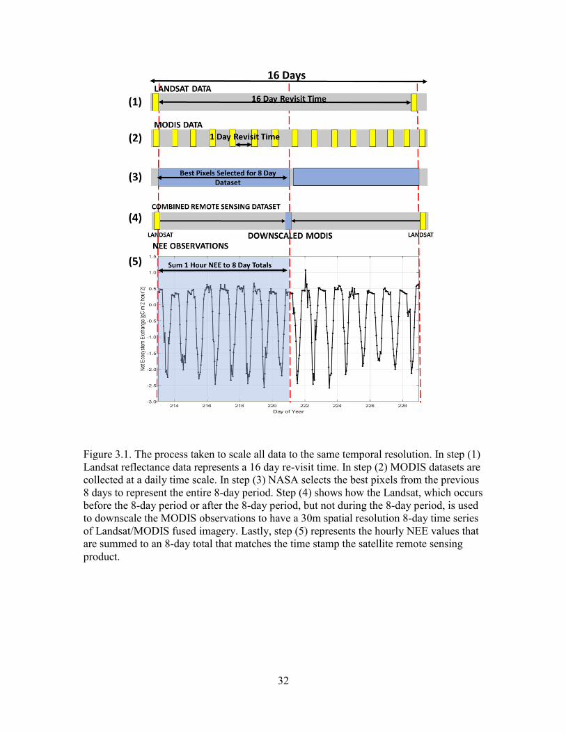
[gCm-2 8days-1]. The process of matching NEE measurements to the remote sensing data
is shown in Figure 3.1. Steps 1-4 are the ESTARFM technique discussed below and step
5 shows the computation of an 8-day NEE value.
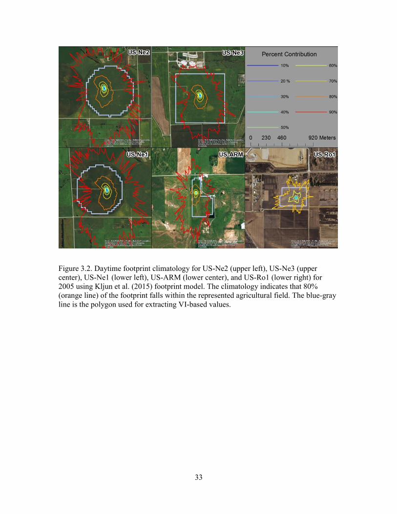
One concern when working with carbon flux measurements is whether the NEE
values represent the land cover that is being evaluated. To determine whether the
13
predominant source locations of NEE fell within the represented agricultural field, a
surface-layer footprint climatology analysis was conducted on all the sites (Figure 3.2).
The footprint climatology was computed using the model developed by Kljun et al.
(2015) for non-gap filled daytime observations when photosynthesis occurs and the
atmosphere is well-mixed. With the exception of US-Ro1 station, where 70%
contribution footprint contour fell outside the agricultural field, all footprint climatologies
had an 80% source contribution during the daytime that fell within the agricultural field
represented by the flux tower. This provides an independent confirmation that NEE
values represent the agricultural crop. Therefore, data were not scaled to a flux footprint
because the samples represent the crop field a majority of the time. Since it was more
important to capture the carbon cycle and the NEE dataset had been already reduced to 8-
day temporal resolution, the nighttime observations were not removed from the 8-day
NEE totals and the use of nighttime NEE data with source locations potentially outside
the agricultural field is a source of uncertainty in this analysis.
3.2.2 REMOTE SENSING DATASETS
During the period of interest, numerous satellite observations have been archived for the
US Great Plains region. Here, we utilized land surface reflectance datasets from MODIS
(500m resolution) and Landsat (30m resolution). The 8-day 500m MODIS surface
reflectance product (MOD09A1) was obtained for 2002 to 2011 for the three tiles that
covered the five AmeriFlux sites of interest (Vermote, 2015; Wan, Hook, & Hulley,
2015). The data was downloaded from the Level 1 and Atmosphere Archive and
Distribution System managed by NASA.

14
The MOD09A1 data product provides the spectral surface reflectance using
MODIS bands 1-7. Each pixel contains the highest quality higher-order gridded level-2
(L2G) observation over an 8-day period (Figure 3.1, steps 2-3). The use of this dataset
minimizes the influences of clouds that will occur in the daily MODIS files. The state
flags provided with the dataset were applied to each image to mask cloudy pixels, snow
or ice, and cloud shadowed pixels. Each image was subset to a 10km × 10km area around
the station to ensure the entirety of the station fetch was included within the subset image
(Horst & Weil, 1994; Leclerc & Foken, 2014).
Landsat datasets have a 16-day revisit cycle and 30m spatial resolution (Figure
3.1, step 1). Images from Landsat-5 Thematic Mapper and Landsat-7 Enhanced Thematic
Mapper Plus were used. All Landsat data were acquired from the United States
Geological Survey’s Earth Resources Observation and Science Center Science
Processing Architecture. This product has been atmospherically corrected and
geometrically corrected using the same subroutines conducted on MODIS surface
reflectance datasets, making these two datasets comparable (Masek et al., 2006). Files
downloaded contained surface reflectance, cloud mask and quality assurance flags. The
10km x 10km subsets of all Landsat surface reflectance products were created to match
the subset of the MODIS datasets. Using the quality control and cloud flags provided by
USGS, all pixels labeled as cloud, adjacent to cloud, snow/ice, or poor quality were
removed.
3.2.3 ESTARFM DOWNSCALING MODEL
The subset images were processed in the ESTARFM image fusion algorithm (Zhu et al.
2010). The MODIS bands 1-7 were reordered and resampled from 500m to 30m to match
15
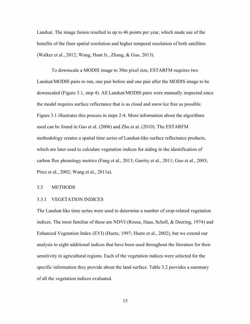
Landsat. The image fusion resulted in up to 46 points per year, which made use of the
benefits of the finer spatial resolution and higher temporal resolution of both satellites
(Walker et al., 2012; Wang, Hunt Jr., Zhang, & Guo, 2013).
To downscale a MODIS image to 30m pixel size, ESTARFM requires two
Landsat/MODIS pairs to run, one pair before and one pair after the MODIS image to be
downscaled (Figure 3.1, step 4). All Landsat/MODIS pairs were manually inspected since
the model requires surface reflectance that is as cloud and snow/ice free as possible.
Figure 3.1 illustrates this process in steps 2-4. More information about the algorithms
used can be found in Gao et al. (2006) and Zhu et al. (2010). The ESTARFM
methodology creates a spatial time series of Landsat-like surface reflectance products,
which are later used to calculate vegetation indices for aiding in the identification of
carbon flux phenology metrics (Fang et al., 2013; Garrity et al., 2011; Guo et al., 2003;
Price et al., 2002; Wang et al., 2011a).
3.3 METHODS
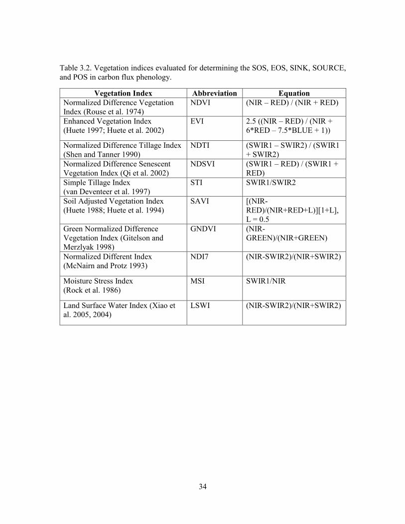
3.3.1 VEGETATION INDICES
The Landsat-like time series were used to determine a number of crop-related vegetation
indices. The most familiar of these are NDVI (Rouse, Haas, Schell, & Deering, 1974) and
Enhanced Vegetation Index (EVI) (Huete, 1997; Huete et al., 2002), but we extend our
analysis to eight additional indices that have been used throughout the literature for their
sensitivity in agricultural regions. Each of the vegetation indices were selected for the
specific information they provide about the land surface. Table 3.2 provides a summary
of all the vegetation indices evaluated.

16
3.3.2 EXTRACTION OF FIELD-SCALE MEASUREMENTS
Crop types grown in each agricultural field where the AmeriFlux site was located was
provided by the station PI. To obtain statistics on surface attributes for the representative
agricultural field, a polygon shapefile was created to extract pixel values for each
downscaled Landsat-like VI values for all years from 2002-2011. The mean and standard
deviation of the extracted values from each image were computed to create an 8-day time
series of the ten vegetation indices at field-scale. Figure 3.2 provides the polygons in
gray-blue that were used for extracting pixel values. If any pixel value was previously
removed due to poor quality, or the value fell outside the upper and lower bounds of the
vegetation index, it was also removed from the computation of the field-scale statistics.
3.3.3 COMPARISON OF VI-BASED AND NEE-BASED PHENOLOGY METRICS
The variables of interest include SOS, SINK, POS, SOURCE and EOS from both the
NEE measurements and the vegetation indices. From this point forward subscripts NEE
and VI will be used to denote which data source was used to find the phenological metric.
All NEE-based metrics were estimated using the ground-based, direct measurement of
carbon dynamics between the atmosphere and the ecosystem, and therefore were
considered “truth.” The VI-based metrics were estimated using vegetation indices that
were calculated from satellite remote sensing, and were assessed in this study against the
NEE-based metrics. The units for each phenological metric are day of the year (DOY)
when it occurs.
At field-scale all NEE and VI data were divided by year and station based on the
crop type grown each site year. There was a total of 27 site years of maize and 15 site
years of soybean. Soybean and maize were the main focus of this analysis, therefore
17
years that US-ARM grew wheat or canola were not included (Raz-Yaseef et al., 2015).
Specific land management activities of the agricultural fields were not considered.
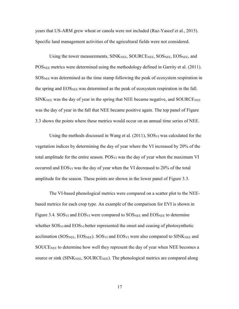
Using the tower measurements, SINKNEE, SOURCENEE, SOSNEE, EOSNEE, and
POSNEE metrics were determined using the methodology defined in Garrity et al. (2011).
SOSNEE was determined as the time stamp following the peak of ecosystem respiration in
the spring and EOSNEE was determined as the peak of ecosystem respiration in the fall.
SINKNEE was the day of year in the spring that NEE became negative, and SOURCENEE
was the day of year in the fall that NEE became positive again. The top panel of Figure
3.3 shows the points where these metrics would occur on an annual time series of NEE.
Using the methods discussed in Wang et al. (2011), SOSVI was calculated for the
vegetation indices by determining the day of year where the VI increased by 20% of the
total amplitude for the entire season. POSVI was the day of year when the maximum VI
occurred and EOSVI was the day of year when the VI decreased to 20% of the total
amplitude for the season. These points are shown in the lower panel of Figure 3.3.
The VI-based phenological metrics were compared on a scatter plot to the NEE-
based metrics for each crop type. An example of the comparison for EVI is shown in
Figure 3.4. SOSVI and EOSVI were compared to SOSNEE and EOSNEE to determine
whether SOSVI and EOSVI better represented the onset and ceasing of photosynthetic
acclimation (SOSNEE, EOSNEE). SOSVI and EOSVI were also compared to SINKNEE and
SOUCENEE to determine how well they represent the day of year when NEE becomes a
source or sink (SINKNEE, SOURCENEE). The phenological metrics are compared along

18
the gray dashed line in Figure 3.4. The mean signed difference (MSD) in days was
determined for each phenology point as:
(1) MSD = (6 (DOYNEE, i – DOYVI, i )) / n
where i is the corresponding value for the same year and station, and n is the number of
values being averaged. Equation 1 was used to calculate the MSD between NEE-based
and VI-based metrics, where SINKNEE and SOSNEE were compared to SOSVI, and
SOURCENEE and EOSNEE were compared to EOSVI, as shown in Figure 3.
The total NEE value was calculated annually from growing season by summing
NEE from the NEE-based SINK to SOURCE dates. This total carbon uptake value was
then compared to the sum of NEE from SOS and EOS dates as estimated by VI-based
phenology. The total growing season carbon uptake as estimated from VI-based SOS to
EOS for each vegetation index was compared to the total carbon uptake value from NEE-
based SINK to SOURCE.
3.4 RESULTS
When considering the performance of each VI as presented here, it is important to
understand about the underlying data sources that any difference less than eight days is
considered to be a good measure because the images used to compute the VI can fall
anywhere in the 8-day time stamp of MODIS (Figure 1 step 4).
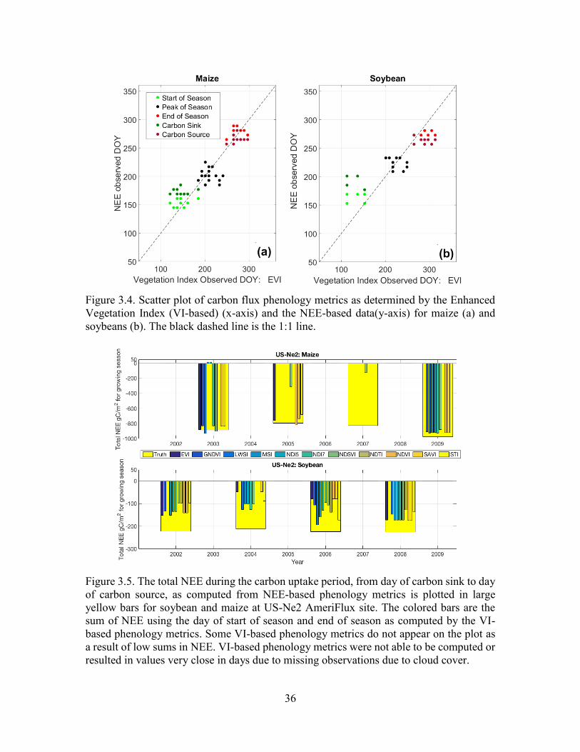
In Figure 3.4, the scatterplot shows that in general for maize (Figure 3.4a) that the
VI-based vs. NEE-based phenological metrics were clustered near the 1:1 line for EVI,
where several site years the VI-based metrics fall before and after the NEE-based metrics.
There is a different pattern that occurs in soybean (Figure 3.4b) for the same vegetation
19
index, where VI-based SOS were estimated before NEE-based SOS and SINK phenology
metrics, and VI-based EOS was estimated after NEE-based SOURCE and EOS dates. A
scatterplot for each vegetation index was visually inspected to visualize the closeness of
the VI-based phenology metrics to the NEE-based phenology metrics. These results are
included in the text of the following sections. A table of relevant values for all VIs and
phenology points is included in Appendix A.
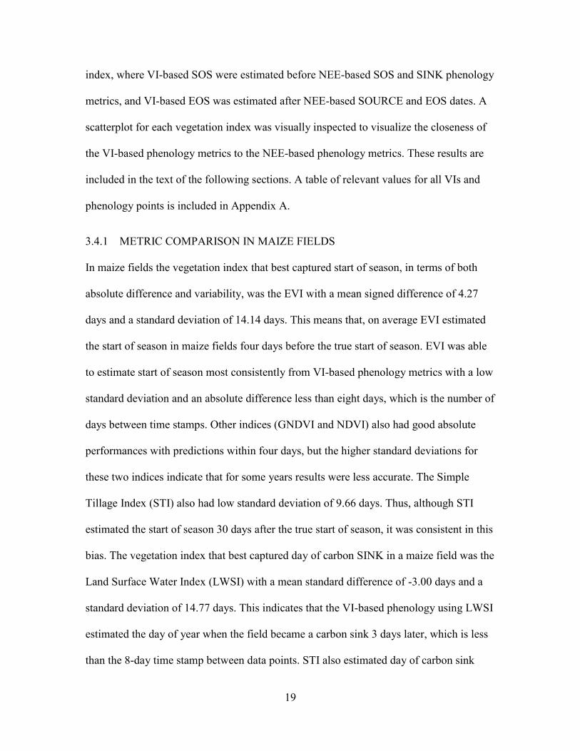
3.4.1 METRIC COMPARISON IN MAIZE FIELDS
In maize fields the vegetation index that best captured start of season, in terms of both
absolute difference and variability, was the EVI with a mean signed difference of 4.27
days and a standard deviation of 14.14 days. This means that, on average EVI estimated
the start of season in maize fields four days before the true start of season. EVI was able
to estimate start of season most consistently from VI-based phenology metrics with a low
standard deviation and an absolute difference less than eight days, which is the number of
days between time stamps. Other indices (GNDVI and NDVI) also had good absolute
performances with predictions within four days, but the higher standard deviations for
these two indices indicate that for some years results were less accurate. The Simple
Tillage Index (STI) also had low standard deviation of 9.66 days. Thus, although STI
estimated the start of season 30 days after the true start of season, it was consistent in this
bias. The vegetation index that best captured day of carbon SINK in a maize field was the
Land Surface Water Index (LWSI) with a mean standard difference of -3.00 days and a
standard deviation of 14.77 days. This indicates that the VI-based phenology using LWSI
estimated the day of year when the field became a carbon sink 3 days later, which is less
than the 8-day time stamp between data points. STI also estimated day of carbon sink
20
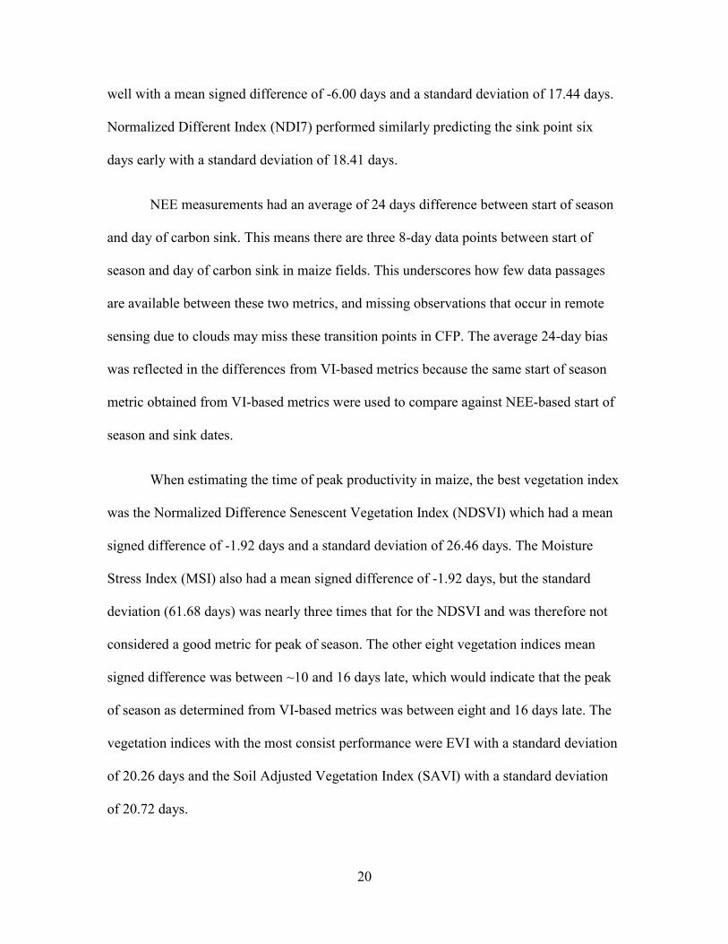
well with a mean signed difference of -6.00 days and a standard deviation of 17.44 days.
Normalized Different Index (NDI7) performed similarly predicting the sink point six
days early with a standard deviation of 18.41 days.
NEE measurements had an average of 24 days difference between start of season
and day of carbon sink. This means there are three 8-day data points between start of
season and day of carbon sink in maize fields. This underscores how few data passages
are available between these two metrics, and missing observations that occur in remote
sensing due to clouds may miss these transition points in CFP. The average 24-day bias
was reflected in the differences from VI-based metrics because the same start of season
metric obtained from VI-based metrics were used to compare against NEE-based start of
season and sink dates.
When estimating the time of peak productivity in maize, the best vegetation index
was the Normalized Difference Senescent Vegetation Index (NDSVI) which had a mean
signed difference of -1.92 days and a standard deviation of 26.46 days. The Moisture
Stress Index (MSI) also had a mean signed difference of -1.92 days, but the standard
deviation (61.68 days) was nearly three times that for the NDSVI and was therefore not
considered a good metric for peak of season. The other eight vegetation indices mean
signed difference was between ~10 and 16 days late, which would indicate that the peak
of season as determined from VI-based metrics was between eight and 16 days late. The
vegetation indices with the most consist performance were EVI with a standard deviation
of 20.26 days and the Soil Adjusted Vegetation Index (SAVI) with a standard deviation
of 20.72 days.
21
Estimating the time when the maize field became a carbon source had similar
challenges as those found when estimating SOS and SINK. The mean signed differences
were large across most vegetation indices tested (see Appendix A), however they were
the most consistent with a smaller standard deviation. The vegetation index that best
captured day of carbon source was EVI with a mean signed difference of -6.40 days with
a standard deviation of 14.01 days. SAVI was able to estimate NEE-based metrics from
VI-based metrics consistently with a larger mean signed difference. The vegetation
indices that performed best in estimating day of carbon source were consistently 8-16
days late. There was a small mean signed difference (-0.89 days) for the Normalized
Difference Tillage Index, but this index was not selected as a good metric for source date
because of the large standard deviation (76.89 days).
The best vegetation indices for estimating end of season dynamics in maize fields
were EVI and SAVI. The mean signed difference for EVI was 7.20 days with a standard
deviation of 15.29 days, and SAVI had a mean signed difference of -1.60 days with a
standard deviation of 14.99 days. This means that EVI and SAVI could accurately
estimate NEE-based end of season within 0 to 8 days.
3.4.2 METRIC COMPARISON IN SOYBEAN FIELDS
In soybean fields, Normalized Difference Senescent Vegetation Index (NDSVI) could
estimate start of season with a lower standard deviation (12.22 days), but had a larger
mean signed difference (29.33 days). This indicates that NDSVI estimated the start of
season 29 days too early. Meanwhile, the Green Normalize Difference Vegetation Index
(GNDVI) estimated the start of season from VI-based data with a bias of 5.33 days, but
had a larger standard deviation of 32.33 days. The standard deviations of the signed
22
differences were larger in soybean fields than in maize, partially due to the limited
number of time series available.
The vegetation indices that best captured the day of carbon sink in soybean fields
were Land Surface Water Index (LWSI) and Normalized Difference Tillage Index
(NDTI) with respective mean signed differences of -11.20 days with a standard deviation
of 9.12 days and 0.00 days and a large standard deviation of 38.09 days. LWSI was also
the best vegetation index for identifying the day of carbon sink in maize fields. Therefore,
there was no difference in vegetation index selection between soybean and maize for
identifying day of carbon sink.
The vegetation indices that identified peak of season in carbon uptake in soybean
fields from VI-based phenology metrics with a small mean signed difference and small
standard deviation were Moisture Stress Index (MSI), GNDVI, and EVI with a mean
signed difference of -0.62, -1.85, and -1.23 days, and a standard deviation of 16.80,
16.70, and 19.55 days. All of these vegetation indices had very good agreement across
sites with a standard deviation in the signed differences between 16 and 20 days. This
was a significantly tighter spread in the signed differences for soybean than maize. The
best metric for identifying peak of season in soybean fields was MSI because it had the
smallest mean signed difference and smaller standard deviation.
The estimation of source date from VI-based phenological metrics for soybean
fields had a similar delay pattern to what was found in maize. The vegetation indices that
most effectively estimated the day of carbon source were MSI, LWSI, and Simple Tillage
Index (STI). MSI had a small mean signed difference of -6.40 days, but had a large
23
standard deviation of 35.51 days. Meanwhile, LWSI and STI had a larger mean signed
difference of -24.00 days, but had a standard deviation less than 10 days, which is within
one 8-day time stamp. MSI was selected as the best vegetation index for estimating day
of carbon source from VI-based phenology metrics.
When estimating the end of season in carbon flux phenology in soybean fields, all
vegetation indices had a higher value in mean signed difference. On average the mean
signed difference ranged from 16-28 days between NEE-based and VI-based phenology
metrics. The vegetation index that had the smallest mean signed difference and standard
deviation was the STI with a mean signed difference of -10.67 days and a standard
deviation of 10.93 days. Other alternatives for estimating the end of season from VI-
based phenology in preference order were LWSI, MSI, GNDVI, and EVI. The statistics
for these additional four vegetation indices can be found in Appendix A.
3.4.3 METRIC COMPARISON FOR SOYBEAN AND MAIZE FIELDS COMBINED
The mean signed differences were computed for all phenology metrics where crop type
was not considered. When crop type was not considered when estimating carbon flux
phenology metrics, there were higher standard deviations of the signed differences. As
expected, the mean signed difference was approximately the mean of the two mean
signed differences of soybean and maize separately. Differences remained low when
estimating sink date using LWSI, which had a mean signed difference of -6.15 days and a
standard deviation 13.13 days; this vegetation index was the best fit for maize and
soybean. All other indices had higher biases when crop type was not considered. A
summary of these statistics are found in Appendix A.
24
3.4.4 TOTAL NET ECOSYSTEM EXCHANGE DURING CARBON UPTAKE PERIOD
Accurately capturing the carbon flux phenology is important for estimating the total
carbon uptake that occurs from day of carbon sink to day of carbon source. The total
NEE was summed using SINK and SOURCE NEE-based phenology metrics and then
compared to the total NEE when using VI-based estimated SOS and EOS phenology
metrics. The phenology metrics were used as start and end of growing season proxies
when summing NEE annually. The results for US-Ne2 (Maize/Soybean Rotation) can be
seen in Figure 3.5. In 2007 there were significant gaps due to cloud cover, so the SOS
and EOS could not be calculated for this year for this station. In this example the VI-
based phenology metrics were not able to capture the true sum of NEE during the carbon
uptake period and typically underestimated the total carbon uptake for the year. The same
pattern was observed in the other four sites in this analysis. The lifecycle and structure of
maize and soybean are starkly different, which results in different reflectance between
each crop type, greater carbon uptake in maize compared to soybean, and affirms the
need for crop type dependent models.
3.5 DISCUSSION
3.5.1 START OF SEASON AND SINK DATE
The vegetation indices that best capture maize and soybean start of season dates were
different. Balzarolo et al. (2016) assessed six indices, where we assessed four of the six in
our analysis. We identified that EVI performed better than NDVI in croplands when
identifying phenological metrics. Our results support that EVI and NDVI can accurately
estimate start of season with biases of approximately eight days when crop type is not
considered. More specifically, our results also show the mean signed differences are
25
larger than 30 days when using EVI for soybean for start of season, but it performs with
acceptable biases of less than eight days for maize fields for start of season.
Contrary to Balzarolo et al. (2016) we found that GNDVI and NDSVI are better
metrics for estimating start of season for soybean or all crops. As a result, while
Balzarolo et al. (2016) is correct in stating that EVI performs best in croplands for
identifying carbon flux phenology metrics, estimates using EVI are more accurate in
maize fields (C4 photosynthetic pathway) than soybean fields (C3 photosynthetic
pathway). The biases tended to be larger for soybean crops than maize because of
differences in early developmental stages and in the timing of the point of photosynthetic
acclimation. Soybean typically has a 5-21 day plant to emergence period, depending on
temperature and moisture availability, while maize has a 7-10 day plant to emergence
time. The period from vegetation emergence to peak photosynthetic uptake (which
typically occurs in reproductive phase 1-2 (R1-R2)), is 39-71 days in soybeans and 69-75
days in maize. Soybean goes through six growing stages while maize goes through 18
growing phases before beginning the reproductive phase (Abendroth, Elmore, Boyer, &
Marlay, 2011; Fehr, Caviness, Burmood, & Pennington, 1971; Licht, 2014). This
apparent temporal mismatch is the main reason why different vegetation indices perform
better for soybean than maize.
When estimating the day of year when the crop field became a carbon sink, both
crops indicate the same vegetation index would be best: the land water surface index
(LWSI). This index relies on the use of the NIR and SWIR2 reflectance bands, which are
sensitive to the amount of water (SWIR2) and there is a higher amount of reflectance of
NIR from chloroplasts which contain chlorophyll (Jensen, 2005). Both maize and
26
soybean are highly sensitive to water availability and temperature in stages of growth
(Fehr et al. 1971; Abendroth et al. 2011), making it logical that a water sensitive index
would best capture this transition.
3.5.2 PEAK OF SEASON
We found peak of season the easiest transition point to identify remotely. The metrics for
soybean had a smaller standard deviation and smaller mean signed differences than maize
metrics, indicating that soybean peak of season can be estimated with better certainty
than maize POS. Maize has a peak in carbon uptake approximately 8-16 days after the
peak greenness, while the peak in greenness is approximately the same as the peak in
carbon uptake in soybean fields. This may be due to the larger amount of biomass that is
visible when viewing maize fields, meaning there is a greater leaf area index (LAI) and
greater chlorophyll concentration. High LAI can saturate the reflectance in a pixel and
there may be points in the time series where the satellite is unable to detect changes in
greenness.
Reflectance saturation is the cause of the 10-day bias in several of the vegetation
indices. This bias can be seen in maize fields when using SAVI or EVI. Maize transitions
to a new vegetation stage every two days, and so the 8-day temporal resolution may be
too coarse to capture changes in maize greenness. This may result in the sensor missing
the appropriate scan time for maximum carbon uptake, which occurs in reproductive
phases 1-2 (Abendroth et al. 2011). It is vitally important to capture the peak LAI in
maize because the maximum LAI is linked to maximum daytime NEE and gross primary
production (Suyker et al., 2004). Meanwhile, soybean has a smaller LAI and therefore
27
will not saturate the remote sensing pixel; as a result the peak of season is easier to
capture.
While POS is easiest to identify, two metrics are most effective: NDSVI for maize
fields and MSI for soybean fields. Both of these vegetation indices make use of the
SWIR1 reflectance band and the secondary bands are Red and NIR respectively. The
results agree well with findings in Viña et al. (2011), which found that soybean had an
increasing reflectance with increasing wavelength while maize had a lower reflectance in
longer wavelengths, indicating that soybean and maize needed different remote sensing
algorithms for estimating LAI.
3.5.3 END OF SEASON AND SOURCE DATE
End of season and source dates were very difficult to estimate. This is not exclusive to
agricultural crops. Garrity et al. (2011) determined that the relationship between
senescence and carbon fluxes were complicated by foliar pigments, meteorological
conditions, and environmental stresses, which will affect all plants. The differences in
structural leaf orientation and chlorophyll content in soybean and maize will appear
differently during senescence (Viña et al. 2011). In maize fields end of season and source
dates had higher standard deviation than those found in soybean fields. In both cases the
mean signed differences were high, but consistent. For instance, there was a three 8-day
time stamp bias (24 days) between the end of season estimated by VI-based phenology
and the NEE-based day of carbon source; this bias will be used to estimate day of source
in future work.
28
3.5.4 IMPLICATIONS AND FUTURE WORK
One limitation of the method demonstrated here was in maize and soybean fields that had
two crop rotations within the same year. This resulted in two growing seasons, making
the differentiation programmatically challenging. The years where maize and soybean
were grown at US-ARM also had wheat grown earlier in the year. As a result of this
challenge, the US-ARM station was omitted from the mean signed differences. Crop
fields where there are two crop rotations per year will not perform well in this
methodology, unless the dates are known when each crop occurred during the year.
Viña et al. (2011) determined differences in the reflectance of soybean and maize
leaves at different wavelengths during peak LAI were due to differences in leaf structure
and leaf chlorophyll content of each crop. Despite soybean having a smaller LAI,
soybean had higher reflectance than maize in longer wavelengths due to higher
chlorophyll content in the adaxial side of soybean leaves and lower water content.
However, the results of this analysis show that the differences between reflectance and
physiological composition between maize and soybean means each crop will appear
different in remote sensing datasets. The downscaling process amplifies these differences.
One limitation of using downscaled MODIS imagery is if a clear sky and snow free
remote sensing pair of Landsat and MODIS cannot be identified before the true start of
season and/or after end of season, then the full growing season cannot be observed. In
this case VI-based phenology metrics will be missing or incorrect. This is especially true
in humid environments where cloud cover is more frequent and northern latitudes where
snow is prevalent for long periods of time, making Landsat’s 16-day revisit time
insufficient. If missing pairs occur within the growing season incorrect VI-based
29
phenology metrics will result regardless of the vegetation index used. A different
downscaling algorithm that does not require Landsat imagery would be required to
address this limitation.
As discussed above, it is common to model NEE, gross primary production, or net
ecosystem production with one agricultural subgroup. However, making use of land
cover analysis techniques to identify crop type, requires the use of VI-based phenology
metrics in modeling efforts (Wang et al. 2011, 2013). This work shows that using the
correct vegetation index for an individual field could improve model results. Future work
will need to make use of land cover datasets, such as USDA’s Cropland data layer, so
that this analysis can be expanded outside of pre-identified cropland fields and the
impacts of maize and soybean agriculture on carbon exchanges in the United States can
be identified.
This approach, however does have a limitation. When using 8-day temporal
resolution datasets a single missing remote sensing image can cause a true phenology
metric to be missed. This will cause total NEE values to be too high, as demonstrated in
Figure 3.5. Future work may have to consider using daily MODIS imagery to limit the
number of holes that may occur due to clouds and snow cover, and capture changes in the
vegetation that are occurring at time scales smaller than 8-days (especially during the
vegetative stage).
3.6 CONCLUSIONS
Modeling and mapping carbon flux phenology in agricultural systems require different
strategies based on crop type when using VI-based products. Here we show that:
30
x A single vegetation index cannot accurately capture the full carbon flux
phenology for all crops because of the differences in crop lifecycle and
chlorophyll content between crop types.
x LWSI best captured SINK date for both soybean and maize.
x In maize fields: EVI best captured SOS and SOURCE, NDSVI best captured peak
of season, and SAVI best captured EOS.
x In soybean fields: NDSVI best captured SOS, MSI best captured peak of season
and SOURCE, and STI best captured EOS.
x The chosen vegetation indices better reflect the physiology of the individual crops
because they use vegetation indices that use reflectance bands to which each crop
is more sensitive.
x This method cannot be used if cover crops or spring crops are grown during or
between crop rotations.
x When total carbon uptake is computed for the growing season, if the SOS, EOS,
SINK, and SOURCE are not properly represented, then the total NEE summed
using VI-based metrics will be overestimated compared to the total NEE using
NEE-based CFP metrics.
Future work will develop and test an empirical model to estimate carbon uptake
period from VI-based indices that is crop type dependent, beginning with maize and
soybean crops. A better estimation of carbon flux dynamics will help to provide better
information about the regional impact of growing maize and soybean in the US Great
Plains on carbon flux dynamics, which will inform future climate models as the
cultivation of maize and soybean expands across the United States.
31
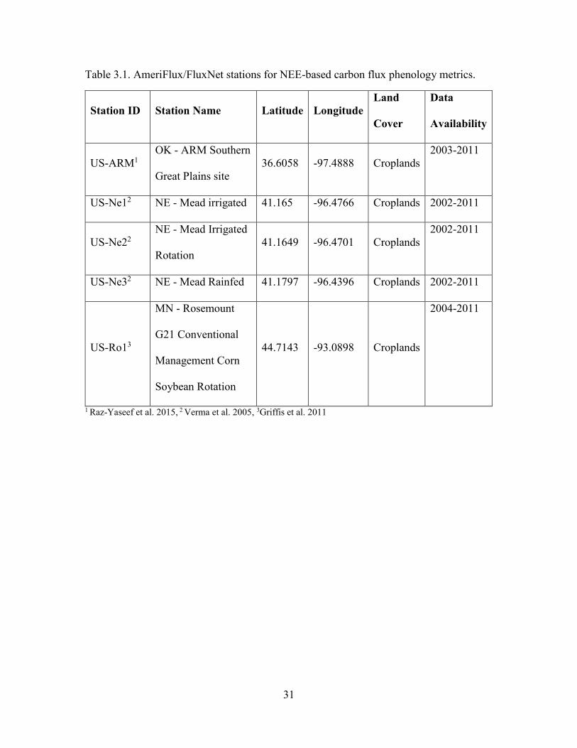
Table 3.1. AmeriFlux/FluxNet stations for NEE-based carbon flux phenology metrics.
Station ID Station Name Latitude Longitude Land
Cover
Data
Availability
US-ARM1 OK - ARM Southern
Great Plains site 36.6058 -97.4888 Croplands
2003-2011
US-Ne12 NE - Mead irrigated 41.165 -96.4766 Croplands 2002-2011
US-Ne22 NE - Mead Irrigated
Rotation 41.1649 -96.4701 Croplands
2002-2011
US-Ne32 NE - Mead Rainfed 41.1797 -96.4396 Croplands 2002-2011
US-Ro13
MN - Rosemount
G21 Conventional
Management Corn
Soybean Rotation
44.7143 -93.0898 Croplands
2004-2011
1 Raz-Yaseef et al. 2015, 2 Verma et al. 2005, 3Griffis et al. 2011
32
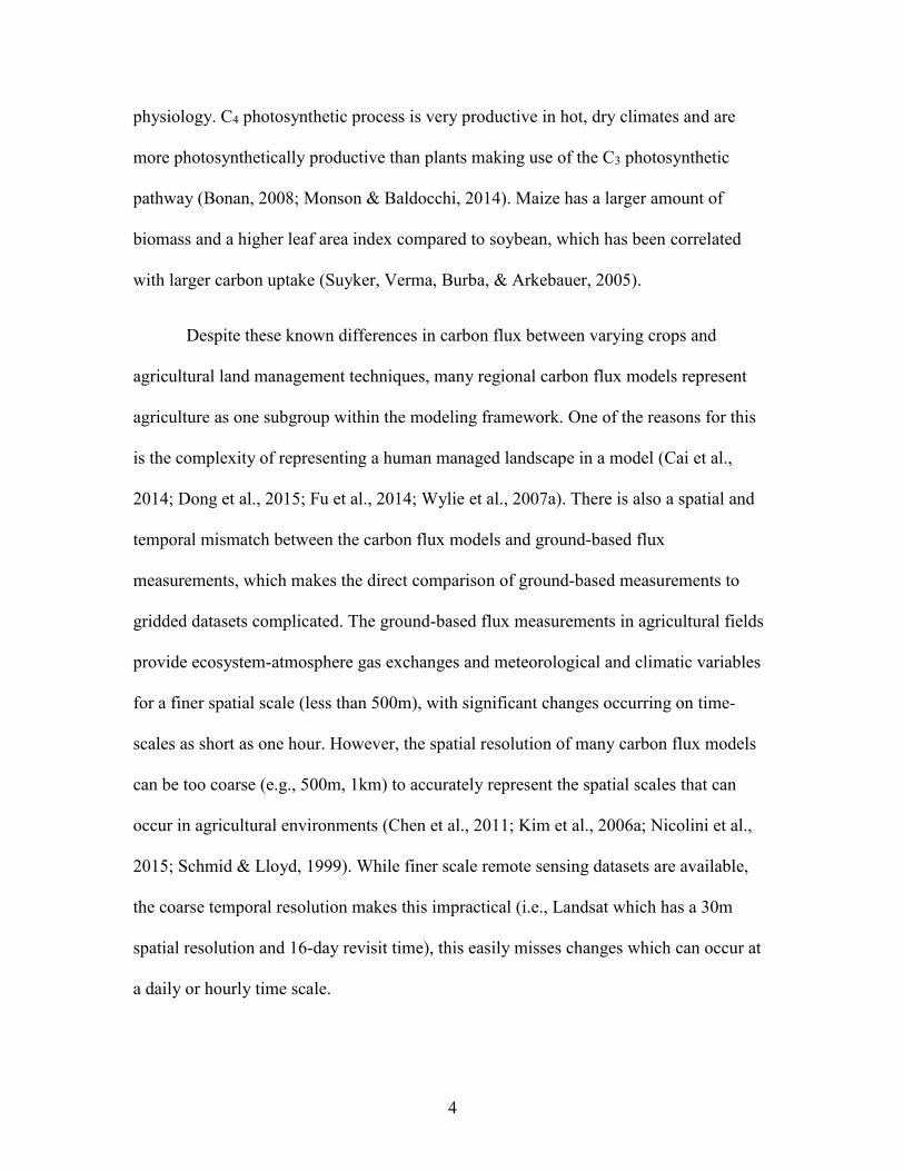
Figure 3.1. The process taken to scale all data to the same temporal resolution. In step (1) Landsat reflectance data represents a 16 day re-visit time. In step (2) MODIS datasets are collected at a daily time scale. In step (3) NASA selects the best pixels from the previous 8 days to represent the entire 8-day period. Step (4) shows how the Landsat, which occurs before the 8-day period or after the 8-day period, but not during the 8-day period, is used to downscale the MODIS observations to have a 30m spatial resolution 8-day time series of Landsat/MODIS fused imagery. Lastly, step (5) represents the hourly NEE values that are summed to an 8-day total that matches the time stamp the satellite remote sensing product.
33
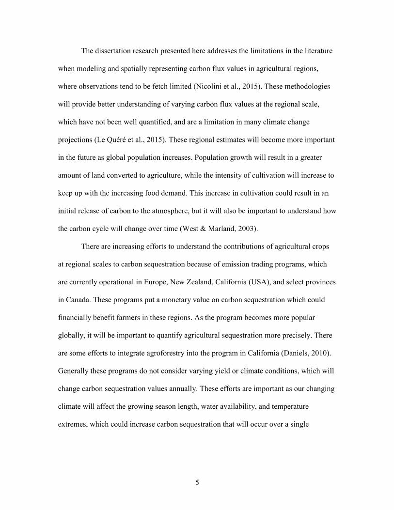
Figure 3.2. Daytime footprint climatology for US-Ne2 (upper left), US-Ne3 (upper center), US-Ne1 (lower left), US-ARM (lower center), and US-Ro1 (lower right) for 2005 using Kljun et al. (2015) footprint model. The climatology indicates that 80% (orange line) of the footprint falls within the represented agricultural field. The blue-gray line is the polygon used for extracting VI-based values.
34
Table 3.2. Vegetation indices evaluated for determining the SOS, EOS, SINK, SOURCE, and POS in carbon flux phenology.
Vegetation Index Abbreviation Equation Normalized Difference Vegetation Index (Rouse et al. 1974)
NDVI (NIR – RED) / (NIR + RED)
Enhanced Vegetation Index (Huete 1997; Huete et al. 2002)
EVI 2.5 ((NIR – RED) / (NIR + 6*RED – 7.5*BLUE + 1))
Normalized Difference Tillage Index (Shen and Tanner 1990)
NDTI (SWIR1 – SWIR2) / (SWIR1 + SWIR2)
Normalized Difference Senescent Vegetation Index (Qi et al. 2002)
NDSVI (SWIR1 – RED) / (SWIR1 + RED)
Simple Tillage Index (van Deventeer et al. 1997)
STI SWIR1/SWIR2
Soil Adjusted Vegetation Index (Huete 1988; Huete et al. 1994)
SAVI [(NIR-RED)/(NIR+RED+L)][1+L], L = 0.5
Green Normalized Difference Vegetation Index (Gitelson and Merzlyak 1998)
GNDVI (NIR-GREEN)/(NIR+GREEN)
Normalized Different Index (McNairn and Protz 1993)
NDI7 (NIR-SWIR2)/(NIR+SWIR2)
Moisture Stress Index (Rock et al. 1986)
MSI SWIR1/NIR
Land Surface Water Index (Xiao et al. 2005, 2004)
LSWI (NIR-SWIR2)/(NIR+SWIR2)
35
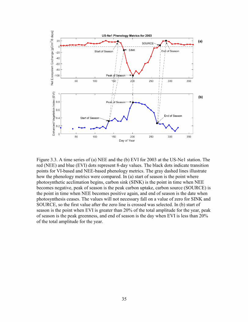
Figure 3.3. A time series of (a) NEE and the (b) EVI for 2003 at the US-Ne1 station. The red (NEE) and blue (EVI) dots represent 8-day values. The black dots indicate transition points for VI-based and NEE-based phenology metrics. The gray dashed lines illustrate how the phenology metrics were compared. In (a) start of season is the point where photosynthetic acclimation begins, carbon sink (SINK) is the point in time when NEE becomes negative, peak of season is the peak carbon uptake, carbon source (SOURCE) is the point in time when NEE becomes positive again, and end of season is the date when photosynthesis ceases. The values will not necessary fall on a value of zero for SINK and SOURCE, so the first value after the zero line is crossed was selected. In (b) start of season is the point when EVI is greater than 20% of the total amplitude for the year, peak of season is the peak greenness, and end of season is the day when EVI is less than 20% of the total amplitude for the year.
36
Figure 3.4. Scatter plot of carbon flux phenology metrics as determined by the Enhanced Vegetation Index (VI-based) (x-axis) and the NEE-based data(y-axis) for maize (a) and soybeans (b). The black dashed line is the 1:1 line.
Figure 3.5. The total NEE during the carbon uptake period, from day of carbon sink to day of carbon source, as computed from NEE-based phenology metrics is plotted in large yellow bars for soybean and maize at US-Ne2 AmeriFlux site. The colored bars are the sum of NEE using the day of start of season and end of season as computed by the VI-based phenology metrics. Some VI-based phenology metrics do not appear on the plot as a result of low sums in NEE. VI-based phenology metrics were not able to be computed or resulted in values very close in days due to missing observations due to cloud cover.
37
CHAPTER 4
AN EMPIRICAL MODELING APPROACH TO ESTIMATING
REGIONAL SCALE NET ECOSYSTEM EXCHANGE IN MAIZE AND
SOYBEAN FIELDS IN THE US CORN BELT1
1McCombs, A.G., A.L. Hiscox, A. Desai, C. Wang, and A. Suyker. To be submitted to
Agricultural and Forest Meteorology.

38
4.1 INTRODUCTION
The estimation of agricultural impacts on the carbon dynamics is not well represented in
climate models, limiting the robustness of future climate projections (Le Quéré et al.,
2015). Satellite remote sensing has been commonly used to model carbon dynamics at
regional scales. Prior modeling efforts have primarily relied on the use of vegetation
indices, which describe the greenness of the surface from a derived combination of
surface reflectance bands, to model NEE, or net primary production in generalized
ecosystem categories at a regional to global scale (i.e., Dong et al., 2015; Fu et al., 2014;
Gu and Wylie, 2015; Kim et al., 2006; Sims et al., 2014; Tang et al., 2012; Wylie et al.,
2007; Xiao et al., 2011). While this is useful globally it is a less accurate approach at the
regional scale, where specific climate impacts need to be better understood for planning
and management purposes. Gitelson et al. (2012) determined that the most significant
bands for modeling carbon exchanges were vegetation indices that included the green and
near-infrared bands for generalized ecotones. However, there has been little work
developing carbon exchange models using satellite remote sensing for agricultural
regions due to the complexity of these systems (Wylie et al., 2007b; Xiao et al., 2011;
Xiao et al., 2004). The reasons for this are both practical and technical. Practically, as
human-managed systems, the “natural” cycles are modified year to year and field to field.
Technically, modelling carbon dynamics at coarser spatial resolutions is challenging due
to varying climatic conditions and heterogeneous land covers within a pixel (Wu et al.,
2012). However, the development of downscaling algorithms such as the Enhanced
Spatial and Temporal Adaptive Reflectance Fusion Model (ESTARFM), which allow
finer temporal resolution MODIS datasets to be fused with finer spatial resolution
39
Landsat (Zhu et al., 2010), removes many of the technical challenges of model
development in agricultural systems because the downscaled pixels are significantly finer
than the agricultural field.
Fu et al. (2014) used downscaled MODIS and Landsat observations to estimate
carbon dynamics. An empirical modeling approach was evaluated using vegetation
indices, reflectance, and land surface temperature to develop a regression tree for varying
land covers. This used predetermined thresholds from vegetation indices and surface
reflectance to account for changes in carbon fluxes and surface reflectance for different
stages of the growing season. However, a limitation of their work was that it was
developed for broad land cover classification, and for the case of agriculture there was
only one subgroup. Here, we demonstrate the ability to model carbon dynamics from
remotely sensed surface reflectance using an empirical approach for particular
agricultural crops.
Kalfas et al. (2011) developed a model to estimate gross primary production in
maize fields using several MODIS computed vegetation indices, as well as
photosynthetically active radiation and air temperature. This model had errors that ranged
from -15% to +20%, but was more successful capturing the timing of carbon uptake and
peak in carbon uptake than previous models where crop type was not considered.
Although it has been shown that there are spectral variations between maize and soybean
(Viña et al., 2011). Maize have lower reflectance in longer wavelength, compared to
soybean which has higher reflectance in longer wavelengths. This is due to the water
content of the leaves, and water absorbs longer wavelengths (Viña et al., 2011). These
differences coupled with the higher carbon uptake that occurs in maize fields compared
40
to soybean fields due to higher biomass, higher leaf area index, and varying
photosynthetic pathways (i.e., C4 vs. C3 photosynthetic pathways), would indicate that
carbon dynamics in agricultural fields need to be modeled by crop type rather than a
combined subgroup.
The models developed by Fu et al. (2014) and Kalfas et al. (2011) make use of the
empirical modelling approach from downscaled remote sensing datasets and modeling
the physics of carbon dynamics in maize fields. Built on this precedence, the work
presented here combines the benefits of these two models to improve our understanding
of the regional scale carbon dynamics in agricultural regions. The use of an empirical
modeling approach is a simplified version of reality, that is much easier to implement and
makes the model more accessible to scientists who do not necessarily have an expertise in
remote sensing or modeling.
The empirical model developed in this work estimates net ecosystem exchange
(NEE) from the surface reflectance deemed significant to explaining the variance in
ground-observed NEE. It was the author’s hypothesis that NEE could be estimated more
precisely using downscaled MODIS and Landsat surface reflectance, and meteorological
observations (i.e., air temperature and vapor pressure deficit) when crop type and time
period in the growing season are considered. The empirical model was calibrated using
gap-filled ground-based NEE values on maize/soybean rotation fields, and was then
evaluated using gap-filled ground-based NEE values from flux towers that were not used
in the calibration stage.
41
4.2 DATA SOURCES
4.2.1 NET ECOSYSTEM EXCHANGE AND METEOROLOGICAL DATASETS
Ground-based datasets collected at FluxNet and AmeriFlux eddy covariance towers were
used for model calibration and evaluation. Gap-filled NEE datasets were obtained from a
total of 6 AmeriFlux/FluxNet stations that were located on maize-soybean rotation, or
maize only agricultural fields within the US Corn Belt. Table 4.1 lists the 6 stations used
in model development, where the station data crosses multiple latitudinal and longitudinal
directions. Non-gap filled variables obtained for calibration of the model included air
temperature, and vapor pressure deficit (VPD). Additional meteorological variables are
collected at these sites and are available through the AmeriFlux/FluxNet network,
although they were not used in this work.
There was a total of 4 stations used for model development and calibration, which
included US-Ne2, US-Ne3, US-Ro1, and US-Bo1 (See Table 4.1). These stations were
selected because they were maize/soybean rotation and provided the greatest amount of
site years. Between 2002 and 2011 there were 17 site years of maize, and 16 site years of
soybean. Additionally, there were 2 stations used for model evaluation, which include
US-IB1 and US-Ne1 (See Table 4.1) for a total of 12 site years of maize, and 2 site years
of soybean.
In all cases, datasets have gone through extensive quality control and gap-filling
prior to download. Net ecosystem exchange (NEE) and meteorological values obtained
from one of three types of gap-filled dataset, which were FluxNet2015, FluxNet LaThuile
2007, Level 2 gap-filled AmeriFlux, or Level 4 gap-filled AmeriFlux datasets.
FluxNet2015 are downloaded from the FluxNet website
42
(http://fluxnet.fluxdata.org/data/fluxnet2015-dataset/) and gap-filled using the
methodology found in Vuichard and Papale (2015). The FluxNet LaThuile 2007 dataset
was downloaded from the FluxNet website (https://fluxnet.ornl.gov/) and was quality
controlled and gap-filled using the methodology found in Papale et al. (2006). The Level
4 gap-filled AmeriFlux datasets were downloaded from the AmeriFlux FTP site, and
were processed with the methodology found in Reichstein et al. (2005). Finally, Level 2
gap-filled AmeriFlux datasets were downloaded from the AmeriFlux website
(http://ameriflux.lbl.gov/); for these datasets, the quality control and gap-filling was
conducted by the station primary investigator, and therefore the gap-filling methodology
will vary from those found in Level 4 AmeriFlux or FluxNet datasets. Additional
information on each of the stations, as well as the dataset type can be found in Table 4.1.
In addition to NEE flux data, meteorological datasets used for calibrating the
empirical model were maximum air temperature (TMAX), minimum temperature
(TMIN), maximum vapor pressure deficit (VPDmax), and minimum vapor pressure
deficit (VPDmin). These datasets were selected to be a dependent variables for estimating
NEE because photosynthetic activity is known to be a function of air temperature and
VPD, which will affect carbon exchanges between the ecosystem and the atmosphere
(Bonan, 2008).
All datasets were obtained as hourly or half hourly values. However, to compare
ground-based NEE and meteorological values to satellite remote sensing reflectance, the
temporal resolution of these datasets had to be reduced to match the 8-day time stamp of
the remote sensing dataset. The NEE dataset units were converted from [PmolCO2 m-2s-1]
to [gC m-2 hr-1] and then summed for the 8-day time stamp identical to the time stamp of
43
the remote sensing images. To compute 8-day TMAX, TMIN, VPDmax, and VPDmin,
the daily respective maximum and minimum air temperatures and VPD were calculated,
then averaged for the 8-day period that matched the time stamp of the remote sensing
images. Additional information regarding data conditioning can be found in Chapter 3.
4.2.2 PRISM CLIMATE DATASET
Meteorological conditions play a significant role in photosynthetic uptake and respiration
of carbon dioxide. If the air temperature is too warm or too cold, then carbon uptake will
decrease. The same is true for atmospheric humidity, if the atmosphere is too dry, the
stomata on the leaves will close causing carbon uptake to decrease (Bonan, 2008). As a
result, it is important to represent these conditions when modeling carbon exchanges.
Additional meteorological data was needed for the evaluation of the empirical
model because there were only 2 stations with gap-filled flux data on soybean or maize
fields to be used for model evaluation. The parameter-elevation relationships on
independent slopes model (PRISM) is an interpolation methodology developed at Oregon
State University to statistically downscale the 30-arcsec (~800m) gridded climate dataset
previously provided by the United States Department of Agriculture. These datasets are
interpolated to consider factors on climate variables from elevation, location, proximity
to the coast, and topographic orientation to a 4km grid cell size. More information on the
PRISM interpolation methodology can be found in Daly et al. (2008). Daily maximum
temperature, minimum temperature, maximum VPD, and minimum VPD were
downloaded from the PRISM website (http://prism.oregonstate.edu). An eight-day
average of the daily values were calculated to match the time stamp found in the remote
sensing datasets.
44
4.2.3 REMOTE SENSING DATASETS
Satellite remote sensing data products are a common input for modeling carbon
exchanges between the atmosphere and biosphere (e.g., Fu et al., 2014; Gu and Wylie,
2016, 2015; Wylie et al., 2007b; Xiao et al., 2008). These datasets passively observe the
reflectance of light to the satellite to tell us something about the conditions of the earth’s
surface. These products are used because they have global coverage and can enhance our
understanding of carbon dynamics in space and time. We use here two common and
publicly available products: MODIS and Landsat.
Imagery from MODIS, aboard the Aqua and Terra satellites, and the Landsat
TM/ETM+ from 2002 to 2011 was used for land surface reflectance datasets. The 8-day
surface reflectance product (MOD09A1), which has a spatial resolution of 500m, was
obtained for the 3 tiles in the US Corn Belt (Vermote, 2015; Wan et al., 2015). MODIS
datasets were downloaded from the Level 1 and Atmosphere Archive and Distribution
System (LAADS, http://ladsweb.nascom.nasa.gov) managed by NASA.
The 8-day MOD09A1 data product minimizes the influence of clouds, snow/ice,
and shadowed pixels by selecting the highest quality pixels that were observed over an 8-
day period. All MODIS datasets are downloaded as HDF files in a sinusoidal projection,
and include state flags and quality flags that were applied prior to analysis. A subset of
the MODIS surface reflectance was created for each of the AmeriFlux/FluxNet stations
for a 10km x 10km area to ensure that the entirety of the station fetch was included in the
subset image (Horst & Weil, 1994).
45
The Landsat-5 Thematic Mapper (TM) and Landsat-7 Enhance Thematic Mapper
(ETM+) missions were also used in this analysis. All Landsat satellites have a 16-day
revisit time and a 30m spatial resolution. An atmospherically corrected surface
reflectance product was obtained from the United States Geological Survey’s Earth
Resources Observation and Science Center Science Processing Architecture (ESPA,
http://espa.cr.usgs.gov). The surface reflectance product is atmospherically corrected and
converted from radiance to surface reflectance using the same procedures used for the
MOD09A1 dataset, which makes these two datasets comparable (Masek, Schwaller, &
Hall, 2006).
There were 6 surface reflectance bands used in this analysis, which included the
following on the electromagnetic spectrum: blue, green, red, near-infrared (NIR), and two
bands falling in the shortwave-infrared spectrum (SWIR1, SWIR2). Table 4.2 provides
the spectral bands from each satellite All bands are referenced by their 3-5 letter identifier
in the remainder of the text.
4.3 MODEL DEVELOPMENT AND CALIBRATION
4.3.1 REPRESENTATIVENESS OF NET ECOSYSTEM EXCHANGE VALUES
For model calibration, the surface reflectance was not scaled by the flux footprint
climatology over the course of the 8-day period. The flux footprint model developed by
Kljun et al. (2015) was run for the 4 sites used for calibration, in all cases the 90% flux
footprint contribution fell within the agricultural field represented. As an example, Figure
4.1 shows the flux footprint climatology for 2005 for the 4 stations used for calibration.
This gives confidence that the ground-based flux observations are representative of the
agricultural field.
46
4.3.2 ESTARFM DOWNSCALING METHODOLOGY
The spatial resolution of MODIS datasets is too coarse to capture field scale carbon
dynamics in agricultural fields, while the temporal resolution of Landsat is too infrequent
to capture the rapidly growing row crops. In order to maintain the spatial resolution of
Landsat and the temporal resolution of MODIS, subset images from each satellite were
fused together to create an 8-day time series using the ESTARFM, which was developed
by Zhu et al. (2010). The model statistically downscales MODIS imagery that occurs
between Landsat scans by using two clear-sky pairs of MODIS and Landsat imagery that
occur before and after the image to be downscaled. The only surface reflectance bands
used in this analysis were bands that overlapped between the two satellites, see Table 4.2.
All 8-day MODIS surface reflectance datasets that occurred between clear sky
Landsat surface reflectance images were downscaled using the ESTARFM fusion
algorithm. Pairs for downscaling were determined through manual inspection. The
appropriate pair was determined for each image with a look up table while data was
stepping through each image. Pairs did not span to the next year because there were cases
during the processing that the last clear sky was during senescence and the next image
did not occur until green-up the following year, this caused winter conditions to be
unrepresented by Landsat datasets. This resulted in a Landsat-like spatial time series of
surface reflectance with a temporal resolution of 8 days and a spatial resolution of 30m
for each AmeriFlux/FluxNet station used in this analysis.
4.3.3 SURFACE REFLECTANCE DATA EXTRACTION
After a Landsat-like time series of 8-day surface reflectance had been created, the surface
reflectance of each time stamp were extracted for homogeneous pixels of the agricultural
47
field. This was done by creating a polygon for each of the agricultural fields, where the
edge of the polygon was 1 pixel inside the edge of the field to remove any mixed pixels
from the computations, see Figure 4.1 for polygons. The median surface reflectance for
the represented agricultural field for each time stamp was used to compare to each NEE
value.
All surface reflectance and NEE values were partitioned by crop type grown each
year. This resulted in 17 site years of maize and 16 site years of soybean data. This was
done to evaluate each relationship of surface reflectance to NEE by crop type. The
datasets were further divided by period of the growing season. These phenology metrics
are defined as three growing season time periods included start of season (SOS) to end of
season (EOS), SOS to peak of season (POS), and POS to EOS. From this point forward
these periods will be called total growing season (SOS to EOS), increasing NEE (SOS to
POS), and decreasing NEE (POS to EOS). SOS was defined as the day of peak soil
respiration before photosynthetic acclimation begins. EOS is defined as the day of peak
respiration after growing season and where photosynthetic acclimation has ceased. POS
is the day of peak carbon uptake. Figure 4.2 shows the different transition points that
occur during the growing season for a time series of NEE over the course of 1 year. All
observations that fell between the two-carbon flux phenology metric points were placed
into the subgroups listed above.
4.3.4 IDENTIFICATION OF SIGNIFICANT SURFACE REFLECTANCE BANDS
There are 6 overlapping surface reflectance bands between MODIS and Landsat, but the
use of all bands may cause the model to be over fit. Therefore, the optimal bands that
would explain the greatest amount of variance of NEE were identified for each part of the
48
growing season. The surface reflectance bands that explained the greatest amount of
variance in ground-based NEE observations were determined by comparing the
individual surface reflectance bands to the ground-based NEE values on a scatterplot. An
example can be seen in Figure 4.3. A quadratic and linear regression analysis was
conducted for each reflectance band to inform the relative fit of the surface reflectance to
NEE. Figure 4.4 outlines the methodology used for selecting the most significant surface
reflectance bands.
The reflectance bands explaining the most amount of variance in NEE were
identified as significant. The F-statistic, p-values, and the coefficient of determination
were used to identify which regression fit (linear or quadratic), and bands were most
significant. To identify the significant bands, the p-value for the regression equation had
to be less than 0.05 and the F-statistic had to be large to have statistical significance. The
p-values for each variable within the regression equation was also evaluated to make sure
they were less than 0.05. This translated to a single reflectance band explaining at least
10% of the variance in NEE. Therefore, if coefficient of determination was greater than
0.10 or 10%, then the band was included in the empirical model explained in the
following section. All criteria had to be met for the band to be selected as significant.
However, if all 6 bands were significant, then only the top 5 most significant bands were
included in the empirical model to keep the model fit and reduce the possibility of
overfitting the model. This analysis was done for each crop type individually, and the
combination of maize and soybeans for each stage of the growing season and the total
growing season. All ground-based stations were combined for this analysis. The
observations were compared for various parts of the growing season by using data points
49
that fell between key transition points in the carbon flux phenology (Figure 4.2). Thus,
for each period of the growing season and crop type, there was 1 to 5 reflectance bands to
be included in the model.
4.3.5 MODEL CALIBRATION
After the most significant reflectance bands were determined for maize, soybean, and
combined crops, a stepwise regression analysis was conducted to determine the best
combination of variables for an empirical model. The stepwise regression tool,
‘stepwiselm’, in MATLAB© R2016b was used. The stepwise regression analysis is a
systematic method of adding and removing variables from a multiple regression model
based on their statistical significance. The method starts with an initial regression model
and then removes variables in the multiple regression model that have a p-value that
exceed a predetermined threshold, for this analysis a p-value greater than 0.06 for a single
term was removed from the regression analysis because this was the minimum p-value
the tool would allow. The starting model type could be specified within the MATLAB©
tool; there were four model types tested: quadratic, linear, interactions, and pure
quadratic. Where interactions are when two variables are multiplied by each other (e.g.,
Red * Blue bands). The result with the best fit from the four choices was selected for use.
The 1-5 most significant surface reflectance bands, and the flux station observed
TMAX, TMIN, VPDmax, and VPDmin were used as inputs in the stepwise regression
analysis. There was a total of 9 models evaluated, where resulting multiple regression
coefficients and model statistics were output for maize, soybean, combined maize and
soybean, the four different model types tested, and each growing season subgroup (e.g.,
increasing NEE, decreasing NEE, etc.). The best empirical model was identified using the
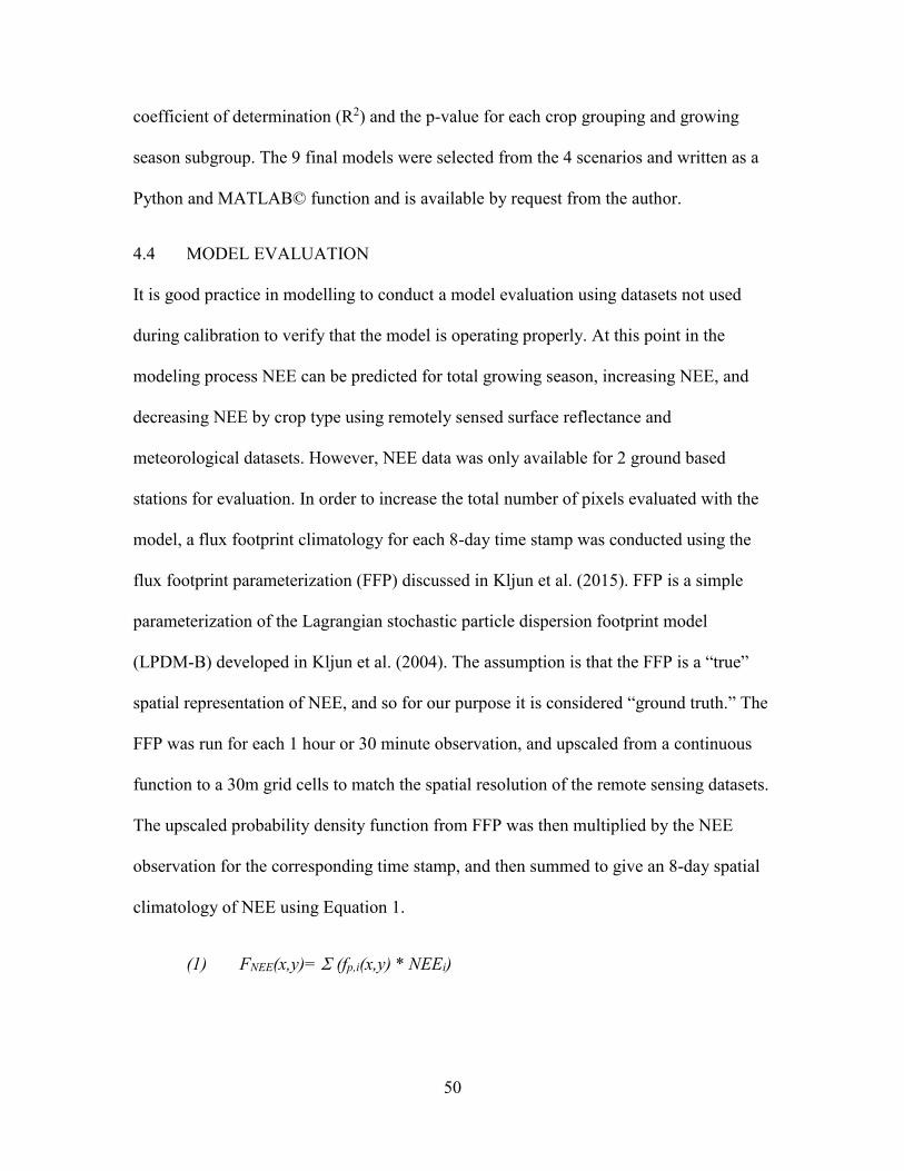
50
coefficient of determination (R2) and the p-value for each crop grouping and growing
season subgroup. The 9 final models were selected from the 4 scenarios and written as a
Python and MATLAB© function and is available by request from the author.
4.4 MODEL EVALUATION
It is good practice in modelling to conduct a model evaluation using datasets not used
during calibration to verify that the model is operating properly. At this point in the
modeling process NEE can be predicted for total growing season, increasing NEE, and
decreasing NEE by crop type using remotely sensed surface reflectance and
meteorological datasets. However, NEE data was only available for 2 ground based
stations for evaluation. In order to increase the total number of pixels evaluated with the
model, a flux footprint climatology for each 8-day time stamp was conducted using the
flux footprint parameterization (FFP) discussed in Kljun et al. (2015). FFP is a simple
parameterization of the Lagrangian stochastic particle dispersion footprint model
(LPDM-B) developed in Kljun et al. (2004). The assumption is that the FFP is a “true”
spatial representation of NEE, and so for our purpose it is considered “ground truth.” The
FFP was run for each 1 hour or 30 minute observation, and upscaled from a continuous
function to a 30m grid cells to match the spatial resolution of the remote sensing datasets.
The upscaled probability density function from FFP was then multiplied by the NEE
observation for the corresponding time stamp, and then summed to give an 8-day spatial
climatology of NEE using Equation 1.
(1) FNEE(x,y)= 6 (fp,i(x,y) * NEEi)

51
Where, FNEE(x,y) is the 8-day total of NEE from pixel x,y in space, fp,i is the probability
density function value of the flux footprint at observation number i for pixel x,y in space,
and NEEi is the NEE value for observation i. To scale the modeled NEE values estimated
from remote sensing observations, the total contribution of each pixel to the total NEE
value was calculated using Equation 2. This was done by dividing the 8-day footprint of
NEE by the 8-day total NEE observed by the tower, giving a ratio of the contribution of
each pixel for each 8-day timestamp. To scale the modeled NEE values to the flux
footprint output, the estimated NEE value for each pixel within the agricultural field was
multiplied by the 8-day percent contribution of the pixel to obtain a total NEE using
Equation 3.
(2) FCont.(x,y) = FNEE(x,y) / NEEtotal
(3) NEEscaled(x,y) = FCont(x,y) * NEERS(x,y)
Where, FCont(x,y) is the 8-day percent contribution of a pixel to the total NEE observed at
the station over 8 days, and NEEtotal is the total 8-day NEE observed at the station. In
equation 3, NEEscaled(x,y) is the total NEE for an 8-day period scaled to the 8-day percent
contribution of a pixel to total NEE observed at the flux tower, and NEERS(x,y) is the
modeled NEE value for an 8-day period at pixel x,y using satellite observed surface
reflectance and PRISM climate variables.
The NEEscaled(x,y) were compared to FNEE(x,y) values on a scatter plot using a one
to one line to determine the overall fit of the estimated NEE values to the “true” NEE
values.
52
4.5 RESULTS
4.5.1 SIGNIFICANT REFLECTANCE BANDS
Overall model calibration results are show in Table 4.3. The surface reflectance bands
that explained the most amount of variance of ground-based NEE values were determined
for each period of the growing season for each crop type. The bands that had a R2 value
greater than or equal to 0.10 are listed in Table 4.3 and the regression model type that
was most significant was selected. Table 4.3 lists all the surface reflectance bands that
met this threshold for period of the growing season and crop type.
For the total growing season, the NIR band was most important for maize, where
the RED band was most important for soybean. The relationships between NEE and the
surface reflectance when soybean and maize were combined were weaker, with lower R2
values. However, the regression model type did not vary between crop type, and were
consistent between maize and soybean, and maize/soybean. When the relationship
between NEE and the surface reflectance was determined based on total period of the
growing season, the fit was significantly better for each individual crop, but not for the
combined soybean/maize fit.
During the increasing NEE portion of the growing season, the significant bands
for maize had a linear relationship with NEE, while soybean had a quadratic relationship.
Also, the most important bands for soybeans were the RED and NIR bands, while only
NIR was the most significant band for maize. Soybean also required the use of BLUE,
GREEN, and SWIR2 bands to explain the full variance in NEE during this time, while
maize required the SWIR1 and SWIR2. The combined soybean/maize comparison used a
53
combination of the bands that were significant for each crop, but with a lower explained
variance, as seen in R2 values in Table 4.3.
The decreasing NEE portion of the growing season had lower R2 values on
average. In all cases the NIR band was the only significant surface reflectance band, with
the exception of decreasing NEE for combined maize/soybean where GREEN also
explained at least 10% of variance. The individual maize relationships used a quadratic
model for NIR, but a linear relationship explained 34% of the variance in NEE for
soybean compared to NIR. However, for the combined maize/soybean comparison, a
linear model for NIR was used and the maximum explained variance of NEE was 16%.
This is significantly lower than relationships between soybean or maize.
4.5.2 MODEL SELECTION
Table 4.4 is a summary of the best empirical model of the 4 models developed for each
crop type and period of growing season that best explained the variance in ground
observed NEE. The period of the growing season represents the values that fell between
the carbon flux phenology metrics discussed in Figure 4.2.
Model fit was typically quadratic because the relationship between several of the
surface reflectance bands and NEE was quadratic (Figure 4.3), and the relationship
between NEE and air temperature is quadratic (Bonan, 2008).Table 4.4 shows that there
is better model fit when modeling by crop type rather than combining maize and soybean
as one model. This is especially true when modeling for the total growing season, where
the R2 values for soybean was 0.674, for maize was 0.630, and combined maize/soybean
was 0.478. All p-value were near 0.0.
54
When modeling by sub period of growing season, there was better fit than
modeling for total season. When modeling maize for the total growing season there were
18 variables required and an R2 value of 0.630; the NIR, Red, SWIR1, SWIR2, and all
climate variables were needed. However, when NEE was estimated for maize increasing
NEE only 11 variables were required and there was an R2 value 0.643, and for decreasing
NEE required 9 variables and had an R2 value of 0.691. When modeling by portion of the
growing season only, the NIR, Red, and all climate variables were needed to model more
than 60% of the variance in NEE.
A stepwise regression model determined the best combination of variables to
empirically model NEE for each crop and period of the growing season using VPDmax,
VPDmin, TMAX, TMIN, and the most significant surface reflectance bands. In many
cases, not all the variables that were individually significant in explaining the variance in
NEE were significant as a variable in the multiple regression model, and therefore were
removed. Figure 4.5 is a summary that shows which surface reflectance bands that were
used as inputs into the stepwise regression analysis and retained in the multiple
regression model, and which variables were removed. The solid colors indicate that the
variable was retained and significant to model performance. Shaded checkered variables
were input into the stepwise regression model, but the variable was deemed insignificant
to the multiple regression model and was removed. As seen in Figure 4.5, the NIR and
TMAX variables were deemed significant to the empirical model for all crops. During the
total growing season or increasing NEE, combinations of Red, Blue, Green, SWIR1, and
SWIR2 were required as inputs. The only instance a significant surface reflectance was
removed from the empirical model was for maize increasing NEE model, where SWIR2
55
was removed from the model. TMIN was removed only one time from the multiple
regression model, this was for the decreasing NEE model for soybean. VPD was found to
be insignificant to the multiple regression model for maize for increasing NEE, but was
significant during decreasing NEE. However, for soybean both VPDmax and VPDmin
were significant for increasing NEE, but VPDmin was insignificant for decreasing NEE.
4.5.3 MODEL PERFORMANCE AND EVALUATION
The estimated NEE for increasing NEE and decreasing NEE were compared to ground-
based NEE on a 1:1 line on a scatter plot, see Figure 4.6. When the footprint scaled
estimated NEE was compared to the footprint scaled ground observed NEE, increasing
and decreasing NEE when modeled by maize or soybean followed the 1:1 line. However,
when the combined soybean maize observations were compared along a 1:1 line the
estimated NEE was underestimated compared to ground-based NEE. The evaluation
results confirm the hypothesis that NEE can be estimated with more certainty when
modeling by crop type.
When estimating NEE, the crop type based model can capture the carbon uptake,
peak carbon uptake and senescence with more certainty than the combined maize and
soybean model. In Figure 4.7, the maize (Figure 4.7a,b) and soybean models(Figure
4.7c,d) are able to capture the timing of increasing/decreasing carbon uptake and peak
carbon uptake better than when compared to the ground-observed data. However, in
Figure 4.7e,f the soybean years overestimate carbon uptake and in the maize years the
carbon uptake is underestimated. There is also a lag in the uptake of maize when
modeling NEE from maize fields using the maize/soybean model.
56
4.6 DISCUSSION
It was determined that there were variations in the precision of fit and the most
explanatory satellite surface reflectance bands that best explained the variance of ground-
observed NEE. The variations depended on crop type, and period of growing season.
Previous modeling efforts have primarily relied heavily on the use of vegetation indices
such as normalized difference vegetation index (NDVI), and the enhanced vegetation
index (EVI), which use the red, NIR, and blue bands to explain variables such as gross
primary production (GPP), net primary production (NPP), NEE, crop yield, leaf area
index (LAI), and evapotranspiration (ET) (e.g., Dong et al., 2015; Kalfas et al., 2011;
Nagler et al., 2005; Sims et al., 2014; Wylie et al., 2007). Our results indicate that while
NIR is always important, red and blue varies with crop type and time of year.
The reflectance bands found in the vegetation indices used for estimating
vegetation dynamics were the same reflectance bands that best explained NEE. NDVI
and EVI make use of the NIR, and were considered significant for all crops and periods
of growing season. However, the degree of variance of NEE explained by NIR, as well
as the other surface reflectance bands that were significant varied by crop type. Viña et
al. (2011) found that soybean and maize reflect light differently. For instance, soybean
has an increasing reflectance with longer wavelengths, while maize has a decreasing
reflectance with longer wavelengths. This is due to differences in the chlorophyll
content, structural leaf orientation, and water content of the plant of each crop. Soybeans
have a higher reflectance in longer wavelengths due to higher chlorophyll content in the
adaxial side of their leaves compared to maize. While higher biomass, which results in
higher amounts of water results in more absorption of longer wavelengths in maize.

57
These physiological differences could cause equal carbon uptake at a set point in time
with very different observed surface reflectance. Thus, the most significant reflectance
bands for explaining NEE for soybean tended be in the visible range where the
reflectance will not saturate the remote sensing pixel, and maize tended to have a better
fit with longer wavelengths.
The NIR band was always a significant band for explaining the variance in NEE
for maize, soybean, combined soybean/maize, and for each portion of the growing
season. This was especially true in post-peak of season for maize and soybean because
the crop is not increasing in biomass, but the chlorophyll content of the leaves will
decrease during senescence. NIR is sensitive to changes in the chlorophyll content
(Jensen, 2005). The surface reflectance bands most significant to explaining the variance
in NEE for increasing NEE for maize were NIR and Red, followed by SWIR1 and
SWIR2 which are most sensitive to water content. This would indicate that water
availability is most important for explaining ground-based NEE. Soybean had a better fit
with the NIR, red, blue and green bands for increasing NEE rather than SWIR1 and
SWIR2. The finding that NIR was the most important surface reflectance for explaining
variance in NEE is in line with findings from Gitelson et al. (2012) that vegetation
indices using the NIR and green bands best explained GPP. The work presented here
does not support the claim that the green band is important to explaining carbon
dynamics with remote sensing for maize, but it is important for soybean.
The use of significant surface reflectance to estimate NEE had been previously
demonstrated in the literature to be a practical method for estimating carbon exchange,
although these other models estimated NEE for much broader land covers (Fu et al.,
58
2014). However, in many cases the coarser pixels from MODIS were too coarse to
properly represent carbon exchanges for a single crop type (Chen et al., 2007). Wu et al.
(2017) found it challenging to model carbon dynamics at coarser scales using vegetation
indices due to varying climatic conditions and heterogeneous land covers within a pixel.
Our results show that downscaled MODIS and Landsat surface reflectance is a good
proxy for estimating carbon exchanges. The use of finer scale surface reflectance
observations allowed the surface to have fewer heterogeneous pixels in monoculture
agricultural fields to capture the true conditions of the crop in the field. This resulted in
better modeling of NEE in soybean and maize fields compared to modeling the two crops
together. Most of the final models used a quadratic regression fit, which is different than
other models that generally use a linear fit (e.g., Fu et al., 2014; Kalfas et al., 2011).
However, the quadratic nature of this model matches what is typically observed in the
field, i.e., air temperature vs. NEE (Bonan, 2008). The same is true for several surface
reflectance bands when compared to NEE, as shown in Figure 4.3.
The use of air temperature and VPD as an explanatory variable was highly
important because it provided information on the spatially varying variable that play a
large role on the photosynthetic capacity of the crop at a single point in time. The
available remotely sensed surface reflectance is not sensitive to changes in air
temperature, and data has been atmospherically corrected to remove the influence of
water vapor and clouds. Thus, it was imperative to account for spatial variations in
meteorological conditions using air temperature and VPD from the PRISM dataset. The
use of temperature and humidity estimates allows the empirical model to estimate the
meteorological impacts on NEE in addition to vegetative stress, biomass, and health that
59
are provided by the surface reflectance data. All of these play a major role in NEE
dynamics (Ciais et al., 2005; Goldstein et al., 2000; Le Quéré et al., 2015; Reichstein et
al., 2002). For this reason, TMAX was always a significant model variable, with a p-
value of 0.00.
There was a significantly better fit when modeling NEE by portion of the growing
season, see Table 4.4. As established in previous work, vegetation indices can be used to
obtain the carbon flux phenology (CFP) metrics (Balzarolo et al., 2016; Garrity et al.,
2011; Wu et al., 2012), but can be obtained with better certainty using the vegetation
index specified for maize and soybean using the methodology discussed in Chapter 3.
Using the CFP metrics obtained from the vegetation phenology, the surface reflectance
can be categorized as increasing NEE or decreasing NEE. This allows the model to
consider changes in biomass in the vegetative period of the growing season. Wu et al.
(2017) determined that it was difficult to detect smaller changes in the vegetative canopy
during the beginning growing season, but modeling by season and finer spatial
resolutions allows better identification of subtle changes in vegetative greenness and
modeling of phenological patterns of carbon dynamics.
NEE was more precisely estimated by crop type, see Table 4.4 and Figure 4.6.
The error was smaller and the fit of the empirical model was higher when modeling by
crop type compared to a combined soybean and maize model. Previous models have
typically modeled all agriculture as one subgroup, but were unable to capture the peak in
carbon uptake (Fu et al., 2014). This occurs for several reasons: (1) some crops have a
higher LAI, which results in higher carbon uptake (Suyker et al., 2004), (2) the leaves
reflect light differently (Viña et al., 2011), (3) crops have varying photosynthetic
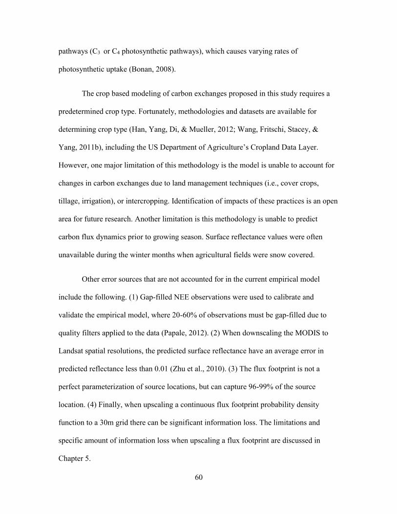
60
pathways (C3 or C4 photosynthetic pathways), which causes varying rates of
photosynthetic uptake (Bonan, 2008).
The crop based modeling of carbon exchanges proposed in this study requires a
predetermined crop type. Fortunately, methodologies and datasets are available for
determining crop type (Han, Yang, Di, & Mueller, 2012; Wang, Fritschi, Stacey, &
Yang, 2011b), including the US Department of Agriculture’s Cropland Data Layer.
However, one major limitation of this methodology is the model is unable to account for
changes in carbon exchanges due to land management techniques (i.e., cover crops,
tillage, irrigation), or intercropping. Identification of impacts of these practices is an open
area for future research. Another limitation is this methodology is unable to predict
carbon flux dynamics prior to growing season. Surface reflectance values were often
unavailable during the winter months when agricultural fields were snow covered.
Other error sources that are not accounted for in the current empirical model
include the following. (1) Gap-filled NEE observations were used to calibrate and
validate the empirical model, where 20-60% of observations must be gap-filled due to
quality filters applied to the data (Papale, 2012). (2) When downscaling the MODIS to
Landsat spatial resolutions, the predicted surface reflectance have an average error in
predicted reflectance less than 0.01 (Zhu et al., 2010). (3) The flux footprint is not a
perfect parameterization of source locations, but can capture 96-99% of the source
location. (4) Finally, when upscaling a continuous flux footprint probability density
function to a 30m grid there can be significant information loss. The limitations and
specific amount of information loss when upscaling a flux footprint are discussed in
Chapter 5.

61
4.7 CONCLUSIONS
When modeling NEE from downscaled MODIS and Landsat surface reflectance, there is
a more precise fit when the model considers crop type, period of growing season, and
meteorological conditions in the modeling methodology. Here we show the following:
• Modeling NEE using surface reflectance gives good results
• NEE is estimated with greater certainty by crop type
• Modeling by period of growing season allows the model to vary throughout the
year, by selecting optimal spectral bands that are most important to crop structure
during that period of the year.
• Use of climate observations in the empirical modeling approach accounts for
variations in NEE due to temperature and atmospheric humidity.
Future work will test other statistical fitting techniques to be ensure that the
quadratic and linear regression techniques is the best approach. Other statistical
techniques that may be considered are partial least squares regression, and fit may be
tested by statistical tests such as Akaike information criterion (AIC) metric.
The empirical model developed here will be used to evaluate the spatial variations
in carbon dynamics from maize and soybean fields. Additional ground based flux tower
datasets will be needed to evaluate the application of the empirical model outside of the
US Corn Belt, where the model was calibrated and evaluated.
Additionally, a regional map of total carbon exchanges for the US corn belt will
be created. This will give regional estimates of carbon uptake from maize and soybean
during growing seasons at a regional scale at spatial resolutions finer than ever before.

62
The total growing season NEE from maize and soybean may show the differences in
management, irrigation, and local droughts that occur at regional scales. This will also
provide better understanding of the implications of the increasing production of soybean
and maize on atmospheric carbon in the United States. Model outputs will also be
compared to existing NEE model outputs, such as Xiao et al. (2004, 2008), to identify if
this modeling approach significantly improves total NEE values compared to work that
has already been done.
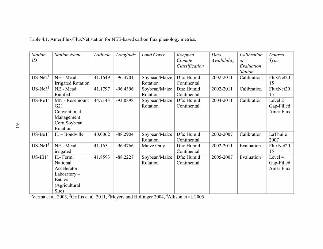
63
Table 4.1. AmeriFlux/FluxNet station for NEE-based carbon flux phenology metrics.
Station ID
Station Name Latitude Longitude Land Cover Koeppen Climate Classification
Data Availability
Calibration or Evaluation Station
Dataset Type
US-Ne21 NE - Mead Irrigated Rotation
41.1649 -96.4701 Soybean/Maize Rotation
Dfa: Humid Continental
2002-2011 Calibration FluxNet2015
US-Ne31 NE - Mead Rainfed
41.1797 -96.4396 Soybean/Maize Rotation
Dfa: Humid Continental
2002-2011 Calibration FluxNet2015
US-Ro12 MN - Rosemount G21 Conventional Management Corn Soybean Rotation
44.7143 -93.0898 Soybean/Maize Rotation
Dfa: Humid Continental
2004-2011 Calibration Level 2 Gap-Filled AmeriFlux
US-Bo13 IL – Bondville 40.0062 -88.2904 Soybean/Maize Rotation
Dfa: Humid Continental
2002-2007 Calibration LaThuile 2007
US-Ne11 NE - Mead irrigated
41.165 -96.4766 Maize Only Dfa: Humid Continental
2002-2011 Evaluation FluxNet2015
US-IB14 IL- Fermi National Accelerator Laboratory – Batavia (Agricultural Site)
41.8593 -88.2227 Soybean/Maize Rotation
Dfa: Humid Continental
2005-2007 Evaluation Level 4 Gap-Filled AmeriFlux
1 Verma et al. 2005, 2Griffis et al. 2011, 3Meyers and Hollinger 2004, 4Allison et al. 2005
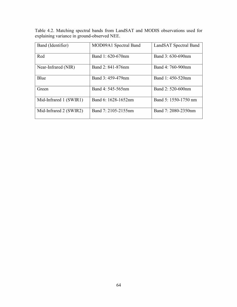
64
Table 4.2. Matching spectral bands from LandSAT and MODIS observations used for explaining variance in ground-observed NEE.
Band (Identifier) MOD09A1 Spectral Band LandSAT Spectral Band
Red Band 1: 620-670nm Band 3: 630-690nm
Near-Infrared (NIR) Band 2: 841-876nm Band 4: 760-900nm
Blue Band 3: 459-479nm Band 1: 450-520nm
Green Band 4: 545-565nm Band 2: 520-600nm
Mid-Infrared 1 (SWIR1) Band 6: 1628-1652nm Band 5: 1550-1750 nm
Mid-Infrared 2 (SWIR2) Band 7: 2105-2155nm Band 7: 2080-2350nm
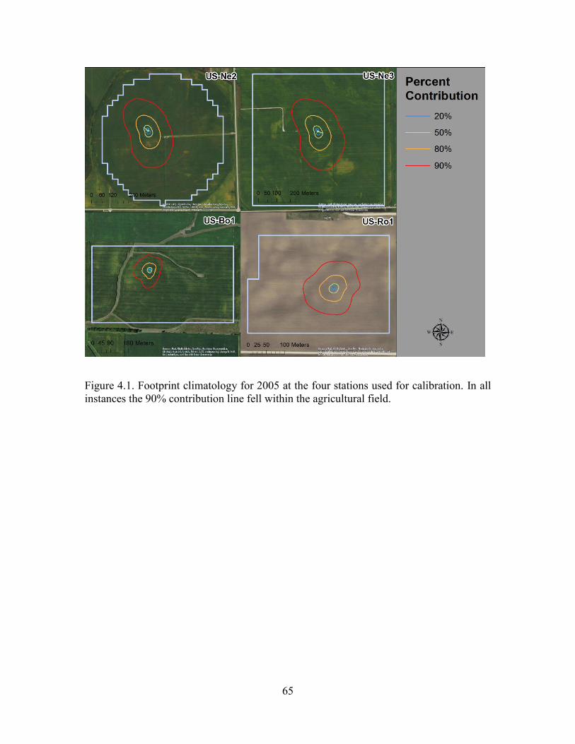
65
Figure 4.1. Footprint climatology for 2005 at the four stations used for calibration. In all instances the 90% contribution line fell within the agricultural field.
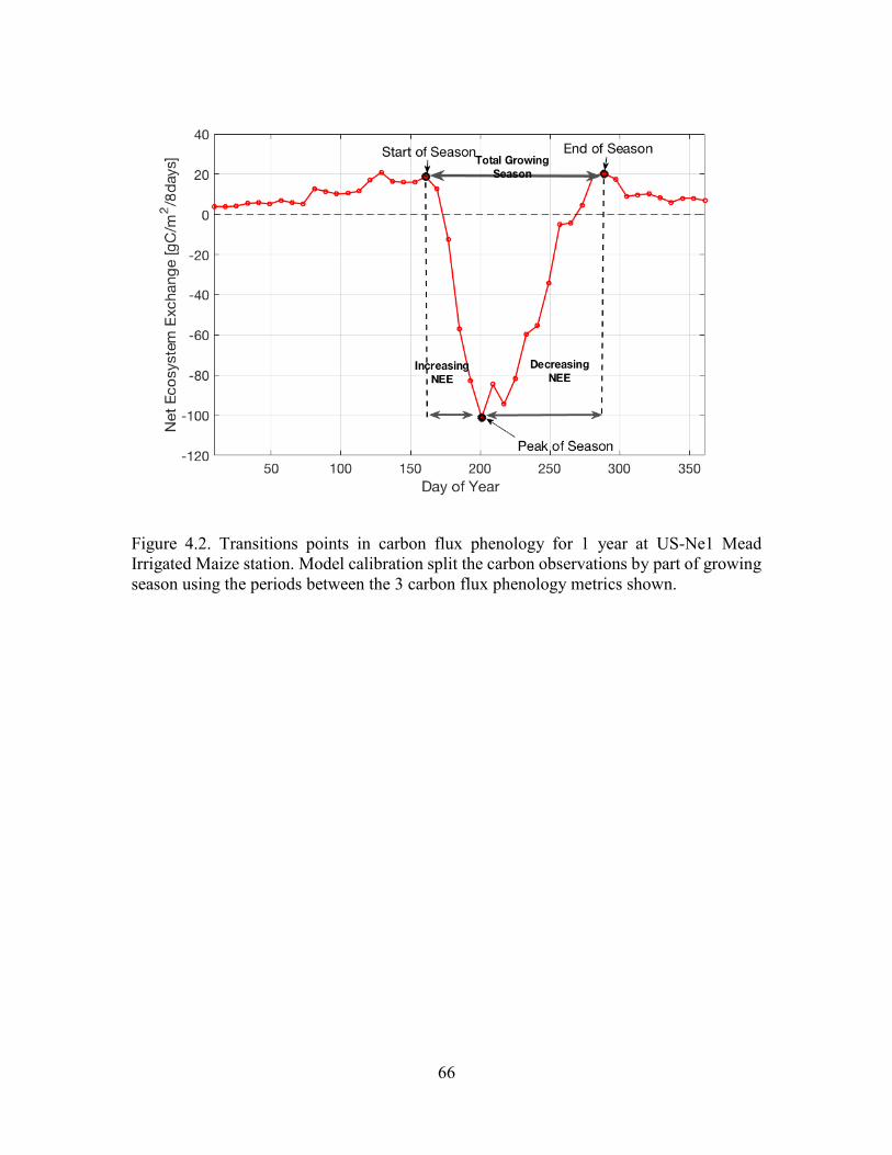
66
Figure 4.2. Transitions points in carbon flux phenology for 1 year at US-Ne1 Mead Irrigated Maize station. Model calibration split the carbon observations by part of growing season using the periods between the 3 carbon flux phenology metrics shown.
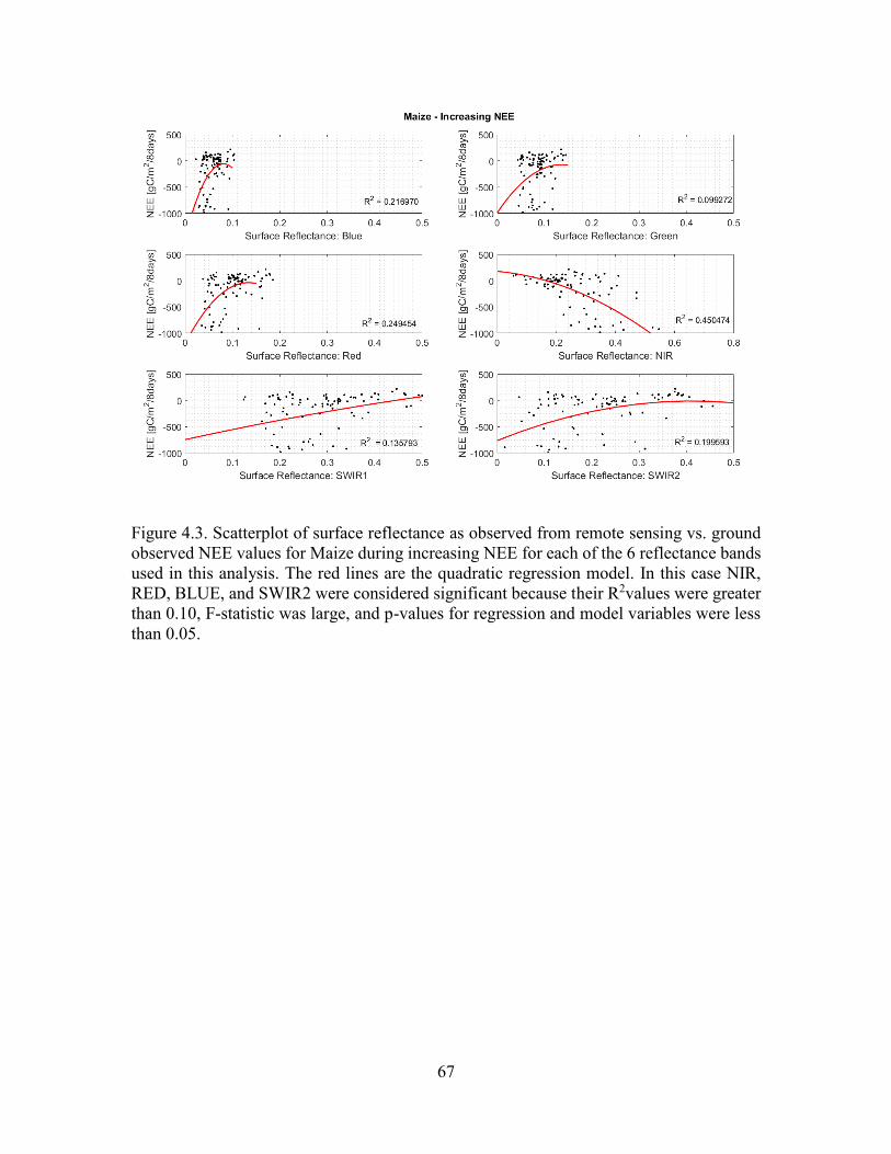
67
Figure 4.3. Scatterplot of surface reflectance as observed from remote sensing vs. ground observed NEE values for Maize during increasing NEE for each of the 6 reflectance bands used in this analysis. The red lines are the quadratic regression model. In this case NIR, RED, BLUE, and SWIR2 were considered significant because their R2values were greater than 0.10, F-statistic was large, and p-values for regression and model variables were less than 0.05.
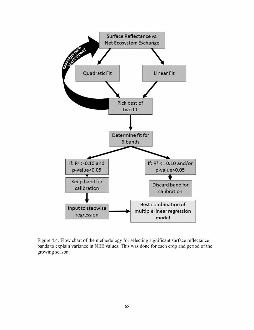
68
Figure 4.4. Flow chart of the methodology for selecting significant surface reflectance bands to explain variance in NEE values. This was done for each crop and period of the growing season.
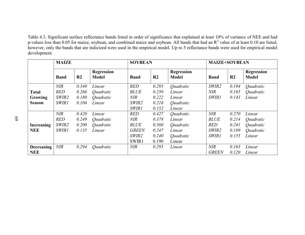
69
Table 4.3. Significant surface reflectance bands listed in order of significance that explained at least 10% of variance of NEE and had p-values less than 0.05 for maize, soybean, and combined maize and soybean. All bands that had an R2 value of at least 0.10 are listed, however, only the bands that are italicized were used in the empirical model. Up to 5 reflectance bands were used for empirical model development.
MAIZE SOYBEAN MAIZE+SOYBEAN
Band R2 Regression Model Band R2
Regression Model Band R2
Regression Model
Total Growing Season
NIR 0.340 Linear RED 0.295 Quadratic SWIR2 0.194 Quadratic RED 0.266 Quadratic BLUE 0.250 Linear NIR 0.165 Quadratic SWIR2 0.180 Quadratic NIR 0.222 Linear SWIR1 0.143 Linear SWIR1 0.106 Linear SWIR2 0.216 Quadratic
SWIR1 0.152 Linear
Increasing NEE
NIR 0.420 Linear RED 0.427 Quadratic NIR 0.270 Linear RED 0.249 Quadratic NIR 0.378 Linear BLUE 0.214 Quadratic SWIR2 0.200 Quadratic BLUE 0.360 Quadratic RED 0.241 Quadratic SWIR1 0.135 Linear GREEN 0.247 Linear SWIR2 0.189 Quadratic
SWIR2 0.240 Quadratic SWIR1 0.155 Linear SWIR1 0.190 Linear
Decreasing NEE
NIR 0.294 Quadratic NIR 0.295 Linear NIR 0.163 Linear GREEN 0.120 Linear
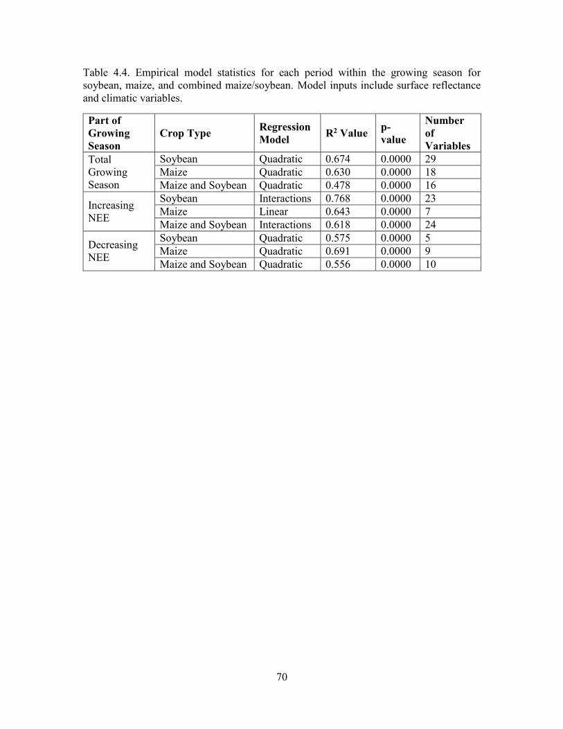
70
Table 4.4. Empirical model statistics for each period within the growing season for soybean, maize, and combined maize/soybean. Model inputs include surface reflectance and climatic variables.
Part of Growing Season
Crop Type Regression Model R2 Value p-
value
Number of Variables
Total Growing Season
Soybean Quadratic 0.674 0.0000 29 Maize Quadratic 0.630 0.0000 18 Maize and Soybean Quadratic 0.478 0.0000 16
Increasing NEE
Soybean Interactions 0.768 0.0000 23 Maize Linear 0.643 0.0000 7 Maize and Soybean Interactions 0.618 0.0000 24
Decreasing NEE
Soybean Quadratic 0.575 0.0000 5 Maize Quadratic 0.691 0.0000 9 Maize and Soybean Quadratic 0.556 0.0000 10
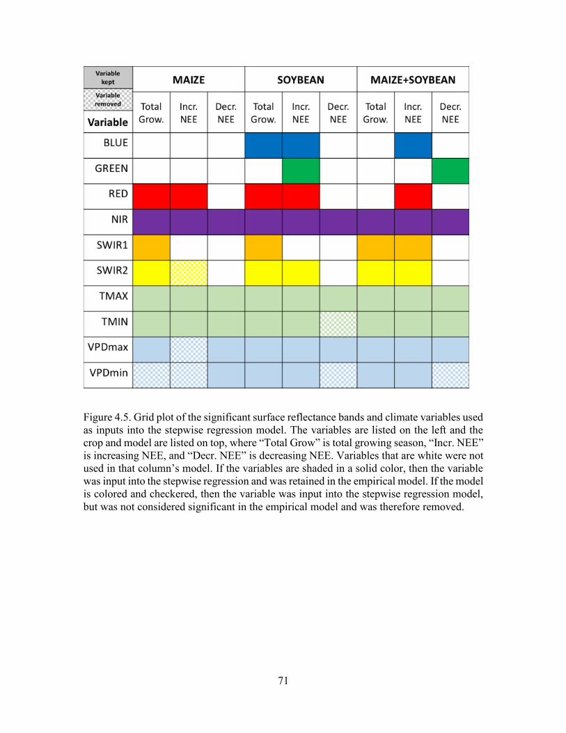
71
Figure 4.5. Grid plot of the significant surface reflectance bands and climate variables used as inputs into the stepwise regression model. The variables are listed on the left and the crop and model are listed on top, where “Total Grow” is total growing season, “Incr. NEE” is increasing NEE, and “Decr. NEE” is decreasing NEE. Variables that are white were not used in that column’s model. If the variables are shaded in a solid color, then the variable was input into the stepwise regression and was retained in the empirical model. If the model is colored and checkered, then the variable was input into the stepwise regression model, but was not considered significant in the empirical model and was therefore removed.
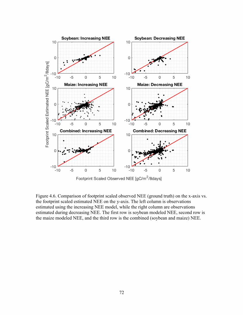
72
Figure 4.6. Comparison of footprint scaled observed NEE (ground truth) on the x-axis vs. the footprint scaled estimated NEE on the y-axis. The left column is observations estimated using the increasing NEE model, while the right column are observations estimated during decreasing NEE. The first row is soybean modeled NEE, second row is the maize modeled NEE, and the third row is the combined (soybean and maize) NEE.
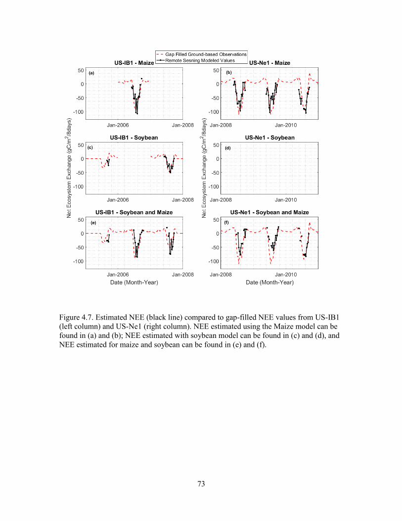
73
Figure 4.7. Estimated NEE (black line) compared to gap-filled NEE values from US-IB1 (left column) and US-Ne1 (right column). NEE estimated using the Maize model can be found in (a) and (b); NEE estimated with soybean model can be found in (c) and (d), and NEE estimated for maize and soybean can be found in (e) and (f).
74
CHAPTER 5
POINT TO GRID CONVERSION IN FLUX FOOTPRINTS:
IMPLICATIONS OF METHOD CHOICE AND SPATIAL RESOLUTION
FOR REGIONAL SCALE STUDIES1
1McCombs, A.G., A.L. Hiscox, and A. Suyker. To be submitted to Boundary Layer
Meteorology. .
75
5.1 INTRODUCTION
Flux footprint modeling is a common approach to determining source areas of
atmospheric tracers and gases. Flux footprint models are widely used in land-atmosphere
exchanges studies for both practical and theoretical investigations (Schmid, 2002).
Increasingly, flux footprints are being used to upscale ground-based flux tower
measurements (e.g., Desai et al., 2008; Schmid, 2002; Xu et al., 2017), and to calibrate
and validate satellite-based gas exchange models (e.g., Xiao et al., 2004) for regional
understanding of climate dynamics. There are five types of footprint models: Analytical,
Lagrangian, Higher-Order Closure, Large-Eddy Simulation and Hybrid models. Each
type of footprint model has varying degrees of complexity, with some being more
computationally expensive than others. Leclerc and Foken (2014) provides a good
explanation of the various models, uses, and limitations of each.
Micrometeorological measurement techniques (e.g., eddy covariance) are used to
quantify the exchange of energy and mass between ecosystems and the atmosphere and
provide the necessary inputs to compute flux footprint models. These techniques employ
multiple assumptions so that only relatively simple measurements (e.g, rapid vertical
velocity measurement at one height) are required to measure fluxes with some accuracy
(e.g., Richardson et al., 2006). One major assumption of eddy covariance is that the
instrument fetch is homogeneous, but this is often not reality (Horst & Weil, 1994).
Despite this assumption, the physical characteristics of the area contributing to the flux
measurements are regularly quantified through flux footprint modeling and provide the
basis for much of our understanding of land-air gas exchanges. The measured flux for a
given period is a spatially averaged ecosystem-atmosphere exchange across the footprint,
76
which is aligned with the mean wind direction. By nature of the surface layer turbulence,
some areas contribute more to the measured flux than others. This makes the use of the
flux footprint important, especially when land cover varies significantly with wind
direction.
In an effort to understand regional and continental ecosystem dynamics of carbon
and water cycling, there has been an increasing interest in upscaling flux measurements
by employing remote sensing datasets (Frank & Karn, 2003; Heinsch et al., 2006; Kim et
al., 2006b; Lafont et al., 2002; Metzger et al., 2013; Wohlfahrt et al., 2008; Wylie et al.,
2007b; J. Xiao et al., 2011, 2014). Unfortunately, a significant limitation of all single
point measurements is that they are not easily upscaled from finer field scale to coarser
spatial resolutions. However, remotely sensed data have been shown to possess
information related to fluxes measured at the surface (e.g., Gitelson, 2003). One
drawback is the pixel information from remotely sensed datasets are too coarse in spatial
resolution to represent flux footprint dynamics, and may represent heterogeneous
surfaces that fall outside of the fetch of the flux tower.
In modeling regional fluxes, footprints are often used for scaling model estimates
to tower estimated fluxes to increase the number of samples during the validation of gas
exchange models (B. Chen et al., 2009; Dong et al., 2015; Fu et al., 2014; Gu & Wylie,
2015, 2016; Kim et al., 2006b; Lafont et al., 2002; Wylie et al., 2007b; J. Xiao et al.,
2011). This requires flux footprint outputs to be upscaled to a raster that has a cell size
equal to remote sensing (or other gridded) datasets used in the modeling process. While
the flux footprint models themselves focus on the underlying physics of representing the
atmosphere, correct scaling of modeled fluxes is required. However, little information is
77
available on the sensitivity of footprint modeling results to varying cell sizes (Chen et al.,
2009). Kim et al. (2006) conducted an analysis on the influence of cell size within the
modeling framework, and found the sensitivity of grid size may be dependent on the
heterogeneity of the land surfaces surrounding the site. More specifically, Kim et al.
(2006) found that the spatial representation was different for forests versus grasslands,
where grasslands and croplands could have larger cell sizes than forested land covers
because grasslands and cropland surfaces have lower roughness lengths than forests. The
reasoning for this is that roughness length is a function of canopy height.
In many studies, the flux footprint function is exported to a raster or other grid
format to visually display and compare the results against gridded datasets. However, it is
often unknown if the grid cell size of a given satellite observation is appropriate for
correctly analyzing flux footprint outputs. With the proliferation of satellites being
launched by government and private industry at varying spatial and temporal resolutions,
a re-evaluation of rasterization of flux footprint methodologies is warranted. The spatial
resolution found in publically available, longer-term moderate resolution satellite
imagery, such as GOES or MODIS, are too coarse to represent turbulent motions in the
boundary layer, which occur on the sub-meter scale. While there are remote sensing
datasets, such as GeoEye, that area collected a fine spatial resolution, these datasets do
not cover climate time scales and are often not publically available. Some analyses have
scaled fluxes in the boundary layer to match that of the land cover grid cell, but this
assumes the surface roughness is homogeneous across the pixel, which is often not the
case (Mihailovic et al., 2005). Despite these limitations, properly gridded flux footprint
models will aid in the data fusion process between satellite datasets and point based flux
78
measurements. This is especially true in places or land covers where ground-based data is
limited. Recent work developed by Xu et al. (2017) made use of methods developed by
Metzger et al. (2013) to create gridded predictions from a temporally varying flux
footprint, and showed promise in providing carbon dioxide fluxes at a regional scale from
tower based measurements. These methods consider heterogeneous land covers that are
typically found, but do not address the sensitivity to cell size.
A large body of literature in GIScience has shown continuous spatial functions
can be difficult to model in a grid format (DeMers, 2002). Incorrect gridding leads to loss
of information and differences in spatial resolution as cell sizes become coarser (Kim et
al., 2006b). Reithmaier et al. (2006) found that the spatial resolution of a grid could cause
significant uncertainty in the specified tower location. A comprehensive sensitivity
analysis is needed for determining spatial scales that are most appropriate for depicting
flux tower information at spatial scales found in land models and remote sensing datasets
(Kim et al., 2006b).
Our goal in this study are to determine the sensitivity of commonly used 1D and
2D flux footprint outputs to the desired spatial resolution. We projected both 1D and 2D
flux footprint functions at spatial resolutions found in commonly available satellite
remote sensing products, which range from 10m (SPOT) to 1km (MODIS). Five vector-
to-raster conversion methods were tested and the results give guidance on how to upscale
flux footprints to represent larger spatial scales. Additionally, the pros and cons of each
of the five methods will be discussed. The sensitivity of changing surface roughness due
to canopy height or spatial heterogeneity were not addressed in this analysis. It is the
assumption in this analysis that each pixel is homogeneous in land cover because the flux
79
footprint models selected assume a homogeneous land cover. While this is not what
occurs in reality, heterogeneity of the land cover will be addressed in future research.
5.2 EDDY COVARIANCE DATA INPUTS
Data from the AmeriFlux network were used as test data in this analysis. AmeriFlux is a
surface network that monitors carbon flux dynamics using the eddy covariance method.
The variables of interest in this analysis are the horizontal wind speed [m/s], vertical
wind speed [m/s], air temperature [degrees Celsius], atmospheric pressure [kPa], sensible
heat flux [W/m2] and wind direction [degrees]. For this analysis, two stations from the
AmeriFlux Network were used: ARM Southern Great Plains main site (US-ARM), and
Mead Irrigated station (US-Ne1). These stations were selected for their relatively flat
topography and homogeneous land cover, thus eliminating potential effects of changing
surface roughness as much as possible. Metadata regarding these stations can be found in
Table 5.1. Data were downloaded from the AmeriFlux website for the entire year of 2004
and 2005 because data was available for both stations. The primary focus is on flux
footprint climatologies for uses in climate sciences rather than short term fluxes.
5.3 MATERIALS AND METHODS
5.3.1 MODELING APPROACHES
The 1D analytical footprint model developed by Hsieh et al. (2000) (H2000), and the 2D
Langrangian stochastic particle dispersion model (LPDM) developed by Kljun et al.
(2015) (K2015) were used in this analysis. While there are a number of more robust
footprint models available (Leclerc & Foken, 2014), the focus of this analysis was to
address the spatial sensitivity of scaling footprint estimates to a landscape, and as a result
these models are overly complex for use in this analysis.
80
The 1D flux footprint model by H2000 is developed using parameters from
Calder's (1952) analytical solution and is fitted to solutions from numerical Lagrangian
stochastic (LS) simulations (Schmid, 2002). The H2000 footprint model compares well
with other widely accepted analytical solutions such as Horst and Weil (1994, 1992) and
Schmid (2002). Due to this model’s simplicity, it is more suitable for long term averaging
of flux footprints because uncertainty in the model are reduced as averaging time
increases (Baldocchi, 2003), thus it is appropriate for climatological applications where it
is desirable to look at inter-annual variability.
The 2D flux footprint model developed by K2015 is a LPDM that parameterizes
turbulence based on the stability of the atmosphere. The parameterization of turbulence is
a major drawback of the simplified footprint models (Horst & Weil, 1992, 1994; Hsieh et
al., 2000; Kljun et al., 2004). K2015 addresses this limitation by providing more detailed
stability parameterizations. The parameterization, called flux footprint parameterization
(FFP), improved upon the Kljun et al. (2004) LPDM footprint model by altering the
scaling of the along wind and crosswind footprint components. Surface roughness has
been implemented into the scaling approach to address the limitation of the cross wind
component to near surface eddy covariance measurements (Kljun et al., 2015; Schmid,
2002). For a comprehensive description of the FFP model, see K2015. This model was
selected because a validated function is available for download in Python, R, and Matlab
(http://footprint.kljun.net/), meaning it is widely accessible to researchers.
Parameters needed to run either flux footprint model included measurement
height, Obukhov length, standard deviation of lateral velocity fluctuations, friction
velocity, planetary boundary layer height, roughness length, mean wind velocity, and
81
mean wind direction. Lateral velocity fluctuations (V) and Obukhov length (L) are not
directly reported by the AmeriFlux network and had to be calculated prior to running
either flux footprint model.
The V and L were calculated prior to running the model using Equations 1 to 2
(Kljun et al., 2015; Leclerc & Foken, 2014).
(1) L = -u*3 �̅� / k g H, where �̅� = T (Po / P) R/c_p
(2) V = (3.0 u*2) (1/2)
Where �̅� is the mean potential temperature, T is air temperature in degrees Kelvin, k is
the von Karvon constant, H is the sensible heat flux in Wm-2, d is the zero-plane
displacement height in meters, hc is the canopy height in meters, g is gravity, zreceptor is the
measurement height above the surface in meters, Po is the average sea level pressure of
1000mb, P is the atmospheric pressure at the station in millibars, R is the gas constant for
dry air, and cp is the specific heat of dry air. These were computed for each 1 hour
observation used to compute the flux footprint climatology. There was 2 annual flux
footprint climatologies using H2000, and 6 8-day flux footprint climatologies using the
K2015.
When computing the boundary layer height to compute the flux footprint model,
the question arose on whether the boundary layer height affected the output of the flux
footprint for short flux towers. This was tested for flux towers with measurement heights
that were less than or equal to 6.2m. It was determined that the variation in the boundary
layer height will not affect short tower flux footprint computations compared to tall tower
flux footprints because scalars will not be carried hundreds to thousands of kilometers
82
(Leclerc & Foken, 2014). Thus, a standard 1000m boundary layer height (h) was selected
for this analysis. To test the effects of this assumption on results a constant h value of
1000m for 4 time stamps where atmosphere was stable and 3 time stamps where
atmospheric stability was unstable. The FFP model by K2015 was used to compute the
flux footprint. The h value was computed using the equations in Appendix A of K2015
for each flux footprint. It was determined that during unstable conditions the change
spatial location in the 10-90% contribution lines were near 0m between a constant h value
of 1000m and the computed h value (Figure 5.1a). However, during stable conditions
there was change in the location of the flux footprint contribution lines that ranged from 0
to 150m (Figure 5.1b). Therefore, it is important to compute h during stable conditions,
but a constant h value of 1000m is appropriate during unstable conditions when the
measurement height is less than or equal to 6.2m.
The H2000 1D flux footprint model was used to calculate an annual climatology
for 2004 using 1 hour mean observations. Meanwhile, an 8-day flux footprint climatology
was calculated for three time stamps during 2005 at the 2 stations. This resulted in 2
annual 1D flux footprint climatologies, and 6 8-day 2D flux footprint climatologies. The
mean wind direction was used to determine the vector direction of each model outputs. If
the wind direction was not available or the footprint function could not be computed, then
the observations were not included in the annual 1D or 8-day 2D flux footprint
climatology. Reasons for missing wind direction datasets include sensor malfunction,
frozen precipitation or an object (e.g., bird) blocking the transducer signal on the 3D
sonic anemometer. The flux footprint probability density function (PDF) was computed
for each 60-minute period and then projected onto a grid via one of the five methods
83
described below and summed to an annual or 8-day flux footprint by grid cell. The
variation of canopy height is important when analyzing footprints, but the sensitivity of a
footprint from varying canopy height was not tested in this analysis because the goal was
to access the sensitivity of upscaling flux footprints to a grid.
5.3.2 RASTER GENERATION
Flux footprint curves were projected on a gridded file format using five different
methods: 1D point sampling, 1D equal interval integration, 1D aggregate assignment, 2D
area integration, and 2D sum integration. These five methods are discussed in more detail
below. Each 1D flux footprint climatology was output to a grid of varying cell sizes
ranging from 10m to 1000m in 10m increments. Because of its increased computational
needs, the 2D flux footprint climatology was output to cell sizes of 10, 30, 250, 500, and
1000m to match the range of grid cell sizes commonly found in multi-or hyper-spectral
satellite remote sensing (i.e., MODIS, Landsat, AVHRR, SPOT).
The three different methods of sampling the continuous 1D flux footprint function
explored were a) point sampling at equal intervals along the PDF, b) integration under the
PDF over equal intervals along the curve, and c) assigning an aggregate value to each
grid cell. The three methods are explained visually in Figure 5.2. In the 1D point
sampling method (Figure 5.2a,b) each PDF curve was sampled at a set interval that was
equal to the raster cell size (10 to 1000 m), and the sampled value was assumed to
represent the entire grid cell. It is understood that spatial imprecision will occur with
increasing cell size when sampling in this manor because the larger the grid cell, the
higher probability of in-cell heterogeneity (DeMers, 2002). The value was found for the
center of the grid cell (Figure 5.2b). To conduct 1D integration over equal intervals
84
(Figure 5.2c,d), each PDF curve was sampled at the start and end point of each grid cell
through which the 1D flux footprint line crossed and then integrated under the curve
between the two points using the trapezoidal rule (Burden & Faires, 1997; Chapra, 2008;
Quarteroni, Sacco, & Saleri, 2000). The sum between the two points (i.e., relative area
under the curve) was assigned to the appropriate grid cell (Figure 5.2d). To assign an
aggregate value to each grid cell (Figure 5.2e,f), the PDF curve was sampled every 4
meters regardless of cell size, and then each point was assigned to the grid cell where the
point was closest to the center of the grid cell as is standard practice converting point to a
raster in raster modeling (DeMers, 2002). The final value for the grid cell is the sum of
all points that fall within it. A value of 4 meters was selected to be in line with the fetch
to height ratio provided in H2000; the interval was computed using equation 3, where µ
varies with stability and zm is the measurement height.
(3) Interval = (µ*zm)/1000, where µstable = 2000, µneutral= 500, µunstable=100
A sensitivity analysis was performed for each method, to identify under which conditions
the least amount of information is lost due to differences in spatial resolution when
projecting a 1D flux footprint function to 2D surface realm. Results are presented in
section 5.4.
To access the cell size sensitivity of the 2D flux footprint function, two methods
were accessed for aggregating the 2D flux footprint function as output by the FFP
function developed in K2015. In both methods the output of the FFP was an array of x, y
and f (footprint function probability) points that sampled the 2D footprint at a frequency
that was dependent on zm, h, mean wind speed, friction velocity, and Obukhov length (L).
85
The sampling interval is calculated using equations 5, 21, and 22 in K2015. The K2015
model has a varying sampling interval from observation to observation, and changes with
atmospheric stability, the upscaling method from the x, y, f array to a grid needed to be
adaptable. This occurs because there is a fixed number of points in the flux footprint
output array. During stable conditions the fetch is further away from the site than during
unstable conditions causing the sampling interval to vary. The 2D flux footprint was
upscaled by integrating using the Trapezoidal rule for each of the points in the x, y and f
(footprint value) arrays using equation 4, where f(x,y) is the footprint function value at
location x and y in m-2. The Trapezoidal rule assumes a linear increase or decrease from
point a to point b, and finds the area of the footprint in the 2D realm using equation 5
(Chapra, 2008) .
(4) ftotal (x,y) = ∫∫f(x,y) dx dy
(5) Iarea = ((c-d)/2) (I(yc) + I(yd)), where I(y) = ((b-a)/2) ( f(xa) + f(xb))
Where I(y) is the area under the curve at a constant y value in the x direction from point a
to point b, f(x) is the footprint function value at x,y, Iarea is the 2D area under the curve
where the integration occurs in the y direction using the integrated values in the x
direction as inputs. The latitude and longitude of the gridded center represented Iarea value
was determined and then aggregated to the grid cell array, where the footprint area is
rasterized by assigning the value to the grid cell that the Iarea center point has the shortest
distance to the center of the grid cell (DeMers, 2002), see Figure 5.3.
In method 1, referred to here as 2D sum integration, we tested for information loss
by assuming each 2D flux footprint was equal to 1, therefore the total of the upscaled
raster should equal the number of observations.
86
For method 2, referred here as the 2D area integration, the physical area on the
earth’s surface of each of the points, in square meters, were determined. The total area
represented within a single grid cell in the 2D flux footprint point was aggregated to a
grid. To spatially represent the grid cell, the sum of the integrated functions was divided
by the total area represented by the 2D flux footprint in each grid cell to obtain an
average f value across the pixel in square meters, see equation 6. This assumes that the
grid cell is homogenous for the flux footprint representation and the ecosystem that is
represented.
(6) farea(x,y)= 6 ftotal (x,y) * (1/AFootprint )
Where farea(x,y) is the average probability value for a single time stamp at location x,y,
AFootprint is the area of the flux footprint that was aggregated to the grid cell, and ftotal(x,y)
is the value total footprint contribution.
5.3.3 SENSITIVITY ANALYSIS
We test sensitivity of 2 key model features: total information loss and source location. To
assess the sensitivity of each of the 5 methods presented above. It was assumed that total
integration of each 30minute/1hour flux footprint output was equal to 1.0, and therefore
summing all the grid values in a flux footprint climatology should equal the number of
observations used to compute the climatology. In this way, the reference truth for the
subsequent analysis is assumed equal to the number of 30-minute observations. Thus, a
percent information loss can be computed using equation 7.
(7) Information Loss = 100% - (∑ fclimatology(x,y) / N)*100%
87
Where, fclimatology(x,y) is the sum of the footprint function computed at point x and y, and
the N is the number of viable observations used to compute the flux footprint
climatology. A value of 0% would indicate that the flux footprint climatology represented
all the information available in flux footprint output. No gas concentrations were applied
to the PDF curve since the main purpose of this analysis was to determine the sensitivity
of a flux footprint to changing grid cell sizes. The sensitivity of gas concentration values
would be the same, because this conversion (from probability to flux concentration) is
simply a multiplier after the footprint is computed.
The primary uses of a flux footprint model is to identify the sink/source location of
measured gases, so the location of this source is a key output. Sensitivity of this location
to size and raster method was also tested. Movement of the peak source location was
identified. To do this, the annual 10-meter footprint climatology from each rasterization
method was used as the reference. The center x,y location of the max cell was found for
each year and the straight-line distances from this reference value were computed for
each cell size. The 10 m footprint was chosen because it was the smallest cell size tested
and is commonly used in the literature (Kim et al., 2006b; Leclerc & Foken, 2014), and
would represent a typical computation method.
5.4 RESULTS
5.4.1 INFORMATION LOSS
Information loss results are presented in Figure 5.4 and Figure 5.6 for the 1D H2000
annual climatology and 2D K2015 8-day climatology. The results found larger amounts
of information loss with increasing grid cell size and sampling intervals when using the
88
1D equal interval sampling, 1D integration at equal intervals, and 2D area integration.
Information loss was highly dependent on the rasterization methodology used.
We investigated the percent information loss for upscaling the 1D flux footprint
point-sampling and equal interval integration methods (Figure 5.4). When using the point
sampling method, a significant amount of information loss was found even at the smallest
cell size. Loss increased with cell size becoming coarser. This was somewhat expected,
as increasingly coarse cell sizes increase the probability of missing small changes in the
footprint function, in effect “smoothing” it. The results in Figure 5.4a indicate that the
information loss leveled off around 100 meters when loss reached 98% and the
differences began changing by <1% with each increase in cell size. The point sampling
method resulted in 90.5% information loss when grid cell sizes were equal to 10m and
increased to nearly 100% when grid cell sizes were larger (Figure 5.4a). This follows
findings of Kim et al. (2006), who also indicated a degradation in model quality, around
100m. The use of larger grid cells results in a large amount of footprint function
information loss when using point sampling methodology.
The equal interval integration method also resulted in information loss between
the continuous PDF curve and the modeled output (Figure 5.4b). Again, as with 1D point
sampling, as the sampling interval increases, the peak source location and small changes
in footprint values can be missed. Overall loss was between 5 and 85 percent. When grid
cell size was between 70m and 120m the information loss is negative at the US-ARM
station. This should not be interpreted as information gain, but rather as an
overestimation of specific footprints, and thus still an error. This is due to the trapezoidal
technique used for integrating under the curve. The trapezoidal integration between two

89
sample points is linear and the error between the continuous 1D flux footprint curve and
the sampled curve can be negative information when the function concaves up and
positive when the 1D curve concaves down (Chapra, 2008). Thus, this method can
overestimate the flux footprint contribution causing the negative loss values (or ratios >
100%) seen in Figure 5.4b (US-ARM, red line). When cell size is between 70m and
120m, the sampling interval is large enough that curvature of the continuous function is
no longer representative and the curve can be overestimated. An illustration of how the
overestimation occurs through the trapezoidal rule can be seen in Figure 5.5. As a result,
the percent information loss indicates that the 1D flux footprint curve was overestimated
at US-ARM (Figure 5.4b, red line). The overestimation of the 1D flux footprint curve is
site specific, this symptom is not seen at US-Ne1 (Figure 5.4b, blue line), but the
information loss is greater for this station because the fetch is larger. The percent
information loss shows a sudden increase at cell size of 120m when cell size is greater
than 120m. At 280m (red, US-ARM), 300m (blue, US-Ne1), and 620 (blue, US-Ne1)
there are abrupt shifts in the increasing trend, this is because the total fetch distance for
the 1D flux footprint curve computed during unstable atmospheric conditions is
approximately 420m at US- ARM and 620m at the US-Ne1. The distance is a function of
measurement height, which is 4.28m at US-ARM and 6.2m at US-Ne1. At 420m (US-
ARM) and 620m (US-Ne1), the unstable atmospheric PDF curves, which are shorter in
distance due to atmospheric mixing, could no longer be computed. Therefore, the size of
the numerator in equation 2 decreases substantially because all unstable atmosphere
observations will no longer be aggregated to the grid when using equal interval
integration or point sampling methodologies because the curve sampling will be larger
90
than the fetch. However, the observation itself is still counted as a value of 1 in the
denominator. These abrupt shifts will change from site to site, as demonstrated in Figure
5.4 because it is dependent on measurement height. Therefore, it is important when
computing flux footprints to consider carefully the fetch of the measurement tower and
the underlying assumptions of the model. Effectively when the desired cell size is greater
than 100 times the measurement height, the flux footprint is smaller than the cell size.
Therefore, the validity of the aggregation is independent of cell size. However, this does
not mean that the observations represent the entire grid cell since coarser grid cells often
represent multiple land covers.
Information loss was computed for the aggregate assignment method for 1D flux
footprint using a consistent sampling interval of 4m. A value of 4m was selected to be in
line with the fetch to height ratio provided in H2000. In theory, information loss should
always be constant for this method, since every point is directly accounted for when
aggregating point to raster, meaning the total sum of footprint values will be constant for
all cell sizes. However, for all the reasons presented above, there is always potential for
some information loss due to the initial curve sampling. For the 4-meter sampling
interval, information loss was 23.6% of the total possible footprint climatology at the US-
ARM station and 24.1% at the US-Ne1 station. The closer the sampling interval is to zero
the smaller the difference is between the continuous PDF function and equal interval
sampled PDF curve. Since a 4m sampling interval was used for aggregate assignment
methodology for 1D flux footprint curves, there was no change in information loss with
increasing cell size. Therefore, it is important to note that while potentially more
91
computationally expensive, aggregating a 1D footprint to a grid is a better practice for
upscaling.
The base curve’s sampling interval of the 2D flux footprint was predefined by the
FFP model, and was dependent on stability and measurement height. The information
loss when conducting 2D sum integration was 39.35% +/- 12%. Just like the 1D
aggregate assignment method, the information loss did not vary with cell size because the
underlying sampling interval did not vary within the footprint model. However, the
information loss when using the 2D area integration method did vary with cell size
because the methodology computes a mean f(x,y) value for the entire pixel. The larger
the pixel, the greater the variety in points aggregated into a single grid cell. The
information loss at each grid cell size tested in the 2D area integration methodology are
shown in Figure 5.6. One limitation that must be considered when thinking about
information loss in the 2D flux footprint is that approximately 97-99% of the total flux
footprint is explained by FFP model (Kljun et al., 2015), meaning 1-3% is not accounted
for in prior to post-processing of the flux footprint.
5.4.2 SOURCE IDENTIFICATION ERROR
The second metric used to assess the quality of each gridding method was computing the
change in the peak source location. In this analysis, the location of the peak value in each
flux footprint climatology was compared to the 10m reference climatology for the same
method. The peak flux footprint source location appears to move further away from the
station with coarser grid cell size for the 1D point sampling, and 1D equal interval
integration methodologies. These methodologies sample the continuous 1D flux footprint
function more infrequently, which causes the true peak source location to be un-sampled.
92
The result is that the peak continually migrates further from the “true” source location as
cell size becomes coarser as shown in Figure 5.7. In some cases, the maximum value
migrates up to 1500m away from that computed by the 10m flux footprint. In Figure 5.8b
(US-ARM) the peak value migrated the furthest from the original 10m grid cell size
maximum footprint climatology location. Figure 5.8a represents the migration of the
maximum footprint climatology location for US-Ne1; the peak location migrates
approximately 500m, which is one third of the migration that occurred at the US-ARM
station. As cell size becomes coarser the spatial precision of the station location decreases
(Reithmaier et al., 2006), which could contribute to the migration of the peak flux
footprint output with increasing cell size. As the peak location migrates further away
from the station, multiple land covers are crossed and ultimately changes the ecosystem
and land cover type that is being represented in the flux footprint climatology and
decreases the maximum value in the flux footprint climatology.
The 1D aggregate assignment method and 2D sum integration method cause the
values of a single cell to be substantially higher than finer grid cells. When using these
methods, coarser grid cells are sampled more frequently than smaller grid cells when
aggregating to grid. It is assumed that a single pixel is homogeneous and therefore the
entire area is contributing equally to a much larger source contribution that what is found
in reality. This is a limitation of rasterizing flux footprint models and upscaling flux
observations. In Figure 5.9, the flux footprint climatology using the 1D aggregate
assignment method for US-ARM is depicted in 10m, 30m, 250m, and 500m grid cell
sizes, Figure 5.9a and Figure 5.9b depict the footprint at a 1:30,000m spatial scale, while
Figure 5.9c and Figure 5.9d depict the footprint climatology at a 1:60,000m spatial scale.
93
As cell size becomes coarser the percent contribution of the footprint with values greater
than 0.03% increases. This results in significant over estimation of source location
contributions.
5.5 DISCUSSIONS
Overall site specifics play the biggest role in sensitivity. That is, regardless of the
rasterization methods, site fetch plays the biggest role in sensitivity. Our results show the
tower fetch needs to be a minimum of 3 times the grid cell size used. Therefore, at sites
where the maximum fetch is 500m upscaling should not be performed for final cell sizes
greater than 166m (500/3m). This limits which flux towers would be available to scale to
250m grid cell size, as found in several bands in MODIS datasets. This is especially an
issue for flux towers within the AmeriFlux network that are located on land covers where
measurement and canopy height are small because their fetch may be smaller than the
remote sensing pixel. This does not infer that these sites represent the entire pixel.
The 1D point sampling and 1D equal interval integration methods resulted in the
migration of the maximum footprint value location away from the flux tower. This is a
result of the sampling intervals that become more infrequent causing the “true” peak in
the flux footprint to be un-sampled (Figure 5.7). Additionally, the 2D sum integration and
1D aggregate assignment methodology caused large footprint values to represent a larger
area than the true size of the peak source location due coarser cell sizes being aggregated
more frequently than finer spatial resolution grid cells. Finally, the 1D point sampling,
1D equal interval integration, and 2D area integration resulted in larger amounts of data
loss. All of these limitations cause upscaling flux footprints to match spatial resolutions
of satellite data products to accurately represent regional land-atmosphere dynamics
94
inherently difficult because the flux footprint is station fetch and cell size dependent
(Mihailovic et al., 2005; Reithmaier et al., 2006). This results in the relationship between
satellite data products and flux footprints being site specific, making modeling at regional
and global scales challenging due to the variability in sensitivity. This further supports
the findings of Kim et al. (2006) that found that the sensitivity of flux footprints to
differing cell sizes was land cover dependent because fetch is a function of land cover
type. These findings will indicate that sensitivity analysis of station to pixel size will need
to conducted for each station because fetch will vary by measurement height and land
cover type.
It is in the best interest of the user to use a sampling interval that is less than
100m, and include integration between points to reduce over estimation of the 1D flux
footprint curve (Figure 5.5) and reduce information loss for the 1D and 2D flux footprint
(Figure 5.4and Figure 5.6). In terms of information loss, 1D aggregate assignment to a
grid or 2D sum integration are the best options. However, it is not without limitations.
One must still take care to select a cell size that will be representative of the underlying
surface cover as the maximum value will represent a larger more heterogeneous area as
cell size increases. This has broader implications for applying flux footprint models in
heterogeneous environments.
It is the authors’ recommendation that scientists who are trying to upscale and
project flux footprints onto a grid should conduct a sensitivity for tower in their study
area. This is because the sensitivity of an upscaled flux footprint is dependent on the fetch
of the station, which will change with measurement height and canopy height, which may
change throughout the growing season. Thus, the authors cannot give specific guidance
95
on an appropriate cell size because this size will change from site to site. Grid cell sizes
greater than 50m incur larger differences when using the 1D integration method, and the
1D point sampling method for cell sizes greater than 10m should not be used. This
analysis will give users assurance when upscaling flux footprints to Landsat (30m) spatial
resolutions using the recommended methodologies, but little assurance is given when
upscaling boundary layer footprints to larger spatial resolution datasets such as MODIS
(250m, 500m, 1km).
Additionally, the 1D point sampling method, 1D integration methods, and 2D area
integration are particularly sensitive to information loss with coarser cell size. The 1D
integration method can both overestimate and underestimate as the sample interval
increases because the integration method will no longer capture the true curvature of the
flux footprint curve. It is more appropriate to use cell sizes that are less than 50m when
using the 1D integration method to avoid overestimating and losing up to 85% of the
PDF curve as cell sizes approach 1000m. The 1D point sampling method should not be
used for cell sizes that are 10m or greater to avoid losing more than 90% of the PDF
curve. The 1D point sampling method and integration methods should not be used to
upscale boundary layer footprints to grid cell sizes that match satellite products such as
MODIS (250m, 500m, 1km) because the spatial resolution is too coarse to appropriately
represent a flux footprint without significant data loss. The 2D area integration method
should not be used for upscaling 2D flux footprints because there is more than 98%
information loss.
This analysis underscores the difficulty of representing land-atmosphere
interactions, such as carbon dynamics, at a regional scale. It was assumed that the land
96
cover was homogeneous across a single pixel in this analysis, which is not the case in
reality. Therefore, spatial heterogeneity was not considered. Other subtle changes that
were not considered were changes in vegetation height, leaf out, leaf area and senescence,
which will result in intra annual changes in sensitivity because these variables have an
effect on the roughness and canopy height, which are used when calculating a flux
footprint (Soegaard et al., 2003). Future work will need to address the sensitivity of
spatial heterogeneity and changes in surface roughness, which may result in a smaller
station fetch and therefore require smaller cell sizes.
5.6 CONCLUSIONS
In order to test the sensitivity of flux footprint models to increasingly coarse cell size, the
H2000 1D and K2015 2D flux footprint models were run for 2004 and 2005 at the US-
ARM and US-Ne1 AmeriFlux stations. The flux footprint output was projected onto
varying grid cell sizes that are found in commonly used satellite platform datasets using
five projection methods, which included 1D equal interval sampling, 1D integration
under the curve at equal intervals, 1D aggregate assignment to a grid, 2D sum integration,
and 2D area integration. The analysis found that the fetch of the flux station should be at
least three times the grid cell size, the maximum flux footprint source location migrated
away from station due to larger sampling intervals, and the flux footprint values increased
with increasing grid cell size to represent a larger more heterogeneous area. The analysis
also determined that the 1D equal interval sampling, 1D integration under the curve at
equal intervals, and 2D area integration methodologies are highly sensitive to information
loss with coarser cell sizes and should not be used to project flux footprints to grid cells
larger than 50m. Each of the five methods had their inherent differences in a modeling
97
framework that is already plagued with significant errors and limitations. This analysis
presented the differences and limitations that can occur when converting 1D or 2D flux
footprint to a 2D spatial grid. Overall, we conclude that users of flux footprint analysis to
not use 1D sampling or 1D integration methods when required grid cell sizes are 10m or
larger. When rasterizing flux footprints to match spatial resolutions found in satellite
platform datasets such as MODIS (250 -1000m grid) and GOES (1000m), rasterization of
flux footprint analysis should not be used if the fetch is not at least three times the spatial
resolution of the grid and should be considered that there will be significant information
loss and spatial mismatch in source locations. When rasterizing flux footprints to match
spatial resolutions from satellites such as SPOT (10m) or Landsat (30m), rasterization
should be conducted with precaution and a sensitivity analysis should be conducted for
each flux station before upscaling to 10m or 30m grid cell sizes.
We show here that simply gridding footprint outputs is not sufficient. It is a
common method to use flux footprint model outputs to scale modeled carbon flux values
in order increase the number of pixels used to evaluate a model. While, new
methodologies have emerged for upscaling ground observed flux values (Metzger et al.,
2013; Xu et al., 2017), they do not consider sensitivity on upscaling for model evaluation
of remote sensing based models, which we show to be important.
Future work will evaluate the effects of differing numerical integration techniques
on the rasterization of flux footprints. This analysis evaluated integration techniques with
trapezoidal techniques, but there are other methodologies such as Simpson’s 1/3 rule and
Romberg integration that will need to be tested. Additionally, the methodologies will be
tested against existing flux footprint studies to verify whether rasterization techniques
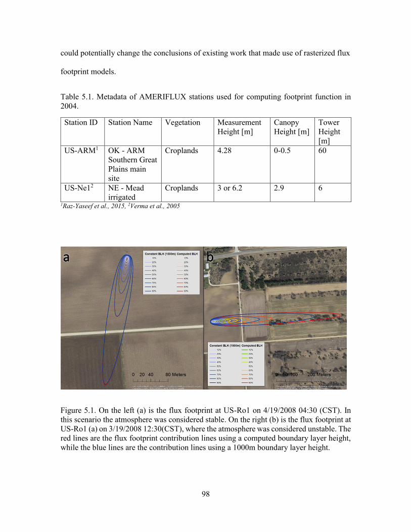
98
could potentially change the conclusions of existing work that made use of rasterized flux
footprint models.
Table 5.1. Metadata of AMERIFLUX stations used for computing footprint function in 2004.
Station ID Station Name Vegetation Measurement Height [m]
Canopy Height [m]
Tower Height [m]
US-ARM1 OK - ARM Southern Great Plains main site
Croplands 4.28 0-0.5 60
US-Ne12 NE - Mead irrigated
Croplands 3 or 6.2 2.9 6
1Raz-Yaseef et al., 2015, 2Verma et al., 2005
Figure 5.1. On the left (a) is the flux footprint at US-Ro1 on 4/19/2008 04:30 (CST). In this scenario the atmosphere was considered stable. On the right (b) is the flux footprint at US-Ro1 (a) on 3/19/2008 12:30(CST), where the atmosphere was considered unstable. The red lines are the flux footprint contribution lines using a computed boundary layer height, while the blue lines are the contribution lines using a 1000m boundary layer height.
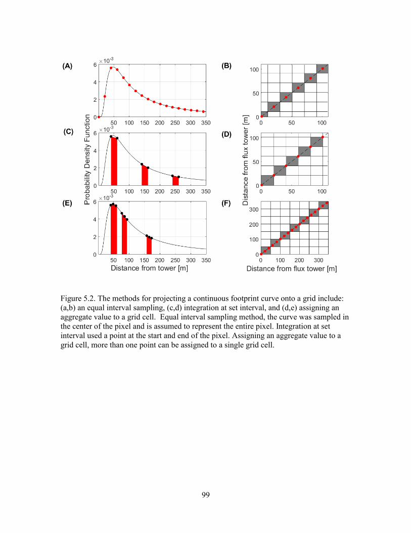
99
Figure 5.2. The methods for projecting a continuous footprint curve onto a grid include: (a,b) an equal interval sampling, (c,d) integration at set interval, and (d,e) assigning an aggregate value to a grid cell. Equal interval sampling method, the curve was sampled in the center of the pixel and is assumed to represent the entire pixel. Integration at set interval used a point at the start and end of the pixel. Assigning an aggregate value to a grid cell, more than one point can be assigned to a single grid cell.
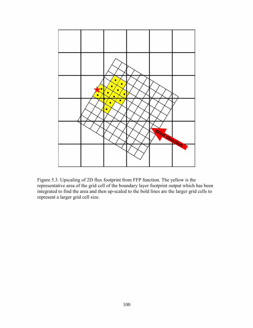
100
Figure 5.3. Upscaling of 2D flux footprint from FFP function. The yellow is the representative area of the grid cell of the boundary layer footprint output which has been integrated to find the area and then up-scaled to the bold lines are the larger grid cells to represent a larger grid cell size.
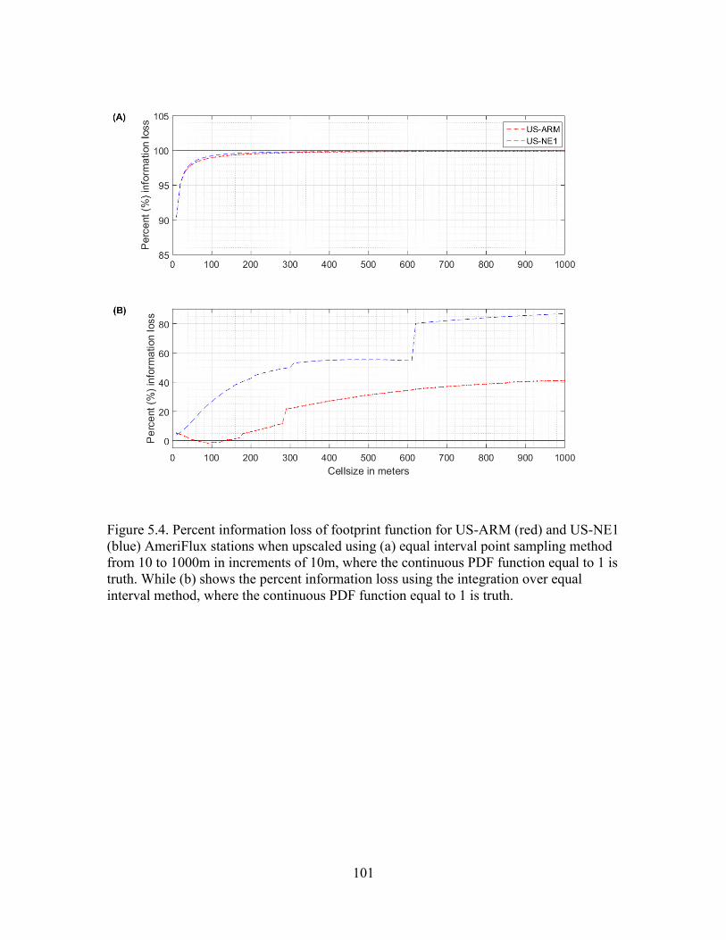
101
Figure 5.4. Percent information loss of footprint function for US-ARM (red) and US-NE1 (blue) AmeriFlux stations when upscaled using (a) equal interval point sampling method from 10 to 1000m in increments of 10m, where the continuous PDF function equal to 1 is truth. While (b) shows the percent information loss using the integration over equal interval method, where the continuous PDF function equal to 1 is truth.
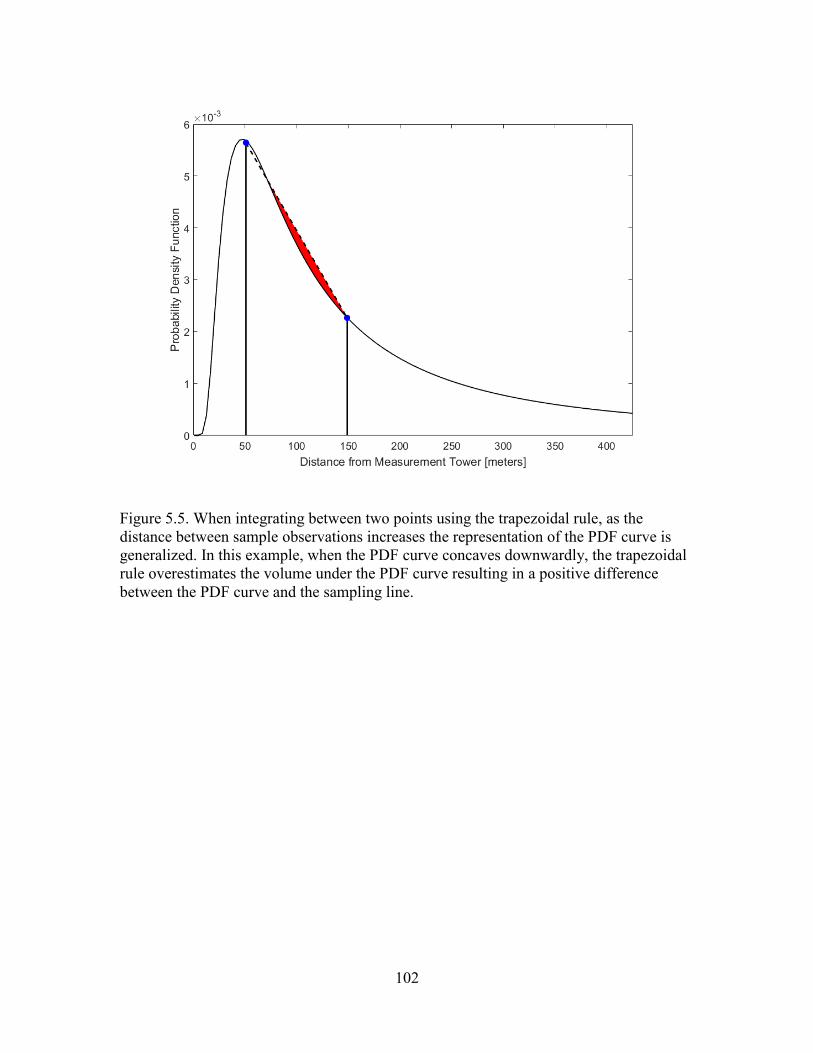
102
Figure 5.5. When integrating between two points using the trapezoidal rule, as the distance between sample observations increases the representation of the PDF curve is generalized. In this example, when the PDF curve concaves downwardly, the trapezoidal rule overestimates the volume under the PDF curve resulting in a positive difference between the PDF curve and the sampling line.
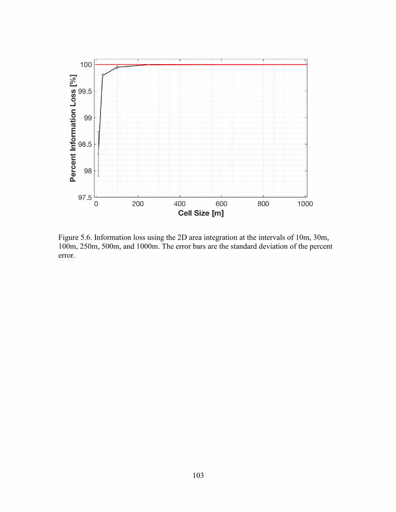
103
Figure 5.6. Information loss using the 2D area integration at the intervals of 10m, 30m, 100m, 250m, 500m, and 1000m. The error bars are the standard deviation of the percent error.
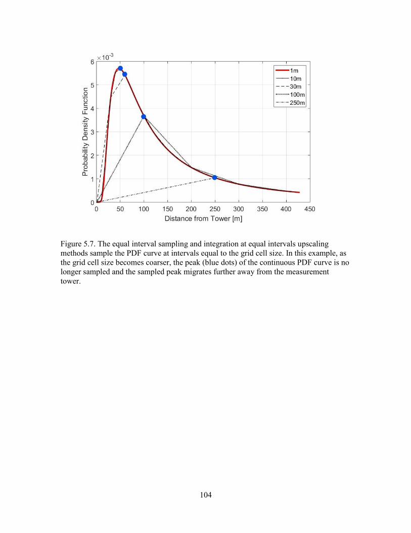
104
Figure 5.7. The equal interval sampling and integration at equal intervals upscaling methods sample the PDF curve at intervals equal to the grid cell size. In this example, as the grid cell size becomes coarser, the peak (blue dots) of the continuous PDF curve is no longer sampled and the sampled peak migrates further away from the measurement tower.
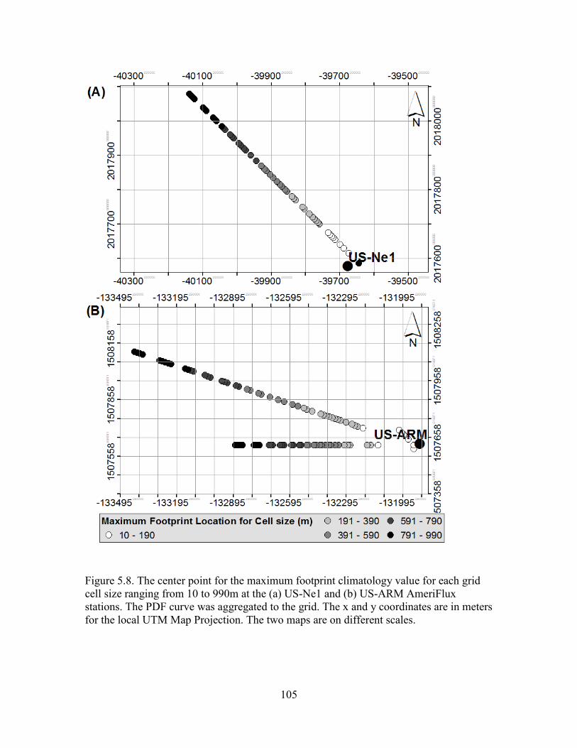
105
Figure 5.8. The center point for the maximum footprint climatology value for each grid cell size ranging from 10 to 990m at the (a) US-Ne1 and (b) US-ARM AmeriFlux stations. The PDF curve was aggregated to the grid. The x and y coordinates are in meters for the local UTM Map Projection. The two maps are on different scales.
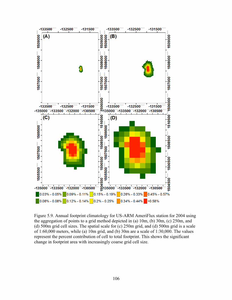
106
Figure 5.9. Annual footprint climatology for US-ARM AmeriFlux station for 2004 using the aggregation of points to a grid method depicted in (a) 10m, (b) 30m, (c) 250m, and (d) 500m grid cell sizes. The spatial scale for (c) 250m grid, and (d) 500m grid is a scale of 1:60,000 meters, while (a) 10m grid, and (b) 30m are a scale of 1:30,000. The values represent the percent contribution of cell to total footprint. This shows the significant change in footprint area with increasingly coarse grid cell size.
107
CHAPTER 6
CONCLUSIONS
Upscaling carbon flux measurements to represent regional scales has its caveats and
should be approached with care. This dissertation examined two approaches extending
ground-based point measurements to a broader spatial scale by using remote sensing. In
Chapter 3, the appropriate vegetation index for identifying carbon flux phenology metrics
was identified, and it was found that the appropriate vegetation index varied by crop type
and the phenology point you are trying estimate. In Chapter 4, an empirical model was
developed and validated by directly using the satellite observed surface reflectance values
to explain NEE by crop type and period of the growing season. In this chapter the surface
reflectance bands that best explained the variance in ground observed NEE were
identified and used in the model calibration. Results indicated that NEE could be
estimated with better certainty when modeling by crop type and period of growing
season. Finally, Chapter 5 presented a sensitivity analysis of various rasterization
methods commonly used in upscaling point measurements. The sensitivity of 1D and 2D
flux footprints to rasterization and varying cell sizes was evaluated, and best practices for
rasterizing these continuous functions were presented.
Overall, several common themes run throughout the three manuscripts presented
here. Most significantly, upscaling flux measurements is extremely sensitive to station
fetch and time varying fetch must be considered before using such measurements to
108
calibrate or validate regional climate models. In Chapter 3 and Chapter 4, a flux footprint
was used to determine whether the flux observations represented the crop planted during
that year. However, there were limited number of datasets (particularly in chapter 4)
available to evaluate the empirical model for estimating regional carbon dynamics in
maize and soybean fields. Therefore, an 8-day flux footprint was used to increase the
number of pixels used for model evaluation. In generating footprints of this nature, the
question arose of how to represent a continuous flux footprint function to a gridded raster
that represented a coarser spatial area than the spatial scales of the flux footprint and how
much information is lost during the conversion (presented in Chapter 5). This is not an
uncommon scenario in merging data sources disparate in time and space, however, no
previous flux studies have specifically addressed this mismatch. When rasterizing a flux
footprint, integrating under the probability density function results in the least amount of
information loss. However, as long as a pixel is homogeneous and represents the same
crop type as the flux observation 80-90% of the time, then no flux footprint needs to be
used. Future work will need to address the influence of heterogeneity of land cover
within an up-scaled flux footprint.
A second theme is that in the broader field of climate studies, models are only as
good as the data used to calibrate them. In the work presented here, new techniques were
used to leverage various data sources, however, a limited availability of station data did
not allow for a full exploration of the effects of land management of agricultural fields.
Future application of these methods to other datasets may allow for such understanding.
Additionally, significant spatial gaps in flux observations to model NEE exchanges,
inhibits the ability for this model to be applied across varying climate zones with

109
different land management techniques. Tillage and irrigation can have a considerable
amount of impact on the amount of carbon cycling, making a land cover more of a sink or
source of carbon. Future research will need additional field data across varying climatic
zones and land management techniques to provide more certainty in the modelling of
maize and soybean. Additionally, the methodologies developed in this dissertation for
estimating NEE from remote sensing will be expanded to other crop types across the US
and the world. Which will also require additional field based datasets.
This collection of manuscripts showed the importance of estimating NEE at
regional scales in agricultural regions using remotely sensed surface reflectance and
meteorological datasets. The new methods developed can identify key carbon flux
phenology metrics and estimate NEE with greater certainty when crop type and period of
the growing season were considered. Previous ground-based research had found that
there were differences in carbon uptake of maize and soybean due to their mismatch in
photosynthetic pathways (C4 vs. C3 pathway), amount of biomass, and differences in the
vegetative stages of each crop. The new methodology addresses limitations of existing
regional climate models that model carbon dynamics. These new methodologies will
allow for better regional estimates of carbon dynamics in agricultural fields.
Understanding the regional contributions of agriculture to the carbon budget is not well
understood. These methodologies will give scientists a better understanding of regional
contributions of agricultural crops to the carbon cycle, which will give a better
understanding of how agriculture will affect carbon dynamics in future climate change
projections. Future research will access the influence of maize and soybean on
atmospheric carbon, by modeling NEE for the entire US Corn Belt. The carbon cycling

110
will be analyzed annually for the US Corn Belt, and then changes will be correlated with
changes due to meteorological conditions, area of land producing crops, and yield for the
year. Ultimately the existing Landsat and MODIS satellites will be retired in the future.
Therefore, newer satellites such as NPP VIIRS and GOES 16 will need to be evaluated
for estimating NEE in agricultural regions. Therefore, it will be important to continue to
improve this work and expand it to new crops and satellite platforms.
111
REFERENCES
Abendroth, L. J., Elmore, R. W., Boyer, M. J., & Marlay, S. K. (2011). Corn Growth and
Development (PMR 1009). Ames, Iowa: Iowa State University Extension and
Outreach. Retrieved from https://store.extension.iastate.edu/Product/Corn-Growth-
and-Development
Allison, V. J., Miller, R. M., Jastrow, J. D., Matamala, R., & Zak, D. R. (2005). Changes
in Soil Microbial Community Structure in a Tallgrass Prairie Chronosequence. Soil
Science Society of America Journal, 69(5), 1412.
http://doi.org/10.2136/sssaj2004.0252
Aubinet, M., Vesala, T., & Papale, D. (2012). Eddy Covariance: A Practical Guide to
Measurement and Data Analysis. Springer. Retrieved from
http://books.google.com/books?id=8a2bIJER5ZwC
Baldocchi, D. D. (2003). Assessing the eddy covariance technique for evaluating carbon
dioxide exchange rates of ecosystems: past, present and future. Global Change
Biology, 9(4), 479–492. http://doi.org/10.1046/j.1365-2486.2003.00629.x
Baldocchi, D., Falge, E., Gu, L., Olson, R., Hollinger, D., Running, S., … Wofsy, S.
(2001). FLUXNET: A New Tool to Study the Temporal and Spatial Variability of
Ecosystem–Scale Carbon Dioxide, Water Vapor, and Energy Flux Densities.
Bulletin of the American Meteorological Society, 82(11), 2415–2434.
112
http://doi.org/10.1175/1520-0477(2001)082<2415:FANTTS>2.3.CO;2
Balzarolo, M., Vicca, S., Nguy-Robertson, A. L., Bonal, D., Elbers, J. A., Fu, Y. H., …
Veroustraete, F. (2016). Matching the phenology of Net Ecosystem Exchange and
vegetation indices estimated with MODIS and FLUXNET in-situ observations.
Remote Sensing of Environment, 174, 290–300. http://doi.org/spa
Basara, J. B., Hall, P. K., Schroeder, A. J., Illston, B. G., & Nemunaitis, K. L. (2008).
Diurnal cycle of the Oklahoma City urban heat island. Journal of Geophysical
Research: Atmospheres, 113(D20), D20109. http://doi.org/10.1029/2008JD010311
Bonan, G. (2008). Ecological Climatology: Concepts and Applications (2nd Ed.). New
York, NY: Cambridge University Press.
Bonfils, C., & Lobell, D. (2007). Empirical evidence for a recent slowdown in irrigation-
induced cooling. Proceedings of the National Academy of Sciences, 104(34), 13582–
13587. http://doi.org/10.1073/pnas.0700144104
Burden, R. L., & Faires, J. D. (1997). Numerical Analysis (6th Editio). Pacific Grove,
CA: Brooks/Cole Publishing Company.
Cai, W., Yuan, W., Liang, S., Zhang, X., Dong, W., Xia, J., … Zhang, Q. (2014).
Improved estimations of gross primary production using satellite-derived
photosynthetically active radiation. Journal of Geophysical Research:
Biogeosciences, 119(1), 2013JG002456. http://doi.org/10.1002/2013JG002456
Calder, K. L. (1952). Some recent British work on teh problem of diffusion in the lower
atmosphere. In Proceedings of the US Technology conference on Air Pollution (pp.
113
787–792). New York, NY: McGraw Hill.
Chapra, S. C. (2008). Applied Numerical Methods with Matlab for Engineers and
Scientists (2nd Editio). Boston, MA: McGraw Hill.
Chen, B., Chen, J. M., Mo, G., Yuen, C.-W., Margolis, H., Higuchi, K., … Chan, D.
(2007). Modeling and Scaling Coupled Energy, Water, and Carbon Fluxes Based on
Remote Sensing: An Application to Canada’s Landmass. Journal of
Hydrometeorology, 8(2), 123–143. http://doi.org/10.1175/JHM566.1
Chen, B., Coops, N. C., Fu, D., Margolis, H. A., Amiro, B. D., Barr, A. G., … Wofsy, S.
C. (2011). Assessing eddy-covariance flux tower location bias across the Fluxnet-
Canada Research Network based on remote sensing and footprint modelling.
Agricultural and Forest Meteorology, 151(1), 87–100.
http://doi.org/10.1016/j.agrformet.2010.09.005
Chen, B., Ge, Q., Fu, D., Liu, G., Yu, G., Sun, X., … Wang, H. (2009). Upscaling of
gross ecosystem production to the landscape scale using multi-temporal Landsat
images, eddy covariance measurements and a footprint model. Biogeosciences
Discuss., 6(6), 11317–11345. http://doi.org/10.5194/bgd-6-11317-2009
Chow, W. T. L., Brennan, D., & Brazel, A. J. (2011). Urban Heat Island Research in
Phoenix, Arizona: Theoretical Contributions and Policy Applications. Bulletin of the
American Meteorological Society, 93(4), 517–530. http://doi.org/10.1175/BAMS-D-
11-00011.1
Ciais, P., Reichstein, M., Viovy, N., Granier, A., Ogée, J., Allard, V., … Valentini, R.
114
(2005). Europe-wide reduction in primary productivity caused by the heat and
drought in 2003. Nature, 437(7058), 529–533. http://doi.org/10.1038/nature03972
Cicuéndez, V., Rodríguez-Rastrero, M., Huesca, M., Uribe, C., Schmid, T., Inclán, R., …
Palacios-Orueta, A. (2015). Assessment of soil respiration patterns in an irrigated
corn field based on spectral information acquired by field spectroscopy. Agriculture,
Ecosystems & Environment, 212, 158–167.
http://doi.org/10.1016/j.agee.2015.06.020
Daly, C., Halbleib, M., Smith, J. I., Gibson, W. P., Doggett, M. K., Taylor, G. H., …
Pasteris, P. P. (2008). Physiographically sensitive mapping of climatological
temperature and precipitation across the conterminous United States. International
Journal of Climatology, 28(15), 2031–2064. http://doi.org/10.1002/joc.1688
Daniels, T. L. (2010). Integrating Forest Carbon Sequestration Into a Cap-and-Trade
Program to Reduce Net CO 2 Emissions. Journal of the American Planning
Association, 76(4), 463–475. http://doi.org/10.1080/01944363.2010.499830
DeMers, M. N. (2002). GIS Modeling in Raster. New York, NY: John Wiley & Sons,
Inc.
Desai, A. R., Noormets, A., Bolstad, P. V., Chen, J., Cook, B. D., Davis, K. J., … Wang,
W. (2008). Influence of vegetation and seasonal forcing on carbon dioxide fluxes
across the Upper Midwest, USA: Implications for regional scaling. Agricultural and
Forest Meteorology, 148(2), 288–308.
http://doi.org/10.1016/j.agrformet.2007.08.001
115
Dong, J., Xiao, X., Wagle, P., Zhang, G., Zhou, Y., Jin, C., … Moore, B. (2015).
Comparison of four EVI-based models for estimating gross primary production of
maize and soybean croplands and tallgrass prairie under severe drought. Remote
Sensing of Environment, 162, 154–168. http://doi.org/10.1016/j.rse.2015.02.022
Fang, B., Lakshmi, V., Bindlish, R., Jackson, T. J., Cosh, M., & Basara, J. (2013).
Passive Microwave Soil Moisture Downscaling Using Vegetation Index and Skin
Surface Temperature. Vadose Zone Journal, 12(3), 0.
http://doi.org/10.2136/vzj2013.05.0089
Fehr, W. R., Caviness, C. E., Burmood, D. T., & Pennington, J. S. (1971). Stage of
development descriptions for soybeans, Glycine max (L.) Merr. Crop Science, 11,
929–931.
Fiebrich, C. A., Morgan, C. R., McCombs, A. G., Hall, P. K., & McPherson, R. A.
(2010). Quality Assurance Procedures for Mesoscale Meteorological Data. Journal
of Atmospheric and Oceanic Technology, 27(10), 1565–1582.
http://doi.org/10.1175/2010JTECHA1433.1
Frank, A. B., & Dugas, W. A. (2001). Carbon dioxide fluxes over a northern, semiarid,
mixed-grass prairie. Agricultural and Forest Meteorology, 108(4), 317–326.
http://doi.org/10.1016/S0168-1923(01)00238-6
Frank, A. B., & Karn, J. F. (2003, June 19). Vegetation indices, CO2 flux, and biomass
for Northern Plains grasslands. Journal of Range Management Archives. Retrieved
from https://journals.uair.arizona.edu/index.php/jrm/article/view/9818
116
Fu, D., Chen, B., Zhang, H., Wang, J., Black, T. A., Amiro, B. D., … Verma, S. (2014).
Estimating landscape net ecosystem exchange at high spatial–temporal resolution
based on Landsat data, an improved upscaling model framework, and eddy
covariance flux measurements. Remote Sensing of Environment, 141, 90–104.
http://doi.org/10.1016/j.rse.2013.10.029
Gao, F., Masek, J., Schwaller, M., & Hall, F. (2006). On the blending of the Landsat and
MODIS surface reflectance: predicting daily Landsat surface reflectance. IEEE
Transactions on Geoscience and Remote Sensing, 44(8), 2207–2218.
http://doi.org/10.1109/TGRS.2006.872081
Garrity, S. R., Bohrer, G., Maurer, K. D., Mueller, K. L., Vogel, C. S., & Curtis, P. S.
(2011). A comparison of multiple phenology data sources for estimating seasonal
transitions in deciduous forest carbon exchange. Agricultural and Forest
Meteorology, 151(12), 1741–1752. http://doi.org/10.1016/j.agrformet.2011.07.008
Gebremedhin, M. T., Loescher, H. W., & Tsegaye, T. D. (2012). Carbon Balance of No-
Till Soybean with Winter Wheat Cover Crop in the Southeastern United States.
Agronomy Journal, 104(5), 1321. http://doi.org/10.2134/agronj2012.0072
Gitelson, A. A. (2003). Novel technique for remote estimation of CO 2 flux in maize.
Geophysical Research Letters, 30(9), 1486. http://doi.org/10.1029/2002GL016543
Gitelson, A. A., Peng, Y., Masek, J. G., Rundquist, D. C., Verma, S., Suyker, A., …
Meyers, T. (2012). Remote estimation of crop gross primary production with
Landsat data. Remote Sensing of Environment, 121, 404–414.
http://doi.org/10.1016/j.rse.2012.02.017
117
Goldstein, A. H., Hultman, N. E., Fracheboud, J. M., Bauer, M. R., Panek, J. A., Xu, M.,
… Baugh, W. (2000). Effects of climate variability on the carbon dioxide, water,
and sensible heat fluxes above a ponderosa pine plantation in the Sierra Nevada
(CA). Agricultural and Forest Meteorology, 101(2–3), 113–129.
http://doi.org/10.1016/S0168-1923(99)00168-9
Griffis, T. J., Lee, X., Baker, J. M., Billmark, K., Schultz, N., Erickson, M., … Hu, N.
(2011). Oxygen isotope composition of evapotranspiration and its relation to C 4
photosynthetic discrimination. Journal of Geophysical Research, 116(G1), G01035.
http://doi.org/10.1029/2010JG001514
Gu, Y., & Wylie, B. K. (2015). Developing a 30-m grassland productivity estimation map
for central Nebraska using 250-m MODIS and 30-m Landsat-8 observations.
Remote Sensing of Environment, 171, 291–298.
http://doi.org/10.1016/j.rse.2015.10.018
Gu, Y., & Wylie, B. K. (2016). Using satellite vegetation and compound topographic
indices to map highly erodible cropland buffers for cellulosic biofuel crop
developments in eastern Nebraska, USA. Ecological Indicators, 60, 64–70.
http://doi.org/10.1016/j.ecolind.2015.06.019
Guo, X., Price, K. P., & Stiles, J. M. (2003). Grasslands Discriminant Analysis Using
Landsat TM Single and Multitemporal Data. Retrieved February 2, 2015, from
http://essential.metapress.com/content/v3528747u4355398/
Hale, R. C., Gallo, K. P., & Loveland, T. R. (2008). Influences of specific land use/land
cover conversions on climatological normals of near-surface temperature. Journal of
118
Geophysical Research, 113(D14), D14113. http://doi.org/10.1029/2007JD009548
Han, W., Yang, Z., Di, L., & Mueller, R. (2012). CropScape: A Web service based
application for exploring and disseminating US conterminous geospatial cropland
data products for decision support. Computers and Electronics in Agriculture, 84,
111–123. http://doi.org/10.1016/j.compag.2012.03.005
Heinsch, F. A., Zhao, M., Running, S. W., Kimball, J. S., Nemani, R. R., Davis, K. J., …
Flanagan, L. B. (2006). Evaluation of remote sensing based terrestrial productivity
from MODIS using regional tower eddy flux network observations. IEEE
Transactions on Geoscience and Remote Sensing, 44(7), 1908–1925.
http://doi.org/10.1109/TGRS.2005.853936
Horst, T. W., & Weil, J. C. (1992). Footprint estimation for scalar flux measurements in
the atmospheric surface layer. Boundary-Layer Meteorology, 59(3), 279–296.
http://doi.org/10.1007/BF00119817
Horst, T. W., & Weil, J. C. (1994). How Far is Far Enough?: The Fetch Requirements for
Micrometeorological Measurement of Surface Fluxes. Journal of Atmospheric and
Oceanic Technology, 11(4), 1018–1025. http://doi.org/10.1175/1520-
0426(1994)011<1018:HFIFET>2.0.CO;2
Hsieh, C.-I., Katul, G., & Chi, T. (2000). An approximate analytical model for footprint
estimation of scalar fluxes in thermally stratified atmospheric flows. Advances in
Water Resources, 23(7), 765–772. http://doi.org/10.1016/S0309-1708(99)00042-1
Huete, A. (1997). A comparison of vegetation indices over a global set of TM images for
119
EOS-MODIS. Remote Sensing of Environment, 59(3), 440–451.
http://doi.org/10.1016/S0034-4257(96)00112-5
Huete, A., Didan, K., Miura, T., Rodriguez, E. ., Gao, X., & Ferreira, L. . (2002).
Overview of the radiometric and biophysical performance of the MODIS vegetation
indices. Remote Sensing of Environment, 83(1–2), 195–213.
http://doi.org/10.1016/S0034-4257(02)00096-2
Jensen, J. R. (2005). Introductory digital image processing: A remote sensing
perspective. Geocarto International (Vol. 2). Taylor & Francis Group.
http://doi.org/10.1080/10106048709354084
Jones, P. D., Groisman, P. Y., Coughlan, M., Plummer, N., Wang, W.-C., & Karl, T. R.
(1990). Assessment of urbanization effects in time series of surface air temperature
over land. Nature, 347(6289), 169–172. http://doi.org/10.1038/347169a0
Kalfas, J. L., Xiao, X., Vanegas, D. X., Verma, S. B., & Suyker, A. E. (2011). Modeling
gross primary production of irrigated and rain-fed maize using MODIS imagery and
CO2 flux tower data. Agricultural and Forest Meteorology, 151(12), 1514–1528.
http://doi.org/10.1016/j.agrformet.2011.06.007
Kim, J., Guo, Q., Baldocchi, D. D., Leclerc, M. Y., Xu, L., & Schmid, H. P. (2006a).
Upscaling fluxes from tower to landscape: Overlaying flux footprints on high-
resolution (IKONOS) images of vegetation cover. Agricultural and Forest
Meteorology, 136(3–4), 132–146. http://doi.org/10.1016/j.agrformet.2004.11.015
Kim, J., Guo, Q., Baldocchi, D. D., Leclerc, M. Y., Xu, L., & Schmid, H. P. (2006b).
120
Upscaling fluxes from tower to landscape: Overlaying flux footprints on high-
resolution (IKONOS) images of vegetation cover. Agricultural and Forest
Meteorology, 136(3–4), 132–146. http://doi.org/10.1016/j.agrformet.2004.11.015
Kljun, N., Calanca, P., Rotach, M. W., & Schmid, H. P. (2004). A Simple
Parameterisation for Flux Footprint Predictions. Boundary-Layer Meteorology,
112(3), 503–523. http://doi.org/10.1023/B:BOUN.0000030653.71031.96
Kljun, N., Calanca, P., Rotach, M. W., & Schmid, H. P. (2015). A simple two-
dimensional parameterisation for Flux Footprint Prediction (FFP). Geoscientific
Model Development, 8(11), 3695–3713. http://doi.org/10.5194/gmd-8-3695-2015
Kort, J., Collins, M., & Ditsch, D. (1998). A review of soil erosion potential associated
with biomass crops. Biomass and Bioenergy, 14(4), 351–359.
http://doi.org/10.1016/S0961-9534(97)10071-X
Lafont, S., Kergoat, L., Dedieu, G., Chevillard, A., Karstens, U., & Kolle, O. (2002).
Spatial and temporal variability of land CO2 fluxes estimated with remote sensing
and analysis data over western Eurasia. Tellus B, 54(5), 820–833.
http://doi.org/10.1034/j.1600-0889.2002.01350.x
Le Quéré, C., Moriarty, R., Andrew, R. M., Canadell, J. G., Sitch, S., Korsbakken, J. I.,
… Zeng, N. (2015). Global Carbon Budget 2015. Earth System Science Data, 7(2),
349–396. http://doi.org/10.5194/essd-7-349-2015
Leclerc, M. Y., & Foken, T. (2014). Footprints in Micrometeorology and Ecology. New
York, NY: Springer. http://doi.org/3642545440
121
Licht, M. (2014). Soybean Growth and Development (PM 1945). Ames, Iowa: Iowa State
University Extension and Outreach. Retrieved from
https://store.extension.iastate.edu/Product/6451
Mahmood, R., Foster, S., Keeling, T., Hubbard, K., Carlson, C., & Leeper, R. (2006).
Impacts of irrigation on 20th century temperature in the northern Great Plains.
Global and Planetary Change, 54(1–2), 1–18.
http://doi.org/10.1016/j.gloplacha.2005.10.004
Mahmood, R., Quintanar, A. I., Conner, G., Leeper, R., Dobler, S., Pielke, R. A., …
Syktus, J. (2010). Impacts of Land Use/Land Cover Change on Climate and Future
Research Priorities. Bulletin of the American Meteorological Society, 91(1), 37–46.
http://doi.org/10.1175/2009BAMS2769.1
Masek, J. G., Vermote, E. F., Saleous, N. E., Wolfe, R., Hall, F. G., Huemmrich, K. F.,
… Lim, T.-K. (2006). A Landsat Surface Reflectance Dataset for North America,
1990–2000. IEEE Geoscience and Remote Sensing Letters, 3(1), 68–72.
http://doi.org/10.1109/LGRS.2005.857030
Masek, J., Schwaller, M., & Hall, F. (2006). On the blending of the Landsat and MODIS
surface reflectance: predicting daily Landsat surface reflectance. IEEE Transactions
on Geoscience and Remote Sensing, 44(8), 2207–2218.
http://doi.org/10.1109/TGRS.2006.872081
McCombs, A. G., Ilk, A. J., & Fiebrich, C. A. (n.d.). Effects of nearby irrigation on
Oklahoma Mesonet observations. In 18th Conference on Integrated Observing and
Assimilation Systems for the Atmosphere, Oceans, and Land Surface. Atlanta, GA.
122
Retrieved from
https://ams.confex.com/ams/94Annual/webprogram/Paper231703.html
Metzger, S., Junkermann, W., Mauder, M., Butterbach-Bahl, K., Trancón y Widemann,
B., Neidl, F., … Foken, T. (2013). Spatially explicit regionalization of airborne flux
measurements using environmental response functions. Biogeosciences, 10(4),
2193–2217. http://doi.org/10.5194/bg-10-2193-2013
Meyers, T. P., & Hollinger, S. E. (2004). An assessment of storage terms in the surface
energy balance of maize and soybean. Agricultural and Forest Meteorology, 125(1),
105–115. http://doi.org/10.1016/j.agrformet.2004.03.001
Mihailovic, D. T., Rao, S. T., Alapaty, K., Ku, J. Y., Arsenic, I., & Lalic, B. (2005). A
study on the effects of subgrid-scale representation of land use on the boundary
layer evolution using a 1-D model. Environmental Modelling & Software, 20(6),
705–714. http://doi.org/10.1016/j.envsoft.2004.04.004
Monson, R., & Baldocchi, D. (2014). Terrestrial Biosphere-Atmosphere Fluxes. New
York, NY: Cambridge University Press.
Nagler, P. L., Cleverly, J., Glenn, E., Lampkin, D., Huete, A., & Wan, Z. (2005).
Predicting riparian evapotranspiration from MODIS vegetation indices and
meteorological data. Remote Sensing of Environment, 94(1), 17–30.
http://doi.org/10.1016/j.rse.2004.08.009
Nicolini, G., Fratini, G., Avilov, V., Kurbatova, J. A., Vasenev, I., & Valentini, R.
(2015). Performance of eddy-covariance measurements in fetch-limited applications.
123
Theoretical and Applied Climatology. http://doi.org/10.1007/s00704-015-1673-x
Noormets, A., Chen, J., Gu, L., & Desai, A. (2009). The Phenology of Gross Ecosystem
Productivity and Ecosystem Respiration in Temperate Hardwood and Conifer
Chronosequences. In Phenology of Ecosystem Processes (pp. 59–85). New York,
NY: Springer New York. http://doi.org/10.1007/978-1-4419-0026-5_3
Papale, D. (2012). Data Gap Filling. In M. Aubinet, T. Vesala, & D. Papale (Eds.), Eddy
Covariance: A Practical Guide to Measurement and Data Analysis (pp. 159–172).
New York, NY: Springer Atmospheric Sciences. http://doi.org/10.1007/978-94-007-
2351-1
Papale, D., Reichstein, M., Aubinet, M., Canfora, E., Bernhofer, C., Kutsch, W., …
Yakir, D. (2006). Towards a standardized processing of Net Ecosystem Exchange
measured with eddy covariance technique: algorithms and uncertainty estimation.
Biogeosciences, 3(4), 571–583. http://doi.org/10.5194/bg-3-571-2006
Pitman, A. J. (2004). Impact of land cover change on the climate of southwest Western
Australia. Journal of Geophysical Research, 109(D18), D18109.
http://doi.org/10.1029/2003JD004347
Price, K. P., Guo, X., & Stiles, J. M. (2002). Optimal Landsat TM band combinations and
vegetation indices for discrimination of six grassland types in eastern Kansas.
International Journal of Remote Sensing, 23(23), 5031–5042.
http://doi.org/10.1080/01431160210121764
Quarteroni, A., Sacco, R., & Saleri, F. (2000). Numerical Mathematics. New York, NY:
124
Springer.
Raich, J. W., & Schlesinger, W. H. (1992). The global carbon dioxide flux in soil
respiration and its relationship to vegetation and climate. Tellus B, 44(2), 81–99.
http://doi.org/10.1034/j.1600-0889.1992.t01-1-00001.x
Raz-Yaseef, N., Billesbach, D., Fischer, M. L., Biraud, S. C., Gunter, S. A., Bradford, J.
A., & Torn, M. S. (2015). Vulnerability of crops and native grasses to summer
drying in the U.S. Southern Great Plains. Agriculture, Ecosystems, and
Environment, 213, 209–218.
http://doi.org/http://dx.doi.org/10.1016/j.agee.2015.07.021
Reichstein, M., Falge, E., Baldocchi, D., Papale, D., Aubinet, M., Berbigier, P., …
Valentini, R. (2005). On the separation of net ecosystem exchange into assimilation
and ecosystem respiration: review and improved algorithm. Global Change Biology,
11(9), 1424–1439. http://doi.org/10.1111/j.1365-2486.2005.001002.x
Reichstein, M., Tenhunen, J. D., Roupsard, O., Ourcival, J., Rambal, S., Miglietta, F., …
Valentini, R. (2002). Severe drought effects on ecosystem CO2 and H2O fluxes at
three Mediterranean evergreen sites: revision of current hypotheses? Global Change
Biology, 8(10), 999–1017. http://doi.org/10.1046/j.1365-2486.2002.00530.x
Reithmaier, L. M., Göckede, M., Markkanen, T., Knohl, A., Churkina, G., Rebmann, C.,
… Foken, T. (2006). Use of remotely sensed land use classification for a better
evaluation of micrometeorological flux measurement sites. Theoretical and Applied
Climatology, 84(4), 219–233. http://doi.org/10.1007/s00704-005-0168-6
125
Richardson, A. D., Hollinger, D. Y., Burba, G. G., Davis, K. J., Flanagan, L. B., Katul, G.
G., … Wofsy, S. C. (2006). A multi-site analysis of random error in tower-based
measurements of carbon and energy fluxes. Agricultural and Forest Meteorology,
136(1–2), 1–18. http://doi.org/10.1016/j.agrformet.2006.01.007
Rouse, J. W., Haas, R. H., Schell, J. A., & Deering, D. W. (1974). Monitoring Vegetation
Systems in the Great Plains with ERTS. In Proceedings, 3rd Earth Resource
Technology Satellite (ERTS) Symposium (pp. 48–62).
Running, S. W., Baldocchi, D. D., Turner, D. P., Gower, S. T., Bakwin, P. S., & Hibbard,
K. A. (1999). A Global Terrestrial Monitoring Network Integrating Tower Fluxes,
Flask Sampling, Ecosystem Modeling and EOS Satellite Data. Remote Sensing of
Environment, 70(1), 108–127. http://doi.org/10.1016/S0034-4257(99)00061-9
Schmid, H. P. (2002). Footprint modeling for vegetation atmosphere exchange studies: a
review and perspective. Agricultural and Forest Meteorology, 113(1–4), 159–183.
http://doi.org/10.1016/S0168-1923(02)00107-7
Schmid, H. P., & Lloyd, C. R. (1999). Spatial representativeness and the location bias of
flux footprints over inhomogeneous areas. Agricultural and Forest Meteorology,
93(3), 195–209. http://doi.org/10.1016/S0168-1923(98)00119-1
Sims, D. A., Brzostek, E. R., Rahman, A. F., Dragoni, D., & Phillips, R. P. (2014). An
improved approach for remotely sensing water stress impacts on forest C uptake.
Global Change Biology, 20(9), 2856–66. http://doi.org/10.1111/gcb.12537
Soegaard, H., Jensen, N. O., Boegh, E., Hasager, C. B., Schelde, K., & Thomsen, A.
126
(2003). Carbon dioxide exchange over agricultural landscape using eddy correlation
and footprint modelling. Agricultural and Forest Meteorology, 114(3–4), 153–173.
http://doi.org/10.1016/S0168-1923(02)00177-6
Suyker, A. ., Verma, S. ., Burba, G. ., Arkebauer, T. ., Walters, D. ., & Hubbard, K. .
(2004). Growing season carbon dioxide exchange in irrigated and rainfed maize.
Agricultural and Forest Meteorology, 124(1–2), 1–13.
http://doi.org/10.1016/j.agrformet.2004.01.011
Suyker, A. E., Verma, S. B., Burba, G. G., & Arkebauer, T. J. (2005). Gross primary
production and ecosystem respiration of irrigated maize and irrigated soybean
during a growing season. Agricultural and Forest Meteorology, 131(3–4), 180–190.
http://doi.org/10.1016/j.agrformet.2005.05.007
Tang, X., Wang, Z., Liu, D., Song, K., Jia, M., Dong, Z., … Liu, X. (2012). Estimating
the net ecosystem exchange for the major forests in the northern United States by
integrating MODIS and AmeriFlux data. Agricultural and Forest Meteorology, 156,
75–84. http://doi.org/10.1016/j.agrformet.2012.01.003
Verma, S. B., Dobermann, A., Cassman, K. G., Walters, D. T., Knops, J. M., Arkebauer,
T. J., … Walter-Shea, E. A. (2005). Annual carbon dioxide exchange in irrigated
and rainfed maize-based agroecosystems. Agricultural and Forest Meteorology,
131(1–2), 77–96. http://doi.org/10.1016/j.agrformet.2005.05.003
Vermote, E. (2015). MOD09A1 MODIS/Terra Surface Reflectance 8-Day L3 Global
500m SIN Grid V006. http://doi.org/http://doi.org/10.5067/MODIS/MOD09A1.006
127
Viña, A., Gitelson, A. A., Nguy-Robertson, A. L., & Peng, Y. (2011). Comparison of
different vegetation indices for the remote assessment of green leaf area index of
crops. Remote Sensing of Environment, 115(12), 3468–3478.
http://doi.org/10.1016/j.rse.2011.08.010
Vose, R. S., Karl, T. R., Easterling, D. R., Williams, C. N., & Menne, M. J. (2004).
Climate (communication arising): impact of land-use change on climate. Nature,
427(6971), 213–4; discussion 214. http://doi.org/10.1038/427213b
Vuichard, N., & Papale, D. (2015). Filling the gaps in meteorological continuous data
measured at FLUXNET sites with ERA-Interim reanalysis. Earth System Science
Data, 7(2), 157–171. http://doi.org/10.5194/essd-7-157-2015
Walker, J. J., de Beurs, K. M., Wynne, R. H., & Gao, F. (2012). Evaluation of Landsat
and MODIS data fusion products for analysis of dryland forest phenology. Remote
Sensing of Environment, 117, 381–393. http://doi.org/10.1016/j.rse.2011.10.014
Wan, Z., Hook, S., & Hulley, G. (2015). MOD11A2 MODIS/Terra Land Surface
Temperature/Emissivity 8-Day L3 Global 1km SIN Grid V006.
http://doi.org/http://doi.org/10.5067/MODIS/MOD11A2.006
Wang, C., Fritschi, F. B., Stacey, G., & Yang, Z. (2011a). Phenology-Based Assessment
of Perennial Energy Crops in North American Tallgrass Prairie. Annals of the
Association of American Geographers, 101(4), 742–751.
http://doi.org/10.1080/00045608.2011.567934
Wang, C., Fritschi, F. B., Stacey, G., & Yang, Z. (2011b). Phenology-Based Assessment
128
of Perennial Energy Crops in North American Tallgrass Prairie. Annals of the
Association of American Geographers, 101(4), 742–751.
http://doi.org/10.1080/00045608.2011.567934
Wang, C., Hunt Jr., E. R., Zhang, L., & Guo, H. (2013). Phenology-assisted classification
of C3 and C4 grasses in the U.S. Great Plains and their climate dependency with
MODIS time series. Remote Sensing of Environment, 138, 90–101.
http://doi.org/10.1016/j.rse.2013.07.025
West, T. O., & Marland, G. (2003). Net carbon flux from agriculture: Carbon emissions,
carbon sequestration, crop yield, and land-use change. Biogeochemistry, 63(1), 73–
83. http://doi.org/10.1023/A:1023394024790
Wohlfahrt, G., Hammerle, A., Haslwanter, A., Bahn, M., Tappeiner, U., & Cernusca, A.
(2008). Seasonal and inter-annual variability of the net ecosystem CO2 exchange of
a temperate mountain grassland: Effects of weather and management. Journal of
Geophysical Research: Atmospheres, 113(D8), D08110.
http://doi.org/10.1029/2007JD009286
Wu, C., Gonsamo, A., Chen, J. M., Kurz, W. A., Price, D. T., Lafleur, P. M., … Munger,
J. W. (2012). Interannual and spatial impacts of phenological transitions, growing
season length, and spring and autumn temperatures on carbon sequestration: A
North America flux data synthesis. Global and Planetary Change, 92, 179–190.
http://doi.org/10.1016/j.gloplacha.2012.05.021
Wu, C., Peng, D., Soudani, K., Siebicke, L., Gough, C. M., Arain, M. A., … Ge, Q.
(2017). Land surface phenology derived from normalized difference vegetation
129
index (NDVI) at global FLUXNET sites. Agricultural and Forest Meteorology, 233,
171–182. http://doi.org/10.1016/j.agrformet.2016.11.193
Wylie, B. K., Fosnight, E. A., Gilmanov, T. G., Frank, A. B., Morgan, J. A., Haferkamp,
M. R., & Meyers, T. P. (2007a). Adaptive data-driven models for estimating carbon
fluxes in the Northern Great Plains. Remote Sensing of Environment, 106(4), 399–
413. http://doi.org/10.1016/j.rse.2006.09.017
Wylie, B. K., Fosnight, E. A., Gilmanov, T. G., Frank, A. B., Morgan, J. A., Haferkamp,
M. R., & Meyers, T. P. (2007b). Adaptive data-driven models for estimating carbon
fluxes in the Northern Great Plains. Remote Sensing of Environment, 106(4), 399–
413. http://doi.org/10.1016/j.rse.2006.09.017
Xiao, J., Ollinger, S. V., Frolking, S., Hurtt, G. C., Hollinger, D. Y., Davis, K. J., …
Suyker, A. E. (2014). Data-driven diagnostics of terrestrial carbon dynamics over
North America. Agricultural and Forest Meteorology, 197, 142–157.
http://doi.org/10.1016/j.agrformet.2014.06.013
Xiao, J., Zhuang, Q., Baldocchi, D. D., Law, B. E., Richardson, A. D., Chen, J., … Torn,
M. S. (2008). Estimation of net ecosystem carbon exchange for the conterminous
United States by combining MODIS and AmeriFlux data. Agricultural and Forest
Meteorology, 148(11), 1827–1847. http://doi.org/10.1016/j.agrformet.2008.06.015
Xiao, J., Zhuang, Q., Law, B. E., Baldocchi, D. D., Chen, J., Richardson, A. D., … Torn,
M. S. (2011). Assessing net ecosystem carbon exchange of U.S. terrestrial
ecosystems by integrating eddy covariance flux measurements and satellite
observations. Agricultural and Forest Meteorology, 151(1), 60–69.
130
http://doi.org/10.1016/j.agrformet.2010.09.002
Xiao, X., Hollinger, D., Aber, J., Goltz, M., Davidson, E. A., Zhang, Q., & Moore, B.
(2004). Satellite-based modeling of gross primary production in an evergreen
needleleaf forest. Remote Sensing of Environment, 89(4), 519–534.
http://doi.org/10.1016/j.rse.2003.11.008
Xu, K., Metzger, S., & Desai, A. R. (2017). Upscaling tower-observed turbulent
exchange at fine spatio-temporal resolution using environmental response functions.
Agricultural and Forest Meteorology, 232, 10–22.
http://doi.org/10.1016/j.agrformet.2016.07.019
Zhang, X., Friedl, M. A., Schaaf, C. B., Strahler, A. H., Hodges, J. C. F., Gao, F., …
Huete, A. (2003). Monitoring vegetation phenology using MODIS. Remote Sensing
of Environment, 84(3), 471–475. http://doi.org/10.1016/S0034-4257(02)00135-9
Zhu, X., Chen, J., Gao, F., Chen, X., & Masek, J. G. (2010). An enhanced spatial and
temporal adaptive reflectance fusion model for complex heterogeneous regions.
Remote Sensing of Environment, 114(11), 2610–2623.
http://doi.org/10.1016/j.rse.2010.05.032
.
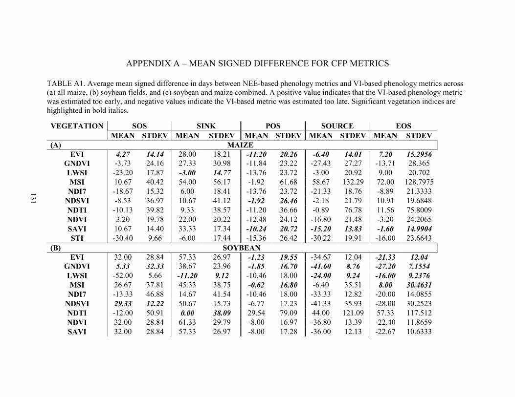
131
APPENDIX A – MEAN SIGNED DIFFERENCE FOR CFP METRICS
TABLE A1. Average mean signed difference in days between NEE-based phenology metrics and VI-based phenology metrics across (a) all maize, (b) soybean fields, and (c) soybean and maize combined. A positive value indicates that the VI-based phenology metric was estimated too early, and negative values indicate the VI-based metric was estimated too late. Significant vegetation indices are highlighted in bold italics.
VEGETATION
INDEX
SOS SINK POS SOURCE EOS MEAN STDEV MEAN STDEV MEAN STDEV MEAN STDEV MEAN STDEV
(A) MAIZE EVI 4.27 14.14 28.00 18.21 -11.20 20.26 -6.40 14.01 7.20 15.2956
GNDVI -3.73 24.16 27.33 30.98 -11.84 23.22 -27.43 27.27 -13.71 28.365 LWSI -23.20 17.87 -3.00 14.77 -13.76 23.72 -3.00 20.92 9.00 20.702 MSI 10.67 40.42 54.00 56.17 -1.92 61.68 58.67 132.29 72.00 128.7975 NDI7 -18.67 15.32 6.00 18.41 -13.76 23.72 -21.33 18.76 -8.89 21.3333
NDSVI -8.53 36.97 10.67 41.12 -1.92 26.46 -2.18 21.79 10.91 19.6848 NDTI -10.13 39.82 9.33 38.57 -11.20 36.66 -0.89 76.78 11.56 75.8009 NDVI 3.20 19.78 22.00 20.22 -12.48 24.12 -16.80 21.48 -3.20 24.2065 SAVI 10.67 14.40 33.33 17.34 -10.24 20.72 -15.20 13.83 -1.60 14.9904 STI -30.40 9.66 -6.00 17.44 -15.36 26.42 -30.22 19.91 -16.00 23.6643
(B) SOYBEAN EVI 32.00 28.84 57.33 26.97 -1.23 19.55 -34.67 12.04 -21.33 12.04
GNDVI 5.33 32.33 38.67 23.96 -1.85 16.70 -41.60 8.76 -27.20 7.1554 LWSI -52.00 5.66 -11.20 9.12 -10.46 18.00 -24.00 9.24 -16.00 9.2376 MSI 26.67 37.81 45.33 38.75 -0.62 16.80 -6.40 35.51 8.00 30.4631 NDI7 -13.33 46.88 14.67 41.54 -10.46 18.00 -33.33 12.82 -20.00 14.0855
NDSVI 29.33 12.22 50.67 15.73 -6.77 17.23 -41.33 35.93 -28.00 30.2523 NDTI -12.00 50.91 0.00 38.09 29.54 79.09 44.00 121.09 57.33 117.512 NDVI 32.00 28.84 61.33 29.79 -8.00 16.97 -36.80 13.39 -22.40 11.8659 SAVI 32.00 28.84 57.33 26.97 -8.00 17.28 -36.00 12.13 -22.67 10.6333
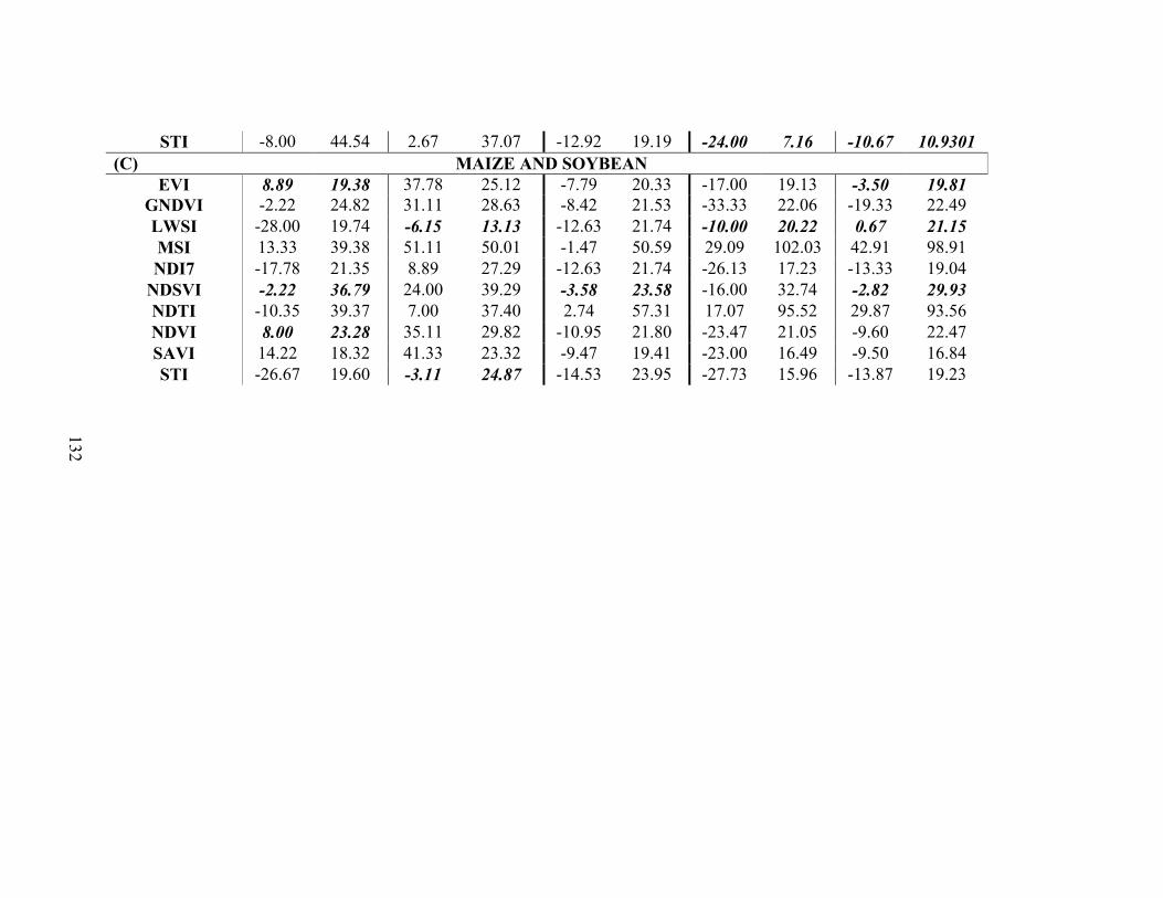
132
STI -8.00 44.54 2.67 37.07 -12.92 19.19 -24.00 7.16 -10.67 10.9301 (C) MAIZE AND SOYBEAN
EVI 8.89 19.38 37.78 25.12 -7.79 20.33 -17.00 19.13 -3.50 19.81 GNDVI -2.22 24.82 31.11 28.63 -8.42 21.53 -33.33 22.06 -19.33 22.49 LWSI -28.00 19.74 -6.15 13.13 -12.63 21.74 -10.00 20.22 0.67 21.15 MSI 13.33 39.38 51.11 50.01 -1.47 50.59 29.09 102.03 42.91 98.91 NDI7 -17.78 21.35 8.89 27.29 -12.63 21.74 -26.13 17.23 -13.33 19.04
NDSVI -2.22 36.79 24.00 39.29 -3.58 23.58 -16.00 32.74 -2.82 29.93 NDTI -10.35 39.37 7.00 37.40 2.74 57.31 17.07 95.52 29.87 93.56 NDVI 8.00 23.28 35.11 29.82 -10.95 21.80 -23.47 21.05 -9.60 22.47 SAVI 14.22 18.32 41.33 23.32 -9.47 19.41 -23.00 16.49 -9.50 16.84 STI -26.67 19.60 -3.11 24.87 -14.53 23.95 -27.73 15.96 -13.87 19.23