TSINGHUA SCIENCE AND TECHNOLOGYISSN 1007-0214 21/21 pp404-407Volume 10, Number 3, June 2005

Rotationally Symmetric Translating Solutions to Curvature Flows in Image Processing*

LIU Qinghua ( )**, CHEN Xiuqing ( )

Department of Mathematical Sciences, Tsinghua University, Beijing 100084, China

Abstract: This paper proves the existence of rotationally symmetric solutions to a curvature flow in image

processing. The flow includes the level sets flow and the mean curvature flow projected onto the normal.

Sharp estimates are obtained for these solutions..

Key words: level sets flow; mean curvature flow; singular ordinary differential equation; priori estimate;rotationally symmetry

Introduction

According to the geometrical framework for image

processing, intensity images can be considered as

surfaces in the spatial-feature space. The image is

thereby a two-dimensional surface in three-

dimensional space (see Refs. [1-3] for a detailed

description of this idea). If we use the graph

of a function to denote

the surface (i.e., the image), various mathematical

flows can be used to model the restoration processing

of the image. In this paper, we study the best-known

flow among these, namely,

={( , ( )) : }X x V x x ( )V x

2

1div

| | +| |

V V

t V V 2 (1)

where 0 is a constant, and is a

function depending on and Here,

and div are the gradient operator and the diver-

gence operator with respect to

( , )V V x tnx R [0, ).t

x (see Ref. [4] for

further details).

In the view of pure mathematics, the flow given by

Eq. (1) is very interesting because it includes two fa-

mous flows:

For 1 , Eq. (1) is the mean curvature flow pro-

jected onto the normal[5,6]

. For 0, Eq. (1) is the

mean curvature flow of the level sets

{ : ( )n

t }M x V x tR (Refs. [7, 8]).

The existence of an entire smooth convex solution

to Eq. (1) for general remains an open issue, al-

though there are some results on smooth solutions

(but not necessarily convex) for the case of 1

(Refs. [5, 6]) and on continuous viscous solutions for

the case of 0 (Refs. [7, 8]). All of these solu-

tions obtained are not necessarily convex. Recently,

to analyze the geometric structure of convex translat-

ing solutions to Eq. (1), Jian[9]

used the maximum

principle and moving plane methods and showed that

such an entire solution may be rotationally symmetric.

In this paper, we will restrict our interest to the

existence of entire rotationally symmetric translating

convex solutions to Eq. (1). This requires us to find a

strictly convex function such that2[0, )r C

( , ) (| |)V x t t r x nRReceived: 2004-01-17; revised: 2004-03-08

Supported by the National Key Basic Research and Devedepment

(973) Program of China (No. G19990751) and the Trans-Century

Training Program Foundation for the Talents of China

To whom correspondence should be addressed.

E-mail: qliu@math.tsinghua.edu.cn; Tel: 86-10-62784334

that solves Eq. (1) in .

We would like to point out that the variational

method in image processing is very active (see

Ref. [10] for the details).

LIU Qinghua ( ) et al Rotationally Symmetric Translating Solutions to 405

1 Main Theorem

Theorem 1 If and 2n 0 , then there exists

a strictly convex function such that

solves Eq. (1) in . Further-

more, r is a solution to the initial value problem of the

following singular ordinary differential equation

(ODE):

2[0, )r C

( , ) (| |)V x t t r x nR

2

( ) 1( ) 1, (0, )

( ( ))

r" t nr' t t

r' t t (2)

and

(3) ( ) 0 for (0, ), (0) (0) 0r" t t r r'

Finally, the function ( ) (| |)u x r x satisfies

| | | |( ) ,

1

nx xu x x

n nR (4)

and2 2

| | | |( ) ,

2 2( 1)

nx xu x x

n nR (5)

2 A Prior Estimate

In this section, assume and sat-

isfies Formulas (2) and (3). We will prove Formulas

(4) and (5).

2n 2[0, )r C

Lemma 1 If 0, 2,n and [0, satis-

fies Formulas (2) and (3), then satisfies

2r C( ) (| |)u x r x

| | | |( ) ,

1

nx xu x x

n nR (6)

and2 2

| | | |( ) ,

2 2( 1)

nx xu x x

n nR (7)

Proof It follows from Formulas (2) and (3) that

1( ) 1, (0, )

nr' t t

t (8)

and

11, (0, )

nr" r' t

t (9)

Obviously, Formula (8) implies2

( ) and ( ) , [0, )1 2( 1)

t tr' t r t t

n n (10)

Let2

( ) ( ) .2

tw t r t

n

Then w satisfies

10, for (0, )

nw'' + w' t

t

'

(11)

and

(0) 0 (0)w w (12)

Consequently, we conclude that

(13) ( ) 0, (0, )w' t t

Otherwise, we could find and0

0t 0 such

that0

( ) 0w' t but for ( ) 0w' t0 0

( , ].t t t

Integrating Formula (11), we would then have

0

00

10 ( ) ( )d

t

t

nw' t w' t t

t0,

a contradiction!

It follows from Formulas (12) and (13) that 2

( ) and ( ), [0, )2

t tr' t r t t

n n (14)

which, together with Formula (10), verfies Formulas

(6) and (7).

3 Existence

In this section, we prove the existence result of

Theorem 1.

Lemma 2 If 0 and , then there exists a

function

2n2[0, )r C which satisfies Formulas (2)

and (3).

Proof Because of the singularity of Eq. (2) at the

origin, we have to consider the approximation

problem,

2

( ) ( ) 1( ) 1, (0, )

( ( ))

r" t nr' t t

r' t t (15)

2

(0) and (0)2

r r'n n

(16)

For each (0,1) , by ODE theory, there exists a

unique smooth solution to Eqs. (15) and (16) in the

maximal interval [0, T) for some We de-

note it by

.T.r Obviously,

2 2

30

( )(0) lim ( )

( )

" "

t

nr r t

n (17)

This leads us to claim that

(18) ( ) 0, [0, )"r t t T

In fact, if there is a such that1

(0, )t T1

( ) 0,"r t

then we may assume:

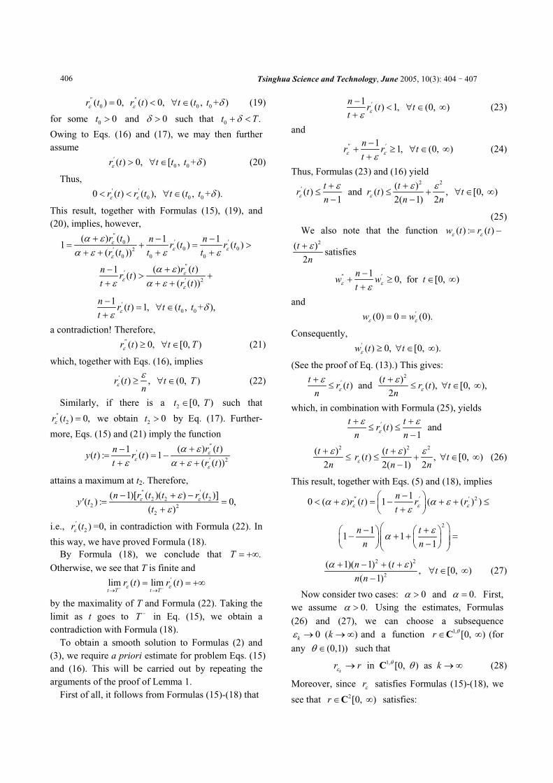
Tsinghua Science and Technology, June 2005, 10(3): 404 407406

00 0( ) 0, ( ) 0, ( , + )

" "r t r t t t t (19)

for some and 0

0t 0 such that0

.t T

Owing to Eqs. (16) and (17), we may then further

assume

0 0( ) 0, [ , + )

'r t t t t (20)

Thus,

0 0 00 ( ) ( ), ( , +

' 'r t r t t t t ).

This result, together with Formulas (15), (19), and

(20), implies, however,

0

0 02

0 0 0

( ) ( ) 1 11 ( ) (

( ( ))

"' '

'

r t n nr t r t

r t t t)

2

( ) ( )1( )

( ( ))

"'

'

r tnr t

t r t

0 0

1( ) 1, ( , + ),

'nr t t t t

t

a contradiction! Therefore,

(21) ( ) 0, [0, )"r t t T

which, together with Eqs. (16), implies

( ) , (0, )'r t t T

n(22)

Similarly, if there is a such that

we obtain by Eq. (17). Further-

more, Eqs. (15) and (21) imply the function

2[0, )t T

2( ) 0,

"r t2

0t

2

( ) ( )1( ) : ( ) 1

( ( ))

"'

'

r tny t r t

t r t

attains a maximum at t2. Therefore,

2 2 2

2 2

2

( 1)[ ( )( ) ( )]( ) : 0,

( )

" 'n r t t r ty' t

t

i.e., =0, in contradiction with Formula (22). In

this way, we have proved Formula (18).

2( )

'r t

By Formula (18), we conclude that .T

Otherwise, we see that T is finite and

lim ( ) lim ( )'

t T t Tr t r t

(18).

.

by the maximality of T and Formula (22). Taking the

limit as t goes T in Eq. (15), we obtain a

contradiction with Formula

to

To obtain a smooth solution to Formulas (2) and

(3), we require a priori estimate for problem Eqs. (15)

and (16). This will be carried out by repeating the

arguments of the proof of Lemma 1

First of all, it follows from Formulas (15)-(18) that

1( ) 1, (0, )

'nr t t

t (23)

and

11, (0, )

" 'nr r t

t (24)

Thus, Formulas (23) and (16) yield2 2

( )( ) and ( ) , [0, )

1 2( 1) 2

' t tr t r t t

n n n

(25)

We also note that the function ( ) : ( )w t r t2

( )

2

t

nsatisfies

10, for [0, )

" 'nw w t

t

and

(0) 0 (0).'w w

Consequently,

( ) 0, [0, ).'w t t

(See the proof of Eq. (13).) This gives: 2

( )( ) and ( ), [0, ),

2

't tr t r t t

n n

which, in combination with Formula (25), yields

( ) and1

't tr t

n n2

( )

2

t

n

2 2( )

( ) , [0, )2( 1) 2

tr t t

n n (26)

This result, together with Eqs. (5) and (18), implies

210 ( ) ( ) 1 ( ( ) )

" 'nr t r r

t'

2

11 1

1

n t

n n

2 2

2

( 1)( 1) ( ), [0, )

( 1)

n tt

n n (27)

Now consider two cases: 0 and 0. First,

we assume 0. Using the estimates, Formulas

(26) and (27), we can choose a subsequence

and a function (for

any

0k (k )1,

[0, )r C

(0,1)) such that

(28) 1,

in [0, ) ask

r r kC

Moreover, since r satisfies Formulas (15)-(18), we

see that 2[0, )r C satisfies:

LIU Qinghua ( ) et al Rotationally Symmetric Translating Solutions to 407

2

( ) 1( ) 1, (0, )

1 ( ( ))

r" t nr' t t

r' t t

'

(29) References

(30)(0) 0 (0)r r

[1] El-Fallah A I, Ford G E. On the mean curvature diffusion

in nonlinear image filtering. Pattern Recognition Letters,

1998, 19: 433-437.

and

(31)( ) 0, [0, )r" t t[2] Sochen N, Kimmel R, Malladi R. A geometrical frame-

work for low level vision. IEEE Transaction on Image

Processing, Special Issue on PDE Based Image Process-

ing, 1998, 7(3): 310-318.

To finish the proof of Lemma 2, we only need to

prove

(32)( ) 0, [0, )r" t t

In fact,

1(0) : lim (0) lim 1 (0)

k

" '

k kk

nr" r r

k

[3] Yezzi A. Modified curvature motion for image smoothing

and enhancement. IEEE Transaction on Image Processing,

Special Issue on PDE Based Image Processing, 1998,

7(3): 345-352.

[4] Aubert G, Kornprobst P. Mathematical Problems in

Image Processing Partial Differential Equations and

Calculus of Variations. New York: Springer-Verlag, 2002. 2

( ( (0)) ) .k

'k r

n[5] Huisken G. Non-parametric mean curvature evolution

with boundary conditions. J. Differ. Equations, 1989, 77:

365-379.

If there is a such that , then

Formulas (29) and (31) imply the function

3(0, )t

3( ) 0r" t

[6] Ecker K, Huisken G. Mean curvature evolution of entire

graphs. Ann. of Math., 1989, 130: 453-471. 2

1( ) : ( ) 1

( )

n rZ t r' t

t r

"

'

attains a maximum at the point t3. Thus,

3 3 3

3 2

3

( 1)( ( ) ( ))( ) 0,

n r" t t r' tZ' t

t

[7] Evans L C, Spruck J. Motion of level sets by mean curva-

tures. J. Diff. Geom., 1991, 33: 635-681.

[8] Chen Y G, Giga Y, Goto S. Uniqueness and existence of

viscosity solutions of generalized mean curvature flow

equations. J. Diff. Geom., 1991, 33: 749-786. which would yield in contradiction with

Eq. (26). Hence, Formula (32) has been proved.

3( ) 0,r' t

[9] Guan B, Jian H. The Monge-Ampere equation with

infinite boundary value. Pacific J. Math., 2004, 216(1):

77-94.Second, assume 0. Then we solve Eq. (2) to

get a function

2

( ) .2( 1)

tr t

n Obviously, this func-

tion satisfies the requirement of Lemma 2. In this way

we have proved the lemma.

Proof of Theorem 1 Theorem 1 is only the

combination of Lemma 1 and Lemma 2.

[10] Chan T F, Shen J, Vese L. Variational PDE methods in

image processing. Notices of the AMS, 2004, 50(1): 14-26.