Embed Size (px)
Citation preview

Roullier, Benjamin David (2017) Modelling the local environmental impact of underground coal gasification. EngD thesis, University of Nottingham.
Access from the University of Nottingham repository: http://eprints.nottingham.ac.uk/40878/1/Modelling%20the%20Local%20Environmental%20Impact%20of%20Underground%20Coal%20Gasification.pdf
Copyright and reuse:
The Nottingham ePrints service makes this work by researchers of the University of Nottingham available open access under the following conditions.
This article is made available under the University of Nottingham End User licence and may be reused according to the conditions of the licence. For more details see: http://eprints.nottingham.ac.uk/end_user_agreement.pdf
For more information, please contact [email protected]

MODELLING THE LOCAL ENVIRONMENTAL
IMPACT OF UNDERGROUND COAL GASIFICATION
BENJAMIN DAVID ROULLIER, MA. MEng.
Thesis submitted to the University of Nottingham
for the degree of Doctor of Engineering


i
ABSTRACT
Underground coal gasification (UCG) has the potential to access vast resources of
stored fossil energy in a safe, clean and environmentally sound manner. Previous
experiments have however led to concerns around surface subsidence, groundwater
pollution and water table lowering. These issues can be prevented through the use of
appropriate site selection and an understanding of the processes which cause these
effects. Numerical simulations provide a cost effective means of predicting these issues
without the need for costly and publically opposed field trials.
This work uses a commercially available discrete element code to simulate the coupled
thermal, hydraulic and mechanical phenomena which cause environmental damage.
Surface subsidence is predicted through the displacements of fully deformable discrete
elements separated by a network of fractures. The flow of groundwater through these
fractures is simulated in order to predict the effects of water table lowering and the
inflow of groundwater into the UCG cavity. Heat conduction from the cavity walls is
simulated using an explicit finite difference algorithm which predicts both thermal
expansion effects and the influence of temperature on rock material properties.
Comparison of results with experimental observations in the literature show good
agreement for subsidence and groundwater behaviour, while initial predictions for a
range of designs show clear relationships between environmental effects and operating
conditions. Additional work is suggested to incorporate groundwater contaminant
transport effects, and it is envisioned that the overall model will provide a valuable
screening tool for the selection of appropriate site designs for the future development
of UCG as an economically viable and environmentally sound source of energy.

ii
LIST OF PUBLICATIONS
Roullier, B.D., Langston, P.A., Li, X. 2015: Effects of Joint Geometry on the Modelled
Material Strengths of Rock Masses in the Distinct Element Method. In: Soga et al eds.
Geomechanics from Micro to Macro. CRC Press. pp 431-436.
Roullier, B.D., Langston, P.A., Li, X. 2016: Modelling the Environmental Impact of
Underground Coal Gasification. In: Proceedings of the 1st International Conference on
Energy Geotechnics. Kiel, Germany, 29-31 August 2016.
Proposed Publications
Roullier, B.D., Langston, P.A., Li, X: Influence of Fracture Geometry on Simulated
Rock Mass Material Behaviour.
This paper will present the theory, methodology and results of the simulated uniaxial
and biaxial rock mass compression testing procedures presented in chapter 4 of this
thesis. Additional discussions on the theory of interfacial behaviour and the process of
rock mass compressive failure will also be presented.

iii
ACKNOWLEDGEMENTS
I would like to take this opportunity to thank a number of people whose help, guidance,
patience and support were invaluable in the creation of this work.
Firstly, to my academic supervisors, Dr Paul Langston and Dr Xia Li, whose continued
support and guidance have been an inspiration throughout the creation of the thesis and
without whom this would never have been possible.
Second, I’d like to thank those colleagues and friends who kept me sane through it all.
In particular I’d like to thank Karen, Gary, Matt and Rachel for the endless discussions,
helpful distractions, long lunch breaks and buckets of coffee that have got me through
the past four years in one piece.
Finally, I’d like to thank those whose support and guidance over the past 27 years have
led to this point. To my father David, for his continual encouragement and optimism
on this and many other long journeys. To my grandfather Terry, for instilling in me the
love of science that got me to this point. To my grandmother Margaret, for always
taking an interest in my ramblings. Finally, and most importantly, to my wife Bethan,
without whose love, patience, care and occasional chastisement I’d never have got this
far in the first place. I love you, and I’m proud to call you my wife.
This thesis is dedicated to the memory of Tina Roullier.

iv
TABLE OF CONTENTS
Abstract i
List of Publications ii
Acknowledgements iii
Table of Contents iv
Glossary of Terms xii
Nomenclature xv
1. INTRODUCTION 1
1.1. BACKGROUND 2
1.1.1. Global Energy Demands 2
1.1.2. Energy Sources 3
1.1.3. Fossil Energy Resources 4
1.2. UNDEGROUND COAL GASIFICATION 6
1.2.1. Process Description 6
1.3. ADVANTAGES AND CHALLENGES OF UCG 8
1.3.1. Political Issues 8
1.3.2. Economic Issues 8
1.3.3. Social Issues 10
1.3.4. Technical Issues 11
1.3.5. Legal Issues 11
1.3.6. Environmental Issues 12
1.3.6.1. Global Environmental Issues 13
1.3.6.2. Local Environmental Issues 14
1.3.7. Geographical Considerations 17
1.3.8. Competing Technologies 18
1.3.9. Principal Challenges to Development 19
1.4. ENVIRONMENTAL MODELLING 20
1.4.1. Modelling Overview 20
1.4.2. Model Aims 21
1.4.3. Proposed Use of Model 22
1.5. THESIS OUTLINE 23

v
2. LITERATURE REVIEW 25
2.1. UNDERGROUND COAL GASIFICATION TECHNOLOGY 26
2.1.1. Gasification Chemistry 26
2.1.2. Cavity Growth Mechanisms 29
2.1.3. Gasifier Designs 30
2.1.4. Coal Chemistry 33
2.1.5. Coal Geology 35
2.1.6. Gasifier Operating Conditions 36
2.2. LOCAL ENVIRONMENTAL ISSUES 40
2.2.1. Surface Subsidence 40
2.2.1.1. Subsidence Mechanisms 41
2.2.1.2. Preventing Subsidence 43
2.2.2. Groundwater Pollution 48
2.2.2.1. Common Pollutants 49
2.2.2.2. Pollution Mechanisms 50
2.2.2.3. Preventing pollution 51
2.2.3. Water Table Lowering 55
2.2.4. Preventing Environmental Damage 56
2.3. UNDERGROUND COAL GASIFICATION FIELD TRIALS 58
2.4. UNDERGROUND COAL GASIFICATION MODELLING 63
2.4.1. Modelled Phenomena 63
2.4.2. Previous Models 65
2.4.3. Modelling Methodologies 68
2.4.3.1. Finite Difference Methods 68
2.4.3.2. Finite Element Methods 69
2.4.3.3. Computational Fluid Dynamics 69
2.4.3.4. Discrete Element Methods 70
2.4.3.5. Compartment Modelling 71
2.4.3.6. Stochastic Methods 72
2.4.3.7. Empirical Modelling 73
2.4.3.8. Combined Methods 73
2.4.4. Future Modelling Developments 74
2.5. INITIAL MODELLING DECISIONS 75
2.5.1. Modelling Assumptions 75
2.5.2. Software and Hardware Considerations 77
2.6. CONCLUDING REMARKS 80

vi
3. UNIVERSAL DISTINCT ELEMENT CODE METHODOLOGY 81
3.1. THE UNIVERSAL DISTINCT ELEMENT CODE 82
3.2. MECHANICAL CALCULATIONS 85
3.2.1. Mechanical Model Formulation 85
3.2.2. Mechanical Validation 90
3.2.2.1. Elastic Deflection Testing 90
3.2.2.2. Plastic Deflection Testing 92
3.2.2.3. Freefall Motion Test 93
3.3. HYDRAULIC CALCULATIONS 95
3.3.1. Hydraulic Model Formulation 95
3.3.2. Hydraulic Validation 98
3.3.2.1. Stress/Aperture Relationship Test 98
3.3.2.2. Flow/Pressure Relationship Test 100
3.4. THERMAL CALCULATIONS 102
3.4.1. Thermal Model Formulation 102
3.4.2. Thermal Validation 104
3.4.2.1. Fixed Temperature Conduction Test 104
3.4.2.2. Fixed Heat Flux Conduction Test 107
3.5. ADVANTAGES, CHALLENGES AND LIMITATIONS 109
3.5.1. Mechanical 109
3.5.2. Hydraulic 111
3.5.3. Thermal 114
3.6. CONCLUDING REMARKS 117

vii
4. SIMULATED LABORATORY SCALE COMPRESSION TESTING 118
4.1. THEORY AND BACKGROUND 119
4.1.1. Representing Rock Masses in the discrete element method 119
4.1.2. Axial Compression Testing 120
4.1.3. Simulated Testing 123
4.2. METHODOLGY OF SIMULATED TESTING 125
4.2.1. Model Design 125
4.2.2. Rock Mass Variations 128
4.2.3. Discrete Fracture Network Design 131
4.3. SIMULATED COMPRESSION TESTING RESULTS 134
4.3.1. Axisymmetric Results 134
4.3.1.1. Effects of Joint Pattern on Strength 135
4.3.1.2. Effects of Joint Pattern on Stiffness 139
4.3.1.3. Effects of Joint Pattern on Failure Criteria 139
4.3.1.4. Effects of Joint Pattern on Lateral Expansion 142
4.3.2. Plane Strain Results 146
4.3.2.1. Comparison of Axisymmetric and Plane Strain Results 146
4.3.2.2. Effects of Block Size on Mechanical Behaviour 149
4.3.2.3. Effects of Joint Material Properties on Mechanical Behaviour 152
4.4. MODEL VALIDATION 155
4.4.1. Comparison with Geological Strength Index 155
4.4.2. Comparison with Experiment 157
4.4.3. Repeatability Testing 158
4.4.4. Observations of Failure Behaviour 161
4.5. MODEL LIMITATIONS 163
4.6. PARAMETER SELECTION 165
4.7. CONCLUDING REMARKS 167

viii
5. MODEL DEVELOPMENT 169
5.1. MODEL STRUCTURE 170
5.1.1. Order of Operations 170
5.1.2. Data Requirements 172
5.1.3. Data Produced 173
5.2. MODEL GEOMETRY 174
5.2.1. Site Geometry 174
5.2.2. Block Geometry 176
5.2.3. Zone Density 178
5.3. MODEL PROPERTIES 179
5.3.1. Mechanical Properties 179
5.3.2. Hydraulic Properties 181
5.3.3. Thermal Properties 183
5.4. BOUNDARY AND INITIAL CONDITIONS 187
5.4.1. Mechanical Boundary Conditions 187
5.4.2. Mechanical Initial Conditions 188
5.4.3. Hydraulic Boundary Conditions 189
5.4.4. Hydraulic Initial Conditions 190
5.4.5. Thermal Boundary Conditions 190
5.4.6. Thermal Initial Conditions 191
5.5. MECHANICAL AND HYDRAULIC LOGIC 192
5.5.1. Termination Criteria 194
5.6. THERMAL MODELLING 197
5.6.1. Underground Coal Gasification Thermal Behaviour 197
5.6.2. Thermal Algorithm 199
5.6.3. Thermal/Hydraulic Coupling 204
5.6.3.1. Fluid Thermal Energy Storage 204
5.6.3.2. Thermal Convection 206
5.6.3.3. Effects of Groundwater on Cavity Wall Temperature 207
5.6.3.4. Temperature Dependent Fluid Properties and Boiling Effects 209
5.7. CONCLUDING REMARKS 211

ix
6. INTERNAL PARAMETER EFFECTS 213
6.1. INTRODUCTION 214
6.2. STANDARD MODEL 215
6.3. EFFECTS OF DISCRETE FRACTURE NETWORK DIMENSIONS 219
6.3.1. Discrete Fracture Network Region Height 219
6.3.2. Discrete Fracture Network Region Width 223
6.3.3. Discrete Fracture Network Joint Density 225
6.3.4. Discrete Fracture Network Joint Isotropy 227
6.4. EFFECTS OF COARSE REGION DIMENSIONS 229
6.4.1. Coarse Region Block Height 229
6.4.2. Coarse Region Block Width 231
6.5. EFFECTS OF MODEL WIDTH 234
6.6. EFFECTS OF ZONE SIZE 237
6.7. EFFECTS OF JOINT PROPERTIES 241
6.7.1. Joint Normal Stiffness 241
6.7.2. Joint Shear Stiffness 242
6.7.3. Joint Friction Angle 243
6.7.4. Joint Cohesion 245
6.7.5. Joint Dilation Angle 247
6.8. EFFECTS OF CONVERGENCE RATIO 249
6.9. CONCLUDING REMARKS 253
7. FIELD TRIAL STUDIES 254
7.1. INTRODUCTION 255
7.2. HOE CREEK 3 UNDERGROUND COAL GASIFICATION 259
7.3. JINCHUAN NICKEL MINE 267
7.4. ANGUS PLACE COLLIERY – SINGLE CAVITY 271
7.5. ANGUS PLACE COLLIERY – MULTIPLE CAVITIES 274
7.6. CONCLUDING REMARKS 278

x
8. SITE DESIGN STUDIES 280
8.1. INTRODUCTION 281
8.2. EFFECTS OF CAVITY GEOMETRY 282
8.2.1. Cavity Height 282
8.2.2. Cavity Width 286
8.2.3. Cavity Depth 289
8.2.4. Combined Geometric Effects 293
8.3. EFFECTS OF MECHANICAL PROPERTIES 295
8.3.1. Rock Mass Stiffness 295
8.3.2. Intact Rock Strength 297
8.3.3. Lateral Earth Pressure 298
8.4. EFFECTS OF HYDRAULIC PROPERTIES 298
8.4.1. Water Table Depth 300
8.4.2. Site Permeability 303
8.4.3. Cavity Operating Pressure 307
8.5. EFFECTS OF THERMAL PROPERTIES 309
8.5.1. Thermal Conductivity 309
8.5.2. Specific Heat Capacity 311
8.5.3. Thermal Expansion Coefficient 313
8.6. BEST PRACTICES GUIDELINES FOR SITE DESIGN 315
8.7. CONCLUDING REMARKS 317
9. CONCLUSIONS AND FURTHER WORK 319
9.1. CONCLUSIONS 319
9.2. SUGGESTIONS FOR FURTHER WORK 322
9.2.1. Short Term Goals 322
9.2.2. Long Term Goals 324
10. REFERENCES 326

xi
APPENDICES
A. UNIVERSAL DISTINCT ELEMENT CODE THEORY 351
A.1. MECHANICAL FORMULATION 351
A.1.1. Mechanical Calculation Cycle 351
A.1.2. Mechanical Timestep Determination 355
A.1.3. Adaptive Local Damping 357
A.2. HYDRAULIC FORMULATION 358
A.2.1. Hydraulic Calculation Cycle 358
A.2.2. Hydraulic Timestep Determination 363
A.3. THERMAL FORMULATION 364
A.3.1. Explicit Thermal Algorithm 364
A.3.2. Implicit Thermal Algorithm 367
A.3.3. Explicit Thermal Timestep Derivation 367
A.3.4. Thermal Zone Generation 368
A.3.5. Thermal Expansion 370
A.3.6. Temperature Dependent Fluid Properties 371
B. DERIVATIONS 372
B.1. STRESS/DISPLACEMENT RELATIONSHIPS 372
B.2. TEMPERATURE DEPENDENT MATERIAL PROPERTIES 375
B.2.1. Friction Angle 376
B.2.2. Cohesion 377
B.2.3. Tensile Limit 377
B.2.4. Normalised Properties 377
B.3. CONDUCTIVE/CONVECTIVE HEAT TRANSFER RATIO 378
B.4. CAVITY WALL TEMPERATURE DERIVATION 380
B.5. THERMAL PENETRATION LENGTH 388
C. GROUNDWATER CONTAMINATION MODELLING 390
xii
GLOSSARY OF TERMS
Axisymmetric – Assumption that a body is identical for all angles of observation
around a central rotational axis.
Block – Single, intact elements used to make up a rock mass in UDEC.
CBM – Coal Bed Methane. An unconventional fossil energy extraction technology
which captures methane released from cleats in underground coal.
CFD – Computational Fluid Dynamics. A branch of the finite element method used to
simulate fluid flow problems.
Chimneying – A form of subsidence in which a single cohesive pillar of earth
undergoes rapid failure.
DEM – Discrete Element Method. Numerical method for simulating the motion and
interaction of a number of independent particles which obey Newtonian mechanics.
DFN – Discrete Fracture Network. A method for stochastically producing sets of
fractures within a material.
Distinct Element Method – A particular form of discrete element method which uses
explicit time integration.
Domain – Discretised regions of fluid within UDEC.
Electrolinking – A method in which high voltages are used to break apart materials.
FDM – Finite Difference Method. Numerical method for simulating the behaviour of a
system at a given point in space/time via numerical integration of differential equations.

xiii
FEM – Finite Element Method. Numerical method for representing the behaviour of a
continuum by considering the forces and displacements on a number of mesh elements.
Fracking – Hydraulic fracturing. A method in which high pressure water is used to
break apart solid materials.
Gasification – Reactions which produce gaseous products from solid reactants.
Gridpoint – The name given to nodes in UDEC.
GSI – Geological Strength Index. Empirical measure of how the strength of a rock mass
relates to the strength of the individual rocks it contains.
Joint – Interfacial elements used to separate blocks and simulate sliding in UDEC.
Mesh – Representation of a continuous body as a number of small, interacting elements.
Mesh Element – The smallest individual region of a continuum model. State variables
are assumed to be constant within a single element.
MODFLOW – MODular finite difference FLOW. Commercial software for modelling
groundwater hydrogeology.
MT3DMS – Modular Transport, 3 Dimensional, Multi-Species Model. Commercial
software for modelling contaminant transport in groundwater.
Node – The vertices of a mesh element. The displacements of nodes determine the
deformation of a continuous body.
PFR – Plug flow reactor.
Plane Strain – Assumption that a material is identical at all points along its longest
axis. Assumption of zero strain in the direction of this axis.
Pyrolysis – Thermal degradation of complex materials into simpler components.

xiv
Reserve – The amount of a material known to exist within a specified area which can
be extracted in an economically viable manner.
Resource – The total amount of a material known to exist within a specified area.
Rock Mass – A large volume of a rocky material made up of a number of individual
rock blocks separated by joints or fractures.
RNG – Random Number Generator.
Shale Gas – An unconventional source of oil. Commonly referred to as fracking.
Spalling – Thermally driven process of mechanical breakage and collapse.
Stoping – A form of subsidence in which voids in a material continuously move
upwards through the material over time.
Syngas – An industrially useful mixture of gases, consisting mainly of carbon
monoxide, carbon dioxide, hydrogen and methane.
UCG – Underground Coal Gasification. An industrial process for converting coal into
syngas in-situ within an unmined coal seam
UCS – Uniaxial Compressive Strength.
UDEC – Universal Distinct Element Code. A commercially available two dimensional
distinct element code for simulating the behaviour of heavily jointed rock masses.
Zone – The name given to mesh elements in UDEC.

xv
NOMENCLATURE
A Area (m2)
B Zone Edge Length (m)
C Cohesion (Pa)
C Specific Heat Capacity (Jkg-1K-1)
D Depth (m)
D Diffusivity (m2s-1)
E Energy (J)
E Young’s Modulus (Pa)
F Flow Rate (mL/day)
F Force (N)
G Shear Modulus (Pa)
H Enthalpy (Jkg-1)
H Height (m)
K Bulk Modulus (Pa)
K0 Lateral Earth Pressure Coefficient (-)
L Length (m)
N Number (-)
P Perimeter (m)
P Pressure (Pa)
Q Specific Drawdown Rate (-)
Q Heat Flux in 2D (Wm-1)
R Rate of Consumption (kgs-1)
R Uniformly Distributed Random Number (-)

xvi
S Saturation (-)
S Subsidence (m) (-)
T Temperature (K)
U Heat Transfer Coefficient (Wm-2K-1)
V Volume per unit depth into page (m2)
W Width (m)
a Hydraulic Aperture (m)
g Acceleration due to gravity (ms-2)
k Stiffness (Nm-1)
k Generic Proportionality Factor (-)
m Mass (kg)
q Flow Rate Per Unit Depth Into Page (m2s-1)
r Radius (m)
s Separation (m)
t Time (s/days)
u Displacement (m)
v Velocity (ms-1)
x Horizontal Position (m)
y Vertical Position (m)
Δ Change/Increment (-)
α Linear Thermal Expansion Coefficient (K-1)
α Subsidence Factor (-)

xvii
β Contact Coefficient (-)
β Damping Factor (-)
γ Angle of Draw (o)
γ Poisson’s Ratio (-)
ε Strain (-)
θ Friction Angle (o)
κ Permeability (m2)
λ Multiplicative error factor (-)
λ Thermal Conductivity (Wm-1K-1)
μ Dynamic Viscosity (Pa s)
ρ Density (kgm-3)
σ Normal Stress / Strength (Pa)
τ Shear Stress / Strength (Pa)
ϕ Joint Angle (o)
ϕ Porosity (-)
ψ Dilation Angle (o)
SUBSCRIPTS
B Block/Bottom
C Compressive/Cavity/Coal
D DFN
F Fluid
G Gridpoint
H Hot

xviii
J Joint
L Lost
N Normal
O Oxidant
P Product
R Rock
S Shear/Steam
T Tensile/Thermal/Top
W Water
Z Zone
a Axial
b Background
c Cavity
e Extraction
f Formation
l Lateral
n Number
p Profile
r Reaction
s Surface
v Volumetric
w Wall
w Width
x Horizontal

xix
y Vertical
0 At Zero Stress/Initial
burn Combustion Zone
crit Critical
in Net Inflow
max Maximum
min Minimum
sat Saturated
tot Total
SUPERSCRIPTS
C Contact
D Damped
L External Load
P Pressure
T Thermal/Temperature
Z Zoneθ At Standard Conditions
ACCENTS
X̂ Unit value of variable X.
�̇� First time derivative of variable X.

1
1. INTRODUCTION
SUMMARY
Underground coal gasification (UCG) is an industrial process which converts coal
into an economically valuable synthesis gas consisting mainly of hydrogen, carbon
monoxide, carbon dioxide and methane in situ within an unmined coal seam. The
product gas can be used as a fuel for electricity generation or as a precursor to
synthetic liquid transport fuels and other chemicals. UCG is potentially safer, cheaper
and less environmentally damaging than traditional methods of coal utilisation, and
offers access to coal resources which would be uneconomical to extract using
conventional means. As with any energy extraction technology however, UCG has the
potential to cause environmental damage on both global and local scales.
The work presented in this thesis aims to further the understanding of the mechanisms
behind the local environmental impact of UCG, with the goal of predicting and
therefore preventing these issues in future operations. This chapter provides an
introduction to both the UCG process and the numerical modelling of environmental
issues. Information is given on the energy system as a whole, as well as the role of
UCG in that system. Various advantages and disadvantages of UCG are presented,
with a particular focus on local environmental issues. The application of numerical
modelling to these issues is discussed and the principal aim, objectives and design
considerations of the model produced in this project are outlined. Finally, this chapter
concludes with a brief outline of the remainder of the thesis.

2
1.1. BACKGROUND
1.1.1. Global Energy Demands
As of the year 2016, global primary energy consumption is at a record high of 155
million GWh/yr, and is increasing at a rate of approximately 1.5% per year (BP,
2016). The upward trend in global energy demand is the product of three key factors:
population, prosperity and energy efficiency. Prosperity has a strong effect on energy
demand as more prosperous groups tend to consume more energy per capita. As
global population and prosperity continue to grow, energy demands will continue to
increase. Improvements in energy efficiency can offset this increase; however
efficiency is ultimately limited by thermodynamic constraints. In order to meet
increasing global energy demands, new sources of energy must therefore be found.
Any energy source must address three key issues, collectively referred to as the
energy trilemma (World Energy Council, 2013a):
Price – New energy sources must be cheap enough to ensure continued access
at current levels, and allow for future increases in demand.
Security – Energy sources must be able to cope with changes in demand,
weather effects, fuel prices and national and international political issues.
Sustainability – Sources must operate without causing environmental damage
through greenhouse gas emissions, resource depletion etc.
Failure to meet any of the above issues can have severe economic, socio-political and
environmental implications on global, national and local scales. A number of potential
energy sources exist which can address these issues.

3
1.1.2. Energy Sources
All of the primary energy sources present on Earth can be classified either as
renewable or exhaustible. Exhaustible sources include coal, oil and natural gas.
Nuclear power is also exhaustible, however its use does not produce significant
greenhouse gas emissions compared to fossil fuels. Renewable sources include wind,
solar, geothermal and hydro power. Biomass is also considered renewable as the fuel
used can be regrown and greenhouse gas emissions effectively offset by this growth.
Table 1.1 highlights the key advantages and challenges of these sources with respect
to the energy trilemma.
Table 1.1 – Advantages and challenges of various energy sources. + implies an
advantage, - implies a challenge.
Exhaustible Renewable
Pri
ce
+ Cheapest energy prices
+ Established technologies
– Fuel price fluctuations
+ No fuel cost
– Large infrastructure requirements
– Currently very low capacity
Sec
uri
ty
+ Flexibility (transport or electricity)
+ Consistent power output
– Dependence on international trade
– Political uncertainty
– Seasonal variability
– Diurnal variability
– Storage requirements
– Geographically limited
Su
stain
ab
ilit
y
– Greenhouse gas emissions
– Air/water pollution
– Resource depletion
+ Near zero emissions
– Land usage

4
Table 1.1 shows that meeting the energy trilemma will be a considerable challenge, as
no single energy source can reliably address all three concerns. While electricity grids
may eventually run entirely on renewable sources, short term plans (i.e. those
involving the current generation of power plants) must include fossil fuels in order to
make up the shortfall in capacity while renewable sources are built. In addition, the
use of renewable energy for transportation is problematic due to the geographical
limitations of renewable energy sources. Renewable transport can be achieved
through electrification, however this further increases electricity demands and the
need for fossil fuels. In order to minimise the environmental impact of fossil fuel
usage, new technologies are required which can extract this energy in an
environmentally sound manner.
1.1.3. Fossil Energy Resources
This section gives a brief summary of global sources of fossil energy. Greater fuel
abundance is beneficial as it keeps prices low. On the other hand, large stores of fossil
fuels may promote the continued use of environmentally damaging sources of energy.
Figure 1.1 shows the total extent of various fossil energy reserves. Coal and shale oil
are seen to have greater reserves than other sources. It is of note that this figure lists
reserves, rather than resources. Reserves are as sources which can be economically
extracted using current technology, while resources are the total amount of fuel
known to exist. Taking unrecoverable resources into account, coal is seen to be the
most abundant fuel, with total resources of over 150 billion GWh (Self et al, 2012).
By comparison, oil and gas resources are estimated as 11.6 and 5.8 billion GWh
respectively (Brownfield et al, 2012; McGlade et al, 2012; Plummer et al, 2012).

5
Figure 1.1 – Total economically recoverable fuel reserves by region. The area of each
graph indicates the amount of energy available. After World Energy Council, 2013b.
As well as abundance, coal has a greater geographical diversity than other fuels. This
is beneficial for both price and security as it helps keep costs low and reduces the
impact of international politics on fuel supplies. On the other hand, coal has several
environmental issues. Coal emits more CO2 per unit energy than other fuels, as shown
in Table 1.2. Coal also has higher sulphur and particulate contents and a greater
number of inorganic contaminants than oil or gas (Kapusta & Stanczyk, 2011).
Traditional coal use is therefore seen to cause a number of concerns which must be
addressed in any future energy system. Underground coal gasification, especially in
concert with carbon capture and storage (CCS), is a technology with the potential to
address these concerns in a safe, cheap and environmentally sound manner.
Table 1.2 – CO2 emissions by fuel (US Energy Information Administration, 2016).
Fuel CO2 Emissions (t/GWh thermal)
Coal 319 – 354
Oil 244 – 250
Natural Gas 181 – 215

6
1.2. UNDERGROUND COAL GASIFICATION
Underground coal gasification (UCG) is an industrial energy extraction technology
with the potential to play an important role in future energy systems. UCG provides a
means by which a great deal of the world’s coal, including both proven reserves and
currently unrecoverable resources, could be used in a safe and economically viable
way. UCG presents a source of energy which is abundant, widely distributed, cost
effective and secure from the external influences of international politics, market
pressures and weather effects. Furthermore, the use of modern emissions reduction
technologies, including CCS, allows UCG to operate in a much more environmentally
friendly manner than traditional fossil energy technologies. Although coal is an
inherently dirty fuel with finite reserves, UCG has the potential to utilise this resource
in a way that many believe could provide an effective bridge to a future energy
system based entirely on renewables (Roddy & Younger, 2010).
1.2.1. Process Description
The process of underground coal gasification involves the partial combustion and
conversion of unmined coal within a coal seam into a synthesis gas (syngas)
comprised mainly of carbon dioxide, carbon monoxide, methane, hydrogen and water
vapour. Figure 1.2 depicts a typical UCG operation.

7
Figure 1.2 – Typical UCG operation. After Green, 2014.
UCG works by drilling two boreholes down into the coal seam and linking them
together to form a gas circuit. One of the boreholes (the injection well) is used to
supply air or oxygen and steam to the coal face, which is then ignited using a propane
burner in the drillhead to begin the gasification reactions. These reactions consume
the coal, converting it into a gaseous mixture of CO, CO2, H2 and CH4, as well as a
number of trace contaminants. The reaction set is autothermic and tends to occur at
temperatures in the range of 800°C to 1800°C (Higman & Van der Burgt, 2008).
Once this temperature is reached, the burner is shut off and the reaction becomes self-
sustaining. The gaseous products then flow along the channel until they reach the
second borehole (the production well) where they are extracted and processed for use
in electricity generation or chemicals production (Couch, 2009). As the underground
reaction proceeds, the coal on the inner wall of the cavity is consumed, causing the
reactor to expand outwards through the coal seam, continually accessing fresh coal.

8
1.3. ADVANTAGES AND CHALLENGES OF UCG
1.3.1. Political Issues
The principal political issues around UCG relate to its status as a fossil fuel
technology. In many developed countries, the continued development of fossil energy
sources is politically unpopular due to their environmental impacts. This issue is less
prevalent in developing countries as security of supply is often considered to be of
greater importance. UCG is also often confused with shale gas extraction and
hydraulic fracturing (fracking), which both have significant public opposition
(Challener, 2013). The political advantages of UCG are mainly driven by increases in
energy security. As shown in Figure 1.1, coal is by far the most geographically
diverse fossil fuel. This diversity reduces dependence on trade and allows many
nations a greater autonomy over their energy supply. This autonomy reduces the
impact of international conflict on national economies and thus increases stability.
1.3.2. Economic Issues
A key economic benefit of UCG is its ability to access coal reserves which would be
uneconomical using traditional means. UCG could potentially increase global coal
reserves by a factor of up to twenty, greatly surpassing both shale oil and shale gas
(Self et al, 2012). UCG is also an efficient method of extraction: Gasification
efficiency (the fraction of the energy in the coal recovered in the syngas) exceeds 75%
when oxygen is used as the injectant gas. Conversion efficiency (the proportion of the
coal’s mass converted to syngas) can be as high as 90% (Couch, 2009).

9
Other economic benefits of UCG arise because its simplicity reduces costs compared
with traditional coal use: Surface infrastructure such as coal washing facilities and
spoil tips are no longer necessary. Underground mine shafts are also not required, and
surface based gasification equipment is eliminated entirely. Furthermore, the transport
of gaseous fuels is easier and cheaper than that of coal, potentially allowing UCG
syngas to displace solid coal imports to countries without indigenous resources.
Because a UCG plant can be run by a small team of operators, overheads are
considerably lower than those of coal mines employing hundreds of miners. Not only
do these effects mean that UCG can generate larger profits for a given amount of coal,
they also allow for the profitable extraction of previously unviable coal seams. This
may allow UCG to operate in regions with large but uneconomically recoverable coal
resources, such as the UK, however socio-political constraints may prevent this. The
above effects suggests that UCG could provide electricity at a much lower cost than
other potential clean energy sources, as shown in Figure 1.3.
Figure 1.3 – Levelised cost of electricity in the UK for various clean energy
technologies. (Department of Energy & Climate Change 2012; Ferguson, 2015).

10
1.3.3. Social Issues
UCG has several social advantages over other extraction technologies, the greatest of
which is its safety compared with coal mining. In 2014, over 900 coal miners were
killed in China alone due to accidents (Lelyveld, 2015). Many miners also suffer long
term injuries and illnesses such as pneumoconiosis (black lung). Because UCG does
not require any workers to be sent underground, these hazards are eliminated,
potentially saving thousands of lives every year. These advantages also apply to other
dangerous methods of energy extraction such as offshore oil and gas drilling.
Other social advantages of UCG include the creation of jobs for skilled workers and
the potential economic benefits to economically deprived regions which previously
depended on coal mining, such as the North East of England. Furthermore, the
reduction in traffic, noise and dust compared with traditional coal mining can be seen
as socially beneficial. On the other hand, in regions with existing coal mining
industries, displacement by UCG could lead to the loss of a great number of jobs.
Finally, the potential environmental impacts of UCG and perceived uncertainties
around the technology may lead to reductions in property prices and considerable
public opposition (Shackley et al, 2006).
11
1.3.4. Technical Issues
The majority of the technical challenges of UCG are caused by the novelty of the
technology and the difficulty in understanding/monitoring the processes involved.
Because of the underground nature of UCG as well as the extremes of temperature
and pressure, much of what occurs in the reactor cavity is difficult and expensive to
measure or observe (Britten & Thorsness, 1988). This not only introduces
considerable difficulty in controlling the process but also makes it difficult to predict
any impact the operation may have on the local environment. Future development of
large scale commercial UCG may exacerbate this effect. Previous trials also had
issues creating the initial connection between the injection and production wells,
however modern operations solve this with the use of directional drilling techniques.
1.3.5. Legal Issues
Many of the legal issues of UCG relate to the novelty and uncertainties of the
technology. Legal issues also tend to be specific to certain nations/regions and may
have implications for international trade partners and countries bordering the target
nation. One particular legal issue in a number of nations is the lack of coherent
regulations regarding UCG. Due to the novelty of the technology, regulatory
frameworks may not yet be present, or may be unclear. In the UK for example, UCG
is overseen by the coal authority. Many of the technologies involved in UCG are
overseen by the oil and gas authority however, leading to conflicting regulations (UK
Oil and Gas Authority, 2015).

12
Other legal issues involve access rights to both the coal itself and the land above.
These issues depend heavily on whether the mining industry in the target country is
privatised or nationally owned. The legal implications of environmental damage also
present a challenge to the development of UCG. For example, laws in the UK prevent
the development of new coal fired power stations unless they are proved to be “CCS-
ready” (Carrington, 2009). The effects of UCG on groundwater also have implications
on local industries such as farms and mines, which depend on certain properties of the
water table. This issue also applies to other nearby energy extraction methods such as
hydraulic fracturing and coal bed methane (CBM) extraction, which both affect the
local water table (Cuff, 2013). Because of these issues, the governments of Scotland,
Wales and Queensland have each recently place moratoria on UCG (Queensland
Government, 2016; Scottish Government, 2015; Welsh Government, 2015).
1.3.6. Environmental Issues
Many of the challenges of UCG relate to the environmental concerns of the
technology. As with any energy extraction method, UCG has both local and global
environmental impacts. In comparison with traditional extraction methods however,
UCG also has several environmental advantages. These issues are summarised below.

13
1.3.6.1. Global Environmental Issues
The main environmental issues with coal are air pollution and greenhouse gas
emissions. As shown in Table 1.2, coal emits more CO2 per unit of thermal energy
than any other fuel. Coal combustion also releases many other compounds, including
sulphur and nitrogen oxides. These compounds both contribute to global warming and
lead to other environmental effects such as acid rain. Compared with traditional
extraction technologies however, UCG can greatly reduce these emissions for several
reasons.
First, because the product of UCG is a combustible gas, it can be used with efficient
combined cycle gas turbines (CCGTs). These turbines can have energy efficiencies of
up to 60% (Seebregts, 2010) compared with values of less than 40% for traditional
steam turbines (International Energy Agency, 2010). This greatly reduces CO2
emissions per unit of electrical energy from UCG compared with traditional coal
plants. Second, UCG reduces the need for many peripheral sources of CO2 emissions
associated with coal power. Because coal no longer needs to be transported, emissions
from transport and shipping are eliminated. In addition, the smaller surface facilities
of UCG reduce the emissions associated with construction.

14
Finally, UCG provides an ideal base for the development of CCS (Snape, 2013): The
high CO2 partial pressure of the syngas is beneficial for precombustion separation,
while the existence of an air separation unit on site (to provide oxygen for
gasification) greatly reduces the cost of oxyfuel capture (Thambimuthu et al, 2005).
Additionally, the cavity itself may provide storage space for some of the captured
CO2. This process is known as reactor zone carbon storage (RZCS) (Burton et al,
2006). RZCS reduces the cost of CCS by eliminating transport costs and using the
same wells that were used for gasification, reducing overall drilling costs. RZCS is
not suitable for all sites however, as it requires a certain geology and a cavity depth of
at least 800m to maintain CO2 in a supercritical state. In addition, the volume of the
CO2 under these conditions would be 5 times greater than that of the gasified coal
(Roddy & Younger, 2010), limiting the amount which can be stored. On the other
hand, UCG suitable coal seams tend to be located in regions with suitable geology for
CO2 sequestration (Walter, 2007), allowing for storage in other nearby sites.
1.3.6.2. Local Environmental Issues
One of the principal advantages of UCG is its reduced effect on local pollution
compared with traditional methods of coal utilisation. In addition to carbon and
hydrogen, coal contains many environmentally damaging impurities, including
sulphur, nitrogen, boron, lead and cadmium (Kapusta & Stanczyk, 2011). Traditional
coal mining brings these to the surface where they are often released into the
atmosphere or washed into rivers and lakes. By comparison, UCG leaves many of
these impurities underground. This both reduces the environmental impact of UCG
and the capital costs of ash clean up and storage.

15
As with any energy extraction method, UCG has a number of negative impacts on the
local environment. While leaving coal impurities underground reduces air pollution,
these impurities may instead migrate into local potable aquifers. This can contaminate
local water sources and pose health risks to local residents, flora, and fauna. The
conditions in the cavity also cause pyrolysis of coal, which produces additional
contaminants (Humenick, 1984). Modern UCG operations aim to avoid this issue
through good site selection. If possible, UCG operations are simply sited in coal
seams which are isolated from any potable aquifers. While this eliminates the issue of
contamination, it can have negative effects on the UCG process, as the presence of
water helps to control gasification. Situation near saline aquifers solves this by
supplying water that is already harmful to life, such that contamination is not an issue.
In cases where UCG operations must be sited near potable water sources,
contamination is addressed using the technique of sub-hydrostatic operation. In this
case, the cavity is operated at a pressure below the local hydrostatic pressure. This
causes groundwater to flow into the cavity rather than allowing contaminants to flow
out. This has been shown to greatly reduce contamination and has the additional
benefit of forming a steam jacket around the cavity, preventing valuable heat and
syngas from escaping into the overburden (Blinderman & Fidler, 2003). On the other
hand, unpredictable groundwater inflow rates can affect gas quality and make process
control difficult.

16
A second environmental issue, which may be caused by sub-hydrostatic operation, is
water table lowering. If the rate of groundwater drawdown is greater than the local
recharge rate, the level of the water table can be depressed. In some cases this can
cause an increase in water table depth of up to 25m, which could lead to local wells
and lakes drying out. (Lindblom & Smith, 1993). This may also exacerbate pollution
if the lowering causes the phreatic surface of water table to enter the cavity, allowing
pollutants to flow unimpeded into the vadose zone above the water table.
The final local environmental issue with UCG is surface subsidence. The removal of
large areas of coal causes stress on the overburden above the cavity. This stress can
cause the overburden to collapse, potentially damaging injection equipment and
blocking the flow of gases. This collapse can propagate to the surface, damaging
surface facilities and local buildings. In addition, the fracturing of rock strata can
increase overburden permeability, potentially exacerbating groundwater effects.
Figure 1.4 shows how these effects are interrelated.
Figure 1.4 – Schematic description of subsidence and water table lowering effects
caused by underground coal gasification. After Couch, 2009.
17
1.3.7. Geographical Considerations
As mentioned above, many of the issues of UCG are geographically specific. The
suitability of a given region for UCG depends on a number of factors, including:
The extent and quality of local coal resources.
The demand for gas, electricity and chemical products.
Political and public support/opposition to fossil fuel technologies.
The history of the region with UCG and other unconventional energy sources.
The main economic competitor for energy supply.
Local competition for coal resources.
Population density in targeted areas. Low populations greatly reduce the
danger associated with local environmental damage.
These issues make the development of UCG easier in some nations than others. Many
European nations, including the UK, have large coal reserves and high energy
demands which currently depend on imported gas. On the other hand, these nations
tend to have considerable public opposition to fossil energy sources. In addition, these
countries tend to be densely populated with a politically active populace. By
comparison, China and the USA have large coal reserves, high energy demands, large
sparsely populated regions and supportive political climates. The USA also has
extensive shale oil reserves however, which may be economically preferable to UCG.
Given these issues, nations including China, India, Canada and the USA are prime
targets for UCG. Australia was also considered a good target, however recent
opposition (Queensland Government, 2016) has reduced this support somewhat.

18
1.3.8. Competing Technologies
The main competitors to UCG can be classified into two groups, depending on
whether UCG is being considered for electricity generation or chemical production. If
used as a source of electricity, UCG’s main competitors are traditional fossil fuel
plants, wind and nuclear power. These technologies are more mature than UCG and
are currently much cheaper to operate. As the technology develops however, the price
of UCG is expected to fall sharply, such that the cost of electricity approaches that
shown in Figure 1.3. Although UCG will never compete environmentally with
renewable energy, it still provides a very promising ‘bridging’ technology towards a
renewable economy (Roddy and Younger, 2010). If UCG is used as a source of
chemicals, its main competitors are oil and gas (traditional and unconventional). As
mentioned in Section 1.3.7, UCG has a number of environmental advantages over
both traditional and unconventional fossil fuel sources. These advantages can partly
offset the increased cost of UCG in relation to these technologies. As such, the initial
development of UCG may be easier as a source of chemicals rather than electricity.
A potential issue of UCG is the energy content of syngas. UCG syngas has a gross
calorific value of 10 ± 4 MJm-3 compared with 37 ± 4 for natural gas (Blindermann &
Fidler, 2003). As UCG would eventually be cheaper than natural gas per MWh this is
not an issue for power generation, however it would affect the economics of syngas
transport for export purposes. The continued development of unconventional oil and
gas may also cause a reduction in the prices of these commodities, further reducing
the relative economic benefit of UCG. Given the cost of long distance fuel transport,
UCG may still be the best choice in regions with large coal and low oil/gas reserves.

19
A final advantage of UCG in comparison with other fossil energy sources is its
reduced resource competition. UCG can operate on coals which are too remote to be
recovered using traditional methods, and as such does not need to compete with other
users for the same coal seam. Coal bed methane operations can conflict with UCG
however, as this technology also targets deep coal seams. Resource competition
between these technologies may also be exacerbated by the requirement of CBM to
reduce groundwater pressure, potentially increasing the risk of contaminant escape
from any nearby UCG activities (Moran et al, 2013).
1.3.9. Principal Challenges to Development
As seen above, UCG has the potential to be a key part of the future energy system or
chemicals industry of many countries. It is seen however, that many challenges must
be overcome before this can become a reality. Most of the greatest challenges relate to
UCG’s potential for environmental damage and its competition with unconventional
oil and gas. Many of the political, social and legal issues are directly caused by these
concerns. Technical and economic issues also relate to environmental damage
because of the cost and difficulty in preventing these effects. As such, it is seen that
reducing the environmental impact of UCG is the largest obstacle to its commercial
development. While the global issues mentioned are serious problems, these are not
specific to UCG itself. Greenhouse gas emissions and related effects are endemic to
all fossil fuel technologies, and much research is currently underway to reduce these
effects. As such, this thesis focuses only on local effects relevant to UCG. Given the
difficulty in observing these effects, it is believed that gaining a better understanding
of the processes involved is an important first step towards reducing their impact.

20
1.4. ENVIRONMENTAL MODELLING
1.4.1. Modelling Overview
As previously mentioned, the behaviour of a UCG operation is difficult to observe
experimentally. The underground nature of the process makes direct observation
impossible, while the high temperatures involved preclude the use of many in-situ
monitoring techniques. In addition, the potential environmental impacts of UCG make
experimental field trials politically and publically unpopular. Finally, the costs
involved in performing trials prohibit their use in many studies. Because of these
issues, much of the current work on UCG is performed using numerical modelling.
Numerical modelling has several advantages and disadvantages compared with
experimentation. Modelling is considerably cheaper than experimentation and has no
negative effects which could concern the public. Numerical modelling also allows for
the evaluation of large numbers of potential sites with almost no increase in cost
compared to that of a single site. On the other hand, the accuracy and usability of any
numerical model is heavily limited by resources: Sufficient computational power,
adequate physical understanding and large quantities of measured data are required to
ensure model accuracy. In particular, a lack of relevant, accurate experimental data on
which to base and verify the model can seriously reduce its usefulness. In effect,
model accuracy is limited by the accuracy of the data used in its construction. Given
the issues inherent in field trials however, numerical modelling is often greatly
preferred for the analysis of UCG. The work presented in this thesis uses numerical
modelling in an attempt to predict and therefore prevent the local environmental
impacts of UCG, allowing for the safe design of future operations.

21
1.4.2. Model Aims
The principal aims of this model are to further the understanding of the local
environmental impacts of underground coal gasification, and to provide simple,
accurate and reliable predictions of these impacts for a range of potential gasifier
designs. The model aims to produce a predictive model of the following highly
coupled environmental concerns:
Surface subsidence due to the removal of underground material.
Contamination of groundwater by the products of gasifier operation.
Water table lowering due to excessive groundwater consumption.
In addition, the model aims to be general, as opposed to site specific, and to produce
results in under 24 hours when running on a standalone desktop PC. The runtime
requirement is considered necessary as it allows the model to be tested against
multiple potential site designs in a short time.
The environmental impacts above are driven by a combination of mechanical,
hydraulic, thermal and chemical processes. These processes are highly coupled and
occur over timescales ranging from milliseconds to days (Langland and Trent, 1981).
Because of these issues, any fully realised model of environmental impact would be
highly complex and would require a great deal of computational effort to simulate a
single cavity design. Given the time and resources available, such a model is outside
the scope of this project. In addition, this model would almost certainly fail to meet
the target of sub 24 hour operation. As such, a greatly simplified model is required.

22
1.4.3. Proposed Use of Model
Given its short runtime, simplicity, and site-generic nature, it is envisioned that the
model presented in this thesis will be used as a ‘first-pass’ screening tool for operators
to choose between potential site designs. The completed model would be used to
investigate the influence of a number of geological, design and operating conditions
on the local environmental impacts of UCG. Trends in results could be used to inform
site selection and operating procedures in order to prevent damage. Promising designs
would then be further investigated using more detailed analyses before final decisions
would be made.
23
1.5. THESIS OUTLINE
This thesis consists of nine chapters, including this introduction. The contents of the
remaining chapters are summarised below:
Chapter 2 – Literature Review. Covers the relevant literature on both the UCG
process and various aspects of environmental modelling. Outlines the choice of
modelling methodology used in this work.
Chapter 3 – Introduction to UDEC. Covers the theory behind the mechanical,
hydraulic and thermal modelling capabilities of the Universal Distinct Element Code,
as well as the advantages, challenges and limitations of the software.
Chapter 4 – Simulated Lab Scale Testing. Introduces the method of simulated
compression testing in UDEC. This novel methodology was used to help represent the
overburden above UCG cavities using a reduced number of discrete elements.
Chapter 5 – UCG Model Development. Shows the design decisions and additional
developments required to create the UCG model in UDEC. Initial validation of the
UDEC software is also presented in this chapter.
Chapter 6 – Internal Parameter Effects. Gives the results of a large number of tests
which were used to inform the selection of many internal (non-physical) parameters
used in the final model.

24
Chapter 7 – Field Trial Validation. Presents the results of validation studies in which
model results are compared to experimental observations from previous field trials.
Discusses the validity of the model and its applicability as a predictive tool.
Chapter 8 – Site Design Studies. Gives the results of a number of simulations of UCG
operations with varying geometric, geological and operating conditions. Identifies
trends in environmental effects based on these conditions and provides guidelines for
future operators.
Chapter 9 – Conclusions and Further Work. Summarises the work presented and
highlights the key observations made during the modelling process. Suggests future
developments in both the modelling and theoretical understanding of UCG.

25
2. LITERATURE REVIEW
SUMMARY
This chapter presents a review of the relevant literature published on the subjects of
underground coal gasification (UCG) and environmental modelling. The chapter
begins with an in-depth explanation of the UCG process, covering gasification
chemistry, cavity growth mechanisms, gasifier designs and the effects of coal
chemistry, site geology and operating conditions on UCG behaviour. The second part
of the chapter presents a detailed explanation of the three main local environmental
issues associated with UCG. The issues of surface subsidence, groundwater pollution
and water table lowering are presented in terms of the mechanisms driving these
processes, their effects on the local area, and the methods used to control and prevent
these issues. A summary of recorded UCG field trials is then given, with a particular
focus on the incidence of environmental damage caused by these trials.
The latter part of this chapter deals with the numerical modelling of the UCG process
and the local environmental effects it can cause. The principal physical processes
driving UCG are identified and the requirements for modelling these processes are
considered. A number of modelling techniques are presented which may be used to
simulate these issues and a summary of previous UCG modelling efforts is given.
Notable gaps in the modelling of UCG are identified and recommendations are made
for future efforts. Finally, the chapter concludes with a brief outline of the model
produced in this work and the initial decisions on the software and assumptions used
to create this model.

26
2.1. UNDERGROUND COAL GASIFICATION TECHNOLOGY
The basic principles of UCG are introduced in Section 1.2.1. This section gives a
detailed overview of the mechanics of UCG, especially where issues relate to the
potential for local scale environmental damage.
2.1.1. Gasification Chemistry
The process of coal gasification involves a complex, multi-step chemistry, as seen in
Figure 2.1. The main chemical reactions involved are listed in Table 2.1. The first step
of the process involves the drying of coal under the application of heat. Water trapped
in the coal is boiled off and provides an important reactant in later stages. After
continued heating, the process of pyrolysis begins. In this step volatile compounds are
driven out of the coal matrix to leave a fixed carbon char (Seifi et al, 2011). The
lighter compounds released are usually extracted with the syngas, while heavier
compounds remain in the cavity and can potentially lead to groundwater pollution.
The final three stages contain the reactions shown in Table 2.1. The combustion step
depletes the injected oxygen in a series of exothermic reactions which provide the
heat for the other stages. The gasification stage is largely endothermic and consists of
a number of solid/gas reactions which produce the syngas. Finally, the refining stage
alters the composition of the syngas. The final product composition can be set by
controlling the equilibrium of this step, either in the cavity or in a separate reactor on
the surface. Figures 2.2 and 2.3 show how syngas composition, temperature and
calorific value vary along the cavity for an air fed gasifier.

27
Figure 2.1 – Chemistry of the UCG Process.
Table 2.1 – Principal chemical reactions of UCG (Perkins & Sahajwalla, 2008)
Enthalpy values from Green & Perry, 2007.
No. Reaction Stage Enthalpy Change
at 1000K
(kJmol-1)
1 C + O2 CO2 Combustion -400
2 CO + ½ O2 CO2 Combustion -288
3 H2 + ½ O2 H2O Combustion -263
4 CH4 + 2 O2 CO2 + 2 H2O Combustion -825
5 C + 2H2 CH4 Gasification -102
6 C + CO2 2 CO Gasification +176
7 C + H2O CO + H2 Gasification +151
8 CO + H2O CO2 + H2 Refining -25
9 CH4 + H2O CO + 3H2 Refining +253

28
Figure 2.2 – Simulated variations in syngas composition as a function of length for an
air blown gasifier. After Perkins & Sahajwalla, 2008.
Figure 2.3 – Simulated variations in syngas temperature (solid line) and calorific
value (dashed line) as a function of length for an air blown gasifier. After Perkins &
Sahajwalla, 2008.

29
2.1.2. Cavity Growth Mechanisms
As gasification proceeds, material is continuously removed from the cavity wall as
coal is converted into syngas and ash. This process constantly exposes fresh coal,
driving gasification and increasing the size of the cavity. The rate at which growth
occurs is fundamental to UCG as it controls both product gas quality and quantity
throughout the life of the cavity. There are three principal mechanisms by which
cavity growth occurs; reaction, thermo-mechanical spalling and large scale collapse:
Reaction is simply the process by which coal at the wall is converted to gas and ash
which falls to the floor of the cavity and exposes fresh coal on the roof and walls.
Reaction growth is a uniform process which causes the cavity wall to retreat at a rate
of around 1cm/hr (Perkins, 2005). Spalling is a cyclic process in which the hot gases
inside the cavity induce a steep temperature gradient in the cavity wall. This
temperature gradient causes thermal stresses which lead to fracturing and cause pieces
of coal to fall into the cavity. This exposes fresh coal to the hot gases, beginning the
cycle again. Spalling is beneficial to UCG as it greatly increases the surface area
available for gasification and promotes reaction within the rubble bed, however the
spalling process itself is not well understood and spalling rates are often predicted
using empirical models (Camp et al, 1980; Thorsness & Britten, 1986). Large scale
collapse refers to roof and sidewall collapse caused by stresses in the coal near the
cavity. The existence of a void where there was once solid coal, coupled with
increased temperatures, causes large sections of coal/rock to fall into the cavity either
as rubble or as coherent blocks. Large scale collapse is to be avoided, as the blocks of
material can disrupt gas flow and their violent separation can exacerbate subsidence.

30
2.1.3. Gasifier Designs
Although the basic principle of UCG remain the same across all operations, factors
such as local geology and the desired end use of syngas give rise to a number of
gasifier designs, as shown in Figure 2.4.
Figure 2.4 – Typical UCG cavity layouts. After Couch et al, 2009.

31
The simplest design of UCG reactor is the linked vertical well (LVW) layout,
comprising a single pair of wells linked by a horizontal channel. Previous trials used a
number of techniques to form this channel, including reverse combustion, hydraulic
fracturing, explosive fracturing and electrolinking. Despite the high costs, modern
operations tend to use directional drilling as this is much more controllable. Once the
coal in the cavity is depleted, gasification ceases and a new pair of wells must be
drilled in order to continue.
The controlled retracting injection point (CRIP) techniques allows access to much
larger amounts of coal using only a single pair of wells (plus a vertical ignition well in
the case of parallel CRIP). The linear CRIP (L-CRIP) technique works by drilling a
single pair of wells several hundred metres apart. The injection well is deviated and
drilled horizontally through the seam to intercept the production well at its base. Once
the wells intersect, the injection point is retracted approximately 20m and gasification
started. Once the coal in the vicinity of the cavity is depleted, gasification is stopped
and the injection point is retracted a further 20m so that the process can be restarted in
fresh coal. This process can be repeated a number of times, allowing for the creation
of several UCG cavities from a single pair of wells (Thorsness & Britten, 1989). A
successful trial of this technique was recently performed at the Swan Hills site in
Canada (Green, 2015). In a commercial scale L-CRIP UCG facility, several CRIP
channels would be bored in parallel so that multiple cavities could be operated
simultaneously. As well as increasing production rates, this would give a tighter
control over product composition through the blending of multiple product streams. A
potential design for commercial scale L-CRIP UCG is shown in Figure 2.5.

32
Figure 2.5 – Proposed layout of a commercial scale, multiple cavity L-CRIP UCG
operation. After Couch et al, 2009.
Parallel CRIP (P-CRIP) is a similar method to L-CRIP, but in which two deviated
wells are drilled in parallel along the coal seam and intercepted with a single vertical
ignition well. Oxidant gases are injected along one of the wells and syngas withdrawn
via the other. As gasification proceeds injection and production points retreat and the
cavity grows in a similar shape to that of a traditional longwall mine. This method has
recently been trialled at the Bloodwood Creek UCG pilot in Queensland (Mallett,
2013).
Steeply dipping coal seams (i.e. seams with an inclination to the horizontal of 60° or
more) present an advantage in UCG operation in that the reaction’s natural propensity
to travel upwards causes the cavity to grow in the direction of further coal. In
addition, heavy pollutants flow downwards, away from the production well. This
technique also allows large deposits of coal to be gasified simply by using two wells
spaced a short distance apart (Friedmann et al, 2007). Two key disadvantages of this
design are its dependence on a certain geology and the potential to cause large
amounts of subsidence due to the height of the cavity.

33
Given the above issues, many operators believe that the CRIP process provides the
most viable technique for the commercial UCG (Couch, 2009). As such, the work in
this thesis focuses on the use of this technique, in particular the L-CRIP configuration,
and how the design and operation of the gasifier affects local environmental issues.
2.1.4. Coal Chemistry
One of the most important decisions in the design of a UCG operation is the location
of the coal seam to be gasified. As well as the economic and political reasons for
using a particular site, the chemistry and geology of the coal seam itself have a
number of impacts on UCG performance. In terms of chemistry, the two main factors
affecting UCG are the rank and grade of the coal.
Coal rank refers to the thermal maturity of the coal (the history of temperature and
pressure which produced the coal). As coal increases in rank its moisture content
decreases, while its carbon content and calorific value increase (Van Krevelen, 1993).
Higher ranked coals contain more energy but also produce more CO2. Low rank coals
contain large amounts of moisture which must be evaporated, reducing their energy
content. While conventional coal plants tend to use high rank coals, UCG can operate
as well, if not better, on low rank coals. Although the moisture reduces the coal’s
calorific value, it also reduces the need to supply water for hydrogen production. The
ability to use low rank coal allows UCG much greater economic flexibility than
traditional methods, however there are efficiency issues. As shown in Figure 2.1, the
energy for gasification is provided by combustion. Low rank coals provide less
energy and thus reduce the conversion efficiency of UCG (Hebden & Stroud, 1981).

34
A particular issue of coal rank in UCG is swelling. When heated, coal undergoes
processes which can lead to a change in density. During pyrolysis, reactions occur
which produce a semi-fluid material called metaplast. Bubbles of volatile material
form in the metaplast and cause the char to swell (Myongsook et al, 1989). Water
present in the coal reduces this effect by promoting crosslinking reactions within the
metaplast, leading to a smaller and more brittle char. As such, low rank coals tend to
shrink, while high rank coals swell (Solomon & Serio, 1993). Shrinking is beneficial
for UCG as swelling coals can block pores in the reactor, reducing efficiency. The
increased brittleness of shrinking coals also promotes spalling, improving gasification
rates (Anthony & Howard, 1976). The proclivity of a coal to shrink or swell is
measured by the coal button profile, which ranges from 0 to 9. It is recommended that
UCG should not be carried on coals with button profiles greater than 3 (Lavis, 2013).
Grade refers to the impurities present in the coal. These impurities are usually classed
either as volatiles (e.g. hydrogen sulphide, ammonia, benzene) or ash (heavy metals,
silicates, clay). Low grade coals have large amounts of impurities, increasing the risk
of pollution from their use (Neavel, 1981). As UCG leaves much of the heavy
contaminants underground, ash has less of an effect on UCG than on traditional coal
uses. Though high ash contents affect calorific values by displacing carbon, the ash
itself may act as a catalyst for gasification (Creedy et al, 2001). Volatiles may still
present an issue with UCG, however these may be easier to deal with than under
traditional combustion. As UCG predominantly takes place in a reducing atmosphere,
sulphur and nitrogen are released as H2S or NH3 rather than SO2, NO or NO2. While
these compounds still present environmental hazards, they are much easier to separate
out of the syngas (Green, 2013a).

35
2.1.5. Coal Geology
While coal chemistry is an important factor in UCG design, the local geology of the
coal seam and surrounding strata can be just as important. Table 2.2 shows how
various local geological conditions affect the performance of UCG.
Table 2.2 – Effects of coal seam geology on UCG performance.
Coal Seam
Characteristic
Advantages Disadvantages
Increased
Depth
- Higher operating pressures
- Reduced risk of subsidence
- Reduced resource competition
- Allows RZCS if below 800m
- Drilling costs
- Oxygen compression costs
Increased
Thickness
- Increased coal access
- Increased conversion
- Reduced heat loss
- Increased risk of subsidence
Increased Dip
Angle
- Enhanced cavity growth
- Tars flow away from surface
- Reduced resource competition
- Variable cavity pressure
- Difficult to control
- Increased risk of subsidence
- Usually found near faults
Increased
Overburden
Strength
- Reduced risk of subsidence
- Reduced risk of pollution
- Drilling costs
Increased
Overburden
Permeability
- Easier use of groundwater - Increased risk of pollution
Proximity to
Aquifers
(Potable)
- Allows use of groundwater
- Risk of quenching reaction
- Increased risk of pollution
Proximity to
Aquifers
(Saline)
- Allows use of groundwater
- Reduced risk of pollution
- Risk of quenching reaction
Proximity to
Faults & Mine
Workings
- None - Increased risk of subsidence
- Increased risk of pollution

36
It can be seen that many factors affect the economics and safety of UCG. As such,
legislators have produced guidelines for acceptable sites. In the UK, the Department
of Trade and Industry (now the Department for Business, Energy and Industrial
Strategy) sets the following criteria (Department of Trade and Industry, 2004):
Coal seam depth between 600 and 1200m.
Coal seam thickness greater than 2m.
Good availability of rock material data.
Horizontal distance of at least 500m from any faults or mine workings.
Vertical distance of at least 100m from any potable groundwater resources.
In addition, the UK environment agency has stipulated that carbon capture and
storage will be mandatory if UCG syngas is used for power generation, however this
requirement is relaxed for other syngas uses such as chemicals production
(Environment Agency, 2013).
2.1.6. Gasifier Operating Conditions
In addition to the properties of the coal seam itself, the economic and environmental
performance of a UCG site also depends on a number of operating decisions.
Essentially, there are six variables which can be controlled by the operator to affect
gasification (Mostade, 2013): Well separation length, cavity operating pressure,
oxidant composition, oxidant flow rate, oxidant/water ratio and channel spacing. The
effects of each of these variables are outlined below.
37
With linked vertical wells or steeply dipping coal seams, well separation length is
usually determined by geology. With CRIP UCG, separation length is a trade-off
between the amount of coal that can be gasified, the pressure drop through the cavity,
and the cost of drilling, which can be up to 70% of the total capital cost of UCG
(Green, 2013b). While longer channels allow more cavities from each pair of wells,
the increased length gives a greater risk of subsidence and higher compression costs.
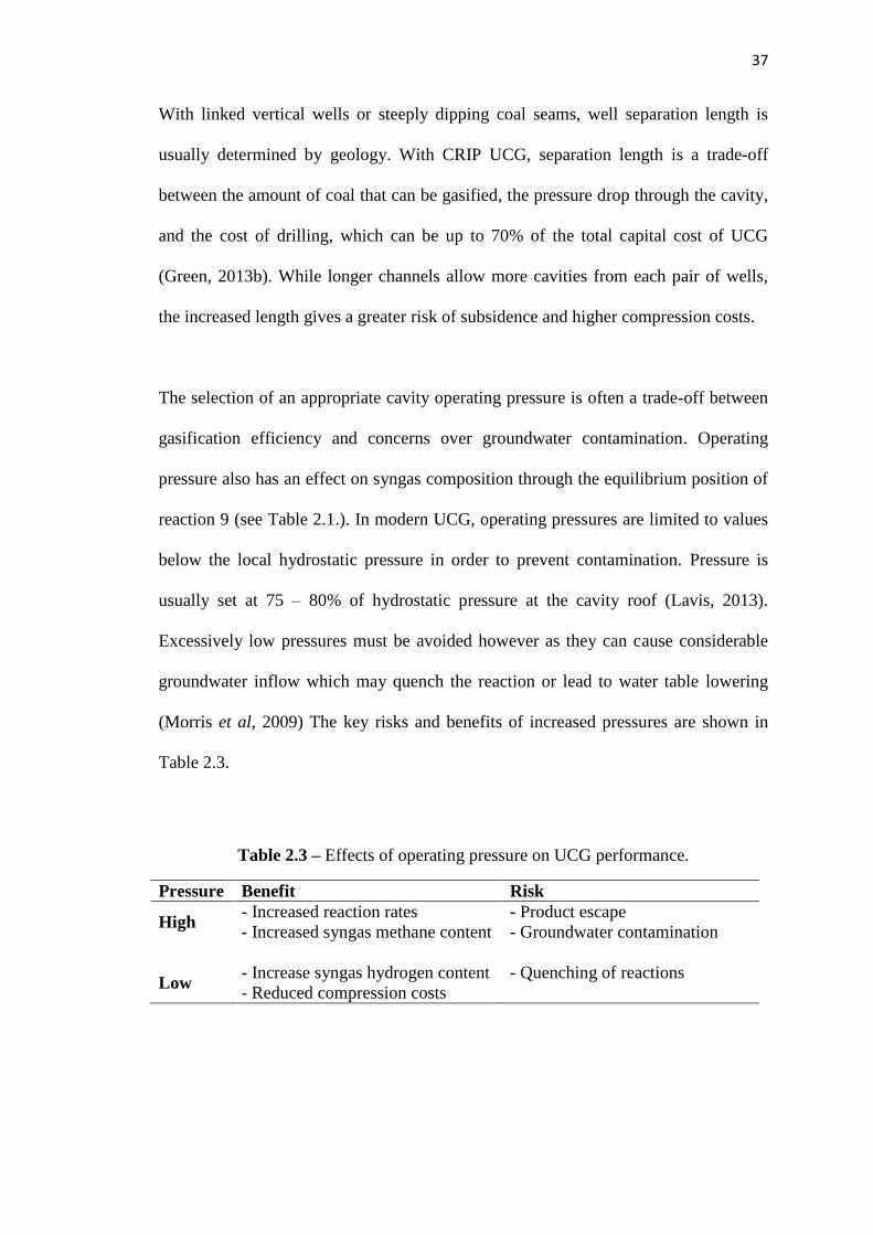
The selection of an appropriate cavity operating pressure is often a trade-off between
gasification efficiency and concerns over groundwater contamination. Operating
pressure also has an effect on syngas composition through the equilibrium position of
reaction 9 (see Table 2.1.). In modern UCG, operating pressures are limited to values
below the local hydrostatic pressure in order to prevent contamination. Pressure is
usually set at 75 – 80% of hydrostatic pressure at the cavity roof (Lavis, 2013).
Excessively low pressures must be avoided however as they can cause considerable
groundwater inflow which may quench the reaction or lead to water table lowering
(Morris et al, 2009) The key risks and benefits of increased pressures are shown in
Table 2.3.
Table 2.3 – Effects of operating pressure on UCG performance.
Pressure Benefit Risk
High - Increased reaction rates
- Increased syngas methane content
- Product escape
- Groundwater contamination
Low - Increase syngas hydrogen content
- Reduced compression costs
- Quenching of reactions
38
Oxidant composition refers to the choice of using either air, enhanced air or oxygen to
drive gasification. This choice is usually made on economic grounds and may vary
based on the intended use of the product gas. Using oxygen rather than air increases
the calorific value of the gas by eliminating diluent nitrogen. In addition, oxygen
fuelled combustion occurs at higher temperatures, driving the endothermic
gasification reactions and increasing syngas production rates. The elimination of
nitrogen is also beneficial for CCS, both increasing CO2 partial pressures and
allowing for oxyfuel combustion. On the other hand, excessive amounts of oxygen
can promote combustion over gasification, producing CO2 and H2O rather than CO
and H2. Finally, the capital and operating expenses of an air separation unit may
considerably increase the cost of UCG.
Oxidant flow rates are much simpler to choose. Low flow rates promote gasification
by more quickly providing a reducing atmosphere. On the other hand, low flow rates
reduce temperatures by limiting the combustion process. Excessively high flow rates
may simply cause the coal to combust rather than gasify. The rate of reaction in UCG
is dominated by the natural convection of gases to and from the cavity wall (Perkins
& Sahajwalla, 2008). As such, oxidant flow rate has little effect on the reaction
beyond stoichiometry and temperature control. This was confirmed by experiments at
the Centralia UCG trial (Burton et al, 2006). Given these considerations, the selection
of an appropriate flow rate is predominantly a matter of stoichiometry and flow rates
are generally selected in order to produce a desired syngas composition. The costs of
compression and air separation (where oxygen is used) may also affect this decision.

39
The oxidant/water flow ratio is one of the most difficult variables to control. Where
water is introduced artificially this can be achieved simply by altering flow rates.
Where groundwater influx is significant however, this becomes more challenging.
The rate of groundwater inflow is controlled by the operating pressure and as such
these two conditions are intrinsically linked. The major effect of the O2/H2O ratio is
its influence on product composition. Wetter ratios provide more hydrogen atoms,
increasing concentrations of H2 in the product. On the other hand, low ratios increase
water flow rates, leading to a cooling effect and inhibiting the endothermic
gasification reactions. Excessively high flowrates can quench gasification entirely,
producing a CO2 rich gas with low calorific value.
In commercial scale L-CRIP UCG, a number of cavities/channels would be drilled in
parallel within the same coal seam, as in Figure 2.5. A key design factor is how many
of these to drill, and how far apart to space them. The main factor determining the
number of channels is economics. More channels imply more coal, increasing
profitably and efficiency. On the other hand, drilling costs are one of the largest
expenses of UCG and the more channels drilled, the greater the expense (Bhutto et al,
2013). The spacing of channels depends on the local stratigraphy and the strength of
the coal and overburden rock. The sections of intact coal left between the channels are
known as ‘coal pillars’ and these act to support the weight of the overburden. The size
and location of these coal pillars, and hence the channels themselves, should be
designed to reduce subsidence (Couch, 2009).

40
2.2. LOCAL ENVIRONMENTAL ISSUES
As mentioned in Section 1.3.7.2, the greatest environmental concerns of UCG on the
local scale are surface subsidence, groundwater pollution and water table lowering.
These issues are heavily coupled and highly dependent on the geological conditions of
the gasifier. This section outlines the mechanisms behind these effects.
2.2.1. Surface Subsidence
Subsidence refers to a vertical movement of the ground’s surface which can affect
buildings, roads and utility pipes. Whenever a void is made in rock, the strata above
the void will deform due to a lack of support from the removed material. In UCG, the
strata are allowed to deform, leading to the collapse of the cavity and damage to the
overburden. If this damage extends to the ground’s surface, subsidence occurs. The
extent of subsidence depends on the geometry of the cavity and the material
properties of the overburden. The region of ground affected is called the subsidence
trough. The height of the trough is ultimately limited by cavity height, which in turn
depends on coal seam thickness. Trough width is defined by a constant angle of draw
between the excavation and the surface. Subsidence occurs to some degree above
almost all excavations, however disturbances of less than 20mm are generally
considered to be harmless (Mine Subsidence Engineering Consultants, 2007). In
addition to surface damage, the deformation of the overburden can also increase the
permeability of the rock mass and connect previously separate groundwater resources,
exacerbating groundwater pollution. This effect is explored in detail in Section 2.2.2.

41
2.2.1.1. Subsidence Mechanisms
While all cases of subsidence lead to vertical ground motion, there are four principal
mechanisms by which this motion occurs (Friedmann et al, 2008; Gregg, 1977):
Stoping is the method of subsidence commonly seen where excavations are performed
in brittle rocks with pre-existing fractures. As extraction continues, rocks fall into the
cavity to fill up the space left behind by the removed material. This in turn creates a
new void above the original which is later filled in by rubble from above. This process
continues over time, causing the void to migrate upwards through the overburden
(Hartman, 1992). Each successive void is smaller than the previous one however,
because of the phenomenon of bulking. This refers to tendency of solid materials to
expand in volume when they are broken up into rubble. The ratio of rubble to solid
volume is known as the bulking factor, and has a value of approximately 1.25 for
most rocks (Gregg, 1977). The void migration and bulking processes continue
upwards until the current void is not large enough to cause roof collapse (Friedmann
et al, 2008). Stoping subsidence can also be arrested when the void intersects a
particularly strong stratigraphic layer known as a spanning unit (Keilich et al, 2006).
Chimneying is a severe form of stoping in which large vertical motion occurs with
little or no bulking. This occurs either because the rock mass has a low bulking factor
or because the rubble is removed from the cavity. Chimneying is common in block
caving mines, where the rubble is intentionally removed in the mining process.
Chimneys can have diameters as low as 3m, but can extend vertically by over 300m in
a matter of days if the rubble is removed fast enough (Brady & Brown, 2005).

42
Bending subsidence is the mechanism seen most often where the overburden is ductile
or where very little fracturing is present. In this mechanism, overburden strata simply
bend under the weight of overlying rocks and sag into the cavity. Successive strata
then continue to bend and fill the space below, causing the subsidence trough to
migrate towards the surface. In many cases it is possible for several layered strata to
bend in concert, causing considerable subsidence regardless of the depth of the initial
void. Bending subsidence has little effect on rock fractures and is therefore unrelated
to issues of groundwater pollution or water table lowering (Kratzsch, 1983).
The final subsidence mechanism is that of plug failure. This is an extreme form of
subsidence in which the entire column of rock above a void fails en-masse and slides
into the void, often in a sudden and violent manner. Almost no bulking occurs in this
case, and the extent of surface subsidence is of a similar height to the initial void
itself. Plug failure is usually caused by planes of weakness within the overburden and
tends to occur in areas which have already undergone some degree of subsidence
(Brady & Brown, 2005)
Figure 2.6 shows the typical overburden behaviour above a UCG cavity. Thin seams
tend to subside via bending as gasification proceeds. Thicker seams tend to fail via
stoping, with the failed region extending to more than twice the cavity height above
the roof (Creedy et al, 2001). Chimneying and plug failure are observed in extreme
cases, such as the Hoe Creek 3 trial. (Ganow, 1984). Significant subsidence is rare
with UCG due to the typical geometry of the cavity. Where subsidence does occur, it
is usually caused by a combination of the stoping and bending mechanisms. As shown
in Chapter 5, it is these mechanisms that the proposed model attempts to simulate.
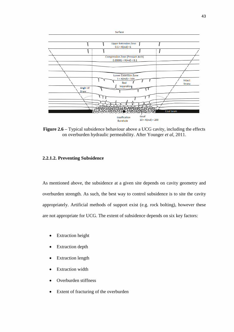
43
Figure 2.6 – Typical subsidence behaviour above a UCG cavity, including the effects
on overburden hydraulic permeability. After Younger et al, 2011.
2.2.1.2. Preventing Subsidence
As mentioned above, the subsidence at a given site depends on cavity geometry and
overburden strength. As such, the best way to control subsidence is to site the cavity
appropriately. Artificial methods of support exist (e.g. rock bolting), however these
are not appropriate for UCG. The extent of subsidence depends on six key factors:
Extraction height
Extraction depth
Extraction length
Extraction width
Overburden stiffness
Extent of fracturing of the overburden

44
Increases in extraction height cause greater surface subsidence by providing a larger
initial void. The relationship between height and subsidence is usually linear, and is
often expressed by means of a subsidence factor α. The subsidence factor is defined as
the ratio of surface subsidence to extraction height for a theoretically infinite cavity
(Brauner, 1973). Subsidence factors are measured experimentally and vary greatly
from site to site. Factors for UCG are commonly found to be in the range of 0.7 to 0.9
(Gregg, 1977).
The depth of a cavity below the ground’s surface has a strong influence over both the
vertical and horizontal extents of subsidence. Increases in depth greatly reduce
subsidence by introducing a larger amount of material above the cavity. This
increases the chance of encountering spanning units before subsidence reaches the
surface, and increases the effect of bulking. Increased depth also reduces the
possibility of connection with potable groundwater sources, because deeper aquifers
are more likely to be saline. Although greater depth reduces the magnitude of
subsidence, it can increase the area over which subsidence is observed. As mentioned
above, the horizontal extent of subsidence depends on the angle of draw γ. This is
defined as the angle between the horizon and an imaginary line drawn between the
edge of the cavity and the corresponding edge of the subsidence trough. The angle of
draw for UCG is around 35o (Brown, 2012). Figure 2.7 shows the effects of the angle
of draw on the subsidence trough.

45
Figure 2.7 – Effects of cavity geometry on subsidence. After Brauner et al, 1973.
Extraction length and width have an effect on both the vertical and horizontal extent
of subsidence. Due to the increased size of the void, larger cavities lead to more
subsidence as more bulking is required to halt the stoping process. Larger voids also
exacerbate bending subsidence by allowing larger sections of the overburden to sag
into the cavity. These effects are often in opposition to those of increased depth. As
such, many empirical methods relate the subsidence factor α to the ratio of W/D
(Keilich et al, 2006; Langland & Trent, 1981).
Increasing cavity size also affects both the size and shape of the subsidence trough.
As shown in Figure 2.7, the width of the trough depends directly on the width of the
cavity. The shape of the trough however, depends on the relationship between cavity
width W and the critical radius rcrit, given in Equation 2.1. The effect of the critical
radius on trough shape is shown in Figure 2.8.
𝑟𝑐𝑟𝑖𝑡 = 2𝐷 cot(𝛾) (2.1)

46
SUBCRITICAL EXTRACTION
CRITICAL EXTRACTION
SUPERCRITICAL EXTRACTION
Figure 2.8 – Effects of cavity width on subsidence profile shape.

47
The effects of overburden material properties on subsidence are simpler to explain.
The stiffness of the overburden is strongly related to the mechanism of bending
subsidence. According to classical beam theory, stiffer strata (effectively acting as
beams) deform to a lesser extent under a given force than softer beams. As such,
stiffer strata lead to less subsidence for a given cavity geometry. Other material
properties of the beam, such as cohesive strength, are irrelevant unless the force on
the beam is large enough to cause brittle failure of the strata. Such a failure is usually
pre-empted however, by failure along existing fractures which are much weaker than
the rock matrix. As such, the degree of fracturing is an important parameter.
Heavily fractured strata contain more planes of weakness than lightly fractured strata.
As such these are more prone to brittle failures, including the separation of discrete
blocks of material from the overburden (i.e. stoping). Therefore the degree of
overburden fracturing is seen to be strongly related to the mechanisms of stoping and
chimney/plug failure. Unlike stiffness, the degree of fracturing of a rock mass is
difficult to quantify. In many cases, empirical measures such as the disturbance factor
(Hoek et al, 2002) are used to represent fracturing in a qualitative manner.
As shown in this section, subsidence above a UCG cavity depends greatly on the
geometry and geology of the cavity. In all cases, these can only be realistically
controlled by the selection of an appropriate site for UCG operation. This site must
contain a coal seam deep enough that there is sufficient overburden to arrest the
stoping and bending processes before they reach the surface. In the case of stoping,
the depth must also be sufficient to ensure the process is stopped before it intersects
any potable groundwater resources.
48
Modern operations suggest UCG should only be performed at depths greater than
300m, leaving at least 150m of undisturbed overburden between the surface and the
roof of the caved zone (Mallett, 2006). The overburden must also be sufficiently stiff
and undisturbed. The influence of cavity length, width and height must be considered,
however the reduction of these dimensions is undesirable due to their influence on
UCG economics.
Given these observations, it is clear that site selection is the most powerful tool for
reducing surface subsidence above UCG cavities, but that the effects of site selection
on other environmental and economic issues should also be considered. The effects of
site geometry, geology and operating conditions on environmental issues are
investigated in detail in Chapter 8. The effects of such properties on the economic
performance of UCG have been considered by many authors, as shown in Table 2.2.
2.2.2. Groundwater Pollution
As previously mentioned, UCG has the potential to cause pollution of local
groundwater resources. A number of pollutant species may be present in the coal
seam, or may be generated by pyrolysis. Several mechanisms exist by which these
species can migrate into groundwater and these may lead to a number of detrimental
effects on local groundwater. This section outlines the common pollutants seen with
UCG, their typical methods of groundwater entry and the effects of various geological
and operating conditions on groundwater pollution.

49
2.2.2.1. Common Pollutants
The contaminants present in groundwater polluted by UCG can be broadly classified
into two groups: coal impurities and pyrolysis products. Coal impurities represent the
species present in the coal which are not converted by the gasification process.
Common impurities include sulphates, ammonium salts, heavy metals and
aluminosilicates. Many of these compounds are incombustible and therefore remain in
the UCG cavity as ash after gasification ceases (Blinderman & Fidler, 2003).
Pyrolysis products are organic compounds liberated by the thermal degradation of
coal during the UCG process. These compounds may have been trapped in the pore
spaces of the coal matrix or may have been produced through chemical reaction under
heating (Seifi et al, 2011). Pyrolysis products include short chain hydrocarbons,
phenols, polyaromatic hydrocarbons (PAHs), heavy hydrocarbon tars and BTEX
compounds (benzene, toluene, ethylbenzene, xylenes) (Kapusta & Stanczyk, 2011).
The identities and concentrations of species present in UCG contaminated
groundwater depend greatly on the rank and grade of the coal used, the composition
of the groundwater and the operating temperature and pressure of UCG process
(Humenick, 1984). The concentrations present also depend on the solubility of the
compounds in water and the environmental persistence of the contaminant species. As
well as affecting the amounts present, these factors can affect how long a contaminant
stays in the groundwater and how far from the gasification cavity it travels in that
time. These factors, along with human and environmental toxicity, determine the
impact of groundwater contamination on the local environment.

50
2.2.2.2. Pollution Mechanisms
The pollutants released by UCG primarily enter groundwater resources through one of
three mechanisms (Burton et al, 2008; Self et al, 2012). Firstly, high operating
pressures and steep thermal gradients can drive product gases into the surroundings,
where they later cool and condense within the pore spaces of the rock. Local
groundwater flows can then dissolve the contaminants or wash them into nearby
aquifers. Second, after UCG has finished, the cavity may fill with groundwater.
Pollutants adsorbed on to the cavity wall and trapped within the pore spaces of the ash
and rubble zones will then be leached out into this water. Over time the natural flows
of the groundwater, coupled with the diffusion of the contaminants, can cause the
pollutant species to migrate towards sources of potable water. The first mechanism
tends to cause pollution in the short term (during or shortly after gasification), while
the second occurs on a longer timescale (Blinderman & Fidler, 2003).
Finally, as mentioned in Section 2.2.1, the deformation of the overburden due to
stoping and cavity collapse can exacerbate pollution. This occurs when the enhanced
fracturing of the overburden creates a flow pathway between the cavity (the pollutant
source) and a previously unconnected potable aquifer (the pollutant receptor). This
method can cause considerable increases in pollutant concentrations in a very short
time. This effect may also occur where production and injection wells are not
correctly cased, allowing product gases to migrate up the sides of the well to impact
aquifers several hundred metres above the cavity (Humenick, 1984).
51
Once contaminants have entered the groundwater, their concentrations vary with
space and time. Contaminants are transported away from the cavity by diffusion and
advection. Note that in the case of advection, net groundwater flow into the cavity
acts to slow the spread of contamination rather than contributing to it. The effects of
advection also vary depending on the stage of the gasification process due to changes
in operating pressure (Lindblom, & Smith, 1993). Contaminant concentrations
decrease over time due to the processes of adsorption, ion exchange, precipitation and
biological conversion. Adsorption is a key mechanism in this process, as some species
adsorb well enough on to the rock for the groundwater to be considered free from
their presence (Stuermer et al, 1982). Biological conversion is the only process which
destroys contaminants outright, however it can also provide a means for them to enter
the food chain (Humenick, 1984). The efficacy of these processes varies between
species, leading to considerable variations in contaminant persistence between sites.
2.2.2.3. Preventing Pollution
As seen above, groundwater pollution depends on the processes of contaminant
generation, destruction and transport. The control of pollution can be achieved either
by curtailing generation and transport, or by enhancing destruction. The control of
contaminant generation is problematic, as the chemical processes which drive
generation are the same as those which produce the syngas. As such, slowing these
processes may be economically unviable. The use of high grade coals reduces
contaminant generation somewhat, though the availability of these coals may restrict
this approach. Coal rank may also affect contamination, as high ranked coals tend to
produce more pyrolysis products than low ranked coals (Kapusta & Stanczyk, 2011).

52
Contaminant destruction processes are often difficult, if not impossible, to control
during the gasification process. The mechanisms of destruction depend heavily on the
local geology, geochemistry and geobiology of the UCG site. The only realistic
method for enhancing these processes during gasification is simply to site the
operation in a location with suitable properties. On the other hand, natural destruction
processes occur on a much longer timescale than that of a typical UCG operation.
Natural pollutant removal can take up to 30 years from the onset of contamination
(Nathanail & Bardos, 2004), compared with UCG operating timescales on the order of
months. Enhanced contaminant destruction processes such as air sparging and
bioremediation could be applied after gasification has finished, however this would
imply that pollution is initially allowed to happen. Such measures would therefore be
politically, economically, ethically, socially and legally unpopular.
The most promising methods of pollutant control involve the alteration of
contaminant transport processes. During gasification, trapping the contaminants
within the cavity (e.g. by operating at sub-hydrostatic pressures) prevents their spread
into the groundwater. Some species may then be destroyed by combustion within the
cavity, or may be entrained in the syngas and brought to the surface where they can be
treated. Heavy and incombustible species remain in the cavity during this process, but
can later be removed through artificial means. The discussion of contaminant
transport must therefore consider the control of groundwater flow both during and
after gasification.

53
The control of contaminant transport during gasification is most easily achieved
simply by locating the UCG cavity sufficiently far away from any potable
groundwater sources. If the operation can be sited in a region which is completely dry,
or in which groundwater sources are already unpotable, then the migration of
contaminants poses no environmental danger. It is of note however that contamination
of land, even in inhospitable locations, may still have political implications. Where a
potable aquifer is present, transport can be avoided by ensuring that no flow pathways
connect the aquifer to the coal seam. This is usually achieved by siting UCG in deep
coal seams with aquitards present between the coal seam and the aquifer. It is
important however that these aquitards are not compromised by the fracturing
processes driven by UCG.
Where the above methods are not possible, contaminant transport can generally be
controlled by reducing the operating pressure of the cavity. By operating below local
hydrostatic pressure, a negative hydraulic gradient is formed, causing groundwater to
flow into the cavity rather than allowing pollutants to flow out. This sub-hydrostatic
operation can have unintended consequences on syngas production however, as
explained in Section 2.1.6. In addition, sub-hydrostatic operation can lead to the
depletion of local water resources, explained further in Section 2.2.3. Finally, because
hydrostatic pressure increases with depth, operating pressure must be lower not only
than that at the roof of the cavity but also that in any connected fractures within the
overburden. As this is difficult to measure, many operators set an upper limit on
operating pressure of 80% of hydrostatic pressure at the cavity roof (Lavis, 2013).

54
Control of contaminant transport after gasification ceases has the aim of removing
pollutants from the cavity before they can spread into the overburden. This is most
commonly achieved using the ‘clean cavern concept’ (Dennis, 2006). This involves
flushing the cavity through with large quantities of injected steam, water and nitrogen
to cool the cavity and halt pyrolysis. This cooling effect is required as, left unchecked,
the UCG cavity could remain hot enough to drive pyrolysis for a number of years.
This heat may also cause cavity pressures to increase above hydrostatic pressure
through the evaporation of pore water (Sarhosis et al, 2013). While flushing proceeds,
the cavity is allowed to vent continuously through the production well. This ensures
cavity pressures remain sub-hydrostatic, and brings the contaminants trapped in the
cavity to the surface where they can be processed. Once flushing is complete, the
wells are sealed and the cavity may be filled with cement or drilling mud in order to
prevent further groundwater motion (Burton et al, 2006). While this is effectively a
remediation process (as opposed to prevention), in concert with sub-hydrostatic
operation it is seen to greatly reduce the risks and extent of groundwater
contamination (Blinderman & Fidler, 2003; Sarhosis et al, 2016).
As seen above, the main techniques for preventing groundwater pollution are sub-
hydrostatic operation and the post gasification flushing of the cavity. Site selection is
also important, as locating a UCG operation far from potable water sources is
guaranteed to limit pollution. The influence of site selection on rock mass
deformation also has a secondary effect on pollution through permeability
enhancement. In summary, while operating conditions and processes may limit
pollution, appropriate site selection to avoid potable groundwater resources and
highly permeable overburden is still the best method for preventing it entirely.

55
2.2.3. Water Table Lowering
The final environmental concern of UCG is that of water table lowering. This refers to
an increase in the depth of the water table in the region of the UCG cavity. This
increase in depth may cause local wells to dry up and reduce water levels in lakes and
streams. The greater depth of the water table also leads to a reduction in hydrostatic
pressure at a given depth. This may exacerbate groundwater pollution issues unless
operating pressures are also reduced to maintain sub-hydrostatic operation. This effect
is greatly complicated by the presence of other nearby UCG cavities, as the reduction
in pressure caused by one operation can cause unforeseen circumstances at another.
Related extraction technologies such as coal bed methane may also contribute to this
issue (Moran et al, 2012). Finally, the downward motion of groundwater caused by
water table lowering can produce a suction force on the rock above, potentially
contributing to surface subsidence (Vorobiev et al, 2008).
As mentioned in the previous section, water table lowering is caused by the sub-
hydrostatic operation of UCG cavities. As such, the easiest way to combat this issue is
to remove the need for such operation. Locating the cavity far from any groundwater
resources is the most effective way of doing this. In many cases however, this is not
practical. An alternative method would be to site the UCG operation near a saline
aquifer, or a potable aquifer which is not currently being accessed by any other users.
Unlike subsidence and pollution, the effects of water table lowering are reversed soon
after gasification ceases (Lindblom & Smith, 1993). As such, provided that these
issues do not occur, the long lasting effects of water table lowering are minimal. In
cases where this is not possible, control of lowering can be difficult.

56
The rate of water table lowering is effectively a balance between the rate at which
water is drawn into the cavity (drawdown rate) and the rate at which it is replenished
by natural flows (recharge rate). As recharge rate cannot realistically be controlled,
the only method to reduce water table lowering is to control the drawdown rate.
Drawdown rate is primarily controlled through the operating pressure of the cavity.
The considerations of operating pressure on water table lowering are the same as
those for groundwater contamination, however there is the added complication that
both effects must be managed simultaneously. This effectively limits the range of
pressures at which UCG can safely occur, as excessively high pressures will lead to
contamination while excessively low pressures will lead to lowering of the water
table. The actual value of the pressures allowed would depend on the current height of
the water table above the cavity. This, coupled with the difficulty in measuring water
table heights and composition in real time, would make the selection of operating
pressure a highly complex matter. In addition, any increase in fracturing caused by
UCG would further complicate this matter by increasing the permeability of the
overburden. As such, site selection is seen to be the best way to combat drawdown
effects, with pressure control providing a potential, if difficult, second option.
2.2.4. Preventing Environmental Damage
As seen above, the best way to prevent environmental damage in UCG is through
appropriate selection of the operating site and cavity pressure. Any UCG site should
meet the following criteria in order to prevent this damage:

57
Cavity depth must be sufficient to reduce the effect of stoping and strata
bending to prevent subsidence. Recent publications suggest a minimum depth
of at least 300m (Mallett, 2006; Sarhosis et al, 2016). Other authors suggest
ranges of 150-500m (Couch, 2009) or 600-1200m (Bhutto et al, 2013).
Cavity overburden must be sufficiently strong to arrest subsidence, preventing
surface deformations of more than 20mm (Mine Subsidence Engineering
Consultants, 2007). Strata must be strong enough to provide at least 150m of
undisturbed rock above the fractured zone (Mallett, 2006).
Wherever possible, UCG operations should be located far from potable
aquifers to prevent contamination. In cases where aquifers overlay the coal
seam, the two strata should be separated by an aquitard layer. The minimum
vertical separation between the strata has been suggested as 40-60m (Younger,
2011) or over 100m (Bhutto et al, 2013)
Cavity operating pressures should be set at a value lower than the local
hydrostatic pressure at the highest point in the fractured zone above the cavity
(Lavis, 2013), but high enough to prevent excessive groundwater inflow.
As seen, the issues of local environmental damage are both complex and highly
coupled. As such, modelling and experimental work is required to improve our
understanding of these effects and ensure future operations do not cause damage.
Despite these issues however, the majority of previous UCG trials have been shown to
give little or no long term environmental damage, as shown in the following section.

58
2.3. UNDERGROUND COAL GASIFICATION FIELD TRIALS
The idea of UCG was first proposed in 1868 (Siemens, 1868), however the first trial
did not take place until 1912. This trial was abandoned however, due to the outbreak
of World War 1 (Klimenko, 2009). No further developments in UCG occurred until
the Soviet Union began their own program in the 1930s. Eight trials were performed
in the USSR between 1933 and 1961, culminating in the development of the
Yerostigaz plant in Uzbekistan which is still operational today (Yerostigaz, 2014).
Much of the theory and technology of modern UCG was developed in the USA during
the 1970s and 1980s at the Lawrence Livermore National Laboratory (LLNL)
(Friedmann et al, 2006). LLNL continues to perform research into UCG in the
modern day (Wampler, 2012). In the late 2000s a number of UCG trials were
proposed in Europe, Australia, Canada and South Africa (Bhutto et al, 2013; Swan
Hills Synfuels, 2012; Underground Coal Gasification Association, 2011). In recent
years however, commercial secrecy, environmental issues, political uncertainty and a
low oil price have reduced interest in UCG. These issues led to the cancellation of the
Mecsek Hills trial (Dodson, 2014), the dissolution of the UCG association (Fergusson,
2015) and the liquidation of Linc Energy (Linc Energy, 2016).
Table 2.4 lists known UCG trials. Other trials exist, particularly in China, but little
published information is available for these. Trials are currently planned in the UK
(Green, 2015), South Africa (Brand. 2014) and China (ENN, 2014). Many of these
trials have recently been cancelled however, due to the political, environmental and
financial concerns mentioned above.

59
Table 2.4 – UCG Field trials to date.
Coal Ranks: L = Lignite, SB = Sub-Bituminous, B = Bituminous, A = Anthracite.
Cavity Designs: SB = Single Borehole, SD = Steeply Dipping, LVW = Linked Vertical Wells, CRIP = Controlled Retracting Injection Point.
Trial Year Country Coal
Rank
Coal Seam
Depth (m)
Coal Seam
Thickness (m)
Cavity
Design
Injectant
Gas
Syngas Calorific
Value (MJ/m3)
Hett Hill 1912 UK - ~ 40m 0.60 SB Air Cancelled
Shakhta 1933 USSR A - 0.38 - Air 0.1 – 0.5
Leninskt 1933 USSR B 30 4.85 - Air 0.2 – 0.6
Lisichansk A 1934 USSR B 24 0.75 SD Air 3 - 4
Gorlovka 1935 USSR - 40 1.9 SD Air/O2 6 – 10
Podmoskova 1940 USSR L 40 - 60 2 – 4 LVW Air/O2 3.4 – 6
Lisichansk B 1943 USSR B 400 0.4 LVW Air 3.2 – 3.8
Bois-La-Dame 1948 Belgium A - 1 - Air -
Newman-Spinney 1949 UK SB 75 1 SB Air 2.6
Yuzhno-Abinsk 1955 USSR B 138 2 SD Air 9 – 12
Angren 1965 Uzbekistan L 110 - 250 4 – 24 LVW Air 3.6
Hanna 1 1973 USA B 120 9.1 LVW Air 4.2
Hanna 2 1975 USA B 85 9.1 LVW Air 5.3
Hoe Creek 1 1976 USA B 40 8 LVW Air 3.6
Hanna 3 1977 USA B 85 9 LVW Air 4.1
Hoe Creek 2A 1977 USA B 40 8 LVW Air 3.4
Hoe Creek 2B 1977 USA B 40 8 LVW O2/H2O 9.0
Hanna 4 1977 USA B 100 9.1 LVW Air 4.1
Hoe Creek 3A 1979 USA B 40 8 LVW Air 3.9
Hoe Creek 3B 1979 USA B 40 8 LVW O2/H2O 6.9
Pricetown 1979 USA B 270 2 LVW Air 6.1
Rawlins 1A 1979 USA SB 105 18 SD Air 5.6

60
Trial Year Country Coal
Rank
Coal Seam
Depth (m)
Coal Seam
Thickness (m)
Cavity
Design
Injectant
Gas
Syngas Calorific
Value (MJ/m3)
Rawlins 1B 1979 USA SB 105 18 SD O2/H2O 8.1
Brauy-en-Artois 1981 France A 1200 - - - -
Centralia A 1984 USA SB 75 6 CRIP O2/H2O 9.7
Centralia B 1984 USA SB 75 6 LVW O2/H2O 8.4
Haute-Duele 1985 France A 880 2 - - -
Thulin 1986 Belgium A 860 6 LVW Air 7.0
Rocky Mountain 1A 1987 USA SB 110 7 CRIP O2/H2O 9.5
Rocky Mountain 1B 1987 USA SB 110 7 LVW O2/H2O 8.8
Huntly 1994 New Zealand - 350 - - - -
El Tremedal 1997 Spain SB 580 2 CRIP O2/H2O 10.9
Chinchilla 2000 Australia SB 140 10 LVW Air 6.6
Barbara 2007 Poland SB 30 1.5-2 - O2 3.8
Majuba 2007 South Africa - 300 3.5 - - -
Bloodwood Creek 2008 Australia - >200 8-10 CRIP O2/H2O 6 – 7.5
Kingaroy 2009 Australia - 130 – 300 5 – 17 - - -
Swan Hills 2009 Canada B 1400 8 CRIP O2/H2O -
Mecsek Hills 2012 Hungary - - - - - Cancelled
Wieczorek 2014 Poland B 430 5.5 - Air/H2O 3.5
Pingdingshan 2014 China - 95 8 - - -
After Burton et al, 2006; Perkins, 2005; Underground Coal Gasification Association, 2011; Bhutto et al, 2013; Swan Hills Synfuels, 2012;
Klimenko, 2009; Kapusta & Stanczyk, 2014; Mocek et al, 2016; Dodson, 2014.

61
Table 2.4 lists 41 known UCG field trials. Despite the lack of published data, it is also
known that at least 15 field trials have also been performed in China (Yang et al,
2014). A number of other trials are known to exist which have not been included in
the table due to a lack of available information, including several trials in the former
USSR (Fergusson, 2011). As such, it is estimated that at least 60 UCG trials have
taken place to date. It is of note that of all the trials mentioned above, only five
(Brauy-en-Artois, Haute-Duele, Thulin, El Tremedal and Swan Hills) operated on
coal seams which met the criteria for safe operation set out in Section 2.1.5. As such,
it is suggested that a greater number of experimental trials which do meet these
criteria are required before commercial scale UCG can become a reality. Additional
field trials meeting these criteria were planned in Hungary (du Plooy et al, 2012) and
Poland (Wildhorse Energy, 2013) however both of these trials have since been
cancelled. Given the political, financial and environmental risks of UCG experiments,
it is seen that these necessary field trials may be difficult to implement.
Finally it is of note that many of the trials above did not produce any environmental
damage, and rarely was more than one issue seen at the same site. Only the Hoe Creek
3 trial showed any significant surface subsidence (Ganow, 1984) while water table
lowering was not seen to notable extents at any of the above trials. On the other hand,
groundwater pollution was observed at many of the Hoe Creek trials (Campbell et al,
1978) and the El Tremedal (Torres et al, 2014), Barbara (Kapusta et al, 2013),
Chinchilla (Australian Broadcasting Corporation, 2016) and Kingaroy trials (Heger,
2010) as well as many of the early trials in the USSR (Klimentov, 1963).

62
It is of note that all of the trials which did see environmental damage, with the
exception of El Tremedal, were sited in coal seams which would now be considered
unsuitable for UCG. Much of the damage at the El Tremedal trial is believed to have
been caused by an explosion within the coal seam after the gasifier pilot light went
out (Creedy et al, 2001). Such an issue is avoidable using modern measuring and
control techniques. Given these issues it is believed that while UCG could potentially
be a clean source of energy, a much greater understanding of the mechanisms behind
its associated environmental issues is required before this can be a reality. Given the
risks inherent in the experimental study of UCG, numerical modelling may provide
the safest means to obtain this understanding. As shown in the following section,
modelling can be used to predict the processes of subsidence, groundwater
contamination and water table lowering over a range of sites without the risk of
causing environmental damage. As such, a great deal of numerical modelling of these
issues is recommended for UCG.

63
2.4. UNDERGROUND COAL GASIFICATION MODELLING
As explained above, experimental studies of UCG are often difficult to justify given
their cost and associated environmental, political and legal issues. In addition, the
underground nature and extremes of temperature and pressure involved in UCG make
it difficult to obtain physical observations of the process. Field trials can be useful for
studying the chemistry of UCG, but generally cannot be used to study environmental
effects without causing environmental damage. Because of these issues, much of the
current work on UCG tends to focus on numerical modelling. Models have been
produced to explain many aspects of UCG, including gasification kinetics, cavity
growth mechanisms, groundwater effects and local rock mass deformation. This
section summarises the models produced to date and the modelling techniques which
can potentially be applied to UCG.
2.4.1. Modelled Phenomena
To effectively simulate the full nature of UCG would require a time dependent, three
dimensional code capable of modelling a number of highly coupled thermal,
hydraulic, chemical and mechanical processes (Nitao et al, 2011; Perkins, 2005).
These processes include:

64
Chemistry of pyrolysis, combustion and gasification reactions
Kinetics of gas phase reactions within the cavity void
Kinetics of gas/solid reactions at the cavity walls and in the rubble zone
Two phase flow of syngas and groundwater both inside and outside the cavity
Convective and radiative heat transfer within the cavity
Cavity growth due to reaction, spallation and roof/sidewall collapse
Calculation of ash, rubble and void volumes within the cavity
Rock fracturing and subsidence caused by UCG
Flow of groundwater around and into the UCG cavity
Transport of UCG generated contaminants within local groundwater resources
Long term effects of UCG on groundwater quality and quantity
The model would need to be accurate enough to provide useful results and stable
enough to cope with changes to input parameters such as coal composition or oxidant
flow rate. Computational efficiency is also a key factor to consider if the model is to
be run on a low powered platform or is required to deliver results quickly. Models
should be able to cope with arbitrary cavity shapes and geological factors such as
faults and stratification. Validation of any model is very important as a model which
gives anomalous results is useless, regardless of its complexity. As such, simulation
results should be compared directly with field trial data and previous models to ensure
the validity of the simulator and to avoid expensive or dangerous mistakes from
basing field work on invalid computational results.
65
Such a model as described above would be highly complex and require a great deal of
both computational resources and programming time. In many cases, where only a
certain piece of information is required (such as syngas composition), many of these
factors can be ignored or assumed and a simpler 1D or 2D model can be used instead.
Because of computational constraints, the vast majority of models produced to date
tend to be in this category.
2.4.2. Previous Models
Mathematical modelling of UCG has been performed since the late 1970s and has
continued to grow in complexity and scope until the present day. Table 2.5 presents
an overview of modelling efforts to date, with a focus on generic (non-site-specific)
models. Because of the complexity involved, early efforts tended either to only model
a certain aspect of the process (single physics models) or to greatly simplify their
models with a large degree of assumption (multi physics models) (Reid et al, 2012a).
While multi-physics models allow a user to simulate a wide range of processes, the
computational time involved can be significant. Single-physics models can be faster
and more accurate though they must be supplied with data or estimates of properties
outside the scope of their own modelling. Single physics models can also be used to
provide estimates for inputs to more complex models. Many existing UCG models are
single-physics models focusing on cavity growth, product composition or single
environmental effects. Many models also tend to be specific to a certain trial site.

66
Table 2.5 – Notable models of UCG produced to date.
Author Focus Geometry Steady State Aspects Modelled Notes
Thorsness et al
(1977)
Cavity growth 2D Yes Gas flow, chemistry Qualitative
Runtime on order of minutes
Langland and Trent
(1981)
Subsidence 2D No Heat transfer, rock fracturing and
subsidence
Underpredicts Subsidence
Validated against HC3 Trial
Britten and
Thorsness (1988)
Cavity growth
Production rate
2D Yes Gas & groundwater flow, heat
transfer, chemistry and kinetics
Highly idealised
Shirsat (1989)
Cavity growth
Product composition
2D No Chemistry and kinetics, heat
transfer, gas flow
Assumes cavity geometry
Pseudo steady-state
Biezen et al (1996)
Cavity growth 3D Yes Chemistry, fluid flow Assumes isothermal cavity
Highly idealised
Yang (2005)
Heat transfer 2D No Heat transfer, gas flow,
groundwater flow
Mostly theoretical
Gives cavity temperature field
Perkins and
Sahajwalla (2008)
Product composition 1D No Chemistry, kinetics, heat
transport
Assumes cavity geometry
No water influx
Vorobiev et al
(2008)
Subsidence 2D No Rock fracturing and subsidence Assumes cavity geometry
No water influx
Yang and Zhang
(2009)
Contamination 2D Yes Groundwater flow, contaminant
transport, heat transport
Overpredicts extent of
contamination

67
Author Focus Geometry Steady State Aspects Modelled Notes
Morris et al (2009)
Cavity growth
Subsidence
3D Yes Rock fracturing and subsidence,
groundwater flow
Parallel code
Mechanical/hydraulic coupling
Seifi et al (2011)
Product Composition 3D Yes Chemistry and kinetics, heat
transport, groundwater inflow
Long runtime
Part of a larger proposed model
Sarraf et al (2011)
Cavity growth 2D Yes Chemistry and kinetics, heat
transfer, gas flow
Results agree well with experiment
Nitao et al (2011)
Multiple aspects 3D Yes Attempts to cover all of the
issues mentioned in Section 2.4.1
Under development
No updates since 2012
Daggupati et al
(2012)
Product Composition 3D No Chemistry and kinetics, heat
transfer, gas flow
Fast runtime
Highly Idealised
Akbarzadeh and
Chalaturnyk (2013)
Subsidence,
Contamination
3D No Rock fracturing and subsidence,
heat transfer, groundwater flow
Axisymmetric
Investigates cavity pressure effects
Sarhosis et al
(2013)
Heat transfer 3D Yes Groundwater flow, heat transport Focuses on post gasification
behaviour and decommissioning
Yang et al (2014)
Subsidence 3D Yes Rock fracturing and subsidence,
heat transfer
Focuses on thermal behaviour
Assumes constant cavity shape
Andrianopoulous et
al (2015)
Product Composition 1D No Chemistry and kinetics, gas and
groundwater flow, heat transport
Highly idealised
Compares cavity design effects
Samdani et al
(2016 a & b)
Cavity growth 2D Yes Heat transfer, chemistry and
kinetics, gas flow
Assumes cavity geometry
Highly idealised

68
2.4.3. Modelling Methodologies
Many techniques exist for modelling large scale problems such as UCG, several of
which have been used in the models above. This section gives a brief overview of the
most common methods and illustrates how they might be used in a UCG simulation.
2.4.3.1. Finite Difference Methods
The finite difference method (FDM) is a simple tool for solving complex problems,
and forms the basis of many other methods. FDM uses Taylor series approximations
to represent differential equations as finite difference equations, as in Equation 2.2:
𝑦𝑡+∆𝑡 ≅ 𝑦𝑡 + ∆𝑡𝛿𝑦
𝛿𝑡 (2.2)
Where y can represent any continuous variable.
FDM discretises time into discrete elements of length Δt and iterates across each until
the final time of the simulation is reached. FDM is relatively fast, though solution
speeds depend upon the length of the timestep. Increasing Δt increases speed, but
reduces accuracy and can cause instability. FDM can be applied to almost any
problem which can be expressed using differential calculus, including chemical,
mechanical, thermal and hydraulic systems. This led it to its use in many early UCG
models, including those of Thorsness et al, (1977), Langland and Trent (1981),
Britten and Thorsness, (1988) and Akbarzadeh and Chalaturnyk (2013).

69
2.4.3.2. Finite Element Methods
The finite element method (FEM) is a powerful tool for modelling continuous systems
with complex geometries. FEM discretises the problem into many small elements (the
mesh) and then finds approximate solutions to characteristic equations in each
element. The overall solution is found from the summation of the elemental solutions.
FEM is numerically stable and allows for the simulation of geometries with moving
boundaries, such as a growing UCG cavity. FEM can capture both local and global
effects and can operate with variable mesh resolutions to improve accuracy in regions
of interest without increasing runtime. FEM is the method of choice for structural
mechanics and cavity growth models, though it is computationally expensive. FEM
models are incapable of modelling brittle failure however, as continuum formulations
preclude the separation of elements (Hammah et al, 2008). Previous UCG models
based on FEM include those of Biezen et al, (1996), Vorobiev et al, (2008), Morris et
al (2009), Yang and Zhang (2009), Sarraf et al (2011) and Yang et al (2014).
2.4.3.3. Computational Fluid Dynamics
Computational fluid dynamics (CFD) is a branch of FEM focused on the modelling of
fluids. CFD solves the Navier Stokes equations over a finite element mesh. Modern
CFD can approximate turbulent flows and additional effects including heat transfer
and chemical reaction. CFD can be faster than FEM, though it is prone to numerical
instabilities. CFD has recently been used in UCG simulations of both syngas and
groundwater flows (Nitao et al, 2011; Sarhosis et al, 2013; Seifi et al, 2011).

70
2.4.3.4. Discrete Element Methods
Discrete element methods (DEM) model physical systems by simulating the position,
velocity and forces acting on several small particles over successive time-steps.
Unlike in FEM, the elements in DEM represent physical bodies and can move relative
to each other. DEM is classified into particle or block based methods. Particle based
methods treat elements as single bodies separated by space (or a fluid). Block based
methods treat the entire domain as a single body which is then broken into smaller
pieces by fractures. Particle based DEM is used to simulate sparse systems such as
hopper flow (Cleary & Sawley, 2002; Li et al, 2004a), solids mixing (Bertrand et al,
2005; Xu et al, 2010), particle milling (Lee et al, 2010; Li et al, 2014; Sato et al,
2010) and heat transfer within granular materials (Chaudhuri et al, 2010; Tsory et al,
2013). Block based DEM is used to simulate cohesive systems such as rock masses
(Barton et al, 1994; Bhasin and Hoeg, 1998; Boon et al, 2014; Coulthard, 1999;
Keilich et al, 2006; Solak, 2009; Vardakos et al, 2007; Vyazmensky et al, 2007).
DEM can model a wide range of forces and particle sizes and shapes, though anything
other than simple polyhedra can greatly increase runtimes. Modern DEM can also
model thermal effects and fluid-mechanical coupling as well as the behaviour of
fractures between elements. The generation of new fractures is problematic however,
due to the need to conserve element volume. Fracturing in many DEM codes is
therefore limited to the breakup of material along predefined planes of weakness
(Lisjak and Grasselli, 2014). The main disadvantage of DEM is its high runtime,
which is heavily dependent on the number of elements used. Large scale problems are
often more easily modelled using continuous methods such as FEM.

71
The combination of particle motion (e.g. cavity collapse) and large scale deformation
(e.g. strata bending) lead many geomechanical simulations to require a combination
of continuum and discrete methods to accurately capture rock mass behaviour (Morris
et al, 2006). Block based DEM codes achieve this by further discretising each discrete
element with its own finite element mesh, allowing individual elements to deform and
providing a means for adaptive mesh sizing in DEM. This is referred to as the
combined finite-discrete element method (Munjiza & John, 2002). Vorobiev et al
(2008) state that “Discrete methods are needed to capture the main features of cavity
collapse. A combination of continuum (numerical or analytical) and discrete
approaches is probably the best strategy in predicting surface subsidence due to UCG”
Such methods are used by Vorobiev et al (2008), Morris et al (2009), Nitao et al
(2011) and others.
2.4.3.5. Compartment Modelling
Compartment modelling is a method of abstracting complex problems as interlinked
networks of simple processes. A common example is the approximation of any real
chemical reactor as a series of perfectly stirred tanks. Complex chemical reaction and
mass transfer problems can relatively easily be set up as compartment models using
process simulation software such as Aspen Hysys (aspentech, 2016) and solved
iteratively. Compartment models have been used in several UCG models to predict
product gas flow rates and compositions (Andrianopoulous et al, 2015; Daggupati et
al, 2012; Samdani et al, 2016a,b; Shirsat, 1989).

72
The main advantage of compartment models is their speed; however they can be less
accurate than other models. Daggupati et al (2012) state that their model is over 6,000
times faster than CFD and produces results accurate to within 10% of those given by
CFD. Figure 2.9 illustrates the comparison of a UCG cavity with Daggupati’s model.
Figure 2.9 – Comparison of UCG compartment model with schematic of a typical
UCG cavity. After Daggupati et al, 2012.
2.4.3.6. Stochastic Methods
Many processes in UCG contain random elements. The orientation of fractures in
rock, chemical diffusion and thermomechanical spalling all contain randomness.
Stochastic methods allow the incorporation of these elements using a random number
generator. This allows for accurate simulation of these processes without the need to
assume data, and simplifies model validation by allowing the user to see how these
processes affect results. The use of the Monte-Carlo method allows the modelling of
random processes a large number of times to give varying outputs. This requires much
less computing power than simply modelling every possible outcome sequentially.
Stochastic methods have been used with UCG to simulate spalling (Biezen, 1996) and
have been used in related fields to generate fractured rock masses for geomechanical
and hydrogeological simulations (Min et al, 2004; Vyazmensky et al, 2007).

73
2.4.3.7. Empirical Modelling
While many models have attempted to simulate their respective processes from first
principles, some issues are either not well enough understood or require too much
computing power to do so. In these cases, empirical models based on experimental
results may be used. Common empirical methods include the many correlations used
to model heat and mass transport processes. Empirical methods are simple, fast and
often accurate, however they do not give any realistic physical explanation of the
processes they simulate. As such, they are of limited use in research.
2.4.3.8. Combined Methods
While many of the methods above can simulate single aspects of UCG, few are
capable of realistically simulating the entire process. While full simulation of UCG
may be possible using combined DEM/FEM/CFD methods, the computational
requirements of such a model would be incredibly high due to the varied length and
timescales involved. Rather than attempting this, conventional models attempt to
integrate the various aspects of UCG using submodels. The submodel concept
involves the use of several smaller codes, each of which simulates a single aspect of
UCG. These are linked together by a control model which passes data between
submodels and calls them at appropriate time intervals. Combined models allow for
the simulation of highly coupled processes by greatly simplifying each individual
process. The use of submodel architecture can therefore greatly reduce CPU runtime
by whilst retaining model accuracy.

74
2.4.4. Future Modelling Developments
As shown in Table 2.5, past models have produced a many useful results and helped
improve the understanding of UCG. Much work still remains to be done in order to
fully understand the processes involved however, especially those associated with
local environmental damage. In addition, most of the models produced consider only
a single UCG cavity. If commercial scale L-CRIP UCG is to become a reality, an
understanding of the interaction of multiple cavities is required. Finally, few models
focus on the long term effects of UCG. As mentioned in Section 2.2.2, groundwater
pollution can occur months after gasification has ceased. As such, it is important that
models cover the full lifetime of UCG, from drilling to decommissioning, which may
take several years depending on the scale of the operation.
Some recent efforts aim to combine the modelling of various aspects of UCG into
single integrated simulators which can predict the overall behaviour of UCG with
little external input. The work of Nitao et al, (2011) attempts this, though no progress
on this model has been reported since 2012 (Reid et al, 2012b). While integrated
simulations would provide valuable tools for the development of UCG, there is still
scope for the use of single physics models related to key areas of the technology. As
mentioned above, the understanding of UCG induced environmental effects is still
incomplete. Given the importance of these issues to the future commercial
development of UCG, modelling efforts should focus on accurately predicting as
many of these effects as possible. The work presented in this thesis therefore aims to
produce a simple but accurate model of the key local environmental issues of UCG,
including surface subsidence, groundwater contamination and water table lowering.

75
2.5. INITIAL MODELLING DECISIONS
The aim of this project is to produce a model which can predict the local
environmental damage caused by UCG. As mentioned in Section 1.3.7.2, this
involves the simulation of surface subsidence, groundwater pollution and water table
lowering. The model is to be general, rather than site-specific, and aims to produce
results in under 24 hours when executed on a standalone desktop PC. The proposed
end use of the model is as a “first pass” screening tool used to compare the
environmental impacts of a number of proposed UCG sites in order to quickly rule out
those which are unsuitable. This section outlines the initial decisions made in the
creation of this model.
2.5.1. Modelling Assumptions
In order to meet the aims of the project, a number of assumptions were used. The
majority of these assumptions are required in order to keep the runtime of the model
within reasonable limits, while others are needed to make up for a lack of data or
physical understanding of the processes involved. The model therefore assumes:
That a 3D cavity can be realistically simulated by a 2D, plane strain geometry.
That the cavity forms instantaneously.
That groundwater behaviour is constant over the time simulated (steady state).
That induced rock fractures extend only a limited distance into the overburden.
That cavity rubble, ash and rock provide no support to the cavity roof.

76
The assumption of 2D geometry is believed to be justified due to shape of an L-CRIP
UCG cavity. As such cavities are often an order magnitude longer than they are wide
or tall, end effects can safely be ignored and a 2D geometry used. The assumptions of
instantaneous cavity formation and steady state groundwater flow effectively remove
the dimension of time from the model, greatly reducing the amount of computational
effort required. Although they limit the accuracy of the model, these assumptions
would both lead to overprediction of environmental damage. As the aim of the model
is to predict the negative consequences of UCG, this overprediction is deemed
acceptable as it effectively acts as a safety factor in the model. The assumption of
limited fracturing is used as a means of mesh refinement, providing a fine mesh near
the cavity and a coarse mesh further away. This allows for reasonable accuracy whilst
retaining a short runtime.
The assumption that ash and rubble provide no support to the roof is required, as
modelling the formation of the ash and rubble zones would be too computationally
expensive. This is also a necessary outcome of assuming steady state behaviour as ash
formation is a time dependent process. Initial results suggest this assumption is valid
however, as surface subsidence is seen to cease long before cavity collapse does.
Though the assumptions reduces accuracy, results show good agreement between
model results and field trial data, suggesting the assumptions are valid.
77
In many cases, the reductions in accuracy caused by these assumptions are smaller
than those caused by uncertainty in material properties. As such, it is believed that the
assumptions are valid. The use of stochastic modelling further alleviates this issue by
introducing similar uncertainties in the model. This causes the model to give results
with a similar degree of uncertainty to that seen in reality. This technique increases
runtime however, as multiple executions are required to obtain the mean result.
Finally, one of the greatest challenges to model accuracy is the lack of available field
data for use in validation. Commercial secrecy and the difficulty of measuring certain
aspects of UCG severely reduces the volume of data available. This lack of data
seriously affects both the accuracy and applicability of the model. Accuracy is
affected as the potential for validation is greatly limited. Applicability is affected as
validation can only cover a small number of experiments with similar geometry and
geology, limiting the range over which model results can be safely extrapolated.
2.5.2. Software and Hardware Considerations
A number of potential methods were considered for the creation of the UCG model.
When comparing options, the following criteria were considered:
Can the method used capture both discrete and continuous subsidence effects?
Can it model large scale UCG in an accurate, fast and reliable manner?
Can it represent coupled thermal, hydraulic, chemical and mechanical effects?
How much does the required software cost?
How easy is the method to learn and use?

78
A number of commercial software packages were considered, as was the option of
creating a new in-house code. Table 2.6 compares the methods considered. Three
dimensional codes were considered as initial plans involved the creation of a 3D
model to better represent multiple cavity UCG.
Based on the information presented in Table 2.6, it was decided that the project would
use a combination of the UDEC v4.01 (DEM) and MODFLOW/MT3DMS (FDM)
codes. UDEC would be used to model the coupled mechanical, thermal and hydraulic
behaviour of the rock mass and groundwater. The results from this model would then
be passed to MODFLOW/MT3DMS to produce a more accurate hydraulic model
incorporating the chemical effects of UCG. This second stage model was not
completed however, due to time constraints. Appendix C shows initial considerations
for how such a model could be produced, and it is envisioned that the production of
such a model could be completed within approximately 6 months of work. Early
modelling efforts also considered using ANSYS to extend the model into three
dimensions but this was found to be incapable of accurately resolving the mechanical
response of the overburden, as predicted by Morris et al (2009).
All of the modelling presented in this work was performed on a standalone 64 bit
desktop PC containing a 3.6GHz Intel quad core processor and 16GB of random
access memory. The processor has been hyper-threaded to produce 8 virtual cores,
allowing up to 8 parallel executions of UDEC v4.01 to be executed simultaneously.
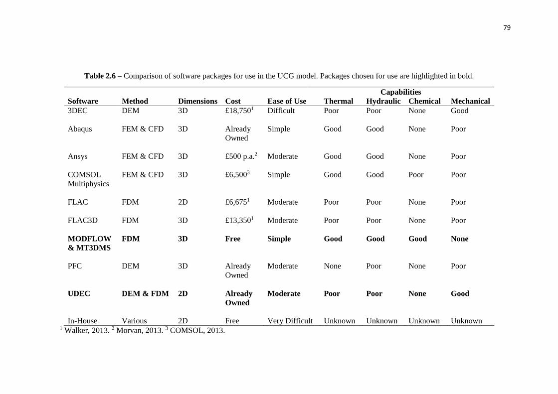
79
Table 2.6 – Comparison of software packages for use in the UCG model. Packages chosen for use are highlighted in bold.
Capabilities
Software Method Dimensions Cost Ease of Use Thermal Hydraulic Chemical Mechanical
3DEC DEM 3D £18,7501 Difficult Poor Poor None Good
Abaqus FEM & CFD 3D Already
Owned
Simple Good Good None Poor
Ansys FEM & CFD 3D £500 p.a.2 Moderate Good Good None Poor
COMSOL
Multiphysics
FEM & CFD 3D £6,5003 Simple Good Good Poor Poor
FLAC FDM
2D £6,6751 Moderate Poor Poor None Poor
FLAC3D FDM
3D £13,3501 Moderate Poor Poor None Poor
MODFLOW
& MT3DMS
FDM 3D Free Simple Good Good Good None
PFC
DEM 3D Already
Owned
Moderate None Poor None Poor
UDEC DEM & FDM 2D Already
Owned
Moderate Poor Poor None Good
In-House Various 2D Free Very Difficult Unknown Unknown Unknown Unknown 1 Walker, 2013. 2 Morvan, 2013. 3 COMSOL, 2013.

80
2.6. CONCLUDING REMARKS
This review has introduced the technology of UCG as a means to produce cheap,
clean and safe chemical products and electricity. Extensive experimental and
theoretical work has been carried out in the field over the past century, particularly in
the last forty years. UCG technology has now developed to the point where
commercialisation may be a reality within the next decade, however there are still
several issues which must be addressed before this can happen. Predominant among
these issues are the negative environmental impacts of surface subsidence,
groundwater pollution and water table lowering. Much work is currently underway to
understand these issues, however the legal and political ramifications of
environmental damage limit the use of experiments in this area. Modelling of UCG is
therefore the principal method by which this understanding must be gained.
While current efforts are beginning to prove useful in understanding UCG behaviour
there are still many areas which require more attention. Predictive modelling of
environmental impacts should continue to progress to the point where operators can
say with certainty that their facility will not cause any of these issues. Models should
be extended to cover commercial scale UCG facilities rather than just demonstration
plants and consideration should be given to the movement of rocks, water and
contaminant species in the time long after UCG reactions have ceased.
The following chapters describe how the UCG model was produced. It is hoped that
this model will prove useful in furthering the understanding of UCG generated
environmental damage, allowing for commercial development of the technology.

81
3. UNIVERSAL DISTINCT ELEMENT CODE METHODOLOGY
SUMMARY
This chapter presents an overview of the theory, numerical formulation and model
set-up of a typical geomechanical model built using the universal distinct element
code (UDEC). The discretisation and calculation cycles for the mechanical, hydraulic
and thermal aspects of the model are presented in detail. The results of initial software
validation tests are presented, showing that UDEC is capable of accurately predicting
the principal physical processes occurring in UCG. Discussions on the advantages,
disadvantages, and challenges of UDEC are given and comparisons are made with
competing methodologies such as the particle based discrete element method and the
finite element method. The limitations of the software are identified and methods for
overcoming these limitations are discussed. UDEC is shown to be a powerful tool for
use in the creation of the UCG model and recommendations are made for how best to
apply the software to this problem.

82
3.1 THE UNIVERSAL DISTINCT ELEMENT CODE
The discrete/distinct element method (DEM) refers to a number of techniques for
simulating the mechanical behaviour of systems comprised of large numbers of
interacting particles. A number of software packages based on this method are
compared in Section 2.5.2. The Universal Distinct Element Code (UDEC) is a
commercially available, two dimensional DEM package which was developed
specifically to model the behaviour of highly jointed rock masses (Itasca Consulting
Group, 2004). UDEC models are comprised of many arbitrarily shaped elements
separated by discontinuities (Cundall, 1980).
Given a full understanding of Newton’s laws of motion and the interaction forces
between the particles (e.g. gravity, friction, electrostatics etc.), UDEC can predict the
motion of complex systems involving thousands of particles. By considering the
position, velocity and forces of every particle in the system at time t, UDEC uses an
explicit finite difference algorithm to find these values again at time t + ∆t. Collisions
between particles use linear springs to calculate reaction forces based on the
interpenetration of the bodies involved. Individual particles used in a UDEC analysis
can be either rigid or deformable and subject to combinations of static and dynamic
external loads. A wide range of constitutive relationships can be simulated, including
isotropic elastic, Mohr-Coulomb and strain softening/hardening behaviours. The value
of the time increment ∆t is kept small in order to minimise the influence of particle
interpenetration on results and to ensure the stability of the simulation.

83
In addition to its mechanical capabilities, UDEC can simulate a range of hydraulic
and thermal phenomena. Linking between these phenomena allows for the simulation
of fully coupled thermal, hydraulic and mechanical systems within rock masses.
Finally, new functionality can be developed using UDEC’s built-in programming
language FISH. Figure 3.1 shows a typical UDEC simulation in progress.
Figure 3.1 – A UDEC simulation before and during mechanical cycling showing the
2D cross section looking along the cavity. The red line shows the original cavity
shape at time t=0.
UCG
CAVITY
JOINT
PATTERN
DISCRETE
ELEMENT
BLOCKS

84
A major disadvantage of DEM is its computational requirements. The CPU time
required by a UDEC model is a product of the simulation time and the number of
elements modelled. As such, the number of elements must be limited to preserve a
reasonable runtime. This often precludes the ability of the method to fully resolve the
behaviour of systems comprised of large numbers of particles or those in which
physical effects manifest over long timescales. Scale up methodologies can be
employed to represent assemblies of a large number of particles using fewer particles
of larger sizes. Such methods can introduce inaccuracies into model results however,
as the behaviour of particulate systems is often heavily scale dependent. Further
discussions of these issues are given in Section 3.5, while Chapter 4 presents an
investigation into the effects of block shape on model behaviour.
UDEC has successfully been applied to a number of issues across many scales and in
several industries, including tunnelling (Boon et al, 2014; Solak, 2009; Vardakos et
al, 2007), mining (Coulthard, 1999; Keilich et al, 2006; Vyazmensky et al, 2007),
underground construction (Barton et al, 1994; Bhasin and Hoeg, 1998), carbon
dioxide sequestration (Fang et al, 2013), hydroelectric dam construction (Bretas et al,
2014) and nuclear waste storage (Ahola et al, 1996; Blum et al, 2005, 2009).

85
3.2 MECHANICAL CALCULATIONS
3.2.1 Mechanical Model Formulation
The simplest simulations in UDEC consider only the mechanical behaviour of the
rock mass. Ground deformation is predicted by altering the geometry of the rock mass
(e.g. by excavating a cavity) and then allowing the system to come to mechanical
equilibrium. This process can be repeated a number of times to simulate excavations
occurring in multiple stages. Fully deformable mechanical simulations in UDEC
consist of the following stages:
1. Select any appropriate model options (symmetry, fluid flow, thermal etc.)
2. Define the full extent of the model in 2D space
3. Define the geometry of discrete elements (blocks) and discontinuities (joints)
4. Discretise blocks into mesh elements (zones) to allow for deformation
5. Assign constitutive relationships to zones and joints
6. Assign material properties to zones, joints, fluids etc.
7. Assign boundary and initial conditions to the appropriate locations
8. Set any appropriate body forces (e.g. gravity)
9. Run the solver algorithm until an initial equilibrium state is reached
10. Perform any changes to the system (excavations, new thermal conditions etc.)
11. Rerun the solver to find the new equilibrium state
12. Repeat Steps 11 and 12 for problems involving multiple sequential stages
13. Analyse the results.

86
UDEC’s calculation cycle for a deformable mechanical system is shown in Figure 3.2.
Technical detail on the formulation of Steps 1 through 6 is given in Appendix A.1.1.
Figure 3.2 – UDEC calculation cycle for a mechanical analysis using deformable
blocks. After Itasca Consulting Group, 2006
The individual elements within a UDEC model are defined below (Itasca Consulting
Group. 2006). Figure 3.3 describes these definitions schematically:
Blocks –Individual discrete elements which make up the model.
Joints – Interfacial discontinuity elements between blocks. Joints allow for the
relative motion of blocks, resisted by joint stiffnesses.
Zones – Triangular finite difference mesh elements used to sub-discretise
single blocks. Zones allow for the deformation of intact blocks.
Gridpoints – Vertices of zones. Fundamental nodes of the geometry.
Contacts – Formed when two or more gridpoints from different blocks are
within a certain distance of each other. Used to transfer forces between blocks.

87
Figure 3.3 - Schematic representation of blocks, zones, joints, gridpoints and contacts
used to represent rock masses in UDEC. After Itasca Consulting Group, 2006.
Where:
C Cohesion (Pa)
E Young’s Modulus (Pa)
k Stiffness (Nm-1)
γ Poisson’s Ratio (-)
θ Friction Angle (o)
σT Tensile Strength (Pa)
Subscripts:
N Normal
S Shear

88
Rather than being set by the user, the value of the timestep ∆t is calculated by UDEC.
This ensures the timestep is small enough to prevent excessive block interpenetration
by limiting how far blocks can move within a single time step. The derivation of the
timestep is given in Appendix A.1.2. Smaller timesteps lead to greater accuracy and
stability, but can greatly increase the computational demands of the model. The
following conditions lead to decreased values of ∆t and therefore increased runtimes:
Decreased block mass
Increased joint stiffnesses
Increased material stiffnesses
Increased slenderness of zones
The above conditions apply to every block in the model, such that a single small block
can cause a considerable reduction in the timestep. In order to prevent this, UDEC
uses the process of mass scaling. As shown in Appendix A.1.2, timestep is
proportional to the square root of density. For a static simulation in which gravity is
the only external force, the actual value of density is irrelevant provided that
gravitational acceleration remains the same. Using this observation, UDEC scales the
density and gravitational acceleration of each block by a factor based on the average
block mass throughout the entire model. This method can greatly speed up solution in
non-uniform models and does not affect model results, provided that inertial forces
are negligible (as they would be for a model with a stationary frame of reference). As
with block size, a single overly stiff joint can also lead to a reduction in the model
timestep. As joint stiffnesses are fully user defined however, this issue can be avoided
by ensuring of uniformity of joint stiffnesses.

89
In addition to maintaining a low value of ∆t, the stability of a numerical calculation
can also be improved with the use of damping. UDEC uses the method of adaptive
local damping to reduce the forces incident on gridpoints at every iteration of the
mechanical cycle. Reduced forces lead to reduced gridpoint acceleration and velocity
without the need to alter any modelled material properties. This effectively increases
the number of timesteps required to generate a given amount of overlap, reducing the
likelihood of overlap errors. The formulation of the damping scheme is given in
Appendix A.1.3.
Zones and joints within a UDEC model can each be represented using many different
constitutive models. These are summarised in Tables 3.1 and 3.2 respectively.
Table 3.1 – Zone constitutive models in UDEC. After Itasca Consulting Group, 2006.
Model Behaviour Simulated Example Uses
Null Zero resistance to deformation.
Zero density. Zero internal stresses.
Voids, holes, cavities.
Elastic Isotropic Linear isotropic stress-strain
relationship. No plastic failure.
Metals loaded below yield
stress.
Drucker-Prager Shear yield failure in low friction
materials. No plastic flow rule.
Soft clays. Comparison with
finite element programs.
Mohr-Coulomb Shear yield failure in geological
materials. No plastic flow rule.
Stress/stability calculations in
soil, rock and concrete.
Strain softening
Mohr-Coulomb
As Mohr-Coulomb, with strain
dependent plastic behaviour.
Post failure analysis of rock.
Tightly bedded rock strata.
Ubiquitous
Joint
As Mohr-Coulomb, with planes of
weakness at given orientations.
Geological materials with
defined strength anisotropy.
Double Yield As Mohr-Coulomb, with
volumetric yield properties.
Compressible material,
hydraulically placed sediment.

90
Table 3.2 – Joint constitutive models in UDEC. After Itasca Consulting Group, 2006.
Model Behaviour simulated Example Uses
Point contact
Coulomb slip
Interaction between particles with
small contact area.
Loosely packed granular
material.
Area contact
Coulomb slip
Interaction between tightly packed
particles.
Joints, faults and bedding
planes within rock masses.
Coulomb slip
residual strength
As area contact Coulomb slip, with
a distinct post-failure strength.
As area contact Coulomb
slip for materials with
residual strength.
Continuously
yielding
Joints subject to continuous
progressive damage and hysteresis.
Cyclic loading with
hysteresis. Dynamic
behaviour (e.g. earthquakes).
Barton-Bandis* Highly accurate joint hydraulic
behaviour.
Simulation of purely
hydraulic phenomena.
*The Barton Bandis model is an optional extra not included in UDEC by default and
not currently licensed by the University of Nottingham.
3.2.2 Mechanical Validation
This section outlines simple tests performed to verify the use of UDEC in simulating
mechanical phenomena. A number of tests have been performed and their results have
been compared with analytical solutions. Similar tests for hydraulic and thermal
phenomena are presented in Sections 3.3.2 and 3.4.2 respectively.
3.2.2.1 Elastic Deflection Testing
This test verifies the mechanical behaviour of deformable bodies in UDEC. An
isotropic elastic cantilever is fixed in place at one end and allowed to deform under
gravity. The vertical displacement at the free end is given by Equation 3.1:

91
𝑢𝑦 = −3𝜌𝑔𝐿4
2𝐸𝐻2 (3.1)
Where:
E Young’s modulus (Pa)
H Height (m)
L Length (m)
g Acceleration due to gravity (ms-2)
u Displacement (m)
ρ Density (kgm-3)
The properties of the beam used are given in Table 3.3:
Table 3.3 – Properties of cantilever used in beam deflection test.
Density (kgm-3) 3000
Height (m) 1.0
Length (m) 10.0
Young’s Modulus (Pa) 2×10¹⁰
Table 3.4 compares the deflection seen in several models with that given by Equation
3.1. As seen, the deflection predicted by UDEC asymptotically approaches the
analytical value as zone density increases. This suggests that high zone densities are
required to give accurate results. Such high densities would greatly increase model
runtime however. Further testing of the effects of zone density on model behaviour is
presented in Section 6.6.

92
Table 3.4 – Results of simulated cantilever bending test.
Zone Edge Length (m) Zone Density (m-2) Displacement (m)
1.00 8.80 0.0146
0.50 25.2 0.0190
0.20 122 0.0212
0.10 444 0.0214
0.05 1690 0.0220
Analytical Result N/A 0.0225
3.2.2.2 Plastic Deflection Testing
In addition to the elastic test above, a test was performed to examine the plastic
deformation of a beam using different constitutive models. Only the isotropic elastic,
Mohr-Coulomb and strain softening models were tested as the others were considered
unsuitable for UCG based on the considerations in Table 3.1. Figure 3.4 shows the
deformation of each cantilever after 5 seconds of simulated time. All models used a
friction angle of 30o and a cohesion of 100kPa. Strain softening parameters were set at
zero as the constitutive model was used to simulate perfectly plastic behaviour.
Figure 3.4 – Plastic deflection of a cantilever under different constitutive models.

93
As seen, the relationship used has a strong effect on behaviour. While the isotropic
model is shown to be valid for the elastic regime, it does not consider plastic strains.
The Mohr Coulomb model does show plastic behaviour, however the predicted shape
of the beam is physically unrealistic. As mentioned in Table 3.1, this model does not
contain a plastic flow rule, leading to an unrealistic failure shape. As such, the model
is seen to be unsuitable when large plastic strains are expected. Finally, the strain
softening Mohr Coulomb model is seen to give realistic behaviour. Although this
model causes a slight increase in runtime, the accuracy of its results justify its use.
3.2.2.3 Freefall Motion Test
This test of UDEC’s mechanical behaviour involves the motion of a single block
under freefall, and its interaction with the ground upon impact. This test was
performed by dropping a 1x1m deformable block from a height of 2m onto a fixed
base 5m wide by 1m high. The velocity of the block’s centroid is tracked for 3
seconds after the initial release of the block and compared with expected behaviour.
All materials in the test were modelled using the isotropic elastic constitutive model
with arbitrarily high Young’s modulus and density of 3000kgm-3. Gravitational
acceleration was set at 9.81ms-2. Figure 3.5 shows the results of this test.

94
Figure 3.5 – Freefall velocity profiles calculated in UDEC and via kinematics.
As seen, the velocity profile given by UDEC is considerably different to the analytical
profile. Firstly, the acceleration of the modelled profile is approximately 2.1ms-2,
whereas the analytical profile gives 9.8ms-2. This discrepancy is due to damping. As
mentioned in Appendix A.1.3, the force on each gridpoint at every calculation cycle is
effectively reduced by a factor of 5. As the only force present in this test is gravity,
the acceleration seen is also reduced by a factor of approximately 5. The factor of
reduction is not exactly 5 due to rounding errors in the calculation process. The
second discrepancy is the brief velocity reversal seen after approximately 1.4 seconds.
This is simply caused by the temporary overlap of the falling block with the base of
the model and the action of the restorative force to remove this overlap. Despite these
discrepancies, the total displacement of the block reaches the expected value of 2m
and then becomes steady for the remaining time, as expected. As such, the use of
UDEC in modelling blocks under freefall is justified.

95
3.3 HYDRAULIC CALCULATIONS
3.3.1 Hydraulic Model Formulation
The UDEC hydraulic algorithm assumes fluids within a rock mass exist entirely
within the joints between blocks. The blocks themselves are assumed to be dry and
impermeable. Two way coupling links the aperture (and hence flow volume) of joints
to both the mechanical stresses of the blocks and the pore pressure of the fluid. Fully
coupled hydraulic/mechanical UDEC models have the capability to simulate a range
of hydraulic effects, including:
The effect of pore pressure on rock blocks
The effect of mechanical stress on fluid volumes and flow behaviour
Pressure driven flow of fluids along joints
Changes in pressure due to inflow/outflow of fluids from joints and/or voids
Flow within fully saturated and partially saturated (vadose) regions
The above effects are added to the mechanical calculation cycle (Figure 3.2) to form a
fully coupled hydraulic/mechanical model. Figure 3.6 shows the additions and how
they connect to the mechanical cycle. The details of the individual steps in the
hydraulic cycle are examined in Appendix A.2.1.

96
Figure 3.6 – Hydraulic calculation cycle for a coupled hydraulic/mechanical model.
The three fluid steps are calculated independently of mechanical Steps 1 through 3.
After Itasca Consulting Group, 2006.
Volumes of fluid within UDEC are discretised into regions known as domains. A
domain is created wherever two or more zones meet, provided these zones are from
different blocks. Domains are defined within joints, voids, and intersections between
joints. Voids are defined as joints with an aperture greater than a predefined
maximum value. Fluid properties are assumed to be constant throughout a domain,
with the notable exception of hydrostatic pressure. When gravity is present, the fluid
pressure within each domain varies linearly with the hydrostatic gradient. Figure 3.7
shows the discretisation of a model into blocks, zones and domains.

97
Figure 3.7 – Schematic representation of domains used to discretise hydraulic
problems. After Itasca Consulting Group, 2006.
As with the mechanical calculation, the timestep used in the hydraulic model is
automatically determined in order to maintain the stability of the model. The
definition of the timestep is given in Appendix A.2.2. In coupled
hydraulic/mechanical models, the value of the overall timestep is chosen as the
smaller of the mechanical or hydraulic timesteps. The hydraulic timestep can be
severely limited in cases with large contact apertures or small domain volumes. In
many cases however, only the steady state solution to the hydraulic problem is of
interest. In this case a simplified steady state algorithm can be used, which greatly
improves computational efficiency.

98
The steady state algorithm works by assuming the volume of each domain is roughly
constant throughout the runtime of the model. As such the actual values of the domain
volumes are irrelevant, as is the fluid bulk modulus. The volumes and bulk moduli
can then be scaled so that each domain gives the same timestep. This method is
analogous to the process of mass scaling mentioned in Section 3.2.1. Assuming
domain volume changes remain low throughout the model, this algorithm greatly
speeds solution. In addition, as the model approaches solution, the pressure variation
in each timestep becomes very small. This allows several fluid steps to be executed
for every mechanical step, further speeding solution. In this method, mechanical steps
are triggered whenever the change in pressure of any domain exceeds a given fraction
of the original pressure in that domain. This method can greatly speed coupled
models, but can lead to inaccuracies if any large scale collapse behaviour is present.
3.3.2 Hydraulic Validation
3.3.2.1 Stress/Aperture Relationship Test
This test verifies UDEC’s hydraulic logic by testing the relationship between stress,
pressure and joint aperture. Consider a single horizontal joint between two rigid
blocks, as shown in Figure 3.8. The only relevant forces in the system are those of
gravity and fluid pressure. By considering these forces, an analytical expression can
be derived for the aperture of the joint. This is given in Equation 3.2.
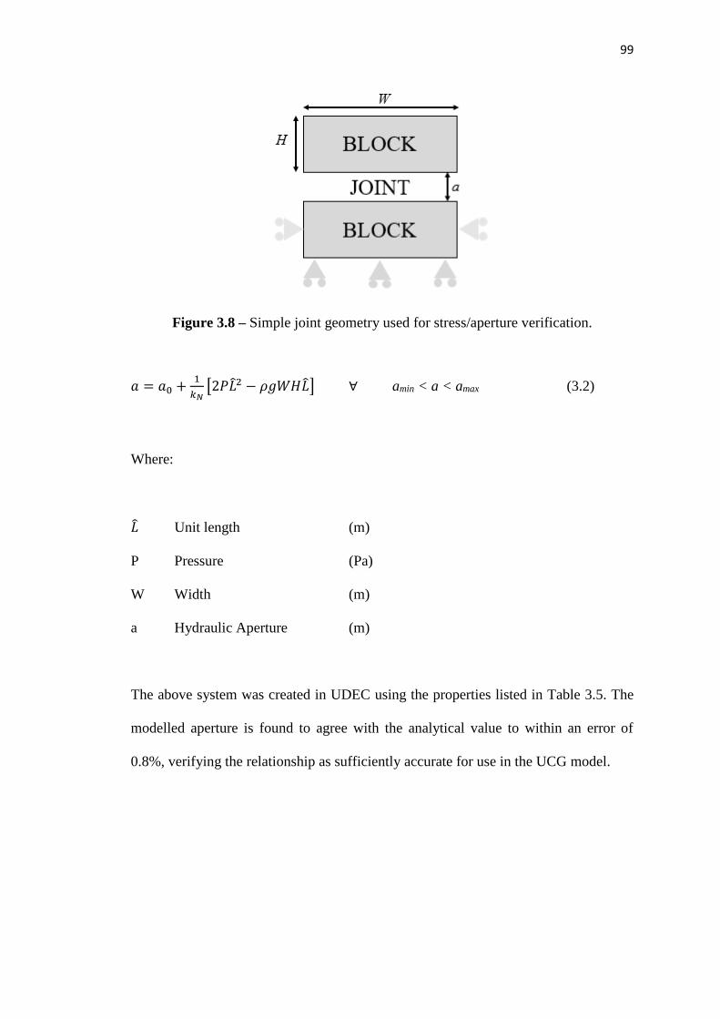
99
Figure 3.8 – Simple joint geometry used for stress/aperture verification.
𝑎 = 𝑎0 +1
𝑘𝑁[2𝑃�̂�2 − 𝜌𝑔𝑊𝐻�̂�] ∀ amin < a < amax (3.2)
Where:
�̂� Unit length (m)
P Pressure (Pa)
W Width (m)
a Hydraulic Aperture (m)
The above system was created in UDEC using the properties listed in Table 3.5. The
modelled aperture is found to agree with the analytical value to within an error of
0.8%, verifying the relationship as sufficiently accurate for use in the UCG model.

100
Table 3.5 – Verification of UDEC’s stress/aperture relationship.
Input Values
Aperture at Zero Stress a0 (mm) 1.00
Normal Stiffness kN (Nm-1) 1×10⁸
Pore Pressure P (Pa) 100,000
Block Density (kgm-3) 2,500
Gravitational Acceleration g (ms-2) 10.0
Block Width W (m) 2.0
Block Height H (m) 1.0
Output Apertures (mm)
Analytical 2.50
UDEC 2.48
3.3.2.2 Flow/Pressure Relationship Test
Fluid flow in UDEC is governed by the cubic flow law, given by Equation 3.3. The
verification of UDEC’s flow logic was performed by applying a pressure gradient
across the joint in Figure 3.8 and measuring the flow rate observed. Table 3.6 shows
the results of this test. The model and theory are again seen to agree to within an error
of 0.8%, verifying the use of the steady state flow algorithm in UDEC.

101
𝑞 = −1
12𝜇𝑎3
∆P
𝐿 (3.3)
Where:
q = Flow rate per unit depth into page (m2s-1)
μ = Dynamic viscosity (Pa s)
Table 3.6 – Verification of UDEC’s fluid flow logic.
Input Values
Fluid Viscosity μ (Pa s) 0.001
Joint Aperture a (mm) 2.50
Pressure Difference ΔP (Pa) 100,000
Joint Length L (m) 2.0
Output Flow Rates (m2s-1)
Analytical 0.0650
UDEC 0.0645

102
3.4 THERMAL CALCULATIONS
3.4.1 Thermal Model Formulation
UDEC’s thermal modelling capabilities include heat conduction, thermal expansion of
intact rocks and the modelling of temperature dependent fluid density and viscosity.
Heat sources and sinks can be included at model boundaries and within the bulk of the
rock mass. Heat sources can have constant magnitudes or can vary with time.
Convective and radiative heat transfer can be simulated as boundary conditions (by
specifying heat transfer coefficient and background temperature), but cannot be
included within the bulk of the model. Due to a number of differences between the
thermal model and the hydraulic/mechanical models, thermal aspects of coupled
simulations must be cycled separately. In most cases the thermal model is run to
completion in between stages of the hydraulic/mechanical model. The temperature
profile found in the thermal model can then influence hydraulic or mechanical effects
via temperature dependent fluid properties and/or thermal expansion.
Thermal modelling in UDEC can be achieved with either an explicitly or implicitly
time stepped algorithm. The calculation cycle for the explicit algorithm is shown in
Figure 3.9. The implicit algorithm works by iteratively finding the solution to a set of
simultaneous equations for the temperature of each zone in the model at the desired
time(s). The full formulations of the explicit and implicit algorithms are given in
Appendices A.3.1 and A.3.2 respectively. A comparison between the methods is
given in Table 3.7. The long timestep means the implicit method can be faster for
simple models, but unsuitable for models with complex geometries, non-linear
phenomena or high accuracy requirements.

103
Figure 3.9 – Calculation cycle for the explicit thermal algorithm. After Itasca
Consulting Group, 2006.
Table 3.7 – Comparison between explicit and implicit thermal algorithms in UDEC.
Consideration Explicit Algorithm Implicit Algorithm
Timestep determination Automatic User controlled
Timestep length Short Long
Cycles per timestep One Many
Stability Depends on timestep Unconditionally stable
Accuracy Depends on timestep Depends on timestep
Non-linear Solutions Possible Not possible

104
Thermal conduction in UDEC is modelled entirely through the intact rock blocks.
Joints are defined as be perfectly conducting while voids are perfectly insulating.
Thermal discretisation is based on the zones used in the mechanical model, however
extra thermal zones must often be created to ensure conservation of energy between
misaligned blocks. The need to generate these zones precludes thermal/mechanical
coupling as new zones would need to be created after every thermal step. This would
greatly increase the complexity and runtime of the model as well as introducing a
large source of error through the need to conserve energy between the meshes. A full
description of thermal zone generation is given in Appendix A.3.4.
In addition to heat transfer, UDEC’s thermal algorithm can also simulate thermal
expansion and the temperature dependent density and viscosity of fluids. The
formulation of these effects is shown in Appendices A.3.5 and A.3.6 respectively. As
shown in Section 3.5.2 however, the temperature dependence of fluid properties
breaks down near the boiling point of the fluid.
3.4.2 Thermal Validation
3.4.2.1 Fixed Temperature Conduction Test
This test verifies UDEC’s thermal logic by modelling temperature conduction along
an insulated rod. This is one of very few transient heat transfer problems which can be
solved analytically. Consider a rod of length L, with initial temperature T0 throughout.
One end of the rod is fixed at a higher temperature of TH. The other edges are
perfectly insulated. It can be shown (e.g. Coulson et al, 2004) that the temperature T
at any given time t and location x along the length of rod is given by Equation 3.4.

105
𝑇 = 𝑇0 + ∑ (−1)𝑛∞𝑛=0 (𝑇𝐻 − 𝑇0) [𝑒𝑟𝑓𝑐 (
2𝑛𝐿+𝑥
2√𝐷𝑇𝑡) + 𝑒𝑟𝑓𝑐 (
2(𝑛+1)𝐿−𝑥
2√𝐷𝑇𝑡)] (3.4)
Where:
T = Temperature (K)
t = Time (s)
x = Length along rod (m)
DT = Thermal diffusivity (m2s-1)
Subscripts:
0 = Initial
H = Hot end.
erfc is the complementary error function:
𝑒𝑟𝑓𝑐(𝜑) =2
√𝜋∫ 𝑒−𝑡
2𝑑𝑡
∞
𝑥
Consider a rod with the properties given in Table 3.8. The temperature profile of the
rod has been found at a number of times using Equation 3.4. A UDEC model has been
created to analyse the same problem. A comparison between the UDEC results and
the analytical solution is shown in Figure 3.10. It is seen that the accuracy of the
UDEC result decreases with distance from the hot end, with a maximum temperature
error of 22K seen after 12 months. UDEC is also seen to consistently overestimate
temperatures. Given the reasonably small degree of error however, the thermal
algorithm in UDEC is considered to be accurate enough for use in the UCG model.
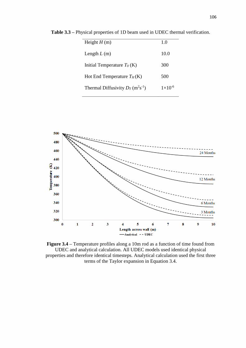
106
Table 3.3 – Physical properties of 1D beam used in UDEC thermal verification.
Height H (m) 1.0
Length L (m) 10.0
Initial Temperature T0 (K) 300
Hot End Temperature TH (K) 500
Thermal Diffusivity DT (m2s-1) 1×10⁻⁶
Figure 3.4 – Temperature profiles along a 10m rod as a function of time found from
UDEC and analytical calculation. All UDEC models used identical physical
properties and therefore identical timesteps. Analytical calculation used the first three
terms of the Taylor expansion in Equation 3.4.

107
3.4.2.2 Fixed Heat Flux Conduction Test
This test verifies the thermal algorithm by modelling how a transient heat transfer
problem reaches steady state. The geometry and material properties used are the same
as those in Section 3.4.2.1, with the exception of thermal diffusivity. This is set to a
value of 1×10⁻³ m2s-1 to speed the establishment of the steady state. Heat is applied to
the left hand end of the rod at a constant rate and is removed from the right hand end
by convection to the surroundings. The model runs for 1 week (modelled time) to
ensure the steady state has been reached. The average temperature of the rod at steady
state can be found by Equation 3.5. Table 3.9 lists the physical properties used in this
calculation alongside the results of the UDEC model and analytical calculation. As
with the previous test, UDEC is seen to slightly overestimate the final temperature.
The thermal model is still considered valid however, as this error is reasonably small.
𝑇 = 𝑇𝑏 +𝑄
𝑈𝐻 (3.5)
Where:
Q = Heat flux (Wm-1)
Tb = Background temperature (K)
U = Convective heat transfer coefficient (Wm-2K-1)

108
Table 3.4 – Input properties and output temperatures of fixed heat flux test.
Input Variables
Background Temperature Tb (K) 300
Heat Flow Rate Q (Wm-1) 10,000
Convective Heat Transfer Coefficient U (Wm-2K-1) 100
Output Temperature (K)
Analytical 400
UDEC 406

109
3.5 ADVANTAGES, CHALLENGES AND LIMITATIONS
3.5.1 Mechanical
UDEC simulates rock masses using a combined finite-discrete element representation.
Table 3.10 compares the relative advantages, disadvantages and capabilities of UDEC
in comparison with both fully discrete (e.g. particle based DEM) and fully continuous
(e.g. FEM) methods.
Table 3.5 – Advantages, disadvantages and capabilities of UDEC relative to
continuum methods and particle based discrete methods of mechanical simulation.
Issue UDEC Discrete
Methods
Continuum
Methods
Rock separation Possible Possible Not Possible1
New Fracture Generation Not Possible Possible Not Possible1
Goafing/Collapse Prediction Possible Possible Not Possible1
Bending Behaviour Possible Not Possible Possible
Solution Speed Moderate Slow Fast
Solution Stability Moderate Moderate High
Mesh Dependence High High Low
Material Property Selection Very Difficult Simple Difficult
1 – These issues can be modelled with continuum methods, but doing so is difficult
and computationally expensive (Hammah et al, 2008).

110
The ability of UDEC to model both discrete (rock separation and collapse) and
continuum (bending) effects allows for a closer representation of reality than that
given by either fully continuum or fully discrete methods. As such, UDEC is often
used in the modelling of complex behaviours of highly jointed rock masses
(Coulthard & Dutton, 1988; Coulthard, 1999; Lisjak & Grasselli, 2014; Morris et al,
2006; Morris et al, 2009; Vorobiev et al, 2008; Wei & Hudson, 1998).
One of the greatest challenges in designing a UDEC model is the selection of an
appropriate joint pattern, which in turn determines block size and shape parameters.
Increased numbers of blocks decrease both solution speed and stability. In addition,
block size and shape can have profound effects on model results, complicating the
selection of appropriate material properties. This issue is referred to as mesh
dependence. The problem is further compounded by the impossibility of creating new
fractures within an existing rock mass. Lorig & Cundall (1987) suggest a method in
which this can be approximated, however this greatly increases model runtimes with
little advantage. Figure 3.11 highlights the effect of block size on model performance.
The influence of block morphology on model results is further examined in Chapter 4.
Despite these issues, UDEC is seen to be a useful tool for modelling the local
environmental impact of UCG.

111
Figure 3.5 – Effects of block size on model behaviour. Results taken from
preliminary designs for a UCG model.
3.5.2 Hydraulic
Hydraulic effects contribute greatly to the environmental impacts of UCG, both in
terms of groundwater issues and their coupling with mechanical effects. Given that
the UDEC model will need to predict both subsidence and groundwater flow rates, it
is essential that the methods used in the model are able to realistically simulate
hydraulic behaviour. Table 3.11 highlights the principal advantages and disadvantages
of UDEC’s hydraulic capability in comparison with continuum methods such as CFD.
Particle based DEM is more suited to modelling fluid dominant systems (i.e. those in
which small solid elements exist surrounded by fluid) than solid dominant systems.
As such, it will not be considered further for this model.

112
Table 3.6 – Advantages, disadvantages and capabilities of UDEC compared with
continuum methods of hydraulic simulation.
Issue UDEC Continuum Methods
Variable Permeability Spatial & Temporal Spatial1
Stress/Pressure Coupling Possible Possible
Stress/Aperture Coupling Simple Difficult
Fluid Phase Change Not Possible Possible
Solution Speed Moderate Fast
Solution Stability Moderate High
Mesh Dependence High Low
1 – Temporal variations in permeability can be modelled with continuum methods,
but doing so is difficult and computationally expensive.
The modelling of hydraulic problems using fluid filled fractures gives UDEC a
considerable advantage over continuum methods, in that the coupled temporal
variations of mechanical stress, hydraulic aperture and fluid pressure are simple to
consider. In comparison, continuum methods tend to assume constant permeabilities
and calculate flow rates using a variant of Darcy’s law (Köhne et al, 2009). A
potential disadvantage with the UDEC representation is the dependence of the
hydraulic model on the joint pattern, further complicating the issues presented in
Section 3.5.1. Fracture patterns must contain enough joints to ensure sufficient
connection of fluid filled regions, and these joints must be oriented in such a way that
any permeability anisotropy is retained. Note that the absolute permeability of a
system can be controlled by altering the aperture of joints, such that the total number
of joints present is not significant. The effects of fracturing on mechanical and
hydraulic results are investigated in detail in Chapters 4 and 6.

113
The principal disadvantage of UDEC’s hydraulic model is the inability to model fluid
phase changes and dissolution. This precludes the modelling of several important
hydrological effects including:
Boiling of groundwater as it enters the UCG cavity
The effects of water inflow rates on cavity heat generation
Thermal convection
Solution, adsorption, diffusion and advection of dissolved species
While some of these issues can be approximated using FISH functions, doing so
greatly increases the computational demands of the model (Tomac & Gutierrez,
2015). As such, full modelling of groundwater contamination is not possible with
UDEC alone. In order to include these effects, alternative modelling methodologies
are required. Another limitation of UDEC’s hydraulic model is the simplistic
definition of joints. The stress/aperture relationship is assumed to be linear (though
cut-offs are used at extreme values) and neither joint roughness nor tortuosity is
considered. Tortuosity can be considered simply by including more complex joint
patterns. Joint roughness and non-linear stress/aperture relationships can be included
by using the Barton-Bandis joint model (Bandis et al, 1985). Both methods can
greatly increase computational runtimes however. Simpler methods involve the use of
corrective factors in the cubic flow law, however these can reduce the overall
accuracy of the model.

114
The final limiting assumption of the hydraulic model applies only where the steady
state approximation is used. Considering the increase in solution speed given by this
approximation, this applies to the majority of large scale models. The assumption of
constant domain volumes is problematic for models containing large amounts of
separation or those considering the formation or collapse of voids. Care should be
taken that pressures in such regions are adequately defined in the event of predictable
void volume changes. Despite the inclusion of void collapse, this assumption is not
considered a problem with UCG, as cavity pressure is controlled by the operator.
Given the above considerations, it is believed that UDEC is more than capable of
simulating the coupled mechanical and hydraulic behaviour of UCG. Full
groundwater contamination modelling will need to be performed using alternative
software however, due to the lack of fluid phase partitioning in UDEC. Appendix C
suggests how this may be possible using the USGS MODFLOW/MT3DMS codes.
3.5.3 Thermal
Table 3.12 compares the thermal modelling capabilities of UDEC with continuum
methods. As seen, UDEC suffers a number of limitations. Initial results show
however that thermal effects have a relatively minor impact on environmental damage
compared with mechanical or hydraulic effects. As such, UDEC is still suggested to
be appropriate for use in a coupled thermal/hydraulic/mechanical UCG model.

115
Table 3.7 – Comparison of the capability of various techniques for modelling thermal
phenomena within a rock mass.
Issue UDEC Continuum
Methods
Thermal Conduction Yes Yes
Thermal Convection No Yes
Thermal Radiation No Yes
Thermal Expansion Yes Yes
Temperature Dependent Solids No Yes
Temperature Dependent Fluids ρ, μ Only Yes
Thermal/Mechanical Coupling Partial Full
Thermal/Hydraulic Coupling Partial Full
Solution Speed Moderate Fast
Solution Stability Low High
Mesh Dependence Moderate Low
The main limitations of UDEC’s thermal model are the lack of thermal/hydraulic
coupling and the separation of thermal and mechanical/hydraulic runtimes. These
issues preclude the modelling of coupled thermal effects such as convection and
thermal spalling (Biezen, 1996), as well as the simulation of temperature dependent
thermal properties such as heat capacity and conductivity. Previous attempts to
include these effects have been moderately successful, but tend to greatly increase
model runtimes (Tomac & Gutierrez, 2015). More realistic thermal modelling can be
achieved by alternating the thermal and mechanical/hydraulic algorithms, though this
also increases runtime. The modelling of temperature dependent rock mechanical
properties can be included using FISH functions, as shown in Section 5.5.

116
As shown in Table 3.12, UDEC is capable of modelling temperature dependent fluid
density and viscosity, however this can cause serious instabilities if the fluid
approaches boiling temperature. In UCG, groundwater can exist either as liquid water
or superheated steam. Given the low flow rates involved, UDEC’s thermal algorithm
assumes fluid temperature equals rock temperature at all times. As such the fluid in
the joints surrounding a rock will instantly boil as soon as the temperature of the rock
exceeds the boiling point of water. This boiling causes fluid density to suddenly
reduce by a factor of approximately 1,000, leading to a sudden change in stress which
causes the rock mass to break apart and the model to crash. In addition, changes in
density can produce a buoyant force which alters fluid flow rates, affecting the
hydraulic model and introducing uncertainty into model results.
Given the above considerations, UDEC is seen to be a poor choice for thermal
modelling. Several attempts to improve the thermal model are presented in Section
5.6.3, however these were seen to be generally unsuccessful. Given that thermal
effects are observed to be relatively unimportant however, these issues are not
considered to be significant to the overall performance of the model. Given its
advantages in hydraulic and mechanical modelling, UDEC is therefore considered to
be the appropriate choice for modelling the local environmental impacts of
underground coal gasification. It is suggested however, that future more detailed work
should use some form of 3D modelling which can accurately couple mechanical,
hydraulic and thermal effects. Such a formulation is currently difficult to achieve with
either discrete or continuum methods however, suggesting that new techniques may
need to be developed.

117
3.6 CONCLUDING REMARKS
This chapter has outlined the capabilities, advantages, challenges and limitations of
UDEC with respect to its use as a tool for modelling the local environmental impacts
of UCG. The combined finite/discrete representation provided by modern DEM codes
such as UDEC has been shown to be a very useful tool for the prediction of
subsidence on a number of occasions. The inclusion of fully coupled hydraulic
modelling based on joint apertures also provides a key advantage in comparison with
many continuum methods. Finally, despite a number of shortcomings, the thermal
algorithm within UDEC adds to the capabilities of the software for predicting the
local effects of UCG.
A number of limitations of the software have been identified, including the strong
influence of joint geometry on results, the dependence of result accuracy and runtime
on zone density and the lack of full thermal/mechanical coupling. Many of these
issues have been overcome somewhat through the use of novel modelling techniques.
Chapter 4 introduces a new methodology for representing the effects of unknown
fracture patterns on rock mass behaviours, while further investigations of zone density
effects are presented in Chapter 6. Chapter 5 presents a number of attempts to include
full thermal modelling in UDEC, though these were met with limited success. Despite
these issues, it is believed that the advantages of UDEC over other modelling methods
lead to it being the best tool for modelling the local environmental impacts of UCG. It
is believed that with a greater understanding of the limitations of the software, UDEC
should prove capable of producing fast, accurate and reliable predictions of
subsidence and groundwater issues associated with underground coal gasification.

118
4. SIMULATED LABORATORY SCALE COMPRESSION TESTING
SUMMARY
When modelling heavily jointed rock masses in the discrete element method,
particular attention must be paid to the selection of appropriate material properties and
joint patterns to give a realistic representation of rock mass behaviour. This chapter
presents a new methodology for choosing these parameters, based on the results of
simulated laboratory scale compression testing. Investigations into the effects of joint
patterns, block geometry and joint properties on rock mass mechanical behaviour are
presented and used to derive sets of rock mass material properties. Validation studies
and a discussion of the limitations of the new methodology are presented to justify its
use in further modelling. Decisions on the joint pattern and material properties to be
used in the underground coal gasification (UCG) model are given based on the results
of the tests performed in this chapter. The chapter concludes with suggestions for
further validation of the method and its potential application to a wider range of rock
materials and modelling scenarios.

119
4.1 THEORY AND BACKGROUND
4.1.1 Representing Rock Masses in the Discrete Element Method
As mentioned in Section 3.5.1, the joint pattern used within model based on the
distinct element method (DEM) can have profound effects on the mechanical
behaviour of that model. The mechanical properties of the blocks within the model are
often altered to take account of these effects. Methods such as the Hoek & Brown
failure criterion and geological strength index (GSI) (Hoek et al, 2002; Marinos et al,
2007) can be used to select these properties based on empirical measurements of real
joint patterns. Such methods tend not to consider the effects of particle shape,
variability and anisotropy on rock mass behaviour however. In order to gain a better
understanding of how joint patterns affect material properties, a number of simulated
laboratory scale compression tests have been performed on rock masses with varying
joint geometries. In addition, a new methodology has been developed in which the
results of such simulations are scaled up to provide material properties for a larger
engineering scale rock mass. Effectively, the entire laboratory scale geometry
represents an assembly of rocks which constitute a single rock block in the
engineering scale model. Figure 4.1 highlights this concept. The remainder of this
section outlines the methodology used to select the rock mass material properties.

120
Figure 4.1 – Representation of a real rock mass as an assembly of large particles,
where each particle has properties based on laboratory scale simulation results.
4.1.2 Axial Compression Testing
Axial compression testing refers to two common laboratory techniques used to
determine the material properties of intact rock specimens. Core samples from the site
of interest are cut down to produce cylindrical test sections with dimensions on the
order of centimetres. These sections are then loaded into a test apparatus, such as that
illustrated in Figure 4.2. The sample is contained within a flexible membrane and is
held between two stiff plates inside a sealed container of hydraulic fluid. Lateral
confining stress σL is applied by controlling the hydrostatic pressure of the fluid. Axial
compressive stress σA is applied to the sample via the upper plate. The total axial
strain of the sample can be derived from measurements of the displacement of the
upper plate. Strain gauges are also often applied to the sample to measure stresses in
the transverse direction (British Standards Institute, 1990).

121
Figure 4.2 – Typical apparatus used for a triaxial compression test.
In cases where zero confining pressure is applied, this technique is referred to as
uniaxial compression. For cases with nonzero confining pressure, the term biaxial
compression is used. In uniaxial compression, the axial stress-strain response of the
sample can be analysed to determine the material Young’s modulus E and axial
compressive strength σC. Measurement of transverse strains gives information on the
material Poisson’s ratio γ and dilation angle ψ. By measuring yield stress over a range
of confining pressures in the biaxial test, it is possible to derive the Mohr-Coulomb
parameters of friction angle θ and cohesion C. Finally, the maximum tensile strength
of the rock mass σT,max can be estimated from the cohesion and friction angle. Figures
4.3 through 4.5 show how these results are derived.
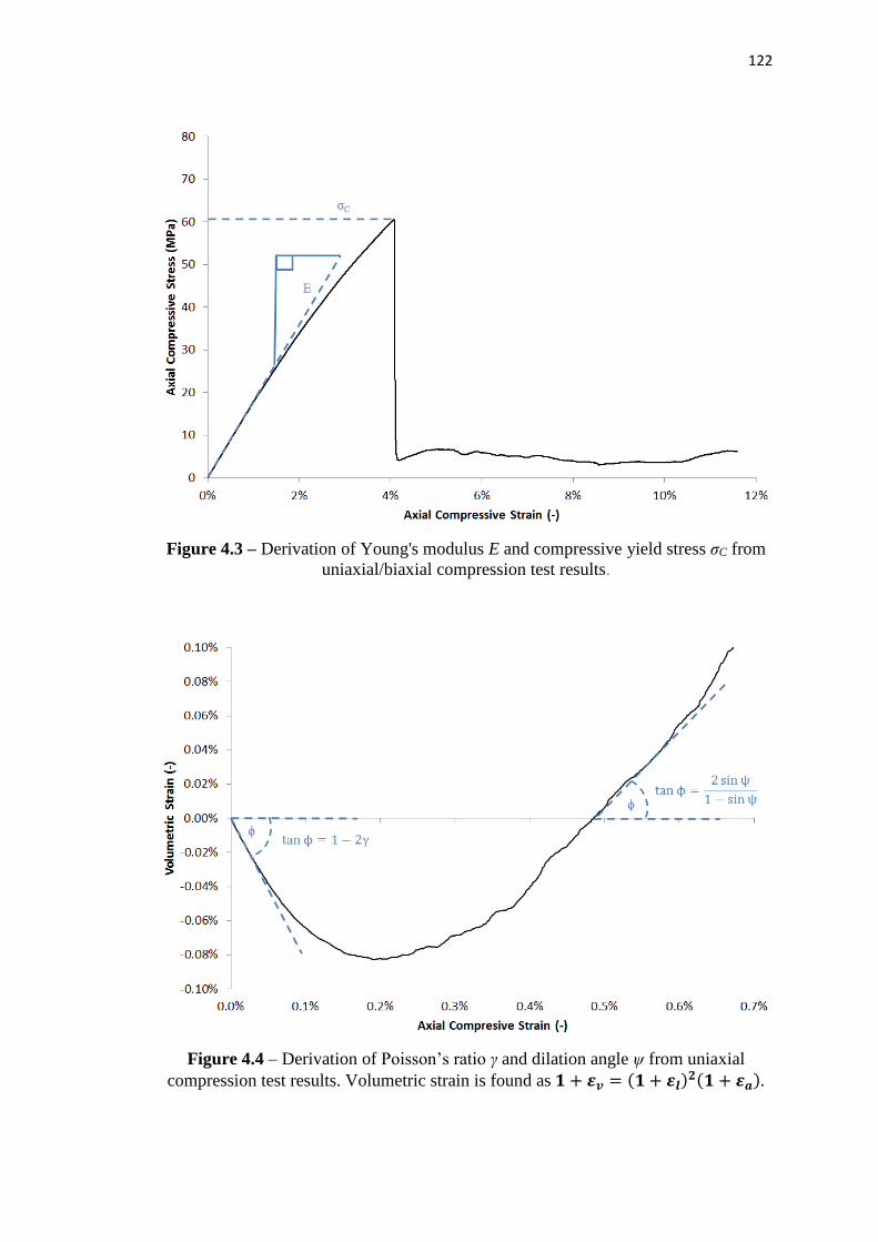
122
Figure 4.3 – Derivation of Young's modulus E and compressive yield stress σC from
uniaxial/biaxial compression test results.
Figure 4.4 – Derivation of Poisson’s ratio γ and dilation angle ψ from uniaxial
compression test results. Volumetric strain is found as 𝟏 + 𝜺𝒗 = (𝟏 + 𝜺𝒍)𝟐(𝟏 + 𝜺𝒂).
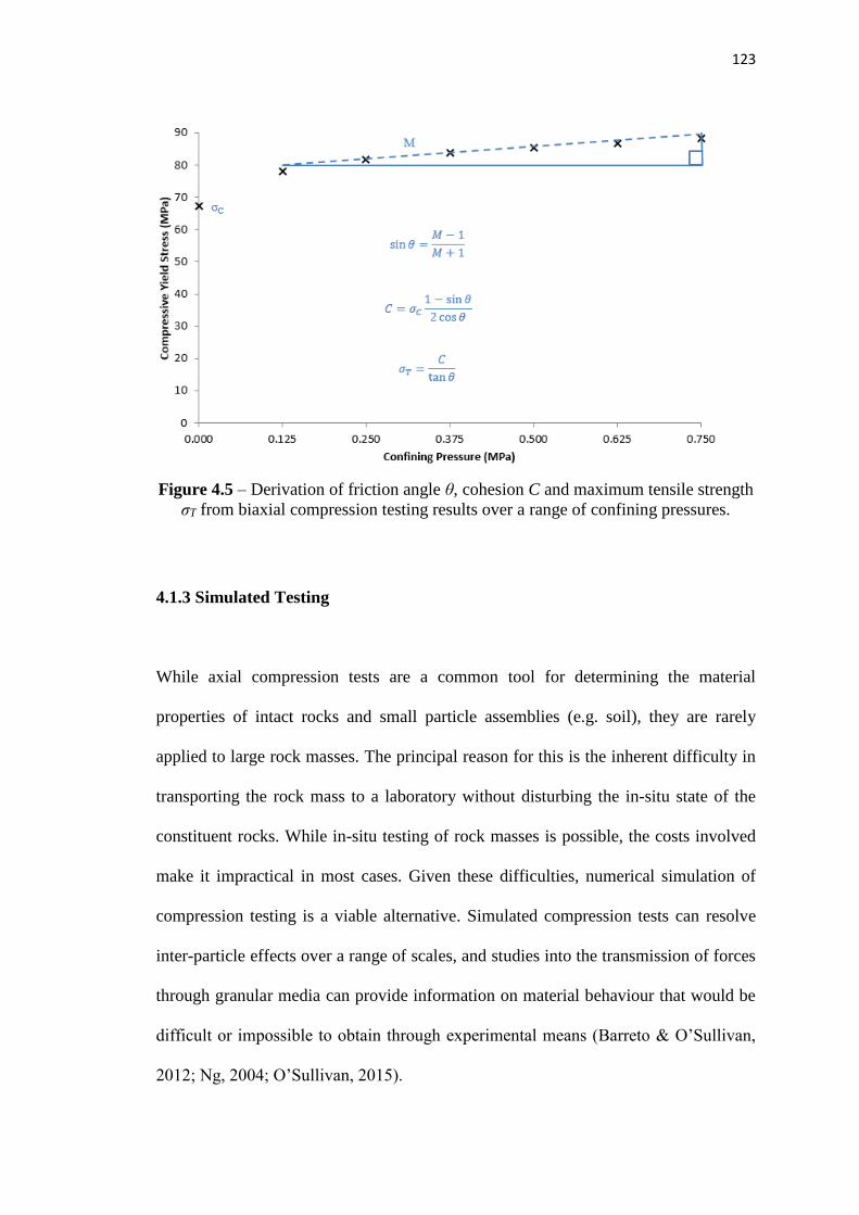
123
Figure 4.5 – Derivation of friction angle θ, cohesion C and maximum tensile strength
σT from biaxial compression testing results over a range of confining pressures.
4.1.3 Simulated Testing
While axial compression tests are a common tool for determining the material
properties of intact rocks and small particle assemblies (e.g. soil), they are rarely
applied to large rock masses. The principal reason for this is the inherent difficulty in
transporting the rock mass to a laboratory without disturbing the in-situ state of the
constituent rocks. While in-situ testing of rock masses is possible, the costs involved
make it impractical in most cases. Given these difficulties, numerical simulation of
compression testing is a viable alternative. Simulated compression tests can resolve
inter-particle effects over a range of scales, and studies into the transmission of forces
through granular media can provide information on material behaviour that would be
difficult or impossible to obtain through experimental means (Barreto & O’Sullivan,
2012; Ng, 2004; O’Sullivan, 2015).

124
The work presented in this chapter aims to use simulated axial compression testing to
achieve a greater understanding of the effects of element morphology on the material
properties of rock masses in DEM. Simulated testing has been performed on rock
masses with varying block geometries and joint mechanical properties. The work aims
to produce a methodology for the selection of material properties to be used in
representing assemblies of small rocks as single large blocks. These properties will
then be applied to the blocks used in the UCG model. It is hoped that the new
property selection methodology will retain both mechanical and hydraulic accuracy
without the need for excessively large numbers of joints and correspondingly large
runtimes. It is also suggested that a successful methodology may be applied to
increase the accuracy of future models of jointed rock masses, including both DEM
models and continuum based simulations.

125
4.2 METHODOLOGY OF SIMULATED TESTING
4.2.1 Model Design
The commercially available Universal Distinct Element Code (UDEC) 4.01 has been
used to simulate uniaxial and biaxial compression of a number of large scale rock
masses with varying joint geometries and material properties. Two methods have been
used to represent the 3D rock mass using the 2D software. The axisymmetric method
assumes a line of rotational symmetry about the left hand edge of the model. This
represents a cylindrical rock mass similar to those used in laboratory tests, with a
radius of 1m and height 5m. The plane strain method represents a geometry extending
an infinite distance into the page, with a square cross section of side length 5m. While
physically unrealistic for a laboratory test, this geometry was chosen for similarity
with the UCG model presented in Chapter 5.
Both models contain rock blocks of average side length 10cm, chosen to represent
single intact rocks on a similar scale to those found at the Rocky Mountain 1 field trial
site (Oliver, 1987). This set up gives approximately 500 blocks in the axisymmetric
model and 2,500 in the plane strain model. The size of the models is sufficient to
exceed the representative elementary volume (REV) (Min et al, 2004) of the system.
Stiff metal plates 1m thick are placed along the top and bottom edges of the rock mass
to ensure even transmission of axial strains. Lateral confining stresses are applied
directly to the side walls of the rock mass to approximate the behaviour of a flexible
membrane. Figure 4.6 shows the two model geometries.
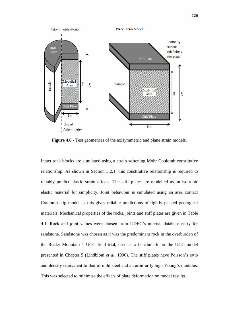
126
Figure 4.6 - Test geometries of the axisymmetric and plane strain models.
Intact rock blocks are simulated using a strain softening Mohr Coulomb constitutive
relationship. As shown in Section 3.2.1, this constitutive relationship is required to
reliably predict plastic strain effects. The stiff plates are modelled as an isotropic
elastic material for simplicity. Joint behaviour is simulated using an area contact
Coulomb slip model as this gives reliable predictions of tightly packed geological
materials. Mechanical properties of the rocks, joints and stiff plates are given in Table
4.1. Rock and joint values were chosen from UDEC’s internal database entry for
sandstone. Sandstone was chosen as it was the predominant rock in the overburden of
the Rocky Mountain 1 UCG field trial, used as a benchmark for the UCG model
presented in Chapter 5 (Lindblom et al, 1990). The stiff plates have Poisson’s ratio
and density equivalent to that of mild steel and an arbitrarily high Young’s modulus.
This was selected to minimise the effects of plate deformation on model results.

127
Table 4.1 - Mechanical Properties for the intact rock material, rock joints and stiff
plates in the laboratory scale models.
Mechanical Property Intact Rock Rock Joints Stiff Plates
Density ρ (kgm-3) 2700 - 7000
Young’s Modulus E (Pa) 1.93×10¹⁰ - 1.00×10¹²
Poisson’s Ratio γ (-) 0.38 - 0.30
Friction Angle ϕ (o) 27.8 30.0 -
Cohesion C (Pa) 2.72×10⁷ 1.00×10⁵ -
Tensile Limit σT (Pa) 1.17×10⁶ 0.00 -
Dilation Angle φ (o) 0.00 5.00 -
Shear Stiffness kS (Nm-1) - 1.00×10⁹ -
Normal Stiffness kN (Nm-1) - 1.00×10¹⁰ -
Testing is performed by holding the lower plate in place while the upper plate moves
downwards at a constant velocity of 0.01ms-1. The models are found to have timesteps
on the order of 1×10⁻⁶ s, giving very low strain rates of approximately 1×10⁻⁸ per
iteration. This helps to maintain a minimal unbalanced force whilst ensuring a
reasonable model runtime. Simulations run to an axial strain of 12%, or until block
contact overlap tolerances are exceeded. Axial stress is measured at the base of the
upper plate. Lateral displacement is measured at nine equally spaced locations along
each side of the rock mass. Young’s modulus, yield stress, Poisson’s ratio and dilation
angle were determined from unconfined results. Young’s modulus and Poisson’s ratio
were determined over an axial strain range of 0.01% to 0.03%. Dilation angle is
determined from the point of zero volumetric strain to an axial strain 0.02% greater
than this.
128
4.2.2 Rock Mass Variations
Eight joint patterns have been tested throughout this work, including an intact
jointless pattern, 4 periodic patterns and 3 stochastically varying patterns. Sample
geometries are shown in Figure 4.7. The Voronoi pattern is generated using UDEC’s
inbuilt Voronoi tessellation algorithm. Further details on the two patterns based on the
discrete fracture network (DFN, Figures 4.7g and 4.7h) are given in Section 4.2.4.
Across all models, the representative edge length L is 10cm unless otherwise stated.
For the Voronoi and DFN patterns, L is the mean edge length across the entire model.
H and W refer to block height and width respectively. All of the DFN models used a
consistent random seed to eliminate random variation from results.
A total of 76 models have been tested under simulated laboratory conditions,
including 53 axisymmetric models and 23 plane strain models. The axisymmetric tests
investigated the behaviour of each of the joint patterns under a range of confining
stresses to determine rock mass material parameters. The plane strain models
investigate the effect of varying geometry, including the effects of changing
geometric parameters of the nominally perpendicular (N-DFN) joint pattern. Further
plane strain models examine the effects of joint mechanical properties on behaviour.
Variations in joint friction angle, dilation angle and normal and shear stiffness were
tested under identical conditions in an attempt to verify relationships between joint
and rock mass properties. Two tests on intact patterns were also performed to
compare model results with experimental data. Finally, repeatability studies of both
axisymmetric and plane strain N-DFN models are performed to investigate the
stochastic variability of the results. The full list of models tested is given in Table 4.2.

129
Figure 4.7a – Intact
Figure 4.7b – Brickwork
Figure 4.7c – Grid
Figure 4.7d – Diamond
Figure 4.7e – Hexagon
Figure 4.7f – Voronoi
Figure 4.7g – Isotropic Discrete
Fracture Network (I-DFN)
Figure 4.7h – Nominally
Perpendicular Discrete Fracture
Network (N-DFN)

130
Table 4.2 – Full list of modelled axial compression tests.
Model(s) Name Geometry Pattern Material
parameters
1 – 7 Brickwork biaxial Axisymmetric Brickwork As Table 4.1
8 – 14 Grid biaxial Axisymmetric Square As Table 4.1
15 – 21 Diamond biaxial Axisymmetric Diamond As Table 4.1
22 – 28 Hexagon biaxial Axisymmetric Hexagon As Table 4.1
29 – 35 Voronoi biaxial Axisymmetric Voronoi As Table 4.1
36 – 42 I-DFN biaxial Axisymmetric I-DFN As Table 4.1
43 – 49 N-DFN biaxial Axisymmetric N-DFN As Table 4.1
50 Brickwork uniaxial Plane Strain Brickwork As Table 4.1
51 Grid uniaxial Plane Strain Square As Table 4.1
52 Diamond uniaxial Plane Strain Diamond As Table 4.1
53 Hexagon uniaxial Plane Strain Hexagon As Table 4.1
54 Voronoi uniaxial Plane Strain Voronoi As Table 4.1
55 I-DFN uniaxial Plane Strain I-DFN As Table 4.1
56 N-DFN uniaxial Plane Strain N-DFN As Table 4.1
57 Small blocks Plane Strain N-DFN L = 7.07cm
58 Large blocks Plane Strain N-DFN L = 14.14cm
59 Tall blocks Plane Strain N-DFN H/W = 2
60 Wide blocks Plane Strain N-DFN H/W = 0.5
61 Low joint friction Plane Strain N-DFN θ = 20.0o
62 High joint friction Plane Strain N-DFN θ = 40.0o
63 Low joint dilation Plane Strain N-DFN ψ = 0.0o
64 High joint dilation Plane Strain N-DFN ψ = 10.0o
65 Low normal stiffness Plane Strain N-DFN kN = 1×10⁹ Nm-1
66 High normal stiffness Plane Strain N-DFN kN = 1×10¹¹ Nm-1
67 Low shear stiffness Plane Strain N-DFN kS = 1×10⁸ Nm-1
68 High shear stiffness Plane Strain N-DFN kS = 1×10¹⁰ Nm-1
69 Intact biaxial Axisymmetric Intact As Table 4.1
70 Intact uniaxial Plane Strain Intact As Table 4.1
71 – 73 Repeatability tests Axisymmetric N-DFN As Table 4.1
74 – 76 Repeatability tests Plane Strain N-DFN As Table 4.1

131
4.2.3 Discrete Fracture Network Design
The discrete fracture network (DFN) patterns (Figures 4.7g, 4.7h) are generated using
a method based on the work of Min et al (2004). DFNs have been used in a number of
successful mechanical and hydraulic models of rock masses (Baghbanan & Jing,
2007; Bidgoli et al, 2013; Bidgoli & Jing, 2014; Blum et al, 2005).
The N-DFN pattern contains two joint sets with normally distributed orientations; one
with a mean angle of 0o and one with mean angle 90o. The isotropic I-DFN pattern
contains a single joint set with a uniformly distributed angle between 0o and 180o. The
position of the centre point of each joint is distributed in a uniformly random manner
within the rock mass. The number of joints within each set is determined by a user
defined joint density. The length of each joint follows a power law distribution with
minimum and maximum cut-offs: The number N of fractures larger than length L is
given as: N = 4L-k, where k is an empirically derived constant with value 2.2 (Min et
al, 2004). The input parameters used in the two DFNs are given in Table 4.3.
Parameters were chosen to give a mean block edge length of 10cm. Block edge length
is a complex function of the density, orientation and length of joints, so choosing
input parameters is often a process of trial and error.

132
Table 4.3 – Geometric parameters for the two joint patterns based on discrete fracture
networks.
Parameter N-DFN I-DFN
Joint Set 1 Joint Set 2
Joint Mean Angle (o) 0 90 90
Standard Deviation in Angle (o) 10 10 180
Joint Minimum Length (m) 1.70 1.70 1.70
Joint Maximum Length (m) 5.00 5.00 5.00
Joint Density (m-2) 5.0 5.0 9.0
The random numbers used to generate the DFN patterns are found using a Poisson
process, as shown in quation 4.1. This gives a good approximation of a uniform
distribution and allows any model to be repeated, provided that the initial random
seed is preserved. The initial seed R1 for the process is determined from the system
clock. This is accurate to 1/100th of a second and covers a 24 hour period, making it
extremely unlikely that two separate models would ever share the same seed.
𝑅𝑛+1 = 27𝑅𝑛 − 𝑖𝑛𝑡(27𝑅𝑛) (4.1)
In order to verify the randomness of the Poisson process, a simple test has been
performed. Ten sets of 1,000 consecutive random numbers between zero and one
were generated using the process. Table 4.4 compares the mean and variance of these
sets with those of the ideal uniform distribution. In addition, the coefficient of
determination (COD) for the plot of Rn against n is given for each set.

133
The results show that the Poisson process is a sufficient method for generating sets of
uniformly distributed random numbers for use in the DFNs. In all cases the mean and
variance of the sets are well within 10% of the ideal value, and the largest coefficient
of determination is well below 1%. The use of the system clock is seen to be a valid
method for generating the random seed, with over 8 million unique values obtainable
in any 24 hour period.
Table 4.4 – Statistical data on random number sets generated using the Poisson
process.
Set Mean Variance COD
1 0.500 0.085 0.00023
2 0.516 0.082 0.00422
3 0.500 0.088 0.00070
4 0.496 0.085 0.00111
5 0.500 0.084 0.00155
6 0.495 0.081 0.00064
7 0.502 0.083 0.00006
8 0.518 0.080 0.00257
9 0.504 0.080 0.00002
10 0.513 0.082 0.00353
Ideal 0.500 0.083 0.00000

134
4.3 SIMULATED COMPRESSION TESTING RESULTS
4.3.1 Axisymmetric Results
Models 1 through 49 used biaxial testing to investigate the effects of joint pattern on
rock mass material properties. Considerable differences in compressive yield strength
and rock mass dilation angle were seen between different geometries. The brickwork
and grid patterns in particular showed very different behaviour to other patterns, with
order of magnitude differences in yield strength and Poisson effect. Material
properties derived from these tests are given in Table 4.5. As shown in Figure 4.8, the
mechanical behaviour of the rock mass depends heavily on the proportion of joints
oriented normally, tangentially or obliquely to the applied strain. Sections 4.3.1.1
through 4.3.1.4 explore this effect in detail for each of the derived material properties.
Table 4.5 – Rock mass material properties derived from simulated triaxial testing.
Geometry E
(Pa)
σC
(Pa)
θ
(o)
C
(Pa)
σT,max
(Pa)
γ
(-)
ψ
(o)
Brickwork 1.58×10⁹ 6.74×10⁷ 61.6 8.54×10⁶ 4.63×10⁶ 0.019 55.2
Grid 1.72×10⁹ 2.57×10⁷ 65.1 2.83×10⁶ 1.31×10⁶ 0.020 77.5
Diamond 1.07×10⁹ 1.01×10⁶ 54.6 1.61×10⁵ 1.15×10⁵ 0.112 38.8
Hexagon 1.37×10⁹ 8.56×10⁶ 67.7 8.43×10⁵ 3.46×10⁵ 0.100 59.3
Voronoi 1.23×10⁹ 1.34×10⁶ 61.0 1.73×10⁵ 9.58×10⁴ 0.110 54.2
I-DFN 1.48×10⁹ 8.03×10⁵ 52.6 1.36×10⁵ 1.04×10⁵ 0.100 38.0
N-DFN 2.68×10⁹ 2.02×10⁶ 57.5 2.94×10⁵ 1.87×10⁵ 0.075 53.3

135
Figure 4.8 – Key effects of joint orientation on mechanical properties derived via
axisymmetric compression testing.
4.3.1.1 Effects of Joint Pattern on Strength
Figures 4.9 and 4.10 show the stress/strain relationships for joint patterns with high
and low compressive strength . Note the considerable difference in compressive
strength between the two figures. The majority of the patterns are seen to behave in
the expected manner for a brittle material such as rock under low confining pressure:
Initial elastic behaviour at low strain is followed by sudden brittle failure and a
considerable reduction in stress. In some models however, strain continues to
accumulate after failure under a reduced value of stiffness to give an overall strain
softening behaviour.

136
Figure 4.9 – Stress/strain relationships seen under axisymmetric testing for patterns
with high yield strength.
Figure 4.10 – Stress/strain relationships seen under axisymmetric testing for patterns
with low yield strength.

137
A strong correlation can be seen between yield strength and joint angle. Patterns
consisting solely of purely horizontal and vertical joints (i.e. the brickwork and grid
models) have considerably higher yield strengths than all other patterns. The hexagon
pattern, in which every third joint is vertical, is also seen to be notably stronger than
the remaining patterns. Of the remaining geometries, the N-DFN pattern (containing
predominantly perpendicular joints) is seen to be the strongest. It is therefore seen that
the presence of normally oriented joints (i.e. those at 0o and 90o angles to the applied
force) considerably strengthens the rock mass, for the following reason:
In all tests, strain is applied in the vertical direction. In the majority of cases failure
occurs by separation along vertical or obliquely angled joints, as seen in Figure 4.11.
Given that all joints have identical material properties, compressive strength must be a
function of joint orientation. It is thought that the principal mechanism behind this
effect is that of strain transfer from the vertical to the horizontal direction.
Figure 4.11 – Failure state of an axisymmetric model using the N-DFN joint pattern.

138
Consider a single joint, at an angle ϕ to the horizontal. This joint is part of a rock mass
subjected to an axially applied strain εa. It can be shown that the total displacement of
this joint in the horizontal (x) and vertical (y) directions are given by Equations 4.2
and 4.3 respectively. The full derivation of these equations is given in Appendix B.1.
𝑢𝑥 =𝐸 𝑎𝐴
2(
1
𝑘𝑠−
1
𝑘𝑛) sin(2𝜙) (4.2)
𝑢𝑦 = 𝐸𝜀𝑎𝐴 (cos2(𝜙)
𝑘𝑛+
sin2(𝜙)
𝑘𝑠) (4.3)
Where A is the surface area of the joint.
The sin(2ϕ) term in Equation 4.2 predicts a maximum horizontal displacement when
joint angle ϕ = 45o, and zero horizontal displacement when ϕ = 0 or 90o. Given that
the majority of models fail by horizontal movement, this explains why patterns
containing normally oriented joints tend to be stronger than those with many oblique
joints. This suggests that the diamond and I-DFN patterns should be the weakest
geometries and the grid/brickwork patterns should be strongest, agreeing with the
results seen in Figures 4.9 and 4.10. Given the difference between the grid and
brickwork results (which have identical joint orientations), some other factor must
also control failure however.

139
4.3.1.2 Effects of Joint Pattern on Stiffness
Rock mass Young’s modulus is seen to vary considerably less with joint orientation
than rock mass strength, suggesting that the fracture pattern has a minor effect on
material stiffness. Definite trends can be observed however, as square based patterns
tend to have the highest stiffnesses, while those with many oblique joints are softer. It
is of note that the N-DFN pattern has a substantially higher stiffness than all other
patterns, including the grid and brickwork geometries. Given that this pattern contains
fewer normally orientated joints than these models, some other effect must be
influencing stiffness. Block interlocking may be a factor, as the N-DFN pattern
produces a number of points at which this may occur. Further investigation is thus
recommended to determine the cause of the trend in rock mass Young’s modulus.
4.3.1.3 Effects of Joint Pattern on Failure Criteria
Figures 4.12 and 4.13 show the relationship between yield strength and confining
pressure for each joint pattern. These relationships are used to examine the effects of
geometry on friction angle, cohesion and maximum tensile strength of the rock mass.
It is of note that the I-DFN and N-DFN curves show a more variable gradient than the
other patterns. This is simply due to the stochastic nature of these patterns increasing
the amount of uncertainty in model results. Interesting behaviour is also seen with the
grid pattern, as an apparent discontinuity in strength occurs at low confining
pressures. As with unconfined failure behaviour, it is interesting to note that this is not
observed with the brickwork pattern.

140
Figure 4.12 – Compressive yield stress as a function of confining pressure under
axisymmetric testing for patterns with high yield strength.
Figure 4.13 – Compressive yield stress as a function of confining pressure under
axisymmetric testing for patterns with low yield strength.

141
Across all geometries, rock mass friction angle is seen to be much greater than that
given by either the intact rocks or joints (as given in Table 4.1). Values given for the
rock masses tend to be of an order similar to the sum of the rock and joint values
(57.8o), suggesting that the frictional resistance of the rock mass may be found
through some additive function based on these component values.
Trends in rock mass friction angle are harder to define than those for other material
parameters. As with unconfined compressive strength, patterns consisting of mainly
horizontal and vertical joints tend to have higher values of friction angle than those
containing many oblique joints. It is of note however that the hexagonal pattern shows
the highest value of friction angle, despite only one in three joints meeting this
criterion. This observation suggests that the presence of vertical joints may be the
deciding factor in rock mass friction. This may be explained by considering how
confining pressure relates to the geometry of the rock mass:
In the biaxial tests, confining pressure is applied in the horizontal direction. As such,
the force is applied most effectively against vertical joints. Because this force acts
against the failure of the rock mass, vertical joints effectively contribute the most to
the strengthening effect of confining pressure. As friction angle relates the yield
strength of a material to an applied confining stress, vertical joints are therefore seen
to give the greatest increase in rock mass friction angles.

142
Cohesion refers to the yield strength of a material under unconfined conditions. As
mentioned in Section 4.3.1.1, it is the yield strength of the normally oriented joints
that gives the largest contribution to rock mass compressive strength. As such,
discussions of the effect of joint pattern on cohesion are identical to those for
unconfined compressive strength. Given that the maximum tensile strength σT is found
as a function of friction angle and cohesion, discussions of the effects of geometry on
this property are also covered in this section.
4.3.1.4. Effects of Joint Pattern on Lateral Expansion
The lateral expansion behaviour of a material under compression depends on the
values of material Poisson’s ratio and dilation angle. These properties predict the
extents of lateral expansion in the elastic and plastic regimes respectively. Figures
4.14 and 4.15 plot the volumetric/axial strain relationships for the patterns showing
high and low extents of peak strain. As with other properties, square based geometries
are seen to give extremes of expansion behaviour.

143
Figure 4.14 – Volumetric/axial strain relationship under axisymmetric testing for
patterns showing high axial yield strains.
Figure 4.15 - Volumetric/axial strain relationship under axisymmetric testing for
patterns showing high axial yield strains.
144
Poisson’s ratio represents the amount of lateral strain observed per unit elastic axial
strain, as shown in Equation 4.4:
𝛾 = −𝛿 𝐿
𝛿 𝐴 (4.4)
In all of the rock masses tested, the measured Poisson’s ratio is considerably lower
than that of the intact rock elements. This can be explained by considering the axial
strain of the entire rock mass compared with that of the intact blocks. For a rock mass,
the total axial strain is found from the contributions of blocks and joints, as shown in
Equation 4.5. Note that this assumes joints have negligible thickness.
𝜀𝑎,𝑡𝑜𝑡 =1
∑ 𝐻𝐵𝐵[∑ (𝐻𝐵𝜀𝑎,𝐵) + ∑ 𝑈𝑎,𝐽𝐽𝐵 ] (4.5)
Where:
H Height (m)
U Displacement (m)
ε Strain (-)
Subscripts:
B = Blocks
J = Joints
a = Axial

145
In effect, Equation 4.5 states that the total strain on the rock mass εa,tot, is greater than
the sum of the strains on the intact blocks. This difference becomes greater as the
degree of jointing increases. This increase in the value of εa gives a corresponding
decrease in the value of γ (as calculated by Equation 4.4), compared with that for the
intact rocks. In essence, much of the axial strain applied to the rock mass is taken up
by the joints as opposed to the rocks. As such, the Poisson’s ratio of any given rock
mass will always be smaller than that of its constituent particles. This is true for real
rock masses as well as those simulated in DEM (Hoek, 2001).
While all geometries show low values of Poisson’s ratio, the grid and brickwork
patterns are seen to be particularly incompressible. This can be explained by Equation
4.2, which suggests that models containing purely horizontal and vertical joints would
not show elastic horizontal expansion. The expansion that is seen in these models is
primarily caused by the Poisson effect of the blocks themselves. The N-DFN pattern
shows the lowest Poisson’s ratio of the remaining geometries. This is expected given
the prevalence of horizontal and vertical joints in this pattern. The diamond pattern,
containing purely oblique joints, shows the highest value. With the exception of the
grid and brickwork geometries, Poisson’s ratio was similar across all geometries. This
suggests that joint orientation only has an effect on this value up to a certain point,
after which other effects dominate.

146
Rock mass dilation refers to the increase in volume of the rock mass under plastic
strain. In all of the models tested, dilation is observed in the sudden transition from
volumetric contraction to expansion at the point of shear yielding. For all joint
patterns, dilation angle is seen to be much greater than that of the individual joints, as
given in Table 4.1. Measured values of dilation angle are also seen to be greatest for
those patterns containing few oblique joints. The high levels of dilation in such
models are caused by the complete separation of the outermost rock blocks from the
main rock mass. These blocks tend to have a horizontal velocity after failure, such
that their displacement from the rock mass increases over time. The motion of these
blocks quickly comes to dominate the dilation process, contributing a much greater
volume increase than simple shear dilation along joints. A more precise understanding
of rock mass dilation is difficult to achieve due to difficulties in accurately measuring
volumetric expansion using only a small number of displacement measuring points.
4.3.2 Plane Strain Results
4.3.2.1 Comparison of Axisymmetric and Plane Strain Results
Models 50 through 56 repeated the unconfined compression tests of various joint
patterns using a plane strain geometry. The plane strain assumption was chosen as it is
required for the UCG model, while the axisymmetric model is a more realistic
representation of an actual lab scale test. Stress/strain and volumetric/axial strain
behaviours were qualitatively similar to those seen under axisymmetric compression,
however a number of quantitative differences are observed. Table 4.6 lists the derived
material properties for the joint patterns tested.

147
Table 4.6 - Derived material properties from plane strain compression testing for
models with varying joint patterns.
Geometry E
(Pa)
σC
(Pa)
γ
(-)
ψ
(o)
Brickwork 6.69×10⁸ Not Reached 0.010 Not Reached
Square 8.33×10⁸ 1.77×10⁷ 0.012 67.6
Diamond 4.65×10⁸ 9.99×10⁵ 0.254 3.23
Hexagon 6.57×10⁸ 1.08×10⁷ 0.246 4.58
Voronoi 6.72×10⁸ 3.53×10⁶ 0.258 12.7
I-DFN 5.91×10⁸ 8.85×10⁵ 0.253 4.99
N-DFN 9.06×10⁸ 3.14×10⁶ 0.114 9.24
While yield strength appears to be unaffected by the method of compression, rock
mass stiffness is observed to be approximately half as large under plane strain testing
for all patterns. Conversely, Poisson’s ratio is twice as large under plane strain testing,
though the square based patterns still show incompressible behaviour. The difference
seen with Poisson’s ratio can be explained with reference to the plane strain
assumption. In an axisymmetric model, the lateral expansion of the rock mass can
occur in both dimensions orthogonal to the vertical axis. In the plane strain model, it
is assumed that no motion occurs into the plane of the page. As such, in order to
maintain the same degree of volumetric expansion, Poisson’s ratio must be twice as
large in the plane strain model as in the axisymmetric model. The reduction in
Young’s modulus is believed to be caused by a similar effect, as the lateral forces
resisting axial strain in the rock mass would only be half as strong for similar reasons.
Although the plane strain assumption is less, it is sufficient for use in the UCG model,
and therefore is acceptable in tests related to this model. Given the differences in
results, it is recommended that the mechanical properties of the UCG model should be
based on axisymmetric results to avoid a doubling of the plane strain effect.

148
Dilation angle is also seen to be considerably smaller under plane strain testing than
under axisymmetric testing, though square based patterns still show extreme values.
Dilation angles measured under plane strain compression were seen to be of an order
similar to that given for the joints. This suggests that large scale horizontal block
motion is rare under plane strain conditions, with rock mass volumetric expansion
being driven principally by the dilation of the joints. In many cases it was seen that
plane strain models did not undergo the same extent of horizontal separation as the
comparative axisymmetric model, confirming this suggestion.
Finally, it is of note that the brickwork pattern never reached failure under plane strain
testing. This model encountered overlap errors after approximately 9.5% axial strain.
Increasing the value of overlap tolerance was not seen to solve this issue. As such,
distinct values for compressive strength and dilation angle cannot be derived for this
pattern. Due to their simplicity, square based joint patterns are often used in discrete
element models (Coulthard and Dutton, 1988; Keilich et al, 2006). Given the results
above however, it is suggested that such patterns should not be used within regions of
high stress, as they are incapable of fully realising plastic behaviours, calling the
results of many previous models into question.
Despite the above limitations, the general similarity between plane strain and
axisymmetric results suggests that the methodology of incorporating material
properties derived from axisymmetric testing into plane strain geomechanical models
is justified. The appropriate selection of material properties for the UCG model is
discussed further in Section 4.6.

149
4.3.2.2 Effects of Block Size on Mechanical Behaviour
In addition to shape, the size and aspect ratio of distinct element blocks are shown to
have a strong effect on the mechanical behaviour of the rock mass. Models 57 through
60 investigated these effects by varying the densities of nominally horizontal and
vertical joints in the N-DFN pattern under plane strain compression testing. This
geometry was chosen as it gave good results in previous tests and has geometric
properties which are easy to adjust.
In the case of the small and large block models, joint density was doubled or halved in
order to produce blocks with average areas equal to half or twice that of the base case.
In the case of the tall and wide models, one density was increased while the other was
decreased by a factor of √2. This produces blocks with an average area equal to that
of the base case models, but in which the ratio of block height to block width is
increased or decreased by a factor of two. Table 4.7 lists the derived material
properties for these rock masses.
Table 4.7 - Derived material properties from plane strain compression testing for
models with varying block size and aspect ratio
Geometry E
(Pa)
σC
(Pa)
γ
(-)
ψ
(o)
Base Case 9.06×10⁸ 3.14×10⁶ 0.114 9.24
Small Blocks 6.73×10⁸ 1.78×10⁶ 0.113 9.07
Large Blocks 1.10×10⁹ 4.47×10⁶ 0.144 9.94
Tall Blocks 9.77×10⁸ 1.99×10⁶ 0.172 6.83
Wide Blocks 5.63×10⁸ 5.26×10⁶ 0.194 29.85

150
Block size and aspect ratio are seen to affect rock mass strength and stiffness in
predictable ways. Increased block size increases both Young’s modulus and
compressive strength. This is to be expected, as larger blocks reduce the total number
of joints in the rock mass. As such, behaviour depends more on the blocks (strong,
stiff) than the joints (weak, soft).
Increasing block width increases rock mass strength but decreases stiffness. The
increase in strength can be explained by Equation 4.2. As blocks get shorter and
wider, the number of horizontal joints (under normal stress) increases while the
number of vertical joints (under shear stress) decreases, as shown in Figure 4.16. Due
to the ratio of joint normal to shear strength (10:1), the increased number of horizontal
joints increases the overall strength of the rock mass.
Area = 0.16m2
No. Blocks = 16
No. Horizontal Joints = 3
No. Vertical Joints = 3
Area = 0.16m2
No. Blocks = 16
No. Horizontal Joints = 7
No. Vertical Joints = 1
Figure 4.16 – Effect of varying block aspect ratio on the numbers of horizontal and
vertical joints in the model. Greater numbers of vertical joints increase the horizontal
motion of the rock mass, promoting failure and thus reducing rock mass strength.

151
The decrease in stiffness with block width is more difficult to understand, but is
predominantly caused by the increased number of horizontal joints causing the rock
mass to depend more on joint behaviour than block behaviour. Although Equation 4.3
suggests the shearing of vertical joints contributes the most to vertical motion,
shearing may not yet have begun at the low values of strain under which Young’s
modulus is derived. In addition, the reduced potential for block interlocking with short
wide blocks also contributes to the reduction in stiffness.
Table 4.7 suggests that rock mass Poisson’s ratio is not greatly affected by block size.
Block aspect ratio is seen to alter the recorded values, but the lack of a clear trend
suggests these differences are simply due to random variations. These results suggest
that the Poisson effect within a rock mass depends entirely on the orientation of the
joints (as in Equation 4.2) and is not affected by their number or length. Dilation
angle appears to be very weakly related to block size, however there is a strong
relationship between block aspect ratio and rock mass dilation angle. Short, wide
blocks are seen to give a much greater extent of dilation than tall, thin blocks. This
effect can be explained with reference to the conservation of block area. Assuming
equal values of Poisson’s ratio, short, wide blocks undergo much greater lateral
expansion than tall, thin blocks when both are compressed by the same height
increment. As such, wide blocks contribute more to the post-failure expansion of the
rock mass than tall blocks, therefore increasing rock mass dilation angle.

152
4.3.2.3 Effects of Joint Material Properties on Mechanical Behaviour
Models 61 through 68 investigated the effects of joint material properties on the
mechanical response of the rock mass. The influence of joint friction angle, dilation
angle and normal and shear stiffnesses were tested under plane strain compression of
the N-DFN geometry. Table 4.8 lists the mechanical properties derived from these
models.
Table 4.8 - Derived material properties from plane strain compression testing for
models with varied joint mechanical properties.
Model E
(Pa)
σC
(Pa)
γ
(-)
ψ
(o)
Base Case 9.06×10⁸ 3.14×10⁶ 0.114 9.24
Low Friction 8.08×10⁸ 1.23×10⁶ 0.127 18.08
High Friction 8.46×10⁸ 4.26×10⁶ 0.151 11.42
Low Dilation 8.33×10⁸ 2.70×10⁶ 0.138 6.62
High Dilation 8.13×10⁸ 2.24×10⁶ 0.127 12.31
Low Normal Stiffness 1.38×10⁸ 1.07×10⁶ 0.021 16.51
High Normal Stiffness 1.99×10⁹ 2.78×10⁶ 0.380* 6.94
Low Shear Stiffness 4.99×10⁸ 1.31×10⁶ 0.346 8.94
High Shear Stiffness 9.88×10⁸ 2.96×10⁶ 0.028 13.13
*Due to this model reaching the volumetric turning point at very low axial strain,
Poisson’s ratio has to be measured at lower strains than in other models.
153
These results suggest that joint friction and dilation angles have little effect on rock
mass behaviour, with two exceptions: Firstly, joint friction angle is correlated with
rock mass compressive strength. As mentioned previously, friction angle relates to the
shear yield strength of a joint under a given normal stress. Given that many joints
within the model fail in shear, this explains the observed correlation. Second, there is
a correlation between the dilation angle of the joints and the rock mass. This is to be
expected, as the dilation of single joints promotes that of the rock mass.
Unlike joint friction and dilation angles, joint stiffnesses have a considerable effect on
rock mass behaviour. Both normal and shear stiffnesses have a strong positive effect
on rock mass Young’s modulus. This is explained with reference to Equation 4.3: As
both stiffnesses are denominators in the calculation of vertical displacement, increases
in stiffness reduce axial displacement and hence increase Young’s modulus. The
relative importance of the two stiffnesses depends on the prevalence of joints at near
horizontal and near vertical angles, based on the cos2 and sin2 terms in the equation.
Both stiffnesses are also seen to have a positive effect on rock mass compressive
strength, though it is of note that the strongest rock mass appears to be that given in
the base case model. Given the inherent randomness of the N-DFN geometry, this
discrepancy is seen to be predominantly due to random variations in the deformation
of the joint pattern. The overall effect can be explained with reference to Equation
4.2. Increased stiffnesses reduce the extent of horizontal motion, in turn leading to a
reduction in joint separation and an increased material strength. As with Young’s
modulus, the relative importance of the stiffness depends on the prevalence of near
horizontal (failing in shear) and near vertical (failing in tension) joints.

154
Joint normal and shear stiffnesses appear to have opposing effects on the lateral
expansion behaviour of rock masses. Increasing joint normal stiffness causes an
increase in rock mass Poisson’s ratio and a decrease in rock mass dilation angle. The
reverse is seen with joint shear stiffness. The influence of joint stiffnesses on the
Poisson effect is explained by Equation 4.2: An increase in kS causes a decrease in the
reciprocal term, which in turn causes an decrease in the total elastic lateral expansion
and hence Poisson’s ratio. Conversely, the negative sign in front of the normal
stiffness term causes the opposite effect, as observed.
Effects of stiffness on dilation appear to oppose those of the Poisson effect. This
opposition can also be observed in the results based on joint pattern, as given in
Tables 4.4 and 4.5. This observation suggests some kind of causal link between the
mechanisms of elastic and plastic lateral expansion, in which reductions in expansion
during the elastic phase lead to increased expansion after failure. It is believed that
this is effect is predominantly caused by the storage of strain energy in the rock mass.
Models which undergo less elastic expansion are seen to reach higher levels of stress
at failure. This stress then manifests as a greater extent of lateral motion in the post-
failure stage of compression, leading to an increase in rock mass dilation.

155
4.4 MODEL VALIDATION
The observations and trends discussed in the previous sections relate only to rock
masses simulated with UDEC (i.e. not real rock masses). In order to obtain confidence
in this methodology when related to real rock material, validation against real world
data and other techniques must be performed. Results of similar compression studies
using different numerical methods agree well with both reality and the results given in
this work (Rong et al, 2013; Tan et al, 2015). Given the highly variable behaviour of
geologic materials under different conditions however; it is essential that any
geotechnical model is proved to be internally valid before its results can be trusted. In
order to ensure the validity of this model, a number of comparative tests have been
performed.
4.4.1 Comparison with Geological Strength Index
Firstly, material properties derived by the axisymmetric simulations are compared
with those obtained by the empirical geological strength index (GSI). Rock mass
Young’s modulus, friction angle and cohesion are calculated according to the method
of Hoek et al (2002), using GSI parameters given in Marinos et al (2007). Results of
the comparison are given in Table 4.9.

156
Table 4.9 – Comparison of axisymmetric results with empirical predictions from
Geological Strength index.
Geometry E (Pa) θ (o) C (Pa)
Brickwork 1.58×10⁹ 61.6 8.54×10⁶
Grid 1.72×10⁹ 65.1 2.83×10⁶
Diamond 1.07×10⁹ 54.6 1.61×10⁵
Hexagon 1.37×10⁹ 67.7 8.43×10⁵
Voronoi 1.23×10⁹ 61.0 1.73×10⁵
I-DFN 1.48×10⁹ 52.6 1.36×10⁵
N-DFN 2.75×10⁹ 57.5 2.78×10⁵
GSI 1.40×10⁹ 41.0 6.01×10⁶
Good agreement is seen between the GSI predictions and model results for rock mass
Young’s modulus and cohesion, especially with the square based patterns. This is to
be expected, given that many real rock masses contain predominantly horizontal
joints. As such, the brickwork pattern is believed to give the most realistic material
properties for a rock mass, although the use of the pattern itself in models under high
stress is not recommended.
It is of note that a considerable difference is seen between UDEC and GSI in terms of
friction angle. This difference may be caused by the kinematic constraints of the
axisymmetric model compared with a real (i.e. 3D) rock mass. As the UDEC model
assumes identical behaviour in the two lateral dimensions, the effects of planes of
weakness in certain directions may be ignored. In reality, these will weaken the rock
mass somewhat at high confining pressures leading to a reduced friction angle
compared with that predicted by UDEC. Considering the inaccuracies of the
geological strength index and the inherent variability of real rock masses however,
model results are considered to be accurate enough for all practical purposes.

157
4.4.2 Comparison with Experiment
Two jointless models (69 and 70) have been tested and compared with experimental
results from a triaxial test performed on Stanton Moor sandstone at the Nottingham
Centre for Geomechanics. Stanton Moor sandstone is a fine to medium grained
carboniferous millstone grit (Building Research Establishment, 2000) typical to the
overburden above coal seams in the north of England. The results of this comparison
are shown in Figure 4.17.
Figure 4.17 – Comparison of stress/strain response between models and experiment.

158
It can be seen that the axisymmetric model agrees well with experiment in terms of
failure prediction. Errors of 5.4% and 14.0% are seen for failure stress and strain
respectively, well within the expected error margins for a geologic material (Cai,
2011). The axisymmetric model is seen to somewhat overpredict stiffness however. It
is believed that the lack of resolution of the rock microstructure (cracks, grain
boundaries etc.) is the main reason for this difference. Given the high variability of
real rocks however, the inaccuracies of the model are considered minor.
The results of the intact plane strain model show considerably less agreement with
experiment. Although model stiffness is reasonable in comparison with the
axisymmetric case, the plane strain model greatly overpredicts the failure strength of
the rock mass. Given the considerable differences in geometry however, close
agreement between the plane strain model and reality was not expected.
4.4.3 Repeatability Testing
In order to better understand the variability of the model, a number of repeats of the
N-DFN models have been performed. Models 71-73 repeated the axisymmetric test
(model 43) while models 74-76 repeated the plane strain test (model 56). Tables 4.10
and 4.11 show the variability in derived material parameters for each of these models.

159
Table 4.10 – Derived material properties and variability statistics for the
axisymmetric repeatability study.
Model E
(Pa)
σC
(Pa)
γ
(-)
ψ
(o)
Base case (model 43) 2.68×10⁹ 2.02×10⁶ 0.075 53.3
Repeat 1 (model 71) 2.74×10⁹ 2.03×10⁶ 0.093 60.4
Repeat 2 (model 72) 2.45×10⁹ 1.88×10⁶ 0.078 56.4
Repeat 3 (model 73) 2.59×10⁹ 1.87×10⁶ 0.089 36.6
Average 2.59×10⁹ 1.95×10⁶ 0.084 51.7
Standard Deviation 1.47×10⁸ 8.68×10⁴ 0.009 10.5
COV 5.7% 4.5% 10.7% 20.3%
Table 4.11 – Derived material properties and variability statistics for the plane strain
repeatability study.
Model E
(Pa)
σC
(Pa)
γ
(-)
ψ
(o)
Base case (model 56) 9.06×10⁸ 3.14×10⁶ 0.114 9.24
Repeat 1 (model 74) 8.32×10⁸ 2.43×10⁶ 0.143 13.57
Repeat 2 (model 75) 8.77×10⁸ 3.66×10⁶ 0.139 13.98
Repeat 3 (model 76) 7.88×10⁸ 3.34×10⁶ 0.129 11.58
Average 8.51×10⁸ 3.14×10⁶ 0.131 12.09
Standard Deviation 5.17×10⁷ 5.21×10⁵ 0.013 2.17
COV 6.1% 16.6% 9.9% 18.0%
In both cases it is seen that the variability in results is reasonably small, and generally
within the range of variation expected for a geological material (Cai, 2011). The small
number of repeats performed does reduce the reliability of these statistics however.
As such, it is suggested that the results of further modelling work based on this pattern
should be repeated a number of times to ensure reliable reporting.

160
Variations in Young’s modulus and Poisson’s ratio are seen to be reasonably small
and unrelated to the geometric assumption used. Given that both of these properties
are determined at low values of axial strain, this suggests that variations in the N-DFN
geometry have little effect on the elastic behaviour of the material. Dilation angle is
also seen to have a variability unrelated to the geometric assumption used, however
the magnitude of this variability is considerably larger.
Variability in dilation is partly due to differences in individual DFN patterns causing
more or less horizontal motion at key locations in the rock mass. As mentioned in
Section 4.3.1.4, accurate derivation of dilation angle is difficult using only a small
number of displacement measuring points. This difficulty exacerbates the measured
variability of dilation angle as the measurement points may or may not be nearest to
the blocks which are undergoing the most dilation. The final parameter considered is
the rock mass compressive strength. This is seen to vary considerably more under
plane strain testing than axisymmetric testing. It is believed that this variation may be
linked to the more ductile behaviour commonly seen in plane strain models (as
evidenced by an increased Poisson’s ratio and reduced dilation angle), as this makes
accurate determination of yield stress more difficult.

161
Despite the above considerations, the methodology of simulated triaxial testing to
determine material properties is believed to be valid, given the inherent difficulties
and variability seen with any method for the prediction of rock mass strength. The N-
DFN pattern is also seen to provide a reasonable means to account for this inherent
uncertainty in modelling geological materials. Considerable reductions in variability
for the axisymmetric model compared with the plane strain model suggest this
geometry should be used for future determinations of rock mass properties. As such,
material properties derived from axisymmetric simulations will be used in all future
UCG models, and the N-DFN pattern will be used within the model to incorporate a
random element into the results.
4.4.4 Observations of Failure Behaviour
In addition to its use in determining material properties, simulated compression
testing allows us to gain a better understanding of the failure mechanisms of granular
materials. Such tests are commonly performed using particle based DEM methods
(Chen et al, 2016; Hadda et al, 2015; Liu et al, 2015), as these are more suited to
investigating fracture and failure behaviour. Comparisons of the behaviour seen
between the UDEC compression models and reality can be used as a means of
validating UDEC results however. Andreev (1995) states that compressive failure of
rock occurs in 6 distinct phases:

162
1. Microscopic cracks in the rock close, giving an increase in strain at low stress.
2. Grains begin to deform elastically, giving an approximately linear stress/strain
relationship.
3. Fractures begin to propagate and dilation begins to occur, causing instabilities
in the stress/strain curve.
4. Fracture propagation accelerates, causing the stress/strain curve to level off.
5. Brittle failure of the rock causes a sudden decrease in stress.
6. Strain accumulates rapidly post-failure, with stress given by the residual
strength of the rock.
Figure 4.18 shows the stress/strain relationship for the axisymmetric N-DFN model
(model 43). The close agreement between model results and expectations provides
further evidence for the validity of simulated compression testing in UDEC.
Figure 4.18 – Comparison of model results with the six stages of rock failure
(Andreev, 1995).

163
4.5 MODEL LIMITATIONS
While the overall result of the new model methodology appears to be a success, a
number of limitations must be discussed: Firstly, it is seen that the choice of
assumption used to represent a 3D material in 2D space has a profound effect on
material behaviour, especially with regards to plastic lateral expansion. Although the
axisymmetric assumption more closely resembles reality, care should be taken
applying results obtained using this method to large scale models represented by the
plane strain assumption. Second, the reported results of all tests are seen to be highly
sensitive to random perturbations of the model. This is especially notable with the
stochastically based I-DFN and N-DFN geometries, but effects are also observed in
the stress/strain response of fully deterministic patterns due to the semi-random nature
of failure mechanics.
Finally, considerable uncertainty is introduced into the derived material properties by
the method of their calculation from stress/strain and volumetric/axial strain graphs.
The turning points and gradients of these graphs can be difficult to accurately
determine, and the uncertainty this causes is often amplified by their conversion into
material properties. The difficulty in calculating accurate material properties is also
greatly affected by the inherent randomness of the model behaviour. These
inaccuracies are similar to the variability seen in reality however, such that the
simulated results are often of an accuracy comparable to that achievable by
experiment.

164
It is important to note that errors inherent in this methodology have the potential to
introduce even larger errors into the results of any model based on this work,
including the UCG model detailed in the remainder of this thesis. Conversely,
currently used empirical models also show very high degrees of variation and low
accuracy, often due to their user based decision making requirements. In addition, real
world rock masses can often vary considerably over short distances, such that
accurate depictions of material properties are not possible without fully representing
every individual rock within the assembly. As previously mentioned, the inaccuracies
of the model are comparable to real word variability (Cai, 2011). Given these
considerations, it is believed that the accuracy of these simulations are appropriate for
the end use of the methodology. Some random variability in model results is desired,
as this reflects the inherent variability of real rock masses. The use of the N-DFN
pattern in future modes should be sufficient to achieve this degree of variability.

165
4.6 PARAMETER SELECTION
Results of both axisymmetric and plane strain simulations have been used to inform
the selection of rock mass material properties and block geometry for use in the UCG
model. This section explains and justifies the decisions made in this regard.
In order to maintain accuracy whilst limiting runtime, the UCG model geometry is
broken into two distinct regions. The region near the cavity must have a high joint
density and a degree of randomness to account for the largely unknown fracturing
behaviour caused by the UCG process. Less resolution is needed further away from
the cavity, therefore the joint pattern is this region can be simplified. Both regions
should still show an appropriately brittle response and give a realistic depiction of
geomechanical behaviour. For these regions the final model uses an N-DFN pattern
within the highly fractured region near the cavity, while a brickwork pattern with a
considerable reduction in joint density is used in the region far from the cavity.
The N-DFN pattern was chosen for four principal reasons: Firstly, the geometry is
somewhat representative of real rock mass stratification. Secondly, the material
behaviour of the pattern, while generally weaker than square based geometries, still
gives an appropriately brittle rock mass response. Third, the stochastic nature of the
N-DFN pattern allows for relatively simple fine-tuning of the random elements of
rock mass behaviour. Finally, the inherent randomness of the N-DFN pattern provides
a simple means to simulate the variability observed in real rock materials.
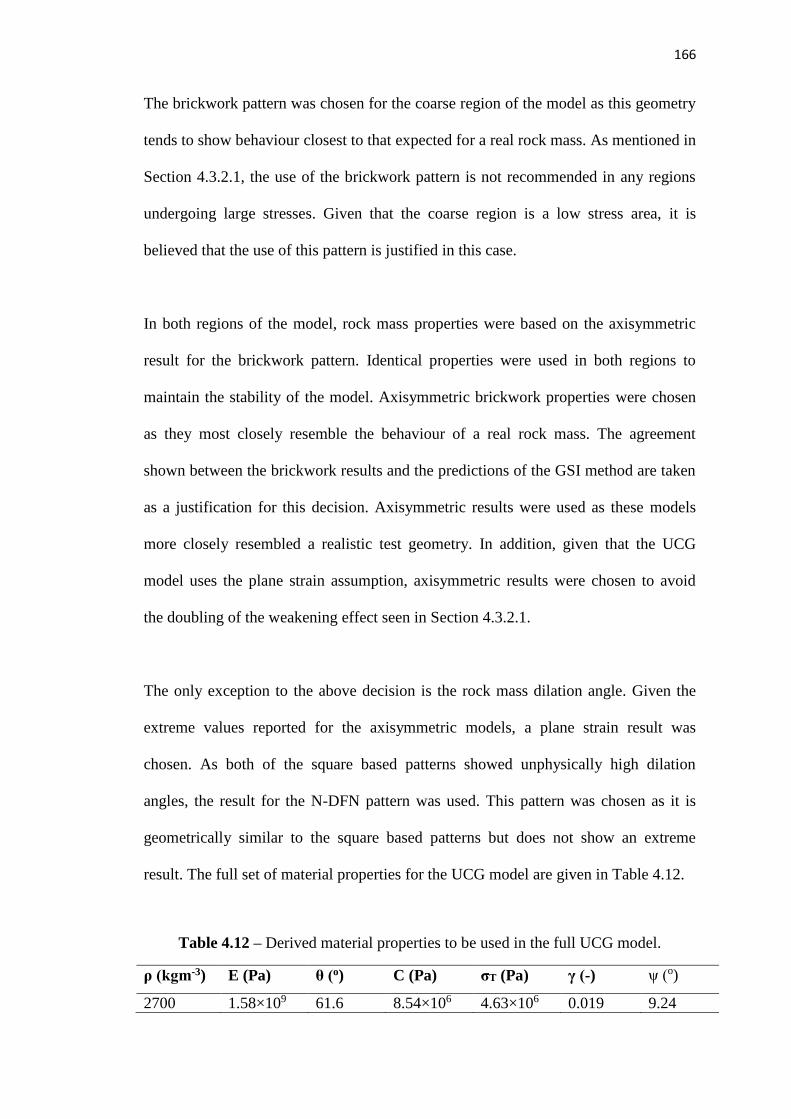
166
The brickwork pattern was chosen for the coarse region of the model as this geometry
tends to show behaviour closest to that expected for a real rock mass. As mentioned in
Section 4.3.2.1, the use of the brickwork pattern is not recommended in any regions
undergoing large stresses. Given that the coarse region is a low stress area, it is
believed that the use of this pattern is justified in this case.
In both regions of the model, rock mass properties were based on the axisymmetric
result for the brickwork pattern. Identical properties were used in both regions to
maintain the stability of the model. Axisymmetric brickwork properties were chosen
as they most closely resemble the behaviour of a real rock mass. The agreement
shown between the brickwork results and the predictions of the GSI method are taken
as a justification for this decision. Axisymmetric results were used as these models
more closely resembled a realistic test geometry. In addition, given that the UCG
model uses the plane strain assumption, axisymmetric results were chosen to avoid
the doubling of the weakening effect seen in Section 4.3.2.1.
The only exception to the above decision is the rock mass dilation angle. Given the
extreme values reported for the axisymmetric models, a plane strain result was
chosen. As both of the square based patterns showed unphysically high dilation
angles, the result for the N-DFN pattern was used. This pattern was chosen as it is
geometrically similar to the square based patterns but does not show an extreme
result. The full set of material properties for the UCG model are given in Table 4.12.
Table 4.12 – Derived material properties to be used in the full UCG model.
ρ (kgm-3) E (Pa) θ (o) C (Pa) σT (Pa) γ (-) ψ (o)
2700 1.58×10⁹ 61.6 8.54×10⁶ 4.63×10⁶ 0.019 9.24

167
4.7 CONCLUDING REMARKS
This work aimed to investigate the effect of joint patterns on rock mass material
properties and develop a methodology for the selection of these properties and
patterns for use in DEM models. Validation studies comparing simulation results with
experiment verify the methodology, while similarities between model results and
empirical correlations show that the method produces usable material parameters.
Although a number of issues limit the accuracy of the methodology, this is considered
reasonable in comparison with the inherent variability of rock mass properties in
reality.
Model results show that the mechanical properties of a rock mass depend heavily on
the ratio of fractures oriented normally, tangentially and obliquely to the direction of
applied strain. The ratio of joint shear to normal stiffness also has a profound effect on
behaviour which is intrinsically linked to geometric properties. Joint dilation angles
are also shown to have a notable influence on the overall mechanical response of rock
masses. The mechanisms behind these effects have been explored and simple
relationships have been drawn which allow for the prediction of rock mass
displacements based on the orientation and stiffness of the joints contained. These
relationships also allow for a qualitative understanding of how these parameters
control the strength, brittleness and lateral expansion behaviour of the rock mass.

168
In addition to the determination of material properties, this work proposes a new joint
pattern based on the discrete fracture network. This geometry allows for the realistic
modelling of fractured rock masses without the need for excessive numbers of
fractures. The stochastic nature of the pattern allows models to be based on available
statistical site data and can account for local variations across a site. The random
nature of the pattern also allows for a realistic representation of the variability
inherent in real rock masses. The use of both the N-DFN geometry and the new
material properties should allow for greater confidence in the modelling of highly
fractured rock masses where the exact pattern of fracturing is unknown. Chapter 5
shows how these principles are applied to the modelling of UCG.
It is suggested that further work in the modelling of simulated compression tests
should be performed in order to improve the accuracy of the method and further prove
its validity. Investigations into the effects of other properties, such as fracture
cohesion, the variability of joint angles and the choice of constitutive model could
provide greater insight into the behaviour of rock masses simulated using DEM. An
extension of this work to cover investigations into the hydraulic behaviour of rock
masses is also suggested. Finally, the application of this methodology to other rock
materials (as opposed to sandstone as used in this work) could be performed in order
to develop a database of reduced material properties or empirical correlations for
various rock types. Such a database could be very useful for future efforts to model
the behaviour of heavily jointed rock masses.

169
5. MODEL DEVELOPMENT
SUMMARY
This chapter discusses the development of the coupled mechanical, hydraulic and
thermal aspects of the underground coal gasification (UCG) model created with the
Universal Distinct Element Code (UDEC). Discussions cover the decisions made with
regards to model geometry, material properties, boundary and initial conditions and
the development of new functionality within UDEC for both mechanical and thermal
simulations. A number of limitations of the software are presented, and methods for
overcoming these are discussed. Throughout the chapter, the conflicting issues of
model accuracy, stability and runtime and analysed and conclusions are drawn about
how these issues should be addressed. With careful model design and the inclusion of
new functionality, UDEC is shown to be more than capable of modelling the
complexities of UCG’s impact on the local environment.

170
5.1 MODEL STRUCTURE
5.1.1 Order of Operations
As mentioned in Section 3.2.1, mechanical simulations in UDEC work by finding the
equilibrium state of the rock mass both before and after excavation. Ground
movements are then determined as the difference in the displacements found at these
states. In the UCG model, the rock mass is simulated at 3 distinct stages:
1. Before – the initial equilibrium stage, before gasification begins.
2. After – the state of the model after gasification ceases.
3. Final – the state of the model after the rock mass has cooled down and
groundwater pressures have reverted to their initial values.
This formulation allows the model to simulate the environmental damage caused by
the UCG operation over the full life cycle of the process, including decommissioning.
Results can be analysed at each of the three stages, and comparisons drawn between
any two points in time. In addition to the three calculation stages, a number of
auxiliary steps are required. Figure 5.1 shows the individual steps involved in the
entire model. Numbers in brackets refer to the section of the thesis in which further
details on the relevant step are given.

171
Figure 5.1 – Schematic description of the calculation steps involved in the fully coupled thermal/hydraulic/mechanical UCG model.

172
5.1.2 Data Requirements
In order to produce results a great deal of input data are required by the model,
however the accuracy of the model is limited by uncertainties in this data. In order to
minimise the risks of erroneous calculations from incorrect data, the number of user
entered values has been minimised. Wherever possible, modelling parameters are
derived from their relationship with other properties, rather than being entered by the
operator. In other cases, constant values have been chosen to give appropriate results.
For a simple, single cavity UCG model, the variables which must be entered by the
user are shown in Table 5.1. The base case values were chosen based on field
measurements from the Rocky Mountain 1 field trial site (Lindblom et al, 1990;
Mason et al, 1987). This site was chosen as a benchmark case for the UCG model as a
considerable amount of published geological and geometric data are available from
this trial.
Table 5.1 – Required input variables for fully coupled UCG model.
Variable Value (base case)
Cavity Height (m)1 14.2
Cavity Width (m)1 12.4
Cavity Depth (m)1 98.4
Water Table Depth (m)2 27.6
Site Permeability (mD)2 5.29
1 – Lindblom et al, 1990. 2 – Mason et al, 1987. Site permeability data are
geometrically averaged.

173
5.1.3 Data Produced
The fully coupled UDEC model produces a large quantity of data at each of the three
stages mentioned in Section 5.1.1. Table 5.2 lists the important outputs produced and
the locations at which they are measured. Many more properties can also be extracted
from the model and used in analysing rock mass behaviour, including forces, stresses,
displacements, flow rates, pressures and joint apertures.
Table 5.2 – Important output data obtained from the coupled UDEC model of UCG.
Output Locations
Surface Displacement 50 equally spaced points along the top edge of the model
Groundwater Pressure At every domain within the model
Rock Mass Temperature At every intact block within the model

174
5.2 MODEL GEOMETRY
5.2.1 Site Geometry
Site geometry refers to the large scale features of the model, including its total width
and height. These properties are derived from the cavity geometry given in Table 5.1.
As mentioned in Section 4.6, the model is broken into ‘coarse’ and ‘fine’ mesh
regions in order to reduce runtime whilst retaining accuracy. Figure 5.2 shows the
model geometry. Numbers in brackets refer to those from the Rocky Mountain 1
model (Lindblom et al, 1990). The effects of variations in these geometric properties
are investigated in Chapter 8. The overall shape of the cavity is assumed to be
identical in all models, though the dimensions of height, width and depth may vary.
The dimensions of the model varied throughout the creation process. The final values
used were chosen in an attempt to give as accurate a model as possible whilst
retaining a runtime under 24 hours. Model width is set at 2.5 times the predicted
width of the subsidence trough (as given by the angle of draw) to avoid the influence
of boundary conditions on results. Determining model width in this manner allows the
model to operate on cavities of any given depth. The factor of 2.5 was chosen based
on the results of initial parametric studies presented in Chapter 6. Model height is
determined by the depth and height of the cavity, however the distance between the
cavity floor and the model base must be manually defined. The model uses a
separation equal to the cavity height, as this is seen to be sufficient to realise the
extent of heaving below the cavity. The height and width of the discrete fracture
network (DFN) region are set at 4 and 3 times the cavity dimensions. Investigations
into the effect of varying these dimensions are presented in Section 6.3

175
Figure 5.2 – Site geometry calculations for the base case UCG model.
Where:
D Depth (m)
H Height (m)
W Width (m)
γ Angle of Draw (o)
Subscripts:
B Bottom
C Cavity
D Discrete Fracture Network
M Model
T Top
W Water Table

176
5.2.2 Block Geometry
As shown in Chapter 4, the size and shape of the individual blocks within the UDEC
model can greatly affect results. A discussion of the selection of appropriate block
shapes is given in Section 4.6. In order to maintain consistency between sites, block
sizes in both regions of the model are defined as functions of cavity geometry.
Regardless of the size or depth of the cavity, all models are designed to contain
approximately 2,000 blocks in the fine (N-DFN) region and 200 blocks in the coarse
(brickwork) region. These values were chosen as a compromise between runtime and
accuracy. Smaller blocks allow for more accurate temperature and pressure
distributions, however they also give a considerable increase in runtime. Smaller
blocks are also seen to affect subsidence results as model behaviour becomes more
dependent on joints (weak) rather than blocks (strong). The use of deterministic
(rather than arbitrary) geometry greatly reduces the effect of model design on results,
increasing confidence that observed trends are due to changes in cavity shape rather
than properties such as joint density, which are not based on measured quantities of
the site. Table 5.3 shows how block geometry is determined in the model. Further
investigations into the effects of block size are given in Section 6.4.

177
Table 5.3 – Determination of block geometric parameters in the UDEC model.
Fine region property Calculation Base case value
Joint density (m-2) 𝜌𝐽 =2 √2000
(𝑊𝐷𝐻𝐷)1.012 0.077
Joint maximum length (m) 𝐿𝑚𝑎𝑥 = 𝑚𝑎𝑥(𝐻𝐷, 𝑊𝐷) 56.8
Joint minimum length (m) 𝐿𝑚𝑖𝑛 = 𝐿𝑚𝑎𝑥 3⁄ 18.9
Joint set angles (o) Fixed 0 ± 10; 90 ± 10
Coarse region property Calculation Base case value
Block height (m) 𝐻𝐵 = 𝐻𝑀 20⁄ 6.34
Block width (m) 𝑊𝐵 = 𝑊𝑀 10⁄ 73.4
The calculations used to determine the DFN joint geometry were chosen based on
experience and recommendations from the literature. As mentioned in Section 4.2.4,
the N-DFN pattern contains two sets of joints oriented perpendicular to each other.
The standard deviation of both sets is set at 10o as this was seen to give appropriate
behaviour. Maximum and minimum lengths are based on the suggestions of Min et al,
(2004). Joint density is designed to give a constant number of joints across all models
and depends on a number of factors. The factor of 2 represents the fact that each block
has an average of 4 joints (2 of each joint set). 2000 is the target number of blocks in
the DFN. The square root is required to convert the number of blocks (2D) into edges
(1D). Initially the area of the DFN was used as the denominator, however this caused
larger models to produce too many joints. The exponent 1.012 was found to give
stable behaviour over a wide range of DFN sizes. The sizes of coarse blocks were
chosen to give appropriate behaviour without increasing runtime. Investigations into
the effects of DFN and coarse region block geometry are given in Chapter 6.

178
5.2.3 Zone Density
In a fully deformable analysis, zones act as the fundamental unit of model geometry.
As shown in Section 3.2.2.1, zone density can have a considerable effect on model
behaviour. UDEC automatically generates zones within each block and attempts to
keep zone sizes approximately uniform throughout each region of the model. In
UDEC, zones are defined by their average edge length. Shorter edges increase zone
density and lead to more accurate models. On the other hand, shorter edges increase
runtime and can lead to overlap errors and model instability. As seen with continuum
methods, there exists a minimum edge length below which further reductions have no
effect on accuracy. Given these considerations, edge lengths are chosen to give
accurate results without excessive runtimes. As with blocks, the model aims to
produce a roughly constant number of zones across all site geometries, with an
average of 10 zones per block. This is achieved by basing zone edge lengths on block
sizes, which are in turn a function of site geometry. Table 5.4 lists the edge lengths
used in each region of the UCG model. Further investigations into the effects of zone
edge length are given in Section 6.6.
Table 5.4 – Zone edge lengths used in the base case UCG model.
Region Calculation Base case value (m)
Fine 𝐿𝑧,𝐹 =√𝑊𝐷𝐻𝐷
2000
0.023
Coarse 𝐿𝑧,𝐶 = √𝑊𝐵𝐻𝐵
2
15.3

179
5.3 MODEL PROPERTIES
Simulation results depend greatly on the properties of the materials modelled within
the simulation. Some of these properties represent measurable quantities, for example
thermal conductivities, which can be obtained from experiments or literature sources.
These are referred to as physical properties. Other properties, such as joint stiffnesses,
relate only to the way in which the system is represented by the UDEC model. These
are referred to as internal properties. This section outlines how the mechanical,
hydraulic and thermal properties used in the UDEC model were selected and
discusses their importance.
5.3.1 Mechanical Properties
Mechanical properties refer to the parameters controlling stress, strain and
displacement relationships for both intact rocks and joints. Blocks in the UCG model
are simulated using a strain-softening Mohr-Coulomb constitutive relationship. This
relationship was chosen as it is the most suitable for the analysis of geomechanical
problems involving collapse behaviour. Joints are modelled using an area contact
Coulomb slip model. This model was chosen as it gives an effective representation of
joint behaviour in heavily jointed rock masses. Discussions on the selection of block
and joint constitutive models are given in Section 3.2.1. Table 5.5 lists the block and
joint mechanical properties used in the model.

180
Table 5.5 – Mechanical properties of base case UCG model.
Property Value Type Source
Intact Rock Properties
Density (kgm-3) 2700 Physical See Chapter 4
Young’s Modulus (Pa) 1.58×10⁹ Physical See Chapter 4
Poisson’s Ratio (-) 0.019 Physical See Chapter 4
Friction Angle (o) 61.6 Physical See Chapter 4
Cohesion (Pa) 8.54×10⁶ Physical See Chapter 4
Tensile Limit (Pa) 4.63×10⁶ Physical See Chapter 4
Dilation Angle (o) 9.24 Physical See Chapter 4
Joint Properties
Normal Stiffness (Nm-1) 1.00×10¹⁰ Internal UDEC database
Shear Stiffness (Nm-1) 1.00×10⁹ Internal UDEC database
Friction Angle (o) 30.0 Internal UDEC database
Cohesion (Pa) 1.00×10⁵ Internal UDEC database
Tensile Limit (Pa) 0.0 Internal UDEC database
Dilation Angle (o) 5.0 Internal UDEC database
The intact rock properties used in the model are based on the results of the simulated
laboratory scale compression tests presented in Chapter 4. Joint properties were
chosen from the sandstone entry of UDEC’s internal property database. Investigations
into the effects of joint properties are presented in Section 6.7.

181
5.3.2 Hydraulic Properties
Hydraulic properties relate joint aperture with groundwater flow velocity and pore
pressure. Flow in the UCG model is simulated using the steady state flow
approximation presented in Section 3.3.1. This approximation is considered necessary
due to the complexity of the joint pattern in the DFN region. Inaccuracies caused by
the approximation are considered to be reasonable, given that the UCG process occurs
over sufficiently long timescales to approach a pseudo-steady state at the times of
interest. Table 5.6 lists the hydraulic properties used in the base case model. In all
cases the fluid simulated was water. The properties used are those of pure water at
standard temperature and pressure. In reality, the groundwater around a UCG cavity
would exist under a range of temperatures and pressures, and would almost certainly
contain high levels of dissolved solids. While this difference would affect the
hydraulic properties of the fluid, the expected scale of the variation was not
considered great enough to justify the extra modelling effort required to simulate it.
Table 5.6 – Hydraulic properties used in the base case UCG model.
Property Value Type Source
Fluid Density (kgm-3) 998 Physical Green & Perry, 2007
Fluid Viscosity (Pas) 1×10⁻³ Physical Green & Perry, 2007
Site Permeability (mD) 52.9 Physical Mason et al, 1987
Joint Aperture at Zero Stress (m) 2.50×10⁻⁷ Internal Equation 5.1
Minimum Joint Aperture (m) 2.50×10⁻⁸ Internal Equation 5.2
Maximum Joint Aperture (m) 2.50×10⁻⁵ Internal Equation 5.3

182
As shown in Section 3.3, the hydraulic response of the model relies heavily on joint
aperture. In order to give accurate flow behaviour, joint aperture is based on the
measured permeability of the Rocky Mountain 1 trial site, as shown in Equation 5.1.
The derivation of this equation is given in Appendix A.2.1. Permeability in the model
can be altered to simulate different sites, as shown in Section 8.4.2.
𝑎0 = √12𝜅 (5.1)
Where:
a0 Aperture at zero stress (m)
𝜅 Permeability (m2)
Note that permeability in Equation 5.1 is in units of m2, whereas most results use units
of millidarcy for convenience. Minimum and maximum apertures are set according to
Equations 5.2 and 5.3. Maximum aperture is set further from zero than minimum
aperture because of the large number of completely separated joints in the model.
𝑎𝑚𝑖𝑛 = 0.1𝑎0 (5.2)
𝑎𝑚𝑎𝑥 = 100𝑎0 (5.3)
The calibration of joint apertures against site measurements allows for increased
confidence in hydraulic model results. Model accuracy is expected to be less than that
which could be achieved using CFD, however the full mechanical/hydraulic coupling
capabilities of UDEC are considered to be more beneficial to the overall model.

183
5.3.3 Thermal Properties
Thermal properties refer not only to parameters which control heat transport, but also
to those which link mechanical properties to temperature. These properties are given
in Table 5.7.
Table 5.7 – Thermal properties used in the base case UCG model.
Property Value Type Source
Thermal Conductivity (Wm-1K-1) 1.39 Physical Robertson, 1988
Specific Heat Capacity (Jkg-1K-1) 920 Physical Robertson, 1988
Linear Thermal Expansion
Coefficient (K-1)
1.16×10⁻⁵ Physical Robertson, 1988
Temperature Dependent
Young’s Modulus See Fig 5.4 Physical Ranjith et al, 2012
Friction Angle See Fig 5.4 Physical Ranjith et al, 2012
Cohesion See Fig 5.4 Physical Ranjith et al, 2012
Tensile Limit See Fig 5.4 Physical Ranjith et al, 2012

184
The first three properties in Table 5.7 can be found from literature sources or
experimental studies and as such are considered sufficiently accurate. A potential
issue with these properties however, is their temperature dependence. For reasons
outlined in Section 3.5.3, simulations of temperature dependent thermal properties are
not possible without a considerable increase in computational runtime. In order to
minimise inaccuracies whilst avoiding this problem, the values of these properties are
set at their mean value over the expected range of temperatures within the model.
Given that the influence of temperature on environmental issues is reasonably minor,
it is believed that this simplification will not greatly affect model accuracy. Tests of
the effects of various thermal properties on results are presented in Section 8.5.
The influence of temperature on the mechanical properties of rocks is difficult to
define. Because of the difficulties in performing compression tests at elevated
temperatures, data on temperature dependent strength and stiffness are rare. Ranjith et
al (2012) present a review of results in this field, in addition to their own results. This
paper highlights the vast differences seen between the results of previous authors, as
shown in Figure 5.3. These differences call into question the validity of the results,
and introduce a large source of uncertainty into any models in which they are used. As
mentioned above however, the relatively low influence of thermal effects on
environmental issues suggest that these uncertainties should not adversely affect the
overall behaviour of the model to a significant degree.

185
Figure 5.3 – Results of a number of studies on the temperature dependence of
compressive strength for sandstone. After Ranjith et al, 2012.
The properties used in this model are based on Ranjith’s own results as these cover
the broadest range of temperature. Values for temperature dependent Young’s
modulus are extracted directly from the paper. Values for temperature dependent
friction angle, cohesion and tensile limit must be derived from the paper’s results for
uniaxial compressive strength. The methods for the above calculations are given in
Appendix B.2. No data are available for temperature dependent Poisson’s ratio or
dilation angle and these are therefore assumed to be constant with temperature. Figure
5.4 presents the final derived parameters. Temperature dependent fluid properties are
not included in the model due to the problems of boiling, as shown in Section 3.5.2.

186
Figure 5.4 – Effects of temperature on various mechanical properties used in the
UCG model.

187
5.4 BOUNDARY AND INITIAL CONDITIONS
Boundary conditions in the UCG model are specified along the side and bottom edges
of the model, as well as at the cavity wall in the case of thermal conditions. Initial
conditions are set prior to the first stage of model cycling, however some hydraulic
and thermal conditions are altered before the second (after) or third (final) stage.
5.4.1 Mechanical Boundary Conditions
Mechanical boundary conditions are applied primarily to hold the model in place and
ensure that internal forces do not cause rigid body motion of the entire model. The
conditions applied are listed below:
Zero horizontal motion along the left and right hand edges of the model.
Zero vertical motion along the bottom edge of model.
These conditions allow full motion over the rest of the model, including the surface.
The lack of a vertical condition on the side boundaries also allows for heave or
subsidence at the model edges, reducing the effect of the boundary conditions on
model results.

188
5.4.2 Mechanical Initial Conditions
Initial conditions in the mechanical model relate to the in-situ stress state of the site.
The normal stress in the vertical (y) direction is given by Equation 5.4. Normal
stresses in the horizontal (x) and out of plane (z) directions are equal, and are given by
Equation 5.5. Shear stresses are initially set at zero throughout the model.
𝜎𝑦 = −𝜌𝑅𝑔𝐷 (5.4)
𝜎𝑥 = 𝜎𝑧 = 𝐾0𝜎𝑦 (5.5)
Where:
D Depth below ground’s surface (m)
K0 Lateral earth pressure coefficient (-)
The application of these stresses speeds solution of the “before” stage by giving an
initial guess of in-situ stresses at that time. The lateral earth pressure coefficient K0 is
set at 0.5 in all models, as this is a commonly used value when measurements are not
available. A sensitivity analysis of the influence of K0 on model results is presented in
Section 8.3.3. Gravitational acceleration is set at 9.81ms-2 directly downwards at all
stages of the model.

189
5.4.3 Hydraulic Boundary Conditions
Hydraulic boundary conditions represent groundwater pressures at great distances
from the cavity. These pressures are set equal to the local hydrostatic pressure on the
side and bottom edges of the model. As with the mechanical model, it is important to
ensure that boundaries are located far enough from the region of interest to prevent
them adversely affecting results. Local hydrostatic pressures are found according to
Equation 5.6.
𝑃 = 𝜌𝐹𝑔(𝐷 − 𝐷𝑊) (5.6)
Where:
D Depth (m)
DW Water Table Depth (m)
P Pressure (Pa)
𝜌𝐹 Fluid Density (kgm-3)
Cavity pressure is set as a hydraulic boundary condition at various stages to simulate
the effects of UCG on groundwater. Pressures are set as fractions of the local
hydrostatic pressure at the roof of the cavity. Table 5.8 lists the pressures set at each
stage of the model. The fraction set during the “after” stage represents the cavity
operating pressure. The value used was suggested based on previous industrial
experience (Lavis, 2013).

190
Table 5.8 – Cavity pressure conditions at various stages of the model.
Stage Pressure Fraction (-) Reason
Before 1.0 Undisturbed water table
After 0.8 UCG operating pressure (see Section 2.1.6)
Final 1.0 Site returned to background conditions
5.4.4 Hydraulic Initial Conditions
The initial hydraulic state of the site is a flat water table DW metres below the
ground’s surface. The hydraulic initial condition applies Equation 5.6 to set pressures
at all points within the model.
5.4.5 Thermal Boundary Conditions
Thermal boundary conditions are required to ensure conservation of energy over long
timescales, and to provide heat sources. Boundaries are set as constant temperature
conditions with associated heat transfer coefficients The cavity wall temperature
varies throughout the model to simulate various stages of the gasification process.
Table 5.9 lists the thermal boundary conditions used within the model.

191
Table 5.9 – Thermal boundary conditions used in base case UCG model.
Location Heat Transfer Coefficient (Wm-2K-1) Temperature (K)
Side edges 1.39 (rock to rock) 300
Bottom Edge 1.39 (rock to rock) 300
Top Edge 10.0 (rock to air) 300
Cavity Wall 1.39 (rock to rock) Varies. See Section 5.6.1
5.4.6 Thermal Initial Conditions
Thermal initial conditions simply set the temperature of the rock mass to 300K before
the thermal model runs (i.e. at the start of model cycling), and then reset temperatures
again after gasification ceases (i.e. before the “final” stage).

192
5.5 MECHANICAL AND HYDRAULIC LOGIC
As shown in Figure 5.1, there are three distinct stages at which the coupled
mechanical and hydraulic models are solved. While the technical details of how these
models are cycled is given in Chapter 3, additional logic is required to ensure the
accuracy and speed of these models. Each “solve hydraulic & mechanical models”
step in Figure 5.1 actually consists of a number of sub-steps used to control cycling
and check for convergence. The overall mechanism of the solution step is shown in
Figure 5.5.
As seen in Figure 5.5, the cycle repeats after every 1,000 iterations. This is done in
order to minimise runtime. Repeating more frequently causes the computationally
intensive termination criterion check to be called more often. Repeating less
frequently can allow the model to cycle for a long time after convergence is reached,
wasting computational resources. The initial 10,000 cycles are performed to ensure
that sufficient motion occurs before the convergence check is called for the first time,
preventing false positives. The maximum number of iterations is set at 2,000,000 to
limit model runtime. Models are generally seen to solve in between 200,000 and
500,000 cycles, so this limit is considered sufficient to avoid causing premature
termination. In general, if a model does not solve within 2,000,000 cycles, it indicates
that there is a problem with this particular execution. An error report is output from
models which reach this limit to allow operators to identify problems.

193
A secondary limit is applied to the final stage of the model. This is necessary due to a
relative lack of motion in this stage. In this stage, all motion is driven by the changes
in temperature and pressure applied before cycling. These changes often cause little to
no motion at the edge of the model. As the termination criterion is based on the ratio
of current to total displacement (see Section 5.5.1) this can prevent the criterion from
ever returning a positive result at these locations. As such, an additional limit is added
to prevent the modelling from running indefinitely. In all cases, it is seen that final
stage motion ceases faster than that in previous stages. As such, the model terminates
if the total cycle count exceeds twice that found at the end of the ‘after’ stage.
Figure 5.5 – Outline of the “solve hydraulic & mechanical models” step.

194
5.5.1 Termination Criteria
In order to check whether a model has reached completion, a termination criterion (or
criteria) must be defined. This may be performed manually (i.e. by the operator
looking to see if the model has changed significantly since the last inspection), but
automatic criteria allow the model to produce results much faster by preventing
unnecessary cycling. Automatic criteria check for completion by comparing some
measurable quantity of the model against a predefined limit. A number of criteria
were considered during the creation of the model, these are briefly outlined below.
The first criterion considered compared the maximum unbalanced force in the model
with a user defined limit. Under this criterion, the model was considered to be solved
if no single block in the model was subject to a net force greater than 0.01% of the
weight of a rectangular column of overburden with unit width and a height equal to
the cavity depth. This value was somewhat arbitrary, however the dependence on
cavity depth ensured that the limit was still appropriate for use in models with
extreme geometries. This criterion was abandoned however, due to issues with
oscillating blocks. Because the criterion is based on an instantaneous measurement of
force taken at every thousandth iteration, small oscillations of single blocks can
prevent it from ever returning a true result. These oscillations are often seen in models
with considerable failure behaviour. As such, the criterion often caused models to fail
to reach convergence and was therefore abandoned.

195
The second attempt at a termination criterion considered the change in displacement
of all the blocks in the model. The criterion calculated the ratio of the change in
displacement of a block over the previous 1,000 iterations (i.e. block velocity) to its
total displacement over the current model stage (before, after or final). The model was
considered converged if no single block had a ratio greater than 0.01%. The averaging
of displacement over 1,000 steps solves the issue of oscillating blocks as their average
velocity over 1,000 iterations tends to zero. This criterion also failed however, due to
the motion of very slowly moving blocks at the model edges. These blocks move
slowly enough to be considered stationary, however their total displacement over a
stage may still be large enough to register. The issue arises when 0.01% of this
velocity is small enough to round to zero when stored as a floating point number,
while 100% of it is not. This gives a convergence limit of zero, preventing the model
from ever finishing. This could be avoided by applying a minimum displacement limit
to the criterion, however this was seen to cause premature termination, as the model
would sometimes report convergence while blocks were still accelerating.
The third attempt at a termination criterion considered only the motion of the
ground’s surface (i.e. the subsidence trough itself). This criterion used the same logic
as the displacement criterion, but rather than applying it to every block in the model,
it was only applied to the 50 surface displacement points defined in Table 5.2. The
cessation of subsidence was considered an acceptable criterion, as subsidence is the
main result of interest from the model. Although this criterion considers only a small
area of the model, it is seen to be both computationally efficient and more reliable
than simple manual inspection. The criterion however does have the potential to cause
premature termination of cycling, as explained below.

196
With some model geometries, it is possible that ground motion may appear to cease
while cavity collapse is ongoing. This collapse can lead to a weakening of the
overburden which may later lead to further subsidence. Under the subsidence
criterion, the model may terminate before this secondary subsidence occurs, leading
to erroneous results. This can only be prevented by ensuring that the model simulates
the full process of cavity collapse from start to finish. Achieving this would require
the model to contain a highly fractured joint pattern (e.g. the fine region) throughout
the entire modelled domain. In addition, the time dependent nature of cavity collapse
would require a fully dynamic simulation of cavity collapse. Incorporating either of
these would lead to order of magnitude increases in model runtime, precluding the
ability to consider the results of several sites in a short timescale. As such, this
method of solution is not appropriate for the envisioned end use of this model.
Despite the above issue it is seen that the subsidence criterion is sufficient to capture
the behaviour of the majority of UCG sites. Chapters 6 through 8 show results both
proving this suitability and highlighting cases in which the model may not be
appropriate. In particular, Section 6.8 shows the results of investigations into the
effect of varying the target convergence ratio (0.01% in the standard case). Given that
the criterion works well in the vast majority of models tested, it is considered to be
more than sufficient for use in the UCG model.

197
5.6 THERMAL MODELLING
The UCG process depends heavily on thermal effects. Heat transfer within the cavity
drives many aspects of UCG, including coal conversion, thermal spalling,
groundwater evaporation and coal shrinking/swelling processes. Temperature effects
are also seen to be heavily coupled with mechanical and hydraulic phenomena. As
such, it is important that thermal effects are considered in the UCG model. Note
however, that the thermal influence of UCG is rarely seen to extend far from the
cavity, with no temperature deviation seen at distances greater than approximately
15m from the cavity wall (Sarhosis et al, 2013; Yang, 2005). As such, the effects of
temperature on environmental issues are minor, and thermal effects are often
considered less important than mechanical or hydraulic effects. Nevertheless, thermal
issues do affect rock mass behaviour, and as such, attempts were made to incorporate
detailed thermal modelling within the UCG model.
5.6.1 Underground Coal Gasification Thermal Behaviour
The thermal evolution of UCG can be broken into four distinct phases:
1. Pre-ignition – the coal seam is at the local background temperature.
2. Combustion – exothermic.
3. Gasification – endothermic.
4. Shutdown – the cavity is artificially cooled back to the initial background
temperature.

198
As the gases flows through the cavity, their temperatures change with position. Over
short timescales (hours), the temperature at a given point is approximately constant. In
effect, the channel acts as a plug flow reactor (PFR). Over longer timescales (days),
the temperature profile moves as the flame front advances towards the injection well.
The rate of movement varies, with values from 0.5 to 1.1 mday-1 being reported for
oxygen blown gasification, with an average of 0.73 mday-1 (Sarraf et al, 2011; Seifi et
al, 2011; Shafirovich & Varma, 2009). Because of the inherent difficulties in
measuring cavity wall temperatures during operation, experimental temperature
profiles are not available. Profiles can be approximated from simulations however,
such as those of Perkins and Sahajwalla (2008). The typical UCG temperature profile
is shown in Figure 5.6. Once operation has ceased, the entire cavity is rapidly cooled
to the initial background temperature of 300K (not shown in this figure).
Figure 5.6 – Temperature profiles within the UCG cavity as a function of time.

199
During operation, heat is transferred away from the cavity, increasing local rock mass
temperatures. This leads to a number of coupled thermal/hydraulic/mechanical
phenomena. Three particular issues are of interest in the environmental model:
Thermally generated stresses in the rock mass.
The effects of increased temperature on the mechanical properties of rock.
The effects of increased temperature on inflowing groundwater.
The first two issues can be simulated using the thermal modelling logic available in
UDEC. The application of UDEC to these issues is discussed in Section 5.6.2. As
mentioned in Section 3.5.2, UDEC is incapable of simulating coupled
thermal/hydraulic phenomena such as convection. A number of attempts have been
made to approximate these effects, however this has proven to be highly impractical
within a model of this complexity. Section 5.6.3 discusses these attempts in detail.
5.6.2 Thermal Algorithm
As shown in Figure 5.1, the thermal model is called prior to the “after” stage of the
model. This ensures that the mechanical response at this stage includes the entire
thermal history of the operation. As mentioned above, the temperature profile in the
cavity moves towards the injection well as gasification proceeds. For a given slice
through the reactor (i.e. the model geometry), cavity wall temperature is therefore
seen to vary with time. The temporal temperature profile can be found by dividing the
spatial profile by the flame front velocity. Figure 5.7 shows this profile, as well as the
stepwise profile used as an approximation in the model. The profile continues to a
time of 100 days after ignition in order to capture the full thermal history of the slice.

200
Figure 5.7 – Cavity wall temperature as a function of time in the thermal model.
After Perkins & Sahajwalla, 2008.
In the case of thermally generated stresses, the temperature of interest is that at the
end of thermal cycling. As such, these stresses can be simulated simply by applying a
thermal expansion coefficient to each block after cycling terminates. In the case of
temperature dependent rock properties however, the physical and chemical changes to
the rock remain after the rock mass cools. As such, it is the historic maximum
temperature of a block that is important, rather than its current temperature. As such,
the model must be able to record the temperature of each block over time and store
the maximum value experienced. The data are then used to assign altered material
properties to the affected blocks. This is achieved by running the thermal algorithm in
discrete sections of one day and recording temperatures at the end of each day. This
formulation also allows for the use of varying cavity wall temperatures. Figure 5.8
describes the full mechanism of the thermal calculation step. The nomenclature for
Figure 5.8 is given on the following page.

201
Figure 5.8 – Thermal solution algorithm.

202
Where:
N Number (-)
T Temperature (K)
t time (days)
Subscripts:
B Block
max Maximum
tot Total
w Cavity Wall
The value of Twall is found by interrogating the stepwise temperature profile (Figure
5.7) for the current day. This temperature is applied as a boundary condition to every
block which makes up the cavity wall. Because of the complex cavity and joint
geometry, it is difficult to exactly specify which blocks constitute the cavity wall. An
approximation is therefore required to allow the model to operate with varied cavity
geometries. A block is assumed to be part of the cavity wall if its centroid is contained
within a rectangle extending a given distance around the cavity itself. The distance
used is equal to the average zone edge length in the fine zone region. As this tends to
capture only the nearest block to the cavity edge, this is seen to be a reasonable
approximation, though there are some issues:
203
Firstly, especially long blocks near the cavity may have their centroids outside the
specified region, preventing their selection, while especially thin blocks may sit so
close to the cavity that the next block out is also close enough to be selected. Second,
the cavity wall must be defined within a rectangular area as UDEC’s initial condition
logic is incapable of using more complex shapes. This leads to a minor distortion of
the temperature profile, causing an extension of the wall region above the curved
regions of the cavity. These issues are considered acceptable however, as the thermal
model runs for a long enough time to smooth out any inaccuracies. In addition, the
minor influence of the thermal model on overall results reduces the importance of
thermal inaccuracies compared with those from other sources.
Once the thermal modelling stage is completed, thermally altered material properties
are assigned to blocks with increased temperatures. The maximum temperature
experienced by a given block is determined by the thermal model and material
properties are set according to the values given in Figure 5.4. In order to simplify this
process, material properties are assigned at a temperature equal to the closest data
point on the graph. This greatly reduces the computational demands of the model by
eliminating the need for interpolation and is considered to be accurate enough for use
in the UCG model.
204
5.6.3 Thermal/Hydraulic Coupling
As mentioned in Section 5.6.1, the thermal algorithm within UDEC cannot reliably
simulate the coupled thermal/hydraulic phenomena occurring near the cavity. As
groundwater flows towards the cavity, it passes through the hot cavity wall. In reality
heat would transfer between the rocks and the fluid, giving rise to a number of effects
which may influence the thermal, hydraulic or mechanical behaviour of the
overburden. The most important effects include:
Storage of thermal energy in the fluid
Heat transfer via convection.
Effects of groundwater on cavity temperature.
Boiling of groundwater within the pore space between rocks.
The influence of each effect is explained below. Attempts to incorporate these issues
into the model and suggestions for future additions to the model are also discussed.
5.6.3.1 Fluid Thermal Energy Storage
In a real rock mass, the pore spaces within rocks are often filled with water. In UDEC,
intact rocks are assumed to be completely dry, with all the fluid existing in the joints.
This is a reasonable approximation for hydraulic effects, but it can under-represent the
total amount of fluid present in a rock mass. Because of the high degree of fluid/rock
contact, this fluid is often assumed to be at the same temperature as the rock material.

205
While this is a valid assumption given the low groundwater flow rates, it does not
consider the heat required to raise the fluid to this temperature. As such, UDEC may
overpredict rock mass temperatures by assigning all of the transferred heat to the solid
material. This overprediction can be accounted for by altering the specific heat
capacity of the rock to include the effect of the fluid, as shown in Equation 5.7:
𝐶𝑃 = 𝜙𝐶𝐹 + (1 − 𝜙)𝐶𝑅 (5.7)
Where ϕ is rock mass porosity.
Carboniferous sandstones tend to have a porosity of around 0.15 (Building Research
Establishment, 2000), giving a corrected heat capacity of 1410 Jkg-1K-1 compared
with 920 Jkg-1K-1 for the intact rock, assuming a fully saturated rock mass. In
addition, this does not consider the contribution from the latent heat of vaporisation,
which may be considerably greater than that of sensible heat. Unlike with sensible
heat however, latent heat cannot be included in the heat capacity of the rock mass, as
its existence depends on temperature. Latent heat could be included with the use of a
temperature dependent heat capacity, though this is impossible due to the separation
of thermal cycling and material property designation, as outlined in Section 3.5.3.
As shown in Section 8.5.2, increases in heat capacity have little effect on mechanical
or hydraulic results. Given this observation, coupled with the increases in complexity
and runtime required to accurately model changing heat capacities, it has been
decided to maintain rock mass heat capacity at 920Jkg-1K-1. While this decision will
overestimate temperatures, this is considered to be justified for two reasons:

206
Firstly, the higher temperatures represent a “worst case scenario” for environmental
damage. As the aim of the model is to predict such damage, overestimation is
generally considered to be preferable to underestimation. Second, this avoids the
complication arising from needing to set heat capacities based on water table height.
In cases where water table lowering is significant, this could greatly increase runtime.
The additional complexity and runtime required to reduce this inaccuracy is therefore
considered too great in comparison to the minor effect this would have on results.
5.6.3.2 Thermal Convection
As well as storing heat, the existence of groundwater greatly affects heat transfer
mechanisms within the rock mass. The only mechanism modelled in UDEC is
conduction through the rocks. In reality, heat is also transferred via convection within
the pore fluid. Convection not only alters the rate of heat transfer through the rock
mass, but causes this rate to be dependent upon the flow rate of groundwater. Because
groundwater tends to flow towards the cavity (i.e. against the direction of
conduction), convection acts to reduce the heat loss to the rock mass and shorten the
thermal penetration length. The relative importance of rock and fluid heat transfer is
estimated by Equation 5.8. The derivation of this equation is given in Appendix B.3.

207
𝑄𝑅
𝑄𝐹= −
𝜆𝐻
𝜌𝑎𝑣𝐶 (5.8)
Where:
C Fluid heat capacity (Jkg-1K-1)
H Average rock height (m)
Q Heat flux (Wm-1)
a Joint aperture (m)
v Fluid velocity (ms-1)
λ Rock thermal conductivity (Wm-2K-1)
ρ Fluid density (kgm-3)
Initial model results give groundwater flow rates of approximately 28 mL/day.
Assuming a cavity length of 600m, this corresponds to a velocity of approximately
4×10-14 ms-1 at the cavity wall. Assuming the maximum joint aperture of 2.50×10⁻⁵ m
and using previously defined values of the other constants, conduction is shown to
have a magnitude approximately 1×10¹² times greater than that of convection. As
such, the assumption that convective heat transfer is negligible is easily justified.
5.6.3.3 Effects of Groundwater on Cavity Wall Temperature
In addition to the above effects, the inflow of groundwater into the cavity also
influences cavity wall temperatures in UCG. This can be explained by considering the
energy balance over the entire UCG process, as shown in Figure 5.9.

208
Figure 5.9 – Principal sources and sinks of thermal energy over the entire
underground coal gasification process.
Knowing the flow rate and composition of the syngas, as well as the elemental
composition of the coal, it is possible to calculate the amounts of water and oxygen
required by the UCG process. This water is supplied by both injected steam and
inflowing groundwater. The amount contributed by groundwater can be found from
the UDEC hydraulic model, allowing the amount supplied by steam to be found
through subtraction. Because groundwater has a lower specific enthalpy than steam,
the total amount of energy in the system decreases as groundwater flow rate increases.
As the enthalpy of the syngas is fixed, this reduction in energy manifests as a
reduction in the heat lost to the rock mass. This is expressed in the UDEC model as a
reduction in cavity wall temperature.
Working through the above energy balance gives a linear relationship between flow
rate and temperature, as shown in Equation 5.12. The full derivation for this equation
is given in Appendix B.4.

209
𝑇𝑤 = 1153 − 4.1 × 10⁶𝑞 (5.12)
Where:
q is the total flowrate of groundwater into the modelled cavity (m2s-1).
Tw is cavity wall temperature (K)
Initial model results give a value for q of approximately 5.4×10⁻¹³ m2s-1 during
operation. As such, groundwater inflow is seen to have a negligible effect on cavity
wall temperature and the assumption of a flow rate independent wall temperature is
seen to be justified. It is of note that Equation 5.12 gives a lower wall temperature
than that used in the model (given by Perkins and Sahajwalla, 2008). It is believed
that this discrepancy is due to oversimplification in the derivation of Equation 5.12.
For this reason, the UCG model continues use the temperature suggested by Perkins
and Sahajwalla. Given the very low influence of flow rate on wall temperature, this
decision is believed to be justified.
5.6.3.4 Temperature Dependent Fluid Properties and Boiling Effects
As mentioned in Section 3.5.2, UDEC has the capability to set fluid density and
viscosity as functions of temperature, however these capabilities fail for temperatures
near the boiling point of the fluid. A number of attempts have been made to solve this
issue, though none have been successful.

210
The simplest method to approximate boiling is to replace the discontinuity in density
with a gradual change. While this reduces stresses in some locations, it has no effect
in regions where temperature changes suddenly. Another method would be to insert
coupled mechanical/hydraulic steps within the thermal model. This would allow
pressure and density to redistribute, reducing the chances of failure. The addition of
these steps would greatly increase runtime however, given how often would they need
to be called. In addition, this method will still fail close to boundary conditions, as
sudden spatial temperature changes will still give sudden temporal density changes.
The final method for incorporating fluid/thermal coupling uses a semi-analytical
relationship between temperature and flow rate. Deriving such a relationship is a
complex matter however. Assuming the temperature profile is known for the fluid,
groundwater behaviour depends on three unknown variables; velocity, pressure and
density. These three variables are interdependent and all are discontinuous at the
interface between water and steam. As such, any relationship between the three
cannot be solved analytically. While it may be possible to solve the relationship
numerically, doing so is difficult due to the the discrepancy between hydraulic and
thermal timescales. In order to accurately capture fluid behaviour, any model would
have to use very small length elements and run for a large number of timesteps
(Abdallah et al, 1995; Jing & Stephansson, 2007; Tomac & Gutierrez, 2015). Given
the minor influence of thermal behaviour on results, the complications of creating
such a model are not considered to be justified in the context of this work. It is
assumed that boiling is a slow enough process that it does not affect UCG induced
environmental effects, however this is not known. As such, it is suggested that further
work should be performed in order to better understand this process.

211
5.7 CONCLUDING REMARKS
The model presented in this chapter is believed to provide a good representation of the
local environmental effects of underground coal gasification. The accuracy and
repeatability of the model are considered to be sufficient for the model’s intended end
use as a first pass screening tool, however there are some limitations to the model.
A termination criterion based on subsidence behaviour has been developed to identify
when the model has converged, however this can lead to inaccurate results. Initial
results suggest that this issue is rare however, and can usually be identified if and
when it occurs. The criterion is generally seen to be sufficient for the degree of
accuracy required by the model, however further development may be required if the
model is to be used for in depth investigations over longer timescales.
A second drawback of the model is the relative inaccuracy of the thermal simulation.
Given the minor influence of thermal effects on environmental issues however, this is
not considered to be an important area for consideration. In addition, many of the
thermal effects present in UCG cannot be realistically modelled in UDEC without
greatly increasing the runtime of the model. While the simplification of thermal
effects is considered to be justified with respects to this model, further developments
are suggested which could improve the usefulness of environmental models and
increase our understanding of the coupled thermal, hydraulic and mechanical
behaviour of UCG overburden. While such developments are outside the scope of this
project they may be very important in the design of future models, particularly those
used to provide in-depth environmental assessments of single sites.

212
In conclusion, the coupled model developed in UDEC is deemed to be sufficient for
its intended use as a first pass screening tool for assessment of large numbers of
potential UCG site designs. While further developments may increase model
accuracy, these should instead be applied to more specialised models dealing with
single sites, in which practical simulation runtimes can be much longer. The validity
of this model for its use an assessment tool is discussed further in Chapters 6 and 7,
while its application to a wide range of sites is presented in Chapter 8.

213
6. INTERNAL PARAMETER EFFECTS
SUMMARY
This chapter investigates the effects of various internal parameters on the results and
behaviour of the underground coal gasification (UCG) model presented in Chapter 5.
Internal parameters are defined as those model variables which are arbitrarily chosen,
rather than being based on site design considerations. Many of these parameters are
shown to have a considerable influence on the results, runtime and stability of the
model. Given that these parameters have little or no basis in reality, these effects must
be understood in order to ensure that predictive results are not skewed by their
influence. As such, these tests act as a form of model validation, ensuring that trends
in predictive results are caused by site design and operating conditions, rather than
arbitrary internal parameters.
The results in this chapter show that internal geometric parameters have the greatest
effect on model behaviour. The dimensions of the discrete fracture network (DFN),
zone density and joint material properties are seen to have a considerable influence on
results. It is for this reason that the final model bases as many of these parameters as
possible on cavity geometry and reliably sourced literature data.
In addition to the above effect, results in this chapter highlight a number of limitations
of the model. In all cases, the reason behind these limitations is identified and
solutions are put forward. As such, the model is considered to be valid for use in
future predictive modelling efforts.

214
6.1. INTRODUCTION
As shown in Chapter 5, the behaviour of the Universal Distinct Element Code
(UDEC) model depends on a large number of parameters which have little or no basis
in real, physical measurements. This chapter aims to examine how these parameters
affect model behaviour. In this work, internal parameters are defined as those model
properties which are neither based on site design (e.g. cavity geometry) nor previous
results (e.g. rock mass properties). Internal parameters were initially chosen
arbitrarily, based on experience from the literature or the default settings in UDEC.
Further developments then adjusted these parameters to give desirable behaviour in
the final model. Once this behaviour was achieved, structured testing was performed
to identify trends in how these parameters affect behaviour and better understand the
operation of the model.
The results presented in this chapter are based on a number of tests in which the final
model has been altered in various ways. These alterations generally involve changing
one or more internal parameters. The influence of these parameters on model results,
are analysed in order to further prove the validity of the model and identify any
important limitations in its application.

215
6.2. STANDARD MODEL
In order to determine the effects of various parameters on results, it is essential to
have a standard case against which variations can be compared. This model is
identical to that presented in Chapter 5, and represents the final model design used in
Chapters 7 and 8. The model has been run 10 times in order to obtain information on
the variability of results. The model with results closest to the mean value is chosen as
a benchmark. Wherever possible, studies have used the same random seed as the
benchmark model in order to eliminate random variation. In cases where this is not
possible, models are repeated 3 times and mean results presented.
Figures 6.1 through 6.3 show the subsidence profile, pore pressure and temperature
distribution for the model. A summary of these results is given in Table 6.1. Results
are reported as the mean and standard deviation over 10 trials. The arithmetic mean is
used for the runtime, mechanical and thermal results, while the geometric mean is
used for the hydraulic results due to the increased variability seen in these results.
Hydraulic errors are therefore given as multiplicative, rather than additive, indicated
by prefixing with an “x”. For example, a value of 28.2 ± x2.8 mL/day implies a range
of results from 10.1 to 79.0 mL/day. Flowrates are produced by the model in units of
m2s-1 and are converted to mL/day to aid in comprehension. This conversion assumes
that flow rate is constant along the length of a 600m long channel. This length was
chosen to be equal to that of the Bloodwood Creek field trial (Mark & Mallett, 2008).

216
Figure 6.1 – Simulated subsidence profile for the initial UCG model.
Figure 6.2 – Simulated pore pressure distribution for the initial UCG model.

217
Figure 6.3 – Simulated temperature distribution for initial UCG model.
Table 6.1 – Selected results from base case UCG model.
Property Value
Runtime (hrs) 37 ± 7
Maximum Subsidence (cm) 1.00 ± 0.29
Water Table Lowering (m) Negligible
Groundwater Inflow Rate (mL/day) 28.2 ± x2.8
Thermal Penetration Length (m) 9.62 ± 1.36
As seen above, the model usually takes around 1.5 days to solve. Throughout this
chapter, reported runtimes were measured when the model was one of seven
simultaneous executions. As such, the average time taken to obtain a single result is
found as 5.3 ± 1.0 hours. This is well within the model aim of producing results
within 24 hours, as outlined in Section 1.4.2.

218
The subsidence profile predicted by the model gives the expected shape for a small
shallow cavity. The profile is found to have an angle of draw of 44o and a subsidence
factor of 0.59, notably different to those suggested by the literature (Brown, 2012;
Gregg, 1977). The variability shown over the 10 trials is considered acceptable in
comparison with that seen in reality for a highly fractured rock mass. It is of note that
a small amount of heave is observed at the model edges. Heave refers to the upward
movement of the rock mass relative to its initial location. The small amounts of heave
seen in these results are principally caused by rounding errors. Given the relative
extents of heave and maximum subsidence, this error is considered acceptable.
Hydraulic results show that although groundwater flow is present at the site, the effect
of UCG on the water table is negligible. Spatial variations in water table height are
caused by the semi-random nature of the joint pattern. Despite a large variability, the
groundwater flow rate into the cavity is low enough to be replenished by natural flows
in all but the driest of sites. The large variability in results is caused by the random
nature of the DFN affecting local permeability. This variability somewhat reduces the
reliability of the hydraulic model, however the results are considered accurate enough
for the intended end use of the model, especially given the intent to produce further
hydraulic models at a later date.
The thermal penetration length of the model is well within the range expected from
the literature (Yang, 2005), and produces results with reasonably low variability. This
suggests that the thermal model is sufficiently accurate for use, despite the large
number of assumptions and simplifications involved.

219
6.3. EFFECTS OF DISCRETE FRACTURE NETWORK DIMENSIONS
The size, number and orientation of the blocks which comprise a discrete element
model have a profound impact on the overall behaviour of that model. This has
already been demonstrated in Chapter 4. Within the UCG model, geometry depends
on the size of both the fine region itself and the blocks within it. Block geometry is in
turn dependent on the density and isotropy of the joints which delineate the blocks
themselves.
6.3.1 Discrete Fracture Network Region Height
As mentioned in Section 5.2.1, the dimensions of the DFN region are defined as
multiples of cavity dimension. In the base case, the height of the DFN region is given
as four times the maximum height of the cavity. In this study, models were produced
with varying ratios of DFN to cavity height. Table 6.2 shows the results of these tests.
Table 6.2 – Effects of DFN height on UCG model results. The standard case is
highlighted in bold
DFN/Cavity
Height
Ratio (-)
Model
Runtime
(hrs)
Maximum
Subsidence
(cm)
Groundwater
Inflow Rate
(mL/day)
Thermal
Penetration
Length (m)
2.00 31 ± 10 0.66 ± 0.14 117.2 ± x2.3 9.34 ± 1.69
2.83 38 ± 14 0.79 ± 0.05 154.7± x1.6 9.51 ± 1.17
4.00 37 ± 7 1.00 ± 0.29 28.2 ± x2.8 9.62 ± 1.36
5.66 43 ± 6 1.07 ± 0.21 42.6 ± x17.2 9.13 ± 1.50
8.00 89 ± 29 4.65 ± 2.29 25.9 ± x1.3 11.21 ± 1.09

220
As seen above, variations in the height of the DFN have a considerable influence on
many aspects of the model. Increases in height tend to have little effect on solution
speed, however a large jump in runtime is seen between the two tallest models.
Runtime should be independent of DFN height, due to the size dependent joint density
explained in Section 5.2.2. It is seen however, that the density function fails
somewhat for extreme values of height. The models with the tallest DFNs were seen
to have up to 50% more blocks than the initial model, leading to the observed
increases in both the magnitude and variability of model runtimes.
In addition to runtime, the increased number of blocks in the models with the tallest
DFNs leads to an increase in subsidence as the relative area of joints (weak) to blocks
(strong) increases. This effect is seen at all values of DFN height and is exacerbated
by the increase in the relative size of the DFN compared with the coarse region of the
model. The dependence of subsidence on DFN height is problematic, as it may mask
the influence of the site geometry on results. For example, because DFN height
changes with cavity height, it is difficult to know how much of the effect of changing
cavity height is due to physical changes, and how much is due to DFN geometry. It is
hoped that maintaining a constant cavity to DFN height ratio will alleviate this
problem somewhat, allowing the model to produce reliable results across a range of
designs. It is suggested however, that further investigations and validation work
should be performed to ensure this reliability.

221
The relationship between DFN height and groundwater flow rate is seen to be
complex. Flow rates are seen to decrease with increasing DFN height, however the
scale of errors in the hydraulic results are large. As such, it is unknown whether the
effects of DFN height on flow rate are caused by a defined relationship between the
two quantities or whether they are simply the result of random variations. The fact
that flowrates appear to decrease with DFN height is also unexpected, as the increased
number of joints in the taller DFNs should increase permeability and therefore
flowrate. As with the effects on subsidence, it is therefore seen that hydraulic results
may be detrimentally affected by DFN height
Finally, it is of note that thermal results are generally unaffected by DFN geometry,
with mean results seen to be within error for all values of height. It is important to
note however, that in the shortest case, the thermal penetration length extends above
the DFN and into the coarse zone of the model. As seen in Figure 6.4, this distorts the
temperature profile around the cavity as heat enters the much larger blocks of the
coarse zone. In order to account for this issue, the thermal penetration length in these
models is not measured in this direction. This issue may be resolved by specifying a
minimum height for DFNs, however this was not implemented in the UCG model due
to the complex effects of DFN height on the other results of the model.

222
Figure 6.4 - Temperature profile for a model with a DFN/cavity height ratio of 2.0.
The results in this section show that DFN height has a powerful and detrimental effect
on the behaviour of the UCG model. For this reason all future models will ensure a
constant ratio of DFN height to cavity height, in an attempt to reduce these effects. As
such, all future models will use a constant height ratio of 4.00, including both the field
trial validation studies in Chapter 7 and the initial predictive results in Chapter 8. It is
hoped that the results of these tests will show that the use of a constant DFN geometry
leads to a reliable and accurate predictive model.

223
6.3.2. Discrete Fracture Network Region Width
The effects of DFN width on model results are shown in Table 6.3.
Table 6.3 – Effects of DFN/cavity width ratio on UCG model results. The standard
case is highlighted in bold.
DFN/Cavity
Width Ratio
(-)
Model
Runtime
(hrs)
Maximum
Subsidence
(cm)
Groundwater
Inflow Rate
(mL/day)
Thermal
Penetration
Length (m)
1.50 46 ± 11 0.57 ± 0.04 1824.3 ± x2.4 8.44 ± 1.11
2.12 49 ± 12 0.83 ± 0.05 63.5 ± x1.6 9.03 ± 0.90
3.00 37 ± 7 1.00 ± 0.29 28.2 ± x2.8 9.62 ± 1.36
4.24 25 ± 3 1.05 ± 0.13 16.7 ± x1.2 10.72 ± 1.12
6.00 46 ± 19 1.51 ± 0.42 9.00 ± x2.8 10.19 ± 1.26
The effects of DFN width are seen to follow similar trends to those seen for DFN
height. Subsidence is seen to increase with DFN width as the relative size of the
highly fractured region increases. The effect is considerably weaker than that seen
with height however. The influence of height is found to be stronger because of the
way in which DFN joint length is defined. As shown in Table 5.3, the length of joints
in the DFN depends on the maximum dimension of the DFN. In all but two cases
(width ratio 6.00 and height ratio 2.00), DFN height is greater than DFN width. As
such, changing DFN height has a greater impact on joint pattern than changing DFN
width, leading to a greater influence on the mechanical results of the model.

224
Unlike with height, changing DFN width is seen to have little effect on runtime.
Although changes are observed, the variations are usually within error, and no
discernible trend is seen. In comparison with height, it is found that altering DFN
width has no effect on the total number of blocks in the model. This is primarily
caused by the dependence of joint length on DFN height, as mentioned above. These
observations suggest that both the total number of blocks and the overall behaviour of
the model depends greatly on whichever of the two DFN dimensions is the largest.
This is not considered a problem however, unless the dimensions of the cavity (and
thus the DFN) are very different from each other. Given the nature of the process, this
is not expected to occur for UCG. As such, the issue is not considered to be important.
As with DFN height, groundwater flow rates are found to decrease as DFN width is
increased. Again this is unexpected, given that larger DFNs correspond to larger areas
with high permeability. The trends in flowrate seen with DFN size therefore suggest
that some other factor has a greater influence on flowrate than the number of joints
near the cavity. It is seen that models with smaller DFNs tend to have larger joint
apertures in the DFN region. In the models with the smallest DFNs, a discontinuity in
flowrate is seen at the boundary between the DFN and coarse regions of the model.
As the coarse region contains fewer joints, the apertures in this region must increase
in order to maintain flow. In models with small DFNs, the apertures inside the DFN
are also increased due to the influence of the boundary with the coarse region. This
effect increases permeability in the small DFNs and therefore increases flowrate.
While this effect may reduce the accuracy of the hydraulic model, it is considered to
be valid, provided that the ratios of DFN to cavity dimensions are held constant. As
such, all further models will use a height ratio of 4.00 and a width ratio of 3.00.

225
Finally, thermal penetration length is seen to increase with width. This is expected,
given that wider DFNs contain wider blocks. As the maximum temperature profile is
discretised to the level of the blocks, wider DFNs stretch the temperature profile in
the horizontal dimension. It is of note that while a trend in length is observed, many of
the results are within the expected level of error from the standard case. As such, part
of this trend is found to be caused simply by random variations in results. As seen in
Section 6.3.1, temperature profiles for the narrowest DFNs are seen to extend into the
coarse zone of the model. To prevent distortion of results, temperature profile lengths
are therefore not measured in the horizontal direction. As with the effects of height,
this may be resolved with the use of a minimum DFN width, however this has not be
carried out in order to reduce the other effects of DFN geometry on results.
6.3.3. Discrete Fracture Network Joint Density
Table 6.4 shows the effects of joint density on model results. Density was varied by
altering the value of the intended number of blocks N in Equation 6.1.
𝜌𝐽 =2√𝑁
(𝑊𝐷𝐻𝐷)1.012 (6.1)
Where:
HD Height of DFN region (m)
N Intended number of blocks (-)
WD Width of DFN region (m)
𝜌𝐽 Joint Density (m-2)

226
Table 6.4 – Effects of DFN joint density on model results. The standard case is
highlighted in bold.
Intended
number of
blocks (-)
Model
Runtime
(hrs)
Maximum
Subsidence
(cm)
Groundwater
Inflow Rate
(mL/day)
Thermal
Penetration
Length (m)
500 17 ± 4 0.79 ± 0.14 38.7 ± x1.4 10.51 ± 1.40
1000 35 ± 25 0.85 ± 0.39 14.5 ± x1.3 9.32 ± 2.20
2000 37 ± 7 1.00 ± 0.29 28.2 ± x2.8 9.62 ± 1.36
4000 58 ± 7 0.97 ± 0.10 76.0 ± x1.6 8.63 ± 1.31
8000 Model failed to generate joint pattern.
Many of the trends seen in Table 6.4 are to be expected. Increased densities lead to
greater runtimes due to the larger number of blocks in the model. Groundwater flow
rates are generally seen to increase with density, as permeability in the DFN is
improved. The effect of density on flow rate is seen to be much less than that of DFN
width or height however, suggesting that the proximity of the coarse region is a more
important factor in results. Furthermore, the scale of variability in the hydraulic
results suggests that these observations are in part due to random variations. Thermal
penetration length is seen to gradually decrease with density, however the decrease is
dwarfed by the uncertainty in results. This decrease is to be expected given that the
maximum temperature profile is found on a block by block basis, and higher densities
produce smaller blocks.

227
Finally, increased joint density is seen to lead to increased subsidence. This is to be
expected, as higher densities imply greater fracturing and a behaviour which is more
dependent on joints than blocks. Overall, the weak dependence of results on DFN
density is beneficial, as it shows that model behaviour is more dependent on physical
(cavity) than nonphysical (DFN) geometry. In addition, these results give further
evidence that maintaining constant DFN size is beneficial to model accuracy. As such,
an intended block number of 2,000 is used in all future models.
6.3.4. Discrete Fracture Network Joint Isotropy
Joint isotropy refers to the standard deviation of joint angles in the DFN. Low
isotropy produces patterns with joints aligned close to parallel with the horizontal or
vertical axes, while high deviations lead to patterns with more randomly distributed
joint orientations. Table 6.5 shows the effect of joint isotropy on model results.
Table 6.5 – Effects of joint angle variance on model results. The standard case is
highlighted in bold.
Joint Angle
Standard
Deviation (o)
Model
Runtime
(hrs)
Maximum
Subsidence
(cm)
Groundwater
Inflow Rate
(mL/day)
Thermal
Penetration
Length (m)
5.00 36 ± 4 0.83 ± 0.11 15.7 ± x4.4 8.89 ± 1.10
7.07 37 ± 9 0.97 ± 0.04 89.3 ± x1.2 10.14 ± 0.98
10.00 37 ± 7 1.00 ± 0.29 28.2 ± x2.8 9.62 ± 1.36
14.14 66 ± 14 0.99 ± 0.62 24.0 ± x8.1 9.15 ± 2.22
20.00 71 ± 19 1.14 ± 0.35 7.59 ± x17.6 10.61 ± 0.56

228
As seen above, joint isotropy has little effect on thermal model results. Although
penetration length is seen to vary considerably between tests, neither the magnitude
nor variability has any direct correlation with isotropy. Groundwater inflow rates are
also seen to be generally unaffected by isotropy, however the variability in these
results increases greatly with joint standard deviation. This is to be expected, given
that flow behaviour depends heavily on joint orientation, and that increasing isotropy
effectively increases the randomness of the joint pattern.
The magnitude and variability of both runtime and subsidence are also seen to
increase with isotropy. The effect on subsidence is to be expected, as Section 4.3.1
shows that isotropic rock masses are weaker than those with perpendicular joints. The
effects on runtime and result variability are caused by an increase in the number of
blocks as the DFN becomes more isotropic. A more uniform distribution of joint
orientation is seen to give greater numbers of blocks as the likelihood of joints
intersecting each other increases with isotropy. Overall, these results show that
maintaining a reasonably low level of joint isotropy is an important step in designing
a realistic model of highly fractured rock masses. A deviation of 10 degrees is
considered low enough to achieve this while still ensuring a reasonable degree of
variability in results.

229
6.4. EFFECTS OF COARSE REGION DIMENSIONS
As with the blocks in the DFN, the dimensions of the blocks in the coarse region of
the model may affect results. This section investigates these effects. Unlike the DFN
region, the blocks in the coarse region follow a completely deterministic pattern. As
such, all tests were performed only once, using the same random seed in all cases.
6.4.1 Coarse Region Block Height
The height of the blocks in the coarse region is expressed as a fraction of cavity depth.
The effects of this height on results were tested, and the results of these tests are
shown in Table 6.6.
Table 6.6 – Effects of coarse region block height on UCG model results. The standard
case is highlighted in bold.
Block Height /
Cavity Depth
Fraction (-)
Model
Runtime
(hrs)
Maximum
Subsidence
(cm)
Groundwater
Inflow Rate
(mL/day)
Thermal
Penetration
Length (m)
2.50% Model failed due to block overlap errors.
3.54% 38 0.92 27.4 10.64
5.00% 31 0.82 26.3 10.36
7.07% 23 0.87 29.0 10.29
10.0% 19 0.86 25.2 10.38

230
As seen above, the height of blocks in the coarse region of the model has little
influence on results, though runtime is affected to a noticeable degree. The effect on
runtime is expected as the increase in height corresponds to a reduction in the total
number of blocks in the model. It is interesting to note that the variation in runtime is
of a similar order to that given by varying DFN joint density. This is unexpected,
given that the model contains approximately 10 times as many blocks in the DFN as
in the coarse region. As such, changes in the size of coarse blocks would be expected
to have a much smaller effect on runtime. This suggests that it is actually the number
of zones which has the greatest effect on runtime, as this is considerably reduced in
models with larger coarse blocks.
The apparent independence of results on coarse block geometry is beneficial, as it
suggests that model behaviour is unaffected by this semi-physical parameter. One
aspect of model results which is affected however, is the accuracy of the pore pressure
distribution. As smaller blocks reduce the number of zones in the model, they also
reduce the resolution of the hydraulic result. This produces a pore pressure
distribution with a much greater degree of spatial variability, as seen in Figure 6.5. As
this result is important for the determination of water table lowering effects, such a
reduction in accuracy is unacceptable. As such, the final model will continue to use a
block height equal to 5% of cavity depth. It is believed that the increase in runtime
caused by this decision is justified, given the increase in accuracy and the fact that
many results can still be produced within a single day.

231
Figure 6.5 – Pore pressure distribution for a model with a coarse block height equal
to 10% of cavity depth, showing considerable spatial variability.
6.4.2. Coarse Region Block Width
The influence of block width on model behaviour is seen to be stronger than that of
block height. As with height, block width is expressed as a fraction of total model
width. The results of investigations into the effect of block width are presented in
Table 6.7.

232
Table 6.7 – Effects of coarse region block width on UCG model results. The standard
case is highlighted in bold.
Block/Model
Width
Fraction (-)
Model
Runtime
(hrs)
Maximum
Subsidence
(cm)
Groundwater
Inflow Rate
(mL/day)
Thermal
Penetration
Length (m)
2.5% 56 0.97 61.0 10.76
5.0% 41 0.81 56.0 9.56
10.0% 31 0.82 26.3 10.36
20.0% 18 0.85 25.3 Failed
33.3% Model failed due to block overlap errors
Block width is seen to have a similar influence on runtime to block height, further
suggesting that zone geometry has a more important effect on runtime than block
geometry. Mechanical results are seen to be mostly unaffected by block width, though
the thinnest model gave increased subsidence. This error is within the expected level
of variation however, suggesting there is no relationship between these properties.
Although the change is relatively minor, coarse region width produces a defined trend
in hydraulic behaviour, with thinner blocks giving increased flow rates. This effect is
due to a reduction in tortuosity. As blocks get thinner, the path of a fluid travelling
vertically through a brickwork pattern gets shorter. This reduces flow path length and
therefore increases the flow rate achieved from a given pressure gradient. The small
increase in flow rate compared with the difference in width suggests that this effect
has only a minor influence on behaviour. Given the considerably reduced number of
joints in the coarse region compared with the fine region, this is expected.

233
Thermal penetration lengths are seen to have no discernible trend with block width.
This is to be expected given that the thermally altered region of the rock mass is
entirely within the DFN. It is of note however, that the thermal model failed to solve
for the 20.0% model. It is believed that this occurred because of the increased size of
the zones in the coarse region. As shown in Appendix A.3, the thermal algorithm
depends heavily on the size of the zones within the model. The greater difference in
zone size between the two regions is therefore believed to have destabilised the
thermal algorithm. Given the above results, it is therefore suggested that block widths
should be limited to no more than 10% of model width in all future trials.

234
6.5. EFFECTS OF MODEL WIDTH
Model width affects behaviour by providing a separation between the region of
interest (i.e. the cavity) and the applied boundary conditions. Decreases in width can
negatively affect behaviour by imposing boundary effects close to the cavity.
Increases in width should have no effects on behaviour above a critical value at which
the cavity is sufficiently far from the boundary conditions. Model width is defined as
given in Equation 6.2. Tests were performed by altering the value of the width
factor 𝑘𝑊. Table 6.8 shows the results of these tests.
𝑊𝑀 = 𝑘𝑊 [𝑊𝐶 +2𝐷𝐶
tan(𝛾)] (6.2)
Where:
D Depth (m)
𝑘𝑊 Width factor (-)
W Width (m)
γ Angle of Draw (35o)
Subscripts:
C Cavity
M Model

235
Table 6.8 – Effects of model width factor on model results. The standard case is
highlighted in bold.
Width
Factor
(-)
Model
Runtime
(hrs)
Maximum
Subsidence
(cm)
Groundwater
Inflow Rate
(mL/day)
Thermal
Penetration
Length (m)
1.0 27 0.56 29.6 8.98
1.5 34 0.85 33.4 10.51
2.0 29 0.89 56.2 10.58
2.5 31 0.82 26.3 10.36
3.0 30 0.87 36.8 11.08
As seen above, model width has little influence on behaviour. Results for runtime,
subsidence, flow rate and thermal penetration length are seen to be constant within
error across all width ratios greater than 1.0. The considerable reductions in
subsidence and penetration length for the thinnest model show that edge effects are
affecting results for this model. The above observations therefore suggest that the
minimum required width ratio for the model is somewhere between 1.0 and 1.5. These
observations do not take into account the behaviour away from the cavity however.
Figure 6.6 shows the subsidence profiles for the models with varying widths. Only
one half of each profile is shown to more clearly demonstrate model behaviour at the
boundaries. It is clearly seen that as width increases, heave at model edges decreases,
before stabilising at a ratio of 2.5. The heave at this ratio is small enough to be
considered negligible, and as such, a width ratio of 2.5 is considered sufficient for use
in all further models.

236
Figure 6.6 – Effects of model with on the behaviour of subsidence profiles.
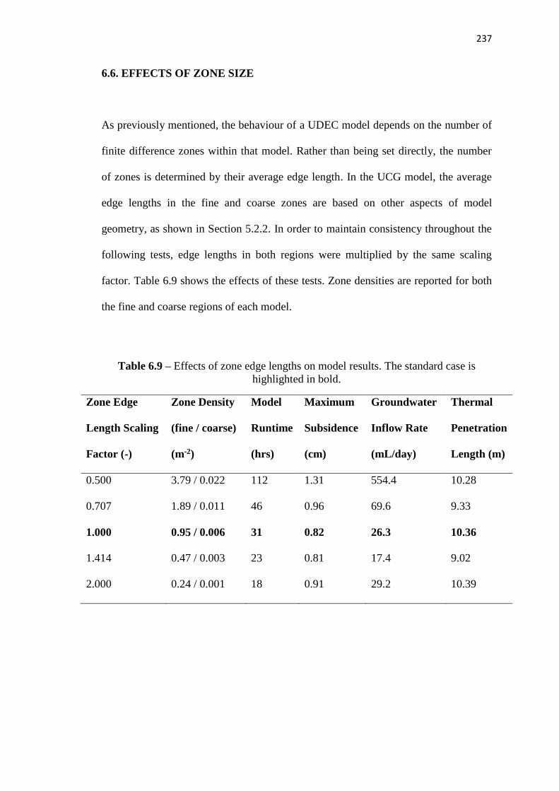
237
6.6. EFFECTS OF ZONE SIZE
As previously mentioned, the behaviour of a UDEC model depends on the number of
finite difference zones within that model. Rather than being set directly, the number
of zones is determined by their average edge length. In the UCG model, the average
edge lengths in the fine and coarse zones are based on other aspects of model
geometry, as shown in Section 5.2.2. In order to maintain consistency throughout the
following tests, edge lengths in both regions were multiplied by the same scaling
factor. Table 6.9 shows the effects of these tests. Zone densities are reported for both
the fine and coarse regions of each model.
Table 6.9 – Effects of zone edge lengths on model results. The standard case is
highlighted in bold.
Zone Edge
Length Scaling
Factor (-)
Zone Density
(fine / coarse)
(m-2)
Model
Runtime
(hrs)
Maximum
Subsidence
(cm)
Groundwater
Inflow Rate
(mL/day)
Thermal
Penetration
Length (m)
0.500 3.79 / 0.022 112 1.31 554.4 10.28
0.707 1.89 / 0.011 46 0.96 69.6 9.33
1.000 0.95 / 0.006 31 0.82 26.3 10.36
1.414 0.47 / 0.003 23 0.81 17.4 9.02
2.000 0.24 / 0.001 18 0.91 29.2 10.39

238
As shown above, zone density has little effect on model results for scaling factors
greater than 0.707. Zone density is seen to have a strong effect on runtime however,
with an approximately exponential relationship between the two. This is the single
greatest contributor to the computational demands of the model and explains the lack
of influence seen with block geometry. These results therefore suggest that in order to
produce fast model results, zone density should be set at the lowest possible value
which still ensures accurate results.
The lack of influence on model results at high scaling factors is an interesting
observation, as it suggests that density is high enough even in these models to avoid
mesh dependency. It is therefore counterintuitive that results appear to diverge for low
scaling factors and high densities. In theory, results should be approximately constant
between high density models, with low density tests producing erroneous behaviour.
This discrepancy between theory and observation suggests that some previously
undetected scale dependent behaviour is occurring within the model. As with the
effect of model width, the influence of zone density on results can be further explored
by considering the full subsidence profiles predicted by the models tested. Figure 6.7
shows these subsidence profiles. In order to highlight the different behaviours
observed, the profiles have been cropped to show only half of the full subsidence
profile.

239
Figure 6.7 – Half subsidence profiles for models with varying zone edge lengths.
It can clearly be seen that a scaling factor of 0.5 produces a subsidence profile with an
incorrect shape. This, coupled with the high groundwater flow rate and extreme
runtime, show that this model has failed to solve correctly. As such, scaling factors
less than 0.707 should not be used in further models. Results for scaling factors of
1.414 and 2.0 show appropriate behaviour at the centreline and edges, but are seen to
give a discontinuity in subsidence approximately 40m from the cavity centre. This
discontinuity is physically unrealistic and is caused by a lack of adequate resolution in
the coarse region of the model at low zone densities. Based on these results, it is
suggested that an upper limit of 1.0 should be set on the zone scaling factor.

240
Results for scaling factors of 0.707 and 1.0 are seen to give the expected profile
shape. As seen in Table 6.9 however, the high density model gives a distinct increase
in groundwater flow rate. Given the constant (within error) flowrates seen at lower
zone densities, it is believed that this effect is the beginning of the considerable
increase in flowrate seen with the 0.5 model. As seen in Table 6.9, the reduction of
the scaling factor from 1.0 to 0.707 also leads to a notable increase in runtime. For
these reasons, as well as that of simplicity, it was decided that future models should
continue to use a scaling factor of 1.0. It is of note however that the results of both the
1.0 and 0.707 models are within expected values for all measurements. Given that
increasing zone density should theoretically increase accuracy, it may be that future
models use the lower version of edge scaling factor. It is therefore suggested that
further testing of these effects should be performed to better understand how zone
densities within this range affect model results.

241
6.7. EFFECTS OF JOINT PROPERTIES
Unlike those of the intact rocks, the mechanical properties of the modelled joints are
not based on physical measurements. The following sections investigate the effects of
these properties on model results.
6.7.1. Joint Normal Stiffness
Joint normal stiffness relates the normal stress on a joint to the normal displacement
of the joint. This is important for mechanical and hydraulic behaviour as it controls
both overburden collapse and the stress/aperture relationship. Table 6.10 shows how
normal stiffness affects model results.
Table 6.10 – Effects of joint normal stiffness on UCG model results. The standard
case is highlighted in bold.
Joint Normal
Stiffness
(Nm-1)
Mechanical
Timestep
(μs)
Model
Runtime
(hrs)
Maximum
Subsidence
(cm)
Groundwater
Inflow Rate
(mL/day)
Thermal
Penetration
Length (m)
1×10⁸ Model failed due to block overlap error
1×10⁹ Model failed due to block overlap error
1×10¹⁰ 180 31 0.82 26.3 10.36
1×10¹¹ 86 57 0.79 37.8 10.44
1×10¹² 42 89 0.98 90.5 10.53

242
As expected, joint normal stiffness has a strong influence over model runtime.
Increases in stiffness lead to a considerable reduction in timestep, as given by
Equation A.11. Joint normal stiffness is seen to have little effect on the thermal
behaviour of the model, however mechanical and hydraulic results are affected.
Groundwater flow rates are seen to increase with normal stiffness. This shows that the
majority of joints tend to close under normal stress, rather than open, as increased
stiffnesses prevent this motion and thus give greater flow rates. Maximum subsidence
is seen to be approximately constant for small increases in stiffness, while larger
changes are seen to give an increase in deformation. This observation is
counterintuitive, as increases in stiffness should act to increase the strength of the rock
mass and therefore reduce subsidence. It is of note however, that the difference in
subsidence is well within the expected level of statistical error for the model. As such,
the increase in subsidence is predominantly caused by random perturbations in the
model, which are in turn exacerbated by the increase in runtime.
6.7.2. Joint Shear Stiffness
Joint shear stiffness has much less of an effect on results than joint normal stiffness,
as seen in Table 6.11. Thermal and hydraulic results are seen to be generally
unaffected by shear stiffness, as is model runtime. Maximum subsidence is seen to
decrease with shear stiffness. This is to be expected, given that increased stiffness
reduces the amount of shearing along fractures in the rock mass. The strong trend
seen with shear stiffness compared with normal stiffness suggests that shearing is the
predominant failure mechanism of the rock mass. This suggestion is further
corroborated by the results for joint friction angle and cohesion.

243
Table 6.11 – Effects of joint shear stiffness on UCG model results. The standard case
is highlighted in bold.
Joint Shear
Stiffness
(Nm-1)
Model
Runtime
(hrs)
Maximum
Subsidence
(cm)
Groundwater
Inflow Rate
(mL/day)
Thermal
Penetration
Length (m)
1×10⁷ Model failed due to block overlap errors.
1×10⁸ 22 0.98 42.2 10.38
1×10⁹ 31 0.82 26.3 10.36
1×10¹⁰ 25 0.58 31.1 10.29
1×10¹¹ Model failed due to block overlap errors.
6.7.3. Joint Friction Angle
Joint friction angle controls the relationship between the normal stress on a joint and
the shear strength of that joint. As such, it is expected to affect subsidence results by
altering the shear stress at which joints fail. The effects of joint friction were tested at
angles chosen such that their tangents were multiples of 0.1, 0.5, 1.0, 2.0 and 10.0
times the standard value. Table 6.12 shows the results of these tests.

244
Table 6.12 – Effects of joint friction angle on UCG model behaviour. The standard
case is highlighted in bold.
Joint
Friction
Angle (o)
Model
Runtime
(hrs)
Maximum
Subsidence
(cm)
Groundwater
Inflow Rate
(mL/day)
Thermal
Penetration
Length (m)
3.3 Model failed due to block overlap errors.
16.1 29 2.56 2.74 10.55
30.0 31 0.82 26.3 10.36
49.1 31 0.60 122.6 10.67
80.2 19 0.68 16.9 10.66
As seen above, joint friction angle appears to have little effect on the thermal results
of the model. Solution speed is also seen to be generally unaffected by joint friction,
although the highest friction angle gives a notable decrease in runtime. This is caused
by a reduction in the extent of joint failure in this model, as explained below.
The friction angle of a joint is directly related to the shear yield strength of that joint.
As friction angle increases, strength increases, preventing the onset of shear failure
and leading to a reduction in overburden collapse. This in turn leads to a reduction in
subsidence and runtime, which is observed in the model results. Variations in friction
angle are seen to have an effect on flow rate, however no discernible trend can be
observed. As such, the effect of friction angle on groundwater flow are seen to be
masked by random effects.

245
Given that friction angle is arbitrarily defined, these observations introduce
considerable uncertainty into model results. In reality, friction angles of rock
discontinuities often take values from less than 10o to over 40o (Hoek, 2007). Such a
range is shown by Table 6.12 to lead to variations in subsidence of a factor of 3 or
greater. As such, joint friction is seen to be a key parameter in subsidence prediction.
It is therefore suggested that future models should endeavour to obtain experimental
data on joint friction wherever possible, rather than relying on arbitrary values.
6.7.4. Joint Cohesion
Joint cohesion controls the shear strengths of unconfined joints. The ratio of frictional
to cohesive forces on a given joint increases with depth, as friction is dependent on
the normal stress on a joint, which in turn depends on lithostatic pressure. As such,
cohesion is of greater importance for joints closer to the ground’s surface. Table 6.13
shows how varying cohesion affects results.
Table 6.13 – Effects of joint cohesive strength on UCG model results. The standard
case is highlighted in bold.
Joint
Cohesion
(Pa)
Model
Runtime
(hrs)
Maximum
Subsidence
(cm)
Groundwater
Inflow Rate
(mL/day)
Thermal
Penetration
Length (m)
1×10³ 68 1.43 211.1 10.36
1×10⁴ 48 0.97 149.7 10.10
1×10⁵ 31 0.82 26.3 10.36
1×10⁶ 29 0.76 0.105 10.24
1×10⁷ 20 0.76 0.065 10.32

246
As shown above, joint cohesion has little effect on thermal results, as expected. All
other results are seen to be greatly affected however. Model runtime is seen to
decrease with increasing cohesion. This is to be expected as the increased strength of
the joints prevents large scale motion and hence reduces the computational demands
of solution.
Groundwater flowrates are seen to decrease considerably with increasing cohesion as
joints remain closed. In comparison with the effects of shear stiffness, this suggests
that hydraulic behaviour depends much more on the plastic (cohesion dependent) than
elastic (stiffness dependent) behaviour of joints. This suggests that it is the total
failure of joints, rather than their partial opening, that has the greatest effect on
groundwater flow behaviour.
As expected, maximum subsidence decreases with cohesion. The rate of decrease is
slower than that seen with friction however, suggesting that friction is the principal
force preventing the shear failure of joints. As mentioned above, the ratio of frictional
to cohesive strength increases with depth. Given that the majority of joint failures
occur near the cavity (at considerable depths), this is to be expected. These results
suggest that both joint friction and cohesion are important parameters controlling the
behaviour of UCG overburden. Further models in this work will continue to use a
cohesion of 100kPa for consistency. It is recommended however that future work
should consider friction and cohesion as site dependent properties, and endeavour to
acquire experimental data for these properties rather than relying on arbitrary values.

247
6.7.5. Joint Dilation Angle
Dilation is the process by which the shear displacement along a joint causes a change
in the normal separation (aperture) of the joint. Greater dilation angles imply a faster
change under shear yielding, which in turn leads to changes in the strength and
permeability of the rock mass. Table 6.14 shows the results of a number of tests using
rock masses with varying joint dilation angles.
Table 6.14 – Effects of joint dilation angle on UCG model results. The standard case
is highlighted in bold.
Joint
Dilation
Angle (o)
Model
Runtime
(hrs)
Maximum
Subsidence
(cm)
Groundwater
Inflow Rate
(mL/day)
Thermal
Penetration
Length (m)
0.0 27 0.62 239.2 10.69
2.5 31 0.83 386.2 10.67
5.0 31 0.82 26.3 10.36
10.0 36 1.18 23.2 10.20
20.0 Model failed due to block overlap errors.
248
Joint dilation is seen to have little effect on thermal results, as expected. Increases in
dilation are seen to give a corresponding increase in subsidence as joints separate and
weaken the rock mass. Runtime is also increases as a greater degree of motion must
be simulated. Groundwater flow rate is seen to decrease with increasing dilation. This
is counterintuitive, as increases in separation should increase flow rates. This
disagreement suggests that the influence of joint dilation on hydraulic results is more
complex than initially thought. It is also of note that the result for an angle of 2.5o
does not follow the general trend. Given the scale of errors in hydraulic results, it may
therefore be the effect of dilation on hydraulic results is masked by random effects.
As such, further repeats of the dilation tests are suggested. It was not possible to
complete these tests within the project timescale however. Finally, as with joint
cohesion and friction, it is suggested that site specific dilation data should be acquired
for future uses of the model.
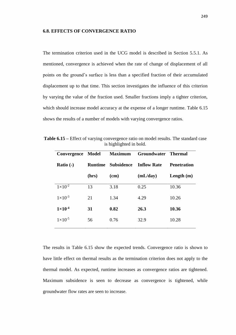
249
6.8. EFFECTS OF CONVERGENCE RATIO
The termination criterion used in the UCG model is described in Section 5.5.1. As
mentioned, convergence is achieved when the rate of change of displacement of all
points on the ground’s surface is less than a specified fraction of their accumulated
displacement up to that time. This section investigates the influence of this criterion
by varying the value of the fraction used. Smaller fractions imply a tighter criterion,
which should increase model accuracy at the expense of a longer runtime. Table 6.15
shows the results of a number of models with varying convergence ratios.
Table 6.15 – Effect of varying convergence ratio on model results. The standard case
is highlighted in bold.
Convergence
Ratio (-)
Model
Runtime
(hrs)
Maximum
Subsidence
(cm)
Groundwater
Inflow Rate
(mL/day)
Thermal
Penetration
Length (m)
1×10⁻² 13 3.18 0.25 10.36
1×10⁻³ 21 1.34 4.29 10.26
1×10⁻⁴ 31 0.82 26.3 10.36
1×10⁻⁵ 56 0.76 32.9 10.28
The results in Table 6.15 show the expected trends. Convergence ratio is shown to
have little effect on thermal results as the termination criterion does not apply to the
thermal model. As expected, runtime increases as convergence ratios are tightened.
Maximum subsidence is seen to decrease as convergence is tightened, while
groundwater flow rates are seen to increase.

250
The increase in subsidence for models with looser convergence ratios is caused by
premature termination of the ‘before’ stage of the model. Given that subsidence
results are found as the difference between the ‘before’ and ‘final’ stages, premature
termination of the before stage acts to increase subsidence. Figures 6.8 and 6.9 show
centreline displacement against iteration count for the 1×10⁻⁴ and 1×10⁻² models
respectively. It is seen that movement has definitely ceased at each stage of the 1×10⁻⁴
model before cycling continues in the following stage, justifying the use of 1×10⁻⁴ as
the standard convergence ratio. The results for the 1×10⁻² model show that motion is
definitely still occurring when the before stage ends. This continuing motion then
contributes to the deformation seen in the following stage, leading to an
overestimation of final subsidence.
It is of note that in both models, the displacement during the ‘before’ stage is
considerably greater than that of the other two stages. This displacement is caused by
the rock mass settling as it reaches the initial equilibrium state. This settling process
establishes the initial stresses and joint apertures of the rock mass. This process is the
reason why UDEC models need to contain the ‘before’ stage. The fact that this stage
tends to undergo an order of magnitude more displacement than the later stages is
actually beneficial in the identification of premature termination errors. If models
appear to have subsided considerably more than expected, especially away from the
centreline, it is often found that the ‘before’ stage has terminated prematurely and the
reason for this can then be sought out.

251
Figure 6.8 – Evolution of centreline vertical displacement during solution for a model
with a convergence ratio of 1×10⁻⁴.
Figure 6.9 – Evolution of centreline vertical displacement during solution for a model
with a convergence ratio of 1×10⁻².

252
Despite the termination criterion applying only to the mechanical aspect of the model,
increasing the tightness of the convergence ratio is seen to lead to a gradual increase
in groundwater flow rate. This is unsurprising, given the extent of coupling between
the hydraulic and mechanical aspects of the model. As with the subsidence result, the
effects of convergence ratio on flow rate are caused by premature termination of
model stages. As shown previously, joints tend to open as the model progresses,
increasing permeability and therefore flowrate. Premature termination stops this effect
from concluding, reducing the flowrates seen in models with looser criteria.
As seen in Table 6.15, the mechanical and hydraulic results are still changing between
the two tightest values of the convergence ratio. This suggests that a ratio of 1×10⁻⁵ is
still not tight enough to ensure accurate results from the model. Although these results
are still changing, their associated rates of change are seen to have slowed
significantly. As such, results would not be expected to change a great deal if the ratio
were reduced any further. Furthermore, it is seen in Table 6.15 that the increases in
runtime associated with tighter criteria are accelerating. As such, tighter ratios are
expected to give impractically long runtimes. For these reasons, it is believed that
further tightening of the convergence ratio would not give a sufficient benefit to be
justified. Given the scale of uncertainty in results caused by other factors (including
arbitrary joint properties, the random nature of the DFN and the inherent uncertainty
of real rock masses), it is believed that the differences between the 1×10⁻⁴ and 1×10⁻⁵
models are small enough to be considered insignificant by comparison. It is therefore
believed that increasing tightness from 1×10⁻⁴ to 1×10⁻⁵ does not give enough of an
increase in accuracy to warrant the associated increase in runtime. As such, a ratio of
1×10⁻⁴ is considered accurate enough for the intended end use of the model.

253
6.9. CONCLUDING REMARKS
The results presented in this chapter show how various parameters affect the
behaviour of the UCG model. Two key limitations of the model have been identified:
Firstly, hydraulic results are seen to vary greatly between trials. In some cases,
variations are seen to be greater than an order of magnitude in scale. This variability is
predominantly caused by the random nature of the DFN pattern, however it is
exacerbated by the small absolute values of flow rate observed. It is therefore
suggested that UDEC results be used only as a basis for further hydraulic modelling,
using separate software. Plans for such a model are given in Appendix C.
Second, results are shown to depend heavily on a number of unphysical internal
parameters. DFN dimensions, zone density and joint failure criteria are seen to have
particularly strong effects. Extreme values of certain parameters may also stop models
from solving at all, reducing model stability. The reliance on these parameters reduces
model validity as results are shown to depend more on unphysical parameters than
actual cavity design. In all cases however, these variables should be fixed in future
predictive models, reducing their effect on the end results of the model.
Despite these limitations, the results of this chapter suggest that the model is
sufficiently accurate for its intended end use. While the variability in results is large,
this is considered acceptable compared with those seen for real rock masses. Chapter
7 aims to further prove model validity by comparing results against site measurements
from UCG field trials. It is hoped that the outcome of these two chapters will thus be
sufficient to ensure confidence in the future use of the model as a predictive tool.

254
7. FIELD TRIAL STUDIES
SUMMARY
This chapter presents comparisons between model results, empirical predictions and
experimental measurements for a number of sites related to underground coal
gasification (UCG). These comparisons provide a method of model validation,
increasing confidence in the prediction of future UCG sites. Due to a relative lack of
published data on UCG induced subsidence, only one UCG trial has been tested.
Further testing is carried out based on the results of longwall mines, which have
similar geometries to UCG cavities. Longwall mines are seen to provide a less
competent analogue than previously thought however, due to significant differences
in operating conditions. As such, the validation potential of these sites is limited.
Despite the lack of data available, the tests performed show reasonable agreement
with UCG trials. Mean subsidence results for the UCG comparison agree to within
6% of the field measurements, however the standard deviation of this result is seen to
be greater than 30% of the mean. Variations in hydraulic results are also seen to be
large, while thermal results behave as expected. Later results show that multiple
cavity modelling is also possible with the Universal Distinct Element Code (UDEC)
model, however a number of alterations are required to give accurate results in these
cases. Together with the observations presented in Chapters 6 and 8, the results
presented herein suggest that the UDEC model is accurate enough for use as a first
pass screening tool for prediction of the local environmental effects of underground
coal gasification.

255
7.1. INTRODUCTION
Validation of results is a key step in the development of any numerical or analytical
model of a physical system. Predictive results derived from such models are of little
to no use if their validity cannot be proven. Throughout the creation of the UCG
model, validation was performed continuously as new model functionality was
developed. Much of this initial validation was performed by comparing model results
with empirical models based on the Rocky Mountain 1 field trial (Lindblom & Smith,
1993). Parametric studies, such as those presented in Chapter 6, also act as initial
methods of validation.
The work presented in this chapter aims to validate the behaviour of the entire model
as a whole. One of the most effective methods for doing so is to simulate the full
behaviour of previous field trials and compare model results with measurements
performed at the field trial site. In the case of UCG however, such measurements are
often difficult to obtain. As mentioned in Section 2.5.1, recent UCG field trials tend to
be private commercial ventures. As such, information on site geology and cavity
operating conditions is often considered commercially sensitive and is therefore
unavailable to the public. While earlier trials tend to publish more information,
measurements are often less accurate or are simply not performed for certain
variables. For example, many early UCG trials did not take any measurements of
ground subsidence, either because very little movement occurred or because it wasn’t
considered important at the time. The expense and negative public perceptions of
UCG also limit the number of trials performed, and hence the data available.

256
One site which can be used for validation purposes is the Hoe Creek 3 UCG trial,
performed in 1979 in Hanna, Wyoming. This trial was part of a series of experiments
performed by the US Department of Energy in the late 1970’s and early 1980s, and
involved the gasification of a sub-bituminous coal seam (the Powder River Basin
Felix No. 2 seam) interbedded between layers of sandstone (Burton et al, 2006). A
large number of measurements were taken at the site and the majority of these are
now publically available. The use of this site for validation purposes is problematic
however, as exceptional behaviour was observed there.
As shown in figure 7.1, the target seam of the Hoe Creek 3 trial is overlaid by a
second coal seam, separated by approximately 7m of interburden. During the trial,
collapse of the interburden allowed heat and oxygen to transfer to this seam, resulting
in its accidental ignition and gasification. This greatly increased the overall size of the
cavity and reduced its depth below the ground’s surface. These issues in turn led to
considerable ground motion, including chimneying subsidence (see Section 2.2.1.1)
which eventually produced an open sinkhole connecting the cavity with the surface.
Furthermore, the enhanced fracturing of the overburden due to the extreme subsidence
led to considerable pollution of the local groundwater. (Ganow, 1984). These issues
combine to make the Hoe Creek 3 trial one of the most environmentally damaging
UCG experiments on record. Because of this damage, and despite the anomalous
behaviour observed, attempts have been made to model the subsidence at this site for
validation purposes. A full description of these attempts is given in Section 7.2.

257
Figure 7.1 – Lithology of the Hoe Creek 3 UCG trial, showing the overlaid Felix coal
seams which produced extreme subsidence at the site.
Other than the Hoe Creek 3 site, very little data are available for the validation of
UCG subsidence models. In order to compensate for this lack of data, validation can
be performed on other sites which are geometrically similar to UCG. Geometric
similarity is based on a number of factors, including:
Cavity length to width ratio – approx. 50 – 70 for linear CRIP UCG.
Cavity depth on the order of 100m.
No artificial support of overburden (e.g. rock bolting).
Full overburden coverage (i.e. no large openings to the surface).

258
A site must conform to all of these criteria to be considered for validation. Sites which
do not conform to one or more of the criteria cannot be used, as it is unknown to what
extent this nonconformity will affect the behaviour of the rock mass. It is difficult to
meet all of these criteria with a single excavation however. For example, many
tunnelling projects satisfy the length and depth criteria, but are intentionally supported
by artificial methods. Many underground mining techniques are unsupported,
however these tend to have large surface openings (e.g. mine shafts) and lower length
to width ratios.
One industry which often fulfils all of the above requirements is that of underground
mining. Longwall mining in particular shares a number of similarities with UCG
(Langland & Trent, 1981; Mallett 2006; Younger, 2011). Two particular sites are of
interest as they both have a lot of data available for comparison with model results.
The Jinchuan No 2 nickel mine in China and Angus Place Colliery in Australia have
been used in this work in lieu of further comparisons with UCG sites. Validation
studies based on these mines are presented in Sections 7.3 and 7.4 respectively.

259
7.2. HOE CREEK 3 UNDERGRROUND COAL GASIFICATION
As mentioned above, the Hoe Creek 3 UCG site is one of very few trials where
sufficient data are available on the post-burn geology of the site. As such, it is used
here as a means of validating the behaviour of the UCG model. The use of this site for
validation purposes is complicated however, by the exceptional subsidence behaviour
which occurred there. As shown in Figure 7.2, this behaviour evolved over time. It is
of note that a considerable change occurred after day 81. This is believed to be the
point at which the interburden collapsed and gasification of the upper coal seam
began. The considerable difference between the results of days 81 and 114 may be
problematic, as the formulation of the model cannot accurately predict the effects
which caused this behaviour.
Figure 7.2 – Subsidence at Hoe Creek 3 UCG trial site as a function of time. After
Ganow, 1984.

260
In order to validate the model against site measurements, an appropriate measurement
time must be chosen. This must represent only the subsidence caused by stoping and
stratal bending (see Section 2.2.1.1), as the UDEC model is incapable of resolving
chimneying or plug failure. In order to choose an appropriate time, a simple empirical
method is used to predict subsidence at the site. The measured time is then chosen as
that which is closest to the empirical result. Empirical calculations are performed
using an influence function method (Brauner, 1973), as given by Equation 7.1.
𝑆𝑠 = ∑3
𝜋
𝑆𝑚𝑎𝑥
𝑟𝑐𝑟𝑖𝑡2 [1 − (
𝑥𝑠−𝑥𝑒
𝐵)
2
]2
𝑒 for 0 ≤ r ≤ rcrit. (7.1)
𝑆 = 0 for r > rcrit.
𝑆𝑚𝑎𝑥 = 𝛼𝐻𝐶 is the maximum possible subsidence.
𝑟𝑐𝑟𝑖𝑡 =2𝐷𝐶
tan(𝛾) is the critical radius of subsidence.
Where:
S Subsidence (m)
α Subsidence factor (-)
γ Angle of draw (o)
Subscripts:
e For a specified area of extraction.
s At the specified point on the surface.
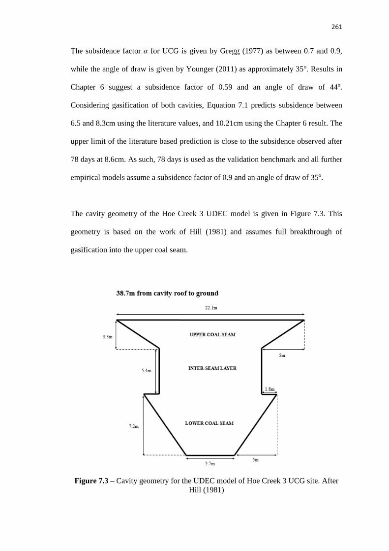
261
The subsidence factor α for UCG is given by Gregg (1977) as between 0.7 and 0.9,
while the angle of draw is given by Younger (2011) as approximately 35o. Results in
Chapter 6 suggest a subsidence factor of 0.59 and an angle of draw of 44o.
Considering gasification of both cavities, Equation 7.1 predicts subsidence between
6.5 and 8.3cm using the literature values, and 10.21cm using the Chapter 6 result. The
upper limit of the literature based prediction is close to the subsidence observed after
78 days at 8.6cm. As such, 78 days is used as the validation benchmark and all further
empirical models assume a subsidence factor of 0.9 and an angle of draw of 35o.
The cavity geometry of the Hoe Creek 3 UDEC model is given in Figure 7.3. This
geometry is based on the work of Hill (1981) and assumes full breakthrough of
gasification into the upper coal seam.
Figure 7.3 – Cavity geometry for the UDEC model of Hoe Creek 3 UCG site. After
Hill (1981)

262
Figure 7.4 compares UDEC model results with empirical predictions and field trial
measurements for the site. The UDEC result is presented as the mean subsidence
taken over 10 executions, with error bars equal to the standard deviation of those
executions. The graph has been cropped to show only the behaviour near the cavity,
as negligible ground movement was observed at greater horizontal distances. It is of
note that very little edge heave was seen in these models compared with those in
Chapter 6. This is primarily due to the extent of subsidence at Hoe Creek compared
with the benchmark model however, as the greater extent of ground motion dwarfs
any movement at the model edges, making edge motion much harder to detect.
Figure 7.4 – Comparison of UDEC results, site measurements and influence function
predictions (Brauner, 1973) for subsidence at the Hoe Creek 3 UCG site.

263
Figure 7.4 shows that the UDEC model accurately predicts the maximum subsidence
seen at the Hoe Creek 3 site after 78 days. Measured subsidence is seen to fall well
within the error margins of the UDEC model at the centreline, while the mean result
differs from measurements by approximately 4mm. The standard deviation of
centreline error predicted by UDEC is approximately 2.6cm, equal to 32% of the
mean. While this is a large variance, it is within the expected range given by the
natural variability of rock masses. It is of note that the UDEC model predicts a
slightly shallower profile than that seen in reality, but the difference is small enough
to consider the profile realistic. In comparison, the empirical method is seen to predict
a profile which is much shallower still. This effect is predominantly caused by the
assumption of rectangular cavity geometry, ignoring the effects of shape on
subsidence. Such results therefore show that the UDEC model gives a considerable
advantage over empirical methods, however the inability to predict chimneying
greatly limits the reliability and applicability of the UDEC model.
Figure 7.5 shows the groundwater pressure distribution for the Hoe Creek 3 site
during gasification (i.e. the “after” stage of the model). Results are taken from the run
in which the subsidence results are closest to the mean. The water table at the Hoe
Creek site was initially located at a depth of 24.5m below the ground (Wang et al,
1981). Permeability at the site is highly anisotropic, with a value of approximately
120mD in the horizontal direction and 22mD in the vertical direction (Buscheck et al,
2009; Snoeberger, 1976). In order to simulate this in the model, permeabilities are set
at 22mD for joints between 60 and 120 degrees from the horizontal, and 120mD for
all other joints. Cavity pressure was set equal to the local hydrostatic pressure at the
roof of the lower seam, as in the field trial (US Department of Energy, 1997).

264
Figure 7.5 – Simulated pore pressure distribution during gasification at the Hoe
Creek 3 trial site.
As seen above, the operation of the Hoe Creek 3 gasification site appears to have a
negligible effect on the pore pressure distribution around the cavity. Given that
overall cavity pressure is roughly equal to hydrostatic pressure, this is to be expected.
Observed perturbations in pressure are predominantly caused by the random nature of
the joint pattern and the interpolation process used to create the diagram.
Unlike modern UCG designs, the Hoe Creek 3 trial was not operated at sub-
hydrostatic pressures. In addition, the accidental gasification of the upper coal seam
actually led to cavity pressures exceeding local hydrostatic pressure in some regions.
While these effects prevented lowering of the water table, they led to considerable
groundwater contamination (Burton et al, 2008; Kapusta & Stanczyk, 2011). The
results of the UDEC model predict both of these effects. As shown in Figure 7.5, the
water table height remains unchanged. Groundwater is found to flow out of the cavity
at a rate of 9.36×10⁻⁸ m2s-1. Given a cavity length of 52m (Hill, 1981) this
corresponds to 421 litres per day, more than sufficient to cause considerable pollution.

265
Figure 7.6 shows how the maximum temperature experienced by the rock mass varies
with position in the Hoe Creek 3 trial. These results are taken from the same run as
those shown in Figure 7.5. As seen, the maximum temperature profile initially follows
the cavity wall, but begins to circularise as distance increases. Random fluctuations in
the temperature contours are caused by the existence of large blocks in the discrete
fracture network (DFN), as temperature transfers more slowly through blocks than
joints. The temperature profile is seen to extend up to 15m from the cavity wall. This
is longer than that suggested by the literature (Sarhosis et al, 2013; Yang, 2005). This
discrepancy is believed to be due to the relatively large surface area of this cavity
geometry compared with standard cavity shapes. Comparisons with field
measurements for this site cannot be made as temperature measurements are not
available for this trial.
Figure 7.6 – Profile of maximum experienced temperature surrounding cavity at Hoe
Creek 3 UCG trial site.

266
The above results show that the UDEC model agrees well with site measurements and
historical predictions for the Hoe Creek 3 UCG site. It is important to note however
that the model does not predict the increase in subsidence seen between days 81 and
114. As mentioned previously, this behaviour was caused by the accidental
gasification of a second coal seam, followed by subsequent chimneying of the
overburden. Despite the inclusion of this second seam in the model, subsidence results
tend to agree with the original measurement taken at 78 days. The failure of the
UDEC model to predict the secondary subsidence events considerably reduces the
reliability of the model for the prediction of future UCG sites.
In order to better predict the secondary subsidence events mentioned above, several
additions to the UDEC model would be required. These additions include full
simulation of coal combustion, cavity growth mechanisms, fully realised roof collapse
and transient hydraulic phenomena. The inclusion of these aspects would greatly
increase the complexity and computational demands of the model. Given that the aim
of the model is to act as a first pass screening tool rather than an in depth simulator,
these complications are not considered important at this stage. It is imperative
however, that any sites which the UDEC model deems as safe are further investigated
using much more rigorous techniques before any experimental or commercial
gasification operations are commissioned.
The agreement of model results with field trial data at day 78 is considered sufficient
to confirm the validity of the model for use as a first pass screening tool for simple
UCG designs. Further modelling should always be carried out using standalone
models for particular sites before any experimental work begins however.

267
7.3. JINCHUAN NICKEL MINE
The Jinchuan No. 2 mine is a Chinese nickel mine operating on a steeply dipping
seam. This site was chosen for model validation purposes as a great deal of data are
available on the site (Li et al, 2004b; Ma et al, 2013; Zhao et al, 2012). Unlike UCG,
underground mining does not involve any thermally driven processes. As such, the
thermal aspect of the UDEC model is turned off for this analysis. In addition, no
information is available on the local groundwater conditions at the mine, precluding
hydraulic modelling.
Figure 7.7 shows a view along the length of the cavity in the UDEC model of
Jinchuan nickel mine. The mine effectively consists of two identical cavities with a
thin slice of material (the filling body) in between. This filling body would then be
mined out at a later date. The model considers the mine with the filling body still in
place as this is the geometry for which field measurements are available. Block, zone
and DFN geometries depend on the total size of a rectangle circumscribed around
both the cavities as well as the filling body. The material properties and boundary
conditions at the site are based on those used by Zhao et al (2012). The UDEC model
assumes that the entire modelled rock mass consists of migmatite as this is the most
predominant rock type in the area. In the absence of information on local hydraulic
conditions, the rock mass is assumed to be saturated with water. In reality, migmatite
based geologies are likely to be dry, however the model considers a wet rock mass in
order to maintain consistency with the UCG model.

268
Figure 7.7 – View along the length of Jinchuan No. 2 nickel mine cavity.
Figure 7.8 compares the results of the UDEC model with site measurements and
empirical predictions. UDEC results are given as the mean of 3 trials, with error bars
given as the standard deviation of these trials. The influence function uses a
subsidence factor of 0.9 and an angle of draw of 29o as suggested by the literature
(Keilich et al, 2006). As shape cannot be incorporated into the influence function, the
cavities are assumed to be rectangles with the same area as the real cavities. The
graph has been cropped to show only the behaviour near the cavity, as no ground
movement was observed at greater horizontal distances. As with the Hoe Creek
model, edge heave was negligible for the Jinchuan results.

269
Figure 7.8 – Comparison of UDEC results, site measurements and empirical
predictions (Brauner, 1973) for subsidence at the Jinchuan No. 2 nickel mine.
As seen above, both the UDEC model and the influence function greatly overpredict
the subsidence seen at the Jinchuan mine. The UDEC model is seen to give a much
more accurate representation of profile shape than the empirical function however. It
is believed that the overprediction in both cases is due to the inability of the models to
accurately represent the support given by the filling body, which acts in a similar
manner to a spanning body. In the UDEC model the filling body is seen to sag into the
lower cavity, as seen in Figure 7.9. This both removes the support of the filling body
and increases the stress on the rocks surrounding the upper cavity, increasing
subsidence. It is of note that a dry model would be likely to produce even greater
subsidence, suggesting that the UDEC UCG model is not appropriate for modelling a
mine such as this. Finally, the model does not consider temporal effects, such as the
order of excavation. Including these effects may improve the accuracy of results,
however it was not possible to test this within the timescale of the project.

270
Figure 7.9 – Filling body failure observed in the UDEC model of the Jinchuan nickel
mine. Red lines indicate the original location of the cavity boundaries. Fractures are
generated via the discrete fracture network method (see Section 4.2.3).
The results above show that while the UDEC model is more accurate than the
empirical model, it is generally incapable of predicting the subsidence seen at the
Jinchuan site. Model realism could be improved by considering the order of
excavation, however this was not attempted due to time constraints. Alternatively,
results could be improved by altering design parameters to more closely fit the site;
however this would preclude the use of the trial as a means of validation for the UCG
model. These results therefore show that while the model can provide much
information on the behaviour of diverse sites, its usefulness as a predictive tool may
be limited to sites broadly similar to the Rocky Mountain 1 trail. The model is
therefore seen to be generally valid for UCG trials, though care should be taken in its
application to cases with notably different geometry from that presented in Chapter 5.
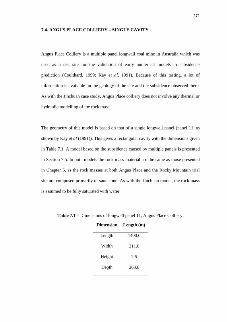
271
7.4. ANGUS PLACE COLLIERY – SINGLE CAVITY
Angus Place Colliery is a multiple panel longwall coal mine in Australia which was
used as a test site for the validation of early numerical models in subsidence
prediction (Coulthard, 1999; Kay et al, 1991). Because of this testing, a lot of
information is available on the geology of the site and the subsidence observed there.
As with the Jinchuan case study, Angus Place colliery does not involve any thermal or
hydraulic modelling of the rock mass.
The geometry of this model is based on that of a single longwall panel (panel 11, as
shown by Kay et al (1991)). This gives a rectangular cavity with the dimensions given
in Table 7.1. A model based on the subsidence caused by multiple panels is presented
in Section 7.5. In both models the rock mass material are the same as those presented
in Chapter 5, as the rock masses at both Angus Place and the Rocky Mountain trial
site are composed primarily of sandstone. As with the Jinchuan model, the rock mass
is assumed to be fully saturated with water.
Table 7.1 – Dimensions of longwall panel 11, Angus Place Colliery.
Dimension Length (m)
Length 1400.0
Width 211.0
Height 2.5
Depth 263.0

272
Figure 7.10 shows the results of the single cavity Angus Place UDEC model
alongside site measurements and empirical predictions. As shown, the UDEC results
overpredict subsidence by approximately 33%, with the subsidence measured at the
site falling far outside the margin of error given by the models. Model results are seen
to give a much better subsidence prediction than that given by the influence function
however, with the empirical method under-predicting subsidence by more than a
factor of 3. In addition, the shape of the profile given by the UDEC model is much
closer to reality than that given by the empirical method.
Figure 7.10 – Subsidence profiles for single cavity Angus Place Colliery Models.
Influence function based on Brauner, 1973.

273
The inaccuracies shown in Figure 7.10 are believed to be caused by the extreme
geometry of the site. The width to height ratio of 84.4 is much greater than that of the
UCG benchmark case at 0.87. Such an extreme ratio of width to height greatly affects
the geometry of the DFN region, as mentioned in Section 6.3. Such geometries have
been shown to increase the subsidence predicted by the model, and therefore may
contribute to the overprediction of subsidence in this case. In addition, the relatively
small length to width ratio of 6.6 suggests that the plane strain geometry of UDEC
may be unsuitable for this site.
In summary, the results show that while the UDEC UCG model cannot accurately
predict subsidence for the Angus Place Colliery, it does give a distinct advantage over
empirical methods in terms of both subsidence extent and profile shape. As with the
Jinchuan site, the accuracy of the UDEC model could be improved by altering various
design parameters for the site in question; however this would reduce its applicability
for the validation of other sites, including UCG operations. As such, these results cast
doubt on the usefulness of longwall mining trials as validation studies for the UCG
model. Given the lack of available field trial data from UCG trials, this seriously
limits the amount of validation which can be performed on the model and therefore
limits the reliability and applicability of the model itself. As such, it is suggested that
efforts should be made to acquire much more data on subsidence at UCG sites, either
through collaboration with the operators of previous trials or by combined
computational and experimental studies in the future.

274
7.5. ANGUS PLACE COLLIERY – MULTIPLE CAVITIES
As mentioned above, the Angus Place Colliery site contains multiple parallel longwall
panels. This section models the interaction between two such panels in an attempt to
validate the future use of the UDEC model with multiple cavity UCG designs. The
geometry of this model is based on that of two parallel longwall panels (panels 11 and
12). The panels have identical dimensions, which were previously given in Table 7.1.
The panels are separated horizontally by a 50m thick coal pillar.
The standard UDEC UCG model is incapable of realising the subsidence profile
produced by parallel cavities, because the stratified blocks can only produce first or
second order bending. In order to predict the profile caused by two cavities, the blocks
must be able to produce fourth order bending, which is impossible in UDEC due to
the formulation of the discrete element method. This behaviour can be approximated
however, by ensuring that block ends always rest in the space between the cavities.
This allows a pair of blocks in second order bending to approximate the behaviour of
a single block showing fourth order bending. This concept is shown in Figure 7.11. In
order to achieve the desired profile for the Angus Place Colliery model, the stratified
beams were shifted horizontally so that the interface between the beams always fell
directly above the coal pillar. In addition, a greater number of subsidence
measurement points were included to capture the full shape of the profile.

275
One block showing 2nd order bending – Standard UDEC Model
One block showing 4th order bending – Not possible in UDEC
Two blocks showing 2nd order bending, approximating an overall 4th order bending
moment – Allowing multiple cavity modelling in UDEC
Figure 7.11 – Approximation of higher order bending modes through an increase in
the number of stratified blocks, allowing for multiple cavity modelling in UDEC.

276
Figure 7.12 compares simulated subsidence profiles with measured field data and
empirical predictions for the two cavity Angus Place Colliery site. As shown, the
shape and extent of subsidence profiles were seen to depend heavily on the density of
finite difference zoning used within the model. Low zone densities (approx. 11 zones
per block) were seen to give a subsidence extent closer to that seen in reality, but
failed to give an appropriate profile shape. Higher zone densities (approx. 95 zones
per block) give the correct shape but greatly overestimate extent. In comparison, the
empirical method is seen to both greatly underestimate the extent of subsidence and
fail to capture the effects of the dual cavity geometry.
Figure 7.12 – Subsidence profile for two cavity Angus Place Colliery Model.
Influence function based on Brauner, 1973.

277
Two principal conclusions can be drawn from Figure 7.12: Firstly, the shape of the
high zone density profile proves that a UDEC model built in this way can predict the
subsidence behaviour of multiple cavity systems. As such, appropriately designed
models should be able to predict the behaviour of commercial scale UCG operations
with several parallel CRIP channels. Second, the numerical results of both models
suggest that they are not valid for this particular site. As with the single cavity model,
the accuracy of results could be improved by altering the model design, though this
would invalidate its use as a tool for the validation of UCG behaviour
Given the observations above, it is suggested that more accurate predictions of
multiple cavity behaviour may be possible with the use of a model with a separate but
similar design to that used for a single cavity. Such a model would need to use an
increased zone density in order to capture the correct profile shape, but would need to
be altered in other ways in order to counter the effect of an altered zone density on
mechanical and hydraulic results. It is suggested that increasing the stiffness of joints
could compensate for these effects. Such a method would greatly change results
however, requiring the model to be calibrated against field trial data in order to
produce a usable simulation. Such a method would require extensive testing to prove
its validity across a number of geometries however, and may be limited to simulating
sites which are already similar in shape to the calibration model. Such a process is
beyond the scope of this project, but it is believed that it could be achieved relatively
easily using similar techniques to those presented within this thesis.
278
7.6. CONCLUDING REMARKS
The studies in this chapter lead to four principal conclusions:
Firstly, the results of the Hoe Creek 3 tests show that the model is capable of
predicting simple thermal, mechanical and hydraulic phenomena associated with
single cavity UCG operations in hard rock. These results also show however, that the
model is incapable of predicting complex subsidence phenomena such as chimneying,
cavity collapse and overburden gasification. Such phenomena could be simulated by
greatly increasing the complexity of the model, however the effect of doing so on
runtime would preclude the use of the model as a first pass screening tool.
The second conclusion is that comparison with longwall mines may be less useful for
predictive models of UCG than previously thought. Although the UDEC model is
seen to be more accurate than empirical methods, the simulation is seen to
consistently overpredict subsidence in these tests. While the accuracy of these models
could be improved by better matching model designs to site parameters, doing so
would greatly reduce their usefulness as validation studies for the UCG model.
Third, the results of the multiple cavity Angus Place study show that, with sufficient
modification, the model is capable of simulating multiple cavity systems. Doing so
requires a considerable increase in model complexity and runtime however. As such,
it is suggested that an alternative model based on that presented in this chapter should
be produced to simulate multiple cavity systems.

279
Finally, a key issue in the validation of the UCG model was the lack of available data
on which to perform comparative work. Data are difficult to obtain in many cases due
to commercial secrecy. As models are the primary tool for ensuring the safety of
future UCG trials, and validation is the most important method of ensuring model
validity, it is essential that a greater amount of data are acquired. Given the cost and
political opposition to UCG experiments, it is suggested that these data would best be
acquired by increasing access to existing trial results. This could be achieved through
widening publication of these results or through closer collaboration between
academic researchers and UCG operators.
Despite the above issues, the model produced in this work is considered to be
sufficiently accurate for use as a first pass screening tool for UCG designs. As such,
the following chapter applies the model to a range of varying UCG site designs in
order to produce an initial set of predictive results and best practice guidelines for
UCG operators. Further modelling of chosen sites should always be carried out using
more detailed simulators before any experiments are performed, but this model should
greatly reduce the demands of such modelling by allowing operators to quickly
eliminate any unsuitable sites. Further work on the validation of the model should also
be carried out using new data as it becomes available.

280
8. SITE DESIGN STUDIES
SUMMARY
This chapter presents the results of a series of tests in which the model is used to
predict the local environmental effects of a range of potential underground coal
gasification (UCG) sites with varying geometric, geological and operating conditions.
These tests are used both to identify limitations in the applicability of the model and
to provide initial predictive results for a range of UCG designs. These results are then
used to produce a set of best practice guidelines for future UCG operations which
allow operators to quickly assess the suitability of a range of site designs.
The majority of the results in this chapter show good agreement with expected trends
in behaviour, providing further validation of the model and allowing for the derivation
of robust guidelines for approximating the extent of subsidence and thermal
penetration length. Hydraulic results are also seen to follow the expected trends,
however the uncertainty in these results is significant, with many results showing a
range of variation greater than 100% of the mean value. Further modelling work is
suggested to improve the hydraulic results, as well as to extend the applicability of the
model over a greater range of site designs. Despite the uncertainties observed, the
results in this chapter suggest that the Universal Distinct Element Code (UDEC)
model provides a sufficiently accurate prediction to satisfy its intended end use as a
first pass screening tool for UCG site selection.

281
8.1. INTRODUCTION
This chapter applies the completed UDEC model to a number of cases with varying
site conditions. This is performed both to test the limits of model validity and to
produce initial predictive results. These results are then used to identify trends in how
certain site parameters influence the local environmental impacts of underground coal
gasification. Finally, these trends are used to produce a set of ‘best practice’
guidelines for UCG operators to minimise the future environmental risks of UCG.
The tests in this chapter were performed by making alterations to the initial model
shown in Section 6.2. These alterations involved varying only those properties which
can be set either through site selection (e.g. cavity depth) or operating decisions (e.g.
operating pressure). As such, these results represent the effects of gasifier design and
measureable physical properties rather than those of model specific variables.
Wherever possible, the models below use a consistent random seed. This allows for a
direct comparison of results without the need to consider random effects, as well as
reducing the number of tests which must be run. For the cavity geometry models,
repeats must be performed as the random geometry of the discrete fracture network
(DFN) depends on cavity geometry. In these cases, three repeats of each test are
performed and the mean and standard deviation of the results are presented.
Groundwater flow rates are given as the geometric mean of three trials and are
expressed in mL/day calculated on the assumption of a 600m long channel, equal to
that of the Bloodwood Creek trial (Mark & Mallett, 2008). Errors in flowrates are
quoted as multiplicative rather than additice, indicated by prefixing with an “x”.

282
8.2. EFFECTS OF CAVITY GEOMETRY
The geometry of a UCG cavity has a considerable influence over the process. UCG
geometry is defined by the width, length and depth of the cavity. As mentioned in
Section 2.1.5, larger cavities are economically beneficial as they increase the amount
of syngas obtained from a single pair of wells. Deeper cavities can also operate at
higher pressures, increasing the quality of syngas. Deeper cavities have a
disadvantage however, as they greatly increase the capital costs of UCG. Cavity
geometry also has a strong influence over the local environmental impacts of UCG.
This section uses the UDEC model to investigate how these properties affect these
environmental issues. In cases where multiple cavity operations are performed, the
separation between cavities is also important. As shown in Section 7.5 however, the
current model is incapable of simulating multiple cavity systems. As such, it is
recommended that an additional model should be produced to simulate these sites.
8.2.1. Cavity Height
The height of a UCG cavity is the vertical distance from the base of the injection well
to the roof of the void, which usually extends a short distance into the overburden
above the coal seam. While cavity height cannot be set by the operator, it can be
approximated as the vertical distance between the base of the injection well and the
roof of the coal seam. Table 8.1 shows the effects of cavity height on local
environmental issues. Figure 8.1 compares model results with empirical predictions
for subsidence across the range of heights modelled.

283
Table 8.1 – Effects of cavity height on local environmental issues. The standard case
is highlighted in bold.
Cavity
Height
(m)
Model
Runtime
(hrs)
Maximum
Subsidence
(cm)
Groundwater
Inflow Rate
(mL/day)
Thermal
Penetration
Length (m)
3.55 35 ± 6 0.47 ± 0.14 91.1 ± x3.4 7.54 ± 1.42
7.10 33 ± 10 0.73 ± 0.03 35.3 ± x1.3 8.98 ± 1.77
14.2 37 ± 7 1.00 ± 0.29 28.2 ± x2.8 9.62 ± 1.36
20.0 57 ± 7 1.39 ± 0.29 119.9 ± x1.9 8.64 ± 1.05
28.4 53 ± 8 1.72 ± 0.66 36.0 ± x1.3 6.24 ± 3.60
Figure 8.1 – Comparison of UDEC and influence function results (Brauner, 1973) for
the effects of cavity height on subsidence, showing linear line of best fit for UDEC
results.

284
Cavity height is seen to have a predictable influence on runtime and subsidence, and a
less obvious effect on hydraulic or thermal results. Runtime is generally seen to
increase with cavity height. This is to be expected, as taller cavities increase the
length of joints in the DFN (see Section 6.3.1), producing more blocks and hence
increasing the computational demands of the model.
Subsidence increases with cavity height as a larger void induces a greater stress on the
cavity roof. In addition, taller cavities allow the stoping process (see Section 2.2.1.1)
to continue to a greater extent, further increasing subsidence. As shown in Figure 8.1,
modelled subsidence increases linearly with cavity height, agreeing with the empirical
prediction. Model results are however seen to give consistently greater subsidence
than empirical results. Given that the empirical model does not account for cavity
shape, thermal or hydraulic effects, this suggests that the UDEC model is generally
more accurate, as previously suggested in Chapter 7.
The hydraulic results shown in Table 8.1 suggest that cavity height has no overall
effect on groundwater flowrate. This is unexpected, as one would expect a taller
cavity to give higher flowrates due to the increase in differential pressure at the floor
(cavity pressure is based on hydrostatic pressure at the roof). On the other hand,
Section 6.3 shows that larger DFNs (associated with larger cavities) reduce flowrates
as joint apertures tend to decrease with DFN size. Finally, given the scale of
uncertainty in the results, it may also be that the effects of height are lost in the
random variability of results. As such, it is suggested that further investigations be
carried out to investigate the effects of cavity height on hydraulic behaviour.

285
The thermal results in Table 8.1 show the greatest thermal penetration length for the
standard model, with shorter lengths observed as cavity height is either increased or
decreased. As all results are within expected error margins, this effect is assumed to
simply be a product of random variations. In addition, it is important to note that the
thermal penetration length in the two shortest trials extends below the base of the
model. This is a problem for any cavity with a height less than approximately 10m.
This can be resolved simply by ensuring a minimum amount of rock is always
simulated underneath the cavity. This was not performed in this work however, due to
time constraints. Ensuring a minimum DFN height is also important to prevent this
from occurring above the cavity roof.
Finally, the above tests highlight an issue with the relationship between DFN height
and cavity depth. As shown in Section 5.2.1., the top of the DFN region extends to
twice the cavity height above the cavity roof. If cavity depth is less than twice cavity
height, the DFN would therefore extend above the ground’s surface. Such a situation
would invalidate model results as the model geometry would be too different from
that used in validation studies. As such, simulated cavity heights should be limited to
less than half the depth of the cavity.

286
8.2.2. Cavity Width
The effects of cavity width follow similar trends to those seen with cavity height. As
with height, cavity width cannot be directly controlled, but can be approximated.
Cavity width is usually found to be of a similar size to cavity height. Table 8.2
summarises the observations of a number of tests on varying cavity widths. Figure 8.2
shows the relationship between cavity width and subsidence for both model results
and influence function predictions (Brauner, 1973).
Table 8.2 – Effect of cavity width on local environmental impacts of UCG. The
standard case is highlighted in bold.
Cavity
Width
(m)
Model
Runtime
(hrs)
Maximum
Subsidence
(cm)
Groundwater
Inflow Rate
(mL/day)
Thermal
Penetration
Length (m)
3.10 Model failed due to block overlap error.
6.20 57 ± 22 0.39 ± 0.08 63.3 ± x2.0 7.44 ± 1.63
8.80 35 ± 4 0.84 ± 0.06 4.14 ± x2.1 10.3 ± 0.71
12.4 37 ± 7 1.00 ± 0.29 28.2 ± x2.8 9.62 ± 1.36
17.5 29 ± 9 1.80 ± 0.39 1.61 ± x1.8 10.3 ± 0.84
24.8 49 ± 9 3.29 ± 1.08 2.72 ± x7.3 9.69 ± 1.36
49.6 Model failed due to block overlap error.

287
Figure 8.2 - Comparison of UDEC and influence function (Brauner, 1973) results for
the effects of cavity width on subsidence, showing original (black) and corrected (red)
trend lines.
As seen above, cavity width appears to have little effect on model runtime, with
variations predominantly caused by the random nature of the DFN geometry. This is
to be expected, given that DFN width has been previously shown (see Section 6.3.2)
to have little influence on runtime. The lack of influence is predominantly due to the
relationships between the size of the DFN and the length and number of joints it
contains. These relationships imply that cavity width will only have an effect on
runtime for designs with a high width to height ratio. As such, runtimes are expected
to be approximately constant across the majority of practical site designs.

288
Groundwater inflow rate and thermal penetration length are also seen to be generally
unaffected by cavity width. In reality, one would expect groundwater flow rates to
increase with cavity width. As with height however, the effects of DFN size on
flowrates prevent this effect. Thermal penetration lengths are constant within error
across all cavity widths. This is to be expected, as cavity width should have no effect
on heat transfer processes. It is of note however that the temperature profile extended
outside of the DFN region in the two thinnest cases. This occurs simply because the
DFN width is significantly reduced (as DFN width is set at three times cavity width).
As with DFN height, this issue can be resolved in future by specifying a minimum
width limit for the DFN region.
Cavity width is seen to have a considerable influence over the extent of surface
subsidence above a UCG operation. Maximum subsidence is seen to increase in an
approximately linear fashion with increasing cavity width, as shown in Figure 8.2.
This behaviour agrees with that given by the empirical method, however the
subsidence predicted by UDEC is seen to increase at a much faster pace than this
method suggests. This difference in results is primarily caused by the large subsidence
seen with the widest cavities. This large extent, and the accompanying large
variability, were caused by a single data point with a much greater value than the
others with that width. Removing this point from consideration gives a much closer
agreement with empirical results, shown by the red trend line on Figure 8.2.

289
8.2.3. Cavity Depth
Cavity depth is defined as the vertical distance from the surface to the roof of the
cavity. As with width and height, cavity depth is dependent more on the geometry of
the coal seam than with operating conditions. Some control over depth is possible
however, as the depth of the injection and production wells are set by the operator.
Table 8.3 shows the results of a number of tests of the effects of cavity depth on
environmental issues. Figure 8.3 compares model results and empirical predictions for
the effects of cavity depth on surface subsidence.
Table 8.3 – Effects of cavity depth on UCG induced environmental impacts. The
standard case is highlighted in bold.
Cavity
Depth
(m)
Model
Runtime
(hrs)
Maximum
Subsidence
(cm)
Groundwater
Inflow Rate
(m2s-1)
Thermal
Penetration
Length (m)
24.6 Failed due to interaction between surface and DFN
49.2 32 ± 2 2.26 ± 0.76 26.4 ± x1.7 10.49 ± 0.80
69.6 37 ± 13 0.86 ± 0.26 32.4 ± x1.5 8.84 ± 2.26
98.4 37 ± 7 1.00 ± 0.29 28.2 ± x2.8 9.62 ± 1.36
139.1 30 ± 7 0.70 ± 0.07 112.9 ± x1.5 3.66 ± 1.32
196.8 30 ± 7 0.69 ± 0.23 224.6 ± x1.6 3.66 ± 1.30
393.6 Failed – predicted upward motion across entire domain

290
Figure 8.3 – Comparison of modelled and influence function (Brauner, 1973)
predictions of the effects of cavity depth on surface subsidence.
Cavity depth is seen to have a negligible effect on runtime. This is expected as depth
only affects the coarse region of the model. Subsidence is generally seen to decrease
with depth, however the results at 69.6m do not follow this trend. It is believed that
this error is simply due to random variations, and is exacerbated by the small number
of trials performed. As such, the data at this depth (highlighted in red) is considered
anomalous and is not included in the line of best fit. While subsidence decreases with
depth as expected, the trend observed is much more gradual than that of the empirical
method. It is of note however, that the results from both methods are close for all but
the deepest data point. As such, it is believed that further trials should be performed in
order to determine which method is more accurate. To further investigate these issues
it is suggested that more data should be gathered, with a greater number of repeats for
each point. Unfortunately, this was not possible within the timescale of the project.

291
As shown in Table 8.3, a model was produced for a depth of 393.6m (equal to four
times the base case), however this model failed to solve. In two cases the model
encountered block overlap errors, while the third predicted upward motion across the
entire modelled domain. This failure was not unexpected however. As seen in Figure
8.3, subsidence is expected to decrease greatly with depth. For a depth of 393.6m, the
empirical function predicts a maximum subsidence of 0.5mm. This is considerably
smaller than the random variation seen in most executions of the model. As such, the
model is shown to be incapable of accurately predicting such small ground
movements. Given that such a small amount of subsidence is effectively harmless
however (and would be difficult to detect in reality), the inability to predict this effect
is not considered to be a problem. As such, the simulation of cavities at depths greater
than approximately 250m is not considered necessary unless cavity width or height is
greatly increased.
The effects of depth on hydraulic results behave as expected. Increases in depth lead
to a steeper pressure gradient across the cavity wall as hydrostatic pressure increases.
This in turn leads to an increase in flow rate which is observed in the results. Flow
rate is seen to increase at a speed faster than the linear rate suggested by the cubic
flow law. This difference caused by the effect of hydrostatic pressure on joints, as
higher pressures force fractures open, increasing permeability. This is primarily seen
with vertical joints, as the effect of pressure on horizontal joints is offset by the
increased weight of the overburden. It is also of note however that the scale of
statistical variations in hydraulic results also contributes to this effect.

292
Finally, cavity depth is seen to have an unexpected effect on thermal results.
Penetration length is roughly constant across the shallower models, however the deep
models give considerably shorter temperature profiles. After inspecting the outputs
from the models it was found that the deeper trials had not successfully completed the
thermal modelling stage. In these models the thermal stage ceased long before the
desired end time of 100 days, however UDEC did not report any errors. It is not
known why this occurred, as cavity depth should have no effect on either the thermal
timestep or zone geometry. Given that this error occurred on every trial with a depth
greater than 98.4m, there is evidently some unknown and potentially erroneous effect
occurring. This issue, in combination with the limitations seen with the mechanical
results, seriously challenges the validity of the model for assessing the effect of cavity
depth on environmental issues. As such, it is suggested that a many more trials should
be performed to identify the limits of the model with regards to depth. Given that
many UCG operators would want to work at depths of several hundred metres, it is
also suggested that separate models be produced (based on the current model) to
simulate operations with much deeper cavities. Such simulations would only be
necessary for larger cavities however, as small cavities at such depths would be
expected to have a negligible influence on the local environment.

293
8.2.4. Combined Geometric Effects
As seen above, cavity height, width and depth all have a considerable influence on the
extent of environmental damage caused by UCG. In the case of subsidence these
properties are heavily interrelated, such that increases in one property could be offset
by decreases in another. As such, directly setting limits for width, height or depth is
not suitable. In order to overcome this issue, an attempt has been made to relate
subsidence to a combined function of these measurements, as shown in Equation 8.1:
𝑆𝑚𝑎𝑥 = 𝑓 (𝑊𝐶𝐻𝐶
𝐷𝑐) (8.1)
Where:
DC Cavity Depth (m)
HC Cavity Height (m)
Smax Maximum Subsidence (m)
WC Cavity Width (m)
The above relationship was derived by considering the apparent relationships between
subsidence and geometry, as shown in Figures 8.1 through 8.3. The factor of 𝑊𝐶𝐻𝐶
𝐷𝐶
was chosen in order to give the correct dimension (metres) for subsidence. Initial
testing showed that this had a negligible effect on the accuracy of the combined
predictor function, and was therefore considered to be justified. Figure 8.4 shows a
plot of subsidence against the combined factor for every test performed in Section 8.2.

294
Figure 8.4 – Relationship between combined cavity geometric properties and
subsidence. The datum point in red was considered anomalous and excluded.
The results in Figure 8.4 show a clear trend between subsidence and the factor
proposed in Equation 8.1. From this trend, a predictive relationship has been
proposed, as shown by the solid line on Figure 8.4. This relationship is given in
Equation 8.2, where all variables are in units of m.
𝑆𝑚𝑎𝑥 = 0.005𝑊𝐶𝐻𝐶
𝐷𝐶 (8.2)
The linear relationship and factor of 0.005 were chosen for reasons of simplicity.
Despite this, the function is seen to give a reasonable estimate for subsidence. While a
slight improvement to accuracy is possible using a different coefficient, this was not
considered worth the increase in complexity. As such, Equation 8.2 is presented as a
simple and fast method for approximating subsidence from a UCG cavity. Further
developments to the equation are presented in Section 8.3.1.

295
8.3. EFFECTS OF MECHANICAL PROPERTIES
Mechanical properties refer to the stiffness and strength of the rock mass in which
UCG is to be carried out, as well as to the local in-situ stresses near the UCG cavity.
As shown in Chapter 4, many of these properties depend on not only the physical
composition of the rocks themselves, but also the geometry and material properties of
the discontinuities between them. Given the complicated relationships between these
properties, an independent analysis of each parameter is impractical. As such, this
section investigates how variations in the properties of the overall rock mass (as found
using the methods in Chapter 4) affect UCG induced environmental effects. In order
to assess a real rock mass, the methods of Chapter 4 would be used to determine
overall properties, and then the results of this section used to show how those
properties affect behaviour.
8.3.1. Rock Mass Stiffness
Stiffness refers to a material’s resistance to elastic strains, and is represented by
Young’s modulus. Increased stiffness allows rock strata to resist bending under their
own weight and that of the strata above them. As such, stiffer rock masses tend to
undergo much less strata bending, reducing subsidence. Stiffness has no effect on the
plastic failure behaviour of the overburden however, as this depends on joint
properties. Rock mass stiffness should have little effect on hydraulic results as flow
occurs entirely within joints. Stiffness should also have no effect on thermal results.
Table 8.4 shows the results of a number of tests using varying values of stiffness.
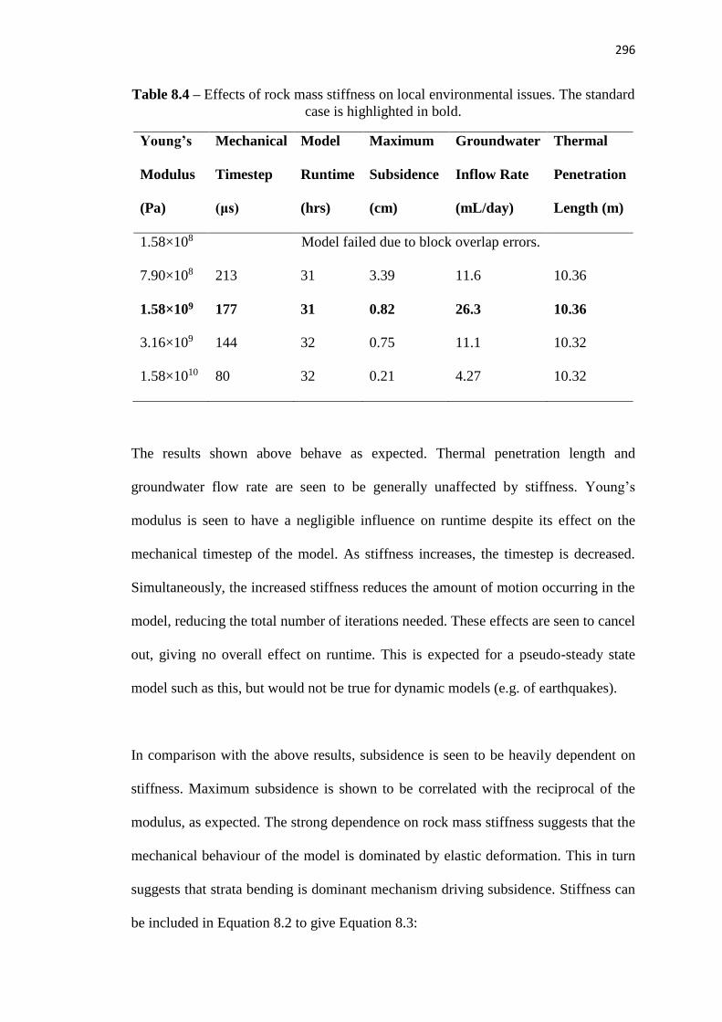
296
Table 8.4 – Effects of rock mass stiffness on local environmental issues. The standard
case is highlighted in bold.
Young’s
Modulus
(Pa)
Mechanical
Timestep
(μs)
Model
Runtime
(hrs)
Maximum
Subsidence
(cm)
Groundwater
Inflow Rate
(mL/day)
Thermal
Penetration
Length (m)
1.58×10⁸ Model failed due to block overlap errors.
7.90×10⁸ 213 31 3.39 11.6 10.36
1.58×10⁹ 177 31 0.82 26.3 10.36
3.16×10⁹ 144 32 0.75 11.1 10.32
1.58×10¹⁰ 80 32 0.21 4.27 10.32
The results shown above behave as expected. Thermal penetration length and
groundwater flow rate are seen to be generally unaffected by stiffness. Young’s
modulus is seen to have a negligible influence on runtime despite its effect on the
mechanical timestep of the model. As stiffness increases, the timestep is decreased.
Simultaneously, the increased stiffness reduces the amount of motion occurring in the
model, reducing the total number of iterations needed. These effects are seen to cancel
out, giving no overall effect on runtime. This is expected for a pseudo-steady state
model such as this, but would not be true for dynamic models (e.g. of earthquakes).
In comparison with the above results, subsidence is seen to be heavily dependent on
stiffness. Maximum subsidence is shown to be correlated with the reciprocal of the
modulus, as expected. The strong dependence on rock mass stiffness suggests that the
mechanical behaviour of the model is dominated by elastic deformation. This in turn
suggests that strata bending is dominant mechanism driving subsidence. Stiffness can
be included in Equation 8.2 to give Equation 8.3:

297
𝑆𝑚𝑎𝑥 = 8 × 10⁶𝑊𝐶𝐻𝐶
𝐸𝐷𝐶 (8.3)
The constant value of 8×10⁶ is chosen for simplicity, and has units of Pa. A slight
increase in accuracy can be achieved using a more precise constant. Given the
approximate nature of the equation however, this was not considered to be worth the
increase in complexity. As such, Equation 8.3 presents a simple and fast method for
estimating the subsidence caused by a UCG cavity of known dimensions in a rock
mass of known stiffness. It is important to note that this is rock mass stiffness, rather
than intact rock stiffness. As such, a method for estimating this stiffness, such as that
presented in Chapter 4, should always be used in conjunction with this equation.
8.3.2. Intact Rock Strength
In the UDEC model, plastic failure of intact rocks is predicted by the strain softening
Mohr-Coulomb yield criterion. The behaviour of this criterion depends on three
properties: rock mass friction angle, cohesion and tensile limit. The effects of each of
these parameters were tested at values of 0.1, 0.5, 2.0 and 10.0 times their base case
values. In the case of friction angle, angles were set such that the tangent function of
the angle was equal to the desired multiple of the base case value. In all cases, results
showed that these properties had negligible influence effect on the runtime or
mechanical, hydraulic or thermal behaviour of the simulation. These observations
therefore show that plastic yielding of intact rocks is not occurring within the model,
and that environmental effects are controlled entirely by the failure of joints and the
elastic deformation of blocks.

298
8.3.3. Lateral Earth Pressure
Lateral earth pressure is a horizontal stress present in all rock masses. The stress can
have a considerable influence over the behaviour of excavations by producing
horizontal motion and/or providing a confining pressure effect. Lateral earth pressure
varies from site to site and therefore its influence on the local environmental impact of
UCG must be understood. Lateral earth pressure is usually referred to by means of the
lateral earth pressure coefficient K0. This is given as the ratio of horizontal to vertical
in-situ stress for a given site. Table 8.5 investigates the effect of K0 on model results.
Table 8.5 – Effects of lateral earth pressure on local environmental impacts of UCG.
The standard case is highlighted in bold.
Lateral Earth
Pressure
Coefficient (-)
Model
Runtime
(hrs)
Maximum
Subsidence
(cm)
Groundwater
Inflow Rate
(mL/day)
Thermal
Penetration
Length (m)
0.00 22 0.79 32.0 10.48
0.25 33 0.96 11.0 10.47
0.50 31 0.82 26.3 10.36
1.00 37 0.89 4.40 10.55
1.50 Model failed due to block overlap errors
2.00 Model failed due to block overlap errors

299
As shown above, lateral earth pressure has a negligible influence over the mechanical
and thermal results of the model. Although results vary between trials there is no
discernible trend, and all results are within expected error margins. Hydraulic results
are also seen to be generally unaffected by lateral earth pressure. Finally, it is of note
that increased earth pressures tend to increase model runtime. This is caused by the
model requiring a greater number of steps to reach equilibrium as horizontal stresses
increase. As such, the extra runtime seen in these models corresponds to an increase
in the length of the “before” stage of the simulation. The overall results suggest that
lateral earth pressure is not a critical parameter in model results. Given the relative
difficulty of measuring this property in reality, it is therefore suggested that models
continue to use the value of 0.5. Alternatively, K0 could be set to zero in an attempt to
speed model solution.

300
8.4. EFFECTS OF HYDRAULIC PROPERTIES
Hydraulic properties refer to parameters which control the flow of groundwater in the
region of a UCG cavity. The most important of these are the local hydrostatic pressure
(determined by the depth of the water table), the permeability of the overburden and
the operating pressure of the cavity. These parameters are expected to have a
considerable influence over the hydraulic results of the model, as well as some degree
of coupling with mechanical results. Thermal results should be unaffected by these
properties given the lack of thermal/hydraulic coupling in the model, however thermal
behaviours would be somewhat affected by these properties in reality.
8.4.1. Water Table Depth
All of the models produced in this work initially contain a flat water table at a given
depth below the surface. The height of this water table has a profound effect on UCG
operations as it controls the value of the local hydrostatic pressure at the cavity. The
height of the water table also has an effect on the material strength of the rock mass,
as the action of groundwater pressure on the rocks acts to oppose the weight of the
overburden. Table 8.6 shows the results of a number of tests which investigated the
effects of water table height on model results. Tests were also produced with negative
water table depths to represent offshore operations, but these failed due to overlap
errors. Note that water table depths of 105.5, 119.7 and 200.0m represent the special
cases in which the water table is inside the cavity, below the cavity, and below the
model base respectively.

301
Table 8.6 – Effects of water table height on UCG induced local environmental issues.
The standard case is highlighted in bold.
Water
Table
Depth (m)
Model
Runtime
(hrs)
Maximum
Subsidence
(cm)
Groundwater
Inflow Rate
(mL/day)
Thermal
Penetration
Length (m)
0.0 26 0.58 404.0 10.82
13.8 27 0.69 382.0 10.65
27.6 31 0.82 26.3 10.36
55.2 33 0.80 1.95 8.56
105.5 a 26 1.18 -0.24 11.02
119.7 b 27 1.31 0.00 10.94
200.0 c 15 1.19 0.00 9.64
a – Inside cavity. b – Below cavity. c – Below base of model (dry model).
Water table height is seen to have little effect on thermal results, with variations in
penetration length seen to be within expected error. In addition, the effects of water
table depth on runtime are seen to occur only with the deepest model. As mentioned
above, this entire model was dry, leading to a considerable reduction in runtime as the
hydraulic aspect of the model was effectively removed.
Water table height is seen to have the expected effect on hydraulic results. Deeper
water tables reduce the pressure gradient across the cavity wall and thus reduce flow
rates. The deepest sites behaved as expected, with zero flow observed in the driest
models. The negative flow rate for the 105.5m model shows that groundwater is
leaching out of the cavity. This is to be expected given that the cavity pressure in this
model is effectively equal to hydrostatic pressure.

302
The only model in which a significant change in water table height was observed was
the 105.5m model. The model is seen to form a small cone of depression and greatly
exacerbate the variability in water table height near the cavity. This variability is
partly caused by the generally low pressures in this model however, as the smaller
range of variation makes minor effects stand out more clearly than in other models.
No significant groundwater lowering was observed in any other trials.
Figure 8.5 – Groundwater pressure distribution during operation of a UCG cavity
initially sited within the water table at 105.5m.
Water table depth had the expected effect on subsidence, with deeper tables leading to
increased ground deformation. As mentioned above, this occurs as reductions in pore
pressure reduce the buoyancy forces opposing the weight of the overburden. As such,
the net force on the rock mass is increased in models with deeper water tables, leading
to greater subsidence. This trend is seen to reverse in the case of the completely dry
200m model; however it is believed that this is simply the result of random error. As
such, further modelling of dry sites is recommended in order to confirm this.

303
The above results suggest higher water tables may benefit UCG by reducing
subsidence. Increases in groundwater inflow rates caused by higher water tables also
act to reduce the risks of groundwater contamination. Finally, the siting of UCG in
offshore locations (i.e. with negative water table depths) may alleviate some of the
social and legal concerns of UCG highlighted in Chapter 2. On the other hand the
high groundwater inflow rates in these cases may act to quench gasification reactions,
reducing syngas quantity and quality. Furthermore, although shallow water tables may
reduce the risks of contamination, operating in completely dry sites eliminates it
entirely. As such, operators should carefully consider the effects of water table height
not only on environmental concerns, but also social and economic issues.
8.4.2. Site Permeability
Groundwater permeability is strongly related to hydraulic behaviour, although it is
expected to also have an effect on subsidence due to the influence of pore pressure on
mechanical results. The effects of permeability were tested at values equal to 0.01,
0.1, 10 and 100 times their base case values. The range of permeabilities tested is
representative of many semi-pervious and impervious rock masses, including
sandstone, limestone and typical oil reservoir rocks (Bear, 1972). Permeabilities
outside this range were not considered relevant. Permeabilities lower than
approximately 0.01mD are generally seen only in igneous rocks, which are not found
near coal seams. Permeabilities greater than 1,000mD would generally be considered
unsuitable for operations in which the control of groundwater flow is important. Table
8.7 shows the results of tests on site permeability.

304
Table 8.7 - Effects of rock mass permeability on local environmental issues of UCG.
The standard case is highlighted in bold.
Permeability
(mD)
Model
Runtime
(hrs)
Maximum
Subsidence
(cm)
Groundwater
Inflow Rate
(mL/day)
Thermal
Penetration
Length (m)
0.053 30 0.77 0.041 10.39
0.53 26 0.76 0.51 10.37
5.3 31 0.82 26.3 10.36
53 37 0.83 435.3 10.32
530 40 0.81 10049.9 10.32
As shown above, permeability is seen to have a negligible influence on thermal
results. Subsidence is seen to increase slightly as permeability increases. This is due
to slight increases in the suction force caused by groundwater flowing downwards
into the cavity. Given the small changes however, this may also be due simply to
random error. Runtime is seen to increase with permeability. This is partly due to
increases in the amount of water flow to be modelled, however it is also affected by
random variation.
As expected, permeability has a strong effect on the hydraulic results of the model.
Figure 8.6 shows the relationship between permeability and flow rate. The exponent
of 1.37 is close to the expected value of 1.5 found from the cubic flow law (with
aperture proportional to the square root of permeability). This small difference in
exponent is due to the opening and closing of joints around the cavity, altering their
actual permeabilities from that of the input value.

305
Figure 8.6 – Effect of site permeability on groundwater inflow rate.
Despite the considerable increases in flowrate, even at the highest permeability the
level of the water table remains unchanged. As such, UCG operations would not be
expected to cause water table lowering unless permeability is increased by a much
greater amount. For example, consider an area of ground covering the entire cavity
and extending to 100m beyond the cavity boundary (approximately equal to the size
of the central subsidence trough). In England, the average annual rainfall rate is
855mm/year (Met Office, 2010). As such, the area above the cavity receives
approximately 4×10⁸ mL/day of rain on average. In order to increase water table
depth, the overburden above the UCG cavity would therefore need a permeability on
the order of 1×10⁶ mD, similar to that of gravel (Bear, 1972). Note that dryer locations
would produce a lowering effect at lower permeabilities however.

306
Despite the lack of influence on the water table, changes in permeability are seen to
affect pressure distributions close to the cavity. As shown in Figure 8.7, models with
decreased permeabilities lead to a greater degree of channelling and a less uniform
pressure gradient around the cavity. These effects are caused by the reduction in
permeability requiring a steeper pressure gradient to cause flow, therefore focusing
groundwater flows in the area with the steepest pressure gradient. Despite the large
variabilities seen between successive trials, the close agreement observed between
theory and results for the effects of permeability gives good evidence for the veracity
of the hydraulic model and its application to UCG cavity behaviour.
κ = 0.053mD κ = 530mD
Figure 8.7 – Effects of permeability on pore pressure distribution.

307
8.4.3. Cavity Operating Pressure
Operating pressure has a considerable influence over UCG behaviour. Pressure is the
primary means by which a UCG operator can control the gasification process. Higher
pressures increase both gasification rates and syngas calorific value. Pressure is
limited however by the need to prevent groundwater contamination. Operating at sub-
hydrostatic pressures reduces the risk of pollution, but can lead to water table
lowering and the quenching of the gasification process. Table 8.8 shows the results of
a number of tests of the effects of operating pressure on the local environmental
impact of UCG. Pressures are defined as a multiple of the local hydrostatic pressure at
the roof of the cavity.
Table 8.8 – Effects of operating pressure on the local environmental impact of UCG.
The standard case is highlighted in bold.
Pressure
Multiple
(-)
Model
Runtime
(hrs)
Maximum
Subsidence
(cm)
Groundwater
Inflow Rate
(mL/day)
Thermal
Penetration
Length (m)
0.00 Model failed due to overlap errors.
0.50 38 0.79 51.9 10.15
0.80 31 0.82 26.3 10.36
1.00 41 0.73 0.16 10.15
1.25 41 0.71 -0.20 10.15
1.50 Model failed due to overlap errors.

308
As shown above, operating pressure appears to have a negligible on many of the
model results. Runtime and thermal penetration length are seen to be generally
unaffected by operating pressure. In reality, decreased pressures would reduce thermal
penetration lengths as increased flow rate would consume more energy to boil the
groundwater. This is not seen in the model due to the lack of thermal/hydraulic
coupling. Subsidence is seen to decrease slightly as pressure increases. This is
expected, as an increase in pressure would reduce groundwater drawdown, leading to
a reduction in the suction force on the overburden and reducing subsidence.
As expected, the greatest influence of operating pressure is seen with the groundwater
inflow rate. For values equal to or lower than one, the relationship between pressure
and flow rate is approximately linear. This is the expected relationship, as based on
the cubic flow law. Theoretically, a pressure multiple of exactly unity should give
zero flow. The small inflow rate observed in Table 8.8 is well within error however,
confirming this behaviour. As expected, outflow is observed for pressures greater than
the local hydrostatic value, confirming that sub-hydrostatic operation is a key
requirement for the safe development of UCG. Extrapolating the above results to zero
(i.e. a vacuum inside the cavity) gives a maximum possible inflow rate of
approximately 105 mL/day for the base case cavity geometry. This is sufficiently low
to prevent drawdown in all but the driest of locations, confirming the observations of
unaltered water table heights throughout this chapter.
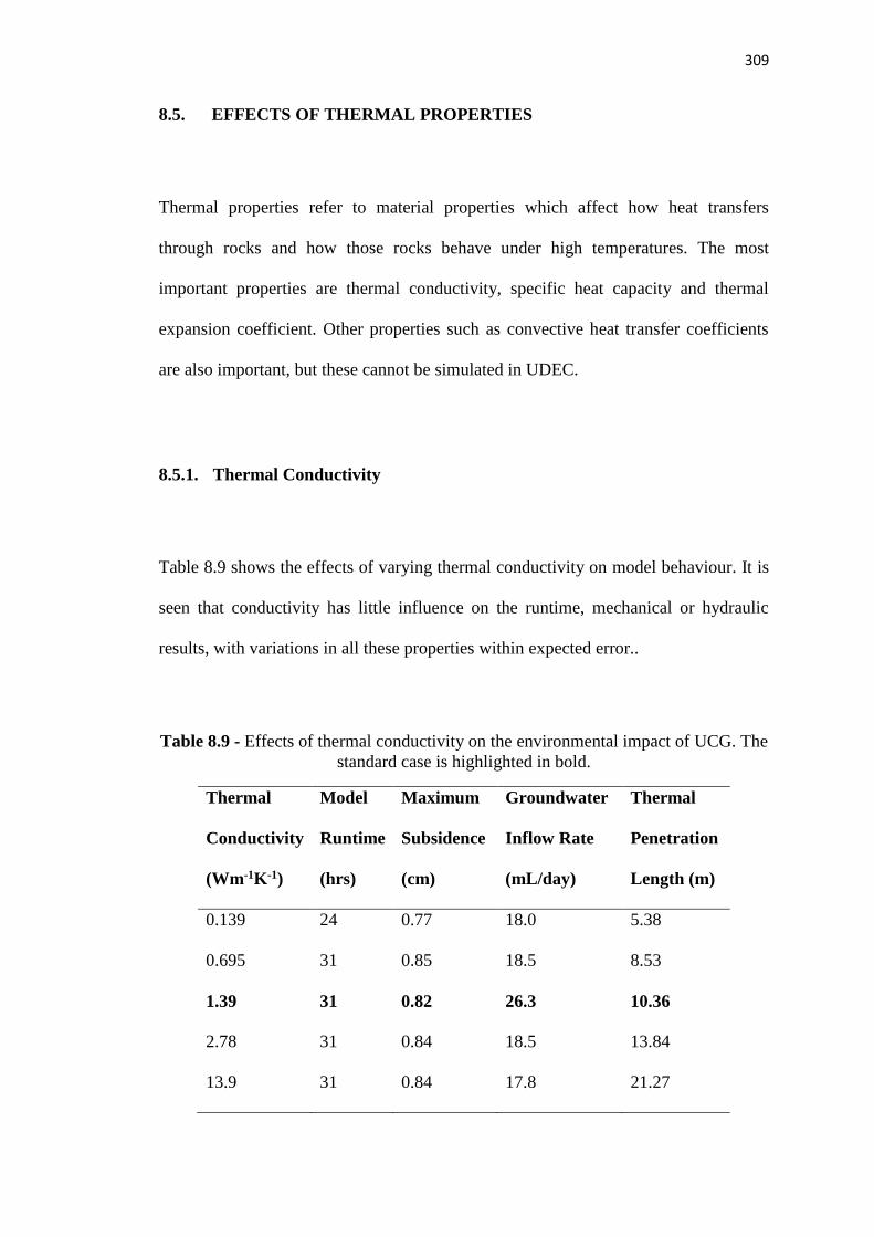
309
8.5. EFFECTS OF THERMAL PROPERTIES
Thermal properties refer to material properties which affect how heat transfers
through rocks and how those rocks behave under high temperatures. The most
important properties are thermal conductivity, specific heat capacity and thermal
expansion coefficient. Other properties such as convective heat transfer coefficients
are also important, but these cannot be simulated in UDEC.
8.5.1. Thermal Conductivity
Table 8.9 shows the effects of varying thermal conductivity on model behaviour. It is
seen that conductivity has little influence on the runtime, mechanical or hydraulic
results, with variations in all these properties within expected error..
Table 8.9 - Effects of thermal conductivity on the environmental impact of UCG. The
standard case is highlighted in bold.
Thermal
Conductivity
(Wm-1K-1)
Model
Runtime
(hrs)
Maximum
Subsidence
(cm)
Groundwater
Inflow Rate
(mL/day)
Thermal
Penetration
Length (m)
0.139 24 0.77 18.0 5.38
0.695 31 0.85 18.5 8.53
1.39 31 0.82 26.3 10.36
2.78 31 0.84 18.5 13.84
13.9 31 0.84 17.8 21.27

310
As expected, thermal conductivity has a strong influence on thermal results. Thermal
penetration length is seen to increase with conductivity to the power of approximately
0.3. This is close to the expected value of 1/3, given by Equation 8.4 (derived in
Appendix B.5). It is of note that in the highest two cases, the thermal penetration
length extends outside of the DFN in some directions. As such, penetration lengths
can only be determined in certain directions. Given this observation it is suggested
that any attempts to incorporate minimum DFN dimensions into the model, (such as
suggested in section 8.1) should consider the thermal conductivity of the rock
material. Despite this issue, the results shown in Table 8.9 behave almost exactly as
expected, showing that the thermal model works as intended.
𝑟𝑝 ≈ (12𝜆𝑟𝑐𝑡
𝜌𝐶)13⁄
(8.4)
Where:
C Specific heat capacity (Jkg-1K-1)
rc Cavity radius (m)
rp Profile radius / Thermal penetration length (m)
t Time (s)
λ Thermal conductivity (Wm-1K-1)
ρ Density (kgm-3)
Equation 8.4 gives good agreement with model results for thermal properties and
reasonable agreement for cavity geometry results, allowing it to be used as a simple
tool to approximate the thermal influence of UCG cavities.

311
8.5.2. Specific Heat Capacity
Table 8.10 shows the effects of heat capacity on results. As with conductivity, this
property has little influence over mechanical behaviour. It is of note however, that the
model with the smallest heat capacity encountered less subsidence than other models.
As shown in Section 5.3.3, rock mass strength increases at elevated temperatures. The
larger thermal penetration length of this model therefore increases strength over a
wider area, leading to a reduction in subsidence. Greater thermal penetration also
drives rock mass expansion, further acting to resist subsidence as shown below.
Hydraulic results are seen to be affected by specific heat capacity, however no
discernible trend is observed. Variations in flow rate are therefore predominantly
caused by random effects. Unlike thermal conductivity, heat capacity is seen to be
related to runtime. As shown in Equation A.34 (repeated below for comparison), the
thermal timestep contains both a convective and a conductive term. The dependence
of runtime on heat capacity but not conduction suggests that for a rock material, the
convective term dominates. Given the low conductivity of rock, this is to be expected.
∆𝑡 = 𝑚𝑖𝑛 (𝐵2
4𝜆
𝜌𝐶[1+
𝑈𝐵
2𝜆]) (A.34)
Where:
B Zone edge length (m)
U Convective (boundary condition) heat transfer coefficient (Wm-2K-1)

312
Table 8.10 - Effects of rock mass specific heat capacity on model results. The
standard case is highlighted in bold.
Specific Heat
Capacity
(Jkg-1K-1)
Model
Runtime
(hrs)
Maximum
Subsidence
(cm)
Groundwater
Inflow Rate
(mL/day)
Thermal
Penetration
Length (m)
92 49 0.62 40.2 21.27
460 40 0.82 3.48 13.83
920 31 0.82 26.3 10.36
4600 25 0.78 10.7 8.38
9200 27 0.84 21.7 5.44
As expected, thermal penetration length is seen to decrease greatly with increasing
heat capacity. In addition, decreased values of CP are seen to give highly circular
temperature profiles. It can be seen that penetration length depends on specific heat
capacity raised to the power of approximately -0.28. This is close to the expected
value of -1/3, given by Equation 8.4. Finally, the temperature profile for the two
lowest values of heat capacity were seen to extend outside the DFN, again suggesting
that a minimum DFN size should be set based on thermal considerations. Despite this
issue however, the close agreement between model and theory further verifies the
behaviour of the UDEC thermal model.

313
8.5.3. Thermal Expansion Coefficient
Unlike thermal conductivity or heat capacity, the rock mass thermal expansion
coefficient is expected to have a strong effect on the mechanical results of the model.
On the contrary, this property is expected to have little to no effect on thermal model
results. Table 8.11 shows the influence of this property on model behaviour.
Table 8.11 - Effects of thermal expansion coefficient on results. The standard case is
highlighted in bold.
Thermal
Expansion
Coefficient (K-1)
Model
Runtime
(hrs)
Maximum
Subsidence
(cm)
Groundwater
Inflow Rate
(mL/day)
Thermal
Penetration
Length (m)
1.16×10⁻⁶ 36 0.93 13.8 10.67
5.80×10⁻⁶ 31 0.88 19.6 10.60
1.16×10⁻⁵ 31 0.82 26.3 10.36
2.32×10⁻⁵ 35 0.80 10.1 10.63
1.16×10⁻⁴ Model failed due to overlap errors.
As expected, the thermal expansion coefficient has a negligible effect on thermal
penetration length. Groundwater inflow rate and model runtime are seen to be
affected, but in both cases the variations are within the expected range of random
variation. In addition, no clear trends can be discerned in either measurement. As
such, these differences are simply caused by random effects.

314
Maximum subsidence is seen to decrease with increasing thermal expansion
coefficient. This is to be expected, as the process of thermal expansion acts in
opposition to that of cavity collapse and subsidence. As such, the situation of UCG in
locations with more expansive overburden (e.g. overburden dominated by quartzite or
sandstone) may act to prevent subsidence somewhat. Considering the relatively small
change in subsidence over the range of measurements tested however, this effect may
be minimal in comparison with other subsidence prevention techniques such as siting
the cavity at greater depths.

315
8.6. BEST PRACTICE GUIDELINES FOR SITE DESGN
The results of this and the previous chapters have identified several trends in how
geometry, geology and operating conditions affect the environmental impact of UCG.
From these trends, a set of best practice guidelines has been produced to suggest how
future operations could avoid environmental damage. These guidelines are based on
those given by Bhutto et al (2013), with additional suggestions based on model
results. In order to avoid environmental damage while remaining economically viable,
all future UCG operations should meet the following criteria:
Coal seam thickness (and thus cavity height) should be at least 4m, in order to
produce economically viable syngas quantities (Bhutto et al, 2013).
Carbon capture and storage should be included on all UCG operations,
regardless of the intended end use of the syngas. (Roddy & Younger, 2010)
Wherever practical, cavity depths should be at least 800m, to allow storage of
supercritical carbon dioxide within the reactor zone (Burton et al, 2006).
UCG operations should be spaced at a horizontal distance of at least 5 times
the critical radius (see Equation 2.1) from any other underground construction
or resource extraction technology. The radius calculation should assume an
angle of draw of 44o (see Section 6.2). The factor of 5 is double that used in
the model, and accounts for the subsidence of the second construction.
Cavity height, depth and width, should be chosen to produce a maximum
surface subsidence of less than 2.0cm, as calculated by Equation 8.2. Equation
8.3 should be used when measurements of rock mass stiffness are available.

316
Overburden Young’s modulus should have a value of at least 1GPa and should
be estimated using simulated axial compression wherever possible.
UCG operations should be sited within a completely saline groundwater
environment or completely dry rock mass if possible.
If UCG must be sited near potable aquifers, the roof of the cavity should be
vertically separated from the water table by at least 80m (see Table 8.6), or
twice the coal seam thickness, whichever is greater. The height of the water
table should be measured throughout operation.
Operating pressure should be set below the local hydrostatic value at a depth
equal to one cavity height above the cavity roof. The exact value to use
depends on the local permeability of the rock mass which will change during
operation. As such, continual monitoring of groundwater inflow is essential.
UCG should not be attempted in saturated rock masses with local permeability
greater than 1×10⁶ mD, to avoid water table lowering. The avoidance of
reaction quenching may require a tighter restriction.
The above guidelines should be followed by all UCG operations in order to prevent
both local and global environmental damage whilst remaining economically
competitive. Finally, it is important to note that these criteria provide a bare minimum
level of safe operation. In reality, a safety factor should be applied to all of the above
suggestions in order to further guarantee that operations will not produce
environmental damage. With such a factor in place, it is believed that UCG could
prove to be a viable energy source used as a bridging technology towards an eventual
renewable economy. It is important to note however, that many of these criteria will
be very difficult to meet in several nations, including the UK.

317
8.7. CONCLUDING REMARKS
This chapter aimed to investigate how a number of UCG design and operating
conditions affect the local environmental damage caused by UCG. These
investigations were performed in order to determine the limitations of the model and
to produce the set of best practice guidelines presented in Section 8.6. The results of
these investigations follow expected trends, showing the model to be capable of
predicting effects over a range of designs, however several limitations are identified:
Firstly, an issue is identified with particularly deep models. For depths greater than
approximately 200m, the UDEC model produces unphysical behaviour. Depths
greater than 100m also cause erroneous thermal results. Given the suggestion that
UCG should be carried out at depths greater than 800m, this greatly reduces the
applicability of the model to many potential site designs. On the other hand, the lack
of expected environmental effects for such deep sits is problematic for model design.
It is therefore suggested that a second model should be developed to extend modelling
capabilities into much greater depths. The simplest way to achieve this would be to
produce a new model, based on this work, but in which designs are calibrated around
a standard depth of around 800m, with a range of applicability from 400 – 1200m.
Such a model would be produced by altering model geometric properties to allow
operation in this range, while altering other parameters to ensure accurate results. A
similar model is also suggested for the simulation of multiple cavity systems, as
suggested in Section 7.5. Further modelling is also suggested for complex geometries,
such as those containing geological faults or abandoned mine workings.

318
A second limitation refers to the dimensions of the DFN region. Cavities with widths
or heights less than 10m often had distorted temperature profiles. This issue can be
solved by setting minimum DFN region dimensions. Doing so may negatively affect
other results however, as seen in Section 6.3. In addition, the model is seen to fail in
cases where cavity height is greater than half cavity depth. This is due to an
interaction between the surface and the DFN. Given that a depth to height ratio of 2 or
less would almost certainly cause subsidence however, this is considered acceptable.
The final limitation of the model refers to the uncertainty in results. As mentioned
previously, the model aims to account for the natural variability of rock masses.
Results in this chapter however, show that variations between identical sites can be as
high as 40% for mechanical results and greater than 200% for hydraulic results. It is
believed that this mechanical uncertainty can be reduced simply by increasing the
number of times a test is repeated, or by small variations to internal model parameters.
Hydraulic uncertainty is a greater concern however. Given the importance of these
results on groundwater contamination and water table lowering, it is suggested that
further hydraulic modelling should be the top priority for further model development.
Despite the above limitations, the results in Chapters 6, 7 and 8 suggest that the model
is a capable tool for predicting the environmental impacts of UCG. It is believed that,
with the further developments suggested, the model could provide a valuable first
pass screening tool for the initial development of UCG as a commercial energy
source. The production of a set of best practice guidelines also allows for the fast
selection of UCG sites, greatly reducing the extent of modelling required.

319
9. CONCLUSIONS AND FURTHER WORK
9.1. CONCLUSIONS
The principal aim of this project was to produce a model capable of accurate
predictions of surface subsidence, groundwater pollution and water table lowering
caused by underground coal gasification (UCG). The model was to be non-site
specific and should produce results within 24 hours on a standalone desktop PC. The
proposed end use of the model was to be a first pass screening tool for the selection of
potential field trial sites and commercial scale operations. The model produced has
successfully met most of these aims, giving accurate results for surface subsidence
and water table lowering over multiple sites whilst retaining a low computational
runtime of approximately 5 hours per result. Further modelling is required however
for groundwater pollution effects. The results from the model have been used to
produce a set of best practice guidelines for future UCG operations.
Initial field trial validation shows that the model is able to predict surface subsidence
with sufficient accuracy, agreeing to within 6% of measured subsidence at a previous
UCG field trial, and producing a considerably more realistic subsidence profile than
that given by empirical methods. The variability in results is large, generally between
10 and 30% of the mean value, however this is considered to be consistent with the
inherent variability of rock masses. Despite significant simplification, the thermal
model produces reliable results, with thermal penetration lengths for all standard
models within the bounds predicted in the literature. Suggestions for improvements to
the thermal model are made, but given the intended end use of the model, the current
state of thermal prediction is considered more than sufficient.

320
Hydraulic results show the expected behaviour, with groundwater flow rates seen to
follow expected trends with up to 99% accuracy, however these results are seen to
have considerable variability. Groundwater flow rates are seen to vary by over 125%
between successive runs of identical models. This scale of variation means that
groundwater contamination may be occurring in models where the mean result shows
a net groundwater inflow. It is of note that in all cases, the absolute value of flow rate
is very low (on the order of 10 mL/day). This exacerbates uncertainty, as very small
changes in behaviour (e.g. the failure of single joints) can greatly change the
magnitude of flow predicted. The accuracy and applicability of the hydraulic model
are limited by the discrete element method (DEM) formulation used, and as such it is
suggested that further work should be performed using an alternative method.
Suggestions for how this could be achieved are given in Appendix C.
Given these observations, the model is considered to be sufficiently accurate for its
intended use. Consistently fast runtimes of approximately 5 hours per simulation
allow many designs to be considered in a short time. Two main challenges were
identified during model development however. Firstly, fracture geometry is seen to
have strong effects on rock mass behaviour, producing order of magnitude differences
in subsidence for otherwise identical sites. The understanding of this issue was greatly
improved however, by the development of a simulated rock mass compression testing
methodology. This technique increases our understanding of the effects of fracturing
on rock mass strength, and can be used to inform the choice of fracture patterns and
reduced rock mass properties in the UCG model and other simulations. It is believed
that the technique could improve the accuracy of many geotechnical simulations in
addition to those of underground coal gasification.

321
The second challenge was the issue of proving the validity of results given a lack of
field trial data. Due to commercial secrecy, very little data is published on UCG trials.
Longwall mining has long been considered a good analogue for UCG, however the
results in this work show that these comparisons are not as useful as previously
thought. Despite these issues, the validation studies performed show that the model is
capable of reasonable predictions of simple UCG cavity designs. In summary, a
simple 2D DEM simulation is shown to be more than capable of predicting the
environmental damage caused by a UCG site with sufficient accuracy to act as a first
pass screening tool.

322
9.2. SUGGESTIONS FOR FURTHER WORK
This section gives recommendations for further work which could both increase the
capabilities of the model and further develop the scientific understanding of UCG.
The first suggestions presented are those which can be achieved in the short term
through improvements to the model. The later suggestions require more work, either
through further modelling, or through research into the phenomena in question.
9.2.1. Short Term Goals
Model validity is currently limited by the lack of field trial data available. While the
performance of additional field trials may be difficult due to costs and political
opposition, it may be possible to acquire data on past sites through collaboration with
operators. Attempts should also be made to identify other sources of data which may
be used as analogues for UCG, such as deep underground tunnelling projects or
nuclear waste storage sites.
A second goal would be the improvement of the thermal model and the incorporation
of thermal/hydraulic coupling within the Universal Distinct Element Code (UDEC).
Model accuracy could be improved with a number of simple additions, such as an
approximation of the energy stored in groundwater and the effects of flow rates on
cavity temperature. Many of these effects may require the development of new
techniques, as well as an increased understanding of thermal/hydraulic coupling. The
lack of influence of temperature on other issues reduces the importance of these
developments however.

323
A third goal of future work would be the application of the model to a wider range of
UCG sites, in particular deep operations and sites with multiple cavities. At present,
the UDEC model is incapable of simulating sites in which the geometry is
considerably different from the initial Rocky Mountain 1 design. It is therefore
suggested that additional models be produced for sites with extreme geometries.
While some development and testing would be required, it is believed that the
creation of these models should be relatively fast, as they would be predominantly
based on the current model. The lack of overburden damage expected with the deep
model may also act to simplify model development, but may make validation more
difficult to the lack of measurable results.
The final suggestion for an improvement to the model is the development of the
contaminant transport simulation. As mentioned previously, this model would be
developed using the USGS MT3DMS code. This software uses the finite difference
method to solve the coupled advection/diffusion equation of mass transport for
groundwater contaminants. Additional processes such as adsorption, reaction and
biological destruction can be included using add on modules. Coupling with UDEC
would be achieved through the use of permeability and pressure distributions based on
UDEC results. As such, a full representation of contaminant generation, transport and
destruction could easily be achieved. The finite difference algorithm can be executed
using parallel processing techniques, allowing the models to solve quickly and
allowing both the UDEC and MT3DMS models to be used as first pass screening
tools. A description of how this model could be produced is given in Appendix C.

324
9.2.2. Long Term Goals
The suggestions in the previous section should greatly improve the accuracy, validity
and capabilities of the current UCG model without significant extra work. In order to
further understanding of UCG induced environmental damage and improve the
accuracy of modelling, a number of longer tem goals have also been identified.
Several suggestions for future work involve the creation of more complex models of
UCG. Extension of modelling efforts into the third dimension, the incorporation of
cavity growth mechanisms and the coupling of environmental effects with gasifier
chemistry and heat transfer would all greatly improve the efficacy of simulations.
While many of these efforts have already been achieved in standalone models, very
little has been achieved in terms of combining these efforts into a single simulation.
Many of the issues above would not be possible using UDEC, requiring an entirely
new model to realistically simulate these effects. Given the time dependent 3D nature
of many of these issues, such a model would require a great deal of both programming
effort and computational resources. As such it is envisioned that such a model would
have to be built in a site-specific manner, and would need to run for a much longer
time than the current model. Such a model would most likely be built out of many
smaller submodels and would almost certainly require the use of high performance
computing capabilities, which may be beyond the capability of some commercial
operators. It is important to note however that the use of models with long runtimes
would still be preferable to the propagation of expensive and publically opposed field
trial experiments.
325
Other long term suggestions include the development of new techniques to improve
the modelling of both UCG and other geomechanical problems. One of the key
problems with geomechanical modelling in DEM is the need to predefine fracture
patterns before model cycling begins. This introduces inaccuracies as these patterns
are often be assumed or based on sparse data. The ability to generate fractures as the
model proceeds would therefore greatly increase the accuracy and usability of large
scale DEM models. The driving of new fractures is not currently possible in block
based DEM however, due to issues with the conservation of element volume. It is
thought that further developments of DEM may be able to overcome this issue and it
is therefore recommended that efforts should be made to development potential
fracture independent DEM methods.
The final suggestion for long term future work is an improvement of both the
modelling and scientific understanding of coupled thermal/hydraulic/mechanical
issues in underground construction. Efforts have already been made to incorporate
convection into DEM, however these greatly increase model runtimes. More
simplistic approaches may be possible in which convection effects are partly assumed
rather than fully simulated. The effects of groundwater boiling within pore spaces also
cannot be simulated, however these issues are also not well understood in reality. It is
therefore suggested that a program of both computational and experimental work be
performed to observe fluid boiling in the pore spaces of rocks and how these effects
influence groundwater flows. Better understanding of these effects will lend itself to
more realistic simulations of a range of problems in geotechnics, including many
energy related applications such as carbon capture and storage and geothermal energy
generation.

326
10. REFERENCES
Abdallah, G., Thoraval, A., Sfeir, A., Piguet, J.P. 1995: Thermal convection of fluid
in fractured media. International journal of rock mechanics and mining sciences &
geomechanics abstracts. 32 (5) pp 481-490
Ahola, M.P., Thoraval, A., Chowdhury, A.H. 1996: Distinct element models for the
coupled T-H-M processes: Theory and implementation. Developments in
Geotechnical Engineering, 79, pp 181-211
Akbarzadeh, H., Chalaturnyk, R.J. 2013. Coupled Fluid-Thermal-Mechanical
Analyses of a Deep Underground Coal Gasification Cavity. Journal of Architecture
and Civil Engineering, 1(1), pp 1-14
Andreev, G.E., 1995: Brittle failure of rock materials: test results and constitutive
models. Taylor & Francis.
Andrianopoulous, E., Korre, A., Durucan, S. 2015. Chemical process modelling of
underground coal gasification and evaluation of produced gas quality for end use.
Energy Proceedia, 76, pp 444-453.
Anthony, D.B., Howard, J.B. 1976: Coal devolatilisation and hydrogasification.
Journal of the American Institute of Chemical Engineers. 22(4), pp 625-656
Aspentech, 2016: Aspen Hysys. Retrieved 29/08/16 from
http://www.aspentech.com/products/aspen-hysys/
Australian Broadcasting Corporation. 2016. UCG banned immediately in Queensland,
laws to follow, mines minister Anthony Lynham says.

327
Baghbanan, A., Jing, L. 2007: Hydraulic properties of fractured rock masses with
correlated fracture length and aperture. International journal of rock mechanics and
mining sciences, 44(5), pp 704-719.
Bandis, S.C., Barton, N.R., Christianson, M. 1985: Applications of a new numerical
model of joint behaviour to rock mechanics problems. In Fundamentals of rock joints
(proceedings of the international symposium on fundamentals of rock joints,
Bjorkliden, Sweden, September 1985), pp 343-356
Barreto, D., O’Sullivan, C. 2012: The influence of inter-particle friction and the
intermediate stress ratio on soil response under generalised stress conditions.
Granular Matter 14 (2012), pp 505-521
Barton, N., By, T.L., Chryssanthakis, P., Tunbridge, L., Kristiansen, J., Loset, F.,
Bhasin, R.K., Westerdahl, H., Vik, G. 1994: Predicted and measured performance of
the 62m span Norwegian Olympic ice hockey cavern at Gjovik. International journal
of rock mechanics, mining sciences and geomechanics, 31(6), pp 617-641
Bear, J. 1972: Dynamics of fluids in porous media. Elsevier, New York.
Bertrand, F., Leclaire, L.A., Levecque, G. 2005: DEM-based models for the mixing of
granular materials, Chemical Engineering Science, 60(8-9), pp 2517-2531
Bhasin, R., Hoeg, K. 1998: Parametric study for a large cavern in jointed rock using a
distinct element model (UDEC-BB). International journal of rock mechanics and
mining science, 35(1), pp 17-29
Bhutto, A.W., Bazmi, A.A., Zahedi, G. 2013: Underground coal gasification: from
fundamentals to applications. Progress in energy and combustion science. 39, pp 189-
214.

328
Bidgoli, M.N., Zhao, Z., Jing, L. 2013: Numerical evaluation of strength and
deformability of fractured rocks. Journal of Rock Mechanics and Geotechnical
Engineering. 5(6), pp 419-430.
Bidgoli, M.N., Jing, L. 2014: Anisotropy of strength and deformability of fractured
rocks. Journal of Rock Mechanics and Geotechnical Engineering. 6(2), pp 156-164.
Biezen, C.E.G. 1996: Modelling underground coal gasification. PhD Thesis, Delft
University of Technology, Delft, The Netherlands.
Blinderman, M.S., Fidler, S. 2003: Groundwater at the underground coal gasification
site at Chinchilla, Australia. Presented at the water in mining conference. 13-15
October 2003, Brisbane.
Blum, P., Mackay, R., Riley, M.S., Knight, J.L. 2005: Performance assessment of a
nuclear waste repository: Upscaling coupled hydro-mechanical properties for a far-
field transport analysis. International journal of rock mechanics and mining sciences,
42(5-6), pp 781 – 792
Blum, P., Mackay, R., Riley, M.S. 2009: Stochastic simulation of regional scale
advective transport in fractured rock masses using block upscaled hydro-mechanical
rock property data. Journal of hydrology, 369 (3-4), pp 318-325
Boon, C.W., Houlsby, G.T, Utili, S. 2014: Designing tunnel support in jointed rock
masses via the DEM. Rock Mechanics and Rock Engineering, 48, pp 603-632
BP p.l.c. 2016: BP Energy Outlook, 2016 edition. London, 2016.
Brady, B.H.G., Brown, E.T. 2005: Rock mechanics for underground mining. Kluwer
Academic Publishers, Berlin

329
Brand, J. 2014. Introduction and update to Africary’s Theunissen UCG project.
Presented at the Theunissen UCG public participation meeting. 18 March 2014,
Theunissen, South Africa.
Brauner, G. 1973: Subsidence due to underground mining (in two parts): 1 – Theory
and practices in predicting surface deformation. US Dept of the interior, Bureau of
mines, Washington DC.
Bretas, E.M., Lemos, J.V., Lourenco, P.B. 2014: A DEM based tool for the safety
analysis of masonry gravity dams. Engineering structures, 59, pp 248-260
British Standards Institution. 1990: BS 1377-7:1990 Methods of test for soils for civil
engineering purposes. Shear strength tests (total stress). London, British Standards
Institute.
Britten, J.A., Thorsness, C.B. 1988: A mechanistic model for axisymmetric cavity
growth during underground coal gasification. Lawrence Livermore National
Laboratory, Livermore, California
Brown, K.M. 2012: In-Situ Coal Gasification: An Emerging Technology. Journal of
the American Society of Mining and Reclamation 1(1)
Brownfield, M.E., Charpentier, R.R., Cook, T.A., Gautier, D.L., Higley, D.K.,
Kirschbaum, M.A., Klett, T.R., Pitman, J.K., Pollastro, R.M., Schenk, C.J., Tennyson,
M.E., Wandrey, C.J., Whidden, K.J. 2012: An estimate of undiscovered conventional
oil and gas resources of the world, 2012. United States Geological Survey.
Building Research Establishment, 2000: Technical Data Sheet – Stanton Moor
Sandstone. Retrieved 03/02/17 from http://projects.bre.co.uk/ConDiv/stonelist/
stantonmoor.html

330
Burton, E., Friedmann, J., Upadhye, R. 2006: Best practises in underground coal
gasification. Lawrence Livermore National Laboratory, Livermore, California.
Burton, E., Friedmann, J., Upadhye, R. 2008: Environmental issues in underground
coal gasification (with Hoe Creek example). Lawrence Livermore National
Laboratory, Livermore, California.
Buscheck, T.A., Hao, Y., Morris, J.P., Burton, E.A. 2009: Thermal-hydrological
sensitivity analysis of underground coal gasification. Proc. 2009 International
Pittsburgh coal conference, Pittsburgh, PA, USA, 20-23 September 2009.
Cai, M. 2011: Rock mass characterisation and rock property variability considerations
for tunnel and cavern design. Rock mechanics and rock engineering, 44, pp 379-399
Camp, D.W., Krantz, W.B., Gunn, R.D. 1980: A water influx model for UCG with
spalling-enhanced drying. Presented at the 15th intersociety energy conversion
engineering conference. 18-22 August 1980, Seattle, Washington
Campbell, J.H., Dalton, V., Busby, J. 1978: Effects of Underground Coal Gasification
on Groundwater Quality. Lawrence Livermore National Laboratory.
Carrington, D. 2009: No new coal without carbon capture, UK government rules. The
Guardian, 23 April 2009.
Challener, C. 2013: Fraught Fracking Future. Chemistry & Industry. 77(2) pp 20-23
Chaudhuri, B., Muzzio, F.J., Silvina Tomassone, M. 2010: Experimentally validated
computations of heat transfer in granular materials in rotary calciners. Powder
technology, 198(1), pp 6-15

331
Chen, W., Konietzky, H., Tan, X., Frühwirt, T. 2016: Pre-failure damage analysis for
brittle rocks under triaxial compression. Computers and Geotechnics, 74, pp 45-55
Cleary, P.W., Sawley. M.L. 2002: DEM modelling of industrial granular flow: 3D
case studies and the effect of particle shape on hopper discharge. Applied
mathematical modelling 26(2), pp 89-111
COMSOL. 2013. Software prices. Retrieved 02/12/13 from https://www.comsol.com/
Couch, G.R. 2009: Underground Coal Gasification. International Energy Agency
Clean Coal Centre. 2009.
Coulson, J.M., Richardson, J.F., Backhurst, J.R., Harker, J.H. 2004: Coulson &
Richardson’s chemical engineering, volume 1 – Fluid flow, heat transfer and mass
transfer. 6th Edition. Butterworth-Heinemann, Oxford. pp 395-400
Coulthard, M.A., Dutton, A.J. 1988: Numerical modelling of subsidence induced by
underground coal mining. The 29th US Symposium on rock mechanics (USRMS), 13-
15 June, Minneapolis, Minnesota
Coulthard, M.A. 1999: Applications of numerical modelling in underground mining
and construction. Geotechnical and geological engineering 17 (1999), pp 373-385
Creedy, D.P., Garner, K., Holloway, S., Jones, N., Ren, T.X. 2001: Review of
underground coal gasification technological advancements. UK Department of trade
and industry. Report No. COAL R211, URN 01/1041. The stationery office, London.
Cuff, C. 2013: Hydrogeology and environmental risk assessment of UCG. Presented
at the 8th International UCGA conference & workshop. 3 – 6 June 2013, London.

332
Cundall, P.A. 1980: UDEC – A generalised distinct element program for modelling
jointed rock. Peter Cundall Associates, Report PCAR-1-80; European Research
Office, U.S. Army.
Daggupati, S., Mandapati, R.N., Mahajani, S.M., Ganesh, A., Pal, A.K., Sharma,
R.K., Aghalayam, P. 2012. Compartment modelling and flow characterisation in non-
isothermal underground coal gasification cavities. Journal of industrial and
engineering chemistry research, 50, pp 4493-4508.
Dennis, D.S. 2006: Rocky Mountain 1 Underground Coal Gasification Test Project,
Hanna, Wyoming. Final Technical Report for the Period 1986 to 2006. US
Department of Energy, National Energy Technology Laboratory, Morgantown, WV.
Department of Energy & Climate Change. 2012. Electricity Generation Costs.
October 2012. London, The stationery office.
Department of Trade and Industry. 2004: Review of the feasibility of underground
coal gasification in the UK. September 2004, London, The Stationery Office.
Dodson, S. 2014: Wildhorse Energy exits Hungarian Underground Coal Gasification
Sector. Retrieved 18/07/16 from http://www.worldcoal.com/
cbm/28102014/Wildhorse-Energy-sells-Hungarian-UCG-assets-131/
ENN. 2014: Underground Coal Gasification. Retrieved 18/07/16 from
http://www.enn.cn/wps/portal/ennen/jsugc/!ut/p/b1/04_SjzQyMDIyMLMwNDDUj9
CPykssy0xPLMnMz0vMAfGjzOLNgpzcHZ0MHQ3cXXydDByD3d3MLYOcDI18jf
RzoxwVAdNOB80!/?pageid=jsugc

333
Environment Agency. 2013: Underground Coal Gasification. Retrieved 29/08/16
from https://www.gov.uk/government/publications/2010-to-2015-government-policy-
low-carbon-technologies
Fang, Y., Nguyen, B.A., Carroll, K., Xu, Z., Yabusaki, S.B., Scheibe, T.D.,
Bonneville, A. 2013: Development of a coupled thermo-hydro-mechanical model in
discontinuous media for carbon sequestration. International journal of rock
mechanics and mining sciences, 62, pp 138-147
Fergusson, K.J. 2011. Underground Coal Gasification: A clean, low cost, source of
gas for power generation and chemical feedstock. Presented at The Energy Institute
East Midlands Meeting. 27th September 2011, Loughborough, UK.
Fergusson, K.J. 2015: Underground Coal Gasification. UCG vs Shale gas – Chalk and
Cheese. Presented at the Coal Research Forum AGM and UCG Workshop. 15 April
2015, Leeds.
Friedmann, S.J., Burton, E., Upadhye, R. 2006: LLNL Capabilities in Underground
Coal Gasification. Lawrence Livermore National Laboratory, Livermore, California.
Friedmann, J., Burton, E., Upadhye, R. 2007: Underground Coal Gasification.
Presented at the potential for underground coal gasification meeting. 5 June 2007,
Washington, D.C.
Friedmann, S.J., Burton E., Ezzedine, S., Wagoner, J. 2008: Report on phase 1 of the
underground coal gasification simulation program: Environmental Management.
Lawrence Livermore National Laboratory, Livermore, California.

334
Ganow, H.C. 1984: Results of long term ground surface measurements at the Hoe
Creek III site. Presented at the 10th Underground Coal Gasification symposium,
Williamsburg, Virginia, 12-15 August, 1984.
Green, D.W., Perry, R.H. 2007: Perry’s Chemical Engineer’s Handbook, 8th Edition.
McGraw-Hill, New York, USA.
Green, M. 2013: Processing and utilisation of UCG syngas. Presented at the 8th
International UCGA conference & workshop. 3 – 6 June 2013, London.
Green, M. 2013: How UCG works. Presented at the 8th International UCGA
conference & workshop. 3 – 6 June 2013, London.
Green, M. 2014: Underground Coal Gasification: On the Road to Commercialisation.
Modern Power Systems. Retrieved 15/08/16 from
http://www.modernpowersystems.com/features/featureunderground-coal-gasification-
on-the-road-to-commercialisation-4198939
Green, M. 2015: Underground coal gasification – practical experience with UCG
trials. Presented at the Coal Research Forum AGM and UCG Workshop. 15 April
2015, Leeds.
Gregg, D.W. 1977: Ground subsidence resulting from underground gasification of
coal. Lawrence Livermore National Laboratory Report, Livermore, California.
Hadda, N., Bourrier, F., Sibille, L., Nicot, F., Wan, R., Darve, F. 2015: A
microstructural cluster-based description of diffuse and localised failures,
Proceedings of the TC105 ISSMGE International Symposium on Geomechanics from
Micro to Macro, Cambridge, UK, 1-3 September 2014, pp 169-174

335
Hammah, R.E., Yacoub, T., Corkum, B., Curran, J.H. 2008: The practical modelling
of discontinuous rock masses with finite element analysis. Proceedings of the 42nd US
rock mechanics symposium and 2nd US-Canada rock mechanics symposium. San
Francisco, California. June 29 – July 2, 2008.
Hartman, H.L. ed. 1992: Mining Engineering Handbook, 2nd Edition. Society for
mining, metallurgy and exploration, Englewood, Colorado.
Hebden, D., Stroud, H.J.F. 1981: Coal gasification processes. In: Elliott, M.A. ed.
1981: Chemistry of coal utilisation. Second supplementary volume. Chapter 24.
Wiley, New York.
Heger, U. 2010. Underground Coal Gasification plant near Kingaroy shut down after
cancer causing chemical found in bores. The Courier Mail, 16 July 2010.
Higman, C., Van der Burgt, M. 2008: Gasification. 2nd edition. Elsevier. Oxford.
Hill, R.W. 1981: Burn cavity growth during the Hoe Creek No. 3 underground coal
gasification experiment. Presented at the 7th Underground coal conversion
symposium, Fallen Leaf Lake, California, 8-11 September 1981.
Hoek, E. 2001: Rock mass properties for underground mines. In: Hustrulid, W.A.,
Bullock, R.L. ed. Underground mining methods: Engineering fundamentals and
international case studies. Litleton, Colorado: Society for mining metallurgy and
exploration, 2001.
Hoek, E., Carranza-Torres, C., Corkum, B. 2002: Hoek-Brown failure criterion –
2002 edition. Proceedings of the 5th North American Rock Mechanics Symposium
and the 17th Tunnelling Association of Canada Conference, Toronto, Canada, July 7 –
10, 2002, 1 pp 267-273
336
Hoek, E. 2007: Practical Rock Engineering, 2007 edition. Retrieved 13/06/16 from
http://www.rocscience.com/documents/hoek/corner/Practical-Rock- Engineering-
Full-Text.pdf
Humenick, M.J. 1984: Water pollution control for underground coal gasification.
Journal of energy engineering. 110. pp 100 – 112.
International Energy Agency. 2010: Power generation from coal. Measuring and
reporting efficiency performance and CO2 emissions. International Energy Agency,
Paris.
Itasca Consulting Group, Inc. 2004: UDEC - Universal Distinct Element Code
(Version 4.01). Minnesota: Itasca Consulting Group, 2004. Software available at
www.itascacg.com
Itasca Consulting Group, Inc. 2006: UDEC – Universal Distinct Element Code User’s
Guide, Second edition (first revision). Minnesota: Itasca Consulting Group, 2006.
Itasca Consulting Group, Inc. 2014: PFC – Particle flow code version 5.0. Retrieved
13/01/16 from http://www.itascacg.com/software/pfc
Jing, L., Stephansson, O. 2007: Fundamentals of discrete element methods for rock
engineering. Theory and Applications. Elsevier, Amsterdam.
Kapusta, K., Stanczyk, K. 2011: Pollution of water during underground coal
gasification of hard coal and lignite. Fuel. 90(5) pp 1927-1934
Kapusta, K., Stanczyk, K., Wiatowski, M., Checko, J. 2013. Environmental aspects of
a field scale underground coal gasification trial in a shallow coal seam at the
experimental mine Barbara in Poland. Fuel. 113, pp 196-208.

337
Kapusta, K., Stanczyk, K. 2014: Underground Coal Gasification in Poland.
Experiences, results and future prospects. Presented at the Minerals Engineering 2014
UK Energy Symposium, 15th May 2014, Kegworth, UK.
Kay, D.R., McNabb, K.E., Carter, J.P. 1991. Numerical modelling of mine subsidence
at Angus Place Colliery, In: Beer, Booker & Carter (eds): Computer methods and
advances in geomechanics, 1991.
Keilich, W., Seedsman, R.W., Aziz, N. 2006: Numerical modelling of mining induced
subsidence. In: Aziz, N. ed. Coal 2006 – Coal operator’s conference, university of
Woolongong & the Australasian institute of mining and metallurgy, 2006, pp 313-
326.
Klimenko, A.Y. 2009: Early Ideas in Underground Coal Gasification and their
Evolution. Energies, 2009(2), pp 456-476
Klimentov, P.P. 1963. Influence of ground water on the process of underground
gasification of coal deposits. Translated into English for Lawrence Livermore
Laboratory, June 1975.
Köhne, J.M., Köhne, S., Šimůnek, J. 2009: A review of model applications for
structured soils: a) water flow and tracer transport. Journal of contaminant hydrology,
104(1-4), pp 4 – 35.
Kratzsch, H. 1983: Mining Subsidence Engineering. Springer-Verlag, Berling
Langland, R.T., Trent, B.C. 1981: Computer models to support investigations of
surface subsidence and associated ground motion induced by underground coal
gasification. Presented at the 7th Annual Underground Coal Conversion Symposium,
Fallen Leaf Lake, California, 8-11 September 1981.

338
Lavis, S. 2013. Coalfield geology and site selection. Presented at the 8th International
UCGA conference & workshop. 3 – 6 June 2013, London.
Lee, H., Cho, H., Kwon, J. 2010: Using the discrete element method to analyse the
breakage rate in a centrifugal/vibration mill. Powder Technology, 198(13), pp 364-
372
Lelyveld, M. 2015: China cuts coal mine deaths, but count in doubt. Radio Free Asia,
16 March 2015. Retrieved 29/06/16 from
http://www.rfa.org/english/commentaries/energy_watch/china-coal-deaths-
03162015103452.html
Li, H., McDowell, G., Lowndes, I. 2014: Discrete-element modelling of rock
comminution in a cone crusher using a bonded particle model. Geotechnique Letters,
4(2), pp 79-82
Li, J., Langston, P.A., Webb, C., Dyakowski, T. 2004: Flow of sphere-disc particles
in rectangular hoppers – a DEM and experimental comparison in 3D. Chemical
engineering science, 59(24), pp 5917-5929
Li, X., Wang, S.J., Liu, T.Y., Ma, F.S. 2004: Engineering geology, ground surface
movement and fissures induced by underground mining in the Jinchuan nickel mine.
Engineering Geology, 76(1-2), pp 93-107.
Linc Energy. 2016: Chapter 11 proceedings. Retrieved 15/07/16 from
http://lincenergy.listedcompany.com/newsroom/20160531_175533_BRE_2YU0YTE
M7N026RX3.1.pdf

339
Lindblom, S.R., Covell, J.R., Oliver, R.L. 1990: Results of phase 1 post-burn drilling
and coring, Rocky Mountain 1 underground coal gasification site, Hanna Basin,
Wyoming. Western Research Institute, Laramie, Wyoming
Lindblom, S.R., Smith, V.E. 1993: Rocky Mountain 1 Underground Coal Gasification
Test. Hanna, Wyoming. Groundwater Evaluation. Final Report, June 10 1988 – June
30 1993. Western Research Institute, Laramie, Wyoming.
Lisjak, A., Grasselli, G. 2014: A review of discrete modelling techniques for
fracturing processes in discontinuous rock masses. Journal of rock mechanics and
geotechnical engineering .6(4) pp 301-314
Liu, G., Rong, G., Peng, J., Zhou, C. 2015: Numerical simulation on undrained
triaxial behaviour of saturated soil by a fluid coupled DEM model, Engineering
Geology, 193, pp 256-266
Lorig, L.J., Cundall, P.A. 1987. Modelling of reinforced concrete using the distinct
element method. Proceedings of the SEM-RILEM International conference on
fracture of concrete and rock. Houston, Texas. June 17th – 19th 1987, pp 276-287.
Ma, F., Deng, Q., Cunningham, D., Yuan, R., Zhao, H. 2013: Vertical shaft collapse
at the Jinchuan nickel mine, Gansu province, China: analysis of contributing factors
and causal mechanisms. Environmental Earth Sciences, 69, pp 21-28.
Mallett, C. 2006: Managing Ground Deformation in UCG. Presented at the
Underground Coal Gasification Workshop, Kolkata, India, 12-15 November 2006.
Mallett, C. 2013: Carbon energy UCG projects update. Presented at the 8th
International UCGA conference & workshop. 3 – 6 June 2013, London.

340
Marinos, P., Marinos, V., Hoek, E. 2007: The geological strength index (GSI): A
characterization tool for assessing engineering properties of rock masses. Proceedings
of the International Workshop on Rock Mass classification for underground mining,
Information circular 9498, NIOSH, Pittsburgh, PA, USA, pp 87-94
Mark, R., Mallett, C. 2008: Wyoming UCG trials at Hanna – a template for
commercial UCG production modules in Queensland. Presented at Clean Coal
Technologies: Queensland and Wyoming – the case for cooperation. 10-11 April
2008, Brisbane.
Mason, J.M., Oliver, R.L., Moody, C.G. 1987: Geology and groundwater hydrology
of the proposed Rocky Mountain 1 underground coal gasification site, Hanna,
Wyoming. Western Research Institute, Laramie, Wyoming.
McGlade, C., Speirs, J., Sorrell, S. 2012: A review of regional and global estimates of
unconventional gas resources. UK Energy Research Centre.
Met Office, 2010. Climate Statistics. Retrieved 16/09/16 from
http://www.metoffice.gov.uk/public/weather/climate/
Min, K.B., Jing, L., Stephansson, O. 2004: Determining the equivalent permeability
tensor for fractured rock masses using a stochastic REV approach: Method and
application to the field data from Sellafield, UK. Hydrogeology Journal, 2004, 12(5)
pp 497 – 510
Mine Subsidence Engineering Consultants. 2007: Introduction to longwall mining
and subsidence. Revision A. August 2007. Mine Subsidence Engineering Consultants,
Chatswood, New South Wales.

341
Mocek, P., Pieszczek, M., Swiadrowski, J., Kapusta, K., Wiatowski, M., Stanczyk, K.
2016: Pilot-scale Underground Coal Gasification (UCG) experiment in an operating
mine “Wieczorek” in Poland. Energy. 111 pp 313-321.
Moran, C., da Costa, J., Cuff, C. 2013: Independent Scientific Panel Report on
Underground Coal Gasification Pilot Trials. Queensland Independent Scientific
Panel for Underground Coal Gasification (ISP).
Morris, J.P., Rubin, M.B., Block, G.I., Bonner, M.P. 2006: Simulations of fracture
and fragmentation of geologic materials using combined FEM/DEM analysis.
International Journal of Impact Engineering. 33 (1-12) pp 463 - 473
Morris, J.P., Buscheck, T.A., Hao, Y. 2009: Coupled geomechanical simulations of
UCG cavity evolution. Proceedings of the International Pittsburgh Coal Conference,
Pittsburgh, PA, USA, 20 – 23 September 2009
Morvan, H. 2013. ANSYS Licensing, University of Nottingham. Personal
Communication.
Mostade, M. 2013: Surface and subsurface gasification process engineering.
Presented at the 8th International UCGA conference & workshop. 3 – 6 June 2013,
London.
Munjiza, A., John, N.W.M. 2002: Mesh size sensitivity of the combined FEM/DEM
fracture and fragmentation algorithms. Engineering Fracture Mechanics, 69(2), pp
281-295.
Myongsook, S.O., Peters, W.A., Howard, J.B. 1989: An experimental and modelling
study of softening coal pyrolysis. Journal of the American institute of Chemical
Engineers. 35(5), pp 775-792.

342
Nathanail, C.P., Bardos, R.P. 2004: Reclamation of contaminated land. Wiley.
Chichester.
Neavel, R.C. 1981: Origin, petrography and classification of coal. In: Elliott, M.A. ed.
1981: Chemistry of coal utilisation. Second supplementary volume. Chapter 3. Wiley,
New York.
Ng, T.T. 2004: Shear strength of assemblies of ellipsoidal particles. Geotechnique. 54
(10), pp 659-669
Nitao, J.J., Camp, D.W., White, T.A., Burton, G.C. Wagoner, J.L., Chen, M. 2011.
Progress on a new integrated 3D UCG simulator and its initial application. Presented
at The International Pittsburgh Coal Conference, 22nd September 2011, Pittsburgh,
PA.
Oliver, R.L. 1987: Geologic evaluation of the proposed Rocky Mountain 1
Underground Coal Gasification Test Site, Hanna, Wyoming. Western Research
Institute, Laramie, Wyoming
O’Sullivan, C. 2015: Advancing geomechanics using DEM. Proceedings of the
TC105 ISSMGE International symposium on geomechanics from micro to macro,
Cambridge, UK, 1-3 September 2014, pp 21-32
Perkins, G.M.P. 2005: Mathematical modelling of underground coal gasification.
PhD Thesis, University of New South Wales, Australia.
Perkins, G., Sahajwalla, V. 2008: Steady state model for estimating gas production
from underground coal gasification. Energy & Fuels, 22, pp 3902-3914

343
du Plooy, A., Majoros, P., Paprika, D., Brand, J., van Vuuren, P. 2012. Coal
Exploration for Underground Gasification – It’s all about planning. Retrieved
31/07/13 from http://www.uni-miskolc.hu/~earthc/6old/A_9_duPlooy-et_al.pdf
Plummer, C.C., Carlson, D.H., Hammersley, L. 2012: Physical Geology, Thirteenth
Edition. McGraw-Hill, New York, USA.
Queensland Government, 2016: Underground Coal Gasification Banned in
Queensland. Retrieved 18/07/16 from http://statements.qld.gov.au/
Statement/2016/4/18/underground-coal-gasification-banned-in-queensland
Ranjith, P.G., Viete, D.R., Chen, B.J., Perera, M.S.A. 2012: Transformation Plasticity
and the Effect of Temperature on the Mechanical Behaviour of Hawkesbury
Sandstone at Atmospheric Pressure. Engineering Geology, 151, pp 120-127
Reid, C., Nitao, J., Camp. D. 2012. Modelling of underground coal gasification –
from simple to simulation. Presented at the 8th International UCGA conference &
workshop. 3 – 6 June 2013, London.
Reid, C., Nitao, J., White, J., Friedmann, J. 2012. Application of an integrated
Multiphysics simulator to underground coal gasification. Presented at the 12th
American Institute of Chemical Engineers Meeting, October 28 – November 2 2012,
Pittsburgh, PA.
Robertson, E.C. 1988: Thermal Properties of Rocks, United States Geological Survey
Report.
344
Roddy, D.J., Younger, P.L. 2010: Underground coal gasification with CCS: A
pathway to decarbonising industry. Energy and Environmental Science. 2010(3), pp
400-407.
Rong, G., Liu, G., Hou, D., Zhou, C-b. 2013: Effect of Particle Shape on Mechanical
Behaviours of Rocks: A Numerical Study Using Clumped Particle Model. Scientific
World Journal, 2013
Samdani, G., Aghalayam, P., Ganesh, A., Sapru, R.K., Lohar, B.L., Mahajani, S.
2016. A process model for underground coal gasification – part I: Cavity growth.
Fuel. 161, pp 690-703
Samdani, G., Aghalayam, P., Ganesh, A., Sapru, R.K., Lohar, B.L., Mahajani, S.
2016. A process model for underground coal gasification – part II: Growth of outflow
channel. Fuel. 181, pp 587-599
Sarhosis, V., Yang, D., Sheng, Y., Kempka, T. 2013: Coupled hydro-thermal analysis
of underground coal gasification reactor cool down for subsequent CO2 storage.
Energy Procedia, 40, pp 428-436
Sarhosis, V., Lavis, S., Mostade, M., Thomas, H.R. 2016: Towards Commercialising
Underground Coal Gasification in the UK. Environmental Geotechnics, 15.
Sarraf,A., Mmbaga, J.P., Gupta, Hayes, R.E. 2011: Modelling cavity growth during
underground coal gasification. Proceedings of the 2011 COMSOL conference,
Boston, MA.
Sato, A., Kano, J., Saito, F. 2010: Analysis of abrasion mechanism of grinding media
in a planetary ball mill with DEM simulation. Advanced Powder Technology, 21(2),
pp 212-216

345
Scottish Government. 2015: Moratorium on Underground Coal Gasification.
Retrieved 30/06/16 from http://news.scotland.gov.uk/News/Moratorium-on-
underground-coal-gasification-1e1a.aspx
Seebregts, A.J. 2010: Energy technology systems analysis programme, technology
brief E02 – Gas fired power. International Energy Agency, Paris.
Seifi, M., Chen, Z., Abedi, J. 2011: Numerical simulation of underground coal
gasification using the CRIP method. The Canadian Journal of Chemical Engineering,
89(6), pp 1528-1535
Self, S.J., Reddy, B.V., Rosen, M.A. 2012: Review of underground coal gasification
technologies and carbon capture. International journal of energy and environmental
engineering. 2012 3(16)
Shackley, S., Mander, S., Reiche A. 2006: Public perceptions of underground coal
gasification in the United Kingdom. Energy Policy. 2006(34) pp 3423-3433
Shafirovich, E., Varma, A. 2009: Underground coal gasification: a brief review of
current status. Industrial and engineering chemistry research, 48, pp 7865-7875
Shirsat, V.A. 1989. Modelling of cavity growth in underground coal gasification.
MSc Thesis. Texas Tech University, Texas
Siemens, C.W. 1868: XXXIII – On the regenerative gas furnace as applied to the
manufacture of cast steel. Journal of the Chemical Society 21(0), pp 279-310
Snape, C. 2013: An overview of CO2 capture technologies and their application in
UCG. Presented at the 8th International UCGA conference & workshop. 3 – 6 June
2013, London.

346
Snoeberger, D.F. 1976: Evaluation of the native hydraulic characteristics of the Felix
coal (Eocene, Wasatch formation) and associated strata, Hoe Creek site, Campbell
County, Wyoming. Lawrence Livermore National Laboratory, Livermore, California.
Solak, T. 2009: Ground behaviour evaluation for tunnels in blocky rock masses.
Tunnelling and underground space technology, 24, pp 323-330.
Solomon, P.R., Serio, M.A. 1993: Progress in coal pyrolysis research. Fuel. 72(5), pp
587-597
Stuermer, D.H., Ng, D.J., Morris, C.J. 1982: Organic contaminants in groundwater
near an underground coal gasification site in north-eastern Wyoming. Environmental
Science & Technology, 16(9), pp 582-587.
Swan Hills Synfuels. 2012: Swan Hills In-Situ Coal Gasification Technology
Development. Final Outcomes Report. May 2012.
Tan, X., Konietsky, H., Frühwirt, T. 2015: Numerical simulation of triaxial
compression test for brittle rock sample using a modified constitutive law considering
degradation and dilation behaviour. Journal of Central South University, 22(8), pp
3097-3107
Thambimuthu, K., Soltanieh, M., Abanades, J.C. 2005: Capture of CO2 in: IPCC
special report on carbon dioxide capture and storage, Cambridge University Press,
Cambridge.
Thorsness, C.B., Rozsa, R.B., Wong, R. 1977. Two-dimensional modelling of in-situ
coal gasification. Presented at the 3rd annual underground coal conversion
symposium, California

347
Thorsness, C.B., Britten, J.A. 1986: A mechanistic model for axisymmetric UCG
cavity growth. Presented at the 12th annual underground coal gasification symposium.
24-28 August 1986, Saarbrucken, Germany.
Thorsness, C.B., Britten, J.A. 1989: Lawrence Livermore National Laboratory
Underground Coal Gasification Project: Final Report. Lawrence Livermore National
Laboratory. Livermore, California.
Tomac, I., Gutierrez, M. 2015: Formulation and implementation of coupled forced
heat convection and heat conduction in DEM. Acta Geotechnica, 10, pp 421-433
Torres, V.N., Atkins, A.S., Singh, R.N. 2014. Assessment of an Environmental
Sustainability Index for the Underground Coal Gasification Process by Using
Numerical Analysis. Presented at the Coal operators conference 2014. 12 – 14
February 2014, Woolongong, New South Wales.
Tsory, T., Ben-Jacob, N., Brosh, T., Levy, A. 2013: Thermal DEM-CFD modelling
and simulation of heat transfer through packed bed. Powder technology, 244, pp 52-
60
UK Oil and Gas Authority, 2015: Oil and Gas: Petroleum licensing guidance.
Retrieved 30/06/16 from http://www.gov.uk/guidance/oil-and-gas-petroleum-
licensing-guidance
Underground Coal Gasification Association. 2011: History of UCG. Retrieved
20/02/15 from https://web.archive.org/web/20150220174707/http://
ucgassociation.org/index.php/ucg-technology/history-of-ucg

348
US Department of Energy, 1997. Environmental assessment of Hoe Creek
underground coal gasification test site remediation. United States Department of
Energy, Environmental, Safety and Health Division, Federal Energy Technology
Center, Morgantown, WV 26507-0880
US Energy Information Administration. 2016. Carbon dioxide emission coefficients.
Retrieved 28/06/16 from http://www.eia.gov/environment/
emissions/co2_vol_mass.cfm
US Geological Survey, 2005: MODFLOW and Related Programs. Retrieved 02/07/16
from http://water.usgs.gov/ogw/modflow/
Van Krevelen, D.W. 1993: Coal – Typology, physics, chemistry, constitution. 3rd Ed.
Elsevier, Amsterdam.
Vardakos, S.S., Gutierrez, M.S., Barton, N.R. 2007: Back-analysis of Shimizu tunnel
no. 3 by distinct element modelling. Tunnelling and underground space technology,
22(4), pp 401-413
Vorobiev, O., Morris, J., Antoun, T., Friedmann, S.J. 2008: Geomechanical
Simulations Related to UCG Activities. Proceedings of the International Pittsburgh
Coal Conference, Pittsburgh, PA, USA, September 29 – October 2, 2008
Vyazmensky, A., Elmo, D., Stead, D., Rance, J.R. 2007: Combined finite-discrete
element modelling of surface subsidence associated with block caving mining.
Proceedings of the 1st Canada-US Rock Mechanics Symposium, Vancouver, Canada,
May 2007.
Walker, G. 2013. Itasca Software Quotes. Personal Communication.
349
Walter, K. 2007: Fire in the hole – Underground coal gasification may provide a
secure energy supply and reduce greenhouse gas emissions. Lawrence Livermore
National Laboratory Science & Technology Review, April 2007.
Wampler, S.P. 2012: LLNL to work with Interior Department on underground coal
gasification. Retrieved 15/07/16 from https://www.llnl.gov/news/llnl-work-interior-
department-underground-coal-gasification
Wang, F.T., Mead, S.W., Stuermer, D.H. 1981: Groundwater Contamination near the
Hoe Creek UCG experiments. Presented at the 7th Annual Underground Coal
Conversion Symposium, Fallen Leaf Lake, California, 7-11 September, 1981.
Wei, L., Hudson, J.A. 1998: A hybrid discrete-continuum approach to model hydro-
mechanical behaviour of jointed rocks. Engineering Geology 49 (3-4), pp 317 – 325
Welsh Government. 2015: Minister extends moratorium to underground coal
gasification. Retrieved 30/06/16 from http://gov.wales/newsroom
/environmentandcountryside /2016/160325-minister-moratorium/?lang=en
Wildhorse Energy. 2013: Wildhorse Energy Limited June 2013 Quarterly Report
World Energy Council. 2013: World Energy Trilemma, 2013 energy sustainability
index. World Energy Council, London, UK.
World Energy Council. 2013: World energy resources, 2013 survey. World Energy
Council, London, UK.
Xu, Y., Xu, C., Zhou, Z., Du.J., Hu. D. 2010: 2D DEM simulation of particle mixing
in rotating drum: A parametric study. Particuology, 8(2), 141-149

350
Yang, D., Sarhosis, V., Sheng, Y. 2014. Thermal-mechanical modelling around the
cavities of underground coal gasification. Journal of the Energy Institute, 87, pp 321-
329.
Yang, D., Sheng, Y., Green, M. 2014. UCG: Where in the world? The Chemical
Engineer. 872, pp 38-41.
Yang, L. 2005: Theoretical analysis of the coupling effect for the seepage field, stress
field and temperature field in underground coal gasification. Numerical heat transfer,
part A: Applications: An international journal of computation and methodology,
48(6), pp 585-606
Yang, L., Zhang, X. 2009. Modelling of contaminant transport in Underground Coal
gasification. Energy & Fuels 23(1), pp 193-201.
Yerostigaz, 2014: About Us. Retrieved 15/07/16 from http://yerostigaz.com/about-us/
Younger, P.L. 2011: Hydrogeological and geomechanical aspects of underground coal
gasification and its direct coupling to carbon capture and storage. Mine water and the
environment, 30, pp 127-140.
Zhao, H., Ma, F., Xu, J., Guo, J. 2012: In-situ stress field inversion and its application
in mining induced rock mass movement. International journal of rock mechanics and
mining sciences. 53, pp 120-128.

351
A. UNIVERSAL DISTINCT ELEMENT CODE THEORY
A.1. MECHANICAL FORMULATION
A.1.1. Mechanical Calculation Cycle
This section outlines the details of UDEC’s mechanical calculation algorithm, as
shown in figure 3.1 (section 3.2.1). The mechanical cycle is broken into the following
six cyclic steps, which repeat until a convergence criterion is met. Each step is
examined in detail below.
1. Calculate contact stresses at gridpoints
2. Find strains within zones
3. Find stresses within zones
4. Determine forces at gridpoints
5. Determine velocities of gridpoints
6. Find new gridpoint locations
STEP 1. Calculate contact stresses at gridpoints
In this step, r stresses at contacts are calculated based on the degree of overlap of
contacting blocks, as shown in equations A.1 through A.5. Tensile and shear strengths
of joints are limited by the tensile limit and Mohr-Coulomb failure criterion
respectively. If block overlap exceeds a set tolerance, UDEC produces an error
message. If block separation exceeds a set limit, the contact is deleted and the two
blocks are treated as independent.

352
Note that a positive value of separation implies detachment while a negative value
implies overlap. Separation is initially defined as zero before cycling begins. By
convention, stresses in UDEC are positive in compression and negative in tension.
∆𝜎 = −𝑘𝑁∆𝑠𝑁 For 𝜎 > −𝜎𝑇 (A.1)
𝜎 = 0 For 𝜎 ≤ −𝜎𝑇 (A.2)
∆𝜏 = −𝑘𝑆∆𝑠𝑆 For 𝜏 < 𝜏𝑚𝑎𝑥 (A.3)
𝜏 = 𝜏𝑚𝑎𝑥 𝑠𝑖𝑔𝑛(𝑠𝑆) For 𝜏 ≥ 𝜏𝑚𝑎𝑥 (A.4)
𝜏𝑚𝑎𝑥 = 𝐶 + 𝜎 tan(𝜃) (A.5)
Where:
k Stiffness (Nm-1)
s Separation (m)
σ Normal Stress (Pa)
σT Tensile Strength (Pa)
τ Shear Stress (Pa)
τmax Shear Strength (Pa)
Subscripts:
N Normal
S Shear

353
STEP 2. Find strains within zones
The strains within a zone are found simply as the difference between the cumulative
displacements (in two dimensions) of the gridpoints which make up the zone.
STEP 3. Find stresses within zones
Zone stresses are determined by applying a onstitutive model to the strains found in
step 2. For example, the stress within an isotropic elastic material is found as:
𝜎𝑖 = 𝐸𝜀𝑖 (A.6)
Where:
E Young’s modulus (Pa)
εi Strain in ith direction (-)
σi Stress in ith direction (Pa)
STEP 4. Determine forces at gridpoints
The forces on a given gridpoint are found as the sum of the following terms:
𝐹𝑖 = 𝐹𝑖𝐿 + 𝐹𝑖
𝐶 + 𝐹𝑖𝑍 (A.7)

354
Where:
𝐹𝑖𝐿 Are any external applied loads (e.g. gravity).
𝐹𝑖𝐶 Are forces resulting from contacts, found in step 1. The force at any gridpoint is
found as half of the sum of all forces incident on all edges connected to that gridpoint.
The factor of two accounts for the fact that all edges are defined by two gridpoints.
𝐹𝑖𝑍 Represents the contribution of the internal stresses (found in step 3) in all zones
within the same block which are adjacent to the gridpoint in question.
STEP 5. Determine velocities of gridpoints
In this step, Newton’s second law is applied to determine the velocity of each
gridpoint. The central differencing scheme of numerical integration is used to
eliminate first order error terms from the solution. Calculation of the new velocity is
described in equation A.8:
𝑣𝑖 (𝑡 +𝛥𝑡
2) = 𝑣𝑖 (𝑡 −
𝛥𝑡
2) + 𝐹𝑖(𝑡)
𝛥𝑡
𝑚𝑖 (A.8)
Where:
mi Mass of gridpoint i (kg)
t Time (s)
vi Velocity of gridpoint i (ms-1)

355
The mass m of a gridpoint is found as one third of the sum of the masses of all of the
zones connected to that gridpoint. The factor of one third accounts for the fact that
each triangular zone consists of three gridpoints.
STEP 6. Find new gridpoint locations
In step six, the new positions of each gridpoint are found using equation A.9:
𝑢𝑖(𝑡 + 𝛥𝑡) = 𝑢𝑖(𝑡) + 𝑣𝑖 (𝑡 +𝛥𝑡
2) 𝛥𝑡 (A.9)
Where:
ui Displacement of gridpoint i
After step six the timestep is iterated, the new positions of each gridpoint are used to
calculate the separation/overlap of joints, and the cycle returns to step 1.
A.1.2. Mechanical Timestep Determination
The mechanical timestep in UDEC is controlled by the software in order to prevent
block interpenetration by limiting the motion of blocks within a single step. Because
the joints and gridpoints are controlled by different mechanical properties, UDEC
finds an appropriate timestep for each and uses the smaller of the two in all
calculations, as shown in equation A.10:

356
𝛥𝑡 = 𝑚𝑖𝑛(𝛥𝑡𝐽, 𝛥𝑡𝐺) (A.10)
The joint based timestep ∆tJ is found as:
𝛥𝑡𝐽 = 2𝛽√𝑚𝑚𝑖𝑛
𝑘𝑚𝑎𝑥 (A.11)
Where:
mmin Mass of the smallest block in the model (kg)
kmax Highest joint stiffness in the model (Nm-1)
β Contact coefficient. (-)
The contact coefficient β is a user defined value (default 0.1) that accounts for the fact
that a single block may be in contact with many others.
The gridpoint based timestep ∆𝑡𝐺 is found as:
𝛥𝑡𝐺 = 𝑚𝑖𝑛 (2√𝑚𝑖
𝑘𝑖) (A.12)
Where:
mi Mass of gridpoint i (kg)
ki Effective stiffness of gridpoint i (Nm-1)
min Implies the minimum value found over all gridpoints in the model

357
The effective gridpoint stiffness ki is a function of the stiffnesses of all of the zones
and joints surrounding the gridpoint.
𝑘𝑖 = ∑ 𝑘𝑖,𝑍 + ∑ 𝑘𝑖,𝐽 (A.13)
𝑘𝑖,𝑍 =8
3(𝐾 +
4
3𝐺)
𝐵𝑚𝑎𝑥2
𝐻𝑚𝑖𝑛 (A.14)
𝑘𝑖,𝐽 = (𝐿𝑖,𝑖+1 + 𝐿𝑖,𝑖−1)2
𝑚𝑎𝑥(𝑘𝑁 , 𝑘𝑆) (A.15)
Where:
Bmax Largest zone edge length (m)
G Shear Modulus (Pa)
Hmin Smallest height of a triangular zone (m)
K Bulk Modulus (Pa)
Li,j Length of the edge between gridpoints i and j (m)
A.1.3. Adaptive Local Damping
Adaptive local damping works by reducing the force incident on each gridpoint within
a UDEC model at every mechanical timestep. Under this scheme, the total force on a
gridpoint is reduced with the use of a damping factor β (set to 0.8 by default). This
alters step 4 of the mechanical cycle by reducing the total gridpoint forces as shown
by equation A.16.
𝐹𝑖𝐷 = 𝐹𝑖 − 𝛽|𝐹𝑖|𝑠𝑖𝑔𝑛 (𝑣𝑖 (𝑡 −
𝛥𝑡
2)) (A.16)

358
A.2. HYDRAULIC FORMULATION
A.2.1. Hydraulic Calculation Cycle
The hydraulic calculation cycle in UDEC couples joint apertures (driven by
mechanical calculations) with fluid pressure and flow rate. This is achieved with the
following steps, which occur alongside the mechanical cycle.
1. Find new gridpoint locations (mechanical step 6)
2. Determine joint apertures
3. Determine flow rates
4. Determine pressure distribution
5. Determine gridpoint forces (mechanical step 4)
Each step is examined in turn, below:
STEP 1. Find new gridpoint locations
This step is effectively identical to the final step of the mechanical cycle (see
appendix A.1.1). The separation of each joint is read into the hydraulic algorithm for
further calculation.

359
STEP 2. Determine joint apertures
Joint hydraulic apertures are controlled by separation. A minimum value is given for
joint aperture to prevent complete closure of joints undergoing overlap. A maximum
value is also given to improve the computational efficiency of the model when large
apertures are present. Joint apertures are found relative to the initial aperture (found
under zero stress conditions) as shown in equations A.17 through A.19:
𝑎 = 𝑎𝑚𝑖𝑛 For 𝑎 < 𝑎𝑚𝑖𝑛 (A.17)
𝑎 = 𝑎0 + 𝑠𝑁 For 𝑎𝑚𝑖𝑛 ≤ 𝑎 ≤ 𝑎𝑚𝑎𝑥 (A.18)
𝑎 = 𝑎𝑚𝑎𝑥 For 𝑎 > 𝑎𝑚𝑎𝑥 (A.19)
Where:
a Joint Aperture (m)
𝑠𝑁 Joint Normal Separation (m)
STEP 3. Determine flow rates
The flow of fluid along joints is driven by pressure differentials between adjacent
domains. Flow rates are found using the cubic flow law, shown in equation A.20:
𝑞 = −1
12𝜇𝑎3 ∆𝑃
𝐿 (A.20)

360
Where:
L Length of joint (m)
P Pressure (Pa)
q Flow rate per unit depth into page (m2s-1)
μ Dynamic viscosity (Pa s)
The length term in equation A.20 is found as the arithmetic mean of the distances to
the nearest contacts in the upstream and downstream directions. The pressure term
takes hydrostatic pressure into account, as shown in equation A.21:
∆𝑃 = 𝑃2 − 𝑃1 + 𝜌𝑔(𝐻2 − 𝐻1) (A.21)
Where:
Hi Height of centre of domain i above datum (m)
g Gravitational acceleration (ms-2)
Note that equation A.21 can allow for flow out of regions with zero pressure. This
could lead to fluid flowing out of a domain which is not fully saturated (i.e. a domain
within the vadose zone), or to more fluid flowing out of a domain than is actually
present within the domain (breaking conservation of mass). In order to account for
this, equation A.20 is multiplied by a corrective factor f. This factor is based on the
saturation S of the upstream domain, as shown in equation A.22:

361
𝑓 = 𝑆2(3 − 2𝑆) (A.22)
Where:
𝑆 =𝑉𝑓𝑙𝑢𝑖𝑑
𝑉𝑑𝑜𝑚𝑎𝑖𝑛 (A.23)
Where:
V Volume, per unit depth into page (m2)
STEP 4. Determine pressure distribution
Pressure changes within a domain are driven by both the flow of fluid into and out of
the domain and by the change in domain volume due to mechanical deformation.
Equation A.24 shows how pressure within a domain is found for the nth timestep.
𝑃𝑛 = 𝑃𝑛−1 + 𝐾𝐹𝑞𝑖𝑛∆𝑡
𝑉𝑛− 2𝐾𝐹
𝑉𝑛−𝑉𝑛−1
𝑉𝑛+𝑉𝑛−1 (A.24)
Where:
KF Bulk modulus of fluid (Pa)
qin Net inflow into domain (m2s-1)
V Domain volume, per unit depth into page (m2)

362
In the case where fluid is flowing out of the domain in question, or where that domain
increases in volume, it is possible for equation A.24 to predict a negative pressure. In
this case, pressure within the domain is set to zero and the calculation changes to a
version based on saturation. This allows water to drain out of a domain and provides
for a definition of saturation (as used in equation A.22):
𝑆𝑛 = 𝑆𝑛−1 + 𝑞𝑖𝑛∆𝑡
𝑉𝑛− 2
𝑉𝑛−𝑉𝑛−1
𝑉𝑛+𝑉𝑛−1 (A.25)
While saturation is less than one, the pressure in the domain remains at zero and A.25
is used. If a saturation greater than one is predicted, saturation is set to a value of one
and control reverts to equation A.24. Initial saturation S0 is set either at 0 or 1 for a
given domain depending on the initial location of the water table within the model.
STEP 5. Determine gridpoint forces
This step is the same as mechanical step 4, with the addition of a term to equation A.7
to account for the forces exerted by fluid pressure on the solid rock block. FiP refers to
the force exerted on a gridpoint due to the pressure of the fluid in each of the domains
connected to that gridpoint. As with FiC, the force at a given gridpoint is found as half
of the sum of all forces incident on all edges connected to that gridpoint. Each
individual contributive force is found as the product of the domain pressure and
length.

363
A.2.2. Hydraulic Timestep Determination
As with the mechanical timestep, the hydraulic timestep in UDEC is limited to
maintain model stability. The value of the timestep is given by equation A.26:
∆𝑡 = 𝑚𝑖𝑛 (𝑉
𝐾𝐹 ∑ [1
12𝜇
𝑎3
𝐿]𝑖
) (A.26)
Where:
min Implies the minimum value over all domains
i Refers to the ith contact associated with the current domain
364
A.3. THERMAL FORMULATION
A.3.1. Explicit Thermal Algorithm
The explicitly time-stepped thermal algorithm in UDEC uses a four step cycle to
determine rock mass temperature profiles at later times based on an initial temperature
profile and any heat sources/sinks. The four steps of the algorithm are:
1. Find temperature gradients within zones
2. Find heat flow rates out of each zone
3. Find heat flow rate in to each gridpoint
4. Find new temperature at each gridpoint
Each step is outlined in turn, below:
STEP 1. Find temperature gradients within zones
Temperature gradients within each zone are found as the area normalised sum of the
product of average temperature and length for each of the three edges making up the
zone, as shown in equations A.27 and A.28
𝛿𝑇
𝛿𝑥=
1
𝐴[
𝑇1+𝑇2
2|𝑥1 − 𝑥2| +
𝑇1+𝑇3
2|𝑥3 − 𝑥1| +
𝑇2+𝑇3
2|𝑥3 − 𝑥2| ] (A.27)
𝛿𝑇
𝛿𝑦=
1
𝐴[
𝑇1+𝑇2
2|𝑦1 − 𝑦2| +
𝑇1+𝑇3
2|𝑦3 − 𝑦1| +
𝑇2+𝑇3
2|𝑦3 − 𝑦2| ] (A.28)

365
Where:
A Area of the zone (m2)
Ti Temperature of gridpoint i (K)
xi Horizontal position of gridpoint i (m)
yi Vertical position of gridpoint i (m)
STEP 2. Find heat flow rates out of each zone
The heat fluxes out of each zone are found according to equations A.29 and A.30:
𝑄𝑥 = −𝜆𝑥𝛿𝑇
𝛿𝑥�̂� (A.29)
𝑄𝑦 = −𝜆𝑦𝛿𝑇
𝛿𝑦�̂� (A.30)
Where:
�̂� Unit length in Z dimension (1m)
Qi Heat flux in i direction (Wm-1)
λi Two dimensional thermal conductivity in i direction (Wm-1K-1)
Note that for a thermally isotropic material, λx = λy = λ.

366
STEP 3. Find heat flow rate into each gridpoint
The heat flow from one zone into another must be allocated between the three
gridpoints that make up the zone receiving the energy. This allocation is achieved by
multiplying directional heat fluxes by the length of a line drawn normal to the heat
flux between the perpendicular bisectors of the two zone edges connected the given
gridpoint. This is illustrated by equation A.31 and figure A.1.
𝛺𝑧,𝑖 = 𝑄𝑥𝐻𝑖 + 𝑄𝑦𝑊𝑖 (A.31)
Where:
Ωz,i Refers to the heat flow from zone z into gridpoint i (W)
Figure A.1 – Definition of the lengths used in equation A.31

367
STEP 4. Find new temperatures for each gridpoint
The incremental temperature change at a gridpoint is found using equation A.32:
∆𝑇 =∑ 𝛺𝑧,𝑖𝑧
𝑚𝐶𝑃∆𝑡 (A.32)
Where:
C Specific Heat Capacity (Jkg-1K-1)
Σz Ωz,i Implies a summation over all of the zones providing heat to gridpoint i.
A.3.2. Implicit Thermal Algorithm
UDEC’s implicit thermal algorithm uses the Crank-Nicholson method to derive an
expression for the finite difference representation of heat transfer. In one dimension,
this is given by equation A.33. UDEC stores temperature data for all gridpoints in a
matrix which is solved using a modified version of the Jacobi transformation method.
𝑇𝑖(𝑡 + ∆𝑡) = 𝑇𝑖(𝑡) +𝜆∆𝑡
𝜌𝐶𝑝[
𝑇𝑖+1(𝑡+∆𝑡)−2𝑇𝑖(𝑡+∆𝑡)+𝑇𝑖−1(𝑡+∆𝑡)
(∆𝑥)2 +𝑇𝑖+1(𝑡)−2𝑇𝑖(𝑡)+𝑇𝑖−1(𝑡)
(∆𝑥)2 ] (A.33)
A.3.3. Explicit Thermal Timestep Derivation
As with the mechanical and hydraulic aspects, an explicitly stepped thermal model
has a maximum timestep above which model stability is not guaranteed. The
definition of this timestep is given in equation A.34:

368
∆𝑡 = 𝑚𝑖𝑛 (𝐵2
4𝜆
𝜌𝐶[1+
𝑈𝐵
2𝜆]) (A.34)
Where:
B Zone edge length (m)
U Convective (boundary condition) heat transfer coefficient (Wm-2K-1)
ρ Material density (kgm-3)
A.3.4. Thermal Zone Generation
In an ideal case, the thermal mesh would be identical to the mechanical mesh (i.e.
thermal zones would perfectly overlay mechanical zones). The need to conserve
energy when heat transfers between blocks which are not perfectly aligned often leads
to the requirement for extra thermal zones however. This concept is highlighted in
figure A.2. In order to conserve energy, some heat must transfer between zones 1C
and 2A, while some must transfer between 3C and 2A. The amount of heat transferred
between any pair of blocks depends on the area of edge to edge contact between those
blocks. In order to correctly determine this contact and thus model heat transfer
between the blocks, new thermal zones (in red) are created. Heat can now transfer
between zones 1Cb and 2Aa, and between zones 3Ca and 2Ab, satisfying the
requirements of complete heat transfer and conservation of energy. Zones 1B and 3D
are already perfectly aligned, so no new thermal zones are required. Note that joints
are considered to have infinitesimal widths for the purposes of thermal calculations.
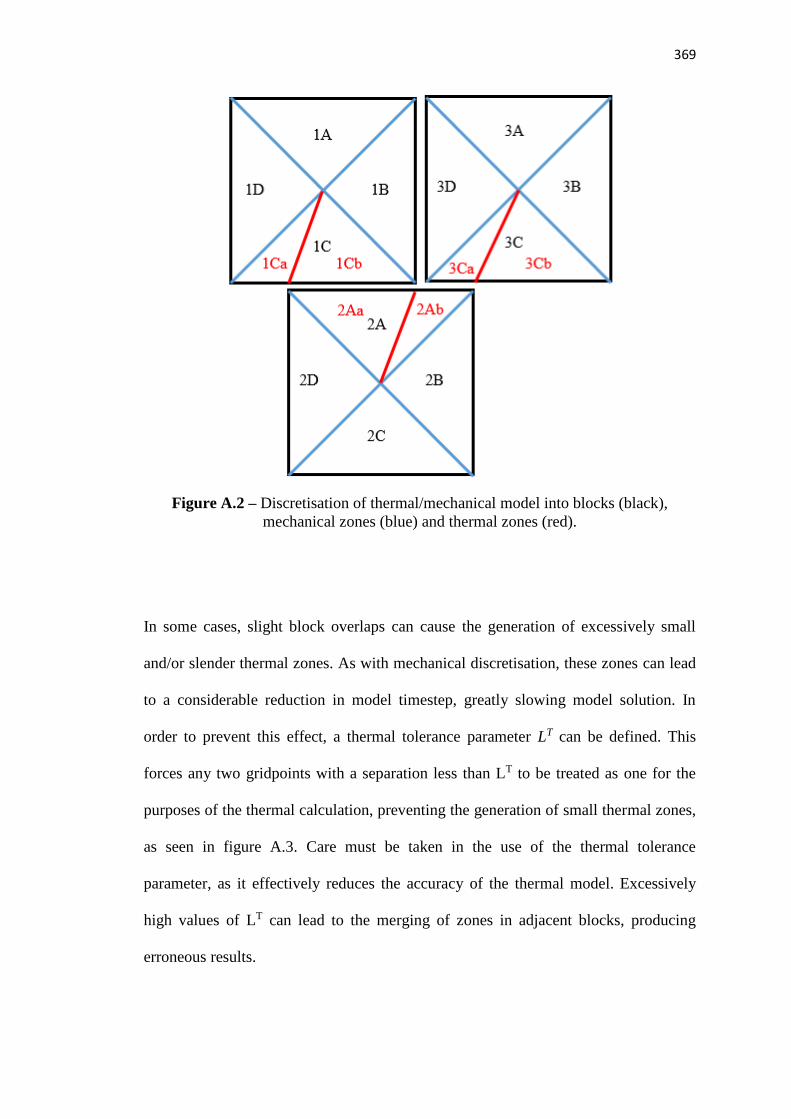
369
Figure A.2 – Discretisation of thermal/mechanical model into blocks (black),
mechanical zones (blue) and thermal zones (red).
In some cases, slight block overlaps can cause the generation of excessively small
and/or slender thermal zones. As with mechanical discretisation, these zones can lead
to a considerable reduction in model timestep, greatly slowing model solution. In
order to prevent this effect, a thermal tolerance parameter LT can be defined. This
forces any two gridpoints with a separation less than LT to be treated as one for the
purposes of the thermal calculation, preventing the generation of small thermal zones,
as seen in figure A.3. Care must be taken in the use of the thermal tolerance
parameter, as it effectively reduces the accuracy of the thermal model. Excessively
high values of LT can lead to the merging of zones in adjacent blocks, producing
erroneous results.

370
Figure A.3 – Effect of thermal tolerance parameter LT on the generation of small
thermal zones.
A.3.5. Thermal Expansion
UDEC is capable of modelling thermally generated stresses within rock blocks, as
shown in equation A.35. The temperature of a zone is defined as the arithmetic mean
of the temperatures of the three gridpoints which constitute that zone.
∆𝜎𝑁 = −3𝐾𝛼∆𝑇 (A.35)
Where α is the linear thermal expansion coefficient (K-1)

371
A.3.6. Temperature Dependent Fluid Properties
The temperature dependence of fluid properties is simulated using a three step
process:
1. Tables of property/temperature data are stored for fluid density and viscosity.
2. Fluid temperature is found as the arithmetic mean temperature of the
gridpoints which define the fluid filled joint.
3. Property tables are linearly interpolated to find the values of density and
viscosity at the given temperature.

372
B. DERIVATIONS
B.1. STRESS/DISPLACEMENT RELATIONSHIPS
This appendix covers the derivation of equations 4.2 and 4.3, which show the
relationship between applied axial strain εa and horizontal and vertical displacements ux
and uy respectively. Consider a single joint at an angle ϕ to the horizontal, as shown in
figure B.1. This joint is part of a rock mass exposed to an applied axial compressive
strain εa.
Figure B.1 – Schematic representation of the forces and motion on a single joint
within a rock mass. N implies normal motion, S implies shear motion.
The force F on the joint due to the applied strain is:
𝐹 = −𝐸휀𝑎𝐴
Where A is the surface area of the joint

373
We can find:
𝐹𝑛 = 𝐹 cos(𝜙) = −𝐸휀𝑎𝐴 cos(𝜙)
𝐹𝑠 = 𝐹 sin(𝜙) = −𝐸휀𝑎 𝐴 sin(𝜙)
The displacement along a joint can be found as:
𝑢𝑖 =𝐹𝑖
𝑘𝑖
Therefore:
𝑢𝑛 = −𝐸휀𝑎𝐴
𝑘𝑛cos(𝜙)
𝑢𝑠 = −𝐸휀𝑎𝐴
𝑘𝑠sin(𝜙)
Convert into Cartesian co-ordinates:
𝑢𝑥 = 𝑢𝑛,𝑥 + 𝑢𝑠,𝑥
𝑢𝑦 = 𝑢𝑛,𝑦 + 𝑢𝑠,𝑦

374
Where:
𝑢𝑛,𝑥 = 𝑢𝑛 sin(𝜙) = −𝐸휀𝑎𝐴
𝑘𝑛cos(𝜙) sin(𝜙) = −
𝐸휀𝑎𝐴
2𝑘𝑛sin(2𝜙)
𝑢𝑠,𝑥 = −𝑢𝑠 cos(𝜙) = 𝐸휀𝑎𝐴
𝑘𝑠sin(𝜙) cos(𝜙) =
𝐸휀𝑎𝐴
2𝑘𝑠sin(2𝜙)
𝑢𝑛,𝑦 = −𝑢𝑛 cos(𝜙) =𝐸휀𝑎𝐴
𝑘𝑛cos2(𝜙)
𝑢𝑠,𝑦 = −𝑢𝑠 sin(𝜙) =𝐸휀𝑎𝐴
𝑘𝑠sin2(𝜙)
Therefore:
𝑢𝑥 =𝐸 𝑎𝐴
2(
1
𝑘𝑠−
1
𝑘𝑛) sin(2𝜙) is equation 4.2
𝑢𝑦 = 𝐸휀𝑎𝐴 (cos2(𝜙)
𝑘𝑛+
sin2(𝜙)
𝑘𝑠) is equation 4.3

375
B.2. TEMPERATURE DEPENDENT MATERIAL PROPERTIES
Ranjith et al (2012) present normalised relationships for the elastic modulus and
uniaxial compressive strength of sandstone over a range of temperatures, as shown in
figure B.2. In order to simulate temperature dependent materials in the UCG model,
compressive strength must be converted into the model parameters of friction angle,
cohesion and tensile limit. This section explains how this is achieved.
Figure B.2 – Temperature dependence of the Young’s modulus and uniaxial
compressive strength of sandstone over a range of temperatures. After Ranjith et al,
2012.
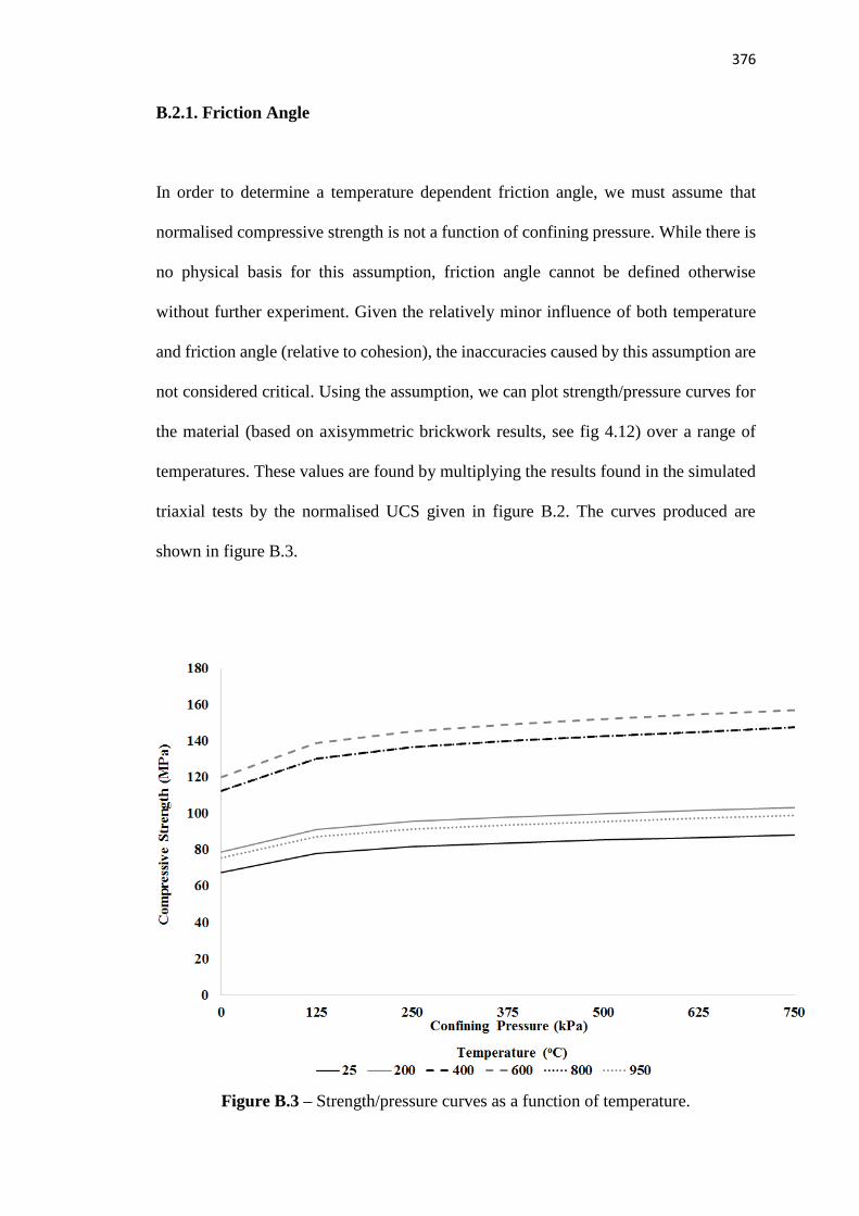
376
B.2.1. Friction Angle
In order to determine a temperature dependent friction angle, we must assume that
normalised compressive strength is not a function of confining pressure. While there is
no physical basis for this assumption, friction angle cannot be defined otherwise
without further experiment. Given the relatively minor influence of both temperature
and friction angle (relative to cohesion), the inaccuracies caused by this assumption are
not considered critical. Using the assumption, we can plot strength/pressure curves for
the material (based on axisymmetric brickwork results, see fig 4.12) over a range of
temperatures. These values are found by multiplying the results found in the simulated
triaxial tests by the normalised UCS given in figure B.2. The curves produced are
shown in figure B.3.
Figure B.3 – Strength/pressure curves as a function of temperature.

377
Friction angles are then found for each temperature as:
𝜃𝑇 =𝑀𝑇−1
𝑀𝑇+1
Where MT is the gradient of the strength/pressure curve at temperature T.
B.2.2. Cohesion
Cohesion is found as:
𝐶𝑇 = 𝜎𝑐,𝑇1−sin(𝜃𝑇)
2 cos(𝜃𝑇)
Where σc,T is the unconfined compressive strength at temperature T.
B.2.3. Tensile Limit
Tensile limit is found as:
𝜎𝑇 =𝐶𝑇
tan(𝜃𝑇)
B.2.4. Normalised Properties
Normalised values of friction angle, cohesion and tensile limit are found by dividing
their absolute values by their value at 25oC. The values found are plotted in figure 5.4.

378
B.3. CONDUCTIVE/CONVECTIVE HEAT TRANSFER RATIO
Consider a single joint in between a pair of blocks, as shown in figure B.4.
Figure B.4 – Schematic of a single joint between a pair of rocks.
Thermal conduction transfers heat from left to right (T1 to T2). This heat is partially
negated by the inflow of cold fluid flowing from right to left (T2 to T1). Assuming fluid
temperature is equal to rock temperature at all points along the joint, the magnitudes of
heat transferred by each mechanism can be found as follows:
𝑄𝑅 = 𝜆𝐻(𝑇1 − 𝑇2)
𝑄𝐹 = �̇�𝐶(𝑇2 − 𝑇1) = 𝜌𝑎𝑣𝐶(𝑇2 − 𝑇1)
The ratio of conduction to convection can then be found as:
𝑄𝑅
𝑄𝐹= −
𝜆𝐻
𝜌𝑎𝑣𝐶
Which is equation 5.8.

379
Where:
C Fluid heat capacity (Jkg-1K-1)
v Fluid velocity (ms-1)
λ Rock thermal conductivity (Wm-2K-1)
ρ Fluid density (kgm-3)

380
B.4. CAVITY WALL TEMPERATURE DERIVATION
As shown in figure 5.10, the energy balance over the UCG cavity consists of 6
components:
Energy stored in the coal EC
Energy stored in the oxidant gas EO
Energy stored in the injected steam ES
Energy stored in the groundwater EW
Energy stored in the product syngas EP
Energy lost to the rock mass EL
For the thermal model, we are interested in the energy lost to the rock mass EL. This can
be found by an energy balance as:
𝐸𝐿 = 𝐸𝐶 + 𝐸𝑂 + 𝐸𝑆 + 𝐸𝑊 − 𝐸𝑃
The terms on the right hand side can be found by considering the stoichiometry of the
reaction and the enthalpies of formation of the compounds involved. ES and EW also
depend on the relative proportions of the water supplied by the injected steam and
groundwater respectively.
Using coal as the basis for the calculation and assuming constant compositions we find
the following stoichiometric relationships, where product gas composition is given by
Perkins & Sahajwalla (2005):

381
𝐶𝐻0.08𝑂0.18 + 𝛼𝑂2 + 𝛽𝐻2𝑂 → 𝛾𝐶𝑂 + 𝛿𝐶𝑂2 + 휀𝐻2 + 𝜃𝐶𝐻4 + 𝜇𝐻2𝑂
Product gas composition, on a molar basis:
CO = 0.35
CO2 = 0.29 ∴ δ = 0.83γ
H2 = 0.21 ∴ ε = 0.60γ
CH4 = 0.06 ∴ θ = 0.17γ
H2O = 0.09 ∴ μ = 0.26γ
By performing an element balance over the stoichiometric equation, we find:
α = 0.36
β = 0.56
γ = 0.50
We can now balance the equation as:
𝐶𝐻0.08𝑂0.18 + 0.36𝑂2 + 0.56𝐻2𝑂 → 0.5𝐶𝑂 + 0.42𝐶𝑂2 + 0.3𝐻2 + 0.09𝐶𝐻4 +
0.13𝐻2𝑂
Combining with the relative molecular weights, we find the total mass fluxes associated
with the process:

382
COMPOUND kmol kg kg/kg coal mass
fraction
CH0.08O0.18 1 (basis) 14.97 1 (basis) -
O2 0.36 11.52 0.770 -
H2O 0.56 10.09 0.674 -
CO 0.50 14.01 0.936 0.380
CO2 0.42 18.48 1.234 0.501
H2 0.30 0.61 0.041 0.017
CH4 0.09 1.44 0.096 0.039
H2O 0.13 2.34 0.156 0.063
Product Gas 1.44 36.88 2.463 -
The energy terms are found as:
𝐸𝑖 = −∆𝐻𝑓,𝑖𝜃 + 𝐻𝑇,𝑃 − 𝐻𝜃
Where:
∆𝐻𝑓,𝑖𝜃 = Standard enthalpy of formation
[Jkg-1]
𝐻𝑇,𝑃 = Thermodynamic enthalpy at given temperature and pressure
[Jkg-1]
𝐻𝜃 = Thermodynamic enthalpy at standard conditions
[Jkg-1]

383
All data is found from Green & Perry (2007). The Hθ term is required because the
formation enthalpy is defined at 298K whereas the thermodynamic enthalpy is defined
as zero at 0K. Differences in enthalpy can also be found via the constant pressure heat
capacity in the case of solid and liquid compounds.
The enthalpy of formation for coal is difficult to define, due to its complex chemical
nature. We can find this using Hess’s law applied to coal combustion:
𝐶𝐻0.08𝑂0.18 + 0.93𝑂2 → 𝐶𝑂2 + 0.04𝐻2𝑂
∆𝐻𝑟𝜃 = ∆𝐻𝑓,𝐶𝑂2
𝜃 + 0.04∆𝐻𝑓,𝐻2𝑂𝜃 − ∆𝐻𝑓,𝐶𝑜𝑎𝑙
𝜃 − 0.93∆𝐻𝑓,𝑂2
𝜃
∆𝐻𝑓,𝑂2
𝜃 equals zero, as oxygen is an element.
Therefore:
∆𝐻𝑓,𝐶𝑜𝑎𝑙𝜃 = ∆𝐻𝑓,𝐶𝑂2
𝜃 + 0.04∆𝐻𝑓,𝐻2𝑂𝜃 − ∆𝐻𝑟
𝜃
From the literature:
∆𝐻𝑓,𝐶𝑂2
𝜃 = −393.51 𝑘𝐽𝑚𝑜𝑙−1
∆𝐻𝑓,𝐻2𝑂𝜃 = −241.81 𝑘𝐽𝑚𝑜𝑙−1
∆𝐻𝑟𝜃 = −319.5 𝑘𝐽𝑚𝑜𝑙−1

384
Therefore:
∆𝐻𝑓,𝐶𝑜𝑎𝑙𝜃 = −84.03 𝑘𝐽𝑚𝑜𝑙−1 = −5613.4 𝑘𝐽𝑘𝑔−1
And:
𝐸𝐶 = −∆𝐻𝑓,𝐶𝑜𝑎𝑙𝜃 + 𝐶𝑃,𝐶𝑜𝑎𝑙(𝑇0 − 298) = 5615.2 𝑘𝐽𝑘𝑔−1
Where:
CC Specific Heat Capacity of Coal (0.920 kJkg-1K-1)
T0 Ambient Temperature at Cavity Depth (300 K)
EO, ES and EW and EP are found as:
EO = 118.4 kJkg-1 (P = 555kPa, T = 429K = Tsat)
ES = 16074 kJkg-1 (P = 555kPa, T = 429K)
EW = 13435 kJkg-1 (P = 555kPa, T = 300K)
EP = 8249.9 kJkg-1 (P = 555kPa, T = 980K)
We now express each term with respect to the basis of coal, giving:
EC = 5615.2 kJkg-1
EO = 91.2 kJkg-1 (coal)
ES = 13435Q kJkg-1 (coal)

385
EW = 16074(0.674-Q) kJkg-1 (coal)
EP = 20320 kJkg-1 (coal)
Therefore:
EL = 3779.6 – 2639.0 Q kJkg-1 (coal)
Where Q is the specific drawdown rate of the groundwater (kg groundwater / kg coal).
We now need to determine the rate of coal consumption in order to obtain the energy
release rate in units of Wm-1. Bhutto et al (2013) report total consumption of
approximately 150 tonnes of coal per day. Assuming a combustion zone length of
approximately 12m (Perkins & Sahajwalla, 2008), gives a consumption of 12.5 tonnes
per metre per day, or 0.145 kgm-1s-1. Multiplying this by EL gives a total energy loss
rate of:
EL = 5.48×10⁵ – 3.83×10⁵ Q Wm-1
We can say that:
𝑄 =𝑞𝜌𝑤𝐿𝑏𝑢𝑟𝑛
𝑅
Where:
q Flow rate of groundwater into cavity (given by UDEC)
(m2s-1)

386
Lburn Combustion zone length (m)
R Coal consumption rate
(kgs-1)
𝜌𝑊 Density of water
(kgm-3)
Therefore:
Q = 6899q
And:
EL = 5.48×10⁵ – 2.64×10⁹ q Wm-1
Is the total amount of power produced by the modelled region.
We can convert this into a wall temperature by equating the power produced with the
heat lost to the surroundings:
𝐸𝐿 = 𝜆𝑃(𝑇𝑤−𝑇0)
𝐿𝑇
Where:

387
P Cavity Wall Perimeter (m)
LT Thermal Penetration Length (m)
Assuming a thermal penetration length of 10m (this can be tested and updated in later
versions of the model to increase accuracy) and a cavity geometry the same as that used
in the Rocky Mountain 1 trial, we find:
𝑇𝑤 = 300 +𝐸𝐿
𝜆𝑃𝐿𝑇
Substituting in the appropriate values gives:
Tw = 1153 - 4.1×10⁶ q Wm-1 which is equation 5.12.

388
B.5. THERMAL PENETRATION LENGTH
Consider a cavity with a circular cross section, surrounded by a temperature profile.
The amount of energy required to produce that profile is given as:
𝑄 = 2𝜋𝜌𝐶 ∫ 𝑟(𝑇 − 𝑇𝑏)𝑑𝑟𝑟𝑝
𝑟𝑐
If we assume a linear temperature profile, we find:
𝑇 = 𝑇𝑊 + (𝑇𝐵 − 𝑇𝑊)𝑟−𝑟𝑐
𝑟𝑝−𝑟𝑐
Therefore:
𝑄 =𝜋𝜌𝐶(𝑇𝑊−𝑇𝐵)
𝑟𝑝−𝑟𝑐∫ 𝑟𝑝𝑟 − 𝑟2𝑑𝑟
𝑟𝑝
𝑟𝑐
Where
Tb Background temperature (K)
Tw Cavity wall temperature (K)
rc Cavity radius (m)
rp Profile radius (m)
Assuming rp >> rc, we find:

389
𝑄 ≈ 𝜋𝜌𝐶
6𝑟𝑝(𝑇𝑊 − 𝑇𝐵)𝑟𝑝
3 =𝜋𝜌𝐶
6(𝑇𝑊 − 𝑇𝐵)𝑟𝑝
2
Note that the above assumption is not true in many cases. Given that this derivation is
only intended to show an approximate relationship however, this error is considered
acceptable.
The amount of heat transferred from the cavity over time t is found as:
𝑄 = −2𝜋𝜆𝑟𝑐𝛿𝑇
𝛿𝑟𝑡 ≈ −2𝜋𝜆𝑟𝑐𝑡
𝑇𝐵−𝑇𝑊
𝑟𝑝
Therefore:
𝜋𝜌𝐶
6(𝑇𝑊 − 𝑇𝐵)𝑟𝑝
2 ≈ −2𝜋𝜆𝑟𝑐𝑡𝑇𝐵−𝑇𝑊
𝑟𝑝
Rearranging terms gives:
𝑟𝑝3 ≈
12𝜆𝑟𝑐𝑡
𝜌𝐶
Finally,
𝑟𝑝 ≈ (12𝜆𝑟𝑐𝑡
𝜌𝐶)
13⁄
Which is equation 8.4.

390
C. GROUNDWATER CONTAMINATION MODELLING
This appendix outlines a brief suggestion for how a model of UCG induced
groundwater pollution could be created using the commercially available Modular 3
Dimensional Transport Model for Multiple Species (MT3DMS) (United States
Geological Survey, 2005). The model would consider contaminant generation,
transport and destruction and would be one-directionally coupled with the existing
UDEC model. The model would effectively produce a two dimensional map of the
spread of several contaminant species over time, both during and after gasification,
using the results of the UDEC model as boundary conditions.
The model would simulate the behaviour of approximately 5 contaminant species, with
each one chosen to represent several similar compounds. For example, benzene could
be used to represent all low molecular weight aromatic hydrocarbons, while lead could
be used to represent all heavy metals. The choice of species used would depend on their
relative transport capabilities and environmental toxicity, with those which travel
furthest or present the most danger used in the model to predict the worst possible
pollution outcomes. A brief outline of the suggested model operation is given below:
391
1. An additional part of the UDEC model reads the “after” stage result and produces
a 2D map of the permeability, pressure and flow distributions during gasification.
2. The data is mapped onto a grid of equally sized 2D elements.
3. The grid element(s) containing the cavity are set to produce contaminants at a fixed
rate based determined from the literature.
4. Any other necessary boundary and initial conditions are set. Examples include
background pollutant concentrations and far field pressure values.
5. MT3DMS is executed over the operational time of the gasifier to find the
distribution of contaminant species at the end of gasification.
6. Steps 1 through 4 are repeated for the “final” stage of the model with appropriate
contaminant generation rates.
7. MT3DMS is executed for a given period after gasification has ceased (years), with
the distribution of contaminants output from the model at regular points in this time.
Given the relatively good scientific understanding of contaminant transport in
groundwater, it is believed that the development of the pollution model should be much
faster than that of the UDEC model. In addition, unlike subsidence, a great deal of field
trial data is available for validation purposes. As such, it is expected that a valid, useful
model could be developed within 12 months, based on the suggested methodology
above. The creation of the model should therefore be considered a key priority in the
further development of UCG modelling capabilities.


![40878 MARGUERITE WUNSCHER Archives Hongroises [InLibroVeritas.net]](https://img.pdfslide.net/doc/110x75/55cf97b3550346d0339313f3/40878-marguerite-wunscher-archives-hongroises-inlibroveritasnet.jpg)