Embed Size (px)
Citation preview
Sample Size Planning for Behavioral Science Research
Douglas G. Bonett
University of California, Santa Cruz
June 2016
How to cite this work:
Bonett, D.G. (2016) Sample Size Planning for Behavioral Science Research. Retrieved
from http://people.ucsc.edu/~dgbonett/sample.html.
1
Contents
1 Preliminaries 1.1 The Importance of Sample Size Planning . . . . . . . . . . . . 2
1.2 Study Populations and Population Parameters. . . . . . . . . . . 2
1.3 Random Samples and Parameter Estimates . . . . . . . . . . . . 3
1.4 Interval Estimation and Hypothesis Testing . . . . . . . . . . . 5
1.5 Sample Size Requirements for Desired Precision . . . . . . . . . . 7
1.6 Sample Size Requirements for Desired Power . . . . . . . . . . . 8
1.7 Power and Precision for Specified Sample Size . . . . . . . . . . 10
1.8 Sample Size Results are Approximations . . . . . . . . . . . . 11
2 Means
2.1 1-group Designs . . . . . . . . . . . . . . . . . . . . . 13
2.2 2-group Designs . . . . . . . . . . . . . . . . . . . . 15
2.3 Multiple Group Designs . . . . . . . . . . . . . . . . . . 20
2.4 Paired-samples Designs . . . . . . . . . . . . . . . . . . 23
2.5 General Within-subjects Designs . . . . . . . . . . . . . . . 27
2.6 Multiple Group Designs with Covariates . . . . . . . . . . . . 31
3 Proportions
3.1 1-group Designs . . . . . . . . . . . . . . . . . . . . . 35
3.2 2-group Designs . . . . . . . . . . . . . . . . . . . . . 37
3.3 Multiple Group Designs . . . . . . . . . . . . . . . . . . 39
3.4 Paired-samples Designs . . . . . . . . . . . . . . . . . . 41
4 Correlation, Regression, and Reliability
4.1 Pearson Correlation . . . . . . . . . . . . . . . . . . . . 48
4.2 Partial Correlation . . . . . . . . . . . . . . . . . . . . . 50
4.3 Multiple Correlation . . . . . . . . . . . . . . . . . . . . 52
4.4 Cronbach’s Alpha Reliability . . . . . . . . . . . . . . . . . 54
4.5 Linear Regression Model . . . . . . . . . . . . . . . . . . 57
4.6 2-group Designs . . . . . . . . . . . . . . . . . . . . . 62
5 Further Topics
5.1 Unequal Sample Sizes . . . . . . . . . . . . . . . . . . . 68
5.2 Two-stage Sampling . . . . . . . . . . . . . . . . . . . . 71
5.3 Iterative Methods . . . . . . . . . . . . . . . . . . . . . 72
5.4 Analyzing Enormous Datasets . . . . . . . . . . . . . . . . 73
5.5 Sample Size Requirements for Distribution-free Tests . . . . . . . 75
5.6 Sample Size Requirements for Desired Precision and Assurance . . . . 77
References . . . . . . . . . . . . . . . . . . . . . . . . . . 79
Study Guide . . . . . . . . . . . . . . . . . . . . . . . . . . 81
2
Chapter 1
Preliminaries
1.1 The Importance of Sample Size Planning
Sample size planning is especially important in studies where statistical methods
will be used to analyze sample data and there are tangible costs of recruiting,
measuring, or treating participants. If the sample size is too small, statistical tests
may not detect important effects, and confidence intervals for an effect size might
be uselessly wide. Using a sample size that is unnecessarily large is wasteful of
valuable resources. Furthermore, a study that uses too many participants could
reduce the number of participants that are available to other researchers.
Funding agencies usually require a justification of the proposed sample size, and
an increasing number of journals now require authors to provide a sample size
justification.
Several studies have shown that most published behavioral science articles
should not have found “significant” results because the sample sizes were too
small to reliably detect the reported effect sizes. This suggests that the reported
effect sizes were inflated due to random sampling error. Sample size planning
should reduce the positive bias in reported effect sizes. Sample size planning
will also reduce the number of published studies with results that cannot be
replicated by other researchers.
Behavioral science publications seldom provide an adequate description of the
meaning and importance of reported effect sizes. Authors who provide a sample
size justification will naturally need to explain why the expected effect size
should have practical or theoretical importance.
1.2 Study Populations and Population Parameters
A study population is a clearly defined collection of people, animals, plants, or
objects. In behavioral research, a study population usually consists of a specific
collection of people. Some examples of a study population are: all elementary
3
school teachers in San Jose, all college students who are enrolled in a research
participant pool, and all registered voters in Santa Cruz County.
A population parameter is a numeric value that describes all people in a specific
study population. Greek letters will be used to represent population parameters
such as a population mean (𝜇), a population proportion (𝜋), a population
standard deviation (𝜎), and a population Pearson correlation between variables y
and x (𝜌𝑦𝑥). Researchers often want know the value of a population parameter
because this information could be used to make an important decision or to
advance knowledge.
1.3 Random Samples and Parameter Estimates
In applications where the study population is large or the cost of measurement is
high, the researcher may not have the necessary resources to measure all people
in the study population. In these applications, the researcher could take a random
sample of n people from the study population. A random sample of size n is
selected in such a way that every possible sample of size n will have the same
chance of being selected. Simple computer programs can be used to generate a
random sample of n participant ID numbers. The n randomly people selected
people are referred to as participants.
A population parameter can be estimated from data obtained from a random
sample of participants. We will consider data that are in the form of quantitative
measurements (e.g., test scores, heart rates, opinion ratings) or dichotomous
measurements (e.g., pass or fail, agree or disagree, correct or incorrect answer).
The measurement for participant i will be denoted as 𝑦𝑖. If the measurement is
quantitative, 𝑦𝑖 could be any numeric value. If the measurement is dichotomous,
𝑦𝑖 could be assigned a value of 0 or 1.
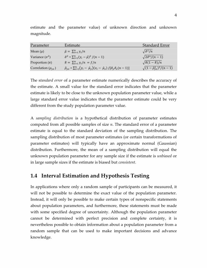
Some examples of parameter estimates are given in the table below. A carat (^) is
placed over the Greek letter to indicate that it is merely an estimate and not the
actual value of population parameter. Parameter estimates by themselves can be
misleading because they will contain sampling error (the difference between the
4
estimate and the parameter value) of unknown direction and unknown
magnitude.
Parameter Estimate Standard Error
Mean (𝜇) �̂� = ∑ 𝑦𝑖/𝑛𝑛𝑖=1 √�̂�2/𝑛
Variance (𝜎2) �̂�2 = ∑ (𝑦𝑖 − �̂�)2𝑛𝑖=1 /(𝑛 − 1) √2�̂�4/(𝑛 − 1)
Proportion (𝜋) �̂� = ∑ 𝑦𝑖/𝑛𝑛𝑖=1 = 𝑓/𝑛 √�̂�(1 − �̂�)/𝑛
Correlation (𝜌𝑦𝑥 ) �̂�𝑦𝑥 = ∑ (𝑦𝑖 − �̂�𝑦)(𝑥𝑖 − �̂�𝑥)𝑛𝑖=1 /[�̂�𝑦�̂�𝑥(𝑛 − 1)] √(1 − �̂�𝑦𝑥
2 )2/(𝑛 − 1)
The standard error of a parameter estimate numerically describes the accuracy of
the estimate. A small value for the standard error indicates that the parameter
estimate is likely to be close to the unknown population parameter value, while a
large standard error value indicates that the parameter estimate could be very
different from the study population parameter value.
A sampling distribution is a hypothetical distribution of parameter estimates
computed from all possible samples of size n. The standard error of a parameter
estimate is equal to the standard deviation of the sampling distribution. The
sampling distribution of most parameter estimates (or certain transformations of
parameter estimates) will typically have an approximate normal (Gaussian)
distribution. Furthermore, the mean of a sampling distribution will equal the
unknown population parameter for any sample size if the estimate is unbiased or
in large sample sizes if the estimate is biased but consistent.
1.4 Interval Estimation and Hypothesis Testing
In applications where only a random sample of participants can be measured, it
will not be possible to determine the exact value of the population parameter.
Instead, it will only be possible to make certain types of nonspecific statements
about population parameters, and furthermore, these statements must be made
with some specified degree of uncertainty. Although the population parameter
cannot be determined with perfect precision and complete certainty, it is
nevertheless possible to obtain information about a population parameter from a
random sample that can be used to make important decisions and advance
knowledge.
5
One type of statement about a population parameter is in the form of a confidence
interval. A confidence interval is a range of possible population parameter values
that is stated with a specified confidence level. For example, a 100(1 − 𝛼)%
confidence interval for 𝜇 is
�̂� ± 𝑡𝛼/2;𝑑𝑓√�̂�2/𝑛 (1.1)
where df = n – 1, 𝑡𝛼/2;𝑑𝑓 is a two-sided critical t-value and 𝑦𝑖 is a quantitative
measurement of some attribute for participant i. A degree of belief definition of
probability is assumed when interpreting a computed confidence interval. Most
confidence intervals that are reported in behavioral science studies use a 95%
confidence level.
Narrow confidence intervals are more informative than wide confidence
intervals, and a larger confidence level (e.g., 99% rather than 95%) provides a
more convincing result than a smaller confidence level. As can be seen in
Equation 1.1, using a larger sample size will decrease the value of √�̂�2/𝑛 which
in turn will decrease the width of the confidence interval. Increasing the level of
confidence (e.g., from 95% to 99%) will increase the width of the confidence
interval because a smaller value of 𝛼 (i.e., higher confidence) corresponds to a
larger critical t-value (see Table 2 of Appendix). Sampling from a more diverse
study population can result in a larger value of �̂�2 which in turn gives a wider
confidence interval.
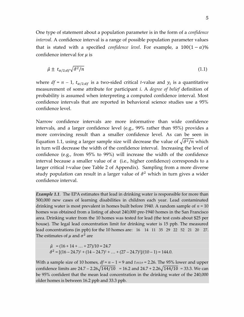
Example 1.1. The EPA estimates that lead in drinking water is responsible for more than
500,000 new cases of learning disabilities in children each year. Lead contaminated
drinking water is most prevalent in homes built before 1940. A random sample of n = 10
homes was obtained from a listing of about 240,000 pre-1940 homes in the San Francisco
area. Drinking water from the 10 homes was tested for lead (the test costs about $25 per
house). The legal lead concentration limit for drinking water is 15 ppb. The measured
lead concentrations (in ppb) for the 10 homes are: 16 14 11 35 29 22 52 21 20 27.
The estimates of 𝜇 and 𝜎2 are
�̂� = (16 + 14 + … + 27)/10 = 24.7
�̂�2 = [(16 – 24.7)2 + (14 – 24.7)2 + … + (27 – 24.7)2]/(10 – 1) = 144.0.
With a sample size of 10 homes, df = n – 1 = 9 and t.05/2;9 = 2.26. The 95% lower and upper
confidence limits are 24.7 – 2.26√144/10 = 16.2 and 24.7 + 2.26√144/10 = 33.3. We can
be 95% confident that the mean lead concentration in the drinking water of the 240,000
older homes is between 16.2 ppb and 33.3 ppb.
6
A second type of statement about a population parameter value is in the form of
a hypothesis test. For example, consider the following hypotheses regarding the
value of 𝜇
H0: 𝜇 = ℎ H1: 𝜇 > ℎ H2: 𝜇 < ℎ
where h is some number specified by the researcher, H0 is called the null
hypothesis, and H1 and H2 are called the alternative hypotheses. In virtually every
application, we know that H0 is false (because 𝜇 will almost never exactly equal
h) and the goal of the study is to decide if 𝜇 > h or 𝜇 < ℎ because accepting 𝜇 > h
would lead to one course of action (or provides support for one theory) while
accepting 𝜇 < h would lead to another course of action (or provide support for
another theory).
A 100(1 − 𝛼)% confidence interval for 𝜇 can be used to choose between H1: 𝜇 > h
and H2: 𝜇 < h using the following rules.
If the upper limit of a 100(1 − 𝛼)% confidence interval is less than h, then H0
is rejected and H2 is accepted.
If the lower limit of a 100(1 − 𝛼)% confidence interval is greater than h, then
H0 is rejected and H1 is accepted.
If the confidence interval includes h, then H0 cannot be rejected and the
results are said to be inconclusive.
This general hypothesis testing procedure is called a three-decision rule because
one of following three decisions will be made: 1) accept H1, 2) accept H2, or 3) fail
to reject H0.. Note that a failure to reject H0 should not be interpreted as evidence
that the null hypothesis is true.
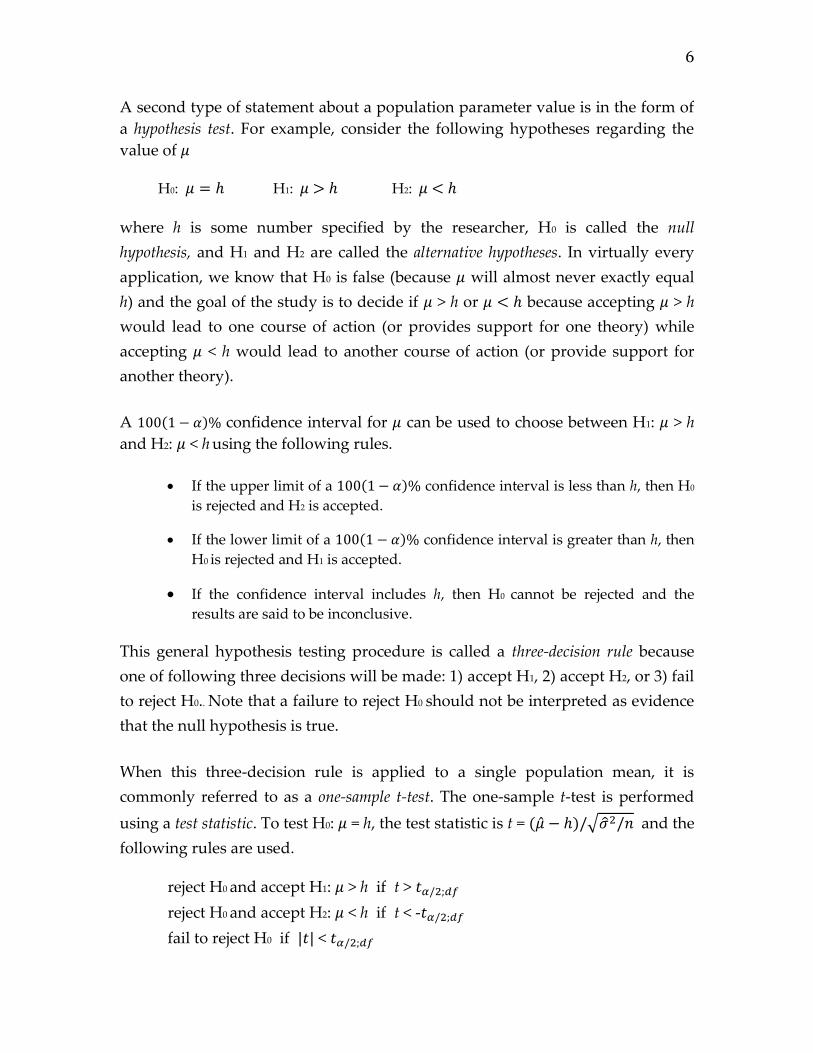
When this three-decision rule is applied to a single population mean, it is
commonly referred to as a one-sample t-test. The one-sample t-test is performed
using a test statistic. To test H0: 𝜇 = h, the test statistic is t = (�̂� − ℎ)/√�̂�2/𝑛 and the
following rules are used.
reject H0 and accept H1: 𝜇 > h if t > 𝑡𝛼/2;𝑑𝑓
reject H0 and accept H2: 𝜇 < h if t < -𝑡𝛼/2;𝑑𝑓
fail to reject H0 if |𝑡| < 𝑡𝛼/2;𝑑𝑓
7
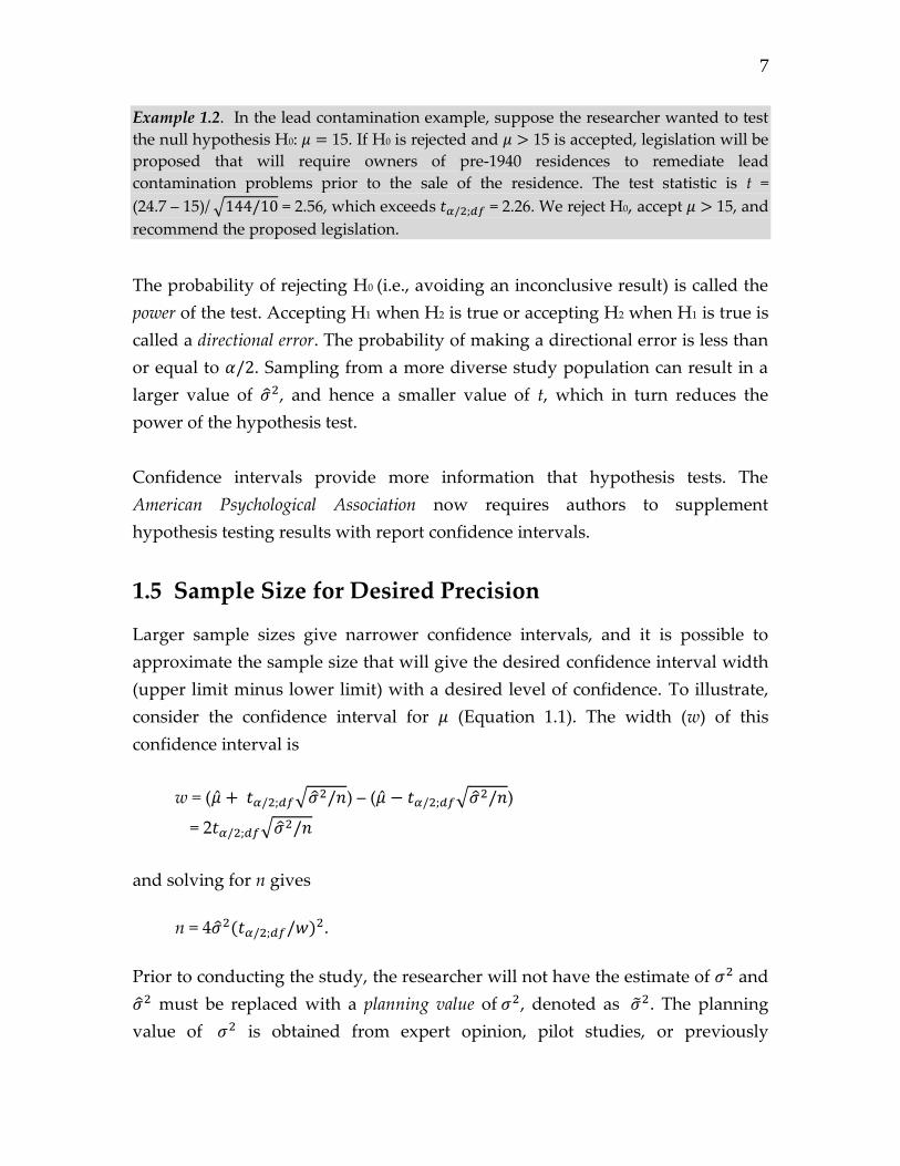
Example 1.2. In the lead contamination example, suppose the researcher wanted to test
the null hypothesis H0: 𝜇 = 15. If H0 is rejected and 𝜇 > 15 is accepted, legislation will be
proposed that will require owners of pre-1940 residences to remediate lead
contamination problems prior to the sale of the residence. The test statistic is t =
(24.7 – 15)/ √144/10 = 2.56, which exceeds 𝑡𝛼/2;𝑑𝑓 = 2.26. We reject H0, accept 𝜇 > 15, and
recommend the proposed legislation.
The probability of rejecting H0 (i.e., avoiding an inconclusive result) is called the
power of the test. Accepting H1 when H2 is true or accepting H2 when H1 is true is
called a directional error. The probability of making a directional error is less than
or equal to 𝛼/2. Sampling from a more diverse study population can result in a
larger value of �̂�2, and hence a smaller value of t, which in turn reduces the
power of the hypothesis test.
Confidence intervals provide more information that hypothesis tests. The
American Psychological Association now requires authors to supplement
hypothesis testing results with report confidence intervals.
1.5 Sample Size for Desired Precision
Larger sample sizes give narrower confidence intervals, and it is possible to
approximate the sample size that will give the desired confidence interval width
(upper limit minus lower limit) with a desired level of confidence. To illustrate,
consider the confidence interval for 𝜇 (Equation 1.1). The width (w) of this
confidence interval is
w = (�̂� + 𝑡𝛼/2;𝑑𝑓√�̂�2/𝑛) – (�̂� − 𝑡𝛼/2;𝑑𝑓√�̂�2/𝑛)
= 2𝑡𝛼/2;𝑑𝑓√�̂�2/𝑛
and solving for n gives
n = 4�̂�2(𝑡𝛼/2;𝑑𝑓/𝑤)2.
Prior to conducting the study, the researcher will not have the estimate of 𝜎2 and
�̂�2 must be replaced with a planning value of 𝜎2, denoted as �̃�2. The planning
value of 𝜎2 is obtained from expert opinion, pilot studies, or previously
8
published research. If there is little prior information about the value of 𝜎2, but
the maximum and minimum possible values of the response variable are known,
[(max – min)/4]2 provides a crude planning value of the population variance. If
prior research suggests a range of plausible variance values, using the largest
value will give a conservatively large sample size requirement.
Since df = n – 1 and n is unknown, 𝑡𝛼/2;𝑑𝑓 is unknown but can be approximated
by 𝑧𝛼/2, a two-sided critical z-value. With these two substitutions, we obtain
n = 4 �̃�2(𝑧𝛼/2/𝑤)2
Finally, since 𝑧𝛼/2 < 𝑡𝛼/2;𝑑𝑓 the above sample size formula will underestimate the
sample size requirement because 𝑧𝛼/2 < 𝑡𝛼/2;𝑑𝑓, but adding an adjustment
proposed by Guenther (1975)
n = 4�̃�2(𝑧𝛼/2/𝑤)2 + 𝑧𝛼/22 /2 (1.2)
gives a very accurate approximation to the sample size requirement. Some
confidence intervals, such as confidence interval for correlations and
proportions, use critical z-values rather than critical t-values and the Guenther
adjustment is not needed for these applications. It is a tradition to round the
results produced by a sample size formula up to the nearest integer.
Critical two-sided z-values for 90%, 95%, and 99% confidence levels are given
below. 95% confidence intervals are recommended for research intended for
publication in scientific journals. In applied research, lower or higher levels of
confidence might be more appropriate.
90% 95% 99%
𝑧𝛼/2 1.645 1.960 2.576
1.6 Sample Size for Desired Power
The power of a test of H0: 𝜇 = ℎ depends on the sample size (greater power for
larger sample sizes), the absolute value of |𝜇 – h| (greater power for larger
absolute values of 𝜇 – h), and the 𝛼 value (lower power for smaller values of 𝛼)
where 𝛼 is the probability of making a decision error. Although using a larger 𝛼
9
level will give a desirable increase in power, the probability of making a decision
error will then be larger, which is undesirable. Most scientific journals require
hypothesis tests to use a 𝛼 = .05.
The power of the test depends on the sample size, and we can solve for the
sample size that gives a desired level of power. Recall that a confidence interval
can be used to test H0: 𝜇 = ℎ. The power of the test is equal to
1 – 𝛽 = P(�̂� − 𝑡𝛼/2;𝑑𝑓√�̂�2/𝑛 > h) + P(�̂� + 𝑡𝛼/2;𝑑𝑓√�̂�2/𝑛 < h)
where 1 – 𝛽 will denote the power of the test.
If 𝜇 > h then the second probability statement on the right hand side of the
equation will be very small, and if 𝜇 < h then the first probability statement will
be very small. In any situation, one of the two probability statement will be very
small and we can set either one to be zero.
Setting the second probability statement to zero gives
1 – 𝛽 = P(�̂� − 𝑡𝛼/2;𝑑𝑓√�̂�2/𝑛 > h).
Subtracting 𝜇 from both sides of the inequality and adding 𝑡𝛼/2;𝑑𝑓√�̂�2/𝑛 to both
sides of the inequality gives
1 – 𝛽 = P(�̂� − 𝜇 > 𝑡𝛼/2;𝑑𝑓√�̂�2/𝑛 − 𝜇 + h).
Dividing both sides of the inequality by √�̂�2/𝑛 gives
1 – 𝛽 = P[(�̂� − 𝜇)/√�̂�2/𝑛 > (𝑡𝛼/2;𝑑𝑓√�̂�2/𝑛 − 𝜇 + h)/√�̂�2/𝑛].
Note that (�̂� − 𝜇)/√�̂�2/𝑛 has an approximate standard unit normal distribution
and it follows that P[(�̂� − 𝜇)/√�̂�2/𝑛 > -𝑧𝛽] = 1 – 𝛽 where 𝑧𝛽 is a one-sided critical
z-value. Thus, we can set (𝑡𝛼/2;𝑑𝑓√�̂�2/𝑛 − 𝜇 + h)/√�̂�2/𝑛 = -𝑧𝛽 and solve for n.
Multiplying both sides of the equation by √�̂�2/𝑛 gives
𝑡𝛼/2;𝑑𝑓√�̂�2/𝑛 − 𝜇 + h = -𝑧𝛽√�̂�2/𝑛
and adding -𝑧𝛽√�̂�2/𝑛 to both sides of the equation gives
10
𝑡𝛼/2;𝑑𝑓√�̂�2/𝑛 + 𝑧𝛽√�̂�2/𝑛 − 𝜇 + h = 0.
After some additional algebraic manipulations we obtain
n = �̂�2(𝑡𝛼/2;𝑑𝑓 + 𝑧𝛽)2/(𝜇 − ℎ)2 .
Replacing �̂�2 and 𝜇 with their planning values, replacing 𝑡𝛼/2;𝑑𝑓 with 𝑧𝛼/2, and
adding a Guenther adjustment gives
n = �̃�2(𝑧𝛼/2 + 𝑧𝛽)2/(�̃� − ℎ)2 + 𝑧𝛼/22 /2 (1.3)
which provides a very good approximation to the sample size requirement for a
test of H0: 𝜇 = ℎ with desired power.
Critical one-sided z-values for power of .80, .90, and .95 are given below.
Funding agencies usually expect research proposals to include a justification of
the sample size that will be used to test hypotheses with power of about .80.
Some researchers will want to design their studies to have higher power.
.80 .90 .95
𝑧𝛽 0.822 1.282 1.645
A power analysis is conducted prior to data collection and hypothesis testing but
some statistical packages will compute a post-hoc power analysis from the sample
data that was used to test a hypothesis. For instance, in a post-hoc power
analysis, Equation 1.3 would be computed using �̂� instead of 𝜇 and �̂�2 instead of
�̃�2. These post-hoc power estimates are not useful because power is irrelevant if
the null hypothesis was rejected, and it can be shown that the post-hoc power
estimate based on sample values will always be low (around .5 or less) if the null
hypothesis was not rejected.
1.7 Power and Precision for a Specified Sample Size
In studies where cost or other constraints impose a limit on the sample size, it is
useful to assess the power of a test or the anticipated width of a confidence
interval for an anticipated sample size. If the power will be unacceptable or if the
confidence interval width will be too large for the anticipated sample size, the
11
researcher could attempt to obtain a larger sample size or decide to abandon the
proposed study and consider other studies that are likely to be more fruitful.
Given the sample size and planning values, the power of a test and the
anticipated width of a confidence interval can be computed. For example, the
power of a test of H0: 𝜇 = ℎ for a specified value of 𝛼 and a sample size of n is
P(�̂� − 𝑡𝛼/2;𝑑𝑓√�̂�2/𝑛 > h) = P[(�̂� − ℎ)/√�̂�2/𝑛 − 𝑡𝛼/2;𝑑𝑓 > 0]. Replacing �̂� and �̂�2
with their planning values gives P[(𝜇 − ℎ)/√�̃�2/𝑛 − 𝑡𝛼/2;𝑑𝑓 > 0]. The power of
the test of H0: 𝜇 = ℎ can be approximated by computing
z = |𝜇 − ℎ|/√�̃�2/𝑛 − 𝑡𝛼/2;𝑑𝑓 (1.4)
and then finding the area under a standard unit normal distribution that is to the
left of the value z. The pnorm function in R can be used to find this area.
Given a sample size and a variance planning value, the width of the anticipated
100(1 − 𝛼)% confidence interval for 𝜇 is
w = 2𝑡𝛼/2;𝑑𝑓√�̃�2/𝑛 (1.5)
where df = n – 1.
1.8 Sample Size Formulas are Approximations
Most sample size formulas require a planning value for one or more population
parameters. Planning values are often determined from sample values
(parameters estimates) that have been reported in prior studies. However, these
sample values contain sampling error of unknown magnitude and direction.
Setting a planning value equal to a sample value will give a sample size
requirement that can be too large or too small.
Many sample size formulas require a planning value for the population variance.
To reduce the possibility of underestimating the actual sample size requirement,
a variance planning value can be set equal to an one-sided upper confidence
limit for 𝜎2 computed from the results of a prior study. An upper 100(1 − 𝛼)%
one-sided confidence limit for 𝜎2 is
12
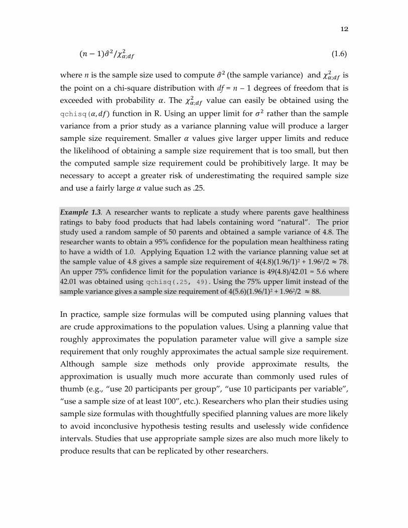
(𝑛 − 1)�̂�2/𝜒𝛼;𝑑𝑓2 (1.6)
where n is the sample size used to compute �̂�2 (the sample variance) and 𝜒𝛼;𝑑𝑓2 is
the point on a chi-square distribution with df = n – 1 degrees of freedom that is
exceeded with probability 𝛼. The 𝜒𝛼;𝑑𝑓2 value can easily be obtained using the
qchisq(𝛼, 𝑑𝑓) function in R. Using an upper limit for 𝜎2 rather than the sample
variance from a prior study as a variance planning value will produce a larger
sample size requirement. Smaller 𝛼 values give larger upper limits and reduce
the likelihood of obtaining a sample size requirement that is too small, but then
the computed sample size requirement could be prohibitively large. It may be
necessary to accept a greater risk of underestimating the required sample size
and use a fairly large 𝛼 value such as .25.
Example 1.3. A researcher wants to replicate a study where parents gave healthiness
ratings to baby food products that had labels containing word “natural”. The prior
study used a random sample of 50 parents and obtained a sample variance of 4.8. The
researcher wants to obtain a 95% confidence for the population mean healthiness rating
to have a width of 1.0. Applying Equation 1.2 with the variance planning value set at
the sample value of 4.8 gives a sample size requirement of 4(4.8)(1.96/1)2 + 1.962/2 ≈ 78.
An upper 75% confidence limit for the population variance is 49(4.8)/42.01 = 5.6 where
42.01 was obtained using qchisq(.25, 49). Using the 75% upper limit instead of the
sample variance gives a sample size requirement of 4(5.6)(1.96/1)2 + 1.962/2 ≈ 88.
In practice, sample size formulas will be computed using planning values that
are crude approximations to the population values. Using a planning value that
roughly approximates the population parameter value will give a sample size
requirement that only roughly approximates the actual sample size requirement.
Although sample size methods only provide approximate results, the
approximation is usually much more accurate than commonly used rules of
thumb (e.g., “use 20 participants per group”, “use 10 participants per variable”,
“use a sample size of at least 100”, etc.). Researchers who plan their studies using
sample size formulas with thoughtfully specified planning values are more likely
to avoid inconclusive hypothesis testing results and uselessly wide confidence
intervals. Studies that use appropriate sample sizes are also much more likely to
produce results that can be replicated by other researchers.
13
Chapter 2
Means
2.1 1-group Designs
A 100(1 − 𝛼)% confidence interval for 𝜇 is
�̂� ± 𝑡𝛼/2;𝑑𝑓√�̂�2/𝑛 (2.1)
where df = n – 1.
A one-sample t-test can be used to determine if H0: 𝜇 = h can be rejected, where h is
a numerical value specified by the researcher. The one-sample t-test uses the
following test statistic
t = (�̂� − ℎ)/ √�̂�2/𝑛. (2.2)
Sample Size for Desired Precision
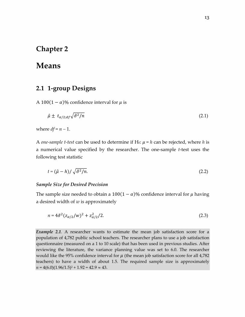
The sample size needed to obtain a 100(1 − 𝛼)% confidence interval for 𝜇 having
a desired width of w is approximately
n = 4�̃�2(𝑧𝛼/2/𝑤)2 + 𝑧𝛼/22 /2. (2.3)
Example 2.1. A researcher wants to estimate the mean job satisfaction score for a
population of 4,782 public school teachers. The researcher plans to use a job satisfaction
questionnaire (measured on a 1 to 10 scale) that has been used in previous studies. After
reviewing the literature, the variance planning value was set to 6.0. The researcher
would like the 95% confidence interval for 𝜇 (the mean job satisfaction score for all 4,782
teachers) to have a width of about 1.5. The required sample size is approximately
n = 4(6.0)(1.96/1.5)2 + 1.92 = 42.9 ≈ 43.
14
Sample Size for Desired Power
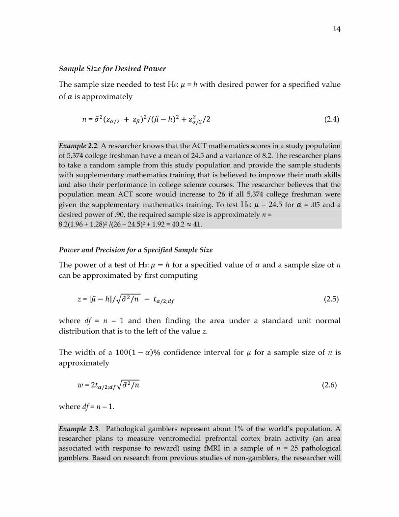
The sample size needed to test H0: 𝜇 = h with desired power for a specified value
of 𝛼 is approximately
n = �̃�2(𝑧𝛼/2 + 𝑧𝛽)2/(�̃� − ℎ)2 + 𝑧𝛼/22 /2 (2.4)
Example 2.2. A researcher knows that the ACT mathematics scores in a study population
of 5,374 college freshman have a mean of 24.5 and a variance of 8.2. The researcher plans
to take a random sample from this study population and provide the sample students
with supplementary mathematics training that is believed to improve their math skills
and also their performance in college science courses. The researcher believes that the
population mean ACT score would increase to 26 if all 5,374 college freshman were
given the supplementary mathematics training. To test H0: 𝜇 = 24.5 for 𝛼 = .05 and a
desired power of .90, the required sample size is approximately n =
8.2(1.96 + 1.28)2 /(26 – 24.5)2 + 1.92 = 40.2 ≈ 41.
Power and Precision for a Specified Sample Size
The power of a test of H0: 𝜇 = ℎ for a specified value of 𝛼 and a sample size of n
can be approximated by first computing
z = |𝜇 − ℎ|/√�̃�2/𝑛 − 𝑡𝛼/2;𝑑𝑓 (2.5)
where df = n – 1 and then finding the area under a standard unit normal
distribution that is to the left of the value z.
The width of a 100(1 − 𝛼)% confidence interval for 𝜇 for a sample size of n is
approximately
w = 2𝑡𝛼/2;𝑑𝑓√�̃�2/𝑛 (2.6)
where df = n – 1.
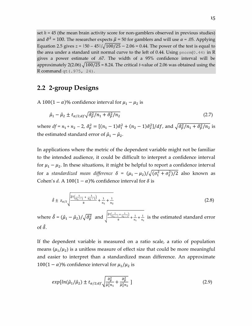
Example 2.3. Pathological gamblers represent about 1% of the world’s population. A
researcher plans to measure ventromedial prefrontal cortex brain activity (an area
associated with response to reward) using fMRI in a sample of n = 25 pathological
gamblers. Based on research from previous studies of non-gamblers, the researcher will
15
set h = 45 (the mean brain activity score for non-gamblers observed in previous studies)
and �̃�2 = 100. The researcher expects 𝜇 = 50 for gamblers and will use 𝛼 = .05. Applying
Equation 2.5 gives z = |50 – 45|/√100/25 − 2.06 = 0.44. The power of the test is equal to
the area under a standard unit normal curve to the left of 0.44. Using pnorm(0.44) in R
gives a power estimate of .67. The width of a 95% confidence interval will be
approximately 2(2.06) √100/25 = 8.24. The critical t-value of 2.06 was obtained using the
R command qt(.975, 24).
2.2 2-group Designs
A 100(1 − 𝛼)% confidence interval for 𝜇1 − 𝜇2 is
�̂�1 − �̂�2 ± 𝑡𝛼/2;𝑑𝑓√�̂�𝑝2/𝑛1 + �̂�𝑝
2/𝑛2 (2.7)
where df = 𝑛1 + 𝑛2 – 2, �̂�𝑝2 = [(𝑛1 − 1)�̂�1
2 + (𝑛2 − 1)�̂�22]/𝑑𝑓, and √�̂�𝑝
2/𝑛1 + �̂�𝑝2/𝑛2 is
the estimated standard error of �̂�1 − �̂�2.
In applications where the metric of the dependent variable might not be familiar
to the intended audience, it could be difficult to interpret a confidence interval
for 𝜇1 − 𝜇2. In these situations, it might be helpful to report a confidence interval
for a standardized mean difference 𝛿 = (𝜇1 − 𝜇2)/√(𝜎12 + 𝜎2
2)/2 also known as
Cohen’s d. A 100(1 − 𝛼)% confidence interval for 𝛿 is
�̂� ± 𝑧𝛼/2√
�̂�2(1
𝑛1 − 1 +
1
𝑛2 − 1)
8+
1
𝑛1+
1
𝑛2 (2.8)
where 𝛿 = (�̂�1 − �̂�2)/√�̂�𝑝2 and √
�̂�2(1
𝑛1 − 1 +
1
𝑛2 − 1)
8+
1
𝑛1+
1
𝑛2 is the estimated standard error
of 𝛿.
If the dependent variable is measured on a ratio scale, a ratio of population
means (𝜇1/𝜇2) is a unitless measure of effect size that could be more meaningful
and easier to interpret than a standardized mean difference. An approximate
100(1 − 𝛼)% confidence interval for 𝜇1/𝜇2 is
𝑒𝑥𝑝 [𝑙𝑛 (�̂�1/�̂�2) ± 𝑡𝛼/2;𝑑𝑓√�̂�𝑝
2
�̂�12𝑛1
+�̂�𝑝
2
�̂�22𝑛2
] (2.9)
16
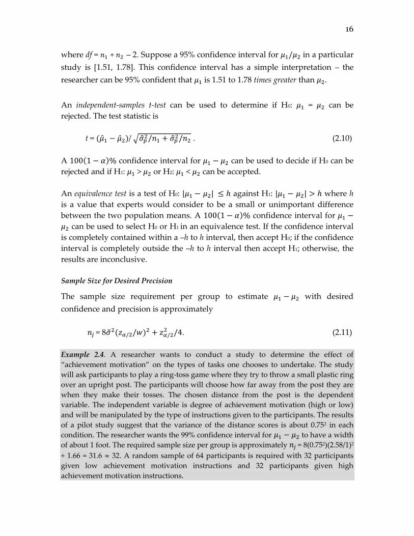
where df = 𝑛1 + 𝑛2 – 2. Suppose a 95% confidence interval for 𝜇1/𝜇2 in a particular
study is [1.51, 1.78]. This confidence interval has a simple interpretation – the
researcher can be 95% confident that 𝜇1 is 1.51 to 1.78 times greater than 𝜇2.
An independent-samples t-test can be used to determine if H0: 𝜇1 = 𝜇2 can be
rejected. The test statistic is
t = (�̂�1 − �̂�2)/ √�̂�𝑝2/𝑛1 + �̂�𝑝
2/𝑛2 . (2.10)
A 100(1 − 𝛼)% confidence interval for 𝜇1 − 𝜇2 can be used to decide if H0 can be
rejected and if H1: 𝜇1 > 𝜇2 or H2: 𝜇1 < 𝜇2 can be accepted.
An equivalence test is a test of H0: |𝜇1 − 𝜇2| ≤ ℎ against H1: |𝜇1 − 𝜇2| > ℎ where h
is a value that experts would consider to be a small or unimportant difference
between the two population means. A 100(1 − 𝛼)% confidence interval for 𝜇1 −
𝜇2 can be used to select H0 or H1 in an equivalence test. If the confidence interval
is completely contained within a –h to h interval, then accept H0; if the confidence
interval is completely outside the –h to h interval then accept H1; otherwise, the
results are inconclusive.
Sample Size for Desired Precision
The sample size requirement per group to estimate 𝜇1 − 𝜇2 with desired
confidence and precision is approximately
𝑛𝑗 = 8�̃�2(𝑧𝛼/2/𝑤)2 + 𝑧𝛼/22 /4. (2.11)
Example 2.4. A researcher wants to conduct a study to determine the effect of
“achievement motivation” on the types of tasks one chooses to undertake. The study
will ask participants to play a ring-toss game where they try to throw a small plastic ring
over an upright post. The participants will choose how far away from the post they are
when they make their tosses. The chosen distance from the post is the dependent
variable. The independent variable is degree of achievement motivation (high or low)
and will be manipulated by the type of instructions given to the participants. The results
of a pilot study suggest that the variance of the distance scores is about 0.752 in each
condition. The researcher wants the 99% confidence interval for 𝜇1 − 𝜇2 to have a width
of about 1 foot. The required sample size per group is approximately 𝑛𝑗 = 8(0.752)(2.58/1)2
+ 1.66 = 31.6 ≈ 32. A random sample of 64 participants is required with 32 participants
given low achievement motivation instructions and 32 participants given high
achievement motivation instructions.
17
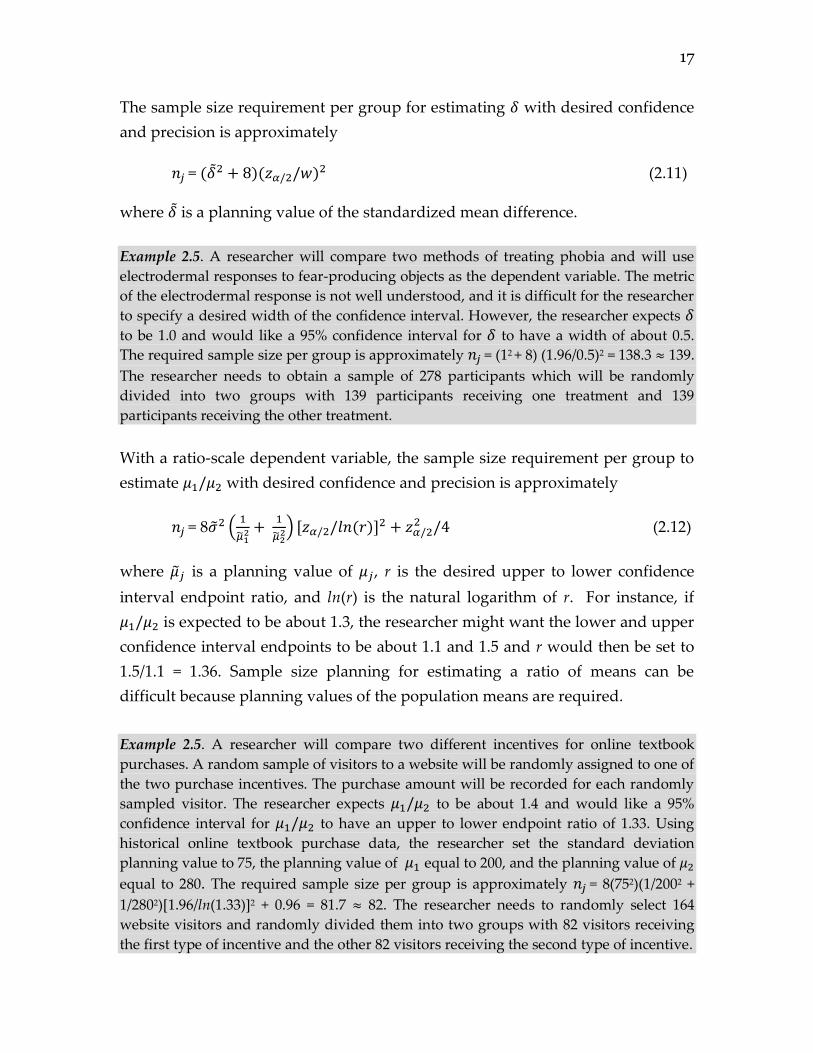
The sample size requirement per group for estimating 𝛿 with desired confidence
and precision is approximately
𝑛𝑗 = (𝛿2 + 8)(𝑧𝛼/2/𝑤)2 (2.11)
where 𝛿 is a planning value of the standardized mean difference.
Example 2.5. A researcher will compare two methods of treating phobia and will use
electrodermal responses to fear-producing objects as the dependent variable. The metric
of the electrodermal response is not well understood, and it is difficult for the researcher
to specify a desired width of the confidence interval. However, the researcher expects 𝛿
to be 1.0 and would like a 95% confidence interval for 𝛿 to have a width of about 0.5.
The required sample size per group is approximately 𝑛𝑗 = (12 + 8) (1.96/0.5)2 = 138.3 ≈ 139.
The researcher needs to obtain a sample of 278 participants which will be randomly
divided into two groups with 139 participants receiving one treatment and 139
participants receiving the other treatment.
With a ratio-scale dependent variable, the sample size requirement per group to
estimate 𝜇1/𝜇2 with desired confidence and precision is approximately
𝑛𝑗 = 8�̃�2 (1
�̃�12 +
1
�̃�22) [𝑧𝛼/2/𝑙𝑛(𝑟)]2 + 𝑧𝛼/2
2 /4 (2.12)
where 𝜇𝑗 is a planning value of 𝜇𝑗, r is the desired upper to lower confidence
interval endpoint ratio, and ln(r) is the natural logarithm of r. For instance, if
𝜇1/𝜇2 is expected to be about 1.3, the researcher might want the lower and upper
confidence interval endpoints to be about 1.1 and 1.5 and r would then be set to
1.5/1.1 = 1.36. Sample size planning for estimating a ratio of means can be
difficult because planning values of the population means are required.
Example 2.5. A researcher will compare two different incentives for online textbook
purchases. A random sample of visitors to a website will be randomly assigned to one of
the two purchase incentives. The purchase amount will be recorded for each randomly
sampled visitor. The researcher expects 𝜇1/𝜇2 to be about 1.4 and would like a 95%
confidence interval for 𝜇1/𝜇2 to have an upper to lower endpoint ratio of 1.33. Using
historical online textbook purchase data, the researcher set the standard deviation
planning value to 75, the planning value of 𝜇1 equal to 200, and the planning value of 𝜇2
equal to 280. The required sample size per group is approximately 𝑛𝑗 = 8(752)(1/2002 +
1/2802)[1.96/ln(1.33)]2 + 0.96 = 81.7 ≈ 82. The researcher needs to randomly select 164
website visitors and randomly divided them into two groups with 82 visitors receiving
the first type of incentive and the other 82 visitors receiving the second type of incentive.
18
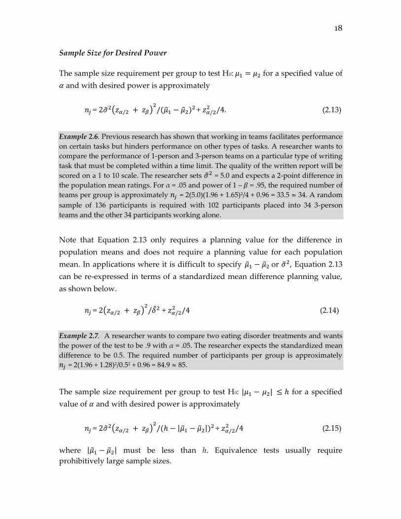
Sample Size for Desired Power
The sample size requirement per group to test H0: 𝜇1 = 𝜇2 for a specified value of
𝛼 and with desired power is approximately
𝑛𝑗 = 2�̃�2(𝑧𝛼/2 + 𝑧𝛽)2
/(𝜇1 − 𝜇2)2 + 𝑧𝛼/22 /4. (2.13)
Example 2.6. Previous research has shown that working in teams facilitates performance
on certain tasks but hinders performance on other types of tasks. A researcher wants to
compare the performance of 1-person and 3-person teams on a particular type of writing
task that must be completed within a time limit. The quality of the written report will be
scored on a 1 to 10 scale. The researcher sets �̃�2 = 5.0 and expects a 2-point difference in
the population mean ratings. For α = .05 and power of 1 – 𝛽 = .95, the required number of
teams per group is approximately 𝑛𝑗 = 2(5.0)(1.96 + 1.65)2/4 + 0.96 = 33.5 ≈ 34. A random
sample of 136 participants is required with 102 participants placed into 34 3-person
teams and the other 34 participants working alone.
Note that Equation 2.13 only requires a planning value for the difference in
population means and does not require a planning value for each population
mean. In applications where it is difficult to specify 𝜇1 − 𝜇2 or �̃�2, Equation 2.13
can be re-expressed in terms of a standardized mean difference planning value,
as shown below.
𝑛𝑗 = 2(𝑧𝛼/2 + 𝑧𝛽)2
/𝛿2 + 𝑧𝛼/22 /4 (2.14)
Example 2.7. A researcher wants to compare two eating disorder treatments and wants
the power of the test to be .9 with α = .05. The researcher expects the standardized mean
difference to be 0.5. The required number of participants per group is approximately
𝑛𝑗 = 2(1.96 + 1.28)2/0.52 + 0.96 = 84.9 ≈ 85.
The sample size requirement per group to test H0: |𝜇1 − 𝜇2| ≤ ℎ for a specified
value of 𝛼 and with desired power is approximately
𝑛𝑗 = 2�̃�2(𝑧𝛼/2 + 𝑧𝛽)2
/(ℎ − |𝜇1 − 𝜇2|)2 + 𝑧𝛼/22 /4 (2.15)
where |𝜇1 − 𝜇2| must be less than h. Equivalence tests usually require
prohibitively large sample sizes.
19
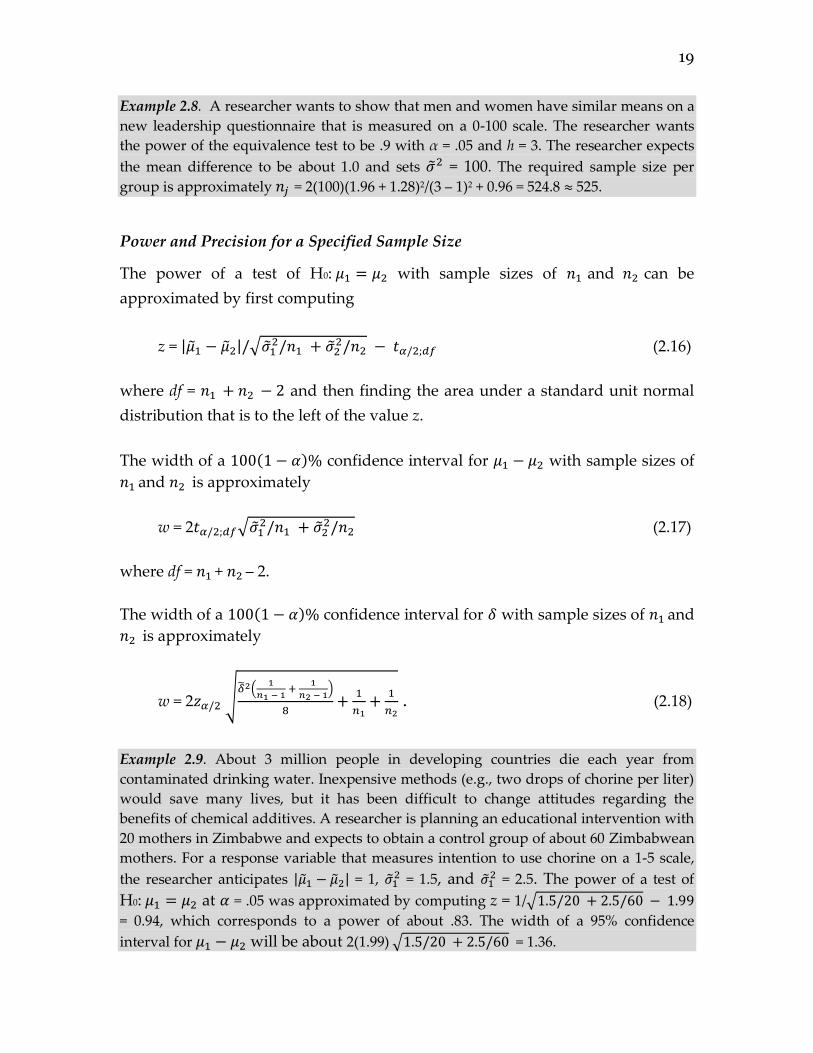
Example 2.8. A researcher wants to show that men and women have similar means on a
new leadership questionnaire that is measured on a 0-100 scale. The researcher wants
the power of the equivalence test to be .9 with α = .05 and h = 3. The researcher expects
the mean difference to be about 1.0 and sets �̃�2 = 100. The required sample size per
group is approximately 𝑛𝑗 = 2(100)(1.96 + 1.28)2/(3 – 1)2 + 0.96 = 524.8 ≈ 525.
Power and Precision for a Specified Sample Size
The power of a test of H0: 𝜇1 = 𝜇2 with sample sizes of 𝑛1 and 𝑛2 can be
approximated by first computing
z = |𝜇1 − 𝜇2|/√�̃�12/𝑛1 + �̃�2
2/𝑛2 − 𝑡𝛼/2;𝑑𝑓 (2.16)
where df = 𝑛1 + 𝑛2 − 2 and then finding the area under a standard unit normal
distribution that is to the left of the value z.
The width of a 100(1 − 𝛼)% confidence interval for 𝜇1 − 𝜇2 with sample sizes of
𝑛1 and 𝑛2 is approximately
w = 2𝑡𝛼/2;𝑑𝑓√�̃�12/𝑛1 + �̃�2
2/𝑛2 (2.17)
where df = 𝑛1 + 𝑛2 – 2.
The width of a 100(1 − 𝛼)% confidence interval for 𝛿 with sample sizes of 𝑛1 and
𝑛2 is approximately
w = 2𝑧𝛼/2 √�̃�2(
1
𝑛1 − 1 +
1
𝑛2 − 1)
8+
1
𝑛1+
1
𝑛2 . (2.18)
Example 2.9. About 3 million people in developing countries die each year from
contaminated drinking water. Inexpensive methods (e.g., two drops of chorine per liter)
would save many lives, but it has been difficult to change attitudes regarding the
benefits of chemical additives. A researcher is planning an educational intervention with
20 mothers in Zimbabwe and expects to obtain a control group of about 60 Zimbabwean
mothers. For a response variable that measures intention to use chorine on a 1-5 scale,
the researcher anticipates |�̃�1 − �̃�2| = 1, �̃�12 = 1.5, and �̃�1
2 = 2.5. The power of a test of
H0: 𝜇1 = 𝜇2 at 𝛼 = .05 was approximated by computing z = 1/√1.5/20 + 2.5/60 − 1.99
= 0.94, which corresponds to a power of about .83. The width of a 95% confidence
interval for 𝜇1 − 𝜇2 will be about 2(1.99) √1.5/20 + 2.5/60 = 1.36.
20
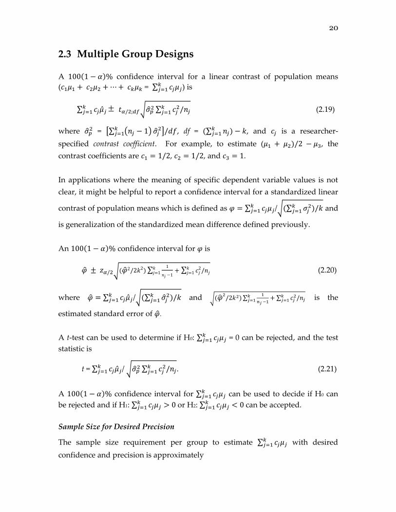
2.3 Multiple Group Designs
A 100(1 − 𝛼)% confidence interval for a linear contrast of population means
(𝑐1𝜇1 + 𝑐2𝜇2 + ⋯ + 𝑐𝑘𝜇𝑘 = ∑ 𝑐𝑗𝜇𝑗𝑘𝑗=1 ) is
∑ 𝑐𝑗�̂�𝑗𝑘𝑗=1 𝑡𝛼/2;𝑑𝑓√�̂�𝑝
2 ∑ 𝑐𝑗2/𝑛𝑗
𝑘𝑗=1 (2.19)
where �̂�𝑝2 = [∑ (𝑛𝑗 − 1)𝑘
𝑗=1 �̂�𝑗2]/𝑑𝑓, df = (∑ 𝑛𝑗) − 𝑘𝑘
𝑗=1 , and 𝑐𝑗 is a researcher-
specified contrast coefficient. For example, to estimate (𝜇1 + 𝜇2)/2 − 𝜇3, the
contrast coefficients are 𝑐1 = 1/2, 𝑐2 = 1/2, and 𝑐3 = 1.
In applications where the meaning of specific dependent variable values is not
clear, it might be helpful to report a confidence interval for a standardized linear
contrast of population means which is defined as 𝜑 = ∑ 𝑐𝑗𝜇𝑗𝑘𝑗=1 /√(∑ 𝜎𝑗
2𝑘𝑗=1 )/𝑘 and
is generalization of the standardized mean difference defined previously.
An 100(1 − 𝛼)% confidence interval for 𝜑 is
�̂� ± 𝑧𝛼/2√(�̂�2/2𝑘2) ∑1
𝑛𝑗 −1+ ∑ 𝑐𝑗
2/𝑛𝑗𝑘𝑗=1
𝑘𝑗=1 (2.20)
where �̂� = ∑ 𝑐𝑗�̂�𝑗𝑘𝑗=1 /√(∑ �̂�𝑗
2𝑘𝑗=1 )/𝑘 and √(�̂�2
/2𝑘2) ∑1
𝑛𝑗 −1+ ∑ 𝑐𝑗
2/𝑛𝑗𝑘𝑗=1
𝑘𝑗=1 is the
estimated standard error of �̂�.
A t-test can be used to determine if H0: ∑ 𝑐𝑗𝜇𝑗𝑘𝑗=1 = 0 can be rejected, and the test
statistic is
t = ∑ 𝑐𝑗�̂�𝑗𝑘𝑗=1 / √�̂�𝑝
2 ∑ 𝑐𝑗2/𝑛𝑗
𝑘𝑗=1 . (2.21)
A 100(1 − 𝛼)% confidence interval for ∑ 𝑐𝑗𝜇𝑗𝑘𝑗=1 can be used to decide if H0 can
be rejected and if H1: ∑ 𝑐𝑗𝜇𝑗𝑘𝑗=1 > 0 or H2: ∑ 𝑐𝑗𝜇𝑗
𝑘𝑗=1 < 0 can be accepted.
Sample Size for Desired Precision
The sample size requirement per group to estimate ∑ 𝑐𝑗𝜇𝑗𝑘𝑗=1 with desired
confidence and precision is approximately
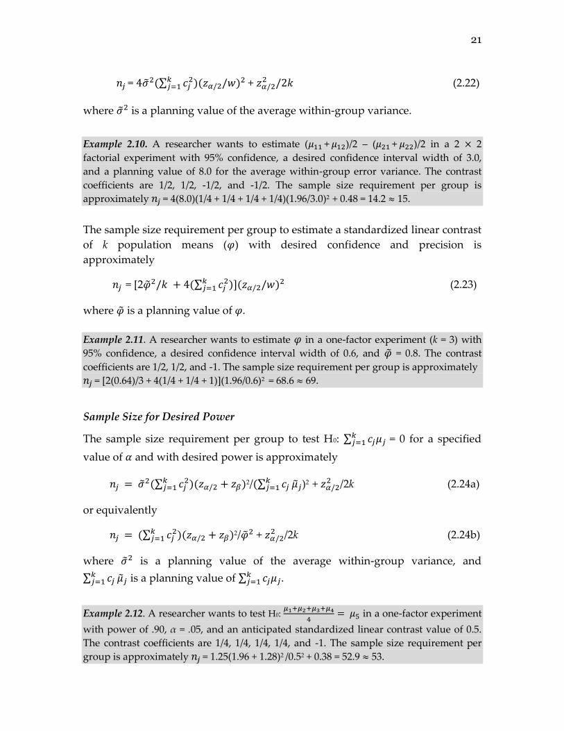
21
𝑛𝑗 = 4�̃�2(∑ 𝑐𝑗2)(𝑧𝛼/2/𝑤)2𝑘
𝑗=1 + 𝑧𝛼/22 /2𝑘 (2.22)
where �̃�2 is a planning value of the average within-group variance.
Example 2.10. A researcher wants to estimate (𝜇11 + 𝜇12)/2 – (𝜇21 + 𝜇22)/2 in a 2 × 2
factorial experiment with 95% confidence, a desired confidence interval width of 3.0,
and a planning value of 8.0 for the average within-group error variance. The contrast
coefficients are 1/2, 1/2, -1/2, and -1/2. The sample size requirement per group is
approximately 𝑛𝑗 = 4(8.0)(1/4 + 1/4 + 1/4 + 1/4)(1.96/3.0)2 + 0.48 = 14.2 ≈ 15.
The sample size requirement per group to estimate a standardized linear contrast
of k population means (𝜑) with desired confidence and precision is
approximately
𝑛𝑗 = [2�̃�2/𝑘 + 4(∑ 𝑐𝑗2)](𝑧𝛼/2/𝑤)2𝑘
𝑗=1 (2.23)
where �̃� is a planning value of 𝜑.
Example 2.11. A researcher wants to estimate 𝜑 in a one-factor experiment (k = 3) with
95% confidence, a desired confidence interval width of 0.6, and �̃� = 0.8. The contrast
coefficients are 1/2, 1/2, and -1. The sample size requirement per group is approximately
𝑛𝑗 = [2(0.64)/3 + 4(1/4 + 1/4 + 1)](1.96/0.6)2 = 68.6 ≈ 69.
Sample Size for Desired Power
The sample size requirement per group to test H0: ∑ 𝑐𝑗𝜇𝑗 𝑘𝑗=1 = 0 for a specified
value of 𝛼 and with desired power is approximately
𝑛𝑗 = �̃�2(∑ 𝑐𝑗2)(𝑧𝛼/2
𝑘𝑗=1 + 𝑧𝛽)2/(∑ 𝑐𝑗
𝑘𝑗=1 𝜇𝑗)2 + 𝑧𝛼/2
2 /2k (2.24a)
or equivalently
𝑛𝑗 = (∑ 𝑐𝑗2)(𝑧𝛼/2
𝑘𝑗=1 + 𝑧𝛽)2/�̃�2 + 𝑧𝛼/2
2 /2k (2.24b)
where �̃�2 is a planning value of the average within-group variance, and
∑ 𝑐𝑗𝑘𝑗=1 𝜇𝑗 is a planning value of ∑ 𝑐𝑗𝜇𝑗
𝑘𝑗=1 .
Example 2.12. A researcher wants to test H0: 𝜇1+𝜇2+𝜇3+𝜇4
4= 𝜇5 in a one-factor experiment
with power of .90, α = .05, and an anticipated standardized linear contrast value of 0.5.
The contrast coefficients are 1/4, 1/4, 1/4, 1/4, and -1. The sample size requirement per
group is approximately 𝑛𝑗 = 1.25(1.96 + 1.28)2 /0.52 + 0.38 = 52.9 ≈ 53.
22
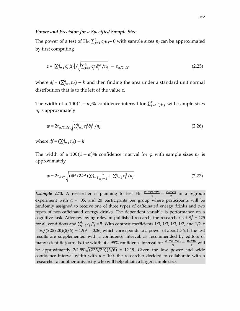
Power and Precision for a Specified Sample Size
The power of a test of H0: ∑ 𝑐𝑗𝜇𝑗𝑘𝑗=1 = 0 with sample sizes 𝑛𝑗 can be approximated
by first computing
z = |∑ 𝑐𝑗𝑘𝑗=1 𝜇𝑗|/√∑ 𝑐𝑗
2�̃�𝑗2𝑘
𝑗=1 /𝑛𝑗 − 𝑡𝛼/2;𝑑𝑓 (2.25)
where df = (∑ 𝑛𝑗) − 𝑘𝑘𝑗=1 and then finding the area under a standard unit normal
distribution that is to the left of the value z.
The width of a 100(1 − 𝛼)% confidence interval for ∑ 𝑐𝑗𝜇𝑗𝑘𝑗=1 with sample sizes
𝑛𝑗 is approximately
w = 2𝑡𝛼/2;𝑑𝑓√∑ 𝑐𝑗2�̃�𝑗
2𝑘𝑗=1 /𝑛𝑗 (2.26)
where df = (∑ 𝑛𝑗) − 𝑘𝑘𝑗=1 .
The width of a 100(1 − 𝛼)% confidence interval for 𝜑 with sample sizes 𝑛𝑗 is
approximately
w = 2𝑧𝛼/2√(�̃�2/2𝑘2) ∑1
𝑛𝑗−1+ ∑ 𝑐𝑗
2/𝑛𝑗𝑘𝑗=1
𝑘𝑗=1 (2.27)
Example 2.13. A researcher is planning to test H0: 𝜇1+𝜇2+𝜇3
3=
𝜇4+𝜇5
2 in a 5-group
experiment with 𝛼 = .05, and 20 participants per group where participants will be
randomly assigned to receive one of three types of caffeinated energy drinks and two
types of non-caffeinated energy drinks. The dependent variable is performance on a
cognitive task. After reviewing relevant published research, the researcher set �̃�𝑗2 = 225
for all conditions and ∑ 𝑐𝑗𝑘𝑗=1 �̃�𝑗 = 5. With contrast coefficients 1/3, 1/3, 1/3, 1/2, and 1/2, z
= 5/√(225/20)(5/6) − 1.99 = -0.36, which corresponds to a power of about .36. If the test
results are supplemented with a confidence interval, as recommended by editors of
many scientific journals, the width of a 95% confidence interval for 𝜇1+𝜇2+𝜇3
3−
𝜇4+𝜇5
2 will
be approximately 2(1.99)√(225/20)(5/6) = 12.19. Given the low power and wide
confidence interval width with n = 100, the researcher decided to collaborate with a
researcher at another university who will help obtain a larger sample size.
23
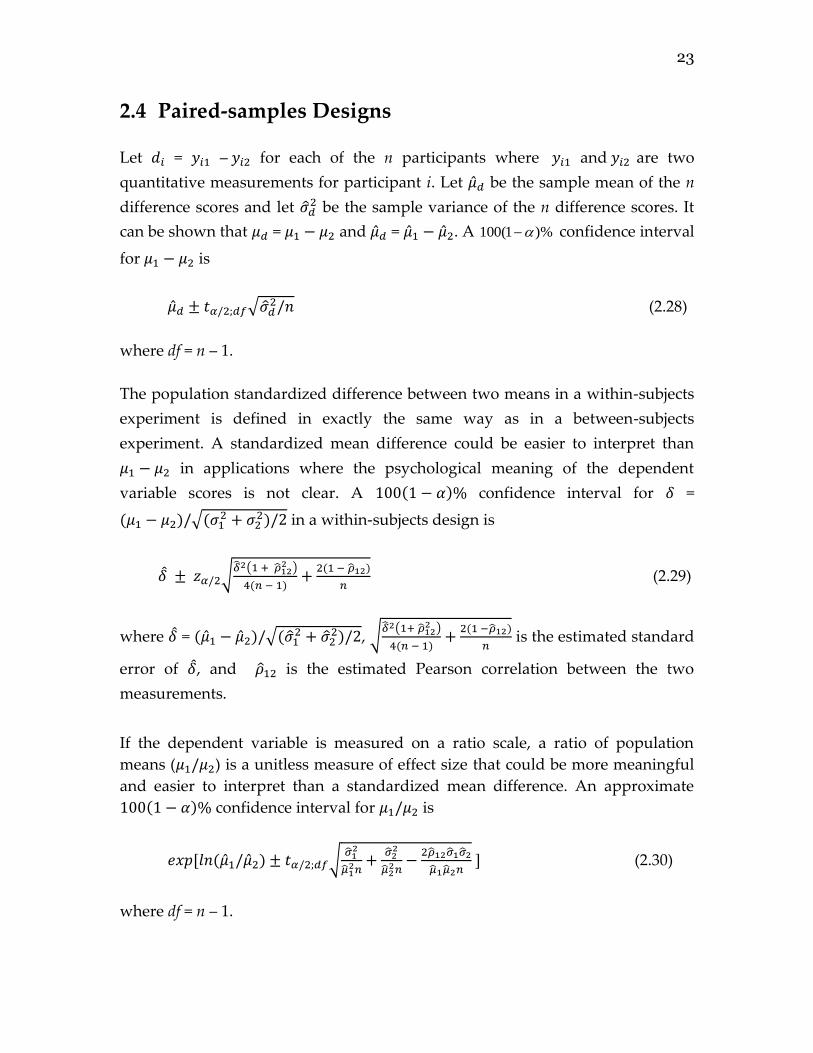
2.4 Paired-samples Designs
Let 𝑑𝑖 = 𝑦𝑖1 – 𝑦𝑖2 for each of the n participants where 𝑦𝑖1 and 𝑦𝑖2 are two
quantitative measurements for participant i. Let �̂�𝑑 be the sample mean of the n
difference scores and let �̂�𝑑2 be the sample variance of the n difference scores. It
can be shown that 𝜇𝑑 = 𝜇1 − 𝜇2 and �̂�𝑑 = �̂�1 − �̂�2. A )%1(100 confidence interval
for 𝜇1 − 𝜇2 is
�̂�𝑑 ± 𝑡𝛼/2;𝑑𝑓√�̂�𝑑2/𝑛 (2.28)
where df = n – 1.
The population standardized difference between two means in a within-subjects
experiment is defined in exactly the same way as in a between-subjects
experiment. A standardized mean difference could be easier to interpret than
𝜇1 − 𝜇2 in applications where the psychological meaning of the dependent
variable scores is not clear. A 100(1 − 𝛼)% confidence interval for 𝛿 =
(𝜇1 − 𝜇2)/√(𝜎12 + 𝜎2
2)/2 in a within-subjects design is
𝛿 ± 𝑧𝛼/2√�̂�2(1 + �̂�12
2 )
4(𝑛 − 1)+
2(1 − �̂�12)
𝑛 (2.29)
where 𝛿 = (�̂�1 − �̂�2)/√(�̂�12 + �̂�2
2)/2, √�̂�2(1+ �̂�12
2 )
4(𝑛 − 1)+
2(1 −�̂�12)
𝑛 is the estimated standard
error of 𝛿, and �̂�12 is the estimated Pearson correlation between the two
measurements.
If the dependent variable is measured on a ratio scale, a ratio of population
means (𝜇1/𝜇2) is a unitless measure of effect size that could be more meaningful
and easier to interpret than a standardized mean difference. An approximate
100(1 − 𝛼)% confidence interval for 𝜇1/𝜇2 is
𝑒𝑥𝑝 [𝑙𝑛 (�̂�1/�̂�2) ± 𝑡𝛼/2;𝑑𝑓√�̂�1
2
�̂�12𝑛
+�̂�2
2
�̂�22𝑛
−2�̂�12�̂�1�̂�2
�̂�1�̂�2𝑛 ] (2.30)
where df = n – 1.
24
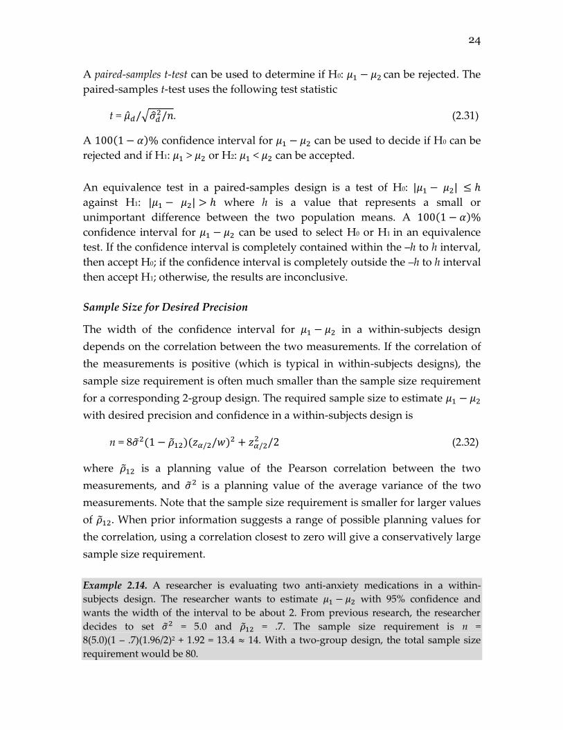
A paired-samples t-test can be used to determine if H0: 𝜇1 − 𝜇2 can be rejected. The
paired-samples t-test uses the following test statistic
t = �̂�𝑑/√�̂�𝑑2/𝑛. (2.31)
A 100(1 − 𝛼)% confidence interval for 𝜇1 − 𝜇2 can be used to decide if H0 can be
rejected and if H1: 𝜇1 > 𝜇2 or H2: 𝜇1 < 𝜇2 can be accepted.
An equivalence test in a paired-samples design is a test of H0: |𝜇1 − 𝜇2| ≤ ℎ
against H1: |𝜇1 − 𝜇2| > ℎ where h is a value that represents a small or
unimportant difference between the two population means. A 100(1 − 𝛼)%
confidence interval for 𝜇1 − 𝜇2 can be used to select H0 or H1 in an equivalence
test. If the confidence interval is completely contained within the –h to h interval,
then accept H0; if the confidence interval is completely outside the –h to h interval
then accept H1; otherwise, the results are inconclusive.
Sample Size for Desired Precision
The width of the confidence interval for 𝜇1 − 𝜇2 in a within-subjects design
depends on the correlation between the two measurements. If the correlation of
the measurements is positive (which is typical in within-subjects designs), the
sample size requirement is often much smaller than the sample size requirement
for a corresponding 2-group design. The required sample size to estimate 𝜇1 − 𝜇2
with desired precision and confidence in a within-subjects design is
n = 8�̃�2(1 − �̃�12)(𝑧𝛼/2/𝑤)2 + 𝑧𝛼/22 /2 (2.32)
where �̃�12 is a planning value of the Pearson correlation between the two
measurements, and �̃�2 is a planning value of the average variance of the two
measurements. Note that the sample size requirement is smaller for larger values
of �̃�12. When prior information suggests a range of possible planning values for
the correlation, using a correlation closest to zero will give a conservatively large
sample size requirement.
Example 2.14. A researcher is evaluating two anti-anxiety medications in a within-
subjects design. The researcher wants to estimate 𝜇1 − 𝜇2 with 95% confidence and
wants the width of the interval to be about 2. From previous research, the researcher
decides to set �̃�2 = 5.0 and �̃�12 = .7. The sample size requirement is n =
8(5.0)(1 – .7)(1.96/2)2 + 1.92 = 13.4 ≈ 14. With a two-group design, the total sample size
requirement would be 80.
25
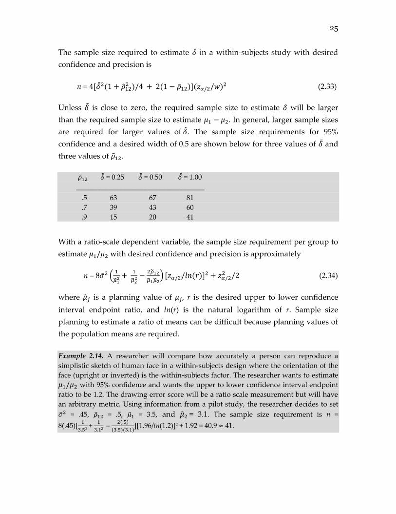
The sample size required to estimate 𝛿 in a within-subjects study with desired
confidence and precision is
n = 4[𝛿2(1 + �̃�122 )/4 + 2(1 − �̃�12)](𝑧𝛼/2/𝑤)2 (2.33)
Unless 𝛿 is close to zero, the required sample size to estimate 𝛿 will be larger
than the required sample size to estimate 𝜇1 − 𝜇2. In general, larger sample sizes
are required for larger values of 𝛿. The sample size requirements for 95%
confidence and a desired width of 0.5 are shown below for three values of 𝛿 and
three values of �̃�12.
�̃�12 𝛿 = 0.25 𝛿 = 0.50 𝛿 = 1.00
____________________________________
.5 63 67 81
.7 39 43 60
.9 15 20 41
With a ratio-scale dependent variable, the sample size requirement per group to
estimate 𝜇1/𝜇2 with desired confidence and precision is approximately
n = 8�̃�2 (1
�̃�12 +
1
�̃�22 −
2�̃�12
�̃�1�̃�2) [𝑧𝛼/2/𝑙𝑛(𝑟)]2 + 𝑧𝛼/2
2 /2 (2.34)
where 𝜇𝑗 is a planning value of 𝜇𝑗, r is the desired upper to lower confidence
interval endpoint ratio, and ln(r) is the natural logarithm of r. Sample size
planning to estimate a ratio of means can be difficult because planning values of
the population means are required.
Example 2.14. A researcher will compare how accurately a person can reproduce a
simplistic sketch of human face in a within-subjects design where the orientation of the
face (upright or inverted) is the within-subjects factor. The researcher wants to estimate
𝜇1/𝜇2 with 95% confidence and wants the upper to lower confidence interval endpoint
ratio to be 1.2. The drawing error score will be a ratio scale measurement but will have
an arbitrary metric. Using information from a pilot study, the researcher decides to set
�̃�2 = .45, �̃�12 = .5, �̃�1 = 3.5, and 𝜇2 = 3.1. The sample size requirement is n =
8(.45)[1
3.52 +
1
3.12 –
2(.5)
(3.5)(3.1)][1.96/ln(1.2)]2 + 1.92 = 40.9 ≈ 41.
26
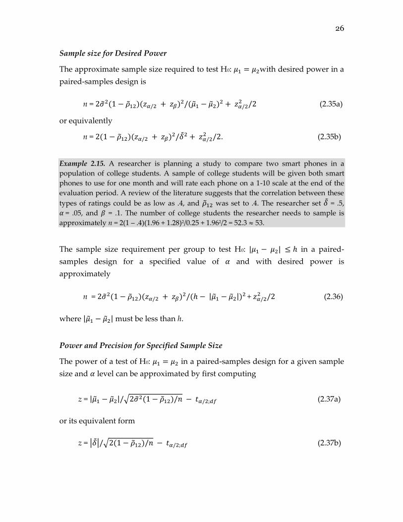
Sample size for Desired Power
The approximate sample size required to test H0: 𝜇1 = 𝜇2with desired power in a
paired-samples design is
n = 2�̃�2(1 − �̃�12)(𝑧𝛼/2 + 𝑧𝛽)2/(�̃�1 − 𝜇2)2 + 𝑧𝛼/22 /2 (2.35a)
or equivalently
n = 2(1 − �̃�12)(𝑧𝛼/2 + 𝑧𝛽)2/𝛿2 + 𝑧𝛼/22 /2. (2.35b)
Example 2.15. A researcher is planning a study to compare two smart phones in a
population of college students. A sample of college students will be given both smart
phones to use for one month and will rate each phone on a 1-10 scale at the end of the
evaluation period. A review of the literature suggests that the correlation between these
types of ratings could be as low as .4, and �̃�12 was set to .4. The researcher set 𝛿 = .5,
𝛼 = .05, and 𝛽 = .1. The number of college students the researcher needs to sample is
approximately n = 2(1 – .4)(1.96 + 1.28)2/0.25 + 1.962/2 = 52.3 ≈ 53.
The sample size requirement per group to test H0: |𝜇1 − 𝜇2| ≤ ℎ in a paired-
samples design for a specified value of 𝛼 and with desired power is
approximately
n = 2�̃�2(1 − �̃�12)(𝑧𝛼/2 + 𝑧𝛽)2/(ℎ − |𝜇1 − 𝜇2|)2 + 𝑧𝛼/22 /2 (2.36)
where |𝜇1 − 𝜇2| must be less than h.
Power and Precision for Specified Sample Size
The power of a test of H0: 𝜇1 = 𝜇2 in a paired-samples design for a given sample
size and 𝛼 level can be approximated by first computing
z = |𝜇1 − 𝜇2|/√2�̃�2(1 − �̃�12)/𝑛 − 𝑡𝛼/2;𝑑𝑓 (2.37a)
or its equivalent form
z = |𝛿|/√2(1 − �̃�12)/𝑛 − 𝑡𝛼/2;𝑑𝑓 (2.37b)
27
where df = n – 1 and then finding the area under a standard unit normal
distribution that is to the left of the value z.
The width of a 100(1 − 𝛼)% confidence interval for 𝜇1 − 𝜇2 in a paired-sample
design with a sample size of n is approximately
w = 2𝑡𝛼/2;𝑑𝑓√2�̃�2(1 − �̃�12)/𝑛 (2.38)
where df = n – 1.
The width of a 100(1 − 𝛼)% confidence interval for 𝛿 in a paired-samples design
with sample size of n is approximately
w = 2𝑧𝛼/2 √�̃�2(1 + �̃�12
2 )
4(𝑛 − 1)+
2(1 − �̃�12)
𝑛 . (2.39)
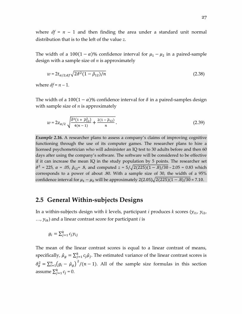
Example 2.16. A researcher plans to assess a company’s claims of improving cognitive
functioning through the use of its computer games. The researcher plans to hire a
licensed psychometrician who will administer an IQ test to 30 adults before and then 60
days after using the company’s software. The software will be considered to be effective
if it can increase the mean IQ in the study population by 5 points. The researcher set
�̃�2 = 225, 𝛼 = .05, �̃�12= .8, and computed z = 5/√2(225)(1 − .8)/30 – 2.05 = 0.83 which
corresponds to a power of about .80. With a sample size of 30, the width of a 95%
confidence interval for 𝜇1 − 𝜇2 will be approximately 2(2.05)√2(225)(1 − .8)/30 = 7.10.
2.5 General Within-subjects Designs
In a within-subjects design with k levels, participant i produces k scores (𝑦𝑖1, 𝑦𝑖2,
…, 𝑦𝑖𝑘) and a linear contrast score for participant i is
𝑔𝑖 = ∑ 𝑐𝑗𝑦𝑖𝑗𝑘𝑗=1
The mean of the linear contrast scores is equal to a linear contrast of means,
specifically, �̂�𝑔 = ∑ 𝑐𝑗�̂�𝑗𝑘𝑗=1 . The estimated variance of the linear contrast scores is
�̂�𝑔2 = ∑ (𝑔𝑖 − �̂�𝑔)
2/(𝑛 − 1)𝑛
𝑖=1 . All of the sample size formulas in this section
assume ∑ 𝑐𝑗𝑘𝑗=1 = 0.
28
A 100(1 − 𝛼)% confidence interval for ∑ 𝑐𝑗𝜇𝑗𝑘𝑗=1 is
�̂�𝑔 ± 𝑡𝛼/2;𝑑𝑓√�̂�𝑔2/𝑛 (2.40)
where df = n – 1.
In applications where the psychological meaning of the dependent variable
scores is not clear, it might be helpful to report a confidence interval for the
following standardized linear contrast of population means
𝜑 = ∑ 𝑐𝑗𝜇𝑗𝑘𝑗=1 /√(∑ 𝜎𝑗
2𝑘𝑗=1 )/𝑘 (2.41)
which is a generalization of the population standardized mean difference. A
)%1(100 confidence interval for 𝜑 is
�̂� ± 𝑧𝛼/2√�̂�2[1 + (𝑘 − 1)�̂�2]
2𝑘(𝑛 − 1)+
(1 − �̂� ) ∑ 𝑐𝑗2𝑘
𝑗=1
𝑛 (2.42)
where �̂� = ∑ 𝑐𝑗�̂�𝑗𝑘𝑗=1 /√(∑ �̂�𝑗
2𝑘𝑗=1 )/𝑘 , and �̂� is the average of the sample
correlations for the k(k – 1)/2 pairs of measurements.
A t-test can be used to determine if H0: ∑ 𝑐𝑗𝜇𝑗𝑘𝑗=1 = 0 can be rejected. The t-test
uses the following test statistic
t = �̂�𝑔/√�̂�𝑔2/𝑛. (2.43)
Sample size for Desired Precision
The approximate sample size requirement to estimate ∑ 𝑐𝑗𝜇𝑗𝑘𝑗=1 with desired
confidence and precision in a within-subjects study is
n = 4�̃�2(∑ 𝑐𝑗2𝑘
𝑗=1 )(1 − �̃�)(𝑧𝛼/2/𝑤)2 + 𝑧𝛼/22 /2 (2.44)
where �̃�2 is a planning value of the largest within-treatment variance, and �̃� is a
planning value of the smallest correlation among all pairs of measurements.
29
Example 2.17. A researcher wants to replicate a study that compared four drugs in a
sample of n = 6 patients using a larger sample size with the goal of achieving a 95%
confidence interval for (𝜇1 + 𝜇2)/2 – (𝜇3 + 𝜇4)/2 that has a width of about 1.5. Using the
sample variances and correlations from the original study as planning values, the largest
sample variance was for Drug 2 (161.9) and the smallest sample correlation was between
Drugs 2 and 4 (0.977). The required number of patients is approximately n =
4(161.9)(1)(1 – 0.977)(1.96/1.5)2 + 1.92 = 26.4 ≈ 27.
The approximate sample size required to estimate 𝜑 with desired confidence and
precision in a within-subjects study is
n = 4[ �̃�2[1 + (𝑘 − 1)�̃�2]
2𝑘+ (1 − �̃�) ∑ 𝑐𝑘
𝑗=1 𝑗
2](𝑧𝛼/2 /𝑤)2 (2.45)
where �̃� is a planning value for 𝜑 and �̃� is a planning value for the smallest
correlation among all pairs of measurements.
Example 2.18. A researcher wants to estimate 𝜑 in a 4-level within-subject experiment
with 95% confidence and contrast coefficients 1/3, 1/3, 1/3, and -1. After reviewing
previous research, the researcher decides to set �̃� = 0.5, �̃� = 0.7, and w = 0.4. The required
sample size is approximately n = 4[0.25{1 + 3(0.49)}/8 + 0.3(1.33)](1.96/0.4)2 = 45.8 ≈ 46.
Sample Size for Desired Power
The approximate sample size required to test H0: ∑ 𝑐𝑗𝑘𝑗=1 𝜇𝑗 = 0 with desired
power in a within-subjects design is
n = �̃�2(∑ 𝑐𝑗2𝑘
𝑗=1 )(1 − �̃�)(𝑧𝛼/2 + 𝑧𝛽)2/(∑ 𝑐𝑗𝜇𝑗)𝑘𝑗=1
2+ 𝑧𝛼/2
2 /2 (2.46a)
or equivalently
n = (∑ 𝑐𝑗2𝑘
𝑗=1 )(1 − �̃�)(𝑧𝛼/2 + 𝑧𝛽)2/�̃�2 + 𝑧𝛼/22 /2 (2.46b)
where �̃�2 is a planning value for the largest variance of the k measurements, and
�̃� is a planning value for the smallest correlation among the k(k – 1) pairs of
measurements.
30
Example 2.19. A researcher is planning a 2 × 2 within-subjects experiment and wants to
test the two-way interaction effect (𝜇1 − 𝜇2 − 𝜇3 + 𝜇4) with power of .95 at α = .05. After
conducting a pilot study and reviewing previous research, the researcher decided to set
�̃�2 = 15 and �̃� = 0.8. The contrast coefficients are 1, -1, -1, and 1. The expected size of the
interaction contrast is 3.0. The required sample size is approximately n =
15(4)(1 – 0.8)(1.96 + 1.65)2/3.02 + 1.92 = 21.2 ≈ 22.
Power and Precision for Specified Sample Size
The power of a test of H0: ∑ 𝑐𝑗𝜇𝑗 𝑘𝑗=1 = 0 for a given sample size and 𝛼 level can be
approximated by first computing
z = |∑ 𝑐𝑗𝑘𝑗=1 𝜇𝑗|/√�̃�2(1 − �̃�) ∑ 𝑐𝑗
2𝑘𝑗=1 /𝑛 − 𝑡𝛼/2;𝑑𝑓 (2.47a)
or its equivalent form
z = |�̃�|/√(1 − �̃�) ∑ 𝑐𝑗2𝑘
𝑗=1 /𝑛 − 𝑡𝛼/2;𝑑𝑓 (2.47b)
where df = n – 1 and then finding the area under a standard unit normal
distribution that is to the left of the value z. In Equations 2.47a and 2.47b, �̃�2 is a
planning value for the largest variance of the k measurements, and �̃� is a
planning value for the smallest correlation among the k(k – 1) pairs of
measurements.
The width of a 100(1 − 𝛼)% confidence interval for ∑ 𝑐𝑗𝜇𝑗𝑘𝑗=1 in a within-subjects
design with a sample size of n is approximately
w = 2𝑡𝛼/2;𝑑𝑓√�̃�2(1 − �̃�) ∑ 𝑐𝑗2𝑘
𝑗=1 /𝑛 (2.48)
where df = n – 1. The width of a 100(1 − 𝛼)% confidence interval for 𝜑 in a
within-subjects design with a sample size of n is approximately
w = 2𝑧𝛼/2 √�̃�2[1 + (𝑘 − 1)�̃�2]
2𝑘(𝑛 − 1)+
(1 − �̃� ) ∑ 𝑐𝑗2𝑘
𝑗=1
𝑛 (2.49)
31
Example 2.20. A researcher wants to assess the effect of an over-the-counter probiotic
supplement for patients diagnosed with an anxiety disorder. The proposed study will
use a sample of 7 anxiety patients who will be tested prior to treatment, 2 weeks after
taking one probiotic capsule per day, and then 2 weeks after taking 1 capsule per day
(k = 3). One test of interest is H0: 𝜇1 = (𝜇2 + 𝜇3)/2. The researcher set �̃� = 0.75, �̃� = .8, and 𝛼
= .05 to obtain z = 0.75/√. 2(1.5)/7 – 2.45 = 1.17, which corresponds to a power of about
.88. With a sample of size 7, the width of a 95% confidence interval for 𝜑 will be
approximately 2(1.96)√.5625[1+2(.64)]
36+
.2(1.5)
7 = 1.1.
2.6 Multiple Group Experiments with Covariates
A covariate is a quantitative variable that is related to the dependent variable
within each group. In an experiment with two or more conditions, including q
covariates in the statistical analysis (called an analysis of covariance) will reduce
the within-group (error) variance which in turn will increase the power of tests
and the precision of confidence intervals for linear contrasts of means.
Alternatively, including q covariates to the statistical analysis can reduce the
sample size required to achieve desired power or confidence interval precision.
Sample Size for Desired Precision
The sample size requirement per group to estimate ∑ 𝑐𝑗𝜇𝑗𝑘𝑗=1 with desired
confidence and precision is approximately
𝑛𝑗 = 4�̃�2(1 − �̃�2)(∑ 𝑐𝑗2)(𝑧𝛼/2/𝑤)2𝑘
𝑗=1 + 𝑧𝛼/22 /2k + 𝑞/𝑘 (2.50)
where �̃�2 is a planning value of the average within-group variance and �̃�2 is a
planning value of the within-group squared multiple correlation between the q
covariates and dependent variable. Note that the sample size requirement is
smaller for larger values of �̃�2.
Example 2.21. A researcher wants to estimate (𝜇11 + 𝜇12)/2 – (𝜇21 + 𝜇22)/2 in a 2 × 2
factorial experiment with 95% confidence, a desired confidence interval width of 3.0,
and a planning value of 8.0 for the average within-group error variance. The final exam
in an introductory psychology course is the dependent variable. Prior research suggests
that high school GPA will correlate about .4 with final exam scores. The contrast
coefficients are 1/2, 1/2, -1/2, and -1/2. The sample size requirement per group is
approximately 𝑛𝑗 = 4(1 – .16)(8.0)(1/4 + 1/4 + 1/4 + 1/4)(1.96/3.0)2 + 0.48 + 1/4 = 12.2 ≈ 13.
32
Sample Size for Desired Power
The sample size requirement per group to test H0: ∑ 𝑐𝑗𝜇𝑗 𝑘𝑗=1 = 0 for a specified
value of 𝛼 and with desired power is approximately
𝑛𝑗 = �̃�2(1 − �̃�2)(∑ 𝑐𝑗2)(𝑧𝛼/2
𝑘𝑗=1 + 𝑧𝛽)2/(∑ 𝑐𝑗
𝑘𝑗=1 𝜇𝑗)2 + 𝑧𝛼/2
2 /2k + q/k (2.51a)
or equivalently
𝑛𝑗 = (1 − �̃�2)(∑ 𝑐𝑗2)(𝑧𝛼/2
𝑘𝑗=1 + 𝑧𝛽)2/�̃�2 + 𝑧𝛼/2
2 /2k + q/k (2.51b)
where �̃�2 is a planning value of the average within-group variance, �̃�2 is a
planning value of the within-group squared multiple correlation between the q
covariates and dependent variable, and ∑ 𝑐𝑗𝑘𝑗=1 𝜇𝑗 is a planning value of ∑ 𝑐𝑗𝜇𝑗
𝑘𝑗=1 .
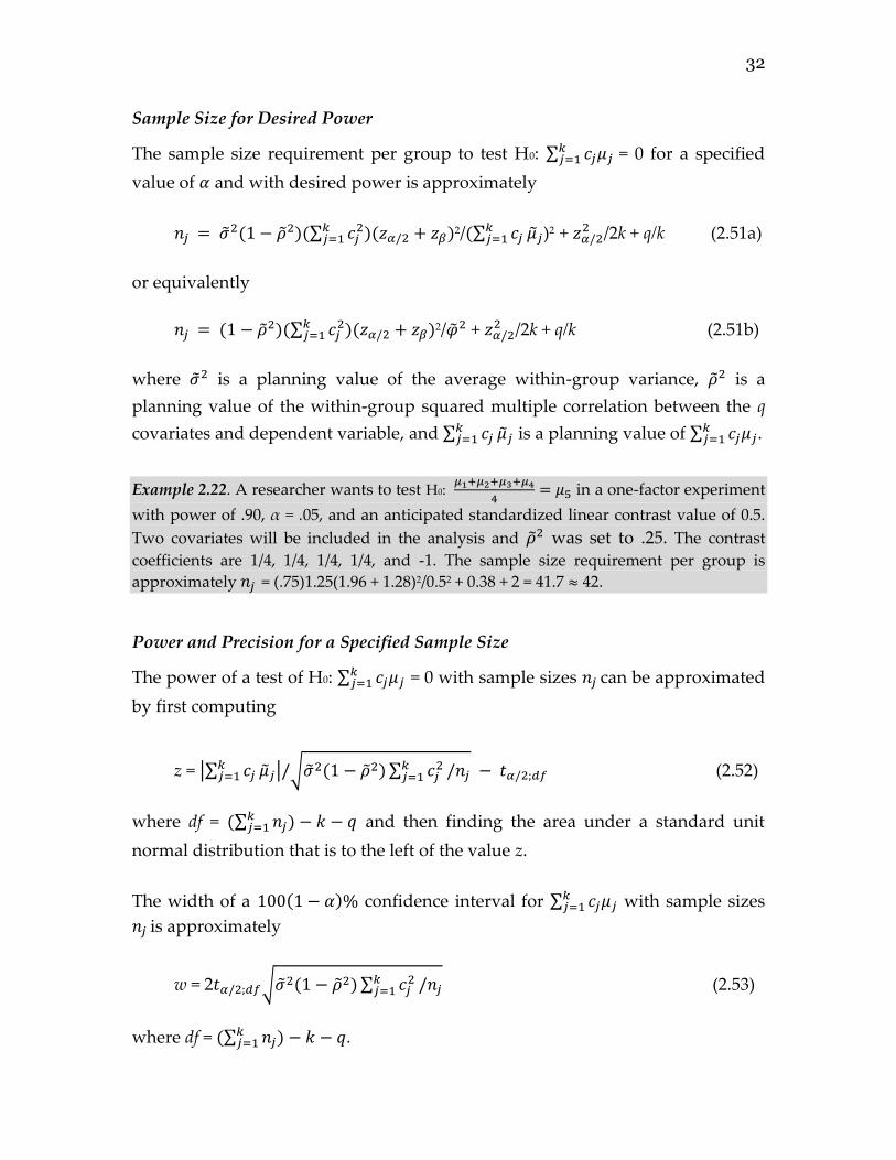
Example 2.22. A researcher wants to test H0: 𝜇1+𝜇2+𝜇3+𝜇4
4= 𝜇5 in a one-factor experiment
with power of .90, α = .05, and an anticipated standardized linear contrast value of 0.5.
Two covariates will be included in the analysis and �̃�2 was set to .25. The contrast
coefficients are 1/4, 1/4, 1/4, 1/4, and -1. The sample size requirement per group is
approximately 𝑛𝑗 = (.75)1.25(1.96 + 1.28)2/0.52 + 0.38 + 2 = 41.7 ≈ 42.
Power and Precision for a Specified Sample Size
The power of a test of H0: ∑ 𝑐𝑗𝜇𝑗 𝑘𝑗=1 = 0 with sample sizes 𝑛𝑗 can be approximated
by first computing
z = |∑ 𝑐𝑗𝑘𝑗=1 𝜇𝑗|/√�̃�2(1 − �̃�2) ∑ 𝑐𝑗
2𝑘𝑗=1 /𝑛𝑗 − 𝑡𝛼/2;𝑑𝑓 (2.52)
where df = (∑ 𝑛𝑗) − 𝑘𝑘𝑗=1 − 𝑞 and then finding the area under a standard unit
normal distribution that is to the left of the value z.
The width of a 100(1 − 𝛼)% confidence interval for ∑ 𝑐𝑗𝜇𝑗𝑘𝑗=1 with sample sizes
𝑛𝑗 is approximately
w = 2𝑡𝛼/2;𝑑𝑓√�̃�2(1 − �̃�2) ∑ 𝑐𝑗2𝑘
𝑗=1 /𝑛𝑗 (2.53)
where df = (∑ 𝑛𝑗) − 𝑘 − 𝑞𝑘𝑗=1 .
33
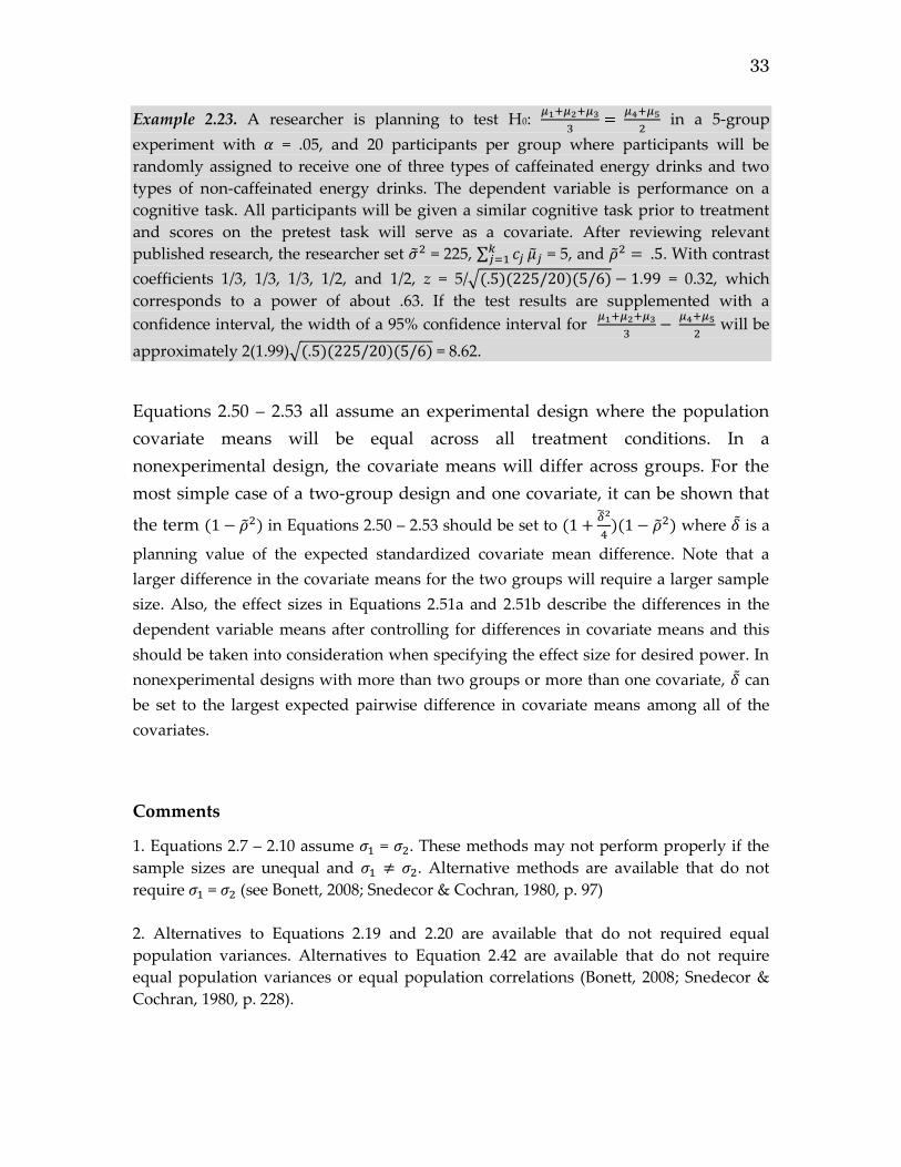
Example 2.23. A researcher is planning to test H0: 𝜇1+𝜇2+𝜇3
3=
𝜇4+𝜇5
2 in a 5-group
experiment with 𝛼 = .05, and 20 participants per group where participants will be
randomly assigned to receive one of three types of caffeinated energy drinks and two
types of non-caffeinated energy drinks. The dependent variable is performance on a
cognitive task. All participants will be given a similar cognitive task prior to treatment
and scores on the pretest task will serve as a covariate. After reviewing relevant
published research, the researcher set �̃�2 = 225, ∑ 𝑐𝑗𝑘𝑗=1 �̃�𝑗 = 5, and �̃�2 = .5. With contrast
coefficients 1/3, 1/3, 1/3, 1/2, and 1/2, z = 5/√(.5)(225/20)(5/6) − 1.99 = 0.32, which
corresponds to a power of about .63. If the test results are supplemented with a
confidence interval, the width of a 95% confidence interval for 𝜇1+𝜇2+𝜇3
3−
𝜇4+𝜇5
2 will be
approximately 2(1.99)√(.5)(225/20)(5/6) = 8.62.
Equations 2.50 – 2.53 all assume an experimental design where the population
covariate means will be equal across all treatment conditions. In a
nonexperimental design, the covariate means will differ across groups. For the
most simple case of a two-group design and one covariate, it can be shown that
the term (1 − �̃�2) in Equations 2.50 – 2.53 should be set to (1 +�̃�2
4)(1 − �̃�2) where 𝛿 is a
planning value of the expected standardized covariate mean difference. Note that a
larger difference in the covariate means for the two groups will require a larger sample
size. Also, the effect sizes in Equations 2.51a and 2.51b describe the differences in the
dependent variable means after controlling for differences in covariate means and this
should be taken into consideration when specifying the effect size for desired power. In
nonexperimental designs with more than two groups or more than one covariate, 𝛿 can
be set to the largest expected pairwise difference in covariate means among all of the
covariates.
Comments
1. Equations 2.7 – 2.10 assume 𝜎1 = 𝜎2. These methods may not perform properly if the
sample sizes are unequal and 𝜎1 ≠ 𝜎2. Alternative methods are available that do not
require 𝜎1 = 𝜎2 (see Bonett, 2008; Snedecor & Cochran, 1980, p. 97)
2. Alternatives to Equations 2.19 and 2.20 are available that do not required equal
population variances. Alternatives to Equation 2.42 are available that do not require
equal population variances or equal population correlations (Bonett, 2008; Snedecor &
Cochran, 1980, p. 228).
34
3. If 𝑛1 ≠ 𝑛2 and �̃�12 ≠ �̃�2
2 in Equations 2.16 or 2.17, the following Satterthwaite df will
give a slightly more accurate result 𝑑𝑓 = (�̂�1
2
𝑛1+
�̂�22
𝑛2)
2
/[�̂�1
4
𝑛12(𝑛1−1)
+�̂�2
4
𝑛22(𝑛2−1)
] but in most
applications, the improvement in accuracy using will be trivial unless the planning
values of the variances are highly unequal and sample sizes are small and highly
unequal.
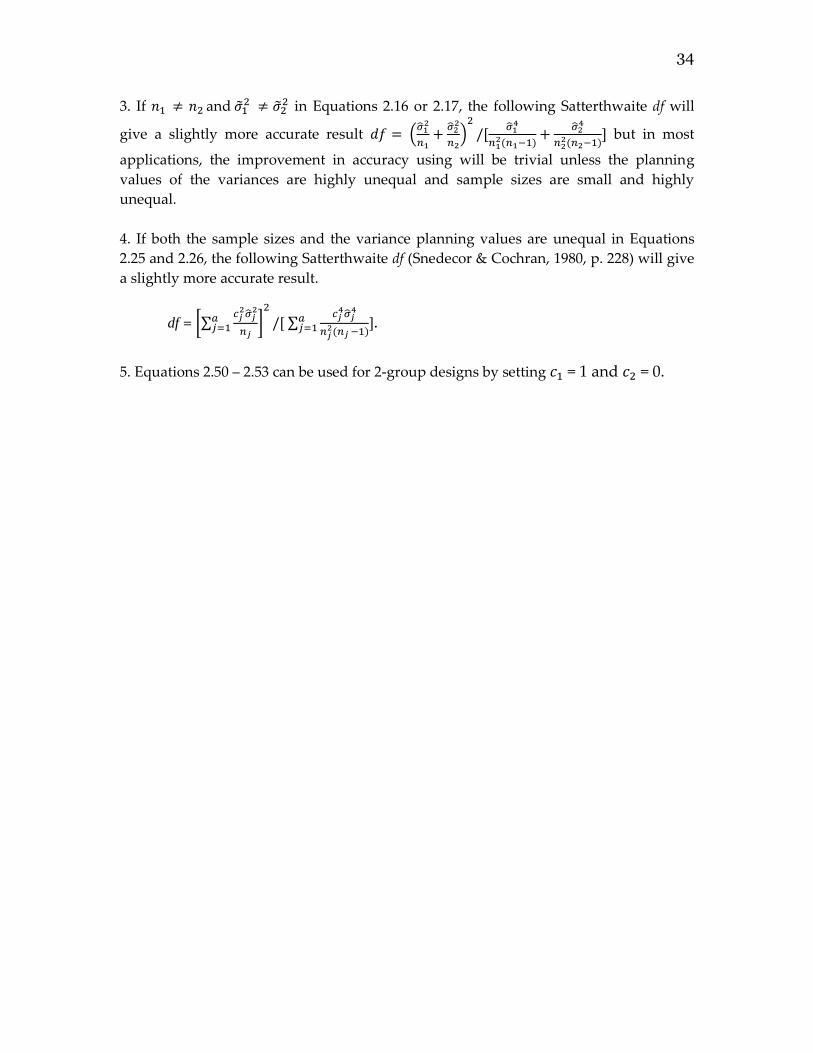
4. If both the sample sizes and the variance planning values are unequal in Equations
2.25 and 2.26, the following Satterthwaite df (Snedecor & Cochran, 1980, p. 228) will give
a slightly more accurate result.
df = [∑𝑐𝑗
2�̂�𝑗2
𝑛𝑗
𝑎𝑗=1 ]
2
/[ ∑𝑐𝑗
4�̂�𝑗4
𝑛𝑗2(𝑛𝑗 −1)
𝑎𝑗=1 ].
5. Equations 2.50 – 2.53 can be used for 2-group designs by setting 𝑐1 = 1 and 𝑐2 = 0.
35
Chapter 3
Proportions
3.1 1-group Designs
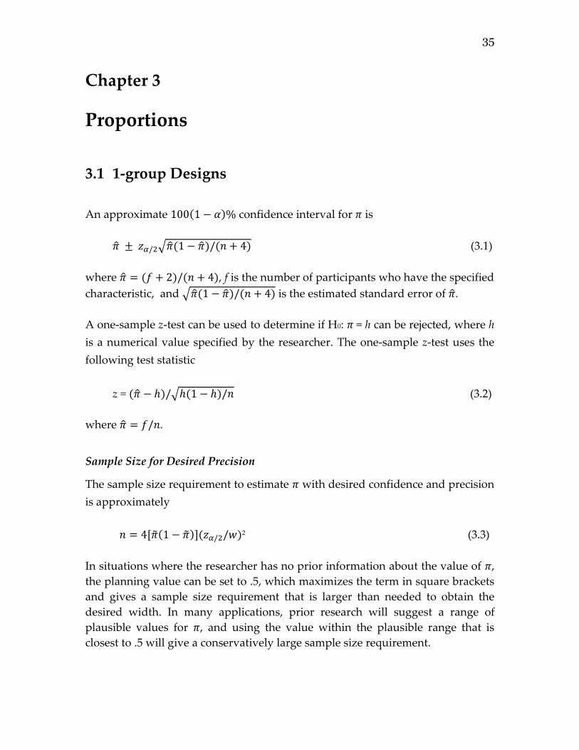
An approximate 100(1 − 𝛼)% confidence interval for 𝜋 is
�̂� ± 𝑧𝛼/2√�̂�(1 − �̂�)/(𝑛 + 4) (3.1)
where �̂� = (𝑓 + 2)/(𝑛 + 4), f is the number of participants who have the specified
characteristic, and √�̂�(1 − �̂�)/(𝑛 + 4) is the estimated standard error of �̂�.
A one-sample z-test can be used to determine if H0: 𝜋 = h can be rejected, where h
is a numerical value specified by the researcher. The one-sample z-test uses the
following test statistic
z = (�̂� − ℎ)/√ℎ(1 − ℎ)/𝑛 (3.2)
where �̂� = 𝑓/𝑛.
Sample Size for Desired Precision
The sample size requirement to estimate 𝜋 with desired confidence and precision
is approximately
𝑛 = 4[�̃�(1 − �̃�)](𝑧𝛼/2/𝑤)2 (3.3)
In situations where the researcher has no prior information about the value of 𝜋,
the planning value can be set to .5, which maximizes the term in square brackets
and gives a sample size requirement that is larger than needed to obtain the
desired width. In many applications, prior research will suggest a range of
plausible values for 𝜋, and using the value within the plausible range that is
closest to .5 will give a conservatively large sample size requirement.
36
Example 3.1. A researcher is working with a public policy group to help design an
advertisement that will persuade voters to support a ¼ cent sales tax increase. The sales
tax will be used fund a new a psychological support program for adolescents who have
entered the criminal justice system as first-time offenders. Before spending 2 million
dollars to air the advertisement on TV, the researcher wants to assess its persuasiveness
using a random sample of registered voters. The researcher set �̃� = .5 and wants a 95%
confidence interval for 𝜋 to have a width of .15. The required number of registered
voters to sample is approximately n = 4[.5(1 – .5)](1.96/0.15)2 = 268.9 ≈ 171.
Sample Size for Desired Power
The sample size needed to test H0: 𝜋 = h with desired power for a specified value
of 𝛼 is approximately
n = [�̃�(1 − �̃�)](𝑧𝛼/2 + 𝑧𝛽)2/(�̃� − ℎ)2 (3.4)
As in Equation 3.3, using a planning value of .5 will give a conservatively large
sample size requirement.
Example 3.2. A researcher is studying overconfidence and will ask a random sample of
college students to describe their driving ability relative to other college students as
“better than the median” or “worse than the median”. The researcher will test H0: 𝜋 = .5
where 𝜋 is the population proportion of college students who would rate their driving
skills as better than the median. A rejection of the null hypothesis with �̂� > .5 would
provide evidence of overconfidence. The researcher set �̃� = .6, 𝛼 = .05, and would like the
statistical test to have power of .9. The required sample size is approximately n =
.24(1.96 + 1.28)2/0.12 = 251.9 ≈ 252.
Power and Precision for Specified Sample Size
The power of a test of H0: 𝜋 = ℎ for a specified value of 𝛼 and a sample size of n
can be approximated by first computing
z = |�̃� − ℎ|/√�̃�(1 − �̃�)/𝑛 − 𝑧𝛼/2 (3.5)
and then finding the area under a standard unit normal distribution that is to the
left of the value z.
The width of a 100(1 − 𝛼)% confidence interval for 𝜋 for a sample size of n is
approximately
37
w = 2𝑧𝛼/2√�̃�(1 − �̃�)/𝑛 (3.6)
Example 3.3. Each year a state agency sends under-aged “customers” into 100
convenience stores to attempt a cigarette purchase, and each year the agency tests
H0: 𝜋 = .01 at 𝛼 = .05 where .01 is considered the largest acceptable value for the
population proportion of convenience stores that will sell to minors. There is a concern
that a failure to reject H0 in previous years (and incorrectly interpreted as evidence that
𝜋 is equal to .01) was due to low power. This year, the agency will estimate the power of
the test assuming the population proportion is as large as .03. Computing Equation 3.5
gives z = . 02/√. 03(. 97)/100 − 1.96 = -.788. The estimated power is only .22, and the
agency will request additional funds to sample a larger number of convenience stores
this year. The width of a 95% confidence interval for 𝜋 with a sample size of 100
would be about 2(1.96)√. 03(. 97)/100 = .067 which would be too wide to provide
useful information.
3.2 2-group Designs
An approximate )%1(100 confidence interval for 𝜋1 – 𝜋2 is
�̂�1 − �̂�2 ± 𝑧𝛼/2√�̂�1(1 − �̂�1)
𝑛1 + 2+
�̂�2(1 − �̂�2)
𝑛2 + 2 (3.7)
where �̂�𝑗 = (𝑓𝑗 + 1)/(𝑛𝑗 + 2) and √�̂�1(1 − �̂�1)
𝑛1+ 2+
�̂�2(1 − �̂�2)
𝑛2 + 2 is the estimated standard
error of �̂�1 − �̂�2. An approximate 100(1 – 𝛼)% confidence interval for 𝜋1/𝜋2 is
𝑒𝑥𝑝[𝑙𝑛(�̂�1/�̂�2) ± 𝑧𝛼/2√1 − �̂�1
�̂�1𝑛1 +
1 − �̂�2
�̂�2𝑛2 ] (3.8)
where 𝑙𝑛(�̂�1/�̂�2) is the natural logarithm of �̂�1/�̂�2.
A chi-squared test of independence can be used to test H0: 𝜋1 = 𝜋2 using the
following test statistic
X2 = 𝑛 [|𝑓1(𝑛2 − 𝑓2) − 𝑓2(𝑛1 − 𝑓1)| −𝑛
2]
2/[𝑛1𝑛2(𝑓1 + 𝑓2)(𝑛 − 𝑓1 − 𝑓2)] (3.9)
where 𝑛 = 𝑛1 + 𝑛2. The n/2 term is called a continuity correction and improves the
small-sample performance of the test.
38
An equivalence test is a test of H0: |𝜋1 – 𝜋2| ≤ ℎ against H1: |𝜋1 – 𝜋2| > ℎ where h
is a value that represents a small or unimportant difference between the two
population proportion. A 100(1 − 𝛼)% confidence interval for 𝜋1 – 𝜋2 (Equation
3.7) can be used to select H0 or H1 in an equivalence test. If the confidence interval
is completely contained within a –h to h interval, then accept H0; if the confidence
interval is completely outside the –h to h interval then accept H1; otherwise, the
results are inconclusive. With a small value of h, a large sample size will be
needed to accept H0.
Sample Size for Desired Precision
The sample size requirement per group to estimate 𝜋1 – 𝜋2 in a two-group design
by desired confidence and precision is approximately
𝑛𝑗 = 4[�̃�1(1 − �̃�1) + �̃�2(1 − �̃�2)](𝑧𝛼/2/𝑤)2 (3.10)
In applications where there is no prior information about the values of 𝜋1 and 𝜋2,
their planning values can be set to .5 to give a conservatively large sample size
requirement.
The sample size requirement per group to estimate 𝜋1/𝜋2 with desired
confidence and precision is approximately
𝑛𝑗 = 4[(1 − �̃�1)/�̃�1 + (1 − �̃�2)/�̃�2][𝑧𝛼/2/𝑙𝑛(𝑟)]2 (3.11)
where r is the desired upper to lower confidence interval endpoint ratio, and
ln(r) is the natural logarithm of r. Some prior information regarding the values
of 𝜋1 and 𝜋2 are needed to use Equation 3.11 because setting the planning values
to .5 will not give a conservatively large sample size.
Example 3.4. Thousands of people are currently serving prison terms because they
confessed to crimes they did not commit. A researcher is trying to understand why
people make false confessions and is planning a study to determine if college students
can be pressured into confessing to a minor crime they did not commit. Participants will
be randomly sampled from a volunteer pool of college students and then randomized
into two groups of equal size with group 1 serving as a control condition. After
reviewing the literature on false confessions, the researcher sets �̃�1 = .05 and �̃�2 = .25. The
researcher would like to obtain a 95% confidence interval for 𝜋1 – 𝜋2 that has a width of
0.2. The sample size requirement per group is about 𝑛𝑗 = 4[.05(.95) + .25(.75)](1.96/0.2)2 =
90.3 ≈ 91.
39
Sample Size for Desired Power
The sample size needed to test H0: 𝜋1 = 𝜋2 with desired power is approximately
𝑛𝑗 = [�̃�1(1 − �̃�1) + �̃�2(1 − �̃�2)](𝑧𝛼/2 + 𝑧𝛽)2/(�̃�1 − �̃�2)2. (3.12)
Example 3.5. A researcher will show a sample of males and a sample of females a 2-
minute video of a married couple having an argument. Each participant will be asked if
the husband is being more reasonable or if the wife is being more reasonable. The
researcher will test H0: 𝜋1 = 𝜋2 at 𝛼 = .05 and wants the power of the test to be .8. Using
�̃�1 = .6 and �̃�2 = .4, the required sample size per group is approximately 𝑛𝑗 =
[.24 + .24](1.96 + .84)2/0.22 = 94.1 ≈ 95.
The sample size needed to test H0: |𝜋1 − 𝜋2| ≤ ℎ with desired power is
approximately
𝑛𝑗 = [�̃�1(1 − �̃�1) + �̃�2(1 − �̃�2)](𝑧𝛼/2 + 𝑧𝛽)2/(ℎ − |�̃�1 − �̃�2|)2 (3.13)
where |�̃�1 − �̃�2| must be less than h.
Example 3.6. A researcher wants show that a new and much less expensive HIV-1 drug
is about as effective as the currently used drug. A random sample of HJIV-1 patents will
be randomly assigned to receive either the new drug or the old drug. After 3 months of
treatment, each patient’s symptoms will be classified as “worse” or “not worse”. The
researcher will test H0: |𝜋1 − 𝜋2| ≤ .05 at 𝛼 = .05 and wants the power of the test to be
.8. Using �̃�1 = .2 and �̃�2 = .2, the required sample size per group is approximately 𝑛𝑗 =
[.16 + .16](1.96 + .84)2/(.05 – 0)2 = 1003.5 ≈ 1004.
Power and Precision for Specified Sample Size
The power of a test of H0: 𝜋1 = 𝜋2 for a specified value of 𝛼 and sample sizes of
𝑛1 and 𝑛2 can be approximated by first computing
z = |�̃�1 − �̃�2|/√�̃�1(1 − �̃�1)/𝑛1 + �̃�2(1 − �̃�2)/𝑛2 − 𝑧𝛼/2 (3.14)
and then finding the area under a standard unit normal distribution that is to the
left of the value z.
The width of a 100(1 − 𝛼)% confidence interval for 𝜋1 – 𝜋2 with sample sizes of
𝑛1 and 𝑛2 is approximately
40
w = 2𝑧𝛼/2√�̃�1(1 − �̃�1)/𝑛1 + �̃�2(1 − �̃�2)/𝑛2 . (3.15)
Example 3.7. Research suggests that people with Alzheimer’s disease may have amyloid
plaques in their retinas which could be detected using a non-invasive and inexpensive
eye examination procedure. A researcher plans to perform the new examination on 40
Alzheimer’s patients and 150 eye-clinic volunteers who are at least 55 years old. The
researcher will test H0: 𝜋1 = 𝜋2 at 𝛼 = .01. Using �̃�1 = .7 and �̃�2 = .4, the researcher
computed z = .3/√. 21/40 + .24/150 − 2.58 = 1.04, which corresponds to power of .85.
With sample sizes of 50 and 150, a 9% confidence interval for 𝜋1 – 𝜋2 will have a width
of about 2(1.96) √. 21/40 + .24/150 = .324.
3.3 Multiple Group Designs
An approximate )%1(100 confidence interval for ∑ 𝑐𝑗𝑘𝑗=1 𝜋𝑗 is
∑ 𝑐𝑗𝑘𝑗=1 �̂�𝑗 ± 𝑧𝛼/2√∑ 𝑐𝑗
2𝑘𝑗=1
�̂�𝑗(1−�̂�𝑗)
𝑛𝑗 + 4/𝑚 (3.16)
where �̂�𝑗 = (𝑓𝑗 + 2/𝑚)/(𝑛𝑗 + 4/𝑚), m is the number of nonzero 𝑐𝑗 values, and
√∑ 𝑐𝑗2𝑘
𝑗=1
�̂�𝑗(1 − �̂�𝑗)
𝑛𝑗 + 4/𝑚 is the estimated standard error of the linear contrast of sample
proportions.
A z-test can be used to test H0: ∑ 𝑐𝑗𝑘𝑗=1 𝜋𝑗 = 0 using the following test statistic
∑ 𝑐𝑗𝑘𝑗=1 �̂�𝑗/ √∑ 𝑐𝑗
2𝑘𝑗=1
�̂�𝑗(1 − �̂�𝑗)
𝑛𝑗 + 4/𝑚 . (3.17)
where �̂�𝑗 = (𝑓𝑗 + 2/𝑚)/(𝑛𝑗 + 4/𝑚).
Sample Size for Desired Precision
The sample size requirement per group to estimate ∑ 𝑐𝑗𝑘𝑗=1 𝜋𝑗 with desired
confidence and precision is approximately
𝑛𝑗 = 4[∑ 𝑐𝑗2�̃�𝑗(1 − �̃�𝑗)𝑘
𝑗=1 ](𝑧𝛼/2/𝑤)2. (3.18)
41
Example 3.8. A 2 × 2 factorial experiment is planned in which college students will
indicate if they would or would not “seriously consider purchasing” a new type of
smart phone. A random sample of college students will be randomized into four groups
and each will be given a new smart phone to try for 30 days. The smart phones will have
either a physical keyboard or a touch screen keyboard (Factor A) and will have one of
two different user interfaces (Factor B). From preliminary marketing research, the
planning values for 𝜋11, 𝜋12, 𝜋21, and 𝜋22 were set to .1, .2, .2, and .3, respectively. The
researcher wants the 95% confidence intervals for each main effect to have a width of
about 0.1. Applying Equation 3.15 gives the following approximate sample size per
group 𝑛𝑗 = 4[.1(.9)/4 + .2(.8)/4 + .2(.8)/4 + .3(.7)/4](1.96/0.1)2 = 238.2 ≈ 239.
Sample Size for Desired Power
The sample size requirement per group to test H0: ∑ 𝑐𝑗𝑘𝑗=1 𝜋𝑗 with desired power
is approximately
𝑛𝑗 = [∑ 𝑐𝑗2�̃�𝑗(1 − �̃�𝑗)𝑘
𝑗=1 ](𝑧𝛼/2 + 𝑧𝛽)2/(∑ 𝑐𝑗𝑘𝑗=1 �̃�𝑗)2. (3.19)
Example 3.9. A 3-group experiment is planned in which anxiety disorder patients will
be randomly assigned to receive one of two types of benzodiazepines or a tricyclic
antidepressant. The dichotomous response variable will be a self-report of improvement
or lack of improvement. One of the planned hypotheses is H0: (𝜋1 + 𝜋2)/2 − 𝜋3. The
researcher will use 𝛼 = .05 and wants the power of the test to be .8. Using �̃�1 =
.25, �̃�2 = .30, and �̃�3 = .20, the required sample size per group is approximately
𝑛𝑗 = [.25(.25)(.75) + .25(.3)(.7) + 1(.2)(.8)](1.96 + 0.84)2/0.0752 = 361.5 ≈ 362.
Power and Precision for Specified Sample Size
The power of a test of H0: ∑ 𝑐𝑗𝑘𝑗=1 𝜋𝑗 for a specified value of 𝛼 and sample sizes
𝑛𝑗 can be approximated by first computing
z = |∑ 𝑐𝑗𝑘𝑗=1 �̃�𝑗|/√∑ 𝑐𝑗
2�̃�𝑗(1 − �̃�𝑗)𝑘𝑗=1 /𝑛𝑗 − 𝑧𝛼/2 (3.20)
and then finding the area under a standard unit normal distribution that is to the
left of the value z.
The width of a 100(1 − 𝛼)% confidence interval for ∑ 𝑐𝑗𝑘𝑗=1 𝜋𝑗 with sample sizes
of 𝑛𝑗 is approximately
42
w = 2𝑧𝛼/2√∑ 𝑐𝑗2�̃�𝑗(1 − �̃�𝑗)𝑘
𝑗=1 /𝑛𝑗 (3.21)
Example 3.10. A new medication for the treatment of panic attacks will be tested in a
random sample of 40 patients who will be randomized into four dosage conditions
(20 mg, 40 mg, 60 mg, and 80 mg) with 10 patients per group. The patients will receive a
particular dosage for 30 days and indicate (yes or no) if they had a panic attack any time
during the last two weeks of treatment. The researcher will test for a linear trend using
contrast coefficients -3, -1, 1, and 3 at 𝛼 = .05. Using .2, .25, .3, and .35 for 𝜋1, 𝜋2, 𝜋3,
and 𝜋4, respectively, the researcher computed z = 0.5/√7.2/10 + .1875/10 + .21/10 + 2.0475/10
– 1.96 = -1.16 which corresponds to a power of only .12.
3.4 Paired-samples Designs
With two dichotomous measurements (coded 1 or 2 with 1 indicating the
presence of the trait) there are four possible response patterns, as shown below:
Measurement 1: 1 1 2 2
Measurement 2: 1 2 1 2 𝜋11 𝜋12 𝜋21 𝜋22
where 𝜋𝑖𝑗 is the proportion of people in the study population who would have
an i response (i = 1 or 2) for Measurement 1 and a j response (j = 1 or 2) for
Measurement 2. In a random sample of size n, 𝑓𝑖𝑗 is the number of participants
who had response i for Measurement 1 and response j for Measurement 2.
The two parameters of primary interest are 𝜋1 = 𝜋11 + 𝜋12 and 𝜋2 = 𝜋11 +
𝜋21 where 𝜋1 is the proportion of people in the study population who would
have a Measurement 1 response of 1 and 𝜋2 is the proportion of people in the
study population who would have a Measurement 2 response of 1.
An approximate 100(1 – 𝛼)% confidence interval for 𝜋1 – 𝜋2 in a paired-samples
design is
�̂�12 − �̂�21 ± 𝑧𝛼/2√[�̂�21 + �̂�12 − (�̂�21− �̂�12)2]/(𝑛 + 2) (3.22)
43
where �̂�𝑖𝑗 = (𝑓𝑖𝑗 + 1)/(𝑛 + 2) and √[�̂�21 + �̂�12 − (�̂�21− �̂�12)2]/(𝑛 + 2) is the
estimated standard error of �̂�12 − �̂�21. Note that 𝜋1 – 𝜋2 = (𝜋11 + 𝜋12) – (𝜋11 + 𝜋21)
= 𝜋12 − 𝜋21 so that Equation 3.19 only requires estimates of 𝜋12 and 𝜋21.
An approximate 100(1 – 𝛼)% confidence interval for 𝜋1/𝜋2 is
𝑒𝑥𝑝[𝑙𝑛(�̂�1/�̂�2) ± 𝑧𝛼/2√(�̂�12 + �̂�21)/{𝑛(�̂�1�̂�2)} ] (3.23)
where �̂�𝑖𝑗 = 𝑓𝑖𝑗/𝑛 , �̂�1 = (𝑓11 + 𝑓21)/𝑛, and �̂�2 = (𝑓11 + 𝑓12)/𝑛.
The McNemar test can be used to test H0: 𝜋1 = 𝜋2 in a paired-samples design. The
McNemar test statistic is
𝑧 = (𝑓12 − 𝑓21)/√𝑓12 + 𝑓21 (3.24)
If measurements 1 and 2 represent the classifications by two different raters, a
useful measure of interrater agreement is
G = 2(𝜋11 + 𝜋22) – 1.
An approximate )%1(100 confidence interval for G is
�̂� ± 𝑧𝛼/2√�̂�(1 − �̂�)/(𝑛 + 4) (3.25)
where �̂� = (𝑓11 + 𝑓22 + 2)/(𝑛 + 4).
Sample Size for Desired Precision
The sample size requirement to estimate 𝜋1 – 𝜋2 in a paired-samples design with
desired confidence and precision is approximately
n = 4[�̃�1(1 − �̃�1) + �̃�2(1 − �̃�2) − 2𝑐𝑜𝑣](𝑧𝛼/2/𝑤)2 (3.26)
where cov = �̃�12√�̃�1(1 − �̃�1)�̃�2(1 − �̃�2) and �̃�12 is a planning value of the Pearson
correlation between the two dichotomous measurements (this type of correlation
is also called a phi coefficient). Setting �̃�12 equal to the smallest value within a
range of plausible values suggested by prior research or expert opinion will give
a conservatively large sample size requirement.
44
The sample size requirement to estimate 𝜋1/𝜋2 in a paired-samples design with
desired confidence and precision is approximately
n = 4[�̃�1(1 − �̃�1)/�̃�1 + �̃�2(1 − �̃�2)/�̃�2 − 2𝑐𝑜𝑣][𝑧𝛼/2/𝑙𝑛(𝑟)]2 (3.27)
where cov = �̃�𝑥𝑦√(1 − �̃�1)(1 − �̃�2)/(�̃�1�̃�2) , �̃�𝑥𝑦 is a planning value of the phi
coefficient, and r is the desired upper to lower confidence interval endpoint ratio.
Example 3.11. A study is planned in which community college students are given $20
and are then asked if they would like to play two different games. In the first game, they
must bet $10 in a coin flip where they will either win another $12 or lose their $10. In the
second game, they must bet $5 in a coin flip where they will either win another $6 or
lose their $5. Each participant can choose to play both games, only the $10 game, only
the $5 game, or neither game. Based on results from a pilot study, the researcher sets �̃�1=
.35 (the expected proportion of students who will play the $5 game), �̃�2 = .25 (the
expected proportion of students who will play the $10 game), and �̃�12 = .6. The sample
size required to estimate 𝜋1 – 𝜋2 with 95% confidence and width of 0.1 is about n =
4[.25(.75) + .35(.65) – 2(.6) √(. 25)(. 35)(.75)(.65)](1.96/0.1)2 = 176.3 ≈ 177.
The sample size requirement to estimate G with desired confidence and precision
is approximately
n = 4(1 − �̃�2)(𝑧𝛼/2/𝑤)2 (3.28)
where �̃� is a planning value of G.
Example 3.12. A sample of parole candidate files will be subjectively reviewed by two
expert raters, and each rater will assign an Approve or Disapprove recommendation for
each candidate. A 95% confidence interval for the G-index of agreement will be
computed from the sample of files. Using a planning value of .8 for the G-index and a
desired confidence interval width of .2, the required number of files that should be
reviewed by both raters is approximately n = 4(1 – .64)(1.96/0.2)2 = 138.3 ≈ 139.
Sample Size for Desired Power
The sample size required for a McNemar test of H0: 𝜋1 = 𝜋2 for a given 𝛼 value
and desired power is approximately
n = [�̃�1(1 − �̃�1) + �̃�2(1 − �̃�2) − 2𝑐𝑜𝑣](𝑧𝛼/2 + 𝑧𝛽)2/(�̃�1 − �̃�2)2 (3.29)
45
where cov = �̃�12√�̃�1(1 − �̃�1)�̃�2(1 − �̃�2). Setting �̃�12 equal to the smallest value
within a range of plausible values suggested by prior research or expert opinion
will give a conservatively large sample size requirement
Example 3.13. Freshman will be randomly sampled from the Federal Service Academies
at West Point, Annapolis, and Colorado Springs. The students will be asked if they agree
or disagree with the notion that the death penalty is a deterrent to violent crime. Two
years later, these students will be asked the same question. The researcher wants the
McNemar test to have power of .9 at 𝛼 = .05. Using �̃�1 = .6, �̃�2 = .7, and �̃�12 = .5, the
required sample size is approximately n = [.24 + .21 −√. 24(.21)](1.96 + 1.28)2/0.12 = 236.7
≈ 237. Assuming a 2-year dropout rate of .21, the researcher will obtain a random
sample of 237/(1 – .21) ≈ 300 freshman.
The sample size required for an equivalence test of H0: |𝜋1 − 𝜋2| ≤ ℎ for a given
𝛼 value and desired power is approximately
n = [�̃�1(1 − �̃�1) + �̃�2(1 − �̃�2) − 𝑣](𝑧𝛼/2 + 𝑧𝛽)2/(ℎ − |�̃�1 − �̃�2|)2 (3.30)
where v is given in Equation 3.25 and |�̃�1 − �̃�2| must be less than h.
The sample size requirement to test H0: G = h for a given 𝛼 value and with
desired power is approximately
n = (1 − �̃�2)(𝑧𝛼/2 + 𝑧𝛽)2/(�̃�2 − ℎ)2 (3.31)
Example 3.14. Written essays of 6th grade students will be independently evaluated by
two teachers and classified as “at or above grade level” or “below grade level”. The
researcher wants the test of H0: G = .7 to have power of .8 at 𝛼 = .05. Using �̃�2 = .8, the
required number of essays to be graded by both teachers is approximately
n = (1 – .64)(1.96 + 0.84)2/0.12 = 282.2 ≈ 283.
Power and Precision for Specified Sample Size
The power of a McNemar test of H0: 𝜋1 = 𝜋2 for a specified 𝛼 value and a sample
size of n can be approximated by first computing
z = |�̃�1 − �̃�2|/√[�̃�1(1 − �̃�1) + �̃�2(1 − �̃�2) − 𝑣]/𝑛 − 𝑧𝛼/2 (3.32)
46
where v = 2�̃�12√�̃�1(1 − �̃�1)�̃�2(1 − �̃�2), and then finding the area under a standard
unit normal distribution that is to the left of the value z.
The width of a 100(1 − 𝛼)% confidence interval for 𝜋1 – 𝜋2 in a paired-samples
design with a sample size of n is approximately
w = 2𝑧𝛼/2√[�̃�1(1 − �̃�1) + �̃�2(1 − �̃�2) − 𝑣 ]/𝑛 (3.33)
Example 3.15. A researcher plans to compare the predictive accuracy of two assessment
tools (clinical and actuarial) of 10-year recidivism in a sample of 50 sex offenders. Prior
research suggests that the clinical assessment method can correctly classify about 40% of
sex offenders, and the researcher believes that the new actuarial method should be able
to correctly classify about 60% of sex offenders. To determine if the McNemar test will
have adequate power with a random sample of 50 sex offenders at 𝛼 = .05, the researcher
set �̃�12 = .5 and computed z = 0.2/√(.24 + .24 − √. 24(. 24) )/50 − 1.96 = 0.927 which
corresponds to a power of .823. The width of a 95% confidence interval for 𝜋1 – 𝜋2 is
approximately 2(1.96) √(.24 + .24 − √. 24(. 24) )/50 = 0.272.
Comments
1. Most introductory statistics texts present a Wald confidence interval for 𝜋 which is
similar to Equation 3.1 but uses �̂� = 𝑓/𝑛. Unlike Equation 3.1, which was proposed by
Agresti and Coull (1998), the Wald confidence interval can perform poorly in small
samples or when 𝜋 is close to 0 or 1. The Wilson interval (see Newcombe, 2013, p. 62) is
another superior alternative to the Wald interval. Equations 3.3 and 3.6 are appropriate
for Wald, Wilson, or Agresti-Coull confidence intervals.
2. Equation 3.7, proposed by Agresti and Caffo (2000), or a method proposed by
Newcombe (2013, p. 132) are the recommended alternatives to the Wald method.
Equations 3.10 and 3.13 are appropriate for Wald, Agresti-Caffo, or Newcombe
confidence intervals.
3. Equation 3.14, proposed by Price and Bonett (2005), or a method proposed by Zou,
Huang, and Zhang (2009), are the recommended alternatives to the Wald method.
Equations 3.16 and 3.17 are appropriate for Wald, Bonett-Prince, and Zou-Huang-
Zhang confidence intervals.
47
4. Equation 3.20, proposed by Bonett and Price (2012), or a method proposed by Tango
(1999) are the recommended alternatives to the traditional Wald method. Equations 3.23
and 3.29 are appropriate for Wald, Bonett-Price, or Tango confidence intervals.
5. If a proportion planning value was determined from a sample proportion in a sample
of size n, the proportion planning value could be set to the value closest to .5 within a
75% two-sided confidence interval for the population proportion (Equation 3.1). Using
the value closest to .5 within the confidence interval will result in a larger sample size
requirement.
6. Equation 3.8 is appropriate only for large sample sizes. The confidence interval for
𝜋1/ 𝜋2 in a 2-group design proposed by Price and Bonett (2008) is the recommended
alternative to Equation 3.8.
7. Equation 3.23 is appropriate only for large sample sizes. The confidence interval for
𝜋1/ 𝜋2 in a paired-samples design proposed by Bonett and Price (2006) is the
recommended alternative to Equation 3.23.
48
Chapter 4
Correlation and Reliability
4.1 Pearson Correlation
An approximate confidence interval for 𝜌𝑦𝑥 is obtained in two steps. First, a
100(1 − 𝛼)% confidence interval for a transformed correlation estimate is
computed
�̂�𝑦𝑥∗ ± 𝑧𝛼/2√1/(𝑛 − 3) (4.1)
where �̂�𝑦𝑥∗ = 𝑙𝑛 ([
1 + �̂�𝑦𝑥
1 − �̂�𝑦𝑥])/2 is called the Fisher transformation of �̂�𝑦𝑥. Let 𝜌𝐿
∗ and 𝜌𝑈∗
denote the endpoints of Equation 4.1. Reverse transforming the endpoints of
Equation 4.1 gives the following lower confidence limit for 𝜌𝑦𝑥
[𝑒𝑥𝑝(2𝜌𝐿
∗) − 1]/[𝑒𝑥𝑝(2𝜌𝐿∗) + 1] (4.2a)
and the following upper confidence limit for 𝜌𝑦𝑥
[𝑒𝑥𝑝(2𝜌𝑈∗ ) − 1]/[𝑒𝑥𝑝(2𝜌𝑈
∗ ) + 1]. (4.2b)
A Fisher z-test of H0: 𝜌𝑦𝑥 = h, where h is some value specified by the researcher,
uses the following test statistic
z = (�̂�𝑦𝑥∗ − ℎ∗)/√1/(𝑛 − 3) (4.3)
where ℎ∗ is a Fisher transformation of h.
Sample Size for Desired Precision
The required sample size to estimate 𝜌𝑦𝑥 with desired precision and confidence is
approximately
𝑛 = 4(1 − �̃�𝑦𝑥2 )2(𝑧𝛼/2/𝑤)2 + 3 (4.4)
49
where �̃�𝑦𝑥 is a planning value of the Pearson correlation between variables y and
x. The researcher typically obtains a range of possible planning values for the
Pearson correlation from previous research, and using the planning value closest
to zero gives a conservatively large sample size requirement.
Example 4.1. A researcher wants to assess the correlation between verbal skills and job
performance in a study population of 1,850 service technicians who work for a large
computer company. Job performance ratings are available for all 1,850 employees but
the verbal skills assessment is costly to administer and will be given only to a random
sample of employees. Previous research in related areas suggests that the Pearson
correlation between verbal skills and job performance could be as low as .3 or as high as
.7, and the researcher decided to use .3 as the planning value. The researcher would like
to estimate the population Pearson correlation with 95% confidence and would like the
95% confidence interval to have a width of about 0.2. The sample size requirement is
approximately n = 4(1 – .32)2(1.96/0.2)2 + 3 = 321.1 ≈ 322.
Equation 4.4 becomes increasingly less accurate as �̃�𝑦𝑥2 approaches 1. For values
of �̃�𝑦𝑥2 greater than .7, a more accurate sample size approximation is obtained by
computing
�̃�𝑦𝑥∗ ± 𝑧𝛼/2√1/(𝑛 − 3) (4.5)
and then computing the width (denoted as 𝑤𝑜) of the reversed transformed
endpoints (using Equations 4.2ab) of Equation 4.5. The revised sample
requirement (n’) is obtained using the following equation
n’ = n(𝑤02/𝑤2). (4.6)
Example 4.2. A researcher used Equation 4.4 with 95% confidence, a desired with of .2,
and planning value of �̃�𝑦𝑥2 = .8. The obtained sample size requirement was 19. Applying
Equation 4.5 and reverse transforming the endpoints gave lower and upper endpoints of
.74 and .96, respectively (a width of .22). Applying Equation 4.6 gives a more accurate
sample size requirement of 19(.222/.22) = 22.9 ≈ 23.
Sample Size for Desired Power
The sample size required to test H0: 𝜌𝑦𝑥 = h for a given 𝛼 value and with desired
power is approximately
50
n = (𝑧𝛼/2 + 𝑧𝛽)2
/(�̃�𝑦𝑥∗ − ℎ∗)2 + 3 (4.7)
where �̃�𝑦𝑥∗ is a Fisher transformation of a planning value for 𝜌𝑦𝑥, and ℎ∗ is a
Fisher transformation of h.
Example 4.3. A researcher wants to reject the null hypothesis that reaction time is
unrelated (𝜌𝑦𝑥 = 0) to recall accuracy with 𝛼 = .05 and power of .95. The researcher
believes that the population correlation is about -.5. The required sample size is
approximately n = (1.96 + 1.65)2/(-.549 – 0)2 + 3 = 46.2 ≈ 47.
Power and Precision for a Specified Sample Size
The power of a test of H0: 𝜌𝑦𝑥 = h for a sample of size n can be approximated by
first computing
z = |�̃�𝑦𝑥∗ − ℎ∗|√𝑛 − 3 − 𝑧𝛼/2 (4.8)
and then finding the area under a standard unit normal distribution that is to the
left of the value z.
The width of a 100(1 − 𝛼)% confidence interval for 𝜌𝑦𝑥 with a sample size of n,
assuming the sample correlation is equal to its planning value, can be
determined by first computing Equation 4.5, reverse transforming the endpoints
using Equations 4.2a and 4.2b, and then computing the upper limit minus the
lower limit.
Example 4.4. A researcher believes that scores on a cognitive functioning test will
correlate at least .5 with cerebral cortex thickness determined from an MRI scan in a
study population of elderly patients who have mild cognitive impairments. The
researcher can afford to examine a sample of only 15 elderly patients. Using a correlation
planning value of .5, the power of a proposed test of H0: 𝜌𝑦𝑥 = 0 for n = 15 and 𝛼 = .05
was approximated by computing z = |�̃�𝑦𝑥∗ − 0|√𝑛 − 3 − 𝑧𝛼/2 = 0.549√12 – 1.96 = -.058
which corresponds to a power of about .48. With a sample size of 15 and assuming the
sample correlation will be .5, the 95% confidence interval will range from -.02 to .81.
Given the low power and wide confidence interval for a sample size of 15, the researcher
will seek federal funding to pay for MRI scans in a larger sample size.
51
4.2 Partial Correlation
A nonzero Pearson correlation between y and x may be due to one or more other
variables that are related to both y and x. A partial correlation between x and y
statistically removes the linear effects of one or more variables, called control
variables, from both x and y. A 100(1 − 𝛼)% confidence interval for a partial
correlation is obtained using Equations 4.1 and 4.2ab with n – 3 replaced with
n – 3 – s where s is the number of control variables. The test statistic for testing a
partial correlation uses Equation 4.3 with n – 3 – s replacing n – 3.
Desired Precision or Power
An approximate confidence interval or a test for a partial correlation with s
control variables can be obtained from Equation 4.4 or Equation 4.7 by simply
replacing 3 with 3 + s.
Example 4.5. A researcher wants to assess the correlation between amount of violent
video playing and aggressive behavior in a study population of high school male
students. Hours of TV viewing and father’s aggressiveness will be used as two control
variables. After reviewing the literature, the researcher decided to use .4 as the planning
value of the partial correlation. The researcher would like to estimate the population
partial correlation with 95% confidence and would like the confidence interval to have a
width of about 0.3. The approximate sample size requirement is n = 4(1 – .42)2(1.96/0.3)2 +
3 + 2 = 125.4 ≈ 126.
Power or Precision for Specified Sample Size
The power of a test or the width of a confidence interval for a partial correlation with s
control variables and a sample size of n can be obtained from Equations 4.5 or 4.8 by
replacing n – 3 with n – 3 – s.
Example 4.6. A researcher plans to examine the correlation between scores on a 2-D
spatial ability test and scores on a 3-D spatial ability test in a random sample of 50
commercial pilots. Both exams involve detailed written instructions. The researcher is
concerned that the correlation between the 2-D and 3-D scores might be confounded
with reading comprehension ability and so reading comprehension will be measured
and used as a control variable. Using a partial correlation planning value of .4, the
power of a test of a zero partial correlation at 𝛼 = .05 was approximated by computing
z = |�̃�𝑦𝑥∗ − 0|√𝑛 − 3 − 1 − 𝑧𝛼/2 = 0.424√46 – 1.96 = 0.916, which corresponds to a power
of about .82. With a sample of 50 and assuming the sample partial correlation will be .4,
52
the 95% confidence interval for the population partial correlation with one control
variable will range from .134 to .612 with a width of about .478.
4.3 Multiple Correlation
In a nonexperimental design with one quantitative response variable (y) and q
quantitative predictor variables, a multiple correlation is equal to a Pearson
correlation between y and a linear function of predictor variables 𝛽1𝑥1 + 𝛽2𝑥2 + …
+ 𝛽𝑞𝑥𝑞. The population multiple correlation is denoted as 𝜌𝑦.𝐱 where x denotes
the set of q predictor variables. The squared multiple correlation 𝜌𝑦.𝐱2 describes
the proportion of the response variable variance that can be predicted from the q
predictor variables. Most researchers report an estimate of 𝜌𝑦.𝐱2 rather than 𝜌𝑦.𝐱.
Most linear regression statistical packages will report an F statistic and its
corresponding p-value to test the null hypothesis H0: 𝛽1 = 𝛽2 = … = 𝛽𝑞 = 0 against
an alternative hypothesis that at least one coefficient is nonzero. This hypothesis
is equivalent to testing H0: 𝜌𝑦.𝐱2 = 0 against H1: 𝜌𝑦.𝐱
2 > 0. A statistical test that allows
the researcher to simply decide if H0: 𝜌𝑦.𝐱2 = 0 can or cannot be rejected does not
provide useful scientific information because the researcher knows, before any
data have been collected, that H0 is almost certainly false and hence H1 is almost
certainly true. Although the researcher knows that 𝜌𝑦.𝐱2 will almost never equal 0,
the value of 𝜌𝑦.𝐱2 will not be known and therefore a confidence interval for 𝜌𝑦.𝐱
2
will provide useful information.
Most statistical packages report a sample estimate of 𝜌𝑦.𝐱2 but confidence interval
for 𝜌𝑦.𝐱2 is computationally intensive. Given the sample estimate, a 100(1 − 𝛼)%
confidence interval for a population squared multiple correlation can be obtained
from the ci.R2 function in R. For example, if the sample correlation is .27 in a
sample of n = 150 with q = 4 predictor variables, the following R code gives a 95%
confidence interval for the population squared multiple correlation (note that the
ci.R2 function requires the sample squared multiple correlation as input and
not the “adjusted” squared multiple correlation that is also reported in most
statistical packages).
library(MBESS)
ci.R2(R2=.27, N=150, K=4, conf.level=.95, Random.Predictors=T)
53
Sample size for Desired Precision
The required sample size to obtain a 100(1 − 𝛼)% confidence interval for 𝜌𝑦.𝐱2
with desired precision is approximately
n = 16�̃�𝑦.𝐱2 (1 − �̃�𝑦.𝐱
2 )2(𝑧𝛼/2/w)2 + q + 1 (4.9)
where �̃�𝑦.𝐱2 is a planning value of 𝜌𝑦.𝐱
2 . A planning value of �̃�𝑦.𝐱2 = 1/3 gives the
largest sample size requirement and this planning value could be used in
situations where researcher does not have helpful prior information regarding
the value of 𝜌𝑦.𝐱2 . In applications where the researcher can specify a range of
plausible values for 𝜌𝑦.𝐱2 , using the value closest to 1/3 will give a conservatively
large sample size requirement.
Equation 4.9 is less accurate than the other sample size formulas given here. The
accuracy of Equation 4.9 can be assessed by computing a confidence interval for
𝜌𝑦.𝐱2 using the ci.R2 function with N set to the sample size given by Equation 4.9
and R2 set to the expected value of the sample value of 𝜌𝑦.𝐱2 . (sample estimates of
𝜌𝑦.𝐱2 are positively biased and are expected to be larger than 𝜌𝑦.𝐱
2 ). The expected
sample value of 𝜌𝑦.𝐱2 is approximately 1 + (n – q – 1)(�̃�𝑦.𝐱
2 − 1)/(n – 1). If the
confidence interval width obtained from the ci.R2 function (𝑤0) is not
acceptably close to the desired width (w), Equation 4.6 can be used to obtain a
revised sample size requirement that is more accurate than Equation 4.9.
Example 4.7. A researcher wants to estimate the squared multiple correlation between a
measure of public speaking skill and four predictor variables in a study population of
college freshman. The researcher believes that 𝜌𝑦.𝐱2 will be about .3 and would like the
95% confidence interval for 𝜌𝑦.𝐱2 to have a width of about .2. Applying Equation 4.9
gives n = 16(.3)(.7)2(1.96/0.2)2 + 4 + 2 = 231.8 ≈ 232. If 𝜌𝑦.𝐱2 = .3, we would expect the
estimate of 𝜌𝑦.𝐱2 to be about 1 + (232 – 5)(.3 −1)/(232 – 1) = .312 in a sample of n = 232. The
ci.R2 function with N = 232, R2 = .312, and K = 4 gives a 95% confidence interval with
a width of 𝑤0 = .402 – .204 = .198. Although 𝑤0 is very close to .2, Equation 4.6 could be
used to give a revised and more accurate sample size approximation of 232(.198/.2)2 =
227.4 ≈ 228.
54
Precision for a Specified Sample Size
To determine the precision of a 100(1 − 𝛼)% confidence interval for a squared
multiple correlation in a sample of size n, use the ci.R2 command in R with the
specified squared multiple correlation planning value, number of predictors
variables, and confidence level. This R function will return lower and upper
limits which can then be used to compute relative or absolute precision for the
specified sample size and confidence level.
4.4 Cronbach’s Alpha Reliability
It can be shown that the squared Pearson correlation between the observed
scores and true scores is equal to an intraclass correlation of m ≥ 2 measurements
of the same attribute. An intraclass correlation is defined as 𝜌𝐼 = 𝑐𝑜𝑣/𝑣𝑎𝑟 where
cov is the average covariance for all m(m – 1)/2 pairs of measurements and var is
the average variance of the m measurements.
The reliability can be assessed in several different ways. If people are measured
using m different but equally reliable forms of a test or questionnaire, the
intraclass correlation of the m measurements is the alternate form reliability of a
single form. If people are measured using the same form on m = 2 occasions, the
intraclass correlation between the two measurements is a test-retest reliability of a
single measurement. If people are measured by m different but equally reliable
raters, the intraclass correlation of the m measurements is an inter-rater reliability
of a single rater. If people are measured on m quantitative items of a
questionnaire, the intraclass correlation of the m equally reliable items is an
internal consistency reliability of a single item.
The population reliability of a sum (or average) of m equally reliable
measurements, typically referred to as Cronbach’s alpha and denoted as 𝜌𝑚, may
be expressed as
𝜌𝑚 = 𝑚𝜌𝐼/[1 + (𝑚 − 1)𝜌𝐼] (4.10)
where 𝜌𝐼 is the intraclass correlation and also the reliability of a single
measurement. An estimate of 𝜌𝑚 can be obtained by replacing 𝜌𝐼 in Equation 4.10
55
with its sample estimate �̂�𝐼 = 𝑐𝑜�̂�/𝑣𝑎�̂� where 𝑐𝑜�̂� is the average of the m(m – 1)/2
sample covariances and 𝑣𝑎�̂� is the average of the m sample variances.
An approximate 100(1 – 𝛼)% confidence interval for 𝜌𝑚 is
1 – exp[ln(1 – �̂�𝑚) – ln[n/(n – 1)] ± 𝑧𝛼/2√2𝑚/[(𝑚 − 1)(𝑛 − 2)] ] (4.11)
where ln[n/(n – 1)] is a bias adjustment.
A z-test of H0: 𝜌𝑚 = h, where h is some value specified by the researcher, uses the
following test statistic
z = (�̂�𝑚∗ − 𝑏∗)/√2𝑚/[(𝑚 − 1)(𝑛 − 2)] (4.12)
where �̂�𝑚∗ = ln(1 – �̂�𝑚) – ln[n/(n – 1)] and h* = ln(1 – h).
Sample size for Desired Precision
The required sample size to obtain a 100(1 − 𝛼)% confidence interval for 𝜌𝑚
with desired precision is approximately
n = [8m(1 − �̃�𝑚)2/(m – 1)](𝑧𝛼/2/w)2 + 2 (4.13)
where �̃�𝑚 is a planning value of 𝜌𝑚. A smaller value of �̃�𝑚 will give a larger
sample size requirement. A more accurate sample size approximation can be
obtained by computing the width of Equation 4.11 using the sample size
obtained from Equation 4.13 and replacing �̂�𝑚 with �̃�𝑚. Let w0 denote the width
of this confidence interval. Next compute Equation 4.6 to obtain an improved
sample size approximation.
Example 4.8. A researcher wants a 95% confidence interval of 𝜌𝑚 for a newly developed
10-item measure of “Integrity” using a random sample of working adults. In a previous
study using college students, the sample value of 𝜌𝑚 was .87 and will be used as a
planning value. The researcher wants the 95% confidence interval in the planned study
to have a width of about .1. The approximate sample size to achieve desired precision is
n = [80(1 – .87)2/9](1.96/.1)2 + 2 = 59.7 ≈ 60.
56
Sample size for Desired Power
The required sample size to test H0: 𝜌𝑚 = h for a given 𝛼 value and with desired
power is approximately
n = [2m/(m – 1)](𝑧𝛼/2 + 𝑧𝛽)2
/(�̃�𝑚∗ − ℎ∗)2 + 2 (4.14)
where �̃�𝑚∗ = ln(1 – �̃�𝑚) and h* = ln(1 – h).
Example 4.9. A researcher plans to test H0: 𝜌𝑚 = .7 at 𝛼 = .05 in a random sample of
preschool children where 𝜌𝑚 is the reliability for the average of teacher and parent
ratings (m = 2). The researcher would like the power of the test to be .8. After reviewing
the literature, the researcher set �̃�𝑚 = .85. The required sample size is approximately n =
4(1.96 + 0.84)2/(-1.9 – (-1.2))2 + 2 ≈ 64.
Power and Precision for a Specified Sample Size
The power of a test of H0: 𝜌𝑚 = h for a specified 𝛼 value and sample size of n can
be approximated by first computing
z = |�̃�𝑚∗ − ℎ∗|/√2𝑚/[(𝑚 − 1)(𝑛 − 2)] − 𝑧𝛼/2 (4.15)
where �̃�𝑚∗ = ln(1 – �̃�𝑚) – ln[n/(n – 1)] and then finding the area under a standard
unit normal distribution that is to the left of the value z.
The width of a 100(1 − 𝛼)% for 𝜌𝑚 with a sample size of n, assuming the sample
reliability is equal to its planning value, can be determined by first computing
Equation 4.11. The lower and upper limits can then be used to compute relative
or absolute precision for the specified sample size and confidence level.
Example 4.10. A researcher has permission to give a 6-item “Generosity” questionnaire
to a sample of 125 seminary students. After reviewing the reliability estimates for this
questionnaire reported in previous studies, the researcher set �̃�𝑚 = .81. With a sample of
n = 125 and an expected reliability of .81, a 95% confidence interval for 𝜌𝑚 should have
lower and upper limits of .75 and .86, corresponding to absolute precision of w = .11 and
relative precision of 1.79. At 𝛼 = .05, the power of the test of H0: 𝜌𝑚 = .7 was
approximated by computing z = |�̃�𝑚∗ − ℎ∗|/√2𝑚/[(𝑚 − 1)(𝑛 − 2)] − 𝑧𝛼/2 = 0.46/√12/615 –
1.96 = 1.33, which corresponds to a power of about .91.
57
4.5 Linear Regression Model
A linear regression model can be used to describe a linear relation between x and y
in a random sample of participants. There are two basic versions of the linear
regression model: a random-x model and a fixed-x model. In the random-x model,
each participant in a random sample is assigned a pair of x and y scores. In this
situation, the x values observed in the sample will not be known in advance. In
the fixed-x model, the values of x are predetermined by the researcher. The fixed
predictor variable can be a treatment factor with quantitative values to which
participants are randomly assigned. For instance, in an experiment where hours
of training is a quantitative treatment factor with predetermined values x = 10,
20, 30, and 40 hours, the researcher would randomly divide the sample into four
groups with each group receiving 10, 20, 30, or 40 hours of training. A fixed
predictor variable also can be a classification factor with values that represent
existing characteristics of the study population. For instance, in a
nonexperimental design a researcher might decide to sample children who are x
= 5, 7, and 12 years old.
The following linear regression model describes an assumed linear relation
between x and y for a randomly selected person
𝑦𝑖 = 𝛽0 + 𝛽1𝑥𝑖 + 𝑒𝑖 (4.16)
where 𝛽0 is the population y-intercept and 𝛽1 is the population slope. The value
𝛽0 + 𝛽1𝑥∗ is the conditional mean of y for x = x*, and 𝑒𝑖 = 𝑦𝑖 – 𝛽0 + 𝛽1𝑥𝑖 is the
prediction error for person i. The variance of the prediction errors is denoted as 𝜎𝑒2.
The formulas for estimating 𝛽0 and 𝛽1 from a random sample of size n are the
same for the random-x and fixed-x models. The estimate of 𝛽1 is
�̂�1 = �̂�𝑦𝑥/�̂�𝑥2 (4.17)
and the estimate of 𝛽0 is
�̂�0 = �̂�𝑦 − �̂�1�̂�𝑥 (4.18)
58
where �̂�𝑦𝑥 = [∑ (𝑦𝑖 − �̂�𝑦)(𝑥𝑖 − �̂�𝑥)]/(𝑛 − 1)𝑛𝑖=1 is the estimated covariance between y
and x. The estimated conditional mean of y for x = x* is �̂�𝑦|𝑥∗ = �̂�0 + �̂�1𝑥∗ and the
estimated prediction error (or residual) for person i is �̂�i = 𝑦𝑖 – �̂�𝑖. Equations 4.17
and 4.18 are called least squares estimates because they are the unique values that
minimize ∑ �̂�𝑖2𝑛
𝑖=1 . An estimate of the variance of the prediction errors in the
study population (𝜎𝑒2) is
�̂�𝑒2 = ∑ �̂�𝑖
2𝑛𝑖=1 /(𝑛 − 2) (4.19)
Taking the square root of Equation 4.19 estimates the residual standard deviation
(�̂�𝑒) which describes how accurately x can predict y. A small value of �̂�𝑒 indicates
that the estimated y-scores tend to be close to the observed y scores.
A 100(1 − 𝛼)% confidence interval for 𝛽1 is
�̂�1 ± 𝑡𝛼/2;𝑑𝑓𝑆𝐸�̂�1 (4.20)
where 𝑆𝐸�̂�1= √�̂�𝑒
2 /[�̂�𝑥2(𝑛 − 1)] is the estimated standard error of �̂�1, 𝑡𝛼/2;𝑑𝑓 is a
two-sided critical t-value with df = n – 2.
A 100(1 − 𝛼)% confidence interval for 𝜇𝑦|𝑥∗ is
�̂�𝑦|𝑥∗ ± 𝑡𝛼/2;𝑑𝑓𝑆𝐸�̂�𝑦|𝑥∗ (4.21)
where �̂�𝑦|𝑥∗ = �̂�0 + �̂�1𝑥∗, 𝑆𝐸�̂�𝑦|𝑥∗ = �̂�𝑒√1/𝑛 + (𝑥∗ − �̂�𝑥)2/[�̂�𝑥2(𝑛 − 1)], and df =
n – 2.
Recall that 𝜎𝑒 describes how accurately y can be predicted from x. An
approximate 100(1 − 𝛼)% confidence interval for 𝜎𝑒 is
√𝑒𝑥𝑝 [𝑙𝑛(�̂�𝑒2) ± 𝑧𝛼/2√2/𝑑𝑓 ] (4.22)
where df = n – 2. The term in square brackets is a confidence interval for l𝑛 (𝜎𝑒2),
and exponentiating the lower and upper limits for 𝑙𝑛 (𝜎𝑒2) gives a confidence
interval for 𝜎𝑒2. Taking the square roots of the lower and upper limits for 𝜎𝑒
2 gives
a confidence interval for 𝜎𝑒.
59
Sample size for Desired Precision
In the fixed-x model, the required total sample size to estimate 𝛽1 with desired
precision and confidence is approximately
n = 4(�̃�𝑒2/𝜎𝑥
2)(𝑧𝛼/2/𝑤)2 + 1 + 𝑧𝛼/22 /2 (4.23)
where �̃�𝑒2 is a planning value of the within-group error variance and 𝜎𝑥
2 is the
known variance of the x values. Note that smaller sample sizes are needed in
designs that use a wider range of x values (i.e., larger 𝜎𝑥2). For instance, an
experiment that randomly assigns participants to 10 mg, 50 mg, and 90 mg
conditions (𝜎𝑥2 = 1067) will require about 1/4th as many participants as an
experiment that uses 30 mg, 50 mg, and 70 mg conditions (𝜎𝑥2 = 267)
In a random-x model 𝜎𝑥2 is unknown and 𝜎𝑥
2 in Equation 4.23 must be replaced
with its planning value. In a random-x model, it may be difficult to specify a
planning value for 𝜎𝑒2, but the researcher might be able to specify planning
values for 𝜎𝑦2 and 𝜌𝑦𝑥. It can be shown that 𝜎𝑒
2 = 𝜎𝑦2(1 − 𝜌𝑦𝑥
2 ) so that �̃�𝑒2 in
Equation 4.23 could be replaced with �̃�𝑦2(1 − �̃�𝑦𝑥
2 ).
Example 4.11. A researcher wants to assess the relation between serving plate diameter
and the amount of ice cream that 5 year old children will serve themselves. The children
will be randomly assigned serving plates that are x = 5, 7, or 9 inches in diameter (𝜎𝑥2 =
8/3). The result of a pilot study was used to set �̃�𝑒2 = 0.75 cups. The researcher would like
to obtain a 95% confidence interval for the population slope that has a width of 0.5 cup.
The required sample size is about n = 4(0.75/2.6)(1.96/0.5)2 + 1 + 1.92 = 20.6 ≈ 21, or
21/3 = 7 children per group.
In a fixed-x model, the required sample size to estimate 𝜇𝑦|𝑥∗ with desired
precision and confidence is approximately
n = 4[�̃�𝑒2{1 + (𝑥∗ − 𝜇𝑥)2/𝜎𝑥
2}](𝑧𝛼/2/𝑤)2 + 1 + 𝑧𝛼/22 /2 (4.24)
where 𝑥∗ is the value of x at which the mean of y will be estimated, and 𝜇𝑥 is the
known mean of the fixed x-values. Larger sample sizes are needed to estimate
𝜇𝑦|𝑥∗ for x* values that are further from 𝜇𝑥. In a random-x model, 𝜎𝑥2 is replaced
with its planning value and �̃�𝑒2 could be replaced with �̃�𝑦
2(1 − �̃�𝑦𝑥2 ).
60
Example 4.12. A researcher wants to estimate the mean drinking water lead
concentration in San Francisco area apartment buildings that were built in the 1920s,
1930, 1940s, and 1950s using a random sample of buildings from each decade. Based on
results from a previous study, �̃�𝑒2 was set at 120. The researcher believes that lead
concentration is linearly related to the year the apartment was built (the researcher will
use x1 = 1920, x2 = 1930, x3 = 1940 and x4 = 1950 where 𝜇𝑥 = 1935 and 𝜎𝑥2 = 125). The
researcher would like to obtain a 95% confidence interval for the population mean lead
concentration (in ppb) at each decade having a width of 5 ppb. The approximate total
sample size requirement is n = 4[120(1 + 152/125)](1.96/5)2 + 1 + 1.962/2 = 209.4 ≈ 210, or
about 53 apartment buildings of each age group.
In a fixed-x or random-x model, the required total sample size to estimate 𝜎𝑒 with
desired relative precision (r) and confidence is approximately
n = 2[𝑧𝛼/2/𝑙𝑛(𝑟)]2 + 2 (4.25)
where r is the desired upper limit to lower limit ratio. Equation 4.25 can be
applied in general linear models with q fixed or random predictor variables by
replacing the 2 with q + 1.
Example 4.13. A researcher wants to predict employee job performance from a new
screening exam and wants a 95% confidence interval for 𝜎𝑒 to have an upper to lower
limit ratio of 1.5. The required sample size is approximately n = 2[1.96/ln(1.5)]2 + 2 = 48.7
≈ 49.
Sample size for Desired Power
In a fixed-x model, the required sample size to test H0: 𝛽1 = h for a given 𝛼 level
and with desired power is approximately
n = (�̃�𝑒2/𝜎𝑥
2)(𝑧𝛼/2 + 𝑧𝛽)2
/(�̃�1 − ℎ)2 + 1 + 𝑧𝛼/22 /2 (4.26)
where 𝛽1 is the anticipated value of 𝛽1, and 𝑧𝛽 is a critical one-sided z-value for 𝛽
= 1 – power (𝛽 should not be confused with a regression coefficient). In a
random-x model, 𝜎𝑥2 is replaced with its planning value and �̃�𝑒
2 could be replaced
with �̃�𝑦2(1 − �̃�𝑦𝑥
2 ). A test of H0: 𝛽1 = 0 is equivalent to a test of H0: 𝜌𝑦𝑥 = 0 and
Equation 4.7, which only requires a planning value for 𝜌𝑦𝑥2 , is easier to use.
61
Hypothesis tests of H0: 𝜇𝑦|𝑥∗ = h and H0: 𝜎𝑒 = h are rare, and sample size formulas
for these tests are not presented here.
Power and Precision for a Specified Sample Size
The power of a test of H0: 𝛽1 = h for a specified 𝛼 value and sample size of n in a
fixed-x model can be approximated by first computing
z = |𝛽1 − ℎ|/√(�̃�𝑒2/𝜎𝑥
2) − 𝑡𝛼/2;𝑑𝑓 (4.27)
where df = 2 and then finding the area under a standard unit normal distribution
that is to the left of the value z. In a random-x model, 𝜎𝑥2 is replaced with its
planning value and �̃�𝑒2 could be replaced with �̃�𝑦
2(1 − �̃�𝑦𝑥2 ).
In a fixed-x model the anticipated width of a 100(1 − 𝛼)% for 𝛽1 with a sample
size of n is
w = 2𝑡𝛼/2;𝑑𝑓√�̃�𝑒2/[𝜎𝑥
2(𝑛 − 1)] (4.28)
and the anticipated width of a 100(1 − 𝛼)% for 𝜇𝑦|𝑥∗ with a sample size of n is
w = 2𝑡𝛼/2;𝑑𝑓√�̃�𝑒2{1 + (𝑥∗ − 𝜇𝑥)2}/[𝜎𝑥
2(𝑛 − 1)] (4.29)
In a random-x model, 𝜎𝑥2 is replaced with its planning value and �̃�𝑒
2 could be
replaced with �̃�𝑦2(1 − �̃�𝑦𝑥
2 ).
Example 4.14. A researcher wants to estimate the mean job satisfaction of college
graduates who have been in the work place for x = 1, 2, 3, 4, and 5 years (𝜎𝑥2 = 2). The
researcher is planning to obtain a random sample of 30 graduates from each of the 5
levels of x (n = 150) and then use a linear regression model to predict mean job
satisfaction from years of work. Based on results from a previous study, �̃�𝑒2 was set at
14.0. The researcher would like to obtain a 95% confidence interval for the population
mean job satisfaction (measured on a 1-10 scale) at each year of work. The anticipated
confidence interval width at x = 1 and x = 5 is about 2(1.98)√14{1 + 22}/[2(149)] = 1.92
which the researcher feels is acceptably precise (the confidence interval will be narrower
at x = 2, 3, and 4).
62
4.5 2-group Designs
Let 𝜌𝑗 represent the population correlation, partial correlation, multiple
correlation, or Cronbach alpha in study population j. A random sample from
study population j is used to estimate 𝜌𝑗 and �̂�𝑗 is the estimate of 𝜌𝑗. Let Lj and Uj
denote the lower and upper 100(1 − 𝛼)% interval estimates of 𝜌𝑗 computed from
sample j. The lower and upper 100(1 − 𝛼)% interval estimates for 𝜌1 − 𝜌2 are
𝐿 = �̂�1 − �̂�2 − √(�̂�1 − 𝐿1)2 + (�̂�2 − 𝑈2)2 (4.30a)
𝑈 = �̂�1 − �̂�2 + √(�̂�1 − 𝑈1)2 + (�̂�2 − 𝐿2)2 . (4.30b)
A z-test of H0: 𝜌1 = 𝜌2 uses the following approximate test statistics.
Pearson (partial) correlation:
z = (�̂�1∗ − �̂�2
∗)/√1
𝑛1 − 3 − 𝑠+
1
𝑛2 − 3 − 𝑠 (4.31)
where �̂�𝑗∗ = 𝑙𝑛 ([
1 + �̂�𝑗
1 − �̂�𝑗])/2 and s is the number of control variables.
Squared multiple correlation:
z = (�̂�1∗ − �̂�2
∗)/√4�̂�1(1 − �̂�1)2
𝑛1 − 𝑞 − 1+
4�̂�2(1 − �̂�2)2
𝑛2 − 𝑞 − 1 (4.32)
where �̂�𝑗∗ = 1 – (𝑛𝑗 – 1)(1 – �̂�𝑗)/( 𝑛𝑗 − 𝑞 − 1) and �̂�𝑗 is a sample squared multiple
correlation.
Cronbach alpha:
z = (�̂�1∗ − �̂�2
∗)/√2𝑚
𝑚 − 1[
1
𝑛1 − 2+
1
𝑛2 − 2] (4.33)
where �̂�𝑗∗ = ln(1 – �̂�𝑗
∗) – ln[𝑛𝑗/(𝑛𝑗 – 1)].
Equations 4.30a, 4.30b, and 4.31 are accurate in small samples (𝑛𝑗 > 15) but
Equation 4.32 requires large sample sizes (𝑛𝑗 > 100 + 𝑞).
63
Suppose a random sample of size 𝑛𝑗 is taken from each of two different study
populations (e.g., males and females, managers and assembly line workers,
democrats and republicans, etc.) and a general linear model with q predictor
variables is fit to each sample. The prediction error variance for study population
j is 𝜎𝑒𝑗2 and the ratio 𝜎𝑒1/𝜎𝑒2 provides useful information about how accurately
the response variable can be predicted from the q predictor variables in the two
study populations. An approximate 100(1 − 𝛼)% confidence interval for 𝜎𝑒1/𝜎𝑒2
is
√𝑒𝑥𝑝 [𝑙𝑛(�̂�𝑒12 /�̂�𝑒1
2 ) ± 𝑧𝛼/2√4/𝑑𝑓 ] (4.34)
where df = n – q – 1.
Sample size for Desired Precision
The required sample size per group to estimate a difference in Pearson
correlations in a 2-group design with desired confidence and precision is
approximately
𝑛𝑗 = 4[(1 − �̃�12)2 + (1 − �̃�2
2)2](𝑧𝛼/2/𝑤)2 + 3 (4.35)
where �̃�1 and �̃�2 are planning values of the Pearson correlations between
variables y and x in study populations 1 and 2, respectively. Equation 4.35 can be
modified for partial correlations by replacing 3 with 3 + s where s is the number
of control variables.
The required sample size per group to estimate a difference in squared multiple
correlations in a 2-group design with desired confidence and precision is
approximately
𝑛𝑗 = 16[�̃�12(1 − �̃�1
2)2 + �̃�22(1 − �̃�2
2)2](𝑧𝛼/2/𝑤)2 + 𝑞 + 1 (4.36)
where �̃�12 and �̃�2
2 are planning values of the squared multiple correlations
between y and the q predictor variables in study populations 1 and 2,
respectively.
64
The required sample size per group to obtain a 100(1 − 𝛼)% confidence interval
for the difference in two Cronbach alpha coefficients with desired confidence and
precision is approximately
𝑛𝑗 = [8m/(m – 1)][(1 − �̃�1)2 + (1 − �̃�2)2](𝑧𝛼/2/w)2 + 2 (4.37)
where �̃�1 and �̃�2 are planning values of Cronbach’s alpha coefficient in study
populations 1 and 2, respectively.
The accuracy of Equations 4.35 to 4.37 can be improved by computing a
100(1 − 𝛼)% interval for 𝜌𝑗 using the sample size given by Equations 4.35, 4.36,
or 4.37 and replacing estimates with planning values in the confidence interval
formulas. The confidence intervals are used to compute the width of Equations
4.30a and 4.30b, denoted as w0, and an improved sample size approximation can
then be obtained from Equation 4.6.
Example 4.15. A researcher wants to compare the correlation between a new job
screening test and an interviewer evaluation for male and female job applicants. After
reviewing the literature, the researcher sets �̃�1 = .5 and �̃�2 = .6. The required sample size
for w = .2 and 95% confidence is approximately 𝑛𝑗 = 4[(1 – .25)2 + (1 – .36)2](1.96/0.2)2 + 3 =
376.4 ≈ 377 per group.
Example 4.16. A researcher wants to compare the Cronbach’s alpha reliability of a 5-item
social justice scale for college educated and non-college educated adults. After reviewing
the literature, the researcher sets �̃�1 = .85 and �̃�2 = .7. The required sample size for w = .2
and 95% confidence is approximately 𝑛𝑗 = [40/4]((1 – .85)2 + (1 – .7)2](1.96/0.2)2 + 2 = 110.1
≈ 110 per group.
The required sample size per group to estimate 𝜎𝑒1/𝜎𝑒2 in a 2-group design with
desired relative precision and confidence is approximately
𝑛𝑗 = 4[𝑧𝛼/2/𝑙𝑛 (𝑟)]2 + 𝑞 + 1 (4.38)
where r is the desired upper limit to lower limit ratio.
65
Example 4.17. A researcher wants to compare the predictive accuracy of a general linear
model of freshman GPA using five predictor variables in study populations of minority
and nonminority freshman. The researcher wants a 95% confidence interval for 𝜎𝑒1/𝜎𝑒2
to have relative precision of 1.5. The required sample size per group is approximately
𝑛𝑗 = 4[1.96/ln(1.5)]2 + 5 = 98.5 ≈ 99 per group.
Sample size for Desired Power
The sample size requirement per group to test the equality of two Pearson or
partial correlations with desired power is approximately
𝑛𝑗 = 2(𝑧𝛼/2 + 𝑧𝛽)2
/(�̃�1∗ − �̃�2
∗)2 + 3 + 𝑠 (4.39)
where �̃�𝑗∗ is a Fisher transformation of a planning value for 𝜌𝑗 and s is the number
of control variables.
The required sample size to test equality of two Cronbach alpha coefficients with
desired power is approximately
𝑛𝑗 = [4m/(m – 1)](𝑧𝛼/2 + 𝑧𝛽)2
/(�̃�1∗ − �̃�1
∗)2 + 2 (4.40)
where �̃�𝑗∗ = ln(1 – �̃�𝑗) and �̃�𝑗 is a planning value of the Cronbach alpha in study
population j.
The required sample size to test equality of two squared multiple correlations
with desired power is approximately
𝑛𝑗 = 4[�̃�12(1 − �̃�1
2)2 + �̃�22(1 − �̃�2
2)2](𝑧𝛼/2 + 𝑧𝛽)2/(�̃�1 − �̃�2)2 + q + 1 (4.41)
where �̃�𝑗2 is a planning value of the squared multiple correlation in study
population j. A planning value of �̃�𝑗2 = 1/3 gives the largest sample size
requirement and this planning value could be used in situations where
researcher does not have helpful prior information regarding the value of
squared multiple correlation.
66
Example 4.18. A researcher wants to compare the partial correlations with two control
variables for 6 and 12 year old students. After reviewing the literature, the researcher set
�̃�1 = .4 and �̃�2 = .2. The required sample size for 𝛼 = .05 and power of .80 is
approximately 𝑛𝑗 = 2 (1.96 + 0.84/(.424 – .203)2 + 3 = 324.1 ≈ 325 per group.
Example 4.19. A researcher wants to compare squared multiple correlations with three
predictor variables for blue collar and white collar job applicants. After reviewing the
literature, the researcher set �̃�1 = .25 and �̃�2 = .10. The required sample size for 𝛼 = .05
and power of .80 is approximately 𝑛𝑗 = 4[.25(.75)2 + .15(.85)2](1.96 + 0.84)2/.152 + 4 = 351.6
≈ 352 per group.
The sample size requirement per group to test H0: 𝜎𝑒1/𝜎𝑒2 = 1 with desired power
is approximately
𝑛𝑗 = 2(𝑧𝛼/2 + 𝑧𝛽)2
/𝑙𝑛(�̃�𝑒1/�̃�𝑒2)2 + 𝑞 + 1 (4.42)
Example 4.20. A researcher wants to test H0: 𝜎𝑒1/𝜎𝑒2 = 1 using a general linear model
with four predictor variables and a “liberal attitudes” response variable in a study
population of first generation Mexican-Americans young adults and a study population
of second generation Mexican-Americans young adults. The researcher wants a sample
size that is large enough to detect a 𝜎𝑒1/𝜎𝑒2 value of 1.25. The required sample size for 𝛼
= .05 and power of .90 is approximately 𝑛𝑗 = 2(1.96 + 1.28)2/ln(1.25)2 + 5 = 99.1 ≈ 100 per
group.
Comments
1. An exact confidence interval for 𝜌𝑚 can be obtained from SPSS and R although
Equation 4.9 is nearly exact for n > 25.
2. If the correlation, partial correlation, or Cronbach alpha planning value was
determined from a sample estimate in a sample of size n, the planning value could be set
to a 75% one-sided lower interval estimate for the population value. Using a lower limit
for the population value will result in a larger sample size requirement. Equations 4.1
(with 𝑧𝛼/2 replaced with 𝑧𝛼) and 4.2a can be used to obtain a lower limit for the
population (partial) correlation. Equations 4.11 (with 𝑧𝛼/2 replaced with 𝑧𝛼) can be used
to obtain a lower limit for the population Cronbach alpha reliability.
67
3. If the squared multiple correlation planning value was determined from a sample
estimate in a sample of size n, the planning value could be set to the value closest to 1/3
in a 75% two-sided confidence interval for the population squared multiple correlation.
Using the value within the interval that is closest to 1/3 will result in a larger sample size
requirement.
4. Eta-squared (𝜂2) is a coefficient of determination for the one-way ANOVA and partial
eta-squared (𝜂2partial) is a coefficient of determination for a specified factor in a factorial
ANOVA. Confidence interval for 𝜂2 and 𝜂2partial can be obtained in SAS and R. The
sample size requirement for desired relative precision can be obtained by first
computing Equation 4.9 to obtain a preliminary sample size requirement and then
computing a 100(1 − 𝛼)% confidence interval for 𝜂2 or 𝜂2partial using the ci.R2 function
with R2 set to the planning value of 𝜂2 or 𝜂2partial, K set to the number of levels for the
specified factor minus 1, N set to the preliminary sample size, and Random.Predictor=F.
Compute the width of the resulting confidence interval and then compute Equation 4.6
to obtain the approximate sample size for desired absolute precision.

68
Chapter 5
Further Topics
5.1 Unequal Sample Sizes
Tests and confidence intervals for means are less sensitive to assumption
violations when sample sizes are equal. With equal sample sizes, tests for means
or proportions are often more powerful and confidence intervals for means and
proportions tend are often more precise. However, there are situations when
equal sample sizes are less desirable. If one treatment is more expensive or risky
than another treatment, the researcher might decide to use fewer participants in
the more expensive or risky treatment condition. Also, in experiments that
include a control group, it might be easy and inexpensive to obtain a larger
sample size for the control group. All of the sample size formulas for desired
power and precision in multiple group designs considered up to this point have
assumed equal sample sizes across groups. A more general sample size formula
can be developed if the researcher can specify the desired sample size ratios.
2-group Designs: Desired Precision
If the researcher requires 𝑛1/𝑛2 = v, the approximate sample size requirement for
group 1 to estimate 𝜇1 − 𝜇2 with desired confidence and precision is
𝑛1 = 4�̃�2(1 + 𝑣)(𝑧𝛼/2/𝑤)2 + 𝑧𝛼/22 /4 (5.1)
and the required sample size for group 1 to estimate 𝛿 with desired confidence
and precision is
𝑛1 = 4[𝛿2(1 + 𝑣)/8 + (1 + 𝑣)](𝑧𝛼/2/𝑤)2. (5.2)
Given the sample size requirement for group 1, the sample size requirement for
group 2 is 𝑛2 = 𝑛1𝑣.
69
Example 5.1. A researcher wants to estimate 𝜇1 − 𝜇2 with 95% confidence and a desired
confidence interval width of 2.5 with a planning value of 4.0 for the variance. The
researcher also wants 𝑛2 to be 2 times greater than 𝑛1. The sample size requirement for
group 1 is approximately 𝑛1 = 4(4.0)(1 + 1/2)(1.96/2.5)2 + 0.96 = 15.7 ≈ 16 with 2(16) = 32
participants required in group 2.
The group 1 sample size required to estimate 𝜋1 – 𝜋2 with desired confidence and
precision is approximately
𝑛1 = 4(�̃�1(1 − �̃�1) + �̃�2(1 − �̃�2)𝑣)(𝑧𝛼/2/𝑤)2 (5.3)
Example 5.2. A researcher wants to estimate 𝜋1 – 𝜋2 with 95% confidence and a desired
confidence interval width of 0.25 with proportion planning values of .1 and .2. The
researcher wants 𝑛1 to be 4 times larger than 𝑛2. The sample size requirement for group
1 is approximately 𝑛1 = 4[.1(.9) + .2(.8)3](1.96/0.25)2 = 179.4 ≈ 180 with 180/4 = 45
participants required in group 2.
2-group Designs: Desired Power
To test H0: 𝜇1 = 𝜇2 with desired power, the approximate sample size requirement
for group 1 is
𝑛1 = �̃�2(1 + 𝑣)(𝑧𝛼/2 + 𝑧𝛽)2/(�̃�1 − 𝜇2)2 + 𝑧𝛼/22 /4 (5.4)
or equivalently, in the case where 𝜇1 − 𝜇2 or �̃�2 is difficult to specify,
𝑛1 = (1 + 𝑣)(𝑧𝛼/2 + 𝑧𝛽)2/𝛿2 + 𝑧𝛼/22 /4. (5.5)
The sample size needed to test H0: 𝜋1 = 𝜋2 with desired power is
𝑛1 = [�̃�1(1 − �̃�1) + �̃�2(1 − �̃�2)𝑣](𝑧𝛼/2 + 𝑧𝛽)2/(�̃�1 − �̃�2)2 (5.6)
Example 5.3. A researcher wants to test H0: 𝜇1 = 𝜇2 with α = .05 and power of .95. The
researcher also wants 𝑛2 to be one-fourth the size of 𝑛1. The researcher expects the
standardized mean difference to be 0.75. The sample size requirement for group 1 is
approximately 𝑛1 = (1 + 1/0.25)(1.96 + 1.65)2/0.752 + 0.96 = 115.8 ≈ 116 with 116/4 = 29
participants required in group 2.
70
k-group Designs: Desired Precision
With k groups, the researcher must specify the ratio of each sample size relative
to group 1. Let 𝑣1 = 1, 𝑣2 = 𝑛1/𝑛2 , … , 𝑣𝑘 = 𝑛1/𝑛𝑘. The group 1 sample size
required to estimate ∑ 𝑐𝑗𝜇𝑗𝑘𝑗=1 with desired confidence and precision is
approximately
𝑛1 = 4�̃�2(𝑐12 + ∑ 𝑐𝑗
2𝑣𝑗)(𝑧𝛼/2/𝑤)2𝑘𝑗=2 + 𝑧𝛼/2
2 /2𝑘. (5.7)
The group 1 sample size required to estimate a standardized linear contrast of k
population means (𝜑) with desired confidence and precision is approximately
𝑛1 = [(2�̃�2/𝑘2)(1 + ∑ 𝑣𝑗)𝑘𝑗=2 + 4(𝑐1
2 + ∑ 𝑐𝑗2𝑣𝑗)](𝑧𝛼/2/𝑤)2𝑘
𝑗=2 . (5.8)
The group 1 sample size requirement to estimate ∑ 𝑐𝑗𝑘𝑗=1 𝜋𝑗 with desired
confidence and precision is approximately
𝑛1 = 4[𝑐12�̃�1(1 − �̃�1) + ∑ 𝑐𝑗
2�̃�𝑗(1 − �̃�𝑗)
𝑘𝑗=2 𝑣𝑗](𝑧𝛼/2/𝑤)2. (5.9)
Example 5.4. A new medication for attention disorders will be compared with two FDA
approved medications. The researcher decided to put three times fewer participants into
the new medication condition (group 1) because of unknown negative side effects with
the new medication and the difficulty in recruiting volunteers to take an unproven
medication. Participants will be classified as improved or not improved. The researcher
wants a 95% confidence interval for 𝜋1 − (𝜋2 + 𝜋3)/2 to have a width of .15. With
planning values of �̃�1 = .6, �̃�2 = .5, and �̃�3 = .5, the required sample size is 4[.24 + .25/12
+ .25/12](1.96/.15)2 = 192.3 ≈ 193 for group 1 and 3(193) = 579 for groups 2 and 3. Note
that with equal sample sizes per group, 250 participants per group are needed to obtain
the same precision.
k-group Designs: Desired Power
The group 1 sample size requirement test H0: ∑ 𝑐𝑗𝜇𝑗𝑘𝑗=1 = 0 with desired power for
a specified 𝛼 value is approximately
𝑛1 = �̃�2(𝑐12 + ∑ 𝑐𝑗
2𝑣𝑗)(𝑧𝛼/2𝑘𝑗=2 + 𝑧𝛽)2/(∑ 𝑐𝑗
𝑘𝑗=1 𝜇𝑗)2 + 𝑧𝛼/2
2 /2k (5.10a)
or equivalently
71
𝑛1 = (𝑐12 + ∑ 𝑐𝑗
2𝑣𝑗)(𝑧𝛼/2𝑘𝑗=2 + 𝑧𝛽)2/�̃�2 + 𝑧𝛼/2
2 /2k (5.10b)
The group 1 sample size requirement to test H0: ∑ 𝑐𝑗𝑘𝑗=1 𝜋𝑗 with desired power for
a specified 𝛼 value is approximately
𝑛1 = [𝑐12�̃�1(1 − �̃�1) + ∑ 𝑐𝑗
2�̃�𝑗(1 − �̃�𝑗)𝑘𝑗=2 𝑣𝑗](𝑧𝛼/2 + 𝑧𝛽)2/(∑ 𝑐𝑗
𝑘𝑗=1 �̃�𝑗)2. (5.11)
Example 5.5. A new online marriage counseling program will be compared with
traditional counseling. Couples seeking marriage counseling are told they can receive
traditional counseling or participate in an experiment where they will be randomly
assigned to receive either online or traditional counseling and receive a $100 gift
certificate. The study will have three groups: couples who request traditional
counseling, couples who were randomly assigned to traditional counseling, and couples
who were randomly assigned to online counseling. The researcher suspects that twice as
many couples will request traditional counseling. The researcher wants the test of
H0: (𝜇1 + 𝜇2)/2 = 𝜇3 to have power of .8 at 𝛼 = .05 with a planning value effect size of 4
where 𝜇𝑗 is a population mean marital satisfaction score following counseling. Using a
variance planning value of 20, the required sample size for group 1 is 20(.25 + .25(2) +
2)(1.96 + 0.84)2/16 + 1.962/6 = 27.6 ≈ 28., and the required sample sizes for groups 2 and 3
are 28/2 = 14.
5.2 Two-Stage Sampling for Desired Precision
In applications where sample data can be collected in two stages, the confidence
interval obtained in the first stage can be used to determine how many additional
participants should be sampled from the same population in the second stage to
obtain desired precision. If the 100(1 − 𝛼)% confidence interval width from a
first-stage sample size of n is 𝑤0, then the number of participants that should be
added to the original sample (𝑛+) in order to obtain a 100(1 − 𝛼)% confidence
interval width of w is approximately
𝑛+ = 𝑛 [(𝑤0
𝑤)
2
− 1]. (5.12)
Equation 5.12 is also useful in applications where reasonable planning values
cannot be obtained. In these situations, an affordable sample size is used to
compute 𝑤0 and then Equation 5.12 gives the number of additional participants
that should be sampled from the same population to achieve desired precision. If
72
the sample can be obtained in two stages, then planning values are not needed.
In multiple group designs with equal sample sizes, n can represent the sample
size per group and then 𝑛+ will represent the additional sample size per group.
Example 5.6. In a 2-group design with 25 participants per group, the 95% confidence
interval for 𝛿 had a width of 0.78. The researcher would like to obtain a 95% confidence
interval for 𝛿 that has a width of 0.5. To achieve this goal, the number of participants
that should be added to each group is 25[(0.78/0.5)2 – 1] = 35.8 ≈ 36 to give a final sample
size per group of 25 + 36 = 61.
Example 5.7. The required sample size to estimate a slope coefficient (𝛽𝑗) in a multiple
linear regression with desired precision requires a planning value for the multiple
correlation between predictor variable j and all other predictor variables. The researcher
is not able to specify a planning value for this multiple correlation. A first-stage random
sample of n = 50 is obtained, and the width of a 95% confidence interval for the slope
coefficient of primary interest was 47.3. The researcher would like the width of the
confidence interval for this slope coefficient to be about 30, and the number of additional
participants to sample is 50[(47.3/30)2 – 1] = 74.37 ≈ 75 for a final sample size of 105.
Example 5.8. The required sample size to estimate a semi-partial correlation with
desired precision requires a planning value for the semi-partial correlation as well as a
planning value for the multiple correlation between the response variable and all
predictor variables. The researcher is not able to specify a planning value for the
multiple correlation. A first-stage random sample of n = 30 is obtained, and the width of
a 95% confidence interval for the semi-partial correlation was .65. The researcher would
like the width of the confidence interval to be about .3, and the number of additional
participants to sample is 30[(.65/.3)2 – 1] = 110.8 ≈ 111 for a final sample size of 141.
Example 5.9. A 95% bootstrap confidence interval for a path coefficient in a structural
equation model had a width of 6.8 in a first-stage random sample of 80 participants. The
researcher would like the 95% bootstrap confidence interval for this path coefficient to
have a width of about 4, and the number of additional participants to sample is
80[6.8/4)2 – 1] = 151.2 ≈ 152 for a final sample size of 232.
5.3 Iterative Methods for Desired Precision
For computationally complex confidence intervals, it may not be possible to
derive a simple sample size formula for desired precision. Some computationally
complex confidence intervals can be computed using only the sample size and
certain sample statistics (e.g., sample means, sample variances, sample
73
covariances, etc.). For instance, confidence intervals for factor loadings or the
RMSEA fit index in a structural equation model (SEM) can be obtained in SEM
programs by specifying the sample size and the sample covariance matrix of the
observed variables.
The required sample size for desired precision can be determined through an
iterative search procedure for any confidence interval that can be computed
using only the sample size and sample statistics. This is accomplished by
replacing the sample statistics with their planning values and choosing an initial
sample size. This information can be entered to a statistical program that will
produce the confidence interval of interest. If the confidence interval is too wide
with the initial sample size, then the sample size can be systematically increased
until the desired confidence interval is obtained. Alternatively, if the initial
sample size produces a confidence interval that is narrower than needed, then
the initial sample size can be systematically decreased until the desired
confidence interval width is obtained. This search procedure can be
computationally intensive but the process can be greatly simplified by using n’ =
n(𝑤02/𝑤2) (Equation 4.6) where n is the initial sample size and 𝑤0 is the width of
the confidence interval based on the initial sample size. The confidence interval
is computed again for a sample size of n’ giving a revised 𝑤0 and Equation 4.6 is
computed a second time to produce the final sample size requirement. This
approach only requires two computations of the confidence interval.
Some confidence intervals, such as bootstrap confidence intervals and
asymptotically distribution free confidence intervals for path coefficients in latent
variable models, cannot be computed in statistical packages by simply providing
summary statistics. In these situations, a confidence interval of interest can be
computed from several computer-generated random samples of size n where n is
chosen to represent a sample size that could reasonably be obtained in the actual
study. Let �̅�02 denote the average width of the confidence intervals from the
multiple computer generated samples. The required sample size can then be
approximated as n’ = n(�̅�02/𝑤2) where w is the desired confidence interval width.
74
5.4 Analyzing Enormous Datasets
Advances in data collection and storage capabilities have progressed much faster
than advances in computer processing speed. Researchers are now able to collect
enormous datasets with billions or trillions of observations that may require days
to analyze using the fastest available personal computers. In these situations,
researchers can more quickly analyze a large random sample of observations and
obtain virtually the same results that would have been obtained from the
complete dataset. When sampling from a very large dataset, the researcher can
determine the sample size that will yield an extremely narrow 99.99% confidence
interval. The required sample size for 99.99% confidence and extreme precision
can be very large – thousands or millions – but still a small fraction of the
complete dataset. Analyzing a small fraction of the complete dataset can be
hundreds or thousands times faster than analyzing the complete dataset as
illustrated in the following examples.
Example 5.10. There were about 100 billion internet searches for education electronic
equipment during a given time period and we want to determine the proportion (𝜋) of
these searchers that lead to an Amazon web site. Setting 𝛼 = .0001, �̃� = 0.01 and w = .0002,
the required number of records to randomly sample is n = 4(.01)(.99)(3.72
.0002)2 ≈ 13.7
million so that 𝜋 can be estimated about 7,300 times faster than from the complete data
set.
Example 5.11. A researcher wants to determine the correlation between the dollar
amount of a recent online purchase with the amount of the customer’s previous
purchase in a database of 500 million transactions. Setting 𝛼 = .0001, w = .01, and �̃�2 = 0
gives a sample size requirement of n = 4(3.72/0.01)2 ≈ 553,536 which will be about 900
times faster than computing the correlation from the complete dataset.
Example 5.12. A researcher wants to estimate the mean price for all 250 million on-line
used book purchases during the month of August. Using a pilot random sample of 1,000
purchases, the variance planning value was set to $25.21. The required sample size to
obtain a 99.99% confidence interval for the mean price of all 250 million purchases with
a width of 10 cents is n = 4(25.21)(3.72/.1)2 ≈ 139,545 which can be computed about 1,800
times faster than computing the mean from the complete dataset.
75
Example 5.13. A company has a database of 700 million online customer transactions
and wants to predict the purchase amount using about 100 customer characteristics as
explanatory variables. Instead of fitting a regression model to all 750 million cases, the
model can be fit quickly to a random sample of transactions such that the 99.99%
confidence interval for the residual standard deviation has an upper to lower endpoint
ratio of 1.02. The regression model can be fit to a random sample of n = 2[3.72/ln(1.02)]2 +
101 ≈ 70,579 cases which would be about 10,000 times faster than analyzing the
complete dataset.
5.5 Sample Size Requirements for Distribution-free Tests
The sign test is a distribution-free alternative to the one-sample t-test. The t-test
assumes that the quantitative y scores have an approximate normal distribution
in the study population, but the t-test will perform properly (the decision error
rate will be close to 𝛼/2) even under non-normality if the sample size is not too
small. The sign test is a test of H0: 𝜏 = h where 𝜏 is the population median. If the
distribution of quantitative y scores is skewed in the study population, the
population median might be a more meaningful measure of centrality than the
population mean. The sign test is also preferred to the one-sample t-test in
applications where the sample size is small and the t-test results could be
misleading because of a suspected violation of the normality assumption.
The sign test is also a distribution-free alternative to the paired-samples t-test.
The sign test can be used to test H0: 𝜏 = 0 where 𝜏 is the study population median
of the difference scores. The sign-test will be preferred to the paired-samples
t-test in applications where the difference scores are believed to be skewed in the
study population and the median would represent a better measure of centrality
than the mean. The paired-sample t-test will perform properly (the decision error
rate will be close to 𝛼/2) even under non-normality of the difference scores if the
sample size is not too small. But if the sample size is small, the paired-samples
t–test results could be misleading if the difference scores in the study population
are highly skewed and the sign test is often recommended in these situations.
The sample size needed to test H0: 𝜏 = h with desired power using the sign test is
approximately
n = (𝑧𝛼/2 + 𝑧𝛽)2
/[4(�̃� − .5)2] (5.13)
76
where �̃� is a planning value of the proportion of people in the study population
who have y scores (or difference scores) that are greater than the hypothesized
median (h). A �̃� value that is closer to .5 will produce a larger sample size
requirement.
Example 5.14. A researcher wants to test H0: 𝜏 = 25 with power of .9 in a study
population of San Francisco residents where 𝜏 is the median age of marijuana users.
Setting 𝛼 = .05 and �̃� = .7 gives a sample size requirement of n = (1.96 + 1.28)2/[4(.22)] =
65.6 ≈ 66.
Example 5.15. A researcher wants to test H0: 𝜏 = 0 with power of .80 in a within-subjects
experiment where the time to complete a set of tasks will be measured for two
competing media applications that will be used in random order. Setting 𝛼 = .05 and �̃� =
.6 gives a sample size requirement of n = (1.96 + 0.84)2/[4(.12)] = 196.
A distribution-free alternative to the independent–samples t-test is the Mann-
Whitney test (also referred to as the Mann-Whitney-Wilcoxon test) which
provides a test of H0: 𝜋 = .5. In an experimental design 𝜋 is the proportion of
people in the study population who would have a larger y score if they had
received treatment 1 rather than treatment 2. In a nonexperimental design, let 𝑝𝑖
denote the proportion of people in subpopulation 2 who have response variable
scores that are less than the response variable score for person i in subpopulation
1. Then 𝜋 is the mean of all 𝑝𝑖 scores. In an experimental design it is reasonable
to assume that – if the null hypothesis was true – the distribution of the response
variable would have the same shape in the two treatment conditions. With this
additional assumption, the Mann-Whitney test is a test of H0: 𝜏1 = 𝜏2 where 𝜏𝑗 is
the population median under treatment j.
The sample size requirement per group to test H0: 𝜋 = .5 with desired power
and a specified level of 𝛼 using the Mann-Whitney test is approximately
𝑛𝑗 = (𝑧𝛼/2 + 𝑧𝛽)2
/[6(�̃� − .5)2] (5.14)
where �̃� is a planning value of 𝜋. Recall that for experimental designs, 𝜋 is the
proportion of people in the study population who would have a larger y score if
they had received treatment 2 rather than treatment 1.
77
Example 5.16. A researcher wants to test H0: 𝜋 = .5 with power of .95 in a two-group
experiment. Setting 𝛼 = .05 and �̃� = .75 gives a sample size requirement per group of 𝑛𝑗 =
(1.96 + 1.65)2/[6(.252)] = 34.7 ≈ 35.
5.5 Sample Size Requirements for Desired Precision and
Assurance
Many sample size formulas for desired precision require a variance planning
value. The variance planning value is usually a rough guess of the population
variance based on expert opinion and various sample estimates of the variance
from one or more prior studies. Suppose the population variance is assumed to
be known but the sample variance in the planned study will be used to compute
a confidence interval. Even if the variance planning value is set equal to the
population variance in a sample size formula for desired confidence interval
precision and the planned study uses the computed sample size, the width of the
confidence interval in the planned study will be less than the desired width if the
sample variance in the planned study is greater than the variance planning
value. In some applications the population variance can be closely approximated
from prior large-sample studies, for example when the response variable is a
standardized test score such as the ACT, SAT, GRE, Iowa Test of Basic Skills, or
Weschler Adult Intelligence Scale. In these admittedly rare situations where the
population variance is known but a sample variance will be used to compute a
confidence interval, the population variance can be replaced with a one-sided
upper 100(1 − 𝛼)% prediction limit for the future sample value of 𝜎2.
Let n be the total sample size obtained from a sample size formula for desired
precision that uses a population variance as a variance planning value. The
upper 100(1 − 𝛾)% prediction limit for the sample value of 𝜎2 in the planned
study is
𝑛𝜎2/𝜒𝑛;1−𝛾2 (5.15)
where 𝛾 is the specified assurance probability. The value of 𝜒𝑛;1−𝛾2 is easily
obtained using the qchisq(𝛼, 𝑛) function in R. Although Equations 5.15 and 1.6
78
are similar, Equation 1.6 uses a sample variance computed from a sample of size
n to obtain an upper limit for the unknown population variance, while Equation
5.15 uses a known population variance to predict the value of the sample
variance in a future sample of size n.
The chosen sample size formula for desired precision is recomputed using the
upper prediction limit as the variance planning value in place of the population
variance. This will produce a larger sample size requirement and Equation 5.15 is
then recomputed with the revised sample size. With the larger revised sample
size, Equation 5.15 will give a slightly smaller upper prediction limit which is
used in another recomputation of the chosen sample size formula for desired
precision. This iterative process could be repeated a few more times but the
sample size requirement is not likely to change much. With this approach, the
100(1 − 𝛼)% confidence interval in the planned study will have a width that is
less than or equal to the desired width with an assurance probability of about
1 – 𝛾.
Example 5.17. A researcher is planning a 2-group experiment for high school students
where one group will serve as a control and the second group will receive 4 weeks of
neuroplasticity training. A separate-variance confidence interval for 𝜇1 − 𝜇2 will be
used. After 4 weeks, both groups of students will take a practice ACT exam which is
known to have a variance of 22 in a large national population of high school students.
The researcher wants 80% assurance that a 95% for 𝜇1 − 𝜇2 will have a width of 2.0 or
less. Applying Equation 2.1 with �̃�2 = 22 gives a sample size requirement of 170 per
group. Computing Equation 5.15 with n = 340, 𝜎2 = 22, and 𝛾 = .8 gives an upper
prediction limit for the sample variance in the planned study of 23.5. Recomputing
Equation 2.1 with �̃�2 = 23.5 gives a sample size requirement of 182 per group. Additional
iterations are not required.
79
References Agresti, A. & Coull, B. (1998). Approximate is better than “exact” for interval estimation of
binomial proportions. American Statistician, 52, 119-126.
Agresti, A. & Caffo (2000). Simple and effective confidence intervals for proportions and
differences in proportions result from adding 2 successes and 2 failures. American Statistician,
54, 280-288.
Bonett, D.G. & Price, R.M. (2006). Confidence intervals for a ratio of binomial proportions based
on paired data. Statistics in Medicine, 25, 3039-3047.
Bonett, D.G. (2008). Confidence intervals for standardized linear contrasts of means. Psychological
Methods, 13, 99-109.
Bonett, D.G. & Price, R.M. (2012). Adjusted Wald interval for a difference of binomial proportions
based on paired data. Journal of Educational and Behavioral Statistics 37, 479-488.
Guenther, W.C. (1975). A Sample Size Formula for a Non-Central t Test. The American Statistician,
29, 120-121.
Newcombe, R. G. (2013). Confidence intervals for proportions and related measures of effect size.
Boca Raton: CRC Press.
Price, R.M. & Bonett, D.G. (2004). Improved confidence interval for a linear function of binomial
proportions. Computational Statistics & Data Analysis 45, 449-456.
Price, R.M. & Bonett, D.G. (2008) Confidence intervals for a ratio of two binomial proportions.
Statistics in Medicine, 27, 5497-5508.
Snedecor, G.W. & Cochran, W.G. (1980). Statistical methods, 7th ed. Ames, IA: Iowa State
University Press.
Tango, T. (1999). Improved confidence intervals for the difference in proportions based on paired
data. Statistics in Medicine, 18, 3511-3513.
Zou, G.Y., Huang, W. & Zhang, X. (2009). A note on confidence interval estimation for a linear
function of binomial proportions. Computational Statistics & Data Analysis, 53, 1080-1085.
80
Additional Readings
Cohen, J. (1988). Statistical power analysis, 2nd ed. LEA: Hillsdale, NJ.
Julious, S.A. (2010). Sample sizes for clinical trials. Chapman & Hall: Boca Raton, FL.
Mathews, P. (2010). Sample size calculations: Practical methods for engineers and scientists. Mathews
Malnar and Bailey: Fairport Harbor, OH.
Ryan, T.P. (2013). Sample size determination and power. Wiley: New York.
81
Study Guide
Concept Questions
1. What are the consequences of using a sample size that is too small?
2. Why should researchers avoid using unnecessarily large samples?
3. How does the sample size affect the width of the confidence interval?
4. How does the confidence level affect the width of the confidence interval?
5. How does the variance of the response variable affect the width of the
confidence interval for 𝜇?
6. How does the sample size affect the power of a statistical test?
7. How does the 𝛼 level affect the power of a statistical test?
8. How does the planning variance of the response variable affect the anticipated
power of a statistical test of H0: 𝜇 = ℎ?
9. How does the sample size affect the p-value?
10. When planning a future study that will report a confidence interval result,
how does decreasing the desired confidence interval width affect the sample size
requirement?
11. When planning a future study that will report a confidence interval result,
how does increasing the desired level of confidence affect the sample size
requirement?
12. When planning a future study that will report a confidence interval result,
how does increasing the value of the planning variance affect the sample size
requirement?
13. When planning a future study that will report a hypothesis testing result,
how does increasing the desired power affect the sample size requirement?
82
14. When planning a future study that will report a hypothesis testing result,
how does decreasing the alpha level affect the sample size requirement?
15. When planning a future study that will report a hypothesis testing result,
how does decreasing the value of the expected effect size affect the sample size
requirement?
16. Why are narrower confidence intervals preferred over wider confidence
intervals?
16. Why is higher power desirable?
17. What are some ways to obtain a planning value for 𝜎?
18. What are the sample size implications of sampling from a diverse study
population rather than a more homogeneous study population?
19. Why can sample size formulas only approximate the true sample size
requirement?
20. What is the advantage of using an upper confidence limit for a population
variance rather than a sample variance as a variance planning value?
21. When planning a future study to estimate 𝜇1 − 𝜇2, how does using a larger
value of the planning variance affect the sample size requirement?
22. When planning a future study to test H0: 𝜇1 = 𝜇2 how does using a larger
value of the planning variance affect the sample size requirement?
23. When planning a future study to estimate 𝛿 (a population standardized mean
difference), how does using a larger value of 𝛿2 affect the sample size
requirement?
24. Why is sample size planning for a ratio of means more difficult than sample
size planning for a difference in means?
25. When testing H0: |𝜇1 − 𝜇2| ≤ ℎ against H1: |𝜇1 − 𝜇2| > ℎ, explain why a large
sample size would be needed to accept H0 when h is small.
83
26. How do you modify the sample size formulas for testing or estimating v
pairwise tests or confidence intervals?
27. How does the planning value of the correlation between the measurements in
a paired-samples designs affect the sample size requirement for a confidence
interval for 𝜇1 − 𝜇2 or a test of H0: 𝜇1 = 𝜇2?
28. How does the planning value of 𝜋 affect the sample size requirement for
estimating 𝜋 with desired precision or testing H0: 𝜋 = ℎ with desired power?
29. What planning value of 𝜋 will give the largest sample size requirement?
30. How does the planning value of 𝜌𝑦𝑥 affect the sample size requirement for
estimating 𝜌𝑦𝑥 with desired precision or testing a hypothesis regarding the value
of 𝜌𝑦𝑥 with desired power?
31. How does the number of control variables affect the sample size requirement
for a confidence interval or hypothesis test regarding the value of a partial
correlation?
32. How does the range (variability) of x values affect the sample size
requirement for testing or estimating a slope in a fixed-x model?
33. To estimate a squared multiple correlation with desired precision, what
planning value of the squared multiple correlation will give the largest sample
size requirement?
34. How does the squared multiple correlation between the covariates and the
dependent variable affect the sample size required to estimate 𝜇1 − 𝜇2 in a
2-group experiment?
35. How does the planning value of Cronbach’s alpha reliability affect the sample
size required to estimate Cronbach’s alpha reliability with desired precision?
36. What are the advantages of using equal sample sizes in a multiple group
design?
37. Why are unequal sample sizes in a multiple group design sometimes
justified?
84
38. When is a two-sage sample size analysis useful?
39. When would an iterative method be used to approximate the sample size
requirement?
40. What is the effect of using a larger assurance probability on the sample size
requirement?
41. The Mann-Whitney test is a test of the null hypothesis H0: 𝜋 = .5. How does
the planning value of 𝜋 affect the sample size requirement for desired power?
Computation Problems
1. How large of a sample is needed to obtain a 95% confidence interval for 𝜇 with
a width of 5.0 based on a variance planning value of 38?
2. A researcher plans to test H0: 𝜇 = 200 at 𝛼 = .05 using a sample size of n = 30.
What is the power of the test if 𝜇 = 240 and 𝜎 = 60?
3. What is the expected width of a 90% confidence interval for 𝜇 in a sample size
of 100 and a variance planning value of 36?
4. What sample size is required to test H0: 𝜇 = 50 with power = .90, �̃�2 = 40,
𝛼 = .05, and 𝜇 = 45?
5. For a 2-group design, what is the sample size requirement per group to obtain
a 95% confidence interval for 𝜇1 − 𝜇2 with a width of 8.0, and a variance
planning value of 50?
6. For a 2-group design, what sample size is required per group to test
H0: 𝜇1 = 𝜇2 with power = .80, �̃�2 = 100, 𝛼 = .05, and 𝜇1 − 𝜇2 = 7?
7. A researcher plans to test H0: 𝜇1 = 𝜇2 at 𝛼 = .05 using a 2-group design and
sample sizes of 𝑛1 = 10 and 𝑛2 = 20. What is the power of the test if 𝜇1 − 𝜇2 = 5
and 𝜎1 = 𝜎2 = 15?
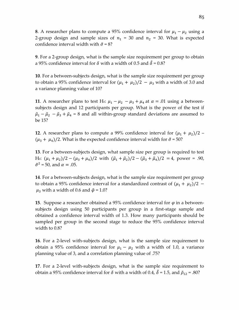
85
8. A researcher plans to compute a 95% confidence interval for 𝜇1 − 𝜇2 using a
2-group design and sample sizes of 𝑛1 = 30 and 𝑛2 = 30. What is expected
confidence interval width with �̃� = 8?
9. For a 2-group design, what is the sample size requirement per group to obtain
a 95% confidence interval for 𝛿 with a width of 0.5 and 𝛿 = 0.8?
10. For a between-subjects design, what is the sample size requirement per group
to obtain a 95% confidence interval for (𝜇1 + 𝜇2)/2 − 𝜇3 with a width of 3.0 and
a variance planning value of 10?
11. A researcher plans to test H0: 𝜇1 − 𝜇2 − 𝜇3 + 𝜇4 at 𝛼 = .01 using a between-
subjects design and 12 participants per group. What is the power of the test if
𝜇1 − 𝜇2 − 𝜇3 + 𝜇4 = 8 and all within-group standard deviations are assumed to
be 15?
12. A researcher plans to compute a 99% confidence interval for (𝜇1 + 𝜇2)/2 –
(𝜇3 + 𝜇4)/2. What is the expected confidence interval width for �̃� = 50?
13. For a between-subjects design, what sample size per group is required to test
H0: (𝜇1 + 𝜇2)/2 − (𝜇3 + 𝜇4)/2 with (�̃�1 + 𝜇2)/2 − (𝜇3 + 𝜇4)/2 = 4, power = .90,
�̃�2 = 50, and 𝛼 = .05.
14. For a between-subjects design, what is the sample size requirement per group
to obtain a 95% confidence interval for a standardized contrast of (𝜇1 + 𝜇2)/2 −
𝜇3 with a width of 0.6 and �̃� = 1.0?
15. Suppose a researcher obtained a 95% confidence interval for 𝜑 in a between-
subjects design using 50 participants per group in a first-stage sample and
obtained a confidence interval width of 1.3. How many participants should be
sampled per group in the second stage to reduce the 95% confidence interval
width to 0.8?
16. For a 2-level with-subjects design, what is the sample size requirement to
obtain a 95% confidence interval for 𝜇1 − 𝜇2 with a width of 1.0, a variance
planning value of 3, and a correlation planning value of .75?
17. For a 2-level with-subjects design, what is the sample size requirement to
obtain a 95% confidence interval for 𝛿 with a width of 0.4, 𝛿 = 1.5, and �̃�12 = .80?
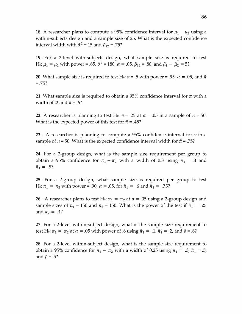
86
18. A researcher plans to compute a 95% confidence interval for 𝜇1 − 𝜇2 using a
within-subjects design and a sample size of 25. What is the expected confidence
interval width with �̃�2 = 15 and �̃�12 = .75?
19. For a 2-level with-subjects design, what sample size is required to test
H0: 𝜇1 = 𝜇2 with power = .85, �̃�2 = 180, 𝛼 = .05, �̃�12 = .80, and 𝜇1 − 𝜇2 = 5?
20. What sample size is required to test H0: 𝜋 = .5 with power = .95, 𝛼 = .05, and �̃�
= .75?
21. What sample size is required to obtain a 95% confidence interval for 𝜋 with a
width of .2 and �̃� = .6?
22. A researcher is planning to test H0: 𝜋 = .25 at 𝛼 = .05 in a sample of n = 50.
What is the expected power of this test for �̃� = .45?
23. A researcher is planning to compute a 95% confidence interval for 𝜋 in a
sample of n = 50. What is the expected confidence interval width for �̃� = .75?
24. For a 2-group design, what is the sample size requirement per group to
obtain a 95% confidence for 𝜋1 − 𝜋2 with a width of 0.3 using �̃�1 = .3 and
�̃�1 = .5?
25. For a 2-group design, what sample size is required per group to test
H0: 𝜋1 = 𝜋2 with power = .90, 𝛼 = .05, for �̃�1 = .6 and �̃�1 = .75?
26. A researcher plans to test H0: 𝜋1 = 𝜋2 at 𝛼 = .05 using a 2-group design and
sample sizes of 𝑛1 = 150 and 𝑛2 = 150. What is the power of the test if 𝜋1 = .25
and 𝜋2 = .4?
27. For a 2-level within-subject design, what is the sample size requirement to
test H0: 𝜋1 = 𝜋2 at 𝛼 = .05 with power of .8 using �̃�1 = .1, �̃�1 = .2, and �̃� = .6?
28. For a 2-level within-subject design, what is the sample size requirement to
obtain a 95% confidence for 𝜋1 − 𝜋2 with a width of 0.25 using �̃�1 = .3, �̃�1 = .5,
and �̃� = .5?
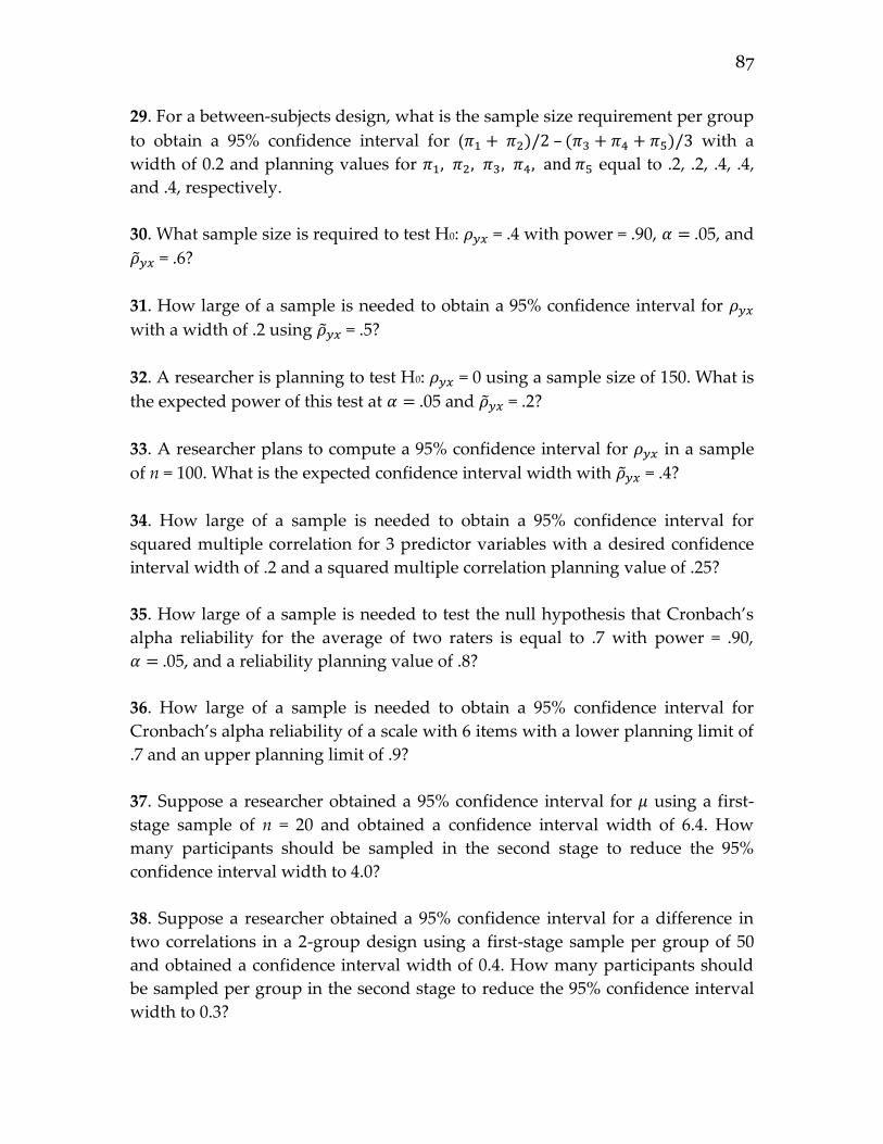
87
29. For a between-subjects design, what is the sample size requirement per group
to obtain a 95% confidence interval for (𝜋1 + 𝜋2)/2 – (𝜋3 + 𝜋4 + 𝜋5)/3 with a
width of 0.2 and planning values for 𝜋1, 𝜋2, 𝜋3, 𝜋4, and 𝜋5 equal to .2, .2, .4, .4,
and .4, respectively.
30. What sample size is required to test H0: 𝜌𝑦𝑥 = .4 with power = .90, 𝛼 = .05, and
�̃�𝑦𝑥 = .6?
31. How large of a sample is needed to obtain a 95% confidence interval for 𝜌𝑦𝑥
with a width of .2 using �̃�𝑦𝑥 = .5?
32. A researcher is planning to test H0: 𝜌𝑦𝑥 = 0 using a sample size of 150. What is
the expected power of this test at 𝛼 = .05 and �̃�𝑦𝑥 = .2?
33. A researcher plans to compute a 95% confidence interval for 𝜌𝑦𝑥 in a sample
of n = 100. What is the expected confidence interval width with �̃�𝑦𝑥 = .4?
34. How large of a sample is needed to obtain a 95% confidence interval for
squared multiple correlation for 3 predictor variables with a desired confidence
interval width of .2 and a squared multiple correlation planning value of .25?
35. How large of a sample is needed to test the null hypothesis that Cronbach’s
alpha reliability for the average of two raters is equal to .7 with power = .90,
𝛼 = .05, and a reliability planning value of .8?
36. How large of a sample is needed to obtain a 95% confidence interval for
Cronbach’s alpha reliability of a scale with 6 items with a lower planning limit of
.7 and an upper planning limit of .9?
37. Suppose a researcher obtained a 95% confidence interval for 𝜇 using a first-
stage sample of n = 20 and obtained a confidence interval width of 6.4. How
many participants should be sampled in the second stage to reduce the 95%
confidence interval width to 4.0?
38. Suppose a researcher obtained a 95% confidence interval for a difference in
two correlations in a 2-group design using a first-stage sample per group of 50
and obtained a confidence interval width of 0.4. How many participants should
be sampled per group in the second stage to reduce the 95% confidence interval
width to 0.3?
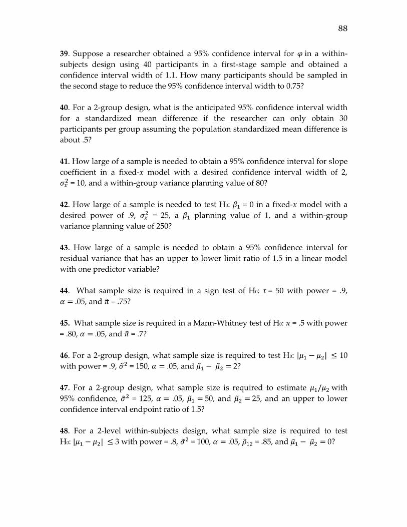
88
39. Suppose a researcher obtained a 95% confidence interval for 𝜑 in a within-
subjects design using 40 participants in a first-stage sample and obtained a
confidence interval width of 1.1. How many participants should be sampled in
the second stage to reduce the 95% confidence interval width to 0.75?
40. For a 2-group design, what is the anticipated 95% confidence interval width
for a standardized mean difference if the researcher can only obtain 30
participants per group assuming the population standardized mean difference is
about .5?
41. How large of a sample is needed to obtain a 95% confidence interval for slope
coefficient in a fixed-x model with a desired confidence interval width of 2,
𝜎𝑥2 = 10, and a within-group variance planning value of 80?
42. How large of a sample is needed to test H0: 𝛽1 = 0 in a fixed-x model with a
desired power of .9, 𝜎𝑥2 = 25, a 𝛽1 planning value of 1, and a within-group
variance planning value of 250?
43. How large of a sample is needed to obtain a 95% confidence interval for
residual variance that has an upper to lower limit ratio of 1.5 in a linear model
with one predictor variable?
44. What sample size is required in a sign test of H0: 𝜏 = 50 with power = .9,
𝛼 = .05, and �̃� = .75?
45. What sample size is required in a Mann-Whitney test of H0: 𝜋 = .5 with power
= .80, 𝛼 = .05, and �̃� = .7?
46. For a 2-group design, what sample size is required to test H0: |𝜇1 − 𝜇2| ≤ 10
with power = .9, �̃�2 = 150, 𝛼 = .05, and 𝜇1 − 𝜇2 = 2?
47. For a 2-group design, what sample size is required to estimate 𝜇1/𝜇2 with
95% confidence, �̃�2 = 125, 𝛼 = .05, 𝜇1 = 50, and 𝜇2 = 25, and an upper to lower
confidence interval endpoint ratio of 1.5?
48. For a 2-level within-subjects design, what sample size is required to test
H0: |𝜇1 − 𝜇2| ≤ 3 with power = .8, �̃�2 = 100, 𝛼 = .05, �̃�12 = .85, and 𝜇1 − 𝜇2 = 0?
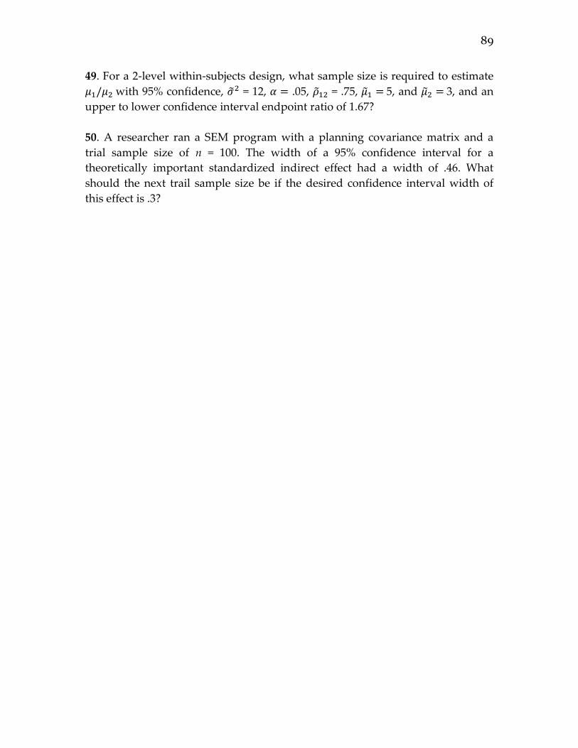
89
49. For a 2-level within-subjects design, what sample size is required to estimate
𝜇1/𝜇2 with 95% confidence, �̃�2 = 12, 𝛼 = .05, �̃�12 = .75, 𝜇1 = 5, and 𝜇2 = 3, and an
upper to lower confidence interval endpoint ratio of 1.67?
50. A researcher ran a SEM program with a planning covariance matrix and a
trial sample size of n = 100. The width of a 95% confidence interval for a
theoretically important standardized indirect effect had a width of .46. What
should the next trail sample size be if the desired confidence interval width of
this effect is .3?
90
Answers to Computational Problems
1. 26
2. .946
3. 1.99
4. 19
5. 25
6. 33
7. .891
8. 8.27
9. 133
10. 27
11.
12.
13. 34
14.
15. 83
16. 25
17. 1.22
18. 2.26
19. 28
20. 39
21. 93
22. .811
23. .240
24. 79
25. 200
26. .802
27. 84
28. 57
29. 62
30. 148
31. 219
32. .691
33. .332
34. 222
35. 258
36. 33
37. 32
38. 39
39. 47
40. 1.03
41. 34
42. 108
43. 49
44. 32
45. 33

91
46. 51
47. 48
48. 29
49. 74
50. 236


![Calculus 1 – Spring 2019 Section 2 - Columbia Universitymath.columbia.edu/~shapiro/PDFs/teaching/calc1_spring_2019/LectureNotes.pdf · some of which include: Spivak [5], Apostol](https://img.pdfslide.net/doc/110x75/5e75573d4f01375926648a3a/calculus-1-a-spring-2019-section-2-columbia-shapiropdfsteachingcalc1spring2019lecturenotespdf.jpg)


![RH Condom Wrkshp Session10 en[1]](https://img.pdfslide.net/doc/110x75/577dab7f1a28ab223f8c8106/rh-condom-wrkshp-session10-en1.jpg)


![Hardware Wrkshp C [Compatibility Mode]](https://img.pdfslide.net/doc/110x75/54b508b84a79590c6e8b45c8/hardware-wrkshp-c-compatibility-mode.jpg)