Embed Size (px)
Citation preview
Scheduling a Maintenance Activity on Parallel Identical Machines
Asaf Levin,1 Gur Mosheiov,1,2 Assaf Sarig1
1 Department of Statistics, The Hebrew University, Jerusalem 91905, Israel
2 School of Business Administration, The Hebrew University, Jerusalem 91905, Israel
Received 22 April 2007; revised 15 July 2008; accepted 9 August 2008DOI 10.1002/nav.20324
Published online 16 December 2008 in Wiley InterScience (www.interscience.wiley.com).
Abstract: We study a problem of scheduling a maintenance activity on parallel identical machines, under the assumption thatall the machines must be maintained simultaneously. One example for this setting is a situation where the entire system must bestopped for maintenance because of a required electricity shut-down. The objective is minimum flow-time. The problem is shownto be NP-hard, and moreover impossible to approximate unless P = NP . We introduce a pseudo-polynomial dynamic program-ming algorithm, and show how to convert it into a bicriteria FPTAS for this problem. We also present an efficient heuristic and alower bound. Our numerical tests indicate that the heuristic provides in most cases very close-to-optimal schedules. © 2008 WileyPeriodicals, Inc. Naval Research Logistics 56: 33–41, 2009
Keywords: scheduling; parallel machines; flow-time; maintenance activity
1. INTRODUCTION
In many manufacturing systems, machines must be main-tained at least once within a given time interval. During themaintenance time, the machine is shut down and the produc-tion is stopped. Thus, processing the jobs scheduled afterthe maintenance is delayed. In some of the relevant pub-lished papers, the maintenance time is fixed. Such models,known as “scheduling with non-availability time intervals,”have been studied by Schmidt [12] and Lee [7] among others.In other models, the (starting) time of the maintenance is adecision variable (in addition to the standard job schedulingdecisions). Some of the published papers within this categoryare Anily et al. [1, 2], Lee and Chen [8], Grigoriev et al. [5],and Kubzin and Strusevich [6]. A slightly different line ofresearch considers a situation where the maintenance activ-ity is optional, and if performed increases the efficiency of theprocessor (i.e., reduces the job processing times). The lattercase has been studied by e.g. Lee and Leon [9] and Mosheiovand Oron [10].
In this article, we focus on scheduling a maintenance activ-ity on parallel identical machines. The objective is minimumflow time. Lee and Chen [8] studied two versions of thisproblem: in the first (called the dependent case), the mainte-nance cannot be performed simultaneously on more than one
Correspondence to: G. Mosheiov ([email protected])
machine. Possible applications contain the case of a singleperson/facility/robot which needs to move from one machineto another to perform the maintenance. In the second setting(the independent case), this restriction is removed and themaintenance may be performed on several machines at thesame time. Our model assumes that all the machines mustbe maintained simultaneously, and the maintenance must becompleted within a prespecified time interval. A reasonablejustification for simultaneous maintenance is the fact thatoften all the production lines must be stopped for mainte-nance e.g. due to a required electricity shut-down. In somecompanies, it is the policy of the management to stop severalsections of the plant (sometimes even the entire plant) becauseof maintenance. A time interval constraint, or more specifi-cally, an upper bound on the maintenance completion time,is justified in systems where any delay of the maintenanceincreases significantly the risk of system failure.
1.1. Problem Formulation
Consider a setting of n jobs and m parallel iden-tical machines. Job processing times are denoted byP1, P2, . . . , Pn, and assumed to be nonnegative integers. Alljobs are available at time zero. For a given schedule, the com-pletion time of the j -th job is denoted by Cj , j = 1, 2, . . . , n.Each machine must be maintained once during a given inter-val [0, T ]. This maintenance activity must be performed
© 2008 Wiley Periodicals, Inc.
34 Naval Research Logistics, Vol. 56 (2009)
Table 1. Average and worst case optimality gap (in %) for α = 0.2 and β = 0.05.
2 Machines 5 Machines 10 Machines
Jobs Average Worst case Average Worst case Average Worst case
100 0.74 1.04 2.8 3.65 5.81 7.51300 0.25 0.34 0.97 1.33 2.18 2.61500 0.15 0.2 0.6 0.75 1.31 1.571000 0.08 0.1 0.3 0.4 0.66 0.84
simultaneously on all machines and during the maintenanceno production is performed. The maintenance activity doesnot affect the processing times of the jobs. Let t denote theduration of the maintenance activity (t ≤ T ). The objectiveis to schedule the jobs and the (common) maintenance activ-ity on the m machines, such that the total completion time,∑n
j=1 Cj , is minimized. If a simultaneous maintenance on allthe machines is denoted by S_MA, then the problem studiedhere is Pm|S_MA| ∑ Cj .
1.2. Paper Outline
We first show in Section 2 that the problem is NP-hard.More precisely, we show that the problem cannot be approx-imated within any polynomial factor (unless P = NP ), andfor nonfixed number of machines the problem becomes NP-hard in the strong sense. Then, in Section 3 we introducea pseudo-polynomial dynamic programming algorithm forany fixed number of machines, implying that the problemis NP-hard in the ordinary sense. Note that by the fact thatthe problem is NP-hard in the strong sense if the numberof machines is not fixed, we cannot hope for a pseudo-polynomial time algorithm for the problem with nonconstantnumber of machines. In Section 4 we show a bicriteria fullypolynomial time approximation scheme (bicriteria FPTAS)for Pm|S_MA| ∑ Cj . That is, for every ε > 0 we show howto find a schedule such that the maintenance activity will endno later than T (1 + ε) and the total completion times of thejobs will be at most (1 + ε) times the optimal cost (the totalcompletion time of the optimal solution that satisfies the duedate of the maintenance activity). Our scheme has time com-plexity that is polynomial in n and 1
ε. In Section 5, we propose
a simple and efficient heuristic and a lower bound on the opti-mal flow time. Our numerical tests indicate that the heuristic
produces very close-to-optimal schedules. We conclude inSection 6 with a few suggestions for future research.
2. NP-HARDNESS
We show that Pm|S_MA| ∑ Cj is NP-hard for all val-ues of m ≥ 2. Moreover, we show that for all values ofm ≥ 2 the optimization problem Pm|S_MA| ∑ Cj cannotbe approximated within a polynomial approximation ratio(unless P = NP ). The proof is based on a reduction from thePartition Problem, which is known to be NP-hard. PartitionProblem: Given a set {a1, a2, . . . , ak} of k positive integerssuch that
∑kj=1 aj = 2A (for some integer A), is there a
subset S ⊆ {1, 2, . . . , k} such that∑
j∈S aj = A?
THEOREM 1: Pm|S_MA| ∑ Cj is NP-hard for all valuesof m ≥ 2. Moreover, for all values of m ≥ 2 the optimizationproblem Pm|S_MA| ∑ Cj cannot be approximated within apolynomial approximation ratio (unless P = NP ).
PROOF: The proof is via reduction from the Partitionproblem. Given an instance of the Partition Problem, we con-struct the following instance of our scheduling problem: Letn = k + m − 2 be the number of jobs. Job processing timesare: Pj = aj for j = 1, 2, . . . , k (“small” jobs), and Pj = A
for j = k + 1, k + 2, . . . , k + m − 2 (“large” jobs). Theduration of the maintenance activity is t = M (where M is alarge constant to be defined later). Its completion time cannotexceed the time T = A+M . The objective function thresholdis An. We now show that there is a schedule for this instancesuch that
∑Cj ≤ An if and only if there is a subset S for the
instance of Partition instance such that∑
j∈S aj = A. More-over, if there is no such solution to the Partition instance, thenthe cost of the optimal solution to Pm|S_MA| ∑ Cj is at least
Table 2. Average and worst case optimality gap (in %) for α = 0.2 and β = 0.01.
2 Machines 5 Machines 10 Machines
Jobs Average Worst case Average Worst case Average Worst case
100 0.76 1.14 2.88 3.7 6.08 7.86300 0.26 0.37 1.01 1.22 2.2 2.67500 0.16 0.21 0.61 0.73 1.35 1.61000 0.08 0.11 0.31 0.4 0.68 0.8
Naval Research Logistics DOI 10.1002/nav
Levin, Mosheiov, and Sarig: Maintenance Activity on Parallel Identical Machines 35
Table 3. Average and worst case optimality gap (in %) for α = 0.2 and β = 0.15.
2 Machines 5 Machines 10 Machines
Jobs Average Worst case Average Worst case Average Worst case
100 0.83 1.17 2.97 3.91 6.29 8.29300 0.28 0.37 1.04 1.23 2.24 2.58500 0.17 0.23 0.62 0.81 1.38 1.681000 0.08 0.11 0.31 0.4 0.69 0.82
M . By letting M be large enough, we conclude that there isno polynomial P(n,
∑Pj ) that is the approximation ratio of
at most P(n,∑
Pj ) (unless P = NP ), proving the claim ofthe theorem.
Hence, to prove the claim it suffices to show that if thereis a feasible solution to the Partition instance, then there is afeasible schedule with total completion time of at most An,and if there is a feasible schedule with total completion timeof at most M − ε (for some ε > 0) then there is a feasiblesolution to the Partition instance.
Suppose that there exist a subset S for the Partition instancesuch that
∑j∈S aj = A. We construct a schedule as fol-
lows: we schedule first the small jobs–on machine 1 the jobsof set S, and on machine 2 the remaining jobs (of the set{1, 2, . . . , k}). On each machine 3, 4, . . . , m we schedule onelarge job. Then, we schedule simultaneously the maintenanceactivity on all machines. This schedule is feasible since themaintenance activity (on all machines) starts at time A andtherefore completed at time T = A + M , i.e., on time. Thetotal completion times of all jobs does not exceed nA, sinceall jobs are finished before the maintenance activity starts attime A.
Assume that there is a feasible schedule with a total com-pletion time of no more than M − ε for some ε > 0. Then,clearly all jobs must be processed before the maintenanceactivity (because a job that is scheduled afterwards has a com-pletion time of at least M). Moreover, if a machine processone of the large jobs, then it does not process other jobs (thisis so because if the machine will process another job then themaintenance activity will not start at time A and hence willnot finish on time). Therefore, there are exactly two machinesthat process the jobs with indices {1, 2, . . . , k} and the pro-cessing of these jobs end at time A. Consider the set S ofindices of jobs that the first such machine processes. Then,
∑j∈S Pj = A and therefore (because these are small jobs),∑j∈S aj = A. �
Note that our reduction shows that Pm|S_MA| ∑ Cj isNP-hard. In the sequel we show a dynamic programmingpseudo-polynomial time algorithm for Pm|S_MA| ∑ Cj
with an arbitrary fixed number of machines. Therefore, ourproblem is NP-hard in the ordinary sense for any fixednumber of machines. We next show that if the number ofmachines is considered to be part of the input then the prob-lem becomes NP-hard in the strong sense, and hence there isno such pseudo-polynomial time algorithm for this problem.We denote by P |S_MA| ∑ Cj the resulting problem, wherethe number of machines m is considered to be part of theinput. We will show that this problem is NP-hard in the strongsense via reduction from the 3-Partition problem defined asfollows: the input consists of 3n positive integers a1, . . . , a3n
such that for all j A4 < aj < A
2 , and∑3n
j=1 aj = nA. The goalis to find whether there is a partition of 1, . . . , 3n into n sets(each of them has exactly three indices) A1, . . . , An such that∑
j∈Aiaj = A for all i = 1, 2, . . . , n. It is known that this
3-Partition problem is NP-complete in the strong sense.
THEOREM 2: P |S_MA| ∑ Cj is NP-hard in the strongsense.
PROOF: Given an instance to the 3-Partition problema1, . . . , a3n such that for all j A
4 < aj < A2 , and
∑3nj=1 aj =
nA, we construct an instance to the P |S_MA| ∑ Cj as fol-lows. We have 3n jobs, where job j has a processing timePj = aj . The number of machines is n. There is a mainte-nance activity of length t = M (where M > 3nA). The duedate of the maintenance activity is T = M + A. Next weshow that there is a solution to the 3-Partition instance if and
Table 4. Average and worst case optimality gap (in %) for α = 0.5 and β = 0.05.
2 Machines 5 Machines 10 Machines
Jobs Average Worst case Average Worst case Average Worst case
100 0.75 1.01 2.82 3.64 6.53 7.87300 0.25 0.32 0.96 1.12 2.1 2.48500 0.15 0.19 0.56 0.69 1.27 1.471000 0.08 0.09 0.29 0.34 0.63 0.76
Naval Research Logistics DOI 10.1002/nav
36 Naval Research Logistics, Vol. 56 (2009)
Table 5. Average and worst case optimality gap (in %) for α = 0.5 and β = 0.1.
2 Machines 5 Machines 10 Machines
Jobs Average Worst case Average Worst case Average Worst case
100 0.91 1.14 3.16 3.87 6.85 8.76300 0.31 0.37 1.08 1.24 2.35 2.72500 0.19 0.22 0.65 0.73 1.41 1.651000 0.09 0.11 0.32 0.4 0.71 0.83
only if the optimal solution to P |S_MA| ∑ Cj costs at most3nA.
First assume that there is a solution A1, . . . , An to the3-Partition instance, then we create a feasible schedule byprocessing the jobs in Ai on machine i in the first A timeunits, and then we perform the (simultaneous) maintenanceactivity starting at time A (and ending at time A+M , i.e., ontime). The completion time of each job in this schedule is atmost A, and therefore the total completion time of the jobs isat most 3nA.
For the other direction, assume that there is a feasibleschedule with total cost of at most 3nA. Note that if a job isprocessed after the maintenance activity then its completiontime is after time M > 3nA and therefore in such a case thetotal completion time is larger than 3nA. By our assumption,we conclude that all jobs are completed before the schedule ofthe maintenance activity. Next, we note that by the due date ofthe maintenance activity, we conclude that all jobs are com-pleted by time A. We denote by Ai the set of indices of the jobsthat are processed on machine i. Then, clearly A1, . . . , An isa partition of {1, 2, . . . , 3n}, such that
∑j∈Ai
aj ≤ A for all
i = 1, 2, . . . , n. Because∑3n
j=1 aj = nA, we conclude thatfor all i,
∑j∈Ai
aj = A, and therefore A1, . . . , An is a feasiblesolution to the 3-Partition instance. �
3. DYNAMIC PROGRAMMING ALGORITHM
In this section, we introduce a pseudo-polynomial dynamicprogramming (DP) for the case of two parallel identicalmachines (see, however, the comment below regarding thegeneral m-machine case). The introduction of this DP impliesthat the problem studied here is NP-hard in the ordinary sense.
First we sort the jobs in a non-decreasing order of theirprocessing times to create the SPT (shortest processing timefirst) list. In each iteration of our proposed DP, the next job inthis list is added to the current schedule. The required knowl-edge (the state variables) at each iteration contains: (i) thenumber of jobs already scheduled, (ii) the completion timeof the last scheduled job on machine i before the maintenanceactivity (for all i = 1, 2, . . . , m), and (iii) the completion timeof the last scheduled job on machine i after the maintenanceactivity (for all i = 1, 2, . . . , m).
Recall that T is an upper bound on the completion time ofthe maintenance activity, and that T − t is an upper bound onits starting time. Our algorithm tries all the possibilities of thestarting time τ ∈ [0, T − t] of the maintenance activity. Foreach (integer) value of τ it applies the following calculation.Let fτ (k, t1, t2, . . . , tm, t1, t2, . . . , tm) be the minimum cost ofscheduling jobs k, k+1, . . . , n, given that jobs 1, 2, . . . , k−1have already been scheduled, and the the total processingtimes of the scheduled jobs on machines i before the main-tenance activity is ti and after the maintenance activity is t i .
In each iteration we consider the possibility of adding jobk to the subset of jobs processed on machine i before or afterthe maintenance activity.
fτ (k, t1, t2, . . . , tm, t1, t2, . . . , tm) =min { min
i=1,2,...,m{fτ (k + 1, t1, t2, . . . , ti−1, ti + Pk ,
ti+1, . . . , tm, t1, t2, . . . , tm) + ti + Pk},min
i=1,2,...,m{fτ (k + 1, t1, t2, . . . , tm, t1, t2, . . . , t i−1,
t i , +Pk , t i+1, . . . , tm) + τ + t + t i + Pk}}.If during the calculation we face a state variable ti that islarger than τ then the value of f is set to ∞ (correspondingto infeasible solution).
Table 6. Average and worst case optimality gap (in %) for α = 0.5 and β = 0.15.
2 Machines 5 Machines 10 Machines
Jobs Average Worst case Average Worst case Average Worst case
100 1.0105 1.013 1.035 1.0424 1.074 1.0908300 1.0035 1.0042 1.0118 1.014 1.0256 1.0287500 1.0021 1.0025 1.007 1.0084 1.0154 1.01741000 1.001 1.0013 1.0036 1.0043 1.0077 1.0091
Naval Research Logistics DOI 10.1002/nav
Levin, Mosheiov, and Sarig: Maintenance Activity on Parallel Identical Machines 37
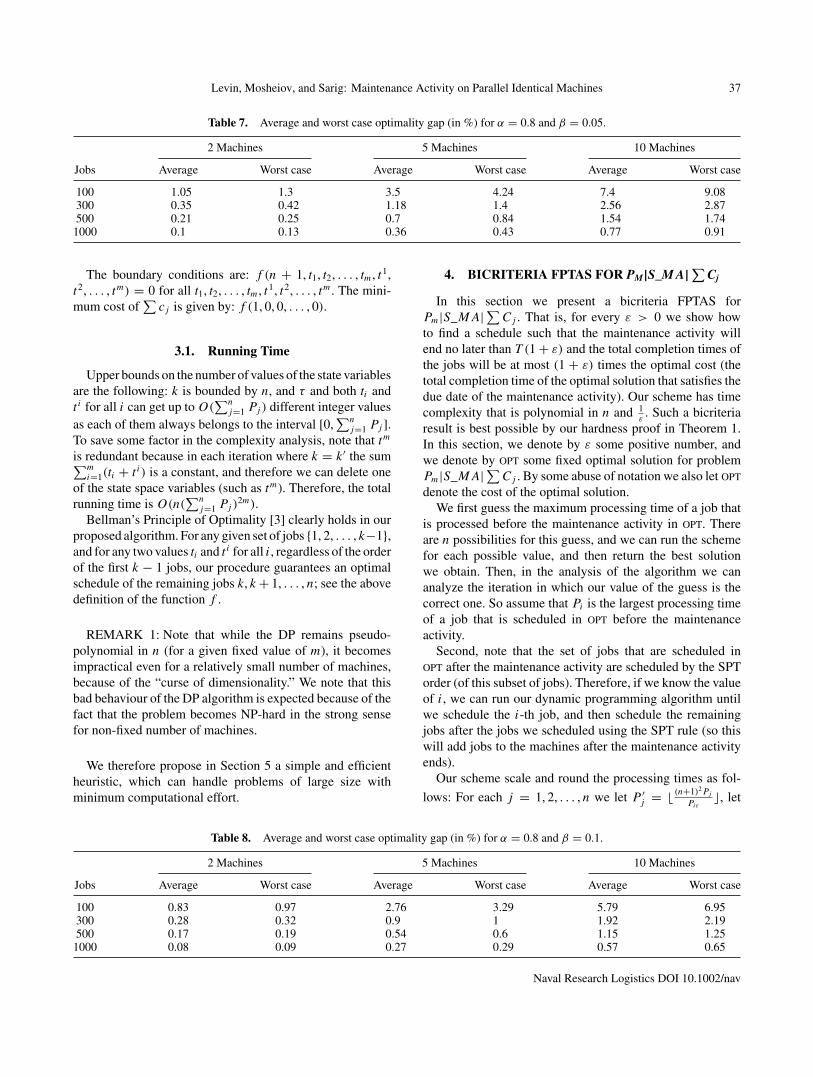
Table 7. Average and worst case optimality gap (in %) for α = 0.8 and β = 0.05.
2 Machines 5 Machines 10 Machines
Jobs Average Worst case Average Worst case Average Worst case
100 1.05 1.3 3.5 4.24 7.4 9.08300 0.35 0.42 1.18 1.4 2.56 2.87500 0.21 0.25 0.7 0.84 1.54 1.741000 0.1 0.13 0.36 0.43 0.77 0.91
The boundary conditions are: f (n + 1, t1, t2, . . . , tm, t1,t2, . . . , tm) = 0 for all t1, t2, . . . , tm, t1, t2, . . . , tm. The mini-mum cost of
∑cj is given by: f (1, 0, 0, . . . , 0).
3.1. Running Time
Upper bounds on the number of values of the state variablesare the following: k is bounded by n, and τ and both ti andt i for all i can get up to O(
∑nj=1 Pj ) different integer values
as each of them always belongs to the interval [0,∑n
j=1 Pj ].To save some factor in the complexity analysis, note that tm
is redundant because in each iteration where k = k′ the sum∑mi=1(ti + t i) is a constant, and therefore we can delete one
of the state space variables (such as tm). Therefore, the totalrunning time is O(n(
∑nj=1 Pj )
2m).Bellman’s Principle of Optimality [3] clearly holds in our
proposed algorithm. For any given set of jobs {1, 2, . . . , k−1},and for any two values ti and t i for all i, regardless of the orderof the first k − 1 jobs, our procedure guarantees an optimalschedule of the remaining jobs k, k + 1, . . . , n; see the abovedefinition of the function f .
REMARK 1: Note that while the DP remains pseudo-polynomial in n (for a given fixed value of m), it becomesimpractical even for a relatively small number of machines,because of the “curse of dimensionality.” We note that thisbad behaviour of the DP algorithm is expected because of thefact that the problem becomes NP-hard in the strong sensefor non-fixed number of machines.
We therefore propose in Section 5 a simple and efficientheuristic, which can handle problems of large size withminimum computational effort.
4. BICRITERIA FPTAS FOR PM|S_M A| ∑ Cj
In this section we present a bicriteria FPTAS forPm|S_MA| ∑ Cj . That is, for every ε > 0 we show howto find a schedule such that the maintenance activity willend no later than T (1 + ε) and the total completion times ofthe jobs will be at most (1 + ε) times the optimal cost (thetotal completion time of the optimal solution that satisfies thedue date of the maintenance activity). Our scheme has timecomplexity that is polynomial in n and 1
ε. Such a bicriteria
result is best possible by our hardness proof in Theorem 1.In this section, we denote by ε some positive number, andwe denote by opt some fixed optimal solution for problemPm|S_MA| ∑ Cj . By some abuse of notation we also let optdenote the cost of the optimal solution.
We first guess the maximum processing time of a job thatis processed before the maintenance activity in opt. Thereare n possibilities for this guess, and we can run the schemefor each possible value, and then return the best solutionwe obtain. Then, in the analysis of the algorithm we cananalyze the iteration in which our value of the guess is thecorrect one. So assume that Pi is the largest processing timeof a job that is scheduled in opt before the maintenanceactivity.
Second, note that the set of jobs that are scheduled inopt after the maintenance activity are scheduled by the SPTorder (of this subset of jobs). Therefore, if we know the valueof i, we can run our dynamic programming algorithm untilwe schedule the i-th job, and then schedule the remainingjobs after the jobs we scheduled using the SPT rule (so thiswill add jobs to the machines after the maintenance activityends).
Our scheme scale and round the processing times as fol-
lows: For each j = 1, 2, . . . , n we let P ′j = � (n+1)2Pj
Piε�, let
Table 8. Average and worst case optimality gap (in %) for α = 0.8 and β = 0.1.
2 Machines 5 Machines 10 Machines
Jobs Average Worst case Average Worst case Average Worst case
100 0.83 0.97 2.76 3.29 5.79 6.95300 0.28 0.32 0.9 1 1.92 2.19500 0.17 0.19 0.54 0.6 1.15 1.251000 0.08 0.09 0.27 0.29 0.57 0.65
Naval Research Logistics DOI 10.1002/nav
38 Naval Research Logistics, Vol. 56 (2009)
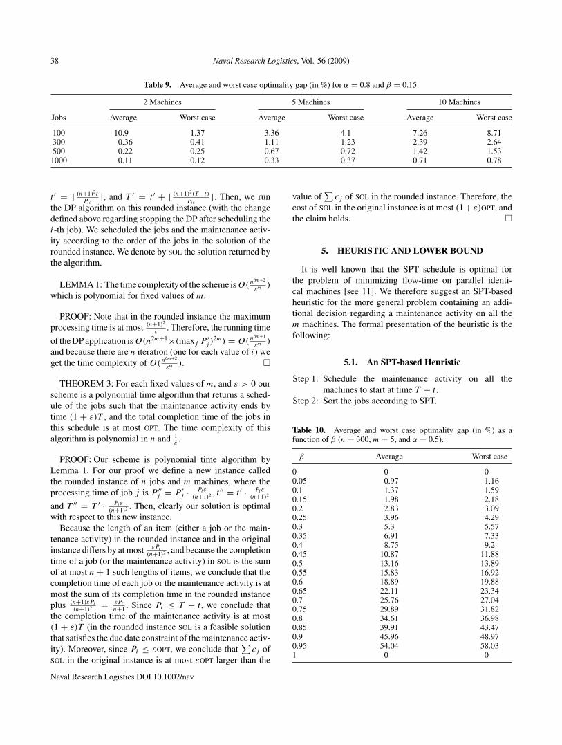
Table 9. Average and worst case optimality gap (in %) for α = 0.8 and β = 0.15.
2 Machines 5 Machines 10 Machines
Jobs Average Worst case Average Worst case Average Worst case
100 10.9 1.37 3.36 4.1 7.26 8.71300 0.36 0.41 1.11 1.23 2.39 2.64500 0.22 0.25 0.67 0.72 1.42 1.531000 0.11 0.12 0.33 0.37 0.71 0.78
t ′ = � (n+1)2t
Piε�, and T ′ = t ′ + � (n+1)2(T −t)
Piε�. Then, we run
the DP algorithm on this rounded instance (with the changedefined above regarding stopping the DP after scheduling thei-th job). We scheduled the jobs and the maintenance activ-ity according to the order of the jobs in the solution of therounded instance. We denote by sol the solution returned bythe algorithm.
LEMMA 1: The time complexity of the scheme isO(n6m+2
εm )
which is polynomial for fixed values of m.
PROOF: Note that in the rounded instance the maximumprocessing time is at most (n+1)2
ε. Therefore, the running time
of the DP application is O(n2m+1×(maxj P ′j )
2m) = O(n6m+1
εm )
and because there are n iteration (one for each value of i) weget the time complexity of O(n6m+2
εm ). �
THEOREM 3: For each fixed values of m, and ε > 0 ourscheme is a polynomial time algorithm that returns a sched-ule of the jobs such that the maintenance activity ends bytime (1 + ε)T , and the total completion time of the jobs inthis schedule is at most opt. The time complexity of thisalgorithm is polynomial in n and 1
ε.
PROOF: Our scheme is polynomial time algorithm byLemma 1. For our proof we define a new instance calledthe rounded instance of n jobs and m machines, where theprocessing time of job j is P ′′
j = P ′j · Piε
(n+1)2 , t ′′ = t ′ · Piε
(n+1)2
and T ′′ = T ′ · Piε
(n+1)2 . Then, clearly our solution is optimalwith respect to this new instance.
Because the length of an item (either a job or the main-tenance activity) in the rounded instance and in the originalinstance differs by at most εPi
(n+1)2 , and because the completiontime of a job (or the maintenance activity) in sol is the sumof at most n + 1 such lengths of items, we conclude that thecompletion time of each job or the maintenance activity is atmost the sum of its completion time in the rounded instanceplus (n+1)εPi
(n+1)2 = εPi
n+1 . Since Pi ≤ T − t , we conclude thatthe completion time of the maintenance activity is at most(1 + ε)T (in the rounded instance sol is a feasible solutionthat satisfies the due date constraint of the maintenance activ-ity). Moreover, since Pi ≤ εopt, we conclude that
∑cj of
sol in the original instance is at most εopt larger than the
value of∑
cj of sol in the rounded instance. Therefore, thecost of sol in the original instance is at most (1+ ε)opt, andthe claim holds. �
5. HEURISTIC AND LOWER BOUND
It is well known that the SPT schedule is optimal forthe problem of minimizing flow-time on parallel identi-cal machines [see 11]. We therefore suggest an SPT-basedheuristic for the more general problem containing an addi-tional decision regarding a maintenance activity on all them machines. The formal presentation of the heuristic is thefollowing:
5.1. An SPT-based Heuristic
Step 1: Schedule the maintenance activity on all themachines to start at time T − t .
Step 2: Sort the jobs according to SPT.
Table 10. Average and worst case optimality gap (in %) as afunction of β (n = 300, m = 5, and α = 0.5).
β Average Worst case
0 0 00.05 0.97 1.160.1 1.37 1.590.15 1.98 2.180.2 2.83 3.090.25 3.96 4.290.3 5.3 5.570.35 6.91 7.330.4 8.75 9.20.45 10.87 11.880.5 13.16 13.890.55 15.83 16.920.6 18.89 19.880.65 22.11 23.340.7 25.76 27.040.75 29.89 31.820.8 34.61 36.980.85 39.91 43.470.9 45.96 48.970.95 54.04 58.031 0 0
Naval Research Logistics DOI 10.1002/nav
Levin, Mosheiov, and Sarig: Maintenance Activity on Parallel Identical Machines 39
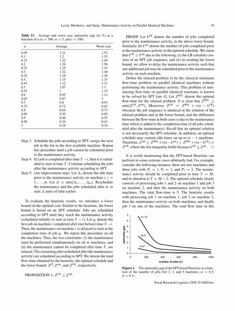
Table 11. Average and worst case optimality gap (in %) as afunction of α (n = 300, m = 5, and t = 100).
α Average Worst case
0.05 1.21 1.520.1 1.2 1.530.15 1.22 1.490.2 1.26 1.560.25 1.25 1.470.3 1.22 1.490.35 1.19 1.380.4 1.15 1.330.45 1.12 1.310.5 1.07 1.30.55 1 1.150.6 0.95 1.120.65 0.87 10.7 0.8 0.930.75 0.72 0.830.8 0.64 0.730.85 0.55 0.650.9 0.46 0.550.95 0.36 0.411 0.28 0.34
Step 3: Schedule the jobs according to SPT: assign the nextjob in the list to the first available machine. Repeatthis procedure until a job cannot be scheduled priorto the maintenance activity.
Step 4: If a job is completed after time T −t , then it is sched-uled to start at time T . Continue scheduling the jobsafter the maintenance activity according to SPT.
Step 5: (An improvement step). Let �i denote the idle timeprior to the maintenance activity on machine i, i =1, . . . , m. Let � = min{�1, . . . , �m}. Reschedulethe maintenance and the jobs scheduled after it, tostart � units of time earlier.
To evaluate the heuristic results, we introduce a lowerbound on the optimal cost. Similar to the heuristic, the lowerbound is based on an SPT schedule. Jobs are scheduledaccording to SPT until they reach the maintenance activity(scheduled initially to start at time T − t). Let qi denote thefirst job on machine i completed after (not before) time T − t .Then, the maintenance on machine i is delayed to start at thecompletion time of job qi . We repeat this procedure on allthe machines. Thus, the two constraints: (i) the maintenancemust be performed simultaneously on all m machines, and(ii) the maintenance cannot be completed after time T , arerelaxed. The remaining jobs (scheduled after the maintenanceactivity) are scheduled according to SPT. We denote the totalflow-time obtained by the heuristic, the optimal schedule andthe lower bound: ZH, Zopt, and ZLB, respectively.
PROPOSITION 1: ZLB ≤ Zopt.
PROOF: Let kLB denote the number of jobs completedprior to the maintenance activity, in the above lower bound.Similarly, let kopt denote the number of jobs completed priorto the maintenance activity in the optimal schedule. We claimthat kLB ≥ kopt due to the following: (i) the LB schedule con-sists of an SPT job sequence, and (ii) in creating the lowerbound, we allow to delay the maintenance activity such thatone additional job may be scheduled prior to the maintenanceactivity on each machine.
Define the relaxed problem to be the classical minimumflow-time problem on parallel identical machines withoutperforming the maintenance activity. This problem of min-imizing flow-time on parallel identical machines is knownto be solved by SPT [see 4]. Let ZREL denote the optimalflow-time for the relaxed problem. It is clear that ZREL ≤min{ZLB, Zopt}. Moreover, ZLB = ZREL + t(n − kLB)
(because the job sequence is identical in the solution of therelaxed problem and in the lower bound, and the differencebetween the flow-time in both cases is due to the maintenancetime which is added to the completion time of all jobs sched-uled after the maintenance). Recall that an optimal solutionis not necessarily the SPT schedule. In addition, an optimalschedule may contain idle times on up to m − 1 machines.Therefore, Zopt ≥ ZREL +t(n−kopt) ≥ ZREL +t(n−kLB) =ZLB, where the last inequality holds because kLB ≥ kopt. �
It is worth mentioning that the SPT-based Heuristic canperform in some extreme cases arbitrarily bad. For example,consider the following instance: there are two machines andthree jobs with P1 = 1, P2 = 1, and P3 = 2. The mainte-nance activity should be completed prior to time T = M ,and its duration is T = M − 2. The optimal schedule clearlyconsists of processing jobs 1 and 2 on machine 1 and job 3on machine 2, and then the maintenance activity on bothmachines. The total flow-time is 5. The heuristic resultswith processing job 1 on machine 1, job 2 on machine 2,then the maintenance activity on both machines, and finallyjob 3 on one of the machines. The total flow time in this
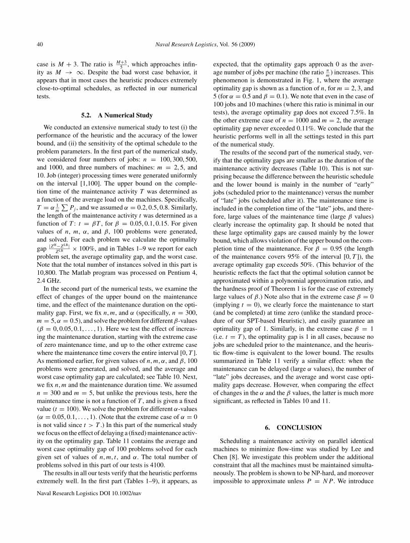
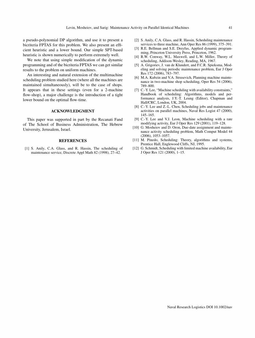
Figure 1. The optimality gap of the SPT-based Heuristic as a func-tion of the number of jobs (for 2, 3, and 5 machines, α = 0.5,β = 0.1).
Naval Research Logistics DOI 10.1002/nav
40 Naval Research Logistics, Vol. 56 (2009)
case is M + 3. The ratio is M+35 , which approaches infin-
ity as M → ∞. Despite the bad worst case behavior, itappears that in most cases the heuristic produces extremelyclose-to-optimal schedules, as reflected in our numericaltests.
5.2. A Numerical Study
We conducted an extensive numerical study to test (i) theperformance of the heuristic and the accuracy of the lowerbound, and (ii) the sensitivity of the optimal schedule to theproblem parameters. In the first part of the numerical study,we considered four numbers of jobs: n = 100, 300, 500,and 1000, and three numbers of machines: m = 2, 5, and10. Job (integer) processing times were generated uniformlyon the interval [1,100]. The upper bound on the comple-tion time of the maintenance activity T was determined asa function of the average load on the machines. Specifically,T = α 1
m
∑Pj , and we assumed α = 0.2, 0.5, 0.8. Similarly,
the length of the maintenance activity t was determined as afunction of T : t = βT , for β = 0.05, 0.1, 0.15. For givenvalues of n, m, α, and β, 100 problems were generated,and solved. For each problem we calculate the optimalitygap |ZH−ZLB|
ZLB × 100%, and in Tables 1–9 we report for eachproblem set, the average optimality gap, and the worst case.Note that the total number of instances solved in this part is10,800. The Matlab program was processed on Pentium 4,2.4 GHz.
In the second part of the numerical tests, we examine theeffect of changes of the upper bound on the maintenancetime, and the effect of the maintenance duration on the opti-mality gap. First, we fix n, m, and α (specifically, n = 300,m = 5, α = 0.5), and solve the problem for different β-values(β = 0, 0.05, 0.1, . . . , 1). Here we test the effect of increas-ing the maintenance duration, starting with the extreme caseof zero maintenance time, and up to the other extreme casewhere the maintenance time covers the entire interval [0, T ].As mentioned earlier, for given values of n, m, α, and β, 100problems were generated, and solved, and the average andworst case optimality gap are calculated; see Table 10. Next,we fix n, m and the maintenance duration time. We assumedn = 300 and m = 5, but unlike the previous tests, here themaintenance time is not a function of T , and is given a fixedvalue (t = 100). We solve the problem for different α-values(α = 0.05, 0.1, . . . , 1). (Note that the extreme case of α = 0is not valid since t > T .) In this part of the numerical studywe focus on the effect of delaying a (fixed) maintenance activ-ity on the optimality gap. Table 11 contains the average andworst case optimality gap of 100 problems solved for eachgiven set of values of n, m, t , and α. The total number ofproblems solved in this part of our tests is 4100.
The results in all our tests verify that the heuristic performsextremely well. In the first part (Tables 1–9), it appears, as
expected, that the optimality gaps approach 0 as the aver-age number of jobs per machine (the ratio n
m) increases. This
phenomenon is demonstrated in Fig. 1, where the averageoptimality gap is shown as a function of n, for m = 2, 3, and5 (for α = 0.5 and β = 0.1). We note that even in the case of100 jobs and 10 machines (where this ratio is minimal in ourtests), the average optimality gap does not exceed 7.5%. Inthe other extreme case of n = 1000 and m = 2, the averageoptimality gap never exceeded 0.11%. We conclude that theheuristic performs well in all the settings tested in this partof the numerical study.
The results of the second part of the numerical study, ver-ify that the optimality gaps are smaller as the duration of themaintenance activity decreases (Table 10). This is not sur-prising because the difference between the heuristic scheduleand the lower bound is mainly in the number of “early”jobs (scheduled prior to the maintenance) versus the numberof “late” jobs (scheduled after it). The maintenance time isincluded in the completion time of the “late” jobs, and there-fore, large values of the maintenance time (large β values)clearly increase the optimality gap. It should be noted thatthese large optimality gaps are caused mainly by the lowerbound, which allows violation of the upper bound on the com-pletion time of the maintenance. For β = 0.95 (the lengthof the maintenance covers 95% of the interval [0, T ]), theaverage optimality gap exceeds 50%. (This behavior of theheuristic reflects the fact that the optimal solution cannot beapproximated within a polynomial approximation ratio, andthe hardness proof of Theorem 1 is for the case of extremelylarge values of β.) Note also that in the extreme case β = 0(implying t = 0), we clearly force the maintenance to start(and be completed) at time zero (unlike the standard proce-dure of our SPT-based Heuristic), and easily guarantee anoptimality gap of 1. Similarly, in the extreme case β = 1(i.e. t = T ), the optimality gap is 1 in all cases, because nojobs are scheduled prior to the maintenance, and the heuris-tic flow-time is equivalent to the lower bound. The resultssummarized in Table 11 verify a similar effect: when themaintenance can be delayed (large α values), the number of“late” jobs decreases, and the average and worst case opti-mality gaps decrease. However, when comparing the effectof changes in the α and the β values, the latter is much moresignificant, as reflected in Tables 10 and 11.
6. CONCLUSION
Scheduling a maintenance activity on parallel identicalmachines to minimize flow-time was studied by Lee andChen [8]. We investigate this problem under the additionalconstraint that all the machines must be maintained simulta-neously. The problem is shown to be NP-hard, and moreoverimpossible to approximate unless P = NP . We introduce
Naval Research Logistics DOI 10.1002/nav
Levin, Mosheiov, and Sarig: Maintenance Activity on Parallel Identical Machines 41
a pseudo-polynomial DP algorithm, and use it to present abicriteria FPTAS for this problem. We also present an effi-cient heuristic and a lower bound. Our simple SPT-basedheuristic is shown numerically to perform extremely well.
We note that using simple modification of the dynamicprogramming and of the bicriteria FPTAS we can get similarresults to the problem on uniform machines.
An interesting and natural extension of the multimachinescheduling problem studied here (where all the machines aremaintained simultaneously), will be to the case of shops.It appears that in these settings (even for a 2-machineflow-shop), a major challenge is the introduction of a tightlower bound on the optimal flow-time.
ACKNOWLEDGMENT
This paper was supported in part by the Recanati Fandof The School of Business Administration, The HebrewUniversity, Jerusalem, Israel.
REFERENCES
[1] S. Anily, C.A. Glass, and R. Hassin, The scheduling ofmaintenance service, Discrete Appl Math 82 (1998), 27–42.
[2] S. Anily, C.A. Glass, and R. Hassin, Scheduling maintenanceservices to three machine, Ann Oper Res 86 (1999), 375–391.
[3] R.E. Bellman and S.E. Dreyfus, Applied dynamic program-ming, Princeton University Press, Princeton, 1962.
[4] R.W. Conway, W.L. Maxwell, and L.W. Miller, Theory ofscheduling, Addison-Wesley, Reading, MA, 1967.
[5] A. Grigoriev, J. van de Klundert, and F.C.R. Spieksma, Mod-eling and solving periodic maintenance problem, Eur J OperRes 172 (2006), 783–797.
[6] M.A. Kubzin and V.A. Strusevich, Planning machine mainte-nance in two-machine shop scheduling, Oper Res 54 (2006),789–800.
[7] C.-Y. Lee, “Machine scheduling with availability constraints,”Handbook of scheduling: Algorithms, models and per-formance analysis, J.Y.-T. Leung (Editor), Chapman andHall/CRC, London, UK, 2004.
[8] C.-Y. Lee and Z.-L. Chen, Scheduling jobs and maintenanceactivities on parallel machines, Naval Res Logist 47 (2000),145–165.
[9] C.-Y. Lee and V.J. Leon, Machine scheduling with a ratemodifying activity, Eur J Oper Res 129 (2001), 119–128.
[10] G. Mosheiov and D. Oron, Due-date assignment and mainte-nance activity scheduling problem, Math Comput Model 44(2006), 1053–1057.
[11] M. Pinedo, Scheduling: Theory, algorithms and systems,Prentice Hall, Englewood Cliffs, NJ, 1995.
[12] G. Schmidt, Scheduling with limited machine availability, EurJ Oper Res 121 (2000), 1–15.
Naval Research Logistics DOI 10.1002/nav