Embed Size (px)
Citation preview

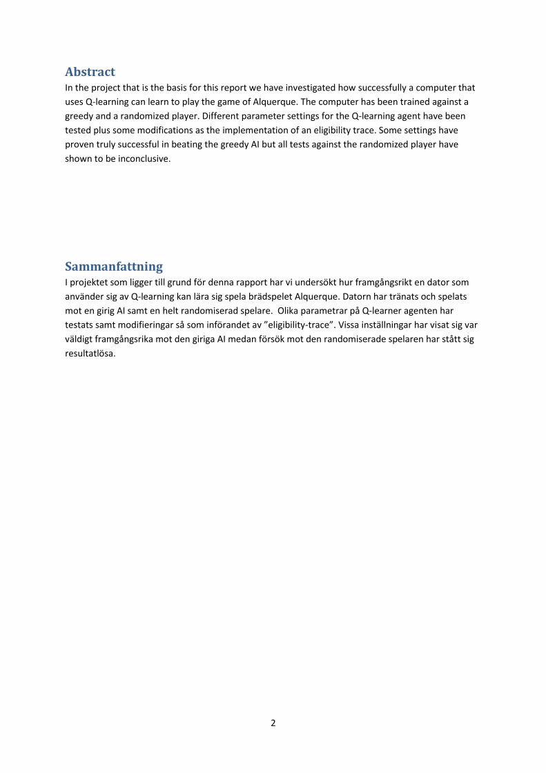
Self-Learning Alquerque Player
M A T T I A S K N U T S S O N a n d S E B A S T I A N R E M N E R U D
Bachelor of Science Thesis Stockholm, Sweden 2011
Self-Learning Alquerque Player
M A T T I A S K N U T S S O N a n d S E B A S T I A N R E M N E R U D
Bachelor’s Thesis in Computer Science (15 ECTS credits) at the School of Computer Science and Engineering Royal Institute of Technology year 2011 Supervisor at CSC was Johan Boye Examiner was Mads Dam URL: www.csc.kth.se/utbildning/kandidatexjobb/datateknik/2011/ knutsson_mattias_OCH_remnerud_sebastian_K11067.pdf Kungliga tekniska högskolan Skolan för datavetenskap och kommunikation KTH CSC 100 44 Stockholm URL: www.kth.se/csc
2
Abstract In the project that is the basis for this report we have investigated how successfully a computer that
uses Q-learning can learn to play the game of Alquerque. The computer has been trained against a
greedy and a randomized player. Different parameter settings for the Q-learning agent have been
tested plus some modifications as the implementation of an eligibility trace. Some settings have
proven truly successful in beating the greedy AI but all tests against the randomized player have
shown to be inconclusive.
Sammanfattning I projektet som ligger till grund för denna rapport har vi undersökt hur framgångsrikt en dator som
använder sig av Q-learning kan lära sig spela brädspelet Alquerque. Datorn har tränats och spelats
mot en girig AI samt en helt randomiserad spelare. Olika parametrar på Q-learner agenten har
testats samt modifieringar så som införandet av ”eligibility-trace”. Vissa inställningar har visat sig var
väldigt framgångsrika mot den giriga AI medan försök mot den randomiserade spelaren har stått sig
resultatlösa.
3
Preface This report and its corresponding project have been carried out as part of (6 credits) a bachelor
degree at the CSC department of the Royal Institute of Technology. The project and this report have
both been carried out by Sebastian Remnerud & Mattias Knutsson with Johan Boye as supervisor.
The Implementations has been a collaborative work. The “Background” part of the report has been
written by Sebastian and the “Implementation of the Software” by Mattias. Rest of the report was
written together.
Furthermore we would like to thank our supervisor Johan Boye for the inspirational and technical
input given during this project.
4
Table of Contents Abstract ................................................................................................................................................... 1
Sammanfattning ...................................................................................................................................... 2
Preface ..................................................................................................................................................... 3
Purpose .................................................................................................................................................... 6
1.1 Main Aim ................................................................................................................................. 6
1.2 Finding a suitable board game ................................................................................................ 6
2 Background ...................................................................................................................................... 6
2.1 The Game ................................................................................................................................ 6
2.1.1 History ............................................................................................................................. 6
2.1.2 Rules ................................................................................................................................ 6
2.2 Reinforcement Learning .......................................................................................................... 8
2.2.1 State Space and Action Space ......................................................................................... 8
2.2.2 Preference Bias ................................................................................................................ 8
2.2.3 The Value Function .......................................................................................................... 9
2.2.4 ɛ-greedy ........................................................................................................................... 9
2.2.5 Eligibility Trace ................................................................................................................. 9
2.3 Q-Learning ............................................................................................................................. 10
3 Implementing the software ........................................................................................................... 10
3.1 Programming Language ......................................................................................................... 10
3.2 Rules and Limitations ............................................................................................................ 10
3.2.1 Rule Set .......................................................................................................................... 10
3.2.2 State Space .................................................................................................................... 11
3.2.3 Action Space .................................................................................................................. 11
3.3 General Layout ...................................................................................................................... 11
3.4 The Game Engine ................................................................................................................... 12
3.5 Q-Learning Agent ................................................................................................................... 13
3.5.1 Rewards ......................................................................................................................... 13
3.5.2 Trace .............................................................................................................................. 13
3.6 Random Player ...................................................................................................................... 14
3.7 The Greedy AI ........................................................................................................................ 14
4 Tests............................................................................................................................................... 14
4.1.1 Test session 1: Reference Tests ..................................................................................... 15
4.1.2 Test session 2: Learning Rate ( η ) and Discount factor ( ɣ ) ........................................ 16
5
4.1.3 Test session 3: Trace ..................................................................................................... 17
4.1.4 Test session 4: ɛ-greedy ............................................................................................... 17
4.1.5 Test session 5: Train against greedy AI, play against Random player ........................... 18
4.1.6 Test Session 6: Internal reward ..................................................................................... 18
5 Results ........................................................................................................................................... 19
5.1 Test Session 1: Reference Test .............................................................................................. 19
5.2 Test Session 2: Learning Rate (ŋ) and Discount factor (γ) ..................................................... 20
5.2.1 Test 2.1 .......................................................................................................................... 20
5.2.2 Test 2.2 .......................................................................................................................... 20
5.3 Test Session 3: Trace ............................................................................................................. 21
5.4 Test Session 4: ɛ-greedy ....................................................................................................... 23
5.5 Test Session 5: Train against AI, play against Random player ............................................... 24
5.6 Test Session 6: Internal Reward ............................................................................................ 25
5.6.1 Test 6.1 .......................................................................................................................... 25
5.6.2 Test 6.2 .......................................................................................................................... 26
6 Discussion ...................................................................................................................................... 26
6.1 The players ............................................................................................................................ 26
6.1.1 The Q-learning agent ..................................................................................................... 26
6.1.2 Greedy AI ....................................................................................................................... 26
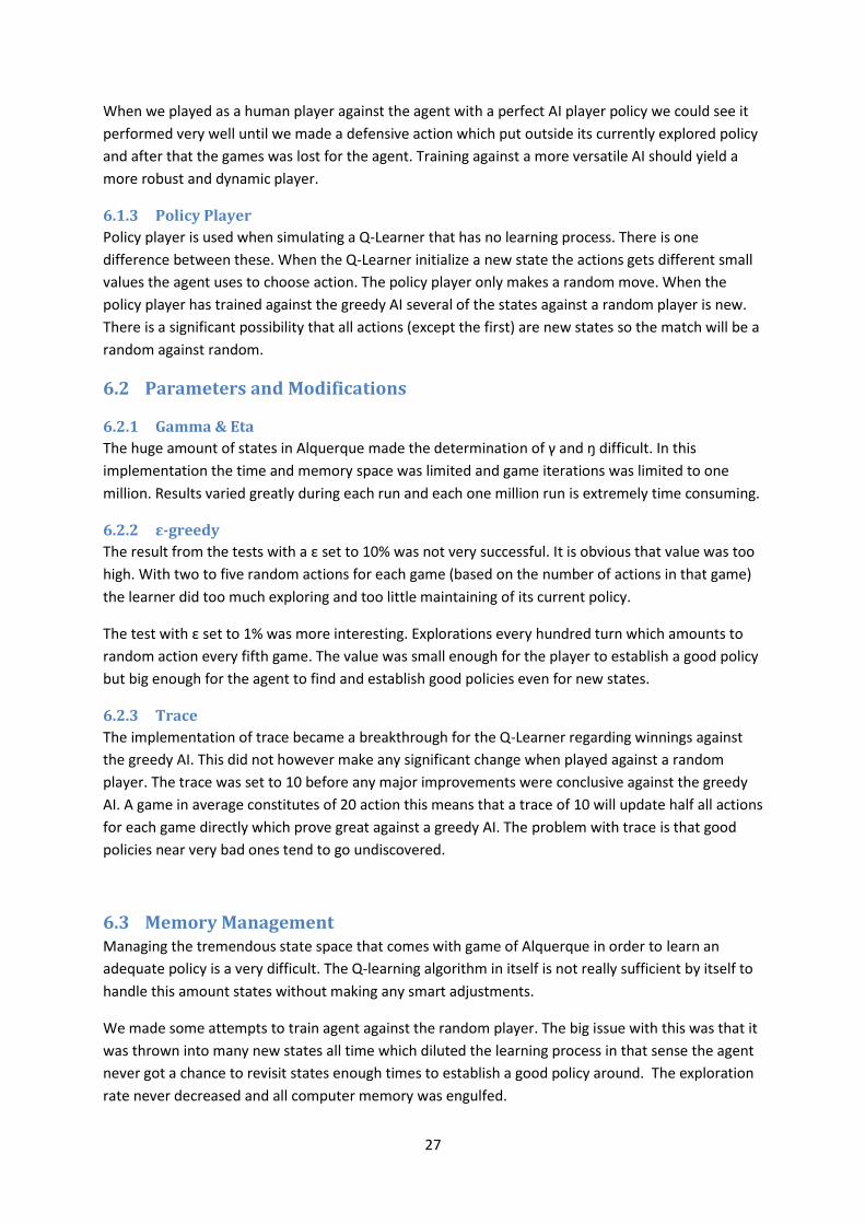
6.1.3 Policy Player................................................................................................................... 27
6.2 Parameters and Modifications .............................................................................................. 27
6.2.1 Gamma & Eta ................................................................................................................. 27
6.2.2 ε-greedy ......................................................................................................................... 27
6.2.3 Trace .............................................................................................................................. 27
6.3 Memory Management .......................................................................................................... 27
7 Sources of Error ............................................................................................................................. 28
8 Conclusions .................................................................................................................................... 28
9 References ..................................................................................................................................... 29
Appendix A - Definitions, Acronyms and Abbreviations ....................................................................... 30
Appendix B - Numbered Board.............................................................................................................. 30
6
Purpose
1.1 Main Aim The main aim of the project is to examine how a self-learning Alquerque player that uses
reinforcement learning behaves during the learning process given different parameters. This involves
implementing the game of Alquerque and then implementing a reinforcement learner using the Q-
learning algorithm.
1.2 Finding a suitable board game In order to facilitate the learning process set up some preferable conditions regarding the game. The game should:
Be free of any random elements such as dice etc.
Have a manageable set of states.
Have a limited set of actions for each state.
Terminate within a reasonable time frame.
Finding a non-trivial game that met all these conditions was not easy so a sacrifice regarding the
manageable set of states was made and we settle for the game Alquerque.
2 Background
2.1 The Game
2.1.1 History
Alquerque is one of the oldest known board games and is believed to have its origin in ancient Egypt.
Stone carvings that depict the game have been found in the temple of Kurna which built in Egypt
1400 before Christ. It is not determined whether these carvings are a later addition. The game is
believed to date at least as far back as 600 B.C. but in literature there are no records of the game
until the late 10th century where the game is mentioned in the book Kitab al-Aghani (book of songs).
Alquerque was originally known as Quirkat and is believed to have gotten its current name when it
was introduced to western world during the Moorish reign of Spain [1].
2.1.2 Rules
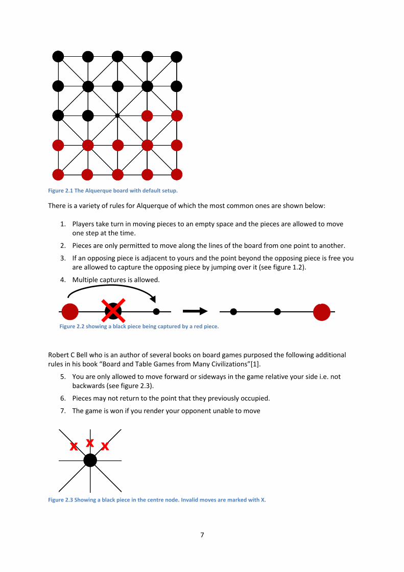
Alquerque is a two-player game played on a 5x5 board (see figure 2.1). Each player has 12 pieces and the goal of the game is to capture your opponent’s pieces. The game is finished when it is apparent that no more moves that will result in capture are available and as an alternative when one player is rendered unable to move.
7
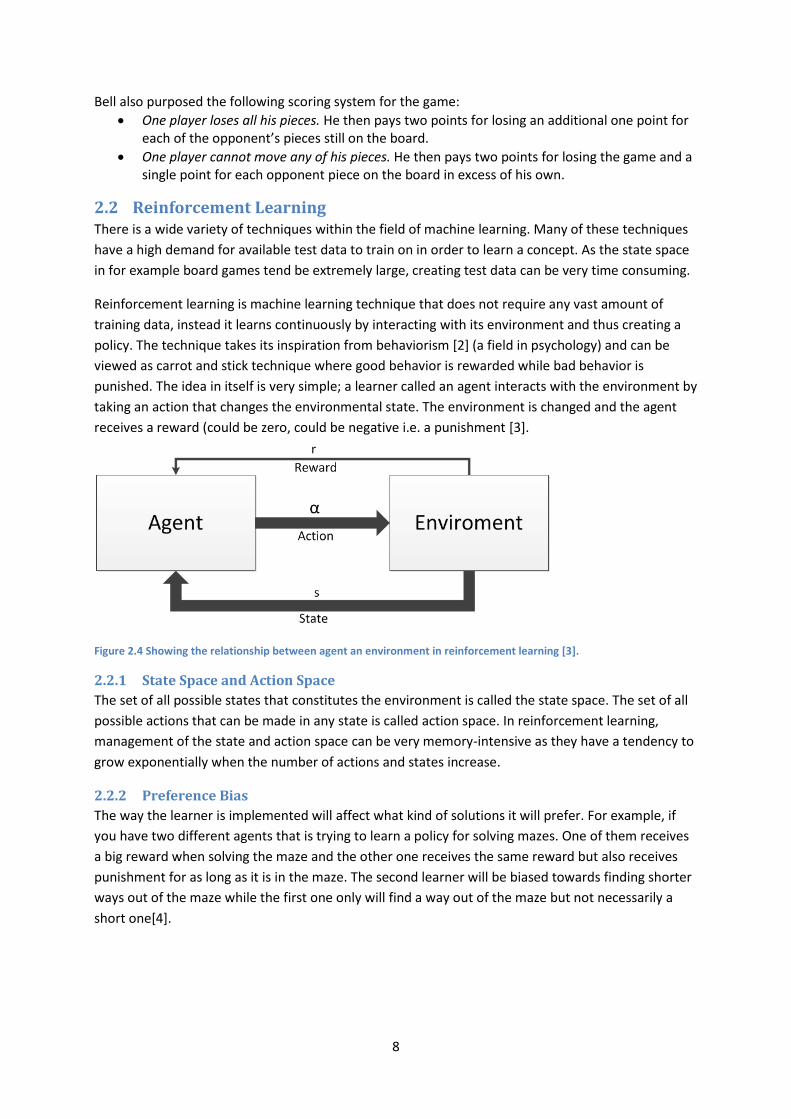
Figure 2.2 showing a black piece being captured by a red piece.
Figure 2.1 The Alquerque board with default setup.
There is a variety of rules for Alquerque of which the most common ones are shown below:
1. Players take turn in moving pieces to an empty space and the pieces are allowed to move one step at the time.
2. Pieces are only permitted to move along the lines of the board from one point to another.
3. If an opposing piece is adjacent to yours and the point beyond the opposing piece is free you are allowed to capture the opposing piece by jumping over it (see figure 1.2).
4. Multiple captures is allowed.
Robert C Bell who is an author of several books on board games purposed the following additional rules in his book “Board and Table Games from Many Civilizations”*1+.
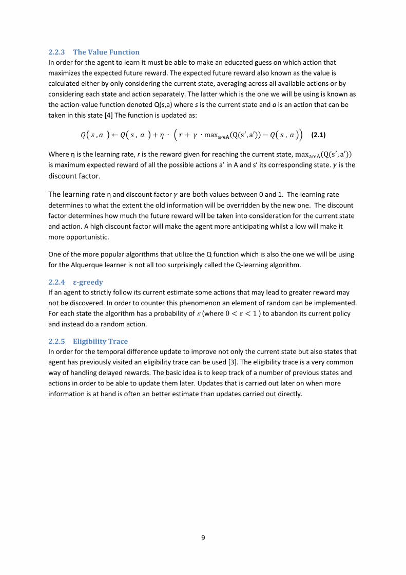
5. You are only allowed to move forward or sideways in the game relative your side i.e. not backwards (see figure 2.3).
6. Pieces may not return to the point that they previously occupied.
7. The game is won if you render your opponent unable to move
Figure 2.3 Showing a black piece in the centre node. Invalid moves are marked with X.
X X X
8
Bell also purposed the following scoring system for the game:
One player loses all his pieces. He then pays two points for losing an additional one point for each of the opponent’s pieces still on the board.
One player cannot move any of his pieces. He then pays two points for losing the game and a single point for each opponent piece on the board in excess of his own.
2.2 Reinforcement Learning There is a wide variety of techniques within the field of machine learning. Many of these techniques
have a high demand for available test data to train on in order to learn a concept. As the state space
in for example board games tend be extremely large, creating test data can be very time consuming.
Reinforcement learning is machine learning technique that does not require any vast amount of
training data, instead it learns continuously by interacting with its environment and thus creating a
policy. The technique takes its inspiration from behaviorism [2] (a field in psychology) and can be
viewed as carrot and stick technique where good behavior is rewarded while bad behavior is
punished. The idea in itself is very simple; a learner called an agent interacts with the environment by
taking an action that changes the environmental state. The environment is changed and the agent
receives a reward (could be zero, could be negative i.e. a punishment [3].
Figure 2.4 Showing the relationship between agent an environment in reinforcement learning [3].
2.2.1 State Space and Action Space
The set of all possible states that constitutes the environment is called the state space. The set of all
possible actions that can be made in any state is called action space. In reinforcement learning,
management of the state and action space can be very memory-intensive as they have a tendency to
grow exponentially when the number of actions and states increase.
2.2.2 Preference Bias
The way the learner is implemented will affect what kind of solutions it will prefer. For example, if
you have two different agents that is trying to learn a policy for solving mazes. One of them receives
a big reward when solving the maze and the other one receives the same reward but also receives
punishment for as long as it is in the maze. The second learner will be biased towards finding shorter
ways out of the maze while the first one only will find a way out of the maze but not necessarily a
short one[4].
9
2.2.3 The Value Function
In order for the agent to learn it must be able to make an educated guess on which action that
maximizes the expected future reward. The expected future reward also known as the value is
calculated either by only considering the current state, averaging across all available actions or by
considering each state and action separately. The latter which is the one we will be using is known as
the action-value function denoted Q(s,a) where s is the current state and a is an action that can be
taken in this state [4] The function is updated as:
( ) ( ) ( ( ( ( )) (2.1)
Where η is the learning rate, r is the reward given for reaching the current state, ( (
is maximum expected reward of all the possible actions a’ in A and s’ its corresponding state. is the
discount factor.
The learning rate η and discount factor are both values between 0 and 1. The learning rate
determines to what the extent the old information will be overridden by the new one. The discount
factor determines how much the future reward will be taken into consideration for the current state
and action. A high discount factor will make the agent more anticipating whilst a low will make it
more opportunistic.
One of the more popular algorithms that utilize the Q function which is also the one we will be using
for the Alquerque learner is not all too surprisingly called the Q-learning algorithm.
2.2.4 ε-greedy
If an agent to strictly follow its current estimate some actions that may lead to greater reward may
not be discovered. In order to counter this phenomenon an element of random can be implemented.
For each state the algorithm has a probability of (where ) to abandon its current policy
and instead do a random action.
2.2.5 Eligibility Trace
In order for the temporal difference update to improve not only the current state but also states that
agent has previously visited an eligibility trace can be used [3]. The eligibility trace is a very common
way of handling delayed rewards. The basic idea is to keep track of a number of previous states and
actions in order to be able to update them later. Updates that is carried out later on when more
information is at hand is often an better estimate than updates carried out directly.
10
2.3 Q-Learning The Q-learning algorithm is basically a search algorithm that explores the state space by taking
actions and establishing a policy by continuous updates using the Q-function. The algorithm in itself
is pretty simple:
Algorithm 2.1: Q-learning
INITALIZE: Q(s,a) small arbitrary values for all states s and actions a
FOR EACH episode:
INITALIZE: s
REPEAT FOR EACH step:
Choose a action a from s based on the policy Q(s,a)
Take action a and observe reward r and next state s’
( ) ( ) ( ( ( ( ))
UNTIL: terminal state
3 Implementing the software
3.1 Programming Language The programming language chosen for this implementation is C#.
3.2 Rules and Limitations
3.2.1 Rule Set
The rule set has been chosen in order to facilitate the learning process as much as possible as this is
the main target. The following rules of the ones stated in 2.2.1 will be included in the game logic:
Players take turn in moving pieces to an empty space and the pieces are allowed to move one step at the time.
Pieces are only permitted to move along the lines of the board from one point to another.
If an opposing piece is adjacent to yours and the point beyond the opposing piece is free you are allowed to capture the opposing piece by jumping over it.
You are only allowed to move forward or sideways in the game relative your side i.e. not backwards.
The game is won if you render your opponent unable to move.
The following rules will be omitted:
Multiple captures is allowed.
Pieces may not return to the point that they previously occupied.
Both of these rules are omitted because they expand the agent’s action space. Expansions of the
actions space inhibits the learning process as more actions have to be explored to gain an adequate
policy. This also inhibits the agent in the sense that a given state can have different sets of actions
11
given how the state was achieved. Programmatically this means that a state can not only be
referenced by a certain state of the board, but also what actions are available i.e. one state on the
board will programmatically constitute to a multitude of states this means that the state space will
grow even further.
3.2.2 State Space
Calculating the exact size of the state space for Alquerque is very complex but as a tremendously
rough estimate one can view each of the 25 positions as having three states: empty or occupied by
either player 1 or player 2. If we disregard the rules for the game the number of permutations
amounts to a staggering 325 i.e. about 847 billion states.
3.2.3 Action Space
The number of actions that can be made for any given state vary depending on the pieces positions.
An estimate to the upper limit is achieved when one player has one piece left and the other one has
at least 10 pieces placed at odd positions of the board. The maximum amount of available actions for
one player is estimated to be 28.
Figure 3.1 showing a state that holds the estimated maximum amount actions.
3.3 General Layout For this project a game engine has to be set up that can run consecutive matches against two
players. Further there are four main players that will be implemented:
A Q-learning agent which is the actual learner.
A random player that is to be used as a reference.
A greedy AI that which the agent will be trained against.
A player that strictly uses a policy learned by an agent in order to test the performance of a
learned policy.
In addition to this a human player will be implemented as reference as to if the agent has developed
any policy that stands against human game player.
12
1
8
7 9 8
3
3.4 The Game Engine The game engine is the core class of the project that takes two players and runs a game against the
two. In order keep track of the available actions for each player the board is view upon as a directed
graph where the positions are nodes and available actions are colored edges corresponding to each
of the two players. As an example figure 3.1 shows a state on the board and its corresponding action
graph.
For each turn the game engine masks out the edges that corresponds to the active player and sends
them as a list of actions to the player. The player returns one of the actions to the game engine and
the game engine executes the action and updates the action graph accordingly.
Algorithm 2.2: The game engine Let Board be 5x5 matrix holding values that correspond to each player where 0 is empty and 1 and 2 is player 1and player 2 respectivly. WHILE (!GameOver) {From,T } GetActionFromActivePlayer(ActionList) Board[To] = ActivePlayer Board[From] = 0 Add to ActionGraph all new possible actions that can be made to From position. Remove from ActionGraph all possible actions that could capture From piece. Remove from ActionGraph all possible actions that can be made to To. Add to ActionGraph all possible actions that can capture To piece. END WHILE
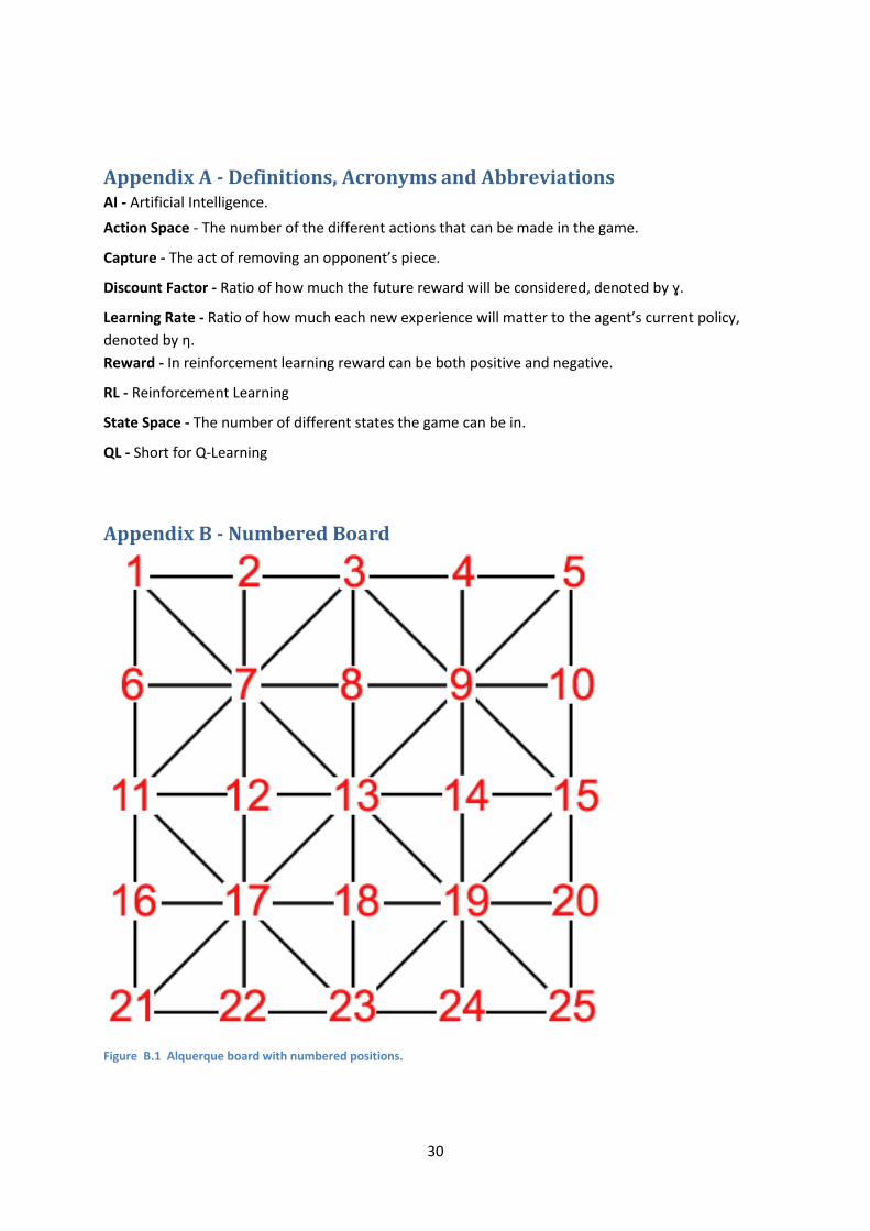
Figure 3.1 shows a state on the board and its corresponding action graph. Node numbering corresponds to the positions on the board where 1 is the top left position (see appendix B for numbered a fully board).
13
3.5 Q-Learning Agent The core of the Q-learning agent will be implemented as stated by algorithm 2.1 with the big difference that the Q(s,a) will not be initialize at start due to the memory limitations. Instead whenever the agent reaches a new state the policy Q(s,a) will be added for each a in state. Each a in the state will be initialized with a small arbitrary value and stored in a hashmap where the key is based on the board state and if agent is player 1 or 2.
3.5.1 Rewards
The agent will always receive a reward of 1 or -1 for winning or losing a game. The ± 1 rewards are to be regarded as infinite positive and infinite negative rewards respectively. In addition to this two different internal reward functions will be implemented. The first one will give a small reward whenever the agent manages to capture an opponent’s piece and small punishment if one of its own pieces gets captured. This means that if the agent captures a piece and then gets captured the reward will amount to 0. The second internal reward function will always give a small negative reward if a piece is captured and else give a small positive reward. The pseudo code below show the two different functions.
Internal Reward Function 1
Internal Reward Function 2
3.5.2 Trace
In order to manage the massive state space a trace of variable length will be implemented. The trace will only update back when hitting the terminal state (winning or losing state) e.g. if the trace is set to 3, the last 3 states and actions that led to the terminal state will be updated (see figure [3.2]).
η=0,2 ɣ =0,8
Figure 3.2 Shows the updated values being updated from a losing terminal state St and 3 steps back when learning rate η is set 0,2 and discount factor ɣ is set to 0,8. The initial policy value of the above states was 0.
14
3.6 Random Player The random player will as the name suggests for each turn pick an action purely at random. As stated
before, the random player will be used as performance reference for the Q-learner to see if any
learning has occurred at all. Establishing a policy when training against a purely random player is
hard can be very memory intensive. The random player has a very high chance of constantly putting
the Q-learning agent in new states which has to be saved into the policy. With a massive state space
like the one for Alquerque it is a high risk that the exploration will cause exhaustion of the memory.
3.7 The Greedy AI When learning against a player that follows a more strict protocol the Q-learner has higher chance of
establishing an adequate policy without having to explore massive amount of states. For this purpose
we will implement a very simple AI that follows a greedy protocol. The greedy AI will first and
foremost try to capture its opponents pieces, if no captures are available it will try to advance as high
up on the board as possible and lastly if only sidestep actions are available pick one of these sidestep
actions at random.
Algorithm 3: Greedy AI Input: Actionlist – A list of available actions Output: Action to take ( ( { } ( //Most frontal forward action END IF RETURN RandomAction(Actionlist) //Only side steps in Actionlist
4 Tests A series of tests has been setup to investigate if and how the Q-learning agent’s behavior changes
when the agent’s parameters are changed. First a reference test will be carried out (see 4.1.1) in
order to establish a performance baseline for the Q-learning agent. For all games and test player 1
will be the one to start.
In all tests involving a Q-learning agent the agent will only be playing as player 1. The reason for this
is in order to maintain consistency when changing the different Q-learning parameters. If there is any
advantage or disadvantage to be first, this should show in the first reference test and then taken into
consideration.
15
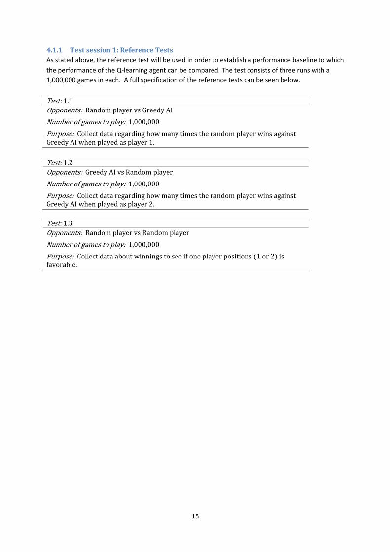
4.1.1 Test session 1: Reference Tests
As stated above, the reference test will be used in order to establish a performance baseline to which
the performance of the Q-learning agent can be compared. The test consists of three runs with a
1,000,000 games in each. A full specification of the reference tests can be seen below.
Test: 1.1
Opponents: Random player vs Greedy AI
Number of games to play: 1,000,000
Purpose: Collect data regarding how many times the random player wins against Greedy AI when played as player 1.
Test: 1.2
Opponents: Greedy AI vs Random player
Number of games to play: 1,000,000
Purpose: Collect data regarding how many times the random player wins against Greedy AI when played as player 2.
Test: 1.3
Opponents: Random player vs Random player
Number of games to play: 1,000,000
Purpose: Collect data about winnings to see if one player positions (1 or 2) is favorable.
16
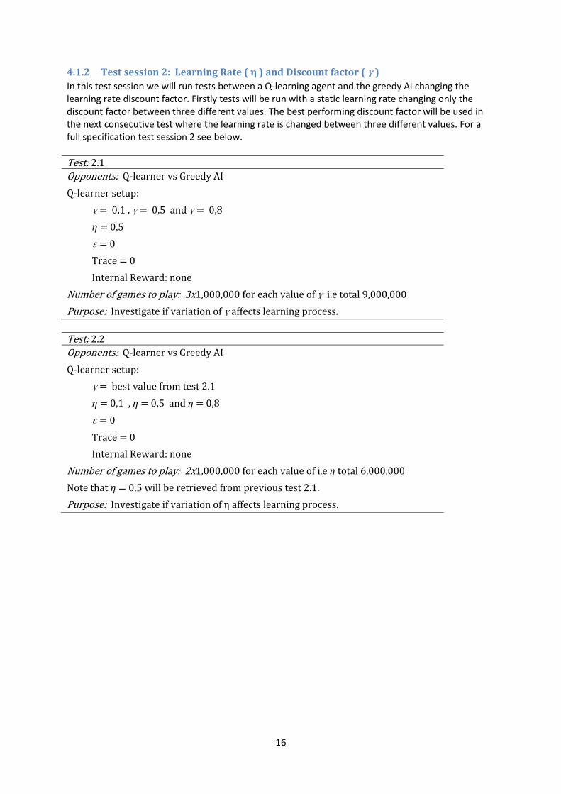
4.1.2 Test session 2: Learning Rate ( η ) and Discount factor ( )
In this test session we will run tests between a Q-learning agent and the greedy AI changing the learning rate discount factor. Firstly tests will be run with a static learning rate changing only the discount factor between three different values. The best performing discount factor will be used in the next consecutive test where the learning rate is changed between three different values. For a full specification test session 2 see below.
Test: 2.1
Opponents: Q-learner vs Greedy AI
Q-learner setup:
= 0,1 , = 0,5 and = 0,8
= 0,5
= 0
Trace = 0
Internal Reward: none
Number of games to play: 3x1,000,000 for each value of i.e total 9,000,000
Purpose: Investigate if variation of affects learning process.
Test: 2.2
Opponents: Q-learner vs Greedy AI
Q-learner setup:
= best value from test 2.1
= 0,1 , = 0,5 and = 0,8
= 0
Trace = 0
Internal Reward: none
Number of games to play: 2x1,000,000 for each value of i.e total 6,000,000
Note that = 0,5 will be retrieved from previous test 2.1.
Purpose: I f f η ff .
17
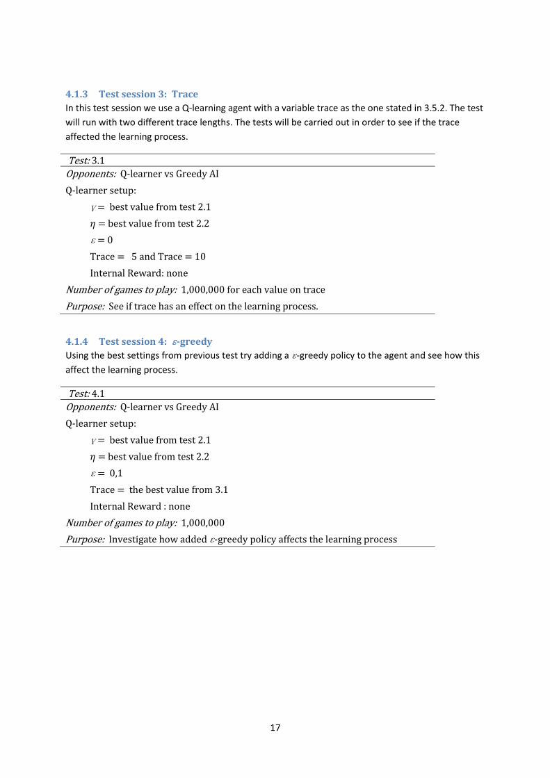
4.1.3 Test session 3: Trace
In this test session we use a Q-learning agent with a variable trace as the one stated in 3.5.2. The test
will run with two different trace lengths. The tests will be carried out in order to see if the trace
affected the learning process.
Test: 3.1
Opponents: Q-learner vs Greedy AI
Q-learner setup:
= best value from test 2.1
= best value from test 2.2
= 0
Trace = 5 and Trace = 10
Internal Reward: none
Number of games to play: 1,000,000 for each value on trace
Purpose: See if trace has an effect on the learning process.
4.1.4 Test session 4: -greedy
Using the best settings from previous test try adding a -greedy policy to the agent and see how this
affect the learning process.
Test: 4.1
Opponents: Q-learner vs Greedy AI
Q-learner setup:
= best value from test 2.1
= best value from test 2.2
= 0,1
Trace = the best value from 3.1
Internal Reward : none
Number of games to play: 1,000,000
Purpose: Investigate how added -greedy policy affects the learning process
18
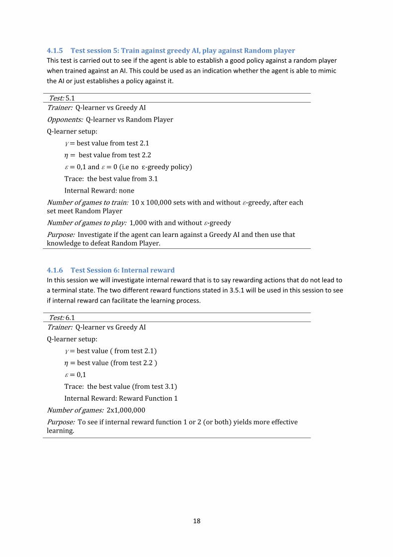
4.1.5 Test session 5: Train against greedy AI, play against Random player
This test is carried out to see if the agent is able to establish a good policy against a random player
when trained against an AI. This could be used as an indication whether the agent is able to mimic
the AI or just establishes a policy against it.
Test: 5.1
Trainer: Q-learner vs Greedy AI
Opponents: Q-learner vs Random Player
Q-learner setup:
= best value from test 2.1
= best value from test 2.2
= 0,1 and = 0 (i.e no ɛ-greedy policy)
Trace: the best value from 3.1
Internal Reward: none
Number of games to train: 10 x 100,000 sets with and without -greedy, after each set meet Random Player
Number of games to play: 1,000 with and without -greedy
Purpose: Investigate if the agent can learn against a Greedy AI and then use that knowledge to defeat Random Player.
4.1.6 Test Session 6: Internal reward
In this session we will investigate internal reward that is to say rewarding actions that do not lead to
a terminal state. The two different reward functions stated in 3.5.1 will be used in this session to see
if internal reward can facilitate the learning process.
Test: 6.1
Trainer: Q-learner vs Greedy AI
Q-learner setup:
= best value ( from test 2.1)
= best value (from test 2.2 )
= 0,1
Trace: the best value (from test 3.1)
Internal Reward: Reward Function 1
Number of games: 2x1,000,000
Purpose: To see if internal reward function 1 or 2 (or both) yields more effective learning.
19
Test: 6.2
Trainer: Q-learner vs Greedy AI
Q-learner setup:
= best value ( from test 2.1)
= best value (from test 2.2 )
= 0
Trace: the best value (from test 3.1)
Internal Reward: Reward Function 1
Number of games: 2x1,000,000
Purpose: To see if internal reward function 1 or 2 (or both) yields more effective learning without using an -greedy policy.
5 Results
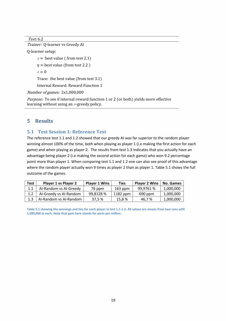
5.1 Test Session 1: Reference Test The reference test 1.1 and 1.2 showed that our greedy AI was far superior to the random player
winning almost 100% of the time, both when playing as player 1 (i.e making the first action for each
game) and when playing as player 2. The results from test 1.3 indicates that you actually have an
advantage being player 2 (i.e making the second action for each game) who won 9.2 percentage
point more than player 1. When comparing test 1.1 and 1.2 one can also see proof of this advantage
where the random player actually won 9 times as player 2 than as player 1. Table 5.1 shows the full
outcome of the games.
Test Player 1 vs Player 2 Player 1 Wins Ties Player 2 Wins No. Games
1.1 AI-Random vs AI-Greedy 76 ppm 163 ppm 99,9761 % 1,000,000
1.2 AI-Greedy vs AI-Random 99,8128 % 1182 ppm 690 ppm 1,000,000
1.3 AI-Random vs AI-Random 37,5 % 15,8 % 46,7 % 1,000,000
Table 5.1 showing the winnings and ties for each player in test 1.1-1.3. All values are means from two runs with 1,000,000 in each. Note that ppm here stands for parts per million.
20
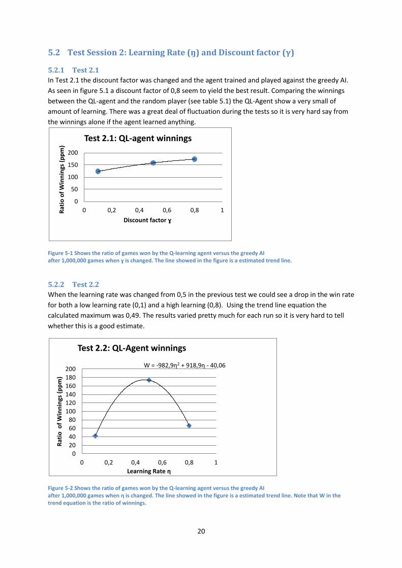
5.2 Test Session 2: Learning Rate (ŋ) and Discount factor (γ)
5.2.1 Test 2.1
In Test 2.1 the discount factor was changed and the agent trained and played against the greedy AI.
As seen in figure 5.1 a discount factor of 0,8 seem to yield the best result. Comparing the winnings
between the QL-agent and the random player (see table 5.1) the QL-Agent show a very small of
amount of learning. There was a great deal of fluctuation during the tests so it is very hard say from
the winnings alone if the agent learned anything.
Figure 5-1 Shows the ratio of games won by the Q-learning agent versus the greedy AI after 1,000,000 games when ɣ is changed. The line showed in the figure is a estimated trend line.
5.2.2 Test 2.2
When the learning rate was changed from 0,5 in the previous test we could see a drop in the win rate
for both a low learning rate (0,1) and a high learning (0,8). Using the trend line equation the
calculated maximum was 0,49. The results varied pretty much for each run so it is very hard to tell
whether this is a good estimate.
Figure 5-2 Shows the ratio of games won by the Q-learning agent versus the greedy AI after 1,000,000 games when η is changed. The line showed in the figure is a estimated trend line. Note that W in the trend equation is the ratio of winnings.
0
50
100
150
200
0 0,2 0,4 0,6 0,8 1Rat
io o
f W
inn
ings
(p
pm
)
Discount factor ɣ
Test 2.1: QL-agent winnings
W = -982,9η2 + 918,9η - 40,06
0
20
40
60
80
100
120
140
160
180
200
0 0,2 0,4 0,6 0,8 1
Rat
io o
f W
inn
ings
(p
pm
)
Learning Rate η
Test 2.2: QL-Agent winnings
21
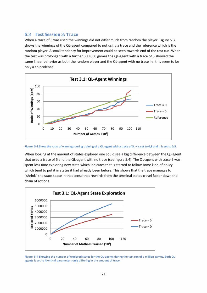
5.3 Test Session 3: Trace When a trace of 5 was used the winnings did not differ much from random the player. Figure 5.3
shows the winnings of the QL-agent compared to not using a trace and the reference which is the
random player. A small tendency for improvement could be seen towards end of the test run. When
the test was prolonged with a further 300,000 games the QL-agent with a trace of 5 showed the
same linear behavior as both the random player and the QL-agent with no trace i.e. this seem to be
only a coincidence.
Figure 5-3 Show the ratio of winnings during training of a QL-agent with a trace of 5. γ is set to 0,8 and η is set to 0,5.
When looking at the amount of states explored one could see a big difference between the QL-agent
that used a trace of 5 and the QL-agent with no trace (see figure 5.4). The QL-agent with trace 5 was
spent less time exploring new state which indicates that is started to follow some kind of policy
which tend to put it in states it had already been before. This shows that the trace manages to
“shrink” the state space in that sense that rewards from the terminal states travel faster down the
chain of actions.
Figure 5-4 Showing the number of explored states for the QL-agents during the test run of a million games. Both QL-agents is set to identical parameters only differing in the amount of trace.
0
20
40
60
80
100
0 10 20 30 40 50 60 70 80 90 100 110
Rat
io o
f W
inn
ings
(p
pm
)
Number of Games (104)
Test 3.1: QL-Agent Winnings
Trace = 0
Trace = 5
Reference
0
1000000
2000000
3000000
4000000
5000000
6000000
0 20 40 60 80 100 120
Exp
lore
d S
tate
s
Number of Mathces Trained (104)
Test 3.1: QL-Agent State Exploration
Trace = 5
Trace = 0
22
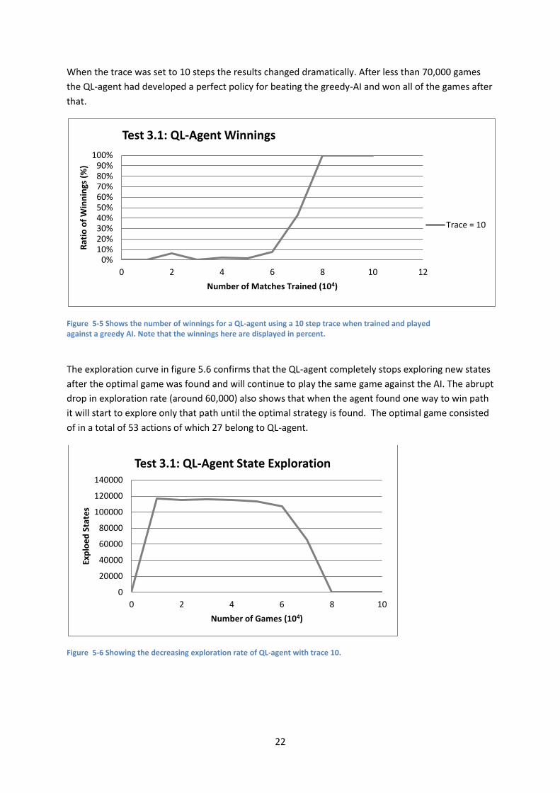
When the trace was set to 10 steps the results changed dramatically. After less than 70,000 games
the QL-agent had developed a perfect policy for beating the greedy-AI and won all of the games after
that.
Figure 5-5 Shows the number of winnings for a QL-agent using a 10 step trace when trained and played against a greedy AI. Note that the winnings here are displayed in percent.
The exploration curve in figure 5.6 confirms that the QL-agent completely stops exploring new states
after the optimal game was found and will continue to play the same game against the AI. The abrupt
drop in exploration rate (around 60,000) also shows that when the agent found one way to win path
it will start to explore only that path until the optimal strategy is found. The optimal game consisted
of in a total of 53 actions of which 27 belong to QL-agent.
Figure 5-6 Showing the decreasing exploration rate of QL-agent with trace 10.
0%10%20%30%40%50%60%70%80%90%
100%
0 2 4 6 8 10 12
Rat
io o
f W
inn
ings
(%
)
Number of Matches Trained (104)
Test 3.1: QL-Agent Winnings
Trace = 10
0
20000
40000
60000
80000
100000
120000
140000
0 2 4 6 8 10
Exp
loe
d S
tate
s
Number of Games (104)
Test 3.1: QL-Agent State Exploration
23
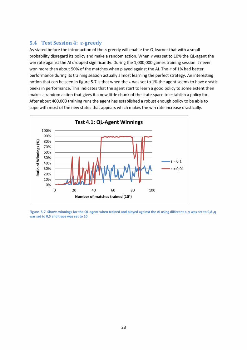
5.4 Test Session 4: ε-greedy As stated before the introduction of the -greedy will enable the Q-learner that with a small
probability disregard its policy and make a random action. When was set to 10% the QL-agent the
win rate against the AI dropped significantly. During the 1,000,000 games training session it never
won more than about 50% of the matches when played against the AI. The of 1% had better
performance during its training session actually almost learning the perfect strategy. An interesting
notion that can be seen in figure 5.7 is that when the was set to 1% the agent seems to have drastic
peeks in performance. This indicates that the agent start to learn a good policy to some extent then
makes a random action that gives it a new little chunk of the state space to establish a policy for.
After about 400,000 training runs the agent has established a robust enough policy to be able to
cope with most of the new states that appears which makes the win rate increase drastically.
Figure 5-7 Shows winnings for the QL-agent when trained and played against the AI using different ε. γ was set to 0,8 ,η was set to 0,5 and trace was set to 10.
0%
10%
20%
30%
40%
50%
60%
70%
80%
90%
100%
0 20 40 60 80 100
Rat
io o
f W
inn
ings
(%
)
Number of matches trained (104)
Test 4.1: QL-Agent Winnings
ε = 0,1
ε = 0,01
24
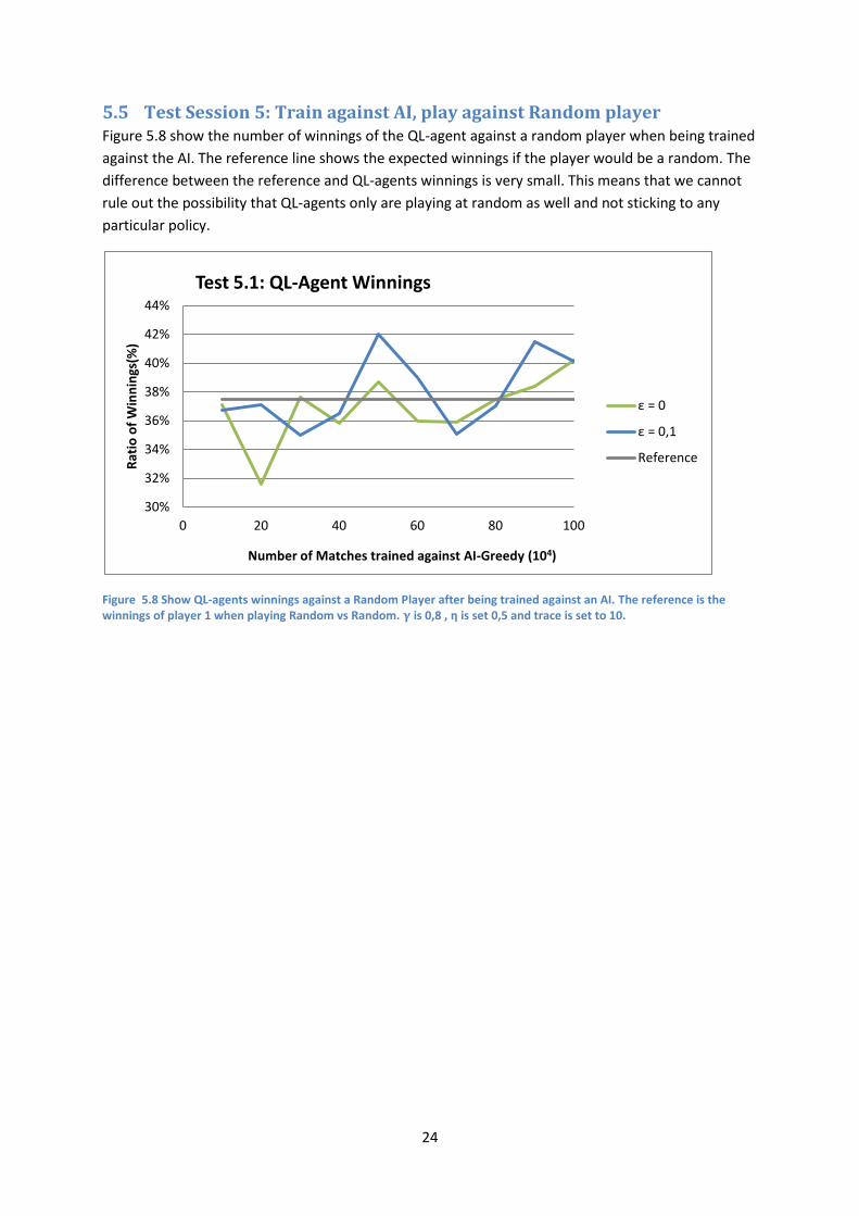
5.5 Test Session 5: Train against AI, play against Random player Figure 5.8 show the number of winnings of the QL-agent against a random player when being trained
against the AI. The reference line shows the expected winnings if the player would be a random. The
difference between the reference and QL-agents winnings is very small. This means that we cannot
rule out the possibility that QL-agents only are playing at random as well and not sticking to any
particular policy.
Figure 5.8 Show QL-agents winnings against a Random Player after being trained against an AI. The reference is the winnings of player 1 when playing Random vs Random. 𝛄 is 0,8 , η is set 0,5 and trace is set to 10.
30%
32%
34%
36%
38%
40%
42%
44%
0 20 40 60 80 100
Rat
io o
f W
inn
ings
(%)
Number of Matches trained against AI-Greedy (104)
Test 5.1: QL-Agent Winnings
ε = 0
ε = 0,1
Reference
25
5.6 Test Session 6: Internal Reward
5.6.1 Test 6.1
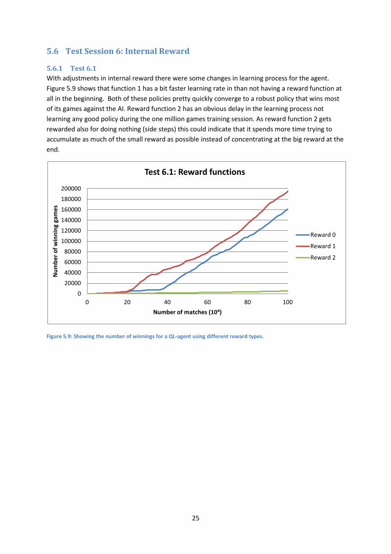
With adjustments in internal reward there were some changes in learning process for the agent.
Figure 5.9 shows that function 1 has a bit faster learning rate in than not having a reward function at
all in the beginning. Both of these policies pretty quickly converge to a robust policy that wins most
of its games against the AI. Reward function 2 has an obvious delay in the learning process not
learning any good policy during the one million games training session. As reward function 2 gets
rewarded also for doing nothing (side steps) this could indicate that it spends more time trying to
accumulate as much of the small reward as possible instead of concentrating at the big reward at the
end.
Figure 5.9: Showing the number of winnings for a QL-agent using different reward types.
0
20000
40000
60000
80000
100000
120000
140000
160000
180000
200000
0 20 40 60 80 100
Nu
mb
er
of
win
nin
g ga
me
s
Number of matches (104)
Test 6.1: Reward functions
Reward 0
Reward 1
Reward 2
26
5.6.2 Test 6.2
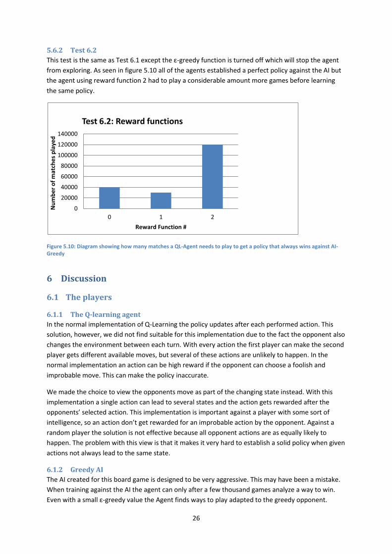
This test is the same as Test 6.1 except the ε-greedy function is turned off which will stop the agent
from exploring. As seen in figure 5.10 all of the agents established a perfect policy against the AI but
the agent using reward function 2 had to play a considerable amount more games before learning
the same policy.
Figure 5.10: Diagram showing how many matches a QL-Agent needs to play to get a policy that always wins against AI-Greedy
6 Discussion
6.1 The players
6.1.1 The Q-learning agent
In the normal implementation of Q-Learning the policy updates after each performed action. This
solution, however, we did not find suitable for this implementation due to the fact the opponent also
changes the environment between each turn. With every action the first player can make the second
player gets different available moves, but several of these actions are unlikely to happen. In the
normal implementation an action can be high reward if the opponent can choose a foolish and
improbable move. This can make the policy inaccurate.
We made the choice to view the opponents move as part of the changing state instead. With this
implementation a single action can lead to several states and the action gets rewarded after the
opponents’ selected action. This implementation is important against a player with some sort of
intelligence, so an action don’t get rewarded for an improbable action by the opponent. Against a
random player the solution is not effective because all opponent actions are as equally likely to
happen. The problem with this view is that it makes it very hard to establish a solid policy when given
actions not always lead to the same state.
6.1.2 Greedy AI
The AI created for this board game is designed to be very aggressive. This may have been a mistake.
When training against the AI the agent can only after a few thousand games analyze a way to win.
Even with a small ε-greedy value the Agent finds ways to play adapted to the greedy opponent.
0
20000
40000
60000
80000
100000
120000
140000
0 1 2
Nu
mb
er
of
mat
che
s p
laye
d
Reward Function #
Test 6.2: Reward functions
27
When we played as a human player against the agent with a perfect AI player policy we could see it
performed very well until we made a defensive action which put outside its currently explored policy
and after that the games was lost for the agent. Training against a more versatile AI should yield a
more robust and dynamic player.
6.1.3 Policy Player
Policy player is used when simulating a Q-Learner that has no learning process. There is one
difference between these. When the Q-Learner initialize a new state the actions gets different small
values the agent uses to choose action. The policy player only makes a random move. When the
policy player has trained against the greedy AI several of the states against a random player is new.
There is a significant possibility that all actions (except the first) are new states so the match will be a
random against random.
6.2 Parameters and Modifications
6.2.1 Gamma & Eta
The huge amount of states in Alquerque made the determination of γ and ŋ difficult. In this
implementation the time and memory space was limited and game iterations was limited to one
million. Results varied greatly during each run and each one million run is extremely time consuming.
6.2.2 ε-greedy
The result from the tests with a ε set to 10% was not very successful. It is obvious that value was too
high. With two to five random actions for each game (based on the number of actions in that game)
the learner did too much exploring and too little maintaining of its current policy.
The test with ε set to 1% was more interesting. Explorations every hundred turn which amounts to
random action every fifth game. The value was small enough for the player to establish a good policy
but big enough for the agent to find and establish good policies even for new states.
6.2.3 Trace
The implementation of trace became a breakthrough for the Q-Learner regarding winnings against
the greedy AI. This did not however make any significant change when played against a random
player. The trace was set to 10 before any major improvements were conclusive against the greedy
AI. A game in average constitutes of 20 action this means that a trace of 10 will update half all actions
for each game directly which prove great against a greedy AI. The problem with trace is that good
policies near very bad ones tend to go undiscovered.
6.3 Memory Management Managing the tremendous state space that comes with game of Alquerque in order to learn an
adequate policy is a very difficult. The Q-learning algorithm in itself is not really sufficient by itself to
handle this amount states without making any smart adjustments.
We made some attempts to train agent against the random player. The big issue with this was that it
was thrown into many new states all time which diluted the learning process in that sense the agent
never got a chance to revisit states enough times to establish a good policy around. The exploration
rate never decreased and all computer memory was engulfed.
28
There are some modifications that could have been done in order to shrink the number of states that
the agent has to keep in the memory in order to establish a good policy. One is to exploit the
symmetry of the Alquerque board and keep a unified policy for all states which mirror each other.
Establishing a smart environment model seems to be the key to success regarding the Q-learning
algorithm in general.
7 Sources of Error When running test against thing with a random nature there is always the possibility for errors. The
initializing of small arbitrary random values in Q(s,a) function may have affected the results during
the tests especially regarding the test session 2 where we saw a lot of fluctuation.
One cannot rule out that the way the trace method was implemented (see 3.5.2) together with giving
a huge reward when winning may have made agent somewhat biased towards finding a perfect
policy against the simple greedy AI.
8 Conclusions This project has been very educational in understanding how the Q-learning algorithm works and
what its limitations are. There are a lot of benefits in using the Q-learning algorithm, one of the big
ones being the simplicity of implementation.
The hard part about Q-learning is figuring out how to model the environment in structured manner
enough for the Q-learner to be able to explore and establish a policy in an effective way. The
algorithm seem to be very effective in finding good policies when there is an underlying order, take
away the order and everything becomes a lot more difficult. The Q-learning agent that used a trace
of 10 proved very effective in finding a policy for beating the greedy AI but when put against a
random player the tests were inconclusive.
During the tests we manage to establish a very good policy for beating the greedy AI but when
playing against a random player there was no verifiable difference between the QL-agent and a
random player. This put the three players in sort of rock paper scissors situation where the QL-agent
beats the AI, the AI beats the random player and the random player beats the QL-agent (when QL-
agent is player 1 that is). This indicates that the QL-agent does not mimic the AI in any way but
merely finds a way to beat it and when faced with a random player it did not have a robust enough
policy.
Many stones have been left unturned; however we both feel that the project has yielded many
interesting inputs for further studies.
29
9 References [1] Bell, Robert.C. (1979). Board and Table Games from Many Civilizations. New York City: Dover Publications. volume 1. pp. 47-48. ISBN 978-0486238555. [2] Sutton, Richard.S & Barto, Andrew.G.(1998). Reinforcement Learning an Introduction. Cambridge: MIT Press. ISBN 978-0262193986
[3 ]Ekeberg, Ö. (2010) Lecture about Reinforcement Learning in course DD2431(KTH) with Örjan Ekeberg Dep. Computational Biology, Royal Institute of Technology. 2010-10-04 (about 2h.)
[4] Marsland, Stephen. (2009). Machine Learning An algorithmic perspective. Boca Raton: Taylor & Francis Group. pp 293-307. ISBN: 978-1420067187
30
Appendix A - Definitions, Acronyms and Abbreviations AI - Artificial Intelligence.
Action Space - The number of the different actions that can be made in the game.
Capture - The act of removing an opponent’s piece.
Discount Factor - Ratio of how much the future reward will be considered, denoted by ɣ.
Learning Rate - Ratio of how much each new experience will matter to the agent’s current policy,
denoted by η.
Reward - In reinforcement learning reward can be both positive and negative.
RL - Reinforcement Learning
State Space - The number of different states the game can be in.
QL - Short for Q-Learning
Appendix B - Numbered Board
Figure B.1 Alquerque board with numbered positions.

www.kth.se