Single-machine scheduling with a time-dependent learning effect

ARTICLE IN PRESS

0925-5273/$ - se

doi:10.1016/j.ijp

�CorrespondiInstitute of Aero

Republic of Ch

E-mail addr

[email protected]

(T.C.E. Cheng),

Int. J. Production Economics 111 (2008) 802–811

www.elsevier.com/locate/ijpe

Single-machine scheduling with a time-dependent learning effect

J.-B. Wanga,b,�, C.T. Ngb, T.C.E. Chengb, L.L. Liub

aDepartment of Science, Shenyang Institute of Aeronautical Engineering, Shenyang 110136, People’s Republic of ChinabDepartment of Logistics, The Hong Kong Polytechnic University, Hung Hom, Kowloon, Hong Kong SAR, People’s Republic of China

Received 22 December 2005; accepted 28 March 2007

Available online 27 April 2007

Abstract

In this paper we consider the single-machine scheduling problem with a time-dependent learning effect. The time-

dependent learning effect of a job is assumed to be a function of the total normal processing time of the jobs scheduled in

front of the job. We show by examples that the optimal schedule for the classical version of the problem is not optimal in

the presence of a time-dependent learning effect for the following three objective functions: the weighted sum of

completion times, the maximum lateness and the number of tardy jobs. But for some special cases, we prove that the

weighted shortest processing time (WSPT) rule, the earliest due date (EDD) rule and Moore’s Algorithm can construct an

optimal schedule for the problem to minimize these objective functions, respectively. We use these three rules as heuristics

for the general cases and analyze their worst-case error bounds. We also provide computational results to evaluate the

performance of the heuristics.

r 2007 Elsevier B.V. All rights reserved.

Keywords: Scheduling; Single machine; Learning effect; Time-dependent

1. Introduction

In classical scheduling problems the processingtime of a job is assumed to be a constant. However,in many realistic production environments, bothmachines and workers can improve their perfor-mance by repeating their operations. Therefore, theactual processing time of a job is shorter if it isprocessed later. This phenomenon is known as the‘‘learning effect’’ in the literature (Badiru, 1992;Chiua and Chen, 2005; Alamri and Balkhi, 2007).

e front matter r 2007 Elsevier B.V. All rights reserved

e.2007.03.013

ng author. Department of Science, Shenyang

nautical Engineering, Shenyang 110136, People’s

ina.

esses: [email protected] (J.-B. Wang),

du.hk (C.T. Ng), [email protected]

[email protected] (L.L. Liu).

Although learning theory was first applied toindustry more than 60 years ago (Wright, 1936), ithas only become a topic in scheduling research inrecent years.

Biskup (1999) and Cheng and Wang (2000) wereamong the pioneers that introduced the concept oflearning into the field of scheduling, although thelearning effect has been widely observed and takeninto account in repetitive manufacturing since itsdiscovery by Wright (1936). Biskup (1999) provedthat single-machine scheduling with a learning effectremains polynomial solvable if its objective is tominimize the deviation of job completion timesfrom a common due date or to minimize the sum ofjob flow times. Cheng and Wang (2000) considereda single-machine scheduling problem in which thejob processing times decrease as a result of learning.

.

www.elsevier.com/locate/ijpe

dx.doi.org/10.1016/j.ijpe.2007.03.013

mailto:[email protected]





ARTICLE IN PRESSJ.-B. Wang et al. / Int. J. Production Economics 111 (2008) 802–811 803

A volume-dependent piecewise linear processingtime function was used to model the learning effect.The objective is to minimize the maximum lateness.They showed that the problem is NP-hard inthe strong sense and then identified two specialcases that are polynomially solvable. They alsoproposed two heuristics and analyzed their worst-case performance. Mosheiov (2001a, b) investigatedseveral other single-machine problems and theproblem of minimizing the total flow time onidentical parallel machines. Liu et al. (2003) provedthat the weighted shortest processing time (WSPT)rule, the earliest due date (EDD) rule and themodified Moore–Hodgson algorithm can, undercertain conditions, construct the optimal schedulefor the problem to minimize the following threeobjectives: the total weighted completion time,the maximum lateness and the number of tardyjobs, respectively. They also gave an error estima-tion for each of these rules for the general cases. Leeand Wu (2004) proposed a heuristic algorithmto solve the problem to minimize the total comple-tion time in a two-machine flow shop with alearning effect. Lee et al. (2004) studied the learningeffect in a bi-criterion single machine schedulingproblem, with the objective of minimizing a linearcombination of the total completion time and themaximum tardiness. They presented a branch-and-bound and a heuristic algorithm to search forthe optimal and near-optimal solutions. Mosheiovand Sidney (2003) considered a job-dependentlearning curve, where the learning rate of some jobsis faster than that of the others. Biskup and Simons(2004) considered a scheduling problem where theprocessing times decrease according to a learningrate, which can be influenced by an initial cost-incurring investment. They presented a formulationof the common due date scheduling problem withautonomous and induced learning effects. Theyfurther proved some structural properties, whichenable the development of a polynomial boundsolution procedure. Mosheiov and Sidney (2005)introduced a polynomial time solution for thesingle-machine scheduling problem to minimizethe number of tardy jobs with general non-increas-ing job-dependent learning curves and a commondue-date. Wang (2005) considered flow shopscheduling problems with a learning effect. Hesuggested the use of Johnson’s rule as a heuristicalgorithm for two-machine flow shop schedulingto minimize the makespan. He also developedpolynomial time solution algorithms for some

special cases of the problem to minimize thefollowing objective functions: the weighted sum ofcompletion times and the maximum lateness. Wangand Xia (2005) considered the same problem ofWang (2005). The objective is to minimize one oftwo regular performance measures, namely themakespan and the total flow time. They gave aheuristic algorithm with a worst-case error boundof m for each criterion, where m is the numberof machines. They also found polynomial timesolutions for two special cases of the problem,i.e., identical processing times on each machineand an increasing series of dominating machines.Kuo and Yang (2006a) considered a single-machinescheduling problem with a time-based learningeffect. They showed that the makespan minimiza-tion problem can be solved in polynomial time.Kuo and Yang (2006b) considered a single-machinescheduling problem with a time-dependent learningeffect. The time-dependent learning effect of ajob is assumed to be a function of the totalnormal processing time of the jobs scheduled infront of it. They showed that the SPT-sequenceis optimal for the objective of minimizing thetotal completion time. Kuo and Yang (2006c)considered the single-machine group schedulingproblem with a time-dependent learning effect.They showed that the single-machine group sche-duling problem with a time-dependent learningeffect remains polynomially solvable for theobjectives of minimizing the makespan and mini-mizing the total completion time. Kuolamas andKyparisis (2007) considered a single-machine sche-duling problem with general learning functions. Thelearning is expressed as a function of the sum of theprocessing times of the already processed jobs. Theyshowed that the SPT-sequence is optimal for theobjectives of minimizing the makespan and totalcompletion time. They also considered two-machineflowshop scheduling with general learning func-tions. A survey of this line of scheduling researchcan be found in Bachman and Janiak (2004). Morerecent papers which have addressed schedulingproblems with learning effect and deteriorating jobsinclude Wang (2006, 2007), and Wang and Cheng(2007a, b).

In this paper we consider the same model as thatof Kuo and Yang (2006b), but with differentobjective functions. The time-dependent learningeffect can be found in many real-life schedulingsituations. Kuolamas and Kyparisis (2007) dis-cussed several real-life examples of this effect in a

ARTICLE IN PRESSJ.-B. Wang et al. / Int. J. Production Economics 111 (2008) 802–811804

scheduling context. For example, steel plates or barsproduced by a foundry need to be inspected forsurface defects. The actual area of each plate or theactual length of each bar to be inspected can beviewed as work content, the plates or the bars canbe viewed as individual jobs, and the inspector canbe viewed as the processor. The learning rate of theinspector depends not on the number of plates orbars he has inspected, but on the actual total area ofplates or the actual total length of bars he hasinspected. Another example is that firms andemployees will learn more from performing jobswith longer processing times, i.e., the more time onehas devoted to practising a skill, the betterperformance one will produce as a result of learning(Kuo and Yang 2006a–c).

The remaining part of this paper is organized asfollows. In Section 2 we formulate the model. InSection 3 we consider three classical single machinescheduling problems. In Section 4 we presentcomputational experiments to evaluate the perfor-mance of the heuristic algorithms. The last sectionpresents the conclusions.

2. Problem formulation

The focus of this paper is to study the time-dependent learning effect in scheduling. The modelis described as follows. There are given a singlemachine and n independent and non-preemptivejobs that are immediately available for processing.The machine can handle one job at a time andpreemption is not allowed. Let pj be the normalprocessing time of job j and p½k� the normalprocessing time of a job if it is scheduled in thekth position in a sequence. Associated with each jobj ðj ¼ 1; 2; . . . ; nÞ is a weight wj and a due-date dj.Let pj;r be the processing time of job j if it isscheduled in position r in a sequence. Then

pj;r ¼ pjð1þ p½1� þ p½2� þ � � � þ p½r�1�Þa, (1)

where ap0 is a constant learning index. It is clearthat the learning effect satisfies the followingconditions: 0oð1þ

Pr�1k¼1 p½k�Þ

ap1.For a given schedule p ¼ ½½1�; ½2�; . . . ; ½n��, where½k� denotes the job in the kth position of p, Cj ¼

CjðpÞ represents the completion time of job j andf ðCÞ ¼ f ðC1;C2; . . . ;CnÞ is a regular measure ofperformance. Let

PwjCj, Lmax ¼ maxfCj � djjj ¼

1; 2; . . . ; ng andP

Uj , where Uj ¼ 1 if Cj4dj (i.e.,the job is late) and Uj ¼ 0 otherwise, j ¼ 1; 2; . . . ; n,

represent the weighted sum of completion times, themaximum lateness and the number of tardy jobs ofa given permutation, respectively. For convenience,we denote by LEt the time-dependent learning effectgiven by (1) (Kuo and Yang, 2006b). We use1jLEtjf ðCÞ to denote single-machine schedulingwith a time-dependent learning effect that is job-independent.

3. Several single-machine scheduling problems

First, we give several lemmas, which are useful forthe ensuing theorems.

Lemma 1. ðx� yÞbaþ yðbþ xÞa � xðbþ yÞap0 if

0oxpy, bX1 and ap0.

Proof. The proof can be found in Kuo and Yang(2006b). &

Lemma 2 (Kuo and Yang, 2006c). For the problem

1jLEtjCmax, there exists an optimal schedule in which

the job sequence is determined by the SPT rule.

Lemma 3. If pi1ppi2

p � � �ppimppimþ1

, then the

makespan of sequence (i1; i2; . . . ; im) is not greater

than the makespan of any sequence of the form

ði1; i2; . . . ; ik�1; ikþ1; . . . ; imþ1Þ; k 2 f1; 2; . . . ;mg.

Proof. The proof is trivial and omitted. &

Similar to Mosheiov (2001a), for the next threeproblems, we show that the optimal schedule of theclassical version is not optimal for the problems1jLEtj

PwjCj, 1jLEtjLmax and 1jLEtj

PUj, respec-

tively.

Example 1. n ¼ 2; p1 ¼ 1; p2 ¼ 2;w1 ¼ 10;w2 ¼ 21;a ¼ �0:5. The schedule according to the WSPTrule is ½2; 1�, yielding the value

PwjCj ¼ 67:77.

Obviously, the optimal sequence is ½1; 2�, yieldingthe optimal value

PwjCj ¼ 60:70.

In order to solve the problem approximately, weuse the WSPT rule as a heuristic for the problem1jLEtj

PwjCj. The performance of the heuristic is

evaluated by its worst-case error bound.

Theorem 1. Let S� be an optimal schedule and S

be a WSPT schedule for the problem 1jLEtjP

wjCj.Then r1¼

PwjCjðSÞ=

PwjCjðS

�Þp1=ð1þPn

j¼1 pj�

pminÞa, where pmin ¼ minfpjjj ¼ 1; 2; . . . ; ng, and the

bound is tight.


Proof. Without loss of generality, we can supposethat p1=w1pp2=w2p � � �ppn=wn. ThenX

wjCjðSÞ ¼ w1p1 þ w2½p1 þ p2ð1þ p1Þa�

þ � � � þ wn½p1 þ p2ð1þ p1Þa

þ � � � þ pnð1þ p1 þ p2 þ � � � þ pn�1Þa�

pXn

j¼1

wj

Xj

k¼1

pk

!,

XwjCjðS

�Þ ¼ w½1�p½1� þ w½2�½p½1� þ p½2�ð1þ p½1�Þa�

þ � � � þ w½n�½p½1� þ p½2�ð1þ p½1�Þa

þ � � � þ p½n�ð1þ p½1� þ p½2� þ � � � þ p½n�1�Þa�

X

Xn

j¼1

w½j�Xj

k¼1

p½k�

!1þ

Xn�1j¼1

p½j�

!a

X

Xn

j¼1

wj

Xj

k¼1

pk

!1þ

Xn

j¼1

pj � pmin

!a

,

hence

r1 ¼X

wjCjðSÞX

wjCjðS�Þ

.

p1 1þXn

j¼1

pj � pmin

, !a

.

It is not difficult to see that the bound is tight, since if

a ¼ 0, we haveP

wjCjðSÞ=P

wjCjðS�Þ ¼ 1. This result is

intuitive because when a ¼ 0, the WSPT schedule is

optimal. &

Obviously, r1 ¼P

wjCjðSÞ=P

wjCjðS�Þ depends

on the parameter values.

Example 2. n ¼ 2; p1 ¼ 1; p2 ¼ 100; d1 ¼ 1; d2 ¼ 0;a ¼ �0:5. The schedule according to the EDD ruleis ½2; 1�, yielding the value Lmax ¼ 100. Obviously,the optimal sequence is ½1; 2�, yielding the optimalvalue Lmax ¼ 71:7.

In order to solve the problem approximately, weuse the EDD rule as a heuristic for the problem1jLEtjLmax. To develop a worst-case performanceratio for a heuristic, we have to avoid casesinvolving nonpositive Lmax. Similar to Cheng andWang (2000), the worst-case error bound is definedas follows:

r2 ¼LmaxðSÞ þ dmax

LmaxðS�Þ þ dmax

,

where S and LmaxðSÞ denote the heuristic scheduleand the corresponding maximum lateness, respec-tively, while S� and LmaxðS

�Þ denote the optimal

schedule and the minimum maximum lateness value,respectively, and dmax ¼ maxfdjjj ¼ 1; 2; . . . ; ng.

Theorem 2. Let S� be an optimal schedule and S be

an EDD schedule for the problem 1jLEtjLmax. Then



pPn

i¼1 pi

C�max

,

and the bound is tight, where C�max is the optimal

makespan of the problem 1jLEtjCmax.

Proof. Without loss of generality, supposing thatd1pd2p � � �pdn, we have

LmaxðSÞ ¼ maxfp1 þ p2ð1þ p1Þa

þ � � � þ pjð1þ p1 þ p2 þ � � � þ pj�1Þa

� djjj ¼ 1; 2; . . . ; ng

pmaxfp1 þ p2 þ � � � þ pj � djjj ¼ 1; 2; . . . ; ng

¼ L0maxðSÞ,

where L0maxðSÞ is the optimal value of the classicalversion of the problem, i.e., pj;r ¼ pj.

LmaxðS�Þ ¼ maxfp½1� þ p½2�ð1þ p½1�Þ

a

þ � � � þ p½j�ð1þ p½1� þ p½2� þ � � � þ p½j�1�Þa

� d ½j�jj ¼ 1; 2; . . . ; ng

¼ maxXj

i¼1

p½i� � d ½j� �Xj

i¼1

p½i�

(

þXj

i¼1

p½i� 1þXi�1k¼1

p½k�

!a��j ¼ 1; 2; . . . ; n

)

XmaxXj

i¼1

p½i� � d ½j�

��j ¼ 1; 2; . . . ; n

( )

�Xn

i¼1

p½i� þXn

i¼1

p½i� 1þXi�1k¼1

p½k�

!a

XL0maxðSÞ �Xn

i¼1

pi þ C�max,

hence,

LmaxðSÞ � LmaxðS�Þp

Xn

i¼1

pi � C�max,

and so



p1þ

Pni¼1 pi � C�max


p1

þ

Pni¼1 pi � C�max

C�max

pPn

i¼1 pi

C�max

,


where C�max can be obtained by the SPT rule (seeLemma 2).

It is not difficult to see that the bound is tight,since if a ¼ 0, we have Cmax ¼

Pni¼1 pi and

r2 ¼ ðLmaxðSÞ þ dmaxÞ=ðLmaxðS�Þ þ dmaxÞ ¼ 1. This

result is intuitive because when a ¼ 0, the EDDschedule is optimal. &

Let J denote the set of jobs already scheduled, Jd

be the set of jobs already considered for schedulingbut having been discarded because they will notmeet their due dates in the optimal schedule, and Jc

denote the set of jobs not yet considered forscheduling. The problem 1k

PUj is known to be

solved by Moore’s (1968) algorithm as follows:

Moore’s Algorithm. Step 1: Order the jobs in non-decreasing order of their due dates (EDD).

Step 2: If no jobs in the sequence are late, stop.The schedule is optimal.

Step 3: Find the first late job in the schedule.Denote this job by a.

Step 4: Find a job b with pb ¼ maxi¼1;2;...;a pi.Remove job b from the schedule and process it afterthe completion of all the jobs that were processed.Go to Step 2.

As a special case, it is known by Jackson’s (1955)lemma that if a schedule has no tardy job, then theEDD sequence will contain no tardy job. Example 3shows that Jackson’s lemma does not hold for1jLEtj

PUj (therefore, Moore’s Algorithm is not

optimal for the problem).

Example 3. n¼ 2; p1¼ 1; p2¼ 100; d1¼ 91; d2¼ 90;a ¼ �0:5. The schedule according to the EDD ruleis ½2; 1�, yielding the value

PUj ¼ 2. Obviously, the

optimal sequence is ½1; 2�, yielding the optimal valuePUj ¼ 0.

In order to solve the problem approximately, weuse Moore’s Algorithm as a heuristic for theproblem 1jLEtj

PUj. The performance of the

heuristic is be evaluated by its worst-case errorbound.

Theorem 3. Let S� be an optimal schedule and S be

the schedule obtained by Moore’s Algorithm for the

problem 1jLEtjP

Uj. Then

r3 ¼X

UjðSÞ �X

UjðS�Þpn� 1.

Proof. It suffices to prove thatP

UjðSÞpn� 1 forthe case

PUjðS

�Þ ¼ 0. Without loss of generality,we can suppose that d1pd2p � � �pdn, the optimal

sequence is ½i1; i2; . . . ; in�, and in this optimalsequence job 1 is the mth job processed, mX1. ByP

UjðS�Þ ¼ 0, we know that

pi1þ pi2ð1þ pi1

Þaþ � � � þ pim

ð1þ pi1

þ pi2þ � � � þ pim�1

Þapdim ,

in which Uim ¼ 1, so pi1pdimpdi1 .

Thus, as we solve the problem by Moore’sAlgorithm, if there is a job completed on time in J

as we pick the jobs successively from Jc ¼

ð1; 2; . . . ; nÞ and put them into set J, then thetheorem has been proved; if all the jobs scheduledbefore job i1 in Jc are tardy in J as they are pickedsuccessively from Jc and put into J, then by Moore’sAlgorithm the next job that may be picked from Jc

is job i1. By pi1pdi1 , we know that job i1 is

completed on time, thusP

UjðSÞpn� 1. The proofis completed. &

For the three objective functions of minimizingthe weighted sum of completion times, minimizingthe maximum lateness, and minimizing the numberof tardy jobs, the above examples show that theoptimal solutions for the classical versions do nothold in the presence of a time-dependent learningeffect. But some special cases of these schedulingproblems with a time-dependent learning effectmodeled as (1) can be solved in polynomial time.

Theorem 4. For the problem 1jLEtjP

wjCj, if the

jobs have agreeable weights, i.e., pjppk implies

wjXwk for all the jobs j and k, an optimal schedule

can be obtained by sequencing the jobs in non-

decreasing order of pj=wj, i.e., the WSPT rule is

optimal.

Proof (By contradiction). Consider an optimalschedule p that does not follow the WSPT rule. Inthis schedule there must be at least two adjacentjobs, say job j followed by job k, such thatpj=wj4pk=wk, which implies pjXpk. Assume thatjob j is scheduled in position r. Perform an adjacentpair-wise interchange of jobs j and k. Whereasunder the original schedule p job j is scheduled inposition r and job k is scheduled in position rþ 1,under the new schedule job k is scheduled inposition r and job j is scheduled in position rþ 1.All the other jobs remain in their original positions.Call the new schedule p0. The completion times ofthe jobs processed before jobs j and k are notaffected by the interchange. Furthermore, thecompletion times of the jobs processed after jobs j

and k are not increased by the interchange since


pjXpk. Under p,

CjðpÞ ¼ p½1� þ p½2�ð1þ p½1�Þa

þ � � � þ p½r�1� 1þXr�2q¼1

p½q�

!a

þ pj 1þXr�1q¼1

p½q�

!a

,

CkðpÞ ¼ p½1� þ p½2�ð1þ p½1�Þa

þ � � � þ p½r�1� 1þXr�2q¼1

p½q�

!a

þ pj 1þXr�1q¼1

p½q�

!a

þ pk 1þXr�1q¼1

p½q� þ pj

!a

,

whereas under p0, they are

Ckðp0Þ ¼ p½1� þ p½2�ð1þ p½1�Þa

þ � � � þ p½r�1� 1þXr�2q¼1

p½q�

!a

þ pk 1þXr�1q¼1

p½q�

!a

,

Cjðp0Þ ¼ p½1� þ p½2�ð1þ p½1�Þa

þ � � � þ p½r�1� 1þXr�2q¼1

p½q�

!a

þ pk 1þXr�1q¼1

p½q�

!a

þ pj 1þXr�1q¼1

p½q� þ pk

!a

.

So we haveXwjCjðpÞ �

XwjCjðp0Þ

Xwjpj 1þXr�1q¼1

p½q�

!a

þ wk pj 1þXr�1q¼1

p½q�

!a"

þpk 1þXr�1q¼1

p½q� þ pj

!a#

� wkpk 1þXr�1q¼1

p½q�

!a

� wj pk 1þXr�1q¼1

p½q�

!a"

þpj 1þXr�1q¼1

p½q� þ pk

!a#

¼ ðwj þ wkÞ ðpj � pkÞ 1þXr�1q¼1

p½q�

!a

þpk 1þXr�1q¼1

p½q� þ pj

!a

� pj 1þXr�1q¼1

p½q� þ pk

!a!

þ wkpj 1þXr�1q¼1

p½q� þ pk

!a

� wjpk 1þXr�1q¼1

p½q� þ pj

!a

.

Since pjXpk, wkpj4wjpk (because pj=wj4pk=wk),

ð1þPr�1

q¼1p½q� þ pkÞaXð1þ

Pr�1q¼1p½q� þ pjÞ

a (because

xa is non-increasing for ap0) and ðpj � pkÞð1þPr�1q¼1p½q�Þ

aþpkð1þ

Pr�1q¼1p½q� þpjÞ

a�pjð1þ

Pr�1q¼1p½q�þ

pkÞaX0 (due to Lemma 1), we have

PwjCjðpÞ�P

wjCjðp0Þ40. It follows that the weighted sum of

completion times under p0 is strictly less than thatunder p. This contradicts the optimality of p andproves the theorem. &

The following two theorems are corollaries ofTheorem 4.

Theorem 5. For the problem 1jLEt; pj ¼ pjP

wjCj,an optimal schedule can be obtained by sequencing the

jobs in non-increasing order of wj.

Theorem 6. For the problem 1jLEt;wj ¼ kpjjP

wjCj,an optimal schedule can be obtained by sequencing the

jobs in non-decreasing order of pj, i.e., the SPT rule is

optimal.

Theorem 7. For the problem 1jLEtjLmax, if the jobs

have agreeable conditions, i.e., pippj implies dipdj

for all the jobs i and j, an optimal schedule can be

obtained by sequencing the jobs in non-decreasing

order of dj , i.e., the EDD rule is optimal.

Proof. Consider an optimal schedule p that doesnot follow the EDD rule. In this schedule there mustbe at least two adjacent jobs, say j and k in the rthand ðrþ 1Þth positions of p, respectively, such thatdj4dk, which implies pjXpk. Schedule p0 isobtained from schedule p by interchanging jobs inthe rth and in the ðrþ 1Þth positions of p. From theproof of Theorem 4, under p, the lateness of the jobsare

LjðpÞ ¼ CjðpÞ � dj,


LkðpÞ ¼ CkðpÞ � dk,

whereas under p0, they are

Lkðp0Þ ¼ Ckðp0Þ � dk,

Ljðp0Þ ¼ Cjðp0Þ � dj.

Since dj4dk and pjXpk, we have Cjðp0ÞpCkðpÞand Ckðp0ÞpCjðpÞ (Kuo and Yang, 2006b); so it iseasily verified that

maxfLjðp0Þ;Lkðp0ÞgomaxfLjðpÞ;LkðpÞg.

Hence, interchanging the positions of jobs j and k

decreases the value of Lmax. This is a contra-diction. &

Theorem 8. For the problem 1jLEt; pj ¼ pjLmax, an

optimal schedule can be obtained by sequencing the

jobs in non-decreasing order of dj , i.e., the EDD rule

is optimal.

If dj ¼ kpj, the jobs have agreeable conditions,i.e., pippj implies dipdj for all the jobs i and j.Hence, the following corollary can be easilyobtained.

Corollary 1. For the problem 1jLEt; dj ¼ kpjjLmax,an optimal schedule can be obtained by sequencing the


is optimal.

Theorem 9. For the problem 1jLEtjP

Uj, if the jobs

have agreeable conditions, i.e., pippj implies dipdj

for all the jobs i and j, an optimal schedule can be

obtained by Moore’s Algorithm.

Proof. Without loss of generality, we can assumethat d1pd2p � � �pdn. Then under the condition ofthe theorem, we can further assume p1pp2p� � �ppn. Let Jk denote a set of jobs f1; 2; . . . ; kgthat satisfies the following two conditions:

(a)
All the jobs in Jk have the maximum number ofno-late jobs, say nk.
(b)
Among all the sets with nk no-late jobs amongthe first k jobs, Jk is a set such that it has thesmallest total processing time.
Note that set Jn corresponds to an optimalschedule. As in Pinedo (1995), the proof that thealgorithm leads to Jn is by induction.

Obviously, for k ¼ 1, it is true that the algorithmthat constructs J1 satisfies conditions (a) and (b).

Suppose for k ¼ m, the set Jm ¼ f1; 2; . . . ;mgconstructed by Moore’s Algorithm satisfies condi-tions (a) and (b). Now we prove for k ¼ mþ 1, theset Jmþ1 constructed starting with set Jm satisfiesconditions (a) and (b), too. There are two cases toconsider.

Case 1. Job mþ 1 is completed by its due date in setfJm;mþ 1g. Conditions (a) and (b) clearly hold forJmþ1 ¼ fJm;mþ 1g, for it is impossible to constructsuch a set in f1; 2; . . . ;mþ 1g with the number of no-late jobs more than the number of no-late jobs inthe set Jmþ1. It is also clear that the last job has tobe part of the set Jmþ1, and the set has the minimumtotal processing time among the sets with the samenumber of no-late jobs.

Case 2. Job mþ 1 is not completed by its due datein set fJm;mþ 1g. From the fact that nm is such a setof f1; 2; . . . ;mg that has the maximum number ofjobs completed on time and that set Jm has thesmallest total processing time among sets with nm

on-time completions, we know that nmþ1 ¼ nm.Adding job mþ 1 to set Jm does not increase thenumber of no-late jobs. And we know from Lemma3 that adding job mþ 1 to the set and deleting thelargest job among fJm;mþ 1g keeps the samenumber of no-late jobs and reduces the total timeit takes to process these jobs. It can be easily shownthat Jmþ1 satisfies conditions (a) and (b). The proofis completed. &

Theorem 10. For the problem 1jLEt; pj ¼ pjP

Uj,an optimal schedule can be obtained by sequencing the


is optimal.

Theorem 11. For the problem 1jLEt; dj ¼ djP

Uj,an optimal schedule can be obtained by sequencing the

jobs in non-decreasing order of pj, i.e., the SPT rule is

optimal.

If dj ¼ kpj, the jobs have agreeable conditions,i.e., pippj implies dipdj for all jobs i and j. Hence,the following corollary can be easily obtained.

Corollary 2. For the problem 1jLEt; dj ¼ kpjjP

Uj,an optimal schedule can be obtained by Moore’sAlgorithm.

4. Computational experiments

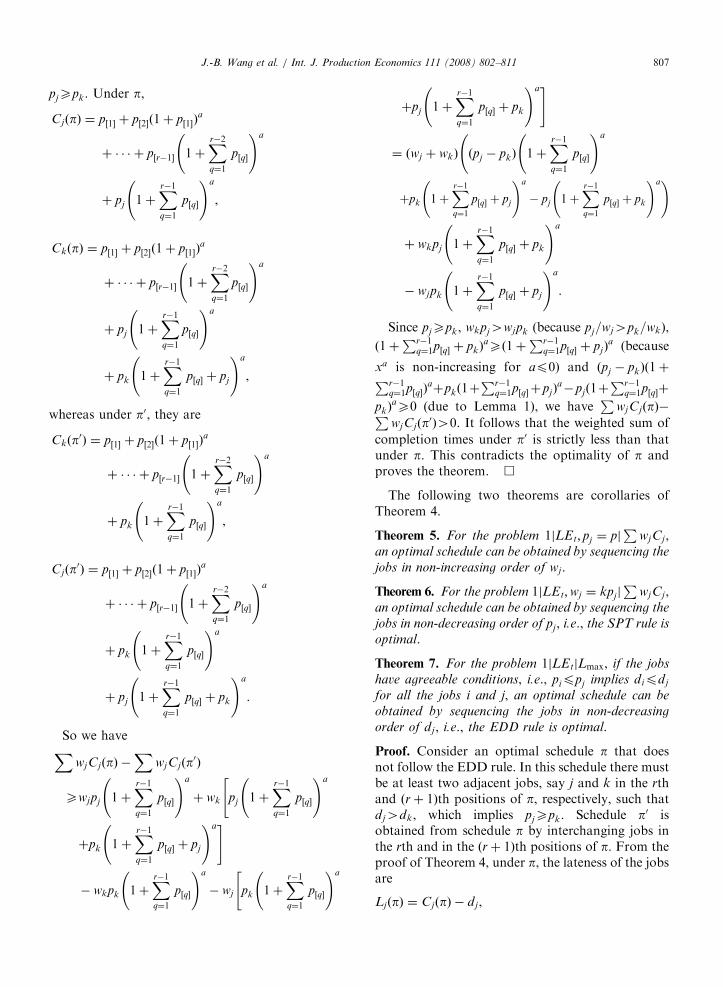
Computational experiments were conductedto evaluate the effectiveness of the heuristics ofWSPT, EDD and Moore’s Algorithm. The heuristic


algorithms were coded in VC++ 6.0 and thecomputational experiments were run on a Pentium 4personal computer. The test problems were gener-ated as follows. For each job Jj, the job normalprocessing time pj were generated from a uniformdistribution over [1, 100], and the weight wj weregenerated from a uniform distribution over [1, 10].For each job Jj , the due date dj was generated froma uniform distribution over ½1; t

Pnj¼1 pj�, where

t 2 f0:25; 0:5; 1g. For each heuristic, seven differentjob sizes, n ¼ 6, 7, 8, 9, 10, 11 and 12 were used. Inaddition, the values a ¼ �0:05;�0:25 and �0:45were used. As a consequence, 63 experimentalconditions were examined and 20 replications wererandomly generated for each condition. A total of1260 problems were tested.

In order to test the performance of the heuristicsof WSPT, EDD and Moore’s Algorithm relative tothe optimal solutions, we develop an enumerativealgorithm to find the optimal value of each testproblem. We did not try to optimize the runningtime of the enumerative algorithm, since our maingoal was to evaluate the performance of theheuristics by comparing the heuristic solutions withthe optimal solutions. The results are summarized in

Table 1

Computational results of the heuristics for t ¼ 0:25

a n r1 1

ð1þPn

j¼1pj�pminÞ

ar2

Mean Max Mean Max Mean

6 1.001 1.014 1.326 1.349 1.017

7 1.002 1.022 1.336 1.357 1.019

�0.05 8 1.001 1.006 1.343 1.356 1.016

9 1.000 1.004 1.349 1.367 1.020

10 1.001 1.005 1.352 1.373 1.027

11 1.002 1.007 1.355 1.379 1.029

12 1.001 1.003 1.359 1.381 1.025

6 1.024 1.120 4.156 4.585 1.098

7 1.039 1.233 4.144 4.415 1.101

�0.25 8 1.028 1.209 4.418 4.697 1.419

9 1.023 1.097 4.102 4.884 1.109

10 1.031 1.195 4.312 4.758 1.129

11 1.035 1.207 4.315 4.779 1.127

12 1.039 1.213 4.325 4.788 1.132

6 1.069 1.638 12.698 14.722 1.177

7 1.028 1.196 14.548 15.568 1.261

�0.45 8 1.065 1.557 13.774 15.803 1.219

9 1.077 1.356 15.982 16.329 1.180

10 1.087 1.569 15.213 17.126 1.281

11 1.095 1.558 15.595 17.752 1.229

12 1.091 1.583 15.359 17.798 1.235

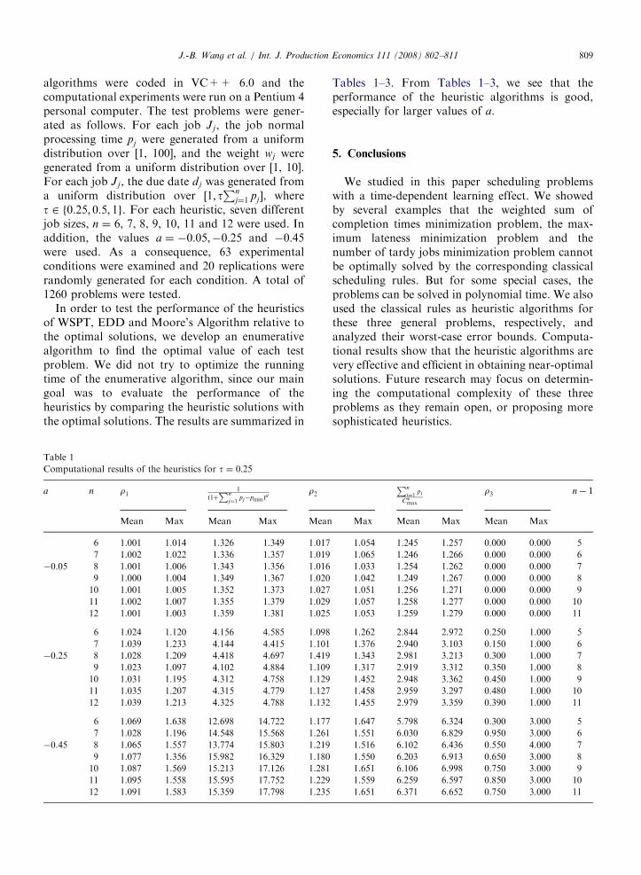
Tables 1–3. From Tables 1–3, we see that theperformance of the heuristic algorithms is good,especially for larger values of a.

5. Conclusions

We studied in this paper scheduling problemswith a time-dependent learning effect. We showedby several examples that the weighted sum ofcompletion times minimization problem, the max-imum lateness minimization problem and thenumber of tardy jobs minimization problem cannotbe optimally solved by the corresponding classicalscheduling rules. But for some special cases, theproblems can be solved in polynomial time. We alsoused the classical rules as heuristic algorithms forthese three general problems, respectively, andanalyzed their worst-case error bounds. Computa-tional results show that the heuristic algorithms arevery effective and efficient in obtaining near-optimalsolutions. Future research may focus on determin-ing the computational complexity of these threeproblems as they remain open, or proposing moresophisticated heuristics.

Pn

i¼1pi

C�max

r3 n� 1

Max Mean Max Mean Max

1.054 1.245 1.257 0.000 0.000 5

1.065 1.246 1.266 0.000 0.000 6

1.033 1.254 1.262 0.000 0.000 7

1.042 1.249 1.267 0.000 0.000 8

1.051 1.256 1.271 0.000 0.000 9

1.057 1.258 1.277 0.000 0.000 10

1.053 1.259 1.279 0.000 0.000 11

1.262 2.844 2.972 0.250 1.000 5

1.376 2.940 3.103 0.150 1.000 6

1.343 2.981 3.213 0.300 1.000 7

1.317 2.919 3.312 0.350 1.000 8

1.452 2.948 3.362 0.450 1.000 9

1.458 2.959 3.297 0.480 1.000 10

1.455 2.979 3.359 0.390 1.000 11

1.647 5.798 6.324 0.300 3.000 5

1.551 6.030 6.829 0.950 3.000 6

1.516 6.102 6.436 0.550 4.000 7

1.550 6.203 6.913 0.650 3.000 8

1.651 6.106 6.998 0.750 3.000 9

1.559 6.259 6.597 0.850 3.000 10

1.651 6.371 6.652 0.750 3.000 11

ARTICLE IN PRESS

Table 2

Computational results of the heuristics for t ¼ 0:5

a n r1 1

ð1þPn

j¼1pj�pminÞ

ar2

Pn

i¼1pi

C�max

r3 n� 1

Mean Max Mean Max Mean Max Mean Max Mean Max

6 1.001 1.010 1.316 1.342 1.010 1.035 1.251 1.256 0.050 1.000 5

7 1.003 1.032 1.332 1.359 1.014 1.030 1.247 1.271 0.000 0.000 6

�0.05 8 1.000 1.004 1.347 1.356 1.015 1.034 1.255 1.263 0.000 0.000 7

9 1.002 1.029 1.349 1.367 1.014 1.031 1.248 1.279 0.000 0.000 8

10 1.004 1.035 1.352 1.369 1.024 1.043 1.256 1.273 0.000 0.000 9

11 1.002 1.027 1.357 1.371 1.028 1.055 1.258 1.276 0.000 0.000 10

12 1.003 1.033 1.365 1.379 1.026 1.057 1.257 1.274 0.000 0.000 11

6 1.024 1.254 4.167 4.575 1.064 1.197 2.824 2.975 0.150 1.000 5

7 1.025 1.130 4.187 4.495 1.096 1.205 2.934 3.107 0.300 1.000 6

�0.25 8 1.012 1.082 4.328 4.717 1.056 1.143 2.981 3.217 0.400 1.000 7

9 1.023 1.117 4.219 4.812 1.055 1.131 2.931 3.328 0.200 1.000 8

10 1.027 1.293 4.325 4.757 1.091 1.156 2.941 3.367 0.300 1.000 9

11 1.025 1.247 4.361 4.879 1.098 1.159 2.958 3.371 0.300 1.000 10

12 1.029 1.283 4.363 4.982 1.095 1.155 2.964 3.471 0.400 1.000 11

6 1.045 1.258 13.125 14.872 1.119 1.329 5.897 6.342 0.300 1.000 5

7 1.057 1.526 14.123 15.517 1.120 1.336 6.019 6.829 0.450 2.000 6

�0.45 8 1.040 1.165 13.789 15.128 1.105 1.313 6.193 6.491 0.300 2.000 7

9 1.022 1.133 15.129 16.312 1.072 1.227 6.213 6.917 0.600 1.000 8

10 1.031 1.145 15.298 17.128 1.196 1.342 6.106 6.982 0.700 1.000 9

11 1.039 1.157 15.364 17.385 1.139 1.349 6.253 6.977 0.800 1.000 10

12 1.045 1.163 15.379 17.386 1.155 1.356 6.548 7.019 0.900 2.000 11

Table 3

Computational results of the heuristics for t ¼ 1

a n r1 1

ð1þPn

j¼1pj�pminÞ

ar2

Pn

i¼1pi

C�max

r3 n� 1

Mean Max Mean Max Mean Max Mean Max Mean Max

6 1.002 1.029 1.327 1.349 1.003 1.023 1.254 1.268 0.000 0.000 5

7 1.001 1.008 1.363 1.369 1.006 1.022 1.254 1.267 0.000 0.000 6

�0.05 8 1.000 1.002 1.313 1.359 1.006 1.022 1.259 1.266 0.050 1.000 7

9 1.001 1.004 1.348 1.360 1.004 1.012 1.249 1.268 0.000 0.000 8

10 1.003 1.006 1.329 1.377 1.007 1.031 1.257 1.271 0.000 0.000 9

11 1.002 1.005 1.332 1.381 1.009 1.037 1.259 1.279 0.000 0.000 10

12 1.003 1.007 1.346 1.386 1.008 1.033 1.261 1.281 0.000 0.000 11

6 1.038 1.253 4.165 4.515 1.040 1.137 2.792 2.923 0.050 1.000 5

7 1.018 1.133 4.134 4.487 1.047 1.278 2.483 3.009 0.150 1.000 6

�0.25 8 1.010 1.036 4.381 4.692 1.038 1.099 2.913 3.112 0.200 1.000 7

9 1.011 1.056 4.112 4.897 1.032 1.092 2.891 3.212 0.050 1.000 8

10 1.013 1.065 4.302 4.748 1.039 1.122 2.874 3.218 0.250 1.000 9

11 1.014 1.075 4.351 4.782 1.041 1.117 2.859 3.279 0.350 1.000 10

12 1.013 1.077 4.343 4.687 1.044 1.123 2.961 3.286 0.300 1.000 11

6 1.114 1.564 12.702 14.689 1.105 1.319 5.569 6.213 0.300 2.000 5

7 1.041 1.408 14.513 15.891 1.073 1.290 5.919 6.516 0.350 2.000 6

�0.45 8 1.058 1.567 14.074 15.713 1.077 1.160 6.012 6.432 0.500 1.000 7

9 1.063 1.442 15.019 16.129 1.054 1.139 6.017 6.907 0.450 1.000 8

10 1.089 1.618 15.219 16.985 1.083 1.191 5.912 6.217 0.550 1.000 9

11 1.084 1.671 15.462 16.789 1.081 1.189 5.951 6.276 0.450 1.000 10

12 1.087 1.678 15.454 16.693 1.084 1.193 5.968 6.389 0.550 1.000 11

J.-B. Wang et al. / Int. J. Production Economics 111 (2008) 802–811810


Acknowledgements

We are grateful to two anonymous referees fortheir helpful comments on an earlier version of thispaper. This research was supported in part by TheHong Kong Polytechnic University under Grantnumber G-YX72. Wang was also partially sup-ported by the Foundation of Shenyang Institute ofAeronautical Engineering under Grant number05YB08.

References

Alamri, A.A., Balkhi, Z.T., 2007. The effects of learning

and forgetting on the optimal production lot size for

deteriorating items with time varying demand and deteriora-

tion rates. International Journal of Production Economics

107, 125–138.

Bachman, A., Janiak, A., 2004. Scheduling jobs with position-

dependent processing times. Journal of the Operational

Research Society 55, 257–264.

Badiru, A.B., 1992. Computational survey of univariate and

multivariate learning curve models. IEEE Transactions on

Engineering Management 39, 176–188.

Biskup, D., 1999. Single-machine scheduling with learning

considerations. European Journal of Operational Research

115, 173–178.

Biskup, D., Simons, D., 2004. Common due date scheduling with

autonomous and induced learning. European Journal of

Operational Research 159, 606–616.

Cheng, T.C.E., Wang, G., 2000. Single machine scheduling with

learning effect considerations. Annals of Operations Research

98, 273–290.

Chiua, H.N., Chen, H.M., 2005. An optimal algorithm for

solving the dynamic lot-sizing model with learning and

forgetting in setups and production. International Journal

of Production Economics 95, 179–193.

Jackson, J.R., 1955. Scheduling a production line to minimize

maximum tardiness. Research Report 43, Management

Sciences Research Project, UCLA, January 1955.

Kuo, W.-H., Yang, D.-L., 2006a. Minimizing the makespan in a

single machine scheduling problem with a time-based learning

effect. Information Processing Letters 97, 64–67.

Kuo, W.-H., Yang, D.-L., 2006b. Minimizing the total comple-

tion time in a single-machine scheduling problem with a time-

dependent learning effect. European Journal of Operational

Research 174, 1184–1190.

Kuo, W.-H., Yang, D.-L., 2006c. Single-machine group schedul-

ing with a time-dependent learning effect. Computers &

Operations Research 33, 2099–2112.

Kuolamas, C., Kyparisis, G.J., 2007. Single-machine and two-

machine flowshop scheduling with general learning functions.

European Journal of Operational Research 178, 402–407.

Lee, W.-C., Wu, C.-C., 2004. Minimizing total completion time

in a two-machine flowshop with a learning effect. Interna-

tional Journal of Production Economics 88, 85–93.

Lee, W.-C., Wu, C.-C., Sung, H.-J., 2004. A bi-criterion single-

machine scheduling problem with learning considerations.

Acta Informatica 40, 303–315.

Liu, J., Sun, S., He, L., 2003. Some single machine scheduling

problems with learning effect under consistent condition. OR

Transactions 7 (3), 21–28.

Moore, J., 1968. An n job, one machine sequencing algorithm for

minimizing the number of late jobs. Management Science 15,

102–109.

Mosheiov, G., 2001a. Scheduling problems with a learning effect.

European Journal of Operational Research 132, 687–693.

Mosheiov, G., 2001b. Parallel machine scheduling with a learning

effect. Journal of the Operational Research Society 52,

1165–1169.

Mosheiov, G., Sidney, J.B., 2003. Scheduling with general job-

dependent learning curves. European Journal of Operational

Research 147, 665–670.

Mosheiov, G., Sidney, J.B., 2005. Note on scheduling with

general learning curves to minimize the number of tardy jobs.

Journal of the Operational Research Society 56, 110–112.

Pinedo, M., 1995. Scheduling Theory, Algorithms, and Systems.

Prentice-Hall, New Jersey.

Wang, J.-B., 2005. Flow shop scheduling jobs with position-

dependent processing times. Journal of Applied Mathematics

and Computing 18, 383–391.

Wang, J.-B., 2006. A note on scheduling problems with learning

effect and deteriorating jobs. International Journal of Systems

Science 37, 827–833.

Wang, J.-B., 2007. Single-machine scheduling problems with the

effects of learning and deterioration. Omega 35, 397–402.

Wang, J.-B., Cheng, T.C.E., 2007a. Scheduling problems with the

effects of deterioration and learning. Asia-Pacific Journal of

Operational Research 24 (2), 245–261.

Wang, J.-B., Xia, Z.-Q., 2005. Flow-shop scheduling with a

learning effect. Journal of the Operational Research Society

56, 1325–1330.

Wang, X., Cheng, T.C.E., 2007b. Single-machine scheduling with

deteriorating jobs and learning effects to minimize the

makespan. European Journal of Operational Research 178,

57–70.

Wright, T.P., 1936. Factors affecting the cost of airplanes.

Journal of Aeronautical Sciences 3, 122–128.

Documents

Single-machine scheduling with a time-dependent learning effect