Embed Size (px)
Citation preview
smarties: user-friendly codes for fast and accurate calculations of lightscattering by spheroids
W. R. C. Somerville, B. Auguié, E. C. Le Ru∗
The MacDiarmid Institute for Advanced Materials and Nanotechnology, School of Chemical and Physical Sciences, VictoriaUniversity of Wellington, PO Box 600, Wellington 6140, New Zealand
Abstract
We provide a detailed user guide for smarties, a suite of Matlab codes for the calculation of the opticalproperties of oblate and prolate spheroidal particles, with comparable capabilities and ease-of-use as Mietheory for spheres. smarties is a Matlab implementation of an improved T -matrix algorithm for thetheoretical modelling of electromagnetic scattering by particles of spheroidal shape. The theory behind theimprovements in numerical accuracy and convergence is briefly summarised, with reference to the originalpublications. Instructions of use, and a detailed description of the code structure, its range of applicability,as well as guidelines for further developments by advanced users are discussed in separate sections of thisuser guide. The code may be useful to researchers seeking a fast, accurate and reliable tool to simulate thenear-field and far-field optical properties of elongated particles, but will also appeal to other developers oflight-scattering software seeking a reliable benchmark for non-spherical particles with a challenging aspectratio and/or refractive index contrast.
Contents
1 Introduction 21.1 Description and overview . . . . . . 21.2 Relation to other codes . . . . . . . 21.3 Aims of this manual . . . . . . . . . 31.4 Licensing . . . . . . . . . . . . . . . 31.5 Disclaimer . . . . . . . . . . . . . . . 41.6 Feedback . . . . . . . . . . . . . . . 4
2 Getting started 42.1 Installation . . . . . . . . . . . . . . 42.2 Octave users . . . . . . . . . . . . . 42.3 Initial steps . . . . . . . . . . . . . . 42.4 Definition of the parameters . . . . . 52.5 Minimal example . . . . . . . . . . . 72.6 Convergence, range of validity . . . . 72.7 Case study: Ag spheroids . . . . . . 8
∗Corresponding authorEmail addresses: [email protected] (W. R.
C. Somerville), [email protected] (B. Auguié),[email protected] (E. C. Le Ru)
3 Underlying principles of the code 93.1 Spherical coordinates . . . . . . . . . 103.2 The spheroid geometry . . . . . . . . 103.3 The T -matrix/EBCM method . . . 103.4 Additional simplifications for spheroids 113.5 Angular functions . . . . . . . . . . . 123.6 Integral quadratures . . . . . . . . . 133.7 Computation of the P and Q matrices 133.8 Matrix inversion for T and R matrices 143.9 Orientation-averaged properties . . . 153.10 Scattering matrix . . . . . . . . . . . 153.11 Incident field . . . . . . . . . . . . . 153.12 Scattered and internal fields . . . . . 163.13 Surface fields . . . . . . . . . . . . . 163.14 Near fields . . . . . . . . . . . . . . . 16
4 Additional implementation details 174.1 Naming conventions and organization 174.2 Storage of matrices . . . . . . . . . . 174.3 Storage of (n,m) arrays . . . . . . . 18
5 References 18
6 Appendix: Convergence tests 19
Preprint submitted to Elsevier February 8, 2016
arX
iv:1
511.
0079
8v2
[ph
ysic
s.op
tics]
5 F
eb 2
016
1. Introduction
We present a user guide and description of smar-ties, a numerically stable and highly accurate im-plementation of the T -matrix/Extended Boundary-Condition Method (EBCM) for light-scattering byspheroids, based on our recent work [1–3]. Thecomplete package can be downloaded freely fromhttp://www.victoria.ac.nz/scps/research/research-groups/raman-lab/numerical-tools, see Sec. 1.4 forlicensing information. The name of the programstands for Spheroids Modelled Accurately witha Robust T-matrix Implementation for Electro-magnetic Scattering, and is also a nod to thewell-known colourful candy of oblate shape.
1.1. Description and overview
This package contains a suite of Matlab codesto simulate the light scattering properties ofspheroidal particles, following the general T -matrixframework [4]. The scatterer should be homoge-neous, and described by a local, isotropic and lin-ear dielectric response (this includes metals, but notperfect conductors). Magnetic, non-linear, and op-tically active materials are not considered. The sur-rounding medium is described by a lossless, homo-geneous and isotropic dielectric medium extendingto infinity.smarties specifically implements recently-developed algorithms for numerically accurate andstable calculations. The general EBCM/T -matrixmethod is described in detail in Ref. [4], while theunderlying theory and relevant formulas for ourspecific improvements are described in Ref. [2],with additional information found in [1, 3]. Therelevant equations and sections from both Ref. [2]and Ref. [4] are referenced when possible as “inlinecomments” to the code.The package includes detailed examples and canalso be used by a non-specialist with an application-oriented perspective, requiring no specific knowl-edge of the underlying theory.The package contains:
• Six ready-to-run example scripts to calculatestandard optical properties, namely: fixed-orientation and orientation-averaged far-fieldcross-sections, near fields, T -matrix elements,and scattering matrix elements. Examples alsocover the simulation of wavelength-dependentspectra of surface-field and far-field properties.
• Two tutorial scripts where such simulations arefurther detailed with step-by-step instructions,exposing the lower-level calculations of inter-mediate quantities.
• Additional high-level and post-processing func-tions, which can be used by users to write newscripts tailored to their specific needs.
• A number of low-level functions, which areused by the code and might be adapted by ad-vanced users.
• Dielectric functions for a few materials suchas gold and silver, implemented via analyticexpressions [5, 6] or silicon, interpolated fromtabulated values.
1.2. Relation to other codesStandard T -matrix/EBCM codes in Fortran havealready been developed [7, 8], with those byMishchenko and co-workers [9] arguably the mostpopular. These freely-available codes provide awide range of capabilities (including for exampledifferent particle shapes) and have been widely usedand tested. The standard EBCM method howeversuffers from a number of numerical problems andinstabilities for large multipole orders, which arenecessary for either high precision, large particles,elongated particles, near-field calculations, or anycombination of the above. This can result in inac-curate results and in some cases in complete loss ofconvergence. This unreliable behaviour for numeri-cally challenging simulations can make the methoddifficult to use for non-experts, who may find ithard to “tune” the parameters that ensure accuracyand convergence. It also impedes the theoreticalstudy of the intrinsic convergence properties of theT -matrix method, obfuscated by (implementation-dependent) numerical loss of precision [3].Recently, we have identified the primary causes fornumerical instabilities in the special (but impor-tant) case of spheroidal particles [1] and proposeda new algorithm to overcome them [2]. Thanksto those improvements, high accuracy and reliableconvergence can be obtained over a wider rangeof parameters, especially toward high aspect-ratio(elongated) particles where the standard EBCMimplementation would fail [3]. This document aimsto present and discuss a publicly available Mat-lab implementation of these recent developments.Our package should complement, rather than re-place, existing T -matrix codes such as those of
2
Mishchenko [9]. The present code offers a numberof advantages:
• Thanks to the improvements in accuracy andconvergence, we believe this code will be read-ily accessible to non-expert users and allowthe routine calculation of optical propertiesof spheroids as easily as with Mie theory forspheres. An example is provided in Section 2.7as a demonstration.
• We also provide specific routines to computenear fields and surface fields, which will bebeneficial to the exploitation of this powerfulmethod in areas such as nanophotonics, opti-cal trapping, plasmonics, etc., where the T -matrix/EBCMmethod has not been widely ap-plied.
• Matlab provides an easy-access, interactiveenvironment to carry out a broad range of nu-merical simulations, and plot/export the re-sults conveniently.
• The accuracy of the obtained results can beeasily estimated for any type of calculation,owing to the well-behaved convergence of theimproved algorithm.
• A wider range of parameters can be simulated,especially scatterers with large aspect ratios.
A number of limitations should be also be noted:
• These codes are limited to spheroidal particles,for which we identified and circumvented nu-merical problems that are very specific to thisgeometrical shape.
• Matlab is inherently slow compared to com-piled languages such as C or Fortran, whichmay be an issue for intensive calculations (forexample the simulation of polydisperse sam-ples, with particles varying in size and shape).We envisage that this implementation couldserve as a template for a future port of thisnew algorithm to a more efficient language.
• The calculation of some derived properties, e.g.the scattering matrix, has not been optimizedand could be particularly slow.
• Although the range of parameters that maybe simulated with reasonable accuracy hasbeen extended toward larger aspect ratios, the
method is still limited to moderate particlesizes; and even small sizes only for particleswith a large relative refractive index. In thiscase, the matrix inversion step is the limitingfactor and extended-precision arithmetic as im-plemented in [9] would be required to overcomeit.
1.3. Aims of this manual
This document was written with two types of usersin mind:
• Researchers interested in simulating electro-magnetic scattering by nonspherical particlesfor practical applications, and seeking an effi-cient and (relatively) fool-proof program withease of use comparable to Mie theory.
• Other developers of electromagnetic scatteringsoftware interested in benchmarking calcula-tions against a highly-accurate reference.
With this dual perspective, we have divided thesource code into low-level and high-level functions,including complete scripts for specific calculations,but also documented how to access intermediatequantities such as the T -matrix elements. This userguide is also divided into sections that reflect thesetwo complementary objectives, with Sections 3 and4 focusing on more theoretical aspects and in-depthdescription of the code implementation.
1.4. Licensing
smarties is licensed under the Creative CommonsAttribution-NonCommercial 4.0 International Li-cense. To view a copy of this license, visit http://creativecommons.org/licenses/by-nc/4.0/.The package, including all its files and contentare under the following copyright: 2015 WalterSomerville, Baptiste Auguié, and Eric Le Ru. Thepackage may be used freely for research, teaching,or personal use. The unmodified complete pack-age may be re-distributed and freely exchanged foracademic research or government use, but cannotbe commercialized or used for commercial purposes.The theory and code should be appropriately refer-enced by citing this user-guide in any presentationof results obtained using this package (or any othercode using it).
3
1.5. Disclaimer
These codes have been developed and tested withMatlab 7.14 (R2012a) [10], GNU Octave 4.0.0 [11](open-source software) and Matlab 8.5 (R2015a)on a PC running Microsoft Windows 7 x64. Thecode is also known to run under MacOS X (10.10)and Linux (Ubuntu 15.04). Slight changes may benecessary to run them on older (or newer!) versionsof Matlab/Octave.Although every effort has been made to get rid ofbugs (programming bugs, or incorrect physical for-mulas) and to test the code against existing ones,some issues may still be present. We hope the userswill help us identify them and we will try to updatethe code when necessary.Note also in this context that these codes do notimplement a strict check of user input; if incorrectparameters are passed in a function call, errors willoccur.The authors do not accept any responsibility forimproper use of the program, accidental errors thatmay still be present, or improper interpretation ofits limitations and/or results derived therefrom. Itis the responsibility of the user to check the validityof the inputs/outputs, their physical interpretation,and their suitability for her/his specific problem.
1.6. Feedback
We would like to hear from the users of this codeto improve it over time. This feedback could in-clude simple issues of layout and organization ofthe information or plain errors. Please feel free tosend us any feedback (good or bad), bug reports,questions, comments, or suggestions to [email protected].
2. Getting started
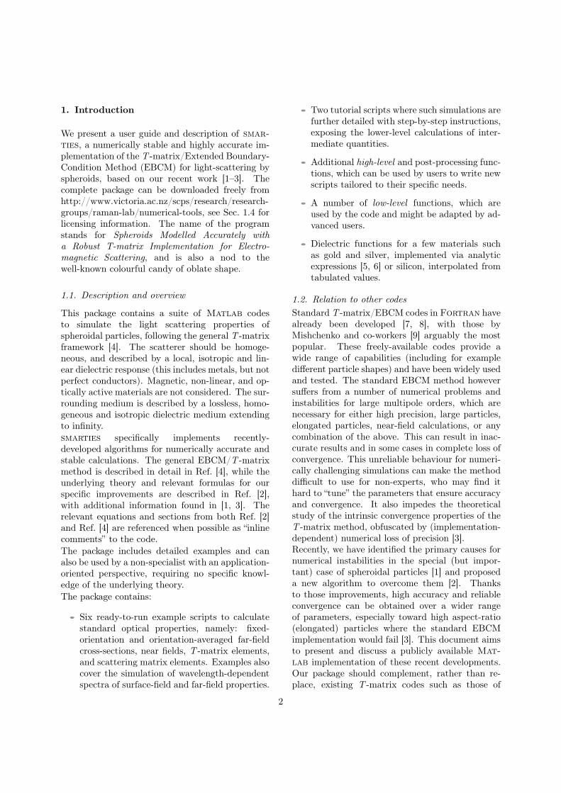
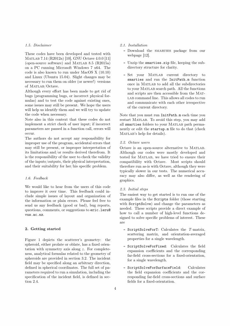
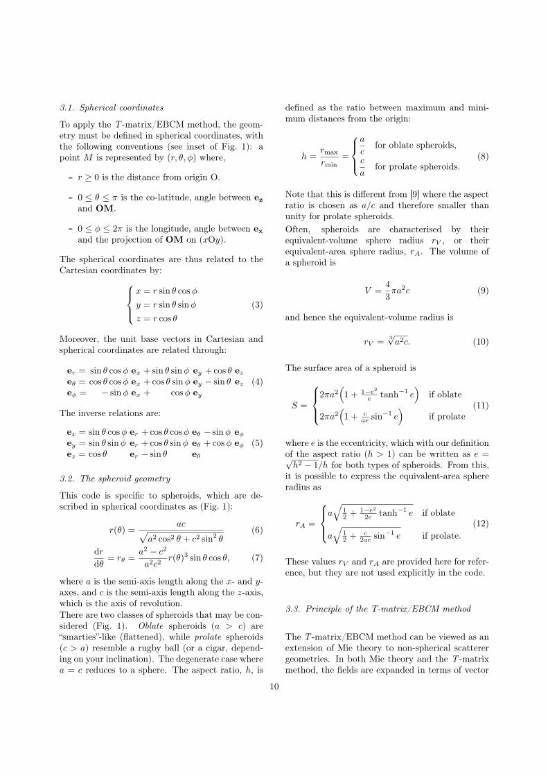
Figure 1 depicts the scatterer’s geometry: thespheroid, either prolate or oblate, has a fixed orien-tation with symmetry axis along z. For complete-ness, analytical formulas related to the geometry ofspheroids are provided in section 3.2. The incidentfield may be specified along an arbitrary direction,defined in spherical coordinates. The full set of pa-rameters required to run a simulation, including thespecification of the incident field, is defined in sec-tion 2.4.
2.1. Installation• Download the smarties package from our
webpage [12].
• Unzip the smarties.zip file, keeping the sub-directory structure for clarity.
• Set your Matlab current directory tosmarties and run the InitPath.m functiononce in Matlab to add all the subdirectoriesto your Matlab search path. All the functionsand scripts are then accessible from the Mat-lab command line. This allows all codes to runand communicate with each other irrespectiveof the current directory.
Note that you must run InitPath.m each time yourestart Matlab. To avoid this step, you may addall smarties folders to your Matlab path perma-nently or edit the startup.m file to do that (checkMatlab’s help for details).
2.2. Octave usersOctave is an open-source alternative to Matlab.Although our codes were mostly developed andtested for Matlab, we have tried to ensure theircompatibility with Octave. Most scripts shouldtherefore run as-is with Octave, although they weretypically slower in our tests. The numerical accu-racy may also differ, as well as the rendering ofgraphics.
2.3. Initial stepsThe easiest way to get started is to run one of theexample files in the Scripts folder (those startingwith ScriptSolve) and change the parameters asneeded. These scripts provide a direct example ofhow to call a number of high-level functions de-signed to solve specific problems of interest. Theseare
• ScriptSolveForT: Calculates the T -matrix,scattering matrix, and orientation-averagedproperties for a single wavelength.
• ScriptSolveForFixed: Calculates the fieldexpansion coefficients and the correspondingfar-field cross-sections for a fixed-orientation,for a single wavelength.
• ScriptSolveForSurfaceField: Calculatesthe field expansion coefficients and the cor-responding far-field cross-sections and surfacefields for a fixed-orientation.
4
z
x y
z
x y
ac
Prolate spheroid Oblate spheroid
a c
x
z
y
r
Spherical coordinates
Figure 1: 3D illustation of spherical coordinates, and the geometrical parameters for prolate (left) and oblate (right) spheroids.The axis of revolution is along z.
• ScriptSolveForTSpectrum: Calculates theT -matrix and the orientation-averaged prop-erties for multiple wavelengths.
• ScriptSolveForFixedSpectrum: Calculatesthe field expansion coefficients and the cor-responding far-field cross-sections for a fixed-orientation, as a function of wavelength.
• ScriptSolveForSurfaceFieldSpectrum:Calculates the field expansion coefficientsand the corresponding far-field cross-sectionsand surface fields for a fixed-orientation, as afunction of wavelength.
Those scripts define the parameters of the simu-lation, call the corresponding high-level functionsto perform the calculations, and output the mostimportant results in the Matlab console and/oras interactive graphics. Convergence tests are alsoperformed as part of the calculations, and accuracyestimates for the results are included in the dis-plays.In order to understand in more detail how thecode operates, we also provide two example scripts,ScriptTutorial and ScriptTutorialSpectrum,where all the main steps in the calculation arelisted explicitly with extensive comments about themeaning of the various parameters. We recom-mend copying and editing these example scripts to
solve user-specific problems and/or implement cus-tom extensions to the current code.Most functions start with a detailed help andare commented within the code. Typing helpFunctionName will display the corresponding helpinformation.The information below summarizes and comple-ments the inline comments included in the six ex-ample scripts ScriptSolve.... It provides themost important technical details of the implemen-tation, for users wishing to write additional customroutines.
2.4. Definition of the parameters
For the calculation of the T -matrix and orientation-averaged cross-sections, only four parameters areneeded to define the scatterer properties:
• a: semi-axis along x, y.
• c: semi-axis along z (axis of rotational symme-try).
• k1: wavevector in embedding medium (possi-bly a wavelength-dependent vector).
• s: relative refractive index s (possibly awavelength-dependent vector).
Note that consistent units must be used for a, c,and k1, e.g. a and c in nm and k1 in nm−1.
5
k1 denotes the wavevector outside the particle,where the refractive index is n1 =
√ε1 (assumed
real positive):
k1 =ω
c
√ε1 =
2π
λ
√ε1. (1)
The relative refractive index (adimensional) is de-fined as
s =
√ε2√ε1. (2)
Both s and ε2 may be complex (for absorbingand/or conducting particles).
The P,Q, T,R-matrices computation requires thefollowing parameters:
• N: Number of multipoles N requested for theT -matrix (and R-matrix).
• nNbTheta: Number of angles θ used in Gaus-sian quadratures for the evaluation of P - andQ-matrix integrals.
The function sphEstimateNandNT may be used toautomatically estimate those latter two parametersfor best convergence, but we we nevertheless rec-ommend that the convergence of the calculationsbe checked to ensure reliable results.
For convenience those six parameters may be col-lated in a structure (a Matlab object akin to a list,called stParams in our example scripts), which ispassed to the high-level (slv...) functions.Additionally, one of the following two parametersis needed if the field expansion coefficients and/orthe cross-sections for a given fixed orientation aresought:
• sIncType: String defining the type of incidentplane wave, e.g. 'KxEz' for a wave incidentalong x and linearly polarized along z. Thisshorthand notation is only defined for a fewstandard combinations, namely KxEz, KxEy,KyEz, KyEx, KzEx, KzEy. In other cases, usestIncPar.
• stIncPar: Structure defining a linearly-polarized incident plane wave excitation viathree Euler angles. It can be obtained fromcalling vshMakeIncidentParameters.
For field calculations (such as surface fields), furtherparameters are required:
• nNbThetaPst: Number of angles θ for post-processing (should typically be larger thannNbTheta for accurate surface averaging).
• lambda: Wavelength (in free space) [in thesame unit as a, c, k−11 ].
• epsilon2: Dielectric function ε2 of scatterer(possibly complex).
• epsilon1: Relative dielectric constant ε1 ofembedding medium (real positive).
Note that the latter three are not independent ofk1 and s that have already been defined. Thoseadditional parameters should also be included instParams.Finally a number of optional settings can also bedefined in a structure stOptions:
• bGetR: Boolean (default: false). If false, theR-matrix and internal field coefficients are notcalculated. The default value will be overrid-den by functions requiring R.
• Delta: Number of extra multipoles for P - andQ- matrices, i.e. NQ = N + ∆. Default is ∆ =0. If Delta=-1, then the code tries to estimateit from the convergence of T 22,m=1
11 (see [3] fordetails), by calling sphEstimateDelta.
• NB: Number of multipoles to compute theBessel functions in the improved algorithm(NB ≥ NQ). If NB=0, then NB is estimatedby calling sphEstimateNB, which is the caseby default.
• absmvec: Vector containing the values of |m|for which T is to be computed. These val-ues are limited to 0 ≤ |m| ≤ N . To com-pute all m (most cases of interest), simply useabsmvec=0:N (which is the default value).
• bGetSymmetricT: Boolean (default: false). Iftrue, T is symmetrized as described in Sec. 3.8.
• bOutput: Boolean (default: true). If false,suppresses some of the output printed in theMatlab console, which is a better option forexample in calculations of spectra with manywavelengths.
6
2.5. Minimal example
The following script is set up to simulate the far-field cross-sections of a gold prolate spheroid in air,at a single wavelength λ = 650nm. The simula-tion parameters are stored in a structure stParamsfor convenience. Only one optional parameter isdefined in stOptions (for the others, default val-ues will be used). These two structures are passedto the high-level slvForFixed function that imple-ments the calculation of the expansion coefficientsand cross-sections for a fixed orientation.
Minimalist script showing how to set up a simulation
% Parameters of the scattering problem% stored in a structurelambda = 650;stParams.a=10; stParams.c=50;stParams.k1=2*pi/lambda;stParams.s=sqrt(epsAu(lambda));stParams.sIncType = 'KxEz';
% Optional control parametersstOptions.bGetR = false;
% Automatically estimates required N and nNbTheta[stParams.N, stParams.nNbTheta] =
sphEstimateNandNT(stParams,stOptions);
%% T−matrix calculation and output of cross−sectionsstC = slvForFixed(stParams, stOptions);sprintf('Cext = %g, Cabs = %g, Csca = %g',
stC.Cext, stC.Cabs, stC.Csca)
This general structure is followed by all the ex-amples, with varying levels of complexity, and thehigh-level functions such as slvForFixed perform-ing the actual calculations are grouped in the Solvedirectory.
2.6. Convergence, accuracy, and range of validity
One of the problems of the conventional T -matrix/EBCM method is to study its convergenceand accuracy. This is because the method be-comes unstable with multipoles of high order, whichmay occur before the results have fully converged.Many of those issues have been solved in the presentmethod, as discussed in Ref. [3]. Ref. [3] also pro-vides a detailed discussion of the parameters affect-ing convergence and accuracy.Thanks to the improved stability, we propose a sim-ple and reliable convergence and accuracy test thatwill work in most cases. It consists in repeatingthe same calculations with a larger number of mul-tipoles N and quadrature points Nθ, for example:N ′ = N + 5 and N ′θ = Nθ + 5. If surface-averaged
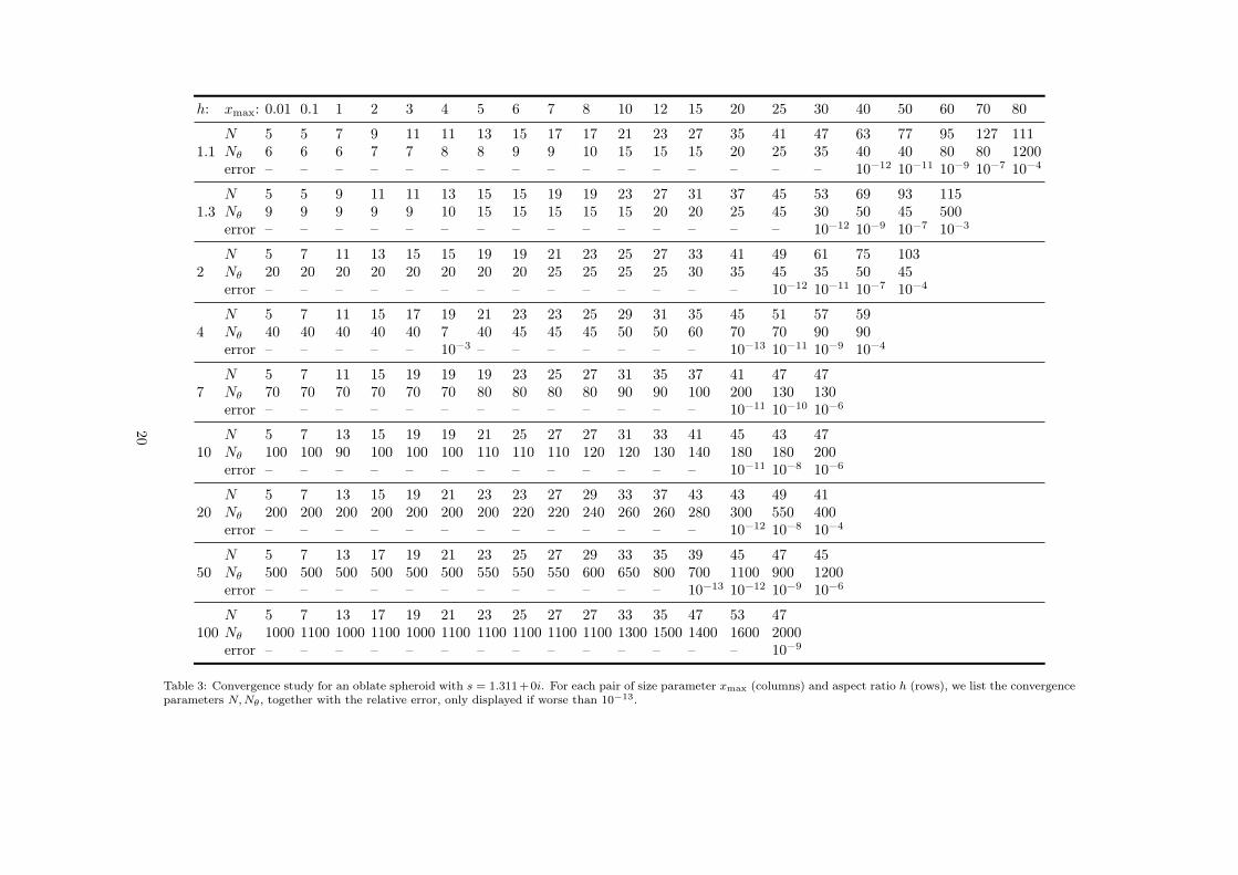
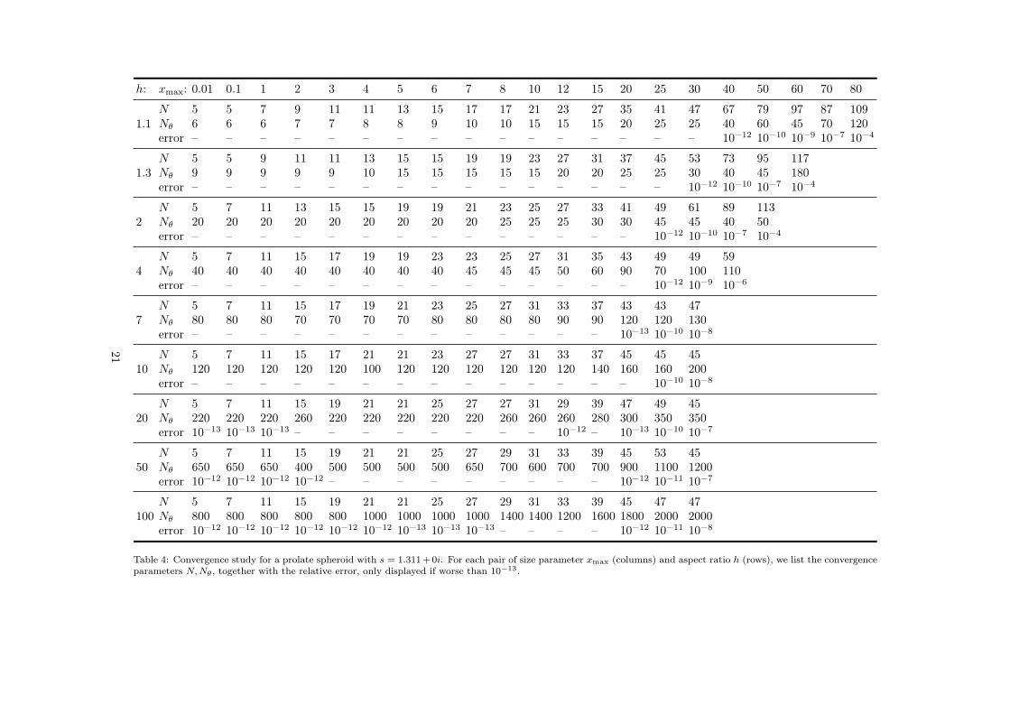
properties are calculated, the number of quadra-ture points used in post-processing should also bechecked independently.In our experience, this simple convergence test pro-vides a reliable estimate of the accuracy of the re-sults. It is implemented in the six example scriptsprovided with the code.Obviously, such a test will double the requiredcomputing times; for repeated computations suchas spectra with many wavelengths, we thereforerecommend to only test the most numerically-challenging cases, typically the largest size param-eter and/or largest value of |s|.The function sphEstimateNandNT can be use to es-timate automatically the required N , Nθ for a sim-ulation. This function should not replace the con-vergence test described above as it only relies onthe convergence of the orientation-averaged extinc-tion cross-section (and only for m = 0, 1) and mayfail in rare cases. It does however provide a goodfirst guess for those parameters, and can in addi-tion be used to study how they depend on the scat-terer properties, or test the range of validity of themethod.An example of such results is given in Tables 3 and4 of the Appendix for oblate and prolate spheroids,respectively, where the required N and Nθ, alongwith the obtained accuracy, are summarized asa function of maximum size parameter and as-pect ratio for s = 1.311. Interestingly, when ex-pressed in terms of the maximum size parameter,xmax = k1max(a, c), almost identical convergencerequirements were obtained for oblate and prolatespheroids. From those tables, we also infer that theaccuracy and stability do not depend strongly onaspect ratio (in stark contrast with the standardEBCM, which rapidly becomes unstable for largeraspect ratios). There remains however an upperlimit on the size of particles that can be modeled,which is comparable to the upper limit of double-precision implementations of the standard EBCMat low aspect ratio [9].Additional automatic tests were carried out to es-timate the maximum computable size parameterfor a given h and s. Those results are summa-rized in Table 1 for oblate spheroids, with the cor-responding table for prolate spheroids in AppendixTable 2. These computer-generated estimates pro-vide an overview of the range of validity of thisnew implementation. These suggest that, as a ruleof thumb, the method will start to fail when themaximum size parameter xmax = k1max(a, c) ap-
7
h→s 1.1 2 4 10 20 100
1.311 + 0.00i 80 50 45 35 30 27
1.500 + 0.00i 50 35 30 25 22 25
1.500 + 0.02i 60 40 30 25 22 25
1.500 + 2.00i 80 20 12 11 11 9
2.500 + 0.00i 22 16 12 11 11 11
4.000 + 0.10i 16 11 8 6 6 6
0.100 + 4.00i 60 10 7 5 5 5
Table 1: Convergence study for oblate spheroids. We hereconsider a number of aspect ratios h ranging from 1.1 to100, and 7 representative values of s. For each, we calcu-late the orientation-averaged extinction cross-section for in-creasing sizes, characterized by the maximum size parameterxmax = k1max(a, c). The values in the table correspond tothe largest xmax for which convergence was obtained. Thosevalues are only indicators of the range of validity of the code;they were obtained via an automated search, which may beslightly inaccurate in some cases.
proaches the limits |s|xmax ≈ 50 for relatively lowaspect ratios, progressively going down to |s|xmax ≈30 for the largest aspect ratios. For relatively largeaspect ratios, for example h = 20, the upper limitof size parameter therefore becomes comparableto extended-precision implementations of the stan-dard EBCM (xmax ≈ 32 for oblate spheroids withs = 1.311 [9]). As for the standard EBCM codes, alarge relative index |s| however remains very chal-lenging.Also notable from these tables is the fact that avery large number of Gaussian quadrature pointsare necessary for large aspect ratios of any size.This can be explained from the high curvature ofthe tip around θ = 0 and suggests that much moreefficient quadrature schemes could be developed forthose cases, e.g. simply using subdivisions of therange of integration with different density of points.
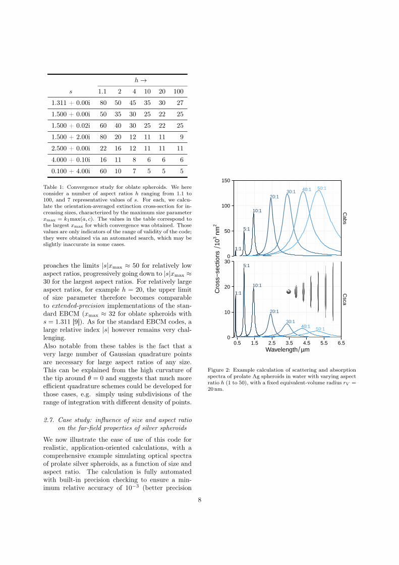
2.7. Case study: influence of size and aspect ratioon the far-field properties of silver spheroids
We now illustrate the ease of use of this code forrealistic, application-oriented calculations, with acomprehensive example simulating optical spectraof prolate silver spheroids, as a function of size andaspect ratio. The calculation is fully automatedwith built-in precision checking to ensure a min-imum relative accuracy of 10−3 (better precision
1:1
5:1
10:1
20:130:1 40:1 50:1
1:1
5:1
10:1
20:1
30:140:1 50:1
0
50
100
150
0
10
20
30
Cabs
Csca
0.5 1.5 2.5 3.5 4.5 5.5 6.5Wavelength µm
Cro
ss−
sect
ions
10
3 nm
2
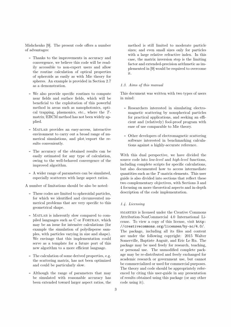
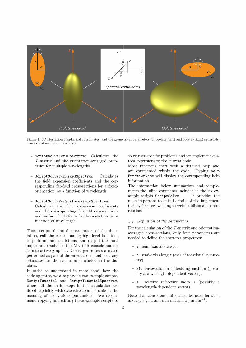
Figure 2: Example calculation of scattering and absorptionspectra of prolate Ag spheroids in water with varying aspectratio h (1 to 50), with a fixed equivalent-volume radius rV =20nm.
8
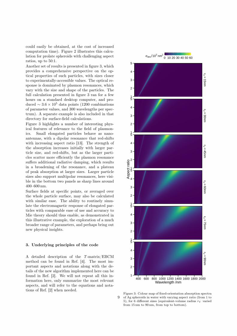
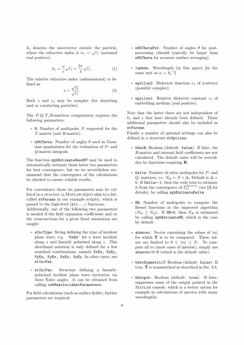
could easily be obtained, at the cost of increasedcomputation time). Figure 2 illustrates this calcu-lation for prolate spheroids with challenging aspectratios, up to 50:1.Another set of results is presented in figure 3, whichprovides a comprehensive perspective on the op-tical properties of such particles, with sizes closerto experimentally-accessible values. The optical re-sponse is dominated by plasmon resonances, whichvary with the size and shape of the particles. Thefull calculation presented in figure 3 ran for a fewhours on a standard desktop computer, and pro-duced ∼ 3.6 × 10⁵ data points (1200 combinationsof parameter values, and 300 wavelengths per spec-trum). A separate example is also included in thatdirectory for surface-field calculations.Figure 3 highlights a number of interesting phys-ical features of relevance to the field of plasmon-ics. Small elongated particles behave as nano-antennas, with a dipolar resonance that red-shiftswith increasing aspect ratio [13]. The strength ofthe absorption increases initially with larger par-ticle size, and red-shifts, but as the larger parti-cles scatter more efficiently the plasmon resonancesuffers additional radiative damping, which resultsin a broadening of the resonance, and a plateauof peak absorption at larger sizes. Larger particlesizes also support multipolar resonances, here visi-ble in the bottom two panels as sharp lines around400–600 nm.Surface fields at specific points, or averaged overthe whole particle surface, may also be calculatedwith similar ease. The ability to routinely simu-late the electromagnetic response of elongated par-ticles with comparable ease of use and accuracy toMie theory should thus enable, as demonstrated inthis illustrative example, the exploration of a muchbroader range of parameters, and perhaps bring outnew physical insights.
3. Underlying principles of the code
A detailed description of the T -matrix/EBCMmethod can be found in Ref. [4]. The most im-portant aspects and notations along with the de-tails of the new algorithm implemented here can befound in Ref. [2]. We will not repeat all this in-formation here, only summarize the most relevantaspects, and will refer to the equations and nota-tions of Ref. [2] when needed.
1
2
3
4
5
1
2
3
4
5
1
2
3
4
5
1
2
3
4
5
1
2
3
4
5
1
2
3
4
5
rV=
15nmrV
=30nm
rV=
45nmrV
=60nm
rV=
75nmrV
=90nm
400 600 800 1000 1200 1400 1600 1800 2000Wavelength /nm
Asp
ect r
atio
0 10 20 30 40 50 60σabs 103 nm2
Figure 3: Colour map of fixed-orientation absorption spectraof Ag spheroids in water with varying aspect ratio (from 1 to5), for 6 different sizes (equivalent-volume radius rV variedfrom 15 nm to 90 nm, from top to bottom).
9
3.1. Spherical coordinates
To apply the T -matrix/EBCM method, the geom-etry must be defined in spherical coordinates, withthe following conventions (see inset of Fig. 1): apoint M is represented by (r, θ, φ) where,
• r ≥ 0 is the distance from origin O.
• 0 ≤ θ ≤ π is the co-latitude, angle between ezand OM.
• 0 ≤ φ ≤ 2π is the longitude, angle between exand the projection of OM on (xOy).
The spherical coordinates are thus related to theCartesian coordinates by:
x = r sin θ cosφ
y = r sin θ sinφ
z = r cos θ
(3)
Moreover, the unit base vectors in Cartesian andspherical coordinates are related through:
er = sin θ cosφ ex + sin θ sinφ ey + cos θ ezeθ = cos θ cosφ ex + cos θ sinφ ey − sin θ ezeφ = − sinφ ex + cosφ ey
(4)
The inverse relations are:
ex = sin θ cosφ er + cos θ cosφ eθ − sinφ eφey = sin θ sinφ er + cos θ sinφ eθ + cosφ eφez = cos θ er − sin θ eθ
(5)
3.2. The spheroid geometry
This code is specific to spheroids, which are de-scribed in spherical coordinates as (Fig. 1):
r(θ) =ac√
a2 cos2 θ + c2 sin2 θ(6)
drdθ
= rθ =a2 − c2
a2c2r(θ)3 sin θ cos θ, (7)
where a is the semi-axis length along the x- and y-axes, and c is the semi-axis length along the z-axis,which is the axis of revolution.There are two classes of spheroids that may be con-sidered (Fig. 1). Oblate spheroids (a > c) are“smarties”-like (flattened), while prolate spheroids(c > a) resemble a rugby ball (or a cigar, depend-ing on your inclination). The degenerate case wherea = c reduces to a sphere. The aspect ratio, h, is
defined as the ratio between maximum and mini-mum distances from the origin:
h =rmax
rmin=
a
cfor oblate spheroids,
c
afor prolate spheroids.
(8)
Note that this is different from [9] where the aspectratio is chosen as a/c and therefore smaller thanunity for prolate spheroids.Often, spheroids are characterised by theirequivalent-volume sphere radius rV , or theirequivalent-area sphere radius, rA. The volume ofa spheroid is
V =4
3πa2c (9)
and hence the equivalent-volume radius is
rV =3√a2c. (10)
The surface area of a spheroid is
S =
2πa2
(1 + 1−e2
e tanh−1 e)
if oblate
2πa2(
1 + cae sin−1 e
)if prolate
(11)
where e is the eccentricity, which with our definitionof the aspect ratio (h > 1) can be written as e =√h2 − 1/h for both types of spheroids. From this,
it is possible to express the equivalent-area sphereradius as
rA =
a√
12 + 1−e2
2e tanh−1 e if oblate
a√
12 + c
2ae sin−1 e if prolate.(12)
These values rV and rA are provided here for refer-ence, but they are not used explicitly in the code.
3.3. Principle of the T-matrix/EBCM method
The T -matrix/EBCM method can be viewed as anextension of Mie theory to non-spherical scatterergeometries. In both Mie theory and the T -matrixmethod, the fields are expanded in terms of vector
10
spherical wavefunctions (VSWFs), as
Einc = E0
∑n,m
anmM(1)nm (k1r) + bnmN(1)
nm (k1r)
(13)
Esca = E0
∑n,m
pnmM(3)nm (k1r) + qnmN(3)
nm (k1r)
(14)
Eint = E0
∑n,m
cnmM(1)nm (k2r) + dnmN(1)
nm (k2r)
(15)
where for convenience the external field is decom-posed into the sum of incident and scattered fieldsas Eout = Einc + Esca. k1 (k2) is the wavevector inthe embedding medium (particle), M(1) and N(1)
are the magnetic and electric regular (finite at theorigin) VSWFs, andM(3) andN(3) are the irregularmagnetic and electric VSWFs that satisfy the radi-ation condition for outgoing spherical waves. Theindicesm and n correspond to the projected and to-tal angular momentum, respectively with |m| ≤ nand n = 1 . . .∞. The VSWFs definition can befound in Appendix C of Ref. [4].A unit incident field (E0 = 1) is assumed every-where in the code (by linearity, the fields scale pro-portionally to E0). We also note that all fieldshere refer to the time-independent complex fields(or phasors), which represent harmonic monochro-matic fields E(t) of angular frequency ω using thefollowing convention:
E(r, t) = Re(E(r)e−iωt
). (16)
By linearity of the scattering equations, the expan-sion coefficients are linearly related and we can de-fine four matrices as follows:(
pq
)= −P
(cd
),
(ab
)= Q
(cd
), (17)
(pq
)= T
(ab
),
(cd
)= R
(ab
), (18)
where the expansions coefficients are formallygrouped in vectors a,b, c,d,p,q with a combinedindex p ≡ (n,m).Each of these matrices can be written in block no-tation as follows, with the block index referring tothe type of multipole (electric or magnetic),
Q =
Q11 Q12
Q21 Q22
. (19)
Each block is an infinite square matrix, which isin practice truncated to only include elements act-ing on multipole orders up to a maximum orderN . Taking into account |m| ≤ n, each block inthe matrix has dimensions N(N + 2) ×N(N + 2).The most common method to calculate those ma-trices is the Extended Boundary-Condition Method(EBCM) also called the Null-Field Method, wherethe matrix elements of P,Q are obtained as surfaceintegrals on the particle as derived for example inRef. [4], Sec. 5.8.In practice, the expansion coefficients of the inci-dent field (a,b) are known, and the scattered fieldcan be obtained from T, while the internal field re-sults from R. From the above equations, those twomatrices can be computed from P and Q as:
T = −PQ−1, R = Q−1. (20)
The matrix T contains all information about thescatterer. It allows in particular for analytical av-eraging over all orientations [9, 14–17] or solvingmultiple scattering problems by an ensemble of par-ticles [16–18].
3.4. Additional simplifications for spheroids
For particles with symmetry of revolution, such asspheroids, expansion coefficients with different mvalues are entirely decoupled, and one can thereforesolve the problem for each value of m, where mcan be viewed as a fixed parameter (which will beimplicit in most of our notations). This means thateach large 2N(N + 2) × 2N(N + 2) matrix can bedecoupled into 2N + 1 independent matrices withm = −N . . .N , each of size 2(N −m+ 1)× 2(N −m+1) (or 2N×2N for m = 0). Moreover, we have:
T 11n,k|−m = T 11
n,k|m, T 12n,k|−m = −T 21
n,k|m,
T 21n,k|−m = −T 12
n,k|m, T 22n,k|−m = T 22
n,k|m. (21)
and therefore only m ≥ 0 values need to be consid-ered in the calculation of T.Furthermore, the surface integrals reduce to line in-tegrals, for which we have recently proposed a num-ber of simplified expressions [19].Reflection symmetry with respect to the equatorialplane also results in a number of additional simpli-fications (see Sec. 5.2.2 of Ref. [4] and Sec. 2.3 ofRef. [2]). Half of the matrix entries are zero be-cause of the symmetry in changing θ → π − θ andthe other integrals are simply twice the integrals
11
evaluated over the half-range 0 to π/2. Explicitly,we have
P 11nk = P 22
nk= Q11nk = Q22
nk= 0 if n+ k odd,
P 12nk = P 21
nk= Q12nk = Q21
nk= 0 if n+ k even, (22)
and identical relations for T and R. From the pointof view of numerical implementation, it means thatonly half the elements need to be computed andstored. More importantly, it also implies that wecan rewrite Eqs. 17-18 as two independent sets ofequations [2]. Explicitly, we define
ae =
a2a4...
,bo =
b1b3...
,ao =
a1a3...
,be =
b2b4...
,
(23)
and similarly for c, d, p, q. We also define thematrices Qeo and Qoe from Q as:
Qeo =
Q11ee Q12
eo
Q21oe Q22
oo
, Qoe =
Q11oo Q12
oe
Q21eo Q22
ee
,
(24)
where Q12eo denotes the submatrix of Q12 with even
row indices and odd column indices, and similarlyfor the others. One can see that Qeo and Qoe con-tain all the non-zero elements of Q and exclude allthe elements that must be zero by reflection sym-metry, so this is an equivalent description of theQ-matrix.The equations relating the expansion coefficientsthen decouple into two sets of independent equa-tions, for example(
aebo
)= Qeo
(cedo
),
(aobe
)= Qoe
(code
),
(25)and similar expressions deduced from Eqs. 17–18for P, T, and R. As a result, the problem of find-ing the 2(N − m + 1) × 2(N − m + 1) T - (or R-)matrix up to multipole order N reduces to findingthe two decoupled T -matrices Teo and Toe, each ofsize (N −m+ 1)× (N −m+ 1), namely:
Teo = −Peo (Qeo)−1, Toe = −Poe (Qoe)
−1.
(26)
These symmetries and the definitions of this sec-tion are used in the code to compute and store thematrices.
3.5. Angular functionsThe T -matrix integrals and many of the physicalproperties are expressed in terms of angular (θ-dependent) functions, which are derived from theassociated Legendre functions Pmn (x). We heresummarize the most important definitions. Theassociated Legendre functions may be written interms of the Legendre polynomials as (for m ≥ 0)
Pmn (x) = (−1)m(1− x2
)m/2 dm
dxmPn(x) (27)
where the polynomial is given by the expression
Pn(x) =1
2nn!
dn
dxn(x2 − 1
)n. (28)
The factor (−1)m in the definition of Eq. (27) isknown as the Condon-Shortley phase. In the caseof negativem, the expression for the associated Leg-endre function is
P−mn (x) = (−1)m(n−m)!
(n+m)!Pmn (x). (29)
Following Ref. [4], we do not use the associated Leg-endre functions directly, but rather some functionsobtained from them, which have more favorable nu-merical properties. We notably use a special caseof the Wigner d-functions,
dnm(θ) ≡ dn0m(θ) = (−1)m
√(n−m)!
(n+m)!Pmn (cos θ)
(30)
where we make use of the simpler dnm(θ) notation.We will also use the functions πnm(θ) and τnm(θ),derived from them as (Eqs. 5.16 and 5.17 of [4]):
πnm(θ) =mdnm(θ)
sin θ,
τnm(θ) =ddθdnm(θ). (31)
The function πnm(θ) is generated for m > 0 usingthe recursion relation (derived from Eq. B.22 in [4],see also [20]):
πn,m(θ) =1√
n2 −m2((2n− 1) cos θ πn−1,m(θ))
−√
(n− 1)2 −m2πn−2,m(θ), (32)
applied for n ≥ m+ 1 with the initial conditions
πm−1,m(θ) = 0
πm,m(θ) = mAm(sin θ)m−1 (33)
12
with Am defined recursively as
A0 = 1
Am+1 = Am
√2m+ 1
2(m+ 1). (34)
τnm is then calculated as
τnm(θ) =−1
m
√n2 −m2πn−1,m(θ) +
n
mcos θ πnm(θ).
(35)
For m < 0, the following relations are used:
πn,−m(θ) = (−1)m+1πnm(θ),
τn,−m(θ) = (−1)mτnm(θ). (36)
Finally, for m = 0, we have
πn,0(θ) = 0
τn,0(θ) = − sin θ P ′n(cos θ). (37)
When dnm(θ) is needed, it is calculated as:dn,m(θ) = 1m sin θ πn,m(θ) if m 6= 0
dn,0(θ) = Pn(cos θ) if m = 0(38)
In those latter expressions, dn,0 and τn,0 are ob-tained by standard recursion for the Legendre poly-nomials and its derivatives. For n ≥ 1:
dn,0 = 2n−1n cos θ dn−1,0 − n−1
n dn−2,0
τn,0 = cos θ τn−1,0 − n sin θ τn−2,0
d−1,0 = 0, d0,0 = 1
τ−1,0 = 0, τ0,0 = − sin θ. (39)
The function vshPinmTaunm computes the requiredangular functions using the above formulas, whichare numerically stable and efficient [4].
3.6. Integral quadraturesAll T -matrix integrals can be written as integralsover the variable cos(θ). The integrals are numer-ically computed using a standard Gauss-Legendrequadrature scheme with Nθ points,∫ π
0
f(θ) sin θ dθ =
∫ 1
−1f(θ) d(cos θ) ≈
Nθ∑p=1
wpf(θp),
(40)
where θp and wp are the nodes and weights ofthe quadrature. The same procedure is also usedfor calculating surface-averaged field properties,but may require a different number of integrationpoints.The function auxInitLegendreQuad calculatesthese nodes and weights for any number Nθ anduses the algorithm developed by Greg von Winckelavailable from the Matlab Central website [21](where it is called lgwt.m). For convenience the fileUtils/quadTable.mat stores pre-calculated nodesand weights by steps of 5 from 50 up to 2000, whichcan reduce the calculation time.For spheroids, the T -matrix integrals can be re-duced to a half-interval by symmetry, so the nodesand weights are computed for quadrature order 2Nθand only the positive nodes θp > 0 are used (givingNθ quadrature points).We note that alternative quadrature schemes couldeasily be used, and may perform better for thesetypes of integrands (requiring fewer function eval-uations). Unfortunately, in order to make the bestuse of vectorised calculations, paramount for effi-cient Matlab code, the implementation of adap-tive quadrature (with internal accuracy estimate)appears challenging and would require an impor-tant refactoring of those functions performing nu-merical integrations.
3.7. Computation of the P and Q matrices
The formulas used for the computation of the inte-grals of theP andQmatrices are given in Sec. 2.2 ofRef. [2]. Explicitly, we use the following equationsfrom Ref. [2]:
P12, Q12 : Eqs. 11,15P21, Q21 : Eqs. 12,16P11, Q11 : Eqs. 17,18P22, Q22 : Eqs. 19–22
(41)
The diagonal terms are treated separately and weuse: {
P 11nn, Q
11nn : Eqs. 23,25,65
P 22nn, Q
22nn : Eqs. 24,26,27
(42)
The algorithm used to avoid numerical cancella-tions was described in detail in [2] and summarizedin Sec. 4.4 of [2]. All the technical details of theimplementation can be found in Ref. [2], in partic-ular in the Appendix. Comments in the code also
13
explain the most important steps, using the samenotation and referring to equations and sections ofRef. [2].The function sphCalculatePQ handles all those cal-culations and returns the two matrices.The functions sphGetModifiedBesselProducts,sphGetXiPsi, and sphGetFpovx are used specifi-cally to implement the new algorithm.One important parameter of the new algorithm isthe number of multipoles, NB , used to estimatethe modified Bessel products. For large size pa-rameters, it may be necessary to use NB > NQto obtain accurate results. Whether this precau-tion is necessary can be easily checked before carry-ing out the bulk of the calculations. The functionsphEstimateNB can be called to provide such anestimate for NB . It calculates the modified Besselproducts (F+/x) for the maximum size parameterand the smallest and largest s (if λ-dependent) forincreasing NB until all results up to n = NQ haveconverged (within a specified relative accuracy, thedefault value is 10−13).
3.8. Matrix inversion for T and R matricesThe inversion of the linear systems for T and Ris performed using block inversion as detailed inSec. 4.5 of [2]. Specifically, the inversion is carriedout with the following steps (Eq. 70 of [2]),
F1 =(Q11
)−1,
G1 = P11F1, G3 = P21F1, G5 = Q21F1.
F2 =[Q22 −G5Q
12]−1
,
G2 = P22F2, G4 = P12F2, G6 = Q12F2.
T12 = G1G6 −G4, T22 = G3G6 −G2,
T11 = G1 −T12G5, T21 = G3 −T22G5. (43)
This is carried out separately for Teo and Toe.Two matrix inversions are needed in those steps (tocompute F1 and F2). Because of the often near-singular nature of the matrices, the choice of the in-version algorithm can have dramatic consequenceson the numerical stability of the calculations. Anumber of options have been proposed and studiedin the literature. In [22], a method based on a LUfactorization with partial row pivoting (equivalentto A/B in Matlab to get AB−1) was proposed.In [2], we observed that (B.'\A.').' appearedto be more numerically stable. This amounts to aLU factorization with partial column pivoting (as
opposed to row pivoting as suggested in [22]). Al-though not explicitly stated as such, we believe thisis equivalent to the improved algorithm proposed in[23] and based on Gaussian elimination with back-substitution.In smarties, we implement the inversion algorithmexplicitly to avoid using the \ operator, which has adifferent behavior in Matlab and Octave for near-singular matrices. The steps are as follows. Thefunction lu is called on the transpose of the matrix,BT, to enforce column pivoting instead of rows, i.e.we obtain lower and upper triangular matrices Land U and a permutation matrix P such that
LU = PBT. (44)
The solution of XB = A is then obtained by suc-cessively solving the following two triangular linearsystems and transposing the result, i.e.
LZ = PAT (45)UY = Z (46)
X = YT (47)
F1 and F2 are calculated with this algorithm bysetting A = I. Note that with this algorithm, wehave not noticed any difference in accuracy whencalculating T directly from solving TQ = −P asopposed to calculating R first from RQ = I andthen deducing T from T = −PR.The function rvhGetTRfromPQ calculates T (andoptionally R).Note that, as explained in detail in Ref. [3], theelements of the T -matrix are not accurate up tomultipole n = NQ even when P and Q are. Ifan accurate T -matrix up to multipole N is re-quired, it is therefore necessary to calculate P andQ with NQ = N + ∆ multipoles, and then trun-cate the obtained T -matrix down to N multipoles(see [3] for full details). In such cases, the functionsphEstimateDelta can be used to estimate ∆ andthe function rvhTruncateMatrices is then used totruncate T down to N multipoles.In principle, the T -matrix should satisfy generalsymmetry relations arising from optical reciprocity[3, 4], namely:
T 11nk = T 11
kn, T 21nk = −T 12
kn,
T 12nk = −T 21
kn, T 22nk = T 22
kn. (48)
It was suggested in [3, 24] that the upper triangu-lar part of the T -matrix is more accurate in chal-lenging cases than the lower triangular part. Us-ing the function rvhGetSymmetricMat, one can use
14
these symmetry relations to deduce the lower partsfrom the upper parts. This can slightly increase therange of validity of the method.As pointed out in [3], these precautions are not nec-essary in many cases, and it is sufficient to checkthat the desired physical properties have converged(see convergence tests in Sec. 2.6).
3.9. Orientation-averaged propertiesOne of the advantages of the T -matrix formalism isthat the optical properties for any orientation canin principle be derived from a single computationof the scatterer T -matrix. In particular, once theT -matrix has been calculated, it is possible to cal-culate analytically the optical properties of a (non-interacting) collection of randomly oriented scat-terers. Such orientation-averaged far-field cross-sections are evaluated as detailed in Ref. [4]. Wehave in particular (Eqs. 5.107 and 5.141 of [4]):
〈Cext〉 =−2π
k21
∑n,m
Re(T 11nn|m + T 22
nn|m
),
=−2π
k21
∑n=1...∞m=0...n
(2− δm,0)Re(T 11nn|m + T 22
nn|m
)(49)
〈Csca〉 =2π
k21
∑n=1...∞k=1...∞
m=0...min(n,k)
(2− δm,0)×
(∣∣∣T 11nk|m
∣∣∣2 +∣∣∣T 12nk|m
∣∣∣2 +∣∣∣T 21nk|m
∣∣∣2 +∣∣∣T 22nk|m
∣∣∣2)(50)
〈Cabs〉 = 〈Cext〉 − 〈Csca〉. (51)
The function rvhGetAverageCrossSections cal-culates those cross-sections from a previously-obtained T -matrix.
3.10. Scattering matrix for random orientationThe T -matrix formalism can also be used to ef-ficiently and accurately compute the scatteringmatrix for randomly-oriented scatterers. Thefull details of such calculations are described inSec. 5.5 of Ref. [4] and the corresponding algo-rithm has been implemented in standard T -matrixcodes [9]. For convenience, we here provide afunction pstScatteringMatrixOA to calculate this
scattering matrix and output the results in the sameformat as in Ref. [9]. This function (and the sub-routines it uses) are a direct port of those Fortranroutines into Matlab and are here provided forconvenience with permission from M.I. Mishchenko.Because no attempt was made to optimize themfor Matlab, they are much slower than the cor-responding Fortran routines. For any intensivescattering matrix calculations, it is therefore rec-ommended to export the T -matrix obtained fromMatlab and run the calculations in Fortran us-ing the code of Ref. [9].
3.11. Incident fieldFor scatterers with a fixed orientation, one firstneeds to define the incident field through its cor-responding expansion coefficients anm and bnm(Eq. 13). Only incident plane waves with linearpolarisation are currently implemented in the code.For a general incident plane wave, those are givenin Eqs. (C.56-C59) of Ref. [4]. Explicitly, the fieldis:
E(r) = E0 exp (ik1 · r) (52)
and we define the incident k-vector direction withits two angles from spherical coordinates θp, φp, i.e.:
k1 = k1erp
= k1 (sin θp cosφpex + sin θp sinφpey + cos θpez) .(53)
The incident field polarisation, which must be per-pendicular to k1 is then defined by one angle αpas:
E0 = E0
(cosαpeθp + sinαpeφp
)= E0 [(cosαp cos θp cosφp − sinαp sinφp) ex
+ (cosαp cos θp sinφp + sinαp cosφp) ey
− cosαp sin θpez] (54)
With those defined, the expansion coefficients arethen obtained from:
anm = dnm [i cosαpπnm(θp) + sinαpτnm(θp)]
bnm = dnm [i cosαpτnm(θp) + sinαpπnm(θp)] (55)
where
dnm = (−1)m+1 exp(−imφp)× in√
4π(2n+ 1)
n(n+ 1).
(56)
15
Note that if the incident field is incident along thez direction, then only |m| = 1 terms are non-zero.
Here are a few examples of common configurations:
KzEx : θp = 0, φp = 0, αp = 0 (57)KzEy : θp = 0, φp = 0, αp = π/2 (58)KxEz : θp = π/2, φp = 0, αp = π (59)KxEy : θp = π/2, φp = 0, αp = π/2 (60)
The function vshMakeIncidentParameterscan be used to define these parameters, andvshGetIncidentCoefficients to get the incidentfield coefficients. We note that these definitionswere chosen for linear polarisation, but elliptic po-larisation could be easily accommodated by amend-ing the function vshGetIncidentCoefficients.
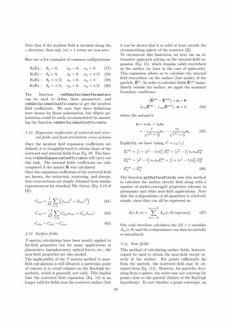
3.12. Expansion coefficients of scattered and inter-nal fields and fixed-orientation cross-sections
Once the incident field expansion coefficients aredefined, it is straightforward to obtain those of thescattered and internal fields from Eq. 18. The func-tion rvhGetExpansionCoefficients will carry outthis task. The internal fields coefficients are onlycomputed if the matrix R was calculated.Once the expansion coefficients of the scattered fieldare known, the extinction, scattering, and absorp-tion cross-sections are simply obtained from similarexpressions as for standard Mie theory (Eq. 5.18 of[4]):
Csca =1
k21
∑n,m
(|cnm|2 + |dnm|2
)(61)
Cext =−1
k21
∑n,m
(c∗nmanm + d∗nmbnm) (62)
Cabs = Cext − Csca. (63)
3.13. Surface fields
T -matrix calculations have been mostly applied tofar-field properties but for many applications inplasmonics, nanophotonics, optical forces, etc., thenear-field properties are also needed.The applicability of the T -matrix method to near-field calculations is still debated; a particular pointof concern is to avoid reliance on the Rayleigh hy-pothesis, which is generally not valid. This impliesthat the scattered field expansion (Eq. 14) is nolonger valid for fields near the scatterer surface (but
it can be shown that it is valid at least outside thecircumscribing sphere of the scatterer [4]).To circumvent this limitation, we here use an al-ternative approach relying on the internal field ex-pansion (Eq. 15), which remains valid everywhereat the surface (at least in the case of spheroids).This expansion allows us to calculate the internalfield everywhere on the surface (but inside) of theparticle, Ein. In order to calculate fields Eout imme-diately outside the surface, we apply the standardboundary conditions:(
Eint − Eout)× n = 0(
εinEint − εoutEout
)· n = 0 (64)
where the normal is
n = nrer + nθeθ
=r√
r2 + r2θer −
rθ√r2 + r2θ
eθ. (65)
Explicitly, we have (using s2 = ε2/ε1)
Eoutr =
[1 + (s2 − 1)n2r
]Einr +
[s2 − 1
]nrnθE
inθ
Eoutθ =
[s2 − 1
]nrnθE
inr +
[1 + (s2 − 1)n2θ
]Einθ
Eoutφ = Ein
φ (66)
The function pstSurfaceFields uses this methodto calculate the surface electric field along with anumber of surface-averaged properties relevant toplasmonics and other near-field applications. Notethat the φ-dependence of all quantities is relativelysimple, since they can all be expressed as:
A(r, θ, φ) =
m=+N∑m=−N
Am(r, θ) exp(imφ). (67)
Our code therefore calculates the 2N + 1 variablesAm(r, θ) and the φ-dependence can then be triviallyre-introduced.
3.14. Near fieldsThis method of calculating surface fields, however,cannot be used to obtain the near-field except ex-actly at the surface. For points sufficiently farfrom the particle, the scattered field may be ob-tained from Eq. (14). However, for particles devi-ating from a sphere, the series may not converge forpoints close to the particle (failure of the Rayleighhypothesis). To test whether a point converges, an
16
indicative test is to increase the number of mul-tipoles considered, and confirm that the calculatedfield converges to some value. If it fails to converge,either insufficient multipoles were considered, or thepoint is in a region where convergence will never beobtained. We have recently studied these aspectsand developed an alternative method of computingnear-fields, which will be discussed in detail else-where [25]. We only here give a brief overview ofthe method, which is implemented in the functionpstGetNearField.As originally suggested in Ref. [26], we make useof the surface integral equation (Eq. 5.168 of [4]),which expresses the scattered field in terms of thesurface fields,
Esca(r′) =
∫S
dS{iωµ0 [n×H(r)] ·
←→G (r, r′)
+ [n×E(r)] ·[∇×←→G (r, r′)
]}, (68)
where←→G is the free-space Green’s function. The
surface fields E,H can be calculated accurately asdescribed earlier and the integral is then performedusing a double quadrature on θ and φ (with thesame number of nodes for simplicity). As a result,this method is slower than the other methods forcalculating the scattered field (where applicable),but will exhibit much better convergence behaviourfor points near the particle [25]. An example of itsuse is given in ScriptTutorial.
4. Additional implementation details
4.1. File naming conventions and organization
The first three letters of each function are used toclassify functions depending on their roles:
• slv: High-level functions solving a specificclass of problems.
• pst: High-level functions used for post-processing.
• vsh: Mostly low-level functions handling thecalculations of quantities related to vectorspherical wavefunctions.
• rvh: T -matrix related functions specific toparticles with mirror-reflection symmetry.
• sph: T -matrix related functions specific tospheroidal particles.
• aux: Auxiliary functions (low-level).
Each m-file is also located in a specific folder withthe following classification,
• High-Level: T -matrix related functions mostlikely to be called directly by the user.
• Low-Level: T -matrix related functions usedby the high-level functions.
• Materials: Includes dielectric functions ofgold (Au) and silver (Ag) for plasmonics appli-cations, as well as an example dielectric func-tion interpolated from tabulated values for sil-icon (Si).
• Post-processing: Functions to calculate op-tical properties.
• Scripts: Contains example and tutorialscripts.
• Solve: Contains the slv functions used tosolve a specific class of problems.
• Utils: Includes miscellaneous utility func-tions, notably to export the T -matrix, testwhether the code is running in Octave orMatlab, or generate quadrature nodes andweights.
4.2. Storage of matrices
All matrices are stored in cell arrays, such asCstPQa of dimensions 1×M , whereM is the numberof m elements in absmvec. As a result, CstPQa{j}corresponds to m=absmvec(j). If all m are com-puted, then absmvec=0:N and the matrices for agiven m are stored in CstPQa{m+1}.Each element CstPQa{j} contains a structure stPQdescribing the matrices for the corresponding m,stored in the following fields:
• stPQ.CsMatList: cell array of strings list-ing the name of the matrices. For examplestPQ.CsMatList = {'st4MP','st4MQ'}.
• For each string in this list, two fieldsare included with eo and oe appended atthe end. For example stPQ.st4MPeo andstPQ.st4MPoe. These st4M structures containthe matrix in a form described below, whichavoids storing the many zeros that are imposedby the reflection symmetry.
17
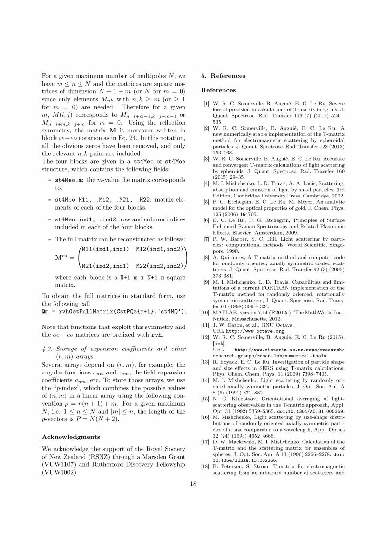
For a given maximum number of multipoles N , wehave m ≤ n ≤ N and the matrices are square ma-trices of dimension N + 1 − m (or N for m = 0)since only elements Mnk with n, k ≥ m (or ≥ 1for m = 0) are needed. Therefore for a givenm, M(i, j) corresponds to Mn=i+m−1,k=j+m−1 orMn=i+m,k=j+m for m = 0. Using the reflectionsymmetry, the matrix M is moreover written inblock oe−eo notation as in Eq. 24. In this notation,all the obvious zeros have been removed, and onlythe relevant n, k pairs are included.The four blocks are given in a st4Meo or st4Moestructure, which contains the following fields:
• st4Meo.m: them-value the matrix correspondsto.
• st4Meo.M11, .M12, .M21, .M22: matrix ele-ments of each of the four blocks.
• st4Meo.ind1, .ind2: row and column indicesincluded in each of the four blocks.
• The full matrix can be reconstructed as follows:
Meo =
M11(ind1,ind1) M12(ind1,ind2)
M21(ind2,ind1) M22(ind2,ind2)
where each block is a N+1-m x N+1-m squarematrix.
To obtain the full matrices in standard form, usethe following callQm = rvhGetFullMatrix(CstPQa{m+1},'st4MQ');
Note that functions that exploit this symmetry andthe oe− eo matrices are prefixed with rvh.
4.3. Storage of expansion coefficients and other(n,m) arrays
Several arrays depend on (n,m), for example, theangular functions πnm and τnm, the field expansioncoefficients anm, etc. To store those arrays, we usethe “p-index”, which combines the possible valuesof (n,m) in a linear array using the following con-vention p = n(n + 1) + m. For a given maximumN , i.e. 1 ≤ n ≤ N and |m| ≤ n, the length of thep-vectors is P = N(N + 2).
Acknowledgments
We acknowledge the support of the Royal Societyof New Zealand (RSNZ) through a Marsden Grant(VUW1107) and Rutherford Discovery Fellowship(VUW1002).
5. References
References
[1] W. R. C. Somerville, B. Auguié, E. C. Le Ru, Severeloss of precision in calculations of T-matrix integrals, J.Quant. Spectrosc. Rad. Transfer 113 (7) (2012) 524 –535.
[2] W. R. C. Somerville, B. Auguié, E. C. Le Ru, Anew numerically stable implementation of the T-matrixmethod for electromagnetic scattering by spheroidalparticles, J. Quant. Spectrosc. Rad. Transfer 123 (2013)153–168.
[3] W. R. C. Somerville, B. Auguié, E. C. Le Ru, Accurateand convergent T-matrix calculations of light scatteringby spheroids, J. Quant. Spectrosc. Rad. Transfer 160(2015) 29–35.
[4] M. I. Mishchenko, L. D. Travis, A. A. Lacis, Scattering,absorption and emission of light by small particles, 3rdEdition, Cambridge University Press, Cambridge, 2002.
[5] P. G. Etchegoin, E. C. Le Ru, M. Meyer, An analyticmodel for the optical properties of gold, J. Chem. Phys.125 (2006) 164705.
[6] E. C. Le Ru, P. G. Etchegoin, Principles of SurfaceEnhanced Raman Spectroscopy and Related PlasmonicEffects, Elsevier, Amsterdam, 2009.
[7] P. W. Barber, S. C. Hill, Light scattering by parti-cles: computational methods, World Scientific, Singa-pore, 1990.
[8] A. Quirantes, A T-matrix method and computer codefor randomly oriented, axially symmetric coated scat-terers, J. Quant. Spectrosc. Rad. Transfer 92 (3) (2005)373–381.
[9] M. I. Mishchenko, L. D. Travis, Capabilities and limi-tations of a current FORTRAN implementation of theT-matrix method for randomly oriented, rotationallysymmetric scatterers, J. Quant. Spectrosc. Rad. Trans-fer 60 (1998) 309 – 324.
[10] MATLAB, version 7.14 (R2012a), The MathWorks Inc.,Natick, Massachusetts, 2012.
[11] J. W. Eaton, et al., GNU Octave.URL http://www.octave.org
[12] W. R. C. Somerville, B. Auguié, E. C. Le Ru (2015).[link].URL http://www.victoria.ac.nz/scps/research/research-groups/raman-lab/numerical-tools
[13] R. Boyack, E. C. Le Ru, Investigation of particle shapeand size effects in SERS using T-matrix calculations,Phys. Chem. Chem. Phys. 11 (2009) 7398–7405.
[14] M. I. Mishchenko, Light scattering by randomly ori-ented axially symmetric particles, J. Opt. Soc. Am. A8 (6) (1991) 871–882.
[15] N. G. Khlebtsov, Orientational averaging of light-scattering observables in the T-matrix approach, Appl.Opt. 31 (1992) 5359–5365. doi:10.1364/AO.31.005359.
[16] M. Mishchenko, Light scattering by size-shape distri-butions of randomly oriented axially symmetric parti-cles of a size comparable to a wavelength, Appl. Optics32 (24) (1993) 4652–4666.
[17] D. W. Mackowski, M. I. Mishchenko, Calculation of theT-matrix and the scattering matrix for ensembles ofspheres, J. Opt. Soc. Am. A 13 (1996) 2266–2278. doi:10.1364/JOSAA.13.002266.
[18] B. Peterson, S. Ström, T-matrix for electromagneticscattering from an arbitrary number of scatterers and
18
representations of E(3), Phys. Rev. D 8 (10) (1973)3661–3678.
[19] W. R. C. Somerville, B. Auguié, E. C. Le Ru, Simplifiedexpressions of the T-matrix integrals for electromag-netic scattering, Opt. Lett. 36 (17) (2011) 3482–3484.
[20] M. I. Mishchenko, Calculation of the amplitude matrixfor a nonspherical particle in a fixed orientation, Appl.Optics 39 (6) (2000) 1026–1031.
[21] G. von Winckel, Legendre-Gauss quadrature weightsand nodes, MATLAB central file exchange.
[22] D. Wielaard, M. Mishchenko, A. Macke, B. Carlson, Im-proved T-matrix computations for large, nonabsorbingand weakly absorbing nonspherical particles and com-parison with geometrical-optics approximation, Appl.Optics 36 (18) (1997) 4305–4313.
[23] A. Moroz, Improvement of Mishchenko’s T-matrix codefor absorbing particles, Appl. Optics 44 (17) (2005)3604–3609.
[24] S. N. Volkov, I. V. Samokhvalov, D. Kim, Assessingand improving the accuracy of T-matrix calculation ofhomogeneous particles with point-group symmetries, J.Quant. Spectrosc. Rad. Transfer 123 (2013) 169 – 175.
[25] E. C. Le Ru, S. Roache, W. R. C. Somerville, B. Auguié,Numerical investigations into the Rayleigh hypothesisfor the T-matrix method, Manuscript in preparation.
[26] A. Doicu, T. Wriedt, Near-field computation using thenull-field method, J. Quant. Spectrosc. Rad. Transfer111 (3) (2010) 466–473.
6. Appendix: Convergence tests
h→s 1.1 2 4 10 20 100
1.311 + 0.00i 80 50 45 35 35 35
1.500 + 0.00i 50 35 30 27 27 25
1.500 + 0.02i 60 40 30 27 27 27
1.500 + 2.00i 80 20 14 12 12 10
2.500 + 0.00i 20 18 12 12 12 12
4.000 + 0.10i 16 11 8 7 7 6
0.100 + 4.00i 60 10 7 6 6 5
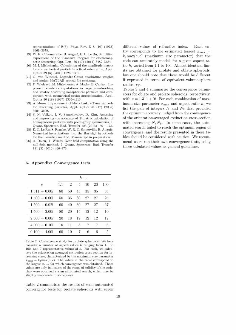
Table 2: Convergence study for prolate spheroids. We hereconsider a number of aspect ratios h ranging from 1.1 to100, and 7 representative values of s. For each, we calcu-late the orientation-averaged extinction cross-section for in-creasing sizes, characterized by the maximum size parameterxmax = k1max(a, c). The values in the table correspond tothe largest xmax for which convergence was obtained. Thosevalues are only indicators of the range of validity of the code;they were obtained via an automated search, which may beslightly inaccurate in some cases.
Table 2 summarises the results of semi-automatedconvergence tests for prolate spheroids with seven
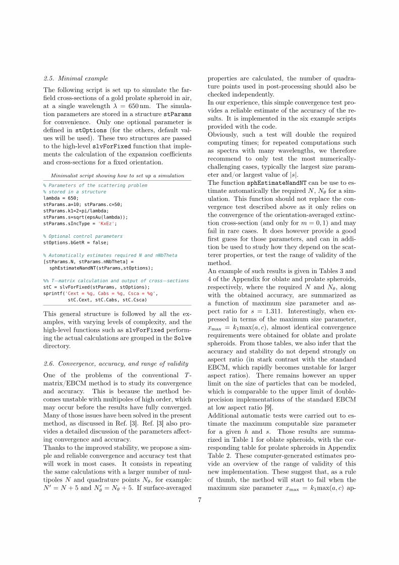
different values of refractive index. Each en-try corresponds to the estimated largest xmax =k1max(a, c) (maximum size parameter) that thecode can accurately model, for a given aspect ra-tio h, varied from 1.1 to 100. Almost identical lim-its are obtained for prolate and oblate spheroids,but one should note that those would be differentif expressed in terms of equivalent-volume-sphereradius, rV .Tables 3 and 4 summarise the convergence param-eters for oblate and prolate spheroids, respectively,with s = 1.311 + 0i. For each combination of max-imum size parameter xmax and aspect ratio h, welist the pair of integers N and Nθ that providedthe optimum accuracy, judged from the convergenceof the orientation-averaged extinction cross-sectionwith increasing N,Nθ. In some cases, the auto-mated search failed to reach the optimum region ofconvergence, and the results presented in those ta-bles should be considered with caution. We recom-mend users run their own convergence tests, usingthose tabulated values as general guidelines.
19
h: xmax: 0.01 0.1 1 2 3 4 5 6 7 8 10 12 15 20 25 30 40 50 60 70 80
1.1NNθerror
56–
56–
76–
97–
117–
118–
138–
159–
179–
1710–
2115–
2315–
2715–
3520–
4125–
4735–
634010−12
774010−11
958010−9
1278010−7
111120010−4
1.3NNθerror
59–
59–
99–
119–
119–
1310–
1515–
1515–
1915–
1915–
2315–
2720–
3120–
3725–
4545–
533010−12
695010−9
934510−7
11550010−3
2NNθerror
520–
720–
1120–
1320–
1520–
1520–
1920–
1920–
2125–
2325–
2525–
2725–
3330–
4135–
494510−12
613510−11
755010−7
1034510−4
4NNθerror
540–
740–
1140–
1540–
1740–
19710−3
2140–
2345–
2345–
2545–
2950–
3150–
3560–
457010−13
517010−11
579010−9
599010−4
7NNθerror
570–
770–
1170–
1570–
1970–
1970–
1980–
2380–
2580–
2780–
3190–
3590–
37100–
4120010−11
4713010−10
4713010−6
10NNθerror
5100–
7100–
1390–
15100–
19100–
19100–
21110–
25110–
27110–
27120–
31120–
33130–
41140–
4518010−11
4318010−8
4720010−6
20NNθerror
5200–
7200–
13200–
15200–
19200–
21200–
23200–
23220–
27220–
29240–
33260–
37260–
43280–
4330010−12
4955010−8
4140010−4
50NNθerror
5500–
7500–
13500–
17500–
19500–
21500–
23550–
25550–
27550–
29600–
33650–
35800–
3970010−13
45110010−12
4790010−9
45120010−6
100NNθerror
51000–
71100–
131000–
171100–
191000–
211100–
231100–
251100–
271100–
271100–
331300–
351500–
471400–
531600–
47200010−9
Table 3: Convergence study for an oblate spheroid with s = 1.311+0i. For each pair of size parameter xmax (columns) and aspect ratio h (rows), we list the convergenceparameters N,Nθ, together with the relative error, only displayed if worse than 10−13.
20
h: xmax: 0.01 0.1 1 2 3 4 5 6 7 8 10 12 15 20 25 30 40 50 60 70 80
1.1NNθerror
56–
56–
76–
97–
117–
118–
138–
159–
1710–
1710–
2115–
2315–
2715–
3520–
4125–
4725–
674010−12
796010−10
974510−9
877010−7
10912010−4
1.3NNθerror
59–
59–
99–
119–
119–
1310–
1515–
1515–
1915–
1915–
2315–
2720–
3120–
3725–
4525–
533010−12
734010−10
954510−7
11718010−4
2NNθerror
520–
720–
1120–
1320–
1520–
1520–
1920–
1920–
2120–
2325–
2525–
2725–
3330–
4130–
494510−12
614510−10
894010−7
1135010−4
4NNθerror
540–
740–
1140–
1540–
1740–
1940–
1940–
2340–
2345–
2545–
2745–
3150–
3560–
4390–
497010−12
4910010−9
5911010−6
7NNθerror
580–
780–
1180–
1570–
1770–
1970–
2170–
2380–
2580–
2780–
3180–
3390–
3790–
4312010−13
4312010−10
4713010−8
10NNθerror
5120–
7120–
11120–
15120–
17120–
21100–
21120–
23120–
27120–
27120–
31120–
33120–
37140–
45160–
4516010−10
4520010−8
20NNθerror
522010−13
722010−13
1122010−13
15260–
19220–
21220–
21220–
25220–
27220–
27260–
31260–
2926010−12
39280–
4730010−13
4935010−10
4535010−7
50NNθerror
565010−12
765010−12
1165010−12
1540010−12
19500–
21500–
21500–
25500–
27650–
29700–
31600–
33700–
39700–
4590010−12
53110010−11
45120010−7
100NNθerror
580010−12
780010−12
1180010−12
1580010−12
1980010−12
21100010−12
21100010−13
25100010−13
27100010−13
291400–
311400–
331200–
391600–
45180010−12
47200010−11
47200010−8
Table 4: Convergence study for a prolate spheroid with s = 1.311+0i. For each pair of size parameter xmax (columns) and aspect ratio h (rows), we list the convergenceparameters N,Nθ, together with the relative error, only displayed if worse than 10−13.
21