SPECTRAL ANALYSIS OF SIGNALS - Lu

“sm2”2004/2/22page i

i

i

i

i

i

i

i

i

SPECTRAL ANALYSIS OFSIGNALS

Petre Stoica and Randolph Moses

PRENTICE HALL, Upper Saddle River, New Jersey 07458

“sm2”2004/2/22page ii

i

i

i

i

i

i

i

i

Library of Congress Cataloging-in-Publication DataSpectral Analysis of Signals/Petre Stoica and Randolph Moses

p. cm.Includes bibliographical references index.ISBN 0-13-113956-81. Spectral theory (Mathematics) I. Moses, Randolph II. Title

512’–dc21 2005QA814.G27 00-055035 CIP

Acquisitions Editor: Tom RobbinsEditor-in-Chief: ?Assistant Vice President of Production and Manufacturing: ?Executive Managing Editor: ?Senior Managing Editor: ?Production Editor: ?Manufacturing Buyer: ?Manufacturing Manager: ?Marketing Manager: ?Marketing Assistant: ?Director of Marketing: ?Editorial Assistant: ?Art Director: ?Interior Designer: ?Cover Designer: ?Cover Photo: ?

c© 2005 by Prentice Hall, Inc.Upper Saddle River, New Jersey 07458

All rights reserved. No part of this book maybe reproduced, in any form or by any means,without permission in writing from the publisher.

Printed in the United States of America10 9 8 7 6 5 4 3 2 1

ISBN 0-13-113956-8

Pearson Education LTD., LondonPearson Education Australia PTY, Limited, SydneyPearson Education Singapore, Pte. LtdPearson Education North Asia Ltd, Hong KongPearson Education Canada, Ltd., TorontoPearson Educacion de Mexico, S.A. de C.V.Pearson Education - Japan, TokyoPearson Education Malaysia, Pte. Ltd

“sm2”2004/2/22page iii

i

i

i

i

i

i

i

i

Contents

1 Basic Concepts 11.1 Introduction . . . . . . . . . . . . . . . . . . . . . . . . . . . . . . . . 11.2 Energy Spectral Density of Deterministic Signals . . . . . . . . . . . 31.3 Power Spectral Density of Random Signals . . . . . . . . . . . . . . 4

1.3.1 First Definition of Power Spectral Density . . . . . . . . . . . 61.3.2 Second Definition of Power Spectral Density . . . . . . . . . . 7

1.4 Properties of Power Spectral Densities . . . . . . . . . . . . . . . . . 81.5 The Spectral Estimation Problem . . . . . . . . . . . . . . . . . . . . 121.6 Complements . . . . . . . . . . . . . . . . . . . . . . . . . . . . . . . 12

1.6.1 Coherency Spectrum . . . . . . . . . . . . . . . . . . . . . . . 121.7 Exercises . . . . . . . . . . . . . . . . . . . . . . . . . . . . . . . . . 14

2 Nonparametric Methods 222.1 Introduction . . . . . . . . . . . . . . . . . . . . . . . . . . . . . . . . 222.2 Periodogram and Correlogram Methods . . . . . . . . . . . . . . . . 22

2.2.1 Periodogram . . . . . . . . . . . . . . . . . . . . . . . . . . . 222.2.2 Correlogram . . . . . . . . . . . . . . . . . . . . . . . . . . . 23

2.3 Periodogram Computation via FFT . . . . . . . . . . . . . . . . . . 252.3.1 Radix–2 FFT . . . . . . . . . . . . . . . . . . . . . . . . . . . 262.3.2 Zero Padding . . . . . . . . . . . . . . . . . . . . . . . . . . . 27

2.4 Properties of the Periodogram Method . . . . . . . . . . . . . . . . . 282.4.1 Bias Analysis of the Periodogram . . . . . . . . . . . . . . . . 282.4.2 Variance Analysis of the Periodogram . . . . . . . . . . . . . 32

2.5 The Blackman–Tukey Method . . . . . . . . . . . . . . . . . . . . . . 372.5.1 The Blackman–Tukey Spectral Estimate . . . . . . . . . . . . 372.5.2 Nonnegativeness of the Blackman–Tukey Spectral Estimate . 39

2.6 Window Design Considerations . . . . . . . . . . . . . . . . . . . . . 392.6.1 Time–Bandwidth Product and Resolution–Variance Trade-

offs in Window Design . . . . . . . . . . . . . . . . . . . . . . 402.6.2 Some Common Lag Windows . . . . . . . . . . . . . . . . . . 412.6.3 Window Design Example . . . . . . . . . . . . . . . . . . . . 452.6.4 Temporal Windows and Lag Windows . . . . . . . . . . . . . 47

2.7 Other Refined Periodogram Methods . . . . . . . . . . . . . . . . . . 482.7.1 Bartlett Method . . . . . . . . . . . . . . . . . . . . . . . . . 492.7.2 Welch Method . . . . . . . . . . . . . . . . . . . . . . . . . . 502.7.3 Daniell Method . . . . . . . . . . . . . . . . . . . . . . . . . . 52

2.8 Complements . . . . . . . . . . . . . . . . . . . . . . . . . . . . . . . 552.8.1 Sample Covariance Computation via FFT . . . . . . . . . . . 552.8.2 FFT–Based Computation of Windowed Blackman–Tukey Pe-

riodograms . . . . . . . . . . . . . . . . . . . . . . . . . . . . 572.8.3 Data and Frequency Dependent Temporal Windows: The

Apodization Approach . . . . . . . . . . . . . . . . . . . . . . 59

iii

“sm2”2004/2/22page iv

i

i

i

i

i

i

i

i

iv

2.8.4 Estimation of Cross–Spectra and Coherency Spectra . . . . . 642.8.5 More Time–Bandwidth Product Results . . . . . . . . . . . . 66

2.9 Exercises . . . . . . . . . . . . . . . . . . . . . . . . . . . . . . . . . 71

3 Parametric Methods for Rational Spectra 863.1 Introduction . . . . . . . . . . . . . . . . . . . . . . . . . . . . . . . . 863.2 Signals with Rational Spectra . . . . . . . . . . . . . . . . . . . . . . 873.3 Covariance Structure of ARMA Processes . . . . . . . . . . . . . . . 883.4 AR Signals . . . . . . . . . . . . . . . . . . . . . . . . . . . . . . . . 90

3.4.1 Yule–Walker Method . . . . . . . . . . . . . . . . . . . . . . . 903.4.2 Least Squares Method . . . . . . . . . . . . . . . . . . . . . . 91

3.5 Order–Recursive Solutions to the Yule–Walker Equations . . . . . . 943.5.1 Levinson–Durbin Algorithm . . . . . . . . . . . . . . . . . . . 963.5.2 Delsarte–Genin Algorithm . . . . . . . . . . . . . . . . . . . . 97

3.6 MA Signals . . . . . . . . . . . . . . . . . . . . . . . . . . . . . . . . 1013.7 ARMA Signals . . . . . . . . . . . . . . . . . . . . . . . . . . . . . . 103

3.7.1 Modified Yule–Walker Method . . . . . . . . . . . . . . . . . 1033.7.2 Two–Stage Least Squares Method . . . . . . . . . . . . . . . 106

3.8 Multivariate ARMA Signals . . . . . . . . . . . . . . . . . . . . . . . 1093.8.1 ARMA State–Space Equations . . . . . . . . . . . . . . . . . 1093.8.2 Subspace Parameter Estimation — Theoretical Aspects . . . 1133.8.3 Subspace Parameter Estimation — Implementation Aspects . 115

3.9 Complements . . . . . . . . . . . . . . . . . . . . . . . . . . . . . . . 1173.9.1 The Partial Autocorrelation Sequence . . . . . . . . . . . . . 1173.9.2 Some Properties of Covariance Extensions . . . . . . . . . . . 1183.9.3 The Burg Method for AR Parameter Estimation . . . . . . . 1193.9.4 The Gohberg–Semencul Formula . . . . . . . . . . . . . . . . 1223.9.5 MA Parameter Estimation in Polynomial Time . . . . . . . . 125

3.10 Exercises . . . . . . . . . . . . . . . . . . . . . . . . . . . . . . . . . 129

4 Parametric Methods for Line Spectra 1444.1 Introduction . . . . . . . . . . . . . . . . . . . . . . . . . . . . . . . . 1444.2 Models of Sinusoidal Signals in Noise . . . . . . . . . . . . . . . . . . 148

4.2.1 Nonlinear Regression Model . . . . . . . . . . . . . . . . . . . 1484.2.2 ARMA Model . . . . . . . . . . . . . . . . . . . . . . . . . . . 1494.2.3 Covariance Matrix Model . . . . . . . . . . . . . . . . . . . . 149

4.3 Nonlinear Least Squares Method . . . . . . . . . . . . . . . . . . . . 1514.4 High–Order Yule–Walker Method . . . . . . . . . . . . . . . . . . . . 1554.5 Pisarenko and MUSIC Methods . . . . . . . . . . . . . . . . . . . . . 1594.6 Min–Norm Method . . . . . . . . . . . . . . . . . . . . . . . . . . . . 1644.7 ESPRIT Method . . . . . . . . . . . . . . . . . . . . . . . . . . . . . 1664.8 Forward–Backward Approach . . . . . . . . . . . . . . . . . . . . . . 1684.9 Complements . . . . . . . . . . . . . . . . . . . . . . . . . . . . . . . 170

4.9.1 Mean Square Convergence of Sample Covariances for LineSpectral Processes . . . . . . . . . . . . . . . . . . . . . . . . 170

4.9.2 The Caratheodory Parameterization of a Covariance Matrix . 172

“sm2”2004/2/22page v

i

i

i

i

i

i

i

i

v

4.9.3 Using the Unwindowed Periodogram for Sine Wave Detectionin White Noise . . . . . . . . . . . . . . . . . . . . . . . . . . 174

4.9.4 NLS Frequency Estimation for a Sinusoidal Signal with Time-Varying Amplitude . . . . . . . . . . . . . . . . . . . . . . . . 177

4.9.5 Monotonically Descending Techniques for Function Minimiza-tion . . . . . . . . . . . . . . . . . . . . . . . . . . . . . . . . 179

4.9.6 Frequency-selective ESPRIT-based Method . . . . . . . . . . 1854.9.7 A Useful Result for Two-Dimensional (2D) Sinusoidal Signals 193

4.10 Exercises . . . . . . . . . . . . . . . . . . . . . . . . . . . . . . . . . 198

5 Filter Bank Methods 2075.1 Introduction . . . . . . . . . . . . . . . . . . . . . . . . . . . . . . . . 2075.2 Filter Bank Interpretation of the Periodogram . . . . . . . . . . . . . 2105.3 Refined Filter Bank Method . . . . . . . . . . . . . . . . . . . . . . . 212

5.3.1 Slepian Baseband Filters . . . . . . . . . . . . . . . . . . . . . 2135.3.2 RFB Method for High–Resolution Spectral Analysis . . . . . 2165.3.3 RFB Method for Statistically Stable Spectral Analysis . . . . 218

5.4 Capon Method . . . . . . . . . . . . . . . . . . . . . . . . . . . . . . 2225.4.1 Derivation of the Capon Method . . . . . . . . . . . . . . . . 2225.4.2 Relationship between Capon and AR Methods . . . . . . . . 228

5.5 Filter Bank Reinterpretation of the Periodogram . . . . . . . . . . . 2315.6 Complements . . . . . . . . . . . . . . . . . . . . . . . . . . . . . . . 235

5.6.1 Another Relationship between the Capon and AR Methods . 2355.6.2 Multiwindow Interpretation of Daniell and Blackman–Tukey

Periodograms . . . . . . . . . . . . . . . . . . . . . . . . . . . 2385.6.3 Capon Method for Exponentially Damped Sinusoidal Signals 2415.6.4 Amplitude and Phase Estimation Method (APES) . . . . . . 2445.6.5 Amplitude and Phase Estimation Method for Gapped Data

(GAPES) . . . . . . . . . . . . . . . . . . . . . . . . . . . . . 2475.6.6 Extensions of Filter Bank Approaches to Two–Dimensional

Signals . . . . . . . . . . . . . . . . . . . . . . . . . . . . . . . 2515.7 Exercises . . . . . . . . . . . . . . . . . . . . . . . . . . . . . . . . . 257

6 Spatial Methods 2636.1 Introduction . . . . . . . . . . . . . . . . . . . . . . . . . . . . . . . . 2636.2 Array Model . . . . . . . . . . . . . . . . . . . . . . . . . . . . . . . 265

6.2.1 The Modulation–Transmission–Demodulation Process . . . . 2666.2.2 Derivation of the Model Equation . . . . . . . . . . . . . . . 268

6.3 Nonparametric Methods . . . . . . . . . . . . . . . . . . . . . . . . . 2736.3.1 Beamforming . . . . . . . . . . . . . . . . . . . . . . . . . . . 2766.3.2 Capon Method . . . . . . . . . . . . . . . . . . . . . . . . . . 279

6.4 Parametric Methods . . . . . . . . . . . . . . . . . . . . . . . . . . . 2816.4.1 Nonlinear Least Squares Method . . . . . . . . . . . . . . . . 2816.4.2 Yule–Walker Method . . . . . . . . . . . . . . . . . . . . . . . 2836.4.3 Pisarenko and MUSIC Methods . . . . . . . . . . . . . . . . . 2846.4.4 Min–Norm Method . . . . . . . . . . . . . . . . . . . . . . . . 2856.4.5 ESPRIT Method . . . . . . . . . . . . . . . . . . . . . . . . . 285

“sm2”2004/2/22page vi

i

i

i

i

i

i

i

i

vi

6.5 Complements . . . . . . . . . . . . . . . . . . . . . . . . . . . . . . . 2866.5.1 On the Minimum Norm Constraint . . . . . . . . . . . . . . . 2866.5.2 NLS Direction-of-Arrival Estimation for a Constant-Modulus

Signal . . . . . . . . . . . . . . . . . . . . . . . . . . . . . . . 2886.5.3 Capon Method: Further Insights and Derivations . . . . . . . 2906.5.4 Capon Method for Uncertain Direction Vectors . . . . . . . . 2946.5.5 Capon Method with Noise Gain Constraint . . . . . . . . . . 2986.5.6 Spatial Amplitude and Phase Estimation (APES) . . . . . . 3056.5.7 The CLEAN Algorithm . . . . . . . . . . . . . . . . . . . . . 3126.5.8 Unstructured and Persymmetric ML Estimates of the Covari-

ance Matrix . . . . . . . . . . . . . . . . . . . . . . . . . . . . 3176.6 Exercises . . . . . . . . . . . . . . . . . . . . . . . . . . . . . . . . . 319

APPENDICES

A Linear Algebra and Matrix Analysis Tools 328A.1 Introduction . . . . . . . . . . . . . . . . . . . . . . . . . . . . . . . . 328A.2 Range Space, Null Space, and Matrix Rank . . . . . . . . . . . . . . 328A.3 Eigenvalue Decomposition . . . . . . . . . . . . . . . . . . . . . . . . 330

A.3.1 General Matrices . . . . . . . . . . . . . . . . . . . . . . . . . 331A.3.2 Hermitian Matrices . . . . . . . . . . . . . . . . . . . . . . . . 333

A.4 Singular Value Decomposition and Projection Operators . . . . . . . 336A.5 Positive (Semi)Definite Matrices . . . . . . . . . . . . . . . . . . . . 341A.6 Matrices with Special Structure . . . . . . . . . . . . . . . . . . . . . 345A.7 Matrix Inversion Lemmas . . . . . . . . . . . . . . . . . . . . . . . . 347A.8 Systems of Linear Equations . . . . . . . . . . . . . . . . . . . . . . . 347

A.8.1 Consistent Systems . . . . . . . . . . . . . . . . . . . . . . . . 347A.8.2 Inconsistent Systems . . . . . . . . . . . . . . . . . . . . . . . 350

A.9 Quadratic Minimization . . . . . . . . . . . . . . . . . . . . . . . . . 353

B Cramer–Rao Bound Tools 355B.1 Introduction . . . . . . . . . . . . . . . . . . . . . . . . . . . . . . . . 355B.2 The CRB for General Distributions . . . . . . . . . . . . . . . . . . . 358B.3 The CRB for Gaussian Distributions . . . . . . . . . . . . . . . . . . 359B.4 The CRB for Line Spectra . . . . . . . . . . . . . . . . . . . . . . . . 364B.5 The CRB for Rational Spectra . . . . . . . . . . . . . . . . . . . . . 365B.6 The CRB for Spatial Spectra . . . . . . . . . . . . . . . . . . . . . . 367

C Model Order Selection Tools 377C.1 Introduction . . . . . . . . . . . . . . . . . . . . . . . . . . . . . . . . 377C.2 Maximum Likelihood Parameter Estimation . . . . . . . . . . . . . . 378C.3 Useful Mathematical Preliminaries and Outlook . . . . . . . . . . . . 381

C.3.1 Maximum A Posteriori (MAP) Selection Rule . . . . . . . . . 382C.3.2 Kullback-Leibler Information . . . . . . . . . . . . . . . . . . 384C.3.3 Outlook: Theoretical and Practical Perspectives . . . . . . . 385

C.4 Direct Kullback-Leibler (KL) Approach: No-Name Rule . . . . . . . 386

“sm2”2004/2/22page vii

i

i

i

i

i

i

i

i

vii

C.5 Cross-Validatory KL Approach: The AIC Rule . . . . . . . . . . . . 387C.6 Generalized Cross-Validatory KL Approach: the GIC Rule . . . . . . 391C.7 Bayesian Approach: The BIC Rule . . . . . . . . . . . . . . . . . . . 392C.8 Summary and the Multimodel Approach . . . . . . . . . . . . . . . . 395

C.8.1 Summary . . . . . . . . . . . . . . . . . . . . . . . . . . . . . 395C.8.2 The Multimodel Approach . . . . . . . . . . . . . . . . . . . 397

D Answers to Selected Exercises 399

Bibliography 401

References Grouped by Subject 413

Index 420

“sm2”2004/2/22page viii

i

i

i

i

i

i

i

i

viii

“sm2”2004/2/22page ix

i

i

i

i

i

i

i

i

List of Exercises

CHAPTER 11.1 Scaling of the Frequency Axis1.2 Time–Frequency Distributions1.3 Two Useful Z–Transform Properties1.4 A Simple ACS Example1.5 Alternative Proof that |r(k)| ≤ r(0)1.6 A Double Summation Formula1.7 Is a Truncated Autocovariance Sequence (ACS) a Valid ACS?1.8 When Is a Sequence an Autocovariance Sequence?1.9 Spectral Density of the Sum of Two Correlated Signals1.10 Least Squares Spectral Approximation1.11 Linear Filtering and the Cross–SpectrumC1.12 Computer Generation of Autocovariance SequencesC1.13 DTFT Computations using Two–Sided SequencesC1.14 Relationship between the PSD and the Eigenvalues of the ACS Matrix

CHAPTER 22.1 Covariance Estimation for Signals with Unknown Means2.2 Covariance Estimation for Signals with Unknown Means (cont’d)2.3 Unbiased ACS Estimates may lead to Negative Spectral Estimates2.4 Variance of Estimated ACS2.5 Another Proof of the Equality φp(ω) = φc(ω)2.6 A Compact Expression for the Sample ACS2.7 Yet Another Proof of the Equality φp(ω) = φc(ω)2.8 Linear Transformation Interpretation of the DFT2.9 For White Noise the Periodogram is an Unbiased PSD Estimator2.10 Shrinking the Periodogram2.11 Asymptotic Maximum Likelihood Estimation of φ(ω) from φp(ω)2.12 Plotting the Spectral Estimates in dB2.13 Finite–Sample Variance/Covariance Analysis of the Periodogram2.14 Data–Weighted ACS Estimate Interpretation of Bartlett and Welch Meth-

ods2.15 Approximate Formula for Bandwidth Calculation2.16 A Further Look at the Time–Bandwidth Product2.17 Bias Considerations in Blackman–Tukey Window Design2.18 A Property of the Bartlett WindowC2.19 Zero Padding Effects on Periodogram EstimatorsC2.20 Resolution and Leakage Properties of the PeriodogramC2.21 Bias and Variance Properties of the Periodogram Spectral EstimateC2.22 Refined Methods: Variance–Resolution TradeoffC2.23 Periodogram–Based Estimators applied to Measured Data

ix

“sm2”2004/2/22page x

i

i

i

i

i

i

i

i

x

CHAPTER 33.1 The Minimum Phase Property3.2 Generating the ACS from ARMA Parameters3.3 Relationship between AR Modeling and Forward Linear Prediction3.4 Relationship between AR Modeling and Backward Linear Prediction3.5 Prediction Filters and Smoothing Filters3.6 Relationship between Minimum Prediction Error and Spectral Flatness3.7 Diagonalization of the Covariance Matrix3.8 Stability of Yule–Walker AR Models3.9 Three Equivalent Representations for AR Processes3.10 An Alternative Proof of the Stability Property of Reflection Coefficients3.11 Recurrence Properties of Reflection Coefficient Sequence for an MA Model3.12 Asymptotic Variance of the ARMA Spectral Estimator3.13 Filtering Interpretation of Numerator Estimators in ARMA Estimation3.14 An Alternative Expression for ARMA Power Spectral Density3.15 Pade Approximation3.16 (Non)Uniqueness of Fully Parameterized ARMA EquationsC3.17 Comparison of AR, ARMA and Periodogram Methods for ARMA SignalsC3.18 AR and ARMA Estimators for Line Spectral EstimationC3.19 Model Order Selection for AR and ARMA ProcessesC3.20 AR and ARMA Estimators applied to Measured Data

CHAPTER 44.1 Speed Measurement by a Doppler Radar as a Frequency Determination

Problem4.2 ACS of Sinusoids with Random Amplitudes or Nonuniform Phases4.3 A Nonergodic Sinusoidal Signal4.4 AR Model–Based Frequency Estimation4.5 An ARMA Model–Based Derivation of the Pisarenko Method4.6 Frequency Estimation when Some Frequencies are Known4.7 A Combined HOYW-ESPRIT Method for the MA Noise Case4.8 Chebyshev Inequality and the Convergence of Sample Covariances4.9 More about the Forward–Backward Approach4.10 ESPRIT and Min–Norm Under the Same Umbrella4.11 Yet Another Relationship between ESPRIT and Min–NormC4.12 Resolution Properties of Subspace Methods for Estimation of Line SpectraC4.13 Model Order Selection for Sinusoidal SignalsC4.14 Line Spectral Methods applied to Measured Data

CHAPTER 55.1 Multiwindow Interpretation of Bartlett and Welch Methods5.2 An Alternative Statistically Stable RFB Estimate5.3 Another Derivation of the Capon FIR Filter5.4 The Capon Filter is a Matched Filter5.5 Computation of the Capon Spectrum5.6 A Relationship between the Capon Method and MUSIC (Pseudo)Spectra5.7 A Capon–like Implementation of MUSIC

“sm2”2004/2/22page xi

i

i

i

i

i

i

i

i

xi

5.8 Capon Estimate of the Parameters of a Single Sine Wave5.9 An Alternative Derivation of the Relationship between the Capon and AR

MethodsC5.10 Slepian Window SequencesC5.11 Resolution of Refined Filter Bank MethodsC5.12 The Statistically Stable RFB Power Spectral EstimatorC5.13 The Capon Method

CHAPTER 66.1 Source Localization using a Sensor in Motion6.2 Beamforming Resolution for Uniform Linear Arrays6.3 Beamforming Resolution for Arbitrary Arrays6.4 Beamforming Resolution for L–Shaped Arrays6.5 Relationship between Beamwidth and Array Element Locations6.6 Isotropic Arrays6.7 Grating Lobes6.8 Beamspace Processing6.9 Beamspace Processing (cont’d)6.10 Beamforming and MUSIC under the Same Umbrella6.11 Subspace Fitting Interpretation of MUSIC6.12 Subspace Fitting Interpretation of MUSIC (cont’d.)6.13 Subspace Fitting Interpretation of MUSIC (cont’d.)6.14 Modified MUSIC for Coherent SignalsC6.15 Comparison of Spatial Spectral EstimatorsC6.16 Performance of Spatial Spectral Estimators for Coherent Source SignalsC6.17 Spatial Spectral Estimators applied to Measured Data

“sm2”2004/2/22page xii

i

i

i

i

i

i

i

i

xii

“sm2”2004/2/22page xiii

i

i

i

i

i

i

i

i

Preface

Spectral analysis considers the problem of determining the spectral content(i.e., the distribution of power over frequency) of a time series from a finite set ofmeasurements, by means of either nonparametric or parametric techniques. Thehistory of spectral analysis as an established discipline started more than a centuryago with the work by Schuster on detecting cyclic behavior in time series. Aninteresting historical perspective on the developments in this field can be found in[Marple 1987]. This reference notes that the word “spectrum” was apparentlyintroduced by Newton in relation to his studies of the decomposition of white lightinto a band of light colors, when passed through a glass prism (as illustrated on thefront cover). This word appears to be a variant of the Latin word “specter” whichmeans “ghostly apparition”. The contemporary English word that has the samemeaning as the original Latin word is “spectre”. Despite these roots of the word“spectrum”, we hope the student will be a “vivid presence” in the course that hasjust started!

This text, which is a revised and expanded version of Introduction to SpectralAnalysis (Prentice Hall, 1997), is designed to be used with a first course in spec-tral analysis that would typically be offered to senior undergraduate or first–yeargraduate students. The book should also be useful for self-study, as it is largelyself-contained. The text is concise by design, so that it gets to the main pointsquickly and should hence be appealing to those who would like a fast appraisal onthe classical and modern approaches of spectral analysis.

In order to keep the book as concise as possible without sacrificing the rigorof presentation or skipping over essential aspects, we do not cover some advancedtopics of spectral estimation in the main part of the text. However, several advancedtopics are considered in the complements that appear at the end of each chapter,and also in the appendices. For an introductory course, the reader can skip thecomplements and refer to results in the appendices without having to understandin detail their derivation.

For the more advanced reader, we have included three appendices and a num-ber of complement sections in each chapter. The appendices provide a summaryof the main techniques and results in linear algebra, statistical accuracy bounds,and model order selection, respectively. The complements present a broad range ofadvanced topics in spectral analysis. Many of these are current or recent researchtopics in the spectral analysis literature.

At the end of each chapter we have included both analytical exercises andcomputer problems. The analytical exercises are more–or–less ordered from leastto most difficult; this ordering also approximately follows the chronological presen-tation of material in the chapters. The more difficult exercises explore advancedtopics in spectral analysis and provide results which are not available in the maintext. Answers to selected exercises are found in Appendix D. The computer prob-lems are designed to illustrate the main points of the text and to provide the readerwith first–hand information on the behavior and performance of the various spectralanalysis techniques considered. The computer exercises also illustrate the relative

xiii

“sm2”2004/2/22page xiv

i

i

i

i

i

i

i

i

xiv

performance of the methods and explore other topics such as statistical accuracy,resolution properties, and the like, that are not analytically developed in the book.We have used Matlab1 to minimize the programming chore and to encouragethe reader to “play” with other examples. We provide a set of Matlab functionsfor data generation and spectral estimation that form a basis for a comprehensiveset of spectral estimation tools; these functions are available at the text web sitewww.prenhall.com/stoica.

Supplementary material may also be obtained from the text web site. Wehave prepared a set of overhead transparencies which can be used as a teachingaid for a spectral analysis course. We believe that these transparencies are usefulnot only to course instructors but also to other readers, because they summarizethe principal methods and results in the text. For readers who study the topic ontheir own, it should be a useful exercise to refer to the main points addressed inthe transparencies after completing the reading of each chapter.

As we mentioned earlier, this text is a revised and expanded version of In-troduction to Spectral Analysis (Prentice Hall, 1997). We have maintained theconciseness and accessability of the main text; the revision has primarily focusedon expanding the complements, appendices, and bibliography. Specifically, we haveexpanded Appendix B to include a detailed discussion of Cramer-Rao bounds fordirection-of-arrival estimation. We have added Appendix C, which covers modelorder selection, and have added new computer exercises on order selection. Wehave more than doubled the number of complements from the previous book to 32,most of which present recent results in spectral analysis. We have also expandedthe bibliography to include new topics along with recent results on more establishedtopics.

The text is organized as follows. Chapter 1 introduces the spectral analysisproblem, motivates the definition of power spectral density functions, and reviewssome important properties of autocorrelation sequences and spectral density func-tions. Chapters 2 and 5 consider nonparametric spectral estimation. Chapter2 presents classical techniques, including the periodogram, the correlogram, andtheir modified versions to reduce variance. We include an analysis of bias andvariance of these techniques, and relate them to one another. Chapter 5 considersthe more recent filter bank version of nonparametric techniques, including bothdata-independent and data-dependent filter design techniques. Chapters 3 and 4consider parametric techniques; Chapter 3 focuses on continuous spectral models(Autoregressive Moving Average (ARMA) models and their AR and MA specialcases), while Chapter 4 focuses on discrete spectral models (sinusoids in noise).We have placed the filter bank methods in Chapter 5, after Chapters 3 and 4,mainly because the Capon estimator has interpretations as both an averaged ARspectral estimator and as a matched filter for line spectral models, and we needthe background of Chapters 3 and 4 to develop these interpretations. The data-independent filter bank techniques in Sections 5.1–5.4 can equally well be covereddirectly following Chapter 2, if desired.

Chapter 6 considers the closely-related problem of spatial spectral estimationin the context of array signal processing. Both nonparametric (beamforming) and

1Matlab R© is a registered trademark of The Mathworks, Inc.

“sm2”2004/2/22page xv

i

i

i

i

i

i

i

i

xv

parametric methods are considered, and tied into the temporal spectral estimationtechniques considered in Chapters 2, 4 and 5.

The Bibliography contains both modern and classical references (ordered bothalphabetically and by subject). We include many historical references as well, forthose interested in tracing the early developments of spectral analysis. However,spectral analysis is a topic with contributions from many diverse fields, includingelectrical and mechanical engineering, astronomy, biomedical spectroscopy, geo-physics, mathematical statistics, and econometrics to name a few. As such, anyattempt to accurately document the historical development of spectral analysis isdoomed to failure. The bibliography reflects our own perspectives, biases, and limi-tations; while there is no doubt that the list is incomplete, we hope that it gives thereader an appreciation of the breadth and diversity of the spectral analysis field.

The background needed for this text includes a basic knowledge of linear al-gebra, discrete-time linear systems, and introductory discrete-time stochastic pro-cesses (or time series). A basic understanding of estimation theory is helpful, thoughnot required. Appendix A develops most of the needed background results on ma-trices and linear algebra, Appendix B gives a tutorial introduction to the Cramer-Rao bound, and Appendix C develops the theory of model order selection. We haveincluded concise definitions and descriptions of the required concepts and resultswhere needed. Thus, we have tried to make the text as self-contained as possible.

We are indebted to Jian Li and Lee Potter for adopting a former version ofthe text in their spectral estimation classes, for their valuable feedback, and forcontributing to this book in several other ways. We would like to thank TorstenSoderstrom for providing the initial stimulus for preparation of lecture notes that ledto the book, and Hung-Chih Chiang, Peter Handel, Ari Kangas, Erlendur Karlsson,and Lee Swindlehurst for careful proofreading and comments, and for many ideason and early drafts of the computer problems. We are grateful to Mats Bengtsson,Tryphon Georgiou, K.V.S. Hari, Andreas Jakobsson, Erchin Serpedin, and AndreasSpanias for comments and suggestions that helped us eliminate some inadvertenciesand typographical errors from the previous edition of the book. We also wishto thank Wallace Anderson, Alfred Hero, Ralph Hippenstiel, Louis Scharf, andDouglas Williams, who reviewed a former version of the book and provided uswith numerous useful comments and suggestions. It was a pleasure to work withthe excellent staff at Prentice Hall, and we are particularly appreciative of TomRobbins for his professional expertise.

Many of the topics described in this book are outgrowths of our research pro-grams in statistical signal and array processing, and we wish to thank the sponsorsof this research: the Swedish Foundation for Strategic Research, the Swedish Re-search Council, the Swedish Institute, the U.S. Army Research Laboratory, the U.S.Air Force Research Laboratory, and the U.S. Defense Advanced Research ProjectsAdministration.

Finally, we are indebted to Anca and Liz for their continuing support andunderstanding throughout this project.

Petre StoicaUppsala University

Randy MosesThe Ohio State University

“sm2”2004/2/22page xvi

i

i

i

i

i

i

i

i

xvi

“sm2”2004/2/22page xvii

i

i

i

i

i

i

i

i

Notational Conventions

R the set of real numbers

C the set of complex numbers

N (A) the null space of the matrix A (p. 328)

R(A) the range space of the matrix A (p. 328)

Dn the nth definition in Appendix A or B

Rn the nth result in Appendix A

‖x‖ the Euclidean norm of a vector x

∗ convolution operator

(·)T transpose of a vector or matrix

(·)c conjugate of a vector or matrix

(·)∗ conjugate transpose of a vector or matrix;also used for scalars in lieu of (·)c

Aij the (i, j)th element of the matrix A

ai the ith element of the vector a

x an estimate of the quantity x

A > 0 (≥ 0) A is positive definite (positive semidefinite) (p. 341)

arg maxx

f(x) the value of x that maximizes f(x)

arg minxf(x) the value of x that minimizes f(x)

covx, y the covariance between x and y

|x| the modulus of the (possibly complex) scalar x

|A| the determinant of the square matrix A

diag(a) the square diagonal matrix whose diagonal elements are the elements ofthe vector a

δk,l Kronecker delta: δk,l = 1 if k = l and δk,l = 0 otherwise

δ(t− t0) Dirac delta: δ(t− t0) = 0 for t 6= t0;∫∞

−∞ δ(t− t0)dt = 1

E x the expected value of x (p. 5)

f (discrete-time) frequency: f = ω/2π, in cycles per samplinginterval (p. 8)

φ(ω) a power spectral density function (p. 6)

Imx the imaginary part of x

O(x) on the order of x (p. 32)

xvii

“sm2”2004/2/22page xviii

i

i

i

i

i

i

i

i

xviii

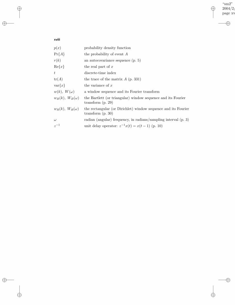
p(x) probability density function

PrA the probability of event A

r(k) an autocovariance sequence (p. 5)

Rex the real part of x

t discrete-time index

tr(A) the trace of the matrix A (p. 331)

varx the variance of x

w(k), W (ω) a window sequence and its Fourier transform

wB(k), WB(ω) the Bartlett (or triangular) window sequence and its Fouriertransform (p. 29)

wR(k), WR(ω) the rectangular (or Dirichlet) window sequence and its Fouriertransform (p. 30)

ω radian (angular) frequency, in radians/sampling interval (p. 3)

z−1 unit delay operator: z−1x(t) = x(t− 1) (p. 10)

“sm2”2004/2/22page xix

i

i

i

i

i

i

i

i

Abbreviations

ACS autocovariance sequence (p. 5)

APES amplitude and phase estimation (p. 244)

AR autoregressive (p. 88)

ARMA autoregressive moving-average (p. 88)

BSP beamspace processing (p. 323)

BT Blackman-Tukey (p. 37)

CM Capon method (p. 222)

CCM constrained Capon method (p. 300)

CRB Cramer-Rao bound (p. 355)

DFT discrete Fourier transform (p. 25)

DGA Delsarte-Genin algorithm (p. 95)

DOA direction of arrival (p. 264)

DTFT discrete-time Fourier transform (p. 3)

ESP elementspace processing (p. 323)

ESPRIT estimation of signal parameters by rotational invariancetechniques (p. 166)

EVD eigenvalue decomposition (p. 330)

FB forward-backward (p. 168)

FBA filter bank approach (p. 208)

FFT fast Fourier transform (p. 26)

FIR finite impulse response (p. 17)

flop floating point operation (p. 26)

GAPES gapped amplitude and phase estimation (p. 247)

GS Gohberg-Semencul (formula) (p. 122)

HOYW high–order Yule–Walker (p. 155)

i.i.d. independent, identically distributed (p. 317)

LDA Levinson–Durbin algorithm (p. 95)

LS least squares (p. 350)

MA moving-average (p. 88)

MFD matrix fraction description (p. 137)

ML maximum likelihood (p. 356)

MLE maximum likelihood estimate (p. 356)

xix

“sm2”2004/2/22page xx

i

i

i

i

i

i

i

i

xx

MSE mean squared error (p. 28)

MUSIC multiple signal classification (or characterization) (p. 159)

MYW modified Yule–Walker (p. 96)

NLS nonlinear least squares (p. 145)

PARCOR partial correlation (p. 96)

PSD power spectral density (p. 5)

RFB refined filter bank (p. 212)

QRD Q-R decomposition (p. 351)

RCM robust Capon method (p. 299)

SNR signal-to-noise ratio (p. 81)

SVD singular value decomposition (p. 336)

TLS total least squares (p. 352)

ULA uniform linear array (p. 271)

YW Yule–Walker (p. 90)

“sm2”2004/2/22page 1

i

i

i

i

i

i

i

i

C H A P T E R 1

Basic Concepts

1.1 INTRODUCTION

The essence of the spectral estimation problem is captured by the following informalformulation.

From a finite record of a stationary data sequence, estimate howthe total power is distributed over frequency.

(1.1.1)

Spectral analysis finds applications in many diverse fields. In vibration monitoring,the spectral content of measured signals give information on the wear and othercharacteristics of mechanical parts under study. In economics, meteorology, astron-omy and several other fields, the spectral analysis may reveal “hidden periodicities”in the studied data, which are to be associated with cyclic behavior or recurringprocesses. In speech analysis, spectral models of voice signals are useful in betterunderstanding the speech production process, and — in addition — can be usedfor both speech synthesis (or compression) and speech recognition. In radar andsonar systems, the spectral contents of the received signals provide information onthe location of the sources (or targets) situated in the field of view. In medicine,spectral analysis of various signals measured from a patient, such as electrocardio-gram (ECG) or electroencephalogram (EEG) signals, can provide useful materialfor diagnosis. In seismology, the spectral analysis of the signals recorded prior toand during a seismic event (such as a volcano eruption or an earthquake) givesuseful information on the ground movement associated with such events and mayhelp in predicting them. Seismic spectral estimation is also used to predict sub-surface geologic structure in gas and oil exploration. In control systems, there isa resurging interest in spectral analysis methods as a means of characterizing thedynamical behavior of a given system, and ultimately synthesizing a controller forthat system. The previous and other applications of spectral analysis are reviewedin [Kay 1988; Marple 1987; Bloomfield 1976; Bracewell 1986; Haykin

1991; Haykin 1995; Hayes III 1996; Koopmans 1974; Priestley 1981; Perci-

val and Walden 1993; Porat 1994; Scharf 1991; Therrien 1992; Proakis,

Rader, Ling, and Nikias 1992]. The textbook [Marple 1987] also containsa well–written historical perspective on spectral estimation which is worth read-ing. Many of the classical articles on spectral analysis, both application–drivenand theoretical, are reprinted in [Childers 1978; Kesler 1986]; these excellentcollections of reprints are well worth consulting.

There are two broad approaches to spectral analysis. One of these derives itsbasic idea directly from definition (1.1.1): the studied signal is applied to a band-pass filter with a narrow bandwidth, which is swept through the frequency band of

1

“sm2”2004/2/22page 2

i

i

i

i

i

i

i

i

2 Chapter 1 Basic Concepts

interest, and the filter output power divided by the filter bandwidth is used as ameasure of the spectral content of the input to the filter. This is essentially whatthe classical (or nonparametric) methods of spectral analysis do. These methods aredescribed in Chapters 2 and 5 of this text (the fact that the methods of Chapter 2can be given the above filter bank interpretation is made clear in Chapter 5). Thesecond approach to spectral estimation, called the parametric approach, is to postu-late a model for the data, which provides a means of parameterizing the spectrum,and to thereby reduce the spectral estimation problem to that of estimating theparameters in the assumed model. The parametric approach to spectral analysisis treated in Chapters 3, 4 and 6. Parametric methods may offer more accuratespectral estimates than the nonparametric ones in the cases where the data indeedsatisfy the model assumed by the former methods. However, in the more likelycase that the data do not satisfy the assumed models, the nonparametric meth-ods may outperform the parametric ones owing to the sensitivity of the latter tomodel misspecifications. This observation has motivated renewed interest in thenonparametric approach to spectral estimation.

Many real–world signals can be characterized as being random (from the ob-server’s viewpoint). Briefly speaking, this means that the variation of such a signaloutside the observed interval cannot be determined exactly but only specified instatistical terms of averages. In this text, we will be concerned with estimating thespectral characteristics of random signals. In spite of this fact, we find it usefulto start the discussion by considering the spectral analysis of deterministic signals(which we do in the first section of this chapter). Throughout this work, we considerdiscrete signals (or data sequences). Such signals are most commonly obtained bythe temporal or spatial sampling of a continuous (in time or space) signal. Themain motivation for focusing on discrete signals lies in the fact that spectral analy-sis is most often performed by a digital computer or by digital circuitry. Chapters2 to 5 of this text deal with discrete–time signals, while Chapter 6 considers thecase of discrete–space data sequences.

In the interest of notational simplicity, the discrete–time variable t, as used inthis text, is assumed to be measured in units of sampling interval. A similar conven-tion is adopted for spatial signals, whenever the sampling is uniform. Accordingly,the units of frequency are cycles per sampling interval.

The signals dealt with in the text are complex–valued. Complex–valued datamay appear in signal processing and spectral estimation applications, for instance,as a result of a “complex demodulation” process (this is explained in detail inChapter 6). It should be noted that the treatment of complex–valued signals is notalways more general or more difficult than the analysis of corresponding real–valuedsignals. A typical example which illustrates this claim is the case of sinusoidalsignals considered in Chapter 4. A real–valued sinusoidal signal, α cos(ωt + ϕ),can be rewritten as a linear combination of two complex–valued sinusoidal signals,α1e

i(ω1t+ϕ1) + α2ei(ω2t+ϕ2), whose parameters are constrained as follows: α1 =

α2 = α/2, ϕ1 = −ϕ2 = ϕ and ω1 = −ω2 = ω. Here i =√

−1. The factthat we need to consider two constrained complex sine waves to treat the caseof one unconstrained real sine wave shows that the real–valued case of sinusoidalsignals can actually be considered to be more complicated than the complex–valuedcase! Fortunately, it appears that the latter case is encountered more frequently

“sm2”2004/2/22page 3

i

i

i

i

i

i

i

i

Section 1.2 Energy Spectral Density of Deterministic Signals 3

in applications, where often both the in–phase and quadrature components of thestudied signal are available. (For more details and explanations on this aspect, seeChapter 6’s introductory section.)

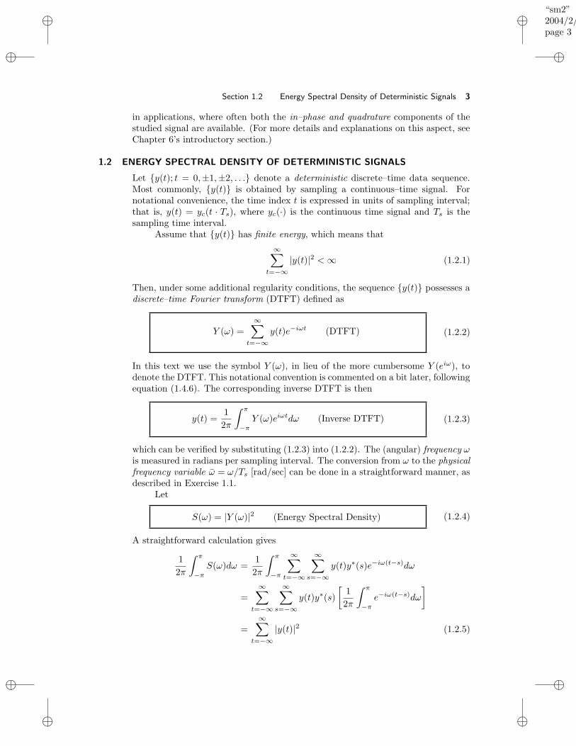
1.2 ENERGY SPECTRAL DENSITY OF DETERMINISTIC SIGNALS

Let y(t); t = 0,±1,±2, . . . denote a deterministic discrete–time data sequence.Most commonly, y(t) is obtained by sampling a continuous–time signal. Fornotational convenience, the time index t is expressed in units of sampling interval;that is, y(t) = yc(t · Ts), where yc(·) is the continuous time signal and Ts is thesampling time interval.

Assume that y(t) has finite energy, which means that

∞∑

t=−∞|y(t)|2 < ∞ (1.2.1)

Then, under some additional regularity conditions, the sequence y(t) possesses adiscrete–time Fourier transform (DTFT) defined as

Y (ω) =

∞∑

t=−∞y(t)e−iωt (DTFT) (1.2.2)

In this text we use the symbol Y (ω), in lieu of the more cumbersome Y (eiω), todenote the DTFT. This notational convention is commented on a bit later, followingequation (1.4.6). The corresponding inverse DTFT is then

y(t) =1

2π

∫ π

−πY (ω)eiωtdω (Inverse DTFT) (1.2.3)

which can be verified by substituting (1.2.3) into (1.2.2). The (angular) frequency ωis measured in radians per sampling interval. The conversion from ω to the physicalfrequency variable ω = ω/Ts [rad/sec] can be done in a straightforward manner, asdescribed in Exercise 1.1.

Let

S(ω) = |Y (ω)|2 (Energy Spectral Density) (1.2.4)

A straightforward calculation gives

1

2π

∫ π

−πS(ω)dω =

1

2π

∫ π

−π

∞∑

t=−∞

∞∑

s=−∞y(t)y∗(s)e−iω(t−s)dω

=

∞∑

t=−∞

∞∑

s=−∞y(t)y∗(s)

[1

2π

∫ π

−πe−iω(t−s)dω

]

=

∞∑

t=−∞|y(t)|2 (1.2.5)

“sm2”2004/2/22page 4

i

i

i

i

i

i

i

i


To obtain the last equality in (1.2.5) we have used the fact that 12π

∫ π

−π e−iω(t−s)dω =

δt,s (the Kronecker delta). The symbol (·)∗ will be used in this text to denote thecomplex–conjugate of a scalar variable or the conjugate transpose of a vector ormatrix. Equation (1.2.5) can be restated as

∞∑

t=−∞|y(t)|2 =

1

2π

∫ π

−πS(ω)dω (1.2.6)

This equality is called Parseval’s theorem. It shows that S(ω) represents the dis-tribution of sequence energy as a function of frequency. For this reason, S(ω) iscalled the energy spectral density.

The previous interpretation of S(ω) also comes up in the following way. Equa-tion (1.2.3) represents the sequence y(t) as a weighted “sum” (actually, an inte-gral) of orthonormal sequences 1√

2πeiωt (ω ∈ [−π, π]), with weighting 1√

2πY (ω).

Hence, 1√2π

|Y (ω)| “measures” the “length” of the projection of y(t) on each of

these basis sequences. In loose terms, therefore, 1√2π

|Y (ω)| shows how much (or

how little) of the sequence y(t) can be “explained” by the orthonormal sequence 1√

2πeiωt for some given value of ω.

Define

ρ(k) =

∞∑

t=−∞y(t)y∗(t− k) (1.2.7)

It is readily verified that

∞∑

k=−∞ρ(k)e−iωk =

∞∑

k=−∞

∞∑

t=−∞y(t)y∗(t− k)e−iωteiω(t−k)

=

[ ∞∑

t=−∞y(t)e−iωt

][ ∞∑

s=−∞y(s)e−iωs

]∗

= S(ω) (1.2.8)

which shows that S(ω) can be obtained as the DTFT of the “autocorrelation”(1.2.7) of the finite–energy sequence y(t).

The above definitions can be extended in a rather straightforward manner tothe case of random signals treated throughout the remaining text. In fact, the onlypurpose for discussing the deterministic case in this section was to provide somemotivation for the analogous definitions in the random case. As such, the discussionin this section has been kept brief. More insights into the meaning and propertiesof the previous definitions are provided by the detailed treatment of the randomcase in the following sections.

1.3 POWER SPECTRAL DENSITY OF RANDOM SIGNALS

Most of the signals encountered in applications are such that their variation in thefuture cannot be known exactly. It is only possible to make probabilistic statementsabout that variation. The mathematical device to describe such a signal is that

“sm2”2004/2/22page 5

i

i

i

i

i

i

i

i

Section 1.3 Power Spectral Density of Random Signals 5

of a random sequence which consists of an ensemble of possible realizations, eachof which has some associated probability of occurrence. Of course, from the wholeensemble of realizations, the experimenter can usually observe only one realizationof the signal, and then it might be thought that the deterministic definitions of theprevious section could be carried over unchanged to the present case. However, thisis not possible because the realizations of a random signal, viewed as discrete–timesequences, do not have finite energy, and hence do not possess DTFTs. A randomsignal usually has finite average power and, therefore, can be characterized by anaverage power spectral density. For simplicity reasons, in what follows we will usethe name power spectral density (PSD) for that quantity.

The discrete–time signal y(t); t = 0,±1,±2, . . . is assumed to be a sequenceof random variables with zero mean:

E y(t) = 0 for all t (1.3.1)

Hereafter, E · denotes the expectation operator (which averages over the ensembleof realizations). The autocovariance sequence (ACS) or covariance function of y(t)is defined as

r(k) = E y(t)y∗(t− k) (1.3.2)

and it is assumed to depend only on the lag between the two samples averaged. Thetwo assumptions (1.3.1) and (1.3.2) imply that y(t) is a second–order stationarysequence. When it is required to distinguish between the autocovariance sequencesof several signals, a lower index will be used to indicate the signal associated witha given covariance lag, such as ry(k).

The autocovariance sequence r(k) enjoys some simple but useful properties:

r(k) = r∗(−k) (1.3.3)

and

r(0) ≥ |r(k)| for all k (1.3.4)

The equality (1.3.3) directly follows from definition (1.3.2) and the stationarityassumption, while (1.3.4) is a consequence of the fact that the covariance matrix ofy(t), defined as follows

Rm =

r(0) r∗(1) . . . r∗(m− 1)

r(1) r(0). . .

......

. . .. . . r∗(1)

r(m− 1) . . . r(1) r(0)

= E

y∗(t− 1)......

y∗(t−m)

[y(t− 1) . . . y(t−m)]

(1.3.5)

“sm2”2004/2/22page 6

i

i

i

i

i

i

i

i


is positive semidefinite for all m. Recall that a Hermitian matrix M is positivesemidefinite if a∗Ma ≥ 0 for every vector a (see Section A.5 for details). Since

a∗Rma = a∗E

y∗(t− 1)...

y∗(t−m)

[y(t− 1) . . . y(t−m)]

a

= E z∗(t)z(t) = E|z(t)|2

≥ 0 (1.3.6)

wherez(t) = [y(t− 1) . . . y(t−m)]a

we see that Rm is indeed positive semidefinite for every m. Hence, (1.3.4) fol-lows from the properties of positive semidefinite matrices (see Definition D11 inAppendix A and Exercise 1.5).

1.3.1 First Definition of Power Spectral Density

The PSD is defined as the DTFT of the covariance sequence:

φ(ω) =

∞∑

k=−∞r(k)e−iωk (Power Spectral Density) (1.3.7)

Note that the previous definition (1.3.7) of φ(ω) is similar to the definition (1.2.8)in the deterministic case. The inverse transform, which recovers r(k) from givenφ(ω), is

r(k) =1

2π

∫ π

−πφ(ω)eiωkdω (1.3.8)

We readily verify that

1

2π

∫ π

−πφ(ω)eiωkdω =

∞∑

p=−∞r(p)

[1

2π

∫ π

−πeiω(k−p)dω

]

= r(k)

which proves that (1.3.8) is the inverse transform for (1.3.7). Note that to obtainthe first equality above, the order of integration and summation has been inverted,which is possible under weak conditions (such as under the requirement that φ(ω)is square integrable; see Chapter 4 in [Priestley 1981] for a detailed discussionon this aspect).

From (1.3.8), we obtain

r(0) =1

2π

∫ π

−πφ(ω)dω (1.3.9)

Since r(0) = E|y(t)|2

measures the (average) power of y(t), the equality (1.3.9)

shows that φ(ω) can indeed be named PSD, as it represents the distribution of the

“sm2”2004/2/22page 7

i

i

i

i

i

i

i

i

Section 1.3 Power Spectral Density of Random Signals 7

(average) signal power over frequencies. Put another way, it follows from (1.3.9)that φ(ω)dω/2π is the infinitesimal power in the band (ω−dω/2, ω+dω/2), and thetotal power in the signal is obtained by integrating these infinitesimal contributions.Additional motivation for calling φ(ω) a PSD is provided by the second definitionof φ(ω), given next, which resembles the usual definition (1.2.2), (1.2.4) in thedeterministic case.

1.3.2 Second Definition of Power Spectral Density

The second definition of φ(ω) is:

φ(ω) = limN→∞

E

1

N

∣∣∣∣∣

N∑

t=1

y(t)e−iωt

∣∣∣∣∣

2

(1.3.10)

This definition is equivalent to (1.3.7) under the mild assumption that the covari-ance sequence r(k) decays sufficiently rapidly, so that

limN→∞

1

N

N∑

k=−N|k||r(k)| = 0 (1.3.11)

The equivalence of (1.3.7) and (1.3.10) can be verified as follows:

limN→∞

E

1

N

∣∣∣∣∣

N∑

t=1

y(t)e−iωt

∣∣∣∣∣

2

= lim

N→∞

1

N

N∑

t=1

N∑

s=1

E y(t)y∗(s) e−iω(t−s)

= limN→∞

1

N

N−1∑

τ=−(N−1)

(N − |τ |)r(τ)e−iωτ

=

∞∑

τ=−∞r(τ)e−iωτ − lim

N→∞

1

N

N−1∑

τ=−(N−1)

|τ |r(τ)e−iωτ

= φ(ω)

The second equality is proven in Exercise 1.6, and we used (1.3.11) in the lastequality.

The above definition of φ(ω) resembles the definition (1.2.4) of energy spec-tral density in the deterministic case. The main difference between (1.2.4) and(1.3.10) consists of the appearance of the expectation operator in (1.3.10) and thenormalization by 1/N ; the fact that the “discrete–time” variable in (1.3.10) runsover positive integers only is just for convenience and does not constitute an es-sential difference, compared to (1.2.2). In spite of these differences, the analogybetween the deterministic formula (1.2.4) and (1.3.10) provides further motivationfor calling φ(ω) a PSD. The alternative definition (1.3.10) will also be quite usefulwhen discussing the problem of estimating the PSD by nonparametric techniquesin Chapters 2 and 5.

“sm2”2004/2/22page 8

i

i

i

i

i

i

i

i


We can see from either of these definitions that φ(ω) is a periodic function,with the period equal to 2π. Hence, φ(ω) is completely described by its variationin the interval

ω ∈ [−π, π] (radians per sampling interval) (1.3.12)

Alternatively, the PSD can be viewed as a function of the frequency

f =ω

2π(cycles per sampling interval) (1.3.13)

which, according to (1.3.12), can be considered to take values in the interval

f ∈ [−1/2, 1/2] (1.3.14)

We will generally write the PSD as a function of ω whenever possible, since thiswill simplify the notation.

As already mentioned, the discrete–time sequence y(t) is most commonlyderived by sampling a continuous–time signal. To avoid aliasing effects which mightbe incurred by the sampling process, the continuous–time signal should be (atleast, approximately) bandlimited in the frequency domain. To ensure this, it maybe necessary to low–pass filter the continuous–time signal before sampling. LetF0 denote the largest (“significant”) frequency component in the spectrum of the(possibly filtered) continuous signal, and let Fs be the sampling frequency. Then itfollows from Shannon’s sampling theorem that the continuous–time signal can be“exactly” reconstructed from its samples y(t), provided that

Fs ≥ 2F0 (1.3.15)

In particular, “no” frequency aliasing will occur when (1.3.15) holds (see, e.g.,[Oppenheim and Schafer 1989]). Since the frequency variable, F , associatedwith the continuous–time signal, is related to f by the equation

F = f · Fs (1.3.16)

it follows that the interval of F corresponding to (1.3.14) is

F ∈[

−Fs2,Fs2

]

(cycles/sec) (1.3.17)

which is quite natural in view of (1.3.15).

1.4 PROPERTIES OF POWER SPECTRAL DENSITIES

Since φ(ω) is a power density, it should be real–valued and nonnegative. That thisis indeed the case is readily seen from definition (1.3.10) of φ(ω). Hence,

φ(ω) ≥ 0 for all ω (1.4.1)

“sm2”2004/2/22page 9

i

i

i

i

i

i

i

i

Section 1.4 Properties of Power Spectral Densities 9

From (1.3.3) and (1.3.7), we obtain

φ(ω) = r(0) + 2

∞∑

k=1

Rer(k)e−iωk

where Re· denotes the real part of the bracketed quantity. If y(t), and hencer(k), is real valued then it follows that

φ(ω) = r(0) + 2

∞∑

k=1

r(k) cos(ωk) (1.4.2)

which shows that φ(ω) is an even function in such a case. In the case of complex–valued signals, however, φ(ω) is not necessarily symmetric about the ω = 0 axis.Thus:

For real–valued signals:φ(ω) = φ(−ω), ω ∈ [−π, π]

For complex–valued signals:in general φ(ω) 6= φ(−ω), ω ∈ [−π, π]

(1.4.3)

Remark: The reader might wonder why we did not define the ACS as

c(k) = E y(t)y∗(t+ k)

Comparing with the ACS r(k) used in this text, as defined in (1.3.2), we obtainc(k) = r(−k). Consequently, the PSD associated with c(k) is related to the PSDcorresponding to r(k) (see (1.3.7)) via:

ψ(ω) ,

∞∑

k=−∞c(k)e−iωk =

∞∑

k=−∞r(k)eiωk = φ(−ω)

It may seem arbitrary as to which definition of the ACS (and corresponding defini-tion of PSD) we choose. In fact, from a mathematical standpoint we can use eitherdefinition of the ACS, but the ACS definition r(k) is preferred from a practicalstandpoint as we now explain.

First, we should stress that the PSD describes the spectral content of theACS, as seen from equation (1.3.7). The PSD φ(ω) is sometimes perceived asshowing the (infinitesimal) power at frequency ω in the signal itself, but that isnot strictly true. If the PSD represented the power in the signal itself, then weshould have had ψ(ω) = φ(ω) because the signal’s spectral content should notdepend on the ACS definition. However, as shown above, in the general complexcase ψ(ω) = φ(−ω) 6= φ(ω), which means that the signal power interpretation ofthe PSD is not (always) correct. Indeed, the PSD φ(ω) “measures” the power atfrequency ω in the signal’s ACS.

“sm2”2004/2/22page 10

i

i

i

i

i

i

i

i


e(t)

φe(ω)

y(t)

φy(ω) = |H(ω)|2φe(ω)H(z) --

Figure 1.1. Relationship between the PSDs of the input and output of a linearsystem.

On the other hand, our motivation for considering spectral analysis is tocharacterize the average power at frequency ω in the signal, as given by the sec-ond definition of the PSD in equation (1.3.10). If c(k) is used as the ACS, itscorresponding second definition of the PSD is

ψ(ω) = limN→∞

E

1

N

∣∣∣∣∣

N∑

t=1

y(t)e+iωt

∣∣∣∣∣

2

which is the average power of y(t) at frequency −ω. Clearly, the second PSDdefinition corresponding to r(k) aligns with this average power motivation, whilethe one for c(k) does not; it is for this reason that we use the definition r(k) for theACS.

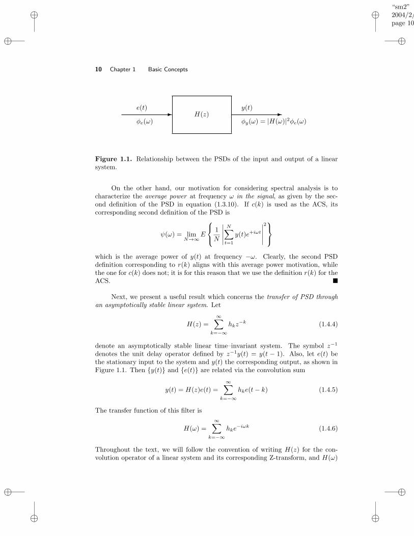
Next, we present a useful result which concerns the transfer of PSD throughan asymptotically stable linear system. Let

H(z) =

∞∑

k=−∞hkz

−k (1.4.4)

denote an asymptotically stable linear time–invariant system. The symbol z−1

denotes the unit delay operator defined by z−1y(t) = y(t − 1). Also, let e(t) bethe stationary input to the system and y(t) the corresponding output, as shown inFigure 1.1. Then y(t) and e(t) are related via the convolution sum

y(t) = H(z)e(t) =

∞∑

k=−∞hke(t− k) (1.4.5)

The transfer function of this filter is

H(ω) =

∞∑

k=−∞hke

−iωk (1.4.6)

Throughout the text, we will follow the convention of writing H(z) for the con-volution operator of a linear system and its corresponding Z-transform, and H(ω)

“sm2”2004/2/22page 11

i

i

i

i

i

i

i

i

Section 1.4 Properties of Power Spectral Densities 11

for its transfer function. We obtain the transfer function H(ω) from H(z) by thesubstitution z = eiω:

H(ω) = H(z)∣∣z=eiω

While we recognize the slight abuse of notation in writing H(ω) instead of H(eiω)and in using z as both an operator and a complex variable, we prefer the simplicityof notation it affords.


ry(k) =

∞∑

p=−∞

∞∑

m=−∞hph

∗mE e(t− p)e∗(t−m− k)

=

∞∑

p=−∞

∞∑

m=−∞hph

∗mre(m+ k − p) (1.4.7)

Inserting (1.4.7) in (1.3.7) gives

φy(ω) =

∞∑

k=−∞

∞∑

p=−∞

∞∑

m=−∞hph

∗mre(m+ k − p)e−iω(k+m−p)eiωme−iωp

=

[ ∞∑

p=−∞hpe

−iωp][ ∞∑

m=−∞h∗me

iωm

][ ∞∑

τ=−∞re(τ)e

−iωτ]

= |H(ω)|2φe(ω) (1.4.8)

From (1.4.8), we get the following important formula

φy(ω) = |H(ω)|2φe(ω) (1.4.9)

that will be much used in the following chapters.Finally, we derive a property that will be of use in Chapter 5. Let the signals

y(t) and x(t) be related byy(t) = eiω0tx(t) (1.4.10)

for some given ω0. Then, it holds that

φy(ω) = φx(ω − ω0) (1.4.11)

In other words, multiplication by eiω0t of a temporal sequence shifts its spectraldensity by the angular frequency ω0. Owing to this interpretation, the processof constructing y(t) as in (1.4.10) is called complex (de)modulation. The proof of(1.4.11) is immediate: since (1.4.10) implies that

ry(k) = eiω0krx(k) (1.4.12)

we obtain

φy(ω) =

∞∑

k=−∞rx(k)e

−i(ω−ω0)k = φx(ω − ω0) (1.4.13)

which is the desired result.

“sm2”2004/2/22page 12

i

i

i

i

i

i

i

i


1.5 THE SPECTRAL ESTIMATION PROBLEM

The spectral estimation problem can now be stated more formally as follows.

From a finite–length record y(1), . . . , y(N) of a second–order

stationary random process, determine an estimate φ(ω) of itspower spectral density φ(ω), for ω ∈ [−π, π]

(1.5.1)

It would, of course, be desirable that φ(ω) is as close to φ(ω) as possible. Aswe shall see, the main limitation on the quality of most PSD estimates is due tothe quite small number of data samples usually available for processing. Note thatN will be used throughout this text to denote the number of points of the availabledata sequence. In some applications, N is small since the cost of obtaining largeamounts of data is prohibitive. Most commonly, the value of N is limited by thefact that the signal under study can be considered second–order stationary onlyover short observation intervals.

As already mentioned in the introductory part of this chapter, there are twomain approaches to the PSD estimation problem. The nonparametric approach,discussed in Chapters 2 and 5, proceeds to estimate the PSD by relying essentiallyonly on the basic definitions (1.3.7) and (1.3.10) and on some properties that di-rectly follow from these definitions. In particular, these methods do not make anyassumption on the functional form of φ(ω). This is in contrast with the parametricapproach, discussed in Chapters 3, 4 and 6. That approach makes assumptions onthe signal under study, which lead to a parameterized functional form of the PSD,and then proceeds by estimating the parameters in the PSD model. The paramet-ric approach can thus be used only when there is enough information about thestudied signal, that allows formulation of a model. Otherwise the nonparametricapproach should be used. Interestingly enough, the nonparametric methods areclose competitors to the parametric ones, even when the model form assumed bythe latter is a reasonable description of reality.

1.6 COMPLEMENTS

1.6.1 Coherency Spectrum

Let

Cyu(ω) =φyu(ω)

[φyy(ω)φuu(ω)]1/2(1.6.1)

denote the so–called complex–coherency of the stationary signals y(t) and u(t). Inthe definition above, φyu(ω) is the cross–spectrum of the two signals, and φyy(ω)and φuu(ω) are their respective PSDs. (We implicitly assume in (1.6.1) that φyy(ω)and φuu(ω) are strictly positive for all ω.) Also, let

ε(t) = y(t) −∞∑

k=−∞hku(t− k) (1.6.2)

“sm2”2004/2/22page 13

i

i

i

i

i

i

i

i

Section 1.6 Complements 13

denote the residues of the least squares problem in Exercise 1.11. Hence, hk inequation (1.6.2) satisfy

∞∑

k=−∞hke

−iωk , H(ω) = φyu(ω)/φuu(ω).

In what follows, we will show that

E|ε(t)|2

=

1

2π

∫ π

−π(1 − |Cyu(ω)|2)φyy(ω) dω (1.6.3)

where |Cyu(ω)| is the so–called coherency spectrum. We will deduce from (1.6.3)that the coherency spectrum shows the extent to which y(t) and u(t) are linearlyrelated to one another, hence providing a motivation for the name given to |Cyu(ω)|.We will also show that |Cyu(ω)| ≤ 1 with equality, for all ω values, if and only ify(t) and u(t) are related as in equation (1.6.2) with ε(t) ≡ 0 (in the mean squaresense). Finally, we will show that |Cyu(ω)| is invariant to linear filtering of u(t) andy(t) (possibly by different filters); that is, if u = g ∗ u and y = f ∗ y where f and gare linear filters, then |Cyu(ω)| = |Cyu(ω)|.

Let x(t) =∑∞k=−∞ hku(t − k). It can be shown that u(t − k) and ε(t) are

uncorrelated with one another for all k. (The reader is required to verify this claim;see also Exercise 1.11). Hence x(t) and ε(t) are also uncorrelated with each other.As

y(t) = ε(t) + x(t), (1.6.4)

it then follows that

φyy(ω) = φεε(ω) + φxx(ω) (1.6.5)

By using the fact that φxx(ω) = |H(ω)|2φuu(ω), we can write

E|ε(t)|2

=

1

2π

∫ π

−πφεε(ω) dω

=1

2π

∫ π

−π

[

1 − |H(ω)|2 φuu(ω)

φyy(ω)

]

φyy(ω) dω

=1

2π

∫ π

−π

[

1 − |φyu(ω)|2φuu(ω)φyy(ω)

]

φyy(ω) dω

=1

2π

∫ π

−π

[1 − |Cyu(ω)|2

]φyy(ω) dω

which is (1.6.3).

Since the left-hand side in (1.6.3) is nonnegative and the PSD function φyy(ω)is arbitrary, we must have |Cyu(ω)| ≤ 1 for all ω. It can also be seen from (1.6.3)that the closer |Cyu(ω)| is to one, the smaller the residual variance. In particular, if|Cyu(ω)| ≡ 1 then ε(t) ≡ 0 (in the mean square sense) and hence y(t) and u(t) mustbe linearly related as in (1.7.11). Owing to the previous interpretation, Cyu(ω) issometimes called the correlation coefficient in the frequency domain.

“sm2”2004/2/22page 14

i

i

i

i

i

i

i

i


Next, consider the filtered signals

y(t) =

∞∑

k=−∞fky(t− k)

and

u(t) =

∞∑

k=−∞gku(t− k)

where the filters fk and gk are assumed to be stable. As

ryu(p) , E y(t)u∗(t− p)

=

∞∑

k=−∞

∞∑

j=−∞fkg

∗jE y(t− k)u∗(t− j − p)

=

∞∑

k=−∞

∞∑

j=−∞fkg

∗j ryu(j + p− k),

it follows that

φyu(ω) =

∞∑

p=−∞

∞∑

k=−∞

∞∑

j=−∞fke

−iωk g∗j eiωj ryu(j + p− k)e−iω(j+p−k)

=

( ∞∑

k=−∞fke

−iωk)

∞∑

j=−∞gje

−iωj

∗ ( ∞∑

s=−∞ryu(s)e

−iωs)

= F (ω)G∗(ω)φyu(ω)

Hence

|Cyu(ω)| =|F (ω)| |G(ω)| |φyu(ω)|

|F (ω)|φ1/2yy (ω)|G(ω)|φ1/2

uu (ω)= |Cyu(ω)|

which is the desired result. Observe that the latter result is similar to the invarianceof the modulus of the correlation coefficient in the time domain,

|ryu(k)|[ryy(0)ruu(0)]1/2

,

to a scaling of the two signals: y(t) = f · y(t) and u(t) = g · u(t).

1.7 EXERCISES

Exercise 1.1: Scaling of the Frequency AxisIn this text, the time variable t has been expressed in units of the sampling

interval Ts (say). Consequently, the frequency is measured in cycles per samplinginterval. Assume we want the frequency units to be expressed in radians per sec-ond or in Hertz (Hz = cycles per second). Then we have to introduce the scaledfrequency variables

ω = ω/Ts ω ∈ [−π/Ts, π/Ts] rad/sec (1.7.1)

“sm2”2004/2/22page 15

i

i

i

i

i

i

i

i

Section 1.7 Exercises 15

and f = ω/2π (in Hz). It might be thought that the PSD in the new frequencyvariable is obtained by inserting ω = ωTs into φ(ω), but this is wrong. Show thatthe PSD, as expressed in units of power per Hz, is in fact given by:

φ(ω) = Tsφ(ωTs) , Ts

∞∑

k=−∞r(k)e−iωTsk, |ω| ≤ π/Ts (1.7.2)

(See [Marple 1987] for more details on this scaling aspect.)

Exercise 1.2: Time–Frequency DistributionsLet y(t) denote a discrete–time signal, and let Y (ω) be its discrete–time

Fourier transform. As explained in Section 1.2, Y (ω) shows how the energy inthe whole sequence y(t)∞

t=−∞ is distributed over frequency.Assume that we want to determine how the energy of the signal is distributed

in time and frequency. If D(t, ω) is a function that characterizes the time–frequencydistribution, then it should satisfy the so–called marginal properties:

∞∑

t=−∞D(t, ω) = |Y (ω)|2 (1.7.3)

and1

2π

∫ π

−πD(t, ω)dω = |y(t)|2 (1.7.4)

Use intuitive arguments to explain why the previous conditions are desirable prop-erties of a time–frequency distribution. Next, show that the so–called Rihaczekdistribution,

D(t, ω) = y(t)Y ∗(ω)e−iωt (1.7.5)

satisfies conditions (1.7.3) and (1.7.4). (For treatments of the time–frequency dis-tributions, the reader is referred to [Therrien 1992] and [Cohen 1995]).

Exercise 1.3: Two Useful Z–Transform Properties

(a) Let hk be an absolutely summable sequence, and let H(z) =∑∞k=−∞ hkz

−k

be its Z–transform. Find the Z–transforms of the following two sequences:

(i) h−k

(ii) gk =∑∞m=−∞ hmh

∗m−k

(b) Show that if zi is a zero of A(z) = 1 + a1z−1 + · · · + anz

−n, then (1/z∗i ) is a

zero of A∗(1/z∗) (where A∗(1/z∗) = [A(1/z∗)]∗).

Exercise 1.4: A Simple ACS ExampleLet y(t) be the output of a linear system as in Figure 1.1 with filter H(z) =

(1 + b1z−1)/(1 + a1z

−1), and whose input is zero mean white noise with varianceσ2 (the ACS of such an input is σ2δk,0).

“sm2”2004/2/22page 16

i

i

i

i

i

i

i

i


(a) Find r(k) and φ(ω) analytically in terms of a1, b1, and σ2.

(b) Verify that r(−k) = r∗(k), and that |r(k)| ≤ r(0). Also verify that when a1

and b1 are real, r(k) can be written as a function of |k|.

Exercise 1.5: Alternative Proof that |r(k)| ≤ r(0)We stated in the text that (1.3.4) follows from (1.3.6). Provide a proof of that

statement. Also, find an alternative, simple proof of (1.3.4) by using (1.3.8).

Exercise 1.6: A Double Summation FormulaA result often used in the study of discrete–time random signals is the follow-

ing summation formula:

N∑

t=1

N∑

s=1

f(t− s) =

N−1∑

τ=−N+1

(N − |τ |)f(τ) (1.7.6)

where f(·) is an arbitrary function. Provide a proof of the above formula.

Exercise 1.7: Is a Truncated Autocovariance Sequence (ACS) a ValidACS?

Suppose that r(k)∞k=−∞ is a valid ACS; thus,

∑∞k=−∞ r(k)e−iωk ≥ 0 for all

ω. Is it possible that for some integer p the partial (or truncated) sum

p∑

k=−pr(k)e−iωk

is negative for some ω? Justify your answer.

Exercise 1.8: When Is a Sequence an Autocovariance Sequence?We showed in Section 1.3 that if r(k)∞

k=−∞ is an ACS, then Rm ≥ 0 form = 0, 1, 2, . . .. We also implied that the first definition of the PSD in (1.3.7)satisfies φ(ω) ≥ 0 for all ω; however, we did not prove this by using (1.3.7) solely.Show that

φ(ω) =

∞∑

k=−∞r(k)e−iωk ≥ 0 for all ω

if and only if

a∗Rma ≥ 0 for every m and for every vector a

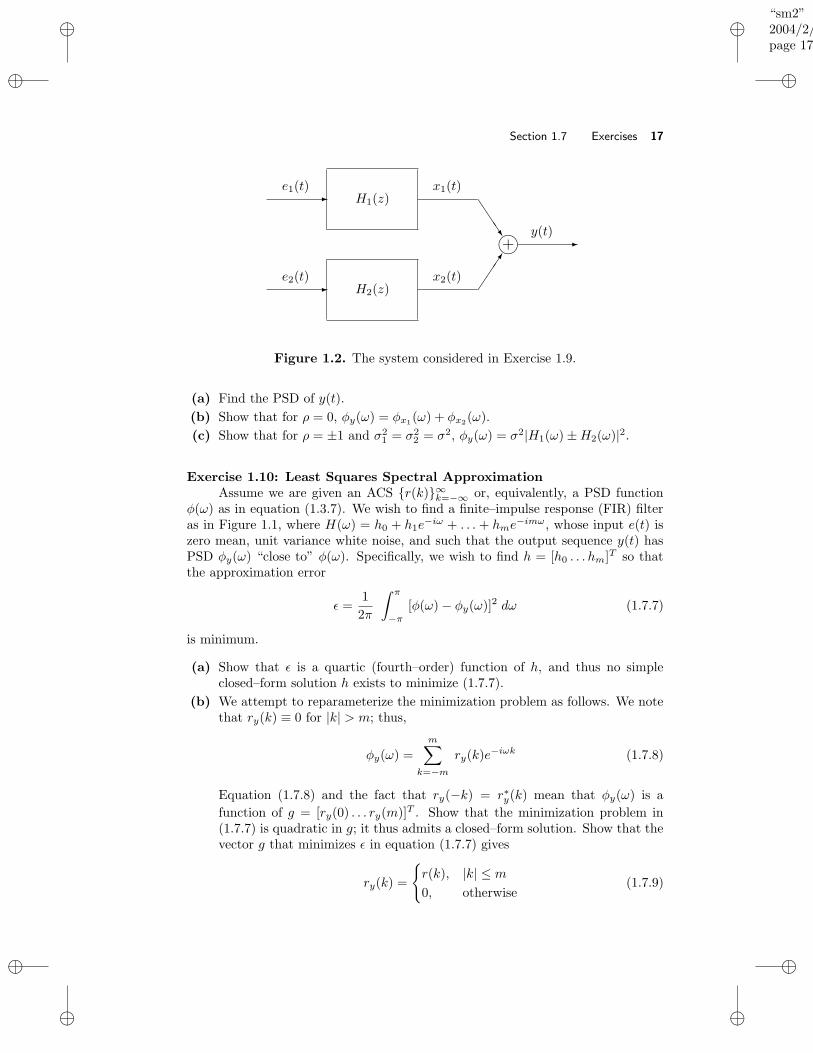
Exercise 1.9: Spectral Density of the Sum of Two Correlated SignalsLet y(t) be the output to the system shown in Figure 1.2. Assume H1(z) and

H2(z) are linear, asymptotically stable systems. The inputs e1(t) and e2(t) are eachzero mean white noise, with

E

[e1(t)e2(t)

][e∗1(s) e∗

2(s)]

=

[σ2

1 ρσ1σ2

ρσ1σ2 σ22

]

δt,s

“sm2”2004/2/22page 17

i

i

i

i

i

i

i

i


H1(z)-

H2(z)-

m+

JJJ

-

e1(t)

e2(t)

x1(t)

x2(t)

y(t)

Figure 1.2. The system considered in Exercise 1.9.

(a) Find the PSD of y(t).

(b) Show that for ρ = 0, φy(ω) = φx1(ω) + φx2(ω).

(c) Show that for ρ = ±1 and σ21 = σ2

2 = σ2, φy(ω) = σ2|H1(ω) ±H2(ω)|2.

Exercise 1.10: Least Squares Spectral ApproximationAssume we are given an ACS r(k)∞

k=−∞ or, equivalently, a PSD functionφ(ω) as in equation (1.3.7). We wish to find a finite–impulse response (FIR) filteras in Figure 1.1, where H(ω) = h0 + h1e

−iω + . . . + hme−imω, whose input e(t) is

zero mean, unit variance white noise, and such that the output sequence y(t) hasPSD φy(ω) “close to” φ(ω). Specifically, we wish to find h = [h0 . . . hm]T so thatthe approximation error

ε =1

2π

∫ π

−π[φ(ω) − φy(ω)]2 dω (1.7.7)

is minimum.

(a) Show that ε is a quartic (fourth–order) function of h, and thus no simpleclosed–form solution h exists to minimize (1.7.7).

(b) We attempt to reparameterize the minimization problem as follows. We notethat ry(k) ≡ 0 for |k| > m; thus,

φy(ω) =

m∑

k=−mry(k)e

−iωk (1.7.8)

Equation (1.7.8) and the fact that ry(−k) = r∗y(k) mean that φy(ω) is a

function of g = [ry(0) . . . ry(m)]T . Show that the minimization problem in(1.7.7) is quadratic in g; it thus admits a closed–form solution. Show that thevector g that minimizes ε in equation (1.7.7) gives

ry(k) =

r(k), |k| ≤ m

0, otherwise(1.7.9)

“sm2”2004/2/22page 18

i

i

i

i

i

i

i

i


(c) Can you identify any problems with the “solution” (1.7.9)?

Exercise 1.11: Linear Filtering and the Cross–SpectrumFor two stationary signals y(t) and u(t), with (cross)covariance sequence

ryu(k) = E y(t)u∗(t− k), the cross–spectrum is defined as:

φyu(ω) =

∞∑

k=−∞ryu(k)e

−iωk(1.7.10)

Let y(t) be the output of a linear filter with input u(t),

y(t) =

∞∑

k=−∞hku(t− k) (1.7.11)

Show that the input PSD, φuu(ω), the filter transfer function

H(ω) =

∞∑

k=−∞hke

−iωk

and φyu(ω) are related through the so–called Wiener–Hopf equation:

φyu(ω) = H(ω)φuu(ω) (1.7.12)

Next, consider the following least squares (LS) problem,

minhk

E

∣∣∣∣∣y(t) −

∞∑

k=−∞hku(t− k)

∣∣∣∣∣

2

(1.7.13)

where now y(t) and u(t) are no longer necessarily related through equation (1.7.11).Show that the filter minimizing the above LS criterion is still given by the Wiener–Hopf equation, by minimizing the expectation in (1.7.13) with respect to the realand imaginary parts of hk (assume that φuu(ω) > 0 for all ω).

COMPUTER EXERCISES

Exercise C1.12: Computer Generation of Autocovariance SequencesAutocovariance sequences are two–sided sequences. In this exercise we develop

computer techniques for generating two–sided ACSs.Let y(t) be the output of the linear system in Figure 1.1 with filter H(z) =

(1 + b1z−1)/(1 + a1z

−1), and whose input is zero mean white noise with varianceσ2.

“sm2”2004/2/22page 19

i

i

i

i

i

i

i

i


(a) Find r(k) analytically in terms of a1, b1, and σ2 (see also Exercise 1.4).

(b) Plot r(k) for −20 ≤ k ≤ 20 and for various values of a1 and b1. Notice thatthe tails of r(k) decay at a rate dictated by |a1|.

(c) When a1 ' b1 and σ2 = 1, then r(k) ' δk,0. Verify this for a1 = −0.95,b1 = −0.9, and for a1 = −0.75, b1 = −0.7.

(d) A quick way to generate (approximately) r(k) on the computer is to use thefact that r(k) = σ2h(k) ∗ h∗(−k) where h(k) is the impulse response of thefilter in Figure 1.1 (see equation (1.4.7)) and ∗ denotes convolution. Considerthe case where

H(z) =1 + b1z

−1 + · · · + bmz−m

1 + a1z−1 + · · · + anz−n .

Write a Matlab function genacs.m whose inputs are M , σ2, a and b, where aand b are the vectors of denominator and numerator coefficients, respectively,and whose output is a vector of ACS coefficients from 0 to M . Your functionshould make use of the Matlab function filter to generate hkMk=0, andconv to compute r(k) = σ2h(k)∗h∗(−k) using the truncated impulse responsesequence.

(e) Test your function using σ2 = 1, a1 = −0.9 and b1 = 0.8. Try M = 20 andM = 150; why is the result more accurate for larger M? Suggest a “rule ofthumb” about a good choice of M in relation to the poles of the filter.

The above method is a “quick and simple” way to compute an approximationto the ACS, but it is sometimes not very accurate because the impulse response istruncated. Methods for computing the exact ACS from σ2, a and b are discussedin Exercise 3.2 and also in [Kinkel, Perl, Scharf, and Stubberud 1979;Demeure and Mullis 1989].

Exercise C1.13: DTFT Computations using Two–Sided Sequences

In this exercise we consider the DTFT of two–sided sequences (including au-tocovariance sequences), and in doing so illustrate some basic properties of autoco-variance sequences.

(a) We first consider how to use the DTFT to determine φ(ω) from r(k) on acomputer. We are given an ACS:

r(k) =

M−|k|M , |k| ≤ M

0, otherwise(1.7.14)

Generate r(k) forM = 10. Now, in Matlab form a vector x of length L = 256as:

x = [r(0), r(1), . . . , r(M), 0 . . . , 0, r(−M), . . . , r(−1)]

Verify that xf=fft(x) gives φ(ωk) for ωk = 2πk/L. (Note that the elementsof xf should be nonnegative and real.). Explain why this particular choice ofx is needed, citing appropriate circular shift and zero padding properties ofthe DTFT.

“sm2”2004/2/22page 20

i

i

i

i

i

i

i

i


Note that xf often contains a very small imaginary part due to computerroundoff error; replacing xf by real(xf) truncates this imaginary componentand leads to more expected results when plotting.

A word of caution — do not truncate the imaginary part unless you are sureit is negligible; the command zf=real(fft(z)) when

z = [r(−M), . . . , r(−1), r(0), r(1), . . . , r(M), 0 . . . , 0]

gives erroneous “spectral” values; try it and explain why it does not work.

(b) Alternatively, since we can readily derive the analytical expression for φ(ω),we can instead work backwards. Form a vector

yf = [φ(0), φ(2π/L), φ(4π/L), . . . , φ((L− 1)2π/L)]

and find y=ifft(yf). Verify that y closely approximates the ACS.

(c) Consider the ACS r(k) in Exercise C1.12; let a1 = −0.9 and b1 = 0, and setσ2 = 1. Form a vector x as above, with M = 10, and find xf. Why is xf

not a good approximation of φ(ωk) in this case? Repeat the experiment forM = 127 and L = 256; is the approximation better for this case? Why?

We can again work backwards from the analytical expression for φ(ω). Forma vector

yf = [φ(0), φ(2π/L), φ(4π/L), . . . , φ((L− 1)2π/L)]

and find y=ifft(yf). Verify that y closely approximates the ACS for large L(say, L = 256), but poorly approximates the ACS for small L (say, L = 20).By citing properties of inverse DTFTs of infinite, two–sided sequences, explainhow the elements of y relate to the ACS r(k), and why the approximation ispoor for small L. Based on this explanation, give a “rule of thumb” on thechoice of L for good approximations of the ACS.

(d) We have seen above that the fft command results in spectral estimates from 0to 2π instead of the more common range of −π to π. The Matlab commandfftshift can be used to exchange the first and second halves of the fft

output to correspond to a frequency range of −π to π. Similarly, fftshift canbe used on the output of the ifft operation to “center” the zero lag of an ACS.Experiment with fftshift to achieve both of these results. What frequencyvector w is needed so that the command plot(w, fftshift(fft(x))) givesthe spectral values at the proper frequencies? Similarly, what time vector t isneeded to get a proper plot of the ACS with stem(t,fftshift(ifft(xf)))?Do the results depend on whether the vectors are even or odd in length?

Exercise C1.14: Relationship between the PSD and the Eigenvalues ofthe ACS Matrix

An interesting property of the ACS matrix R in equation (1.3.5) is that forlarge dimensions m, its eigenvalues are close to the values of the PSD φ(ωk) forωk = 2πk/m, k = 0, 1, . . . ,m− 1 (see, e.g., [Gray 1972]). We verify this propertyhere.

Consider the ACS in Exercise C1.12, with the values a1 = −0.9, b1 = 0.8, andσ2 = 1.

“sm2”2004/2/22page 21

i

i

i

i

i

i

i

i


(a) Compute a vector phi which contains the values of φ(ωk) for ωk = 2πk/m,with m = 256 and k = 0, 1, . . . ,m− 1 . Plot a histogram of these values withhist(phi). Also useful is the cumulative distribution of the values of phi(plotted on a logarithmic scale), which can be found with the commandsemilogy( (1/m:1/m:1), sort(phi) ).

(b) Compute the eigenvalues of R in equation (1.3.5) for various values of m. Plotthe histogram of the eigenvalues, and their cumulative distribution. Verifythat as m increases, the cumulative distribution of the eigenvalues approachesthe cumulative distribution of the φ(ω) values. Similarly, the histogramsalso approach the histogram for φ(ω), but it is easier to see this result usingcumulative distributions than using histograms.

“sm2”2004/2/22page 22

i

i

i

i

i

i

i

i

C H A P T E R 2

Nonparametric Methods

2.1 INTRODUCTION

The nonparametric methods of spectral estimation rely entirely on the definitions(1.3.7) and (1.3.10) of PSD to provide spectral estimates. These methods constitutethe “classical means” for PSD estimation [Jenkins and Watts 1968]. The presentchapter reviews the main nonparametric methods, their properties and the FastFourier Transform (FFT) algorithm for their implementation. A related discussionis to be found in Chapter 5, where the nonparametric approach to PSD estimationis given a filter bank interpretation.

We first introduce two common spectral estimators, the periodogram and thecorrelogram, derived directly from (1.3.10) and (1.3.7), respectively. These methodsare then shown to be equivalent under weak conditions. The periodogram andcorrelogram methods provide reasonably high resolution for sufficiently long datalengths, but are poor spectral estimators because their variance is high and does notdecrease with increasing data length. (In Chapter 5 we provide an interpretationof the periodogram and correlogram methods as a power estimate based on a singlesample of a filtered version of the signal under study; it is thus not surprising thatthe periodogram or correlogram variance is large).

The high variance of the periodogram and correlogram methods motivates thedevelopment of modified methods that have lower variance, at a cost of reducedresolution. Several modified methods have been introduced, and we present someof the most popular ones. We show them all to be more–or–less equivalent in theirproperties and performance for large data lengths.

2.2 PERIODOGRAM AND CORRELOGRAM METHODS

2.2.1 Periodogram

The periodogram method relies on the definition (1.3.10) of the PSD. Neglectingthe expectation and the limit operation in (1.3.10), which cannot be performedwhen the only available information on the signal consists of the samples y(t)Nt=1,we get

φp(ω) =1

N

∣∣∣∣∣

N∑

t=1

y(t)e−iωt

∣∣∣∣∣

2

(Periodogram) (2.2.1)

One of the first uses of the periodogram spectral estimator, (2.2.1), has been indetermining possible “hidden periodicities” in time series, which may be seen as amotivation for the name of this method [Schuster 1900].

22

“sm2”2004/2/22page 23

i

i

i

i

i

i

i

i

Section 2.2 Periodogram and Correlogram Methods 23

2.2.2 Correlogram

The correlation–based definition (1.3.7) of the PSD leads to the correlogram spectralestimator [Blackman and Tukey 1959]:

φc(ω) =

N−1∑

k=−(N−1)

r(k)e−iωk (Correlogram) (2.2.2)

where r(k) denotes an estimate of the covariance lag r(k), obtained from the avail-able sample y(1), . . . , y(N). When no assumption is made on the signal understudy, except for the stationarity assumption, there are two standard ways to obtainthe sample covariances required in (2.2.2):

r(k) =1

N − k

N∑

t=k+1

y(t)y∗(t− k), 0 ≤ k ≤ N − 1 (2.2.3)

and

r(k) =1

N

N∑

t=k+1

y(t)y∗(t− k) 0 ≤ k ≤ N − 1 (2.2.4)

The sample covariances for negative lags are then constructed using the property(1.3.3) of the covariance function:

r(−k) = r∗(k), k = 0, . . . , N − 1 (2.2.5)

The estimator (2.2.3) is called the standard unbiased ACS estimate, and(2.2.4) is called the standard biased ACS estimate. The biased ACS estimate ismost commonly used, for the following reasons:

• For most stationary signals, the covariance function decays rather rapidly, sothat r(k) is quite small for large lags k. Comparing the definitions (2.2.3) and(2.2.4), it can be seen that r(k) in (2.2.4) will be small for large k (provided Nis reasonably large), whereas r(k) in (2.2.3) may take large and erratic valuesfor large k, as it is obtained by averaging only a few products in such a case(in particular, only one product for k = N − 1!). This observation impliesthat (2.2.4) is likely to be a more accurate estimator of r(k), than (2.2.3), formedium and large values of k (compared to N). For small values of k, thetwo estimators in (2.2.3) and (2.2.4) can be expected to behave in a similarmanner.

• The sequence r(k), k = 0,±1,±2, . . . obtained with (2.2.4) is guaranteed tobe positive semidefinite (as it should, see equation (1.3.5) and the related dis-cussion), while this is not the case for (2.2.3). This fact is especially importantfor PSD estimation, since a sample covariance sequence that is not positivedefinite, when inserted in (2.2.2), may lead to negative spectral estimates,and this is undesirable in most applications.

“sm2”2004/2/22page 24

i

i

i

i

i

i

i

i

24 Chapter 2 Nonparametric Methods

When the sample covariances (2.2.4) are inserted in (2.2.2), it can be shownthat the so–obtained spectral estimate is identical to (2.2.1). In other words, wehave the following result.

φc(ω) evaluated using the standard biased ACS estimates

coincides with φp(ω)(2.2.6)

A simple proof of (2.2.6) runs as follows. Consider the signal

x(t) =1√N

N∑

k=1

y(k)e(t− k) (2.2.7)

where y(k) are considered to be fixed (nonrandom) constants and e(t) is a whitenoise of unit variance: E e(t)e∗(s) = δt,s (= 1 if t = s; and = 0 otherwise). Hencex(t) is the output of a filter with the following transfer function:

Y (ω) =1√N

N∑

k=1

y(k)e−iωk

Since the PSD of the input to the filter is given by φe(ω) = 1, it follows from (1.4.5)that

φx(ω) = |Y (ω)|2 = φp(ω) (2.2.8)

On the other hand, a straightforward calculation gives (for k ≥ 0):

rx(k) = E x(t)x∗(t− k)

=1

N

N∑

p=1

N∑

s=1

y(p)y∗(s)E e(t− p)e∗(t− k − s)

=1

N

N∑

p=1

N∑

s=1

y(p)y∗(s)δp,k+s =1

N

N∑

p=k+1

y(p)y∗(p− k)

=

r(k) given by (2.2.4), k = 0, . . . , N − 1

0, k ≥ N(2.2.9)

Inserting (2.2.9) in the definition (1.3.7) of PSD, the following alternative expressionfor φx(ω) is obtained:

φx(ω) =

N−1∑

k=−(N−1)

r(k)e−iωk = φc(ω) (2.2.10)

Comparing (2.2.8) and (2.2.10) concludes the proof of the claim (2.2.6).The equivalence of the periodogram and correlogram spectral estimators can

be used to derive their properties simultaneously. These two methods are shown inSection 2.4 to provide poor estimates of the PSD. There are two reasons for this,and both can be explained intuitively using φc(ω).

“sm2”2004/2/22page 25

i

i

i

i

i

i

i

i

Section 2.3 Periodogram Computation via FFT 25

• The estimation errors in r(k) are on the order of 1/√N for large N (see

Exercise 2.4), at least for |k| not too close to N . Because φc(ω) = φp(ω) is asum that involves (2N − 1) such covariance estimates, the difference betweenthe true and estimated spectra will be a sum of “many small” errors. Hencethere is no guarantee that the total error will die out as N increases. Thespectrum estimation error is even larger than what is suggested by the abovediscussion, because errors in r(k), for |k| close to N , are typically of an

order larger than 1/√N . The consequence is that the variance of φc(ω) does

not go to zero as N increases.

• In addition, if r(k) converges slowly to zero, then the periodogram estimateswill be biased. Indeed, for lags |k| ' N , r(k) will be a poor estimate of r(k)since r(k) is the sum of only a few lag products that are divided by N (seeequation (2.2.4)). Thus, r(k) will be much closer to zero than r(k) is; in fact,E r(k) = [(N − |k|)/N ]r(k), and the bias is significant for |k| ' N if r(k)is not close to zero in this region. If r(k) decays rapidly to zero, the bias

will be small and will not contribute significantly to the total error in φc(ω);however, the nonzero variance discussed above will still be present.

Both the bias and the variance of the periodogram are discussed more quantitativelyin Section 2.4.

Another intuitive explanation for the poor statistical accuracy of the peri-odogram and correlogram methods is given in Chapter 5, where it is shown, roughlyspeaking, that these methods can be viewed as procedures attempting to estimatethe variance of a data sequence from a single sample.

In spite of their poor quality as spectral estimators, the periodogram andcorrelogram methods form the basis for the improved nonparametric spectral es-timation methods, to be discussed later in this chapter. As such, computationof these two basic estimators is relevant to many other nonparametric estimatorsderived from them. The next section addresses this computational task.

2.3 PERIODOGRAM COMPUTATION VIA FFT

In practice it is not possible to evaluate φp(ω) (or φc(ω)) over a continuum offrequencies. Hence, the frequency variable must be sampled for the purpose ofcomputing φp(ω). The following frequency sampling scheme is most commonlyused:

ω =2π

Nk, k = 0, . . . , N − 1 (2.3.1)

DefineW = e−i 2π

N (2.3.2)

Then, evaluation of φp(ω) (or φc(ω)) at the frequency samples in (2.3.1) basicallyreduces to the computation of the following Discrete Fourier Transform (DFT):

Y (k) =

N∑

t=1

y(t)W tk, k = 0, . . . , N − 1 (2.3.3)

“sm2”2004/2/22page 26

i

i

i

i

i

i

i

i


A direct evaluation of (2.3.3) would require about N2 complex multiplications andadditions, which might be a prohibitive burden for large values of N . Any proce-dure that computes (2.3.3) in less than N2 flops (1 flop = 1 complex multiplicationplus 1 complex addition) is called a Fast Fourier Transform (FFT) algorithm. Inrecent years, there has been significant interest in developing more and more com-putationally efficient FFT algorithms. In the following, we review one of the firstFFT procedures — the so–called radix–2 FFT — which, while not being the mostcomputationally efficient of all, is easy to program in a computer and yet quitecomputationally efficient [Cooley and Tukey 1965; Proakis, Rader, Ling,

and Nikias 1992].

2.3.1 Radix–2 FFT

Assume that N is a power of 2,

N = 2m (2.3.4)

If this is not the case, then we can resort to zero padding, as described in the nextsubsection. By splitting the sum in (2.3.3) into two parts, we get

Y (k) =

N/2∑

t=1

y(t)W tk +

N∑

t=N/2+1

y(t)W tk

=

N/2∑

t=1

[y(t) + y(t+N/2)WNk2 ]W tk (2.3.5)

Next, note that

WNk2 =

1, for even k

−1, for odd k(2.3.6)

Using this simple observation in (2.3.5), we obtain:

For k = 2p = 0, 2, . . .

Y (2p) =

N∑

t=1

[y(t) + y(t+ N)]W tp (2.3.7)

For k = 2p+ 1 = 1, 3, . . .

Y (2p+ 1) =

N∑

t=1

[y(t) − y(t+ N)]W tW tp (2.3.8)

where N = N/2 and W = W 2 = e−i2π/N .The above two equations are the core of the radix–2 FFT algorithm. Both of

these equations represent DFTs for sequences of length equal to N . Computationof the sequences transformed in (2.3.7) and (2.3.8) requires roughly N flops. Hence,

“sm2”2004/2/22page 27

i

i

i

i

i

i

i

i

Section 2.3 Periodogram Computation via FFT 27

the computation of an N–point transform has been reduced to the evaluation of twoN/2–point transforms plus a sequence computation requiring about N/2 flops. Thisreduction process is continued until N = 1 (which is made possible by requiring Nto be a power of 2).

In order to evaluate the number of flops required by a radix–2 FFT, let ckdenote the computational cost (expressed in flops) of a 2k–point radix–2 FFT.According to the discussion in the previous paragraph, ck satisfies the followingrecursion:

ck = 2k/2 + 2ck−1 = 2k−1 + 2ck−1 (2.3.9)

with initial condition c1 = 1 (the number of flops required by a 1–point transform).By iterating (2.3.9), we obtain the solution

ck = k2k−1 =1

2k2k (2.3.10)

from which it follows that cm = 12m2m = 1

2N log2N ; thus

An N–point radix–2 FFT requires about 12N log2N flops (2.3.11)

As a comparison, the number of complex operations required to carry out anN–point split–radix FFT, which at present appears to be the most practical algo-rithm for general–purpose computers when N is a power of 2, is about 1

3N log2N(see [Proakis, Rader, Ling, and Nikias 1992]).

2.3.2 Zero Padding

In some applications, N is not a power of 2 and hence the previously describedradix–2 FFT algorithm cannot be applied directly to the original data sequence.However, this is easily remedied since we may increase the length of the givensequence by means of zero padding y(1), . . . , y(N), 0, 0, . . . until the length of theso–obtained sequence is, say, L (which is generally chosen as a power of 2).

Zero padding is also useful when the frequency sampling (2.3.1) is consideredto be too sparse to provide a good representation of the continuous–frequencyestimated spectrum, for example φp(ω). Applying the FFT algorithm to the datasequence padded with zeroes, which gives

φp(ω) at frequencies ωk =2πk

L, 0 ≤ k ≤ L− 1

may reveal finer details in the spectrum, which were not visible without zeropadding.

Since the continuous–frequency spectral estimate, φp(ω), is the same for boththe original data sequence and the sequence padded with zeroes, zero paddingcannot of course improve the spectral resolution of the periodogram methods. See[Oppenheim and Schafer 1989; Porat 1997] for further discussion.

In a zero-padded data sequence the number of nonzero data points may beconsiderably smaller than the total number of samples, i.e., N L. In such a casea significant time saving can be obtained by pruning the FFT algorithm, which is

“sm2”2004/2/22page 28

i

i

i

i

i

i

i

i


done by reducing or eliminating operations on zeroes (see, e.g., [Markel 1971]).FFT pruning, along with a decimation in time, can also be used to reduce thecomputation time when we want to evaluate the FFT only in a narrow region ofthe frequency domain (see [Markel 1971]).

2.4 PROPERTIES OF THE PERIODOGRAM METHOD

The analysis of the statistical properties of φp(ω) (or φc(ω)) is important in thatit shows the poor quality of the periodogram as an estimator of the PSD and, inaddition, provides some insight into how we can modify the periodogram so as toobtain better spectral estimators. We split the analysis in two parts: bias analysisand variance analysis (see also [Priestley 1981]).

The bias and variance of an estimator are two measures often used to char-acterize its performance. A primary motivation is that the total squared error ofthe estimate is the sum of the bias squared and the variance. To see this, let adenote any quantity to be estimated, and let a be an estimate of a. Then the meansquared error (MSE) of the estimate is:

MSE , E|a− a|2

= E

|a− E a + E a − a|2

= E|a− E a |2

+ |E a − a|2

+2 Re [E a− E a · (E a − a)]

= vara + |biasa|2 (2.4.1)

By separately considering the bias and variance components of the MSE, we gainsome additional insight into the source of error and in ways to reduce the error.

2.4.1 Bias Analysis of the Periodogram

By using the result (2.2.6), we obtain

E

φp(ω)

= E

φc(ω)

=

N−1∑

k=−(N−1)

E r(k) e−iωk (2.4.2)

For r(k) defined in (2.2.4)

E r(k) =

(

1 − k

N

)

r(k), k ≥ 0 (2.4.3)

and

E r(−k) = E r∗(k) =

(

1 − k

N

)

r(−k), −k ≤ 0 (2.4.4)

Hence

E

φp(ω)

=

N−1∑

k=−(N−1)

(

1 − |k|N

)

r(k)e−iωk (2.4.5)

Define

wB(k) =

1 − |k|N , k = 0,±1, . . . ,±(N − 1)

0, otherwise(2.4.6)

“sm2”2004/2/22page 29

i

i

i

i

i

i

i

i

Section 2.4 Properties of the Periodogram Method 29

The above sequence is called the triangular window, or the Bartlett window. Byusing wB(k), we can write (2.4.5) as a DTFT:

E

φp(ω)

=

∞∑

k=−∞[wB(k)r(k)]e−iωk (2.4.7)

The DTFT of the product of two sequences is equal to the convolution of theirrespective DTFTs. Hence, (2.4.7) leads to

E

φp(ω)

=1

2π

∫ π

−πφ(ψ)WB(ω − ψ)dψ (2.4.8)

where WB(ω) is the DTFT of the triangular window. For completeness, we includea direct proof of (2.4.8). Inserting (1.3.8) in (2.4.7), we get

E

φp(ω)

=

∞∑

k=−∞wB(k)

[1

2π

∫ π

−πφ(ψ)eiψkdψ

]

e−iωk (2.4.9)

=1

2π

∫ π

−πφ(ψ)

[ ∞∑

k=−∞wB(k)e−ik(ω−ψ)

]

dψ (2.4.10)

=1

2π

∫ π

−πφ(ψ)WB(ω − ψ)dψ (2.4.11)

which is (2.4.8).We can find an explicit expression for WB(ω) as follows. A straightforward

calculation gives

WB(ω) =

N−1∑

k=−(N−1)

N − |k|N

e−iωk (2.4.12)

=1

N

N∑

t=1

N∑

s=1

e−iω(t−s) =1

N

∣∣∣∣∣

N∑

t=1

eiωt

∣∣∣∣∣

2

(2.4.13)

=1

N

∣∣∣∣

eiωN − 1

eiω − 1

∣∣∣∣

2

=1

N

∣∣∣∣

eiωN/2 − e−iωN/2

eiω/2 − e−iω/2

∣∣∣∣

2

(2.4.14)

or, in final form,

WB(ω) =1

N

[sin(ωN/2)

sin(ω/2)

]2

(2.4.15)

WB(ω) is sometimes referred to as the Fejer kernel. As an illustration, WB(ω) isdisplayed as a function of ω, for N = 25, in Figure 2.1.

The convolution formula (2.4.8) is the key equation to understanding the

behavior of the mean estimated spectrum Eφp(ω). In order to facilitate the in-terpretation of this equation, the reader may think of it as representing a dynamicalsystem with “input” φ(ω), “weighting function” WB(ω) and “output” Eφp(ω).

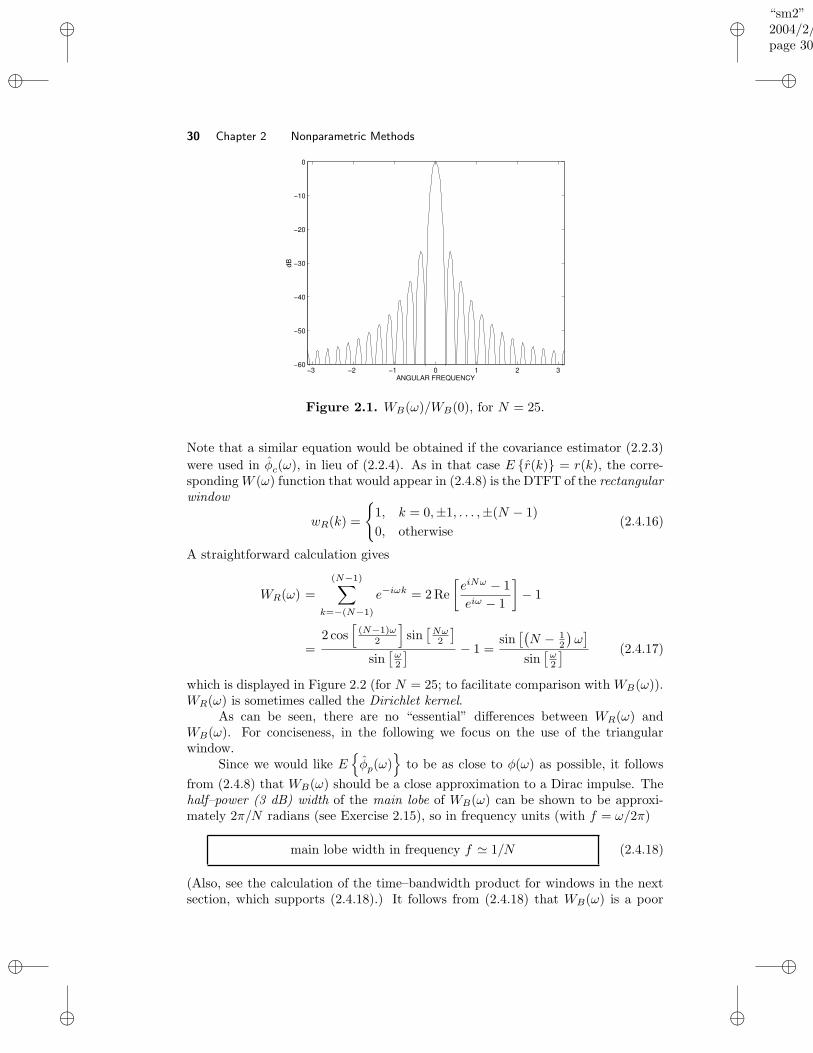
“sm2”2004/2/22page 30

i

i

i

i

i

i

i

i


−3 −2 −1 0 1 2 3−60

−50

−40

−30

−20

−10

0

dB

ANGULAR FREQUENCY

Figure 2.1. WB(ω)/WB(0), for N = 25.

Note that a similar equation would be obtained if the covariance estimator (2.2.3)

were used in φc(ω), in lieu of (2.2.4). As in that case E r(k) = r(k), the corre-spondingW (ω) function that would appear in (2.4.8) is the DTFT of the rectangularwindow

wR(k) =

1, k = 0,±1, . . . ,±(N − 1)

0, otherwise(2.4.16)


WR(ω) =

(N−1)∑

k=−(N−1)

e−iωk = 2 Re

[eiNω − 1

eiω − 1

]

− 1

=2 cos

[(N−1)ω

2

]

sin[Nω2

]

sin[ω2

] − 1 =sin[(N − 1

2

)ω]

sin[ω2

] (2.4.17)

which is displayed in Figure 2.2 (for N = 25; to facilitate comparison with WB(ω)).WR(ω) is sometimes called the Dirichlet kernel.

As can be seen, there are no “essential” differences between WR(ω) andWB(ω). For conciseness, in the following we focus on the use of the triangularwindow.

Since we would like E

φp(ω)

to be as close to φ(ω) as possible, it follows

from (2.4.8) that WB(ω) should be a close approximation to a Dirac impulse. Thehalf–power (3 dB) width of the main lobe of WB(ω) can be shown to be approxi-mately 2π/N radians (see Exercise 2.15), so in frequency units (with f = ω/2π)

main lobe width in frequency f ' 1/N (2.4.18)

(Also, see the calculation of the time–bandwidth product for windows in the nextsection, which supports (2.4.18).) It follows from (2.4.18) that WB(ω) is a poor

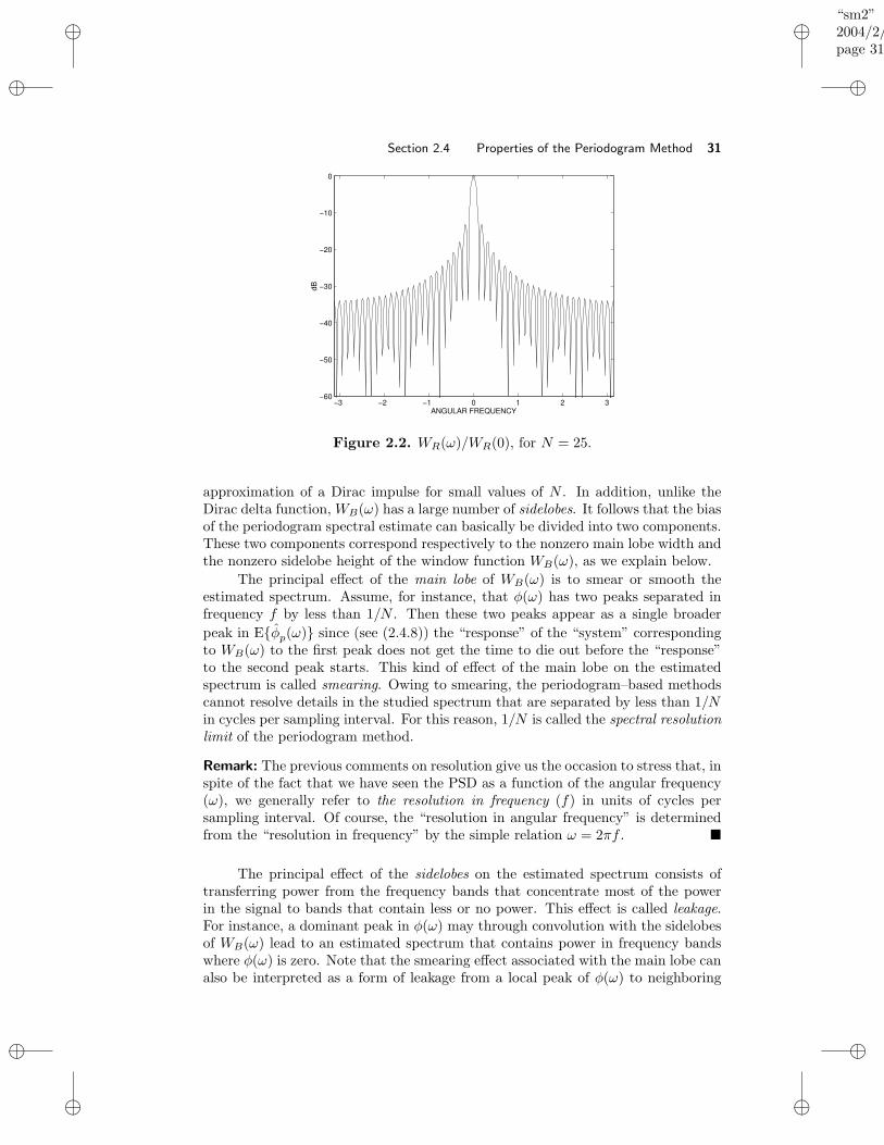
“sm2”2004/2/22page 31

i

i

i

i

i

i

i

i


−3 −2 −1 0 1 2 3−60

−50

−40

−30

−20

−10

0

dB

ANGULAR FREQUENCY

Figure 2.2. WR(ω)/WR(0), for N = 25.

approximation of a Dirac impulse for small values of N . In addition, unlike theDirac delta function, WB(ω) has a large number of sidelobes. It follows that the biasof the periodogram spectral estimate can basically be divided into two components.These two components correspond respectively to the nonzero main lobe width andthe nonzero sidelobe height of the window function WB(ω), as we explain below.

The principal effect of the main lobe of WB(ω) is to smear or smooth theestimated spectrum. Assume, for instance, that φ(ω) has two peaks separated infrequency f by less than 1/N . Then these two peaks appear as a single broader

peak in Eφp(ω) since (see (2.4.8)) the “response” of the “system” correspondingto WB(ω) to the first peak does not get the time to die out before the “response”to the second peak starts. This kind of effect of the main lobe on the estimatedspectrum is called smearing. Owing to smearing, the periodogram–based methodscannot resolve details in the studied spectrum that are separated by less than 1/Nin cycles per sampling interval. For this reason, 1/N is called the spectral resolutionlimit of the periodogram method.

Remark: The previous comments on resolution give us the occasion to stress that, inspite of the fact that we have seen the PSD as a function of the angular frequency(ω), we generally refer to the resolution in frequency (f) in units of cycles persampling interval. Of course, the “resolution in angular frequency” is determinedfrom the “resolution in frequency” by the simple relation ω = 2πf .

The principal effect of the sidelobes on the estimated spectrum consists oftransferring power from the frequency bands that concentrate most of the powerin the signal to bands that contain less or no power. This effect is called leakage.For instance, a dominant peak in φ(ω) may through convolution with the sidelobesof WB(ω) lead to an estimated spectrum that contains power in frequency bandswhere φ(ω) is zero. Note that the smearing effect associated with the main lobe canalso be interpreted as a form of leakage from a local peak of φ(ω) to neighboring

“sm2”2004/2/22page 32

i

i

i

i

i

i

i

i


frequency bands.

It follows from the previous discussion that smearing and leakage are partic-ularly critical for spectra with large amplitude ranges, such as peaky spectra. Forsmooth spectra, these effects are less important. In particular, we see from (2.4.7)that for white noise (which has a maximally smooth spectrum) the periodogram is

an unbiased spectral estimator: Eφp(ω) = φ(ω) (see also Exercise 2.9).

The bias of the periodogram estimator, even though it might be severe forspectra with large dynamic ranges when the sample length is small, does not con-stitute the main limitation of this spectral estimator. In fact, if the bias were theonly problem, then by increasing N (assuming this is possible) the bias in φp(ω)would be eliminated. In order to see this, note from (2.4.5), for example, that

limN→∞

E

φp(ω)

= φ(ω)

Hence, the periodogram is an asymptotically unbiased spectral estimator. The mainproblem of the periodogram method lies in its large variance, as explained next.

2.4.2 Variance Analysis of the Periodogram

The finite–sample variance of φp(ω) can be easily established only in some specific

cases, such as in the case of Gaussian white noise. The asymptotic variance of φp(ω),however, can be derived for more general signals. In the following, we present anasymptotic (for N 1) analysis of the variance of φp(ω) since it turns out tobe sufficient for showing the poor statistical accuracy of the periodogram (for afinite–sample analysis, see Exercise 2.13).

Some preliminary discussion is required. A sequence e(t) is called complex(or circular) white noise if it satisfies

E e(t)e∗(s) = σ2δt,s

E e(t)e(s) = 0, for all t and s(2.4.19)

Note that σ2 = E|e(t)|2

is the variance (or power) of e(t). Equation (2.4.19) can

be rewritten as

E Re[e(t)] Re[e(s)] = σ2

2 δt,s

E Im[e(t)] Im[e(s)] = σ2

2 δt,s

E Re[e(t)] Im[e(s)] = 0

(2.4.20)

Hence, the real and imaginary parts of a complex/circular white noise are real–valued white noise sequences of identical power equal to σ2/2, and uncorrelatedwith one another. See Appendix B for more details on circular random sequences,such as e(t) above.

In what follows, we shall also make use of the symbol O(1/Nα), for someα > 0, to denote a random variable which is such that the square root of itssecond–order moment goes to zero at least as fast as 1/Nα, as N tends to infinity.

“sm2”2004/2/22page 33

i

i

i

i

i

i

i

i


First, we establish the asymptotic variance/covariance of φp(ω) in the case ofGaussian complex/circular white noise. The following result holds.

limN→∞

E

[φp(ω1) − φ(ω1)][φp(ω2) − φ(ω2)]

=

φ2(ω1), ω1 = ω2

0, ω1 6= ω2

(2.4.21)

Note that, for white noise, φ(ω) = σ2 (for all ω). Since limN→∞E φp(ω) =φ(ω) (cf. the analysis in the previous subsection), in order to prove (2.4.21) itsuffices to show that

limN→∞

E

φp(ω1)φp(ω2)

= φ(ω1)φ(ω2) + φ2(ω1)δω1,ω2 (2.4.22)


E

φp(ω1)φp(ω2)

=1

N2

N∑

t=1

N∑

s=1

N∑

p=1

N∑

m=1

E e(t)e∗(s)e(p)e∗(m)

·e−iω1(t−s)e−iω2(p−m)

(2.4.23)

For general random processes, the evaluation of the expectation in (2.4.23) is rel-atively complicated. However, the following general result for Gaussian randomvariables can be used: If a, b, c, and d are jointly Gaussian (complex or real)random variables, then

E abcd = E abE cd + E acE bd + E adE bc−2E aE bE cE d

(2.4.24)

For a proof of (2.4.24), see, e.g., [Janssen and Stoica 1988] and referencestherein. Thus, if the white noise e(t) is Gaussian as assumed, the fourth–ordermoment in (2.4.23) is found to be:

E e(t)e∗(s)e(p)e∗(m) = [E e(t)e∗(s)] [E e(p)e∗(m)]

+ [E e(t)e(p)] [E e(s)e(m)]∗

+ [E e(t)e∗(m)] [E e∗(s)e(p)]

= σ4(δt,sδp,m + δt,mδs,p) (2.4.25)


E

φp(ω1)φp(ω2)

= σ4 +σ4

N2

N∑

t=1

N∑

s=1

e−i(ω1−ω2)(t−s)

= σ4 +σ4

N2

∣∣∣∣∣

N∑

t=1

ei(ω1−ω2)t

∣∣∣∣∣

2

= σ4 +σ4

N2

sin[(ω1 − ω2)N/2]

sin[(ω1 − ω2)/2]

2

(2.4.26)

“sm2”2004/2/22page 34

i

i

i

i

i

i

i

i


The limit of the second term in (2.4.26) is σ4 when ω1 = ω2 and zero otherwise,and (2.4.22) follows at once.

Remark: Note that in the previous case, it was indeed possible to derive the finite–sample variance of φp(ω). For colored noise the above derivation becomes moredifficult, and a different approach (presented below) is needed. See Exercise 2.13for yet another approach that applies to general Gaussian signals.

Next, we consider the case of a much more general signal obtained by linearlyfiltering the Gaussian white noise sequence e(t) considered above:

y(t) =

∞∑

k=1

hke(t− k) (2.4.27)

whose PSD is given by

φy(ω) = |H(ω)|2φe(ω) (2.4.28)

(cf. (1.4.9)). Here H(ω) =∑∞k=1 hke

−iωk. The following intermediate result, con-cerned with signals of the above type, appears to have an independent interest.(Below, we omit the index “p” of φp(ω) in order to simplify the notation.)

For N 1,

φy(ω) = |H(ω)|2φe(ω) + O(1/√N) (2.4.29)

Hence, the periodograms approximately satisfy an equation of the form of (2.4.28)that is satisfied by the true PSDs.

In order to prove (2.4.29), first observe that

1√N

N∑

t=1

y(t)e−iωt =1√N

N∑

t=1

∞∑

k=1

hke(t− k)e−iω(t−k)e−iωk

=1√N

∞∑

k=1

hke−iωk

N−k∑

p=1−ke(p)e−iωp

=1√N

∞∑

k=1

hke−iωk

·

N∑

p=1

e(p)e−iωp +

0∑

p=1−ke(p)e−iωp −

N∑

p=N−k+1

e(p)e−iωp

, H(ω)

[

1√N

N∑

p=1

e(p)e−iωp]

+ ρ(ω) (2.4.30)

“sm2”2004/2/22page 35

i

i

i

i

i

i

i

i


where

ρ(ω) =1√N

∞∑

k=1

hke−iωk

0∑

p=1−ke(p)e−iωp −

N∑

p=N−k+1

e(p)e−iωp

,1√N

∞∑

k=1

hke−iωkεk(ω) (2.4.31)

Next, note that

E εk(ω) = 0,

E εk(ω)εj(ω) = 0 for all k and j, and

Eεk(ω)ε∗

j (ω)

= 2σ2 min(k, j)

which implyE ρ(ω) = 0, E

ρ2(ω)

= 0

and

E|ρ(ω)|2

=

1

N

∣∣∣∣∣∣

∞∑

k=1

∞∑

j=1

hke−iωkh∗

jeiωjE

εk(ω)ε∗

j (ω)

∣∣∣∣∣∣

=2σ2

N

∣∣∣∣∣∣

∞∑

k=1

hke−iωk

k∑

j=1

h∗jeiωjj +

∞∑

j=k+1

h∗jeiωjk

∣∣∣∣∣∣

≤ 2σ2

N

∞∑

k=1

|hk|

∞∑

j=1

|hj |j +

∞∑

j=1

|hj |k

=4σ2

N

( ∞∑

k=1

|hk|)

∞∑

j=1

|hj |j

If∑∞j=1 k|hk| is finite (which, for example, is true if hk is exponentially stable;

see [Soderstrom and Stoica 1989]), we have

E|ρ(ω)|2

≤ constant

N(2.4.32)

Now, from (2.4.30) we obtain

φy(ω) = |H(ω)|2φe(ω) + γ(ω) (2.4.33)

whereγ(ω) = H∗(ω)E∗(ω)ρ(ω) +H(ω)E(ω)ρ∗(ω) + ρ(ω)ρ∗(ω)

and where

E(ω) =1√N

N∑

t=1

e(t)e−iωt

“sm2”2004/2/22page 36

i

i

i

i

i

i

i

i


Since E(ω) and ρ(ω) are linear combinations of Gaussian random variables, theyare also Gaussian distributed. This means that the fourth–order moment formula(2.4.24) can be used to obtain the second–order moment of γ(ω). By doing so, andalso by using (2.4.32) and the fact that, for example,

|E ρ(ω)E∗(ω)| ≤[E|ρ(ω)|2

]1/2 [E|E(ω)|2

]1/2

=constant√

N·[

E

|φe(ω)|2]1/2

=constant√

N

we can verify that γ(ω) = O(1/√N), and hence the proof of (2.4.29) is concluded.

The main result of this section is derived by combining (2.4.21) and (2.4.29).

The asymptotic variance/covariance result (2.4.21) is also validfor a general linear signal as defined in (2.4.27).

(2.4.34)

Remark: In the introduction to Chapter 1, we mentioned that the analysis of acomplex–valued signal is not always more general than the analysis of the corre-sponding real–valued signal; we supported this claim by the example of a complexsine wave. Here, we have another instance where the claim is valid. Similarly tothe complex sinusoidal signal case, the complex (or circular) white noise does notspecialize, in a direct manner, to real white noise. Indeed, if we would let e(t) in(2.4.19) be real, then the two equations in (2.4.19) would conflict with each other(for t = s). The real white noise random process is a stationary signal which satisfies

E e(t)e(s) = σ2δt,s (2.4.35)

If we try to carry out the proof of (2.4.21) under (2.4.35), then we find that the proof

has to be modified. This was expected: both φ(ω) and φp(ω) are even functions inthe real–valued case; hence (2.4.21) should be modified to include the case of bothω1 = ω2 and ω1 = −ω2.

It follows from (2.4.34) that for a fairly general class of signals, the peri-odogram values are asymptotically (for N 1) uncorrelated random variableswhose means and standard deviations are both equal to the corresponding truePSD values. Hence, the periodogram is an inconsistent spectral estimator whichcontinues to fluctuate around the true PSD, with a nonzero variance, even if thelength of the processed sample increases without bound. Furthermore, the factthat the periodogram values φp(ω) are uncorrelated (for large N values) makes theperiodogram exhibit an erratic behavior (similar to that of a white noise realiza-tion). These facts constitute the main limitations of the periodogram approach toPSD estimation. In the next sections, we present several modified periodogram–based methods which attempt to cure the aforementioned difficulties of the basicperiodogram approach. As we shall see, the “improved methods” decrease the vari-ance of the estimated spectrum at the expense of increasing its bias (and, hence,decreasing the average resolution).

“sm2”2004/2/22page 37

i

i

i

i

i

i

i

i

Section 2.5 The Blackman–Tukey Method 37

2.5 THE BLACKMAN–TUKEY METHOD

In this section we develop the Blackman–Tukey method [Blackman and Tukey

1959] and compare it to the periodogram. In later sections we consider several otherrefined periodogram–based methods that, like the Blackman–Tukey (BT) method,seek to reduce the statistical variability of the estimated spectrum; we will comparethese methods to one another and to the Blackman–Tukey method.

2.5.1 The Blackman–Tukey Spectral Estimate

As we have seen, the main problem with the periodogram is the high statisticalvariability of this spectral estimator, even for very large sample lengths. The poorstatistical quality of the periodogram PSD estimator has been intuitively explainedas arising from both the poor accuracy of r(k) in φc(ω) for extreme lags (|k| 'N) and the large number of (even if small) covariance estimation errors that are

cumulatively summed up in φc(ω). Both these effects may be reduced by truncating

the sum in the definition formula of φc(ω), (2.2.2). Following this idea leads to theBlackman–Tukey estimator, which is given by

φBT (ω) =

M−1∑

k=−(M−1)

w(k)r(k)e−iωk(2.5.1)

where w(k) is an even function (i.e., w(−k) = w(k)) which is such that w(0) = 1,w(k) = 0 for |k| ≥ M , and w(k) decays smoothly to zero with k, and where M < N .Since w(k) in (2.5.1) weights the lags of the sample covariance sequence, it is calleda lag window.

If w(k) in (2.5.1) is selected as the rectangular window, then we simply obtain

a truncated version of φc(ω). However, we may choose w(k) in many other ways,and this flexibility may be employed to improve the accuracy of the Blackman–Tukey spectral estimator or to emphasize some of its characteristics that are ofparticular interest in a given application. In the following subsections, we addressthe principal issues which concern the problem of window selection. However, beforedoing so we rewrite (2.5.1) in an alternative form that will be used in several placesof the discussion that follows.

Let W (ω) denote the DTFT of w(k),

W (ω) =

∞∑

k=−∞w(k)e−iωk =

M−1∑

k=−(M−1)

w(k)e−iωk (2.5.2)

“sm2”2004/2/22page 38

i

i

i

i

i

i

i

i


Making use of the DTFT property that led to (2.4.8), we can then write

φBT (ω) =

∞∑

k=−∞w(k)r(k)e−iωk

= DTFT of the product of the sequences

. . . , 0, 0, w(−(M − 1)), . . . , w(M − 1), 0, 0, . . . and

. . . , 0, 0, r(−(N − 1)), . . . , r(N − 1), 0, 0, . . .= DTFT(r(k)) ∗ DTFT(w(k))

As DTFT. . . , 0, 0, r(−(N − 1)), . . . , r(N − 1), 0, 0, . . . = φp(ω), we obtain

φBT (ω) = φp(ω) ∗W (ω) =1

2π

∫ π

−πφp(ψ)W (ω − ψ)dψ (2.5.3)

This equation is analogous to (2.4.8) and can be interpreted in the same way.Hence, since for most windows in common use W (ω) has a dominant, relativelynarrow peak at ω = 0, it follows from (2.5.3) that

The Blackman–Tukey spectral estimator (2.5.1) corresponds to a“locally” weighted average of the periodogram.

(2.5.4)

Since the function W (ω) in (2.5.3) acts as a window (or weighting) in thefrequency domain, it is sometimes called a spectral window. As we shall see, severalrefined periodogram–based spectral estimators discussed in what follows can begiven an interpretation similar to that afforded by (2.5.3).

The form (2.5.3) under which the Blackman–Tukey spectral estimator hasbeen put is quite appealing from an intuitive standpoint. The main problem withthe periodogram lies in its large variations about the true PSD. The weightedaverage in (2.5.3), in the neighborhood of the current frequency point ω, shouldsmooth the periodogram and hence eliminate its large fluctuations.

On the other hand, this smoothing by the spectral window W (ω) will alsohave the undesirable effect of reducing the resolution. We may expect that thesmaller the M , the larger the reduction in variance and the lower the resolution.These qualitative arguments may be made exact by a statistical analysis of φBT (ω),similar to that in the previous section. In fact, it is clear from (2.5.3) that the mean

and variance of φBT (ω) can be derived from those of φp(ω). Roughly speaking, the

results that can be established by the analysis of φBT (ω), based on (2.5.3), showthat the resolution of this spectral estimator is on the order of 1/M , whereas itsvariance is on the order of M/N . The compromise between resolution and variance,which should be considered when choosing the window’s length, is clearly seen fromthe above considerations. We will look at the tradeoff resolution–variance in moredetail in what follows. The next discussion addresses some of the main issues whichconcern window design.

“sm2”2004/2/22page 39

i

i

i

i

i

i

i

i

Section 2.6 Window Design Considerations 39

2.5.2 Nonnegativeness of the Blackman–Tukey Spectral Estimate

Since φ(ω) ≥ 0, it is natural to also require that φBT (ω) ≥ 0. The lag windowcan be selected to achieve this desirable property of the estimated spectrum. Thefollowing result holds true.

If the lag window w(k) is positive semidefinite (i.e., W (ω) ≥ 0),then the windowed covariance sequence w(k)r(k) (with r(k)given by (2.2.4)) is positive semidefinite, too; which implies that

φBT (ω) ≥ 0 for all ω.

(2.5.5)

In order to prove the above result, first note that φBT (ω) ≥ 0 if and only ifthe sequence . . . , 0, 0, w(−(M − 1))r(−(M − 1)), . . . , w(M − 1)r(M − 1), 0, 0, . . .is positive semidefinite or, equivalently, the following Toeplitz matrix is positivesemidefinite for all dimensions:

w(0)r(0) . . . w(M − 1)r(M − 1) 0...

. . .

w(−M + 1)r(−M + 1). . . w(M − 1)r(M − 1)

. . ....

0 w(−M + 1)r(−M + 1) . . . w(0)r(0)

=

w(0) . . . w(M − 1) 0...

. . .

w(−M + 1). . . w(M − 1)

. . ....

0 w(−M + 1) . . . w(0)

r(0) . . . r(M − 1) 0...

. . .

r(−M + 1). . . r(M − 1)

. . ....

0 r(−M + 1) . . . r(0)

The symbol denotes the Hadamard matrix product (i.e., element–wise multi-plication). By a result in matrix theory, the Hadamard product of two positivesemidefinite matrices is also a positive semidefinite matrix (see Result R19 in Ap-pendix A). Thus, the proof of (2.5.5) is concluded.

Another, perhaps simpler, proof of (2.5.5) makes use of (2.5.3) in the followingway. Since the sequence w(k) is real and symmetric about the point k = 0, itsDTFT W (ω) is an even, real–valued function. Furthermore, if w(k) is a positivesemidefinite sequence then W (ω) ≥ 0 for all ω values (see Exercise 1.8). By (2.5.3),

W (ω) ≥ 0 immediately implies φBT (ω) ≥ 0, as φp(ω) ≥ 0 by definition.It should be noted that some lag windows, such as the rectangular window,

do not satisfy the assumption made in (2.5.5) and hence their use may lead toestimated spectra that take negative values. The Bartlett window, on the otherhand, is positive semidefinite (as can be seen from (2.4.15)).

2.6 WINDOW DESIGN CONSIDERATIONS

The properties of the Blackman–Tukey estimator (and of other refined periodogrammethods discussed in the next section) are directly related to the choice of the lag

“sm2”2004/2/22page 40

i

i

i

i

i

i

i

i


window. In this section, we discuss several relevant properties of windows that areuseful in selecting or designing a window to use in a refined spectral estimationprocedure.

2.6.1 Time–Bandwidth Product and Resolution–Variance Tradeoffs in Window Design

Most windows are such that they take only nonnegative values in both time andfrequency domains (or, if they also take negative values, these are much smallerthan the positive values of the window). In addition, they peak at the origin inboth domains. For this type of window, it is possible to define an equivalent timewidth, Ne, and an equivalent bandwidth, βe, as follows:

Ne =

∑M−1k=−(M−1) w(k)

w(0)(2.6.1)

and

βe =12π

∫ π

−πW (ω)dω

W (0)(2.6.2)

From the definitions of direct and inverse DTFTs, we obtain

W (0) =

∞∑

k=−∞w(k) =

M−1∑

k=−(M−1)

w(k) (2.6.3)

and

w(0) =1

2π

∫ π

−πW (ω)dω (2.6.4)

Using (2.6.3) and (2.6.4) in (2.6.1) and (2.6.2) gives the following result.

The (equivalent) time–bandwidth product equals unity:Neβe = 1

(2.6.5)

As already indicated, the result above applies to window–like signals. Someextended results of the time–bandwidth product type, which apply to more generalclasses of signals, are presented in Complement 2.8.5.

It is clearly seen from (2.6.5) that a window cannot be both time–limited andband–limited. The more slowly the window decays to zero in one domain, the moreconcentrated it is in the other domain. The simple result above, (2.6.5), has severalother interesting consequences, as explained below.

The equivalent temporal extent (or aperture), Ne, of w(k) is essentially de-termined by the window’s length. For example, for a rectangular window we haveNe ' 2M , whereas for a triangular window Ne ' M . This observation, togetherwith (2.6.5), implies that the equivalent bandwidth βe is basically determined bythe window’s length. More precisely, βe = O(1/M). This fact lends support to aclaim made previously that for a window which concentrates most of its energy inits main lobe, the width of that lobe should be on the order of 1/M . Since themain lobe’s width sets a limit on the spectral resolution achievable (as explained

“sm2”2004/2/22page 41

i

i

i

i

i

i

i

i


in Section 2.4), the above observation shows that the spectral resolution limit of awindowed method should be on the order of 1/M . On the other hand, as explainedin the previous section, the statistical variance of such a method is essentially pro-portional to M/N . Hence, we reached the following conclusion.

The choice of window’s length should be based on a tradeoff be-tween spectral resolution and statistical variance

(2.6.6)

As a rule of thumb, we should choose M ≤ N/10 in order to reduce thestandard deviation of the estimated spectrum at least three times, compared withthe periodogram.

Once M is determined, we cannot decrease simultaneously the energy in themain lobe (to reduce smearing) and the energy in the sidelobes (to reduce leakage).This follows, for example, from (2.6.4) which shows that the area of W (ω) is fixedonce w(0) is fixed (such as w(0) = 1). In other words, if we want to decrease themain lobe’s width then we should accept an increase in the sidelobe energy andvice versa. In summary:

The selection of window’s shape should be based on a tradeoffbetween smearing and leakage effects.

(2.6.7)

The above tradeoff is usually dictated by the specific application at hand. Anumber of windows have been developed to address this tradeoff. In some sense,each of these windows can be seen as a design at a specific point in the resolu-tion/leakage tradeoff curve. We consider several such windows in the next subsec-tion.

2.6.2 Some Common Lag Windows

In this section, we list some of the most common lag windows and outline their rele-vant properties. Our purpose is not to provide a detailed derivation or an exhaustivelisting of such windows, but rather to provide a quick reference of common windows.More detailed information on these and other windows can be found in [Harris

1978; Kay 1988; Marple 1987; Oppenheim and Schafer 1989; Priestley

1981; Porat 1997], where many of the closed–form windows have been compiled.Table 2.1 lists some common windows along with some useful properties.

In addition to the fixed window designs in Table 2.1, there are windows thatcontain a design parameter which may be varied to trade between resolution andsidelobe leakage. Two such common designs are the Chebyshev window and theKaiser window. The Chebyshev window has the property that the peak level of thesidelobe “ripples” is constant. Thus, unlike most other windows, the sidelobe leveldoes not decrease as ω increases. The Kaiser window is defined by

w(k) =I0

(

γ√

1 − [k/(M − 1)]2)

I0(γ), −(M − 1) ≤ k ≤ M − 1 (2.6.8)

where I0(·) is the zeroth–order modified Bessel function of the first kind. Theparameter γ trades the main lobe width for the sidelobe leakage level; γ = 0

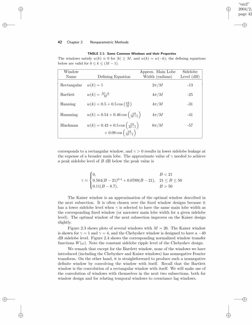
“sm2”2004/2/22page 42

i

i

i

i

i

i

i

i


TABLE 2.1: Some Common Windows and their Properties

The windows satisfy w(k) ≡ 0 for |k| ≥ M , and w(k) = w(−k); the defining equations

below are valid for 0 ≤ k ≤ (M − 1).

Window Approx. Main Lobe SidelobeName Defining Equation Width (radians) Level (dB)

Rectangular w(k) = 1 2π/M -13

Bartlett w(k) = M−kM 4π/M -25

Hanning w(k) = 0.5 + 0.5 cos(πkM

)4π/M -31

Hamming w(k) = 0.54 + 0.46 cos(

πkM−1

)

4π/M -41

Blackman w(k) = 0.42 + 0.5 cos(

πkM−1

)

6π/M -57

+ 0.08 cos(

πkM−1

)

corresponds to a rectangular window, and γ > 0 results in lower sidelobe leakage atthe expense of a broader main lobe. The approximate value of γ needed to achievea peak sidelobe level of B dB below the peak value is

γ '

0, B < 21

0.584(B − 21)0.4 + 0.0789(B − 21), 21 ≤ B ≤ 50

0.11(B − 8.7), B > 50

The Kaiser window is an approximation of the optimal window described inthe next subsection. It is often chosen over the fixed window designs because ithas a lower sidelobe level when γ is selected to have the same main lobe width asthe corresponding fixed window (or narrower main lobe width for a given sidelobelevel). The optimal window of the next subsection improves on the Kaiser designslightly.

Figure 2.3 shows plots of several windows with M = 26. The Kaiser windowis shown for γ = 1 and γ = 4, and the Chebyshev window is designed to have a −40dB sidelobe level. Figure 2.4 shows the corresponding normalized window transferfunctions W (ω). Note the constant sidelobe ripple level of the Chebyshev design.

We remark that except for the Bartlett window, none of the windows we haveintroduced (including the Chebyshev and Kaiser windows) has nonnegative Fouriertransform. On the other hand, it is straightforward to produce such a nonnegativedefinite window by convolving the window with itself. Recall that the Bartlettwindow is the convolution of a rectangular window with itself. We will make use ofthe convolution of windows with themselves in the next two subsections, both forwindow design and for relating temporal windows to covariance lag windows.

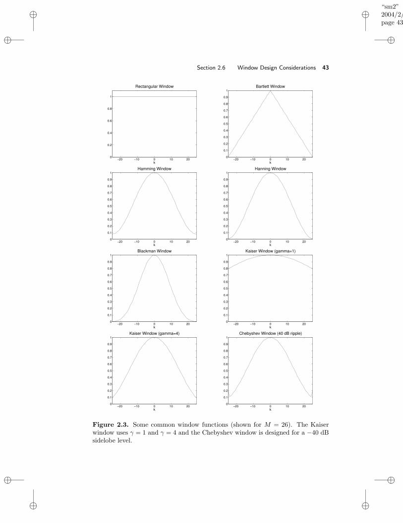
“sm2”2004/2/22page 43

i

i

i

i

i

i

i

i


−20 −10 0 10 200

0.2

0.4

0.6

0.8

1

Rectangular Window

k−20 −10 0 10 20

0

0.1

0.2

0.3

0.4

0.5

0.6

0.7

0.8

0.9

1Bartlett Window

k

−20 −10 0 10 200

0.1

0.2

0.3

0.4

0.5

0.6

0.7

0.8

0.9

1Hamming Window

k−20 −10 0 10 20

0

0.1

0.2

0.3

0.4

0.5

0.6

0.7

0.8

0.9

1Hanning Window

k

−20 −10 0 10 200

0.1

0.2

0.3

0.4

0.5

0.6

0.7

0.8

0.9

1Blackman Window

k−20 −10 0 10 20

0

0.1

0.2

0.3

0.4

0.5

0.6

0.7

0.8

0.9

1Kaiser Window (gamma=1)

k

−20 −10 0 10 200

0.1

0.2

0.3

0.4

0.5

0.6

0.7

0.8

0.9


k−20 −10 0 10 20

0

0.1

0.2

0.3

0.4

0.5

0.6

0.7

0.8

0.9

1Chebyshev Window (40 dB ripple)

k

Figure 2.3. Some common window functions (shown for M = 26). The Kaiserwindow uses γ = 1 and γ = 4 and the Chebyshev window is designed for a −40 dBsidelobe level.

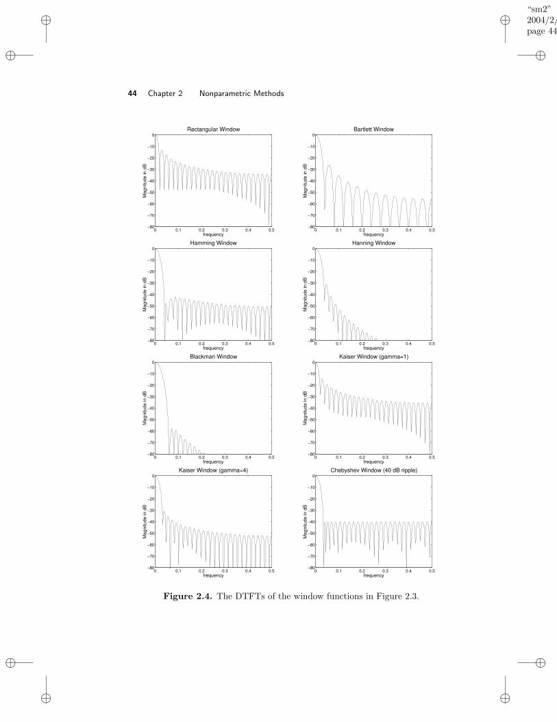
“sm2”2004/2/22page 44

i

i

i

i

i

i

i

i


0 0.1 0.2 0.3 0.4 0.5−80

−70

−60

−50

−40

−30

−20

−10

0Rectangular Window

Mag

nitu

de in

dB

frequency0 0.1 0.2 0.3 0.4 0.5

−80

−70

−60

−50

−40

−30

−20

−10

0Bartlett Window

Mag

nitu

de in

dB

frequency

0 0.1 0.2 0.3 0.4 0.5−80

−70

−60

−50

−40

−30

−20

−10

0Hamming Window

Mag

nitu

de in

dB

frequency0 0.1 0.2 0.3 0.4 0.5

−80

−70

−60

−50

−40

−30

−20

−10

0Hanning Window

Mag

nitu

de in

dB

frequency

0 0.1 0.2 0.3 0.4 0.5−80

−70

−60

−50

−40

−30

−20

−10

0Blackman Window

Mag

nitu

de in

dB

frequency0 0.1 0.2 0.3 0.4 0.5

−80

−70

−60

−50

−40

−30

−20

−10


Mag

nitu

de in

dB

frequency

0 0.1 0.2 0.3 0.4 0.5−80

−70

−60

−50

−40

−30

−20

−10


Mag

nitu

de in

dB

frequency0 0.1 0.2 0.3 0.4 0.5

−80

−70

−60

−50

−40

−30

−20

−10

0Chebyshev Window (40 dB ripple)

Mag

nitu

de in

dB

frequency

Figure 2.4. The DTFTs of the window functions in Figure 2.3.

“sm2”2004/2/22page 45

i

i

i

i

i

i

i

i


2.6.3 Window Design Example

Assume a situation where it is known that the observed signal consists of a usefulweak signal and a strong interference, and that both the useful signal and theinterference can be assumed to be narrowband signals which are well separated infrequency. However, there is no a priori quantitative information available on thefrequency separation between the desired signal and the interference. It is requiredto design a lag window for use in a Blackman–Tukey spectral estimation method,with the purpose of detecting and locating in frequency the useful signal.

The main problem in the application outlined above lies in the fact thatthe (strong) interference may completely mask the (weak) desired signal throughleakage. In order to get rid of this problem, the window design should compromisesmearing for leakage. Note that the smearing effect is not of main concern in thisapplication, as the useful signal and the interference are well separated in frequency.Hence, smearing cannot affect our ability to detect the desired signal; it will onlylimit, to some degree, our ability to accurately locate in frequency the signal inquestion.

We consider a window sequence whose DTFT W (ω) is constructed as thesquared magnitude of the DTFT of another sequence v(k); in this way, weguarantee that the constructed window is positive semidefinite. Mathematically,the above design problem can be formulated as follows. Consider a sequencev(0), . . . , v(M − 1), and let

V (ω) =

M−1∑

k=0

v(k)e−iωk (2.6.9)

The DTFT V (ω) can be rewritten in the more compact form

V (ω) = v∗a(ω) (2.6.10)

wherev = [v(0) . . . v(M − 1)]∗ (2.6.11)

anda(ω) = [1 e−iω . . . e−i(M−1)ω]T (2.6.12)

Define the spectral window as

W (ω) = |V (ω)|2 (2.6.13)

The corresponding lag window can be obtained from (2.6.13) as follows:

M−1∑

k=−(M−1)

w(k)e−iωk =

M−1∑

n=0

M−1∑

p=0

v(n)v∗(p)e−iω(n−p)

=

M−1∑

n=0

n−(M−1)∑

k=n

v(n)v∗(n− k)e−iωk

=

M−1∑

k=−(M−1)

[M−1∑

n=0

v(n)v∗(n− k)

]

e−iωk (2.6.14)

“sm2”2004/2/22page 46

i

i

i

i

i

i

i

i


which gives

w(k) =

M−1∑

n=0

v(n)v∗(n− k) (2.6.15)

The last equality in (2.6.14), and hence the equality (2.6.15), are valid under theconvention that v(k) = 0 for k < 0 and k ≥ M .

As already mentioned, this method of constructing w(k) from the convolu-tion of the sequence v(k) with itself has the advantage that the so–obtained lagwindow is always positive semidefinite or, equivalently, the corresponding spectralwindow satisfies W (ω) ≥ 0 (which is easily seen from (2.6.13)). Besides this, thedesign of w(k) can be reduced to the selection of v(k) which may be moreconveniently done, as explained next.

In the present application, the design objective is to reduce the leakage in-curred by w(k) as much as possible. This objective can be formulated as theproblem of minimizing the relative energy in the sidelobes of W (ω) or, equivalently,as the problem of maximizing the relative energy in the main lobe of W (ω):

maxv

∫ βπ

−βπW (ω)dω∫ π

−πW (ω)dω

(2.6.16)

Here, β is a design parameter which quantifies how much smearing (or, basicallyequivalent, resolution) we can tradeoff for leakage reduction. The larger the β,the more leakage free the optimal window derived from (2.6.16) but also the morediminished the spectral resolution associated with that window.

By writing the criterion in (2.6.16) in the following form

12π

∫ βπ

−βπ |V (ω)|2dω12π

∫ π

−π |V (ω)|2dω =v∗[

12π

∫ βπ

−βπ a(ω)a∗(ω)dω]

v

v∗v(2.6.17)

(cf. (2.6.10) and Parseval’s theorem, (1.2.6)), the optimization problem (2.6.16)becomes

maxv

v∗Γv

v∗v(2.6.18)

where

Γ =1

2π

∫ βπ

−βπa(ω)a∗(ω)dω , [γm−n] (2.6.19)

and where

γm−n =1

2π

∫ βπ

−βπe−i(m−n)ωdω =

sin[(m− n)βπ]

(m− n)π(2.6.20)

(note that γ0 = β). By using the function

sinc(x) ,sinx

x, (sinc(0) = 1) (2.6.21)

we can write (2.6.20) as

γm−n = βsinc[(m− n)βπ] (2.6.22)

“sm2”2004/2/22page 47

i

i

i

i

i

i

i

i


The solution to the problem (2.6.18) is well known: the maximizing v is given bythe dominant eigenvector of Γ, associated with the maximum eigenvalue of thismatrix (see Result R13 in Appendix A). To summarize:

The optimal lag window which minimizes the relative energy inthe sidelobe interval [−π,−βπ]∪[βπ, π] is given by (2.6.15), wherev is the dominant eigenvector of the matrix Γ defined in (2.6.19)and (2.6.22).

(2.6.23)

Regarding the choice of the design parameter β, it is clear that β should belarger than 1/M in order to allow for a significant reduction of leakage. Otherwise,by selecting for example β ' 1/M , we weigh the resolution issue too much in thedesign problem, with unfavorable consequences for leakage reduction.

Finally, we remark that a problem quite similar to the above one, althoughderived from different considerations, will be encountered in Chapter 5 (see also[Mullis and Scharf 1991]).

2.6.4 Temporal Windows and Lag Windows

As we have seen previously, the unwindowed periodogram coincides with the un-windowed correlogram. The Blackman–Tukey estimator is a windowed correlogramobtained using a lag window. Similarly, we can define a windowed periodogram

φW (ω) =1

N

∣∣∣∣∣

N∑

t=1

v(t)y(t)e−iωt

∣∣∣∣∣

2

(2.6.24)

where the weighting sequence v(t) may be called a temporal window. A tem-poral window is sometimes called a taper. Welch [Welch 1967] was one of thefirst researchers who considered windowed periodogram spectral estimators (seeSection 2.7.2 for a description of Welch’s method), and hence the subscript “W”

attached to φ(ω) in (2.6.24). However, while the reason for windowing the cor-relogram is clearly motivated, the reason for windowing the periodogram is lessobvious. In order to motivate (2.6.24), at least partially, write this equation as

φW (ω) =1

N

N∑

t=1

N∑

s=1

v(t)v∗(s)y(t)y∗(s)e−iω(t−s) (2.6.25)

Next, take expectation of both sides of (2.6.25) to obtain

E

φW (ω)

=1

N

N∑

t=1

N∑

s=1

v(t)v∗(s)r(t− s)e−iω(t−s) (2.6.26)

Inserting

r(t− s) =1

2π

∫ π

−πφ(ω)eiω(t−s)dω (2.6.27)

“sm2”2004/2/22page 48

i

i

i

i

i

i

i

i


in (2.6.26) gives

E

φW (ω)

=1

N2π

∫ π

−πφ(ψ)

[N∑

t=1

N∑

s=1

v(t)v∗(s)e−i(ω−ψ)(t−s)]

dψ

=1

N2π

∫ π

−πφ(ψ)

∣∣∣∣∣

N∑

t=1

v(t)e−i(ω−ψ)t

∣∣∣∣∣

2

dψ (2.6.28)

Define

W (ω) =1

N

∣∣∣∣∣

N∑

t=1

v(t)e−iωt

∣∣∣∣∣

2

(2.6.29)

By using this notation, we can write (2.6.28) as

E

φW (ω)

=1

2π

∫ π

−πφ(ψ)W (ω − ψ)dψ (2.6.30)

As the equation (2.6.29) is similar to (2.6.13), the sequence whose DTFT is equalto W (ω) immediately follows from (2.6.15):

w(k) =1

N

N∑

n=1

v(n)v∗(n− k) (2.6.31)

Next, by comparing (2.6.30) and (2.5.3), we get the following result.

The windowed periodogram and the windowed correlogram havethe same average behavior, provided the temporal and lag win-dows are related as in (2.6.31).

(2.6.32)

Hence EφW (ω) = EφBT (ω), provided the temporal and lag windows

are matched to one another. A similarly simple relationship between φW (ω) and

φBT (ω), however, does not seem to exist. This makes it somewhat difficult tomotivate the windowed periodogram as defined in (2.6.24). The Welch periodogram,though, does not weigh all data samples as in (2.6.24), and is a useful spectralestimator (see the next section).

2.7 OTHER REFINED PERIODOGRAM METHODS

In Section 2.5 we introduced the Blackman–Tukey estimator as an alternative tothe periodogram. In this section we present three other modified periodograms:the Bartlett, Welch, and Daniell methods. Like the Blackman–Tukey method, theyseek to reduce the variance of the periodogram by smoothing or averaging theperiodogram estimates in some way. We will relate these methods to one anotherand to the Blackman–Tukey method.

“sm2”2004/2/22page 49

i

i

i

i

i

i

i

i

Section 2.7 Other Refined Periodogram Methods 49

2.7.1 Bartlett Method

The basic idea of the Bartlett method [Bartlett 1948; Bartlett 1950] is sim-ple: to reduce the large fluctuations of the periodogram, split up the availablesample of N observations into L = N/M subsamples of M observations each, andthen average the periodograms obtained from the subsamples for each value of ω.Mathematically, the Bartlett method can be described as follows. Let

yj(t) = y((j − 1)M + t),t = 1, . . . ,Mj = 1, . . . , L

(2.7.1)

denote the observations of the jth subsample, and let

φj(ω) =1

M

∣∣∣∣∣

M∑

t=1

yj(t)e−iωt

∣∣∣∣∣

2

(2.7.2)

denote the corresponding periodogram. The Bartlett spectral estimate is then givenby

φB(ω) =1

L

L∑

j=1

φj(ω) (2.7.3)

Since the Bartlett method operates on data segments of length M , the resolutionafforded should be on the order of 1/M . Hence, the spectral resolution of theBartlett method is reduced by a factor L, compared to the resolution of the originalperiodogram method. In return for this reduction in resolution, we can expect thatthe Bartlett method has a reduced variance. It can, in fact, be shown that theBartlett method reduces the variance of the periodogram by the same factor L (seebelow). The compromise between resolution and variance when selecting M (or L)is thus evident.

An interesting way to look at the Bartlett method and its properties is byrelating it to the Blackman–Tukey method. As we know, φj(ω) of (2.7.2) can berewritten as

φj(ω) =

M−1∑

k=−(M−1)

rj(k)e−iωk (2.7.4)

where rj(k) is the sample covariance sequence corresponding to the jth subsam-ple. Inserting (2.7.4) in (2.7.3) gives

φB(ω) =

M−1∑

k=−(M−1)

1

L

L∑

j=1

rj(k)

e−iωk (2.7.5)

We see that φB(ω) is similar in form to the Blackman–Tukey estimator that usesa rectangular window. The average, over j, of the subsample covariance rj(k) isan estimate of the ACS r(k). However, the ACS estimate in (2.7.5) does not makeefficient use of available data lag products y(t)y∗(t−k), especially for |k| near M−1(see Exercise 2.14). In fact, for k = M − 1, only about 1/Mth of the available lagproducts are used to form the ACS estimate in (2.7.5). We expect that the variance

“sm2”2004/2/22page 50

i

i

i

i

i

i

i

i


of these lags is higher than for the corresponding r(k) lags used in the Blackman–

Tukey estimate, and similarly, the variance of φB(ω) is higher than that of φBT (ω).In addition, the Bartlett method uses a fixed rectangular lag window, and thushas less flexibility in resolution–leakage tradeoff than does the Blackman–Tukeymethod. For these reasons, we conclude that

The Bartlett estimate, as defined in (2.7.1)–(2.7.3), is similarin form to, but typically has a slightly higher variance than,the Blackman–Tukey estimate with a rectangular lag window oflength M .

(2.7.6)

The reduction in resolution and the decrease of variance (both by a factorL = N/M) for the Bartlett estimate, as compared to the basic periodogram method,follows from (2.7.6) and the properties of the Blackman–Tukey spectral estimatorgiven previously.

The main lobe of the rectangular window is narrower than that associatedwith most other lag windows (this follows from the observation that the rectangularwindow clearly has the largest equivalent time width , and the fact that the time–bandwidth product is constant, see (2.6.5)). Thus, it follows from (2.7.6) that inthe class of Blackman–Tukey estimates, the Bartlett estimator can be expected tohave the least smearing (and hence the best resolution) but the most significantleakage.

2.7.2 Welch Method

The Welch method [Welch 1967] is obtained by refining the Bartlett method intwo respects. First, the data segments in the Welch method are allowed to overlap.Second, each data segment is windowed prior to computing the periodogram. Todescribe the Welch method in a mathematical form, let

yj(t) = y((j − 1)K + t),t = 1, . . . ,Mj = 1, . . . , S

(2.7.7)

denote the jth data segment. In (2.7.7), (j − 1)K is the starting point for the jthsequence of observations. If K = M , then the sequences do not overlap (but arecontiguous) and we get the sample splitting used by the Bartlett method (whichleads to S = L = N/M data subsamples). However, the value recommended for Kin the Welch method is K = M/2, in which case S ' 2M/N data segments (with50% overlap between successive segments) are obtained.

The windowed periodogram corresponding to yj(t) is computed as

φj(ω) =1

MP

∣∣∣∣∣

M∑

t=1

v(t)yj(t)e−iωt

∣∣∣∣∣

2

(2.7.8)

where P denotes the “power” of the temporal window v(t):

P =1

M

M∑

t=1

|v(t)|2 (2.7.9)

“sm2”2004/2/22page 51

i

i

i

i

i

i

i

i


The Welch estimate of PSD is determined by averaging the windowed periodogramsin (2.7.8):

φW (ω) =1

S

S∑

j=1

φj(ω) (2.7.10)

The reasons for the above modifications to the Bartlett method, which led to theWelch method, are simple to explain. By allowing overlap between the data seg-ments and hence by getting more periodograms to be averaged in (2.7.10), we hopeto decrease the variance of the estimated PSD. By introducing the window in theperiodogram computation it may be hoped to get more control over the bias/re-solution properties of the estimated PSD (see Section 2.6.4). Additionally, thetemporal window may be used to give less weight to the data samples at the endsof each subsample, hence making the consecutive subsample sequences less corre-lated to one another, even though they are overlapping. The principal effect of this“decorrelation” should be a more effective reduction of variance via the averagingin (2.7.10).

The analysis that led to the results (2.6.30)–(2.6.32) can be modified to showthat the use of windowed periodograms in the Welch method, as contrasted to theunwindowed periodograms in the Bartlett method, indeed offers more flexibilityin controlling the bias properties of the estimated spectrum. The variance of theWelch spectral estimator is more difficult to analyze (except in some special cases).However, there is empirical evidence that the Welch method can offer lower variancethan the Bartlett method but the difference in the variances corresponding to thetwo methods is not dramatic.

We can relate the Welch estimator to the Blackman–Tukey spectral estimatorby a straightforward calculation as we did for the Bartlett method. By inserting(2.7.8) in (2.7.10), we obtain

φW (ω) =1

S

S∑

j=1

1

MP

M∑

t=1

M∑

k=1

v(t)v∗(k)yj(t)y∗j (k)e

−iω(t−k) (2.7.11)

For large values of N and for K = M/2 or smaller, S results sufficiently large for

the average (1/S)∑Sj=1 yj(t)y

∗j (k) to be close to the covariance r(t−k). We do not

replace the previous sum by the true covariance lag. However, we assume that thissum does not depend on both t and k, but only on their difference (t− k), at leastapproximately; say

r(t, k) =1

S

S∑

j=1

yj(t)y∗j (k) ' r(t− k) (2.7.12)

“sm2”2004/2/22page 52

i

i

i

i

i

i

i

i


Using (2.7.12) in (2.7.11) gives

φW (ω) ' 1

MP

M∑

t=1

M∑

k=1

v(t)v∗(k)r(t− k)e−iω(t−k)

=1

MP

M∑

t=1

t−M∑

τ=t−1

v(t)v∗(t− τ)r(τ)e−iωτ

=

M−1∑

τ=−(M−1)

[

1

MP

M∑

t=1

v(t)v∗(t− τ)

]

r(τ)e−iωτ (2.7.13)

By introducing

w(τ) =1

MP

M∑

t=1

v(t)v∗(t− τ) (2.7.14)

(under the convention that v(k) = 0 for k < 1 and k > M), we can write (2.7.13)as

φW (ω) 'M−1∑

τ=−(M−1)

w(τ)r(τ)e−iωτ (2.7.15)

which is to be compared to the form of the Blackman–Tukey estimator. To summa-rize, the Welch estimator has been shown to approximate a Blackman–Tukey–typeestimator for the estimated covariance sequence (2.7.12) (which may be expectedto have finite–sample properties different from those of r(k)).

The Welch estimator can be efficiently computed via the FFT, and is one ofthe most frequently used PSD estimation methods. Its previous interpretation ispleasing, even if approximate, since the Blackman–Tukey form of spectral estimatoris theoretically the most favored one. This interpretation also shows that we maythink of replacing the usual covariance estimates r(k) in the Blackman–Tukeyestimator by other sample covariances, with the purpose of either reducing thecomputational burden or improving the statistical accuracy.

2.7.3 Daniell Method

As shown in (2.4.21), the periodogram values φ(ωk) corresponding to different fre-quency values ωk are (asymptotically) uncorrelated random variables. One maythen think of reducing the large variance of the basic periodogram estimator byaveraging the periodogram over small intervals centered on the current frequencyω. This is the idea behind the Daniell method [Daniell 1946]. The practical formof the Daniell estimate, which can be implemented by means of the FFT, is thefollowing:

φD(ωk) =1

2J + 1

k+J∑

j=k−Jφp(ωj) (2.7.16)

where

ωk =2π

Nk, k = 0, . . . , N − 1 (2.7.17)

“sm2”2004/2/22page 53

i

i

i

i

i

i

i

i


and where N is (much) larger than N to ensure a fine sampling of φp(ω). Theperiodogram samples needed in (2.7.16) can be obtained, for example, by using aradix–2 FFT algorithm applied to the zero–padded data sequence, as described inSection 2.3. The parameter J in the Daniell method should be chosen sufficientlysmall to guarantee that φ(ω) is nearly constant on the interval(s):

[

ω − 2π

NJ, ω +

2π

NJ

]

(2.7.18)

Since N can in principle be chosen as large as we want, we can choose J fairlylarge without violating the above requirement that φ(ω) is nearly constant overthe interval in (2.7.18). For the sake of illustration, let us assume that we keepthe ratio J/N constant, but increase both J and N significantly. As J/N is con-stant, the resolution/bias properties of the Daniell estimator should be basicallyunaffected. On the other hand, the fact that the number of periodogram valuesaveraged in (2.7.16) increases with increased J might suggest that the variance de-creases. However, we know that this should not be possible, as the variance canbe decreased only at the expense of increasing the bias (and vice versa). Indeed,in the case under discussion the periodogram values averaged in (2.7.16) become

more and more correlated as N increases and hence the variance of φD(ω) does notnecessarily decrease with J if N is larger than N (see, e.g., Exercise 2.13). We willreturn to the bias and variance properties of the Daniell method a bit later.

By introducing β = 2J/N , one can write (2.7.18) in a form that is moreconvenient for the discussion that follows, namely

[ω − πβ, ω + πβ] (2.7.19)

Equation (2.7.16) is a discrete approximation of the theoretical version of theDaniell estimator, which is given by

φD(ω) =1

2πβ

∫ ω+βπ

ω−βπφp(ψ)dψ (2.7.20)

The larger the N , the smaller the difference between the approximation (2.7.16)and the continuous version, (2.7.20), of the Daniell spectral estimator.

It is intuitively clear from (2.7.20) that as β increases, the resolution of theDaniell estimator decreases (or, essentially equivalent, the bias increases) and thevariance gets lower. In fact, if we introduce

M = 1/β (2.7.21)

(in an approximate sense, as 1/β is not necessarily an integer) then we may expectthat the resolution and the variance of the Daniell estimator are both decreased bya factor M , compared to the basic periodogram method. In order to support thisclaim, we relate the Daniell estimator to the Blackman–Tukey estimation technique.

“sm2”2004/2/22page 54

i

i

i

i

i

i

i

i


By simply comparing (2.7.20) and (2.5.3), we obtain the following result.

The Daniell estimator is a particular case of the Blackman–Tukeyclass of spectral estimators, corresponding to a rectangular spec-tral window:

W (ω) =

1/β, ω ∈ [−βπ, βπ]

0, otherwise

(2.7.22)

The above observation, along with the time–bandwidth product result andthe properties of the Blackman–Tukey spectral estimator, lends support to the pre-viously made claim on the Daniell estimator. Note that the Daniell estimate of PSDis a nonnegative function by its very definition, (2.7.20), which is not necessarilythe case for several members of the Blackman–Tukey class of PSD estimators.

The lag window corresponding to the W (ω) in (2.7.22) is readily evaluated asfollows:

w(k) =1

2π

∫ π

−πW (ω)eiωkdω =

1

2πβ

∫ πβ

−πβeiωkdω

=sin(kπβ)

kπβ= sinc(kπβ) (2.7.23)

Note that w(k) does not vanish as k increases, which leads to a subtle (but notessential) difference between the lag windowed forms of the Daniell and Blackman–

Tukey estimators. Since the inverse DTFT of φp(ω) is given by the sequence. . . , 0, 0, r(−(N − 1)), . . . , r(N − 1), 0, 0, . . ., it follows immediately from (2.7.20)

that φD(ω) can also be written as

φD(ω) =

N−1∑

k=−(N−1)

w(k)r(k)e−iωk (2.7.24)

It is seen from (2.7.24) that, like the Blackman–Tukey estimator, φD(ω) is a win-dowed version of the correlogram but, unlike the Blackman–Tukey estimator, thesum in (2.7.24) is not truncated to a value M < N . Hence, contrary to what mighthave been expected intuitively, the parameter M defined in (2.7.21) cannot be ex-

actly interpreted as a “truncation point” for the lag windowed version of φD(ω).However, since the equivalent bandwidth of W (ω) is clearly equal to β,

βe = β

it follows that the equivalent time width of w(k) is

Ne = 1/βe = M

which shows that M plays essentially the same role here as the “truncation point”in the Blackman–Tukey estimator (and, indeed, it can be verified that w(k) in(2.7.23) takes small values for |k| > M).

“sm2”2004/2/22page 55

i

i

i

i

i

i

i

i


In closing this section and this chapter, we point out that the periodogram–based methods for spectrum estimation are all variations on the same theme. Thesemethods attempt to reduce the variance of the basic periodogram estimator, at theexpense of some reduction in resolution, by various means such as: averaging peri-odograms derived from data subsamples (Bartlett and Welch methods); averagingperiodogram values locally around the frequency of interest (Daniell method); andsmoothing the periodogram (Blackman–Tukey method). The unifying theme ofthese methods is seen in that they are essentially special forms of the Blackman–Tukey approach. In Chapter 5 we will push the unifying theme one step furtherby showing that the periodogram–based methods can also be obtained as specialcases of the filter bank approach to spectrum estimation described there (see also[Mullis and Scharf 1991]).

Finally, it is interesting to note that, while the modifications of the peri-odogram described in this chapter are indeed required when estimating a continu-ous PSD, the unmodified periodogram can be shown to be a satisfactory estimator(actually, the best one in large samples) for discrete (or line) spectra correspondingto sinusoidal signals. This is shown in Chapter 4.

2.8 COMPLEMENTS

2.8.1 Sample Covariance Computation via FFT

Computation of the sample covariances is a ubiquitous problem in spectral esti-mation and signal processing applications. In this complement we make use of theDTFT–like formula (2.2.2), relating the periodogram and the sample covariance se-quence, to devise an FFT–based algorithm for computation of the r(k)N−1

k=0 . Wealso compare the computational requirements of such an algorithm with those cor-responding to the evaluation of r(k) via the temporal averaging formula (2.2.4),and show that the former may be computationally more efficient than the latter ifN is larger than a certain value.

From (2.2.2) and (2.2.6) we have that (we omit the subscript p of φp(ω) fornotational simplicity):

φ(ω) =

N−1∑

k=−N+1

r(k)e−iωk =

2N−1∑

p=1

r(p−N)e−iω(p−N)

or, equivalently,

e−iωN φ(ω) =

2N−1∑

p=1

ρ(p)e−iωp (2.8.1)

where ρ(p) , r(p − N). Equation (2.8.1) has the standard form of a DFT. It isevident from (2.8.1) that in order to determine the sample covariance sequence weneed at least (2N − 1) values of the periodogram. This is expected: the sequencer(k)N−1

k=0 contains (2N − 1) real–valued unknowns for the determination of which

at least (2N − 1) periodogram values should be necessary (as φ(ω) is real valued).Let

ωk =2π

2N − 1(k − 1), k = 1, . . . , 2N − 1

“sm2”2004/2/22page 56

i

i

i

i

i

i

i

i


Also, let the sequence y(t)2N−1t=1 be obtained by padding the raw data sequence

with (N − 1) zeroes. Compute

Yk =

2N−1∑

t=1

y(t)e−iωkt (k = 1, 2, . . . , 2N − 1) (2.8.2)

by means of a (2N − 1)–point FFT algorithm. Next, evaluate

φk = e−iωkN |Yk|2/N (k = 1, . . . , 2N − 1) (2.8.3)

Finally, determine the sample covariances via the “inversion” of (2.8.1):

ρ(p) =

2N−1∑

k=1

φkeiωkp/(2N − 1)

=

2N−1∑

k=1

φkeiωpk/(2N − 1) (2.8.4)

The previous computation may once again be done by using a (2N −1)–point FFTalgorithm. The bulk of the procedure outlined above consists of the FFT–basedcomputation of (2.8.2) and (2.8.4). That computation requires about 2N log2(2N)flops (assuming that the radix–2 FFT algorithm is used; the required number ofoperations is larger than the one previously given whenever N is not a power oftwo). The direct evaluation of the sample covariance sequence via (2.2.4) requires

N + (N − 1) + · · · + 1 ' N2/2 flops

Hence, the FFT–based computation would be more efficient whenever

N > 4 log2(2N)

This inequality is satisfied for N ≥ 32. (Actually, N needs to be greater than 32because we neglected the operations needed to implement equation (2.8.3).)

The previous discussion assumes that N is a power of two. If this is not thecase then the relative computational efficiency of the two procedures may be differ-ent. Note, also, that there are several other issues that may affect this comparison.For instance, if only the lags r(k)M−1

k=0 (with M N) are required, then the num-ber of computations required by (2.2.4) is drastically reduced. On the other hand,the FFT–based procedure can also be implemented in a more efficient way in sucha case, so that it remains computationally more efficient than a direct calculation,for instance, for N ≥ 100 [Oppenheim and Schafer 1989]. We conclude thatthe various implementation details may change the value of N beyond which theFFT–based procedure is more efficient than the direct approach, and hence mayinfluence the decision as to which of the two procedures should be used in a givenapplication.

“sm2”2004/2/22page 57

i

i

i

i

i

i

i

i


2.8.2 FFT–Based Computation of Windowed Blackman–Tukey Periodograms

The windowed Blackman–Tukey periodogram (2.5.1), unlike its unwindowed ver-sion, is not amenable to a direct computation via a single FFT. In this complementwe show that three FFTs are sufficient to evaluate (2.5.1): two FFTs for the compu-tation of the sample covariance sequence entering the equation (2.5.1) (as describedin Complement 2.8.1), and one FFT for the evaluation of (2.5.1). We also show thatthe computational formula for r(k) derived in Complement 2.8.1 can be used to

obtain an FFT–based algorithm for evaluation of (2.5.1) directly in terms of φp(ω).

We relate the latter way of computing (2.5.1) to the evaluation of φBT (ω) fromthe integral equation (2.5.3). Finally, we compare the two ways outlined above forevaluating the windowed Blackman–Tukey periodogram.

The windowed Blackman–Tukey periodogram can be written as

φBT (ω) =

N−1∑

k=−(N−1)

w(k)r(k)e−iωk

=

N−1∑

k=0

w(k)r(k)e−iωk +

N−1∑

k=0

w(k)r∗(k)eiωk − w(0)r(0)

= 2 Re

N−1∑

k=0

w(k)r(k)e−iωk

− w(0)r(0) (2.8.5)

where we made use of the facts that the window sequence is even and r(−k) =

r∗(k). It is now evident that an N–point FFT can be used to evaluate φBT (ω)at ω = 2πk/N (k = 0, . . . , N − 1). This requires about 1

2N log2(N) flops thatshould be added to the 2N log2(2N) flops required to compute r(k) (as in Com-plement 2.8.1), hence giving a total of about N [ 12 log2(N) + 2 log2(2N)] flops for

this way of evaluating φBT (ω).

Next, we make use of the expression (2.8.4) for r(k) that is derived inComplement 2.8.1,

r(p−N) =1

2N − 1

2N−1∑

k=1

φ(ωk)eiωk(p−N) (p = 1, . . . , 2N − 1) (2.8.6)

where ωk = 2π(k − 1)/(2N − 1), (k = 1, . . . , 2N − 1), and where φ(ω) is theunwindowed periodogram. Inserting (2.8.6) into (2.5.1), we obtain

φBT (ω) =1

2N − 1

N−1∑

s=−(N−1)

w(s)e−iωs2N−1∑

k=1

φ(ωk)eiωks

=1

2N − 1

2N−1∑

k=1

φ(ωk)

N−1∑

s=−(N−1)

w(s)e−i(ω−ωk)s

(2.8.7)

“sm2”2004/2/22page 58

i

i

i

i

i

i

i

i


which gives

φBT (ω) =1

2N − 1

2N−1∑

k=1

φ(ωk) W (ω − ωk) (2.8.8)

where W (ω) is the spectral window.It might be thought that the last step in the above derivation requires that

w(k) is a “truncated–type” window (i.e., w(k) = 0 for |k| ≥ N). However, nosuch requirement on w(k) is needed, as explained next. By inserting the usual

expression for φ(ω) into (2.8.6) we obtain:

r(p−N) =1

2N − 1

2N−1∑

k=1

N−1∑

s=−(N−1)

r(s)e−iωks

eiωk(p−N)

=1

2N − 1

N−1∑

s=−(N−1)

r(s)

[2N−1∑

k=1

eiωk(p−N−s)]

,1

2N − 1

N−1∑

s=−(N−1)

r(s)∆(s, p)

where

∆(s, p) =

2N−1∑

k=1

eiωp−N−sk = eiωp−N−sei(2N−1)ωp−N−s − 1

eiωp−N−s − 1

As (2N − 1)ωp−N−s = 2π(p−N − s), it follows that

∆(s, p) = (2N − 1)δp−N,s

from which we immediately get

1

2N − 1

N−1∑

s=−(N−1)

r(s)∆(s, p) =

r(p−N) p = 1, . . . , 2N − 1

0, otherwise(2.8.9)

First, the above calculation provides a cross–checking of the derivation of equation(2.8.6) in Complement 2.8.1. Second, the result (2.8.9) implies that the valuesof r(p − N) calculated with the formula (2.8.6) are equal to zero for p < 1 orp > 2N − 1. It follows that the limits for the summation over s in (2.8.7) can beextended to ±∞, hence showing that (2.8.8) is valid for an arbitrary window. Inthe general case there seems to be no way for evaluating (2.8.8) by means of anFFT algorithm. Hence, it appears that for a general window it is more efficientto base the computation of φBT (ω) on (2.8.5) rather than on (2.8.8). For certainwindows, however, (2.8.8) may be computationally more efficient than (2.8.5). Forinstance, in the case of the Daniell method, which corresponds to a rectangularspectral window, (2.8.8) takes a very convenient computational form and should

“sm2”2004/2/22page 59

i

i

i

i

i

i

i

i


be preferred to (2.8.5). It should be noted that (2.8.8) can be viewed as an exactformula for evaluation of the integral in equation (2.5.3). In particular, (2.8.8)provides an exact implementation formula for the Daniell periodogram (2.7.20)(whereas (2.7.16) is only an approximation of the integral (2.7.20) that is valid forsufficiently large values of N).

2.8.3 Data and Frequency Dependent Temporal Windows: The Apodization Approach

All windows discussed so far are both data and frequency independent; in otherwords, the window used is the same at any frequency of the spectrum and for anydata sequence. Apparently this is a rather serious restriction. A consequence ofthis restriction is that for such non-adaptive windows (i.e., windows that do notadapt to the data under analysis) any attempt to reduce the leakage effect (bykeeping the sidelobes low) inherently leads to a reduction of the resolution (due tothe widening of the main lobe), and vice versa; see Section 2.6.1.

In this complement we show how to design a data and frequency dependenttemporal window that has the following desirable properties:

• It mitigates the leakage problem of the periodogram without compromisingits resolution; and

• It does so with only a very marginal increase in the computational burden.

Our presentation is based on the apodization approach of [Stankwitz, Dal-

laire, and Fienup 1994], even though in some places we will deviate from it tosome extent. Apodization is a term borrowed from optics where it has been usedto mean a reduction of the sidelobes induced by diffraction.

We begin our presentation with a derivation of the temporally windowed pe-riodogram, (2.6.24), in a least-squares (LS) framework. Consider the followingweighted LS fitting problem

mina

N∑

t=1

ρ(t)∣∣y(t) − aeiωt

∣∣2

(2.8.10)

where ω is given and so are the weights ρ(t) ≥ 0. It can be readily verified that theminimizer of (2.8.10) is given by

a =

∑Nt=1 ρ(t)y(t)e

−iωt∑Nt=1 ρ(t)

(2.8.11)

If we let

v(t) =ρ(t)

∑Nt=1 ρ(t)

(2.8.12)

then we can rewrite (2.8.11) as a windowed DFT

a =

N∑

t=1

v(t)y(t)e−iωt (2.8.13)

“sm2”2004/2/22page 60

i

i

i

i

i

i

i

i


The squared magnitude of (2.8.13) appears in the windowed periodogram formula(2.6.24), which of course is not accidental as |a|2 should indicate the power in y(t)at frequency ω (cf. (2.8.10)).

The usefulness of the LS-based derivation of (2.6.24) above lies in the factthat it reveals two constraints which must be satisfied by a temporal window:

v(t) ≥ 0 (2.8.14)

which follows from ρ(t) ≥ 0, and

N∑

t=1

v(t) = 1 (2.8.15)

which follows from (2.8.12). The constraint (2.8.15) can also be obtained by in-spection of (2.6.24); indeed, if y(t) had a component with frequency ω then thatcomponent would pass undistorted (or unbiased) through the DFT in (2.6.24) ifand only if (2.8.15) holds. For this reason, (2.8.15) is sometimes called the unbi-asedness condition. On the other hand, the constraint (2.8.14) appears to be moredifficult to obtain directly from (2.6.24).

Next, we turn our attention to window design, which is the problem of main in-terest here. To emphasize the dependence of the temporally windowed periodogramin (2.6.24) on v(t) we use the notation φv(ω):

φv(ω) = N

∣∣∣∣∣

N∑

t=1

v(t)y(t)e−iωt

∣∣∣∣∣

2

(2.8.16)

Note that in (2.8.16) the squared modulus is multiplied by N whereas in (2.6.24)it is divided by N ; this difference is due to the fact that the window v(t) in thiscomplement is constrained to satisfy (2.8.15), whereas in Section 2.6 it is implicitly

assumed to satisfy∑Nt=1 v(t) = N .

In the apodization approach the window is selected such that

φv(ω) = minimum (2.8.17)

for each ω and for the given data sequence. Evidently, the apodization window willin general be both frequency and data dependent. Sometimes such a window is saidto be frequency and data adaptive. Let C denote the class of windows over which weperform the minimization in (2.8.17). Each window in C must satisfy the constraints(2.8.14) and (2.8.15). Usually, C is generated by an archetype window that dependson a number of unknown or free parameters, most commonly in a linear manner.It is important to observe that we should not use more than two free parametersto describe the windows v(t) ∈ C. Indeed, one parameter is needed to satisfy theconstraint (2.8.15) and the remaining one(s) to minimize the function in (2.8.17)

under the inequality constraint (2.8.14); if in the minimization operation, φv(ω)

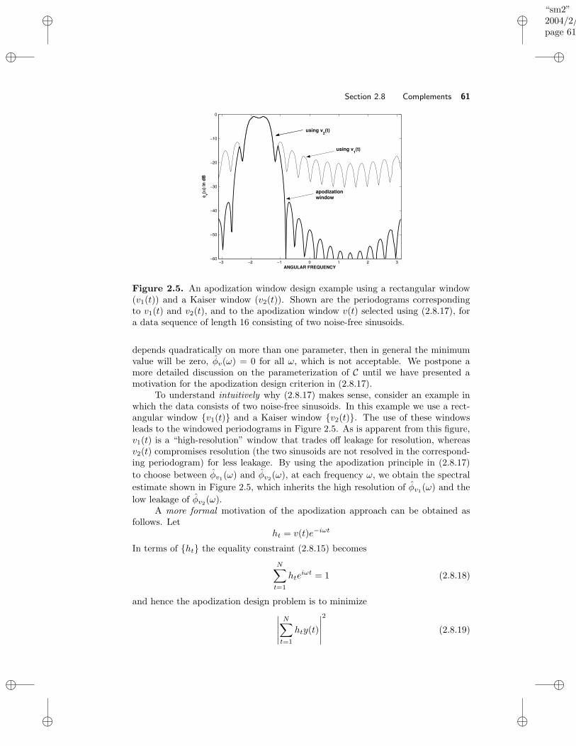
“sm2”2004/2/22page 61

i

i

i

i

i

i

i

i


−3 −2 −1 0 1 2 3−60

−50

−40

−30

−20

−10

0

ANGULAR FREQUENCY

φ v(ω) i

n dB

using v2(t)

using v1(t)

apodizationwindow

Figure 2.5. An apodization window design example using a rectangular window(v1(t)) and a Kaiser window (v2(t)). Shown are the periodograms correspondingto v1(t) and v2(t), and to the apodization window v(t) selected using (2.8.17), fora data sequence of length 16 consisting of two noise-free sinusoids.

depends quadratically on more than one parameter, then in general the minimumvalue will be zero, φv(ω) = 0 for all ω, which is not acceptable. We postpone amore detailed discussion on the parameterization of C until we have presented amotivation for the apodization design criterion in (2.8.17).

To understand intuitively why (2.8.17) makes sense, consider an example inwhich the data consists of two noise-free sinusoids. In this example we use a rect-angular window v1(t) and a Kaiser window v2(t). The use of these windowsleads to the windowed periodograms in Figure 2.5. As is apparent from this figure,v1(t) is a “high-resolution” window that trades off leakage for resolution, whereasv2(t) compromises resolution (the two sinusoids are not resolved in the correspond-ing periodogram) for less leakage. By using the apodization principle in (2.8.17)

to choose between φv1(ω) and φv2(ω), at each frequency ω, we obtain the spectral

estimate shown in Figure 2.5, which inherits the high resolution of φv1(ω) and the

low leakage of φv2(ω).A more formal motivation of the apodization approach can be obtained as

follows. Letht = v(t)e−iωt

In terms of ht the equality constraint (2.8.15) becomes

N∑

t=1

hteiωt = 1 (2.8.18)

and hence the apodization design problem is to minimize

∣∣∣∣∣

N∑

t=1

hty(t)

∣∣∣∣∣

2

(2.8.19)

“sm2”2004/2/22page 62

i

i

i

i

i

i

i

i


subject to (2.8.18) as well as (2.8.14) and any other conditions resulting from theparameterization used for v(t) (and therefore for ht). We can interpret htas an FIR filter of length N , and consequently (2.8.19) is the “power” of the filteroutput and (2.8.18) is the (complex) gain of the filter at frequency ω. Therefore,making use of ht, we can describe the apodization principle in words as follows:find the (parameterized) FIR filter ht which passes without distortion the sinu-soid with frequency ω (see (2.8.18)) and minimizes the output power (see (2.8.19)),and thus attenuates any other frequency components in the data as much as pos-sible. The (normalized) power at the output of the filter is taken as an estimateof the power in the data at frequency ω. This interpretation can clearly serve as amotivation of the apodization approach and it sheds more light on the apodizationprinciple. In effect, minimizing (2.8.19) subject to (2.8.18) (along with the otherconstraints on ht resulting from the parameterization used for v(t)) is a specialcase of a sound approach to spectral analysis that will be described in Section 5.4.1(a fact apparently noted for the first time in [Lee and Munson Jr. 1995]).

As already stated above, an important aspect that remains to be discussedis the parameterization of v(t). For the apodization principle to make sense, theclass C of windows must be chosen carefully. In particular, as explained above,we should not use more than two parameters to describe v(t) (to prevent the

meaningless “spectral estimate” φv(ω) ≡ 0). The choice of the class C is alsoimportant from a computational standpoint. Indeed, the task of solving (2.8.17),

for each ω, and then computing the corresponding φv(ω) may be computationallydemanding unless C is carefully chosen.

In the following we will consider the class of temporal windows used in [Stank-

witz, Dallaire, and Fienup 1994]:

v(t) =1

N

[

α− β cos

(2π

Nt

)]

, t = 1, . . . , N (2.8.20)

It can be readily checked that (2.8.20) satisfies the constraints (2.8.14) and (2.8.15)if and only if

α = 1 and |β| ≤ 1 (2.8.21)

In addition we require that

β ≥ 0 (2.8.22)

to ensure that the peak of v(t) occurs in the middle of the interval [1, N ]; thiscondition guarantees that the window in (2.8.20) (with β > 0) has lower sidelobesthan the rectangular window corresponding to β = 0 (the window (2.8.20) withβ < 0 generally has higher sidelobes than the rectangular window, and hence β < 0cannot be a solution to the apodization design problem).

Remark: The temporal window (2.8.20) is of the same type as the lag Hanning andHamming windows in Table 2.1. For the latter windows the interval of interest is[−N,N ] and hence for the peak of these windows to occur in the middle of theinterval of interest, we need β ≤ 0 (cf. Table 2.1). This observation explains thedifference between (2.8.20) and the lag windows in Table 2.1.

“sm2”2004/2/22page 63

i

i

i

i

i

i

i

i


Combining (2.8.20), (2.8.21), and (2.8.22) leads to the following (constrained)parameterization of the temporal windows:

v(t) =1

N

[

1 − β cos

(2π

Nt

)]

=1

N

[

1 − β

2

(

ei2πN t + e−i 2π

N t)]

, β ∈ [0, 1] (2.8.23)

Assume, for simplicity, that N is a power of two (for the general case we refer to[DeGraaf 1994]) and that a radix-2 FFT algorithm is used to compute

Y (k) =

N∑

t=1

y(t)e−i 2πkN t, k = 1, . . . , N (2.8.24)

(see Section 2.3). Then the windowed periodogram corresponding to (2.8.23) canbe conveniently computed as follows:

φv(k) =1

N

∣∣∣∣Y (k) − β

2

[Y (k − 1) + Y (k + 1)

]∣∣∣∣

2

, k = 2, . . . , N − 1 (2.8.25)

Furthermore, in (2.8.25) β is the solution to the following apodization design prob-lem:

minβ∈[0,1]

∣∣∣∣Y (k) − β

2

[Y (k − 1) + Y (k + 1)

]∣∣∣∣

2

(2.8.26)

The unconstrained minimizer of the above function is given by:

β0 = Re

[2Y (k)

Y (k − 1) + Y (k + 1)

]

(2.8.27)

Because the function in (2.8.26) is quadratic in β, it follows that the constrainedminimizer of (2.8.26) is given by

β =

0, if β0 < 0

β0, if 0 ≤ β0 ≤ 1

1, if β0 > 1

(2.8.28)

Remark: It is interesting to note from (2.8.28) that a change of the value of α inthe window expression (2.8.20) will affect the apodization (optimal) window in amore complicated way than just a simple scaling. Indeed, if we change the value ofα, for instance to α = 0.75, then the interval for β becomes β ∈ [0, 0.75] and thismodification will affect the apodization window nonlinearly via (2.8.28).

The apodizaton-based windowed periodogram is simply obtained by using βgiven by (2.8.28) in (2.8.25). Hence, despite the fact that the apodization window isboth frequency and data dependent (via β in (2.8.27), (2.8.28)) the implementation

“sm2”2004/2/22page 64

i

i

i

i

i

i

i

i


of the corresponding spectral estimate is only marginally more computationally de-manding than the implementation of an unwindowed periodogram. Compared withthe latter, however, the apodization-based windowed periodogram has a consider-ably reduced leakage problem and essentially the same resolution (see [Stankwitz,

Dallaire, and Fienup 1994; DeGraaf 1994] for numerical examples illustrat-ing this fact).

2.8.4 Estimation of Cross–Spectra and Coherency Spectra

As can be seen from Complement 1.6.1, the estimation of the cross–spectrum φyu(ω)of two stationary signals, y(t) and u(t), is a useful operation when studying possiblelinear (dynamic) relations between y(t) and u(t). Let z(t) denote the bivariate signal

z(t) = [y(t) u(t)]T

and let

φ(ω) =1

NZ(ω)Z∗(ω) (2.8.29)

denote the unwindowed periodogram estimate of the spectral density matrix of z(t).In equation (2.8.29),

Z(ω) =

N∑

t=1

z(t)e−iωt

is the DTFT of z(t)Nt=1. Partition φ(ω) as

φ(ω) =

[φyy(ω) φyu(ω)

φ∗yu(ω) φuu(ω)

]

(2.8.30)

As indicated by the notation previously used, estimates of φyy(ω), φuu(ω) and ofthe cross–spectrum φyu(ω) may be obtained from the corresponding elements of

φ(ω).We first show that the estimate of the coherency spectrum obtained from

(2.8.30) is always such that

|Cyu(ω)| = 1 for all ω (2.8.31)

and hence it is useless. To see this, note that since the rank of the 2 × 2 matrix in(2.8.30) is equal to one (see Result R22 in Appendix A), we must have

φuu(ω)φyy(ω) = |φyu(ω)|2

which readily leads to the conclusion that the coherency spectrum estimate obtainedfrom the elements of φ(ω) is bound to satisfy (2.8.31), and hence is meaningless.This result is yet another indication that the unwindowed periodogram is a poorestimate of the PSD.

Consider next a windowed Blackman–Tukey periodogram estimate of thecross–spectrum:

φyu(ω) =

M∑

k=−Mw(k)ryu(k)e

−iωk (2.8.32)

“sm2”2004/2/22page 65

i

i

i

i

i

i

i

i


where w(k) is the lag window, and ryu(k) is some usual estimate of ryu(k). Unlikeryy(k) or ruu(k), ryu(k) does not necessarily peak at k = 0 and, moreover, is notan even function in general. The choice of the lag window for estimating cross–spectra may hence be governed by different rules from those commonly used in theautospectrum estimation.

The main task of a lag window is to retain the “essential part” of the covari-ance sequence in the defining equation for the spectral density. In this way the biasis kept small and the variance is also reduced as the noisy tails of the sample co-variance sequence are weighted out. For simplicity of discussion, assume that mostof the area under the plot of ryu(k) is concentrated about k = k0, with |k0| N .As ryu(k) is a reasonably accurate estimate of ryu(k), provided |k| N , we canassume that ryu(k) and ryu(k) have similar shapes. In such a case, one canredefine (2.8.32) as

φyu(ω) =

M∑

k=−Mw(k − k0)ryu(k)e

−iωk

where the lag window w(s) is of the type recommended for autospectrum estimation.The choice of an appropriate value for k0 in the above cross–spectral estimator isessential, for if k0 is poorly selected the following situations can occur:

• If M is chosen small to reduce the variance, the bias may be significant as“essential” lags of the cross–covariance sequence may be left out.

• If M is chosen large to reduce the bias, the variance may significantly beinflated as poorly estimated high–order “nonessential” lags are included intothe spectral estimation formula.

Finally, let us look at the cross–spectrum estimators derived from (2.8.30) and(2.8.32), respectively, with a view of establishing a relation between them. PartitionZ(ω) as

Z(ω) =

[Y (ω)U(ω)

]

and observe that

1

2πN

∫ π

−πY (ω)U∗(ω)eiωk dω

=1

2πN

∫ π

−π

N∑

t=1

N∑

s=1

y(t)u∗(s)e−iω(t−s) eiωk dω

=1

N

N∑

t=1

N∑

s=1

y(t)u∗(s)δk,t−s

=1

N

∑

t∈[1,N ]∩[1+k,N+k]

y(t)u∗(t− k) , ryu(k) (2.8.33)

“sm2”2004/2/22page 66

i

i

i

i

i

i

i

i


where ryu(k) can be rewritten in the following more familiar form:

ryu(k) =

1

N

N∑

t=k+1

y(t)u∗(t− k), k = 0, 1, 2, . . .

1

N

N+k∑

t=1

y(t)u∗(t− k), k = 0,−1,−2, . . .

Let

φpyu(ω) =1

NY (ω)U∗(ω)

denote the unwindowed cross–spectral periodogram–like estimator, given by the off–diagonal element of φ(ω) in (2.8.30). With this notation, (2.8.33) can be writtenmore compactly as

ryu(k) =1

2π

∫ π

−πφpyu(µ)eiµk dµ

By using the above equation in (2.8.32), we obtain:

φyu(ω) =1

2π

∫ π

−πφpyu(µ)

M∑

k=−Mw(k)e−i(ω−µ)k dµ

=1

2π

∫ π

−πW (ω − µ)φpyu(µ) dµ (2.8.34)

where W (ω) =∑∞k=−∞ w(k)e−iωk is the spectral window. The previous equation

should be compared with the similar equation, (2.5.3), that holds in the case ofautospectra.

For implementation purposes, one can use the following discrete approxima-tion of (2.8.34):

φyu(ω) =1

N

N∑

k=−NW (ω − ωk)φ

pyu(ωk)

where ωk = 2πN k are the Fourier frequencies. The periodogram (cross–spectral)

estimate that appears in the above equation can be efficiently computed by meansof an FFT algorithm.

2.8.5 More Time–Bandwidth Product Results

The time (or duration)–bandwidth product result (2.6.5) relies on the assumptionsthat both w(t) and W (ω) have a dominant peak at the origin, that they both arereal–valued, and that they take on nonnegative values only. While most window–like signals (nearly) satisfy these assumptions, many other signals do not satisfythem. In this complement we obtain time–bandwidth product results that applyto a much broader class of signals.

“sm2”2004/2/22page 67

i

i

i

i

i

i

i

i


We begin by showing how the result (2.6.5) can be extended to a more generalclass of signals. Let x(t) denote a general discrete–time sequence and let X(ω)denote its DTFT. Both x(t) and X(ω) are allowed to take negative or complexvalues, and neither is required to peak at the origin. Let t0 and ω0 denote themaximum points of |x(t)| and |X(ω)|, respectively. The time width (or duration)and bandwidth definitions in (2.6.1) and (2.6.2) are modified as follows:

Ne =

∑∞t=−∞ |x(t)||x(t0)|

and

βe =12π

∫ π

−π |X(ω)|dω|X(ω0)|

Because x(t) and X(ω) form a Fourier transform pair, we obtain

|X(ω0)| =

∣∣∣∣∣

∞∑

t=−∞x(t)e−iω0t

∣∣∣∣∣≤

∞∑

t=−∞|x(t)|

and

|x(t0)| =

∣∣∣∣

1

2π

∫ π

−πX(ω)eiωt0dω

∣∣∣∣≤ 1

2π

∫ π

−π|X(ω)|dω

which implies that

Neβe ≥ 1 (2.8.35)

The above result, similar to (2.6.5), can be used to conclude that:

A sequence x(t) cannot be narrow in both time and frequency. (2.8.36)

More precisely, if x(t) is narrow in one domain it must be wide in the other domain.However, the inequality result (2.8.35), unlike (2.6.5), does not necessarily implythat βe decreases whenever Ne increases (or vice versa). Furthermore, the result(2.8.35) — again unlike (2.6.5) — does not exclude the possibility that the signalis broad in both domains. In fact, in the general class of signals to which (2.8.35)applies there are signals which are broad in both the time and frequency domains(for such signals Neβe 1); see, e.g., [Papoulis 1977]. Evidently, the significantconsequence of (2.8.35) is (2.8.36), which is precisely what makes the duration–bandwidth result an important one.

The duration–bandwidth product type of result (such as (2.6.5) or (2.8.35),and (2.8.40) below) has been sometimes referred to by using the generic name ofuncertainty principle, in an attempt to relate it to the Heisenberg Uncertainty Prin-ciple in quantum mechanics. (Briefly stated, the Heisenberg Uncertainty Principleasserts that the position and velocity of a particle cannot be simultaneously speci-fied to arbitrary precision.) To support the relationship, one can argue as follows:

“sm2”2004/2/22page 68

i

i

i

i

i

i

i

i


Suppose that we are given a sequence with (equivalent) duration equal to Ne andthat we are asked to use a linear filtering device to determine the sequence’s spec-tral content in a certain narrow band. Because the filter impulse response cannotbe longer than Ne (in fact, it should be (much) shorter!), it follows from the time–bandwidth product result that the filter’s bandwidth can be on the order of 1/Nebut not smaller. Hence, the sequence’s spectral content in fine bands on an ordersmaller than 1/Ne cannot be exactly determined and therefore is “uncertain”. Thisis in effect the type of limitation that applies to the nonparametric spectral meth-ods discussed in this chapter. However, this way of arguing is related to a specificapproach to spectral estimation and not to a fundamental limitation associated withthe signal itself. (As we will see in later chapters of this text, there are parametricmethods of spectral analysis that can provide the “high resolution” necessary todetermine the spectral content in bands that are on an order less than 1/Ne).

Next, we present another, slightly more general form of time–bandwidth prod-uct result. The definitions of duration and bandwidth used to obtain (2.8.35) makefull sense whenever |x(t)| and |X(ω)| are single pulse–like waveforms, though thesedefinitions may give reasonable results in many other instances as well. Thereare several other possible definitions of the broadness of a waveform in either thetime or frequency domain. The definition used below and the corresponding time–bandwidth product result appear to be among the most general.

Let

x(t) =x(t)

√∑∞t=−∞ |x(t)|2

(2.8.37)

and

X(ω) =X(ω)

√12π

∫ π

−π |X(ω)|2dω(2.8.38)

By Parseval’s theorem (see (1.2.6)) the denominators in (2.8.37) and (2.8.38) areequal to each other. Therefore, X(ω) is the DTFT of x(t) as is already indicatedby notation. Observe that

∞∑

t=−∞|x(t)|2 =

1

2π

∫ π

−π|X(ω)|2dω = 1

Hence, both |x(t)|2 and |X(ω)|2/2π can be interpreted as probability densityfunctions in the sense that they are nonnegative and that they sum or integrateto one. The means and variances associated with these two “probability” densitiesare given by the following equations.

Time Domain:

µ =

∞∑

t=−∞t|x(t)|2

σ2 =

∞∑

t=−∞(t− µ)2|x(t)|2

“sm2”2004/2/22page 69

i

i

i

i

i

i

i

i


Frequency Domain:

ν =1

(2π)2

∫ π

−πω|X(ω)|2dω

ρ2 =1

(2π)3

∫ π

−π(ω − 2πν)2|X(ω)|2dω

The values of the “standard deviations” σ and ρ show whether the normalizedfunctions |x(t)| and |X(ω)|, respectively, are narrow or broad. Hence, we canuse σ and ρ as definitions for the duration and bandwidth, respectively, of theoriginal functions x(t) and X(ω).

In what follows, we assume that:

µ = 0, ν = 0 (2.8.39)

For continuous–time signals, the zero–mean assumptions can always be made tohold by appropriately translating the origin on the time and frequency axes (see,e.g., [Cohen 1995]). However, doing the same in the case of the discrete–timesequences considered here does not appear to be possible. Indeed, µ may not beinteger–valued, and the support of X(ω) is finite and hence is affected by transla-tion. Consequently, in the present case the zero–mean assumption introduces somerestriction; nevertheless we impose it to simplify the analysis.

According to the discussion above and assumption (2.8.39), we define the(equivalent) time width and bandwidth of x(t) as follows:

Ne =

[ ∞∑

t=−∞t2|x(t)|2

]1/2

βe =1

2π

[1

2π

∫ π

−πω2|X(ω)|2dω

]1/2

In the remainder of this complement, we prove the following time–bandwidth prod-uct result:

Neβe ≥ 1

4π(2.8.40)

which holds true under (2.8.39) and the weak additional assumption that

|X(π)| = 0 (2.8.41)

To prove (2.8.40), first we note that

X ′(ω) ,dX(ω)

dω= −i

∞∑

t=−∞tx(t)e−iωt

“sm2”2004/2/22page 70

i

i

i

i

i

i

i

i


Hence, iX ′(ω) is the DTFT of tx(t), which implies (by Parseval’s theorem) that

∞∑

t=−∞t2|x(t)|2 =

1

2π

∫ π

−π|X ′(ω)|2dω (2.8.42)

Consequently, by the Cauchy–Schwartz inequality for functions (see Result R23 inAppendix A),

Neβe =

[1

2π

∫ π

−π|X ′(ω)|2dω

]1/2 [1

(2π)3

∫ π

−πω2|X(ω)|2dω

]1/2

≥ 1

(2π)2

∣∣∣∣

∫ π

−πωX∗(ω)X ′(ω)dω

∣∣∣∣

=1

2(2π)2

∣∣∣∣

∫ π

−πωX∗(ω)X ′(ω)dω

∣∣∣∣

+

∣∣∣∣

∫ π

−πωX(ω)X∗′(ω)dω

∣∣∣∣

(2.8.43)

(the first equality above follows from (2.8.42) and the last one from a simple calcu-lation). Hence

Neβe ≥ 1

2(2π)2

∣∣∣∣

∫ π

−πω[

X∗(ω)X ′(ω) + X(ω)X∗′(ω)]

dω

∣∣∣∣

=1

2(2π)2

∣∣∣∣

∫ π

−πω[

|X(ω)|2]′dω

∣∣∣∣

which, after integrating by parts and using (2.8.41), yields

Neβe ≥ 1

2(2π)2

∣∣∣∣∣ω|X(ω)|2

∣∣∣∣

π

−π−∫ π

−π|X(ω)|2dω

∣∣∣∣∣=

1

2(2π)

and the proof is concluded.

Remark: There is an alternative way to complete the proof above, starting from theinequality in (2.8.43). In fact, as we will see, this alternative proof yields a tighterinequality than (2.8.40). Let ϕ(ω) denote the phase of X(ω):

X(ω) = |X(ω)|eiϕ(ω)

Then,

ωX∗(ω)X ′(ω) = ω|X(ω)|[

|X(ω)|]′

+ iωϕ′(ω)|X(ω)|2

=1

2

[

ω|X(ω)|2]′

− 1

2|X(ω)|2 + iωϕ′(ω)|X(ω)|2 (2.8.44)

Inserting (2.8.44) into (2.8.43) yields

Neβe ≥ 1

(2π)2

∣∣∣∣∣

ω

2|X(ω)|2

∣∣∣∣

π

−π− π + i2πγ

∣∣∣∣∣

(2.8.45)

“sm2”2004/2/22page 71

i

i

i

i

i

i

i

i


where

γ =1

2π

∫ π

−πωϕ′(ω)|X(ω)|2dω

can be interpreted as the “covariance” of ω and ϕ′(ω) under the “probability densityfunction” given by |X(ω)|2/(2π). From (2.8.45) we obtain at once

Neβe ≥ 1

4π

√

1 + 4γ2 (2.8.46)

which is a slightly stronger result than (2.8.40).

The results (2.8.40) and (2.8.46) are similar to (2.8.35), and hence the type ofcomments previously made about (2.8.35) applies to (2.8.40) and (2.8.46) as well.

For a more general time-bandwidth product result than the one above, see[Doroslovacki 1998]; the papers [Calvez and Vilbe 1992] and [Ishii and

Furukawa 1986] contain similar results to the one presented in this complement.

2.9 EXERCISES

Exercise 2.1: Covariance Estimation for Signals with Unknown MeansThe sample covariance estimators (2.2.3) and (2.2.4) are based on the assump-

tion that the signal mean is equal to zero. A simple calculation shows that, underthe zero–mean assumption,

E r(k) = r(k) (2.9.1)

and

E r(k) =N − |k|N

r(k) (2.9.2)

where r(k) denotes the sample covariance estimate in (2.2.3). Equations (2.9.1)and (2.9.2) show that r(k) is an unbiased estimate of r(k), whereas r(k) is a biasedone (note, however, that the bias in r(k) is small for N |k|). For this reason,r(k) and r(k) are often called the unbiased and, respectively, biased samplecovariances.

Whenever the signal mean is unknown, a most natural modification of thecovariance estimators (2.2.3) and (2.2.4) is as follows:

r(k) =1

N − k

N∑

t=k+1

[y(t) − y] [y(t− k) − y]∗ (2.9.3)

and

r(k) =1

N

N∑

t=k+1

[y(t) − y] [y(t− k) − y]∗ (2.9.4)

“sm2”2004/2/22page 72

i

i

i

i

i

i

i

i


where y is the sample mean

y =1

N

N∑

t=1

y(t) (2.9.5)

Show that in the unknown mean case, the usual names of unbiased and biasedsample covariances associated with (2.9.3) and (2.9.4), respectively, may no longerbe appropriate. Indeed, in such a case both estimators may be biased; furthermore,r(k) may be less biased than r(k). To simplify the calculations, assume that y(t) iswhite noise.

Exercise 2.2: Covariance Estimation for Signals with Unknown Means(cont’d)

Show that the sample covariance sequence r(k) in equation (2.9.4) of Exer-cise 2.1 satisfies the following equality:

N−1∑

k=−(N−1)

r(k) = 0 (2.9.6)

The above equality may seem somewhat surprising. (Why should the r(k) satisfysuch a constraint, which the true covariances do not necessarily satisfy? Note, forinstance, that the latter covariance sequence may well comprise only positive ele-ments.) However, the equality in (2.9.6) has a natural explanation when viewed inthe context of periodogram–based spectral estimation. Derive and explain formula(2.9.6) in the aforementioned context.

Exercise 2.3: Unbiased ACS Estimates may lead to Negative SpectralEstimates

We stated in Section 2.2.2 that if unbiased ACS estimates, given by equation(2.2.3), are used in the correlogram spectral estimate (2.2.2), then negative spectralestimates may result. Find an example data sequence y(t)Nt=1 that gives such anegative spectral estimate.

Exercise 2.4: Variance of Estimated ACSLet y(t)Nt=1 be real Gaussian (for simplicity), with zero mean, ACS equal

to r(k), and ACS estimate (either biased or unbiased) equal to r(k) (given byequation (2.2.3) or (2.2.4); we treat both cases simultaneously). Assume, withoutloss of generality, that k ≥ 0.

(a) Make use of equation (2.4.24) to show that

varr(k) = α2(k)

N−k−1∑

m=−(N−k−1)

(N − k − |m|)[r2(m) + r(m+ k)r(m− k)

]

where

α(k) =

1

N − kfor unbiased ACS estimates

1

Nfor biased ACS estimates

“sm2”2004/2/22page 73

i

i

i

i

i

i

i

i


Hence, for large N , the standard deviation of the ACS estimate is O(1/√N)

under weak conditions on the true ACS r(k).

(b) For the special case that y(t) is white Gaussian noise, show thatcovr(k), r(l) = 0 for k 6= l, and find a simple expression for varr(k).

Exercise 2.5: Another Proof of the Equality φp(ω) = φc(ω)The proof of the result (2.2.6) in the text introduces an auxiliary random

sequence and treats the original data sequence as deterministic (nonrandom). Thatproof relies on several results previously derived. A more direct proof of (2.2.6) canbe found using only (2.2.1), (2.2.2), and (2.2.4). Find such a proof.

Exercise 2.6: A Compact Expression for the Sample ACSShow that the expressions for the sample ACS given in the text (equations

(2.2.3) or (2.2.4) for k ≥ 0 and (2.2.5) for k < 0) can be rewritten using a singleformula as follows:

r(k) = ρ

N∑

p=1

N∑

s=1

y(p)y∗(s)δs,p−k, k = 0,±1, . . . ,±(N − 1) (2.9.7)

where ρ = 1N for (2.2.4) and ρ = 1

N−|k| for (2.2.3).

Exercise 2.7: Yet Another Proof of the Equality φp(ω) = φc(ω)Use the compact expression for the sample ACS derived in Exercise 2.6 to

obtain a very simple proof of (2.2.6).

Exercise 2.8: Linear Transformation Interpretation of the DFTLet F be the N × N matrix whose (k, t)th element is given by W kt, where

W is as defined in (2.3.2). Then the DFT, (2.3.3), can be written as a lineartransformation of the data vector y , [y(1) . . . y(N)]T ,

Y , [Y (0) . . . Y (N − 1)]T = Fy (2.9.8)

Show that F is an orthogonal matrix that satisfies

1

NFF ∗ = I (2.9.9)

and, as a result, that the inverse transform is

y =1

NF ∗Y (2.9.10)

Deduce from the above that the DFT is nothing but a representation of the datavector y via an orthogonal basis in Cn (the basis vectors are the columns of F ∗).Also, deduce that if the sequence y(t) is periodic with a period equal to N , thenthe Fourier coefficient vector, Y , determines the whole sequence y(t)t=1,2,..., andthat in effect the inverse transform (2.9.10) can be extended to include all samplesy(1), . . . , y(N), y(N + 1), y(N + 2), . . .

“sm2”2004/2/22page 74

i

i

i

i

i

i

i

i


Exercise 2.9: For White Noise the Periodogram is an Unbiased PSDEstimator

Let y(t) be a zero–mean white noise with variance σ2 and let

Y (ωk) =1√N

N−1∑

t=0

y(t)e−iωkt ; ωk =2π

Nk (k = 0, . . . , N − 1)

denote its (normalized) DFT evaluated at the Fourier frequencies.

(a) Derive the covariances

E Y (ωk)Y∗(ωr) , k, r = 0, . . . , N − 1

(b) Use the result of the previous calculation to conclude that the periodogram

φ(ωk) = |Y (ωk)|2 is an unbiased estimator of the PSD of y(t).

(c) Explain whether the unbiasedness property holds for ω 6= ωk as well. Presentan intuitive explanation for your finding.

Exercise 2.10: Shrinking the PeriodogramFirst, we introduce a simple general result on mean squared error (MSE)

reduction by shrinking. Let x be some estimate of a true (and unknown) parameterx. Assume that x is unbiased, i.e., E(x) = x, and let σ2

x denote the MSE of x

σ2x = E

(x− x)2

(Since x is unbiased, σ2x also equals the variance of x.) For a fixed (nonrandom) ρ,

letx = ρx

be another estimate of x. The “shrinkage coefficient” ρ can be chosen so as to makethe MSE of x (much) smaller than σ2

x. (Note that x, for ρ 6= 1, is a biased estimateof x; hence x trades off bias for variance.) More precisely, show that the MSE of x,σ2x, achieves its minimum value (with respect to ρ) of

σ2xo

= ρo σ2x

for

ρo =x2

x2 + σ2x

Next, consider the application of the previous result to the periodogram. As weexplained in the chapter, the periodogram–based spectral estimate is asymptoticallyunbiased and has an asymptotic MSE equal to the squared PSD value:

E

φp(ω)

→ φ(ω), E

(φp(ω) − φ(ω))2

→ φ2(ω) as N → ∞

Show that the “optimally shrunk” periodogram estimate is

φ(ω) = φp(ω)/2

“sm2”2004/2/22page 75

i

i

i

i

i

i

i

i


and that the MSE of φ(ω) is half the MSE of φp(ω).Finally, comment on the general applicability of this extremely simple tool for

MSE reduction.

Exercise 2.11: Asymptotic Maximum Likelihood Estimation of φ(ω)from φp(ω)

It follows from the calculations in Section 2.4 that, asymptotically in N , φp(ω)

has mean φ(ω) and variance φ2(ω). In this exercise we assume that φp(ω) is (asymp-totically) Gaussian distributed (which is not necessarily the case; however, thespectral estimator derived here under the Gaussian assumption may also be usedwhen this assumption does not hold). Hence, the asymptotic probability density

function of φp(ω) is (we omit the index p as well as the dependence on ω to simplifythe notation):

pφ(φ) =1

√

2πφ2exp

[

− (φ− φ)2

2φ2

]

Show that the maximum likelihood estimate (MLE) of φ based on φ, which by

definition is equal to the maximizer of pφ(φ) (see Appendices B and C for a shortintroduction of maximum likelihood estimation) is given by

φ =

√5 − 1

2φ

Compare φ with the “optimally shrunk” estimate of φ derived in Exercise 2.10.

Exercise 2.12: Plotting the Spectral Estimates in dBIt has been shown in this chapter that the spectral estimate φ(ω), obtained

via an improved periodogram method, is asymptotically unbiased with a varianceof the form µ2φ2(ω), where µ is a constant that can be made (much) smaller thanone by appropriately choosing the window. This fact implies that the confidenceinterval φ(ω) ± µφ(ω), constructed around the estimated PSD, should include thetrue (and unknown) PSD with a large probability. Now, obtaining a confidenceinterval as above has a twofold drawback: first, φ(ω) is unknown; secondly, theinterval may have significantly different widths for different frequency values.

Show that plotting φ(ω) in decibels eliminates the previous drawbacks. More

precisely, show that when φ(ω) is expressed in dB, its asymptotic variance is c2µ2

(with c = 10 log10 e), and hence that the confidence interval for a log–scale plot hasthe same width (independent of φ(ω)) for all ω.

Exercise 2.13: Finite–Sample Variance/Covariance Analysis of the Peri-odogram

This exercise has two aims. First, it shows that in the Gaussian case thevariance/covariance analysis of the periodogram can be done in an extremely simplemanner (even without the assumption that the data comes from a linear process, asin (2.4.26)). Secondly, the exercise asks for a finite–sample analysis which, for somepurposes, may be more useful than the asymptotic analysis presented in the text.Indeed, the asymptotic analysis result (2.4.21) may be misleading if not interpreted

“sm2”2004/2/22page 76

i

i

i

i

i

i

i

i


with care. For instance, (2.4.21) says that asymptotically (for N → ∞) φ(ω1)

and φ(ω2) are uncorrelated with one another, no matter how close ω1 and ω2 are.This cannot be true in finite samples, and hence the following question naturallyarises: For a given N , how close can ω1 be to ω2 such that φ(ω1) and φ(ω2) are(nearly) uncorrelated with each other? The finite–sample analysis of this exercisecan provide an answer to such questions, whereas the asymptotic analysis cannot.Let

a(ω) = [eiω . . . eiNω]T

y = [y(1) . . . y(N)]T

Then the periodogram, (2.2.1), can be written as (we omit the subindex p of φp(ω)in this exercise):

φ(ω) = |a∗(ω)y|2/N (2.9.11)

Assume that y(t) is a zero mean, stationary circular Gaussian process. The“circular Gaussianity” assumption (see, e.g., Appendix B) allows us to write thefourth–order moments of y(t) as (see equation (2.4.24)):

E y(t)y∗(s)y(u)y∗(v) = E y(t)y∗(s)E y(u)y∗(v)+E y(t)y∗(v)E y(u)y∗(s) (2.9.12)

Make use of (2.9.11) and (2.9.12) to show that

covφ(µ), φ(ν) , E[

φ(µ) − Eφ(µ)] [

φ(ν) − Eφ(ν)]

= |a∗(µ)Ra(ν)|2/N2(2.9.13)

where R = E yy∗. Deduce from (2.9.13) that

varφ(µ) = |a∗(µ)Ra(µ)|2/N2 (2.9.14)

Use (2.9.14) to readily rederive the variance part of the asymptotic result (2.4.21).

Next, use (2.9.14) to show that the covariance between φ(µ) and φ(ν) is not signif-icant if

|µ− ν| > 4π/N

and also that it may be significant otherwise. Hint: To show the inequality above,make use of the Caratheodory parameterization of a covariance matrix in Sec-tion 4.9.2.

Exercise 2.14: Data–Weighted ACS Estimate Interpretation of Bartlettand Welch Methods

Consider the Bartlett estimator, and assume LM = N .

(a) Show that the Bartlett spectral estimate can be written as:

φB(ω) =

M−1∑

k=−(M−1)

r(k)e−iωk

“sm2”2004/2/22page 77

i

i

i

i

i

i

i

i


where

r(k) =

N∑

t=k+1

α(k, t)y(t)y∗(t− k), 0 ≤ k < M

for some α(k, t) to be derived. Note that this is nearly of the form of theBlackman–Tukey spectral estimator, with the exception that the “standard”biased ACS estimate that is used in the Blackman–Tukey estimator is replacedby the “generalized” ACS estimate r(k).

(b) Make use of the derived expression for α(k, t) to conclude that the Bartlettestimator is inferior to the Blackman–Tukey estimator (especially for smallN) because it fails to use all available lag products in forming ACS estimates.

(c) Find α(k, t) for the Welch method. What overlap values (K in equation(2.7.7)) give lag product usage similar to the Blackman–Tukey method?

Exercise 2.15: Approximate Formula for Bandwidth CalculationLet W (ω) denote a general spectral window that has a peak at ω = 0 and is

symmetric about that point. In addition, assume that the peak of W (ω) is narrow(as usually it should be). Under these assumptions, make use of a Taylor seriesexpansion to show that an approximate formula for calculating the bandwidth B ofthe peak of W (ω) is the following:

B ' 2√

|W (0)/W ′′(0)| (2.9.15)

The spectral peak bandwidth B is mathematically defined as follows. Let ω1 andω2 denote the “half–power points,” defined through

W (ω1) = W (ω2) = W (0)/2, ω1 < ω2

(hence the ratio 10 log10 (W (0)/W (ωj)) ' 3dB for j = 1, 2; we use 10 log10 ratherthan 20 log10 because the spectral window is applied to a power quantity, φ(ω)).Then since W (ω) is symmetric, so ω2 = −ω1,

B , ω2 − ω1 = 2ω2

As an application of (2.9.15), show that

B ' 0.78 · 2π/N (in radians per sampling interval)

or, equivalently, that

B ' 0.78/N (in cycles per sampling interval)

for the Bartlett window (2.4.15).Note that this formula remains approximate even as N → ∞. Even though

the half power bandwidth of the window gets smaller as N increases (so that onewould expect the Taylor series expansion to be more accurate), the curvature ofthe window at ω = 0 increases without bound as N increases. For the Bartlett

“sm2”2004/2/22page 78

i

i

i

i

i

i

i

i


window, verify that B ' 0.9 · 2π/N for N large, which differs from the predictionin this exercise by about 16%.

Exercise 2.16: A Further Look at the Time–Bandwidth Product

We saw in Section 2.6.1 that the product between the equivalent time andfrequency widths of a regular window equals unity. Use the formula (2.9.15) derivedin Exercise 2.15 to show that the spectral peak bandwidth B of a window w(k) thatis nonzero only for |k| < N , satisfies

B ·N ≥ 1/π, (in cycles per sampling interval) (2.9.16)

This once again illustrates the “time–bandwidth product” type of result. Notethat (2.9.16) involves the effective window time length and spectral peak width, asopposed to (2.6.5) which is concerned with equivalent time and frequency widths.

Exercise 2.17: Bias Considerations in Blackman–Tukey Window Design

The discussion in this chapter treated the bias of a spectral estimator and itsresolution as two interrelated properties. This exercise illustrates further the strongrelationship between bias and resolution.

Consider φBT (ω) as in (2.5.1), and without loss of generality assume thatEr(k) = r(k). (Generality is not lost because, if Er(k) = α(k)r(k), thenreplacing w(k) by α(k)w(k) and r(k) by r(k)/α(k) results in an equivalent estimatorwith unbiased ACS estimates.) Find the weights w(k)M−1

k=−M+1 that minimize thesquared bias, as given by the error measure:

ε =1

2π

∫ π

−π

[

φ(ω) − EφBT (ω)]2

dω (2.9.17)

In particular, show that the weight function that minimizes ε is the rectangularwindow. Recall that the rectangular window also has the narrowest main lobe, andhence the best resolution.

Exercise 2.18: A Property of the Bartlett Window

Let the window length, M , be given. Then, in the general case, the rectan-gular window can be expected to yield the windowed spectral estimate with themost favorable bias properties, owing to the fact that the sample covariance lagsr(k)M−1

k=−(M−1), appearing in (2.5.1), are left unchanged by this window (also see

Exercise 2.17). The rectangular window, however, has the drawback that it is notpositive definite and hence may produce negative spectral estimates. The Bartlettwindow, on the other hand, is positive definite and therefore yields a spectral esti-mate that is positive for all frequencies. Show that the latter window is the positivedefinite window which is closest to the rectangular one, in the sense of minimizing

“sm2”2004/2/22page 79

i

i

i

i

i

i

i

i


the following criterion:

minw(k)

M−1∑

k=0

|1 − w(k)| subject to:

1) w(k) ≡ 0 for |k| ≥ M2) w(k)∞

k=−∞ is a positive definite sequence3) w(0) = 1

(2.9.18)Conclude that the Bartlett window is the positive definite window that distortsthe sample covariances r(k)M−1

k=−(M−1) least in the windowed spectral estimate

formula. Hint: Any positive definite real window w(k)M−1k=−(M−1) can be written

as

w(k) =

M−1∑

i=0

bi bi+k (bi = 0 for i ≥ M) (2.9.19)

for some real–valued parameters biM−1i=0 . Make use of the above parameterization

of the set of positive definite windows to transform (2.9.18) into an optimizationproblem without constraints.

COMPUTER EXERCISES

Tools for Periodogram Spectral Estimation:The text web site www.prenhall.com/stoica contains the following Matlab

functions for use in computing periodogram-based spectral estimates. In each case,y is the input data vector, L controls the frequency sample spacing of the output, andthe output vector phi= φ(ωk) where ωk = 2πk

L . Matlab functions that generatethe Correlogram, Blackman–Tukey, Windowed Periodogram, Bartlett, Welch, andDaniell spectral estimates are as follows:

• phi = correlogramse(y,L)

Implements the correlogram spectral estimate in equation (2.2.2).

• phi = btse(y,w,L)

Implements the Blackman–Tukey spectral estimate in equation (2.5.1); w isthe vector [w(0), . . . , w(M − 1)]T .

• phi = periodogramse(y,v,L)

Implements the windowed periodogram spectral estimate in equation (2.6.24);v is a vector of window function elements [v(1), . . . , v(N)]T , and should bethe same size as y. If v is a vector of ones, this function implements theunwindowed periodogram spectral estimate in equation (2.2.1).

• phi = bartlettse(y,M,L)

Implements the Bartlett spectral estimate in equations (2.7.2) and (2.7.3); Mis the size of each subsequence as in equation (2.7.2).

• phi = welchse(y,v,K,L)

Implements the Welch spectral estimate in equation (2.7.8); M is the size of

“sm2”2004/2/22page 80

i

i

i

i

i

i

i

i


each subsequence, v is the window function [v(1), . . . , v(M)]T applied to eachsubsequence, and K is the overlap parameter, as in equation (2.7.7).

• phi = daniellse(y,J,Ntilde)

Implements the Daniell spectral estimate in equation (2.7.16); J and Ntilde

correspond to J and N there.

Exercise C2.19: Zero Padding Effects on Periodogram EstimatorsIn this exercise we study the effect zero padding has on the periodogram.Consider the sequence

y(t) = 10 sin(0.2 · 2πt+ φ1) + 5 sin((0.2 + 1/N)2πt+ φ2) + e(t), (2.9.20)

where t = 0, . . . , N − 1, and e(t) is white Gaussian noise with variance 1. LetN = 64 and φ1 = φ2 = 0.

From the results in Chapter 4, we find the spectrum of y(t) to be

φ(ω) = 50π [δ(ω − 0.2 · 2π) + δ(ω + 0.2 · 2π)]

+12.5π [δ(ω − (0.2 + 1/N) · 2π) + δ(ω + (0.2 + 1/N) · 2π)] + 1

Plot the periodogram for the sequence y(t), and the sequence y(t) zeropadded with N , 3N , 5N , and 7N zeroes.

Explain the difference between the five periodograms. Why does the firstperiodogram not give a good description of the spectral content of the signal? Notethat zero padding does not change the resolution of the estimator.

Exercise C2.20: Resolution and Leakage Properties of the PeriodogramWe have seen from Section 2.4 that the expected value of the periodogram is

the convolution of the true spectrum φy(ω) with the Fourier transform of a Bartlettwindow, denoted WB(ω) (see equation (2.4.15)). The shape and size of the WB(ω)function determines the amount of smearing and leakage in the periodogram. Sim-ilarly, in Section 2.5 we introduced a windowed periodogram in (2.6.24) whoseexpected value is equal to the expected value of a corresponding Blackman–Tukeyestimate with weights w(k) given by (2.6.31). Different window functions thanthe rectangular window could be used in the periodogram estimate, giving rise tocorrespondingly different windows in the correlogram estimate. The choice of win-dow affects the resolution and leakage properties of the periodogram (correlogram)spectral estimate.

Resolution Properties: The amount of smearing of the spectral estimate is de-termined by the width of the main lobe, and the amount of leakage is determinedby the energy in the sidelobes. The amount of smearing is what limits the resolvingpower of the periodogram, and is studied empirically below.

We first study the resolution properties by considering a sequence made up oftwo sinusoids in noise, where the two sinusoidal frequencies are “close”. Consider

y(t) = a1 sin(f0 · 2πt+ φ1) + a2 sin((f0 + α/N)2πt+ φ2) + e(t), (2.9.21)

where e(t) is real–valued Gaussian white noise with zero mean and variance σ2. Wechoose f0 = 0.2 and N = 256, but the results are nearly independent of f0 and N .

“sm2”2004/2/22page 81

i

i

i

i

i

i

i

i


(a) Determine empirically the 3 dB width of the main lobe of WB(ω) as a functionof N , and verify equation (2.4.18). Also determine the peak sidelobe height(in dB) as a function of N . Note that the sidelobe level of a window function isgenerally independent of N . Verify this by examining plots of the magnitudeof WB(ω) for several values of N ; try both linear and dB scales in your plots.

(b) Set σ2 = 0 (this eliminates the statistical variation in the periodogram, sothat the bias properties can be isolated and studied). Set a1 = a2 = 1 andφ1 = φ2 = 0. Plot the (zero–padded) periodogram of y(t) for various α anddetermine the resolution threshold (i.e., the minimum value of α for whichthe two frequency components can be resolved). How does this value of αcompare with the predicted resolution in Section 2.4?

(c) Repeat part (b) for a Hamming–windowed correlogram estimate.

(d) For reasonably high signal–to–noise ratio (SNR) values and reasonably closesignal amplitudes, the resolution thresholds in parts (b) and (c) above arenot very sensitive to variations in the signal amplitudes and frequency f0.However, these thresholds are sensitive to the phases φ1 and φ2, especially ifα is smaller than 1. Try two pairs (φ1, φ2) so that the two sinusoids are inphase and out of phase, respectively, at the center of the observation interval,and compare the resolution thresholds. Also, try different values of a1, a2,and σ2 to verify that their values have relatively little effect on the resolutionthreshold.

Spectral Leakage: In this part we analyze the effects of leakage on the peri-odogram estimate. Leakage properties can be clearly seen when trying to estimatetwo sinusoidal terms that are well separated but have greatly differing amplitudes.

(a) Generate the sinusoidal sequence above for α = 4, σ2 = 0, and φ1 = φ2 = 0.Set a1 = 1 and vary a2 (choose a2 = 1, 0.1, 0.01, and 0.001, for example).Compute the periodogram (using a rectangular data window), and commenton the ability to identify the second sinusoidal term from the spectral estimate.

(b) Repeat part (a) for α = 12. Does the amplitude threshold for identifiabilityof the second sinusoidal term change?

(c) Explain your results in parts (a) and (b) by looking at the amplitude of theBartlett window’s Fourier transform at frequencies corresponding to α/N forα = 4 and α = 12.

(d) The Bartlett window (and many other windows) has the property that theleakage level depends on the distance between spectral components in thedata, as seen in parts (a) and (b). For many practical applications it may beknown what dynamic range the sinusoidal components in the data may have,and it is thus desirable to use a data window with a constant sidelobe levelthat can be chosen by the user. The Chebyshev window (or Taylor window) isa good choice for these applications, because the user can select the (constant)sidelobe level in the window design (see the Matlab command chebwin).

Assume we know that the maximum dynamic range of sinusoidal componentsis 60 dB. Design a Chebyshev window v(t) and corresponding Blackman–Tukey window w(k) using (2.6.31) so that the two sinusoidal components of

“sm2”2004/2/22page 82

i

i

i

i

i

i

i

i


the data can be resolved for this dynamic range using (i) the Blackman–Tukeyspectral estimator with window w(k), and (ii) the windowed periodogrammethod with window v(t). Plot the Fourier transform of the window anddetermine the spectral resolution of the window.

Test your window design by computing the Blackman–Tukey and windowedperiodogram estimates for two sinusoids whose amplitudes differ by 50 dBin dynamic range, and whose frequency separation is the minimum value youpredicted. Compare the resolution results with your predictions. Explain whythe smaller amplitude sinusoid can be detected using one of the methods butnot the other.

Exercise C2.21: Bias and Variance Properties of the Periodogram Spec-tral Estimate

In this exercise we verify the theoretical predictions about bias and varianceproperties of the periodogram spectral estimate. We use autoregressive movingaverage (ARMA) signals (see Chapter 3) as test signals.

Bias Properties — Resolution and Leakage: We consider a random processy(t) generated by filtering white noise:

y(t) = H(z)e(t)

where e(t) is zero mean Gaussian white noise with variance σ2 = 1, and the filterH(z) is given by:

H(z) =

2∑

k=1

Ak

[1 − zkz

−1

1 − pkz−1+

1 − z∗kz

−1

1 − p∗kz

−1

]

(2.9.22)

withp1 = 0.99ei2π0.3 p2 = 0.99ei2π(0.3+α)

z1 = 0.95ei2π0.3 z2 = 0.95ei2π(0.3+α) (2.9.23)

We first let A1 = A2 = 1 and α = 0.05.

(a) Plot the true spectrum φ(ω). Using a sufficiently fine grid for ω so thatapproximation errors are small, plot the ACS using an inverse FFT of φ(ω).

(b) For N = 64, plot the Fourier transform of the Bartlett window, and also

plot the expected value of the periodogram estimate φp(ω) as given by equa-tion (2.4.8). We see that for this example and data length, the main lobewidth of the Bartlett window is wider than the distance between the spectralpeaks in φ(ω). Discuss how this relatively wide main lobe width affects theresolution properties of the estimator.

(c) Generate 50 realizations of y(t), each of length N = 64 data points. Youcan generate the data by passing white noise through the filter H(z) (see theMatlab commands dimpulse and filter); be sure to discard a sufficientnumber of initial filter output points to effectively remove the transient partof the filter output. Compute the periodogram spectral estimates for each data

“sm2”2004/2/22page 83

i

i

i

i

i

i

i

i


sequence; plot 10 spectral estimates overlaid on a single plot. Also plot theaverage of the 50 spectral estimates. Compare the average with the predictedexpected value as found in part (b).

(d) The resolution of the spectral peaks in φ(ω) will depend on their separationrelative to the width of the Bartlett window main lobe. Generate realizationsof y(t) for N = 256, and find the minimum value of α so that the spectralpeaks can be resolved in the averaged spectral estimate. Compare your resultswith the predicted formula (2.4.18) for spectral resolution.

(e) Leakage from the Bartlett window will impact the ability to identify peaksof different amplitudes. To illustrate this, generate realizations of y(t) forN = 64, for both α = 4/N and α = 12/N . For each value of α, set A1 = 1,and vary A2 to find the minimum amplitude for which the lower amplitudepeak can reliably be identified from the averaged spectral estimate. Comparethis value with the Bartlett window sidelobe level for ω = 2πα and for the twovalues of α. Does the window sidelobe level accurately reflect the amplitudeseparation required to identify the second peak?

Variance Properties: In this part we will verify that the variance of the pe-riodogram is almost independent of the data length, and compare the empiricalvariance with theoretical predictions. For this part, we consider a broadband signaly(t) for which the Bartlett window smearing and leakage effects are small.

Consider the broadband ARMA process

y(t) =B1(z)

A1(z)e(t)

with

A1(z) = 1 − 1.3817z−1 + 1.5632z−2 − 0.8843z−3 + 0.4096z−4

B1(z) = 1 + 0.3544z−1 + 0.3508z−2 + 0.1736z−3 + 0.2401z−4

(a) Plot the true spectrum φ(ω).

(b) Generate 50 Monte–Carlo data realizations using different noise sequences,and compute the corresponding 50 periodogram spectral estimates. Plot thesample mean, the sample mean plus one sample standard deviation and samplemean minus one sample standard deviation spectral estimate curves. Do thisfor N = 64, 256, and 1024. Note that the variance does not decrease with N .

(c) Compare the sample variance to the predicted variance in equation (2.4.21).

It may help to plot stdevφ(ω)/φ(ω) and determine to what degree this curveis approximately constant. Discuss your results.

Exercise C2.22: Refined Methods: Variance–Resolution TradeoffIn this exercise we apply the Blackman–Tukey and Welch estimators to both

a narrowband and broadband random process. We consider the same processes inChapters 3 and 5 to facilitate comparison with the spectral estimation methodsdeveloped in those chapters.

“sm2”2004/2/22page 84

i

i

i

i

i

i

i

i


Broadband ARMA Process: Generate realizations of the broadband autore-gressive moving–average (ARMA) process

y(t) =B1(z)

A1(z)e(t)

with

A1(z) = 1 − 1.3817z−1 + 1.5632z−2 − 0.8843z−3 + 0.4096z−4

B1(z) = 1 + 0.3544z−1 + 0.3508z−2 + 0.1736z−3 + 0.2401z−4

Choose the number of samples as N = 256.

(a) Generate 50 Monte–Carlo data realizations using different noise sequences,and compute the corresponding 50 spectral estimates using the followingmethods:

• The Blackman–Tukey spectral estimate using the Bartlett window wB(t).Try both M = N/4 and M = N/16.

• The Welch spectral estimate using the rectangular window wR(t), andusing both M = N/4 and M = N/16 and overlap parameter K = M/2.

Plot the sample mean, the sample mean plus one sample standard devia-tion and sample mean minus one sample standard deviation spectral estimatecurves. Compare with the periodogram results from Exercise C2.21, and witheach other.

(b) Judging from the plots you have obtained, how has the variance decreasedin the refined estimates? How does this variance decrease compare to thetheoretical expectations?

(c) As discussed in the text, the value of M should be chosen to compromise be-tween low “smearing” and low variance. For the Blackman–Tukey estimate,experiment with different values of M and different window functions to finda “best design” (in your judgment), and plot the corresponding spectral esti-mates.

Narrowband ARMA Process: Generate realizations of the narrowband ARMAprocess

y(t) =B2(z)

A2(z)e(t)

with

A2(z) = 1 − 1.6408z−1 + 2.2044z−2 − 1.4808z−3 + 0.8145z−4

B2(z) = 1 + 1.5857z−1 + 0.9604z−2

and N = 256.Repeat the experiments and comparisons in the broadband example for the

narrowband process.

“sm2”2004/2/22page 85

i

i

i

i

i

i

i

i


Exercise C2.23: Periodogram–Based Estimators applied to MeasuredData

Consider the data sets in the files sunspotdata.mat and lynxdata.mat.These files can be obtained from the text web site www.prenhall.com/stoica.Apply periodogram–based estimation techniques (possibly after some preprocess-ing; see the following) to estimate the spectral content of these data. Try to answerthe following questions:

(a) Are there sinusoidal components (or periodic structure) in the data? If so,how many components and at what frequencies?

(b) Nonlinear transformations and linear or polynomial trend removal are oftenapplied before spectral analysis of a time series. For the lynx data, compareyour spectral analysis results from the original data, and the data transformedfirst by taking the logarithm of each sample and then by subtracting thesample mean of this logarithmic data. Does the logarithmic transformationmake the data more sinusoidal in nature?

“sm2”2004/2/22page 86

i

i

i

i

i

i

i

i

C H A P T E R 3

Parametric Methods forRational Spectra

3.1 INTRODUCTION

The principal difference between the spectral estimation methods of Chapter 2 andthose in this chapter, is that in Chapter 2 we made no assumption on the stud-ied signal (except for its stationarity). The parametric or model–based methods ofspectral estimation assume that the signal satisfies a generating model with knownfunctional form, and then proceed by estimating the parameters in the assumedmodel. The signal’s spectral characteristics of interest are then derived from theestimated model. In those cases where the assumed model is a close approximationto the reality, it is no wonder that the parametric methods provide more accu-rate spectral estimates than the nonparametric techniques. The nonparametricapproach to PSD estimation remains useful, though, in applications where there islittle or no information about the signal in question.

Our discussion of parametric methods for spectral estimation is divided intotwo parts. In this chapter, we discuss parametric methods for rational spectra whichform a dense set in the class of continuous spectra (see Section 3.2) [Anderson

1971; Wei 1990]; more precisely, we discuss methods for estimating the param-eters in rational spectral models. The parametric methods of spectral analysis,unlike the nonparametric approaches, also require the selection of the structure(or order) of the spectral model. A review of methods that can be used to solvethe structure selection problem can be found in Appendix C. Furthermore, in Ap-pendix B we discuss the Cramer–Rao bound and the best accuracy achievable in therational class of spectral models. However, we do not include detailed results on thestatistical properties of the estimation methods discussed in the following sectionssince: (i) such results are readily available in the literature [Kay 1988; Priestley

1981; Soderstrom and Stoica 1989]; (ii) parametric methods provide consistentspectral estimates and hence (for large sample sizes, at least) the issue of statisticalbehavior is not so critical; and (iii) a detailed statistical analysis is beyond thescope of an introductory course.

The second part of our discussion on parametric methods is contained inthe next chapter where we consider discrete spectra such as those associated withsinusoidal signals buried in white noise. Mixed spectra (containing both continuousand discrete spectral components, such as in the case of sinusoidal signals corruptedby colored noise) are not covered explicitly in this text, but we remark that somemethods in Chapter 4 can be extended to deal with such spectra as well.

86

“sm2”2004/2/22page 87

i

i

i

i

i

i

i

i

Section 3.2 Signals with Rational Spectra 87

3.2 SIGNALS WITH RATIONAL SPECTRA

A rational PSD is a rational function of e−iω (i.e., the ratio of two polynomials ine−iω):

φ(ω) =

∑mk=−m γke

−iωk∑nk=−n ρke

−iωk (3.2.1)

where γ−k = γ∗k and ρ−k = ρ∗

k. The Weierstrass Theorem from calculus asserts thatany continuous PSD can be approximated arbitrarily closely by a rational PSD ofthe form (3.2.1), provided the degrees m and n in (3.2.1) are chosen sufficientlylarge; that is, the rational PSDs form a dense set in the class of all continuousspectra. This observation partly motivates the significant interest in the model(3.2.1) for φ(ω), among the researchers in the “spectral estimation community”.

It is not difficult to show that, since φ(ω) ≥ 0, the rational spectral densityin (3.2.1) can be factored as follows:

φ(ω) =

∣∣∣∣

B(ω)

A(ω)

∣∣∣∣

2

σ2 (3.2.2)

where σ2 is a positive scalar, and A(ω) and B(ω) are the polynomials

A(ω) = 1 + a1e−iω + . . .+ ane

−inω

B(ω) = 1 + b1e−iω + . . .+ bme

−imω (3.2.3)

The result (3.2.2) can similarly be expressed in the Z–domain. With the notationφ(z) =

∑mk=−m γkz

−k/∑nk=−n ρkz

−k, we can factor φ(z) as:

φ(z) = σ2B(z)B∗(1/z∗)

A(z)A∗(1/z∗)(3.2.4)

where, for example,

A(z) = 1 + a1z−1 + · · · + anz

−n

A∗(1/z∗) = [A(1/z∗)]∗ = 1 + a∗1z + · · · + a∗

nzn

Recall the notational convention in this text that we write, for example, A(z) andA(ω) with the implicit understanding that when we convert from a function of zto a function of ω, we use the substitution z = eiω.

We note that the zeroes and poles of φ(z) are in symmetric pairs about theunit circle; if zi = reiθ is a zero (pole) of φ(z), then (1/z∗

i ) = (1/r)eiθ is also azero (pole) (see Exercise 1.3). Under the assumption that φ(z) has no pole withmodulus equal to one, the region of convergence of φ(z) includes the unit circlez = eiω. The result that (3.2.1) can be written as in (3.2.2) and (3.2.4) is called thespectral factorization theorem (see, e.g., [Soderstrom and Stoica 1989; Kay

1988]).The next point of interest is to compare (3.2.2) and (1.4.9). This comparison

leads to the following result.

The arbitrary rational PSD in (3.2.2) can be associated with asignal obtained by filtering white noise of power σ2 through therational filter with transfer function H(ω) = B(ω)/A(ω).

(3.2.5)

“sm2”2004/2/22page 88

i

i

i

i

i

i

i

i

88 Chapter 3 Parametric Methods for Rational Spectra

The filtering referred to in (3.2.5) can be written in the time domain as

y(t) =B(z)

A(z)e(t) (3.2.6)

or, alternatively,A(z)y(t) = B(z)e(t) (3.2.7)

where y(t) is the filter output, and

z−1 = the unit delay operator (z−ky(t) = y(t− k))e(t) = white noise of variance equal to σ2

Hence, by means of the spectral factorization theorem, the parameterizedmodel of φ(ω) turned into a model of the signal itself. The spectral estimationproblem can then be reduced to a problem of signal modeling. In the following sec-tions, we present several methods for estimating the parameters in the signal model(3.2.7) and in two of its special cases corresponding to m = 0 and, respectively,n = 0.

A signal y(t) satisfying the equation (3.2.6) is called an autoregressive movingaverage (ARMA or ARMA(n,m)) signal. If m = 0 in (3.2.6), then y(t) is anautoregressive (AR or AR(n)) signal; and y(t) is a moving average (MA or MA(m))signal if n = 0. For easy reference, we summarize these naming conventions below.

ARMA : A(z)y(t) = B(z)e(t)

AR : A(z)y(t) = e(t)

MA : y(t) = B(z)e(t)

(3.2.8)

By assumption, φ(ω) is finite for all ω values; as a result, A(z) cannot have anyzero exactly on the unit circle. Furthermore, since the poles and zeroes of φ(z) arein reciprocal pairs, as explained before, it is always possible to choose A(z) to haveall its zeroes strictly inside the unit disc. The corresponding model (3.2.6) is thensaid to be stable. If we assume, for simplicity, that φ(ω) does not vanish at any ωthen — similarly to the above — we can choose the polynomial B(z) so that it hasall zeroes inside the unit (open) disc. The corresponding model (3.2.6) is said to beminimum phase (see Exercise 3.1 for a motivation for the name minimum phase).

We remark that in the previous paragraph we actually provided a sketch ofthe proof of the spectral factorization theorem. That discussion also showed thatthe spectral factorization problem associated with a rational PSD has multiplesolutions, with the stable and minimum phase ARMA model being only one ofthem. In the following, we will consider the problem of estimating the parametersin this particular ARMA equation. When the final goal is the estimation of φ(ω),focusing on the stable and minimum phase ARMA model is no restriction.

3.3 COVARIANCE STRUCTURE OF ARMA PROCESSES

In this section we derive an expression for the covariances of an ARMA processin terms of the parameters aini=1, bimi=1, and σ2. The expression provides a

“sm2”2004/2/22page 89

i

i

i

i

i

i

i

i

Section 3.3 Covariance Structure of ARMA Processes 89

convenient method for estimating the ARMA parameters by replacing the trueautocovariances with estimates obtained from data. Nearly all ARMA spectralestimation methods exploit this covariance structure either explicitly or implicitly,and thus it will be widely used in the remainder of the chapter.

Equation (3.2.7) can be written as

y(t) +

n∑

i=1

aiy(t− i) =

m∑

j=0

bje(t− j), (b0 = 1) (3.3.1)

Multiplying (3.3.1) by y∗(t− k) and taking expectation yields

r(k) +

n∑

i=1

air(k − i) =

m∑

j=0

bjE e(t− j)y∗(t− k) (3.3.2)

Since the filter H(z) = B(z)/A(z) is asymptotically stable and causal, we can write

H(z) = B(z)/A(z) =

∞∑

k=0

hkz−k, (h0 = 1)

which gives

y(t) = H(z)e(t) =

∞∑

k=0

hke(t− k).

Then the term E e(t− j)y∗(t− k) becomes

E e(t− j)y∗(t− k) = E

e(t− j)

∞∑

s=0

h∗se

∗(t− k − s)

= σ2∞∑

s=0

h∗sδj,k+s = σ2h∗

j−k

where we use the convention that hk = 0 for k < 0. Thus, equation (3.3.2) becomes

r(k) +

n∑

i=1

air(k − i) = σ2m∑

j=0

bjh∗j−k (3.3.3)

In general, hk is a nonlinear function of the ai and bi coefficients. However,since hs = 0 for s < 0, equation (3.3.3) for k ≥ m+ 1 reduces to

r(k) +

n∑

i=1

air(k − i) = 0, for k > m (3.3.4)

Equation (3.3.4) is the basis for many estimators of the AR coefficients of AR(MA)processes, as we will see.

“sm2”2004/2/22page 90

i

i

i

i

i

i

i

i


3.4 AR SIGNALS

In the ARMA class, the autoregressive or all–pole signals constitute the type thatis most frequently used in applications. The AR equation may model spectra withnarrow peaks by placing zeroes of the A–polynomial in (3.2.2) (with B(ω) ≡ 1) closeto the unit circle. This is an important feature since narrowband spectra are quitecommon in practice. In addition, the estimation of parameters in AR signal modelsis a well–established topic; the estimates are found by solving a system of linearequations, and the stability of the estimated AR polynomial can be guaranteed.

We consider two methods for AR spectral estimation. The first is based di-rectly on the linear relationship between the covariances and the AR parametersderived in equation (3.3.4); it is called the Yule–Walker method. The second methodis based on a least squares solution of AR parameters using the time–domain equa-tion A(z)y(t) = e(t). This so–called least squares method is closely related to theproblem of linear prediction, as we shall see.

3.4.1 Yule–Walker Method

In this section, we focus on a technique for estimating the AR parameters whichis called the Yule–Walker (YW) method [Yule 1927; Walker 1931]. For ARsignals, m = 0 and B(z) = 1. Thus, equation (3.3.4) holds for k > 0. Also, we havefrom equation (3.3.3) that

r(0) +

n∑

i=1

air(−i) = σ20∑

j=0

bjh∗j = σ2 (3.4.1)

Combining (3.4.1) and (3.3.4) for k = 1, . . . , n gives the following system of linearequations

r(0) r(−1) . . . r(−n)

r(1) r(0)...

.... . . r(−1)

r(n) . . . r(0)

1a1

...an

=

σ2

0...0

(3.4.2)

The above equations are called the Yule–Walker equations or Normal equations,and form the basis of many AR estimation methods. If r(k)nk=0 were known, wecould solve (3.4.2) for

θ = [a1, . . . , an]T (3.4.3)

by using all but the first row of (3.4.2):

r(1)...

r(n)

+

r(0) · · · r(−n+ 1)...

. . ....

r(n− 1) · · · r(0)

a1

...an

=

0...0

(3.4.4)

or, with obvious definitions,

rn +Rnθ = 0. (3.4.5)

“sm2”2004/2/22page 91

i

i

i

i

i

i

i

i

Section 3.4 AR Signals 91

The solution is θ = −R−1n rn. Once θ is found, σ2 can be obtained from the first

row of (3.4.2) or, equivalently, from (3.4.1).

The Yule–Walker method for AR spectral estimation is based directly on(3.4.2). Given data y(t)Nt=1, we first obtain sample covariances r(k)nk=0 usingthe standard biased ACS estimator (2.2.4). We insert these ACS estimates in (3.4.2)

and solve for θ and σ2 as explained above in the known–covariance case.

Note that the covariance matrix in (3.4.2) can be shown to be positive definitefor any n, and hence the solution to (3.4.2) is unique [Soderstrom and Stoica

1989]. When the covariances are replaced by standard biased ACS estimates,the matrix can be shown to be positive definite for any sample (not necessarilygenerated by an AR equation) that is not identically equal to zero; see the remarkin the next section for a proof.

To explicitly stress the dependence of θ and σ2 on the order n, we can write(3.4.2) as

Rn+1

[1θn

]

=

[σ2n

0

]

(3.4.6)

We will return to the above equation in Section 3.5.

3.4.2 Least Squares Method

The Yule–Walker method for estimating the AR parameters is based on equation(3.4.2) with the true covariance elements r(k) replaced by the sample covariancesr(k). In this section, we derive another type of AR estimator based on a leastsquares (LS) minimization criterion using the time–domain relation A(z)y(t) = e(t).We develop the LS estimator by considering the closely related problem of linearprediction. We then interpret the LS method as a Yule–Walker-type method thatuses a different estimate of Rn+1 in equation (3.4.6).

We first relate the Yule–Walker equations to the linear prediction problem.Let y(t) be an AR process of order n. Then y(t) satisfies

e(t) = y(t) +

n∑

i=1

aiy(t− i) = y(t) + ϕT (t)θ (3.4.7)

, y(t) + y(t)

where ϕ(t) = [y(t − 1), . . . , y(t − n)]T . We interpret y(t) as a linear prediction ofy(t) from the n previous samples y(t − 1), . . . , y(t − n), and we interpret e(t) asthe corresponding prediction error . See Complement 3.9.1 and also Exercises 3.3–3.5 for more discussion on this and other related linear prediction problems. Thevector θ that minimizes the prediction error variance σ2

n , E|e(t)|2

is the AR

coefficient vector in (3.4.6), as we will show. From (3.4.7) we have

σ2n = E

|e(t)|2

= E

[y∗(t) + θ∗ϕc(t)

] [y(t) + ϕT (t)θ

]

= r(0) + r∗nθ + θ∗rn + θ∗Rnθ (3.4.8)

“sm2”2004/2/22page 92

i

i

i

i

i

i

i

i


where rn and Rn are defined in equations (3.4.4)–(3.4.5). The vector θ that mini-mizes (3.4.8) is given by (see Result R34 in Appendix A)

θ = −R−1n rn (3.4.9)

with corresponding minimum prediction error

σ2n = r(0) − r∗

nR−1n rn (3.4.10)

Equations (3.4.9) and (3.4.10) are exactly the Yule–Walker equations in (3.4.5) and(3.4.1) (or, equivalently, in (3.4.6)). Thus, we see that the Yule–Walker equationscan be interpreted as the solution to the problem of finding the best linear predictorof y(t) from its n most recent past samples. For this reason, AR modeling issometimes referred to as linear predictive modeling.

The Least Squares AR estimation method is based on a finite–sample ap-proximate solution of the above minimization problem. Given a finite set of mea-surements y(t)Nt=1, we approximate the minimization of E

|e(t)|2

by the finite–

sample cost function

f(θ) =

N2∑

t=N1

|e(t)|2 =

N2∑

t=N1

∣∣∣∣∣y(t) +

n∑

i=1

aiy(t− i)

∣∣∣∣∣

2

=

∥∥∥∥∥∥∥∥∥

y(N1)y(N1 + 1)

...y(N2)

+

y(N1 − 1) · · · y(N1 − n)y(N1) · · · y(N1 + 1 − n)

......

y(N2 − 1) · · · y(N2 − n)

θ

∥∥∥∥∥∥∥∥∥

2

, ‖y + Y θ‖2 (3.4.11)

where we assume y(t) = 0 for t < 1 and t > N . The vector θ that minimizes f(θ)is given by (see Result R32 in Appendix A)

θ = −(Y ∗Y )−1(Y ∗y) (3.4.12)

where, as seen from (3.4.11), the definitions of Y and y depend on the choice of

“sm2”2004/2/22page 93

i

i

i

i

i

i

i

i

Section 3.4 AR Signals 93

(N1, N2) considered. If N1 = 1 and N2 = N + n we have:

y =

y(1)

y(2)...

y(n+ 1)y(n+ 2)

...y(N)

00...0

, Y =

0 0 . . . 0

y(1) 0...

.... . .

. . . 0y(n) y(n− 1) · · · y(1)

y(n+ 1) y(n) · · · y(2)...

...y(N − 1) y(N − 2) · · · y(N − n)y(N) y(N − 1) · · · y(N − n+ 1)

0 y(N)...

. . .. . .

...0 . . . 0 y(N)

(3.4.13)Notice the Toeplitz structure of Y , and also that y matches this Toeplitz structurewhen it is appended to the left of Y ; that is, [y|Y ] also shares this Toeplitz structure.

The two most common choices for N1 and N2 are:

• N1 = 1, N2 = N + n (considered above). This choice yields the so–calledautocorrelation method.

• N1 = n+1, N2 = N . This choice corresponds to removing the first n and lastn rows of Y and y in equation (3.4.13), and hence eliminates all the arbitraryzero values there. The estimate (3.4.12) with this choice of (N1, N2) is oftennamed the covariance method. We refer to this method as the covariance LSmethod, or the LS method .

Other choices for N1 and N2 have also been suggested. For example, the prewindowmethod uses N1 = 1 and N2 = N , and the postwindow method uses N1 = n+1 andN2 = N .

The least squares methods can be interpreted as approximate solutions to theYule–Walker equations in (3.4.4) by recognizing that Y ∗Y and Y ∗y are, to within amultiplicative constant, finite–sample estimates of Rn and rn, respectively. In fact,it is easy to show that for the autocorrelation method, the elements of (Y ∗Y )/Nand (Y ∗y)/N are exactly the biased ACS estimates (2.2.4) used in the Yule–Walker

AR estimate. Writing θ in (3.4.12) as

θ = −[

1

N(Y ∗Y )

]−1 [1

N(Y ∗y)

]

we see as a consequence that

The autocorrelation method of least squares AR estimation isequivalent to the Yule–Walker method.

Remark: We can now prove a claim made in the previous subsection that thematrix Y ∗Y in (3.4.12), with Y given by (3.4.13), is positive definite for any sample

“sm2”2004/2/22page 94

i

i

i

i

i

i

i

i


y(t)Nt=1 that is not identically equal to zero. To prove this claim it is necessaryand sufficient to show that rank(Y ) = n. If y(1) 6= 0, then clearly rank(Y ) = n. Ify(1) = 0 and y(2) 6= 0, then again we clearly have rank(Y ) = n, and so on.

For the LS estimator, (Y ∗Y )/(N − n) and (Y ∗y)/(N − n) are unbiased es-timates of Rn and rn in equations (3.4.4) and (3.4.5), and they do not use anymeasurement data outside the available interval 1 ≤ t ≤ N . On the other hand, thematrix (Y ∗Y )/(N − n) is not Toeplitz, so the Levinson–Durbin or Delsarte–Geninalgorithms in the next section cannot be used (although similar fast algorithms forthe LS method have been developed; see, e.g., [Marple 1987]).

AsN increases, the difference between the covariance matrix estimates used bythe Yule–Walker and the LS methods diminishes. Consequently, for large samples(i.e., for N 1), the YW and LS estimates of the AR parameters nearly coincidewith one another.

For small or medium sample lengths, the Yule–Walker and covariance LSmethods may behave differently. First, the estimated AR model obtained with theYule–Walker method is always guaranteed to be stable (see, e.g., [Stoica and Ne-

horai 1987] and Exercise 3.8), whereas the estimated LS model may be unstable.For applications in which one is interested in the AR model (and not just the ARspectral estimate), stability of the model is often an important requirement. It may,therefore, be thought that the potential instability of the AR model provided bythe LS method is a significant drawback of this method. The case, however, is thatestimated LS models which are unstable only appear infrequently and, moreover,when they do occur there are simple means to “stabilize” them (for instance, byreflecting the unstable poles inside the unit circle). Hence, to conclude this point,the lack of guaranteed stability is a drawback of the LS method, when comparedwith the Yule–Walker method, but often not a serious one.

Second, the LS method has been found to be more accurate than the Yule–Walker method in the sense that the estimated parameters of the former are on theaverage closer to the true values than those of the latter [Marple 1987; Kay 1988].Since the finite–sample statistical analysis of these methods is underdeveloped, atheoretical explanation of this behavior is not possible at this time. Only heuristicexplanations are available. One such explanation is that the assumption that y(t) =0 outside the interval 1 ≤ t ≤ N , and the corresponding zero elements in Y and y,result in bias in the Yule–Walker estimates of the AR parameters. When N is notmuch greater than n, this bias can be significant.

3.5 ORDER–RECURSIVE SOLUTIONS TO THE YULE–WALKER EQUATIONS

In applications, where a priori information about the true order n is usually lacking,AR models with different orders have to be tested and hence the Yule–Walkersystem of equations, (3.4.6), has to be solved for n = 1 up to n = nmax (someprespecified maximum order); see Appendix C. By using a general solving method,this task requires O(n4

max) flops. This may be a significant computational burdenif nmax is large. This is, for example, the case in the applications dealing withnarrowband signals, where values of 50 or even 100 for nmax are not uncommon.In such applications, it may be important to reduce the number of flops required

“sm2”2004/2/22page 95

i

i

i

i

i

i

i

i

Section 3.5 Order–Recursive Solutions to the Yule–Walker Equations 95

to determine θn, σ2n in (3.4.6). In order to be able to do so, the special algebraic

structure of (3.4.6) should be exploited, as explained next.The matrix Rn+1 in the Yule–Walker system of equations is highly struc-

tured: it is Hermitian and Toeplitz. The first algorithm which exploited this factto determine θn, σ2

nnmaxn=1 in n2

max flops is the Levinson–Durbin algorithm (LDA)[Levinson 1947; Durbin 1960]. The number of flops required by the LDA ison the order of nmax times smaller than that required by a general linear equationsolver to determine (θnmax , σ

2nmax

), and on the order of n2max times smaller than that

required by a general linear equation solver to determine θn, σ2nnmaxn=1 . The LDA

is discussed in Section 3.5.1. In Section 3.5.2 we present another algorithm, theDelsarte–Genin algorithm (DGA), also named the split–Levinson algorithm, whichin the case of real–valued signals is about two times faster than the LDA [Delsarte

and Genin 1986].Both the LDA and DGA solve, recursively in the order n, equation (3.4.6).

The only requirement is that the matrix there be positive definite, Hermitian, andToeplitz. Thus, the algorithms apply equally well to the Yule–Walker AR estimator(or, equivalently, the autocorrelation least squares AR method), in which the “true”ACS elements are replaced by estimates. Hence, to cover both cases simultaneously,in the following:

ρk is used to represent either r(k) or r(k) (3.5.1)

By using the above convention, we have

Rn+1 =

ρ0 ρ−1 . . . ρ−n

ρ1 ρ0

......

. . . ρ−1

ρn . . . ρ1 ρ0

=

ρ0 ρ∗1 . . . ρ∗

n

ρ1 ρ0

......

. . . ρ∗1

ρn . . . ρ1 ρ0

(3.5.2)

The following notational convention will also be frequently used in this section.For a vector x = [x1 . . . xn]

T , we define

x = [x∗n . . . x

∗1]T

An important property of any Hermitian Toeplitz matrix R is that

y = Rx ⇒ y = Rx (3.5.3)

The result (3.5.3) follows from the following calculation

yi = y∗n−i+1 =

n∑

k=1

R∗n−i+1,kx

∗k

=

n∑

k=1

ρ∗n−i+1−kx

∗k =

n∑

p=1

ρ∗p−ix

∗n−p+1 =

n∑

p=1

Ri,pxp

= (Rx)i

where Ri,j denotes the (i, j)th element of the matrix R.

“sm2”2004/2/22page 96

i

i

i

i

i

i

i

i


3.5.1 Levinson–Durbin Algorithm

The basic idea of the LDA is to solve (3.4.6) recursively in n, starting from thesolution for n = 1 (which is easily determined). By using (3.4.6) and the nestedstructure of the R matrix, we can write

Rn+2

1θn0

=

Rn+1

ρ∗n+1

rnρn+1 r∗

n ρ0

1θn0

=

σ2n

0αn

(3.5.4)

where

rn = [ρ1 . . . ρn]T (3.5.5)

αn = ρn+1 + r∗nθn (3.5.6)

Equation (3.5.4) would be the counterpart of (3.4.6) when n is increased by one, ifαn in (3.5.4) could be nulled. To do so, let

kn+1 = −αn/σ2n (3.5.7)

It follows from (3.5.3) and (3.5.4) that

Rn+2

1θn0

+ kn+1

0

θn1

=

σ2n

0αn

+ kn+1

α∗n

0σ2n

=

[σ2n + kn+1α

∗n

0

]

(3.5.8)

which has the same structure as

Rn+2

[1

θn+1

]

=

[σ2n+1

0

]

(3.5.9)

Comparing (3.5.8) and (3.5.9) and making use of the fact that the solution to (3.4.6)is unique for any n, we reach the conclusion that

θn+1 =

[θn0

]

+ kn+1

[

θn1

]

(3.5.10)

andσ2n+1 = σ2

n

(1 − |kn+1|2

)(3.5.11)

constitute the solution to (3.4.6) for order (n+ 1).Equations (3.5.10) and (3.5.11) form the core of the LDA. The initialization of

these recursive–in–n equations is straightforward. The box below summarizes theLDA in a form that should be convenient for machine coding. The LDA has manyinteresting properties and uses for which we refer to [Soderstrom and Stoica

1989; Marple 1987; Kay 1988]. The coefficients ki in the LDA are often calledthe reflection coefficients; −ki are also called the partial correlation (PARCOR) co-efficients. The motivation for the name “partial correlation coefficient” is developedin Complement 3.9.1

“sm2”2004/2/22page 97

i

i

i

i

i

i

i

i


The Levinson–Durbin Algorithm

Initialization:

θ1 = −ρ1/ρ0 = k1 [1 flop]

σ21 = ρ0 − |ρ1|2/ρ0 [1 flop]

For n = 1, . . . , nmax, do:

kn+1 = −ρn+1 + r∗nθn

σ2n

[n+ 1 flops]

σ2n+1 = σ2

n(1 − |kn+1|2) [2 flops]

θn+1 =

[θn0

]

+ kn+1

[

θn1

]

[n flops]

It can be seen from the box above that the LDA requires on the order of 2nflops to compute θn+1, σ

2n+1 from θn, σ2

n. Hence a total of about n2max flops

is needed to compute all the solutions to the Yule–Walker system of equations,from n = 1 to n = nmax. This confirms the claim that the LDA reduces thecomputational burden associated with a general solver by two orders of magnitude.

3.5.2 Delsarte–Genin Algorithm

In the real data case (i.e., whenever y(t) is real valued), the Delsarte–Genin al-gorithm (DGA), or the split Levinson algorithm, exploits some further structureof the Yule–Walker problem, which is not exploited by the LDA, to decrease evenmore the number of flops required to solve for θn, σ2

n [Delsarte and Genin

1986]. In the following, we present a derivation of the DGA which is simpler thanthe original derivation. As already stated, we assume that the covariance elementsρk in the Yule–Walker equations are real valued.

Let ∆n be defined by

Rn+1∆n = βn

1...1

(3.5.12)

where the scalar βn is unspecified for the moment. As the matrix Rn+1 is positivedefinite, the (n+1)–vector ∆n is uniquely defined by (3.5.12) (once βn is specified;as a matter of fact, note that βn only has a scaling effect on the components of∆n). It follows from (3.5.12) and (3.5.3) that ∆n is a “symmetric vector”, i.e., itsatisfies

∆n = ∆n (3.5.13)

The key idea of the DGA is to introduce such symmetric vectors into the compu-tations involved by the LDA, as only half of the elements of these vectors need tobe computed.

“sm2”2004/2/22page 98

i

i

i

i

i

i

i

i


Next, note that by using the nested structure of Rn+1 and the defining equa-tion (3.5.12), we can write:

Rn+1

[0

∆n−1

]

=

[ρ0 rTnrn Rn

] [0

∆n−1

]

=

γn−1

βn−1

...βn−1

(3.5.14)

where rn is defined in (3.5.5) and

γn−1 = rTn∆n−1 (3.5.15)

The systems of equations (3.5.12) and (3.5.14) can be linearly combined into asystem having the structure of (3.4.6). To do so, let

λn = βn/βn−1 (3.5.16)

Then, from (3.5.12), (3.5.14) and (3.5.16), we get

Rn+1

∆n − λn

[0

∆n−1

]

=

[βn − λnγn−1

0

]

(3.5.17)

It will be shown that βn can always be chosen so as to make the first element of∆n equal to one,

(∆n)1 = 1 (3.5.18)

In such a case, (3.5.17) has exactly the same structure as (3.4.6) and, as the solutionsto these two systems of equations are unique, we are led to the following relations:

[1θn

]

= ∆n − λn

[0

∆n−1

]

(3.5.19)

σ2n = βn − λnγn−1 (3.5.20)

Furthermore, since (∆n)1 = 1 and ∆n is a symmetric vector, we must also have(∆n)n+1 = 1. This observation, along with (3.5.19) and the fact that kn is the lastelement of θn (see (3.5.10)), gives the following expression for kn:

kn = 1 − λn (3.5.21)

The equations (3.5.19)–(3.5.21) express the LDA variables θn, σ2n, kn as functions

of ∆n and βn. It remains to derive recursive–in–n formulas for ∆n and βn,and also to prove that (3.5.18) really holds. This is done in the following.

Let βn be defined recursively by the following second–order difference equa-tion:

βn = 2βn−1 − αnβn−2 (3.5.22)

where

αn = (βn−1 − γn−1)/(βn−2 − γn−2) (3.5.23)

“sm2”2004/2/22page 99

i

i

i

i

i

i

i

i


The initial values required to start the recursion (3.5.22) are: β0 = ρ0 and β1 =ρ0 + ρ1. With this definition of βn, we claim that the vectors ∆n (as definedin (3.5.12)) satisfy (3.5.18) as well as the following second–order recursion:

∆n =

[∆n−1

0

]

+

[0

∆n−1

]

− αn

0∆n−2

0

(3.5.24)

In order to prove the above claim, we first apply the result (3.5.3) to (3.5.14) to get

Rn+1

[∆n−1

0

]

=

βn−1

...βn−1

γn−1

(3.5.25)

Next, we note that

Rn+1

0∆n−2

0

=

ρ0 rTn−1 ρnrn−1 Rn−1 rn−1

ρn rTn−1 ρ0

0∆n−2

0

=

γn−2

βn−2

...βn−2

γn−2

(3.5.26)

The right–hand sides of equations (3.5.14), (3.5.25) and (3.5.26) can be linearlycombined, as described below, to get the right–hand side of (3.5.12):

γn−1

βn−1

...βn−1

+

βn−1

...βn−1

γn−1

− αn

γn−2

βn−2

...βn−2

γn−2

= βn

1...1

(3.5.27)

The equality in (3.5.27) follows from the defining equations of βn and αn. Thisobservation, in conjunction with (3.5.14), (3.5.25) and (3.5.26), gives the followingsystem of linear equations

Rn+1

[∆n−1

0

]

+

[0

∆n−1

]

− αn

0∆n−2

0

= βn

1...1

(3.5.28)

which has exactly the structure of (3.5.12). Since the solutions to (3.5.12) and(3.5.28) are unique, they must coincide and hence (3.5.24) follows.

Next, turn to the condition (3.5.18). From (3.5.24) we see that (∆n)1 =(∆n−1)1. Hence, in order to prove that (3.5.18) holds, it suffices to show that∆1 = [1 1]T . The initial values β0 = ρ0 and β1 = ρ0 + ρ1 (purposely chosen forthe sequence βn), when inserted in (3.5.12), give ∆0 = 1 and ∆1 = [1 1]T . Withthis observation, the proof of (3.5.18) and (3.5.24) is finished.

“sm2”2004/2/22page 100

i

i

i

i

i

i

i

i


The DGA consists of the equations (3.5.16) and (3.5.19)–(3.5.24). Theseequations include second–order recursions and appear to be more complicated thanthe first–order recursive equations of the LDA. In reality, owing to the symmetryof the ∆n vectors, the DGA is computationally more efficient than the LDA (seebelow). The DGA equations are summarized in the box below, along with anapproximate count of the number of flops required for implementation.

The Delsarte–Genin Algorithm

DGA equations Operation countno. of (×) no. of (+)

Initialization:∆0 = 1, β0 = ρ0, γ0 = ρ1 – –∆1 = [1 1]T , β1 = ρ0 + ρ1, γ1 = ρ1 + ρ2 – 2

For n = 2, . . . , nmax do:

(a) αn = (βn−1 − γn−1)/(βn−2 − γn−2) 1 2βn = 2βn−1 − αnβn−2 2 1

∆n =

[∆n−1

0

]

+

[0

∆n−1

]

− αn

0∆n−2

0

∼ n/2 ∼ n

γn = rTn+1∆n = (ρ1 + ρn+1)+∆n,2(ρ2 + ρn) + . . . ∼ n/2 ∼ n

(b) λn = βn/βn−1 1 –σ2n = βn − λnγn−1 1 1kn = 1 − λn – 1

(c)

[1θn

]

= ∆n − λn

[0

∆n−1

]

∼ n/2 ∼ n

The DGA can be implemented in two principal modes, depending on theapplication at hand.

DGA — Mode 1: In most AR modeling exercises, we do not really need allθnnmax

n=1 . We do, however, need σ21 , σ

22 , . . . for the purpose of order selection (see

Appendix C). Assume that we determined the AR order on the basis of the σ2

sequence. For simplicity, let this order be denoted by nmax. Then the only θ vectorto be computed is θnmax . We may also need to compute the kn sequence sincethis bears useful information about the stability of the determined AR model (see,e.g., [Soderstrom and Stoica 1989; Kay 1988; Therrien 1992]).

In the modeling application outlined above, we need to iterate only the groups(a) and (b) of equations in the previous DGA summary. The matrix equation (c) iscomputed only for n = nmax. This way of implementing the DGA requires thefollowing number of multiplications and additions:

no. of (×) ' n2max/2 no. of (+) ' n2

max (3.5.29)

“sm2”2004/2/22page 101

i

i

i

i

i

i

i

i

Section 3.6 MA Signals 101

Recall that, for LDA, no. of (×) = no. of (+) ' n2max. Thus, the DGA is

approximately two times faster than the LDA (on computers for which multiplica-tion is much more time consuming than addition). We may remark that in someparameter estimation applications, the equations in group (b) of the DGA can alsobe left out, but this will speed up the implementation of the DGA only slightly.

DGA — Mode 2: In other applications, we need all θnnmaxn=1 . An example of

such an application is the Cholesky factorization of the inverse covariance matrixR−1nmax

(see, e.g., Exercise 3.7 and [Soderstrom and Stoica 1989]). In such acase, we need to iterate all equations in the DGA, which results in the followingnumber of arithmetic operations:

no. of (×) ' 0.75n2max no. of (+) ' 1.5n2

max (3.5.30)

This is still about 25% faster than the LDA (assuming, once again, that the com-putation time required for multiplication dominates the time corresponding to anaddition).

In closing this section, we note that the computational comparisons betweenthe DGA and the LDA above neglected terms on the order O(nmax). This isacceptable if nmax is reasonably large (say, nmax ≥ 10). If nmax is small, thenthese comparisons are no longer valid and, in fact, LDA may be computationallymore efficient than the DGA in such a case. In such low–dimensional applications,the LDA is therefore to be preferred to the DGA. Also recall that the LDA is thealgorithm to use with complex–valued data, since the DGA does not appear to havea computationally efficient extension for complex–valued data.

3.6 MA SIGNALS

According to the definition in (3.2.8), an MA signal is obtained by filtering whitenoise with an all–zero filter. Owing to this all–zero structure, it is not possible touse an MA equation to model a spectrum with sharp peaks unless the MA orderis chosen “sufficiently large”. This is to be contrasted to the ability of the AR(or “all–pole”) equation to model narrowband spectra by using fairly low modelorders (cf. the discussion in the previous sections). The MA model provides a goodapproximation for those spectra which are characterized by broad peaks and sharpnulls. Such spectra are encountered less frequently in applications than narrowbandspectra, so there is a somewhat limited engineering interest in using the MA signalmodel for spectral estimation. Another reason for this limited interest is that theMA parameter estimation problem is basically a nonlinear one, and is significantlymore difficult to solve than the AR parameter estimation problem. In any case, thetypes of difficulties we must face in MA and ARMA estimation problems are quitesimilar, and hence we may almost always prefer to use the more general ARMAmodel in lieu of the MA one. For these reasons, our discussion of the MA spectralestimation will be brief.

One method to estimate an MA spectrum consists of two steps: (i) Estimatethe MA parameters bkmk=1 and σ2; and (ii) Insert the estimated parameters fromthe first step in the MA PSD formula (see (3.2.2)):

φ(ω) = σ2|B(ω)|2 (3.6.1)

“sm2”2004/2/22page 102

i

i

i

i

i

i

i

i


The difficulty with this approach lies in step (i) which is a nonlinear estimationproblem. Approximate linear solutions to this problem do, however, exist. One ofthese approximate procedures, perhaps the most used method for MA parameterestimation, is based on a two–stage least squares methodology [Durbin 1959]. Itis called Durbin’s method and will be described in the next section in the moregeneral context of ARMA parameter estimation.

Another method to estimate an MA spectrum is based on the reparameter-ization of the PSD in terms of the covariance sequence. We see from (3.2.8) thatfor an MA of order m,

r(k) = 0 for |k| > m (3.6.2)

Owing to this simple observation, the definition of the PSD as a function of r(k)turns into a finite–dimensional spectral model:

φ(ω) =

m∑

k=−mr(k)e−iωk (3.6.3)

Hence a simple estimator of MA PSD is obtained by inserting estimates ofr(k)mk=0 in (3.6.3). If the standard sample covariances r(k) are used to estimater(k), then we obtain:

φ(ω) =

m∑

k=−mr(k)e−iωk

(3.6.4)

This spectral estimate is of the form of the Blackman–Tukey estimator (2.5.1). Moreprecisely, (3.6.4) coincides with a Blackman–Tukey estimator using a rectangularwindow of length 2m + 1. This is not unexpected. If we impose the zero–biasrestriction on the nonparametric approach to spectral estimation (to make thecomparison with the parametric approach fair) then the Blackman–Tukey estimatorwith a rectangular window of length 2m+ 1 implicitly assumes that the covariancelags outside the window interval are equal to zero. This is, however, precisely theassumption behind the MA signal model; see (3.6.2). Alternatively, if we make useof the assumption (3.6.2) in a Blackman–Tukey estimator, then we definitely end upwith (3.6.4) as in such a case this is the spectral estimator in the Blackman–Tukeyclass with zero bias and “minimum” variance.

The analogy between the Blackman–Tukey and MA spectrum estimationmethods makes it simpler to understand a problem associated with the MA spectralestimator (3.6.4). Owing to the (implicit) use of a rectangular window in (3.6.4),the so–obtained spectral estimate is not necessarily positive at all frequencies (see(2.5.5) and the discussion following that equation). Indeed, it is often noted inapplications that (3.6.4) produces negative PSD estimates. In order to cure thisdeficiency of (3.6.4), we may use another lag window which is guaranteed to be

positive semidefinite, in lieu of the rectangular one. This way of correcting φ(ω)in (3.6.4) is, of course, reminiscent of the Blackman–Tukey approach. It should be

“sm2”2004/2/22page 103

i

i

i

i

i

i

i

i

Section 3.7 ARMA Signals 103

noted, however, that the so–corrected φ(ω) is no longer an unbiased estimator ofthe PSD of an MA(m) signal (see, e.g., [Moses and Beex 1986] for details onthis aspect).

3.7 ARMA SIGNALS

Spectra with both sharp peaks and deep nulls cannot be modeled by either AR orMA equations of reasonably small orders. There are, of course, other instances ofrational spectra that cannot be exactly described as AR or MA spectra. It is inthese cases where the more general ARMA model, also called the pole–zero model,is valuable. However, the great initial promise of ARMA spectral estimation di-minishes to some extent because there is yet no well–established algorithm, fromboth theoretical and practical standpoints, for ARMA parameter estimation. The“theoretically optimal ARMA estimators” are based on iterative procedures whoseglobal convergence is not guaranteed. The “practical ARMA estimators”, on theother hand, are computationally simple and often quite reliable, but their statisticalaccuracy may be poor in some cases. In the following, we describe two ARMA spec-tral estimation algorithms which have been used in applications with a reasonabledegree of success (see also [Byrnes, Georgiou, and Lindquist 2000; Byrnes,

Georgiou, and Lindquist 2001] for some recent results on ARMA parameterestimation).

3.7.1 Modified Yule–Walker Method

The modified Yule–Walker method is a two–stage procedure for estimating theARMA spectral density. In the first stage we estimate the AR coefficients usingequation (3.3.4). In the second stage, we use the AR coefficient and ACS estimatesin equation (3.2.1) to estimate the γk coefficients. We describe the two steps below.

Writing equation (3.3.4) for k = m + 1,m + 2, . . . ,m + M in a matrix formgives

r(m) r(m− 1) . . . r(m− n+ 1)r(m+ 1) r(m) r(m− n+ 2)

.... . .

...r(m+M − 1) . . . . . . r(m− n+M)

a1

...an

= −

r(m+ 1)r(m+ 2)

...r(m+M)

(3.7.1)If we set M = n in (3.7.1) we obtain a system of n equations in n unknowns. Thisconstitutes a generalization of the Yule–Walker system of equations that holds inthe AR case. Hence, these equations are said to form the modified Yule–Walker(MYW) system of equations [Gersh 1970; Kinkel, Perl, Scharf, and Stub-

berud 1979; Beex and Scharf 1981; Cadzow 1982]. Replacing the theoreticalcovariances r(k) by their sample estimates r(k) in these equations leads to:

r(m) . . . r(m− n+ 1)...

...r(m+ n− 1) . . . r(m)

a1

...an

= −

r(m+ 1)...

r(m+ n)

(3.7.2)

“sm2”2004/2/22page 104

i

i

i

i

i

i

i

i


The above linear system can be solved for ai, which are called the modifiedYule–Walker estimates of ai. The square matrix in (3.7.2) can be shown to benonsingular under mild conditions. Note that there exist fast algorithms of theLevinson type for solving non–Hermitian Toeplitz systems of equations of the formof (3.7.2); they require about twice the computational burden of the LDA algorithm(see [Marple 1987; Kay 1988; Soderstrom and Stoica 1989]).

The MYW AR estimate has reasonable accuracy if the zeroes of B(z) in theARMA model are well inside the unit circle. However, (3.7.2) may give very in-accurate estimates in those cases where the poles and zeroes of the ARMA modeldescription are closely spaced together at positions near the unit circle. Such ARMAmodels, with nearly coinciding poles and zeroes of modulus close to one, correspondto narrowband signals. The covariance sequence of narrowband signals decays veryslowly. Indeed, as we know, the more concentrated a signal is in frequency, usuallythe more expanded it is in time, and vice versa. This means that there is “informa-tion” in the higher–lag covariances of the signal that can be exploited to improve theaccuracy of the AR coefficient estimates. We can exploit the additional informationby choosing M > n in equation (3.7.1) and solving the so–obtained overdeterminedsystem of equations. If we replace the true covariances in (3.7.1) with M > n byfinite–sample estimates, there will in general be no exact solution. A most naturalidea to overcome this problem is to solve the resultant equations

Ra ' −r (3.7.3)

in a least squares (LS) or total least squares (TLS) sense (see Appendix A). Here,R and r represent the ACS matrix and vector in (3.7.1) with sample ACS estimatesreplacing the true ACS there. For instance, the (weighted) least squares solutionto (3.7.3) is mathematically given by1

a = −(R∗WR)−1(R∗Wr) (3.7.4)

where W is an M×M positive definite weighting matrix. The AR estimate derivedfrom (3.7.3) with M > n is called the overdetermined modified YW estimate [Beex

and Scharf 1981; Cadzow 1982].Some notes on the choice between (3.7.2) and (3.7.3), and on the selection of

M , are in order.

• Choosing M > n does not always improve the accuracy of the previous ARcoefficient estimates. In fact, if the poles and zeroes are not close to the unitcircle, choosing M > n can make the accuracy worse. When the ACS decaysslowly to zero, however, choosing M > n generally improves the accuracyof a [Cadzow 1982; Stoica, Friedlander, and Soderstrom 1987b].A qualitative explanation for this phenomenon can be seen by thinking of afinite–sample ACS estimate as being the sum of its “signal” component r(k)and a “noise” component due to finite–sample estimation: r(k) = r(k)+n(k).If the ACS decays slowly to zero, the signal component is “large” comparedto the noise component even for relatively large values of k, and including

1From a numerical viewpoint, equation (3.7.4) is not a particularly good way to solve (3.7.3).A more numerically sound approach is to use the QR decomposition; see Section A.8.2 for details.

“sm2”2004/2/22page 105

i

i

i

i

i

i

i

i


r(k) in the estimation of a improves accuracy. If the noise component of r(k)dominates, including r(k) in the estimation of a may decrease the accuracyof a.

• The statistical and numerical accuracies of the solution ai to (3.7.3) arequite interrelated. In more exact but still loose terms, it can be shown thatthe statistical accuracy of ai is poor (good) if the condition number ofthe matrix R in (3.7.3) is large (small) (see [Stoica, Friedlander, and

Soderstrom 1987b; Soderstrom and Stoica 1989] and also AppendixA). This observation suggests that M should be selected so as to make thematrix in (3.7.3) reasonably well–conditioned. In order to make a connectionbetween this rule of thumb for selecting M and the previous explanation forthe poor accuracy of (3.7.2) in the case of narrowband signals, note that forslowly decaying covariance sequences the columns of the matrix in (3.7.2) arenearly linearly dependent. Hence, the condition number of the covariancematrix may be quite high in such a case, and we may need to increase M inorder to lower the condition number to a reasonable value.

• The weighting matrix W in (3.7.4) can also be chosen to improve the accu-racy of the AR coefficient estimates. A simple first choice is W = I, resultingin the regular (unweighted) least squares estimate. Some accuracy improve-ment can be obtained by choosing W to be diagonal with decreasing positivediagonal elements (to reflect the decreased confidence in higher ACS lag es-timates). In addition, optimal weighting matrices have been derived (see[Stoica, Friedlander, and Soderstrom 1987a]); the optimal weightminimizes the covariance of a (for large N) over all choices of W . Unfor-tunately, the optimal weight depends on the (unknown) ARMA parameters.Thus, to use optimally weighted methods, a two–step “bootstrap” approachis used, in which a fixed W is first chosen and initial parameter estimates areobtained; these initial estimates are used to form an optimal W , and a secondestimation gives the “optimal accuracy” AR coefficients. As a general rule,the performance gain in using optimal weighting is relatively small comparedto the computational overhead required to compute the optimal weightingmatrix. Most accuracy improvement can be realized by choosing M > n andW = I for many problems. We refer the reader to [Stoica, Friedlander,

and Soderstrom 1987a; Cadzow 1982] for a discussion on the effect ofW on the accuracy of a and on optimal weighting matrices.

Once the AR estimates are obtained, we turn to the problem of estimatingthe MA part of the ARMA spectrum. Let

γk = E [B(z)e(t)][B(z)e(t− k)]∗ (3.7.5)

denote the covariances of the MA part. Since the PSD of this part of the ARMAsignal model is given by (see (3.6.1) and (3.6.3)):

σ2|B(ω)|2 =

m∑

k=−mγke

−iωk (3.7.6)

“sm2”2004/2/22page 106

i

i

i

i

i

i

i

i


it suffices to estimate γk in order to characterize the spectrum of the MA part.From (3.2.7) and (3.7.5), we obtain

γk = E [A(z)y(t)][A(z)y(t− k)]∗

=

n∑

j=0

n∑

p=0

aja∗pE y(t− j)y∗(t− k − p)

=

n∑

j=0

n∑

p=0

aja∗pr(k + p− j) (a0 , 1) (3.7.7)

for k = 0, . . . ,m. Inserting the previously calculated estimates of ak and rk in(3.7.7) leads to the following estimator of γk

γk =

n∑

j=0

n∑

p=0

aj a∗pr(k + p− j), k = 0, . . . ,m (a0 , 1)

γ∗−k, k = −1, . . . ,−m

(3.7.8)

Finally, the ARMA spectrum is estimated as follows:

φ(ω) =

m∑

k=−mγke

−iωk

|A(ω)|2(3.7.9)

The MA estimate used by the above ARMA spectral estimator is of the type (3.6.4)encountered in the MA context. Hence, the criticism of (3.6.4) in the previoussection is still valid. In particular, the numerator in (3.7.9) is not guaranteed tobe positive for all ω values, which may lead to negative ARMA spectral estimates(see, e.g., [Kinkel, Perl, Scharf, and Stubberud 1979; Moses and Beex

1986]).Since (3.7.9) relies on the modified YW method of AR parameter estimation,

we call (3.7.9) the modified YW ARMA spectral estimator. Refined versions of thisARMA spectral estimator, which improve the estimation accuracy if N is suffi-ciently large, were proposed in [Stoica and Nehorai 1986; Stoica, Friedlan-

der, and Soderstrom 1987a; Moses, Simonyte, Stoica, and Soderstrom

1994]. A related ARMA spectral estimation method is outlined in Exercise 3.14.

3.7.2 Two–Stage Least Squares Method

If the noise sequence e(t) were known, then the problem of estimating the param-eters in the ARMA model (3.2.7) would have been a simple input–output systemparameter estimation problem which could be solved by a diversity of means ofwhich the most simple is the least squares (LS) method. In the LS method, weexpress equation (3.2.7) as

y(t) + ϕT (t)θ = e(t) (3.7.10)

“sm2”2004/2/22page 107

i

i

i

i

i

i

i

i


where

ϕT (t) = [y(t− 1), . . . , y(t− n)| − e(t− 1), . . . ,−e(t−m)]

θ = [a1, . . . , an|b1, . . . , bm]T

Writing (3.7.10) in matrix form for t = L + 1, . . . , N (for some L > max(m,n))gives

z + Zθ = e (3.7.11)

where

Z =

y(L) . . . y(L− n+ 1) −e(L) . . . −e(L−m+ 1)y(L+ 1) . . . y(L− n+ 2) −e(L+ 1) . . . −e(L−m+ 2)

......

......

y(N − 1) . . . y(N − n) −e(N − 1) . . . −e(N −m)

(3.7.12)

z = [y(L+ 1), y(L+ 2), . . . , y(N)]T (3.7.13)

e = [e(L+ 1), e(L+ 2), . . . , e(N)]T (3.7.14)

Assume we know Z; then we could solve for θ in (3.7.11) by minimizing ‖e‖2.This leads to a least squares estimate similar to the AR LS estimate introduced inSection 3.4.2 (see also Result R32 in Appendix A):

θ = −(Z∗Z)−1(Z∗z) (3.7.15)

Of course, the e(t) in Z are not known. However, they may be estimated asdescribed next.

Since the ARMA model (3.2.7) is minimum phase, by assumption, it canalternatively be written as an infinite–order AR equation:

(1 + α1z−1 + α2z

−2 + . . .)y(t) = e(t) (3.7.16)

where the coefficients αk of 1+α1z−1+α2z

−2+ · · · , A(z)/B(z) converge to zeroas k increases. An idea to estimate e(t) is to first determine the AR parametersαk in (3.7.16) and next obtain e(t) by filtering y(t) as in (3.7.16). Of course,we cannot estimate an infinite number of (independent) parameters from a finitenumber of samples. In practice, the AR equation must be approximated by one oforder K (say). The parameters in the truncated AR model of y(t) can be estimatedby using either the YW or the LS procedure in Section 3.4.

The above discussion leads to the two–stage LS algorithm summarized in thebox below. The two–stage LS parameter estimator is also discussed, for example,in [Mayne and Firoozan 1982; Soderstrom and Stoica 1989]. The spectralestimate is guaranteed to be positive for all frequencies by construction. Owingto the practical requirement to truncate the AR model (3.7.16), the two–stage LSestimate is biased. The bias can be made small by choosing K sufficiently large;however, K should not be too large with respect to N or the accuracy of θ in Step 2

“sm2”2004/2/22page 108

i

i

i

i

i

i

i

i


will decrease. The difficult case for this method is apparently that of ARMA signalswith zeroes close to the unit circle. In such a case, it may be necessary to selecta very large value of K in order to keep the approximation (bias) errors in Step1 at a reasonable level. The computational burden of Step 1 may then becomeprohibitively large. It should be noted, however, that the case of ARMA signalswith zeroes near the unit circle is a difficult one for all known ARMA estimationmethods [Kay 1988; Marple 1987; Soderstrom and Stoica 1989].

The Two–Stage Least Squares ARMA Method

Step 1. Estimate the parameters αk in an AR(K) model of y(t) by the YWor covariance LS method. Let αkKk=1 denote the estimated parameters.

Obtain an estimate of the noise sequence e(t) by

e(t) = y(t) +

K∑

k=1

αky(t− k)

for t = K + 1, . . . , N .

Step 2. Replace e(t) in (3.7.12) by e(t) determined in Step 1. Obtain θ from(3.7.15) with L = K +m. Estimate

σ2 =1

N − Le∗e

where e = Zθ + z is the LS error from (3.7.11).

Insert θ, σ2 into the PSD expression (3.2.2) to estimate the ARMA spectrum.

Finally, we remark that the two–stage LS algorithm may be modified to esti-mate the parameters in MA models, simply by skipping over the estimation of ARparameters in Step 2. The so–obtained method was for the first time suggested in[Durbin 1959], and is often called Durbin’s Method.

“sm2”2004/2/22page 109

i

i

i

i

i

i

i

i

Section 3.8 Multivariate ARMA Signals 109

3.8 MULTIVARIATE ARMA SIGNALS

The multivariate analog of the ARMA signal in equation (3.2.7) is:

A(z)y(t) = B(z)e(t) (3.8.1)

where y(t) and e(t) are ny×1 vectors, and A(z) and B(z) are ny×ny matrix poly-nomials in the unit delay operator. The task of estimating the matrix coefficients,Ai, Bj say, of the AR and MA polynomials in (3.8.1) is much more complicatedthan in the scalar case for at least one reason: The representation of y(t) in (3.8.1),with all elements in Ai, Bj assumed to be unknown, may well be nonunique eventhough the orders of A(z) and B(z) may have been chosen correctly. More pre-cisely, assume that we are given the spectral density matrix of an ARMA signaly(t) along with the (minimal) orders of the AR and MA polynomials in its ARMAequation. If all elements of Ai, Bj are considered to be unknown, then, unlikein the scalar case, the previous information may not be sufficient to determine thematrix coefficients Ai, Bj uniquely (see, e.g., [Hannan and Deistler 1988]and also Exercise 3.16). The lack of uniqueness of the representation may leadto a numerically ill–conditioned parameter estimation problem. For instance, thiswould be the case with the multivariate analog of the modified Yule–Walker methoddiscussed in Section 3.7.1.

Apparently the only possible cure to the aforementioned problem consistsof using a canonical parameterization for the AR and MA coefficients. Basicallythis amounts to setting some of the elements of Ai, Bj to known values, suchas 0 or 1, hence reducing the number of unknowns. The problem, however, isthat to know which elements should be set to 0 or 1 in a specific case, we need toknow ny indices (called “structure indices”) which are usually difficult to determinein practice [Kailath 1980; Hannan and Deistler 1988]. The difficulty inobtaining those indices has hampered the use of canonical parameterizations inapplications. For this reason we do not go into any detail of the canonical formsfor ARMA signals. The nonuniqueness of the fully parameterized ARMA equationwill, however, receive further attention in the next subsection.

Concerning the other approach to ARMA parameter estimation discussed inSection 3.7.2, namely the two–stage least squares method, it is worth noting that itcan be extended to the multivariate case in a straightforward manner. In particularthere is no need for using a canonical parameterization in either step of the extendedmethod (see, e.g., [Soderstrom and Stoica 1989]). Working the details of theextension is left as an interesting exercise to the reader. We stress that the two–stage LS approach is perhaps the only real competitor to the subspace ARMAparameter estimation method described in the next subsections.

3.8.1 ARMA State–Space Equations

The difference equation representation in (3.8.1) can be transformed into the fol-lowing state–space representation, and vice versa (see, e.g., [Aoki 1987; Kailath

1980]):

x(t+ 1) = Ax(t) +Be(t) (n× 1)y(t) = Cx(t) + e(t) (ny × 1)

(3.8.2)

“sm2”2004/2/22page 110

i

i

i

i

i

i

i

i


Thereafter, x(t) is the state vector of dimension n; A, B, and C are matrices ofappropriate dimensions (with A having all eigenvalues inside the unit circle); ande(t) is white noise with zero mean and covariance matrix denoted by Q:

E e(t) = 0 (3.8.3)

E e(t)e∗(s) = Qδt,s (3.8.4)

where Q is positive definite by assumption.The transfer filter corresponding to (3.8.2), also called the ARMA shaping

filter, is readily seen to be:

H(z) = z−1C(I −Az−1)−1B + I (3.8.5)

By paralleling the calculation leading to (1.4.9), it is then possible to show that theARMA power spectral density (PSD) matrix is given by:

φ(ω) = H(ω)QH∗(ω) (3.8.6)

(The derivation of (3.8.6) is left as an exercise to the reader.)In the next subsections, we will introduce a methodology for estimating the

matrices A, B, C, and Q of the state–space equation (3.8.2), and hence the ARMA’spower spectral density (via (3.8.5) and (3.8.6)). In this subsection, we derive anumber of results that prepare the discussion in the next subsections.

Let

Rk = E y(t)y∗(t− k) (3.8.7)

P = E x(t)x∗(t) (3.8.8)

Observe that, for k ≥ 1,

Rk = E [Cx(t+ k) + e(t+ k)][x∗(t)C∗ + e∗(t)]= CE x(t+ k)x∗(t)C∗ + CE x(t+ k)e∗(t) (3.8.9)

From equation (3.8.2), we obtain (by induction):

x(t+ k) = Akx(t) +

k−1∑

`=0

Ak−`−1 Be(t+ `) (3.8.10)

which implies thatE x(t+ k)x∗(t) = AkP (3.8.11)

andE x(t+ k)e∗(t) = Ak−1BQ (3.8.12)

Inserting (3.8.11) and (3.8.12) into (3.8.9) yields:

Rk = CAk−1D (for k ≥ 1) (3.8.13)

“sm2”2004/2/22page 111

i

i

i

i

i

i

i

i


where

D = APC∗ +BQ (3.8.14)

From the first equation in (3.8.2), we also readily obtain

P = APA∗ +BQB∗ (3.8.15)

and from the second equation,

R0 = CPC∗ +Q (3.8.16)


B = (D −APC∗)Q−1 (3.8.17)

and, respectively,

Q = R0 − CPC∗ (3.8.18)

Finally, inserting (3.8.17) and (3.8.18) into (3.8.15) gives the following Riccati equa-tion for P :

P = APA∗ + (D −APC∗)(R0 − CPC∗)−1(D −APC∗)∗ (3.8.19)

The above results lead to a number of interesting observations.

The (Non)Uniqueness Issue: It is well known that a linear nonsingular transfor-mation of the state vector in (3.8.2) leaves the transfer function matrix associatedwith (3.8.2) unchanged. To be more precise, let the new state vector be given by:

x(t) = Tx(t), (|T | 6= 0) (3.8.20)

It can be verified that the state–space equations in x(t), corresponding to (3.8.2),are:

x(t+ 1) = Ax(t) + Be(t)

y(t) = Cx(t) + e(t)(3.8.21)

whereA = TAT−1; B = TB; C = CT−1 (3.8.22)

As y(t) and e(t) in (3.8.21) are the same as in (3.8.2), the transfer functionH(z) from e(t) to y(t) must be the same for both (3.8.2) and (3.8.21). (Verifyingthis by direct calculation is left to the reader.) The consequence is that thereexists an infinite number of triples (A,B,C) (with all matrix elements assumedunknown) that lead to the same ARMA transfer function, and hence the sameARMA covariance sequence and PSD matrix. For the transfer function matrix, thenonuniqueness induced by the similarity transformation (3.8.22) is the only type

“sm2”2004/2/22page 112

i

i

i

i

i

i

i

i


possible (as we know from the deterministic system theory, e.g., [Kailath 1980]).For the covariance sequence and the PSD, however, other types of nonuniquenessare also possible (see, e.g., [Faurre 1976] and [Soderstrom and Stoica 1989,Problem 6.3]).

Most ARMA estimation methods require the use of a uniquely parameterizedrepresentation. The previous discussion has clearly shown that letting all elementsof A, B, C, and Q be unknown does not lead to such a unique representation.The latter representation is obtained only if a canonical form is used. As alreadyexplained, the ARMA parameter estimation methods relying on canonical param-eterizations are impractical. The subspace–based estimation approach discussed inthe next subsection circumvents the canonical parameterization requirement in aninteresting way: The nonuniqueness of the ARMA representation with A, B, C,and Q fully parameterized is reduced to the nonuniqueness of a certain decompo-sition of covariance matrices; then by choosing a specific decomposition, a triplet(A,B,C) is isolated and determined in a numerically well–posed manner.

The Minimality Issue: Let, for some integer–valued m,

O =

CCA...CAm−1

(3.8.23)

and

C∗ = [D AD · · · Am−1D] (3.8.24)

The similarity between the above matrices and the observability and controllabilitymatrices, respectively, from the theory of deterministic state–space equations is ev-ident. In fact, it follows from the aforementioned theory and from (3.8.13) that thetriplet (A,D,C) is a minimal representation (i.e., one with the minimum possibledimension n) of the covariance sequence Rk if and only if (see, e.g., [Kailath

1980; Hannan and Deistler 1988]):

rank(O) = rank(C) = n (for m ≥ n) (3.8.25)

As shown previously, the other matrices P , Q, and B of the state–space equation(3.8.2) can be obtained from A, C, and D (see equations (3.8.19), (3.8.18), and(3.8.17), respectively). It follows that the state–space equation (3.8.2) is a minimalrepresentation of the ARMA covariance sequence Rk if and only if the condition(3.8.25) is satisfied. In what follows, we assume that the “minimality condition”(3.8.25) holds true.

“sm2”2004/2/22page 113

i

i

i

i

i

i

i

i


3.8.2 Subspace Parameter Estimation — Theoretical Aspects

We begin with showing how A, C, and D can be obtained from a sequence oftheoretical ARMA covariances. Let

R =

R1 R2 · · · RmR2 R3 · · · Rm+1

......

...Rm Rm+1 · · · R2m−1

= E

y(t)...

y(t+m− 1)

[y∗(t− 1) · · · y∗(t−m)]

(3.8.26)

denote the block–Hankel matrix of covariances. (The name given to (3.8.26) is due toits special structure: the submatrices on its block antidiagonals are identical. Sucha matrix is a block extension to the standard Hankel matrix; see Definition D14 inAppendix A.) According to (3.8.13), we can factor R as follows:

R =

CCA...

CAm−1

[D AD · · ·Am−1 D] = OC∗ (3.8.27)

It follows from (3.8.25) and (3.8.27) that (see Result R4 in Appendix A):

rank(R) = n (for m ≥ n) (3.8.28)

Hence, n could in principle be obtained as the rank of R. To determine A, C, andD let us consider the singular value decomposition (SVD) of R (see Appendix A):

R = UΣV ∗ (3.8.29)

where Σ is a nonsingular n× n diagonal matrix, and

U∗U = V ∗V = I (n× n)

By comparing (3.8.27) and (3.8.29), we obtain

O = UΣ1/2T for some nonsingular transformation matrix T (3.8.30)

because the columns of both O and UΣ1/2 are bases of the range space of R.Henceforth, Σ1/2 denotes a square root of Σ (that is, Σ1/2Σ1/2 = Σ). By inserting(3.8.30) in the equation OC∗ = UΣV ∗, we also obtain:

C = V Σ1/2(T−1)∗ (3.8.31)

Next, observe that

OT−1 =

(CT−1)(CT−1)(TAT−1)

...(CT−1)(TAT−1)m−1

(3.8.32)

“sm2”2004/2/22page 114

i

i

i

i

i

i

i

i


andTC∗ = [(TD) · · · (TAT−1)m−1(TD)] (3.8.33)

This implies that by identifying O and C with the matrices made from allpossible bases of the range spaces of R and R∗, respectively, we obtain the set ofsimilarity–equivalent triples (A,D,C). Hence, picking up a certain basis yields aspecific triple (A,D,C) in the aforementioned set. This is how the subspace ap-proach to ARMA state–space parameter estimation circumvents the nonuniquenessproblem associated with a fully parameterized model.

In view of the previous discussion we can, for instance, set T = I in (3.8.30)and (3.8.31) and obtain C as the first ny rows of UΣ1/2 and D as the first nycolumns of Σ1/2V ∗. Then, A may be obtained as the solution to the linear systemof equations

(UΣ1/2)A = U¯Σ1/2 (3.8.34)

where U and U¯

are the matrices made from the first and, respectively, the last(m− 1) block rows of U . Once A, C, and D have been determined, P is obtainedby solving the Riccati equation (3.8.19) and then Q and B are derived from (3.8.18)and (3.8.17). Algorithms for solving the Riccati equation are presented, for instance,in [van Overschee and de Moor 1996] and the references therein.

A modification of the above procedure that does not change the solutionobtained in the theoretical case but which appears to have beneficial effects on theparameter estimates obtained from finite samples is as follows. Let us denote thetwo vectors appearing in (3.8.26) by the following symbols:

f(t) = [yT (t) · · · yT (t+m− 1)]T (3.8.35)

p(t) = [yT (t− 1) · · · yT (t−m)]T (3.8.36)

LetRfp = E f(t)p∗(t) (3.8.37)

and let Rff and Rpp be similarly defined. Redefine the matrix in (3.8.26) as

R = R−1/2ff RfpR

−1/2pp (3.8.38)

where R−1/2ff and R

−1/2pp are the Hermitian square roots of R−1

ff and R−1pp (see Ap-

pendix A). A heuristic explanation why the previous modification should lead tobetter parameter estimates in finite samples is as follows. The matrix R in (3.8.26)is equal to Rfp, whereas the R in (3.8.38) can be written as Rf p where both

f(t) = R−1/2ff f(t) and p(t) = R

−1/2pp p(t) have unity covariance matrices. Owing to

the latter property the cross–covariance matrix Rf p and its singular elements areusually estimated more accurately from finite samples than are Rfp and its singularelements. This fact should eventually lead to better parameter estimates.

By making use of the factorization (3.8.27) of Rfp along with the formula(3.8.38) for the matrix R, we can write:

R = R−1/2ff RfpR

−1/2pp =

= R−1/2ff OC∗R−1/2

pp = UΣV ∗ (3.8.39)

“sm2”2004/2/22page 115

i

i

i

i

i

i

i

i


where UΣV ∗ is now the SVD of R in (3.8.38). Identifying R−1/2ff O with UΣ1/2 and

R−1/2pp C with V Σ1/2, we obtain

O = R1/2ff UΣ1/2 (3.8.40)

C = R1/2pp V Σ1/2 (3.8.41)

The matrices A, C, and D can be determined from these equations as previouslydescribed. Then we can derive P , Q, and B as has also been indicated before.

3.8.3 Subspace Parameter Estimation — Implementation Aspects

Let Rfp be the sample estimate of Rfp, for example,

Rfp =1

N

N−m+1∑

t=m+1

f(t)p∗(t) (3.8.42)

and let Rff etc be similarly defined. Compute R as

R = R−1/2ff RfpR

−1/2pp (3.8.43)

and its SVD. Estimate n as the “practical rank” of R:

n = p-rank(R) (3.8.44)

(i.e., the number of singular values of R which are significantly larger than theremaining ones; statistical tests for deciding whether a singular value of a givensample covariance matrix is significantly different from zero are discussed in, e.g.,[Fuchs 1987].) Let U , Σ and V denote the matrices made from the n principalsingular elements of R, corresponding to the matrices U , Σ and V in (3.8.39). Take

C = the first ny rows of R1/2ff U Σ1/2

D = the first ny columns of Σ1/2V ∗R1/2pp

(3.8.45)

Next, let

Γ and Γ¯

= the matrices made from the first and, respectively, last

(m− 1) block rows of R1/2ff U Σ1/2.

(3.8.46)

Estimate A as

A = the LS or TLS solution to ΓA ' Γ¯

(3.8.47)

Finally, estimate P as

P = the positive definite solution, if any, of the Riccati equation(3.8.19) with A, C, D and R0 replaced by their estimates

(3.8.48)

“sm2”2004/2/22page 116

i

i

i

i

i

i

i

i


and Q and B as:

Q = R0 − CP C∗

B = (D − AP C∗)Q−1(3.8.49)

In some cases, the previous procedure cannot be completed because the Riccati equa-tion has no positive definite solution or even no solution at all. (In the case ofa real–valued ARMA signal, for instance, that equation may have no real–valuedsolution.) In such cases, we can approximately determine P as follows. (Note thatonly the estimation of P has to be modified; all the other parameter estimates canbe obtained as described above.)

A straightforward calculation making use of (3.8.11) and (3.8.12) yields:

E x(t)y∗(t− k) = AkPC∗ +Ak−1BQ

= Ak−1D (for k ≥ 1) (3.8.50)

Hence,C∗ = E x(t)p∗(t) (3.8.51)

Letψ = C∗R−1

pp (3.8.52)

and define ε(t) via the equation:

x(t) = ψp(t) + ε(t) (3.8.53)

It is not difficult to verify that ε(t) is uncorrelated with p(t). Indeed,

E ε(t)p∗(t) = E [x(t) − ψp(t)]p∗(t) = C∗ − ψRpp = 0 (3.8.54)

This implies that the first term in (3.8.53) is the least squares approximation ofx(t) based on the past signal values in p(t) (see, e.g., [Soderstrom and Stoica

1989] and Appendix A). It follows from this observation that ψp(t) approaches x(t)as m increases. Hence,

ψRppψ∗ = C∗R−1

pp C → P (as m → ∞) (3.8.55)

However, in view of (3.8.41),C∗R−1

pp C = Σ (3.8.56)

The conclusion is that, provided m is chosen large enough, we can approximate Pas

P = Σ, for m 1 (3.8.57)

This is the alternative estimate of P which can be used in lieu of (3.8.48) wheneverthe latter estimation procedure fails. The estimate P approaches the true value Pas N tends to infinity provided m is also increased without bound at an appropriate

“sm2”2004/2/22page 117

i

i

i

i

i

i

i

i


rate. However, if (3.8.57) is used with too small a value of m the estimate of P soobtained may be heavily biased.

The reader interested in more aspects on the subspace approach to parameterestimation for rational models should consult [Aoki 1987; van Overschee and

de Moor 1996; Rao and Arun 1992; Viberg 1995] and the references therein.

3.9 COMPLEMENTS

3.9.1 The Partial Autocorrelation Sequence

The sequence kj computed in equation (3.5.7) of the LDA has an interestingstatistical interpretation, as explained next. The covariance lag ρj “measures” thedegree of correlation between the data samples y(t) and y(t − j) (in the chapterρj is equal to either r(j) or r(j); here ρj = r(j)). The normalized covariancesequence ρj/ρ0 is often called the autocorrelation function. Now, y(t) and y(t−j)are related to one another not only “directly” but also through the intermediatesamples:

[y(t− 1) . . . y(t− j + 1)]T , ϕ(t)

Let εf (t) and εb(t − j) denote the errors of the LS linear predictions of y(t) andy(t−j), respectively, based on ϕ(t) above; in particular, εf (t) and εb(t−j) must thenbe uncorrelated with ϕ(t): E εf (t)ϕ∗(t) = E εb(t− j)ϕ∗(t) = 0. (Note thatεf (t) and εb(t− j) are termed forward and backward prediction errors respectively;see also Exercises 3.3 and 3.4.) We show that

kj = − E εf (t)ε∗b(t− j)[E |εf (t)|2E |εb(t− j)|2]

1/2 (3.9.1)

Hence, kj is the negative of the so–called partial correlation (PARCOR) coefficientof y(t), which measures the “partial correlation” between y(t) and y(t− j) afterthe correlation due to the intermediate values y(t − 1), . . . , y(t − j + 1) has beeneliminated.

Letεf (t) = y(t) + ϕT (t)θ (3.9.2)

where, similarly to (3.4.9),

θ = −Eϕc(t)ϕT (t)

−1 E ϕc(t) y(t) , −R−1r

It is readily verified (by making use of the previous definition for θ) that:

E ϕc(t)εf (t) = 0

which shows that εf (t), as defined above, is indeed the error of the linear forwardLS prediction of y(t), based on ϕ(t).

Similarly, define the following linear backward LS prediction error:

εb(t− j) = y(t− j) + ϕT (t)α

“sm2”2004/2/22page 118

i

i

i

i

i

i

i

i


whereα = −E

ϕc(t)ϕT (t)

−1E ϕc(t)y(t− j) = −R−1r = θ

The last equality above follows from (3.5.3). We thus have

E ϕc(t)εb(t− j) = 0

as required.Next, some simple calculations give:

E|εf (t)|2

= E

y∗(t)[y(t) + ϕT (t)θ]

= ρ0 + [ρ∗1 . . . ρ

∗j−1]θ = σ2

j−1

E|εb(t− j)|2

= E

y∗(t− j)[y(t− j) + ϕT (t)α]

= ρ0 + [ρj−1 . . . ρ1]θ = σ2j−1

and

E εf (t)ε∗b(t− j) = E[y(t) + ϕT (t)θ]y∗(t− j)

= ρj + [ρj−1 . . . ρ1]θ = αj−1

(cf. (3.4.1) and (3.5.6)). By using the previous equations in (3.9.1), we obtain

kj = −αj−1/σ2j−1

which coincides with (3.5.7).

3.9.2 Some Properties of Covariance Extensions

Assume we are given a finite sequence r(k)m−1k=−(m−1) with r(−k) = r∗(k), and such

that Rm in equation (3.4.6) is positive definite. We show that the finite sequencecan be extended to an infinite sequence that is a valid ACS. Moreover, there arean infinite number of possible covariance extensions and we derive an algorithm toconstruct these extensions. One such extension, in which the reflection coefficientskm, km+1, . . . are all zero (and thus the infinite ACS corresponds to an AR process oforder less than or equal to (m−1)), gives the so-called Maximum Entropy extension[Burg 1975].

We begin by constructing the set of r(m) values for which Rm+1 > 0. Usingthe result of Exercise 3.7, we have

|Rm+1| = σ2m|Rm| (3.9.3)

From the Levinson–Durbin algorithm,

σ2m = σ2

m−1

[1 − |km|2

]= σ2

m−1

[

1 − |r(m) + r∗m−1θm−1|2

σ4m−1

]

(3.9.4)

Combining (3.9.3) and (3.9.4) gives

|Rm+1| = |Rm| · σ2m−1

[

1 − |r(m) + r∗m−1θm−1|2

σ4m−1

]

(3.9.5)

“sm2”2004/2/22page 119

i

i

i

i

i

i

i

i


which shows that |Rm+1| is quadratic in r(m). Since σ2m−1 > 0 and Rm is positive

definite, it follows that

|Rm+1| > 0 if and only if |r(m) + r∗m−1θm−1|2 < σ4

m−1 (3.9.6)

The above region is an open disk in the complex plane whose center is −r∗m−1θm−1

and radius is σ2m−1.

Equation (3.9.6) leads to a construction of all possible covariance extenstions.Note that if Rp > 0 and we choose r(p) inside the disk |r(p) + r∗

p−1θp−1|2 < σ4p−1,

then |Rp+1| > 0. This implies σ2p > 0, and the admissible disk for r(p + 1) has

nonzero radius, so there are an infinite number of possible choices for r(p+ 1) suchthat |Rp+2| > 0. Arguing inductively in this way for p = m,m + 1, . . . shows thatthere are an infinite number of covariance extensions and provides a constructionfor them.

If we choose r(p) = −r∗p−1θp−1 for p = m,m + 1, . . . (i.e., r(p) is chosen to

be at the center of each disk in (3.9.6)), then from (3.9.4) we see that the reflec-tion coefficient kp = 0. Thus, from the Levinson–Durbin algorithm (see equation(3.5.10)) we have

θp =

[θp−1

0

]

(3.9.7)

andσ2p = σ2

p−1 (3.9.8)

Arguing inductively again, we find that kp = 0, θp =

[θm−1

0

]

, and σ2p = σ2

m−1 for

p = m,m + 1, . . .. This extension, called the Maximum Entropy extension [Burg

1975], thus gives an ACS sequence that corresponds to an AR process of orderless than or equal to (m− 1). The name maximum entropy arises because the so–obtained spectrum has maximum entropy rate

∫ π

−π lnφ(ω)dω under the Gaussianassumption [Burg 1975]; the entropy rate is closely related to the numerator inthe spectral flatness measure introduced in Exercise 3.6.

For some recent results on the covariance extension problem and its variations,we refer to [Byrnes, Georgiou, and Lindquist 2001] and the references therein.

3.9.3 The Burg Method for AR Parameter Estimation

The thesis [Burg 1975] developed a method for AR parameter estimation that isbased on forward and backward prediction errors, and on direct estimation of thereflection coefficients in equation (3.9.1). In this complement, we develop the Burgestimator and discuss some of its properties.

Assume we have data measurements y(t) for t = 1, 2, . . . , N . Similarlyto Complement 3.9.1, we define the forward and backward prediction errors for apth–order model as:

ef,p(t) = y(t) +

p∑

i=1

ap,iy(t− i), t = p+ 1, . . . , N (3.9.9)

eb,p(t) = y(t− p) +

p∑

i=1

a∗p,iy(t− p+ i), t = p+ 1, . . . , N (3.9.10)

“sm2”2004/2/22page 120

i

i

i

i

i

i

i

i


(we have shifted the time index in the definition of eb(t) from that in equation(3.9.2) to reflect that eb,p(t) is computed using data up to time t; also, the factthat the coefficients in (3.9.10) are given by a∗

p,i follows from Complement 3.9.1).We use hats to denote estimated quantities, and we explicitly denote the order p inboth the prediction error sequences and the AR coefficients. The AR parametersare related to the reflection coefficient kp by (see (3.5.10))

ap,i =

ap−1,i + kpa∗p−1,p−i, i = 1, . . . , p− 1

kp, i = p(3.9.11)

Burg’s method considers the recursive–in–order estimation of kp given that the ARcoefficients for order p− 1 have been computed. In particular, Burg’s method findskp to minimize the arithmetic mean of the forward and backward prediction errorvariance estimates:

minkp

1

2[ρf (p) + ρb(p)] (3.9.12)

where

ρf (p) =1

N − p

N∑

t=p+1

|ef,p(t)|2

ρb(p) =1

N − p

N∑

t=p+1

|eb,p(t)|2

and where ap−1,ip−1i=1 are assumed to be known from the recursion at the previous

order.The prediction errors satisfy the following recursive–in–order expressions

ef,p(t) = ef,p−1(t) + kpeb,p−1(t− 1) (3.9.13)

eb,p(t) = eb,p−1(t− 1) + k∗p ef,p−1(t) (3.9.14)

Equation (3.9.13) follows directly from (3.9.9)–(3.9.11) as

ef,p(t) = y(t) +

p−1∑

i=1

(

ap−1,i + kpa∗p−1,p−i

)

y(t− i) + kpy(t− p)

=

[

y(t) +

p−1∑

i=1

ap−1,iy(t− i)

]

+ kp

[

y(t− p) +

p−1∑

i=1

a∗p−1,iy(t− p+ i)

]

= ef,p−1(t) + kpeb,p−1(t− 1)

Similarly,

eb,p(t) = y(t− p) +

p−1∑

i=1

[a∗p−1,i + k∗

p ap−1,p−i]y(t− p+ i) + k∗py(t)

= eb,p−1(t− 1) + k∗p ef,p−1(t)

“sm2”2004/2/22page 121

i

i

i

i

i

i

i

i


which shows (3.9.14).We can use the above expressions to develop a recursive–in–order algorithm

for estimating the AR coefficients. Note that the quantity to be minimized in(3.9.12) is quadratic in kp since

1

2[ρf (p) + ρb(p)] =

1

2(N − p)

N∑

t=p+1

∣∣∣ef,p−1(t) + kpeb,p−1(t− 1)

∣∣∣

2

+∣∣∣eb,p−1(t− 1) + k∗

p ef,p−1(t)∣∣∣

2

=1

2(N − p)

N∑

t=p+1

[

|ef,p−1(t)|2 + |eb,p−1(t− 1)|2] [

1 + |kp|2]

+2ef,p−1(t)e∗b,p−1(t− 1)k∗

p

+ 2e∗f,p−1(t)eb,p−1(t− 1)kp

Using Result R34 in Appendix A, we find that the kp that minimizes the abovequantity is given by

kp =−2∑Nt=p+1 ef,p−1(t)e

∗b,p−1(t− 1)

∑Nt=p+1

[

|ef,p−1(t)|2 + |eb,p−1(t− 1)|2] (3.9.15)

A recursive–in–order algorithm for estimating the AR parameters, called theBurg algorithm, is as follows:

The Burg AlgorithmStep 0. Initialize ef,0(t) = eb,0(t) = y(t).Step 1. For p = 1, . . . , n,

(a) Compute ef,p−1(t) and eb,p−1(t) for t = p + 1, . . . , N from (3.9.13) and(3.9.14).

(b) Compute kp from (3.9.15).

(c) Compute ap,i for i = 1, . . . , p from (3.9.11).

Then θ = [ap,1, . . . , ap,p]T is the vector of AR coefficient estimates.

Finally, we show that the resulting AR model is stable; this is accomplishedby showing that |kp| ≤ 1 for p = 1, . . . , n (see Exercise 3.9). To do so, we express

kp as

kp =−2c∗d

c∗c+ d∗d(3.9.16)

where

c = [eb,p−1(p), . . . , eb,p−1(N − 1)]T

d = [ef,p−1(p+ 1), . . . , ef,p−1(N)]T

“sm2”2004/2/22page 122

i

i

i

i

i

i

i

i


Then

0 ≤ ‖c− eiαd‖2 = c∗c+ d∗d− 2 Re eiαc∗d for every α ∈ [−π, π]

=⇒ 2 Re eiαc∗d ≤ c∗c+ d∗d for every α ∈ [−π, π]

=⇒ 2|c∗d| ≤ c∗c+ d∗d =⇒ |kp| ≤ 1

The Burg algorithm is computationally simple, and is amenable to both order–recursive and time–recursive solutions. In addition, the Burg AR model estimateis guaranteed to be stable. On the other hand, the Burg method is suboptimalin that it estimates the n reflection coefficients by decoupling an n–dimensionalminimization problem into the n one–dimensional minimizations in (3.9.12). Thisis in contrast to the Least Squares AR method in Section 3.4.2, in which the ARcoefficients are found by an n–dimensional minimization. For large N , the twoalgorithms give very similar performance; for short or medium data lengths, theBurg algorithm usually behaves somewhere between the LS method and the Yule–Walker method.

3.9.4 The Gohberg–Semencul Formula

The Hermitian Toeplitz matrix Rn+1 in (3.4.6) is highly structured. In particular,it is completely defined by its first column (or row). As shown in Section 3.5,exploitation of the special algebraic structure of (3.4.6) makes it possible to solvethis system of equations very efficiently. In this complement we show that theToeplitz structure of Rn+1 may also be exploited to derive a closed–form expressionfor the inverse of this matrix. This expression is what is usually called the Gohberg–Semencul (GS) formula (or the Gohberg–Semencul–Heining formula, in recognitionof the contribution also made by Heining to its discovery) [Soderstrom and

Stoica 1989; Iohvidov 1982; Bottcher and Silbermann 1983]. As will beseen, an interesting consequence of the GS formula is the fact that, even if R−1

n+1 isnot Toeplitz in general, it is still completely determined by its first column. Observefrom (3.4.6) that the first column of R−1

n+1 is given by [1 θ]T /σ2. In what follows,we drop the subscript n of θ for notational convenience.

The derivation of the GS formula requires some preparations. First, note thatthe following nested structures of Rn+1,

Rn+1 =

[ρ0 r∗

n

rn Rn

]

=

[Rn rnr∗n ρ0

]

along with (3.4.6) and the result (3.5.3), imply that

θ = −R−1n rn, θ = −R−1

n rn

σ2n = ρ0 − r∗

nR−1n rn = ρ0 − r∗

nR−1n rn

Next, make use of the above equations and a standard formula for the inverse of a

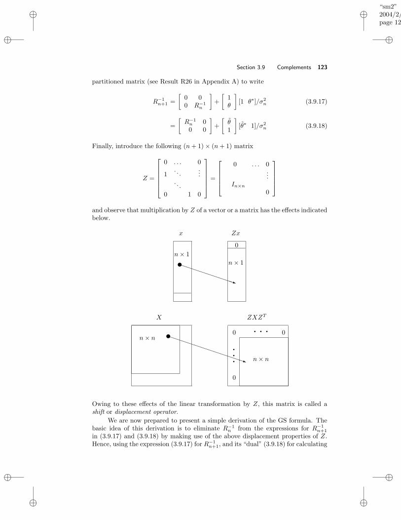
“sm2”2004/2/22page 123

i

i

i

i

i

i

i

i


partitioned matrix (see Result R26 in Appendix A) to write

R−1n+1 =

[0 00 R−1

n

]

+

[1θ

]

[1 θ∗]/σ2n (3.9.17)

=

[R−1n 00 0

]

+

[

θ1

]

[θ∗ 1]/σ2n (3.9.18)

Finally, introduce the following (n+ 1) × (n+ 1) matrix

Z =

0 . . . 0

1. . .

.... . .

0 1 0

=

0 . . . 0...

In×n0

and observe that multiplication by Z of a vector or a matrix has the effects indicatedbelow.

q

qq

q q q

0

00

0

n× n

n× n

n× 1

n× 1

ZXZTX

Zxx

PPPPPPPPPPPPq

u

PPPPPPPPPq

u

Owing to these effects of the linear transformation by Z, this matrix is called ashift or displacement operator.

We are now prepared to present a simple derivation of the GS formula. Thebasic idea of this derivation is to eliminate R−1

n from the expressions for R−1n+1

in (3.9.17) and (3.9.18) by making use of the above displacement properties of Z.Hence, using the expression (3.9.17) for R−1

n+1, and its “dual” (3.9.18) for calculating

“sm2”2004/2/22page 124

i

i

i

i

i

i

i

i


ZR−1n+1Z

T , gives

R−1n+1 − ZR−1

n+1ZT =

1

σ2n

1a1

...an

[1 a∗1 . . . a

∗n] −

0a∗n...a∗1

[0 an . . . a1]

(3.9.19)

Premultiplying and postmultiplying (3.9.19) by Z and ZT , respectively, and thencontinuing to do so with the resulting equations, we obtain

ZR−1n+1Z

T − Z2R−1n+1Z

2T =

1

σ2n

01a1

...an−1

[0 1 a∗1 . . . a

∗n−1] −

00a∗n...a∗2

[0 0 an . . . a2]

(3.9.20)

...

ZnR−1n+1Z

nT − 0 =1

σ2n

0...01

[0 . . . 0 1]

(3.9.21)

In (3.9.21), use is made of the fact that Z is a nilpotent matrix of order n + 1, inthe sense that:

Zn+1 = 0

(which can be readily verified). Now, by simply summing up the above equations(3.9.19)–(3.9.21), we derive the following expression for R−1

n+1:

R−1n+1 =

1

σ2n

1 0

a1. . .

.... . .

. . .

an . . . a1 1

1 a∗1 . . . a∗

n

. . .. . .

.... . . a∗

1

0 1

−

0 0

a∗n

. . ....

. . .. . .

a∗1 . . . a∗

n 0

0 an . . . a1

. . .. . .

.... . . an

0 0

(3.9.22)

which is the GS formula. Note from (3.9.22) that R−1n+1 is, indeed, completely

determined by its first column, as is claimed earlier.

“sm2”2004/2/22page 125

i

i

i

i

i

i

i

i


The GS formula is inherently related to the Yule–Walker method of AR mod-eling, and this is one of the reasons for including it in this book. The GS formulais also useful in studying other spectral estimators, such as the Capon method,which is discussed in Chapter 5. The hope that the curious reader who studies thispart will become interested in the fascinating topic of Toeplitz matrices and alliedsubjects is another reason for its inclusion. In particular, it is indeed fascinatingto be able to derive an analytical formula for the inverse of a given matrix, as isshown above to be the case for Toeplitz matrices. The basic ideas of the previousderivation may be extended to more general matrices. Let us explain this briefly.For a given matrix X, the rank of X −ZXZT is called the displacement rank of Xunder Z. As can be seen from (3.9.19), the inverse of a Hermitian Toeplitz matrixhas a displacement rank equal to two. Now, assume we are given a (structured)matrix X for which we are able to find a nilpotent matrix Y such that X−1 has alow displacement rank under Y ; the matrix Y does not need to have the previousform of Z. Then, paralleling the calculations in (3.9.19)–(3.9.22), we might be ableto derive a simple “closed–form” expression for X−1. See [Friedlander, Morf,

Kailath, and Ljung 1979] for more details on the topic of this complement.

3.9.5 MA Parameter Estimation in Polynomial Time

The parameter estimation of an AR process via the LS method leads to a quadraticminimization problem that can be solved in closed form (see (3.4.11), (3.4.12)). Onthe other hand, for an MA process the LS criterion similar to (3.4.11), which isgiven by

N2∑

t=N1

∣∣∣∣

1

B(z)y(t)

∣∣∣∣

2

(3.9.23)

is a highly nonlinear function of the MA parameters (and likewise for an ARMAprocess).

A simple MA spectral estimator, that does not require solving a nonlinearminimization problem, is given by equation (3.6.4) and is repeated here:

φ(ω) =

m∑

k=−mr(k)e−iωk (3.9.24)

where m is the assumed MA order and r(k) are the standard sample covariances.As explained in Section 3.6 the main problem associated with (3.9.24) is the fact

that φ(ω) is not guaranteed to be positive for all ω ∈ [0, 2π]. If the final goal of thesignal processing exercise is spectral analysis then an occurrence of negative valuesφ(ω) < 0 (for some values of ω) is not acceptable, as the true spectral density ofcourse satisfies φ(ω) ≥ 0 for all ω ∈ [0, 2π]. If the goal is MA parameter estimation,

then the problem induced by φ(ω) < 0 (for some values of ω) is even more serious

because in such a case φ(ω) cannot be factored as in (3.6.1), and hence no MA

parameter estimates can be determined directly from φ(ω). In this complement we

will show how to get around the problem of φ(ω) < 0, and hence how to obtainMA parameter estimates from such an invalid MA spectral density estimate, usingan indirect but computationally efficient method (see [Stoica, McKelvey, and

“sm2”2004/2/22page 126

i

i

i

i

i

i

i

i


Mari 2000; Dumitrescu, Tabus, and Stoica 2001]). Note that obtaining

MA parameter estimates from the φ(ω) in (3.9.24) is not only of interest for MAestimation, but also as a step of some ARMA estimation methods (see, e.g., (3.7.9)as well as Exercise 3.12).

A sound way of tackling this problem of “factoring the unfactorable” is asfollows. Let φ(ω) denote the PSD of an MA process of order m:

φ(ω) =

m∑

k=−mr(k)e−iωk ≥ 0, ω ∈ [0, 2π] (3.9.25)

We would like to determine the φ(ω) in (3.9.25) that is closest to φ(ω) in (3.9.24),in the following LS sense:

min1

2π

∫ π

−π

[

φ(ω) − φ(ω)]2

dω (3.9.26)

The order m in (3.9.25) may be different from the order m in (3.9.24). Withoutloss of generality we can assume that m ≤ m (indeed, if m > m we can extendthe sequence r(k) with zeroes to make m ≤ m). Once φ(ω) has been obtainedby solving (3.9.26) we can factor it by using any of a number of available spectralfactorization algorithms (see, e.g., [Wilson 1969; Vostry 1975; Vostry 1976]),and in this way derive MA parameter estimates bk satisfying

φ(ω) = σ2|B(ω)|2 (3.9.27)

(see (3.6.1)). This step of obtaining bk and σ2 from φ(ω) can be computed inO(m2) flops. The problem that remains is to solve (3.9.26) for φ(ω) in a similarlyefficient computational way.

As

φ(ω) − φ(ω) =

m∑

k=−m[r(k) − r(k)] e−iωk +

∑

|k|>mr(k)e−iωk

it follows from Parseval’s theorem (see (1.2.6)) that the spectral LS criterion of(3.9.26) can be rewritten as a covariance fitting criterion:

1

2π

∫ π

−π

[

φ(ω) − φ(ω)]2

dω =

m∑

k=−m

∣∣r(k) − r(k)

∣∣2

+∑

|k|>m|r(k)|2

Consequently, the approximation problem (3.9.26) is equivalent to:

minr(k)

‖r − r‖2W subject to (3.9.25) (3.9.28)

“sm2”2004/2/22page 127

i

i

i

i

i

i

i

i


where ‖x‖2W = x∗Wx and

r =[r(0) . . . r(m)

]T

r =[r(0) . . . r(m)

]T

W =

1 02

. . .

0 2

In the following we will describe a computationally efficient and reliable algorithmfor solving problem (3.9.28) (with a general W matrix) in a time that is a polynomialfunction of m (a more precise flop count is given below). Note that a possible wayof tackling (3.9.28) would consist of writing the covariances r(k) as functions ofthe MA parameters (see (3.3.3)), which would guarantee that they satisfy (3.9.25),and then minimize the function in (3.9.28) with respect to the MA parameters.However, the so-obtained minimization problem would be, similarly to (3.9.23),nonlinear in the MA parameters (more precisely, the criterion in (3.9.28) is quarticin bk), which is exactly the type of problem we tried to avoid in the first place.

As a preparation step for solving (3.9.28) we first derive a parameterizationof the MA covariance sequence r(k), which will turn out to be more convenientthan the parameterization via bk. Let Jk denote the (m + 1) × (m + 1) matrixwith ones on the (k + 1)st diagonal and zeroes everywhere else:

Jk =

k+1︷︸︸︷

0 . . . 0 1 0... 0

. . .

. . . 1... 0 0

...0 . . . . . . . . . 0

, (m+ 1) × (m+ 1)

(for k = 0, . . . ,m). Note that J0 = I. Then the following result holds:

Any MA covariance sequence r(k)mk=0 can be written as r(k) =tr(JkQ) for k = 0, . . . ,m, where Q is an (m+1)×(m+1) positivesemidefinite matrix.

(3.9.29)

To prove this result, let

a(ω) =[1 eiω . . . eimω

]T

“sm2”2004/2/22page 128

i

i

i

i

i

i

i

i


and observe that

a(ω)a∗(ω) =

1 e−iω · · · e−imω

eiω 1. . .

......

. . .. . . e−iω

eimω · · · eiω 1

=

m∑

k=−mJke

−ikω

where J−k = JTk (for k ≥ 0). Hence, for the sequence parameterized as in (3.9.29),we have that

m∑

k=−mr(k)e−ikω = tr

[m∑

k=−mJkQe

−ikω]

= tr [a(ω)a∗(ω)Q] = a∗(ω)Qa(ω) ≥ 0, for ω ∈ [0, 2π]

which implies that r(k) indeed is an MA(m) covariance sequence. To show thatany MA(m) covariance sequence can be parameterized as in (3.9.29), we make useof (3.3.3) to write (for k = 0, . . . ,m)

r(k) = σ2m∑

j=k

bjb∗j−k = σ2

[b∗0 · · · b∗m

]Jk

b0...bm

= tr

Jk · σ2

b0...bm

[b∗0 · · · b∗m

]

(3.9.30)

Evidently (3.9.30) has the form stated in (3.9.29) with

Q = σ2

b0...bm

[b∗0 · · · b∗m

]

With this observation, the proof of (3.9.29) is complete.We can now turn our attention to the main problem, (3.9.28). We will describe

an efficient algorithm for solving (3.9.28) with a general weighting matrix W > 0(as already stated.). For a choice of W that usually yields more accurate MAparameter estimates than the simple diagonal weighting in (3.9.28), we refer thereader to [Stoica, McKelvey, and Mari 2000]. Let

µ = C(r − r)

where C is the Cholesky factor of W (i.e., C is an upper triangular matrix andW = C∗C). Also, let α be a vector containing all the elements in the upper triangleof Q, including the diagonal:

α = [Q1,1 Q1,2 . . . Q1,m+1 ; Q2,2 . . . Q2,m+1 ; . . . ;Qm+1,m+1]T

“sm2”2004/2/22page 129

i

i

i

i

i

i

i

i


Note that α defines Q; that is, the elements of Q are either elements of α or complexconjugates of elements of α. Making use of this notation and of (3.9.29) we canrewrite (3.9.28) in the following form (for real-valued sequences):

minρ,µ,α

ρ subject to:

‖µ‖ ≤ ρ

Q ≥ 0

tr[Q]tr[12

(J1 + JT1

)Q]

...tr[12

(Jm + JTm

)Q]

+ C−1µ = r

(3.9.31)

Note that to obtain the equality constraint in (3.9.31) we used the fact that (in thereal-valued case; the complex-valued case can be treated similarly):

r(k) = tr(JkQ) = tr(QTJTk ) = tr(JTk Q) =1

2tr[(Jk + JTk )Q

]

The reason for this seemingly artificial trick is that we need the matrices multiplyingQ in (3.9.31) to be symmetric. In effect, the problem (3.9.31) has precisely theform of a semidefinite quadratic program (SQP) which can be solved efficientlyby means of interior point methods (see [Sturm 1999] and also [Dumitrescu,

Tabus, and Stoica 2001] and references therein). Specifically, it can be shownthat an interior point method (such as the ones in [Sturm 1999]) when applied tothe SQP in (3.9.31) requires O(m4) flops per iteration; furthermore, the number ofiterations needed to achieve practical convergence of the method is typically quitesmall (and nearly independent of m), for instance between 10 and 20 iterations.The overall conclusion, therefore, is that (3.9.31), and hence the original problem(3.9.28), can be efficiently solved in O(m4) flops. Once the solution to (3.9.31)has been computed, we can obtain the corresponding MA covariances either asr = r − C−1µ or as r(k) = tr(JkQ) for k = 0, . . . ,m. Numerical results obtainedwith the MA parameter estimation algorithm outlined above have been reported in[Dumitrescu, Tabus, and Stoica 2001] (see also [Stoica, McKelvey, and

Mari 2000]).

3.10 EXERCISES

Exercise 3.1: The Minimum Phase Property

As stated in the text, a polynomial A(z) is said to be minimum phase if all itszeroes are inside the unit circle. In this exercise, we motivate the name minimumphase. Specifically, we will show that if A(z) = 1 + a1z

−1 + · · · + anz−n has real-

valued coefficients and has all its zeroes inside the unit circle, and if B(z) is anyother polynomial in z−1 with real-valued coefficients that satisfies |B(ω)| = |A(ω)|and B(0) = A(0) (where B(ω) , B(z)|z=eiω ), then the phase lag of B(ω), given by

“sm2”2004/2/22page 130

i

i

i

i

i

i

i

i


− argB(ω)), is greater than or equal to the phase lag of A(ω):

− argB(ω) ≥ − argA(ω)

Since we can factor A(z) as

A(z) =

n∏

k=1

(1 − αkz−1)

and argA(ω) =∑nk=1 arg

(1 − αke

−iω), we begin by proving the minimum phaseproperty for first–order polynomials. Let

C(z) = 1 − αz−1, α , reiθ, r < 1

D(z) = z−1 − α∗ = C(z)z−1 − α∗

1 − αz−1, C(z)E(z)

(3.10.1)

(a) Show that the zero ofD(z) is outside the unit circle, and that |D(ω)| = |C(ω)|.(b) Show that

− argE(ω) = ω + 2 tan−1

[r sin(ω − θ)

1 − r cos(ω − θ)

]

Also, show that the above function is increasing.

(c) If α is real, conclude that − argD(ω) ≥ − argC(ω) for 0 ≤ ω ≤ π, whichjustifies the name minimum phase for C(z) in the first–order case.

(d) Generalize the first–order results proven in parts (a)–(c) to polynomials A(z)and B(z) of arbitrary order; in this case, the αk are either real or occur incomplex-conjugate pairs.

Exercise 3.2: Generating the ACS from ARMA ParametersIn this chapter we developed equations expressing the ARMA coefficients

σ2, ai, bj in terms of the ACS r(k)∞k=−∞. Find the inverse map; that is, given

σ2, a1, . . . , an, b1 . . . , bm, find equations to determine r(k)∞k=−∞.

Exercise 3.3: Relationship between AR Modeling and Forward LinearPrediction

Suppose we have a zero mean stationary process y(t) (not necessarily AR)with ACS r(k)∞

k=−∞. We wish to predict y(t) by a linear combination of its npast values; that is, the predicted value is given by

yf (t) =

n∑

k=1

(−ak)y(t− k)

We define the forward prediction error as

ef (t) = y(t) − yf (t) =

n∑

k=0

aky(t− k)

“sm2”2004/2/22page 131

i

i

i

i

i

i

i

i


with a0 = 1. Show that the vector θf = [a1 . . . an]T of prediction coefficients that

minimizes the prediction error variance σ2f , E|ef (t)|2 is the solution to (3.4.2).

Show also that σ2f = σ2

n, i.e., that σ2n in (3.4.2) is the prediction error variance.

Furthermore, show that if y(t) is an AR(p) process with p ≤ n, then theprediction error is white noise, and that

kj = 0 for j > p

where kj is the jth reflection coefficient defined in (3.5.7). Show that, as a conse-quence, ap+1, . . . , an = 0. Hint: The calculations performed in Section 3.4.2 andin Complement 3.9.2 will be useful in solving this problem.

Exercise 3.4: Relationship between AR Modeling and Backward LinearPrediction

Consider the signal y(t) as in Exercise 3.3. This time, we will considerbackward prediction; that is, we will predict y(t) from its n immediate futurevalues:

yb(t) =

n∑

k=1

(−bk)y(t+ k)

with corresponding backward prediction error eb(t) = y(t) − yb(t). Such backwardprediction is useful in applications where noncausal processing is permitted; forexample, when the data has been prerecorded and is stored in memory or on atape and we want to make inferences on samples that precede the observed ones.Find an expression similar to (3.4.2) for the backward prediction coefficient vectorθb = [b1 . . . bn]

T . Find a relationship between the θb and the corresponding forwardprediction coefficient vector θf . Relate the forward and backward prediction errorvariances.

Exercise 3.5: Prediction Filters and Smoothing FiltersThe smoothing filter is a practically useful variation on the theme of linear

prediction. A result of Exercises 3.3 and 3.4 should be that for the forward andbackward prediction filters

A(z) = 1 +

n∑

k=1

akz−k and B(z) = 1 +

n∑

k=1

bkz−k,

the prediction coefficients satisfy ak = b∗k, and the prediction error variances areequal.

Now consider the smoothing filter

es(t) =

m∑

k=1

cky(t− k) + y(t) +

m∑

k=1

dky(t+ k).

(a) Derive a system of linear equations, similar to the forward and backwardlinear prediction equations, that relate the smoothing filter coefficients, thesmoothing prediction error variance σ2

s = E|es(t)|2

, and the ACS of y(t).

“sm2”2004/2/22page 132

i

i

i

i

i

i

i

i


(b) For n = 2m, provide an example of a zero–mean stationary random processfor which the minimum smoothing prediction error variance is greater than theminimum forward prediction error variance. Also provide a second examplewhere the minimum smoothing filter prediction error variance is less than thecorresponding minimum forward prediction error variance.

(c) Assume m = n, but now constrain the smoothing prediction coefficients to becomplex–conjugate symmetric: ck = d∗

k for k = 1, . . . ,m. In this case the twoprediction filters and the smoothing filter have the same number of degreesof freedom. Prove that the minimum smoothing prediction error variance isless than or equal to the minimum (forward or backward) prediction errorvariance. Hint: Show that the unconstrained minimum smoothing errorvariance solution (where we do not impose the constraint ck = d∗

k) satisfiesck = d∗

k anyway.

Exercise 3.6: Relationship between Minimum Prediction Error and Spec-tral Flatness

Consider a random process y(t) with ACS r(k) (y(t) is not necessarily anAR process). We find an AR(n) model for y(t) by solving (3.4.6) for σ2

n and θn.These parameters generate an AR PSD model:

φAR(ω) =σ2n

|A(ω)|2

whose inverse Fourier transform we denote by rAR(k)∞k=−∞. In this exercise

we explore the relationship between r(k) and rAR(k), and between φy(ω) andφAR(ω).

(a) Verify that the AR model has the property that

rAR(k) = r(k), k = 0, . . . , n.

(b) We have seen from Exercise 3.3 that the AR model minimizes the nth–orderforward prediction error variance; that is, the variance of

e(t) = y(t) + a1y(t− 1) + . . .+ any(t− n).

For the special case that y(t) is AR of order n or less, we also know thate(t) is white noise, so φe(ω) is flat. We will extend this last property byshowing that, for general y(t), φe(ω) is maximally flat in the sense that theAR model maximizes the spectral flatness measure given by

fe =exp

[12π

∫ π

−π lnφe(ω)dω]

12π

∫ π

−π φe(ω) dω(3.10.2)

where

φe(ω) = |A(ω)|2 φy(ω) = σ2n

φy(ω)

φAR(ω).

Show that the measure fe has the following “desirable” properties of a spectralflatness measure:

“sm2”2004/2/22page 133

i

i

i

i

i

i

i

i


(i) fe is unchanged if φe(ω) is multiplied by a constant.

(ii) 0 ≤ fe ≤ 1.

(iii) fe = 1 if and only if φe(ω) = constant.

Hint: Use the fact that

1

2π

∫ π

−πln |A(ω)|2 dω = 0 (3.10.3)

(The above result can be proven using the Cauchy integral formula). Showthat (3.10.3) implies

fe = fyry(0)

re(0)(3.10.4)

and thus that minimizing re(0) maximizes fe.

Exercise 3.7: Diagonalization of the Covariance MatrixShow that Rn+1 in equation (3.5.2) satisfies

L∗Rn+1L = D

where

L =

1 0 . . . 0 0

1...

.... . . 0

1 0θn θn−1 θ1 1

and D = diag [σ2n σ

2n−1 . . . σ

20 ]

and where θk and σ2k are defined in (3.4.6). Use this property to show that

|Rn+1| =

n∏

k=0

σ2k

Exercise 3.8: Stability of Yule–Walker AR ModelsAssume that the matrix Rn+1 in equation (3.4.6) is positive definite. (This can

be achieved by using the sample covariances in (2.2.4) to build Rn+1, as explainedin Section 2.2.) Then show that the AR model obtained from the Yule–Walkerequations (3.4.6) is stable in the sense that the polynomial A(z) has all its zeroesstrictly inside the unit circle. (Most of the available proofs for this property arediscussed in [Stoica and Nehorai 1987]).

Exercise 3.9: Three Equivalent Representations for AR ProcessesIn this chapter we have considered three ways to parameterize an AR(n),

but we have not explicitly shown when they are equivalent. Show that, for anondegenerate AR(n) process (i.e., one for which Rn+1 is positive definite), thefollowing three parameterizations are equivalent:

(R) r(0), . . . , r(n) such that Rn+1 is positive definite.

(K) r(0), k1, . . . , kn such that r(0) > 0 and |ki| < 1 for i = 1, . . . , n.

“sm2”2004/2/22page 134

i

i

i

i

i

i

i

i


(A) σ2n, a1, . . . , an such that σ2

n > 0 and all the zeroes of A(z) are inside the unitcircle.

Find the mapping from each parameterization to the others (some of these havealready been derived in the text and in the previous exercises).

Exercise 3.10: An Alternative Proof of the Stability Property of Reflec-tion Coefficients

Prove that kp which minimizes (3.9.12) must be such that |kp| ≤ 1, without

using the expression (3.9.15) for kp. Hint: Write the criterion in (3.9.12) as

f(kp) = E

(∥∥∥∥

[1 kpk∗p 1

]

z(t)

∥∥∥∥

2)

where

E(·) =1

2(N − p)

N∑

t=p+1

(·)

z(t) =[ef,p−1(t) eb,p−1(t− 1)

]T

and show that if |kp| > 1 then f(kp) > f(1/k∗p).

Exercise 3.11: Recurrence Properties of Reflection Coefficient Sequencefor an MA Model

For an AR process of order n, the reflection coefficients satisfy ki = 0 fori > n (see Exercise 3.3), and the ACS satisfies the linear recurrence relationshipA(z)r(k) = 0 for k > 0. Since an MA process of order m has the property thatr(i) = 0 for i > m, we might wonder if a recurrence relationship holds for thereflection coefficients corresponding to a MA process. We will investigate this “con-jecture” for a simple case.

Consider an MA process of order 1 with parameter b1. Show that |Rn| satisfiesthe relationship

|Rn| = r(0)|Rn−1| − |r(1)|2|Rn−2|, n ≥ 2

Show that kn = (−r(1))n/|Rn| and that the reflection coefficient sequence satisfiesthe recurrence relationship:

1

kn= −r(0)

r(1)

1

kn−1− r∗(1)

r(1)

1

kn−2(3.10.5)

with appropriate initial conditions (state them). Show that the solution to (3.10.5)for |b1| < 1 is

kn =(1 − |b1|2)(−b1)n

1 − |b1|2n+2(3.10.6)

This sequence decays exponentially to zero. When b1 = −1, show that kn = 1/n.

“sm2”2004/2/22page 135

i

i

i

i

i

i

i

i


It has been shown that for large n, B(z)kn ' 0, where ' 0 means that theresidue is small compared to the kn terms [Georgiou 1987]. This result holdseven for MA processes of order higher than 1. Unfortunately, the result is of littlepractical use as a means of estimating the bk coefficients since for large n the knvalues are (very) small.

Exercise 3.12: Asymptotic Variance of the ARMA Spectral EstimatorConsider the ARMA spectral estimator (3.2.2) with any consistent estimate

of σ2 and ai, bj. For simplicity, assume that the ARMA parameters are real;however, the result holds for complex ARMA processes as well. Show that theasymptotic (for large data sets) variance of this spectral estimator can be writtenin the form

E

[φ(ω) − φ(ω)]2

= C(ω)φ2(ω) (3.10.7)

where C(ω) = ϕT (ω)Pϕ(ω). Here, P is the covariance matrix of the estimate ofthe parameter vector [σ2, aT , bT ]T and the vector ϕ(ω) has an expression that isto be found. Deduce that (3.10.7) has the same form as the asymptotic varianceof the periodogram spectral estimator but with the essential difference that in theARMA estimator case C(ω) goes to zero as the number of data samples processedincreases (and that C(ω) in (3.10.7) is a function of ω). Hint: Use a Taylor series

expansion of φ(ω) as a function of the estimated parameters σ2, ai, bj (see, e.g.,Appendix B).

Exercise 3.13: Filtering Interpretation of Numerator Estimators in AR-MA Estimation

An alternative method for estimating the MA part of an ARMA PSD is asfollows. Assume we have estimated the AR coefficients (e.g., from equation (3.7.2)or (3.7.4)). We filter y(t) by A(z) to form f(t):

f(t) = y(t) +

n∑

i=1

aiy(t− i), t = n+ 1, . . . , N.

Then estimate the ARMA PSD as

φ(ω) =

∑mk=−m rf (k)e

−iωk

|A(ω)|2

where rf (k) are the standard ACS estimates for f(t). Show that the above estimatoris quite similar to (3.7.8) and (3.7.9) for large N .

Exercise 3.14: An Alternative Expression for ARMA Power SpectralDensity

Consider an ARMA(n,m) process. Show that

φ(z) = σ2B(z)B∗(1/z∗)

A(z)A∗(1/z∗)

can be written as

φ(z) =C(z)

A(z)+C∗(1/z∗)

A∗(1/z∗)(3.10.8)

“sm2”2004/2/22page 136

i

i

i

i

i

i

i

i


where

C(z) =

max(m,n)∑

k=0

ckz−k

Show that the polynomial C(z) satisfying (3.10.8) is unique, and find an expressionfor ck in terms of ai and r(k).

Equation (3.10.8) motivates an alternative estimation procedure to that inequations (3.7.8) and (3.7.9) for ARMA spectral estimation. In the alternativeapproach, we first estimate the AR coefficients aini=1 using, e.g., equation (3.7.2).We then estimate the ck coefficients using the formula found in this exercise, andfinally insert the estimates ak and ck into the right–hand side of (3.10.8) to obtaina spectral estimate. Prove that this alternative estimator is equivalent to that in(3.7.8)–(3.7.9) under certain conditions, and find conditions on ak so that they areequivalent. Also, compare (3.7.9) and (3.10.8) for ARMA(n,m) spectral estimationwhen m < n.

Exercise 3.15: Pade ApproximationA minimum phase (or causally invertible) ARMA(n,m) model B(z)/A(z) can

be equivalently represented as an AR(∞) model 1/C(z). The approximation of aratio of polynomials by a polynomial of higher order was considered by Pade inthe late 1800s. One possible application of the Pade approximation is to obtain anARMA spectral model by first estimating the coefficients of a high–order AR model,then solving for a (low–order) ARMA model from the estimated AR coefficients.In this exercise we investigate the model relationships and some consequences oftruncating the AR model polynomial coefficients.

Define:

A(z) = 1 + a1z−1 + · · · + anz

−n

B(z) = 1 + b1z−1 + · · · + bmz

−m

C(z) = 1 + c1z−1 + c2z

−2 + · · ·

(a) Show that

ck =

1, k = 0

ak −∑mi=1 bick−i, 1 ≤ k ≤ n

−∑mi=1 bick−i, k > n

where we assume any polynomial coefficient is equal to zero outside its definedrange.

(b) Using the equations above, derive a procedure for computing the ai and bjparameters from a given set of ckm+n

k=0 parameters. Assume m and n areknown.

(c) The above equations give an exact representation using an infinite–order ARpolynomial. In the Pade method, an approximation to B(z)/A(z) = 1/C(z)is obtained by truncating (setting to zero) the ck coefficients for k > m+ n.

“sm2”2004/2/22page 137

i

i

i

i

i

i

i

i


Suppose a stable minimum phase ARMA(n,m) filter is approximated by anAR(m + n) filter using the Pade approximation. Give an example to showthat the resulting AR approximation is not necessarily stable.

(d) Suppose a stable AR(m+n) filter is approximated by a ratio Bm(z)/An(z) asin part (b). Give an example to show that the resulting ARMA approximationis not necessarily stable.

Exercise 3.16: (Non)Uniqueness of Fully Parameterized ARMA Equa-tions

The shaping filter (or transfer function) of the ARMA equation (3.8.1) is givenby the following matrix fraction:

H(z) = A−1(z)B(z), (ny × ny) (3.10.9)

where z is a dummy variable, and

A(z) = I +A1z−1 + · · · +Apz

−p

B(z) = I +B1z−1 + · · · +Bpz

−p

(if the AR and MA orders, n and m, are different, then p above is equal tomax(m,n)). Assume that A(z) and B(z) are “fully parameterized” in the sensethat all elements of the matrix coefficients Ai, Bj are unknown.

The matrix fraction description (MFD) (3.10.9) of the ARMA shaping filteris unique if and only if there exist no matrix polynomials A(z) and B(z) of degreep and no matrix polynomial L(z) 6= I such that

A(z) = L(z)A(z) B(z) = L(z)B(z) (3.10.10)

This can be verified by making use of (3.10.9); see, e.g., [Kailath 1980].Show that the above uniqueness condition is satisfied for the fully parameter-

ized MFD if and only if

rank[Ap Bp] = ny (3.10.11)

Comment on the character of this condition: is it restrictive or not?

COMPUTER EXERCISES

Tools for AR, MA, and ARMA Spectral Estimation:The text web site www.prenhall.com/stoica contains the following Matlab

functions for use in computing AR, MA, and ARMA spectral estimates and selectingthe model order. For the first four functions, y is the input data vector, n is thedesired AR order, and m is the desired MA order (if applicable). The outputs are a,

the vector [a1, . . . , an]T of estimated AR parameters, b, the vector [b1, . . . , bm]T of

MA parameters (if applicable), and sig2, the noise variance estimate σ2. Variabledefinitions specific to a particular functions are given below.

“sm2”2004/2/22page 138

i

i

i

i

i

i

i

i


• [a,sig2]=yulewalker(y,n)

The Yule–Walker AR method given by equation (3.4.2).

• [a,sig2]=lsar(y,n)

The covariance Least Squares AR method given by equation (3.4.12).

• [a,gamma]=mywarma(y,n,m,M)

The modified Yule–Walker based ARMA spectral estimate given by equation(3.7.9), where the AR coefficients are estimated from the overdetermined setof equations (3.7.4) with W = I. Here, M is the number of Yule-Walkerequations used in (3.7.4) and gamma is the vector [γ0, . . . , γm]T .

• [a,b,sig2]=lsarma(y,n,m,K)

The two–stage Least Squares ARMA method given in Section 3.7.2; K is thenumber of AR parameters to estimate in Step 1 of that algorithm.

• order=armaorder(mo,sig2,N,nu)

Computes the AIC, AICc, GIC, and BIC model order selections for generalparameter estimation problems (see Appendix C for details on the derivationsof these methods). Here, mo is a vector of possible model orders, sig2 is thevector of estimated residual variances corresponding to the model orders inmo, N is the length of the observed data vector, and nu is a parameter in theGIC method. The output 4-element vector order contains the model ordersselected using AIC, AICc, GIC, and BIC, respectively.

Exercise C3.17: Comparison of AR, ARMA and Periodogram Methodsfor ARMA Signals

In this exercise we examine the properties of parametric methods for PSDestimation. We will use two ARMA signals, one broadband and one narrowband,to illustrate the performance of these parametric methods.

Broadband ARMA Process: Generate realizations of the broadband ARMAprocess

y(t) =B1(z)

A1(z)e(t)

with σ2 = 1 and

A1(z) = 1 − 1.3817z−1 + 1.5632z−2 − 0.8843z−3 + 0.4096z−4

B1(z) = 1 + 0.3544z−1 + 0.3508z−2 + 0.1736z−3 + 0.2401z−4

Choose the number of samples as N = 256.

(a) Estimate the PSD of the realizations by using the four AR and ARMA esti-mators described above. Use AR(4), AR(8), ARMA(4,4), and ARMA(8,8);for the MYW algorithm, use both M = n and M = 2n; for the LS AR(MA)algorithms, use K = 2n. Illustrate the performance by plotting ten overlaidestimates of the PSD. Also, plot the true PSD on the same diagram.

“sm2”2004/2/22page 139

i

i

i

i

i

i

i

i


In addition, plot pole or pole–zero estimates for the various methods. (Forthe MYW method, the zeroes can be found by spectral factorization of thenumerator; comment on the difficulties you encounter, if any.)

(b) Compare the two AR algorithms. How are they different in performance?

(c) Compare the two ARMA algorithms. How does M impact performance ofthe MYW algorithm? How do the accuracies of the respective pole and zeroestimates compare?

(d) Use an ARMA(4,4) model for the LS ARMA algorithm, and estimate the PSDof the realizations for K = 4, 8, 12, and 16. How does K impact performanceof the algorithm?

(e) Compare the lower–order estimates with the higher–order estimates. In whatway(s) does increasing the model order improve or degrade estimation perfor-mance?

(f) Compare the AR to the ARMA estimates. How does the AR(8) model performwith respect to the ARMA(4,4) model and the ARMA(8,8) model?

(g) Compare your results with those using the periodogram method on the sameprocess (from Exercise C2.21 in Chapter 2). Comment on the difference be-tween the methods with respect to variance, bias, and any other relevantproperties of the estimators you notice.

Narrowband ARMA Process: Generate realizations of the narrowband ARMAprocess

y(t) =B2(z)

A2(z)e(t)

with σ2 = 1 and

A2(z) = 1 − 1.6408z−1 + 2.2044z−2 − 1.4808z−3 + 0.8145z−4

B2(z) = 1 + 1.5857z−1 + 0.9604z−2

(a) Repeat the experiments and comparisons in the broadband example for thenarrowband process; this time, use the following model orders: AR(4), AR(8),AR(12), AR(16), ARMA(4,2), ARMA(8,4), and ARMA(12,6).

(b) Study qualitatively how the algorithm performances differ for narrowbandand broadband data. Comment separately on performance near the spectralpeaks and near the spectral valleys.

Exercise C3.18: AR and ARMA Estimators for Line Spectral EstimationThe ARMA methods can also be used to estimate line spectra (estimation

of line spectra by other methods is the topic of Chapter 4). In this application,AR(MA) techniques are often said to provide super–resolution capabilities becausethey are able to resolve sinusoids too closely spaced in frequency to be resolved byperiodogram–based methods.

We again consider the four AR and ARMA estimators described above.

“sm2”2004/2/22page 140

i

i

i

i

i

i

i

i


(a) Generate realizations of the signal

y(t) = 10 sin(0.24πt+ ϕ1) + 5 sin(0.26πt+ ϕ2) + e(t), t = 1, . . . , N

where e(t) is (real) white Gaussian noise with variance σ2, and where ϕ1, ϕ2

are independent random variables each uniformly distributed on [0, 2π]. Fromthe results in Chapter 4, we find the spectrum of y(t) to be

φ(ω) = 50π [δ(ω − 0.24π) + δ(ω + 0.24π)]

+12.5π [δ(ω − 0.26π) + δ(ω + 0.26π)] + σ2

(b) Compute the “true” AR polynomial (using the true ACS sequence; see equa-tion (4.1.6)) using the Yule–Walker equations for both AR(4), AR(12), AR-MA(4,4) and ARMA(12,12) models when σ2 = 1. This experiment corre-sponds to estimates obtained as N → ∞. Plot 1/|A(ω)|2 for each case, andfind the roots of A(z). Which method(s) are able to resolve the two sinusoids?

(c) Consider now N = 64, and set σ2 = 0; this corresponds to the finite datalength but infinite SNR case. Compute estimated AR polynomials using thefour spectral estimators and the AR and ARMA model orders described above;for the MYW technique consider both M = n and M = 2n, and for the LSARMA technique use both K = n and K = 2n. Plot 1/|A(ω)|2, overlaid, for50 different Monte–Carlo simulations (using different values of ϕ1 and ϕ2 foreach). Also plot the zeroes of A(z), overlaid, for these 50 simulations. Whichmethod(s) are reliably able to resolve the sinusoids? Explain why. Note thatas σ2 → 0, y(t) corresponds to a (limiting) AR(4) process. How does thechoice of M or K in the ARMA methods affect resolution or accuracy of thefrequency estimates?

(d) Obtain spectral estimates (σ2|B(ω)|2/|A(ω)|2 for the ARMA estimators andσ2/|A(ω)|2 for the AR estimators) for the four methods when N = 64 andσ2 = 1. Plot ten overlaid spectral estimates and overlaid polynomial zeroes ofthe A(z) estimates. Experiment with different AR and ARMA model ordersto see if the true frequencies are estimated more accurately; note also theappearance and severity of “spurious” sinusoids in the estimates for highermodel orders. Which method(s) give reliable “super–resolution” estimation ofthe sinusoids? How does the model order influence the resolution properties?Which method appears to have the best resolution?

You may want to experiment further by changing the SNR and the relativeamplitudes of the sinusoids to gain a better understanding of the relativedifferences between the methods. Also, experiment with different model ordersand parameters K and M to understand their impact on estimation accuracy.

(e) Compare the estimation results with periodogram–based estimates obtainedfrom the same signals. Discuss differences in resolution, bias, and variance ofthe techniques.

Exercise C3.19: Model Order Selection for AR and ARMA Processes

“sm2”2004/2/22page 141

i

i

i

i

i

i

i

i


In this exercise we examine four methods for model order selection in ARand ARMA spectral estimation. We will experiment with both broadband andnarrowband processes.

As discussed in Appendix C, several important model order selection ruleshave the following general form (see (C.8.1)–(C.8.2)):

−2 ln pn(y, θn) + η(n,N)n (3.10.12)

with different penalty coefficients η(n,N) for the different methods:

AIC : η(n,N) = 2

AICc : η(n,N) = 2N

N − n− 1

GIC : η(n,N) = ν (e.g., ν = 4)

BIC : η(n,N) = lnN

(3.10.13)

The term ln pn(y, θn) is the log-likelihood of the observed data vector y given the

maximum-likelihood (ML) estimate of the parameter vector θ for a model of ordern (where n is the total number of estimated real-valued parameters in the model);for the case of AR, MA, and ARMA models, a large-sample approximation for−2 ln pn(y, θ

n) that is commonly used for order selection (see, e.g., [Ljung 1987;Soderstrom and Stoica 1989]) is given by:

−2 ln pn(y, θn) ' Nσ2

n + constant (3.10.14)

where σ2n is the sample estimate of σ2 in (3.2.2) corresponding to the model of

order n. The selected order is the value of n that minimizes (3.10.12). The orderselection rules above, while derived for ML estimates of θ, can be used even withapproximate ML estimates of θ, albeit with some loss of performance.

Broadband AR Process: Generate 100 realizations of the broadband AR process

y(t) =1

A1(z)e(t)

with σ2 = 1 and

A1(z) = 1 − 1.3817z−1 + 1.5632z−2 − 0.8843z−3 + 0.4096z−4

Choose the number of samples as N = 128. For each realization:

(a) Estimate the model parameters using the LS AR estimator, and using ARmodel orders from 1 to 12.

(b) Find the model orders that minimize the AIC, AICc, GIC (with ν = 4),and BIC criteria (See Appendix C). Note that for an AR model of order m,n = m+ 1.

(c) For each of the four order selection methods, plot a histogram of the selectedorders for the 100 realizations. Comment on their relative performance.

“sm2”2004/2/22page 142

i

i

i

i

i

i

i

i


Repeat the above experiment using N = 256 and N = 1024 samples. Discuss therelative performance of the order selection methods as N increases.

Narrowband AR Process: Repeat the above experiment using the narrowbandAR process:

y(t) =1

A2(z)e(t)

with σ2 = 1 and

A2(z) = 1 − 1.6408z−1 + 2.2044z−2 − 1.4808z−3 + 0.8145z−4

Compare the narrowband AR and broadband AR order selection results, and dis-cuss the relative order selection performance for these two AR processes.

Broadband ARMA Process: Repeat the broadband AR experiment using thebroadband ARMA process

y(t) =B1(z)

A1(z)e(t)

with σ2 = 1 and

A1(z) = 1 − 1.3817z−1 + 1.5632z−2 − 0.8843z−3 + 0.4096z−4

B1(z) = 1 + 0.3544z−1 + 0.3508z−2 + 0.1736z−3 + 0.2401z−4

For the broadband ARMA process, use N = 256 and N = 1024 data samples. Foreach value of N , find ARMA(m,m) models (so n = 2m+ 1 in equation (3.10.12))for m = 1, . . . , 12. Use the two-stage LS ARMA method with K = 4m to estimateparameters.

Narrowband ARMA Process: Repeat the broadband ARMA experiment usingthe narrowband ARMA process:

y(t) =B2(z)

A2(z)e(t)

with σ2 = 1 and

A2(z) = 1 − 1.6408z−1 + 2.2044z−2 − 1.4808z−3 + 0.8145z−4

B2(z) = 1 + 1.1100z−1 + 0.4706z−2

Find ARMA(2m,m) models for m = 1, . . . , 6 (so n = 3m+1 in equation (3.10.12))using the two-stage LS ARMA method with K = 8m. Compare the narrowbandARMA and broadband ARMA order selection results, and discuss the relative orderselection performance for these two ARMA processes.

Exercise C3.20: AR and ARMA Estimators applied to Measured DataConsider the data sets in the files sunspotdata.mat and lynxdata.mat.

These files can be obtained from the text web site www.prenhall.com/stoica.

“sm2”2004/2/22page 143

i

i

i

i

i

i

i

i


Apply your favorite AR and ARMA estimator(s) (for the lynx data, use both theoriginal data and the logarithmically transformed data as in Exercise C2.23) toestimate the spectral content of these data. You will also need to determine ap-propriate model orders m and n (see, e.g., Exercise C3.19). As in Exercise C2.23,try to answer the following questions: Are there sinusoidal components (or peri-odic structure) in the data? If so, how many components and at what frequencies?Discuss the relative strengths and weaknesses of parametric and nonparametric es-timators for understanding the spectral content of these data. In particular, discusshow a combination of the two techniques can be used to estimate the spectral andperiodic structure of the data.

“sm2”2004/2/22page 144

i

i

i

i

i

i

i

i

C H A P T E R 4

Parametric Methods for LineSpectra

4.1 INTRODUCTION

In several applications, particularly in communications, radar, sonar, geophysicalseismology and so forth, the signals dealt with can be well described by the followingsinusoidal model:

y(t) = x(t) + e(t) ; x(t) =

n∑

k=1

αkei(ωkt+ϕk) (4.1.1)

where x(t) denotes the noise–free complex–valued sinusoidal signal; αk, ωk,ϕk are its amplitudes, (angular) frequencies and initial phases, respectively; ande(t) is an additive observation noise. The complex–valued form (4.1.1), of course, isnot encountered in practice as it stands; practical signals are real valued. However,as already mentioned in Chapter 1, in many applications both the in–phase andquadrature components of the studied signal are available. (See Chapter 6 for moredetails on this aspect.) In the case of a (real–valued) sinusoidal signal, this meansthat both the sine and the corresponding cosine components are available. Thesetwo components may be processed by arranging them in a two–dimensional vectorsignal or a complex–valued signal of the form of (4.1.1). Since the complex–valueddescription (4.1.1) of the in–phase and quadrature components of a sinusoidal signalis the most convenient one from a mathematical standpoint, we focus on it in thischapter.

The noise e(t) in (4.1.1) is usually assumed to be (complex–valued) circularwhite noise as defined in (2.4.19). We also make the white noise assumption inthis chapter. We may argue in the following way that the white noise assumptionis not particularly restrictive. Let the continuous–time counterpart of the noise in(4.1.1) be correlated, but assume that the “correlation time” of the continuous–time noise is less than half of the shortest period of the sine wave componentsin the continuous–time counterpart of x(t) in (4.1.1). If this mild condition issatisfied, then choosing the sampling period larger than the noise correlation time(yet smaller than half the shortest sinusoidal signal period, to avoid aliasing) resultsin a white discrete–time noise sequence e(t). If the correlation condition above isnot satisfied, but we know the shape of the noise spectrum, we can filter y(t) by alinear whitening filter which makes the noise component at the filter output white;the sinusoidal components remain sinusoidal with the same frequencies, and withamplitudes and phases altered in a known way.

144

“sm2”2004/2/22page 145

i

i

i

i

i

i

i

i

Section 4.1 Introduction 145

If the noise process is not white and has unknown spectral shape, then accu-rate frequency estimates can still be found if we estimate the sinusoids using thenonlinear least squares (NLS) method in Section 4.3 (see [Stoica and Nehorai

1989b], for example). Indeed, the properties of the NLS estimates in the coloredand unknown noise case are quite similar to those for the white noise case, onlywith the sinusoidal signal amplitudes “adjusted” to give corresponding local SNRs— the signal–to–noise power ratio at each frequency ωk. This amplitude adjust-ment is the same as that realized by the whitening filter approach. It is importantto note that these comments only apply if the NLS method is used. The otherestimation methods in this chapter (e.g., the subspace–based methods) depend onthe assumption that the noise is white, and may be adversely affected if the noiseis not white (or is not prewhitened).

Concerning the signal in (4.1.1), we assume that ωk ∈ [−π, π] and that αk > 0.We need to specify the sign of αk; otherwise we are left with a phase ambigu-ity. More precisely, without the condition αk > 0 in (4.1.1), both αk, ωk, ϕkand −αk, ωk, ϕk + π give the same signal x(t), so the parameterization is notunique. As to the initial phases ϕk in (4.1.1), one could assume that they arefixed (nonrandom) constants, which would result in x(t) being a deterministicsignal. In most applications, however, ϕk are nuisance parameters and it is moreconvenient to assume that they are random variables. Note that if we try to mimicthe conditions of a previous experiment as much as possible, we will usually be un-able to ensure the same initial phases of the sine waves in the observed sinusoidalsignal (this will be particularly true for received signals). Since there is usually noreason to believe that a specific set of initial phases is more likely than anotherone, or that two different initial phases are interrelated, we make the followingassumption:

The initial phases ϕk are independent random variables uni-formly distributed on [−π, π]

(4.1.2)

The covariance function and the PSD of the noisy sinusoidal signal y(t) canbe calculated in a straightforward manner under the assumptions made above. Byusing (4.1.2), we get

Eeiϕpe−iϕj

= 1 for p = j

and for p 6= j

Eeiϕpe−iϕj

= E

eiϕp

Ee−iϕj

=

[1

2π

∫ π

−πeiϕdϕ

] [1

2π

∫ π

−πe−iϕdϕ

]

= 0

Thus,Eeiϕpe−iϕj

= δp,j (4.1.3)

Letxp(t) = αpe

i(ωpt+ϕp) (4.1.4)

denote the pth sine wave in (4.1.1). It follows from (4.1.3) that

Exp(t)x

∗j (t− k)

= α2

peiωpkδp,j (4.1.5)

“sm2”2004/2/22page 146

i

i

i

i

i

i

i

i

146 Chapter 4 Parametric Methods for Line Spectra

which, in turn, gives

r(k) = E y(t)y∗(t− k) =

n∑

p=1

α2peiωpk + σ2δk,0 (4.1.6)

and the derivation of the covariance function of y(t) is completed. The PSD of y(t)is given by the DTFT of r(k) in (4.1.6), which is

φ(ω) = 2π

n∑

p=1

α2pδ(ω − ωp) + σ2

(4.1.7)

where δ(ω−ωp) is the Dirac impulse (or Dirac delta “function”) which, by definition,has the property that

∫ π

−πF (ω)δ(ω − ωp)dω = F (ωp) (4.1.8)

for any function F (ω) that is continuous at ωp. The expression (4.1.7) for φ(ω) maybe verified by inserting it in the inverse transform formula (1.3.8) and checking thatthe result is the covariance function. Doing so, we obtain

1

2π

∫ π

−π[2π

n∑

p=1

α2pδ(ω − ωp) + σ2]eiωkdω =

n∑

p=1

α2peiωpk + σ2δk,o = r(k) (4.1.9)

which is the desired result.The PSD (4.1.7) is depicted in Figure 4.1. It consists of a “floor” of constant

level equal to the noise power σ2, along with n vertical lines (or impulses) locatedat the sinusoidal frequencies ωk and having zero support but nonzero areas equalto 2π times the sine wave powers α2

k. Owing to its appearance, as exhibited inFigure 4.1, φ(ω) in (4.1.7) is called a line or discrete spectrum.

It is evident from the previous discussion that a spectral analysis based on theparametric PSD model (4.1.7) reduces to the problem of estimating the parametersof the signal in (4.1.1). In most applications, such as those listed at the beginning ofthis chapter, the parameters of major interest are the locations of the spectral lines,namely the sinusoidal frequencies. In the following sections, we present a number ofmethods for spectral line analysis. We focus on the problem of frequency estimationmeaning determination of ωknk=1 from a set of observations y(t)Nt=1. Once thefrequencies have been determined, estimation of the other signal parameters (orPSD parameters) becomes a simple linear regression problem. More precisely, forgiven ωk the observations y(t) can be written as a linear regression function whosecoefficients are equal to the remaining unknowns αkeiϕk , βk:

y(t) =

n∑

k=1

βkeiωkt + e(t) (4.1.10)

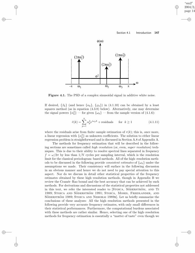
“sm2”2004/2/22page 147

i

i

i

i

i

i

i

i


σ2

(2πα12)

(2πα22)

(2πα32)

−π πω

φ(ω)

ω1 ω2 ω3

Figure 4.1. The PSD of a complex sinusoidal signal in additive white noise.

If desired, βk (and hence αk, ϕk) in (4.1.10) can be obtained by a leastsquares method (as in equation (4.3.8) below). Alternatively, one may determinethe signal powers α2

k — for given ωk — from the sample version of (4.1.6):

r(k) =

n∑

p=1

α2peiωpk + residuals for k ≥ 1 (4.1.11)

where the residuals arise from finite–sample estimation of r(k); this is, once more,a linear regression with α2

p as unknown coefficients. The solution to either linearregression problem is straightforward and is discussed in Section A.8 of Appendix A.

The methods for frequency estimation that will be described in the follow-ing sections are sometimes called high–resolution (or, even, super–resolution) tech-niques. This is due to their ability to resolve spectral lines separated in frequencyf = ω/2π by less than 1/N cycles per sampling interval, which is the resolutionlimit for the classical periodogram–based methods. All of the high–resolution meth-ods to be discussed in the following provide consistent estimates of ωk under theassumptions we made. Their consistency will surface in the following discussionin an obvious manner and hence we do not need to pay special attention to thisaspect. Nor do we discuss in detail other statistical properties of the frequencyestimates obtained by these high–resolution methods, though in Appendix B wereview the Cramer–Rao bound and the best accuracy that can be achieved by suchmethods. For derivations and discussions of the statistical properties not addressedin this text, we refer the interested reader to [Stoica, Soderstrom, and Ti

1989; Stoica and Soderstrom 1991; Stoica, Moses, Friedlander, and

Soderstrom 1989; Stoica and Nehorai 1989b]. Let us briefly summarize theconclusions of these analyses: All the high–resolution methods presented in thefollowing provide very accurate frequency estimates, with only small differences intheir statistical performances. Furthermore, the computational burdens associatedwith these methods are rather similar. Hence, selecting one of the high–resolutionmethods for frequency estimation is essentially a “matter of taste” even though we

“sm2”2004/2/22page 148

i

i

i

i

i

i

i

i


will identify some advantages of one of these methods, named ESPRIT, over theothers.

We should point out that the comparison in the previous paragraph betweenthe high–resolution methods and the periodogram–based techniques is unfair in thesense that periodogram–based methods do not assume any knowledge about thedata, whereas high–resolution methods exploit an exact description of the stud-ied signal. Owing to the additional information assumed, a parametric methodshould be expected to offer better resolution than the nonparametric method of theperiodogram. On the other hand, when no two spectral lines in the spectrum areseparated by less than 1/N , the unmodified periodogram turns out to be an excellentfrequency estimator which may outperform any of the high–resolution methods (aswe shall see). One may ask why the unmodified periodogram is preferred over themany windowed or smoothed periodogram techniques to which we paid so muchattention in Chapter 2. The explanation actually follows from the discussion in thatchapter. The unmodified periodogram can be viewed as a Blackman–Tukey “win-dowed” estimator with a rectangular window of maximum length equal to 2N + 1.Of all window sequences, this is exactly the one which has the narrowest main lobeand hence the one which affords the maximum spectral resolution, a desirable prop-erty for high-resolution spectral line scenarios. It should be noted, however, that ifthe sinusoidal components in the signal are not too closely spaced in frequency, buttheir amplitudes differ significantly from one another, then a mildly windowed peri-odogram (to avoid leakage) may perform better than the unwindowed periodogram(in the unwindowed periodogram, the weaker sinusoids may be obscured by theleakage from the stronger ones, and hence they may not be visible in a plot of theestimated spectrum).

In order to simplify the discussion in this chapter, we assume that the numberof sinusoidal components, n, in (4.1.1) is known. When n is unknown, which maywell be the case in many applications, it can be determined from the available dataas described for example in [Fuchs 1988; Kay 1988; Marple 1987; Proakis,

Rader, Ling, and Nikias 1992; Soderstrom and Stoica 1989] and in Ap-pendix C.

4.2 MODELS OF SINUSOIDAL SIGNALS IN NOISE

The frequency estimation methods presented in this chapter rely on three differentmodels for the noisy sinusoidal signal (4.1.1). This section introduces the threemodels of (4.1.1).

4.2.1 Nonlinear Regression Model

The nonlinear regression model is given by (4.1.1). Note that ωk enter in anonlinear fashion in (4.1.1), hence the name “nonlinear regression” given to thistype of model for y(t). The other two models for y(t), to be discussed inthe following, are derived from (4.1.1); they are descriptions of the data that arenot as complete as (4.1.1). However, they preserve the information required todetermine the frequencies ωk which, as already stated, are the parameters ofmajor interest. Hence, in some sense, these two models are more appropriate forfrequency estimation since they do not include some of the nuisance parameters

“sm2”2004/2/22page 149

i

i

i

i

i

i

i

i

Section 4.2 Models of Sinusoidal Signals in Noise 149

which appear in (4.1.1).

4.2.2 ARMA Model

It can be readily verified that

(1 − eiωkz−1)xk(t) ≡ 0 (4.2.1)

where z−1 denotes the unit delay (or shift) operator introduced in Chapter 1. Hence,(1 − eiωkz−1) is an annihilating filter for the kth component in x(t). By using thissimple observation, we obtain the following homogeneous AR equation for x(t)

A(z)x(t) = 0 (4.2.2)

and the following ARMA model for the noisy data y(t):

A(z)y(t) = A(z)e(t)

A(z) =

n∏

k=1

(1 − eiωkz−1)(4.2.3)

It may be a useful exercise to derive equation (4.2.2) in a different way. The PSDof x(t) consists of n spectral lines located at ωknk=1. It should then be clear, inview of the relation (1.4.9) governing the transfer of a PSD through a linear system,that any filter which has zeroes at frequencies ωk is an annihilating filter for x(t).The polynomial A(z) in (4.2.3) is the simplest kind of such an annihilating filter.This polynomial bears complete information about ωk and hence the problem ofestimating the frequencies can be reduced to that of determining A(z).

We remark that the ARMA model (4.2.3) has a very special form (a reasonfor which it is sometimes called a “degenerate” ARMA). All its poles and zeroes arelocated exactly on the unit circle. Furthermore, its AR and MA parts are identical.It might be tempting to cancel the common poles and zeroes in (4.2.3). However,such an operation leads to the wrong conclusion that y(t) = e(t) and, therefore,should be invalid. Let us explain briefly why cancelation in (4.2.3) is not allowed.The ARMA equation description of a signal y(t) is asymptotically equivalent to theassociated transfer function description (in the sense that both give the same signalsequence, for t → ∞) if and only if the poles are situated strictly inside the unitcircle. If there are poles on the unit circle, then the equivalence between these twodescriptions ceases. In particular, the solution of an ARMA equation with poleson the unit circle strongly depends on the initial conditions, whereas the transferfunction description does not include a dependence on initial values.

4.2.3 Covariance Matrix Model

A notation that will often be used in the following is:

a(ω) , [1 e−iω . . . e−i(m−1)ω]T (m× 1)

A = [a(ω1) . . . a(ωn)] (m× n)(4.2.4)

“sm2”2004/2/22page 150

i

i

i

i

i

i

i

i


In (4.2.4), m is a positive integer which is not yet specified. Note that the matrix Aintroduced above is a Vandermonde matrix which enjoys the following rank property(see Result R24 in Appendix A):

rank(A) = n if m ≥ n and ωk 6= ωp for k 6= p (4.2.5)

By making use of the previous notation, along with (4.1.1) and (4.1.4), we can write

y(t) ,

y(t)y(t− 1)

...y(t−m+ 1)

= Ax(t) + e(t)

x(t) = [x1(t) . . . xn(t)]T

e(t) = [e(t) . . . e(t−m+ 1)]T

(4.2.6)

The following expression for the covariance matrix of y(t) can be readily derivedfrom (4.1.5) and (4.2.6)

R , E y(t)y∗(t) = APA∗ + σ2I ; P =

α21 0

. . .

0 α2n

(4.2.7)

The above equation constitutes the covariance matrix model of the data. As we willshow later, the eigenstructure of R contains complete information on the frequenciesωk, and this is exactly where the usefulness of (4.2.7) lies.

From equations (4.2.6) and (4.1.5), we also derive for later use the followingresult:

Γ , E

y(t− L− 1)...

y(t− L−M)

[y∗(t) . . . y∗(t− L)]

= EAM x(t− L− 1)x∗(t)A∗

L+1

= AMPL+1A∗L+1 (L,M ≥ 1)

(4.2.8)

where AK stands for A in (4.2.4) with m = K, and

PK =

α21e

−iω1K 0. . .

0 α2ne

−iωnK

As we explain in detail later, the null space of the matrix Γ (with L,M ≥ n)gives complete information on the frequencies ωk.

“sm2”2004/2/22page 151

i

i

i

i

i

i

i

i

Section 4.3 Nonlinear Least Squares Method 151

4.3 NONLINEAR LEAST SQUARES METHOD

An intuitively appealing approach to spectral line analysis, based on the nonlinearregression model (4.1.1), consists of determining the unknown parameters as theminimizers of the following criterion:

f(ω, α, ϕ) =

N∑

t=1

∣∣∣∣∣y(t) −

n∑

k=1

αkei(ωkt+ϕk)

∣∣∣∣∣

2

(4.3.1)

where ω is the vector of frequencies ωk, and similarly for α and ϕ. The sinusoidalmodel determined as above has the smallest “sum of squares” distance to the ob-served data y(t)Nt=1. Since f is a nonlinear function of its arguments ω, ϕ, α,the method which obtains parameter estimates by minimizing (4.3.1) is called thenonlinear least squares (NLS) method. When the (white) noise e(t) is Gaussiandistributed, the minimization of (4.3.1) can also be interpreted as the method ofmaximum likelihood (see Appendices B and C); in that case, minimization of (4.3.1)can be shown to provide the parameter values which are most likely to “explain” theobserved data sequence (see [Soderstrom and Stoica 1989; Kay 1988; Marple

1987]).The criterion in (4.3.1) depends on both αk and ϕk as well as on ωk.

However, it can be concentrated with respect to the nuisance parameters αk, ϕk,as explained next. By making use of the following notation,

βk = αkeiϕk (4.3.2)

β = [β1 . . . βn]T (4.3.3)

Y = [y(1) . . . y(N)]T (4.3.4)

B =

eiω1 . . . eiωn

......

eiNω1 . . . eiNωn

(4.3.5)

we can write the function f in (4.3.1) as

f = (Y −Bβ)∗(Y −Bβ) (4.3.6)

The Vandermonde matrix B in (4.3.5) (which resembles the matrix A defined in(4.2.4)) has full column rank equal to n under the weak condition that N ≥ n;in this case, (B∗B)−1 exists. By using this observation, we can put (4.3.6) in themore convenient form:

f = [β − (B∗B)−1B∗Y ]∗[B∗B][β − (B∗B)−1B∗Y ]

+ Y ∗Y − Y ∗B(B∗B)−1B∗Y (4.3.7)

For any choice of ω = [ω1, . . . , ωn]T in B (which is such that ωk 6= ωp for k 6= p),

we can choose β to make the first term of f zero; thus, we see that the vectors βand ω which minimize f are given by

ω = arg maxω[Y ∗B(B∗B)−1B∗Y ]

β = (B∗B)−1B∗Y |ω=ω

(4.3.8)

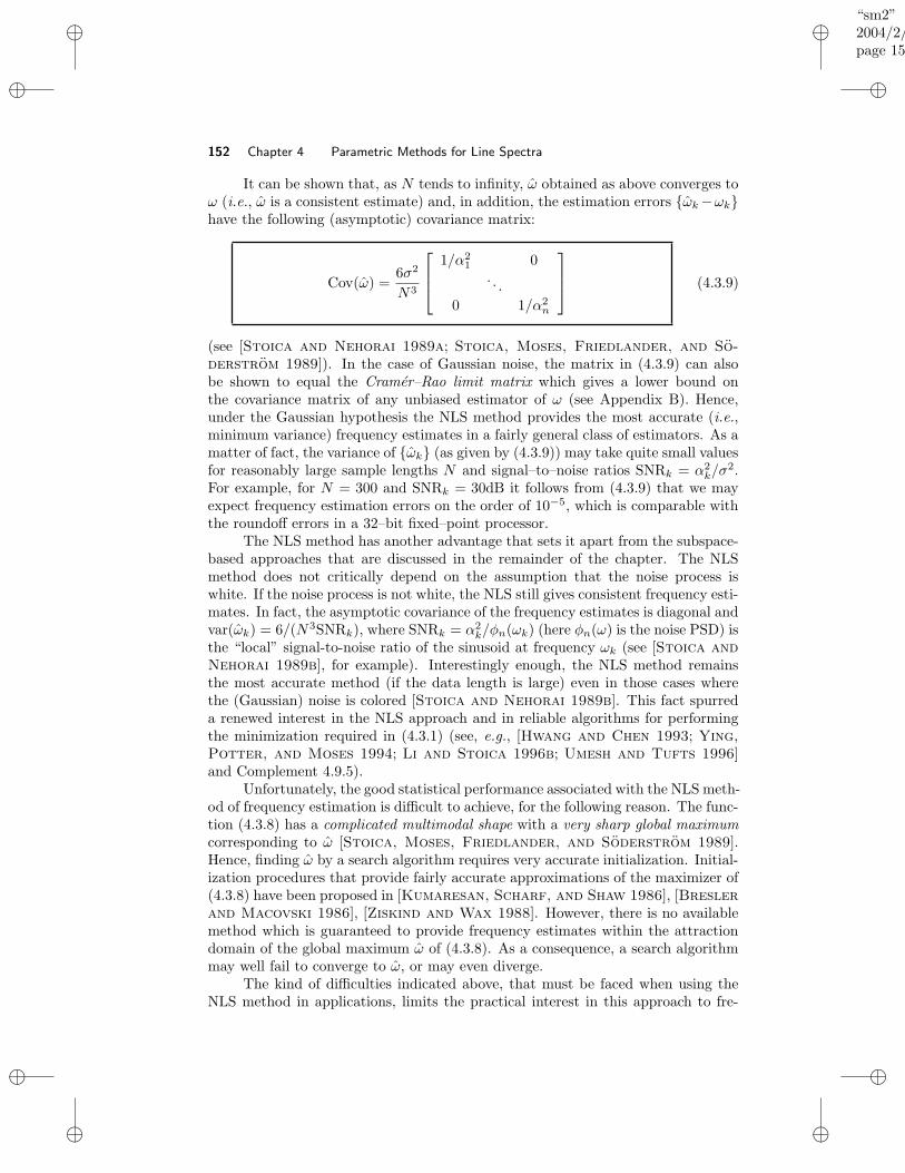
“sm2”2004/2/22page 152

i

i

i

i

i

i

i

i


It can be shown that, as N tends to infinity, ω obtained as above converges toω (i.e., ω is a consistent estimate) and, in addition, the estimation errors ωk−ωkhave the following (asymptotic) covariance matrix:

Cov(ω) =6σ2

N3

1/α21 0

. . .

0 1/α2n

(4.3.9)

(see [Stoica and Nehorai 1989a; Stoica, Moses, Friedlander, and So-

derstrom 1989]). In the case of Gaussian noise, the matrix in (4.3.9) can alsobe shown to equal the Cramer–Rao limit matrix which gives a lower bound onthe covariance matrix of any unbiased estimator of ω (see Appendix B). Hence,under the Gaussian hypothesis the NLS method provides the most accurate (i.e.,minimum variance) frequency estimates in a fairly general class of estimators. As amatter of fact, the variance of ωk (as given by (4.3.9)) may take quite small valuesfor reasonably large sample lengths N and signal–to–noise ratios SNRk = α2

k/σ2.

For example, for N = 300 and SNRk = 30dB it follows from (4.3.9) that we mayexpect frequency estimation errors on the order of 10−5, which is comparable withthe roundoff errors in a 32–bit fixed–point processor.

The NLS method has another advantage that sets it apart from the subspace-based approaches that are discussed in the remainder of the chapter. The NLSmethod does not critically depend on the assumption that the noise process iswhite. If the noise process is not white, the NLS still gives consistent frequency esti-mates. In fact, the asymptotic covariance of the frequency estimates is diagonal andvar(ωk) = 6/(N3SNRk), where SNRk = α2

k/φn(ωk) (here φn(ω) is the noise PSD) isthe “local” signal-to-noise ratio of the sinusoid at frequency ωk (see [Stoica and

Nehorai 1989b], for example). Interestingly enough, the NLS method remainsthe most accurate method (if the data length is large) even in those cases wherethe (Gaussian) noise is colored [Stoica and Nehorai 1989b]. This fact spurreda renewed interest in the NLS approach and in reliable algorithms for performingthe minimization required in (4.3.1) (see, e.g., [Hwang and Chen 1993; Ying,

Potter, and Moses 1994; Li and Stoica 1996b; Umesh and Tufts 1996]and Complement 4.9.5).

Unfortunately, the good statistical performance associated with the NLS meth-od of frequency estimation is difficult to achieve, for the following reason. The func-tion (4.3.8) has a complicated multimodal shape with a very sharp global maximumcorresponding to ω [Stoica, Moses, Friedlander, and Soderstrom 1989].Hence, finding ω by a search algorithm requires very accurate initialization. Initial-ization procedures that provide fairly accurate approximations of the maximizer of(4.3.8) have been proposed in [Kumaresan, Scharf, and Shaw 1986], [Bresler

and Macovski 1986], [Ziskind and Wax 1988]. However, there is no availablemethod which is guaranteed to provide frequency estimates within the attractiondomain of the global maximum ω of (4.3.8). As a consequence, a search algorithmmay well fail to converge to ω, or may even diverge.

The kind of difficulties indicated above, that must be faced when using theNLS method in applications, limits the practical interest in this approach to fre-

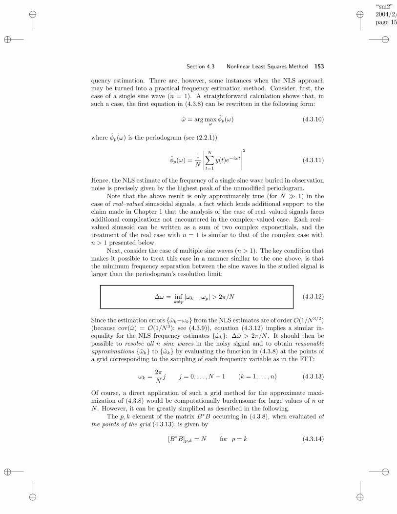
“sm2”2004/2/22page 153

i

i

i

i

i

i

i

i

Section 4.3 Nonlinear Least Squares Method 153

quency estimation. There are, however, some instances when the NLS approachmay be turned into a practical frequency estimation method. Consider, first, thecase of a single sine wave (n = 1). A straightforward calculation shows that, insuch a case, the first equation in (4.3.8) can be rewritten in the following form:

ω = arg maxω

φp(ω) (4.3.10)

where φp(ω) is the periodogram (see (2.2.1))

φp(ω) =1

N

∣∣∣∣∣

N∑

t=1

y(t)e−iωt

∣∣∣∣∣

2

(4.3.11)

Hence, the NLS estimate of the frequency of a single sine wave buried in observationnoise is precisely given by the highest peak of the unmodified periodogram.

Note that the above result is only approximately true (for N 1) in thecase of real–valued sinusoidal signals, a fact which lends additional support to theclaim made in Chapter 1 that the analysis of the case of real–valued signals facesadditional complications not encountered in the complex–valued case. Each real–valued sinusoid can be written as a sum of two complex exponentials, and thetreatment of the real case with n = 1 is similar to that of the complex case withn > 1 presented below.

Next, consider the case of multiple sine waves (n > 1). The key condition thatmakes it possible to treat this case in a manner similar to the one above, is thatthe minimum frequency separation between the sine waves in the studied signal islarger than the periodogram’s resolution limit:

∆ω = infk 6=p

|ωk − ωp| > 2π/N (4.3.12)

Since the estimation errors ωk−ωk from the NLS estimates are of order O(1/N3/2)(because cov(ω) = O(1/N3); see (4.3.9)), equation (4.3.12) implies a similar in-equality for the NLS frequency estimates ωk: ∆ω > 2π/N . It should then bepossible to resolve all n sine waves in the noisy signal and to obtain reasonableapproximations ωk to ωk by evaluating the function in (4.3.8) at the points ofa grid corresponding to the sampling of each frequency variable as in the FFT:

ωk =2π

Nj j = 0, . . . , N − 1 (k = 1, . . . , n) (4.3.13)

Of course, a direct application of such a grid method for the approximate maxi-mization of (4.3.8) would be computationally burdensome for large values of n orN . However, it can be greatly simplified as described in the following.

The p, k element of the matrix B∗B occurring in (4.3.8), when evaluated atthe points of the grid (4.3.13), is given by

[B∗B]p,k = N for p = k (4.3.14)

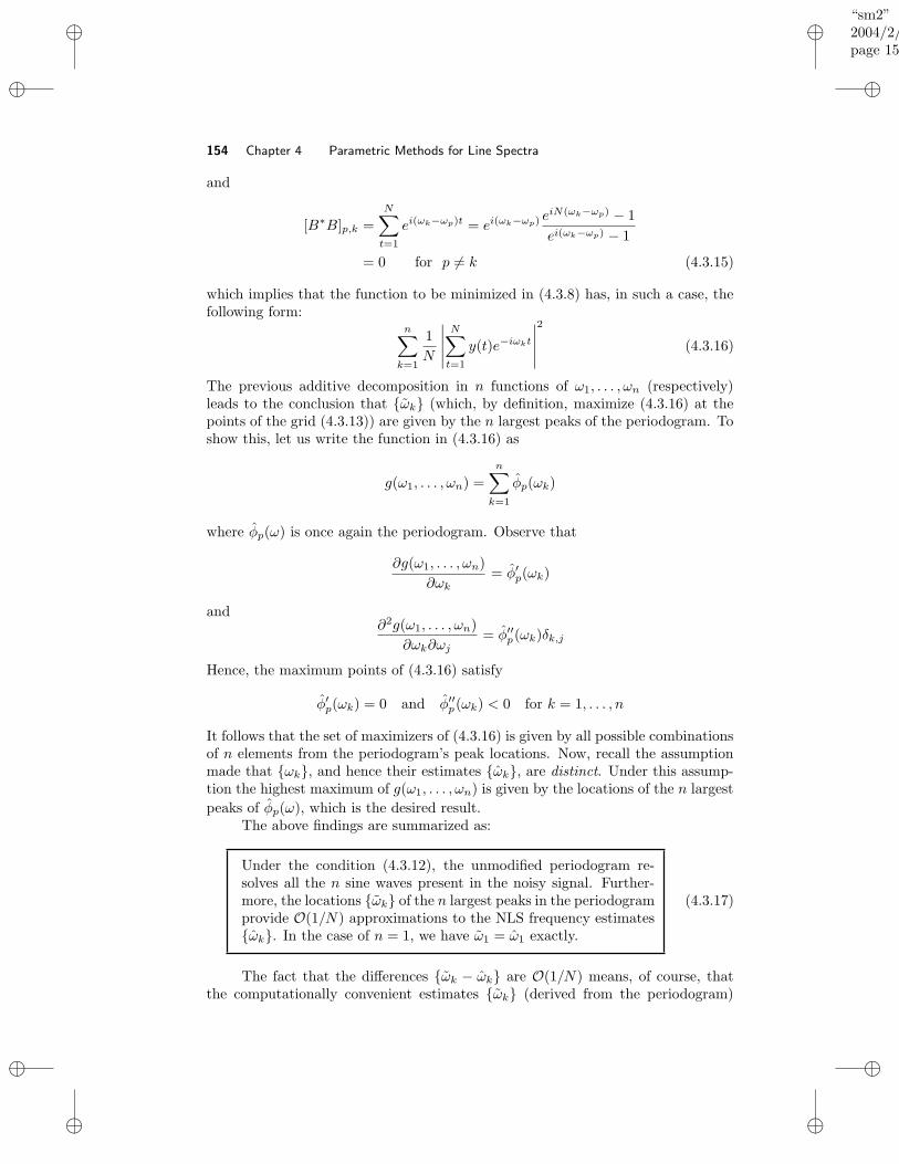
“sm2”2004/2/22page 154

i

i

i

i

i

i

i

i


and

[B∗B]p,k =

N∑

t=1

ei(ωk−ωp)t = ei(ωk−ωp) eiN(ωk−ωp) − 1

ei(ωk−ωp) − 1

= 0 for p 6= k (4.3.15)

which implies that the function to be minimized in (4.3.8) has, in such a case, thefollowing form:

n∑

k=1

1

N

∣∣∣∣∣

N∑

t=1

y(t)e−iωkt

∣∣∣∣∣

2

(4.3.16)

The previous additive decomposition in n functions of ω1, . . . , ωn (respectively)leads to the conclusion that ωk (which, by definition, maximize (4.3.16) at thepoints of the grid (4.3.13)) are given by the n largest peaks of the periodogram. Toshow this, let us write the function in (4.3.16) as

g(ω1, . . . , ωn) =

n∑

k=1

φp(ωk)

where φp(ω) is once again the periodogram. Observe that

∂g(ω1, . . . , ωn)

∂ωk= φ′

p(ωk)

and∂2g(ω1, . . . , ωn)

∂ωk∂ωj= φ′′

p(ωk)δk,j

Hence, the maximum points of (4.3.16) satisfy

φ′p(ωk) = 0 and φ′′

p(ωk) < 0 for k = 1, . . . , n

It follows that the set of maximizers of (4.3.16) is given by all possible combinationsof n elements from the periodogram’s peak locations. Now, recall the assumptionmade that ωk, and hence their estimates ωk, are distinct. Under this assump-tion the highest maximum of g(ω1, . . . , ωn) is given by the locations of the n largest

peaks of φp(ω), which is the desired result.The above findings are summarized as:

Under the condition (4.3.12), the unmodified periodogram re-solves all the n sine waves present in the noisy signal. Further-more, the locations ωk of the n largest peaks in the periodogramprovide O(1/N) approximations to the NLS frequency estimatesωk. In the case of n = 1, we have ω1 = ω1 exactly.

(4.3.17)

The fact that the differences ωk − ωk are O(1/N) means, of course, thatthe computationally convenient estimates ωk (derived from the periodogram)

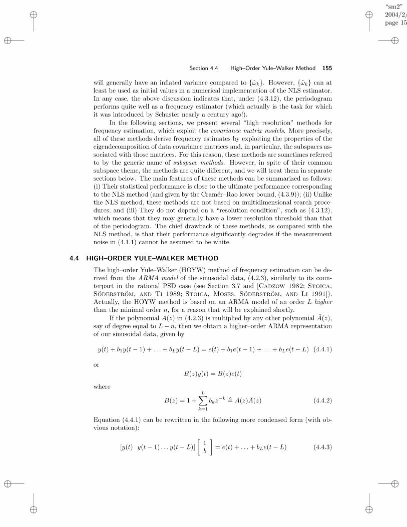
“sm2”2004/2/22page 155

i

i

i

i

i

i

i

i

Section 4.4 High–Order Yule–Walker Method 155

will generally have an inflated variance compared to ωk. However, ωk can atleast be used as initial values in a numerical implementation of the NLS estimator.In any case, the above discussion indicates that, under (4.3.12), the periodogramperforms quite well as a frequency estimator (which actually is the task for whichit was introduced by Schuster nearly a century ago!).

In the following sections, we present several “high–resolution” methods forfrequency estimation, which exploit the covariance matrix models. More precisely,all of these methods derive frequency estimates by exploiting the properties of theeigendecomposition of data covariance matrices and, in particular, the subspaces as-sociated with those matrices. For this reason, these methods are sometimes referredto by the generic name of subspace methods. However, in spite of their commonsubspace theme, the methods are quite different, and we will treat them in separatesections below. The main features of these methods can be summarized as follows:(i) Their statistical performance is close to the ultimate performance correspondingto the NLS method (and given by the Cramer–Rao lower bound, (4.3.9)); (ii) Unlikethe NLS method, these methods are not based on multidimensional search proce-dures; and (iii) They do not depend on a “resolution condition”, such as (4.3.12),which means that they may generally have a lower resolution threshold than thatof the periodogram. The chief drawback of these methods, as compared with theNLS method, is that their performance significantly degrades if the measurementnoise in (4.1.1) cannot be assumed to be white.

4.4 HIGH–ORDER YULE–WALKER METHOD

The high–order Yule–Walker (HOYW) method of frequency estimation can be de-rived from the ARMA model of the sinusoidal data, (4.2.3), similarly to its coun-terpart in the rational PSD case (see Section 3.7 and [Cadzow 1982; Stoica,

Soderstrom, and Ti 1989; Stoica, Moses, Soderstrom, and Li 1991]).Actually, the HOYW method is based on an ARMA model of an order L higherthan the minimal order n, for a reason that will be explained shortly.

If the polynomial A(z) in (4.2.3) is multiplied by any other polynomial A(z),say of degree equal to L− n, then we obtain a higher–order ARMA representationof our sinusoidal data, given by

y(t) + b1y(t− 1) + . . .+ bLy(t− L) = e(t) + b1e(t− 1) + . . .+ bLe(t− L) (4.4.1)

or

B(z)y(t) = B(z)e(t)

where

B(z) = 1 +

L∑

k=1

bkz−k , A(z)A(z) (4.4.2)

Equation (4.4.1) can be rewritten in the following more condensed form (with ob-vious notation):

[y(t) y(t− 1) . . . y(t− L)]

[1b

]

= e(t) + . . .+ bLe(t− L) (4.4.3)

“sm2”2004/2/22page 156

i

i

i

i

i

i

i

i


Premultiplying (4.4.3) by [y∗(t−L−1) . . . y∗(t−L−M)]T and taking the expectationleads to

Γc[

1b

]

= 0 (4.4.4)

where the matrix Γ is defined in (4.2.8) and M is a positive integer which is yet tobe specified. In order to obtain (4.4.4) as indicated above, we made use of the factthat E y∗(t− k)e(t) = 0 for k > 0.

The similarity of (4.4.4) with the Yule–Walker system of equations encoun-tered in Chapter 3 (see equation (3.7.1)) is more readily seen if (4.4.4) is rewrittenin the following more detailed form:

r(L) . . . r(1)...

...r(L+M − 1) . . . r(M)

b = −

r(L+ 1)...

r(L+M)

(4.4.5)

Owing to this analogy, the set of equations (4.4.5) associated with the noisy sinu-soidal signal y(t) is said to form a HOYW system.

The HOYW matrix equation (4.4.4) can also be obtained directly from (4.2.8).For any L ≥ n and any polynomial A(z) (used in the defining equation, (4.4.2), forb), the elements of the vector

ATL+1

[1b

]

(4.4.6)

are equal to zero. Indeed, the kth row of (4.4.6) is

[1 e−iωk . . . e−iLωk ]

[1b

]

= 1 +

L∑

p=1

bpe−iωkp

= A(ωk)A(ωk) = 0, k = 1, . . . , n (4.4.7)

(since A(ωk) = 0, cf. (4.2.3)). It follows from (4.2.8) and (4.4.7) that the vector[

1b

]

lies in the null space of Γc (see Definition D2 in Appendix A),

Γc[

1b

]

= 0

which is the desired result, (4.4.4).The HOYW system of equations derived above can be used for frequency

estimation in the following way. By replacing the unavailable theoretical covariancesr(k) in (4.4.5) by the sample covariances r(k), we obtain

r(L) . . . r(1)...

...r(L+M − 1) . . . r(M)

b ' −

r(L+ 1)...

r(L+M)

(4.4.8)

Owing to the estimation errors in r(k) the matrix equation (4.4.8) cannot hold

exactly in the general case, for any vector b, which is indicated above by the use of

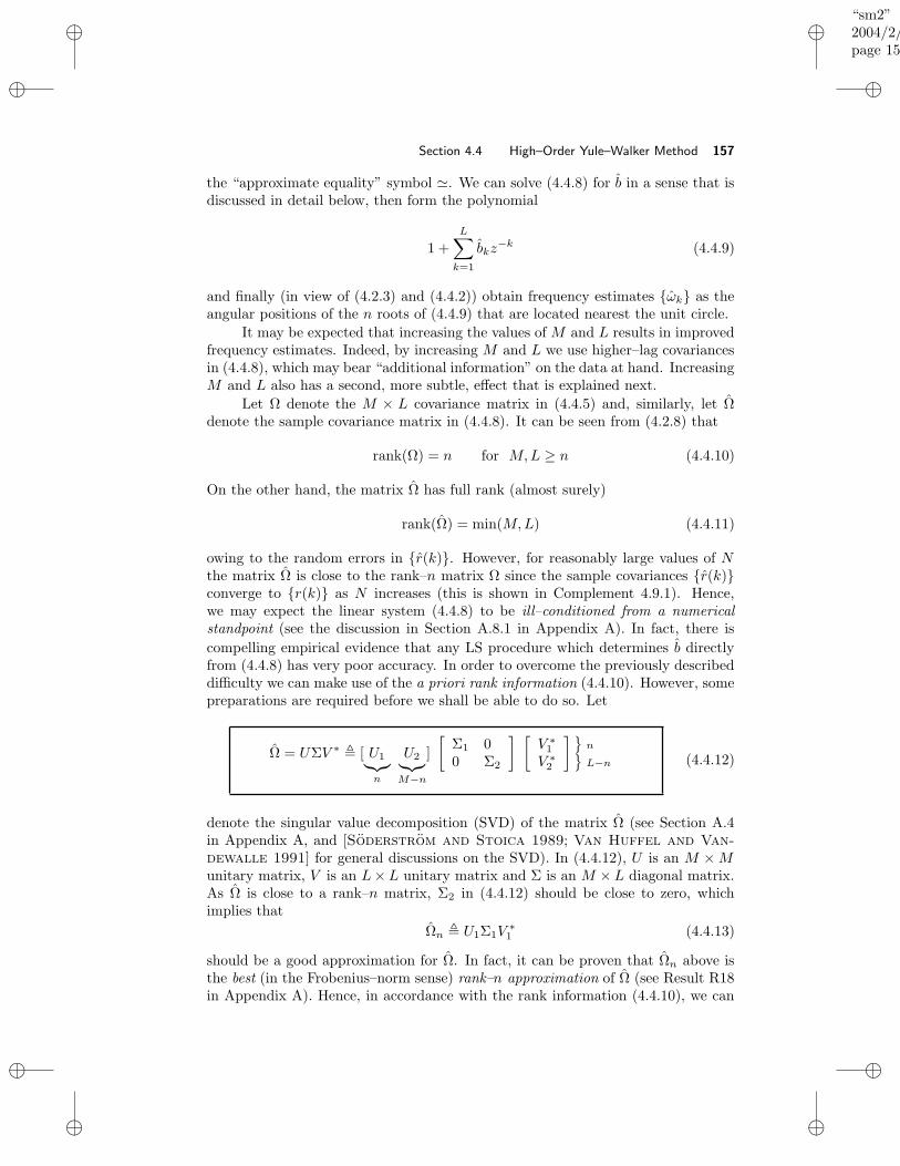
“sm2”2004/2/22page 157

i

i

i

i

i

i

i

i

Section 4.4 High–Order Yule–Walker Method 157

the “approximate equality” symbol '. We can solve (4.4.8) for b in a sense that isdiscussed in detail below, then form the polynomial

1 +

L∑

k=1

bkz−k (4.4.9)

and finally (in view of (4.2.3) and (4.4.2)) obtain frequency estimates ωk as theangular positions of the n roots of (4.4.9) that are located nearest the unit circle.

It may be expected that increasing the values of M and L results in improvedfrequency estimates. Indeed, by increasing M and L we use higher–lag covariancesin (4.4.8), which may bear “additional information” on the data at hand. IncreasingM and L also has a second, more subtle, effect that is explained next.

Let Ω denote the M × L covariance matrix in (4.4.5) and, similarly, let Ωdenote the sample covariance matrix in (4.4.8). It can be seen from (4.2.8) that

rank(Ω) = n for M,L ≥ n (4.4.10)

On the other hand, the matrix Ω has full rank (almost surely)

rank(Ω) = min(M,L) (4.4.11)

owing to the random errors in r(k). However, for reasonably large values of Nthe matrix Ω is close to the rank–n matrix Ω since the sample covariances r(k)converge to r(k) as N increases (this is shown in Complement 4.9.1). Hence,we may expect the linear system (4.4.8) to be ill–conditioned from a numericalstandpoint (see the discussion in Section A.8.1 in Appendix A). In fact, there is

compelling empirical evidence that any LS procedure which determines b directlyfrom (4.4.8) has very poor accuracy. In order to overcome the previously describeddifficulty we can make use of the a priori rank information (4.4.10). However, somepreparations are required before we shall be able to do so. Let

Ω = UΣV ∗ , [ U1︸︷︷︸

n

U2︸︷︷︸

M−n

]

[Σ1 00 Σ2

] [V ∗

1

V ∗2

] n

L−n (4.4.12)

denote the singular value decomposition (SVD) of the matrix Ω (see Section A.4in Appendix A, and [Soderstrom and Stoica 1989; Van Huffel and Van-

dewalle 1991] for general discussions on the SVD). In (4.4.12), U is an M ×Munitary matrix, V is an L×L unitary matrix and Σ is an M ×L diagonal matrix.As Ω is close to a rank–n matrix, Σ2 in (4.4.12) should be close to zero, whichimplies that

Ωn , U1Σ1V∗1 (4.4.13)

should be a good approximation for Ω. In fact, it can be proven that Ωn above isthe best (in the Frobenius–norm sense) rank–n approximation of Ω (see Result R18in Appendix A). Hence, in accordance with the rank information (4.4.10), we can

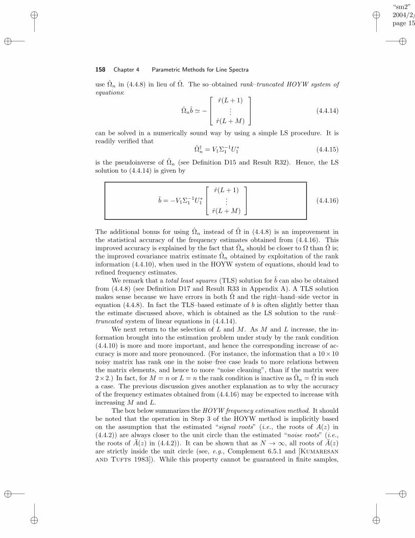
“sm2”2004/2/22page 158

i

i

i

i

i

i

i

i


use Ωn in (4.4.8) in lieu of Ω. The so–obtained rank–truncated HOYW system ofequations:

Ωnb ' −

r(L+ 1)...

r(L+M)

(4.4.14)

can be solved in a numerically sound way by using a simple LS procedure. It isreadily verified that

Ω†n = V1Σ

−11 U∗

1 (4.4.15)

is the pseudoinverse of Ωn (see Definition D15 and Result R32). Hence, the LSsolution to (4.4.14) is given by

b = −V1Σ−11 U∗

1

r(L+ 1)...

r(L+M)

(4.4.16)

The additional bonus for using Ωn instead of Ω in (4.4.8) is an improvement inthe statistical accuracy of the frequency estimates obtained from (4.4.16). Thisimproved accuracy is explained by the fact that Ωn should be closer to Ω than Ω is;the improved covariance matrix estimate Ωn obtained by exploitation of the rankinformation (4.4.10), when used in the HOYW system of equations, should lead torefined frequency estimates.

We remark that a total least squares (TLS) solution for b can also be obtainedfrom (4.4.8) (see Definition D17 and Result R33 in Appendix A). A TLS solutionmakes sense because we have errors in both Ω and the right–hand–side vector inequation (4.4.8). In fact the TLS–based estimate of b is often slightly better thanthe estimate discussed above, which is obtained as the LS solution to the rank–truncated system of linear equations in (4.4.14).

We next return to the selection of L and M . As M and L increase, the in-formation brought into the estimation problem under study by the rank condition(4.4.10) is more and more important, and hence the corresponding increase of ac-curacy is more and more pronounced. (For instance, the information that a 10×10noisy matrix has rank one in the noise–free case leads to more relations betweenthe matrix elements, and hence to more “noise cleaning”, than if the matrix were2×2.) In fact, for M = n or L = n the rank condition is inactive as Ωn = Ω in sucha case. The previous discussion gives another explanation as to why the accuracyof the frequency estimates obtained from (4.4.16) may be expected to increase withincreasing M and L.

The box below summarizes the HOYW frequency estimation method. It shouldbe noted that the operation in Step 3 of the HOYW method is implicitly basedon the assumption that the estimated “signal roots” (i.e., the roots of A(z) in(4.4.2)) are always closer to the unit circle than the estimated “noise roots” (i.e.,the roots of A(z) in (4.4.2)). It can be shown that as N → ∞, all roots of A(z)are strictly inside the unit circle (see, e.g., Complement 6.5.1 and [Kumaresan

and Tufts 1983]). While this property cannot be guaranteed in finite samples,

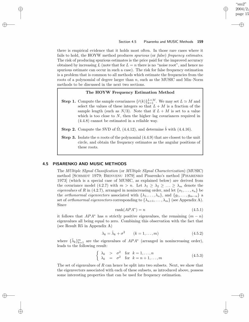
“sm2”2004/2/22page 159

i

i

i

i

i

i

i

i

Section 4.5 Pisarenko and MUSIC Methods 159

there is empirical evidence that it holds most often. In those rare cases where itfails to hold, the HOYW method produces spurious (or false) frequency estimates.The risk of producing spurious estimates is the price paid for the improved accuracyobtained by increasing L (note that for L = n there is no “noise root”, and hence nospurious estimate can occur in such a case). The risk for false frequency estimationis a problem that is common to all methods which estimate the frequencies from theroots of a polynomial of degree larger than n, such as the MUSIC and Min–Normmethods to be discussed in the next two sections.

The HOYW Frequency Estimation Method

Step 1. Compute the sample covariances r(k)L+Mk=1 . We may set L ' M and

select the values of these integers so that L + M is a fraction of thesample length (such as N/3). Note that if L + M is set to a valuewhich is too close to N , then the higher–lag covariances required in(4.4.8) cannot be estimated in a reliable way.

Step 2. Compute the SVD of Ω, (4.4.12), and determine b with (4.4.16).

Step 3. Isolate the n roots of the polynomial (4.4.9) that are closest to the unitcircle, and obtain the frequency estimates as the angular positions ofthese roots.

4.5 PISARENKO AND MUSIC METHODS

The MUltiple SIgnal Classification (or MUltiple SIgnal Characterization) (MUSIC)method [Schmidt 1979; Bienvenu 1979] and Pisarenko’s method [Pisarenko

1973] (which is a special case of MUSIC, as explained below) are derived fromthe covariance model (4.2.7) with m > n. Let λ1 ≥ λ2 ≥ . . . ≥ λm denote theeigenvalues of R in (4.2.7), arranged in nonincreasing order, and let s1, . . . , sn bethe orthonormal eigenvectors associated with λ1, . . . , λn, and g1, . . . , gm−n aset of orthonormal eigenvectors corresponding to λn+1, . . . , λm (see Appendix A).Since

rank(APA∗) = n (4.5.1)

it follows that APA∗ has n strictly positive eigenvalues, the remaining (m − n)eigenvalues all being equal to zero. Combining this observation with the fact that(see Result R5 in Appendix A)

λk = λk + σ2 (k = 1, . . . ,m) (4.5.2)

where λkmk=1 are the eigenvalues of APA∗ (arranged in nonincreasing order),leads to the following result:

λk > σ2 for k = 1, . . . , nλk = σ2 for k = n+ 1, . . . ,m

(4.5.3)

The set of eigenvalues of R can hence be split into two subsets. Next, we show thatthe eigenvectors associated with each of these subsets, as introduced above, possesssome interesting properties that can be used for frequency estimation.

“sm2”2004/2/22page 160

i

i

i

i

i

i

i

i


Let

S = [s1, . . . , sn] (m× n), G = [g1, . . . , gm−n] (m× (m− n)) (4.5.4)

From (4.2.7) and (4.5.3), we get at once:

RG = G

λn+1 0. . .

0 λm

= σ2G = APA∗G+ σ2G. (4.5.5)

The first equality in (4.5.5) follows from the definition of G and λkmk=n+1, thesecond equality follows from (4.5.3), and the third from (4.2.7). The last equalityin equation (4.5.5) implies that APA∗G = 0, or (as the matrix AP has full columnrank)

A∗G = 0 (4.5.6)

In other words, the columns gk of G belong to the null space of A∗, a fact whichis denoted by gk ∈ N (A∗). Since rank(A) = n, the dimension of N (A∗) is equal tom − n which is also the dimension of the range space of G, R(G). It follows fromthis observation and (4.5.6) that

R(G) = N (A∗) (4.5.7)

In words (4.5.7) says that the vectors gk span both R(G) and N (A∗). Now, sinceby definition

S∗G = 0 (4.5.8)

we also have R(G) = N (S∗); hence, N (S∗) = N (A∗). Since R(S) and R(A) arethe orthogonal complements to N (S∗) and N (A∗), it follows that

R(S) = R(A) (4.5.9)

We can also derive the equality (4.5.9) directly from (4.2.7). Set

Λ

=

λ1 − σ2 0. . .

0 λn − σ2

(4.5.10)

From

RS = S

λ1 0. . .

0 λn

= APA∗S + σ2S (4.5.11)

we obtainS = A

(

PA∗SΛ −1

)

(4.5.12)

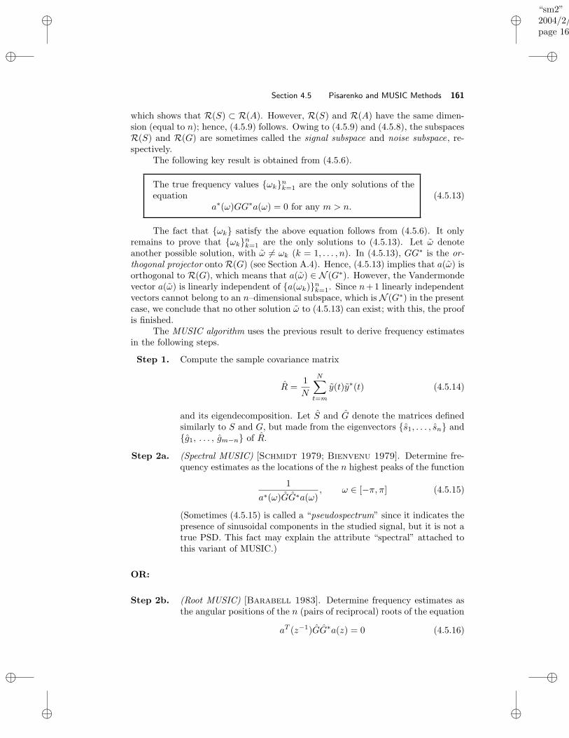
“sm2”2004/2/22page 161

i

i

i

i

i

i

i

i


which shows that R(S) ⊂ R(A). However, R(S) and R(A) have the same dimen-sion (equal to n); hence, (4.5.9) follows. Owing to (4.5.9) and (4.5.8), the subspacesR(S) and R(G) are sometimes called the signal subspace and noise subspace, re-spectively.

The following key result is obtained from (4.5.6).

The true frequency values ωknk=1 are the only solutions of theequation

a∗(ω)GG∗a(ω) = 0 for any m > n.(4.5.13)

The fact that ωk satisfy the above equation follows from (4.5.6). It onlyremains to prove that ωknk=1 are the only solutions to (4.5.13). Let ω denoteanother possible solution, with ω 6= ωk (k = 1, . . . , n). In (4.5.13), GG∗ is the or-thogonal projector onto R(G) (see Section A.4). Hence, (4.5.13) implies that a(ω) isorthogonal to R(G), which means that a(ω) ∈ N (G∗). However, the Vandermondevector a(ω) is linearly independent of a(ωk)nk=1. Since n+1 linearly independentvectors cannot belong to an n–dimensional subspace, which is N (G∗) in the presentcase, we conclude that no other solution ω to (4.5.13) can exist; with this, the proofis finished.

The MUSIC algorithm uses the previous result to derive frequency estimatesin the following steps.

Step 1. Compute the sample covariance matrix

R =1

N

N∑

t=m

y(t)y∗(t) (4.5.14)

and its eigendecomposition. Let S and G denote the matrices definedsimilarly to S and G, but made from the eigenvectors s1, . . . , sn andg1, . . . , gm−n of R.

Step 2a. (Spectral MUSIC) [Schmidt 1979; Bienvenu 1979]. Determine fre-quency estimates as the locations of the n highest peaks of the function

1

a∗(ω)GG∗a(ω), ω ∈ [−π, π] (4.5.15)

(Sometimes (4.5.15) is called a “pseudospectrum” since it indicates thepresence of sinusoidal components in the studied signal, but it is not atrue PSD. This fact may explain the attribute “spectral” attached tothis variant of MUSIC.)

OR:

Step 2b. (Root MUSIC) [Barabell 1983]. Determine frequency estimates asthe angular positions of the n (pairs of reciprocal) roots of the equation

aT (z−1)GG∗a(z) = 0 (4.5.16)

“sm2”2004/2/22page 162

i

i

i

i

i

i

i

i


which are located nearest the unit circle. In (4.5.16), a(z) stands forthe vector a(ω), (4.2.4), with eiω replaced by z, so

a(z) = [1, z−1, . . . , z−(m−1)]T

For m = n+1 (which is the minimum possible value) the MUSIC algorithm reducesto the Pisarenko method, which was the earliest proposal for an eigenanalysis–based(or subspace–based) method of frequency estimation [Pisarenko 1973].

The Pisarenko method is MUSIC with m = n+ 1 (4.5.17)

In the Pisarenko method, the estimated frequencies are determined from (4.5.16).For m = n + 1 this 2(m − 1)–degree equation can be reduced to the followingequation of degree m− 1 = n:

aT (z−1)g1 = 0 (4.5.18)

The Pisarenko frequency estimates are obtained as the angular positions of theroots of (4.5.18). The Pisarenko method is the simplest version of MUSIC froma computational standpoint. In addition, unlike MUSIC with m > n + 1, thePisarenko procedure does not have the problem of separating the “signal roots”from the “noise roots” (see the discussion on this point at the end of Section 4.4).However, it can be shown that the accuracy of the MUSIC frequency estimates in-creases significantly with increasing m. Hence, the price paid for the computationalsimplicity of the Pisarenko method may be a relatively poor statistical accuracy.

Regarding the selection of a value for m, this parameter may be chosen aslarge as possible, but not too close toN , in order to still allow a reliable estimation ofthe covariance matrix (for example, as in (4.5.14)). In some applications, the largestpossible value that may be selected for m may also be limited by computationalcomplexity considerations.

Whenever the tradeoff between statistical accuracy and computational com-plexity is an important issue, the following simple ideas may be valuable.

The finite–sample statistical accuracy of MUSIC frequency estimates may beimproved by modifying the covariance estimator (4.5.14). For instance, R is notToeplitz whereas the true covariance matrix R is. We may correct this situation byreplacing the elements in each diagonal of R with their average. The so–correctedsample covariance matrix can be shown to be the best (in the Frobenius–norm sense)Toeplitz approximation of R. Another modification of R, with the same purposeof improving the finite–sample statistical accuracy, is described in Section 4.8.

The computational complexity of MUSIC, for a given m, may be reduced invarious ways. Quite often, m is such that m − n > n. Then, the computationalburdens associated with both Spectral and Root MUSIC may be reduced by usingI − SS∗ in (4.5.15) or (4.5.16) in lieu of GG∗. (Note that SS∗ + GG∗ = I by thevery definition of the eigenvector matrices.) The computational burden of RootMUSIC may be further reduced as explained in the following. The polynomial in(4.5.16) is a self–reciprocal (or symmetric) one: its roots appear in reciprocal pairs(ρeiϕ, 1

ρeiϕ). On the unit circle z = eiω, (4.5.16) is nonnegative and hence may be

“sm2”2004/2/22page 163

i

i

i

i

i

i

i

i


interpreted as a PSD. Owing to the properties mentioned above, (4.5.16) can befactored as

aT (z−1)GG∗a(z) = α(z)α∗(1/z∗) (4.5.19)

where α(z) is a polynomial of degree (m−1) with all its zeroes located within or onthe unit circle. We may then determine the frequency estimates from the n roots ofα(z) that are closest to the unit circle. Since there are efficient numerical proceduresfor spectral factorization, determining α(z) as in (4.5.19) and then computing itszeroes is usually computationally more efficient than finding the (reciprocal) rootsof the 2(m− 1)–degree polynomial (4.5.16).

Finally, we address the issue of spurious frequency estimates. As implied bythe result (4.5.13), forN → ∞ there is no risk of obtaining false frequency estimates.However, in finite samples such a risk always exists. Usually, this risk is quite smallbut it may become a real problem ifm takes on large values. The key result on whichthe standard MUSIC algorithm, (4.5.15), is based can be used to derive a modifiedMUSIC which does not suffer from the spurious estimate problem. In the following,we only explain the basic ideas leading to the modified MUSIC method withoutgoing into details of its implementation (for such details, the interested reader mayconsult [Stoica and Sharman 1990]). Let cknk=1 denote the coefficients of thepolynomial A(z) defined in (4.2.3):

A(z) = 1 + c1z−1 + . . .+ cnz

−n =

n∏

k=1

(1 − eiωkz−1) (4.5.20)

Introduce the following matrix made from ck:

C∗ =

1 c1 . . . cn 0. . .

. . .. . .

0 1 c1 . . . cn

, (m− n) ×m (4.5.21)

It is readily verified that

C∗A = 0, (m− n) × n (4.5.22)

where A is defined in (4.2.4). Combining (4.5.9) and (4.5.22) gives

C∗S = 0, (m− n) × n (4.5.23)

which is the key property here. The matrix equation (4.5.23) can be rewritten inthe following form

φc = µ (4.5.24)

where the (m − n)n × n matrix φ and the (m − n)n × 1 vector µ are entirelydetermined from the elements of S, and where

c = [c1 . . . cn]T (4.5.25)

By replacing the elements of S in φ and µ by the corresponding entries of S, weobtain the sample version of (4.5.24)

φc ' µ (4.5.26)

“sm2”2004/2/22page 164

i

i

i

i

i

i

i

i


from which an estimate c of c may be obtained by an LS or TLS algorithm; seeSection A.8 for details. The frequency estimates can then be derived from the rootsof the estimated polynomial (4.5.20) corresponding to c. Since this polynomial hasa (minimal) degree equal to n, there is no risk for false frequency estimation.

4.6 MIN–NORM METHOD

MUSIC uses (m−n) linearly independent vectors in R(G) to obtain the frequencyestimates. Since any vector in R(G) is (asymptotically) orthogonal to a(ωk)nk=1

(cf. (4.5.7)), we may think of using only one such vector for frequency estima-tion. By doing so, we may achieve some computational saving, hopefully withoutsacrificing too much accuracy.

The Min–Norm method proceeds to estimate the frequencies along these lines[Kumaresan and Tufts 1983]. Let

[1g

]

=the vector in R(G), with first element equal to one,that has minimum Euclidean norm.

(4.6.1)

Then, the Min–Norm frequency estimates are determined as

(Spectral Min–Norm). The locations of the n highest peaks in thepseudospectrum

1∣∣∣∣a∗(ω)

[1g

]∣∣∣∣

2 (4.6.2)

or, alternatively,

(Root Min–Norm). The angular positions of the n roots of thepolynomial

aT (z−1)

[1g

]

that are located nearest the unit circle.

(4.6.3)

It remains to determine the vector in (4.6.1) and, in particular, to show thatits first element can always be normalized to one. We will later comment on thereason behind the specific selection (4.6.1) of a vector in R(G). In the following,the Euclidean norm of a vector is denoted by ‖ · ‖.

Partition the matrix S as

S =

[α∗

S

] 1 m− 1

(4.6.4)

As

[1g

]

∈ R(G), it must satisfy the equation

S∗[

1g

]

= 0 (4.6.5)

“sm2”2004/2/22page 165

i

i

i

i

i

i

i

i

Section 4.6 Min–Norm Method 165

which, using (4.6.4), can be rewritten as

S∗g = −α (4.6.6)

The minimum–norm solution to (4.6.6) is given by (see Result R31 in Appendix A):

g = −S(S∗S)−1α (4.6.7)

assuming that the inverse exists. Noting that

I = S∗S = αα∗ + S∗S (4.6.8)

and also that one eigenvalue of I − αα∗ is equal to 1 − ‖α‖2 and the remaining(n − 1) eigenvalues of I − αα∗ are equal to 1, it follows that the inverse in (4.6.7)exists if and only if

‖α‖2 6= 1 (4.6.9)

If the above condition is not satisfied, there will be no vector of the form of (4.6.1)in R(G). We postpone the study of (4.6.9) until we obtain a final–form expressionfor g.

Under the condition (4.6.9), a simple calculation shows that

(S∗S)−1α = (I − αα∗)−1α = α/(1 − ‖α‖2) (4.6.10)


g = −Sα/(1 − ‖α‖2) (4.6.11)

which expresses g as a function of the elements of S.We can also obtain g as a function of the entries in G. To do so, partition G

as

G =

[β∗

G

]

(4.6.12)

Since SS∗ = I − GG∗ by the definition of the matrices S and G, it follows that[

‖α‖2 (Sα)∗

Sα SS∗

]

=

[1 − ‖β‖2 −(Gβ)∗

−Gβ I − GG∗

]

(4.6.13)

Comparing the blocks in (4.6.13) makes it possible to express ‖α‖2 and Sα asfunctions of G and β, which leads to the following equivalent expression for g:

g = Gβ/‖β‖2 (4.6.14)

If m − n > n, then it is computationally more advantageous to obtain g from(4.6.11); otherwise, (4.6.14) should be used.

Next, we return to the condition (4.6.9) that is implicitly assumed to holdin the previous derivations. As already mentioned, this condition is equivalent torank(S∗S) = n which, in turn, holds if and only if

rank(S) = n (4.6.15)

“sm2”2004/2/22page 166

i

i

i

i

i

i

i

i


Now, it follows from (4.5.9) that any block of S made from more than n consec-utive rows should have rank equal to n. Hence, (4.6.15) must hold at least for Nsufficiently large. With this observation, the derivation of the Min–Norm frequencyestimator is complete.

The statistical accuracy of the Min–Norm method is similar to that corre-sponding to MUSIC. Hence, Min–Norm achieves MUSIC’s performance at a re-duced computational cost. It should be noted that the selection (4.6.1) of thevector in R(G), used in the Min–Norm algorithm, is critical in obtaining frequencyestimates with satisfactory statistical accuracy. Other choices of vectors in R(G)may give rather poor accuracy. In addition, there is empirical evidence that theuse of the minimum–norm vector in R(G), as in (4.6.1), may decrease the risk ofspurious frequency estimates compared with other vectors in R(G) or even withMUSIC (see Complement 6.5.1 for details on this aspect).

4.7 ESPRIT METHOD

LetA1 = [Im−1 0]A (m− 1) × n (4.7.1)

andA2 = [0 Im−1]A (m− 1) × n (4.7.2)

where Im−1 is the identity matrix of dimension (m − 1) × (m − 1) and [Im−1 0]and [0 Im−1] are (m− 1) ×m. It is readily verified that

A2 = A1D (4.7.3)

where

D =

e−iω1 0. . .

0 e−iωn

(4.7.4)

Since D is a unitary matrix, the transformation in (4.7.3) is a rotation. ES-PRIT, i.e., Estimation of Signal Parameters by Rotational Invariance Techniques([Paulraj, Roy, and Kailath 1986; Roy and Kailath 1989]; see also [Kung,

Arun, and Rao 1983]), relies on the rotational transformation (4.7.3) as we detailbelow.

Similarly to (4.7.1) and (4.7.2), define

S1 = [Im−1 0]S (4.7.5)

S2 = [0 Im−1]S (4.7.6)

From (4.5.12), we have thatS = AC (4.7.7)

where C is the n× n nonsingular matrix given by

C = PA∗SΛ −1 (4.7.8)

(Observe that both S and A in (4.7.7) have full column rank, and hence C mustbe nonsingular; see Result R2 in Appendix A). The above explicit expression for C

“sm2”2004/2/22page 167

i

i

i

i

i

i

i

i

Section 4.7 ESPRIT Method 167

actually has no relevance to the present discussion. It is only (4.7.7), and the factthat C is nonsingular, that counts.

By using (4.7.1)–(4.7.3) and (4.7.7), we can write

S2 = A2C = A1DC = S1C−1DC = S1φ (4.7.9)

where

φ , C−1DC (4.7.10)

Owing to the Vandermonde structure of A, the matrices A1 and A2 have full columnrank (equal to n). In view of (4.7.7), S1 and S2 must also have full column rank.It then follows from (4.7.9) that the matrix φ is uniquely given by

φ = (S∗1S1)

−1S∗1S2 (4.7.11)

This formula expresses φ as a function of some quantities which can be estimatedfrom the available sample. The importance of being able to estimate φ stems fromthe fact that φ and D have the same eigenvalues. (This can be seen from theequation (4.7.10), which is a similarity transformation relating φ and D, alongwith Result R6 in Appendix A.)

ESPRIT uses the previous observations to determine frequency estimates asdescribed next.

ESPRIT estimates the frequencies ωknk=1 as − arg(νk), whereνknk=1 are the eigenvalues of the following (consistent) estimateof the matrix φ:

φ = (S∗1 S1)

−1S∗1 S2

(4.7.12)

It should be noted that the above estimate of φ is implicitly obtained bysolving the following linear system of equations:

S1φ ' S2 (4.7.13)

by an LS method. It has been empirically observed that better finite–sample accu-racy may be achieved if (4.7.13) is solved for φ by a Total LS method (see Section A.8and [Van Huffel and Vandewalle 1991] for discussions on the TLS approach).

The statistical accuracy of ESPRIT is similar to that of the previously de-scribed methods: HOYW, MUSIC and Min–Norm. In fact, in most cases, ESPRITmay provide slightly more accurate frequency estimates than the other methodsmentioned above; and this at similar computational cost. In addition, unlike theseother methods, ESPRIT has no problem with separating the “signal roots” fromthe “noise roots”, as can be seen from (4.7.12). Note that this property is sharedby the modified MUSIC method (discussed in Section 4.5); however, in many casesESPRIT outperforms modified MUSIC in terms of statistical accuracy. All theseconsiderations recommend ESPRIT as the first choice in a frequency estimationapplication.

“sm2”2004/2/22page 168

i

i

i

i

i

i

i

i


4.8 FORWARD–BACKWARD APPROACH

The previously described eigenanalysis–based methods (MUSIC, Min–Norm andESPRIT) derive their frequency estimates from the eigenvectors of the sample co-variance matrix R, (4.5.14), which is restated here for easy reference:

R =1

N

N∑

t=m

y(t)...

y(t−m+ 1)

[y∗(t) . . . y∗(t−m+ 1)] (4.8.1)

The R above is recognized to be the matrix that appears in the least squares (LS)estimation of the coefficients αk of an mth–order forward linear predictor ofy∗(t+ 1):

y∗(t+ 1) = α1y∗(t) + . . .+ αmy

∗(t−m+ 1) (4.8.2)

For this reason, the methods which obtain frequency estimates from R are namedforward (F) approaches.

Extensive numerical experience with the aforementioned methods has shownthat the corresponding frequency estimation accuracy can be enhanced by usingthe following modified sample covariance matrix, in lieu of R,

R =1

2(R+ JRTJ) (4.8.3)

where

J =

0 1. .

.

1 0

(4.8.4)

is the so–called “exchange” (or “reversal”) matrix. The second term in (4.8.3) hasthe following detailed form:

JRTJ =1

N

N∑

t=m

y∗(t−m+ 1)...

y∗(t)

[y(t−m+ 1) . . . y(t)] (4.8.5)

The matrix (4.8.5) is the one that appears in the LS estimate of the coefficients ofan mth–order backward linear predictor of y(t−m):

y(t−m) = µ1y(t−m+ 1) + . . .+ µmy(t) (4.8.6)

This observation, along with the previous remark made about R, suggests thename of forward–backward (FB) approaches for methods that determine frequencyestimates from R in (4.8.3).

The (i, j) element of R is given by:

Ri,j =1

2N

N∑

t=m

[y(t− i)y∗(t− j) + y∗(t−m+ 1 + i)y(t−m+ 1 + j)]

, T1 + T2 (i, j = 0, . . . ,m− 1) (4.8.7)

“sm2”2004/2/22page 169

i

i

i

i

i

i

i

i

Section 4.8 Forward–Backward Approach 169

Assume that i ≤ j (the other case i ≥ j can be similarly treated). Let r(j − i)denote the usual sample covariance:

r(j − i) =1

N

N∑

t=(j−i)+1

y(t)y∗(t− (j − i)) (4.8.8)

A straightforward calculation shows that the two terms T1 and T2 in (4.8.7) can bewritten as

T1 =1

2N

N−i∑

p=m−iy(p)y∗(p− (j − i)) =

1

2r(j − i) + O(1/N) (4.8.9)

and

T2 =1

2N

N−m+j+1∑

p=j+1

y(p)y∗(p− (j − i)) =1

2r(j − i) + O(1/N) (4.8.10)

where O(1/N) denotes a term that tends to zero as 1/N when N increases (it ishere assumed that m N). It follows from (4.8.7)–(4.8.10) that, for large N , thedifference between Ri,j or Ri,j and the sample covariance lag r(j − i) is “small”.

Hence, the frequency estimation methods based on R or R (or on [r(j − i)]) maybe expected to have similar performances in large samples.

In summary, it follows from the previous discussion that the empirically ob-served performance superiority of the forward–backward approach over the forward–only approach should only be manifest in samples with relatively small lengths. Assuch, this superiority cannot be easily established by theoretical means. Let usthen argue heuristically.

First, note that the transformation J(.)TJ is such that the following equalitieshold:

(R)i,j = (JRJ)m−i,m−j = (JRTJ)m−j,m−i (4.8.11)

and(R)m−j,m−i = (JRTJ)i,j (4.8.12)

This implies that the (i, j) and (m− j,m− i) elements of R are both given by

Ri,j = Rm−j,m−i =1

2(Ri,j + Rm−j,m−i) (4.8.13)

Equations (4.8.11)–(4.8.12) imply that R is invariant to the transformation J(.)TJ :

JRTJ = R (4.8.14)

Such a matrix is said to be persymmetric (also called centrosymmetric). In orderto see the reason for this name, note that R is Hermitian (symmetric in the real–valued case) with respect to its main diagonal; in addition, R is symmetric aboutits main antidiagonal. Indeed, the equal elements Ri,j and Rm−j,m−i of R belongto the same diagonal as i − j = (m − j) − (m − i). They are also symmetrically

“sm2”2004/2/22page 170

i

i

i

i

i

i

i

i


placed with respect to the main antidiagonal; Ri,j lies on antidiagonal (i + j),

Rm−j,m−i on the [2m − (j + i)]th one, and the main antidiagonal is the mth one(and m = [(i+ j) + 2m− (i+ j)]/2).

The theoretical (and unknown) covariance matrix R is Toeplitz and hencepersymmetric. Since R is persymmetric like R, whereas R is not, we may expectR to be a better estimate of R than R. In turn, this means that the frequencyestimates derived from R are likely to be more accurate than those obtained fromR.

The impact of enforcing the persymmetric property can be seen by examining,say, the (1, 1) and (m,m) elements of R and R. Both the (1,1) and (m,m) elementsof R are estimates of r(0); however, the (1,1) element does not use the first (m− 1)lag products |y(1)|2, . . . , |y(m− 1)|2, and the (m,m) element does not use the last(m−1) lag products |y(N −m+2)|2, . . . , |y(N)|2. If N m, the omission of theselag products is negligible; for small N , however, this omission may be significant.On the other hand, all lag products of y(t) are used to form the (1, 1) and (m,m)elements of R, and in general the (i, j) element of R uses more lag products of y(t)than the corresponding element of R. For more details on the FB approach, we referthe reader to, e.g., [Rao and Hari 1993; Pillai 1989]; see also Complement 6.5.8.

Finally, the reader might wonder why we do not replace R by a Toeplitzestimate, obtained for example by averaging the elements along each diagonal of R.This Toeplitz estimate would at first seem to be a better approximation of R thaneither R or R. The reason why we do not “Toeplitz–ize” R or R is that for finiteN , and infinite signal–to–noise ratio (σ2 → 0), the use of either R or R gives exactfrequency estimates, whereas the Toeplitz–averaged approximation of R does not.As σ2 → 0, both R and R have rank n, but the Toeplitz–averaged approximationof R has full rank in general.

4.9 COMPLEMENTS

4.9.1 Mean Square Convergence of Sample Covariances for Line Spectral Processes

In this complement we prove that

limN→∞

r(k) = r(k) (in a mean square sense) (4.9.1)

(that is, limN→∞E|r(k) − r(k)|2

= 0 ). The above result has already been

referred to in Section 4.4, in the discussion on the rank properties of Ω and Ω. It isalso the basic result from which the consistency of all covariance–based frequencyestimators discussed in this chapter can be readily concluded. Note that a signaly(t) satisfying (4.9.1) is said to be second–order ergodic (see [Soderstrom and

Stoica 1989; Brockwell and Davis 1991] for a more detailed discussion of theergodicity property).

“sm2”2004/2/22page 171

i

i

i

i

i

i

i

i



r(k) =1

N

N∑

t=k+1

[x(t) + e(t)][x∗(t− k) + e∗(t− k)]

=1

N

N∑

t=k+1

[x(t)x∗(t− k) + x(t)e∗(t− k) + e(t)x∗(t− k)

+e(t)e∗(t− k)] , T1 + T2 + T3 + T4 (4.9.2)

The limit of T1 is found as follows. First note that:

limN→∞

E|T1 − rx(k)|2

= lim

N→∞

1

N2

N∑

t=k+1

N∑

s=k+1

E x(t)x∗(t− k)x∗(s)x(s− k)

−(

2

N

N∑

t=k+1

|rx(k)|2)

+ |rx(k)|2

= limN→∞

1

N2

N∑

t=k+1

N∑

s=k+1

E x(t)x∗(t− k)x∗(s)x(s− k)

−|rx(k)|2

Now,

E x(t)x∗(t− k)x∗(s)x(s− k) =

n∑

p=1

n∑

j=1

n∑

l=1

n∑

m=1

apajalamei(ωp−ωj)tei(ωm−ωl)s

·ei(ωj−ωm)kEeiϕpe−iϕjeiϕme−iϕl

=

n∑

p=1

n∑

j=1

n∑

l=1

n∑

m=1

apajalamei(ωp−ωj)tei(ωm−ωl)s

·ei(ωj−ωm)k (δp,jδm,l + δp,lδm,j − δp,jδm,lδp,m)

where the last equality follows from the assumed independence of the initial phasesϕk. Combining the results of the above two calculations yields:

limN→∞

E|T1 − rx(k)|2

= lim

N→∞

1

N2

N∑

t=k+1

N∑

s=k+1

n∑

p=1

n∑

m=1

a2pa

2me

i(ωp−ωm)k

+

n∑

p=1

n∑

m=1

a2pa

2me

i(ωp−ωm)(t−s) −n∑

p=1

a4p

− |rx(k)|2

=

n∑

p=1

n∑

m=1m6=p

a2pa

2m limN→∞

1

N2

N∑

τ=−N(N − |τ |)ei(ωp−ωm)τ

= 0 (4.9.3)

It follows that T1 converges to r(k) (in the mean square sense) as N tends to infinity.

“sm2”2004/2/22page 172

i

i

i

i

i

i

i

i


The limits of T2 and T3 are equal to zero, as shown below for T2; the proof forT3 is similar. Using the fact that x(t) and e(t) are by assumption independentrandom signals, we get

E|T2|2

=

1

N2

N∑

t=k+1

N∑

s=k+1

E x(t)e∗(t− k)x∗(s)e(s− k)

=σ2

N2

N∑

t=k+1

N∑

s=k+1

E x(t)x∗(s) δt,s

=σ2

N2

N∑

t=k+1

E|x(t)|2

=

(N − k)σ2

N2E|x(t)|2

(4.9.4)

which tends to zero, as N → ∞. Hence, T2 (and, similarly, T3) converges to zeroin the mean square sense.

The last term, T4, in (4.9.2) converges to σ2δk,0 by the “law of large numbers”(see [Soderstrom and Stoica 1989; Brockwell and Davis 1991]). In fact,it is readily verified, at least under the Gaussian hypothesis, that

E|T4 − σ2δk,0|2

=

1

N2

N∑

t=k+1

N∑

s=k+1

E e(t)e∗(t− k)e∗(s)e(s− k)

−σ2δk,0

1

N

N∑

t=k+1

E e(t)e∗(t− k) + e∗(t)e(t− k)

+σ4δk,0

=1

N2

N∑

t=k+1

N∑

s=k+1

[σ4δk,0 + σ4δt,s]

−2σ4δk,01

N

N∑

t=k+1

(δk,0) + σ4δk,0

→ σ4δk,0 − 2σ4δk,0 + σ4δk,0 = 0 (4.9.5)

Hence, T4 converges to σ2δk,0 in the mean square sense if e(t) is Gaussian. It canbe shown using the law of large numbers that T4 → σ2δk,0 in the mean square senseeven if e(t) is non–Gaussian, as long as the fourth–order moment of e(t) is finite.

Next, observe that since, for example, E|T2|2 and E|T3|2 converge tozero, then ET2T

∗3 also converges to zero (as N → ∞); this is so because

|E T2T∗3 | ≤

[E|T2|2

E|T3|2

]1/2

With this observation, the proof of (4.9.1) is complete.

4.9.2 The Caratheodory Parameterization of a Covariance Matrix

The covariance matrix model in (4.2.7) is more general than it might appear atfirst sight. We show that for any given covariance matrix R = r(i − j)mi,j=1,

“sm2”2004/2/22page 173

i

i

i

i

i

i

i

i


there exist n ≤ m, σ2 and ωk, αknk=1 such that R can be written as in (4.2.7).Equation (4.2.7), associated with an arbitrary given covariance matrix R, is namedthe Caratheodory parameterization of R.

Let σ2 denote the minimum eigenvalue of R. As σ2 is not necessarily unique,let n denote its multiplicity and set n = m− n. Define

Γ = R− σ2I

The matrix Γ is positive semidefinite and Toeplitz and, hence, must be the covari-ance matrix associated with a stationary signal, say y(t):

Γ = E

y(t)...

y(t−m+ 1)

[y∗(t) . . . y∗(t−m+ 1)]

By definition,rank(Γ) = n (4.9.6)

which implies that there must exist a linear combination between y(t), . . . , y(t−n)for all t. Moreover, both y(t) and y(t−n) must appear with nonzero coefficients inthat linear combination (otherwise either y(t) . . . y(t−n+1) or y(t−1) . . . y(t−n) would be linearly related, and rank(Γ) would be less than n, which wouldcontradict (4.9.6)). Hence y(t) obeys the following homogeneous AR equation:

B(z)y(t) = 0 (4.9.7)

where z−1 is the unit delay operator, and

B(z) = 1 + b1z−1 + · · · + bnz

−n

with bn 6= 0. Let φ(ω) denote the PSD of y(t). Then we have the followingequivalences:

B(z)y(t) = 0 ⇐⇒∫ π

−π|B(ω)|2 φ(ω) dω = 0

⇐⇒ |B(ω)|2 φ(ω) = 0

⇐⇒ If φ(ω) > 0 then B(ω) = 0⇐⇒ φ(ω) > 0 for at most n values of ω

Furthermore,

y(t), . . . y(t− n+ 1) are linearly independent⇐⇒

E|g0y(t) + . . .+ gn−1y(t− n+ 1)|2

> 0 for every [g0 . . . gn−1]

T 6= 0

⇐⇒∫ π

−π |G(ω)|2 φ(ω) dω > 0 for every G(z) =∑n−1k=0 gkz

−k 6= 0

⇐⇒ φ(ω) > 0 for at least n distinct values of ω

It follows from the two results above that φ(ω) > 0 for exactly n distinct values ofω. Furthermore, the values of ω for which φ(ω) > 0 are given by the n roots of the

“sm2”2004/2/22page 174

i

i

i

i

i

i

i

i


equation B(ω) = 0. A signal y(t) with such a PSD consists of a sum of n sinusoidalcomponents with an m×m covariance matrix given by

Γ = APA∗ (4.9.8)

(cf. (4.2.7)). In (4.9.8), the frequencies ωknk=1 are defined as indicated above, andcan be found from Γ using any of the subspace–based frequency estimation methodsin this chapter. Once ωk are available, α2

i can be determined from Γ. (Showthat.) By combining the additive decomposition R = Γ+σ2I and (4.9.8) we obtain(4.2.7). With this observation, the derivation of the Caratheodory parameterizationis complete.

It is interesting to note that the sinusoids–in–noise signal which “realizes”a given covariance sequence r(0), . . . , r(m) (as described above) also provides apositive definite extension of that sequence. More precisely, the covariance lagsr(m + 1), r(m + 2), . . . derived from the sinusoidal signal equation, when ap-pended to r(0), . . . , r(m), provide a positive definite covariance sequence of in-finite length. The AR covariance realization is the other well–known method forobtaining a positive definite extension of a given covariance sequence of finite length(see Complement 3.9.2).

4.9.3 Using the Unwindowed Periodogram for Sine Wave Detection in White Noise

As shown in Section 4.3, the unwindowed periodogram is an accurate frequency es-timation method whenever the minimum frequency separation is larger than 1/N .A simple intuitive explanation as to why the unwindowed periodogram is a betterfrequency estimator than the windowed periodogram(s) is as follows. The principaleffect of a window is to remove the tails of the sample covariance sequence fromthe periodogram formula; while this is appropriate for signals whose covariancesequence “rapidly” goes to zero, it is inappropriate for sinusoidal signals whosecovariance sequence never dies out (for sinusoidal signals, the use of a window isexpected to introduce a significant bias in the estimated spectrum). Note, however,that if the data contains sinusoidal components with significantly different ampli-tudes, then it may be advisable to use a (mildly) windowed periodogram. Thiswill induce bias in the frequency estimates, but, on the other hand, will reduce theleakage and hence make it possible to detect the low–amplitude components.

When using the (unwindowed) periodogram for frequency estimation, an im-portant problem is to infer whether any of the many peaks of the erratic peri-odogram plot can really be associated with the existence of a sinusoidal componentin the data. In order to be more precise, consider the following two hypotheses.

H0: the data consists of (complex circular Gaussian) white noise only (with un-known variance σ2).

H1: the data consists of a sum of sinusoidal components and noise.

Deciding between H0 and H1 constitutes the so–called (signal) detection prob-lem. A solution to the detection problem can be obtained as follows. From the cal-culations leading to the result (2.4.21) one can see that the normalized periodogram

“sm2”2004/2/22page 175

i

i

i

i

i

i

i

i


values in (4.9.15) are independent random variables (under H0). It remains to de-rive their distribution. Let

εr(ω) =

√2

σ√N

N∑

t=1

Re[e(t)e−iωt]

εi(ω) =

√2

σ√N

N∑

t=1

Im[e(t)e−iωt]

With this notation and under the null hypothesis H0,

2φp(ω)/σ2 = ε2r(ω) + ε2i (ω) (4.9.9)

For any two complex scalars z1 and z2 we have

Re(z1) Im(z2) =z1 + z∗

1

2

z2 − z∗2

2i=

1

2Im (z1z2 + z∗

1z2) (4.9.10)

and, similarly,

Re(z1) Re(z2) =1

2Re(z1z2 + z∗

1z2) (4.9.11)

Im(z1) Im(z2) =1

2Re(−z1z2 + z∗

1z2) (4.9.12)

By making use of (4.9.10)–(4.9.12), we can write

E εr(ω)εi(ω) =1

σ2NIm

N∑

t=1

N∑

s=1

E

e(t)e(s)e−iω(t+s) + e∗(t)e(s)eiω(t−s)

= Im1 = 0

Eε2r(ω)

=

1

σ2NRe

N∑

t=1

N∑

s=1

E

e(t)e(s)e−iω(t+s) + e∗(t)e(s)eiω(t−s)

= Re1 = 1 (4.9.13)

Eε2i (ω)

=

1

σ2NRe

N∑

t=1

N∑

s=1

E

−e(t)e(s)e−iω(t+s) + e∗(t)e(s)eiω(t−s)

= Re1 = 1 (4.9.14)

In addition, note that the random variables εr(ω) and εi(ω) are zero–mean Gaussiandistributed because they are linear transformations of the Gaussian white noisesequence. Then, it follows that under H0

The random variables

2φp(ωk)/σ2Nk=1,

with mink 6=j |ωk − ωj | ≥ 2π/N , are asymptotically independentand χ2 distributed with 2 degrees of freedom.

(4.9.15)

“sm2”2004/2/22page 176

i

i

i

i

i

i

i

i


(See, e.g., [Priestley 1981] and [Soderstrom and Stoica 1989] for the defini-tion and properties of the χ2 distribution.) It is worth noting that if ωk are equalto the Fourier frequencies 2πk/NN−1

k=0 , then the previous distributional result isexactly valid (i.e., it holds in samples of finite length; see, for example, equation(2.4.26)). However, this observation is not as important as it might seem at firstsight, since σ2 in (4.9.15) is unknown. When the noise power in (4.9.15) is replacedby a consistent estimate σ2, the so–obtained normalized periodogram values

2φp(ωk)/σ2 (4.9.16)

are χ2(2) distributed only asymptotically (for N 1). A consistent estimate of σ2

can be obtained as follows. From (4.9.9), (4.9.13), and (4.9.14) we have that underH0

E

φp(ωk)

= σ2 for k = 1, 2, . . . , N

Since φp(ωk)Nk=1 are independent random variables, a consistent estimate of σ2

is given by

σ2 =1

N

N∑

k=1

φp (ωk)

Inserting this expression for σ2 into (4.9.16) leads to the following “test statistic”:

µk =2Nφp(ωk)N∑

k=1

φp(ωk)

In accordance with the (asymptotic) χ2 distribution of µk, we have (for any givenc ≥ 0; see, e.g., [Priestley 1981]):

Pr(µk ≤ c) =

∫ c

0

1

2e−x/2 dx = 1 − e−c/2. (4.9.17)

Let

µ = maxk

[µk]

Using (4.9.17) and the fact that µk are independent random variables, gives (forany c ≥ 0):

Pr(µ > c) = 1 − Pr(µ ≤ c)

= 1 − Pr(µk ≤ c for all k)

= 1 − (1 − e−c/2)N (under H0)

“sm2”2004/2/22page 177

i

i

i

i

i

i

i

i


This result can be used to set a bound on µ that, under H0, holds with a (high)preassigned probability 1 − α (say). More precisely, let α be given (e.g., α = 0.05)and solve for c from the equation

(1 − e−c/2)N = 1 − α

Then

• If µ ≤ c, accept H0 with an unknown risk. (That riskdepends on the signal–to–noise ratio (SNR). The lower theSNR, the larger the risk of accepting H0 when it does nothold.)

• If µ > c, reject H0 with a risk equal to α.

It should be noted that whenever H0 is rejected by the above test, what wecan really infer is that the periodogram peak in question is significant enough tomake the existence of a sinusoidal component in the studied data highly probable.However, the previous test does not tell us the number of sinusoidal componentsin the data. In order to determine that number, the test should be continued bylooking at the second highest peak in the periodogram. For a test of the significanceof the second highest value of the periodogram, and so on, we refer to [Priestley

1981].

Finally, we note that in addition to the test presented in this complement,there are several other tests to decide between the hypotheses H0 and H1 above;see [Priestley 1997] for a review.

4.9.4 NLS Frequency Estimation for a Sinusoidal Signal with Time-Varying Amplitude

Consider the sinusoidal data model in (4.1.1) for the case of a single component(n = 1) but with a time-varying amplitude:

y(t) = α(t)ei(ωt+ϕ) + e(t), t = 1, . . . , N (4.9.18)

where α(t) ∈ R is an arbitrary unknown envelope modulating the sinusoidal signal.The NLS estimates of α(t), ω, and ϕ are obtained by minimizing the followingcriterion:

f =

N∑

t=1

∣∣∣y(t) − α(t)ei(ωt+ϕ)

∣∣∣

2

(cf. (4.3.1)). In this complement we show that the above seemingly complicatedminimization problem has in fact a simple solution. We also discuss briefly an FFT-based algorithm for computing that solution. The reader interested in more detailson the topic of this complement can consult [Besson and Stoica 1999; Stoica,

Besson, and Gershman 2001] and references therein.

“sm2”2004/2/22page 178

i

i

i

i

i

i

i

i


A straightforward calculation shows that:

f =

N∑

t=1

∣∣y(t)

∣∣2

+[

α(t) − Re(

e−i(ωt+ϕ)y(t))]2

−[

Re(


(4.9.19)The minimization of (4.9.19) with respect to α(t) is immediate:

α(t) = Re(

e−i(ωt+ϕ)y(t))

(4.9.20)

where the NLS estimates ω and ϕ are yet to be determined. Inserting (4.9.20) into(4.9.19) shows that the NLS estimates of ϕ and ω are obtained by maximizing thefunction

g = 2

N∑

t=1

[

Re(


where the factor 2 has been introduced for the sake of convenience. For any complexnumber c we have

[Re(c)]2

=1

4(c+ c∗)2 =

1

2

[|c|2 + Re

(c2)]

It follows that

g =

N∑

t=1

|y(t)|2 + Re[

e−2i(ωt+ϕ)y2(t)]

= constant +

∣∣∣∣∣

N∑

t=1

y2(t)e−i2ωt

∣∣∣∣∣· cos

[

arg

(N∑

t=1

y2(t)e−i2ωt)

− 2ϕ

]

(4.9.21)

Clearly the maximizing ϕ is given by

ϕ =1

2arg

(N∑

t=1

y2(t)e−i2ωt)

with the NLS estimate of ω given by

ω = arg maxω

∣∣∣∣∣

N∑

t=1

y2(t)e−i2ωt

∣∣∣∣∣

(4.9.22)

It is important to note that the maximization in (4.9.22) should be conductedover [0, π] instead of over [0, 2π]; indeed, the function in (4.9.22) is periodic with aperiod equal to π. The restriction of ω to [0, π] is not a peculiar feature of the NLSapproach, but rather it is a consequence of the generality of the problem consideredin this complement. This is easily seen by making the substitution ω → ω + π in(4.9.18), which yields

y(t) = α(t)ei(ωt+ϕ) + e(t), t = 1, . . . , N

“sm2”2004/2/22page 179

i

i

i

i

i

i

i

i


where α(t) = (−1)tα(t) is another valid (i.e., real-valued) envelope. This simplecalculation confirms the fact that ω is uniquely identifiable only in the interval[0, π]. In applications, the frequency can be made to belong to [0, π] by using asufficiently small sampling period.

The above estimate of ω should be contrasted with the NLS estimate of ω inthe constant-amplitude case (see (4.3.11), (4.3.17)):

ω = arg maxω

∣∣∣∣∣

N∑

t=1

y(t)e−iωt

∣∣∣∣∣

(for α(t) = constant) (4.9.23)

There is a striking similarity between (4.9.22) and (4.9.23); the only differencebetween these equations is the squaring of the terms in (4.9.22). As a consequence,we can apply the FFT to the squared data sequence y2(t) to obtain the ω in(4.9.22).

The reader may wonder if there is an intuitive reason for the occurrence of thesquared data in (4.9.22). A possible way to explain this occurrence goes as follows.Assume that α(t) has zero average value. Hence the DFT of α(t), denoted A(ω),takes on small values (theoretically zero) at ω = 0. As the DFT of α(t)eiωt isA(ω−ω), it follows that the modulus of this DFT has a valley instead of a peak atω = ω, and hence the standard periodogram (see (4.9.23)) should not be used todetermine ω. On the other hand, α2(t) always has a nonzero average value (or DCcomponent), and hence the modulus of the DFT of α2(t)ei2ωt will typically havea peak at ω = 2ω. This observation provides an heuristic reason for the squaringoperation in (4.9.22).

4.9.5 Monotonically Descending Techniques for Function Minimization

As explained in Section 4.3, minimizing the NLS criterion with respect to theunknown frequencies is a rather difficult task owing to the existence of possiblymany local minima and the sharpness of the global minimum. In this complement1

we will discuss a number of methods that can be used to solve such a minimizationproblem. Our discussion is quite general and applies to many other functions, notto just the NLS criterion that is used as an illustrating example in what follows.

We will denote the function to be minimized by f(θ), where θ is a vector.Sometimes we will write this function as f(x, y) where [xT , yT ]T = θ. The al-gorithms for minimizing f(θ) discussed in this complement are iterative. We letθi denote the value taken by θ at the ith iteration (and similarly for x and y).The common feature of the algorithms included in this complement is that they allmonotonically decrease the function at each iteration:

f(θi+1) ≤ f(θi) for i = 0, 1, 2, . . . (4.9.24)

Hereafter θ0 denotes the initial value (or estimate) of θ used by the minimizationalgorithm in question. Clearly (4.9.24) is an appealing property which in effect is the

1Based on “Cyclic minimizers, majorization techniques, and the expectation-maximizationalgorithm: A refresher,” by P. Stoica and Y. Selen, IEEE Signal Processing Magazine, 21(1),January, 2004, pp. 112–114.

“sm2”2004/2/22page 180

i

i

i

i

i

i

i

i


main reason for the interest in the algorithms discussed here. However, we shouldnote that usually (4.9.24) can only guarantee the convergence to a local minimumof f(θ). The goodness of the initial estimate θ0 will often determine whether thealgorithm will converge to the global minimum. In fact, for some of the algorithmsdiscussed below not even the convergence to a local minimum is guaranteed. Forexample, the EM algorithm (discussed later in this complement) can converge tosaddle points or local maxima (see, e.g., [McLachlan and Krishnan 1997]).However, such a behavior is rare in applications, provided that some regularityconditions are satisfied.

Cyclic Minimizer

To describe the main idea of this type of algorithm in its simplest form, let uspartition θ into two subvectors:

θ =

[xy

]

Then the generic iteration of a cyclic algorithm for minimizing f(x, y) will havethe following form:

y0 = given

For i = 1, 2, . . . compute:

xi = arg minxf(x, yi−1)

yi = arg minyf(xi, y)

(4.9.25)

Note that (4.9.25) alternates (or cycles) between the minimization of f(x, y) withrespect to x for given y and the minimization of f(x, y) with respect to y for givenx, and hence the name of “cyclic” given to this type of algorithm. An obviousmodification of (4.9.25) allows us to start with x0, if so desired. It is readilyverified that the cyclic minimizer (4.9.25) possesses the property (4.9.24):

f(xi, yi) ≤ f(xi, yi−1) ≤ f(xi−1, yi−1)

where the first inequality follows from the definition of yi and the second from thedefinition of xi.

The partitioning of θ into subvectors is usually done in such a way that theminimization operations in (4.9.25) (or at least one of them) are “easy” (in anycase, easier than the minimization of f jointly with respect to x and y). Quiteoften, to achieve this desired property we need to partition θ in more than twosubvectors. The extension of (4.9.25) to such a case is straightforward and will notbe discussed here. However, there is one point about this extension that we wouldlike to make briefly: whenever θ is partitioned into three or more subvectors wecan choose the way in which the various minimization subproblems are iterated.For instance, if θ = [xT , yT , zT ]T then we may iterate the minimization steps withrespect to x and with respect to y a number of times (with z being fixed), beforere-determining z, and so forth.

“sm2”2004/2/22page 181

i

i

i

i

i

i

i

i


With reference to the NLS problem in Section 4.3, we can apply the aboveideas to the following natural partitioning of the parameter vector:

θ =

γ1

γ2

...γn

, γk =

ωkϕkαk

(4.9.26)

The main virtue of this partitioning of θ is that the problem of minimizing the NLScriterion with respect to γk, for given γj (j = 1, . . . , n; j 6= k), can be solved viathe FFT (see (4.3.10), (4.3.11)). Furthermore, the cyclic minimizer correspondingto (4.9.26) can be simply initialized with γ2 = · · · = γn = 0, in which case γ1

minimizing the NLS criterion is obtained from the highest peak of the periodogram(which should give a reasonably accurate estimate of γ1), and so on.

An elaborated cyclic algorithm, called RELAX, for the minimization of theNLS criterion based on the above ideas (see (4.9.26)), was proposed in [Li and

Stoica 1996b]. Note that cyclic minimizers are sometimes called relaxation al-gorithms, which provides a motivation for the name given to the algorithm in [Li

and Stoica 1996b].

Majorization Technique

The main idea of this type of iterative technique for minimizing a given functionf(θ) is quite simple (see, e.g., [Heiser 1995] and the references therein). Assumethat, at the ith iteration, we can find a function gi(θ) (the subindex i indicates thedependence of this function on θi) which possesses the following three properties:

gi(θi) = f(θi) (4.9.27)

gi(θ) ≥ f(θ) (4.9.28)

and

the minimization of gi(θ) with respect to θ is “easy” (or, in anycase, easier than the minimization of f(θ)).

(4.9.29)

Owing to (4.9.28), gi(θ) is called a majorizing function for f(θ) at the ith iteration.In the majorization technique, the parameter vector at iteration (i+ 1) is obtainedfrom the minimization of gi(θ):

θi+1 = arg minθgi(θ) (4.9.30)

The key property (4.9.24) is satisfied for (4.9.30), since

f(θi) = gi(θi) ≥ gi(θ

i+1) ≥ f(θi+1) (4.9.31)

The first inequality in (4.9.31) follows from the definition of θi+1 in (4.9.30), andthe second inequality from (4.9.28).

“sm2”2004/2/22page 182

i

i

i

i

i

i

i

i


Note that any parameter vector θi+1 which gives a smaller value of gi(θ) thangi(θ

i) will satisfy (4.9.31). Consequently, whenever the minimum point of gi(θ) (see(4.9.30)) cannot be derived in closed-form we can think of determining θi+1, forexample, by performing a few iterations with a gradient-based algorithm initializedat θi and using a line search (to guarantee that gi(θ

i+1) ≤ gi(θi)). We should note

that a similar observation could be made on the cyclic minimizer in (4.9.25) whenthe minimization of either f(x, yi−1) or f(xi, y) cannot be done in closed-form.The modification of either (4.9.30) or (4.9.25) in this way usually simplifies thecomputational effort of each iteration, but may slow down the convergence speed ofthe algorithm by increasing the number of iterations needed to achieve convergence.

An interesting question regarding the two algorithms discussed so far is whetherwe could obtain the cyclic minimizer by using the majorization principle on a cer-tain majorizing function. In general it appears difficult or impossible to do so; norcan the majorization technique be obtained as a special case of a cyclic minimizer.Hence, these two iterative minimization techniques appear to have “independentlives”.

To draw more parallels between the cyclic minimizer and the majorizationtechnique, we remark on the fact that in the former the user has to choose thepartitioning of θ that makes the minimization in, e.g., (4.9.25) “easy”, whereas inthe latter a function gi(θ) has to be found that is not only “easy” to minimize butalso possesses the essential property (4.9.28). Fortunately for the majorization ap-proach, finding such functions gi(θ) is not as hard as it may at first seem. Below wewill develop a method for constructing a function gi(θ) possessing the desired prop-erties (4.9.27) and (4.9.28) for a general class of functions f(θ) (including the NLScriterion) that are commonly encountered in parameter estimation applications.

EM Algorithm

The NLS criterion (see (4.3.1)),

f(θ) =

N∑

t=1

∣∣∣∣∣y(t) −

n∑

k=1

αkei(ωkt+ϕk)

∣∣∣∣∣

2

(4.9.32)

where θ is defined in (4.9.26), is obtained from the data equation (4.1.1) in whichthe noise e(t) is assumed to be circular and white with mean zero and varianceσ2. Let us also assume that e(t) is Gaussian distributed. Then, the probabilitydensity function of the data vector y = [y(1), . . . , y(N)]T , for given θ, is

p(y, θ) =1

(πσ2)Ne− f(θ)

σ2 (4.9.33)

where f(θ) is as defined in (4.9.32) above. The method of maximum likelihood (ML)obtains an estimate of θ by maximizing (4.9.33) (see (B.1.7) in Appendix B) or,equivalently, by minimizing the so-called negative log-likelihood function:

− ln p(y, θ) = constant +N lnσ2 +f(θ)

σ2(4.9.34)

Minimizing (4.9.34) with respect to θ is equivalent to minimizing (4.9.32),

“sm2”2004/2/22page 183

i

i

i

i

i

i

i

i


which shows that the NLS method is identical to the ML method under the as-sumption that e(t) is Gaussian white noise.

The ML is without a doubt the most widely studied method of parameterestimation. In what follows we assume that this is the method used for parameterestimation, and hence that the function we want to minimize with respect to θ isthe negative log-likelihood:

f(θ) = − ln p(y, θ) (4.9.35)

Our main goal in this subsection is to show how to construct a majorizing func-tion for the estimation criterion in (4.9.35) and how the use of the correspondingmajorization technique leads to the expectation-maximization (EM) algorithm in-troduced in [Dempster, Laird, and Rubin 1977] (see also [McLachlan and

Krishnan 1997] and [Moon 1996] for more recent and detailed accounts on theEM algorithm).

A notation that will be frequently used below concerns the expectation withrespect to the distribution of a certain random vector, let us say z, which wewill denote by Ez·. When the distribution concerned is conditioned on anotherrandom vector, let us say y, we will use the notation Ez|y·. If we also want tostress the dependence of the distribution (with respect to which the expectation istaken) on a certain parameter vector θ, then we write Ez|y,θ·.

The main result which we will use in the following is Jensen’s inequality. Itasserts that for any concave function h(x), where x is a random vector, the followinginequality holds:

E h(x) ≤ h (E x) (4.9.36)

The proof of (4.9.36) is simple. Let d(x) denote the plane tangent to h(x) at thepoint Ex. Then

Eh(x) ≤ Ed(x) = d(Ex) = h(Ex) (4.9.37)

which proves (4.9.36). The inequality in (4.9.37) follows from the concavity of h(x),the first equality follows from the fact that d(x) is a linear function of x, and thesecond equality from the fact that d(x) is tangent (and hence equal) to h(x) at thepoint Ex.

Remark: We note in passing that, despite its simplicity, Jensen’s inequality is apowerful analysis tool. As a simple illustration of this fact, consider a scalar randomvariable x with a discrete probability distribution:

Prx = xk = pk, k = 1, . . . ,M

Then, using (4.9.36) and the fact that the logarithm is a concave function we obtain(assuming xk > 0)

Eln(x) =

M∑

k=1

pk ln(xk) ≤ ln [Ex] = ln

[M∑

k=1

pkxk

]

“sm2”2004/2/22page 184

i

i

i

i

i

i

i

i


or, equivalently,

M∑

k=1

pkxk ≥M∏

k=1

xpk

k (for xk > 0 and

M∑

k=1

pk = 1) (4.9.38)

For pk = 1/M , (4.9.38) reduces to the well-known inequality between the arithmeticand geometric means:

1

M

M∑

k=1

xk ≥(

M∏

k=1

xk

)1/M

which is so easily obtained in the present framework.

After these preparations, we turn our attention to the main question of findinga majorizing function for (4.9.35). Let z be a random vector whose probabilitydensity function conditioned on y is completely determined by θ, and let

gi(θ) = f(θi) − Ez|y,θi

ln

[p(y, z, θ)

p(y, z, θi)

]

(4.9.39)

Clearly gi(θ) satisfies:

gi(θi) = f(θi) (4.9.40)

Furthermore, it follows from Jensen’s inequality (4.9.36), the concavity of the func-tion ln(·), and Bayes’ rule for conditional probabilities that:

gi(θ) ≥ f(θi) − ln

[

Ez|y,θi

p(y, z, θ)

p(y, z, θi)

]

= f(θi) − ln

[

Ez|y,θi

p(y, z, θ)

p(z|y, θi)p(y, θi)

]

= f(θi) − ln

[1

p(y, θi)

∫

p(y, z, θ) dz

︸︷︷︸

p(y,θ)

]

= f(θi) + ln

[p(y, θ)

p(y, θi)

]

= f(θi) +[f(θ) − f(θi)

]= f(θ) (4.9.41)

which shows that the function gi(θ) in (4.9.39) also satisfies the key majorizationcondition (4.9.28). Usually, z is called the unobserved data (to distinguish it fromthe observed data vector y), and the combination (z, y) is called the complete datawhile y is called the incomplete data.

It follows from (4.9.40) and (4.9.41), along with the discussion in the previ-ous subsection about the majorization approach, that the following algorithm will

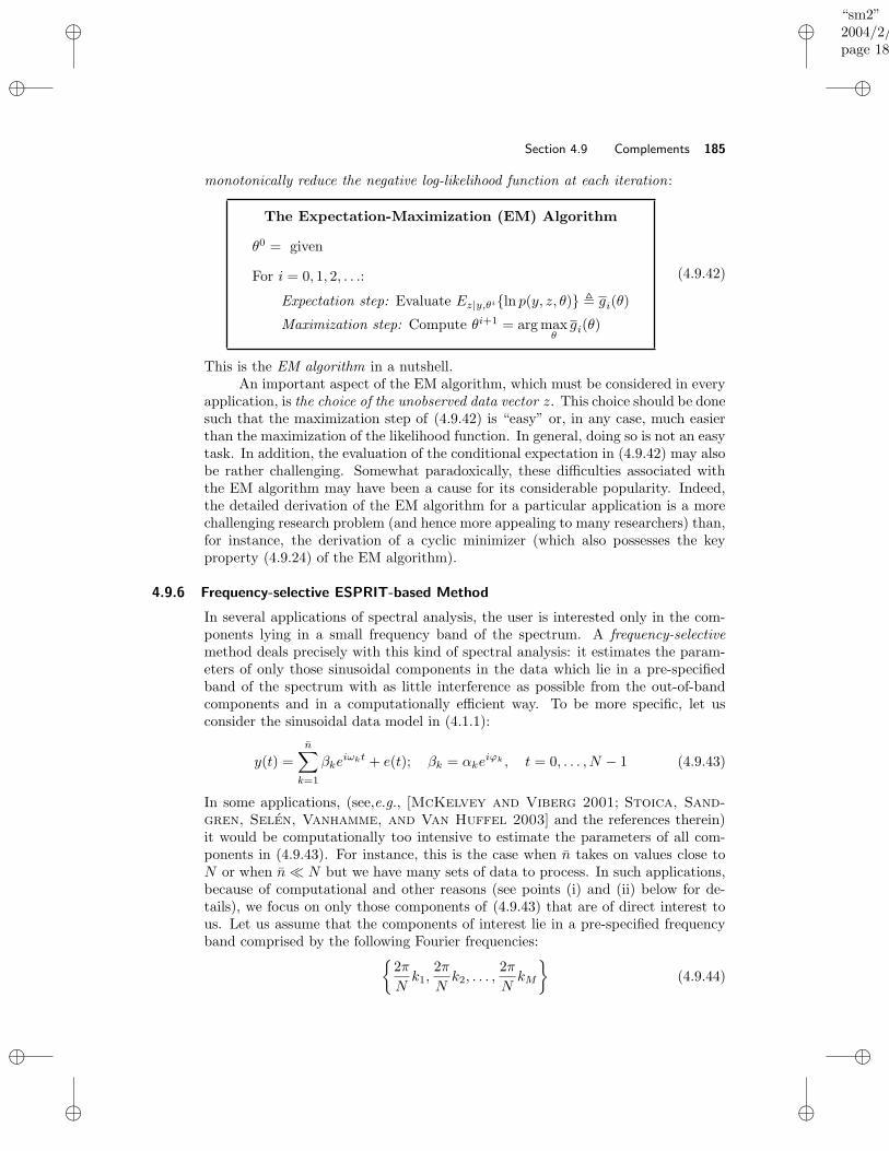
“sm2”2004/2/22page 185

i

i

i

i

i

i

i

i


monotonically reduce the negative log-likelihood function at each iteration:

The Expectation-Maximization (EM) Algorithm

θ0 = given

For i = 0, 1, 2, . . .:

Expectation step: Evaluate Ez|y,θiln p(y, z, θ) , gi(θ)

Maximization step: Compute θi+1 = arg maxθgi(θ)

(4.9.42)

This is the EM algorithm in a nutshell.An important aspect of the EM algorithm, which must be considered in every

application, is the choice of the unobserved data vector z. This choice should be donesuch that the maximization step of (4.9.42) is “easy” or, in any case, much easierthan the maximization of the likelihood function. In general, doing so is not an easytask. In addition, the evaluation of the conditional expectation in (4.9.42) may alsobe rather challenging. Somewhat paradoxically, these difficulties associated withthe EM algorithm may have been a cause for its considerable popularity. Indeed,the detailed derivation of the EM algorithm for a particular application is a morechallenging research problem (and hence more appealing to many researchers) than,for instance, the derivation of a cyclic minimizer (which also possesses the keyproperty (4.9.24) of the EM algorithm).

4.9.6 Frequency-selective ESPRIT-based Method

In several applications of spectral analysis, the user is interested only in the com-ponents lying in a small frequency band of the spectrum. A frequency-selectivemethod deals precisely with this kind of spectral analysis: it estimates the param-eters of only those sinusoidal components in the data which lie in a pre-specifiedband of the spectrum with as little interference as possible from the out-of-bandcomponents and in a computationally efficient way. To be more specific, let usconsider the sinusoidal data model in (4.1.1):

y(t) =

n∑

k=1

βkeiωkt + e(t); βk = αke

iϕk , t = 0, . . . , N − 1 (4.9.43)

In some applications, (see,e.g., [McKelvey and Viberg 2001; Stoica, Sand-

gren, Selen, Vanhamme, and Van Huffel 2003] and the references therein)it would be computationally too intensive to estimate the parameters of all com-ponents in (4.9.43). For instance, this is the case when n takes on values close toN or when n N but we have many sets of data to process. In such applications,because of computational and other reasons (see points (i) and (ii) below for de-tails), we focus on only those components of (4.9.43) that are of direct interest tous. Let us assume that the components of interest lie in a pre-specified frequencyband comprised by the following Fourier frequencies:

2π

Nk1,

2π

Nk2, . . . ,

2π

NkM

(4.9.44)

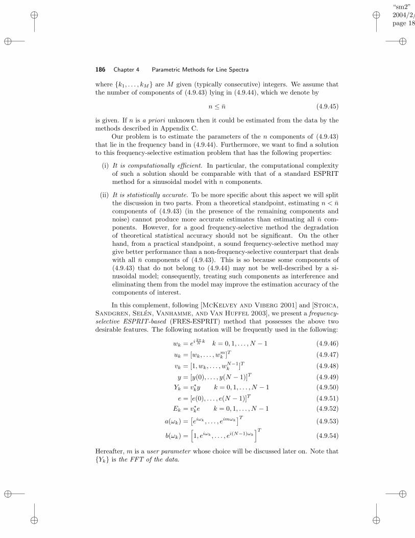
“sm2”2004/2/22page 186

i

i

i

i

i

i

i

i


where k1, . . . , kM are M given (typically consecutive) integers. We assume thatthe number of components of (4.9.43) lying in (4.9.44), which we denote by

n ≤ n (4.9.45)

is given. If n is a priori unknown then it could be estimated from the data by themethods described in Appendix C.

Our problem is to estimate the parameters of the n components of (4.9.43)that lie in the frequency band in (4.9.44). Furthermore, we want to find a solutionto this frequency-selective estimation problem that has the following properties:

(i) It is computationally efficient. In particular, the computational complexityof such a solution should be comparable with that of a standard ESPRITmethod for a sinusoidal model with n components.

(ii) It is statistically accurate. To be more specific about this aspect we will splitthe discussion in two parts. From a theoretical standpoint, estimating n < ncomponents of (4.9.43) (in the presence of the remaining components andnoise) cannot produce more accurate estimates than estimating all n com-ponents. However, for a good frequency-selective method the degradationof theoretical statistical accuracy should not be significant. On the otherhand, from a practical standpoint, a sound frequency-selective method maygive better performance than a non-frequency-selective counterpart that dealswith all n components of (4.9.43). This is so because some components of(4.9.43) that do not belong to (4.9.44) may not be well-described by a si-nusoidal model; consequently, treating such components as interference andeliminating them from the model may improve the estimation accuracy of thecomponents of interest.

In this complement, following [McKelvey and Viberg 2001] and [Stoica,

Sandgren, Selen, Vanhamme, and Van Huffel 2003], we present a frequency-selective ESPRIT-based (FRES-ESPRIT) method that possesses the above twodesirable features. The following notation will be frequently used in the following:

wk = ei2πN k k = 0, 1, . . . , N − 1 (4.9.46)

uk = [wk, . . . , wmk ]T (4.9.47)

vk = [1, wk, . . . , wN−1k ]T (4.9.48)

y = [y(0), . . . , y(N − 1)]T (4.9.49)

Yk = v∗ky k = 0, 1, . . . , N − 1 (4.9.50)

e = [e(0), . . . , e(N − 1)]T (4.9.51)

Ek = v∗ke k = 0, 1, . . . , N − 1 (4.9.52)

a(ωk) =[eiωk , . . . , eimωk

]T(4.9.53)

b(ωk) =[

1, eiωk , . . . , ei(N−1)ωk

]T

(4.9.54)

Hereafter, m is a user parameter whose choice will be discussed later on. Note thatYk is the FFT of the data.

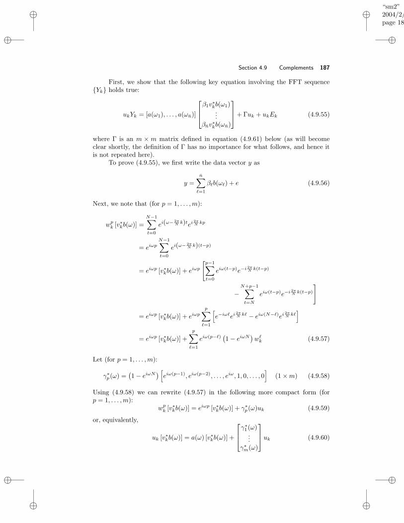
“sm2”2004/2/22page 187

i

i

i

i

i

i

i

i


First, we show that the following key equation involving the FFT sequenceYk holds true:

ukYk = [a(ω1), . . . , a(ωn)]

β1v∗kb(ω1)...

βnv∗kb(ωn)

+ Γuk + ukEk (4.9.55)

where Γ is an m × m matrix defined in equation (4.9.61) below (as will becomeclear shortly, the definition of Γ has no importance for what follows, and hence itis not repeated here).

To prove (4.9.55), we first write the data vector y as

y =

n∑

`=1

β`b(ω`) + e (4.9.56)

Next, we note that (for p = 1, . . . ,m):

wpk [v∗kb(ω)] =

N−1∑

t=0

ei(ω− 2πN k)tei

2πN kp

= eiωpN−1∑

t=0

ei(ω− 2πN k)(t−p)

= eiωp [v∗kb(ω)] + eiωp

[p−1∑

t=0

eiω(t−p)e−i 2πN k(t−p)

−N+p−1∑

t=N

eiω(t−p)e−i 2πN k(t−p)

]

= eiωp [v∗kb(ω)] + eiωp

p∑

`=1

[

e−iωèi2πN k` − eiω(N−`)ei

2πN k`

]

= eiωp [v∗kb(ω)] +

p∑

`=1

eiω(p−`) (1 − eiωN)w`k (4.9.57)

Let (for p = 1, . . . ,m):

γ∗p(ω) =

(1 − eiωN

) [

eiω(p−1), eiω(p−2), . . . , eiω, 1, 0, . . . , 0]

(1 ×m) (4.9.58)

Using (4.9.58) we can rewrite (4.9.57) in the following more compact form (forp = 1, . . . ,m):

wpk [v∗kb(ω)] = eiωp [v∗

kb(ω)] + γ∗p(ω)uk (4.9.59)

or, equivalently,

uk [v∗kb(ω)] = a(ω) [v∗

kb(ω)] +

γ∗1 (ω)...

γ∗m(ω)

uk (4.9.60)

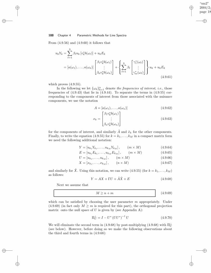
“sm2”2004/2/22page 188

i

i

i

i

i

i

i

i


From (4.9.56) and (4.9.60) it follows that

ukYk =

n∑

`=1

βùk [v∗kb(ω`)] + ukEk

= [a(ω1), . . . , a(ωn)]

β1v∗kb(ω1)...

βnv∗kb(ωn)

+

n∑

`=1

β`

γ∗1 (ω`)

...γ∗m(ω`)

uk + ukEk

(4.9.61)

which proves (4.9.55).In the following we let ωknk=1 denote the frequencies of interest, i.e., those

frequencies of (4.9.43) that lie in (4.9.44). To separate the terms in (4.9.55) cor-responding to the components of interest from those associated with the nuisancecomponents, we use the notation

A = [a(ω1), . . . , a(ωn)] (4.9.62)

xk =

β1v∗kb(ω1)...

βnv∗kb(ωn)

(4.9.63)

for the components of interest, and similarly A and xk for the other components.Finally, to write the equation (4.9.55) for k = k1, . . . , kM in a compact matrix formwe need the following additional notation:

Y = [uk1Yk1 , . . . , ukMYkM

] , (m×M) (4.9.64)

E = [uk1Ek1 , . . . , ukMEkM

] , (m×M) (4.9.65)

U = [uk1 , . . . , ukM] , (m×M) (4.9.66)

X = [xk1 , . . . , xkM] , (n×M) (4.9.67)

and similarly for X. Using this notation, we can write (4.9.55) (for k = k1, . . . , kM )as follows:

Y = AX + ΓU + AX + E (4.9.68)

Next we assume that

M ≥ n+m (4.9.69)

which can be satisfied by choosing the user parameter m appropriately. Under(4.9.69) (in fact only M ≥ m is required for this part), the orthogonal projectionmatrix onto the null space of U is given by (see Appendix A):

Π⊥U = I − U∗ (UU∗)−1

U (4.9.70)

We will eliminate the second term in (4.9.68) by post-multiplying (4.9.68) with Π⊥U

(see below). However, before doing so we make the following observations aboutthe third and fourth terms in (4.9.68):

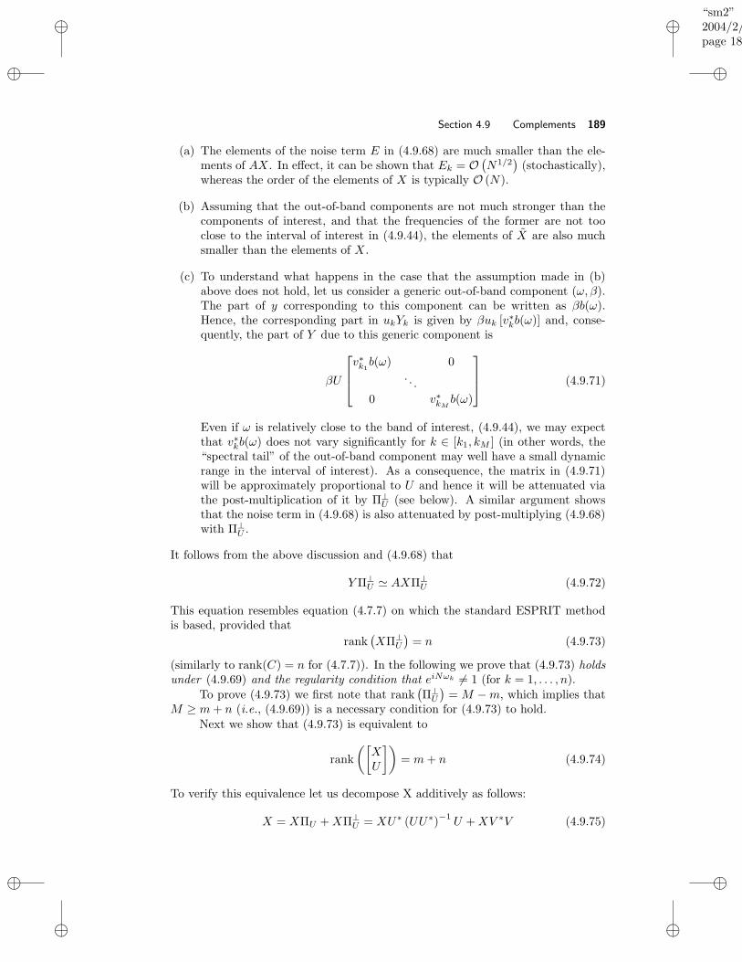
“sm2”2004/2/22page 189

i

i

i

i

i

i

i

i


(a) The elements of the noise term E in (4.9.68) are much smaller than the ele-ments of AX. In effect, it can be shown that Ek = O

(N1/2

)(stochastically),

whereas the order of the elements of X is typically O (N).

(b) Assuming that the out-of-band components are not much stronger than thecomponents of interest, and that the frequencies of the former are not tooclose to the interval of interest in (4.9.44), the elements of X are also muchsmaller than the elements of X.

(c) To understand what happens in the case that the assumption made in (b)above does not hold, let us consider a generic out-of-band component (ω, β).The part of y corresponding to this component can be written as βb(ω).Hence, the corresponding part in ukYk is given by βuk [v∗

kb(ω)] and, conse-quently, the part of Y due to this generic component is

βU

v∗k1b(ω) 0

. . .

0 v∗kMb(ω)

(4.9.71)

Even if ω is relatively close to the band of interest, (4.9.44), we may expectthat v∗

kb(ω) does not vary significantly for k ∈ [k1, kM ] (in other words, the“spectral tail” of the out-of-band component may well have a small dynamicrange in the interval of interest). As a consequence, the matrix in (4.9.71)will be approximately proportional to U and hence it will be attenuated viathe post-multiplication of it by Π⊥

U (see below). A similar argument showsthat the noise term in (4.9.68) is also attenuated by post-multiplying (4.9.68)with Π⊥

U .

It follows from the above discussion and (4.9.68) that

YΠ⊥U ' AXΠ⊥

U (4.9.72)

This equation resembles equation (4.7.7) on which the standard ESPRIT methodis based, provided that

rank(XΠ⊥

U

)= n (4.9.73)

(similarly to rank(C) = n for (4.7.7)). In the following we prove that (4.9.73) holdsunder (4.9.69) and the regularity condition that eiNωk 6= 1 (for k = 1, . . . , n).

To prove (4.9.73) we first note that rank(Π⊥U

)= M −m, which implies that

M ≥ m+ n (i.e., (4.9.69)) is a necessary condition for (4.9.73) to hold.Next we show that (4.9.73) is equivalent to

rank

([XU

])

= m+ n (4.9.74)

To verify this equivalence let us decompose X additively as follows:

X = XΠU +XΠ⊥U = XU∗ (UU∗)−1

U +XV ∗V (4.9.75)

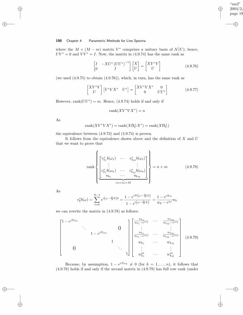
“sm2”2004/2/22page 190

i

i

i

i

i

i

i

i


where the M × (M − m) matrix V ∗ comprises a unitary basis of N (U); hence,UV ∗ = 0 and V V ∗ = I. Now, the matrix in (4.9.74) has the same rank as

[

I −XU∗ (UU∗)−1

0 I

] [XU

]

=

[XV ∗VU

]

(4.9.76)

(we used (4.9.75) to obtain (4.9.76)), which, in turn, has the same rank as

[XV ∗VU

][V ∗V X∗ U∗] =

[XV ∗V X∗ 0

0 UU∗

]

(4.9.77)

However, rank(UU∗) = m. Hence, (4.9.74) holds if and only if

rank(XV ∗V X∗) = n

As

rank(XV ∗V X∗) = rank(XΠ⊥UX

∗) = rank(XΠ⊥U )

the equivalence between (4.9.73) and (4.9.74) is proven.

It follows from the equivalence shown above and the definition of X and Uthat we want to prove that

rank

v∗k1b(ω1) · · · v∗

kMb(ω1)

......

v∗k1b(ωn) · · · v∗

kMb(ωn)

uk1 · · · ukM

︸︷︷︸

(n+m)×M

= n+m (4.9.78)

As

v∗kb(ω) =

N−1∑

t=0

ei(ω− 2πN k)t =

1 − eiN(ω− 2πN k)

1 − ei(ω− 2πN k)

=1 − eiNω

wk − eiωwk

we can rewrite the matrix in (4.9.78) as follows:

1 − eiNω1

. . . 01 − eiNωn

1

0. . .

1

wk1

wk1−eiω1

· · · wkM

wkM−eiω1

......

wk1

wk1−eiωn · · · wkM

wkM−eiωn

wk1 · · · wkM

......

wmk1 · · · wmkM

(4.9.79)

Because, by assumption, 1 − eiNωk 6= 0 (for k = 1, . . . , n), it follows that(4.9.78) holds if and only if the second matrix in (4.9.79) has full row rank (under

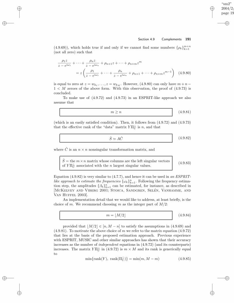
“sm2”2004/2/22page 191

i

i

i

i

i

i

i

i


(4.9.69)), which holds true if and only if we cannot find some numbers ρkm+nk=1

(not all zero) such that

ρ1z

z − eiω1+ · · · +

ρnz

z − eiωn+ ρn+1z + · · · + ρn+mz

m

= z

(ρ1

z − eiω1+ · · · +

ρnz − eiωn

+ ρn+1 + · · · + ρn+mzm−1

)

(4.9.80)

is equal to zero at z = wk1 , . . . , z = wkM. However, (4.9.80) can only have m+n−

1 < M zeroes of the above form. With this observation, the proof of (4.9.73) isconcluded.

To make use of (4.9.72) and (4.9.73) in an ESPRIT-like approach we alsoassume that

m ≥ n (4.9.81)

(which is an easily satisfied condition). Then, it follows from (4.9.72) and (4.9.73)that the effective rank of the “data” matrix YΠ⊥

U is n, and that

S ' AC (4.9.82)

where C is an n× n nonsingular transformation matrix, and

S = the m×n matrix whose columns are the left singular vectorsof YΠ⊥

U associated with the n largest singular values.(4.9.83)

Equation (4.9.82) is very similar to (4.7.7), and hence it can be used in an ESPRIT-like approach to estimate the frequencies ωknk=1. Following the frequency estima-tion step, the amplitudes βknk=1 can be estimated, for instance, as described in[McKelvey and Viberg 2001; Stoica, Sandgren, Selen, Vanhamme, and

Van Huffel 2003].An implementation detail that we would like to address, at least briefly, is the

choice of m. We recommend choosing m as the integer part of M/2:

m = bM/2c (4.9.84)

provided that bM/2c ∈ [n,M − n] to satisfy the assumptions in (4.9.69) and(4.9.81). To motivate the above choice of m we refer to the matrix equation (4.9.72)that lies at the basis of the proposed estimation approach. Previous experiencewith ESPRIT, MUSIC and other similar approaches has shown that their accuracyincreases as the number of independent equations in (4.9.72) (and its counterparts)increases. The matrix YΠ⊥

U in (4.9.72) is m ×M and its rank is generically equalto

minrank(Y ), rank(Π⊥U ) = min(m,M −m) (4.9.85)

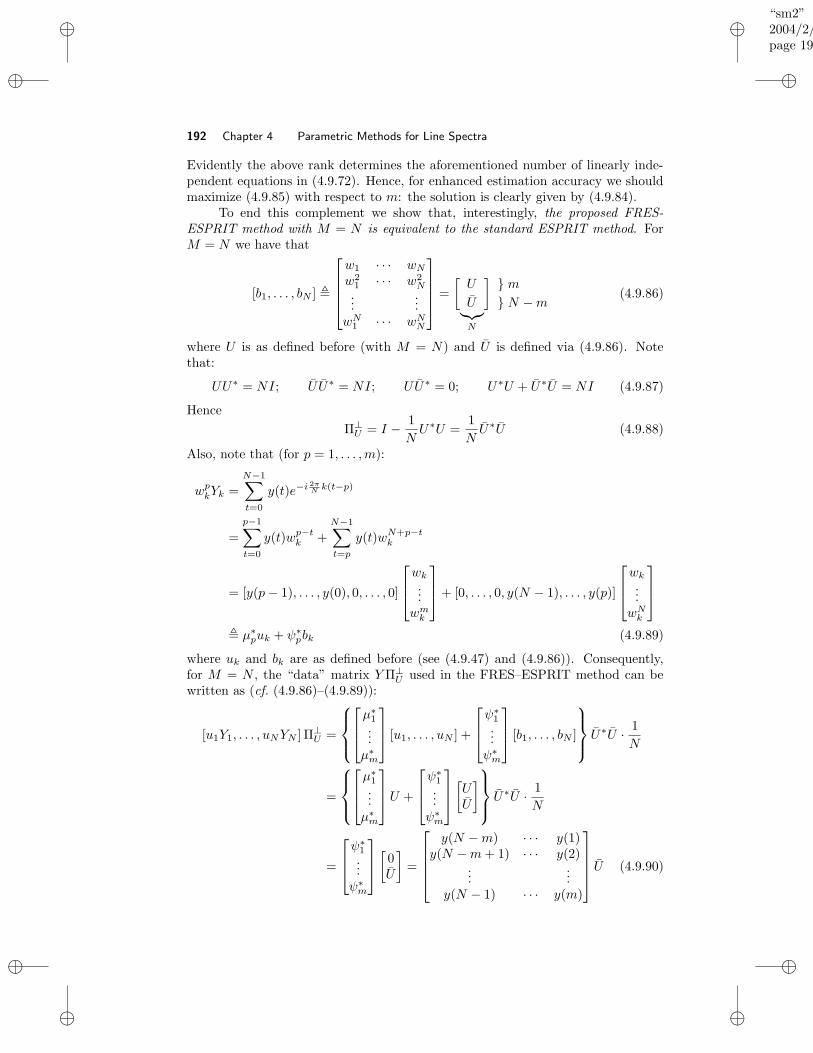
“sm2”2004/2/22page 192

i

i

i

i

i

i

i

i


Evidently the above rank determines the aforementioned number of linearly inde-pendent equations in (4.9.72). Hence, for enhanced estimation accuracy we shouldmaximize (4.9.85) with respect to m: the solution is clearly given by (4.9.84).

To end this complement we show that, interestingly, the proposed FRES-ESPRIT method with M = N is equivalent to the standard ESPRIT method. ForM = N we have that

[b1, . . . , bN ] ,

w1 · · · wNw2

1 · · · w2N

......

wN1 · · · wNN

=

[U

U︸︷︷︸

N

] m N −m

(4.9.86)

where U is as defined before (with M = N) and U is defined via (4.9.86). Notethat:

UU∗ = NI; U U∗ = NI; UU∗ = 0; U∗U + U∗U = NI (4.9.87)

Hence

Π⊥U = I − 1

NU∗U =

1

NU∗U (4.9.88)

Also, note that (for p = 1, . . . ,m):

wpkYk =

N−1∑

t=0

y(t)e−i 2πN k(t−p)

=

p−1∑

t=0

y(t)wp−tk +

N−1∑

t=p

y(t)wN+p−tk

= [y(p− 1), . . . , y(0), 0, . . . , 0]

wk...wmk

+ [0, . . . , 0, y(N − 1), . . . , y(p)]

wk...wNk

, µ∗puk + ψ∗

pbk (4.9.89)

where uk and bk are as defined before (see (4.9.47) and (4.9.86)). Consequently,for M = N , the “data” matrix YΠ⊥

U used in the FRES–ESPRIT method can bewritten as (cf. (4.9.86)–(4.9.89)):

[u1Y1, . . . , uNYN ] Π⊥U =

µ∗1...µ∗m

[u1, . . . , uN ] +

ψ∗1...ψ∗m

[b1, . . . , bN ]

U∗U · 1

N

=

µ∗1...µ∗m

U +

ψ∗1...ψ∗m

[UU

]

U∗U · 1

N

=

ψ∗1...ψ∗m

[0U

]

=

y(N −m) · · · y(1)y(N −m+ 1) · · · y(2)

......

y(N − 1) · · · y(m)

U (4.9.90)

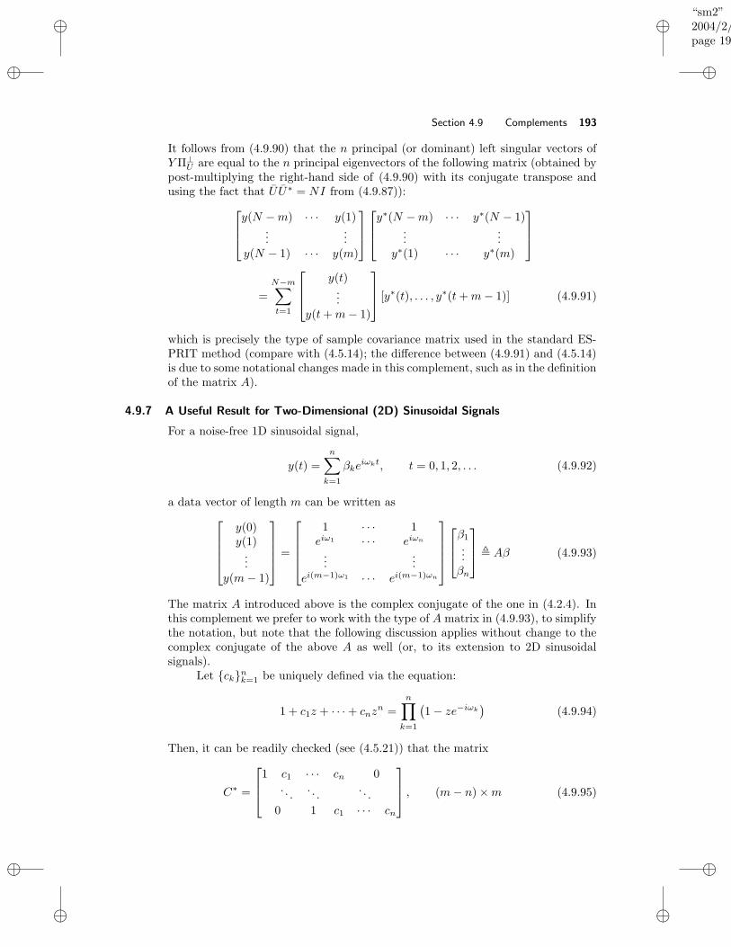
“sm2”2004/2/22page 193

i

i

i

i

i

i

i

i


It follows from (4.9.90) that the n principal (or dominant) left singular vectors ofYΠ⊥

U are equal to the n principal eigenvectors of the following matrix (obtained bypost-multiplying the right-hand side of (4.9.90) with its conjugate transpose andusing the fact that U U∗ = NI from (4.9.87)):

y(N −m) · · · y(1)...

...y(N − 1) · · · y(m)

y∗(N −m) · · · y∗(N − 1)...

...y∗(1) · · · y∗(m)

=

N−m∑

t=1

y(t)...

y(t+m− 1)

[y∗(t), . . . , y∗(t+m− 1)] (4.9.91)

which is precisely the type of sample covariance matrix used in the standard ES-PRIT method (compare with (4.5.14); the difference between (4.9.91) and (4.5.14)is due to some notational changes made in this complement, such as in the definitionof the matrix A).

4.9.7 A Useful Result for Two-Dimensional (2D) Sinusoidal Signals

For a noise-free 1D sinusoidal signal,

y(t) =

n∑

k=1

βkeiωkt, t = 0, 1, 2, . . . (4.9.92)

a data vector of length m can be written as

y(0)y(1)

...y(m− 1)

=

1 · · · 1eiω1 · · · eiωn

......

ei(m−1)ω1 · · · ei(m−1)ωn

β1

...βn

, Aβ (4.9.93)

The matrix A introduced above is the complex conjugate of the one in (4.2.4). Inthis complement we prefer to work with the type of A matrix in (4.9.93), to simplifythe notation, but note that the following discussion applies without change to thecomplex conjugate of the above A as well (or, to its extension to 2D sinusoidalsignals).

Let cknk=1 be uniquely defined via the equation:

1 + c1z + · · · + cnzn =

n∏

k=1

(1 − ze−iωk

)(4.9.94)

Then, it can be readily checked (see (4.5.21)) that the matrix

C∗ =

1 c1 · · · cn 0. . .

. . .. . .

0 1 c1 · · · cn

, (m− n) ×m (4.9.95)

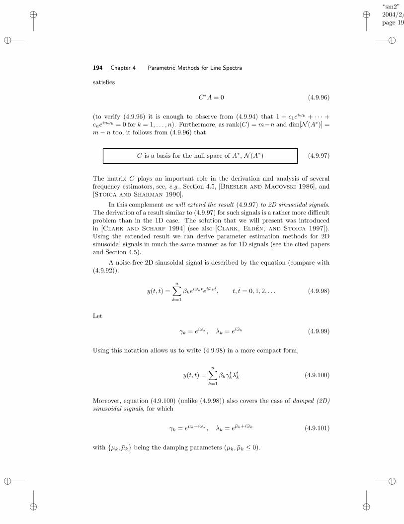
“sm2”2004/2/22page 194

i

i

i

i

i

i

i

i


satisfies

C∗A = 0 (4.9.96)

(to verify (4.9.96) it is enough to observe from (4.9.94) that 1 + c1eiωk + · · · +

cneinωk = 0 for k = 1, . . . , n). Furthermore, as rank(C) = m−n and dim[N (A∗)] =

m− n too, it follows from (4.9.96) that

C is a basis for the null space of A∗, N (A∗) (4.9.97)

The matrix C plays an important role in the derivation and analysis of severalfrequency estimators, see, e.g., Section 4.5, [Bresler and Macovski 1986], and[Stoica and Sharman 1990].

In this complement we will extend the result (4.9.97) to 2D sinusoidal signals.The derivation of a result similar to (4.9.97) for such signals is a rather more difficultproblem than in the 1D case. The solution that we will present was introducedin [Clark and Scharf 1994] (see also [Clark, Elden, and Stoica 1997]).Using the extended result we can derive parameter estimation methods for 2Dsinusoidal signals in much the same manner as for 1D signals (see the cited papersand Section 4.5).

A noise-free 2D sinusoidal signal is described by the equation (compare with(4.9.92)):

y(t, t) =

n∑

k=1

βkeiωkteiωk t, t, t = 0, 1, 2, . . . (4.9.98)

Let

γk = eiωk , λk = eiωk (4.9.99)

Using this notation allows us to write (4.9.98) in a more compact form,

y(t, t) =

n∑

k=1

βkγtkλ

tk (4.9.100)

Moreover, equation (4.9.100) (unlike (4.9.98)) also covers the case of damped (2D)sinusoidal signals, for which

γk = eµk+iωk , λk = eµk+iωk (4.9.101)

with µk, µk being the damping parameters (µk, µk ≤ 0).

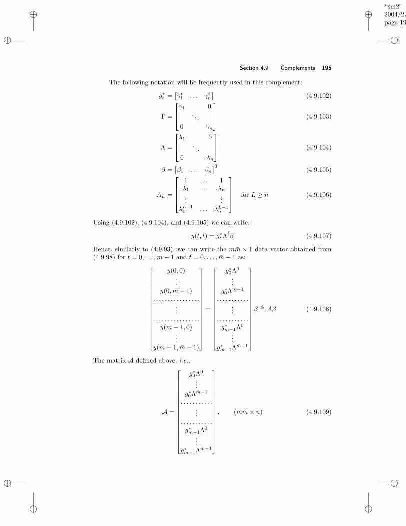
“sm2”2004/2/22page 195

i

i

i

i

i

i

i

i


The following notation will be frequently used in this complement:

g∗t =

[γt1 . . . γtn

](4.9.102)

Γ =

γ1 0. . .

0 γn

(4.9.103)

Λ =

λ1 0. . .

0 λn

(4.9.104)

β =[β1 . . . βn

]T(4.9.105)

AL =

1 . . . 1λ1 . . . λn...

...

λL−11 . . . λL−1

n

for L ≥ n (4.9.106)

Using (4.9.102), (4.9.104), and (4.9.105) we can write:

y(t, t) = g∗tΛ

tβ (4.9.107)

Hence, similarly to (4.9.93), we can write the mm × 1 data vector obtained from(4.9.98) for t = 0, . . . ,m− 1 and t = 0, . . . , m− 1 as:

y(0, 0)...

y(0, m− 1). . . . . . . . . . . . . . . .

.... . . . . . . . . . . . . . . .y(m− 1, 0)

...y(m− 1, m− 1)

=

g∗0Λ0

...g∗0Λm−1

. . . . . . . . . . ....

. . . . . . . . . . .g∗m−1Λ

0

...g∗m−1Λ

m−1

β , Aβ (4.9.108)

The matrix A defined above, i.e.,

A =

g∗0Λ0

...g∗0Λm−1

. . . . . . . . . . ....

. . . . . . . . . . .g∗m−1Λ

0

...g∗m−1Λ

m−1

, (mm× n) (4.9.109)

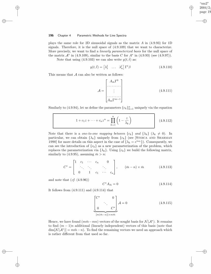
“sm2”2004/2/22page 196

i

i

i

i

i

i

i

i


plays the same role for 2D sinusoidal signals as the matrix A in (4.9.93) for 1Dsignals. Therefore, it is the null space of (4.9.109) that we want to characterize.More precisely, we want to find a linearly parameterized basis for the null space ofthe matrix A∗ in (4.9.109), similar to the basis C for A∗ in (4.9.93) (see (4.9.97)).

Note that using (4.9.103) we can also write y(t, t) as:

y(t, t) =[λt1 . . . λtn

]Γtβ (4.9.110)

This means that A can also be written as follows:

A =

AmΓ0

. . . . . . . . ....

. . . . . . . . .AmΓm−1

(4.9.111)

Similarly to (4.9.94), let us define the parameters cknk=1 uniquely via the equation

1 + c1z + · · · + cnzn =

n∏

k=1

(

1 − z

λk

)

(4.9.112)

Note that there is a one-to-one mapping between ck and λk (λk 6= 0). Inparticular, we can obtain λk uniquely from ck (see [Stoica and Sharman

1990] for more details on this aspect in the case of λk = eiωk). Consequently, wecan see the introduction of ck as a new parameterization of the problem, whichreplaces the parameterization via λk. Using ck we build the following matrix,similarly to (4.9.95), assuming m > n:

C∗ =

1 c1 · · · cn 0. . .

. . .. . .

0 1 c1 · · · cn

, (m− n) × m (4.9.113)

and note that (cf. (4.9.96))C∗Am = 0 (4.9.114)


C∗ 0. . .

0 C∗

︸︷︷︸

[m(m−n)]×mm

A = 0 (4.9.115)

Hence, we have found (mm−mn) vectors of the sought basis for N (A∗). It remainsto find (m − 1)n additional (linearly independent) vectors of this basis (note thatdim[N (A∗)] = mm−n). To find the remaining vectors we need an approach whichis rather different from that used so far.

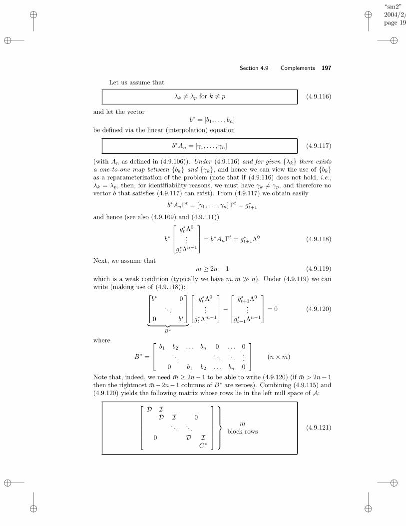
“sm2”2004/2/22page 197

i

i

i

i

i

i

i

i


Let us assume that

λk 6= λp for k 6= p (4.9.116)

and let the vectorb∗ = [b1, . . . , bn]

be defined via the linear (interpolation) equation

b∗An = [γ1, . . . , γn] (4.9.117)

(with An as defined in (4.9.106)). Under (4.9.116) and for given λk there existsa one-to-one map between bk and γk, and hence we can view the use of bkas a reparameterization of the problem (note that if (4.9.116) does not hold, i.e.,λk = λp, then, for identifiability reasons, we must have γk 6= γp, and therefore novector b that satisfies (4.9.117) can exist). From (4.9.117) we obtain easily

b∗AnΓt = [γ1, . . . , γn] Γ

t = g∗t+1

and hence (see also (4.9.109) and (4.9.111))

b∗

g∗tΛ

0

...g∗tΛ

n−1

= b∗AnΓ

t = g∗t+1Λ

0 (4.9.118)

Next, we assume thatm ≥ 2n− 1 (4.9.119)

which is a weak condition (typically we have m, m n). Under (4.9.119) we canwrite (making use of (4.9.118)):

b∗ 0. . .

0 b∗

︸︷︷︸

B∗

g∗tΛ

0

...g∗tΛ

m−1

−

g∗t+1Λ

0

...g∗t+1Λ

n−1

= 0 (4.9.120)

where

B∗ =

b1 b2 . . . bn 0 . . . 0. . .

. . .. . .

...0 b1 b2 . . . bn 0

(n× m)

Note that, indeed, we need m ≥ 2n− 1 to be able to write (4.9.120) (if m > 2n− 1then the rightmost m−2n−1 columns of B∗ are zeroes). Combining (4.9.115) and(4.9.120) yields the following matrix whose rows lie in the left null space of A:

D ID I 0

. . .. . .

0 D IC∗

mblock rows

(4.9.121)

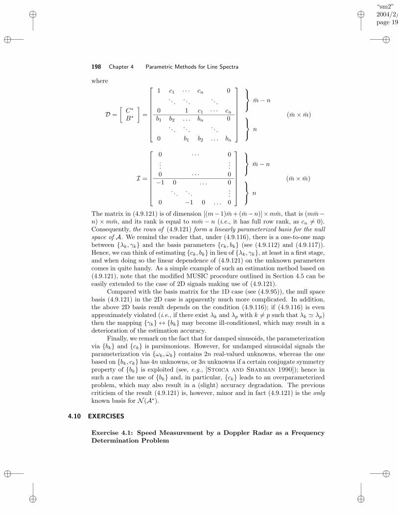
“sm2”2004/2/22page 198

i

i

i

i

i

i

i

i


where

D =

[C∗

B∗

]

=

1 c1 · · · cn 0. . .

. . .. . .

0 1 c1 · · · cnb1 b2 . . . bn 0

. . .. . .

. . .

0 b1 b2 . . . bn

m− n

n

(m× m)

I =

0 · · · 0...

...0 · · · 0

−1 0 . . . 0. . .

. . ....

0 −1 0 . . . 0

m− n

n

(m× m)

The matrix in (4.9.121) is of dimension [(m− 1)m+(m−n)]×mm, that is (mm−n) × mm, and its rank is equal to mm − n (i.e., it has full row rank, as cn 6= 0).Consequently, the rows of (4.9.121) form a linearly parameterized basis for the nullspace of A. We remind the reader that, under (4.9.116), there is a one-to-one mapbetween λk, γk and the basis parameters ck, bk (see (4.9.112) and (4.9.117)).Hence, we can think of estimating ck, bk in lieu of λk, γk, at least in a first stage,and when doing so the linear dependence of (4.9.121) on the unknown parameterscomes in quite handy. As a simple example of such an estimation method based on(4.9.121), note that the modified MUSIC procedure outlined in Section 4.5 can beeasily extended to the case of 2D signals making use of (4.9.121).

Compared with the basis matrix for the 1D case (see (4.9.95)), the null spacebasis (4.9.121) in the 2D case is apparently much more complicated. In addition,the above 2D basis result depends on the condition (4.9.116); if (4.9.116) is evenapproximately violated (i.e., if there exist λk and λp with k 6= p such that λk ' λp)then the mapping γk ↔ bk may become ill-conditioned, which may result in adeterioration of the estimation accuracy.

Finally, we remark on the fact that for damped sinusoids, the parameterizationvia bk and ck is parsimonious. However, for undamped sinusoidal signals theparameterization via ωk, ωk contains 2n real-valued unknowns, whereas the onebased on bk, ck has 4n unknowns, or 3n unknowns if a certain conjugate symmetryproperty of bk is exploited (see, e.g., [Stoica and Sharman 1990]); hence insuch a case the use of bk and, in particular, ck leads to an overparameterizedproblem, which may also result in a (slight) accuracy degradation. The previouscriticism of the result (4.9.121) is, however, minor and in fact (4.9.121) is the onlyknown basis for N (A∗).

4.10 EXERCISES

Exercise 4.1: Speed Measurement by a Doppler Radar as a FrequencyDetermination Problem

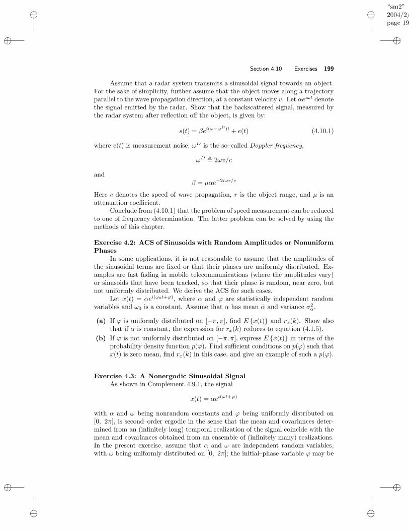
“sm2”2004/2/22page 199

i

i

i

i

i

i

i

i


Assume that a radar system transmits a sinusoidal signal towards an object.For the sake of simplicity, further assume that the object moves along a trajectoryparallel to the wave propagation direction, at a constant velocity v. Let αeiωt denotethe signal emitted by the radar. Show that the backscattered signal, measured bythe radar system after reflection off the object, is given by:

s(t) = βei(ω−ωD)t + e(t) (4.10.1)

where e(t) is measurement noise, ωD is the so–called Doppler frequency,

ωD , 2ωv/c

andβ = µαe−2iωr/c

Here c denotes the speed of wave propagation, r is the object range, and µ is anattenuation coefficient.

Conclude from (4.10.1) that the problem of speed measurement can be reducedto one of frequency determination. The latter problem can be solved by using themethods of this chapter.

Exercise 4.2: ACS of Sinusoids with Random Amplitudes or NonuniformPhases

In some applications, it is not reasonable to assume that the amplitudes ofthe sinusoidal terms are fixed or that their phases are uniformly distributed. Ex-amples are fast fading in mobile telecommunications (where the amplitudes vary)or sinusoids that have been tracked, so that their phase is random, near zero, butnot uniformly distributed. We derive the ACS for such cases.

Let x(t) = αei(ω0t+ϕ), where α and ϕ are statistically independent randomvariables and ω0 is a constant. Assume that α has mean α and variance σ2

α.

(a) If ϕ is uniformly distributed on [−π, π], find E x(t) and rx(k). Show alsothat if α is constant, the expression for rx(k) reduces to equation (4.1.5).

(b) If ϕ is not uniformly distributed on [−π, π], express E x(t) in terms of theprobability density function p(ϕ). Find sufficient conditions on p(ϕ) such thatx(t) is zero mean, find rx(k) in this case, and give an example of such a p(ϕ).

Exercise 4.3: A Nonergodic Sinusoidal SignalAs shown in Complement 4.9.1, the signal

x(t) = αei(ωt+ϕ)

with α and ω being nonrandom constants and ϕ being uniformly distributed on[0, 2π], is second–order ergodic in the sense that the mean and covariances deter-mined from an (infinitely long) temporal realization of the signal coincide with themean and covariances obtained from an ensemble of (infinitely many) realizations.In the present exercise, assume that α and ω are independent random variables,with ω being uniformly distributed on [0, 2π]; the initial–phase variable ϕ may be

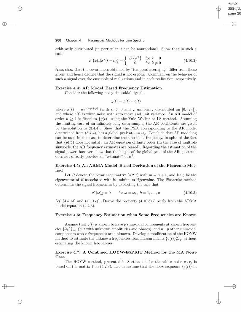
“sm2”2004/2/22page 200

i

i

i

i

i

i

i

i


arbitrarily distributed (in particular it can be nonrandom). Show that in such acase,

E x(t)x∗(t− k) =

Eα2

for k = 00 for k 6= 0

(4.10.2)

Also, show that the covariances obtained by “temporal averaging” differ from thosegiven, and hence deduce that the signal is not ergodic. Comment on the behavior ofsuch a signal over the ensemble of realizations and in each realization, respectively.

Exercise 4.4: AR Model–Based Frequency EstimationConsider the following noisy sinusoidal signal:

y(t) = x(t) + e(t)

where x(t) = αei(ω0t+ϕ) (with α > 0 and ϕ uniformly distributed on [0, 2π]),and where e(t) is white noise with zero mean and unit variance. An AR model oforder n ≥ 1 is fitted to y(t) using the Yule–Walker or LS method. Assumingthe limiting case of an infinitely long data sample, the AR coefficients are givenby the solution to (3.4.4). Show that the PSD, corresponding to the AR modeldetermined from (3.4.4), has a global peak at ω = ω0. Conclude that AR modelingcan be used in this case to determine the sinusoidal frequency, in spite of the factthat y(t) does not satisfy an AR equation of finite order (in the case of multiplesinusoids, the AR frequency estimates are biased). Regarding the estimation of thesignal power, however, show that the height of the global peak of the AR spectrumdoes not directly provide an “estimate” of α2.

Exercise 4.5: An ARMA Model–Based Derivation of the Pisarenko Met-hod

Let R denote the covariance matrix (4.2.7) with m = n+ 1, and let g be theeigenvector of R associated with its minimum eigenvalue. The Pisarenko methoddetermines the signal frequencies by exploiting the fact that

a∗(ω)g = 0 for ω = ωk, k = 1, . . . , n (4.10.3)

(cf. (4.5.13) and (4.5.17)). Derive the property (4.10.3) directly from the ARMAmodel equation (4.2.3).

Exercise 4.6: Frequency Estimation when Some Frequencies are Known

Assume that y(t) is known to have p sinusoidal components at known frequen-cies ωkpk=1 (but with unknown amplitudes and phases), and n−p other sinusoidalcomponents whose frequencies are unknown. Develop a modification of the HOYWmethod to estimate the unknown frequencies from measurements y(t)Nt=1, withoutestimating the known frequencies.

Exercise 4.7: A Combined HOYW-ESPRIT Method for the MA NoiseCase

The HOYW method, presented in Section 4.4 for the white noise case, isbased on the matrix Γ in (4.2.8). Let us assume that the noise sequence e(t) in

“sm2”2004/2/22page 201

i

i

i

i

i

i

i

i


(4.1.1) is known to be an MA process of order m, and that m is given. A simpleway to handle such a colored noise in the HOYW method consists of modifying theexpression (4.2.8) of Γ as follows:

Γ = E

y(t− L− 1 −m)...

y(t− L−M −m)

[y∗(t), . . . , y∗(t− L)]

(4.10.4)

Derive an expression for Γ similar to the one for Γ in (4.2.8). Furthermore, makeuse of that expression in an ESPRIT-like method to estimate the frequencies ωk,instead of using it in an HOYW-like method (see Section 4.4). Discuss the advan-tage of the so-obtained HOYW-ESPRIT method over the HOYW method basedon Γ. Assuming that the noise is white (i.e., m = 0) and hence that ESPRIT isdirectly applicable, would you prefer using HOYW-ESPRIT (with m = 0) in lieuof ESPRIT? Why or why not?

Exercise 4.8: Chebyshev Inequality and the Convergence of Sample Co-variances

Let x be a random variable with finite mean µ and variance σ2. Show that,for any positive constant c, the so–called Chebyshev inequality holds:

Pr(|x− µ| ≥ cσ) ≤ 1/c2 (4.10.5)

Use (4.10.5) to show that if a sample covariance lag rN (estimated from N datasamples) converges to the true value r in the mean square sense, i.e.,

limN→∞

E|rN − r|2

= 0 (4.10.6)

then rN also converges to r in probability:

limN→∞

Pr(|rN − r| 6= 0) = 0 (4.10.7)

For sinusoidal signals, the mean square convergence of rN (k) to r(k), as N →∞, has been proven in Complement 4.9.1. (In this exercise, we omit the argument kin rN (k) and r(k), for notational simplicity.) Additionally, discuss the use of (4.10.5)to set bounds (which hold with a specified probability) on an arbitrary randomvariable with given mean and variance. Comment on the conservatism of the boundsobtained from (4.10.5) by comparing them with the bounds corresponding to aGaussian random variable.

Exercise 4.9: More about the Forward–Backward ApproachThe sample covariance matrix in (4.8.3), used by the forward–backward ap-

proach, is often a better estimate of the theoretical covariance matrix than R is (asargued in Section 4.8). Another advantage of (4.8.3) is that the forward–backwardsample covariance is always numerically better conditioned than the usual (forward–only) sample covariance matrix R. To explain this statement, let R be a Hermitian

“sm2”2004/2/22page 202

i

i

i

i

i

i

i

i


matrix (not necessarily a Toeplitz one, as the R in (4.2.7)). The “condition number”of R is defined as

cond(R) = λmax(R)/λmin(R)

where λmax(R) and λmin(R) are the maximum and minimum eigenvalues of R,respectively. The numerical errors that affect many algebraic operations on R,such as inversion, eigendecomposition and so on, are essentially proportional tocond(R). Hence, the smaller cond(R) the better. (See Appendix A for details onthis aspect.)

Next, let U be a unitary matrix (the J in (4.8.3) is a special case of such amatrix). Observe that the forward–backward covariance in equation (4.8.3) is ofthe form R+ U∗RTU . Prove that

cond(R) ≥ cond(R+ U∗RTU) (4.10.8)

for any unitary matrix U . We note that the result (4.10.8) applies to any Hermitianmatrix R and unitary matrix U , and thus is valid in more general cases than theforward–backward approach in Section 4.8, in which R is Toeplitz and U = J .

Exercise 4.10: ESPRIT and Min–Norm Under the Same Umbrella

ESPRIT and Min–Norm methods are seemingly quite different from one an-other, and hence it might seem unlikely that there is any strong relationship betweenthem. It is the goal of this exercise to show that in fact ESPRIT and Min–Norm arequite related to each other. We will see that ESPRIT and Min–Norm are membersof a well-defined class of frequency estimates.

Consider the equation

S∗2 Ψ = S∗

1 (4.10.9)

where S1 and S2 are as defined in Section 4.7. The (m− 1) × (m− 1) matrix Ψ in(4.10.9) is the unknown. First show that the asymptotic counterpart of (4.10.9),

S∗2Ψ = S∗

1 (4.10.10)

has the property that any of its solutions Ψ has n eigenvalues equal to e−iωknk=1.

This property, along with the fact that there is an infinite number of matrices Ψsatisfying (4.10.9) (see Section A.8 in Appendix A), imply that (4.10.9) generatesa class of frequency estimators with an infinite number of members.

As a second task, show that ESPRIT and Min–Norm belong to this classof estimators. In other words, prove that there is a solution of (4.10.9) whosenonzero eigenvalues have exactly the same arguments as the eigenvalues of theESPRIT matrix φ in (4.7.12), and also that there is another solution of (4.10.9)whose eigenvalues are equal to the roots of the Min–Norm polynomial in (4.6.3).For more details on the topic of this exercise, see [Hua and Sarkar 1990].

Exercise 4.11: Yet Another Relationship between ESPRIT and Min–Norm

“sm2”2004/2/22page 203

i

i

i

i

i

i

i

i


Let the vector [ρT , 1]T be defined similarly to the Min–Norm vector [1, gT ]T

(see (4.6.1)), with the only difference that we now constrain the last element to beequal to one. Hence, ρ is the minimum-norm solution to (see (4.6.5)):

S∗[ρ1

]

= 0

Use the Min–Norm vector ρ to build the following matrix

φ = S∗[

0Im−1

−ρ∗

]

S (n× n)

Prove the somewhat curious fact that φ above is equal to the ESPRIT matrix, φ,in (4.7.12).

COMPUTER EXERCISES

Tools for Frequency Estimation:

The text web site www.prenhall.com/stoica contains the following Matlab

functions for use in computing frequency estimates and estimating the number ofsinusoidal terms. In the first four functions, y is the data vector and n is the desirednumber of frequency estimates. The remaining variables are described below.

• w=hoyw(y,n,L,M)

The HOYW estimator given in the box on page 159; L and M are the matrixdimensions as in (4.4.8).

• w=music(y,n,m)

The Root MUSIC estimator given by (4.5.12); m is the dimension of a(ω).This function also implements the Pisarenko method by setting m = n+ 1.

• w=minnorm(y,n,m)

The Root Min–Norm estimator given by (4.6.3); m is the dimension of a(ω).

• w=esprit(y,n,m)

The ESPRIT estimator given by (4.7.12); m is the size of the square matrixR there, and S1 and S2 are chosen as in equations (4.7.5) and (4.7.6).

• order=sinorder(mvec,sig2,N,nu)

Computes the AIC, AICc, GIC, and BIC model order selections for sinusoidalparameter estimation problems (see Appendix C for details on the derivationsof these methods). Here, mvec is a vector of candidate sinusoidal modelorders, sig2 is the vector of estimated residual variances corresponding tothe model orders in mvec, N is the length of the observed data vector, andnu is a parameter in the GIC method. The 4-element output vector order

contains the selected model orders obtained from AIC, AICc, GIC, and BIC,respectively.

“sm2”2004/2/22page 204

i

i

i

i

i

i

i

i


Exercise C4.12: Resolution Properties of Subspace Methods for Estima-tion of Line Spectra

In this exercise we test and compare the resolution properties of four subspacemethods, Min–Norm, MUSIC, ESPRIT, and HOYW.

Generate realizations of the sinusoidal signal

y(t) = 10 sin(0.24πt+ ϕ1) + 5 sin(0.26πt+ ϕ2) + e(t), t = 1, . . . , N

where N = 64, e(t) is Gaussian white noise with variance σ2, and where ϕ1, ϕ2 areindependent random variables each uniformly distributed on [−π, π].

Generate 50 Monte–Carlo realizations of y(t), and present the results fromthese experiments. The results of frequency estimation can be presented compar-ing the sample means and variances of the frequency estimates from the variousestimators.

(a) Find the exact ACS for y(t). Compute the “true” frequency estimates fromthe four methods, for n = 4 and various choices of the order m ≥ 5 (andcorresponding choices of M and L for HOYW). Which method(s) are able toresolve the two sinusoids, and for what values of m (or M and L)?

(b) Consider now N = 64, and set σ2 = 0; this corresponds to the finite datalength but infinite SNR case. Compute frequency estimates for the four tech-niques again using n = 4 and various choices ofm, M and L. Which method(s)are reliably able to resolve the sinusoids? Explain why.

(c) Obtain frequency estimates from the four methods when N = 64 and σ2 = 1.Use n = 4, and experiment with different choices of m, M and L to see theeffect on estimation accuracy (e.g., try m = 5, 8, and 12 for MUSIC, Min–Norm and ESPRIT, and try L = M = 4, 8, and 12 for HOYW). Whichmethod(s) give reliable “super–resolution” estimation of the sinusoids? Is itpossible to resolve the two sinusoids in the signal? Discuss how the choices ofm, M and L influence the resolution properties. Which method appears tohave the best resolution?

You may want to experiment further by changing the SNR and the relativeamplitudes of the sinusoids to gain a better understanding of the differencesbetween the methods.

(d) Compare the estimation results with the AR and ARMA results obtained inExercise C3.18 in Chapter 3. What are the major differences between thetechniques? Which method(s) do you prefer for this problem?

Exercise C4.13: Model Order Selection for Sinusoidal Signals

In this exercise we examine four methods for model order selection for sinu-soidal signals. As discussed in Appendix C, several important model order selectionrules have the following general form (see (C.8.1)–(C.8.2)):

−2 ln pn(y, θn) + η(r,N)r (4.10.11)

“sm2”2004/2/22page 205

i

i

i

i

i

i

i

i


with different penalty coefficients η(r,N) for the different methods:

AIC : η(r,N) = 2

AICc : η(r,N) = 2N

N − r − 1

GIC : η(r,N) = ν (e.g., ν = 4)

BIC : η(r,N) = lnN

(4.10.12)

Here, N is the length of the observed data vector y and for sinusoidal signals r isgiven by (see Appendix C):

r = 3n+ 1 for AIC, AICc, and GIC

r = 5n+ 1 for BIC

where n is the number of sinusoids in the model. The term ln pn(y, θn) is the

log-likelihood of the observed data vector y given the maximum-likelihood (ML)estimate of the parameter vector θ for a model order of n; it is given by (cf. (C.2.7)–(C.2.8) in Appendix C):

−2 ln pn(y, θn) = Nσ2

n + constant (4.10.13)

where

σ2n =

1

N

N∑

t=1

∣∣∣∣∣y(t) −

n∑

k=1

αkei(ωkt+ϕk)

∣∣∣∣∣

2

(4.10.14)

The selected model order is the value of n that minimizes (4.10.11). The orderselection rules above, while derived for ML estimates of θ, can be used even withapproximate ML estimates of θ, albeit with some loss of performance.

Well-Separated Sinusoids:

(a) Generate 100 realizations of

y(t) = 10 sin[2πf0t+ ϕ1] + 5 sin[2π(f0 + ∆f)t+ ϕ2] + e(t), t = 1, . . . , N

for f0 = 0.24, ∆f = 3/N , and N = 128. Here, e(t) is real-valued whitenoise with variance σ2. For each realization, generate ϕ1 and ϕ2 as randomvariables uniformly distributed on [0, 2π].

(b) Set σ2 = 10. For each realization, estimate the frequencies of n = 1, . . . , 10real-valued sinusoidal components using ESPRIT, and estimate the ampli-tudes and phases using the second equation in (4.3.8) where ω is the vectorof ESPRIT frequency estimates. Note that you will need to use two complexexponentials to model each real-valued sinusoid, so the number of frequenciesto estimate with ESPRIT will be 2, 4, . . . , 20; however, the frequency esti-mates will be in symmetric pairs. Use m = 40 as the covariance matrix sizein ESPRIT.

(c) Find the model orders that minimize AIC, AICc, GIC (with ν = 4), and BIC.For each of the four order selection methods, plot a histogram of the selectedorders for the 100 realizations. Comment on their relative performance.

“sm2”2004/2/22page 206

i

i

i

i

i

i

i

i


(d) Repeat the above experiment using σ2 = 1 and σ2 = 0.1, and comment onthe performance of the order selection methods as a function of SNR.

Closely-Spaced Sinusoids:Generate 100 realizations of y(t) as above, but this time using ∆f = 0.5/N . Repeatthe experiments above. In addition, compare the relative performance of the orderselection methods for well-separated versus closely-spaced sinusoidal signals.

Exercise C4.14: Line Spectral Methods applied to Measured DataApply the Min–Norm, MUSIC, ESPRIT, and HOYW frequency estimators

to the data in the files sunspotdata.mat and lynxdata.mat (use both the originallynx data and the logarithmically transformed data as in Exercise C2.23). Thesefiles can be obtained from the text web site www.prenhall.com/stoica. Try toanswer the following questions:

(a) Is the sinusoidal model appropriate for the data sets under study?

(b) Suggest how to choose the number of sinusoids in the model (see Exer-cise C4.13).

(c) What periodicities can you find in the two data sets?

Compare the results you obtain here to the AR(MA) and nonparametric spectralestimation results you obtained in Exercises C2.23 and C3.20.

“sm2”2004/2/22page 207

i

i

i

i

i

i

i

i

C H A P T E R 5

Filter Bank Methods

5.1 INTRODUCTION

The problem of estimating the PSD function φ(ω) of a signal from a finite num-ber of observations N is ill posed from a statistical standpoint, unless we makesome appropriate assumptions on φ(ω). More precisely, without any assumptionon the PSD we are required to estimate an infinite number of independent valuesφ(ω)πω=−π from a finite number of samples. Evidently, we cannot do that in aconsistent manner. In order to overcome this problem, we can either

Parameterize φ(ω) by means of a finite–dimensional model (5.1.1)

or

Smooth the set φ(ω)πω=−π by assuming that φ(ω) is constant(or nearly constant) over the band [ω − βπ, ω + βπ], for somegiven β 1.

(5.1.2)

The approach based on (5.1.1) leads to the parametric spectral methods ofChapters 3 and 4, for which the estimation of φ(ω) is reduced to the problemof estimating a number of parameters that is usually much smaller than the datalength N .

The other approach to PSD estimation, (5.1.2), leads to the methods to bedescribed in this chapter. The nonparametric methods of Chapter 2 are also (im-plicitly) based on (5.1.2), as shown in Section 5.2. The approach (5.1.2) should, ofcourse, be used for PSD estimation when we do not have enough information aboutthe studied signal to be able to describe it (and its PSD) by a simple model (suchas the ARMA equation in Chapter 3 or the equation of superimposed sinusoidalsignals in Chapter 4). On one hand, this implies that the methods derived from(5.1.2) can be used in cases where those based on (5.1.1) cannot.1 On the otherhand, we should expect to pay some price in using (5.1.2) over (5.1.1). Under theassumption in (5.1.2), φ(ω) is described by 2π/2πβ = 1/β values. In order to esti-mate these values from the available data in a consistent manner, we must require

1This statement should be interpreted with some care. One can certainly use, for instance,an ARMA spectral model even if one does not know that the studied signal is really an ARMAsignal. However, in such a case one does not only have to estimate the model parameters butmust also face the rather difficult task of determining the structure of the parametric model used(for example, the orders of the ARMA model). The nonparametric approach to PSD estimationdoes not require any structure determination step.

207

“sm2”2004/2/22page 208

i

i

i

i

i

i

i

i

208 Chapter 5 Filter Bank Methods

that 1/β < N or

Nβ > 1 (5.1.3)

As β increases, the achievable statistical accuracy of the estimates of φ(ω) shouldincrease (because the number of PSD values estimated from the given N data sam-ples decreases) but the resolution decreases (because φ(ω) is assumed to be constanton a larger interval). This tradeoff between statistical variability and resolution isthe price paid for the generality of the methods derived from (5.1.2). We alreadymet this tradeoff in our discussion of the periodogram–based methods in Chapter2. Note from (5.1.3) that the resolution threshold β of the methods based on (5.1.2)can be lowered down to 1/N only if we are going to accept a significant statisticalvariability for our spectral estimates (because for β = 1/N we will have to estimateN spectral values from the available N data samples). The parametric (or model–based) approach embodied in (5.1.1) describes the PSD by a number of parametersthat is often much smaller than N , and yet it may achieve better resolution (i.e., aresolution threshold less than 1/N) compared to the approach derived from (5.1.2).

When taking the approach (5.1.2) to PSD estimation, we are basically fol-lowing the “definition” (1.1.1) of the spectral estimation problem, which we restatehere (in abbreviated form) for easy reference:

From a finite–length data sequence, estimate how the power isdistributed over narrow spectral bands.

(5.1.4)

There is an implicit assumption in (5.1.4) that the power is (nearly) constant over“narrow spectral bands”, which is a restatement of (5.1.2).

The most natural implementation of the approach to spectral estimation re-sulting from (5.1.2) and (5.1.4) is depicted in Figure 5.1. The bandpass filter inthis figure, which sweeps through the frequency interval of interest, can be viewedas a bank of (bandpass) filters. This observation motivates the name of filter bankapproach given to the PSD estimation scheme sketched in Figure 5.1. Depending onthe bandpass filter chosen, we may obtain various filter bank methods of spectralestimation. Even for a given bandpass filter, we may implement the scheme of Fig-ure 5.1 in different ways, which leads to an even richer class of methods. Examplesof bandpass filters that can be used in the scheme of Figure 5.1, as well as specificways in which they may be implemented, are given in the remainder of this chapter.First, however, we discuss a few more aspects regarding the scheme in Figure 5.1.

As a mathematical motivation of the filter bank approach (FBA) to spectral

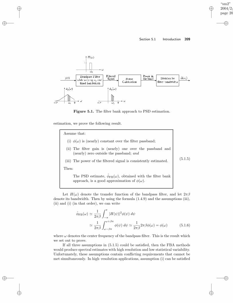
“sm2”2004/2/22page 209

i

i

i

i

i

i

i

i


!" #!$ %&')( * +-,.*/ 0

1243 ,.5687!9;:<*= >? @ :A B >CDE= F ? :< :GCH = I >B FJ 3 K5

L

M

NO ,. O ,

2P'3 ,*5

Q QRRRRS SUT T

L

M

N)O ,. O ,

2VP'3 ,5S S

L

MW

,. ,

XY3 ,*5

Figure 5.1. The filter bank approach to PSD estimation.

estimation, we prove the following result.

Assume that:

(i) φ(ω) is (nearly) constant over the filter passband;

(ii) The filter gain is (nearly) one over the passband and(nearly) zero outside the passband; and

(iii) The power of the filtered signal is consistently estimated.

Then:

The PSD estimate, φFB(ω), obtained with the filter bankapproach, is a good approximation of φ(ω).

(5.1.5)

Let H(ω) denote the transfer function of the bandpass filter, and let 2πβdenote its bandwidth. Then by using the formula (1.4.9) and the assumptions (iii),(ii) and (i) (in that order), we can write

φFB(ω) ' 1

2πβ

∫ π

−π|H(ψ)|2φ(ψ) dψ

' 1

2πβ

∫ ω+βπ

ω−βπφ(ψ) dψ ' 1

2πβ2πβφ(ω) = φ(ω) (5.1.6)

where ω denotes the center frequency of the bandpass filter. This is the result whichwe set out to prove.

If all three assumptions in (5.1.5) could be satisfied, then the FBA methodswould produce spectral estimates with high resolution and low statistical variability.Unfortunately, these assumptions contain conflicting requirements that cannot bemet simultaneously. In high–resolution applications, assumption (i) can be satisfied

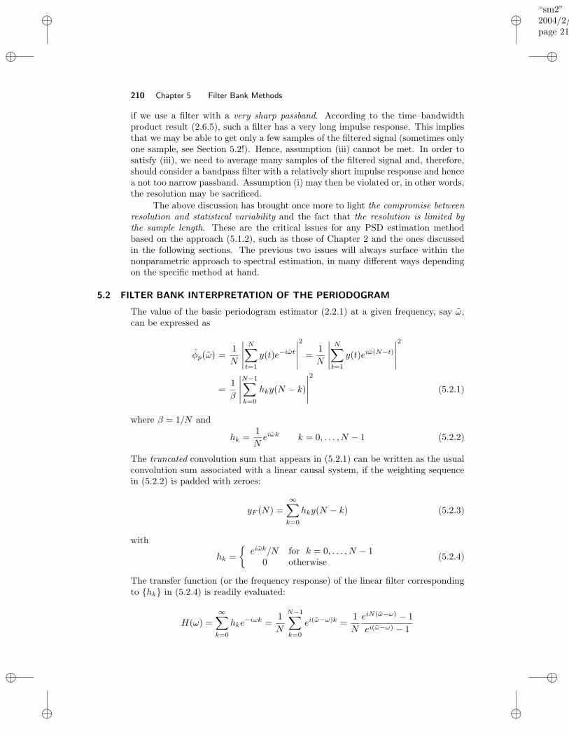
“sm2”2004/2/22page 210

i

i

i

i

i

i

i

i


if we use a filter with a very sharp passband. According to the time–bandwidthproduct result (2.6.5), such a filter has a very long impulse response. This impliesthat we may be able to get only a few samples of the filtered signal (sometimes onlyone sample, see Section 5.2!). Hence, assumption (iii) cannot be met. In order tosatisfy (iii), we need to average many samples of the filtered signal and, therefore,should consider a bandpass filter with a relatively short impulse response and hencea not too narrow passband. Assumption (i) may then be violated or, in other words,the resolution may be sacrificed.

The above discussion has brought once more to light the compromise betweenresolution and statistical variability and the fact that the resolution is limited bythe sample length. These are the critical issues for any PSD estimation methodbased on the approach (5.1.2), such as those of Chapter 2 and the ones discussedin the following sections. The previous two issues will always surface within thenonparametric approach to spectral estimation, in many different ways dependingon the specific method at hand.

5.2 FILTER BANK INTERPRETATION OF THE PERIODOGRAM

The value of the basic periodogram estimator (2.2.1) at a given frequency, say ω,can be expressed as

φp(ω) =1

N

∣∣∣∣∣

N∑

t=1

y(t)e−iωt

∣∣∣∣∣

2

=1

N

∣∣∣∣∣

N∑

t=1

y(t)eiω(N−t)

∣∣∣∣∣

2

=1

β

∣∣∣∣∣

N−1∑

k=0

hky(N − k)

∣∣∣∣∣

2

(5.2.1)

where β = 1/N and

hk =1

Neiωk k = 0, . . . , N − 1 (5.2.2)

The truncated convolution sum that appears in (5.2.1) can be written as the usualconvolution sum associated with a linear causal system, if the weighting sequencein (5.2.2) is padded with zeroes:

yF (N) =

∞∑

k=0

hky(N − k) (5.2.3)

with

hk =

eiωk/N for k = 0, . . . , N − 1

0 otherwise(5.2.4)

The transfer function (or the frequency response) of the linear filter correspondingto hk in (5.2.4) is readily evaluated:

H(ω) =

∞∑

k=0

hke−iωk =

1

N

N−1∑

k=0

ei(ω−ω)k =1

N

eiN(ω−ω) − 1

ei(ω−ω) − 1

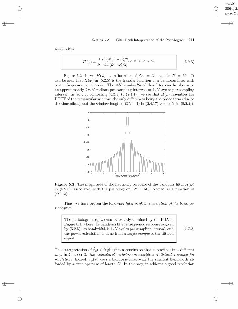
“sm2”2004/2/22page 211

i

i

i

i

i

i

i

i

Section 5.2 Filter Bank Interpretation of the Periodogram 211

which gives

H(ω) =1

N

sin[N(ω − ω)/2]

sin[(ω − ω)/2]ei(N−1)(ω−ω)/2 (5.2.5)

Figure 5.2 shows |H(ω)| as a function of ∆ω = ω − ω, for N = 50. Itcan be seen that H(ω) in (5.2.5) is the transfer function of a bandpass filter withcenter frequency equal to ω. The 3dB bandwidth of this filter can be shown tobe approximately 2π/N radians per sampling interval, or 1/N cycles per samplinginterval. In fact, by comparing (5.2.5) to (2.4.17) we see that H(ω) resembles theDTFT of the rectangular window, the only differences being the phase term (due tothe time offset) and the window lengths ((2N − 1) in (2.4.17) versus N in (5.2.5)).

−3 −2 −1 0 1 2 3−40

−35

−30

−25

−20

−15

−10

−5

0

dB

ANGULAR FREQUENCY

Figure 5.2. The magnitude of the frequency response of the bandpass filter H(ω)in (5.2.5), associated with the periodogram (N = 50), plotted as a function of(ω − ω).

Thus, we have proven the following filter bank interpretation of the basic pe-riodogram.

The periodogram φp(ω) can be exactly obtained by the FBA inFigure 5.1, where the bandpass filter’s frequency response is givenby (5.2.5), its bandwidth is 1/N cycles per sampling interval, andthe power calculation is done from a single sample of the filteredsignal.

(5.2.6)

This interpretation of φp(ω) highlights a conclusion that is reached, in a differentway, in Chapter 2: the unmodified periodogram sacrifices statistical accuracy forresolution. Indeed, φp(ω) uses a bandpass filter with the smallest bandwidth af-forded by a time aperture of length N . In this way, it achieves a good resolution

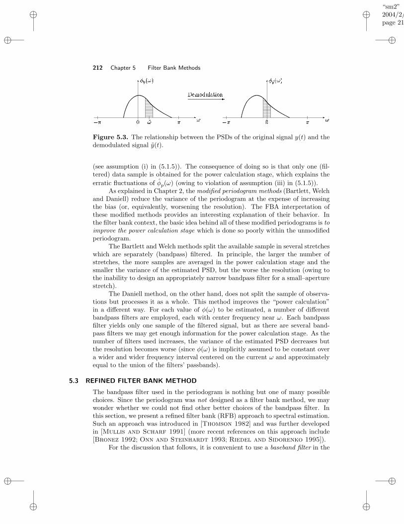
“sm2”2004/2/22page 212

i

i

i

i

i

i

i

i


Z\[]Y^8_`4a bc d ê fghi j-k

jl\m n m

o

pj q

g)rhi j-k

jl\m n m

o

q

Figure 5.3. The relationship between the PSDs of the original signal y(t) and thedemodulated signal y(t).

(see assumption (i) in (5.1.5)). The consequence of doing so is that only one (fil-tered) data sample is obtained for the power calculation stage, which explains the

erratic fluctuations of φp(ω) (owing to violation of assumption (iii) in (5.1.5)).As explained in Chapter 2, the modified periodogram methods (Bartlett, Welch

and Daniell) reduce the variance of the periodogram at the expense of increasingthe bias (or, equivalently, worsening the resolution). The FBA interpretation ofthese modified methods provides an interesting explanation of their behavior. Inthe filter bank context, the basic idea behind all of these modified periodograms is toimprove the power calculation stage which is done so poorly within the unmodifiedperiodogram.

The Bartlett and Welch methods split the available sample in several stretcheswhich are separately (bandpass) filtered. In principle, the larger the number ofstretches, the more samples are averaged in the power calculation stage and thesmaller the variance of the estimated PSD, but the worse the resolution (owing tothe inability to design an appropriately narrow bandpass filter for a small–aperturestretch).

The Daniell method, on the other hand, does not split the sample of observa-tions but processes it as a whole. This method improves the “power calculation”in a different way. For each value of φ(ω) to be estimated, a number of differentbandpass filters are employed, each with center frequency near ω. Each bandpassfilter yields only one sample of the filtered signal, but as there are several band-pass filters we may get enough information for the power calculation stage. As thenumber of filters used increases, the variance of the estimated PSD decreases butthe resolution becomes worse (since φ(ω) is implicitly assumed to be constant overa wider and wider frequency interval centered on the current ω and approximatelyequal to the union of the filters’ passbands).

5.3 REFINED FILTER BANK METHOD

The bandpass filter used in the periodogram is nothing but one of many possiblechoices. Since the periodogram was not designed as a filter bank method, we maywonder whether we could not find other better choices of the bandpass filter. Inthis section, we present a refined filter bank (RFB) approach to spectral estimation.Such an approach was introduced in [Thomson 1982] and was further developedin [Mullis and Scharf 1991] (more recent references on this approach include[Bronez 1992; Onn and Steinhardt 1993; Riedel and Sidorenko 1995]).

For the discussion that follows, it is convenient to use a baseband filter in the

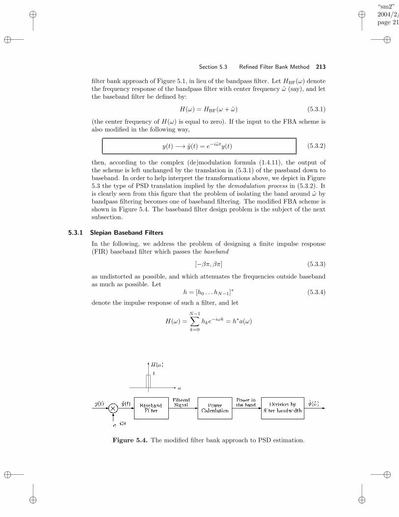
“sm2”2004/2/22page 213

i

i

i

i

i

i

i

i

Section 5.3 Refined Filter Bank Method 213

filter bank approach of Figure 5.1, in lieu of the bandpass filter. Let HBF(ω) denotethe frequency response of the bandpass filter with center frequency ω (say), and letthe baseband filter be defined by:

H(ω) = HBF(ω + ω) (5.3.1)

(the center frequency of H(ω) is equal to zero). If the input to the FBA scheme isalso modified in the following way,

y(t) −→ y(t) = e−iωty(t) (5.3.2)

then, according to the complex (de)modulation formula (1.4.11), the output ofthe scheme is left unchanged by the translation in (5.3.1) of the passband down tobaseband. In order to help interpret the transformations above, we depict in Figure5.3 the type of PSD translation implied by the demodulation process in (5.3.2). Itis clearly seen from this figure that the problem of isolating the band around ω bybandpass filtering becomes one of baseband filtering. The modified FBA scheme isshown in Figure 5.4. The baseband filter design problem is the subject of the nextsubsection.

5.3.1 Slepian Baseband Filters

In the following, we address the problem of designing a finite impulse response(FIR) baseband filter which passes the baseband

[−βπ, βπ] (5.3.3)

as undistorted as possible, and which attenuates the frequencies outside basebandas much as possible. Let

h = [h0 . . . hN−1]∗ (5.3.4)

denote the impulse response of such a filter, and let

H(ω) =

N−1∑

k=0

hke−iωk = h∗a(ω)

ssss t suwvxwyz | 8| ~!| w4 EEE-| ' E |

~ EE | !''U; - G -¡8¢£¤¥ ¦ G £§ ¨ ¢¦© ª © ª

«4¬® ¯°4±

²

³´

µ U

Figure 5.4. The modified filter bank approach to PSD estimation.

“sm2”2004/2/22page 214

i

i

i

i

i

i

i

i


(where a(ω) = [1 e−iω . . . e−i(N−1)ω]T ) be the corresponding frequency response.The two design objectives can be turned into mathematical specifications in thefollowing way. Let the input to the filter be white noise of unit variance. Then thepower of the output is:

1

2π

∫ π

−π|H(ω)|2dω =

N−1∑

k=0

N−1∑

p=0

hkh∗p

[1

2π

∫ π

−πeiω(p−k)dω

]

=

N−1∑

k=0

N−1∑

p=0

hkh∗pδk,p = h∗h (5.3.5)

We note in passing that equation (5.3.5) above can be recognized as the Parseval’stheorem (1.2.6). The part of the total power, (5.3.5), that lies in the baseband isgiven by

1

2π

∫ βπ

−βπ|H(ω)|2dω = h∗

1

2π

∫ βπ

−βπa(ω)a∗(ω)dω

h , h∗Γh (5.3.6)

The k, p element of the N ×N matrix Γ defined in (5.3.6) is given by

Γk,p =1

2π

∫ βπ

−βπe−i(k−p)ωdω =

sin[(k − p)βπ]

(k − p)π(5.3.7)

which, using the sinc function, can be written as

Γk,p = βsinc[(k − p)βπ] , γ|k−p| (5.3.8)

Note that the matrix Γ is symmetric and Toeplitz. Also, note that this matrix hasalready been encountered in the window design example in Section 2.6.3. In fact,as we will shortly see, the window design strategy in that example is quite similarto the baseband filter design method employed here.

Since the filter h must be such that the power of the filtered signal in thebaseband is as large as possible relative to the total power, we are led to thefollowing optimization problem:

maxh

h∗Γh subject to h∗h = 1 (5.3.9)

The solution to the problem above is given in Result R13 in Appendix A: the maxi-mizing h is equal to the eigenvector of Γ corresponding to its maximum eigenvalue.Hence, we have proven the following result.

The impulse response h of the “most selective” baseband filter(according to the design objectives in (5.3.9)) is given by thedominant eigenvector of Γ, and is called the first Slepian sequence.

(5.3.10)

“sm2”2004/2/22page 215

i

i

i

i

i

i

i

i


The matrix Γ played a key role in the foregoing derivation. In what follows,we look in more detail at the eigenstructure of Γ. In particular, we provide anintuitive explanation as to why the first dominant eigenvector of Γ behaves like abaseband filter. We also show that, depending on the relation between β and N ,the next dominant eigenvectors of Γ might also be used as baseband filters. Ourdiscussion of these aspects will be partly heuristic. Note that the eigenvectors of Γare called the Slepian sequences [Slepian 1964] (as already indicated in (5.3.10)).We denote these eigenvectors by skNk=1.

Remark: The Slepian sequences should not be computed by the eigendecompositionof Γ. Numerically more efficient and reliable ways for computing these sequencesexist (see, e.g., [Slepian 1964]), for instance as solutions to some differential equa-tions or as eigenvectors of certain tridiagonal matrices.

The theoretical eigenanalysis of Γ is a difficult problem in the case of finiteN . (Of course, the eigenvectors and eigenvalues of Γ may always be computed, forgiven β and N ; here we are interested in establishing theoretical expressions for Γ’seigenelements.) For N sufficiently large, however, “reasonable approximations” tothe eigenelements of Γ can be derived. Let a(ω) be defined as before:

a(ω) = [1 e−iω . . . e−i(N−1)ω]T (5.3.11)

Assume that β is chosen larger than 1/N , and define

K = Nβ ≥ 1 (5.3.12)

(To simplify the discussion, K and N are assumed to be even integers in whatfollows.) With these preparations and assuming thatN is large, we can approximatethe integral in (5.3.6) and write Γ as

Γ ' 1

2π

K/2−1∑

p=−K/2a

(2π

Np

)

a∗(

2π

Np

)2π

N

=1

N

K/2−1∑

p=−K/2a

(2π

Np

)

a∗(

2π

Np

)

, Γ0 (5.3.13)

The vectors a( 2πN p)/

√N

N2

p=− N2 +1

, part of which appears in (5.3.13), can be readily

shown to form an orthonormal set:

1

Na∗(

2π

Np

)

a

(2π

Ns

)

=1

N

N−1∑

k=0

ei2πN (p−s)k

=

1

N

ei2π(p−s) − 1

ei2πN (p−s) − 1

= 0, s 6= p

1, s = p

(5.3.14)

“sm2”2004/2/22page 216

i

i

i

i

i

i

i

i


The eigenvectors of the matrix on the right hand side of equation (5.3.13), Γ0, are

therefore given by a(

2πN p)/√NN/2p=−N/2+1, with eigenvalues of 1 (with multiplicity

K) and 0 (with multiplicity N −K). The eigenvectors corresponding to the eigen-

values equal to one are a(

2πN p)/√NK/2p=−K/2+1. By paralleling the calculations

in (5.2.3)–(5.2.5), it is not hard to show that each of these dominant eigenvectorsof Γ0 is the impulse response of a narrow bandpass filter with bandwidth equal toabout 1/N and center frequency 2π

N p; the set of these filters therefore covers theinterval [−βπ, βπ].

Now, the elements of Γ approach those of Γ0 as N increases; more precisely,|[Γ]i,j − [Γ0]i,j | = O(1/N) for sufficiently large N . However, this does not meanthat ‖Γ − Γ0‖ → 0, as N → ∞, for any reasonable matrix norm, because Γ andΓ0 are (N ×N) matrices. Consequently, the eigenelements of Γ do not necessarilyconverge to the eigenelements of Γ0 as N → ∞. However, based on the previousanalysis, we can at least expect that the eigenelements of Γ are not “too different”from those of Γ0. This observation of the theoretical analysis, backed up withempirical evidence from the computation of the eigenelements of Γ in specific cases,leads us to conclude the following.

The matrix Γ has K eigenvalues close to one and (N −K) eigen-values close to zero, provided N is large enough, where K is givenby the “time–bandwidth” product (5.3.12). The dominant eigen-vectors corresponding to the K largest eigenvalues form a set oforthogonal impulse responses of K bandpass filters that approx-imately cover the baseband [−βπ, βπ].

(5.3.15)

As we argue in the next subsections, in some situations (specified there) wemay want to use the whole set of K Slepian baseband filters, not only the dominantSlepian filter in this set.

5.3.2 RFB Method for High–Resolution Spectral Analysis

Assume that the spectral analysis problem dealt with is one in which it is impor-tant to achieve the maximum resolution afforded by the approach at hand (sucha problem appears, for instance, in the case of PSD’s with closely spaced peaks).Then we set

β = 1/N ⇐⇒ K = 1 (5.3.16)

(Note that we cannot set β to a value less than 1/N since that choice would lead toK < 1, which is meaningless; the fact that we must choose β ≥ 1/N is one of themany facets of the 1/N–resolution limit of the nonparametric spectral estimation.)

Since K = 1, we can only use the first Slepian sequence as a bandpass filter

h = s1 (5.3.17)

The way in which the RFB scheme based on (5.3.17) works is described in thefollowing.

“sm2”2004/2/22page 217

i

i

i

i

i

i

i

i


First, note from (5.3.5), (5.3.9) and (5.3.16) that

1 = h∗h =1

2π

∫ π

−π|H(ω)|2dω ' 1

2π

∫ βπ

−βπ|H(ω)|2dω

' β|H(0)|2 =1

N|H(0)|2 (5.3.18)

Hence, under the (idealizing) assumption that H(ω) is different from zero only inthe baseband where it takes a constant value, we have

|H(0)|2 ' N (5.3.19)

Next, consider the sample at the filter’s output obtained by the convolution of thewhole input sequence y(t)Nt=1 with the filter impulse response hk:

x ,

N−1∑

k=0

hky(N − k) =

N∑

t=1

hN−ty(t) (5.3.20)

The power of x should be approximately equal to the PSD value φ(ω), which isconfirmed by the following calculation:

E|x|2

=1

2π

∫ π

−π|H(ω)|2φy(ω)dω

' N

2π

∫ βπ

−βπφy(ω)dω =

N

2π

∫ βπ

−βπφy(ω + ω)dω

' N

2πφy(ω) × 2πβ = Nβφy(ω) = φy(ω) (5.3.21)

The second “equality” above follows from the properties ofH(ω) (see, also, (5.3.19)),the third from the complex demodulation formula (1.4.11), and the fourth from theassumption that φy(ω) is nearly constant over the passband considered.

In view of (5.3.21), the PSD estimation problem reduces to estimating thepower of the filtered signal. Since only one sample, x, of that signal is available,the obvious estimate for the signal power is |x|2. This leads to the following estimateof φ(ω):

φ(ω) =

∣∣∣∣∣

N∑

t=1

hN−ty(t)e−iωt

∣∣∣∣∣

2

(5.3.22)

where hk is given by the first Slepian sequence (see (5.3.17)). The reason we didnot divide (5.3.22) by the filter bandwidth is that |H(0)|2 ' N by (5.3.19), whichdiffers from assumption (ii) in (5.1.5).

The spectral estimate (5.3.22) is recognized to be a windowed periodogramwith temporal window hN−k. For large values of N , it follows from the analysisin the previous section that h can be expected to be reasonably close to the vector[1 . . . 1]T /

√N . When inserting the latter vector in (5.3.22), we get the unwindowed

“sm2”2004/2/22page 218

i

i

i

i

i

i

i

i


periodogram. Hence, we reach the conclusion that for N large enough, the RFBestimate (5.3.22) will behave not too differently from the unmodified periodogram(which is quite natural in view of the fact that we wanted a high–resolution spectralestimator, and the basic periodogram is known to be such an estimator).

Remark: We warn the reader, once again, that the above discussion is heuristic.As explained before (see the discussion related to (5.3.15)), as N increases hkmay be expected to be “reasonably close” but not necessarily converge to 1/

√N .

In addition, even if hk in (5.3.22) converges to 1/√N as N → ∞, the function

in (5.3.22) may not converge to φp(ω) if the convergence rate of hk is too slow

(note that the number of hk in (5.3.22) is equal to N). Hence φ(ω) in (5.3.22)

and the periodogram φp(ω) may differ from one another even for large values of N .

In any case, even though the two estimators φ(ω) in (5.3.22) and φp(ω) gen-erally give different PSD values, they both base the power calculation stage of theFBA scheme on only a single sample. Hence, similarly to φp(ω), the RFB estimate(5.3.22) is expected to exhibit erratic fluctuations. The next subsection discussesa way in which the variance of the RFB spectral estimate can be reduced, at theexpense of reducing the resolution of this estimate.

5.3.3 RFB Method for Statistically Stable Spectral Analysis

The FBA interpretation of the modified periodogram methods, as explained in Sec-tion 5.2, highlighted two approaches to reduce the statistical variability of the spec-tral estimate (5.3.22). The first approach consists of splitting the available sampley(t)Nt=1 into a number of subsequences, computing (5.3.22) for each stretch, andthen averaging the so–obtained values. The problem with this way of proceeding isthat the values taken by (5.3.22) for different subsequences are not guaranteed tobe statistically independent. In fact, if the subsequences overlap then those valuesmay be strongly correlated. The consequence of this fact is that one can never besure of the “exact” reduction of variance that is achieved by averaging, in a givensituation.

The second approach to reduce the variance consists of using several bandpassfilters, in lieu of only one, which operate on the whole data sample [Thomson

1982]. This approach aims at producing statistically independent samples for thepower calculation stage. When this is achieved the variance is reduced K times,where K is the number of samples averaged (which equals the number of bandpassfilters used).

In the following, we focus on this second approach which appears particularlysuitable for the RFB method. We set β to some value larger than 1/N , which gives(cf. (5.3.12))

K = Nβ > 1 (5.3.23)

The larger β (i.e., the lower the resolution), the larger K and hence the larger thereduction in variance that can be achieved. By using the result (5.3.15), we define

“sm2”2004/2/22page 219

i

i

i

i

i

i

i

i


K baseband filters as

hp = [hp,0 . . . hp,N−1]∗ = sp, (p = 1, . . . ,K) (5.3.24)

Here hp denotes the impulse response vector of the pth filter, and sp is the pth domi-nant Slepian sequence. Note that sp is real–valued (see Result R12 in Appendix A),and thus so is hp. According to the discussion leading to (5.3.15), the set of filters(5.3.24) covers the baseband [−βπ, βπ], with each of these filters passing (roughlyspeaking) (1/K)th of this baseband. Let xp be defined similarly to x in (5.3.20),but now for the pth filter:

xp =

N−1∑

k=0

hp,ky(N − k) =

N∑

t=1

hp,N−ty(t) (5.3.25)

The calculation (5.3.21) applies to xp in exactly the same way, and hence

E|xp|2

' φy(ω), p = 1, . . . ,K (5.3.26)

In addition, a straightforward calculation gives

E xpx∗k = E

[N−1∑

t=0

hp,ty(N − t)

][N−1∑

s=0

h∗k,sy

∗(N − s)

]

=

N−1∑

t=0

N−1∑

s=0

hp,th∗k,sry(s− t)

=1

2π

∫ π

−π

N−1∑

t=0

N−1∑

s=0

hp,th∗k,sφy(ω)ei(s−t)ωdω

=1

2π

∫ π

−πHp(ω)H∗

k(ω)φy(ω)dω

' φy(0)h∗p

[

1

2π

∫ βπ

−βπa(ω)a∗(ω)dω

]

hk

= φy(ω)h∗pΓhk = 0 for k 6= p (5.3.27)

Thus, the random variables xp and xk (for p 6= k) are approximately uncorrelatedunder the assumptions made. This implies, at least under the assumption that thexk are Gaussian, that |xp|2 and |xk|2 are statistically independent (for p 6= k).

According to the calculations above, |xp|2Kp=1 can approximately be consid-ered to be independent random variables all with the same mean φy(ω). Then, we

can estimate φy(ω) by the following average of |xp|2: 1K

∑Kp=1 |xp|2, or

φ(ω) =1

K

K∑

p=1

∣∣∣∣∣

N∑

t=1

hp,N−ty(t)e−iωt

∣∣∣∣∣

2

(5.3.28)

“sm2”2004/2/22page 220

i

i

i

i

i

i

i

i


We may suspect that the random variables |xp|2 have not only the same mean,but also the same variance (this can, in fact, be readily shown under the Gaussianhypothesis). Whenever this is true, the variance of the average in (5.3.28) isK timessmaller than the variance of each of the variables averaged. The above findings aresummarized in the following.

If the resolution threshold β is increased K times from β = 1/N(the lowest value) to β = K/N , then the variance of the RFBestimate in (5.3.22) may be reduced by a factor K by construct-ing the spectral estimate as in (5.3.28), where the pth basebandfilter’s impulse response hp,tN−1

t=0 is given by the pth dominantSlepian sequence (p = 1, . . . ,K).

(5.3.29)

The RFB spectral estimator (5.3.28) can be given two interpretations. First,arguments similar with those following equation (5.3.22) suggest that for large Nthe RFB estimate (5.3.28) behaves similarly to the Daniell method of periodogramaveraging. For small or medium–sized values of N , the RFB and Daniell methodsbehave differently. In such a case, we can relate (5.3.28) to the class of multiwindowspectral estimators [Thomson 1982]. Indeed, the RFB estimate (5.3.28) can be in-terpreted as the average of K windowed periodograms, where the pth periodogramis computed from the raw data sequence y(t) windowed with the pth dominantSlepian sequence. Note that since the Slepian sequences are given by the eigenvec-tors of the real Toeplitz matrix Γ, they must be either symmetric: hp,N−t = hp,t−1;or skew–symmetric: hp,N−t = −hp,t−1 (see Result R25 in Appendix A). This meansthat (5.3.28) can alternatively be written as

φ(ω) =1

K

K∑

p=1

∣∣∣∣∣

N∑

t=1

hp,t−1y(t)e−iωt

∣∣∣∣∣

2

(5.3.30)

This form of the RFB estimate makes its interpretation as a multiwindow spectrumestimator more direct.

For a second interpretation of the RFB estimate (5.3.28), consider the follow-

“sm2”2004/2/22page 221

i

i

i

i

i

i

i

i


ing (Daniell–type) spectrally smoothed periodogram estimator of φ(ω):

φ(ω) =1

2πβ

∫ ω+βπ

ω−βπφp(ω)dω =

1

2πβ

∫ βπ

−βπφp(ω + ω)dω

=1

2πβ

∫ βπ

−βπ

1

N

∣∣∣∣∣

N∑

t=1

y(t)e−i(ω+ω)t

∣∣∣∣∣

2

dω

=1

2πK

∫ βπ

−βπ

N∑

t=1

N∑

s=1

y(t)y∗(s)e−iωteiωsdω

=1

K[y∗(1) . . . y∗(N)]

·

1

2π

∫ βπ

−βπ

1eiω

...ei(N−1)ω

[1 e−iω . . . e−i(N−1)ω]dω

y(1)...

y(N)

=1

K[y∗(1) . . . y∗(N)]Γ

y(1)...

y(N)

(5.3.31)

where we made use of the fact that Γ is real–valued. It follows from the result(5.3.15) that Γ can be approximated by the rank–K matrix:

Γ 'K∑

p=1

spsTp =

K∑

p=1

hphTp (5.3.32)

Inserting (5.3.32) into (5.3.31) and using the fact that the Slepian sequences sp = hpare real–valued leads to the following PSD estimator:

φ(ω) ' 1

K

K∑

p=1

∣∣∣∣∣

N∑

t=1

hp,t−1y(t)

∣∣∣∣∣

2

(5.3.33)

which is precisely the RFB estimator (5.3.30). Hence, the RFB estimate of thePSD can also be interpreted as a reduced–rank smoothed periodogram.

We might think of using the full–rank smoothed periodogram (5.3.31) as anestimator for PSD, in lieu of the reduced–rank smoothed periodogram (5.3.33)which coincides with the RFB estimate. However, from a theoretical standpointwe have no strong reason to do so. Moreover, from a practical standpoint we haveclear reasons against such an idea. We can explain this briefly as follows. TheK dominant eigenvectors of Γ can be precomputed with satisfactory numerical ac-curacy. Then, evaluation of (5.3.33) can be done by using an FFT algorithm inapproximately 1

2KN log2N = 12βN

2 log2N flops. On the other hand, a directevaluation of (5.3.31) would require N2 flops for each value of ω, which leads to aprohibitively large total computational burden. A computationally efficient evalu-ation of (5.3.31) would require some factorization of Γ to be performed, such as the

“sm2”2004/2/22page 222

i

i

i

i

i

i

i

i


eigendecomposition of Γ. However, Γ is an extremely ill–conditioned matrix (recallthat N −K = N(1−β) of its eigenvalues are close to zero), which means that sucha complete factorization cannot easily be performed with satisfactory numericalaccuracy. In any case even if we were able to precompute the eigendecompositionof Γ, evaluation of (5.3.31) would require 1

2N2 log2N flops, which is still larger by

a factor of 1/β than what is required for (5.3.33).

5.4 CAPON METHOD

The periodogram was previously shown to be a filter bank approach which usesa bandpass filter whose impulse response vector is given by the standard Fouriertransform vector (i.e., [1, e−iω, . . . , e−i(N−1)ω]T ). In the periodogram approachthere is no attempt to purposely design the bandpass filter to achieve some desiredcharacteristics (see, however, Section 5.5). The RFB method, on the other hand,uses a bandpass filter specifically designed to be “as selective as possible” for awhite noise input (see (5.3.5) and the discussion preceding it). The RFB’s filteris still data independent in the sense that it does not adapt to the processed datain any way. Presumably, it might be valuable to take the data properties intoconsideration when designing the bandpass filter. In other words, the filter shouldbe designed to be “as selective as possible” (according to a criterion to be specified)not for a fictitious white noise input, but for the input consisting of the studieddata themselves. This is the basic idea behind the Capon method, which is an FBAprocedure based on a data–dependent bandpass filter [Capon 1969; Lacoss 1971].

5.4.1 Derivation of the Capon Method

The Capon method (CM), in contrast to the RFB estimator (5.3.28), uses only onebandpass filter for computing one estimated spectrum value. This suggests that ifthe CM is to provide statistically stable spectral estimates, then it should make useof the other approach which affords this: splitting the raw sample into subsequencesand averaging the results obtained from each subsequence. Indeed, as we shall seethe Capon method is essentially based on this second approach.

Consider a filter with a finite impulse response of length m, denoted by

h = [h0 h1 . . . hm]∗ (5.4.1)

where m is a positive integer that is unspecified for the moment. The output of thefilter at time t, when the input is the raw data sequence y(t), is given by

yF (t) =

m∑

k=0

hky(t− k)

= h∗

y(t)y(t− 1)

...y(t−m)

(5.4.2)

Let R denote the covariance matrix of the data vector in (5.4.2). Then the power

“sm2”2004/2/22page 223

i

i

i

i

i

i

i

i

Section 5.4 Capon Method 223

of the filter output can be written as:

E|yF (t)|2

= h∗Rh (5.4.3)

where, according to the definition above,

R = E

y(t)...

y(t−m)

[y∗(t) . . . y∗(t−m)]

(5.4.4)

The response of the filter (5.4.2) to a sinusoidal component of frequency ω (say) isdetermined by the filter’s frequency response:

H(ω) =

m∑

k=0

hke−iωk = h∗a(ω) (5.4.5)

wherea(ω) = [1 e−iω . . . e−imω]T (5.4.6)

If we want to make the filter as selective as possible for a frequency band aroundthe current value ω, then we may think of minimizing the total power in (5.4.3)subject to the constraint that the filter passes the frequency ω undistorted. Thisidea leads to the following optimization problem:

minhh∗Rh subject to h∗a(ω) = 1 (5.4.7)

The solution to (5.4.7) is given in Result R35 in Appendix A:

h = R−1a(ω)/a∗(ω)R−1a(ω) (5.4.8)

Inserting (5.4.8) into (5.4.3) gives

E|yF (t)|2

= 1/a∗(ω)R−1a(ω) (5.4.9)

This is the power of y(t) in a passband centered on ω. Then, assuming that the(idealized) conditions (i) and (ii) in (5.1.5) hold, we can approximately determinethe value of the PSD of y(t) at the passband’s center frequency as

φ(ω) ' E|yF (t)|2

β=

1

βa∗(ω)R−1a(ω)(5.4.10)

where β denotes the frequency bandwidth of the filter given by (5.4.8). The divisionby β, as above, is sometimes omitted in the literature, but it is required to completethe FBA scheme in Figure 5.1. Note that since the bandpass filter (5.4.8) is datadependent, its bandwidth β is not necessarily data independent, nor is it necessarilyfrequency independent. Hence, the division by β in (5.4.10) may not represent a

“sm2”2004/2/22page 224

i

i

i

i

i

i

i

i


simple scaling of E|yF (t)|2

, but it may change the shape of this quantity as a

function of ω.There are various possibilities for determining the bandwidth β, depending

on the degree of precision we are aiming for. The simplest possibility is to set

β = 1/(m+ 1) (5.4.11)

This choice is motivated by the time–bandwidth product result (2.6.5), which saysthat for a filter whose temporal aperture is equal to (m+1), the bandwidth shouldroughly be given by 1/(m+ 1). By inserting (5.4.11) in (5.4.10), we obtain

φ(ω) ' (m+ 1)

a∗(ω)R−1a(ω)(5.4.12)

Note that if y(t) is white noise of variance σ2, (5.4.12) takes the correct value:φ(ω) = σ2. In the general case, however, (5.4.11) gives only a rough indication ofthe filter’s bandwidth, as the time–bandwidth product result does not apply exactlyto the present situation (see the conditions under which (2.6.5) has been derived).

An often more exact expression for β can be obtained as follows [Lagunas,

Santamaria, Gasull, and Moreno 1986]. The (equivalent) bandwidth of abandpass filter can be defined as the support of the rectangle centered on ω (thefilter’s center frequency) that concentrates the whole energy in the filter’s frequencyresponse. According to this definition, β can be assumed to satisfy:

∫ π

−π|H(ψ)|2dψ = |H(ω)|22πβ (5.4.13)

Since in the present case H(ω) = 1 (see (5.4.7)), we obtain from (5.4.13):

β =1

2π

∫ π

−π|h∗a(ψ)|2dψ = h∗

[1

2π

∫ π

−πa(ψ)a∗(ψ)dψ

]

h (5.4.14)

The (k, p) element of the central matrix in the above quadratic form is given by

1

2π

∫ π

−πe−iψ(k−p)dψ = δk,p (5.4.15)

With this observation and (5.4.8), (5.4.14) leads to

β = h∗h =a∗(ω)R−2a(ω)

[a∗(ω)R−1a(ω)]2(5.4.16)

Note that this expression of the bandwidth is both data and frequency dependent(as was alluded to previously). Inserting (5.4.16) in (5.4.10) gives

φ(ω) ' a∗(ω)R−1a(ω)

a∗(ω)R−2a(ω)(5.4.17)

Remark: The expression for β in (5.4.16) is based on the assumption that mostof the area under the curve of |H(ψ)|2 = |h∗a(ψ)|2 (for ψ ∈ [−π, π]) is located

“sm2”2004/2/22page 225

i

i

i

i

i

i

i

i


around the center frequency ω. This assumption is often true, but not always true.For instance, consider a data sequence y(t) consisting of a number of sinusoidalcomponents with frequencies ωk in noise with small power. Then the Capon filter(5.4.8) with center frequency ω will likely place nulls at ψ = ωk to annihilatethe strong sinusoidal components in the data, but will pay little attention to theweak noise component. The consequence is that |H(ψ)|2 will be nearly zero atψ = ωk, and one at ψ = ω (by (5.4.7)), but may take rather large values atother frequencies (see, for example, the numerical examples in [Li and Stoica

1996a], which demonstrate this behavior of the Capon filter). In such a case, theformula (5.4.16) may significantly overestimate the “true” bandwidth, and hencethe spectral formula (5.4.17) may significantly underestimate the PSD φ(ω).

In the derivations above, the true data covariance matrix R has been assumedavailable. In order to turn the previous PSD formulas into practical spectral esti-mation algorithms, we must replace R in these formulas by a sample estimate, forinstance by

R =1

N −m

N∑

t=m+1

y(t)...

y(t−m)

[y∗(t) . . . y∗(t−m)] (5.4.18)

Doing so, we obtain the following two spectral estimators corresponding to (5.4.12)and (5.4.17), respectively:

CM–Version 1: φ(ω) =m+ 1

a∗(ω)R−1a(ω)(5.4.19)

CM–Version 2: φ(ω) =a∗(ω)R−1a(ω)

a∗(ω)R−2a(ω)(5.4.20)

There is an implicit assumption in both (5.4.19) and (5.4.20) that R−1 exists. Thisassumption sets a limit on the maximum value that can be chosen for m:

m < N/2 (5.4.21)

(Observe that rank(R) ≤ N −m, which is less than dim(R) = m + 1 if (5.4.21) isviolated.) The inequality (5.4.21) is important since it sets a limit on the resolutionachievable by the Capon method. Indeed, since the Capon method is based ona bandpass filter with impulse response’s aperture equal to m, we may expect itsresolution threshold to be on the order of 1/m > 2/N (with the inequality followingfrom (5.4.21)).

As m is decreased, we can expect the resolution of Capon method to becomeworse (cf. the previous discussion). On the other hand, the accuracy with which Ris determined increases with decreasing m (since more outer products are averaged

“sm2”2004/2/22page 226

i

i

i

i

i

i

i

i


in (5.4.18)). The main consequence of the increased accuracy of R is to statisticallystabilize the spectral estimate (5.4.19) or (5.4.20). Hence, the choice of m shouldbe done with the ubiquitous tradeoff between resolution and statistical accuracy inmind. It is interesting to note that for the Capon method both the filter design andpower calculation stages are data dependent. The accuracy of both these stagesmay worsen if m is chosen too large. In applications, the maximum value thatcan be chosen for m might also be limited from considerations of computationalcomplexity.

Empirical studies have shown that the ability of the Capon method to resolvefine details of a PSD, such as closely spaced peaks, is superior to the correspondingperformance of the periodogram–based methods. This superiority may be attributedto the higher statistical stability of Capon method, as explained next. Form smallerthan N/2 (see (5.4.21)), we may expect the Capon method to possess worse res-olution but better statistical accuracy compared with the unwindowed or “mildlywindowed” periodogram method. It should be stressed that the notion of “reso-lution” refers to the ability of the theoretically averaged spectral estimate Eφ(ω)to resolve fine details in the true PSD φ(ω). This resolution is roughly inverselyproportional to the window’s length or the bandpass filter impulse response’s aper-ture. The “resolving power” corresponding to the estimate φ(ω) is more difficultto quantify, but — of course — it is what interests the most. It should be clearthat the resolving power of φ(ω) depends not only on the bias of this estimate (i.e.,

on Eφ(ω)), but also on its variance. A spectral estimator with low bias–basedresolution but high statistical accuracy may be better able to resolve finer details ina studied PSD than can a high resolution/low accuracy estimator. Since the pe-riodogram may achieve better bias–based resolution than the Capon method, thehigher (empirically observed) “resolving power” of the latter should be due to abetter statistical accuracy (i.e., a lower variance).

In the context of the previous discussion, it is interesting to note that theBlackman–Tukey periodogram with a Bartlett window of length 2m + 1, which isgiven by (see (2.5.1)):

φBT(ω) =

m∑

k=−m

(m+ 1 − |k|)m+ 1

r(k)e−iωk

can be written in a form that bears some resemblance with the form (5.4.19) of theCM–Version 1 estimator. A straightforward calculation gives

φBT(ω) =

m∑

t=0

m∑

s=0

r(t− s)e−iω(t−s)/(m+ 1) (5.4.22)

=1

m+ 1a∗(ω)Ra(ω) (5.4.23)

where a(ω) is as defined in (5.4.6), and R is the Hermitian Toeplitz sample covari-

“sm2”2004/2/22page 227

i

i

i

i

i

i

i

i


ance matrix

R =

r(0) r(1) . . . r(m)

r∗(1) r(0). . .

......

. . .. . . r(1)

r∗(m) . . . r∗(1) r(0)

Comparing the above expression for φBT(ω) with (5.4.19), it is seen that the CM–Version 1 can be obtained from Blackman–Tukey estimator by replacing R in theBlackman–Tukey estimator with R−1, and then inverting the so–obtained quadraticform. Below we provide a brief explanation as to why this replacement and inversionmake sense. That is, if we ignore for a moment the technically sound filter bankderivation of the Capon method, then why should the above way of obtainingCM–Version 1 from the Blackman–Tukey method provide a reasonable spectralestimator? We begin by noting that (cf. Section 1.3.2):

limm→∞

E

1

m+ 1

∣∣∣∣∣

m∑

t=0

y(t)e−iωt

∣∣∣∣∣

2

= φ(ω)

However, a simple calculation shows that

E

1

m+ 1

∣∣∣∣∣

m∑

t=0

y(t)e−iωt

∣∣∣∣∣

2

=

1

m+ 1

m∑

t=0

m∑

s=0

r(t−s)e−iωteiωs =1

m+ 1a∗(ω)Ra(ω)

Hence,

limm→∞

1

m+ 1a∗(ω)Ra(ω) = φ(ω) (5.4.24)

Similarly, one can show that

limm→∞

1

m+ 1a∗(ω)R−1a(ω) = φ−1(ω) (5.4.25)

(see, e.g., [Hannan and Wahlberg 1989]). Comparing (5.4.24) with (5.4.25) pro-vides the explanation we were looking for. Observe that the CM–Version 1 estimatoris a finite–sample approximation to equation (5.4.25), whereas the Blackman–Tukeyestimator is a finite–sample approximation to equation (5.4.24).

The Capon method has also been compared with the AR method of spectralestimation (see Section 3.2). It has been empirically observed that the CM–Version1 possesses less variance but worse resolution than the AR spectral estimator. Thismay be explained by making use of the relationship that exists between the CM–Version 1 and AR spectral estimators; see the next subsection (and also [Burg

1972]). The CM–Version 2 spectral estimator is less well studied and hence itsproperties are not so well understood. In the following subsection, we also relatethe CM–Version 2 to the AR spectral estimator. In the case of CM–Version 2, therelationship is more involved, hence leaving less room for intuitive explanations.

“sm2”2004/2/22page 228

i

i

i

i

i

i

i

i


5.4.2 Relationship between Capon and AR Methods

The AR method of spectral estimation has been described in Chapter 3. In thefollowing we consider the covariance matrix estimate in (5.4.18). The AR methodcorresponding to this sample covariance matrix is the LS method discussed in Sec-tion 3.4.2. Let us denote the matrix R in (5.4.18) by Rm+1 and its principallower–right k × k block by Rk (k = 1, . . . ,m+ 1), as shown below:

R =

k 1m+ 1

m+ 1

1

k

R1

Rk

Rm+1

(5.4.26)With this notation, the coefficient vector θk and the residual power σ2

k of the kth–order AR model fitted to the data y(t) are obtained as the solutions to thefollowing matrix equation (refer to (3.4.6)):

Rk+1

[1

θck

]

=

[σ2k

0

]

(5.4.27)

(the complex conjugate in (5.4.27) appears owing to the fact that Rk above is equalto the complex conjugate of the sample covariance matrix used in Chapter 3). Thenested structure of (5.4.26) along with the defining equation (5.4.27) imply:

Rm+1

1 0 . . . 0 0

1...

.... . . 0

1 0

θcm θcm−1 θc1 1

=

σ2m x . . . x

0 σ2m−1

. . ....

.... . .

. . . x0 · · · 0 σ2

0

(5.4.28)

“sm2”2004/2/22page 229

i

i

i

i

i

i

i

i


where “x” stands for undetermined elements. Let

H =

1 0 . . . 0 0

1...

.... . . 0

1 0


(5.4.29)

It follows from (5.4.28) that

H∗Rm+1H =

σ2m x . . . x

σ2m−1

. . ....

0. . . x

σ20

(5.4.30)

(where, once more, x denotes undetermined elements). Since H∗Rm+1H is a Her-mitian matrix, the elements designated by “x” in (5.4.30) must be equal to zero.Hence, we have proven the following result which is essential in establishing a rela-tion between the AR and Capon methods of spectral estimation (this result extendsthe one in Exercise 3.7 to the non–Toeplitz covariance case).

The parameters θk, σ2k of the AR models of orders k =

1, 2, . . . ,m determine the following factorization of the inverse(sample) covariance matrix:

R−1m+1 = HΣ−1H∗ ; Σ =

σ2m 0

σ2m−1

. . .

0 σ20

(5.4.31)

Let

Ak(ω) = [1 e−iω . . . e−ikω]

[1

θk

]

(5.4.32)

denote the polynomial corresponding to the kth–order AR model, and let

φARk (ω) =

σ2k

|Ak(ω)|2(5.4.33)

denote its associated PSD (see Chapter 3). It is readily verified that

a∗(ω)H = [1 eiω . . . eimω]

1 0 . . . 0 0

1...

.... . . 0

1 0


= [A∗m(ω), eiωA∗

m−1(ω), . . . , eimωA∗0(ω)] (5.4.34)

“sm2”2004/2/22page 230

i

i

i

i

i

i

i

i


It follows from (5.4.31) and (5.4.34) that the quadratic form in the denominator ofthe CM–Version 1 spectral estimator can be written as

a∗(ω)R−1a(ω) = a∗(ω)HΣ−1H∗a(ω)

=

m∑

k=0

|Ak(ω)|2/σ2k =

m∑

k=0

1/φARk (ω) (5.4.35)

which leads at once to the following result:

φCM–1(ω) =1

1

m+ 1

m∑

k=0

1/φARk (ω)

(5.4.36)

This is the desired relation between the CM–Version 1 and the AR spectral esti-mates. This relation says that the inverse of the CM–Version 1 spectral estimatorcan be obtained by averaging the inverse estimated AR spectra of orders from 0 tom. In view of the averaging operation in (5.4.36), it is not difficult to understandwhy the CM–Version 1 possesses less statistical variability than the AR estimator.Moreover, the fact that the CM–Version 1 has also been found to have worse res-olution and bias properties than the AR spectral estimate should be due to thepresence of low–order AR models in (5.4.36).

Next, consider the CM–Version 2. The previous analysis of CM–Version 1already provides a relation between the numerator in the spectral estimate corre-sponding to CM–Version 2, (5.4.20), and the AR spectra. In order to obtain asimilar expression for the denominator in (5.4.20), some preparations are required.The (sample) covariance matrix R can be used to define m+ 1 AR models of orderm, depending on which coefficient of the AR equation

a0y(t) + a1y(t− 1) + . . .+ amy(t−m) = residuals (5.4.37)

we choose to set to one. The AR model θm, σ2m used in the previous analysis

corresponds to setting a0 = 1 in (5.4.37). However, in principle, any other ARcoefficient in (5.4.37) may be normalized to one. The mth–order LS AR modelobtained by setting ak = 1 in (5.4.37) is denoted by µk = coefficient vector andγk = residual variance, and is given by the solution to the following linear systemof equations (compare with (5.4.27)):

Rm+1µck = γkuk (5.4.38)

where the (k + 1)st component of µk is equal to one (k = 0, . . . ,m), and where ukstands for the (k + 1)st column of the (m+ 1) × (m+ 1) identity matrix:

uk = [0 . . . 0︸︷︷︸

k

1 0 . . . 0︸︷︷︸

m−k

]T (5.4.39)

Evidently, [1 θTm]T = µ0 and σ2m = γ0.

“sm2”2004/2/22page 231

i

i

i

i

i

i

i

i

Section 5.5 Filter Bank Reinterpretation of the Periodogram 231

Similarly to (5.4.32) and (5.4.33), the (estimated) PSD corresponding to thekth mth–order AR model given by (5.4.38) is obtained as

φAR(m)k (ω) =

γk|a∗(ω)µck|2

(5.4.40)

It is shown in the following calculation that the denominator in (5.4.20) can beexpressed as a (weighted) average of the AR spectra in (5.4.40):

m∑

k=0

1

γkφAR(m)k (ω)

=

m∑

k=0

|a∗(ω)µck|2γ2k

= a∗(ω)

[m∑

k=0

µckµTk

γ2k

]

a(ω)

= a∗(ω)R−1

[m∑

k=0

uku∗k

]

R−1a(ω) = a∗(ω)R−2a(ω)

(5.4.41)

Combining (5.4.35) and (5.4.41) gives

φCM–2 (ω) =

∑mk=0 1/φAR

k (ω)∑mk=0 1/γkφ

AR(m)k (ω)

(5.4.42)

The above relation appears to be more involved, and hence more difficult to in-terpret, than the similar relation (5.4.36) corresponding to CM–Version 1. Nev-ertheless, since (5.4.42) is still obtained by averaging various AR spectra, we mayexpect that the CM–Version 2 estimator, like the CM–Version 1 estimator, is morestatistically stable but has poorer resolution than the AR spectral estimator.

5.5 FILTER BANK REINTERPRETATION OF THE PERIODOGRAM

As we saw in Section 5.2, the basic periodogram spectral estimator can be in-terpreted as an FBA method with a preimposed bandpass filter (whose impulseresponse is equal to the Fourier transform vector). In contrast, RFB and Caponare FBA methods based on designed bandpass filters. The filter used in the RFBmethod is data independent, whereas it is a function of the data covariances in theCapon method. The use of a data–dependent bandpass filter, such as in the Caponmethod, is intuitively appealing but it also leads to the following drawback: sincewe need to consistently estimate the filter impulse response, the temporal apertureof the filter should be chosen (much) smaller than the sample length, which sets arather hard limit on the achievable spectral resolution. In addition, it appears thatany other filter design methodology, except the one originally suggested by Capon,will most likely lead to a problem (such as an eigenanalysis) that should be solvedfor each value of the center frequency; which — of course — would be a ratherprohibitive computational task. With these difficulties of the data–dependent de-sign in mind, we may content ourselves with a “well–designed” data–independentfilter. The purpose of this section is to show that the basic periodogram and theDaniell method can be interpreted as FBA methods based on well–designed data–independent filters, similar to the RFB method. As we will see, the bandpass filters

“sm2”2004/2/22page 232

i

i

i

i

i

i

i

i


used by the aforementioned periodogram methods are obtained by combining thedesign procedures employed in the RFB and Capon methods.

The following result is required (see R35 in Appendix A for a proof). Let R,H, A and C be matrices of dimensions (m ×m), (m ×K), (m × n) and (K × n),respectively. Assume that R is positive definite and A has full column rank equalto n (hence, m ≥ n). Then the solution to the following quadratic optimizationproblem with linear constraints:

minH

(H∗RH) subject to H∗A = C

is given byH = R−1A(A∗R−1A)−1C∗ (5.5.1)

We can now proceed to derive our “new” FBA–based spectral estimationmethod (as we will see below, it turns out that this method is not really new!). Wewould like this method to possess a facility for compromising between the bias andvariance of the estimated PSD. As explained in the previous sections of this chapter,there are two main ways of doing this within the FBA: we either (i) use a bandpassfilter with temporal aperture less than N , obtain the allowed number of samplesof the filtered signal and then calculate the power from these samples; or (ii) usea set of K bandpass filters with length–N impulse responses, that cover a bandcentered on the current frequency value, obtain one sample of the filtered signalsfor each filter in the set and calculate the power by averaging these K samples. Asargued in Section 5.3, approach (ii) may be more effective than (i) in reducing thevariance of the estimated PSD, while keeping the bias low. In the sequel, we followapproach (ii).

Let β ≥ 1/N be the prespecified (desired) resolution and let K be definedby equation (5.3.12): K = βN . According to the time–bandwidth product result,a bandpass filter with a length–N impulse response may be expected to have abandwidth on the order of 1/N (but not less). Hence, we can cover the preimposedpassband

[ω − βπ, ω + βπ] (5.5.2)

(here ω stands for the current frequency value) by using 2πβ/(2π/N) = K filters,which pass essentially nonoverlapping 1/N–length frequency bands in the interval(5.5.2). The requirement that the filters’ passbands are (nearly) nonoverlapping is akey condition for variance reduction. In order to see this, let xp denote the sampleobtained at the output of the pth filter:

xp =

N−1∑

k=0

hp,ky(N − k) =

N∑

t=1

hp,N−ty(t) (5.5.3)

Here hp,kN−1k=0 is the pth filter’s impulse response. The associated frequency re-

sponse is denoted by Hp(ω). Note that in the present case we consider bandpassfilters operating on the raw data, in lieu of baseband filters operating on demod-ulated data (as in RFB). Assume that the center–frequency gain of each filter isnormalized so that

Hp(ω) = 1, p = 1, . . . ,K (5.5.4)

“sm2”2004/2/22page 233

i

i

i

i

i

i

i

i

Section 5.5 Filter Bank Reinterpretation of the Periodogram 233

Then, we can write

E|xp|2

=

1

2π

∫ π

−π|Hp(ω)|2φ(ω)dω

' 1

2π

∫ ω+π/N

ω−π/Nφ(ω)dω ' 2π/N

2πφ(ω) =

1

Nφ(ω) (5.5.5)

The second “equality” in (5.5.5) follows from (5.5.4) and the assumed bandpasscharacteristics of Hp(ω), and the third equality results from the assumption thatφ(ω) is approximately constant over the passband. (Note that the angular frequencypassband ofHp(ω) is 2π/N , as explained before.) In view of (5.5.5), we can estimateφ(ω) by averaging over the squared magnitudes of the filtered samples xpKp=1. Bydoing so, we may achieve a reduction in variance by a factor K, provided xp arestatistically independent (see Section 5.3 for details). Under the assumption thatthe filters Hp(ω) pass essentially nonoverlapping frequency bands, we readily get(compare (5.3.27)):

E xpx∗k =

1

2π

∫ π

−πHp(ω)H∗

k(ω)φ(ω)dω ' 0 (5.5.6)

which implies that the random variables |xp|2 are independent at least under theGaussian hypothesis. Without the previous assumption on Hp(ω), the filteredsamples xp may be strongly correlated and, therefore, a reduction in variance bya factor K cannot be guaranteed.

The conclusion from the previous (more or less heuristic) discussion is sum-marized in the following.

If the passbands of the filters used to cover the prespecified inter-val (5.5.2) do not overlap, then by using all filters’ output samples— as contrasted to using the output sample of only one filter —we achieve a reduction in the variance of the estimated PSD bya factor equal to the number of filters. The maximum number ofsuch filters that can be found is given by K = βN .

(5.5.7)

By using the insights provided by the above discussion, as summarized in(5.5.7), we can now approach the bandpass filters design problem. We sample thefrequency axis as in the FFT (as almost any practical implementation of a spectralestimation method does):

ωs =2π

Ns s = 0, . . . , N − 1 (5.5.8)

The frequency samples that fall within the passband (5.5.2) are readily seen to bethe following:

2π

N(s+ p) p = −K/2, . . . , 0, . . . ,K/2 − 1 (5.5.9)

(to simplify the discussion we assume that K is an even integer). Let

H = [h1 . . . hK ] (N ×K) (5.5.10)

“sm2”2004/2/22page 234

i

i

i

i

i

i

i

i


denote the matrix whose pth column is equal to the impulse response vector cor-responding to the pth bandpass filter. We assume that the input to the filters iswhite noise (as in RFB) and design the filters so as to minimize the output powerunder the constraint that each filter passes undistorted one (and only one) of thefrequencies in (5.5.9) (as in Capon). These design objectives lead to the followingoptimization problem:

minH

(H∗H) subject to H∗A = I

where A =[a(

2πN

(s− K

2

)), . . . , a

(2πN

(s+ K

2 − 1))] (5.5.11)

and where a(ω) = [1 e−iω . . . e−i(N−1)ω]T . Note that the constraint in (5.5.11)guarantees that each frequency in the passband (5.5.9) is passed undistorted byone filter in the set, and it is annihilated by all the other (K − 1) filters. Inparticular, observe that (5.5.11) implies (5.5.4).

The solution to (5.5.11) follows at once from the result (5.5.1): the minimizingH matrix is given by

H = A(A∗A)−1 (5.5.12)

However, the columns in A are orthogonal

A∗A = NI

(see (4.3.15)); therefore, (5.5.12) simplifies to

H =1

NA (5.5.13)

which is the solution of the filter design problem previously formulated.By using (5.5.13) in (5.5.3), we get

|xp|2 =1

N2

∣∣∣∣∣

N∑

t=1

ei(N−t) 2πN (s+p)y(t)

∣∣∣∣∣

2

=1

N2

∣∣∣∣∣

N∑

t=1

y(t)e−i 2πN (s+p)t

∣∣∣∣∣

2

=1

Nφp

(2π

N(s+ p)

)

p = −K/2, . . . ,K/2 − 1 (5.5.14)

where the dependence of |xp|2 on s (and hence on ωs) is omitted to simplify the

notation, and where φp(ω) is the standard periodogram. Finally, (5.5.14) alongwith (5.5.5) lead to the following FBA spectral estimator:

φ

(2π

Ns

)

=1

K

K/2−1∑

p=−K/2N |xp|2 =

1

K

s+K/2−1∑

l=s−K/2φp

(2π

Nl

)

(5.5.15)

“sm2”2004/2/22page 235

i

i

i

i

i

i

i

i


which coincides with the Daniell periodogram estimator (2.7.16). Furthermore, forK = 1 (i.e., β = 1/N , which is the choice suitable for “high–resolution” applica-tions), (5.5.15) reduces to the unmodified periodogram. Recall also that the RFBmethod in Section 5.3, for large data lengths, is expected to have similar per-formance to the Daniell method for K > 1 and to the basic periodogram forK = 1. Hence, in the family of nonparametric spectral estimation methods theperiodograms “are doing well”.

5.6 COMPLEMENTS

5.6.1 Another Relationship between the Capon and AR Methods

The relationship between the AR and Capon spectra established in Section 5.4.2involves all AR spectral models of orders 0 through m. Another interesting rela-tionship, which involves the AR spectrum of order m alone, is presented in thiscomplement.

Let θ = [a0 a1 . . . am]T (with a0 = 1) denote the vector of the coefficients ofthe mth–order AR model fitted to the data sample covariances, and let σ2 denotethe corresponding residual variance (see Chapter 3 and (5.4.27)). Then the mth–order AR spectrum is given by:

φAR(ω) =σ2

|a∗(ω)θc|2=

σ2

|∑mk=0 ake−iωk|2 (5.6.1)

By a simple calculation, φAR(ω) above can be rewritten in the following form:

φAR(ω) =σ2

∑ms=−m ρ(s)eiωs

(5.6.2)

where

ρ(s) =

m−s∑

k=0

aka∗k+s = ρ∗(−s), s = 0, . . . ,m. (5.6.3)

To show this, note that

∣∣∣∣∣

m∑

k=0

ake−iωk

∣∣∣∣∣

2

=

m∑

k=0

m∑

p=0

aka∗pe

−iω(k−p) =

m∑

k=0

k∑

s=k−maka

∗k−se

−iωs

=

m∑

k=0

m∑

s=−maka

∗k−se

−iωs =

m∑

s=−m

m∑

k=0

aka∗k+se

iωs

=

m∑

s=−m

(m−s∑

k=0

aka∗k+s

)

eiωs

and (5.6.2)–(5.6.3) immediately follows.

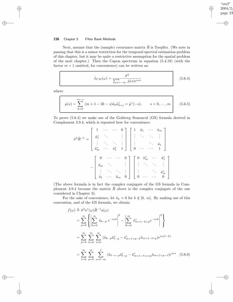
“sm2”2004/2/22page 236

i

i

i

i

i

i

i

i


Next, assume that the (sample) covariance matrix R is Toeplitz. (We note inpassing that this is a minor restriction for the temporal spectral estimation problemof this chapter, but it may be quite a restrictive assumption for the spatial problemof the next chapter.) Then the Capon spectrum in equation (5.4.19) (with thefactor m+ 1 omitted, for convenience) can be written as:

φCM (ω) =σ2

∑ms=−m µ(s)eiωs

(5.6.4)

where

µ(s) =

m−s∑

k=0

(m+ 1 − 2k − s)aka∗k+s = µ∗(−s), s = 0, . . . ,m (5.6.5)

To prove (5.6.4) we make use of the Gohberg–Semencul (GS) formula derived inComplement 3.9.4, which is repeated here for convenience:

σ2R−1 =

1 · · · · · · 0

a∗1

. . ....

.... . .

. . ....

a∗m · · · a∗

1 1

1 a1 · · · am...

. . .. . .

......

. . . a1

0 · · · · · · 1

−

0 · · · · · · 0

am. . .

......

. . .. . .

...a1 · · · am 0

0 a∗m · · · a∗

1...

. . .. . .

......

. . . a∗m

0 · · · · · · 0

(The above formula is in fact the complex conjugate of the GS formula in Com-plement 3.9.4 because the matrix R above is the complex conjugate of the oneconsidered in Chapter 3).

For the sake of convenience, let ak = 0 for k /∈ [0, m]. By making use of thisconvention, and of the GS formula, we obtain:

f(ω) , σ2a∗(ω)R−1a(ω)

=

m∑

p=0

∣∣∣∣∣

m∑

k=0

ak−p e−iωk

∣∣∣∣∣

2

−∣∣∣∣∣

m∑

k=0

a∗m+1−k+pe

−iωk

∣∣∣∣∣

2

=

m∑

p=0

m∑

k=0

m∑

`=0

(ak−pa∗`−p − a∗

m+1+p−kam+1−`+p)eiω(`−k)

=

m∑

`=0

m∑

p=0

∑

s=`−m(a`−s−pa

∗`−p − a∗

m+1−`+s+pam+1+p−`)eiωs (5.6.6)

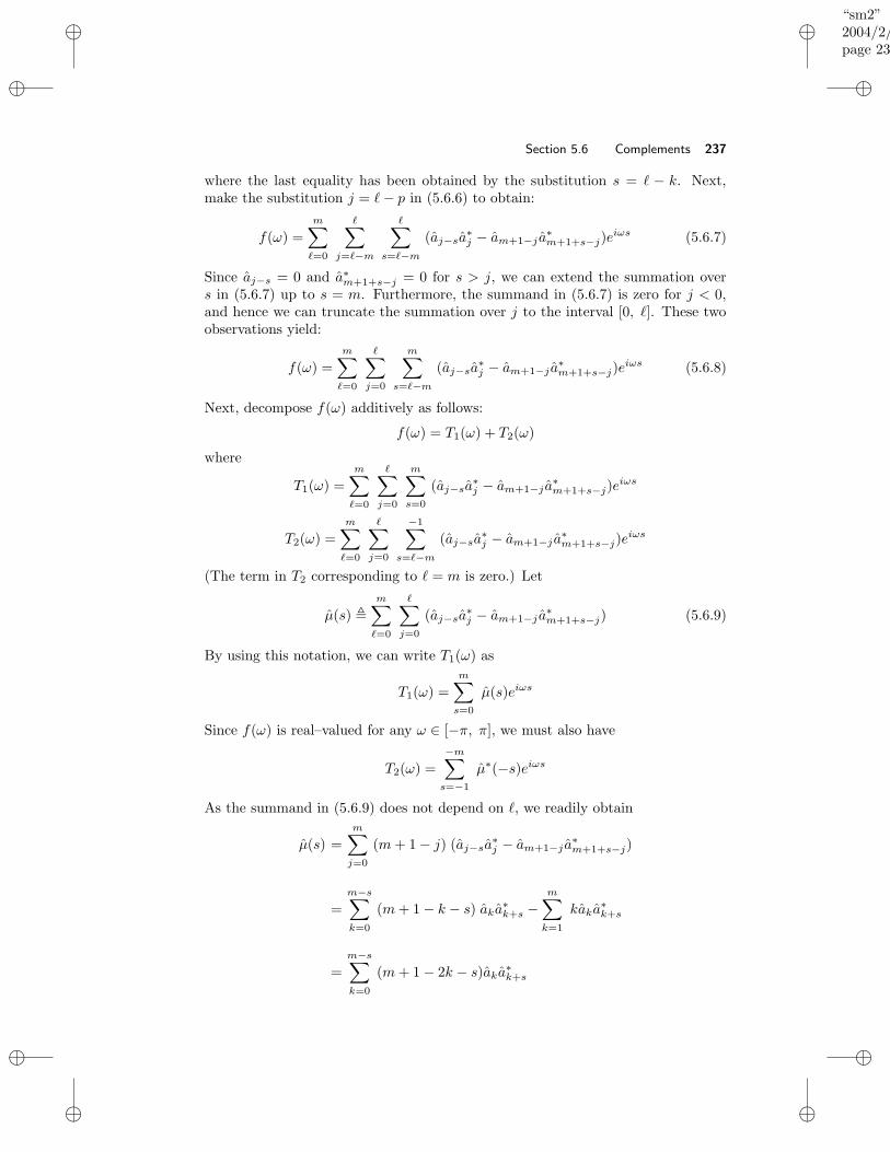
“sm2”2004/2/22page 237

i

i

i

i

i

i

i

i


where the last equality has been obtained by the substitution s = ` − k. Next,make the substitution j = `− p in (5.6.6) to obtain:

f(ω) =

m∑

`=0

∑

j=`−m

∑

s=`−m(aj−sa

∗j − am+1−j a

∗m+1+s−j)e

iωs (5.6.7)

Since aj−s = 0 and a∗m+1+s−j = 0 for s > j, we can extend the summation over

s in (5.6.7) up to s = m. Furthermore, the summand in (5.6.7) is zero for j < 0,and hence we can truncate the summation over j to the interval [0, `]. These twoobservations yield:

f(ω) =

m∑

`=0

∑

j=0

m∑

s=`−m(aj−sa

∗j − am+1−j a

∗m+1+s−j)e

iωs (5.6.8)

Next, decompose f(ω) additively as follows:

f(ω) = T1(ω) + T2(ω)

where

T1(ω) =

m∑

`=0

∑

j=0

m∑

s=0

(aj−sa∗j − am+1−j a

∗m+1+s−j)e

iωs

T2(ω) =

m∑

`=0

∑

j=0

−1∑

s=`−m(aj−sa

∗j − am+1−j a

∗m+1+s−j)e

iωs

(The term in T2 corresponding to ` = m is zero.) Let

µ(s) ,

m∑

`=0

∑

j=0

(aj−sa∗j − am+1−j a

∗m+1+s−j) (5.6.9)

By using this notation, we can write T1(ω) as

T1(ω) =

m∑

s=0

µ(s)eiωs

Since f(ω) is real–valued for any ω ∈ [−π, π], we must also have

T2(ω) =

−m∑

s=−1

µ∗(−s)eiωs

As the summand in (5.6.9) does not depend on `, we readily obtain

µ(s) =

m∑

j=0

(m+ 1 − j) (aj−sa∗j − am+1−j a

∗m+1+s−j)

=

m−s∑

k=0

(m+ 1 − k − s) aka∗k+s −

m∑

k=1

kaka∗k+s

=

m−s∑

k=0

(m+ 1 − 2k − s)aka∗k+s

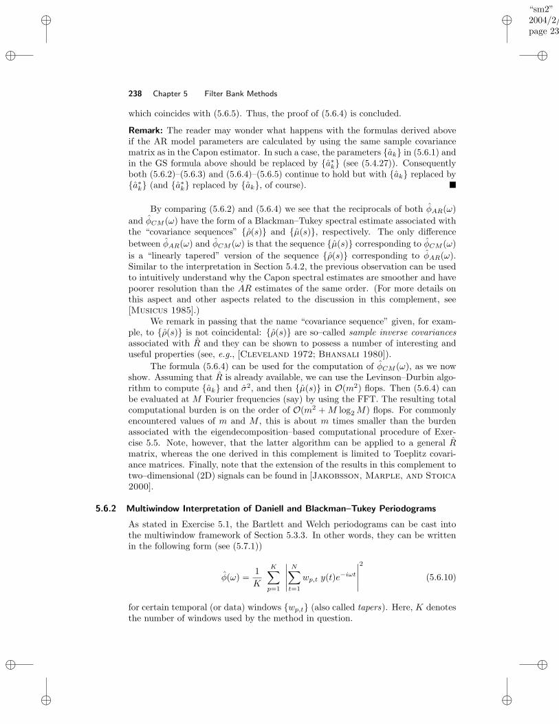
“sm2”2004/2/22page 238

i

i

i

i

i

i

i

i


which coincides with (5.6.5). Thus, the proof of (5.6.4) is concluded.

Remark: The reader may wonder what happens with the formulas derived aboveif the AR model parameters are calculated by using the same sample covariancematrix as in the Capon estimator. In such a case, the parameters ak in (5.6.1) andin the GS formula above should be replaced by a∗

k (see (5.4.27)). Consequentlyboth (5.6.2)–(5.6.3) and (5.6.4)–(5.6.5) continue to hold but with ak replaced bya∗k (and a∗

k replaced by ak, of course).

By comparing (5.6.2) and (5.6.4) we see that the reciprocals of both φAR(ω)

and φCM (ω) have the form of a Blackman–Tukey spectral estimate associated withthe “covariance sequences” ρ(s) and µ(s), respectively. The only difference

between φAR(ω) and φCM (ω) is that the sequence µ(s) corresponding to φCM (ω)

is a “linearly tapered” version of the sequence ρ(s) corresponding to φAR(ω).Similar to the interpretation in Section 5.4.2, the previous observation can be usedto intuitively understand why the Capon spectral estimates are smoother and havepoorer resolution than the AR estimates of the same order. (For more details onthis aspect and other aspects related to the discussion in this complement, see[Musicus 1985].)

We remark in passing that the name “covariance sequence” given, for exam-ple, to ρ(s) is not coincidental: ρ(s) are so–called sample inverse covariancesassociated with R and they can be shown to possess a number of interesting anduseful properties (see, e.g., [Cleveland 1972; Bhansali 1980]).

The formula (5.6.4) can be used for the computation of φCM (ω), as we nowshow. Assuming that R is already available, we can use the Levinson–Durbin algo-rithm to compute ak and σ2, and then µ(s) in O(m2) flops. Then (5.6.4) canbe evaluated at M Fourier frequencies (say) by using the FFT. The resulting totalcomputational burden is on the order of O(m2 +M log2M) flops. For commonlyencountered values of m and M , this is about m times smaller than the burdenassociated with the eigendecomposition–based computational procedure of Exer-cise 5.5. Note, however, that the latter algorithm can be applied to a general Rmatrix, whereas the one derived in this complement is limited to Toeplitz covari-ance matrices. Finally, note that the extension of the results in this complement totwo–dimensional (2D) signals can be found in [Jakobsson, Marple, and Stoica

2000].

5.6.2 Multiwindow Interpretation of Daniell and Blackman–Tukey Periodograms

As stated in Exercise 5.1, the Bartlett and Welch periodograms can be cast intothe multiwindow framework of Section 5.3.3. In other words, they can be writtenin the following form (see (5.7.1))

φ(ω) =1

K

K∑

p=1

∣∣∣∣∣

N∑

t=1

wp,t y(t)e−iωt

∣∣∣∣∣

2

(5.6.10)

for certain temporal (or data) windows wp,t (also called tapers). Here, K denotesthe number of windows used by the method in question.

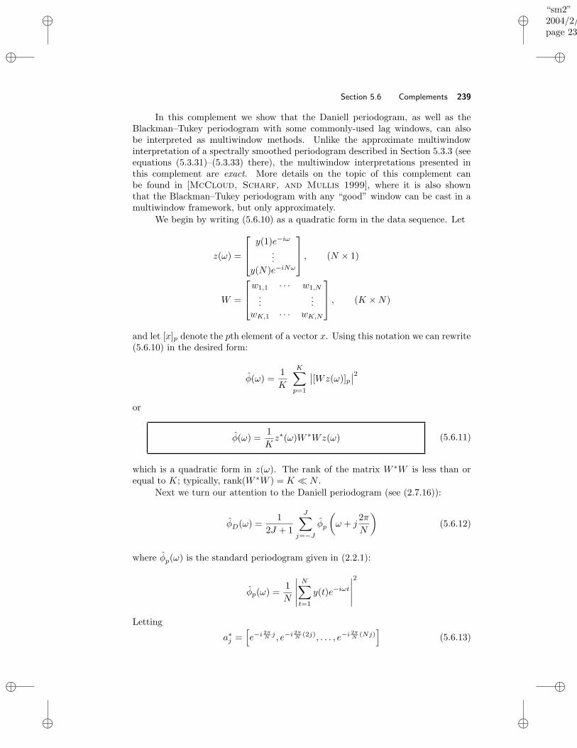
“sm2”2004/2/22page 239

i

i

i

i

i

i

i

i


In this complement we show that the Daniell periodogram, as well as theBlackman–Tukey periodogram with some commonly-used lag windows, can alsobe interpreted as multiwindow methods. Unlike the approximate multiwindowinterpretation of a spectrally smoothed periodogram described in Section 5.3.3 (seeequations (5.3.31)–(5.3.33) there), the multiwindow interpretations presented inthis complement are exact. More details on the topic of this complement canbe found in [McCloud, Scharf, and Mullis 1999], where it is also shownthat the Blackman–Tukey periodogram with any “good” window can be cast in amultiwindow framework, but only approximately.

We begin by writing (5.6.10) as a quadratic form in the data sequence. Let

z(ω) =

y(1)e−iω

...y(N)e−iNω

, (N × 1)

W =

w1,1 · · · w1,N

......

wK,1 · · · wK,N

, (K ×N)

and let [x]p denote the pth element of a vector x. Using this notation we can rewrite(5.6.10) in the desired form:

φ(ω) =1

K

K∑

p=1

∣∣[Wz(ω)]p

∣∣2

or

φ(ω) =1

Kz∗(ω)W ∗Wz(ω) (5.6.11)

which is a quadratic form in z(ω). The rank of the matrix W ∗W is less than orequal to K; typically, rank(W ∗W ) = K N .

Next we turn our attention to the Daniell periodogram (see (2.7.16)):

φD(ω) =1

2J + 1

J∑

j=−Jφp

(

ω + j2π

N

)

(5.6.12)

where φp(ω) is the standard periodogram given in (2.2.1):

φp(ω) =1

N

∣∣∣∣∣

N∑

t=1

y(t)e−iωt

∣∣∣∣∣

2

Letting

a∗j =

[

e−i 2πN j , e−i 2π

N (2j), . . . , e−i 2πN (Nj)

]

(5.6.13)

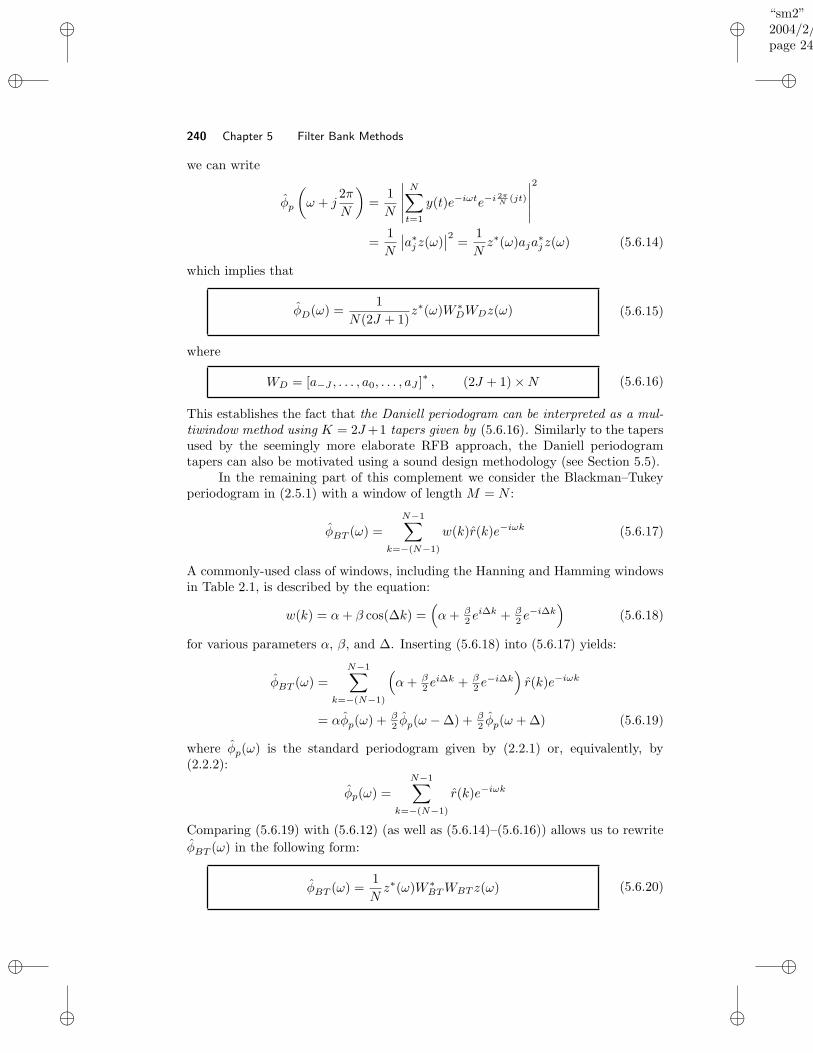
“sm2”2004/2/22page 240

i

i

i

i

i

i

i

i


we can write

φp

(

ω + j2π

N

)

=1

N

∣∣∣∣∣

N∑

t=1

y(t)e−iωte−i 2πN (jt)

∣∣∣∣∣

2

=1

N

∣∣a∗jz(ω)

∣∣2

=1

Nz∗(ω)aja

∗jz(ω) (5.6.14)

which implies that

φD(ω) =1

N(2J + 1)z∗(ω)W ∗

DWDz(ω) (5.6.15)

where

WD = [a−J , . . . , a0, . . . , aJ ]∗, (2J + 1) ×N (5.6.16)

This establishes the fact that the Daniell periodogram can be interpreted as a mul-tiwindow method using K = 2J+1 tapers given by (5.6.16). Similarly to the tapersused by the seemingly more elaborate RFB approach, the Daniell periodogramtapers can also be motivated using a sound design methodology (see Section 5.5).

In the remaining part of this complement we consider the Blackman–Tukeyperiodogram in (2.5.1) with a window of length M = N :

φBT (ω) =

N−1∑

k=−(N−1)

w(k)r(k)e−iωk (5.6.17)

A commonly-used class of windows, including the Hanning and Hamming windowsin Table 2.1, is described by the equation:

w(k) = α+ β cos(∆k) =(

α+ β2 ei∆k + β

2 e−i∆k

)

(5.6.18)

for various parameters α, β, and ∆. Inserting (5.6.18) into (5.6.17) yields:

φBT (ω) =

N−1∑

k=−(N−1)

(

α+ β2 ei∆k + β

2 e−i∆k

)

r(k)e−iωk

= αφp(ω) + β2 φp(ω − ∆) + β

2 φp(ω + ∆) (5.6.19)

where φp(ω) is the standard periodogram given by (2.2.1) or, equivalently, by(2.2.2):

φp(ω) =

N−1∑

k=−(N−1)

r(k)e−iωk

Comparing (5.6.19) with (5.6.12) (as well as (5.6.14)–(5.6.16)) allows us to rewrite

φBT (ω) in the following form:

φBT (ω) =1

Nz∗(ω)W ∗

BTWBT z(ω) (5.6.20)

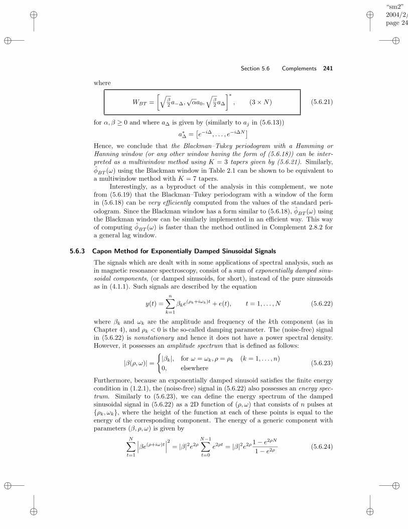
“sm2”2004/2/22page 241

i

i

i

i

i

i

i

i


where

WBT =

[√β2 a−∆,

√αa0,

√β2 a∆

]∗, (3 ×N) (5.6.21)

for α, β ≥ 0 and where a∆ is given by (similarly to aj in (5.6.13))

a∗∆ =

[e−i∆, . . . , e−i∆N ]

Hence, we conclude that the Blackman–Tukey periodogram with a Hamming orHanning window (or any other window having the form of (5.6.18)) can be inter-preted as a multiwindow method using K = 3 tapers given by (5.6.21). Similarly,

φBT (ω) using the Blackman window in Table 2.1 can be shown to be equivalent toa multiwindow method with K = 7 tapers.

Interestingly, as a byproduct of the analysis in this complement, we notefrom (5.6.19) that the Blackman–Tukey periodogram with a window of the formin (5.6.18) can be very efficiently computed from the values of the standard peri-

odogram. Since the Blackman window has a form similar to (5.6.18), φBT (ω) usingthe Blackman window can be similarly implemented in an efficient way. This wayof computing φBT (ω) is faster than the method outlined in Complement 2.8.2 fora general lag window.

5.6.3 Capon Method for Exponentially Damped Sinusoidal Signals

The signals which are dealt with in some applications of spectral analysis, such asin magnetic resonance spectroscopy, consist of a sum of exponentially damped sinu-soidal components, (or damped sinusoids, for short), instead of the pure sinusoidsas in (4.1.1). Such signals are described by the equation

y(t) =

n∑

k=1

βke(ρk+iωk)t + e(t), t = 1, . . . , N (5.6.22)

where βk and ωk are the amplitude and frequency of the kth component (as inChapter 4), and ρk < 0 is the so-called damping parameter. The (noise-free) signalin (5.6.22) is nonstationary and hence it does not have a power spectral density.However, it possesses an amplitude spectrum that is defined as follows:

|β(ρ, ω)| =

|βk|, for ω = ωk, ρ = ρk (k = 1, . . . , n)

0, elsewhere(5.6.23)

Furthermore, because an exponentially damped sinusoid satisfies the finite energycondition in (1.2.1), the (noise-free) signal in (5.6.22) also possesses an energy spec-trum. Similarly to (5.6.23), we can define the energy spectrum of the dampedsinusoidal signal in (5.6.22) as a 2D function of (ρ, ω) that consists of n pulses atρk, ωk, where the height of the function at each of these points is equal to theenergy of the corresponding component. The energy of a generic component withparameters (β, ρ, ω) is given by

N∑

t=1

∣∣∣βe(ρ+iω)t

∣∣∣

2

= |β|2e2ρN−1∑

t=0

e2ρt = |β|2e2ρ 1 − e2ρN

1 − e2ρ(5.6.24)

“sm2”2004/2/22page 242

i

i

i

i

i

i

i

i


It follows from (5.6.24) and the above discussion that the energy spectrum can beexpressed as a function of the amplitude spectrum in (5.6.23) via the formula:

E(ρ, ω) = |β(ρ, ω)|2L(ρ) (5.6.25)

where

L(ρ) = e2ρ1 − e2ρN

1 − e2ρ(5.6.26)

The amplitude spectrum, and hence the energy spectrum, of the signal in (5.6.22)can be estimated by using an extension of the Capon method that is introduced inSection 5.4. To develop this extension, we consider the following data vector

y(t) = [y(t), y(t+ 1), . . . , y(t+m)] (5.6.27)

in lieu of the data vector used in (5.4.2). First we explain why, in the case ofdamped sinusoidal signals, the use of (5.6.27) is preferable to that of

[y(t), y(t− 1), . . . , y(t−m)]T

(5.6.28)

(as is used in (5.4.2)). Let h denote the coefficient vector of the Capon FIR filter asin (5.4.1). Then, the output of the filter using the data vector in (5.6.27) is givenby:

yF (t) = h∗y(t) = h∗

y(t)...

y(t+m)

, t = 1, . . . , N −m (5.6.29)

Hence, when performing the filtering operation as in (5.6.29), we lose m samplesfrom the end of the data string. Because the SNR of those samples is typicallyrather low (owing to the damping of the signal components), the data loss is notsignificant. In contrast, the use of (5.4.2) leads to a loss of m data samples from thebeginning of the data string (since (5.4.2) can be computed for t = m+ 1, . . . , N),where the SNR is higher. Hence, in the case of damped sinusoidal signals we shouldindeed prefer (5.6.29) to (5.4.2).

Next, we derive Capon-like estimates of the amplitude and energy spectra of(5.6.22). Let

R =1

N −m

N−m∑

t=1

y(t)y∗(t) (5.6.30)

denote the sample covariance matrix of the data vector in (5.6.27). Then the samplevariance of the filter output can be written as:

1

N −m

N−m∑

t=1

|yF (t)|2 = h∗Rh (5.6.31)

By definition, the Capon filter minimizes (5.6.31) under the constraint that the filterpasses, without distortion, a generic damped sinusoid with parameters (β, ρ, ω).

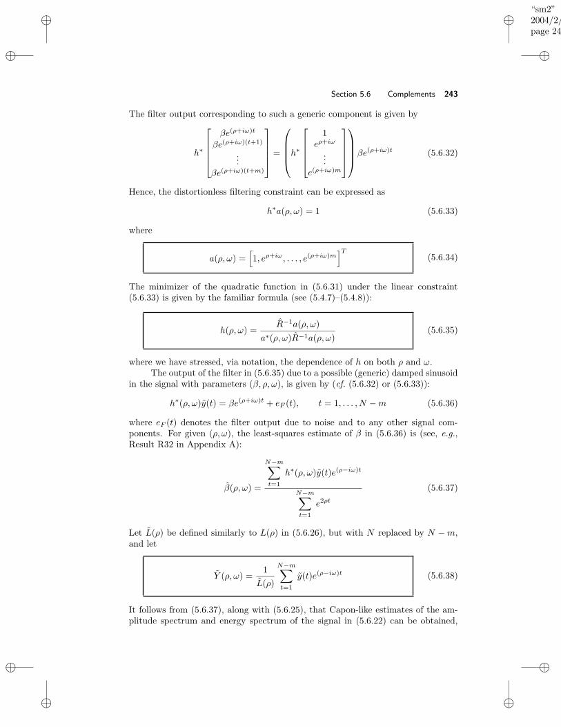
“sm2”2004/2/22page 243

i

i

i

i

i

i

i

i


The filter output corresponding to such a generic component is given by

h∗

βe(ρ+iω)t

βe(ρ+iω)(t+1)

...βe(ρ+iω)(t+m)

=

h∗

1eρ+iω

...e(ρ+iω)m

βe(ρ+iω)t (5.6.32)

Hence, the distortionless filtering constraint can be expressed as

h∗a(ρ, ω) = 1 (5.6.33)

where

a(ρ, ω) =[

1, eρ+iω, . . . , e(ρ+iω)m]T

(5.6.34)

The minimizer of the quadratic function in (5.6.31) under the linear constraint(5.6.33) is given by the familiar formula (see (5.4.7)–(5.4.8)):

h(ρ, ω) =R−1a(ρ, ω)

a∗(ρ, ω)R−1a(ρ, ω)(5.6.35)

where we have stressed, via notation, the dependence of h on both ρ and ω.The output of the filter in (5.6.35) due to a possible (generic) damped sinusoid

in the signal with parameters (β, ρ, ω), is given by (cf. (5.6.32) or (5.6.33)):

h∗(ρ, ω)y(t) = βe(ρ+iω)t + eF (t), t = 1, . . . , N −m (5.6.36)

where eF (t) denotes the filter output due to noise and to any other signal com-ponents. For given (ρ, ω), the least-squares estimate of β in (5.6.36) is (see, e.g.,Result R32 in Appendix A):

β(ρ, ω) =

N−m∑

t=1

h∗(ρ, ω)y(t)e(ρ−iω)t

N−m∑

t=1

e2ρt

(5.6.37)

Let L(ρ) be defined similarly to L(ρ) in (5.6.26), but with N replaced by N −m,and let

Y (ρ, ω) =1

L(ρ)

N−m∑

t=1

y(t)e(ρ−iω)t (5.6.38)

It follows from (5.6.37), along with (5.6.25), that Capon-like estimates of the am-plitude spectrum and energy spectrum of the signal in (5.6.22) can be obtained,

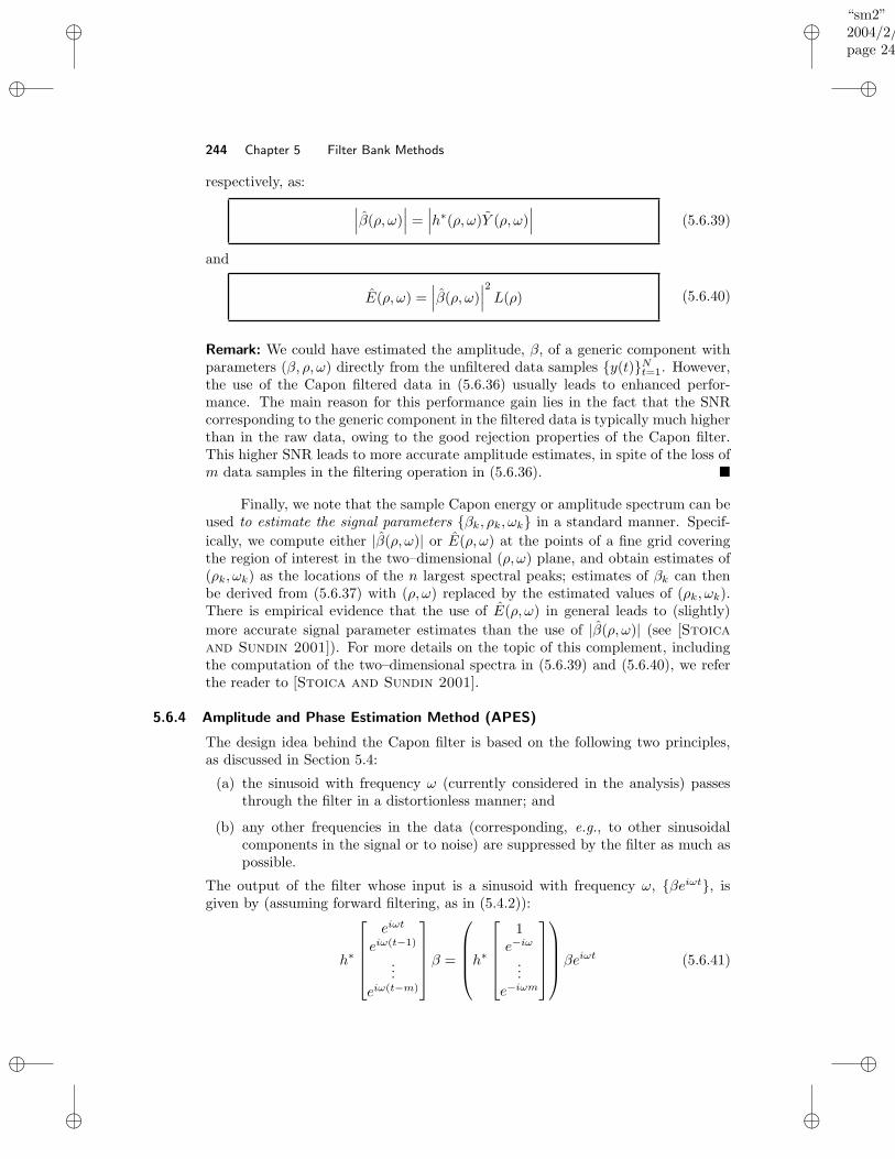
“sm2”2004/2/22page 244

i

i

i

i

i

i

i

i


respectively, as:

∣∣∣β(ρ, ω)

∣∣∣ =

∣∣∣h∗(ρ, ω)Y (ρ, ω)

∣∣∣ (5.6.39)

and

E(ρ, ω) =∣∣∣β(ρ, ω)

∣∣∣

2

L(ρ) (5.6.40)

Remark: We could have estimated the amplitude, β, of a generic component withparameters (β, ρ, ω) directly from the unfiltered data samples y(t)Nt=1. However,the use of the Capon filtered data in (5.6.36) usually leads to enhanced perfor-mance. The main reason for this performance gain lies in the fact that the SNRcorresponding to the generic component in the filtered data is typically much higherthan in the raw data, owing to the good rejection properties of the Capon filter.This higher SNR leads to more accurate amplitude estimates, in spite of the loss ofm data samples in the filtering operation in (5.6.36).

Finally, we note that the sample Capon energy or amplitude spectrum can beused to estimate the signal parameters βk, ρk, ωk in a standard manner. Specif-

ically, we compute either |β(ρ, ω)| or E(ρ, ω) at the points of a fine grid coveringthe region of interest in the two–dimensional (ρ, ω) plane, and obtain estimates of(ρk, ωk) as the locations of the n largest spectral peaks; estimates of βk can thenbe derived from (5.6.37) with (ρ, ω) replaced by the estimated values of (ρk, ωk).There is empirical evidence that the use of E(ρ, ω) in general leads to (slightly)

more accurate signal parameter estimates than the use of |β(ρ, ω)| (see [Stoica

and Sundin 2001]). For more details on the topic of this complement, includingthe computation of the two–dimensional spectra in (5.6.39) and (5.6.40), we referthe reader to [Stoica and Sundin 2001].

5.6.4 Amplitude and Phase Estimation Method (APES)

The design idea behind the Capon filter is based on the following two principles,as discussed in Section 5.4:

(a) the sinusoid with frequency ω (currently considered in the analysis) passesthrough the filter in a distortionless manner; and

(b) any other frequencies in the data (corresponding, e.g., to other sinusoidalcomponents in the signal or to noise) are suppressed by the filter as much aspossible.

The output of the filter whose input is a sinusoid with frequency ω, βeiωt, isgiven by (assuming forward filtering, as in (5.4.2)):

h∗

eiωt

eiω(t−1)

...eiω(t−m)

β =

h∗

1e−iω

...e−iωm

βeiωt (5.6.41)

“sm2”2004/2/22page 245

i

i

i

i

i

i

i

i


For backward filtering, as used in Complement 5.6.3, a similar result can be derived.It follows from (5.6.41) that the design objective in (a) above can be expressedmathematically via the following linear constraint on h:

h∗a(ω) = 1 (5.6.42)

where

a(ω) =[1, e−iω, . . . , e−iωm]T (5.6.43)

(see (5.4.5)–(5.4.7)). Regarding the second design objective, its statement in (b)above is sufficiently general to allow several different mathematical formulations.The Capon method is based on the idea that the goal in (b) is achieved if the powerat the filter output is minimized (see (5.4.7)). In this complement, another way toformulate (b) mathematically is described.

At a given frequency ω, let us choose h such that the filter output, h∗y(t),where

y(t) = [y(t), y(t− 1), . . . , y(t−m)]T

is as close as possible in a least-squares (LS) sense to a sinusoid with frequency ωand constant amplitude β. Mathematically, we obtain both h and β, for a given ω,by minimizing the LS criterion:

minh,β

1

N −m

N∑

t=m+1

∣∣h∗y(t) − βeiωt

∣∣2

subject to h∗a(ω) = 1 (5.6.44)

Note that the estimation of the amplitude and phase (i.e., |β| and arg(β)) of thesinusoid with frequency ω is an intrinsic part of the method based on (5.6.44). Thisobservation motives the name of Amplitude and Phase EStimation (APES) givento the method described by (5.6.44).

Because (5.6.44) is a linearly constrained quadratic problem, we should beable to find its solution in closed form. Let

g(ω) =1

N −m

N∑

t=m+1

y(t)e−iωt (5.6.45)

Then, a straightforward calculation shows that the criterion function in (5.6.44)can be rewritten as:

1

N −m

N∑

t=m+1

∣∣h∗y(t) − βeiωt

∣∣2

= h∗Rh− β∗h∗g(ω) − βg∗(ω)h+ |β|2

= |β − h∗g(ω)|2 + h∗Rh− |h∗g(ω)|2

= |β − h∗g(ω)|2 + h∗[R− g(ω)g∗(ω)]h (5.6.46)

“sm2”2004/2/22page 246

i

i

i

i

i

i

i

i


where

R =1

N −m

N∑

t=m+1

y(t)y∗(t) (5.6.47)

(see (5.4.18)). The minimization of (5.6.46) with respect to β is immediate:

β(ω) = h∗g(ω) (5.6.48)

Inserting (5.6.48) into (5.6.46) yields the following problem whose solution willdetermine the filter coefficient vector:

minhh∗Q(ω)h subject to h∗a(ω) = 1 (5.6.49)

whereQ(ω) = R− g(ω)g∗(ω) (5.6.50)

As (5.6.49) has the same form as the Capon filter design problem (see (5.4.7)), thesolution to (5.6.49) is readily derived (compare with (5.4.8)):

h(ω) =Q−1(ω)a(ω)

a∗(ω)Q−1(ω)a(ω)(5.6.51)

A direct implementation of (5.6.51) would require the inversion of the matrixQ(ω) for each value of ω ∈ [0, 2π] considered. To avoid such an intensive compu-tational task, we can use the matrix inversion lemma (Result R27 in Appendix A)to express the inverse in (5.6.51) as follows:

Q−1(ω) =[

R− g(ω)g∗(ω)]−1

= R−1 +R−1g(ω)g∗(ω)R−1

1 − g∗(ω)R−1g(ω)(5.6.52)

Inserting (5.6.52) into (5.6.51) yields the following expression for the APES filter :

h(ω) =

[

1 − g∗(ω)R−1g(ω)]

R−1a(ω) +[

g∗(ω)R−1a(ω)]

R−1g(ω)[

1 − g∗(ω)R−1g(ω)]

a∗(ω)R−1a(ω) +∣∣∣a∗(ω)R−1g(ω)

∣∣∣

2 (5.6.53)

From (5.6.48) and (5.6.53) we obtain the following formula for the APES estimateof the (complex) amplitude spectrum (see Complement 5.6.3 for a definition of theamplitude spectrum):

β(ω) =a∗(ω)R−1g(ω)

[

1 − g∗(ω)R−1g(ω)]

a∗(ω)R−1a(ω) +∣∣∣a∗(ω)R−1g(ω)

∣∣∣

2 (5.6.54)

Compared with the Capon estimate of the amplitude spectrum given by

β(ω) =a∗(ω)R−1g(ω)

a∗(ω)R−1a(ω)(5.6.55)

“sm2”2004/2/22page 247

i

i

i

i

i

i

i

i


we see that the APES estimate in (5.6.54) is more computationally involved, butnot by much.

Remark: Our discussion has focused on the estimation of the amplitude spectrum.If the power spectrum is what we want to estimate, then we can use the APESfilter, (5.6.53), in the PSD estimation approach described in Section 5.4, or we cansimply take |β(ω)|2 (along with a possible scaling) as an estimate of the PSD.

The above derivation of APES is adapted from [Stoica, Li, and Li 1999].The original derivation of APES, provided in [Li and Stoica 1996a], was different:it was based on an approximate maximum likelihood approach. We refer the readerto [Li and Stoica 1996a] for the original derivation of APES as well as manyother details on this approach to spectral analysis.

We end this complement with a brief comparison of Capon and APES froma performance standpoint. Extensive empirical and analytical studies of these twomethods (see, e.g., [Larsson, Li, and Stoica 2003] and its references) haveshown that Capon has a (slightly) higher resolution than APES and also that theCapon estimates of the frequencies of a multicomponent sinusoidal signal in noiseare more accurate than the APES estimates. On the other hand, for a given set offrequency estimates ωk in the vicinity of the true frequencies, the APES estimatesof the amplitudes βk are much more accurate than the Capon estimates; theCapon estimates are always biased towards zero, sometimes significantly so. Thissuggests that, at least for spectral line analysis, a better method than both Caponand APES can be obtained by combining them in the following way:

• Estimate the frequencies ωk as the locations of the dominant peaks of theCapon spectrum.

• Estimate the amplitudes βk using the APES formula (5.6.54) evaluated atthe frequency estimates obtained in the previous step.

The above combined Capon-APES (CAPES) method was introduced in [Jakobsson

and Stoica 2000].

5.6.5 Amplitude and Phase Estimation Method for Gapped Data (GAPES)

In some applications of spectral analysis the data sequence has gaps, owing to thefailure of a measuring device, or owing to the impossibility to perform measurementsfor some periods of time (such as in astronomy). In this complement we will presentan extension of the Amplitude and Phase EStimation (APES) method, outlined inComplement 5.6.4, to gapped-data sequences. Gapped-data sequences are evenlysampled data strings that contain unknown samples which are usually, but notalways, clustered together in groups of reasonable size. We will use the acronymGAPES to designate the extended approach.

Most of the available methods for the spectral analysis of gapped data perform(either implicitly or explicitly) an interpolation of the missing data, followed by astandard full-data spectral analysis. The data interpolation step is critical and itcannot be completed without making (sometimes hidden) assumptions on the datasequence. For example, one such assumption is that the data is bandlimited with a

“sm2”2004/2/22page 248

i

i

i

i

i

i

i

i


known cutoff frequency. Intuitively, these assumptions can be viewed as attemptsto add extra “information” to the spectral analysis problem, which might be able tocompensate for the lost information due to the missing data samples. The problemwith these assumptions, though, is that they are not generally easy to check inapplications, either a priori or a posteriori. The GAPES approach presented hereis based on the sole assumption that the spectral content of the missing data issimilar to that of the available data. This assumption is very natural, and onecould argue that it introduces no restriction at all.

We begin the derivation of GAPES by rewriting the APES least-squares fit-ting criterion (see equation (5.6.44) in Complement 5.6.4) in a form that is moreconvenient for the discussion here. Specifically, we use the notation h(ω) and β(ω)to stress the dependence on ω of both the APES filter and the amplitude spec-trum. Also, we note that in applications the frequency variable is usually sampledas follows:

ωk =2π

Kk, k = 1, . . . ,K (5.6.56)

where K is an integer (much) larger than N . Making use of the above notationand (5.6.56) we rewrite the APES criterion as follows:

min

K∑

k=1

N∑

t=m+1

∣∣h∗(ωk)y(t) − β(ωk)e

iωkt∣∣2

subject to h∗(ωk)a(ωk) = 1 for k = 1, . . . ,K

(5.6.57)

Evidently, the minimization of the criterion in (5.6.57) with respect to h(ωk) andβ(ωk) reduces to the minimization of the inner sum in (5.6.57) for each k. Hence,in the full-data case the problem in (5.6.57) is equivalent to the standard APESproblem in equation (5.6.44) in Complement 5.6.4. However, in the gapped datacase the form of the APES criterion in (5.6.57) turns out to be more convenientthan that in (5.6.44), as we will see below.

To continue, we need some additional notation. Let

ya = the vector containing the available samples in y(t)Nt=1

yu = the vector containing the unavailable samples in y(t)Nt=1

The main idea behind the GAPES approach is to minimize (5.6.57) with respectto both h(ωk) and β(ωk) as well as with respect to yu. Such a formulation ofthe gapped-data problem is appealing, because it leads to:

(i) an analysis filter bank h(ωk) for which the filtered sequence is as close aspossible in a LS sense to the (possible) sinusoidal component in the data thathas frequency ωk, which is the main design goal in the filter bank approachto spectral analysis; and

(ii) an estimate of the missing samples in yu whose spectral content mimics thespectral content of the available data as much as possible in the LS sense of(5.6.57).

“sm2”2004/2/22page 249

i

i

i

i

i

i

i

i


The criterion in (5.6.57) is a quartic function of the unknowns h(ωk),β(ωk), and yu. Consequently, in general, its minimization requires the use ofan iterative algorithm; that is, a closed-form solution is unlikely to exist. TheGAPES method uses a cyclic minimizer to minimize the criterion in (5.6.57) (seeComplement 4.9.5 for a general description of cyclic minimizers). A step-by-stepdescription of GAPES is as follows:

The GAPES AlgorithmStep 0. Obtain initial estimates of h(ωk) and β(ωk).Step 1. Use the most recent estimates of h(ωk) and β(ωk) to estimate yuvia the minimization of (5.6.57).Step 2. Use the most recent estimate of yu to estimate h(ωk) and β(ωk)via the minimization of (5.6.57).Step 3. Check the convergence of the iteration, e.g., by checking whether therelative change of the criterion between two consecutive iterations is smaller thana pre-assigned value. If no, then go to Step 1. If yes, then we have a final am-plitude spectrum estimate given by β(ωk)Kk=1. If desired, this estimate can betransformed into a power spectrum estimate as explained in Complement 5.6.4.

To reduce the computational burden of the above algorithm we can run itwith a value of K that is not much larger than N (e.g., K ∈ [2N, 4N ]). After theiterations are terminated, the final spectral estimate can be evaluated on a (much)finer frequency grid, if desired.

A cyclic minimizer reduces the criterion function at each iteration (see thediscussion in Complement 4.9.5). Furthermore, in the present case this reduction isstrict because the solutions to the minimization problems with respect to yu and toh(ωk), β(ωk) in Steps 1 and 2 are unique under weak conditions. Combining thisobservation with the fact that the criterion in (5.6.57) is bounded from below byzero, we can conclude that the GAPES algorithm converges to a minimum point of(5.6.57). This minimum may be a local or global minimum, depending in part on thequality of the initial estimates of h(ωk), β(ωk) used in Step 0. The initializationstep, as well as the remaining steps in the GAPES algorithm, are discussed in moredetail below.

Step 0. A simple way to obtain initial estimates of h(ωk), β(ωk) is to applyAPES to the full-data sequence with yu = 0. This way of initializing GAPES canbe interpreted as permuting Step 1 with Step 2 in the algorithm and initializingthe algorithm in Step 0 with yu = 0.

A more elaborate initialization scheme consists of using only the available datasamples to build the sample covariance matrix R in (5.6.47) needed in APES. Pro-vided that there are enough samples so that the resulting R matrix is nonsingular,this initialization scheme usually gives more accurate estimates of h(ωk), β(ωk)than the ones obtained by setting yu = 0 (see [Stoica, Larsson, and Li 2000]for details).

Step 1. We want to find the solution yu to the problem:

minyu

K∑

k=1

N∑

t=m+1

∣∣∣h∗(ωk)y(t) − β(ωk)e

iωkt∣∣∣

2

(5.6.58)

“sm2”2004/2/22page 250

i

i

i

i

i

i

i

i


where y(t) = [y(t), y(t− 1), . . . , y(t−m)]T. We will show that the above minimiza-

tion problem is quadratic in yu (for given h(ωk) and β(ωk)), and thus admitsa closed-form solution.

Let h∗(ωk) = [h0,k, h1,k, . . . , hm,k] and define

Hk =

h0,k h1,k · · · hm,k 0. . .

. . .. . .

0 h0,k h1,k · · · hm,k

, (N −m) ×N

µk = β(ωk)

eiωkN

...eiωk(m+1)

, (N −m) × 1

Using this notation we can write the quadratic criterion in (5.6.58) as

K∑

k=1

∥∥∥∥∥∥∥

Hk

y(N)...

y(1)

− µk

∥∥∥∥∥∥∥

2

(5.6.59)

Next, we define the matrices Ak and Uk via the following equality:

Hk

y(N)...

y(1)

= Akya + Ukyu (5.6.60)

With this notation, the criterion in (5.6.59) becomes:

K∑

k=1

‖Ukyu − (µk −Akya)‖2(5.6.61)

The minimizer of (5.6.61) with respect to yu is readily found to be (see Result R32in Appendix A):

yu =

[K∑

k=1

U∗kUk

]−1 [ K∑

k=1

U∗k (µk −Akya)

]

(5.6.62)

The inverse matrix above exists under weak conditions; for details, see [Stoica,

Larsson, and Li 2000].

Step 2. The solution to this step can be computed by applying the APESalgorithm in Complement 5.6.4 to the data sequence made from ya and yu.

The description of the GAPES algorithm in now complete. Numerical experi-ence with this algorithm, reported in [Stoica, Larsson, and Li 2000], suggeststhat GAPES has good performance, particularly for data consisting of a mixtureof sinusoidal signals superimposed in noise.

“sm2”2004/2/22page 251

i

i

i

i

i

i

i

i


5.6.6 Extensions of Filter Bank Approaches to Two–Dimensional Signals

The following filter bank approaches for one-dimensional (1D) signals were discussedso far in this chapter and its complements:

• the periodogram,

• the refined filter bank method,

• the Capon method, and

• the APES method

In this complement we will explain briefly how the above nonparametric spectralanalysis methods can be extended to the case of two–dimensional (2D) signals. Inthe process, we also provide new interpretations for some of these methods, whichare particularly useful when we want very simple (although somewhat heuristic)derivations of the methods in question. We will in turn discuss the extension ofeach of the methods listed above. Note that 2D spectral analysis finds applica-tions in image processing, synthetic aperture radar imagery, and so forth. See[Larsson, Li, and Stoica 2003] for a review that covers the 2D methods dis-cussed in this complement, and their application to synthetic aperture radar. The2D extension of some parametric methods for spectral line analysis is discussed inComplement 4.9.7.

Periodogram

The 1D periodogram can be obtained by a least-squares (LS) fitting of the datay(t) to a generic 1D sinusoidal sequence βeiωt:

minβ

N∑

t=1

∣∣y(t) − βeiωt

∣∣2

(5.6.63)

The solution to (5.6.63) is readily found to be

β(ω) =1

N

N∑

t=1

y(t)e−iωt (5.6.64)

The squared modulus of (5.6.64) (scaled by N ; see Section 5.2) gives the 1D peri-odogram

1

N

∣∣∣∣∣

N∑

t=1

y(t)e−iωt

∣∣∣∣∣

2

(5.6.65)

In the 2D case, let y(t, t ) (for t = 1, . . . , N and t = 1, . . . , N) denote the availabledata matrix, and let βei(ωt+ωt ) denote a generic 2D sinusoid. The LS fit of thedata to the generic sinusoid, that is:

minβ

N∑

t=1

N∑

t=1

∣∣∣y(t, t ) − βei(ωt+ωt )

∣∣∣

2

⇐⇒ minβ

N∑

t=1

N∑

t=1

∣∣∣y(t, t )e−i(ωt+ωt ) − β

∣∣∣

2

(5.6.66)

“sm2”2004/2/22page 252

i

i

i

i

i

i

i

i


has the following solution:

β(ω, ω) =1

NN

N∑

t=1

N∑

t=1

y(t, t )e−i(ωt+ωt ) (5.6.67)

Similarly to the 1D case, the scaled squared magnitude of (5.6.67) yields the 2Dperiodogram

1

NN

∣∣∣∣∣∣

N∑

t=1

N∑

t=1

y(t, t )e−i(ωt+ωt )

∣∣∣∣∣∣

2

(5.6.68)

which can be efficiently computed by means of a 2D FFT algorithm as describedbelow.

The 2D FFT algorithm computes the 2D DTFT of a sequence y(t, t ) (fort = 1, . . . , N ; t = 1, . . . , N ) on a grid of frequency values defined by

ωk =2πk

N, k = 0, . . . , N − 1

ω` =2π`

N, ` = 0, . . . , N − 1

The 2D FFT algorithm achieves computational efficiency by making use of the 1DFFT described in Section 2.3. Let

Y (k, `) =

N∑

t=1

N∑

t=1

y(t, t )e−i(

2πk

Nt+ 2π`

Nt)

=

N∑

t=1

e−i 2πk

NtN∑

t=1

y(t, t )e−i 2π`

Nt

︸︷︷︸

,Vt(`)

(5.6.69)

=

N∑

t=1

Vt(`)e−i 2πk

Nt

(5.6.70)

For each t = 1, . . . , N , the sequence Vt(`)N−1`=0 defined in (5.6.69) can be efficiently

computed using a 1D FFT of length N (cf. Section 2.3). In addition, for each` = 0, . . . , N − 1, the sum in (5.6.70) can be efficiently computed using a 1D FFTof length N . If N is a power of two, an N -point 1D FFT requires N

2 log2N flops.Thus, if N and N are powers of two, then the number of operations needed tocompute Y (k, `) is

NN

2log2 N + N

N

2log2N =

NN

2log2(NN) flops (5.6.71)

If N or N is not a power of two, zero padding can be used.

“sm2”2004/2/22page 253

i

i

i

i

i

i

i

i


Refined Filter Bank (RFB) Method

Similarly to the 1D case (see (5.3.30) or (5.7.1)), the 2D RFB method can beimplemented as a multiwindowed periodogram (cf. (5.6.68)):

1

K

K∑

p=1

∣∣∣∣∣∣

N∑

t=1

N∑

t=1

wp(t, t ) y(t, t ) e−i(ωt+ωt )

∣∣∣∣∣∣

2

(5.6.72)

where wp(t, t )Kp=1 are the 2D Slepian data windows (or tapers). The problem leftis to derive 2D extensions of the 1D Slepian tapers discussed in Section 5.3.1.

The frequency response of a 2D taper w(t, t ) is given by

N∑

t=1

N∑

t=1

w(t, t )e−i(ωt+ωt ) (5.6.73)

Let us define the matrices

W =

w(1, 1) · · · w(1, N)...

...w(N, 1) · · · w(N, N)

B =

e−i(ω+ω) · · · e−i(ω+ωN)

......

e−i(ωN+ω) · · · e−i(ωN+ωN)

and let vec(·) denote the vectorizaton operator which stacks the columns of itsmatrix argument into a single vector. Also, let

a(ω) =

e−iω

...e−iNω

, a(ω) =

e−iω

...

e−iNω

(5.6.74)

and let the symbol ⊗ denote the Kronecker matrix product; the Kronecker productof two matrices, X of size m×n and Y of size m× n, is an mm×nn matrix whose(i, j) block of size m × n is given by Xij · Y , for i = 1, . . . ,m and j = 1, . . . , n,where Xij denotes the (i, j)th element of X (see, e.g., [Horn and Johnson 1985]for the properties of ⊗). Finally, let

w = vec(W )

=[w(1, 1), . . . , w(N, 1)| · · · |w(1, N), . . . , w(N, N)

]T(5.6.75)

and

b(ω, ω) = vec(B)

=[

e−i(ω+ω), . . . , e−i(ωN+ω)| · · · |e−i(ω+ωN), . . . , e−i(ωN+ωN)]T

= a(ω) ⊗ a(ω) (5.6.76)

“sm2”2004/2/22page 254

i

i

i

i

i

i

i

i


(the last equality in (5.6.76) follows from the definition of ⊗). Using (5.6.75) and(5.6.76), we can write (5.6.73) as

w∗b(ω, ω) (5.6.77)

which is similar to the expression h∗a(ω) for the 1D frequency response in Sec-tion 5.3.1. Hence, the analysis in Section 5.3.1 carries over to the 2D case, with theonly difference that now the matrix Γ is given by

Γ2D =1

(2π)2

∫ βπ

−βπ

∫ βπ

−βπb(ω, ω)b∗(ω, ω)dω dω

=1

(2π)2

∫ βπ

−βπ

∫ βπ

−βπ[a(ω)a∗(ω)] ⊗ [a(ω)a∗(ω)] dω dω

where we have used the fact that (A⊗B)(C⊗D) = AC⊗BD for any conformablematrices (see, e.g., [Horn and Johnson 1985]). Hence,

Γ2D = Γ1D ⊗ Γ1D (5.6.78)

where

Γ1D =1

2π

∫ βπ

−βπa(ω)a∗(ω)dω, Γ1D =

1

2π

∫ βπ

−βπa(ω)a∗(ω)dω (5.6.79)

The above Kronecker product expression of Γ2D implies that (see [Horn and

Johnson 1985]):

(a) The eigenvalues of Γ2D are equal to the products of the eigenvalues of Γ1D

and Γ1D.

(b) The eigenvectors of Γ2D are given by the Kronecker products of the eigenvec-tors of Γ1D and Γ1D.

The conclusion is that the computation of 2D Slepian tapers can be reduced to thecomputation of 1D Slepian tapers. We refer the reader to Section 5.3.1, and thereferences cited there, for details on 1D Slepian taper computation.

Capon and APES Methods

In the 1D case we can obtain the Capon and APES methods by a weighted LS fitof the data vectors y(t), where

y(t) = [y(t), y(t− 1), . . . , y(t−m)]T

(5.6.80)

to the vectors corresponding to a generic sinusoidal signal with frequency ω. Specif-ically, consider the LS problem:

minβ

N∑

t=m+1

[y(t) − a(ω)βeiωt

]∗W−1

[y(t) − a(ω)βeiωt

](5.6.81)

“sm2”2004/2/22page 255

i

i

i

i

i

i

i

i


where W−1 is a weighting matrix which is yet to be specified, and where

a(ω) =[1, e−iω, . . . , e−imω]T (5.6.82)

Note that the definition of a(ω) in (5.6.82) differs from that of a(ω) in (5.6.74).The solution to (5.6.81) is given by

β(ω) =a∗(ω)W−1g(ω)

a∗(ω)W−1a(ω)(5.6.83)

where

g(ω) =1

N −m

N∑

t=m+1

y(t)e−iωt (5.6.84)

For

W = R ,1

N −m

N∑

t=m+1

y(t)y∗(t) (5.6.85)

the weighted LS estimate of the amplitude spectrum in (5.6.83) reduces to theCapon method (see equation (5.6.55) in Complement 5.6.4), whereas for

W = R− g(ω)g∗(ω) , Q(ω) (5.6.86)

equation (5.6.83) gives the APES method (see equations (5.6.48), (5.6.49), and(5.6.51) in Complement 5.6.4).

The extension of the above derivation to the 2D case is straightforward. Byanalogy with the 1D data vector in (5.6.80), let

[y(t− k, t− k)

]=

y(t, t ) · · · y(t, t− m )...

...y(t−m, t ) · · · y(t−m, t− m )

(5.6.87)

be the 2D data matrix, and let

y(t, t ) = vec([y(t− k, t− k)

])

=[y(t, t ), . . . , y(t−m, t )| · · · |y(t, t− m ), . . . , y(t−m, t− m )

]T(5.6.88)

Our goal is to fit the data matrix in (5.6.87) to the matrix corresponding to ageneric 2D sinusoid with frequency pair (ω, ω), that is:

[

βei[ω(t−k)+ω(t−k )]]

= β

ei[ωt+ωt ] · · · ei[ωt+ω(t−m )]

......

ei[ω(t−m)+ωt ] · · · ei[ω(t−m)+ω(t−m )]

(5.6.89)

Similarly to (5.6.88), let us vectorize (5.6.89):

vec([

βei[ω(t−k)+ω(t−k )]])

= βei(ωt+ωt ) vec([

e−i(ωk+ωk )])

= βei(ωt+ωt )a(ω) ⊗ a(ω) (5.6.90)

“sm2”2004/2/22page 256

i

i

i

i

i

i

i

i


As in (5.6.76), let

b(ω, ω) = a(ω) ⊗ a(ω), (m+ 1)(m+ 1) × 1 (5.6.91)

We deduce from (5.6.88)–(5.6.91) that the 2D counterpart of the 1D weighted LSfitting problem in (5.6.81) is the following:

minβ

N∑

t=m+1

N∑

t=m+1

[

y(t, t ) − βei(ωt+ωt )b(ω, ω)]∗W−1

·[

y(t, t ) − βei(ωt+ωt )b(ω, ω)]

(5.6.92)

The solution to (5.6.92) is given by:

β(ω, ω) =b∗(ω, ω)W−1g(ω, ω)

b∗(ω, ω)W−1b(ω, ω)(5.6.93)

where

g(ω, ω) =1

(N −m)(N − m )

N∑

t=m+1

N∑

t=m+1

y(t, t )e−i(ωt+ωt ) (5.6.94)

The 2D Capon method is given by (5.6.93) with

W =1

(N −m)(N − m )

N∑

t=m+1

N∑

t=m+1

y(t, t )y∗(t, t ) , R (5.6.95)

whereas the 2D APES method is given by (5.6.93) with

W = R− g(ω, ω)g∗(ω, ω) , Q(ω, ω) (5.6.96)

Note that g(ω, ω) in (5.6.94) can be efficiently evaluated using a 2D FFT algo-rithm. However, an efficient implementation of the 2D spectral estimate in (5.6.93)is not so direct. A naive implementation may be rather time consuming owing tothe large dimensions of the vectors and matrices involved, as well as the need toevaluate β(ω, ω) on a 2D frequency grid. We refer the reader to [Larsson, Li,

and Stoica 2003] and the references therein for a discussion of computationallyefficient implementations of 2D Capon and 2D APES spectral estimation methods.

“sm2”2004/2/22page 257

i

i

i

i

i

i

i

i


5.7 EXERCISES

Exercise 5.1: Multiwindow Interpretation of Bartlett and Welch Meth-ods

Equation (5.3.30) allows us to interpret the RFB method as a multiwindow(or multitaper) approach. Indeed, according to equation (5.3.30), we can write theRFB spectral estimator as:

φ(ω) =1

K

K∑

p=1

∣∣∣∣∣

N∑

t=1

wp,ty(t)e−iωt

∣∣∣∣∣

2

(5.7.1)

where K is the number of data windows (or tapers), and where in the case of RFBthe wp,t are obtained from the pth dominant Slepian sequence (p = 1, . . . ,K).

Show that the Bartlett and Welch methods can also be cast into the previousmultiwindow framework. Make use of the multiwindow interpretation of thesemethods to compare them with one another and with the RFB approach.

Exercise 5.2: An Alternative Statistically Stable RFB EstimateIn Section 5.3.3 we developed a statistically stable RFB spectral estimator

using a bank of narrow bandpass filters. In Section 5.4 we derived the Caponmethod, which employs a shorter filter length than the RFB. In this exercise wederive the RFB analog of the Capon approach and show its correspondence withthe Welch and Blackman–Tukey estimators.

As an alternative technique to the filter in (5.3.4), consider a passband filterof shorter length:

h = [h0, . . . , hm]∗ (5.7.2)

for some m < N . The optimal h will be the first Slepian sequence in (5.3.10) foundusing a Γ matrix of size m×m. In this case, the filtered output

yF (t) =

m∑

k=0

hky(t− k) (5.7.3)

(with y(t) = y(t)e−iωt) can be computed for t = m+ 1, . . . , N . The resulting RFBspectral estimate is given by

φ(ω) =1

N −m

N∑

t=m+1

|yF (t)|2 (5.7.4)

(a) Show that the estimator in (5.7.4) is an unbiased estimate of φ(ω), under thestandard assumptions considered in this chapter.

(b) Show that φ(ω) can be written as

φ(ω) =1

m+ 1h∗(ω)R h(ω) (5.7.5)

where R is an (m+1)× (m+1) Hermitian (but not Toeplitz) estimate of thecovariance matrix of y(t). Find the corresponding filter h(ω).

“sm2”2004/2/22page 258

i

i

i

i

i

i

i

i


(c) Compare (5.7.5) with the Blackman–Tukey estimate in equation (5.4.22). Dis-cuss how the two compare when N is large.

(d) Interpret φ(ω) as a Welch–type estimator. What is the overlap parameter Kin the corresponding Welch method?

Exercise 5.3: Another Derivation of the Capon FIR FilterThe Capon FIR filter design problem can be restated as follows:

minh

h∗Rh/|h∗a(ω)|2 (5.7.6)

Make use of the Cauchy–Schwartz inequality (Result R22 in Appendix A) to obtaina simple proof of the fact that h given by (5.4.8) is a solution to the optimizationproblem above.

Exercise 5.4: The Capon Filter is a Matched FilterCompare the Capon filter design problem (5.4.7) with the following classical

matched filter design.

• Filter: A causal FIR filter with an (m + 1)–dimensional impulse responsevector denoted by h.

• Signal–in–noise model: y(t) = αeiωt + ε(t), which gives the following expres-sion for the input vector to the filter:

z(t) = αa(ω)eiωt + e(t) (5.7.7)

where a(ω) is as defined in (5.4.6), αeiωt is a sinusoidal signal,

z(t) = [y(t), y(t− 1), . . . , y(t−m)]T

and e(t) is a possibly colored noise vector defined similarly to z(t). The signaland noise terms above are assumed to be uncorrelated.

• Design goal: Maximize the signal–to–noise ratio in the filter’s output,

maxh

|h∗a(ω)|2/h∗Qh (5.7.8)

where Q is the noise covariance matrix.

Show that the Capon filter is identical to the matched filter which solves the abovedesign problem. The adjective “matched” attached to the above filter is motivatedby the fact that the filter impulse response vector h depends on, and hence is“matched to”, the signal term in (5.7.7).

Exercise 5.5: Computation of the Capon SpectrumThe Capon spectral estimators are defined in equations (5.4.19) and (5.4.20).

The bulk of the computation of either estimator consists in the evaluation of anexpression of the form a∗(ω)Qa(ω), where Q is a given positive definite matrix, at

“sm2”2004/2/22page 259

i

i

i

i

i

i

i

i


a number of points on the frequency axis. Let these evaluation points be given byωk = 2πk/MM−1

k=0 for some sufficiently large M value (which we assume to be apower of two). The direct evaluation of a∗(ωk)Qa(ωk), for k = 0, . . . ,M − 1, wouldrequire O(Mm2) flops. Show that an evaluation based on the eigendecompositionof Q and the use of FFT is usually much more efficient computationally.

Exercise 5.6: A Relationship between the Capon Method and MUSIC(Pseudo)Spectra

Assume that the covariance matrix R, entering the Capon spectrum formula,has the expression (4.2.7) in the frequency estimation application. Then, show that

limσ2→0

(σ2R−1) = I −A(A∗A)−1A∗ (5.7.9)

Conclude that the limiting (for N 1) Capon and MUSIC (pseudo)spectra, asso-ciated with the frequency estimation data, are close to one another, provided thatall signal–to–noise ratios are large enough.

Exercise 5.7: A Capon–like Implementation of MUSICThe Capon and MUSIC (pseudo)spectra, as the data length N increases, are

given by the functions in equations (5.4.12) and (4.5.13), respectively. Recall thatthe columns of the matrix G in (4.5.13) are equal to the (m − n) eigenvectorscorresponding to the smallest eigenvalues of the covariance matrix R in (5.4.12).

Consider the following Capon–like pseudospectrum:

gk(ω) = a∗(ω)R−ka(ω)λk (5.7.10)

where λ is the minimum eigenvalue of R; the covariance matrix R is assumed tohave the form (4.2.7) postulated by MUSIC. Show that, under this assumption,

limk→∞

gk(ω) = a∗(ω)GG∗a(ω) = (4.5.13) (5.7.11)

(where the convergence is uniform in ω). Explain why the convergence in (5.7.11)may be slow in difficult scenarios, such as those with closely spaced frequencies,and hence the use of (5.7.10) with a large k to approximate the MUSIC pseu-dospectrum may be computationally inefficient. However, the use of (5.7.10) forfrequency estimation has a potential advantage over MUSIC that may outweigh itscomputational inefficiency. Find and comment on that advantage.

Exercise 5.8: Capon Estimate of the Parameters of a Single Sine WaveAssume that the data under study consists of a sinusoidal signal observed in

white noise. In such a case, the covariance matrix R is given by (cf. (4.2.7)):

R = α2a(ω0)a(ω0)∗ + σ2I, (m×m)

where ω0 denotes the true frequency value. Show that the limiting (as N → ∞)Capon spectrum (5.4.12) peaks at ω = ω0. Derive the height of the peak and show

“sm2”2004/2/22page 260

i

i

i

i

i

i

i

i


that it is not equal to α2 (as might have been expected) but is given by a function ofα2, m and σ2. Conclude that the Capon method can be used to obtain a consistentestimate of the frequency of a single sinusoidal signal in white noise (but not of thesignal power).

We note that, for two or more sinusoidal signals, the Capon frequency esti-mates are inconsistent. Hence the Capon frequency estimator behaves somewhatsimilarly to the AR frequency estimation method in this respect; see Exercise 4.4.

Exercise 5.9: An Alternative Derivation of the Relationship between theCapon and AR Methods

Make use of the equation (3.9.17) relating R−1m+1 to R−1

m to obtain a simpleproof of the formula (5.4.36) relating the Capon and AR spectral estimators.

COMPUTER EXERCISES

Tools for Filter Bank Spectral Estimation:The text web site www.prenhall.com/stoica contains the following Matlab

functions for use in computing filter bank spectral estimates.

• h=slepian(N,K,J)

Returns the first J Slepian sequences given N and K as defined in Section 5.3;h is an N × J matrix whose ith column gives the ith Slepian sequence.

• phi=rfb(y,K,L)

The RFB spectral estimator. The vector y is the input data vector, L controlsthe frequency sample spacing of the output, and the output vector phi= φ(ωk)where ωk = 2πk

L . For K = 1, this function implements the high resolutionRFB method in equation (5.3.22), and for K > 1 it implements the statisti-cally stable RFB method.

• phi=capon(y,m,L)

The CM Version–1 spectral estimator in equation (5.4.19); y, L, and phi areas for the RFB spectral estimator, and m is the size of the square matrix R.

Exercise C5.10: Slepian Window SequencesWe consider the Slepian window sequences for both K = 1 (high resolution)

and K = 4 (lower resolution, higher statistical stability) and compare them withclassical window sequences.

(a) Evaluate and plot the first 8 Slepian window sequences and their Fouriertransforms for K = 1 and 4 and for N = 32, 64, and 128 (and perhaps othervalues, too). Qualitatively describe the filter passbands of these first 8 Slepiansequences for K = 1 and K = 4. Which act as lowpass filters and which actas “other” types of filters?

(b) In this chapter we showed that for “large N” and K = 1, the first Slepiansequence is “reasonably close to” the rectangular window; compare the first

“sm2”2004/2/22page 261

i

i

i

i

i

i

i

i


Slepian sequence and its Fourier transform for N = 32, 64, and 128 to therectangular window and its Fourier transform. How do they compare as afunction of N? Based on this comparison, how do you expect the high reso-lution RFB PSD estimator to perform relative to the periodogram?

Exercise C5.11: Resolution of Refined Filter Bank MethodsWe will compare the resolving power of the RFB spectral estimator with

K = 1 to that of the periodogram. To do so we look at the spectral estimatesof sequences which are made up of two sinusoids in noise, and where we vary thefrequency difference.

Generate the sequences

yα(t) = 10 sin(0.2 · 2πt) + 5 sin((0.2 + α/N)2πt)

for various values of α near 1. Compare the resolving ability of the RFB powerspectral estimate for K = 1 and of the periodogram for both N = 32 and N = 128.Discuss your results in relation to the theoretical comparisons between the twoestimators. Do the results echo the theoretical predictions based on the analysis ofSlepian sequences?

Exercise C5.12: The Statistically Stable RFB Power Spectral EstimatorIn this exercise we will compare the RFB power spectral estimator whenK = 4

to the Blackman–Tukey and Daniell estimators. We will use the narrowband andbroadband processes considered in Exercise C2.22.

Broadband ARMA Process:

(a) Generate 50 realizations of the broadband ARMA process in Exercise C2.22,using N = 256. Estimate the spectrum using:

• The RFB method with K = 4.

• The Blackman–Tukey method with an appropriate window (such as theBartlett window) and window length M . Choose M to obtain similarperformance to the RFB method (you can select an appropriate value ofM off–line and verify it in your experiments).

• The Daniell method with N = 8N and an appropriate choice of J .Choose J to obtain similar performance to the RFB method (you canselect J off–line and verify it in your experiments).

(b) Evaluate the relative performance of the three estimators in terms of bias andvariance. Are the comparisons in agreement with the theoretical predictions?

Narrowband ARMA Process: Repeat parts (a) and (b) above using 50 real-izations (with N = 256) of the narrowband ARMA process in Exercise C2.22.

Exercise C5.13: The Capon Method

“sm2”2004/2/22page 262

i

i

i

i

i

i

i

i


In this exercise we compare the Capon method to the RFB and AR methods.Consider the sinusoidal data sequence in equation (2.9.20) from Exercise C2.19,with N = 64.

(a) We first compare the data filters corresponding to a RFB method (in which thefilter is data independent) with the filter corresponding to the CM Version–1method using both m = N/4 and m = N/2 − 1; we choose the Slepian RFBmethod with K = 1 and K = 4 for this comparison. For two estimationfrequencies, ω = 0 and ω = 2π · 0.1, plot the frequency response of the fivefilters (1 for K = 1 and 4 for K = 4) shown in the first block of Figure 5.1for the two RFB methods, and also plot the response of the two Capon filters(one for each value of m; see (5.4.5) and (5.4.8)). What are their characteristicfeatures in relation to the data? Based on these plots, discuss how datadependence can improve spectral estimation performance.

(b) Compare the two Capon estimators with the RFB estimator for both K = 1and K = 4. Generate 50 Monte–Carlo realizations of the data and overlayplots of the 50 spectral estimates for each estimator. Discuss the similaritiesand differences between the RFB and Capon estimators.

(c) Compare Capon and Least Squares AR spectral estimates, again by generating50 Monte–Carlo realizations of the data and overlaying plots of the 50 spectralestimates. Use m = 8, 16, and 30 for both the Capon method and the ARmodel order. How do the two methods compare in terms of resolution andvariance? What are your main summarizing conclusions? Explain your resultsin terms of the data characteristics.

“sm2”2004/2/22page 263

i

i

i

i

i

i

i

i

C H A P T E R 6

Spatial Methods

6.1 INTRODUCTION

In this chapter, we consider the problem of locating n radiating sources by using anarray of m passive sensors, as shown in Figure 6.1. The emitted energy from thesources may for example be acoustic, electromagnetic, and so on, and the receiv-ing sensors may be any transducers that convert the received energy to electricalsignals. Examples of sensors include electromagnetic antennas, hydrophones, andseismometers. This type of problem finds applications in radar and sonar systems,communications, astrophysics, biomedical research, seismology, underwater surveil-lance (also called passive listening) and many other fields. This problem basicallyconsists of determining how the “energy” is distributed over space (which may beair, water or the earth), with the source positions representing points in space withhigh concentrations of energy. Hence, it can be named a spatial spectral estima-tion problem. This name is also motivated by the fact that there are close tiesbetween the source location problem and the problem of temporal spectral estima-tion treated in Chapters 1–5. In fact, as we will see, almost any of the methodsencountered in the previous chapters may be used to derive a solution for the sourcelocation problem.

The emphasis in this chapter will be on developing a model for the outputsignal of the receiving sensor array. When this model is derived, the source locationproblem is turned into a parameter estimation problem that is quite similar to thetemporal–frequency finding application discussed in Chapter 4. Hence, as we shallsee, most of the methods developed for frequency estimation can be used to solvethe spatial problem of source location.

The sources in Figure 6.1 generate a wave field that travels through space andis sampled, in both space and time, by the sensor array. By making analogy withtemporal sampling, we may expect that the spatial sampling done by the arrayprovides more and more information on the incoming waves as the array’s apertureincreases. The array’s aperture is the space occupied by the array, as measuredin units of signal wavelength. It is then no surprise that an array of sensors mayprovide significantly enhanced location performance as compared to the use of asingle antenna (which was the system used in the early applications of the sourcelocation problem.)

The development of the array model in the next section is based on a numberof simplifying assumptions. Some of these assumptions, which have a more generalcharacter, are listed below. The sources are assumed to be situated in the far fieldof the array. Furthermore, we assume that both the sources and the sensors in thearray are in the same plane and that the sources are point emitters. In addition,it is assumed that the propagation medium is homogeneous (i.e., not dispersive) so

263

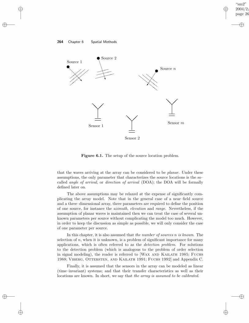
“sm2”2004/2/22page 264

i

i

i

i

i

i

i

i

264 Chapter 6 Spatial Methods

Source n

Source 2Source 1

BBBBBN

@@

@@R

v

vv

Sensor 1

@@

@@ @@

Sensor 2

Sensor m

cc

ccc

cc

cc

cc

c

,,

,,,

,,

,,

,,,

Figure 6.1. The setup of the source location problem.

that the waves arriving at the array can be considered to be planar. Under theseassumptions, the only parameter that characterizes the source locations is the so–called angle of arrival, or direction of arrival (DOA); the DOA will be formallydefined later on.

The above assumptions may be relaxed at the expense of significantly com-plicating the array model. Note that in the general case of a near–field sourceand a three–dimensional array, three parameters are required to define the positionof one source, for instance the azimuth, elevation and range. Nevertheless, if theassumption of planar waves is maintained then we can treat the case of several un-known parameters per source without complicating the model too much. However,in order to keep the discussion as simple as possible, we will only consider the caseof one parameter per source.

In this chapter, it is also assumed that the number of sources n is known. Theselection of n, when it is unknown, is a problem of significant importance for manyapplications, which is often referred to as the detection problem. For solutionsto the detection problem (which is analogous to the problem of order selectionin signal modeling), the reader is referred to [Wax and Kailath 1985; Fuchs

1988; Viberg, Ottersten, and Kailath 1991; Fuchs 1992] and Appendix C.

Finally, it is assumed that the sensors in the array can be modeled as linear(time–invariant) systems; and that their transfer characteristics as well as theirlocations are known. In short, we say that the array is assumed to be calibrated.

“sm2”2004/2/22page 265

i

i

i

i

i

i

i

i

Section 6.2 Array Model 265

6.2 ARRAY MODEL

We begin by considering the case of a single source. Once we establish a modelof the array for this case, the general model for the multiple source case is simplyobtained by the superposition principle.

Suppose that a single waveform impinges upon the array and let x(t) denotethe value of the signal waveform as measured at some reference point, at time t. The“reference point” may be one of the sensors in the array, or any other point placednear enough to the array so that the previously made assumption of planar wavepropagation holds true. The physical signals received by the array are continuoustime waveforms and hence t is a continuous variable here, unless otherwise stated.

Let τk denote the time needed for the wave to travel from the reference pointto sensor k (k = 1, . . . ,m). Then the output of sensor k can be written as

yk(t) = hk(t) ∗ x(t− τk) + ek(t) (6.2.1)

where hk(t) is the impulse response of the kth sensor, “∗” denotes the convolu-tion operation, and ek(t) is an additive noise. The noise may enter in equation(6.2.1) either as “thermal noise” generated by the sensor’s circuitry, as “randombackground radiation” impinging on the array, or in other ways. In (6.2.1), hk(t)is assumed known and the “input” signal x(t) as well as the delay τk are unknown.The parameters characterizing the source location enter in (6.2.1) through τk.Hence, the source location problem is basically one of time–delay estimation for theunknown input case.

The model equation (6.2.1) can be simplified significantly if the signals areassumed to be narrowband. In order to show how this can be done, a number ofpreliminaries are required.

Let X(ω) denote the Fourier transform of the (continuous–time) signal x(t):

X(ω) =

∫ ∞

−∞x(t)e−iωtdt (6.2.2)

(which is assumed to exist and be finite for all ω ∈ (−∞,∞)). The inverse trans-form, which expresses x(t) as a linear functional of X(ω), is given by

x(t) =1

2π

∫ ∞

−∞X(ω)eiωtdω (6.2.3)

Similarly, we define the transfer function Hk(ω) of the kth sensor as the Fouriertransform of hk(t). In addition, let Yk(ω) and Ek(ω) denote the Fourier trans-forms of the signal yk(t) and noise ek(t) in (6.2.1). By using this notation and theproperties of the Fourier transform, Yk(ω) can be written as

Yk(ω) = Hk(ω)X(ω)e−iωτk + Ek(ω) (6.2.4)

For a general class of physical signals, such as carrier modulated signals encounteredin communications, the energy spectral density of x(t) has the form shown in Figure6.2. There, ωc denotes the center (or carrier) frequency which is usually the centerof the frequency band occupied by the signal (hence its name). A signal having an

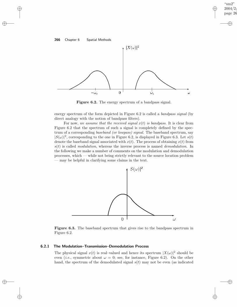
“sm2”2004/2/22page 266

i

i

i

i

i

i

i

i


¶¸·¹ ¶¸· º

» ¼¾½ ¶Y¿ » À

¶Á

Â

Figure 6.2. The energy spectrum of a bandpass signal.

energy spectrum of the form depicted in Figure 6.2 is called a bandpass signal (bydirect analogy with the notion of bandpass filters).

For now, we assume that the received signal x(t) is bandpass. It is clear fromFigure 6.2 that the spectrum of such a signal is completely defined by the spec-trum of a corresponding baseband (or lowpass) signal. The baseband spectrum, say|S(ω)|2, corresponding to the one in Figure 6.2, is displayed in Figure 6.3. Let s(t)denote the baseband signal associated with x(t). The process of obtaining x(t) froms(t) is called modulation, whereas the inverse process is named demodulation. Inthe following we make a number of comments on the modulation and demodulationprocesses, which — while not being strictly relevant to the source location problem— may be helpful in clarifying some claims in the text.

Ã ÄÆÅ ÇÉÈÃ Ê

ÇË

Ì

Í

Figure 6.3. The baseband spectrum that gives rise to the bandpass spectrum inFigure 6.2.

6.2.1 The Modulation–Transmission–Demodulation Process

The physical signal x(t) is real–valued and hence its spectrum |X(ω)|2 should beeven (i.e., symmetric about ω = 0; see, for instance, Figure 6.2). On the otherhand, the spectrum of the demodulated signal s(t) may not be even (as indicated

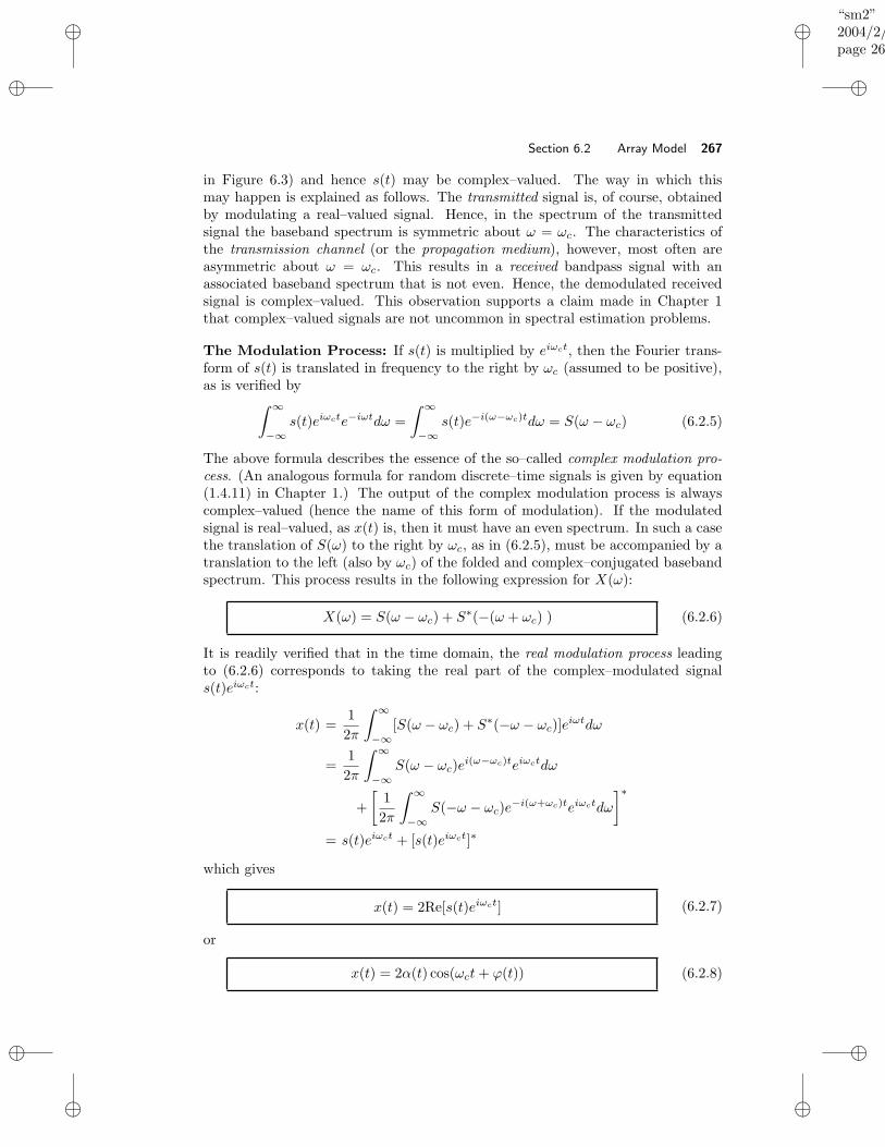
“sm2”2004/2/22page 267

i

i

i

i

i

i

i

i


in Figure 6.3) and hence s(t) may be complex–valued. The way in which thismay happen is explained as follows. The transmitted signal is, of course, obtainedby modulating a real–valued signal. Hence, in the spectrum of the transmittedsignal the baseband spectrum is symmetric about ω = ωc. The characteristics ofthe transmission channel (or the propagation medium), however, most often areasymmetric about ω = ωc. This results in a received bandpass signal with anassociated baseband spectrum that is not even. Hence, the demodulated receivedsignal is complex–valued. This observation supports a claim made in Chapter 1that complex–valued signals are not uncommon in spectral estimation problems.

The Modulation Process: If s(t) is multiplied by eiωct, then the Fourier trans-form of s(t) is translated in frequency to the right by ωc (assumed to be positive),as is verified by

∫ ∞

−∞s(t)eiωcte−iωtdω =

∫ ∞

−∞s(t)e−i(ω−ωc)tdω = S(ω − ωc) (6.2.5)

The above formula describes the essence of the so–called complex modulation pro-cess. (An analogous formula for random discrete–time signals is given by equation(1.4.11) in Chapter 1.) The output of the complex modulation process is alwayscomplex–valued (hence the name of this form of modulation). If the modulatedsignal is real–valued, as x(t) is, then it must have an even spectrum. In such a casethe translation of S(ω) to the right by ωc, as in (6.2.5), must be accompanied by atranslation to the left (also by ωc) of the folded and complex–conjugated basebandspectrum. This process results in the following expression for X(ω):

X(ω) = S(ω − ωc) + S∗(−(ω + ωc) ) (6.2.6)

It is readily verified that in the time domain, the real modulation process leadingto (6.2.6) corresponds to taking the real part of the complex–modulated signals(t)eiωct:

x(t) =1

2π

∫ ∞

−∞[S(ω − ωc) + S∗(−ω − ωc)]e

iωtdω

=1

2π

∫ ∞

−∞S(ω − ωc)e

i(ω−ωc)teiωctdω

+

[1

2π

∫ ∞

−∞S(−ω − ωc)e

−i(ω+ωc)teiωctdω

]∗

= s(t)eiωct + [s(t)eiωct]∗

which gives

x(t) = 2Re[s(t)eiωct] (6.2.7)

or

x(t) = 2α(t) cos(ωct+ ϕ(t)) (6.2.8)

“sm2”2004/2/22page 268

i

i

i

i

i

i

i

i


where α(t) and ϕ(t) are the amplitude and phase of s(t), respectively:

s(t) = α(t)eiϕ(t)

If we let sI(t) and sQ(t) denote the real and imaginary parts of s(t), then we canalso write (6.2.7) as

x(t) = 2[sI(t) cos(ωct) − sQ(t) sin(ωct)] (6.2.9)

We note in passing the following terminology associated with the equivalent time–domain representations (6.2.7)–(6.2.9) of a bandpass signal: s(t) is called the com-plex envelope of x(t); and sI(t) and sQ(t) are said to be the in–phase and quadraturecomponents of x(t).

The Demodulation Process: A calculation similar to (6.2.5) shows that theFourier transform of x(t)e−iωct is given by

[S(ω) + S∗(−ω − 2ωc)]

which is simply X(ω) translated in frequency to the left by ωc. The baseband (orlowpass) signal s(t) can then be obtained by filtering x(t)e−iωct with a baseband(or lowpass) filter whose bandwidth is matched to that of S(ω). The hardwareimplementation of the demodulation process is presented later on, in block form,in Figure 6.4.

6.2.2 Derivation of the Model Equation

Given the background of the previous subsection, we return to equation (6.2.4)describing the output of sensor k. Since x(t) is assumed to be a bandpass signal,X(ω) is given by (6.2.6) which, when inserted in (6.2.4), leads to

Yk(ω) = Hk(ω)[S(ω − ωc) + S∗(−ω − ωc)]e−iωτk + Ek(ω) (6.2.10)

Let yk(t) denote the demodulated signal:

yk(t) = yk(t)e−iωct

It follows from (6.2.10) and the previous discussion on the demodulation processthat the Fourier transform of yk(t) is given by

Yk(ω) = Hk(ω + ωc)[S(ω) + S∗(−ω − 2ωc)]e−i(ω+ωc)τk

+Ek(ω + ωc) (6.2.11)

When yk(t) is passed through a lowpass filter with bandwidth matched to S(ω),in the filter output (say, yk(t)) the component in (6.2.11) centered at ω = −2ωc iseliminated along with all the other frequency components that fall in the stopbandof the lowpass filter. Hence, we obtain:

Yk(ω) = Hk(ω + ωc)S(ω)e−i(ω+ωc)τk + Ek(ω + ωc) (6.2.12)

“sm2”2004/2/22page 269

i

i

i

i

i

i

i

i


whereHk(ω+ωc) and Ek(ω+ωc) denote the parts of Hk(ω+ωc) and Ek(ω+ωc) thatfall within the lowpass filter’s passband, Ω, and where the frequency ω is restrictedto Ω.

We now make the following key assumption.

The received signals are narrowband, so that |S(ω)| decreasesrapidly with increasing |ω|. (6.2.13)

Under the assumption above, (6.2.12) reduces (in an approximate way) to thefollowing equation:

Yk(ω) = Hk(ωc)S(ω)e−iωcτk + Ek(ω + ωc) for ω ∈ Ω (6.2.14)

Because Hk(ωc) must be different from zero, the sensor transfer function Hk(ω)should pass frequencies near ω = ωc (as expected, since ωc is the center frequencyof the received signal). Also note that we do not replace Ek(ω + ωc) in (6.2.14) byEk(ωc) since this term might not be (nearly) constant over the signal bandwidth(for instance, this would be the case when the noise term in (6.2.12) contains anarrowband interference with the same center frequency as the signal).

Remark: It is sometimes claimed that (6.2.12) can be reduced to (6.2.14) even ifthe signals are broadband but the sensors in the array are narrowband with centerfrequency ω = ωc. Under such an assumption, |Hk(ω+ωc)| goes quickly to zero as|ω| increases and hence (6.2.12) becomes

Yk(ω) = Hk(ω + ωc)S(0)e−iωcτk + Ek(ω + ωc) (6.2.15)

which apparently is different from (6.2.14). In order to obtain (6.2.14) from (6.2.12)under the previous conditions, we need to make some additional assumptions.Hence, if we further assume that the sensor frequency response is flat over thepassband (so that Hk(ω + ωc) = Hk(ωc)) and that the signal spectrum varies overthe sensor passband (so that S(ω) differs quite a bit from S(0) over the passbandin question) then we can still obtain (6.2.14) from (6.2.12).

The model of the array is derived in a straightforward manner from equation(6.2.14). The time–domain counterpart of (6.2.14) is the following:

yk(t) = Hk(ωc)e−iωcτks(t) + ek(t) (6.2.16)

where yk(t) and ek(t) are the inverse Fourier transforms of the corresponding termsin (6.2.14) (by a slight abuse of notation, ek(t) is associated with Ek(ω + ωc), notEk(ω)).

The hardware implementation required to obtain yk(t), as defined above,is indicated in Figure 6.4. Note that the scheme in Figure 6.4 generates samplesof the real and imaginary components of yk(t). These samples are paired in thedigital machine following the analog scheme of Figure 6.4 to obtain samples of thecomplex–valued signal yk(t). (We stress once more that all physical analog signalsare real–valued.) Note that the continuous–time signal in (6.2.16) is bandlimited:according to (6.2.14) (and the related discussion), Yk(ω) is approximately equal to

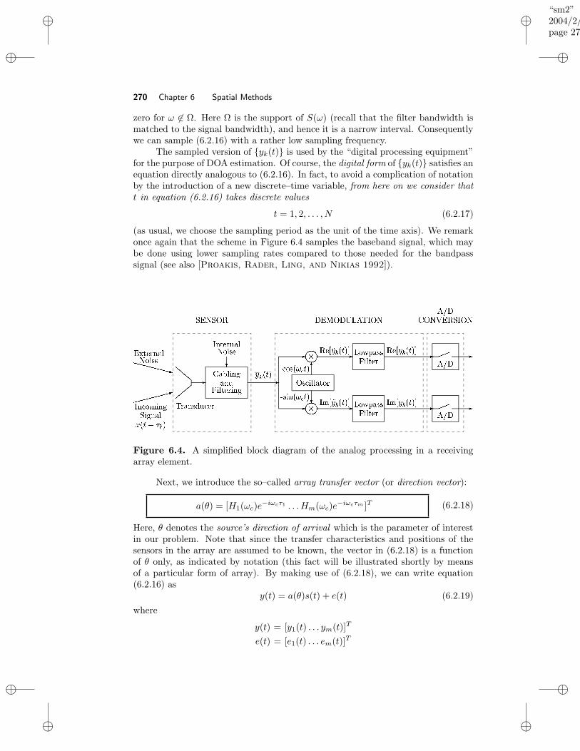
“sm2”2004/2/22page 270

i

i

i

i

i

i

i

i


zero for ω 6∈ Ω. Here Ω is the support of S(ω) (recall that the filter bandwidth ismatched to the signal bandwidth), and hence it is a narrow interval. Consequentlywe can sample (6.2.16) with a rather low sampling frequency.

The sampled version of yk(t) is used by the “digital processing equipment”for the purpose of DOA estimation. Of course, the digital form of yk(t) satisfies anequation directly analogous to (6.2.16). In fact, to avoid a complication of notationby the introduction of a new discrete–time variable, from here on we consider thatt in equation (6.2.16) takes discrete values

t = 1, 2, . . . , N (6.2.17)

(as usual, we choose the sampling period as the unit of the time axis). We remarkonce again that the scheme in Figure 6.4 samples the baseband signal, which maybe done using lower sampling rates compared to those needed for the bandpasssignal (see also [Proakis, Rader, Ling, and Nikias 1992]).

Î Î Î Î Î Î Î Ï

Ð Ð Ð Ð Ð Ð Ð Ñ

ÒÓEÔÕ'Ö×4ØÙÚÛÜ ÝGÕ

Þ×4ß'ÛàwÜ ×Eáâ Ü á×4ØÙãä å*æÉçè'é

â ÒêÚ â4ëíì

î î îï ï ï ð ñ Øò4Ù Ü ×EáØ×4óô)Ü Ù ÔÕ'ÖÜ ×Eá

õÞ×Ô!Õ'Ö ×4ØÙÚÛÜ ÝGÕ

ö*ÖØ×4ÝóE÷4ßÕÖ

ðø è ä å!é

ùÒUú ë ùûü*ý)öþÞ ë Ú

ÿ

ÿ

ë Ýß'Ü Ù Ù ØÔ ÛÖ

ü®Û4ØÝ!ÝôÜ Ù Ô!Õ'Ö

ü®Û4ØÝ!ÝôÜ Ù Ô!Õ'Öð

ð

õ Ý!Ü × ä å!éß'ÛÝ ä å!é

ð

ð Þà øèä å!é

ì Õ ø è ä å!é ð

ðÞà øèä å!é

ì Õ ø è ä å!é

ýùñ ë ÚíÒ ìâ Þ ë Ú

ð

ð

ýù

ýù

Figure 6.4. A simplified block diagram of the analog processing in a receivingarray element.

Next, we introduce the so–called array transfer vector (or direction vector):

a(θ) = [H1(ωc)e−iωcτ1 . . . Hm(ωc)e

−iωcτm ]T (6.2.18)

Here, θ denotes the source’s direction of arrival which is the parameter of interestin our problem. Note that since the transfer characteristics and positions of thesensors in the array are assumed to be known, the vector in (6.2.18) is a functionof θ only, as indicated by notation (this fact will be illustrated shortly by meansof a particular form of array). By making use of (6.2.18), we can write equation(6.2.16) as

y(t) = a(θ)s(t) + e(t) (6.2.19)

where

y(t) = [y1(t) . . . ym(t)]T

e(t) = [e1(t) . . . em(t)]T

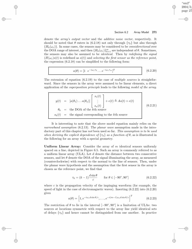
“sm2”2004/2/22page 271

i

i

i

i

i

i

i

i


denote the array’s output vector and the additive noise vector, respectively. Itshould be noted that θ enters in (6.2.18) not only through τk but also throughHk(ωc). In some cases, the sensors may be considered to be omnidirectional overthe DOA range of interest, and then Hk(ωc)mk=1 are independent of θ. Sometimes,the sensors may also be assumed to be identical. Then by redefining the signal(H(ωc)s(t) is redefined as s(t)) and selecting the first sensor as the reference point,the expression (6.2.18) can be simplified to the following form:

a(θ) = [1 e−iωcτ2 . . . e−iωcτm ]T (6.2.20)

The extension of equation (6.2.19) to the case of multiple sources is straightfor-ward. Since the sensors in the array were assumed to be linear elements, a directapplication of the superposition principle leads to the following model of the array.

y(t) = [a(θ1) . . . a(θn)]

s1(t)...

sn(t)

+ e(t) , As(t) + e(t)

θk = the DOA of the kth source

sk(t) = the signal corresponding to the kth source

(6.2.21)

It is interesting to note that the above model equation mainly relies on thenarrowband assumption (6.2.13). The planar wave assumption made in the intro-ductory part of this chapter has not been used so far. This assumption is to be usedwhen deriving the explicit dependence of τk as a function of θ, as is illustrated inthe following for an array with a special geometry.

Uniform Linear Array: Consider the array of m identical sensors uniformlyspaced on a line, depicted in Figure 6.5. Such an array is commonly referred to asa uniform linear array (ULA). Let d denote the distance between two consecutivesensors, and let θ denote the DOA of the signal illuminating the array, as measured(counterclockwise) with respect to the normal to the line of sensors. Then, underthe planar wave hypothesis and the assumption that the first sensor in the array ischosen as the reference point, we find that

τk = (k − 1)d sin θ

cfor θ ∈ [−90, 90] (6.2.22)

where c is the propagation velocity of the impinging waveform (for example, thespeed of light in the case of electromagnetic waves). Inserting (6.2.22) into (6.2.20)gives

a(θ) =[

1, e−iωcd sin θ/c, . . . , e−i(m−1)ωcd sin θ/c]T

(6.2.23)

The restriction of θ to lie in the interval [−90, 90] is a limitation of ULAs: twosources at locations symmetric with respect to the array line yield identical setsof delays τk and hence cannot be distinguished from one another. In practice

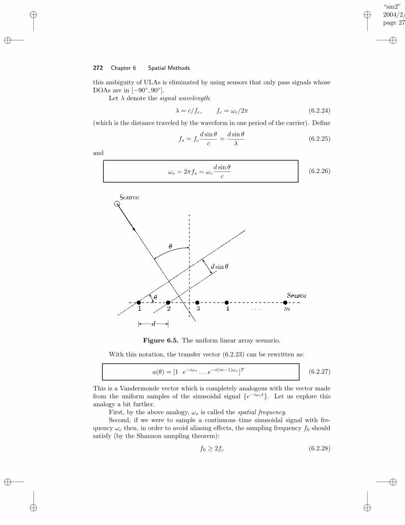
“sm2”2004/2/22page 272

i

i

i

i

i

i

i

i


this ambiguity of ULAs is eliminated by using sensors that only pass signals whoseDOAs are in [−90, 90].

Let λ denote the signal wavelength:

λ = c/fc, fc = ωc/2π (6.2.24)

(which is the distance traveled by the waveform in one period of the carrier). Define

fs = fcd sin θ

c=d sin θ

λ(6.2.25)

and

ωs = 2πfs = ωcd sin θ

c(6.2.26)

! #"%$&

'(

)

*+ ) ,,-,&.#/%!"

01234

5 /6.7)8 8988 +

5 ':

8 8 8 8 8 8 8 8 8 8 8 8 8 8 8 8 8 8 8 8 8

; ; ; ; ; <

=

> > > > >

Figure 6.5. The uniform linear array scenario.

With this notation, the transfer vector (6.2.23) can be rewritten as:

a(θ) = [1 e−iωs . . . e−i(m−1)ωs ]T (6.2.27)

This is a Vandermonde vector which is completely analogous with the vector madefrom the uniform samples of the sinusoidal signal e−iωst. Let us explore thisanalogy a bit further.

First, by the above analogy, ωs is called the spatial frequency.Second, if we were to sample a continuous–time sinusoidal signal with fre-

quency ωc then, in order to avoid aliasing effects, the sampling frequency f0 shouldsatisfy (by the Shannon sampling theorem):

f0 ≥ 2fc (6.2.28)

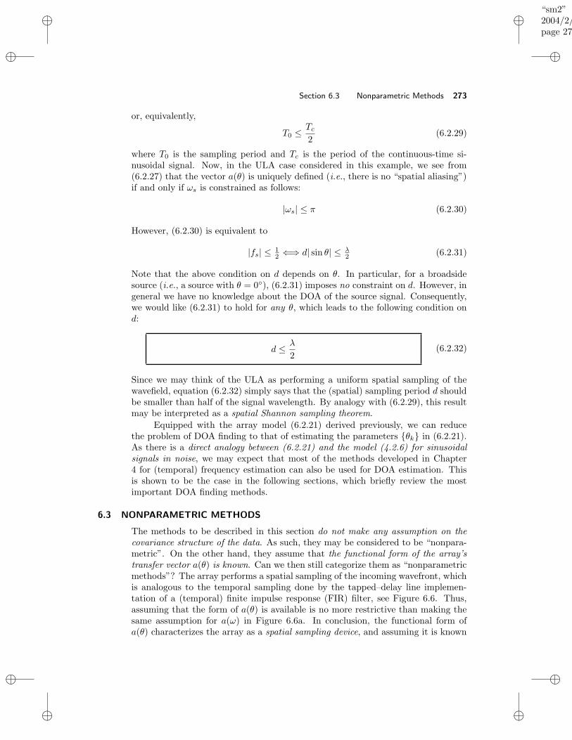
“sm2”2004/2/22page 273

i

i

i

i

i

i

i

i

Section 6.3 Nonparametric Methods 273

or, equivalently,

T0 ≤ Tc2

(6.2.29)

where T0 is the sampling period and Tc is the period of the continuous-time si-nusoidal signal. Now, in the ULA case considered in this example, we see from(6.2.27) that the vector a(θ) is uniquely defined (i.e., there is no “spatial aliasing”)if and only if ωs is constrained as follows:

|ωs| ≤ π (6.2.30)

However, (6.2.30) is equivalent to

|fs| ≤ 12 ⇐⇒ d| sin θ| ≤ λ

2 (6.2.31)

Note that the above condition on d depends on θ. In particular, for a broadsidesource (i.e., a source with θ = 0), (6.2.31) imposes no constraint on d. However, ingeneral we have no knowledge about the DOA of the source signal. Consequently,we would like (6.2.31) to hold for any θ, which leads to the following condition ond:

d ≤ λ

2(6.2.32)

Since we may think of the ULA as performing a uniform spatial sampling of thewavefield, equation (6.2.32) simply says that the (spatial) sampling period d shouldbe smaller than half of the signal wavelength. By analogy with (6.2.29), this resultmay be interpreted as a spatial Shannon sampling theorem.

Equipped with the array model (6.2.21) derived previously, we can reducethe problem of DOA finding to that of estimating the parameters θk in (6.2.21).As there is a direct analogy between (6.2.21) and the model (4.2.6) for sinusoidalsignals in noise, we may expect that most of the methods developed in Chapter4 for (temporal) frequency estimation can also be used for DOA estimation. Thisis shown to be the case in the following sections, which briefly review the mostimportant DOA finding methods.

6.3 NONPARAMETRIC METHODS

The methods to be described in this section do not make any assumption on thecovariance structure of the data. As such, they may be considered to be “nonpara-metric”. On the other hand, they assume that the functional form of the array’stransfer vector a(θ) is known. Can we then still categorize them as “nonparametricmethods”? The array performs a spatial sampling of the incoming wavefront, whichis analogous to the temporal sampling done by the tapped–delay line implemen-tation of a (temporal) finite impulse response (FIR) filter, see Figure 6.6. Thus,assuming that the form of a(θ) is available is no more restrictive than making thesame assumption for a(ω) in Figure 6.6a. In conclusion, the functional form ofa(θ) characterizes the array as a spatial sampling device, and assuming it is known

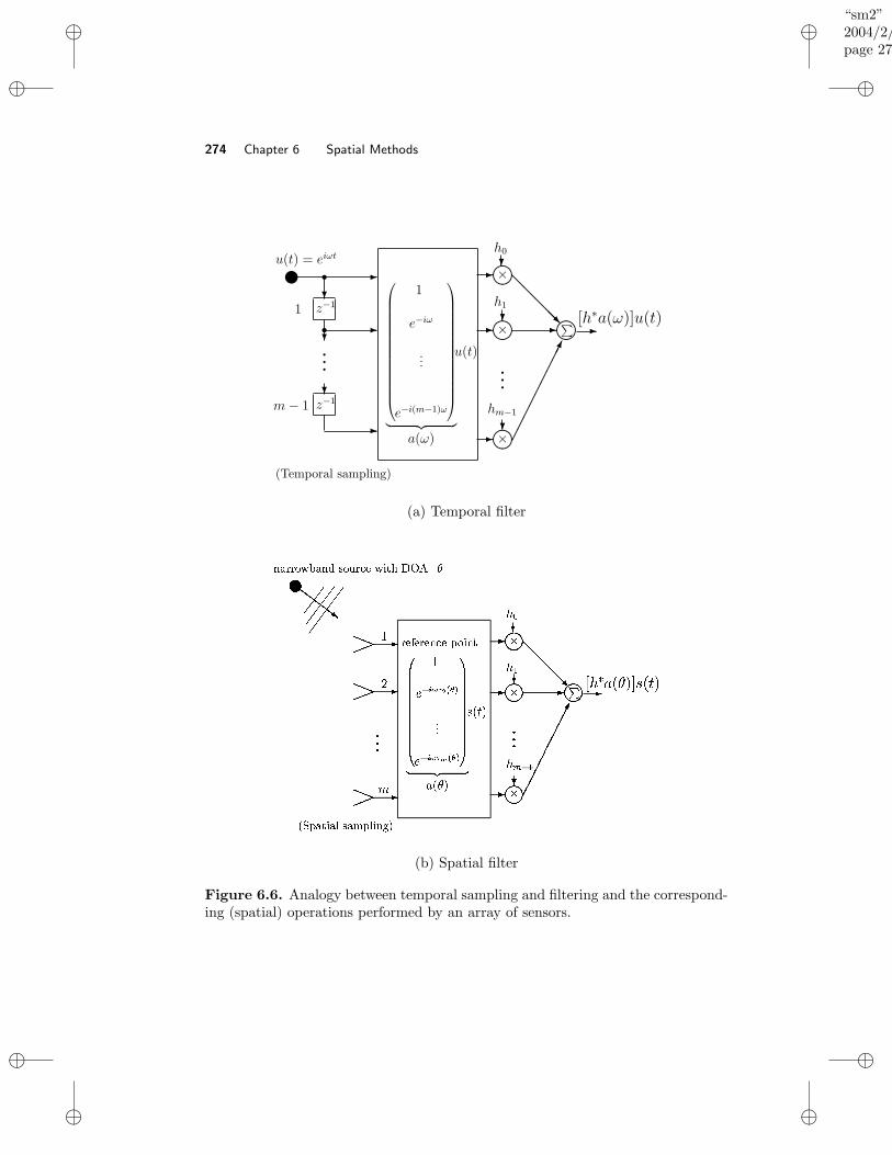
“sm2”2004/2/22page 274

i

i

i

i

i

i

i

i


(Temporal sampling)

z

-

qqq

?

?

?

-

-

-

-

@@

@@@R

-

?

?

qqq

-s

-

?

s

×

×

×

∑

u(t) = eiωt

z−1

z−1

1

m − 1

1

e−iω

...

e−i(m−1)ω

︸︷︷︸

a(ω)

u(t)

h0

h1

hm−1

[h∗a(ω)]u(t)

(a) Temporal filter

? ? ? ? ?@AAAAAAAAA

AAABCDDFEHGJIKCBLNME%ODFPRQGS TFUNVWJXYZ

[ \^] CTFS C_`MFCa ] _ S Bbdce

e

e

f

g

h

iiij

j

j

k kk kk kk k k l

m m m m monh

h

h

h

pqrJspJqrJs

pJqrJs

pJqrJs

httuu

httuu

httuu

iii

DQwv QRDFQwBPRQ ] EdS B%Txy

z

|||||||||||

x~d do

~d d

F

^

o

K

#¡ ¢R£ ¤H¥F¦§¢F¨%¤

(b) Spatial filter

Figure 6.6. Analogy between temporal sampling and filtering and the correspond-ing (spatial) operations performed by an array of sensors.

“sm2”2004/2/22page 275

i

i

i

i

i

i

i

i


should not be considered to be parametric (or model–based) information. As al-ready mentioned, an array for which the functional form of a(θ) is know is said tobe calibrated.

Figure 6.6 also makes an analogy between temporal FIR filtering and spatialfiltering using an array of sensors. In what follows, we comment briefly on thisanalogy since it is of interest for the nonparametric approach to DOA finding. Inthe time series case, a FIR filter is defined by the relation

yF (t) =

m−1∑

k=0

hku(t− k) , h∗y(t) (6.3.1)

where hk are the filter weights, u(t) is the input to the filter and

h = [h0 . . . hm−1]∗ (6.3.2)

y(t) = [u(t) . . . u(t−m+ 1)]T (6.3.3)

Similarly, we can use the spatial samples yk(t)mk=1 obtained with a sensorarray to define a spatial filter:

yF (t) = h∗y(t) (6.3.4)

A temporal filter can be made to enhance or attenuate some selected frequencybands by appropriately choosing the vector h. More precisely, since the filter outputfor a sinusoidal input u(t) is given by

yF (t) = [h∗a(ω)]u(t) (6.3.5)

(where a(ω) is as defined, for instance, in Figure 6.6), then by selecting h so thath∗a(ω) is large (small) we can enhance (attenuate) the power of yF (t) at frequencyω.

In direct analogy with (6.3.5), the (noise–free) spatially filtered output (as in(6.3.4)) of an array illuminated by a narrowband wavefront with complex envelopes(t) and DOA equal to θ is given by (cf. (6.2.19)):

yF (t) = [h∗a(θ)]s(t) (6.3.6)

This equation clearly shows that the spatial filter can be selected to enhance (at-tenuate) the signals coming from a given direction θ, by making h∗a(θ) in (6.3.6)large (small). This observation lies at the basis of the DOA finding methods to bedescribed in this section. All of these methods can be derived by using the filterbank approach of Chapter 5. More specifically, assume that a filter h has been foundsuch that

(i) It passes undistorted the signals with a given DOA θ; and

(ii) It attenuates all the other DOAs different from θ as muchas possible.

(6.3.7)

“sm2”2004/2/22page 276

i

i

i

i

i

i

i

i


Then, the power of the spatially filtered signal in (6.3.4),

E|yF (t)|2

= h∗Rh, R = E y(t)y∗(t) (6.3.8)

should give a good indication of the energy coming from direction θ. (Note thatθ enters in (6.3.8) via h.) Hence, h∗Rh should peak at the DOAs of the sourceslocated in the array’s viewing field when evaluated over the DOA range of interest.This fact may be exploited for the purpose of DOA finding. Depending on thespecific way in which the (loose) design objectives in (6.3.7) are formulated, theabove approach can lead to different DOA estimation methods. In the following,we present spatial extensions of the periodogram and Capon techniques. The RFBmethod of Chapter 5 may also be extended to the spatial processing case, providedthe array’s geometry is such that the transfer vector a(θ + α) can be factored as

a(θ + α) = D(θ)a(α) (6.3.9)

where D is a unitary (possibly diagonal) matrix. Without such a property, the RFBspatial filter should be computed, for each θ, by solving an m×m eigendecompo-sition problem, which would be computationally prohibitive in most applications.Since it is not a priori obvious that an arbitrary array satisfies (6.3.9), we do notconsider the RFB approach in what follows.1 Finally, we remark that a spatial filtersatisfying the design objectives in (6.3.7) can be viewed as forming a (reception)beam in the direction θ, as pictorially indicated in Figure 6.7. Because of this inter-pretation, the methods resulting from this approach to the DOA finding problem,in particular the method of the next subsection, are called beamforming methods[Van Veen and Buckley 1988; Johnson and Dudgeon 1992].

6.3.1 Beamforming

In view of (6.3.6), condition (i) of the filter design problem (6.3.7) can be formulatedas:

h∗a(θ) = 1 (6.3.10)

In what follows, we assume that the transfer vector a(θ) has been normalized sothat

a∗(θ)a(θ) = m (6.3.11)

Note that in the case of an array with identical sensors, the condition (6.3.11) isautomatically met (cf. (6.2.20)).

Regarding condition (ii) in (6.3.7), if y(t) in (6.3.8) were spatially white withR = I, then we would obtain the following expression for the power of the filteredsignal:

E|yF (t)|2

= h∗h (6.3.12)

which is different from zero for every θ (note that we cannot have h = 0, becauseof condition (6.3.10)). This fact indicates that a spatially white signal in the ar-ray output can be considered as impinging on the array with equal power from all

1Referring back to Chapter 5 may prove useful for understanding these comments on RFB andfor several other discussions in this section.

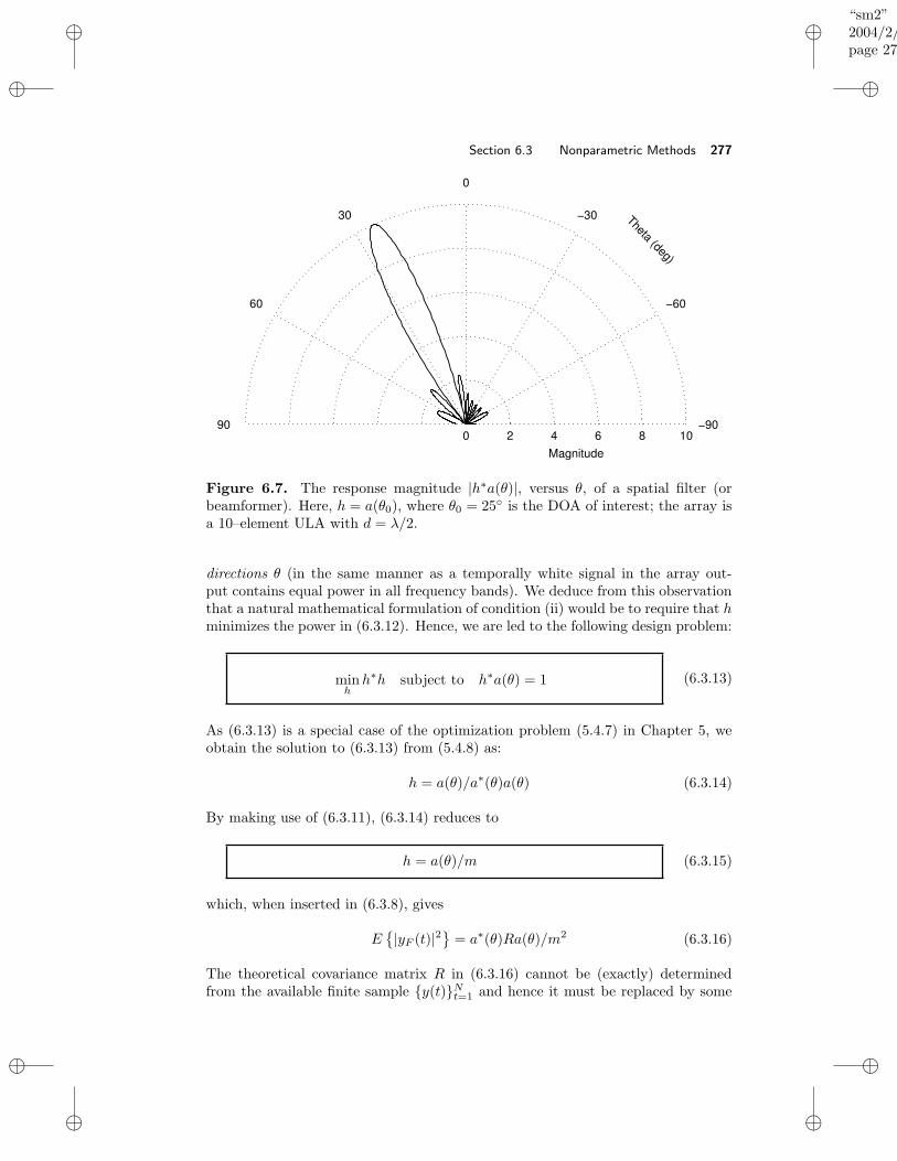
“sm2”2004/2/22page 277

i

i

i

i

i

i

i

i


2 4 6 8 100Magnitude

Theta (deg)

−90

−60

−30

0

30

60

90

Figure 6.7. The response magnitude |h∗a(θ)|, versus θ, of a spatial filter (orbeamformer). Here, h = a(θ0), where θ0 = 25 is the DOA of interest; the array isa 10–element ULA with d = λ/2.

directions θ (in the same manner as a temporally white signal in the array out-put contains equal power in all frequency bands). We deduce from this observationthat a natural mathematical formulation of condition (ii) would be to require that hminimizes the power in (6.3.12). Hence, we are led to the following design problem:

minhh∗h subject to h∗a(θ) = 1 (6.3.13)

As (6.3.13) is a special case of the optimization problem (5.4.7) in Chapter 5, weobtain the solution to (6.3.13) from (5.4.8) as:

h = a(θ)/a∗(θ)a(θ) (6.3.14)

By making use of (6.3.11), (6.3.14) reduces to

h = a(θ)/m (6.3.15)

which, when inserted in (6.3.8), gives

E|yF (t)|2

= a∗(θ)Ra(θ)/m2 (6.3.16)

The theoretical covariance matrix R in (6.3.16) cannot be (exactly) determinedfrom the available finite sample y(t)Nt=1 and hence it must be replaced by some

“sm2”2004/2/22page 278

i

i

i

i

i

i

i

i


estimate, such as

R =1

N

N∑

t=1

y(t)y∗(t) (6.3.17)

By doing so and omitting the factor 1/m2 in (6.3.16), which has no influence on theDOA estimates, we obtain the beamforming method which determines the DOAsas summarized in the next box.

The beamforming DOA estimates are given by the locations ofthe n highest peaks of the function

a∗(θ)Ra(θ)

(6.3.18)

When the estimated spatial spectrum in (6.3.18) is compared to the expres-sion derived in Section 5.4 for the Blackman–Tukey periodogram, it is seen thatbeamforming is a direct (spatial) extension of the periodogram. In fact, the func-tion in (6.3.18) may be thought of as being obtained by averaging the “spatialperiodograms”

|a∗(θ)y(t)|2 (6.3.19)

over the set of available “snapshots” (t = 1, . . . , N).The connection established in the previous paragraph, between beamform-

ing and the (averaged) periodogram, suggests that the resolution properties of thebeamforming method are analogous to those of the periodogram method. In fact, byan analysis similar to that in Chapters 2 and 5 it can be shown that the beamwidth2

of the spatial filter used by beamforming is approximately equal to the inverse ofthe array’s aperture (as measured in signal wavelengths). This sets a limit on theresolution achievable with beamforming, as indicated below (see Exercise 6.2):

Beamforming DOA resolution limit ' wavelength / array “length” (6.3.20)

Next, we note that as N increases, the sample spatial spectrum in (6.3.18)converges (under mild conditions) to (6.3.16), uniformly in θ. Hence the beam-forming estimates of the DOAs converge to the n maximum points of (6.3.16), asN tends to infinity. If the array model (6.2.21) holds (it has not been used so far!),the noise e(t) is spatially white and has the same power σ2 in all sensors, and ifthere is only one source (with DOA denoted by θ0, for convenience), then R in(6.3.16) is given by

R = a(θ0)a∗(θ0)P + σ2I (6.3.21)

where P = E|s(t)|2

denotes the signal power. Hence,

a∗(θ)Ra(θ) = |a∗(θ)a(θ0)|2P + a∗(θ)a(θ)σ2

≤ |a∗(θ)a(θ)||a∗(θ0)a(θ0)|P + σ2a∗(θ)a(θ)

= m(mP + σ2) (6.3.22)2The beamwidth is the spatial counterpart of the temporal notion of bandwidth associated

with a bandpass filter.

“sm2”2004/2/22page 279

i

i

i

i

i

i

i

i


where the inequality follows from the Cauchy–Schwartz lemma (see Result R22 inAppendix A) and the last equality from (6.3.11). The upper bound in (6.3.22) isachieved for a(θ) = a(θ0) which, under mild conditions, implies θ = θ0. In conclu-sion, the beamforming DOA estimate is consistent under the previous assumptions(n = 1, etc.). In the general case of multiple sources, however, the DOA esti-mates obtained with beamforming are inconsistent. The (asymptotic) bias of theseestimates may be significant if the sources are strongly correlated or closely spaced.

As explained above, beamforming is the spatial analog of the Blackman–Tukeyperiodogram (with a certain covariance estimate) and the Bartlett periodogram(if we interpret the m–dimensional snapshots in (6.3.19) as “subsamples” of theavailable “sample” [yT (1), . . . , yT (N)]T ). Note, however, that the value of m inthe periodogram methods can be chosen by the user, whereas in the beamformingmethod m is fixed. This difference might seem small at first, but it has a significantimpact on the consistency properties of beamforming. More precisely, it can beshown that, for instance, the Bartlett periodogram estimates of temporal frequenciesare consistent under the model (4.2.7), provided that m increases without bound asthe number of samples N tends to infinity (e.g., we can set m = N , which yieldsthe unmodified periodogram).3 For beamforming, on the other hand, the value ofm (i.e., the number of array elements) is limited by physical considerations. Thisprevents beamforming from providing consistent DOA estimates in the multiplesignal case. An additional difficulty is that in the spatial scenario the signals can becorrelated with one another, whereas they are always uncorrelated in the temporalfrequency estimation case. Explaining why this is so and completing a consistencyanalysis of the beamforming DOA estimates is left as an exercise for the reader.

Now, if the model (6.2.21) holds, if the minimum DOA separation is largerthan the array beamwidth (which implies that m is sufficiently large), if the sig-nals are uncorrelated, and if the noise is spatially white, then it is readily seen thatthe multiple–source spectrum (6.3.16) decouples (approximately) in n single–sourcespectra; this means that beamforming may provide reasonably accurate DOA esti-mates in such a case. In fact, in this case beamforming can be shown to providean approximation to the nonlinear LS DOA estimation method discussed in Sec-tion 6.4.1; see the remark in that section.

6.3.2 Capon Method

The derivation of the Capon method for array signal processing is entirely analogouswith the derivation of the Capon method for the time series data case developed inSection 5.4 [Capon 1969; Lacoss 1971]. The Capon spatial filter design problemis the following:

minhh∗Rh subject to h∗a(θ) = 1 (6.3.23)

3The unmodified periodogram in an inconsistent estimator for continuous PSDs (as shown inChapter 2). However, as asserted above, the plain periodogram estimates of discrete (or line)PSDs are consistent. Showing this is left as an exercise to the reader. (Make use of the covariancematrix model (4.2.7) with m → ∞, and the fact that the Fourier (or Vandermonde) vectors, atdifferent frequencies, become orthogonal to one another as their dimension increases.)

“sm2”2004/2/22page 280

i

i

i

i

i

i

i

i


Hence, objective (i) in the general design problem (6.3.7) is ensured by constrainingthe filter exactly as in the beamforming approach (see (6.3.10)). Objective (ii) in(6.3.7), however, is accomplished in a more sound way: by requiring the filter tominimize the output power, when fed with the actual array data y(t). Hence,in the Capon approach, objective (ii) is formulated in a “data–dependent” way,whereas it is formulated independently of the data in the beamforming method.As a consequence, the goal of the Capon filter steered to a certain direction θ isto attenuate any other signal that actually impinges on the array from a DOA 6=θ, whereas the beamforming filter pays uniform attention to all other DOAs 6= θ,even though there might be no incoming signal for many of those DOAs.

The solution to (6.3.23), as derived in Section 5.4, is given by

h =R−1a(θ)

a∗(θ)R−1a(θ)(6.3.24)

which, when inserted in the output power formula (6.3.8), leads to

E|yF (t)|2

=

1

a∗(θ)R−1a(θ)(6.3.25)

It only remains to replace R in (6.3.25) by a sample estimate, such as R in (6.3.17),to obtain the Capon DOA estimator.

The Capon DOA estimates are obtained as the locations of then largest peaks of the following function:

1

a∗(θ)R−1a(θ)

(6.3.26)

There is an implicit assumption in (6.3.26) that R−1 exists, but this canbe ensured under weak conditions (in particular, R−1 exists with probability 1 ifN ≥ m and if the noise term has a positive definite spatial covariance matrix).Note that the “spatial spectrum” in (6.3.26) corresponds to the “CM–Version 1”PSD in the time series case (see equation (5.4.12) in Section 5.4). A Capon spatialspectrum similar to the “CM–Version 2” PSD formula (see (5.4.17)) might also bederived, but it appears to be more complicated than the time series formula if thearray is not a ULA.

Capon DOA estimation has been empirically found to possess superior per-formance as compared with beamforming. The common advantage of these twononparametric methods is that they do not assume anything about the statisticalproperties of the data and, therefore, they can be used in situations where we lackinformation about these properties. On the other hand, in the cases where such in-formation is available, for example in the form of a covariance model of the data, anonparametric approach does not give the performance that one can achieve with aparametric (model–based) approach. The parametric approach to DOA estimationis the subject of the next section.

“sm2”2004/2/22page 281

i

i

i

i

i

i

i

i

Section 6.4 Parametric Methods 281

6.4 PARAMETRIC METHODS

In this section, we postulate the array model (6.2.21). Furthermore, the noise e(t)is assumed to be spatially white with components having identical variance:

E e(t)e∗(t) = σ2I (6.4.1)

In addition, the signal covariance matrix

P = E s(t)s∗(t) (6.4.2)

is assumed to be nonsingular (but not necessarily diagonal; hence the signals may be(partially) correlated). When the signals are fully correlated, so that P is singular,they are said to be coherent. Finally, we assume that the signals and the noise areuncorrelated with one another.

Under the previous assumptions, the theoretical covariance matrix of the arrayoutput vector is given by

R = E y(t)y∗(t) = APA∗ + σ2I (6.4.3)

There is a direct analogy between the array models above, (6.2.21) and (6.4.3),and the corresponding models encountered in our discussion of the sinusoids–in–noise case in Chapter 4. More specifically, the “nonlinear regression” model (6.2.21)of the array is analogous to (4.2.6), and the array covariance model (6.4.3) is muchthe same as (4.2.7). The consequence of these analogies is that all methods intro-duced in Chapter 4 for frequency estimation can also be used for DOA estimationwithout any essential modification. In the following, we briefly review these meth-ods with a view of pointing out any differences from the frequency estimationapplication. When the assumed array model is a good representation of reality, theparametric DOA estimation methods reviewed in the sequel provide highly accu-rate DOA estimates, even in adverse situations (such as low SNR scenarios). Asour main thrust in this text has been the understanding of the basic ideas behindthe presented spectral estimation methodologies, we do not dwell on the details ofthe analysis required to establish the statistical properties of the DOA estimatorsdiscussed in the following; see, however, Appendix B for a discussion on the Cramer–Rao bound and the best accuracy achievable in DOA estimation problems. Suchanalysis details are available in [Stoica and Nehorai 1989a; Stoica and Ne-

horai 1990; Stoica and Sharman 1990; Stoica and Nehorai 1991; Viberg

and Ottersten 1991; Rao and Hari 1993]. For reviews of many of the re-cent advances in spatial spectral analysis, the reader can consult [Pillai 1989],[Ottersten, Viberg, Stoica, and Nehorai 1993], and [Van Trees 2002].

6.4.1 Nonlinear Least Squares Method

This method determines the unknown DOAs as the minimizing elements of thefollowing function

f =1

N

N∑

t=1

‖ y(t) −As(t) ‖2 (6.4.4)

“sm2”2004/2/22page 282

i

i

i

i

i

i

i

i


Minimization with respect to s(t) gives (see Result R32 in Appendix A)

s(t) = (A∗A)−1A∗y(t) t = 1, . . . , N (6.4.5)

By inserting (6.4.5) into (6.4.4), we get the following concentrated nonlinear leastsquares (LS) criterion:

f =1

N

N∑

t=1

‖ I −A(A∗A)−1A∗y(t) ‖2

=1

N

N∑

t=1

y∗(t)[I −A(A∗A)−1A∗]y(t)

= tr[I −A(A∗A)−1A∗]R (6.4.6)

The second equality in (6.4.6) follows from the fact that the matrix I−A(A∗A)−1A∗

is idempotent (it is the orthogonal projector onto N (A∗)), and the third from theproperties of the trace operator (see Result R8 in Appendix A). It follows from(6.4.6) that the nonlinear LS DOA estimates are given by

θk = arg maxθk

tr[A(A∗A)−1A∗R] (6.4.7)

Remark: Similar to the frequency estimation case, it can be shown that beam-forming provides an approximate solution to the previous nonlinear LS problemwhenever the DOAs are known to be well separated. To see this, let us assume thatwe restrict the search for the maximizers of (6.4.7) to a set of well–separated DOAs(according to the a priori information that the true DOAs belong to this set.) Insuch a set, A∗A ' mI under weak conditions, and hence the function in (6.4.7) canapproximately be written as:

tr[

A(A∗A)−1A∗R]

' 1

m

n∑

k=1

a∗(θk)Ra(θk)

Paralleling the discussion following equation (4.3.16) in Chapter 4 we can show thatthe beamforming DOA estimates maximize the right–hand side of the above equa-tion over the set under consideration. With this observation, the proof of the factthat the computationally efficient beamforming method provides an approximatesolution to (6.4.7) in scenarios with well–separated DOAs is concluded.

One difference between (6.4.7) and the corresponding optimization problem inthe frequency estimation application (see (4.3.8) in Section 4.3) lies in the fact thatin the frequency estimation application only one “snapshot” of data is available, incontrast to the N snapshots available in the DOA estimation application. Another,more important difference is that for non–ULA cases the matrix A in (6.4.7) doesnot have the Vandermonde structure of the corresponding matrix in (4.3.8). As aconsequence, several of the algorithms used to (approximately) solve the frequencyestimation problem (such as the one in [Kumaresan, Scharf, and Shaw 1986]and [Bresler and Macovski 1986]) are no longer applicable to solving (6.4.7)unless the array is a ULA.

“sm2”2004/2/22page 283

i

i

i

i

i

i

i

i


6.4.2 Yule–Walker Method

The matrix Γ, which lies at the basis of the Yule–Walker method (see Section 4.4),can be constructed from any block of R in (6.4.3) that does not include diagonalelements. To be more precise, partition the array model (6.2.21) into the followingtwo nonoverlapping parts:

y(t) =

[y(t)y(t)

]

=

[A

A

]

s(t) +

[e(t)e(t)

]

(6.4.8)

Since e(t) and e(t) are uncorrelated (by assumption), we have

Γ , E y(t)y∗(t) = AP A∗ (6.4.9)

which is assumed to be of dimension M × L (with M + L = m). For

M > n, L > n (6.4.10)

(which cannot hold unless m > 2n), the rank of Γ is equal to n (under weak con-ditions) and the (L − n)–dimensional null space of this matrix contains completeinformation about the DOAs. To see this, let G be an L × (L − n) matrix whosecolumns form a basis of N (Γ) (G can be obtained from the SVD of Γ; see Re-sult R15 in Appendix A). Then we have ΓG = 0, which implies (using the fact thatrank(AP ) = n):

A∗G = 0

This observation can be used, in the manner of Sections 4.4 (YW) and 4.5 (MUSIC),to estimate the DOAs from a sample estimate of Γ such as

Γ =1

N

N∑

t=1

y(t)y∗(t) (6.4.11)

Unlike all the other methods discussed in the following, the Yule–Walker methoddoes not impose the rather stringent condition (6.4.1). The Yule–Walker methodrequires only that E e(t)e∗(t) = 0, which is a much weaker assumption. Thisis a distinct advantage of the Yule–Walker method (see [Viberg, Stoica, and

Ottersten 1995] for details). Its relative drawback is that it can only be usedif m > 2n (all the other methods require only that m > n); in general, it hasbeen found to provide accurate DOA estimates only in those applications involvinglarge–aperture arrays.

Interestingly enough, whenever the condition (6.4.1) holds (i.e., the noise atthe array output is spatially white) we can use a modification of the above techniquethat does not require that m > 2n [Fuchs 1996]. To see this, let

Γ , E y(t)y∗(t) = R

[0IL

]

(m× L)

“sm2”2004/2/22page 284

i

i

i

i

i

i

i

i


where y(t) is as defined in (6.4.8); hence Γ is made from the last L columns of R.By making use of the expression (6.4.3) for R, we obtain

Γ = APA∗ + σ2

[0IL

]

(6.4.12)

Because the noise terms in y(t) and y(t) are correlated, the noise is still present in Γ(as can be seen from (6.4.12)), and hence Γ is not really a YW matrix. Nevertheless,Γ has a property similar to that of the YW matrix Γ above, as we now show.

First observe that

Γ∗Γ = A(2σ2P + PA∗AP )A∗ + σ4I

The matrix 2σ2P + PA∗AP is readily shown to be nonsingular if and only if Pis nonsingular. As Γ∗Γ has the same form as R in (6.4.3), we conclude that (form ≥ L > n) the L× (L− n) matrix G, whose columns are the eigenvectors of Γ∗Γthat correspond to the multiple minimum eigenvalue of σ4, satisfies

A∗G = 0 (6.4.13)

The columns of G are also equal to the (L − n) right singular vectors of Γ corre-sponding to the multiple minimum singular value of σ2. For numerical precisionreasons G should be computed from the singular vectors of Γ rather than from theeigenvectors of Γ∗Γ (see Section A.8.2).

Because (6.4.13) has the same form as A∗G = 0, we can use (6.4.13) forsubspace–based DOA estimation in exactly the same way as we used A∗G = 0 (seeequation (4.5.6) and the discussion following it in Chapter 4). Note that for themethod based on Γ to be usable, we require only that

m ≥ L > n (6.4.14)

instead of the more restrictive conditions m − L > n, L > n (see (6.4.10))required in the YW method based on Γ. Observe that (6.4.14) can always besatisfied if m > n, whereas (6.4.10) requires that m > 2n. Finally, note that Γ ismade from the first m−L rows of Γ, and hence Γ contains “less information” thanΓ; this provides a quick intuitive explanation why the method based on Γ requiresmore sensors to be applicable than does the method based on Γ.

6.4.3 Pisarenko and MUSIC Methods

The MUSIC algorithm (with Pisarenko as a special case), developed in Section 4.5for the frequency estimation application, can be used without modification for DOAestimation [Bienvenu 1979; Schmidt 1979; Barabell 1983]. There are onlyminor differences between the DOA and the frequency estimation applications ofMUSIC, as pointed out below.

First, in the spatial application we can choose between the Spectral and RootMUSIC estimators only in the case of a ULA. For most of the other array geometries,only Spectral MUSIC is applicable.

Second, the standard MUSIC algorithm (4.5.15) breaks down in the case ofcoherent signals, as in that case the rank condition (4.5.1) no longer holds. (Such

“sm2”2004/2/22page 285

i

i

i

i

i

i

i

i


a situation cannot happen in the frequency estimation application, because P isalways (diagonal and) nonsingular there.) However, the modified MUSIC algorithm(outlined at the end of Section 4.5) can be used when the signals are coherent pro-vided that the array is uniform and linear. This is so because the property (4.5.23),on which the modified MUSIC algorithm is based, continues to hold even if P issingular (see Exercise 6.14).

6.4.4 Min–Norm Method

There is no essential difference between the use of the Min–Norm method for fre-quency estimation and for DOA finding in the noncoherent case. As for MUSIC, inthe DOA estimation application the Min–Norm method should not be used in sce-narios with coherent signals, and the Root Min–Norm algorithm can only be usedin the ULA case [Kumaresan and Tufts 1983]. In addition, the key propertythat the true DOAs are asymptotically the unique solutions of the Min–Norm esti-mation problem holds in the ULA case (see Complement 6.5.1) but not necessarilyfor other array geometries.

6.4.5 ESPRIT Method

In the ULA case, ESPRIT can be used for DOA estimation exactly as it is forfrequency estimation (see Section 4.7). In the non–ULA case ESPRIT can be usedonly in certain situations. More precisely, and unlike the other algorithms in thissection, ESPRIT can be used for DOA finding only if the array at hand containstwo identical subarrays which are displaced by a known displacement vector [Roy

and Kailath 1989; Stoica and Nehorai 1991]. Mathematically, this conditioncan be formulated as follows. Let m denote the number of sensors in the two twinsubarrays, and let A1 and A2 denote the sub–matrices of A corresponding to thesesubarrays. Since the sensors in the array are arbitrarily numbered, there is norestriction to assume that A1 is made from the first m rows in A and A2 from thelast m:

A1 = [Im 0]A (m× n) (6.4.15)

A2 = [0 Im]A (m× n) (6.4.16)

(here Im denotes the m× m identity matrix). Note that the two subarrays overlapif m > m/2; otherwise, they might not overlap. If the array is purposely built tomeet ESPRIT’s subarray condition, then normally m = m/2 and the two subarraysare nonoverlapping.

Mathematically, the ESPRIT requirement means that

A2 = A1D (6.4.17)

where

D =

e−iωcτ(θ1) 0. . .

0 e−iωcτ(θn)

(6.4.18)

“sm2”2004/2/22page 286

i

i

i

i

i

i

i

i


and where τ(θ) denotes the time needed by a wavefront impinging upon the arrayfrom the direction θ to travel between (the “reference points” of) the two twinsubarrays. If the angle of arrival θ is measured with respect to the perpendicularof the line between the subarrays’ center points, then a calculation similar to theone that led to (6.2.22) shows that:

τ(θ) = d sin(θ)/c (6.4.19)

where d is the distance between the two subarrays. Hence, estimates of the DOAscan readily be derived from estimates of the diagonal elements of D in (6.4.18).

Equations (6.4.17) and (6.4.18) are basically equivalent to (4.7.3) and (4.7.4)in Section 4.7, and hence the ESPRIT DOA estimation method is analogous to theESPRIT frequency estimator.

The ESPRIT DOA estimation method, like the ESPRIT frequency estimator,determines the DOA estimates by solving an n×n eigenvalue problem. There is nosearch involved, in contrast to the previous methods; in addition, there is no problemof separating the “signal DOAs” from the “noise DOAs”, once again in contrastto the Yule–Walker, MUSIC and Min–Norm methods. However, unlike these othermethods, ESPRIT can only be used with the special array configuration describedearlier. In particular, this requirement limits the number of resolvable sources atn < m (as both A1 and A2 must have full column rank). Note that the two subarraysdo not need to be calibrated although they need to be identical, and ESPRIT may besensitive to differences between the two subarrays in the same way as Yule–Walker,MUSIC, and Min–Norm are sensitive to imperfections in array calibration. Finally,note that similar to the other DOA finding algorithms presented in this section(with the exception of the NLS method), ESPRIT is not usable in the case ofcoherent signals.

6.5 COMPLEMENTS

6.5.1 On the Minimum Norm Constraint

As explained in Section 6.4.4 the Root Min–Norm (temporal) frequency estimator,introduced in Section 4.6, can without modification be used for DOA estimationwith a uniform linear array. Using the definitions and notation in Section 4.6, letg = [1 g1 . . . gm−1]

T denote the vector in R(G) that has first element equal to oneand minimum Euclidean norm. Then, the Root Min–Norm DOA estimates areobtained from the roots of the polynomial

g(z) = 1 + g1z−1 + · · · + gm−1z

−(m−1) (6.5.1)

which are located nearest the unit circle. (See the description of Min–Norm inSection 4.6.) As N increases, the polynomial in (6.5.1) approaches

g(z) = 1 + g1z−1 + · · · + gm−1z

−(m−1) (6.5.2)

where g = [1 g1 . . . gm−1]T is the minimum–norm vector in R(G). In this com-

plement we show that (6.5.2) has n zeroes at e−iωknk=1 (the so–called “signalzeroes”) and (m − n − 1) extraneous zeroes situated strictly inside the unit circle

“sm2”2004/2/22page 287

i

i

i

i

i

i

i

i


(the latter are normally called “noise zeroes”); here ωknk=1 are either temporalfrequencies, or spatial frequencies as in (6.2.27).

Let g = [1, g1, . . . , gm−1]T ∈ R(G). Then (4.2.4) and (4.5.6) imply that

a∗(ωk)

1g1...gm−1

= 0 ⇐⇒

1 + g1eiωk + · · · + gm−1e

i(m−1)ωk = 0 (for k = 1, . . . , n) (6.5.3)

Hence, any polynomial g(z) whose coefficient vector belongs to R(G) must havezeroes at e−iωknk=1, and thus it can be factored as:

g(z) = gs(z)gn(z) (6.5.4)

where

gs(z) =

n∏

k=1

(1 − e−iωkz−1)

The (m− n− 1)–degree polynomial gn(z) in (6.5.4) contains the noise zeroes, andat this point is arbitrary. (As the coefficients of gn(z) vary, the vectors made fromthe corresponding coefficients of g(z) span R(G).)

Next, assume that g satisfies the minimum norm constraint:

m−1∑

k=0

|gk|2 = min (g0 , 1) (6.5.5)

By using Parseval’s theorem (see (1.2.6)), we can rewrite (6.5.5) as follows:

1

2π

∫ π

−π|g(ω)|2 dω = min ⇐⇒ 1

2π

∫ π

−π|gn(ω)|2 |gs(ω)|2 dω = min

(where, by convention, g(ω) = g(z)∣∣z=eiω ). Since gs(z) in (6.5.4) is fixed, the

minimization in (6.5.6) is over gn(z).To proceed, some additional notation is required. Let

gn(z) = 1 + α1z−1 + · · · + αm−n−1z

−(m−n−1)

and let y(t) be a signal whose PSD is equal to |gs(ω)|2; hence, y(t) is an nth–orderMA process. By making use of (1.3.9) and (1.4.9), along with the above notation,we can write (6.5.6) in the following equivalent form:

minαk

E|y(t) + α1y(t− 1) + · · · + αm−n−1y(t−m+ n+ 1)|2

(6.5.7)

The minimizing coefficients αk are given by the solution to a Yule–Walkersystem of equations similar to (3.4.6). (To show this, parallel the calculation lead-ing to (3.4.8) and (3.4.12).) Since the covariance matrix, of any finite dimension,associated with a moving average signal is positive definite, it follows that:

“sm2”2004/2/22page 288

i

i

i

i

i

i

i

i


• The coefficients αk, and hence gk, are uniquely determined by the mini-mum norm constraint.

• The polynomial gn(z) whose coefficients are obtained from (6.5.7) has all itszeroes strictly inside the unit circle (cf. Exercise 3.8).

which was to be proven.Thus, the choice of g in the Min–Norm algorithm makes it possible to separate

the signal zeroes from the noise zeroes, at least for data samples that are sufficientlylong. (For small or medium–sized samples, it might happen that noise zeroes getcloser to the unit circle than signal zeroes, which would lead to spurious frequencyor DOA estimates.)

As a final remark, note from (6.5.6) that there is little reason for gn(z) tohave zeroes in the sectors where the signal zeroes are present (since the integrandin (6.5.6) is already quite small for ω values close to ωknk=1). Hence, we canexpect the extraneous zeroes to be more–or–less uniformly distributed inside theunit circle, in sectors which do not contain signal zeroes (see, e.g., [Kumaresan

1983]).For more details on the topic of this complement, see [Tufts and Kumare-

san 1982; Kumaresan 1983].

6.5.2 NLS Direction-of-Arrival Estimation for a Constant-Modulus Signal

The NLS estimation of the DOA of a single signal impinging on an array of sensorsis obtained by minimizing the criterion (6.4.4) with n = 1,

N∑

t=1

‖y(t) − a(θ)s(t)‖2 (6.5.8)

with respect to s(t)Nt=1 and θ. The result is obtained from equation (6.4.7), whichfor n = 1 reduces to:

θ = arg maxθa∗(θ)Ra(θ) = arg max

θ

N∑

t=1

|a∗(θ)y(t)|2 (6.5.9)

This, of course, is nothing but the beamforming DOA estimate for n = 1 (see(6.3.18)). Hence, as expected (see the Remark following (6.4.7) and also (4.3.11)),the NLS estimate of the DOA of an arbitrary signal coincides with the beamformingestimate.

In this complement we will solve the NLS direction-of-arrival estimation prob-lem in (6.5.8), under the assumption that s(t) is a constant-modulus signal :

s(t) = αeiφ(t) (6.5.10)

where α > 0 denotes the unknown signal amplitude and φ(t) is its unknown phasesequence. We assume α > 0 to avoid a phase ambiguity in φ(t). Signals of thistype are often encountered in communication applications with phase-modulatedwaveforms.

“sm2”2004/2/22page 289

i

i

i

i

i

i

i

i


Inserting (6.5.10) in (6.5.8) yields the following criterion which is to be mini-mized with respect to φ(t)Nt=1, α, and θ:

N∑

t=1

∥∥∥y(t) − αeiφ(t)a(θ)

∥∥∥

2

=

N∑

t=1

‖y(t)‖2+ α2‖a(θ)‖2 − 2αRe

[

a∗(θ)y(t)e−iφ(t)]

(6.5.11)

It follows from (6.5.11) that the NLS estimate of φ(t)Nt=1 is given by the maximizerof the function:

Re[

a∗(θ)y(t)e−iφ(t)]

= Re[

|a∗(θ)y(t)| ei arg[a∗(θ)y(t)]e−iφ(t)]

= |a∗(θ)y(t)| cos[arg(a∗(θ)y(t)

)− φ(t)

](6.5.12)

which is easily seen to be

φ(t) = arg [a∗(θ)y(t)] , t = 1, . . . , N (6.5.13)

From (6.5.11)–(6.5.13), along with the assumption that ‖a(θ)‖ is constant (whichis also used to derive (6.5.9)), we can readily verify that the NLS estimate of θ forthe constant modulus signal case is given by:

θ = arg maxθ

N∑

t=1

|a∗(θ)y(t)| (6.5.14)

Finally, the NLS estimate of α is obtained by minimizing (6.5.11) (with φ(t) andθ replaced by (6.5.13) and (6.5.14), respectively):

α =1

N‖a(θ)‖2

N∑

t=1

∣∣∣a∗(θ)y(t)

∣∣∣ (6.5.15)

Remark: It follows easily from the above derivation that if α is known (which maybe the case when the emitted signal has a known amplitude that is not significantlydistorted during propagation), the NLS estimates of θ and φ(t) are still given by(6.5.13) and (6.5.14).

Interestingly, the only difference between the beamformer for an arbitrary sig-nal, (6.5.9), and the beamformer for a constant-modulus signal, (6.5.14), is that the“squaring operation” is missing in the latter. This difference is somewhat analogousto the one pointed out in Complement 4.9.4, even though the models consideredthere and in this complement are rather different from one another.

For more details on the subject of this complement, see [Stoica and Besson

2000] and its references.

“sm2”2004/2/22page 290

i

i

i

i

i

i

i

i


6.5.3 Capon Method: Further Insights and Derivations

The spatial filter (or beamformer) used in the beamforming method is data-inde-pendent. In contrast, the Capon spatial filter is data-dependent, or data-adaptive;see equation (6.3.24). It is this data-adaptivity that confers to the Capon methodbetter resolution and significantly reduced leakage compared with the beamformingmethod.

An interesting fact about the Capon method for temporal or spatial spec-tral analysis is that it can be derived in several ways. The standard derivationis given in Section 6.3.2. This complement presents four additional derivations ofthe Capon method, which are not as well-known as the standard derivation. Eachof the derivations presented here is based on an intuitively appealing design cri-terion. Collectively, they provide further insights into the features and possibleinterpretations of the Capon method.

APES-Like Derivation

Let θ denote a generic DOA, and consider equation (6.2.19):

y(t) = a(θ)s(t) + e(t) (6.5.16)

that describes the array output, y(t), as a sum of a possible signal componentimpinging from the generic DOA θ and a term e(t) that includes noise and anyother signals with DOAs different from θ. Let σ2

s denote the power of the signals(t) in (6.5.16), which is the main parameter we want to estimate: σ2

s as a functionof θ provides an estimate of the spatial spectrum. Let us estimate the spatial filtervector, h, as well as the signal power, σ2

s , by solving the following least squares(LS) problem:

minh,σ2

s

E|h∗y(t) − s(t)|2

(6.5.17)

Of course, the signal s(t) in (6.5.17) is not known. However, as we show below,(6.5.17) does not depend on s(t) but only on its power σ2

s , so the fact that s(t)in (6.5.17) is unknown does not pose a problem. Also, note that the vector h in(6.5.17) is not constrained, as it is in (6.3.24).

Assuming that s(t) in (6.5.16) is uncorrelated with the noise-plus-interferenceterm e(t), we obtain:

E y(t)s∗(t) = a(θ)σ2s (6.5.18)

which implies that

E|h∗y(t) − s(t)|2

= h∗Rh− h∗a(θ)σ2

s − a∗(θ)hσ2s + σ2

s

=[h− σ2

sR−1a(θ)

]∗R[h− σ2

sR−1a(θ)

]

+ σ2s

[1 − σ2

sa∗(θ)R−1a(θ)

](6.5.19)

Omitting the trivial solution (h = 0, σ2s = 0), the minimization of (6.5.19) with

“sm2”2004/2/22page 291

i

i

i

i

i

i

i

i


respect to h and σ2s yields:

h =R−1a(θ)

a∗(θ)R−1a(θ)(6.5.20)

σ2s =

1

a∗(θ)R−1a(θ)(6.5.21)

which coincides with the Capon solution in (6.3.24) and (6.3.25). To obtain σ2s in

(6.5.21) we used the fact that the criterion in (6.5.19) should be greater than orequal to zero for any h and σ2

s .The LS fitting criterion in (6.5.17) is reminiscent of the APES approach dis-

cussed in Complement 5.6.4. The use of APES for array processing is discussed inComplement 6.5.6, under the assumption that s(t) is an unknown deterministicsequence. Interestingly, using the APES design principle in the above manner, un-der the assumption that the signal s(t) in (6.5.16) is stochastic, leads to the Caponmethod.

Inverse-Covariance Fitting Derivation

The covariance matrix of the signal term a(θ)s(t) in (6.5.16) is given by

σ2sa(θ)a

∗(θ) (6.5.22)

We can obtain the beamforming method (see Section 6.3.1) by fitting (6.5.22) to Rin a least squares sense:

minσ2

s

∥∥R− σ2

sa(θ)a∗(θ)

∥∥

2

= minσ2

s

constant + σ4

s [a∗(θ)a(θ)]2 − 2σ2

sa∗(θ)Ra(θ)

(6.5.23)

As a∗(θ)a(θ) = m (by assumption; see (6.3.11)), it follows from (6.5.23) that theminimizing σ2

s is given by:

σ2s =

1

m2a∗(θ)Ra(θ) (6.5.24)

which coincides with the beamforming estimate of the power coming from DOA θ(see (6.3.16)).

To obtain the Capon method by following a similar idea to the one above, wefit the pseudoinverse of (6.5.22) to the inverse of R:

minσ2

s

∥∥∥R−1 −

[σ2sa(θ)a

∗(θ)]†∥∥∥

2

(6.5.25)

It is easily verified that the Moore–Penrose pseudoinverse of σ2sa(θ)a

∗(θ) is givenby

[σ2sa(θ)a

∗(θ)]†

=1

σ2s

a(θ)a∗(θ)

[a∗(θ)a(θ)]2=

1

σ2s

a(θ)a∗(θ)

m2(6.5.26)

“sm2”2004/2/22page 292

i

i

i

i

i

i

i

i


This follows, for instance, from (A.8.8) and the fact that

σ2sa(θ)a

∗(θ) =[σ2s‖a(θ)‖2

][a(θ)

‖a(θ)‖

] [a(θ)

‖a(θ)‖

]∗, σuv∗ (6.5.27)

is the singular value decomposition (SVD) of σ2sa(θ)a

∗(θ). Inserting (6.5.26) into(6.5.25) leads to the problem

minσ2

s

∥∥∥∥R−1 − 1

σ2s

a(θ)a∗(θ)

m2

∥∥∥∥

2

(6.5.28)

whose solution, by analogy with (6.5.23)–(6.5.24), is given by the Capon estimateof the signal power:

σ2s =

1

a∗(θ)R−1a(θ)(6.5.29)

It is worth noting that in the present covariance fitting-based derivation, the signalpower σ2

s is estimated directly without the need to first obtain an intermediatespatial filter h. The remaining two derivations of the Capon method are of thesame type.

Weighted Covariance Fitting Derivation

The least squares criterion in (6.5.23), which yields the beamforming method, doesnot take into account the fact that the sample estimates of the different elementsof the data covariance matrix do not have the same accuracy. It was shown, e.g., in[Ottersten, Stoica, and Roy 1998] (and its references) that the followingweighted LS covariance fitting criterion takes the accuracies of the different elementsof the sample covariance matrix into account in an optimal manner :

minσ2

s

∥∥∥R−1/2

[R− σ2

sa(θ)a∗(θ)

]R−1/2

∥∥∥

2

(6.5.30)

Here, R−1/2 denotes the Hermitian square root of R−1. By a straightforwardcalculation, we can rewrite the criterion in (6.5.30) in the following equivalent form:

∥∥∥I − σ2

sR−1/2a(θ)a∗(θ)R−1/2

∥∥∥

2

= constant − 2σ2sa

∗(θ)R−1a(θ) + σ4s

[a∗(θ)R−1a(θ)

]2(6.5.31)

The minimization of (6.5.31) with respect to σ2s yields:

σ2s =

1

a∗(θ)R−1a(θ)

which coincides with the Capon solution in (6.3.26).

“sm2”2004/2/22page 293

i

i

i

i

i

i

i

i


Constrained Covariance Fitting Derivation

The final derivation of the Capon method that we will present is also based ona covariance fitting criterion, but in a manner which is quite different from thosein the previous two derivations. Our goal here is still to obtain the signal powerby fitting σ2

sa(θ)a∗(θ) to R, but now we explicitly impose the condition that the

residual covariance matrix, R−σ2sa(θ)a

∗(θ), should be positive semidefinite, and we“minimize” the approximation (or fitting) error by choosing the maximum possiblevalue of σ2

s for which this condition holds. Mathematically, σ2s is the solution to

the following constrained covariance fitting problem:

maxσ2

s

σ2s subject to R− σ2

sa(θ)a∗(θ) ≥ 0 (6.5.32)

The solution to (6.5.32) can be obtained in the following way, which is a simplifiedversion of the original derivation in [Marzetta 1983]. Let R−1/2 again denotethe Hermitian square root of R−1. Then, the following equivalences can be readilyverified:

R− σ2sa(θ)a

∗(θ) ≥ 0

⇐⇒ I − σ2sR

−1/2a(θ)a∗(θ)R−1/2 ≥ 0

⇐⇒ 1 − σ2sa

∗(θ)R−1a(θ) ≥ 0

⇐⇒ σ2s ≤ 1

a∗(θ)R−1a(θ)(6.5.33)

The third line in equation (6.5.33) follows from the fact that the eigenvalues ofthe matrix I − σ2

sR−1/2a(θ)a∗(θ)R−1/2 are equal to one minus the eigenvalues of

σ2sR

−1/2a(θ)a∗(θ)R−1/2 (see Result R5 in Appendix A), and the latter eigenvaluesare given by σ2

sa∗(θ)R−1a(θ) (which is the trace of the previous matrix) along with

(m − 1) zeroes. From (6.5.33) we can see that the Capon spectral estimate is thesolution to the problem (6.5.32) as well.

The equivalence between the formulation of the Capon method in (6.5.32)and the standard formulation in Section 6.3.2 can also be shown as follows. Theconstraint in (6.5.32) is equivalent to the requirement that

h∗ [R− σ2sa(θ)a

∗(θ)]h ≥ 0 for any h ∈ Cm×1 (6.5.34)

which, in turn, is equivalent to


∗(θ)]h ≥ 0

for any h such that h∗a(θ) = 1(6.5.35)

Clearly, (6.5.34) implies (6.5.35). To also show that (6.5.35) implies (6.5.34), let hbe such that h∗a(θ) = α 6= 0; then h/α∗ satisfies (h/α∗)∗a(θ) = 1 and hence, bythe assumption that (6.5.35) holds,

1

|α|2h∗ [R− σ2

sa(θ)a∗(θ)

]h ≥ 0

“sm2”2004/2/22page 294

i

i

i

i

i

i

i

i


which shows that (6.5.35) implies (6.5.34) for any h satisfying h∗a(θ) 6= 0. Now, ifh is such that h∗a(θ) = 0 then


∗(θ)]h = h∗Rh ≥ 0

because R > 0 by assumption. This observation concludes the proof that (6.5.34)is equivalent to (6.5.35).

Using the equivalence of (6.5.34) and (6.5.35), we can rewrite (6.5.34) asfollows

h∗Rh ≥ σ2s for any h such that h∗a(θ) = 1 (6.5.36)

From (6.5.36) we can see that the solution to (6.5.32) is given by

σ2s = min

hh∗Rh subject to h∗a(θ) = 1

which coincides with the standard formulation of the Capon method in (6.3.24).The formulation of the Capon method in (6.5.32) will be used in Comple-

ment 6.5.4 to extend the method to the case where the direction vector a(θ) isimprecisely known.

6.5.4 Capon Method for Uncertain Direction Vectors

The Capon method has better resolution and much better interference rejectioncapability (i.e., much lower leakage) than the beamforming method, provided thatthe direction vector, a(θ), is accurately known. However, whenever the knowledgeof a(θ) is imprecise, the performance of the Capon method may become worse thanthat of the beamforming method. To see why this is so, consider a scenario in whichthe problem is to determine the power coming from a source with DOA assumed tobe equal to θ0. Let us assume that in actuality the true DOA of the source is θ0+∆.For the Capon beamformer pointed toward θ0, the source of interest (located atθ0 + ∆) will play the role of an interference and will be attenuated. Consequently,the power of the signal of interest will be underestimated; the larger ∆ is, thelarger the underestimation error. Because steering vector errors are common inapplications, it follows that a robust version of the Capon method (i.e., one that isas insensitive to steering vector errors as possible) would be highly desirable.

In this complement we will present an extension of the Capon method to thecase of uncertain direction vectors. Specifically, we will assume that the only knowl-edge we have about a(θ) is that it belongs to the following uncertainty ellipsoid:

(a− a)∗C−1(a− a) ≤ 1 (6.5.37)

where the vector a and the positive definite matrix C are given. Note that botha and a, as well as C, usually depend on θ; however, for the sake of notationalconvenience, we drop the θ dependence of these variables.

In some applications there may be too little available information about theerrors in the steering vector to make a competent choice of the full matrix C in(6.5.37). In such cases we may simply set C = εI, so that (6.5.37) becomes

‖a− a‖2 ≤ ε (6.5.38)

“sm2”2004/2/22page 295

i

i

i

i

i

i

i

i


where ε is a positive number. Let a0 denote the true (and unknown) directionvector, and let ε0 = ‖a0 − a‖2 where, as before, a is the assumed direction vector.Ideally we should choose ε = ε0. However, it can be shown that the performance ofthe robust Capon method remains almost unchanged when ε is varied in a relativelylarge interval around ε0 (see [Stoica, Wang, and Li 2003], [Li, Stoica, and

Wang 2003]).

As already stated, our goal here is to obtain a robust Capon method that isinsensitive to errors in the direction (or steering) vector. We will do so by combiningthe covariance fitting formulation in (6.5.32) for the standard Capon method withthe steering uncertainty set in (6.5.37). Hence, we aim to derive estimates of bothσ2s and a by solving the following constrained covariance fitting problem:

maxa,σ2

s

σ2s subject to: R− σ2

saa∗ ≥ 0

(a− a)∗C−1(a− a) ≤ 1(6.5.39)

To avoid the trivial solution (a → 0, σ2s → ∞), we assume that a = 0 does not

belong to the uncertainty ellipsoid in (6.5.39), or equivalently that

a∗C−1a > 1 (6.5.40)

(which is a regularity condition).

Because both σ2s and a are considered to be free parameters in the above fitting

problem, there is a scaling ambiguity in the signal covariance term in (6.5.39), inthe sense that both (σ2

s , a) and (σ2s/µ, µ

1/2a) for any µ > 0 give the same covarianceterm σ2

saa∗. To eliminate this ambiguity we can use the knowledge that the true

steering vector satisfies the condition (see (6.3.11)):

a∗a = m (6.5.41)

However, the constraint in (6.5.41) is non-convex, which makes the combined prob-lem (6.5.39) and (6.5.41) somewhat more difficult to solve than (6.5.39). On theother hand, (6.5.39) (without (6.5.41)) can be quite efficiently solved, as we showbelow. To take advantage of this fact, we can make use of (6.5.41) to eliminate thescaling ambiguity in the following pragmatic way:

• Obtain the solution (σ2s , a) of (6.5.39).

• Obtain an estimate of a which satisfies (6.5.41) by scaling a:

a =

√m

‖a‖ a

and a corresponding estimate of σ2s by scaling σ2

s such that the signal covari-ance term is left unchanged, i.e., σ2

s aa∗ = σ2

s aa∗, which gives:

σ2s = σ2

s

‖a‖2

m(6.5.42)

“sm2”2004/2/22page 296

i

i

i

i

i

i

i

i


To derive the solution (σ2s , a) of (6.5.39) we first note that, for any fixed a, the

maximizing σ2s is given by

σ2s =

1

a∗R−1a(6.5.43)

(see equation (6.5.33) in Complement 6.5.3). This simple observation allows us toeliminate σ2

s from (6.5.39) and hence reduce (6.5.39) to the following problem:

minaa∗R−1a subject to: (a− a)∗C−1(a− a) ≤ 1 (6.5.44)

Under the regularity condition in (6.5.40), the solution a to (6.5.44) will occur onthe boundary of the constraint set, and therefore we can reformulate (6.5.44) as thefollowing quadratic problem with a quadratic equality constraint

minaa∗R−1a subject to: (a− a)∗C−1(a− a) = 1 (6.5.45)

This problem can be solved efficiently by using the Lagrange multiplier approach,see [Li, Stoica, and Wang 2003]. In the remaining part of this complement wederive the Lagrange multiplier solver in [Li, Stoica, and Wang 2003], but in amore self-contained way.

To simplify the notation, consider (6.5.45) with C = εI as in (6.5.38):

minaa∗R−1a subject to: ‖a− a‖2 = ε (6.5.46)

(the case of C 6= εI can be similarly treated). Define

x = a− a (6.5.47)

and rewrite (6.5.46) using x in lieu of a:

minx

[x∗R−1x+ x∗R−1a+ a∗R−1x

]subject to: ‖x‖2 = ε (6.5.48)

Owing to the constraint in (6.5.48), the x that solves (6.5.48) is also a solution tothe problem:

minx

[x∗(R−1 + λI)x+ x∗R−1a+ a∗R−1x

]subject to: ‖x‖2 = ε (6.5.49)

where λ is an arbitrary constant. Let us consider a particular choice of λ, which isa solution of the equation:

a∗(I + λR)−2a = ε (6.5.50)

and which is also such thatR−1 + λI > 0 (6.5.51)

Then, the unconstrained minimizer of the function in (6.5.49) is given by

x = −(R−1 + λI

)−1R−1a = − (I + λR)

−1a (6.5.52)

and it satisfies the constraint in (6.5.49) (cf. (6.5.50)). It follows that x in (6.5.52)with λ given by (6.5.50) and (6.5.51) is the solution to (6.5.49) (and hence to

“sm2”2004/2/22page 297

i

i

i

i

i

i

i

i


(6.5.48)). Hence, what is left to explain is how to solve (6.5.50) under the condition(6.5.51) in an efficient manner, which we do next.

LetR = UΛU∗ (6.5.53)

denote the eigenvalue decomposition (EVD) of R, where U∗U = UU∗ = I and

Λ =

λ1 0. . .

0 λm

; λ1 ≥ λ2 ≥ · · · ≥ λm (6.5.54)

Also, letb = U∗a (6.5.55)

Using (6.5.53)–(6.5.55) we can rewrite the left-hand side of equation (6.5.50) as:

g(λ) , a∗ [I + λR]−2a = a∗ [U(I + λΛ)U∗]−2

a

= b∗(I + λΛ)−2b =

m∑

k=1

|bk|2(1 + λλk)2

(6.5.56)

where bk is the kth element of the vector b. Note that

m∑

k=1

|bk|2 = ‖b‖2 = ‖a‖2 > ε (6.5.57)

(see (6.5.55) and (6.5.40)). It follows from (6.5.56) and (6.5.57) that λ can be asolution of the equation g(λ) = ε only if

(1 + λλk)2 > 1 (6.5.58)

for some value of k. At the same time, λ should be such that (see (6.5.51)):

R−1 + λI > 0 ⇐⇒ I + λR > 0

⇐⇒ 1 + λλk > 0 for k = 1, . . . ,m (6.5.59)

It follows from (6.5.58) and (6.5.59) that 1 + λλk > 1 for at least one value of k,which implies that

λ > 0 (6.5.60)

This inequality sets a lower bound on the solution to (6.5.50). To refine this lowerbound, and also to obtain an upper bound, first observe that g(λ) is a monotonicallydecreasing function of λ for λ > 0. Furthermore, for

λL =‖a‖ − √

ε

λ1√ε

(6.5.61)

we have that

g(λL) >1

(1 + λLλ1)2‖b‖2 =

ε

‖a‖2‖a‖2 = ε (6.5.62)

“sm2”2004/2/22page 298

i

i

i

i

i

i

i

i


Similarly, for

λU =‖a‖ − √

ε

λm√ε

≥ λL (6.5.63)

we can verify that

g(λU ) <1

(1 + λUλm)2‖b‖2 = ε (6.5.64)

Summarizing the previous facts, it follows that equation (6.5.50) has a unique so-lution for λ that satisfies (6.5.51), which belongs to the interval [λL, λU ] ⊂ (0,∞).With this observation, the derivation of the robust version of the Capon method iscomplete. The following is a step-by-step summary of the Robust Capon algorithm.

The Robust Capon AlgorithmStep 1. Compute the eigendecomposition R = UΛU∗ and set b = U∗a.Step 2. Solve the equation g(λ) = ε for λ using, e.g., a Newton method alongwith the fact that there is a unique solution in the interval [λL, λU ].Step 3. Compute (cf. (6.5.47), (6.5.52), (6.5.53)):

a = a− U(I + λΛ)−1b (6.5.65)

and, finally, compute the power estimate (see (6.5.42) and (6.5.43))

σ2s =

a∗a

m a∗UΛ−1U∗a(6.5.66)

where, from (6.5.65), U∗a = b− (I + λΛ)−1b.

The bulk of the computation in the algorithm involves computing the EVDof R, which requires O(m3) arithmetic operations. Hence, the computational com-plexity of the above Robust Capon method is comparable to that of the standardCapon method. We refer the reader to [Li, Stoica, and Wang 2003] and alsoto [Stoica, Wang, and Li 2003] for further computational considerations andinsights, as well as many numerical examples illustrating the good performance ofthe Robust Capon method, including its insensitivity to the choice of ε in (6.5.38)or C in (6.5.37).

6.5.5 Capon Method with Noise Gain Constraint

As explained in Complement 6.5.4, the Capon method performs poorly as a powerestimator in the presence of steering vector errors (yet, it may perform fairly well asa DOA estimator, provided that the SNR is reasonably large; see [Cox 1973; Li,

Stoica, and Wang 2003] and references therein). The same happens whenthe number of snapshots, N , is relatively small, such as when N is equal to oronly slightly larger than the number of sensors, m. In fact, there is a close rela-tionship between the cases of steering vector errors and small-sample errors, seee.g. [Feldman and Griffiths 1994]. More precisely, the sampling estimationerrors of the covariance matrix can be viewed as steering vector errors in a cor-responding theoretical covariance matrix, and vice versa. For example, consider auniform linear array and assume that the source signals are uncorrelated with one

“sm2”2004/2/22page 299

i

i

i

i

i

i

i

i


another. In this case, the theoretical covariance matrix R of the array output isToeplitz. Assume that the sample covariance matrix R is also Toeplitz. Accordingto the Caratheodory parameterization of Toeplitz matrices (see Complement 4.9.2),we can view R as being the theoretical covariance matrix associated with a ficti-tious ULA on which uncorrelated signals impinge, but the powers and DOAs of thelatter signals are different from those of the actual signals. Hence, the small sampleestimation errors in R can be viewed as being due to steering vector errors in acorresponding theoretical covariance matrix.

The robust Capon method (RCM) presented in Complement 6.5.4 significantlyoutperforms the standard Capon method (CM) in power estimation applications inwhich the sample length is insufficient for accurate estimation of R, or in which thesteering vector is imprecisely known. The RCM was introduced in [Stoica, Wang,

and Li 2003; Li, Stoica, and Wang 2003]. An earlier approach, whose goalis also to enhance the performance of CM in the presence of sampling estimationerrors or steering vector mismatch, is the so-called diagonal loading approach (see,e.g., [Hudson 1981; Van Trees 2002] and references therein). The main ideaof diagonal loading is to replace R in the Capon formula for the spatial filter h,(6.3.24), by the following matrix:

R+ λI (6.5.67)

where the diagonal loading factor λ > 0 is a user-selected parameter. The so-obtained filter vector h is given by

h =(R+ λI)−1a

a∗(R+ λI)−1a(6.5.68)

The use of the diagonally-loaded matrix in (6.5.67) instead of R is the reason forthe name of the approach based on (6.5.68). The symbol R in this complementrefers to either a theoretical covariance matrix or a sample covariance matrix.

There have been several rules proposed in the literature for choosing theparameter λ in (6.5.68). Most of these rules choose λ in a rather ad-hoc anddata-independent manner. As illustrated in [Li, Stoica, and Wang 2003] andits references, a data-independent selection of the diagonal loading factor cannotimprove the performance for a reasonably large range of SNR values. Hence, adata-dependent choice of λ is desired.

One commonly-used data-dependent rule selects the diagonal loading factorλ > 0 that satisfies

‖h‖2 =a∗(R+ λI)−2a

[a∗(R+ λI)−1a]2 = c (6.5.69)

where the constant cmust be chosen by the user. Let us explain briefly why choosingλ via (6.5.69) makes sense intuitively. Assume that the array output vector containsa spatially white noise component whose covariance matrix is proportional to I(see (6.4.1)). Then the power at the output of the spatial filter h due to the noisecomponent is ‖h‖2; for this reason ‖h‖2 is sometimes called the (white) noise gain ofh. In scenarios with a large number of (possibly closely-spaced) source signals, theCapon spatial filter h in (6.3.24) may run out of “degrees of freedom” and hencemay not pay enough attention to the noise in the data (unless the SNR is very

“sm2”2004/2/22page 300

i

i

i

i

i

i

i

i


low). The result is a relatively high noise gain, ‖h‖2, which may well degrade theaccuracy of signal power estimation. To prevent this from happening, it makes senseto limit ‖h‖2 as in (6.5.69). By doing so we are left with the problem of choosingc. While the choice of c may be easier than the direct choice of λ in (6.5.68), itis far from trivial, and in fact clear-cut rules for selecting c are hardly available.In particular, a “too small” value of c may limit the noise gain unnecessarily, andresult in decreased resolution and increased leakage.

In this complement we will show that the spatial filter of the diagonally-loadedCapon method in (6.5.68), (6.5.69) is the solution to the following design problem:

minhh∗Rh subject to: h∗a = 1 and ‖h‖2 ≤ c (6.5.70)

Because (6.5.70) is obtained by adding the noise gain constraint ‖h‖2 ≤ c to thestandard Capon problem in (6.3.23), we will call the method that follows from(6.5.70) the constrained Capon method (CCM). While the fact that (6.5.68), (6.5.69)is the solution to (6.5.70) is well known from the previous literature (see, e.g.,[Hudson 1981]), we present a rigorous and thorough analysis of this solution. Asa byproduct, the following analysis also suggests some guidelines for choosing theuser parameter c in (6.5.69). Note that in general a, c, and h in (6.5.70) depend onthe DOA θ; to simplify notation we will omit the functional dependence on θ here.

It is interesting to observe that the RCM, described in Complement 6.5.4, canalso be cast into a diagonal loading framework. To see this, first note from (6.5.47)and (6.5.52) that the steering vector estimate used in the RCM is given by:

a = a− (I + λR)−1a = (I + λR)−1 [(I + λR) − I] a

=(

1λR

−1 + I)−1

a (6.5.71)

The RCM estimates the signal power by

1

a∗R−1a(6.5.72)

with a as given in (6.5.71) above, and hence RCM does not directly use any spatialfilter. However, the power estimate in (6.5.72) is equal to h∗Rh, where

h =R−1a

a∗R−1a(6.5.73)

and hence (6.5.72) can be viewed as being obtained by the (implicit) use of thespatial filter in (6.5.71), (6.5.73). Inserting (6.5.71) into (6.5.73) we obtain:

h =

(R+ 1

λI)−1

a

a∗ [(R+ 1λI)R−1

(R+ 1

λI)]−1

a(6.5.74)

which, except for the scalar in the denominator, has the form in (6.5.68) of thespatial filter used by the diagonal loading approach. Note that the diagonal loadingfactor, 1/λ, in (6.5.74) is data-dependent. Furthermore, the selection of λ in the

“sm2”2004/2/22page 301

i

i

i

i

i

i

i

i


RCM (see Complement 6.5.4 for details on this aspect) relies entirely on informationabout the uncertainty set of the steering vector, as defined, for instance, by thesphere with radius ε1/2 in (6.5.38). Such information is more readily available inapplications than is information which would help the user select the noise gainconstraint c in the CCM. Indeed, in many applications we should be able to make amore competent guess about ε than about c (for all DOAs of interest in the analysis).This appears to be a significant advantage of RCM over CCM, despite the fact thatboth methods can be interpreted as data-dependent diagonal loading approaches.

Remark: The reader may have noted by now that the CCM problem in (6.5.70)is similar to the combined RCM problem in (6.5.44), (6.5.41) discussed in Com-plement 6.5.4. This observation has two consequences. First, it follows that thecombined RCM design problem in (6.5.44), (6.5.41) could be solved by an algorithmsimilar to the one presented below for solving the CCM problem; indeed, this isthe case as shown in [Li, Stoica, and Wang 2004]. Second, the CCM problem(6.5.70) and the combined RCM problem (6.5.44), (6.5.41) both have two con-straints, and are more complicated than the RCM problem (6.5.44), which has onlyone constraint. Hence, the CCM algorithm described below will be (slightly) moreinvolved computationally than the RCM algorithm outlined in Complement 6.5.4.

We begin the analysis of the CCM problem in (6.5.70) by deriving a feasiblerange for the user parameter c. Let S denote the set of vectors h that satisfy bothconstraints in (6.5.70):

S =h∣∣ h∗a = 1 and ‖h‖2 ≤ c

(6.5.75)

By the Cauchy–Schwartz inequality (see Result R12 in Appendix A), we have that:

1 = |h∗a|2 ≤ ‖h‖2‖a‖2 ≤ cm =⇒ c ≥ 1

m(6.5.76)

where we also used the fact that (by assumption; see (6.3.11))

‖a‖2 = m (6.5.77)

The inequality in (6.5.76) sets a lower bound on c; otherwise, S is empty. To obtainan upper bound we can argue as follows. The vector h used in the CM has thefollowing norm:

‖hCM‖2 =a∗R−2a

(a∗R−1a)2 (6.5.78)

As the noise gain of the CM is typically too high, we should like to choose c so that

c <a∗R−2a

(a∗R−1a)2 (6.5.79)

Note that if c does not satisfy (6.5.79), then the CM spatial filter h satisfies bothconstraints in (6.5.70) and hence it is the solution to the CCM problem. Combining

“sm2”2004/2/22page 302

i

i

i

i

i

i

i

i


(6.5.76) and (6.5.79) yields the following interval for c:

c ∈[

1

m,a∗R−2a

(a∗R−1a)2

]

(6.5.80)

Similarly to (6.5.53), letR = UΛU∗ (6.5.81)

be the eigenvalue decomposition (EVD) of R, where U∗U = UU∗ = I and

Λ =

λ1 0. . .

0 λm

; λ1 ≥ λ2 ≥ · · · ≥ λm (6.5.82)

Asa∗R−2a

[a∗R−1a]2 ≤ ‖a‖2/λ2

m

[‖a‖2/λ1]2 =

λ21

mλ2m

(6.5.83)

it follows from (6.5.79) that c also satisfies:

mc <λ2

1

λ2m

(6.5.84)

The above inequality will be useful later on.Next, let us define the function

g(h, λ, µ) = h∗Rh+ λ(‖h‖2 − c) + µ(−h∗a− a∗h+ 2) (6.5.85)

where µ ∈ R is arbitrary and where

λ > 0 (6.5.86)

Remark: We note in passing that λ and µ are the so-called Lagrange multipliers, andg(h, λ, µ) is the so-called Lagrangian function associated with the CCM problem in(6.5.70); however, to make the following derivation as self-contained as possible, wewill not explicitly use any result from Lagrange multiplier theory.

Evidently, by the definition of g(h, λ, µ) we have that:

g(h, λ, µ) ≤ h∗Rh for any h ∈ S (6.5.87)

and for any µ ∈ R and λ > 0. The part of (6.5.85) that depends on h can bewritten as

h∗(R+ λI)h− µh∗a− µa∗h

=[h− µ(R+ λI)−1a

]∗(R+ λI)

[h− µ(R+ λI)−1a

]

− µ2a∗(R+ λI)−1a (6.5.88)

“sm2”2004/2/22page 303

i

i

i

i

i

i

i

i


Hence, for fixed λ and µ, the unconstrained minimizer of g(h, λ, µ) with respect toh is given by:

h(λ, µ) = µ(R+ λI)−1a (6.5.89)

Let us choose µ such that (6.5.89) satisfies the first constraint in (6.5.70):

h∗(λ, µ)a = 1 ⇐⇒ µ =1

a∗(R+ λI)−1a(6.5.90)

(which is always possible, for λ > 0). Also, let us choose λ so that (6.5.89) alsosatisfies the second constraint in (6.5.70) with equality, i.e.,

‖h(λ, µ)‖2 = c ⇐⇒ a∗(R+ λI)−2a[

a∗(R+ λI)−1a]2 = c (6.5.91)

We will show shortly that the above equation has a unique solution λ > 0 for anyc satisfying (6.5.80). Before doing so, we remark on the following important fact.Inserting (6.5.90) into (6.5.89), we get the diagonally-loaded version of the Caponmethod (see (6.5.68)):

h(λ, µ) =(R+ λI)−1a

a∗(R+ λI)−1a(6.5.92)

As λ satisfies (6.5.91), the above vector h(λ, µ) lies on the boundary of S, and hence(see also (6.5.87)):

g(

h(λ, µ), λ, µ)

= h∗(λ, µ)Rh(λ, µ) ≤ h∗Rh for any h ∈ S (6.5.93)

From (6.5.93) we conclude that (6.5.92) is the (unique) solution to the CCM prob-lem.

It remains to show that, indeed, equation (6.5.91) has a unique solution λ > 0

under (6.5.80), and also to provide a computationally convenient way of finding λ.

Towards that end, we use the EVD of R in (6.5.91) (with the hat on λ omitted, fornotational simplicity) to rewrite (6.5.91) as follows:

f(λ) = c (6.5.94)

where

f(λ) =a∗(R+ λI)−2a

[a∗(R+ λI)−1a]2 =

[m∑

k=1

|bk|2(λk + λ)2

]

[m∑

k=1

|bk|2(λk + λ)

]2 (6.5.95)

and where bk is the kth element of the vector

b = U∗a (6.5.96)

“sm2”2004/2/22page 304

i

i

i

i

i

i

i

i


Differentiation of (6.5.95) with respect to λ yields:

f ′(λ) =

−2

[m∑

k=1

|bk|2(λk + λ)3

][m∑

k=1

|bk|2(λk + λ)

]2

+2

[m∑

k=1

|bk|2(λk + λ)2

][m∑

k=1

|bk|2(λk + λ)

][m∑

k=1

|bk|2(λk + λ)2

]

· 1[m∑

k=1

|bk|2(λk + λ)

]4

= −2

[m∑

k=1

|bk|2(λk + λ)3

][m∑

k=1

|bk|2(λk + λ)

]

−[

m∑

k=1

|bk|2(λk + λ)2

]2

·

[m∑

k=1

|bk|2(λk + λ)

]

[m∑

k=1

|bk|2(λk + λ)

]4 (6.5.97)

Making use of the Cauchy–Schwartz inequality once again, we can show that

[m∑

k=1

|bk|2(λk + λ)2

]2

=

[m∑

k=1

|bk|(λk + λ)3/2

|bk|(λk + λ)1/2

]2

<

[m∑

k=1

|bk|2(λk + λ)3

][m∑

k=1

|bk|2(λk + λ)

]

(6.5.98)

Hence,

f ′(λ) <0 for any λ > 0

(and λk 6= λp for at least one pair k 6= p)(6.5.99)

which means that f(λ) is a monotonically strictly decreasing function for λ > 0.Combining this observation with the fact that f(0) > c (see (6.5.79)) shows thatindeed the equation f(λ) = c in (6.5.91) has a unique solution for λ > 0.

For efficiently solving the equation f(λ) = c, an upper bound on λ would alsobe useful. Such a bound can be obtained as follows. A simple calculation showsthat

c = f(λ) <

‖b‖2

(λm + λ)2

‖b‖4

(λ1 + λ)2

=(λ1 + λ)2

m(λm + λ)2

=⇒ mc(λm + λ)2 < (λ1 + λ)2 (6.5.100)

“sm2”2004/2/22page 305

i

i

i

i

i

i

i

i


where we used the fact that ‖b‖2 = ‖a‖2 = m. From (6.5.100) we see that λ mustsatisfy the inequality

λ <λ1 − √

mcλm√mc− 1

, λU (6.5.101)

Note that both the numerator and the denominator in (6.5.101) are positive; see(6.5.76) and (6.5.84).

The derivation of the constrained Capon method is now complete. The fol-lowing is a step-by-step summary of the CCM.

The Constrained Capon AlgorithmStep 1. Compute the eigendecomposition R = UΛU∗ and set b = U∗a.Step 2. Solve the equation f(λ) = c for λ using, e.g., a Newton method alongwith the fact that there is a unique solution which lies in the interval (0, λU ).Step 3. Compute the (diagonally-loaded) spatial filter vector

h =(R+ λI)−1a

a∗(R+ λI)−1a=U(Λ + λI)−1b

b∗(Λ + λI)−1b

where λ is found in Step 2, and estimate the signal power as h∗Rh.

To conclude this complement, we note that the above CCM algorithm is quitesimilar to the RCM algorithm presented in Complement 6.5.4. The only differencesare that the equation for λ associated with the CCM is slightly more complicated,and more importantly, that it is harder to select c needed in the CCM (for anyDOA of interest) than it is to select ε in the RCM. As we have shown, for CCMone should choose c in the interval (6.5.80). Note that for c = 1/m we get λ → ∞and h = a/m, which is the beamforming method. For c = a∗R−2a/(a∗R−1a)2 weobtain λ = 0 and h = hCM, which is the standard Capon method. Values of cbetween these two extremes should be chosen in an application-dependent manner.

6.5.6 Spatial Amplitude and Phase Estimation (APES)

As explained in Section 6.3.2, the Capon method estimates the spatial spectrum byusing a spatial filter that passes the signal impinging on the array from directionθ in a distortionless manner, and at the same time attenuates signals with DOAsdifferent from θ as much as possible. The Capon method for temporal spectralanalysis is based on exactly the same idea (see Section 5.4), as is the temporalAPES method described in Complement 5.6.4. In this complement we will presentan extension of APES that can be used for spatial spectral analysis.

Let θ denote a generic DOA and consider the equation (6.2.19),

y(t) = a(θ)s(t) + e(t), t = 1, . . . , N (6.5.102)

that describes the array output, y(t), as a function of a signal, s(t), possibly im-pinging on the array from a DOA equal to θ, and a term, e(t), that includes noisealong with any other signals whose DOAs are different from θ. We assume that thearray is uniform and linear, in which case a(θ) is given by

a(θ) =[

1, e−iωs , . . . , e−i(m−1)ωs

]T

(6.5.103)

“sm2”2004/2/22page 306

i

i

i

i

i

i

i

i


where m denotes the number of sensors in the array, and ωs = (ωcd sin θ)/c is thespatial frequency (see (6.2.26) and (6.2.27)). As we will explain later, the spatialextension of APES presented in this complement appears to perform well only inthe case of ULAs. While this is a limitation, it is not a serious one because thereare techniques which can be used to approximately transform the direction vectorof a general array into the direction vector of a fictitious ULA (see, e.g., [Doron,

Doron, and Weiss 1993]). Such a technique performs a relatively simple DOA-independent linear transformation of the array output snapshots; the so-obtainedlinearly transformed snapshots can then be used as the input to the spatial APESmethod presented here. See [Abrahamsson, Jakobsson, and Stoica 2004] fordetails on how to use the spatial APES approach of this complement for arrays thatare not uniform and linear.

Let σ2s denote the power of the signal s(t) in (6.5.102), which is the main

parameter we want to estimate; note that the estimated signal power σ2s , as a

function of θ, provides an estimate of the spatial spectrum. In this complement, weassume that s(t)Nt=1 is an unknown deterministic sequence, and hence we defineσ2s as

σ2s = lim

N→∞

1

N

N∑

t=1

|s(t)|2 (6.5.104)

An important difference between equation (6.5.102) and its temporal counter-part (see, e.g., equation (5.6.81) in Complement 5.6.6) is that in (6.5.102) the signals(t) is completely unknown, whereas in the temporal case we had s(t) = βeiωt andonly the amplitude is unknown. Because of this difference, the use of the APESprinciple for spatial spectral estimation is somewhat different from its use for tem-poral spectral estimation.

Remark: We remind the reader that s(t)Nt=1 is assumed to be an unknown de-terministic sequence here. The case in which s(t) is assumed to be stochastic isconsidered in Complement 6.5.3. Interestingly, application of the APES principlein the stochastic signal case leads to the (standard) Capon method!

Let m < m be an integer, and define the following two vectors:

ak =[

e−i(k−1)ωs , e−ikωs , . . . , e−i(k+m−2)ωs

]T

(m× 1) (6.5.105)

yk(t) = [yk(t), yk+1(t), . . . , yk+m−1(t)]T

(m× 1) (6.5.106)

for k = 1, . . . , L, with

L = m− m+ 1 (6.5.107)

In (6.5.106), yk(t) denotes the kth element of y(t); also, we omit the dependence ofak on θ to simplify notation. The choice of the user parameter m will be discussedlater.

Owing to the assumed ULA structure, the direction subvectors ak satisfythe following relations:

ak = e−i(k−1)ωs a1, k = 2, . . . , L (6.5.108)

“sm2”2004/2/22page 307

i

i

i

i

i

i

i

i


Consequently, yk(t) can be written as (see (6.5.102)):

yk(t) = aks(t) + ek(t) = e−i(k−1)ωs a1s(t) + ek(t) (6.5.109)

where ek(t) is a noise vector defined similarly to yk(t). Let h denote the (m × 1)coefficient vector of a spatial filter that is applied to ei(k−1)ωs yk(t)Lk=1. Then itfollows from (6.5.109) that h passes the signal s(t) in each of these data sets in adistortionless manner if and only if:

h∗a1 = 1 (6.5.110)

Using the above observations along with the APES principle presented in Com-plement 5.6.4, we can determine both the spatial filter h and an estimate of thecomplex-valued sequence s(t)Nt=1 (we estimate both amplitude and phase — recallthat APES stands for Amplitude and Phase EStimation) by solving the followinglinearly-constrained least squares (LS) problem:

minh;s(t)

N∑

t=1

L∑

k=1

∣∣∣h∗yk(t)e

i(k−1)ωs − s(t)∣∣∣

2

subject to: h∗a1 = 1 (6.5.111)

The quadratic criterion in (6.5.111) expresses our desire to make the outputs ofthe spatial filter, h∗yk(t)ei(k−1)ωsLk=1, resemble a signal s(t) (that is indepen-dent of k) as much as possible, in a least squares sense. Said another way, theabove LS criterion expresses our goal to make the filter h attenuate any signal inyk(t)ei(k−1)ωsLk=1, whose DOA is different from θ, as much as possible. The linearconstraint in (6.5.111) forces the spatial filter h to pass the signal s(t) undistorted.

To derive a solution to (6.5.111), let

g(t) =1

L

L∑

k=1

yk(t)ei(k−1)ωs (6.5.112)

and observe that

1

L

L∑

k=1

∣∣∣h∗yk(t)e

i(k−1)ωs − s(t)∣∣∣

2

= |s(t)|2 + h∗[

1

L

L∑

k=1

yk(t)y∗k(t)

]

h− h∗g(t)s∗(t) − g∗(t)hs(t)

= h∗[

1

L

L∑

k=1

yk(t)y∗k(t)

]

h− h∗g(t)g∗(t)h+ |s(t) − h∗g(t)|2 (6.5.113)

Hence, the sequence s(t) that minimizes (6.5.111), for fixed h, is given by

s(t) = h∗g(t) (6.5.114)

Inserting (6.5.114) into (6.5.111) (see also (6.5.113)) we obtain the reduced problem:

minhh∗Qh subject to: h∗a1 = 1 (6.5.115)

“sm2”2004/2/22page 308

i

i

i

i

i

i

i

i


whereQ = R− G

R =1

N

N∑

t=1

1

L

L∑

k=1

yk(t)y∗k(t)

G =1

N

N∑

t=1

g(t)g∗(t)

(6.5.116)

The solution to the quadratic problem with linear constraints in (6.5.115) canbe obtained by using Result R35 in Appendix A:

h =Q−1a1

a∗1Q

−1a1

(6.5.117)

Using (6.5.117) in (6.5.114) we can obtain an estimate of the signal sequence,which may be of interest in some applications, as well as an estimate of the signalpower:

σ2s =

1

N

N∑

t=1

|s(t)|2 = h∗Gh (6.5.118)

The above equation, as a function of DOA θ, provides an estimate of the spatialspectrum.

The matrix Q in (6.5.116) can be rewritten in the following form:

Q =1

N

N∑

t=1

1

L

L∑

k=1

[

ei(k−1)ωs yk(t) − g(t)] [

ei(k−1)ωs yk(t) − g(t)]∗

(6.5.119)

It follows from (6.5.119) that Q is always positive semidefinite. For L = 1 (or,equivalently, m = m) we have Q = 0 because g(t) = y1(t) for t = 1, . . . , N . Thus,for L = 1 (6.5.117) is not valid. This is expected: indeed, for L = 1 we can make(6.5.111) equal to zero, for any h, by choosing s(t) = h∗y1(t); consequently, theproblem of minimizing (6.5.111) with respect to (h; s(t)Nt=1) is underdeterminedfor L = 1, and hence an infinite number of solutions exist. To prevent this fromhappening, we should choose L ≥ 2 (or, equivalently, m ≤ m − 1). For L ≥ 2 the(m × m) matrix Q is a sum of NL outer products; if NL ≥ m, which is a weakcondition, Q is almost surely strictly positive definite and hence nonsingular.

From a performance point of view, it turns out that a good choice of m is itsmaximum possible value:

m = m− 1 ⇐⇒ L = 2 (6.5.120)

A numerical study of performance, reported in [Gini and Lombardini 2002],supports the above choice of m, and also suggests that the spatial APES methodmay outperform the Capon method in both spatial spectrum estimation and DOA

“sm2”2004/2/22page 309

i

i

i

i

i

i

i

i


estimation applications. The APES spatial filter is, however, more difficult tocompute than is the Capon spatial filter, owing to the dependence of Q in (6.5.117)on the DOA.

In the remainder of this complement we will explain why the APES methodmay be expected to outperform the Capon method. In doing so we assume thatm = m−1 (and thus L = 2) as in (6.5.120). Intuitively, this choice of m provides theAPES filter with the maximum possible number of degrees of freedom, and henceit makes sense that it should lead to better resolution and interference rejectioncapability than would smaller values of m. For L = 2 we have

g(t) =1

2

[y1(t) + eiωs y2(t)

](6.5.121)

and hence

Q =1

2N

N∑

t=1

1

4

[y1(t) − eiωs y2(t)

] [y1(t) − eiωs y2(t)

]∗

+1

4

[eiωs y2(t) − y1(t)

] [eiωs y2(t) − y1(t)

]∗

=1

4N

N∑

t=1


] [y1(t) − eiωs y2(t)

]∗(6.5.122)

It follows that the APES spatial filter is the solution to the problem (see (6.5.115))

minh

N∑

t=1

∣∣∣h∗ [y1(t) − eiωs y2(t)

]∣∣∣

2

subject to: h∗a1 = 1 (6.5.123)

and that the APES signal estimate is given by (see (6.5.114))

s(t) =1

2h∗ [y1(t) + eiωs y2(t)

](6.5.124)

On the other hand, the Capon spatial filter is obtained as the solution to theproblem

minh

N∑

t=1

|h∗y(t)|2 subject to: h∗a = 1 (6.5.125)

and the Capon signal estimate is given by

s(t) = h∗y(t) (6.5.126)

To explain the main differences between the APES and Capon approaches let usassume that, in addition to the signal of interest (SOI) s(t) impinging on the arrayfrom the DOA under consideration θ, there is an interference signal i(t) that im-pinges on the array from another DOA, denoted θi. We consider the situation inwhich only one interference signal is present to simplify the discussion, but the case

“sm2”2004/2/22page 310

i

i

i

i

i

i

i

i


of multiple interference signals can be similarly treated. The array output vectorin (6.5.102) and the subvectors in (6.5.109) become

y(t) = a(θ)s(t) + b(θi)i(t) + e(t) (6.5.127)

y1(t) = a1(θ)s(t) + b1(θi)i(t) + e1(t) (6.5.128)

y2(t) = a2(θ)s(t) + b2(θi)i(t) + e2(t) (6.5.129)

where the quantities b, b1, and b2 are defined similarly to a, a1, and a2. We haveshown the dependence of the various quantities on θ and θi in equations (6.5.127)–(6.5.129), but will drop the DOA dependence in the remainder of the derivation tosimplify notation.

For the above scenario, the Capon method is known to have poor performancein either of the following two situations:

(i) The SOI steering vector is imprecisely known, for example owing to pointingor calibration errors.

(ii) The SOI is highly correlated or coherent with the interference, which happensin multipath propagation or smart jamming scenarios.

To explain the difficulty of the Capon method in case (i), let us assume that the truesteering vector of the SOI is a0 6= a. Then, by design, the Capon filter will be suchthat |h∗a0| ' 0 (where ' 0 denotes a “small” value). Therefore, the SOI, whosesteering vector is different from the assumed vector a, is treated as an interferencesignal and is attenuated or cancelled. As a consequence, the power of the SOIwill be significantly underestimated, unless special measures are taken to make theCapon method robust against steering vector errors (see Complements 6.5.4 and6.5.5).

The performance degradation of the Capon method in case (ii) is also easy tounderstand. Assume that the interference is coherent with the SOI and hence thati(t) = ρs(t) for some nonzero constant ρ. Then (6.5.127) can be rewritten as

y(t) = (a+ ρb)s(t) + e(t) (6.5.130)

which shows that the SOI steering vector is given by (a+ρb) in lieu of the assumedvector a. Consequently, the Capon filter will by design be such that |h∗(a+ρb)| ' 0,and therefore the SOI will be attenuated or cancelled in the filter output h∗y(t), asin case (i). In fact, case (ii) can be considered as an extreme example of case (i),in which the SOI steering vector errors can be significant. Modifying the Caponmethod to work well in the case of coherent multipath signals is thus a more difficultproblem than modifying it to be robust to small steering vector errors.

Next, let us consider the APES method in case (ii). From (6.5.128) and(6.5.129), along with (6.5.108), we get


]

=(a1 − eiωs a2

)s(t) +

(b1 − eiωs b2

)i(t) +

[e1(t) − eiωs e2(t)

]

=[

1 − ei(ωs−ωi)]

b1i(t) +[e1(t) − eiωs e2(t)

](6.5.131)

“sm2”2004/2/22page 311

i

i

i

i

i

i

i

i


and

1

2

[y1(t) + eiωs y2(t)

]

=1

2

(a1 + eiωs a2

)s(t) +

1

2

(b1 + eiωs b2

)i(t) +

1

2

[e1(t) + eiωs e2(t)

]

= a1s(t) +1

2

[

1 + ei(ωs−ωi)]

b1i(t) +1

2

[e1(t) + eiωs e2(t)

](6.5.132)

where ωi = (ωcd sin θi)/c denotes the spatial frequency of the interference. It followsfrom (6.5.131) and the design criterion in (6.5.123) that the APES spatial filter willbe such that

|1 − ei(ωs−ωi)| · |h∗b1| ' 0 (6.5.133)

Hence, because the SOI is absent from the data vector in (6.5.131), the APES filteris able to cancel the interference only, despite the fact that the interference andthe SOI are coherent. This interference rejection property of the APES filter (i.e.,|h∗b1| ' 0) is precisely what is needed when estimating the SOI from the data in(6.5.132).

To summarize, the APES method circumvents the problem in case (ii) byimplicitly eliminating the signal from the data that is used to derive the spatialfilter. However, if there is more than one coherent interference in the observeddata, then APES also breaks down similarly to the Capon method. The reasonis that the vector multiplying i(t) in (6.5.131) is no longer proportional to thevector multiplying i(t) in (6.5.132), and hence a filter h that, by design, cancelsthe interference i(t) in (6.5.131) is not guaranteed to have the desirable effect ofcancelling i(t) in (6.5.132); the details are left to the interested reader.

Remark: A similar argument to the one above explains why APES will not workwell for non-ULA array geometries, in spite of the fact that it can be extended tosuch geometries in a relatively straightforward manner. Specifically, for non-ULAgeometries, the steering vectors of the interference terms in the data sets used toobtain h and to estimate s(t), respectively, are not proportional to one another.As a consequence, the design objective does not provide the APES filter with thedesired capability of attenuating the interference terms in the data that is used toestimate s(t).

Next consider the APES method in case (i). To simplify the discussion, let usassume that there are no calibration errors but only a pointing error, so that thetrue spatial frequency of the SOI is ω0

s 6= ωs. Then equation (6.5.131) becomes

y1(t) − eiωs y2(t) =[

1 − ei(ωs−ω0s)]

a01s(t) +

[

1 − ei(ωs−ωi)]

b1i(t)

+[e1(t) − eiωs e2(t)

] (6.5.134)

It follows that in case (i) the APES spatial filter tends to cancel the SOI as well,in addition to cancelling the interference. However, the pointing errors are usuallyquite small, and therefore the residual term of s(t) in (6.5.134) is small as well.Hence, the SOI may well pass through the APES filter (i.e., |h∗a0

1| may be reason-ably close to |h∗a1| = 1), because the filter uses most of its degrees of freedom to

“sm2”2004/2/22page 312

i

i

i

i

i

i

i

i


cancel the much stronger interference term in (6.5.134). As a consequence, APESis less sensitive to steering vector errors than is the Capon method.

The above discussion also explains why APES can provide better power esti-mates than the Capon method, even in “ideal” cases in which there are no multipathsignals that are coherent with the SOI and no steering vector errors, but the num-ber of snapshots N is not very large. Indeed, as argued in Complement 6.5.5, thefinite-sample effects associated with practical values of N can be viewed as inducingboth correlation among the signals and steering vector errors, to which the APESmethod is less sensitive than the Capon method as explained above.

We also note that the power of the elements of the noise vector in the data in(6.5.131), that is used to derive the APES filter, is larger than the power of the noiseelements in the raw data y(t) that is used to compute the Capon filter. Somewhatcounterintuitively, this is another potential advantage of the APES method overthe Capon method. Indeed, the increased noise power in the data used by APEShas a regularizing effect on the APES filter, which keeps the filter noise gain down,whereas the Capon filter is known to have a relatively large noise gain that canhave a detrimental effect on signal power estimation (see Complement 6.5.5).

On the downside, APES has been found to have a slightly lower resolutionthan the Capon method (see, e.g., [Jakobsson and Stoica 2000]. Our previousdiscussion also provides a simple explanation to this result: when the interferenceand the SOI are closely-spaced (i.e., when ωs ' ωi), the first factor in (6.5.133)becomes rather small, which may allow the second factor to increase somewhat.This explains why the beamwidth of the APES spatial filter may be larger thanthat of the Capon filter, and hence why APES may have a slightly lower resolution.

6.5.7 The CLEAN Algorithm

The CLEAN algorithm is a semi-parametric method that can be used for spatialspectral estimation. As we will see, this algorithm can be introduced in a non-parametric fashion (see [Hogbom 1974]), yet its performance depends heavily onan implicit parametric assumption about the structure of the spatial covariancematrix; thus, CLEAN lies in between the class of nonparametric and parametricapproaches, and it can be called a semi-parametric approach.

There is a significant literature about CLEAN and its many applications indiverse areas, including array signal processing, image processing, and astronomy(see, e.g., [Cornwell and Bridle 1996] and its references). Our discussion ofCLEAN will focus on its application to spatial spectral analysis and DOA estima-tion.

First, we present an intuitive motivation of CLEAN. Consider the beamform-ing spatial spectral estimate in (6.3.18):

φ1(θ) = a∗(θ)Ra(θ) (6.5.135)

where a(θ) and R are defined as in Section 6.3.1. Let

θ1 = arg maxθφ1(θ) (6.5.136)

σ21 =

1

m2φ1(θ1) (6.5.137)

“sm2”2004/2/22page 313

i

i

i

i

i

i

i

i


In words, σ21 is the scaled height of the highest peak of φ1(θ), and θ1 is its corre-

sponding DOA (see (6.3.16) and (6.3.18)). As we know, the beamforming methodsuffers from resolution and leakage problems. However, the dominant peak of thebeamforming spectrum, φ1(θ), is likely to indicate that there is a source, or possibly

several closely-spaced sources, at or in the vicinity of θ1. The covariance matrixof the part of the array output due to a source signal with DOA equal to θ1 andpower equal to σ2

1 is given by (see, e.g., (6.2.19)):

σ21a(θ1)a

∗(θ1) (6.5.138)

Consequently, the expected term in φ1(θ) due to (6.5.138) is

σ21

∣∣∣a∗(θ)a(θ1)

∣∣∣

2

(6.5.139)

We partly eliminate the term (6.5.139) from φ1(θ), and hence define a new spectrum

φ2(θ) = φ1(θ) − ρσ21

∣∣∣a∗(θ)a(θ1)

∣∣∣

2

(6.5.140)

where ρ is a user parameter that satisfies

ρ ∈ (0, 1] (6.5.141)

The reason for using a value of ρ < 1 in (6.5.140) can be explained as follows.

(a) The assumption that there is a source with parameters (σ21 , θ1) corresponding

to the maximum peak of the beamforming spectrum, which led to (6.5.140),may not necessarily be true. For example, there may be several sources clus-tered around θ1 that were not resolved by the beamforming method. Sub-tracting only a (small) part of the beamforming response to a source signal

with parameters (σ21 , θ1) leaves “some power” at and around θ1. Hence, the

algorithm will likely return to this DOA region of the beamforming spectrumin future iterations when it may have a better chance to resolve the poweraround θ1 into its true constituent components.

(b) Even if there is indeed a single source at or close to θ1, the estimation of itsparameters may be affected by leakage from other sources; this leakage will beparticularly strong when the source signal in question is correlated with othersource signals. In such a case, (6.5.139) is a poor estimate of the contributionof the source in question to the beamforming spectrum. By subtracting onlya part of (6.5.139) from φ1(θ), we give the algorithm a chance to improve

the parameter estimates of the source at or close to θ1 in future iterations,similarly to what we said in (a) above.

(c) In both situations above, and possibly in other cases as well, in which (6.5.139)is a poor approximation of the part of the beamforming spectrum that is dueto the source(s) at or around θ1, subtracting (6.5.139) from φ1(θ) fully (i.e.,using ρ = 1) may yield a spatial spectrum that takes on negative values at someDOAs (which it should not). Using ρ < 1 in (6.5.140) reduces the likelihoodthat this undesirable event happens too early in the iterative process of theCLEAN algorithm (see below).

“sm2”2004/2/22page 314

i

i

i

i

i

i

i

i


The calculation of φ2(θ), as in (6.5.140), completes the first iteration of

CLEAN. In the second iteration, we proceed similarly but using φ2(θ) instead of

φ1(θ). Hence, we let

θ2 = arg maxθφ2(θ) (6.5.142)

σ22 =

1

m2φ2(θ2) (6.5.143)

and

φ3(θ) = φ2(θ) − ρσ22

∣∣∣a∗(θ)a(θ2)

∣∣∣

2

(6.5.144)

Continuing the iterations in the same manner as above yields the CLEAN algorithm,a compact description of which is as follows:

The CLEAN Algorithm

Initialization: φ1(θ) = a∗(θ)Ra(θ)

For k = 1, 2, . . . do:

θk = arg maxθφk(θ)

σ2k =

1

m2φk(θk)

φk+1(θ) = φk(θ) − ρσ2k

∣∣∣a∗(θ)a(θk)

∣∣∣

2

We continue the iterative process in the CLEAN algorithm until either wecomplete a prespecified number of iterations or until φk(θ) for some k has become(too) negative at some DOAs (see, e.g., [Hogbom 1974; Cornwell and Bridle

1996]).Regarding the choice of ρ in the CLEAN algorithm, while there are no clear

guidelines about how this choice should be made to enhance the performance of theCLEAN algorithm in a given application, ρ ∈ [0.1, 0.25] is usually recommended(see, e.g., [Hogbom 1974; Cornwell and Bridle 1996; Schwarz 1978b]). Wewill make further comments on the choice of ρ later in this complement.

In the CLEAN literature, the beamforming spectral estimate φ1(θ) that formsthe starting point of CLEAN is called the “dirty” spectrum due to its mainlobesmearing and sidelobe leakage problems. The discrete spatial spectral estimateρσ2

k, θkk=1,2,... provided by the algorithm (or a suitably smoothed version of it) iscalled the “clean” spectrum. The iterative process that yields the “clean” spectrumis, then, called the CLEAN algorithm.

It is interesting to observe that the above derivation of CLEAN is not basedon a parametric model of the array output or of its covariance matrix, of the typeconsidered in (6.2.21) or (6.4.3). More precisely, we have not made any assumptionthat there is a finite number of point source signals impinging on the array, nor

“sm2”2004/2/22page 315

i

i

i

i

i

i

i

i


that the noise is spatially white. However, we have used the assumption that thecovariance matrix due to a source signal has the form in (6.5.138), which cannot betrue unless the signals impinging on the array are uncorrelated with one another.CLEAN is known to have poor performance if this parametric assumption does nothold. Hence, CLEAN is a combined nonparametric-parametric approach, which wecall semi-parametric for short.

Next, we present a more formal derivation of the CLEAN algorithm. Considerthe following semi-parametric model of the array output covariance matrix

R = σ21a(θ1)a

∗(θ1) + σ22a(θ2)a

∗(θ2) + · · · (6.5.145)

As implied by the previous discussion, this is the covariance model assumed byCLEAN. Let us fit (6.5.145) to the sample covariance matrix R in a least squaressense:

minσ2

k,θk

∥∥∥R− σ2

1a(θ1)a∗(θ1) − σ2

2a(θ2)a∗(θ2) − · · ·

∥∥∥

2

(6.5.146)

We will show that CLEAN is a sequential algorithm for approximately minimizingthe above LS covariance fitting criterion.

We begin by assuming that the initial estimates of σ22 , σ

23 , . . . are equal to zero

(in which case θ2, θ3, . . . are immaterial). Consequently, we obtain an estimate ofthe pair (σ2

1 , θ1) by minimizing (6.5.146) with σ22 = σ2

3 = · · · = 0:

minσ21 ,θ1

∥∥∥R− σ2

1a(θ1)a∗(θ1)

∥∥∥

2

(6.5.147)

As shown in Complement 6.5.3, the solution to (6.5.147) is given by

θ1 = arg maxθφ1(θ); σ2

1 =1

m2φ1(θ1) (6.5.148)

where φ1(θ) is as defined previously. We reduce the above power estimate by usingρσ2

1 in lieu of σ21 . The reasons for this reduction are discussed in points (a)–(c)

above; in particular, we would like the residual covariance matrix R−ρσ21a(θ1)a

∗(θ1)to be positive definite. We will discuss this aspect in more detail after completingthe derivation of CLEAN.

Next, we obtain an estimate of the pair (σ22 , θ2) by minimizing (6.5.146) with

σ21 = ρσ2

1 , θ1 = θ1 and σ23 = σ2

4 = · · · = 0:

minσ22 ,θ2

∥∥∥R− ρσ2

1a(θ1)a∗(θ1) − σ2

2a(θ2)a∗(θ2)

∥∥∥

2

(6.5.149)

The solution to (6.5.149) can be shown to be (similarly to solving (6.5.147)):

θ2 = arg maxθφ2(θ); σ2

2 =1

m2φ2(θ2) (6.5.150)

where

φ2(θ) = a∗(θ)[

R− ρσ21a(θ1)a

∗(θ1)]

a(θ)

= φ1(θ) − ρσ21

∣∣∣a∗(θ)a(θ1)

∣∣∣

2

(6.5.151)

“sm2”2004/2/22page 316

i

i

i

i

i

i

i

i


Observe that (6.5.148) and (6.5.150) coincide with (6.5.136)–(6.5.137) and (6.5.142)–(6.5.143). Evidently, continuing the above iterative process, for which (6.5.148) and(6.5.150) are the first two steps, leads to the CLEAN algorithm on page 314.

The above derivation of CLEAN sheds some light on the properties of thisalgorithm. First, note that the LS covariance fitting criterion in (6.5.146) is de-creased at each iteration of CLEAN. For instance, consider the first iteration. Astraightforward calculation shows that:

∥∥∥R− ρσ2

1a(θ1)a∗(θ1)

∥∥∥

2

= ‖R‖2 − 2ρσ21a

∗(θ1)Ra(θ1) +m2ρ2σ41

= ‖R‖2 − ρ(2 − ρ)m2σ41 (6.5.152)

Clearly, (6.5.152) is less than ‖R‖2 for any ρ ∈ (0, 2), and the maximum decreaseoccurs for ρ = 1 (as expected). A similar calculation shows that the criterionin (6.5.146) monotonically decreases as we continue the iterative process, for anyρ ∈ (0, 2), and that at each iteration the maximum decrease occurs for ρ = 1. Asa consequence, we might think of choosing ρ = 1, but this is not advisable. Thereason is that our goal is not only to decrease the fitting criterion (6.5.146) as muchand as fast as possible, but also to ensure that the residual covariance matrices

Rk+1 = Rk − ρσ2ka(θk)a

∗(θk); R1 = R (6.5.153)

remain positive definite for k = 1, 2, . . .; otherwise, fitting σ2k+1a(θk+1)a

∗(θk+1) to

Rk+1 would make little statistical sense. By a calculation similar to that in equation(6.5.33) of Complement 6.5.3, it can be shown that the condition Rk+1 > 0 isequivalent to

ρ <1

σ2ka

∗(θk)R−1k a(θk)

(6.5.154)

Note that the right-hand side of (6.5.154) is bounded above by one, because by theCauchy–Schwartz inequality:

σ2ka

∗(θk)R−1k a(θk) =

1

m2

[

a∗(θk)Rka(θk)] [

a∗(θk)R−1k a(θk)

]

=1

m2

∥∥∥R

1/2k a(θk)

∥∥∥

2 ∥∥∥R

−1/2k a(θk)

∥∥∥

2

≥ 1

m2

∣∣∣a∗(θk)R

1/2k R

−1/2k a(θk)

∣∣∣

2

=1

m2

∣∣∣a∗(θk)a(θk)

∣∣∣

2

= 1

Also note that, depending on the scenario under consideration, satisfaction of theinequality in (6.5.154) for k = 1, 2, . . . may require choosing a value for ρ much lessthan one. In summary, the above discussion has provided a a precise argument forchoosing ρ < 1 (or even ρ 1) in the CLEAN algorithm.

The LS covariance fitting derivation of CLEAN also makes the semi-parametricnature of CLEAN more transparent. Specifically, the discussion has shown that

“sm2”2004/2/22page 317

i

i

i

i

i

i

i

i


CLEAN fits the semi-parametric covariance model in (6.5.145) to the sample co-variance matrix R.

Finally, note that although there is a significant literature on CLEAN, its sta-tistical properties are not well understood; in fact, other than the preliminary studyof CLEAN reported in [Schwarz 1978b] there appear to be very few statisticalstudies in the literature. The derivation of CLEAN based on the LS covariancefitting criterion in (6.5.146) may also be useful to understand the statistical prop-erties of CLEAN. However, we will not attempt to provide a statistical analysis ofCLEAN in this complement.

6.5.8 Unstructured and Persymmetric ML Estimates of the Covariance Matrix

Let y(t)t=1,2,... be a sequence of independent and identically distributed (i.i.d.)m× 1 random vectors with mean zero and covariance matrix R. The array outputgiven by equation (6.2.21) is an example of such a sequence, under the assumptionthat the signal s(t) and the noise e(t) in (6.2.21) are temporally white. Furthermore,let y(t) be circularly Gaussian distributed (see Section B.3 in Appendix B), in whichcase its probability density function is given by

p(y(t)

)=

1

πm|R|e−y∗(t)R−1y(t) (6.5.155)

Assume that N observations of y(t) are available:

y(1), . . . , y(N) (6.5.156)

Owing to the i.i.d. assumption made on the sequence y(t)t=1,2,... the probabilitydensity function of the sample in (6.5.156) is given by:

p(y(1), . . . , y(N)

)=

N∏

t=1

p(y(t)

)

=1

πmN |R|N e−∑N

t=1y∗(t)R−1y(t) (6.5.157)

The maximum likelihood (ML) estimate of the covariance matrix R, based on thesample in (6.5.156), is given by the maximizer of the likelihood function in (6.5.157)(see Section B.1 in Appendix B) or, equivalently, by the minimizer of the negativelog-likelihood function:

− ln p(y(1), . . . , y(N)

)= mN ln(π) +N ln |R| +

N∑

t=1

y∗(t)R−1y(t) (6.5.158)

The part of (6.5.158) that depends on R is given by (after multiplying by 1N )

ln |R| + 1

N

N∑

t=1

y∗(t)R−1y(t) = ln |R| + tr(

R−1R)

(6.5.159)

where

R =1

N

N∑

t=1

y(t)y∗(t) (m×m) (6.5.160)

“sm2”2004/2/22page 318

i

i

i

i

i

i

i

i


In this complement we discuss the minimization of (6.5.159) with respect to R,which yields the ML estimate of R, under either of the following two assumptions:

A: R has no assumed structure

or

B: R is persymmetric

As explained in Section 4.8, R is persymmetric (or centrosymmetric) if and only if

JRTJ = R ⇐⇒ R =1

2

(R+ JRTJ

)(6.5.161)

where J is the so-called reversal matrix defined in (4.8.4).

Remark: If y(t) is the output of an array that is uniform and linear and the sourcesignals are uncorrelated with one another, then the covariance matrix R is Toeplitz,and hence persymmetric.

We will show that the unstructured ML estimate of R, denoted RU,ML, isgiven by the standard sample covariance matrix in (6.5.160),

RU,ML = R (6.5.162)

whereas the persymmetric ML estimate of R, denoted RP,ML, is given by

RP,ML =1

2

(

R+ JRTJ)

(6.5.163)

To prove (6.5.162) we need to show that (see (6.5.159)):

ln |R| + tr(

R−1R)

≥ ln |R| +m for any R > 0 (6.5.164)

Let C be a square root of R (see Definition D12 in Appendix A) and note that

tr(

R−1R)

= tr(

R−1CC∗)

= tr(

C∗R−1C)

(6.5.165)

Using (6.5.165) in (6.5.164) we obtain the following series of equivalences:

(6.5.164) ⇐⇒ tr(

C∗R−1C)

− ln∣∣∣R−1R

∣∣∣ ≥ m

⇐⇒ tr(

C∗R−1C)

− ln∣∣∣C∗R−1C

∣∣∣ ≥ m

⇐⇒m∑

k=1

(λk − lnλk − 1) ≥ 0 (6.5.166)

where λk are the eigenvalues of the matrix C∗R−1C.

“sm2”2004/2/22page 319

i

i

i

i

i

i

i

i


Next we show, with reference to (6.5.166), that

f(λ) , λ− lnλ− 1 ≥ 0 for any λ > 0 (6.5.167)

To verify (6.5.167), observe that

f ′(λ) = 1 − 1

λ; f ′′(λ) =

1

λ2

Hence, the function f(λ) in (6.5.167) has a unique minimum at λ = 1, and f(1) = 0;this proves (6.5.167). With this observation, the proof of (6.5.166), and thereforeof (6.5.162), is complete.

The proof of (6.5.163) is even simpler. In view of (6.5.161), we have that

tr(

R−1R)

= tr[(JRTJ

)−1R]

= tr(

R−TJRJ)

= tr(

R−1JRTJ)

(6.5.168)

Hence, the function to be minimized with respect to R (under the constraint(6.5.161)) can be written as:

ln |R| + tr[

R−1 · 12

(

R+ JRTJ)]

(6.5.169)

As shown earlier in this complement, the unstructured minimizer of (6.5.169) isgiven by

R =1

2

(

R+ JRTJ)

(6.5.170)

Because (6.5.170) satisfies the persymmetry constraint, by construction, it alsogives the constrained minimizer of the negative log-likelihood function, and hencethe proof of (6.5.163) is concluded as well.

The reader interested in more details on the topic of this complement, includ-ing a comparison of the statistical estimation errors associated with RU,ML and

RP,ML, can consult [Jansson and Stoica 1999].

6.6 EXERCISES

Exercise 6.1: Source Localization using a Sensor in MotionThis exercise illustrates how the directions of arrival of planar waves can be

determined by using a single moving sensor. Conceptually this problem is relatedto that of DOA estimation by sensor array methods. Indeed, we can think of asensor in motion as creating a synthetic aperture similar to the one correspondingto a physical array of spatially distributed sensors.

Assume that the sensor has a linear motion with constant speed equal tov. Also, assume that the sources are far field point emitters at fixed locations inthe same plane as the sensor. Let θk denote the kth DOA parameter (defined asthe angle between the direction of wave propagation and the normal to the sensortrajectory). Finally, assume that the sources emit sinusoidal signals αkeiωtnk=1

with the same (center) frequency ω. These signals may be reflections of a probing

“sm2”2004/2/22page 320

i

i

i

i

i

i

i

i


sinusoidal signal from different point scatterers of a target, in which case it is notrestrictive to assume that they all have the same frequency.

Show that, under the previous assumptions and after elimination of the high–frequency component corresponding to the frequency ω, the sensor output signalcan be written as

s(t) =

n∑

k=1

αkeiωD

k t + e(t) (6.6.1)

where e(t) is measurement noise, and where ωDk is the kth Doppler frequency definedby:

ωDk = −v · ωc

sin θk

with c denoting the velocity of signal propagation. Conclude from (6.6.1) that theDOA estimation problem associated with the scenario under consideration can besolved by using the estimation methods discussed in this chapter and in Chapter 4(provided that the sensor speed v can be accurately determined).

Exercise 6.2: Beamforming Resolution for Uniform Linear ArraysConsider a ULA comprising m sensors, with inter-element spacing equal to

d. Let λ denote the wavelength of the signals impinging on the array. Accordingto the discussion in Chapter 2, the spatial frequency resolution of the beamformingused with the above ULA is given by

∆ωs =2π

m⇐⇒ ∆fs =

1

m(6.6.2)

Make use of the previous observation to show that the DOA resolution of beam-forming for signals coming from broadside is

∆θ ' sin−1(1/L) (6.6.3)

where L is the array’s length measured in wavelengths:

L =(m− 1)d

λ(6.6.4)

Explain how (6.6.3) approximately reduces to (6.3.20), for sufficiently large L.Next, show that for signals impinging from an arbitrary direction angle θ, the

DOA resolution of beamforming is approximately:

∆θ ' 1

L| cos θ| (6.6.5)

Hence, for signals coming from nearly end–fire directions, the DOA resolution ismuch worse than what is suggested in (6.3.20).

Exercise 6.3: Beamforming Resolution for Arbitrary Arrays

“sm2”2004/2/22page 321

i

i

i

i

i

i

i

i


The beampattern

W (θ) = |a∗(θ)a(θ0)|2, (some θ0)

has the same shape as a spectral window: it has a peak at θ = θ0, is symmetric aboutthat point, and the peak is narrow (for large enough values of m). Consequentlythe beamwidth of the array with direction vector a(θ) can approximately be derivedby using the window bandwidth formula proven in Exercise 2.15:

∆θ ' 2√

|W (θ0)/W ′′(θ0)| (6.6.6)

Now, the array’s beamwidth and the resolution of beamforming are closely related.To see this, consider the case where the array output covariance matrix is given by(6.4.3). Let n = 2, and assume that P = I (for simplicity of explanation). Theaverage beamforming spectral function is then given by:

a∗(θ)Ra(θ) = |a∗(θ)a(θ1)|2 + |a∗(θ)a(θ2)|2 +mσ2

which clearly shows that the sources with DOAs θ1 and θ2 are resolvable by beam-forming if and only if |θ1 − θ2| is larger than the array’s beamwidth. Consequently,we can approximately determine the beamforming resolution by using (6.6.6). Spe-cialize equation (6.6.6) to a ULA and compare to the results obtained in Exer-cise 6.2.

Exercise 6.4: Beamforming Resolution for L–Shaped ArraysConsider an m–element array, with m odd, shaped as an “L” with element

spacing d. Thus, the array elements are located at points (0, 0), (0, d), . . . , (0, d(m−1)/2) and (d, 0), . . . , (d(m−1)/2, 0). Using the results in Exercise 6.3, find the DOAresolution of beamforming for signals coming from an angle θ. What is the mini-mum and maximum resolution, and for what angles are these extremal resolutionsrealized? Compare your results with the m–element ULA case in Exercise 6.2.

Exercise 6.5: Relationship between Beamwidth and Array Element Lo-cations

Consider an m-element planar array with elements located at rk = [xk, yk]T

for k = 1, . . . ,m. Assume that the array is centered at the origin, so∑mk=1 rk = 0.

Use equation (6.6.6) to show that the array beamwidth at direction θ0 is given by

∆θ '√

2λ

2π

1

D(θ0)(6.6.7)

where D(θ0) is the root mean square distance of the array elements to the originin the direction orthogonal to θ0 (see Figure 6.8):

D(θ0) =

√√√√

1

m

m∑

k=1

d2k(θ0), dk(θ0) = xk sin θ0 − yk cos θ0

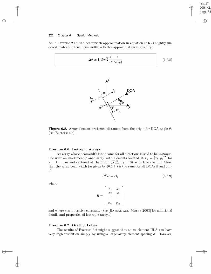
“sm2”2004/2/22page 322

i

i

i

i

i

i

i

i


As in Exercise 2.15, the beamwidth approximation in equation (6.6.7) slightly un-derestimates the true beamwidth; a better approximation is given by:

∆θ ' 1.15√

2λ

2π

1

D(θ0)(6.6.8)

DOA

rk

dk x

y

r1

r2 θ0

Figure 6.8. Array element projected distances from the origin for DOA angle θ0(see Exercise 6.5).

Exercise 6.6: Isotropic Arrays

An array whose beamwidth is the same for all directions is said to be isotropic.Consider an m-element planar array with elements located at rk = [xk, yk]

T fork = 1, . . . ,m and centered at the origin (

∑mk=1 rk = 0) as in Exercise 6.5. Show

that the array beamwidth (as given by (6.6.7)) is the same for all DOAs if and onlyif

RTR = cI2 (6.6.9)

where

R =

x1 y1x2 y2...

...xm ym

and where c is a positive constant. (See [Baysal and Moses 2003] for additionaldetails and properties of isotropic arrays.)

Exercise 6.7: Grating Lobes

The results of Exercise 6.2 might suggest that an m–element ULA can havevery high resolution simply by using a large array element spacing d. However,

“sm2”2004/2/22page 323

i

i

i

i

i

i

i

i


there is an ambiguity associated with choosing d > λ/2; this drawback is sometimesreferred to as the problem of grating lobes. Identify this drawback, and discuss whatambiguities exist as a function of d (refer to the discussion on ULAs in Section 6.2.2).

One potential remedy to this drawback is to use two ULAs: one with m1

elements and element spacing d1 = λ/2, and another with m2 elements and elementspacing d2. Discuss how to choose m1, m2, and d2 to both avoid ambiguities andincrease resolution over a conventional ULA with element spacing d = λ/2 andm1+m2 elements. Consider as an example using a 10–element ULA with d2 = 3λ/2for the second ULA; find m1 to resolve ambiguities in this array. Finally, discussany potential drawbacks of the two–array approach.

Exercise 6.8: Beamspace ProcessingConsider an array comprising many sensors (m 1). Such an array should be

able to resolve sources that are quite closely spaced (cf. (6.3.20) and the discussionin Exercise 6.3). There is, however, a price to be paid for the high–resolutionperformance achieved by using many sensors: the computational burden associatedwith the elementspace processing (ESP) (i.e., the direct processing of the output ofall sensors) may be prohibitively high, and the involved circuitry (A–D converters,etc.) may be quite expensive.

Let B∗ be an m×m matrix with m < m, and consider the transformed outputvector B∗y(t). The latter vector satisfies the following equation (cf. (6.2.21)):

B∗y(t) = B∗As(t) +B∗e(t) (6.6.10)

The transformation matrix B∗ above can be interpreted as a beamformer or spatialfilter acting on y(t). Determination of the DOAs of the signals impinging on thearray using B∗y(t) is called beamspace processing (BSP). Since m < m, BSP shouldhave a lower computational burden than ESP. The critical question is then howto choose the beamformer B so as not to significantly degrade the performanceachievable by ESP.

Assume that a certain DOA sector is known to contain the source(s) of interest(whose DOAs are designated by the generic variable θ0). By using this informa-tion, design a matrix B∗ which passes the signals from direction θ0 approximatelyundistorted. Choose B in such a way that the noise in beamspace, B∗e(t), is stillspatially white. For a given sector size, discuss the tradeoff between the computa-tional burden associated with BSP and the distorting effect of the beamformer onthe desired signals. Finally, use the results of Exercise 6.3 to show that the reso-lution of beamforming in elementspace and beamspace are nearly the same, underthe previous conditions.

Exercise 6.9: Beamspace Processing (cont’d)In this exercise, for simplicity, we consider the Beamspace Processing (BSP)

equation (6.6.10) for the case of a single source (n = 1):

B∗y(t) = B∗a(θ)s(t) +B∗e(t) (6.6.11)

The Elementspace Processing (ESP) counterpart of (6.6.11) is (cf. (6.2.19))

y(t) = a(θ)s(t) + e(t) (6.6.12)

“sm2”2004/2/22page 324

i

i

i

i

i

i

i

i


Assume that ‖a(θ)‖2 = m (see (6.3.11)), and that the m×m matrix B∗ is unitary(i.e., B∗B = I). Furthermore, assume that

a(θ) ∈ R(B) (6.6.13)

To satisfy (6.6.13) we need knowledge about a DOA sector that contains θ, whichis usually assumed to be available in BSP applications; note that the narrower thissector, the smaller the value we can choose for m. As m decreases, the implemen-tation advantages of BSP compared with ESP become more significant. However,the DOA estimation performance achievable by BSP might be expected to decreaseas m decreases. As indicated in Exercise 6.8, this is not necessarily the case. Inthe present exercise we lend further support to the fact that the estimation per-formances of ESP and BSP can be quite similar to one another, provided that thecondition (6.6.13) is satisfied. To be specific, define the array SNR for (6.6.12) as

E‖a(θ)s(t)‖2

E‖e(t)‖2=

mP

mσ2=

P

σ2(6.6.14)

where P denotes the power of s(t). Show that the “array SNR” for the BPSequation, (6.6.11), is m/m times that in (6.6.14). Conclude that this increasein the array SNR associated with BPS may well counterbalance the presumablynegative impact on DOA performance caused by the decrease from m to m in thenumber of observed output signals.

Exercise 6.10: Beamforming and MUSIC under the Same UmbrellaDefine the scalars

Y ∗t (θ) = a∗(θ)y(t), t = 1, . . . , N.

By using previous notation, we can write the beamforming spatial spectrum in(6.3.18) as follows:

Y ∗(θ)WY (θ) (6.6.15)

whereW = (1/N)I (for beamforming)

andY (θ) = [Y1(θ) . . . YN (θ)]T

Show that the MUSIC spatial pseudospectrum

a∗(θ)SS∗a(θ) (6.6.16)

(see Sections 4.5 and 6.4.3) can also be put in the form (6.6.15), for a certain“weighting matrix” W . The columns of the matrix S in (6.6.16) are the n principaleigenvectors of the sample covariance matrix R in (6.3.17).

Exercise 6.11: Subspace Fitting Interpretation of MUSICIn words, the result (4.5.9) (on which MUSIC for both frequency and DOA

estimation is based) says that the direction vectors a(θk) belong to the subspace

“sm2”2004/2/22page 325

i

i

i

i

i

i

i

i


spanned by the columns of S. Therefore, we can think of estimating the DOAsby choosing θ (a generic DOA variable) so that the distance between a(θ) and theclosest vector in the span of S is minimized:

minβ,θ

‖a(θ) − Sβ‖2 (6.6.17)

where ‖·‖ denotes the Euclidean vector norm. Note that the dummy vector variableβ in (6.6.17) is defined in such a way so that Sβ is closest to a(θ) in Euclidean norm.

Show that the DOA estimation method derived from the subspace fittingcriterion (6.6.17) is the same as MUSIC.

Exercise 6.12: Subspace Fitting Interpretation of MUSIC (cont’d.)The result (4.5.9) can also be invoked to arrive at the following subspace

fitting criterion:minB,θ

‖A(θ) − SB‖2F (6.6.18)

where ‖ · ‖F stands for the Frobenius matrix norm, and θ is now the vector of allDOA parameters. This criterion seems to be a more general version of equation(6.6.17) in Exercise 6.11. Show that the minimization of the multidimensionalsubspace fitting criterion in (6.6.18), with respect to the DOA vector θ, still leadsto the one–dimensional MUSIC method. Hint: It will be useful to refer to the typeof result proven in equations (4.3.12)–(4.3.16) in Section 4.3.

Exercise 6.13: Subspace Fitting Interpretation of MUSIC (cont’d.)The subspace fitting interpretations of the previous two exercises provide some

insights into the properties of the MUSIC estimator. Assume, for instance, that twoor more source signals are coherent. Make use of the subspace fitting interpretationin Exercise 6.12 to show that MUSIC cannot be expected to yield meaningful resultsin such a case. Follow the line of your argument explaining why MUSIC fails in thecase of coherent signals, to suggest a subspace fitting criterion that works in sucha case. Discuss the computational complexity of the method based on the lattercriterion.

Exercise 6.14: Modified MUSIC for Coherent SignalsConsider an m–element ULA. Assume that n signals impinge on the array

at angles θknk=1, and also that some signals are coherent (so that the signalcovariance matrix P is singular). Derive a modified MUSIC DOA estimator forthis case, analogous to the modified MUSIC frequency estimator in Section 4.5,and show that this method is capable of determining the n DOAs even in thecoherent signal case.

COMPUTER EXERCISES

Tools for Array Signal Processing:The text web site www.prenhall.com/stoica contains the following Matlab

functions for use in DOA estimation.

“sm2”2004/2/22page 326

i

i

i

i

i

i

i

i


• Y=uladata(theta,P,N,sig2,m,d)

Generates an m × N data matrix Y = [y(1), . . . , y(N)] for a ULA with n

sources arriving at angles (in degrees from −90 to 90) given by the elementsof the n × 1 vector theta. The source signals are zero mean Gaussian withcovariance matrix P = E s(t)s∗(t). The noise component is spatially whiteGaussian with covariance σ2I, where σ2 =sig2. The element spacing is equalto d in wavelengths.

• phi=beamform(Y,L,d)

Implements the beamforming spatial spectral estimate in equation (6.3.18) foran m–element ULA with sensor spacing d in wavelengths. The m×N matrixY is as defined above. The parameter L controls the DOA sampling, and phi

is the spatial spectral estimate phi= [φ(θ1), . . . , φ(θL)] where θk = −π2 + πk

L .

• phi=capon_sp(Y,L,d)

Implements the Capon spatial spectral estimator in equation (6.3.26); theinput and output parameters are defined as those in beamform.

• theta=root_music_doa(Y,n,d)

Implements the Root MUSIC method in Section 4.5, adapted for spatial spec-tral estimation using a ULA. The parameters Y and d are as in beamform, andtheta is the vector containing the n DOA estimates [θ1, . . . , θn]

T .

• theta=esprit_doa(Y,n,d)

Implements the ESPRIT method for a ULA. The parameters Y and d areas in beamform, and theta is the vector containing the n DOA estimates[θ1, . . . , θn]

T . The two subarrays for ESPRIT are made from the first m − 1and last m− 1 elements of the array.

Exercise C6.15: Comparison of Spatial Spectral EstimatorsSimulate the following scenario. Two signals with wavelength λ impinge on

an array of sensors from DOAs θ1 = 0 and a θ2 that will be varied. The sig-nals are mutually uncorrelated complex Gaussian with unit power, so that P =E s(t)s∗(t) = I. The array is a 10–element ULA with element spacing d = λ/2.The measurements are corrupted by additive complex Gaussian white noise withunit power. A total of N = 100 snapshots are collected.

(a) Let θ2 = 15. Compare the results of the beamforming, Capon, Root MUSIC,and ESPRIT methods for this example. The results can be shown by plottingthe spatial spectrum estimates from beamforming and Capon for 50 Monte–Carlo experiments; for Root MUSIC and ESPRIT, plot vertical lines of equalheight located at the DOA estimates from the 50 Monte–Carlo experiments.How do the methods compare? Are the properties of the various estimatorsanalogous to the time series case for two sinusoids in noise?

(b) Repeat for θ2 = 7.5.

“sm2”2004/2/22page 327

i

i

i

i

i

i

i

i


Exercise C6.16: Performance of Spatial Spectral Estimators for CoherentSource Signals

In this exercise we will see what happens when the source signals are fullycorrelated (or coherent). Use the same parameters and estimation methods as inExercise C6.15 with θ2 = 15, but with

P =

(1 11 1

)

Note that the sources are coherent as rank(P ) = 1.Compare the results of the four methods for this case, again by plotting the

spatial spectrum and “DOA line spectrum” estimates (as in Exercise C6.15) for 50Monte–Carlo experiments from each estimator. Which method appears to be thebest in this case?

Exercise C6.17: Spatial Spectral Estimators applied to Measured DataApply the four DOA estimators from Exercise C6.15 to the real data in the file

submarine.mat, which can be found at the text web site www.prenhall.com/stoica.These data are underwater measurements collected by the Swedish Defense Agencyin the Baltic Sea. The 6–element array of hydrophones used in the experiment canbe assumed to be a ULA with inter-element spacing equal to 0.9m. The wavelengthof the signal is approximately 5.32m. Can you find the “submarine(s)”?

“sm2”2004/2/22page 328

i

i

i

i

i

i

i

i

A P P E N D I X A

Linear Algebra and MatrixAnalysis Tools

A.1 INTRODUCTION

In this appendix we provide a review of the linear algebra terms and matrix proper-ties used in the text. For the sake of brevity we do not present proofs for all resultsstated in the following, nor do we discuss related results which are not needed inthe previous chapters. For most of the results included, however, we do provideproofs and motivation. The reader interested in finding out more about the topicof this appendix can consult the books [Stewart 1973; Horn and Johnson

1985; Strang 1988; Horn and Johnson 1989; Golub and Van Loan 1989]to which we also refer for the proofs omitted here.

A.2 RANGE SPACE, NULL SPACE, AND MATRIX RANK

Let A be an m × n matrix with possibly complex–valued elements, A ∈ Cm×n,and let (·)T and (·)∗ denote the transpose and the conjugate transpose operators,respectively.

Definition D1: The range space of A, also called the column space , is thesubspace spanned by (all linear combinations of) the columns of A:

R(A) = α ∈ Cm×1|α = Aβ for β ∈ Cn×1 (A.2.1)

The range space of AT is usually called the row space of A, for obvious reasons.

Definition D2: The null space of A, also called kernel , is the following subspace:

N (A) = β ∈ Cn×1|Aβ = 0 (A.2.2)

The previous definitions are all that we need to introduce the matrix rank andits basic properties. We return to the range and null subspaces in Section A.4where we discuss the singular value decomposition. In particular, we derive theresome convenient bases and useful projectors associated with the previous matrixsubspaces.

Definition D3: The following are equivalent definitions of the rank of A,

r , rank(A).

328

“sm2”2004/2/22page 329

i

i

i

i

i

i

i

i

Section A.2 Range Space, Null Space, and Matrix Rank 329

(i) r is equal to the maximum number of linearly independent columns of A. Thelatter number is by definition the dimension of the R(A); hence

r = dim R(A) (A.2.3)

(ii) r is equal to the maximum number of linearly independent rows of A,

r = dim R(AT ) = dim R(A∗) (A.2.4)

(iii) r is the dimension of the nonzero determinant of maximum size that can bebuilt from the elements of A.

The equivalence between the definitions (i) and (ii) above is an importantand pleasing result (without which one should have considered the row rank andcolumn rank of a matrix separately!).

Definition D4: A is said to be:

• Rank deficient whenever r < min(m,n).

• Full column rank if r = n ≤ m.

• Full row rank if r = m ≤ n

• Nonsingular whenever r = m = n.

Result R1: Premultiplication or postmultiplication of A by a nonsingular matrixdoes not change the rank of A.

Proof: This fact directly follows from the definition of rank(A) because the afore-mentioned multiplications do not change the number of linearly independent columns(or rows) of A.

Result R2: Let A ∈ Cm×n and B ∈ Cn×p be two conformable matrices of rank rAand rB , respectively. Then:

rank(AB) ≤ min(rA, rB) (A.2.5)

Proof: We can prove the previous assertion by using the definition of the rank onceagain. Indeed, premultiplication of B by A cannot increase the number of linearlyindependent columns of B, hence rank(AB) ≤ rB . Similarly, post–multiplication ofA by B cannot increase the number of linearly independent columns of AT , whichmeans that rank(AB) ≤ rA.

“sm2”2004/2/22page 330

i

i

i

i

i

i

i

i

330 Appendix A Linear Algebra and Matrix Analysis Tools

Result R3: Let A ∈ Cm×m be given by

A =

N∑

k=1

xk y∗k

where xk, yk ∈ Cm×1. Then,

rank(A) ≤ min(m,N)

Proof: Since A can be rewritten as

A = [x1 . . . xN ]

y∗1...y∗N

the result follows from R2.

Result R4: Let A ∈ Cm×n with n ≤ m, let B ∈ Cn×p, and let

rank(A) = n (A.2.6)

Thenrank(AB) = rank(B) (A.2.7)

Proof: Assumption (A.2.6) implies that A contains a nonsingular n×n submatrix,the post–multiplication of which by B gives a block of rank equal to rank(B)(cf. R1). Hence,

rank(AB) ≥ rank(B)

However, by R2, rank(AB) ≤ rank(B) and hence (A.2.7) follows.

A.3 EIGENVALUE DECOMPOSITION

Definition D5: We say that the matrix A ∈ Cm×m is Hermitian if A∗ = A. Inthe real–valued case, such an A is said to be symmetric.

Definition D6: A matrix U ∈ Cm×m is said to be unitary (orthogonal if U isreal–valued) whenever

U∗U = UU∗ = I

If U ∈ Cm×n, with m > n, is such that U∗U = I then we say that U is semiuni-

tary .

Next, we present a number of definitions and results pertaining to the matrixeigenvalue decomposition (EVD), first for general matrices and then for Hermitianones.

“sm2”2004/2/22page 331

i

i

i

i

i

i

i

i

Section A.3 Eigenvalue Decomposition 331

A.3.1 General Matrices

Definition D7: A scalar λ ∈ C and a (nonzero) vector x ∈ Cm×1 are an eigenvalue

and its associated eigenvector of a matrix A ∈ Cm×m if

Ax = λx (A.3.1)

In particular, an eigenvalue λ is a solution of the so–called characteristic equa-

tion of A:|A− λI| = 0 (A.3.2)

and x is a vector in N (A− λI). The pair (λ, x) is called an eigenpair.

Observe that if (λi, xi)pi=1 are p eigenpairs of A (with p ≤ m) then we canwrite the defining equations Axi = λxi (i = 1, . . . , p) in the following compact form:

AX = XΛ (A.3.3)

whereX = [x1 . . . xp]

and

Λ =

λ1 0...

0 λp

Result R5: Let (λ, x) be an eigenpair of A ∈ Cm×m. If B = A+ αI, with α ∈ C,then (λ+ α, x) is an eigenpair of B.

Proof: The result follows from the fact that

Ax = λx =⇒ (A+ αI)x = (λ+ α)x.

Result R6: The matrices A and B , Q−1AQ, where Q is any nonsingular ma-trix, share the same eigenvalues. (B is said to be related to A by a similarity

transformation).

Proof: Indeed, the equation

|B − λI| = |Q−1(A− λI)Q| = |Q−1||A− λI||Q| = 0

is equivalent to |A− λI| = 0.

In general there is no simple relationship between the elements Aij of A andits eigenvalues λk. However, the trace of A, which is the sum of the diagonalelements of A, is related in a simple way to the eigenvalues, as described next.

Definition D8: The trace of a square matrix A ∈ Cm×m is defined as

tr(A) =

m∑

i=1

Aii (A.3.4)

“sm2”2004/2/22page 332

i

i

i

i

i

i

i

i


Result R7: If λimi=1 are the eigenvalues of A ∈ Cm×m, then

tr(A) =

m∑

i=1

λi (A.3.5)

Proof: We can write

|λI −A| =

n∏

i=1

(λ− λi) (A.3.6)

The right hand side of (A.3.6) is a polynomial in λ whose λn−1 coefficient is∑ni=1 λi.

From the definition of the determinant (see, e.g., [Strang 1988]) we find that theleft hand side of (A.3.6) is a polynomial whose λn−1 coefficient is

∑ni=1Aii = tr(A).

This proves the result.

Interestingly, while the matrix product is not commutative, the trace is in-variant to commuting the factors in a matrix product, as shown next.

Result R8: Let A ∈ Cm×n and B ∈ Cn×m. Then:

tr(AB) = tr(BA) (A.3.7)

Proof: A straightforward calculation, based on the definition of tr(·) in (A.3.4),shows that

tr(AB) =

m∑

i=1

n∑

j=1

AijBji

=

n∑

j=1

m∑

i=1

BjiAij =

n∑

j=1

[BA]jj = tr(BA)

We can also prove (A.3.7) by using Result R7. Along the way we will obtainsome other useful results. First we note the following.

Result R9: Let A,B ∈ Cm×m and let α ∈ C. Then

|AB| = |A| |B||αA| = αm|A|

Proof: The identities follow directly from the definition of the determinant; see,e.g., [Strang 1988].

Next we prove the following results.

“sm2”2004/2/22page 333

i

i

i

i

i

i

i

i


Result R10: Let A ∈ Cm×n and B ∈ Cn×m. Then:

|I −AB| = |I −BA|. (A.3.8)

Proof: It is straightforward to verify that:[I A0 I

] [I −A

−B I

] [I 0B I

]

=

[I −AB 0

0 I

]

(A.3.9)

and [I 0B I

] [I −A

−B I

] [I A0 I

]

=

[I 00 I −BA

]

(A.3.10)

Because the matrices in the left–hand sides of (A.3.9) and (A.3.10) have the same

determinant, equal to

∣∣∣∣

I −A−B I

∣∣∣∣, it follows that the right–hand sides must also

have the same determinant, which concludes the proof.

Result R11: Let A ∈ Cm×n and B ∈ Cn×m. The nonzero eigenvalues of AB andof BA are identical.

Proof: Let λ 6= 0 be an eigenvalue of AB. Then,

0 = |AB − λI| = λm|AB/λ− I| = λm|BA/λ− I| = λm−n|BA− λI|where the third equality follows from R10. Hence, λ is also an eigenvalue of BA.

We can now obtain R8 as a simple corollary of R11, by using the property(A.3.5) of the trace operator.

A.3.2 Hermitian Matrices

An important property of the class of Hermitian matrices, which does not neces-sarily hold for general matrices, is the following.

Result R12:

(i) All eigenvalues of A = A∗ ∈ Cm×m are real–valued.

(ii) The m eigenvectors of A = A∗ ∈ Cm×m form an orthonormal set. In otherwords, the matrix whose columns are the eigenvectors of A is unitary .

It follows from (i) and (ii) and from (A.3.3) that for a Hermitian matrix wecan write:

AU = UΛ

where U∗U = UU∗ = I and the diagonal elements of Λ are real numbers. Equiva-lently,

A = UΛU∗ (A.3.11)

which is the so–called eigenvalue decomposition (EVD) of A = A∗. The EVD of aHermitian matrix is a special case of the singular value decomposition of a generalmatrix discussed in the next section.

The following is a useful result associated with Hermitian matrices.

“sm2”2004/2/22page 334

i

i

i

i

i

i

i

i


Result R13: Let A = A∗ ∈ Cm×m and let v ∈ Cm×1 (v 6= 0). Also, let theeigenvalues of A be arranged in a nonincreasing order:

λ1 ≥ λ2 ≥ · · · ≥ λm.

Then:

λm ≤ v∗Av

v∗v≤ λ1 (A.3.12)

The ratio in (A.3.12) is called the Rayleigh quotient . As this ratio is invariantto the multiplication of v by any complex number, we can rewrite (A.3.12) in theform:

λm ≤ v∗Av ≤ λ1 for any v ∈ Cm×1 with v∗v = 1 (A.3.13)

The equalities in (A.3.13) are evidently achieved when v is equal to the eigen-vector of A associated with λm and λ1, respectively.

Proof: Let the EVD of A be given by (A.3.11), and let

w = U∗v =

w1

...wm

We need to prove that

λm ≤ w∗Λw =

m∑

k=1

λk|wk|2 ≤ λ1

for any w ∈ Cm×1 satisfying

w∗w =

m∑

k=1

|wk|2 = 1.

However, this is readily verified as follows:

λ1 −m∑

k=1

λk|wk|2 =

m∑

k=1

(λ1 − λk)|wk|2 ≥ 0

andm∑

k=1

λk|wk|2 − λm =

m∑

k=1

(λk − λm)|wk|2 ≥ 0

and the proof is concluded.

The following result is an extension of R13.

Result R14: Let V ∈ Cm×n, with m > n, be a semiunitary matrix (i.e., V ∗V = I),and let A = A∗ ∈ Cm×m have its eigenvalues ordered as in R13. Then:

m∑

k=m−n+1

λk ≤ tr(V ∗AV ) ≤n∑

k=1

λk (A.3.14)

“sm2”2004/2/22page 335

i

i

i

i

i

i

i

i


where the equalities are achieved, for instance, when the columns of V are the eigen-vectors of A corresponding to (λm−n+1, . . . , λm) and, respectively, to (λ1, . . . , λn).The ratio

tr(V ∗AV )

tr(V ∗V )=

tr(V ∗AV )

n

is sometimes called the extended Rayleigh quotient .

Proof: LetA = UΛU∗

(cf. (A.3.11)), and let

S = U∗V ,

s∗1...s∗m

(m× n)

(hence s∗k is the kth row of S). By making use of the above notation, we can write:

tr(V ∗AV ) = tr(V ∗UΛU∗V ) = tr(S∗ΛS) = tr(ΛSS∗) =

m∑

k=1

λkck (A.3.15)

whereck , s∗

ksk, k = 1, . . .m (A.3.16)

Clearly,ck ≥ 0, k = 1, . . . ,m (A.3.17)

andm∑

k=1

ck = tr(SS∗) = tr(S∗S) = tr(V ∗UU∗V ) = tr(V ∗V ) = tr(I) = n (A.3.18)

Furthermore,ck ≤ 1, k = 1, . . . ,m. (A.3.19)

To see this, let G ∈ Cm×(m−n) be such that the matrix [S G] is unitary; and let g∗k

denote the kth row of G. Then, by construction,

[s∗k g

∗k]

[skgk

]

= ck + g∗kgk = 1 =⇒ ck = 1 − g∗

kgk ≤ 1

which is (A.3.19).Finally, by combining (A.3.15) with (A.3.17)–(A.3.19) we can readily verify

that tr(V ∗AV ) satisfies (A.3.14), where the equalities are achieved for

c1 = · · · = cm−n = 0; cm−n+1 = · · · = cm = 1

and, respectively,

c1 = · · · = cn = 1; cn+1 = · · · = cm = 0

These conditions on ck are satisfied if, for example, S is equal to [0 I]T and [I 0]T ,respectively. With this observation, the proof is concluded.

Result R13 is clearly a special case of Result R14. The only reason for consid-ering R13 separately is that the simpler result R13 is more often used in the textthan R14.

“sm2”2004/2/22page 336

i

i

i

i

i

i

i

i


A.4 SINGULAR VALUE DECOMPOSITION AND PROJECTION OPERATORS

For any matrix A ∈ Cm×n there exist unitary matrices U ∈ Cm×m and V ∈ Cn×n

and a diagonal matrix Σ ∈ Rm×n with nonnegative diagonal elements, such that

A = UΣV ∗ (A.4.1)

By appropriate permutation, the diagonal elements of Σ can be arranged in anonincreasing order:

σ1 ≥ σ2 ≥ · · · ≥ σmin(m,n)

The factorization (A.4.1) is called the singular value decomposition (SVD) of A andits existence is a significant result from both a theoretical and practical standpoint.We reiterate that the matrices U , Σ, and V in (A.4.1) satisfy:

U∗U = UU∗ = I (m×m)V ∗V = V V ∗ = I (n× n)

Σij =

σi ≥ 0

0for i = jfor i 6= j

The following terminology is most commonly associated with the SVD:

• The left singular vectors of A are the columns of U . These singular vectorsare also the eigenvectors of the matrix AA∗.

• The right singular vectors of A are the columns of V . These vectors are alsothe eigenvectors of the matrix A∗A.

• The singular values of A are the diagonal elements σi of Σ. Note that σiare the square roots of the largest min(m,n) eigenvalues of AA∗ or A∗A.

• The singular triple of A is the triple (singular value, left singular vector, andright singular vector) (σk, uk, vk), where uk (vk) is the kth column of U (V ).

Ifrank(A) = r ≤ min(m,n)

then one can show that:

σk > 0, k = 1, . . . , r

σk = 0, k = r + 1, . . . ,min(m,n)

Hence, for a matrix of rank r the SVD can be written as:

A = [ U1︸︷︷︸

r

U2︸︷︷︸

m−r

]

[Σ1 00 0

] [V ∗

1

V ∗2

] r

n−r

= U1Σ1V∗1 (A.4.2)

where Σ1 ∈ Rr×r is nonsingular. The factorization of A in (A.4.2) has a numberof important consequences.

Result R15: Consider the SVD of A ∈ Cm×n in (A.4.2), where r ≤ min(m,n).Then:

“sm2”2004/2/22page 337

i

i

i

i

i

i

i

i

Section A.4 Singular Value Decomposition and Projection Operators 337

(i) U1 is an orthonormal basis of R(A)

(ii) U2 is an orthonormal basis of N (A∗)

(iii) V1 is an orthonormal basis of R(A∗)

(iv) V2 is an orthonormal basis of N (A).

Proof: We see that (iii) and (iv) follow from the properties (i) and (ii) applied toA∗. To prove (i) and (ii), we need to show that:

R(A) = R(U1) (A.4.3)

and, respectively,N (A∗) = R(U2) (A.4.4)

To show (A.4.3), note that

α ∈ R(A) ⇒ there exists β such that α = Aβ ⇒⇒ α = U1(Σ1V

∗1 β) = U1γ ⇒ α ∈ R(U1)

so R(A) ⊂ R(U1). Also,

α ∈ R(U1) ⇒ there exists β such that α = U1β

From (A.4.2), U1 = AV1Σ−11 ; it follows that

α = A(V1Σ−11 β) = Aρ ⇒ α ∈ R(A)

which shows R(U1) ⊂ R(A). Combining R(U1) ⊂ R(A) with R(A) ⊂ R(U1) gives(A.4.3). Similarly,

α ∈ N (A∗) ⇒ A∗α = 0 ⇒ V1Σ1U∗1α = 0 ⇒ Σ−1

1 V ∗1 V1Σ1U

∗1α = 0 ⇒ U∗

1α = 0

Now, any vector α can be written as

α = [U1 U2]

[γβ

]

since [U1 U2] is nonsingular. However, 0 = U∗1α = U∗

1U1γ + U∗1U2β = γ, so γ = 0,

and thus α = U2β. Thus, N (A∗) ⊂ R(U2). Finally,

α ∈ R(U2) ⇒ there exists β such that α = U2β

ThenA∗α = V1Σ1U

∗1U2β = 0 ⇒ α ∈ N (A∗)

which leads to (A.4.4).

The previous result, readily derived by using the SVD, has a number of in-teresting corollaries which complement the discussion on range and null subspacesin Section A.2.

“sm2”2004/2/22page 338

i

i

i

i

i

i

i

i


Result R16: For any A ∈ Cm×n the subspaces R(A) and N (A∗) are orthogonal toeach other and they together span Cm. Consequently, we say that N (A∗) is theorthogonal complement of R(A) in Cm, and vice versa. In particular, we have:

dim N (A∗) = m− r (A.4.5)

dim N (A) = n− r (A.4.6)

(Recall that dim R(A) = dim R(A∗) = r.)

Proof: This result is a direct corollary of R15.

The SVD of a matrix also provides a convenient representation for the pro-jectors onto the range and null spaces of A and A∗.

Definition D9: Let y ∈ Cm×1 be an arbitrary vector. By definition the orthogonal

projector onto R(A) is the matrix Π, which is such that (i) R(Π) = R(A) and(ii) the Euclidean distance between y and Πy ∈ R(A) is minimum:

‖y − Πy‖2 = min over R(A)

Hereafter, ‖x‖2 = x∗x denotes the Euclidean vector norm .

Result R17: Let A ∈ Cm×n. The orthogonal projector onto R(A) is given by

Π = U1U∗1 (A.4.7)

whereas the orthogonal projector onto N (A∗) is

Π⊥ = I − U1U∗1 = U2U

∗2 (A.4.8)

Proof: Let y ∈ Cm×1 be an arbitrary vector. As R(A) = R(U1), according toR15, we can find the vector in R(A) that is of minimal distance from y by solvingthe problem:

minβ

‖y − U1β‖2 (A.4.9)

Because

‖y − U1β‖2 = (β∗ − y∗U1)(β − U∗1 y) + y∗(I − U1U

∗1 )y

= ‖β − U∗1 y‖2 + ‖U∗

2 y‖2

it readily follows that the solution to the minimization problem (A.4.9) is given byβ = U∗

1 y. Hence the vector U1U∗1 y is the orthogonal projection of y onto R(A) and

the minimum distance from y to R(A) is ‖U∗2 y‖. This proves (A.4.7). Then (A.4.8)

follows immediately from (A.4.7) and the fact that N (A∗) = R(U2).

Note, for instance, that for the projection of y onto R(A) the error vector isy − U1U

∗1 y = U2U

∗2 y, which is in R(U2) and is therefore orthogonal to R(A) by

R15. For this reason, Π is given the name “orthogonal projector” in D9 and R17.As an aside, we remark that the orthogonal projectors in (A.4.7) and (A.4.8)

are idempotent matrices; see the next definition.

“sm2”2004/2/22page 339

i

i

i

i

i

i

i

i

Section A.4 Singular Value Decomposition and Projection Operators 339

Definition D10: The matrix A ∈ Cm×m is idempotent if

A2 = A (A.4.10)

Furthermore, observe by making use of R11 that the idempotent matrix in(A.4.7), for example, has r eigenvalues equal to 1 and (m − r) eigenvalues equalto zero. This is a general property of idempotent matrices: their eigenvalues areeither zero or one.

Finally we present a result that even alone would be enough to make the SVDan essential matrix analysis tool.

Result R18: Let A ∈ Cm×n, with elements Aij . Let the SVD of A (with thesingular values arranged in a nonincreasing order) be given by:

A = [ U1︸︷︷︸

p

U2︸︷︷︸

m−p

]

[Σ1 00 Σ2

] [V ∗

1

V ∗2

] p

n−p

(A.4.11)

where p ≤ min(m,n) is an integer. Let

‖A‖2 = tr(A∗A) =

m∑

i=1

n∑

j=1

|Aij |2 =

min(m,n)∑

k=1

σ2k (A.4.12)

denote the square of the so–called Frobenius norm . Then the best rank–papproximant of A in the Frobenius norm metric, that is, the solution to

minB

‖A−B‖2 subject to rank(B) = p , (A.4.13)

is given byB0 = U1Σ1V

∗1 (A.4.14)

Furthermore, B0 above is the unique solution to the approximation problem (A.4.13)if and only if σp > σp+1.

Proof: It follows from R4 and (A.4.2) that we can parameterize B in (A.4.13) as:

B = CD∗ (A.4.15)

where C ∈ Cm×p and D ∈ Cn×p are full column rank matrices. The previousparameterization of B is of course nonunique but, as we will see, this fact doesnot introduce any problem. By making use of (A.4.15) we can rewrite the problem(A.4.13) in the following form:

minC,D

‖A− CD∗‖2 rank(C) = rank(D) = p (A.4.16)

The reparameterized problem is essentially constraint free. Indeed, the full columnrank condition that must be satisfied by C and D can be easily handled, see below.

“sm2”2004/2/22page 340

i

i

i

i

i

i

i

i


First, we minimize (A.4.16) with respect to D, for a given C. To that end,observe that:

‖A− CD∗‖2 = tr[D −A∗C(C∗C)−1](C∗C)[D∗ − (C∗C)−1C∗A]

+A∗[I − C(C∗C)−1C∗]A (A.4.17)

By result (iii) in Definition D11 in the next section, the matrix [D−A∗C(C∗C)−1]·(C∗C)[D∗ − (C∗C)−1C∗A] is positive semidefinite for any D. This observationimplies that (A.4.17) is minimized with respect to D for

D0 = A∗C(C∗C)−1 (A.4.18)

and the corresponding minimum value of (A.4.17) is given by

trA∗[I − C(C∗C)−1C∗]A (A.4.19)

Next we minimize (A.4.19) with respect to C. Let S ∈ Cm×p denote an orthogonalbasis of R(C); that is, S∗S = I and

S = CΓ

for some nonsingular p× p matrix Γ. It is then straightforward to verify that

I − C(C∗C)−1C∗ = I − SS∗ (A.4.20)

By combining (A.4.19) and (A.4.20) we can restate the problem of minimizing(A.4.19) with respect to C as:

maxS; S∗S=I

tr[S∗(AA∗)S] (A.4.21)

The solution to (A.4.21) follows from R14: the maximizing S is given by

S0 = U1

which yieldsC0 = U1Γ

−1 (A.4.22)

It follows that:

B0 = C0D∗0 = C0(C

∗0C0)

−1C∗0A = S0S

∗0A

= U1U∗1 (U1Σ1V

∗1 + U2Σ2V

∗2 )

= U1Σ1V∗1 .

Furthermore, we observe that the minimum value of the Frobenius distance in(A.4.13) is given by

‖A−B0‖2 = ‖U2Σ2V∗2 ‖2 =

min(m,n)∑

k=p+1

σ2k

If σp > σp+1 then the best rank–p approximant B0 derived above is unique. Other-wise it is not unique. Indeed, whenever σp = σp+1 we can obtain B0 by using eitherthe singular vectors associated with σp or those corresponding to σp+1, which willgenerally lead to different solutions.

“sm2”2004/2/22page 341

i

i

i

i

i

i

i

i

Section A.5 Positive (Semi)Definite Matrices 341

A.5 POSITIVE (SEMI)DEFINITE MATRICES

Let A = A∗ ∈ Cm×m be a Hermitian matrix, and let λkmk=1 denote its eigenvalues.

Definition D11: We say that A is positive semidefinite (psd) or positive defi-

nite (pd) if any of the following equivalent conditions holds true.

(i) λk ≥ 0 (λk > 0 for pd) for k = 1, . . . ,m.

(ii) α∗Aα ≥ 0 (α∗Aα > 0 for pd) for any nonzero vector α ∈ Cm×1

(iii) There exists a matrix C such that

A = CC∗ (A.5.1)

(with rank(C) = m for pd)

(iv) |A(i1, . . . , ik)| ≥ 0 (> 0 for pd) for all k = 1, . . . ,m and all indices i1, . . . , ik ∈[1,m], where A(i1, . . . , ik) is the submatrix formed from A by eliminatingthe i1, . . . , ik rows and columns of A. (A(i1, . . . , ik) is called a principal

submatrix of A). The condition for A to be positive definite can be simplifiedto requiring that |A(k + 1, . . . ,m)| > 0 (for k = 1, . . . ,m − 1) and |A| > 0.(A(k + 1, . . . ,m) is called a leading submatrix of A).

The notation A > 0 (A ≥ 0) is commonly used to denote that A is pd (psd).

Of the previous defining conditions, (iv) is apparently more involved. Thenecessity of (iv) can be proven as follows. Let α be a vector in Cm with zeroes atthe positions i1, . . . , ik and arbitrary elements elsewhere. Then, by using (ii) wereadily see that A ≥ 0 (> 0) implies A(i1, . . . , ik) ≥ 0 (> 0) which, in turn, implies(iv) by making use of (i) and the fact that the determinant of a matrix equals theproduct of its eigenvalues. The sufficiency of (iv) is shown in [Strang 1988].

The equivalence of the remaining conditions, (i), (ii), and (iii), is easily provenby making use of the EVD of A: A = UΛU∗. To show that (i) ⇔ (ii), assume firstthat (i) holds and let β = U∗α. Then:

α∗Aα = β∗Λβ =

m∑

k=1

λk|βk|2 ≥ 0 (A.5.2)

and hence, (ii) holds as well. Conversely, since U is invertible it follows from (A.5.2)that (ii) can hold only if (i) holds; indeed, if (i) does not hold one can choose β tomake (A.5.2) negative; thus there exists an α = Uβ such that α∗Aα < 0, whichcontradicts the assumption that (ii) holds. Hence (i) and (ii) are equivalent. Toshow that (iii) ⇒ (ii), note that

α∗Aα = α∗CC∗α = ‖C∗α‖2 ≥ 0

and hence (ii) holds as well. Since (iii) ⇒ (ii) and (ii) ⇒ (i), we have (iii) ⇒ (i).To show that (i) ⇒ (iii), we assume (i) and write

A = UΛU∗ = (UΛ1/2Λ1/2U∗) = (UΛ1/2U∗)(UΛ1/2U∗) , CC∗ (A.5.3)

“sm2”2004/2/22page 342

i

i

i

i

i

i

i

i


and hence (iii) is also satisfied. In (A.5.3), Λ1/2 is a diagonal matrix the diagonal

elements of which are equal to λ1/2k . In other words, Λ1/2 is the “square root” of

Λ.In a general context, the square root of a positive semidefinite matrix is defined

as follows.

Definition D12: Let A = A∗ be a positive semidefinite matrix. Then any matrixC that satisfies

A = CC∗ (A.5.4)

is called a square root of A. Sometimes such a C is denoted by A1/2.

If C is a square root of A, then so is CB for any unitary matrix B, and hencethere are an infinite number of square roots of a given positive semidefinite matrix.Two often–used particular choices for square roots are:

(i) Hermitian square root : C = C∗. In this case we can simply write (A.5.4)as A = C2. Note that we have already obtained such a square root of A in(A.5.3):

C = UΛ1/2U∗ (A.5.5)

If C is also constrained to be positive semidefinite (C ≥ 0) then the Hermitiansquare root is unique.

(ii) Cholesky factor . If C is lower triangular with nonnegative diagonal elements,then C is called the Cholesky factor of A. In computational exercises, thetriangular form of the square–root matrix is often preferred to other forms.If A is positive definite, the Cholesky factor is unique.

We also note that equation (A.5.4) implies that A and C have the same rankas well as the same range space. This follows easily, for example, by inserting theSVD of C into (A.5.4).

Next we prove three specialized results on positive semidefinite matrices re-quired in Section 2.5 and in Appendix B.

Result R19: Let A ∈ Cm×m and B ∈ Cm×m be positive semidefinite matri-ces. Then the matrix A B is also positive semidefinite, where denotes theHadamard matrix product (also called elementwise multiplication: [A B]ij = AijBij ).

Proof: Because B is positive semidefinite it can be written as B = CC∗ for somematrix C ∈ Cm×m. Let c∗k denote the kth row of C. Then,

[AB]ij = AijBij = Aij c∗i cj

and hence, for any α ∈ Cm×1,

α∗(AB)α =

m∑

i=1

m∑

j=1

α∗iAijc

∗i cjαj (A.5.6)

“sm2”2004/2/22page 343

i

i

i

i

i

i

i

i

Section A.5 Positive (Semi)Definite Matrices 343

By letting cjkmk=1 denote the elements of the vector cj , we can rewrite (A.5.6) as:

α∗(AB)α =

m∑

k=1

m∑

i=1

m∑

j=1

α∗i c

∗ikAijαjcjk =

m∑

k=1

β∗kAβk (A.5.7)

whereβk , [α1c1k · · ·αmcmk]T

As A is positive semidefinite by assumption, β∗kAβk ≥ 0 for each k, and it follows

from (A.5.7) that AB must be positive semidefinite as well.

Result R20: Let A ∈ Cm×m and B ∈ Cm×m be Hermitian matrices. Assume thatB is nonsingular and that the partitioned matrix

[A II B

]

is positive semidefinite. Then the matrix (A−B−1) is also positive semidefinite,

A ≥ B−1

Proof: By Definition D11, part (ii),

[α∗

1 α∗2

][A II B

] [α1

α2

]

≥ 0 (A.5.8)

for any vectors α1, α2 ∈ Cm×1. Let

α2 = −B−1α1

Then (A.5.8) becomes:α∗

1(A−B−1)α1 ≥ 0

As the above inequality must hold for any α1 ∈ Cm×1, the proof is concluded.

Result R21: Let C ∈ Cm×m be a (Hermitian) positive definite matrix dependingon a real–valued parameter α. Assume that C is a differentiable function of α.Then

∂

∂α[ln |C|] = tr

[

C−1 ∂C

∂α

]

Proof: Let λi ∈ R (i = 1, . . . ,m) denote the eigenvalues of C. Then

∂

∂α[ln |C|] =

∂

∂α

[

ln

m∏

k=1

λk

]

=

m∑

k=1

∂

∂α(lnλk)

=

m∑

k=1

1

λk

∂λk∂α

= tr

[

Λ−1 ∂Λ

∂α

]

“sm2”2004/2/22page 344

i

i

i

i

i

i

i

i


where Λ = diag(λ1, . . . , λm). Let Q be a unitary matrix such that Q∗ΛQ = C(which is the EVD of C). Since Q is unitary, Q∗Q = I, we obtain

∂Q∗

∂αQ+Q∗ ∂Q

∂α= 0

Thus, we get

tr

[

Λ−1 ∂Λ

∂α

]

= tr

[(Q∗Λ−1Q

)(

Q∗ ∂Λ

∂αQ

)]

= tr

[

C−1

(∂

∂α(Q∗ΛQ) − ∂Q∗

∂αΛQ−Q∗Λ

∂Q

∂α

)]

= tr

[

C−1 ∂C

∂α

]

− tr

[

Q∗Λ−1Q

(∂Q∗

∂αΛQ+Q∗Λ

∂Q

∂α

)]

= tr

[

C−1 ∂C

∂α

]

− tr

[∂Q∗

∂αQ+Q∗ ∂Q

∂α

]

= tr

[

C−1 ∂C

∂α

]

which is the result stated.

Finally we make use of a simple property of positive semidefinite matrices toprove the Cauchy–Schwartz inequality for vectors and for functions.

Result R22: (Cauchy–Schwartz inequality for vectors). Let x, y ∈ Cm×1. Then:

|x∗y|2 ≤ ‖x‖2 ‖y‖2 (A.5.9)

where | · | denotes the modulus of a possibly complex–valued number, and ‖ · ‖denotes the Euclidean vector norm ( ‖x‖2 = x∗x). Equality in (A.5.9) is achievedif and only if x is proportional to y.

Proof: The (2 × 2) matrix

[‖x‖2 x∗yy∗x ‖y‖2

]

=

[x∗

y∗

][x y

](A.5.10)

is clearly positive semidefinite (observe that condition (iii) in D11 is satisfied). Itfollows from condition (iv) in D11 that the determinant of the above matrix mustbe nonnegative:

‖x‖2 ‖y‖2 − |x∗y|2 ≥ 0

which gives (A.5.9). Equality in (A.5.9) holds if and only if the determinant of(A.5.10) is equal to zero. The latter condition is equivalent to requiring that x isproportional to y (cf. D3: the columns of the matrix [x y] will then be linearlydependent).

“sm2”2004/2/22page 345

i

i

i

i

i

i

i

i

Section A.6 Matrices with Special Structure 345

Result R23: (Cauchy–Schwartz inequality for functions). Let f(x) and g(x) betwo complex–valued functions defined for real–valued argument x. Then, assumingthat the integrals below exist,

∣∣∣∣

∫

I

f(x)g∗(x)dx

∣∣∣∣

2

≤[∫

I

|f(x)|2dx] [∫

I

|g(x)|2dx]

where I ⊂ R is an integration interval. The inequality above becomes an equalityif and only if f(x) is proportional to g(x) on I.

Proof: The following matrix∫

I

[f(x)g(x)

]

[f∗(x) g∗(x)] dx

is seen to be positive semidefinite (since the integrand is a positive semidefinitematrix for every x ∈ I). Hence the stated result follows from the type of argumentused in the proof of Result R22.

A.6 MATRICES WITH SPECIAL STRUCTURE

In this section we consider several types of matrices with a special structure, forwhich we prove some basic properties used in the text.

Definition D13: A matrix A ∈ Cm×n is called Vandermonde if it has the follow-ing structure:

A =

1 · · · 1z1 zn...

...zm−11 · · · zm−1

n

(A.6.1)

where zk ∈ C are usually assumed to be distinct.

Result R24: Consider the matrix A in (A.6.1) with zk 6= zp for k, p = 1, . . . , n andk 6= p . Also let m ≥ n and assume that zk 6= 0 for all k. Then any n consecutiverows of A are linearly independent.

Proof: To prove the assertion, it is sufficient to show that the following n × nVandermonde matrix is nonsingular:

A =

1 · · · 1z1 zn...

...zn−11 · · · zn−1

n

Let β = [β0 · · ·βn−1]∗ 6= 0. The equation β∗A = 0 is equivalent to

β0 + β1z + · · · + βn−1zn−1 = 0 at z = zk (k = 1, . . . , n) (A.6.2)

However, (A.6.2) is impossible as a (n−1)-degree polynomial cannot have n zeroes.Hence, A has full rank.

“sm2”2004/2/22page 346

i

i

i

i

i

i

i

i


Definition D14: A matrix A ∈ Cm×n is called:

• Toeplitz when Aij = Ai−j

• Hankel when Aij = Ai+j

Observe that a Toeplitz matrix has the same element along each diagonal,whereas a Hankel matrix has identical elements on each of the antidiagonals.

Result R25: The eigenvectors of a symmetric Toeplitz matrix A ∈ Rm×m areeither symmetric or skew–symmetric. More precisely, if J denotes the exchange (orreversal) matrix

J =

0 1. .

.

1 0

and if x is an eigenvector of A, then either x = Jx or x = −Jx.

Proof: By the property (3.5.3) proven in Section 3.5, A satisfies

AJx = JAx

or equivalently(JAJ)x = Ax

for any x ∈ Cm×1. Hence, we must have:

JAJ = A (A.6.3)

Let (λ, x) denote an eigenpair of A:

Ax = λx (A.6.4)

Combining (A.6.3) and (A.6.4) yields:

λJx = JAx = J(JAJ)x = A(Jx) (A.6.5)

Because the eigenvectors of a symmetric matrix are unique modulo multiplicationby a scalar, it follows from (A.6.5) that:

x = αJx for some α ∈ R

As x and hence Jx must have unit norm, α must satisfy α2 = 1 ⇒ α = ±1; thus,either x = Jx (x is symmetric) or x = −Jx (x is skew–symmetric).

One can show that for m even, the number of symmetric eigenvectors is m/2,as is the number of skew–symmetric eigenvectors; for odd m the number of sym-metric eigenvectors is (m + 1)/2 and the number of skew–symmetric eigenvectorsis (m− 1)/2 (see [Cantoni and Butler 1976]).

For many additional results on Toeplitz matrices, the reader can consult[Iohvidov 1982; Bottcher and Silbermann 1983].

“sm2”2004/2/22page 347

i

i

i

i

i

i

i

i

Section A.7 Matrix Inversion Lemmas 347

A.7 MATRIX INVERSION LEMMAS

The following formulas for the inverse of a partitioned matrix are used in the text.

Result R26: Let A ∈ Cm×m, B ∈ Cn×n, C ∈ Cm×n and D ∈ Cn×m. Then,provided that the matrix inverses appearing below exist,

[A CD B

]−1

=

[I0

]

A−1[I 0

]+

[−A−1C

I

]

(B −DA−1C)−1[−DA−1 I]

=

[0I

]

B−1[

0 I]+

[I

−B−1D

]

(A− CB−1D)−1[I − CB−1]

Proof: By direct verification.

By equating the top–left blocks in the above two equations we obtain theso–called Matrix Inversion Lemma.

Result R27: (Matrix Inversion Lemma) Let A, B, C and D be as in R26. Then,assuming that the matrix inverses appearing below exist,

(A− CB−1D)−1 = A−1 +A−1C(B −DA−1C)−1DA−1

A.8 SYSTEMS OF LINEAR EQUATIONS

Let A ∈ Cm×n, B ∈ Cm×p, and X ∈ Cn×p. A general system of linear equationsin X can be written as:

AX = B (A.8.1)

where A and B are given and X is the unknown matrix. The special case of (A.8.1)corresponding to p = 1 (for which X and B are vectors) is perhaps the mostcommon one in applications. For the sake of generality, we consider the system(A.8.1) with p ≥ 1. (The ESPRIT system of equations encountered in Section 4.7is of the form of (A.8.1) with p > 1.) We say that (A.8.1) is exactly determinedwhenever m = n, overdetermined if m > n and underdetermined if m < n. In thefollowing discussion, we first address the case where (A.8.1) has an exact solutionand then the case where (A.8.1) cannot be exactly satisfied.

A.8.1 Consistent Systems

Result R28: The linear system (A.8.1) is consistent , that is it admits an exactsolution X, if and only if R(B) ⊂ R(A) or equivalently

rank([A B]) = rank(A) (A.8.2)

Proof: The result is readily shown by using simple rank and range properties.

“sm2”2004/2/22page 348

i

i

i

i

i

i

i

i


Result R29: Let X0 be a particular solution to (A.8.1). Then the set of all

solutions to (A.8.1) is given by:

X = X0 + ∆ (A.8.3)

where ∆ ∈ Cn×p is any matrix whose columns are in N (A).

Proof: Obviously (A.8.3) satisfies (A.8.1). To show that no solution outside theset (A.8.3) exists, let Ω ∈ Cn×p be a matrix whose columns do not all belong toN (A). Then AΩ 6= 0 and

A(X0 + ∆ + Ω) = AΩ +B 6= B

and hence X0 + ∆ + Ω is not a solution to AX = B.

Result R30: The system of linear equations (A.8.1) has a unique solution if andonly if (A.8.2) holds and A has full column rank:

rank(A) = n ≤ m (A.8.4)

Proof: The assertion follows from R28 and R29.

Next let us assume that (A.8.1) is consistent but A does not satisfy (A.8.4)(hence dim N (A) ≥ 1). Then, according to R29 there are an infinite set of solutions.In what follows we obtain the unique solution X0, which has minimum norm.

Result R31: Consider a linear system that satisfies the consistency condition in(A.8.2). Let A have rank r ≤ min (m,n), and let

A = [ U1︸︷︷︸

r

U2︸︷︷︸

m−r

]

[Σ1 00 0

] [V ∗

1

V ∗2

] r

n−r

= U1Σ1V∗1

denote the SVD of A. (Here Σ1 is nonsingular, cf. the discussion in Section A.4).Then:

X0 = V1Σ−11 U∗

1B (A.8.5)

is the minimum Frobenius norm solution of (A.8.1) in the sense that

‖X0‖2 < ‖X‖2 (A.8.6)

for any other solution X 6= X0.

Proof: First we verify that X0 satisfies (A.8.1). We have

AX0 = U1U∗1B (A.8.7)

In (A.8.7) U1U∗1 is the orthogonal projector onto R(A) (cf. R17). Because B must

belong to R(A) (see R28), we conclude that U1U∗1B = B and hence that X0 is

indeed a solution.

“sm2”2004/2/22page 349

i

i

i

i

i

i

i

i

Section A.8 Systems of Linear Equations 349

Next note that, according to R15,

N (A) = R(V2)

Consequently, the general solution (A.8.3) can be written as (cf. R29)

X = X0 + V2Q ; Q ∈ C(n−r)×p

from which we obtain:

‖X‖2 = tr[(X∗0 +Q∗V ∗

2 )(X0 + V2Q)]

= ‖X0‖2 + ‖V2Q‖2 > ‖X0‖2 for X 6= X0

Definition D15: The matrixA† , V1Σ

−11 U∗

1 (A.8.8)

in (A.8.5) is the so–called Moore–Penrose pseudoinverse (or generalized in-

verse) of A.

It can be shown that A† is the unique solution to the following set of equations:

AA†A = AA†AA† = A†

A†A and AA† are Hermitian

Evidently whenever A is square and nonsingular we have A† = A−1, which partlymotivates the name of “generalized inverse” (or “pseudoinverse”) given to A† inthe general case.

The computation of a solution to (A.8.1), whenever one exists, is an importantissue which we address briefly in the following. We begin by noting that in thegeneral case there is of course no computer algorithm which can compute a solutionto (A.8.1) exactly (i.e., without any numerical errors). In effect, the best we canhope for is to compute the exact solution to a slightly perturbed (fictitious) systemof linear equations:

(A+ ∆A)(X + ∆X) = B + ∆B (A.8.9)

where ∆A and ∆B are small perturbation terms, the magnitude of which dependson the algorithm and the length of the computer word, and where ∆X is the solu-tion perturbation induced. An algorithm which, when applied to (A.8.1), providesa solution to (A.8.9) corresponding to perturbation terms (∆A,∆B) whose mag-nitude is of the order afforded by the “machine epsilon” is said to be numericallystable. Now, assuming that (A.8.1) has a unique solution (and hence that A satisfies(A.8.4)), one can show that the perturbations in A and B in (A.8.9) are retrievedin ∆X multiplied by a proportionality factor given by

cond(A) = σ1/σn (A.8.10)

where σ1 and σn are the largest and smallest singular values of A, respectively,and where “cond” is short for “condition”. The system (A.8.1) is said to be well–conditioned if the corresponding ratio (A.8.10) is “small” (that is, not much larger

“sm2”2004/2/22page 350

i

i

i

i

i

i

i

i


than one). The ratio in (A.8.10) is called the condition number of the matrix Aand is an important parameter of a given system of linear equations. Note fromthe previous discussion that even a numerically stable algorithm (i.e., one that in-duces quite small ∆A and ∆B) can yield an inaccurate solution X when appliedto an ill–conditioned system of linear equations (i.e., a system with a very largecond(A)). For more details on the topic of this paragraph, including specific algo-rithms for solving linear systems, we refer the reader to [Stewart 1973; Golub

and Van Loan 1989].

A.8.2 Inconsistent Systems

The systems of linear equations that appear in applications (such as those in thetext) are quite often perturbed versions of a “nominal system” and usually theydo not admit any exact solution. Such systems are said to be inconsistent, andfrequently they are overdetermined and have a matrix A that has full column rank:

rank(A) = n ≤ m (A.8.11)

In what follows, we present two approaches to obtain an approximate solution toan inconsistent system of linear equations

AX ' B (A.8.12)

under the condition (A.8.11).

Definition D16: The least squares (LS) approximate solution to (A.8.12) is givenby the minimizer XLS of the following criterion:

‖AX −B‖2

Equivalently, XLS can be defined as follows. Obtain the minimal perturbation ∆B

that makes the system (A.8.12) consistent:

min ‖∆B‖2 subject to AX = B + ∆B (A.8.13)

Then derive XLS by solving the system in (A.8.13) corresponding to the optimalperturbation ∆B .

The LS solution introduced above can be obtained in several ways. A simpleway is as follows.

Result R32: The LS solution to (A.8.12) is given by:

XLS = (A∗A)−1A∗B (A.8.14)

The inverse matrix in the above equation exists in view of (A.8.11).

Proof: The matrix B0 that makes the system consistent and which is of mini-mal distance (in the Frobenius norm metric) from B is given by the orthogonalprojection of (the columns of) B onto R(A):

B0 = A(A∗A)−1A∗B (A.8.15)

“sm2”2004/2/22page 351

i

i

i

i

i

i

i

i

Section A.8 Systems of Linear Equations 351

To motivate (A.8.15) by using only the results proven so far in this appendix, wedigress from the main proof and let U1 denote an orthogonal basis of R(A). ThenR17 implies that B0 = U1U

∗1B. However, U1 and A span the same subspace and

hence they must be related to one another by a nonsingular linear transformation:U1 = AQ ( |Q| 6= 0). It follows from this observation that U1U

∗1 = AQQ∗A∗ and

also that Q∗A∗AQ = I, which lead to the following projector formula: U1U∗1 =

A(A∗A)−1A∗ (as used in (A.8.15)).Next, we return to the proof of (A.8.14). The unique solution to

AX −B0 = A[X − (A∗A)−1A∗B]

is obviously (A.8.14) since dim N (A) = 0 by assumption.

The LS solution XLS can be computed by means of the SVD of the m × nmatrix A. The XLS can, however, be obtained in a computationally more efficientway as briefly described below. Note that XLS should not be computed by directlyevaluating the formula in (A.8.14) as it stands. Briefly stated, the reason is asfollows. Recall from (A.8.10) that the condition number of A is given by:

cond(A) = σ1/σn (A.8.16)

(note that σn 6= 0 under (A.8.11)). When working directly on A, the numericalerrors made in the computation ofXLS can be shown to be proportional to (A.8.16).However, in (A.8.14) one would need to invert the matrix A∗A whose conditionnumber is:

cond(A∗A) = σ21/σ

2n = [cond(A)]2 (A.8.17)

Working with (A∗A) may hence induce much larger numerical errors during thecomputation of XLS and is therefore not advisable. The algorithm sketched inwhat follows derives XLS by operating on A directly.

For any matrix A satisfying (A.8.11) there exist a unitary matrix Q ∈ Cm×m

and nonsingular upper–triangular matrix R ∈ Cn×n such that

A = Q

[R0

]

, [ Q1︸︷︷︸

n

Q2︸︷︷︸

m−n

]

[R0

]

(A.8.18)

The previous factorization of A is called the QR decomposition (QRD). Inserting(A.8.18) into (A.8.14) we obtain

XLS = R−1Q∗1B

Hence, once the QRD of A has been performed, XLS can be conveniently obtainedas the solution of a triangular system of linear equations:

RXLS = Q∗1B (A.8.19)

We note that the computation of the QRD is faster than that of the SVD (see, e.g.,[Stewart 1973; Golub and Van Loan 1989]).

The previous definition and derivation of XLS make it clear that the LSapproach derives an approximate solution to (A.8.12) by implicitly assuming that

“sm2”2004/2/22page 352

i

i

i

i

i

i

i

i


only the right–hand side matrix B is perturbed. In applications quite frequentlyboth A and B can be considered to be perturbed versions of some nominal (andunknown) matrices. In such cases we may think of determining an approximatesolution to (A.8.12) by explicitly recognizing the fact that neither A nor B areperturbation free. An approach based on this idea is described next (see, e.g.,[Van Huffel and Vandewalle 1991]).

Definition D17: The total least squares (TLS) approximate solution to (A.8.12)is defined as follows. First derive the minimal perturbations ∆A and ∆B that makethe system consistent:

min ‖[∆A ∆B ]‖2 subject to (A+ ∆A)X = B + ∆B (A.8.20)

Then obtain XTLS by solving the system in (A.8.20) corresponding to the optimalperturbations (∆A, ∆B).

A simple way to derive a more explicit formula for calculating the XTLS runsas follows.

Result R33: Let

[A B] = [ U1︸︷︷︸

n

U2︸︷︷︸

m−n

]

[Σ1 0

0 Σ2

] [V ∗

1

V ∗2

] n

p

(A.8.21)

denote the SVD of the matrix [A B]. Furthermore, partition V ∗2 as

V ∗2 = [ V ∗

21︸︷︷︸

n

V ∗22︸︷︷︸

p

] (A.8.22)

ThenXTLS = −V21 V

−122 (A.8.23)

if V −122 exists.

Proof: The optimization problem with constraints in (A.8.20) can be restated inthe following way: Find the minimal perturbation [∆A ∆B ] and the correspondingmatrix X such that

[A B] + [∆A ∆B ] [

−XI

]

= 0 (A.8.24)

Since rank

[−XI

]

= p it follows that [∆A ∆B ] should be such that dim N ( [A B]+

[∆A ∆B ] ) ≥ p or, equivalently,

rank( [A B] + [∆A ∆B ] ) ≤ n (A.8.25)

According to R18, the minimal perturbation matrix [∆A ∆B ] that achieves (A.8.25)is given by

[∆A ∆B ] = −U2Σ2V∗2 (A.8.26)

“sm2”2004/2/22page 353

i

i

i

i

i

i

i

i

Section A.9 Quadratic Minimization 353

Inserting (A.8.26) along with (A.8.21) into (A.8.24), we obtain the following matrixequation in X:

U1Σ1V∗1

[−XI

]

= 0

or, equivalently,

V ∗1

[−XI

]

= 0 (A.8.27)

Equation (A.8.27) implies that X must satisfy

[−XI

]

= V2Q =

[V21

V22

]

Q (A.8.28)

for some nonsingular normalizing matrix Q. The expression (A.8.23) for XTLS isreadily obtained from (A.8.28).

The TLS solution in (A.8.23) is unique if and only if the singular values σkof the matrix [A B] are such that σn > σn+1 (this follows from R18). When V22

is singular, the TLS solution does not exist; see [Van Huffel and Vandewalle

1991].The computation of the XTLS requires the SVD of the m × (n + p) matrix

[A B]. The solution XTLS can be rewritten in a slightly different form. Let V11, V12

be defined via the following partition of V ∗1

V ∗1 = [ V11

︸︷︷︸

n

V12︸︷︷︸

p

]

The orthogonality condition V ∗1 V2 = 0 can be rewritten as

V11V21 + V12V22 = 0

which yieldsXTLS = −V21V

−122 = V −1

11 V12 (A.8.29)

Since usually p is (much) smaller than n, the formula (A.8.23) for XTLS may oftenbe computationally more convenient than (A.8.29) (for example, in the commoncase of p = 1, (A.8.23) does not require any matrix inversion whereas (A.8.29)requires the calculation of an n× n matrix inverse).

A.9 QUADRATIC MINIMIZATION

Several problems in this text require the solution to quadratic minimization prob-lems. In this section, we make use of matrix analysis techniques to derive tworesults: one on unconstrained minimization, and the other on constrained mini-mization.

Result R34: Let A be an (n× n) Hermitian positive definite matrix, let X and Bbe (n ×m) matrices, and let C be an m ×m Hermitian matrix. Then the uniquesolution to the minimization problem

minX

F (X), F (X) = X∗AX +X∗B +B∗X + C (A.9.1)

“sm2”2004/2/22page 354

i

i

i

i

i

i

i

i


is given byX0 = −A−1B, F (X0) = C −B∗A−1B (A.9.2)

Here, the matrix minimization means F (X0) ≤ F (X) for every X 6= X0; that is,F (X) − F (X0) is a positive semidefinite matrix.

Proof: Let X = X0 + ∆, where ∆ is an arbitrary (n×m) complex matrix. Then

F (X) = (−A−1B + ∆)∗A(−A−1B + ∆) + (−A−1B + ∆)∗B

+B∗(−A−1B + ∆) + C

= ∆∗A∆ + F (X0) (A.9.3)

Since A is positive definite, ∆∗A∆ ≥ 0 for all nonzero ∆; thus, the minimum valueof F (X) is F (X0), and the result is proven.

We next present a result on linearly constrained quadratic minimization.

Result R35: Let A be an (n× n) Hermitian positive definite matrix, and let X ∈Cn×m, B ∈ Cn×k, and C ∈ Cm×k. Assume that B has full column rank equal tok (hence n ≥ k). Then the unique solution to the minimization problem

minX

X∗AX subject to X∗B = C (A.9.4)

is given byX0 = A−1B(B∗A−1B)−1C∗. (A.9.5)

Proof: First note that (B∗A−1B)−1 exists and that X∗0B = C. Let X = X0 +∆,

where ∆ ∈ Cn×m satisfies ∆∗B = 0 (so that X also satisfies the constraint X∗B =C). Then

X∗AX = X∗0AX0 +X∗

0A∆ + ∆∗AX0 + ∆∗A∆ (A.9.6)

where the two middle terms are equal to zero:

∆∗AX0 = ∆∗B(B∗A−1B)−1C∗ = 0

Hence,X∗AX −X∗

0AX0 = ∆∗A∆ ≥ 0 (A.9.7)

as A is positive definite. It follows from (A.9.7) that the minimizing X matrix isgiven by X0.

A common special case of Result R35 is m = k = 1 (so X and B are bothvectors) and C = 1. Then

X0 =A−1B

B∗A−1B

“sm2”2004/2/22page 355

i

i

i

i

i

i

i

i

A P P E N D I X B

Cramer–Rao Bound Tools

B.1 INTRODUCTION

In the text we have kept the discussion of statistical aspects at a minimum for con-ciseness reasons. However, we have presented certain statistical tools and analysesthat we have found useful to the understanding of the spectral analysis materialdiscussed. In this appendix we introduce some basic facts on an important statis-tical tool: the Cramer–Rao bound (abbreviated as CRB). We begin our discussionby explaining the importance of the CRB for parametric spectral analysis.

Let φ(ω, θ) denote a parametric spectral model, depending on a real–valued

vector θ, and let φ(ω, θ) denote the spectral density estimated from N data samples.

Assume that the estimate θ of θ is consistent such that the estimation error issmall for large values of N . Then, by making use of a Taylor series expansiontechnique, we can approximately write the estimation error [φ(ω, θ) − φ(ω, θ)] as a

linear function of θ − θ:

[φ(ω, θ) − φ(ω, θ)] ' ψT (ω, θ)(θ − θ) (B.1.1)

where the symbol ' denotes an asymptotically (in N) valid approximation, andψ(ω, θ) is the gradient of φ(ω, θ) with respect to θ (evaluated at the true parametervalues):

ψ(ω, θ) =∂φ(ω, θ)

∂θ(B.1.2)

It follows from (B.1.1) that the mean squared error (MSE) of φ(ω, θ) is approxi-mately given by

MSE[φ(ω, θ)] ' ψT (ω, θ)Pψ(ω, θ) (for N 1) (B.1.3)

whereP = MSE[θ] = E

(θ − θ)(θ − θ)T

(B.1.4)

We see from (B.1.3) that the variance (or MSE) of the estimation errors in thespectral domain are linearly related to the variance (or MSE) of the parameter

vector estimate θ, so that we can get an accurate spectral estimate only if we use anaccurate parameter estimator. We start from this simple observation, which reducesthe statistical analysis of φ(ω, θ) to the analysis of θ, to explain the importance ofthe CRB for the performance study of spectral analysis. Toward that end, wediscuss several facts in the paragraphs that follow.

Assume that θ is some unbiased estimate of θ (that is Eθ = θ), and let P

denote the covariance matrix of θ (cf. (B.1.4)):

P = E

(θ − θ)(θ − θ)T

(B.1.5)

355

“sm2”2004/2/22page 356

i

i

i

i

i

i

i

i

356 Appendix B Cramer–Rao Bound Tools

(Note that here we do not require that N be large). Then, under quite generalconditions, there is a matrix (which we denote by Pcr) such that

P ≥ Pcr (B.1.6)

in the sense that the difference (P − Pcr) is a positive semidefinite matrix. Thisis basically the celebrated Cramer–Rao bound result [Cramer 1946; Rao 1945].We will derive the inequality (B.1.6) along with an expression for the CRB in thenext section.

In view of (B.1.6) we may think of assessing the performance of a given es-timation method by comparing its covariance matrix P with the CRB. Such acomparison would make perfect sense whenever the CRB is achievable; that is,whenever there exists an estimation method such that its P equals the CRB. Un-fortunately, this is rarely the case for finite N . Additionally, biased estimators mayexist whose MSEs are smaller than the CRB under discussion (see, for example,[Stoica and Moses 1990; Stoica and Ottersten 1996]). Hence, in the finitesample case (particularly for small samples) comparing with the CRB does notreally make too much sense because:

(i) There might be no unbiased estimator that attains the CRB and, conse-quently, a large difference (P −Pcr) may not necessarily mean bad accuracy;and

(ii) The equality P = Pcr does not necessarily mean that we have achieved theultimate possible performance, as there might be biased estimators with lowerMSE than the CRB.

In the large sample case, on the other hand, the utility of the CRB result for the typeof parameter estimation problems addressed in the text is significant, as explainednext.

Let y ∈ RN×1 denote the sample of available observations. Any estimate θ ofθ will be a function of y. We assume that both θ and y are real–valued. Workingwith real θ and y vectors appears to be the most convenient way when discussing theCRB theory, even when the original parameters and measurements are complex–valued. (If the parameters and measurements are complex–valued, θ and y areobtained by concatenating the real and imaginary parts of the complex parameterand data vectors, respectively.) We also assume that the probability density of y,which we denote by p(y, θ), is a differentiable function of θ. An important generalmethod for parameter estimation consists of maximizing p(y, θ) with respect to θ:

θ = arg maxθp(y, θ) (B.1.7)

The p(y, θ) in (B.1.7) with y fixed and θ variable is called the likelihood function, and

θ is called the maximum likelihood (ML) estimate of θ. Under regularity conditions

the ML estimate (MLE) is consistent (i.e., limN→∞ θ = θ stochastically) and itscovariance matrix approaches the CRB as N increases:

P ' Pcr for a MLE with N 1 (B.1.8)

“sm2”2004/2/22page 357

i

i

i

i

i

i

i

i

Section B.1 Introduction 357

The aforementioned regularity conditions basically amount to requiring that thenumber of free parameters does not increase with N , which is true for all but oneof the parametric spectral estimation problems discussed in the text. The arrayprocessing problem of Chapter 6 does not satisfy the previous requirement whenthe signal snapshots are assumed to be unknown deterministic variables; in such acase the number of unknown parameters grows without bound as N increases, andthe equality in (B.1.8) does not hold, see [Stoica and Nehorai 1989a; Stoica

and Nehorai 1990] and also Section B.6.In summary, then, in large samples the ML method attains the ultimate per-

formance corresponding to the CRB, under rather general conditions. Furthermore,there are no other known practical methods that can provide consistent estimatesof θ with lower variance than the CRB1. Hence, the ML method can be said to beasymptotically a statistically efficient practical estimation approach. The accuracyachieved by any other estimation method can therefore be assessed by comparingthe (large sample) covariance matrix of that method with the CRB, which approxi-mately equals the covariance matrix of the MLE in large samples (cf. (B.1.8)). Thisperformance comparison ability is one of the most important uses of the CRB.

With reference to the spectral estimation problem, it follows from (B.1.3) andthe previous observation that we can assess the performance of a given spectralestimator by comparing its large sample MSE values with

ψT (ω, θ)[Pcr]ψ(ω, θ) (B.1.9)

The MSE values can be obtained by the Monte–Carlo simulation of a typical sce-nario representative of the problem of interest, or by using analytical MSE formulaswhenever they are available. In the text we have emphasized the former, more prag-matic way of determining the MSE of a given spectral estimator.

Remark: The CRB formula (B.1.9) for parametric (or model-based) spectral anal-ysis holds in the case where the model order (i.e., the dimension of θ) is equal tothe “true order”. Of course, in any practical spectral analysis exercise using theparametric approach we will have to estimate n, the model order, in addition to θ,the (real-valued) model parameters. The need for order estimation is a distinctivefeature and an additional complication of parametric spectral analysis, as comparedwith nonparametric spectral analysis.

There are several available rules for order selection (see Appendix C). Formost of these rules, the probability of underestimating the true order approacheszero as N increases (if that is not the case, then the estimated spectrum may beheavily biased). The probability of overestimating the true order, on the otherhand, may be nonzero even when N → ∞. Let n denote the estimated order, n0

the true order, and pn = Pr(n = n) for N → ∞. Assume that pn = 0 for n < n0

and that the CRB formula (B.1.9) holds for any n ≥ n0 (which is a relativelymild restriction). Then it can be shown (see [Sando, Mitra, and Stoica 2002]

1Consistent estimation methods whose asymptotic variance is lower than the CRB, at certainpoints in the parameter set, do exist! However, such methods (which are called “asymptoti-cally statistically super–efficient”) have little practical relevance (they are mainly of a theoreticalinterest); see, e.g., [Stoica and Ottersten 1996].

“sm2”2004/2/22page 358

i

i

i

i

i

i

i

i


and the references therein) that whenever n is estimated along with θ the formula(B.1.9) should be replaced with its average over the distribution of order estimates:

nMAX∑

n=n0

pnψTn (ω, θn)[Pcr,n]ψn(ω, θn) (B.1.10)

where we have emphasized by notation the dependence of ψ, θ, and Pcr on themodel order n, and where nMAX denotes the maximum order value consideredin the order selection rule. The set of probabilities pn associated with variousorder estimation rules are tabulated, e.g., in [McQuarrie and Tsai 1998]. Asexpected, it can be proven that the spectral CRB in (B.1.10) increases (for each ω)with increasing nMAX (see [Sando, Mitra, and Stoica 2002]). This increaseof the spectral estimation error is the price paid for not knowing the true modelorder.

B.2 THE CRB FOR GENERAL DISTRIBUTIONS

Result R36: (Cramer–Rao Bound) Consider the likelihood function p(y, θ), intro-duced in the previous section, and define

Pcr =

(

E

[∂ ln p(y, θ)

∂θ

] [∂ ln p(y, θ)

∂θ

]T)−1

(B.2.1)

where the inverse is assumed to exist. Then

P ≥ Pcr (B.2.2)

holds for any unbiased estimate of θ. Furthermore, the CRB matrix can alterna-tively be expressed as:

Pcr = −(

E

∂2 ln p(y, θ)

∂θ ∂θT

)−1

(B.2.3)

Proof: As p(y, θ) is a probability density function,

∫

p(y, θ)dy = 1 (B.2.4)

where the integration is over RN . The assumption that θ is an unbiased estimateimplies

∫

θp(y, θ)dy = θ (B.2.5)

“sm2”2004/2/22page 359

i

i

i

i

i

i

i

i

Section B.3 The CRB for Gaussian Distributions 359

Differentiation of (B.2.4) and (B.2.5) with respect to θ yields, under regularityconditions,

∫∂p(y, θ)

∂θdy =

∫∂ ln p(y, θ)

∂θp(y, θ)dy = E

∂ ln p(y, θ)

∂θ

= 0 (B.2.6)

and∫

θ∂p(y, θ)

∂θdy =

∫

θ∂ ln p(y, θ)

∂θp(y, θ)dy = E

θ∂ ln p(y, θ)

∂θ

= I (B.2.7)

It follows from (B.2.6) and (B.2.7) that

E

(θ − θ)∂ ln p(y, θ)

∂θ

= I (B.2.8)

Next note that the matrix

E

(θ − θ)

∂ ln p(y, θ)

∂θ

[

(θ − θ)T(∂ ln p(y, θ)

∂θ

)T ]

=

[P II P−1

cr

]

(B.2.9)

is, by construction, positive semidefinite. (To obtain the equality in (B.2.9) we used(B.2.8)). This observation implies (B.2.2) (see Result R20 in Appendix A).

Next we prove the equality in (B.2.3). Differentiation of (B.2.6) gives:

∫∂2 ln p(y, θ)

∂θ ∂θTp(y, θ)dy +

∫ [∂ ln p(y, θ)

∂θ

] [∂ ln p(y, θ)

∂θ

]T

p(y, θ)dy = 0

or, equivalently,

E

[∂ ln p(y, θ)

∂θ

] [∂ ln p(y, θ)

∂θ

]T

= −E∂2 ln p(y, θ)

∂θ ∂θT

which is precisely what we had to prove.

The matrix

J = E

[∂ ln p(y, θ)

∂θ

] [∂ ln p(y, θ)

∂θ

]T

= −E∂2 ln p(y, θ)

∂θ ∂θT

, (B.2.10)

the inverse of which appears in the CRB formula (B.2.1) (or (B.2.3)), is called the(Fisher) information matrix [Fisher 1922].

B.3 THE CRB FOR GAUSSIAN DISTRIBUTIONS

The CRB matrix in (B.2.1) depends implicitly on the data properties via the prob-ability density function p(y, θ). To obtain a more explicit expression for the CRB

“sm2”2004/2/22page 360

i

i

i

i

i

i

i

i


we should specify the data distribution. A particularly convenient CRB formula isobtained if the data vector is assumed to be Gaussian distributed:

p(y, θ) =1

(2π)N/2|C|1/2 e−(y−µ)TC−1(y−µ)/2 (B.3.1)

where µ and C are, respectively, the mean and the covariance matrix of y (C isassumed to be invertible). In the case of (B.3.1), the log–likelihood function thatappears in (B.2.1) is given by:

ln p(y, θ) = −N2

ln 2π − 1

2ln |C| − 1

2(y − µ)TC−1(y − µ) (B.3.2)

Result R37: The CRB matrix corresponding to the Gaussian data distribution in(B.3.1) is given (elementwise) by:

[P−1cr ]ij =

1

2tr[C−1C ′

iC−1C ′

j

]+[µ′Ti C

−1µ′j

](B.3.3)

where C ′i denotes the derivative of C with respect to the ith element of θ (and

similarly for µ′i).

Proof: By using Result R21 and the notational convention for the first–order andsecond–order derivatives, we obtain:

2[ln p(y, θ)]′′ij =∂

∂θi

− tr

[C−1C ′

j

]+ 2µ′T

j C−1(y − µ)

+(y − µ)TC−1C ′jC

−1(y − µ)

= tr[C−1C ′

iC−1C ′

j

]− tr

[C−1C ′′

ij

]

+2[µ′Tj C

−1]′i(y − µ) − µ′T

j C−1µ′

i

−2µ′Ti C

−1C ′jC

−1(y − µ)

+ tr(y − µ)(y − µ)T

·[−C−1C ′

iC−1C ′

jC−1 + C−1C ′′

ijC−1 − C−1C ′

jC−1C ′

iC−1]

Taking the expectation of both sides of the equation above yields:

2[P−1cr

]

ij= − tr

[C−1C ′

iC−1C ′

j

]+ tr

[C−1C ′′

ij

]+ 2µ′T

i C−1µ′

j

+ tr[C−1C ′

iC−1C ′

j

]− tr

[C−1C ′′

ij

]+ tr

[C−1C ′

iC−1C ′

j

]

= tr[C−1C ′

iC−1C ′

j

]+ 2µ′T

i C−1µ′

j

which concludes the proof.

The CRB expression in (B.3.3) is sometimes referred to as the Slepian–Bangsformula. (The second term in (B.3.3) is due to Slepian [Slepian 1954] and thefirst to Bangs [Bangs 1971]).

“sm2”2004/2/22page 361

i

i

i

i

i

i

i

i


Next we specialize the CRB formula (B.3.3) to a particular type of Gaussiandistribution. Let N = 2N (hence, N is assumed to be even). Partition the vectory as

y =

[y1y2

]NN (B.3.4)

Accordingly, partition µ and C as

µ =

[µ1

µ2

]

(B.3.5)

and

C =

[C11 C12

CT12 C22

]

(B.3.6)

The vector y is said to have a circular (or circularly symmetric) Gaussian distribu-tion if

C11 = C22 (B.3.7)

CT12 = −C12 (B.3.8)

Let

y4= y1 + iy2 (B.3.9)

and

µµ = µ1 + iµ2 (B.3.10)

We also say that the complex–valued random vector y has a circular Gaussian distri-bution whenever the conditions (B.3.7) and (B.3.8) are satisfied. It is a straightfor-ward exercise to verify that the aforementioned conditions can be more compactlywritten as:

E(y − µµ)(y − µµ)T

= 0 (B.3.11)

The Fourier transform, as well as the complex demodulation operation (see Chapter6), often lead to signals satisfying (B.3.11) (see, e.g., [Brillinger 1981]). Hence,the circularity is a relatively frequent property of the Gaussian random signalsencountered in the spectral analysis problems discussed in this text.

Remark: If a random vector y satisfies the “circularity condition” (B.3.11) then itis readily verified that y and yeiz have the same second–order properties for everyconstant z in [−π, π]. Hence, the second–order properties of y do not change if itsgeneric element yk is replaced by any other value, yke

iz, on the circle with radius|yk| (recall that z is nonrandom and it does not depend on k). This observationprovides a motivation for the name “circularly symmetric” given to such a randomvector y.

“sm2”2004/2/22page 362

i

i

i

i

i

i

i

i


LetΓ = E (y − µµ)(y − µµ)∗ (B.3.12)

For circular Gaussian random vectors y (or y), the CRB formula (B.3.3) can berewritten in a compact form as a function of Γ and µµ. (Note that the dimensionsof Γ and µµ are half the dimensions of C and µ appearing in (B.3.3).) In order toshow how this can be done, we need some preparations.

LetC = C11 = C22 (B.3.13)

C = CT12 = −C12 (B.3.14)

Hence,

C =

[C −CC C

]

(B.3.15)

andΓ = 2(C + iC) (B.3.16)

To any complex–valued matrix C = C + iC we associate a real–valued matrix C asdefined in (B.3.15), and vice versa. It is a simple exercise to verify that if

A = BC ⇐⇒ A+ iA = (B + iB)(C + iC) (B.3.17)

then the real–valued matrix associated with A is given by

A = BC ⇐⇒[A −AA A

]

=

[B −BB B

] [C −CC C

]

(B.3.18)

In particular, it follows from (B.3.17) and (B.3.18) with A = I (and hence A = I)that the matrices C−1 and C−1 form a real–complex pair as defined above.

We deduce from the results previously derived that the matrix in the firstterm of (B.3.3),

D = C−1C ′iC

−1C ′j (B.3.19)

is associated withD = C−1C′

iC−1C′j = Γ−1Γ′

iΓ−1Γ′

j (B.3.20)

Furthermore, we have1

2tr(D) = tr(D) = tr(D) (B.3.21)

The second equality above follows from the fact that C is Hermitian, and hence

tr(D∗) = tr(C′jC−1C′

iC−1) = tr(C−1C′iC−1C′

j) = tr(D)

which in turn implies that tr(D) = 0 and therefore that tr(D) = tr(D). Combining(B.3.20) and (B.3.21) shows that the first term in (B.3.3) can be rewritten as:

tr(Γ−1Γ′iΓ

−1Γ′j) (B.3.22)

Next we consider the second term in (B.3.3). Let

x =

[x1

x2

]

and z =

[z1z2

]

“sm2”2004/2/22page 363

i

i

i

i

i

i

i

i


be two arbitrary vectors partitioned similarly to µ, and let x = x1 + ix2 andz = z1 + iz2. A straightforward calculation shows that:

xTAz = xT1 Az1 + xT2 Az2 + xT2 Az1 − xT1 Az2

= Re x∗Az (B.3.23)

Hence,

µ′Ti C

−1µ′j = Re

µµ′∗i C−1µµ′

j

= 2 Reµµ′∗i Γ−1µµ′

j

(B.3.24)

Insertion of (B.3.22) and (B.3.24) into (B.3.3) yields the following CRB formulathat holds in the case of circularly Gaussian distributed data vectors y (or y):

[P−1cr ]ij = tr

[Γ−1Γ′

iΓ−1Γ′

j

]+ 2 Re

[µµ′∗i Γ−1µµ′

j

](B.3.25)

The importance of the Gaussian CRB formulas lies not only in the fact that Gaus-sian data are rather frequently encountered in applications, but also in a moresubtle aspect explained in what follows. Briefly stated, the second reason for theimportance of the CRB formulas derived in this section is that:

Under rather general conditions and (at least) in large samples,the Gaussian CRB is the largest of all CRB matrices correspond-ing to different congruous distributions of the data sample2.

(B.3.26)

To motivate the previous assertion, consider the ML estimate of θ derived underthe Gaussian data hypothesis, which we denote by θG. According to the discus-sion around equation (B.1.8), the large sample covariance matrix of θ equals PGcr(similar to θG, we use an index G to denote the CRB matrix in the Gaussian hy-pothesis case). Now, under rather general conditions, the large sample propertiesof the Gaussian ML estimator are independent of the data distribution (see, e.g.,[Soderstrom and Stoica 1989]). In other words, the large sample covariance

matrix of θG is equal to PGcr for many other data distributions besides the Gaussianone. This observation, along with the general CRB inequality, implies that:

PGcr ≥ Pcr (B.3.27)

where the right–hand side is the CRB matrix corresponding to the data distributionat hand.

The inequality (B.3.27) (or, equivalently, the assertion (B.3.26)) shows thata method whose covariance matrix is much larger than PGcr cannot be a good esti-mation method. As a matter of fact, the “asymptotic properties” of most existing

2A meaningful comparison of the CRBs under two different data distributions requires that thehypothesized distributional models do not contain conflicting assumptions. In particular, whenone of the two distributions is the Gaussian, the mean and covariance matrix should be the samefor both distributions.

“sm2”2004/2/22page 364

i

i

i

i

i

i

i

i


parameter estimation methods do not depend on the data distribution. This meansthat PGcr is a lower bound for the covariance matrices of a large class of estimationmethods, regardless of the data distribution. On the other hand, the inequal-ity (B.3.27) also shows that for non–Gaussian data it should be possible to beatthe Gaussian CRB (for instance by exploiting higher–order moments of the data,beyond the first and second–order moments used in the Gaussian ML method).However, general estimation methods with covariance matrices uniformly smallerthan PGcr are yet to be discovered. In summary, comparing against the PGcr makessense in most parameter estimation exercises.

In what follows, we briefly consider the application of the general GaussianCRB formulas derived above to the three main parameter estimation problemstreated in the text.

B.4 THE CRB FOR LINE SPECTRA

As explained in Chapter 4 the estimation of line spectra is basically a parameterestimation problem. The corresponding parameter vector is

θ =[α1 . . . αn, ϕ1 . . . ϕn, ω1 . . . ωn, σ

2]T

(B.4.1)

and the data vector isy = [y(1) · · · y(N)]

T(B.4.2)

or, in real–valued form,

y =[

Re[y(1)] · · · Re[y(N)] Im[y(1)] · · · Im[y(N)]]T

(B.4.3)

When ϕk are assumed to be random variables uniformly distributed on [0, 2π](whereas αk and ωk are deterministic constants), the distribution of y is notGaussian and hence neither of the CRB formulas of the previous section are usable.To overcome this difficulty it is customary to consider the distribution of y condi-tioned on ϕk (i.e., for ϕk fixed). This distribution is circular Gaussian, underthe assumption that the (white) noise is circularly Gaussian distributed, with thefollowing mean and covariance matrix:

µµ = E y =

1 · · · 1eiω1 · · · eiωn

......

ei(N−1)ω1 · · · ei(N−1)ωn

α1eiϕ1

...αne

iϕn

(B.4.4)

Γ = E (y − µµ)(y − µµ)∗ = σ2I (B.4.5)

The differentiation of (B.4.4) and (B.4.5) with respect to the elements of theparameter vector θ can be easily done (we leave the details of this differentiationoperation as an exercise to the reader). Hence, we can readily obtain all ingredientsrequired to evaluate the CRB matrix in equation (B.3.25). If the distributionof y (or y) is Gaussian but not circular, we need additional parameters, besidesσ2, to characterize the matrix E

(y − µµ)(y − µµ)T

. Once these parameters are

introduced, the use of formula (B.3.3) to obtain the CRB is straightforward.

“sm2”2004/2/22page 365

i

i

i

i

i

i

i

i

Section B.5 The CRB for Rational Spectra 365

In Section 4.3 we have given a simple formula for the block of the CRB matrixcorresponding to the frequency estimates ωk. That formula holds asymptotically,as N increases. For finite values of N , it is a good approximation of the exact CRBwhenever the minimum frequency separation is larger than 1/N [Stoica, Moses,

Friedlander, and Soderstrom 1989]. In any case, the approximate (largesample) CRB formula given in Section 4.3 is computationally much simpler toimplement than the exact CRB.

The computation and properties of the CRB for line spectral models arediscussed in great detail in [Ghogho and Swami 1999]. In particular, a modifiedlower bound on the variance of any unbiased estimates of αk and ωk is derivedfor the case in which ϕk are independent random variables uniformly distributedon [0, 2π]. That bound, which was obtained using the so-called posterior CRBintroduced in [Van Trees 1968] (as indicated above, the standard CRB does notapply to such a case), has an expression that is quite similar to the large-sampleCRB given in [Stoica, Moses, Friedlander, and Soderstrom 1989] (seeSection 4.3 for the large-sample CRB for ωk). The paper [Ghogho and Swami

1999] also discusses the derivation of the CRB in the case of non-Gaussian noisedistributions. The extension of the asymptotic CRB formula in Section 4.3 to thecase of colored noise can be found in [Stoica, Jakobsson, and Li 1997].

B.5 THE CRB FOR RATIONAL SPECTRA

For rational (or ARMA) spectra, the Cramer–Rao lower bound on the variance ofany consistently estimated spectrum is asymptotically (forN 1) given by (B.1.9).The CRB matrix for the parameter vector estimate, which appears in (B.1.9), canbe evaluated as outlined in what follows.

In the case of ARMA spectral models, the parameter vector consists of thewhite noise power σ2 and the polynomial coefficients ak, bk. We arrange theARMA coefficients in the following real–valued vector:

θ = [Re(a1) · · · Re(an) Re(b1) · · · Re(bm) Im(a1) · · · Im(an) Im(b1) · · · Im(bm)]T

The data vector is defined as in equations (B.4.2) or (B.4.3) and has zero mean(µ = 0). The calculation of the covariance matrix of the data vector reduces to thecalculation of ARMA covariances:

r(k) = σ2E

[B(z)

A(z)w(t)

] [B(z)

A(z)w(t− k)

]∗

where the white noise sequence w(t) is normalized such that its variance is one.Methods for computation of rk (for given values of σ2 and θ) were outlined inExercises C1.12 and 3.2. The method in Exercise C1.12 should perform reasonablywell as long as the zeroes of A(z) are not too close to the unit circle. If the zeroesof A(z) are close to the unit circle, it is advisable to use the method in Exercise 3.2or in [Kinkel, Perl, Scharf, and Stubberud 1979; Demeure and Mullis

1989].

The calculation of the derivatives of r(k) with respect to σ2 and the elementsof θ, which appear in the CRB formulas (B.3.3) or (B.3.25), can also be reduced to

“sm2”2004/2/22page 366

i

i

i

i

i

i

i

i


ARMA (cross)covariance computation. To see this, let α and γ be the real partsof ap and bp, respectively. Then

∂r(k)

∂α= −σ2E

[B(z)

A2(z)w(t− p)

] [B(z)

A(z)w(t− k)

]∗

+

[B(z)

A(z)w(t)

] [B(z)

A2(z)w(t− k − p)

]∗

and

∂r(k)

∂γ= σ2E

[1

A(z)w(t− p)

] [B(z)

A(z)w(t− k)

]∗

+

[B(z)

A(z)w(t)

] [1

A(z)w(t− k − p)

]∗

The derivatives of r(k) with respect to the imaginary parts of ap and bp can be sim-ilarly obtained. The differentiation of r(k) with respect to σ2 is immediate. Hence,by making use of an algorithm for ARMA cross–covariance calculation (similar tothe ones for autocovariance calculation in Exercises C1.12 and 3.2) we can readilyobtain all the ingredients needed to evaluate the CRB matrix in equation (B.3.3)or (B.3.25).

Similarly to the case of line spectra, for relatively large values of N (e.g.,on the order of hundreds) the use of the exact CRB formula for rational spectramay be computationally burdensome (owing to the need to multiply and invertmatrices of large dimensions). In such large–sample cases, we may want to use anasymptotically valid approximation of the exact CRB such as the one developed in[Soderstrom and Stoica 1989]. Below we present such an approximate (largesample) CRB formula for ARMA parameter estimates.

Let

Λ = E

[Re[e(t)]Im[e(t)]

][

Re[e(t)] Im[e(t)]]

(B.5.1)

Typically the real and imaginary parts of the complex–valued white noise sequencee(t) are assumed to be mutually uncorrelated and have the same variance σ2/2.In such a case, we have Λ = (σ2/2)I. However, this assumption is not necessaryfor the result discussed below to hold, and hence we do not impose it (in otherwords, Λ in (B.5.1) is only constrained to be a positive definite matrix). We shouldalso remark that, for the sake of simplicity, we assumed the ARMA signal underdiscussion is scalar. Nevertheless, the extension of the discussion that follows tomultivariate ARMA signals is immediate. Finally, note that for real–valued signalsthe imaginary parts in (B.5.1) (and in equation (B.5.2)) should be omitted.

The real–valued white noise vector in (B.5.1) satisfies the following equation:

Re[e(t)]

Im[e(t)]

︸︷︷︸

ε(t)

=

Re

[A(z)

B(z)

]

− Im

[A(z)

B(z)

]

Im

[A(z)

B(z)

]

Re

[A(z)

B(z)

]

︸︷︷︸

H(z)

Re[y(t)]

Im[y(t)]

︸︷︷︸

v(t)

(B.5.2)

“sm2”2004/2/22page 367

i

i

i

i

i

i

i

i

Section B.6 The CRB for Spatial Spectra 367

where z−1 is to be treated as the unit delay operator (not as a complex variable). Asthe coefficients of the polynomials A(z) and B(z) in H(z) above are the unknownsin our estimation problem, we can rewrite (B.5.2) in the following form to stressthe dependence of ε(t) on θ:

ε(t, θ) = H(z, θ)v(t) (B.5.3)

Because the polynomials of the ARMA model are monic by assumption, we have:

H(z, θ)|z−1=0 = I (for any θ) (B.5.4)

This observation, along with the fact that ε(t) is white and the “whitening fil-ter” H(z) is stable and causal (which follows from the fact that the complex–

valued (equivalent) counterpart of (B.5.2), e(t) = A(z)B(z)y(t), is stable and causal)

implies that (B.5.3) is a standard prediction error model to which the CRB resultof [Soderstrom and Stoica 1989] applies.

Let

∆(t) =∂εT (t, θ)

∂θ(B.5.5)

(ε(t, θ) depends on θ via H(z, θ) only; see (B.5.2)). Then an asymptotically validexpression for the CRB block corresponding to the parameters in θ is given by:

Pcr,θ =(E∆(t)Λ−1∆T (t)

)−1(B.5.6)

The calculation of the derivative matrix in (B.5.5) is straightforward. The eval-uation of the statistical expectation in (B.5.6) can be reduced to ARMA cross–covariance calculations. Since equation (B.5.6) does not require handling matricesof large dimensions (on the order of N), its implementation is much simpler thanthat of the exact CRB formula.

For some recent results on the CRB for rational spectral analysis, see [Ninness

2003].

B.6 THE CRB FOR SPATIAL SPECTRA

Consider the model (6.2.21) for the output sequence y(t)Nt=1 of an array thatreceives the signals emitted by n narrowband point sources:

y(t) = As(t) + e(t)

A = [a(θ1), . . . , a(θn)](B.6.1)

The noise term, e(t), in (B.6.1) is assumed to be circularly Gaussian distributedwith mean zero and the following covariances:

E e(t)e∗(τ) = σ2Iδt,τ (B.6.2)

Regarding the signal vector, s(t), in the equation (B.6.1), we can assume that either:

Det: s(t) is a deterministic, unknown sequence

“sm2”2004/2/22page 368

i

i

i

i

i

i

i

i


or

Sto: s(t) is a random sequence which is circularly Gaussian dis-tributed with mean zero and covariances

E s(t)s∗(τ) = Pδt,τ (B.6.3)

Hereafter, the acronyms Det and Sto are used to designate the case of deterministicor stochastic signals, respectively. Note that making one of these two assumptionson s(t) is similar to assuming in the line spectral analysis problem that theinitial phases ϕk are deterministic or random (see Section B.4). As we will seeshortly, both the CRB analysis and the resulting CRB formulas depend heavilyon which of the two assumptions we make on s(t). The reader may alreadywonder which assumption should then be used in a given application. This is nota simple question, and we will be better prepared to answer it after deriving thecorresponding CRB formulas.

In Chapter 6 we used the symbol θ to denote the DOA vector. To conformwith the notation used in this appendix (and by a slight abuse of notation), we willhere let θ denote the entire parameter vector.

As explained in Chapter 6, the use of array processing for spatial spectralanalysis leads essentially to a parameter estimation problem. Under the Det as-sumption the parameter vector to be estimated is given by:

θ =[θ1, . . . , θn ; sT (1), . . . , sT (N) ; . . . ; sT (1), . . . , sT (N) ; σ2

]T(B.6.4)

whereas under the Sto assumption

θ =[

θ1, . . . , θn ; P11, P12, P12, . . . , P1n, P1n, P22, P23, P23, . . . , Pnn, ; σ2]T

(B.6.5)

Hereafter, s(t) and s(t) denote the real and imaginary parts of s(t), and Pij de-notes the (i, j)th element of the matrix P . Furthermore, under both Det and Stoassumptions the observed array output sample,

y(t) =[yT (1), . . . , yT (N)

]T(B.6.6)

is circularly Gaussian distributed with the following mean µ and covariance Γ:

Under Det:

µ =

As(1)...

As(N)

, Γ =

σ2I 0. . .

0 σ2I

(B.6.7)

Under Sto:

µ = 0, Γ =

R 0. . .

0 R

(B.6.8)

where R is given by (see (6.4.3))

R = APA∗ + σ2I (B.6.9)

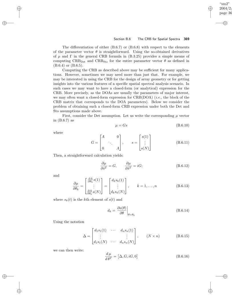
“sm2”2004/2/22page 369

i

i

i

i

i

i

i

i


The differentiation of either (B.6.7) or (B.6.8) with respect to the elementsof the parameter vector θ is straightforward. Using the so-obtained derivativesof µ and Γ in the general CRB formula in (B.3.25) provides a simple means ofcomputing CRBDet and CRBSto for the entire parameter vector θ as defined in(B.6.4) or (B.6.5).

Computing the CRB as described above may be sufficient for many applica-tions. However, sometimes we may need more than just that. For example, wemay be interested in using the CRB for the design of array geometry or for gettinginsights into the various features of a specific spatial spectral analysis scenario. Insuch cases we may want to have a closed-form (or analytical) expression for theCRB. More precisely, as the DOAs are usually the parameters of major interest,we may often want a closed-form expression for CRB(DOA) (i.e., the block of theCRB matrix that corresponds to the DOA parameters). Below we consider theproblem of obtaining such a closed-form CRB expression under both the Det andSto assumptions made above.

First, consider the Det assumption. Let us write the corresponding µ vectorin (B.6.7) as

µ = Gs (B.6.10)

where

G =

A 0. . .

0 A

, s =

s(1)...

s(N)

(B.6.11)

Then, a straightforward calculation yields:

∂µ

∂sT= G,

∂µ

∂sT= iG; (B.6.12)

and

∂µ

∂θk=

∂A∂θk

s(1)...

∂A∂θk

s(N)

=

dksk(1)...

dksk(N)

, k = 1, . . . , n (B.6.13)

where sk(t) is the kth element of s(t) and

dk =∂a(θ)

∂θ

∣∣∣∣θ=θk

(B.6.14)

Using the notation

∆ =

d1s1(1) · · · dnsn(1)...

...d1s1(N) · · · dnsn(N)

, (N × n) (B.6.15)

we can then write:dµ

d θT=[∆, G, iG, 0

](B.6.16)

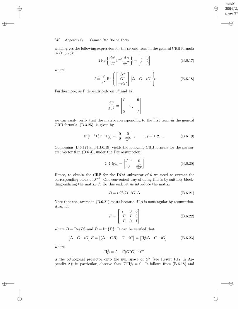
“sm2”2004/2/22page 370

i

i

i

i

i

i

i

i


which gives the following expression for the second term in the general CRB formulain (B.3.25):

2 Re

dµ∗

dθΓ−1 dµ

dθT

=

[J 00 0

]

(B.6.17)

where

J ,2

σ2Re

∆∗

G∗

−iG∗

[∆ G iG

]

(B.6.18)

Furthermore, as Γ depends only on σ2 and as

dΓ

d σ2=

I 0. . .

0 I

we can easily verify that the matrix corresponding to the first term in the generalCRB formula, (B.3.25), is given by

tr[Γ−1Γ′

iΓ−1Γ′

j

]=

[0 00 mN

σ4

]

, i, j = 1, 2, . . . (B.6.19)

Combining (B.6.17) and (B.6.19) yields the following CRB formula for the param-eter vector θ in (B.6.4), under the Det assumption:

CRBDet =

[J−1 0

0 σ4

mN

]

(B.6.20)

Hence, to obtain the CRB for the DOA subvector of θ we need to extract thecorresponding block of J−1. One convenient way of doing this is by suitably block-diagonalizing the matrix J . To this end, let us introduce the matrix

B = (G∗G)−1G∗∆ (B.6.21)

Note that the inverse in (B.6.21) exists because A∗A is nonsingular by assumption.Also, let

F =

I 0 0−B I 0

−B 0 I

(B.6.22)

where B = ReB and B = ImB. It can be verified that

[∆ G iG

]F =

[(∆ −GB) G iG

]=[Π⊥G∆ G iG

](B.6.23)

where

Π⊥G = I −G(G∗G)−1G∗

is the orthogonal projector onto the null space of G∗ (see Result R17 in Ap-pendix A); in particular, observe that G∗Π⊥

G = 0. It follows from (B.6.18) and

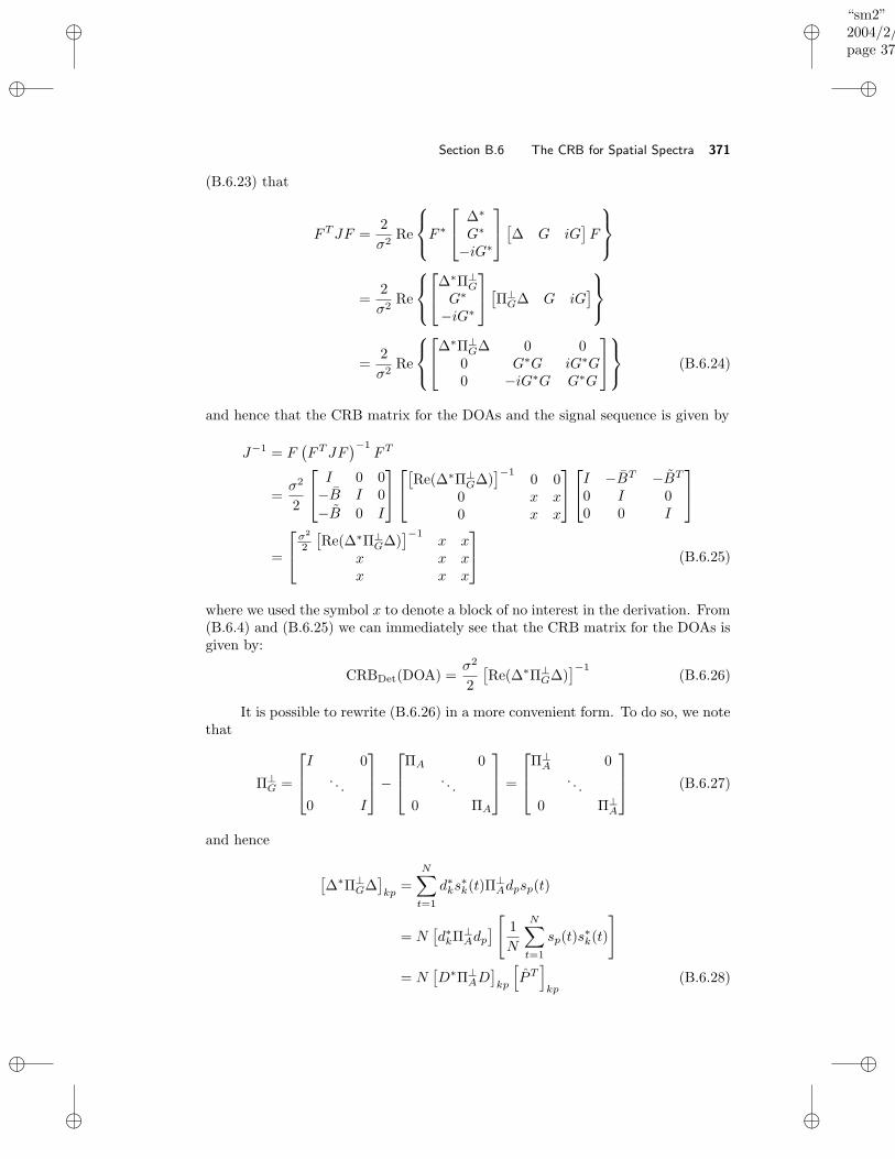
“sm2”2004/2/22page 371

i

i

i

i

i

i

i

i


(B.6.23) that

FTJF =2

σ2Re

F ∗

∆∗

G∗

−iG∗

[∆ G iG

]F

=2

σ2Re

∆∗Π⊥G

G∗

−iG∗

[Π⊥G∆ G iG

]

=2

σ2Re

∆∗Π⊥G∆ 0 0

0 G∗G iG∗G0 −iG∗G G∗G

(B.6.24)

and hence that the CRB matrix for the DOAs and the signal sequence is given by

J−1 = F(FTJF

)−1FT

=σ2

2

I 0 0−B I 0

−B 0 I

[Re(∆∗Π⊥

G∆)]−1

0 00 x x0 x x

I −BT −BT0 I 00 0 I

=

σ2

2

[Re(∆∗Π⊥

G∆)]−1

x xx x xx x x

(B.6.25)

where we used the symbol x to denote a block of no interest in the derivation. From(B.6.4) and (B.6.25) we can immediately see that the CRB matrix for the DOAs isgiven by:

CRBDet(DOA) =σ2

2

[Re(∆∗Π⊥

G∆)]−1

(B.6.26)

It is possible to rewrite (B.6.26) in a more convenient form. To do so, we notethat

Π⊥G =

I 0. . .

0 I

−

ΠA 0. . .

0 ΠA

=

Π⊥A 0

. . .

0 Π⊥A

(B.6.27)

and hence

[∆∗Π⊥

G∆]

kp=

N∑

t=1

d∗ks

∗k(t)Π

⊥Adpsp(t)

= N[d∗kΠ

⊥Adp

]

[

1

N

N∑

t=1

sp(t)s∗k(t)

]

= N[D∗Π⊥

AD]

kp

[

PT]

kp(B.6.28)

“sm2”2004/2/22page 372

i

i

i

i

i

i

i

i


where

D =[d1 . . . dn

](B.6.29)

P =1

N

N∑

t=1

s(t)s∗(t) (B.6.30)

It follows from (B.6.28) that

∆∗Π⊥G∆ = N

(D∗Π⊥

AD)

PT (B.6.31)

where denotes the Hadamard (or elementwise) matrix product (see the definitionin Result R19 in Appendix A). Inserting (B.6.31) in (B.6.26) yields the followinganalytical expression for the CRB matrix associated with the DOA vector under theDet assumption:

CRBDet(DOA) =σ2

2N

Re[(D∗Π⊥

AD)

PT]−1

(B.6.32)

We refer the reader to [Stoica and Nehorai 1989a] for more details about(B.6.32) and its possible uses in array processing. The presented derivation of(B.6.32) has been adapted from [Stoica and Larsson 2001]. Note that (B.6.32)can be directly applied to the temporal line spectral model in Section B.4 (seeequations (B.4.4) and (B.4.5) there) to obtain an analytical CRB formula for thesinusoidal frequencies.

The derivation of an analytical expression for the CRB matrix associated withthe DOAs under the Sto assumption is more intricate, and we give only the finalformula here (see [Stoica, Larsson, and Gershman 2001] and its references fora derivation):

CRBSto(DOA) =σ2

2N

Re[(D∗Π⊥

AD)

(PA∗R−1AP )T

)]−1 (B.6.33)

At this point we should emphasize the fact that the two CRBs discussedabove, CRBDet and CRBSto, correspond to two different models of the data vectory (see (B.6.7) and (B.6.8)), and hence they are not directly comparable. On theother hand, the CRBs for the DOA parameters can be compared with one another.To make this comparison possible, let us introduce the assumption that the samplecovariance matrix P in (B.6.30) converges to the P matrix in (B.6.3), as N → ∞.Let CRBDet(DOA) denote the CRB matrix in (B.6.32) with P replaced by P . Then,the following interesting order relation holds true:

CRBSto(DOA) ≥ CRBDet(DOA) (B.6.34)

To prove (B.6.34) we need to show that (see (B.6.32) and (B.6.33)):

Re[(D∗Π⊥

AD)

(PA∗R−1AP )T

)]−1 ≥Re[(D∗Π⊥

AD)

PT]−1

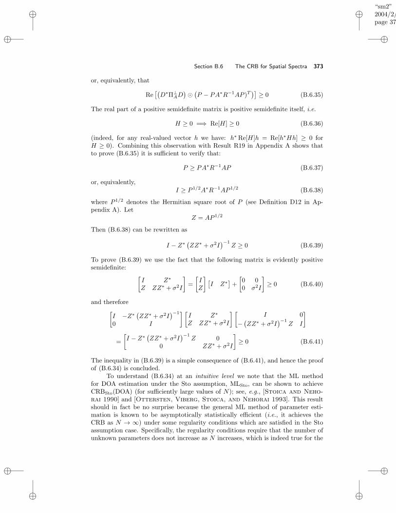
“sm2”2004/2/22page 373

i

i

i

i

i

i

i

i


or, equivalently, that

Re[(D∗Π⊥

AD)

(P − PA∗R−1AP )T

)]≥ 0 (B.6.35)

The real part of a positive semidefinite matrix is positive semidefinite itself, i.e.

H ≥ 0 =⇒ Re[H] ≥ 0 (B.6.36)

(indeed, for any real-valued vector h we have: h∗ Re[H]h = Re[h∗Hh] ≥ 0 forH ≥ 0). Combining this observation with Result R19 in Appendix A shows thatto prove (B.6.35) it is sufficient to verify that:

P ≥ PA∗R−1AP (B.6.37)

or, equivalently,I ≥ P 1/2A∗R−1AP 1/2 (B.6.38)

where P 1/2 denotes the Hermitian square root of P (see Definition D12 in Ap-pendix A). Let

Z = AP 1/2

Then (B.6.38) can be rewritten as

I − Z∗ (ZZ∗ + σ2I)−1

Z ≥ 0 (B.6.39)

To prove (B.6.39) we use the fact that the following matrix is evidently positivesemidefinite:

[I Z∗

Z ZZ∗ + σ2I

]

=

[IZ

][I Z∗]+

[0 00 σ2I

]

≥ 0 (B.6.40)

and therefore

[

I −Z∗ (ZZ∗ + σ2I)−1

0 I

] [I Z∗

Z ZZ∗ + σ2I

] [I 0

−(ZZ∗ + σ2I

)−1Z I

]

=

[

I − Z∗ (ZZ∗ + σ2I)−1

Z 00 ZZ∗ + σ2I

]

≥ 0 (B.6.41)

The inequality in (B.6.39) is a simple consequence of (B.6.41), and hence the proofof (B.6.34) is concluded.

To understand (B.6.34) at an intuitive level we note that the ML methodfor DOA estimation under the Sto assumption, MLSto, can be shown to achieveCRBSto(DOA) (for sufficiently large values of N); see, e.g., [Stoica and Neho-

rai 1990] and [Ottersten, Viberg, Stoica, and Nehorai 1993]. This resultshould in fact be no surprise because the general ML method of parameter esti-mation is known to be asymptotically statistically efficient (i.e., it achieves theCRB as N → ∞) under some regularity conditions which are satisfied in the Stoassumption case. Specifically, the regularity conditions require that the number ofunknown parameters does not increase as N increases, which is indeed true for the

“sm2”2004/2/22page 374

i

i

i

i

i

i

i

i


Sto model (see (B.6.5)). Let CMLSto(DOA) denote the asymptotic covariance ma-trix of the MLSto estimate of the DOA parameter vector. According to the abovediscussion, we have that

CMLSto(DOA) = CRBSto(DOA) (B.6.42)

At the same time, under the Det assumption the MLSto can be viewed as somemethod for DOA estimation, and hence its asymptotic covariance matrix mustsatisfy the CRB inequality (corresponding to the Det assumption):

CMLSto(DOA) ≥ CRBDet(DOA) (B.6.43)

(Note that the asymptotic covariance matrix of MLSto can be shown to be thesame under either the Sto or Det assumption). The above equation along with(B.6.42) provide a heuristic motivation for the relationship between CRBSto(DOA)and CRBDet(DOA) in (B.6.34). Note that the inequality in (B.6.34) is in gen-eral strict, but the relative difference between CRBSto(DOA) and CRBDet(DOA)is usually fairly small (see, e.g., [Ottersten, Viberg, Stoica, and Nehorai

1993]).A similar remark to the one in the previous paragraph can be made on the

ML method for DOA estimation under the Det assumption, which we abbreviateas MLDet. Note that MLDet can be readily seen to coincide with the NLS methoddiscussed in Section 6.4.1. Under the Sto assumption, MLDet (i.e., the NLS method)can be viewed as just some method for DOA estimation. Hence, its (asymptotic)covariance matrix must be bounded below by the CRB corresponding to the Stoassumption:

CMLDet(DOA) ≥ CRBSto(DOA) (B.6.44)

Similarly to MLSto, the asymptotic covariance matrix of MLDet can also be shownto be the same under either the Sto or Det assumption. Hence, we can infer from(B.6.34) and (B.6.44) that MLDet may not attain CRBDet(DOA) which is indeed thecase (as is shown in, e.g., [Stoica and Nehorai 1989a]). To understand why thishappens, note that the Det model contains (2N+1)n+1 real-valued parameters (see(B.6.4)) which must be estimated from 2mN data samples. Hence, for large N , theratio between the number of unknown parameters and the available data samplesapproaches a constant (equal to n/m), which violates one of the aforementionedregularity conditions for the statistical efficiency of the ML method.

Remark: CRBDet(DOA) depends on the signal sequence s(t)Nt=1. However, nei-ther CRBDet(DOA) nor the asymptotic covariance matrices of MLSto, MLDet, or infact many other DOA estimation methods depend on this sequence. We will use thesymbol C to denote the (asymptotic) covariance matrix of such a DOA estimationmethod for which C is independent of the signal sequence.

From CRBDet(DOA) we can obtain a matrix, different from CRBDet(DOA),which is independent of the signal sequence, in the following manner:

ACRBDet(DOA) = E CRBDet(DOA) (B.6.45)

where E is an averaging operator, and ACRBDet stands for Averaged CRBDet. Forexample, E· in (B.6.45) can be a simple arithmetic averaging of CRBDet(DOA)

“sm2”2004/2/22page 375

i

i

i

i

i

i

i

i


over a set of signal sequences. Using the fact that E C = C (since C does notdepend on the sequence s(t)Nt=1), we can apply the operator E· to both sidesof the following CRB inequality:

C ≥ CRBDet(DOA) (B.6.46)

to obtainC ≥ ACRBDet(DOA) (B.6.47)

(Note that the inequality in (B.6.46) and hence that in (B.6.47) hold at least for suf-ficiently large values of N). It follows from (B.6.47) that ACRBDet(DOA) can alsobe used as a lower bound on the DOA estimation error covariance. Furthermore,it can be shown that ACRBDet(DOA) is tighter than CRBDet(DOA):

ACRBDet(DOA) ≥ CRBDet(DOA) (B.6.48)

To prove (B.6.48), we introduce the matrix:

X =2N

σ2Re[

(D∗Π⊥AD) PT

]

(B.6.49)

Using this notation along with the fact that EP = P (which holds under mildconditions), we can rewrite (B.6.48) as follows:

EX−1

≥[

E X]−1

(B.6.50)

To prove (B.6.50), we note that the matrix

E

[X−1 II X

]

= E

[X−1/2

X1/2

][X−1/2 X1/2

]

(where X1/2 and X−1/2 denote the Hermitian square roots of X and X−1, re-spectively) is clearly positive semidefinite, and therefore so must be the followingmatrix:

[

I −[

E X]−1

0 I

] [EX−1

I

I E X

] [ I 0

−[

E X]−1

I

]

=

[

EX−1

−[

E X]−1

0

0 E X

]

≥ 0

(B.6.51)

The matrix inequality in (B.6.50), which is somewhat similar to the scalar Jenseninequality (see, e.g., Complement 4.9.5) readily follows from (B.6.51).

The inequality (B.6.48) looks appealing. On the other hand, ACRBDet(DOA)should be less tight than CRBSto(DOA), in view of the results in (B.6.42) and(B.6.47). Also, CRBSto(DOA) has a simpler analytical form. Hence, we may havelittle reason to use ACRBDet(DOA) in lieu of CRBSto(DOA). Despite these draw-backs of ACRBDet(DOA), we have included this discussion for the potential use-fulness of the inequality in (B.6.50) and of the basic idea behind the introductionof ACRBDet(DOA).

“sm2”2004/2/22page 376

i

i

i

i

i

i

i

i


In the remainder of this section we rely on the previous results to comparethe Det and Sto model assumptions, to discuss the consequences of making theseassumptions, and to draw some conclusions.

First, consider the array output model in equation (B.6.1). To derive the MLestimates of the unknown parameters in (B.6.1) we must make some assumptionson the signal sequence s(t). The MLSto method for DOA estimation (derivedunder the Sto assumption) turns out to be more accurate than the MLDet method(obtained under the Det assumption), under quite general conditions on s(t).However, the MLSto method is somewhat more complicated computationally thanthe MLDet method; see, e.g., [Ottersten, Viberg, Stoica, and Nehorai 1993].

The previous discussion implies that the question as to which assumptionshould be used (because “it is more likely to be true”) is in fact irrelevant in thiscase. Indeed, we should see the two assumptions only as instruments for derivingthe two corresponding ML methods. Once we have completed the derivations, theassumption issue is no longer important and we can simply choose the ML methodthat we prefer, regardless of the nature of s(t). The choice should be based onthe facts that (a) MLDet is computationally simpler than MLSto, and (b) MLSto isstatistically more accurate than MLDet under quite general conditions on s(t).

Second, regarding the two CRB matrices that correspond to the Det and Stoassumptions, respectively, we can argue as follows. Under the Sto assumption,CRBSto(DOA) is the Cramer–Rao bound and hence the lower bound to use. Underthe Det assumption, while CRBSto(DOA) is no longer the true CRB, it is still atight lower bound on the asymptotic covariance matrix of any known DOA esti-mation method. CRBDet(DOA) is also a lower bound, but it is not tight. HenceCRBSto(DOA) should be the normal choice for a lower bound, regardless of the as-sumption (Det or Sto) that the signal sequence is likely to satisfy. Note that, underthe Det assumption, MLSto can be seen as some DOA estimation method. There-fore, in principle, a better DOA estimation method than MLSto may exist (whereby “better” we mean that the covariance matrix of such an estimation methodwould be smaller than CRBSto(DOA)). However, no such DOA estimation methodappears to be available, in spite of a significant literature on the so-called problemof “estimation in the presence of many nuisance parameters,” of which the DOAestimation problem under the Det assumption is a special case.

“sm2”2004/2/22page 377

i

i

i

i

i

i

i

i

A P P E N D I X C

Model Order Selection Tools

C.1 INTRODUCTION

The parametric methods of spectral analysis (discussed in Chapters 3, 4, and 6)require not only the estimation of a vector of real-valued parameters but also theselection of one or several integer-valued parameters that are equally important forthe specification of the data model. Specifically, these integer-valued parametersof the model are the ARMA model orders in Chapter 3, the number of sinusoidalcomponents in Chapter 4, and the number of source signals impinging on the arrayin Chapter 6. In each of these cases, the integer-valued parameters determine thedimension of the real-valued parameter vector of the data model. In what followswe will use the following symbols:

y = the vector of available data (of size N)

θ = the (real-valued) parameter vector

n = the dimension of θ

For short, we will refer to n as the model order, even though sometimes n is notreally an order (see, e.g., the above examples). We assume that both y and θ arereal-valued:

y ∈ RN , θ ∈ Rn

Whenever we need to emphasize that the number of elements in θ is n, we will usethe notation θn. A method that estimates n from the data vector y will be calledan order selection rule. Note that the need for estimating a model order is typicalof the parametric approaches to spectral analysis. The nonparametric methods ofspectral analysis do not have such a requirement.

The discussion in the text on the parametric spectral methods has focusedon estimating the model parameter vector θ for a specific order n. In this generalappendix1 we explain how to estimate n as well. The literature on order selectionis as considerable as that on (real-valued) parameter estimation (see, e.g., [Choi

1992; Soderstrom and Stoica 1989; McQuarrie and Tsai 1998; Linhart

and Zucchini 1986; Burnham and Anderson 2002; Sakamoto, Ishiguro,

and Kitagawa 1986; Stoica, Eykhoff, Jannsen, and Soderstrom 1986]and the many references therein). However, many order selection rules are tiedto specific parameter estimation methods and hence their applicability is ratherlimited. Here we will concentrate on order selection rules that are associated withthe maximum likelihood method (MLM) of parameter estimation. As explained

1Based on “Model order selection: A review of the AIC, GIC, and BIC rules,” by P. Stoicaand Y. Selen, IEEE Signal Processing Magazine, 21(2), March 2004.

377

“sm2”2004/2/22page 378

i

i

i

i

i

i

i

i

378 Appendix C Model Order Selection Tools

briefly in Appendix B (see also below), the MLM is likely the most commonly usedparameter estimation method. Consequently, the order estimation rules that canbe used with the MLM are of quite a general interest. In the next section we reviewbriefly the ML method of parameter estimation and some of its main properties.

C.2 MAXIMUM LIKELIHOOD PARAMETER ESTIMATION

Letp(y, θ) = the probability density function (pdf) of the data vec-tor y, which depends on the parameter vector θ; also called thelikelihood function.

The ML estimate of θ, which we denote by θ, is given by the maximizer ofp(y, θ) (see, e.g., [Anderson 1971; Brockwell and Davis 1991; Hannan and

Deistler 1988; Papoulis 1977; Porat 1994; Priestley 1981; Scharf 1991;Therrien 1992; Soderstrom and Stoica 1989] and also Appendix B). Alter-natively, as ln(·) is a monotonically increasing function,

θ = arg maxθ

ln p(y, θ) (C.2.1)

Under the Gaussian data assumption, the MLM typically reduces to the nonlinearleast-squares (NLS) method of parameter estimation (particular forms of which arediscussed briefly in Chapter 3 and in more detail in Chapters 4 and 6). To illustratethis fact, let us assume that the observation vector y can be written as:

y = µ(γ) + e (C.2.2)

where e is a (real-valued) Gaussian white noise vector with mean zero and covariancematrix given by E

eeT

= σ2I, γ is an unknown parameter vector, and µ(γ) is adeterministic function of γ. It follows readily from (C.2.2) that

p(y, θ) =1

(2π)N/2(σ2)N/2e− ‖y−µ(γ)‖2

2σ2 (C.2.3)

where

θ =

[γσ2

]

(C.2.4)

Remark: Note that in this appendix we use the symbol θ for the whole parametervector, unlike in some previous discussions where we used θ to denote the signalparameter vector (which is denoted by γ here).

We deduce from (C.2.3) that

−2 ln p(y, θ) = N ln(2π) +N lnσ2 +‖y − µ(γ)‖2

σ2(C.2.5)

“sm2”2004/2/22page 379

i

i

i

i

i

i

i

i

Section C.2 Maximum Likelihood Parameter Estimation 379

A simple calculation based on (C.2.5) shows that the ML estimates of γ and σ2 aregiven by:

γ = arg minγ

‖y − µ(γ)‖2 (C.2.6)

σ2 =1

N‖y − µ(γ)‖2 (C.2.7)

The corresponding value of the likelihood function is given by

−2 ln p(y, θ) = constant +N ln σ2 (C.2.8)

As can be seen from (C.2.6), in the present case the MLM indeed reduces to theNLS. In particular, note that the NLS method for sinusoidal parameter estimationdiscussed in Chapter 4 is precisely of the form of (C.2.6). If we let Ns denote thenumber of observed complex-valued samples of the noisy sinusoidal signal, and ncdenote the number of sinusoidal components present in the signal, then:

N = 2Ns (C.2.9)

n = 3nc + 1 (C.2.10)

We will use the sinusoidal signal model of Chapter 4 as a vehicle for illustrating howthe various general order selection rules presented in what follows should be usedin a specific situation. These rules can also be used with the parametric spectralanalysis methods of Chapters 3 and 6. The task of deriving explicit forms of theseorder selection rules for the aforementioned methods is left as an interesting exerciseto the reader (see, e.g., [McQuarrie and Tsai 1998; Brockwell and Davis

1991; Porat 1994]).

Next, we note that under regularity conditions the pdf of the ML estimate θconverges, as N → ∞, to a Gaussian pdf with mean θ and covariance matrix equalto the Cramer–Rao Bound (CRB) matrix (see Section B.2 for a discussion about

the CRB). Consequently, asymptotically in N , the pdf of θ is given by:

p(θ) =1

(2π)n/2|J−1|1/2 e− 1

2 (θ−θ)T J(θ−θ) (C.2.11)

where (see (B.2.10))

J = −E∂2 ln p(y, θ)

∂θ ∂θT

(C.2.12)

Remark: To simplify the notation, we use the symbol θ for both the true parametervector and the parameter vector viewed as an unknown variable (as we also did inAppendix B). The exact meaning of θ should be clear from the context.

The “regularity conditions” referred to above require that n is not a functionof N , and hence that the ratio between the number of unknown parameters and thenumber of observations tends to zero as N → ∞. This is true for the parametric

“sm2”2004/2/22page 380

i

i

i

i

i

i

i

i


spectral analysis problems discussed in Chapters 3 and 4. However, the previouscondition does not hold for the parametric spectral analysis problem addressed inChapter 6. Indeed, in the latter case the number of parameters to be estimatedfrom the data is proportional to N , owing to the assumption that the signal se-quence is completely unknown. To overcome this difficulty we can assume thatthe signal vector is temporally white and Gaussian distributed, which leads to aML problem that satisfies the previously stated regularity condition (we refer theinterested reader to [Ottersten, Viberg, Stoica, and Nehorai 1993; Stoica

and Nehorai 1990; Van Trees 2002] for details on this ML approach to thespatial spectral analysis problem of Chapter 6).

To close this section, we note that under mild conditions:

[

− 1

N

∂2 ln p(y, θ)

∂θ ∂θT− 1

NJ

]

→ 0 as N → ∞ (C.2.13)

To motivate (C.2.13) for the fairly general data model in (C.2.2) we can argue asfollows. Let us rewrite the negative log-likelihood function associated with (C.2.2)as (see (C.2.5)):

− ln p(y, θ) = constant +N

2ln(σ2) +

1

2σ2

N∑

t=1

[yt − µt(γ)]2

(C.2.14)

where the subindex t denotes the t-th component. From (C.2.14) we obtain by asimple calculation:

−∂ ln p(y, θ)

∂θ=

− 1

σ2

N∑

t=1

[yt − µt(γ)]µ′t(γ)

N

2σ2− 1

2σ4

N∑

t=1

[yt − µt(γ)]2

(C.2.15)

where

µ′t(γ) =

∂µt(γ)

∂γ(C.2.16)

Differentiating (C.2.15) once again gives:

− ∂2 ln p(y, θ)

∂θ ∂θT

=

− 1

σ2

N∑

t=1

etµ′′t (γ) +

1

σ2

N∑

t=1

µ′t(γ)µ

′Tt (γ)

1

σ4

N∑

t=1

etµ′t(γ)

1

σ4

N∑

t=1

etµ′t(γ) − N

2σ4+

1

σ6

N∑

t=1

e2t

(C.2.17)

where et = yt − µt(γ) and

µ′′t (γ) =

∂2µt(γ)

∂γ ∂γT(C.2.18)

“sm2”2004/2/22page 381

i

i

i

i

i

i

i

i

Section C.3 Useful Mathematical Preliminaries and Outlook 381

Taking the expectation of (C.2.17) and dividing by N , we get:

1

NJ =

1

σ2

(

1

N

N∑

t=1

µ′t(γ)µ

′Tt (γ)

)

0

01

2σ4

(C.2.19)

We assume that µ(γ) is such that the above matrix has a finite limit as N → ∞.Under this assumption, and the previously-made assumption on e, we can also showfrom (C.2.17) that

− 1

N

∂2 ln p(y, θ)

∂θ ∂θT

converges (as N → ∞) to the right side of (C.2.19), which concludes the motivationof (C.2.13). Letting

J = −∂2 ln p(y, θ)

∂θ ∂θT

∣∣∣∣θ=θ

(C.2.20)

we deduce from (C.2.13), (C.2.19), and the consistency of θ that, for sufficientlylarge values of N ,

1

NJ ' 1

NJ = O(1) (C.2.21)

Hereafter, ' denotes an asymptotic (approximate) equality, in which the higher-order terms have been neglected, and O(1) denotes a term that tends to a constantas N → ∞.

Interestingly enough, the assumption that the right side of (C.2.19) has a finitelimit, as N → ∞, holds for many problems, but not for the sinusoidal parameterestimation problem of Chapter 4. In the latter case, (C.2.21) needs to be modifiedas follows (see, e.g., Appendix B):

KN JKN ' KNJKN = O(1) (C.2.22)

where

KN =

[1

N3/2s

Inc 0

0 1

N1/2s

I2nc+1

]

(C.2.23)

and where Ik denotes the k×k identity matrix; to write (C.2.23), we assumed thatthe upper-left nc×nc block of J corresponds to the sinusoidal frequencies, but thisfact is not really important for the analysis in this appendix, as we will see below.

C.3 USEFUL MATHEMATICAL PRELIMINARIES AND OUTLOOK

In this section we discuss a number of mathematical tools that will be used in thenext sections to derive several important order selection rules. We will keep thediscussion at an informal level to make the material as accessible as possible. InSection C.3.1 we will formulate the model order selection as a hypothesis testingproblem, with the main goal of showing that the maximum a posteriori (MAP)approach leads to the optimal order selection rule (in a sense specified there). InSection C.3.2 we discuss the Kullback-Leibler information criterion, which lies atthe basis of another approach that can be used to derive model order selection rules.

“sm2”2004/2/22page 382

i

i

i

i

i

i

i

i


C.3.1 Maximum A Posteriori (MAP) Selection Rule

Let Hn denote the hypothesis that the model order is n, and let n denote a knownupper bound on n:

n ∈ [1, n] (C.3.1)

We assume that the hypotheses Hnnn=1 are mutually exclusive (i.e., only one ofthem can hold true at a time). As an example, for a real-valued AR signal withcoefficients ak we can define Hn as follows:

Hn : an 6= 0 and an+1 = · · · = an = 0 (C.3.2)

For a sinusoidal signal we can proceed similarly, after observing that for such asignal the number of components nc is related to n as in (C.2.10), viz.

n = 3nc + 1 (C.3.3)

Hence, for a sinusoidal signal with amplitudes αk we can consider the followinghypotheses:

Hnc : αk 6= 0 for k = 1, . . . , nc, and αk = 0 for k = nc + 1, . . . , nc (C.3.4)

for nc ∈ [1, nc] (with the corresponding “model order” n being given by (C.3.3)).

Remark: The hypotheses Hn can be either nested or non-nested. We say thatH1 and H2 are nested whenever the model corresponding to H1 can be obtainedas a special case of that associated with H2. To give an example, the followinghypotheses

H1 : the signal is a first-order AR process

H2 : the signal is a second-order AR process

are nested, whereas the above H1 and

H3 : the signal consists of one sinusoid in noise

are non-nested.

Letpn(y|Hn) = the pdf of y under Hn (C.3.5)

Whenever we want to emphasize the possible dependence of the pdf in (C.3.5) onthe parameter vector of the model corresponding to Hn, we write:

pn(y, θn) , pn(y|Hn) (C.3.6)

Assuming that (C.3.5) is available, along with the a priori probability of Hn,pn(Hn), we can write the conditional probability of Hn, given y, as:

pn(Hn|y) =pn(y|Hn)pn(Hn)

p(y)(C.3.7)

“sm2”2004/2/22page 383

i

i

i

i

i

i

i

i


The maximum a posteriori probability (MAP) rule selects the order n (or thehypothesis Hn) that maximizes (C.3.7). As the denominator in (C.3.7) does notdepend on n, the MAP rule is given by:

maxn∈[1,n]

pn(y|Hn)pn(Hn) (C.3.8)

Most typically, the hypotheses Hn are a priori equiprobable, i.e.,

pn(Hn) =1

n, n = 1, . . . , n (C.3.9)

in which case the MAP rule reduces to:

maxn∈[1,n]

pn(y|Hn) (C.3.10)

Next, we define the average (or total) probability of correct detection as

Pcd = Pr[(decide H1) ∩ (H1 =true)] ∪ · · · ∪ [(decide Hn) ∩ (Hn =true)] (C.3.11)

The attribute “average” that has been attached to Pcd is motivated by the factthat (C.3.11) gives the probability of correct detection “averaged” over all possiblehypotheses (as opposed, for example, to only considering the probability of correctlydetecting that the model order is 2 (let us say), which is Prdecide H2|H2).

Remark: Regarding the terminology, note that the determination of a real-valuedparameter from the available data is called “estimation,” whereas it is usually called“detection” for an integer-valued parameter, such as a model order.

In the following we prove that the MAP rule is optimal in the sense of max-imizing Pcd. To do so, consider a generic rule for selecting n, or, equivalently, fortesting the hypotheses Hn against each other. Such a rule will implicitly or ex-plicitly partition the observation space, RN , into n sets Snnn=1, which are suchthat:

We decide Hn if and only if y ∈ Sn (C.3.12)

Making use of (C.3.12) along with the fact that the hypotheses Hn are mutuallyexclusive, we can write Pcd in (C.3.11) as:

Pcd =

n∑

n=1

Pr(decide Hn) ∩ (Hn =true)

=

n∑

n=1

Pr(decide Hn)|Hn PrHn

=

n∑

n=1

∫

Sn

pn(y|Hn)pn(Hn) dy

=

∫

RN

[n∑

n=1

In(y)pn(y|Hn)pn(Hn)

]

dy

(C.3.13)

“sm2”2004/2/22page 384

i

i

i

i

i

i

i

i


where In(y) is the so-called indicator function given by:

In(y) =

1, if y ∈ Sn

0, otherwise(C.3.14)

Next, observe that for any given data vector, y, one and only one indicator functioncan be equal to one (as the sets Sn do not overlap and their union is RN ). Thisobservation along with the expression (C.3.13) for Pcd imply that the MAP rulein (C.3.8) maximizes Pcd, as stated. Note that the sets Sn corresponding to theMAP rule are implicitly defined via (C.3.8); however, Sn are of no real interest inthe proof, as both they and the indicator functions are introduced only to simplifythe above proof. For more details on the topic of this subsection, we refer the readerto [Scharf 1991; Van Trees 2002].

C.3.2 Kullback-Leibler Information

Let p0(y) denote the true pdf of the observed data vector y, and let p(y) denote thepdf of a generic model of the data. The “discrepancy” between p0(y) and p(y) canbe measured using the Kullback-Leibler (KL) information or discrepancy function(see [Kullback and Leibler 1951]):

D(p0, p) =

∫

p0(y) ln

[p0(y)

p(y)

]

dy (C.3.15)

To simplify the notation, we omit the region of integration when it is the entirespace. Letting E0· denote the expectation with respect to the true pdf, p0(y), wecan rewrite (C.3.15) as:

D(p0, p) = E0

ln

[p0(y)

p(y)

]

= E0ln p0(y) − E0ln p(y) (C.3.16)

Next, we prove that (C.3.15) possesses some properties of a suitable discrepancyfunction, viz.

D(p0, p) ≥ 0

D(p0, p) = 0 if and only if p0(y) = p(y)(C.3.17)

To verify (C.3.17) we use the fact shown in Complement 6.5.8 that

− lnλ ≥ 1 − λ for any λ > 0 (C.3.18)

and

− lnλ = 1 − λ if and only if λ = 1 (C.3.19)

Hence, letting λ(y) = p(y)/p0(y), we have that:

D(p0, p) =

∫

p0(y) [− lnλ(y)] dy

≥∫

p0(y) [1 − λ(y)] dy =

∫

p0(y)

[

1 − p(y)

p0(y)

]

dy = 0

“sm2”2004/2/22page 385

i

i

i

i

i

i

i

i


where the equality holds if and only if λ(y) ≡ 1, i.e. p(y) ≡ p0(y).

Remark: The inequality in (C.3.17) also follows from Jensen’s inequality (see equa-tion (4.9.36) in Complement 4.9.5) and the concavity of the function ln(·):

D(p0, p) = −E0

ln

[p(y)

p0(y)

]

≥ − ln

[

E0

p(y)

p0(y)

]

= − ln

[∫p(y)

p0(y)p0(y) dy

]

= − ln(1) = 0

The KL discrepancy function can be viewed as quantifying the “loss of in-formation” induced by the use of p(y) in lieu of p0(y). For this reason, D(p0, p)is sometimes called an information function, and the order selection rules derivedfrom it are called information criteria (see Sections C.4–C.6).

C.3.3 Outlook: Theoretical and Practical Perspectives

Neither the MAP rule nor the KL information can be directly used for order se-lection because neither the pdfs of the data vector under the various hypothesesnor the true data pdf are available in any of the parametric spectral analysis prob-lems discussed in the text. A possible way of using the MAP approach for orderestimation consists of assuming an a priori pdf for the unknown parameter vector,θn, and integrating θn out of pn(y, θ

n) to obtain pn(y|Hn). This Bayesian-typeapproach will be discussed in Section C.7. Regarding the KL approach, a naturalway of using it for order selection consists of using an estimate, D(p0, p), in lieu ofthe unavailable D(p0, p) (for a suitably chosen model pdf, p(y)), and determiningthe model order by minimizing D(p0, p). This KL-based approach will be discussedin Sections C.4–C.6.

The derivations of all model order selection rules in the sections that followrely on the assumption that one of the hypotheses Hn is true. As this assumptionis unlikely to hold in applications with real-life data, the reader may justifiablywonder whether an order selection rule derived under such an assumption has anypractical value. To address this concern, we remark that good parameter estimationmethods (such as the MLM), derived under rather strict modeling assumptions,perform quite well in applications where the assumptions made are rarely satisfiedexactly. Similarly, order selection rules based on sound theoretical principles (suchas the ML, KL, and MAP principles used in this text) are likely to perform well inapplications despite the fact that some of the assumptions made when deriving themdo not hold exactly. While the precise behavior of order selection rules (such asthose presented in the sections to follow) in various mismodeling scenarios is not wellunderstood, extensive simulation results (see, e.g., [McQuarrie and Tsai 1998;Linhart and Zucchini 1986; Burnham and Anderson 2002]) lend support tothe above claim.

“sm2”2004/2/22page 386

i

i

i

i

i

i

i

i


C.4 DIRECT KULLBACK-LEIBLER (KL) APPROACH: NO-NAME RULE

The model-dependent part of the Kullback-Leibler (KL) information, (C.3.16), isgiven by

−E0ln p(y) (C.4.1)

where p(y) is the pdf or likelihood of the model (to simplify the notation, we omit theindex n of p(y); we will reinstate the index n later on, when needed). Minimizationof (C.4.1) with respect to the model order is equivalent to maximization of thefunction:

I(p0, p) , E0ln p(y) (C.4.2)

which is sometimes called the relative KL information. The ideal choice for p(y) in(C.4.2) would be the model likelihood, pn(y|Hn) = pn(y, θ

n). However, the modellikelihood function is not available, and hence this choice is not possible. Instead,we might think of using

p(y) = p(y, θ) (C.4.3)

in (C.4.2), which would give

I(

p0, p(y, θ))

= E0

ln p(y, θ)

(C.4.4)

Because the true pdf of the data vector is unknown, we cannot evaluate the ex-pectation in (C.4.4). Apparently, what we could easily do is to use the following

unbiased estimate of I(

p0, p(y, θ))

, instead of (C.4.4) itself,

I = ln p(y, θ) (C.4.5)

However, the order selection rule that maximizes (C.4.5) does not have satisfactoryproperties. This is especially true for nested models, in the case of which the orderselection rule based on the maximization of (C.4.5) fails completely : indeed, fornested models this rule will always choose the maximum possible order, n, owingto the fact that ln pn(y, θ

n) monotonically increases with increasing n.A better idea consists of approximating the unavailable log-pdf of the model,

ln pn(y, θn), by a second-order Taylor series expansion around θn, and using the

so-obtained approximation to define ln p(y) in (C.4.2):

ln pn(y, θn) ' ln pn(y, θ

n) + (θn − θn)T[∂ ln pn(y, θ

n)

∂θn

∣∣∣∣θn=θn

]

+1

2(θn − θn)T

[∂2 ln pn(y, θ

n)

(∂θn) (∂θn)T

∣∣∣∣θn=θn

]

(θn − θn) , ln pn(y)

(C.4.6)

Because θn is the maximizer of ln pn(y, θn), the second term in (C.4.6) is equal to

zero. Hence, we can write (see also (C.2.21)):

ln pn(y) ' ln pn(y, θn) − 1

2(θn − θn)TJ(θn − θn) (C.4.7)

According to (C.2.11),

E0

(θn − θn)TJ(θn − θn)

= tr[

JE0

(θn − θn)(θn − θn)T]

= tr[In] = n

(C.4.8)

“sm2”2004/2/22page 387

i

i

i

i

i

i

i

i

Section C.5 Cross-Validatory KL Approach: The AIC Rule 387

which means that, for the choice of pn(y) in (C.4.7), we have

I = E0

ln pn(y, θn) − n

2

(C.4.9)

An unbiased estimate of the above relative KL information is given by

ln pn(y, θn) − n

2(C.4.10)

The corresponding order selection rule maximizes (C.4.10), or, equivalently, mini-mizes

NN(n) = −2 ln pn(y, θn) + n (C.4.11)

with respect to model order n. This no-name (NN) rule can be shown to performbetter than that based on (C.4.5), but worse than the rules presented in the nextsections. Essentially, the problem with (C.4.11) is that it tends to overfit (i.e.,to select model orders larger than the “true” order). To understand intuitivelyhow this happens, note that the first term in (C.4.11) decreases with increasing n(for nested models), whereas the second term increases. Hence, the second termin (C.4.11) penalizes overfitting ; however, it turns out that it does not penalizequite enough. The rules presented in the following sections have a form similarto (C.4.11), but with a larger penalty term, and they do have better propertiesthan (C.4.11). Despite this fact, we have chosen to present (C.4.11) briefly in thissection for two reasons: (i) the discussion here has revealed the failure of using

maxn ln pn(y, θn) as an order selection rule, and has shown that it is in effect quite

easy to obtain rules with better properties; and (ii) this section has laid groundworkfor the derivation of better order selection rules based on the KL approach in thenext two sections.

To close this section, we motivate the multiplication by -2 in going from(C.4.10) to (C.4.11). The reason for preferring (C.4.11) to (C.4.10) is that for thefairly common NLS model in (C.2.2) and the associated Gaussian likelihood in

(C.2.3), −2 ln pn(y, θn) takes on the following convenient form:

−2 ln pn(y, θn) = N ln σ2

n + constant (C.4.12)

(see (C.2.5)–(C.2.7)). Hence, in such a case we can replace −2 ln pn(y, θn) in

(C.4.11) by the scaled logarithm of the residual variance, N ln σ2n. This remark

also applies to the order selection rules presented in the following sections, whichare written in a form similar to (C.4.11).

C.5 CROSS-VALIDATORY KL APPROACH: THE AIC RULE

As explained in the previous section, a possible approach to model order selectionconsists of minimizing the KL discrepancy between the “true” pdf of the data andthe pdf (or likelihood) of the model, or equivalently maximizing the relative KLinformation (see (C.4.2)):

I(p0, p) = E0ln p(y) (C.5.1)

When using this approach, the first (and, likely the main) hurdle that we have toovercome is the choice of the model likelihood, p(y). As discussed in the previous

“sm2”2004/2/22page 388

i

i

i

i

i

i

i

i


section, we would ideally like to use the true pdf of the model as p(y) in (C.5.1),i.e. p(y) = pn(y, θ

n), but this is not possible since pn(y, θn) is unknown. Hence, we

have to choose p(y) in a different way. This choice is important, as it eventuallydetermines the model order selection rule that we will obtain. The other issue weshould consider when using the approach based on (C.5.1) is that the expectationin (C.5.1) cannot be evaluated because the true pdf of the data is unknown. Con-sequently, we will have to use an estimate, I, in lieu of the unavailable I(p0, p) in(C.5.1).

Let x denote a fictitious data vector with the same size, N , and the same pdfas y, but which is independent of y. Also, let θx denote the ML estimate of themodel parameter vector that would be obtained from x if x were available (we omit

the superindex n of θx as often as possible, to simplify notation). In this sectionwe will consider the following choice of the model’s pdf:

ln p(y) = Ex

ln p(y, θx)

(C.5.2)

which, when inserted in (C.5.1), yields:

I = Ey

Ex

ln p(y, θx)

(C.5.3)

Hereafter, Ex· and Ey· denote the expectation with respect to the pdf of xand y, respectively. The above choice of p(y), which was introduced in [Akaike

1974; Akaike 1978], has an interesting cross-validation interpretation: we usethe sample x for estimation and the independent sample y for validation of theso-obtained model’s pdf. Note that the dependence of (C.5.3) on the fictitioussample x is eliminated (as it should be, since x is unavailable) via the expectationoperation Ex·; see below for details.

An asymptotic second-order Taylor series expansion of ln p(y, θx) around θy,similar to (C.4.6)–(C.4.7), yields:

ln p(y, θx) ' ln p(y, θy) + (θx − θy)T

[

∂ ln p(y, θ)

∂θ

∣∣∣∣θ=θy

]

+1

2(θx − θy)

T

[

∂2 ln p(y, θ)

∂θ ∂θT

∣∣∣∣θ=θy

]

(θx − θy)

' ln p(y, θy) − 1

2(θx − θy)

TJy(θx − θy) (C.5.4)

where Jy is the J matrix, as defined in (C.2.20), associated with the data vector y.Using the fact that x and y have the same pdf (which implies that Jy = Jx) alongwith the fact that they are independent of each other, we can show that:

Ey

Ex

(θx − θy)TJy(θx − θy)

= Ey

Ex

tr

(

Jy

[

(θx − θ) − (θy − θ)] [

(θx − θ) − (θy − θ)]T)

= tr[Jy(J−1x + J−1

y

)]= 2n (C.5.5)

“sm2”2004/2/22page 389

i

i

i

i

i

i

i

i

Section C.5 Cross-Validatory KL Approach: The AIC Rule 389

Inserting (C.5.5) in (C.5.4) yields the following asymptotic approximation of therelative KL information in (C.5.3):

I ' Ey

ln pn(y, θn) − n

(C.5.6)

(where we have omitted the subindex y of θ but reinstated the superindex n).Evidently, (C.5.6) can be estimated in an unbiased manner by

ln pn(y, θn) − n (C.5.7)

Maximizing (C.5.7) with respect to n is equivalent to minimizing the followingfunction of n:

AIC = −2 ln pn(y, θn) + 2n (C.5.8)

where the acronym AIC stands for Akaike Information Criterion (the reasons formultiplying (C.5.7) by -2 to get (C.5.8), and for the use of the word “information”in the name given to (C.5.8) have been explained before, see the previous twosections).

As an example, for the sinusoidal signal model with nc components (see Sec-tion C.2), AIC takes on the following form (see (C.2.6)–(C.2.10)):

AIC = 2Ns ln σ2nc

+ 2(3nc + 1) (C.5.9)

where Ns denotes the number of available complex-valued samples, yc(t)Nst=1, and

σ2nc

=1

Ns

Ns∑

t=1

∣∣∣∣∣yc(t) −

nc∑

k=1

αkei(ωkt+ϕk)

∣∣∣∣∣

2

(C.5.10)

Remark: AIC can also be obtained by using the following relative KL informationfunction, in lieu of (C.5.3),

I = Ey

Ex

ln p(x, θy)

(C.5.11)

Note that, in (C.5.11), x is used for validation and y for estimation. However, thederivation of AIC from (C.5.11) is more complicated; such a derivation, which isleft as an exercise to the reader, will make use of two Taylor series expansions, andthe fact that Exln p(x, θ) = Eyln p(y, θ).

The performance of AIC has been found to be satisfactory in many case studiesand applications to real-life data reported in the literature (see, e.g., [McQuarrie

and Tsai 1998; Linhart and Zucchini 1986; Burnham and Anderson 2002;Sakamoto, Ishiguro, and Kitagawa 1986]). The performance of a model orderselection rule, such as AIC, can be measured in different ways, as explained in thenext two paragraphs.

“sm2”2004/2/22page 390

i

i

i

i

i

i

i

i


As a first possibility, we can consider a scenario in which the data generatingmechanism belongs to the class of models under test, and thus there is a trueorder. In such a case, analytical or numerical studies can be used to determinethe probability with which the rule selects the true order. For AIC, it can be shownthat, under quite general conditions,

the probability of underfitting → 0 (C.5.12)

the probability of overfitting → constant > 0 (C.5.13)

as N → ∞ (see, e.g., [McQuarrie and Tsai 1998; Kashyap 1980]). We can seefrom (C.5.13) that the behavior of AIC with respect to the probability of correctdetection is not entirely satisfactory. Interestingly, it is precisely this kind of be-havior that appears to make AIC perform satisfactorily with respect to the otherpossible type of performance measure, as explained below.

An alternative way of measuring the performance is to consider a more prac-tical scenario in which the data generating mechanism is more complex than any ofthe models under test, which is usually the case in practical applications. In such acase we can use analytical or numerical studies to determine the performance of themodel picked by the rule as an approximation of the data generating mechanism:for instance, we can consider the average distance between the estimated and truespectral densities, or the average prediction error of the model. With respect tosuch a performance measure, AIC performs well, partly because of its tendency toselect models with relatively large orders, which may be a good thing to do in a casein which the data generating mechanism is more complex than the models used tofit it.

The nonzero overfitting probability of AIC is due to the fact that the term2n in (C.5.8) (that penalizes high-order models), while larger than the term nthat appears in the NN rule, is still too small. Extensive simulation studies (see,e.g., [Bhansali and Downham 1977]) have empirically found that the followingGeneralized Information Criterion (GIC):

GIC = −2 ln pn(y, θn) + νn (C.5.14)

may outperform AIC with respect to various performance measures if ν > 2. Specif-ically, depending on the considered scenario as well as the value of N and the per-formance measure, values of ν in the interval ν ∈ [2, 6] have been found to give thebest performance.

In the next section we show that GIC can be obtained as a natural theoreticalextension of AIC. Hence, the use of (C.5.14) with ν > 2 can be motivated on formalgrounds. However, the choice of a particular ν in GIC is a more difficult problemthat cannot be solved in the current KL framework (see the next section for details).The different framework of Section C.7 appears to be necessary to arrive at a rulehaving the form of (C.5.14) with a specific expression for ν.

We close this section with a brief discussion on another modification of the AICrule suggested in the literature (see, e.g., [Hurvich and Tsai 1993]). As explainedbefore, AIC is derived by maximizing an asymptotically unbiased estimate of therelative KL information I in (C.5.3). Interestingly, for linear regression models

“sm2”2004/2/22page 391

i

i

i

i

i

i

i

i

Section C.6 Generalized Cross-Validatory KL Approach: the GIC Rule 391

(given by (C.2.2) where µ(γ) is a linear function of γ), the following corrected AICrule, AICc, can be shown to be an exactly unbiased estimate of I:

AICc = −2 ln pn(y, θn) +

2N

N − n− 1n (C.5.15)

(see, e.g., [Hurvich and Tsai 1993; Cavanaugh 1997]). As N → ∞, AICc →AIC (as expected). However, for finite values of N the penalty term of AICc islarger than that of AIC. Consequently, in finite samples AICc has a smaller riskof overfitting than AIC, and therefore we can say that AICc trades off a decreaseof the risk of overfitting (which is rather large for AIC) for an increase in therisk of underfitting (which is quite small for AIC, and hence it can be slightlyincreased without a significant deterioration of performance). With this fact inmind, AICc can be used as an order selection rule for more general models thanjust linear regressions, even though its motivation in the general case is pragmaticrather than theoretical. For other finite-sample corrections of AIC we refer thereader to [de Waele and Broersen 2003; Broersen 2000; Broersen 2002;Seghouane, Bekara, and Fleury 2003].

C.6 GENERALIZED CROSS-VALIDATORY KL APPROACH: THE GIC RULE

In the cross-validatory approach of the previous section, the estimation sample xhas the same length as the validation sample y. In that approach, θx (obtained

from x) is used to approximate the likelihood of the model via Exp(y, θx). TheAIC rule so obtained has a nonzero probability of overfitting (even asymptotically).Intuitively, the risk of overfitting will decrease if we let the length of the validationsample be (much) larger than that of the estimation sample, i.e.

N , length(y) = ρ · length(x), ρ ≥ 1 (C.6.1)

Indeed, overfitting occurs when the model corresponding to θx also fits the “noise”in the sample x so that p(x, θx) has a “much” larger value than the true pdf, p(x, θ).Such a model may behave reasonably well on a short validation sample y, but not ona long validation sample (in the latter case, p(y, θx) will take on very small values).The simple idea in (C.6.1) of letting the lengths of the validation and estimationsamples be different leads to a natural extension of AIC, as shown below.

A straightforward calculation shows that under (C.6.1) we have

Jy = ρJx (C.6.2)

(see, e.g., (C.2.19)). With this small difference, the calculations in the previoussection carry over to the present case and we obtain (see (C.5.4)–(C.5.5)):

I ' Ey

ln pn(y, θy)

− 1

2Ey

Ex

tr

(

Jy

[

(θx − θ) − (θy − θ)] [

(θx − θ) − (θy − θ)]T)

= Ey

ln pn(y, θy) − 1

2tr[Jy(ρJ−1

y + J−1y

)]

= Ey

ln pn(y, θy) − 1 + ρ

2n

(C.6.3)

“sm2”2004/2/22page 392

i

i

i

i

i

i

i

i


An unbiased estimate of the right side in (C.6.3) is given by:

ln p(y, θy) − 1 + ρ

2n (C.6.4)

The generalized information criterion (GIC) rule maximizes (C.6.4) or, equiva-lently, minimizes

GIC = −2 ln pn(y, θn) + (1 + ρ)n (C.6.5)

As expected, (C.6.5) reduces to AIC for ρ = 1. Note also that, for a given y, theorder selected by (C.6.5) with ρ > 1 is always smaller than the order selected byAIC (because the penalty term in (C.6.5) is larger than that in (C.5.8)); hence,as predicted by the previous intuitive discussion, the risk of overfitting associatedwith GIC is smaller than for AIC when ρ > 1.

On the negative side, there is no clear guideline for choosing ρ in (C.6.5).The “optimal” value of ρ in the GIC rule has been empirically shown to dependon the performance measure, the number of data samples, and the data generatingmechanism itself [McQuarrie and Tsai 1998; Bhansali and Downham 1977].Consequently, ρ should be chosen as a function of all these factors, but there is noclear rule as to how that should be done. The approach of the next section appearsto be more successful than the present approach in suggesting a specific choice forρ in (C.6.5). Indeed, as we will see, that approach leads to an order selection ruleof the GIC type but with a concrete expression for ρ as a function of N .

C.7 BAYESIAN APPROACH: THE BIC RULE

The order selection rule to be presented in this section can be obtained in two ways.First, let us consider the KL framework of the previous sections. Therefore, ourgoal is to maximize the relative KL information (see (C.5.1)):

I(p0, p) = E0ln p(y) (C.7.1)

The ideal choice of p(y) would be p(y) = pn(y, θn). However, this choice is not

possible since the likelihood of the model, pn(y, θn), is not available. Hence we

have to use a “surrogate likelihood” in lieu of pn(y, θn). Let us assume, as before,

that a fictitious sample x is used to make inferences about θ. The pdf of theestimate, θx, obtained from x can alternatively be viewed as an a priori pdf ofθ, and hence it will be denoted by p(θ) in what follows (once again, we omit the

superindex n of θ, θ, etc. to simplify the notation, whenever there is no risk forconfusion). Note that we do not constrain p(θ) to be Gaussian. We only assumethat:

p(θ) is flat around θ (C.7.2)

where, as before, θ denotes the ML estimate of the parameter vector obtained fromthe available data sample, y. Furthermore, now we assume that the length of thefictitious sample is a constant that does not depend on N , which implies that:

p(θ) is independent of N (C.7.3)

“sm2”2004/2/22page 393

i

i

i

i

i

i

i

i

Section C.7 Bayesian Approach: The BIC Rule 393

As a consequence of assumption (C.7.3), the ratio between the lengths of the val-idation sample and the (fictitious) estimation sample grows without bound as Nincreases. According to the discussion in the previous section, this fact should leadto an order selection rule with an asymptotically much larger penalty term thanthat of AIC or GIC (with ρ =constant), and hence with a reduced risk of overfitting.

The scenario introduced above leads naturally to the following choice of sur-rogate likelihood:

p(y) = Eθ p(y, θ) =

∫

p(y, θ)p(θ) dθ (C.7.4)

Remark: In the previous sections we used a surrogate likelihood given by (see(C.5.2)):

ln p(y) = Ex

ln p(y, θx)

(C.7.5)

However, we could have instead used a p(y) given by

p(y) = Eθx

p(y, θx)

(C.7.6)

The rule that would be obtained by using (C.7.6) can be shown to have the sameform as AIC and GIC, but with a (slightly) different penalty term. Note that thechoice of p(y) in (C.7.6) is similar to the choice in (C.7.4), with the difference that

for (C.7.6) the “a priori” pdf, p(θx), depends on N .

To obtain a simple asymptotic approximation of the integral in (C.7.4) wemake use of the asymptotic approximation of p(y, θ) given by (C.4.6)–(C.4.7):

p(y, θ) ' p(y, θ)e− 12 (θ−θ)T J(θ−θ) (C.7.7)

which holds for θ in the vicinity of θ. Inserting (C.7.7) in (C.7.4) and using theassumption in (C.7.2) along with the fact that p(y, θ) is asymptotically much larger

at θ = θ than at any θ 6= θ, we obtain:

p(y) ' p(y, θ)p(θ)

∫

e− 12 (θ−θ)T J(θ−θ) dθ

=p(y, θ)p(θ)(2π)n/2

|J |1/2∫

1

(2π)n/2|J−1|1/2e− 1

2 (θ−θ)T J(θ−θ) dθ

︸︷︷︸

=1

=p(y, θ)p(θ)(2π)n/2

|J |1/2(C.7.8)

(see [Djuric 1998] and references therein for the exact conditions under which theabove approximation holds true). It follows from (C.7.1) and (C.7.8) that

I = ln p(y, θ) + ln p(θ) +n

2ln 2π − 1

2ln |J | (C.7.9)

is an asymptotically unbiased estimate of the relative KL information. Note, how-ever, that (C.7.9) depends on the a priori pdf of θ, which has not been specified.

“sm2”2004/2/22page 394

i

i

i

i

i

i

i

i


To eliminate this dependence, we use the fact that |J | increases without bound asN increases. Specifically, in most cases (but not in all; see below) we have that(cf. (C.2.21)):

ln |J | = ln∣∣∣N · 1

N J∣∣∣ = n lnN + ln

∣∣∣

1N J∣∣∣ = n lnN + O(1) (C.7.10)

where we used the fact that |cJ | = cn|J | for a scalar c and an n × n matrix J .Using (C.7.10) and the fact that p(θ) is independent of N (see (C.7.3)) yields thefollowing asymptotic approximation of the right side in (C.7.9):

I ' ln pn(y, θn) − n

2lnN (C.7.11)

The Bayesian information criterion (BIC) rule selects the order that maximizes(C.7.11), or, equivalently, minimizes:

BIC = −2 ln pn(y, θn) + n lnN (C.7.12)

We remind the reader that (C.7.12) has been derived under the assumption that(C.2.21) holds, which is not always true. As an example (see [Djuric 1998] formore examples), consider once again the sinusoidal signal model with nc com-ponents (as also considered in Section C.5), in the case of which we have that(cf. (C.2.22)–(C.2.23)):

ln |J | = ln∣∣K−2

N

∣∣+ ln

∣∣∣KN JKN

∣∣∣

= (2nc + 1) lnNs + 3nc lnNs + O(1)

= (5nc + 1) lnNs + O(1) (C.7.13)

Hence, in the case of sinusoidal signals, BIC takes on the form:

BIC = −2 ln pnc(y, θnc) + (5nc + 1) lnNs

= 2Ns ln σ2nc

+ (5nc + 1) lnNs (C.7.14)

where σ2nc

is as defined in (C.5.10), and Ns denotes the number of complex-valueddata samples.

The attribute Bayesian in the name of the rule in (C.7.12) or (C.7.14) ismotivated by the use of the a priori pdf, p(θ), in the rule derivation, which istypical of a Bayesian approach. In fact, the BIC rule can be obtained using a fullBayesian approach, as explained next.

To obtain the BIC rule in a Bayesian framework we assume that the parametervector θ is a random variable with a given a priori pdf denoted by p(θ). Owing tothis assumption on θ, we need to modify the previously used notation as follows:p(y, θ) will now denote the joint pdf of y and θ, and p(y|θ) will denote the conditionalpdf of y given θ. Using this notation and Bayes’ rule we can write:

p(y|Hn) =

∫

pn(y, θn) dθn =

∫

pn(y|θn)pn(θn) dθn (C.7.15)

“sm2”2004/2/22page 395

i

i

i

i

i

i

i

i

Section C.8 Summary and the Multimodel Approach 395

The right side of (C.7.15) is identical to that of (C.7.4). It follows from thisobservation and the analysis conducted in the first part of this section that, underthe assumptions (C.7.2) and (C.7.3) and asymptotically in N ,

ln p(y|Hn) ' ln pn(y, θn) − n

2lnN = −1

2BIC (C.7.16)

(see (C.7.12)). Hence, maximizing p(y|Hn) is asymptotically equivalent with min-imizing BIC, independently of the prior p(θ) (as long as it satisfies (C.7.2) and(C.7.3)). The rediscovery of BIC in the above Bayesian framework is important, asit reveals the interesting fact that the BIC rule is asymptotically equivalent to theoptimal MAP rule (see Section C.3.1), and hence that the BIC rule can be expectedto maximize the total probability of correct detection, at least for sufficiently largevalues of N .

The BIC rule has been proposed in [Schwarz 1978a; Kashyap 1982] amongothers. In [Rissanen 1978; Rissanen 1982] the same type of rule has been ob-tained by a different approach based on coding arguments and the minimum descrip-tion length (MDL) principle. The fact that the BIC rule can be derived in severaldifferent ways suggests that it may have a fundamental character. In particular,it can be shown that, under the assumption that the data generating mechanismbelongs to the model class considered, the BIC rule is consistent ; that is,

For BIC: the probability of correct detection → 1 as N → ∞ (C.7.17)

(see, e.g., [Soderstrom and Stoica 1989; McQuarrie and Tsai 1998]). Thisshould be contrasted with the nonzero overfitting probability of AIC and GIC(with ρ=constant), see (C.5.12)–(C.5.13). Note that the result in (C.7.17) is notsurprising in view of the asymptotic equivalence between the BIC rule and theoptimal MAP rule.

Finally, we note in passing that if we remove the condition in (C.7.3) that p(θ)

is independent of N , then the term ln p(θ) may no longer be eliminated from (C.7.9)by letting N → ∞. Consequently, (C.7.9) would lead to a prior-dependent rulewhich could be used to obtain any other rule described in this appendix by suitablychoosing the prior. While this line of argument can serve the theoretical purposeof interpreting various order selection rules in a common Bayesian framework, itappears to have little practical value, as it can hardly be used to derive new soundorder selection rules.

C.8 SUMMARY AND THE MULTIMODEL APPROACH

In the first part of this section we summarize the model order selection rules pre-sented in the previous sections. Then we briefly discuss and motivate the multi-model approach which, as the name suggests, is based on the idea of using morethan just one model for making inferences about the signal under study.

C.8.1 Summary

We begin with the observation that all the order selection rules discussed in thisappendix have a common form, i.e.:

−2 ln pn(y, θn) + η(n,N)n (C.8.1)

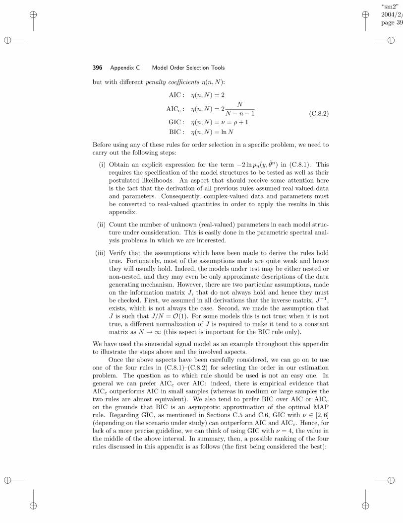
“sm2”2004/2/22page 396

i

i

i

i

i

i

i

i


but with different penalty coefficients η(n,N):

AIC : η(n,N) = 2

AICc : η(n,N) = 2N

N − n− 1

GIC : η(n,N) = ν = ρ+ 1

BIC : η(n,N) = lnN

(C.8.2)

Before using any of these rules for order selection in a specific problem, we need tocarry out the following steps:

(i) Obtain an explicit expression for the term −2 ln pn(y, θn) in (C.8.1). This

requires the specification of the model structures to be tested as well as theirpostulated likelihoods. An aspect that should receive some attention hereis the fact that the derivation of all previous rules assumed real-valued dataand parameters. Consequently, complex-valued data and parameters mustbe converted to real-valued quantities in order to apply the results in thisappendix.

(ii) Count the number of unknown (real-valued) parameters in each model struc-ture under consideration. This is easily done in the parametric spectral anal-ysis problems in which we are interested.

(iii) Verify that the assumptions which have been made to derive the rules holdtrue. Fortunately, most of the assumptions made are quite weak and hencethey will usually hold. Indeed, the models under test may be either nested ornon-nested, and they may even be only approximate descriptions of the datagenerating mechanism. However, there are two particular assumptions, madeon the information matrix J , that do not always hold and hence they mustbe checked. First, we assumed in all derivations that the inverse matrix, J−1,exists, which is not always the case. Second, we made the assumption thatJ is such that J/N = O(1). For some models this is not true; when it is nottrue, a different normalization of J is required to make it tend to a constantmatrix as N → ∞ (this aspect is important for the BIC rule only).

We have used the sinusoidal signal model as an example throughout this appendixto illustrate the steps above and the involved aspects.

Once the above aspects have been carefully considered, we can go on to useone of the four rules in (C.8.1)–(C.8.2) for selecting the order in our estimationproblem. The question as to which rule should be used is not an easy one. Ingeneral we can prefer AICc over AIC: indeed, there is empirical evidence thatAICc outperforms AIC in small samples (whereas in medium or large samples thetwo rules are almost equivalent). We also tend to prefer BIC over AIC or AICc

on the grounds that BIC is an asymptotic approximation of the optimal MAPrule. Regarding GIC, as mentioned in Sections C.5 and C.6, GIC with ν ∈ [2, 6](depending on the scenario under study) can outperform AIC and AICc. Hence, forlack of a more precise guideline, we can think of using GIC with ν = 4, the value inthe middle of the above interval. In summary, then, a possible ranking of the fourrules discussed in this appendix is as follows (the first being considered the best):

“sm2”2004/2/22page 397

i

i

i

i

i

i

i

i

Section C.8 Summary and the Multimodel Approach 397

101 102 1030

1

2

3

4

5

6

7

Data Length, N

η(n,

N)

GIC with ν=4

BIC

AIC AIC

c for n=5

Figure C.1. Penalty coefficients of AIC, GIC with ν = 4 (ρ = 3), AICc (forn = 5), and BIC, as functions of data length N .

• BIC

• GIC with ν = 4 (ρ = 3)

• AICc

• AIC

In Figure C.1 we show the penalty coefficients of the above rules, as functionsof N , to further illustrate the relationship between them.

C.8.2 The Multimodel Approach

We close this section with a brief discussion on a multimodel approach. Assumethat we have used our favorite information criterion, let us say XIC, and havecomputed its values for the model orders under test:

XIC(n); n = 1, . . . , n (C.8.3)

We can then pick the order that minimizes XIC(n) and hence end up using a singlemodel; this is the single model approach.

Alternatively, we can consider a multimodel approach. Specifically, let us picka M ∈ [1, n] (such as M = 3) and consider the model orders that give the Msmallest values of XIC(n), let us say n1, . . . , nM . From the derivations presented

“sm2”2004/2/22page 398

i

i

i

i

i

i

i

i


in the previous sections of this appendix, we can see that all information criteriaattempt to estimate twice the negative log-likelihood of the model:

−2 ln pn(y, θn) = −2 ln p(y|Hn) (C.8.4)

Hence, we can usee− 1

2XIC(n) (C.8.5)

as an estimate of the likelihood of the model with order equal to n (to within a mul-tiplicative constant). Consequently, instead of using just one model correspondingto the order that minimizes XIC(n), we can think of considering a combined useof the selected models (with orders n1, . . . , nM ) in which the contribution of eachmodel is proportional to its likelihood value, viz.:

e− 12XIC(nk)

∑Mj=1 e

− 12XIC(nj)

, k = 1, . . . ,M (C.8.6)

For more details on the multimodel approach, including guidelines for choosingM , we refer the interested reader to [Burnham and Anderson 2002; Stoica,

Selen, and Li 2004].

“sm2”2004/2/22page 399

i

i

i

i

i

i

i

i

A P P E N D I X D

Answers to Selected Exercises

1.3(a): Zh−k = H(1/z); Zgk = H(z)H∗(1/z∗)

1.4(a):

φ(ω) =σ2

(1 + a1e−iω)(1 + a∗1eiω)

[1 + |b1|2 + b1e

−iω + b∗1eiω]

r(0) =σ2

1 − |a1|2|1 − b1a

∗1|2 + |b1|2(1 − |a1|2)

r(k) =σ2

1 − |a1|2(

1 − b1a1

)

(1 − b∗1a1)

(−a1)k, k ≥ 1

1.9(a): φy(ω) = σ21 |H1(ω)|2 + ρσ1σ2 [H1(ω)H∗

2 (ω) +H2(ω)H∗1 (ω)] + σ2

2 |H2(ω)|2

2.3: An example is y(t) = 1, 1.1, 1, whose unbiased ACS estimate is r(k) =

1.07, 1.1, 1, giving φ(ω) = 1.07 + 2.2 cos(ω) + 2 cos(2ω).

2.4(b): varr(k) = σ4α2(k)(N − k) [1 + δk,0]

2.9:

(a) E Y (ωk)Y∗(ωr) =

σ2

N

N−1∑

t=0

ei(ωr−ωk)t =

σ2 k = r0 k 6= r

(c) E

φ(ω)

= σ2 = φ(ω), so φ(ω) is an unbiased estimate.

3.2: Decompose the ARMA system as x(t) = 1A(z)e(t) and y(t) = B(z)x(t).

Then x(t) is an AR(n) process. To find rx(k) from σ2, a1 . . . an, write theYule–Walker equations as:

1 0

a1. . .

.... . .

an . . . a1 1

rx(0)rx(1)

...rx(n)

+

0 a1 . . . an...

... 0... an 0

...0 0 . . . 0

r∗x(0)r∗x(1)...

r∗x(n)

=

σ2

0...0

or

A1rx +A2rcx =

[σ2

0

]

which can be solved for rx(m)nm=0. Then find rx(k) for k > n from equation(3.3.4) and rx(k) for k < 0 from r∗

x(−k). Finally,

ry(k) =

m∑

j=0

m∑

p=0

rx(k + p− j) bjb∗p

399

“sm2”2004/2/22page 400

i

i

i

i

i

i

i

i

400 Appendix D Answers to Selected Exercises

3.4: σ2b = E

|eb(t)|2

= [1 θTb ]Rn+1

[1θcb

]

= [1 θ∗b ]R

cn+1

[1θb

]

giving θb = θf and σ2b = σ2

f .

3.5(a):

RT2m+1

cm...c11d1

...dm

=

0...0σ2s

0...0

3.14: c` =∑ni=0 air(` − i) for 0 ≤ ` ≤ p, where r(k) = r(k) for k ≥ 1 ,

r(0) = r(0)/2, and r(k) = 0 for k < 0.

3.15(b): First solve for b1, . . . , bm from

cn cn−1 · · · cn−m+1

cn+1 cn · · · cn−m+2

......

. . ....

cn+m−1 cn+m−2 . . . cn

b1b2...bm

= −

cn+1

cn+2

...cn+m

Then a1, . . . , an can be obtained from ak = ck +∑mi=1 bick−i.

4.2:(a) E x(t) = 0; rx(k) = (α2 + σ2

α)eiω0k

(b) Let p(ϕ) =∑∞k=−∞ cke

−ikϕ be the Fourier series of p(ϕ) for ϕ ∈ [−π, π]. Then

E x(t) = αeiω0t

2π c1. Thus, E x(t) = 0 if and only if either α = 0 or c1 = 0. Inthis case, rx(k) is the same as in part (a).

5.8: The height of the peak of the (unnormalized) Capon spectrum is

1/a∗(ω)R−1a(ω)|ω=ω0 =mα2 + σ2

m

“sm2”2004/2/22page 401

i

i

i

i

i

i

i

i

Bibliography

Abrahamsson, R., A. Jakobsson, and P. Stoica (2004). Spatial Amplitude and PhaseEstimation Method for Arbitrary Array Geometries. Technical report, IT Department,Uppsala University, Sweden.

Akaike, H. (1974). “A new look at the statistical model identification,” IEEE Transactionson Automatic Control 19, 716–723.

Akaike, H. (1978). “On the likelihood of a time series model,” The Statistician 27, 217–235.

Anderson, T. W. (1971). The Statistical Analysis of Time Series. New York: Wiley.

Aoki, M. (1987). State Space Modeling of Time Series. Berlin: Springer-Verlag.

Bangs, W. J. (1971). Array Processing with Generalized Beamformers. Ph. D. thesis, YaleUniversity, New Haven, CT.

Barabell, A. J. (1983). “Improving the resolution performance of eigenstructure-baseddirection-finding algorithms,” in Proceedings of the International Conference on Acoustics,Speech, and Signal Processing, Boston, MA, pp. 336–339.

Bartlett, M. S. (1948). “Smoothing periodograms for time series with continuous spectra,”Nature 161, 686–687. (reprinted in [Kesler 1986]).

Bartlett, M. S. (1950). “Periodogram analysis and continuous spectra,” Biometrika 37,1–16.

Baysal, U. and R. Moses (2003). “On the geometry of isotropic arrays,” IEEE Transactionson Signal Processing 51 (6), 1469–1478.

Beex, A. A. and L. L. Scharf (1981). “Covariance sequence approximation for paramet-ric spectrum modeling,” IEEE Transactions on Acoustics, Speech, and Signal Process-ing ASSP–29 (5), 1042–1052.

Besson, O. and P. Stoica (1999). “Nonlinear least-squares approach to frequency estima-tion and detection of sinusoidal signals with arbitrary envelope,” Digital Signal Processing:A Review Journal 9, 45–56.

Bhansali, R. J. (1980). “Autoregressive and window estimates of the inverse correlationfunction,” Biometrika 67, 551–566.

Bhansali, R.-J. and D. Y. Downham (1977). “Some properties of the order of an autore-gressive model selected by a generalization of Akaike’s FPE criterion,” Biometrika 64,547–551.

Bienvenu, G. (1979). “Influence of the spatial coherence of the background noise on highresolution passive methods,” in Proceedings of the International Conference on Acoustics,Speech, and Signal Processing, Washington, DC, pp. 306–309.

Blackman, R. B. and J. W. Tukey (1959). The Measurement of Power Spectra from thePoint of View of Communication Engineering. New York: Dover.

Bloomfield, P. (1976). Fourier Analysis of Time Series — An Introduction. New York:Wiley.

401

“sm2”2004/2/22page 402

i

i

i

i

i

i

i

i

402 BIBLIOGRAPHY

Bohme, J. F. (1991). “Array processing,” in S. Haykin (Ed.), Advances in SpectrumAnalysis and Array Processing, Volume 2, pp. 1–63. Englewood Cliffs, NJ: Prentice Hall.

Bottcher, A. and B. Silbermann (1983). Invertibility and Asymptotics of Toeplitz Matrices.Berlin: Akademie-Verlag.

Bracewell, R. N. (1986). The Fourier Transform and its Applications, 2nd Edition. NewYork: McGraw-Hill.

Bresler, Y. and A. Macovski (1986). “Exact maximum likelihood parameter estimation ofsuperimposed exponential signals in noise,” IEEE Transactions on Acoustics, Speech, andSignal Processing ASSP-34 (5), 1081–1089.

Brillinger, D. R. (1981). Time Series — Data Analysis and Theory. New York: Holt,Rinehart, and Winston.

Brockwell, R. J. and R. A. Davis (1991). Time Series — Theory and Methods, 2nd Edition.New York: Springer-Verlag.

Broersen, P. M. T. (2000). “Finite sample criteria for autoregressive order selection,”IEEE Transactions on Signal Processing 48 (12), 3550–3558.

Broersen, P. M. T. (2002). “Automatic spectral analysis with time series models,” IEEETransactions on Instrumentation and Measurement 51 (2), 211–216.

Bronez, T. P. (1992). “On the performance advantage of multitaper spectral analysis,”IEEE Transactions on Signal Processing 40 (12), 2941–2946.

Burg, J. P. (1972). “The relationship between maximum entropy spectra and maximumlikelihood spectra,” Geophysics 37, 375–376. (reprinted in [Childers 1978]).

Burg, J. P. (1975). Maximum Entropy Spectral Analysis. Ph. D. thesis, Stanford University.

Burnham, K. P. and D. R. Anderson (2002). Model Selection and Multi-Model Inference.New York: Springer.

Byrnes, C. L., T. T. Georgiou, and A. Lindquist (2000). “A new approach to spectralestimation: a tunable high-resolution spectral estimator,” IEEE Transactions on SignalProcessing 48 (11), 3189–3205.

Byrnes, C. L., T. T. Georgiou, and A. Lindquist (2001). “A generalized entropy cri-terion for Nevanlinna-Pick interpolation with degree constraint,” IEEE Transactions onAutomatic Control 46 (6), 822–839.

Cadzow, J. A. (1982). “Spectrum estimation: An overdetermined rational model equationapproach,” Proceedings of the IEEE 70 (9), 907–939.

Calvez, L. C. and P. Vilbe (1992). “On the uncertainty principle in discrete signals,” IEEETransactions on Circuits and Systems 39 (6), 394–395.

Cantoni, A. and P. Butler (1976). “Eigenvalues and eigenvectors of symmetric centrosym-metric matrices,” Linear Algebra and its Applications 13 (3), 275–288.

Capon, J. (1969). “High-resolution frequency-wavenumber spectrum analysis,” Proceed-ings of the IEEE 57 (8), 1408–1418. (reprinted in [Childers 1978]).

Cavanaugh, J. E. (1997). “Unifying the derivations for the Akaike and corrected Akaikeinformation criteria,” Statistics and Probability Letters 23, 201–208.

Childers, D. G. (Ed.) (1978). Modern Spectrum Analysis. New York: IEEE Press.

“sm2”2004/2/22page 403

i

i

i

i

i

i

i

i

BIBLIOGRAPHY 403

Choi, B. (1992). ARMA Model Identification. New York: Springer-Verlag.

Clark, M. P., L. Elden, and P. Stoica (1997). “A computationally efficient implementationof 2D IQML,” in Proceedings of the 31st Asilomar Conference on Signals, Systems, andComputers, Pacific Grove, CA, pp. 1730–1734.

Clark, M. P. and L. L. Scharf (1994). “Two-dimensional modal analysis based on maximumlikelihood,” IEEE Transactions on Signal Processing 42 (6), 1443–1452.

Cleveland, W. S. (1972). “The inverse autocorrelations of a time series and their applica-tions,” Technometrics 14, 277–298.

Cohen, L. (1995). Time-Frequency Analysis. Englewood Cliffs, NJ: Prentice Hall.

Cooley, J. W. and J. W. Tukey (1965). “An algorithm for the machine calculation ofcomplex Fourier series,” Math. Computation 19, 297–301.

Cornwell, T. and A. Bridle (1996). Deconvolution Tutorial. Technical report, National Ra-dio Astronomy Observatory. http://www.cv.nrao.edu/ãbridle/deconvol/deconvol.html.

Cox, H. (1973). “Resolving power and sensitivity to mismatch of optimum array proces-sors,” Journal of the Acoustical Society of America 54, 771–785.

Cramer, H. (1946). Mathematical Methods of Statistics. Princeton, NJ: Princeton Univer-sity Press.

Daniell, P. J. (1946). “Discussion of ‘On the theoretical specification and sampling prop-erties of autocorrelated time-series’,” Journal of the Royal Statistical Society 8, 88–90.

de Waele, S. and P. M. T. Broersen (2003). “Order selection for vector autoregressivemodels,” IEEE Transactions on Signal Processing 51 (2), 427–433.

DeGraaf, S. R. (1994). “Sidelobe reduction via adaptive FIR filtering in SAR imagery,”IEEE Transactions on Image Processing 3 (3), 292–301.

Delsarte, P. and Y. Genin (1986). “The split Levinson algorithm,” IEEE Transactions onAcoustics, Speech, and Signal Processing ASSP–34 (3), 470–478.

Demeure, C. J. and C. T. Mullis (1989). “The Euclid algorithm and the fast computation ofcross–covariance and autocovariance sequences,” IEEE Transactions on Acoustics, Speech,and Signal Processing ASSP–37 (4), 545–552.

Dempster, A., N. Laird, and D. Rubin (1977). “Maximimum likelihood from incompletedata via the EM algorithm,” Journal of the Royal Statistical Society 39, 1–38.

Djuric, P. (1998). “Asymptotic MAP criteria for model selection,” IEEE Transactions onSignal Processing 46 (10), 2726–2735.

Doron, M., E. Doron, and A. Weiss (1993). “Coherent wide-band processing for arbitraryarray geometry,” IEEE Transactions on Signal Processing 41 (1), 414–417.

Doroslovacki, M. I. (1998). “Product of second moments in time and frequency for discrete-time signals and the uncertainty limit,” Signal Processing 67 (1), 59–76.

Dumitrescu, B., I. Tabus, and P. Stoica (2001). “On the parameterization of positivereal sequences and MA parameter estimation,” IEEE Transactions on Signal Process-ing 49 (11), 2630–2639.

Durbin, J. (1959). “Efficient estimation of parameters in moving-average models,”Biometrika 46, 306–316.

“sm2”2004/2/22page 404

i

i

i

i

i

i

i

i

404 BIBLIOGRAPHY

Durbin, J. (1960). “The fitting of time series models,” Review of the International Instituteof Statistics 28, 233–244.

Faurre, P. (1976). “Stochastic realization algorithms,” in R. K. Mehra and D. G. Lainiotis(Eds.), System Identification: Advances and Case Studies. London, England: AcademicPress.

Feldman, D. D. and L. J. Griffiths (1994). “A projection approach for robust adaptivebeamforming,” IEEE Transactions on Signal Processing 42 (4), 867–876.

Fisher, R. A. (1922). “On the mathematical foundations of theoretical statistics,” Philo-sophical Transactions of the Royal Society of London 222, 309–368.

Friedlander, B., M. Morf, T. Kailath, and L. Ljung (1979). “New inversion formulas formatrices classified in terms of their distance from Toeplitz matrices,” Linear Algebra andits Applications 27, 31–60.

Fuchs, J. J. (1987). “ARMA order estimation via matrix perturbation theory,” IEEETransactions on Automatic Control AC–32 (4), 358–361.

Fuchs, J. J. (1988). “Estimating the number of sinusoids in additive white noise,” IEEETransactions on Acoustics, Speech, and Signal Processing ASSP–36 (12), 1846–1854.

Fuchs, J. J. (1992). “Estimation of the number of signals in the presence of unknowncorrelated sensor noise,” IEEE Transactions on Signal Processing 40 (5), 1053–1061.

Fuchs, J. J. (1996). “Rectangular Pisarenko method applied to source localization,” IEEETransactions on Signal Processing 44 (10), 2377–2383.

Georgiou, T. T. (1987). “Realization of power spectra from partial covariance sequences,”IEEE Transactions on Acoustics, Speech, and Signal Processing ASSP–35 (4), 438–449.

Gersh, W. (1970). “Estimation of the autoregressive parameters of mixed autoregressivemoving–average time series,” IEEE Transactions on Automatic Control AC–15 (5), 583–588.

Ghogho, M. and A. Swami (1999). “Fast computation of the exact FIM for deterministicsignals in colored noise,” IEEE Transactions on Signal Processing 47 (1), 52–61.

Gini, F. and F. Lombardini (2002). “Multilook APES for multibaseline SAR interferom-etry,” IEEE Transactions on Signal Processing 50 (7), 1800–1803.

Golub, G. H. and C. F. Van Loan (1989). Matrix Computations, 2nd Edition. Baltimore:The Johns Hopkins University Press.

Gray, R. M. (1972). “On the asymptotic eigenvalue distribution of Toeplitz matrices,”IEEE Transactions on Information Theory IT–18, 725–730.

Hannan, E. and B. Wahlberg (1989). “Convergence rates for inverse Toeplitz matrixforms,” Journal of Multivariate Analysis 31, 127–135.

Hannan, E. J. and M. Deistler (1988). The Statistical Theory of Linear Systems. NewYork: Wiley.

Harris, F. J. (1978). “On the use of windows for harmonic analysis with the discreteFourier transform,” Proceedings of the IEEE 66 (1), 51–83. (reprinted in [Kesler 1986]).

Hayes III, M. H. (1996). Statistical Digital Signal Processing and Modeling. New York:Wiley.

“sm2”2004/2/22page 405

i

i

i

i

i

i

i

i

BIBLIOGRAPHY 405

Haykin, S. (Ed.) (1991). Advances in Spectrum Analysis and Array Processing, Volumes1 and 2. Englewood Cliffs, NJ: Prentice Hall.

Haykin, S. (Ed.) (1995). Advances in Spectrum Analysis and Array Processing, Volume 3.Englewood Cliffs, NJ: Prentice Hall.

Heiser, W. J. (1995). “Convergent computation by iterative majorization: theory and ap-plications in multidimensional data analysis,” in W. J. Krzanowski (Ed.), Recent Advancesin Descriptive Multivariate Analysis, pp. 157–189. Oxford: Oxford University Press.

Hogbom, J. (1974). “Aperture synthesis with a non-regular distribution of interferometerbaselines,” Astronomy and Astrophysics, Supplement 15, 417–426.

Horn, R. A. and C. A. Johnson (1985). Matrix Analysis. Cambridge, England: CambridgeUniversity Press.

Horn, R. A. and C. A. Johnson (1989). Topics in Matrix Analysis. Cambridge, England:Cambridge University Press.

Hua, Y. and T. Sarkar (1990). “Matrix pencil method for estimating parameters of expo-nentially damped/undamped sinusoids in noise,” IEEE Transactions on Acoustics, Speech,and Signal Processing 38 (5), 814–824.

Hudson, J. E. (1981). Adaptive Array Principles. London: Peter Peregrinus.

Hurvich, C. and C. Tsai (1993). “A corrected Akaike information criterion for vectorautoregressive model selection,” Journal of Time Series Analysis 14, 271–279.

Hwang, J.-K. and Y.-C. Chen (1993). “A combined detection-estimation algorithm forthe harmonic-retrieval problem,” Signal Processing 30 (2), 177–197.

Iohvidov, I. S. (1982). Hankel and Toeplitz Matrices and Forms. Boston, MA: Birkhauser.

Ishii, R. and K. Furukawa (1986). “The uncertainty principle in discrete signals,” IEEETransactions on Circuits and Systems 33 (10), 1032–1034.

Jakobsson, A., L. Marple, and P. Stoica (2000). “Computationally efficient two-dimensional Capon spectrum analysis,” IEEE Transactions on Signal Processing 48 (9),2651–2661.

Jakobsson, A. and P. Stoica (2000). “Combining Capon and APES for estimation ofspectral lines,” Circuits, Systems, and Signal Processing 19, 159–169.

Janssen, P. and P. Stoica (1988). “On the expectation of the product of four matrix-valued Gaussian random variables,” IEEE Transactions on Automatic Control AC–33 (9),867–870.

Jansson, M. and P. Stoica (1999). “Forward-only and forward-backward sample covari-ances — a comparative study,” Signal Processing 77 (3), 235–245.

Jenkins, G. M. and D. G. Watts (1968). Spectral Analysis and its Applications. SanFrancisco, CA: Holden-Day.

Johnson, D. H. and D. E. Dudgeon (1992). Array Signal Processing — Concepts andMethods. Englewood Cliffs, NJ: Prentice Hall.

Kailath, T. (1980). Linear Systems. Englewood Cliffs, NJ: Prentice Hall.

Kashyap, R. L. (1980). “Inconsistency of the AIC rule for estimating the order of autore-gressive models,” IEEE Transactions on Automatic Control 25 (5), 996–998.

“sm2”2004/2/22page 406

i

i

i

i

i

i

i

i

406 BIBLIOGRAPHY

Kashyap, R. L. (1982). “Optimal choice of AR and MA parts in autoregressive movingaverage models,” IEEE Transactions on Pattern Analysis and Machine Intelligence 4 (2),99–104.

Kay, S. M. (1988). Modern Spectral Estimation, Theory and Application. EnglewoodCliffs, NJ: Prentice Hall.

Kesler, S. B. (Ed.) (1986). Modern Spectrum Analysis II. New York: IEEE Press.

Kinkel, J. F., J. Perl, L. Scharf, and A. Stubberud (1979). “A note on covariance–invariantdigital filter design and autoregressive–moving average spectral estimation,” IEEE Trans-actions on Acoustics, Speech, and Signal Processing ASSP–27 (2), 200–202.

Koopmans, L. H. (1974). The Spectral Analysis of Time Series. New York: AcademicPress.

Kullback, S. and R. A. Leibler (1951). “On information and sufficiency,” Annals of Math-ematical Statistics 22, 79–86.

Kumaresan, R. (1983). “On the zeroes of the linear prediction-error filter for deterministicsignals,” IEEE Transactions on Acoustics, Speech, and Signal Processing ASSP–31 (1),217–220.

Kumaresan, R., L. L. Scharf, and A. K. Shaw (1986). “An algortihm for pole-zero model-ing and spectral analysis,” IEEE Transactions on Acoustics, Speech, and Signal Process-ing ASSP–34 (6), 637–640.

Kumaresan, R. and D. W. Tufts (1983). “Estimating the angles of arrival of multiple planewaves,” IEEE Transactions on Aerospace and Electronic Systems AES–19, 134–139.

Kung, S. Y., K. S. Arun, and D. V. B. Rao (1983). “State-space and singular-valuedecomposition-based approximation methods for the harmonic retrieval problem,” J. Op-tical Soc. Amer. 73, 1799–1811.

Lacoss, R. T. (1971). “Data adaptive spectral analysis methods,” Geophysics 36, 134–148.(reprinted in [Childers 1978]).

Lagunas, M., M. Santamaria, A. Gasull, and A. Moreno (1986). “Maximum likelihoodfilters in spectral estimation problems,” Signal Processing 10 (1), 7–18.

Larsson, E., J. Li, and P. Stoica (2003). “High-resolution nonparametric spectral analysis:Theory and applications,” in Y. Hua, A. Gershman, and Q. Cheng (Eds.), High-Resolutionand Robust Signal Processing. New York: Marcel Dekker.

Lee, J. and D. C. Munson Jr. (1995). “Effectiveness of spatially-variant apodization,” inProceedings of the International Conference on Image Processing, Volume 1, pp. 147–150.

Levinson, N. (1947). “The Wiener RMS (root mean square) criterion in filter design andprediction,” Journal of Math. and Physics 25, 261–278.

Li, J. and P. Stoica (1996a). “An adaptive filtering approach to spectral estimation andSAR imaging,” IEEE Transactions on Signal Processing 44 (6), 1469–1484.

Li, J. and P. Stoica (1996b). “Efficient mixed-spectrum estimation with applications totarget feature extraction,” IEEE Transactions on Signal Processing 44 (2), 281–295.

Li, J., P. Stoica, and Z. Wang (2003). “On robust Capon beamforming and diagonalloading,” IEEE Transactions on Signal Processing 51 (7), 1702–1715.

“sm2”2004/2/22page 407

i

i

i

i

i

i

i

i

BIBLIOGRAPHY 407

Li, J., P. Stoica, and Z. Wang (2004). “Doubly constrained robust Capon beamformer,”IEEE Transactions on Signal Processing 52.

Linhart, H. and W. Zucchini (1986). Model Selection. New York: Wiley.

Ljung, L. (1987). System Identification — Theory for the User. Englewood Cliffs, NJ:Prentice Hall.

Markel, J. D. (1971). “FFT pruning,” IEEE Transactions on Audio and Electroacous-tics AU–19 (4), 305–311.

Marple, L. (1987). Digital Spectral Analysis with Applications. Englewood Cliffs, NJ:Prentice Hall.

Marzetta, T. L. (1983). “A new interpretation for Capon’s maximum likelihood methodof frequency-wavenumber spectrum estimation,” IEEE Transactions on Acoustics, Speech,and Signal Processing ASSP–31 (2), 445–449.

Mayne, D. Q. and F. Firoozan (1982). “Linear identification of ARMA processes,” Auto-matica 18, 461–466.

McCloud, M., L. Scharf, and C. Mullis (1999). “Lag-windowing and multiple-data-windowing are roughly equivalent for smooth spectrum estimation,” IEEE Transactionson Signal Processing 47 (3), 839–843.

McKelvey, T. and M. Viberg (2001). “A robust frequency domain subspace algorithm formulti-component harmonic retrieval,” in Proceedings of the 35th Asilomar Conference onSignals, Systems, and Computers, Pacific Grove, CA, pp. 68–72.

McLachlan, G. J. and T. Krishnan (1997). The EM Algorithm and Extensions. New York:Wiley.

McQuarrie, A. D. R. and C.-L. Tsai (1998). Regression and Time Series Model Selection.Singapore: World Scientific Publishing.

Moon, T. K. (1996). “The expectation-maximization algorithm,” IEEE Signal ProcessingMagazine 13, 47–60.

Moses, R. and A. A. Beex (1986). “A comparison of numerator estimators for ARMAspectra,” IEEE Transactions on Acoustics, Speech, and Signal Processing ASSP–34 (6),1668–1671.

Moses, R., V. Simonyte, P. Stoica, and T. Soderstrom (1994). “An efficient linear methodfor ARMA spectral estimation,” International Journal of Control 59 (2), 337–356.

Mullis, C. T. and L. L. Scharf (1991). “Quadratic estimators of the power spectrum,” inS. Haykin (Ed.), Advances in Spectrum Analysis and Array Processing. Englewood Cliffs,NJ: Prentice Hall.

Musicus, B. (1985). “Fast MLM power spectrum estimation from uniformly spaced cor-relations,” IEEE Transactions on Acoustics, Speech, and Signal Processing ASSP-33 (6),1333–1335.

Naidu, P. S. (1996). Modern Spectrum Analysis of Time Series. Boca Raton, FL: CRCPress.

Ninness, B. (2003). “The asymptotic CRLB for the spectrum of ARMA processes,” IEEETransactions on Signal Processing 51 (6), 1520–1531.

“sm2”2004/2/22page 408

i

i

i

i

i

i

i

i

408 BIBLIOGRAPHY

Onn, R. and A. O. Steinhardt (1993). “Multi-window spectrum estimation — a linearalgebraic approach,” International Journal on Adaptive Control and Signal Processing 7,103–116.

Oppenheim, A. V. and R. W. Schafer (1989). Discrete-Time Signal Processing. EnglewoodCliffs, NJ: Prentice Hall.

Ottersten, B., P. Stoica, and R. Roy (1998). “Covariance matching estimation techniquesfor array signal processing applications,” Digital Signal Processing 8, 185–210.

Ottersten, B., M. Viberg, P. Stoica, and A. Nehorai (1993). “Exact and large sample max-imum likelihood techniques for parameter estimation and detection in array processing,”in S. Haykin, J.Litva, and T. J. Shephard (Eds.), Radar Array Processing, pp. 99–151.New York: Springer Verlag.

Papoulis, A. (1977). Signal Analysis. New York: McGraw-Hill.

Paulraj, A., R. Roy, and T. Kailath (1986). “A subspace rotation approach to signalparameter estimation,” Proceedings of the IEEE 74 (7), 1044–1046.

Percival, D. B. and A. T. Walden (1993). Spectral Analysis for Physical Applications —Multitaper and Conventional Univariate Techniques. Cambridge, England: CambridgeUniversity Press.

Pillai, S. U. (1989). Array Signal Processing. New York: Springer-Verlag.

Pisarenko, V. F. (1973). “The retrieval of harmonics from a covariance function,” Geo-physical Journal of the Royal Astronomical Society 33, 347–366. (reprinted in [Kesler

1986]).

Porat, B. (1994). Digital Processing of Random Signals — Theory and Methods. Engle-wood Cliffs, NJ: Prentice Hall.

Porat, B. (1997). A Course in Digital Signal Processing. New York: Wiley.

Priestley, M. B. (1981). Spectral Analysis and Time Series. London, England: AcademicPress.

Priestley, M. B. (1997). “Detection of periodicities,” in T. S. Rao, M. B. Priestley, andO. Lessi (Eds.), Applications of Time Series Analysis in Astronomy and Meteorology, pp.65–88. London, England: Chapman and Hall.

Proakis, J. G., C. M. Rader, F. Ling, and C. L. Nikias (1992). Advanced Digital SignalProcessing. New York: Macmillan.

Rao, B. D. and K. S. Arun (1992). “Model based processing of signals: A state spaceapproach,” Proceedings of the IEEE 80 (2), 283–309.

Rao, B. D. and K. V. S. Hari (1993). “Weighted subspace methods and spatial smoothing:Analysis and comparison,” IEEE Transactions on Signal Processing 41 (2), 788–803.

Rao, C. R. (1945). “Information and accuracy attainable in the estimation of statisticalparameters,” Bulletin of the Calcutta Mathematical Society 37, 81–91.

Riedel, K. and A. Sidorenko (1995). “Minimum bias multiple taper spectral estimation,”IEEE Transactions on Signal Processing 43 (1), 188–195.

Rissanen, J. (1978). “Modeling by the shortest data description,” Automatica 14 (5),465–471.

“sm2”2004/2/22page 409

i

i

i

i

i

i

i

i

BIBLIOGRAPHY 409

Rissanen, J. (1982). “Estimation of structure by minimum description length,” Circuits,Systems, and Signal Processing 1 (3–4), 395–406.

Roy, R. and T. Kailath (1989). “ESPRIT—Estimation of signal parameters via rota-tional invariance techniques,” IEEE Transactions on Acoustics, Speech, and Signal Pro-cessing ASSP-37 (7), 984–995.

Sakamoto, Y., M. Ishiguro, and G. Kitagawa (1986). Akaike Information Criterion Statis-tics. Tokyo: KTK Scientific Publishers.

Sando, S., A. Mitra, and P. Stoica (2002). “On the Cramer-Rao bound for model-basedspectral analysis,” IEEE Signal Processing Letters 9 (2), 68–71.

Scharf, L. L. (1991). Statistical Signal Processing — Detection, Estimation, and TimeSeries Analysis. Reading, MA: Addison-Wesley.

Schmidt, R. O. (1979). “Multiple emitter location and signal parameter estimation,”in Proc. RADC, Spectral Estimation Workshop, Rome, NY, pp. 243–258. (reprinted in[Kesler 1986]).

Schuster, A. (1898). “On the investigation of hidden periodicities with application to asupposed twenty-six-day period of meteorological phenomena,” Teor. Mag. 3 (1), 13–41.

Schuster, A. (1900). “The periodogram of magnetic declination as obtained from therecords of the Greenwich Observatory during the years 1871–1895,” Trans. CambridgePhilos. Soc 18, 107–135.

Schwarz, G. (1978a). “Estimating the dimension of a model,” Annals of Statistics 6,461–464.

Schwarz, U. J. (1978b). “Mathematical-statistical description of the iterative beam re-moving technique (method CLEAN),” Astronomy and Astrophysics 65, 345–356.

Seghouane, A.-K., M. Bekara, and G. Fleury (2003). “A small sample model selectioncriterion based on Kullback’s symmetric divergence,” in Proceedings of the InternationalConference on Acoustics, Speech, and Signal Processing, Volume 6, Hong Kong, pp. 145–148.

Slepian, D. (1954). “Estimation of signal parameters in the presence of noise,” Transac-tions of the IRE Professional Group on Information Theory 3, 68–89.

Slepian, D. (1964). “Prolate spheroidal wave functions, Fourier analysis and uncertainty— IV,” Bell System Technical Journal 43, 3009–3057. (see also Bell System TechnicalJournal, vol. 40, pp. 43–64, 1961; vol. 44, pp. 1745–1759, 1965; and vol. 57, pp. 1371–1429, 1978).

Soderstrom, T. and P. Stoica (1989). System Identification. London, England: PrenticeHall International.

Stankwitz, H. C., R. J. Dallaire, and J. R. Fienup (1994). “Spatially variant apodization forsidelobe control in SAR imagery,” in Record of the 1994 IEEE National Radar Conference,pp. 132–137.

Stewart, G. W. (1973). Introduction to Matrix Computations. New York: Academic Press.

Stoica, P. and O. Besson (2000). “Maximum likelihood DOA estimation for constant-modulus signal,” Electronics Letters 36 (9), 849–851.

Stoica, P., O. Besson, and A. Gershman (2001). “Direction-of-arrival estimation of anamplitude-distorted wavefront,” IEEE Transactions on Signal Processing 49 (2), 269–276.

“sm2”2004/2/22page 410

i

i

i

i

i

i

i

i

410 BIBLIOGRAPHY

Stoica, P., P. Eykhoff, P. Jannsen, and T. Soderstrom (1986). “Model structure selectionby cross-validation,” International Journal of Control 43 (11), 1841–1878.

Stoica, P., B. Friedlander, and T. Soderstrom (1987a). “Approximate maximum-likelihoodapproach to ARMA spectral estimation,” International Journal of Control 45 (4), 1281–1310.

Stoica, P., B. Friedlander, and T. Soderstrom (1987b). “Instrumental variable methodsfor ARMA models,” in C. T. Leondes (Ed.), Control and Dynamic Systems — Advancesin Theory and Applications, Volume 25, pp. 79–150. New York: Academic Press.

Stoica, P., A. Jakobsson, and J. Li (1997). “Cisoid parameter estimation in the colorednoise case — asymptotic Cramer-Rao bound, maximum likelihood, and nonlinear leastsquares,” IEEE Transactions on Signal Processing 45 (8), 2048–2059.

Stoica, P. and E. G. Larsson (2001). “Comments on ‘Linearization method for find-ing Cramer-Rao bounds in signal processing’,” IEEE Transactions on Signal Process-ing 49 (12), 3168–3169.

Stoica, P., E. G. Larsson, and A. B. Gershman (2001). “The stochastic CRB for arrayprocessing: a textbook derivation,” IEEE Signal Processing Letters 8 (5), 148–150.

Stoica, P., E. G. Larsson, and J. Li (2000). “Adaptive filter-bank approach to restorationand spectral analysis of gapped data,” The Astronomical Journal 120 (4), 2163–2173.

Stoica, P., H. Li, and J. Li (1999). “A new derivation of the APES filter,” IEEE SignalProcessing Letters 6 (8), 205–206.

Stoica, P., T. McKelvey, and J. Mari (2000). “MA estimation in polynomial time,” IEEETransactions on Signal Processing 48 (7), 1999–2012.

Stoica, P. and R. Moses (1990). “On biased estimators and the unbiased Cramer-Raolower bound,” Signal Processing 21, 349–350.

Stoica, P., R. Moses, B. Friedlander, and T. Soderstrom (1989). “Maximum likelihoodestimation of the parameters of multiple sinusoids from noisy measurements,” IEEE Trans-actions on Acoustics, Speech, and Signal Processing ASSP–37 (3), 378–392.

Stoica, P., R. Moses, T. Soderstrom, and J. Li (1991). “Optimal high-order Yule-Walkerestimation of sinusoidal frequencies,” IEEE Transactions on Signal Processing 39 (6),1360–1368.

Stoica, P. and A. Nehorai (1986). “An asymptotically efficient ARMA estimator based onsample covariances,” IEEE Transactions on Automatic Control AC–31 (11), 1068–1071.

Stoica, P. and A. Nehorai (1987). “On stability and root location of linear predictionmodels,” IEEE Transactions on Acoustics, Speech, and Signal Processing ASSP-35, 582–584.

Stoica, P. and A. Nehorai (1989a). “MUSIC, maximum likelihood, and Cramer-Raobound,” IEEE Transactions on Acoustics, Speech, and Signal Processing ASSP–37 (5),720–741.

Stoica, P. and A. Nehorai (1989b). “Statistical analysis of two nonlinear least-squaresestimators of sine-wave parameters in the colored-noise case,” Circuits, Systems, andSignal Processing 8 (1), 3–15.

Stoica, P. and A. Nehorai (1990). “Performance study of conditional and unconditionaldirection-of-arrival estimation,” IEEE Transactions on Signal Processing SP-38 (10),1783–1795.

“sm2”2004/2/22page 411

i

i

i

i

i

i

i

i

BIBLIOGRAPHY 411

Stoica, P. and A. Nehorai (1991). “Performance comparison of subspace rotation andMUSIC methods for direction estimation,” IEEE Transactions on Signal Processing 39 (2),446–453.

Stoica, P. and B. Ottersten (1996). “The evil of superefficiency,” Signal Processing 55 (1),133–136.

Stoica, P., N. Sandgren, Y. Selen, L. Vanhamme, and S. Van Huffel (2003). “Frequency-domain method based on the singular value decomposition for frequency-selective NMRspectroscopy,” Journal of Magnetic Resonance 165 (1), 80–88.

Stoica, P. and Y. Selen (2004a). “Cyclic minimizers, majorization techniques, andthe expectation-maximization algorithm: A refresher,” IEEE Signal Processing Maga-zine 21 (1), 112–114.

Stoica, P. and Y. Selen (2004b). “Model order selection: A review of the AIC, GIC, andBIC rules,” IEEE Signal Processing Magazine 21 (2).

Stoica, P., Y. Selen, and J. Li (2004). Multi-Model Approach to Model Selection. Technicalreport, IT Department, Uppsala University, Sweden.

Stoica, P. and K. C. Sharman (1990). “Maximum likelihood methods for direction-of-arrival estimation,” IEEE Transactions on Acoustics, Speech, and Signal Process-ing ASSP-38 (7), 1132–1143.

Stoica, P., T. Soderstrom, and F. Ti (1989). “Asymptotic properties of the high-order Yule-Walker estimates of sinusoidal frequencies,” IEEE Transactions on Acoustics, Speech, andSignal Processing ASSP–37 (11), 1721–1734.

Stoica, P. and T. Soderstrom (1991). “Statistical analysis of MUSIC and subspace rotationestimates of sinusoidal frequencies,” IEEE Transactions on Signal Processing SP-39 (8),1836–1847.

Stoica, P. and T. Sundin (2001). “Nonparametric NMR spectroscopy,” Journal of Mag-netic Resonance 152 (1), 57–69.

Stoica, P., Z. Wang, and J. Li (2003). “Robust Capon beamforming,” IEEE Signal Pro-cessing Letters 10 (6), 172–175.

Strang, G. (1988). Linear Algebra and its Applications. Orlando, FL: Harcourt BraceJovanovich.

Sturm, J. F. (1999). “Using SeDuMi, a Matlab toolbox for optimization over symmetriccones,” Optimization Methods and Software 11–12, 625–653. Software available on-line athttp://fewcal.uvt.nl/sturm/software/sedumi.html.

Therrien, C. W. (1992). Discrete Random Signals and Statistical Signal Processing. En-glewood Cliffs, NJ: Prentice Hall.

Thomson, D. J. (1982). “Spectrum estimation and harmonic analysis,” Proceedings of theIEEE 72 (9), 1055–1096.

Tufts, D. W. and R. Kumaresan (1982). “Estimation of frequencies of multiple sinu-soids: Making linear prediction perform like maximum likelihood,” Proceedings of theIEEE 70 (9), 975–989.

Umesh, S. and D. W. Tufts (1996). “Estimation of parameters of exponentially dampedsinusoids using fast maximum likelihood estimation with application to NMR spectroscopydata,” IEEE Transactions on Signal Processing 44 (9), 2245–2259.

“sm2”2004/2/22page 412

i

i

i

i

i

i

i

i

412 BIBLIOGRAPHY

Van Huffel, S. and J. Vandewalle (1991). The Total Least Squares Problem: ComputationalAspects and Analysis. Philadelphia, PA: SIAM.

van Overschee, P. and B. de Moor (1996). Subspace Identification for Linear Systems:Theory - Implementation - Methods. Boston, MA: Kluwer Academic.

Van Trees, H. L. (1968). Detection, Estimation, and Modulation Theory, Part I. NewYork: Wiley.

Van Trees, H. L. (2002). Optimum Array Processing (Part IV of Detection, Estimation,and Modulation Theory). New York: Wiley.

Van Veen, B. D. and K. M. Buckley (1988). “Beamforming: A versatile approach tospatial filtering,” IEEE ASSP Magazine 5 (2), 4–24.

Viberg, M. (1995). “Subspace-based methods for the identification of linear time-invariantsystems,” Automatica 31 (12), 1835–1851.

Viberg, M. and B. Ottersten (1991). “Sensor array processing based on subspace fitting,”IEEE Transactions on Signal Processing 39 (5), 1110–1121.

Viberg, M., B. Ottersten, and T. Kailath (1991). “Detection and estimation in sensorarrays using weighted subspace fitting,” IEEE Transactions on Acoustics, Speech, andSignal Processing ASSP–34 (11), 2436–2449.

Viberg, M., P. Stoica, and B. Ottersten (1995). “Array processing in correlated noisefields based on instrumental variables and subspace fitting,” IEEE Transactions on SignalProcessing 43 (5), 1187–1195.

Vostry, Z. (1975). “New algorithm for polynomial spectral factorization with quadraticconvergence, Part I,” Kybernetika 11, 415–422.

Vostry, Z. (1976). “New algorithm for polynomial spectral factorization with quadraticconvergence, Part II,” Kybernetika 12, 248–259.

Walker, G. (1931). “On periodicity in series of related terms,” Proceedings of the RoyalSociety of London 131, 518–532.

Wax, M. and T. Kailath (1985). “Detection of signals by information theoretic criteria,”IEEE Transactions on Acoustics, Speech, and Signal Processing ASSP-33 (2), 387–392.

Wei, W. (1990). Time Series Analysis. New York: Addison-Wesley.

Welch, P. D. (1967). “The use of fast Fourier transform for the estimation of powerspectra: A method based on time averaging over short, modified periodograms,” IEEETransactions on Audio and Electroacoustics AU–15 (2), 70–76. (reprinted in [Kesler

1986]).

Wilson, G. (1969). “Factorization of the covariance generating function of a pure movingaverage process,” SIAM Journal on Numerical Analysis 6 (1), 1–7.

Ying, C. J., L. C. Potter, and R. Moses (1994). “On model order determination for complexexponential signals: Performance of an FFT-initialized ML algorithm,” in Proceedings ofIEEE Seventh SP workshop on SSAP, Quebec City, Quebec, pp. 43–46.

Yule, G. U. (1927). “On a method of investigating periodicities in disturbed series, withspecial reference to Wolfer’s sunspot numbers,” Philos. Trans. R. Soc. London 226, 267–298. (reprinted in [Kesler 1986]).

Ziskind, I. and M. Wax (1988). “Maximum likelihood localization of multiple sourcesby alternating projection,” IEEE Transactions on Acoustics, Speech, and Signal Process-ing ASSP–36 (10), 1553–1560.

“sm2”2004/2/22page 413

i

i

i

i

i

i

i

i

References Grouped by Subject

Books on Spectral Analysis

[Bloomfield 1976]

[Bracewell 1986]

[Childers 1978]

[Cohen 1995]

[Hayes III 1996]

[Haykin 1991]

[Haykin 1995]

[Kay 1988]

[Kesler 1986]

[Koopmans 1974]

[Marple 1987]

[Naidu 1996]

[Percival and Walden 1993]

[Priestley 1981]

Books about Spectral Analysis and Allied Topics

[Aoki 1987]

[Porat 1994]

[Proakis, Rader, Ling, and Nikias 1992]

[Scharf 1991]

[Soderstrom and Stoica 1989]

[Therrien 1992]

[van Overschee and de Moor 1996]

Books on Linear Systems and Signals

[Hannan and Deistler 1988]

[Kailath 1980]

[Oppenheim and Schafer 1989]

[Porat 1997]

Books on Array Signal Processing

413

“sm2”2004/2/22page 414

i

i

i

i

i

i

i

i

414 BIBLIOGRAPHY

[Haykin 1991]

[Haykin 1995]

[Hudson 1981]

[Pillai 1989]

[Van Trees 2002]

Works on Time Series, Estimation Theory, and Statistics

[Anderson 1971]

[Bhansali 1980]

[Brillinger 1981]

[Brockwell and Davis 1991]

[Cleveland 1972]

[Cramer 1946]

[Dempster, Laird, and Rubin 1977]

[Fisher 1922]

[Heiser 1995]

[Janssen and Stoica 1988]

[McLachlan and Krishnan 1997]

[Moon 1996]

[Rao 1945]

[Slepian 1954]

[Stoica and Moses 1990]

[Stoica and Ottersten 1996]

[Stoica and Selen 2004a]

[Viberg 1995]

[Wei 1990]

Works on Matrix Analysis and Linear Algebra

[Bottcher and Silbermann 1983]

[Cantoni and Butler 1976]

[Golub and Van Loan 1989]

[Gray 1972]

[Horn and Johnson 1985]

[Horn and Johnson 1989]

[Iohvidov 1982]

[Stewart 1973]

“sm2”2004/2/22page 415

i

i

i

i

i

i

i

i

BIBLIOGRAPHY 415

[Strang 1988]

[Van Huffel and Vandewalle 1991]

Works on Nonparametric Temporal Spectral Analysis

(a) Historical

[Bartlett 1948]

[Bartlett 1950]

[Daniell 1946]

[Schuster 1898]

[Schuster 1900]

(b) Classical

[Blackman and Tukey 1959]

[Burg 1972]

[Cooley and Tukey 1965]

[Harris 1978]

[Jenkins and Watts 1968]

[Lacoss 1971]

[Slepian 1964]

[Thomson 1982]

[Welch 1967]

(c) More Recent

[Bronez 1992]

[Calvez and Vilbe 1992]

[DeGraaf 1994]

[Doroslovacki 1998]

[Ishii and Furukawa 1986]

[Jakobsson, Marple, and Stoica 2000]

[Lagunas, Santamaria, Gasull, and Moreno 1986]

[Larsson, Li, and Stoica 2003]

[Lee and Munson Jr. 1995]

[Li and Stoica 1996a]

[McCloud, Scharf, and Mullis 1999]

[Mullis and Scharf 1991]

[Musicus 1985]

[Onn and Steinhardt 1993]

[Riedel and Sidorenko 1995]

[Stankwitz, Dallaire, and Fienup 1994]

[Stoica, Larsson, and Li 2000]

“sm2”2004/2/22page 416

i

i

i

i

i

i

i

i

416 BIBLIOGRAPHY

[Stoica, Li, and Li 1999]

Works on Parametric Temporal Rational Spectral Analysis

(a) Historical

[Yule 1927]

[Walker 1931]

(b) Classical

[Burg 1975]

[Cadzow 1982]

[Durbin 1959]

[Durbin 1960]

[Gersh 1970]

[Levinson 1947]

(c) More Recent

[Byrnes, Georgiou, and Lindquist 2000]

[Byrnes, Georgiou, and Lindquist 2001]

[Choi 1992]

[Delsarte and Genin 1986]

[Dumitrescu, Tabus, and Stoica 2001]

[Fuchs 1987]

[Kinkel, Perl, Scharf, and Stubberud 1979]

[Mayne and Firoozan 1982]

[Moses and Beex 1986]

[Moses, Simonyte, Stoica, and Soderstrom 1994]

[Stoica, Friedlander, and Soderstrom 1987a]

[Stoica, Friedlander, and Soderstrom 1987b]

[Stoica, McKelvey, and Mari 2000]

[Stoica and Nehorai 1986]


Works on Parametric Temporal Line Spectral Analysis

(a) Classical

[Bangs 1971]

[Hogbom 1974]

[Kumaresan 1983]

[Kung, Arun, and Rao 1983]

[Paulraj, Roy, and Kailath 1986]

[Pisarenko 1973]

“sm2”2004/2/22page 417

i

i

i

i

i

i

i

i

BIBLIOGRAPHY 417

[Tufts and Kumaresan 1982]

(b) More Recent

[Besson and Stoica 1999]

[Bresler and Macovski 1986]

[Clark, Elden, and Stoica 1997]

[Clark and Scharf 1994]

[Cornwell and Bridle 1996]

[Fuchs 1988]

[Hua and Sarkar 1990]

[Jakobsson, Marple, and Stoica 2000]

[Kumaresan, Scharf, and Shaw 1986]

[Li and Stoica 1996b]

[McKelvey and Viberg 2001]

[Schwarz 1978a]

[Stoica, Besson, and Gershman 2001]

[Stoica, Jakobsson, and Li 1997]

[Stoica, Moses, Friedlander, and Soderstrom 1989]

[Stoica, Moses, Soderstrom, and Li 1991]

[Stoica and Nehorai 1989b]

[Stoica and Soderstrom 1991]

[Stoica, Soderstrom, and Ti 1989]

[Umesh and Tufts 1996]

Works on Nonparametric Spatial Spectral Analysis

(a) Classical

[Capon 1969]

(b) More Recent

[Abrahamsson, Jakobsson, and Stoica 2004]

[Bangs 1971]

[Feldman and Griffiths 1994]

[Gini and Lombardini 2002]

[Johnson and Dudgeon 1992]

[Li, Stoica, and Wang 2003]

[Li, Stoica, and Wang 2004]

[Marzetta 1983]

[Stoica, Wang, and Li 2003]

[Van Veen and Buckley 1988]

“sm2”2004/2/22page 418

i

i

i

i

i

i

i

i

418 BIBLIOGRAPHY

Works on Parametric Spatial Spectral Analysis

(a) Classical

[Barabell 1983]

[Bienvenu 1979]

[Kumaresan and Tufts 1983]

[Roy and Kailath 1989]

[Schmidt 1979]

[Wax and Kailath 1985]

(b) More Recent

[Bohme 1991]

[Doron, Doron, and Weiss 1993]

[Fuchs 1992]

[Fuchs 1996]

[Ottersten, Viberg, Stoica, and Nehorai 1993]

[Pillai 1989]

[Rao and Hari 1993]

[Stoica and Besson 2000]

[Stoica, Besson, and Gershman 2001]

[Stoica and Nehorai 1989a]



[Stoica and Sharman 1990]

[Viberg and Ottersten 1991]

[Viberg, Ottersten, and Kailath 1991]

[Viberg, Stoica, and Ottersten 1995]

[Ziskind and Wax 1988]

Works on Model Order Selection

(a) Classical

[Akaike 1974]

[Akaike 1978]

[Bhansali and Downham 1977]

[Kashyap 1980]

[Kashyap 1982]

[Rissanen 1978]

[Rissanen 1982]

[Schwarz 1978b]

(b) More Recent

“sm2”2004/2/22page 419

i

i

i

i

i

i

i

i

BIBLIOGRAPHY 419

[Broersen 2000]

[Broersen 2002]

[Burnham and Anderson 2002]

[Cavanaugh 1997]

[Choi 1992]

[de Waele and Broersen 2003]

[Djuric 1998]

[Hurvich and Tsai 1993]

[Linhart and Zucchini 1986]

[McQuarrie and Tsai 1998]

[Sakamoto, Ishiguro, and Kitagawa 1986]

[Seghouane, Bekara, and Fleury 2003]

[Stoica, Eykhoff, Jannsen, and Soderstrom 1986]

[Stoica and Selen 2004b]

“sm2”2004/2/22page 420

i

i

i

i

i

i

i

i

Index

Akaike information criterion, 387–391corrected, 391generalized, 390–392

all-pole signals, 90amplitude and phase estimation (APES)

method, 244–247, 291for gapped data, 247–250for spatial spectra, 305–312for two–dimensional signals, 254–256

amplitude spectrum, 241, 246Capon estimates of, 242–244

angle of arrival, 264aperture, 263APES method, see amplitude and phase

estimation methodapodization, 59–64AR process, see autoregressive processAR spectral estimation, see autoregres-

sive spectral estimationARMA process, see autoregressive mov-

ing average processarray

aperture of, 263beamforming resolution, 320beamspace processing, 323beamwidth, 278, 321broadband signals in, 269coherent signals in, 281, 325isotropic, 322L–shaped, 321narrowband, 269, 271planar, 263uniform linear, 271–273

array model, 265–273autocorrelation function, 117autocorrelation method, 93autocovariance sequence

computation using FFT, 55–56computer generation of, 18definition of, 5estimates, 23estimation variance, 72extensions, 118–119, 174for signals with unknown means, 71for sinusoidal signals, 145, 146generation from ARMA parameters,

130mean square convergence of, 170of ARMA processes, 88–89properties, 5–6

autoregressive (AR) processcovariance structure, 88definition of, 88stability of, 133

autoregressive moving average (ARMA)process

covariance structure, 88definition of, 88multivariate, 109–117state–space equations, 109

autoregressive moving average spectralestimation, 103–117

least squares method, 106–108modified Yule–Walker method, 103–

106multivariate, 113–117

autoregressive spectral estimation, 90–94

autocorrelation method, 93Burg method, 119–122covariance method, 90, 93least squares method, 91–94postwindow method, 93prewindow method, 93Yule–Walker method, 90

backward prediction, 117, 131bandpass signal, 266bandwidth

approximate formula, 77definition of, 67equivalent, 40, 54, 69, 224

Bartlett method, 49–50Bartlett window, 29, 42baseband signal, 266basis

linearly parameterized, 193–198null space, 193–198

Bayesian information criterion, 392–395beamforming, 276–279, 288–290beamforming method, 294

and CLEAN, 312–317

420

“sm2”2004/2/22page 421

i

i

i

i

i

i

i

i

Index 421

beamspace processing, 323beamwidth, 278, 321, 322BIC rule, 392–395Blackman window, 42Blackman–Tukey method, 37–39

computation using FFT, 57–59nonnegativeness property, 39

block–Hankel matrix, 113broadband signal, 269Burg method, 119–122

CAPES method, 247Capon method, 222–231, 290–294

as a matched filter, 258comparison with APES, 246–247constrained, 298–305derivation of, 222–227, 258for damped sinusoids, 241–244for DOA estimation, 279–280for two–dimensional signals, 254–256relationship to AR methods, 228–

231, 235–238robust, 294–305spectrum of, 258stochastic signal, 290–291

Caratheodory parameterization, 299carrier frequency, 265Cauchy–Schwartz inequality, 258, 279, 301,

304, 316, 344–345for functions, 345for vectors, 344

centrosymmetric matrix, 169, 318Chebyshev inequality, 201Chebyshev window, 41chi-squared distribution, 176Cholesky factor, 128, 342circular Gaussian distribution, 76, 317,

361, 367, 368circular white noise, 32, 36CLEAN algorithm, 312–317coherency spectrum, 64–66coherent signals, 281, 325column space, 328complex demodulation, 268complex envelope, 268complex modulation, 267complex white noise, 32concave function, 183condition number, 202

and AR parameter estimation, 105and forward–backward approach, 201

definition of, 349confidence interval, 75consistent estimator, 355consistent linear equations, 347–350constant-modulus signal, 288–289constrained Capon method, 298–305continuous spectra, 86convergence

in probability, 201mean square, 170, 172, 201uniform, 259

corrected Akaike information criterion,391

correlation coefficient, 13correlogram method, 23–25covariance

definition of, 5matrix, 5

covariance fitting, 291–294, 315using CLEAN, 315–317

covariance fitting criterion, 126covariance function, see autocovariance

sequencecovariance matrix

diagonalization of, 133eigenvalue decomposition of, 297, 302persymmetric, 169, 318properties of, 5

covariance method, 93covariance sequence, see autocovariance

sequenceCramer–Rao bound, 355–376, 379

for Gaussian distributions, 359–364for general distributions, 358–359for line spectra, 364–365for rational spectra, 365–367for spatial spectra, 367–376for unknown model order, 357

cross covariance sequence, 18cross–spectrum, 12, 18, 64cyclic minimization, 180–181cyclic minimizer, 249

damped sinusoidal signals, 193–198, 241–244

Daniell method, 52–54delay operator, 10Delsarte–Genin Algorithm, 97–101demodulation, 268diagonal loading, 299–305Dirac impulse, 146

“sm2”2004/2/22page 422

i

i

i

i

i

i

i

i

422 Index

direction of arrival, 264

direction of arrival estimation, 263–286

beamforming, 276–279

Capon method, 279–280

ESPRIT method, 285–286

Min–Norm method, 285

MUSIC method, 284

nonlinear least squares method, 281

nonparametric methods, 273–280

parametric methods, 281–286

Pisarenko method, 284

Yule–Walker method, 283

direction vector uncertainty, 294–305

Dirichlet kernel, 30

discrete Fourier transform (DFT), 25

linear transformation interpretation,73

discrete signals, 2

discrete spectrum, 146

discrete–time Fourier transform (DTFT),3

discrete–time system, 10

finite impulse response (FIR), 17

frequency response, 210

minimum phase, 88, 129

transfer function, 210

displacement operator, 123

displacement rank, 125

Doppler frequency, 320

Durbin’s method, 102, 108

efficiency, statistical, 357

eigenvalue, 331

of a matrix product, 333

eigenvalue decomposition, 297, 302, 330–335

eigenvector, 331

EM algorithm, 179–185

energy spectral density, 3

Capon estimates of, 242–244

of damped sinusoids, 241

ergodic, 170

ESPRIT method

and min–norm, 202

combined with HOYW, 200

for DOA estimation, 285–286

for frequency estimation, 166–167

frequency selective, 185–193

statistical accuracy of, 167

estimate

consistent, 86, 135, 147, 152, 176,260, 279, 355

statistically efficient, 357unbiased, 355

Euclidean vector norm, 338exchange matrix, 346Expectation-Maximization algorithm, 179–

185expected value, 5exponentially damped sinusoids, 241–244extended Rayleigh quotient, 335

far field, 263fast Fourier transform (FFT), 26–27

for two–sided sequences, 19pruning in, 28radix–two, 26–27two–dimensional, 252, 256zero padding and, 27

Fejer kernel, 29filter bank methods, 207–222

and periodogram, 210–211, 231–235APES, 244–247, 291for gapped data, 247–250for two–dimensional signals, 253–254refined, 212–222spatial APES, 305–312

Fisher information matrix, 359flatness, spectral, 132forward prediction, 117, 130forward–backward approach, 168–170frequency, 2, 3, 8

angular, 3conversion, 3resolution, 31scaling, 14spatial, 272

frequency band, 185frequency estimation, 146–170

ESPRIT method, 166–167forward–backward approach, 168–170frequency-selective ESPRIT, 185–193FRES-ESPRIT, 185–193high–order Yule–Walker method, 155–

159Min–Norm method, 164–166modified MUSIC method, 163MUSIC method, 159–162nonlinear least squares, 151–155Pisarenko method, 162spurious estimates, 163

“sm2”2004/2/22page 423

i

i

i

i

i

i

i

i

Index 423

two–dimensional, 193–198frequency-selective method, 185–193Frobenius norm, 339, 348, 350

GAPES method, 247–250gapped data, 247–250Gaussian distribution

circular, 361, 367, 368Gaussian random variable

circular, 76Cramer–Rao bound for, 359–364moment property, 33

generalized Akaike information criterion,390

generalized inverse, 349Gohberg–Semencul formula, 122–125grating lobes, 322

Hadamard matrix product, 342, 372Hamming window, 42Hankel matrix, 346

block, 113Hanning window, 42Heisenberg uncertainty principle, 67Hermitian matrix, 330, 333–335Hermitian square root, 342hypothesis testing, 175

idempotent, 282, 339impulse response, 19, 68, 210, 213, 214,

216, 265in–phase component, 268inconsistent linear equations, 350–353information matrix, 359interior point methods, 129inverse covariances, 238

Jensen’s inequality, 183, 375

Kaiser window, 41, 42kernel, 328Kronecker delta, 4Kronecker product, 253, 254Kullback-Leibler information metric, 384–

385

Lagrange multiplier, 296–297, 302leading submatrix, 341least squares, 18, 104, 164, 290, 291, 307,

315spectral approximation, 17with quadratic constraints, 296

least squares method, 90–94, 228, 243,245, 248, 251, 254, 256

least squares solution, 350

Levinson–Durbin algorithm, 96

split, 97–101

likelihood function, 182, 356, 358, 360,378

line spectrum, 146

linear equations

consistent, 347–350

inconsistent, 350–353

least squares solution, 350

minimum norm solution, 348

systems of, 347–353

total least squares solution, 352

linear prediction, 91, 117, 119, 130–132

linear predictive modeling, 92

linearly parameterized basis, 193–198

lowpass signal, 266

MA covariance parameterization, 127

MA parameter estimation, 125–129

MA process, see moving average process

majorization, 181–182

majorizing function, 181

matrix

centrosymmetric, 169, 318

Cholesky factor, 342

condition, 202, 349

eigenvalue decomposition, 330–335

exchange, 346

fraction, 137

Frobenius norm, 339, 348, 350

Hankel, 346

idempotent, 282, 339

inversion lemma, 347

Moore–Penrose pseudoinverse, 349

orthogonal, 330

partition, 343, 347

persymmetric, 169, 318

positive (semi)definite, 341–345

QR decomposition, 351

rank, 328

rank deficient, 329

semiunitary, 330, 334

singular value decomposition, 113,157, 336–340

square root, 318, 342

Toeplitz, 346

trace, 331, 332

“sm2”2004/2/22page 424

i

i

i

i

i

i

i

i

424 Index

unitary, 157, 166, 202, 330, 333, 336,344, 351

Vandermonde, 345matrix fraction description, 137matrix inversion lemma, 246, 347maximum a posteriori detection, 381–384maximum likelihood estimate, 75, 151,

356, 363, 373, 377of covariance matrix, 317–319

maximum likelihood estimation, 378–381regularity conditions, 379

maximum likelihood method, 182MDL principle, 395mean square convergence, 170mean squared error, 28Min–norm

and ESPRIT, 202Min–Norm method

and ESPRIT, 202for DOA estimation, 285for frequency estimation, 164–166root, 164spectral, 164

minimizationcyclic, 180–181majorization, 181–182quadratic, 353–354relaxation algorithms, 181

minimum description length, 395minimum norm constraint, 286–288minimum norm solution, 348minimum phase, 88, 129missing data, 247–250model order selection, 357–358, 377–398

AIC rule, 387–391BIC rule, 392–395corrected AIC rule, 391generalized AIC rule, 391–392generalized information criterion, 390Kullback-Leibler metric, 384–385maximum a posteriori, 381–384MDL rule, 395multimodel, 397

modified MUSIC method, 163, 193–198modified Yule–Walker method, 103–106modulation, 267Moore–Penrose pseudoinverse, 291, 349moving average noise, 200moving average parameter estimation, 125–

129moving average process

covariance structure, 88definition of, 88parameter estimation, 125–129reflection coefficients of, 134

moving average spectral estimation, 101–103, 125–129

multimodel order selection, 397multiple signal classification, see MUSIC

methodmultivariate systems, 109–117MUSIC method

for DOA estimation, 284modified, 163, 325root, 161spectral, 161subspace fitting interpretation, 324

narrowband, 271nilpotent matrix, 124NLS method, see nonlinear least squares

methodnoise

complex white, 32noise gain, 299–301nonlinear least squares method

for direction estimation, 281–282for frequency estimation, 151–155

nonsingular, 329normal equations, 90null space, 160, 328null space basis, 193–198

order selection, see model order selectionorthogonal complement, 338orthogonal matrix, 330orthogonal projection, 161, 188, 189, 338overdetermined linear equations, 104, 347,

350–353

Pade approximation, 136parameter estimation

maximum likelihood, 378–381PARCOR coefficient, 96Parseval’s theorem, 4, 126partial autocorrelation sequence, 117partial correlation coefficients, 96partitioned matrix, 343, 347periodogram

and frequency estimation, 153bias analysis of, 28–32definition of, 22

“sm2”2004/2/22page 425

i

i

i

i

i

i

i

i

Index 425

FFT computation of, 25–27for two–dimensional signals, 251–252properties of, 28–36variance analysis of, 32–36windowed, 47

periodogram method, 22periodogram–based methods

Bartlett, 49–50Daniell, 52–54refined, 48–54Welch, 50–52

persymmetric matrix, 169, 318Pisarenko method

ARMA model derivation of, 200for DOA estimation, 284for frequency estimation, 159, 162relation to MUSIC, 162

planar wave, 264, 271positive (semi)definite matrices, 341–345postwindow method, 93power spectral density

and linear systems, 11continuous, 86definition of, 6, 7properties of, 8rational, 87

predictionbackward, 117forward, 130linear, 91, 117, 119, 130–132, 367

prediction error, 91, 367prewindow method, 93principal submatrix, 341probability density function, 68, 75, 356,

359projection matrix, 188, 189projection operator, 338

QR decomposition, 351quadratic minimization, 353–354quadratic program, 129quadrature component, 268

random signals, 2range space, 160, 328rank, 189rank deficient, 329rank of a matrix, 328rank of a matrix product, 329rational spectra, 87Rayleigh quotient, 334

extended, 335rectangular window, 42reflection coefficient, 96

properties of, 134region of convergence, 87RELAX algorithm, 181relaxation algorithms, 181resolution

and time–bandwidth product, 68and window design, 40–41and zero padding, 27for filter bank methods, 208for parametric methods, 155, 204frequency, 31limit, 31of beamforming method, 278, 320of Blackman–Tukey method, 38of Capon method, 225, 230, 238of common windows, 42of Daniell method, 53of periodogram, 22, 31of periodogram–based methods, 83spatial, 278, 320–323super–resolution, 139, 140, 147

Riccati equation, 111Rihaczek distribution, 15robust Capon method, 299–305root MUSIC

for DOA estimation, 284for frequency estimation, 161

row space, 328

sample covariance, 23, 49, 55, 71–73, 75,78

sample covariance matrixML estimates of, 317–319

samplingShannon sampling theorem, 8spatial, 263, 272, 273temporal, 3

semi-parametric estimation, 312semidefinite quadratic program, 129semiunitary matrix, 330, 334Shannon sampling theorem

spatial, 273temporal, 8

sidelobe, 31, 41, 42signal modeling, 88similarity transformation, 111, 167, 331singular value decomposition (SVD), 113,

157, 292, 336–340

“sm2”2004/2/22page 426

i

i

i

i

i

i

i

i

426 Index

sinusoidal signalsamplitude estimation, 146ARMA model, 149covariance matrix model, 149damped, 193–198, 241–244frequency estimation, 146–170models of, 144, 148–150nonlinear regression model, 148phase estimation, 146two–dimensional, 251–256

skew–symmetric vector, 346Slepian sequences, 215–216

two–dimensional, 253–254smoothed periodogram, 221smoothing filter, 131spatial filter, 275, 278spatial frequency, 272spatial sampling, 273spatial spectral estimation problem, 263spectral analysis

high–resolution, 147nonparametric, 2parametric, 2semi-parametric, 312super–resolution, 147

spectral densityenergy, 3power, 4

spectral estimationdefinition of, 1, 12

spectral factorization, 87, 126, 163spectral flatness, 132spectral line analysis, 146spectral LS criterion, 126spectral MUSIC

for DOA estimation, 284for frequency estimation, 161

spectrumcoherency, 12–14continuous, 86cross, 18discrete, 146rational, 87

split Levinson algorithm, 97square root of a matrix, 318, 342stability

for AR models, 133of AR estimates, 90of Pade approximation, 136of Yule–Walker estimates, 94, 133

state–space equations

for ARMA process, 109minimality, 112nonuniqueness of, 111

statistically efficient estimator, 357steering vector uncertainty, 294–305structure indices, 109subarrays, 285submatrix

leading, 341principal, 341

subspaceand state–space representations, 109,

112–117noise, 161signal, 161

super–resolution, 139, 147symmetric matrix, 330symmetric vector, 346synthetic aperture, 319systems of linear equations, 347–353

taper, 47Taylor series expansion, 355time width

definition of, 67equivalent, 40, 50, 54, 69

time–bandwidth product, 40–41, 66–71time–frequency distributions, 15Toeplitz matrix, 346total least squares, 104, 158, 164, 167,

352trace of a matrix, 331trace of a matrix product, 332transfer function, 10two–dimensional sinusoidal signals, 193–

198two–dimensional spectral analysis

APES method, 254–256Capon method, 254–256periodogram, 251–252refined filter bank method, 253–254

two–sided sequences, 19

unbiased estimate, 355uncertainty principle, 67uniform linear array, 271–273

beamforming resolution, 320spatial APES, 305–312

unitary matrix, 157, 166, 202, 330, 333,336, 344, 351

Vandermonde matrix, 345

“sm2”2004/2/22page 427

i

i

i

i

i

i

i

i

Index 427

vectorskew–symmetric, 346symmetric, 346

vectorization, 253, 255

wave field, 263planar, 264

Welch method, 50–52white noise

complex, 32real, 36

whitening filter, 144Wiener–Hopf equation, 18window function

Bartlett, 42Chebyshev, 41common, 41–42data and frequency dependent, 59design of, 39Hamming, 42Hanning, 42Kaiser, 41leakage, 31main lobe, 30rectangular, 42resolution, 31resolution–variance tradeoffs, 40–41sidelobes, 31

Yule–Walker equations, 90Yule–Walker method

for AR processes, 90for DOA estimation, 283for frequency estimation, 155–159modified, 103–106overdetermined, 104stability property, 94

zero padding, 26–27zeroes

extraneous, 286, 288in ARMA model, 87, 108

Documents

SPECTRAL ANALYSIS OF SIGNALS - Lu