SPH6004: Advanced Biostatistics - NUS Blog - National University of

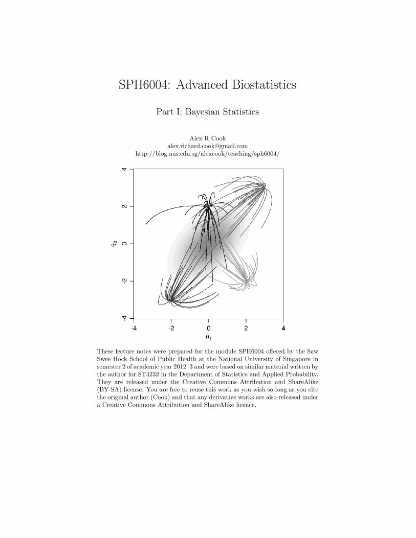
SPH6004: Advanced Biostatistics

Part I: Bayesian Statistics

Alex R [email protected]

http://blog.nus.edu.sg/alexcook/teaching/sph6004/

These lecture notes were prepared for the module SPH6004 offered by the SawSwee Hock School of Public Health at the National University of Singapore insemester 2 of academic year 2012–3 and were based on similar material written bythe author for ST4232 in the Department of Statistics and Applied Probability.They are released under the Creative Commons Attribution and ShareAlike(BY-SA) license. You are free to reuse this work as you wish so long as you citethe original author (Cook) and that any derivative works are also released undera Creative Commons Attribution and ShareAlike licence.

Chapter 1

Introduction to Bayesianstatistics

This chapter provides some of the basic terminology for the first third of themodule, and is written with the aim of conveying the main ideas upon which thefollowing chapters will build. We shall introduce Bayes’ rule (which you shouldhave learned already) in a probabilistic, non-statistical way, and thence moveto Bayesian statistical inference. We conclude the chapter with a discussion ofvarious forms of priors.

We shall look at three examples in this chapter: the use of mammographyfor breast cancer screening, a randomised clinical trial of a vaccine for HIV inyoung Thai adults, and the frequency of influenza pandemics.

1.1 Bayes’ rule

Bayes’ rule, or theorem, is well known and widely used by all kinds of statisti-cians, as well as probabilists. Its simplicity belies its power and utility. The rulestates that

p(A = A|B = B) =p(B = B|A = A)p(A = A)

p(B = B)(1.1)

or

p(A = A|B = B) =p(B = B|A = A)p(A = A)�p(B = B|A = a)p(A = a) da

. (1.2)

(A note about notation: I will frequently abuse notation in this part ofthe course in the aim of simplicity. The notation above uses A for the randomvariable and A for the realisation, p() for both probability mass and density, andintegral signs even for random variables with discrete support [you may mentallysubstitute summations where appropriate]. Where the random variable is [to mymind] obvious, I will often omit it, so that, say, p(A) is to be taken to meanp(A = A).)

Although the equation appears innocous, it is, in reality, profound, for itprovides a way to invert conditional probabilities. Because all probabilities are,actually, conditional (though the conditions are sometimes supressed, the cause

2

1.1. BAYES’ RULE 3

of much confusion), Bayes’ rule provides a way to manipulate probabilities andmove from one to another, in the above, from p(B|A) to p(A|B). We shall seewhy this is important in the following example.

Example: breast cancer screening in Germany

Gerd Gigerenzer is a psychologist of medicine, who heads the prestigious MaxPlanck Institute for Human Development in Germany. In his quite wonderfulbook, Reckoning with Risk (Gigerenzer, 2003, which should be required readingfor all statistics students), he describes an experiment he performed on Germanphysicians. The 24 participating physicians were all volunteers, and had a varietyof experience levels and backgrounds: some were newly qualified, others headedpractices or departments, some worked in teaching hospitals, others in privatepractice. They were given the following information and task (paraphrased frommemory):

Imagine you are using mammography to screen asymptomaticwomen for cancer. The probability that an asymptomatic woman inher 50s in your area attending regular screening has breast canceris 0.8%. If she actually has breast cancer, the probability is 90%that her mammogram will be positive. If she does not have breastcancer, the probability is 7% that she will, nevertheless, test postive.A woman sits in front of you with a positive mammogram. What isthe probability that she actually has breast cancer?

Gigerenzer describes how some physicians were nervous, or agitated, in an-swering this question; others stormed away without answering it, some requestedhelp from their children. The answers provided straddled almost two orders ofmagnitude: four thought the probability was around 1%, eight that it was about90%. Only two got the correct answer—that there was about a 10% chance thewoman actually had breast cancer. Let us use Bayes’ theorem to show that thisis the correct probability.

Let B = 1 if the woman has breast cancer and 0 otherwise. Let M = 1if her mammogram is positive and 0 if not. Let A = 1 if the woman isasymptomatic, lives in the area, is aged in her 50s, and is attending forregular screening, and 0 if not. The information Gigerenzer gave the participantsis thus:

p(B = 1|A = 1) = 0.008, (1.3)

p(M = 1|B = 1, A = 1) = 0.9, (1.4)

p(M = 1|B = 0, A = 1) = 0.07. (1.5)

Note that the information he gave relates to women satisfying certain condi-tions, which is why for all equations we have conditioned on A = 1. We want theprobability of breast cancer given the information we already had (i.e. A = 1)and the new information that the mammogram reveals (i.e. M = 1). UsingBayes’ theorem we have:

4 CHAPTER 1. INTRODUCTION TO BAYESIAN STATISTICS

p(B = 1|M = 1, A = 1) =p(M = 1|B = 1, A = 1)p(B = 1|A = 1)

p(M = 1|A = 1). (1.6)

The numerator follows directly from the information provided. Obtainingthe denominator requires (ever so slightly) more work:

p(M = 1|A = 1) =

1�

b=0

p(M = 1|B = b, A = 1)p(B = b|A = 1). (1.7)

Using the numbers given in the problem statement gives

p(B = 1|M = 1, A = 1) =0.9× 0.008

0.9× 0.008 + 0.07× 0.992= 9.4%. (1.8)

The very high false positive rate of mammography is one reason it has manydetractors (see for example the references in Gigerenzer, 2003).

Note that there are two probabilities of having breast cancer in the equationabove: a probability based on the risk group A only, i.e. prior to obtaining theaddition information from the mammogram, p(B = 1|A = 1); and a probabil-ity that accounts additionally for the state of knowledge after obtaining thisinformation, p(B = 1|M = 1, A = 1). These are called prior and posterior prob-abilities, and Bayes’ rule provides the calculus by which the prior probability ismodified by the new evidence, p(M = 1|B = 1, A = 1), to obtain the posterior.You will realise that even the prior probability is in fact a posterior in the sensethat it represents the information after A is observed.

Note also that this analysis makes a strong (if justified) assumption: thatthese probabilities all apply to the individual woman sitting in front of you, thephysician. Let’s give her a name, Marianne, and some other details: she’s di-vorced, has two daughters, drives a red Skoda, plays tennis. The probability of0.8% is, presumably, derived from the overall prevalence in her age group. Doyou think it is appropriate to apply that probability to Marianne? Some peoplewould argue, yes, without additional relevant information to condition on, thisis appropriate (note that having had two children does modify her risk of breastcancer, however). Others would argue that it is inappropriate unless she hadsomehow been randomly selected (equiprobably) from the population of womenwith condition A = 1 before coming for screening. If other relevant informa-tion were provided (e.g. it would be sensible for the physician to ask if there isa family history of breast cancer, or to check for a palpable lump), this addi-tional information should really be incorporated in the probability calculationby conditioning on it.

Finally, observe how Bayes’ rule allows you to flip the conditioning round,from the probability of something known given something unknown (the testresult given the underlying cancer status) to the probability of something un-known and uncertain (cancer status) given the knowledge that you have (thetest result).

1.2. INFERENCE FOR A PROBABILITY 5

Historical background

Bayes’ rule was developed by an English minister and amateur mathematician,Thomas Bayes. It was published in 1763, some time after his death, by a self-declared friend, Richard Price, who appears to have edited the manuscript heav-ily, and heavy handedly. The paper (Bayes, 1763) is hard to read due to thearchaic prose, but rewards the careful reader: confidence intervals are imaginedabout 200 years before Neyman and Pearson (fils) described them, as is the betaconjugate prior for the binomial, described later in this chapter.

1.2 Inference for a probability

The breast cancer example above illustrates a fairly non-controversial use ofBayes’ theorem. Almost all statisticians would be happy with the calculationsprovided and the interpretation of the final result (exceptions make the world amore interesting place). However, traditionally the statistical world was split intotwo camps according to how else this formula could be used. One camp, whichI will usually call frequentists, though they are also called classical statisticians,argued that Bayes’ rule could only be used to make probabilistic statementsabout events. The other group, Bayesians, argued that Bayes’ rule could beused to make probabilistic statements about anything, including unknowns suchas parameters. (Nowadays, the culture wars between frequentists and Bayesiansare much rarer as most statisticians are more pragmatic than once they were.)Let us see how Bayesians might tackle one of the simplest, and most important,tasks that a statistician may face: estimating a proportion from a binomialsample.

Let us enliven the task by using a concrete example. Rerks-Ngarm et al(2009) describe interim results from a high profile vaccine trial carried out inThailand that hit the main media sources worldwide. The trial had a good,standard design: eligible participants were randomly split into two arms, onegiven the putative vaccine, the other a placebo, and they were followed up for3.5 years, at which point they were invited back to take an HIV test. Theendpoint is HIV conversion. There were some complications due to drop outand the decision of which analysis to use, and I will present the simplest one(the data used in the modified intention-to-treat analysis). Consider (for now)only the vaccine arm. Of 8197 eligible participants, 51 were infected during thetrial period (so straight away we know the vaccine is not perfect). The questionwe will answer is, what is the “underlying” probability, pv, of infection over thistime window for those vaccinated?

Before we answer that, let us ensure we know what this probability repre-sents. Participants in trials are, of course, not randomly selected from a pop-ulation and forced to participate. They are referred to the trial, or volunteer,and must meet eligibility requirements (not being pregnant, for example, in theThai trail) and must give written informed consent. This means they are notreally representative of the population to which they belong. So pv doesn’t rep-resent the probability of infection among vaccinees in the whole population. Andthe risk of infection is different in, say, Thailand and Singapore, so pv doesn’trepresent the probability of infection in trial participants in other countries. It


represents something more metaphysical/airy-fairy, the probability of infectionin a hypothetical second trial in the same participants. Usually the airy-fairinessof this is brushed off by hoping that the ratio of pv to pu, the proportion infectedin unvaccinated participants, generalises to the population as a whole, thoughthere is no deductive reasoning that leads to that conclusion. But let us assumethat pv represents something of interest and try to estimate it nevertheless.

It seems appropriate to assume that Xv ∼ Bin(Nv, pv), where Xv is the num-ber of vaccinees infected (i.e. 51) and Nv the number of vaccinees (i.e. 8197).Theoretically this would be inappropriate if the infection of one participant in-fluenced the risk of infection of another (if they were sexual partners or sharedneedles to inject drugs, for example) but the effect of such non-independence isprobably small since the number of participants is small relative to the popula-tion as a whole. The probability (mass) function for the data is then

p(Xv = 51|Nv = 8197, pv) ∝ pXvv (1− pv)

Nv−Xv , (1.9)

(being a bit loose with notation by omitting the pv).We would like a point estimate to summarise the data, an interval estimate

to summarise uncertainty, and possibly (later) a measure of the evidence thatthe vaccine was effective. You should know how to do all these already, but itmay be useful to phrase the solution in our notation.

The frequentist approach: refresher

The traditional approach to estimating pv is to find the value of pv that max-imises the likelihood of the data given that hypothetical value were the truevalue. This maximum likelihood estimate can be obtained using calculus (forvery simple problems like this one) or numerically (using Newton–Raphson, sim-ulated annealing, cross entropy, etc.). Since we can do the calculus quite easilyhere, let us do that. Differentiation for many problems is simplified by work-ing with the log-likelihood (which, more importantly, dramatically minimisesoverflow issues in numerical methods, see later),

log[p(Xv|Nv, pv)] = c1 +Xv log pv + (Nv −Xv) log(1− pv). (1.10)

Differentiating with respect to the argument we wish to maximise over,

d log[p(Xv|Nv, pv)]

dpv=

Xv

pv− Nv −Xv

1− pv, (1.11)

replacing pv by pv on setting the derivative equal to 0, and solving, gives pv =Xv/Nv = 51/8197 = 0.62% which, reassuring to non-statisticians, is just theempirical proportion infected.

The method you probably know best to quantify the uncertainty in thisestimate is to derive a 95% (confidence) interval using the standard error of pv,

SE(pv) =

�pv(1− pv)

Nv. (1.12)

Note that in deriving this, you have to cheat, by assuming pv = pv, and waveyour hands around, by assuming that the sample size is large enough to warrant


using asymptotics in an actual application. Here, this is okay, because thesample size is actually pretty big, so both assumptions are reasonable. In smallsamples, though, uncertainty intervals derived from this standard error can bevery misleading (Agresti and Coull, 1998).

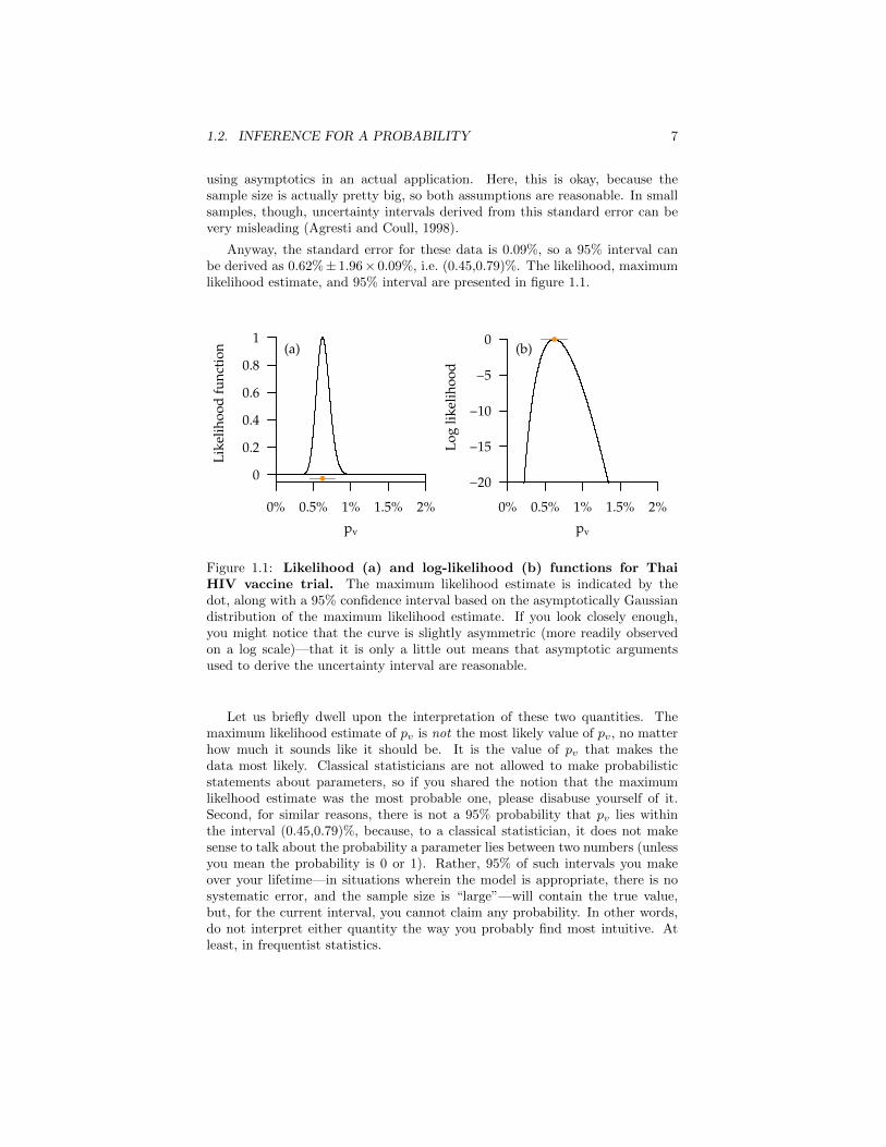
Anyway, the standard error for these data is 0.09%, so a 95% interval canbe derived as 0.62%± 1.96× 0.09%, i.e. (0.45,0.79)%. The likelihood, maximumlikelihood estimate, and 95% interval are presented in figure 1.1.

(a)

0

0.2

0.4

0.6

0.8

1

Like

lihoo

d fu

nctio

n

●

0% 0.5% 1% 1.5% 2%pv

(b)●

0% 0.5% 1% 1.5% 2%

−20

−15

−10

−5

0

pv

Log

likel

ihoo

d

Figure 1.1: Likelihood (a) and log-likelihood (b) functions for ThaiHIV vaccine trial. The maximum likelihood estimate is indicated by thedot, along with a 95% confidence interval based on the asymptotically Gaussiandistribution of the maximum likelihood estimate. If you look closely enough,you might notice that the curve is slightly asymmetric (more readily observedon a log scale)—that it is only a little out means that asymptotic argumentsused to derive the uncertainty interval are reasonable.

Let us briefly dwell upon the interpretation of these two quantities. Themaximum likelihood estimate of pv is not the most likely value of pv, no matterhow much it sounds like it should be. It is the value of pv that makes thedata most likely. Classical statisticians are not allowed to make probabilisticstatements about parameters, so if you shared the notion that the maximumlikelhood estimate was the most probable one, please disabuse yourself of it.Second, for similar reasons, there is not a 95% probability that pv lies withinthe interval (0.45,0.79)%, because, to a classical statistician, it does not makesense to talk about the probability a parameter lies between two numbers (unlessyou mean the probability is 0 or 1). Rather, 95% of such intervals you makeover your lifetime—in situations wherein the model is appropriate, there is nosystematic error, and the sample size is “large”—will contain the true value,but, for the current interval, you cannot claim any probability. In other words,do not interpret either quantity the way you probably find most intuitive. Atleast, in frequentist statistics.


Tackling it Bayesianly

How does the Bayesian derive point and interval estimates for this problem?Bayes’ rule is used to describe the probability density of the parameter, pv,given the data, Xv and Nv, in exactly the same way as it would be to describethe probability of cancer given a positive test, i.e. the Bayesian is interested in

p(pv|Xv, Nv) =p(Xv|pv, Nv)p(pv|Nv)� 1

0p(Xv|π, Nv)p(π|Nv) dπ

(1.13)

over the range of pv, which is [0, 1]. The term p(pv|Xv, Nv) is the posterior for pv,and should be seen as a function of pv. On the numerator are p(Xv|pv, Nv), thelikelihood function, and p(pv|Nv), the prior for pv. The denominator includesa dummy variable π in place of pv. Note that the likelihood function hereis just the regular likelihood function introduced by Fisher in the 1920s anddescribed above, i.e. it is p(Xv|pv, Nv) ∝ pXv

v (1 − pv)Nv−Xv . What is the prior

distribution? Well, there is no the prior distribution: just as you choose one ofmany possible models for the data, must you choose one of many possible modelsfor the parameters. The prior represents the information on the parameter—the proportion of vaccinees who would be infected by HIV during the trial—before any data are observed. One justifiable approach would be to assume allprobabilities on [0, 1] are equally likely until the trial is performed, which can bewritten as a formula thus

p(pv|Nv) = p(pv) = 1{pv ∈ [0, 1]} (1.14)

where 1{A} is the indicator function equal to 1 if A is true and 0 otherwise.This is equivalent to the formulæ

pv ∼ U(0, 1) or (1.15)

pv ∼ Be(1, 1). (1.16)

Note that we drop Nv from the condition because this prior is under the as-sumption that the sample size and probability of infection are independent.

The posterior under this model for data and parameter is thus

p(pv|Xv, Nv) = CpXvv (1− pv)

Nv−Xv (1.17)

over the range [0, 1], where C is some constant. There are two ways to proceed:a smart way, which I’ll describe later in the chapter, and a dumb way, whichwe’ll use now. The latter involves taking a grid of values for pv, spaced close toeach other, evaluating the function f1(pv) = pXv

v (1 − pv)Nv−Xv , approximating

the integral by the sum of f over this grid times the spacing between successivegrid values, and exploiting the fact that the integral of p(pv|Xv, Nv) is unity(because it is a probability density) to approximate C. Using R code, this canbe implemented as follows.

pv = seq(0.00001,0.05,0.00001)

xv = 51; nv = 8197

logf1 = xv*log(pv) + (nv-xv)*log(1-pv)


f2 = exp(logf1-max(logf1))

intf2 = sum(f2)*(pv[2]-pv[1])

post = f2/intf2

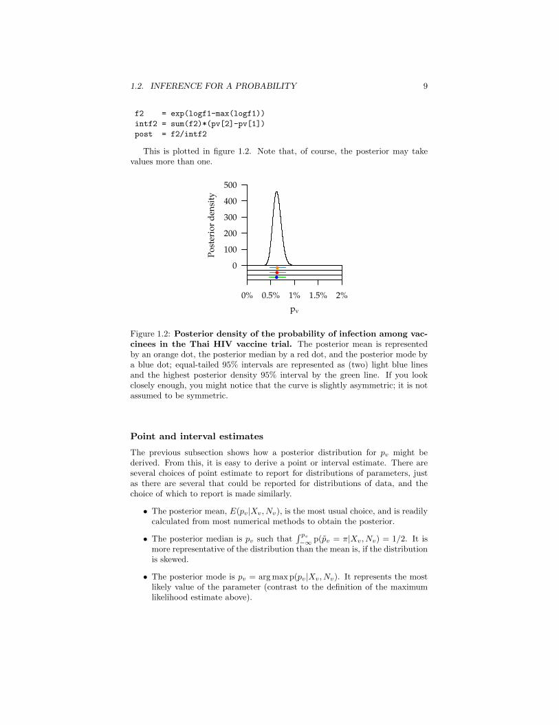
This is plotted in figure 1.2. Note that, of course, the posterior may takevalues more than one.

0

100

200

300

400

500

Post

erio

r de

nsity

●●●

0% 0.5% 1% 1.5% 2%pv

Figure 1.2: Posterior density of the probability of infection among vac-cinees in the Thai HIV vaccine trial. The posterior mean is representedby an orange dot, the posterior median by a red dot, and the posterior mode bya blue dot; equal-tailed 95% intervals are represented as (two) light blue linesand the highest posterior density 95% interval by the green line. If you lookclosely enough, you might notice that the curve is slightly asymmetric; it is notassumed to be symmetric.

Point and interval estimates

The previous subsection shows how a posterior distribution for pv might bederived. From this, it is easy to derive a point or interval estimate. There areseveral choices of point estimate to report for distributions of parameters, justas there are several that could be reported for distributions of data, and thechoice of which to report is made similarly.

• The posterior mean, E(pv|Xv, Nv), is the most usual choice, and is readilycalculated from most numerical methods to obtain the posterior.

• The posterior median is pv such that� pv

−∞ p(pv = π|Xv, Nv) = 1/2. It ismore representative of the distribution than the mean is, if the distributionis skewed.

• The posterior mode is pv = argmax p(pv|Xv, Nv). It represents the mostlikely value of the parameter (contrast to the definition of the maximumlikelihood estimate above).


To obtain these three estimates using R and following on from the code above:

pmean = sum(pv*post)/sum(post)

pcdf = cumsum(post)/sum(post)

pmedian = 0.5*(max(pv[pcdf<0.5])+min(pv[pcdf>0.5]))

pmode = pv[which.max(post)]

For the Thai HIV trial example, these estimates are 0.63%, 0.63% and 0.62%,respectively. Note how close they are to each other and to the maximum likeli-hood estimate.

To obtain an uncertainty interval (usually called a credible interval, but Ishall call them just “intervals” for short) there are two frequently used ap-proaches. One is to use the quantiles of the posterior distribution; for a 95%interval these would usually be the 2.5%ile and the 97.5%ile, though any intervalspanning 95% could be taken. Because the posterior distribution represents thedistribution of the parameter after accounting for the data, the interpretationof this equal-tailed interval is that there is a 95% chance that the parameter liesin the interval (again, compare to the definition of the frequentist confidenceinterval above). Note that because the posterior distribution is not necessarilysymmetric, there may be some parameter values that are outside the intervalthat have higher probability than some parameter values inside the interval. Ifthis is a concern, a highest posterior density interval can be obtained, with alittle more work. To do this, start with the abscissa of the posterior mode, grad-ually reduce the abscissa, including any parameter with posterior higher thanthis in the interval, until the interval first spans 95% (or whatever coverage issought).

To obtain these interval estimates in R, you may do the following:

CI1 = c(max(pv[pcdf<0.025]),min(pv[pcdf>0.975]))

threshold = max(post)

coverage = 0

for(i in seq(0.999,0.001,-0.001))

{

threshold = i*max(post)

within = which(post>=threshold)

coverage = pcdf[max(within)]-pcdf[min(within)]

if(coverage>=0.95)break()

}

CI2 = pv[range(within)]

These two interval estimates are (0.47, 0.82)% and (0.47, 0.81)%, respectively.Not only are the close to each other, but they are close to the classical 95% con-fidence interval. This illustrates one very important point, namely that in somesituations it really doesn’t matter whether you use a classical or Bayesian ap-proach, because both will give effectively the same answers. The situations inwhich the classical estimate is as good as the Bayesian are those when (i) thesample size is large, so classical results which rely on asymptotics are a good ap-proximation to the actual sampling distribution of statistics such as estimators,(ii) there is no real prior information to be incorporated in the analysis, and (iii)

1.3. PRIOR DISTRIBUTIONS 11

when someone has already developed a classical numerical routine that you canuse. Bayesian methods come into their own when any of these conditions arenot met.

A further point worth making, is that the close correspondence betweenclassical and Bayesian estimates in situations in which both can be used meansthat one can be used as an approximation to the other. If your philosophicalproclivities are not Bayesianly-aligned, you can still use Bayesian methods asif they were classical and interpret them thus. More relevant for this part ofthe course, you can use classical estimates from the literature as if they wereBayesian in deriving prior distributions, and can arguably interpret classicalpoint and interval estimates the way you wish to, as if they were Bayesian.

1.3 Prior distributions

We have heretofore not directly addressed the question of what actually is aprior distribution and how is one chosen? Under the Bayesian paradigm, onerepresents uncertainty by a probability distribution. What is the probability awoman has cancer given she has a positive mammogram? What is the distri-bution of risk of getting infected by HIV given that we observed 51 infectionsout of 8197 participants? The posterior distribution encapsulates the residualuncertainty after analysing your data set. The prior represents the uncertaintybefore.

Just as you, the statistician analysing a data set, must choose a model for thedata in terms of unknown parameters, so too must you, the Bayesian statisticiananalysing the data set, choose a model for the parameters of that model. So youmay think of the likelihood as representing the model for the data and the priorthe model for the parameters. Just as you must justify the former, so must youjustify the choice of prior.

The prior distribution should have correct support for the parameters itrepresents. If p is a probability then taking a normal distribution as the priorfor p would be silly, for it would give support to p > 1 or < 0. Similarly, aregression coefficient β can take values on the real line, so an exponential priorthat forced β to be positive might not be considered appropriate.

For models with multiple parameters, a joint prior distribution must be spec-ified. This often assumes that the joint prior is the product of one distributionfor each parameter, e.g. p(a, b) = p(a)p(b), i.e. the parameters are a priori in-dependent. However, priors need not be taken to be independent, and there aresome fairly common situations in which they are not: for instance, if a posteriordistribution from dataset 1 is used as a prior for dataset 2, then any correlationsin the first posterior should be accounted for in the second prior.

Informative and non-informative priors

An informative prior for a parameter (or parameters) encapsulates informationbeyond that solely available in the data directly at hand. For instance, perhapssomeone has estimated the same parameter in a previous study and reported apoint and interval estimate for it in the literature: you might take these and use


them to create a normal distribution with an appropriate mean and variance toact as a prior for your study. We will see an example of this early in the nextchapter.

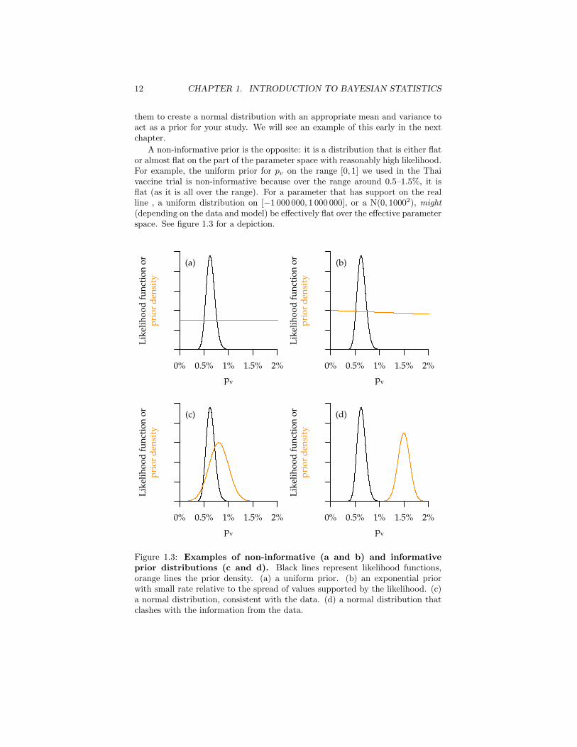
A non-informative prior is the opposite: it is a distribution that is either flator almost flat on the part of the parameter space with reasonably high likelihood.For example, the uniform prior for pv on the range [0, 1] we used in the Thaivaccine trial is non-informative because over the range around 0.5–1.5%, it isflat (as it is all over the range). For a parameter that has support on the realline , a uniform distribution on [−1 000 000, 1 000 000], or a N(0, 10002), might(depending on the data and model) be effectively flat over the effective parameterspace. See figure 1.3 for a depiction.

(a)

Like

lihoo

d fu

nctio

n or

prio

r de

nsity

0% 0.5% 1% 1.5% 2%pv

(b)

Like

lihoo

d fu

nctio

n or

prio

r de

nsity

0% 0.5% 1% 1.5% 2%pv

(c)

Like

lihoo

d fu

nctio

n or

prio

r de

nsity

0% 0.5% 1% 1.5% 2%pv

(d)

Like

lihoo

d fu

nctio

n or

prio

r de

nsity

0% 0.5% 1% 1.5% 2%pv

Figure 1.3: Examples of non-informative (a and b) and informativeprior distributions (c and d). Black lines represent likelihood functions,orange lines the prior density. (a) a uniform prior. (b) an exponential priorwith small rate relative to the spread of values supported by the likelihood. (c)a normal distribution, consistent with the data. (d) a normal distribution thatclashes with the information from the data.

1.3. PRIOR DISTRIBUTIONS 13

Proper and improper priors

Recall that a distribution has integral one, and prior distributions really oughtto, too. A proper prior distribution is one that integrate to one,

�Θp(θ) dθ = 1,

where θ is the parameter and Θ its support. Sometimes, you might choose to usean improper prior, i.e. one in which

�Θp(θ) dθ is not finite. Examples include

assuming θ ∼ U(−∞,∞), i.e. p(θ) ∝ 1; θ ∼ U(0,∞), i.e. p(θ) ∝ 1{θ > 0}; orp(θ) ∝ 1{θ > 0}/θ.

Posteriors, too, can be proper or improper. Improper posteriors are a prob-lem. Improper priors are not necessarily bad, though, for depending on thedata and model, some improper priors lead to fully proper posteriors. Properpriors beget proper posteriors; improper priors may beget proper or improperposteriors. An improper posterior may result if the likelihood is badly behaved,for example, by having an asymptotic non-zero value as a parameter tends toinfinity. In such situations, though, not only is a proper prior called for, aninformative prior is vital to substitute for the lack of information in the dataset.

Conjugate priors

A final kind of prior, always proper, but which can be either informative ornon-informative, is the conjugate prior. If a parameter for a model belongs toa specific family a priori and the same family a posteriori, then that family issaid to be conjugate to the model and the prior a conjugate prior.

Let us use the Thai HIV trial as an example again. Above we chose to takea uniform prior for pv, and I wrote this as a Be(1, 1), which may have seemedodd. The posterior we found had form

p(pv|Xv, Nv) ∝ pXvv (1− pv)

Nv−Xv . (1.18)

Those of you who are particularly au fait with your distributions might haverecognised this as proportional to a Be(1+Xv, 1+Nv−Xv) distribution. (If youdid, congratulations. I didn’t the first time.) But the posterior is a density so ifit’s proportional to a particular beta distribution it must equal that particularbeta distribution (as both have integral one). So here we moved from a prior inwhich pv was beta to a posterior in which pv is beta. Ergo the beta distributionis conjugate to the binomial.

In general, if p ∼ Be(α, β), X ∼ Bin(N, p) and Y = N−X, then the posterioris:

p(p|X,N) ∝ pα−1(1− p)β−1 pX(1− p)Y (1.19)

= pX+α−1(1− p)Y+β−1 (1.20)

∝ Γ(α+X + β + Y )

Γ(α+X)Γ(β + Y )pX+α−1(1− p)Y+β−1 (1.21)

where Γ() is the gamma function. Thus (p|X,N) ∼ Be(α+X, β + Y ).A few other models have conjugate priors available to them and we shall

encounter some as we move through the course. Most real problems do not havea suitable conjugate prior however. In situations in which a conjugate priorexists, it can be useful to exploit it, as analysis can be more analytic. For the


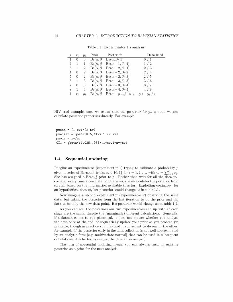
Table 1.1: Experimentor 1’s analysis.

i xi yi Prior Posterior Data used1 0 0 Be(α, β) Be(α, β + 1) 0 / 12 1 1 Be(α, β) Be(α+ 1, β + 1) 1 / 23 1 2 Be(α, β) Be(α+ 2, β + 1) 2 / 34 0 2 Be(α, β) Be(α+ 2, β + 2) 2 / 45 0 2 Be(α, β) Be(α+ 2, β + 3) 2 / 56 1 3 Be(α, β) Be(α+ 3, β + 3) 3 / 67 0 3 Be(α, β) Be(α+ 3, β + 4) 3 / 78 1 4 Be(α, β) Be(α+ 4, β + 4) 4 / 8i xi yi Be(α, β) Be(α+ y i, β + n i − yi) yi / i

HIV trial example, once we realise that the posterior for pv is beta, we cancalculate posterior properties directly. For example:

pmean = (1+xv)/(2+nv)

pmedian = qbeta(0.5,1+xv,1+nv-xv)

pmode = xv/nv

CI1 = qbeta(c(.025,.975),1+xv,1+nv-xv)

1.4 Sequential updating

Imagine an experimentor (experimentor 1) trying to estimate a probability p

given a series of Bernoulli trials, xi ∈ {0, 1} for i = 1, 2, . . ., with yi =�i

j=1 xj .She has assigned a Be(α, β) prior to p. Rather than wait for all the data tocome in, every time a new data point arrives, she recalculates the posterior fromscratch based on the information available thus far. Exploiting conjugacy, foran hypothetical dataset, her posterior would change as in table 1.1.

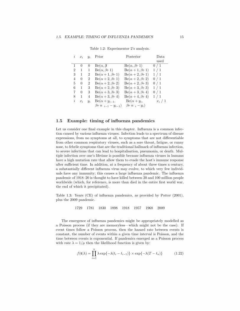
Now imagine a second experimentor (experimentor 2) observing the samedata, but taking the posterior from the last iteration to be the prior and thedata to be only the new data point. His posterior would change as in table 1.2.

As you can see, the posteriors our two experimentors end up with at eachstage are the same, despite the (marginally) different calculations. Generally,if a dataset comes to you piecemeal, it does not matter whether you analysethe data once at the end, or sequentially update your prior as you proceed (inprinciple, though in practice you may find it convenient to do one or the other:for example, if the posterior early in the data collection is not well approximatedby an analytic form [e.g. multivariate normal] that can be used in subsequentcalculations, it is better to analyse the data all in one go.)

The idea of sequential updating means you can always treat an existingposterior as a prior for the next analysis.

1.5. EXAMPLE: TIMING OF INFLUENZA PANDEMICS 15

Table 1.2: Experimentor 2’s analysis.

i xi yi Prior Posterior Dataused

1 0 0 Be(α, β) Be(α, β + 1) 0 / 12 1 1 Be(α, β + 1) Be(α+ 1, β + 1) 1 / 13 1 2 Be(α+ 1, β + 1) Be(α+ 2, β + 1) 1 / 14 0 2 Be(α+ 2, β + 1) Be(α+ 2, β + 2) 0 / 15 0 2 Be(α+ 2, β + 2) Be(α+ 2, β + 3) 0 / 16 1 3 Be(α+ 2, β + 3) Be(α+ 3, β + 3) 1 / 17 0 3 Be(α+ 3, β + 3) Be(α+ 3, β + 4) 0 / 18 1 4 Be(α+ 3, β + 4) Be(α+ 4, β + 4) 1 / 1i xi yi Be(α+ yi−1, Be(α+ yi, xi / 1

β + n i−1 − yi−1) β + n i − yi)

1.5 Example: timing of influenza pandemics

Let us consider one final example in this chapter. Influenza is a common infec-tion caused by various influenza viruses. Infection leads to a spectrum of diseaseexpressions, from no symptoms at all, to symptoms that are not differentiablefrom other common respiratory viruses, such as a sore throat, fatigue, or runnynose, to febrile symptoms that are the traditional hallmark of influenza infection,to severe infections that can lead to hospitalisation, pneumonia, or death. Mul-tiple infection over one’s lifetime is possible because influenza viruses in humanshave a high mutation rate that allow them to evade the host’s immune responseafter sufficient time. In addition, at a frequency of about three times a century,a substantially different influenza virus may evolve, to which very few individ-uals have any immunity; this causes a large influenza pandemic. The influenzapandemic of 1918–20 is thought to have killed between 20 and 100 million peopleworldwide (which, for reference, is more than died in the entire first world war,the end of which it precipitated).

Table 1.3: Years (CE) of influenza pandemics, as provided by Potter (2001),plus the 2009 pandemic.

1729 1781 1830 1898 1918 1957 1968 2009

The emergence of influenza pandemics might be appropriately modelled asa Poisson process (if they are memoryless—which might not be the case). Ifevent times follow a Poisson process, then the hazard rate between events isconstant, the number of events within a given time interval is Poisson, and thetime between events is exponential. If pandemics emerged as a Poisson processwith rate λ = 1/µ then the likelihood function is given by:

f(t|λ) =n�

i=1

λ exp{−λ(ti − ti−1)} × exp{−λ(T − tn)} (1.22)


where we might justifiably set t0 to be 1700, and T is the present (at the timeof writing, T = 2013). We might choose a uniform prior for µ, the average timebetween outbreaks, in the absence of additional external data. This model wecan fit by considering a grid for µ over a plausible range using the following R

code:

loglikelihood=function(mu)

{

tpan = c(1729,1781,1830,1898,1918,1957,1968,2009)

tnow = 2013

tstart = 1700

tdeltas = c(tpan,tnow)-c(tstart,tpan)

output = sum(dexp(tdeltas[1:8],rate=1/mu,log=TRUE))

+ pexp(tdeltas[9],rate=1/mu,log=TRUE,lower.tail=FALSE)

output

}

mu = 1:1000

logposterior = 0*mu

for(i in 1:length(mu))

logposterior[i] = loglikelihood(mu[i])

+ dunif(mu[i],0,1000)

logposterior = logposterior-max(logposterior)

posterior = exp(logposterior)

posterior = posterior/(sum(posterior)*(mu[2]-mu[1]))

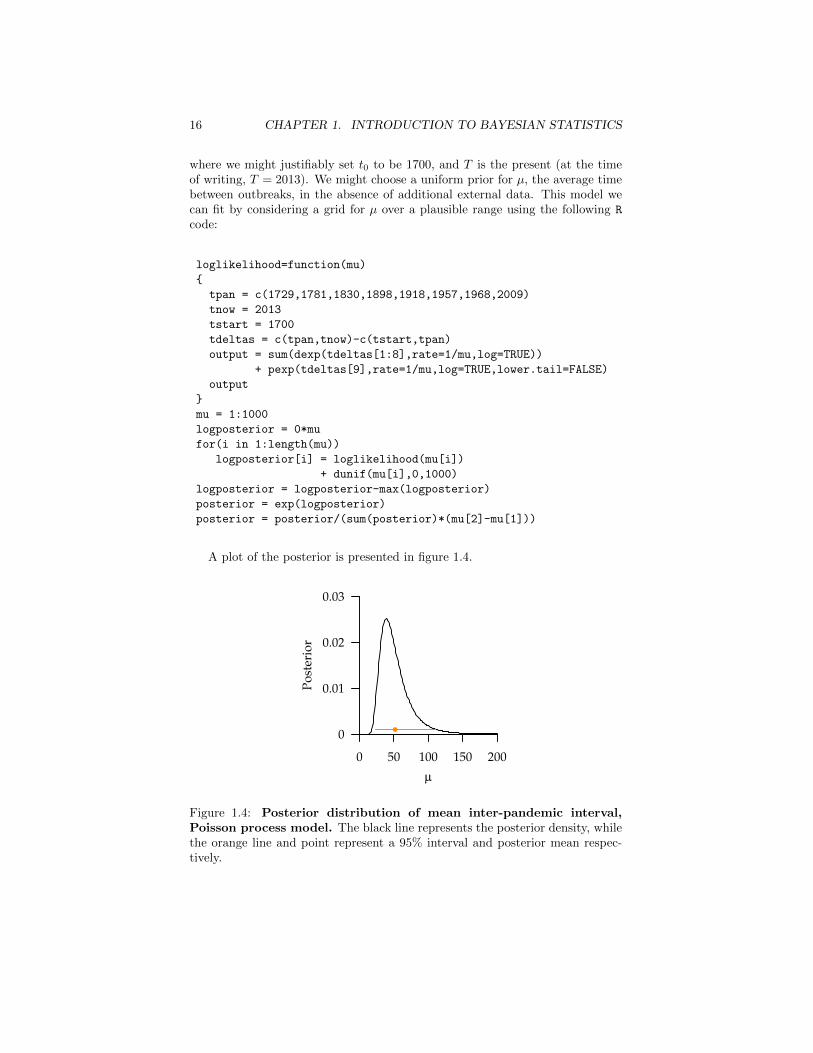
A plot of the posterior is presented in figure 1.4.

●

0 50 100 150 200

0

0.01

0.02

0.03

µ

Post

erio

r

Figure 1.4: Posterior distribution of mean inter-pandemic interval,Poisson process model. The black line represents the posterior density, whilethe orange line and point represent a 95% interval and posterior mean respec-tively.

1.6. METHODS TO CALCULATE POSTERIORS 17

The posterior mean average inter-pandemic interval is 52y (95%I 23–110y),in other words, roughly one pandemic per two human generations. Note thatthe distribution is asymmetric as a result of the small sample size, and so anasymptotic classical confidence interval would be inappropriate.

1.6 Methods to calculate posteriors

We have seen two methods that can be used for simple problems (like thoseencountered so far): Monte Carlo, and grid search.

In the first analysis of the Thai AIDS trial example, we used the following R

code to estimate the proportion infected on the vaccinated arm:

pv = seq(0.00001,0.05,0.00001)

xv = 51; nv = 8197

logf1 = xv*log(pv) + (nv-xv)*log(1-pv)

f2 = exp(logf1-max(logf1))

intf2 = sum(f2)*(pv[2]-pv[1])

post = f2/intf2

This took a subset, [0.00001, 0.05], of the parameter support, [0, 1], in whichwe thought the parameter lay, and split it up into bins. The posterior (toa constant of proportionality) was evaluated at each point on the grid and,making the assumption that the posterior does not change much from bin tobin, the integral of the posterior can be approximated by the sum of the area ofrectangles with width the inter-bin spacing and height the provisional posterior(to a constant), allowing the approximate posterior to be scaled appropriatelyto integrate to unity. In performing this calculation the decision has to be madeas to how to set up the grid—in an earlier version, I tried

pv = seq(0,1,0.01)

but the grid was too coarse and many points were far from the values given highweight by the likelihood, leading to subsequent refinements.

Note that if there are multiple parameters, then the grid must have multipledimensions, with several deleterious effects. More function calls will be needed,for a start. If 100 grid points are satisfactory to evaluate a single parameterover a plausible support, then 1002 = 10 000 are needed for two parameters,1003 = 1000 000 for three parameters, and many more for even moderatelysized problems. Each function call takes time, and although this time is (often orusually) negligible if a thousand or hundred thousand calls are made, it certainlyis not for millions, billions or more. Even if the time needed is manageable,values need to be stored to be used for subsequent analysis. If the space neededexceeds your available ram, then either the computer will crash, or it will startshunting information to the hard disk, which slows things down even more. Oneoption is to reduce the fineness of the grid’s spacing, so that only 20 (say) pointsspan the plausible support, perhaps also shrinking in the minima and maximaof the grid’s range, and hope that the consequent loss in accuracy caused by theresulting truncation is minimal. I rarely use grid searches for more than two orthree dimensions for these reasons.


An alternative that generalises to the methods we will discuss in the next twochapters is Monte Carlo. Imagine that you were interested in the size of elephanttusks in the population of wild African elephants (perhaps because you are inter-ested in the effect of poaching on selection pressure for small tusks)—and thatyou had enough money to fly to Africa. How would you do it? One approachwould be to find elephants (preferably with a well designed sampling protocol)and measure their tusks—the larger the sample of tusks you measured, the closerthe empirical distribution of tusk lengths to the corresponding unknown popula-tion distribution. Time or money limitations would inevitably limit the numberof samples you could take—at which point you would use statistical methodsto work out plausible values for characteristics of the population distribution,such as its mean—but were money no concern, you could keep sampling untilyour sample was so large it effectively was the population, and you wouldn’tneed to do any statistical inference anymore, because whatever characteristicsof the population you were interested in could be obtained just by inspectingthe sample.

In Bayesian statistics, there is likewise an unknown distribution for the pa-rameters θ, and you wish to characterise that distribution. If it were possible todraw a sample of the parameters from their posterior distribution, andto make that sample very very big, then the sample you thus obtained would besufficiently close to the actual distribution that it could be used as if it were theactual distribution, for example by calculating the sample mean and equatingit to the posterior mean, or finding the 2.5 and 97.5%iles and equating these tothe equal tailed 95% uncertainty interval. If your sample were as large as anelephants, you wouldn’t need to do any statistical inference with it anymore.

This idea is called Monte Carlo sampling, named after the capital of Monaco,the Mediterranean principality famous for its casinos and glamour. More for-mally, if θi is the ith independent draw from p(θ = θi|data) and

gm(θ) =

m�

i=1

g(θi)/m (1.23)

is the Monte Carlo estimate of the posterior of the function g(θ), then

gm(θ) →�

g(θ)p(θ|data) dθ (1.24)

as m → ∞. Note that g() could be any function, such as the identity function(for the mean), or square (to get the variance).

To use Monte Carlo sampling in its simplest form, you need to be able towork out the form for the posterior in a way that permits simulation. This maybe possible for some simple examples for which a conjugate prior can be found.For more complicated models, in which the posterior’s form is non-standard anddoes not belong to a simple parametric family of distributions, you do not knowwhat distribution to sample from and so must ‘guess’ the distribution and then‘correct’ it to make the sample fair.


Example: Thai HIV vaccine trial

The oft-aforementioned Thai HIV vaccine trial was not performed to estimate theproportion of vaccinees infected after 3.5 years—it was to compare the proportioninfected on the vaccinated and unvaccinated arms. If we assume independencein infection status between individuals within and between arms, and take aprior distribution p(pv, pu) = 1{(pv, pu) ∈ [0, 1]2}, i.e. both proportions are apriori uniform on [0, 1] and independent, then the posterior factorises nicely, asfollows (note that I’m dropping the dependency on Nu and Nv for brevity):

p(pv, pu|Xv, Xu) ∝ p(Xv, Xu|pv, pu)p(pv, pu) (1.25)

= p(Xv|pv, pu)p(Xu|pv, pu)p(pv)p(pu) (1.26)

= p(Xv|pv)p(Xu|pu)p(pv)p(pu) (1.27)

∝ p(pv|Xv)× p(pu|Xu) (1.28)

both of which are beta, independently. So the posterior distribution of pv isBe(52, 8197) independently of pu which is, a posteriori, Be(75, 8199).

Now, we could do a grid search here (and this would be useful practice) butwe could also just simulate directly from these two beta distributions, as R hasa built-in routine to sample betas quickly. R code to do this follows.

xv=51;nv=8197

xu=74;nu=8198

M=10000

pv=rbeta(M,1+xv,1+nv-xv)

pu=rbeta(M,1+xu,1+nu-xu)

summariser=function(x)

{

cat(’Posterior mean:’,signif(mean(x),3),

’95%I:’,signif(quantile(x,c(0.025,0.975)),3),

’\n’)

}

summariser(pv)

summariser(pu)

summariser(pv/pu)

summariser(pu-pv)

mean(pu<pv)

The summariser function prints the mean and 95% equal tailed interval for itsvector argument. Note that the posterior distribution of functions of the param-eters can readily be obtained once you have samples from the posterior, but thatyou must retain the indexing (so don’t scramble the order of one or more of theparameter sample vectors). This is a substantial benefit of a Bayesian approach,because in the classical paradigm, obtaining confidence intervals of functions ofparameters, such as the ratio of means from two normal distributions, requirestedius calculus and approximations based on the delta method.

In the last line of code, we calculate the proportion of samples for which oneparameter is bigger than the other. In notation, this is

p(pu < pv|Xu, Xv, Nu, Nv) (1.29)


i.e. the posterior probability that the proportion infected in the unvaccinatedgroup is less than that of the vaccinated group. Note the distinction betweenthis—the probability an hypothesis is true given the observed data—with thedefinition of a p-value—the probability of imaginary data that were not observedbut would have been more extreme than the actual data given that the hypoth-esis were true. The classical approach to hypothesis testing involves taking,typically, a point null hypothesis, that in most cases would not plausibly be trueanyway (for instance, in an observational study, assuming a covariate has noasociation with the outcome after adjusting for a small number of other covari-ates), assuming it to be true, and calculating the probability of non-observeddata, and using that to try to demonstrate that the null hypothesis is wrong.The Bayesian approach can naturally assess the evidence for any non-point hy-pothesis by simply calculating the probability the hypothesis is true.

For point hypotheses, if the prior assigns zero probability to their being true,are impossible a posteriori. Given that there are very few instances in which a nilhypothesis is likely to be true anyway (two examples might be in a randomisedclinical trial of one placebo against another, or in evaluating claims of scientificfraud in which patients were not randomly allocated to treatment arms), I findthis to be not a great weakness, though others might.

Activities

[1] Consider the problem we focused much of our efforts on in this chapter, thatof estimating a proportion p given data X and N and the model X ∼ Bin(N, p).In frequentist statistics, the performance of a method is often evaluated viarepeat sampling, evaluated using, usually, simulated “data sets. Consider thefollowing three properties: (i) bias of the estimator (i.e. of a point estimate),(ii) mean squared error of the estimator (ditto) and (iii) coverage of the 95%uncertainty interval.

Considering a scenario like the AIDS vaccine trial and a smaller study, eval-uate these three properties for the following: maximum likelihood estimates andposterior means (i and ii) and for confidence intervals constructed using theregular ±1.96SE(p) approximation and Bayesian equal tailed credible intervals(iii). Use this to compare the performance of the two approaches.

[2] Consider the HIV vaccine trial in Thailand again. Again, focus on thevaccine arm. We took a Be(1, 1) prior for pv. Consider a range of other priordistributions and, for each, derive the resulting posterior, calculate posteriorpoint and interval estimates, and plot the prior and posterior. How much do thefindings change?

[3] Read Cohen (1994), Gigerenzer (2004) and Gelman (2008).

References

Agresti A, Coull BA (1998). Approximate is better than “exact” for in-terval estimation of binomial proportions. Am Stat 52:119–26.

Bayes T (1763). An essay towards solving a problem in the doctrine ofchances. Phil Trans Roy Soc 53:370–418.


Cohen J (1994). The Earth is round (p < .05). Am Psychol 49:997–1003.

Gelman A (2008). Objections to Bayesian statistics. Bayesian Anal 3:445–50.

Gigerenzer G (2003). Reckoning with Risk: Learning to Live with Uncer-tainty. Penguin.

Gigerenzer G (2004). Mindless statistics. J Socio-econ. 33:587–606.

Potter CW (2001). A history of influenza. J Appl Microbiol 91:572–9.

Rerks-Ngarm S, Pitisuttithum P, Nitayaphan S et al (2009). Vaccinationwith ALVAC and AIDSVAX to prevent HIV-1 infection in Thailand. NewEngl J Med 361:2209–20.

Documents

SPH6004: Advanced Biostatistics - NUS Blog - National University of