Stable URL - UVic Department of Electrical and Computer

Spline Adaptation in Extended Linear ModelsAuthor(s): Mark H. Hansen and Charles KooperbergSource: Statistical Science, Vol. 17, No. 1 (Feb., 2002), pp. 2-20Published by: Institute of Mathematical StatisticsStable URL: http://www.jstor.org/stable/3182801 .Accessed: 06/03/2011 02:28

Your use of the JSTOR archive indicates your acceptance of JSTOR's Terms and Conditions of Use, available at .http://www.jstor.org/page/info/about/policies/terms.jsp. JSTOR's Terms and Conditions of Use provides, in part, that unlessyou have obtained prior permission, you may not download an entire issue of a journal or multiple copies of articles, and youmay use content in the JSTOR archive only for your personal, non-commercial use.

Please contact the publisher regarding any further use of this work. Publisher contact information may be obtained at .http://www.jstor.org/action/showPublisher?publisherCode=ims. .

Each copy of any part of a JSTOR transmission must contain the same copyright notice that appears on the screen or printedpage of such transmission.

JSTOR is a not-for-profit service that helps scholars, researchers, and students discover, use, and build upon a wide range ofcontent in a trusted digital archive. We use information technology and tools to increase productivity and facilitate new formsof scholarship. For more information about JSTOR, please contact [email protected].

Institute of Mathematical Statistics is collaborating with JSTOR to digitize, preserve and extend access toStatistical Science.

http://www.jstor.org

http://www.jstor.org/action/showPublisher?publisherCode=ims

http://www.jstor.org/stable/3182801?origin=JSTOR-pdf

http://www.jstor.org/page/info/about/policies/terms.jsp

http://www.jstor.org/action/showPublisher?publisherCode=ims

Statistical Science 2002, Vol. 17, No. 1, 2-51

Spline Adaptation in Extended Linear Models Mark H. Hansen and Charles Kooperberg

Abstract. In many statistical applications, nonparametric modeling can provide insights into the features of a dataset that are not obtainable by other means. One successful approach involves the use of (univariate or multivariate) spline spaces. As a class, these methods have inherited much from classical tools for parametric modeling. For example, stepwise variable selection with spline basis terms is a simple scheme for locating knots (breakpoints) in regions where the data exhibit strong, local features. Similarly, candidate knot configurations (generated by this or some other search technique), are routinely evaluated with traditional selection criteria like AIC or BIC. In short, strategies typically applied in parametric model selection have proved useful in constructing flexible, low-dimensional models for nonparametric problems.

Until recently, greedy, stepwise procedures were most frequently suggested in the literature. Research into Bayesian variable selection, however, has given rise to a number of new spline-based methods that primarily rely on some form of Markov chain Monte Carlo to identify promising knot locations. In this paper, we consider various alternatives to greedy, deterministic schemes, and present a Bayesian framework for studying adaptation in the context of an extended linear model (ELM). Our major test cases are Logspline density estimation and (bivariate) Triogram regression models. We selected these because they illustrate a number of computational and methodological issues concerning model adaptation that arise in ELMs.

Key words andphrases: Adaptive triangulations, AIC, BIC, density estimation, extended linear models, finite elements, free knot splines, GCV, linear splines, multivariate splines, regression.

1. INTRODUCTION

Polynomial splines are at the heart of many popu- lar techniques for nonparametric function estimation. For regression problems, TURBO (Friedman and Sil- verman, 1989), multivariate adaptive regression splines or MARS (Friedman, 1991) and nI (Breiman, 1991) have all met with considerable success. In the context of density estimation, the Logspline procedure

Mark H. Hansen is a Member of the Technical Staff, Bell Laboratories, Lucent Technologies, Murray Hill, New Jersey 07974 (e-mail: [email protected]). Charles Kooperberg is Member, Division of Public Health Sciences, Fred Hutchinson Cancer Research Center, Seattle, Washington 98109-1024.

of Kooperberg and Stone (1991, 1992) exhibits ex- cellent spatial adaptation, capturing the full height of spikes without overfitting smoother regions. And finally, among classification procedures, classification and regression trees (CART) (Breiman, Friedman, 01- shen and Stone, 1984) is a de facto standard, while the more recent PolyMARS models (Kooperberg, Bose and Stone, 1997) have been able to tackle even large problems in speech recognition. Stone et al. (1997) and a forthcoming monograph by Hansen, Huang, Kooper- berg, Stone and Truong are the prime references for the application of polynomial splines to function estimation. In this paper, we review a general methodological framework common to procedures like MARS and Logspline, and contrast it with several Bayesian

2

SPLINE ADAPTATION IN ELMs

approaches to spline modeling. We begin with some background material on splines.

1.1 Splines

Univariate, polynomial splines are piecewise polynomials of some degree d. The breakpoints marking a transition from one polynomial to the next are referred to as knots. In this paper, we will let the vector t = (tl, ..., tK) E RK denote a collection of K knots.

Typically, a spline will also satisfy smoothness constraints describing how the different pieces are to be joined. These restrictions are specified in terms of the number of continuous derivatives, s, exhibited by the piecewise polynomials. Consider, for example, piecewise linear curves. Without any constraints, these functions can have discontinuities at the knots. By adding the condition that the functions be globally continuous, we force the separate linear pieces to meet at each knot. If we demand even greater smoothness (say, continuous first derivatives), we loose flexibility at the knots and the curves become simple linear functions. In the literature on approximation theory, the term "linear spline" is applied to a continuous, piecewise linear function. Similarly, the term "cubic spline" is reserved for piecewise cubic functions having two continuous derivatives, allowing jumps in the third derivative at the knots. In general, it is common to work with splines having maximal smoothness in the sense that any more continuity conditions would result in a global polynomial.

Given a degree d and a knot vector t, the collection of polynomial splines having s continuous derivatives forms a linear space. For example, the collection of linear splines with knot sequence t is spanned by the functions

(1) 1, x, (x -tl)+, (.. - tK)+,

where (.)+ = max(., 0). We refer to this set as the truncated power basis of the space. In general, the basis for a spline space of degree d and smoothness s is made up of monomials up to degree d together with terms of the form (x - tk++, where 1 < j < d - s.

Using this formula the classical cubic splines have d = 3 and s = 2 so that the basis has elements

(2) 1,x, x2, x3, (x-tl),..., (x-tk)

From a modeling standpoint, the truncated power basis is convenient because the individual functions are tied to knot locations. In the expressions (1) and (2), there is exactly one function associated with each knot, and eliminating that function effectively removes the knot.

This observation is at the heart of many statistical methods that involve splines and will be revisited shortly.

The truncated power functions (1) and (2) are known to have rather poor numerical properties. In linear regression problems, for example, the condition of the design matrix deteriorates rapidly as the number of knots increases. An important alternative rep- resentation is the so-called B-spline basis (de Boor, 1978). These functions are constructed to have support only on a few neighboring intervals defined by the knots. (For splines having maximal smoothness, this means d + 1 neighboring intervals.) A detailed de- scription of this basis is beyond the scope of this paper, but the interested reader is referred to Schumaker (1993). For the moment, assume we can find a basis B1(x; t), ..., Bj(x; t) for the space of splines of de-

gree d with smoothness s and knot sequence t so that any function in the space can be written as

(3) g(x; , t)= /lBI(x;t) +... + jBj(x;t),

for some coefficient vector f = (,1, ... , f)t. If we are dealing with spline spaces of maximal smoothness, then J = K + d + 1, as we have seen in (1) and (2). Given this structure, we now briefly describe a broad collection of estimation problems that admit relatively natural techniques for identifying good fitting functions g.

1.2 Extended Linear Models

Extended linear models (ELMs) were originally defined as a theoretical tool for understanding the properties of spline-based procedures in a large class of estimation problems (Hansen, 1994; Stone et al., 1997; Huang, 1998, 2001). This class is extremely rich, con- taining all of the standard generalized linear models as well as density and conditional density estimation, hazard regression, censored regression, spectral density estimation and polychotomous regression. To describe an ELM, we begin with a probability model p(WIh) for a (possibly vector-valued) random variable W E 'W that depends on an unknown (also possibly vector-valued) function h. Typically, h represents some component of the probability model about which we hope to make inferences. For example, in a normal linear model, h is the regression function; while for density estimation, we take h to be the log-density.

Let I(WIh) = log p(WIh) denote the log-likelihood for an ELM, and assume that there exists a unique

3

M. H. HANSEN AND C. KOOPERBERG

function 0 that maximizes the expected log-likelihood El(WIh) over some linear space of real-valued functions H. The maximizer 0 defines "truth," and is the target of our estimation procedures. [In Stone et al. (1997) a slightly more general notion of "truth" is developed to handle ANOVA-like functional decompo- sitions.] We refer to this set-up as an extended linear model for 0. In this case, the term "linear" refers to our use of a linear model space H. The class H is chosen to capture our beliefs about ?, and is commonly defined through smoothness conditions (e.g., we might assume that the true regression function in a linear model has two continuous, bounded derivatives). These weak assumptions about 0 tend to result in classes H that are infinite dimensional. Therefore, for estimation purposes we choose to work with flexible, finite- dimensional spaces G that have good approximation properties. That is, the elements g E G can capture the major features of functions 0 E H, or mingEG IIg - 011 is small in some norm for all 0 E H. Splines are one such approximation space.

Given a series of observations W1,..., Wn from the distribution of W, we estimate 0 by maximizing the log-likelihood

where g E G.

Our appeal to maximum likelihood in this context does not imply that we believe p(W ?) to be the true, data- generating distribution for W. Rather, p may be chosen for computational ease in the same way that ordinary least squares can be applied when the assumption of strict normality is violated. In theoretical studies, it is common to let the dimension of G depend on the sample size n. For example, if G is a spline space with K knots, we let K = K(n) -+ oo as n -- oo. As we collect more data, we are able to entertain more flexible descriptions of ?. Asymptotic results describing the number of knots K(n) and their placement needed to achieve optimal mean squared error behavior are given in Stone (1985), Stone (1994), Hansen (1994), and Huang (1998, 2001), and Stone and Huang (2002).

An ELM is said to be concave if the log-likelihood l(wlh) is concave in h E H for each value of w E W3 and if El(WIh) is strictly concave in h [when restricted to those h for which El(WIh) > -oo]. Strict concavity holds for all of the estimation problems listed at the beginning of this section. Now, let G be a spline space with knot sequence t so that any g E G can be written in the form (3). Then since g(.) = g(.; f, t), the log- likelihood (4) can be written as l (B, t). Because of con-

cavity, the maximum likelihood estimates (MLEs) f for the coefficients f and a fixed t can be found ef- ficiently in reasonably-sized problems through simple Newton-Raphson iterations. Therefore, it is possible to compute

(5) (t) = max 1 (i, t). P

After making the dependence on t explicit in this way, we can consider adjusting the knot locations tl < ... < tK to maximize the log-likelihood. It is

intuitively clear that the knot sequence t = (tl, ..., tK) controls the flexibility of elements in g to track local features: tightly-spaced knots can capture peaks, while widely-separated knots produce smooth fits.

However, even in the simplest case, linear regression with a single univariate predictor, maximizing (5) over knot sequences is a difficult optimization problem. To see this, we first translate univariate regression into an ELM: let W = (X, Y) and define p(WI( ) via the

relationship Y =+(X) +e,

for an unknown regression function 0. The error E is assumed independent of X with a normal distribution having mean zero and variance a2. For a spline space G, the negative log-likelihood for 8 is propor- tional to the regression sum of squares

RSS(f, t) = (Y - g(Xi; ,, t))2

i = L(Yi - ,1B1(X,; t) -..

- BJ Bj(Xi; t))2. If we hold t fixed, then

(6) I(t) o -RSS(t) = max{-RSS(/B, t)}

- -RSS(fi, t),

where ,B is the ordinary least squares estimate of f. Jupp (1978) demonstrated that -RSS(t) has local maxima along lines of the form tk = tk+l, making the solution to (6) difficult for standard optimization software. Not surprisingly, this problem persists in even more exotic ELMs.

Several authors have considered special transforma- tions, penalties or ad hoc optimization schemes to maximize the log-likelihood with respect to t (Jupp, 1978; Lindstrom, 1999; Kooperberg and Stone, 2002). In this paper, we will instead consider an approximate solution that begins by connecting knot placement with model selection.

4

(4) l(g) = E l(Wilg)


1.3 Model Selection

The concavity of an ELM together with the asso- ciation of knot locations to terms in the truncated power basis suggests simple approximations to maximizing (5) based on fast, stepwise approaches to model selection. Consider splines of degree d having maximal smoothness and knot sequence t. According to Section 1.1, this means that s = d - 1 and each knot

point tk in t is associated with only one of the truncated monomials (x - tk)d; the linear (1) and cubic (2) splines are two examples. Therefore, moving tk effects only one basis element in G, and in fact removing tk entirely is equivalent to deleting (x - tk)d from the model. Many existing spline methods use this idea in some form. It was originally proposed by Smith (1982a, b) and it has been the workhorse of many procedures suggested since (TURBO, DKCV, MARS, PolyMARS).

Returning to the problem of maximizing (5), suppose we have a finite set of candidate knots T = {t, ..., t, }, from which we want to select a subset of size K, t = (tl,..., tK), K < K'. The connection between knots and basis functions suggests that finding a good sequence t is really a problem in model selection where we are choosing from among candidate basis functions of the form (x - t)d_, t E T. For linear regression and moderate numbers of candidate knots K', we can find the sequence of length K that minimizes (6) using traditional branch-and-bound techniques. How- ever, when K' gets large, or when we have a more exotic ELM requiring Newton-Raphson iterations to evaluate (5), this approach quickly becomes infeasible.

For computational efficiency, the algorithms discussed by Stone et al. (1997) take a stepwise approach, introducing knots in regions where the unknown function 0 exhibits significant features, as evaluated through the log-likelihood, and deleting knots in regions where / appears relatively smooth. More formally, starting from a simple spline model, knots are added successively, at each step choosing the location that produces the greatest increase in the log- likelihood. This is followed by a pruning phase in which unnecessary knots are removed, at each stage eliminating the basis element that results in the smallest change in the log-likelihood. Because we are always taking the best single alteration to the current model, these schemes are often referred to as greedy. To prevent this process from tracking spurious patterns in the data, it is common to impose constraints on the initial model, the size M of the largest model fit during addition, and the minimal number of data points

between each knot. These restrictions are defined in terms of allowable spaces, a topic we will discuss in more detail in the next section.

Several facts about ELMs make this approach attrac- tive computationally. Consider placing a single knot in a linear regression model. Then, among all basis sets of the form 1,x, (x - t)+, we want to find the one that minimizes the criterion (6), which in this case is a function of t. It is not hard to show that RSS(t) is a piecewise smooth function of t, with breaks in the first derivative at each of the data points. This means we can derive fast heuristics to guide the search for new knots during the addition phase without having to evaluate all the candidates. Next, the concavity of the ELMs listed in Section 1.2 means that we can quickly approximate the change in log-likelihood from either adding or deleting a knot without actually fitting each candidate model. We now describe each alteration or "move" in more detail.

Knot addition. Let G be a J-dimensional spline space with a given knot sequence, t, and let B denote the MLE of f. When using the truncated power basis inserting a new knot is equivalent to adding a single basis function to G, taking us to a new (J + 1)- dimensional space G1 with coefficient vector fl and knot sequence tl (where we let Bj+I be the basis function associated with the new knot). To evaluate the improvement, we employ a Taylor expansion of the log-likelihood (fil, tl) around fi1 = (t, 0), which specifies a function in G1. This approximation yields the well-known Rao (score) statistic and is convenient because it allows us to entertain a large number of candidate knot locations without having to compute the MLE f1 in each candidate space.

Knot deletion. Again, let G be a given spline space and f, the associated MLE. Removing a knot from G reduces the dimension of G by one and takes us to a space Go. To evaluate the impact of this alteration, we again employ a Taylor expansion, this time around f. If a E IRJ represents the linear constraint that effectively removes a given knot, this expansion yields the Wald statistic for testing the hypothesis that at f = 0. For the truncated power basis, a is a binary vector with a single nonzero entry. With this approach, we can compare the impact of removing each knot in G without having to compute the MLE in these reduced spaces.

Alternating phases of knot addition and deletion produces a sequence of models, from which we select

5


the single best according to some selection criterion like generalized cross validation (GCV)

(7) GCVa(t) RSS(t) /1 a(J(t)1)2 n _ n

or a variant of the Akaike information criterion (AIC)

(8) AICa (t) = -21(t) + aJ(t)

(Akaike, 1974), where J(t) is the dimension of the spline space. The parameter a in each of these expressions controls the penalty assigned to models with more knots and is introduced to offset the effects of selection bias (Friedman and Silverman, 1989; Fried- man, 1991). In Stone et al. (1997) the default value of a in (8) is log n, resulting in a criterion that is commonly referred to as BIC (Schwarz, 1978).

Notice that our search for good knot locations based on the log-likelihood (5) has led to a heuristic minimization of a selection criterion like (7) or (8). Several comments about this reduction are in order. First, greedy schemes are often criticized for not exploring a large enough set of candidate models. In the stepwise algorithms of Stone et al. (1997), for example, the simple two-pass scheme (knot addition to a model of size M followed by deletion) evaluates essentially 2M different knot sequences. These 2M candidates are also highly constrained, representing a potentially narrow path through the search space. As a result, when we identify the "best model" according to some selection criterion, we have visited at most a handful of its "good-fitting" neighbors, those spline spaces with about the same number of knots found during either addition or deletion. However, as is typical with variable selection problems, many spline models offer essentially equivalent fits (in terms of AIC or GCV).

Despite these caveats, examples in Stone et al. (1997) and other papers show that greedy algorithms for knot selection can work quite well. They lead to a surprising amount of spatial adaptivity, easily locating extra knots near sharp features, while removing knots in smooth areas. It is natural, however, to question whether or not alternative methods might prove more effective. In the discussion following Stone et al. (1997), for example, the Bayesian framework of Smith and Kohn (1996) is shown to approximately minimize the same objective function (8), but with a stochastic search algorithm. In general, the recent work on Bayesian model selection offers interesting solutions to the shortcomings of greedy methods.

1.4 A Bayesian Approach

The desire to compare alternative search schemes is half the motivation for this paper. As mentioned earlier, a major source of inspiration comes from the recent work on Bayesian model selection and the accompanying Markov chain Monte Carlo (MCMC) methods for identifying promising models. To date, several Bayesian spline methods have appeared that make the connections with model selection listed above. The first was Halpern (1973), who constructed a hierarchical model for regression with linear splines. This application necessarily focused on small problems with a limited number of potential knots, succumb- ing to the computational resources of the day. More moder research in this area has followed a similar approach in terms of prior assignment, but makes use of MCMC to sample from a (possibly very) large set of candidate knots. Perhaps the first such procedure was exhibited by Smith (1996) and Smith and Kohn (1996) for univariate and additive regression models. Simi- lar in spirit are the Bayesian versions of TURBO and CART proposed by Denison et al. (1998a, b), which employ reversible jump MCMC (Green, 1995).

In a Bayesian setup, model uncertainty comes from both the structural aspects of the space G-knot placement-as well as from our selection of members g E G-determining coefficients in expression (3). We now spell out a simple hierarchical formulation that we will revisit in the next section. At the first level of the hierarchy, we assign a prior distribution p(G) to some set of candidate models G. In the setup for univariate regression using linear splines, for example, we would typically do that by first choosing a prior distribution on the number of knots p(K), and then by choosing an additional prior on the collection of knots t given K, p(tlK). Through p(tlK) we can prevent knots from getting too close, reducing the chance that the fitted model will track spurious features in the data. Next, given a space G, we generate elements g according to the distribution p(glG). Consistent with our motivation for modeling with splines in the first place, our priors on K, t and g should somehow reflect our beliefs about the smoothness of the underlying function of interest in an ELM, 0. In the literature on smoothing splines we find a class of priors for g that given a basis for G and an expansion (3) involves the coefficients fi = (,8, ..., 1BJ). This amounts to a partially improper, normal distribution for f (Silverman, 1985; Wahba, 1990; and Green and Silverman, 1994), which we will return to in Section 2.

6


Given a prior for spline functions g, we can generate a sample from the posterior distribution of g us-

ing MCMC. In particular, in Sections 2 and 3 we will use the reversible jump algorithm of Green (1995) for Logspline density estimation and Triogram regression, respectively. Details about how to choose priors and how to tune algorithms are discussed in these sections. When properly tuned, these stochastic methods can identify many more good-fitting knot configurations than their greedy, deterministic competitors. By focus- ing their search in regions of model space that have high posterior probabilities, the MCMC schemes listed above visit many more "promising" configurations.

The second major motivation for this paper is the form of the final function estimate itself. Since deterministic searches identify a very small number of us- able models, the unknown function is typically estimated by straight maximum likelihood applied to some basis for the identified spline space. Suppose for the moment, that the function being estimated is smooth in some region, perhaps requiring not more than a single knot to adequately describe the curve. From the point of view of mean squared error, there are many roughly equivalent ways to place this knot in the region. There- fore, if given a number of good knot configurations, it might be more reasonable to combine these estimates in some way. This is roughly a spline or knot-selection version of the classical motivation for Bayesian model averaging. In later versions of the Gibbs sampling approach of Smith and Kohn (1998) and the Bayesian versions of TURBO and MARS by Denison, Mallick and Smith (1998a, b), the final function estimate is a posterior mean.

In this paper, we compare greedy (stepwise) algorithms with nongreedy (stochastic, Bayesian) algorithms for model selection. We evaluate different approaches to adaptation by examining strategies for both knot placement and coefficient estimation. We focus on four classes of methods: greedy, stepwise procedures with maximum likelihood estimates in the final spline space; MCMC for selecting a single model; model averaging using maximum likelihood estimates of the coefficients; and finally a fully Bayesian approach with model and coefficient averaging. Our two main estimation problems will be Logspline density estimation and (bivariate) Triogram regression. We selected these because they illustrate a number of computational and methodological issues concerning model adaptation that arise in ELMs.

In Section 2 we discuss greedy and Bayesian model selection approaches in the context of Logspline density estimation. In Section 3 we turn to Triogram regression, contrasting it with Logspline. Finally, in Sec- tion 4 we identify areas of future research. Our goal in preparing this paper was not to advocate one scheme over another, but rather to investigate the performance of various approaches to model selection in the context of univariate and multivariate nonparametric estimation with splines.

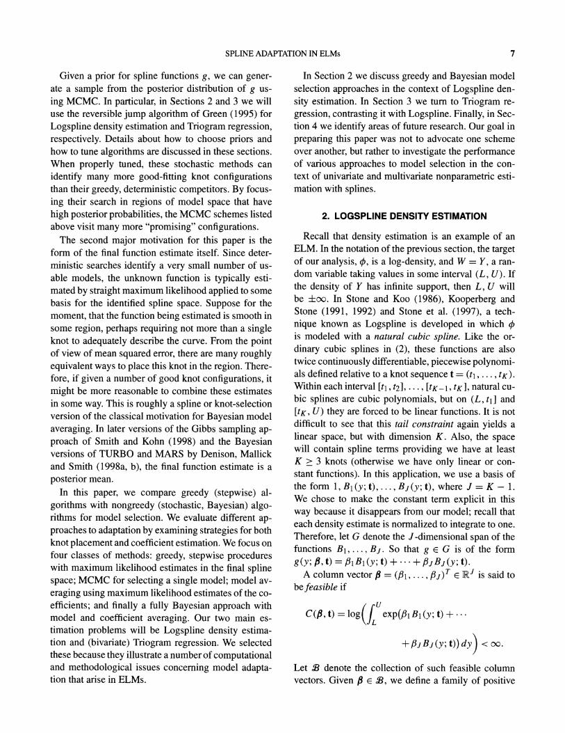
2. LOGSPLINE DENSITY ESTIMATION

Recall that density estimation is an example of an ELM. In the notation of the previous section, the target of our analysis, 0, is a log-density, and W = Y, a random variable taking values in some interval (L, U). If the density of Y has infinite support, then L, U will be ?oc. In Stone and Koo (1986), Kooperberg and Stone (1991, 1992) and Stone et al. (1997), a technique known as Logspline is developed in which 0 is modeled with a natural cubic spline. Like the ordinary cubic splines in (2), these functions are also twice continuously differentiable, piecewise polynomials defined relative to a knot sequence t = (t, ..., tK). Within each interval [tl, t2],..., [tK-1, tK], natural cubic splines are cubic polynomials, but on (L, tl] and [tK, U) they are forced to be linear functions. It is not difficult to see that this tail constraint again yields a linear space, but with dimension K. Also, the space will contain spline terms providing we have at least K > 3 knots (otherwise we have only linear or constant functions). In this application, we use a basis of the form 1, Bl(y; t),..., Bj(y; t), where J = K - 1. We chose to make the constant term explicit in this way because it disappears from our model; recall that each density estimate is normalized to integrate to one. Therefore, let G denote the J-dimensional span of the functions B1, ..., Bj. So that g E G is of the form

g(y; , t) = f1 B1 (y; t) + . + /JBj(y; t). A column vector f - = (B1, ...., pj)T E IRJ is said to

be feasible if

C(/f, t) = log( exp(8Bi (y; t) +.

+ jBj(y; t)) dy) <oo.

Let 2 denote the collection of such feasible column vectors. Given B E 2, we define a family of positive

7


density functions on (L, U) of the form

f(y; fB, t) = exp(g(y; ,, t) - C(fi, t))

(9) = exp(1i B1 (y; t) + * . + BSjBj(y; t)

- C(fi, t)), L <y < U.

Now, given a random sample Y1,..., Yn of size n from a distribution on (L, U) having an unknown density function exp(q), the log-likelihood function corresponding to the Logspline model (9) is given by

l(f, t) = log f(Yi; B, t) i

= E EijBj(Yi;t)-nC(#; t), / E S. i j

The maximum likelihood estimate f is given by B =

argmaxfEi/l(B, t), corresponding to g(y) = g(y; B, t) for L < y < U.

Stepwise knot addition begins from an initial model with Kinit knots, positioned according to the rule described in Kooperberg and Stone (1992). Given a knot sequence tl, ..., tK, the addition scheme finds a location for a candidate knot corresponding to the

largest Rao statistic. For numerical stability, we do not allow the breakpoints tl,..., tK to be separated by fewer than nsep data points. We say that in this context, a space G is allowable, providing the knot

sequence satisfies this condition. Stepwise addition continues until a maximum number of knots Kmax is reached. Knot deletion is then performed according to the outline in the previous section, and a final model is selected according to the generalized AIC criterion (8) with parameter a = log n.

2.1 A Bayesian Framework

We set up the framework for a Bayesian approach to Logspline density estimation by selecting several

priors: first a prior p(G) on the structure of the model

space G, and then a prior p(gIG) on the splines g in a

given space. In addition, we will need to specify how we sample from the posterior distributions.

Priors on model space. For Logspline we choose to specify p(G) by creating a distribution on knot sequences t formed from some large collection of candidates T = {t, ..., tK,}. We construct p(G) hierarchi-

cally, first choosing the number of knots K < K' (in this case recall that the dimension J of G is K - 1) according to p(K), and then given K, we generate t from the distribution p(tlK). Regularity conditions on the structural aspects of the associated spline space

G can be imposed by restricting the placement of tl,..., tK through p(tlK). While other authors have also considered a discrete set of candidate knot se-

quences (Denison, Mallick and Smith, 1998a; Smith and Kohn, 1996), we could also specify a distribution that treats the elements of t as continuous variables

(e.g., Green 1995). In our experiments we have found that for Logspline density estimation the discrete approach is sufficient, and we consider those spaces G for which all K knots are located at data points. This restriction is purely for convenience, but represents lit- tle loss of flexibility especially in the context of den-

sity estimation (where peaks in the underlying density naturally produce more candidate knots). For numerical stability, we require that there are at least nsep data

points in between any two knots. This leaves us with the task of specifying p(K).

To the extent that the number of knots also acts as a smoothing parameter, this distribution can have a considerable effect on the look of the final curves

produced. We explore several of the proposals that have

appeared in the literature. The first is a simple Poisson distribution with mean y suggested by Green (1995). Denison et al. (1998a) take the same distribution for more general spline spaces and argue that their results are somewhat insensitive to the value of y. The next

prior we will consider was suggested by Smith and Kohn (1996). Either by greatly reducing the number of candidate knots or by scaling the prior on the coefficients, these authors suggest that K be distributed

uniformly on the set Kmin ... . Kmax. The final proposal for p(K) is somewhat more ag-

gressive in enforcing small models. To properly motivate this distribution, we think of the model selection

procedure as two stages: in the first we find the posterior average of all models with k knots by integrating out t and g, to obtain, say gk and its posterior probability p(gklY1, , Y,, K = k). Suppose that we consider

gk to have k degrees of freedom (an admittedly ques- tionable assumption). If we now were to use an AIC- like criterion to choose among the gk, we would select the model that minimized

-2logp(gklY, ..., Yn, K = k) + ak,

compare (8). On the other hand, using the posterior to evaluate the best model suggests maximizing

p(gk Y,..., Yn, K = k)p(K = k).

If we take p(K = k) oc exp(-ak/2) these two approaches agree. Thus, taking a geometric distribution

8


for p(K) implies an AIC-like penalty on model dimension. In particular a = log n and q = 1//n imposes the same cost per knot as AIC with penalty log n. For reasonable settings of Kmin and Kmax, however, the expected prior number of knots under this prior will tend to zero with n. While it is certainly inituitive that the prior probability of K decreases monotonically with k, this drop may be at a faster rate than we would expect! If a >2 then p(K = k + 1)/p(K = k) < 1/e.

Priors on splines in a given space. We parameterize p(g G) through the coefficients fi in the expansion (3), and consider priors on fi that relate to our assumptions about the smoothness of g. Recall that as the solution to a penalized maximum likelihood fit, smoothing splines (Wahba, 1990) have a straightforward Bayesian inter- pretation (Silverman, 1985). In univariate smoothing, for example, G is a space of natural splines (given some knot sequence t), and the "roughness" of any g E G is measured by the quantity ffS(g,)2. Expand- ing g in a basis, it is not hard to see that

(10)

U~ rU (whee A = 'A

where Aij =- f B(x)B fr (x) dx

for I < i, j < J.

The traditional smoothing spline fit maximizes the penalized likelihood

arg max{l(i) + Xf'Afi},

for some parameter X. Silverman (1985) observes that the solution to this problem can be viewed as a posterior mode, where f is assigned a partially improper, normal prior having mean 0 and variance- covariance matrix (XA)-1. This setup has the favorable property that it is invariant to our choice of basis. This is desirable, as the choice of the basis will often be made for computational reasons.

In our simulations we will compare this smoothing prior to the scheme of Denison et al. (1998a) in which no stochastic structure is assigned to the coefficients fB once G is selected. Instead, these authors employ maximum likelihood to make a deterministic choice of fB.

Markov chain Monte Carlo. In order to treat a variety of estimation problems simultaneously, we have chosen the reversible jump MCMC scheme developed by Green (1995). Denison et al. (1998a) implement this

technique in the context of general univariate and additive regression. We refer to these papers for the details of the scheme, and we instead focus on the type of moves that we need to implement the sampler. In general, we alternate (possibly at random) between the following moves.

* Increase model dimension. In this step, we intro- duce a new knot into an existing collection of breakpoints. Given the concavity properties of ELMs the change in the log-likelihood could either be computed exactly or approximated using the appropriate Rao statistic. In our experiments we have computed the change in the log-likelihood exactly. The new knot is selected uniformly from among the set that yields an allowable space.

* Decrease model dimension. As with the greedy scheme, knots are deleted by imposing a constraint on one or more coefficients in the spline expansion. We can either evaluate the drop in the log-likelihood exactly, or through the Wald statistics. Any knot can be removed at any time (assuming we have more than Kmin breakpoints to chose from).

* Make structural changes to G that do not change dimension. Unlike our standard greedy scheme, nonnested steps like moving a knot are now possible. Moving a knot from tk to tk technically involves deleting tk and then inserting a new breakpoint at tk. With smart initial conditions on the Newton-Raphson steps, we can calculate the change in the log-likelihood exactly and still maintain an efficient algorithm.

* Update (possibly) g. In a nonlinear model like Logspline, we can either apply a suitable approximation to the posterior and integrate with respect to the coefficients fi, or we can fold sampling them into our Markov chain.

Following Green (1995) and Denison et al. (1998a), we cycle between proposals for adding, deleting and moving knots, assigning these moves probabilities bj, dj and 1 - bj - dj (see Denison et al., 1998a). New knots can be positioned at any data point that is at least nsep data points removed from one of the current knots. Subject to this constraint, knot addition follows a simple two step procedure. First, we select one of the intervals (L, tl), (tl, t2), ..., (tK, U) uniformly at random (where the tk are the current breakpoints). Within this interval, the candidate knot is then selected uniformly at random from one of the allowable data points. When moving a knot, we either propose a large move (in which a knot is first deleted, and then added using the addition scheme just described) or a small

9


move (in which the knot is only moved within the interval between its two neighbors). Each of these two proposals have probability (1 - dj - bj)/2.

After each reversible jump step, we update the coefficients /. To do this, we use the fact that for a given set of knots, we have a parametric model, and that the posterior distribution of / given G and the data is thus approximately multivariate normal with covariance matrix E = (XA + H)-1, and mean E HB, where / is the maximum likelihood estimate of / in G, and H is the Hessian of the log-likelihood function at B. An observation from this distribution is used as a proposal in a Metropolis step. Because we are using (partially improper) smoothing priors, the acceptance ratio for this proposal is formally undetermined (recall that the prior covariance matrices are degenerate). We solve this problem by "canceling" the zero eigenvalue in the numerator and the denominator (see also Besag and Higdon, 1999).

2.2 A Simulation Study

To compare the performance of the various possible implementations of Logspline density model selection procedures, we carried out a simulation study. We generated data from three densities:

* normal-the standard normal density; * slight bimodal-f (y) = 0.5fz(y; 1.25, 1) + 0.5

fz(y; -1.25, 1.1), where fz (y; /, r) is the normal density with mean ,t and standard deviation a;

* sharp peak-f(y) = 0.8g(y) + 0.2fz(y;2, 0.07), where g(Y) is the density of the lognormal random variable Y = exp(Z/2) and Z has a standard normal distribution.

These three densities are displayed in Figure 1. From each we generated 100 independent samples of size n = 50, 200, 1,000 and 10,000. We applied a variety of Logspline methods, see Table 1. For all the Bayesian methods we estimated the posterior mean by a simple pointwise average of the MCMC samples. Otherwise, the Bayesian approaches differ in two aspects:

normal slight bimodal sharp peak

FIG. 1. Densities used in the simulation study.

TABLE 1 Versions of Logspline density estimation used in

the simulation study

Model size Parameters

(i) Greedy optimization of AIC

proposed by Stone et al. (1997) (ii) Simulated annealing optimization

of AIC (SALSA) (iii) Geometric ML (iv) Poisson (5) ML (v) Uniform X = l/n

(vi) Uniform X = 1/ (vii) Uniform X = 1

(viii) Geometric A = 1/n

* the prior on the model size-we used the geometric prior with parameter p = 1 - 1/v/n, the Poisson

prior with parameter 5, and a uniform prior; * parameter estimates f-we took either the maxi-

mum likelihood (ML) estimate, or we assigned a multivariate normal prior to / (for one of several choices for X).

Table 1 summarizes the versions of Logspline which are reported here.

For simulated annealing (ii) (termed SALSA for "Simulated Annealing LogSpline Approximation") we ran the same MCMC iterations as for version (iii), but rather than selecting the mean of the sampled densities, we chose the density which minimizes AIC. As described above this is very similar to taking the density with the largest a posteriori probability (the mode), except that we ignore the prior on knot locations given the number of knots, K. This would have changed the penalty in the AIC criterion from K log n to K logn + log ('). Since version (ii) begins with the fit obtained by the greedy search (i), it is guaran- teed to improve as far as AIC is concerned. Version (iii) uses the same penalty structure as version (ii), but av- erages over MCMC samples. Version (iv) is included since a Poisson (5) prior was proposed by Denison et al. (1998a). It applies a considerably smaller penalty on model size. Versions (v)-(viii) experiment with penalties on the coefficients. Generating the parameters using a multivariate normal prior distribution implies smoothing with a AIC-like penalty. As such, we would expect that using A = 1/n with a uniform prior [version (v)] may give reasonable results, but that using a geometric prior [version (ix)] would smooth too much. Choosing A too large, as in versions (vi)-(vii), leads to oversmoothing, while choosing X too small tends to produce overly wiggly fits.

10


TABLE 2 Mean integrated squared error (MISE)for the simulation study

Version

(i) (ii) (iii) (iv) (v) (vi) (vii) (viii)

Distribution n MISE Ratio of MISE over MISE of the greedy version (i)

Normal 50 0.02790 0.73 1.52 1.84 0.66 0.40 0.26 0.67 Normal 200 0.01069 0.49 0.60 1.23 0.79 0.50 0.24 0.66 Normal 1,000 0.00209 0.59 0.58 1.33 0.87 0.90 0.42 0.73 Bormal 10,000 0.00020 0.33 0.49 1.45 1.35 1.10 0.80 0.87

Slight bimodal 50 0.02502 0.88 1.09 1.34 0.48 0.36 0.36 0.50

Slight bimodal 200 0.00770 0.80 0.61 1.14 0.70 0.38 0.46 0.61

Slight bimodal 1,000 0.00164 0.57 0.60 1.13 0.89 0.66 0.40 0.77

Slight bimodal 10,000 0.00020 0.77 0.61 0.88 0.71 0.82 0.51 0.84

Sharp peak 50 0.15226 0.97 0.78 0.81 0.68 0.90 1.12 0.72

Sharp peak 200 0.03704 0.89 0.75 0.94 0.93 2.02 3.62 1.13

Sharp peak 1,000 0.00973 0.81 0.67 0.81 0.67 2.01 8.90 0.74

Sharp peak 10,000 0.00150 0.72 0.57 0.57 0.64 0.58 21.43 0.76

Average 1.00 0.71 0.74 1.12 0.78 0.89 3.21 0.75

For versions (iii) and (iv) we ran 600 MCMC iterations, of which we discarded the first 100 as bum- in. Some simple diagnostics (not reported) suggest that after 100 iterations the chain is properly mixed. For versions (v)-(viii) each structural change was followed by an update of the coefficients f8.

In Table 2, we report ratios of integrated squared errors between the greedy scheme and the other methods outlined above. In addition, we feel that it is at least as important for a density estimate to provide the correct general "shape" of a density as to have a low integrated squared error. To capture the shape of our estimates, we counted the number of times that a scheme produced densities having too few, too many and the correct number of modes. These results are summarized in Tables 3 and 4. Table 5 calculates the "total" lines of

Tables 3 and 4. Note that for simulations of a normal distribution it is not possible for an estimate to have too few modes.

From Table 2 we note that most methods show a moderate overall improvement over the greedy version of Logspline, except for (vii). This scheme over- smoothes the data, so that the details (like the mode in the sharp-peaked distribution) are frequently missed. We note that version (iii), choosing the mode of a Bayesian approach, is the only version that outper- forms the greedy version for all 12 simulation setups. Otherwise, the difference between versions (ii), (iii), and (viii) seems to be minimal. In particular, if we had chosen another set of results than those for (i) to nor- malize by, the order of the average MISE for these four methods was often changed.

TABLE 3 Number of times out of 100 simulations that a Logspline density estimate had too few modes

Version

Distribution n (i) (ii) (iii) (iv) (v) (vi) (vii) (viii)

Slight bimodal 50 45 52 4 0 21 74 99 31 Slight bimodal 200 6 22 13 0 1 18 96 19 Slight bimodal 1,000 5 17 19 0 7 6 45 16 Slight bimodal 10,000 4 12 4 1 3 4 2 10 Sharp peak 50 24 38 1 0 9 56 99 13 Sharp peak 200 0 1 0 0 0 0 89 1 Sharp peak 1,000 0 0 0 0 0 0 0 0 Sharp peak 10,000 0 0 0 0 0 0 0 0

Total 84 142 41 1 41 158 430 90

11


Number of times out of TABLE 4

100 simulations that a Logspline density estimate had too many modes

Version

Distribution n (i) (ii) (iii) (iv) (v) (vi) (vii) (viii)

Normal 50 18 11 94 100 49 5 0 28 Normal 200 34 9 38 100 81 21 0 24 Normal 1,000 26 4 15 91 68 54 32 32 Normal 10,000 4 1 7 61 31 29 1 17

Slight bimodal 50 4 1 84 99 6 0 0 4

Slight bimodal 200 16 1 19 99 55 4 0 5

Slight bimodal 1,000 15 1 13 93 51 31 1 17

Slight bimodal 10,000 6 1 8 68 33 39 0 6

Sharp peak 50 15 8 90 93 3 1 0 2

Sharp peak 200 36 19 46 94 43 5 0 5

Sharp peak 1,000 28 14 30 77 32 12 1 9

Sharp peak 10,000 25 12 15 31 20 30 11 7 Total 227 82 459 1006 472 231 46 156

From Table 3 we note that version (vii), and to a lesser extent (ii) and (vi), have trouble with the slight bimodal density, preferring a model with just one peak. Versions (vi) and (vii) find too few modes, leading us to conclude that X should be chosen smaller than 1// I when using a uniform prior on model size. On the other hand, the Poisson prior leads to models exhibiting too

many peaks, as do versions (iii) and (v). Overall, it appears that the greedy, stepwise search

is not too bad. It is several orders of magnitude faster than any of the other methods. The greedy approach, as well as SALSA have the advantage that the final model is again a Logspline density, which can be stored for later use. For the other methods, we must record the posterior mean at a number of points. This has the potential of complicating later uses of our estimate. Among the Bayesian versions that employ ML estimates, version (iii) seems to perform best overall, while among those that put a prior on the coefficient vector, versions (v) and (viii) (both of which set A = l/n) are best. It is somewhat surprising that version (viii) performs so well, since it effectively imposes twice the AIC penalty on model size: one

coming from the geometric prior, and one from the normal prior on the parameters. Kooperberg and Stone (1992) argue that the Logspline method is not very sensitive to the exact value of the parameter, possibly explaining the behavior of version (viii). In Kooperberg and Stone (2002) a double penalty is also employed in the context of free knot Logspline density estimation.

2.3 Income Data

We applied the nine versions of Logspline used for the simulation study to the income data discussed in Stone et al. (1997), and the results are displayed in Figure 2. For the computations on the income data we ran the MCMC chain for 5000 iterations in which a new model was proposed, after discarding the first 500 iterations for bur-in. For the versions with

priors on the parameters we alternated these iterations with updates of the parameters. The estimates for versions (ii), which was indistinguishable from version (iii), and versions (viii) which was indistinguishable from version (v) are not shown. In Kooperberg and Stone (1992) it was argued that the height of the peak should be at least about 1. Thus, it appears that versions

TABLE 5 Number of times that a Logspline density estimate had an incorrect number of modes

(i) (ii) (iii) (iv) (v) (vi) (vii) (viii)

Too few modes 84 142 41 1 41 158 430 90 Too many modes 227 82 459 1,006 472 231 46 156 Total 311 224 500 1,007 513 389 476 246

12


o

uO 0

o 0

0

uO 0

o O

0.5 1.5 2.5 0.5 1.5 2.5 0.5 1.5 2.5

Income Income Income

FIG. 2. Logspline density estimates for the income data.

(vi) and (vii) have oversmoothed the peak. On the other hand, version (iv) seems to have too many small peaks.

It is interesting to compare the number of knots for the various schemes. The greedy estimate (version i) has 8 knots, and the simulated annealing estimate (version ii) has 7 knots. The Bayesian versions (iii), (v) and (viii) have an average number of knots between 5 and 8, while the three versions that produced unsatis-

factory results (iv, vi and vii) have an average number of knots between 14 and 17.

The MCMC iterations can also give us information about the uncertainty in the knot locations. To

study this further, we ran a chain for version (iii) with 500,000 iterations. Since the knots are highly correlated from one iteration to the next (at most one knot moves at each step), we only considered every 250th iteration. The autocorrelation function of the fitted log- likelihood suggested that this was well beyond the time over which iterations are correlated. This yielded 2,000 sets of knot locations: 1,128 with five knots, 783 with six knots, 84 with seven knots, and 5 with eight knots. When there were five knots, the first three were always located close to the mode, the fourth one was virtually always between 0.5 and 1.25, and the last knot between 1 and 2. The locations of the first three knots overlap considerably. When there are six knots, the extra knot can either be a fourth knot in the peak, or it is beyond the fifth knot.

3. TRIOGRAM REGRESSION

When estimating a univariate function 0, our "pieces" in a piecewise polynomial model were intervals of the form (tk, tk+l). Through knot selection, we

adjusted these intervals to capture the major features in 0. When 0 is a function of two variables, we have more freedom in how we define a piecewise polynomial model. In this section we take our separate pieces to be triangles in the plane, and consider data- drive-techniques that adapt these pieces to best fit 0. Our starting point is the Triogram methodology of Hansen et al. (1998) which employs continuous, piecewise linear (planar) bivariate splines. Triograms are based on a greedy, stepwise algorithm that builds on the ideas in Section 1 and can be applied in the context of any ELM where 0 is a function of two variables. After reviewing some notation, we present a Bayesian version of Triograms for ordinary regression. An alternative approach to piecewise linear modeling was proposed in Breiman (1993) and given a Bayesian extension in Holmes and Mallick (2001).

Let A be a collection of triangles 8 (having disjoint interiors) that partition a bounded, polygonal region in the plane X = UeAES. The set A is said to be a triangulation of X. Furthermore, A is conforming if the nonempty intersection between pairs of triangles in the collection consists of either a single, shared vertex or an entire common edge. Let vi, ... , VK represent the collection of (unique) vertices of the triangles in A.

U,

C

Co 0) c

13


Over X, we consider the collection G of continuous, piecewise-linear functions which are allowed to break (or hinge) along the edges in A. It is not hard to show that G is a linear space having dimension equal to the number of vertices K. A simple basis composed of "tent functions" was derived in Courant (1943): for each j = 1,..., K, we define Bj(x; A) to be the unique function that is linear on each of the triangles in A and takes on the value 1 at vj and 0 at the remaining vertices in the triangulation. The set Bl (x; A), ..., BK(x; A) is a basis for G. Also notice that each function Bj (x; A) is associated with a single vertex vj, and in fact each g E G

(11) K

g(x; ,B, A) = ?,j Bj(x; A), j=1

interpolates the coefficients f/ = (B1,..., fK) at the

points vl,..., VK. We now apply the space of linear splines to estimate

an unknown regression function. In the notation of an ELM, we let W = (X, Y), where X e X is a two- dimensional predictor and Y is a univariate response. We are interested in exploring the dependence of Y on X by estimating the regression function 0(x)= E(YIX = x). Given a triangulation A, we employ linear splines over A of the form (11). For a collection of (possibly random) design points X, ... , Xn taken from X and corresponding observations Y1, ..., Yn, we apply ordinary least squares to estimate P/. That is, we take = arg max Ei [Yi - g(Xi; /B, A)]2, and use g(x) = g(x; /, A) as an estimate for b.

As with the univariate spline models, we now consider stepwise alterations to the space G. Following Hansen, Kooperberg and Sardy (1998), the one-to-one correspondence between vertices and the "tent" basis functions suggests a direct implementation of the greedy schemes in Section 1. Stepwise addition involves introducing a new vertex into an existing triangulation, thereby adding one new basis function to the original spline space. This operation requires a rule for connecting the new point to the vertices in A so that the new mesh is again a conforming triangulation. In Figure 3, we illustrate three options for vertex addition: we can place a new vertex on either a boundary or an interior edge, splitting the edge, or we an add a point to the interior of one of the triangles in A. Given a triangulation A, candidate vertices are selected from a regular triangular grid in each of the existing triangles, as well as a number of locations on each of the existing edges (for details see Hansen et al., 1998).

Splitting an Interior Edge Subdividing a Triangle

FIG. 3. Three "moves" that add a new vertex to an existing triangulation. Each addition represents the introduction of a single basis function, the support of which is colored gray.

We impose constraints on our search by limiting, say, the area of the triangles in a mesh, their aspect ratio, or perhaps the number of data points they contain. As with Logspline, spaces satisfying these restrictions are referred to as allowable. At each step in the addition process, we select from the set of candidate vertices (that result in an allowable space), the point that maximizes the decrease in residual sum of squares when the Triogram model (11) is fitted to sample data. (In regression, the Rao and Wald statistics are the same and reduce to the change in the residual sum of squares between two nested models.)

Deleting a knot from an existing triangulation can be accomplished most easily by simply reversing one of the steps in Figure 3. Observe that removing a vertex in one of these three settings is equivalent to enforcing continuity of the first partial derivatives across any of the "bold edges" in this figure. Such continuity conditions are simple linear constraint on the coefficients of the fitted model, allowing us to once

again apply a Wald test to evaluate the rise in the residual sum of squares after the vertex is deleted.

3.1 A Bayesian Framework

Priors on model space. As with univariate spline models, a prior on the space of Triograms is most easily defined by first specifying the structure of the approximation space, which in this case is a triangulation A. For any A, we need to select the number of vertices K, their placement v, and the triangles that connect them.

14


Original Triangulation Swapping a Diagonal

FIG . Additional structural movesfor the reversible jump MCMC scheme. Note that these two proposals result in a nonnested sequence of spaces.

Each set v can be joined by a number of different triangulations (assuming v has more than 3 points). Sibson (1978) shows that by starting from one triangulation of v, we can generate any other by a sequence of "edge swaps." (This operation is given in Figure 4 and will come up later when we discuss MCMC for bivariate splines.) Unfortunately, a closed-form expression for the number of triangulations associated with a given set of vertices does not exist. Computing this number for even moderately sized configurations is difficult because two sets each with K vertices can have different numbers of triangulations.

To see how this complicates matters, suppose we follow the strategy for Logspline and propose a hierarchical prior of the form

(12) p(Alv, K)p(vlK)p(K),

where A is a triangulation of the vertices v = {vl,..., VK }. Assigning any proper distribution to A given v introduces a normalizing constant in p (AIv, K) that involves enumerating the different triangulations of v. Therefore, when taking ratios of (12) for two different sets of vertices, we are usually left with a prohibitively expensive computational problem. MCMC methods for exploring the model space are not possible.

To avoid this problem, we will use a tractable prior on triangulations developed by Nicholls (1998). This distribution depends on a pair of Poisson point processes, one that generates vertices on the interior of X and one for the boundary. As constructed, there is one parameter f that controls the intensity of this process, where larger values of / produce triangulations with more vertices. Nicholls (1998) avoids count- ing triangulations by normalizing across all triangulations obtainable from all vertex sets generated by this point process, and produces a distribution p(A). Bounds on the number of triangulations obtainable from a given vertex set are used to show that this kind of normalization is possible. This construction also has the advantage that restrictions on the size and shape

of triangles are easily enforced and only change the (global) normalization constant in p(A). In our experiments, we set 8 so that the expected number of vertices for this base process is 5. We then adapted Nicholls's approach, so that the underlying point process produces a geometric (with parameter 1 - 1/v/n) or a uniform (on Kmin, . .., Kmax) number of vertices, follow-

ing the simulation setup in the previous section.

Priors on splines in a given space. Unlike the Log- spline example, we do not have a single obvious choice for the smoothing prior for linear splines g E G defined relative to a triangulation A. Dyn, Levin and Rippa (1990a, b) propose several criteria of the form

Es2(g,e) forgeG, e

where the summation is over all edges in A. Their cost function s(g, e) evaluates the behavior of g along an edge, assigning greater weight when the hinged linear pieces are farther from a single plane. Koenker and Mizera (2001) elegantly motivate a cost function s(g, e) = 1I g+ - Vge I.lell, where Vg+ and vge are the gradients of g computed over the triangles that share the common edge e having length Ilell. This is similar to the approach taken by Nicholls (1998) who derived an edge-based smoothness penalty for piecewise constant functions defined over triangulations.

We choose to work with the cost function of Koenker and Mizera (2001). It is not hard to show that this gives rise to a quadratic penalty on the coefficient vector f = (81, ... , BK) which can be written BtAfB for a positive-semidefinite matrix A. Since constant and linear functions have zero roughness by this measure, A has two zero eigenvalues. As was done for Logspline, we use A to generate a partially improper normal prior on fB (with prior variance a2/X, where a2 is the error variance). Following Denison et al. (1998a), we assign a proper, inverse-gamma distribution to a, and experiment with various fixed choices for X that depend on sample size.

Moving a Vertex

15


Markov chain Monte Carlo (MCMC). Our approach to MCMC for Triograms is similar to that with Log- spline except that we need to augment our set of structural changes to A to include more moves than simple vertex addition and deletion. In Figure 4, we present two additional moves that maintain the dimension of the space G but change its structure. The middle panel illustrates swapping an edge, an operation that we have already noted is capable of generating all triangulations of a given vertex set v. Quak and Schumaker (1991) use random swaps of this kind to come up with a good triangulation for a fixed set of vertices. In in the final panel of Figure 4, we demonstrate moving a vertex inside the union of triangles that contain it. These changes to A are non-nested in the sense that they produce spline spaces that do not differ by the presence or absence of a single basis function. For Triograms, the notion of an allowable space can appear through size or aspect ratio restrictions on the triangulations, and serves to limit the region in which we can place new vertices or to which we can move existing vertices. For example, given a triangle, the set into which we can insert a new vertex and still maintain a minimum area condition is a subtriangle, easily computable in terms of barycentric coordinates (see Hansen et al., 1998). As with Logspline, we alternate between these

True surface

08 0~ 4 P3

06 O / o y 0.2

Greedy fit

0.6 02O, q y O. 0 i

structural moves and updating the model parameters, following essentially the recipe in Denison et al. (1998a). Because we are working with regression, we can integrate out fi and only have to update a2 at each pass. This approach allows us to focus on structural changes as was done by Smith and Kohn (1996) for univariate regression. [Of course, we can also integrate out a2, but to retain consistency with Denison et al. (1998a) we chose to sample.]

3.2 Simulations

In Figure 5, we present a series of three fits to a simulated surface plotted in the upper lefthand corer. A data set consisting of 100 observations was generated by first sampling 100 design points uniformly in the unit square. The actual surface is described by the function

f(x) = 40exp{8[(xl - 0.5)2 + (x2 - 0.5)2]}

(exp{8[(xl - 0.2)2 + (X2 - 0.7)2]}

+ exp{8[(xl - 0.7)2 + (X2 - 0.2)2]})-1,

to which we add standard Gaussian errors. This function first appeared in Gu et al. (1989), and it will be hereafter referred to as simply GBCW. The signal-to- noise ratio in this setup is about 3. In the lower lefthand panel in Figure 5, we present the result of apply- ing the greedy, Triogram algorithm. As is typical, the

Model averaging, smoothing prior

0.0 ~~~~~~~~ ,P~-, + 04

Simulated annealing

00 +

0 0.2

0

0

FIG. 5. In the top row we have the true surface (left) and the it resultingfrom model averaging (right). In the bottom row we have two isolated fits, each a "minimal" BIC model, the leftmost coming from a greedy search, and the rightmost produced by simulated annealing (the triangulations appear at the top of each panel).

16


procedure has found a fairly regular, low-dimensional mesh describing the surface (the MISE is 0.31). For the fit plotted in the lower righthand panel, we employed a simulated annealing scheme similar to that described for Logspline. The geometric prior for A is used to guide the sampler through triangulations, and in each corresponding spline space G we consider g, the MLE (or in this case the ordinary least squares fit). In this way, the objective function matches that of the greedy search, the generalized AIC criterion (8). The scheme alternates between (randomly selected) structural changes (edge swaps and vertex moves, additions and deletions) and updating the estimate a2 of the noise variance. After 6,000 iterations, the sampler has managed to find a less regular, and marginally poorer- fitting model (the MISE is 0.32). In the context of triangulations, the greedy search is subject to a certain regularity that prevents configurations like the one in Figure 5. We can recapture this in the MCMC simulations either by placing restrictions on the triangulations in each mesh (say, imposing a smallest allowable size or aspect ratio) or by increasing the penalty on dimension, specified through our geometric prior.

In the last panel, we present the result of model averaging using a uniform prior on model size and a smoothing prior on the coefficients (3, = l/n). The sampler is run for a total of 6,000 iterations, of which 1,000 are discarded as bur-in. We then estimate the mean as a pointwise average of the sampled surfaces. The final fit is smoother in part because we are combining many piecewise-planar surfaces. We still see sharp effects, however, where features like the central ridge are present. The model in the lower righthand panel is not unlike the surfaces visited by this chain. As spaces G are generated, the central spine (along the line y = x) of this surface is always present. The same is true for the hinged portions of the surface

TABLE 6 Versions of Triogram used in the simulation study

Model size Parameters

(i) Greedy optimization of AIC (ii) Simulated annealing optimization of AIC

(iii) Poisson (5) ML (iv) Geometric ML (v) Uniform X = 1/n

along the lines x = 0 and y = 0. With these caveats in mind, the MISE of the averaged surface is about half of the other two estimates (0.15). We repeated these simulations for several sample sizes, taking n = 100, 500 and 1000 (100 repetitions for each value of n). In Table 6, we present several variations in the prior specification and search procedure. In addition to GBCW, we also borrow a test function from Breiman (1991), which we will refer to as Exp. Here, points X = (X1, X2) are selected uniformly from the square [-1, 1]2. The response is given by exp(xl sin(7rx2)) to which normal noise is added (a = 0.5). The signal-to- noise ratio in this setup is much lower, 0.9. The results are presented in Table 7. It seems reasonably clear that the simulated annealing approach can go very wrong, especially when the sample size is small. Again, this argues for the use of greater constraints in terms of allowable spaces when n is moderate. It seems that model averaging with the smoothing prior (. = 1/n) and the Poisson/ML prior of Denison et al. (1998a) perform the best. A closer examination of the fitted surfaces reveals the same kinds of secondary structure as we saw in Figure 5. To be sure, smoother basis functions would eliminate this behavior. It is not clear at present, however, if a different smoothing prior on the coefficients might serve to "unkink" these fits.

TABLE 7 Mean integrated squared error (MISE)for two smooth test functions

Version

(i) (ii) (iii) (iv) (v)

Distribution n MISE Ratio of MISE over (i)

GBCW (high snr) 100 0.31 1.35 0.85 0.78 0.77 GBCW (high snr) 500 0.10 1.0 0.64 0.76 0.80 GBCW (high snr) 1,000 0.08 0.91 0.82 0.94 0.79 Exp (low snr) 100 0.15 0.90 0.52 0.51 0.49 Exp (low snr) 500 0.04 0.85 0.46 0.50 0.47 Exp (low snr) 1,000 0.03 0.51 0.32 0.40 0.46

17


TABLE 8

Mean integrated squared error (MISE)for two piecewise-planar test functions

Version

(i) (ii) (iii) (iv) (v)

Distribution n MISE Ratio of MISE over (i)

Model 1 50 0.16 0.97 0.70 0.35 0.80 Model 1 200 0.04 0.82 0.95 0.52 0.62 Model 1 1,000 0.01 0.63 0.72 0.76 0.40 Model 3 50 0.70 1.40 0.86 0.51 0.50 Model 3 200 0.17 0.85 0.63 0.27 0.30 Model 3 1,000 0.03 0.34 0.45 0.21 0.20

The performance of the Poisson (5) distribution is somewhat surprising. While for Logspline this choice led to undersmoothed densities, it would appear that the Triogram scheme benefits from slightly larger models. We believe that this is because of the bias involved in estimating a smooth function by a piecewise-linear surface. In general, these experiments indicate that tun- ing the Bayesian schemes in the context of a Triogram model is much more difficult than univariate set-ups. One comforting conclusion, however, is that essentially each of the schemes considered outperform the simple greedy search.

As a final test, we repeated the simulations from Hansen et al. (1998). We took as our trial functions two piecewise-planar surfaces, one that the greedy scheme can jump to in a single move (Model 1), and one that requires several moves (Model 3). In this case, the model averaged fits (iv) were better than both simulated annealing and the greedy procedure. The estimate built from the Poisson prior tends to spend too much time in larger models, leading to its slightly poorer MISE results, while the geometric prior extracts a heavy price for stepping off of the "true" model. (Unlike the smooth cases examined above, the extra degrees of freedom do not help the Poisson scheme.) The simulations are summarized in Table 8. One message from this suite of simulations, therefore, is that a posterior mean does not oversmooth edges, and in fact identifies them better than the greedy alternatives.

4. DISCUSSION

Early applications of splines were focused mainly on curve estimation. In recent years, these tools have proved effective for multivariate problems as well. By extending the concepts of "main effects" and "interactions" familiar in traditional d-way analysis of variance

(ANOVA), techniques have been developed that produce so-called functional ANOVAs. Here, spline basis elements and their tensor products are used to construct the main effects and interactions, respectively. In these problems, one must determine which knot sequence to employ for each covariate, as well as what interactions are present.

In this paper we have discussed a general framework for adaptation in the context of an extended linear model. Traditionally, model-selection for these problems is accomplished through greedy, stepwise algorithms. While these approaches appear to perform reasonably well in practice, they visit a relatively small number of candidate configurations. By casting knot selection into a Bayesian framework, we have discussed an MCMC algorithms that sample many more promising models. We have examined various techniques for calibrating the prior specifications in this setup to more easily compare the greedy searches and the MCMC schemes. An effective penalty on model size can be imposed either explicitly (through a prior distribution on dimension), or through the smoothness prior assigned to the coefficient vector. In general, we have demonstrated a gain in final mean squared error when appealing to the more elaborate sampling schemes.

We have also gone to great lengths to map out connections between this Bayesian method and other approaches to the knot placement problem. For example, a geometric prior distribution on model size, has a natural link to (stepwise) model selection with BIC, while we can choose a multivariate normal prior on the coefficients to connect us with the penalized likelihood methods employed in classical smoothing splines. In addition, the Bayesian formalism allows us to account for the uncertainty in both the structural aspects of our estimates (knot configurations and triangulations) as

18


well as the coefficients in any given expansion. Model averaging in this context seems to provide improvement over simply selecting a single "optimal" model in terms of say BIC. The disadvantage of this approach is that we do not end up with a model based on one set of knots (or one triangulation).

While running our experiments, we quickly reached the conclusion that the priors play an important role: an inappropriate prior can easily lead to results that are much worse than the greedy algorithms. However, in our experiments we found out that, when the priors are in the right ballpark, Bayesian procedures do perform somewhat better than greedy schemes in a mean squared error sense. This improvement in performance is larger for a relatively "unstable" procedures such as Triogram, while the improvement for a "stable" procedure such as Logspline is smaller.

For the Triogram methodology there is an additional effect of model averaging: the average of many piecewise-planar surfaces will give the impression of being smoother. Whether this is an advantage or not probably depends on the individual user and her/his application: when we gave seminars about the original Triogram paper, there were people who saw the piecewise-planar approach as a major strength, while others saw it as a major weakness of the methodology.

ACKNOWLEDGMENTS

Charles Kooperberg was supported in part by NIH Grant R29 CA 74841. The authors wish to thank Merlise Clyde, David Denison, Ed George, Peter Green, Robert Kohn, Charles Stone and Bin Yu for many help- ful discussions.

REFERENCES

AKAIKE, H. (1974). A new look at the statistical model identifica- tion. IEEE Trans. Automat. Control AC-19 716-723.

BESAG, J. and HIGDON, D. (1999). Bayesian inference for agricul- tural field experiments (with discussion). J. Roy. Statist. Soc. Ser B 61 691-746.

BREIMAN, L. (1991). The f-method for estimating multivariate functions from noisy data. Technometrics 33 125-143.

BREIMAN, L. (1993). Hinging hyperplanes for regression, classification and function approximation. IEEE Trans. Inform. The- ory 39 999-1013.

BREIMAN, L., FRIEDMAN, J. H., OLSHEN, R. A. and STONE, C. J. (1984). Classification and Regression Trees. Wadsworth, Pacific Grove, CA.

COURANT, R. (1943). Variational methods for the solution of problems of equilibrium and vibrations. Bull. Amer. Math. Soc. 49 1-23.

DE BOOR, C. (1978). A Practical Guide to Splines. Springer, New York.

DENISON, D. G. T., MALLICK, B. K. and SMITH, A. F. M. (1998a). Automatic Bayesian curve fitting. J. Roy. Statist. Soc. Ser. B 60 333-350.

DENISON, D. G. T., MALLICK, B. K. and SMITH, A. F. M. (1998b). A Bayesian CART algorithm. Biometrika 85 363-377.

DYN, N., LEVIN, D. and RIPPA, S. (1990a). Data dependent triangulations for piecewise linear interpolation. IMA J. Numer. Anal. 10 137-154.

DYN, N., LEVIN, D. and RIPPA, S. (1990b). Algorithms for the construction of data dependent triangulations. In Algorithms for Approximation 2 (J. C. Mason and M. G. Cox, eds.) 185- 192. Chapman and Hall, New York.

FRIEDMAN, J. H. (1991). Multivariate adaptive regression splines (with discussion). Ann. Statist. 19 1-141.

FRIEDMAN, J. H. and SILVERMAN, B. W. (1989). Flexible parsi- monious smoothing and additive modeling (with discussion). Technometrics 31 3-39.

GREEN, P. J. (1995). Reversible jump Markov chain Monte Carlo computation and Bayesian model determination. Biometrika 82 711-732.

GREEN, P. J. and SILVERMAN, B. W. (1994). Nonparametric Regression and Generalized Linear Models. Chapman and Hall, London.

Gu, C., BATES, D. M., CHEN, Z. and WAHBA, G. (1989). The

computation of generalized cross-validation functions through a Householder tridiagonalization with applications to the fitting of interaction spline models. SIAM J. Matrix Appl. Anal. 10 457-480.

HALPERN, E. F. (1973). Bayesian spline regression when the number of knots is unknown. J. Roy. Statist. Soc. Ser. B 35 347-360.

HANSEN, M. (1994). Extended linear models, multivariate splines and ANOVA. Ph.D. dissertation, Univ. California, Berkeley.

HANSEN, M., KOOPERBERG, C. and SARDY, S. (1998). Triogram models. J. Amer. Statist. Assoc. 93 101-119.

HOLMES, C. C. and MALLICK, B. K. (2001). Bayesian regression with multivariate linear splines. J. Roy. Statist. Soc. Ser. B 63 3-18.

HUANG, J. Z. (1998). Projection estimation in multiple regression with application to functional ANOVA models. Ann. Statist. 26 242-272.

HUANG, J. Z. (2001). Concave extended linear modeling: A theoretical synthesis. Statist. Sinica 11 173-197.

JUPP, D. L. B. (1978). Approximation to data by splines with free knots. SIAM J. Numer. Anal. 15 328-343.

KOENKER, R. and MIZERA, I. (2001). Penalized Triograms: To- tal variation regularization for bivariate smoothing. Techni- cal report. (Available at www.econ.uiuc.edu/roger/research/ goniolatry/gon.html.)

KOOPERBERG, C., BOSE, S. and STONE, C. J. (1997). Polychoto- mous regression. J. Amer. Statist. Assoc. 92 117-127.

KOOPERBERG, C. and STONE, C. J. (1991). A study of logspline density estimation. Comput. Statist. Data Anal. 12 327-347.

KOOPERBERG, C. and STONE, C. J. (1992). Logspline density estimation for censored data. J. Comput. Graph. Statist. 1 301-328.

19

M. H. HANSEN AND C. KOOPERBERG M. H. HANSEN AND C. KOOPERBERG

KOOPERBERG, C. and STONE, C. J. (2002). Comparison of parametric, bootstrap, and Bayesian approaches to obtaining confidence intervals for logspline density estimation. Unpublished manuscript.

KOOPERBERG, C. and STONE, C. J. (2002). Confidence intervals for logspline density estimation. Available at http://bear. fhcrc.org/-clk/ref.html.

LINDSTROM, M. (1999). Penalized estimation of free-knot splines. J. Comput. Graph. Statist. 8 333-352.

NICHOLLS, G. (1998). Bayesian image analysis with Markov chain Monte Carlo and colored continuum triangulation models. J. Roy. Statist. Soc. Ser. B 60 643-659.

QUAK, E. and SCHUMAKER, L. L. (1991). Least squares fitting by linear splines on data dependent triangulations. In Curves and Surfaces (P. J. Laurent, A. Le Mehaut6 and L. L. Schumaker, eds.) 387-390. Academic Press, New York.

SCHUMAKER, L. L. (1993). Spline Functions: Basic Theory. Wiley, New York.

SCHWARZ, G. (1978). Estimating the dimension of a model. Ann. Statist. 6 461-464.

SIBSON, R. (1978). Locally equiangular triangulations. Computer Journal 21 243-245.

SILVERMAN, B. W. (1985). Some aspects of the spline smoothing approach to nonparametric regression curve fitting (with discussion). J. Roy. Statist. Soc. Ser. B 47 1-52.

SMITH, M. (1996). Nonparametric regression: A Markov chain Monte Carlo approach. Ph.D. dissertation, Univ. New South Wales, Australia.

KOOPERBERG, C. and STONE, C. J. (2002). Comparison of parametric, bootstrap, and Bayesian approaches to obtaining confidence intervals for logspline density estimation. Unpublished manuscript.

KOOPERBERG, C. and STONE, C. J. (2002). Confidence intervals for logspline density estimation. Available at http://bear. fhcrc.org/-clk/ref.html.

LINDSTROM, M. (1999). Penalized estimation of free-knot splines. J. Comput. Graph. Statist. 8 333-352.

NICHOLLS, G. (1998). Bayesian image analysis with Markov chain Monte Carlo and colored continuum triangulation models. J. Roy. Statist. Soc. Ser. B 60 643-659.

QUAK, E. and SCHUMAKER, L. L. (1991). Least squares fitting by linear splines on data dependent triangulations. In Curves and Surfaces (P. J. Laurent, A. Le Mehaut6 and L. L. Schumaker, eds.) 387-390. Academic Press, New York.

SCHUMAKER, L. L. (1993). Spline Functions: Basic Theory. Wiley, New York.

SCHWARZ, G. (1978). Estimating the dimension of a model. Ann. Statist. 6 461-464.

SIBSON, R. (1978). Locally equiangular triangulations. Computer Journal 21 243-245.

SILVERMAN, B. W. (1985). Some aspects of the spline smoothing approach to nonparametric regression curve fitting (with discussion). J. Roy. Statist. Soc. Ser. B 47 1-52.

SMITH, M. (1996). Nonparametric regression: A Markov chain Monte Carlo approach. Ph.D. dissertation, Univ. New South Wales, Australia.

SMITH, M. and KOHN, R. (1996). Nonparametric regression using Bayesian variable selection. J. Econometrics 75 317-344.

SMITH, M. and KOHN, R. (1998). Nonparametric estimation of

irregular functions with independent or autocorrelated errors. In Practical Nonparametric and Semiparametric Bayesian Statistics (D. Dey, P. Muller and D. Sinha, eds.) 133-150.

Springer, New York. SMITH, P. L. (1982a). Curve fitting and modeling with splines

using statistical variable selection techniques. Report NASA 166034, NASA, Langley Research Center, Hampton, VA.

SMITH, P. L. (1982b). Hypothesis testing in B-spline regression. Comm. Statist. Part B-Simulation and Comput. 11 143-157.

STONE, C. J. (1985). Additive regression and other nonparametric models. Ann. Statist. 13 689-705.

STONE, C. J. (1994). The use of polynomial splines and their tensor

products in multivariate function estimation (with discussion). Ann. Statist. 22 118-184.

STONE, C. J., HANSEN M., KOOPERBERG, C. and TRUONG, Y. K. (1997). Polynomial splines and their tensor products in extended linear modeling (with discussion). Ann. Statist. 25 1371-1470.

STONE, C. J. and HUANG, J. Z. (2002). Free knot splines in concave extended linear modeling. J. Statist. Plann. Inference. To appear.

STONE, C. J. and Koo, C.-Y. (1986). Logspline density estimation.

Contemp. Math. 59 1-15. WAHBA, G. (1990). Spline Models for Observational Data. SIAM,

Philadelphia.

SMITH, M. and KOHN, R. (1996). Nonparametric regression using Bayesian variable selection. J. Econometrics 75 317-344.

SMITH, M. and KOHN, R. (1998). Nonparametric estimation of

irregular functions with independent or autocorrelated errors. In Practical Nonparametric and Semiparametric Bayesian Statistics (D. Dey, P. Muller and D. Sinha, eds.) 133-150.

Springer, New York. SMITH, P. L. (1982a). Curve fitting and modeling with splines

using statistical variable selection techniques. Report NASA 166034, NASA, Langley Research Center, Hampton, VA.

SMITH, P. L. (1982b). Hypothesis testing in B-spline regression. Comm. Statist. Part B-Simulation and Comput. 11 143-157.

STONE, C. J. (1985). Additive regression and other nonparametric models. Ann. Statist. 13 689-705.

STONE, C. J. (1994). The use of polynomial splines and their tensor

products in multivariate function estimation (with discussion). Ann. Statist. 22 118-184.

STONE, C. J., HANSEN M., KOOPERBERG, C. and TRUONG, Y. K. (1997). Polynomial splines and their tensor products in extended linear modeling (with discussion). Ann. Statist. 25 1371-1470.

STONE, C. J. and HUANG, J. Z. (2002). Free knot splines in concave extended linear modeling. J. Statist. Plann. Inference. To appear.

STONE, C. J. and Koo, C.-Y. (1986). Logspline density estimation.

Contemp. Math. 59 1-15. WAHBA, G. (1990). Spline Models for Observational Data. SIAM,

Philadelphia.

Comment

Hugh A. Chipman, Edward 1. George and Robert E. McCulloch

Comment

Hugh A. Chipman, Edward 1. George and Robert E. McCulloch

This paper uses ideas for stochastic search implementations of adaptive Bayesian models, such as those

outlined in Denison, Mallick and Smith (1998a, b) and

Chipman, George and McCulloch (1998a) and effec-

tively applies these ideas to logspline density estima-

tion and triogram regression. Interesting comparisons are made to assess the effect of greedy search, stochas-

tic search and model averaging. Such comparisons are

Hugh A. Chipman is Associate Professor, Department of Statistics and Acturial Science, University of Wa-

terloo, Waterloo, Ontario, N2L 3GI Canada (e-mail: [email protected]). Edward I. George is Pro-

fessor, Department of Statistics, The Wharton School,

University of Pennsylvania, Philadelphia, PA 19104- 6302 (e-mail: [email protected]). Robert E. McCulloch is Professor, Graduate School of Busi-

ness, University of Chicago, Chicago, IL 60637

(e-mail: robert.mcculloch @gsb. uchicago.edu).

This paper uses ideas for stochastic search implementations of adaptive Bayesian models, such as those

outlined in Denison, Mallick and Smith (1998a, b) and

Chipman, George and McCulloch (1998a) and effec-

tively applies these ideas to logspline density estima-

tion and triogram regression. Interesting comparisons are made to assess the effect of greedy search, stochas-

tic search and model averaging. Such comparisons are

Hugh A. Chipman is Associate Professor, Department of Statistics and Acturial Science, University of Wa-

terloo, Waterloo, Ontario, N2L 3GI Canada (e-mail: [email protected]). Edward I. George is Pro-

fessor, Department of Statistics, The Wharton School,

University of Pennsylvania, Philadelphia, PA 19104- 6302 (e-mail: [email protected]). Robert E. McCulloch is Professor, Graduate School of Busi-

ness, University of Chicago, Chicago, IL 60637

(e-mail: robert.mcculloch @gsb. uchicago.edu).

valuable, since readily available computing power en- ables the construction of many methods, and an under-

standing of what works is important in developing new

methodology. It is very important to note the role of the prior

when adaptive models are used in conjunction with stochastic searches. Inevitably, priors guide and temper our wandering in a large space of models. This benefit comes with a price: the need to select a prior that is

appropriate for the problem at hand. It is important to acknowledge the simple fact that a prior choice

represents a bet on what kind of models we want to consider.

If we skip to the end of the paper and read the

discussion, what lessons have been learned? We have that (i) "... we have demonstrated a gain... when

appealing to the more elaborate sampling schemes"

(relative to simple greedy search) and that (ii) "priors

play an important role." These things we know to be

valuable, since readily available computing power en- ables the construction of many methods, and an under-

standing of what works is important in developing new

methodology. It is very important to note the role of the prior

when adaptive models are used in conjunction with stochastic searches. Inevitably, priors guide and temper our wandering in a large space of models. This benefit comes with a price: the need to select a prior that is

appropriate for the problem at hand. It is important to acknowledge the simple fact that a prior choice

represents a bet on what kind of models we want to consider.

If we skip to the end of the paper and read the

discussion, what lessons have been learned? We have that (i) "... we have demonstrated a gain... when

appealing to the more elaborate sampling schemes"

(relative to simple greedy search) and that (ii) "priors

play an important role." These things we know to be

20 20

Documents

Stable URL - UVic Department of Electrical and Computer