Embed Size (px)
Citation preview
I N S T I T U T E O F W A T E R A C O U S T I C S,
S O N A R E N G I N E E R I N G A N DS I G N A L T H E O R Y
Chapter 6 / Stochastic Signals and Systems / Prof. Dr.-Ing. Dieter Kraus 1
Stochastic Signals and Systems
Contents
1. Probability Theory
2. Stochastic Processes
3. Parameter Estimation
4. Signal Detection
5. Spectrum Analysis
6. Optimal Filtering
I N S T I T U T E O F W A T E R A C O U S T I C S,
S O N A R E N G I N E E R I N G A N DS I G N A L T H E O R Y
Chapter 6 / Stochastic Signals and Systems / Prof. Dr.-Ing. Dieter Kraus 2
6 Optimal Filtering 3
6.1 Introduction 3
6.2 Matched Filtering 4
6.2.1 Matched Filtering for White Noise 106.2.2 Matched Filtering as Correlation Processing 17
6.3 Wiener Filtering 19
6.3.1 Wiener-Hopf Equation 226.3.2 Finite Wiener Filtering 266.3.3 Noncausal Wiener Filtering 32 6.3.4 Causal Wiener Filtering 39
6.4 Kalman Filtering 50
6.4.1 State Space Model 516.4.2 State Estimation 546.4.3 Kalman Filter Approach 56
I N S T I T U T E O F W A T E R A C O U S T I C S,
S O N A R E N G I N E E R I N G A N DS I G N A L T H E O R Y
Chapter 6 / Stochastic Signals and Systems / Prof. Dr.-Ing. Dieter Kraus 3
6 Optimal Filtering6.1 IntroductionA basic problem in the application of stochastic proces-ses is the estimation of a signal in the presence of addi-tive noise. The signal may be random or deterministic, and the noise may be colored or white.
The problem consists of establishing the presence of the signal or of estimating its form. The solution of this prob-lem depends on the state of prior knowledge concerning the signal and the noise, e.g. we may be able to specify signal and noise covariance functions, power spectra or probability densities.
I N S T I T U T E O F W A T E R A C O U S T I C S,
S O N A R E N G I N E E R I N G A N DS I G N A L T H E O R Y
Chapter 6 / Stochastic Signals and Systems / Prof. Dr.-Ing. Dieter Kraus 4
Furthermore, system constraints define the form of the solution. For example we might allow the system to be nonlinear/linear, time-variant/invariant, realizable, etc.
In the following, we shall be exclusively concerned with linear time-variant/invariant systems but will not neces-sarily require that they be realizable.
6.2 Matched FilteringIn chapter 2 we considered stochastic processes and described the impact of linear systems on these proces-ses. Now, we develop techniques for designing linear filters to minimize the effect of noise.
I N S T I T U T E O F W A T E R A C O U S T I C S,
S O N A R E N G I N E E R I N G A N DS I G N A L T H E O R Y
Chapter 6 / Stochastic Signals and Systems / Prof. Dr.-Ing. Dieter Kraus 5
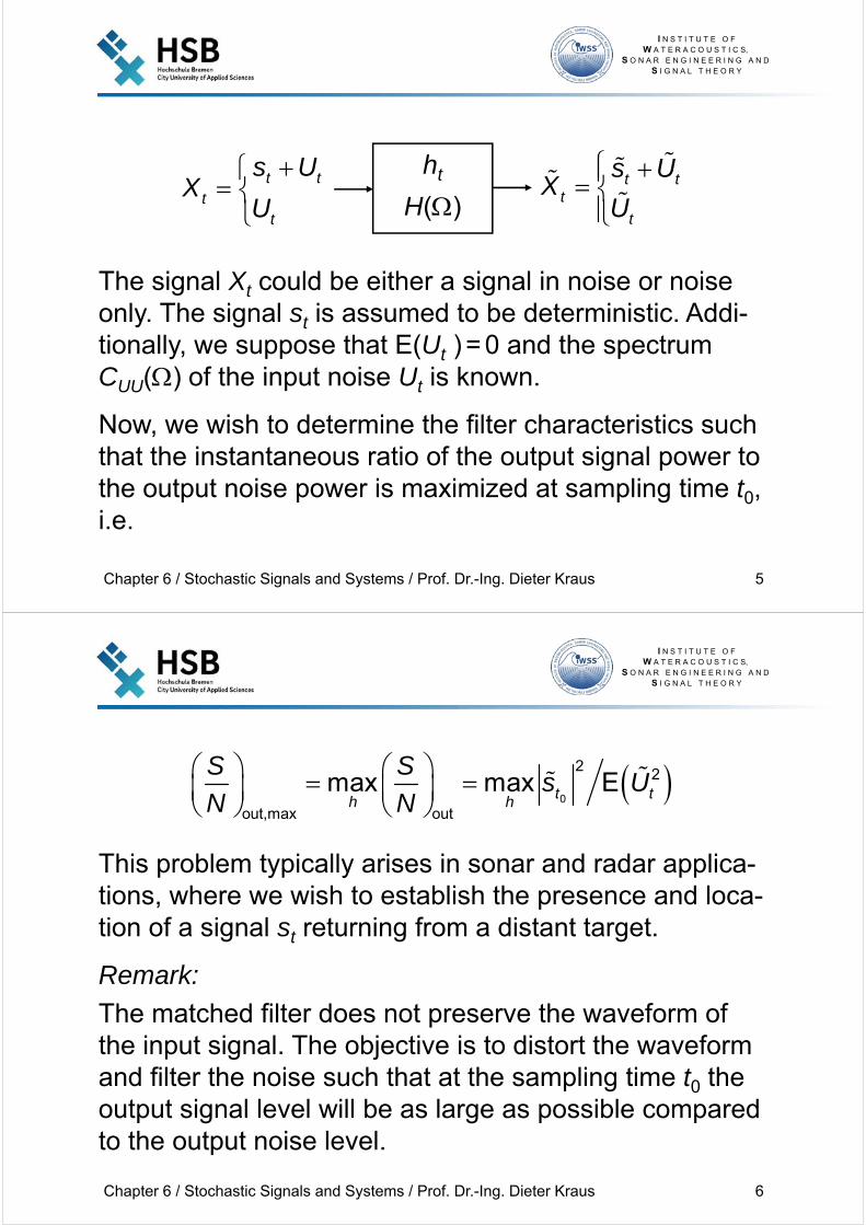
The signal Xt could be either a signal in noise or noise only. The signal st is assumed to be deterministic. Addi-tionally, we suppose that E(Ut ) = 0 and the spectrum CUU() of the input noise Ut is known.
Now, we wish to determine the filter characteristics such that the instantaneous ratio of the output signal power to the output noise power is maximized at sampling time t0, i.e.
t tt
t
s UX
U
t tt
t
s UX
U
ht
H()
I N S T I T U T E O F W A T E R A C O U S T I C S,
S O N A R E N G I N E E R I N G A N DS I G N A L T H E O R Y
Chapter 6 / Stochastic Signals and Systems / Prof. Dr.-Ing. Dieter Kraus 6
This problem typically arises in sonar and radar applica-tions, where we wish to establish the presence and loca-tion of a signal st returning from a distant target.
Remark:
The matched filter does not preserve the waveform of the input signal. The objective is to distort the waveform and filter the noise such that at the sampling time t0 the output signal level will be as large as possible compared to the output noise level.
0
2 2
out,max out
max max Et th h
S Ss U
N N
I N S T I T U T E O F W A T E R A C O U S T I C S,
S O N A R E N G I N E E R I N G A N DS I G N A L T H E O R Y
Chapter 6 / Stochastic Signals and Systems / Prof. Dr.-Ing. Dieter Kraus 7
Theorem:The matched filter that maximizes
has a transfer function given by
where
are the Fourier transform of st and the spectrum of Ut, respectively, k is an arbitrary real constant and t0 is the sampling time when (S/N) is evaluated.
0
2 2
out
Et t
Ss U
N
0
*( )( ) ,
( )j t
optUU
SH k e
C
F F( ) and ( ) ( )t UU UUS s C c
I N S T I T U T E O F W A T E R A C O U S T I C S,
S O N A R E N G I N E E R I N G A N DS I G N A L T H E O R Y
Chapter 6 / Stochastic Signals and Systems / Prof. Dr.-Ing. Dieter Kraus 8
Exercise 6.2-1:(Proof of the Theorem)
I N S T I T U T E O F W A T E R A C O U S T I C S,
S O N A R E N G I N E E R I N G A N DS I G N A L T H E O R Y
Chapter 6 / Stochastic Signals and Systems / Prof. Dr.-Ing. Dieter Kraus 9
Remarks:
k is an arbitrary constant since the signal and the noise at the input are both multiplied by k. Thus k cancels in the relation for (S/N)out.
The filter found may or may not be causal. If it is not causal, it has to be approximated by a causal filter.
The transfer function of the optimum filter is proportional to the complex conjugate of the spectrum of the input signal. Hence, we might say that the linear system is matched to the specified signal.
I N S T I T U T E O F W A T E R A C O U S T I C S,
S O N A R E N G I N E E R I N G A N DS I G N A L T H E O R Y
Chapter 6 / Stochastic Signals and Systems / Prof. Dr.-Ing. Dieter Kraus 10
6.2.1 Matched Filtering for White Noise
Theorem:Suppose the input noise is white. Then the impulse res-ponse of the matched filter is given by
where c is an arbitrary real constant, t0 is the time of the peak signal output, and st is the known input signal wave-form.
Consequently, the impulse response of the matched filter is simply a time reversed, complex conjugated and by t0translated version of the known signal waveform. There-fore, the filter is said to be "matched to the signal".
0, ,t opt t th c s
I N S T I T U T E O F W A T E R A C O U S T I C S,
S O N A R E N G I N E E R I N G A N DS I G N A L T H E O R Y
Chapter 6 / Stochastic Signals and Systems / Prof. Dr.-Ing. Dieter Kraus 11
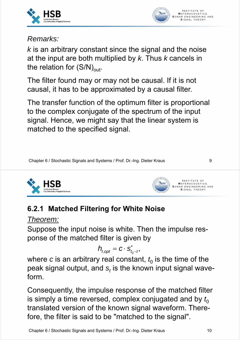
Exercise 6.2-2:(Proof of the Theorem)
t tt
t
s ZX
Z
t tt
t
s ZX
Z
ht
H()
I N S T I T U T E O F W A T E R A C O U S T I C S,
S O N A R E N G I N E E R I N G A N DS I G N A L T H E O R Y
Chapter 6 / Stochastic Signals and Systems / Prof. Dr.-Ing. Dieter Kraus 12
The signal-to-noise ratio at the output is given by
where is the energy of the input signal of finite length T.
Remarks:The signal-to-noise ratio at the output of the filter depends on the signal energy and power level of the noise and not on the particular signal waveform used.
To improve the signal-to-noise ratio, we can increase the signal amplitude or the signal length.
12 22
2 20out
11( ) ,
2
Ts
Z ttZ Z
ESS d s
N
1 2
0
T
s ttE s
I N S T I T U T E O F W A T E R A C O U S T I C S,
S O N A R E N G I N E E R I N G A N DS I G N A L T H E O R Y
Chapter 6 / Stochastic Signals and Systems / Prof. Dr.-Ing. Dieter Kraus 13
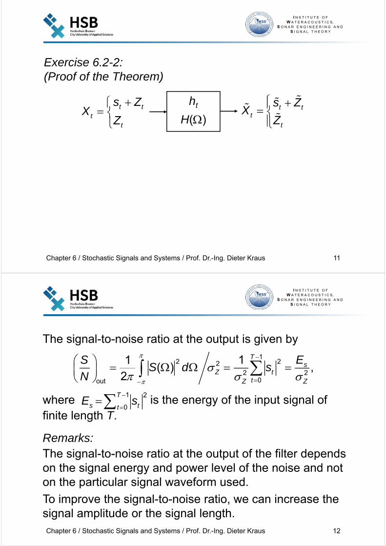
Example:
We want to find the matched filter for the known signal
of finite extent T t2 t1 + 1, as visualized below,
that is imbedded in additive white noise. Hence, the impulse response of the matched filter is given by
1 21 if
0 elsewheret
t t ts
t2t1 t
…
1 ts
I N S T I T U T E O F W A T E R A C O U S T I C S,
S O N A R E N G I N E E R I N G A N DS I G N A L T H E O R Y
Chapter 6 / Stochastic Signals and Systems / Prof. Dr.-Ing. Dieter Kraus 14
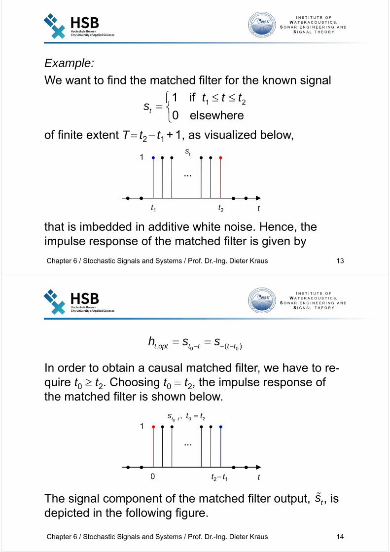
In order to obtain a causal matched filter, we have to re-quire t0 t2. Choosing t0 t2, the impulse response of the matched filter is shown below.
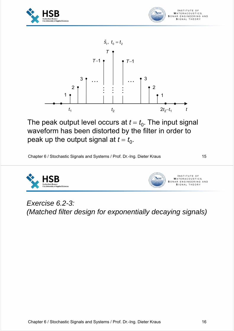
The signal component of the matched filter output, , is depicted in the following figure.
0 0, ( )t opt t t t th s s
ts
t2 t10 t
…
10 0 2,t ts t t
I N S T I T U T E O F W A T E R A C O U S T I C S,
S O N A R E N G I N E E R I N G A N DS I G N A L T H E O R Y
Chapter 6 / Stochastic Signals and Systems / Prof. Dr.-Ing. Dieter Kraus 15
The peak output level occurs at t t0. The input signal waveform has been distorted by the filter in order to peak up the output signal at t t0.
2t2t1 t
1
2
3
t1 t2
1
2
3
T1
T
T1
0 2,ts t t
I N S T I T U T E O F W A T E R A C O U S T I C S,
S O N A R E N G I N E E R I N G A N DS I G N A L T H E O R Y
Chapter 6 / Stochastic Signals and Systems / Prof. Dr.-Ing. Dieter Kraus 16
Exercise 6.2-3:(Matched filter design for exponentially decaying signals)
I N S T I T U T E O F W A T E R A C O U S T I C S,
S O N A R E N G I N E E R I N G A N DS I G N A L T H E O R Y
Chapter 6 / Stochastic Signals and Systems / Prof. Dr.-Ing. Dieter Kraus 17
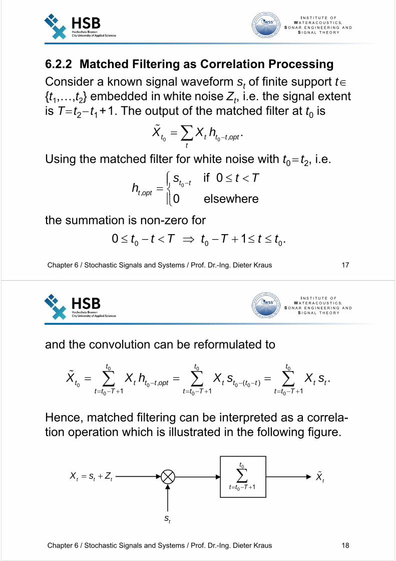
6.2.2 Matched Filtering as Correlation Processing
Consider a known signal waveform st of finite support t{t1,…,t2} embedded in white noise Zt, i.e. the signal extent is T t2 t1+1. The output of the matched filter at t0 is
Using the matched filter for white noise with t0 t2, i.e.
the summation is non-zero for
0 0 , .t t t t optt
X X h
0
,
if 0
0 elsewhere
t t
t opt
s t Th
0 0 00 1 .t t T t T t t
I N S T I T U T E O F W A T E R A C O U S T I C S,
S O N A R E N G I N E E R I N G A N DS I G N A L T H E O R Y
Chapter 6 / Stochastic Signals and Systems / Prof. Dr.-Ing. Dieter Kraus 18
and the convolution can be reformulated to
Hence, matched filtering can be interpreted as a correla-tion operation which is illustrated in the following figure.
tXt t tX s Z
ts
0
0 1
t
t t T
0 0 0
0 0 0 0
0 0 0
, ( )1 1 1
.t t t
t t t t opt t t t t t tt t T t t T t t T
X X h X s X s
I N S T I T U T E O F W A T E R A C O U S T I C S,
S O N A R E N G I N E E R I N G A N DS I G N A L T H E O R Y
Chapter 6 / Stochastic Signals and Systems / Prof. Dr.-Ing. Dieter Kraus 19
6.3 Wiener FilteringThe matched filter considered in the previous section is an optimal filter in the sense that it provides the highest SNR at the output for detecting the presence of a known signal.
The Wiener filter considered now aims to provide an opti-mal estimation of the realization of one stochastic process from observations of another stochastic process.
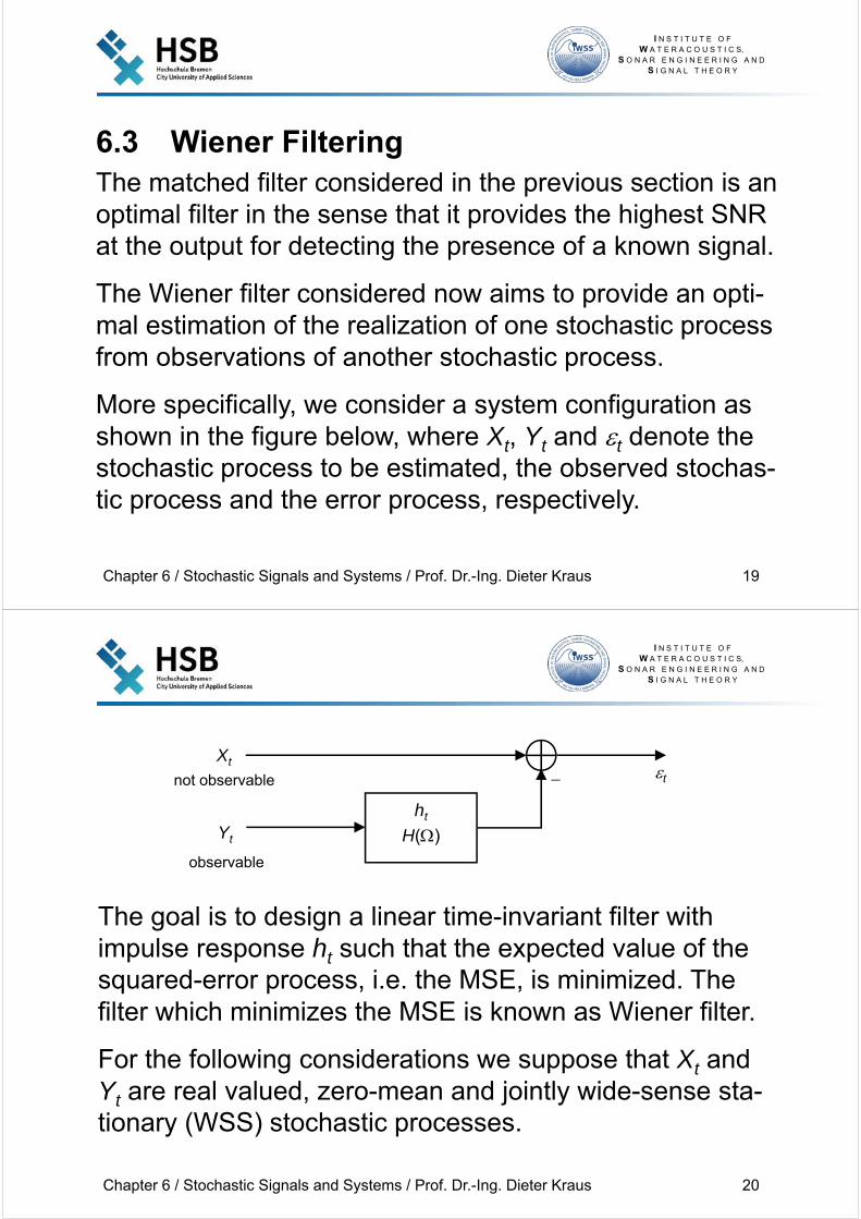
More specifically, we consider a system configuration as shown in the figure below, where Xt, Yt and t denote the stochastic process to be estimated, the observed stochas-tic process and the error process, respectively.
I N S T I T U T E O F W A T E R A C O U S T I C S,
S O N A R E N G I N E E R I N G A N DS I G N A L T H E O R Y
Chapter 6 / Stochastic Signals and Systems / Prof. Dr.-Ing. Dieter Kraus 20
The goal is to design a linear time-invariant filter with impulse response ht such that the expected value of the squared-error process, i.e. the MSE, is minimized. The filter which minimizes the MSE is known as Wiener filter.
For the following considerations we suppose that Xt and Yt are real valued, zero-mean and jointly wide-sense sta-tionary (WSS) stochastic processes.
t
ht
H()
Xt
not observable
observable
Yt
I N S T I T U T E O F W A T E R A C O U S T I C S,
S O N A R E N G I N E E R I N G A N DS I G N A L T H E O R Y
Chapter 6 / Stochastic Signals and Systems / Prof. Dr.-Ing. Dieter Kraus 21
Since the processes Xt and Yt are jointly WSS and the filter with impulse response ht is assumed to be stable, the error process t is also WSS.
Hence, the MSE, which is the second-order moment of t, does not depend on the index t. The MSE can be ex-pressed in terms of the filter response ht by
1 2 1 2
1 2
1 2
1 2
2
2
2
2 1
( ) E ( ) E
E( ) E( ) 2 E( )
(0) ( ) 2 ( ).
t t t t t
t t t t t
XX YY XY
q h h X h Y
X h h Y Y h X Y
c h h c h c
I N S T I T U T E O F W A T E R A C O U S T I C S,
S O N A R E N G I N E E R I N G A N DS I G N A L T H E O R Y
Chapter 6 / Stochastic Signals and Systems / Prof. Dr.-Ing. Dieter Kraus 22
The impulse response of the optimal (Wiener) filter ht,opt
is defined by
where H denotes the set of all absolutely summable im-pulse responses.
6.3.1 Wiener-Hopf Equation
Now, we would like to solve the MSE problem
The solution of this problem is provided by exploiting the orthogonality principle stated in the following theorem.
, argmin ( ),t
t opt thh q h
H
2min ( ) minE .
t tt t th h
q h X h Y H H
I N S T I T U T E O F W A T E R A C O U S T I C S,
S O N A R E N G I N E E R I N G A N DS I G N A L T H E O R Y
Chapter 6 / Stochastic Signals and Systems / Prof. Dr.-Ing. Dieter Kraus 23
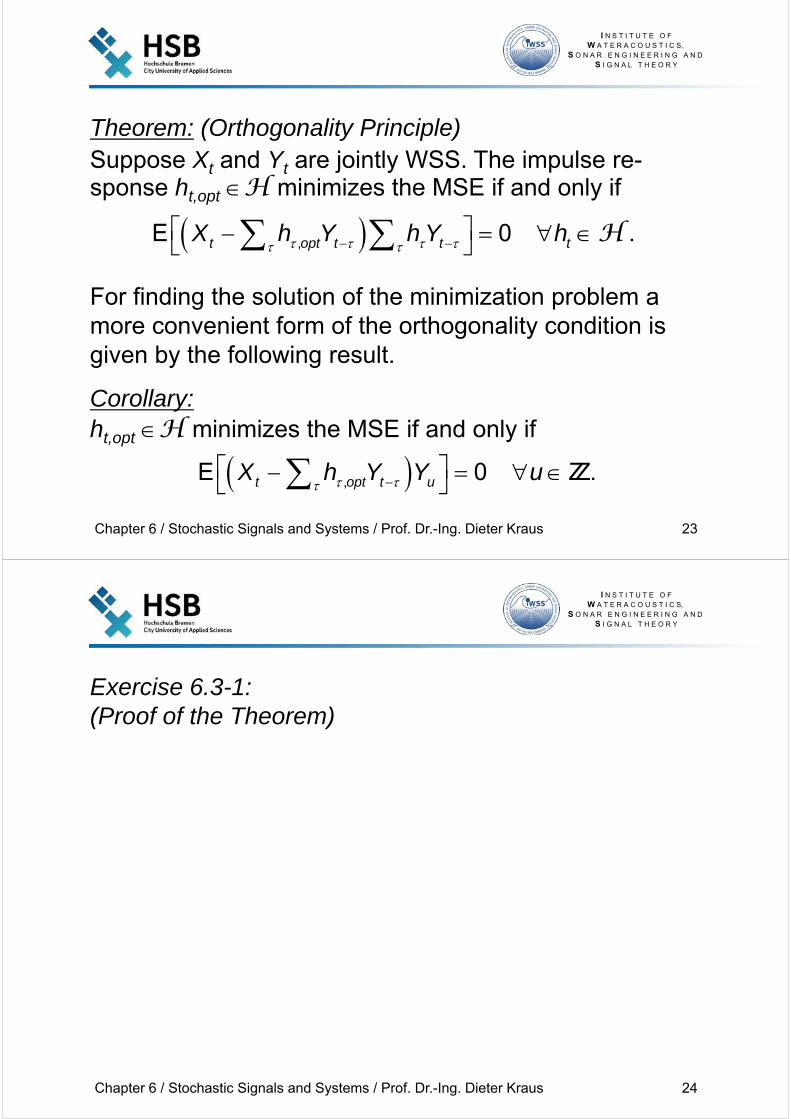
Theorem: (Orthogonality Principle)Suppose Xt and Yt are jointly WSS. The impulse re-sponse ht,opt H minimizes the MSE if and only if
For finding the solution of the minimization problem a more convenient form of the orthogonality condition is given by the following result.
Corollary:ht,opt H minimizes the MSE if and only if
,E 0 .t opt t t tX h Y h Y h H
,E 0 .t opt t uX h Y Y u
I N S T I T U T E O F W A T E R A C O U S T I C S,
S O N A R E N G I N E E R I N G A N DS I G N A L T H E O R Y
Chapter 6 / Stochastic Signals and Systems / Prof. Dr.-Ing. Dieter Kraus 24
Exercise 6.3-1:(Proof of the Theorem)
I N S T I T U T E O F W A T E R A C O U S T I C S,
S O N A R E N G I N E E R I N G A N DS I G N A L T H E O R Y
Chapter 6 / Stochastic Signals and Systems / Prof. Dr.-Ing. Dieter Kraus 25
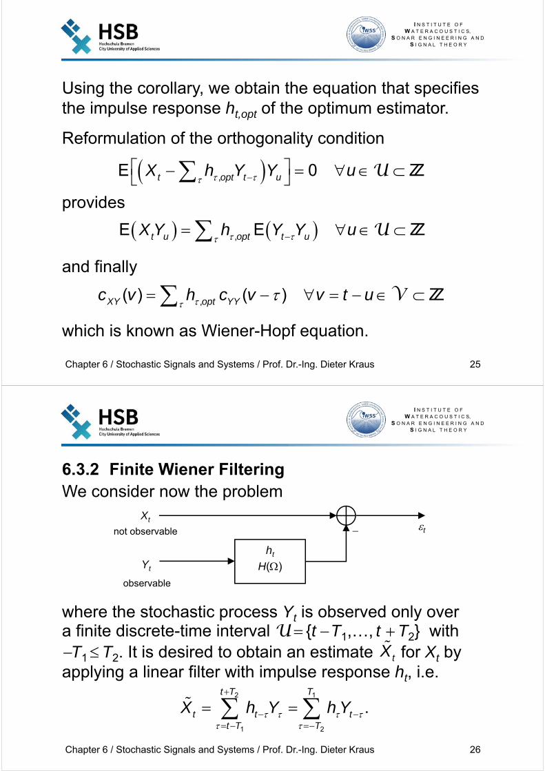
Using the corollary, we obtain the equation that specifies the impulse response ht,opt of the optimum estimator.
Reformulation of the orthogonality condition
provides
and finally
which is known as Wiener-Hopf equation.
,E Et u opt t uX Y h Y Y u U
,E 0t opt t uX h Y Y u U
,( ) ( )XY opt YYc v h c v v t u V
I N S T I T U T E O F W A T E R A C O U S T I C S,
S O N A R E N G I N E E R I N G A N DS I G N A L T H E O R Y
Chapter 6 / Stochastic Signals and Systems / Prof. Dr.-Ing. Dieter Kraus 26
6.3.2 Finite Wiener FilteringWe consider now the problem
where the stochastic process Yt is observed only over a finite discrete-time interval U {tT1,…, t T2} with T1T2. It is desired to obtain an estimate for Xt by applying a linear filter with impulse response ht, i.e.
t
ht
H()
Xt
not observable
observable
Yt
tX
2 1
1 2
.t T T
t t tt T T
X h Y h Y
I N S T I T U T E O F W A T E R A C O U S T I C S,
S O N A R E N G I N E E R I N G A N DS I G N A L T H E O R Y
Chapter 6 / Stochastic Signals and Systems / Prof. Dr.-Ing. Dieter Kraus 27
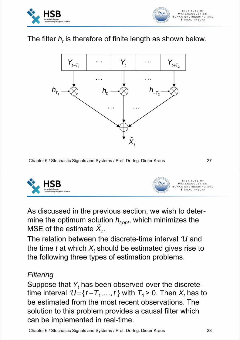
The filter ht is therefore of finite length as shown below.
tX
1Th
1t TY tY2t TY
2Th0h
I N S T I T U T E O F W A T E R A C O U S T I C S,
S O N A R E N G I N E E R I N G A N DS I G N A L T H E O R Y
Chapter 6 / Stochastic Signals and Systems / Prof. Dr.-Ing. Dieter Kraus 28
As discussed in the previous section, we wish to deter-mine the optimum solution ht,opt, which minimizes the MSE of the estimate . The relation between the discrete-time interval U and the time t at which Xt should be estimated gives rise to the following three types of estimation problems.
FilteringSuppose that Yt has been observed over the discrete-time interval U { tT1,…, t } with T1 > 0. Then Xt has to be estimated from the most recent observations. The solution to this problem provides a causal filter which can be implemented in real-time.
tX
I N S T I T U T E O F W A T E R A C O U S T I C S,
S O N A R E N G I N E E R I N G A N DS I G N A L T H E O R Y
Chapter 6 / Stochastic Signals and Systems / Prof. Dr.-Ing. Dieter Kraus 29
SmoothingIf the observations are taken over the discrete-time inter-val U { tT1,…,tT2 } with T1,T2 > 0 then Xt can be esti-mated from past and future observations. This is appli-cable in post-processing situations, when a realization of Yt has been recorded and can be played back.
PredictionLet Yt be given over the discrete-time interval U { tT1, …,t k } with T1 > k > 0. Then Xt has to be predicted from past observations. Since the filtering procedure is de-fined by a linear operation represents a k-step linear predictor for Xt.
tX
I N S T I T U T E O F W A T E R A C O U S T I C S,
S O N A R E N G I N E E R I N G A N DS I G N A L T H E O R Y
Chapter 6 / Stochastic Signals and Systems / Prof. Dr.-Ing. Dieter Kraus 30
Now, the optimum solution ht,opt has to satisfy the Wiener-Hopf equation
which can be expressed in matrix form (also known as Yule-Walker equation) as
where
and
1
2
, 2 1{ , , }T
XY opt YYT
c v h c v v T TV
,YY opt XYC h c
2
1
, 2
, 1
( ),
( )
T opt XY
opt XY
T opt XY
h c T
h c T
h c
I N S T I T U T E O F W A T E R A C O U S T I C S,
S O N A R E N G I N E E R I N G A N DS I G N A L T H E O R Y
Chapter 6 / Stochastic Signals and Systems / Prof. Dr.-Ing. Dieter Kraus 31
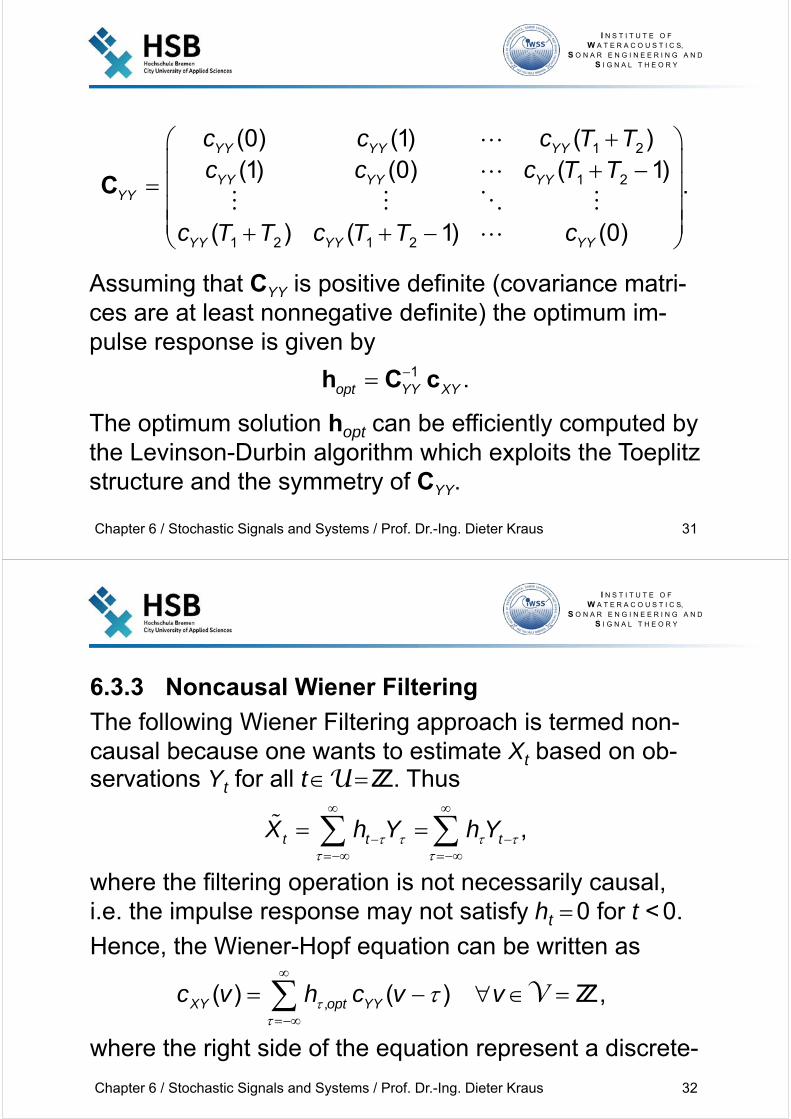
Assuming that CYY is positive definite (covariance matri-ces are at least nonnegative definite) the optimum im-pulse response is given by
The optimum solution hopt can be efficiently computed by the Levinson-Durbin algorithm which exploits the Toeplitz structure and the symmetry of CYY.
1 2
1 2
1 2 1 2
(0) (1) ( )(1) (0) ( 1)
.
( ) ( 1) (0)
YY YY YY
YY YY YYYY
YY YY YY
c c c T Tc c c T T
c T T c T T c
C
1 .opt YY XYh C c
I N S T I T U T E O F W A T E R A C O U S T I C S,
S O N A R E N G I N E E R I N G A N DS I G N A L T H E O R Y
Chapter 6 / Stochastic Signals and Systems / Prof. Dr.-Ing. Dieter Kraus 32
6.3.3 Noncausal Wiener Filtering
The following Wiener Filtering approach is termed non-causal because one wants to estimate Xt based on ob-servations Yt for all tU. Thus
where the filtering operation is not necessarily causal, i.e. the impulse response may not satisfy ht 0 for t < 0.
Hence, the Wiener-Hopf equation can be written as
where the right side of the equation represent a discrete-
,( ) ( ) ,XY opt YYc v h c v v V
,t t tX h Y h Y
I N S T I T U T E O F W A T E R A C O U S T I C S,
S O N A R E N G I N E E R I N G A N DS I G N A L T H E O R Y
Chapter 6 / Stochastic Signals and Systems / Prof. Dr.-Ing. Dieter Kraus 33
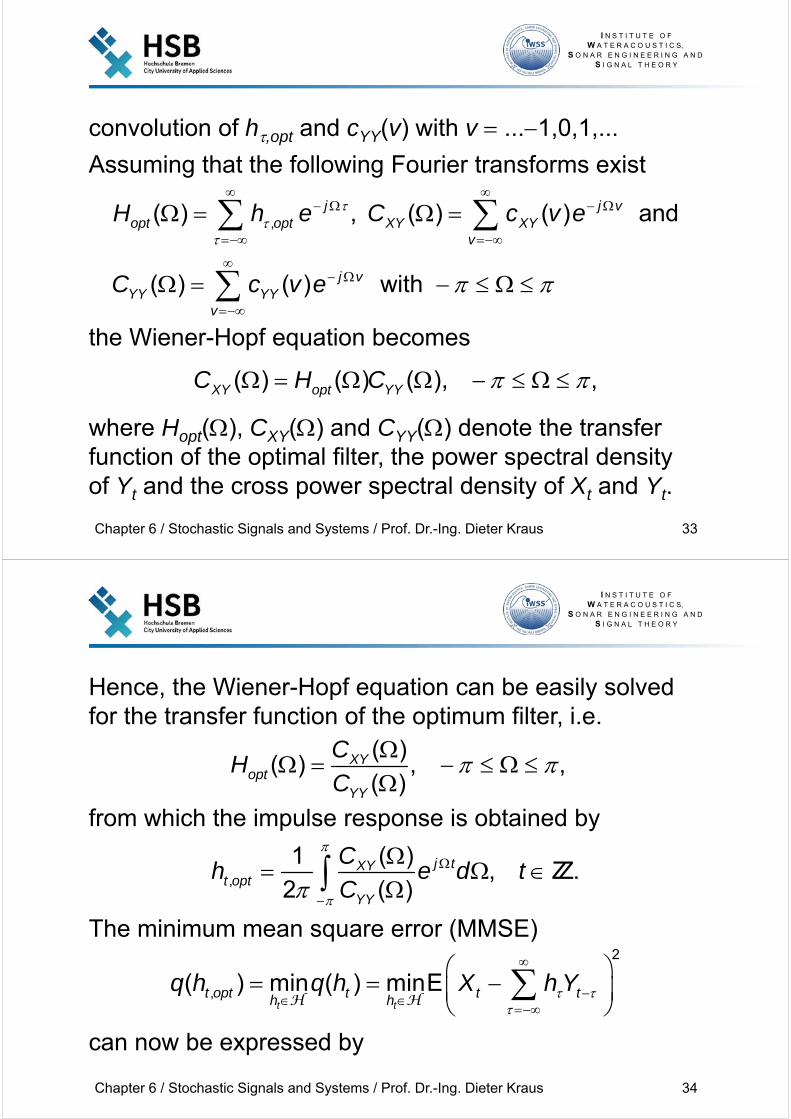
convolution of h,opt and cYY(v) with v ...1,0,1,...
Assuming that the following Fourier transforms exist
the Wiener-Hopf equation becomes
where Hopt(), CXY() and CYY() denote the transfer function of the optimal filter, the power spectral density of Yt and the cross power spectral density of Xt and Yt.
,( ) , ( ) ( ) and
( ) ( ) with
j j vopt opt XY XY
v
j vYY YY
v
H h e C c v e
C c v e
( ) ( ) ( ), ,XY opt YYC H C
I N S T I T U T E O F W A T E R A C O U S T I C S,
S O N A R E N G I N E E R I N G A N DS I G N A L T H E O R Y
Chapter 6 / Stochastic Signals and Systems / Prof. Dr.-Ing. Dieter Kraus 34
Hence, the Wiener-Hopf equation can be easily solved for the transfer function of the optimum filter, i.e.
from which the impulse response is obtained by
The minimum mean square error (MMSE)
can now be expressed by
,
1 ( ), .
2 ( )j tXY
t optYY
Ch e d t
C
( )( ) , ,
( )XY
optYY
CH
C
2
,( ) min ( ) minEt t
t opt t t th hq h q h X h Y
H H
I N S T I T U T E O F W A T E R A C O U S T I C S,
S O N A R E N G I N E E R I N G A N DS I G N A L T H E O R Y
Chapter 6 / Stochastic Signals and Systems / Prof. Dr.-Ing. Dieter Kraus 35
Since the infinite sum in the equation above can be written as
2
, , ,
2, ,
( ) E E
E( ) E( ) (0) ( ).
t opt t opt t t opt t t
t opt t t XX opt XY
q h X h Y X h Y X
X h X Y c h c
, ,
2
1( ) ( ) ( ) ( )
2
1 ( ) 1 | ( )|( ) .
2 ( ) 2 ( )
opt XY opt YX opt YX
XY XYYX
YY YY
h c h c H C d
C CC d d
C C
( ) ( ) and ( ) ( )XY YX YX XYc c C C
I N S T I T U T E O F W A T E R A C O U S T I C S,
S O N A R E N G I N E E R I N G A N DS I G N A L T H E O R Y
Chapter 6 / Stochastic Signals and Systems / Prof. Dr.-Ing. Dieter Kraus 36
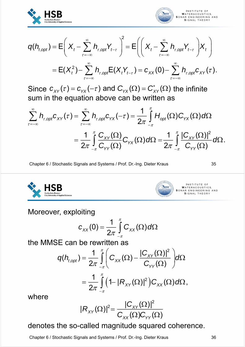
Moreover, exploiting
the MMSE can be rewritten as
where
denotes the so-called magnitude squared coherence.
1(0) ( )
2XX XXc C d
2
,
2
1 | ( )|( ) ( )
2 ( )
11 | ( )| ( ) ,
2
XYt opt XX
YY
XY XX
Cq h C d
C
R C d
2
2 | ( )|| ( )|
( ) ( )XY
XYXX YY
CR
C C
I N S T I T U T E O F W A T E R A C O U S T I C S,
S O N A R E N G I N E E R I N G A N DS I G N A L T H E O R Y
Chapter 6 / Stochastic Signals and Systems / Prof. Dr.-Ing. Dieter Kraus 37
Applying the results stated in chapter 2.6.3, RXY() can be expressed by
so that RXY() can be interpreted as the correlation coef-ficient between the random components of Xt and Yt at frequency . Thus,
Moreover, the equality sign holds for all [, ] if and only if Xt and Yt are related by a linear transformation
2| ( )| 1, .XYR
.t tX h Y
Cov ( ), ( )( )
Var ( ) Var ( )X Y
XY
X Y
dZ dZR
dZ dZ
I N S T I T U T E O F W A T E R A C O U S T I C S,
S O N A R E N G I N E E R I N G A N DS I G N A L T H E O R Y
Chapter 6 / Stochastic Signals and Systems / Prof. Dr.-Ing. Dieter Kraus 38
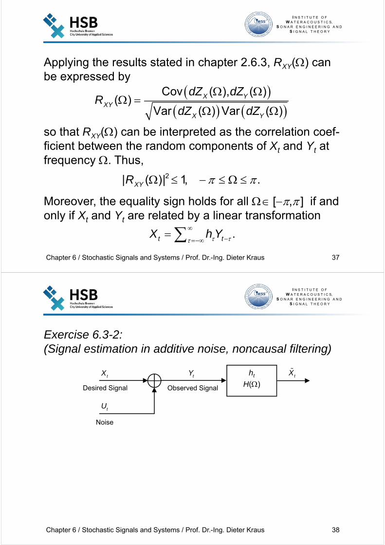
Exercise 6.3-2:(Signal estimation in additive noise, noncausal filtering)
ht
H()Desired Signal
Noise
tX
tU
tXtY
Observed Signal
I N S T I T U T E O F W A T E R A C O U S T I C S,
S O N A R E N G I N E E R I N G A N DS I G N A L T H E O R Y
Chapter 6 / Stochastic Signals and Systems / Prof. Dr.-Ing. Dieter Kraus 39
6.3.4 Causal Wiener Filtering
Noncausal Wiener filtering is improper for applications in which real-time estimation is required. Therefore, it is of practical relevance to consider the causal Wiener filtering problem in which we wish to estimate Xt based on obser-vations Yu for all uU { : t }.
Hence, with the causal filter approach
the Wiener-Hopf equation becomes
0
t
t t tX h Y h Y
, 00
( ) ( ) .XY opt YYc v h c v v V
I N S T I T U T E O F W A T E R A C O U S T I C S,
S O N A R E N G I N E E R I N G A N DS I G N A L T H E O R Y
Chapter 6 / Stochastic Signals and Systems / Prof. Dr.-Ing. Dieter Kraus 40
Since the Wiener-Hopf equation is only defined for v 0it can not be solved by Fourier transform. Before we can derive the solution we first have to discuss the so-called spectral factorization.
Spectral Factorization and Linear Representation
Suppose Yt has an absolutely continuous and integrable spectral density CYY(). Then Yt can be represented as noncausal filtered white noise
and CYY() can be written as
2with | | , ( ) 0 and ( )t t t t zz tt
Y g Z g E Z c t
( ) ( ) ( ) with ( ) .j tYY t
t
C G G G g e
I N S T I T U T E O F W A T E R A C O U S T I C S,
S O N A R E N G I N E E R I N G A N DS I G N A L T H E O R Y
Chapter 6 / Stochastic Signals and Systems / Prof. Dr.-Ing. Dieter Kraus 41
Moreover, if CYY() satisfies the Paley-Wiener condition
an unique causal impulse response gt with g0 > 0 and exists, such that
has no zeros outside the unit circle (minimum phase fil-ter) and provides a factorization for CYY() in the form
Furthermore, implies that no poles of are lying outside the unit circle.
0
( ) with ( ) ( )t jt
t
G z g z G e G
log ( )YYC
2
0| |ttg
2 2( ) ( ) ( ) | ( )| | ( )| .jYYC G G G G e
2
0| |ttg ( )G z
I N S T I T U T E O F W A T E R A C O U S T I C S,
S O N A R E N G I N E E R I N G A N DS I G N A L T H E O R Y
Chapter 6 / Stochastic Signals and Systems / Prof. Dr.-Ing. Dieter Kraus 42
The Paley-Wiener condition is a fairly weak condition that may hold in any situation of practical interest.
However, if we impose the additional constraints
an explicit expression can be obtain for .
The constraints imply that all zeros and poles of are lying within the unit circle. Thus, can be interpreted as the z-Transform of a linear, causal, stable, minimum phase and invertible stable filter.
Now, the spectral density of Xt given by
( )G z0 0
| | and ( ) 0 | | 1tt t
t t
g G z g z z
( )G z( )G z
2 2( ) | ( )| | ( )|jYYC G G e
I N S T I T U T E O F W A T E R A C O U S T I C S,
S O N A R E N G I N E E R I N G A N DS I G N A L T H E O R Y
Chapter 6 / Stochastic Signals and Systems / Prof. Dr.-Ing. Dieter Kraus 43
can be analytically continued
in an annulus that contains |z| 1. Since
we can conclude that if are zeros and poles of respectively then are also zeros and poles of .
Hence, we obtain the so-called canonical factorization
where and contain all zeros and poles of
1( ) ( ) ( ) ( ) tYY YY
t
C z G z G z c t z
1( ) ( )YY YYC z C z
1 1 1 10, 0, 0, , , ,, , and , ,i i i j j jz z z z z z
0, ,andi jz z
( )YYC z( )YYC z
( ) ( ) ( ),YY YY YYC z C z C z
( )YYC z ( )YYC z
I N S T I T U T E O F W A T E R A C O U S T I C S,
S O N A R E N G I N E E R I N G A N DS I G N A L T H E O R Y
Chapter 6 / Stochastic Signals and Systems / Prof. Dr.-Ing. Dieter Kraus 44
that are lying within or outside the unit circle re-spectively. Since the zeros and poles of are rela-ted to the zeros and poles of by mirroring at the unit circle we can write
Solution of the Wiener-Hopf Equation
Due to the preceding assumptions and explanations we are now able to solve the Wiener-Hopf equation. For this purpose we define the sequence
which has obviously to satisfy qv0 for all v 0.
( )YYC z
( )YYC z
( )YYC z
1( ) ( ).YY YYC z C z
,0
( ) ( )v XY opt YYq c v h c v
I N S T I T U T E O F W A T E R A C O U S T I C S,
S O N A R E N G I N E E R I N G A N DS I G N A L T H E O R Y
Chapter 6 / Stochastic Signals and Systems / Prof. Dr.-Ing. Dieter Kraus 45
After applying the two-sided z-Transform we obtain
where the convolution theorem for z-Transforms and the canonical factorization has been exploited.
Since qv is anticausal its z-Transform does not con-tain a constant component and can only possess poles outside the unit circle.
Dividing the former equation by we can write
( ) ( ) ( ) ( )
( ) ( ) ( ),
XY opt YY
XY opt YY YY
Q z C z H z C z
C z H C z C z
( )Q z
( )YYC z
( ) ( )( ) ( ).
( ) ( )XY
opt YYYY YY
Q z C zH z C z
C z C z
I N S T I T U T E O F W A T E R A C O U S T I C S,
S O N A R E N G I N E E R I N G A N DS I G N A L T H E O R Y
Chapter 6 / Stochastic Signals and Systems / Prof. Dr.-Ing. Dieter Kraus 46
Due to the aforementioned properties of and sincehas only zeros outside the unit circle we can infer
that does not contain a constant component and possesses only poles outside the unit circle.
Moreover, as the poles of are lying within the unit circle its inverse z-Transform represents a cau-sal sequence.
Hence, after defining the operation
we can state that
( )YYC z
( ) ( )YYQ z C z
( )Q z
( ) ( )opt YYH z C z
0
( ) t tt t
t t
F z f z f z
I N S T I T U T E O F W A T E R A C O U S T I C S,
S O N A R E N G I N E E R I N G A N DS I G N A L T H E O R Y
Chapter 6 / Stochastic Signals and Systems / Prof. Dr.-Ing. Dieter Kraus 47
Finally, the latter provides together with
the desired solution for the Wiener filter in the z-domain
which in the frequency domain can be expressed by
1 ( )( )
( ) ( )XY
optYY YY
C zH z
C z C z
1 ( ) 1 ( )( ) ( ).
( ) ( ) ( ) ( )
jj XY XY
opt optj jYY YY YY YY
C e CH e H
C e C e C C
( ) ( ) 0 and ( ) ( ) ( ) ( ).YY opt YY opt YYQ z C z H z C z H z C z
( ) ( ) ( ) ( ) ( ) ( )YY XY YY opt YYQ z C z C z C z H z C z
I N S T I T U T E O F W A T E R A C O U S T I C S,
S O N A R E N G I N E E R I N G A N DS I G N A L T H E O R Y
Chapter 6 / Stochastic Signals and Systems / Prof. Dr.-Ing. Dieter Kraus 48
Exercise 6.3-3:(Solution of the Wiener-Hopf equation for white noise and its application after prewhitening)
I N S T I T U T E O F W A T E R A C O U S T I C S,
S O N A R E N G I N E E R I N G A N DS I G N A L T H E O R Y
Chapter 6 / Stochastic Signals and Systems / Prof. Dr.-Ing. Dieter Kraus 49
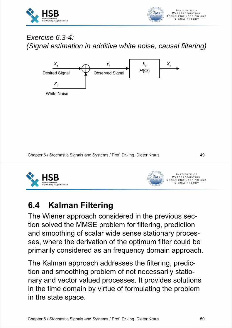
Exercise 6.3-4:(Signal estimation in additive white noise, causal filtering)
ht
H()Desired Signal
White Noise
tX
tZ
tXtY
Observed Signal
I N S T I T U T E O F W A T E R A C O U S T I C S,
S O N A R E N G I N E E R I N G A N DS I G N A L T H E O R Y
Chapter 6 / Stochastic Signals and Systems / Prof. Dr.-Ing. Dieter Kraus 50
6.4 Kalman FilteringThe Wiener approach considered in the previous sec-tion solved the MMSE problem for filtering, prediction and smoothing of scalar wide sense stationary proces-ses, where the derivation of the optimum filter could be primarily considered as an frequency domain approach.
The Kalman approach addresses the filtering, predic-tion and smoothing problem of not necessarily statio-nary and vector valued processes. It provides solutions in the time domain by virtue of formulating the problem in the state space.
I N S T I T U T E O F W A T E R A C O U S T I C S,
S O N A R E N G I N E E R I N G A N DS I G N A L T H E O R Y
Chapter 6 / Stochastic Signals and Systems / Prof. Dr.-Ing. Dieter Kraus 51
6.4.1 State Space Model
Discrete-time dynamic systems can be represented by a state equation
and a measurement equation
where (ft)t0 and (ht)t0 are sequences of functions, (Xt)t0
is a sequence in p describing the states of interest, (Ut)t0
is a sequence in q acting on (Xt)t1 and where (Yt)t0 and (Vt)t0 are sequences in r representing the measure-ments and the measurement noise, respectively.
1 ( , ), 0,1,2,t t t t t X f X U
1 ( , ), 0,1,2, ,t t t t t Y h X V
I N S T I T U T E O F W A T E R A C O U S T I C S,
S O N A R E N G I N E E R I N G A N DS I G N A L T H E O R Y
Chapter 6 / Stochastic Signals and Systems / Prof. Dr.-Ing. Dieter Kraus 52
If the discrete-time system is linear the state and mea-surement equations can be expressed by
and
where Ft, Gt and Ht are pp, pq and rp matrices, res-pectively, for each t.
Furthermore, if the system is time-invariant the matrices Ft, Gt and Ht become constant coefficient matrices which are accordingly denoted by F, G and H. Hence, the state and measurement equations simplify to
, 0,1,2, ,t t t t t Y H X V
1 , 0,1,2, ,t t t t t t X FX G U
1 and , 0,1,2, .t t t t t t t X FX GU Y HX V
I N S T I T U T E O F W A T E R A C O U S T I C S,
S O N A R E N G I N E E R I N G A N DS I G N A L T H E O R Y
Chapter 6 / Stochastic Signals and Systems / Prof. Dr.-Ing. Dieter Kraus 53
Exercise 6.4-1:(State space representation of the one-dimensional motion of a particle)
I N S T I T U T E O F W A T E R A C O U S T I C S,
S O N A R E N G I N E E R I N G A N DS I G N A L T H E O R Y
Chapter 6 / Stochastic Signals and Systems / Prof. Dr.-Ing. Dieter Kraus 54
6.4.2 State Estimation
Now, we suppose that the sequence Y0,...,Yt has been observed and that the state X should be estimated.
This estimation problem is known asa) filtering problem if t ,b) smoothing problem if t > ,c) prediction problem if t < .
To estimate the state X by means of realizations of the measurement sequence Y0,...,Yt in the minimum mean square error sense we have to find an estimating func-tion that minimizes
2
02
ˆ ˆ( ) E ( , , ) .MSE tR X X X Y Y
0ˆ ( , , )tX y y
I N S T I T U T E O F W A T E R A C O U S T I C S,
S O N A R E N G I N E E R I N G A N DS I G N A L T H E O R Y
Chapter 6 / Stochastic Signals and Systems / Prof. Dr.-Ing. Dieter Kraus 55
We know from chapter 3.7.1 that the optimum estimating function is given by the conditional mean, i.e.
However, we are usually interested in generating esti-mates in real time as t increases. Since the data in-crease linear with t, an efficient calculation of the con-ditional mean will be impossible unless suitable restric-tions on the system model structure are imposed, e.g. restriction to discrete-time linear systems with indepen-dent input and measurement noise sequences of inde-pendent zero-mean Gaussian random vectors.
0 0 0ˆ ( , , ) E | , , .t t tX y y X Y y Y y
I N S T I T U T E O F W A T E R A C O U S T I C S,
S O N A R E N G I N E E R I N G A N DS I G N A L T H E O R Y
Chapter 6 / Stochastic Signals and Systems / Prof. Dr.-Ing. Dieter Kraus 56
6.4.3 Kalman Filter Approach
Within the assumptions mentioned above a computatio-nal efficient and simultaneous solution of the filtering and one step prediction problem can be stated.
Theorem:For the linear, finite-dimensional, discrete-time system
where (Ut) and (Vt) are independent sequences of inde-pendent zero-mean Gaussian vectors which are inde-pendent of the Gaussian initial condition X0 with
1 and , 0,1,2, ,t t t t t t t t t t X FX G U Y H X V
0 0 0 0E( ) ( ), E( ) ( ), E( ) , Cov( ) ,T Tt t t tt tUU VVU U Σ V V Σ X μ X Σ
I N S T I T U T E O F W A T E R A C O U S T I C S,
S O N A R E N G I N E E R I N G A N DS I G N A L T H E O R Y
Chapter 6 / Stochastic Signals and Systems / Prof. Dr.-Ing. Dieter Kraus 57
the estimators
can be recursively determined by the following equations.
and
with initialization and Kalman gain matrix
where
| 0 1| 1 0E( | , , ) and E( | , , )t t t t t t t t X X Y Y X X Y Y
| | 1 | 1 0,1,2, ,t t t t t t t t t t X X K Y H X
1| | 0,1,2, ,t t t t t t X FX
1
| 1 | 1 ( ) ,T Tt t t t t t t t t
VVK Σ H H Σ H Σ
0| 1 0 X μ
I N S T I T U T E O F W A T E R A C O U S T I C S,
S O N A R E N G I N E E R I N G A N DS I G N A L T H E O R Y
Chapter 6 / Stochastic Signals and Systems / Prof. Dr.-Ing. Dieter Kraus 58
is the covariance of the prediction error which can be computed jointly with the filtering error covariance
by the recursion
and
with the initialization .
| | 1 | 1, 0,1,2, ,t t t t t t t t tΣ Σ K H Σ
1| | ( ) , 0,1,2, ,T Tt t t t t t t tt tUUΣ F Σ F G Σ G
| 1 0 1
| 1 | 1 0 1
Cov( | , , )
E ( )( ) | , ,
t t t t
Tt t t t t t t
Σ X Y Y
X X X X Y Y
| 0 | | 0Cov( | , , ) E ( )( ) | , ,Tt t t t t t t t t t t Σ X Y Y X X X X Y Y
0| 1 0 Σ Σ
I N S T I T U T E O F W A T E R A C O U S T I C S,
S O N A R E N G I N E E R I N G A N DS I G N A L T H E O R Y
Chapter 6 / Stochastic Signals and Systems / Prof. Dr.-Ing. Dieter Kraus 59
Exercise 6.4-2:(Proof of the Theorem)
I N S T I T U T E O F W A T E R A C O U S T I C S,
S O N A R E N G I N E E R I N G A N DS I G N A L T H E O R Y
Chapter 6 / Stochastic Signals and Systems / Prof. Dr.-Ing. Dieter Kraus 60
The recursions consist of the following two basic steps.
Measurement update
which updates the – state estimate of Xt by incorporating the new measurement Yt,
– filter error covariance matrix.
Time update
which provides the– one-step prediction of the state estimate,
– prediction error covariance matrix.
| | 1 | 1 | | 1 | 1andt t t t t t t t t t t t t t t t tX X K Y H X Σ Σ K H Σ
1| | 1| |and ( )T Tt t t t t t t t t t t t ttUUX FX Σ F Σ F G Σ G
I N S T I T U T E O F W A T E R A C O U S T I C S,
S O N A R E N G I N E E R I N G A N DS I G N A L T H E O R Y
Chapter 6 / Stochastic Signals and Systems / Prof. Dr.-Ing. Dieter Kraus 61
The measurement update equation
can be viewed as a combination of the predicted state vector and a correction term. Since
the difference in the correction term can be interpreted as an error signal
which is known as innovation. The term innovation comes from the fact that It is the part of
| | 1 | 1t t t t t t t t tX X K Y H X
| 1 0 1
0 1 0 1 | 1
E( | , , )
E( | , , ) E( | , , )
t t t t
t t t t t t t t
Y Y Y Y
H X Y Y V Y Y H X
| 1 | 1,t t t t t t t tI Y Y Y H X
I N S T I T U T E O F W A T E R A C O U S T I C S,
S O N A R E N G I N E E R I N G A N DS I G N A L T H E O R Y
Chapter 6 / Stochastic Signals and Systems / Prof. Dr.-Ing. Dieter Kraus 62
that cannot be predicted and therefore contains the newinformation that is gained by the current observation.
Remarks:
The innovation sequence It is a sequence of indepen-dent not identically distributed zero-mean Gaussian ran-dom vectors.
Yt consists of a part, Yt|t1, completely dependent and a part, It, completely independent of the past. Thus It pro-vides a set of independent observations that forms suit-ably scaled the output of a prewhitening operation.
| 1t t t tY Y I
I N S T I T U T E O F W A T E R A C O U S T I C S,
S O N A R E N G I N E E R I N G A N DS I G N A L T H E O R Y
Chapter 6 / Stochastic Signals and Systems / Prof. Dr.-Ing. Dieter Kraus 63
Exercise 6.4-3:(Proof of the remarks)
I N S T I T U T E O F W A T E R A C O U S T I C S,
S O N A R E N G I N E E R I N G A N DS I G N A L T H E O R Y
Chapter 6 / Stochastic Signals and Systems / Prof. Dr.-Ing. Dieter Kraus 64
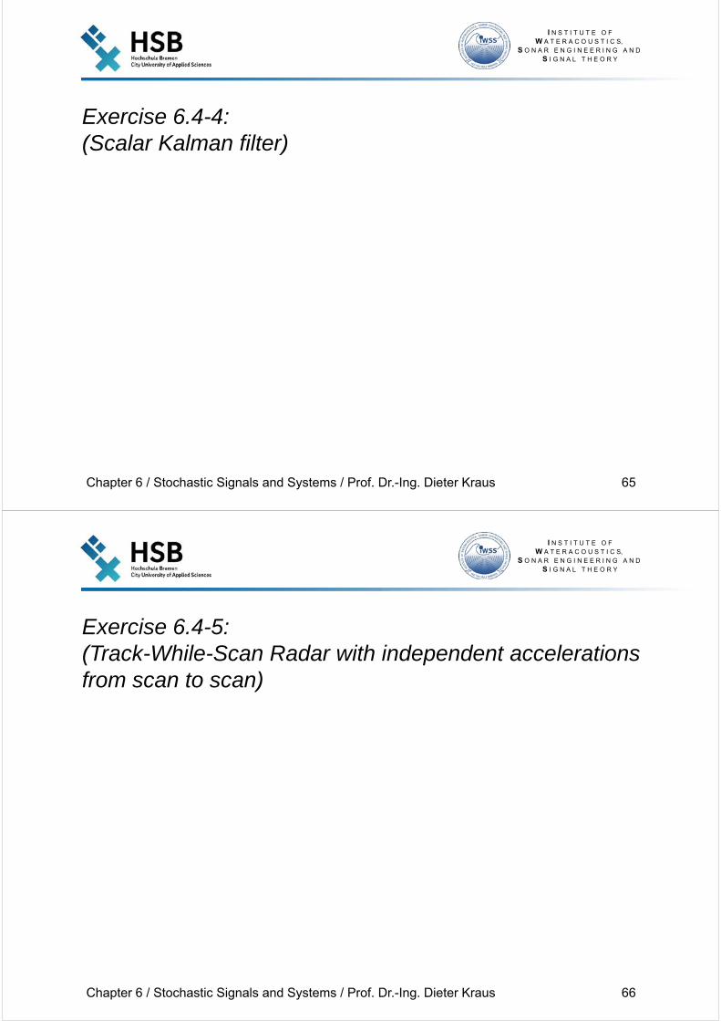
Kalman Filtering Algorithm
Measurement update (Correction)
Time update (Prediction)
Initialize the state prediction Initialize the prediction error covariance matrix
Update the state vector
Projection of state vector ahead
Calculate the Kalman gain matrix
Update the error covariance matrix
Projection of error covariance matrix ahead
0| 1 0X μ
1| |t t t t t X FX
| | 1t t t t t tX X K I
1
| 1 | 1 ( )T Tt t t t t t t t tVVK Σ H H Σ H Σ
1| | ( )T Tt t t t t t t ttUUΣ F Σ F G Σ G
0| 1 0Σ Σ
| | 1 | 1t t t t t t t tΣ Σ K H Σ
Calculate the Innovation
| 1t t t t tI Y H X
I N S T I T U T E O F W A T E R A C O U S T I C S,
S O N A R E N G I N E E R I N G A N DS I G N A L T H E O R Y
Chapter 6 / Stochastic Signals and Systems / Prof. Dr.-Ing. Dieter Kraus 65
Exercise 6.4-4:(Scalar Kalman filter)
I N S T I T U T E O F W A T E R A C O U S T I C S,
S O N A R E N G I N E E R I N G A N DS I G N A L T H E O R Y
Chapter 6 / Stochastic Signals and Systems / Prof. Dr.-Ing. Dieter Kraus 66
Exercise 6.4-5:(Track-While-Scan Radar with independent accelerations from scan to scan)
I N S T I T U T E O F W A T E R A C O U S T I C S,
S O N A R E N G I N E E R I N G A N DS I G N A L T H E O R Y
Chapter 6 / Stochastic Signals and Systems / Prof. Dr.-Ing. Dieter Kraus 67
Exercise 6.4-6:(Track-While-Scan Radar with dependent accelerations from scan to scan)
I N S T I T U T E O F W A T E R A C O U S T I C S,
S O N A R E N G I N E E R I N G A N DS I G N A L T H E O R Y
Chapter 6 / Stochastic Signals and Systems / Prof. Dr.-Ing. Dieter Kraus 68
Exercise 6.4-7:(State space representation of AR(p)-, MA(q)-, and ARMA(p,q)-Processes)
I N S T I T U T E O F W A T E R A C O U S T I C S,
S O N A R E N G I N E E R I N G A N DS I G N A L T H E O R Y
Chapter 6 / Stochastic Signals and Systems / Prof. Dr.-Ing. Dieter Kraus 69
References to Chapter 6[1] B.D.O. Anderson and J.B. Moore, Optimal Filtering, Dover, 2005
[2] A. Gelb, Applied Optimal Estimation, MIT Press, 1974
[3] T. Kailath, A.H. Sayed and B. Hassibi, Linear Estimation, Prentice Hall, 2000
[4] S. Kay, Fundamentals of Statistical Signal Processing, Vol. 1: Estimation Theory, Prentice Hall, 1993
[5] L. Ljung, System Identification: Theory for the User, Prentice Hall, 1998
[6] M.B. Priestley, Spectral Analysis and Time Series, Academic Press, 1984
[7] H.V. Poor, An Introduction to Signal Detection and Estimation, Springer, 1994


![On the Evolutionary Characteristics of the Acceleration ...research.shahed.ac.ir/.../84656_9405789536.pdf · the stochastic methods in generating high-frequency signals [11] and availability](https://img.pdfslide.net/doc/110x75/5fc3a2e100d7882c03228396/on-the-evolutionary-characteristics-of-the-acceleration-the-stochastic-methods.jpg)