Study of Maximum Power Point Tracking (MPPT) in Solar Panels

International Journal of Science and Research (IJSR) ISSN: 2319-7064

ResearchGate Impact Factor (2018): 0.28 | SJIF (2018): 7.426

Volume 8 Issue 6, June 2019

www.ijsr.net Licensed Under Creative Commons Attribution CC BY

Study of Maximum Power Point Tracking (MPPT)

in Solar Panels

Chandra Prakash Meena

M. Tech. (Power system) Student, Electrical Engineering Department, Career Point University, Kota, Rajasthan, India

Abstract: In the world of technological advancement, conventional resources of energy (fossil fuels, nuclear fuels, gas etc.) are at the

edge of extinct. To overcome this problem, non-conventional energy sources (solar energy, wind energy, ocean thermal energy, biomass

or biogas, geothermal, tidal energy etc.) play a vital role, in which solar energy is most important energy source, which produces

electricity by the photovoltaic effect. Solar photovoltaic (PV) cells are used to convert solar energy into unregulated electrical energy.

These solar PV cells exhibit nonlinear characteristics and give very low efficiency. Therefore, it becomes essential to extract maximum

power from solar PV cells using maximum power point tracking (MPPT). The power output from a PV panel depends on a few

parameters, such as the irradiation received by the panel, voltage, panel temperature, and so forth. The power output also varies

continuously throughout the day as the conditions affecting it change. In recent years, a large number of techniques have been

purposed for tracking the maximum power point (MPP). Maximum power point tracking is used in photovoltaic (PV) systems to

maximize the photovoltaic array output power, irrespective of the temperature and radiation conditions and of the load electrical

characteristics. The PV array is modeled using basic circuit equations. Its voltage-current characteristics are simulated with different

conditions. The algorithms utilized for MPPT are generalized algorithms and are easy to model or use as a code. The algorithms are

written in m-files of MATLAB.

Keywords: Photovoltaic System, Maximum Power Point Tracking (MPPT), solar cells, PV Systems, Solar module etc

1. Introduction

Renewable energy is the energy which comes from natural

resources such as sunlight, wind, rain, tides and geothermal

heat. These resources are renewable and can be naturally

replenished. Therefore, for all practical purposes, these

resources can be considered to be inexhaustible, unlike

dwindling conventional fossil fuels. The global energy

crunch has provided a renewed impetus to the growth and

development of Clean and Renewable Energy sources. Clean

Development Mechanisms (CDMs) are being adopted by

organizations all across the globe. Apart from the rapidly

decreasing reserves of fossil fuels in the world, another

major factor working against fossil fuels is the pollution

associated with their combustion. Contrastingly, renewable

energy sources are known to be much cleaner and produce

energy without the harmful effects of pollution unlike their

conventional counterparts.

1.1. Different sources of Renewable Energy

a) Wind power

Wind turbines can be used to harness the energy available in

airflows. Current day turbines range from around 600 kW to

5 MW of rated power. Since the power output is a function

of the cube of the wind speed, it increases rapidly with an

increase in available wind velocity. Recent advancements

have led to aerofoil wind turbines, which are more efficient

due to a better aerodynamic structure.

b) Solar power

The tapping of solar energy owes its origins to the British

astronomer John Herschel who famously used a solar

thermal collector box to cook food during an expedition to

Africa. Solar energy can be utilized in two major ways.

Firstly, the captured heat can be used as solar thermal

energy, with applications in space heating. Another

alternative is the conversion of incident solar radiation to

electrical energy, which is the most usable form of energy.

This can be achieved with the help of solar photovoltaic

cells or with concentrating solar power plants.

c) Small hydropower Hydropower installations up to 10MW are considered as

small hydropower and counted as renewable energy sources.

These involve converting the potential energy of water

stored in dams into usable electrical energy through the use

of water turbines. Run-of-the-river Hydro-electricity aims to

utilize the kinetic energy of water without the need of

building reservoirs or dams.

d) Biomass Plants capture the energy of the sun through the process of

photosynthesis. On combustion, these plants release the

trapped energy. This way, biomass works as a natural

battery to store the sun’s energy and yield it on requirement.

e) Geothermal

Geothermal energy is the thermal energy which is generated

and stored within the layers of the Earth. The gradient thus

developed gives rise to a continuous conduction of heat from

the core to the surface of the earth. This gradient can be

utilized to heat water to produce superheated steam and use

it to run steam turbines to generate electricity. The main

disadvantage of geothermal energy is that it is usually

limited to regions near tectonic plate boundaries, though

recent advancements have led to the propagation of this

technology.

1.2. Renewable Energy trends across the globe

The current trend across developed economies tips the scale

in favour of Renewable Energy. For the last three years, the

continents of North America and Europe have embraced

more renewable power capacity as compared to

conventional power capacity. Renewable accounted for 60%

Paper ID: ART20198530 10.21275/ART20198530 315





of the newly installed power capacity in Europe in 2009 and

nearly 20% of the annual power production.

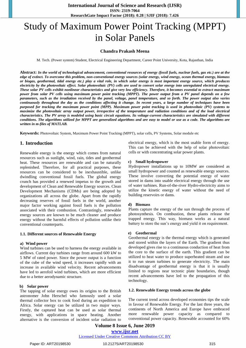
Figure 1: Global energy consumption in the year 2008.

As can be seen from the figure 1 wind and biomass occupy a

major share of the current renewable energy consumption.

Recent advancements in solar photovoltaic technology and

constant incubation of projects in countries like Germany

and Spain have brought around tremendous growth in the

solar PV market as well, which is projected to surpass other

renewable energy sources in the coming years. By 2009,

more than 85 countries had some policy target to achieve a

predetermined share of their power capacity through

renewable. This was an increase from around 45 countries in

2005. Most of the targets are also very ambitious, landing in

the range of 30-90% share of national production through

renewable. Noteworthy policies are the European Union’s

target of achieving 20% of total energy through renewable

by 2020 and India’s Jawaharlal Nehru Solar Mission,

through which India plans to produce 20GW solar energy by

the year 2022.

2. Photovoltaic System

2.1 Photovoltaic cell

A photovoltaic cell or photoelectric cell is a semiconductor

device that converts light to electrical energy by

photovoltaic effect. If the energy of photon of light is greater

than the band gap then the electron is emitted and the flow

of electrons creates current. However a photovoltaic cell is

different from a photodiode. In a photodiode light falls on n-

channel of the semiconductor junction and gets converted

into current or voltage signal but a photovoltaic cell is

always forward biased. Figure 2 shows the Working of PV

cell.

Figure 2: Working of PV cell.

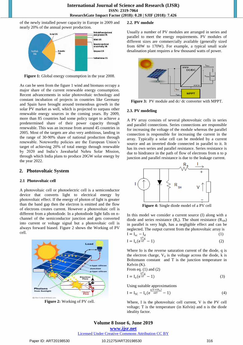
2.2. PV module

Usually a number of PV modules are arranged in series and

parallel to meet the energy requirements. PV modules of

different sizes are commercially available (generally sized

from 60W to 170W). For example, a typical small scale

desalination plant requires a few thousand watts of power.

Figure 3: PV module and dc/ dc converter with MPPT.

2.3. PV modeling

A PV array consists of several photovoltaic cells in series

and parallel connections. Series connections are responsible

for increasing the voltage of the module whereas the parallel

connection is responsible for increasing the current in the

array. Typically a solar cell can be modeled by a current

source and an inverted diode connected in parallel to it. It

has its own series and parallel resistance. Series resistance is

due to hindrance in the path of flow of electrons from n to p

junction and parallel resistance is due to the leakage current.

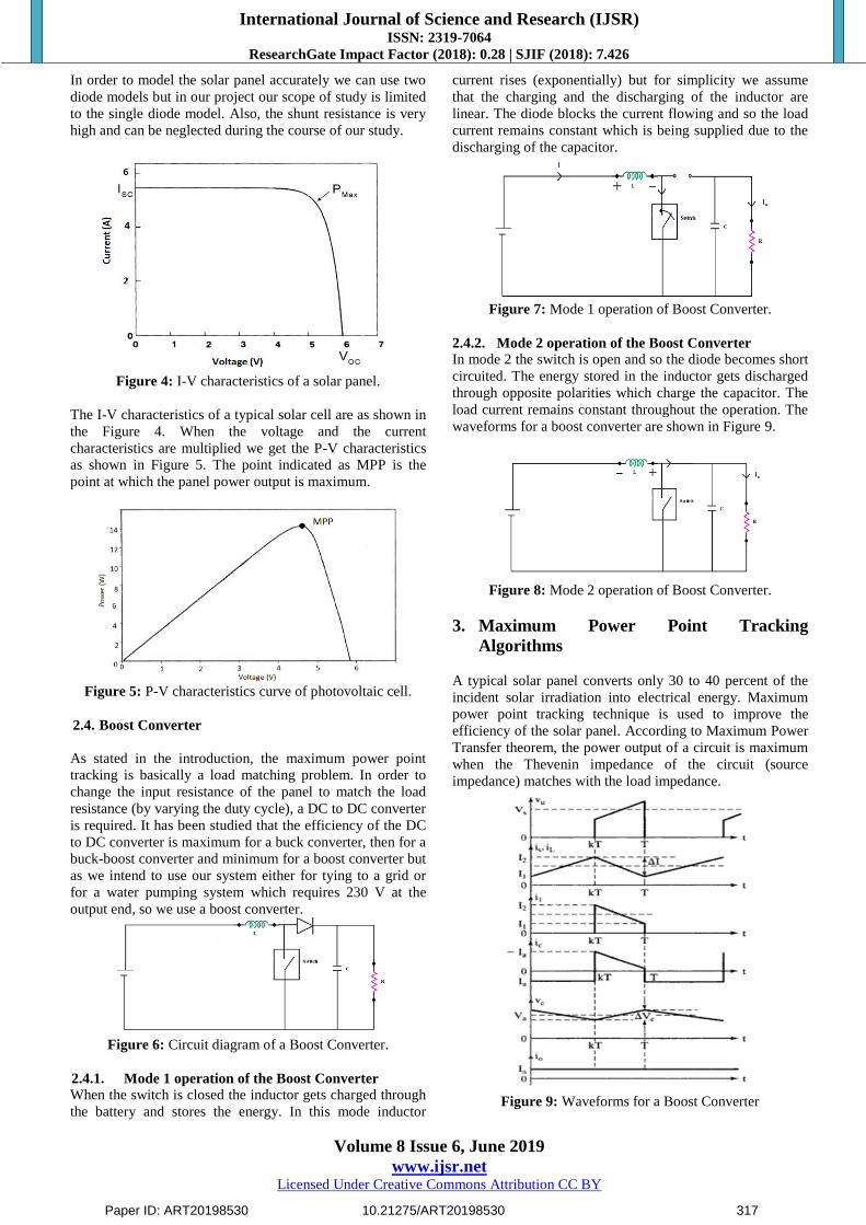
Figure 4: Single diode model of a PV cell

In this model we consider a current source (I) along with a

diode and series resistance (Rs). The shunt resistance (RSH)

in parallel is very high, has a negligible effect and can be

neglected. The output current from the photovoltaic array is

I = Isc − Id (1)

I = Io(eqVdkT − 1) (2)

Where Io is the reverse saturation current of the diode, q is

the electron charge, Vd is the voltage across the diode, k is

Boltzmann constant and T is the junction temperature in

Kelvin (K).

From eq. (1) and (2)

I = Io(eqVdkT − 1) (3)

Using suitable approximations

I = ISC − Io(eq V+IRs

nkT − 1) (4)

Where, I is the photovoltaic cell current, V is the PV cell

voltage; T is the temperature (in Kelvin) and n is the diode

ideality factor.

Paper ID: ART20198530 10.21275/ART20198530 316





In order to model the solar panel accurately we can use two

diode models but in our project our scope of study is limited

to the single diode model. Also, the shunt resistance is very

high and can be neglected during the course of our study.

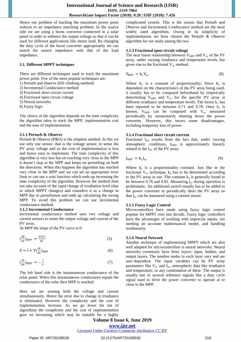
Figure 4: I-V characteristics of a solar panel.

The I-V characteristics of a typical solar cell are as shown in

the Figure 4. When the voltage and the current

characteristics are multiplied we get the P-V characteristics

as shown in Figure 5. The point indicated as MPP is the

point at which the panel power output is maximum.

Figure 5: P-V characteristics curve of photovoltaic cell.

2.4. Boost Converter

As stated in the introduction, the maximum power point

tracking is basically a load matching problem. In order to

change the input resistance of the panel to match the load

resistance (by varying the duty cycle), a DC to DC converter

is required. It has been studied that the efficiency of the DC

to DC converter is maximum for a buck converter, then for a

buck-boost converter and minimum for a boost converter but

as we intend to use our system either for tying to a grid or

for a water pumping system which requires 230 V at the

output end, so we use a boost converter.

Figure 6: Circuit diagram of a Boost Converter.

2.4.1. Mode 1 operation of the Boost Converter

When the switch is closed the inductor gets charged through

the battery and stores the energy. In this mode inductor

current rises (exponentially) but for simplicity we assume

that the charging and the discharging of the inductor are

linear. The diode blocks the current flowing and so the load

current remains constant which is being supplied due to the

discharging of the capacitor.

Figure 7: Mode 1 operation of Boost Converter.

2.4.2. Mode 2 operation of the Boost Converter

In mode 2 the switch is open and so the diode becomes short

circuited. The energy stored in the inductor gets discharged

through opposite polarities which charge the capacitor. The

load current remains constant throughout the operation. The

waveforms for a boost converter are shown in Figure 9.

Figure 8: Mode 2 operation of Boost Converter.

3. Maximum Power Point Tracking

Algorithms

A typical solar panel converts only 30 to 40 percent of the

incident solar irradiation into electrical energy. Maximum

power point tracking technique is used to improve the

efficiency of the solar panel. According to Maximum Power

Transfer theorem, the power output of a circuit is maximum

when the Thevenin impedance of the circuit (source

impedance) matches with the load impedance.

Figure 9: Waveforms for a Boost Converter

Paper ID: ART20198530 10.21275/ART20198530 317





Hence our problem of tracking the maximum power point

reduces to an impedance matching problem. In the source

side we are using a boost convertor connected to a solar

panel in order to enhance the output voltage so that it can be

used for different applications like motor load. By changing

the duty cycle of the boost converter appropriately we can

match the source impedance with that of the load

impedance.

3.1. Different MPPT techniques

There are different techniques used to track the maximum

power point. Few of the most popular techniques are:

1) Perturb and observe (hill climbing method)

2) Incremental Conductance method

3) Fractional short circuit current

4) Fractional open circuit voltage

5) Neural networks

6) Fuzzy logic

The choice of the algorithm depends on the time complexity

the algorithm takes to track the MPP, implementation cost

and the ease of implementation.

3.1.1 Perturb & Observe

Perturb & Observe (P&O) is the simplest method. In this we

use only one sensor, that is the voltage sensor, to sense the

PV array voltage and so the cost of implementation is less

and hence easy to implement. The time complexity of this

algorithm is very less but on reaching very close to the MPP

it doesn’t stop at the MPP and keeps on perturbing on both

the directions. When this happens the algorithm has reached

very close to the MPP and we can set an appropriate error

limit or can use a wait function which ends up increasing the

time complexity of the algorithm. However the method does

not take account of the rapid change of irradiation level (due

to which MPPT changes) and considers it as a change in

MPP due to perturbation and ends up calculating the wrong

MPP. To avoid this problem we can use incremental

conductance method.

3.1.2 Incremental Conductance

Incremental conductance method uses two voltage and

current sensors to sense the output voltage and current of the

PV array.

At MPP the slope of the PV curve is 0.

(dP

dV)MPP =

d(VI)

dV (5)

0 = I + V(dI

dV)MPP (6)

(dI

dV)MPP = −

I

V (7)

The left hand side is the instantaneous conductance of the

solar panel. When this instantaneous conductance equals the

conductance of the solar then MPP is reached.

Here we are sensing both the voltage and current

simultaneously. Hence the error due to change in irradiance

is eliminated. However the complexity and the cost of

implementation increase. As we go down the list of

algorithms the complexity and the cost of implementation

goes on increasing which may be suitable for a highly

complicated system. This is the reason that Perturb and

Observe and Incremental Conductance method are the most

widely used algorithms. Owing to its simplicity of

implementation we have chosen the Perturb & Observe

algorithm for our study among the two.

3.1.3 Fractional open circuit voltage

The near linear relationship between VMPP and Voc of the PV

array, under varying irradiance and temperature levels, has

given rise to the fractional Voc method.

VMPP = k1Voc (8)

Where 𝑘1 is a constant of proportionality; Since 𝑘1 is

dependent on the characteristics of the PV array being used,

it usually has to be computed beforehand by empirically

determining VMPP and Voc for the specific PV array at

different irradiance and temperature levels. The factor k1 has

been reported to be between 0.71 and 0.78. Once k1 is

known, VMPP can be computed with Voc measured

periodically by momentarily shutting down the power

converter. However, this incurs some disadvantages,

including temporary loss of power.

3.1.4 Fractional short circuit current

Fractional ISC results from the fact that, under varying

atmospheric conditions, IMPP is approximately linearly

related to the ISC of the PV array.

IMPP = k2Isc (9)

Where k2 is a proportionality constant. Just like in the

fractional Voc technique, k2 has to be determined according

to the PV array in use. The constant k2 is generally found to

be between 0.78 and 0.92. Measuring Isc during operation is

problematic. An additional switch usually has to be added to

the power converter to periodically short the PV array so

that Isc can be measured using a current sensor.

3.1.5 Fuzzy Logic Control

Microcontrollers have made using fuzzy logic control

popular for MPPT over last decade. Fuzzy logic controllers

have the advantages of working with imprecise inputs, not

needing an accurate mathematical model, and handling

nonlinearity.

3.1.6 Neural Network Another technique of implementing MPPT which are also

well adapted for microcontrollers is neural networks. Neural

networks commonly have three layers: input, hidden, and

output layers. The number nodes in each layer vary and are

user-dependent. The input variables can be PV array

parameters like Voc and Isc, atmospheric data like irradiance

and temperature, or any combination of these. The output is

usually one or several reference signals like a duty cycle

signal used to drive the power converter to operate at or

close to the MPP.

Paper ID: ART20198530 10.21275/ART20198530 318





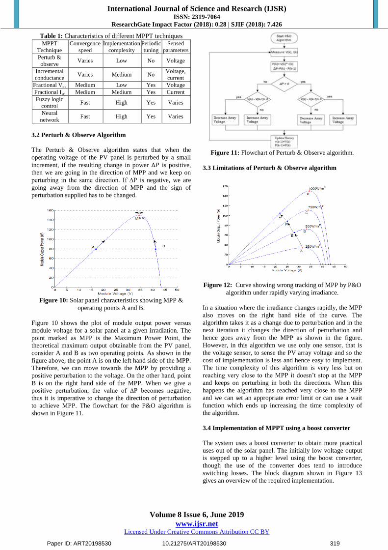
Table 1: Characteristics of different MPPT techniques MPPT

Technique

Convergence

speed

Implementation

complexity

Periodic

tuning

Sensed

parameters

Perturb &

observe Varies Low No Voltage

Incremental

conductance Varies Medium No

Voltage,

current

Fractional Voc Medium Low Yes Voltage

Fractional Isc Medium Medium Yes Current

Fuzzy logic

control Fast High Yes Varies

Neural

network Fast High Yes Varies

3.2 Perturb & Observe Algorithm

The Perturb & Observe algorithm states that when the

operating voltage of the PV panel is perturbed by a small

increment, if the resulting change in power ∆𝑃 is positive,

then we are going in the direction of MPP and we keep on

perturbing in the same direction. If ∆P is negative, we are

going away from the direction of MPP and the sign of

perturbation supplied has to be changed.

Figure 10: Solar panel characteristics showing MPP &

operating points A and B.

Figure 10 shows the plot of module output power versus

module voltage for a solar panel at a given irradiation. The

point marked as MPP is the Maximum Power Point, the

theoretical maximum output obtainable from the PV panel,

consider A and B as two operating points. As shown in the

figure above, the point A is on the left hand side of the MPP.

Therefore, we can move towards the MPP by providing a

positive perturbation to the voltage. On the other hand, point

B is on the right hand side of the MPP. When we give a

positive perturbation, the value of ∆P becomes negative,

thus it is imperative to change the direction of perturbation

to achieve MPP. The flowchart for the P&O algorithm is

shown in Figure 11.

Figure 11: Flowchart of Perturb & Observe algorithm.

3.3 Limitations of Perturb & Observe algorithm

Figure 12: Curve showing wrong tracking of MPP by P&O

algorithm under rapidly varying irradiance.

In a situation where the irradiance changes rapidly, the MPP

also moves on the right hand side of the curve. The

algorithm takes it as a change due to perturbation and in the

next iteration it changes the direction of perturbation and

hence goes away from the MPP as shown in the figure.

However, in this algorithm we use only one sensor, that is

the voltage sensor, to sense the PV array voltage and so the

cost of implementation is less and hence easy to implement.

The time complexity of this algorithm is very less but on

reaching very close to the MPP it doesn’t stop at the MPP

and keeps on perturbing in both the directions. When this

happens the algorithm has reached very close to the MPP

and we can set an appropriate error limit or can use a wait

function which ends up increasing the time complexity of

the algorithm.

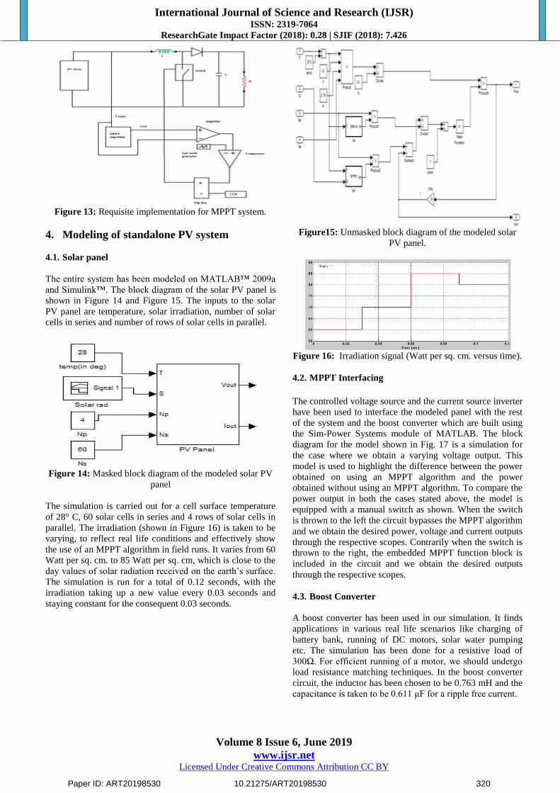
3.4 Implementation of MPPT using a boost converter

The system uses a boost converter to obtain more practical

uses out of the solar panel. The initially low voltage output

is stepped up to a higher level using the boost converter,

though the use of the converter does tend to introduce

switching losses. The block diagram shown in Figure 13

gives an overview of the required implementation.

Paper ID: ART20198530 10.21275/ART20198530 319





Figure 13: Requisite implementation for MPPT system.

4. Modeling of standalone PV system

4.1. Solar panel

The entire system has been modeled on MATLAB™ 2009a

and Simulink™. The block diagram of the solar PV panel is

shown in Figure 14 and Figure 15. The inputs to the solar

PV panel are temperature, solar irradiation, number of solar

cells in series and number of rows of solar cells in parallel.

Figure 14: Masked block diagram of the modeled solar PV

panel

The simulation is carried out for a cell surface temperature

of 28° C, 60 solar cells in series and 4 rows of solar cells in

parallel. The irradiation (shown in Figure 16) is taken to be

varying, to reflect real life conditions and effectively show

the use of an MPPT algorithm in field runs. It varies from 60

Watt per sq. cm. to 85 Watt per sq. cm, which is close to the

day values of solar radiation received on the earth’s surface.

The simulation is run for a total of 0.12 seconds, with the

irradiation taking up a new value every 0.03 seconds and

staying constant for the consequent 0.03 seconds.

Figure15: Unmasked block diagram of the modeled solar

PV panel.

Figure 16: Irradiation signal (Watt per sq. cm. versus time).

4.2. MPPT Interfacing

The controlled voltage source and the current source inverter

have been used to interface the modeled panel with the rest

of the system and the boost converter which are built using

the Sim-Power Systems module of MATLAB. The block

diagram for the model shown in Fig. 17 is a simulation for

the case where we obtain a varying voltage output. This

model is used to highlight the difference between the power

obtained on using an MPPT algorithm and the power

obtained without using an MPPT algorithm. To compare the

power output in both the cases stated above, the model is

equipped with a manual switch as shown. When the switch

is thrown to the left the circuit bypasses the MPPT algorithm

and we obtain the desired power, voltage and current outputs

through the respective scopes. Contrarily when the switch is

thrown to the right, the embedded MPPT function block is

included in the circuit and we obtain the desired outputs

through the respective scopes.

4.3. Boost Converter

A boost converter has been used in our simulation. It finds

applications in various real life scenarios like charging of

battery bank, running of DC motors, solar water pumping

etc. The simulation has been done for a resistive load of

300Ω. For efficient running of a motor, we should undergo

load resistance matching techniques. In the boost converter

circuit, the inductor has been chosen to be 0.763 mH and the

capacitance is taken to be 0.611 μF for a ripple free current.

Paper ID: ART20198530 10.21275/ART20198530 320





PI Controller

The system also employs a PI controller. The task of the

MPPT algorithm is just to calculate the reference voltage

Vref towards which the PV operating voltage should move

next for obtaining maximum power output. This process is

repeated periodically with a slower rate of around 1-10

samples per second. The external control loop is the PI

controller, which controls the input voltage of the converter.

The pulse width modulation is carried in the PWM block at

a considerably faster switching frequency of 100 KHz. In

our simulation, KP is taken to be 0.006 and KI is taken to be

7. A relatively high KI value ensures that the system

stabilizes at a faster rate. The PI controller works towards

minimizing the error between Vref and the measured voltage

by varying the duty cycle through the switch. The switch is

physically realized by using a MOSFET with the gate

voltage controlled by the duty cycle. Table 2 shows the

different parameters taken during the simulation of the

model.

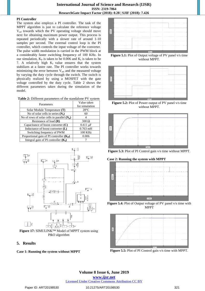
Table 2: Different parameters of the standalone PV system

Parameters Value taken

for simulation

Solar Module Temperature (T) 28°C

No of solar cells in series (Ns) 60

No of rows of solar cells in parallel (Np) 4

Resistance of load (R) 300 Ω

Capacitance of boost converter (C) 0.611 μF

Inductance of boost converter (L) 0.763 mH

Switching frequency of PWM 100 KHz

Proportional gain of PI controller (KP) 0.006

Integral gain of PI controller (KI) 7

Figure 17: SIMULINK™ Model of MPPT system using

P&O algorithm

5. Results

Case 1: Running the system without MPPT

Figure 5.1: Plot of Output voltage of PV panel v/s time

without MPPT.

Figure 5.2: Plot of Power output of PV panel v/s time

without MPPT.

Figure 5.3: Plot of PI Control gain v/s time without MPPT.

Case 2: Running the system with MPPT

Figure 5.4: Plot of Output voltage of PV panel v/s time with

MPPT

Figure 5.5: Plot of PI Control gain v/s time with MPPT.

Paper ID: ART20198530 10.21275/ART20198530 321





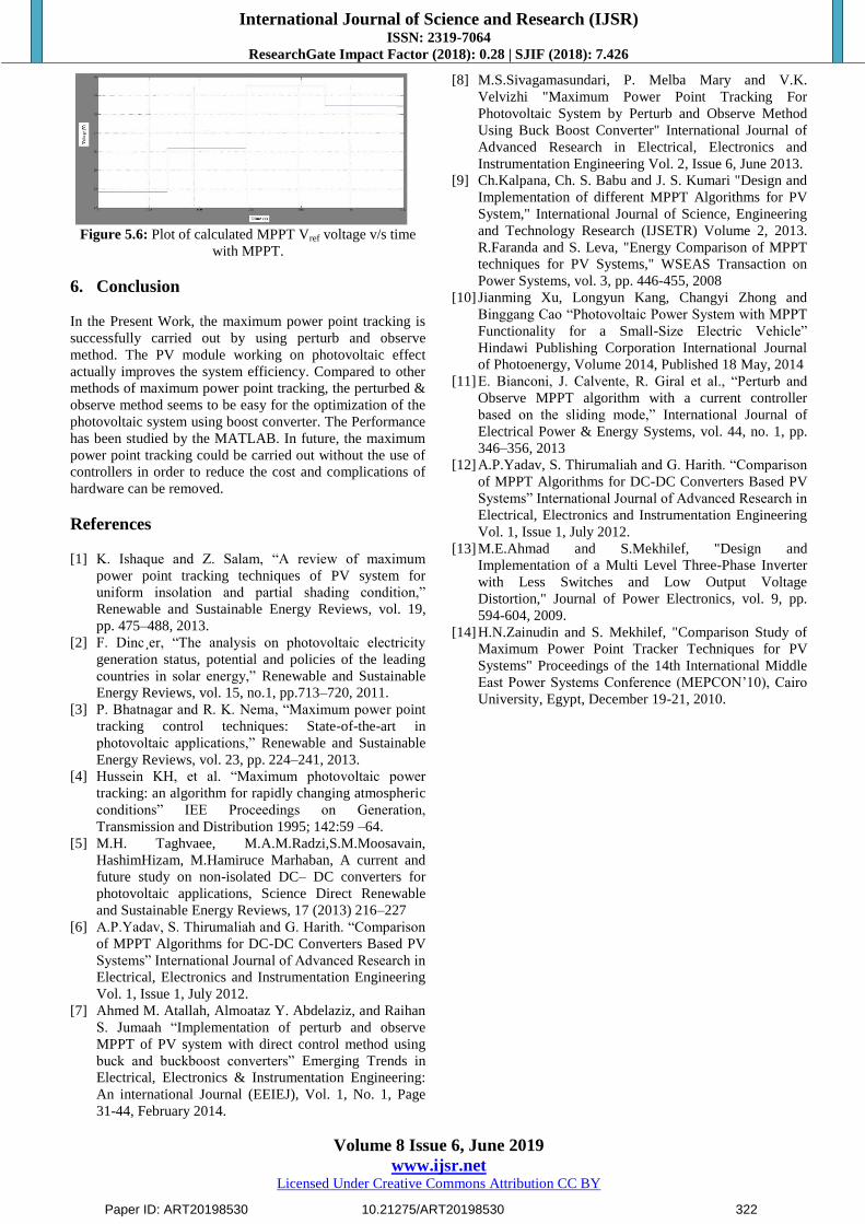
Figure 5.6: Plot of calculated MPPT Vref voltage v/s time

with MPPT.

6. Conclusion

In the Present Work, the maximum power point tracking is

successfully carried out by using perturb and observe

method. The PV module working on photovoltaic effect

actually improves the system efficiency. Compared to other

methods of maximum power point tracking, the perturbed &

observe method seems to be easy for the optimization of the

photovoltaic system using boost converter. The Performance

has been studied by the MATLAB. In future, the maximum

power point tracking could be carried out without the use of

controllers in order to reduce the cost and complications of

hardware can be removed.

References

[1] K. Ishaque and Z. Salam, “A review of maximum

power point tracking techniques of PV system for

uniform insolation and partial shading condition,”

Renewable and Sustainable Energy Reviews, vol. 19,

pp. 475–488, 2013.

[2] F. Dinc¸er, “The analysis on photovoltaic electricity

generation status, potential and policies of the leading

countries in solar energy,” Renewable and Sustainable

Energy Reviews, vol. 15, no.1, pp.713–720, 2011.

[3] P. Bhatnagar and R. K. Nema, “Maximum power point

tracking control techniques: State-of-the-art in

photovoltaic applications,” Renewable and Sustainable

Energy Reviews, vol. 23, pp. 224–241, 2013.

[4] Hussein KH, et al. “Maximum photovoltaic power

tracking: an algorithm for rapidly changing atmospheric

conditions” IEE Proceedings on Generation,

Transmission and Distribution 1995; 142:59 –64.

[5] M.H. Taghvaee, M.A.M.Radzi,S.M.Moosavain,

HashimHizam, M.Hamiruce Marhaban, A current and

future study on non-isolated DC– DC converters for

photovoltaic applications, Science Direct Renewable

and Sustainable Energy Reviews, 17 (2013) 216–227

[6] A.P.Yadav, S. Thirumaliah and G. Harith. “Comparison

of MPPT Algorithms for DC-DC Converters Based PV

Systems” International Journal of Advanced Research in

Electrical, Electronics and Instrumentation Engineering

Vol. 1, Issue 1, July 2012.

[7] Ahmed M. Atallah, Almoataz Y. Abdelaziz, and Raihan

S. Jumaah “Implementation of perturb and observe

MPPT of PV system with direct control method using

buck and buckboost converters” Emerging Trends in

Electrical, Electronics & Instrumentation Engineering:

An international Journal (EEIEJ), Vol. 1, No. 1, Page

31-44, February 2014.

[8] M.S.Sivagamasundari, P. Melba Mary and V.K.

Velvizhi "Maximum Power Point Tracking For

Photovoltaic System by Perturb and Observe Method

Using Buck Boost Converter" International Journal of

Advanced Research in Electrical, Electronics and

Instrumentation Engineering Vol. 2, Issue 6, June 2013.

[9] Ch.Kalpana, Ch. S. Babu and J. S. Kumari "Design and

Implementation of different MPPT Algorithms for PV

System," International Journal of Science, Engineering

and Technology Research (IJSETR) Volume 2, 2013.

R.Faranda and S. Leva, "Energy Comparison of MPPT

techniques for PV Systems," WSEAS Transaction on

Power Systems, vol. 3, pp. 446-455, 2008

[10] Jianming Xu, Longyun Kang, Changyi Zhong and

Binggang Cao “Photovoltaic Power System with MPPT

Functionality for a Small-Size Electric Vehicle”

Hindawi Publishing Corporation International Journal

of Photoenergy, Volume 2014, Published 18 May, 2014

[11] E. Bianconi, J. Calvente, R. Giral et al., “Perturb and

Observe MPPT algorithm with a current controller

based on the sliding mode,” International Journal of

Electrical Power & Energy Systems, vol. 44, no. 1, pp.

346–356, 2013

[12] A.P.Yadav, S. Thirumaliah and G. Harith. “Comparison

of MPPT Algorithms for DC-DC Converters Based PV

Systems” International Journal of Advanced Research in

Electrical, Electronics and Instrumentation Engineering

Vol. 1, Issue 1, July 2012.

[13] M.E.Ahmad and S.Mekhilef, "Design and

Implementation of a Multi Level Three-Phase Inverter

with Less Switches and Low Output Voltage

Distortion," Journal of Power Electronics, vol. 9, pp.

594-604, 2009.

[14] H.N.Zainudin and S. Mekhilef, "Comparison Study of

Maximum Power Point Tracker Techniques for PV

Systems" Proceedings of the 14th International Middle

East Power Systems Conference (MEPCON’10), Cairo

University, Egypt, December 19-21, 2010.

Paper ID: ART20198530 10.21275/ART20198530 322

Documents

Study of Maximum Power Point Tracking (MPPT) in Solar Panels