Embed Size (px)
Citation preview
JME Journal of Mining & Environment, Vol.6, No.1, 2015, 31-39.
Subsurface modeling of mud volcanoes, using density model and analysis
of seismic velocity
H. R. Baghzendani, H. Aghajani
* and M. Solimani
School of Mining, Petroleum & Geophysics Engineering, University of Shahrood, Shahrood, Iran
Received 8 July 2014; received in revised form 4 September 2014; accepted 14 September 2014 *Corresponding author: [email protected] (H. Aghajani).
Abstract Detection of subsurface structures by means of gravity method can be used to determine mass distribution
and density contrast of rock units. This distribution could be detected by different geophysical methods,
especially gravity method. However, gravity techniques have some drawbacks and can't be always successful
in distinguishing subsurface structures. Performance of the gravity technique could be further improved by
simultaneous combination and introducing additional information from other geophysical data. This study
used existing relation between seismic and gravity methods to better clarify subsurface structures. This
relationship relates mass distribution of the medium to velocity of wave propagation in that media. This
method was applied on an area that consists of three mud volcanoes. After completion of the primary model
by forward modeling, mass distribution and analysis of seismic velocity were provided on a 2-D profile.
Bouguer anomaly map of gravity data of the area was obtained and negative anomalies were identified.
These negative anomalies could be related to the existence of mud volcanoes. A 2-D seismic line was also
acquired over the greatest mud volcano, as additional information for direct modeling. The Gardner equation
was used for further velocity estimation by density values. This velocity model also compared with seismic
velocity analysis for evaluation. The final results indicated that density modeling and the use of seismic
velocity model increases the resolution of subsurface structures imaging. Separation of subsurface layers was
implemented correctly in the velocity model resulting from gravity data and subsurface discontinuities of the
area that become more obvious by this technique.
Keywords: Gardner Equation, Seismic Imaging, Velocity Analysis, Bouguer Anomaly, Mud Volcano.
1. Introduction
The origin of mud volcano phenomenon has close
relations with subduction areas, oil fields in the
margins and coasts of seas, oceans, and faults [1].
Most of the mud volcanoes, which are their most
active ones, are located on the margins and coastal
zones of the Caspian Sea, Black sea, Oman Sea
and Indian Ocean and mainly have magma and
tectonic origins. Mud volcanoes of South Eastern
part of the Caspian Sea in countries of Iran and
Turkmenistan, are related to subduction zones and
oil and gas field. Focus point of mud volcano is
mainly created in depth due to pressure on fine
sediments. Some of mud volcanoes such as those
in the borders of the Caspian Sea, which are
related to the fault activities, have diaperic shape
and exert pressure to the walls of gaps while
coming up through them. Therefore, the liquid
saturated with gas appears in drips on surface of
sediments. By decreasing the pressure, the under
pressure liquid on the surface of sediment is
moved toward the crest of the diaper [2].
Investigations have indicated that there is a close
relation between mud volcano phenomenon and
the aggregation of oil and gas in subsurface
layers. Although this phenomenon can't be
definitely as a result of the existence of
hydrocarbon materials or considerable resources,
it can give much information about subsurface
layers [3].
Research history of mud volcano has mostly been
accompanied by researches on oil fields,
conducted by a number of researchers and
Baghzendani et al./ Journal of Mining & Environment, Vol.6, No.1, 2015
32
included structural stratigraphy and geology of
establishment of this phenomenon [4]. Many
researches have been conducted to identify the
structure of mud volcanoes. Various geophysical
methods were applied solely or by simultaneous
application of several methods to investigate
characteristics and structure of this phenomenon.
Combination of gravity and seismic data were
applied in determination of Gungula sedimentary
field structures in Nigeria and identification of
geometry of stratigraphical sequences to explore
hydrocarbon resources. Based on these researches,
the estimated depth of the bedrock of the area and
existing faults of the area were mapped very well.
Existence of high values of gravity anomalies in
the area is indicative of penetrative masses of
ocean bed which it is assumed that it has brought
about termination of a portion of hydrocarbon
resources [5]. Gauch et al. (2010), in their
commentary about complex geology of thrust belt
of Manadom area of India, used a combination of
gravity, magnetic, seismic, and magneto-telluric
data. Through their research, they succeeded to
identify a map of rock units in the area, and
determined main effective faults and depth of
stratums [6]. In a same study, results of
geophysical gravimetric and magnetic methods
used to design seismic acquisition profiles.
Consequently, combining results of 3D seismic
and gravity data resulted in accurate structure
imaging of sedimentary basins of Santos and
Campus of Brazil. The results show that the
estimated depth of bed rock of the area is about 10
kilometers, the minimum value of which is about
8 kilometers [7].
Anderson and Liemen (2002), used gravimetric
data as an auxiliary tools to clarify and improve
seismic data processing result [8]. In order to
achieve more reliable results on subsurface
structures, Cai et al. (2009), identified the arrival
time of the wave and gravity anomaly value
among low-thickness layers existing in rocks by
improving inverse modeling of seismic data and
Jakobian matrix [9]. Colombo and De Stephano
(2007) succeeded to improve velocity model by
using gravity data and the relation between
density and velocity (Gardner equation), they also
determined the real depth of each layer in
seismography profile using this model [10].
Montovani and Dagojard (2011) obtained velocity
model on a data from an oil field by using density
(surface exploration and well measuring) and
seismography data and considered migration
correction. They also succeeded to correct salt
layer boundary in this data which was determined
by seismic reflection [11]. Investigation of
Colombo and De Stephano (2007) shows another
example of this method based on Gardner
equation [12]. The purpose of this study is to
simultaneously use gravity and seismic data to
obtain a high resolution image of the subsurface,
enhance the location and define the boundary of
mud volcanoes in Gorgan area.
This issue could be a crucial problem in
sedimentary some basins with thick sequence of
mud. Existence of mud could distort the seismic
image and gravity maps in such areas. Therefore,
one of the potential methods to suppress this
problem is to combine both gravity and seismic
information to draw an integrated model. The
researchers faced in interpreting seismic data from
the Gorgan region to image boundary of mud
volcanoes. Based on the seismic data only, it was
difficult to create a perfect model of mud volcano.
Thus, it was decided to create velocity model by
using relationship between porosity and density of
the medium. Therefore, after gravity data
acquisition, processing of the data and making the
Bouguer anomaly, different profile in different
azimuth were obtained.
These profiles were obtained from different parts
of the medium, where considerable velocity
variation observed in the model.
2. Methodology
Obtaining a reliable seismic velocity model, in
spite of lateral and vertical velocity variations, is a
crucial task. Contamination by noise, will
suppress the accuracy and validity of this model.
Thus, other geological and geophysical data can
improve the accuracy of the velocity model as
complementary data. Using these auxiliary data
will needs integrating modelling techniques to be
applied on the data. Modeling techniques make
relations between observation data, define
variation of physical characteristics of the media
and illuminate discontinuities due to these
variations. Consequently, modeling can estimate
physical and geometrical characteristic
distribution through the medium [13]. Having
combined geological data of the study area and
the primary estimation of model parameters, a
physical model which includes anomaly
characteristics is proposed.
The beginning of the model building procedure is
the forward modeling. Forward modelling consists
of predicting measurement results (data
prediction) based on a primary model and its
parameters. Forward modeling procedure includes
the calculation of an anomaly from an imaginary
Baghzendani et al./ Journal of Mining & Environment, Vol.6, No.1, 2015
33
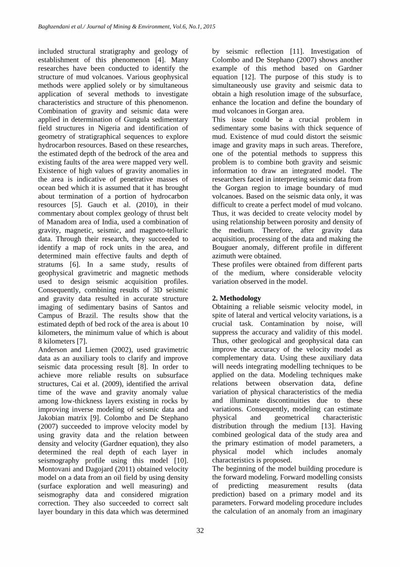
supposed model based on repeating calculations
on the basis of changing model parameters such as
density contrast and depth, until appropriate
fitting between computational anomaly and
observational anomaly (Figure 1).
Primary model is guessed
based on anomaly observations
According to geometrical and physical
parameters and calculate effect of gravity
Comparison of calculated model
with observation dataEffect of gravity observation data
Is the fitting between
calculated and observation
data well?
No, change and adjust
the model parameters
Final model
Yes
No
Figure 1. Forward modeling stage [13].
This kind of modeling can be executed manually
or by using semi-automatic techniques. Error
decreasing is executed by using trial and error
method, which is a very timeconsuming
procedure, that sometimes never reach an
appropriate fitness between observation and
computational data by changing model
parameters. Undoubtedly, this modeling is also
accompanied with deficits that if the interpreter
conducts the action intelligently, the model will
preserve its geological validity [13].
According to Figure 1, for forward modeling, the
value of gravity effect is computed by a primary
guess of the model based on gravity data and
existing geological information. Then the
computed gravity anomaly is compared with
observed value. In case of lack of appropriate
fitness, unknown characteristics (density, depth
and location) of target in the model will be
repeatedly changed to reach the best fitness
between gravity effect of the model and observed
gravity anomaly. In order to better process gravity
and seismic data to achieve the best subsurface
image, seismic and gravity data were used to
perform density and velocity analysis. In this
regard, having conducted empirical researches,
Gardner et al. (1974), presented an equation for
velocity and density relationship [12]: 40.31 V (1)
where V (m/s2), is the velocity and ρ (gr/cm
3) is
density of the environment.
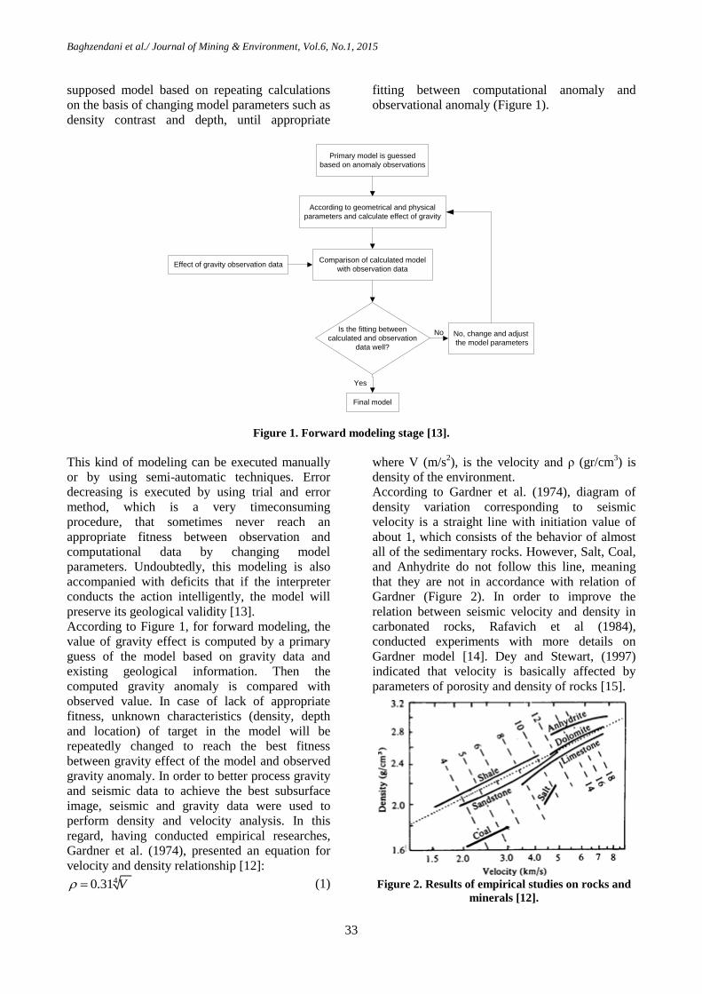
According to Gardner et al. (1974), diagram of
density variation corresponding to seismic
velocity is a straight line with initiation value of
about 1, which consists of the behavior of almost
all of the sedimentary rocks. However, Salt, Coal,
and Anhydrite do not follow this line, meaning
that they are not in accordance with relation of
Gardner (Figure 2). In order to improve the
relation between seismic velocity and density in
carbonated rocks, Rafavich et al (1984),
conducted experiments with more details on
Gardner model [14]. Dey and Stewart, (1997)
indicated that velocity is basically affected by
parameters of porosity and density of rocks [15].
Figure 2. Results of empirical studies on rocks and
minerals [12].
Baghzendani et al./ Journal of Mining & Environment, Vol.6, No.1, 2015
34
3. Real data and geology of the area
To investigate efficiency of the introduced
technique above, a real seismic and gravity data
from a same region were selected. The study area
is located in the north east of Iran, in the eastern
bank of the Caspian Sea. This area was selected
for this study due to existence of several mud
volcanoes. The aim of modeling is therefore,
defining exact location and the boundary of these
mud volcanoes.
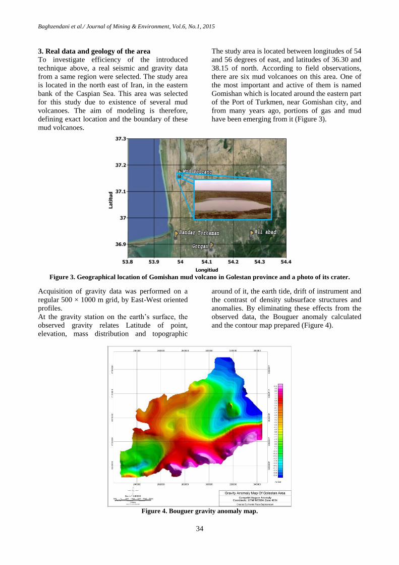
The study area is located between longitudes of 54
and 56 degrees of east, and latitudes of 36.30 and
38.15 of north. According to field observations,
there are six mud volcanoes on this area. One of
the most important and active of them is named
Gomishan which is located around the eastern part
of the Port of Turkmen, near Gomishan city, and
from many years ago, portions of gas and mud
have been emerging from it (Figure 3).
Figure 3. Geographical location of Gomishan mud volcano in Golestan province and a photo of its crater.
Acquisition of gravity data was performed on a
regular 500 × 1000 m grid, by East-West oriented
profiles.
At the gravity station on the earth’s surface, the
observed gravity relates Latitude of point,
elevation, mass distribution and topographic
around of it, the earth tide, drift of instrument and
the contrast of density subsurface structures and
anomalies. By eliminating these effects from the
observed data, the Bouguer anomaly calculated
and the contour map prepared (Figure 4).
Figure 4. Bouguer gravity anomaly map.
Baghzendani et al./ Journal of Mining & Environment, Vol.6, No.1, 2015
35
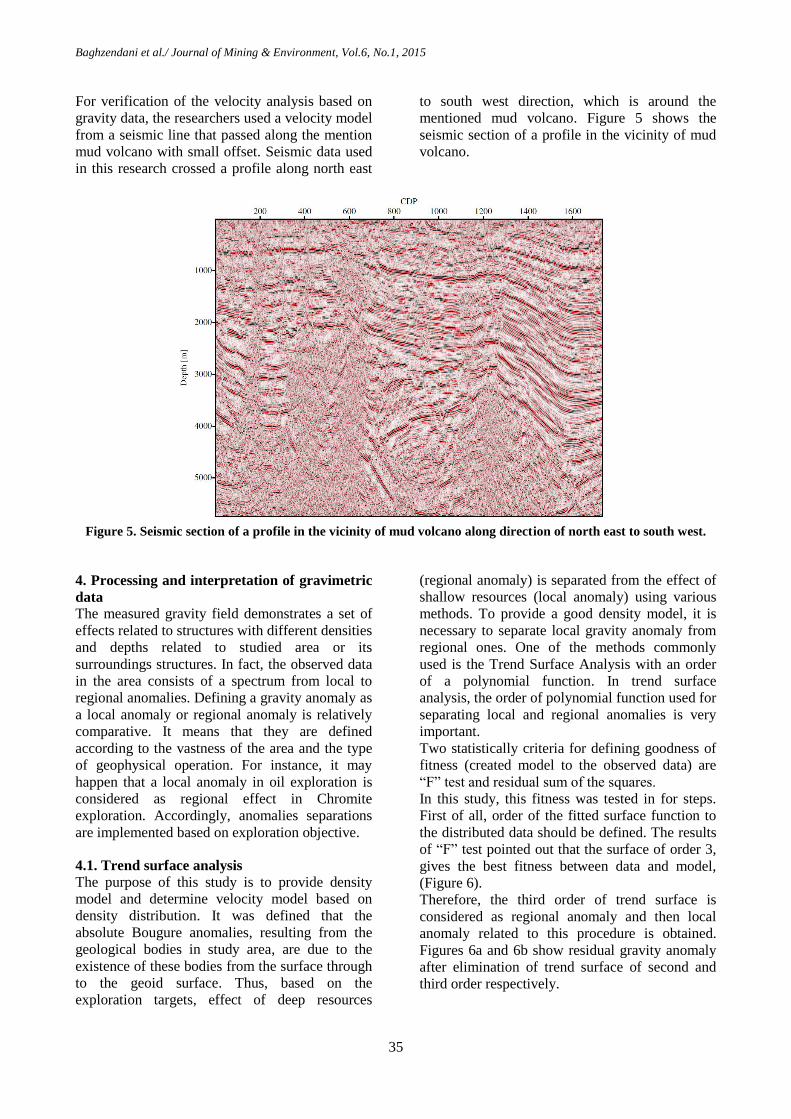
For verification of the velocity analysis based on
gravity data, the researchers used a velocity model
from a seismic line that passed along the mention
mud volcano with small offset. Seismic data used
in this research crossed a profile along north east
to south west direction, which is around the
mentioned mud volcano. Figure 5 shows the
seismic section of a profile in the vicinity of mud
volcano.
Figure 5. Seismic section of a profile in the vicinity of mud volcano along direction of north east to south west.
4. Processing and interpretation of gravimetric
data
The measured gravity field demonstrates a set of
effects related to structures with different densities
and depths related to studied area or its
surroundings structures. In fact, the observed data
in the area consists of a spectrum from local to
regional anomalies. Defining a gravity anomaly as
a local anomaly or regional anomaly is relatively
comparative. It means that they are defined
according to the vastness of the area and the type
of geophysical operation. For instance, it may
happen that a local anomaly in oil exploration is
considered as regional effect in Chromite
exploration. Accordingly, anomalies separations
are implemented based on exploration objective.
4.1. Trend surface analysis
The purpose of this study is to provide density
model and determine velocity model based on
density distribution. It was defined that the
absolute Bougure anomalies, resulting from the
geological bodies in study area, are due to the
existence of these bodies from the surface through
to the geoid surface. Thus, based on the
exploration targets, effect of deep resources
(regional anomaly) is separated from the effect of
shallow resources (local anomaly) using various
methods. To provide a good density model, it is
necessary to separate local gravity anomaly from
regional ones. One of the methods commonly
used is the Trend Surface Analysis with an order
of a polynomial function. In trend surface
analysis, the order of polynomial function used for
separating local and regional anomalies is very
important.
Two statistically criteria for defining goodness of
fitness (created model to the observed data) are
“F” test and residual sum of the squares.
In this study, this fitness was tested in for steps.
First of all, order of the fitted surface function to
the distributed data should be defined. The results
of “F” test pointed out that the surface of order 3,
gives the best fitness between data and model,
(Figure 6).
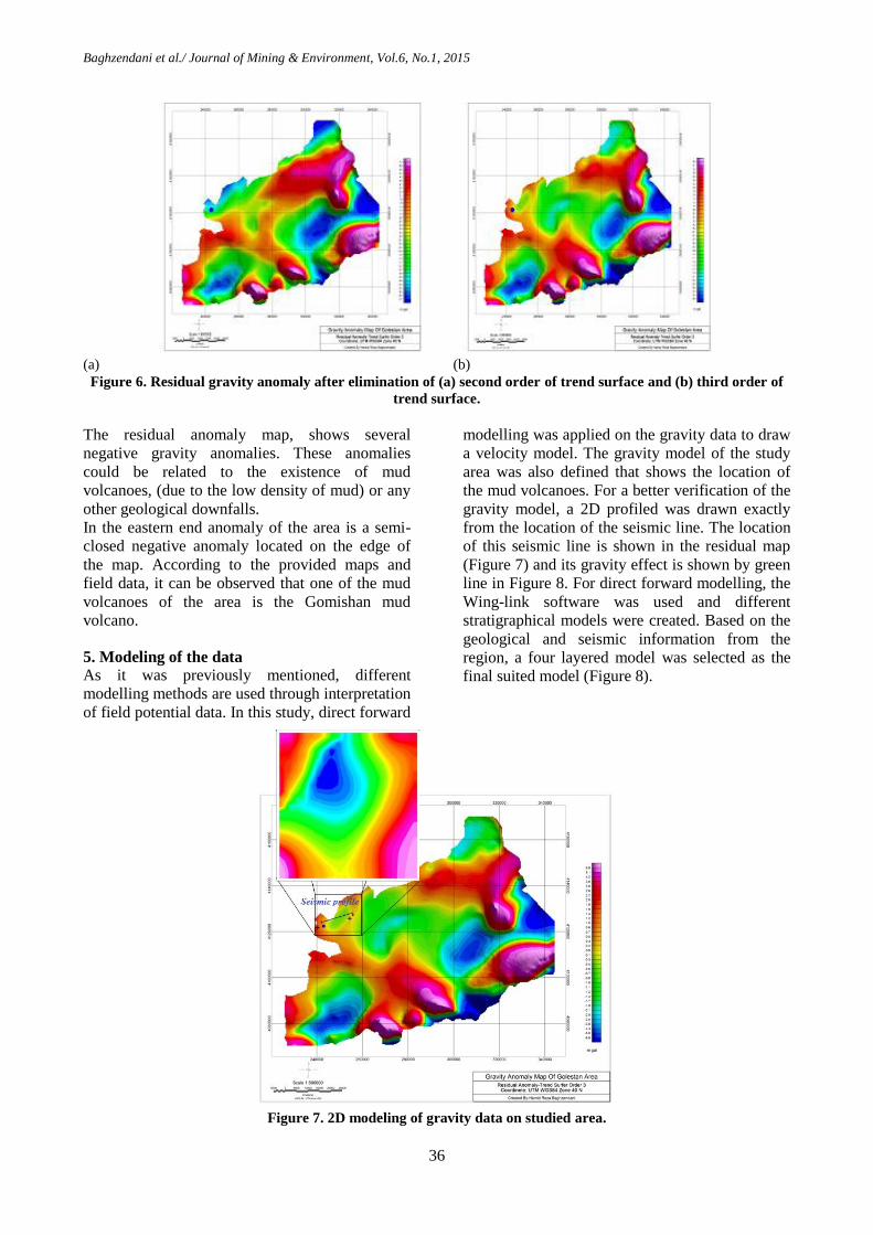
Therefore, the third order of trend surface is
considered as regional anomaly and then local
anomaly related to this procedure is obtained.
Figures 6a and 6b show residual gravity anomaly
after elimination of trend surface of second and
third order respectively.
Baghzendani et al./ Journal of Mining & Environment, Vol.6, No.1, 2015
36
(a) (b)
Figure 6. Residual gravity anomaly after elimination of (a) second order of trend surface and (b) third order of
trend surface.
The residual anomaly map, shows several
negative gravity anomalies. These anomalies
could be related to the existence of mud
volcanoes, (due to the low density of mud) or any
other geological downfalls.
In the eastern end anomaly of the area is a semi-
closed negative anomaly located on the edge of
the map. According to the provided maps and
field data, it can be observed that one of the mud
volcanoes of the area is the Gomishan mud
volcano.
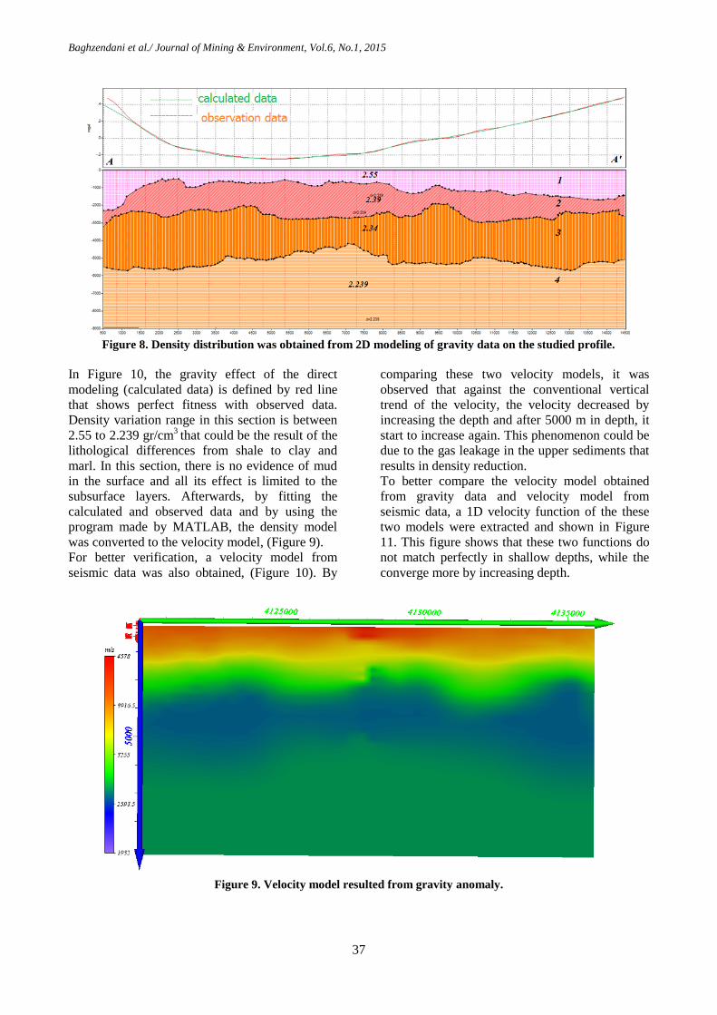
5. Modeling of the data
As it was previously mentioned, different
modelling methods are used through interpretation
of field potential data. In this study, direct forward
modelling was applied on the gravity data to draw
a velocity model. The gravity model of the study
area was also defined that shows the location of
the mud volcanoes. For a better verification of the
gravity model, a 2D profiled was drawn exactly
from the location of the seismic line. The location
of this seismic line is shown in the residual map
(Figure 7) and its gravity effect is shown by green
line in Figure 8. For direct forward modelling, the
Wing-link software was used and different
stratigraphical models were created. Based on the
geological and seismic information from the
region, a four layered model was selected as the
final suited model (Figure 8).
Figure 7. 2D modeling of gravity data on studied area.
Baghzendani et al./ Journal of Mining & Environment, Vol.6, No.1, 2015
37
Figure 8. Density distribution was obtained from 2D modeling of gravity data on the studied profile.
In Figure 10, the gravity effect of the direct
modeling (calculated data) is defined by red line
that shows perfect fitness with observed data.
Density variation range in this section is between
2.55 to 2.239 gr/cm3 that could be the result of the
lithological differences from shale to clay and
marl. In this section, there is no evidence of mud
in the surface and all its effect is limited to the
subsurface layers. Afterwards, by fitting the
calculated and observed data and by using the
program made by MATLAB, the density model
was converted to the velocity model, (Figure 9).
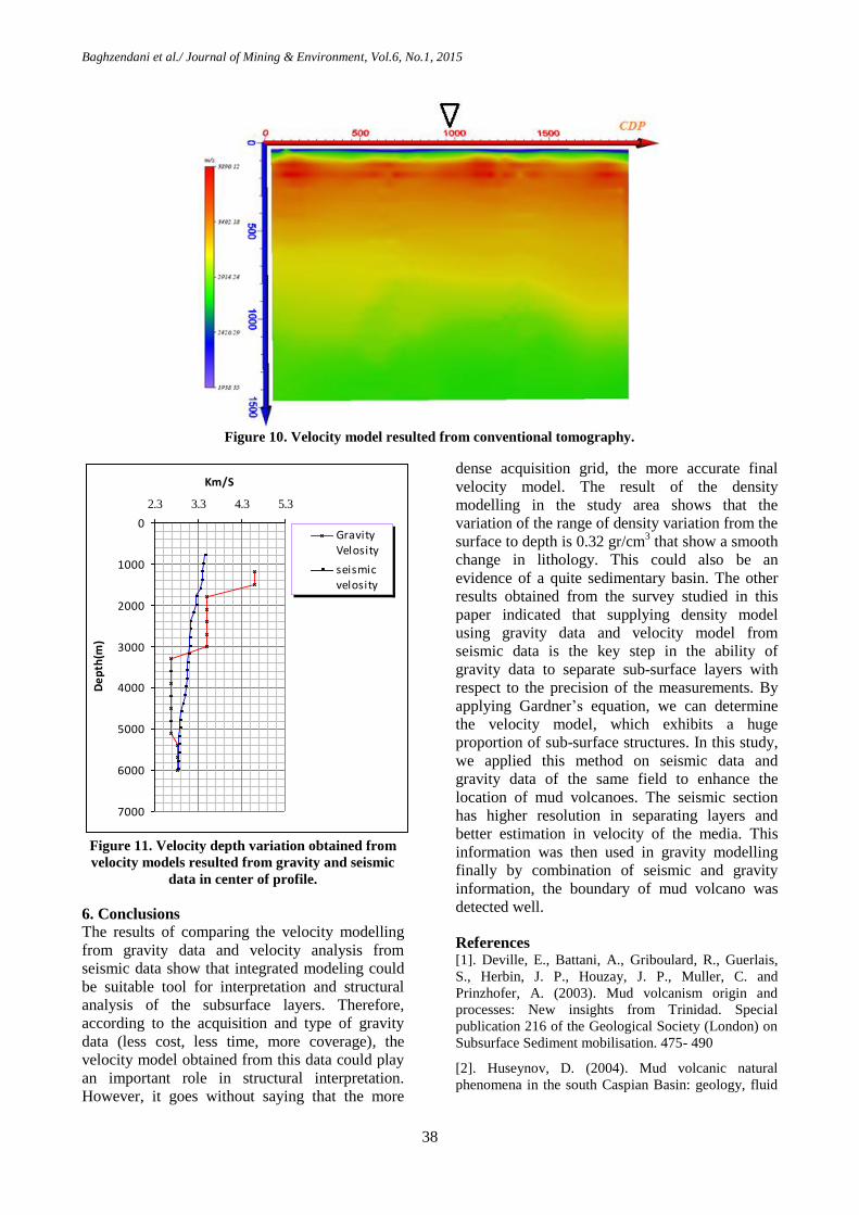
For better verification, a velocity model from
seismic data was also obtained, (Figure 10). By
comparing these two velocity models, it was
observed that against the conventional vertical
trend of the velocity, the velocity decreased by
increasing the depth and after 5000 m in depth, it
start to increase again. This phenomenon could be
due to the gas leakage in the upper sediments that
results in density reduction.
To better compare the velocity model obtained
from gravity data and velocity model from
seismic data, a 1D velocity function of the these
two models were extracted and shown in Figure
11. This figure shows that these two functions do
not match perfectly in shallow depths, while the
converge more by increasing depth.
Figure 9. Velocity model resulted from gravity anomaly.
Baghzendani et al./ Journal of Mining & Environment, Vol.6, No.1, 2015
38
Figure 10. Velocity model resulted from conventional tomography.
0
1000
2000
3000
4000
5000
6000
7000
2.3 3.3 4.3 5.3
Km/S
De
pth
(m)
GravityVelosity
seismicvelosity
Figure 11. Velocity depth variation obtained from
velocity models resulted from gravity and seismic
data in center of profile.
6. Conclusions
The results of comparing the velocity modelling
from gravity data and velocity analysis from
seismic data show that integrated modeling could
be suitable tool for interpretation and structural
analysis of the subsurface layers. Therefore,
according to the acquisition and type of gravity
data (less cost, less time, more coverage), the
velocity model obtained from this data could play
an important role in structural interpretation.
However, it goes without saying that the more
dense acquisition grid, the more accurate final
velocity model. The result of the density
modelling in the study area shows that the
variation of the range of density variation from the
surface to depth is 0.32 gr/cm3 that show a smooth
change in lithology. This could also be an
evidence of a quite sedimentary basin. The other
results obtained from the survey studied in this
paper indicated that supplying density model
using gravity data and velocity model from
seismic data is the key step in the ability of
gravity data to separate sub-surface layers with
respect to the precision of the measurements. By
applying Gardner’s equation, we can determine
the velocity model, which exhibits a huge
proportion of sub-surface structures. In this study,
we applied this method on seismic data and
gravity data of the same field to enhance the
location of mud volcanoes. The seismic section
has higher resolution in separating layers and
better estimation in velocity of the media. This
information was then used in gravity modelling
finally by combination of seismic and gravity
information, the boundary of mud volcano was
detected well.
References [1]. Deville, E., Battani, A., Griboulard, R., Guerlais,
S., Herbin, J. P., Houzay, J. P., Muller, C. and
Prinzhofer, A. (2003). Mud volcanism origin and
processes: New insights from Trinidad. Special
publication 216 of the Geological Society (London) on
Subsurface Sediment mobilisation. 475- 490
[2]. Huseynov, D. (2004). Mud volcanic natural
phenomena in the south Caspian Basin: geology, fluid
Baghzendani et al./ Journal of Mining & Environment, Vol.6, No.1, 2015
39
dynamics and environmental impact, Environmental
geology. 46: 1012- 1023.
[3]. Michaiel, C. and Daneile, D. (2007). Geophysical
modeling via simultaneous joint inversion of seismic-
gravity and electromagnetic data, Society of
Exploration Geophysicists. 26: 326- 331.
[4]. Reynolds, J. M. (1997). An introduction to applied
and environmental geophysics, John Wiley &Sons, 796
p.
[5]. Epuh, E. and Olorode, D. (2012). Analysis of
Gongola Basin Depositional Sequence Using Seismic
Stratigraphy, European Journal of Scientific. 3: 42- 58.
[6]. Gosh, G. K., Basha, S. K., Salim, M. and
Kulshreshth, V. K. (2010). Integrated interpretation of
seismic, gravity, magnetic and magneto-telluric data in
geologically complex thrust belt areas of Manabum,
Arunachal Pradesh, Journal of Indian Geophysical
Union. 14 (1): 1- 14.
[7]. Yalamanchili, S. V. and Nieuwenhuise, B. V.
(2002). Arial Gravity and Magnetic Data Usage for
Seismic Survey Planning and the Integration of 3-D
Gravity and Seismic Data in the Santos a Campos
Basins, Brazil, Society of Exploration Geophysicists. 1:
775- 778.
[8]. Anderson, B. and Lyman, G. (2002). Using
Gravity and Magnetics to Enhance Seismic Velocity
Models - Case Study form Offshore Brazil, 64th EAGE
Conference & Exhibition. 1- 10.
[9]. Cai, W. Z., You, L. T. and Yao, G. J. (2009). 3D
Joint Inversion of Gravity and Seismic Data for
Multilayer Medium” Chinese Journal Geophysics. 24:
1216- 1224.
[10]. Telford, W. M. Geldart, L. P. and Sheriff, R. C.
(1991). Applied geophysics, 2nd edition, Combridge
University press, 770 p.
[11]. Mantovani, M. and Dugoujard, T. (2011). Salt
detection and interactive interpretation by seismic-
gravity simultaneous joint inversion, First Break. 29:
59- 64.
[12]. Gardner, G. H. F., Gardner, L. W. and Gregory,
A. R. (1974). Formation Velocity and Density the
Diagnostic Basics for Stratigraphic Traps, Geophysics.
39: 770- 780.
[13]. Blakely, R. J. (1996). Potential Theory in Gravity
and Magnetic Applications, English, 440 p.
[14]. Rafavich, F., Kendall, C. H. S. T .C. and Todd, T.
P. (1984). The relationship between acoustic properties
and the petrographic character of carbonate rocks,
Geophysics. 49: 1622- 1636.
[15]. Dey, A. K. and Stewart, R. R. (1997(. Predicting
density using Vs and Gardner’s relationship, CREWES
Research Report. 9: 1- 9.
9314، سال اول ، شمارهششمدوره زیست، پژوهشی معدن و محیط -و همکاران/ نشریه علمی باغزندانی
یامدل چگالی و آنالیز سرعت لرزه به کمک ها فشان گلسازی زیرسطحی مدل
مهرداد سلیمانی و *حمیدرضا باغزندانی، حمید آقاجانی
، دانشگاه شاهرود، ایرانمعدن، نفت و ژئوفیزیکدانشکده مهندسی
94/1/4194، پذیرش 8/7/4194ارسال
[email protected]* نویسنده مسئول مکاتبات:
چکیده:
تعیین سنجی با آشکارسازی ساختارهای زیرسطحی به روش گرانیتوان در یک منطقه را می نقشه توزیع جرمی و اختالف چگالی واحدهای سنگی ن مقاله،در ای
ها دارای سنجی همانند سایر روشرانید. روش گکرتوان استفاده سنجی میروش گرانی یژهو بههای ژئوفیزیکی مختلفی توزیع جرمی از روش یبارز سازبرای د.کر
همزمان یریکارگ به. کیفیت عملکرد این روش با یستنهمیشه در تشخیص و تفکیک ساختارهای زیرسطحی موفق ییتنها بهسری معایب و مشکالتی بوده و یک
ای و های لرزهارتباط موجود بین داده تحقیق ازاین تواند افزایش یابد. در های ژئوفیزیکی و استفاده از اطالعات جانبی میو ترکیبی با دیگر روش
های منطقه جنوب فشانتر ساختارهای زیرسطحی مثل گلسنجی یعنی رابطه بین توزیع جرمی و سرعت سیر موج در یک محیط برای وضوح بهتر و مناسبگرانی
ای در یک فضای دوبعدی محاسبه و نقشه آن جرمی و آنالیز سرعت موج لرزه شرق دریای خزر استفاده شد. بعد از تهیه یک مدل اولیه به روش مستقیم، توزیع
فشان و محیط اطراف آن، های گرانی و تهیه نقشه آنومالی بوگه، با توجه به اختالف چگالی منفی بین گلد. پس از تصحیح و پردازش دادهیتهیه و ترسیم گرد
ده کرعبور ها فشان گلای که از باالی یکی از این های یک خط لرزهای از وجود گلفشان باشد. از دادهانهتواند نشهای منفی و کمینه مشخص شدند که میآنومالی
سازی مستقیم بهره گرفته شد. برای تخمین توزیع سرعت موج از مقادیر چگالی رابطه گاردنر بکار رفته است. سپس این مدل داده جانبی برای مدل عنوان بهاست
سازی چگالی و استفاده از مدل سرعت دهد که مدلها نشان میای مقایسه و مورد ارزیابی قرار گرفته است. نتایج بررسیهای لرزهاز داده شده یهتهسرعت با مدل
های ادههای زیرسطحی با دقت مناسبی در مدل سرعت حاصل از دالیه یبارز سازد. تفکیک و شوای سبب افزایش قدرت تفکیک ساختارهای زیرسطحی میلرزه
.شده است شناسایی یش پهای زیرسطحی در این حالت بهتر از شود و همچنین ناپیوستگیگرانی دیده می
ن.فشاای، آنالیز سرعت، آنومالی گرانی، گلرابطه گاردنر، تصویرسازی لرزه کلمات کلیدی: