Technological Change and the Distribution of Schooling:

Evidence from Green-Revolution India

Andrew D. Foster

Brown University

Mark R. Rosenzweig

University of Pennsylvania

December 2000

1

The case for raising schooling levels in developing countries has traditionally rested on two key

assertions: that the returns to education in most developing countries are high and that low levels of

schooling are particularly problematic for poor households. Recent investigations into the first of these

assertions, however, have argued for a more nuanced view. In particular, evidence has been presented

that the returns to education arise primarily from increased skill in decoding information and in

decision-making under changing circumstances as hypothesized by Shultz (1976) and Nelson and

Phelps (1966) and thus are only likely to be high in circumstances of substantial technological

change. Foster and Rosenzweig (1996), in particular, show that rates of return to schooling among

farmers in green-revolution India were highest in those regions experiencing substantial agricultural

productivity growth. They also show (Foster and Rosenzweig 1994) that for workers engaged exclusively

in menial tasks, increased schooling attainment has little effect on productivity.

Sector-specific rates of technological progress are also likely to have important implications for

the distributions of schooling and schooling returns. The results from Foster and Rosenzweig (1996), for

example, suggest that agricultural technical change is likely to increase inequality in schooling in rural

areas because it increases schooling returns for landed households, who make decisions about the

adoption and management of new seeds, but not for landless households, who undertake such tasks as

weeding or harvesting crops. However, there may be important interactions between these two strata that

either attenuate or strengthen this effect. There are two mechanisms. First, children in landed and

landless households may compete in the labor market, so that changes in the time landed children

allocate to school can have important effects of the demand for the labor supplied by children from

landless households. Second, given the public-good nature of schools, increased returns to schooling

among only a subset of households, such as farm households, may result in greater school construction,

which may affect schooling investments in landless households. Despite increased interest in child labor

in developing countries and its interaction with school attendance (e.g., Basu 1999), however, little

2

evidence is available on the likely magnitudes of these effects.

In this paper we develop a two-strata general-equilibrium model of human capital acquisition

with endogenous school construction that permits an assessment of the relative impacts of technological

change and school availability on schooling investments in landless and landed households and

illuminates how these choices interact through the adult and child labor markets. In particular, we

consider a model of technical change in agriculture in which higher levels of technology increase the

return to schooling among landed households but have no direct impact on the returns to schooling in

landless households and in which schools are allocated among localities to fulfill some optimization

problem.

The implications of the model are tested using a unique household-level panel data set which

constitutes a representative sample of rural India during the peak period of agricultural innovation

associated with the green revolution, 1968-1982. In particular, we establish that land prices capitalize

expected future technologies and use the spatial and temporal variation in land prices to determine how

household schooling decisions by land status are influenced by technological change along with school

availability. Consistent with previous work we find that higher expected future technology and increases

in the number of schools raise schooling in landed households. While increased school availability also

increases schooling in landless households we find that, consistent with the operation of a child labor

market, high rates of expected technology for given school availability tends to substantially decrease

schooling investment in landless households. We also find, however, that schools are allocated to areas in

which agricultural technical change is expected by the local farmers to advance most rapidly, the more so

the greater the proportion of households in an area that are farming households. This school building

effect attenuates, but does not eliminate, the negative direct effect of advancing agricultural productivity

on landless schooling operating through the child labor market. The results thus suggest that schooling-

related spillovers between landed and landless households, via labor markets and via the allocation of

1We separate the adult and child labor forces to simplify the analysis Allowing substitutionwould introduce additional income effects arising from the fact that changes in child enrollment wouldaffect adult wages. In Foster and Rosenzweig (2000b) we focus on the labor market for adult wageworkers, allow for substitution between children and adults in the labor market and test for its presence.The reason for introducing a labor market for children is to allow for the possibility that children’s timeis productive in both landed and landless households and that decreases in participation by landedchildren impacts the return to child labor of landless households and vice versa. Even in the absence of amarket for child labor these conditions would be met if children specialized in the production of a locallymarketed good such as firewood.

2Alternatively we could allow child schooling to earn a return outside of agriculture that is thesame for both landless and landed households. Doing so would not change the main points of theanalysis.

3

public goods, can substantially affect the distributional impacts of economic change and social policy.

1. Model

a. Schooling decisions in landless and landed households

We construct a two-period general-equilibrium model with two household types, landless and

landed, in which the level of agricultural technology in the second period is stochastic. The two

household types are distributed among villages, with distinct labor markets and technologies, with a

varying fraction λj of households in each village j owning land. In this environment each household in the

first period is endowed with T units of adult labor, which earns a village-specific return wjt and T units of

child labor. Children participate, when not in school, in a child-intensive activity (e.g., herding) carried

out in landed households for which a competitively-determined wage wcjt is paid to hired children1.

Schooling is valued by parents in both landed and landless households for its own sake.2 It is assumed

that the landless are hired by landed households as workers, and that the schooling of hired adult workers

does not augment their productivity. The schooling of landowners, who make input decisions, contributes

to productivity in direct relation to the level of agricultural productivity.

All households in the first period earn income, choose how much time to allocate their children

to school, and consume. Income in landed households is obtained from the wage labor of both children

and adults, the profits from agricultural production using adult labor, and the child-intensive activity.

3Adopting quadratic utility substantially simplifies the treatment of uncertainty about futuretechnology as discussed below.

4Evidence suggests that, for the purpose of determining household productivity, family schoolingis best summarized by maximal schooling within the household (e.g., Berhman et al 1999). We alsoassume for simplicity that children have lower schooling than parents in period one (while the childrenare being educated) and have higher schooling than parents in period two. That is hfAjt is parentalschooling hpAj in period one and child schooling hAj in period two.

4

Income in landless households arises solely from the wage labor of both adults and children. In the first

period a social planner also allocates funds to villages to build schools. Schools are public goods that

must accommodate all village children, and all school costs are due to travel time and opportunity costs.

In the second period the first-period children are adults, the new technology is realized and the

households again earn income and consume, with landed households hiring labor and producing and

landless households selling labor.

We assume that the preferences of landless (k=N) and landed (k=A) households are identical and

are concave and separable in first and second period consumption and child’s human capital:

(1) ,v (

kj'v(ckj1,ckj2,hkj)'u(ckj1)%βu(ckj2)%z(hkj)

where the single-period utility function u is increasing and concave and has a zero third derivative;3

ckj1 and ckj2 denote first and second period consumption respectively of households of type k in village j;

and hkj denotes child human capital, in units of time, for households of type k in village j. The production

function is assumed to have two inputs - land and adult manual labor - and to be multiplicative in the

technology level and family human capital so that higher technology increases the returns to family

human capital. Hired and family adult farm manual labor are assumed to be perfect substitutes.

Agricultural profits in period t in village j are thus

(2) ,πjt ' θjthfAjtAjf(ljt) & ljtwjt

where θj1 denotes state-t technology in village j, hfAjt summarizes family human capital in landed

households in period t,4 f() is the per-unit of assets agricultural production function for given technology

5To simplify the analysis we assume that child labor supply is not influenced by schoolconstruction except through its effect on human capital. A more sophisticated model would assume thatschool construction can increase child labor supply given human capital by reducing travel time.

5

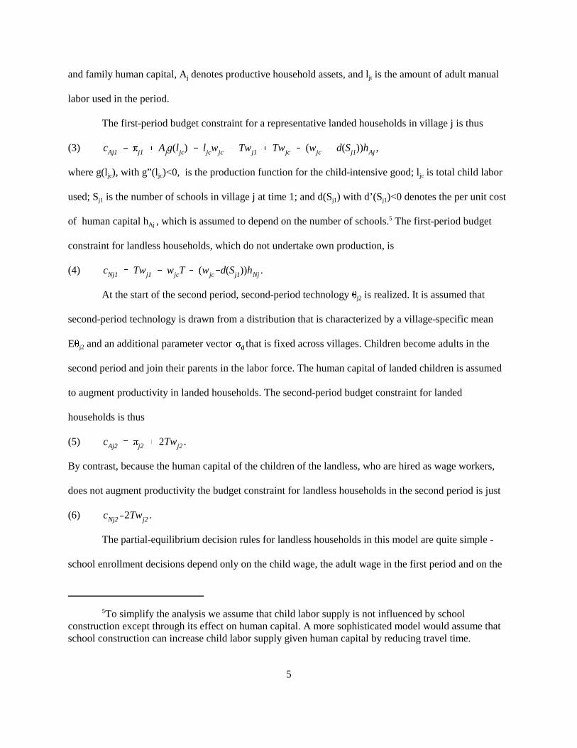
and family human capital, Aj denotes productive household assets, and ljt is the amount of adult manual

labor used in the period.

The first-period budget constraint for a representative landed households in village j is thus

(3) ,cAj1 ' πj1 % Ajg(ljc) & ljcwjc % Twj1 % Twjc & (wjc % d(Sj1))hAj

where g(ljc), with g”(ljc)<0, is the production function for the child-intensive good; ljc is total child labor

used; Sj1 is the number of schools in village j at time 1; and d(Sj1) with d’(Sj1)<0 denotes the per unit cost

of human capital hAj , which is assumed to depend on the number of schools.5 The first-period budget

constraint for landless households, which do not undertake own production, is

(4) .cNj1 ' Twj1 % wjcT & (wjc%d(Sj1))hNj

At the start of the second period, second-period technology θj2 is realized. It is assumed that

second-period technology is drawn from a distribution that is characterized by a village-specific mean

Eθj2 and an additional parameter vector that is fixed across villages. Children become adults in theσθ

second period and join their parents in the labor force. The human capital of landed children is assumed

to augment productivity in landed households. The second-period budget constraint for landed

households is thus

(5) .cAj2 ' πj2 % 2Twj2

By contrast, because the human capital of the children of the landless, who are hired as wage workers,

does not augment productivity the budget constraint for landless households in the second period is just

(6) .cNj2'2Twj2

The partial-equilibrium decision rules for landless households in this model are quite simple -

school enrollment decisions depend only on the child wage, the adult wage in the first period and on the

6

stock (proximity) of local schools. There are no effects of variation in expected second-period wages or

technology on the human capital investment made by landless because there is no capital market and no

second period labor-market return to human capital investment for the landless. Thus there is no

opportunity for these households to transfer resources across time through human capital investment. In

particular, maximizing expected utility over consumption and human capital investment for landless

households subject to (4) and (6) yields a landless-household human capital demand function given by

(7) .hNj'h (

N(wj1,wjc,Sj1)

The partial-equilibrium effect of increasing the stock of schools on child human capital

investment in landless households is given by,

(8) ,Mh (

N

MS' d )(S)(

Mh (ck

Mph

&

Mh (

k

Mr1

hN)

where is the compensated own-price effect on human capital demand (i.e., the effect of aMh (c

A

Mph

<0

compensated increase in the monetary cost of schooling given wages and technology) and is theMh (

A

Mr1

>0

first-period income effect. Assuming income effects are non-negative, both the income and price effects

operate in the same direction so that (unsurprisingly) building schools would increase landless schooling

investment if wage rates were unaffected by school building. The effect of an increase in the child wage

on the amount of schooling among the landless households is also straightforward, and is given by

(9) .Mh (

N

Mwc

'

Mh (cN

Mph

%

Mh (

N

Mr1

(T&hN)

Whether an increase in the child wage increases or decreases child human capital in landless households

thus depends on whether the higher opportunity cost of child time is offset by the higher earnings per

child. If income effects are weak, increases in the demand for child labor reduces child schooling for

landless households.

b. General-equilibrium effects

Because changes in agricultural technology have no direct effect on the returns to hired-worker

schooling investments, whether and how a change in expected technology affects landless schooling

7

decisions depends on how such changes affect child wages and the stock of schools, which will in turn

depend on the decisions of the landed households that employ labor and decisions by the school

authority. To assess the spillover effects of agricultural technical change on landless-household schooling

investment thus requires assessing general-equilibrium effects, in particular the operation of child and

adult labor markets. In order to determine the general-equilibrium effects of increasing the number of

schools and the level of agricultural technology on schooling investment, by land status, it is necessary to

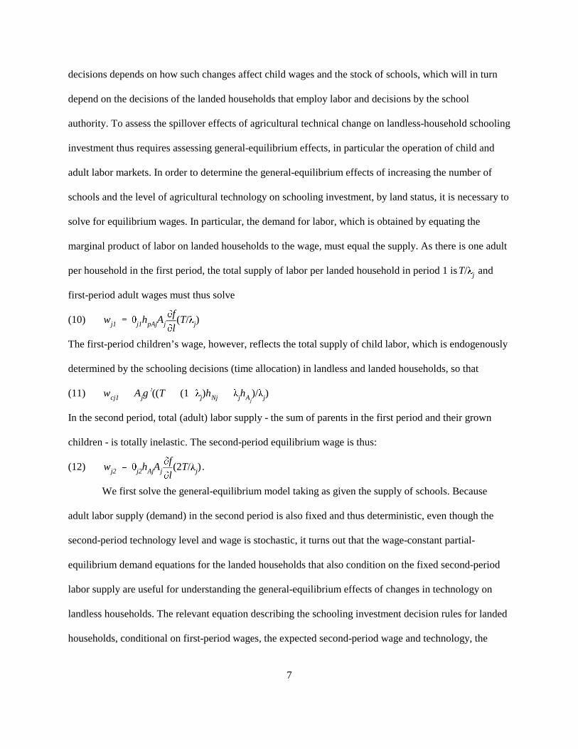
solve for equilibrium wages. In particular, the demand for labor, which is obtained by equating the

marginal product of labor on landed households to the wage, must equal the supply. As there is one adult

per household in the first period, the total supply of labor per landed household in period 1 is andT/λj

first-period adult wages must thus solve

(10) wj1 ' θj1hpAjAjMfMl

(T/λj)

The first-period children’s wage, however, reflects the total supply of child labor, which is endogenously

determined by the schooling decisions (time allocation) in landless and landed households, so that

(11) wcj1 ' Ajg)((T & (1&λj)hNj & λjhAj

)/λj)

In the second period, total (adult) labor supply - the sum of parents in the first period and their grown

children - is totally inelastic. The second-period equilibrium wage is thus:

(12) .wj2 ' θj2hAjAjMfMl

(2T/λj)

We first solve the general-equilibrium model taking as given the supply of schools. Because

adult labor supply (demand) in the second period is also fixed and thus deterministic, even though the

second-period technology level and wage is stochastic, it turns out that the wage-constant partial-

equilibrium demand equations for the landed households that also condition on the fixed second-period

labor supply are useful for understanding the general-equilibrium effects of changes in technology on

landless households. The relevant equation describing the schooling investment decision rules for landed

households, conditional on first-period wages, the expected second-period wage and technology, the

8

stock of schools and second-period labor usage (2T/λ) is given by

(13) ,hAj ' h (

A (wj1,Ewj2,wjc,θj1,Eθj2,Sj1,Aj,hpAj,2T/λ,σθ)

where Ewj2 denotes the expected second-period wage.

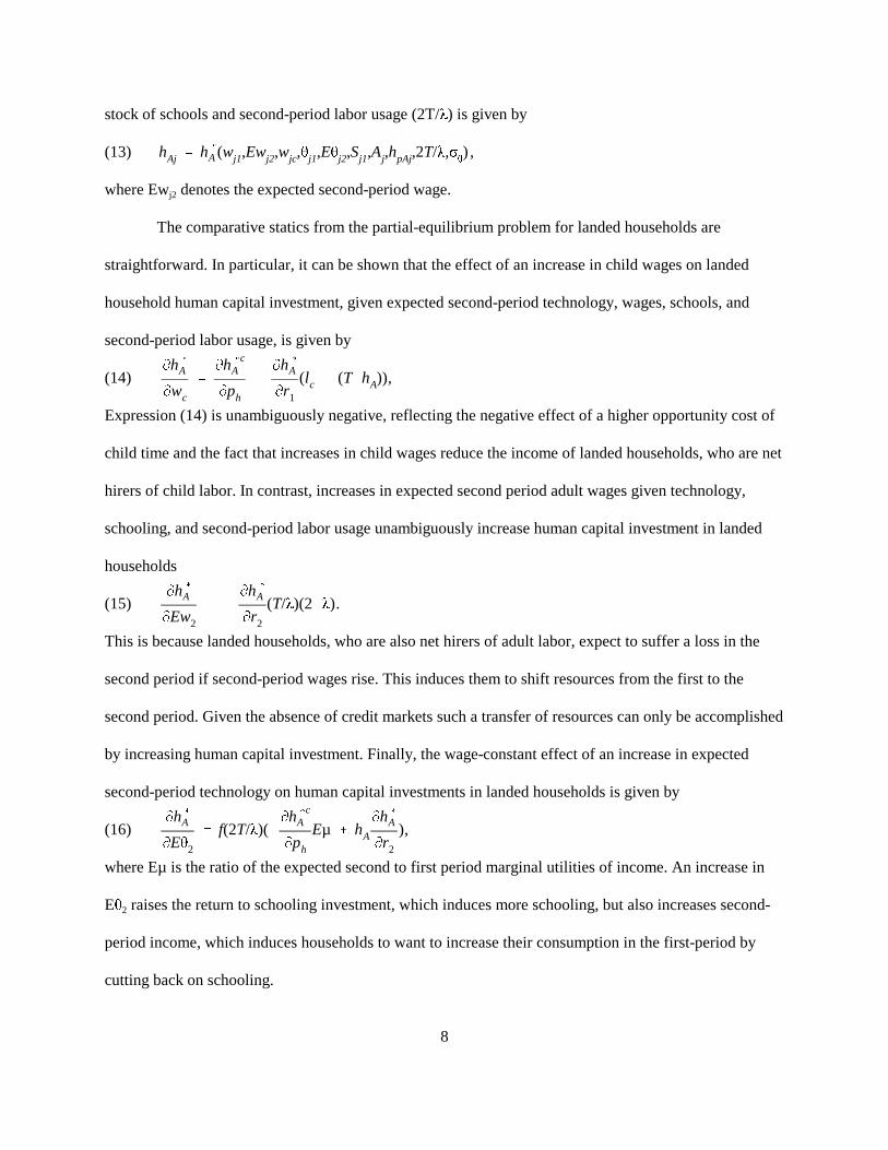
The comparative statics from the partial-equilibrium problem for landed households are

straightforward. In particular, it can be shown that the effect of an increase in child wages on landed

household human capital investment, given expected second-period technology, wages, schools, and

second-period labor usage, is given by

(14) ,Mh (

A

Mwc

'

Mh (cA

Mph

&

Mh (

A

Mr1

(lc & (T&hA))

Expression (14) is unambiguously negative, reflecting the negative effect of a higher opportunity cost of

child time and the fact that increases in child wages reduce the income of landed households, who are net

hirers of child labor. In contrast, increases in expected second period adult wages given technology,

schooling, and second-period labor usage unambiguously increase human capital investment in landed

households

(15) .Mh (

A

MEw2

' &

Mh (

A

Mr2

(T/λ)(2&λ)

This is because landed households, who are also net hirers of adult labor, expect to suffer a loss in the

second period if second-period wages rise. This induces them to shift resources from the first to the

second period. Given the absence of credit markets such a transfer of resources can only be accomplished

by increasing human capital investment. Finally, the wage-constant effect of an increase in expected

second-period technology on human capital investments in landed households is given by

(16) ,Mh (

A

MEθ2

' f(2T/λ)(&Mh (c

A

Mph

Eµ % hA

Mh (

A

Mr2

)

where Eµ is the ratio of the expected second to first period marginal utilities of income. An increase in

Eθ2 raises the return to schooling investment, which induces more schooling, but also increases second-

period income, which induces households to want to increase their consumption in the first-period by

cutting back on schooling.

9

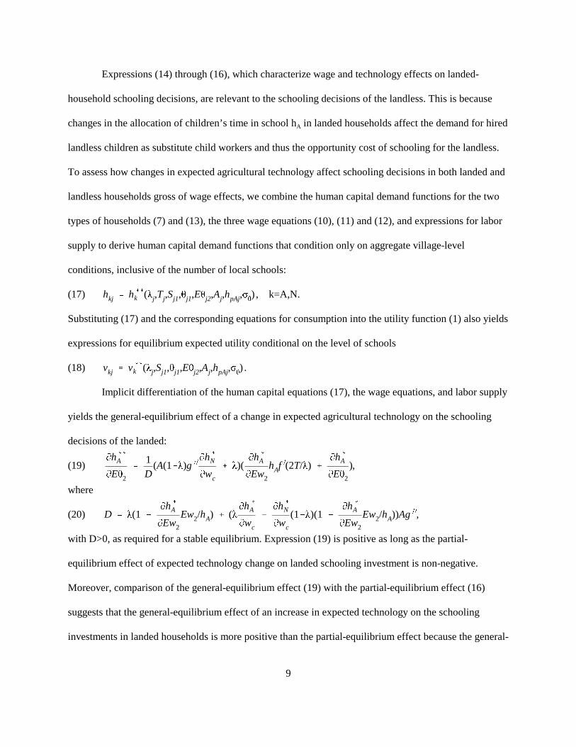
Expressions (14) through (16), which characterize wage and technology effects on landed-

household schooling decisions, are relevant to the schooling decisions of the landless. This is because

changes in the allocation of children’s time in school hA in landed households affect the demand for hired

landless children as substitute child workers and thus the opportunity cost of schooling for the landless.

To assess how changes in expected agricultural technology affect schooling decisions in both landed and

landless households gross of wage effects, we combine the human capital demand functions for the two

types of households (7) and (13), the three wage equations (10), (11) and (12), and expressions for labor

supply to derive human capital demand functions that condition only on aggregate village-level

conditions, inclusive of the number of local schools:

(17) , k=A,N.hkj ' h ((

k (λj,Tj,Sj1,θj1,Eθj2,Aj,hpAj,σθ)

Substituting (17) and the corresponding equations for consumption into the utility function (1) also yields

expressions for equilibrium expected utility conditional on the level of schools

(18) .vkj ' v ((

k (λj,Sj1,θj1,Eθj2,Aj,hpAj,σθ)

Implicit differentiation of the human capital equations (17), the wage equations, and labor supply

yields the general-equilibrium effect of a change in expected agricultural technology on the schooling

decisions of the landed:

(19) ,Mh ((

A

MEθ2

'

1D

(A(1&λ)g ))Mh (

N

Mwc

% λ)(Mh (

A

MEw2

hAf )(2T/λ) %Mh (

A

MEθ2

)

where

(20) ,D ' λ(1 &

Mh (

A

MEw2

Ew2/hA) % (λMh (

A

Mwc

%

Mh (

N

Mwc

(1&λ)(1 &

Mh (

A

MEw2

Ew2/hA))Ag ))

with D>0, as required for a stable equilibrium. Expression (19) is positive as long as the partial-

equilibrium effect of expected technology change on landed schooling investment is non-negative.

Moreover, comparison of the general-equilibrium effect (19) with the partial-equilibrium effect (16)

suggests that the general-equilibrium effect of an increase in expected technology on the schooling

investments in landed households is more positive than the partial-equilibrium effect because the general-

10

equilibrium effect contains both the direct partial-equilibrium technology effect (16) and the second-

period wage effect, which is positive. The intuition is that if technology is expected to improve, second-

period wages will also be expected to increase (given the fixity of labor supply), which will further

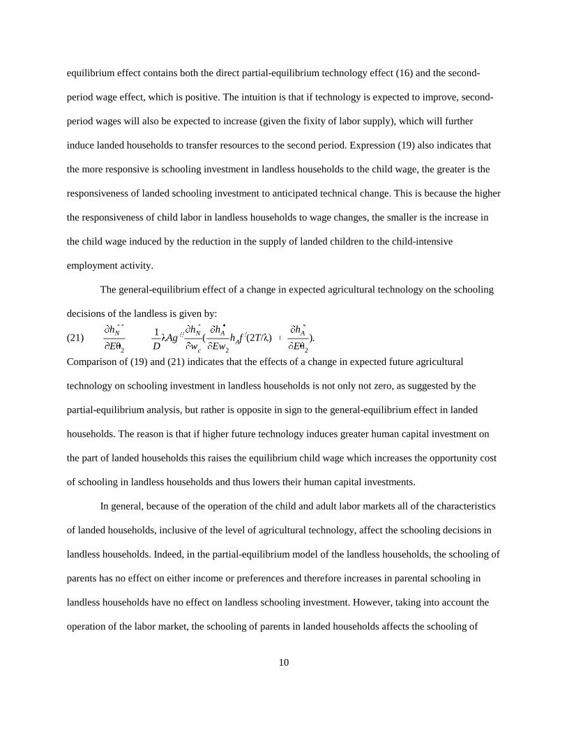
induce landed households to transfer resources to the second period. Expression (19) also indicates that

the more responsive is schooling investment in landless households to the child wage, the greater is the

responsiveness of landed schooling investment to anticipated technical change. This is because the higher

the responsiveness of child labor in landless households to wage changes, the smaller is the increase in

the child wage induced by the reduction in the supply of landed children to the child-intensive

employment activity.

The general-equilibrium effect of a change in expected agricultural technology on the schooling

decisions of the landless is given by:

(21) .Mh ((

N

MEθ2

' &

1DλAg ))

Mh (

N

Mwc

(Mh (

A

MEw2

hAf )(2T/λ) %Mh (

A

MEθ2

)

Comparison of (19) and (21) indicates that the effects of a change in expected future agricultural

technology on schooling investment in landless households is not only not zero, as suggested by the

partial-equilibrium analysis, but rather is opposite in sign to the general-equilibrium effect in landed

households. The reason is that if higher future technology induces greater human capital investment on

the part of landed households this raises the equilibrium child wage which increases the opportunity cost

of schooling in landless households and thus lowers their human capital investments.

In general, because of the operation of the child and adult labor markets all of the characteristics

of landed households, inclusive of the level of agricultural technology, affect the schooling decisions in

landless households. Indeed, in the partial-equilibrium model of the landless households, the schooling of

parents has no effect on either income or preferences and therefore increases in parental schooling in

landless households have no effect on landless schooling investment. However, taking into account the

operation of the labor market, the schooling of parents in landed households affects the schooling of

6This is because we have assumed that the adult and child labor are separable.

11

landless children because the schooling of landed-household parents in the first period affects the

demand for both adult and child laborers.

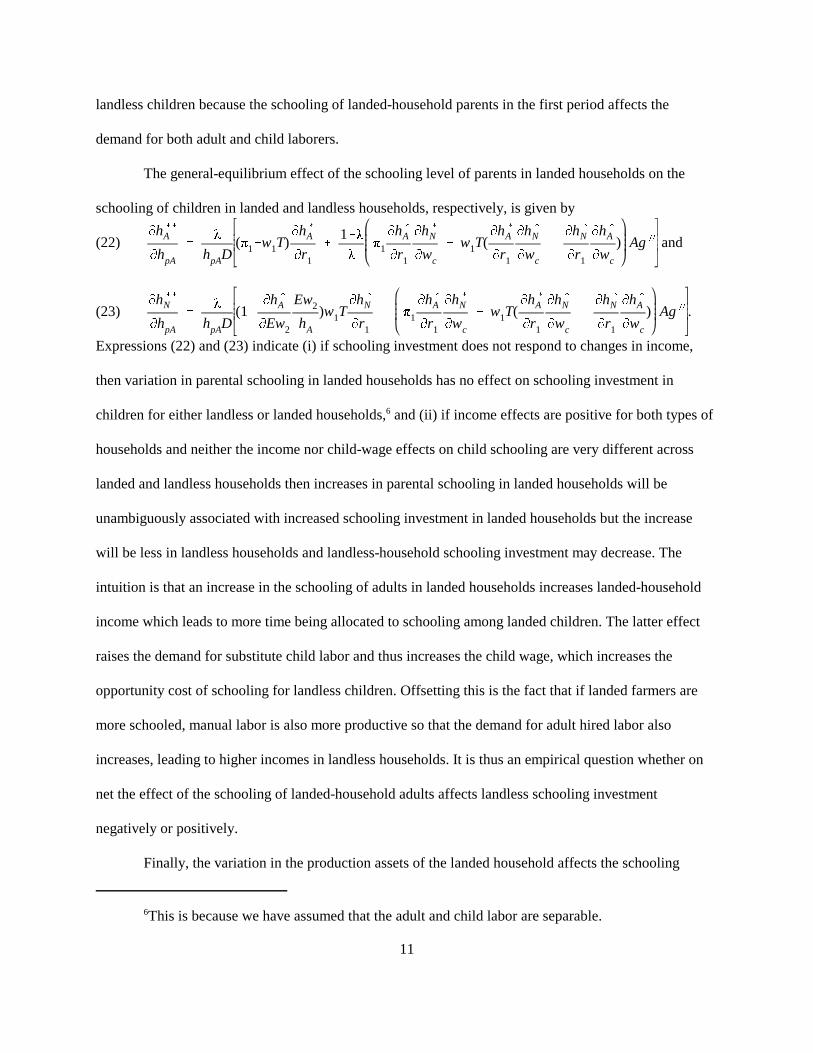
The general-equilibrium effect of the schooling level of parents in landed households on the

schooling of children in landed and landless households, respectively, is given by

(22) andMh ((

A

MhpA

'

λ

hpAD(π1%w1T)

Mh (

A

Mr1

%

1&λλ

π1

Mh (

A

Mr1

Mh (

N

Mwc

% w1T(Mh (

A

Mr1

Mh (

N

Mwc

&

Mh (

N

Mr1

Mh (

A

Mwc

) Ag ))

(23) .Mh ((

N

MhpA

'

λ

hpAD(1&

Mh (

A

MEw2

Ew2

hA

)w1TMh (

N

Mr1

& π1

Mh (

A

Mr1

Mh (

N

Mwc

% w1T(Mh (

A

Mr1

Mh (

N

Mwc

&

Mh (

N

Mr1

Mh (

A

Mwc

) Ag ))

Expressions (22) and (23) indicate (i) if schooling investment does not respond to changes in income,

then variation in parental schooling in landed households has no effect on schooling investment in

children for either landless or landed households,6 and (ii) if income effects are positive for both types of

households and neither the income nor child-wage effects on child schooling are very different across

landed and landless households then increases in parental schooling in landed households will be

unambiguously associated with increased schooling investment in landed households but the increase

will be less in landless households and landless-household schooling investment may decrease. The

intuition is that an increase in the schooling of adults in landed households increases landed-household

income which leads to more time being allocated to schooling among landed children. The latter effect

raises the demand for substitute child labor and thus increases the child wage, which increases the

opportunity cost of schooling for landless children. Offsetting this is the fact that if landed farmers are

more schooled, manual labor is also more productive so that the demand for adult hired labor also

increases, leading to higher incomes in landless households. It is thus an empirical question whether on

net the effect of the schooling of landed-household adults affects landless schooling investment

negatively or positively.

Finally, the variation in the production assets of the landed household affects the schooling

12

decisions in both landed and landless households. The effect of a change in the level of the landed

household asset on landed schooling investment is given by

(24) ,Mh ((

A

MA'

λ

ADwc

Mh (

A

Mwc

% HA %

1&λλ

(HA

Mh (

N

Mwc

& w1TMh (

N

Mr1

Mh (

A

Mwc

)g ))A

where .HA ' &

Mh c(A

Mph

EµEθ2Af(l2) % (π1 % w1T)Mh (

A

Mr1

% (π2 % 2Ew2T)Mh (

A

Mr2

There are three effects, corresponding to the three terms in (24). First, an increase in productive assets

raises the return to first-period child labor, given child wage rates, and thus reduces child time allocated

to schooling. Second, as given by the second term H A, an increase in the size of the asset stock increases

the return to schooling in the second period, which raises schooling if the difference between the first-

and second-period income effects is small. Finally there is a general-equilibrium effect which partly

offsets any change in schooling via its feedback on child wages.

Variation in the productive assets of the landed affects the schooling in landless households

according to:

(25) .Mh ((

N

MA'

λ

AD(1&

Mh (

A

MEw2

Ew2

hA

)(wc

Mh (

N

Mwc

% w1TMh (

N

Mr1

) & 1&λλ

(HA

Mh (

N

Mwc

& w1TMh (

N

Mr1

Mh (

A

Mwc

)g ))A

Here, there are only two effects because changes in landed-household assets do not change the second-

period return to schooling for the landless. Thus, increasing the assets in landed households

unambiguously reduces landless schooling, because it raises the demand for child labor in the first period

and because landed children may reduce their time spent in the non-school activity, with this only partly

offset by the general-equilibrium effect of the rise in child wages.

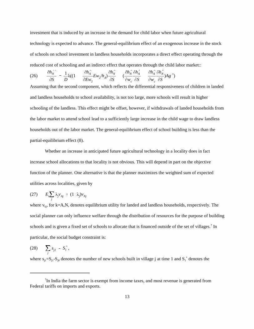
c. Endogenous school allocations and schooling investment

With endogenous school allocations, the effects of expected improvements in agricultural

technology or landed assets on the schooling of landless-household children will also depend on how

changes in expectations about future technology or changes in asset holdings also affect the allocation of

schools. Increased schooling availability can offset the reduction in landless-household schooling

7In India the farm sector is exempt from income taxes, and most revenue is generated fromFederal tariffs on imports and exports.

13

investment that is induced by an increase in the demand for child labor when future agricultural

technology is expected to advance. The general-equilibrium effect of an exogenous increase in the stock

of schools on school investment in landless households incorporates a direct effect operating through the

reduced cost of schooling and an indirect effect that operates through the child labor market::

(26)Mh ((

N

MS'

1Dλ((1 &

Mh (

A

MEw2

Ew2/hA)Mh (

N

MS& (

Mh (

N

Mwc

Mh (

A

MS&

Mh (

A

Mwc

Mh (

N

MS)Ag )))

Assuming that the second component, which reflects the differential responsiveness of children in landed

and landless households to school availability, is not too large, more schools will result in higher

schooling of the landless. This effect might be offset, however, if withdrawals of landed households from

the labor market to attend school lead to a sufficiently large increase in the child wage to draw landless

households out of the labor market. The general-equilibrium effect of school building is less than the

partial-equilibrium effect (8).

Whether an increase in anticipated future agricultural technology in a locality does in fact

increase school allocations to that locality is not obvious. This will depend in part on the objective

function of the planner. One alternative is that the planner maximizes the weighted sum of expected

utilities across localities, given by

(27) Etjj

λjvAj % (1&λj)vNj

where vkj, for k=A,N, denotes equilibrium utility for landed and landless households, respectively. The

social planner can only influence welfare through the distribution of resources for the purpose of building

schools and is given a fixed set of schools to allocate that is financed outside of the set of villages.7 In

particular, the social budget constraint is:

(28) ,jj

sj1 ' S (

1

where sj1=Sj1-Sj0 denotes the number of new schools built in village j at time 1 and S1* denotes the

8Note that, as is common in the theoretical literature examining the interaction between socialplanners and household fertility and human capital choices (Nerlove et al.1987), we assume that thesocial planner only cares about welfare from the standpoint of the current generation.

14

maximum number of schools across all villages that may be built at time 1.8

Maximizing the planner objective function (25) taking into account the behavior of the landless

and landed and the constraint (26) yields the first-order condition

(29) ,λj

Mv ((

A

MSj

% (1&λj)Mv ((

N

MSj

& ζ ' 0

where ζ is the Lagrange multiplier on the school construction constraint (26). Equation (27) may then be

solved implicitly obtain schooling investment decision rules

(30) .Sj ' S (3)(λj,θj1,Eθj2,Aj,hpAj,S0j,σθ,ζ)

In this problem it is not possible to predict how school building will respond to anticipated region-

specific changes in technology. Although the allocation of schools to those regions with the highest

technology tends to yield the highest increases in total income across villages, this effect will be offset at

least in part by the diminishing marginal utility of income: a given increase in consumption or human

capital induced by schooling subsidies may yield a higher welfare gain in low technology relative to high

technology areas even if it results in a higher income gain in the latter. It is clear, however, that the effect

of technology on schooling investment will differ importantly according to village landholding

composition. Because technology only has a direct impact on income and returns to schooling for landed

households, the magnitude of the response of schools to technology should be decreasing to zero in the

share of landless households. This is most clear in the case where the planner is maximizing the sum of

second-period village incomes. In that case, schools will be allocated to where technology is expected to

be the most advanced, because schooling has the highest return in those localities, but the positive

expected technology effect in a village will be smaller the higher the proportion of landless households

located there This is because advancing agricultural technology always benefits the income of the landed

more than the landless.

9Suppose, for example, that a primary educated individual can achieve the maximal yields giventechnology. Then land prices would reflect the expected yields that could be achieved by primaryeducated individuals rather than the yields obtained given the actual and expected actual schooling levelsin that village. The underlying assumption is that educated individuals have sufficient access to capitalthat they could in principle enter the market and bid up the price of land.

15

d. Agricultural technology expectations and land prices

An important feature of the model is that it incorporates expectations about future technology as

a key determinant of schooling investment. Given that data on expectations are not in general available, it

is important to reformulate the model in terms of observables that reflect these expectations. Because

land prices capitalize the expected discounted stream of future returns on land and land rents are

increasing in technology, land prices reflect both current and expected future technology. We posit in

particular that land prices are determined by the price that an individual with a high level of schooling h*

would be willing to pay for land.9 In particular, if pAt denotes the price of land at time t, then using the

notation of the model

(31) ,pAjt ' Etjs'0

δsθjt%sh

(fA(A,T/λj)

where δ is the discount factor. To simplify, we assume further that technological innovation takes place

only once such that at t=τ and for all s>1,

(32) Eτθjτ%1hjτ%1f(A,T/λj) ' E

τθjτ%shjτ%sf(A,T/λj)

Thus for period t=τ,

(33) pAjτ ' θjτh(fA(A,T/λj) %

δ

1&δE

τθjτ%1h

(fA(A,T/λj)

With estimates of the production technology and information on land inputs, so that the marginal

product of land can be computed, (31) can be solved for Eθjt+1 in terms of current land prices. However, if

it assumed that production is Cobb-Douglas it is possible to identify future technology effects using

information only on current land prices and yields. In particular in that case, land yields yjt in j at time t

are

(34) ,yjt ' θjthjtf(Aj,T/λj)/Aj ' θjthjtfA(Aj,T/λj)/α

16

where α is the Cobb-Douglas land-share parameter. Substituting and solving implicitly yields a function

of the form

(35) Eτθjτ%1 ' Eθ(pAjτ,yjτ,hj,Aj,T/λj,h

()

where

(36) MlnEθMlnpAjτ

' pAjτhjτ/(pAjτhjτ & αyh () > 0

(37) MlnEθMlnyjτ

' &αyjτh(/(pAjτhjτ & αyjτh

() < 0

Substitution of (33) into (17) and (18) then yields the general-equilibrium relationships for

school allocations and child schooling expressed in terms of contemporaneous village-specific yields and

land prices, as:

(38) Sj'S (4)(λj,yj1,pAj1,Aj,hpAj,S0j,σθ,ζ)

and

(39) ,hkj'h (3)k (λj,Sj1,yj1,pAj1,Aj,hpAj,σθ

)

respectively, where

MS (4)

MpAj1

'

MS (3)/MEθ2

MpA/MEθ2

and so forth.

3. Data

Our main objective in the empirical analysis is to identify how agricultural technical change

affects the schooling decisions of rural households by land ownership status. We do this by estimating

approximations to the general-equilibrium relationships (38) and (39) relating (i) school enrollment in

landed and landless households, conditional on local school availability, and (ii) school building to

expected local agricultural technology, as reflected in local land prices conditional on yields. We use

information constructed from data files produced by the National Council of Applied Economic Research

(NCAER) from six rural surveys carried out in the crop years 1968-69, 1969-70,1970-71, 1981-82, and

17

1999-2000. The first set of three survey rounds from the Additional Rural Incomes Survey (ARIS)

provides information on over 4500 households located in 261 villages in 100 districts. These sample

households are meant to be representative of all households residing in rural areas of India in the initial

year of the survey excluding households residing in Andaman and Nicobar and Lakshadwip Islands. The

most detailed information from the initial set of three surveys is available for the 1970-71 crop year and

covers 4,27 households in 259 villages. The 1981-82 survey, the Rural Economic and Demographic

Survey (REDS), was of a subset of the households in the 1970-71 ARIS survey plus a randomly-chosen

set of households in the same set of villages, excluding the state of Assam, providing information on

4,596 households in 250 villages. 248 of these are the same villages as in the ARIS. Finally, in1999 a

village-level survey (REDS99) was carried out in the same set of original ARIS villages, this time

excluding villages in the states of Jammu and Kashmir. Among other data, the survey obtained

information on the schools in each of the villages, including information on when they were constructed.

The existence of comparable household surveys at two points in time separated by 11 years

enables the construction of a panel data set at the lowest administrative level, the village, for 245 villages

that can be used to assess the effects of the changing economic circumstances on household and school

allocations. There are three other key features of the data: First, the first survey took place in the initial

years of the Indian green revolution, when rates of agricultural productivity growth began to increase

substantially in many areas of India. Second, two-thirds of the households surveyed in 1981-82 were the

same as those in 1970-71. This merged household panel, the original 1968-71 panel and information on

profits, inputs and capital stocks were used by Behrman et al. (1999) based on methodology developed in

Foster and Rosenzweig (1996) to estimate rates of technical change for each of the villages between the

two survey dates and between 1968 and 1971. Third, in each survey there is information provided on the

prices of irrigated and unirrigated land, as well as information on crop prices, crop- and seed-specific

output and planted area by land type that permit the construction of yield rates for high-yielding variety

18

crops on the two types of land.

We aggregated the household survey data at the village level by landownership status to form

two panel data sets in order to estimate the determinants of changes in school enrollment rates in landed

and landless households. In particular, we chose households with children aged 10 through 14 years of

age and constructed the proportions of children in that age group who were attending school in each

village separately for households owning land and for landless households in the two survey years using

sample weights. We also constructed weighted, village-level aggregates of the schooling and wealth of

the parents of the children in this age group for each of the two land groups at each survey date. Slightly

over 30% of children 10-14 resided in landless households in 1971. 37% of the children in this age group

in the landless households were attending school, compared with 41% in landless households in that

year.

The data indicate that in both 1971 and 1982 a significant proportion of the primary school-age

children who were not attending school participated in the labor market. In landless households 34.9% of

the non-attendee children aged 10-14 worked for wages. Although only 8.3% of the non-attending 10-14

year-olds in landed households worked for wages off the farm, an additional 28% of these landed

children worked as “family” workers. In 1982, 30.3% of landless children aged 10-14 who were not

attending school worked as wage workers, compared with 22.4% in landed households. In the latter,

however, 38.6% of the children not in school worked as family laborers.

Crop yields and land prices play a prominent role in our model. We computed village-specific

yield rates for the high-yielding seed varieties of the four major green revolution crops - wheat, rice, corn

and sorghum - on irrigated land for 1971 and 1982. We aggregated the total output in each of the years

for these crop/seeds using 1971 prices and sample weights and divided by the weighted sum of the

irrigated area devoted to these crops for each village and survey year. The 1982 survey data provides

information at the village level on the prices of irrigated and unirrigated land. The 1971 survey provides

10There is one caveat - if there are schools that have been destroyed over the period these wouldnot be reflected in a school-building history based on schools in existence in the villages in 1999.

19

information on the value and quantity of owned land, by irrigation status, for each household. We

constructed the village median price of irrigated land for 1971 from the weighted household-level data,

and deflated the 1982 village-level irrigated land prices to 1971 equivalents using the rural consumer

price index. The measures of the village-specific rates of technical change over the period 1971-82 and

the land price and yield data were appended to the two village-specific data sets describing schooling

investments in landless and landed households.

The 1999 REDS school building histories provide the dates of establishment for all schools

located within10 kilometers of the villages classified by whether they were public, private, aided, or

parochial and by schooling level - primary, middle, secondary, and upper secondary. It is thus possible to

examine the determinants of school building over the 1971-82 survey span as well as for the decade

subsequent to the 1981-82 survey round, relating comparable intervals of school investment to initial

village conditions. In Foster and Rosenzweig (2000a) we carried out investigations of the accuracy of

recall data pertaining to village infrastructure based on comparisons of the overlapping years for the

histories of electrification that were obtained in the 1970-71 and 1981-82 surveys. The results, to the

extent that they carry over to the similarly-obtained school histories, suggest that the school building

histories accurately reflect the true changes in school availability over the survey period.10

For the analyses here, we look at the determinants of changes in the spatial allocation of

secondary, inclusive of upper secondary, schools. We do this because even in the 1960's primary schools

were nearly universal - by 1971 primary schools were located within 90% of the sample villages. The

relevant margin is at the secondary school level. In 1971, only 41% of villages were proximate to a

secondary school. However there was considerable school building - by 1981 secondary school village

coverage had reached 57% and coverage increased to 73% by 1991. As documented in detail in Foster

20

and Rosenzweig (2000a), the school establishment histories also indicate that there were large inter-state

disparities in the presence of rural secondary schools 1971, but show as well that there have been

substantial variations in state-wide school investments since then.

Table 1 provides the means and standard deviations for the constructed village-level variables for

the 1970-71 and 1981-82 survey rounds. As noted, in 1971 the average primary school enrollment rate

among children in landed households was about 11% higher than that in landless households. In the

subsequent 11 years, enrollment rates for both sets of households increased, but at a faster rate in landed

households, so that by 1982 the disparity in enrollment rates between landed and landless households had

increased to over 25%. Over the same period output per acre of HYV crops approximately doubled and

the real price of irrigated land increased by a factor of 2.4, suggesting that expectations of future growth

rose more than did real output. And, the number of secondary schools built between 1971 and 1982

represented a 38% increase in the stock of secondary schools, with school building continuing in the next

11 years at similar rate.

4. Land Prices and Expected Future Yields

We first investigate whether land price variation captures, in accordance with economic theory,

variation in expectations about future productivity that are assumed to condition the current decisions of

the forward-looking households. In particular, we estimate a log-log approximation to (33) using data on

land prices and HYV yields from the 1971 round of the data and “future” yields from the 1982 data using

OLS and instrumental variables, the latter to deal with possible measurement error in the land price and

yield measure. We instrument the log price of land in 1971 using the estimated village-level technical

change measure for the interval 1968-71. In addition to this variable, we make use of the fact that the

Indian government made a forecast “announcement” at the initial stages of the green revolution. In the

late 1960's, two programs - the Intensive Agricultural District Program (IADP ) and the Intensive

Agricultural Advancement District Program (IAADP) - were introduced in selected districts, roughly one

11Inspection of equations (36) and (37) suggests that the sum of the log land price and yieldcoefficients should be unity if the technology is Cobb-Douglas and technology improves in a discretejump. Our estimates clearly reject this combination of assumptions.

21

in each state. These programs were purposively placed in areas the government had identified as having

substantial potential for agricultural productivity growth due to the newly-available high-yielding seed

varieties. The programs were designed to provide more assured supplies of credit and fertilizer. As part

of the ARIS sampling design, moreover, households residing in these program districts were oversampled

(as reflected in the sample weights), so that roughly a third of the households (villages) are represented in

each program area. We assume that the existence of these well-publicized programs affected positively

farmer’s expectations about future growth in addition to augmenting yields.

The first and second columns report OLS and two-stage least squares (2SLS) estimates,

respectively, of the relationship between the log of HYV crop yields in 1982 and the log of HYV crop-

yields and land prices in 1971. In both columns 1971 yields are negatively related to 1982 yields,

controlling for 1971 land prices, while 1971 land prices and 1982 yields are positively and significantly

related, in accordance with expressions (36) and (37). The two variables, plus the initial stock of schools

and the schooling of farmers, together explain 14% of the variation in the actual variation in crop yields

11 years in the future. As expected, moreover, relative to the 2SLS estimates the OLS estimates of the

yield and price effects are biased towards zero, due presumably to measurement error.11

5. The Determinants of School Enrollment

We estimate a linear approximation to equation (39) determining the school enrollment rates of

10-14 year-olds in landless and landed households. In particular, the equations we estimate (for k= A,N)

are

(40) ,hkjt'αk1yjt%αk2pAjt%αk3Ajt%αk4hhjt%αk5Sjt%αk6λjt%µ j%εkjt

where the subscript t denotes time; µi captures unobserved time-invariant characteristics of villages,

including second moments of the technology distribution (σθ) and preferences for schooling; and εjt

12We use the information on inherited assets rather than the 1971 wealth level as an instrumentbecause it is likely that wealth, as in most surveys, is measured with error. We assume that the correlationbetween the measurement error in the inherited wealth variable and the measurement error in the 1971-82wealth change variable is substantially less than that between the error in the initial wealth level and thechange in wealth.

22

denotes an i.i.d. mean-zero taste shock.

Because parental human capital reflects investments made in the village in previous periods,

OLS estimation of (40) given the unobservability of the fixed preference factors embedded in µ will in

general yield biased estimates of the coefficients. Moreover, cross-sectional variation in land prices may

reflect variations in such permanent qualities as location, inclusive of proximity to cities or even

attractiveness, rather than just expectations of future changes in agricultural technology and current

yields. These problems may be addressed in part by estimating (40) in cross-time differences:

(41) ∆hkjt'αk1∆yjt%αk2∆pAjt%αk3∆Ajt%αk4∆hhjt%αk5∆Sjt%∆εkjt

so that the fixed unobservables are swept out.

There are two additional problems, however. First, because an exogenous (say, taste- or income-

driven) shock to the demand for schooling in period t will, given the model, result in, among other things

a higher level of parental schooling and possibly a higher level of wealth A in period t+1, there will be a

correlation between the differenced regressors in (41) and the differenced residual. To eliminate this

correlation, we employ instrumental variables, using the initial values of the variables in (40), including

the survey information on pre-1971inherited assets and the period-t adult schooling, which will be

uncorrelated with the differenced residuals given the assumption of i.i.d. taste shocks, as instruments.12

A second problem is that land prices, as noted, may measure expectations of future profitability

with error and the yield variables may be error-ridden, as we have seen in the estimation of the yield

forecast equations. We also use instrumental-variables estimation to deal with these problems, adding to

the list of instruments the technical change and pre-1971 program variables used to estimate the yield

forecast equation.

23

The first column of Table 3 reports the fixed-effects instrumental-variables (FE-IV) estimates of

the determinants of school enrollment in the landed households. The estimates indicate that, for given

current yields, in villages in which land prices are higher, school enrollment rates in landed households

are also higher, consistent with the hypothesis that expectations of future higher levels of technology

raise the returns to landed schooling investments. In addition, adding a secondary school increases school

enrollment for 10-14 year-olds in the landed households, for given expectations and yield levels. The

point estimates indicate that increasing expectations of future productivity such that land prices doubled

would raise the school enrollment rates in landed households by 14%. This would imply, given

expression (33) and a discount rate of 3%, a rate of growth in agricultural technology over the next 11

years of 7.4% per year. Adding a school raises enrollment by 68%, although that estimate is not very

precise. Finally, increases in the total wealth of the landed households appears on net to depress landed

child school enrollment, consistent with most wealth being land wealth and with the opportunity cost

effect outweighing the second-period schooling gains as seen in expression (24).

The estimates of the determinants of schooling enrollment for landless households, based on the

same specification, are given in the second column. As expected given the operation of a child labor

market and the effects of anticipated technical change on landed schooling seen in column one, increases

in expected future productivity reduce schooling enrollment in the landless households, and the effect is

strong - the same doubling of land prices induced by an expected rise in agricultural productivity reduces

landless schooling enrollment by over 90%.. For given expectations about future productivity, increases

in current yields also lower landless schooling. These effects, however, are more than offset by building a

school, which evidently would more than double landless enrollment in the same technology regime.

Finally, given yields and land prices, an increase in the schooling of farmers appears to also

reduce the schooling investment made by landless households. This effect also operates through the child

labor market, but requires care in interpretation given the inclusion of the yield and land price variables

24

in the specification - among farm households with the same yields, assets and land prices, those with

more productive (schooled) farmers must have poorer land quality and thus must expect higher future

levels of technology growth. If so, we should expect to observe more schooling investment in the farm

households and less in the landless households, which is what the columns one and two estimates

indicate, although the effects are imprecise. In contrast, the schooling of the landless household adults

should have no effect, given our assumption of the absence of schooling returns for the landless, on

landless schooling investment. This is confirmed in the column-three specification, in which the

schooling of the landless adults is included in the landless enrollment equation - the coefficient for

landless adult schooling is less than half of that of the schooling of the landed-household adults, is small

in magnitude and not statistically significantly different from zero by any conventional standard.

6. The Determinants of School Building

The estimates in Table 3 suggest that the gap between landless and landed schooling widens with

increased agricultural technical change and that there is an absolute decline in landless schooling

investment where the landed are increasing their schooling in response to technological advances, in the

absence of offsetting forces. One offsetting factor is school building. The net effect of technical change

on schooling investment in landless households depends therefore on how changes in expected

technology impact on school construction. The first column of Table 4 reports estimates of the school

building equation (38), using the same estimation procedure as was used to estimate the enrollment

equations. The estimates indicate that schools are built where agricultural productivity is expected to

increase in the future. On average, a doubling of land prices, for given current productivity, results in .16

schools being built in the subsequent 11 years, which represents more than a doubling in the average rate

at which schools were built between 1971 and 1982.

The responsiveness of school building in a village to changes in expectations about future farm

productivity appears to be significantly related to the proportion of landless in the village, as seen in the

25

estimates reported in the second column of Table 4 in which the log of the land price is interacted with

the proportion of landless households. In particular, as is consistent with school allocation rules that

maximize total incomes, more schools are evidently built in response to an increase in anticipated

productivity in villages with few landless households compared with villages with many households who

have no land. The point estimates suggest that if almost all of the households in a village are landless,

school building is almost totally unresponsive to agricultural change. In contrast, if almost all households

are farm households, an increase in expected local increases in future agricultural productivity that

results in a doubling of land prices would increase the number of schools built over the next 11 years by

almost one-half of a school on average, which is 2.5 times the average rate.

The estimate in column three suggest that for the average village in which 30% of the households

dot not own land, the number of schools built in response to a doubling of land prices associated with

increased expectations of improved agricultural technology is .32. The estimates from column three of

Table 3 suggest that this increase in school availability would raise landless schooling enrollments by

almost 41% (.15/.367). This would cut the direct negative effect of the rising land price on landless

school enrollment by almost half. Put another way, ignoring the endogenous response of school building

to spatial differences in expectations about future agricultural technical change would lead to a

substantial overestimate of the negative impact of agricultural technical change on the disparities

between landless and landed schooling investment.

7. Conclusion

While it has long been argued that the process of economic growth importantly affects

inequality, few micro-level empirical studies have explored the underlying mechanisms of this

relationship. This fact is likely due not only to the limited availability of longitudinal data that permits

one to examine these relationships at units of analysis below that of the country or state, but also to the

methodological difficulties that arise in attempts to account for general-equilibrium effects that are likely

26

to importantly influence the growth-inequality relationship.

By focusing on inequality in school attendance in a setting for which the nature of technical

change, the operation of labor markets, and the extent of schooling returns are well understood, we have

in this paper provided one example of how individual responses interact in the market place to

importantly alter the distributional consequences of economic growth. The partial equilibrium-responses

in this paper are straightforward. Because there is no market return to schooling for landless households,

expected agricultural technological change increases schooling in landed but not landless households

thus increasing school inequality. From a general-equilibrium perspective, however, two additional

factors come into play: the market for child labor and school construction. The operation of the market

for child labor worsens the distributional impact of agricultural productivity on school investment across

landless and landed households, as landless child labor is used to replace landed child labor lost due to

increased child school attendance in landed households. Our results suggest, however, that school

construction increases in areas in which there are expectations of greater future productivity increases

and that the closer proximity of schools differentially benefits landless households. Thus endogenous

school building tends to offset the adverse distributional consequences of agricultural technological

change.

These additional general-equilibrium effects may have significant implications for policies

directed at increasing the level and equality of schooling. If technical change increases the returns to

schooling then a partial-equilibrium approach would suggest that there is a tradeoff between directing

educational resources towards high technical change areas, which maximizes productivity gain, and

allocating them towards low-technical change areas, which will reduce schooling and income inequality.

The results from this paper suggest that the inequality effects are more complex. Because, for given

school availability, technical change has opposite effects on schooling for landed and landless

households, differential technical change will have a diminished impact, relative to the partial-

27

equilibrium case, on inter-regional average schooling differentials. Moreover, because schooling

differentials between the landed and landless will be higher in high relative to low technical change

areas, intra-regional inequality is likely to be lower if schools are targeted towards high technical change

areas. There may, in fact, not be a tradeoff between productivity gains and overall schooling inequality

in decisions about the allocation of schools.

28

References

Basu, Kaushik. (1999) "Child Labor: Cause, Consequence, and Cure," Journal of Economic

Literature, 37:3, pp.1083-1119.

Behrman, Jere, Andrew D. Foster, Mark R. Rosenzweig, and Prem Vashishtha, 1999, "Women's

Schooling, Home Teaching, and Economic Growth", Journal of Political Economy,

Foster, Andrew D. and Mark R. Rosenzweig, 1996, "Technical Change and Human Capital Returns and

Investments: Evidence from the Green Revolution", American Economic Review 86(4): 931-953

September.

Foster, Andrew D. and Mark R. Rosenzweig 2000a "Does Economic Growth Increase the Demand for

Schools? Evidence from Rural India, 1960-1999," manuscript.

Foster, Andrew D. and Mark R. Rosenzweig 2000b "Child labor, Adult Wages, and the Welfare

Consequences of the Green Revolution in Rural India.," manuscript.

Foster, Andrew D. and Mark R. Rosenzweig,1994, "Information, Learning, and Wage Rates in Rural

Labor Markets", Journal of Human Resources, 28(4): 759-790.

Nelson, Richard R. and Edmund S. Phelps. 1966. "Investments in Humans, Technological Diffusion and

Economic Growth." American Economic Review 56:69-75.

Nerlove, Marc Assaf Razin and Efraim Sadka, 1987, Household and Economy : Welfare Economics of

Endogenous Fertility Boston : Academic Press, 1987

Schultz, Theodore W., 1975, "The Value of the Ability to Deal with Disequilibria," Journal of Economic

Literature 13:3, 827-846.

Table 1Means and Standard Deviations of Key Variables, by Survey Year

Variable 1971 1982

Primary school enrollment rate, children 10-14 - landed .408(.302)

.503(.359)

Primary school enrollment rate, children 10-14 - landless .367(.373)

.401(.385)

Number of secondary schools built in subsequent 11 years .157(.371)

.170(.382)

Number of secondary schools .410(.630)

.568(.703)

Price of irrigated land, 1971 rupees 4405(3581)

10848(9713)

Per-acre yield index using 1971 prices, HYV crops 289.3(257.0)

586.0(348.5)

Wealth, 1971 rupees 13647(12947)

12091(10060)

Proportion of landed households with a primary-schooled male .449(.326)

.421(.365)

Proportion of landless households with a primary-schooled male .171(.321)

.269(.383)

Proportion children 10-14 who are boys - landed households .541(.231)

.533(.285)

Proportion children 10-14 who are boys - landless households .575(.316)

.506(.378)

Table 2Land Prices in 1971 and Future (1982) Yields

OLS 2SLS

Log irrigated land price, 1971a .223(3.48)b

.762(2.20)

Log yields, 1971a -.0553(1.00)

-.581(1.68)

Number of secondary schools in village, 1971 .167(2.04)

.299(2.37)

Proportion of farm households with a primaryschooled male, 1971

.191(1.30)

.227(0.91)

Adverse weather in 1971 .217(1.91)

.0311(0.16)

Constant 3.83(8.21)

2.80(1.15

R2 .140 -

N 229 229

aInstrumented variable. Instruments are: estimated technical change, 1968-71; presence ofIADP program; presence of IAADP program. See text.bAbsolute value of t-ratio in parentheses.

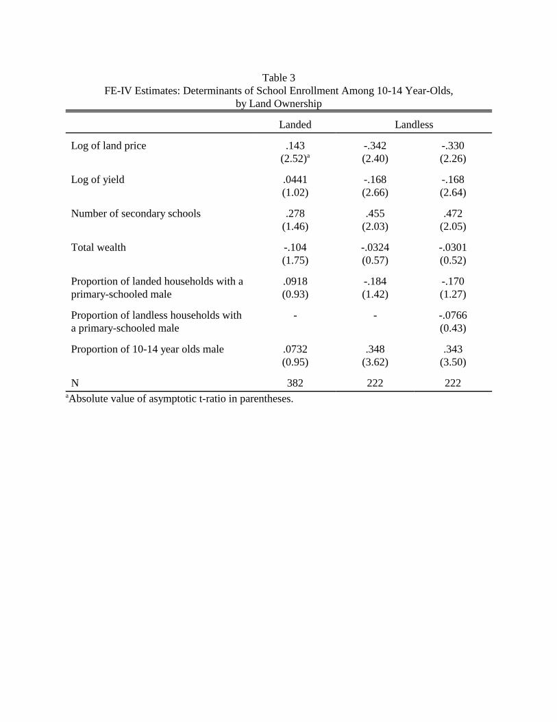
Table 3FE-IV Estimates: Determinants of School Enrollment Among 10-14 Year-Olds,

by Land Ownership

Landed Landless

Log of land price .143(2.52)a

-.342(2.40)

-.330(2.26)

Log of yield .0441(1.02)

-.168(2.66)

-.168(2.64)

Number of secondary schools .278(1.46)

.455(2.03)

.472(2.05)

Total wealth -.104(1.75)

-.0324(0.57)

-.0301(0.52)

Proportion of landed households with aprimary-schooled male

.0918(0.93)

-.184(1.42)

-.170(1.27)

Proportion of landless households witha primary-schooled male

- - -.0766(0.43)

Proportion of 10-14 year olds male .0732(0.95)

.348(3.62)

.343(3.50)

N 382 222 222aAbsolute value of asymptotic t-ratio in parentheses.

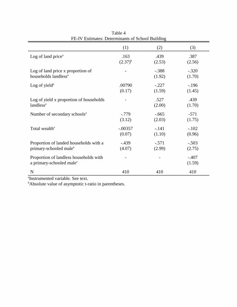
Table 4FE-IV Estimates: Determinants of School Building

(1) (2) (3)

Log of land pricea .163(2.37)b

.439(2.53)

.387(2.56)

Log of land price x proportion ofhouseholds landlessa

- -.388(1.92)

-.320(1.70)

Log of yielda .00790(0.17)

-.227(1.59)

-.196(1.45)

Log of yield x proportion of householdslandlessa

- .527(2.00)

.439(1.70)

Number of secondary schoolsa -.779(3.12)

-.665(2.03)

-571(1.75)

Total wealtha -.00357(0.07)

-.141(1.10)

-.102(0.96)

Proportion of landed households with aprimary-schooled malea

-.439(4.07)

-.571(2.99)

-.503(2.75)

Proportion of landless households witha primary-schooled malea

- - -.407(1.59)

N 410 410 410aInstrumented variable. See text.bAbsolute value of asymptotic t-ratio in parentheses.