Ten Issues About Hysteresis

Acta Appl MathDOI 10.1007/s10440-014-9936-6

Ten Issues About Hysteresis

Augusto Visintin

Received: 9 December 2013 / Accepted: 25 January 2014© Springer Science+Business Media Dordrecht 2014

Abstract In this note some basic models of hysteresis are reviewed: the linear and general-ized plays, the relay and the Preisach model. Some related questions are also illustrated.

Keywords Hysteresis · Ferromagnetism · Elasto-plasticity

1 Introduction

This note deals with models of hysteresis phenomena, and expands part of a talk that theauthor gave at the “Waves and Stability in Continuous Media” (WASCOM) conference, heldin Levico in June 2013. These models were already surveyed by this author in a numberof works, in particular in [28] and in the recently issued notes [30]. Here the emphasis ison some specific issues, that are briefly discussed after reviewing some basic hysteresisoperators.

Historical Note Ferromagnetism, elasto-plasticity and some other hysteresis phenomenahave been raising the concern of physicists, engineers and other applicative scientists fora long time. However the point of view of functional analysis emerged only recently, firstwith the pioneering works of Bouc [4, 5] in the 1960s, and then more systematically with thedeep and extensive research of the Russian school of M.A. Krasnosel’skiı, A.V. Pokrovskiıand co-workers [13, 14] in the 1970s.

At the basis of this approach there is the definition of hysteresis as rate-independentmemory,1 and the introduction of the notion of (continuous) hysteresis operator acting be-tween Banach spaces of time-dependent functions. Hysteresis in space-distributed systems

1We shall see that by rate-independence we mean invariance under time rescaling.

In honor of Professor Salvatore Rionero, on the occasion of His 80th birthday

A. Visintin (B)Dipartimento di Matematica, Università degli Studi di Trento, via Sommarive 14, 38050 Povo di Trento,Italye-mail: [email protected]

mailto:[email protected]

A. Visintin

was addressed only in the early 1980s. More specifically, continuous hysteresis relationswere extended to space-time dependent variables, regarding the space variable as a parame-ter; these hysteresis models were then coupled with PDEs [21, 22]. At the same time a firstweak model was proposed for discontinuous hysteresis, and was coupled with PDEs [23].This started an extensive research, see e.g. the mathematical monographs [6, 15, 24]. On themore physical and engineering side, ferromagnetic hysteresis was studied e.g. in [1–3, 10,16, 17].

The coupling of PDEs with continuous hysteresis was extensively addressed, much morethan the coupling with discontinuous hysteresis [24]. More recently, a different approachto discontinuous hysteresis emerged for quasi-static evolution (under the key-word of rate-independence, rather than that of hysteresis, although the two terms are essentially equiv-alent). Rate-independent quasi-static evolution was introduced about fifteen years ago byFrancfort and Marigo [11], and was independently rediscovered by Dal Maso and Toader [8],Mielke, Theil, Levitas [19]. This also triggered an intense research, which started with con-tinuous mechanics but then embraced a large number of physical phenomena; see e.g. thesurvey [18].

In particular, Mielke and coworkers developed a notion of energetic solution, that is char-acterized by a system of two conditions: a stability condition and the energy balance [18].This has some elements of contact with the representation of [23], that was revisited in [24]and further developed in [26, 27]. However these two theories were developed in differentdirections.

Outline In Sect. 2 we review the notion of hysteresis operator. In Sect. 3 we outline twoclassical models of continuous hysteresis: the linear play and the generalized play. In Sect. 4we deal with discontinuous hysteresis: we introduce the relay operator, its multi-valued clo-sure in natural topologies, and its vector extension. We also provide a weak formulation ofthis operator, as a system of two variational inequalities; this makes this relation prone tocoupling with partial differential equations (PDEs). In Sect. 5 we then introduce the cele-brated Preisach model, and point out some of its extensions. Finally in Sect. 6 we brieflydiscuss the extension of the traditional classification of PDEs to equations with hysteresis.

Throughout we formulate a number of issues. This author is able to provide an answeronly to some of them; he is thus induced to point out that some problems are not aimed tobe solved, but rather to stimulate reflection.

2 Hysteresis Operators

Although by now this notion has become almost self-evident, it needed some time to emergeand then to be accepted by the scientific community—as it sometimes happens for newfounding concepts.

Hysteresis phenomena are met in physics, chemistry, biology, engineering and so on.Typical examples include ferromagnetism, ferroelectricity, elasto-plasticity, superconduc-tivity, adsorption and desorption; hysteresis also occurs in shape-memory materials, and inseveral phase transitions.

Issue 1: Hysteresis and Loops. In several phenomena the evolution of two variables ap-pears to be strongly correlated, although no relation can be established between their in-stantaneous values. For the sake of simplicity, let us assume that these variables are bothscalar, and denote them by u and w. As in several cases the pair (u,w) evolves along closedcurves, several applicative scientists associated hysteresis to the occurrence of loops. These


loops however should not be confused with those related to phenomena like viscosity: hys-teresis loops are rate-independent, whereas viscosity loops are rate-dependent.Mathematical analysts adopted a more general point of view. In order to single out a featurethat might be common to several phenomena, they defined hysteresis as rate-independentmemory, without any reference to the occurrence of loops. However this encompasses alsofriction, and other examples that a physicist might not label as hysteretic. Moreover quan-titatively it does not perfectly fit typical hysteresis phenomena like ferromagnetism, ferro-electricity, and so on; these indeed are rate-independent just in first approximation, becauseof the simultaneous occurrence of viscous-type effects. Nevertheless it seems that the abovedefinition of hysteresis catches the main common denominator of hysteresis phenomena,and actually nowadays both the mathematical and the scientific community tend to use it.

An Example Let us revisit a standard picture, and consider a system whose state is char-acterized by two scalar variables, u and w, which we assume to depend continuously ontime, t . A typical measurement procedure of ferromagnetic magnetization consists in in-ducing a magnetic field by applying an electric current along a conducting solenoid woundaround a ring of ferromagnetic material. In this way one can induce a co-axial magneticfield, H, in the ferromagnet and control its intensity, that we shall denote by u. This mag-netic field in turn determines a magnetic induction field, B, in the ferromagnet; we shalldenote its intensity by w.

It is clear that at any instant t the output w(t) is determined by the previous evolution ofthe input function u(t) (and by the initial state), rather than just by the value of the input u(t)

at the same instant. In this case one says that the system exhibits memory.2 We can expressthis as follows:

w(t) = [F

(u,w0

)](t) ∀t ∈ [0, T ]. (2.1)

Here F(·,w0) represents an operator that acts among suitable spaces of time-dependentfunctions, for any fixed w0. As it is natural, we also assume that F(·,w0) is causal: for anyt ∈ [0, T ], the output w(t) is independent of u|]t,T ].

Several continuous hysteresis operators are constructed as follows: first the operator isdefined for piecewise monotone (equivalently, piecewise linear) input functions. A uniformcontinuity property is then established; this allows one to extend the operator by continuityto a complete function space, most often either C0([0, T ]) or W 1,1(0, T ).

Issue 2: Characterization of the State. In the most elementary models one assumes thatat any instant t the state of the system is completely characterized by the pair (u(t),w(t)).Accordingly, the initial state is characterized by (u(0),w0); as an input it thus suffices tospecify the function u and the real w0. But this is a severe restriction, that fails in severalexamples of major physical interest. Ahead we shall also outline the Preisach model, whichaccounts for the occurrence of internal variables.

Rate-Independence We require the path of the pair (u(t),w(t)) to be invariant with respectto any increasing diffeomorphism ϕ : [0, T ] → [0, T ], that is,

F(u ◦ ϕ,w0

) = F(u,w0

) ◦ ϕ in [0, T ]; (2.2)

2In order to avoid cumbersome distinctions, when we speak of memory we shall include the case in which thememory degenerates, i.e. w(t) is determined by u(t) at the same instant. Just as, when dealing with nonlinearoperators, usually one does not exclude linear operators.

A. Visintin

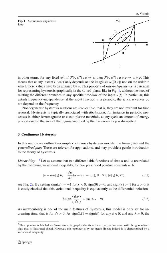
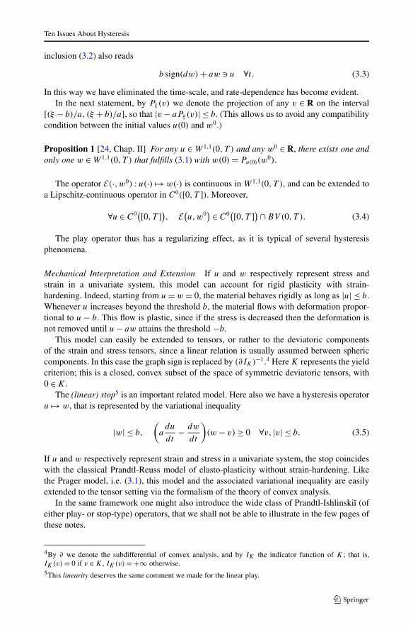
Fig. 1 A continuous hysteresisloop

in other terms, for any fixed w0, if F(·,w0) : u �→ w then F(·,w0) : u ◦ ϕ �→ w ◦ ϕ. Thismeans that at any instant t , w(t) only depends on the image set u([0, t]) and on the order inwhich these values have been attained by u. This property of rate-independence is essentialfor representing hysteresis graphically in the (u,w)-plane, like in Fig. 1, without the need ofrelating the different branches to any specific time-law of the input u(t). In particular, thisentails frequency-independence: if the input function u is periodic, the w vs. u curves donot depend on the frequency.

Nondegenerate hysteresis relations are irreversible, that is, they are not invariant for timereversal. Hysteresis is typically associated with dissipation; for instance in periodic pro-cesses in either ferromagnetic or elasto-plastic materials, at any cycle an amount of energyproportional to the area of the region encircled by the hysteresis loop is dissipated.

3 Continuous Hysteresis

In this section we outline two simple continuous hysteresis models: the linear play and thegeneralized play. These are relevant for applications, and may provide a gentle introductionto the theory of hysteresis.

Linear Play 3 Let us assume that two differentiable functions of time u and w are relatedby the following variational inequality, for two prescribed positive constants a, b:

|u − aw| ≤ b,dw

dt(u − aw − v) ≥ 0 ∀v, |v| ≤ b,∀t; (3.1)

see Fig. 2a. By setting sign(x) := −1 for x < 0, sign(0) := 0, and sign(x) := 1 for x > 0, itis easily checked that this variational inequality is equivalently to the differential inclusion

b sign

(dw

dt

)+ aw u ∀t. (3.2)

As irreversibility is one of the main features of hysteresis, this model is only set for in-creasing time, that is for dt > 0. As sign(λξ) = sign(ξ) for any ξ ∈ R and any λ > 0, the

3This operator is labeled as linear since its graph exhibits a linear part, at variance with the generalizedplay that is illustrated ahead. However, this operator is by no means linear; indeed it is characterized by avariational inequality.


inclusion (3.2) also reads

b sign(dw) + aw u ∀t. (3.3)

In this way we have eliminated the time-scale, and rate-dependence has become evident.In the next statement, by Pξ (v) we denote the projection of any v ∈ R on the interval

[(ξ − b)/a, (ξ + b)/a], so that |v − aPξ (v)| ≤ b. (This allows us to avoid any compatibilitycondition between the initial values u(0) and w0.)

Proposition 1 [24, Chap. II] For any u ∈ W 1,1(0, T ) and any w0 ∈ R, there exists one andonly one w ∈ W 1,1(0, T ) that fulfills (3.1) with w(0) = Pu(0)(w

0).

The operator E(·,w0) : u(·) �→ w(·) is continuous in W 1,1(0, T ), and can be extended toa Lipschitz-continuous operator in C0([0, T ]). Moreover,

∀u ∈ C0([0, T ]), E

(u,w0

) ∈ C0([0, T ]) ∩ BV (0, T ). (3.4)

The play operator thus has a regularizing effect, as it is typical of several hysteresisphenomena.

Mechanical Interpretation and Extension If u and w respectively represent stress andstrain in a univariate system, this model can account for rigid plasticity with strain-hardening. Indeed, starting from u = w = 0, the material behaves rigidly as long as |u| ≤ b.Whenever u increases beyond the threshold b, the material flows with deformation propor-tional to u − b. This flow is plastic, since if the stress is decreased then the deformation isnot removed until u − aw attains the threshold −b.

This model can easily be extended to tensors, or rather to the deviatoric componentsof the strain and stress tensors, since a linear relation is usually assumed between sphericcomponents. In this case the graph sign is replaced by (∂IK)−1.4 Here K represents the yieldcriterion; this is a closed, convex subset of the space of symmetric deviatoric tensors, with0 ∈ K .

The (linear) stop5 is an important related model. Here also we have a hysteresis operatoru �→ w, that is represented by the variational inequality

|w| ≤ b,

(a

du

dt− dw

dt

)(w − v) ≥ 0 ∀v, |v| ≤ b. (3.5)

If u and w respectively represent strain and stress in a univariate system, the stop coincideswith the classical Prandtl-Reuss model of elasto-plasticity without strain-hardening. Likethe Prager model, i.e. (3.1), this model and the associated variational inequality are easilyextended to the tensor setting via the formalism of the theory of convex analysis.

In the same framework one might also introduce the wide class of Prandtl-Ishlinskiı (ofeither play- or stop-type) operators, that we shall not be able to illustrate in the few pages ofthese notes.

4By ∂ we denote the subdifferential of convex analysis, and by IK the indicator function of K ; that is,IK(v) = 0 if v ∈ K , IK(v) = +∞ otherwise.5This linearity deserves the same comment we made for the linear play.

A. Visintin

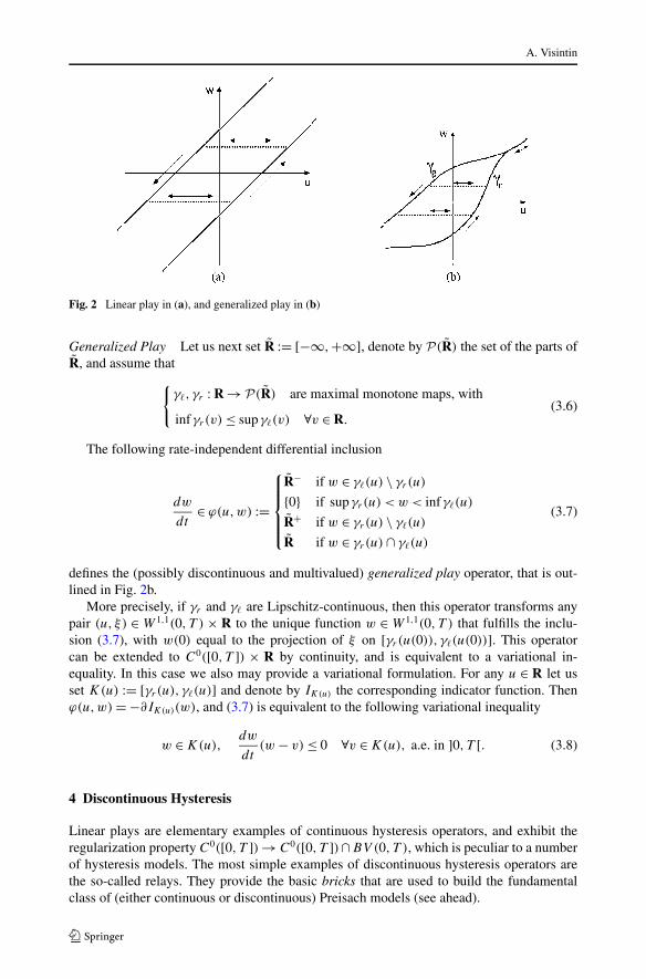
Fig. 2 Linear play in (a), and generalized play in (b)

Generalized Play Let us next set R := [−∞,+∞], denote by P(R) the set of the parts ofR, and assume that

{γ�, γr : R → P(R) are maximal monotone maps, with

infγr(v) ≤ supγ�(v) ∀v ∈ R.(3.6)

The following rate-independent differential inclusion

dw

dt∈ ϕ(u,w) :=

⎧⎪⎪⎪⎨

⎪⎪⎪⎩

R− if w ∈ γ�(u) \ γr(u)

{0} if supγr(u) < w < infγ�(u)

R+ if w ∈ γr(u) \ γ�(u)

R if w ∈ γr(u) ∩ γ�(u)

(3.7)

defines the (possibly discontinuous and multivalued) generalized play operator, that is out-lined in Fig. 2b.

More precisely, if γr and γ� are Lipschitz-continuous, then this operator transforms anypair (u, ξ) ∈ W 1,1(0, T ) × R to the unique function w ∈ W 1,1(0, T ) that fulfills the inclu-sion (3.7), with w(0) equal to the projection of ξ on [γr(u(0)), γ�(u(0))]. This operatorcan be extended to C0([0, T ]) × R by continuity, and is equivalent to a variational in-equality. In this case we also may provide a variational formulation. For any u ∈ R let usset K(u) := [γr(u), γ�(u)] and denote by IK(u) the corresponding indicator function. Thenϕ(u,w) = −∂IK(u)(w), and (3.7) is equivalent to the following variational inequality

w ∈ K(u),dw

dt(w − v) ≤ 0 ∀v ∈ K(u), a.e. in ]0, T [. (3.8)

4 Discontinuous Hysteresis

Linear plays are elementary examples of continuous hysteresis operators, and exhibit theregularization property C0([0, T ]) → C0([0, T ])∩BV (0, T ), which is peculiar to a numberof hysteresis models. The most simple examples of discontinuous hysteresis operators arethe so-called relays. They provide the basic bricks that are used to build the fundamentalclass of (either continuous or discontinuous) Preisach models (see ahead).


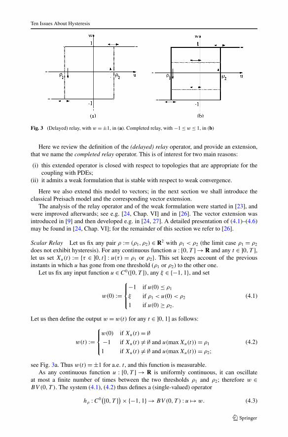
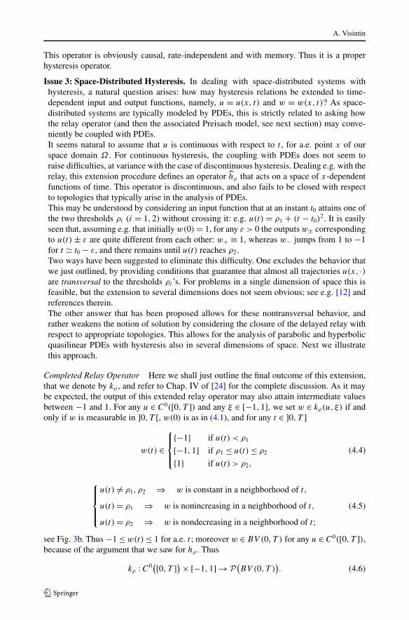
Fig. 3 (Delayed) relay, with w = ±1, in (a). Completed relay, with −1 ≤ w ≤ 1, in (b)

Here we review the definition of the (delayed) relay operator, and provide an extension,that we name the completed relay operator. This is of interest for two main reasons:

(i) this extended operator is closed with respect to topologies that are appropriate for thecoupling with PDEs;

(ii) it admits a weak formulation that is stable with respect to weak convergence.

Here we also extend this model to vectors; in the next section we shall introduce theclassical Preisach model and the corresponding vector extension.

The analysis of the relay operator and of the weak formulation were started in [23], andwere improved afterwards; see e.g. [24, Chap. VI] and in [26]. The vector extension wasintroduced in [9] and then developed e.g. in [24, 27]. A detailed presentation of (4.1)–(4.6)may be found in [24, Chap. VI]; for the remainder of this section we refer to [26].

Scalar Relay Let us fix any pair ρ := (ρ1, ρ2) ∈ R2 with ρ1 < ρ2 (the limit case ρ1 = ρ2

does not exhibit hysteresis). For any continuous function u : [0, T ] → R and any t ∈ ]0, T ],let us set Xu(t) := {τ ∈ ]0, t] : u(τ) = ρ1 or ρ2}. This set keeps account of the previousinstants in which u has gone from one threshold (ρ1 or ρ2) to the other one.

Let us fix any input function u ∈ C0([0, T ]), any ξ ∈ {−1,1}, and set

w(0) :=

⎧⎪⎨

⎪⎩

−1 if u(0) ≤ ρ1

ξ if ρ1 < u(0) < ρ2

1 if u(0) ≥ ρ2.

(4.1)

Let us then define the output w = w(t) for any t ∈ ]0,1] as follows:

w(t) :=

⎧⎪⎨

⎪⎩

w(0) if Xu(t) = ∅−1 if Xu(t) = ∅ and u(maxXu(t)) = ρ1

1 if Xu(t) = ∅ and u(maxXu(t)) = ρ2;(4.2)

see Fig. 3a. Thus w(t) = ±1 for a.e. t , and this function is measurable.As any continuous function u : [0, T ] → R is uniformly continuous, it can oscillate

at most a finite number of times between the two thresholds ρ1 and ρ2; therefore w ∈BV (0, T ). The system (4.1), (4.2) thus defines a (single-valued) operator

hρ : C0([0, T ]) × {−1,1} → BV (0, T ) : u �→ w. (4.3)

A. Visintin

This operator is obviously causal, rate-independent and with memory. Thus it is a properhysteresis operator.

Issue 3: Space-Distributed Hysteresis. In dealing with space-distributed systems withhysteresis, a natural question arises: how may hysteresis relations be extended to time-dependent input and output functions, namely, u = u(x, t) and w = w(x, t)? As space-distributed systems are typically modeled by PDEs, this is strictly related to asking howthe relay operator (and then the associated Preisach model, see next section) may conve-niently be coupled with PDEs.It seems natural to assume that u is continuous with respect to t , for a.e. point x of ourspace domain Ω . For continuous hysteresis, the coupling with PDEs does not seem toraise difficulties, at variance with the case of discontinuous hysteresis. Dealing e.g. with therelay, this extension procedure defines an operator hρ that acts on a space of x-dependentfunctions of time. This operator is discontinuous, and also fails to be closed with respectto topologies that typically arise in the analysis of PDEs.This may be understood by considering an input function that at an instant t0 attains one ofthe two thresholds ρi (i = 1,2) without crossing it: e.g. u(t) = ρ1 + (t − t0)

2. It is easilyseen that, assuming e.g. that initially w(0) = 1, for any ε > 0 the outputs w± correspondingto u(t) ± ε are quite different from each other: w+ ≡ 1, whereas w− jumps from 1 to −1for t � t0 − ε, and there remains until u(t) reaches ρ2.Two ways have been suggested to eliminate this difficulty. One excludes the behavior thatwe just outlined, by providing conditions that guarantee that almost all trajectories u(x, ·)are transversal to the thresholds ρi ’s. For problems in a single dimension of space this isfeasible, but the extension to several dimensions does not seem obvious; see e.g. [12] andreferences therein.The other answer that has been proposed allows for these nontransversal behavior, andrather weakens the notion of solution by considering the closure of the delayed relay withrespect to appropriate topologies. This allows for the analysis of parabolic and hyperbolicquasilinear PDEs with hysteresis also in several dimensions of space. Next we illustratethis approach.

Completed Relay Operator Here we shall just outline the final outcome of this extension,that we denote by kρ , and refer to Chap. IV of [24] for the complete discussion. As it maybe expected, the output of this extended relay operator may also attain intermediate valuesbetween −1 and 1. For any u ∈ C0([0, T ]) and any ξ ∈ [−1,1], we set w ∈ kρ(u, ξ) if andonly if w is measurable in ]0, T [, w(0) is as in (4.1), and for any t ∈ ]0, T ]

w(t) ∈

⎧⎪⎨

⎪⎩

{−1} if u(t) < ρ1

[−1,1] if ρ1 ≤ u(t) ≤ ρ2

{1} if u(t) > ρ2,

(4.4)

⎧⎪⎪⎨

⎪⎪⎩

u(t) = ρ1, ρ2 ⇒ w is constant in a neighborhood of t,

u(t) = ρ1 ⇒ w is nonincreasing in a neighborhood of t,

u(t) = ρ2 ⇒ w is nondecreasing in a neighborhood of t;(4.5)

see Fig. 3b. Thus −1 ≤ w(t) ≤ 1 for a.e. t ; moreover w ∈ BV (0, T ) for any u ∈ C0([0, T ]),because of the argument that we saw for hρ . Thus

kρ : C0([0, T ]) × [−1,1] → P

(BV (0, T )

). (4.6)


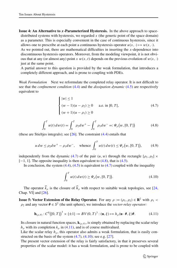
Issue 4: An Alternative to x-Parameterized Hysteresis. In the above approach to space-distributed systems with hysteresis, we regarded x (the generic point of the space domain)as a parameter. This is especially convenient in the case of continuous hysteresis, since itallows one to prescribe at each point a continuous hysteresis operator u(x, ·) �→ w(x, ·).As we pointed out, there are mathematical difficulties in inserting the x-dependence intodiscontinuous hysteresis operators. Moreover, from the modeling viewpoint, it is not obvi-ous that at any (or almost any) point x w(x, t) depends on the previous evolution of w(x, ·)just at the same point.A partial answer to this question is provided by the weak formulation, that introduces acompletely different approach, and is prone to coupling with PDEs.

Weak Formulation Next we reformulate the completed relay operator. It is not difficult tosee that the confinement condition (4.4) and the dissipation dynamic (4.5) are respectivelyequivalent to

⎧⎪⎪⎨

⎪⎪⎩

|w| ≤ 1

(w − 1)(u − ρ2) ≥ 0

(w + 1)(u − ρ1) ≥ 0

a.e. in ]0, T [, (4.7)

∫ T

0u(t) dw(t) =

∫ T

0ρ2dw+ −

∫ T

0ρ1dw− =: Ψρ

(w, [0, T ]) (4.8)

(these are Stieltjes integrals); see [26]. The constraint (4.4) entails that

udw ≤ ρ2dw+ − ρ1dw−, whence∫ T

0u(t) dw(t) ≤ Ψρ

(w, [0, T ]), (4.9)

independently from the dynamic (4.7) of the pair (u,w) through the rectangle [ρ1, ρ2] ×[−1,1]. The opposite inequality is then equivalent to (4.8), that is (4.5).

In conclusion, the system (4.4), (4.5) is equivalent to (4.7) coupled with the inequality

∫ T

0u(t) dw(t) ≥ Ψρ

(w, [0, T ]). (4.10)

The operator kρ is the closure of hρ with respect to suitable weak topologies, see [24,Chap. VI] and [26].

Issue 5: Vector Extension of the Relay Operator. For any ρ := (ρ1, ρ2) ∈ R2 with ρ1 <

ρ2 and any vector θ ∈ S2 (the unit sphere), we introduce the vector-relay operator:

h(ρ,θ) : C0([0, T ])3 × {±1} → BV (0, T )3 : (u, ξ) �→ hρ(u · θ , ξ)θ . (4.11)

Its closure in natural function spaces, k(ρ,θ), is simply obtained by replacing the scalar relayhρ with its completion kρ in (4.11), and is of course multivalued.Like the scalar relay hρ , this operator also admits a weak formulation, that is easily con-structed on the basis of the system (4.7), (4.10); see e.g. [27].The present vector extension of the relay is fairly satisfactory, in that it preserves severalproperties of the scalar model: it has a weak formulation, and is prone to be coupled with

A. Visintin

PDEs. Moreover, just as the scalar relay is the basic element for the scalar Preisach model,the vector relay may efficiently be used to construct the scalar Preisach model, as we shallsee in the next section.

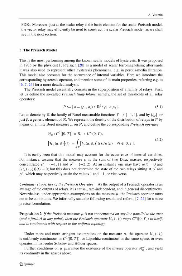
5 The Preisach Model

This is the most performing among the known scalar models of hysteresis. It was proposedin 1935 by the physicist F. Preisach [20] as a model of scalar ferromagnetism; afterwardsit was also used to represent other hysteresis phenomena, e.g. in porous-media filtration.This model also accounts for the occurrence of internal variables. Here we introduce thecorresponding hysteresis operator, and mention some of its main properties, referring e.g. to[6, 7, 24] for a more detailed analysis.

The Preisach model essentially consists in the superposition of a family of relays. First,let us define the so-called Preisach (half-)plane, namely, the set of thresholds of all relayoperators:

P := {ρ = (ρ1, ρ2) ∈ R2 : ρ1 < ρ2

}. (5.1)

Let us denote by R the family of Borel measurable functions P → {−1,1}, and by {ξρ}, orjust ξ , a generic element of R. We represent the density of the distribution of relays in P bymeans of a finite Borel measure μ on P , and define the corresponding Preisach operator

Hμ : C0([0, T ]) ×R → L∞(0, T ),

[Hμ(u, ξ)

](t) :=

∫

P

[hρ(u, ξρ)

](t) dμ(ρ) ∀t ∈ [0, T ].

(5.2)

It is easily seen that this model may account for the occurrence of internal variables.For instance, assume that the measure μ is the sum of two Dirac masses, respectivelyconcentrated ρ ′ = {−1,1} and ρ ′′ = {−2,2}. At an instant t one may have u(t) = 0 and[Hμ(u, ξ)](t) = 0; but this does not determine the state of the two relays sitting at ρ ′ andρ ′′, which may respectively attain the values 1 and −1, or vice versa.

Continuity Properties of the Preisach Operator As the output of a Preisach operator is anaverage of the outputs of relays, it is causal, rate-independent, and in general discontinuous.Nevertheless, under appropriate assumptions on the measure μ, the Preisach operator turnsout to be continuous. We informally state the following result, and refer to [7, 24] for a moreprecise formulation.

Proposition 2 If the Preisach measure μ is not concentrated on any line parallel to the axes(and a fortiori at any point), then the Preisach operator Hμ(·, ξ) maps C0([0, T ]) to itself,and is continuous with respect to the uniform topology.

Under more and more stringent assumptions on the measure μ, the operator Hμ(·, ξ)

is uniformly continuous in C0([0, T ]), or Lipschitz-continuous in the same space, or evenoperates in first-order Sobolev and Hölder spaces.

Further conditions on μ guarantee the existence of the inverse operator H−1μ , and yield

its continuity in the spaces above.


Issue 6: Vector Extension of the Preisach Operator. The extension of the relays andmore generally of the Preisach model to vectors is especially relevant for applications.For instance, one may integrate a family of vector relays with respect to a suitable mea-sure ν = ν(ρ, θ), that represents the distribution of relays with respect to thresholds anddirections. This was proposed in [9], and was then extensively investigated especially byMayergoyz [16, 17].We saw that the completed relay kρ admits a weak formulation, and that the same then ap-plies to vector relays. This then takes over to families of relays, namely to the Preisach op-erator; a wide class of (either continuous or discontinuous) hysteresis relations can thus becoupled with PDEs. Existence of a weak solution can be proved for associated boundary-and initial-value problems.

Issue 7: Justification by Homogenization of the Preisach Model. The coupling of relaysthat is implicit in the Preisach model is based on two simple rules:

(i) all relays hρ experience the same input, u;(ii) the output of the overall model is obtained by integrating the outputs wρ = hρ(u)

produced by the individual relays.

Analogous rules are the basis of the synthesis of so called analogical models (e.g., rheo-logical models in continuum mechanics, and circuital models in electrical engineering).It looks natural to wonder whether these constructions may be justified by homogenization.May one assume that there is a population of elements at a finer length-scale, and thenretrieve the composed model via a homogenization procedure?In [25] it was proved that this justification by homogenization of the Preisach model isnot consistent with the Maxwell equations. A similar failure was illustrated in [29] for thePrandtl-Ishlinskiı models of continuum mechanics.

Issue 8: Preisach Model and Ferromagnetism. Ferromagnetic hysteresis remains chal-lenging from both the modeling and the analytical viewpoints. The physics of ferromag-netism is indeed rather complex, with several overlapping effects. This induced physiciststo suggest alternative representations at different length-scales and for different materials.The Preisach model is often used to represent the relation between magnetization and mag-netic field in a ferromagnetic body formed by an aggregate of single-domain particles. Al-though the properties that can be derived from this model are in good qualitative agreementwith physical measurements, for several ferromagnetic materials there are quantitative dis-crepancies. Analogous remarks apply to the vector Preisach model. In order to provide amore adequate representation of ferromagnetic processes, physicists and engineers thenproposed several variants of the Preisach model; see e.g. [10, 16, 17].Despite of these limitations, the Preisach model remains a powerful tool for representingmacroscopic ferromagnetic hysteresis. The theory of micromagnetics, which was pioneeredby Landau and Lifshitz in 1935 and then extensively investigated, is closer to representingthe physical reality; but it is a mesoscopic model, and does not account for rate-independentmacroscopic processes. Here we shall not dwell on this theory and on its macroscopicimplications, and just refer to the recently published monograph [3].Concerning the analytical aspects of ferromagnetic hysteresis, in the scalar set-up theMaxwell system may efficiently be coupled with the scalar Preisach model. Existence of aweak solution was proved for both parabolic and hyperbolic processes, see [26].The vector set-up is more demanding, due to the occurrence of the curl operator in theMaxwell equation and to the lack of monotonicity of hysteresis operators—a drawbackthat is not remedied by the weak formulation. If at each point the hysteresis operator is

A. Visintin

reduced to a single vector relay, existence of a solution has been proved for parabolicand hyperbolic processes [27]. But the extension to the vector Maxwell-Preisach modelremains an open problem.

6 On PDEs with Hysteresis

In these few pages we cannot even touch on the analysis of PDEs with hysteresis. We justbriefly discuss how the standard classification of nonlinear evolutionary PDEs may be ex-tended to equations that include an (either continuous or discontinuous) hysteresis operator.

Issue 9: Classification of PDEs with Hysteresis. The interest for this question goes be-yond the formal exigence of classifying equations in a proper way: the classical theoryof hysteresis-free PDEs shows how the basic qualitative properties of the solutions arestrictly related to the type of the equation.We suggest to regard a scalar equation that contains a hysteresis operator as either semilin-ear, or quasilinear, or fully nonlinear (respectively), if so is the associated hysteresis-freeequation, that is obtained by replacing the hysteresis operator by any (x-dependent andpossibly multivalued) superposition operator.In semilinear equations the principal part of the equation is linear, hence it cannot includeany hysteresis operator. In this case the standard distinction between parabolic or hyper-bolic PDEs is thus trivially extended without any difficulty.Quasilinear equations with hysteresis look more interesting under this respect. Let us firstconsider piecewise monotone (scalar) input functions; as we saw, on any time interval inwhich the input function is either nondecreasing or nonincreasing, the action of any scalarhysteresis operator, F , is reduced to an (x-dependent and possibly multivalued) superpo-sition operator. Let us denote by SF this class of superposition operators. In most of theexamples of applicative interest, these operators are associated to nondecreasing functions:F is said to be piecewise monotone whenever this occurs; here we confine ourselves to thatcase.We suggest to regard a scalar equation that contains a piecewise monotone hysteresis op-erator as either parabolic or hyperbolic, whenever so is the associated nondecreasingsuperposition operator.These definitions can be extended to vector hysteresis operators, provided that if a vectorinput function evolves monotonically along any fixed (possibly x-dependent) direction,then the vector output is reduced to a (possibly multivalued) superposition operator. Thisproperty is fulfilled by some of the main models of vector hysteresis, including the vectorrelay and the vector Preisach operator that we outlined above.

Issue 10: Oscillations in Quasilinear Hyperbolic PDEs with Hysteresis. In presence ofhysteresis operators, in general these parabolic and hyperbolic equations do not exhibitsome of the properties that characterize these classes of equations in the hysteresis-freecase. This is especially evident for hyperbolic equations, since several hysteresis modelsdamp small amplitude oscillations of the input. This is at variance with the standard defini-tion of hyperbolicity in the hysteresis-free case. For instance, this damping appears in thecase of play and relay operators, and is at the basis of the BV -regularization in time thatwe already pointed out. This provides existence of a solution for a large class of quasilinearhyperbolic equations with hysteresis, see e.g. [26, 27].On the other hand, quasilinear hyperbolic equations exhibit a finite velocity of propagation,just as in the hysteresis-free case.


Acknowledgements This work was partly supported by the P.R.I.N. project “Calculus of Variations” ofItalian M.I.U.R.

References

1. Bertotti, G.: Hysteresis in Magnetism. Academic Press, Boston (1998)2. Bertotti, G., Mayergoyz, I. (eds.): The Science of Hysteresis. Elsevier, Oxford (2006)3. Bertotti, G., Mayergoyz, I., Serpico, C.: Nonlinear Magnetization Dynamics in Nanosystems. Elsevier,

Amsterdam (2009)4. Bouc, R.: Solution périodique de l’équation de la ferrorésonance avec hystérésis. C.R. Acad. Sci. Paris,

Sér. A 263, 497–499 (1966)5. Bouc, R.: Modèle mathématique d’hystérésis et application aux systèmes à un degré de liberté. Thèse,

Marseille (1969)6. Brokate, M., Sprekels, J.: Hysteresis and Phase Transitions. Springer, Heidelberg (1996)7. Brokate, M., Visintin, A.: Properties of the Preisach model for hysteresis. J. Reine Angew. Math. 402,

1–40 (1989)8. Dal Maso, G., Toader, R.: A model for the quasi-static growth or brittle fractures: existence and approx-

imation results. Arch. Ration. Mech. Anal. 162, 101–135 (2002)9. Damlamian, A., Visintin, A.: Une généralisation vectorielle du modèle de Preisach pour l’hystérésis. C.

R. Acad. Sci., Sér. 1 Math. 297, 437–440 (1983)10. Della Torre, E.: Magnetic Hysteresis. Wiley/IEEE Press, New York (1999)11. Francfort, G.A., Marigo, J.-J.: Revisiting brittle fracture as an energy minimization problem: existence

and approximation results. J. Mech. Phys. Solids 46, 1319–1342 (1998)12. Gurevich, P., Shamin, R., Tikhomirov, S.: Reaction-diffusion equations with spatially distributed hys-

teresis. SIAM J. Math. Anal. 45, 1328–1355 (2013)13. Krasnosel’skiı, M.A., Darinskiı, B.M., Emelin, I.V., Zabreıko, P.P., Lifsic, E.A., Pokrovskiı, A.V.: Hys-

terant operator. Sov. Math. Dokl. 11, 29–33 (1970)14. Krasnosel’skiı, M.A., Pokrovskiı, A.V.: Systems with Hysteresis. Springer, Berlin (1989). Russian edi-

tion: Nauka, Moscow (1983)15. Krejcí, P.: Convexity, Hysteresis and Dissipation in Hyperbolic Equations. Gakkotosho, Tokyo (1996)16. Mayergoyz, I.D.: Mathematical Models of Hysteresis. Springer, New York (1991)17. Mayergoyz, I.D.: Mathematical Models of Hysteresis and Their Applications. Elsevier, Amsterdam

(2003)18. Mielke, A.: Evolution of rate-independent systems. In: Dafermos, C., Feireisl, E. (eds.) Handbook of Dif-

ferential Equations: Evolutionary Differential Equations, vol. II, pp. 461–559. Elsevier/North-Holland,Amsterdam (2005)

19. Mielke, A., Theil, F., Levitas, V.: A variational formulation of rate-independent phase transformationsusing an extremum principle. Arch. Ration. Mech. Anal. 162, 137–177 (2002)

20. Preisach, F.: Über die magnetische Nachwirkung. Z. Phys. 94, 277–302 (1935)21. Visintin, A.: Hystérésis dans les systèmes distribués. C. R. Acad. Sci., Sér. 1 Math. 293, 625–628 (1981)22. Visintin, A.: A model for hysteresis of distributed systems. Ann. Mat. Pura Appl. 131, 203–231 (1982)23. Visintin, A.: A phase transition problem with delay. Control Cybern. 11, 5–18 (1982)24. Visintin, A.: Differential Models of Hysteresis. Springer, Berlin (1994)25. Visintin, A.: Vector Preisach model and Maxwell’s equations. Physica B 306, 21–25 (2001)26. Visintin, A.: Quasi-linear hyperbolic equations with hysteresis. Ann. Inst. Henri Poincaré, Anal. Non

Linéaire 19, 451–476 (2002)27. Visintin, A.: Maxwell’s equations with vector hysteresis. Arch. Ration. Mech. Anal. 175, 1–38 (2005)28. Visintin, A.: Mathematical models of hysteresis. In: Bertotti, G., Mayergoyz, I. (eds.) The Science of

Hysteresis, pp. 1–123. Elsevier, Amsterdam (2006). Chap. 129. Visintin, A.: Rheological models vs. homogenization. GAMM-Mitt. 34, 113–117 (2011)30. Visintin, A.: P.D.E.s with hysteresis 30 years later. In: Proceedings of a School on “Rate-Independent

Evolutions and Hysteresis Modelling”, held in Milan (May 2013, in press)

Documents

Ten Issues About Hysteresis