Politecnico di Milano

Scuola di Ingegneria Industriale edell’Informazione

Corso di Laurea Magistrale in Engineering Physics

Terahertz Generation by Optical Rectificationin an Enhancement Cavity of Femtosecond

Ti:Sa Laser

Supervisor:Dr. Gianluca GALZERANOAssistant supervisor:Eng. Yuchen WANG

Master Thesis of:Andrea MAZZANTI

Matr. 836712

Academic Year 2015-2016

Contents

List of Figures iii

List of Tables vii

Acknowledgements viii

Abstract ix

Sommario x

Introduction xiii

1 Optical Generation of Pulsed THz Radiation 11.1 The Terahertz Gap . . . . . . . . . . . . . . . . . . . . . . . . 11.2 Generation through Photoconductive Method . . . . . . . . . 2

1.2.1 Theoretical Model . . . . . . . . . . . . . . . . . . . . 21.2.2 Photoconductive Antenna . . . . . . . . . . . . . . . . 5

1.3 Generation through Second Order Effects . . . . . . . . . . . . 71.3.1 Optical Rectification . . . . . . . . . . . . . . . . . . . 71.3.2 Difference Frequency Generation . . . . . . . . . . . . 14

1.4 Media for Optical Rectification . . . . . . . . . . . . . . . . . 161.4.1 Zinc-blende Crystals . . . . . . . . . . . . . . . . . . . 161.4.2 Typical THz Crystals . . . . . . . . . . . . . . . . . . . 18

2 Design of an Enhancement Cavity for fs Pulses 252.1 Optical Resonator . . . . . . . . . . . . . . . . . . . . . . . . . 25

2.1.1 General Treatment of a Linear Configuration . . . . . . 252.1.2 Impedance Matching . . . . . . . . . . . . . . . . . . . 29

2.2 Resonant Gaussian Modes in a Cavity . . . . . . . . . . . . . 322.2.1 Resonant Gaussian Frequencies . . . . . . . . . . . . . 322.2.2 Mode Matching . . . . . . . . . . . . . . . . . . . . . . 35

2.3 Coupling of fs Pulses to a Passive Cavity . . . . . . . . . . . . 38

i

2.3.1 Mode-Locking Pulses Analysis . . . . . . . . . . . . . . 382.3.2 Cavity FSR Dispersion . . . . . . . . . . . . . . . . . . 39

2.4 Retroactive Locking of the Cavity . . . . . . . . . . . . . . . . 462.4.1 Dithering Method . . . . . . . . . . . . . . . . . . . . . 462.4.2 Closed Loop System . . . . . . . . . . . . . . . . . . . 50

2.5 Realized Resonator . . . . . . . . . . . . . . . . . . . . . . . . 532.5.1 Resonator Setup . . . . . . . . . . . . . . . . . . . . . 532.5.2 ABCD Matrix . . . . . . . . . . . . . . . . . . . . . . . 542.5.3 Cavity Mode Matching . . . . . . . . . . . . . . . . . . 562.5.4 Coupled Bandwidth . . . . . . . . . . . . . . . . . . . . 58

3 Experimental Characterization of the Cavity Enhanced Sys-tem 613.1 Ti:Sapphire Mode-Locked Laser Characterization . . . . . . . 61

3.1.1 Laser Output Power . . . . . . . . . . . . . . . . . . . 633.1.2 Duration of the Pulses . . . . . . . . . . . . . . . . . . 643.1.3 M2 Measurement . . . . . . . . . . . . . . . . . . . . . 67

3.2 Scanning Cavity Characterization . . . . . . . . . . . . . . . . 703.3 Locked Cavity Characterization . . . . . . . . . . . . . . . . . 75

Conclusion and perspectives 81

Bibliography 81

List of Figures

1.1 most common THz sources . . . . . . . . . . . . . . . . . . . . 21.2 THz emission power as a function of frequency. Solid lines are

for the conventional THz sources. Ovals denote recent THzsources for which an exact characterization is under investiga-tions. The values of the last two are indicated by peak power;others are by CW power. . . . . . . . . . . . . . . . . . . . . . 2

1.3 Dipole antenna microscope picture. . . . . . . . . . . . . . . . 31.4 Scheme of the photoconductive dipole antenna, the photocon-

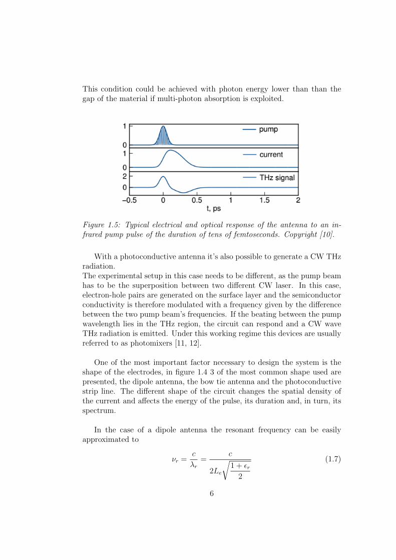
ductive strip line and the bow tie antenna. . . . . . . . . . . . 51.5 Typical electrical and optical response of the antenna to an

infrared pump pulse of the duration of tens of femtoseconds. . 61.6 Difference frequency generation intensity . . . . . . . . . . . . 141.8 GaP refractive index . . . . . . . . . . . . . . . . . . . . . . . 191.9 Coherence length vs THz frequency for ZnTe using optical

excitation at 800 nm. . . . . . . . . . . . . . . . . . . . . . . . 201.10 Optical Rectification in CdTe . . . . . . . . . . . . . . . . . . 211.11 Setup used to avoid total internal reflection when generating

THz inside lithium niobate. . . . . . . . . . . . . . . . . . . . 221.12 Spectra of THz pulses generated in a 0.69mm thick DAST

crystal. . . . . . . . . . . . . . . . . . . . . . . . . . . . . . . . 231.13 Crystals’ absorption coefficient. . . . . . . . . . . . . . . . . . 23

2.1 Model of a linear resonator. . . . . . . . . . . . . . . . . . . . 262.2 Enhancement of the field inside a resonator. . . . . . . . . . . 272.3 Cavity reflection and transmission. . . . . . . . . . . . . . . . 282.4 Derivative of EN with respect to the input mirror R. . . . . . 292.5 Cavity enhancement for an impedance matched cavity . . . . . 302.8 Linear cavity equivalent to a ring resonator of length d with

N mirrors, a non linear crystal and an output coupler. . . . . . 322.9 Examples of resonating mode’s frequencies . . . . . . . . . . . 352.10 scheme of the setup needed to mode match a laser into a pas-

sive cavity. . . . . . . . . . . . . . . . . . . . . . . . . . . . . . 35

iii

2.11 Mode matching efficiency as a funcition of mismatch betweenbeam waist radii. . . . . . . . . . . . . . . . . . . . . . . . . . 37

2.12 mode-locked laser electric field . . . . . . . . . . . . . . . . . . 382.13 linear approximation for the behavior of FSR as a function of

the resonant peak considered if dispersive media are found inthe cavity. . . . . . . . . . . . . . . . . . . . . . . . . . . . . . 40

2.14 Detuning between comb modes and resonant frequency of thepassive cavity. . . . . . . . . . . . . . . . . . . . . . . . . . . . 41

2.15 Difference between a comb with and without νceo coupled toa cavity . . . . . . . . . . . . . . . . . . . . . . . . . . . . . . 43

2.16 Simulation of coupled bandwidth to a dispersive cavity. . . . . 432.17 Simulation of coupled bandwidth for a non negligible νceo . . . 442.18 Simulation of coupled bandwidth with respect to cavity Fi-

nesse. nuceo = 0 and GDD=50 fs2 . . . . . . . . . . . . . . . . 442.19 Simulation of coupled bandwidth in the case of detuned mode

index. . . . . . . . . . . . . . . . . . . . . . . . . . . . . . . . 452.20 Simulation of coupled bandwidth for a plausible real cavity.

GDD=155 fs2 . . . . . . . . . . . . . . . . . . . . . . . . . . . 452.21 input of the LIA compared to output. . . . . . . . . . . . . . . 462.22 Bode diagram of the Lock-in Amplifier amplitude transfer

function. . . . . . . . . . . . . . . . . . . . . . . . . . . . . . . 492.23 Typical Bode diagram of the amplitude transfer function of a

piezo electric actuator. . . . . . . . . . . . . . . . . . . . . . . 502.24 Bode diagram of the ideal transfer function of a PID controller 512.25 Scheme of the retroactive feedback system. The error signal

inside the dashed box is the detuning between the resonancefrequency of the cavity ν0 and the central frequency of the laserνlaser. the photo-detector converts back the optical signal intoa voltage onto which the controller and amplifier can work. . . 51

2.26 Bode diagram of amplitude transfer function of the three maincomponent and of Gloop . . . . . . . . . . . . . . . . . . . . . . 52

2.27 Enhancement cavity . . . . . . . . . . . . . . . . . . . . . . . 542.28 six mirror cavity with its equivalent lens guide for a round trip. 552.29 Implemented telescope used to increase mode matching effi-

ciency. . . . . . . . . . . . . . . . . . . . . . . . . . . . . . . . 572.30 Simulation of the beam dimension at the output of the Ti:Sa

laser. Two lenses have been put before the cavity to better fitthe beam radius inside the cavity. . . . . . . . . . . . . . . . . 57

2.31 Simulation of the resonating mode dimension inside the pas-sive cavity. . . . . . . . . . . . . . . . . . . . . . . . . . . . . . 58

2.32 Simulations in the specific case of 1% OC cavity. . . . . . . . . 59

iv

2.33 Simulations in the specific case of 2% OC. . . . . . . . . . . . 60

3.1 Ti:Sa pump laser scheme. . . . . . . . . . . . . . . . . . . . . 613.2 Laser resonator . . . . . . . . . . . . . . . . . . . . . . . . . . 623.3 Measured output power of the Ti:Sa laser. The value for CW

are calculated by summing both the output of the laser. . . . . 633.4 Intensity Autocorrelator . . . . . . . . . . . . . . . . . . . . . 653.5 autocorrelation of the Ti:Sa pulse . . . . . . . . . . . . . . . . 663.6 Mode-Locking beam profile at the output of the Ti:Sa laser . . 693.7 Matlab fit of the gathered data for x axis. . . . . . . . . . . . 703.8 Matlab fit of the gathered data for y axis . . . . . . . . . . . . 703.9 Realized enhancement cavity. . . . . . . . . . . . . . . . . . . 713.10 Cavity transmission and reflection signal measured with the

pump operating in c.w. regime. . . . . . . . . . . . . . . . . . 723.11 Cavity transmission and reflection signal measured with the

pump operating in m.l. regime. . . . . . . . . . . . . . . . . . 743.12 transmission and Lock-in Amplifier signal . . . . . . . . . . . . 753.13 Reflected locked cavity power . . . . . . . . . . . . . . . . . . 763.14 Unlocked cavity spectrum . . . . . . . . . . . . . . . . . . . . 763.15 Measured spectra with 1% OC. . . . . . . . . . . . . . . . . . 773.16 Measured spectra with 2% OC. . . . . . . . . . . . . . . . . . 783.17 most symmetric TEM00 mode resonating inside the cavity,

spectrum and spatial profile. . . . . . . . . . . . . . . . . . . . 783.18 high order modes spectra resonating inside the cavity on the

left, one of the measured spatial distribution for such modeson the right. . . . . . . . . . . . . . . . . . . . . . . . . . . . . 79

v

vi

List of Tables

1.1 Geometrical specification of antennas drawn in fig 1.4. . . . . 51.2 Measured power for different antenna’s geometries . . . . . . . 7

2.1 Beam radii of pump beam at the position of the waist of theresonant cavity and resonating mode inside the cavity. . . . . 58

3.1 central wavelength and FWHM of the spectrum of the mode-locked laser with respect to different pump power. . . . . . . . 64

3.2 Parameters returned from Matlab fit. . . . . . . . . . . . . . . 693.3 Calculated values of the mode matching efficiency . . . . . . . 723.4 Measured coupling efficiency under c.w. regime . . . . . . . . 733.5 Cavity finesse measured, on the left, and theoretical, on the

right. . . . . . . . . . . . . . . . . . . . . . . . . . . . . . . . . 733.6 Measured coupling efficiency under m.l. regime . . . . . . . . 74

vii

Acknowledgements

I would like to express my deepest gratitude toward my supervisor Dr. Galz-erano Gianluca for his teachings, his enormous help and active participationto my work and research through every aspect of this thesis. Special thanksto my assistant supervisor Eng. Yuchen Wang and to Dr. Fernandez T.Toney for the much needed (and welcomed) assistance in learning my wayaround in the lab. I’d like also to thank Dr. Coluccelli Nicola and Dr. Gam-betta Alessio for being willing to help me each time I asked. Lastly, I wouldlike to thank my family and friends for the patience shown in bearing meduring the writing process.Superamici 4evah.

viii

Abstract

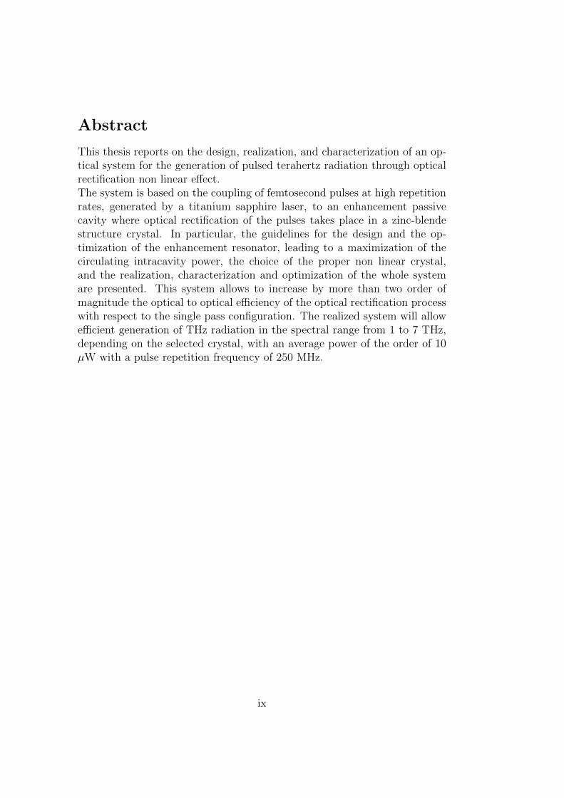
This thesis reports on the design, realization, and characterization of an op-tical system for the generation of pulsed terahertz radiation through opticalrectification non linear effect.The system is based on the coupling of femtosecond pulses at high repetitionrates, generated by a titanium sapphire laser, to an enhancement passivecavity where optical rectification of the pulses takes place in a zinc-blendestructure crystal. In particular, the guidelines for the design and the op-timization of the enhancement resonator, leading to a maximization of thecirculating intracavity power, the choice of the proper non linear crystal,and the realization, characterization and optimization of the whole systemare presented. This system allows to increase by more than two order ofmagnitude the optical to optical efficiency of the optical rectification processwith respect to the single pass configuration. The realized system will allowefficient generation of THz radiation in the spectral range from 1 to 7 THz,depending on the selected crystal, with an average power of the order of 10µW with a pulse repetition frequency of 250 MHz.

ix

Sommario

In questo lavoro di tesi si presenta la progettazione, realizzazione e carat-terizzazione di un sistema ottico per la generazione di impulsi a frequenzaterahertz mediante il processo non lineare della rettificazione ottica.Il sistema e basato sull’accoppiamento di impulsi a femtosecondi ad elevatafrequenza di ripetizione, generati da un laser titano in zaffiro, ad una cavitadi arricchimento passiva nella quale si verifica la rettificazione ottica degliimpulsi in un cristallo non lineare. In particolare sono presentate le lineeguida per la progettazione della cavita di arricchimento per l’ottimizzazionedella potenza ottica circolante in cavita e quindi nel cristallo, la scelta delcristallo non lineare e la realizzazione nonche la ottimizzazione e la carat-terizzazione di tutto il sistema sperimentale. L’utilizzo di tale sistema trovainteresse in campo applicativo in quanto permette di aumentare l’efficienzadi generazione della radiazione THz di piu di due ordini di grandezza rispettoalla configurazione a singlo passaggio. Il sistema consentira la generazioneefficiente di radiazione THz nell’intervallo da 1-7 THz a seconda del cristalloimpiegato con potenza media dell’ordine di 10 µW a frequenza di ripetizionedegli impulsi di 250 MHz.

x

Introduction

The vastness of the electromagnetic spectrum implies a differentiations ofpossible generation processes and of relative applications that range fromphotonics to fundamental physics, material science, biomedicine, securityand communications. For example, high frequency radiations like gammaand x rays are generated from nuclear transitions and transitions related tothe lower atomic shells, ultraviolet and visible frequencies are instead relatedto optical transition between atomic states in higher shells reaching as lowas hundreds of THz. On the other side there are electronic devices which, inmost cases, operate at low frequencies (few hundreds of GHz).

For technological reasons some spectral intervals of the electromagneticspectrum are not yet well investigated. In particular, in the last 10 years,many efforts have been made to develop efficient technology at frequenciesaround THz, the so called ”Terahertz gap”. Even though there is no objec-tive criterion to define the region, it’s vastly accepted to be placed between0.1 to 30 THz (10 µm to 3 mm), in this range neither optical or electricalprocesses prevail [1].

Before exploiting the advantages of this unexplored region, the use of THzradiation were mainly associated to astrophysical applications [2]. However,since 1975, time period in which extensive research about the subject wereconducted, the scientific community began to manifest a growing interest andwith the works of Hu and Nuss [3], who demonstrated the biomedical appli-cations for this radiation, in particular in the field of diagnostic and imaging,THz radiation was revealed to be an innovative resource able to be appliedin a multitude of fields like chemistry, biology and telecommunications [4].Another interesting application of this radiation is in airport security. Infact, explosives and narcotics have a recognizable spectral signature in theTHz region, making THz spectroscopy particularly useful, as it’s possible todistinguish benign compounds form illegal drugs, given also that clothes andenvelopes show high transmission in this region [5].

Given the possible applications of the THz radiation, many sources havebeen developed, however the most common problem found is the low powerachieved in the THz range combined also with the fact that most demon-strated high power sources in this spectral region work around cryogenictemperature.

The work presented in this master thesis focused on the generation of

xi

THz pulses, in the frequency range from 1 to 7 THz, using optical rectifica-tion of femtosecond near infrared pulses in a passive enhancement cavity.The near infrared pulses are generated by a Ti:Sapphire laser with centralwavelength of 810 nm, bandwidth of 35 nm, pulse duration of 25 fs, averageoutput power of 400 mW and repetition frequency of 250 MHz.The designed enhancement ring cavity is established by five chirped dichroicmirror, two of which are curved with a radius of 100 mm, highly reflectivearound 800 nm and an output coupler of 2% transmittance. The group de-lay dispersion of the cavity amounts to '-350 fs2 to compensate the highlypositive dispersive behavior of the non linear crystals used in OR.The laser was coupled into the cavity through a telescope made of two con-verging lenses of focal length 300 mm and 200 mm to achieve a mode match-ing efficiency of 90%.The measurements performed showed an efficiently coupled bandwidth of 15nm limited by GDD once a GaP crystal was inserted in the cavity, leadingto an enhancement factor of the pump power of one order of magnitude.

THz generation by non linear effects is particularly promising given thepossibility to tune the radiation in the THz range with respect to the pumpwavelength and to operate the system at room temperature. The realized sys-tem has the advantage of being able to enhance near infrared pulsed sourcesto amplify the generated THz radiation power, with the possibility to changethe crystal inside the cavity to cover different region of the THz gap. TheTHz radiation generated by this system, once properly characterized, couldbe applied in the above mentioned fields, particularly in the filed of spec-troscopy to identify peculiar low energy excitations in molecules.

This thesis is structured in the following way:

• Chapter 1In this chapter the main optical THz generation methods are presented,with particular attention to the photoconductive method exploited incommercially available antennas and to second order non linear effectsin crystal.

• Chapter 2This section reports the theoretical description of the passive cav-ity used to enhance the circulating pump radiation together with thescheme of the designed enhancement cavity.

• Chapter 3This final chapter reports the experimental validation of the proposed

xii

THz generation solution. In particular: the characterization of thenear infrared pump radiation and the characterization of the cavityenhancement factor, in different operating conditions.

xiii

Chapter 1

Optical Generation of PulsedTHz Radiation

1.1 The Terahertz Gap

The ”terahertz gap” is the spectral region between 0.1 THz and 30 THz.This specific range of frequencies is interesting to investigate upon given itsmany possible applications in various scientific and technological fields. Oneof the main goal driving research in this field is to achieve efficient sources.

State-of-the-art sources emitting in the THz gap are shown in figure 1.2.It should be noted that solid state electronic devices have lately started tocover the gap between 0.1 and 1 THz. One of the most noticeable of this de-vices is the uni-travelling-current photodiode (UTC-PD) which can generateTHz radiation by photomixing of two different wavelength laser diodes. Onthe other hand, optical devices have started to extend their reach to coverthe high frequency portion of the gap, in particular quantum cascade laser(QCL). This kind of devices shows the best efficiency in the region directlyabove 30 THz and can generate laser radiation with a frequency as low as1.39 THz, however their power output in the gap is still not as good as powersobtained through non linear effects in crystal [5]. However an improvementto this field has been brought by this devices as they are more practical thancomplex optical system and don’t need cryogenic temperature [6].

Difference frequency generation (DFG) and optical rectification (OR) aretwo of the best available methods to generate tunable radiation, pulsed orcontinuous, in the middle of the terahertz gap, for this reason their relevancehas lately been highlighted. These two effects are both second order effect

1

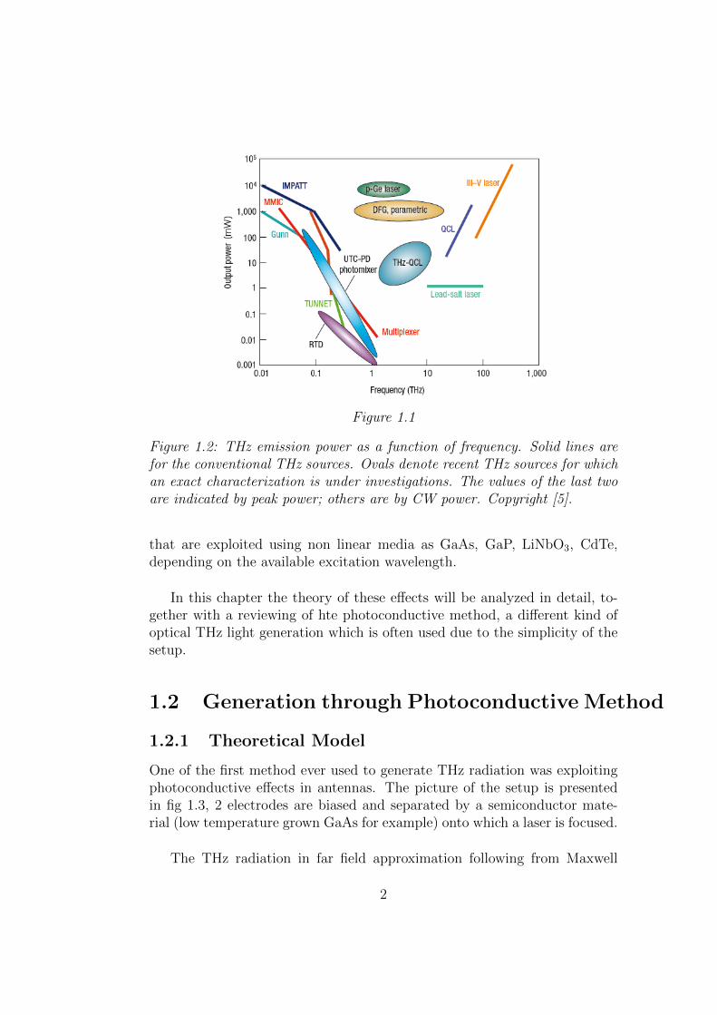
Figure 1.1

Figure 1.2: THz emission power as a function of frequency. Solid lines arefor the conventional THz sources. Ovals denote recent THz sources for whichan exact characterization is under investigations. The values of the last twoare indicated by peak power; others are by CW power. Copyright [5].

that are exploited using non linear media as GaAs, GaP, LiNbO3, CdTe,depending on the available excitation wavelength.

In this chapter the theory of these effects will be analyzed in detail, to-gether with a reviewing of hte photoconductive method, a different kind ofoptical THz light generation which is often used due to the simplicity of thesetup.

1.2 Generation through Photoconductive Method

1.2.1 Theoretical Model

One of the first method ever used to generate THz radiation was exploitingphotoconductive effects in antennas. The picture of the setup is presentedin fig 1.3, 2 electrodes are biased and separated by a semiconductor mate-rial (low temperature grown GaAs for example) onto which a laser is focused.

The THz radiation in far field approximation following from Maxwell

2

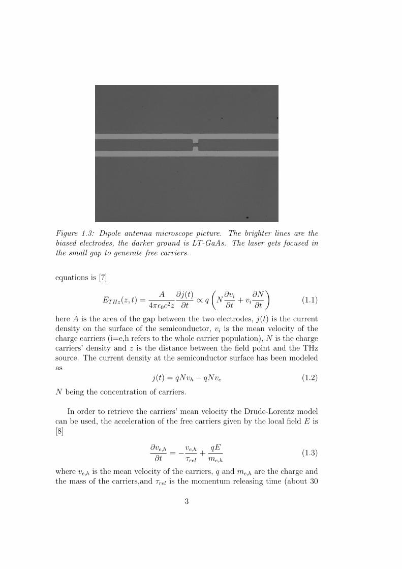
Figure 1.3: Dipole antenna microscope picture. The brighter lines are thebiased electrodes, the darker ground is LT-GaAs. The laser gets focused inthe small gap to generate free carriers.

equations is [7]

ETHz(z, t) =A

4πε0c2z

∂j(t)

∂t∝ q

(N∂vi∂t

+ vi∂N

∂t

)(1.1)

here A is the area of the gap between the two electrodes, j(t) is the currentdensity on the surface of the semiconductor, vi is the mean velocity of thecharge carriers (i=e,h refers to the whole carrier population), N is the chargecarriers’ density and z is the distance between the field point and the THzsource. The current density at the semiconductor surface has been modeledas

j(t) = qNvh − qNve (1.2)

N being the concentration of carriers.

In order to retrieve the carriers’ mean velocity the Drude-Lorentz modelcan be used, the acceleration of the free carriers given by the local field E is[8]

∂ve,h∂t

= −ve,hτrel

+qE

me,h

(1.3)

where ve,h is the mean velocity of the carriers, q and me,h are the charge andthe mass of the carriers,and τrel is the momentum releasing time (about 30

3

fs in LT-GaAs).The local field is a function of both the bias field applied and the polarizationinduced by the pump field into the semiconductor

E = Eb −P

αε0εr(1.4)

where α is the geometric factor of the semiconductor (3 for LT-GaAs).Lastly, to derive the induced polarization it’s enough to solve the partialdifferential equation describing its time evolution

∂P

∂t= − P

τrec+ j(t) (1.5)

where τrec is the recombination time between electrons and holes.These equations can be combined to obtain a closed system of equations andthe THz field can be consequentially calculated.

The dependence of the generated electric field from the derivative of thecurrent density implies that it’s possible to tailor a pump beam system anda precise shape for the electrodes in order to generate the desired field.

As a last consideration it can be noticed that this result seem to implythat the amplitude of the THz field is not dependent on the intensity ofthe pump beam impinging on the antenna, which is a counter intuitive resultbecause higher energy for the pump pulse implies a larger quantity of carriersflowing through the circuit increasing the amplitude of the generated field.In fact, these calculations are made under the assumption that the substratematerial is a semi-insulator, which is not true for an excited substrate, inthis case the current can be modeled as [2]

j(t) =σ(t)Eb

σ(t)η0

1 + n+ 1

(1.6)

where n is the refractive index of the substrate, η0 is the impedance of air(377Ω) and σ is the conductivity of the substrate.

Since, as already said, the conductivity of the substrate is proportional tothe incident intensity, combining equation 1.6 with equation 1.1 it’s possibleto get a linear dependence of the amplitude of the generated field from theintensity of the pump beam.

4

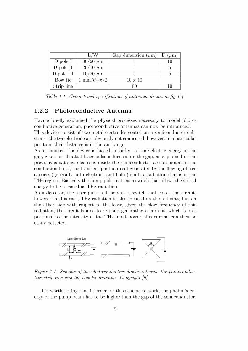
L/W Gap dimension (µm) D (µm)Dipole I 30/20 µm 5 10Dipole II 20/10 µm 5 5Dipole III 10/20 µm 5 5Bow tie 1 mm/θ=π/2 10 x 10

Strip line 80 10

Table 1.1: Geometrical specification of antennas drawn in fig 1.4.

1.2.2 Photoconductive Antenna

Having briefly explained the physical processes necessary to model photo-conductive generation, photoconductive antennas can now be introduced.This device consist of two metal electrodes coated on a semiconductor sub-strate, the two electrode are obviously not connected; however, in a particularposition, their distance is in the µm range.As an emitter, this device is biased, in order to store electric energy in thegap, when an ultrafast laser pulse is focused on the gap, as explained in theprevious equations, electrons inside the semiconductor are promoted in theconduction band, the transient photocurrent generated by the flowing of freecarriers (generally both electrons and holes) emits a radiation that is in theTHz region. Basically the pump pulse acts as a switch that allows the storedenergy to be released as THz radiation.As a detector, the laser pulse still acts as a switch that closes the circuit,however in this case, THz radiation is also focused on the antenna, but onthe other side with respect to the laser, given the slow frequency of thisradiation, the circuit is able to respond generating a current, which is pro-portional to the intensity of the THz input power, this current can then beeasily detected.

Figure 1.4: Scheme of the photoconductive dipole antenna, the photoconduc-tive strip line and the bow tie antenna. Copyright [9].

It’s worth noting that in order for this scheme to work, the photon’s en-ergy of the pump beam has to be higher than the gap of the semiconductor.

5

This condition could be achieved with photon energy lower than than thegap of the material if multi-photon absorption is exploited.

Figure 1.5: Typical electrical and optical response of the antenna to an in-frared pump pulse of the duration of tens of femtoseconds. Copyright [10].

With a photoconductive antenna it’s also possible to generate a CW THzradiation.The experimental setup in this case needs to be different, as the pump beamhas to be the superposition between two different CW laser. In this case,electron-hole pairs are generated on the surface layer and the semiconductorconductivity is therefore modulated with a frequency given by the differencebetween the two pump beam’s frequencies. If the beating between the pumpwavelength lies in the THz region, the circuit can respond and a CW waveTHz radiation is emitted. Under this working regime this devices are usuallyreferred to as photomixers [11, 12].

One of the most important factor necessary to design the system is theshape of the electrodes, in figure 1.4 3 of the most common shape used arepresented, the dipole antenna, the bow tie antenna and the photoconductivestrip line. The different shape of the circuit changes the spatial density ofthe current and affects the energy of the pulse, its duration and, in turn, itsspectrum.

In the case of a dipole antenna the resonant frequency can be easilyapproximated to

νr =c

λr=

c

2Le

√1 + εr

2

(1.7)

6

where εr = 13 for GaAs in THz range [9], Le is the effective length, whichcan be evaluated to be between the length of the dipole L and the diagonallength of the structure [(L+ 2D)2 +W 2]

12 .

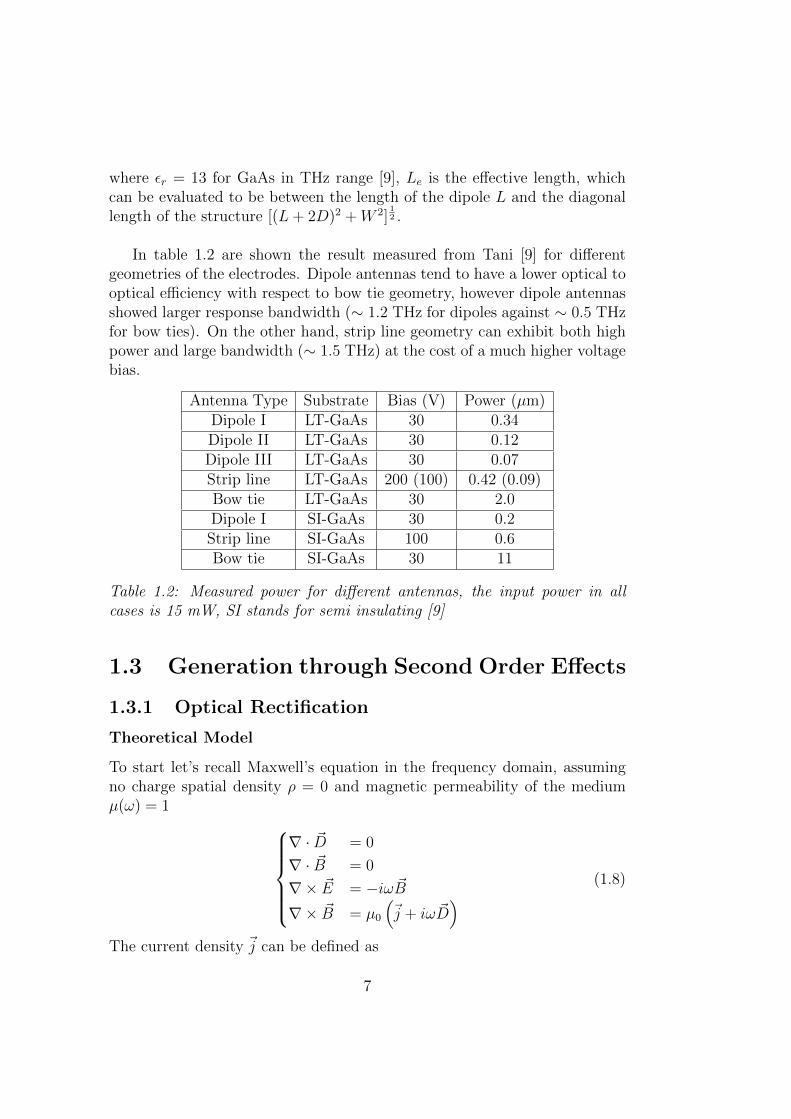
In table 1.2 are shown the result measured from Tani [9] for differentgeometries of the electrodes. Dipole antennas tend to have a lower optical tooptical efficiency with respect to bow tie geometry, however dipole antennasshowed larger response bandwidth (∼ 1.2 THz for dipoles against ∼ 0.5 THzfor bow ties). On the other hand, strip line geometry can exhibit both highpower and large bandwidth (∼ 1.5 THz) at the cost of a much higher voltagebias.

Antenna Type Substrate Bias (V) Power (µm)Dipole I LT-GaAs 30 0.34Dipole II LT-GaAs 30 0.12Dipole III LT-GaAs 30 0.07Strip line LT-GaAs 200 (100) 0.42 (0.09)Bow tie LT-GaAs 30 2.0Dipole I SI-GaAs 30 0.2Strip line SI-GaAs 100 0.6Bow tie SI-GaAs 30 11

Table 1.2: Measured power for different antennas, the input power in allcases is 15 mW, SI stands for semi insulating [9]

1.3 Generation through Second Order Effects

1.3.1 Optical Rectification

Theoretical Model

To start let’s recall Maxwell’s equation in the frequency domain, assumingno charge spatial density ρ = 0 and magnetic permeability of the mediumµ(ω) = 1

∇ · ~D = 0

∇ · ~B = 0

∇× ~E = −iω ~B∇× ~B = µ0

(~j + iω ~D

) (1.8)

The current density ~j can be defined as

7

~j = σ(ω)⊗ ~E(ω) (1.9)

where σ(ω) is the conductivity of the material and ⊗ is the tensor product.

In an optically non linear medium, the electric displacement ~D can bedefined, in SI units, as

~D = ε0 ~E + ~PL + ~PNL (1.10)

where ~PNL is the non linear polarization and the linear polarization ~PL canbe defined in analogy to equation 1.9 as

~PL = ε0χ(ω)⊗ ~E(ω) (1.11)

where χ is the linear susceptibility of the material. Substituting in equation1.10 The electric displacement becomes

~D = ε0ε(ω)⊗ ~E + ~PNL (1.12)

where ε(ω) = χ+ I, and I is the identity tensor.

Manipulating Maxwell’s equation and substituting eq 1.12 and eq 1.9 itis possible to write the non linear wave equation in frequency domain:

∇2 ~E(~r, ω)+ω2

c2ε(ω)⊗ ~E(~r, ω)−iωµ0σ(ω)⊗ ~E(~r, ω) = −µ0ω

2 ~PNL(~r, ω) (1.13)

Other than the non linear effects, solely given by the term ~PNL, this equa-tion describes the propagation, the dispersion and the absorption of a waveinside a material.

In order to model the non linear term in the equation is now necessary todefine the non linear susceptibility χNL. since optical rectification is beinginvestigated, only the second order non linearity will be taken into consid-eration. In this condition the non linear polarization is given by the thirdorder tensor χ(2)(ω) [13]

PNL,i(ω) = ε0

∫ +∞

−∞χ

(2)i,j,k(ω;ω′, ω − ω′)Ej(ω′)Ek(ω − ω′)dω′ (1.14)

It is possible to simplify the above equation to a scalar equation withoutloss of generality. To do so, it’s enough to assume a fixed polarization for the

8

field j = k.Since there is no analytical solution for the above equation it’s necessary tomodel the electric field according to the system that is being investigated.Forgetting about space dependence, which is not relevant for this discussion,the electric field of a plane pulsed beam can be expressed as

E(t) =1

2

[E0(t)eiω0t + c.c.

](1.15)

where E0(t) is the time-varying complex amplitude and ω0 is the opticalcarrier frequency.The Fourier transform of 1.15 is therefore the spectrum of the field

E(ω) =1

2[E0(ω − ω0) + E∗0(ω + ω0)] (1.16)

For a laser pulse of duration T longer than the optical cycle i.e. T 2π/ω0, the bandwidth ∆ω of E0(ω) is smaller than ω0, and the integration ineq 1.14 runs only over (−ω0−∆ω/2,−ω0+∆ω/2) and (ω0−∆ω/2, ω0+∆ω/2).Therefore PNL is nonzero only in three distinct spectral ranges; two of theseregions are centered around ±2ω0, these terms are used for sum frequencygeneration around the value for second harmonic generation (SHG) for thecarrier frequency ω0, which is not relevant for this discussion. The last re-gion lies in between −∆ω and +∆ω and is responsable for THz radiationgeneration.

A further approximation that can be done is to consider χ(2) to be con-stant for frequencies inside the intervals ± (ω0 −∆ω/2, ω0 + ∆ω/2), this istrue if the carrier frequency is not close to any resonance frequency of thematerial.Under this assumption the optical rectification susceptibility becomes

χOR(ω : ω0) = χ2(ω;ω′, ω − ω′), |ω0 − ω′| << ω0 (1.17)

and the integral of eq 1.14 can be rewritten, reminding the definition of

intensity of an electric field I(ω) =ε0cn(ω)

2E(ω) ∗ E(ω)

PORNL = (ω)

1

2ε0χ

OR(ω;ω0)(E0 ∗ E∗0)(ω) =χOR(ω;ω0)

n(ω0)cI(ω) (1.18)

If the pump beam is modeled as a plane wave, and the THz field is weakenough to guarantee no non linear cascade effect the intensity spectrum ofthe pump beam is given by Lambert-Beer law

9

I(ω) = I0(ω)e−iωngc

ze−α0z (1.19)

Having defined the absorption coefficient at optical wavelength α0 and thegroup index as

ng(ω) = n(ωopt) + ω∂n(ω)

∂ω

∣∣∣ωopt

(1.20)

Combining equation 1.19, 1.18 and equation 1.13 the wave equation be-comes:

∂2E(ω)

∂z2+

[ω2n2(ω)

c2− iωµ0σ(ω)

]E(ω) = −ω2µ0

χOR(ω;ω0)

n(ω0)ce−i

ωngcze−α0zI0(ω)

(1.21)This equation can be solved by considering wave propagating along with

the pump beam and, having as a boundary condition E(ω, 0) = 0.

Reminding the relation between absorption and conductivity

αT (ω) =µ0c

n(ω)σ(ω)(1.22)

the equation for the THz electric field can be finally written

E(ω, z) =µ0χ

OR(ω;ω0)ωI0(ω)

n(ω0)

[c

ω

(αT (ω)

2+ α0

)+ i(n(ω) + ng)

]×

× e−iωn(ω)

cze−αT (ω)

2z− e

−iωngc

ze−α0z

αT (ω)

2− α0 + i

ω

c(n(ω)− ng)

(1.23)

Many consideration can be made about this field.First we can see that, as for any other second order effect, the amplitude ofthe field increases with the input pump intensity, with the χ(2) of the mate-rial and gets attenuated by absorption both at the THz wavelength and atthe pump wavelength.

In order to have an exact model for the efficiency of generated THz ηTHz =ITHzI0

it would be necessary to make a convolution product of the field with itself;or analogously, anti Fourier transform the field, take its square modulus, and

10

Fourier transform it again. Both of this procedure can be carried out numer-ically but don’t have an analytical solution for the field shown in equation1.23.It’s anyway reported in literature that the optical to optical efficiency is inthe order of 10−6 ÷ 10−5, however it was demonstrated more recently an ef-ficiency of ∼ 5× 10−4 in LiNbO3 [14].

Another possible consideration is that the z dependence of the field isconfined in the second half of the formula. The amplitude of the THz electricfield is

|E(ω, z)| = µ0χOR(ω;ω0)ωI0(ω)

n(ω0)

[c2

ω2

(αT (ω)

2+ α0

)2

+ (n(ω) + ng)2

] 12

Lgen(ω, z) (1.24)

where the generation length Lgen has been defined as

Lgen(ω, z) =

√√√√√√√√√e−αT (ω)z + e−2α0z − 2e

−

αT (ω)

2+α0

zcosωc

(n(ω)− ng)z

[αT (ω)

2− α0

]2

+(ωc

)2

(n(ω)− ng)2

(1.25)

This term is the one that dictates the z dependence of the whole THzfield, moreover, this length strongly depends on the linear optical propertiesof the material considered (refractive index, absorption coefficient).In the ideal case of no absorption at both pump and THz wavelength, thisterm can be rewritten as a cardinal sine multiplied by the position z

Lgen(ω, z) =

∣∣∣∣∣∣∣∣sin

(ω

c

(n(ω)− ng)2

z

)ω

c

(n(ω)− ng)2

z

∣∣∣∣∣∣∣∣ z (1.26)

The ideal case is achieved when the field function is maximized, whichmeans that the cardinal sine has to be equal to one.In order to understand the physical origins of this behavior it’s not necessaryto study the field equation as a simpler method is available.

11

Group Velocity Phase Matching

The term (ng − n(ω)) is limiting the intensity of the THz field generatedby optical rectification by giving an oscillatory behavior with respect to thelength of the crystal as shown in equation 1.25. If (ng − n(ω)) was equal to0, the intensity would grow quadratically with the length.This condition is know as phase matching condition, let’s investigate theorigin of this behavior.Optical rectification is an intraband difference frequency generation (DFG),therefore the difference between the two pump k(ω) and the generated THzrange k is [15]

∆k = k(ωopt + ωTHz)− k(ωopt)− k(ωTHz) (1.27)

The main difference with respect to DFG is that, since ωTHz ωopt, theexpression in 1.27 can be simplified by expanding the function as a first orderTaylor series

k(ωopt + ωTHz) = k(ωopt) + ωTHz∂k

∂ω

∣∣∣ωopt

Since

∂k

∂ω

∣∣∣ωopt

=1

vg=ngc

substituting this result into 1.27 the wave number mismatch can be writtenas

∆k =ωTHzc

(ng − n(ωTHz)) (1.28)

The inefficiency of the process is therefore given solely by the mismatchbetween the mixing of the wave vectors. This result could have been obtainedby another approach worth mentioning.

Phase matching is met when the three combined fields can conserve en-ergy and momentum by themselves (without contribution coming from othersources like phonons)

ωopt1 − ωopt2 = ωTHz

kopt1 − kopt2 = kTHz(1.29)

where ωopt1 and ωopt2 are frequencies in the optical region belonging tothe bandwidth of the pump pulse trains.

12

if other effects have to come into play to conserve these quantities theoverall efficiency of the process is lowered.

The ratio of the equations in 1.29 can be written as∂ω

∂k

∣∣∣ωopt

=ωTHzkTHz

since

the two frequencies considered to generate THz are close. This equality canbe rewritten as

vg,opt = vp,THz (1.30)

This means phase matching is satisfied in THz wave generation when thegroup velocity of the optical beam equals phase velocity of the THz beam.The phase matching condition can, in light of this result, be better under-stood. The wavelength of the optical pulse is shorter by order of magnitudeswith respect to the THz pulse, therefore the THz pulse is so slow that itcannot see the optical pump field, it can only experience the overall profileof the pulse. Equation 1.30 refers the collinear phase matching condition,meaning that phase matching occurs when the pump and THz beams prop-agate collinearly through the nonlinear crystal. It can be demonstrated thatthis type of phase matching generates THz radiation with very good beamquality aside from giving a high generation coefficient due to long interactionlength [2].

If ∆k 6= 0 i.e. ng 6= nTHz It is possible to define a coherence length lcas the length after which the non phase matched radiation start decaying,this happens because the generated radiation is not phase locked and duringpropagation starts to interfere destructively with its replica generated indifferent crystals position; said length is achieved for perfect phase oppositioni.e. a phase difference of π.

lc =π

∆k=

πc

ωTHz|ng − nTHz|(1.31)

In order to go further in the discussion is necessary to consider a specificpump wavelength and non linear crystal to be able to evaluate both ng andnTHz.It can anyway be said that for two perfectly matched indexes the coherencelength becomes infinite and therefore other factors have to be considered inorder to model the generation correctly. The coherence length can in factbe modeled in order to take into account α0, to set a limit even in perfectlymatched conditions.

13

1.3.2 Difference Frequency Generation

An alternative to optical rectification in the field of non linear effects is dif-ference frequency generation.This process requires two different monochromatic pump beam (with fre-quency ωopt1 and ωopt2) impinging on the non linear crystal, by tuning theirwavelength is possible to obtain a three wave mixing for which the generatedwavelength is in the THz region. The main advantages with respect to opti-cal rectification are the possibility to exploit quasi phase matching conditionthrough periodically poled crystal for achieving higher power efficiency andan higher tunability of the generated radiation due to the possibility of tiltingthe pump beams and, as a consequence, change the phase matching condi-tion. On the other hand, the downside is that such an effect doesn’t allow togenerate large bandwidth radiation given the continuous wave regime of thepump beams.

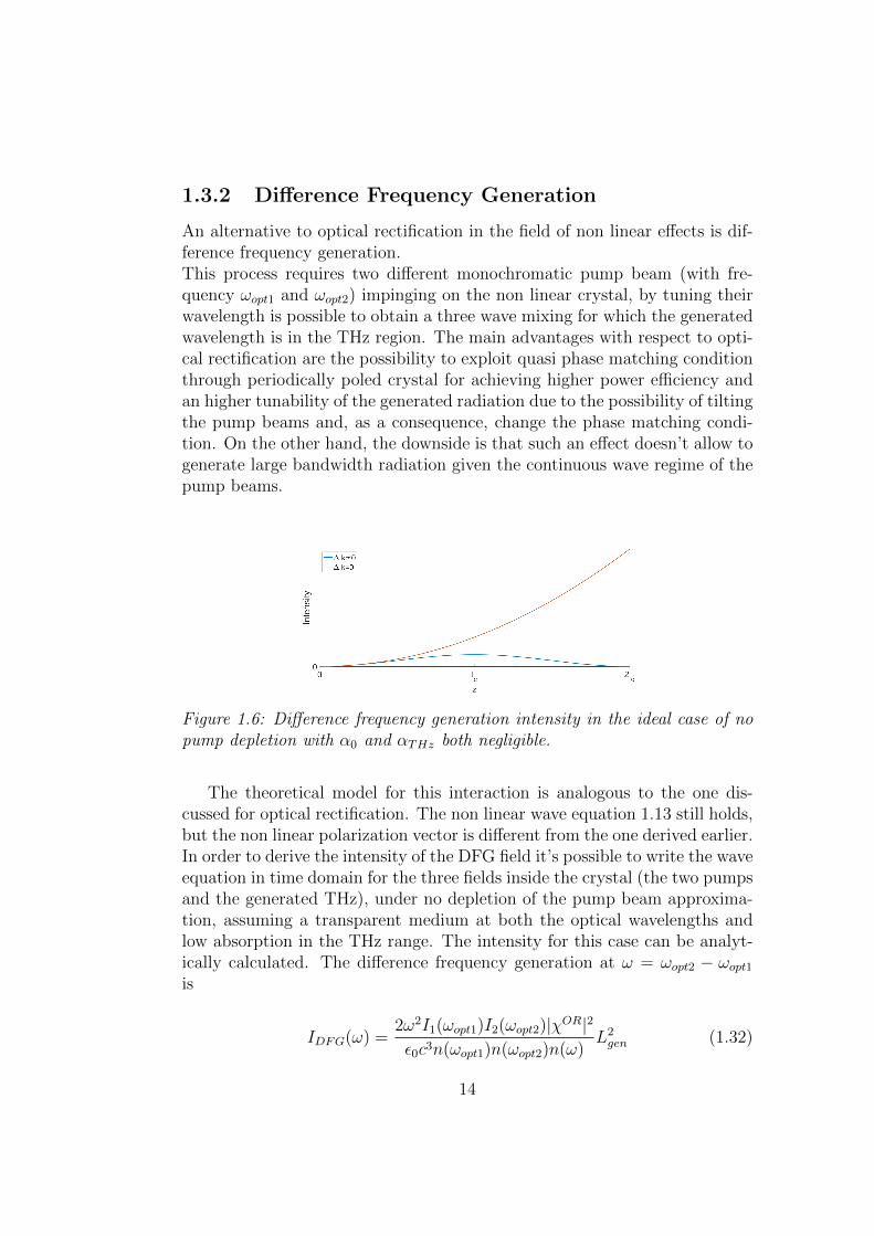
Figure 1.6: Difference frequency generation intensity in the ideal case of nopump depletion with α0 and αTHz both negligible.

The theoretical model for this interaction is analogous to the one dis-cussed for optical rectification. The non linear wave equation 1.13 still holds,but the non linear polarization vector is different from the one derived earlier.In order to derive the intensity of the DFG field it’s possible to write the waveequation in time domain for the three fields inside the crystal (the two pumpsand the generated THz), under no depletion of the pump beam approxima-tion, assuming a transparent medium at both the optical wavelengths andlow absorption in the THz range. The intensity for this case can be analyt-ically calculated. The difference frequency generation at ω = ωopt2 − ωopt1is

IDFG(ω) =2ω2I1(ωopt1)I2(ωopt2)|χOR|2

ε0c3n(ωopt1)n(ωopt2)n(ω)L2gen (1.32)

14

where I1(ωopt1) and I2(ωopt2) are the intensity of the two pump beams.While considering this process it is important to notice that also the phasemismatch term is different from the optical rectification case, in particular itis equal to:

∆k =1

c[ωnTHz − ωopt2n(ωopt2) + ωopt1n(ωopt1)] (1.33)

from which it follows that the coherence length is

lc =π

k(ω)− (k(ωopt2)− k(ωopt1))(1.34)

The dependence of the generated intensity with respect to the interactionlength is shown in figure 1.6. If the effects absorption are neglected (i.e. if thecrystal length is much shorter than the inverse of the absorption coefficient)and the pump beams’ intensities are considered constant, the behavior of thegenerated field is parabolic with respect to the crystal length in case of phasematched radiation. If phase matching is not met the behavior is sinusoidal.

If the two pump beams have equal intensity I1 = I2 = Iopt and therefractive index is considered equal for the pump frequencies (n(ωopt1) 'n(ωopt2)) the efficiency is

ηTHz =2ω2|χOR|2L2

gen

ε0c3n2(ωopt)n(ω)Iopt (1.35)

This result holds if the pump beam is not tightly focused, otherwise theefficiency would scale proportionally to ω3 [16].

When generating THz radiation with high optical to optical efficiencyby exploiting a long crystal, pump absorption and depletion effects cannotbe overlooked. If absorption at the optical wavelength is considered i.e.α0 6= 0 the coherence length model does not have a singularity for ∆k = 0,therefore, the generated THz radiation is going to get eventually out of phase;for this reason, periodically poled crystal are used. These crystal are realizedby putting in contact crystals as long as the coherence length with flippedcrystallographic axes. The overall effect is that the phase of the generatedTHz radiation is reset every integer multiple of lc, leading to a generationprofile related to a phase relation referred to as the quasi phase matchingcondition.

15

1.4 Media for Optical Rectification

1.4.1 Zinc-blende Crystals

Many of the crystal used to generate THz radiation are Zinc-Blende crystals.The cut given to these crystals determines the phase matching condition(possible different refractive index), the polarization of the generated radia-tion and the intensity of its field; for these reasons, it’s interesting to modelthe non linear response of these kind of crystal.

Generally, for these crystals the only elements of the non linear suscepti-bility tensor different from zero are χ14=χ25=χ36 [17].

χijk = χij =

0 0 0 χ14 0 00 0 0 0 χ25 00 0 0 0 0 χ36

(1.36)

The non linear polarization field is therefore defined as

PxPyPz

=1

2

0 0 0 χ14 0 00 0 0 0 χ25 00 0 0 0 0 χ36

E2x

E2y

E2z

2EyEz2ExEz2ExEy

(1.37)

PxPyPz

= χ14

ExEzExEzExEy

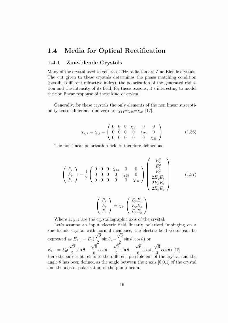
Where x, y, z are the crystallographic axis of the crystal.Let’s assume an input electric field linearly polarized impinging on a

zinc-blende crystal with normal incidence, the electric field vector can be

expressed as E110 = E0(

√2

2sin θ,−

√2

2sin θ, cos θ) or

E111 = E0(

√2

2sin θ −

√6

6cos θ,−

√2

2sin θ −

√6

6cos θ,

√6

3cos θ) [18].

Here the subscript refers to the different possible cut of the crystal and theangle θ has been defined as the angle between the z axis [0,0,1] of the crystaland the axis of polarization of the pump beam.

16

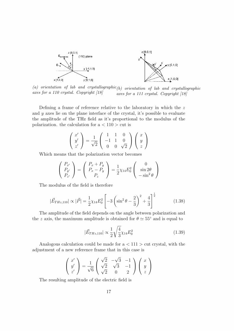
(a) orientation of lab and crystallographicaxes for a 110 crystal. Copyright [18]

(b) orientation of lab and crystallographicaxes for a 111 crystal. Copyright [18]

Defining a frame of reference relative to the laboratory in which the zand y axes lie on the plane interface of the crystal, it’s possible to evaluatethe amplitude of the THz field as it’s proportional to the modulus of thepolarization. the calculation for a < 110 > cut is x′

y′

z′

=1√2

1 1 0−1 1 0

0 0√

2

xyz

Which means that the polarization vector becomes Px′

Py′Pz′

=

Px + PyPx − PyPz

=1

2χ14E

20

0sin 2θ− sin2 θ

The modulus of the field is therefore

| ~ETHz,110| ∝ |~P | =1

2χ14E

20

[−3

(sin2 θ − 2

3

)2

+4

3

] 12

(1.38)

The amplitude of the field depends on the angle between polarization andthe z axis, the maximum amplitude is obtained for θ ' 55 and is equal to

| ~ETHz,110| ∝1

2

√4

3χ14E

20 (1.39)

Analogous calculation could be made for a < 111 > cut crystal, with theadjustment of a new reference frame that in this case is x′

y′

z′

=1√6

√2 −√

3 −1√2√

3 −1√2 0 2

xyz

The resulting amplitude of the electric field is

17

| ~ETHz,111| ∝ |~P | =1

2χ14E

20 (1.40)

For this cut orientation the amplitude of the field doesn’t depend on theangle between pump polarization and the z axis of the crystal.

if the goal of the experiment is to generate the highest intensity possibleof THz radiation by optical rectification in a zinc-blende crystal it’s generallysafe to assume that a < 110 > cut is better, giving it’s higher efficiency by a

factor of

√4

3.

1.4.2 Typical THz Crystals

This subsection is devoted to reviewing the main crystals used to generateTHz radiation via optical rectification given the possible pump wavelengthwidely available commercially in the range of NIR, in particular around 800nm.

Many options for what regards optical rectification in non linear crystalare available, obviously one aspect that has to be taken into consideration isthe magnitude of non linearity of the crystal, modeled by the absolute valueof what we defined as χOR, greater second order susceptibility implies greaterintensity of the THz field.The second main aspect is the possibility to reach a group velocity phasematching condition for the generated radiation inside the medium.As discussed in the previous section this condition relies on the equality be-tween the group index calculated at the pump wavelength and the refractiveindex of the medium at THz frequency. One aspect worth noting is that forthis kind of phase matching it is not necessary to have a birefringent ma-terial, which would be the case for SHG or DFG given the usual frequencydependence of the refractive index [17].

One additional remark to be made is that, in order to generate a pulsedradiation, the bandwidth of the THz radiation should be as large as possible.Unfortunately the frequencies being discussed are comparable to the typicalphonon energy of these crystal. Therefore achieving phase matching is notenough, the matched frequency should also lie in a relatively flat zone ofthe refractive index, both to have a smaller mismatch for neighboring wave-lengths (with respect to the central one) and to limit the THz absorption of

18

the material itself.

Here follows some of the most commonly used crystal used for opticalrectification.

1. GaP

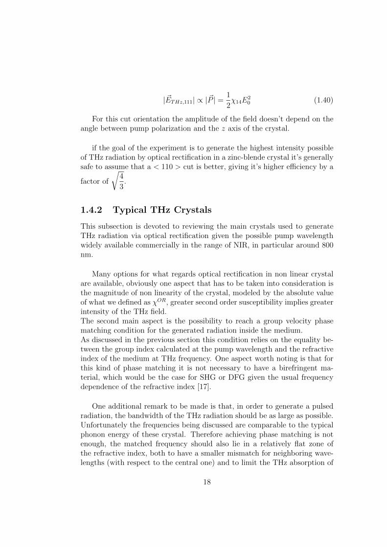
Gallium Phosphide is a non birefringent zinc-blende crystal. Litera-ture shows the possibility to generate THz from this medium usingboth non collinear [19] and collinear [20] phase matching, showing, forboth phase matching condition, a high tunability for the central wave-length. Experimental results show a bandwidth of the pulsed radiationup to 3.5 THz [21], this crystal is usually pumped with a Nd:YAG laser(1064 µm) but it has also been used in a quasi phase matched regimepumped at 1.55 µm [22]. If pumped with a 800 nm Ti:Sapphire laserit’s possible to have optical rectification phase matched at around 45µm (6.6 THz). At 800 nm GaP shows negligible absorption and a flatrefractive index, in the THz range the refractive index is flat before thelowest optical phonon resonance that is, at room temperature, locatedat 10.96 THz [23].

Figure 1.8: Gap real and imaginary refractive index. box data taken from[24] and triangle data taken from [25]. The imaginary part shows the lowestenergy phonon absorption, which is far from the region of interest. Copyright[26].

2. ZnTe

Zinc Telluride is a non birefringent zinc-blende crystal. For this par-ticular crystal is possible to have a phase matching pumping with a

19

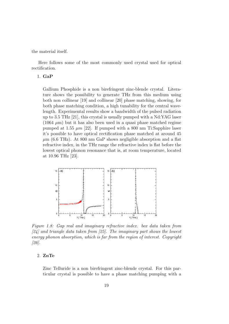
Ti:Sapphire laser at around 1.6 THz [27]. This crystal has also beenshown to be able to generate a 3 THz bandwidth pulse [28]. The maindownside of this crystal is it’s two photon absorption which limits thegenerated THz power [29]. In this case the lowest phonon resonanceis at 5.4 THz [30], which close is to the range of interest and thereforelimits the bandwidth.

Figure 1.9: Coherence length vs THz frequency for ZnTe using optical exci-tation at 800 nm. The dotted line neglects dispersion effects, substituting thegroup index at 800 nm with the refractive index at 800 nm. The solid lineinstead includes the effects of dispersion at optical frequencies. Copyright[27].

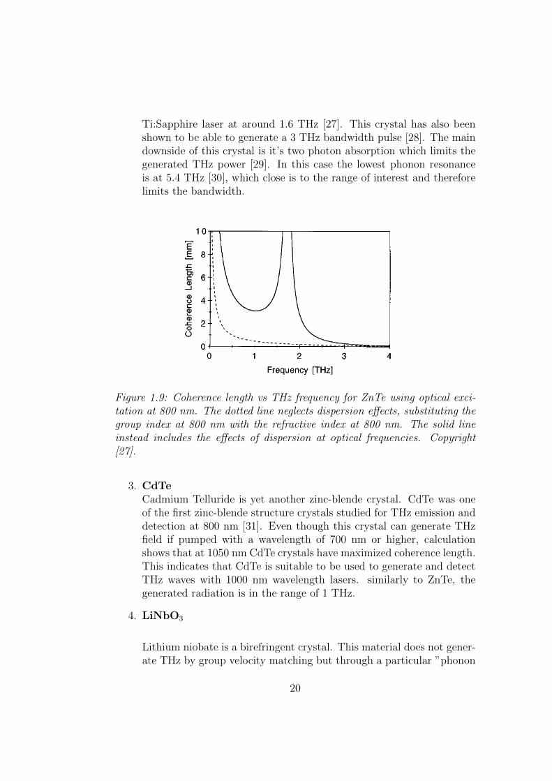
3. CdTeCadmium Telluride is yet another zinc-blende crystal. CdTe was oneof the first zinc-blende structure crystals studied for THz emission anddetection at 800 nm [31]. Even though this crystal can generate THzfield if pumped with a wavelength of 700 nm or higher, calculationshows that at 1050 nm CdTe crystals have maximized coherence length.This indicates that CdTe is suitable to be used to generate and detectTHz waves with 1000 nm wavelength lasers. similarly to ZnTe, thegenerated radiation is in the range of 1 THz.

4. LiNbO3

Lithium niobate is a birefringent crystal. This material does not gener-ate THz by group velocity matching but through a particular ”phonon

20

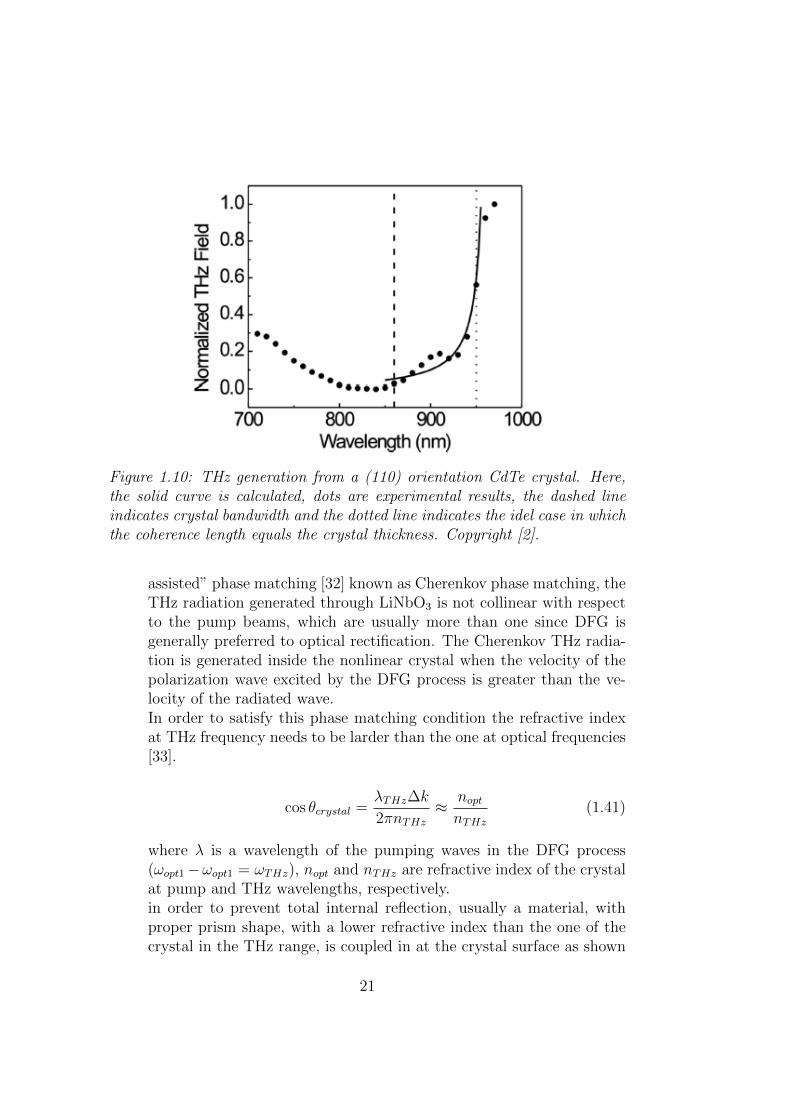
Figure 1.10: THz generation from a (110) orientation CdTe crystal. Here,the solid curve is calculated, dots are experimental results, the dashed lineindicates crystal bandwidth and the dotted line indicates the idel case in whichthe coherence length equals the crystal thickness. Copyright [2].

assisted” phase matching [32] known as Cherenkov phase matching, theTHz radiation generated through LiNbO3 is not collinear with respectto the pump beams, which are usually more than one since DFG isgenerally preferred to optical rectification. The Cherenkov THz radia-tion is generated inside the nonlinear crystal when the velocity of thepolarization wave excited by the DFG process is greater than the ve-locity of the radiated wave.In order to satisfy this phase matching condition the refractive indexat THz frequency needs to be larder than the one at optical frequencies[33].

cos θcrystal =λTHz∆k

2πnTHz≈ noptnTHz

(1.41)

where λ is a wavelength of the pumping waves in the DFG process(ωopt1−ωopt1 = ωTHz), nopt and nTHz are refractive index of the crystalat pump and THz wavelengths, respectively.in order to prevent total internal reflection, usually a material, withproper prism shape, with a lower refractive index than the one of thecrystal in the THz range, is coupled in at the crystal surface as shown

21

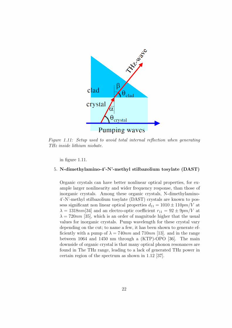
Figure 1.11: Setup used to avoid total internal reflection when generatingTHz inside lithium niobate.

in figure 1.11.

5. N-dimethylamino-4’-N’-methyl stilbazolium tosylate (DAST)

Organic crystals can have better nonlinear optical properties, for ex-ample larger nonlinearity and wider frequency response, than those ofinorganic crystals. Among these organic crystals, N-dimethylamino-4’-N’-methyl stilbazolium tosylate (DAST) crystals are known to pos-sess significant non linear optical properties d11 = 1010± 110pm/V atλ = 1318nm[34] and an electro-optic coefficient r11 = 92 ± 9pm/V atλ = 720nm [35], which is an order of magnitude higher that the usualvalues for inorganic crystals. Pump wavelength for these crystal varydepending on the cut; to name a few, it has been shown to generate ef-ficiently with a pump of λ = 740nm and 710nm [13]. and in the rangebetween 1064 and 1450 nm through a (KTP)-OPO [36]. The maindownside of organic crystal is that many optical phonon resonances arefound in The THz range, leading to a lack of generated THz power incertain region of the spectrum as shown in 1.12 [37].

22

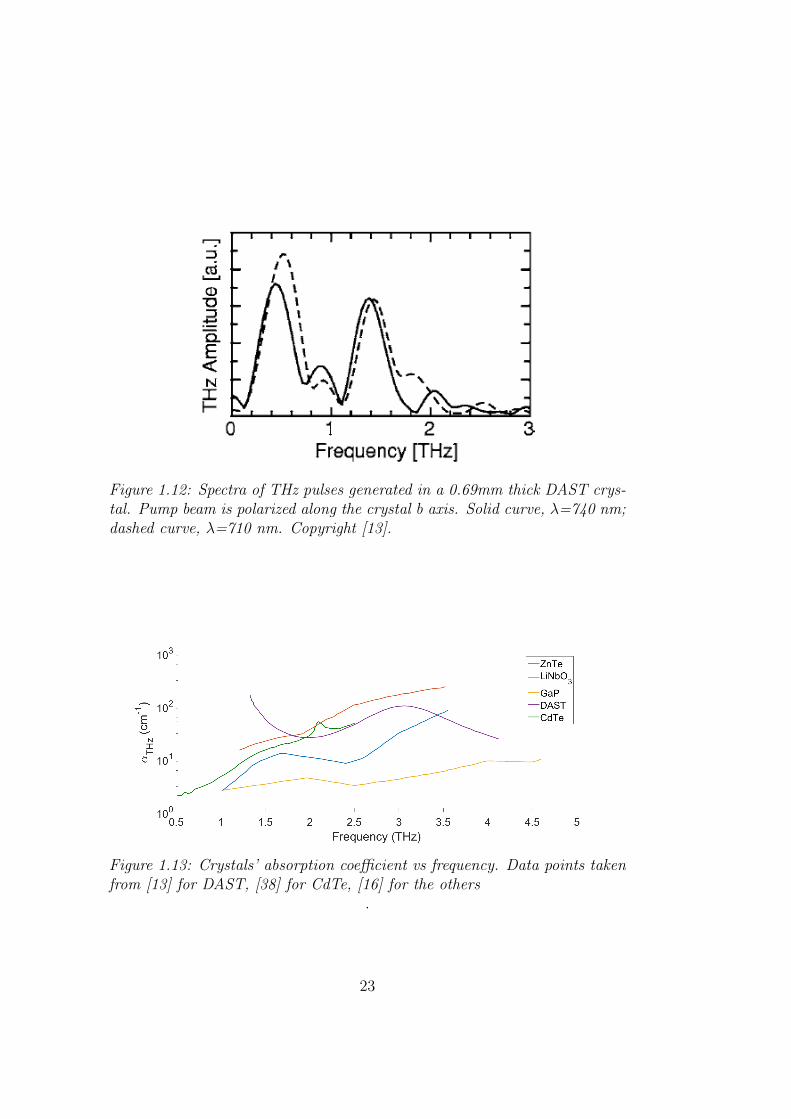
Figure 1.12: Spectra of THz pulses generated in a 0.69mm thick DAST crys-tal. Pump beam is polarized along the crystal b axis. Solid curve, λ=740 nm;dashed curve, λ=710 nm. Copyright [13].

Figure 1.13: Crystals’ absorption coefficient vs frequency. Data points takenfrom [13] for DAST, [38] for CdTe, [16] for the others

.

23

24

Chapter 2

Design of an EnhancementCavity for fs Pulses

2.1 Optical Resonator

2.1.1 General Treatment of a Linear Configuration

This chapter is devoted to understanding the behavior of a femtosecond laserbeam fed into a passive cavity. The general purpose of coupling a laserinto a passive cavity is to get an higher intensity inside the cavity withrespect to the one a laser beam would have in free propagation. This isinteresting in our case since in order to exploit a second order phenomenonwhich, as it has been discussed in the previous chapter, have a quadraticdependence from the input intensity. In order to have a basic understandingof what happens let’s first take into consideration a two mirrors cavity oflength d

2shown in figure 2.1 into which a plane wave with fixed wavelength

λ is being coupled with normal incidence. The equations for the reflected,transmitted and intracavity electric fields are given by the superposition ofthe reflected, transmitted and intracavity field for every round trip insidethe cavity. Remembering that |ri| < 1, its possible to derive the followingequations

Eintracavity =∞∑n=0

E0t1(r1r2ei 2πλd)n = E0

t1

1− r1r2ei 2πλd

(2.1)

Etransmitted =∞∑n=0

E0t1t2eiπλd(r1r2e

i 2πλd)n

= E0t1t2

1− r1r2ei 2πλdeiπλd = Eintracavityt2e

iπλd

(2.2)

25

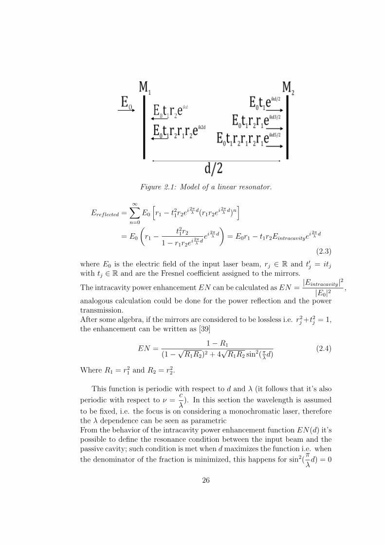
Figure 2.1: Model of a linear resonator.

Ereflected =∞∑n=0

E0

[r1 − t21r2e

i 2πλd(r1r2e

i 2πλd)n]

= E0

(r1 −

t21r2

1− r1r2ei 2πλdei

2πλd

)= E0r1 − t1r2Eintracavitye

i 2πλd

(2.3)

where E0 is the electric field of the input laser beam, rj ∈ R and t′j = itjwith tj ∈ R and are the Fresnel coefficient assigned to the mirrors.

The intracavity power enhancement EN can be calculated asEN =|Eintracavity|2

|E0|2,

analogous calculation could be done for the power reflection and the powertransmission.After some algebra, if the mirrors are considered to be lossless i.e. r2

j +t2j = 1,the enhancement can be written as [39]

EN =1−R1

(1−√R1R2)2 + 4

√R1R2 sin2(π

λd)

(2.4)

Where R1 = r21 and R2 = r2

2.

This function is periodic with respect to d and λ (it follows that it’s also

periodic with respect to ν =c

λ). In this section the wavelength is assumed

to be fixed, i.e. the focus is on considering a monochromatic laser, thereforethe λ dependence can be seen as parametricFrom the behavior of the intracavity power enhancement function EN(d) it’spossible to define the resonance condition between the input beam and thepassive cavity; such condition is met when d maximizes the function i.e. when

the denominator of the fraction is minimized, this happens for sin2(π

λd) = 0

26

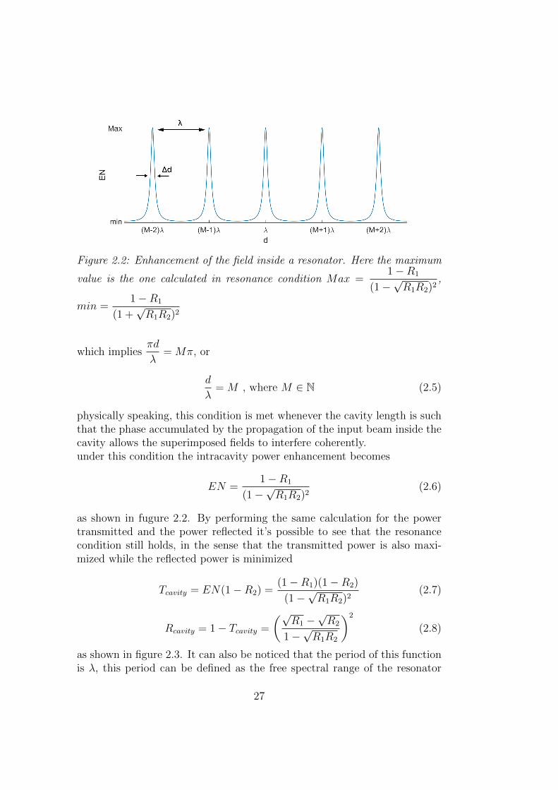
Figure 2.2: Enhancement of the field inside a resonator. Here the maximum

value is the one calculated in resonance condition Max =1−R1

(1−√R1R2)2

,

min =1−R1

(1 +√R1R2)2

which impliesπd

λ= Mπ, or

d

λ= M , where M ∈ N (2.5)

physically speaking, this condition is met whenever the cavity length is suchthat the phase accumulated by the propagation of the input beam inside thecavity allows the superimposed fields to interfere coherently.under this condition the intracavity power enhancement becomes

EN =1−R1

(1−√R1R2)2

(2.6)

as shown in fugure 2.2. By performing the same calculation for the powertransmitted and the power reflected it’s possible to see that the resonancecondition still holds, in the sense that the transmitted power is also maxi-mized while the reflected power is minimized

Tcavity = EN(1−R2) =(1−R1)(1−R2)

(1−√R1R2)2

(2.7)

Rcavity = 1− Tcavity =

(√R1 −

√R2

1−√R1R2

)2

(2.8)

as shown in figure 2.3. It can also be noticed that the period of this functionis λ, this period can be defined as the free spectral range of the resonator

27

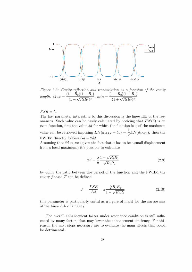
Figure 2.3: Cavity reflection and transmission as a function of the cavity

length. Max =(1−R2)(1−R1)

(1−√R1R2)2

, min =(1−R2)(1−R1)

(1 +√R1R2)2

FSR = λ.The last parameter interesting to this discussion is the linewidth of the res-onances. Such value can be easily calculated by noticing that EN(d) is aneven function, first the value δd for which the function is 1

2of the maximum

value can be retrieved imposing EN(dMAX + δd) =1

2EN(dMAX), then the

FWHM directly follows ∆d = 2δd.Assuming that δd nπ (given the fact that it has to be a small displacementfrom a local maximum) it’s possible to calculate

∆d =λ

π

1−√R1R2

4√R1R2

(2.9)

by doing the ratio between the period of the function and the FWHM thecavity finesse F can be defined

F =FSR

∆d= π

4√R1R2

1−√R1R2

(2.10)

this parameter is particularly useful as a figure of merit for the narrownessof the linewidth of a cavity.

The overall enhancement factor under resonance condition is still influ-enced by many factors that may lower the enhancement efficiency. For thisreason the next steps necessary are to evaluate the main effects that couldbe detrimental.

28

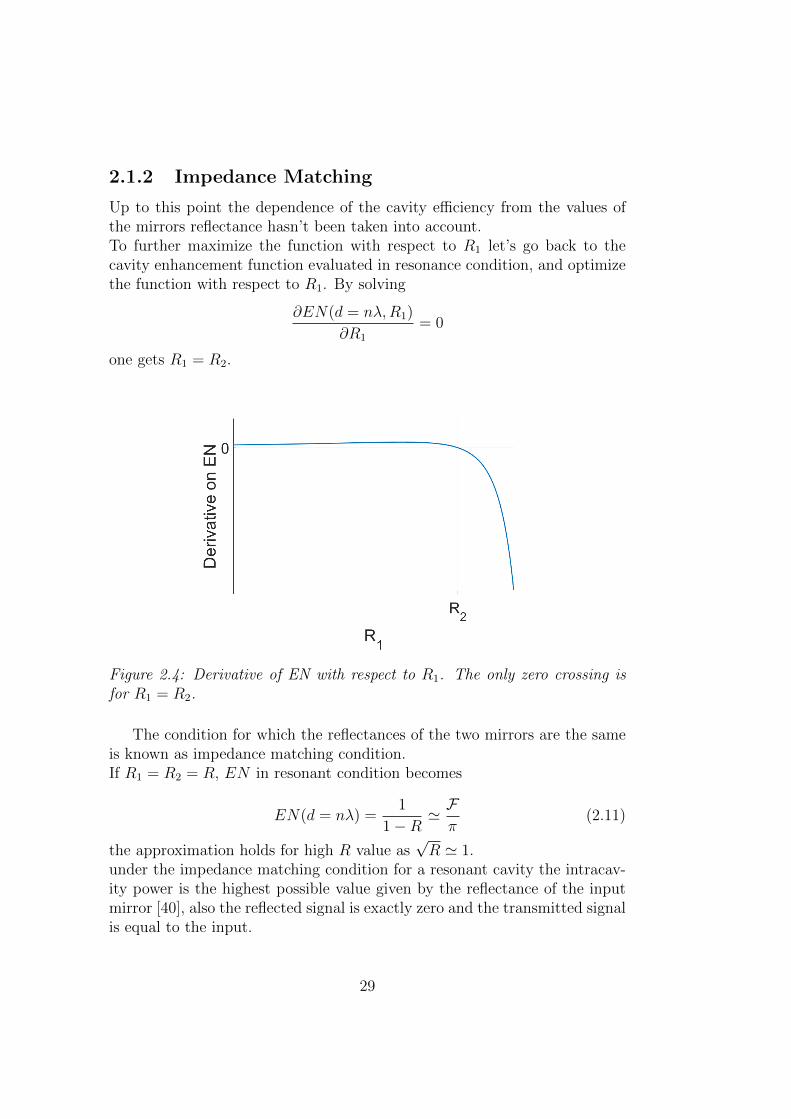
2.1.2 Impedance Matching

Up to this point the dependence of the cavity efficiency from the values ofthe mirrors reflectance hasn’t been taken into account.To further maximize the function with respect to R1 let’s go back to thecavity enhancement function evaluated in resonance condition, and optimizethe function with respect to R1. By solving

∂EN(d = nλ,R1)

∂R1

= 0

one gets R1 = R2.

Figure 2.4: Derivative of EN with respect to R1. The only zero crossing isfor R1 = R2.

The condition for which the reflectances of the two mirrors are the sameis known as impedance matching condition.If R1 = R2 = R, EN in resonant condition becomes

EN(d = nλ) =1

1−R' Fπ

(2.11)

the approximation holds for high R value as√R ' 1.

under the impedance matching condition for a resonant cavity the intracav-ity power is the highest possible value given by the reflectance of the inputmirror [40], also the reflected signal is exactly zero and the transmitted signalis equal to the input.

29

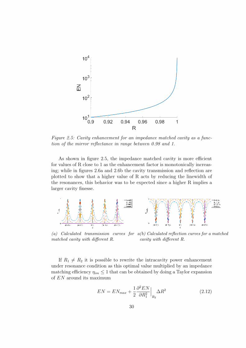
Figure 2.5: Cavity enhancement for an impedance matched cavity as a func-tion of the mirror reflectance in range between 0.98 and 1.

As shown in figure 2.5, the impedance matched cavity is more efficientfor values of R close to 1 as the enhancement factor is monotonically increas-ing; while in figures 2.6a and 2.6b the cavity transmission and reflection areplotted to show that a higher value of R acts by reducing the linewidth ofthe resonances, this behavior was to be expected since a higher R implies alarger cavity finesse.

(a) Calculated transmission curves for amatched cavity with different R.

(b) Calculated reflection curves for a matchedcavity with different R.

If R1 6= R2 it is possible to rewrite the intracavity power enhancementunder resonance condition as this optimal value multiplied by an impedancematching efficiency ηim ≤ 1 that can be obtained by doing a Taylor expansionof EN around its maximum

EN = ENmax +1

2

∂2EN

∂R21

∣∣∣R2

∆R2 (2.12)

30

Note that the first derivative is zero and second derivative of the enhance-ment function is always negative around the maximum by definition.

EN =1

1−R1

ηim where ηim = 1 +1

2

1

ENmax

∂2EN

∂R21

∣∣∣R2

∆R2 (2.13)

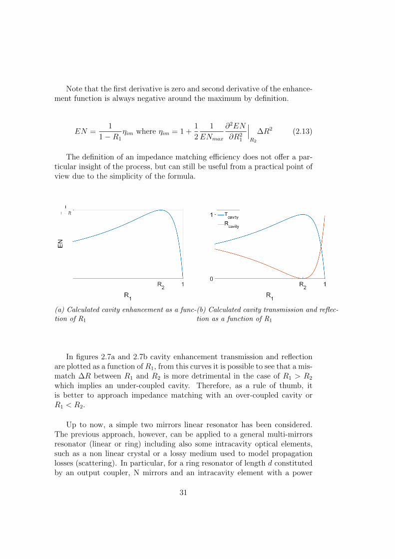
The definition of an impedance matching efficiency does not offer a par-ticular insight of the process, but can still be useful from a practical point ofview due to the simplicity of the formula.

(a) Calculated cavity enhancement as a func-tion of R1

(b) Calculated cavity transmission and reflec-tion as a function of R1

In figures 2.7a and 2.7b cavity enhancement transmission and reflectionare plotted as a function of R1, from this curves it is possible to see that a mis-match ∆R between R1 and R2 is more detrimental in the case of R1 > R2

which implies an under-coupled cavity. Therefore, as a rule of thumb, itis better to approach impedance matching with an over-coupled cavity orR1 < R2.

Up to now, a simple two mirrors linear resonator has been considered.The previous approach, however, can be applied to a general multi-mirrorsresonator (linear or ring) including also some intracavity optical elements,such as a non linear crystal or a lossy medium used to model propagationlosses (scattering). In particular, for a ring resonator of length d constitutedby an output coupler, N mirrors and an intracavity element with a power

31

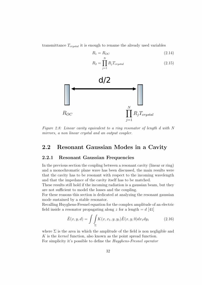
transmittance Tcrystal it is enough to rename the already used variables

R1 = ROC (2.14)

R2 =N∏j=1

RjTcrystal (2.15)

Figure 2.8: Linear cavity equivalent to a ring resonator of length d with Nmirrors, a non linear crystal and an output coupler.

2.2 Resonant Gaussian Modes in a Cavity

2.2.1 Resonant Gaussian Frequencies

In the previous section the coupling between a resonant cavity (linear or ring)and a monochromatic plane wave has been discussed, the main results werethat the cavity has to be resonant with respect to the incoming wavelengthand that the impedance of the cavity itself has to be matched.These results still hold if the incoming radiation is a gaussian beam, but theyare not sufficient to model the losses and the coupling.For these reasons this section is dedicated at analyzing the resonant gaussianmode sustained by a stable resonator.Recalling Huyghens-Fresnel equation for the complex amplitude of an electricfield inside a resonator propagating along z for a length = d [41]

E(x, y, d) =

∫ ∫Σ

K(x, x1, y, y1)E(x, y, 0)dx1dy1 (2.16)

where Σ is the area in which the amplitude of the field is non negligible andK is the kernel function, also known as the point spread function.For simplicity it’s possible to define the Huyghens-Fresnel operator

32

Kf =

∫∫Σ

fKdy1x1 (2.17)

for a beam that is a resonating mode inside the cavity, a self consistencycondition can be imposed since the positions z = 0 and z = d are the sameaside from a propagation term (this is true if the losses during the propagationinside the cavity are not considered).

E(x, y, d) = E(x, y, 0)eikd (2.18)

Combining equations 2.16 and 2.18 the eigenvalue problem is defined

KE(x, y, 0) = σnE(x, y, 0) (2.19)

where σn = eiknd are the eigenvalues for the possible eigenfunction E of theoperator K. Since there are no losses in this discussion, which implies thatduring propagation the total intensity of the beam is not changed, gaussianeigenfunctions can be assumed

E(x, y, 0) = E0Hl

(√2x

w0

)Hm

(√2y

w0

)eik

2q0

(x2+y2)

(2.20)

where E0 is the amplitude of the field, Hl,m(·) are the Herimite polynomials,w0 is the beam waist radius and q0 is the complex beam parameter, definedas q(z) = z + izr, calculated in position z=0.The orders l and m of the Hermite polynomials define the the shape of thebeam, in order to address a particular transverse spatial configuration of theintensity the beam is labeled TEMl,m, which stands for transverse electro-magnetic mode.Let’s consider a resonator (linear or ring), it’s possible can define an equiva-lent periodic lens guide structure for the beam inside the cavity, and calculatethe ABCD matrix [39] for the propagation during a round trip. Under theassumption of no photon losses it’s possible to derive the kernel [41]

K (x, y) =i

λBe−ik

A(x21 + y2

1) +D(x2 + y2)− 2xx1 − 2yy1

2B (2.21)

with these assumptions the left hand side of equation 2.19 becomes

KE(x, y, 0) =E0(

A+B

q0

)1+l+mHl

(√2x

w0

)Hm

(√2y

w0

)eik

2q(x2+y2)

(2.22)

33

where q(z) =Aq0 +B

Cq0 +D.

Combining equation 2.22 with equation 2.19 the following relations have tobe fulfilled

q = q0

σ = eikd =1(

A+B

q0

)1+l+m

By solving the system it’s finally possible to find the frequencies ν ofthe gaussian modes resonant inside a cavity. Under the assumption that E

is spatially confined, which is true for

∣∣∣∣A+D

2

∣∣∣∣ < 1 (which is the stability

condition for a resonator)

νn,l,m =c

d

[n± (1 + l +m)

2πarccos

(A+D

2

)](2.23)

First, to further prove the validity of the stability condition, it is possibleto notice that if the condition is not met the frequency of the mode becomesa complex number, which means that the beam is damped during propaga-tion.It’s possible to compare this result with what has been found about the caseof a cavity coupled to a plane wave.Even for a TEM00 mode the frequency is different, there is an ”offset” thatcan be corrected by changing the cavity length, the more important differ-ence is that between two different longitudinal resonant modes there is amultitude of resonant frequencies belonging to higher order modes. In figure2.9 the spectrum of different resonator are shown in order to highlight thedependence of the spectrum with respect to the term (A+D)/2.

In the real case of a lossy optical resonator the result is slightly different.an additional term to take into account the field decay introduced by the

propagation losses has to be considered, e−d

2τcc . This in turn changes thekernel operator and the corresponding eigenvalues, leading to |σn| < 1. Thefinal result is that the power spectrum of the eigenfunction that are foundhave a finite linewidth inversely proportional to the photons lifetime τc, it’spossible to define a quality factor of the cavity Q defined has the ratio be-tween the energy inside the resonator and the energy lost per round trip,after some calculation this term can be written as

Qn,l,m = 2πτcνn,l,m =νn,l,m∆ν

(2.24)

34

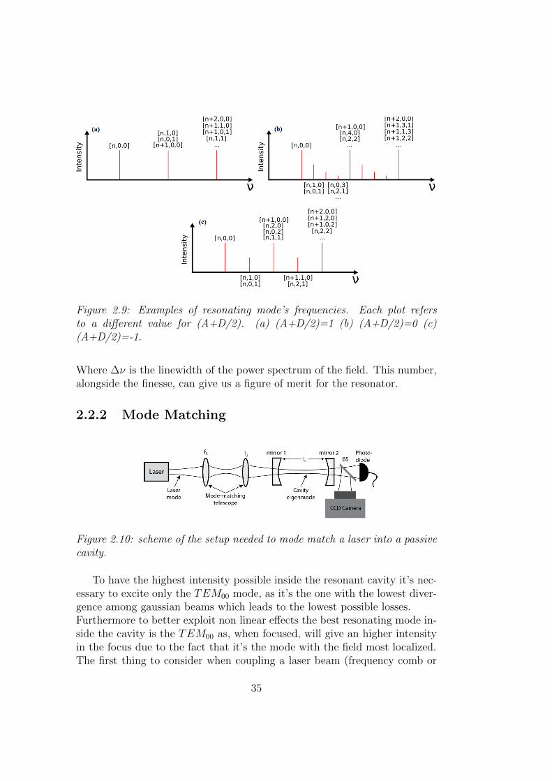
Figure 2.9: Examples of resonating mode’s frequencies. Each plot refersto a different value for (A+D/2). (a) (A+D/2)=1 (b) (A+D/2)=0 (c)(A+D/2)=-1.

Where ∆ν is the linewidth of the power spectrum of the field. This number,alongside the finesse, can give us a figure of merit for the resonator.

2.2.2 Mode Matching

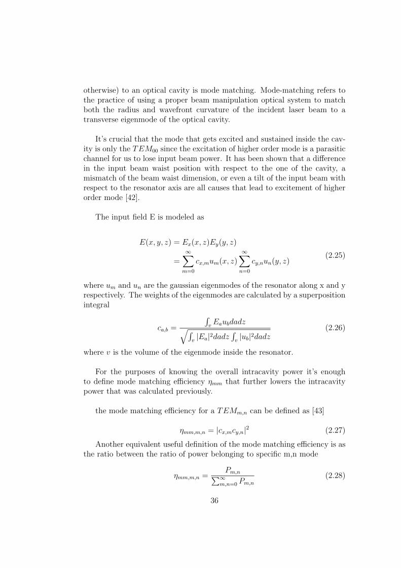
Figure 2.10: scheme of the setup needed to mode match a laser into a passivecavity.

To have the highest intensity possible inside the resonant cavity it’s nec-essary to excite only the TEM00 mode, as it’s the one with the lowest diver-gence among gaussian beams which leads to the lowest possible losses.Furthermore to better exploit non linear effects the best resonating mode in-side the cavity is the TEM00 as, when focused, will give an higher intensityin the focus due to the fact that it’s the mode with the field most localized.The first thing to consider when coupling a laser beam (frequency comb or

35

otherwise) to an optical cavity is mode matching. Mode-matching refers tothe practice of using a proper beam manipulation optical system to matchboth the radius and wavefront curvature of the incident laser beam to atransverse eigenmode of the optical cavity.

It’s crucial that the mode that gets excited and sustained inside the cav-ity is only the TEM00 since the excitation of higher order mode is a parasiticchannel for us to lose input beam power. It has been shown that a differencein the input beam waist position with respect to the one of the cavity, amismatch of the beam waist dimension, or even a tilt of the input beam withrespect to the resonator axis are all causes that lead to excitement of higherorder mode [42].

The input field E is modeled as

E(x, y, z) = Ex(x, z)Ey(y, z)

=∞∑m=0

cx,mum(x, z)∞∑n=0

cy,nun(y, z)(2.25)

where um and un are the gaussian eigenmodes of the resonator along x and yrespectively. The weights of the eigenmodes are calculated by a superpositionintegral

ca,b =

∫vEaubdadz√∫

v|Ea|2dadz

∫v|ub|2dadz

(2.26)

where v is the volume of the eigenmode inside the resonator.

For the purposes of knowing the overall intracavity power it’s enoughto define mode matching efficiency ηmm that further lowers the intracavitypower that was calculated previously.

the mode matching efficiency for a TEMm,n can be defined as [43]

ηmm,m,n = |cx,mcy,n|2 (2.27)

Another equivalent useful definition of the mode matching efficiency is asthe ratio between the ratio of power belonging to specific m,n mode

ηmm,m,n =Pm,n∑∞

m,n=0 Pm,n(2.28)

36

for both definition the following relation holds

∑m,n

ηmm,m,n = 1 (2.29)

For a TEM00 input mode, the mode matching efficiency with respect tothe TEM00 mode of the cavity, if the position of the waists is the same forboth beam, is

ηmm,0,0 ≡ ηmm =

16∏

a=x,y

[∫ Lc0

1

w2a(z) + w2

a,r(z)dz

]2

∏a=x,y

[∫ Lc0

1

w2a(z)

dz

] [∫ Lc0

1

w2a,r(z)

dz

] (2.30)

where wa and wa,r are the beam radii of the input mode and of the resonatingeigenmode inside the cavity respectively.

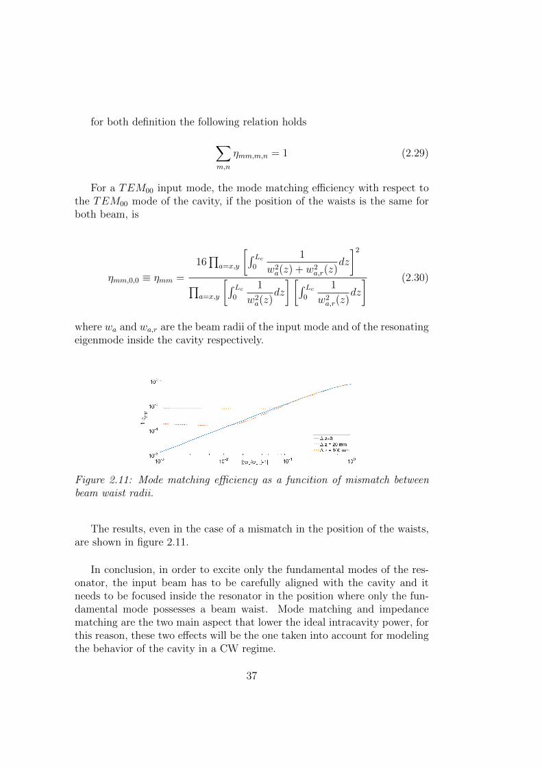
Figure 2.11: Mode matching efficiency as a funcition of mismatch betweenbeam waist radii.

The results, even in the case of a mismatch in the position of the waists,are shown in figure 2.11.

In conclusion, in order to excite only the fundamental modes of the res-onator, the input beam has to be carefully aligned with the cavity and itneeds to be focused inside the resonator in the position where only the fun-damental mode possesses a beam waist. Mode matching and impedancematching are the two main aspect that lower the ideal intracavity power, forthis reason, these two effects will be the one taken into account for modelingthe behavior of the cavity in a CW regime.

37

2.3 Coupling of fs Pulses to a Passive Cavity

2.3.1 Mode-Locking Pulses Analysis

As it’s already been stated, optical rectification is a second order non lin-ear effect which relies on the difference in frequencies between two differentwavelength inside the spectrum of a pulsed mode-locked laser. The descrip-tion so far proposed refers to a continuous wave regime. For this model tobe applied in a scenario in which the input beam has a broad bandwidthcentered around a wavelength λ0, further considerations have to be done.As it’s well known, the spectrum of a mode-locked laser is given by a largenumber of discrete spectral components of frequencies

νcomb = νceo + nνrep (2.31)

where νceo is the carrier envelope offset frequency, νrep is the repetition fre-quency of the pulses and n is an integer number [44].

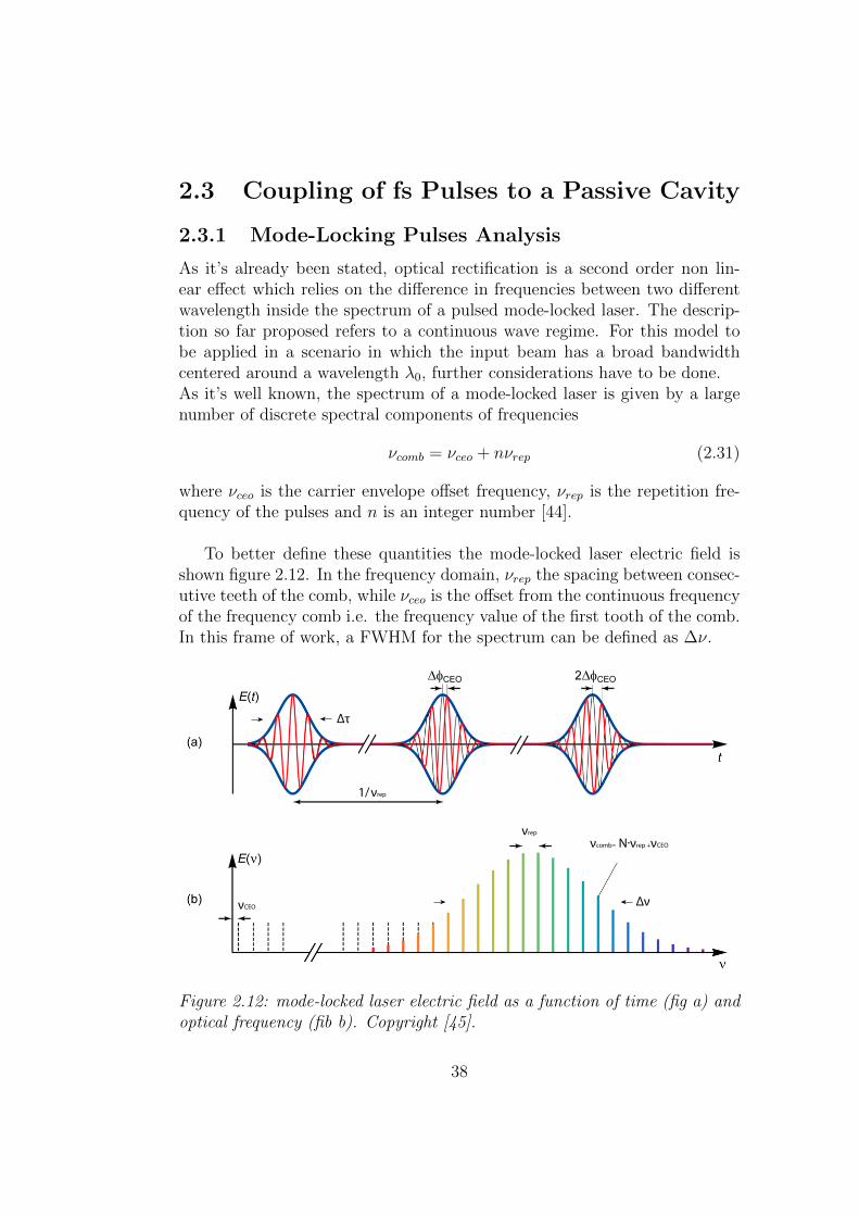
To better define these quantities the mode-locked laser electric field isshown figure 2.12. In the frequency domain, νrep the spacing between consec-utive teeth of the comb, while νceo is the offset from the continuous frequencyof the frequency comb i.e. the frequency value of the first tooth of the comb.In this frame of work, a FWHM for the spectrum can be defined as ∆ν.

νcomb= N·νrep +νCEO

νrep

1/ νrep

νCEO Δν

Δτ

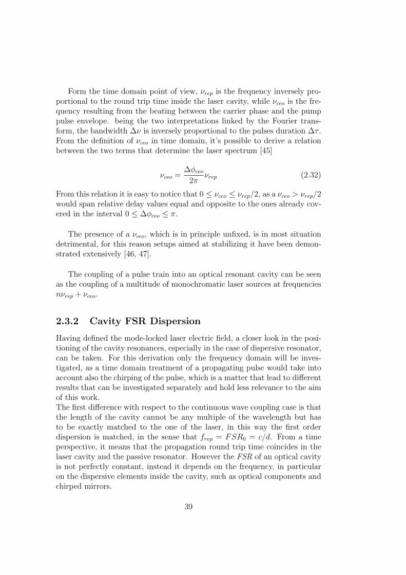
Figure 2.12: mode-locked laser electric field as a function of time (fig a) andoptical frequency (fib b). Copyright [45].

38

Form the time domain point of view, νrep is the frequency inversely pro-portional to the round trip time inside the laser cavity, while νceo is the fre-quency resulting from the beating between the carrier phase and the pumppulse envelope. being the two interpretations linked by the Fourier trans-form, the bandwidth ∆ν is inversely proportional to the pulses duration ∆τ .From the definition of νceo in time domain, it’s possible to derive a relationbetween the two terms that determine the laser spectrum [45]

νceo =∆φceo

2πνrep (2.32)

From this relation it is easy to notice that 0 ≤ νceo ≤ νrep/2, as a νceo > νrep/2would span relative delay values equal and opposite to the ones already cov-ered in the interval 0 ≤ ∆φceo ≤ π.

The presence of a νceo, which is in principle unfixed, is in most situationdetrimental, for this reason setups aimed at stabilizing it have been demon-strated extensively [46, 47].

The coupling of a pulse train into an optical resonant cavity can be seenas the coupling of a multitude of monochromatic laser sources at frequenciesnνrep + νceo.

2.3.2 Cavity FSR Dispersion

Having defined the mode-locked laser electric field, a closer look in the posi-tioning of the cavity resonances, especially in the case of dispersive resonator,can be taken. For this derivation only the frequency domain will be inves-tigated, as a time domain treatment of a propagating pulse would take intoaccount also the chirping of the pulse, which is a matter that lead to differentresults that can be investigated separately and hold less relevance to the aimof this work.The first difference with respect to the continuous wave coupling case is thatthe length of the cavity cannot be any multiple of the wavelength but hasto be exactly matched to the one of the laser, in this way the first orderdispersion is matched, in the sense that frep = FSR0 = c/d. From a timeperspective, it means that the propagation round trip time coincides in thelaser cavity and the passive resonator. However the FSR of an optical cavityis not perfectly constant, instead it depends on the frequency, in particularon the dispersive elements inside the cavity, such as optical components andchirped mirrors.

39

The phase accumulated during a round trip inside the cavity by the beam is

Φ =2πd

cν + φcav(ν) (2.33)

where φcav is the phase shift introduced by the elements in the cavity.the resonant frequencies are the one that satisfy the equation

Φ = 2Nπ i.e. νN =c

d

(N − φ(νN)

2π

)(2.34)

Knowing the definition of FSR it’s possible to calculate it

FSR(νN) = νN+1 − νN =c

d

[1− φcav(νN+1)− φcav(νN)

2π

](2.35)

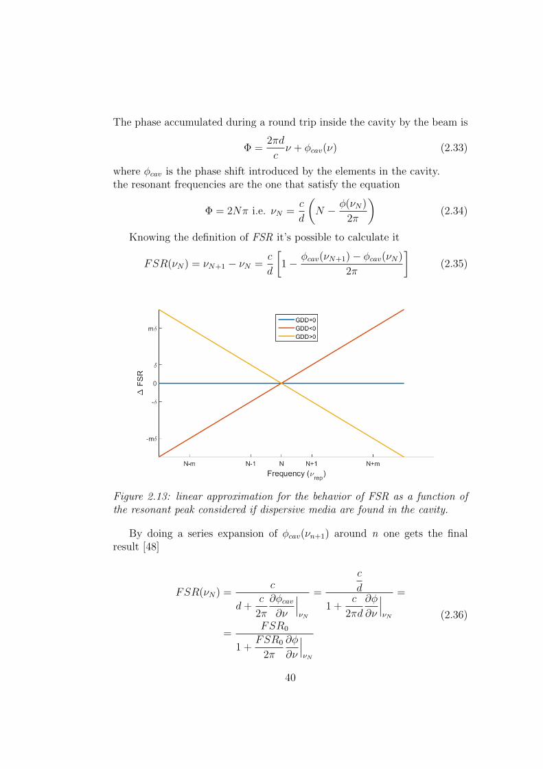
Figure 2.13: linear approximation for the behavior of FSR as a function ofthe resonant peak considered if dispersive media are found in the cavity.

By doing a series expansion of φcav(νn+1) around n one gets the finalresult [48]

FSR(νN) =c

d+c

2π

∂φcav∂ν

∣∣∣νN

=

c

d

1 +c

2πd

∂φ

∂ν

∣∣∣νN

=

=FSR0

1 +FSR0

2π

∂φ

∂ν

∣∣∣νN

(2.36)

40

The degree to which the cavity FSR is wavelength (or optical frequency)

dependent is determined by the intracavity dispersion term∂φcav∂ν

∣∣∣νn

[49, 50].

By knowing the GDD of the cavity in the neighboring of the central wave-length of the pulses it’s possible to approximate the intracavity dispersionterm following from the definition of the GDD

1

2π

∂φcav∂ν

=∂φcav∂ω

=

∫ ω

ωN

GDD(ω)dω = 2π

∫ ν

νN

GDD(ν)dν (2.37)

where νN is an integer number and the definition of GDD has been ex-ploited.

Having defined the relation between group delay dispersion and the phasefrequency derivative, equation 2.36 can be rewritten as

FSR(νN) =FSR0

1 + 2πFSR0

∫ νNνN

GDD(ν)dν(2.38)

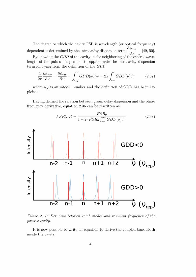
Figure 2.14: Detuning between comb modes and resonant frequency of thepassive cavity.

It is now possible to write an equation to derive the coupled bandwidthinside the cavity.

41

First it can be assumed that for a number N this condition is verified

νN = νcomb

which, recalling previous definition in equations 2.35 and 2.31, can be ex-pressed as a condition between FSR0 and the comb parameters

FSR0 =νceo +Nνrep

1− φ(νN)

2π

(2.39)

this will be the better coupled mode of the whole spectrum. For every othertooth of the comb the detuning between the frequencies of the comb and thepeak of resonance of the cavity is increasing, up to the point when one of thetooth of the comb corresponds to half of the peak value of resonant intensity(it’s assumed that the comb tooth has a negligible linewidth), which meansa detuning of

1

2∆νresonance =

FSR0

2FThe comb tooth which gets coupled with half the efficiency can be assumedto be at a frequency νceo + (N + m)νrep. These premises are translated intothe following equation∣∣∣νceo + (N +m)νrep − FSR0

[(N +m)− 1

2πφ(νN+m)

]∣∣∣ ≤ FSR0

2F(2.40)

The retrieved interval of values for ∆m = mMax − mmin can be linkedto the resonant bandwidth inside the resonator by a direct proportionalityrelation

∆νcoupled = ∆mνrep (2.41)

From these equation it’s possible to roughly estimate the bandwidthwhich can resonate inside the cavity under the condition of resonance be-tween cavity and laser.Assuming a dispersion contribution given by the second order dispersion onlyfor the frequencies belonging to the pump pulse, the phase can be modeledvia Taylor expansion as

φ(νN+m) = 2π2GDD(νceo + (N +m)νrep − νceo −Nνrep)2 = 2π2GDDm2ν2rep

(2.42)

42

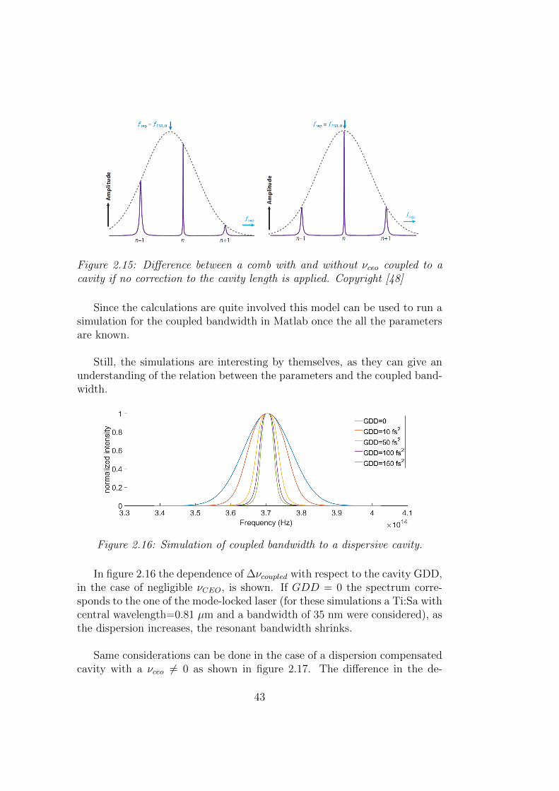
Figure 2.15: Difference between a comb with and without νceo coupled to acavity if no correction to the cavity length is applied. Copyright [48]

Since the calculations are quite involved this model can be used to run asimulation for the coupled bandwidth in Matlab once the all the parametersare known.

Still, the simulations are interesting by themselves, as they can give anunderstanding of the relation between the parameters and the coupled band-width.

Figure 2.16: Simulation of coupled bandwidth to a dispersive cavity.

In figure 2.16 the dependence of ∆νcoupled with respect to the cavity GDD,in the case of negligible νCEO, is shown. If GDD = 0 the spectrum corre-sponds to the one of the mode-locked laser (for these simulations a Ti:Sa withcentral wavelength=0.81 µm and a bandwidth of 35 nm were considered), asthe dispersion increases, the resonant bandwidth shrinks.

Same considerations can be done in the case of a dispersion compensatedcavity with a νceo 6= 0 as shown in figure 2.17. The difference in the de-

43

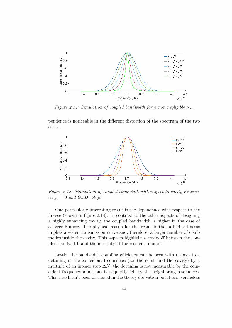
Figure 2.17: Simulation of coupled bandwidth for a non negligible νceo

pendence is noticeable in the different distortion of the spectrum of the twocases.

Figure 2.18: Simulation of coupled bandwidth with respect to cavity Finesse.nuceo = 0 and GDD=50 fs2

One particularly interesting result is the dependence with respect to thefinesse (shown in figure 2.18). In contrast to the other aspects of designinga highly enhancing cavity, the coupled bandwidth is higher in the case ofa lower Finesse. The physical reason for this result is that a higher finesseimplies a wider transmission curve and, therefore, a larger number of combmodes inside the cavity. This aspects highlight a trade-off between the cou-pled bandwidth and the intensity of the resonant modes.

Lastly, the bandwidth coupling efficiency can be seen with respect to adetuning in the coincident frequencies (for the comb and the cavity) by amultiple of an integer step ∆N , the detuning is not measurable by the coin-cident frequency alone but it is quickly felt by the neighboring resonances.This case hasn’t been discussed in the theory derivation but it is nevertheless

44

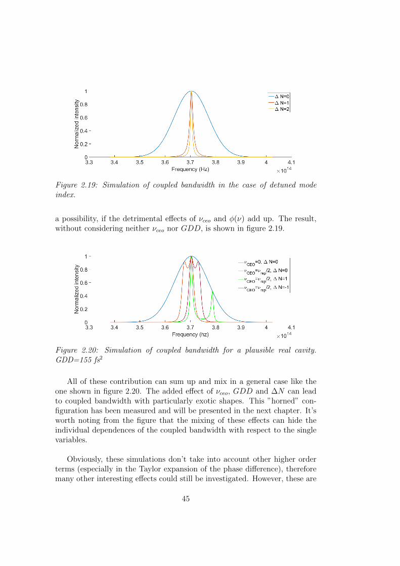
Figure 2.19: Simulation of coupled bandwidth in the case of detuned modeindex.

a possibility, if the detrimental effects of νceo and φ(ν) add up. The result,without considering neither νceo nor GDD, is shown in figure 2.19.

Figure 2.20: Simulation of coupled bandwidth for a plausible real cavity.GDD=155 fs2

All of these contribution can sum up and mix in a general case like theone shown in figure 2.20. The added effect of νceo, GDD and ∆N can leadto coupled bandwidth with particularly exotic shapes. This ”horned” con-figuration has been measured and will be presented in the next chapter. It’sworth noting from the figure that the mixing of these effects can hide theindividual dependences of the coupled bandwidth with respect to the singlevariables.

Obviously, these simulations don’t take into account other higher orderterms (especially in the Taylor expansion of the phase difference), thereforemany other interesting effects could still be investigated. However, these are

45

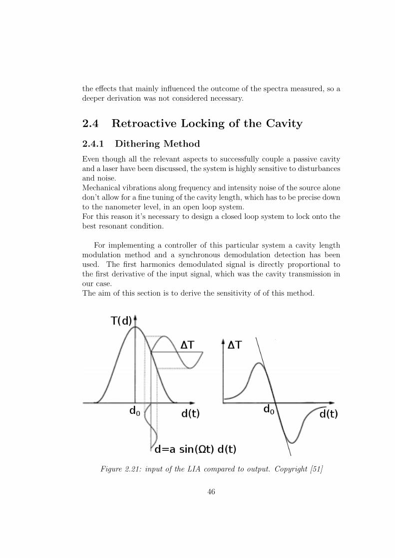
the effects that mainly influenced the outcome of the spectra measured, so adeeper derivation was not considered necessary.

2.4 Retroactive Locking of the Cavity

2.4.1 Dithering Method

Even though all the relevant aspects to successfully couple a passive cavityand a laser have been discussed, the system is highly sensitive to disturbancesand noise.Mechanical vibrations along frequency and intensity noise of the source alonedon’t allow for a fine tuning of the cavity length, which has to be precise downto the nanometer level, in an open loop system.For this reason it’s necessary to design a closed loop system to lock onto thebest resonant condition.

For implementing a controller of this particular system a cavity lengthmodulation method and a synchronous demodulation detection has beenused. The first harmonics demodulated signal is directly proportional tothe first derivative of the input signal, which was the cavity transmission inour case.The aim of this section is to derive the sensitivity of of this method.

Figure 2.21: input of the LIA compared to output. Copyright [51]

46

Let’s start by defining the input signal for the electronic system, whichis being detected by a photodiode

IT (d) = I0Tcavity(d) (2.43)

The length of the cavity as a function of time can be described as

dc(t) = d(t) + a sin(Ωt) (2.44)

where d(t) is a linear ramp, a and Ω are the modulation amplitude and fre-quency respectively.If the amplitude of the modulation is assumed to be small, the cavity trans-mitted intensity profile can be expanded as a Taylor series

IT (dc) = IT (d) +∞∑n=1

an sinn (Ωt)

n!

(∂nIT∂dn

)(2.45)

From eq 2.43 it follows that(∂nIT∂dn

)= I0

(∂nTcavity∂dn

)The processing of the signal that the demodulation electronics (lock-in

amplifier) does is [51]

IT (dc)− IT (d)

I0

=∞∑n=1

an sinn (Ωt)

n!

(∂nTcavity∂dn

)(2.46)

using trigonometric formulas it’s able to reshape n-th powers of a sinefunction as sines and cosines with n times the frequency, the firsts threeterms of the expansion becomes

∞∑n=1

an sinn (Ωt)

n!

(∂nTcavity∂dn

)= + a sin(Ωt)

∂Tcavity∂d

+a2

2

∂2Tcavity∂d2

(1− cos(2Ωt)

2

)+a3

6

∂3Tcavity∂d3

(3 sin(Ωt)− sin(3Ωt)

4

)+ ...

(2.47)there will be infinitely many terms at every frequency nΩ. In general it

can be written that the processed signal as a function of the frequency is

47

S(nΩ) =

bn sin(nΩt) n = 2m+ 1

cn cos(nΩt) n = 2m(2.48)

Where bn and cn are the sum of every term at nΩ.As a first order approximation, for a small modulation amplitude a, we canconsider only the first term of the whole series.In conclusion the signals at the three lowest frequencies are

S(Ω) = a∂Tcavity∂d

sin(Ωt) (2.49)

S(2Ω) = −a2

4

∂2Tcavity∂d2

cos(2Ωt) (2.50)

S(3Ω) = −a3

24

∂3Tcavity∂d3

sin(3Ωt) (2.51)

further terms can be discarded for a small a.At this point the amplifier demodulates the signal, in order to do so it’senough to multiply the signal by a replica of the modulation signal.Let’s consider S(Ω) (analogous discussion could be done for any S(nΩ))

sin(Ωt+ φ)S(Ω) = a∂Tcavity∂d

[(1− cos(2Ωt)

2cosφ

)+

1

2sin(2Ωt) sinφ

](2.52)

where φ is an fixed phase term, used in the demodulation process.

As a last step a low pass filer (LPF) is applied, assuming an unitarytransfer function for frequencies smaller than Ω/2 and 0 elsewhere, the finaloutput Y of the LIA is

Y (d) =a

2

∂Tcavity(d)

∂dcosφ (2.53)

This holds if there is no aliasing i.e. the bandwidth of the signal is ≤ Ω/2,which means that when setting the cutoff frequency and the modulation fre-quency Shannon theorem should be taken into consideration.

It’s possible to manually set the delay of the demodulating sine wave to

set the phase φ =π

2k in order to maximize the amplitude of the Y signal.

Y (d) = ±a2

∂Tcavity∂d

(2.54)

48

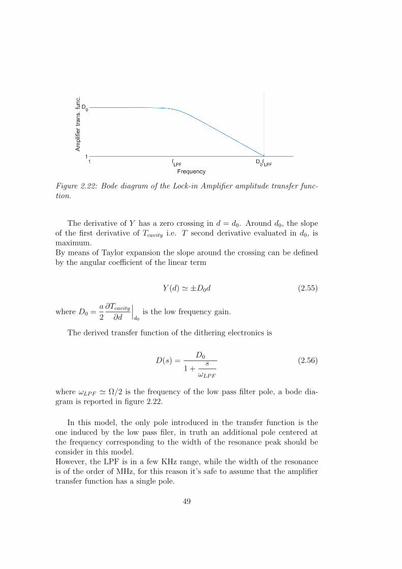
Figure 2.22: Bode diagram of the Lock-in Amplifier amplitude transfer func-tion.

The derivative of Y has a zero crossing in d = d0. Around d0, the slopeof the first derivative of Tcavity i.e. T second derivative evaluated in d0, ismaximum.By means of Taylor expansion the slope around the crossing can be definedby the angular coefficient of the linear term

Y (d) ' ±D0d (2.55)

where D0 =a

2

∂Tcavity∂d

∣∣∣d0

is the low frequency gain.

The derived transfer function of the dithering electronics is

D(s) =D0

1 +s

ωLPF

(2.56)

where ωLPF ' Ω/2 is the frequency of the low pass filter pole, a bode dia-gram is reported in figure 2.22.

In this model, the only pole introduced in the transfer function is theone induced by the low pass filer, in truth an additional pole centered atthe frequency corresponding to the width of the resonance peak should beconsider in this model.However, the LPF is in a few KHz range, while the width of the resonanceis of the order of MHz, for this reason it’s safe to assume that the amplifiertransfer function has a single pole.

49

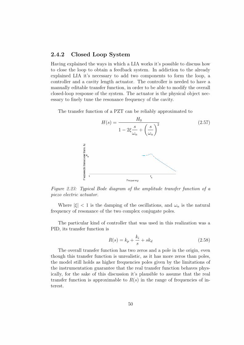
2.4.2 Closed Loop System

Having explained the ways in which a LIA works it’s possible to discuss howto close the loop to obtain a feedback system. In addiction to the alreadyexplained LIA it’s necessary to add two components to form the loop, acontroller and a cavity length actuator. The controller is needed to have amanually editable transfer function, in order to be able to modify the overallclosed-loop response of the system. The actuator is the physical object nec-essary to finely tune the resonance frequency of the cavity.

The transfer function of a PZT can be reliably approximated to

H(s) =H0

1− 2ξs

ωn+

(s

ωn

)2 (2.57)

Figure 2.23: Typical Bode diagram of the amplitude transfer function of apiezo electric actuator.

Where |ξ| < 1 is the damping of the oscillations, and ωn is the naturalfrequency of resonance of the two complex conjugate poles.

The particular kind of controller that was used in this realization was aPID, its transfer function is

R(s) = kp +kis

+ skd (2.58)

The overall transfer function has two zeros and a pole in the origin, eventhough this transfer function is unrealistic, as it has more zeros than poles,the model still holds as higher frequencies poles given by the limitations ofthe instrumentation guarantee that the real transfer function behaves phys-ically, for the sake of this discussion it’s plausible to assume that the realtransfer function is approximable to R(s) in the range of frequencies of in-terest.

50

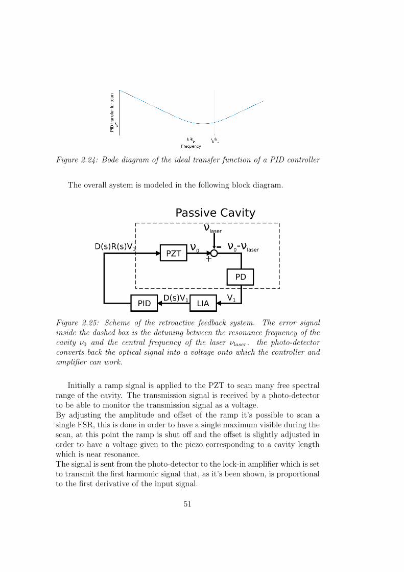
Figure 2.24: Bode diagram of the ideal transfer function of a PID controller

The overall system is modeled in the following block diagram.

Figure 2.25: Scheme of the retroactive feedback system. The error signalinside the dashed box is the detuning between the resonance frequency of thecavity ν0 and the central frequency of the laser νlaser. the photo-detectorconverts back the optical signal into a voltage onto which the controller andamplifier can work.

Initially a ramp signal is applied to the PZT to scan many free spectralrange of the cavity. The transmission signal is received by a photo-detectorto be able to monitor the transmission signal as a voltage.By adjusting the amplitude and offset of the ramp it’s possible to scan asingle FSR, this is done in order to have a single maximum visible during thescan, at this point the ramp is shut off and the offset is slightly adjusted inorder to have a voltage given to the piezo corresponding to a cavity lengthwhich is near resonance.The signal is sent from the photo-detector to the lock-in amplifier which is setto transmit the first harmonic signal that, as it’s been shown, is proportionalto the first derivative of the input signal.

51

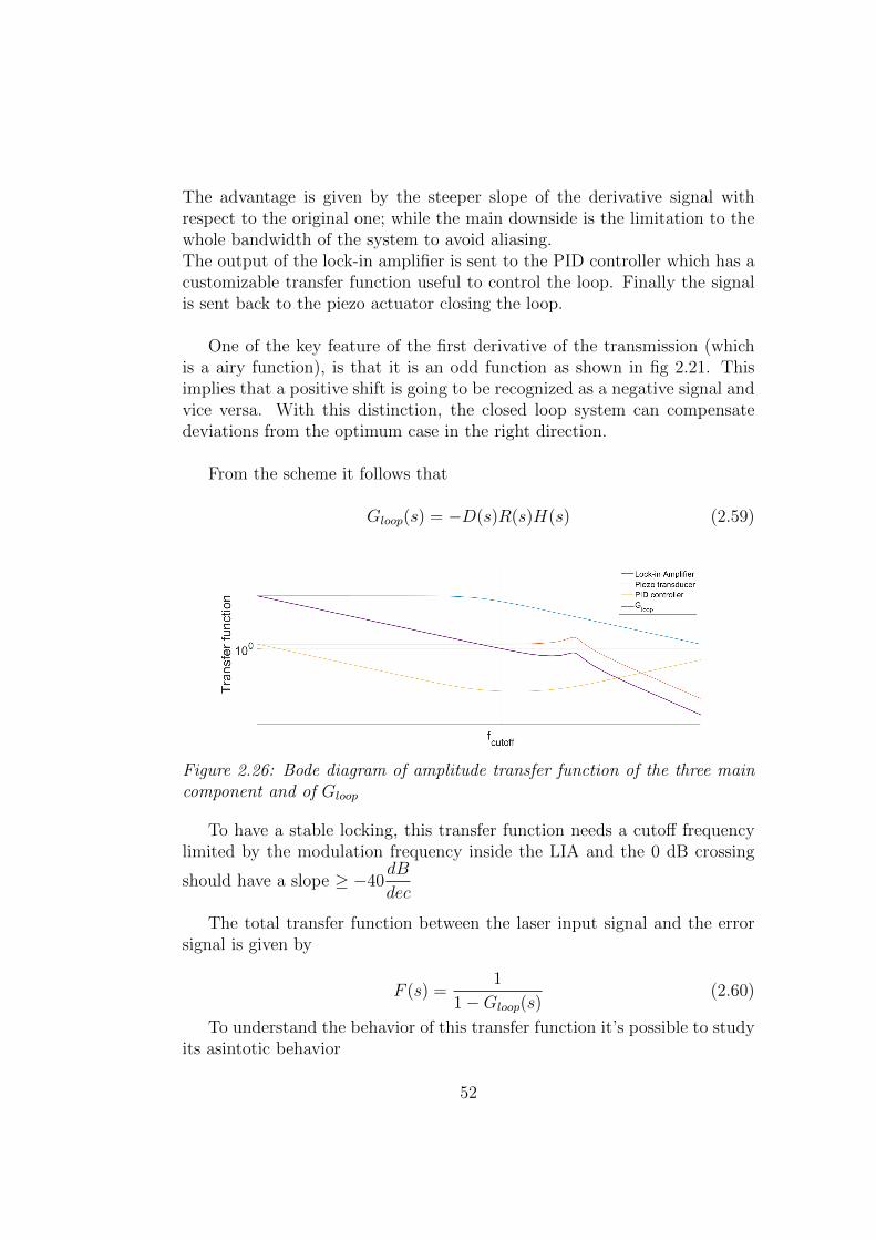
The advantage is given by the steeper slope of the derivative signal withrespect to the original one; while the main downside is the limitation to thewhole bandwidth of the system to avoid aliasing.The output of the lock-in amplifier is sent to the PID controller which has acustomizable transfer function useful to control the loop. Finally the signalis sent back to the piezo actuator closing the loop.

One of the key feature of the first derivative of the transmission (whichis a airy function), is that it is an odd function as shown in fig 2.21. Thisimplies that a positive shift is going to be recognized as a negative signal andvice versa. With this distinction, the closed loop system can compensatedeviations from the optimum case in the right direction.

From the scheme it follows that

Gloop(s) = −D(s)R(s)H(s) (2.59)

Figure 2.26: Bode diagram of amplitude transfer function of the three maincomponent and of Gloop

To have a stable locking, this transfer function needs a cutoff frequencylimited by the modulation frequency inside the LIA and the 0 dB crossing

should have a slope ≥ −40dB

dec

The total transfer function between the laser input signal and the errorsignal is given by

F (s) =1

1−Gloop(s)(2.60)

To understand the behavior of this transfer function it’s possible to studyits asintotic behavior

52

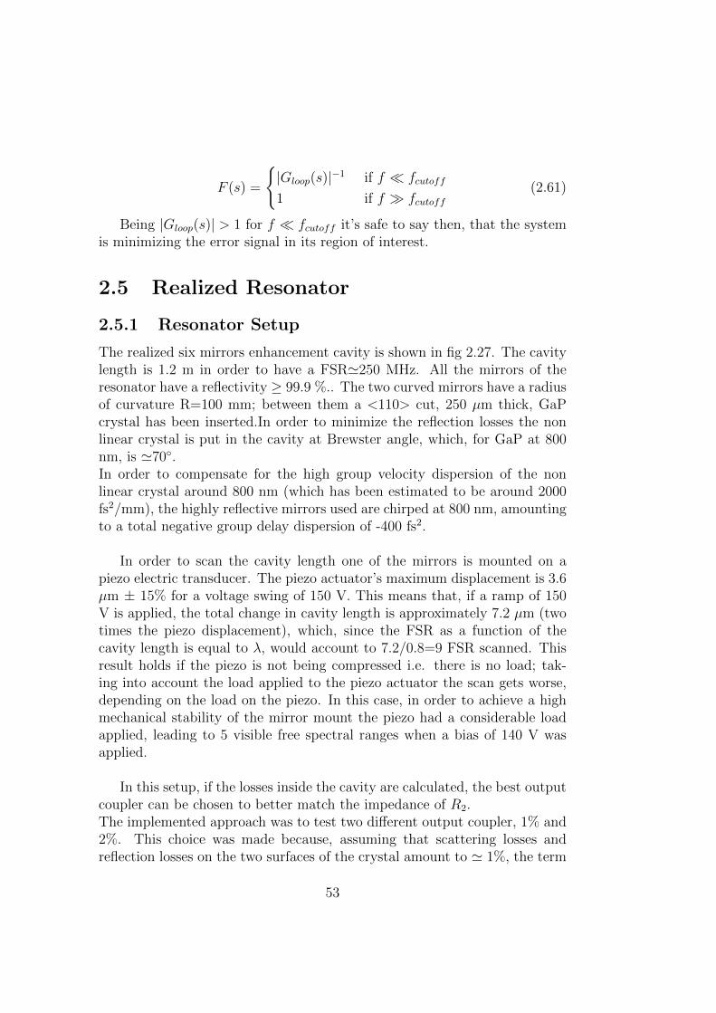
F (s) =

|Gloop(s)|−1 if f fcutoff

1 if f fcutoff(2.61)

Being |Gloop(s)| > 1 for f fcutoff it’s safe to say then, that the systemis minimizing the error signal in its region of interest.

2.5 Realized Resonator

2.5.1 Resonator Setup

The realized six mirrors enhancement cavity is shown in fig 2.27. The cavitylength is 1.2 m in order to have a FSR'250 MHz. All the mirrors of theresonator have a reflectivity ≥ 99.9 %.. The two curved mirrors have a radiusof curvature R=100 mm; between them a <110> cut, 250 µm thick, GaPcrystal has been inserted.In order to minimize the reflection losses the nonlinear crystal is put in the cavity at Brewster angle, which, for GaP at 800nm, is '70.In order to compensate for the high group velocity dispersion of the nonlinear crystal around 800 nm (which has been estimated to be around 2000fs2/mm), the highly reflective mirrors used are chirped at 800 nm, amountingto a total negative group delay dispersion of -400 fs2.

In order to scan the cavity length one of the mirrors is mounted on apiezo electric transducer. The piezo actuator’s maximum displacement is 3.6µm ± 15% for a voltage swing of 150 V. This means that, if a ramp of 150V is applied, the total change in cavity length is approximately 7.2 µm (twotimes the piezo displacement), which, since the FSR as a function of thecavity length is equal to λ, would account to 7.2/0.8=9 FSR scanned. Thisresult holds if the piezo is not being compressed i.e. there is no load; tak-ing into account the load applied to the piezo actuator the scan gets worse,depending on the load on the piezo. In this case, in order to achieve a highmechanical stability of the mirror mount the piezo had a considerable loadapplied, leading to 5 visible free spectral ranges when a bias of 140 V wasapplied.

In this setup, if the losses inside the cavity are calculated, the best outputcoupler can be chosen to better match the impedance of R2.The implemented approach was to test two different output coupler, 1% and2%. This choice was made because, assuming that scattering losses andreflection losses on the two surfaces of the crystal amount to ' 1%, the term

53

Figure 2.27: Scheme of the enhancement cavity, the total length is 1.2 m tomatch the repetition frequency of the laser, the two lower mirror in the cavityhave a radius of curvature R=100 mm. One of the mirror is mounted on apiezoelectric actuator to tune the cavity length, the crystal is put at Brewsterangle to minimize the losses induced by reflection.

R2 = 98.5% is placed in between these two values. Not having a directway to measure the cavity losses, their value could be either over or underestimated. For this reason the measures have have been taken with bothoutput couplers.

2.5.2 ABCD Matrix

We can explicitly calculate the ABCD matrix for our six mirrors ring cavityshown in figure 2.28. The overall propagation matrix is given by the productof the matrices of the propagation terms, and the bounce on the curved

mirrors, which is equivalent to have a converging lens of focal length f =R

2.(

1 L3

0 1

) 1 0

− 1

f1

( 1 L2

0 1

) 1 0

− 1

f1

( 1 L1

0 1

)=

(A BC D

)By doing the calculation it’s possible to retrieve the whole round trip

propagation matrix

54

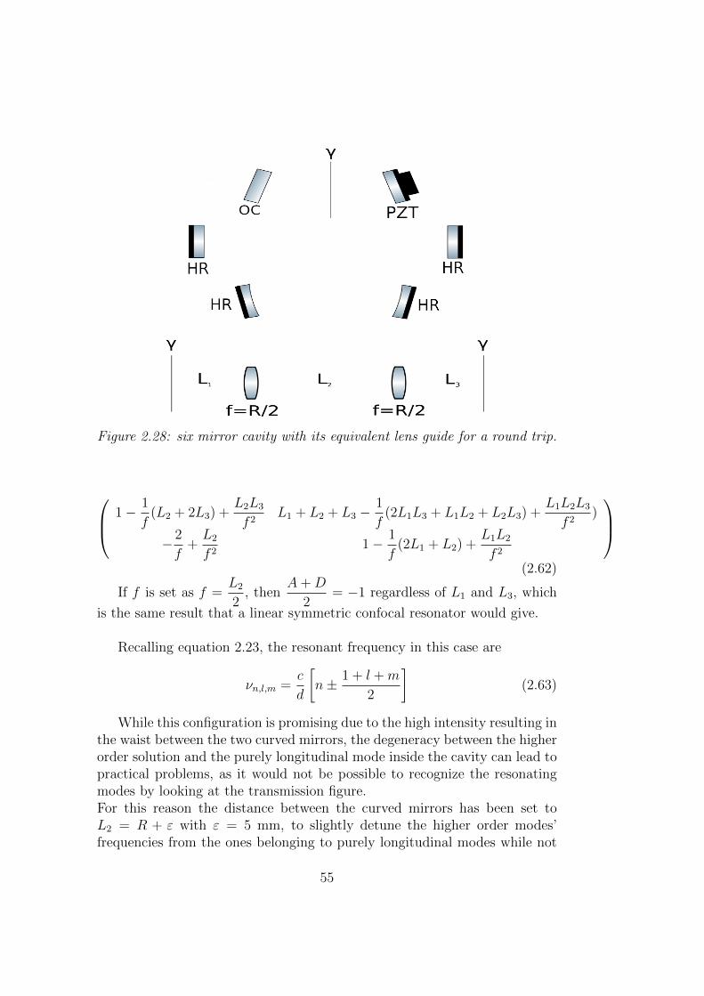
Figure 2.28: six mirror cavity with its equivalent lens guide for a round trip.

1− 1

f(L2 + 2L3) +

L2L3

f 2L1 + L2 + L3 −

1

f(2L1L3 + L1L2 + L2L3) +

L1L2L3

f 2)

− 2

f+L2

f 21− 1

f(2L1 + L2) +

L1L2

f 2

(2.62)

If f is set as f =L2

2, then

A+D

2= −1 regardless of L1 and L3, which

is the same result that a linear symmetric confocal resonator would give.

Recalling equation 2.23, the resonant frequency in this case are

νn,l,m =c

d

[n± 1 + l +m

2

](2.63)

While this configuration is promising due to the high intensity resulting inthe waist between the two curved mirrors, the degeneracy between the higherorder solution and the purely longitudinal mode inside the cavity can lead topractical problems, as it would not be possible to recognize the resonatingmodes by looking at the transmission figure.For this reason the distance between the curved mirrors has been set toL2 = R + ε with ε = 5 mm, to slightly detune the higher order modes’frequencies from the ones belonging to purely longitudinal modes while not

55

changing drastically the spatial profile of the confocal configuration. In thiscase the cavity is still stable as shown by the ABCD calculation

A+D

2= −1− 2

ε

R

(1− L1 + L3

R

)= −0.9805 (2.64)

2.5.3 Cavity Mode Matching

As previously discussed, an optical system is necessary to couple the outputbeam of the laser to the passive resonator to excite the TEM00 mode insidethe cavity.In our case, since the cavity is highly symmetric, it’s enough to focus thebeam between the output coupler and the first mirror. This position is sym-metric with respect to the focus between the two curved mirrors, the onlymode that has these kind of waist inside a resonator is a TEM00 [40, chapter6].

In order to force a waist in a specific position it’s enough to use a systemof 2 lenses between the laser and the cavity with the right spacing betweenthe two lenses, and with the right focal lengths f1 and f2 it’s possible to tailorthe input beam finely to match the fundamental mode inside the cavity.

The law of propagation of a gaussian beam have been partially discussedalready, to find the spatial width of the field (calculated as 1/e of the peakvalue of the field) the round trip propagation matrix 2.62 can be recalled,alongside with the definition of q parameter of a gaussian, applying againthe self consistency condition

q =Aq +B

Cq +D

the parameters that give the mode are found once the parameters for theinput beam are known. To know the parameter of the input beam it’s suffi-cient to measure the radii in two different position.for a linear cavity the system of equation to solve is

w(z1) =

√√√√λzRπ

[1 +

(x+ z1

zR

)2]

w(z2) =

√√√√λzRπ

[1 +

(x+ z2

zR

)2] (2.65)

56

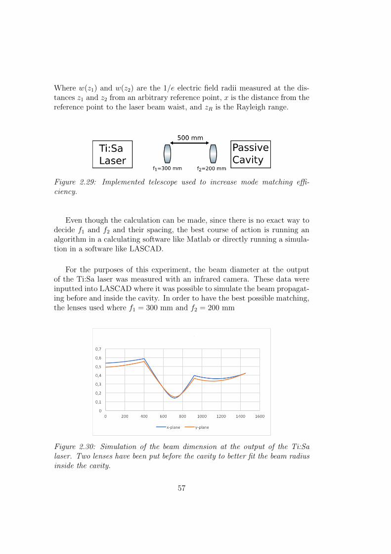
Where w(z1) and w(z2) are the 1/e electric field radii measured at the dis-tances z1 and z2 from an arbitrary reference point, x is the distance from thereference point to the laser beam waist, and zR is the Rayleigh range.

Figure 2.29: Implemented telescope used to increase mode matching effi-ciency.

Even though the calculation can be made, since there is no exact way todecide f1 and f2 and their spacing, the best course of action is running analgorithm in a calculating software like Matlab or directly running a simula-tion in a software like LASCAD.

For the purposes of this experiment, the beam diameter at the outputof the Ti:Sa laser was measured with an infrared camera. These data wereinputted into LASCAD where it was possible to simulate the beam propagat-ing before and inside the cavity. In order to have the best possible matching,the lenses used where f1 = 300 mm and f2 = 200 mm

Figure 2.30: Simulation of the beam dimension at the output of the Ti:Salaser. Two lenses have been put before the cavity to better fit the beam radiusinside the cavity.

57

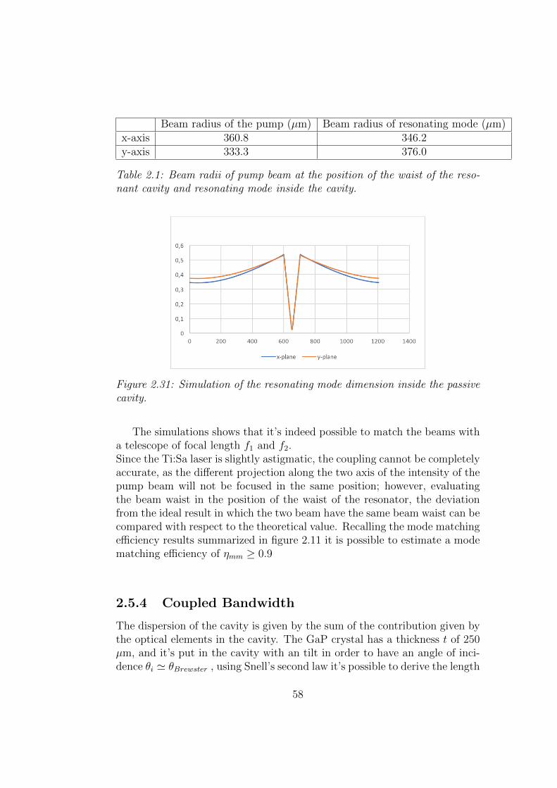
Beam radius of the pump (µm) Beam radius of resonating mode (µm)x-axis 360.8 346.2y-axis 333.3 376.0

Table 2.1: Beam radii of pump beam at the position of the waist of the reso-nant cavity and resonating mode inside the cavity.

Figure 2.31: Simulation of the resonating mode dimension inside the passivecavity.

The simulations shows that it’s indeed possible to match the beams witha telescope of focal length f1 and f2.Since the Ti:Sa laser is slightly astigmatic, the coupling cannot be completelyaccurate, as the different projection along the two axis of the intensity of thepump beam will not be focused in the same position; however, evaluatingthe beam waist in the position of the waist of the resonator, the deviationfrom the ideal result in which the two beam have the same beam waist can becompared with respect to the theoretical value. Recalling the mode matchingefficiency results summarized in figure 2.11 it is possible to estimate a modematching efficiency of ηmm ≥ 0.9

2.5.4 Coupled Bandwidth

The dispersion of the cavity is given by the sum of the contribution given bythe optical elements in the cavity. The GaP crystal has a thickness t of 250µm, and it’s put in the cavity with an tilt in order to have an angle of inci-dence θi ' θBrewster , using Snell’s second law it’s possible to derive the length

58

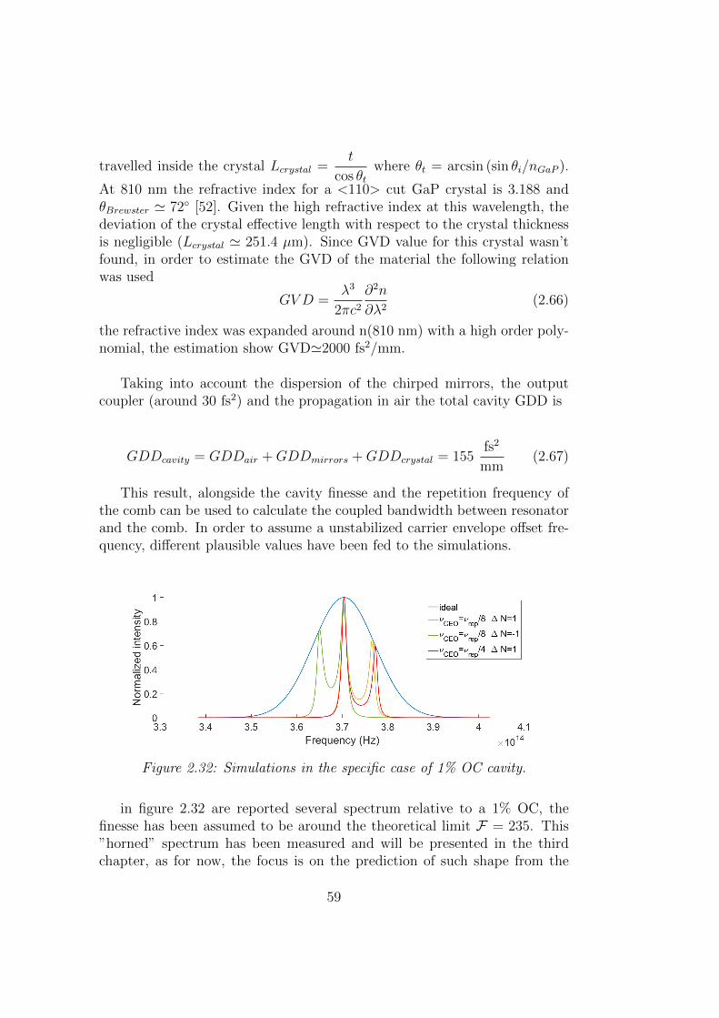
travelled inside the crystal Lcrystal =t

cos θtwhere θt = arcsin (sin θi/nGaP ).

At 810 nm the refractive index for a <110> cut GaP crystal is 3.188 andθBrewster ' 72 [52]. Given the high refractive index at this wavelength, thedeviation of the crystal effective length with respect to the crystal thicknessis negligible (Lcrystal ' 251.4 µm). Since GVD value for this crystal wasn’tfound, in order to estimate the GVD of the material the following relationwas used

GVD =λ3

2πc2

∂2n

∂λ2(2.66)

the refractive index was expanded around n(810 nm) with a high order poly-nomial, the estimation show GVD'2000 fs2/mm.

Taking into account the dispersion of the chirped mirrors, the outputcoupler (around 30 fs2) and the propagation in air the total cavity GDD is

GDDcavity = GDDair +GDDmirrors +GDDcrystal = 155fs2

mm(2.67)

This result, alongside the cavity finesse and the repetition frequency ofthe comb can be used to calculate the coupled bandwidth between resonatorand the comb. In order to assume a unstabilized carrier envelope offset fre-quency, different plausible values have been fed to the simulations.

Figure 2.32: Simulations in the specific case of 1% OC cavity.

in figure 2.32 are reported several spectrum relative to a 1% OC, thefinesse has been assumed to be around the theoretical limit F = 235. This”horned” spectrum has been measured and will be presented in the thirdchapter, as for now, the focus is on the prediction of such shape from the

59

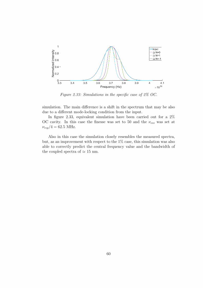
Figure 2.33: Simulations in the specific case of 2% OC.

simulation. The main difference is a shift in the spectrum that may be alsodue to a different mode-locking condition from the input.

In figure 2.33, equivalent simulation have been carried out for a 2%OC cavity. In this case the finesse was set to 50 and the νceo was set atνrep/4 = 62.5 MHz.

Also in this case the simulation closely resembles the measured spectra,but, as an improvement with respect to the 1% case, this simulation was alsoable to correctly predict the central frequency value and the bandwidth ofthe coupled spectra of ' 15 nm.

60

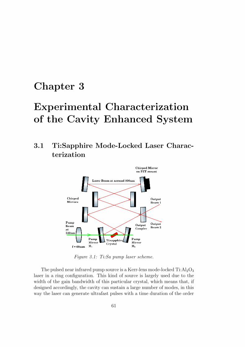
Chapter 3

Experimental Characterizationof the Cavity Enhanced System

3.1 Ti:Sapphire Mode-Locked Laser Charac-

terization

Figure 3.1: Ti:Sa pump laser scheme.

The pulsed near infrared pump source is a Kerr-lens mode-locked Ti:Al2O3

laser in a ring configuration. This kind of source is largely used due to thewidth of the gain bandwidth of this particular crystal, which means that, ifdesigned accordingly, the cavity can sustain a large number of modes, in thisway the laser can generate ultrafast pulses with a time duration of the order

61

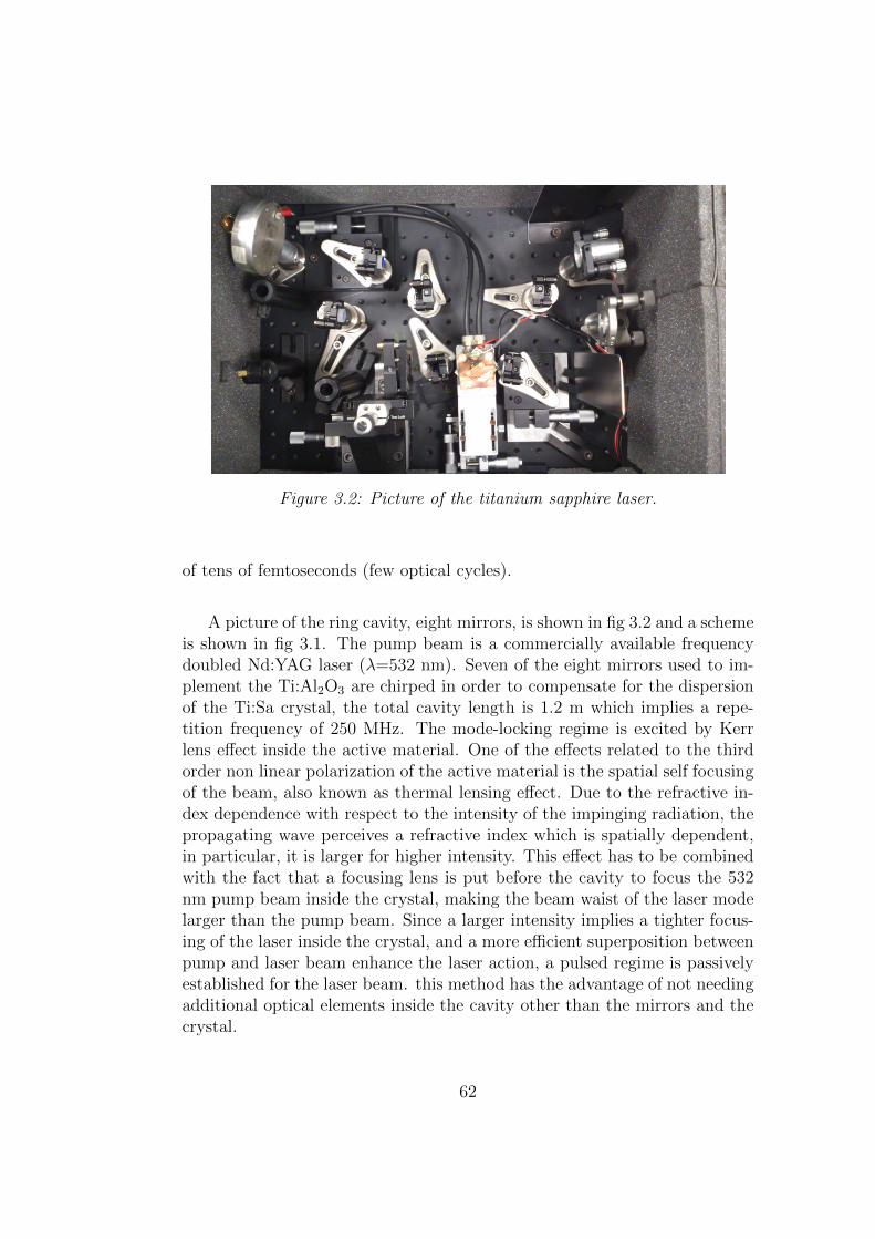
Figure 3.2: Picture of the titanium sapphire laser.

of tens of femtoseconds (few optical cycles).

A picture of the ring cavity, eight mirrors, is shown in fig 3.2 and a schemeis shown in fig 3.1. The pump beam is a commercially available frequencydoubled Nd:YAG laser (λ=532 nm). Seven of the eight mirrors used to im-plement the Ti:Al2O3 are chirped in order to compensate for the dispersionof the Ti:Sa crystal, the total cavity length is 1.2 m which implies a repe-tition frequency of 250 MHz. The mode-locking regime is excited by Kerrlens effect inside the active material. One of the effects related to the thirdorder non linear polarization of the active material is the spatial self focusingof the beam, also known as thermal lensing effect. Due to the refractive in-dex dependence with respect to the intensity of the impinging radiation, thepropagating wave perceives a refractive index which is spatially dependent,in particular, it is larger for higher intensity. This effect has to be combinedwith the fact that a focusing lens is put before the cavity to focus the 532nm pump beam inside the crystal, making the beam waist of the laser modelarger than the pump beam. Since a larger intensity implies a tighter focus-ing of the laser inside the crystal, and a more efficient superposition betweenpump and laser beam enhance the laser action, a pulsed regime is passivelyestablished for the laser beam. this method has the advantage of not needingadditional optical elements inside the cavity other than the mirrors and thecrystal.

62

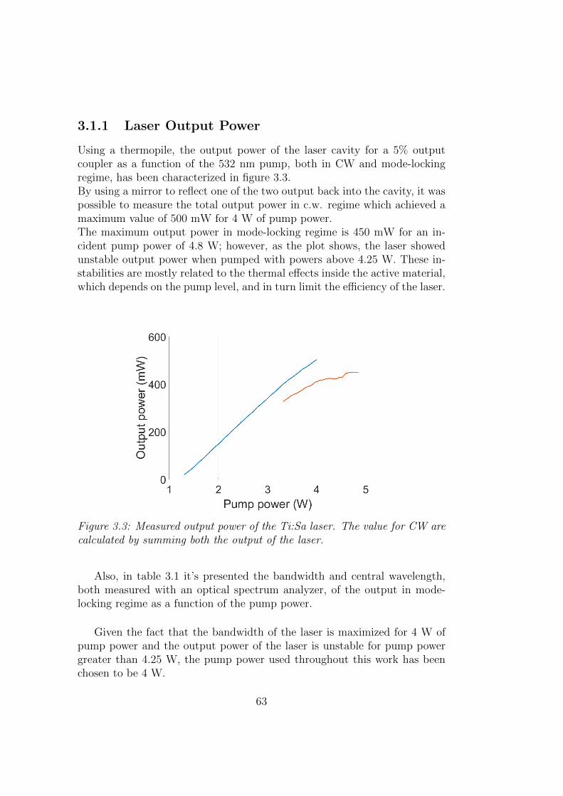
3.1.1 Laser Output Power

Using a thermopile, the output power of the laser cavity for a 5% outputcoupler as a function of the 532 nm pump, both in CW and mode-lockingregime, has been characterized in figure 3.3.By using a mirror to reflect one of the two output back into the cavity, it waspossible to measure the total output power in c.w. regime which achieved amaximum value of 500 mW for 4 W of pump power.The maximum output power in mode-locking regime is 450 mW for an in-cident pump power of 4.8 W; however, as the plot shows, the laser showedunstable output power when pumped with powers above 4.25 W. These in-stabilities are mostly related to the thermal effects inside the active material,which depends on the pump level, and in turn limit the efficiency of the laser.

Figure 3.3: Measured output power of the Ti:Sa laser. The value for CW arecalculated by summing both the output of the laser.

Also, in table 3.1 it’s presented the bandwidth and central wavelength,both measured with an optical spectrum analyzer, of the output in mode-locking regime as a function of the pump power.

Given the fact that the bandwidth of the laser is maximized for 4 W ofpump power and the output power of the laser is unstable for pump powergreater than 4.25 W, the pump power used throughout this work has beenchosen to be 4 W.

63

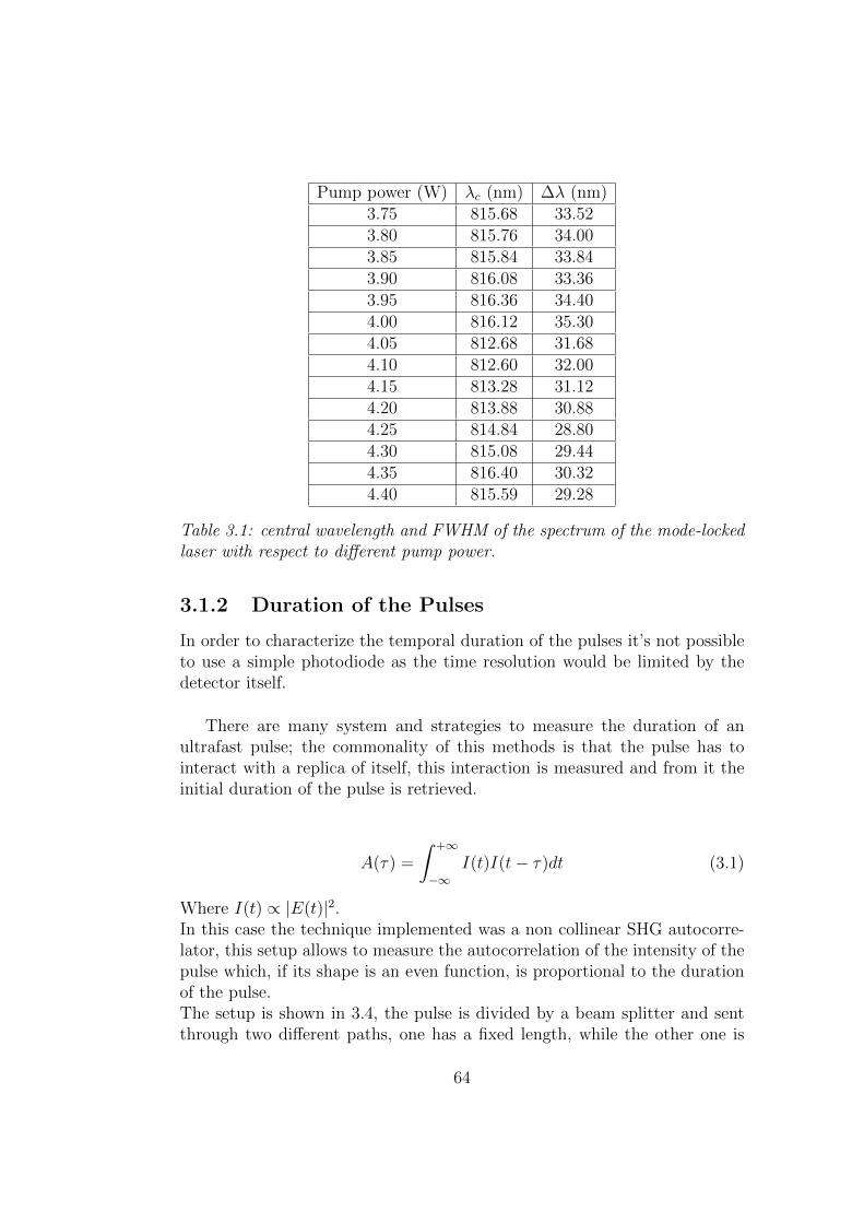
Pump power (W) λc (nm) ∆λ (nm)3.75 815.68 33.523.80 815.76 34.003.85 815.84 33.843.90 816.08 33.363.95 816.36 34.404.00 816.12 35.304.05 812.68 31.684.10 812.60 32.004.15 813.28 31.124.20 813.88 30.884.25 814.84 28.804.30 815.08 29.444.35 816.40 30.324.40 815.59 29.28

Table 3.1: central wavelength and FWHM of the spectrum of the mode-lockedlaser with respect to different pump power.

3.1.2 Duration of the Pulses

In order to characterize the temporal duration of the pulses it’s not possibleto use a simple photodiode as the time resolution would be limited by thedetector itself.

There are many system and strategies to measure the duration of anultrafast pulse; the commonality of this methods is that the pulse has tointeract with a replica of itself, this interaction is measured and from it theinitial duration of the pulse is retrieved.

A(τ) =

∫ +∞

−∞I(t)I(t− τ)dt (3.1)

Where I(t) ∝ |E(t)|2.In this case the technique implemented was a non collinear SHG autocorre-lator, this setup allows to measure the autocorrelation of the intensity of thepulse which, if its shape is an even function, is proportional to the durationof the pulse.The setup is shown in 3.4, the pulse is divided by a beam splitter and sentthrough two different paths, one has a fixed length, while the other one is

64

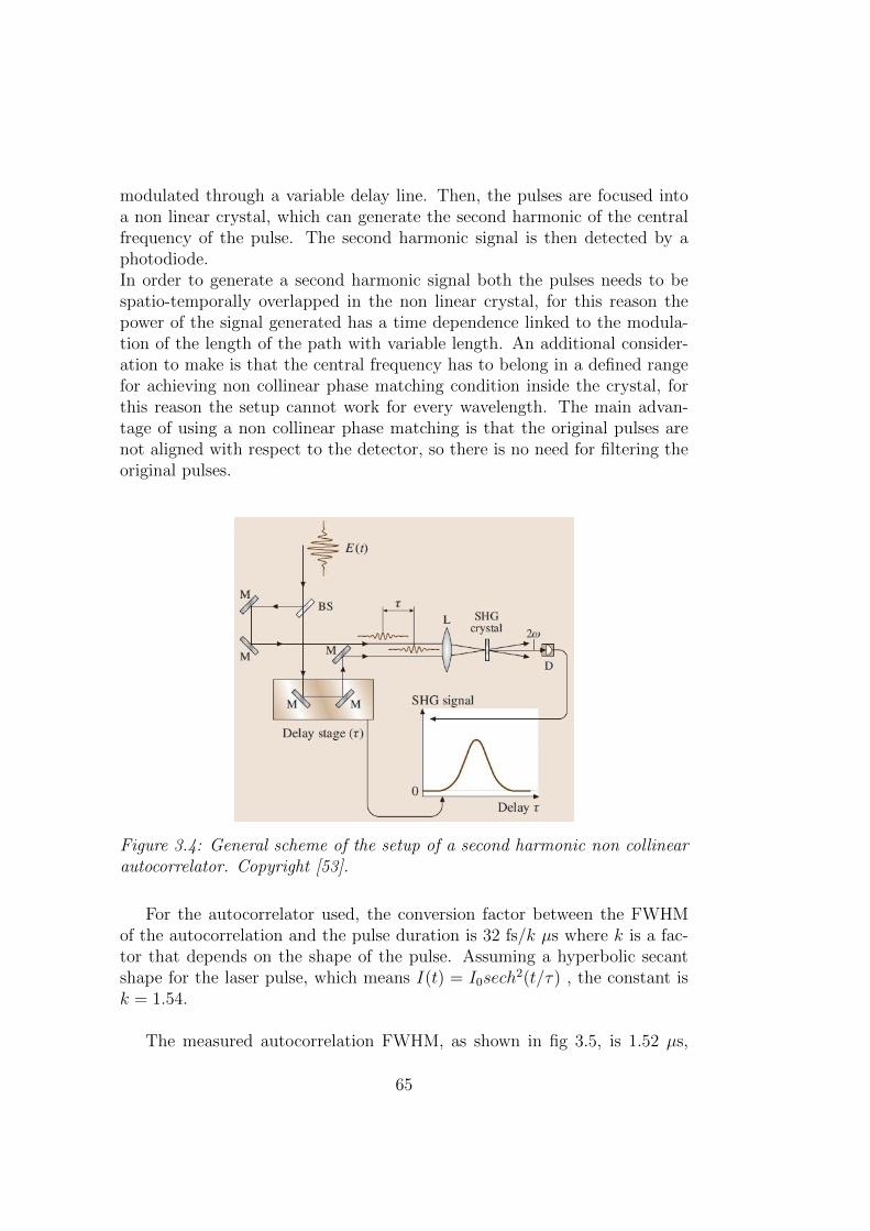
modulated through a variable delay line. Then, the pulses are focused intoa non linear crystal, which can generate the second harmonic of the centralfrequency of the pulse. The second harmonic signal is then detected by aphotodiode.In order to generate a second harmonic signal both the pulses needs to bespatio-temporally overlapped in the non linear crystal, for this reason thepower of the signal generated has a time dependence linked to the modula-tion of the length of the path with variable length. An additional consider-ation to make is that the central frequency has to belong in a defined rangefor achieving non collinear phase matching condition inside the crystal, forthis reason the setup cannot work for every wavelength. The main advan-tage of using a non collinear phase matching is that the original pulses arenot aligned with respect to the detector, so there is no need for filtering theoriginal pulses.

Figure 3.4: General scheme of the setup of a second harmonic non collinearautocorrelator. Copyright [53].

For the autocorrelator used, the conversion factor between the FWHMof the autocorrelation and the pulse duration is 32 fs/k µs where k is a fac-tor that depends on the shape of the pulse. Assuming a hyperbolic secantshape for the laser pulse, which means I(t) = I0sech

2(t/τ) , the constant isk = 1.54.

The measured autocorrelation FWHM, as shown in fig 3.5, is 1.52 µs,

65

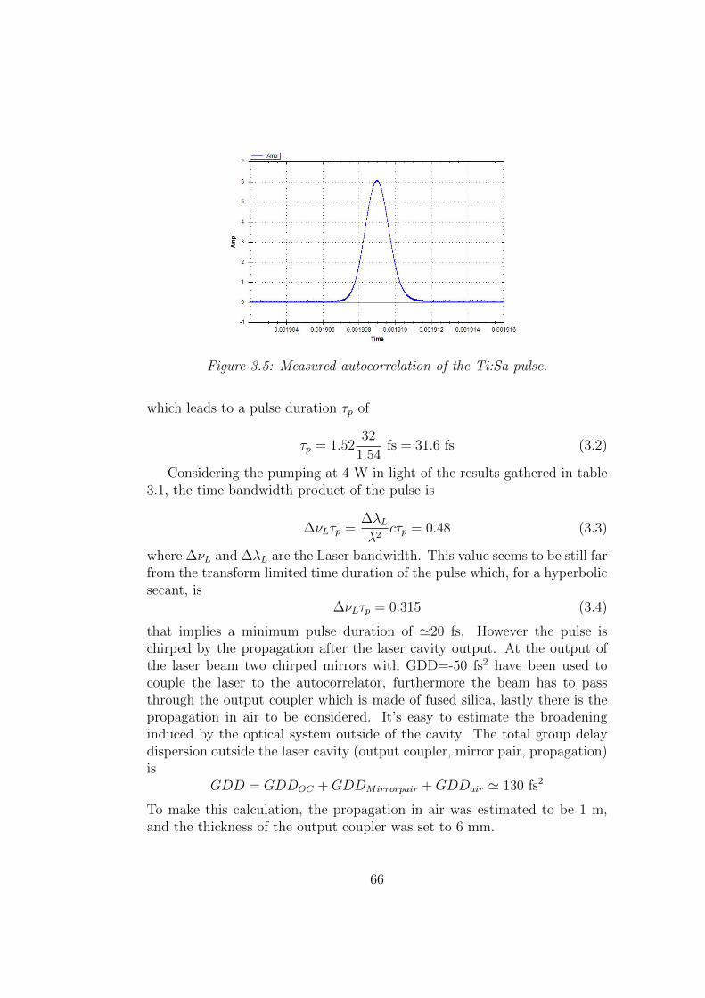
Figure 3.5: Measured autocorrelation of the Ti:Sa pulse.

which leads to a pulse duration τp of

τp = 1.5232

1.54fs = 31.6 fs (3.2)

Considering the pumping at 4 W in light of the results gathered in table3.1, the time bandwidth product of the pulse is

∆νLτp =∆λLλ2

cτp = 0.48 (3.3)

where ∆νL and ∆λL are the Laser bandwidth. This value seems to be still farfrom the transform limited time duration of the pulse which, for a hyperbolicsecant, is

∆νLτp = 0.315 (3.4)

that implies a minimum pulse duration of '20 fs. However the pulse ischirped by the propagation after the laser cavity output. At the output ofthe laser beam two chirped mirrors with GDD=-50 fs2 have been used tocouple the laser to the autocorrelator, furthermore the beam has to passthrough the output coupler which is made of fused silica, lastly there is thepropagation in air to be considered. It’s easy to estimate the broadeninginduced by the optical system outside of the cavity. The total group delaydispersion outside the laser cavity (output coupler, mirror pair, propagation)is

GDD = GDDOC +GDDMirrorpair +GDDair ' 130 fs2

To make this calculation, the propagation in air was estimated to be 1 m,and the thickness of the output coupler was set to 6 mm.

66

Having retrieved this information, the duration of a chirped pulse τp canbe estimated from the initial duration τ0 by the relation

τp = τ0

√1 +

(4 ln 2

GDD

τ 20

)(3.5)

which lead to a initial duration τ0 = 25 fs, this value is much closer to theminimum pump duration and corresponds to a time bandwidth product of0.39. Equation 3.5 is true for a gaussian pulse, so it’s important to noticethat the result is not precise in this case.

3.1.3 M2 Measurement

The beam radius of a TEM00 gaussian is determined by 2 factors (asidefrom the position of the waist), the beam waist w0 and the beam divergence

θd =λ

πw0

. The product between these two quantity is a constant value which

depends parametrically by the wavelength

θdw0 =λ

π

and their ratio is the Rayleigh range

zr =πw2

0

λ

If the laser beam is not a perfect TEM00 this result is going to be different.To model the non ideal behavior of the beam, a factor M is introduced. Thisfactor multiplies both the beam waist and the divergence angle, the definitionof Rayleigh range clearly isn’t affected by this factor, but the product ofdivergence angle and beam waist changes

θd,realw0,real =λ

πM2 (3.6)

For this reason, we introduce a nonideality factor known as Beam qualityfactor M2. it can be demonstrated that this factor is related to the powerof the higher order modes in the following way [54]

M2x =

∞∑i=1

(2pi + 1)ci , M2y =

∞∑i=1

(2qi + 1)ci (3.7)

having defined q and p as TEMpiqi .

67

The formula used to calculate the beam radius of a gaussian beam is

wideal(z) = w0

√1 +

(z − z0

zr

)2

(3.8)

Despite the fact that this equation is only valid for a TEM00 gaussianmode, having introduced the beam quality factor, this formula is still validif properly adjusted. Since the definition of Rayleigh range is unaffected bythe presence of higher order mode

wreal(z) = w0M

√1 +

(z − z0

zr

)2

= Mwideal (3.9)

Another equivalent way of writing the formula is by keeping the definitionof the real beam waist w0,real = Mw0

wreal(z) = w0,real

√√√√1 +

((z − z0)λ

πw20,real

M2

)2

(3.10)

This formulation is more useful to directly evaluate the real beam waist.In order to evaluate the beam quality factor the standard ISO procedure wasfollowed. Given the aim of the project, the M2 value was measured undermode-locking condition regime. The procedure states that the beam has tobe focused using a converging lens of focal length f . Then the radius of thebeam (calculated as the 1/e2 value of the peak intensity) needs to be mea-sured in various positions. Ten equally spaced points have to be taken in theinterval between z = ±zr, the value for zr can be calculated as the position inwhich the spot size becomes

√2 times the beam waist. Other ten points need

to be taken, five from z = 2zr forward and the same has to be done backward.

A picture of the laser beam profile at the input of the focusing lens isshown in figure 3.6. In our setup, the lens used had a 200 mm focal length,the beam diameter was measured using an infrared camera set to return thevalue 4σ of the spot size. Since the laser beam was slightly astigmatic theposition of the waist in the 2 axes was different, therefore, more points weretaken to have an accurate model.

The data gathered was inputed in Matlab and the points were fitted withthe custom function curve fitting tool. Figure 3.7 and 3.8 show the measured4σ values of the beam together with the best interpolation using equation

68

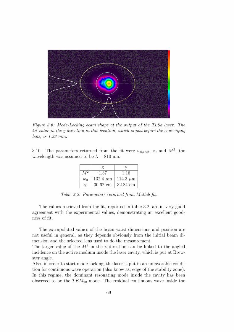
Figure 3.6: Mode-Locking beam shape at the output of the Ti:Sa laser. The4σ value in the y direction in this position, which is just before the converginglens, is 1.23 mm.

3.10. The parameters returned from the fit were w0,real, z0 and M2, thewavelength was assumed to be λ = 810 nm.

x yM2 1.37 1.16w0 132.4 µm 114.3 µmz0 30.62 cm 32.84 cm

Table 3.2: Parameters returned from Matlab fit.

The values retrieved from the fit, reported in table 3.2, are in very goodagreement with the experimental values, demonstrating an excellent good-ness of fit.

The extrapolated values of the beam waist dimensions and position arenot useful in general, as they depends obviously from the initial beam di-mension and the selected lens used to do the measurement.The larger value of the M2 in the x direction can be linked to the angledincidence on the active medium inside the laser cavity, which is put at Brew-ster angle.Also, in order to start mode-locking, the laser is put in an unfavorable condi-tion for continuous wave operation (also know as, edge of the stability zone).In this regime, the dominant resonating mode inside the cavity has beenobserved to be the TEM20 mode. The residual continuous wave inside the

69

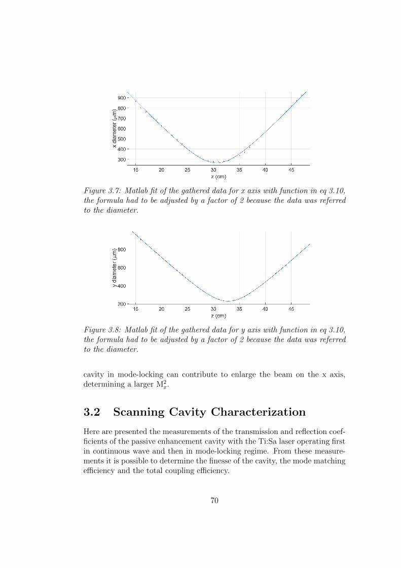
Figure 3.7: Matlab fit of the gathered data for x axis with function in eq 3.10,the formula had to be adjusted by a factor of 2 because the data was referredto the diameter.

Figure 3.8: Matlab fit of the gathered data for y axis with function in eq 3.10,the formula had to be adjusted by a factor of 2 because the data was referredto the diameter.

cavity in mode-locking can contribute to enlarge the beam on the x axis,determining a larger M2

x.

3.2 Scanning Cavity Characterization

Here are presented the measurements of the transmission and reflection coef-ficients of the passive enhancement cavity with the Ti:Sa laser operating firstin continuous wave and then in mode-locking regime. From these measure-ments it is possible to determine the finesse of the cavity, the mode matchingefficiency and the total coupling efficiency.

70

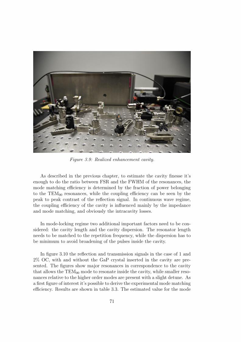
Figure 3.9: Realized enhancement cavity.

As described in the previous chapter, to estimate the cavity finesse it’senough to do the ratio between FSR and the FWHM of the resonances, themode matching efficiency is determined by the fraction of power belongingto the TEM00 resonances, while the coupling efficiency can be seen by thepeak to peak contrast of the reflection signal. In continuous wave regime,the coupling efficiency of the cavity is influenced mainly by the impedanceand mode matching, and obviously the intracavity losses.

In mode-locking regime two additional important factors need to be con-sidered: the cavity length and the cavity dispersion. The resonator lengthneeds to be matched to the repetition frequency, while the dispersion has tobe minimum to avoid broadening of the pulses inside the cavity.

In figure 3.10 the reflection and transmission signals in the case of 1 and2% OC, with and without the GaP crystal inserted in the cavity are pre-sented. The figures show major resonances in correspondence to the cavitythat allows the TEM00 mode to resonate inside the cavity, while smaller reso-nances relative to the higher order modes are present with a slight detune. Asa first figure of interest it’s possible to derive the experimental mode matchingefficiency. Results are shown in table 3.3. The estimated value for the mode

71

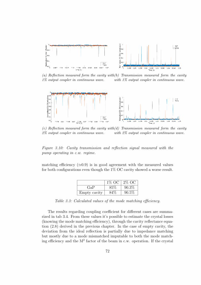
(a) Reflection measured form the cavity with1% output coupler in continuous wave.

(b) Transmission measured form the cavitywith 1% output coupler in continuous wave.

(c) Reflection measured form the cavity with2% output coupler in continuous wave.

(d) Transmission measured form the cavitywith 2% output coupler in continuous wave.

Figure 3.10: Cavity transmission and reflection signal measured with thepump operating in c.w. regime.

matching efficiency ('0.9) is in good agreement with the measured valuesfor both configurations even though the 1% OC cavity showed a worse result.

1% OC 2% OCGaP 85% 90.3%

Empty cavity 84% 90.5%

Table 3.3: Calculated values of the mode matching efficiency.

The results regarding coupling coefficient for different cases are summa-rized in tab 3.4. From these values it’s possible to estimate the crystal losses(knowing the mode matching efficiency), through the cavity reflectance equa-tion (2.8) derived in the previous chapter. In the case of empty cavity, thedeviation from the ideal reflection is partially due to impedance matchingbut mostly due to a mode mismatched imputable to both the mode match-ing efficiency and the M2 factor of the beam in c.w. operation. If the crystal

72

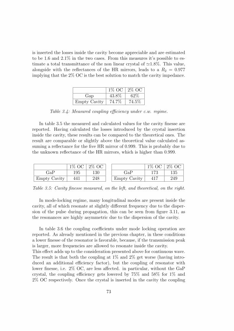
is inserted the losses inside the cavity become appreciable and are estimatedto be 1.6 and 2.1% in the two cases. From this measures it’s possible to es-timate a total transmittance of the non linear crystal of '1.8%. This value,alongside with the reflectances of the HR mirrors, leads to a R2 = 0.977implying that the 2% OC is the best solution to match the cavity impedance.

1% OC 2% OCGap 43.8% 62%

Empty Cavity 74.7% 74.5%

Table 3.4: Measured coupling efficiency under c.w. regime.

In table 3.5 the measured and calculated values for the cavity finesse arereported. Having calculated the losses introduced by the crystal insertioninside the cavity, these results can be compared to the theoretical ones. Theresult are comparable or slightly above the theoretical value calculated as-suming a reflectance for the five HR mirror of 0.999. This is probably due tothe unknown reflectance of the HR mirrors, which is higher than 0.999.

1% OC 2% OCGaP 195 130

Empty Cavity 441 248

1% OC 2% OCGaP 173 135

Empty Cavity 417 249

Table 3.5: Cavity finesse measured, on the left, and theoretical, on the right.

In mode-locking regime, many longitudinal modes are present inside thecavity, all of which resonate at slightly different frequency due to the disper-sion of the pulse during propagation, this can be seen from figure 3.11, asthe resonances are highly asymmetric due to the dispersion of the cavity.

In table 3.6 the coupling coefficients under mode locking operation arereported. As already mentioned in the previous chapter, in these conditionsa lower finesse of the resonator is favorable, because, if the transmission peakis larger, more frequencies are allowed to resonate inside the cavity.This effect adds up to the consideration presented above for continuous wave.The result is that both the coupling at 1% and 2% get worse (having intro-duced an additional efficiency factor), but the coupling of resonator withlower finesse, i.e. 2% OC, are less affected. in particular, without the GaPcrystal, the coupling efficiency gets lowered by 75% and 58% for 1% and2% OC respectively. Once the crystal is inserted in the cavity the coupling

73

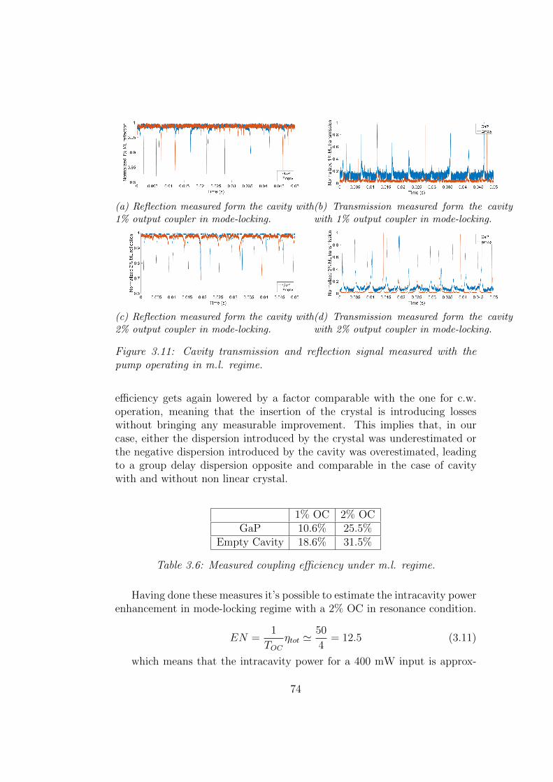
(a) Reflection measured form the cavity with1% output coupler in mode-locking.

(b) Transmission measured form the cavitywith 1% output coupler in mode-locking.

(c) Reflection measured form the cavity with2% output coupler in mode-locking.

(d) Transmission measured form the cavitywith 2% output coupler in mode-locking.

Figure 3.11: Cavity transmission and reflection signal measured with thepump operating in m.l. regime.

efficiency gets again lowered by a factor comparable with the one for c.w.operation, meaning that the insertion of the crystal is introducing losseswithout bringing any measurable improvement. This implies that, in ourcase, either the dispersion introduced by the crystal was underestimated orthe negative dispersion introduced by the cavity was overestimated, leadingto a group delay dispersion opposite and comparable in the case of cavitywith and without non linear crystal.

1% OC 2% OCGaP 10.6% 25.5%

Empty Cavity 18.6% 31.5%

Table 3.6: Measured coupling efficiency under m.l. regime.

Having done these measures it’s possible to estimate the intracavity powerenhancement in mode-locking regime with a 2% OC in resonance condition.

EN =1

TOCηtot '

50

4= 12.5 (3.11)

which means that the intracavity power for a 400 mW input is approx-

74

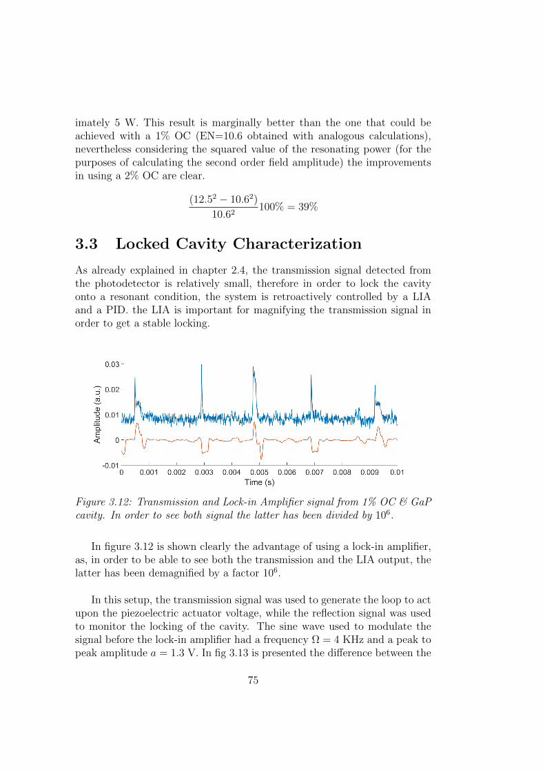
imately 5 W. This result is marginally better than the one that could beachieved with a 1% OC (EN=10.6 obtained with analogous calculations),nevertheless considering the squared value of the resonating power (for thepurposes of calculating the second order field amplitude) the improvementsin using a 2% OC are clear.

(12.52 − 10.62)

10.62100% = 39%

3.3 Locked Cavity Characterization

As already explained in chapter 2.4, the transmission signal detected fromthe photodetector is relatively small, therefore in order to lock the cavityonto a resonant condition, the system is retroactively controlled by a LIAand a PID. the LIA is important for magnifying the transmission signal inorder to get a stable locking.

Figure 3.12: Transmission and Lock-in Amplifier signal from 1% OC & GaPcavity. In order to see both signal the latter has been divided by 106.

In figure 3.12 is shown clearly the advantage of using a lock-in amplifier,as, in order to be able to see both the transmission and the LIA output, thelatter has been demagnified by a factor 106.

In this setup, the transmission signal was used to generate the loop to actupon the piezoelectric actuator voltage, while the reflection signal was usedto monitor the locking of the cavity. The sine wave used to modulate thesignal before the lock-in amplifier had a frequency Ω = 4 KHz and a peak topeak amplitude a = 1.3 V. In fig 3.13 is presented the difference between the

75

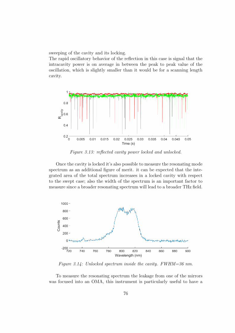
sweeping of the cavity and its locking.The rapid oscillatory behavior of the reflection in this case is signal that theintracavity power is on average in between the peak to peak value of theoscillation, which is slightly smaller than it would be for a scanning lengthcavity.

Figure 3.13: reflected cavity power locked and unlocked.

Once the cavity is locked it’s also possible to measure the resonating modespectrum as an additional figure of merit. it can be expected that the inte-grated area of the total spectrum increases in a locked cavity with respectto the swept case; also the width of the spectrum is an important factor tomeasure since a broader resonating spectrum will lead to a broader THz field.

Figure 3.14: Unlocked spectrum inside the cavity. FWHM=36 nm.

To measure the resonating spectrum the leakage from one of the mirrorswas focused into an OMA, this instrument is particularly useful to have a

76

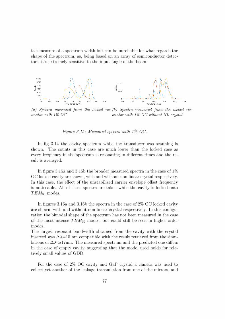
fast measure of a spectrum width but can be unreliable for what regards theshape of the spectrum, as, being based on an array of semiconductor detec-tors, it’s extremely sensitive to the input angle of the beam.

(a) Spectra measured from the locked res-onator with 1% OC.

(b) Spectra measured from the locked res-onator with 1% OC without NL crystal.

Figure 3.15: Measured spectra with 1% OC.

In fig 3.14 the cavity spectrum while the transducer was scanning isshown. The counts in this case are much lower than the locked case asevery frequency in the spectrum is resonating in different times and the re-sult is averaged.

In figure 3.15a and 3.15b the broader measured spectra in the case of 1%OC locked cavity are shown, with and without non linear crystal respectively.In this case, the effect of the unstabilized carrier envelope offset frequencyis noticeable. All of these spectra are taken while the cavity is locked ontoTEM00 modes.

In figures 3.16a and 3.16b the spectra in the case of 2% OC locked cavityare shown, with and without non linear crystal respectively. In this configu-ration the bimodal shape of the spectrum has not been measured in the caseof the most intense TEM00 modes, but could still be seen in higher ordermodes.The largest resonant bandwidth obtained from the cavity with the crystalinserted was ∆λ=15 nm compatible with the result retrieved from the simu-lations of ∆λ '17nm. The measured spectrum and the predicted one differsin the case of empty cavity, suggesting that the model used holds for rela-tively small values of GDD.

For the case of 2% OC cavity and GaP crystal a camera was used tocollect yet another of the leakage transmission from one of the mirrors, and

77

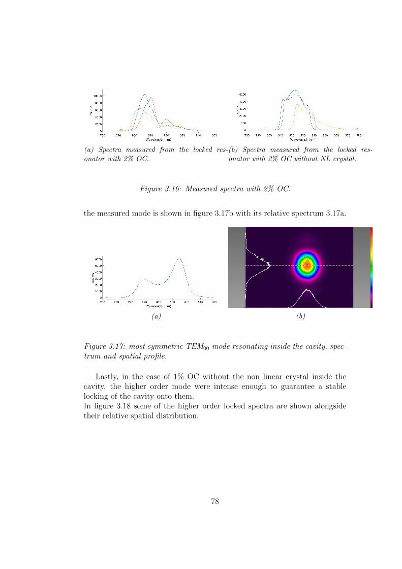
(a) Spectra measured from the locked res-onator with 2% OC.

(b) Spectra measured from the locked res-onator with 2% OC without NL crystal.

Figure 3.16: Measured spectra with 2% OC.

the measured mode is shown in figure 3.17b with its relative spectrum 3.17a.

(a) (b)

Figure 3.17: most symmetric TEM00 mode resonating inside the cavity, spec-trum and spatial profile.

Lastly, in the case of 1% OC without the non linear crystal inside thecavity, the higher order mode were intense enough to guarantee a stablelocking of the cavity onto them.In figure 3.18 some of the higher order locked spectra are shown alongsidetheir relative spatial distribution.

78

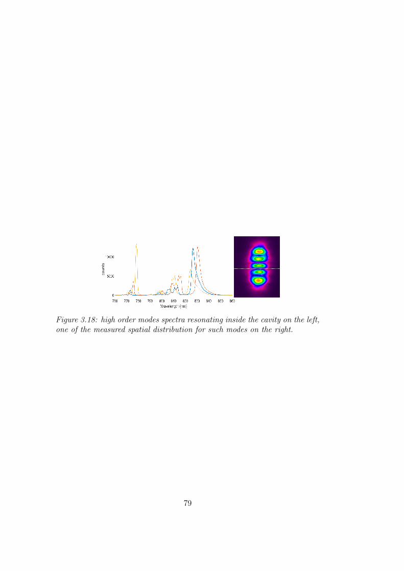
Figure 3.18: high order modes spectra resonating inside the cavity on the left,one of the measured spatial distribution for such modes on the right.

79

80

Conclusion and Perspectives

We described the design, realization and characterization of an enhancementring resonator for THz generation by intracavity optical rectification of nearinfrared femtosecond pulses. The cavity, a six mirror ring resonator, has aFSR around 250 MHz, after having compared different output couplers theoptimal case selected was to use a 2% output coupler. In this configurationthe finesse was measured to be around 240 for the case of empty cavity and50 with the non linear crystal, which is close to the theoretical limit.The coupling efficiency between pump laser and resonator was also measuredto be comparable to the theoretical result which is around 90%.The resonator mirrors are chirped in order to compensate for the dispersionintroduced by the crystal, a value of group delay dispersion of 155 fs2 forthe whole system was evaluated. Various locking conditions spectra weremeasured showing a resonant bandwidth ∆λ ' 15 nm with a bimodal dis-tribution given by the pump laser νceo, this result is in agreement with thesimulations. The overall efficiency of the cavity for a mode-locked input wasmeasured to be one fourth of the ideal value leading to a enhancement factorof one order of magnitude with respect to the input power.The realized resonator can be exploited to generate THz radiation by opticalrectification in a variety of non linear crystal such as GaP, ZnTe and LiNbO3.Further activity could be to stabilize the νceo of the pump laser to have abetter couple the radiation to the cavity; but the efforts towards improve-ment will mostly be concentrated on the measurement and characterizationthrough coherent detection by a GaAs photoconductive antenna of the pulsedTHz radiation generated in GaP and in AR coated ZnTe.

81

82

Bibliography

[1] E Pickwell and VP Wallace. Biomedical applications of terahertz tech-nology. Journal of Physics D: Applied Physics, 39(17):R301, 2006.

[2] X.C. Zhang and J. Xu. Introduction to THz Wave Photonics. Springer-Link : Bucher. Springer US, 2009.

[3] B. B. Hu and M. C. Nuss. Imaging with terahertz waves. Opt. Lett.,20(16):1716–1718, Aug 1995.

[4] S.L. Dexheimer. Terahertz Spectroscopy: Principles and Applications.Optical Science and Engineering. CRC Press, 2007.

[5] Masayoshi Tonouchi. Cutting-edge terahertz technology. Nature pho-tonics, 1(2):97–105, 2007.

[6] Federico; Belyanin Alexey; Sivco Deborah L.; Cho Alfred Y.; OakleyDouglas C.; Vineis Christopher J.; Turner George W. Belkin, MikhailA.; Capasso. Terahertz quantum-cascade-laser source based on intra-cavity difference-frequency generation. Nature Photonics, 1, 2007.

[7] A. J. Rodriguez, G.; Taylor. Screening of the bias field in terahertzgeneration from photoconductors. Optics Letters, 21, 1996.

[8] Chia-En; Chang Yunching; Yao Jimmy; Yin Stuart; Luo Claire; Ruf-fin Paul; Brantley Christina; Edwards Eugene Gao, Yaohui; Yang.Terahertz-radiation-enhanced broadband terahertz generation fromlarge aperture photoconductive antenna. Applied Physics B: Lasers andOptics, 109, 10 2012.

[9] Masahiko Tani, Shuji Matsuura, Kiyomi Sakai, and Shin ichi Nakashima.Emission characteristics of photoconductive antennas based on low-temperature-grown gaas and semi-insulating gaas. Appl. Opt.,36(30):7853–7859, Oct 1997.

83

[10] Andrei; Krasnok Alexander; Rafailov Edik; Belov Pavel Lepeshov,Sergey; Gorodetsky. Enhancement of terahertz photoconductive antennaoperation by optical nanoantennas (laser photonics rev. 11(1)/2017).Laser & Photonics Reviews, 11, 01 2017.

[11] G. H.; Malzer S.; Wang L. J.; Gossard A. C. Preu, S.; Dohler. Tunable,continuous-wave terahertz photomixer sources and applications. Journalof Applied Physics, 109, 2011.

[12] K. A. McIntosh, E. R. Brown, K. B. Nichols, O. B. McMahon, W. F.DiNatale, and T. M. Lyszczarz. Terahertz photomixing with diode lasersin low-temperature-grown gaas. Applied Physics Letters, 67(26):3844–3846, 1995.

[13] Max; Stillhart Marcel; Ruiz Blanca; Khan Rizwan U. A.; Gunter PeterSchneider, Arno; Neis. Generation of terahertz pulses through opticalrectification in organic dast crystals: theory and experiment. Journal ofthe Optical Society of America B, 23, 2006.

[14] Konstantin L Vodopyanov. Optical thz-wave generation withperiodically-inverted gaas. Laser & Photonics Reviews, 2(1-2):11–25,2008.

[15] Ajay Nahata, Aniruddha S. Weling, and Tony F. Heinz. A widebandcoherent terahertz spectroscopy system using optical rectification andelectrooptic sampling. Applied Physics Letters, 69(16):2321–2323, 1996.

[16] Konstantin L. Vodopyanov. Optical generation of narrow-band tera-hertz packets in periodically-inverted electro-optic crystals: conversionefficiency and optimal laser pulse format. Opt. Express, 14(6):2263–2276,Mar 2006.

[17] R.W. Boyd. Nonlinear Optics. Nonlinear Optics Series. Elsevier Science,2008.

[18] M.; Jiang Zhiping; Zhang X.-C. Chen, Q.; Tani. Electro-optictransceivers for terahertz-wave applications. Journal of the Optical So-ciety of America B, 18, 2001.

[19] Ken; Nishizawa Jun-ichi; Saito-Kyosuke; Kimura Tomoyuki Tanabe,Tadao; Suto. Frequency-tunable terahertz wave generation via excita-tion of phonon-polaritons in gap. Journal of Physics D Applied Physics,36, 04 2003.

84

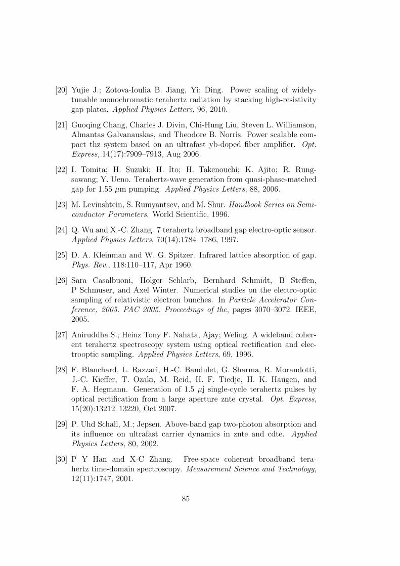
[20] Yujie J.; Zotova-Ioulia B. Jiang, Yi; Ding. Power scaling of widely-tunable monochromatic terahertz radiation by stacking high-resistivitygap plates. Applied Physics Letters, 96, 2010.

[21] Guoqing Chang, Charles J. Divin, Chi-Hung Liu, Steven L. Williamson,Almantas Galvanauskas, and Theodore B. Norris. Power scalable com-pact thz system based on an ultrafast yb-doped fiber amplifier. Opt.Express, 14(17):7909–7913, Aug 2006.

[22] I. Tomita; H. Suzuki; H. Ito; H. Takenouchi; K. Ajito; R. Rung-sawang; Y. Ueno. Terahertz-wave generation from quasi-phase-matchedgap for 1.55 µm pumping. Applied Physics Letters, 88, 2006.

[23] M. Levinshtein, S. Rumyantsev, and M. Shur. Handbook Series on Semi-conductor Parameters. World Scientific, 1996.

[24] Q. Wu and X.-C. Zhang. 7 terahertz broadband gap electro-optic sensor.Applied Physics Letters, 70(14):1784–1786, 1997.

[25] D. A. Kleinman and W. G. Spitzer. Infrared lattice absorption of gap.Phys. Rev., 118:110–117, Apr 1960.

[26] Sara Casalbuoni, Holger Schlarb, Bernhard Schmidt, B Steffen,P Schmuser, and Axel Winter. Numerical studies on the electro-opticsampling of relativistic electron bunches. In Particle Accelerator Con-ference, 2005. PAC 2005. Proceedings of the, pages 3070–3072. IEEE,2005.

[27] Aniruddha S.; Heinz Tony F. Nahata, Ajay; Weling. A wideband coher-ent terahertz spectroscopy system using optical rectification and elec-trooptic sampling. Applied Physics Letters, 69, 1996.

[28] F. Blanchard, L. Razzari, H.-C. Bandulet, G. Sharma, R. Morandotti,J.-C. Kieffer, T. Ozaki, M. Reid, H. F. Tiedje, H. K. Haugen, andF. A. Hegmann. Generation of 1.5 µj single-cycle terahertz pulses byoptical rectification from a large aperture znte crystal. Opt. Express,15(20):13212–13220, Oct 2007.

[29] P. Uhd Schall, M.; Jepsen. Above-band gap two-photon absorption andits influence on ultrafast carrier dynamics in znte and cdte. AppliedPhysics Letters, 80, 2002.

[30] P Y Han and X-C Zhang. Free-space coherent broadband tera-hertz time-domain spectroscopy. Measurement Science and Technology,12(11):1747, 2001.

85

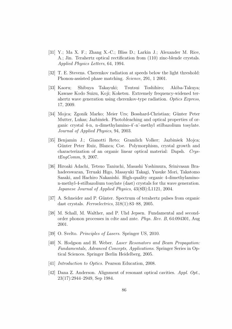
[31] Y.; Ma X. F.; Zhang X.-C.; Bliss D.; Larkin J.; Alexander M. Rice,A.; Jin. Terahertz optical rectification from (110) zinc-blende crystals.Applied Physics Letters, 64, 1994.

[32] T. E. Stevens. Cherenkov radiation at speeds below the light threshold:Phonon-assisted phase matching. Science, 291, 1 2001.

[33] Kaoru; Shibuya Takayuki; Tsutsui Toshihiro; Akiba-Takuya;Kawase Kodo Suizu, Koji; Koketsu. Extremely frequency-widened ter-ahertz wave generation using cherenkov-type radiation. Optics Express,17, 2009.

[34] Mojca; Zgonik Marko; Meier Urs; Bosshard-Christian; Gunter PeterMutter, Lukas; Jazbinsek. Photobleaching and optical properties of or-ganic crystal 4-n, n-dimethylamino-4’-n’-methyl stilbazolium tosylate.Journal of Applied Physics, 94, 2003.

[35] Benjamin J.; Gianotti Reto; Gramlich Volker; Jazbinsek Mojca;Gunter Peter Ruiz, Blanca; Coe. Polymorphism, crystal growth andcharacterization of an organic linear optical material: Dapsh. Crys-tEngComm, 9, 2007.

[36] Hiroaki Adachi, Tetsuo Taniuchi, Masashi Yoshimura, Srinivasan Bra-hadeeswaran, Teruaki Higo, Masayuki Takagi, Yusuke Mori, TakatomoSasaki, and Hachiro Nakanishi. High-quality organic 4-dimethylamino-n-methyl-4-stilbazolium tosylate (dast) crystals for thz wave generation.Japanese Journal of Applied Physics, 43(8B):L1121, 2004.

[37] A. Schneider and P. Gunter. Spectrum of terahertz pulses from organicdast crystals. Ferroelectrics, 318(1):83–88, 2005.

[38] M. Schall, M. Walther, and P. Uhd Jepsen. Fundamental and second-order phonon processes in cdte and znte. Phys. Rev. B, 64:094301, Aug2001.

[39] O. Svelto. Principles of Lasers. Springer US, 2010.

[40] N. Hodgson and H. Weber. Laser Resonators and Beam Propagation:Fundamentals, Advanced Concepts, Applications. Springer Series in Op-tical Sciences. Springer Berlin Heidelberg, 2005.

[41] Introduction to Optics. Pearson Education, 2008.

[42] Dana Z. Anderson. Alignment of resonant optical cavities. Appl. Opt.,23(17):2944–2949, Sep 1984.

86

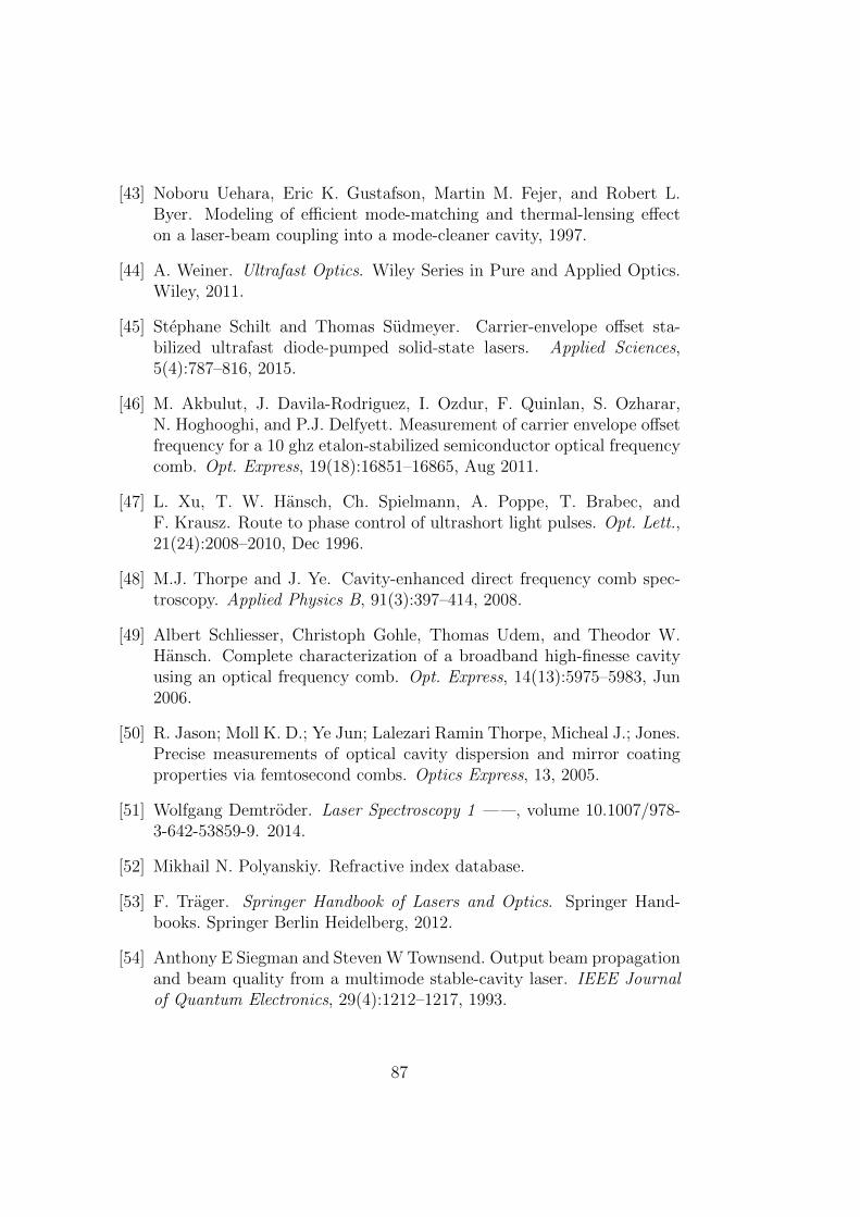
[43] Noboru Uehara, Eric K. Gustafson, Martin M. Fejer, and Robert L.Byer. Modeling of efficient mode-matching and thermal-lensing effecton a laser-beam coupling into a mode-cleaner cavity, 1997.

[44] A. Weiner. Ultrafast Optics. Wiley Series in Pure and Applied Optics.Wiley, 2011.

[45] Stephane Schilt and Thomas Sudmeyer. Carrier-envelope offset sta-bilized ultrafast diode-pumped solid-state lasers. Applied Sciences,5(4):787–816, 2015.

[46] M. Akbulut, J. Davila-Rodriguez, I. Ozdur, F. Quinlan, S. Ozharar,N. Hoghooghi, and P.J. Delfyett. Measurement of carrier envelope offsetfrequency for a 10 ghz etalon-stabilized semiconductor optical frequencycomb. Opt. Express, 19(18):16851–16865, Aug 2011.

[47] L. Xu, T. W. Hansch, Ch. Spielmann, A. Poppe, T. Brabec, andF. Krausz. Route to phase control of ultrashort light pulses. Opt. Lett.,21(24):2008–2010, Dec 1996.

[48] M.J. Thorpe and J. Ye. Cavity-enhanced direct frequency comb spec-troscopy. Applied Physics B, 91(3):397–414, 2008.

[49] Albert Schliesser, Christoph Gohle, Thomas Udem, and Theodor W.Hansch. Complete characterization of a broadband high-finesse cavityusing an optical frequency comb. Opt. Express, 14(13):5975–5983, Jun2006.

[50] R. Jason; Moll K. D.; Ye Jun; Lalezari Ramin Thorpe, Micheal J.; Jones.Precise measurements of optical cavity dispersion and mirror coatingproperties via femtosecond combs. Optics Express, 13, 2005.

[51] Wolfgang Demtroder. Laser Spectroscopy 1 ——, volume 10.1007/978-3-642-53859-9. 2014.

[52] Mikhail N. Polyanskiy. Refractive index database.

[53] F. Trager. Springer Handbook of Lasers and Optics. Springer Hand-books. Springer Berlin Heidelberg, 2012.

[54] Anthony E Siegman and Steven W Townsend. Output beam propagationand beam quality from a multimode stable-cavity laser. IEEE Journalof Quantum Electronics, 29(4):1212–1217, 1993.

87