Embed Size (px)
Citation preview
Thames Water Stochastic Resource Modelling Stage 2&3 Report Thames Water
28 October 2016
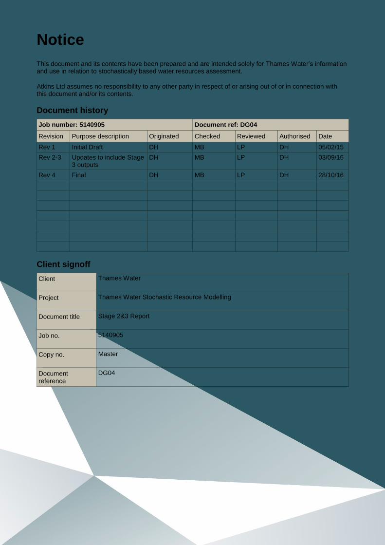
Notice
This document and its contents have been prepared and are intended solely for Thames Water’s information and use in relation to stochastically based water resources assessment.
Atkins Ltd assumes no responsibility to any other party in respect of or arising out of or in connection with this document and/or its contents.
Document history
Job number: 5140905 Document ref: DG04
Revision Purpose description Originated Checked Reviewed Authorised Date
Rev 1 Initial Draft DH MB LP DH 05/02/15
Rev 2-3 Updates to include Stage 3 outputs
DH MB LP DH 03/09/16
Rev 4 Final DH MB LP DH 28/10/16
Client signoff
Client Thames Water
Project Thames Water Stochastic Resource Modelling
Document title Stage 2&3 Report
Job no. 5140905
Copy no. Master
Document reference
DG04
Atkins Stage 2&3 Report | Version 4 | 28 October 2016 | 5140905 3
Table of contents
Chapter Pages
Executive summary 5
1. Introduction and Overview 7
2. Analysis Stages 2a & 2b: Stochastic Weather Generation 8 2.1. Methodology Overview and Key Assumptions 8 2.2. Alternatives Considered 14 2.3. Data Used 15 2.4. Methodology Details 16 2.5. Results 19
3. Analysis Stage 2c: Flow Modelling 25 3.1. Methodology and Key Assumptions 25 3.2. Results 27
4. Analysis Stage 2d: Water Resource Modelling 32
5. Analysis Stage 3: Deployable Output and Climate Change Analysis 34 5.1. Method and Key Assumptions 34 5.2. Results 36
6. Conclusions and Recommendations 39
7. References 41
Appendices 42
Appendix A. Contextualising the 20th Century Drought Record 43 A.1. 18th to 20th Century Rainfall, Temperature and Flow Records 43 A.2. Analysis of Older Historic Droughts 46
Appendix B. Weather Generation Modelling Results 48 B.1. Rainfall Totals – Q-Q Plots 48 B.2. Hydrologically Effective Rainfall – Probability Plots 55
Figures Figure 1-1 Summary Overview of the Stage 2 and 3 Tasks 7 Figure 2-1 Example of the Nature of the Statistical Relationships between Catchment Rainfall, NAO and SST (national example taken from Serinaldi et al 2012 to highlight location/distance trends) 10 Figure 2-2 Overview of the Weather Generator Modelling Process 11 Figure 2-3 Example of the Influence of Multi-Metric Curve Fitting 12 Figure 2-4 Historic versus Simulated PET without Spring/Summer Persistence Fitting (hydrological year – exaggerated scale) 13 Figure 2-5 Historic versus Simulated PET with Spring/Summer Persistence Fitting 13 Figure 2-8 Comparison of Winter Average PET against Central England Winter Temperature 15 Figure 2-9 Analysis of Rainfall Anomalies for Hydrological Year Events 17 Figure 2-10 Analysis of Rainfall Anomalies for the 9 Months Ending August 18 Figure 2-11 Analysis of Rainfall Anomalies for the 5 Months Ending August 18 Figure 2-12 Log-log plot of Hydrological Year Rainfall Totals 20 Figure 2-13 Log-log plot of Calendar Year Rainfall Totals 21 Figure 2-14 Log-log Plot of Rainfall Totals for 9 months ending August 21 Figure 2-15 Log-log Plot of Hydrological Year HER 22 Figure 2-16 Log-Log Plot of Calendar Year HER 23 Figure 2-17 Log-log Plot of December to August HER 23 Figure 3-1 Calibration Results for the Updated Teddington Weir Catchmod Model 26 Figure 3-2 Summary of Flow Duration Curve (FDCs) for all Modelled Rivers 28 Figure 4-1 London Aggregated Storage Outputs for IRAS compared with WARMS 32

Atkins Stage 2&3 Report | Version 4 | 28 October 2016 | 5140905 4
Figure 5-1 Comparison of IRAS and WARMS2 Yields; before Catchmod Re-Calibration (but with hydrological algorithm adjustment) 35 Figure 5-2 Comparison of IRAS and WARMS2 Yields; after Catchmod Re-Calibration 35 Figure 5-3 Analysis of WARMS2 Yield/Return Period Curve before Catchmod Re-Calibration 36 Figure 5-4 Analysis of WARMS2 Yield/Return Period Curve after Catchmod Re-Calibration 37 Figure 5-5 Phase 3 Analysis of Climate Change Impacts 38
Atkins Stage 2&3 Report | Version 4 | 28 October 2016 | 5140905 5
Executive summary
This report forms the main technical summary of the stochastic water resource analysis work that has been carried out for Thames Water for WRMP19. It contains a summary of the stochastic weather generator, the weather generator outputs, the flow modelling and the water resource modelling carried out for the London Water Resource Zone (WRZ). It is intended to act as a ‘reference’ for the practical applications of the stochastic water resources data sets, which will be reported under Phase 4 to support the Drought Plan and the WRMP19 options appraisals. It incorporates both the baseline (20th Century) stochastic analysis of water resources and an analysis of the behaviour of the Thames system under 2080 climate change factors.
The stochastic weather generation was carried out using a model that was ‘trained’ to emulate the 20th Century climate, based on observed weather data and regional climatic drivers. This was linked with pre-existing rainfall-runoff models to provide very large data flow sets at all of the points that required to model the water resource system Deployable Output. The weather generator and associated flow modelling were designed to work in a spatially coherent way across the whole of the Thames and Severn catchments, so the outputs can be used to:
Evaluate the resilience of the existing Thames Water supply system to a wide range of drought severities (in accordance with the most advanced Risk Composition referred to in the WRMP19 UKWIR Risk Based Methods guidance).
Evaluate the impacts of climate change on the range of droughts that were generated.
Evaluate the Deployable Output (DO) benefit of new options within the Thames catchment and the benefits that potential transfers from the River Severn might provide. This last item will be reported separately, but the analysis uses the data sets described within this report.
The stochastic weather generator that was used reflects the latest research in this field, and the methods that were developed have now been applied to a range of water resources applications, including Water Resources in the South East (WRSE), Water Resources in the East (WRE), Water UK, and other individual water companies. It has been successfully applied for a wide geographical range of Water Resource Zones ranging from United Utilities’ Cumbria WRZ, right across to the Thanet WRZ in the far south east of Kent. Other weather generation approaches were considered as part of this project, but the described approach represents the best method that is currently, reliably available for water resources planning. It was able to demonstrably generate rainfall, potential evapotranspiration (PET) and hydrologically effective rainfall (HER) outputs that validated well against the 20th Century droughts in a spatially coherent way across both the Thames and Severn catchments. Whilst the emulation of severe droughts will always require some key planning assumptions due to the scarcity of relevant data on which to ‘train’ weather generators, in this case this was done in a structured, considered way that incorporated conceptual understanding of drought anomalies and fully allowed for the literature that is available in relation to historic droughts.
Although large volumes of daily weather data were involved, the study was able to use Catchmod and Kestrel-IHM rainfall-runoff models linked through to an IRAS water resource simulator to run yield analyses based on the full data sets. The close validation between the weather generator and the 20th Century record for rainfall and HER metrics translated to a good validation against the 20th Century flow/duration curves, and it was found that the stochastically generated yields that were generated from these flows provided return period estimates that were compatible with the 20th Century observations.
Calibration of the IRAS rapid water resource simulator confirmed that this was suitable for the purposes of ranking of stochastic drought years according to their relative yield, and for analysing the impact of climate change on the yield/return period relationship. This same principle can be used to generate yield/return period impacts from new water resource options such as the Severn-Thames transfer schemes. The use of ‘Drought Libraries’ was shown to provide a practicable method for addressing the largest difficulty encountered in the study, which related to hydrological modelling rather than any actual weather generation issues. It also provided a convenient approach using the weather generator outputs for more detailed analysis within Thames Water’s detailed WARMS2 water resources simulator, which can be used for WRMP19 options appraisal modelling if required.

Atkins Stage 2&3 Report | Version 4 | 28 October 2016 | 5140905 6
Testing of the baseline climate using the weather generator, hydrological models and IRAS/WARMS2, indicated that:
The 2305 Ml/d DO currently quoted for the historic record represents an approximately 1 in 100 year event according to the stochastically generated weather. This provided the most definitive indication that the weather generator created plausible results that validated well against the 20th Century record.
For a 1 in 200 year event, the weather generator suggest that yield (and hence DO) would be around 130 to 150Ml/d lower than the worst historic event.
For a 1 in 500 year event the weather generator suggest that yield (and hence DO) would be around 260 to 300Ml/d lower than the worst historic event.
Testing of climate change impacts using the stochastically generated data set highlighted the sensitivity of the WRMP14 climate change analysis to the exact patterns of the 20th Century droughts. It showed that the relationship between climate change risk percentiles and yield impacts is likely to be different when a wider range of droughts is considered. Limited testing of climate change impacts at 2080 indicated that impacts are reasonably consistent across the 1 in 100 to 1 in 200 year return period drought range, within 50th percentile climate change impacts reducing yield by around 150Ml/d to 200Ml/d, and the 97th percentile approximately double that. Because impacts were relatively consistent across severity ranges under the 2080 time horizon, testing of time horizons prior to that was not carried out.
Atkins Stage 2&3 Report | Version 4 | 28 October 2016 | 5140905 7
1. Introduction and Overview
This report describes the Thames Water WRMP19 stochastic water resource modelling process. It contains a summary of the stochastic weather generator, the weather generator outputs, the flow modelling and the analysis of the impact of drought return periods on the yield of the London system, with and without climate change. It follows on from the Stage 1 scoping study report and forms the basis of future Stage 4 options appraisal reports.
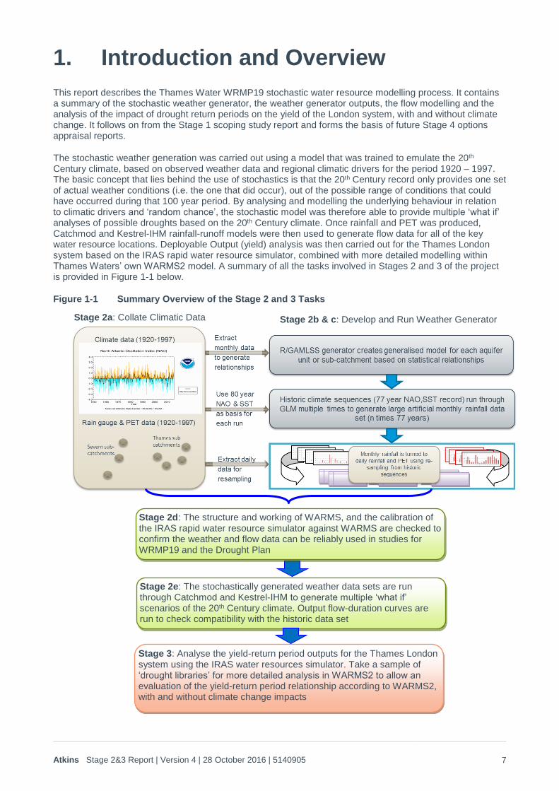
The stochastic weather generation was carried out using a model that was trained to emulate the 20th Century climate, based on observed weather data and regional climatic drivers for the period 1920 – 1997. The basic concept that lies behind the use of stochastics is that the 20th Century record only provides one set of actual weather conditions (i.e. the one that did occur), out of the possible range of conditions that could have occurred during that 100 year period. By analysing and modelling the underlying behaviour in relation to climatic drivers and ‘random chance’, the stochastic model was therefore able to provide multiple ‘what if’ analyses of possible droughts based on the 20th Century climate. Once rainfall and PET was produced, Catchmod and Kestrel-IHM rainfall-runoff models were then used to generate flow data for all of the key water resource locations. Deployable Output (yield) analysis was then carried out for the Thames London system based on the IRAS rapid water resource simulator, combined with more detailed modelling within Thames Waters’ own WARMS2 model. A summary of all the tasks involved in Stages 2 and 3 of the project is provided in Figure 1-1 below.
Figure 1-1 Summary Overview of the Stage 2 and 3 Tasks
Stage 2e: The stochastically generated weather data sets are run through Catchmod and Kestrel-IHM to generate multiple ‘what if’ scenarios of the 20th Century climate. Output flow-duration curves are run to check compatibility with the historic data set
Stage 2d: The structure and working of WARMS, and the calibration of the IRAS rapid water resource simulator against WARMS are checked to confirm the weather and flow data can be reliably used in studies for WRMP19 and the Drought Plan
Stage 2a: Collate Climatic Data Stage 2b & c: Develop and Run Weather Generator
Stage 3: Analyse the yield-return period outputs for the Thames London system using the IRAS water resources simulator. Take a sample of ‘drought libraries’ for more detailed analysis in WARMS2 to allow an evaluation of the yield-return period relationship according to WARMS2, with and without climate change impacts
Atkins Stage 2&3 Report | Version 4 | 28 October 2016 | 5140905 8
2. Analysis Stages 2a & 2b: Stochastic Weather Generation
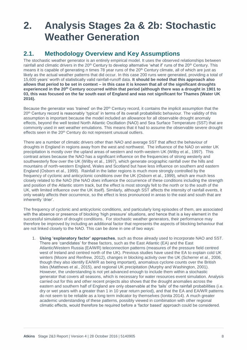
2.1. Methodology Overview and Key Assumptions The stochastic weather generator is an entirely empirical model. It uses the observed relationships between rainfall and climatic drivers in the 20th Century to develop alternative ‘what if’ runs of the 20th Century. This means it is capable of generating n times 78 year runs of the 20th Century climate, all of which are just as likely as the actual weather patterns that did occur. In this case 200 runs were generated, providing a total of 15,600 years’ worth of statistically valid rainfall-runoff data. It should be noted that this approach also allows that period to be set in context – in this case it is known that all of the significant droughts experienced in the 20th Century occurred within that period (although there was a drought in 1901 to 03, this was focused on the far south east of England and was not significant for Thames (Water UK 2016).
Because the generator was ‘trained’ on the 20th Century record, it contains the implicit assumption that the 20th Century record is reasonably ‘typical’ in terms of its overall probabilistic behaviour. The validity of this assumption is important because the model included an allowance for all observable drought anomaly effects, beyond the well tested North Atlantic Oscillation (NAO) and Sea Surface Temperature (SST) that are commonly used in wet weather emulations. This means that it had to assume the observable severe drought effects seen in the 20th Century do not represent unusual outliers.
There are a number of climatic drivers other than NAO and average SST that affect the behaviour of droughts in England in regions away from the west and northwest. The influence of the NAO on winter UK precipitation is mostly over the upland areas of western and north-western UK (Wilby et al., 1997). This contrast arises because the NAO has a significant influence on the frequencies of strong westerly and southwesterly flow over the UK (Wilby et al., 1997), which generate orographic rainfall over the hills and mountains of north-western England, Wales and Scotland but have less influence on southern and eastern England (Osborn et al., 1999). Rainfall in the latter regions is much more strongly controlled by the frequency of cyclonic and anticyclonic conditions over the UK (Osborn et al., 1999), which are much less closely related to the NAO (the NAO does influence the occurrence of these conditions including the strength and position of the Atlantic storm track, but the effect is most strongly felt to the north or to the south of the UK, with limited influence over the UK itself). Similarly, although SST affects the intensity of rainfall events, it only weakly affects their occurrence, so the effect is less pronounced in areas to the east and south that are inherently ‘drier’.
The frequency of cyclonic and anticyclonic conditions, and particularly long episodes of them, are associated with the absence or presence of blocking ‘high pressure’ situations, and hence that is a key element in the successful simulation of drought conditions. For stochastic weather generators, their performance may therefore be improved by including an additional factor that represents the aspects of blocking behaviour that are not linked closely to the NAO. This can be done in one of two ways:
1. Using ‘explanatory factor’ approaches, such as those already used to incorporate NAO and SST. There are ‘candidates’ for these factors, such as the East Atlantic (EA) and the East Atlantic/Western Russia (EA/WR) teleconnection patterns (measures of the pressure field centred west of Ireland and centred north of the UK). Previous studies have used the EA to explain cold UK winters (Moore and Renfrew, 2012), changes in blocking activity over the UK (Scherrer et al., 2006, though they also identify EA/WR as being important), anomalous cyclone counts over the British Isles (Matthews et al., 2015), and regional UK precipitation (Murphy and Washington, 2001). However, the understanding is not yet advanced enough to include them within a stochastic generator that covers all seasons, which is necessary for water resources event simulation. Analysis carried out for this and other recent projects also shows that the drought anomalies across the eastern and southern half of England are only observable at the ‘tails’ of the rainfall probabilities (i.e. dry or wet years with a greater than 1 in 10 year return period), and that the EA and EA/WR patterns do not seem to be reliable as a long term indicator by themselves (Ionita 2014). A much greater academic understanding of these patterns, possibly viewed in combination with other regional climatic effects, would therefore be required before a ‘factor based’ approach could be considered.
Atkins Stage 2&3 Report | Version 4 | 28 October 2016 | 5140905 9
2. Multi-metric curve fitting. This approach works by using observed anomalies that show deviation of the statistical behaviour of the historic climate from predictions that incorporate NAO, SST and ‘random’ variability. These anomalies act as a ‘proxy’ for all of the other potential influences, so the observed anomalies for various metrics of cumulative rainfall (e.g. calendar year, hydrological year, winter etc) can be used to adjust (curve fit) the stochastic weather generator outputs and produce an accurate emulator of the 20th Century climate.
For the sake of practicality and reconciliation with the data that are used for WRMP DO assessment, the analysis described in this report has therefore used the second approach, with suitable checks to ensure that the curve fitting process has not unacceptably affected spatial coherence in the modelling at any of the metric levels. On an academic basis there were four important findings relating to the nature of drought behaviour in England that were achieved as part of this and other similar projects carried out during 2015/16:
1. It was found that ‘droughts’ behave differently to the rest of the rainfall record. Under ‘normal’ years there is no statistically significant correlation between monthly rainfall values. However, in the central, south and east of England, under drought conditions (generally years with a 1 in 10 year or greater low rainfall return period) some between month persistence in low rainfall can be observed, beyond that ‘explained’ by NAO and SST patterns. This persistence ‘anomaly’ becomes observably stronger towards the south and east of the country.
2. It was found that the 20th Century record contained sufficient trend based data to allow an analysis of the statistical behaviour of these ‘persistence’ anomalies, incorporating duration, intensity and patterns. This is described further in Section 2.4.1
3. The ‘natural scale’ of the drought anomalies was analysed, and it was found that the spatial coherence of droughts could be very well maintained if this ‘natural scale’ was incorporated into the curve fitting. Again, this principle is described further in Section 2.4.1.
4. PET also demonstrates a ‘persistence’ anomaly, whereby the total PET that occurs over the spring
and summer period is higher during drought conditions than would be expected if there were no correlation between months. There is a significant correlation between this PET persistence and ‘anomaly’ persistence of low rainfall that is encountered under drought conditions.
These findings were used to create a weather generator that was able to statistically emulate observed 20th Century behaviour to a high degree of validation, even down to the most severe events. The use of this approach does mean that the model effectively assumes that anomalies that are demonstrated by the droughts (greater than 1 in 10 year return period) in the 20th Century are ‘typical’ for the climate in the central, south and east of England (i.e. the regions with less NAO/SST influence). On a planning basis this assumption was considered to be reasonable, provided that the curve fitting was able to replicate the underlying statistical behaviour of the anomalies, and the available academic literature confirmed that the more severe events contained within the 20th Century (e.g. 1921-22, 1932-34, 1975-1976) are not notable outliers within a longer term record.
The academic literature was therefore reviewed to examine the availability of longer term data sets and confirm whether there is evidence that the 20th Century droughts have been exceeded by drought events in the past. A summary of this literature review is provided in Appendix A of this report. Overall this indicated that:
1. In terms of rainfall, the 20th Century does not display any ‘unusual’ behaviour compared with longer term gauges and river flows. There is some evidence that the 20th Century actually included less drought persistence than earlier records, which could mean that this analysis is too conservative (i.e. the generated droughts are not severe enough). However, this is offset by other, marginal evidence that a warming trend has affected summer moisture availability due to increases in PET compared with longer term historic records. Overall those longer term studies indicate that the use of the 20th Century data on severe droughts, as the basis for a pre-21st Century climate change emulator, is likely to be the most robust approach if a stochastically based weather generator is being used.
2. The individual severe’ droughts in the 20th Century do not appear to be particular outliers when compared with longer term records. Even 1921, which included unusually dry full-year conditions does not appear to be exceptional (i.e. significantly beyond a 1 in 100 year type return period) when viewed in the context of the central-northern continental effects that contributed to the drought in southern England. The limited evidence that is available also indicates that much more severe
Atkins Stage 2&3 Report | Version 4 | 28 October 2016 | 5140905 10
events than those encountered in the 20th Century are possible, and did occur over the last millennium.
This ability to emulate and extrapolate historic drought data, whilst at the same time using available research and hindcasting information to check the key assumptions surrounding extreme droughts, is valuable. Because the validation of artificial drought generators will only ever be able to use a few ‘reliable’ data points for the more severe events, it is very advantageous to be able to use the findings of more general data in this way. It allows plausible, probabilistically based drought generation, without having to over-rely on the large uncertainties associated with hindcasting beyond the 20th Century, including error/inconsistency in the older weather records (referred to by numerous authors), and the large, unknown biases that occur as a result of the spatial scarcity of older weather records.
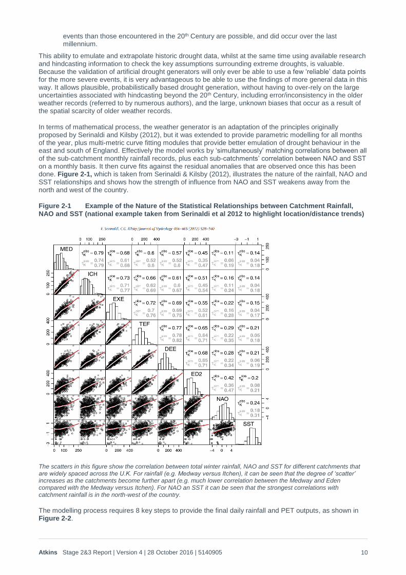
In terms of mathematical process, the weather generator is an adaptation of the principles originally proposed by Serinaldi and Kilsby (2012), but it was extended to provide parametric modelling for all months of the year, plus multi-metric curve fitting modules that provide better emulation of drought behaviour in the east and south of England. Effectively the model works by ‘simultaneously’ matching correlations between all of the sub-catchment monthly rainfall records, plus each sub-catchments’ correlation between NAO and SST on a monthly basis. It then curve fits against the residual anomalies that are observed once this has been done. Figure 2-1, which is taken from Serinaldi & Kilsby (2012), illustrates the nature of the rainfall, NAO and SST relationships and shows how the strength of influence from NAO and SST weakens away from the north and west of the country.
Figure 2-1 Example of the Nature of the Statistical Relationships between Catchment Rainfall, NAO and SST (national example taken from Serinaldi et al 2012 to highlight location/distance trends)
The scatters in this figure show the correlation between total winter rainfall, NAO and SST for different catchments that are widely spaced across the U.K. For rainfall (e.g. Medway versus Itchen), it can be seen that the degree of ‘scatter’ increases as the catchments become further apart (e.g. much lower correlation between the Medway and Eden compared with the Medway versus Itchen). For NAO an SST it can be seen that the strongest correlations with catchment rainfall is in the north-west of the country.
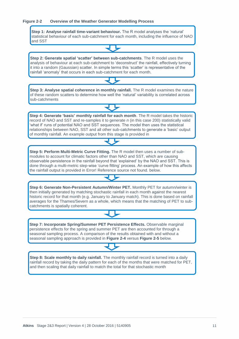
The modelling process requires 8 key steps to provide the final daily rainfall and PET outputs, as shown in Figure 2-2.
Atkins Stage 2&3 Report | Version 4 | 28 October 2016 | 5140905 11
Figure 2-2 Overview of the Weather Generator Modelling Process
Step 1: Analyse rainfall time-variant behaviour. The R model analyses the ‘natural’ statistical behaviour of each sub-catchment for each month, including the influence of NAO and SST
Step 2: Generate spatial ‘scatter’ between sub-catchments. The R model uses the analysis of behaviour at each sub-catchment to ‘deconstruct’ the rainfall, effectively turning it into a random (Gaussian) scatter. In simple terms this ‘scatter’ is representative of the rainfall ‘anomaly’ that occurs in each sub-catchment for each month.
Step 3: Analyse spatial coherence in monthly rainfall. The R model examines the nature of these random scatters to determine how well the ‘natural’ variability is correlated across sub-catchments
Step 4: Generate ‘basic’ monthly rainfall for each month. The R model takes the historic record of NAO and SST and re-samples it to generate n (in this case 200) statistically valid ‘what if’ runs of potential NAO and SST sequences. The model then uses the statistical relationships between NAO, SST and all other sub-catchments to generate a ‘basic’ output of monthly rainfall. An example output from this stage is provided in
Figure 2-3 below. Step 5: Perform Multi-Metric Curve Fitting. The R model then uses a number of sub-modules to account for climatic factors other than NAO and SST, which are causing observable persistence in the rainfall beyond that ‘explained’ by the NAO and SST. This is done through a multi-metric step-wise ‘curve fitting’ process. An example of how this affects the rainfall output is provided in Error! Reference source not found. below.
Step 6: Generate Non-Persistent Autumn/Winter PET. Monthly PET for autumn/winter is then initially generated by matching stochastic rainfall in each month against the nearest historic record for that month (e.g. January to January match). This is done based on rainfall averages for the Thames/Severn as a whole, which means that the matching of PET to sub-catchments is spatially coherent.
Step 7: Incorporate Spring/Summer PET Persistence Effects. Observable marginal persistence effects for the spring and summer PET are then accounted for through a seasonal sampling process. A comparison of the results obtained with and without a seasonal sampling approach is provided in Figure 2-4 versus Figure 2-5 below.
Step 8: Scale monthly to daily rainfall. The monthly rainfall record is turned into a daily rainfall record by taking the daily pattern for each of the months that were matched for PET, and then scaling that daily rainfall to match the total for that stochastic month
Atkins Stage 2&3 Report | Version 4 | 28 October 2016 | 5140905 12
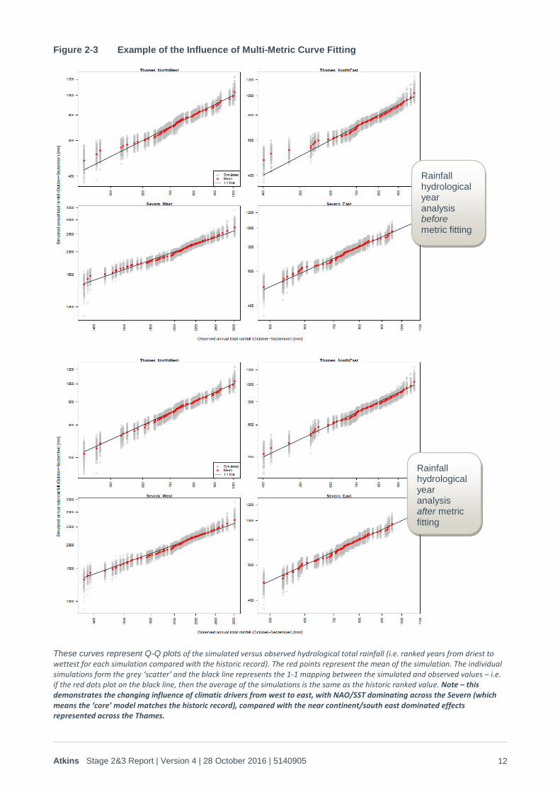
Figure 2-3 Example of the Influence of Multi-Metric Curve Fitting
These curves represent Q-Q plots of the simulated versus observed hydrological total rainfall (i.e. ranked years from driest to wettest for each simulation compared with the historic record). The red points represent the mean of the simulation. The individual simulations form the grey ‘scatter’ and the black line represents the 1-1 mapping between the simulated and observed values – i.e. if the red dots plot on the black line, then the average of the simulations is the same as the historic ranked value. Note – this demonstrates the changing influence of climatic drivers from west to east, with NAO/SST dominating across the Severn (which means the ‘core’ model matches the historic record), compared with the near continent/south east dominated effects represented across the Thames.
Rainfall hydrological year analysis before metric fitting
Rainfall hydrological year analysis after metric fitting

Atkins Stage 2&3 Report | Version 4 | 28 October 2016 | 5140905 13
Figure 2-4 Historic versus Simulated PET without Spring/Summer Persistence Fitting (hydrological year – exaggerated scale)
Figure 2-5 Historic versus Simulated PET with Spring/Summer Persistence Fitting
The key checks on the plausibility of the generator for providing reliable drought outputs for water resource planning purposes can be defined as its ability to:
1. Match the observed historic records in terms of the probability of exceedance of a number of different rainfall total metrics (hydrological year totals, calendar year totals, 1, 2 and 3 winter totals)
2. Maintain spatial coherence in rainfall, as evidenced by the matches that are achieved at both the sub-catchment level, and the regional average level.
3. Provide a spatially coherent estimate of hydrologically effective rainfall (HER), equal to rainfall minus PET for each month, which also matches the percentile behaviour for the same metrics as tested for rainfall (i.e. hydrological year, calendar year, winter totals).
4. Generate a ‘plausible’ pattern of the daily rainfall that would occur in each stochastically generated month. In this case ‘plausible’ reflects the sort of rainfall patterns that could actually be observed given the monthly rainfall total and PET that occurred in that month.
The first three items were tested in detail following the weather generation stage, and are summarised in Section 2.5. The final check was effectively performed as part of the flow analysis, as the key risk from a
Atkins Stage 2&3 Report | Version 4 | 28 October 2016 | 5140905 14
poor representation of daily rainfall patterns is under or over estimation of recharge. The validity against this fourth check is therefore provided in Section 3.2.
2.2. Alternatives Considered Two potential alternative approaches were considered for this project:
1. The use of an alternative stochastic approach that used temperature/PET rather than monthly rainfall as the initial ‘match’, and then generated rainfall as a second stage.
2. The use of weather generators based on ‘downscaling’ of results from physically based Regional Climate models (e.g. UKCP09).
For the first alternative (a temperature ‘led’ approach), daily temperature is the primary factor that is generated, and then rainfall is estimated based on the probability of a wet day occurring and the rainfall total within each wet day. Although this approach is less well researched than the rainfall led approach described in this report, it does have some potential advantages, including a stronger correlation with weather types (e.g. low versus high pressure) and more of a direct link with climate change effects such as heatwaves. However, because the rainfall led approach described in this report is based on twelve monthly models (which inherently means that weather types are well represented), and because it is linked to hydrological models (which store moisture and hence reduce the importance of features such as summer heatwaves), then those advantages are likely to be marginal. This needs to be set against two significant drawbacks that would have to be addressed if a temperature led model were to be used:
Because rainfall variability is much larger than temperature, it is not possible to use a re-sampling approach to generate daily rainfall from monthly temperature. This means temperature led models would have to be based on daily time steps, which makes the longer term, marginal persistence effects associated with droughts very hard to emulate.
Temperature anomalies tend to have a wider spatial coverage and consistency than rainfall. This means that the more highly variable component, rainfall, would have to be generated using secondary relationships that ensure consistency with the emulated temperature record. As shown above, when a rainfall led model is used, then residual persistence in temperature can easily be incorporated through curve fitting, and its wide spatial nature means that this doesn’t disrupt the spatial correlation in PET. Rainfall does not have the same degree of spatial coherence, so attempting to curve fit the persistence in rainfall after temperature has been generated would require additional, highly complex spatial correlation analysis that would not be able to rely on the same ‘de-construction’ approach used in the rainfall generator.
These issues, along with the fact that temperature led approaches have not been adequately tested and calibrated for drought application in the U.K. context, means that a rainfall led approach was recommended for application to this project. This was endorsed by Professor Chris Kilsby, meteorologist, University of Newcastle
In terms of physical climate model based weather generators, previous ‘downscaling’ approaches such as UKCP09 have not been able to replicate droughts very well, although it is noted that this was not their primary purpose. However, academic literature shows that the regionally based climate models (RCMs) that such generators sample from are effectively too small to simulate blocking situations within their domain. They therefore rely on ‘importing’ that behaviour from a Global Climate Model (GCM). A number of studies have evaluated the ability of GCMs to simulate realistic blocking climatologies over the Northern Hemisphere and in the Atlantic/European region (e.g. Vial and Osborn (2012)). These have found very mixed results, but all GCMs simulated fewer episodes than observed, especially longer lasting ones. Many of the errors are related to biases in the GCMs’ mean circulation over these regions, and simple bias corrections were able to yield a much improved simulation of blocking frequency and duration (Vial and Osborn, 2012). However, because the influence of blocking on extreme weather events can be complex (e.g. depending not just on the intensity of blocking but also on its duration), success in bias correcting the atmospheric circulation does not guarantee that bias correction of the simulated precipitation or temperature by the GCM (or by an embedded RCM) would recover the correct statistics of extreme weather events. What determines blocking in the real world is an active area of research (e.g. Vial et al., 2013), but this is not yet advanced enough to allow accurate drought representation. There are a number of projects that will seek to overcome these issues (e.g. MaRIUS, UKCP18), but these are not yet advanced enough to determine the level of ‘success’ that they might achieve.
Atkins Stage 2&3 Report | Version 4 | 28 October 2016 | 5140905 15
2.3. Data Used Rainfall data for this project was taken from the existing sub-catchment data used in the WARMS and Kestrel-IHM models. The data set was limited to the period 1920 to 1997 because:
Actual records pre 1920 are sparse and rely heavily on interpolation. Tests carried out for this project indicated that the statistical behaviour of the data in the period 1920 – 1935 is only just coherent enough to allow valid statistical analysis. Before 1920 a number of sub-catchments would have to rely on rainfall records from gauges that are not located within the sub-catchment, and that starts to affect the statistical consistency of the data set, particularly when it is linked to periods such as 1961 – 1998, where there are large numbers of gauges within all sub-catchments.
After the 1997 drought there is a rapid, observable increase in SST associated with climate change, so data after this point have not been included as part of a ‘stationary’ climate baseline.
Rainfall inputs were formulated as a sub-catchment average for the 11 individual sub-catchments that are already used in WARMS. For the Severn, 12 sub-catchments were created and catchment average data sets were created based on the CEH GEAR 1km gridded data set. This version of the Kestrel-IHM model was then used for calibration checking and analysis of the historical performance of the River Severn flows (i.e. it is the same as the data set that is being used in other WRMP19 studies by Thames).
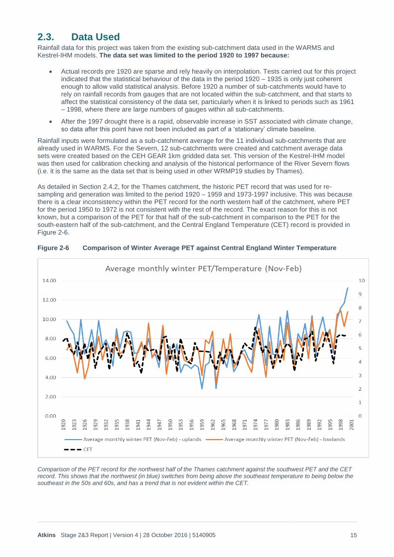
As detailed in Section 2.4.2, for the Thames catchment, the historic PET record that was used for re-sampling and generation was limited to the period 1920 – 1959 and 1973-1997 inclusive. This was because there is a clear inconsistency within the PET record for the north western half of the catchment, where PET for the period 1950 to 1972 is not consistent with the rest of the record. The exact reason for this is not known, but a comparison of the PET for that half of the sub-catchment in comparison to the PET for the south-eastern half of the sub-catchment, and the Central England Temperature (CET) record is provided in Figure 2-6.
Figure 2-6 Comparison of Winter Average PET against Central England Winter Temperature
Comparison of the PET record for the northwest half of the Thames catchment against the southwest PET and the CET record. This shows that the northwest (in blue) switches from being above the southeast temperature to being below the southeast in the 50s and 60s, and has a trend that is not evident within the CET.

Atkins Stage 2&3 Report | Version 4 | 28 October 2016 | 5140905 16
2.4. Methodology Details
2.4.1. Monthly Rainfall Generation Details of the mathematical processes used to generate the basic monthly rainfall outputs are fully described within Serinaldi & Kilsby (2012). In simple terms, the R module initially uses a standard de-seasonalising approach to generate de-seasonalised rainfall probability distributions for each calendar month in each sub-catchment, and then creates Generalised Linear Models that describe the nature of this rainfall. Each GLM contains two components, which describe the mean and standard deviation of rainfall for each sub-catchment for that month, based on NAO, SST and the observed ‘natural variability’ that is not accounted for by NAO and SST, i.e. :
𝜇𝑥𝑎 = 𝑓𝑛(𝑁𝐴𝑂𝑥) + 𝑓𝑛(𝑆𝑆𝑇𝑥) + 𝜀𝑥𝑎
𝜎𝑥𝑎 = 𝑓𝑛(𝑁𝐴𝑂𝑥) + 𝑓𝑛(𝑆𝑆𝑇𝑥)
Where:
μxa = the mean of the rainfall for site a in month x
fn (NAOx) = function of the observed North Atlantic Oscillation index anomaly for month x
fn (SSTx) = function of the observed sea surface temperature anomaly for month x
εxa = the amount of de-seasonalised ‘error’ (random variability) for month x at site a
𝜎xa = the variance (standard deviation squared) for site a in month x
The R model uses these GLMs to ‘deconstruct’ the rainfall record at each sub-catchment (i.e. it removes the specific seasonal, NAO and SST influences), and generates ‘Gaussian’ distributions that are statistically comparable across all the sub-catchments, and describe the random variability in rainfall at each site for each month. The model then generates an n-dimensional copula (where n is equal to the number of sub-catchments), which effectively describes how much correlation there is in this ‘random variability’ between all the sub-catchments. In other words, it evaluates the spatial coherence of monthly rainfall totals across the region.
The multi-metric curve fitting of the observable anomalies between historic and stochastic rainfall after the NAO/SST based generator has produced its initial simulations is then carried out within the model. The multi-metric curve fitting was carried out based on the following two key principles:
1. The ‘natural scale’ of the anomalies was found to be at the sub-regional scale. This does not mean that droughts only occur at that scale, but rather that, on a statistical basis, if the anomaly curve fitting is carried out at that scale then the covariant structure of the droughts is maintained across all spatial scales. It also means that individual sub-catchments are not over-fitted, but rather general drought behaviour is replicated across the catchments as a whole. The four sub-regions that were used were:
a. Thames southeast
b. Thames northwest
c. Severn east
d. Severn west
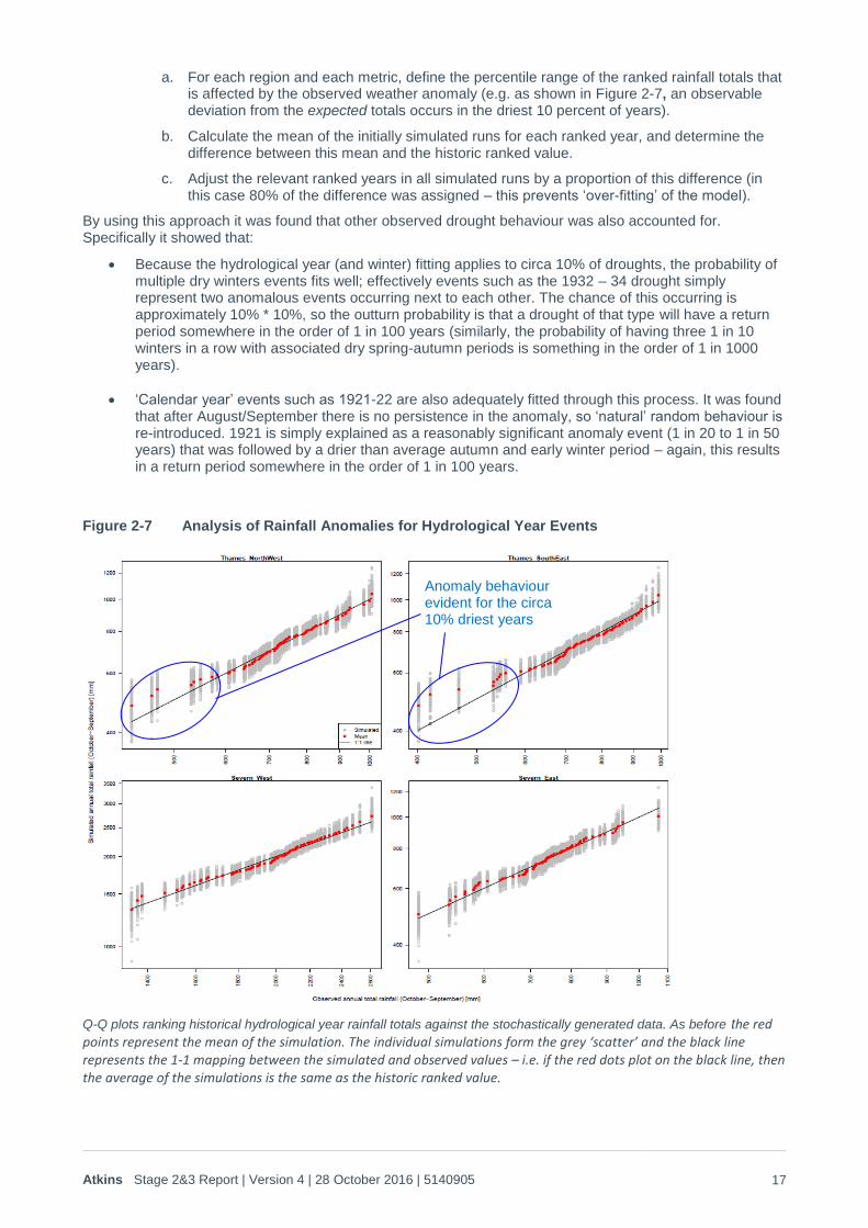
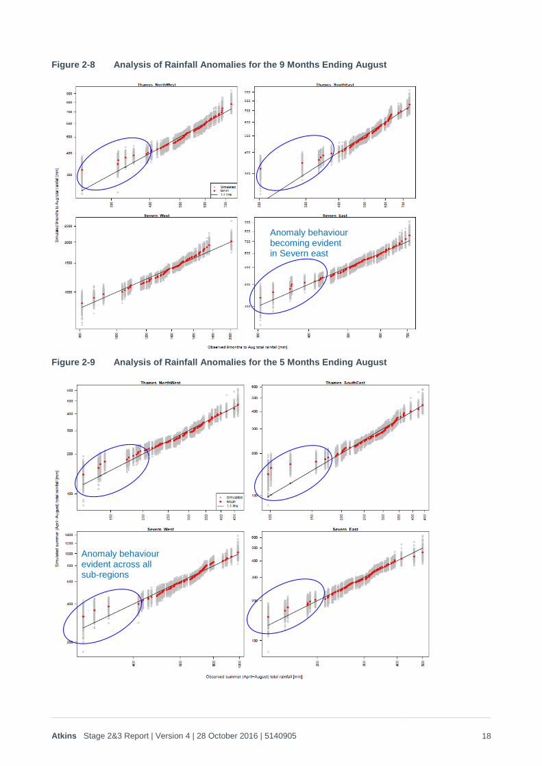
2. Generation of Q-Q plots showed that the anomaly occurs over a hydrological year (October to September), affecting around 10% of years in the Thames catchment, but with relatively little influence on the Severn catchment (Figure 2-7). The anomaly then intensifies significantly during the December to August period, and starts to become apparent over the eastern side of the Severn catchment (Figure 2-8). The intensity over April to August is then similar (Figure 2-9), but there is some evidence that the very driest (5%) years demonstrate this summer anomaly right the way across to the western side of the Severn catchment that it intensifies during the 9 months December to August and is at its most intense over the April to August period. In order to reflect this behaviour, the curve fitting was therefore carried out on a step-wise basis, starting with the hydrological year and then fitting to the December-August, winter only and finally April to August period. In each step only 80% of the observed anomaly was accounted for to prevent over-fitting and hence hydrological year totals that were lower than they should be. The following process was therefore used for the curve fitting:
Atkins Stage 2&3 Report | Version 4 | 28 October 2016 | 5140905 17
a. For each region and each metric, define the percentile range of the ranked rainfall totals that is affected by the observed weather anomaly (e.g. as shown in Figure 2-7, an observable deviation from the expected totals occurs in the driest 10 percent of years).
b. Calculate the mean of the initially simulated runs for each ranked year, and determine the difference between this mean and the historic ranked value.
c. Adjust the relevant ranked years in all simulated runs by a proportion of this difference (in this case 80% of the difference was assigned – this prevents ‘over-fitting’ of the model).
By using this approach it was found that other observed drought behaviour was also accounted for. Specifically it showed that:
Because the hydrological year (and winter) fitting applies to circa 10% of droughts, the probability of multiple dry winters events fits well; effectively events such as the 1932 – 34 drought simply represent two anomalous events occurring next to each other. The chance of this occurring is approximately 10% * 10%, so the outturn probability is that a drought of that type will have a return period somewhere in the order of 1 in 100 years (similarly, the probability of having three 1 in 10 winters in a row with associated dry spring-autumn periods is something in the order of 1 in 1000 years).
‘Calendar year’ events such as 1921-22 are also adequately fitted through this process. It was found that after August/September there is no persistence in the anomaly, so ‘natural’ random behaviour is re-introduced. 1921 is simply explained as a reasonably significant anomaly event (1 in 20 to 1 in 50 years) that was followed by a drier than average autumn and early winter period – again, this results in a return period somewhere in the order of 1 in 100 years.
Figure 2-7 Analysis of Rainfall Anomalies for Hydrological Year Events
Q-Q plots ranking historical hydrological year rainfall totals against the stochastically generated data. As before the red points represent the mean of the simulation. The individual simulations form the grey ‘scatter’ and the black line represents the 1-1 mapping between the simulated and observed values – i.e. if the red dots plot on the black line, then the average of the simulations is the same as the historic ranked value.
Anomaly behaviour evident for the circa 10% driest years
Atkins Stage 2&3 Report | Version 4 | 28 October 2016 | 5140905 18
Figure 2-8 Analysis of Rainfall Anomalies for the 9 Months Ending August
Figure 2-9 Analysis of Rainfall Anomalies for the 5 Months Ending August
Anomaly behaviour becoming evident in Severn east
Anomaly behaviour evident across all sub-regions
Atkins Stage 2&3 Report | Version 4 | 28 October 2016 | 5140905 19
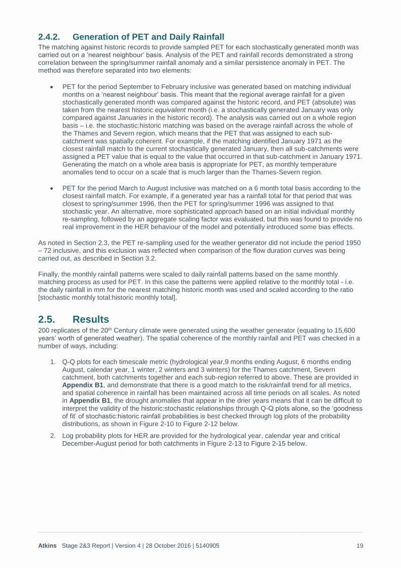
2.4.2. Generation of PET and Daily Rainfall The matching against historic records to provide sampled PET for each stochastically generated month was carried out on a ‘nearest neighbour’ basis. Analysis of the PET and rainfall records demonstrated a strong correlation between the spring/summer rainfall anomaly and a similar persistence anomaly in PET. The method was therefore separated into two elements:
PET for the period September to February inclusive was generated based on matching individual months on a ‘nearest neighbour’ basis. This meant that the regional average rainfall for a given stochastically generated month was compared against the historic record, and PET (absolute) was taken from the nearest historic equivalent month (i.e. a stochastically generated January was only compared against Januaries in the historic record). The analysis was carried out on a whole region basis – i.e. the stochastic:historic matching was based on the average rainfall across the whole of the Thames and Severn region, which means that the PET that was assigned to each sub-catchment was spatially coherent. For example, if the matching identified January 1971 as the closest rainfall match to the current stochastically generated January, then all sub-catchments were assigned a PET value that is equal to the value that occurred in that sub-catchment in January 1971. Generating the match on a whole area basis is appropriate for PET, as monthly temperature anomalies tend to occur on a scale that is much larger than the Thames-Severn region.
PET for the period March to August inclusive was matched on a 6 month total basis according to the closest rainfall match. For example, if a generated year has a rainfall total for that period that was closest to spring/summer 1996, then the PET for spring/summer 1996 was assigned to that stochastic year. An alternative, more sophisticated approach based on an initial individual monthly re-sampling, followed by an aggregate scaling factor was evaluated, but this was found to provide no real improvement in the HER behaviour of the model and potentially introduced some bias effects.
As noted in Section 2.3, the PET re-sampling used for the weather generator did not include the period 1950 – 72 inclusive, and this exclusion was reflected when comparison of the flow duration curves was being carried out, as described in Section 3.2.
Finally, the monthly rainfall patterns were scaled to daily rainfall patterns based on the same monthly matching process as used for PET. In this case the patterns were applied relative to the monthly total - i.e. the daily rainfall in mm for the nearest matching historic month was used and scaled according to the ratio [stochastic monthly total:historic monthly total].
2.5. Results 200 replicates of the 20th Century climate were generated using the weather generator (equating to 15,600 years’ worth of generated weather). The spatial coherence of the monthly rainfall and PET was checked in a number of ways, including:
1. Q-Q plots for each timescale metric (hydrological year,9 months ending August, 6 months ending August, calendar year, 1 winter, 2 winters and 3 winters) for the Thames catchment, Severn catchment, both catchments together and each sub-region referred to above. These are provided in Appendix B1, and demonstrate that there is a good match to the risk/rainfall trend for all metrics, and spatial coherence in rainfall has been maintained across all time periods on all scales. As noted in Appendix B1, the drought anomalies that appear in the drier years means that it can be difficult to interpret the validity of the historic:stochastic relationships through Q-Q plots alone, so the ‘goodness of fit’ of stochastic:historic rainfall probabilities is best checked through log plots of the probability distributions, as shown in Figure 2-10 to Figure 2-12 below.
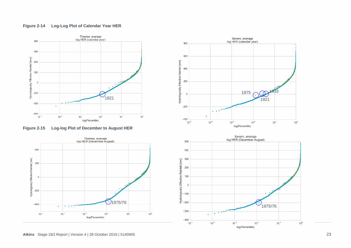
2. Log probability plots for HER are provided for the hydrological year, calendar year and critical December-August period for both catchments in Figure 2-13 to Figure 2-15 below.
Atkins Stage 2&3 Report | Version 4 | 28 October 2016 | 5140905 20
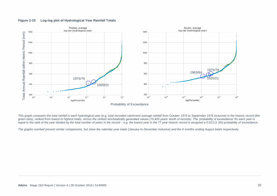
Figure 2-10 Log-log plot of Hydrological Year Rainfall Totals
This graph compares the total rainfall in each hydrological year (e.g. total recorded catchment average rainfall from October 1975 to September 1976 inclusive) in the historic record (the green dots), ranked from lowest to highest totals, versus the ranked stochastically generated values (15,400 years’ worth of records). The ‘probability of exceedance’ for each year is equal to the rank of the year divided by the total number of years in the record – e.g. the lowest year in the 77 year historic record is assigned a 0.013 (1.3%) probability of exceedance. The graphs overleaf present similar comparisons, but show the calendar year totals (January to December inclusive) and the 9 months ending August totals respectively.
Tota
l A
nnua
l R
ain
fall
with
in M
etr
ic P
eri
od (
mm
)
Probability of Exceedance
1975/76
1920/21
1963/64
1920/21
1975/76
Atkins Stage 2&3 Report | Version 4 | 28 October 2016 | 5140905 21
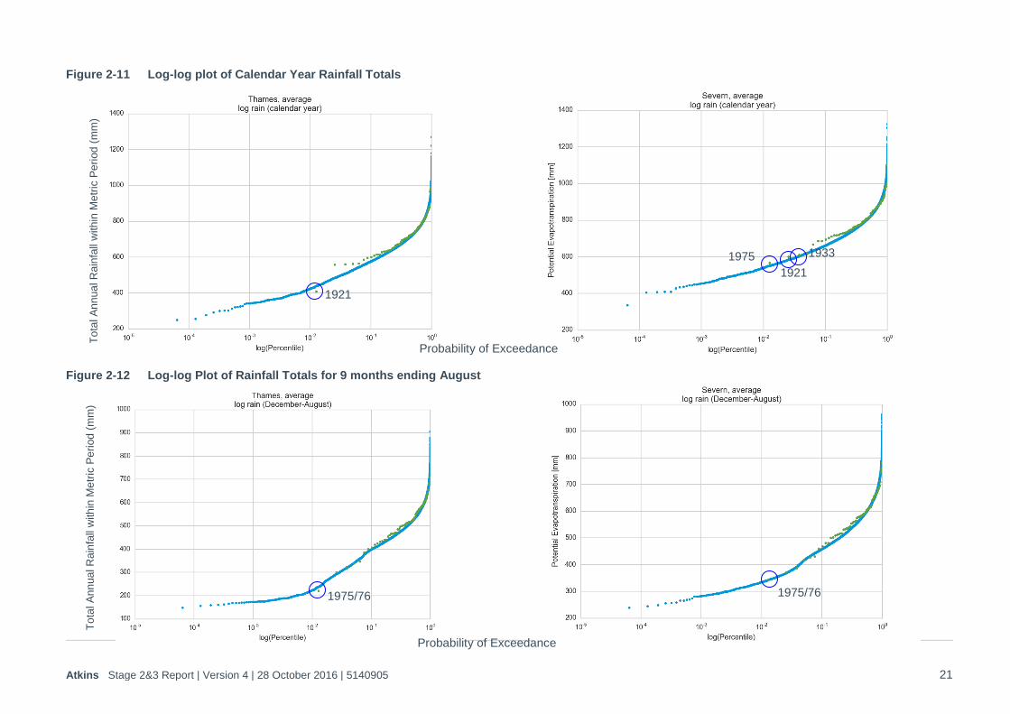
Figure 2-11 Log-log plot of Calendar Year Rainfall Totals
Figure 2-12 Log-log Plot of Rainfall Totals for 9 months ending August
To
tal A
nn
ua
l R
ain
fall
with
in M
etr
ic P
eri
od
(m
m)
1975/76
1921
To
tal A
nn
ua
l R
ain
fall
with
in M
etr
ic P
eri
od
(m
m)
Probability of Exceedance
1975/76
Probability of Exceedance
1975
1921
1933
Atkins Stage 2&3 Report | Version 4 | 28 October 2016 | 5140905 22
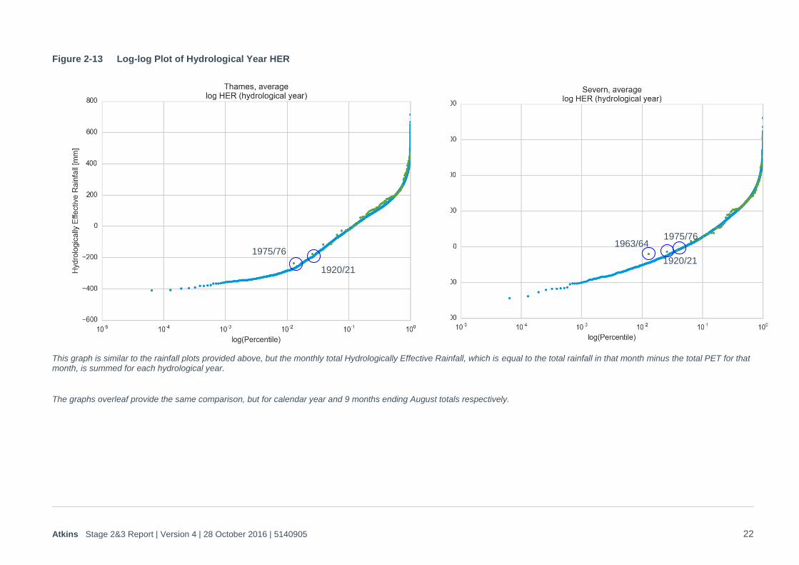
Figure 2-13 Log-log Plot of Hydrological Year HER
This graph is similar to the rainfall plots provided above, but the monthly total Hydrologically Effective Rainfall, which is equal to the total rainfall in that month minus the total PET for that month, is summed for each hydrological year.
The graphs overleaf provide the same comparison, but for calendar year and 9 months ending August totals respectively.
1975/76
1920/21
1963/64
1920/21
1975/76
Atkins Stage 2&3 Report | Version 4 | 28 October 2016 | 5140905 23
Figure 2-14 Log-Log Plot of Calendar Year HER
Figure 2-15 Log-log Plot of December to August HER
1921
1975/76 1975/76
1975
1921
1933

Atkins Stage 2&3 Report | Version 4 | 28 October 2016 | 5140905 24
The above charts confirm that the historic years tend to provide a scatter around the stochastically generated curve. In some cases there is a tendency for the historic years to plot slightly above the tail of the stochastic curve (e.g. HER calendar year), but in others the driest historic years have a probability of exceedance < 0.01 (equivalent to a >1 in 100 year return period). This demonstrates that the stochastic data has not been ‘over-fitted’, but generally forms a good underlying probability curve across all of the tested metrics.
The only notable metric that plotted above the curve were 1963/64 (the lower HER for a hydrological year) and 1975 (the lower HER for a calendar year) for the Severn catchment. In both cases this was because the years had a significantly below trend PET for the summer period (i.e. dry but relatively cold), when compared with the rainfall. As shown in the 9 months to August plot, if the ‘hydrological year’ had been taken from September to August inclusive, then 1975/76 would have plotted well below the stochastic curve. It is also noted that the only significant anomaly adjustment to the Severn was for the 9 month December to August period (where the worst history plotted below the historic line). It was therefore concluded that the deviation from the stochastic record was entirely due to the randomly colder nature of those two summers (1964 and 1975), and did not represent an issue with the stochastic modelling.
It is noted that the analyses are potentially slightly conservative, as the anomalies were fitted on a ratio rather than absolute basis - i.e. the worst year in each run was multiplied by a factor, rather than reduced by an absolute mm rainfall value, which means the relative strength of the anomaly reduces for very dry events. It is therefore feasible that the very high return period droughts (1 in 500+) could be drier than shown. This accounts for the ‘flattening off’ of the curves at high return periods. However, as the underlying cause of the anomalies is not well understood it was considered that a conservative approach was appropriate for planning purposes.
The attribution of daily rainfall patterns is comparatively trivial compared with monthly rainfall and PET, and only needs to be representative enough to ensure that there is no bias in the recharge calculation when compared with the historic record. This is therefore demonstrated through the flow-duration analyses presented in Section 3.2.
Atkins Stage 2&3 Report | Version 4 | 28 October 2016 | 5140905 25
3. Analysis Stage 2c: Flow Modelling
3.1. Methodology and Key Assumptions The weather data were used to develop a large set of daily flow timeseries by running the following existing
catchment models that were developed during previous studies for Thames:
Catchmod, which was originally developed by the NRA for the Thames catchment. This uses the
same model structure as the aquifer unit based model that is incorporated into WARMS2, and for
this study the Catchmod model was re-calibrated to ensure consistency with the WARMS2 flow
outputs. This was done using the historic sub-catchment data contained in WARMS2. It provides
flows at the three locations required for WARMS and IRAS – Days Weir and Teddington Weir on the
Thames, and Fieldes Weir on the Lower Lee. Both the WARMS2 and Catchmod models are
calibrated against ‘semi-naturalised’ flows in the Thames. These are equal to the recorded flows at
the Kingston gauge, minus the Thames Water London abstractions.
Kestrel-IHM, which is an HR Wallingford rainfall-runoff model that has been used by the EA for flow
assessments on the Severn, and is currently being used by Thames Water to investigate the
Severn-Thames transfer. It uses sub-catchment average GEAR rainfall inputs. The flow
denaturalisation process is complex as it involves emulation of the ‘water bank’ control rules that are
used to control discharges from the Vyrnwy and Clywedog reservoirs, plus ‘best estimates’ of the
abstractions and discharge returns recorded for Severn Trent and South Staffs water. Kestrel-IMH
contains a water resource simulation module that is able to emulate this process, and the workings
have been checked with both the EA and other water companies. The calibration process was
carried out mainly for other Thames projects, and is not described here, but the model is the same
as that used in those other ongoing Thames Water investigations.
The rainfall-runoff modelling process itself was exactly the same as a climate change type analysis, whereby
the multiple (200) rainfall and PET data sets for the 77 year sequence are loaded sequentially into the model
and processed on a batch-run basis.
For the Thames Catchmod models initial yield analysis showed that the low flow match between Catchmod
and WARMS was not accurate enough to provide a reliable ranking of drought sequences within IRAS. This
affected both the stochastic sequences, and historic years that were run through the Catchmod model (for
example the Catchmod run historic sequence generated flows that resulted in the yield for 1921 being much
higher than 1976 – this was clearly caused by Catchmod failing to replicate the early recession that occurred
in 1921). Two methods were therefore used to achieve a better calibration between the lumped Catchmod
and WARMS2 hydrology:
1. An algorithm based flow-duration curve (FDC) method, where the baseflow and spate flows were
separated and adjusted according to the observed differences for FDC percentiles during the 20th
Century droughts. Whilst this provided a reasonable outturn calibration, it did cause concerns that
the Catchmod model outputs would not be reliable for the purposes of climate change analysis.
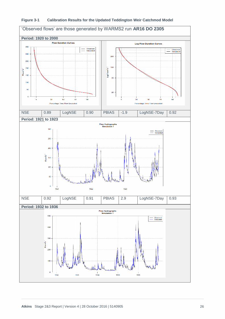
2. A re-calibration of the Thames Catchmod model, which involved some separation into sub-
catchments. The calibration fit of the new model at Teddington Weir is shown in Figure 3-1 covering
both the whole FDC and the calibration during the key 20th Century droughts.
The availability of two different hydrological modelling approaches was used as an opportunity to further test
the robustness of the weather generator. Flow comparisons for both the original adjusted model and the re-
calibrated model are therefore provided within Section 3.2 below.
Atkins Stage 2&3 Report | Version 4 | 28 October 2016 | 5140905 26
Figure 3-1 Calibration Results for the Updated Teddington Weir Catchmod Model
‘Observed flows’ are those generated by WARMS2 run AR16 DO 2305
Period: 1920 to 2000
NSE 0.89 LogNSE 0.90 PBIAS -1.9 LogNSE-7Day 0.92
Period: 1921 to 1923
NSE 0.92 LogNSE 0.91 PBIAS 2.9 LogNSE-7Day 0.93
Period: 1932 to 1936
Atkins Stage 2&3 Report | Version 4 | 28 October 2016 | 5140905 27
NSE 0.91 LogNSE 0.92 PBIAS 1.2 LogNSE-7Day 0.94
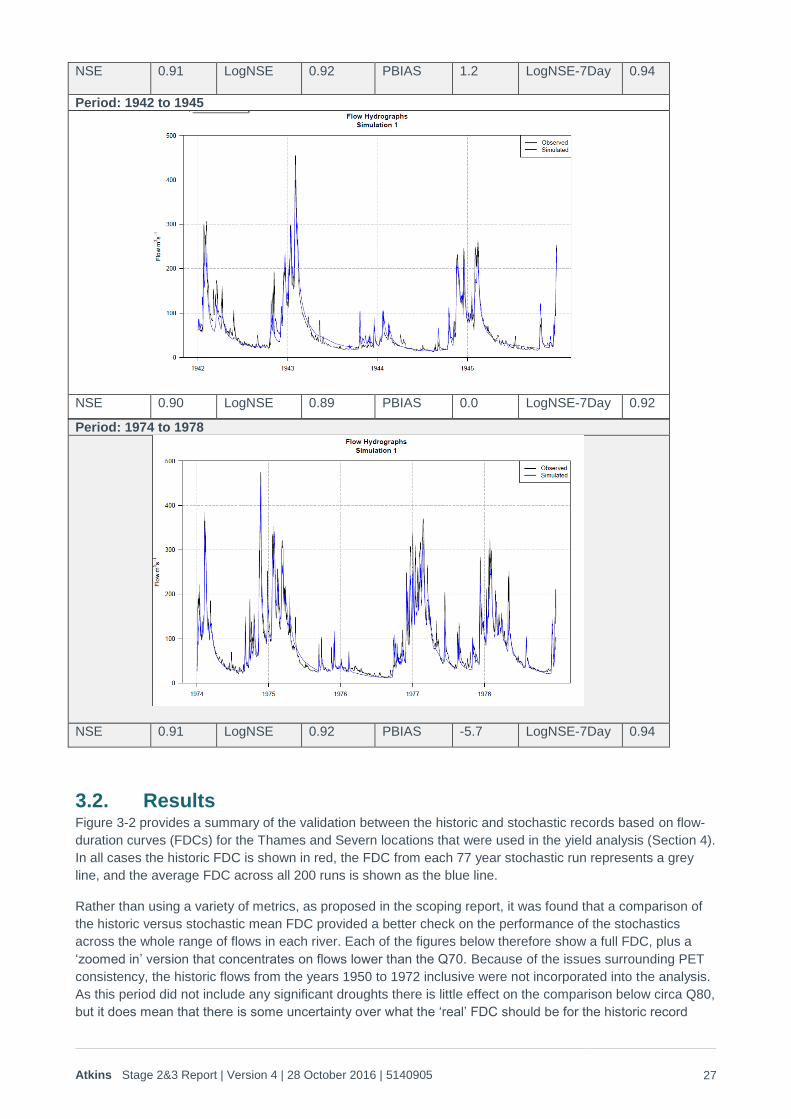
Period: 1942 to 1945
NSE 0.90 LogNSE 0.89 PBIAS 0.0 LogNSE-7Day 0.92
Period: 1974 to 1978
NSE 0.91 LogNSE 0.92 PBIAS -5.7 LogNSE-7Day 0.94
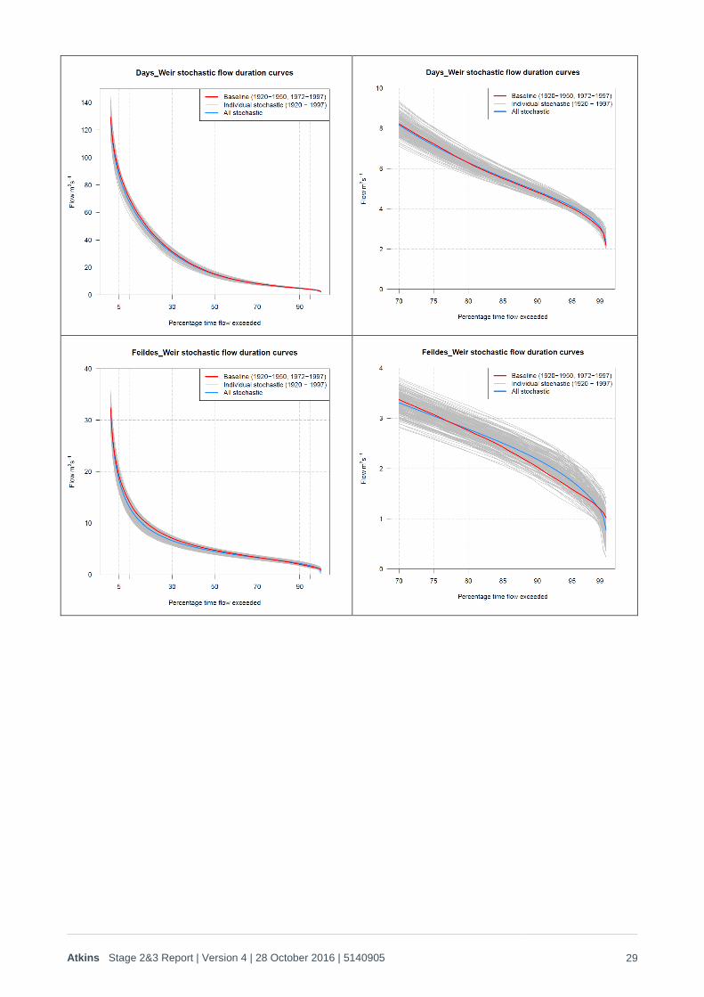
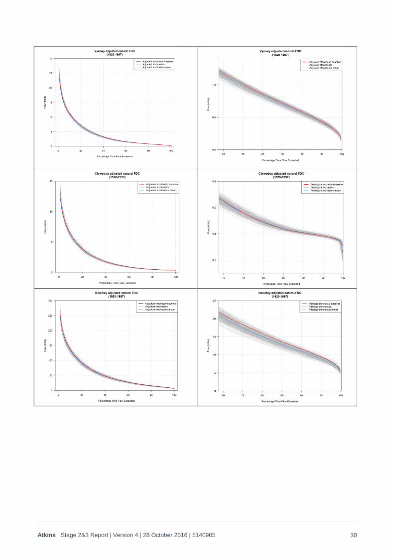
3.2. Results Figure 3-2 provides a summary of the validation between the historic and stochastic records based on flow-
duration curves (FDCs) for the Thames and Severn locations that were used in the yield analysis (Section 4).
In all cases the historic FDC is shown in red, the FDC from each 77 year stochastic run represents a grey
line, and the average FDC across all 200 runs is shown as the blue line.
Rather than using a variety of metrics, as proposed in the scoping report, it was found that a comparison of
the historic versus stochastic mean FDC provided a better check on the performance of the stochastics
across the whole range of flows in each river. Each of the figures below therefore show a full FDC, plus a
‘zoomed in’ version that concentrates on flows lower than the Q70. Because of the issues surrounding PET
consistency, the historic flows from the years 1950 to 1972 inclusive were not incorporated into the analysis.
As this period did not include any significant droughts there is little effect on the comparison below circa Q80,
but it does mean that there is some uncertainty over what the ‘real’ FDC should be for the historic record
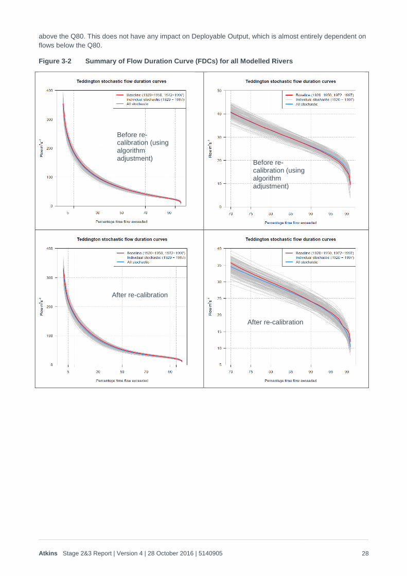
Atkins Stage 2&3 Report | Version 4 | 28 October 2016 | 5140905 28
above the Q80. This does not have any impact on Deployable Output, which is almost entirely dependent on
flows below the Q80.
Figure 3-2 Summary of Flow Duration Curve (FDCs) for all Modelled Rivers
Before re-calibration (using algorithm adjustment)
Before re-calibration (using algorithm adjustment)
After re-calibration
After re-calibration
Atkins Stage 2&3 Report | Version 4 | 28 October 2016 | 5140905 29
Atkins Stage 2&3 Report | Version 4 | 28 October 2016 | 5140905 30
Atkins Stage 2&3 Report | Version 4 | 28 October 2016 | 5140905 31
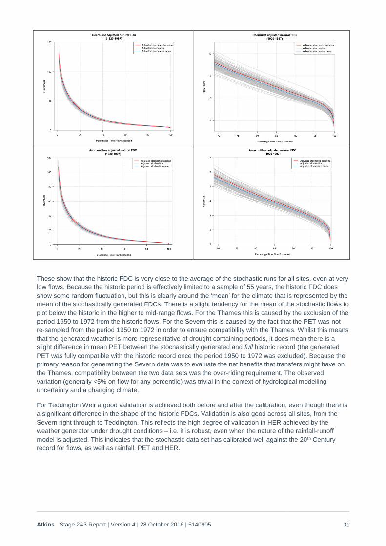
These show that the historic FDC is very close to the average of the stochastic runs for all sites, even at very
low flows. Because the historic period is effectively limited to a sample of 55 years, the historic FDC does
show some random fluctuation, but this is clearly around the ‘mean’ for the climate that is represented by the
mean of the stochastically generated FDCs. There is a slight tendency for the mean of the stochastic flows to
plot below the historic in the higher to mid-range flows. For the Thames this is caused by the exclusion of the
period 1950 to 1972 from the historic flows. For the Severn this is caused by the fact that the PET was not
re-sampled from the period 1950 to 1972 in order to ensure compatibility with the Thames. Whilst this means
that the generated weather is more representative of drought containing periods, it does mean there is a
slight difference in mean PET between the stochastically generated and full historic record (the generated
PET was fully compatible with the historic record once the period 1950 to 1972 was excluded). Because the
primary reason for generating the Severn data was to evaluate the net benefits that transfers might have on
the Thames, compatibility between the two data sets was the over-riding requirement. The observed
variation (generally <5% on flow for any percentile) was trivial in the context of hydrological modelling
uncertainty and a changing climate.
For Teddington Weir a good validation is achieved both before and after the calibration, even though there is
a significant difference in the shape of the historic FDCs. Validation is also good across all sites, from the
Severn right through to Teddington. This reflects the high degree of validation in HER achieved by the
weather generator under drought conditions – i.e. it is robust, even when the nature of the rainfall-runoff
model is adjusted. This indicates that the stochastic data set has calibrated well against the 20th Century
record for flows, as well as rainfall, PET and HER.
Atkins Stage 2&3 Report | Version 4 | 28 October 2016 | 5140905 32
4. Analysis Stage 2d: Water Resource Modelling
This section covers the technical methods used to create and validate the water resources modelling used in
the project. The processes and key assumptions used in modelling yields, Deployable Output and climate
change are Section 5 of this report.
Stochastic water resources modelling requires that multiple thousands of years’ worth of data are run
through a large number of demand increments. The Thames Water WARMS2 model is a complex water
resources simulator that includes a number of distributed rainfall-runoff models as well as the operational
mass-balance simulator that is incorporated into all water resources simulators. This means that WARMS2 is
relatively slow to run, and produces hydrological flows that cannot be completely accurately simulated in a
lumped catchment model (see Section 3.1 for details of the calibration between the two). In order to carry out
the stochastic water resource modelling, two main procedures were therefore required:
The creation of a rapid water resources simulator (IRAS), which needed to be ‘calibrated’ against the
WARMS2 water resources model, based on the aggregated storage and abstraction behaviour
generated in WARMS2.
A process of checking stochastically generated outputs from IRAS against the same droughts run
through WARMS2 to account for the differences in hydrology.
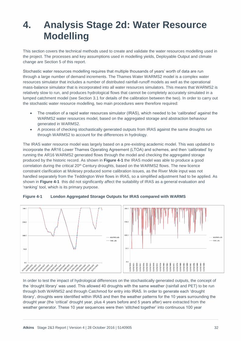
The IRAS water resource model was largely based on a pre-existing academic model. This was updated to
incorporate the AR16 Lower Thames Operating Agreement (LTOA) and schemes, and then ‘calibrated’ by
running the AR16 WARMS2 generated flows through the model and checking the aggregated storage
produced by the historic record. As shown in Figure 4-1 the IRAS model was able to produce a good
correlation during the critical 20th Century droughts, based on the WARMS2 flows. The new licence
constraint clarification at Molesey produced some calibration issues, as the River Mole input was not
handled separately from the Teddington Weir flows in IRAS, so a simplified adjustment had to be applied. As
shown in Figure 4-1 this did not significantly affect the suitability of IRAS as a general evaluation and
‘ranking’ tool, which is its primary purpose.
Figure 4-1 London Aggregated Storage Outputs for IRAS compared with WARMS
In order to test the impact of hydrological differences on the stochastically generated outputs, the concept of
the ‘drought library’ was used. This allowed 40 droughts with the same weather (rainfall and PET) to be run
through both WARMS2 and through Catchmod for entry into IRAS. In order to generate each ‘drought
library’, droughts were identified within IRAS and then the weather patterns for the 10 years surrounding the
drought year (the ‘critical’ drought year, plus 4 years before and 5 years after) were extracted from the
weather generator. These 10 year sequences were then ‘stitched together’ into continuous 100 year

Atkins Stage 2&3 Report | Version 4 | 28 October 2016 | 5140905 33
sequences, plus a 10 year warm up period, to form 4 * 110 years sequences for input to WARMS2.
WARMS2 was then run at incremental levels of demand, which allowed the WARMS2 calculated yield of
each drought to be generated and compared against IRAS. This was then used to ‘calibrate’ the IRAS
outputs for system yield estimates, climate change evaluations and options appraisal, as described in
Section 5.
Atkins Stage 2&3 Report | Version 4 | 28 October 2016 | 5140905 34
5. Analysis Stage 3: Deployable Output and Climate Change Analysis
5.1. Method and Key Assumptions According to the historic record, the Deployable Output of the London reservoir system is constrained by the requirement that there are no ‘Level 4’ failures of the system, so it is effectively equal to the level of demand (2305Ml/d) that can just be met during the 1921/22 drought without breaching the Level 4 control curve. However, the frequency of Level 3 restrictions, which should be no more than once every 20 years, is also a potential restriction on DO, as this occurs 4 times in the 1920 – 2010 historic record under the 2305Ml/d demand level.
The first Task for the stochastic data set was therefore to check that this constraint remains the same when the full stochastically generated data set was tested. When the system was subjected to the level of demand that is representative of the yield under the worst historic event, then the stochastic data set indicates that Level 3 restrictions are introduced, on average, approximately once every 25 years. This demonstrates that, if Thames maintains or improves its Level of Service to Level 4 events, then the Level 4 constraint will always remain the critical constraint on DO. To put this another way, once the yield/return period curve goes beyond the circa 1 in 100 year mark, then the ‘yield’ and DO are the same value.
The yield and climate change analyses presented below therefore concentrated on defining the yield/return period for the existing system under the baseline (20th Century) climate and defining the impact that climate change might have on that yield/return period relationship.
As noted in Section 4, because WARMS2 and IRAS (Catchmod) used different hydrological models, a relatively complex approach was required to derive the final estimates of yield for the whole stochastic data set:
1. All years were run through IRAS, and all droughts were assigned a yield, equivalent to the demand just below that at which they first demonstrated failure against the Level 4 control curve.
2. A count of the number of failures within the record was taken at each level of demand and then divided by 20,000 to generate a return period for that yield. [The value 20,000 was taken rather than the 15,400 years of generated data, as the anomaly fitting was designed to make the weather generator reflective of the 20th Century climate overall. The literature review confirmed that there were no ‘level 4’ type droughts in the first 20 years of the 20th Century for the Thames basin, so the full period was taken as the denominator to avoid biasing the yield results]. The return period/yield relationship was then plotted for IRAS based on this data.
3. A total of 40 droughts (arranged into 4 ‘drought libraries, as described in 4) were then sampled from
the IRAS data set and the associated weather timeseries were run through WARMS2. The 40 droughts were sampled from IRAS on a random stratified basis so that one drought was selected for each yield increment of 15Ml/d (according to IRAS). This provided droughts with an IRAS calculated yield from 1800Ml/d through to 2400Ml/d, which could be run through WARMS2 to determine the nature of the WARMS2/IRAS yield relationship.
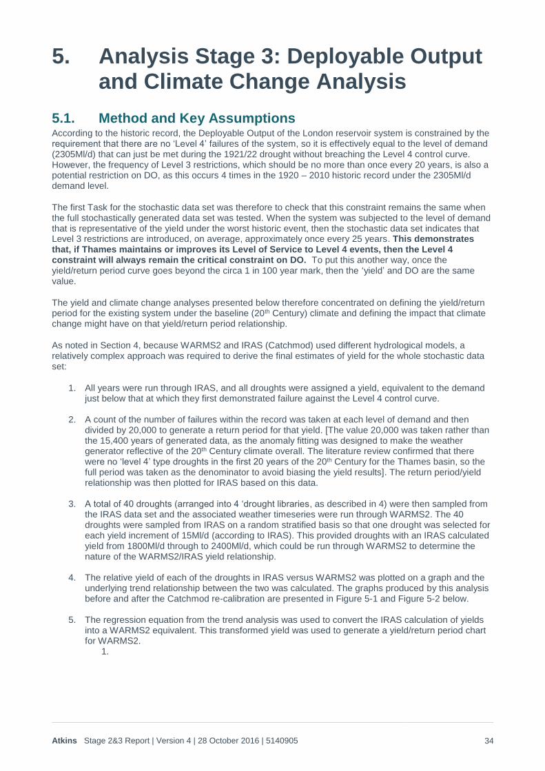
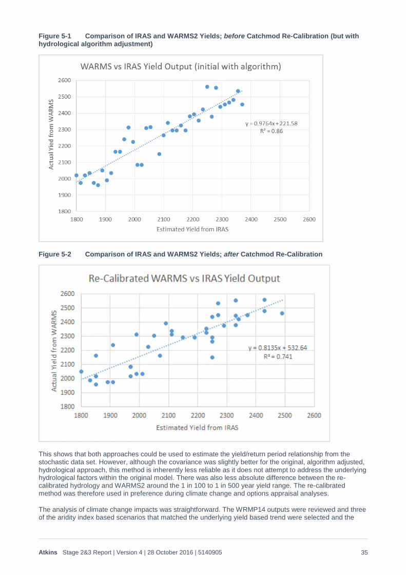
4. The relative yield of each of the droughts in IRAS versus WARMS2 was plotted on a graph and the
underlying trend relationship between the two was calculated. The graphs produced by this analysis before and after the Catchmod re-calibration are presented in Figure 5-1 and Figure 5-2 below.
5. The regression equation from the trend analysis was used to convert the IRAS calculation of yields
into a WARMS2 equivalent. This transformed yield was used to generate a yield/return period chart for WARMS2.
1.
Atkins Stage 2&3 Report | Version 4 | 28 October 2016 | 5140905 35
Figure 5-1 Comparison of IRAS and WARMS2 Yields; before Catchmod Re-Calibration (but with hydrological algorithm adjustment)
Figure 5-2 Comparison of IRAS and WARMS2 Yields; after Catchmod Re-Calibration
This shows that both approaches could be used to estimate the yield/return period relationship from the stochastic data set. However, although the covariance was slightly better for the original, algorithm adjusted, hydrological approach, this method is inherently less reliable as it does not attempt to address the underlying hydrological factors within the original model. There was also less absolute difference between the re-calibrated hydrology and WARMS2 around the 1 in 100 to 1 in 500 year yield range. The re-calibrated method was therefore used in preference during climate change and options appraisal analyses.
The analysis of climate change impacts was straightforward. The WRMP14 outputs were reviewed and three of the aridity index based scenarios that matched the underlying yield based trend were selected and the
Atkins Stage 2&3 Report | Version 4 | 28 October 2016 | 5140905 36
perturbation factors were imposed upon the stochastic weather data set. The yield/return period relationship was then generated as before. The three climate change scenarios that were tested were:
1. 50th percentile = UKCP09 run ID 9613, 2. 70th percentile = UKCP09 run ID 4402, 3. 97th percentile = UKCP09 run ID 508
N.B. the percentiles refer to the estimates from WRMP14, which evaluated the DO/climate change relationship based perturbation of the historic record.
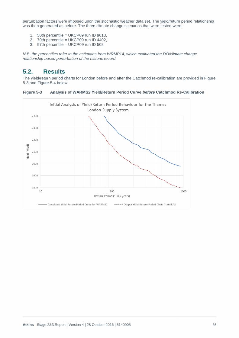
5.2. Results The yield/return period charts for London before and after the Catchmod re-calibration are provided in Figure 5-3 and Figure 5-4 below.
Figure 5-3 Analysis of WARMS2 Yield/Return Period Curve before Catchmod Re-Calibration
Atkins Stage 2&3 Report | Version 4 | 28 October 2016 | 5140905 37
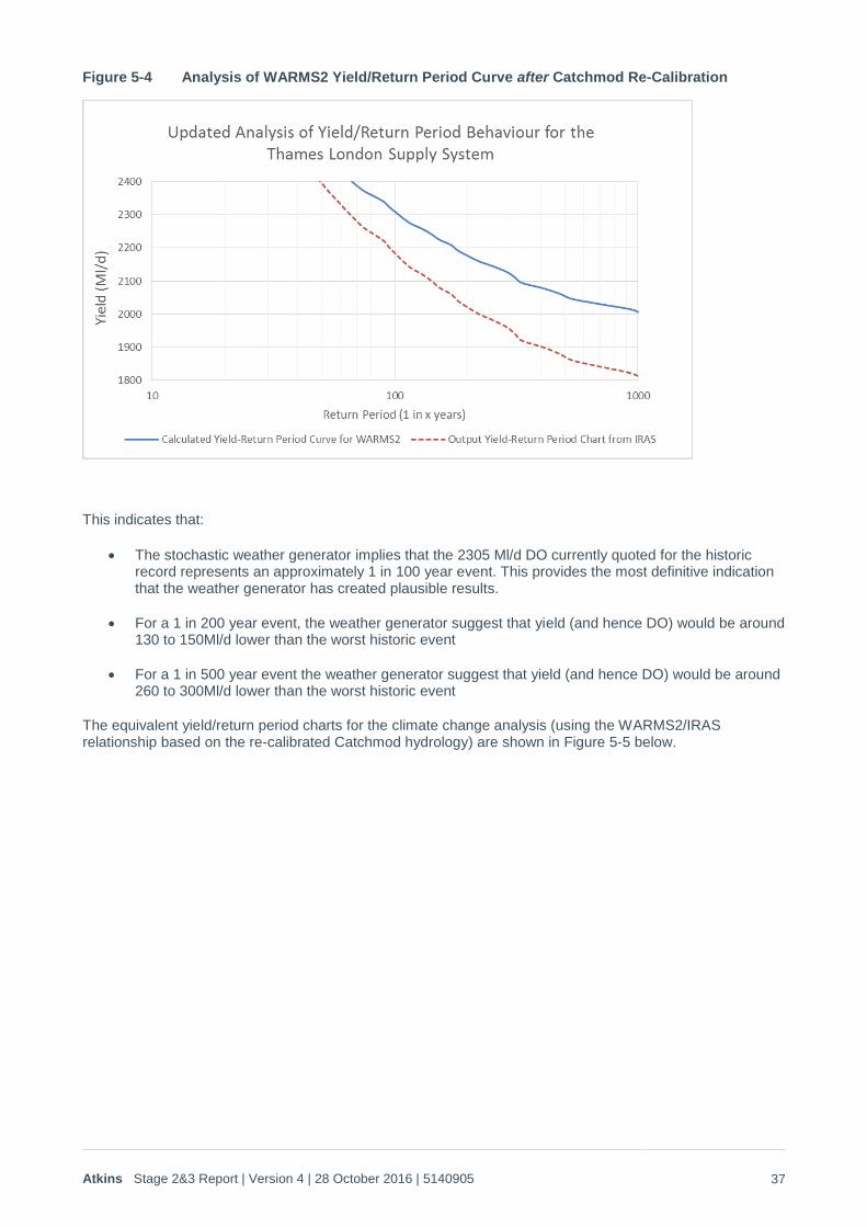
Figure 5-4 Analysis of WARMS2 Yield/Return Period Curve after Catchmod Re-Calibration
This indicates that:
The stochastic weather generator implies that the 2305 Ml/d DO currently quoted for the historic record represents an approximately 1 in 100 year event. This provides the most definitive indication that the weather generator has created plausible results.
For a 1 in 200 year event, the weather generator suggest that yield (and hence DO) would be around 130 to 150Ml/d lower than the worst historic event
For a 1 in 500 year event the weather generator suggest that yield (and hence DO) would be around 260 to 300Ml/d lower than the worst historic event
The equivalent yield/return period charts for the climate change analysis (using the WARMS2/IRAS relationship based on the re-calibrated Catchmod hydrology) are shown in Figure 5-5 below.
Atkins Stage 2&3 Report | Version 4 | 28 October 2016 | 5140905 38
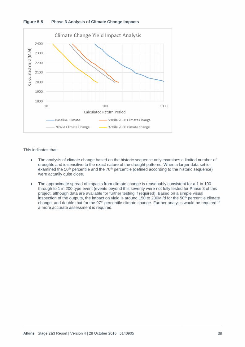
Figure 5-5 Phase 3 Analysis of Climate Change Impacts
This indicates that:
The analysis of climate change based on the historic sequence only examines a limited number of droughts and is sensitive to the exact nature of the drought patterns. When a larger data set is examined the 50th percentile and the 70th percentile (defined according to the historic sequence) were actually quite close.
The approximate spread of impacts from climate change is reasonably consistent for a 1 in 100 through to 1 in 200 type event (events beyond this severity were not fully tested for Phase 3 of this project, although data are available for further testing if required). Based on a simple visual inspection of the outputs, the impact on yield is around 150 to 200Ml/d for the 50th percentile climate change, and double that for the 97th percentile climate change. Further analysis would be required if a more accurate assessment is required.
Atkins Stage 2&3 Report | Version 4 | 28 October 2016 | 5140905 39
6. Conclusions and Recommendations
Stochastically generated rainfall and potential evapotranspiration (PET) were successfully produced in a spatially coherent way across all of the sub-catchments for the Thames and Severn catchments. These data provide an effective ‘what if’ analysis of rainfall and PET that emulate the underlying variability demonstrated in the 20th Century record, and allow alternative drought patterns and severities to be generated in a probabilistically coherent way. Whilst the emulation of severe droughts will always require some key planning assumptions due to the scarcity of relevant data on which to ‘train’ weather generators, in this case this was done in a considered way that fully allowed for the available literature that is available in relation to historic droughts. The validation against both rainfall and hydrologically effective rainfall (HER – equal to rainfall minus PET) was excellent, and maintained the validation across the sub-catchment, catchment and regional scales, which proved the spatially coherent nature of the analysis.
Although large volumes of daily weather data were involved, the study was able to use Catchmod and Kestrel-IHM rainfall-runoff models linked through to an IRAS water resource simulator to run analyses of the full data sets. The Catchmod rainfall-runoff model has the same structure as WARMS2, and was re-calibrated against WARMS2 flow outputs as part of this study. The Kestrel-IHM model was reviewed with the EA and is being used for Thames’ other WRMP19 studies. The close match on the rainfall and HER metrics translated to a good match on flow/duration curves, with the 20th Century reconciling well with the average of the stochastically generated runs across the whole FDC range across both catchments.
Calibration of the IRAS rapid water resource simulator confirmed that this was suitable for the purposes of ranking of stochastic drought years according to their relative yield, and for analysing the impact of climate change on the yield/return period relationship. This same principle can be used to generate yield/return period impacts from new water resource options such as the Severn-Thames transfer schemes.
By far the biggest challenge for the stochastic water resource analysis was caused by the differences in the lumped Catchmod hydrological model used for generating flow data for IRAS, and the more granular, distributed hydrological modelling contained within WARMS2. Although they both used the same weather generator outputs, the generated flows were sufficiently different to cause notable differences in estimated yields for the same droughts. However, this issue was addressed through the use of ‘Drought Libraries’ which provided a practicable method for using the weather generator outputs for more detailed analysis within WARMS2. This meant that IRAS and WARMS2 outputs could be directly compared, providing the necessary conversion factors and allowing for future detailed analysis of new water resource options and climate change within WARMS2.
Testing of the baseline climate using the weather generator, hydrological models and IRAS/WARMS2, indicated that:
The 2305 Ml/d DO currently quoted for the historic record represents an approximately 1 in 100 year event according to the stochastically generated weather. This provided the most definitive indication that the weather generator created plausible results that validated well against the 20th Century record.
For a 1 in 200 year event, the weather generator suggest that yield (and hence DO) would be around 130 to 150Ml/d lower than the worst historic event.
For a 1 in 500 year event the weather generator suggest that yield (and hence DO) would be around 260 to 300Ml/d lower than the worst historic event.
Testing of climate change impacts using the stochastically generated data set highlighted the sensitivity of the WRMP14 climate change analysis to the exact patterns of the 20th Century droughts. It showed that the relationship between climate change risk percentiles and yield impacts is likely to be different when a wider range of droughts is considered. Limited testing of climate change impacts at 2080 indicated that impacts are reasonably consistent across the 1 in 100 to 1 in 200 year return period drought range, within 50th percentile climate change impacts reducing yield by around 150Ml/d to 200Ml/d, and the 97th percentile approximately double that. (i.e. 300 to 400Ml/d).
In terms of potential future development of the weather generator, the only significant recommendation relates to the potential creation of a stochastically based model that directly incorporates regional climate

Atkins Stage 2&3 Report | Version 4 | 28 October 2016 | 5140905 40
drivers other than NAO and SST as explanatory factors, as opposed to accounting for them using the anomaly based curve fitting process described here. However, other studies have shown that the main ‘candidate’ factor (the east Atlantic – Western Russia index) does not provide the required explanatory factor, and further primary meteorological research is required before this anomaly can be incorporated into weather generators or climate models. It is therefore recommended that any such efforts should wait until the outputs from new academic studies such as MaRIUS and/or UKCP18 have been made available, as these will provide some indication of the ability of physically based models to replicate the ‘blocking high pressure’ behaviour that drives such anomalies.
.
Atkins Stage 2&3 Report | Version 4 | 28 October 2016 | 5140905 41
7. References
Briffa et al 2009 ‘Wet and dry summers in Europe since 1750:Evidence of Increasing Drought’ International Journal Of Climatology Int. J. Climatol. 29: 1894–1905 (2009)
Cook et al 2015 ‘Old World Megadroughts and Pluvials during the Common Era’. Climatology research article, published in http://advances.sciencemag.org.
Crawford, N.H. and R.K. Linsley, 1966. Digital Simulation on Hydrology: Stanford Watershed Model IV. Stanford University. Technical Report No. 39, Stanford University, Palo Alto, CA.
EA 2004 ‘Reconstructed River Flow Series from 1860s to Present’ Science Report SC040052/SR
EA 2006 ‘The impact of climate change on severe droughts: Major droughts in England and Wales from 1800 and evidence of impact’ Science Report SC040068/SR1
Keller, V. D. J., Tanguy, M., Prosdocimi, I., Terry, J. A., Hitt, O., Cole, S. J., Fry, M., Morris, D. G., and Dixon, H., 2015. CEH-GEAR: 1 km resolution daily and monthly areal rainfall estimates for the UK for hydrological and other applications, Earth Syst. Sci. Data, 7, 143-155, doi:10.5194/essd-7-143-2015.
Marsh, T, Cole, G and Wilby, R ‘Major Droughts in England & Wales 1800 – 2006’. Weather April 2007, Vol 62, No. 4
Matthews, T., Murphy, C., Wilby, R. and Harrigan S., 2015. A cyclone climatology of the British Isles 1871-2012. Int. J. Climatol. doi: 10.1002/joc.4425
Mayes, J 2004. ‘London’s Wettest Summer and Wettest Year – 1903’ Weather Oct 2004, Vol 59, No. 10
Murphy, S.J. and Washington, R., 2001. United Kingdom and Ireland precipitation variability and the North Atlantic sea-level pressure field. Int. J. Climatol. 21, 939-959.
Osborn, T.J., Conway, D., Hulme, M., Gregory, J.M. and Jones, P.D, 1999. Air flow influences on local climate: observed and simulated mean relationships for the United Kingdom. Climate Research 13, 173-191.
Scherrer, S.C., et al., 2006. Two-dimensional indices of atmospheric blocking and their statistical relationship with winter climate patterns in the Euro-Atlantic region. Int. J. Climatol. 26, 233-249.
Serinaldi, F & Kilsby, C 2012 ‘’A modular class of multisite monthly rainfall generators for water resource management and impact studies’ Journal of Hydrology 464–465 (2012) 528–540
Spraggs et al 2015. ‘Re-construction of historic drought in the Anglian Region (UK) over the period 1798–2010 and the implications for water resources and drought management’ J. Hydrol. (2015), http://dx.doi.org/10.1016/j.jhydrol.2015.01.015
Tanguy, M., Dixon, H., Prosdocimi, I., Morris, D.G., Keller V. D. J., 2014. Gridded Estimates of daily and monthly Areal Rainfall for the United Kingdom (1890-2012) [CEH-GEAR], NERC Environmental Information Data Centre.
Thames Water 2015 Data provided for the Oxford Rain Gauge
Thompson, N., Barrie, I. A., and Ayles, M., 1982. The Meteorological Office Rainfall and Evaporation Calculation System: MORECS. Hydrological Memorandum N 45 (Vol. 45). Bracknell, UK: Met. Office.
UKWIR 2016a ‘WRMP19 Decision Making Tools Guidance’ UKWIR
UKWIR2016b ‘WRMP19 Risk Based Methods’ UKWIR
Watts et al 2012 ‘Testing the Resilience of Water Supply Systems to Long Droughts’. Journal of Hydrology 414-415 (2012) 255-267
Wilby et al 2015 ‘Persistence of Hydrometeorological Droughts in the United Kingdom: A Regional Analysis of Multi-Season Rainfall and River Flow Anomalies’ Journal of Extreme Events Vol 2, No. 2
WIlby, R.L., O’Hare, G. and Barnsley, N., 1997. The North Atlantic Oscillation and British Isles climate variability, 1865-1996. Weather 52, 266-276.

Appendices
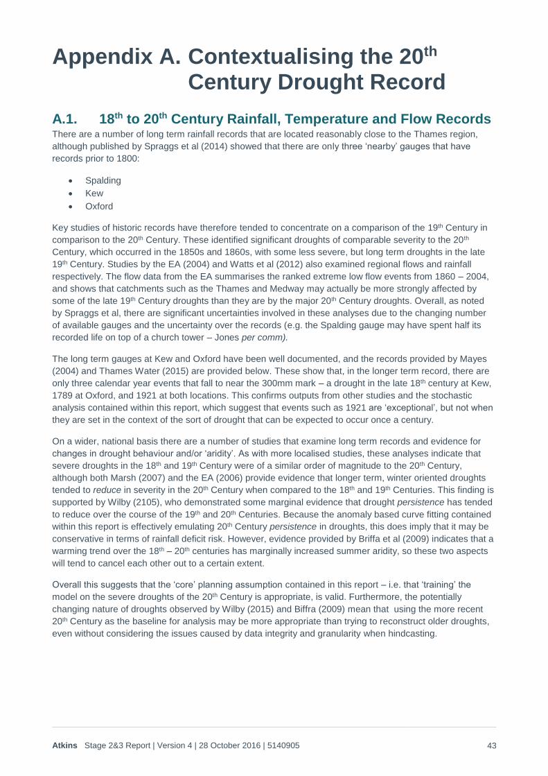
Atkins Stage 2&3 Report | Version 4 | 28 October 2016 | 5140905 43
Appendix A. Contextualising the 20th Century Drought Record
A.1. 18th to 20th Century Rainfall, Temperature and Flow Records There are a number of long term rainfall records that are located reasonably close to the Thames region,
although published by Spraggs et al (2014) showed that there are only three ‘nearby’ gauges that have
records prior to 1800:
Spalding
Kew
Oxford
Key studies of historic records have therefore tended to concentrate on a comparison of the 19th Century in
comparison to the 20th Century. These identified significant droughts of comparable severity to the 20th
Century, which occurred in the 1850s and 1860s, with some less severe, but long term droughts in the late
19th Century. Studies by the EA (2004) and Watts et al (2012) also examined regional flows and rainfall
respectively. The flow data from the EA summarises the ranked extreme low flow events from 1860 – 2004,
and shows that catchments such as the Thames and Medway may actually be more strongly affected by
some of the late 19th Century droughts than they are by the major 20th Century droughts. Overall, as noted
by Spraggs et al, there are significant uncertainties involved in these analyses due to the changing number
of available gauges and the uncertainty over the records (e.g. the Spalding gauge may have spent half its
recorded life on top of a church tower – Jones per comm).
The long term gauges at Kew and Oxford have been well documented, and the records provided by Mayes
(2004) and Thames Water (2015) are provided below. These show that, in the longer term record, there are
only three calendar year events that fall to near the 300mm mark – a drought in the late 18th century at Kew,
1789 at Oxford, and 1921 at both locations. This confirms outputs from other studies and the stochastic
analysis contained within this report, which suggest that events such as 1921 are ‘exceptional’, but not when
they are set in the context of the sort of drought that can be expected to occur once a century.
On a wider, national basis there are a number of studies that examine long term records and evidence for
changes in drought behaviour and/or ‘aridity’. As with more localised studies, these analyses indicate that
severe droughts in the 18th and 19th Century were of a similar order of magnitude to the 20th Century,
although both Marsh (2007) and the EA (2006) provide evidence that longer term, winter oriented droughts
tended to reduce in severity in the 20th Century when compared to the 18th and 19th Centuries. This finding is
supported by Wilby (2105), who demonstrated some marginal evidence that drought persistence has tended
to reduce over the course of the 19th and 20th Centuries. Because the anomaly based curve fitting contained
within this report is effectively emulating 20th Century persistence in droughts, this does imply that it may be
conservative in terms of rainfall deficit risk. However, evidence provided by Briffa et al (2009) indicates that a
warming trend over the 18th – 20th centuries has marginally increased summer aridity, so these two aspects
will tend to cancel each other out to a certain extent.
Overall this suggests that the ‘core’ planning assumption contained in this report – i.e. that ‘training’ the
model on the severe droughts of the 20th Century is appropriate, is valid. Furthermore, the potentially
changing nature of droughts observed by Wilby (2015) and Biffra (2009) mean that using the more recent
20th Century as the baseline for analysis may be more appropriate than trying to reconstruct older droughts,
even without considering the issues caused by data integrity and granularity when hindcasting.
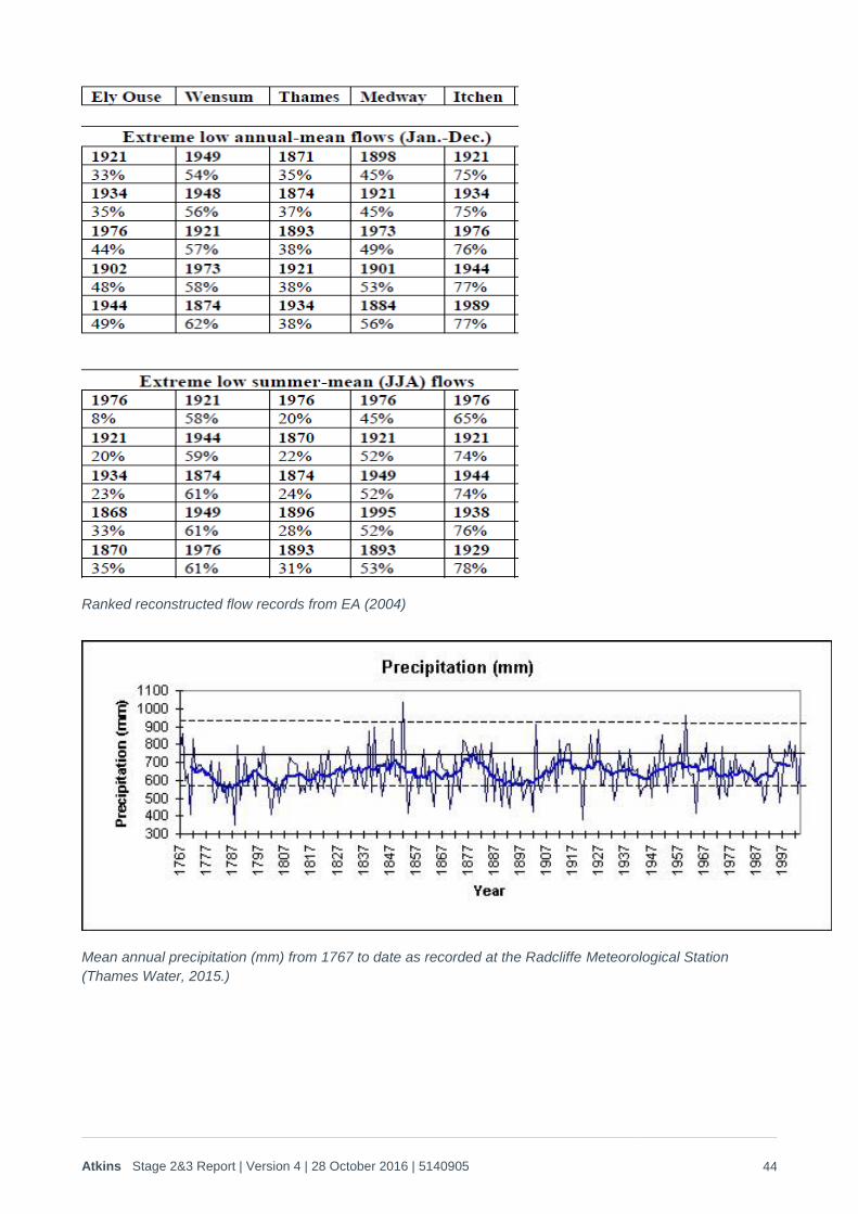
Atkins Stage 2&3 Report | Version 4 | 28 October 2016 | 5140905 44
Ranked reconstructed flow records from EA (2004)
Mean annual precipitation (mm) from 1767 to date as recorded at the Radcliffe Meteorological Station
(Thames Water, 2015.)
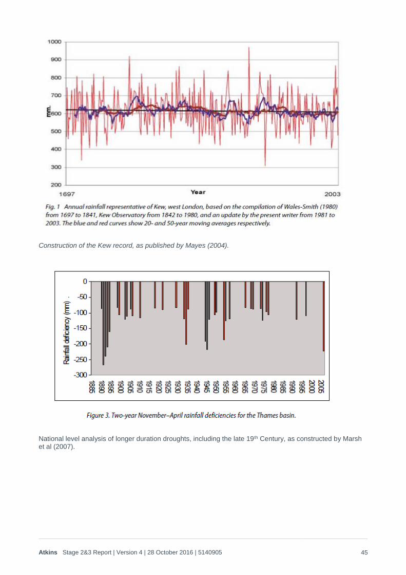
Atkins Stage 2&3 Report | Version 4 | 28 October 2016 | 5140905 45
Construction of the Kew record, as published by Mayes (2004).
National level analysis of longer duration droughts, including the late 19th Century, as constructed by Marsh et al (2007).
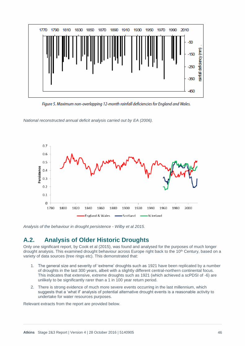
Atkins Stage 2&3 Report | Version 4 | 28 October 2016 | 5140905 46
National reconstructed annual deficit analysis carried out by EA (2006).
Analysis of the behaviour in drought persistence - Wilby et al 2015.
A.2. Analysis of Older Historic Droughts Only one significant report, by Cook et al (2015), was found and analysed for the purposes of much longer drought analysis. This examined drought behaviour across Europe right back to the 10th Century, based on a variety of data sources (tree rings etc). This demonstrated that:
1. The general size and severity of ‘extreme’ droughts such as 1921 have been replicated by a number of droughts in the last 300 years, albeit with a slightly different central-northern continental focus. This indicates that extensive, extreme droughts such as 1921 (which achieved a scPDSI of -6) are unlikely to be significantly rarer than a 1 in 100 year return period.
2. There is strong evidence of much more severe events occurring in the last millennium, which suggests that a ‘what if’ analysis of potential alternative drought events is a reasonable activity to undertake for water resources purposes.
Relevant extracts from the report are provided below.
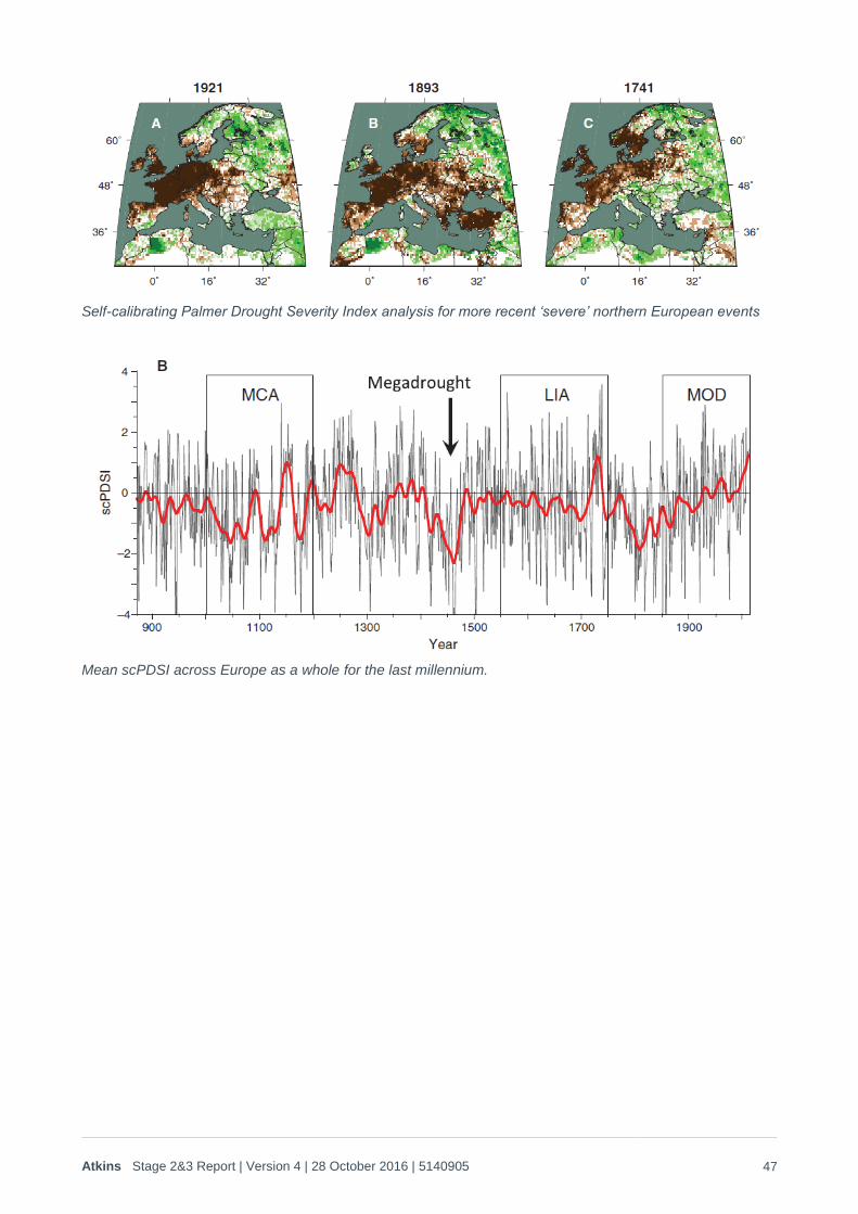
Atkins Stage 2&3 Report | Version 4 | 28 October 2016 | 5140905 47
Self-calibrating Palmer Drought Severity Index analysis for more recent ‘severe’ northern European events
Mean scPDSI across Europe as a whole for the last millennium.
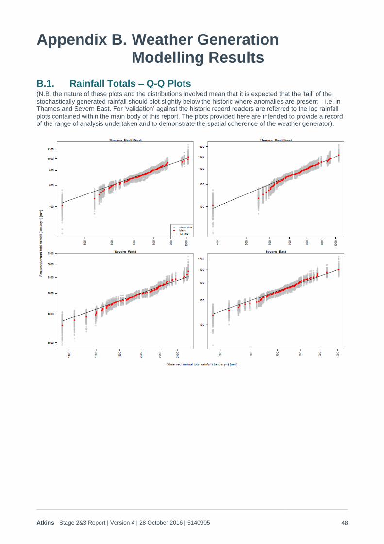
Atkins Stage 2&3 Report | Version 4 | 28 October 2016 | 5140905 48
Appendix B. Weather Generation Modelling Results
B.1. Rainfall Totals – Q-Q Plots (N.B. the nature of these plots and the distributions involved mean that it is expected that the ‘tail’ of the stochastically generated rainfall should plot slightly below the historic where anomalies are present – i.e. in Thames and Severn East. For ‘validation’ against the historic record readers are referred to the log rainfall plots contained within the main body of this report. The plots provided here are intended to provide a record of the range of analysis undertaken and to demonstrate the spatial coherence of the weather generator).
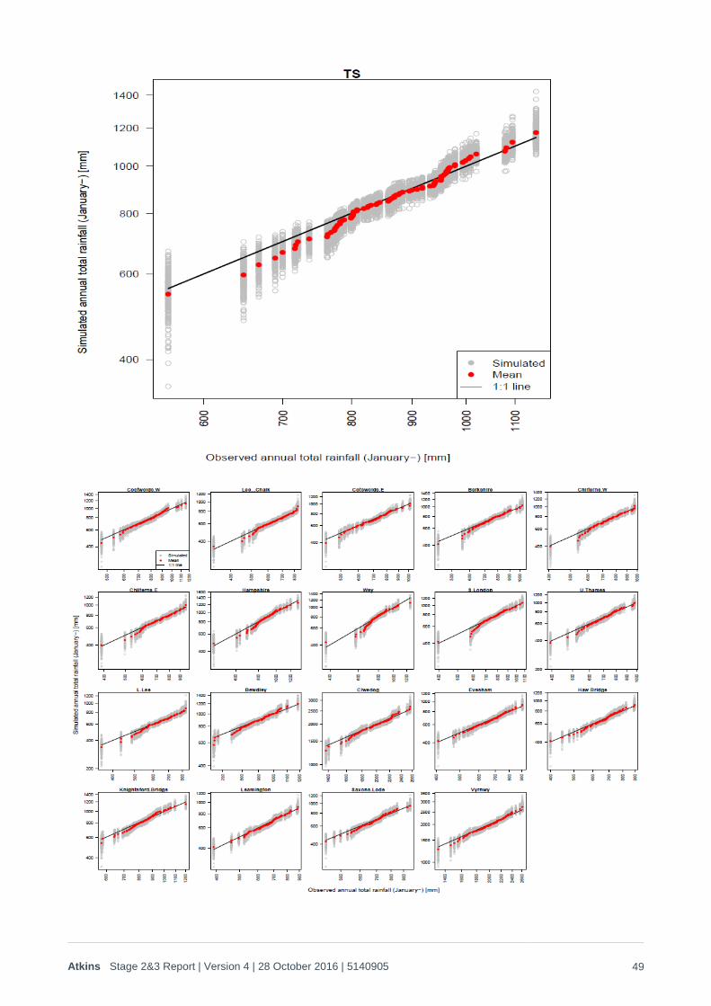
Atkins Stage 2&3 Report | Version 4 | 28 October 2016 | 5140905 49

Atkins Stage 2&3 Report | Version 4 | 28 October 2016 | 5140905 50
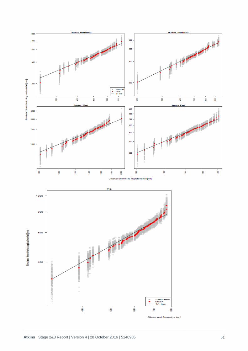
Atkins Stage 2&3 Report | Version 4 | 28 October 2016 | 5140905 51

Atkins Stage 2&3 Report | Version 4 | 28 October 2016 | 5140905 52
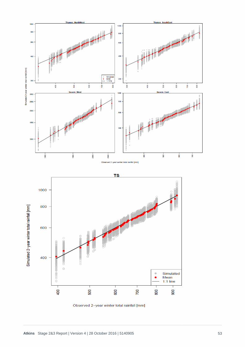
Atkins Stage 2&3 Report | Version 4 | 28 October 2016 | 5140905 53
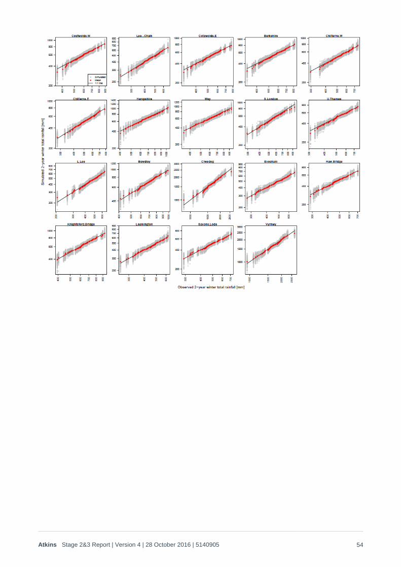
Atkins Stage 2&3 Report | Version 4 | 28 October 2016 | 5140905 54
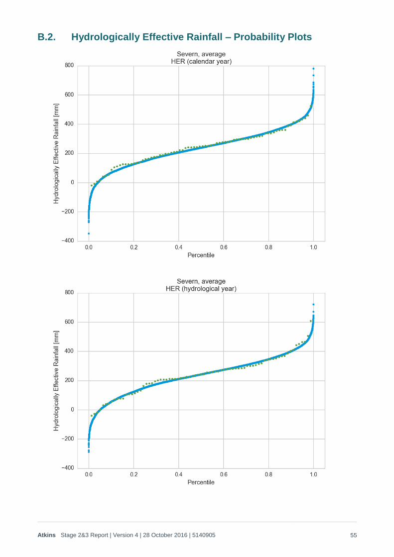
Atkins Stage 2&3 Report | Version 4 | 28 October 2016 | 5140905 55
B.2. Hydrologically Effective Rainfall – Probability Plots
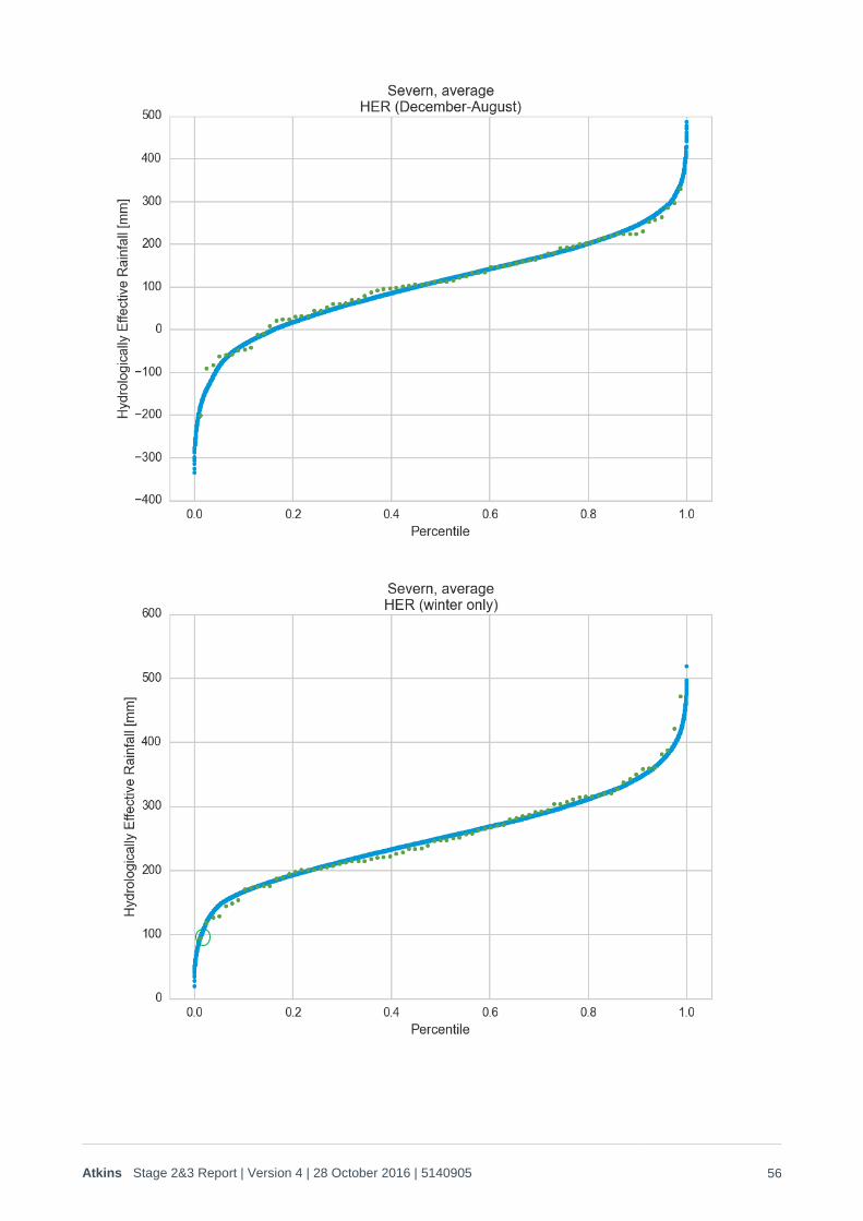
Atkins Stage 2&3 Report | Version 4 | 28 October 2016 | 5140905 56
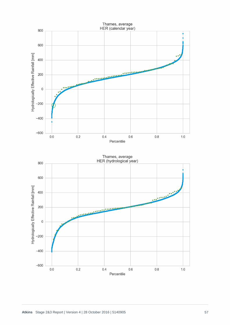
Atkins Stage 2&3 Report | Version 4 | 28 October 2016 | 5140905 57

Atkins Stage 2&3 Report | Version 4 | 28 October 2016 | 5140905 58

© Atkins Ltd except where stated otherwise. The Atkins logo, ‘Carbon Critical Design’ and the strapline ‘Plan Design Enable’ are trademarks of Atkins Ltd.
Contact name Atkins company name Office address
Email Telephone Direct telephone Fax


![New Approach for Stochastic Modelling of Microgrid ... · involves various stochastic modelling and simulation methods [4, 6, 7]. The survey of stochastic modelling of microgrid is](https://img.pdfslide.net/doc/110x75/5f4190048356da16412b2f00/new-approach-for-stochastic-modelling-of-microgrid-involves-various-stochastic.jpg)