Embed Size (px)
Citation preview

2005-23Final Report
THE COST AND EFFECTIVENESS OF STORMWATER
MANAGEMENT PRACTICES
Technical Report Documentation Page1. Report No. 2. 3. Recipients Accession No. MN/RC – 2005-23 4. Title and Subtitle 5. Report Date
June 2005 6.
THE COST AND EFFECTIVENESS OF STORMWATER MANAGEMENT PRACTICES
7. Author(s) 8. Performing Organization Report No.
Peter T. Weiss, John S. Gulliver, Andrew J. Erickson
9. Performing Organization Name and Address 10. Project/Task/Work Unit No.
11. Contract (C) or Grant (G) No.
Department of Civil Engineering University of Minnesota 500 Pillsbury Drive SE Minneapolis, MN 55455 (c) 81655 (wo) 78 12. Sponsoring Organization Name and Address 13. Type of Report and Period Covered
Final Report
14. Sponsoring Agency Code
Minnesota Department of Transportation Research Services Section 395 John Ireland Boulevard Mail Stop 330 St. Paul, Minnesota 55155
15. Supplementary Notes
http://www.lrrb.org/pdf/200523.pdf 16. Abstract (Limit: 200 words)
Stormwater management practices for treating urban rainwater runoff were evaluated for cost and effectiveness in removing suspended sediments and phosphorus. Construction and annual operating and maintenance cost data was collected and analyzed for dry detention basins, wet basins, sand filters, constructed wetlands, bioretention filters, infiltration trenches, and swales using literature that reported on existing SMP sites across the United States. After statistical analysis on historical values of inflation and bond yields, the annual operating and maintenance costs were converted to a present worth based on a 20-year life and added to the construction cost. The total present cost of each SMP with the 67% confidence interval was reported as a function of the water quality design volume or, in the case of swales as a function of the swale top width, again with a 67% confidence interval. Finally, the mass of total suspended solids and total phosphorus removed over the 20-year life was estimated as a function of the water quality volume. The results can be used by planners and designers to estimate both the total cost of installing a stormwater management practice at a given site and the corresponding total suspended solids and phosphorus removal. 17. Document Analysis/Descriptors 18.Availability Statement
Stormwater Construction Constructed wetlands
Detention basins Sand filters Swales
No restrictions. Document available from: National Technical Information Services, Springfield, Virginia 22161
19. Security Class (this report) 20. Security Class (this page) 21. No. of Pages 22. Price
Unclassified Unclassified 103
THE COST AND EFFECTIVENESS OF STORMWATER MANAGEMENT PRACTICES
Final Report
Prepared by:
Peter T. Weiss Department of Civil Engineering
Valparaiso University
John S. Gulliver Andrew J. Erickson
Department of Civil Engineering University of Minnesota
June 2005
Published by: Minnesota Department of Transportation
Research Services Section 395 John Ireland Boulevard, MS 330
St. Paul, MN 55155
This report represents the results of research conducted by the authors and does not necessarily represent the views or policies of the Minnesota Department of Transportation and/or the Center for Transportation Studies. This report does not contain a standard or specified technique.
Table of Contents
Introduction..................................................................................................................................... 1
Literature Review............................................................................................................................ 2
Dry Detention Basins.................................................................................................................. 7
Constructed Wetlands ................................................................................................................. 9
Infiltration Practices.................................................................................................................. 11
Sand Filtration........................................................................................................................... 15
Vegetated Systems .................................................................................................................... 17
Commercial Products................................................................................................................ 18
Review Summary...................................................................................................................... 18
Cost Estimation............................................................................................................................. 19
Water Quality Volume.............................................................................................................. 19
Total Construction Costs........................................................................................................... 20
Land-Area Requirements .......................................................................................................... 27
Operating and Maintenance Costs ............................................................................................ 28
Total Present Cost ..................................................................................................................... 30
Effectiveness of Contaminant Removal........................................................................................ 38
Runoff Fraction Treated............................................................................................................ 42
Pollutant Loading...................................................................................................................... 46
Fraction of Contaminants Removed ......................................................................................... 49
Examples....................................................................................................................................... 59

References..................................................................................................................................... 62
Appendix A - Pollutant Removal Capability Table: References, Notes and Notation............... A-1
Appendix B – Data used to estimate average SMP effectiveness .............................................. B-1

List of Figures
Figure 1. Grain size distribution of highway stormwater runoff in Lake Tahoe basin.................. 4
Figure 2. Retention basin cross section.......................................................................................... 8
Figure 3. One example of a constructed wetland system............................................................. 10
Figure 4. Infiltration trench design. ............................................................................................. 13
Figure 5. Unit construction costs of dry detention basins............................................................ 22
Figure 6. Unit construction costs of wet basins. .......................................................................... 23
Figure 7. Unit construction costs of constructed wetlands. ......................................................... 23
Figure 8. Unit construction costs of infiltration trenches. ........................................................... 24
Figure 9. Unit construction costs of bioinfiltration filters. .......................................................... 24
Figure 10. Unit Construction Costs of Sand Filters. .................................................................... 25
Figure 11. Unit Construction Costs of Grassed/Vegetative Swales. ........................................... 25
Figure 12. Annual O&M costs of dry detention basins. .............................................................. 30
Figure 13. Annual O&M costs of wet basins............................................................................... 31
Figure 14. Annual O&M costs of constructed wetlands.............................................................. 31
Figure 15. Annual O&M costs of infiltration trenches. ............................................................... 32
Figure 16. Annual O&M costs of bioinfiltration filters. .............................................................. 32
Figure 17. Annual O&M costs of sand filters.............................................................................. 33
Figure 18. Annual O&M costs of Grassed/Vegetative Swales.................................................... 33
Figure 19. Total Present Cost (TPC) of dry detention basins with 67% CI................................. 38
Figure 20. Total Present Cost (TPC) of wet basins with 67% CI. ............................................... 39
Figure 21. Total Present Cost (TPC) of constructed wetlands with 67% CI. .............................. 39
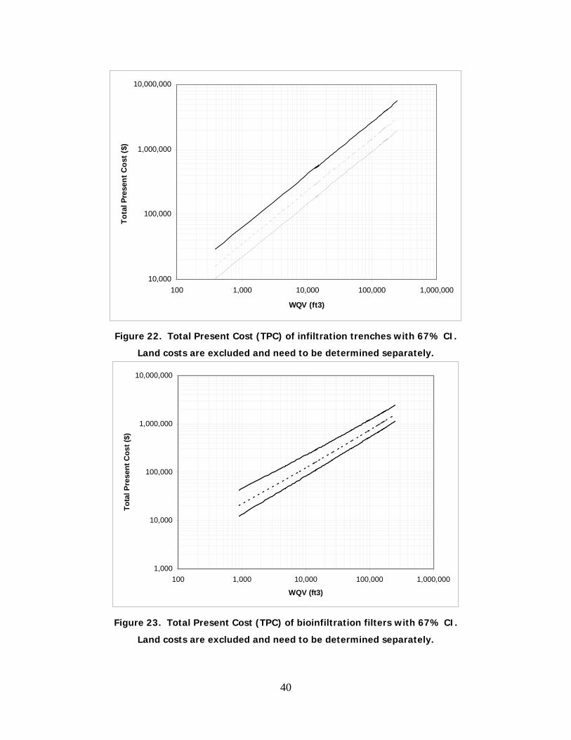
Figure 22. Total Present Cost (TPC) of infiltration trenches with 67% CI. ................................ 40

Figure 23. Total Present Cost (TPC) of bioinfiltration filters with 67% CI. ............................... 40
Figure 24. Total Present Cost (TPC) of sand filters with 67% CI. .............................................. 41
Figure 25. Total Present Cost (TPC) of 1000’ long grassed/vegetative swales with 67% CI. .... 41
Figure 26. Exceedance probabilities of two-day precipitation depths in the Twin Cities. .......... 45
Figure 27. Estimated TSS removed in 20 years for dry detention basins with the 67% CI. ....... 53
Figure 28. Estimated TSS removed in 20 years for wet basins with the 67% CI........................ 53
Figure 29. Estimated TSS removed in 20 years for constructed wetlands with the 67% CI. ...... 54
Figure 30. Estimated TSS removed in 20 years for infiltration trenches with the 67% CI. ........ 54
Figure 31. Estimated TSS removed in 20 years for bioinfiltration filters with the 67% CI. ....... 55
Figure 32. Estimated TSS removed in 20 years for sand filters with the 67% CI. ...................... 55
Figure 33. Estimated P removed in 20 years for dry detention basins with the 67% CI. ............ 56
Figure 34. Estimated P removed in 20 years for wet basins with the 67% CI............................. 56
Figure 35. Estimated P removed in 20 years for constructed wetlands with the 67% CI............ 57
Figure 36. Estimated P removed in 20 years for infiltration trenches with the 67% CI. ............. 57
Figure 37. Estimated P removed in 20 years for Bioinfiltration Filters with the 67% CI. .......... 58
Figure 38. Estimated P removed in 20 years for sand filters with the 67% CI............................ 58
List of Tables
Table 1. Grain size distribution of highway stormwater runoff in Lake Tahoe Basin. ................. 4
Table 2. Expected phosphorus removal. ....................................................................................... 6
Table 3. Reported SMP land area requirements for effective treatment...................................... 28
Table 4. Typical land area requirements (% of total watershed) for wet ponds (i.e. basins)....... 28
Table 5. Typical annual O&M costs of SMPs. ............................................................................ 29
Table 6. Yearly 20-year running average values of E. ................................................................ 37
Table 7. Statistical analysis of historical 2-day precip. amounts at the MPLS-St. Paul airport. . 44
Table 8. Average percent removal rates of SMPs with corresponding confidence interval........ 51
Table 9. Average Total Present Cost (in $1,000) of SMPs at varying WQVs. ........................... 61
Executive Summary
Historical data has been used to compare the cost and effectiveness of several common
stormwater management practices (SMP) including dry detention basins, wet detention basins,
constructed wetlands, infiltration trenches, bioinfiltration filters, and sand filters. Data on
construction costs and annual operating and maintenance costs have been combined to estimate
the total present cost (TPC) of the SMPs in 2005 dollars as a function of water quality volume
(WQV) or, in the case of swales, the swale top width. The TPC is based on 20 years of annual
O&M costs which have been converted to a present value based on historical values of inflation
and municipal bond yield rates.
The effectiveness of the SMPs as a function of WQV have been assessed by estimating
the total amount of total suspended solids (TSS) and phosphorus (P) removed over a 20-year
time period. Both the cost (i.e. TPC) and effectiveness (i.e. amount of TSS and P removed)
estimates are presented with 67% confidence intervals. Also, in order to help the user
incorporate land costs, typical land-area requirements for each SMP as a function of watershed
area are presented.
For the six SMPs investigated, results show that, ignoring land costs, constructed
wetlands are the least expensive to construct and maintain. However, since wetlands typically
require more land area to be effective, land acquisition costs may result in wetlands being
significantly more expensive then other SMPs that require less area. Also, the long-term
capability of wetlands to remove phosphorus has been questioned by other authors.
The results presented in this report can be used by decision makers as a preliminary tool to
compare SMPs in the categories of cost and impact on water quality. However, due to the wide

scatter in the original data, the confidence intervals associated with the estimates of TPC and
amount of TSS and P removed also exhibit a relatively wide range.
Even with the scatter, the results can be used as a preliminary tool to compare SMPs
which are under consideration for a given project.
For a more complete estimate of SMP cost and effectiveness, a more rigorous and
detailed comparison which involves, as a minimum, a preliminary SMP design, should be
performed.

1
Introduction
With the implementation of the United States Environmental Protection Agency’s
(USEPA) National Pollution Discharge Elimination Systems (NPDES) Phase I and II programs,
strong interest has developed in the area of water quality treatment of stormwater runoff. While
little is known about the cost effectiveness of available stormwater treatment technologies, called
Stormwater Management Practices (SMPs) in this report, municipal agencies are now, or soon
will be, required to meet certain pollutant removal criteria based on the Phase I and II
regulations.
Of primary concern are nutrients such as phosphorus (P) and nitrogen (N), which are just
one of the pollutant categories being targeted for removal from stormwater runoff. Excess
nutrients can initiate large algae blooms that generate negative aesthetic and eutrophic conditions
in receiving lakes and rivers (USEPA, 1999a). In inland water bodies phosphorus is typically
the limiting nutrient (Schindler, 1977) and can be contributed to stormwater from various sources
such as fertilizers, leaves, grass clippings, etc. (USEPA, 1999a). Another pollutant of primary
concern in stormwater is dirt, sand, and other solid particles which are commonly quantified by
measuring the Total Suspended Solids (TSS) of a water sample. TSS can severely and
negatively impact an aquatic environment. The solids increase turbidity, inhibit plant growth
and diversity, affect river biota and reduce the number of aquatic species (Shammaa et al., 2002).
Also, organic suspended solids can be biologically degraded by microorganisms in a process
which consumes oxygen, which is important to the aquatic biota.
With total suspended solids and phosphorus a primary concern of most stormwater
management plans, and with little known about the cost effectiveness of available stormwater
treatment options, this report seeks to fill a need by developing both a cost-comparison tool

2
(based on total construction cost not including land acquisition) and an effectiveness comparison
tool (based on pounds of total suspended solids and phosphorus removed) for common SMPs.
The method is based on published, credible information of existing SMPs relating to their
construction and annual operating and maintenance (O&M) costs and their ability to remove TSS
and P from stormwater runoff. The goal of the report is to provide planners and engineers with a
pre-feasibility tool that can be used to compare the costs and impact on water quality of available
SMPs.
Literature Review
Phosphorus can occur in both dissolved and particulate form in stormwater runoff. The
dissolved fraction is often in the form of phosphates ( −34PO ) (Jenkins et al., 1971) which
undergo hydrolysis in water to form H3PO4 (pH<2.16), -42POH (2.16 < pH < 7.20), -2
4HPO
(7.20 < pH < 12.35), or -34PO (12.35 < pH). Dissolved phosphorus is usually and somewhat
arbitrarily defined as that portion which can pass through a 0.45 micron filter. Solid or
particulate phosphorus, defined as that portion which is retained by a 0.45 micron filter, can
originate from grass clippings, leaves, animal waste or any other solid organic matter and may
also be included as part of the TSS.
The Water Environment Federation in conjunction with the American Society of Civil
Engineers (WEF and ASCE, 1998) site a USEPA (1983) publication that reports the expected
event mean concentrations for total and dissolved phosphorus in urban runoff as 0.33 mg/L and
0.12 mg/L, respectively. A more recent report (Brown et al., 2003) based upon three different
studies that incorporated data from approximately 500, 107, and more than 3,783 storm events,
respectively, claims that a total phosphorus concentration of 0.3 mg/L is adequate to describe
3
both new and old urban development stormwater runoff. Brezonik and Stadelmann (2002)
investigated urban runoff in the Twin Cities Metropolitan Area (Minneapolis and St. Paul, MN)
and found that event mean concentrations for total and dissolved phosphorus varied as a function
of climatic season as follows: 1.37 and 0.37 mg/L for winter, 0.85 and 0.53 mg/L for spring, 0.59
and 0.21 mg/L for summer, and 0.55 and 0.21 mg/L for fall. It must be noted that the values
used to calculate average values often varied widely. Based on the wide scatter of data it can be
concluded that phosphorus concentrations may vary widely both from site to site and at one
location from one storm event to another.
The literature contains little information regarding typical size distributions of solids in
stormwater runoff. However, one report published by California State University Sacramento
(2002) reported size distributions recorded over a two-year span for highway runoff in the Lake
Tahoe basin. The runoff analyzed upstream of any treatment system was reported to have the
grain size distribution shown in Table 1 and Figure 1 (Note: Mass finer should decrease with
decreasing grain size thus there appears to be a mistake in the values reported for grain sizes of
0.0328 and 0.0196 mm).
Ghani et al. (2000) also report grain size distributions of sediment in urban runoff for five
cities in Malaysia with average d50 values (mm) of 0.6, 0.9, 0.8, 0.6, and 0.7. These values are
similar to the d50 observed in the Lake Tahoe basin which, by interpolating values in Table 1, can
be estimated to be 0.67 mm.

4
Grain Size (mm)
Mass Finer (%)
Grain Size (mm)
Mass Finer (%)
12.7 97.70 0.15 10.229.525 97.33 0.075 5.164.75 95.49 0.0716 0.802.36 91.25 0.051 0.73
2 84.12 0.0328 1.231.18 74.23 0.0196 1.060.85 56.84 0.0141 0.530.6 47.58 0.0102 0.45
0.425 30.78 0.0055 0.330.3 21.24 0.0024 0.20
Table 1. Grain size distribution of highway stormwater runoff in Lake Tahoe Basin.
0.0010.0020.0030.0040.0050.0060.0070.0080.0090.00100.00
0.0010.010.1110100
Diameter (mm)
Mas
s Fi
ner (
%)
Figure 1. Grain size distribution of highway stormwater runoff in Lake Tahoe basin.
Removal of TSS and phosphorus from water may be achieved by a handful of different
mechanisms. Much of the particulate or solid phosphorus can be removed via settling or
mechanical filtration such as that which occurs in sand filters and when stormwater flows
through adequately spaced and selected vegetation. As with particulate phosphorus, TSS levels
may be reduced by settling and/or filtration.
To remove dissolved phosphorus from stormwater, the phosphorus must be converted, by
means of a chemical reaction or adsorption, to a solid phase and removed as particulate (Jenkins
et al., 1971). In wastewater treatment applications, where ambient conditions can be more
readily controlled, bacteria have been employed to convert dissolved phosphorus to the

5
particulate phase. While the use of bacteria in stormwater treatment may be difficult, the use of
wetland plants has rapidly become a commonly used process to remove both particulate and
dissolved phosphorus. The plants filter TSS and particulate phosphorus out of the water while
their roots absorb dissolved phosphorus. Both forms of phosphorus eventually end up in the
sediments or plant matter. Once the plants have reached their capacity with regards to
phosphorus, the wetland needs to be rehabilitated (typically dredged) in order to prevent the
system from becoming a phosphorus source.
In an attempt to keep costs low, current SMPs typically do not include the construction of
a treatment facility or a mechanical treatment process such as is commonly found in wastewater
treatment plants. For example, some of today’s most common SMPs include dry detention
basins, wet/retention basins, constructed wetlands, infiltration practices, sand filters,
grassed/vegetative swales, and filter strips, all of which will be defined and discussed below.
Alternative options for low-cost solutions to pollutant removal may involve slight alterations to
these common techniques to improve water quality treatment without significantly increasing
construction or maintenance costs. For example, additional media such as limestone or steel
wool has been added to sand filters to enhance dissolved phosphorus removal by precipitation
and/or adsorption.
A report by Schueler et al. (1992) which summarizes studies that have determined
removal efficiencies for several stormwater management practices and pollutants of concern is
included in Appendix A. This collection illustrates the wide variability in pollutant removal
effectiveness typically observed with SMPs.
The USEPA (1999) reported phosphorus removal efficiencies for several stormwater
management practices as shown in Table 2. Also included are the minima and maxima data

6
related to each median value, illustrating the range with which phosphorus removal efficiencies
have been reported. In fact, every median reported came from a data set that included negative
removal efficiencies indicative of phosphorus contributions to the effluent. Some of the most
common SMPs, including those of Table 2, are explained in more detail below.
Median Removal Efficiency (%) TYPE
Typical Phosphorus
Removal (%)1 Total Dissolved Ortho-
No. of Observations (respectively)
Dry Detention Basin 15 - 45 Wet/Retention Basins 30 - 65 463 343 44, 20 Constructed Wetlands 15 - 45 462 232 282 37, 12, 7 Infiltration Basins 50 - 80 Infiltration Trenches/Dry Wells 15 - 45 653 5
Porous Pavements 30 - 65 Grassed Swales 15 - 45 Vegetated Filter Strips 50 - 80 153 113 18, 8 Surface Sand Filters 50 - 80 Other Media Filters < 30 453 -313 15, 2
Table 2. Expected phosphorus removal.
Sources: 1modified from USEPA (1993), 2Strecker (1992), 3Brown and Schueler (1997)
To aid in evaluating the efficiency of stormwater management practices, the American
Society of Civil Engineers (ASCE) and the USEPA have developed a website,
www.bmpdatabase.org, which contains data regarding SMPs throughout the country. A team of
stormwater experts have evaluated over 800 bibliographic sources and posted credible
information from full and pilot scale and monitoring studies regarding the efficiency of scores of
SMPs. They continue to review submissions and recent studies for incorporation into the
database to provide the most accurate, relevant, and current information.
To better understand the cost-effectiveness of today’s SMPs and to enable planners and
engineers to make wise choices with limited resources, these SMPs must be reviewed for both

7
their cost and contaminant removal potential and then compared amongst each other. While the
final objective of this report is to provide such a comparison, a review and discussion of some
common SMPs is presented below.
Dry Detention Basins
Definition: “Detention systems capture a volume of runoff and temporarily retain that
volume for subsequent release. Detention systems do not retain a significant permanent pool of
water between rainfall events.” (USEPA, 1999a)
The primary function of dry detention basins is to reduce the risk of flooding by
attenuating the peak storm flow rate by temporarily storing the runoff and releasing it through
outlet structures. Compared to other SMPs, dry detention basins typically provide less water
quality treatment. While properly designed detention basins can remove large solid particles via
settling they often do not detain runoff long enough to allow finer particles to be removed. As
the detention time of the basin is increased, however, the amount of solids removed will also
increase. Also, dry detention basins may require frequent cleaning to reduce re-suspension
during subsequent rainfall events (USEPA, 1999a). Of the phosphorus removed by a dry
detention pond, most occurs by means of gravity settling of particulate phosphorus in the pond.
Thus dry ponds usually remove little, if any, dissolved phosphorus.
Wet/Retention Basins
Definition: “Retention systems capture a volume of runoff and retain that volume until it
is displaced in part or in total by the next runoff event. Retention systems therefore maintain a
significant permanent pool volume of water between runoff events.” (USEPA, 1999a)
8
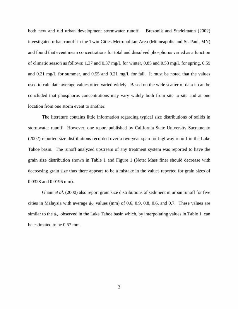
Also termed wet ponds in some contexts, these basins are similar to dry detention ponds
except the outlet structure is set at a higher elevation to create a permanent pool within the pond.
Retention basins utilize gravity settling as the major removal mechanism but nutrient and organic
removal can be achieved through aquatic vegetation and microorganism uptake. Figure 2 below
shows a cross section of a retention pond illustrating this type of outlet structure.
Figure 2. Retention basin cross section.
Source: Barr Engineering Company, 2001.
Limitations of these systems are typically related to retention time. During high flows, or
freezing weather (when the permanent pool is frozen or covered with ice) influent runoff can
short-circuit through the retention system and reduce the effectiveness of the sedimentation
mechanism. Pond characteristics can also affect the removal efficiency. Changes in pH or
hardness can alter the solubility of many contaminants and thus release them to the effluent
(USEPA, 1999a). Another possible limitation of retention systems is high temperature effluent.
9
The water in the pond may absorb enough solar energy to significantly increase the temperature
of the effluent which may adversely impact fish and other aquatic species in the receiving waters.
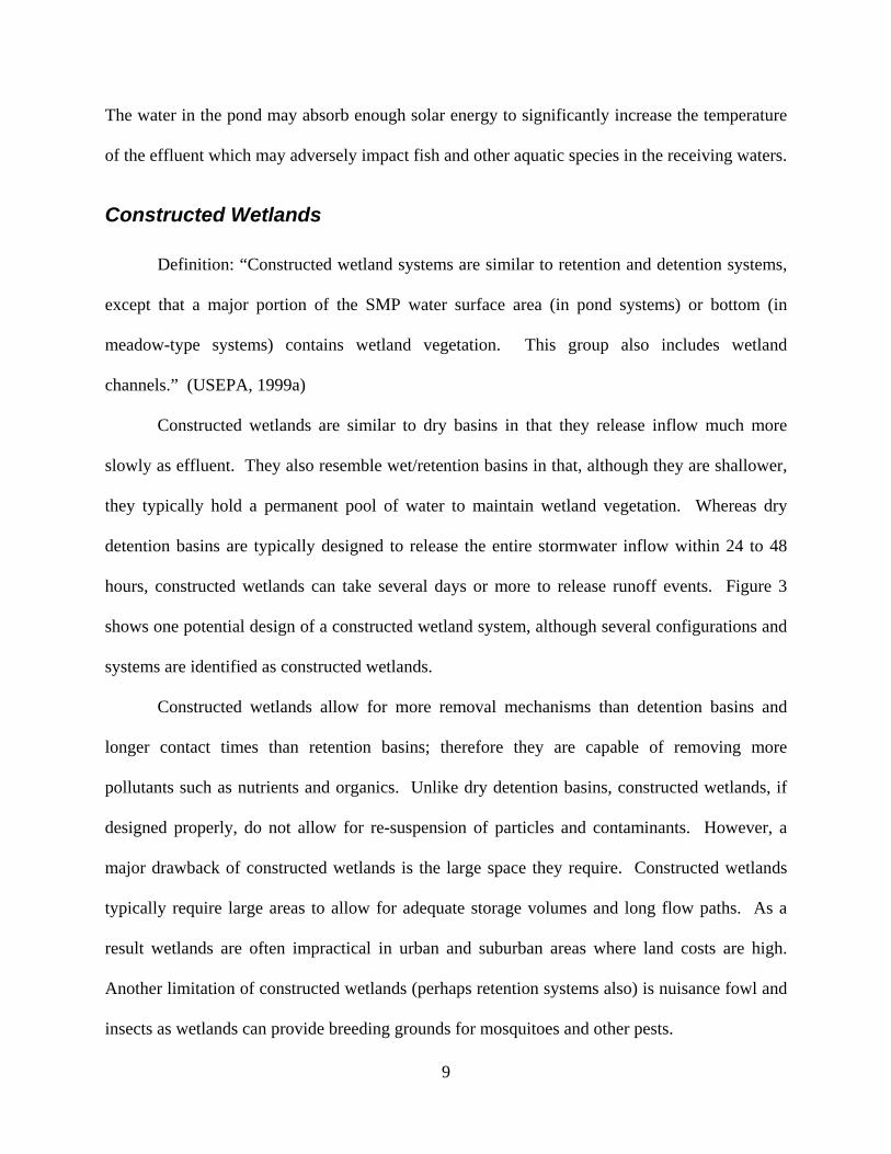
Constructed Wetlands
Definition: “Constructed wetland systems are similar to retention and detention systems,
except that a major portion of the SMP water surface area (in pond systems) or bottom (in
meadow-type systems) contains wetland vegetation. This group also includes wetland
channels.” (USEPA, 1999a)
Constructed wetlands are similar to dry basins in that they release inflow much more
slowly as effluent. They also resemble wet/retention basins in that, although they are shallower,
they typically hold a permanent pool of water to maintain wetland vegetation. Whereas dry
detention basins are typically designed to release the entire stormwater inflow within 24 to 48
hours, constructed wetlands can take several days or more to release runoff events. Figure 3
shows one potential design of a constructed wetland system, although several configurations and
systems are identified as constructed wetlands.
Constructed wetlands allow for more removal mechanisms than detention basins and
longer contact times than retention basins; therefore they are capable of removing more
pollutants such as nutrients and organics. Unlike dry detention basins, constructed wetlands, if
designed properly, do not allow for re-suspension of particles and contaminants. However, a
major drawback of constructed wetlands is the large space they require. Constructed wetlands
typically require large areas to allow for adequate storage volumes and long flow paths. As a
result wetlands are often impractical in urban and suburban areas where land costs are high.
Another limitation of constructed wetlands (perhaps retention systems also) is nuisance fowl and
insects as wetlands can provide breeding grounds for mosquitoes and other pests.

10
Figure 3. One example of a constructed wetland system.
Source: Barr Engineering Company, 2001.
As with any SMP, constructed wetlands require regular maintenance to remain effective.
Faulkner and Richardson (1991) attributed a significant reduction in nutrient removal to the
wetland vegetation reaching maximum density. Thus, wetlands plants may have to be harvested
to remove overabundant vegetation. Furthermore, overabundant and decaying vegetation can
deposit large amounts of soluble and particulate phosphorus into the wetlands system; typically
more than the living vegetation can uptake. This can result in an addition of phosphorus to the
system. However it is questionable if harvesting plants will adequately remove phosphorus
11
because in studies where vegetation has been harvested in an attempt to remove phosphorus,
only minimal amounts of phosphorus have been recovered (Kadlec and Knight, 1996). These
factors may make it difficult for constructed wetlands to be a long-term cost-effective quality
control technique.
As with other SMPs, removal efficiencies of TSS and P for constructed wetlands vary
widely among monitoring studies. This may be partly attributed to the fact that constructed
wetlands can lose their capacity to remove phosphorus over time (Oberts, 1999). Even when
phosphorus removal occurs, wetlands usually remove a significantly higher fraction of TSS than
phosphorus.
Infiltration Practices
Definition: “Infiltration systems capture a volume of runoff and infiltrate it into the
ground” (USEPA, 1999a). Any technique that does not discharge effluent to surface waters, or
reduces total discharge, can be categorized as an infiltration practice. Infiltration practices
encompass a number of techniques utilized for the treatment of stormwater runoff. Most
infiltration practices require some form of pretreatment along with frequent maintenance to
prevent blockage and ensure proper operation of the system.
The removal performance of infiltration practices has not been thoroughly reported. The
difficulty in determining the quality of the effluent is most likely the chief reason for this lack of
information. The data regarding infiltration practices that is available varies drastically due to
many factors such as varying soil conditions, influent water quality, depth to water table, degree
of pretreatment, maintenance protocols, etc. In areas with highly permeable soil, poor quality
effluent may not receive adequate contact time and may be released to aquifers with little or no
treatment (USEPA 1999a). It is also very difficult to monitor the effluent of infiltration practices
12
and confidently report that the findings are solely attributed to the infiltration system itself. Four
common infiltration practices are discussed below.
Infiltration Basins
Infiltration basins are similar to detention or retention basins in design and appearance,
but do not use an outlet structure to convey effluent, except when the runoff volume is too large
and cannot be stored in the basin. These basins release treated water directly to the groundwater
after filtration through the basin media which may be comprised of the existing soil and/or a
specified filtration media introduced during construction. As mentioned previously, an overflow
outlet to a receiving water body is usually installed to discharge the excess water volume of large
storms.
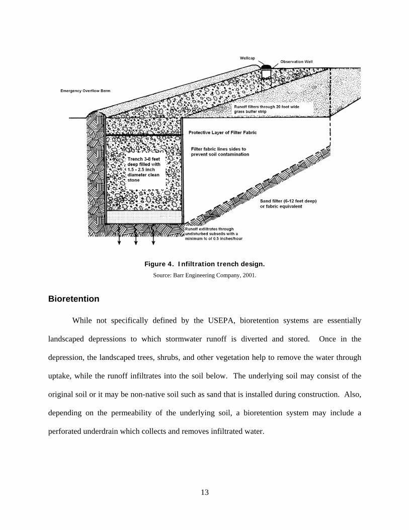
Infiltration Trenches
Infiltration trenches can be thought of as constructed channels filled with filtration media
or soil which allows for the infiltration of stormwater. These trenches are often placed around
the perimeter of parking lots or other structures to treat the runoff generated by the site. With
sufficient sizing and properly designed flow regulators (typically check dams), infiltration
trenches can infiltrate a large portion of the runoff. Figure 4 shows an example of a typical
infiltration trench design.
13
Figure 4. Infiltration trench design.
Source: Barr Engineering Company, 2001.
Bioretention
While not specifically defined by the USEPA, bioretention systems are essentially
landscaped depressions to which stormwater runoff is diverted and stored. Once in the
depression, the landscaped trees, shrubs, and other vegetation help to remove the water through
uptake, while the runoff infiltrates into the soil below. The underlying soil may consist of the
original soil or it may be non-native soil such as sand that is installed during construction. Also,
depending on the permeability of the underlying soil, a bioretention system may include a
perforated underdrain which collects and removes infiltrated water.

14
Bioretention systems are rapidly gaining in popularity because it is assumed they
incorporate the best of vegetative systems and filtration systems. However, their impact on
water quality is neither well known nor documented.
Porous Pavements
Definition: “Porous pavement systems consist of permeable pavements or other stabilized
surfaces that allow stormwater runoff to infiltrate through the surface and into the groundwater.”
(USEPA, 1999a)
Porous pavement comes in many forms, some of which are commercially available.
Unlike typical asphalt or concrete pavements, porous pavements allow runoff to seep through the
pavement surface which reduces the amount of runoff. Porous pavements are categorized as an
infiltration practice because they allow runoff to infiltrate into the underlying soil.
Limitations of porous pavements are similar to other infiltration practices and usually
involve maintenance and clogging issues. Porous pavements typically contain small voids (or
seams between bricks) that can become clogged with sediments. Frequent surface vacuuming or
flushing is usually required to keep porous pavements free of sediments and other debris,
allowing prompt infiltration of surface runoff.
Water quality treatment of runoff by porous pavements is similar to that of other
infiltration practices. The porous pavement itself provides little actual removal while the
infiltration of the runoff to receiving groundwater can remove significant amounts of
contaminants.

15
Sand Filtration
Definition: Sand filtration systems utilize granular media to filter stormwater runoff that
is collected and discharged as effluent to other treatment systems or directly to receiving waters.
Those called “Austin” sand filters appear much like a dry detention basin but include built-in
sand filled areas that filter the water and release it to an underdrain. The “Delaware” sand filters
are usually smaller, low retention filters that can be placed underground in concrete chambers
and are typically designed to capture and treat only the first portion (often called the “first flush”)
of most runoff events.
Herrera Environmental Consultants (1995) performed a study which showed that sand
filters provide little (i.e. 20 - 50 % total, 5 - 30 % soluble) capacity for phosphorus removal
compared to other SMPs. Anderson et al. (1985) monitored several water-quality parameters of
more than a dozen intermittent sand filters for the USEPA. Their results also concur that a pure
sand-filter media provides “only limited removal of phosphorus” (Anderson, 1985).
Harper and Herr (1993) performed pilot-scale and full-scale monitoring studies in Florida
for the removal of several water quality contaminants. It was estimated that typical sand filters
remove approximately 40 to 50 percent particulate and total phosphorus, but at most only five
percent soluble phosphorus. Another sand filter utilizing a silica sand media exhibited better
results for soluble and total phosphorus (35 and 55 percent, respectively) but also contributed
particulate phosphorus to the effluent. Harper and Herr acknowledged that the silica sand was
considerably coarser than the typical sand media used in their other experiments. Harper and
Herr (1993) also conducted experiments comparing sod coverings placed on top of sand filters.
Four types of sod were tested in a fashion similar to their previous study. It was determined that

16
all but one sod covering contributed dissolved phosphorus to the effluent, and removal rates for
particulate or total phosphorus were at most 54 percent.
The full scale monitoring performed by Harper and Herr (1993) encompassed many
water quality and quantity characteristics of a basin that incorporated both infiltration and
filtration practices in what the authors deemed a “Wet detention basin.” By performing a mass
balance on the pond it was determined that the pond removed roughly 30 to 40 percent of the
ortho-phosphorus, 80 percent of the particulate phosphorus, and 60 percent of the total
phosphorus over the six month monitoring period. However, the configuration of the pond
created a permanent pool of water which allowed for algae growth. Harper and Herr (1993)
attribute the high removal rates of ortho-phosphorus to algae uptake by the biomass that
developed within the pond and the particulate phosphorus removal to filtration processes.
Bell et al. (undated) conducted an assessment of Delaware (also referred to as
intermittent) sand filters for their removal efficiencies of several pollutants found in urban
stormwater runoff. The study was based on the monitoring of an existing sand filter constructed
in Northern Virginia (pg. 5-1) over the course of 20 storm events during the summer of 1994.
Among many other pollutants, Bell et al. reported removal rates of up to 90 percent for
phosphorus (pg. 5-20) and suggested that their results “may not reflect the true potential of
intermittent sand filter BMPs.” Even though average removals of 60 to 70 percent were
reported, an analysis of the filter media revealed constituents of iron (3000 mg/kg), calcium (4-6
mg/kg), and aluminum (2900 mg/kg). Based on evidence provided by Baker et al. (1997) and
Anderson et al. (1985), it can be postulated that these “involuntary” additives affected the
removal efficiencies of the sand filters assessed by Bell et al. (undated).

17
Other additives such as peat or compost have been studied for their effectiveness at
removing contaminants from stormwater runoff. Farnham and Noonan (1988) conducted a study
of peat-sand combination filter efficiencies and reported a direct relationship between
phosphorus removal efficiency as percent removal and input phosphorus concentration. Galli
(1990) also suggested the use of a peat-sand filter for urbanized runoff treatment and predicted
70 percent removal of total phosphorus for peat species that contain minimal, if any, phosphorus
content. The USEPA monitored a filter built to Galli’s design specifications and reported
instances of both phosphorus removal and phosphorus addition through leaching of the media
into the water (USEPA, 1999a, pg. 5-80, 5-81). Other sources (Koerlsman et al., 1993) have
also reported peat as a source of phosphorus when used as filter media. Stewart (1992) reported
that a leaf compost filter can also leach phosphorus into stormwater effluent (Section 3, Table
12).
Vegetated Systems
Definition: “Vegetated systems such as grassed swales and filter strips are designed to
convey and treat either shallow flow (swales) or sheet flow (filter strips) runoff.” (USEPA,
1999a)
Vegetated systems are a special application of infiltration practices that utilize vegetated
cover for two purposes. Vegetated cover on sloped applications slow the overland flow to allow
greater opportunity for infiltration into the soil while also providing an opportunity for nutrient
uptake through the root system. Vegetated systems suffer the same monitoring difficulties as
other infiltration practices, and can be more difficult to maintain. As with infiltration trenches
and basins, vegetated systems can become clogged with particles and debris in the absence of
proper pretreatment and maintenance. In some cases the sediment deposits can begin to choke

18
out the vegetated cover and create an erodible surface capable of contributing sediment and other
pollutants directly downstream.
Commercial Products
Commercially available products include, but are not limited to, DrainPac™,
HydroKleen™, StormTreatTM System, BaySaver™, Stormceptor®, Vortechs ™, Downstream
Defender®, Continuous Deflective Separation (CDS®), and StormFilter™. Other commercially
available products are available and new products will almost certainly be introduced in the
future. Brueske (2000) performed a review of several commercial products, however an
unbiased review of the performance of these products can be difficult to obtain and reported
removal rates must be used with caution. The relatively small size of the commercial products
(as compared to wet basins, wetlands, detention ponds, etc.) may result in their long-term
effectiveness being much lower than reported. For example, one product with a reported TSS
removal rate of over 80% was field tested and found to remove only about one-third of the
sediment load and 19 percent of total phosphorus (Waschbusch, 1999).
Review Summary
The ability of SMPs to remove TSS and phosphorus effectively is dependant on many
factors and can occur by various mechanisms. Many researchers have studied SMPs for their
capability to remove TSS and phosphorus and some have investigated the mechanisms by which
removal occurs. Designers, planners, and other decision makers have little guidance that
incorporates this information in combination with SMP costs to aid them in the selection of a
SMP. Comparisons of the cost-effectiveness of SMPs are, at best, rare and yet decision makers
are continually forced to spend limited resources on technologies whose costs and benefits are

19
not well understood. A comparison of this nature would enable decision makers to better
appropriate limited resources as they strive to meet federal regulations by improving the water
quality of stormwater effluent.
This report helps fill a critical knowledge gap by quantitatively comparing the cost and
effectiveness of several of the most common SMPs for which reliable data was available. More
direct comparisons, however, are needed, including comparisons with and between commercial
products.
Cost Estimation
Based on published cost data of actual SMPs a method, which is described below, was
developed that will enable designers and planners to make estimates of the Total Present Cost
(TPC) of various SMPs if the size of the SMP is known. In this report, the TPC is defined as the
present worth of the total construction cost of the project plus the present worth of 20 years of
annual operating and maintenance (O&M) costs. The values reported do not include costs of
pretreatment units (which may be required), design or engineering fees, permit fees, land costs,
or contingencies, etc.
Water Quality Volume
The costs of SMP projects are usually reported along with the corresponding watershed
size (usually in acres or square feet) and/or the water quality volume (WQV) for which the SMP
was designed. The water quality volume is often defined as the volume (typically in acre-feet or
cubic feet) of runoff that the SMP is designed to store and treat.
Claytor and Schueler (1996) calculate the WQV (ft3) for a particular precipitation amount
as:

20
ARP12
43560 WQV V ∗∗∗⎟⎠⎞
⎜⎝⎛= (1)
where: P = Precipitation depth (inches)
RV = Ratio of runoff to rainfall in the watershed
A = Watershed area (acres), and the constants are conversion factors.
The ratio of runoff to rainfall, RV, has the most uncertainty of the parameters in Equation
1. For this analysis, a relatively simple relationship was used (Claytor and Schueler, 1996;
Young et al., 1996)
( )I0.0090.05R V ∗+= (2)
where I is the percent (0-100) of the watershed that is impervious. Equation 2 indicates that, for
a 100% impervious watershed, 95% of the rainfall becomes runoff.
Total Construction Costs
Values of total construction costs of SMPs throughout the United States were collected
from published literature. Although data was collected on many SMP technologies, sufficient
data to perform a cost analysis could be found for only dry detention basins, wet/retention basins,
constructed wetlands, infiltration trenches, bioinfiltration filters, sand filters, and swales. All
data were adjusted to reflect costs in Minnesota by means of ‘Regional Cost Adjustment
Factors’ as reported by the United States Environmental Protection Agency (USEPA, 1999a) and
were also adjusted to year 2005 dollars using an annual inflation rate of 3 percent. A value of 3
percent was chosen after an analysis of building cost indexes for the past 11 years (Turner
Construction, 2004) revealed that the average annual inflation was 3.26 percent with a range
from 0.3 to 5.4 percent.
21
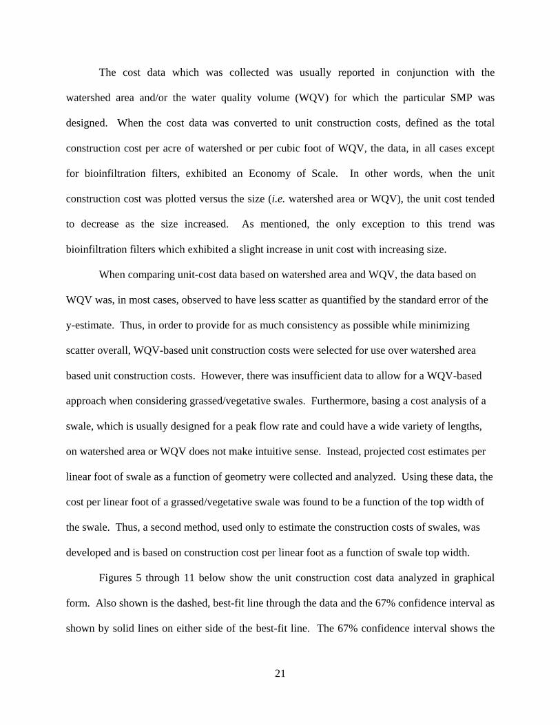
The cost data which was collected was usually reported in conjunction with the
watershed area and/or the water quality volume (WQV) for which the particular SMP was
designed. When the cost data was converted to unit construction costs, defined as the total
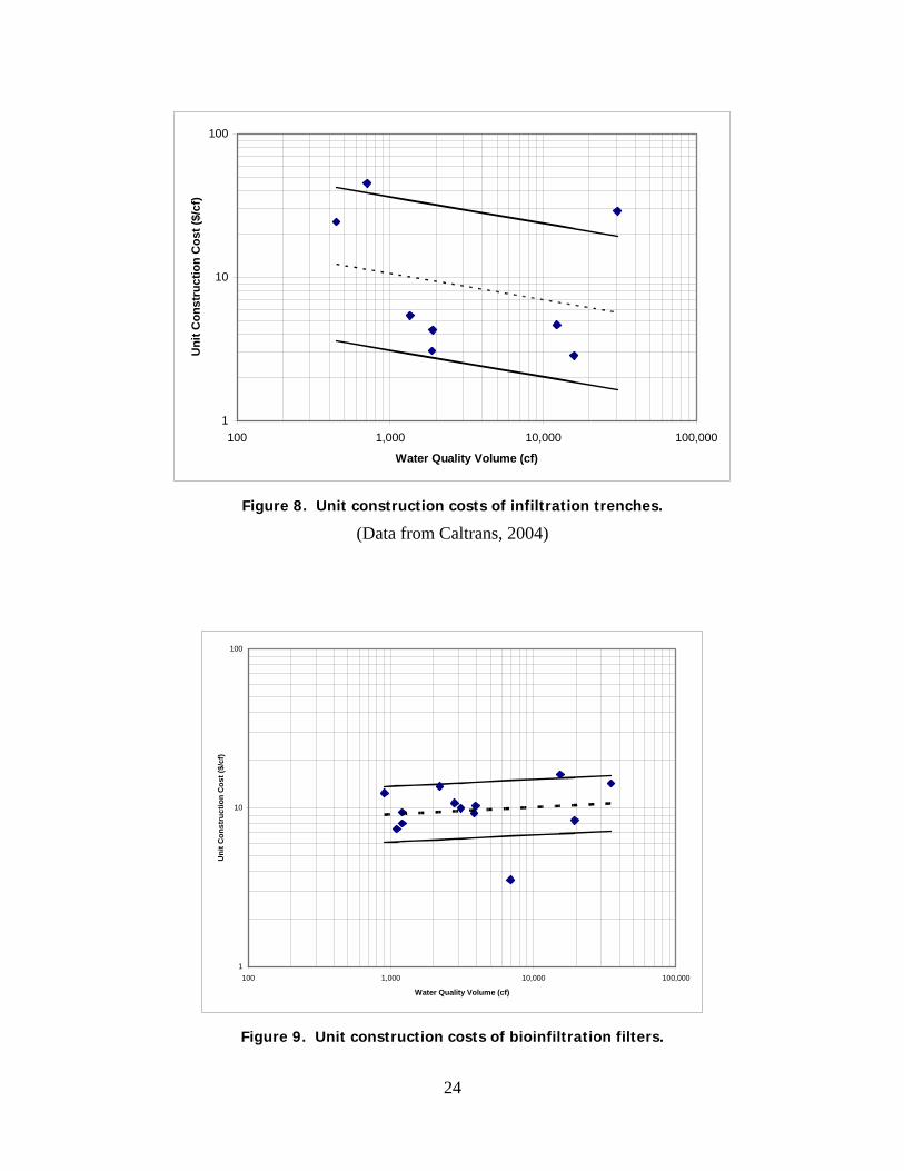
construction cost per acre of watershed or per cubic foot of WQV, the data, in all cases except
for bioinfiltration filters, exhibited an Economy of Scale. In other words, when the unit
construction cost was plotted versus the size (i.e. watershed area or WQV), the unit cost tended
to decrease as the size increased. As mentioned, the only exception to this trend was
bioinfiltration filters which exhibited a slight increase in unit cost with increasing size.
When comparing unit-cost data based on watershed area and WQV, the data based on
WQV was, in most cases, observed to have less scatter as quantified by the standard error of the
y-estimate. Thus, in order to provide for as much consistency as possible while minimizing
scatter overall, WQV-based unit construction costs were selected for use over watershed area
based unit construction costs. However, there was insufficient data to allow for a WQV-based
approach when considering grassed/vegetative swales. Furthermore, basing a cost analysis of a
swale, which is usually designed for a peak flow rate and could have a wide variety of lengths,
on watershed area or WQV does not make intuitive sense. Instead, projected cost estimates per
linear foot of swale as a function of geometry were collected and analyzed. Using these data, the
cost per linear foot of a grassed/vegetative swale was found to be a function of the top width of
the swale. Thus, a second method, used only to estimate the construction costs of swales, was
developed and is based on construction cost per linear foot as a function of swale top width.
Figures 5 through 11 below show the unit construction cost data analyzed in graphical
form. Also shown is the dashed, best-fit line through the data and the 67% confidence interval as
shown by solid lines on either side of the best-fit line. The 67% confidence interval shows the
22
bounds that will, on average, contain 67% of the data. In other words, one-third of the data could
fall outside of the 67% confidence interval. If there is sufficient data (~20) and the distribution
is, in this case, truly log-normal, then one-third of the data will fall outside of the 67%
confidence interval. The data originating from Brown and Schueler (1997) were read graphically
whereas the values from SWRPC (1991), Caltrans (2004), and ASCE (2004) were given in
tabular form. The data from Caltrans (2004) was collected by means of a survey distributed by
Caltrans to other agencies throughout the country. It should be noted that the total construction
costs of SMPs installed by Caltrans were also available but these values were omitted from this
0.1
1.0
10.0
100.0
1,000 10,000 100,000 1,000,000 10,000,000
WQV (cf)
Uni
t Cos
t ($/
cf)
Figure 5. Unit construction costs of dry detention basins.
(Data from Brown and Schueler, 1997; ASCE, 2004; Caltrans, 2004)

23
0.10
1.00
10.00
10,000 100,000 1,000,000 10,000,000
Water Quality Volume (cf)
Uni
t Con
stru
ctio
n C
ost (
$/cf
)
Figure 6. Unit construction costs of wet basins.
(Data from Brown and Schueler, 1997; Caltrans, 2004)
0.1
1.0
10.0
100.0
1,000 10,000 100,000 1,000,000 10,000,000
Water Quality Volume (cf)
Uni
t Con
stru
ctio
n C
ost (
$/cf
)
Figure 7. Unit construction costs of constructed wetlands.
(Data from Brown and Schueler, 1997, Caltrans, 2004; ASCE, 2004)
24
1
10
100
100 1,000 10,000 100,000
Water Quality Volume (cf)
Uni
t Con
stru
ctio
n C
ost (
$/cf
)
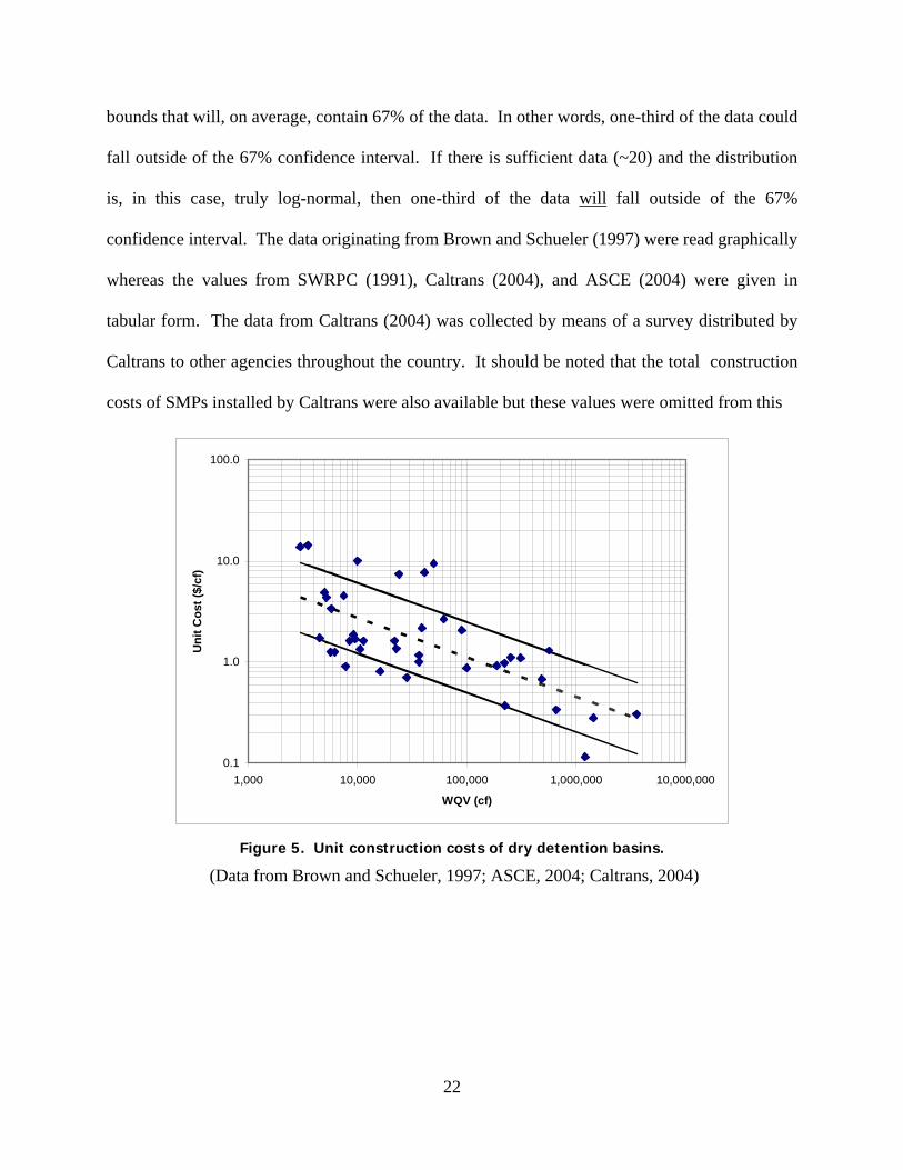
Figure 8. Unit construction costs of infiltration trenches.
(Data from Caltrans, 2004)
1
10
100
100 1,000 10,000 100,000
Water Quality Volume (cf)
Uni
t Con
stru
ctio
n C
ost (
$/cf
)
Figure 9. Unit construction costs of bioinfiltration filters.

25
(Data from Brown and Schueler, 1997; Caltrans, 2004)
0.1
1.0
10.0
100.0
1,000.0
100 1,000 10,000 100,000 1,000,000
Water Quality Volume (cf)
Uni
t Con
stru
ctio
n C
ost (
$/cf
)
Austin Delaware Undefined
Figure 10. Unit construction costs of sand filters.
(Data from Brown and Schueler, 1997; Caltrans, 2004)
0
5
10
15
20
25
30
35
0 5 10 15 20 25
Top Width of Swale (ft)
Cos
t ($/
lf)
Figure 11. Unit construction costs of grassed/vegetative swales.
(Data from SWRPC, 1991)

26
analysis because their costs were typically about ten times higher than similarly sized projects
constructed by other agencies. Caltrans attributed these high costs to the fact that their projects
were retrofits and were not installed as part of larger construction projects.
Of the data collected for sand filters, some contained information on the type of sand
filter (e.g. Austin or Delaware) while other data included no such description. Interestingly,
when analyzing the sand-filter data for unit costs, there was essentially the same amount of
scatter when the data of each sand-filter type was analyzed alone as there was when all sand-
filter data was combined and analyzed together. This suggests that sand-filter unit-construction
costs are independent of the type of filter and, as a result, cost estimates developed herein do not
differentiate between sand-filter types. Figure 10 does differentiate between the Austin,
Delaware, and undefined data by the data marker but, since no trend was observed for individual
filter types, the best-fit line is drawn through the combined data.
The uncertainty observed in the data for all SMPs is most likely due to several factors
such as design parameters, regulation requirements, soil conditions, site specifics, etc. For
example, variable design parameters that would affect the total construction cost include pond
side slopes, depth and free board on ponds, total wet pond volume, outlet structures, the need for
retaining walls, etc. Site specific variables include clearing and grubbing costs, fencing around
the SMP, etc. Due to the wide number of undocumented variables that affect the data, this
scatter would be extremely difficult, if not impossible, to minimize.
Later in this report the data shown in Figures 5 through 11 will be combined with annual
O&M cost data to estimate the TPC of each SMP as a function of size. After a discussion of
typical land-area requirements, the methods and data used to incorporate O&M costs into this
analysis are described.
27
Land-Area Requirements
An important cost of any SMP is that of the land area on which the SMP will be located.
For urban areas, in which land is typically at a premium, this cost can be relatively large. On the
contrary, in more open, rural areas, land costs might be a very small percentage of the total
project costs. Due to the extreme range of land costs and variability from site to site, no attempt
was made to incorporate this cost into the Total Present Cost analysis. However, the land area
requirements, and therefore the associated land costs, of each SMP technology can vary
dramatically and would, in many scenarios, have a significant impact on the total cost of a
project. For example, a sand filter placed underground, below a parking lot would, in effect,
require no additional land area. However, a constructed wetland designed to treat the same
volume of runoff as the underground sand filter would require significant additional land area
that may preclude the use of wetlands. Given the variability of land costs and the variety of
potential SMPs that could be used, the impact of land costs must be done on an individual, case-
by-case basis. Table 3, which lists typical SMP land-area requirements for effective treatment, is
presented to assist designers and planners in making such a comparison. Values reported in
Table 3 by Claytor and Schueler (1996) are for the general category of SMP system and may
include more than one specific type of SMP. For example, their pond category may include both
wet and dry ponds. Table 4 lists wet pond areas required for control of particles that are 5 and 20
microns in size as reported by Pitt and Voorhees (1997). If the land costs in the locale of a
particular project are known, these costs can be combined with the information presented in the
tables to estimate a range of possible land area costs associated with each SMP under
consideration. This information is intended to give only a possible range of land area costs. For
more accurate land area cost estimates, a preliminary SMP design should be performed.
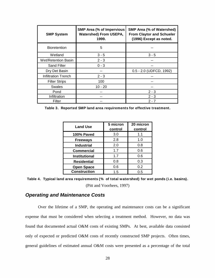
28
SMP SystemSMP Area (% of Impervious Watershed) From USEPA,
1999.
SMP Area (% of Watershed) From Claytor and Schueler
(1996) Except as noted.
Bioretention 5 --
Wetland 3 - 5 3 - 5Wet/Retention Basin 2 - 3 --
Sand Filter 0 - 3 --Dry Det Basin -- 0.5 - 2.0 (UDFCD, 1992)
Infiltration Trench 2 - 3 --Filter Strips 100 --
Swales 10 - 20 --Pond -- 2 - 3
Infiltration -- 2 - 3Filter -- 2 - 7
Table 3. Reported SMP land area requirements for effective treatment.
Land Use 5 micron control
20 micron control
100% Paved 3.0 1.1Freeways 2.8 1.0Industrial 2.0 0.8
Commercial 1.7 0.6Institutional 1.7 0.6Residential 0.8 0.3Open Space 0.6 0.2
Construction 1.5 0.5 Table 4. Typical land area requirements (% of total watershed) for wet ponds (i.e. basins).
(Pitt and Voorhees, 1997)
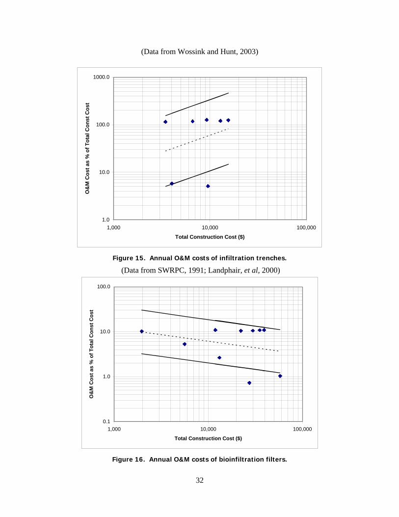
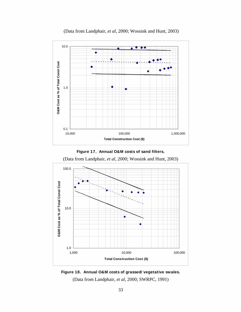
Operating and Maintenance Costs
Over the lifetime of a SMP, the operating and maintenance costs can be a significant
expense that must be considered when selecting a treatment method. However, no data was
found that documented actual O&M costs of existing SMPs. At best, available data consisted
only of expected or predicted O&M costs of recently constructed SMP projects. Often times,
general guidelines of estimated annual O&M costs were presented as a percentage of the total

29
construction cost. For example, the USEPA (1999a) gives a summary of typical SMP annual
O&M costs as shown in the middle column of Table 5. Also included in the right column of
Table 5 is the range of the authors’ collection of predicted O&M costs as a percent of the
construction cost.
Ideally the estimate of TPC would be based on actual O&M costs of existing SMPs but,
as mentioned above, estimated annual O&M costs were the only available data. When this data
was evaluated to determine how the estimated O&M costs compared to those summarized by the
USEPA, a trend was observed for all SMPs except infiltration trenches in which the annual
O&M cost as a percentage of the construction cost decreased with increasing construction cost.
The collected annual O&M cost data are shown as log-log plots in Figures 12 through 18. As
with the construction cost data, the best-fit line through the data and the 67% confidence interval
are shown.
SMP Summary of Typical AOM Costs
(% of Construction Cost) (USEPA, 1999A)
Collected Cost Data: Estimated Annual O&M Costs (% of Construction Costs)
Retention Basins and Constructed
Wetlands 3%-6%
--
Detention Basins <1% 1.8%-2.7% Constructed
Wetlands 2% 4%-14.1%
Infiltration Trench 5%-20% 5.1%-126%
Infiltration Basin 1%-3% 5%-10%
2.8%-4.9%
Sand Filters 11%-13% 0.9%-9.5% Swales 5%-7% 4.0%-178%
Bioretention 5%-7% 0.7%-10.9% Filter Strips $320/Acre (maintained) -- Wet Basins Not Reported 1.9%-10.2%
Table 5. Typical annual O&M costs of SMPs.

30
In the following section the annual O&M costs will be combined with the unit
construction costs to develop an estimate for the Total Present Cost of each SMP as a function of
WQV or, in the case of swales, as a cost per linear foot as a function of swale top width.
Total Present Cost
If an estimate of the total construction cost of a SMP were desired, the data presented in
Figures 5 through 10 could be used in a stand-alone manner simply by multiplying the unit
construction cost ($/ft3) by WQV (ft3). The construction cost of swales could also be easily
estimated by multiplying the unit cost ($/ft) by the swale length (ft). However, a more practical
estimate is that of the total costs needed to not only construct but also to maintain and operate the
SMP. Rather than provide one estimate for total construction cost and another estimate for
annual O&M expenditures, the data presented in the previous two sections will be combined in
1
10
10,000 100,000 1,000,000
Total Construction Cost ($)
O&
M C
ost a
s %
of T
otal
Con
st C
ost
Figure 12. Annual O&M costs of dry detention basins.
(Data from Landphair, et al, 2000)

31
1
10
100
1,000 10,000 100,000 1,000,000
Total Construction Cost ($)
O&
M C
ost a
s %
of T
otal
Con
st C
ost
Figure 13. Annual O&M costs of wet basins.
(Data from SWRPC, 1991; Wossink and Hunt, 2003)
1
10
100
1,000 10,000 100,000Total Construction Cost ($)
O&
M C
ost a
s %
of T
otal
Con
st C
ost
Figure 14. Annual O&M costs of constructed wetlands.
32
(Data from Wossink and Hunt, 2003)
1.0
10.0
100.0
1000.0
1,000 10,000 100,000
Total Construction Cost ($)
O&
M C
ost a
s %
of T
otal
Con
st C
ost
Figure 15. Annual O&M costs of infiltration trenches.
(Data from SWRPC, 1991; Landphair, et al, 2000)
0.1
1.0
10.0
100.0
1,000 10,000 100,000
Total Construction Cost ($)
O&
M C
ost a
s %
of T
otal
Con
st C
ost
Figure 16. Annual O&M costs of bioinfiltration filters.
33
(Data from Landphair, et al, 2000; Wossink and Hunt, 2003)
0.1
1.0
10.0
10,000 100,000 1,000,000
Total Construction Cost ($)
O&
M C
ost a
s %
of T
otal
Con
st C
ost
Figure 17. Annual O&M costs of sand filters.
(Data from Landphair, et al, 2000; Wossink and Hunt, 2003)
1.0
10.0
100.0
1,000 10,000 100,000
Total Construction Cost ($)
O&
M C
ost a
s %
of T
otal
Con
st C
ost
Figure 18. Annual O&M costs of grassed/vegetative swales.
(Data from Landphair, et al, 2000; SWRPC, 1991)
34
order to estimate the Total Present Cost (TPC) of each SMP as a function of size. As previously
defined, the TPC is the sum of the total construction cost and the equivalent present cost of 20
years of annual O&M expenses. For each SMP, the TPC is estimated as a function of size (i.e.
WQV or swale top width).
The Total Present Cost with a 67% confidence interval for six of the seven SMPs was
estimated as a function of water-quality volume (WQV). Also, the total present cost of a 1000’
long grassed/vegetative swale was estimated as a function of the swale top width. The TPC
estimates incorporate the total construction cost data and annual O&M cost data presented in the
previous sections. In this estimate, the annual O&M costs are converted to an equivalent present
cost using historical data on the rates of municipal bond yields and inflation. The analysis
method and the results for each of the seven SMPs are presented below.
In order to estimate the TPC of each SMP the total construction cost was calculated as a
function of size (i.e. WQV or swale top width) by multiplying the corresponding unit
construction cost by WQV or, in the case of swales, by the swale length. Using these values of
total construction cost and the annual O&M cost data best-fit line, the annual O&M cost was
estimated for each WQV or swale top width. For example, for a dry detention basin, the unit
construction costs for a range of WQVs were calculated from the best-fit line shown in Figure 6.
The total construction costs were then estimated by multiplying the unit construction costs by the
corresponding WQV. The annual O&M costs (as a percentage of construction cost) were then
estimated using the best-fit line of Figure 12. Next, the value of the annual O&M cost estimates
were calculated by multiplying each percentage (as found from the best-fit line) by the
corresponding total construction cost. Finally, the annual O&M costs for a 20-year period were
35
converted to an equivalent present cost (based on historical values of interest and inflation rates
as described below) and added to the total construction cost.
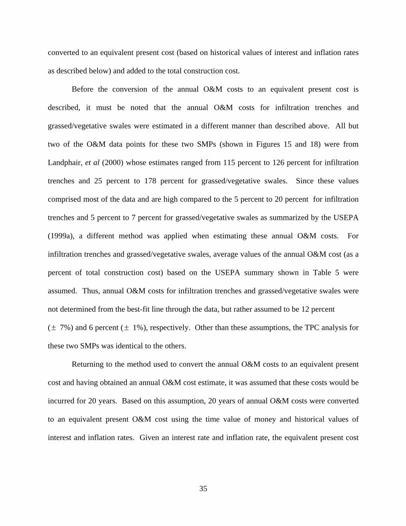
Before the conversion of the annual O&M costs to an equivalent present cost is
described, it must be noted that the annual O&M costs for infiltration trenches and
grassed/vegetative swales were estimated in a different manner than described above. All but
two of the O&M data points for these two SMPs (shown in Figures 15 and 18) were from
Landphair, et al (2000) whose estimates ranged from 115 percent to 126 percent for infiltration
trenches and 25 percent to 178 percent for grassed/vegetative swales. Since these values
comprised most of the data and are high compared to the 5 percent to 20 percent for infiltration
trenches and 5 percent to 7 percent for grassed/vegetative swales as summarized by the USEPA
(1999a), a different method was applied when estimating these annual O&M costs. For
infiltration trenches and grassed/vegetative swales, average values of the annual O&M cost (as a
percent of total construction cost) based on the USEPA summary shown in Table 5 were
assumed. Thus, annual O&M costs for infiltration trenches and grassed/vegetative swales were
not determined from the best-fit line through the data, but rather assumed to be 12 percent
( ± 7%) and 6 percent ( ± 1%), respectively. Other than these assumptions, the TPC analysis for
these two SMPs was identical to the others.
Returning to the method used to convert the annual O&M costs to an equivalent present
cost and having obtained an annual O&M cost estimate, it was assumed that these costs would be
incurred for 20 years. Based on this assumption, 20 years of annual O&M costs were converted
to an equivalent present O&M cost using the time value of money and historical values of
interest and inflation rates. Given an interest rate and inflation rate, the equivalent present cost
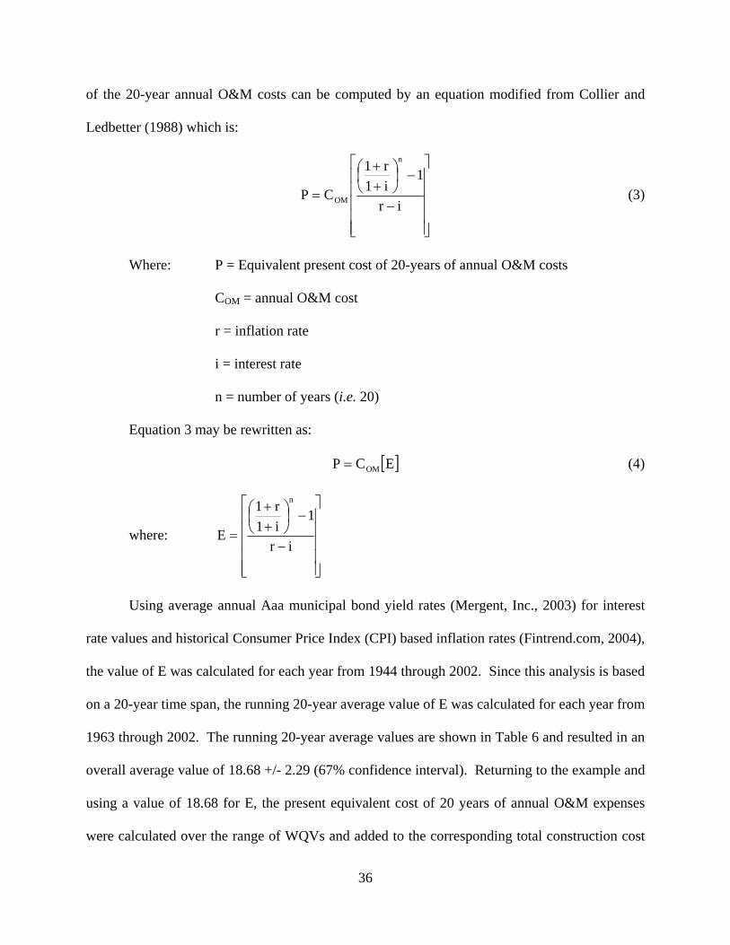
36
of the 20-year annual O&M costs can be computed by an equation modified from Collier and
Ledbetter (1988) which is:
⎥⎥⎥⎥⎥
⎦
⎤
⎢⎢⎢⎢⎢
⎣
⎡
−
−⎟⎠⎞
⎜⎝⎛
++
=ir
1i1r1
CP
n
OM (3)
Where: P = Equivalent present cost of 20-years of annual O&M costs
COM = annual O&M cost
r = inflation rate
i = interest rate
n = number of years (i.e. 20)
Equation 3 may be rewritten as:
[ ]ECP OM= (4)
where:
⎥⎥⎥⎥⎥
⎦
⎤
⎢⎢⎢⎢⎢
⎣
⎡
−
−⎟⎠⎞
⎜⎝⎛
++
=ir
1i1r1
E
n
Using average annual Aaa municipal bond yield rates (Mergent, Inc., 2003) for interest
rate values and historical Consumer Price Index (CPI) based inflation rates (Fintrend.com, 2004),
the value of E was calculated for each year from 1944 through 2002. Since this analysis is based
on a 20-year time span, the running 20-year average value of E was calculated for each year from
1963 through 2002. The running 20-year average values are shown in Table 6 and resulted in an
overall average value of 18.68 +/- 2.29 (67% confidence interval). Returning to the example and
using a value of 18.68 for E, the present equivalent cost of 20 years of annual O&M expenses
were calculated over the range of WQVs and added to the corresponding total construction cost

37
to give the Total Present Cost (TPC) in 2005 dollars as a function of WQV. The uncertainties
associated with the 67% confidence intervals of the unit construction costs, annual O&M costs as
a percent of the construction cost, and inflation and interest rates (i.e. E) were incorporated into
the TPC as described by Kline (1985).
Year20-yr
running Avg. E
Year20-yr
running Avg. E
Year20-yr
running Avg. E
Year20-yr
running Avg. E
1963 23.94 1973 17.55 1983 20.22 1993 18.231964 23.73 1974 18.25 1984 19.98 1994 17.411965 23.46 1975 18.68 1985 19.75 1995 16.911966 22.28 1976 18.74 1986 19.46 1996 16.741967 19.17 1977 18.82 1987 19.27 1997 16.361968 18.38 1978 19.02 1988 19.01 1998 15.931969 18.55 1979 19.80 1989 18.83 1999 15.121970 18.53 1980 20.56 1990 18.73 2000 14.321971 17.56 1981 20.66 1991 18.62 2001 14.121972 17.35 1982 20.46 1992 18.53 2002 14.27
Table 6. Yearly 20-year running average values of E.
(average of values shown is 18.68±2.29).
This method propagates the uncertainty found in each of the three above-mentioned
variables (i.e. unit construction costs, annual O&M costs, and E) and determines the resulting
uncertainty on the total present cost. Kline (1985) discusses two methods of calculating this
uncertainty propagation; the first being a direct analytical solution and the second method being
an approximate perturbation method. Since the unit-construction cost data is linear on a log-log
plot, the linear regression through the data which gave the best-fit line was performed on the log
of the unit construction costs and log of the water quality volume. Therefore, the corresponding
uncertainty was also based on the log of the data and the uncertainty of the unit-cost values was
estimated from this uncertainty. More specifically, the uncertainty of the unit-construction costs
was estimated by raising 10 to the α power where α equals the uncertainty on the log of the data.
This estimation dictated that the perturbation method be employed rather than the direct
analytical solution.
38
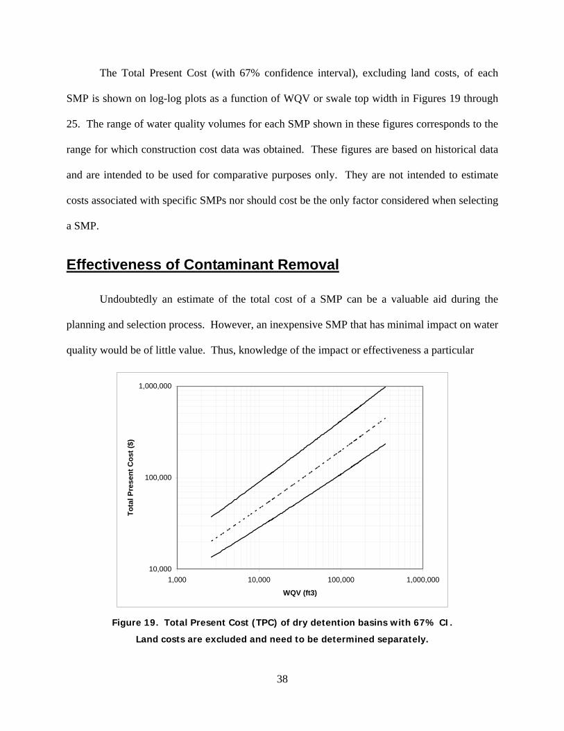
The Total Present Cost (with 67% confidence interval), excluding land costs, of each
SMP is shown on log-log plots as a function of WQV or swale top width in Figures 19 through
25. The range of water quality volumes for each SMP shown in these figures corresponds to the
range for which construction cost data was obtained. These figures are based on historical data
and are intended to be used for comparative purposes only. They are not intended to estimate
costs associated with specific SMPs nor should cost be the only factor considered when selecting
a SMP.
Effectiveness of Contaminant Removal
Undoubtedly an estimate of the total cost of a SMP can be a valuable aid during the
planning and selection process. However, an inexpensive SMP that has minimal impact on water
quality would be of little value. Thus, knowledge of the impact or effectiveness a particular
10,000
100,000
1,000,000
1,000 10,000 100,000 1,000,000
WQV (ft3)
Tota
l Pre
sent
Cos
t ($)
Figure 19. Total Present Cost (TPC) of dry detention basins with 67% CI.
Land costs are excluded and need to be determined separately.
39
10,000
100,000
1,000,000
10,000,000
10,000 100,000 1,000,000 10,000,000
WQV (ft3)
Tota
l Pre
sent
Cos
t ($)
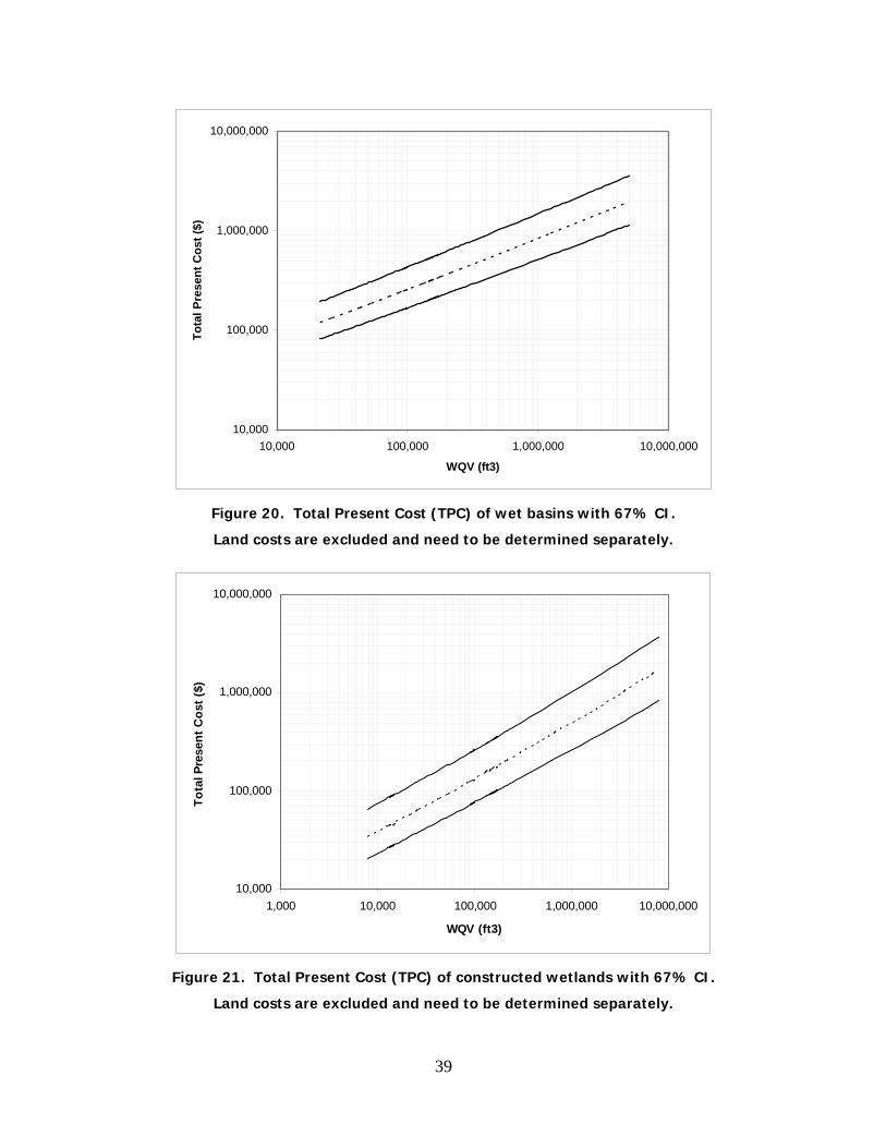
Figure 20. Total Present Cost (TPC) of wet basins with 67% CI.
Land costs are excluded and need to be determined separately.
10,000
100,000
1,000,000
10,000,000
1,000 10,000 100,000 1,000,000 10,000,000
WQV (ft3)
Tota
l Pre
sent
Cos
t ($)
Figure 21. Total Present Cost (TPC) of constructed wetlands with 67% CI.
Land costs are excluded and need to be determined separately.
40
10,000
100,000
1,000,000
10,000,000
100 1,000 10,000 100,000 1,000,000
WQV (ft3)
Tota
l Pre
sent
Cos
t ($)
Figure 22. Total Present Cost (TPC) of infiltration trenches with 67% CI.
Land costs are excluded and need to be determined separately.
1,000
10,000
100,000
1,000,000
10,000,000
100 1,000 10,000 100,000 1,000,000
WQV (ft3)
Tota
l Pre
sent
Cos
t ($)
Figure 23. Total Present Cost (TPC) of bioinfiltration filters with 67% CI.
Land costs are excluded and need to be determined separately.

41
10,000
100,000
1,000,000
10,000,000
100 10,000 1,000,000
WQV (ft3)
Tota
l Pre
sent
Cos
t ($)
Figure 24. Total Present Cost (TPC) of sand filters with 67% CI.
Land costs are excluded and need to be determined separately.
0
10,000
20,000
30,000
40,000
50,000
60,000
70,000
0 5 10 15 20 25
Swale Top Width (ft)
Tota
l Pre
sent
Cos
t ($)
Figure 25. Total Present Cost (TPC) of 1000’ long grassed/vegetative swales with 67% CI.
Land costs are excluded and need to be determined separately.

42
SMP will have on water quality is just as important as the cost. In an effort to provide
information in this area, an analysis was performed in which the total amount of TSS and
phosphorus removed over a 20-year span was estimated as a function of water-quality volume.
In this analysis the amount of TSS and P removed is considered to be a function of the fraction
of stormwater runoff that will be treated by the SMP, the pollutant load which reaches the SMP,
and the removal performance of the SMP itself. Of course, some of the variables listed above
depend on other variables such as watershed area, impervious area, rainfall amounts, etc. All of
these variables and the analytical method which was used to incorporate them into the estimate
of total pollutant load removal is described and discussed below.
Runoff Fraction Treated
Most SMPs are designed for a particular rainfall depth used to estimate a water-quality
volume or, in the case of swales, filter strips, and similar SMPs, a peak flow rate. The WQV or
peak flow rate is used to size the SMP. Since an SMP is designed for a finite value of rainfall
and/or runoff, there is always the chance that a given storm will produce more runoff than the
unit was designed to store and/or treat. When that happens, a portion of the runoff bypasses the
SMP or is discharged from the SMP via an overflow outlet and receives no treatment. In order
to account for this untreated fraction of the runoff, a statistical analysis was performed on
historical rainfall data in the Twin Cities. Given the design rainfall depth, the process, as
described below, can be used to estimate the fraction of stormwater runoff that will be bypassed
or exit the SMP without treatment.
Since design recommendations for SMPs usually state that the devices should be
designed to drain in two days, two-day running sum precipitation amounts in the Twin Cities
were calculated and analyzed from 1950 through 2003. For example, if the precipitation depths

43
measured on four consecutive days were 0.21 in., 0.13 in., 0.35 in., and 0.07 in., the data would
be combined into two-day precipitation amounts of 0.34 in., 0.48 in., and 0.42 in., respectively.
Using the combined data, a two-day running sum (RS) histogram was generated using 0.10 inch
increments from zero to four inches, with the last bin including any two-day sum that was greater
than or equal to four inches. Of the 9,720 non-zero entries, five fell into the latter category, with
the largest having a value of 10.00 inches. Columns 1 through 4 of Table 7 show the histogram
in tabular form along with the frequency and cumulative frequency distributions. Subtracting the
cumulative frequency from 1.00 and multiplying by 100 gives the percent exceedance as shown
in column 5 and plotted in Figure 26.
Thus Table 7 and/or Figure 26 can be used to determine the fraction of two-day
precipitation events that exceeded a particular precipitation depth. For example, based on Figure
26, a two-day rainfall depth of 1.00 inch was exceeded approximately 7 percent of the time over
the 54-year period analyzed. Alternatively, using Table 7 and linearly interpolating between
7.43% and 6.24% gives a value of 6.84% exceedance for a precipitation depth of one inch.
Furthermore, if an SMP were designed for a precipitation depth of 1.00 inch, the graph area that
is both under the curve and below the horizontal line that corresponds to an abscissa value of
1.00 inch divided by the total area under the curve, equals the fraction of the two-day summed
precipitation amounts that were below the 1.00 inch design storm depth. The values of the graph
area, cumulative area, and percent of total area corresponding to each precipitation depth have
been calculated and are shown in columns 6, 7, and 8, respectively, of Table 7. Due to
infiltration and other abstractions of the stormwater which occur as the runoff makes it way to
the SMP, this ratio is not exactly the fraction of runoff that would be treated by the SMP. That
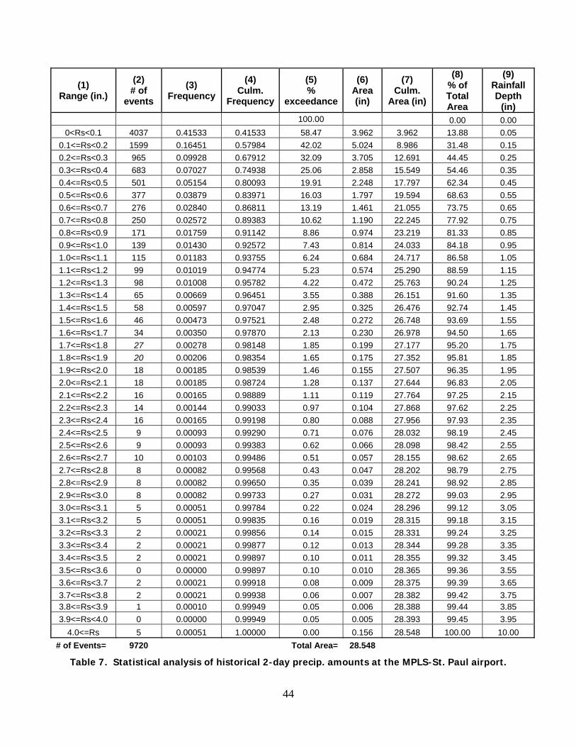
44
(1) Range (in.)
(2) # of
events (3)
Frequency (4)
Culm. Frequency
(5) %
exceedance
(6) Area (in)
(7) Culm.
Area (in)
(8) % of Total Area
(9) Rainfall Depth
(in) 100.00 0.00 0.00
0<Rs<0.1 4037 0.41533 0.41533 58.47 3.962 3.962 13.88 0.05 0.1<=Rs<0.2 1599 0.16451 0.57984 42.02 5.024 8.986 31.48 0.15 0.2<=Rs<0.3 965 0.09928 0.67912 32.09 3.705 12.691 44.45 0.25 0.3<=Rs<0.4 683 0.07027 0.74938 25.06 2.858 15.549 54.46 0.35 0.4<=Rs<0.5 501 0.05154 0.80093 19.91 2.248 17.797 62.34 0.45 0.5<=Rs<0.6 377 0.03879 0.83971 16.03 1.797 19.594 68.63 0.55 0.6<=Rs<0.7 276 0.02840 0.86811 13.19 1.461 21.055 73.75 0.65 0.7<=Rs<0.8 250 0.02572 0.89383 10.62 1.190 22.245 77.92 0.75 0.8<=Rs<0.9 171 0.01759 0.91142 8.86 0.974 23.219 81.33 0.85 0.9<=Rs<1.0 139 0.01430 0.92572 7.43 0.814 24.033 84.18 0.95 1.0<=Rs<1.1 115 0.01183 0.93755 6.24 0.684 24.717 86.58 1.05 1.1<=Rs<1.2 99 0.01019 0.94774 5.23 0.574 25.290 88.59 1.15 1.2<=Rs<1.3 98 0.01008 0.95782 4.22 0.472 25.763 90.24 1.25 1.3<=Rs<1.4 65 0.00669 0.96451 3.55 0.388 26.151 91.60 1.35 1.4<=Rs<1.5 58 0.00597 0.97047 2.95 0.325 26.476 92.74 1.45 1.5<=Rs<1.6 46 0.00473 0.97521 2.48 0.272 26.748 93.69 1.55 1.6<=Rs<1.7 34 0.00350 0.97870 2.13 0.230 26.978 94.50 1.65 1.7<=Rs<1.8 27 0.00278 0.98148 1.85 0.199 27.177 95.20 1.75 1.8<=Rs<1.9 20 0.00206 0.98354 1.65 0.175 27.352 95.81 1.85 1.9<=Rs<2.0 18 0.00185 0.98539 1.46 0.155 27.507 96.35 1.95 2.0<=Rs<2.1 18 0.00185 0.98724 1.28 0.137 27.644 96.83 2.05 2.1<=Rs<2.2 16 0.00165 0.98889 1.11 0.119 27.764 97.25 2.15 2.2<=Rs<2.3 14 0.00144 0.99033 0.97 0.104 27.868 97.62 2.25 2.3<=Rs<2.4 16 0.00165 0.99198 0.80 0.088 27.956 97.93 2.35 2.4<=Rs<2.5 9 0.00093 0.99290 0.71 0.076 28.032 98.19 2.45 2.5<=Rs<2.6 9 0.00093 0.99383 0.62 0.066 28.098 98.42 2.55 2.6<=Rs<2.7 10 0.00103 0.99486 0.51 0.057 28.155 98.62 2.65 2.7<=Rs<2.8 8 0.00082 0.99568 0.43 0.047 28.202 98.79 2.75 2.8<=Rs<2.9 8 0.00082 0.99650 0.35 0.039 28.241 98.92 2.85 2.9<=Rs<3.0 8 0.00082 0.99733 0.27 0.031 28.272 99.03 2.95 3.0<=Rs<3.1 5 0.00051 0.99784 0.22 0.024 28.296 99.12 3.05 3.1<=Rs<3.2 5 0.00051 0.99835 0.16 0.019 28.315 99.18 3.15 3.2<=Rs<3.3 2 0.00021 0.99856 0.14 0.015 28.331 99.24 3.25 3.3<=Rs<3.4 2 0.00021 0.99877 0.12 0.013 28.344 99.28 3.35 3.4<=Rs<3.5 2 0.00021 0.99897 0.10 0.011 28.355 99.32 3.45 3.5<=Rs<3.6 0 0.00000 0.99897 0.10 0.010 28.365 99.36 3.55 3.6<=Rs<3.7 2 0.00021 0.99918 0.08 0.009 28.375 99.39 3.65 3.7<=Rs<3.8 2 0.00021 0.99938 0.06 0.007 28.382 99.42 3.75 3.8<=Rs<3.9 1 0.00010 0.99949 0.05 0.006 28.388 99.44 3.85 3.9<=Rs<4.0 0 0.00000 0.99949 0.05 0.005 28.393 99.45 3.95
4.0<=Rs 5 0.00051 1.00000 0.00 0.156 28.548 100.00 10.00 # of Events= 9720 Total Area= 28.548
Table 7. Statistical analysis of historical 2-day precip. amounts at the MPLS-St. Paul airport.

45
2-Day Running Sum - Precipitation Depths in Minneapolis/St. Paul 1950-2003
0
1
2
3
4
5
6
7
8
9
10
0 10 20 30 40 50 60 70 80 90 100
Percent Exceedence
Rai
nfal
l Dep
th (i
n)
Figure 26. Exceedance probabilities of two-day precipitation depths in the Twin Cities.
would only be the case if 100 percent of the precipitation were to reach the SMP as runoff.
However, the percent of total area values shown in column 8 can be used as an approximate
estimate of the fraction of runoff that would be treated by an SMP designed for the
corresponding rainfall depth in column 9. For example, based on columns 8 and 9 of Table 7, if
an SMP was designed for a precipitation depth of 2.25 inches, it could be estimated that, based
on historical data, the SMP would treat 97.62 percent of the stormwater runoff over time.
For the purposes of this report it was assumed that all SMPs would be designed for a
precipitation depth of 1.45 inches which is approximately the three-month, 24-hour storm for the
Twin Cities metro region (Huff and Angel, 1992). As shown in Table 7, a depth of 1.45 inches
corresponds to approximately 93 percent of the area under the curve. As discussed above, it was
estimated that 93 percent of all stormwater runoff will be treated by an SMP which is designed
for the volume of runoff corresponding to this precipitation depth. Thus, when estimating the

46
total amount of TSS and P removed over 20 years, it was assumed that 93 percent of all
stormwater runoff will be treated by the SMPs and the remaining 7 percent of the runoff will
receive no treatment. Thus, total suspended sediment and phosphorus removal are given by:
( )SMPby %Removal0.93Removal %Total ∗= (5)
where the “%Removal by SMP” is the removal based on inflow and treated outflow
concentrations and does not consider overflow conditions. Overflow and/or bypass conditions
are accounted for by multiplying the “%Removal by SMP” by 0.93.
Pollutant Loading
Several methods with a wide degree of complexity are available to estimate stormwater
pollutant loads. For example, the Stormwater Management Model (SWMM) is public domain
software and can be used to model single storm events or watershed basins over time.
Additional methods described Young, et al. (1995) include regional United States Geological
Survey (USGS) equations for estimation of storm loads, runoff volumes, and event mean
concentrations. These equations have been developed for three regions in the United States and
are based on regression analysis of nationwide data. A simplified, but less accurate, set of USGS
regression equations are also available and can be used to estimate storm runoff loads and
volumes. The USGS has also derived a set of equations to estimate storm mean concentrations
and mean seasonal or annual loads.
The Federal Highway Administration (FHWA) has developed a method to estimate
pollutant loading from highway runoff (Driscoll, et al., 1990). As with the USGS methods, the
FHWA method is a regional method, in this case with nine regions, which involves a relatively
large amount of detailed input to arrive at an estimate of annual pollutant mass loading.

47
The methods described above require a level of detail that is well beyond what is
necessary (or perhaps possible) for the comparative purposes of this report. Thus, for this report,
a modified version of a less involved method, the Simple Method, was selected to estimate
pollutant loads. The Simple Method, first proposed by Schueler (1987), is widely accepted and
requires only the mean annual precipitation, percent of rainfall events that produce no runoff, the
drainage area, and a runoff coefficient be known. The modified Simple Method used in this
report is used by the Lower Colorado River Authority (1998) and has been recommended for use
by the State of Texas, Department of Transportation (Landphair, et al., 2000). In its modified
form, the simple method is:
CRRA(0.2266)L VF ∗∗∗∗= (6)
where: L = Annual pollutant load (lb.)
A = Watershed area (acre)
RF = Average annual rainfall (in.)
RV = Average annual runoff coefficient (i.e. runoff:rainfall ratio)
C = Average annual contaminant (i.e. TSS & P) concentration (mg/L)
The runoff coefficient RV, was described for water quality volume calculations and is
estimated as:
( )I0.0090.05R V ∗+= (2)
where: I = Percent of watershed that is impervious
In order to coincide with the 20-year time span used to estimate the total present cost, the
pollutant loading must also be estimated for 20 years. To accomplish this, Equation 5 must be
multiplied by 20. Also, the variable RF, must no longer be defined as the average annual rainfall
but rather, the 20-year running average of annual rainfall (inches). Incorporating these small but

48
significant changes, the equation used to estimate the TSS and P loading over a 20-year span
becomes:
CRRA0.226620L VF2020 ∗∗∗∗∗= (7)
Where: L20 = Estimated pollutant load over 20 years (lb.)
RF20 = 20-year running average of annual rainfall (in.)
and all other variables are as previously defined.
For the purposes of this report it was assumed that the watershed area A, percent
impervious I, and therefore the runoff coefficient RV, would be known without any uncertainty.
To obtain an estimate of RF20, a statistical analysis on historical precipitation data in Minneapolis
and St. Paul from 1950 through 2003 was performed. The results showed that the 20-year
running average precipitation depth is 28.44 inches +/- 1.80 inches (67% confidence interval).
In order to determine estimates of the average annual concentration of TSS and P in
stormwater runoff, data was compiled from several studies and dozens of sites (Moxness, 1986;
Moxness, 1987; Moxness, 1988; Driscoll, et al., 1990; Oberts, 1994; Barrett, et al., 1995;
Stanley, 1996; Wu, J.S., et al., 1996; Sansalone and Buchberger, 1997; Barrett, et al., 1998;
Anderle, T.A., 1999; Legret and Colandini, 1999; Waschbusch, et al., 1999; Carleton, et al.,
2000; Drapper, et al., 2000; Brezonik and Stadelmann, 2002; Harper, et al., undated). Data
analysis revealed that the average values of stormwater concentrations of TSS and P from sites
located in the Twin Cities were essentially the same as average values of all other sites located
throughout the nation and Australia. Since the data was similar, the national average values of
131 mg/L +/- 77 mg/L (67% confidence interval) for TSS and 0.55 mg/L +/- 0.41 mg/L (67%
confidence interval) for total P were used. With values for RF20 and C estimated, the total
pollutant load for TSS and P in pounds over a 20-year time frame, as estimated by Equation 7,
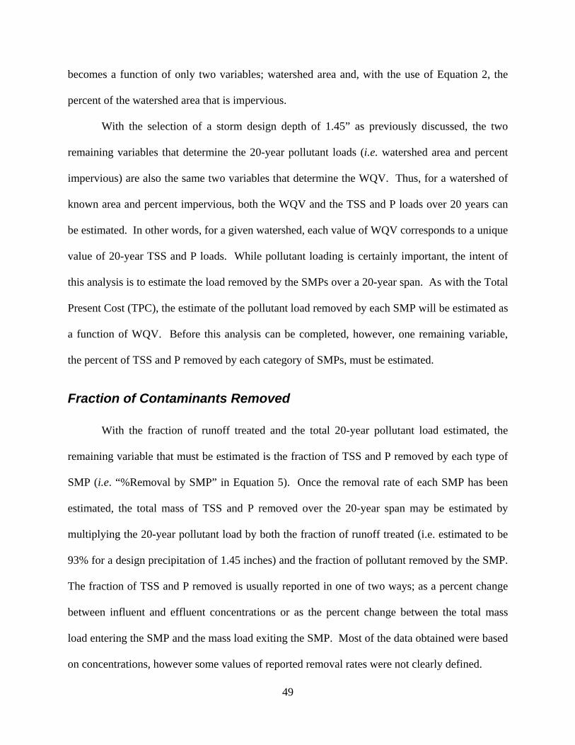
49
becomes a function of only two variables; watershed area and, with the use of Equation 2, the
percent of the watershed area that is impervious.
With the selection of a storm design depth of 1.45” as previously discussed, the two
remaining variables that determine the 20-year pollutant loads (i.e. watershed area and percent
impervious) are also the same two variables that determine the WQV. Thus, for a watershed of
known area and percent impervious, both the WQV and the TSS and P loads over 20 years can
be estimated. In other words, for a given watershed, each value of WQV corresponds to a unique
value of 20-year TSS and P loads. While pollutant loading is certainly important, the intent of
this analysis is to estimate the load removed by the SMPs over a 20-year span. As with the Total
Present Cost (TPC), the estimate of the pollutant load removed by each SMP will be estimated as
a function of WQV. Before this analysis can be completed, however, one remaining variable,
the percent of TSS and P removed by each category of SMPs, must be estimated.
Fraction of Contaminants Removed
With the fraction of runoff treated and the total 20-year pollutant load estimated, the
remaining variable that must be estimated is the fraction of TSS and P removed by each type of
SMP (i.e. “%Removal by SMP” in Equation 5). Once the removal rate of each SMP has been
estimated, the total mass of TSS and P removed over the 20-year span may be estimated by
multiplying the 20-year pollutant load by both the fraction of runoff treated (i.e. estimated to be
93% for a design precipitation of 1.45 inches) and the fraction of pollutant removed by the SMP.
The fraction of TSS and P removed is usually reported in one of two ways; as a percent change
between influent and effluent concentrations or as the percent change between the total mass
load entering the SMP and the mass load exiting the SMP. Most of the data obtained were based
on concentrations, however some values of reported removal rates were not clearly defined.

50
In order to make the estimate of SMP removal performance (i.e. %Removal SMP in
Equation 5) as realistic as possible, published data on the performance of the various types of
SMPs analyzed in this study was collected and the average removal rate with 67% confidence
interval calculated. Only data from actual sites which were field tested were included. When a
single site was monitored over time and had more than one removal rate reported, only the
average value of the data for that site was included in the analysis.
Ideally, the estimate of total contaminant load removed over 20 years would be based on
data reported as the percent of total mass load removed. However, due to limited data of this
kind, this analysis combined removal rates based on mass load removed and removal rates based
on the percent change in contaminant concentration between inflow to the SMP and treated
outflow from the SMP. For each type of SMP the average percent removal of the combined data
was calculated and assumed to be the average percent of mass load removed. When accounting
for infiltration of stormwater which may occur inside some SMPs (e.g. wetlands, dry basins,
etc.), the percent drop in the influent to effluent concentration should be smaller than the percent
of mass load removed. Thus, by combining concentration-based removal rates with those based
on mass loads and assuming the resulting average to be the percent of mass load removed is a
conservative one.
The results are summarized in Table 8 below and the full data is included in Appendix B.
Sufficient amounts of reliable data which are needed to estimate the TSS removal rate of
bioretention filters and TSS and phosphorus removal rates of infiltration trenches were not
available. As denoted by the asterisks in Table 8, typical values of 90 percent and 75 percent for
TSS removal (for bioretention filters and infiltration trenches, respectively) as reported by the
Idaho BMP Manual (undated), were used. Also assumed was the Idaho BMP Manual typical

51
infiltration trench phosphorus removal of 55%. The assumed values for TSS removal were
either in agreement with other reported typical ranges of effectiveness, or conservative as
Caltrans (2004) assumed infiltration trenches and basins remove 100 percent of TSS. Some
literature, such as Caltrans (2004), have reasoned that since any water entering these SMPs is
removed from the surface water, these SMPs achieve 100% removal of TSS and P. However,
some dissolved contaminants may potentially reach the groundwater (MPCA, 2000) and could
reenter as surface water at a later time. If this were to occur, the actual TSS and phosphorus
removal of some SMPs would be less than 100%. The 67% confidence interval for these SMPs
were also assumed and are denoted by an asterisk in Table 8.
SMP %TSS Removal
TSS 67% CI
% P Removal
P 67% CI
Dry Detention Basins 53 ±28 25 ±15
Wet Basins 65 ±32 52 ±23
Stormwater Wetland 68 ±25 42 ±26
Bioretention Filter 90* ±10* 72 ±11
Sand Filter 82 ±14 46 ±21
Infiltration Trench 75* ±10* 55* ±35*
Filter Strips/Grassed Swales 75 ±20 41 ±33
Table 8. Average percent removal rates of SMPs with corresponding confidence interval.
(* denotes assumed value) As previously discussed, the published data used to calculate the values shown in Table 8
were reported in either percent drop in concentration between influent and effluent stormwater or
percent removal of the total mass load entering the SMP. The values are based only on
stormwater treated by the SMP and do not account for any portion of the flow that bypasses the
SMP or exits through an overflow outlet. The confidence intervals reported in Table 8 reveal a

52
large amount of uncertainty in the reported data. The uncertainty is likely due to variations in
design and maintenance of the SMPs. If proper maintenance is not performed, removal levels
will drop. Also, parameters such as swale slope, pond and wetland residence time, etc. affect
removal.
The total amount of TSS that can be expected to be removed by each SMP (except for
grassed/vegetative swales) was calculated by multiplying the 20-year total TSS load by 93
percent (i.e. estimated percent of runoff treated) and by the corresponding removal rate as shown
in Table 8. The results, with a 67% confidence interval, are shown as a function of WQV in
Figures 27 through 32 below. Similarly, the amounts of phosphorus that can be expected to be
removed from the various SMPs are shown in Figures 33 through 38. As with the Total Present
Cost graphs, the contaminant removal estimates are shown on a log-log scale where appropriate.
Also, uncertainties in contaminant concentration, 20-year running average precipitation, and
percent of contaminant removal by the SMPs were incorporated by the direct analytical method
described by Kline (1985).
Since swales are designed for a peak flow rate and not WQV, an estimate of the total load
removed by swales over 20 years could not be estimated as a function of WQV. However, if the
volume of runoff which will be treated by a swale can be estimated, the removal rates reported in
Table 8 for Filter Strips/Grassed Swales may be used to estimate the corresponding total
contaminant load removed.
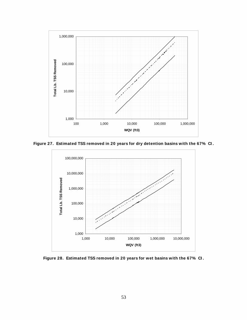
53
1,000
10,000
100,000
1,000,000
100 1,000 10,000 100,000 1,000,000
WQV (ft3)
Tota
l Lb.
TSS
Rem
oved
Figure 27. Estimated TSS removed in 20 years for dry detention basins with the 67% CI.
1,000
10,000
100,000
1,000,000
10,000,000
100,000,000
1,000 10,000 100,000 1,000,000 10,000,000
WQV (ft3)
Tota
l Lb.
TSS
Rem
oved
Figure 28. Estimated TSS removed in 20 years for wet basins with the 67% CI.

54
1,000
10,000
100,000
1,000,000
10,000,000
100,000,000
1,000 10,000 100,000 1,000,000 10,000,000
WQV (ft3)
Tota
l Lb.
TSS
Rem
oved
Figure 29. Estimated TSS removed in 20 years for constructed wetlands with the 67% CI.
1,000
10,000
100,000
1,000,000
1,000 10,000 100,000 1,000,000
WQV (ft3)
Tota
l TSS
Rem
oved
(lb.
)
Figure 30. Estimated TSS removed in 20 years for infiltration trenches with the 67% CI.
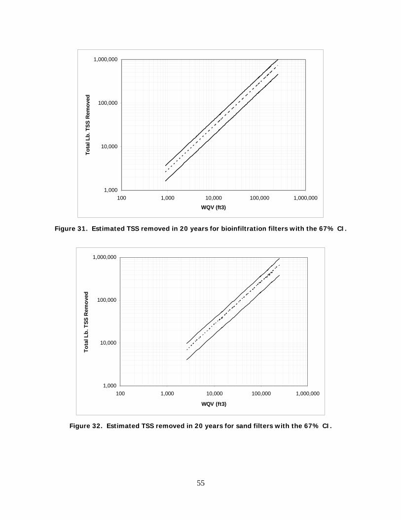
55
1,000
10,000
100,000
1,000,000
100 1,000 10,000 100,000 1,000,000
WQV (ft3)
Tota
l Lb.
TSS
Rem
oved
Figure 31. Estimated TSS removed in 20 years for bioinfiltration filters with the 67% CI.
1,000
10,000
100,000
1,000,000
100 1,000 10,000 100,000 1,000,000
WQV (ft3)
Tota
l Lb.
TSS
Rem
oved
Figure 32. Estimated TSS removed in 20 years for sand filters with the 67% CI.
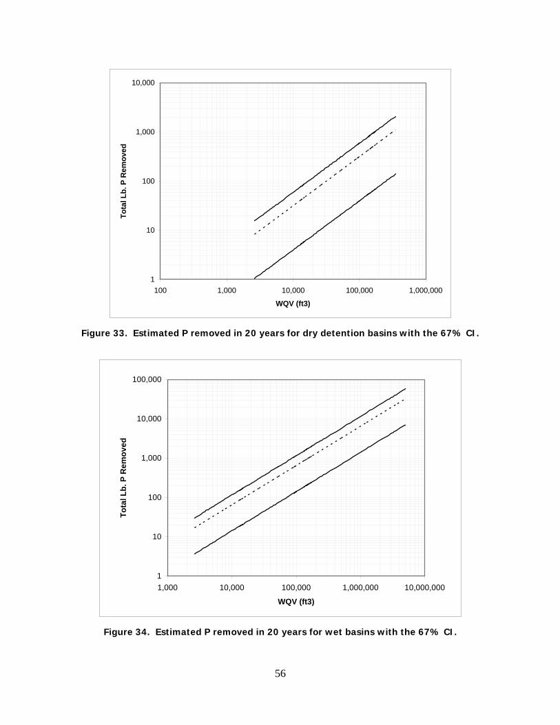
56
1
10
100
1,000
10,000
100 1,000 10,000 100,000 1,000,000
WQV (ft3)
Tota
l Lb.
P R
emov
ed
Figure 33. Estimated P removed in 20 years for dry detention basins with the 67% CI.
1
10
100
1,000
10,000
100,000
1,000 10,000 100,000 1,000,000 10,000,000
WQV (ft3)
Tota
l Lb.
P R
emov
ed
Figure 34. Estimated P removed in 20 years for wet basins with the 67% CI.

57
1
10
100
1,000
10,000
100,000
1,000 10,000 100,000 1,000,000 10,000,000
WQV (ft3)
Tota
l Lb.
P R
emov
ed
Figure 35. Estimated P removed in 20 years for constructed wetlands with the 67% CI.
1
10
100
1,000
1,000 10,000 100,000
WQV (ft3)
Tota
l Lb.
P R
emov
ed
Figure 36. Estimated P removed in 20 years for infiltration trenches with the 67% CI.

58
1
10
100
1,000
10,000
100 1,000 10,000 100,000 1,000,000
WQV (ft3)
Tota
l Lb.
P R
emov
ed
Figure 37. Estimated P removed in 20 years for bioinfiltration filters with the 67% CI.
1
10
100
1,000
10,000
100 1,000 10,000 100,000 1,000,000
WQV (ft3)
Tota
l Lb.
P R
emov
ed
Figure 38. Estimated P removed in 20 years for sand filters with the 67% CI.

59
Examples
SMPs under consideration for a 50-acre watershed that is 80 percent impervious include a
dry detention basin and a constructed wetland. The SMP is to be designed for a 1.45-inch
precipitation depth and a comparison of the cost and effectiveness of both SMPs is desired.
Using Equations 1 and 2, the WQV can be determined as follows:
( )3ft 200,000 WQV
50)80(009.005.045.112
43560 WQV
≈
∗+∗∗⎟⎠⎞
⎜⎝⎛=
From Figure 19, the TPC of an average dry detention basin of this size is just over
$300,000 with a 67% confidence interval range of about $170,000 to $675,000. A similarly
sized average wetland would, based on Figure 21, cost approximately $200,000 with a 67%
confidence interval range of $110,000 to $400,000. For a comparison among all SMPs, Table 9
lists the estimated average TPC of all practices analyzed herein for various WQVs. For each
SMP, TPCs are not estimated for WQVs that are outside the range of the original construction
cost data. Thus some values in Table 9 do not have a cost entry.
Investigation of Table 9 reveals that, based on the collected data and in terms of TPC,
wetlands are the least expensive SMP for the range of WQVs listed. This finding is somewhat
similar to that of Wossink and Hunt (2003) who concluded that, in terms of construction costs,
wetlands were the least expensive of four SMPs (wet ponds, constructed wetlands, sand filters,
bioretention basins) for watersheds larger than 10 acres in sandy soils. Contrary to the previous
conclusions, the California Stormwater Quality Association (2003) states that wetlands are
relatively inexpensive but are typically 25% more expensive than stormwater ponds of
equivalent volume. One must also remember that since wetlands generally require more land
area, any savings in TPC may potentially be more than offset by larger land acquisition costs.

60
Over 20 years the estimated TSS removal and 67% confidence interval for the dry
detention basin can, with the use of Figure 27, be estimated to be 344,000 pounds with a range of
120,000 pounds to 570,000 pounds. The corresponding wetland TSS removal based on
Figure 29 is estimated to be 440,000 pounds with a range of 210,000 pounds to 673,000 pounds.
The phosphorus removed over 20 years can be estimated in a similar manner using
Figures 33 and 35. For the dry detention basin the average P removal is approximately
630 pounds with a range of 80 to 1,200 pounds (67% confidence interval). The wetland average
P removal is about 1,050 pounds with a range from about 110 pounds to about 2,000 pounds.
Thus, for this watershed and design depth, the wetland, on average, would cost less to construct
(not including land costs) and it would also remove more TSS and phosphorus. However, land
costs must always be considered.
Focusing on associated land costs of each SMP under consideration, Table 3 can be used to
estimate the range of expected land area required for each SMP. Using the values based on total
watershed area and selecting the high end of each range, the dry detention basin would require
2.0 percent of the total watershed area resulting in a basin land area of 1 acre. Similarly, the
wetland would require 5.0 percent of 50 acres or 2.5 acres. If land costs are known, the land
areas can be used to estimate land costs associated with each SMP. For example, if land costs
were $10,000 per acre, acquiring the land for the detention basin would cost an additional
$10,000 and the land for the wetland would cost $25,000. The resulting total cost (now
including a rough estimate for land acquisition) for the detention basin and wetland would be
$310,000 and $225,000, respectively. Thus, in this relatively low land-cost scenario, the wetland
would still be cheaper and more effective, on average. However, if land costs in the vicinity of
the project were $250,000 per acre, an average dry detention basin would, including land, have

61
an estimated total cost of $550,000 and the wetland under consideration would have a total cost
of $825,000. Thus, with more expensive land, wetlands are no longer the less expensive option.
Water Quality Volume (ft3) SMP 3,000 10,000 30,000 100,000 250,000
Dry Det. Basin 22 46 91 198 359 Wet/Ret. Basin 47 83 141 256 407 Const. Wetland 21 38 68 131 219 Infilt. Trench 84 226 554 -- --
Bioinfilt. Filter 49 122 286 -- -- Sand Filter 86 176 338 691 --
Table 9. Average Total Present Cost (in $1,000) of SMPs at varying WQVs.
Land costs are excluded, and need to be determined separately.
However, wetlands are still estimated to remove more TSS and phosphorus, meaning that the
parties involved would have to weigh the increased cost of the wetland against its added benefit
(i.e. more contaminant removal). This example and the intended use for this report are
preliminary in nature; to obtain a more accurate estimate of costs a more detailed design of each
SMP should be completed.
62
References
ASCE. 2004. International Stormwater Best Management Practices (SBMP) Database. American Society of Civil Engineers, http://www.SBMPdatabase.org/
Anderle, T.A. 1999. Analysis of stormwater runoff and lake water quality for the Twin Cities
metropolitan area. M.S. Thesis, University of Minnesota. Anderson, Damann L., Robert L. Siegrist, and Richard J. Otis. 1985. Technology assessment of
intermittent sand filters. Municipal Environmental Research Laboratory, Office of Research and Development, USEPA, Washington, D.C.
Baker, Michael J., David W. Blowes, and Carol J. Ptacek. 1998. Laboratory development of permeable reactive mixtures for the removal of phosphorus from onsite wastewater disposal systems. Environ. Sci. Technol. 32 (15): 2308-2316.
Baker, Michael J., David W. Blowes, Carol J. Ptacek. 1997. Phosphorus adsorption and precipitation in a permeable reactive wall: application for wastewater disposal systems. Land Contamination & Reclamation 5(3): 189-193.
Barr Engineering Company. 2001. Minnesota urban small sites BMP manual: stormwater best management practices for cold climates. Metropolitan Council Environmental Services, St. Paul, MN.
Barrett, Malina, Charbeneau and Ward. 1995. Characterization of highway runoff in the Austin, TX area. Center for Research in Water Resources, UT-Austin, Austin, TX.
Barrett, Walsh, Malina and Charbeneau. 1998. Performance of vegetative controls for treating
highway runoff. Jour. Environ. Engrg. 124: 1121-1128. Bell, Warren., Lucky Stokes, Lawrence J. Gavan, and Trong Ngu Nguyen. Undated. Assessment
of the pollutant removal efficiencies of Delaware sand filter BMPs. City of Alexandria Department of Transportation and Environmental Services, Alexandria, Virginia.
Brezonik and Stadelmann. 2002. Analysis and predictive models of stormwater runoff volumes,
loads, and pollutant concentrations from watersheds in the Twin Cities metropolitan area, Minnesota, USA. Water Research 36: 1743-1757.
Brown, T., T. Schueler, T. Wright, R Winer, and J. Zielinkski. 2003. Maryland, Chesapeake
and Atlantic coastal bays - critical area 10% rule guidance manual. Center for Watershed Protection, Ellicott City, Maryland.
Brown, W. and T. Schueler. 1997a. National pollutant removal performance database of
current urban stormwater best management practices. Center for Watershed Protection. Ellicott City, MD.
63
Brown, W., and T. Schueler. 1997b. The economics of stormwater BMPs in the mid-Atlantic region: final report. Center for Watershed Protection, Silver Spring, MD.
Brueske, Christopher C. 2000. Technology review: ultra-urban stormwater treatment
technologies. University of Washington, Department of Civil and Environmental Engineering, Seattle Washington.
California State University Sacramento. 2000. Particles and the associated pollutant
concentrations in highway runoff in Lake Tahoe, California. CSUS Office of Water Programs, Sacramento, CA.
California Stormwater Quality Association. 2003. California stormwater BMP handbook – new
development and redevelopment. Menlo Park, CA, USA. Also available online at http://www.cabmphandbooks.com/Documents/Development/TC-21.pdf
Caltrans, 2004. BMP retrofit pilot program – final report, Appendix C3. California Department
of Transportation, Division of Environmental Analysis, Sacramento, CA. Also available at
Carleton, Grizzard, Godrej, Post, Lampe, and Kenel. 2000. Performance of a constructed
wetlands in treating urban stormwater runoff. Water Environ. Research 72(3):295-304. City of Lincoln, NE. 2000. Drainage Criteria Manual. Public Works and Utilities Department
and the Lower Platte South Natural Resources Department, Lincoln, NE. Also available at http://www.ci.lincoln.ne.us/city/pworks/watrshed/drainage/
Claytor, R.A., and Schueler, T.R. 1996. Design of stormwater filtering systems. Center for
Watershed Protection, Silver Spring, MD. Drapper, D., R. Tomlinson and P. Williams. 2000. Pollutant concentrations in road runoff:
southeast Queensland case study. Jour. Environ. Engineering 126(4):313-320. Driscoll, E., P.E. Shelley, and E.W. Strecker. 1990. Pollutant loadings and impacts from
highway stormwater runoff, volumes I-IV. United States Department of Transportation, Federal Highway Administration, Report No. FHWA/RD-88-006-9.
Engineering News Record. 1997. Low-tech filtration system uses leaves to remove solids. 248:
12.
Farnham, R.S. and T. Noonan. 1988. An evaluation of secondary treatment of stormwater inflows to Como Lake, MN using a peat-sand filter. EPA Proj. S-005660-02. USEPA, Washington, D.C.
Fintrend.com, 2004. InflationData.com. Financial Trend Forcaster, http://inflationdata.com/inflation/Inflation_Rate/HistoricalInflation.aspx.

64
Faulkner, S., and C. Richardson. 1991. Physical and chemical characteristics of freshwater wetlands soils. In Constructed Wetlands for Wastewater Treatment, edited by D. Hammer. CRC Press, Boca Raton, FL, USA.
Ghani A.A., Zakaria N.Z., Kassim M., and B.A. Nasir. 2000. Sediment size characteristics of
urban drains in Malaysian cities. Urban Water 2: 335-341.
Galli, J. 1990. Peat-sand filters: a proposed stormwater management practice for urbanized areas. Metropolitan Washington Council of Governments. Prepared for the Coordinated Anacostia Retrofit Program. Washington, D.C.
Harper, Harvey H., and Jeffery L. Herr. 1993. Treatment efficiencies of detention with filtration systems. Final Report submitted to the St. John’s River Water Management District, SJRWMD Contract No. 90B103.
Harper, H.H., Herr, J.L., and E.H. Livingston. Undated. Alum treatment of stormwater Runoff-an innovative BMP for urban runoff problems. Unpublished. Environmental Research and Design, Inc., Orlando, FL and Florida Department of Environmental Protection, Tallahassee, FL.
Herrera Environmental Consultants. 1995. Memorandum to the City of Bellevue (Washington).
Lake Sammammish phase II restoration project, Lake Park stormwater treatment facility, task 2: bench scale test results.
Huff, F.A., and Angel, J.R.. 1992. Rainfall frequency atlas of the Midwest. State Water Survey Division, State of Illinois, Champaign, IL.
Idaho Department of Environmental Quality. Undated. BMP manual. Boise, ID, USA. Jenkins, David., John F. Ferguson, and Arnold B. Menar. 1971. Chemical processes for
phosphate removal. Water Research 5:369-389.
Kline, S.J. 1985. The purposes of uncertainty analysis. Jour. of Fluids Engineering 107:153-160.
Kadlec, R.H., and R.L. Knight. 1996. Treatment wetlands. CRC Press. Boca Raton, FL, USA. Koerlsman, W., M.B. Van Kerkhoven, and J.T.A. Verhoeven. 1993. Release of inorganic N, P,
and K in peat soils: effect of temperature, water chemistry and water level. Biogeochemistry 20: 63-81.
Landphair, H.C., McFalls, J.A., and Thompson, D. 2000. Design methods, selections, and cost-effectiveness of stormwater quality structures. Texas Transportation Institute, The Texas A&M University System, College Station, TX.
Ledbetter, W.B. and C.A. Collier. 1988. Engineering economic and cost analysis, second
edition. Harper & Row, Publishers, Inc. New York, NY, USA.

65
Legret and Colandini. 1999. Effects of a porous pavement with reservoir structure on runoff water: water quality and fate of heavy metals. Water Sci. Tech. 39(2):111-117.
Lower Colorado River Authority. 1998. Nonpoint source pollution control technical manual,
third ddition. LCRA, Austin, TX, USA. Mergent, Inc. 2003. Mergent municipal & government manual. Mergent, Inc. New York, NY,
USA Minnesota Pollution Control Agency. 2000. Protecting water quality in urban areas-best
management practices for dealing with stormwater runoff from urban, suburban, and developing areas of Minnesota. MPCA. St. Paul, MN, USA.
Moxness. 1986. Characteristics of urban freeway runoff, phase I. Water Quality Unit,
Environmental Services Section, Office of Technical Support, Minnesota Department of Transportation, St. Paul, MN, USA.
Moxness. 1987. Characteristics of urban freeway runoff, phase II. Water Quality Unit,
Environmental Services Section, Office of Technical Support, Minnesota Department of Transportation, St. Paul, MN, USA.
Moxness. 1988. Characteristics of urban freeway runoff, phase III. Water Quality Unit,
Environmental Services Section, Office of Technical Support, Minnesota Department of Transportation, St. Paul, MN, USA.
Oberts, G. 1994. Influence of snowmelt dynamics on stormwater runoff quality. Watershed
protection techniques 1(2), Center for Watershed Protection, Elliott City, MD, USA. Oberts, G. 1999. Return to Lake McCarrons: does the performance of wetlands hold up over
time? Watershed Protection Technique 3(1): 597-600. Pratt, C. 1996. Laboratory test on X-cepter concrete bypass intercepter. Conventry University,
Conventry, United Kingdom.
Pitt, R.E. and J.G. Voorhees. 1997. Storm water quality management through the use of detention basins, a short course on storm water detention basin design basics by integrating water quality with drainage objectives. April 29-30 and May 21-22, University of Minnesota, St. Paul, MN.
Sansalone, J.J., and S.G. Buchberger. 1997. Partitioning and first flush of metals in urban roadway stormwater. Jour. Environ. Engrg. 123: 134.
Schindler, D. W. 1977. Evolution of phosphorus limitation in lakes. Science, New Series
195(4275): 260-262.
Schueler, T. R. 1987. Controlling urban runoff: a practical manual for planning and designing urban BMPs. Department of Environmental Programs, Metropolitan Council of Governments, Washington, D.C., USA.
66
Schueler, Thomas R., Peter A. Kumble, and Maureen A. Heraty. 1992. A current assessment of urban best management practices: techniques for reducing non-point source pollution in the coastal zone. Anacostia Restoration Team, Department of Environmental Programs, Metropolitan Washington Council of Governments, Washington, D.C.
Shammaa, Y., Zhu, D.Z., Gyurek, L.L., and C.W. Labatiuk. 2002. Effectiveness of dry ponds for stormwater total suspended solids removal. Can. Jour. Civ. Engrg, 29: 316-324.
Southeastern Wisconsin Regional Planning Commission. 1991. Costs of urban nonpoint source water pollution control measures. SWRPC, Waukesha, WI, USA.
Stanley, 1996. Pollutant Removal by a stormwater dry detention pond. Water Environ.
Research 68(6): 1076-1083. Stein, W. 1999. CDS® general information and discussion: continuous deflective separation
(CDS®) – treatment of stormwater runoff. CDS® Technologies, Inc., Morgan Hill, California.
Strecker, E.W., J.M. Kersner, E.D. Driscoll and R.R. Horner. 1992. The use of wetlands for controlling stormwater pollution. Terrence Institute. Washington, DC. Reprinted by USEPA as EPA 904-R-92-012.
Stewart, Bill. 1992. Final report: compost stormwater treatment system. W&H Pacific, Portland, Oregon.
StormTreat Systems, Inc. 1998. StormTreatTM Systems newsletter. Barnstable, Massachusetts (relocated to Hyannis, MA).
Turner Construction. 2004. “Building cost index, 2004 fourth quarter forcast”. New York, NY. http://www.turnerconstruction.com/corporate/content.asp?d=20
Urban Drainage Flood Control District. 1992. Best Management Practices. Urban Storm Drainage Criteria Manual, Vol. 3, UDFCD, Denver, CO, USA.
USEPA. 1993. Handbook urban runoff pollution prevention and control planning. EPA 625-R-
93-004. Washington, D.C. USEPA. 1999a. Preliminary data summary of urban stormwater best management practices.
EPA-821-R-99-012, Washington, D.C.
USEPA. 1999b. Storm water technology fact sheet – modular treatment systems. EPA-832-F-99-044, Washington, D.C.
USEPA. 2000. Stormwater phase II final rule. http://www.epa.gov/npdes/pubs/fact1-0.pdf
Vortechnics. 2002. Technical bulletin #1: Vortechs® Stormwater Treatment System performance: removal efficiencies for selected particle gradations. http://www.vortechnics.com/techbulletins/TB1.pdf
67
Waschbusch. 1999. Evaluation of the effectiveness of an urban stormwater treatment unit in Madison, Wisconsin, 1996-97. USGS Water-Resources Investigations Report, 99-4195.
Waschbusch, Selbig, and Bannerman. 1999. Sources of Phosphorus in Stormwater and Street Dirt from Two Urban Residential Basins in Madison, WI, 1994-95. USGS Water-Resources Investigations Report 99-4021.
W.E.F., and A.S.C.E. 1998. Urban runoff quality management, WEF Manual of Practice No 23,
ASCE Manual and Report on Engineering Practice No 87. Reston, VA. Wossink, A., and Hunt, B. 2003. The economics of structural stormwater BMPs in North
Carolina. University of North Carolina Water Resources Research Institute report #UNC-WRRI-2003-344.
Wu, J.S., R.E. Holman, and J.R. Dorney. 1996. Systematic Evaluation of Pollutant Removal by
Urban Wet Detention Ponds. Jour. Environmental Engineering 122(11): 983-988. Young, G.K., Stein, S., Cole, P., Kammer T., Graziano, F., and F. Bank. 1995. Evaluation and
management of highway runoff water quality. United States Department of Transportation, Federal Highway Administration, Pub. No. FHWA-PD-96-032. Washington, D.C.
A-1
Appendix A - Pollutant Removal Capability Table: References, Notes and Notation

A-2
Note: DRY ED stands for Dry Extended Detention. Extended detention systems, as referred to in the above table are synonymous with dry detention basins, and are designed to release all runoff influent within a 24 hour period.

A-3

A-4

A-5
Note: WET ED stands for Wet Extended Detention. Extended detention systems, as referred to in the above table are synonymous with retention basins, and are designed to store runoff until a runoff event displaces the amount of water stored.

A-6
Note: ED Wetlands stand for Extended Detention Wetlands. Extended detention systems, as referred to in the above table are similar to wetlands, but may store stormwater runoff for a longer period than typical wetland systems. Natural Wetlands refers to systems that have been modified or utilized for stormwater treatment from natural wetlands, as opposed to constructed systems.

B-1
Appendix B – Data used to estimate average SMP effectiveness

B-2
Appendix B1 – Dry Detention Ponds
Source ID Inflow [TSS}
Outflow [TSS]
Inflow [P]
Outflow [P]
% TSS removed
% P removed Comment
Winer, Nat'l Poll. Rem. Database, 2000 #1 77 10 0.188 0.112 87 40 Conc. BasisWiner, Nat'l Poll. Rem. Database, 2000 #3 68 38 0.21 0.18 44 14 "Winer, Nat'l Poll. Rem. Database, 2000 #6 98 28 0.35 0.27 71 23 "Winer, Nat'l Poll. Rem. Database, 2000 #6 -- -- -- -- 71 14 "
Caltrans 2004 BMP Retrofit Pilot Program Final Report, App F I5/605 Int -- -- -- -- 5 -4 "Caltrans 2004 BMP Retrofit Pilot Program Final Report, App F Manchester -- -- -- -- 70 42 "Caltrans 2004 BMP Retrofit Pilot Program Final Report, App F SR56/I5 -- -- -- -- 43 21 "Caltrans 2004 BMP Retrofit Pilot Program Final Report, App F SR78/I5 -- -- -- -- 55 33 "Environ & Conservation Services Dept. Austin TX. Removal
Efficiencies of Stormwater Control Structures. May 1990. Maple Run III -- -- -- -- 30 18 Mass BasisCommings, Booth, & Horner, 2000. Stormwater Pollutant Removal in two wet ponds in Bellevue, WA. Jour. Environ. Engrg, 126(4):321-
330-- -- -- -- -- 61.60 20.00 "
Stanley, 1996. Pollutant Removal by a stormwater dry detention pond. Water Environ. Research, 68(6):1076-1083. -- 127 32 0.41 0.3 75 27 Conc. Basis
Harper. Pollutant Removal Efficiences for Typical Stormwater Management Systems in Florida. -- -- -- -- -- 85 61 "
BMP Database. Greenville Pond, Greenville, NC -- -- -- -- -- -- 27 "
Dry Detention Ponds

B-3
Source ID Inflow [TSS}
Outflow [TSS]
Inflow [P]
Outflow [P]
% TSS removed
% P removed Comment
Metropoliton Washington Council of Governments, 1992. A Current Assessment of Urban Best Management Practices-Techniques for
Reducing Non-Point Source Pollution in the Coastal Zone.Lakeridge, VA -- -- -- -- 14 20 unknown basis
Metropoliton Washington Council of Governments, 1992. A Current Assessment of Urban Best Management Practices-Techniques for
Reducing Non-Point Source Pollution in the Coastal Zone.
London Commons,
VA-- -- -- -- 52 48 unknown basis
Metropoliton Washington Council of Governments, 1992. A Current Assessment of Urban Best Management Practices-Techniques for
Reducing Non-Point Source Pollution in the Coastal Zone.Stedwick, MD -- -- -- -- 70 13 unknown basis
Metropoliton Washington Council of Governments, 1992. A Current Assessment of Urban Best Management Practices-Techniques for
Reducing Non-Point Source Pollution in the Coastal Zone.
Oakhampton, MD -- -- -- -- 30 18 unknown basis
Metropoliton Washington Council of Governments, 1992. A Current Assessment of Urban Best Management Practices-Techniques for
Reducing Non-Point Source Pollution in the Coastal Zone.Unknown -- -- -- -- 87 26 unknown basis
Pope, L..M. and L.G. Hess, Date unknown. "Load Detention Efficiencies in a Dry-Pond Basin," from Kansas State Library. Topeka, KS -- -- -- -- 3 19 Mass Basis
Dry Extended Detention Pond (cont'd)
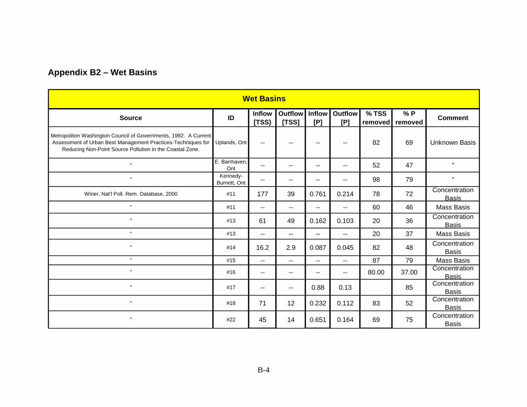
B-4
Appendix B2 – Wet Basins
Source ID Inflow [TSS}
Outflow [TSS]
Inflow [P]
Outflow [P]
% TSS removed
% P removed Comment
Metropoliton Washington Council of Governments, 1992. A Current Assessment of Urban Best Management Practices-Techniques for
Reducing Non-Point Source Pollution in the Coastal Zone.Uplands, Ont -- -- -- -- 82 69 Unknown Basis
" E. Barrhaven, Ont -- -- -- -- 52 47 "
" Kennedy-Burnett, Ont -- -- -- -- 98 79 "
Winer, Nat'l Poll. Rem. Database, 2000 #11 177 39 0.761 0.214 78 72 Concentration Basis
" #11 -- -- -- -- 60 46 Mass Basis
" #13 61 49 0.162 0.103 20 36 Concentration Basis
" #13 -- -- -- -- 20 37 Mass Basis
" #14 16.2 2.9 0.087 0.045 82 48 Concentration Basis
" #15 -- -- -- -- 87 79 Mass Basis
" #16 -- -- -- -- 80.00 37.00 Concentration Basis
" #17 -- -- 0.88 0.13 85 Concentration Basis
" #18 71 12 0.232 0.112 83 52 Concentration Basis
" #22 45 14 0.651 0.164 69 75 Concentration Basis
Wet Basins
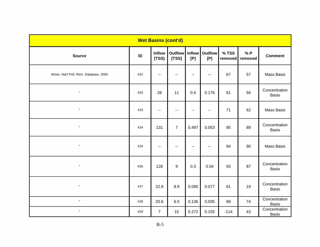
B-5
Source ID Inflow [TSS}
Outflow [TSS]
Inflow [P]
Outflow [P]
% TSS removed
% P removed Comment
Winer, Nat'l Poll. Rem. Database, 2000 #22 -- -- -- -- 67 57 Mass Basis
" #23 28 11 0.4 0.176 61 56 Concentration Basis
" #23 -- -- -- -- 71 62 Mass Basis
" #24 131 7 0.497 0.053 95 89 Concentration Basis
" #24 -- -- -- -- 94 90 Mass Basis
" #26 128 9 0.3 0.04 93 87 Concentration Basis
" #27 22.8 8.9 0.095 0.077 61 19 Concentration Basis
" #28 20.6 6.5 0.136 0.035 68 74 Concentration Basis
" #29 7 15 0.272 0.155 -114 43 Concentration Basis
Wet Basins (cont'd)
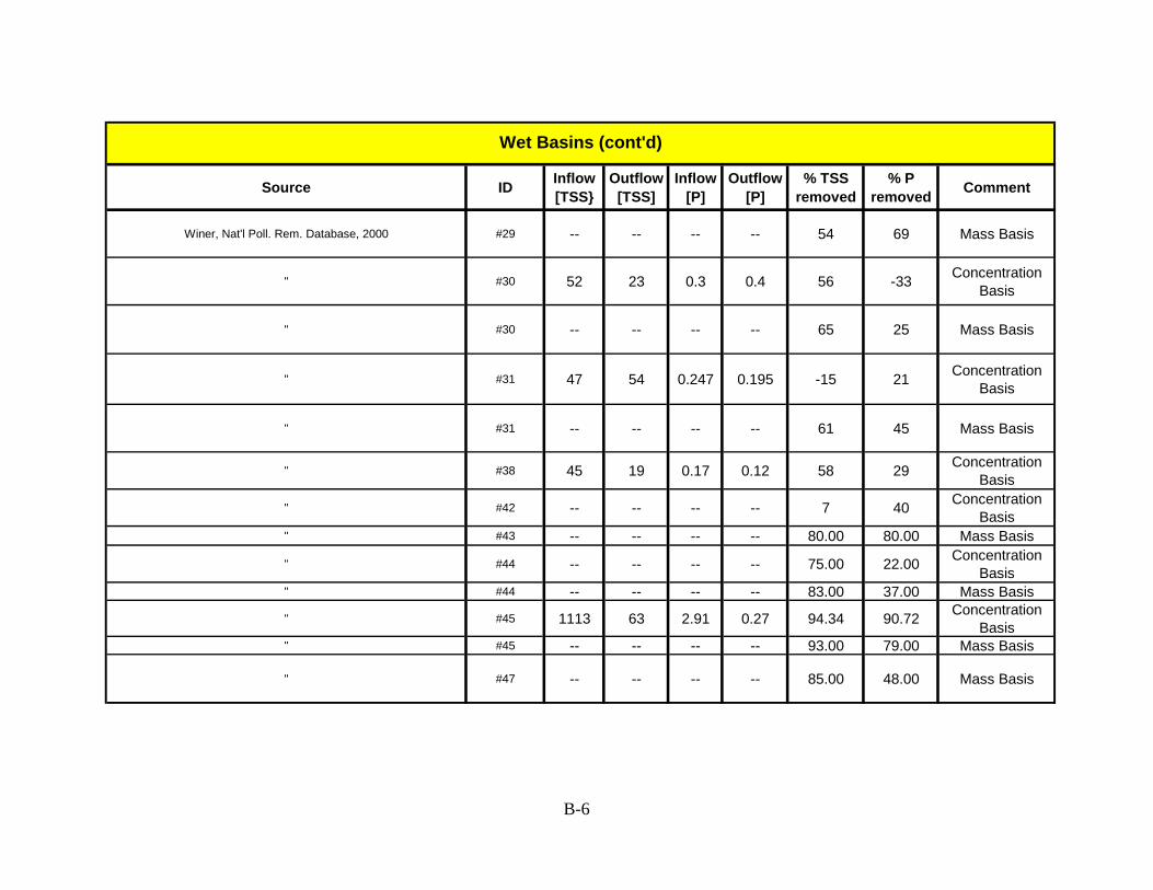
B-6
Source ID Inflow [TSS}
Outflow [TSS]
Inflow [P]
Outflow [P]
% TSS removed
% P removed Comment
Winer, Nat'l Poll. Rem. Database, 2000 #29 -- -- -- -- 54 69 Mass Basis
" #30 52 23 0.3 0.4 56 -33 Concentration Basis
" #30 -- -- -- -- 65 25 Mass Basis
" #31 47 54 0.247 0.195 -15 21 Concentration Basis
" #31 -- -- -- -- 61 45 Mass Basis
" #38 45 19 0.17 0.12 58 29 Concentration Basis
" #42 -- -- -- -- 7 40 Concentration Basis
" #43 -- -- -- -- 80.00 80.00 Mass Basis
" #44 -- -- -- -- 75.00 22.00 Concentration Basis
" #44 -- -- -- -- 83.00 37.00 Mass Basis
" #45 1113 63 2.91 0.27 94.34 90.72 Concentration Basis
" #45 -- -- -- -- 93.00 79.00 Mass Basis
" #47 -- -- -- -- 85.00 48.00 Mass Basis
Wet Basins (cont'd)
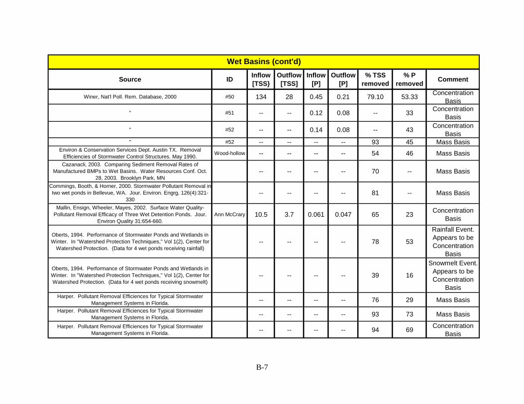
B-7
Source ID Inflow [TSS}
Outflow [TSS]
Inflow [P]
Outflow [P]
% TSS removed
% P removed Comment
Winer, Nat'l Poll. Rem. Database, 2000 #50 134 28 0.45 0.21 79.10 53.33 Concentration Basis
" #51 -- -- 0.12 0.08 -- 33 Concentration Basis
" #52 -- -- 0.14 0.08 -- 43 Concentration Basis
" #52 -- -- -- -- 93 45 Mass BasisEnviron & Conservation Services Dept. Austin TX. Removal
Efficiencies of Stormwater Control Structures. May 1990. Wood-hollow -- -- -- -- 54 46 Mass BasisCazanacli, 2003. Comparing Sediment Removal Rates of
Manufactured BMPs to Wet Basins. Water Resources Conf. Oct. 28, 2003. Brooklyn Park, MN
-- -- -- -- 70 -- Mass Basis
Commings, Booth, & Horner, 2000. Stormwater Pollutant Removal in two wet ponds in Bellevue, WA. Jour. Environ. Engrg, 126(4):321-
330-- -- -- -- 81 -- Mass Basis
Mallin, Ensign, Wheeler, Mayes, 2002. Surface Water Quality-Pollutant Removal Efficacy of Three Wet Detention Ponds. Jour.
Environ Quality 31:654-660.Ann McCrary 10.5 3.7 0.061 0.047 65 23 Concentration
Basis
Oberts, 1994. Performance of Stormwater Ponds and Wetlands in Winter. In "Watershed Protection Techniques," Vol 1(2), Center for
Watershed Protection. (Data for 4 wet ponds receiving rainfall)-- -- -- -- 78 53
Rainfall Event. Appears to be Concentration
Basis
Oberts, 1994. Performance of Stormwater Ponds and Wetlands in Winter. In "Watershed Protection Techniques," Vol 1(2), Center for Watershed Protection. (Data for 4 wet ponds receiving snowmelt)
-- -- -- -- 39 16
Snowmelt Event. Appears to be Concentration
BasisHarper. Pollutant Removal Efficiences for Typical Stormwater
Management Systems in Florida. -- -- -- -- 76 29 Mass BasisHarper. Pollutant Removal Efficiences for Typical Stormwater
Management Systems in Florida. -- -- -- -- 93 73 Mass Basis
Harper. Pollutant Removal Efficiences for Typical Stormwater Management Systems in Florida. -- -- -- -- 94 69 Concentration
Basis
Wet Basins (cont'd)

B-8
Source ID Inflow [TSS}
Outflow [TSS]
Inflow [P]
Outflow [P]
% TSS removed
% P removed Comment
Harper. Pollutant Removal Efficiences for Typical Stormwater Management Systems in Florida. -- -- -- -- -- 68 55 Concentration
BasisHarper. Pollutant Removal Efficiences for Typical Stormwater
Management Systems in Florida. -- -- -- -- -- 64 60 Mass Basis
Harper. Pollutant Removal Efficiences for Typical Stormwater Management Systems in Florida. -- -- -- -- -- -- 81 Concentration
BasisHarper. Pollutant Removal Efficiences for Typical Stormwater
Management Systems in Florida. -- -- -- -- -- -- 62 Concentration Basis
Harper. Pollutant Removal Efficiences for Typical Stormwater Management Systems in Florida. -- -- -- -- -- 66 38 Concentration
BasisHarper. Pollutant Removal Efficiences for Typical Stormwater
Management Systems in Florida. -- -- -- -- -- 82 91 Mass BasisHarper. Pollutant Removal Efficiences for Typical Stormwater
Management Systems in Florida. -- -- -- -- -- 85 60 Mass BasisHarper. Pollutant Removal Efficiences for Typical Stormwater
Management Systems in Florida. -- -- -- -- -- 85 70 Mass BasisHarper. Pollutant Removal Efficiences for Typical Stormwater
Management Systems in Florida. -- -- -- -- -- 55 65 Mass BasisWu, J.S., R.E. Holman, and J.R. Dorney, 1996. Systematic
Evaluation of Pollutant Removal by Urban Wet Detention Ponds. (Lake Side Pond)
-- -- -- -- -- 93 45 Concentration Basis
Wu, J.S., R.E. Holman, and J.R. Dorney, 1996. Systematic Evaluation of Pollutant Removal by Urban Wet Detention Ponds.
(Waterford Pond)-- -- -- -- -- 41 -- Concentration
BasisWu, J.S., R.E. Holman, and J.R. Dorney, 1996. Systematic
Evaluation of Pollutant Removal by Urban Wet Detention Ponds. (Runaway Bay Pond)
-- -- -- -- -- 62 36 Concentration Basis
BMP Database. Site: Lake Ridge Det. Pond, Woodbury, MN -- -- -- -- -- 58 Concentration Basis
Wet Basins (cont'd)

B-9
Source ID Inflow [TSS}
Outflow [TSS]
Inflow [P]
Outflow [P]
% TSS removed
% P removed Comment
BMP Database. Site: Lakeside Pond, Charlotte, NC. -- -- -- -- -- -- 44 Concentration Basis
-- -- -- -- -- -- Concentration Basis
BMP Database. Site: Pittsfield Ret. Pond, Ann Arbor, MI -- -- -- -- -- -- 15 Concentration Basis
BMP Database. Site: Tampa Office Pond, Tampa, FL -- -- -- -- -- -- 77 Concentration Basis
BMP Database. Site: Traver Creek Ret. Pond, Ann Arbor, MI -- -- -- -- -- -- 40 Concentration Basis
Metropoliton Washington Council of Governments, 1992. A Current Assessment of Urban Best Management Practices-Techniques for
Reducing Non-Point Source Pollution in the Coastal Zone.Seattle, WA -- -- -- -- 87 78 Concentration
Basis
" Boynton Beach -- -- -- -- 91 -- "
" Grace Street -- -- -- -- 32 12 "
" Pitt-AA -- -- -- -- 32 18 "" Unqua -- -- -- -- 60 45 "
" Waverly Hills -- -- -- -- 91 79 "
" Lake Ellyn, IL -- -- -- -- 84 34 "
" Lake Ridge, MN -- -- -- -- 88 49 "
" West Pond, MN -- -- -- -- 25 -- "
" McCarrons, MN -- -- -- -- 78 -- "
Wet Basins (cont'd)

B-10
Source ID Inflow [TSS}
Outflow [TSS]
Inflow [P]
Outflow [P]
% TSS removed
% P removed Comment
Metropoliton Washington Council of Governments, 1992. A Current Assessment of Urban Best Management Practices-Techniques for
Reducing Non-Point Source Pollution in the Coastal Zone.
McKnight Basin, MN -- -- -- -- 41 13 Concentration
Basis
" Monroe St., WI -- -- -- -- 65 70 "
" Runaway Bay, NC -- -- -- -- 24 -- "
" Buckland, CT -- -- -- -- 61 45 "
" Highway Site, FL -- -- -- -- 65 17 "
" Woodhollow, TX -- -- -- -- 54 46 "
" SR204, WA -- -- -- -- 99 91 "
" Farm Pond, VA -- -- -- -- 85 86 "
" Burke, VA -- -- -- -- -33 39 "
" Westleigh, MD -- -- -- -- 81 54 "
" Mercer, WA -- -- -- -- 75 67 "" I-4, FL -- -- -- -- 54 69 "
" Timber Creek, FL -- -- -- -- 64 60 "
" Lakeside, NC -- -- -- -- 91 23 "
Wet Basins (cont'd)
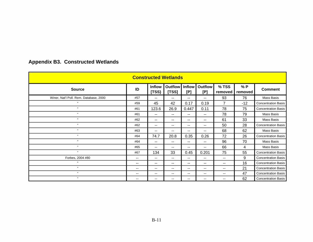
B-11
Appendix B3. Constructed Wetlands
Source ID Inflow [TSS}
Outflow [TSS]
Inflow [P]
Outflow [P]
% TSS removed
% P removed Comment
Winer, Nat'l Poll. Rem. Database, 2000 #57 -- -- -- -- 93 76 Mass Basis
" #59 45 42 0.17 0.19 7 -12 Concentration Basis
" #61 123.6 26.9 0.447 0.11 78 75 Concentration Basis
" #61 -- -- -- -- 78 79 Mass Basis
" #62 -- -- -- -- 61 33 Mass Basis
" #62 -- -- -- -- 50 28 Concentration Basis
" #63 -- -- -- -- 68 62 Mass Basis
" #64 74.7 20.8 0.35 0.26 72 26 Concentration Basis
" #64 -- -- -- -- 96 70 Mass Basis
" #65 -- -- -- -- 66 4 Mass Basis
" #67 134 33 0.45 0.201 75 55 Concentration Basis
Forbes, 2004 #80 -- -- -- -- -- -- 9 Concentration Basis" -- -- -- -- -- -- 16 Concentration Basis" -- -- -- -- -- -- 21 Concentration Basis" -- -- -- -- -- -- 47 Concentration Basis" -- -- -- -- -- -- 62 Concentration Basis
Constructed Wetlands
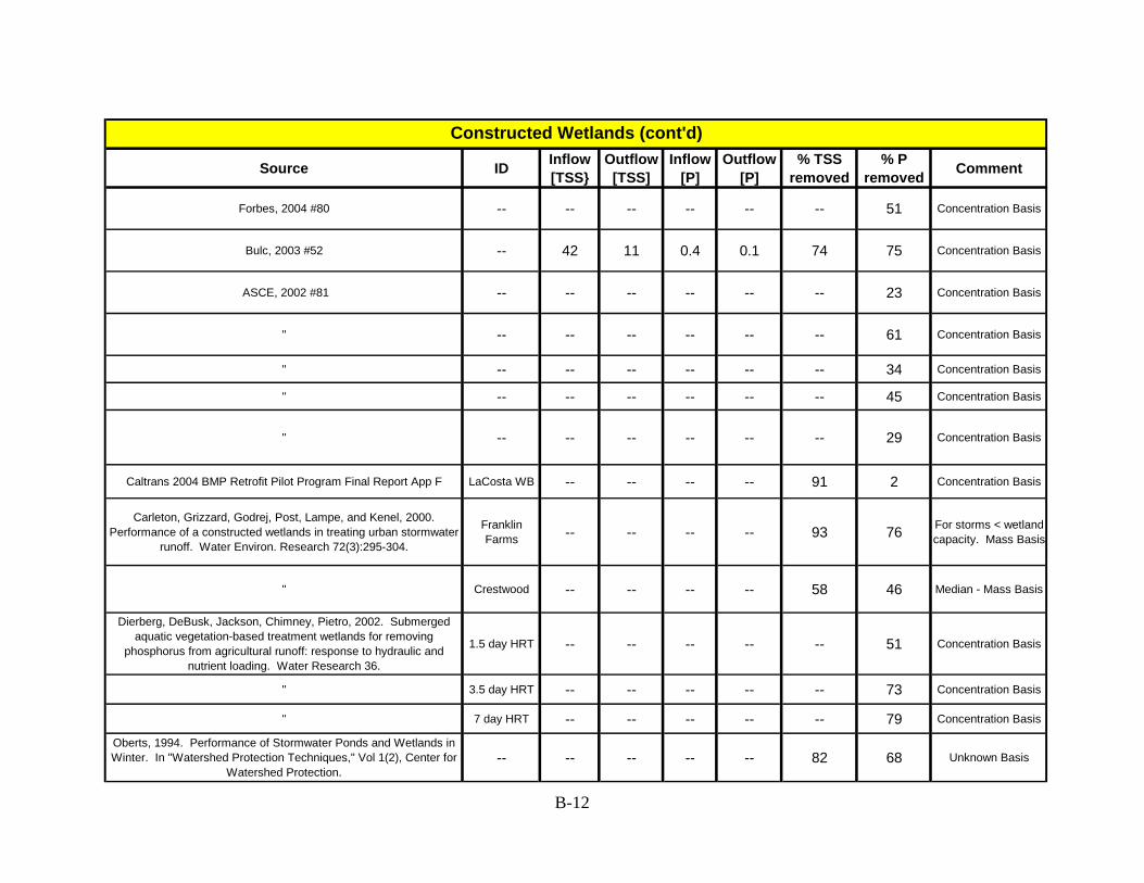
B-12
Source ID Inflow [TSS}
Outflow [TSS]
Inflow [P]
Outflow [P]
% TSS removed
% P removed Comment
Forbes, 2004 #80 -- -- -- -- -- -- 51 Concentration Basis
Bulc, 2003 #52 -- 42 11 0.4 0.1 74 75 Concentration Basis
ASCE, 2002 #81 -- -- -- -- -- -- 23 Concentration Basis
" -- -- -- -- -- -- 61 Concentration Basis
" -- -- -- -- -- -- 34 Concentration Basis
" -- -- -- -- -- -- 45 Concentration Basis
" -- -- -- -- -- -- 29 Concentration Basis
Caltrans 2004 BMP Retrofit Pilot Program Final Report App F LaCosta WB -- -- -- -- 91 2 Concentration Basis
Carleton, Grizzard, Godrej, Post, Lampe, and Kenel, 2000. Performance of a constructed wetlands in treating urban stormwater
runoff. Water Environ. Research 72(3):295-304.
Franklin Farms -- -- -- -- 93 76 For storms < wetland
capacity. Mass Basis
" Crestwood -- -- -- -- 58 46 Median - Mass Basis
Dierberg, DeBusk, Jackson, Chimney, Pietro, 2002. Submerged aquatic vegetation-based treatment wetlands for removing
phosphorus from agricultural runoff: response to hydraulic and nutrient loading. Water Research 36.
1.5 day HRT -- -- -- -- -- 51 Concentration Basis
" 3.5 day HRT -- -- -- -- -- 73 Concentration Basis
" 7 day HRT -- -- -- -- -- 79 Concentration Basis
Oberts, 1994. Performance of Stormwater Ponds and Wetlands in Winter. In "Watershed Protection Techniques," Vol 1(2), Center for
Watershed Protection.-- -- -- -- -- 82 68 Unknown Basis
Constructed Wetlands (cont'd)

B-13
Source ID Inflow [TSS}
Outflow [TSS]
Inflow [P]
Outflow [P]
% TSS removed
% P removed Comment
Oberts, 1994. Performance of Stormwater Ponds and Wetlands in Winter. In "Watershed Protection Techniques," Vol 1(2), Center for
Watershed Protection.-- -- -- -- -- 4 7 Unknown Basis
BMP Database. Site: Franklin Wood, Chantilly, VA -- -- -- -- -- -- 5 Concentration Basis
BMP Database. Franklin Wetland, Chantilly, VA -- -- -- -- -- -- 23 Concentration Basis
BMP Database. Site: Hidden River Wetland, Tampa, FL -- -- -- -- -- -- 61 Concentration Basis
BMP Database. Site: Queen Anne's Pond, Centreville, MD -- -- -- -- -- -- 34 Concentration Basis
BMP Database. Site: Swift Run Wetland, Ann Arbor, MI -- -- -- -- -- -- 45 Concentration Basis
Metropoliton Washington Council of Governments, 1992. A Current Assessment of Urban Best Management Practices-Techniques for
Reducing Non-Point Source Pollution in the Coastal Zone.EWA3, IL -- -- -- -- 72 59 Unknown Basis
" EWA4, IL -- -- -- -- 76 55 Unknown Basis" EWA5, IL -- -- -- -- 89 69 Unknown Basis" EWA6, IL -- -- -- -- 98 79 Unknown Basis" B31, WA -- -- -- -- 14 -2 Unknown Basis" PC12, WA -- -- -- -- 56 -2 Unknown Basis
" McCarrons, MN -- -- -- -- 87 36 Unknown Basis
" Queen Anne's, MD -- -- -- -- 65 39 Unknown Basis
" Swift Run, MI -- -- -- -- 85 3 Unknown Basis
" Tampa Office Pond, FL -- -- -- -- 64 55 Unknown Basis
" Highway Site, FL -- -- -- -- 66 19 Unknown Basis
" Palm Beach, PGA, FL -- -- -- -- 50 62 Unknown Basis
Constructed Wetlands (cont'd)

B-14
Appendix B4. Bioretention Filters
Source ID Inflow [TSS}
Outflow [TSS]
Inflow [P]
Outflow [P]
% TSS removed
% P removed Comment
Winer, Nat'l Poll. Rem. Database, 2000 #93 -- -- 0.52 0.18 -- 65.38 Concentration Basis
Winer, Nat'l Poll. Rem. Database, 2000 #93 -- -- -- -- -- 65 Mass Basis
Idaho DEQ BMP Manual (undated) -- -- -- -- -- 90 75 unknown
Caltrans 2002 as ref'd in "Bioretention TC32," found in CA Stormwater BMP Handbook Developement &
Redevelopment at http://www.cabmphandbooks.com/Development.asp
-- -- -- -- -- 90 76 unknown
Low Impact Development (LID) A Literature Review, EPA-841-B-00-005. USEPA, Oct. 2000
Beltway Plaza,
Greenbelt, MD
-- -- -- -- -- 65 unknown
Low Impact Development (LID) A Literature Review, EPA-841-B-00-005. USEPA, Oct. 2000
Peppercorn Plaza,
Landover MD
-- -- -- -- -- 87 unknown
Bioretention Filters
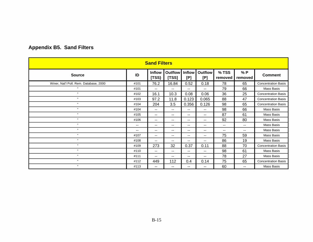
B-15
Appendix B5. Sand Filters
Source ID Inflow [TSS}
Outflow [TSS]
Inflow [P]
Outflow [P]
% TSS removed
% P removed Comment
Winer, Nat'l Poll. Rem. Database, 2000 #101 76.2 16.84 0.52 0.18 78 65 Concentration Basis" #101 -- -- -- -- 79 66 Mass Basis" #102 16.1 10.3 0.08 0.06 36 25 Concentration Basis" #103 97.2 11.8 0.123 0.065 88 47 Concentration Basis" #104 204 3.5 0.356 0.126 98 65 Concentration Basis" #104 -- -- -- -- 98 66 Mass Basis" #105 -- -- -- -- 87 61 Mass Basis" #106 -- -- -- -- 92 80 Mass Basis" -- -- -- -- -- -- -- Mass Basis" -- -- -- -- -- -- -- Mass Basis" #107 -- -- -- -- 75 59 Mass Basis" #108 -- -- -- -- 86 19 Mass Basis" #109 273 32 0.37 0.11 88 70 Concentration Basis" #110 -- -- -- -- 98 61 Mass Basis" #111 -- -- -- -- 78 27 Mass Basis" #112 449 112 0.4 0.14 75 65 Concentration Basis" #113 -- -- -- -- 60 -- Mass Basis
Sand Filters

B-16
Source ID Inflow [TSS}
Outflow [TSS]
Inflow [P]
Outflow [P]
% TSS removed
% P removed Comment
Division, 1990 #79 -- -- -- -- -- -- 0 Concentration Basis
" -- -- -- -- -- -- 45 Concentration Basis
" -- -- -- -- -- -- 59 Concentration Basis
Caltrans 2004 BMP Retrofit Pilot Program Final Report App F E Reg MS -- -- -- -- 75 23 Concentration Basis
Glick, et al, 1998. Referenced in above report (pg 2-10) -- -- -- -- -- 89 59 Concentration Basis
Caltrans 2004 BMP Retrofit Pilot Program Final Report App F Foothill MS -- -- -- -- 86 21 Concentration Basis
Caltrans 2004 BMP Retrofit Pilot Program Final Report App F Term P&R -- -- -- -- 89 24 Concentration Basis
Caltrans 2004 BMP Retrofit Pilot Program Final Report App F Escon MS -- -- -- -- 58 37 Concentration Basis
Caltrans 2004 BMP Retrofit Pilot Program Final Report App F LaCosta P&R -- -- -- -- 91 30 Concentration Basis
Caltrans 2004 BMP Retrofit Pilot Program Final Report App F SR78/I%P&R -- -- -- -- 87 29 Concentration Basis
Glick, et al, 1998. Monitoring and evaluation of stormwater quality control basins in watershed mgt: Moving from theory to -- -- -- -- -- 89 59 Concentration Basis
Environ & Conservation Services Dept. Austin TX. Removal Efficiencies of Stormwater Control Structures. May 1990. Highwood Apt -- -- -- -- 86 19 Mass Basis
Environ & Conservation Services Dept. Austin TX. Removal Efficiencies of Stormwater Control Structures. May 1990.
Barton Creek Squ. Mall -- -- -- -- 75 59 Mass Basis
Environ & Conservation Services Dept. Austin TX. Removal Efficiencies of Stormwater Control Structures. May 1990. Jollyville -- -- -- -- 87 61 Mass Basis
Sand Filters (cont'd)

B-17
Appendix B6. Filter Strips/Grass Swales
Source ID Inflow [TSS}
Outflow [TSS]
Inflow [P]
Outflow [P]
% TSS removed
% P removed Comment
Barrett, Walsh, Malina and Charbeneau, 1998. Performance of Vegetative Controls for Treating Highway Runoff. Jour. Environ.
Engrg. 1121-1128. US 183 median.US 183 157 21 0.55 0.31 87 44 Concentration
Basis/Grassy Median
" MoPac expway 190 29 0.24 0.16 85 33 Concentration
Basis/Grassy MedianBMP Data Base. Austin, TX. Site: Alta Vista planned development
det. w/ swales -- -- -- -- -- 29 84 Concentration Basis/Grassy Median
EPA Data Base: Dayton Swale - Dayton Biofilter with grassed Swale (Site ID 1645113921) -- -- -- 0.183 0.192 -- -5 "
BMP Data Base, Seattle. Site: Dayton Biofilter-Grass Swale -- -- -- -- -- -- -5 "
"Field Test of Grassed Swale Performance in Removing Runoff Pollution," by Jan-Tai Kuo, Shaw L. Yu et al. University of VA
Goose Creek-upper -- -- -- -- 29.7 73.4 Mass Basis/Swale
" Goose Creek-lower -- -- -- -- 97.2 96.8 Mass Basis/Swale
" Goose Creek-entire -- -- -- --
94 98.6Mass Basis/Swale
Caltrans 2002 as ref'd in "Vegetative Swale TC30," found at http://www.cabmphandbooks.com/Development.asp -- -- -- -- -- 77 8 Mass Basis/Dry Swale
Goldberg, 2003 as ref'd in "Vegetative Swale TC30," found at http://www.cabmphandbooks.com/Development.asp -- -- -- -- -- 67.8 4.5 Mass Basis/Grassed
ChannelSeattle Metro & Washington Dept. of Ecology, 1992 as ref'd in
"Vegetative Swale TC30," found at http://www.cabmphandbooks.com/Development.asp
-- -- -- -- -- 60 45 "
" -- -- -- -- -- 83 29 "
Filter Strips/Grass Swales

B-18
Source ID Inflow [TSS}
Outflow [TSS]
Inflow [P]
Outflow [P]
% TSS removed
% P removed Comment
Wang et al., 1981 as ref'd in "Vegetative Swale TC30," found in CA Stormwater BMP Handbook Developement & Redevelopment at
http://www.cabmphandbooks.com/Development.asp-- -- -- -- -- 80 -- Mass Basis/Dry Swale
Dorman et al., 1989 as ref'd in "Vegetative Swale TC30," found in CA Stormwater BMP Handbook Developement & Redevelopment at
http://www.cabmphandbooks.com/Development.asp-- -- -- -- -- 98 18 "
Harper, et al., 1988 as ref'd in "Vegetative Swale TC30," found in CA Stormwater BMP Handbook Developement & Redevelopment at
http://www.cabmphandbooks.com/Development.asp-- -- -- -- -- 87 83 "
Kercher et al., as ref'd in "Vegetative Swale TC30," found in CA Stormwater BMP Handbook Developement & Redevelopment at
http://www.cabmphandbooks.com/Development.asp-- -- -- -- -- 99 99 "
Harper, et al., 1988 as ref'd in "Vegetative Swale TC30," found in CA Stormwater BMP Handbook Developement & Redevelopment at
http://www.cabmphandbooks.com/Development.asp-- -- -- -- -- 81 17 Mass Basis/Wet Swale
Koon, 1995 as ref'd in "Vegetative Swale TC30," found in CA Stormwater BMP Handbook Developement & Redevelopment at
http://www.cabmphandbooks.com/Development.asp-- -- -- -- -- 67 39 "
City of Austin. 1995 (draft). Characterization of Stormwater Pollution for the Austin, Texas Area. Environmental Resources Management
Division, Environmental and Conservation Services Department, City of Austin, Austin, Texas. As found at http://www.fhwa.
-- -- -- -- -- 68 43 Concentration Basis
Yu, S.L., S.L. Barnes, and V.W. Gerde. 1993. Testing of Best Management Practices for Controlling Highway Runoff. Virginia Department of Transportation, Report No. FHWA/VA-93-R16,
Richmond, VA. As found at http://www.fhwa.dot.gov/environment/ultraurb/3fs1
-- -- -- -- -- 49 33 Mass Basis
Filter Strips/Grass Swales (cont'd)
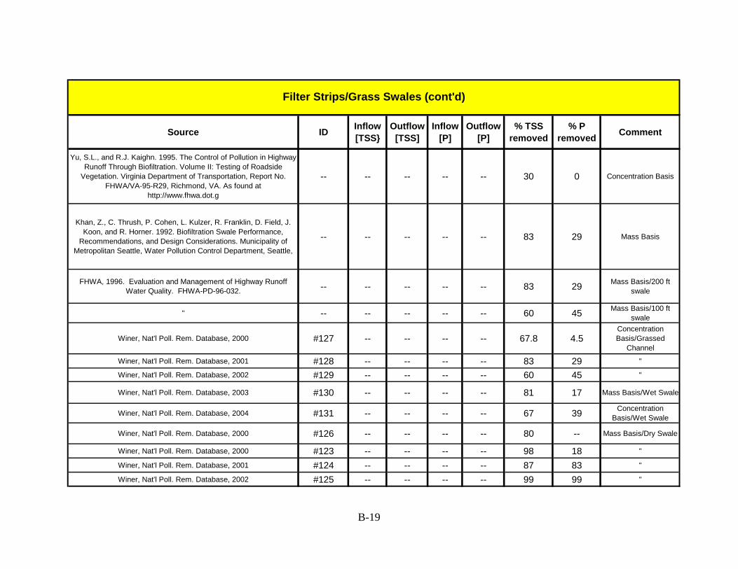
B-19
Source ID Inflow [TSS}
Outflow [TSS]
Inflow [P]
Outflow [P]
% TSS removed
% P removed Comment
Yu, S.L., and R.J. Kaighn. 1995. The Control of Pollution in Highway Runoff Through Biofiltration. Volume II: Testing of Roadside
Vegetation. Virginia Department of Transportation, Report No. FHWA/VA-95-R29, Richmond, VA. As found at
http://www.fhwa.dot.g
-- -- -- -- -- 30 0 Concentration Basis
Khan, Z., C. Thrush, P. Cohen, L. Kulzer, R. Franklin, D. Field, J. Koon, and R. Horner. 1992. Biofiltration Swale Performance,
Recommendations, and Design Considerations. Municipality of Metropolitan Seattle, Water Pollution Control Department, Seattle,
-- -- -- -- -- 83 29 Mass Basis
FHWA, 1996. Evaluation and Management of Highway Runoff Water Quality. FHWA-PD-96-032. -- -- -- -- -- 83 29 Mass Basis/200 ft
swale
" -- -- -- -- -- 60 45 Mass Basis/100 ft swale
Winer, Nat'l Poll. Rem. Database, 2000 #127 -- -- -- -- 67.8 4.5Concentration Basis/Grassed
Channel
Winer, Nat'l Poll. Rem. Database, 2001 #128 -- -- -- -- 83 29 "
Winer, Nat'l Poll. Rem. Database, 2002 #129 -- -- -- -- 60 45 "
Winer, Nat'l Poll. Rem. Database, 2003 #130 -- -- -- -- 81 17 Mass Basis/Wet Swale
Winer, Nat'l Poll. Rem. Database, 2004 #131 -- -- -- -- 67 39 Concentration Basis/Wet Swale
Winer, Nat'l Poll. Rem. Database, 2000 #126 -- -- -- -- 80 -- Mass Basis/Dry Swale
Winer, Nat'l Poll. Rem. Database, 2000 #123 -- -- -- -- 98 18 "
Winer, Nat'l Poll. Rem. Database, 2001 #124 -- -- -- -- 87 83 "
Winer, Nat'l Poll. Rem. Database, 2002 #125 -- -- -- -- 99 99 "
Filter Strips/Grass Swales (cont'd)

B-20
Appendix B7. Infiltration Trenches
Source ID Inflow [TSS}
Outflow [TSS]
Inflow [P]
Outflow [P]
% TSS removed
% P removed Comment
Winer, Nat'l Poll. Rem. Database, 2000 Study 132 -- -- 0.66 0.63 -- 4.5 --
Winer, Nat'l Poll. Rem. Database, 2000 Study 133 -- -- 0.2 0 -- 100.0 --
Winer, Nat'l Poll. Rem. Database, 2000 Study 134 -- -- 0.24 0 -- 84.0 --
IDAHO BMP Manual -- -- -- -- -- 90 55 --
Infiltration Trenches