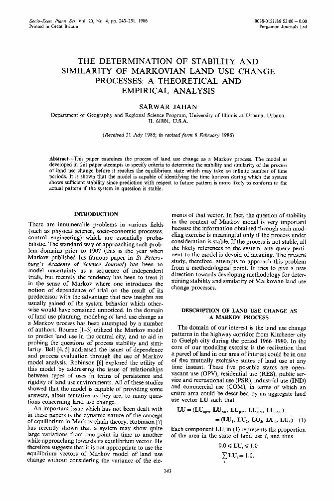
Socio-Econ. Plann Sci. Vol. 20, No. 4, PP. 243-251, 1986 0038-0121/86 $3.00 + 0.00 Printed in Great Britain Pergamon Journals Ltd

THE DETERMINATION OF STABILITY AND SIMILARITY OF MARKOVIAN LAND USE CHANGE

PROCESSES: A THEORETICAL AND EMPIRICAL ANALYSIS

SARWAR JAI-IAN

Department of Geography and Regional Science Program, University of Illinois at Urbana, Urbana, IL 61801, U.S.A.

(Received 31 July 1985; in revisedform 8 February 1986)

Abstract-This paper examines the process of land use change as a Markov process. The model as developed in this paper ateempts to specify criteria to determine the stability and similarity of the process of land use change before it reaches the equilibrium state which may take an infinite number of time periods. It is shown that the model is capable of identifying the time horizon during which the system shows sufficient stability since prediction with respect to future pattern is more likely to conform to the actual pattern if the system in question is stable.

INTRODUCTION

There are innumerable problems in various fields (such as physical science, socio-economic processes, control engineering) which are essentially proba- bilistic. The standard way of approaching such prob- lem domains prior to 1907 (this is the year when Markov published his famous paper in St Peters- burg’s Academy of Science Journal) has been to model uncertainty as a sequence of independent trials, but recently the tendency has been to treat it in the sense of Markov where one introduces the notion of dependence of trial on the result of its predecessor with the advantage that new insights are usually gained of the system behavior which other- wise would have remained unnoticed. In the domain of land use planning, modeling of land use change as a Markov process has been attempted by a number of authors. Bourne [l-3] utilized the Markov model to predict land use in the central city, and to aid in probing the questions of process stability and simi- larity. Bell [4,5] addressed the issues of dependence and process evaluation through the use of Markov model analysis. Robinson [6] explored the utility of this model by addressing the issue of relationships between types of uses in terms of persistence and rigidity of land use environments. All of these studies showed that the model is capable of providing some answers, albeit tentative as they are, to many ques- tions concerning land use change.

An important issue which has not been dealt with in these papers is the dynamic nature of the concept of equilibrium in Markov chain theory. Robinson [7] has recently shown that a system may show quite large variations from one point in time to another while approaching towards its equilibrium vector. He therefore suggests that it is not appropriate to use the equilibrium vectors of Markov model of land use change without considering the variance of the ele-

ments of that vector. In fact, the question of stability in the context of Markov model is very important because the information obtained through such mod- eling exercise is meaningful only if the process under consideration is stable. If the process is not stable, all the likely references to the system, any query perti- nent to the model is devoid of meaning. The present study, therefore, attempts to approach this problem from a methodological point. It tries to give a new direction towards developing methodology for deter- mining stability and similarity of Markovian land use change processes.

DESCRIPTION OF LAND USE CHANGE AS

A MARKOV PROCESS

The domain of our interest is the land use change patterns in the highway corridor from Kitchener city to Guelph city during the period 1966-1980. In the core of our modeling exercise is the realization that a parcel of land in our area of interest could be in one of five mutually exclusive states of land use at any time instant. These five possible states are open- vacant use (OPV), residential use (RES), public ser- vice and recreational use (PSR), industrial use (IND) and commercial use (COM), in terms of which an entire area could be described by an aggregate land use vector LU such that

LU = (Lu,r”, W,,, LUps,, L&l, > L%n)

= WJ,, w, LU,, LU,, LUJ (1)

Each component LU, in (1) represents the proportion of the area in the state of land use i, and thus

0.0 < LU, < 1.0

c LU, = 1.0. I

243

Let us assume that we observe the profile of land use patterns over a time period and notice that at time t the aggregate vector is given by LU,, at time (t + 1) the land use vector is LU,, !, and so on for the same area. If the sequence of vectors LU,, LU,+i,... remain the same for a su~ciently long observation period we identify the system to be in a state of equilibrium as LU, is invariant with respect to time. If the sequence is a string of different vectors we may concede the system to be in a transition state. In the latter case, two successive vectors in the sequence spanned by our five dimensional orthogonal basis set could be assumed related through a transi- tion (transfo~ation) matrix U such that

LU,., = (LU,)U (2)

The first assumption our model suggests is that (2) is true for all subsequent values of t, in which case

of U, Uk, where k is a rational number. The element (U$ would then be the magnitude of the probability of transition from a state i to the state j in k units of time.

The interesting part that now emerges is this: if we let k -+ co then under certain conditions it could be shown [8] that the transition matrix Uk stabilizes to a matrix Q such that

$tI;ik=UC1=Q (6)

or, equivalently, QU = Q. Furthermore, when (6) does materialize, the

matrix Q displays an important property that al1 its rows become identical to a vector, say x. The vector R is then the limiting state probability vector or an equilibrium distribution vector which has the prop- erty that

n =aU LU,+i = (LU,)U

LU,,, = (LU,. W

L&-/J = (LU,+,- W. (3)

The ramifications of our proposals are then: (a) whatever process is responsible for changing the land use vector LU at each subsequent time point remains stationary throughout, and (b) the change to a new land use vector at a time t depends solely on the land use vector profile at a time (t - 1), and not at all on the process by which the system did arrive at LU, _ J in the first place. Thus the process is a stationary memoryless process. It should be noted that the transition matrix U is such that

The equilib~um dist~bution vector shows the land use ahocation at t = cr) if the system were left to itself to evolve. Note that if U is stationary and irreducible (i.e. no ZQ = 1 .O), once the system reaches its equili- brium it will remain there.

In our study, however, the frequency of land use change over a unit of time period is not available; instead, our observation of the process begins with the identification of a frequency matrix over a wider time period of 11 and 14 yr for the areas concerned. How to obtain the unit (or one-step) transition matrix U* from the transition matrix U is considered next.

The unit transition matrix U* is related to the transition matrix U as

and

0.0 G ?$ < 1.0

x2$= 1.0 (4) i

where i, j refer to indices associated with the com- ponents of the land use vector (basis set).

Let us now make an attempt to identify the matrix U in terms of observables. Since U transforms a vector of land use profile LU, into a vector LU,+ , at time (t + I), U must be directly related to observed changes to amount of land allocation in use i at time t. Suppose, P is the matrix such that [x, is its (Q’) element3

U$= U or Ux= Vi” (7)

where n is the number of observation years. U* can be realized through a diagonalization procedure in which U can be transformed into a diagonal matrix such as A. However, a matrix U can be transformed into a diagonal matrix A if and only if it has linearly independent eigenvectors. Then the eigenvector mat- rix H, consisting of linearly independent eigenvectors of U as its columns, can be used to transform U into a diagonal matrix A = HUH-‘. The diagonal matrix A will then have eigenvalues of U as diagonal ele- ments.

iF’, = xx, = amount of land in use i at time t ,

To compute U* from U let us assume that the eigenvectors of U are h,, i = 1,5 associated with which is a distinct eigenvalue. Thus,

Uh, = I, h,

pt,,. = CF, = total amount of land in question ,

and

j;, = amount of land originally in use i at time t, but changed to use j at time (t -I- 1)

then U could be expressed in terms of P simply as

%J =jr,iR (5)

Note that (5) satisfies the requirement in (4). Further- more, if E? is a diagonal matrix then U emerges as an identity matrix.

and, the column h, naturally now could comprise the eigenvector matrix H associated with which is a diagonal matrix such that

UH=HA (8) and

A = diag (A,, AZ, . . . , A,).

From (S), one then obtains

U = HAH-’

and hence, u, = U’/” = H/t l/“H-1 (10) Now we may form successive powers of U and

since U is a stochastic matrix so will be the k th power where A “n = diag (A !I”, nil”, . . . , A:‘“).

244 SARWAR JAHAN

(9)

Stability and similarity of Markovian land use change processes 245

Once U* is thus realizable through a diagonal- ization procedure (10) any arbitrary powers of U* could be formed and the process behavior over a specific time interval may then be observed accord- ingly.

AN APPROACH TO THE DETERMINATION OF PROCESS STABILITY AND

SIMILARITY

One way of comparing two stochastic processes is through their equilibrium distribution vectors. If two such vectors corresponding to two processes are close to each other, the processes could be similar-if they are widely different then there is little similarity between the two processes. However, we need to exercise some caution in this regard.

The problem is that the equilibrium state vector Z, if it uniquely exists, represents an equilibrium state at a time t = 00. It is a system based property realizable at a time t = co, a sort of asymptotic measure. Now, planners and the decision makers who might be inclined to make use of the system, to question it, to use its attributes for further use, may not be inter- ested to wait until the system reaches its equilibrium; in all likelihood, all observations and queries with regard to the system are usually made within a time domain in which the system has some relevance. If that time domain is the planning horizon then the appropriate question to ask is: is the system in this specified planning interval sufficiently stable so as to allow us the possibility of raising system related issues in that interval. In other words, although the system may exhibit an eq~librium state at a time t = co, no one has time to wait that long, and yet one must know quite early whether or not the process in which one is embedded is, indeed, a stable process.

How does one specify the criteria or the notion of sufficient stability at a time point before the system in question has entered the equilibrium state? In this

section we propose an approach toward this problem which, even though lacking the depth of a formalized concrete methodology, points the direction along which such a methodology could be developed in the future.

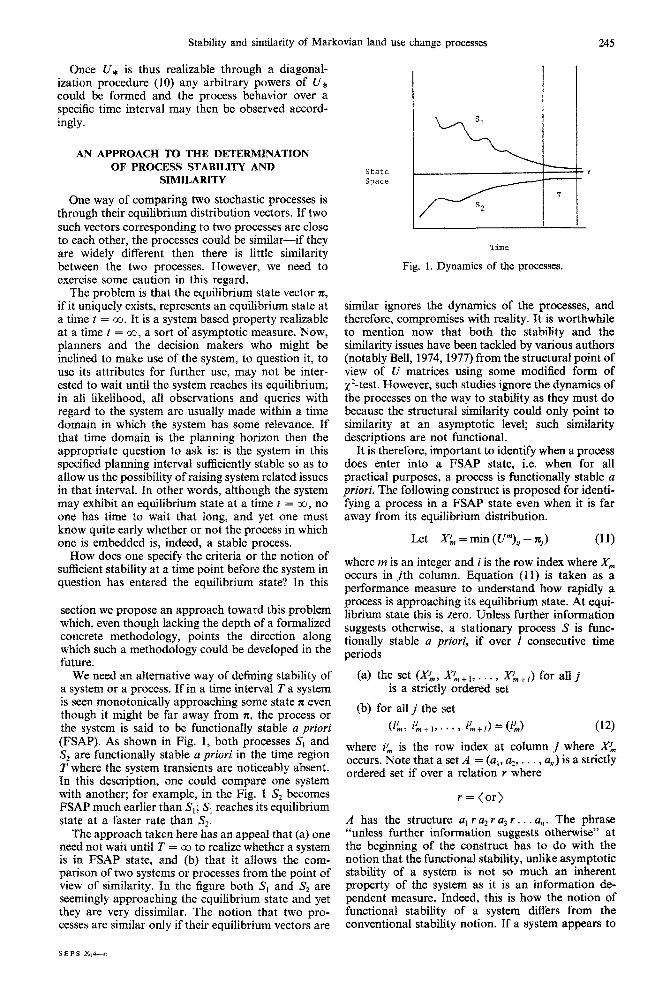
We need an alternative way of defining stability of a system or a process. If in a time interval T a system is seen monotonically approaching some state z even though it might be far away from ?c, the process or the system is said to be functionally stable a priori (FSAP). As shown in Fig. 1, both processes S, and S, are functionally stable a pvio~i in the time region T where the system transients are noticeably absent. In this description, one could compare one system with another; for example, in the Fig. 1 3, becomes FSAP much earlier than S,; S, reaches its equilibrium state at a faster rate than S,.

The approach taken here has an appeal that (a) one need not wait until T = co to realize whether a system is in FSAP state, and (b) that it allows the com- parison of two systems or processes from the point of view of similarity. In the figure both S, and S, are seemingly approaching the equilibrium state and yet they are very dissimilar. The notion that two pro- cesses are similar only if their equilibrium vectors are

state Sp.W

Time

Fig. 1. Dynamics of the processes.

similar ignores the dynamics of the processes, and therefore, compromises with reality. It is worthw~le to mention now that both the stability and the similarity issues have been tackled by various authors (notably Bell, 1974, 1977) from the structural point of view of U matrices using some modified form of X2-test. However, such studies ignore the dynamics of the processes on the way to stability as they must do because the structural similarity could only point to similarity at an asymptotic level; such similarity descriptions are not functional.

It is therefore, important to identify when a process does enter into a FSAP state, i.e. when for all practical purposes, a process is functionally stable a priori. The following construct is proposed for identi- fying a process in a FSAP state even when it is far away from its equilibrium distribution.

Let Xi = min ( Um)l/ - n,) (11)

where m is an integer and i is the row index where X, occurs in jth column. Equation (I 1) is taken as a performance measure to understand how rapidly a process is approaching its equilibrium state. At equi- librium state this is zero. Unless further information suggests otherwise, a stationary process S is func- tionally stable a priori, if over I consecutive time periods

(a) the~t(~~,~~+,,...,~~+,)forallj is a strictly ordered set

(b) for all j the set

(i’,, iA+,, . . . , i’,+[) = (i”,) (12)

where i$ is the row index at column j where X/, occurs. Note that a set A = (a,, a,, . . . , a,) is a strictly ordered set if over a relation I where

r = (or)

A has the structure a, r a, r a, r . . . a,,. The phrase “‘unless further information suggests otherwise” at the beginning of the construct has to do with the notion that the functional stability, unlike asymptotic stability of a system is not so much an inherent property of the system as it is an information de- pendent measure. Indeed, this is how the notion of functional stability of a system differs from the conventional stability notion. If a system appears to

246 SARWAR JAHAN

be stable a priori against all pertinent measures and it is impractical to wait until it arrives at its equi- librium state then for all practical purposes it should be construed stable in a functional sense as long as one is eminently ignorant of the process in the future.

Secondly, we note that our definition, albeit a weak one, is a parametric construct over integers pn and a: If for some m, we find that (11) and (12) are true for I --f co then the construct is compatible with the notion of asymptotic stability. In our study, we fixed the value of 1 at 30 because for planning purposes it is practicable to keep the time horizon below this limit.

Given (11) and (12), further information about the process S may be obtained as shown in the following construct. Suppose S is realized FSAP over par- ameters m and 1. Now for each j, j between 1 and 5, the subset A, is ordered, where .

A,=G%, x!+,,..., -%+,>.

Assume Was the positive integer set (1,2, . . . , d + 1). If A, is an ordered set then its elements over W could be realized in a functional form in the sense of a least square curve, such as

_J,=a,W,+ q. (13)

How well (13) dete~ines A, is expressable in terms of a correlation measure corr,, which is bounded between - 1 .O and 1 .O. The slope a, in (13) is the rate of approach to its equilibrium vector a.

In terms of (13), two systems Si and S2 could now be compared in one of the following three ways:

(a) as~ptoti~lly similar (b) asymptotically dissimilar but dynamically simi-

lar (c) globally similar

which are as follows:

(a) Asymptotically similar

Here, two processes are characterized by equili- brium vectors xS,, nS, which are close to each other as shown in Fig. 1. Note that only at the asymptote do the two processes converge to the vector A, even though, as shown, the processes in the interim period display different dynamics.

(b) Asymptotically ~~similar but ~y~am~~ally similar

Here nS, $zS,, but a,(S,)a,(S,) and the functional forms fg,( .) at S, and S, are the same. For most purposes, we find that usually with

fg,(X’,) = X!, or = ln(X$J

One may get corr, close to + 1.0 or - 1.0 within 3-4 decimal places. Here, the systems are as~ptotically different and yet the way they approach their own asymptotes are the same.

(c) Globally similar

In this case, not only xS, = nS2, but for all j, a,(&) = a,&) along with same functional form f&C * >-

TComputation was done on an AMDAHL 470 under an IBM operating system. The IMSl computer program package was used for mathematical analysis.

In our study we carefully studied each stochastic process governed by some matrix U in terms of its stability and similarity performance with other pro- cesses. First, for each U* we assess its scope for FSAP obtaining its parametric values m and 1. Next we compare U* pertaining to different spatial units in order to determine if they are similar.

Even when a process appears FSAP it is possible that upon further investigation it may appear to be unstable, or weakly stable. This posterior claim to stability or instability is assessed by randomly per- turbing the observed transition matrix and noting the effect of its pe~urbation. If the amount of per- turbation is small and its effect is finite then the process in addition to being in FSAP is stable against perturbation. This is carried out in detail in our study.

EMPIRICAL ANALYSIS

Calculation of transition probability matrices has resulted in two transition probability matrices, one for the period 1955-1966 and the other for the period 19661980.1\ Our analysis, however, is based on the matrices representing the period 1966-1980 since each of these matrices appears to lend to a relatively more uniform process than the corres~nding 1955-1966 matrices.

In order to show the stability and similarity of the land use change processes we have calculated the variables as defined earlier for each of the spatial units, that is, the Waterloo and Guelph regions and the cities of Kitchener and Guelph in Ontario. In addition we have calculated the ratio of the smallest to the largest components of the equilibrium distribu- tion vector pertaining to each spatial unit as well as the angle (as a measure of difference) between the original equilibrium distribution vector of each spa- tial unit and the equilibrium distribution vector after perturbation of arbitrarily selected elements of the frequency matrix (observed ~ansition matrix) of that spatial unit.

It is important to note that once a system enters the state of functional stability a priori (FSAP) the next 30 yr are observed to see if the system remains in that state. However, for the sake of convenience the rates of approach of different columns (or components of land use) of U* toward the equiIibri~ ~stribution are calculated for the first 9yr of this period of functional stability. The results of perturbation of the system are also recorded for these 9 yr.

Stability of the processes

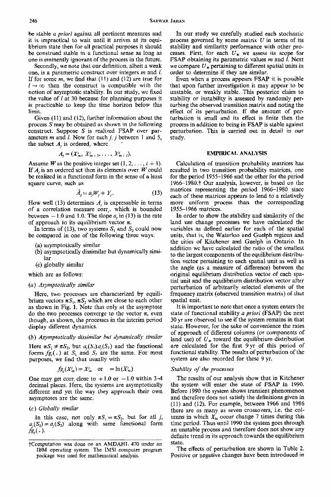
The results of our analysis show that in Kitchener the system will enter the state of FSAP in 1990. Before 1990 the system shows transient phenomenon and therefore does not satisfy the definitions given in (11) and (12). For example, between 1966 and 1986 there are as many as seven crossovers, i.e. the COI- umns in which X, occur change 7 times during this time period. Thus until 1990 the system goes through an unstable process and therefore does not show any definite trend in its approach towards the equilibrium state.

The effects of perturbation are shown in Table 2. Positive or negative changes have been introduced in

Stability and similarity of Markovian land use change processes 247

Table 1. Kitchener city (19661980) Table 3. Waterloo region (1966-1980)

(a) Unit transition matrrx (a) Unit transition matrix TO OPV RES PSR IND COM To OPV RES PSR IND COM

From From OPV 0.96865 0.01429 0.00643 0.00178 0.00885 OPV 0.99478 0.00298 0.00094 0.00085 0.00045 RES 0.00000 0.99359 0.00334 0.00107 0.00199 RES 0.00000 0.99479 0.00280 0.00093 0.00149

U=PSR 0.00000 0.00281 0.99719 0.00000 0.00000 U=PSR 0.00000 0.00268 0.99732 0.00000 0.00000 IND 0.01582 0.00000 0.00000 0.95689 0.02729 IND 0.00000 0.00000 0.00000 0.99858 0.00142 COM 0.01063 0.00236 0.00038 0.00313 0.98350 COM 0.01339 0.00000 0.00000 0.00000 0.98661

(b) Equilibrium distribution: (b) Equili6rium distribution: 0.0389897 0.3439680 0.5102168 0.0167066 0.0901189 0.1490031 0.2418356 0.3045574 0.2465388 0.0580651

(c) Ratio of the smallest to the largest components of the equilibrium distribution vector: 0.0327441

(c) Ratio of the smallest to the largest components of the equilibrium dtitribution vector: 0.1906540.

(d) Rates of approach’ to equilibrium distribution (199G1998): c,: -0.00503 (corr -0.999115) C,: 0.00043 (corr 0.99936)

(d) Rates of approach’ to equilibrwn distributton (1998-2006). C,: -0.00211 (con -0.999938) C,: 0.00085 (corr --0.99986)

(e) Number of crossouers2 during 19661986: 7

‘Slope. *Number of tnnes X, [defined in (ll)] changes columns.

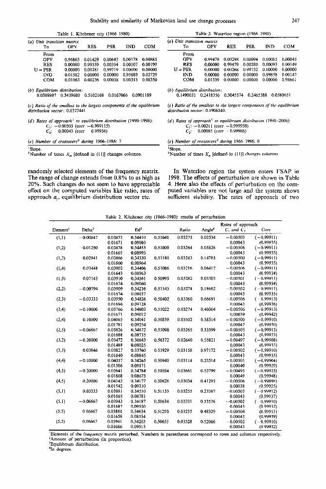
randomly selected elements of the frequency matrix. In Waterloo region the system enters FSAP in The range of change extends from 0.8% to as high as 1998. The effects of perturbation are shown in Table 20%. Such changes do not seem to have appreciable 4. Here also the effects of perturbation on the com- effect on the computed variables like ratio, rates of puted variables are not large and the system shows approach a,, equilibrium distribution vector etc. sufficient stability. The rates of approach of two

(e) Number of crossovers* during 19661986: 0

’ Slope. ‘Number of times X, [defined in (1 l)] changes columns

Table 2. Kitchener citv 11966-1980): results of oerturbation

Element’ Delta2 Ed” Ratio Rates of approach

Angle4 C, and C2 Corr

&I) -0.00847

W) -0.01250

(L3) 0.02941

(134) -0.03448

(1>5) 0.07143

(2>2) -0.00794

(2,3) -0.03333

(2,4) -0.10000

(2,4) 0.10000

(235) -0.06667

(3,2) -0.20000

(3>3) 0.03846

(494) -0.10000

(435) -0.20000

(435) 0.20000

(5>1) 0.03333

(5.1) - 0.06667

(535) -0 06667

(5>5) 0.06667

0.03875 0.34410 0.01671 0.09003 0.03878 0.34455 0.01665 0.08993 0.03866 0.34330 0.01660 0.08964 0.03902 0.34406 0.01643 0.08963 0.03910 0.34361 0.01674 0.09060 0.03909 0.34236 0.01674 0.09037 0.03950 0.34826 0.01694 0.09128 0.03766 0.34803 0.01671 0.09012 0.04065 0.34041 0.01781 0.09254 0.03826 0.34672 0.01688 0.08735 0.03472 0.30643 0.01488 0.08025 0.03827 0.33760 0.01640 0.08845 0.04037 0.34265 0.01586 0.09171 0.03641 0.34784 0.01868 0.08673 0.04143 0.34177 0.01542 0.09310 0.03891 0.34510 0.01665 0.08781 0.03943 0.34187 0.01687 0.09550 0.03881 0.34634 0.01659 0.08534 0.03941 0.34203 0.01686 0.09515

0.51041 0.03273 0.02534

0.51009 0.03264 0.05826

0.51180 0.03243 0.14785

0.51086 0.03216 0.06417

0.50995 0.03282 0.05303

0.51143 0.03274 0.18662

0.50402 0.03360 0.66691

0.51022 0.03274 0.40304

0.50859 0.03502 0.38314

0.51098 0.03265 0.33599

0.56372 0.02640 0.55821

0.51929 0.03 158 0.97172

0.50940 0.03114 0.23514

0.51034 0.03661 0.53799

0.50828 0.03034 0.41295

0.51153 0.03255 0.23387

0.50634 0.03331 0.55576

0.51293 0.03235 0.48329

0.50655 0.03328 0.52066

-0.00503 (-0.99911) 0.00043 (0.99935)

-0.00506 (-0.99911) 0.00043 (0.99935)

- 0.00500 (-0.99911) 0.00043 (0.99935)

-0.00506 (-0.99911) 0.00043 (0.99934)

-0.00501 (-0.99911) 0.00043 (0.99934)

-0.00502 (-0.99911) 0.00043 (0.99935)

-0.00506 (-0.99913) 0.00043 (0.99936)

- 0.00506 (-0.99913) 0.00039 (0.99942)

- 0.00500 (-0.99910) 0.00047 (0.99930)

-0.00505 (-0.99913) 0.00043 (0.99933)

-0.00497 ( - 0.99908) 0.00043 (0.99935)

-0.00502 (-0.99910) 0.00043 (0.99935)

-0.00505 (-0.99904) 0.00040 (0.99929)

-0.00495 (-0.99925) 0.00049 (0.99948)

-0.00506 (- 0.99898) 0.00038 (0.99925)

-0.00503 (-099912) 0.00043 (0.99937)

-0.00502 (-0.99910) 0.00043 (0 99932)

-0.00504 (0.999 13) 0.00043 (0.99939)

-0.00502 (-0.99910) 0.00043 (0 99932)

‘Elements of the frequency matrix perturbed. Numbers in parentheses correspond to rows and columns respectively. *Amount of perturbation (in proportion). 3Equdlbrmm distribution. ‘In degrees.

248 SARWAR JAHAN

Table 4. Waterloo region (1966-1980): results of uerturbation

Element’ Delta* Ed” Ratio Rates of approach

Angle4 C, and C, Corr

(131) -0.00081

W) 0.00962

(L3) 0.02857

(L4) -0.03226

(lY5) -0.06250

(292) 0.01333

(2,2) -0.01333

~2~3) -0.03333

t2,4) 010000

(2,5) -0.06667

(3,2) -0.20000

(373) 0.03704

(494) 0.01852

(4-4) -0.01852

(435) -0.10000

(5,1) -0.06667

(575) 0.06667

(5s) -0.06667

0.14890 0.24657 0.14829 0.24643 0.14807 0.24605 0.14946 0.24439 0.14903 0.24663 0.14853 0.24575 0.14948 0.24733 0.15025 0.24860 0.14763 0.23436 0.14497 0.24639 0.13880 0.22966 0.14740 0.24388 0.14834 0.24990 0.14967 .0.24315 0.14510 0.26627 0.14796 0.24654 0.14803 0.24655 0.15005 0.24643

0.24186 0.05807 0.24237 0.05807 0.24197 0.05799 0.24263 0.05796 0.24192 0.05776 0.24413 0.05788 0.23953 0.05825 0.24370 0.05855 0.24879 0.05753 0.24517 0.05650 0.22531 0.05409 0.23924 0.05744 0.24076 0.05781 0.24293 0.05833 0.23550 0.05655 0.24090 0.06138 0.24096 0.06116 0.24272 0.0549s

0.30459 0.19065 0.01301

0.30483 0.19052 0.10848

0.30593 0.18954 0.19950

0.30556 0.18967 0.29873

0.30466 0.18958 0.038 16

0.30371 0.19057 0.30717

0.30540 0.19074 0.30908

0.29890 0.19588 0.74739

0.3ll69 0.18458 1 &I562

0.30697 0.18404 0.67209

0.35214

0.31204 0.18408 0.98461

0.30320 0.19065 0.45247

0.30593 0.19065 0.45670

0.29658 0.19066 2.65157

0.30321 0.20242 0.42849

0.30330 0.20164 0.40008

0.30585 0.17967 0.40526

-0.00211 0.00085

-0.00213 -0.00085 -0.00211 -0.00085 -0.00212 - 0.00085 -0.00211 -0.00085 -0.00212 -0.00085 -0.00211 -0.00080 -0.00212 -0.00085 -0.00212 -0.00085 -0.00212 - 0.00085 -0.00210 -0.00085 -0.00211 -0.00085 -0.00211 -0.00080 -0.0021 I -0.~86 -0.00211 -0.00078 -0.00211 -0.00087 -0.00211 -0.~087 -0.00211 -0.000x.2

( - 0.99994) (-0.99986) (-0.99994) ( - 0.99986) (-0.99996) (-0.99986) (-0.99994) (-0.99986) (-099994) (-0.99986) (-0.99994) (-0.99986) (-0.99994) ( - 0.99994) (- 0.99994) (-0.99986) ( - 0.99994) (-0.99986) ( - 0.99994) (- 0.99986) (-0.99993) (- 0.99986) (-0.99994) (-0.99986) (-0.99994) ( - 0.99976) (- 0.99994) (-0.99986) ( - 0.99994) (- 0.99976) (- 0.99994) (- 0.99987) (- 0.99994) (-0.99987) (-0.99994) ( - 0.99984)

‘Elements of the frequency matrix perturbed. Numbers m parentheses correspond to rows and columns respectrvely. *Amount of perturbation (in proportion). 3Eq~iib~um dis~ibution. % degrees.

arbitrarily selected columns C, and C, toward the eq~librium vector remain the same as before per- turbation. no appreciable change in correlation is also observed.

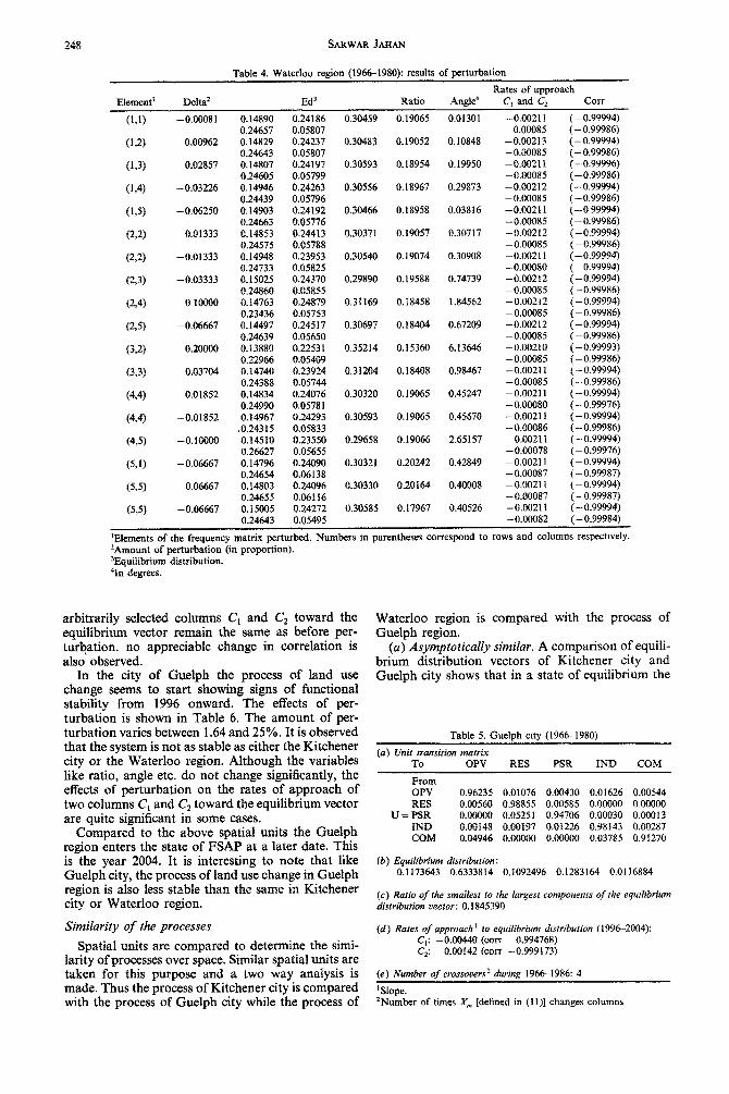
In the city of Guelph the process of land use change seems to start showing signs of functional stability from 1996 onward. The effects of per- turbation is shown in Table 6. The amount of per- turbation varies between 1.64 and 25%. It is observed that the system is not as stable as either the Kitchener city or the Waterloo region. Although the variables like ratio, angle etc. do not change significantly, the effects of perturbation on the rates of approach of two columns C, and C, toward the equilibrium vector are quite significant in some cases.

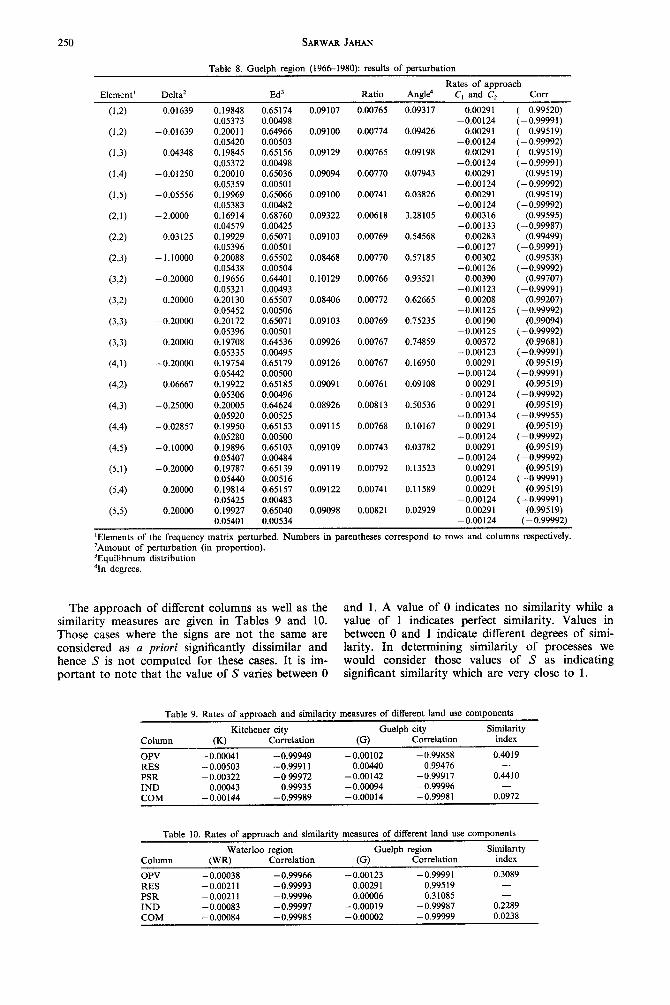
Compared to the above spatial units the Guelph region enters the state of FSAP at a later date. This is the year 2004. It is interesting to note that like Guelph city, the process of land use change in Guelph region is also less stable than the same in Kitchener city or Waterloo region.

Similarity of the processes

Spatial units are compared to determine the simi- larity of processes over space. Similar spatial units are taken for this purpose and a two way analysis is made. Thus the process of Kitchener city is compared with the process of Guelph city while the process of

Waterloo region is compared with the process of Guelph region.

(a) Asymptotically similar. A comparison of equili- brium distribution vectors of Kitchener city and Guelph city shows that in a state of equilibrium the

Table 5. Guelph crty (19661980)

(a) Unit tmmitian matrix To OPV RES PSR IND &OM

From OPV 0.96235 0.01076 0.00430 0.01626 0.00544 RES 0.00560 0.98855 0.00585 0.00000 0.00000

U=PSR 0.00000 0.05251 0.94706 0.00030 0.00013 IND 0.00148 0.00197 0.01226 0.98143 0.00287 COM 0.04946 0.00000 0.00000 0.03785 0.91270

(b) Equilibrium distribution: 0.1173643 0.6333814 0.1092496 0.1283164 0.0116884

(d) Rates of approach ’ to equilibrium dtstribution (1996-2004): C,: -0.00440 (con 0.994768) C2: 0.00142 (corr -0.999173)

’ Slope. ‘Number of times X,,, [defined in (1 I)] changes columns

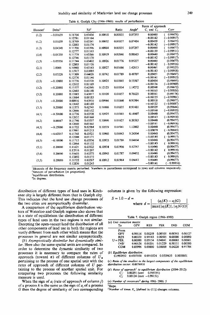
Stability and similarity of Markovian land use change processes 249

Table 6. Guelph City (1966-1980): results of perturbation

Element’ Delta* Ed3 Ratio Rates of approach

Angle4 C, and C, Corr

(1x2) -0.01639

(12) 0.01639

(133) 0.04348

(1>4) -0.01250

(135) -0.05556

(2,l) - 1 .oooo

(222) 0.03226

(2,3) -0.10000

(3,2) -0.20000

(3,2) 0.20000

(373) -0.20000

(3>3) 0.20000

(4>1) - 0 20000

(4,2) 0.06667

(4>3) - 0.25000

(4>4) -0.02857

(4>5) -0.10000

(5,l) - 0.20000

(5>4) 0.20000

(5>5) 0.20000

0.11704 0.63434 0.12781 0.01164 0.11769 0.63241 0.12883 0.01174 0 11700 0.63396 0.12777 0.01163 0.11779 0.63386 0.12746 0.01170 0.11744 0.63402 0 12803 0.01126 0.10908 0.65163 0.11917 0.01085 0.11509 0.64028 0.12576 0.01146 0.11736 0.63338 0.12832 0.01169 0.11537 0.62590 0.12603 0.01148 0.11885 0.63817 0.13OQ4 0.01185 0.00916 0.63910 0.13042 0.01189 0.11575 0.62741 0.12646 0.01152 0.11736 0.63338 0.12832 0.01169 0.11746 0.63557 0.12640 0.01161 0.11722 0.62584 0.13961 0.01215 0.11768 0.63521 0.12580 0.01171 0.11715 0.63356 0.12864 0.01132 0.11621 0.63322 0.12916 0.01207 0.11655 0.63375 0.12892 0.01133 0.11722 0.63287 0.12836 0.01243

0.10918 0.01835 0.07395

0.10932 0.01857 0.07484

0.10964 0.01835 0.07297

0.10919 0.01846 0.08663

0.10926 0.01776 0.05227

0.10927 0.01666 1.42613

0.10742 0.01789 0.49707

0.10925 0.01845 0.55567

0.12123 0.01834 1.14272

0.10109 0.01857 0.76623

0.09944 0.01860 0.91994

0.11886 0.01835 0.91481

0.10925 0.01845 0.14407

0.10896 0.01827 0.20583

0.10519 0.01941 1.12802

0.10960 0.01843 0.24304

0.10933 0.01786 0.04604

0.10934 0.01906 0.12767

0.10945 0.01787 0.09452

0.10912 0.01964 0.06612

0.00440 ( 0.99478) -0.00142 (-0.99917)

0.00439 ( 0.99475) -0.00142 (-0.99917)

0.00440 ( 0.99477) -0.00139 (-0.99911)

0.00440 (0.99477) -0.00142 (-0.99917)

0.00440 (0.99477) -0.00142 (-0.99916)

0.0046 1 (0.99523) -0.00143 (-0.99918)

0.00451 (0.99497) -0.00141 (-0.99915)

0.00454 (0.99495) -0.00136 (-0.99909)

0.00548 (0.99672) -0 00165 (- 0.99936)

0.00341 (0.99178) -0.00125 (-0.99901)

0.00318 (0.99077) -0.00122 (- 0.99897)

0.00529 (0.99644) -0.00160 (-0.99933)

0.00440 (0.99477) -0.00143 (-0.99918)

0.00440 (0.99477) -0.00141 (-0.99916)

0.00440 (0.99477) -0.00079 (-0.99885)

0.00440 (0.99477) -0.00145 (-0.99917)

0.00440 (0.99477) -0.00143 (-0.99918)

0.00440 (0.99477) -0.00142 (-0.99918)

0.00440 (0.99477) -0.00143 (-0.99919)

0.00440 (0.99477) -0.00141 (-0.99916)

lElements of the frequency matrix perturbed. Numbers in parentheses correspond to rows and columns respectwely. ‘Amount of perturbation (m proportion). ‘Equilibnum distribution. “In degrees.

distribution of different types of land uses in Kitch- ener city is largely different from that in Guelph city. This indicates that the land use change processes of the two cities are asymptotically dissimilar.

A comparison of the equilibrium distribution vec- tors of Waterloo and Guelph regions also shows that in a state of equilibrium the distribution of different types of land uses in the two regions is not similar. Excepting the open-vacant land the distribution of all other components of land use in both the regions are vastly different from each other which means that the processes in general are not similar asymptotically.

(b) Asymptotically dissimilar but dynamically simi- lar. Here also the same spatial units are compared. In order to determine the dynamic similarity of two processes it is necessary to compare the rates of approach (toward n) of different columns of U* pertaining to the process of one spatial unit with the rates of approach of different columns of U per- taining to the process of another spatial unit. For comparing two processes the following similarity measure is used.

When the sign of aj (rate of approach of columnj) of a process k is the same as the sign of a, of a process G then the degree of similarity of two corresponding

columns is given by the following expression:

S=l.O-d=

where d = (ai - a,(G)

max(la,W)l, la,(G)I) ’

Table 7. Gueloh region (1966-1980)

(a) Unit transition mat$x To OPV RES PSR IND COM

From OPV 0.99116 0.00259 0.00105 O.(M393 0.00127 RES 0.00229 0.99183 0.00585 0.00000 0.00000

U=PSR 0.00000 0.05154 0.94841 O.OooO3 0.00001 IND’ 0.00128 0.00201 0.01229 0.98151 0.00300 COM 0.03996 0.00000 0.00000 0.04220 0.91784

(b) Equilibrium distribution : 0.1992932 0.6507058 0.0910324 0.0539635 0.0050051

(c) Ratio of the smallest to the largest components of the equilibrium distribution vector: 0.0076918

(d) Rates of approach’ to equilibrium distribution (2004-2012): C,: -0.00291 (corr 0.995191) C,: 0.00124 (corr -0.99151)

(e) Number of crossovers* during 19661986: 5

’ Slope. 2Number of times X, [defined in (1 l)] changes columns.

250 SARWAR JAHAN

Element’ Delta’

Table 8. Guelph region (1966-1980): results of perturbation

Rates of approach Ed3 Ratio Angle4 C, and C, C0rr

(12) 0.01639

(12) -0.01639

(133) 0.04348

(134) -0.01250

(1>5) -0.05556

(2,l) - 2.0000

(2.2) 0.03125

(2>3) -1.10000

(3,2) -0.20000

(3,2) 0.20000

(3>3) - 0.20000

(3>3) 0.20000

(4>1) - 0.20000

(4,2) 0.06667

(433) -0.25000

(4.4) -0.02857

(4,5) -0.10000

(5.1) -0.20000

(534) 0.20000

(5>5) 0.20000

0.19848 0.05373 0.20011 0.05420 0.19845 0.05372 0.20010 0.05359 0.19969 0.05383 0.16914 0.04579 0.19929 0.05396 0.20088 0.05438 0.19656 0.05321 0.20130 0.05452 0.20172 0.05396 0.19708 0.05335 0.19754 0.05442 0.19922 0.05306 0.20005 0.05920 0.19950 0.05280 0.19896 0.05407 0.19787 0.05440

0.65174 0.00498 0.64966 0.00503 0.65156 0.00498 0.65036 0.00501 0.65066 0.00482 0.68760 0.00425 0.65071 0.00501 0.65502 0.00504 0.64401 0.00493 0.65507 0.00506 0.65071 0.00501 0.64536 0.00495 0.65179 0.00500 0.65185 0.00496 0.64624 0.00525 0.65153 0.00500 0.65103 0.00484 0.65139 0.00516 0.65157

0.00765 0.09317

0.19814 0.05425 0.19927

0.00483 0.65040

0.09107

0.09100

0.09129

0.09094

0.09100

0.09322

0.09103

0.08468

0.10129

0.08406

0.09103

0.09926

0.09126

0.0909 1

0.08926

0.09115

0.09109

0.09119

0.09122

0.09098

0.00774

0.00765

0.00770

0.00741

0.00618

0.00769

0.00770

0.00766

0.00772

0.00769

0.00767

0.00767

0.00761

0.008 13

0.00768

0.00743

0.00792

0.00741

0.00821

0.09426

0.09198

0.07943

0.03826

3.28105

0.54568

0.57185

0.93521

0.62665

0.75235

0.74859

0.16950

0.09108

0.50536

0.10167

0.03782

0.13523

0.11589

0.02929

0.0029 I -0.00124

0.00291 -0.00124

0.00291 -0.00124

0.00291 -0.00124

0.00291 -0.00124

0.00316 -0.00133

0.00283 -0.00127

0.00302 -0.00126

0.00390 -0.00123

0.00208 -0.00125

0.00190 -0.00125

0.00372 -0.00123

0.00291 -0.00124

0 00291 -0.00124

0 00291 -0.00134

0 00291 -0.00124

0.00291 -0.00124

0.00291 -0.00124

0.0029 1 -0.00124

0.0029 1 -0.00124

( 0.99520) (-0.99991) ( 0.99519) ( - 0.99992) ( 0.99519) (-0.99991)

(0.99519) (- 0.99992)

(0.99519) (-0.99992)

(0.99595) (-0.99987)

(0.99499) (-0.99991)

(0.99538) (-0.99992)

(0.99707) (-0.99991)

(0.99207) (-0.99992)

(0.99094) (-0.99992)

(0.99681) (-0.99991)

(0.99519) (-0.99991)

(0.99519) (-0.99992)

(0.99519) (-0.99955)

(0.99519) (-0.99992)

(0.99519) (-0.99992)

(0.99519) (-0 99991)

(0.99519) (-0.99991)

(0.99519) 0.05401 0.00534 (-0.99992)

‘Elements of the frequency matrix perturbed. Numbers in parentheses correspond to rows and columns respectively. ‘Amount of perturbation (in proportion). ‘Equilibnum distribution “In degrees.

The approach of different columns as well as the and 1. A value of 0 indicates no similarity while a similarity measures are given in Tables 9 and 10. value of 1 indicates perfect similarity. Values in Those cases where the signs are not the same are between 0 and 1 indicate different degrees of simi- considered as a priori significantly dissimilar and larity. In determining similarity of processes we hence S is not computed for these cases. It is im- would consider those values of S as indicating portant to note that the value of S varies between 0 significant similarity which are very close to 1.

Table 9. Rates of aaoroach and similaritv measures of different land use components

Column

OPV RES

PSR IND COM

Kitchener city

(K) Correlation

-0.00041 -0.99949 -0.00503 -0.99911

-0.00322 -0 99972 0.00043 0.99935

-0.00144 -0.99989

Guelph city

(G) Correlation

-0.00102 -0.99858 0.00440 0.99476

-0.00142 -0.99917 - 0.00094 -0.99996 -0.00014 -0.99981

Similarity index

0.4019 -

0.4410

0.0972

Table 10. Rates of auaroach and similaritv measures of different land use components

Column

OPV RES PSR

IND COM

Waterloo region (WR) Correlation

-0.00038 -0.99966 -0.00211 -0.99993 -0.0021 I -0.99996

-0.00083 -0.99997 -0.00084 -0.99985

Guelph region (G) Correlation

-0.00123 - 0.9999 1 0.00291 0.99519 0.00006 0.31085

-0.00019 -0.99987 -0.00002 -0.99999

Similanty index

0.3089

-

0.2289 0.0238

Stability and similarity of Markovian land use change processes 251

It is observed from the tables that the rates of approach of different columns (representing com- ponents of land use) toward the equilibrium vectors do not show any similarity between the cities of Kitchener and Guelph. Also, no similarity can be observed when Waterloo and Guelph regions are compared. Thus the analysis indicates that the pro- cesses of Kitchener city and Guelph city as well as the processes of Waterloo region and Guelph region are neither asymptotically similar nor dynamically simi- lar.

(c) Globally similar. Since our earlier analysis es- tablished that the processes under consideration are both asymptotically and dynamically dissimilar we can conclude that they are globally dissimilar as well.

CONCLUDING REMARKS

In this paper we have looked into the process of land use change as a Markov process. We have developed a model that allows us to address im- portant issues concerning stability and similarity of land use change processes. It has been observed from the analysis of stability that the land use change processes in Guelph city and Guelph region are less stable than the land use change processes in Kitch- ener city and Waterloo region. Consequently, the likelihood of predictions with respect to future land use patterns to match satisfactorily with future obser- vations is lower in Guelph city and Guelph region than in Kitchener city and Waterloo region. Thus the model has been able to provide information which is useful for a better understanding of the land use dynamics in a changing area.

Acknowledgements-The author expresses his sincere thanks to Professors L.R.G. Martin and R. T. Newkirk of the University of Waterloo, Canada and Professor Sam Sengupta of the State University of New York at Utica, for their valuable help and guidance in carrying out this re- search. The author is also thankful to an anonvmous referee for his/her invaluable comments.

REFERENCES

1.

2.

3.

4.

5.

6.

7.

8.

L. S. Boume. Forecasting Land Occupancy Changes through Markovian Probability Matrices: A Central City Example, Research Report No. 14, Center for Urban and Community Studies, University of Toronto, Tor- onto (1969). L. S. Bourne. Physical adjustment processes and land use succession: a conceptual review and central city example. Econ. Geogr. 47, 1-15 (1971). L. S. Bourne. Monitoring change and evaluating the impact of planning policy on urban structure: a markov chain experiment. Plan Canada 5-14 (1976). E. J. Bell. Markov analysis of land use change: an application of stochastic processes to remotely sensed data. Socio-Econ. Plann. Sci. 8, 311-316 (1974). E. J. Bell and R. C. Hinojosa. Markov analysis of land use change: continuous time and stationary processes. Socio-Econ. Plann. Sci. 11, 13-17 (1977). V. B. Robinson. Land Use Changes on the Urban Fringe: A Stochastic Model Analysis. Discussion Paper No. 3, Dept. of Geography, Kent State University, Kent, Ohio (1978). V. B. Robinson. On the use of markovian equilibrium distribution for land use policy evaluation. Sicio-Econ Plann. Sci. 14. 85-89 (1980). J. G. Kernen; and J. -L. Snell. Finite Markou Chains. Van Nostrand, Princeton (1969).