Trinity College Trinity College

Trinity College Digital Repository Trinity College Digital Repository

Senior Theses and Projects Student Scholarship

Spring 2019

The Economic Impact of Mega Sport Event The Economic Impact of Mega Sport Event

William Baker william.baker@trincoll.edu

Follow this and additional works at: https://digitalrepository.trincoll.edu/theses

Part of the Business Analytics Commons, Social and Behavioral Sciences Commons, Sports

Management Commons, and the Tourism and Travel Commons

Recommended Citation Recommended Citation Baker, William, "The Economic Impact of Mega Sport Event". Senior Theses, Trinity College, Hartford, CT 2019. Trinity College Digital Repository, https://digitalrepository.trincoll.edu/theses/793

A Billion Dollar Investment: Is it worth it to host a Mega-Sport Event?

William R.T. Baker

April 27th, 2019

Advisors:

Prof. Nicholas Woolley

&

Prof. Mark Stater

2

Abstract

Hallmark sporting events have evolved from a competitive opportunity of showing national pride

to commercially driven entertainment entities which seem to prosper from the economic stimulation of the

event. Due to the growing popularity of these mega-sport events, cities and countries around the world are

continually evaluating the potential of using these events to draw attention to the host. This thesis seeks to

contribute to the controversial discussion of whether or not to invest in hosting a mega-sport event. Every

stage of sporting events can reveal positive or negative influences, starting from a competitive bidding

process, to the construction of infrastructure, and to the post-event effects. This thesis will focus on three

aspects: (i) the anticipated impact of hosting a mega sport event in the short run versus long run by analyzing

notable macroeconomic variables: expenditure, investment, and government spending; (ii) econometric

analysis of long run panel data of gross domestic product per capita growth; and (iii) will also attempt to

answer the question of why hosting a mega sport event did or did not work via. Applying basic

macroeconomic principles, the original hypothesis suggested that the impact of hosting a mega-sport event

would result in an expected short-run burst domestic product per capita (GDPPC) followed by a slight

leveling off of the GDPPC in the medium and long term. Applying linear regressions over a twenty-year

period, it is possible to evaluate the impact of hosting an event. Such analysis of the data indicated that it

may be worthwhile for a country to host the World Cup but hosting either of the Olympic Games would

likely be a costly endeavor.

3

Acknowledgments

I would like to express my gratitude to my first advisor Professor Nicholas Woolley for guiding me

through the initial processes of writing a thesis. His insights and shrewd economic intuition helped me

understand the complexities of the topic and begin the planning process throughout the year. His

knowledge of macroeconomic theory inspired the first half of this thesis and into the subsequent parts.

I would like to thank my second advisor Professor Mark Stater for helping me see this thesis through. His

resourcefulness and expertise in the area econometrics cannot be overstated. Time and time again he

helped the reworking of the numerous regressions run until the theory of a triple difference-in-difference

model seemed correct.

Lastly, I would like to thank my friends and family for standing by me through the entire process.

4

List of Figures

Figure 1: Long-run average GDP per capita of host versus runner-up bidder (11)

Figure 2: Money Market (16)

Figure 3: Timeline of Infrastructure Investment (19)

Figure 4: Types of Infrastructure for a mega-sport event (21)

Figure 5: Tourism supply-demand market model (26)

Figure 6: Hypothesized empirical GDP per capita trend (29)

List of Tables

Table 1: Difference-in-Difference model (33)

Table 2: World Cup summary of statistics without control variables (40)

Table 3: World Cup summary of statistics with control variables (40)

Table 4: Summer Olympics summary of statistics without control variables (41)

Table 5: Summer Olympics summary of statistics with control variables (41)

Table 6: Winter Olympics summary of statistics with control variables (41)

Table 7: Winter Olympics summary of statistics without control variables (41)

Tables 8-13: Preliminary model output tables (44-51)

Tables 9-18: Econometric assumption tests (52-61)

Tables 19-22: Final model output tables (62-65)

5

Table of Contents: Page

1. Abstract ...................................................................................................................................................................2

2. Acknowledgments ...................................................................................................................................................3

3. List of Figures .........................................................................................................................................................4

4. List of Tables ..........................................................................................................................................................4

5. Introduction .............................................................................................................................................................6

6. Literature Review .....................................................................................................................................................8

7. Theoretical Model .................................................................................................................................................14

Short-Term Economic Impact ....................................................................................................................14

Impact of Infrastructure .............................................................................................................................18

Long-term Infrastructure Planning ............................................................................................................20

Long-Term Theoretical Impact ..................................................................................................................24

8. Connecting Theory to the Empirical ......................................................................................................................29

9. Data …. ..................................................................................................................................................................31

Variable List ..............................................................................................................................................33

Diff-in-Diff Model .....................................................................................................................................35

10. Methodology ........................................................................................................................................................38

Regression Equations ................................................................................................................................34

11. Preliminary Model ..............................................................................................................................................40

Descriptive Statistics .................................................................................................................................40

Result of Preliminary Model ............................................................................................................... 44-51

12. Analysis of the Primary Model ...................................................................................................................... 44-51

Econometric Assumption Tests: World Cup ...........................................................................................52

Econometric Assumption Tests: Summer Olympics ...............................................................................56

Econometric Assumption Tests: Winter Olympics ..................................................................................59

13. Final Model .........................................................................................................................................................62

14. Conclusion ..........................................................................................................................................................66

Potential Errors ........................................................................................................................................69

15. Appendices ...........................................................................................................................................................70

Appendix A: Economic Figures ................................................................................................................70

Appendix B: Supportive Figures ..............................................................................................................71

Appendix C: Graphical Analysis ..............................................................................................................72

Appendix D: Tables ...................................................................................................................................72

Appendix E: Equations ..............................................................................................................................72

Appendix F: Descriptive Statistics ............................................................................................................73

Appendix G: Preliminary Model ..............................................................................................................75

Appendix H: World Cup Assumption Tests ..............................................................................................78

Appendix I: Summer Olympics Assumption Tests ...................................................................................80

Appendix J: Winter Olympic Assumption Tests .......................................................................................82

Appendix K: Final Model ..........................................................................................................................84

16. References ............................................................................................................................................................86

6

Overview/Intro

High-profile sporting events have increasingly been advocated by governments and marketing

and decision-making strategists as high impact catalysts for economic development in cities and nations.

In particular, the events such as the FIFA World Cup and the Olympic Games draw significant numbers

of domestic and international tourists, attract television and corporate sponsorship (Lee, C; 2009).1 Since

1984, the competition to host the Olympic Games has grown immensely. Economists repeatedly refer to

key goals/outcomes behind why cities are so keen to host such an event. These factors that are often

though tot motivate corporate involvement and public support include: the opportunity to advertise

products to a global audience (raising a host country’s or city’s corporate investment value), leverage

business opportunities in export and new investment, enhance the tourist industry of the host country, and

boost citizen pride (Barney, 2002).2 In reality, the Games begin when cities and nations first devote

enormous amounts of organizational time and money with somewhat outlandish expectations of

benefiting both empirically and implicitly. Hosting major sporting events is associated with the belief that

the ‘buzz’ will draw sizeable crowds and tourists who will spend money in the city/nation. Further,

another perceived economic benefit is than an event is a powerful stimulus due to multiplier effects,

employment bonuses, and the overall economic stimulus supplement that a major sporting event naturally

offers. On the other hand, organizers often overlook or discount the operational, implicit, and opportunity

costs that are associated with this type of event and assume unreasonable expectations. Despite the natural

overhyped characteristic linked with mega-sport events, the initial default policy/economic policy

expectation is that of a city/nation can afford to host a mega event, the benefits that a nation implicitly

acquires, in addition to its tangible benefits (money, revenue), outweigh these inherent up-front incurred

costs.

1 Lee, C., Taylor, T.; University of Technology (Sydney); Journal of Macroeconomics; Critical Reflections on the Economic Impact Assessment of a Mega-Event: The Case of the 2002 FIFA World Cup; https://ac.els-cdn.com/S0261517704000640/1-s2.0-S0261517704000640-main.pdf?_tid=933e6f76-8351-4eed-bc55-020b2952ac15&acdnat=1537848847_0c6d34aa900e40113854713150398b22

2R. Barney, S. Wenn, S. Martyn; Selling the Five Rings: The International Olympic Committee and the Rise of Olympic Commercialism, The University of Utah Press, Salt Lake City (2002)

7

The merit of hosting a sporting event is much more than the event itself where sporting events, such as the

World Cup and Summer/Winter Olympic Games, are viewed as valuable opportunities for the host

nations and urban economies to stimulate economic growth, urban renewal, employment and improve

nation stature. There are also intangible benefits (legacy benefits) (Preuss, 2011) of hosting such as: (i)

media presence which can lead to long-term increase in tourism and be an attraction of new foreign

investment; (ii) long-lasting infrastructure with a potential for a variety of uses; (iii) and a signal of trade

liberalization that promotes greater trade activity in the long term. If such results were consistently true,

however, then every city, state and nation-governing body would apply to host this world invitational

event. Hosting mega-events requires significant investments. Zimbalist (2015) notes emerging economies

like China, Brazil, and South Africa have increasingly perceived “mega-events as a sort of coming-out

party signaling that [they are] now a modernized economy, ready to make [their] presence felt in world

trade and politics.”3 Their intentions may be noble, but the intention of using mega-events as a “coming-

out party” means developing countries hoping to host them need to make massive investments. Notably,

the 2004 Sumer Olympic Games in Greece cost roughly $16 billion, 2014 World Cup cost Brazil $20

billion, and the 2008 Olympics cost Beijing roughly $40 billion. Prior to the bidding process, should

overestimate the total incurred costs and underestimate the total produced benefits.

3 Zimbalist 2015; Is It Worth It?; Finance and Development; Vol. 47 p. 8-11

8

Literature Review

In recent decades, major sporting events have been recognized as an opportunity to stimulate

economic growth through government expenditure, foreign investment, new money consumption and the

introduction of future trade possibilities. Substantiated author and grad student publications have

illuminated analysis and measurements of the economic impacts of these major sporting events. Their

research has evaluated whether or not mega-events lead to access to previously inaccessible funds and

increased investments. These investments would theoretically come from supranational organizations,

private stakeholders, public stakeholders, or tourists (Barrios). We also consider whether or not these new

expenditures and investments have the direct, indirect, multiplicative, or induced effects (Kasimati). In

this field, Kasimati (date), and Lee (date) recognize the different economic approaches that have been

considered when trying to measure the impact that hosting mega sporting events incur. On the other hand,

Brunet, Overmyer and Plenderleith illustrate strict cost-benefit analysis to indicate the direct impact on

the hosts of the major sporting events. Furthermore, studies conducted from Preuss (date) and Collett of

Colorado College (date) justify the substantial economic burden incurred for the organization of the

mega-event in the face of the consequent increase in consumption spending, foreign investment, and

employment. In this line of research are inserted contributions from: (i) Kasimati (date) and Lee (date)

that demonstrate the importance of incorporating multipliers into the calculations of macroeconomic

impact; (ii) Meurer (date), ERNST & Young Terco (2015) and Collett (date) indicate how the

introduction of new money directly and indirectly connected to a mega event, specifically the 1984 Los

Angeles Olympics, the 1992 Barcelona Summer Olympics, 2002 FIFA World Cup in South Korea/Japan,

and the 2014 FIFA World Cup in Brazil; (iii) and Gong (2008) that theorizes the fragility of the mega

investment profile, indicating that a mega-sporting event is a double-edged sword. If it could be used in

the right way, it would bring magnificent benefits; otherwise the hosting opportunity of a mega-sporting

event would be costly.

Conversely, there are some authors that tend to analyze the adverse effects and consequences that

negatively impact economies the of the host country. Barrios and Russel of Harvard Kennedy School

(2011) as well as Plenderleith (2012) argue that the vast majority of literature fails to substantiate a

relationship between mega-events and the increased economic activity. Overall, the expected economic

benefits of hosting an event are vastly overstated and the real benefits are outweighed by the costs

associated with event preparation and execution. The only case where the argument of failed

substantiation could be justified was made by Kim (2008) and (Lee, 2002) who theorized that in the long

term, the Games and world mega events significantly contribute in economic reputation and stature.

9

The first part of this paper will use macroeconomic theory and analysis to create a generalized

hypothesis as to what should happen if a city or country decides to take on the responsibility of hosting

such an event. Several authors have ventured into the idea of analyzing the theoretical short term and long

term benefits and costs of hosting mega events. One of the most significant of which is Professor Victor

Matheson (2006) of Holy Cross, who measured the impact of such events through data and logic and

concluded that hosting these events are seemingly high costs and low reward. The early spending may

spur quick economic activity, but the tangible benefits in the end are outweighed by the initial costs. He

also noted economic variations in hosting economies. The data gathered for the econometric side of this

thesis has a wide variance in term of economic differences (developed versus developing) from the World

Cup to the Olympics. Essentially, the World Cup hosts are more varied in terms of economic variation

where developing countries in South America are just as probable to host the World Cup as developed

European or North American countries. The Summer Olympic Games are a little less varied but we see

smallest variation in hosting nations of the Winter Olympic Games. The Winter Olympic Games are

mainly hosted by Nordic, prosperous European, or North American countries, most of which are

characterized with a substantially higher gross domestic product per capita. Matheson stresses that if

developing countries want to experience more economy growth, they stay away from hosting the games

where the initial costs are too great to overcome.

Events end up not being profitable for primarily one of two reasons: early overestimation of

profits or underestimation of costs. While this may be the ‘classic’ investment theory, this just happens to

be on a billion-dollar scale. Per the overestimation of revenue streams, both Matheson and Késenne

(2005) demonstrate that although mega sport events can generate adequate revenue for a cost-benefit

spreadsheet, the distribution of the money does not automatically favor the host city where a substantial

portion often falls on the international investors, non-local hospitality and service suppliers, and

international sporting government bodies.4 A possible positive effect was noted by Qi Gong (2012), from

the University of Nevada, that building stadiums for the hosting of the Games often create spill-over

effects. Infrastructure is often built where the land is cheap and impoverished, any presence of money in

those areas due to the mega sport event would be considered a benefit regardless of how much.5 A

possible negative is the aforementioned where the local economy often sees less revenue than originally

estimated from the hosted event and thus the overestimation hurts in budgeting for the future, ultimately

landing the host in debt. Despite a multitude of documented research that suggests the complexity and

4 Késeenne, S.; European Sports Management Quarterly, 5, 133-142 (2005); Do we need an economic impact study or a cost-benefit analysis of a sports event? 5Gong, Qi.; University of Nevada; The Positive and Negative Economic Contributions of Mega-Sporting Events to Local Communities; https://digitalscholarship.unlv.edu/cgi/viewcontent.cgi?article=2363&context=thesesdissertations

10

profitability, applicant cities often take for granted the disparity in the generated revenues in the short-run

versus the anticipated long-run revenues generated from trade, upgrading their infrastructure, and

attracting future corporate investment (local and foreign) into their local economy.

The second reason why countries become unsuccessful hosts is due to their underestimation of

investment costs. A majority of these costs are found in the investment in infrastructure in preparation for

the event: stadiums, media villages, and structures to host the influx of millions of people. Harry Arne

Solberg and Holger Preuss (2007) analyze the reasoning behind that and conclude that cities spend

substantial amounts of money rebuilding versus upgrading infrastructure. While this can create welfare-

economic gains (long term implicit benefits), this does not assure that the tangible benefits will exceed the

costs. With many of these host cities placing a significant part of their revenue on inbound tourism, this

also creates such a high risk gamble on people. When circumstances allow, events can stimulate tourism

but this visitor influx is not indicative of a long-term demand curve (of a normal supply demand market)

outward shift, but rather a short term burst. If producers behave rationally, they will supply the market

with more goods and the supply curve would shift outward as well to regulate the equilibrium price.

Indirectly, tourism can improve the host’s ability to capitalize on economies of scale but local residents

would obtain non-local goods and services, which would disappear over time.

The largest component of hosting is the short term investment and long term impact in

infrastructure. A number of factors can inhibit long-term tourism demand but the event’s promotion will

not consistently be able to draw in the same amount of tourists post-event as during the event. One of the

few analysis using (publicly available) data sets was created by Anita Mehrotra (2011).The thesis was a

comparative study on the long run impacts specific to the Olympic Games. The study took into account

the massive pre-event expenditure on infrastructure and tourism expenditure during the event and

compared it to the lack-there-of in a non-host city over a twenty-year period. The study ultimately found

that after the initial spurt in economic activity around the event (at time = 0), the economic progress, in

terms of gross domestic product (GDP), significantly slowed. In some comparative cases, the GDP

growth slowed so much that the control country (non-host) ended up surpassing the host country within

ten years after the event.6 This ultimately led her to conclude that the initial ‘sugar rush’ of hosting a

mega sport event was not worth it in the end on average. The figure below illustrates the long-term

comparative study:7

6 Mehrotra, A., Saez, E.; UC Berkeley; To Host or Not to Host? A comparison Study of the Long-Run Impacts of the Olympic Games https://www.econ.berkeley.edu/sites/default/files/mehrotra_anita.pdf 7 Mehrotra, A., Saez, E.; UC Berkeley; To Host or Not to Host? A comparison Study of the Long-Run Impacts of the Olympic Games https://www.econ.berkeley.edu/sites/default/files/mehrotra_anita.pdf

11

There are many theories that can explain why this conclusion may occur: variances in countries

chosen, elimination of positive outliers (Barcelona, Spain), Dutch disease (a net negative impact on an

economy that originated from a sharp inflow of foreign currency), or poor allocation of resources. For the

most part, research would suggest that it is not worth it to host such an event where the intangible benefits

are nearly impossible to measure and the tangible benefits are surpassed by the cost. Based on the leading

literature, authors (Victor Matheson, Thomas Miceli, Andrew Zimbalist) would generally conclude that it

just purely based on revenue streams, it is possible to generate a profit from a structured event such as the

World Cup due to the sheer size, but highly unlikely to yield a profit from an event such as the Olympic

Games. Upon attending an economist panel concerning this topic, Victor Matheson and Andrew

Zimbalist clarified that it is possible for outliers to occur such as Los Angeles ’84 or Barcelona ’92. Mr.

Matheson dubbed this as the ‘hidden gem theory’ where the city must be characterized with the right

potential in resources to have a long-term positive effect. When Salt Lake City hosted the Winter

Olympic Games (’02), their revenue change over the past fifteen years compared to Denver ski slopes

have increased significantly. In this sense, a city’s potential relies on its ability to change for its future

economy and its location. For example, Salt Lake City was a growing and well-known ski destination. Its

hosting of the Games only required the park to invest in park improvements for the future (that would

have been made anyway) and further boosted its already recognized name. In the case of Atlanta,

however, it is not an internationally recognized city. Hosting the Olympics would certainly help in the

Figure1

12

short term, but the city location and culture is constantly second-rate to Nashville and people naturally

regress back to the larger well-known cities. If people ask where someone wants to go on vacation, they

would likely say Salt Lake City for a ski vacation or Los Angeles in the winter. This is where the

retention of natural tourism differs between cities already developed or considered to be a ‘hidden gem’

and cities that are not prime for a breakout on the world stage.8

The general consensus explains that through econometrics, it nearly impossible to yield positive

statistically significant results when analyzing data surrounding the Olympics. According to Mr.

Zimbalist, “hosting the event creates the same short-run economic boost equivalent to borrowing a billion

dollars and using it to build a hole in the city center.” There would be a billion dollars in short term

spending, but the city and country would be a billion dollars more in debt than before and have no way to

turn that into a profit. Hosting a mega-sport event comes down to the incurred costs, as mentioned before.

At the panel, Mr. Zimbalist stated that the cost-overruns are almost the sole reason why hosting fails. If a

politician wants to get elected or focus on bring in the Olympics or World Cup, he or she will absolutely

understate the costs to gain public support. At a minimum, the bidding cost for the World Cup or

Olympics costs anywhere from $60-$100 million. There are four categories of spending: (i) operations

budget, which is the cost of operating the event; (ii) permanent sports venues, which include the Olympic

village, (iii) infrastructure, which will be stressed later; (iv) and security. The aggregate of such categories

varies between $14.8-$23.1 billion. In conclusion, the investment in these games would spur billions of

dollars in economic activity, but would not be sustained and would eventually hurt the economy.

Econometric analysis illustrates this relationship of an unsustainable expenditure pattern where a short-

term economic boost is completely undermined by the long-term downfall, per the Olympic Games. This

is why it is nearly impossible to yield statistically positive results when examining the impact of the

Games.

8 Victor Matheson, Andrew Zimbalist, Thomas Miceli; “Olympics Lecture” (University of Connecticut Law, April 12th, 2019.)

13

The differentiation between the Games and the World Cup was examined by Dr. Miceli. He explained

that due to the spread out nature, size, and duration of the World Cup, the revenue streams will be

astronomically larger. This is in part why the World Cup hosts experience just made the games longer and

larger to create more revenue. Another reason that World Cup host experience marginally more success is

due to the destinations chosen: all places with soccer (fútbol) leagues. This makes the infrastructure costs

significantly less. Due to the spread out nature of the event, the costs are spread out among different cities

(sometimes other nations) and the profits created catalyze economic activity in all of the different places

where the competitions are held; unlike the centralized pattern of the Olympics. Theoretically, it is more

probable that hosting the World Cup would produce more positive outcomes than hosting either of the

Olympic Games.

14

Theoretical Model

The literature review suggests there is no general consensus as to whether or not hosting a mega-sport

event helps or hinders economic growth. One theory supported by several macroeconomists suggests that

hosting a mega-sport event increases international awareness and thus results in a positive, short-lived,

economic effect on the output. Conversely, a numerous amount of existing literature indicates the

opposite: that hosting such an event causes a negative short-term impact on the growth of the economy.

Short-Term Economic Impact:

We will briefly touch on the subject of legacies and implicit benefits/costs to address possible

reasoning as to why host countries and cities primarily desire to host the event and yet some are unable to

consistently replicate these results. A legacy is an externality (external phenomenon) that arises in the

wake of the event which attempts to capture people’s behavior. Some of the positive legacies include:

urban revival, improved public welfare, reduced unemployment, host city marketing, projection of

cultural values, and economic signaling that the host is ready to engage in business with the rest of the

world (if not already). On the other hand, negative legacies include: traffic produced from incoming

visitors, production of real estate bubble due to raised prices, employment is only temporary, and further

socioeconomic hierarchical differentiation. Unfortunately, further research would suggest that there is no

accurate way to accurately measure the impact of the implicit benefits or costs. Two different methods

have been used in attempt to capture the gravity of the implicit benefits: top down approach and the

bottom up approach. The top down approach is very controversial where one author stated that “In theory

one only needs to compare the economic variables of a city/region, which staged the event with the same

variables of the city/region not staging the event” (Hanusch, 1992).9 This model was found to be

oversimplified as it assumed many variables were equal between the control and treatment group. The

bottom up approach attempted to measure the value of the values by measuring the lasting infrastructure

the investment into the games produced. The approach considered the development of the city between

the control city versus the treatment (host) city. While both approaches were attempted, both were found

to be static and unable to truly capture unforeseen elasticities.

9 Preuss, H.; Johannes Guttenberg-Universitat Mainz, Germany; Lasting Effects of Major Sporting Events; https://idrottsforum.org/articles/preuss/preuss061213.pdf

15

While some theories also address the implicit and intangible benefits (country image leading to

increased tourism) and costs (increase in human traffic and pollution from increased tourism), this section

will primarily focus on the tangible Gross Domestic Product of a country and equation-driven aspects of

theoretical macroeconomics. Normally, an economy is determined by either measuring the gross domestic

product per a given year via the expenditure, income, or value added approach. The theory explained will

use the expenditure approach which suggests GDP is determined by the equation:

Y = C(Y - T) + G + I(r) + NX(r)

This equation identifies the expenditure approach to measuring the output of an economy (GDP)

by accruing the total amount of spending in the economy from consumers, government, investment, and

foreign trades. Consumption (C) is normally the largest GDP component in the economy consisting of

private (household) expenditures. It is a function of how much income people have subtracted by the

amount they owe the government in taxes. Investment (I) includes the purchasing of intermediary goods

that would help create the final goods such as business investment in equipment to produce their final

good that would appear on store shelves. Government (G) spending is measured as the aggregate if all

government purchases of final goods and services. It includes salaries of public servants, purchase of

military weapons, and any foreign expenditure by the government. Next exports (NX) represents the gross

exports subtracting the total imports. GDP captures the amount a country produces including those from

foreign nations’ consumption, thus exports are added. Imported goods are deduced to avoid counting the

foreign supply as domestic.

Nations and cities compete to host international sporting events such as the World Cup and

Summer and Winter Olympic Games even if large investment costs are incurred. When a city decides to

undertake a mega sporting event, they do so with the intention that hosting such an event will provide

many direct financial benefits as well as countless indirect benefits. Since there has been no credible way

of calculating the intangible benefits a country receives due to hosting a mega sport event, this analysis

will focus on the theoretical benefits: taxes, income, unemployment, and small project investment and

how these variables affect the larger economic indicators a country reflects.

Y= Gross Domestic Product

C = aggregate consumption expenditure of country’s goods and services

I = aggregate amount of a country’s investment

G = aggregate of a country’s government expenditure

NX = net result of a country’s exports and imports

16

Theoretically, hosting such events as the World Cup would elicit a positive impact on the

economy provided that the incurred costs are not exorbitantly larger. Usually, the main source of revenue

is generated by the influx of tourists. This mass attraction of international tourists should cause an

aggregate increase in the consumption variable (C) in the Keynesian equation. Let us estimate a minimum

of two million people enter the country for the duration of the event and each spend a minimum $100 per

jersey of their favorite player (World Cup). Conservatively, tourists will contribute a positive $200

million in aggregate expenditure (C).

Hosting a mega sport event would also enact a multitude of chain reactions due to an influx of

tourism: (i) decrease in unemployment where there would be more employment opportunities for local

workers; (ii) ultimate increase in government spending; (iii) and in increase in net exports due to pre-

event spending in infrastructure. With more expenditure occurring in the economy, businesses would

have more resources to pay workers higher wages. This increase in income would allow for either more

expenditure (increase in C), more savings (more bank lending), and a higher tax rate. A higher tax rate

means the government has more money to spend on local projects, such as pre-event investing in

infrastructure. This investment in infrastructure in addition to an increase in aggregate expenditure would

elicit an increase in Gross Domestic Product (Y) and thus an increase in the overall country interest rate.

The figure below illustrates the increase in the interest rate due to an aggregate increase in a country’s

GDP where liquidity demand (L) is a function of Y (GDP).

L’(i,Y)

i’

Figure2

17

As seen in the above figure, an increase in aggregate expenditure elicits an increase in the

liquidity demand and macro interest rate. This results in an increase a decrease in the exchange rate where

domestic currency becomes more affordable and desirable to foreign nations. An increase in the foreign

desire of domestic products indicates a positive sum in net exports. Logically, in influx of tourism should

elicit a positive aggregate impact on the economy.

Commonly found, however, is that there appears to be a negative impact on host countries for

several years after the Olympic Games are held. As pointed out in the most current research on the long-

run effects (PricewaterhouseCoopers, 2002) this negative impact on the host countries may be a result of

the increase in domestic investment and excitement for hosting the Olympics. This, in turn, would lead to

an increase in domestic and international demand for host country's products and would most likely be

seen through the consumption channel of the classic macroeconomic equation for output:

Y = C(Y - T) + G + I(r) + NX(r)

However, this spike in consumption would be relatively short-lived and as public infrastructure

built for the Games remains unused, negative capacity effects could result in a decline in long-run output.

Thus though an increase in government spending is expansionary fiscal policy, the spending on the

Olympic Games may have an even smaller multiplier effect than current research suggests (Ball, 1999).10

This may partially be attributed to the multiplier working the opposite direction: the non-recurring boost

to expenditure results in a longer-run fall in demand as the economy returns to its pre-Olympic

equilibrium income (PricewaterhouseCoopers, 2002).11 This suggests an explanation for why the impact

is negative for a long period of time after the Games are hosted.

Another explanation for results in contradiction of basic macroeconomic theory would be a loss

of local expenditure. One of the largest positive explanations promoting hosting a mega sport event is due

to the resulting mass of expenditure from tourists and media rights. What is not necessarily considered,

however, is the investment from transnational organizations or international investors. Money originally

invested by I.e. Coca Cola, a global organization, will be paid back by the revenues generated from tourist

expenditures. This money will go to the Coca Cola organization and not necessarily to the local economy.

Per the 2014 Brazil, Coca Cola invested around $7.6 billion; since the organization reported a return

10PricewaterhouseCoopers (2002); Business and Economic Benefits of the Sydney 2000 Olympics: A collation of evidence. Sydney 11 PricewaterhouseCoopers (2002); Business and Economic Benefits of the Sydney 2000 Olympics: A collation of evidence. Sydney

18

roughly 5%, therefore an extra $380 million generated revenues would return to the Coca Cola company

and thus out of the local economy.12 The supplementary part of this theory of generated money leaving

the economy can be connected through housing. Mega events are frequently characterized by high

capacity constraints and thus high prices for accommodations and hospitality services. Hotel rooms,

villas, and village lodges can sell as high as three times the normal rate during a globalized event because

many people are initially price inelastic. Out of these inflated prices, the desk clerks, valets, cleaning

staff, and complementary services employees’ wages do not triple. Thus as the tourist industry allows for

a significant returns to capital for these hospitality conglomerates, the majority of these services are based

exterior to the local economy and event expenditure leaks of the host economy.

The Impact of Infrastructure Investment:

The empirical section of this thesis will focus on the empirical consequences for long-term

economic growth with hosting a mega event. As such it is imperative to cover the main reason of how a

host economy fails or prospers: infrastructure. Infrastructure is the largest form of investment (majority of

early spending) and government spending with each government’s highest hope of profit attached with it.

This section will focus on the theoretical direct and implicit effects of infrastructure as a long-term

venture due to its sheer importance. The investment in infrastructure is both the key to the financial

success of hosting a mega-sport event and the bridge between the short run costs (pre event) and the long

term economic progress. The major question is whether or not it is worth it to largely finance a billion-

dollar project for the hope that it will pay off in a decade’s time. The goal of any business investment is

for it to be financially beneficial to the investor. In economics, the objective is to maximize the total

amount of profit filling the demand for a product. An investment in infrastructure is a little riskier where

the investment guarantees a supply of new infrastructure in hopes that the demand will be met by the

sporting event and in the long term by the normal populace. On this supply side of this equation, a city

(Olympics) or country (World Cup) needs to be prepared to host millions of new tourists as well as

accommodate the countries’ sports teams. Precedent illustrates that all hallmark events go through a long

period of preparation ranging from four to eleven years.

12 Narula, S.; Coca-Cola’s investment in the World Cup didn’t exactly pay off; qz.com; https://qz.com/238538/coca-colas-investment-in-the-world-cup-didnt-exactly-pay-off/

19

The figure above depicts the timeline necessary for the usual amount of time required to be

prepared for the hosting of the mega sport event.13 Countries and cities often require at least six years to

adequately host the event. On the other hand, some cities have infrastructure that enables them to stage

major events with very little need for investment. Consequently, a significantly lower amount of revenue

generated via ticket sales or media coverage is required; this is where most hosts of mega sport events

have come close or experienced profitable returns in both the short and long run.

Many investors understand that while infrastructure investments typically do not generate

economic benefits for another decade, they can create many positives if done correctly. Advocates of

hosting a mega sporting event claim that stadiums and sports infrastructure can serve as a base element to

promoting local economic development. It is envisioned that the stadiums and new transportation build in

tandem would serve as an integrated component of an (often times) gentrifying and diversifying local

economy. Camp Nou (FC Barcelona Stadium) is an easy representation of advocates’ theory; a stadium

that has hosted many international events and tournaments. The stadium was built in 1957 and rests in an

area known as Les Corts, which fifty years ago was a ghetto. This venture posted the highest revenue in

sports history at $770 million annually and generates a host of spillover effects for the local community as

millions of fans travel internationally, not necessarily just for the international competition, to watch the

event. An improved and almost thriving entertainment district has developed around the stadium with

dozens of eating and drinking establishments within a few blocks. While Camp Nou is an example of a

thriving measurable economic benefits, advocates also argue that in certain cases, hosting a mega event

can create significant intangible benefits (novelty effect) for a country, cultural site restoration, and short

term jobs. Some of these short term, intangible benefits stem from the ‘novelty effect’ where more people

13 Solberg, H.; Preuss, H.; Major Sporting Events and Long-Term Tourism Impacts; https://pdfs.semanticscholar.org/2425/5462c4984e01c1aa075c1be8ac95f74f172b.pdf

Figure3

20

come to view the iconic site because it is ‘new or substantially rebranded as new.’ For example, a recent

study was performed suggesting that a city or country having a UNESCO site would significantly

improve a city’s annual tourism influx. Per the over-hauling of a once-great or outdated sports

arena, these restoration projects would theoretically draw more tourists in towards the event area, if not

for the event. Another argument is that this investment will create short term jobs until completion, for the

duration of nearly a decade. It would not be a solve to unemployment, but it would certainly decrease the

rate for the next country census and create a better image for the country.

Long-Term Infrastructure Planning:

Long-term infrastructure investment is dependent upon the amount of existing infrastructure and

the amount that needs to be built. The equation below indicates that the amount of literature required to be

built is dependent on the amount of infrastructure a host already possesses. Therefore, if a country already

possesses a majority of the edifices in a quality required to host the event or support the influx of tourists

for the event, then the initial investment will be sizably less than those without.

I (I0, In)

I = I0 + In

This implies that city planners would objectively (mathematically) analyze the cost-benefit of

refurbishing stadiums and other infrastructure versus new construction of the same. However, many city

planners do not take this into account. Research shows that many of the investment costs historically

incurred are attributed to the new construction of stadiums that could have been refurbished or building

structures in city areas that impede the existing flow of architecture of a city (all primary structures).

Figure 2 below illustrates an overview of the structures generally required to host such an event: (i) the

primary structure entails the immediate necessities of the athletes for the performance show, (ii) the

secondary structure entails the often illustrious Olympic or World Cup Village and all tributary structures

that athletes require; (iii) the tertiary structure provides for the influx of tourism for the event and

hopefully in the long term.14

14 Solberg, H.; Preuss, H.; Major Sporting Events and Long-Term Tourism Impacts; https://pdfs.semanticscholar.org/2425/5462c4984e01c1aa075c1be8ac95f74f172b.pdf

21

The primary structure of the event-specific construction is for facilities intended for the use by

athletes. This includes the stadiums, required arenas, (indoor and outdoor) and Olympic swimming pools.

Additional to the stage elements, athletic leisure is also built: locker rooms and spas are considered to be

an integral a part of these athletic-specific resorts. The successful host cities tend to transform these

facilities into full time resorts or men’s fitness clubs. This section of infrastructure is the most impactful

in terms of potential costs or benefits. It is necessary for cities to correctly design, integrate and convert

these up-front investments into their respective cities’ long-term economic plans. Research illustrates that

this investment is a ‘double-edged sword’ and could be worth the risk: difficult to execute, expensive, and

necessary for the event; but if performed correctly, this investment could yield positive long-term

benefits.

The secondary structure invested in for a mega event is the development of housing: villages for

athletes, officials, and media representatives. A benefit of this is the resulting gentrification of that part of

the city, which is often a distinct contrast with the previous economic and lifestyle character of the

neighborhood. Barcelona, Spain was completely transformed into a tourist city with its creation of a

beach and its restructuring of the transportation system to fit the new ‘destination city’ style. Other

examples include Seoul and Atlanta for their prosperous hosting of their Summer Olympic Games. In

Figure4

22

addition, the sport parks often created around the city as professional training facilities are typically

converted in the future to recreational fields or resorts. All of these types of investments anchor future

ways for a city to generate long term money from its initial investment into the mega sport event.

The tertiary structure covers all supplementary elements to stage the events: classified herein as

destination city tourism structures. This includes hospitality investments in the form of hotels, new public

transportation from the airport or train station, and restaurants/bars/clubs that promote lively nightlife. To

create destination city structure, further labor is required, which will temporarily allow for the creation of

more jobs. Not every host city invests in a tertiary/destination city structure; yet, most cities have yielded

a long term benefit in their local economies. Theoretically correlated, the tertiary structure, if built

correctly, becomes the building base for rebranding and anchoring the new destination city the mega sport

event. The immediate peak demand (tourism, attendance, media attention, etc.) that accompanies such

events exceeds the capacity in almost every host city (Essex & Chalkley, 1999),15 and as such it is

imperative that every host city is ready to take in the demand of new tourists or they will lose probably

revenue.

When playing the long game, politicians must consider and account for the current infrastructure

the city possesses. A city should consider three areas of its development plan when organizing a major

event: (i) the city development that is necessary irrespective of the sport event, (ii) the infrastructure

required for the sport event that is planned anyway for the general development of the city, and (iii) the

infrastructure that is needed for the event that is not yet included in the city’s long-term plan.16 There is a

possibility that this third aspect can be so expensive, if In = 0, further development of the rest (planned

development that is not related to the event) slows down. One must take into consideration whether event-

specific development exceeds the long-term demand from locals and visitors. A city of 150,000 residents,

for example, does not need a stadium with capacity for 80,000 spectators. It may not be able to host as

many international tourists at a specific venue but in the long run, there may not be as many empty seats

from unsold tickets; thus the initial cost would be minimized. Cities that regard major sport events as

instruments to improve their attractiveness as tourist destinations should consider all three areas of their

city-development plans before bidding for or creating events. This normally would entail taking structural

inventory and then determining the future direction of the city or country: if the host should change

economic strategies as Barcelona did (towards Tourism), use this event as an excuse to build more

sporting stadiums for their host teams as Brazil did, or if the host will simply use it as an excuse to branch

15Essex,S.;Chalkley,B.,LeisureStudies,17,187-207(1999);OlympicGames:CatalystofUrbanChange16 https://pdfs.semanticscholar.org/2425/5462c4984e01c1aa075c1be8ac95f74f172b.pdf

23

their country/city image to the world. Most successful case occur when cities use mega-events and their

investments as a catalyst for a full-scale change; whereas countries that justify hosting the event and its

costs solely to leverage or alter the host image with means to attract ‘other people’s money’ and not help

the city build new infrastructure in anticipation of creating a new destination city, have failed to achieve

the sough after, long-term sustained economic benefits.

An alternative argument that has been recurrently made is that infrastructure not only entails

stadiums, but also freeways and train systems. This is considered a large scale hard-infrastructure change

where the whole city landscape can be adapted to the its future. While most cities seem to falter in this

area, an example of profit comes from Barcelona’s hosting of the 1992 Summer Olympics. The regional

commissioner of Catalunya decided to completely redo Barcelona’s train system, city layout, and beach

sites in effort to brand Barcelona as a tourist city. This is one of the few examples in history of long term

economic prosperity from a massive change to infrastructure, but it shows that hosting a mega event

allows for a large scale investment or reinvention of a city in effort for its betterment. Another instance

exemplifies Japan and its use of their upcoming bid for the 2002 FIFA World Cup as an opportunity to

expand upon their initial investment in a technologically advanced subway system. Many people express

their train system today is still one of the best innovations and train systems the world has to offer. While

Japan’s economy and demographics struggles in many other ways, technological advancement and

implementation into their city foundations is not one of those.

Long-term investment structure is one of the large make-or-break points when preparing to host a

mega sport event. Conventional economic theory suggests that the increase in spending via the

government, consumers, and private investment would increase short run gross domestic products. In fact,

many large sporting events do often generate revenues that cover the operational costs of the event, but

not the full investment costs. Despite a large spurt of spending, what the expenditure approach does not

indicate, is the big crater of debt this mass-spending creates (per the investment in infrastructure). This

can create negative long run effects by reducing other activities that require tax funding. The 2002 Athens

Summer Olympics, which left the city with enormous financial debt, is a well-known example of this

phenomenon. In general, public and private investment often share the burden of financing the

investments but with hefty interest percentage (cost of debt) placed on the returns. Government revenue

needed to pay these interest rates and re-pay principal amounts depends on government returns from the

initial investment into hosting the event and a higher collection of taxes generated, ironically, by the

expected growth in the local economy generated by the event. It is a higher interdependent circle where if

the investment is not mapped and carried out correctly, a billion-dollar investment goes to waste (does not

generate any return that would go back into the positive-feedback-looped economy). Taxes can also be an

24

independent variable. Whether or not the additional revenue generated by the event or the creation of new

jobs makes its way to citizens’ pockets (because of their new wages can be taxed) is not necessarily felt

by the local individual or health of the city.

Long-Term Theoretical Economic Impact:

The long run goal of hosting a mega-sport event will be to sustain the theoretical economic

benefit (from spending in the short run) and capitalizing on the investments made on infrastructure and

transportation. The previous few pages have covered the importance of infrastructure investment in the

short and long run. This subsequent section will focus on economic theories that relate to the empirical

conclusions of this paper: Dutch disease, three forms of overspending and the crowding out effect, and

population growth rate as it affects GDP per capita. These theories often examine phenomena that are not

taken into account when correlating data empirically and thus it is important to introduce these so they

can be addressed as explanations for specific data patterns. The empirical section of this paper will aim to

illustrate how hosting a mega event would help or hurt a city/country measured against an averaged

timeline of gross domestic product per capita growth.

Dutch disease is a theory that encompasses the idea of a quick unsustainable surge in economic

spending. Initially, Dutch disease was first developed in the 1960s when the discovery of Natural gas

generated a sharp inflow of currency. This quick inflow of currency lead to very high currency

appreciation, which made the country’s other products less price competitive in the forex market. In this

case, a short run tourism spike as well as foreign investment are natural occurrences when hosting a mega

sport event. This sharp increase in expenditure is, in most cases, unsustainable after hosting the event and

ends up hurting the rest of the export products for the host country. Analogous to a sugar high, the body

feels amazing for a short amount of time until the sugar is completely processed. At the end of the spike,

the body regresses to feeling sluggish and takes a few hours to produce the necessary amount of

endorphins to make a person feel ‘normal’ again. This empirical section of this paper will be essentially

testing this theory: after the initial spike, a natural downturn in exports will occur due to appreciate

currency. Is there a correlation in certain characteristics that allow for certain countries to recover from

this natural downturn and perform better in the long run?

The crowding out effect will be measured in three aspects: one with regards to the displacement

of routine tourists; the second with regards to an overestimation of the purchasing of tourism products;

and the third with regards to overshadowing large government spending. The late half of (Northern

25

Hemisphere) spring and summer are the natural traveling periods for most tourists around the world.

Europe is habitually visited when a down-jacket is maximum layer required and South America is more

frequently visited when the temperature is less than 100 degrees. Normally, Europe receives around 670

million tourists per year with nearly 60% during those time periods and South America also receives

roughly 60% of their 100 million of their annual tourists during those seasons as well. With the exception

of the winter Olympic Games, the Summer Olympics and World Cup normally happen during those

months of frequent international travel. Michael Overmyer authored a thesis about the displacement of

tourists from the London 2012 Olympic Games opinionating that London might have actually been better

off had it not hosted the event.17 A city’s hotels and restaurants are often at capacity with sports fans, and

had those same hotel rooms and restaurants been full of business executives or routine vacationers, the

tournament may not have resulted in a short-run net increase in economic activity. His article indicates

the primary idealism of the crowding out effect where the influx of tourists caused a less-than-expected

number of tourists the year the Olympics occurred. Pre-tournament tourism predictions were clearly

overstated as seasonal vacationers cannot be considered if they are displaced. Mr. Overmyer also noted

that this displacement of tourists during the event effected the number of routine tourists a year post-

event. Tourists who believe the host city will be too crowded look for other places to vacation and thus

the following when the tournament effects become minimal, the host would actually lose cyclic tourists.

The second illustration of the crowding out effect come due to an excessive amount of spending

on tourism products. Naturally, as a demand for a product increases or the supply of the product

decreases, its price will decrease incentivizing consumers to purchase less. There are a couple possibilities

as to why this occurs during a mega sports event: a monopolized market for tourism products and a fixed

supply of products. As visitors influx into the host economy, the sellers can essentially charge an

exorbitant price they desire. Tourists, many traveling internationally, are likely to still buy the

memorabilia offered at the event making tourism products a slightly more inelastic good in the beginning.

On the other hand, however, local demand of the memorabilia will likely be displaced by the tourists

purchases. The other possibility is that the host economy vendors have a select supply of goods and thus

as the supply decreases with each purchase, the price of such products increases. For this example, it will

be assumed that there not a fixed supply of tourist products. Figure 5 below illustrates the crowding out

effect’s impact on the demand for tourism products and thus the resulting long term consequences as

more expenditure occurs.

17 Overmyer, M.; Grand Valley State University; Economic Impact Analysis on Olympic Host-Cities; https://scholarworks.gvsu.edu/cgi/viewcontent.cgi?article=1646&context=honorsprojects

26

The figure above illustrates the long term potential changes in demand and supply to tourism

products due to a country’s hosting of an event.18 In this figure, tourism products are represented as a

single market commodity. D0 is the initial downward sloping demand curve and S0 is the initial upward

sloping supply curve. Another simplification, we assume that the D0 curve only includes local residents

and the S0 curve only consists of local producers. Point (P0, Q0) represents the initial market equilibrium

where P0 is the equilibrium price and Q0 is the initial equilibrium quantity. Consumer incentive to buy can

be captured by the area P0eh and producer surplus can be represented by the area P0ae.

Hosting a mega sport event causes an outward shift in the demand curve due to arrival of tourists.

This shift brings the new equilibrium to the point (P1, Q1). A shift in the demand curve lessens the

incentive to consumers to purchase tourist products as the price increases (area P1jg). This change in the

consumer surplus affects both residential and tourist expenditures. Just as locals would be less

18 Solberg, H.; Preuss, H.; Major Sporting Events and Long-Term Tourism Impacts; https://pdfs.semanticscholar.org/2425/5462c4984e01c1aa075c1be8ac95f74f172b.pdf

Figure5

27

incentivized to purchase high priced items, purchases by regularly-travelled tourists would likely be

displaced due to the increase in price.

As the price increases, the producer incentive to keep supplying products into the market decreases. This

can only be remedied by attracting more tourists with a higher willingness to pay (who are price inelastic)

than those being displaced. Depending on the place, the event may attract more than leisure vacationers

such as business executives or convention delegates, who commonly spend more than the average

vacationer (Solberg, Andersson, Shibli, 2001).19 If the venue fails to attract these types of consumers with

deeper pockets, then fewer commodities will be purchased.

The subsequent shift in the tourism product market is an outward shift in the supply curve from

S0 to S1. As producers see the influx of tourists purchasing goods, they become more optimistic and

supply more product to match the demand of the consumers. This positive shift in the supply curve will

lower the price equilibrium price and increase the quantity of goods bought to the new equilibrium (P2,

Q2). The supply curve needs to be shifted such that the new price is equal to the initial price (P0) to

simplify the progressing theory. This shift hypothetically compensates for the crowding-out effect from

the previous demand curve shift. Despite the initial simplification of having the demand curve only apply

to local consumers, this would likely not be the case. In reality, the initial demand curve, D0, would

contain tourists where producers would only logically only supply more goods with the confidence that

the products will be bought by incoming consumers. The consumer surplus has increased to the area of

P2di, but the aggregate consumer surplus will have increased to the original level. The price reduction

increases the quantity of goods traded but lessens the amount of revenue generated per item exchanged.

The final stage of the long term analysis in the displacement of tourism product expenditure is the

final inward shift in demand. Long term assumes that the event has passed and tourism is fading out

significantly. While it can be assumed that a lack of tourists would allow for local residents, the test

subject in the displayed model, to purchase more goods, the ultimate lack in promotion (of the product)

and ‘buzz’ surrounding the event would have died out leaving the products less desirable. Realistically,

the initial demand curve, D0, would have included tourists, thus as tourists leave the host country, there

will be a heavy decrease in the amount of consumers. The demand curve is allowed to shift back to the

starting position D0=D2 to simplify the theory. This implies and important assumption that there are no

19 Solberg, H.; Preuss, H.; Major Sporting Events and Long-Term Tourism Impacts; https://pdfs.semanticscholar.org/2425/5462c4984e01c1aa075c1be8ac95f74f172b.pdf

28

legacies, implicit externalities, surrounding the event. To be clear, legacies are an important part to a host

country, but are nearly impossible to calculate and are not implemented into this theoretical model.

The third illustration of the crowding out effect: an alternate direction of expenditure where the

government could have invested its billions of currency on other city projects instead of on the specific

event. Logically, the initial increase in GDP, income, and thus raised taxes would allow for a larger

government budget. If the government had decided to not to invest in event infrastructure, but rather

natural infrastructure (i.e. freeways) or improving other means of transportation. Without the event, the

government would have spent money on numerous other projects, which theoretically would have still

improved the aggregate gross domestic product of the country. Who’s to say this would not have been the

more efficient and beneficial option? Hypothetically had the event not occurred, London could have spent

the billions of investment money on other pressing projects.

29

Connection to the Empirical Model:

Theory would naturally suggest that a host of such an event as the World Cup, Summer

Olympics, or Winter Olympics would incur a positive short term boost in the country’s gross domestic

product per capita due to excessive spending (C), Investment (I), Government spending (G), and a

positive change in New Exports (NX). Not taking into account any legacy, externalities, or implicit

benefits, the following figure (Figure 6) illustrates what is generally hypothesized from the data gathered

from each of the events. It is hypothesized that the host country will incur a short-run boost in economic

activity surrounding the time of the event.

Macroeconomic theory would suggest that, holding the total population of a country constant, the

host economy would experience a short-term boost due to expected increases in aggregate consumption

and government spending. As tourism dissipates, this expected boost is suggested to leave with it and

would thusly cause an overall decreasing of the GDPPC growth rate. The empirical portion of this paper

will test (with data from the World Bank) the validity of the theory.

Figure6

30

This model will make a parallel trends assumption which insinuates that the difference between

the ‘treatment’ and ‘control’ group will remain constant over time. The figure above illustrates the initial

difference as zero but will be represented by an interactive variable, which will be explained further in the

next section. It is hypothesized that at Time = 0, the short term tangible benefits will come into full effect

within a year and shift the intercept and slope the GDPPC of the host country by the start of a year after

the event (Time = 1). One factor that is not accurately displayed in the graph above is that it is expected

that the slope of the GDPPC curve will eventually begin to level out (similar to that of a Solow growth

output curve) versus keeping its new steep shape (from the Time = 1 ‘jump’). On the other hand, it is

expected that the non-host country GDPPC will neither change in slope or intercept as it has not

undertaken or invested in any substantial event that would allow for a drastic change in its GDPPC. The

aforementioned hypothesis will be tested with data from a twenty year (long run) period per event in

attempt to answer the question of whether or not it is worth it to host a mega sport event.

*Note: that the theoretical model and empirical are separate entities. The theoretical model speculates what should happen in the short run, according to economic theory, if a country decided to host a mega sport event. The empirical model will test the validity of the macroeconomic theory against the data in the short and long run where the effects of such can also be seen by the β5 and β6

variables. *

31

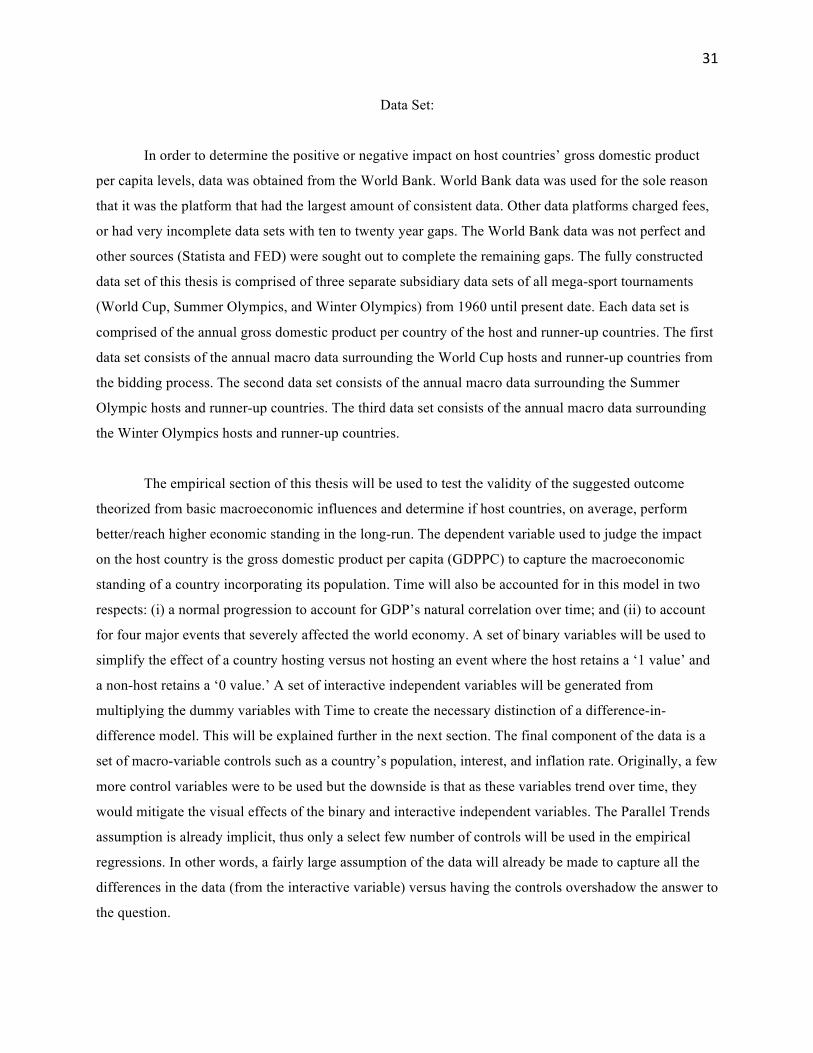
Data Set:

In order to determine the positive or negative impact on host countries’ gross domestic product

per capita levels, data was obtained from the World Bank. World Bank data was used for the sole reason

that it was the platform that had the largest amount of consistent data. Other data platforms charged fees,

or had very incomplete data sets with ten to twenty year gaps. The World Bank data was not perfect and

other sources (Statista and FED) were sought out to complete the remaining gaps. The fully constructed

data set of this thesis is comprised of three separate subsidiary data sets of all mega-sport tournaments

(World Cup, Summer Olympics, and Winter Olympics) from 1960 until present date. Each data set is

comprised of the annual gross domestic product per country of the host and runner-up countries. The first

data set consists of the annual macro data surrounding the World Cup hosts and runner-up countries from

the bidding process. The second data set consists of the annual macro data surrounding the Summer

Olympic hosts and runner-up countries. The third data set consists of the annual macro data surrounding

the Winter Olympics hosts and runner-up countries.

The empirical section of this thesis will be used to test the validity of the suggested outcome

theorized from basic macroeconomic influences and determine if host countries, on average, perform

better/reach higher economic standing in the long-run. The dependent variable used to judge the impact

on the host country is the gross domestic product per capita (GDPPC) to capture the macroeconomic

standing of a country incorporating its population. Time will also be accounted for in this model in two

respects: (i) a normal progression to account for GDP’s natural correlation over time; and (ii) to account

for four major events that severely affected the world economy. A set of binary variables will be used to

simplify the effect of a country hosting versus not hosting an event where the host retains a ‘1 value’ and

a non-host retains a ‘0 value.’ A set of interactive independent variables will be generated from

multiplying the dummy variables with Time to create the necessary distinction of a difference-in-

difference model. This will be explained further in the next section. The final component of the data is a

set of macro-variable controls such as a country’s population, interest, and inflation rate. Originally, a few

more control variables were to be used but the downside is that as these variables trend over time, they

would mitigate the visual effects of the binary and interactive independent variables. The Parallel Trends

assumption is already implicit, thus only a select few number of controls will be used in the empirical

regressions. In other words, a fairly large assumption of the data will already be made to capture all the

differences in the data (from the interactive variable) versus having the controls overshadow the answer to

the question.

32

The empirical section of this thesis will utilize a difference-in-difference (DID) model. It is a

quasi-experimental technique that uses longitudinal data (against time) from treatment versus control

groups to obtain an appropriate counterfactual and measure a casual effect.20 The basic idea is to compare

the treatment group and the control group before and after the stimulus. In this model, the treatment group

are all the host cities and countries of either an Olympic Games or World Cup and the control group are

the runner-up cities that were unable to host the event. Should it be found that the runner-up hosted the

event later on, the runner-up was replaced with another (runner-up) country that displayed a similar

GDPPC growth rate as the host country.

In order to estimate any casual effect from a sudden stimulus, three assumptions must hold:

exchangeability, positivity, and a Stable Unit Treatment Value Assumption. In this model a fourth

assumption must also hold: Parallel Trends in outcome. This assumption ensures internal validity of the

difference-in-difference model where it requires that the difference between the ‘treatment’ and control

group is constant over time. It is imperative that this assumption hold such that violation of the

assumption would lead to a biased estimation of the casual effect.

20 Pinschke, J.; University of Columbia; Difference-in-Difference Estimation; https://www.mailman.columbia.edu/research/population-health-methods/difference-difference-estimation

33

Variable List

Dependent Variable:

GDPPC: (Gross domestic product per capita) A measure of a country's economic output accounting for

its number of people

Independent Variables:

Time:

Time: progression of years from t=0 per the year 1960.

Time2, Time3, Time4: 1st-4th degree polynomials in time.

Event_year: accounts for years preceding and post event.

Event_timeline: timeline established of 10 years before the event to 10 years post event.

Host_announced: whether or not a country will host the event activated when host country is announced

to the host and public. Captures the amount of prep time a host has prior to the event. 1=country selected

to host, 0=not selected.

Binary Comparisons:

Host_wc: whether or not a country hosts a World Cup Event. 1= host, 0 = not host

Host_wc: whether or not a country hosts the Summer Olympic Games. 1= host, 0 = not host

Host_wo: whether or not a country hosts the Winter Olympic Games. 1= host, 0 = not host

Post_wc: whether or not a country successfully hosts the event. Accounts for difference in intercept for

non-hosts. 1= host, 0 = not host

Post_so: whether or not a country successfully hosts the event. Accounts for difference in intercept for

Summer Olympics non-hosts. 1= host, 0 = not host

Post_wo: whether or not a country successfully hosts the event. Accounts for difference in intercept for

Winter Olympics non-hosts. 1= host, 0 = not host

Interactive Variables:

Time_Post_wc: Captures the Pre-Post time trend difference for the non-hosts of the World Cup.

Time_Post_so: Captures the Pre-Post time trend difference for the non-hosts of the Summer Olympics.

Time_Post_wo: Captures the Pre-Post time trend difference for the non-hosts of the Winter Olympics.

Time_host_post_wc: Captures the difference of the change (diff in diff) in World Cup host GDPPC

compared to non-host GDPPC over time.

34

Time_host_post_so: Captures the difference of the change (diff in diff) in Summer Olympics host

GDPPC compared to non-host GDPPC over time.

Time_host_post_wo: Captures the difference of the change (diff in diff) in Winter Olympics host

GDPPC compared to non-host GDPPC over time.

Host_post_wc: Captures intercept difference in GDPPC ‘jump’ over one year between World Cup hosts

versus non-hosts.

Host_post_so: Captures intercept difference in GDPPC ‘jump’ over one year between Summer Olympics

hosts versus non-hosts.

Host_post_wo: Captures intercept difference in GDPPC ‘jump’ over one year between Winter Olympics

hosts versus non-hosts.

*Did not interact Host_time where the interaction that would represent the difference in time trend for hosts and non-hosts prior to the

event. Not including it shows parallel trends assumption and allows for diff in diff approach.

Controls:

Total_Population: Total population of a country.

Gov_spending_gdp_ratio: fractional amount of government expenditure compared to a country’s gross

domestic product.

Real_interst_rate: aggregate rate of a proportion of a loan charged as interest to the borrower adjusted

for inflation.

Inflation_rate: is the percent growth in the price levels from the previous year.

Broad_money_billions: the sum of currency outside banks; demand deposits other than those of the

central government; the time, savings, and foreign currency deposits of resident sectors other than the

central government; bank and traveler’s checks; and other securities such as certificates of deposit and

commercial paper.

35

Difference-in-Difference Model Table 1:

Treatment Group Control Group

Pre-Stimulus Treatment*pre Control*pre

Post-Stimulus Treatment*post Control*post

Intuitively, a difference-in-difference is a comparison of four cell-level means where only once cell is

treated per regression.21 When this occurs, it can be simplified to the [treatment*post-stimulus], which is

essentially an interactive independent variable in a simple OLS regression. A typical regression of this

model should be shown as followed at the minimum:

Yi,t = β0 + β1[Host] + β2[Post_Stimulus] + β3[Host*Post_Stimulus] + β4*[Control] + εt

Where:

Post_Stimulus is an indicator = 1 when t=0 B3 is the coefficient of interest (the treatment effect)

Time is the time trend Control are various independent bases

εt is the random error term

21 Jagielka, P., Ozier, O.; University of Maryland, College Park; Applied Econometrics: Difference-in-Difference Estimation; http://economics.ozier.com/econ626/lec/econ626lecture3_handout.pdf

36

To allow for the differences in intercepts and time trends, this method has been adapted to create a triple

interaction between the independent variables where Time and whether or not a country hosted the event

have to be taken into account. This thesis-specific regression is as shown without controls:

GDPPCt = β0 + β1[Host] + β2[Time] +𝛿1[Time2] +𝛿1[Time3] +𝛿1[Time4] + β3[Post] + β4[Time*Post] +

β5[Time*Host*Post] + β6[Post*Host] + εt

Where:

*Did not interact Host_time where the interaction that would represent the difference in time trend for hosts and non-hosts prior to the

event. Not including it shows parallel trends assumption and allows for diff in diff approach.

Thesis-specific regression with controls:

GDPPCt = β0 + β1[Host] + β2[Time] +𝛿1[Time2] +𝛿1[Time3] +𝛿1[Time4] + β3[Post] + β4[Time*Post] +

β5[Time*Host*Post] + β6[Post*Host] + β7[Total_population] + β8[Inflation_rate] + εt

Where:

Total_population is the country initial population at the time of the event

Inflation-rate is the country inflation rate at the time of the event

GDPPCt = gross domestic product per capita per country

Host is binary for hosting an event

Time is an annual progression from t =0 to t = 64

Time2, Time3, and Time4 are fourth degree polynomial terms in the time trend to account for

possible changes to the GDPPC slope

Post is binary hosting an event and accounts for extra event stimulus

Time*Post is the primary difference between hosts v. non-hosts

Time*Host*Post is the difference in pre-post time trend differences for hosts and non-hosts

Post*Host is the primary change in GDPPC slopes

εt is the random error term

37

Gross domestic product per capita has often been thought to be a better indicator of the

development of an economy as it takes into account in the population versus just an aggregate of total

goods bought and sold. Often times, a country’s gross domestic product can be due to size of the country.

The total population (at the time of the event) allows for the control of the initial state of the economy to

ensure a better estimation of tourism effects. The inflation rate was also included as a key control to

account for the purchasing power in the host country’s economy. The inclusion of the total population and

inflation improved the R2 (linear indicator) value but, as predicted, made most of the interactive variable

coefficients insignificant. This may be due to increased multicollinearity, but further research would

suggest that the inclusion of these controls simply overshadowed the impact of the interactive variables of

interest. This is partially why more macro-variable controls were not included. Since GDP trends over

time (serial correlation is almost certain) with these macro-variable controls, it was likely that these

controls would improve the linear significance but would mitigate the diff-in-diff effects.

The regressions were created to illustrate the full impact of hosting a mega-sport event. The

βHost variable is a summation of the βPost and βPost*Host variables where βPost and βPost*Host

indicate the difference between hosting and not hosting the event. When ‘time’ is factored in, then this

allows for the calculation of GDP per capita growth where the summation of βTime*Post and

βTime*Host*Post are equal to the aggregate effect on the long-term growth GDP per capita growth rate.

Theory would indicate that the overall effect should be positive, but literature would indicate otherwise.

The manufactured regressions were set up to indicate what parts of the ‘full impact’ cause the difference

between what theory suggests than what literature concludes.

38

Methodology

The theory previously stated suggests that a positive relationship should occur between GDPPC

and hosting a mega-sport event. Referring to previous research, however, long-run graphs showing ten

years before and after the mega-sport events were hosted illustrate that runner-up countries fared better

than the host countries of the Olympics (Figure 1).

Subsequently, regressions were run to test the theory. Since there were three events, the

regressions were run individually to ensure a better estimation of the effect of hosting the individual

events. This also allows for an easier analysis of the effect on a country’s GDP per capita of each event.

For each of the three events, two regressions were performed: one without controls to measure the full

consequence of hosting the event and the other with controls. These regressions were as follows:

OLS1: World Cup no controls

GDPPCt = β0 + β1[Host_wc] + β2[Time] +𝛿1[Time2] +𝛿1[Time3] +𝛿1[Time4] + β3[Post_wc] + β4[Time*Post_wc] + β5[Time*Host*Post_wc] + β6[Post*Host_wc] + εt

OLS2: World Cup no controls

GDPPCt β0 + β1[Host_wc] + β2[Time] +𝛿1[Time2] +𝛿1[Time3] +𝛿1[Time4] + β3[Post_wc] + β4[Time*Post_wc] + β5[Time*Host*Post_wc] + β6[Post*Host_wc] + β7[Total_population] +

β8[Inflation_rate] + εt

OLS3: Summer Olympics no controls

GDPPCt = β0 + β1[Host_so] + β2[Time] +𝛿1[Time2] +𝛿1[Time3] +𝛿1[Time4] + β3[Post_so] + β4[Time*Post_so] + β5[Time*Host*Post_so] + β6[Post*Host_so] + εt

OLS4: Summer Olympics with controls

GDPPCt β0 + β1[Host_so] + β2[Time] +𝛿1[Time2] +𝛿1[Time3] +𝛿1[Time4] + β3[Post_so]

+ β4[Time*Post_so] + β5[Time*Host*Post_so] + β6[Post*Host_so] + β7[Total_population] + β8[Inflation_rate] + εt

OLS5: Winter Olympics no controls

GDPPCt = β0 + β1[Host_wo] + β2[Time] +𝛿1[Time2] +𝛿1[Time3] +𝛿1[Time4] + β3[Post_wo] + β4[Time*Post_wo] + β5[Time*Host*Post_wo] + β6[Post*Host_wo] + εt

OLS6: Winter Olympics with controls

GDPPCt β0 + β1[Host_wo] + β2[Time] +𝛿1[Time2] +𝛿1[Time3] +𝛿1[Time4] + β3[Post_wo] + β4[Time*Post_wo] + β5[Time*Host*Post_wo] + β6[Post*Host_wo] + β7[Total_population] +

β8[Inflation_rate] + εt

39

After the results were obtained, several tests were conducted to examine the possible extent of

heteroscedasticity, multicollinearity, and serial correlation. Heteroscedasticity occurs when the spread of

the error term, GDPPC, is related to the values of an independent variable. In other words, the variance of

the error term (at the end of the regression equation) is changing, which alters the significance of the

results and hypothesis testing. Multicollinearity is problematic because it increases the chance of

identifying a relevant variable as insignificant within the model. It is likely that this model will have some

multicollinearity since many of the control variables may trend over time. Gross domestic product is a

macroeconomic variable that depends on its value from the previous period; therefore, the data will likely

exhibit serial correlation. Since no variables can be omitted without unsatisfying the basic necessities of

performing a standard difference-in-difference OLS regression, the final model can only be corrected for

the aforementioned variations of econometric assumptions. The only independent variables that will be

omitted from the final model are the control variables, total population and inflation rate, to capture the

full possible impact of a country hosting a mage-sport event.

40

Results: i. Descriptive Statistics:

Descriptive statistics provide insight into the sample used in the study. The mean, median,

maximum, minimum, standard deviation, and the coefficient of variation (CV%) all reveal some different

aspects of variables in the sample. The statistics for each of the events with and without controls are

displayed below: Tables 2-5.

The coefficient of variation (CV%) represents the ratio of the standard deviation to the mean and

is used when comparing the degree of variation from one data series to another. Since the increased

spread decreases the standard error of the coefficient, an independent variable with a high CV% value

will have a decreased standard error and a higher t-statistic. Thus, the CV% value can be used to predict

whether or not a variable may be significant when included in the model. Although none of the variables

will be removed from the model, apart from the controls, these significant suggestions can be concluded

in further analysis and discussion of the final-adjusted model.

TABLE 2: SUMMARY OF STATISTSICS: WORLD CUP

Mean Median

Maximum

Minimum

Std. Dev.

CV% Sum Sum Sq. Dev.

GDPPC 9953.595 4596.88 48603.48 341.5928 11617.22 117% 4857354 6.57E+10 TIME 31.68443 33 57 0 14.13759 45% 15462 97337.4 HOST_WC 0.526639 1 1 0 0.499802 95% 257 121.6537 POST_WC 0.522541 1 1 0 0.500004 96% 255 121.752

TABLE 3: SUMMARY OF STATISTSICS: WORLD CUP WITH CONTROLS

Mean Median Maximum Minimum Std. Dev. CV% Sum Sum Sq. Dev.

GDPPC 10797.03 5617.742 48603.48 341.5928 12058.07 112% 4653520 6.25E+10 TIME 32.79814 34 57 0 13.61236 42% 14136 79677.44 HOST_WC 0.545244 1 1 0 0.498527 91% 235 106.8677 POST_WC 0.522042 1 1 0 0.500094 96% 225 107.5406 EVENT_TIMELINE -0.06033 0 10 -10 5.935003 -26 15146.43 GDPPC_BASE 8875.49 2982 48603.48 341.5928 12935.14 146% 3825336 7.19E+10 TOTAL_POPULATION 75173651 56797087 2.93E+08 22037610 56794476 76% 3.24E+10 1.39E+18 INFLATION_RATE 12.79106 5.017158 874.2457 -1.352837 48.05608 376% 5512.946 993036.3

41

TABLE 4: SUMMARY OF STATISTSICS: WORLD CUP

Mean Median Maximum

Minimum

Std. Dev. CV% Sum Sum Sq. Dev.

GDPPC 23691.32 22061.16 60283.25 828.5805 13955.76 59% 7675987 6.29E+10 TIME 37.19753 37.5 57 14 10.36118 28% 12052 34675.36 HOST_SO 0.5 0.5 1 0 0.500773 100% 162 81 POST_SO 0.506173 1 1 0 0.500735 99% 164 80.98765

TABLE 5: SUMMARY OF STATISTSICS: SUMMER OLYMPICS WITH CONTROLS

Mean Median Maximum Minimum Std. Dev. CV% Sum Sum Sq. Dev.

GDPPC 20317.79 20087.54 51936.89 1398.479 11035.55 54% 4266735 2.55E+10 TIME 32 32 50 14 8.306336 26% 6720 14420 HOST_SO 0.5 0.5 1 0 0.501195 100% 105 52.5 POST_SO 0.52381 1 1 0 0.500626 96% 110 52.38095 EVENT_TIMELINE 0 0 10 -10 6.06977 0 7700 GDPPC_BASE 10920.78 9646.252 19115.05 1398.479 6122.532 56% 2293365 7.83E+09 TOTAL_POPULATION 93231492 57482591 2.98E+08 17065100 84811355 91% 1.96E+10 1.50E+18 INFLATION_RATE 4.398682 3.127596 28.69759 -0.12790 3.869783 88% 923.7231 3129.82

TABLE 6: SUMMARY OF STATISTSICS: WINTER OLYMPICS

Mean Median Maximum

Minimum

Std. Dev. CV% Sum Sum Sq. Dev.

GDPPC 21284.31 20670.82 57579.5 1148.494 13800.32 65% 6853548 6.11E+10 TIME 31.13354 31 54 8 10.23086 33% 10025 33599.26 HOST_WO 0.521739 1 1 0 0.500305 96% 168 80.34783 POST_WO 0.546584 1 1 0 0.4986 91% 176 79.80124

TABLE 7: SUMMARY OF STATISTSICS: WINTER OLYMPICS WITH CONTROLS

Mean Median Maximum Minimum

Std. Dev. CV% Sum Sum Sq. Dev.

GDPPC 22028.39 21427.26 57579.5 1148.494 13525.51 61% 6828801 5.65E+10 TIME 31.46774 31 54 8 10.27694 33% 9755 32635.18 HOST_WO 0.541935 1 1 0 0.499044 92% 168 76.95484 POST_WO 0.548387 1 1 0 0.498458 91% 170 76.77419 EVENT_TIMELINE 0.332258 1 10 -10 6.100766 103 11500.78 GDPPC_BASE 12002 10587.29 25646.7 2238.803 8037.756 67% 3720620 2.00E+10 TOTAL_POPULATION 66954272 24746500 2.88E+08 3985258 84852574 127% 2.08E+10 2.22E+18 INFLATION_RATE 8.916902 2.940634 338.4491 -13.70632 35.57829 399% 2764.24 391136.7

42

Two types of regressions were run for each of the three types of events. In general, the summary

of statistics would indicate a minimal difference between the aggregated values. The difference in the

means seem to be +/- a standard deviation and the CV-percentage change seems to only vary about five

percent. The negative change in the coefficient of variation-percentage is indicative that the inclusion of

the control variables allow for a more precise estimate of the coefficients where a lessened CV percentage

means that the data is more centered around the regressed expected value (line). This, however would

only further the theory that the inclusion of the control independent variables would only mitigate the

visual effects (in the data) of the stimulus (event) effect. The inclusion of the control variables centers the

data but since these controls move linearly (across time) with GDPPC, it only mitigates the impact of

hosting a mega-sport event.

A comparison of the summary of statistics (Tables 2-3) of the first regression (World Cup)

exhibits a wide variation in the gross domestic product per capita between both hosts and runner up

countries: a minimum value of $341.59 and a maximum value of $48603.48, and an average of

$10797.03. It is important to mention that these two (hosts and runner-ups) should be able to be

compared because of the parallel trends assumption where the difference in GDPPC slope and intercept

should be mitigated. Concerning the hosts of the World Cup, there is large variation in this number across

the countries where the CV is 117% without controls and 112% with controls. With that said, the

GDPPC_BASE, the gross domestic product per capita at the beginning of the twenty-year period has a

lower GDPPC with a higher CV. One theory driving the difference between the averaged GDPPC and the

averaged base year of GDPPC is overall, the taking on of the bidding process and hosting of the World

Cup not only raised the GDPPC higher than normal inflation would have, but also brought some of the

developing countries closer in GDPPC to being developed. The variance in the CV narrows from the

averaged base year towards the averaged GDPPC, which suggests that countries’ GDPPC are slowly

starting to converge despite only half hosting the World Cup.

43

A comparison of the summary of statistics (Tables 4-5) of the second regression (Summer

Olympics) displays a wide variation in the gross domestic product per capita: a minimum value of

$828.58, a maximum value of $60283.25, and an average of $22061.16. Concerning the hosts of the

Summer Olympics, there is a significantly lessened variation in this number across the countries where

the CV is 59% without controls and 54% with controls. Although both of these values are considered as

not-reasonably high, the still indicate that there is a realistic amount of variation in the data but a

significantly lessened amount than the World Cup. This could merely suggest that more places considered

to host the Summer Olympics were more developed. This is substantiated by the data where the mean

GDPPC_BASE and GDPPC are significantly higher than those representing the World Cup.

A comparison of the summary of statistics (Tables 6-7) of the second regression (Winter

Olympics) indicates a wide variation: a minimum value of $1148.49, a maximum value of $57579.50, and

an average of $21284.31. While the variance is somewhat wide, CV is 65% without controls and 61%

with controls, the GDPPC numbers are significantly higher than either of the other two mega-sport

events. The GDPPC_BASE starts at $12002, over $1000 per capita higher than the Summer Olympic

considered countries and $2000 per capita higher than countries considered to host (and hosts) of the

World Cup. This, in theory, fits where most Winter Olympic hosts are both Nordic, Western Europe, or

North American developed countries and the GDPPC are historically higher.

44

Preliminary Model: World Cup:

The first independent variables regarding time are constants to account for in the model, thus their

relative insignificance is justified. The Host_WC variable is an indicator of the binary effect of hosting an

event. It is the total intercept difference for hosting an event: B3 + B6. The variable Host_WC = 8535.50

suggests that overall, countries that host the World Cup exhibit a positive $8535.50 difference in their

gross domestic product per capita compared to non-hosts countries. The Post_WC variable indicates the

binary effect of successfully hosting the World Cup. It represents the intercept difference for the non-host.

Post_WC = 3437.06 indicates that on average, non-hosts experience a positive $3437.06 short-term effect

on host GDPPC despite not hosting. This variable is relatively insignificant and will be tested for one of

the econometric assumption violations. The variable Time_Post_WC captures the change in GDPPC

growth non-host countries. Although statistically insignificant, its value of -72.06 indicates that overall,

non-hosts countries exhibit a relatively horizontal (slightly negative) response in the years of not hosting

the World Cup compared to the host countries. The main variable of interest is Time_Host_Post_WC,

which indicates the difference in the change in long-run GDPPC growth. Its value of 699.07 indicates that

overall, host countries exhibit a $699.07 increase in GDPPC growth over a ten-year span compared to

non-host countries. The final variable, Host_Post_WC, represents the difference in difference of the

45

GDPPC intercept of host versus non-host countries. In essence, how much larger or smaller the intercept

jump is (in terms of GDPPC) in that year of hosting the event. Its value of -20673.82 illustrates that on

average, host countries exhibit a negative $2067.82 short-term change in GDPPC. This is surprising

where macroeconomic theory would suggest the exact opposite. Due to a tourism influx, one can expect

an increase aggregate spending in addition to a heavy increase government spending would result in

short-run increase in the aggregate gross domestic product per capita. The data clearly suggests if a

country hosts the World Cup, the resulting stimulation may not impact in the short-run as economic

theory would normally indicate.

46

World Cup: With Controls

The differences exhibited in this regression with controls have been restated throughout the paper.

Although the R2 value increases dramatically and the t-statistics became more significant for the most

part, all of the coefficients diminished distinctively. According to the data, all of the control variables

appear to be significant, which intuitively makes sense, as they are macroeconomic independent variables

correlating with the macroeconomic dependent variable across time. The final model will not take into

account the control independent variables to ensure that the full impact of the binary and interactive

independent variables is captured.

47

Summer Olympics:

The first independent variables regarding time are constants to account for in the model, thus their

relative insignificance is justified. The variable Host_SO = -10268.28 suggests that overall, countries that

host the World Cup exhibit a negative -$10268.28 difference in their gross domestic product per capita

compared to non-hosts countries. Post_SO = 1409.47 indicates that on average, non-hosts experience a

positive $1409.47 short-term effect on host GDPPC despite not hosting. The variable Time_Post_SO

captures the change in GDPPC growth non-host countries. Although statistically insignificant, its value of

55.58 indicates that overall, non-hosts countries exhibit a relatively horizontal (slightly positive) response

in the years of not hosting the World Cup compared to the host countries. The variable

Time_Host_Post_SO has a value of -296.13, which indicates that overall, host countries exhibit a -

$296.13 decrease in GDPPC growth over a ten-year span compared to non-host countries. This would

essentially suggest that it is not worth it for countries to host the Summer Olympics. Host_Post_SO

exhibits a value of 6462.09, which illustrates that on average, host countries exhibit a positive $6462.09

short-term change in GDPPC. Despite being insignificant, this positive change is in-line with the

macroeconomic theory. This analysis of the impact of the Summer Olympic Games is somewhat

problematic where most of the variables are insignificant in the model and the binary ‘Host_SO’ variable

is negative.

48

Summer Olympics: With Controls

The differences exhibited in this regression with controls have been restated throughout the paper.

Similarly to the World Cup controlled regressions, the R2 value dramatically increased but at the cost of

minimization of the coefficients of the independent variables. The final model will not take into account

the control independent variables to ensure that the full impact of the binary and interactive independent

variables is captured.

49

Winter Olympics

The first independent variables regarding time are constants to account for in the model, thus their

relative insignificance is justified. The variable Host_WO = -10554.72 suggests that overall, countries

that host the World Cup exhibit a negative -$10554.72 difference in their gross domestic product per

capita compared to non-hosts countries. Post_WO = -42882.61 indicates that on average, non-hosts

experience a negative $42882.61 short-term effect on host GDPPC despite not hosting. The variable

Time_Post_WO exhibited a value of 1302.19 indicates that overall, non-hosts countries exhibit a

$1302.19 postive response in the years of not hosting the World Cup compared to the host countries. The

variable Time_Host_Post_WO has a value of -940.78, which indicates that overall, host countries exhibit

a $940.78 decrease in GDPPC growth over a ten-year span compared to non-host countries. This would

essentially suggest that it is not worth it for countries to host the Winter Olympics. Host_Post_WO

exhibits a value of 36939.058, which illustrates that on average, host countries exhibit a positive

$36939.058 short-term boost in GDPPC. This analysis of the impact of the Winter Olympic Games also

shows that hosting this event would go against general academic macroeconomic theory, but there are

possible theories why. The data essentially indicates that although host countries may fair better in the

short term, the non-host countries experience a better growth in GDPPC over the long-term and that

50

hosting of the Winter Olympics is not worth it. One possible theory as to why non-hosts may fair better is

because of the type of countries that are chosen to host. For the most part, developed nations are

considered to host (either host or are the runner-up in bidding) and it may fair that more ‘less-developed’

countries are chosen to host (to hopefully boost their economies). On the average, this would show that

the more developed countries not chosen to host fair better than the ‘less-developed’ nations (I.e. Russia

and South Korea).

51

Winter Olympics: With Controls

The differences exhibited in this regression with controls are similar to those above. The R2 value

increased, the t-statistics became partially less significant for the independent variables, while the control

variables show their significance. The coefficient effects are lessened due to the addition of the control

variables where their linear correlation with gross domestic product per capita only improves the value of

the data on the expected value line. The final model will not take into account the control independent

variables to ensure that the full impact of the binary and interactive independent variables is captured.

52

Violation of the Assumptions:

World Cup: White Test:

The White test determines if one or more of the independent variables is causing

heteroscedasticity. In this test, the residuals squared are run as a function of all other independent

variables. A white test performed illustrates the F-statistic of the set of heteroscedastic variables and

probability of the F-statistic being significant. If the probability is less than 0.05 accompanied with a

significant F statistic, then reject the null hypothesis and conclude that the data set has heteroscedasticity.

If heteroscedasticity is found, the model will be corrected using a Newey-West correction.

H0: Homoscedasticity with respect to one or more independent variables

HA: Heteroscedasticity with respect to one or more independent variables

F-statistic = 40.69

Prob(F-Statistic) = 0.00

Reject Ho if Prob(F-statistic) < 0.05

Conclusion: Reject H0 and conclude that there is heteroscedasticity in the model. Multicollinearity:

53

Multicollinearity:

A way to detect multicollinearity is by calculating the Variance Inflation Factor (VIF), which

estimates the inflation on the standard error of each coefficient due to the presence of multicollinearity. In

short, this test measures the degree to which the variation in an independent variable is explained by the

other independent variables. To calculate VIF, a regression using one independent variable is run against

all remaining independent variables. The R2 for this model is plugged into following equation:

VIF = ##$%&

A generated rule of thumb indicates that a VIF value less than five can be accepted as the data not having

any multicollinearity. Some research would suggest that any value less than ten is acceptable as well but

further tests would also have to be utilized. Any value greater than ten essentially signifies that the

variable identified exhibits multicollinearity.

Table 1:

Variable VIF Conclusion Host_WC 2.11 VIF < 10.0 suggests there is no multicollinearity due to Host_WC. Post_WC 11.44 VIF > 10.0 suggests there is multicollinearity due to Post_WC Time_Post_WC 15.03 VIF > 10.0 suggests there is multicollinearity due to Time_Post_WC Time_Host_Post_WC 13.13 VIF > 10.0 suggests there is multicollinearity due to

Time_Host_Post_WC Host_Post_WC 13.89 VIF > 10.0 suggests there is multicollinearity due to Host_Post_WC

In conclusion, these calculated VIFS suggest a severe multicollinearity problem throughout the regression. The normal solution to a multicollinearity problem is to minimize the collinear variables. A possibly significant error in this model, however, is that since the minimum independent variables for a diff-in-diff regression have already been met, there is no way to correct for the suggested multicollinearity.

54

Serial Correlation:

Serial correlation occurs when corr(εi, εi-1) ≠ 0, the random error terms from different

observations are correlated. This correlation indicates a pattern across the random error terms and,

therefore, there is a pattern to what should be a random term. Serial correlation does not cause a bias on

the coefficient of the independent variable, but rather may make the coefficients easier to accept.

In any given model, serial correlation might depend upon how the data is organized. Per this

model, it is possible for there to be serial correlation across a region. If a shock had occurred in a region

early in the timeline, then it may influence the error team of the subsequent city but at a later point in

time. More than likely, however, this model displays serial correlation across time where gross domestic

product per capita is naturally a serially correlated variable as it depends on the past period’s value. To

determine if this model exhibits serial correlation, we conduct the Breusch-Godfrey/LM Test. If it is

found, serial correlation can be corrected by and estimating the standard errors using the Newey-West

method.

55

Breusch-Godfrey LM Test The Breusch-Godfrey, or LM Test, is used for determining if there is serial correlation between the error

terms of consecutive periods. In this test, a t-test will be run on the coefficient of the lagged residual. If it

turns out to be significant, then it can be determined that there is serial correlation in the regression.

H0: βResid(-1) ≤ 0

HA: βResid(-1) > 0

Level of Significance = 5 %

tcritical: 1.960

tcomputed: 46.45

Decision rule: reject if tcomputed> tcritical

Conclusion:

Reject H0 and conclude that there is serial correlation in the model.

56

Summer Olympics: Heteroscedasticity: White Test

H0: Homoscedasticity with respect to one or more independent variables

HA: Heteroscedasticity with respect to one or more independent variables

F-statistic = 21.52

Prob(F-Statistic) = 0.00

Reject Ho if Prob(F-statistic) < 0.05

Conclusion:

Reject H0 and conclude that there is heteroscedasticity in the model.

57

Multicollinearity:

Decision Rule: Acceptable VIF values < 10 < definite multicollinearity Table 2:

Host_WC 6.62 VIF < 10.0 suggests there is no multicollinearity due to Host_WC.

Post_WC 64.09 VIF > 10.0 suggests there is multicollinearity due to Post_WC

Time_Post_WC 78.86 VIF > 10.0 suggests there is multicollinearity due to Time_Post_WC

Time_Host_Post_WC 37.40 VIF > 10.0 suggests there is multicollinearity due to Time_Host_Post_WC

Host_Post_WC 38.06 VIF > 10.0 suggests there is multicollinearity due to Host_Post_WC

58

Serial Correlation: Correction with Newey-West

Breusch-Godfrey LM test H0: βResid(-1) ≤ 0

HA: βResid(-1) > 0

Level of Significance = 5 %

tcritical: 1.960

tcomputed: 42.06

Decision rule: reject if tcomputed> tcritical

Conclusion:

Reject Ho and conclude that there is serial correlation in the model.

59

Winter Olympics:

Heteroscedasticity:

White Test:

H0: Homoscedasticity with respect to one or more independent variables

HA: Heteroscedasticity with respect to one or more independent variables

F-statistic = 9.97

Prob(F-Statistic) = 0.00

Reject Ho if Prob(F-statistic) < 0.05

Conclusion:

Reject H0 and conclude that there is heteroscedasticity in the model.

60

Multicollinearity:

Decision Rule: Acceptable VIF values < 10 < definite multicollinearity

Table 3:

Host_WC 5.78 VIF < 10.0 suggests there is no multicollinearity due to Host_WC.

Post_WC 201.23 VIF > 10.0 suggests there is multicollinearity due to Post_WC

Time_Post_WC 192.77 VIF > 10.0 suggests there is multicollinearity due to Time_Post_WC

Time_Host_Post_WC 73.51 VIF > 10.0 suggests there is multicollinearity due to

Time_Host_Post_WC

Host_Post_WC 114.61 VIF > 10.0 suggests there is multicollinearity due to Host_Post_WC

61

Serial Correlation: Correction with Newey-West

Breusch-Godfrey LM test

H0: βResid(-1) ≤ 0

HA: βResid(-1) > 0

Level of Significance = 5 %

tcritical: 1.960

tcomputed: 34.58

Decision rule: reject if tcomputed> tcritical

Conclusion:

Reject Ho and conclude that there is serial correlation in the model.

62

Final Model:

The final model will not include any of the control variables to show the full impact of hosting a

mega sport event. Previous analysis of regressions with the control variables illustrated that they lessened

the effect of the binary and interactive independent variables. The final model also employs the

Newey_West method to correct for heteroscedasticity and serial correlation. Newey-West method

produces standard errors for coefficients estimated by an OLS regression where the error structure is

assumed heteroscedastic and somewhat serially correlated up to a determined lag. The traditional route in

correcting for multicollinearity would be to limit the number of irrelevant variables. The final model uses

the minimum amount of independent variables needed to satisfy the diff-in-diff requirement.

World Cup:

63

Variable Interpretation:

βHost_WC = 8535.50; On average, the host country experienced a positive $8535.50 impact on its

GDPPC over a twenty-year period.

βPost_WC = 3437.06; On average, the non-host country exhibits a positive $3437.06 change in GDPPC

over a twenty-year period.

βTime_Post_WC = -72.06; On average, the non-host country exhibits a slight negative $72.06 change in

GDPPC growth over a twenty-period.

βTime_Host_Post_WC = 699.07; On average, the host country exhibits a positive $699.07 difference in

GDPPC growth compared to a non-host country over a twenty-year period.

βHost_Post_WC = -20673.82; On average, the host country exhibits a negative $20673.82 difference in

short-term GDPPC change compared to non-host countries over a one-year period.

64

Summer Olympics:

Variable Interpretation:

βHost_SO = -10268.28; On average, the host country experienced a negative $10268.28 impact on its

GDPPC over a twenty-year period.

βPost_SO = 1409.47; On average, the non-host country exhibits a positive $1409.47 change in GDPPC

over a twenty-year period.

βTime_Post_SO = 55.58; On average, the non-host country exhibits a slight positive $55.58 change in

GDPPC growth over a twenty-period.

βTime_Host_Post_SO = -296.13; On average, the host country exhibits a negative $296.13 difference in

GDPPC growth compared to a non-host country over a twenty-year period.

βHost_Post_SO = 6462.09; On average, the host country exhibits a positive $6462.09 difference in short-

term GDPPC change compared to non-host countries over a one-year period.

65

Winter Olympics:

Variable Interpretation:

βHost_WO = -10554.72; On average, the host country experienced a negative $10554.72impact on its

GDPPC over a twenty-year period.

βPost_WO = -42882.61; On average, the non-host country exhibits a negative $42882.61change in

GDPPC over a twenty-year period.

βTime_Post_WO = 1302.19; On average, the non-host country exhibits a positive $1302.19 change in

GDPPC growth over a twenty-period.

βTime_Host_Post_WO = -940.78; On average, the host country exhibits a negative $940.78 difference in

GDPPC growth compared to a non-host country over a twenty-year period.

βHost_Post_WO = 36939.12; On average, the host country exhibits a positive $36939.12 difference in

short-term GDPPC change compared to non-host countries over a one-year period.

66

Conclusion: Is it worth it to host a mega-sport event?

Preceding analysis provides insight into the theoretical and empirically measured impact of

hosting a mega sport event. Unlike previous literature that only measure one event, this thesis empirically

measured the effect across all three of the mega-sport events: World Cup, Summer Olympics, and Winter

Olympics. Due to this, it is possible to not only conclude if this billion-dollar investment is worth it, but

what type of event would best be host if a country decided to host one. Previous literature and basic

macroeconomic theory have allowed for the drawing of a uniform hypothesis on the ten-year impact of

hosting this type of event: the massive heighten of expenditure in preparation for the events accompanied

with a generous influx of tourism would create a short run burst of economic activity with slight leveling

off of GDPPC curve (slope) in the long run. To test this theory, three empirical regressions were run to

measure the full impact of hosting the games and three more were run to test the impact of

macroeconomic control variables.

It was determined empirically that overall, a mega-sport event is not the most efficient use of

resources and is probably not worth the investment. One of the exceptions to this, however, is dependent

on the type of economy hosting the event: developed versus developing. Previous literature suggests that

hosting a mega-sport event is only an investment that should be made by developed countries and that the

risk of investment is significantly higher for developing countries. Developing countries usually lack the

base resources to host such a tournament and end up incurring the incurred startup costs in infrastructure,

which are already hard enough to overcome. Developed countries, on the other hand, are usually

somewhat prepared with having multiple sports arenas and developed cities that could be easily

refurbished or already are state-of-the-art. Since infrastructure is the largest investment any country or

city has to sustain, developed countries spend millions of dollars less in aggregate versus the developing

countries. Therefore, developed economies generally begin from a place of economic neutrality versus

that of the underdeveloped economy/country.

It can also be determined from the empirical model that if an attempt to host such an event did

occur, then the best option would be to host the World Cup. It is a substantially larger event compared to

either of the Olympic Games and would yield significantly more tangible benefits (revenue). Results

indicated that although there may be a slight economic downturn relative to investment surrounding the

event, countries that hosted the event yielded a significantly higher GDPPC growth curve over a ten-year

span after hosting the World Cup. The Olympic Games, although almost requiring almost as much

funding and preparation costs, are city or county specific and thus yield a fraction of the benefits. One of

67

the downfalls is the Olympic Games’ city-specific nature of the event is that the event is city-specific

where it is unlikely that the revenue would spread beyond thirty miles outside the city. The lack of wide-

spread economic activity over the entire country is what can be captured and evaluated by the regression

analysis. If city data had been used, the results may have been slightly different. Based on country data,

however, it can be theorized that hosting the World Cup would be the best option.

Upon meeting and discussing this thesis results with economists Dr. Thomas Miceli, Mr. Victor

Matheson, Mr. Andrew Zimbalist, we decided to create a theoretical model that couple possibly resolve

some of the issues surrounding hosting the Olympic Games. Since the econometric analysis indicated that

hosting the World Cup could end up benefiting the host nation, some of the principles of the World Cup

were adapted to an Olympic model. Some aspects that cannot be avoided or changed include: security,

transportation, and events themselves. The major issues surrounding the Olympics, however, rest in sport-

specific infrastructure, size, and centralization. When considering sport specific infrastructure, this

ultimately comes down to the International Olympic Committee (IOC) choosing hosts that are already

better prepared. This reflects on Victor Matheson’s theory that developing countries should not use

hosting a mega-sport event as opportunities to bolster their economies. The size of the competition has

more to do with the duration of the event versus the international recognition. It will be assumed that

these types of events already capture the attention of the world and thus do not need extra marketing.

Certain events cannot be made longer where almost every race is a medal event with the preceding event

the qualifying for the medal round. What could happen is that more time is allotted between each event

where this would also give athletes extra time to rest. The largest issue with the Olympic Games is its

centralization. History recognizes the Olympic Games as a tournament celebrating a coming together of

athletes to show a lack in differences among people. This is what all the athletes stay in the Olympic

village and compete in a maximum of four locations (with the exception of soccer and occasional other

field sports). A brief note about this: The Olympics has a history of this and people like to preserve

history, but any athlete competing international sporting event is respected based on his or her

performance. If a city wants to successfully host the Olympics, history may need to be forgone in order to

maximize business, as hosting mega-sport events have become a business decision.

68

The proposed adapted model is the decentralization of the competitions (not the opening

ceremony) such that competitions are paired by rank and location. This way, an A-rank sport (Women’s

Volleyball) is in the same city (location) as a B-rank Sport (Fencing, Judo) and a C-rank rank sport

(speed-walking) to attract an evenly distributed amount of tourism. This also makes revenue streams

easier where consumers can buy single event or a package of tickets based on location such that host

would create a boosted viewership and revenue on the non-A-rank sports.22 This would theoretically spur

economic activity in different places, which improves money-in-circulation and thus would increase those

macroeconomic variables. The incurred costs of security and transportation would increase but these costs

can be spread out over other cities such that one city is not suffering all of them. In theory, this could

increase revenue and spread out the cost of hosting where the event is larger and longer, and would retain

more tourism to yield an evener and wider boost in economic activity.

22 Victor Matheson, Andrew Zimbalist, Thomas Miceli; “Olympics Lecture” (University of Connecticut Law, April 12th, 2019.)

69

Errors and Possible Deviations:

Possibilities and limitations of these results include: variation of destinations of the hosted events,

empirical errors, and data retained. The reason the data could be skewed in favor of hosting the World

Cup is because there is a larger variation in the types of countries that hosted the event: countries that

hosted are on the upper scale of developing or developed. Therefore, the model would show a positive

difference when comparing hosts to non-hosts. Summer Olympics and Winter Olympic hosts have less

differences in GDPPC level between hosts and non-hosts; in fact, more developing countries or less

developed countries hosted the Winer Olympics. Therefore, intuitively it would make sense that non-

hosts would fair just as well if not better than the hosts. Empirical error is always something to be

accounted for and is another term for human error. The data retained was from the World Bank, if the

source of that data is skewed, then this thesis results would also be incorrect.

70

Appendix:

Appendix A: Economic Figures: Literature Review: Host GDPPC v. Runner-Up

Real Money Market

L’(i,Y)

71

Tourism Supply and Demand: Crowding Out Effect

Appendix B: Supportive Figures Infrastructure Timeline:

Infrastructure Type:

72

Appendix C: Graphical Hypothesis

Appendix D: Tables Difference-in-Difference Model

Treatment Group Control Group

Pre-Stimulus Treatment*pre Control*pre

Post-Stimulus Treatment*post Control*post

Appendix E: Equations Sample Diff-in-Diff

Yi,t = β0 + β1[Time] + β2[Post_Stimulus] + β3[Time*Post_Stimulus] + β4*[Control] + εt Thesis Regression:

GDPPCt = β0 + β1[Host] + β2[Time] +𝛿1[Time2] +𝛿1[Time3] +𝛿1[Time4] + β3[Post] + β4[Time*Post] + β5[Time*Host*Post] + β6[Post*Host] + εt

Thesis Regression with Controls:

GDPPCt β0 + β1[Host] + β2[Time] +𝛿1[Time2] +𝛿1[Time3] +𝛿1[Time4] + β3[Post] + β4[Time*Post] + β5[Time*Host*Post] + β6[Post*Host] + β7[Total_population] + β8[Inflation_rate] + εt

73

Appendix F: Descriptive Statistics

OLS1_NO_CONTROLS_WC Mean Median

Maximum Minimum

Std. Dev.

CV% Sum Sum Sq. Dev.

GDPPC 9953.595 4596.88 48603.48 341.5928 11617.22 117% 4857354 6.57E+10 TIME 31.68443 33 57 0 14.13759 45% 15462 97337.4 TIME2 1203.365 1089 3249 0 884.8115 74% 587242 3.81E+08 TIME3 50289.87 35937 185193 0 48622.99 97% 24541458 1.15E+12 TIME4 2229374 1185921 10556001 0 2607402 117% 1.09E+09 3.31E+15 HOST_WC 0.526639 1 1 0 0.499802 95% 257 121.6537 POST_WC 0.522541 1 1 0 0.500004 96% 255 121.752 TIME_POST_WC 18.42828 13 57 0 20.13035 109% 8993 197347.5 TIME_HOST_POST_WC 9.829918 0 57 0 17.4287 177% 4797 147930.9 HOST_POST_WC 0.272541 0 1 0 0.445724 164% 133 96.75205

OLS1_WCONTROLS_WC Mean Median Maximum Minimum Std. Dev. CV% Sum Sum Sq.

Dev. GDPPC 10797.03 5617.742 48603.48 341.5928 12058.07 112% 4653520 6.25E+10 TIME 32.79814 34 57 0 13.61236 42% 14136 79677.44 TIME2 1260.585 1156 3249 0 866.6131 69% 543312 3.23E+08 TIME3 52814.92 39304 185193 0 48100.09 91% 22763232 9.95E+11 TIME4 2338350 1336336 10556001 0 2595047 111% 1.01E+09 2.90E+15 HOST_WC 0.545244 1 1 0 0.498527 91% 235 106.8677 POST_WC 0.522042 1 1 0 0.500094 96% 225 107.5406 TIME_POST_WC 19.12993 14 57 0 20.58893 108% 8245 182278.7 TIME_HOST_POST_WC 10.4594 0 57 0 18.08951 173% 4508 140709 HOST_POST_WC 0.280742 0 1 0 0.449884 160% 121 87.03016 EVENT_TIMELINE -0.06033 0 10 -10 5.935003 -26 15146.43 GDPPC_BASE 8875.49 2982 48603.48 341.5928 12935.14 146% 3825336 7.19E+10 TOTAL_POPULATION 75173651 56797087 2.93E+08 22037610 56794476 76% 3.24E+10 1.39E+18 INFLATION_RATE 12.79106 5.017158 874.2457 -1.352837 48.05608 376% 5512.946 993036.3

OLS2_NO_CONTROLS_SO Mean Median Maximum Minimum Std. Dev. CV% Sum Sum Sq.

Dev. GDPPC 23691.32 22061.16 60283.25 828.5805 13955.76 59% 7675987 6.29E+10 TIME 37.19753 37.5 57 14 10.36118 28% 12052 34675.36 TIME2 1713.988 1640.5 3481 256 777.7444 45% 555332 1.95E+08 TIME3 76462.94 66460.5 205379 4096 49336.35 65% 24773992 7.86E+11 TIME4 3540773 2692881 12117361 65536 2918352 82% 1.15E+09 2.75E+15 HOST_SO 0.5 0.5 1 0 0.500773 100% 162 81 POST_SO 0.506173 1 1 0 0.500735 99% 164 80.98765 TIME_POST_SO 21.14815 24.5 57 0 21.85747 103% 6852 154312.9 TIME_HOST_POST_SO 10.57407 0 57 0 18.73584 177% 3426 113383.2 HOST_POST_SO 0.253086 0 1 0 0.435453 172% 82 61.24691

74

OLS2_WCONTROLS_SO Mean Median Maximum Minimum Std. Dev. CV% Sum Sum Sq.

Dev. GDPPC 20317.79 20087.54 51936.89 1398.479 11035.55 54% 4266735 2.55E+10 TIME 32 32 50 14 8.306336 26% 6720 14420 TIME2 1333.467 1296 2704 256 580.2408 44% 280028 70365984 TIME3 52135.2 46656 140608 4096 32752.46 63% 10948392 2.24E+11 TIME4 2113209 1679616 7311616 65536 1718913 81% 4.44E+08 6.18E+14 HOST_SO 0.5 0.5 1 0 0.501195 100% 105 52.5 POST_SO 0.52381 1 1 0 0.500626 96% 110 52.38095 TIME_POST_SO 19.38095 26 50 0 19.11055 99% 4070 76329.52 TIME_HOST_POST_SO 9.690476 0 50 0 16.64215 172% 2035 57884.88 HOST_POST_SO 0.261905 0 1 0 0.440722 168% 55 40.59524 EVENT_TIMELINE 0 0 10 -10 6.06977 0 7700 GDPPC_BASE 10920.78 9646.252 19115.05 1398.479 6122.532 56% 2293365 7.83E+09 TOTAL_POPULATION 93231492 57482591 2.98E+08 17065100 84811355 91% 1.96E+10 1.50E+18 INFLATION_RATE 4.398682 3.127596 28.69759 -0.12790 3.869783 88% 923.7231 3129.82

OLS3_NO_CONTROLS_WO Mean Median Maximum Minimum Std. Dev. CV% Sum Sum Sq.

Dev. GDPPC 21284.31 20670.82 57579.5 1148.494 13800.32 65% 6853548 6.11E+10 TIME 31.13354 31 54 8 10.23086 33% 10025 33599.26 TIME2 1839.444 1764 4096 256 839.5193 46% 592301 2.26E+08 TIME3 85009.81 74088 262144 4096 56245.77 66% 27373159 1.02E+12 TIME4 4086158 3111696 16777216 65536 3523494 86% 1.32E+09 3.99E+15 HOST_WO 0.521739 1 1 0 0.500305 96% 168 80.34783 POST_WO 0.546584 1 1 0 0.4986 91% 176 79.80124 TIME_POST_WO 19.40373 23 54 0 18.93862 98% 6248 115133.5 TIME_HOST_POST_WO 9.701863 0 54 0 16.54555 171% 3124 87875.38 HOST_POST_WO 0.273292 0 1 0 0.446343 163% 88 63.95031

OLS3_WCONTROLS_WO Mean Median Maximum

Minimum Std. Dev. CV% Sum Sum Sq.

Dev. GDPPC 22028.39 21427.26 57579.5 1148.494 13525.51 61% 6828801 5.65E+10 TIME 31.46774 31 54 8 10.27694 33% 9755 32635.18 TIME2 1872.087 1764 4096 256 838.3756 45% 580347 2.17E+08 TIME3 87076.28 74088 262144 4096 56303.87 65% 26993647 9.80E+11 TIME4 4205316 3111696 16777216 65536 3537297 84% 1.30E+09 3.87E+15 HOST_WO 0.541935 1 1 0 0.499044 92% 168 76.95484 POST_WO 0.548387 1 1 0 0.498458 91% 170 76.77419 TIME_POST_WO 19.69355 24 54 0 19.0998 97% 6105 112723.9 TIME_HOST_POST_WO 10.07742 0 54 0 16.7508 166% 3124 86702.14 HOST_POST_WO 0.283871 0 1 0 0.451604 159% 88 63.01935 EVENT_TIMELINE 0.332258 1 10 -10 6.100766 103 11500.78 GDPPC_BASE 12002 10587.29 25646.7 2238.803 8037.756 67% 3720620 2.00E+10 TOTAL_POPULATION 66954272 24746500 2.88E+08 3985258 84852574 127% 2.08E+10 2.22E+18 INFLATION_RATE 8.916902 2.940634 338.4491 -13.70632 35.57829 399% 2764.24 391136.7

75

Appendix G: Preliminary Model World Cup:

World Cup with controls:

76

Summer Olympics:

Summer Olympics: With Controls

77

Winter Olympics

Winter Olympics: With Controls

78

Appendix H: World Cup Econometric Assumption Tests White Test: H0: Homoscedasticity with respect to one or more independent variables HA: Heteroscedasticity with respect to one or more independent variables Critical value = 31.410 Obs*R-squared = 18.77 Decision rule: reject H0 IFF and only if Obs*R-squared > critical value (Chi squared)

VIFS

79

LM Test for serial correlation: Ho: There is no serial correlation HA: There is serial correlation Chi-Squared test at 5% level of significant Degrees of freedom (# of lags) = p = 1 Critical value = 3.841 Reject Ho if Critical Value ≤ Observed R2

Observed R2 = 399.66

80

Appendix I: Summer Olympics Econometric Assumption Tests White Test H0: Homoscedasticity with respect to one or more independent variables HA: Heteroscedasticity with respect to one or more independent variables Critical value = 31.410 Obs*R-squared = 18.77 Decision rule: reject H0 IFF and only if Obs*R-squared > critical value (Chi squared)

Multicollinearity:

81

Breusch-Godfrey LM test for serial correlation: Ho: There is no serial correlation HA: There is serial correlation Chi-Squared test at 5% level of significant Degrees of freedom (# of lags) = p = 1 Critical value = 3.841 Reject Ho if Critical Value ≤ Observed R2

Observed R2 = 275.30

82

Appendix J: Winter Olympics Econometric Assumption Tests White Test: H0: Homoscedasticity with respect to one or more independent variables HA: Heteroscedasticity with respect to one or more independent variables Critical value = 31.410 Obs*R-squared = 18.77 Decision rule: reject H0 IFF and only if Obs*R-squared > critical value (Chi squared)

Multicollinearity:

83

Breusch-Godfrey LM test for serial correlation: Ho: There is no serial correlation HA: There is serial correlation Chi-Squared test at 5% level of significant Degrees of freedom (# of lags) = p = 1 Critical value = 3.841 Reject Ho if Critical Value ≤ Observed R2

Observed R2 = 399.66

84

Appendix K: Final Model World Cup:

Summer Olympics:

85

Winter Olympics:

86

References:

Key words: mega-events, implicit benefits, underestimated costs, overestimated benefits, crowding out, empirical costs/benefits, profit prediction

1. Barrios, D.; Russel, S.; Andrews, M.; Harvard Kennedy School; Bringing Home the Gold?; https://growthlab.cid.harvard.edu/files/growthlab/files/cid_wp320_megaevents.pdf

2. Preuss, H.; Johannes Gutenberg-Universität Mainz, Germany; Lasting Effects of Major Sporting Events; https://idrottsforum.org/articles/preuss/preuss061213.pdf

3. Collett, J.; Colorado College; The Economic Impact of Hosting The Olympic Game; https://digitalccbeta.coloradocollege.edu/pid/coccc:9796/datastream/OBJ

4. Brunet, F.; Universitat Autónoma de Barcelona; An Economic Analysis of the Barcelona ’92 Olympic Games: Resources, Financing and Impacts; http://citeseerx.ist.psu.edu/viewdoc/download?doi=10.1.1.617.4939&rep=rep1&type=pdf

5. Plenderleith, L.; University of Toronto; Sport and the Making of World Cities: A Case Study of South Africa; https://tspace.library.utoronto.ca/bitstream/1807/43302/6/Plenderleith_Lisa_D_201311_MA_thesis.pdf

6. Overmyer, M; Grand Valley State University; Economic Impact Analysis on Olympic Host-Cities; https://scholarworks.gvsu.edu/cgi/viewcontent.cgi?article=1646&context=honorsprojects

7. ERNST & Young Terco; Sustainable Brazil: Social and Economic Impacts of the 2014 World Cup; https://www.ey.com/Publication/vwLUAssets/Sustainable_Brazil_-_World_Cup/%24FILE/copa_2014.pdf

8. Meurer, R., Lins H.; Federal University of Santa Catarina, Brazil; the Effects of the 2014 World Cup and the 2016 Olympic Games on Brazilian International Travel Receipts; http://journals.sagepub.comBoth /doi/pdf/10.1177/1354816617746261

9. Kim, H., Gursoy, D., Lee, S.; Kyung Hee University (Seoul); Journal of Macroeconomics; The Impact of the 2002 World Cup on South Korea: Comparisons of Pre- and Post-games; https://ac.els-cdn.com/S0261517704001712/1-s2.0-S0261517704001712-main.pdf?_tid=0289953both3-b426-4c1c-80d3-b34c4cbf3769&acdnat=1537847440_66cf1756752a9c8a7d1a82d90a1458ae

10. Lee, C., Taylor, T.; University of Technology (Sydney); Journal of Macroeconomics; Critical Reflections on the Economic Impact Assessment of a Mega-Event: The Case of the 2002 FIFA World Cup; https://ac.els-cdn.com/S0261517704000640/1-s2.0-S0261517704000640-main.pdf?_tid=933e6f76-8351-4eed-bc55-020b2952ac15&acdnat=1537848847_0c6d34aa900e40113854713150398b22

11. R. Barney, S. Wenn, S. Martyn; Selling the Five Rings: The International Olympic Committee and the Rise of Olympic Commercialism, The University of Utah Press, Salt Lake City (2002)

12. Kasimati, E.; International Journalism of Tourism Research; University of Bath, UK; Economic Aspects and the Summer Olympics: a Review of Related Research; https://onlinelibrary.wiley.com/doi/pdf/10.1002/jtr.449

87

13. Gong, Qi.; University of Nevada; The Positive and Negative Economic Contributions of Mega-Sporting Events to Local Communities; https://digitalscholarship.unlv.edu/cgi/viewcontent.cgi?article=2363&context=thesesdissertations

14. MATHESON, VICTOR A. Mega-Events: The Effect of the World's Biggest Sporting Events on Local, Regional and National Economies. (2006). Olympic Fact Sheet. Accessed 25 Feb 2011. http://www.olympic.org/Documents/Reference_documents_Factsheets/Host_city_election.pdf

15. World Bank; Gross Domestic Product Per capita; https://data.worldbank.org/indicator/ny.gdp.pcap.cd

16. World Bank; Real inflation rate: https://data.worldbank.org/indicator/FP.CPI.TOTL.ZG 17. World Bank; Total Population: https://data.worldbank.org/indicator/SP.POP.TOTL 18. World Bank; Gross Domestic Product Per Capita Annual Growth:

https://data.worldbank.org/indicator/NY.GDP.PCAP.KD.ZG 19. World Bank; Expenditure to Gross Domestic Product Ratio;

https://data.worldbank.org/indicator/GC.XPN.TOTL.GD.ZS 20. Mehrotra, A., Saez, E.; UC Berkeley; To Host or Not to Host? A comparison Study of the Long-

Run Impacts of the Olympic Games https://www.econ.berkeley.edu/sites/default/files/mehrotra_anita.pdf

21. Solberg, H.; Preuss, H.; Major Sporting Events and Long-Term Tourism Impacts; https://pdfs.semanticscholar.org/2425/5462c4984e01c1aa075c1be8ac95f74f172b.pdf

22. Amponsah, C., Ahmed, G., Kumar, M., Adams, S.; Business Perspectives; The Business Effects of Mega-Sporting Events on Host Cities: An Empirical View; https://businessperspectives.org/images/pdf/applications/publishing/templates/article/assets/10806/PPM_2018_03_Amponsah.pdf

23. Victor Matheson, Andrew Zimbalist, Thomas Miceli; “Olympics Lecture” (University of Connecticut Law, April 12th, 2019.)

24. Edds, S.; Freakonomics.com; Economic Impacts of the Olympic Games through State Comparison; April 2012, http://freakonomics.com/media/Economic_Impacts_of_the_Olympic_Games.pdf

-wb