The Hierarchical Rater Model for Rated Test Items and Its ... · The Hierarchical Rater Model for Rated Test Items and Its Application to Large-Scale Educational Assessment Data Author(s):

The Hierarchical Rater Model for Rated Test Items and Its Application to Large-ScaleEducational Assessment DataAuthor(s): Richard J. Patz, Brian W. Junker, Matthew S. Johnson, Louis T. MarianoReviewed work(s):Source: Journal of Educational and Behavioral Statistics, Vol. 27, No. 4 (Winter, 2002), pp.341-384Published by: American Educational Research Association and American Statistical AssociationStable URL: http://www.jstor.org/stable/3648122 .Accessed: 06/11/2011 14:01

Your use of the JSTOR archive indicates your acceptance of the Terms & Conditions of Use, available at .http://www.jstor.org/page/info/about/policies/terms.jsp

JSTOR is a not-for-profit service that helps scholars, researchers, and students discover, use, and build upon a wide range ofcontent in a trusted digital archive. We use information technology and tools to increase productivity and facilitate new formsof scholarship. For more information about JSTOR, please contact [email protected].

American Educational Research Association and American Statistical Association are collaborating withJSTOR to digitize, preserve and extend access to Journal of Educational and Behavioral Statistics.

http://www.jstor.org

http://www.jstor.org/action/showPublisher?publisherCode=aera

http://www.jstor.org/action/showPublisher?publisherCode=astata

http://www.jstor.org/stable/3648122?origin=JSTOR-pdf

http://www.jstor.org/page/info/about/policies/terms.jsp

Journal of Educational and Behavioral Statistics Winter 2002, Vol. 27, No. 4, pp. 341-384

The Hierarchical Rater Model for Rated Test Items and its Application to Large-Scale Educational

Assessment Data

Richard J. Patz Brian W. Junker CTB/McGraw-Hill Carnegie Mellon University

Matthew S. Johnson Baruch College

Louis T. Mariano RAND

Open-ended or "constructed" student responses to test items have become a stock component of standardized educational assessments. Digital imaging of examinee work now enables a distributed rating process to be flexibly managed, and alloca- tion designs that involve as many as six or more ratings for a subset of responses are now feasible. In this article we develop Patz's (1996) hierarchical rater model (HRM)forpolytomous item response data scored by multiple raters, and show how it can be used to scale examinees and items, to model aspects of consensus among raters, and to model individual rater severity and consistency effects. The HRM treats examinee responses to open-ended items as unobsered discrete varibles, and it explicitly models the "proficiency" of raters in assigning accurate scores as well as the proficiency ofexaminees in providing correct responses. We show how the HRM "fits in" to the generalizability theoryframework that has been the traditional tool of analysis for rated item response data, and give some relationships between the HRM, the design effects correction of Bock, Brennan and Muraki (1999), and the rater bundle model of Wilson and Hoskens (2002). Using simulated and real data, we compare the HRM to the conventional IRT Facets model for rating data (e.g., Linacre, 1989; Engelhard, 1994, 1996), and we explore ways that information from HRM analyses may improved the quality of the rating process.

Keywords: generalizability, hierarchical Bayes modeling, item response theory, latent response model, Markov chain Monte Carlo, Multiple ratings, rater consensus, rater consistency, rater severity

This research was supported in part by National Science Foundation grant to Junker, and by a NAEP Secondary Data Analysis Grant, Award from the National Center for Educational Statistics to Richard Patz, Mark Wilson, Brian Junker and Machteld Hoskens. In addition to Wilson and Hoskens, we have benefitted from discussions with Darrell Bock, Bob Mislevy, Eiji Muraki and Carol Myford. We also wish to thank the Florida Department of Education for generously making available data from the study of rating modalities in the Florida Comprehensive Assessment Test. A preliminary version of this work was presented at the Annual Meeting of the American Educational Research Association, April 1999, Montreal Canada. The opinions expressed are solely the authors' and do not represent those of their institutions or sponsors.

341

1. Introduction

Rated responses to open-ended or "constructed response" test items have become a standard part of the educational assessment landscape. Some achievement targets are easier to emphasize with constructed response formats than with multiple choice and other selected response formats (Stiggins, 1994, Chap. 5) and their inclusion is thought to have positive consequences for education (Mes- sick, 1994). But open-ended items are also frequently challenged on reliability grounds (e.g., Lukhele, Thissen, & Wainer, 1994). Determining the reliability of assessments including rated open-ended items requires replication of the scoring process, leading to multiple ratings of student work. Traditional uses of multiple ratings include "check-sets" consisting of papers rated in advance by experts and used to monitor rater accuracy during operational scoring, "blind double reads" used to monitor consistency of the scoring process, and "anchor papers" with responses from previous administrations used to monitor year-to-year consistency in the rating process (Wilson & Hoskens, 2001). Recent improvements in the avail- ability of imaging technology and computer-based scoring also make multiple rating designs easier to implement, more effective, and less expensive. With imagine-based scoring technology as many as six or more truly independent ratings may be gathered for monitoring, evaluation, or experimental purposes (see, for example, Sykes, Heidorn, & Lee, 1999).

In addition to increasing the precision of examinee proficiency estimates, multiple ratings allow us to directly model aspects of consensus (or its lack) among groups of raters, and-as we shall see-to model bias and consistency within individual raters. With these possibilities come challenges: when using multiple ratings, we must be sure that the statistical model is appropriately aggregating evidence from the set of ratings for each examinee or item. This affects both precision of examinee proficiency estimates and assessment of individual rater effects. Moreover, the benefits of multiple ratings must be weighed against the increased cost of collecting them. While these costs are greatly mitigated with computer image-based scoring systems, it is still necessary to do the cost-benefit analysis in the context of models that appropriately model single and multiple ratings of responses from the same examinee. Even with as few as one or two ratings per response, important differences emerge in the ways that various rated response models handle both single and multiple ratings (Donoghue & Hombo, 2000a; 2000b).

In this article, we develop and illustrate the Hierarchical Rater Model (HRM) (Patz, 1996). The HRM is one of several recent approaches (see also Bock, Brennan, & Muraki, 1999; Junker & Patz, 1998; Verhelst & Verstralen, 2001; and Wilson & Hoskens, 2001) to correcting a problem in how the Facets model within item response theory (Linacre, 1989) accumulates information in multiple ratings to estimate examinee proficiency. It is related to other recent approaches to explicitly modeling local dependence in IRT data (cf. Bradlow, Wainer, & Wang, 1999;

342

The Hierarchical Rater Model for Rated Test Items

Ip & Scott, 2002). The HRM provides an appropriate way to combine information from multiple raters to learn about examinee performance, item parameters, etc., because it accounts for marginal dependence between different ratings of the same examinee's work. It makes available tools for assessing the rater component of variability in IRT modeling of rating data analogous to those available in traditional generalizability models for rating data. The HRM also makes possible cali- bration and monitoring of individual rater effects that become visible in multiple rating designs.

In Section 2 we develop the HRM for polytomous data, and show some con- nections between the HRM and some other approaches to rated examinee performance data by analogy with a simple generalizability theory model. In Section 3 we give the specific parameterization and estimation methods for the Bayesian formulation of the HRM that we use in this article (Hombo & Donoghue, 2001, pur- sued a non-Bayesian formulation). In Section 4 we describe two interesting data sets: a data set simulated from the HRM itself to explore parameter recovery and similar issues under the Facets model and the HRM; and a real data set derived from a study of multiple raters in the Florida State Grade Five Mathematics Assess- ment (Sykes, Heidorn, & Lee, 1999). These data sets are analyzed in Section 5 to show how the HRM can be used to identify individual raters of poor reliability or excessive severity, how standard errors of estimation of examinee proficiency scores are affected by multiple reads, and how the HRM performs with rating designs involving large numbers of raters in loosely connected rating designs. We also briefly discuss overall model fit issues. Some extensions of the HRM, and speculations about the future of multiple rating designs and analyses, can be found in Section 6.

2. Some Models for Multiple Ratings of Test Items

Rater effects have been traditionally modeled and analyzed on the raw score scale using analysis of variance (ANOVA) or generalizability methodology (e.g., Brennan, 1992; Cronbach, Linn, Brennan, & Haertel, 1995; Koretz, Stecher, Klein, & McCaffrey, 1994). When greater measurement precision is required from a test containing rated responses of examinees to open-ended items, we may consider obtaining either (a) responses to additional items (i.e., a longer test with the same rating scheme), or (b) additional ratings per response (i.e., unchanged test length but more extensive ratings). The choice between the two (or a combination of both) may be considered in a generalizability or variance components framework. By first estimating (in a "G-study") a rater variance component and an item variance component, we can then explore manipulations of the test design (in a "D-study") to make either component arbitrarily small.

Figure 1 presents a hierarchical view of a simple generalizability theory model for a situation in which R raters, J items, and N examinees are completely crossed; incompletely crossed and unbalanced designs are all modifications of this setup. The

343

Patz, Junker, Johnson, and Mariano

variance components, or facets of variability, are displayed at different levels in the tree, and labeled at right in Figure 1. The branches of the tree represent probability distributions that relate parameters or observations at each level. As usual in such displays, variables at one level of the tree are conditionally independent, given the "parent" variable(s) to which they are connected at the next higher level of the tree. The variables 80,, i = 1 ... N, represent examinee proficiencies, modeled as being randomly sampled from some examinee population of interest. For each i, the variables ij, j = 1

.. . , J, are (unobservable) scores representing the

actual quality of examinee i's response on item j, most likely expressed using the same rubric that the raters are trained on. For each i and j the variables Xijr, r = 1,...., R, represent the observed rating that rater r has given for examinee i's response on itemj. Thus, the (q are the values that an ideal rater with no bias and perfect reliability would assign to each item response, and henceforth the ij will be referred to as "ideal ratings". In the usual generalizability theory setup, the ideal ratings 5i are in fact the expected values, or true scores, for the observed ratings Xir,.

If we parameterize the branches in Figure 1 with the usual Normal-theory true score models

,i - i.i.d. N(g,2), 2 i 1 1

i i.i.d. N(,, ), j =

1,.... ,J, for each i (1)

Xyr ~ i.i.d. N(r, 2), r = 1 ..., R, for eachi, j

we obtain a connection between generalizability theory and hierarchical modeling, that has been noticed several times in the literature (e.g., Lord & Novick, 1968; Mislevy, Beaton, Kaplan, & Sheehan, 1992). Under this Normal theory model, the expected a-posteriori (EAP) estimate of an examinee proficiency parameter 0 is always expressible as the weighted average of the relevant data mean and prior mean. The generalizability coefficients are the "data weights" in these weighted averages: the larger the generalizability coefficient, the less the data mean is shrunk toward the prior mean in the EAP estimate. For example (see Gelman, Carlin, Stern, & Rubin, 1995, pp. 42ff; compare Bock, Brennan, & Muraki, 1999), focus- ing on a single branch connecting a 0i to a

gj we may compute the posterior mean

of 0, given ij

as

02 2

E[0,Ilvj= 2e 2CI 2 r=(l-P4CL+P pc 02 +O 2 + o

where p is the usual per-item generalizability. For a set of branches connecting an examinee's 0i to his/her ideal ratings il, ., 5ig,

the sufficient statistic for 8, is

i N(0,, (/J), so that

344

r~ I ?~ c? Y ~t

O P, L~f 9, s= ~f

O ~ C7

Y C1 t) it F~ Et Ea ^? ~;t P, r F ~f o 21 ~ a, 9,

c3?rr1~ 54~

A,?z: a= O

s= S Z~~ A ~~ .~Y

st -Et

EOc" ~~ ~~ ?S

s=~~ cvlC3 ~tsO

IIQOOSr) ~2

a E ~ ~-g

.~ fit e~ O 00~

52 E r;t E O o

?~3 E: r; ~ ~f~

rZ: ~ ?r ~

+Y' SCO

Cu?kdch:

?~;=Po

:3 ?cJI---"- +v) o "c~

r t~r C~ ;Y d~ -Y O ?h)

~ tC~c~ :3

SC O ~it Ec~~

c~f ~1JI i? o i~ ?-

6\


E[Oi ,] = (1 - p,)g + p,.,

where p = 02/(@2 + Oc/J) is the usual test generalizability. And finally, using a similar analysis,

E[OI Xi..]

= (1 - PJR) 4 + pJRXi..,

where PJR = 02/(2 + Oa /J + 0X /JR) is a generalizability coefficient for the information in all ratings of examinee i for estimating that examinee's

Oi. Thus, we

reduce the item variance component by increasing test length, and we reduce the rater variance component by obtaining additional ratings (see for example, Brennan, 1992; and Cronbach et al., 1995). The same manipulations reduce the posterior standard error

pos, = [1/a2 + 1/(a~/J + 2 /JR)]-1/2 for estimating 0i from Xi..

under the model in Equation 1. This approach has not been sufficiently developed for applications involving

nonlinear transformations of raw test scores (Brennan, 1997), individual discrete item responses/ratings, etc., and so has limited ability to quantify the relationships between raters, individual items, and subjects. A popular (e.g., Engelhard, 1994, 1996; Heller, Sheingold, & Myford, 1998; Myford & Mislevy, 1995; and Wilson & Wang, 1995) item response theory (IRT) based approach to modeling rater effects is the "Facets" model (Linacre, 1989), which has the same mathematical form as the Linear Logistic Test Model (LLTM, Scheiblechner, 1972; Fischer, 1973, 1983). IRT Facets models and their generalizations (e.g., Patz, Wilson, & Hoskens, 1997) produce an ANOVA-like decomposition of effects for persons, items and raters on the logit scale, and thus appear to be directly analogous to generalizability analysis on the raw score scale. For example, a Facets model based on the partial credit model (PCM) (Masters, 1982) may provide additive fixed effects for rater severity,

logit P[X,. = kI 6i, Xirj e {k, k - 1}] = 0i - 1j- yk - 4r, (2)

where Xjr,

is the integer polytomous rating given to examinee i on itemj by rater r, 0, is the latent proficiency of the examinee, 3j is the item difficulty, Yjk is the item step parameter, and 4, is the rater severity.

The analogy between IRT Facets models and generalizability theory models breaks down in a fundamental way when multiple measures are obtained from multiple facets. In IRT Facets models the likelihood for the rating data is typically constructed by multiplying together the probabilities displayed in Equation 2 for all observed examinee x item x rater combination (e.g., the examples in Wu, Adams, & Wilson, 1997). Figure 2 presents a hierarchical view of this model. Essentially, the IRT Facets model removes the layer of ideal rating variables 5it in the middle of Figure 1, so that all JR observed ratings

X,jr become locally independent given

examinee proficiency 0,. This ignores the dependence between ratings of the same

346

Population Parameters Population

Examinee

i Proficiencies

Observed

Xl1 Xljr X1JR Xill Xijr XiJR

XNIl XNjr XNJR Ratings

FIGURE 2. A hierarchical view of the standard Facets model corresponding to Figure 1. The layer of ideal rating variables (, present in the generalizability and HRM setups, is missing in this model.

P \3


item J given examinee proficiency 0i that is implicit in the generalizability theory model, and leads to a distortion in standard error calculations for estimates of 0i and other model parameters.

Indeed, using standard test information function calculations (e.g., Birnbaum, 1968, Chapter 20), Patz (1996) and Junker & Patz (1998) argued that as the number of raters per item increases, IRT Facets models appear to give infinitely pre- cise measurement of the examinee's latent proficiency 06, even though the examinee answers no more items. Wilson and Hoskens (2001) and Bock, Brennan, and Muraki (1999) have also noted the downward bias of standard errors of estimation in IRT Facets models, and simulation work of Donoghue and Hombo (2000a) has confirmed empirically that for as few as two raters per item the IRT Facets model can bias standard errors for 0i well below what would be seen in the corresponding IRT model with no raters. Model fit studies (see Section 5.3; as well as Wilson & Hoskens, 2001) also suggest that the linear logistic form of the IRT Facets model may not track the variability in actual rating data as well as models that explicitly take into account the dependence between ratings due to their nesting within raters on the one hand and within examinees on the other.

The HRM (Patz, 1996) corrects the problem of downward bias of standard errors in conventional IRT Facets models by breaking the data generation process down into two stages. In the first stage, the HRM posits ideal rating variables (q, describing examinee i's performance on itemj, as unobserved per-item latent variables. This ideal rating variable may follow, for example, a standard PCM,

logit P[5i

= (1 i, Xij

E {(, 5 - 1}] = i-

- - 7?j,

(3)

or any other IRT model appropriate for the application. Conceptually, when we define a scoring rubric for an item, we are defining a map from the space of all possible examinee responses to an ordinal set of score points; ij can be viewed as the result of an ideal application of this mapping to examinee i's response to item j. Statistically, the ideal rating 5i captures dependence between multiple ratings of the same piece of examinee work (this is how the HRM corrects the IRT Facets model's underestimation of standard errors); it is related to the latent response variables of Maris (1995) within psychometrics, and to data-augmentation and missing data models (e.g., Tanner, 1996) in applied Bayesian statistics. In the second stage, one or more raters produces a rating k for examinee i's performance on item j, which may or may not be the same as the ideal rating category. In the HRM, this rating process is modeled as a discrete signal detection problem, using a matrix of rating probabilities P~kr - [Rater r rates k I ideal rating ] as displayed in Table 1.

The rating probabilities Pgkr in each row of this matrix can be constrained to focus attention on specific features of rater behavior. For example, we can posit a unimodal (unfolding) discrete distribution in each row of the table, with the location of the mode indicating rater severity and the spread of the distribution indicating rater unreliability. Estimates of ij might then be viewed as a kind of

348


TABLE 1 The Matrix of Rating Probabilities Describing the Signal Detection Process Modeled in the HRM

Observed Rating (k)

Ideal Rating (5) 0 1 2 3 4

0 Poor Polr PO2r PO3r Po4r

1 Pior Pllr Pl2r Pl3r Pl4r

2 P20r P21r P22r P23r P24r

3 P30r P31r P32r P33r P34r

4 P4or P41r P42r P43r P44r

Note. Pskr - P[Rater r rates k IIdeal rating 5] in each row of this matrix.

consensus rating for examinee i's work on item j, among the raters who actually rated it. Dependence of ratings on various rater covariates (differences in training, background,) and interactions between raters and items or examinees, may also be modeled at this stage.

The HRM can immediately be seen as a reparameterization of the lower two sets of branches in Figure 1:

0, ~ i.i.d. N(g, 02), i = 1 .

.. N, (as before);

ij ~ an IRT model (e.g., PCM), j = 1, ... , J, for each i (4)

Xij, the signal detection model in Table 1, r =1 ...,

R, for each i,j

Thus, the HRM is the generalizability theory model in Figure 1, but with modifications to the distributions that link the facets of variability, to reflect the discrete nature of IRT rating data. Mariano (2002) confirms that under the Facets model, test information increases without limit when raters but not items are added. He also proves rigorously that under the HRM, test information is limited in a natural way by test length, regardless of the number of raters. In particular, under the HRM, standard errors of proficiency estimates can never be smaller than they would be in the corresponding IRT model for •i with no raters.

It is valuable to compare the HRM approach to correcting the IRT Facets model with other recent approaches. For example, Bock, Brennan, and Muraki (1999) compare standard errors for estimating 0 under generalizability theory models corresponding to Figures 1 and 2. They compute a "design effects" correction that approximately corrects the conventional IRT Facets likelihood for omitting the Slayer. Their approach should produce point estimates and standard errors for 0 very

similar to the HRMs. Verhelst and Verstralen (2001) have developed an IRT-based model for multiple

ratings that is closely related to the HRM, in which a continuous latent "quality" variable plays a role similar to that of the HRM's ideal ratings ij, and a logit or pro-

349


bit response model plays the role of the discrete rating probabilities in Table 1. This is very much in line with the view of some authors (e.g., Cronbach et al., 1995, p. 7), who see examinee performance as developing along a linear continuum, so that ide- ally a continuous rating would be given to each performance. In this view, categori- cal or integer ratings are a practical necessity, but they result in a loss of information relative to the ideal continuous rating that is to be minimized, for example by using rubrics with many allowable score points, half points, etc.

However, in some settings it does seem reasonable to view examinee performance as classifiable into qualitatively distinct categories (e.g., Baxter & Junker, 2001). In such settings, it is natural to interpret ij as resulting from an ideal use of the scoring rubric to classify examinee performance, and to interpret Xi, as possibly fallible clas- sifications by raters. This helps clarify what is good or bad about rubrics (e. g., under- or over-specification), and what is good or bad about ratings (e.g., more or less severity, under-use of one or more categories, etc.). For example, mismatches between the granularity (i.e., number of readily distinguishable categories) of examinee performance and the granularity of the scoring rubric can be modeled with nonsquare matrices of rating probabilities in Table 1. More generally, comparing raters' actual use of rating categories (as reflected by the

Xo, with the intended categories of the

scoring rubric (as reflected by the ij) may also help to identify changes over time that are good (e.g., more complete specification of the rubric), and that are bad (e.g., increasing individual rater severity, individual rater variability, etc.).

Wilson and Hoskens (2001) take a somewhat different approach, building "rater bundles" (cf. Rosenbaum's, 1988, item bundles) that explicitly model dependence between multiple reads of the same examinee work, by replacing the conditional independence model in each subtree of Figure 2 with an appropriate log-linear model. This rater bundle model (RBM) works quite well for modeling a few specific dependencies, between specific pairs of raters, or between specific raters and specific items. The HRM may be viewed as a kind of restriction of Wilson and Hoskens' RBM that is more feasible to implement for larger numbers of ratings per item, because it provides a simpler model of dependence between ratings.

Finally, we note that the generalizability coefficients indicated at the beginning of this section do not have direct correspondents in the HRM, because as with most IRT-based models (and in contrast to models motivated from Normal distribution theory), location and scale parameters are tied together, so that the sizes of the variance components that make up the generalizability coefficients change as we move along the latent proficiency and ideal rating scales. However, our formulation of the HRM in the next section makes available analogous tools, such as per-rater measures of reliability, that in some ways improve our ability to monitor rater uncertainty and incorporate it appropriately into estimates of examinee proficiency.

3. Model Specification and Estimation Methods

In this section we describe the specific version of the HRM used in this article and lay out a Markov Chain Monte Carlo (MCMC) algorithm for estimating the

350


model. The reader interested primarily in how the model performs with data should skim Section 3.1 and then skip to Section 4.

3.1 The Hierarchical Rater Model

To apply the HRM in practice, we need to make specific modeling choices in the hierarchy in Equation 4. At the lowest level of Equation 4, we will parameterize the rating probabilities in each row of Table 1 so that the model is sensitive to each individual rater's severity and consistency. We do this by making the probabilities Pkr -- [rater r rates k Ideal rating ] in each row of this matrix proportional to a Normal density in k with mean ( + 4, and standard deviation r,:

Pikr P[Xijr = k = =

] c

exp - 2~ [k - + )]2

i = 1 ... N; j = 1,

... ,J; r = 1 ... R. (5)

The parameter •, measures rater r's individual bias or severity. When jr = 0, rater r is most likely to rate in the "ideal" rating category, k = Q. When 4, < -0.5, rater r is most likely to rate in some category k < ( (exhibiting severity relative to the ideal category), and when 4r, > 0.5, rater r is most likely to rate in some category k > 5 (exhibiting leniency relative to the ideal category). Similarly, the parameter Nr reflects rater r' s individual variability or lack of reliability. When ,t is small, the probability of rater r rating in category k falls to zero quickly as k moves away from the most likely category, 5 + ~,. When j, is large, there is a substantial probability of a rating in any of several categories k near ( + r,. More generally, we may say that a group of raters have established reliable consensus with each other to the extent that both •4, and W, are close to zero across all raters.

At the next level in Equation 4, we will assume that the ideal ratings (ii follow a K-category PCM as in Equation 3,

exp (~(Oi - ) - Yjk P[5, = 5 18i, B y, Yg 3 = K-1 k=l (6)

1lexp{_

(Oi- )

-- )Yjk} h=0 L=

where sums whose indices run from 1 to 0 are defined to be zero. In the application to follow we will also see that the number of categories K need not be the same from one item to the next. Finally, at the highest level of Equation 4, we take the population model for the examinee proficiency distribution to be

0, i.i.d. N(g, 2),

i = 1

.... N, (7)

as indicated in Section 2. Of course any other plausible population distribution for 0 could be used as well.

The model up to this point can be fitted using a variety of methods. For example, Hombo and Donoghue (2001) explored marginal maximum likelihood for the

351


HRM. In this article we develop a Bayesian version of the HRM, since the Bayesian model-building and model-fitting framework is a natural one in which to explore novel, highly parameterized latent variable models (see also Patz & Junker, 1999a, 1999b). To do so we need to specify prior distributions on the rating parameters (r and W,, the item parameters pj and Yjk, and the population parameters t and 02.

Since we do not have strong information about any of the rater parameters in our analyses below we take the prior distribution for the (, to be a relatively uninformative Normal distribution with mean 0 and variance 10, N(0, 10), and for N, we take a similar log-Normal density, log(ir) - N(0, 10). In practice it is common for raters to qual- ify for live scoring by performing sufficiently well on examinee responses for which the "ideal rating" has been determined in advance. Information from these so-called "qualifying rounds" and "check-sets" could be analyzed in terms of the rating probabilities in Table 1, and these preliminary analyses might support the use of more informative prior probabilities on each rater's parameters (P, and Yr,.

In developing priors for Pi in the PCM we must address a well-known location indeterminacy: Either Ct or the ps must be constrained to get an identified model. We allow the prior for Ct to be N(0, 10) and take the ps to be i.i.d. from the same

Normal prior, subject to the sum-to-zero constraint f, = -I 3",.

This has the

effect of using all the data to estimate overall location once in g, rather than repeat- edly inferring overall location information in each P separately. This makes the MCMC estimation procedures described below somewhat more stable (see e.g., Gilks, Richardson, & Spiegelhalter, 1995).

Turning to priors for the 'jkS, we first note that for a k-category item, the quantities

pj + k are the locations of the K-1 points at which adjacent category response curves cross; so only K-1 yjkS are formally included in the model. There is still a location indeterminacy in the y s (add a constant to P3 and subtract the same constant from all the corresponding yjk). Thus we take the K- 1 item step parameters yj to be i.i.d. from N(0, 10) priors, except that the last Yk for each item is a linear function of the others,

according to the sum-to-zero constraint Yj(K- = -1kK12 jk" 1

Finally, it is convenient to place the prior distribution ? - Gamma(a, Tl) on

02, the population variance of 0. To reflect little prior knowledge about 02 we have chosen a = 1 = 1 for our analyses.

For incomplete designs, such as the real-data example we consider later, we include only those factors implied by the model specification in Equations 5-7, that are relevant to the observed data in the likelihood. This has the effect of treating data missing due to incompleteness as missing completely at random (MCAR) (e.g., Mislevy & Wu, 1996). The MCAR assumption is usually correct for data missing by design in straightforward survey and experimental designs where missingness is not informative about the parameters of interest. However, MCAR is not innocuous; for example Wilson and Hoskens (2001) point out some "multiple-read" designs (such as formative read-behinds by expert raters) in which the presence or absence of a second rating can be quite informative about the quality of the first rating.

352

3.2 Markov Chain Monte Carlo Estimation

Estimation of the HRM as in the preceeding text was carried out using a MCMC algorithm. Given the ideal rating variables 5i, MCMC estimation of the PCM is straightforward (e.g., Patz & Junker, 1999a, 1999b). Johnson, Cohen, and Junker (1999) implement MCMC estimation of the PCM model parameters in BUGS (Spiegelhalter, Thomas, Best, & Gilks, 1996), and we extend their MCMC procedure for the PCM to the HRM by adding steps that draw rater parameters and ideal ratings from the relevant complete conditional distributions. The result was pro- grammed in C++, and is available at StatLib (http://lib.stat.cmu.edu).

In the remainder of this subsection we indicate the complete conditional distributions needed to construct a MCMC estimation procedure for the specification of the HRM laid out in Section 3.1. In what follows, the (incomplete) array of all observed ratings is denoted X the notationf(a I b, c, .. .) is used generically to indicate the density or probability mass function of parameter a given parameters b, c, etc.; and underlining such as "a" indicates a vector of parameters with similar names in the model.

We begin with each subject's ideal rating •i on each item. The complete conditional distribution for 5i, i = 1

...., N; j = 1 ...., J is

expfi (x /jr -2 _ ,)2

}

-1 (k

_ i

-

r)2

exp{(ij(O8, -

PJ)

- 'Aij

,HrER

K-O

exp - 2r k=0 2y,

where R13 is the set of raters that graded the response of subject i to itemj. Similarly the complete conditional density distribution for the rater bias parameters 4, is

exp{(ij)s,(Xir

-

-ij

- r)2}

(2,2j)2efS (2r), f(4rl 1lr' •,

X) K-2

k- -r

Q

n(i, j)e~sr C exp 1 -

2i 1

k=0 2y,

where S, is the set of subject-item pairs that were rated by rater r, andfe(4) is the prior distribution for each 4. The complete conditional density for the rater variability parameter xr is almost identical, replacing f,() withfyc(W), the prior distribution for each W.

Conditional on the ideal ratings ( the PCM parameters are independent of the data X. The complete conditional density for each item difficulty parameter p3j is

exp{-,•; ., }f

(- •-)exp{ (0i

--J

)

--Jl}fB

j ), i=1 ~h=Op

( -

)353 353


where 4+

j =

N- and sums that run from 1 to 0 are defined to be zero, as in Equa-

tion 6. Similarly the complete conditional density for each item-step parameter yjk is

exp{njkY jk f(Yjk _ j)

e

Nn-1, fF (j k),

INi= h exp{l=, (0i

-

fj)

-

Yh,}

where lik =

iI ij=k},

the number of respondents whose ideal rating category was k on itemj. The conditional posterior distribution for examinee proficiency 0i is

exp{i+ O, (Oi - 0

)2}2 /(oil G2r~ T)-

,j=1 h=- exp{(

= (0

i - I3) - 7

where Si+ =

_1 i .

The complete conditional density for the variance of the

examinee proficiency distribution is 02 I0, g - Inverse-Gamma (a + N/2, r +

iN (0i - g)2/2), where

a•= = 1. Finally, the complete conditional density for j

is gOi.

Ni /2 +ziNi2 1 is -

1/To + N/o2••

2/ + N/o

where go = 0 and t"

= 10(e.g., Gelman et al., 1995, pp 42-47). Correlations between parameters in the posterior distribution can be large, so to

ensure adequate mixing it is necessary to perform moderately long MCMC simu- lations. For our analyses we have used 10,000 Markov chain steps, after a burn-in period of 1,000 steps. Fitting the HRM to the Florida assessment data described below, with 537 examinees, 38 raters and 11 items, our C++ software can do this analysis in approximately 30 minutes, on a Pentium 4 Linux workstation with a processor speed of 1.8 GHz.

The Facets model can be estimated via MCMC using essentially the same software, by first removing the signal-detection (matrix of rating probabilities) level of the algorithm, and then using the PCM level of the algorithm to connect each rater x item combination directly to examinee proficiencies, as separate "virtual items" (e.g., Fischer & Ponocny, 1994) with additive effects for raters, item locations and item steps. Thus although the HRM and IRT Facets models are related, they are not nested in the likelihood-ratio testing sense (there is no locally linear restriction of the HRM parameters that yields the Facets model; cf. Serfling, 1980, pp. 151-160), which necessitates the more complex model comparisons in 5.3.

4. The Example Data Sets

We will explore the use of the HRM in two examples. In the first example, we examine data simulated from the HRM as described in Section 3.1, and compare the

354


fit of the HRM itself to the fit of an analogous IRT Facets model. In the second example, we apply the HRM to data from a rating modality study conducted by CTB/McGraw-Hill for the Florida Comprehensive Assessment Test (FCAT).

4.1 Simulated Data

Using the HRM as described in Section 3, we simulated a completely crossed design with R = 3 ratings for each of N = 500 examinees on J= 5 test items, using five categories per item for both observed and ideal ratings. The examinee proficiencies 0i, were drawn from a N(0, 4) distribution, and the ideal rating variables ij followed the partial credit model (PCM) with item location (difficulty) parameters S= (2, 1, 0, -1, -2), and item-step parameters yjk drawn from a N(0, 1) distribution (subject to a sum-to-zero constraint within each item). Observed ratings were then simulated according to the matrices of rating probabilities as in Table 1 with rows modeled as in Equation 5. The values of 4r and W,, used to simulate the three raters, r= 1, 2, 3, are given in the rightmost column of Table 3 (see Section 5.1). These values were chosen to reflect realistic within-rater severity and reliability, at levels we found in our initial analyses of the FCAT data described below (Section 5.2.1). We will analyze the observed ratings only, treating the ideal ratings as missing data.

4.2 The Grade 5 Florida Mathematics Assessment

These data come from a study conducted by CTB/McGraw-Hill in support of the Florida Comprehensive Assessment Test (FCAT), described by Sykes, Heidorn, and Lee (1999). Responses to a booklet of J = 11 constructed-response items (two 3- category items and nine 5-category items) from a field test of the FCAT Grade 5 Mathematics Exam were scored by raters under several designs for assigning examinee responses to raters, using a computer image-based scoring system. Because of the reduced logistical burden associated with the management of scoring sessions under image-based scoring, we are free to choose the rating design that most mitigates the effects of rater severity and other rater features on differences in student scores.

Three designs, called "scoring modalities" by Sykes et al. (1999), were investi- gated. In Modality One, raters trained and qualified to score the entire booklet of eleven items. In Modality Two, a single item was assigned to each rater. In Modal- ity Three, blocks of three-to-four items were assigned to each rater. The study design is incomplete and unbalanced in the assignment of items and item responses to raters, as could be expected to be true of essentially all practical multiple rating situations; see Table 2.

A total of 557 papers were scored twice in each modality for a total of six ratings per item response. Thirty-eight raters participated in the study, each rater scoring any item in at most one modality. The raters were a subset of the raters used for operational scoring of the FCAT. Seven raters scored papers only in Modality One. Eleven raters scored papers only in Modality Two. Fifteen raters scored papers in Modalities Two and Three (different items in each modality). Five raters scored papers only in Modality Three. Items within a block were contiguous on the test form but not passage-linked or otherwise related; the items themselves are not available for public release.

355


TABLE 2 Distribution ofRaters Among Modalities and Item Responses Among Raters in the Grade 5 Mathematics Test Rating Modality Study

Modality 1

Rater 1 2 3 4 5 6 7 Responses rated 187 2068 1859 2376 2651 1914 1199

Modality 2

Rater 9 10 11 12 13 15 16 17 18 19

Responses rated 486 412 423 573 530 449 517 537 426 70 Rater 20 21 22 23 24 25 27 28 29 30

Responses rated 550 547 543 915 554 442 433 404 521 502 Rater 31 32 33 36 37 38

Responses rated 306 459 382 557 466 250

Modality 3

Rater 8 9 10 11 12 13 14 15 16 17 Responses rated 244 268 596 276 676 1168 800 792 776 1012 Rater 20 21 23 24 25 26 28 33 34 35

Responses rated 1008 676 279 594 465 620 594 405 378 627

Despite the fact that every piece of student work is rated six times in this study, the data can be extremely sparse, as illustrated by Figure 3, which tabulates rating agreements and disagreements among pairs of raters rating Items 9, 10 and 11 in Modality Two. Considering Item 9 subtable for example, we see that of the 40 occasions on which Raters 12 and 13 both rated an Item 9 response, 20 times they agreed that the response should be rated 0, four times Rater 12 rated the response as a 1 and Rater 13 rated it as a 0, three times they agreed on a rating of 1, and so forth. For all three items, most of the action is in the low rating categories, indicating that these items are relatively difficult for these students.

5. Analyses with the HRM

Our analyses concentrate on the two data sets that we described in Section 4. In Section 5.1 we describe analyses of the simulated data, comparing a Facets model with additive effects for items and raters with the analogous HRM. This allows us to illustrate some qualities of using the HRM when it fits well, and also allows us to examine the Facets model fit when the data clearly contains more dependence than the Facets model is designed to accommodate. A more extensive simulation study comparing the performance of the IRT Facets model and the HRM was reported by Donoghue and Hombo (2000a). In Section 5.2 we use the HRM to examine three subsets of the Florida mathematics assessment rater study data. In Section 5.2.1 we examine a small subset of the Modality Two ratings whose rater x items design is relatively balanced. In Section 5.2.2, we briefly consider all of the rated items in Modality Two, which is the same subset of the data that Wilson and Hoskens (2001)

356

Item 9 Score Rater Combination ombination 12-13 12-16 13-16 Total

-0 20 9 235 264 -1 0 1 37 38 -2 0 0 9 9 -3 0 0 0 0 -4 0 0 0 0

1-0 4 1 9 14 1-1 3 4 22 29 1-2 2 0 4 6 1-3 1 0 0 1 1-4 0 0 0 0 -0 1 0 1 2 -1 1 0 20 21 -2 2 6 54 62 -3 1 1 5 7 -4 0 0 1 1

3-0 0 0 2 2 3-1 1 0 2 3 3-2 0 0 14 14 3-3 2 1 14 17 3-4 0 0 0 0 -0 0 0 2 2 -1 0 0 1 1 -2 0 0 3 3 -3 0 0 4 4 -4 2 4 51 57 otal 40 27 490 557

FIGURE 3. Cross-tabulations of Modality Two ratings by pairs of raters, for items 9, 10, and 11 of the Florida Grade 5 Mathematics Assessment. (continued on page 358)

used to illustrate the Rater Bundle Model. In Section 5.2.3 we extend the analysis to all the rating data from all three rating modalities in the Florida rater study and illustrate the effects of increasing the number of items and the number of ratings on shrinking interval estimates of examinee proficiencies. We also consider the effect of scoring modality on bias and variability of raters. Finally, in Section 5.3 we compare the fits of Facets and HRM models in the simulated and real data sets.

Working with a fully Bayesian formulation of the model, we provide posterior medians (50th posterior percentiles) as point estimates, and equal-tailed 95% credible interval (CI) estimates running from the 2.5th posterior percentile to the 97.5th posterior percentile, for each parameter of interest. Because of heavy skewing and other deviations from symmetric unimodal shapes that sometimes occur in IRT posterior distributions, we do not report posterior means and standard deviations.

357


Item 10 Score Rater Combination ombination 12-15 12-36 15-36 Total

0-0 45 74 278 397 -1 0 2 5 7 -2 0 0 0 0

1-0 0 0 6 6 1-1 4 4 34 42 1-2 4 7 15 26

2-O 0 0 0 0 2-1 0 0 1 1 2-2 3 21 54 78

otal 56 108 393 557

Item 11 Score Rater Combination ombination 12-37 12-38 36-37 37-38 Total -0 231 84 53 146 514 -1 0 0 0 0 0 -2 0 0 0 0 0

1-0 0 0 0 0 0 1-1 9 3 0 6 18 1-2 0 0 0 1 1 2-0 0 0 0 0 0 -1 2 0 0 0 2 -2 9 4 3 6 22 otal 251 91 56 159 557

FIGURE 3. (Continued)

5.1 Simulated Data

Table 3 displays the item parameter estimates and proficiency distribution parameter estimates found using the two approaches. All parameters for the two models admit comparison-in the sense that they are intended to be sensitive to the same effects on the same scale-except for the rater variability parameters Ar, which are only estimated in the HRM, and the rater severities r,. Rater severities are reported for both models for completeness, and to show that at least the direction of the severity estimates is consistent between models. However, the severity parameters are estimated on nonequivalent scales: the IRT Facets model estimates rater bias as an additive shift in the adjacent rating category logits in Equation 2, and the HRM estimates rater bias as a shift in the modal rating category used by the rater, as in Equation 5. In addition, there is a sign change: severe raters get positive bias parameters under Facets, and negative bias parameters under the HRM.

358


TABLE 3 MCMC Parameter Estimates for the Additive Facets Model and HRM, Using Data Simulated from the HRM

Facets Fit HRM Fit True

Parameter Median 95% CI Median 95% CI Value

Proficiency mean g 0* - -0.13 (-0.32, 0.05) 0

Proficiency variance 02 3.32 (2.82, 3.89) 4.25 (3.12, 5.40) 4 Item 1

3~l -1.79 (-1.99, -1.57) -1.96 (-2.19, -1.69) -2

Item 2 32 -0.98 (-1.18, -0.78) -0.97 (-1.12, -0.81) -1 Item 3 ~3 -0.25 (-0.46, -0.04) -0.16 (-0.27, -0.05) 0 Item 4 [4 0.68 (0.48, 0.87) 0.96 (0.82, 1.10) 1 Item 5 Ps 1.74 (1.52, 1.99) 2.13 (1.84, 2.37) 2

Item 1 Step 1 yIi 0.18 (-0.01, 0.34) -0.37 (-0.81, -0.00) -0.26 Step 2 712 -0.21 (-0.51, 0.05) 0.34 (-0.15, 0.82) 0.25 Step 3 y713 -0.02 (-0.33, 0.35) -0.26 (-0.83, 0.25) 0.02

Item 2

Step 1 721 0.27 (0.08, 0.44) -0.08 (-0.48, 0.31) -0.21 Step 2 722 0.38 (0.12, 0.62) 0.66 (0.22, 1.09) 0.58 Step 3 723 0.48 (0.27, 0.75) 0.62 (0.18, 1.02) 0.77

Item 3 Step 1 731 0.41 (0.22, 0.58) 0.27 (-0.09, 0.60) 0.34 Step 2 732 0.15 (-0.07, 0.38) 0.17 (-0.20, 0.60) 0.12 Step 3 733 0.01 (-0.22, 0.23) -0.04 (-0.43, 0.43) -0.07

Item 4

Step 1 741 0.89 (0.69, 1.07) 1.03 (0.66, 1.36) 0.79 Step 2 742 -0.00 (-0.21, 0.20) -0.14 (-0.50, 0.19) 0.03 Step 3 743 -0.48 (-0.68, -0.26) -1.24 (-1.74, -0.74) -1.31

Item 5 Step 1 751, 0.63 (0.28, 0.97) -0.06 (-0.74, 0.51) 0.13 Step 2 752 1.56 (1.22, 1.85) 2.21 (1.41, 2.84) 2.05 Step 3 753 -0.30 (-0.46, -0.11) -0.36 (-0.68, -0.06) -0.36

Rater 1 Bias 41 0.05 (0.02, 0.12) -0.08 (-0.11, -0.06) -0.07 Variability V1 0.43 (0.42, 0.44) 0.43

Rater 2 Bias 42 0.23 (0.16, 0.31) -0.26 (-0.29, -0.22) -0.25 Variability x2 0.73 (0.70, 0.75) 0.72

Rater 3 Bias 43 0* - 0.01 (-0.40, 0.41) -0.02 Variability i3 0.01 (0.0005, 0.20) 0.06

Note. The posterior median and 95% equal-tailed credible interval (CI) are given for each of the item parameters, the rater parameters and the standard deviation of the examinee proficiency distribution. Values marked with an asterisk

(*) were fixed at zero to identify the Facets model. Positive rater bias parameters indicate rater severity under the Facets model; negative bias parameters indicate severity under the HRM. True HRM parameter values used to simulate the data are given in the rightmost column.

359


We notice in Table 3 that the parameters used to simulate the data are recovered quite well by the HRM; all true parameter values are contained within the corresponding 95% CI. On the other hand, only two of the five item difficulty parameters ( js) and eight of the 15 item step parameters (yjkS) were contained in the IRT Facets CI's. In addition, it appears that the item difficulty parameter estimates (f3s) found using the IRT Facets model have been shrunk toward zero. The item difficulty estimates for the Facets model are on average 0.2 units closer to zero than either the HRM estimates or the true values, with the shrinkage effect more pro- nounced for the more extreme Items 1 and 5. The Facets model also underestimates the variance 02 Of the examinee proficiency distribution.

These estimation biases are to be expected; the IRT Facets model is being fitted to data that was generated from the HRM and therefore has structure that Facets was not designed to accommodate. However, the specific nature of the bias excessive shrinkage in the latent examinee proficiency scale--is interesting and important to think about. We believe that this shrinkage is exacerbated when individual rater reliability is poor (as it is with Raters 1 and 2 in this simulation). When the individual rater reliabilities are low (rater variability parameters are large), then the "observed" ratings from an HRM simulation tend be in more middling categories, even if the ideal ratings are extreme. The HRM model automatically discounts this since it estimates rater reliability directly along with everything else, but the IRT Facets model assumes, in essence, that all raters have equal reliability and thus takes these amelio- rated ratings as evidence that the item wasn't so extremely difficult or extremely easy. Patz, Junker, and Johnson (1999) found even more extreme shrinkage effects under the Facets model when raters of even lower reliability were simulated. It is important to keep this behavior of the IRT Facets model in mind, if it is being fitted to data where we suspect that some raters have low reliabilities.

Although rater parameters are not directly comparable in the two models, it is interesting to note that under the HRM, rater bias (4,) and variability (Wr) parameters are estimated with little uncertainty for Raters 1 and 2, but with rather high uncertainty for Rater 3. We will return to this point, which we believe is also due to high rater reliability (low true x3), in Section 5.2.1.

Table 4 gives posterior median and 95% credible interval estimates for five of the simulated examinees in this simulation. The simulated examinees displayed are located at the minimum, maximum, and quartiles of the simulated 8 distribution. Except for the most extreme examinees, both models produce interval estimates that contain the true 0 values. However, we note that the estimates of subject ability parameters obtained from the Facets model are closer to zero (reflecting again latent proficiency scale shrinkage in the IRT Facets model due to rater unreliability), and have substantially narrower 95% intervals than those from the HRM, even after accounting for differences in the two models' estimates of the variance 02 of the latent proficiency distribution in Table 3. Table 3 also shows that that there is generally more uncertainty (wider interval estimates) in item parameter estimates under the HRM than under the Facets model.

360


TABLE 4 Estimated Examinee Proficiencies for the Additive Facets Model and HRM, Using Data Simulated from the HRM

Simulated Facets Fit HRM Fit True proficiency Median 95% Interval Median 95% Interval Value

Minimum: -2.99 (-4.11, -1.97) -3.96 (-6.46, -2.28) -5.64 1st Quartile: -1.78 (-2.67, -0.91) -2.05 (-3.57, -0.80) -1.53 Median: -0.69 (-1.36, -0.10) -0.83 (-2.03, 0.15) -0.13 3rd Quartile: 1.39 (0.81, 2.06) 1.32 (0.35, 2.39) 1.21 Maximum: 2.72 (1.98, 3.78) 3.46 (1.89, 6.12) 6.03 Note. The simulated examinees displayed are located at the minimum, maximum, and quartiles of the simulated 8 distribution. MCMC-based posterior median and 95% equal-tailed credible interval (CI) are given for each simulated examinee. True parameter values used to simulate the data are given in the rightmost column.

Because the data were simulated from the HRM itself, we know the greater uncertainty represented in the HRM item parameter estimates is more appropriate. The reduction in uncertainty in the IRT Facets parameter estimates is an artifact of that model's assumption, discussed in Section 2 and in Junker and Patz (1998), that response ratings are conditionally independent given examinee proficiencies 0i. This effect is clearest for standard errors of 0, but it also narrows somewhat the interval estimates of the item parameters (Table 3) of the underlying PCM model. By contrast the HRM assumes that ratings are dependent given examinee proficiencies (they are conditionally independent only given the ideal ratings pi), and the extra dependence generally drives up uncertainty of parameter estimates. When similar dependence between ratings exists in real data, then the HRM can be used to correct the downward bias in standard errors from the IRT Facets model. Wilson and Hoskens (2001) demonstrate a similar effect, by showing that the model reliability for their rater bundle model (which also accommodates dependence between raters) was lower than the model reliability of the Facets model, in both simulated and real data.

5.2 The Grade 5 Florida Mathematics Assessment Rater Study

5.2.1 Items 9, 10, and 11 of the Florida data

We first examine Items 9, 10, and 11, scored in Modality Two in the Florida mathematics assessment rater study, because this data extract exhibited fairly well- balanced rater x item design (though as illustrated in Figure 3 the rater x examinee balance is not very good); each response was rated by two of seven raters. Item nine was rated in five categories (0-4), and Items 10 and 11 were rated in three categories (0-2). In Table 5 we report the median and 95% equal-tailed credible intervals (CIs) for HRM parameters for item difficulty, mean and variance of the examinee proficiency distribution, and rater bias and variability. (For brevity we show item step parameter estimates only for the full data analysis in Section 5.2.3).

The item difficulty parameter estimates (es) show that item 11 is difficult in comparison to Items 9 and 10; indeed Item 1l's f11 = 0.84 is quite far from the

361


TABLE 5 MCMC Estimated Posterior Median and 95% Equal-Tailed Credible Intervals (CIs) for the HRM Item Difficulty, Rater, and Examinee Proficiency Mean and Variance Parameters, for These Items

Parameter Median 95% CI

Item 9 ( 9) -0.53 (-0.64, -0.41) Item 10 (310) -0.31 (-0.44, -0.19) Item 11

(p•l) 0.84 (0.66, 1.02)

Mean (g) -1.31 (-1.51,-1.15) Variance (&2) 0.84 (0.56, 1.24) Rater 12 Bias (412) -0.27 (-0.40, -0.18) Variability (l12) 0.40 (0.27, 0.44)

Rater 13 Bias (413) -0.07 (-0.19, 0.05) Variability (Wl3) 0.43 (0.37, 0.49)

Rater 15 Bias ()15) -0.22 (-0.29, -0.14) Variability (W5) 0.43 (0.39, 0.46)

Rater 16 Bias (416) -0.25 (-0.36, -0.14) Variability (W16) 0.72 (0.65, 0.79)

Rater 36 Bias (436) -0.01 (-0.45, 0.44) Variability ('I36) 0.05 (0.005, 0.26)

Rater 37 Bias (4)37) -0.36 (-0.49, -0.17) Variability (f37) 0.24 (0.07, 0.35)

Rater 38 Bias (4)38) -0.02 (-0.46, 0.44) Variability (W38) 0.06 (0.005, 0.26)

Note. Based on 557 student responses to Items 9, 10, and 11 of the Florida Grade 5 Mathematics Assessment.

examinee proficiency distribution mean of t = -1.31. The extreme difficulty of

Item 11 is already evident in the raw data (see Figure 3): only 43 out of 557 examinees were given a nonzero score by at least one of the raters. More generally, we note that the mean of

t = -1.31 the examinee proficiency distribution is low in

comparison to all three item difficulty estimates, confirming the impression from Figure 3 that all three items are difficult for these examinees.

Turning to the rater parameter estimates in Table 5, we see that all seven rater bias parameters satisfy I 0, 1<0.5. As discussed in Section 3.1, this means that they are each more likely to score an item in the ideal rating category than any other category. Because the ideal rating category is inferred by the HRM from the pooled rating data, the ideal rating category is essentially a "consensus rating," and so the small rater bias parameters suggest that the raters agree on average about how each

362


piece of examinee work should be rated. Substantial inter-rater agreement is of course to be expected from raters selected and trained by an established state assessment program. Despite this agreement on average, the seven raters are not equally reliable: Raters 36 and 38 are quite reliable, with low rater variability estimates of Wj36 = 0.05 and '38 = 0.06, respectively. The other raters have rater variability estimates ranging from 0.24 to 0.72.

The rater variability estimate iI16 = 0.72 for Rater 16 is a surprisingly large value, suggesting that this rater is inconsistent in assigning the same score to work of the same quality. The evidence presented in Section 5.1, as well as simulation results not shown here (see Patz, Junker, & Johnson, 1999), suggests that this level of unreliability within raters can lead to severe shrinkage in the item difficulty and examinee proficiency estimates in an IRT Facets model, as well as poor 0 estimates under either HRM or Facets.

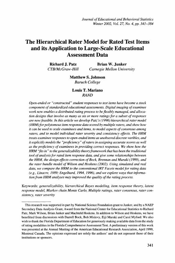
The relative inconsistency of rater 16 can be seen more vividly in bar plots depict- ing the rating probabilities Pkr = P [rater r rates category k I ideal rating 5]. Figure 4 compares bar plots of Pikr for raters r = 16, 13, and 38, obtained by substituting the point estimates of the rater bias and variability parameters in Table 5 into Equation 5. Each row shows the rating probabilities of each rater, rating items of similar caliber (represented by the value of ( for that row). Looking from one bar plot to the next within each row, we see that Rater 16 is somewhat more severe, and substantially more variable, than either Rater 13 or Rater 38; this holds for comparisons of Rater 16 with other raters as well. Such information could be used to focus diagno- sis and quality improvement efforts on increasing the internal consistency or reliability of individual raters. Gathering this information through the rating model is especially important when images of examinee work are sent to raters at remote locations (say, over a computer network), rather than assembling raters in a single location where they can be directly monitored by table leaders, room leaders, and so forth.

Plots of the posterior distributions of the rater bias and variability parameters, shown in Figures 5a and 5b, can help justify decisions about individual raters by providing visual assessments of the statistical significance of differences between raters. Scanning down the column labeled "Bias" in these figures, we see that the posterior distributions of rater bias for all raters overlap to some extent, suggesting that the evidence for differences in bias among the raters is not strong. There is some evidence that Raters 12, 15, and 16 are more severe than Rater 13 (this can also be seen by comparing credible intervals in Table 5) but no substantial differences can be seen with Raters 36, 37, and 38, whose posterior distributions for rater bias are more spread out. On the other hand, scanning down the column labeled "variability" in each figure, we see that the entire posterior distribution for Rater 16's variability parameter lies to the right of 0.6, whereas all of the other raters' variability parameter posteriors lie to the left of 0.6. On the basis of this data, therefore, P[y16 > 0.6] = 1, but for all other raters, P[Ir, > 0.6] = 0. This is strong evidence that Rater 16's internal variability in rating is different from the other raters, and might well justify a search for causes of this extra variability, including fatigue, misunderstanding of the scoring rubric, etc.

363


= 0:

to~ ]A .r d I I I

... I 0 .... , I I

o 1:

d d i d 1 I I 0 1 2 3 4 0 1 2 3 4 0 1 2 3 4

= 2:

d d d

0 1 3 4003 0 1 2 3 4

o o o

0 1 2 3 4 0 1 2 3 4 0 1 2 3 4 S= 4:

d d d

o o o

d 0. 12.0 1 23d '4 c 0 1 2 3

0 1 2 3 4 0 1 2 3 4 0 1 2 3 4

Rater 16 Rater 13 Rater 38

FIGURE 4. Bar plots of estimated category rating probabilities Pkr = P[rater r rates category k I ideal rating ] for a five-category item, for Raters 16, 13, and 38 based on 557 students responses to Items 9, 10, and 11 of the Florida Grade 5 Mathematics Assess- ment. Height of each bar indicates estimated P~krfor the ideal rating 5 indicated at left, the rating category k indicated on the horizontal axis of each plot, and rater r indicated at the bottom of each column. Rater bias and variability parameter estimates may be found in Table 5.

364


Bias Variability

Rater 12:

Ift us

c.o o

o [

- T

. .... ..... -- o I t 1

-0.4 -0.2 0.0 0.2 0.4 0.0 0.2 0.4 0,6 0.8

Rater 13:

COv

i i I

-0.4 -0.2 0.0 0.2 0.4 0.0 0.2 0.4 0.6 0.8

Rater 15:

-0.4 0.2 0.0 0.2 0.4 0.0 0.2 0.4 0.6 0.8

Rater 16:

,r,,

to o -0.4 02 0.0 0.2 0.4 0.0 0.2 04 06 0. I

-0.4 -0.2 0.0 0.2 0.4 0.0 0.2 0.4 0.6 0.8

O ... I I I I l o i 8• i 1

-0.4 -0,2 0.0 0.2 0.4 0.0 0.2 0.4 0.6 0.8

FIGURE 5a. Histograms of the posterior distributions of rater bias and variability parameters based on 557 student responses to Items 9, 10 and 11 of the Florida Grade 5 Mathematics Assess- ment. Each histogram is scaled to have unit area.

365


Bias Variability

Rater 36:

C\J

I I

C:, [I I. .t I I l I i

-0.4 -0.2 0.0 0.2 0.4 0.0 0.2 0.4 0.6 0.8

Rater 37:

',1 Q o

S ! i 1 "• 1

-0.4 -0.2 0.0 0.2 0.4 0.0 0.2 0.4 0.6 0.8

Rater 38:

cj

0 0.2 0.4 0.0 0.2 0.4 0.6 0.8 -0.4 -0.2 0.0 0.2 0.4 0>.0 0.2 0.4 0.6 0.8

FIGURE 5b. Histograms of the posterior distributions of rater bias and variability parameters based on 557 student responses to Items 9, 10 and 11 of the Florida Grade 5 Mathematics Assessment. Each histogram is scaled to have unit area.

Finally we point out an issue in model development and estimation methodology that is vividly revealed in Figures 5a and 5b. The most reliable raters, 36 and 38 in Figure 5b, have the least-well estimated rater bias parameters; indeed, the posterior distributions for ?36 and $38 appear to be nearly uniform in the range -0.5 to +0.5. On the other hand the raters with poorer consistency (higher rater variability estimates) have tighter, clearly unimodal distributions for the bias parameters C, see Figure 5a. We believe this is an artifact of using a continuous rating bias parameter 4, to model discrete, whole unit shifts in the observed rating ijr away from the ideal rating category 5i. Since Raters 36 and 38 essentially always score items in the ideal rating category identified by the HRM, we know their bias parameters 4. must be between -0.5 and +0.5; but since they do so with such high consistency,

366


there is essentially no information in the data to determine where in this range their bias parameters 4 lie.

5.2.2 All assessment items rated in Modality Two

We now turn to an analysis of all eleven items graded in Modality Two. One of the additional items, Item 2, was scored in five response categories 0-4, and the remaining 7 were scored in three categories 0-2. A total of 26 raters graded at least one of the eleven items in Modality Two. The number of ratings per item was two, and the number of items rated by individual raters ranged from one to three, with the most common number of items per rater being one.

The item difficulty and examinee proficiency distribution mean and variance estimates for the PCM underlying the ideal ratings appear in Table 6, and the rater bias and variability estimates are contained in Table 7. The point estimates for the item difficulties agree quite well with the difficulty estimates under the Facets model as reported by Wilson and Hoskens (2001), after a linear transformation to adjust for different latent proficiency means and variances in the two analyses. The items and raters analyzed in the smaller, more balanced data set in Section 5.2.1 are indicated by asterisks in these tables. Comparing with Table 5 we see very little difference in the estimated rater parameters, and small differences in the item difficulty parameters that seem mostly to be due to the different effects that the sum- to-zero constraint has on them in the model for 3 items vs. 11 items.

Judging from the PCM estimates in Table 6 we find that Items 3, 6, and 11 are the most difficult items; referring to the raw data for each item, respectively, 422,

TABLE 6 MCMC Estimated Posterior Median and 95% Equal-Tailed Credible Intervals (CIs) for HRM Item Difficulties and Examinee Proficiency Mean and Variance Parameters, for 11 Items Rated in Modality Two

Parameter Median 95% CI

Item 1 -0.06 (-0.19, 0.07) Item 2 -0.25 (-0.49, 0.12) Item 3 0.62 (0.43, 0.84) Item 4 0.08 (-0.14, 0.30) Item 5 -0.68 (-0.81, -0.56) Item 6 0.29 (0.15, 0.43) Item 7 -0.39 (-0.50, -0.27) Item 8 -0.27 (-0.41, -0.13) Item 9* -0.31 (-0.41, -0.21) Item 10" -0.08 (-0.21, 0.04) Item 11* 1.03 (0.83, 1.25) Mean -1.05 (-1.15, -0.96) Variance 0.73 (0.61, 0.88) Note. Based on two ratings per item response in Modality Two, for each of 557 student responses to 11 items on the Florida Grade 5 Mathematics Assessment. Items analyzed in the smaller extract in Section 5.2.1 are indicated by asterisks (*).

367


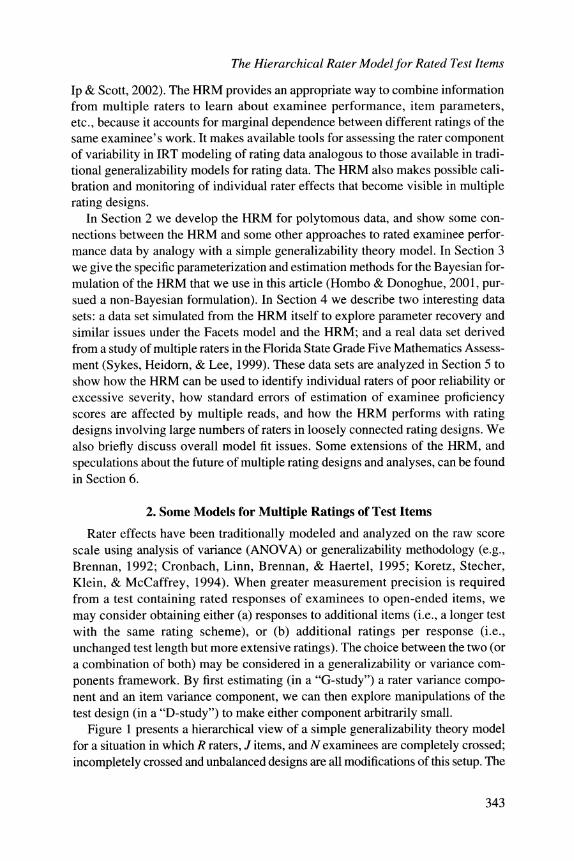
TABLE 7 MCMC Estimated Posterior Median and 95% Equal-Tailed Credible Intervals (Cls) for HRM Rater Parameters, for 11 Items Rated in Modality Two

Rater Median 95% CI

Rater 9 Bias -0.03 (-0.15, 0.14) Variability 0.36 (0.28, 0.40)


Rater 10 Bias -0.10 (-0.26, -0.01) Variability 0.38 (0.27, 0.41)


Rater 18 Bias 0.22 (0.09, 0.36) Variability 0.56 (0.46, 0.69)




Rater 22 Bias 0.14 (-0.02, 0.45) Variability 0.31 (0.12, 0.38)






368


TABLE 7 (Continued)

Rater Median 95% CI





Rater 33 Bias 0.04 (-0.07, 0.17) Variability 0.37 (0.32, 0.41)

Rater 12" Bias -0.26 (-0.35, -0.18) Variability 0.40 (0.33, 0.44)

Rater 13" Bias -0.09 (-0.19, 0.02) Variability 0.42 (0.38, 0.48)



Rater 36* Bias -0.01 (-0.45, 0.43) Variability 0.05 (0.003, 0.27)


Rater 38* Bias -0.05 (-0.45, 0.44) Variability 0.06 (0.007, 0.25)

Note. Based on two ratings per item response in Modality Two for each of 557 student responses to 11 items on the Florida Grade 5 Mathematics Assessment. Raters analyzed in our initial analysis of Items 9, 10, and 11 (Table 5) are marked with asterisks(*).

369


443, and 514 examinees out of 557 were assigned a score of 0 by both raters. Items 5, 7, 8, and 9 appear to be the least difficult of the Mathematics exam items. For Item 5, the easiest of these items as determined by the PCM difficulty parameter estimates, both raters assigned the highest possible score to 140 of the 557 examinees that they both scored. As noted in the analysis of Items 9, 10 and 11 in Section 5.2.1, the mean Ct of the examinee proficiency distribution was quite low, relative to the difficulty of the items. We also note that, as expected, the confidence interval for g is smaller when using all eleven items than when using only the last three items.

Finally, we examine the performance of the 26 raters in Modality Two. All raters, with the exception of Rater 19, appear to be in agreement with one another, in the sense that their rater bias parameters 4, all have point estimates between -0.5 and +0.5: they are all more likely to give the examinee a score equal to the ideal rating category than any other score. The point estimate for Rater 19's bias parameter

)19 is -0.60. At this value of the bias parameter Rater 19 becomes more likely

to score examinees' responses one category lower than the ideal rating category. Rater 11, Rater 36, and Rater 38 are very reliable, with rater variability param-

eter (Wr) estimates of 0.09, 0.05 and 0.06, respectively. These raters essentially always score examinee work in the category k nearest to 5 + 4. On the other hand, Raters 16, 17, and Rater 19 have variability estimates that seem high in comparison to the others. This suggests that the individual reliability or consistency of these raters is poor: such a rater would be less likely to give consistent ratings on separate reads of equivalent examinee work.

5.2.3 The full Florida data set

Finally, we examine the full FCAT data set, in which all eleven items were rated twice in each of three rating modalities, for a total of six ratings per item using a pool of 38 raters. Table 8 contains the estimated HRM rater parameters.

The modalities of those raters who rated in one modality only are identified in bold face type. In addition, the raters from our initial analysis of Items 9, 10, and 11 in Modality Two only are indicated again by asterisks. Comparing the starred raters in Table 8 with the parameter estimates in Table 5, and with the starred entries in Table 7, we see that estimates of these raters' parameters are all fairly stable across the three fits, except for Rater 36. This rater's bias parameter stays fairly stable, mov- ing only from -0.01 to +0.05, but the rater's original variability estimate of 0.05 is now replaced by an estimate of 0.37. This suggests a fair amount of disagreement between Rater 36, who only rates in Modality Two, and raters in other modalities, but no strong trend in the direction of disagreement. Some corroboration of this inter- pretation is suggested in Table 2 and Figure 3, where, for example, Rater 36 disagrees relatively often on Item 10 with Raters 12 and 15, who also rated in Modality Three.

The item parameter estimates for the PCM layer of the HRM are listed in Table 9. The item difficulty parameter estimates (f3s) are quite similar to those of the Modal- ity Two based estimates of Table 6; the primary difference is that the item difficulties are somewhat more spread out in Table 9, compared to Table 6. All of the item difficulties are above the estimated mean of the examinee proficiency

370


TABLE 8 MCMC Estimated Posterior Median and 95% Equal-Tailed Credible Intervals (Cls) for HRM Rater Parameters, for 11 Items Rated in all Modalities

Rater Median 95% CI

Rater 1, Modality 1 Bias -0.10 (-0.21, 0.01) Variability 0.42 (0.38, 0.47)

Rater 2, Modality 1 Bias 0.00 (-0.03, 0.03) Variability 0.48 (0.46, 0.50)

Rater 3, Modality 1 Bias -0.13 (-0.16, -0.09) Variability 0.43 (0.41, 0.44)












371


TABLE 8 (Continued)

Rater Median 95% CI
















372


TABLE 8 (Continued)

Rater Median 95% CI



Rater 32, Modality 2 Bias 0.03 (-0.04, 0.10) Variability 0.39 (0.36, 0.42)




Rater 36", Modality 2 Bias 0.05 (-0.04, 0.16) Variability 0.37 (0.33, 0.41)

Rater 37", Modality 2 Bias -0.34 (-0.49, -0.13) Variability 0.24 (0.07, 0.34)

Rater 38", Modality 2 Bias -0.02 (-0.44, 0.43) Variability 0.06 (0.01, 0.30)

Note. Based on six ratings per item response aggregated over all modalities, for each of 557 student responses to 11 items on the Florida Grade 5 Mathematics Assessment. The modality of raters who rated in only one modality is indicated in bold; the other raters are rated in both Modalities Two and Three. Raters analyzed in our initial analysis of Items 9, 10, and 11 (Table 5) are marked with asterisks(*).

distribution, suggesting that these items were relatively difficult for the examinees. This finding was also suggested by our earlier analyses, and is consistent with results reported by Sykes, Heidorn, and Lee (1999).

In addition, we have listed the estimated item-step parameters for the PCM layer; item-step parameters not listed here may be obtained from these via the relevant sum-to-zero constraint (recall from Section 3.1 that we only estimate K- 2 item- step parameters for each k-category item). Item 2, for example, has estimated item-step parameters Y21 = -1.26, j22 = -0.72, j23 = 0.54, and y24 = 1.26 + 0.72 - 0.64 = 1.34. These item-step parameters are well separated and increase with k, indicating a well-behaved item: ideal rating category 0 is most likely for examinees whose proficiency 0 is below -1.86 (= 2 +

/21 from Table 9), ideal rating category I

373


TABLE 9 MCMC Estimated Posterior Median and 95% Equal-Tailed Credible Intervals (CI) for HRM Item Difficulty, Item-step, and Examinee Proficiency Mean and Variance Parameters

Item Median 95% CI

Item 1

Difficulty P -0.02 (-0.16, 0.11) Step 1 y ( 0.05 (-0.16, 0.26)

Item 2

Difficulty [2 -0.66 (-0.54, -0.77) Step 1 721 -1.26 (-1.53, -0.99) Step 2 722 -0.72 (-0.99, -0.47) Step 3 723 0.54 (0.25, 0.84)

Item 3 Difficulty f3 0.84 (0.65, 1.04) Step 1 '31 -0.09 (-0.21, 0.38)

Item 4 Difficulty P4 -0.00 (-0.18, 0.20) Step 1

y41 -1.79 (-2.01, -1.57) Item 5

Difficulty [5 -0.67 (-0.79, -0.55) Step 1 yS1 -0.06 (-0.25, 0.13)

Item 6 Difficulty [6 0.29 (0.15, 0.43) Step 1 '61 1.43 (1.07, 1.85)

Item 7 Difficulty [7 -0.36 (-0.47, -0.25) Step 1 y71 2.43 (1.96, 2.97)

Item 8 Difficulty fs -0.28 (-0.41, -0.15) Step 1

781 -0.41 (-0.60, -0.22) Item 9

Difficulty P9 -0.28 (-0.38, -0.19) Step 1 ,91 0.24 (-0.02, 0.51) Step 2 (92 -0.54 (-0.86, -0.22) Step 3 793 0.64 (0.20, 1.09)

Item 10 Difficulty 31o 0.05 (-0.08, 0.18) Step 1 720.2 0.96 (0.67, 1.26)

Item 11 Difficulty 312 1.09 (0.89, 1.32) Step 1

•'1., 1.44 (0.97, 1.96)

Proficiency Mean g -1.01 (-1.10, -0.92) Variance a2 0.73 (0.60, 0.88)

Note. Based on six ratings per item response aggregated over all modalities, for each of 557 student responses to 11 items on the Florida Grade 5 Mathematics Assessment.

374


is most likely for examinees whose proficiency is between -1.86 and -1.38 (= f2 + 722 from Table 9), etc.

Several items are not so well behaved: For example, Item 10 has estimated item step parameters ilo, 1 = 0.96 and 10,2 = -0.96. For this item, ideal rating category 1 is never more likely than categories 0 and 2. This is consistent with the observed ratings shown in Figure 3, where for example, we note that the number of cases in which the raters shown there agreed on a category 1 rating is about half as large as the number of cases in which they agreed on a category 2 rating (they agreed on category 0 about ten times more often; since with estimated difficulty I0 = 0.05 this item was relatively difficult for the examinees, whose estimated mean proficiency was

t= -1.01 with

SD ~^= 0.85). Indeed, middle categories appear to be severely under-used in all of these items, except for 2, 4, and possibly 8; this may suggest revisiting the item con- tent, scoring rubrics, and/or rater training procedures and materials, for these items.

5.2.4 Modality effects

The FCAT study was designed to explore effects of rating modality (how items are assigned to each rater) on rating behavior. It is difficult to see what these effects are by scanning down Table 8, especially since some raters rated in more than one modality. We can consider aggregate effects of modality on rater bias and rater variability by replacing the original rater bias (,r) and rater variability (Wr,) parameters with parameters #rm and I,m, defined as:

Prr = 0+ 1m

log •,m

= log x0 + log tm. (8)

This allows both rater-specific bias (4 ) and variability (y4 ) and modality-specific bias (Tlm) and variability (tm) effects (see Mariano, 2002, for elaboration and expansion of this idea). The assignment of raters to modalities in the FCAT study (see Table 2) creates two distinct groups of raters, those who rated exclusively in Modal- ity One and those who rated in Modalities Two and Three. Raters who rated only in Modality One are represented in the design matrix for each additive-effects model in Equation 8 as a single row, for example

rater modality (00010000000000000000000000000000000000 100).

while those who rated in both Modalities Two and Three are represented with a pair of rows, for example

(00000000000100000000000000000000000000 010) and

(00000000000100000000000000000000000000 001).

375


It is readily verified that the complete design matrix, which is the same for both models in Equation 8, has 53 rows and 41 columns, and is of rank 39. Two linear constraints are therefore required to identify the models. Since we are interested in contrasting modality effects, we leave these free and constrain the rater effects to sum to zero within the group of raters who rated in Modality One (raters 1-7) and within the group of raters who rated in Modalities Two and Three (Raters 8-38). For the rater bias model in Equation 8, the constraints are

C = 0, and 38 = 0, and for the rater variability model in Equation 8,

l= In ? = 0 and

38=8 In x? = 0.

Refitting this expansion of the model, using independent N(0, 10) prior distributions on each #0, rim, log

r and log tm, we obtained the estimates for modality

components of rater bias and variability shown in Table 10. These estimates suggest an aggregate effect of modality on rating bias. Ratings in Modalities Two and Three (individual items and blocks of items) tended to be lower

(T12 = -0.189 and

13 = -0.148) than ratings of entire 11-item booklets (Modality One, T1 = -0.076), with no overlap in the 95% CIs. Also, individual item ratings (Modality Two) appear to be somewhat lower than block item rating (Modality Three), albeit with substantial overlap in the 95% CIs. The evidence for corresponding differences in rater variability also distinguishes Modality One from Modalities Two and Three: ratings in Modalities Two and Three tend to be less variable (t2 = 0.401, t3 = 0.398) than ratings in Modality One (t1 = 0.456), with no overlap in the 95% CIs from either Modality Two or Three with the 95% CI from Modality One.

5.2.5 The information for scoring examinees in multiple ratings

To illustrate the effects of increasing the number of items and the number of ratings per item on estimates of examinee proficiencies, we examined the 0 estimates of five examinees taken from the full data set in Section 5.2.3. In Table 11, we have compared these examinees' posterior median and equal-tailed 95% CI estimates for 0, under all three models estimated in Sections 5.2.1, 5.2.2 and 5.2.3. The 95% CIs using only Items 9, 10, and 11 in Modality Two are widest; these correspond to J= 3 items per examinee and R = 2 ratings per item. The CI widths reduce by a factor of about two thirds as we move to the complete Modality Two data, for which J = 11 and R = 2. Finally, there is little improvement, or even some degra- dation, in the CIs as we move to the full dataset using all three modalities, for which J= 11 andR = 6.

These effects on CI width as we move from 3 to 11 items, and from 2 to 6 raters, are quite similar to what we would see if we computed CIs for 0 from the normal- theory model in Equation 1. More surprisingly, the CI widths can actually increase, as with Subject 175, when we move from the Modality Two data to the full data set, despite tripling the number of raters. This may in part be due to the multiple- modality design: although the aggregate differences in Table 10 are not large, there is some suggestion of less reliability, and perhaps more severity, in ratings in

376


TABLE 10 MCMC-Estimated Posterior Median and 95% Credible Intervals (Cls) for Modality Components of Rater Bias and Rater Variability

Modality (m)

Parameter 1: Booklet 2: One Item 3:1/3 Booklet

Bias (7i1,,) -0.076 -0.189 -0.148 95% CI (-0.097, -0.055) (-0.208, -0.164) (-0.168, -0.120)

Variability (t,,) 0.456 0.401 0.398 95% CI (0.447, 0.465) (0.371, 0.431) (0.369, 0.431)

Note. Using the reparameterization in Equation 8, for the group of 38 raters displayed in Table 8.

Modality One vs. the other modalities; this may stem from substantial disagreements about particular subject responses.

Clearly, adding more raters yields a benefit (more raters reduces uncertainty in estimating examinee proficiencies) and a cost (disagreement across modalities in how to score examinee work increases uncertainty in estimating examinee proficiencies), and the cost may outweigh the benefit among raters assigned to score Subject 175's work. In situations where we are adding raters who share stronger consensus on examinees'

TABLE 11 Comparison of 0 (proficiency) Estimates for Five Examinees, Under each of the Three HRM Models Estimated in Section 5

Subject Median 95% CI CI width

Subject 115 Modality 2 (9, 10, 11) -1.83 (-3.23, -0.69) 2.54 Modality 2 -1.98 (-3.21, -1.18) 2.03 Full data -1.85 (-2.89, -0.97) 1.92




Subject 175 Modality 2 (9, 10, 11) -0.56 (-1.63, 0.57) 2.20 Modality 2 -0.85 (-1.62, -0.36) 1.26 Full data -0.93 (-1.71, -0.21) 1.50

377


work, we might expect to see a more consistent decrease in the standard errors for examinee proficiencies. Mariano (2002) explores these issues in more detail.

5.3 Model Comparisons

In Table 12 we compare the fits of the IRT Facets model with additive rater effects to the fit of the HRM model, on the simulated data from Section 5.1 and the full Florida rater study data from Section 5.2.3. Because the models are not nested in the usual sense (the IRT Facets model is not obtained by constraining the HRM parameters in a locally linear way; see discussion at the end of Section 3.2), likelihood ratio chi-squared tests cannot be used. Instead, we use a measure of fit known as the Schwarz (1978) Criterion, also known as the Bayes Information Cri- terion (BIC) (e.g., Kass & Raftery, 1995). The difference between BIC values for two models approximates the logarithm of the Bayes Factor, which is often used for comparing models in Bayesian statistics; the Bayes Factor can be difficult to compute directly, especially for large models estimated with MCMC methods (see, for example, DiCiccio, Kass, Raftery, & Wasserman, 1997). For any IRT-like model with p parameters and sample size N, we calculate the BIC as:

BIC = -2 . log(maximum marginal likelihood) + p log(N).

We apply this to the marginal HRM after integrating out 5 and 0. The BIC can be interpreted as the usual log-likelihood statistic, penalized for

the number of parameters in the model. Any reduction in BIC is considered good, since the penalty p log(N) compensates for capitalization on chance; however, a commonly used rule of thumb (Kass & Raftery, 1995) for Bayes Factors is that a decrease of 2-6 in this BIC statistic is considered moderately good evidence, and a change of 10 or more is considered strong evidence, in favor of the model with the lower BIC.

It is no surprise that in Table 12 the HRM fits better than the Facets model in the simulated data, since this data was simulated from the HRM itself. The large

TABLE 12 Model Fit Comparisons for the HRM-Simulated Data (Section 5.1) and for the Full Rater Study Data Set from the Florida Grade 5 Mathematics Assessment (Section 5.2.3)

Parameters Examinees Model -2log (marginal likelihood) (p) (N) BIC

HRM Simulated Data

IRT Facets 14,505 23 500 14,648 HRM 10,405 27 500 10,573

Florida Data

IRT Facets 55,256 65 557 55,667 HRM (w/o modality) 34,546 103 557 35,198 HRM (with modality) 34,536 105 557 35,200

378


change in BIC, a decrease of 4,000 for an increase of only three additional parameters (essentially, the three rater variability parameters), is very strong evidence that the dependence modeled by the HRM cannot somehow be accommodated by the Facets model. Much more impressive is the decrease of over 20,000 for an increase of 38 parameters (again, essentially the rater variability parameters), in favor of the HRM in fitting the Florida mathematics assessment rating study data set. Thus, in the real data too, the HRM is providing a dramatically better fit for the dependence structure of the data.

Finally, the BIC comparison of the HRM accounting for rating modalities as in Equation 8 with the HRM without modalities mildly favors the no-modality model. This seems inconsistent with our earlier results (Table 10) showing clear bias and variability differences between Modality One and Modalities Two and Three. To reconcile these results, we note that, because of the nesting of raters within Modal- ity One and Modalities Two and Three, the no-modality model can already accommodate additive effects distinguishing Modality One from the other two modalities. For example, averaging the bias of the seven Modality One raters provides the bias attributable to Modality One. For this data, the modality model in Equation 8 adds flexibility only in distinguishing Modality Two from Modality Three. Therefore, the BIC's lack of preference for the modality model is precisely a lack of preference for modeling distinctions between Modalities Two and Three, which is entirely consistent with the overlapping CIs in Table 10. Further comparisons employing explicit calculation of Bayes Factors (Mariano, 2002) yield similar conclusions.

6. Discussion

In this article we have implemented Patz's (1996) hierarchical rater model (HRM) for polytomously scored item response data, so that it can be employed with data sets approaching the sizes of those encountered in large-scale educational assessments, or at least in rater studies supporting those assessments. We have shown how the HRM "fits in" to the generalizability theory framework that has been the traditional analysis tool for rated item response data. Indeed, the HRM is a standard generalizability theory model for rating data, with IRT distributions replacing the normal theory true score distributions that are usually implicit in infer- ential applications of the model. Observed ratings are related to ideal ratings of each piece of student work through a simple signal detection model that can be further parameterized to be sensitive to individual rater severity and reliability effects, and ideal ratings are related to latent examinee proficiency via a conventional IRT model such as the Partial Credit Model.

The HRM is one of several current approaches to correcting this underestimation of standard errors for estimating examinee proficiency, as reported by Patz (1996), Junker and Patz (1998), Donoghue and Hombo (2000a; 2000b), and others. Bock, Brennan, and Muraki (1999) construct a generalizability theory based "design effects" correction for the conventional IRT Facets model, and Wilson and Hoskens (2001) replace the conditional independence assumptions of the conventional IRT

379


Facets model with a rater bundle model analogous to Rosenbaum's (1988) item bundles. Verhelst and Verstralen's (2001) IRT model for multiple raters is also closely related to the HRM.

Using polytomous response data simulated from the HRM, we showed that the HRM is effective at item and rater parameter recovery, and displayed some biases in IRT Facets model (Linacre, 1989) item parameter estimates that we believe occur when some raters are relatively unreliable or inconsistent in their ratings. In addition, both models produce interval estimates for examinee proficiencies that capture the true 0 values, but the IRT Facets model substantially underestimates interval widths relative to the HRM.

We also examined successively larger data extracts from a study of three different rating modalities intended to support a Grade 5 mathematics assessment given in the State of Florida (Sykes, Heidorn, & Lee 1999), and showed how the current implementation of the HRM can be used to scale items and examinees, and learn about rater quality. Using Schwarz's (1987; see also Kass and Raftery, 1995) Infor- mation Criterion we showed that the HRM fits data from this study far better than the IRT Facets model, suggesting that the dependence between multiple ratings of the same student work that the Facets model fails to capture is an important component of multiple-rating assessment data.

The parameterization of the HRM used in this article emphasizes raters' individual severity and reliability. One natural set of extensions of our parameterization of the HRM would allow us to assess effects and interactions among rater background variables, examinee background variables, item features, and time of rating. Such analyses within the HRM only require that the relevant covariates be collected, and then incorporated as in Equation 8 into the model. Our exploration of rating modality in the Florida rating study is an example of this type of analysis. Rater drift over time, rating table effects in a centralized rating system, and halo effects, might all be analyzed in this way.

Other questions may be handled by a more radical reparameterization of the probabilities in Table 1. To explore over-use of inner categories of a rating scale, for example, one might allow the rater bias parameter to depend on the ideal rating category as well as the rater. The new bias parameter

,r would be expected to

be positive for ideal categories below the middle one, and negative for ideal categories above it. Differential reliability across categories, for example due to disagreement only about what constitutes a poor performance, might be handled with a similar modification of the rater variability parameter. Either phenomenon might be modeled to operate only for particular items. In addition, the unimodal shape suggested by Equation 5 might be replaced with some other shape.

We expect that as digital imaging technology improves, decentralized online scoring may replace centralized scoring sessions where all raters are in one room, supervised closely at separate tables by table leaders. In a decentralized scoring system, raters work on their own in front of a computer terminal at a location of their choosing. A supervisor is online to provide assistance when needed, but much of the valuable qualitative information that supervisors in centralized scoring ses-

380


sions use to monitor and maintain rating quality-raters' body language, raters flip- ping back and forth from the rubrics to the student work, discussion with raters of difficult-to-rate cases-is not available. Consequently, there is greater opportunity for raters to get off track and less opportunity to quickly bring them back into the fold when they stray, unless supervisors have adequate statistical tools to monitor rater performance at a distance. Multiple ratings can provide the data needed for adequate statistical monitoring on the basis of rating data alone, as well as providing some improvement in the precision of estimation of examinee proficiencies. We hope that the HRM, and similar approaches such as that of Wilson and Hoskens (2001) and Verhelst and Verstralen (2001) that appropriately account for dependence between ratings, can provide the basis for statistical monitoring in distributed rating systems.

References

Baxter, G. P., & Junker, B. W. (2001, April). Designing cognitive-developmental assessments: a case study in proportional reasoning. Paper presented at the Annual Meeting of the National Council for Measurement in Education. Seattle, Washington.

Birnbaum, A. (1968). Some latent trait models and their use in inferring an examinee's ability. In, F. M. Lord and M. R. Novick (Eds.), Statistical theories ofmental test scores. Read- ing, Massachusetts: Addison-Wesley.

Bock, R. D., Brennan, R. L., & Muraki, E. (1999, April). The introduction of essay questions to the GRE: Toward a synthesis of item response theory and generalizability theory. Paper presented at the Annual meeting of the American Educational Research Association, 1999, Montreal, Canada.

Bradlow, E. T., Wainer, H., & Wang, X. H. (1999). A Bayesian random effects model for testlets. Psychometrika, 64, 153-168.

Brennan, R. L. (1992). Elements of generalizability theory (revised edition). Iowa City IA: ACT Publications.

Brennan, R. L. (1997). A perspective on the history of generalizability theory. Educational Researcher, 16, 14-20.

Cronbach, L. J., Linn, R. L., Brennan, R. L., & Haertel, E. (1995). Generalizability analysis for educational assessments. Evaluation Comment. Los Angeles, CA: UCLA's Center for the Study of Evaluation and The National Center for Research on Evaluation, Standards and Student Testing. Retrieved May 16, 2000 from http://www.cse.ucla.edu/CRESST/ Newsletters/CSU95.pdf.

DiCiccio, T. J., Kass, R. E., Raftery, A., & Wasserman, L. (1997). Computing Bayes factors by combining simulation and asymptotic approximations. Journal of the American Statistical Association, 92, 903-915.

Donoghue, J. R., & Hombo, C. M. (2000a, April). A comparison of different model assumptions about rater effects. Paper presented at the Annual Meeting of the National Council on Measurement in Education. New Orleans, LA.

Donoghue, J. R., & Hombo, C. M. (2000b, June). How rater effects are related to reliability indices. Paper presented at the North American Meeting of the Psychometric Society. Vancouver BC, Canada.

Engelhard, G., Jr. (1994). Examining rater errors in the assessment of written composition with many-faceted Rasch models. Journal ofEducational Measurement, 31, 93-112.

381


Engelhard, G., Jr. (1996). Evaluating rater accuracy in performance assessments. Journal ofEducational Measurement, 33, 56-70.

Fischer, G. H. (1973). The linear logistic model as an instrument in educational research. Acta Psychologica, 37, 359-374.

Fischer, G. H. (1983). Logistic latent trait models with linear constraints. Psychometrika, 48, 3-26.

Fischer, G. H., & Ponocny, I. (1994). An extension of the partial credit model with an application to the measurement of change. Psychometrika, 59, 177-192.

Gelman, A., Carlin, J. B., Stern, H. S., & Rubin, D. B. (1995). Bayesian data analysis. New York: Chapman and Hall.

Gilks, W. R., Richardson, S., & Spiegelhalter, D. (1995). Practical Markov Chain Monte Carlo. New York: Chapman and Hall.

Heller, J., Sheingold, K., & Myford, C. (1998). Reasoning about evidence in portfolios: Cog- nitive foundations for valid and reliable assessment. Educational Assessment, 5, 5-40.

Hombo, C., & Donoghue, J. R. (2001, April). Applying the hierarchical raters model to NAEP. Paper presented at the Annual Meeting of the National Council on Measurement in Education, Seattle Washington.

Johnson, M. S., Cohen, W., & Junker, B. W. (1999). Measuring appropriability in research and development with item response models. (Carnegie Mellon Statistics Department Tech- nical Report #690). Retrieved May 16, 2000 from http://www.stat.cmu.edu/cmu-stats/tr.

Junker, B. W., & Patz, R. J. (1998, June). The hierarchical rater model for rated test items. Presented at the Annual North American Meeting of the Psychometric Society, Champaign- Urbana, IL.

Kass, R. E., & Raftery A. E. (1995). Bayes factors. Journal of The American Statistical Association, 90, 773-795.

Koretz, D., Stecher, B., Klein, S., & McCaffrey, D. (1994). The Vermont Portfolio Assess- ment Program: Findings and implications. Educational Measurement: Issues and Prac- tice, 13, 5-16.

Linacre, J. M. (1989). Many-faceted Rasch Measurement. Chicago, IL: MESA Press. Lord, F. M., & Novick, M. R. (1968). Statistical theories of mental test scores. Reading,

MA: Addison-Wesley. Lukhele, R., Thissen, D., & Wainer, H. (1994). On the relative value of multiple choice,

constructed response, and examinee selected items on two achievement tests. Journal of Educational Measurement, 31, 234-250.

Mariano, L. T. (2002). Information accumulation, model selection and rater behavior in constructed response student assessments. Unpublished doctoral dissertation, Depart- ment of Statistics, Carnegie Mellon University, Pittsburgh PA.

Maris, E. (1995). Psychometric latent response models. Psychometrika, 60, 523-547. Masters, G. N. (1982). A Rasch model for partial credit scoring. Psychometrika, 47, 149-174. Messick, S. (1994). The interplay of evidence and consequences in the validation of per-

formance assessments. Educational Researcher, 23, 13-23. Mislevy, R. J., Beaton, A. E., Kaplan, B., & Sheehan, K. M. (1992). Estimating population

characteristics from a sparse matrix sample of item responses. Journal of Educational Measurement, 29, 131-154.

Mislevy, R. J., & Wu, P. K. (1996). Missing responses and IRT ability estimation: Omits, choice, time limits, and adaptive testing. ETS Technical Report, RR-96-30-ONR. Prince- ton, NJ: Educational Testing Service.

382


Myford, C. M., & Mislevy, R. J. (1995). Monitoring and improving a portfolio assessment system. Center for Performance Assessment Research Report. Princeton, NJ: Educational Testing Service.

Patz, R. J. (1996). Markov Chain Monte Carlo methods for item response theory models with applications for the National Assessment of Educational Progress. Unpublished doctoral dissertation, Carnegie Mellon University, Pittsburgh PA.

Patz, R. J., & Junker, B. W. (1999a). A straightforward approach to Markov Chain Monte Carlo methods for item response models. Journal of Educational and Behavioral Statis- tics, 24, 146-178.

Patz, R. J., & Junker, B. W. (1999b). Applications and extensions of MCMC in IRT: Mul- tiple item types, missing data, and rated responses. Journal of Educational and Behav- ioral Statistics, 24, 342-366.

Patz, R. J., Junker, B. W. & Johnson, M. S. (1999, April). The hierarchical rater model for rated test items and its application to large-scale educational assessment data. Paper presented at the Annual Meeting of the American Educational Research Association, Mon- treal Canada.

Patz, R. J., Wilson, M., & Hoskens, M. (1997). Optimal rating procedures for NAEP open- ended items. Final report to the National Center for Education Statistics under the redesign of NAEP.

Rosenbaum, P. R. (1988). Item bundles. Psychometrika, 53, 349-359. Scheiblechner, H. (1972). Das Lernen und Lisen komplexer Denkaufgaben. [The learning

and solving of complex reasoning items.] Zeitschriftfur Experimentelle undAngewandte Psychologie, 3, 456-506.

Schwarz, G. (1978). Estimating the dimension of a model. The Annals ofStatistics, 6, 461-464. Scott, S. L., & Ip, E. H. (2002). Empirical Bayes and item clustering effects in a latent vari-

able hierarchical model: A case study of the National Assessment of Educational Progress. Journal of the American Statistical Association, 97, 409-419.

Serfling, R. J. (1980). Approximation theorems ofmathematical statistics. New York: Wiley. Spiegelhalter, D., Thomas, A., Best, N., & Gilks, W. (1996). BUGS 0.5: Bayesian inference

using Gibbs Sampling, Version ii. Technical report of the MRC Biostatistics Unit, Insti- tute of Public Health, Cambridge, UK. Retrieved May 16, 2000 http://www.mrc-bsu.cam. ac.uk/bugs/.

Stiggins, R. (1994). Student-centered classroom assessment. New York: Macmillan College Publishing.

Sykes, R. C., Heidorn, M., & Lee, G. (1999, April). The assignment of raters to items: Con- trolling for rater bias. Paper presented at the annual meeting of the National Council on Measurement in Education, Montreal Canada.

Tanner, M. A. (1996). Tools for statistical inference: Methods for the exploration of posterior distributions and likelihood functions. 3rd Edition. New York: Springer-Verlag.

Verhelst, N. D., & Verstralen, H. H. F. M. (2001). An IRT model for multiple raters. In A. Boomsma, M. A. J. Van Duijn, and T. A. B. Snijders (Eds.), Essays on item response modeling (pp. 89-108). New York: Springer-Verlag.

Wilson, M., & Hoskens, M. (2001). The rater bundle model. Journal of Educational and Behavioral Statistics, 26, 283-306.

Wilson, M., & Wang, W. (1995). Complex composites: Issues that arise in combining different modes of assessment. Applied Psychological Measurement, 19(1), 51-72.

Wu, M. L., Adams, R. J., & Wilson, M. R. (1997). ConQuest: Generalized item response modeling software. ACER.

383

Authors

RICHARD J. PATZ is Senior Director of Research, CTB/McGraw-Hill, Monterey, CA 93940; [email protected]. He specializes in educational measurement, large-scale assessment, and Bayesian statistical inference in behavioral research.

BRIAN JUNKER is Professor, Department of Statistics, Carnegie Mellon University, Pitts- burgh PA 15213; [email protected]. He specializes in the statistics of latent variable models for measurement, and adaptations of parametric and nonparametric item response models to novel repeated measures settings.

MATTHEW S. JOHNSON is Assistant Professor, Department of Statistics and Computer Information Systems, Baruch College, City University of New York, New York, NY 10010; [email protected]. He specializes in the development and estimation of heirarchical Bayesian models for educational and behavioral data.

LOUIS T. MARIANO is Associate Statistician, RAND, 1200 S. Hayes Street, Arlington, VA 22202; [email protected]. He specializes in latent variable models, Bayesian hierarchical models, model selection and education policy applications.

384

Documents

The Hierarchical Rater Model for Rated Test Items and Its ... · The Hierarchical Rater Model for Rated Test Items and Its Application to Large-Scale Educational Assessment Data Author(s):