Embed Size (px)
Citation preview
Computation
Visualization
Programming
Getting Started with MATLABVersion 6
MATLAB®
The Language of Technical Computing
How to Contact The MathWorks:
www.mathworks.com Webcomp.soft-sys.matlab Newsgroup
[email protected] Technical [email protected] Product enhancement [email protected] Bug [email protected] Documentation error [email protected] Order status, license renewals, [email protected] Sales, pricing, and general information
508-647-7000 Phone
508-647-7001 Fax
The MathWorks, Inc. Mail3 Apple Hill DriveNatick, MA 01760-2098
For contact information about worldwide offices, see the MathWorks Web site.
Getting Started with MATLAB COPYRIGHT 1984 - 2002 by The MathWorks, Inc. The software described in this document is furnished under a license agreement. The software may be used or copied only under the terms of the license agreement. No part of this manual may be photocopied or repro-duced in any form without prior written consent from The MathWorks, Inc.
FEDERAL ACQUISITION: This provision applies to all acquisitions of the Program and Documentation by or for the federal government of the United States. By accepting delivery of the Program, the government hereby agrees that this software qualifies as "commercial" computer software within the meaning of FAR Part 12.212, DFARS Part 227.7202-1, DFARS Part 227.7202-3, DFARS Part 252.227-7013, and DFARS Part 252.227-7014. The terms and conditions of The MathWorks, Inc. Software License Agreement shall pertain to the government’s use and disclosure of the Program and Documentation, and shall supersede any conflicting contractual terms or conditions. If this license fails to meet the government’s minimum needs or is inconsistent in any respect with federal procurement law, the government agrees to return the Program and Documentation, unused, to MathWorks.
MATLAB, Simulink, Stateflow, Handle Graphics, and Real-Time Workshop are registered trademarks, and TargetBox is a trademark of The MathWorks, Inc.
Other product or brand names are trademarks or registered trademarks of their respective holders.
Printing History: December 1996 First printing For MATLAB 5May 1997 Second printing For MATLAB 5.1September 1998 Third printing For MATLAB 5.3September 2000 Fourth printing Revised for MATLAB 6 (Release 12)June 2001 Online only Minor update for MATLAB 6.1,
Release 12.1July 2002 Online only Revised for MATLAB 6.5 (Release 13)
Contents
1Introduction
What Is MATLAB? . . . . . . . . . . . . . . . . . . . . . . . . . . . . . . . . . . . . 1-2The MATLAB System . . . . . . . . . . . . . . . . . . . . . . . . . . . . . . . . . 1-3
MATLAB Documentation . . . . . . . . . . . . . . . . . . . . . . . . . . . . . . 1-4MATLAB Online Help . . . . . . . . . . . . . . . . . . . . . . . . . . . . . . . . . 1-4
2Development Environment
Starting and Quitting MATLAB . . . . . . . . . . . . . . . . . . . . . . . . 2-2Starting MATLAB . . . . . . . . . . . . . . . . . . . . . . . . . . . . . . . . . . . . 2-2Quitting MATLAB . . . . . . . . . . . . . . . . . . . . . . . . . . . . . . . . . . . . 2-2
MATLAB Desktop . . . . . . . . . . . . . . . . . . . . . . . . . . . . . . . . . . . . . 2-3
Desktop Tools . . . . . . . . . . . . . . . . . . . . . . . . . . . . . . . . . . . . . . . . 2-5Command Window . . . . . . . . . . . . . . . . . . . . . . . . . . . . . . . . . . . 2-5Start Button and Launch Pad . . . . . . . . . . . . . . . . . . . . . . . . . . 2-7Help Browser . . . . . . . . . . . . . . . . . . . . . . . . . . . . . . . . . . . . . . . . 2-7Current Directory Browser . . . . . . . . . . . . . . . . . . . . . . . . . . . . 2-10Workspace Browser . . . . . . . . . . . . . . . . . . . . . . . . . . . . . . . . . . 2-12Editor/Debugger . . . . . . . . . . . . . . . . . . . . . . . . . . . . . . . . . . . . 2-14Profiler . . . . . . . . . . . . . . . . . . . . . . . . . . . . . . . . . . . . . . . . . . . . 2-15
Other Development Environment Features . . . . . . . . . . . . 2-16
i
ii Contents
3Manipulating Matrices
Matrices and Magic Squares . . . . . . . . . . . . . . . . . . . . . . . . . . . 3-2Entering Matrices . . . . . . . . . . . . . . . . . . . . . . . . . . . . . . . . . . . . 3-3sum, transpose, and diag . . . . . . . . . . . . . . . . . . . . . . . . . . . . . . . 3-4Subscripts . . . . . . . . . . . . . . . . . . . . . . . . . . . . . . . . . . . . . . . . . . . 3-6The Colon Operator . . . . . . . . . . . . . . . . . . . . . . . . . . . . . . . . . . . 3-7The magic Function . . . . . . . . . . . . . . . . . . . . . . . . . . . . . . . . . . . 3-8
Expressions . . . . . . . . . . . . . . . . . . . . . . . . . . . . . . . . . . . . . . . . . 3-10Variables . . . . . . . . . . . . . . . . . . . . . . . . . . . . . . . . . . . . . . . . . . . 3-10Numbers . . . . . . . . . . . . . . . . . . . . . . . . . . . . . . . . . . . . . . . . . . . 3-10Operators . . . . . . . . . . . . . . . . . . . . . . . . . . . . . . . . . . . . . . . . . . 3-11Functions . . . . . . . . . . . . . . . . . . . . . . . . . . . . . . . . . . . . . . . . . . 3-11Examples of Expressions . . . . . . . . . . . . . . . . . . . . . . . . . . . . . . 3-13
Working with Matrices . . . . . . . . . . . . . . . . . . . . . . . . . . . . . . . 3-14Generating Matrices . . . . . . . . . . . . . . . . . . . . . . . . . . . . . . . . . 3-14The load Function . . . . . . . . . . . . . . . . . . . . . . . . . . . . . . . . . . . 3-15M-Files . . . . . . . . . . . . . . . . . . . . . . . . . . . . . . . . . . . . . . . . . . . . 3-15Concatenation . . . . . . . . . . . . . . . . . . . . . . . . . . . . . . . . . . . . . . 3-16Deleting Rows and Columns . . . . . . . . . . . . . . . . . . . . . . . . . . . 3-17
More About Matrices and Arrays . . . . . . . . . . . . . . . . . . . . . . 3-18Linear Algebra . . . . . . . . . . . . . . . . . . . . . . . . . . . . . . . . . . . . . . 3-18Arrays . . . . . . . . . . . . . . . . . . . . . . . . . . . . . . . . . . . . . . . . . . . . . 3-21Multivariate Data . . . . . . . . . . . . . . . . . . . . . . . . . . . . . . . . . . . 3-24Scalar Expansion . . . . . . . . . . . . . . . . . . . . . . . . . . . . . . . . . . . . 3-25Logical Subscripting . . . . . . . . . . . . . . . . . . . . . . . . . . . . . . . . . 3-26The find Function . . . . . . . . . . . . . . . . . . . . . . . . . . . . . . . . . . . . 3-27
Controlling Command Window Input and Output . . . . . . . 3-28The format Function . . . . . . . . . . . . . . . . . . . . . . . . . . . . . . . . . 3-28Suppressing Output . . . . . . . . . . . . . . . . . . . . . . . . . . . . . . . . . . 3-30Entering Long Statements . . . . . . . . . . . . . . . . . . . . . . . . . . . . 3-30Command Line Editing . . . . . . . . . . . . . . . . . . . . . . . . . . . . . . . 3-30
4Graphics
Basic Plotting . . . . . . . . . . . . . . . . . . . . . . . . . . . . . . . . . . . . . . . . . 4-2Creating a Plot . . . . . . . . . . . . . . . . . . . . . . . . . . . . . . . . . . . . . . . 4-2Multiple Data Sets in One Graph . . . . . . . . . . . . . . . . . . . . . . . . 4-3Specifying Line Styles and Colors . . . . . . . . . . . . . . . . . . . . . . . . 4-4Plotting Lines and Markers . . . . . . . . . . . . . . . . . . . . . . . . . . . . . 4-5Imaginary and Complex Data . . . . . . . . . . . . . . . . . . . . . . . . . . . 4-6Adding Plots to an Existing Graph . . . . . . . . . . . . . . . . . . . . . . . 4-7Figure Windows . . . . . . . . . . . . . . . . . . . . . . . . . . . . . . . . . . . . . . 4-8Multiple Plots in One Figure . . . . . . . . . . . . . . . . . . . . . . . . . . . . 4-9Controlling the Axes . . . . . . . . . . . . . . . . . . . . . . . . . . . . . . . . . 4-10Axis Labels and Titles . . . . . . . . . . . . . . . . . . . . . . . . . . . . . . . . 4-12Saving a Figure . . . . . . . . . . . . . . . . . . . . . . . . . . . . . . . . . . . . . 4-13
Editing Plots . . . . . . . . . . . . . . . . . . . . . . . . . . . . . . . . . . . . . . . . 4-14Interactive Plot Editing . . . . . . . . . . . . . . . . . . . . . . . . . . . . . . . 4-14Using Functions to Edit Graphs . . . . . . . . . . . . . . . . . . . . . . . . 4-14Using Plot Editing Mode . . . . . . . . . . . . . . . . . . . . . . . . . . . . . . 4-15Using the Property Editor . . . . . . . . . . . . . . . . . . . . . . . . . . . . . 4-16
Mesh and Surface Plots . . . . . . . . . . . . . . . . . . . . . . . . . . . . . . . 4-18Visualizing Functions of Two Variables . . . . . . . . . . . . . . . . . . 4-18
Images . . . . . . . . . . . . . . . . . . . . . . . . . . . . . . . . . . . . . . . . . . . . . . 4-22
Printing Graphics . . . . . . . . . . . . . . . . . . . . . . . . . . . . . . . . . . . . 4-24
Handle Graphics . . . . . . . . . . . . . . . . . . . . . . . . . . . . . . . . . . . . . 4-26Graphics Objects . . . . . . . . . . . . . . . . . . . . . . . . . . . . . . . . . . . . 4-26Setting Object Properties . . . . . . . . . . . . . . . . . . . . . . . . . . . . . . 4-28Finding the Handles of Existing Objects . . . . . . . . . . . . . . . . . 4-31
Graphics User Interfaces . . . . . . . . . . . . . . . . . . . . . . . . . . . . . 4-33Graphical User Interface Design Tools . . . . . . . . . . . . . . . . . . . 4-33
Animations . . . . . . . . . . . . . . . . . . . . . . . . . . . . . . . . . . . . . . . . . . 4-34Erase Mode Method . . . . . . . . . . . . . . . . . . . . . . . . . . . . . . . . . . 4-34Creating Movies . . . . . . . . . . . . . . . . . . . . . . . . . . . . . . . . . . . . . 4-35
iii
iv Contents
5Programming with MATLAB
Flow Control . . . . . . . . . . . . . . . . . . . . . . . . . . . . . . . . . . . . . . . . . 5-2if . . . . . . . . . . . . . . . . . . . . . . . . . . . . . . . . . . . . . . . . . . . . . . . . . . 5-2switch and case . . . . . . . . . . . . . . . . . . . . . . . . . . . . . . . . . . . . . . 5-3for . . . . . . . . . . . . . . . . . . . . . . . . . . . . . . . . . . . . . . . . . . . . . . . . . 5-4while . . . . . . . . . . . . . . . . . . . . . . . . . . . . . . . . . . . . . . . . . . . . . . . 5-5continue . . . . . . . . . . . . . . . . . . . . . . . . . . . . . . . . . . . . . . . . . . . . 5-5break . . . . . . . . . . . . . . . . . . . . . . . . . . . . . . . . . . . . . . . . . . . . . . . 5-6
Other Data Structures . . . . . . . . . . . . . . . . . . . . . . . . . . . . . . . . . 5-7Multidimensional Arrays . . . . . . . . . . . . . . . . . . . . . . . . . . . . . . . 5-7Cell Arrays . . . . . . . . . . . . . . . . . . . . . . . . . . . . . . . . . . . . . . . . . . 5-9Characters and Text . . . . . . . . . . . . . . . . . . . . . . . . . . . . . . . . . 5-11Structures . . . . . . . . . . . . . . . . . . . . . . . . . . . . . . . . . . . . . . . . . . 5-14
Scripts and Functions . . . . . . . . . . . . . . . . . . . . . . . . . . . . . . . . 5-17Scripts . . . . . . . . . . . . . . . . . . . . . . . . . . . . . . . . . . . . . . . . . . . . . 5-18Functions . . . . . . . . . . . . . . . . . . . . . . . . . . . . . . . . . . . . . . . . . . 5-19Global Variables . . . . . . . . . . . . . . . . . . . . . . . . . . . . . . . . . . . . . 5-21Passing String Arguments to Functions . . . . . . . . . . . . . . . . . . 5-21The eval Function . . . . . . . . . . . . . . . . . . . . . . . . . . . . . . . . . . . 5-23Vectorization . . . . . . . . . . . . . . . . . . . . . . . . . . . . . . . . . . . . . . . 5-23Preallocation . . . . . . . . . . . . . . . . . . . . . . . . . . . . . . . . . . . . . . . . 5-24Function Handles . . . . . . . . . . . . . . . . . . . . . . . . . . . . . . . . . . . . 5-24Function Functions . . . . . . . . . . . . . . . . . . . . . . . . . . . . . . . . . . 5-25
Demonstration Programs Included with MATLAB . . . . . . 5-28Matrix Demonstration Programs . . . . . . . . . . . . . . . . . . . . . . . 5-29Numeric Demonstration Programs . . . . . . . . . . . . . . . . . . . . . . 5-30Graphics Demonstration Programs . . . . . . . . . . . . . . . . . . . . . 5-31Language Demonstration Programs . . . . . . . . . . . . . . . . . . . . . 5-32Differential Equations Demonstration Programs . . . . . . . . . . 5-33Automation Client Interface (COM) . . . . . . . . . . . . . . . . . . . . . 5-34Gallery Demonstration Programs . . . . . . . . . . . . . . . . . . . . . . . 5-34Miscellaneous Demonstration Programs . . . . . . . . . . . . . . . . . 5-36Getting More Information . . . . . . . . . . . . . . . . . . . . . . . . . . . . . 5-36
1
Introduction
What Is MATLAB? (p. 1-2) Provides an overview of the main features of MATLAB.
MATLAB Documentation (p. 1-4) Describes the MATLAB documentation, including online and printed user guides and reference materials.
1 Introduction
1-2
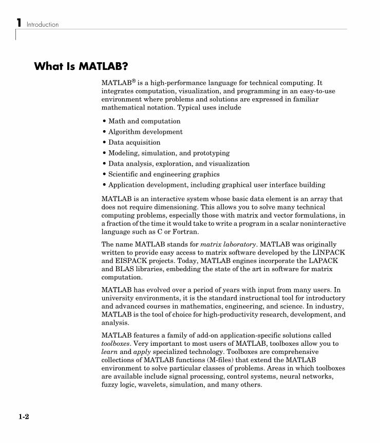
What Is MATLAB? MATLAB® is a high-performance language for technical computing. It integrates computation, visualization, and programming in an easy-to-use environment where problems and solutions are expressed in familiar mathematical notation. Typical uses include
• Math and computation
• Algorithm development
• Data acquisition
• Modeling, simulation, and prototyping
• Data analysis, exploration, and visualization
• Scientific and engineering graphics
• Application development, including graphical user interface building
MATLAB is an interactive system whose basic data element is an array that does not require dimensioning. This allows you to solve many technical computing problems, especially those with matrix and vector formulations, in a fraction of the time it would take to write a program in a scalar noninteractive language such as C or Fortran.
The name MATLAB stands for matrix laboratory. MATLAB was originally written to provide easy access to matrix software developed by the LINPACK and EISPACK projects. Today, MATLAB engines incorporate the LAPACK and BLAS libraries, embedding the state of the art in software for matrix computation.
MATLAB has evolved over a period of years with input from many users. In university environments, it is the standard instructional tool for introductory and advanced courses in mathematics, engineering, and science. In industry, MATLAB is the tool of choice for high-productivity research, development, and analysis.
MATLAB features a family of add-on application-specific solutions called toolboxes. Very important to most users of MATLAB, toolboxes allow you to learn and apply specialized technology. Toolboxes are comprehensive collections of MATLAB functions (M-files) that extend the MATLAB environment to solve particular classes of problems. Areas in which toolboxes are available include signal processing, control systems, neural networks, fuzzy logic, wavelets, simulation, and many others.
What Is MATLAB?
The MATLAB SystemThe MATLAB system consists of five main parts:
Development Environment. This is the set of tools and facilities that help you use MATLAB functions and files. Many of these tools are graphical user interfaces. It includes the MATLAB desktop and Command Window, a command history, an editor and debugger, and browsers for viewing help, the workspace, files, and the search path.
The MATLAB Mathematical Function Library. This is a vast collection of computational algorithms ranging from elementary functions like sum, sine, cosine, and complex arithmetic, to more sophisticated functions like matrix inverse, matrix eigenvalues, Bessel functions, and fast Fourier transforms.
The MATLAB Language. This is a high-level matrix/array language with control flow statements, functions, data structures, input/output, and object-oriented programming features. It allows both “programming in the small” to rapidly create quick and dirty throw-away programs, and “programming in the large” to create complete large and complex application programs.
Graphics. MATLAB has extensive facilities for displaying vectors and matrices as graphs, as well as annotating and printing these graphs. It includes high-level functions for two-dimensional and three-dimensional data visualization, image processing, animation, and presentation graphics. It also includes low-level functions that allow you to fully customize the appearance of graphics as well as to build complete graphical user interfaces on your MATLAB applications.
The MATLAB Application Program Interface (API). This is a library that allows you to write C and Fortran programs that interact with MATLAB. It includes facilities for calling routines from MATLAB (dynamic linking), calling MATLAB as a computational engine, and for reading and writing MAT-files.
1-3
1 Introduction
1-4
MATLAB DocumentationMATLAB provides extensive documentation, in both printed and online format, to help you learn about and use all of its features. If you are a new user, start with this book, Getting Started with MATLAB, which introduces you to MATLAB. It covers all the primary MATLAB features at a high level, including many examples to help you to learn the material quickly:
• Chapter 2, “Development Environment”—Introduces the MATLAB development environment, including information about tools and the MATLAB desktop.
• Chapter 3, “Manipulating Matrices”—Introduces how to use MATLAB to generate matrices and perform mathematical operations on matrices.
• Chapter 4, “Graphics”—Introduces MATLAB graphic capabilities, including information about plotting data, annotating graphs, and working with images.
• Chapter 5, “Programming with MATLAB”—Describes how to use the MATLAB language to create scripts and functions, and manipulate data structures, such as cell arrays and multidimensional arrays. This section also provides an overview of the demo programs included with MATLAB.
To find more detailed information about any of these topics, use the MATLAB online help. The online help provides task-oriented and reference information about MATLAB features. The MATLAB documentation is also available in printed form and in PDF format.
MATLAB Online HelpTo view the online documentation, select MATLAB Help from the Help menu in MATLAB. For more information about using the online documentation, see “Help Browser” on page 2-7.
For MATLAB, the documentation is organized into these main topics:
• Development Environment—Provides complete information on the MATLAB desktop.
• Mathematics—Describes how to use MATLAB mathematical and statistical capabilities.
MATLAB Documentation
• Programming and Data Types—Describes how to create scripts and functions using the MATLAB language.
• Graphics—Describes how to plot your data using MATLAB graphics capabilities.
• 3-D Visualization—Introduces how to use views, lighting, and transparency to achieve more complex graphic effects than can be achieved using the basic plotting functions.
• Creating Graphical User Interfaces—Describes how to use MATLAB graphical user interface layout tools.
• External Interfaces/API—Describes MATLAB interfaces to C and Fortran programs, Java classes and objects, COM objects, data files, serial port I/O, and DDE.
In addition to the above documentation, MATLAB documentation includes the following reference material:
• Functions - By Category—Lists all the core MATLAB functions. Each function has a reference page that provides the syntax, description, mathematical algorithm (where appropriate), and related functions.
You can also access any function reference page using the “Functions - Alphabetical List”.
• Handle Graphics Property Browser—Enables you to easily access descriptions of graphics object properties. For more information about MATLAB graphics, see “Handle Graphics” on page 4-26
• External Interfaces/API Reference—Covers those functions used by the MATLAB external interfaces, providing information on syntax in the calling language, description, arguments, return values, and examples.
MATLAB online documentation also includes
• Examples—An index of major examples included in the documentation.
• Release Notes—Introduces new features and identifies known problems in the current release.
• Printable Documentation—Provides access to the PDF versions of the documentation, which are suitable for printing.
1-5

1 Introduction
1-6
2
Development EnvironmentThe Development Environment covers starting and quitting MATLAB, and the tools and functions that help you to work with MATLAB variables and files, including the MATLAB desktop. For more information about the topics covered here, see the corresponding topics in “Development Environment”, which is available in the online as well as in the printed manual, Using MATLAB.
Starting and Quitting MATLAB (p. 2-2)
Start and quit MATLAB and perform operations upon startup and shutdown.
MATLAB Desktop (p. 2-3) The graphical user interface to MATLAB.
Desktop Tools (p. 2-5) Use the Command Window for running functions and entering variables, Start button for launching tools, demos, and documentation, Help browser for accessing documentation, Current Directory browser for accessing files, Workspace browser for viewing variables, Editor/Debugger for modifying MATLAB program files (M-files), and Profiler for optimizing M-file performance.
Other Development Environment Features (p. 2-16)
Import and export data, improve M-file performance, interface with source control systems, and access MATLAB from Microsoft Word using the MATLAB Notebook feature.
2 Development Environment
2-2
Starting and Quitting MATLAB
Starting MATLABOn Windows platforms, to start MATLAB, double-click the MATLAB shortcut icon on your Windows desktop.
On UNIX platforms, to start MATLAB, type matlab at the operating system prompt.
After starting MATLAB, the MATLAB desktop opens—see “MATLAB Desktop” on page 2-3.
You can change the directory in which MATLAB starts, define startup options including running a script upon startup, and reduce startup time in some situations. For more information, see the documentation for starting MATLAB.
Quitting MATLABTo end your MATLAB session, select Exit MATLAB from the File menu in the desktop, or type quit in the Command Window. To execute specified functions each time MATLAB quits, such as saving the workspace, you can create and run a finish.m script.
MATLAB Desktop
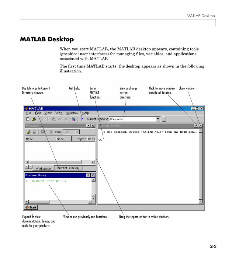
MATLAB DesktopWhen you start MATLAB, the MATLAB desktop appears, containing tools (graphical user interfaces) for managing files, variables, and applications associated with MATLAB.
The first time MATLAB starts, the desktop appears as shown in the following illustration.
View or change current directory.
View or use previously run functions.
Enter MATLAB functions.
Close window.
Drag the separator bar to resize windows.
Click to move window outside of desktop.
Get help.
Expand to view documentation, demos, and tools for your products.
Use tab to go to Current Directory browser.
2-3
2 Development Environment
2-4
You can change the way your desktop looks by opening, closing, moving, and resizing the tools in it. Use the View menu to open or close the tools. You can also move tools outside the desktop or move them back into the desktop (docking). All the desktop tools provide common features such as context menus and keyboard shortcuts.
You can specify certain characteristics for the desktop tools by selecting Preferences from the File menu. For example, you can specify the font characteristics for Command Window text. For more information, click the Help button in the Preferences dialog box.
Desktop Tools
Desktop ToolsThis section provides an introduction to the MATLAB desktop tools. You can also use MATLAB functions to perform most of the features found in the desktop tools. The tools are
• “Command Window”
• “Command History”
• “Start Button and Launch Pad”
• “Help Browser”
• “Current Directory Browser”
• “Workspace Browser”
• “Array Editor”
• “Editor/Debugger”
• “Profiler”
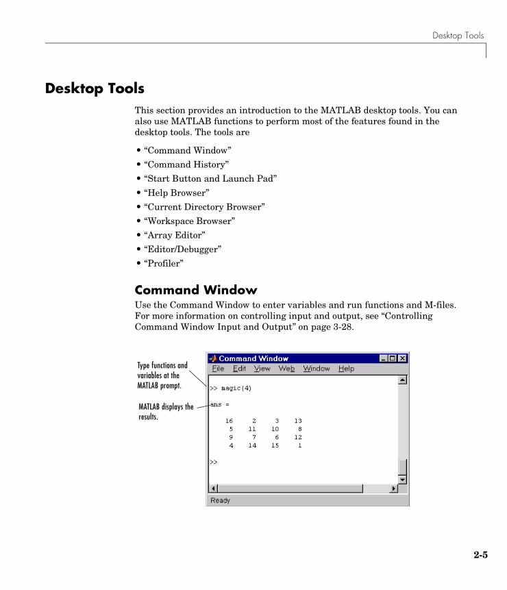
Command WindowUse the Command Window to enter variables and run functions and M-files. For more information on controlling input and output, see “Controlling Command Window Input and Output” on page 3-28.
Type functions and variables at the MATLAB prompt.
MATLAB displays the results.
2-5
2 Development Environment
2-6
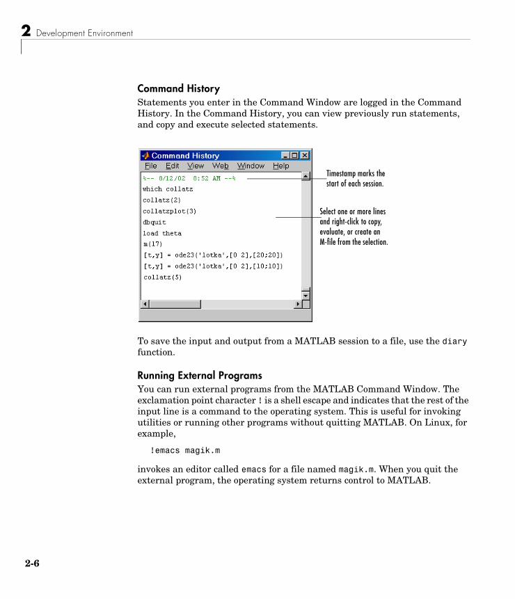
Command HistoryStatements you enter in the Command Window are logged in the Command History. In the Command History, you can view previously run statements, and copy and execute selected statements.
To save the input and output from a MATLAB session to a file, use the diary function.
Running External Programs You can run external programs from the MATLAB Command Window. The exclamation point character ! is a shell escape and indicates that the rest of the input line is a command to the operating system. This is useful for invoking utilities or running other programs without quitting MATLAB. On Linux, for example,
!emacs magik.m
invokes an editor called emacs for a file named magik.m. When you quit the external program, the operating system returns control to MATLAB.
Timestamp marks the start of each session.
Select one or more lines and right-click to copy, evaluate, or create an M-file from the selection.
Desktop Tools
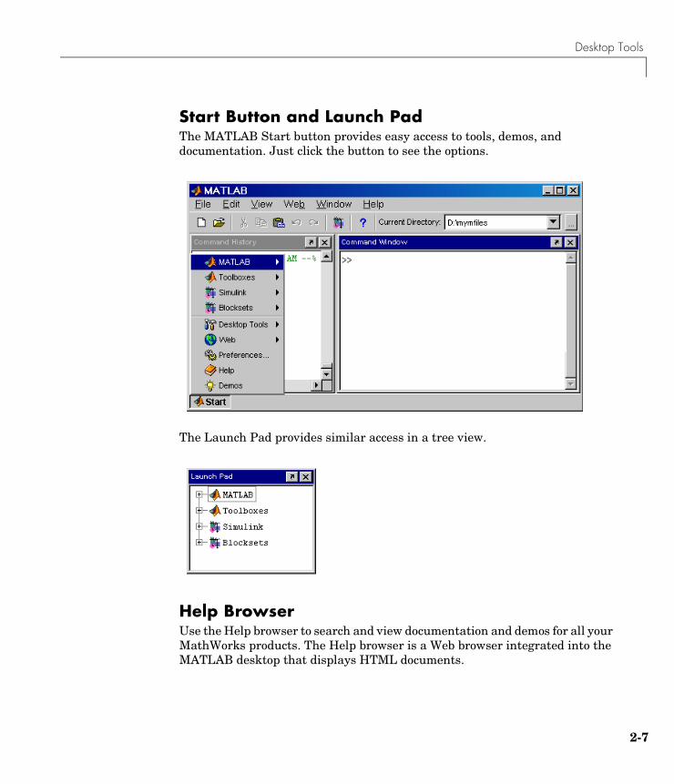
Start Button and Launch PadThe MATLAB Start button provides easy access to tools, demos, and documentation. Just click the button to see the options.
The Launch Pad provides similar access in a tree view.
Help BrowserUse the Help browser to search and view documentation and demos for all your MathWorks products. The Help browser is a Web browser integrated into the MATLAB desktop that displays HTML documents.
2-7
2 Development Environment
2-8
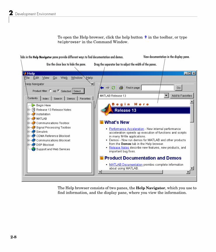
To open the Help browser, click the help button in the toolbar, or type helpbrowser in the Command Window.
The Help browser consists of two panes, the Help Navigator, which you use to find information, and the display pane, where you view the information.
Tabs in the Help Navigator pane provide different ways to find documentation and demos.
Drag the separator bar to adjust the width of the panes.
View documentation in the display pane.
Use the close box to hide the pane.
Desktop Tools
Help NavigatorUse the Help Navigator to find information. It includes
• Product filter—Set the filter to show documentation only for the products you specify.
• Contents tab—View the titles and tables of contents of documentation for your products.
• Index tab—Find specific index entries (selected keywords) in the MathWorks documentation for your products.
• Demos tab—View and run demonstrations for your MathWorks products.
• Search tab—Look for a specific word or phrase in the documentation. To get help for a specific function, set the Search type to Function Name.
• Favorites tab—View a list of links to documents you previously designated as favorites.
Display PaneAfter finding documentation using the Help Navigator, view it in the display pane. While viewing the documentation, you can
• Browse to other pages—Use the arrows at the tops and bottoms of the pages to move through the document, or use the back and forward buttons in the toolbar to go to previously viewed pages.
• Bookmark pages—Click the Add to Favorites button in the toolbar.
• Print pages—Click the print button in the toolbar.
• Find a term in the page—Type a term in the Find in page field in the toolbar and click Go.
Other features available in the display pane are copying information, evaluating a selection, and viewing Web pages.
2-9
2 Development Environment
2-1
For More HelpIn addition to the Help browser, you can use help functions. To get help for a specific function, use doc. For example, doc format displays documentation for the format function in the Help browser. If you type help followed by the function name, a briefer form of the documentation appears in the Command Window. Other means for getting help include contacting Technical Support (http://www.mathworks.com/support) and participating in the newsgroup for MATLAB users, comp.soft-sys.matlab.
Current Directory BrowserMATLAB file operations use the current directory and the search path as reference points. Any file you want to run must either be in the current directory or on the search path.
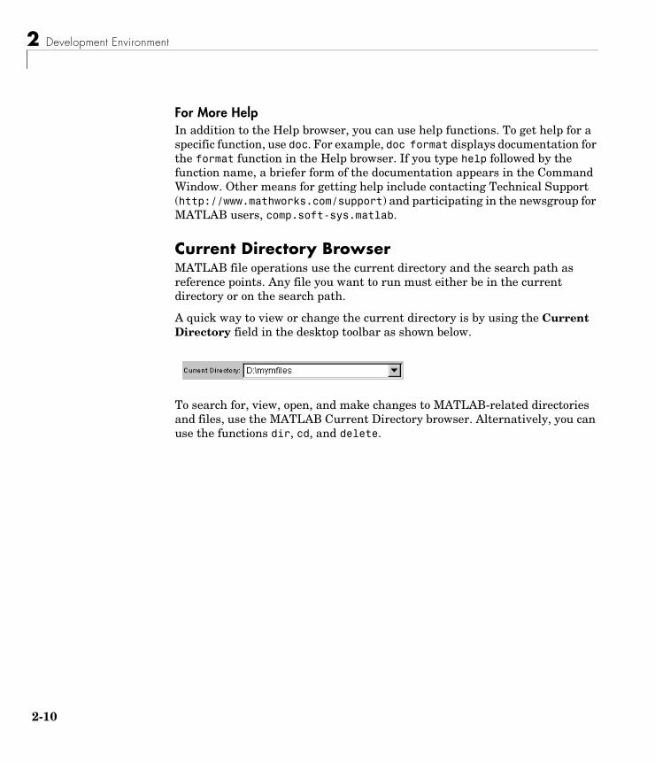
A quick way to view or change the current directory is by using the Current Directory field in the desktop toolbar as shown below.
To search for, view, open, and make changes to MATLAB-related directories and files, use the MATLAB Current Directory browser. Alternatively, you can use the functions dir, cd, and delete.
0
Desktop Tools
Search PathMATLAB uses a search path to find M-files and other MATLAB-related files, which are organized in directories on your file system. Any file you want to run in MATLAB must reside in the current directory or in a directory that is on the search path. Add the directories containing files you create to the MATLAB search path. By default, the files supplied with MATLAB and MathWorks toolboxes are included in the search path.
To see which directories are on the search path or to change the search path, select Set Path from the File menu in the desktop, and use the Set Path dialog box. Alternatively, you can use the path function to view the search path, addpath to add directories to the path, and rmpath to remove directories from the path.
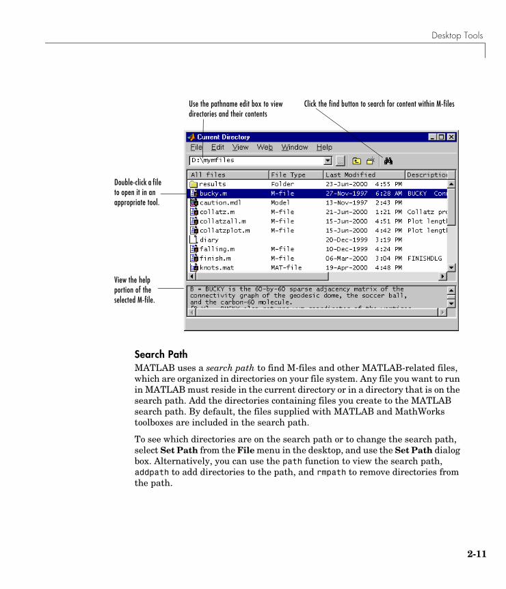
Use the pathname edit box to view directories and their contents
Click the find button to search for content within M-files
Double-click a file to open it in an appropriate tool.
View the help portion of the selected M-file.
2-11
2 Development Environment
2-1
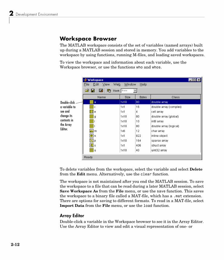
Workspace BrowserThe MATLAB workspace consists of the set of variables (named arrays) built up during a MATLAB session and stored in memory. You add variables to the workspace by using functions, running M-files, and loading saved workspaces.
To view the workspace and information about each variable, use the Workspace browser, or use the functions who and whos.
To delete variables from the workspace, select the variable and select Delete from the Edit menu. Alternatively, use the clear function.
The workspace is not maintained after you end the MATLAB session. To save the workspace to a file that can be read during a later MATLAB session, select Save Workspace As from the File menu, or use the save function. This saves the workspace to a binary file called a MAT-file, which has a .mat extension. There are options for saving to different formats. To read in a MAT-file, select Import Data from the File menu, or use the load function.
Array EditorDouble-click a variable in the Workspace browser to see it in the Array Editor. Use the Array Editor to view and edit a visual representation of one- or
Double-click a variable to see and change its contents in the Array Editor.
2
Desktop Tools
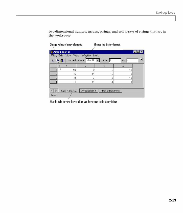
two-dimensional numeric arrays, strings, and cell arrays of strings that are in the workspace.
Change values of array elements. Change the display format.
Use the tabs to view the variables you have open in the Array Editor.
2-13
2 Development Environment
2-1
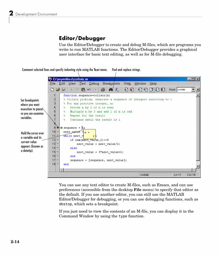
Editor/DebuggerUse the Editor/Debugger to create and debug M-files, which are programs you write to run MATLAB functions. The Editor/Debugger provides a graphical user interface for basic text editing, as well as for M-file debugging.
You can use any text editor to create M-files, such as Emacs, and can use preferences (accessible from the desktop File menu) to specify that editor as the default. If you use another editor, you can still use the MATLAB Editor/Debugger for debugging, or you can use debugging functions, such as dbstop, which sets a breakpoint.
If you just need to view the contents of an M-file, you can display it in the Command Window by using the type function.
Set breakpoints where you want execution to pause so you can examine variables.
Find and replace strings.Comment selected lines and specify indenting style using the Text menu.
Hold the cursor over a variable and its current value appears (known as a datatip).
4
Desktop Tools
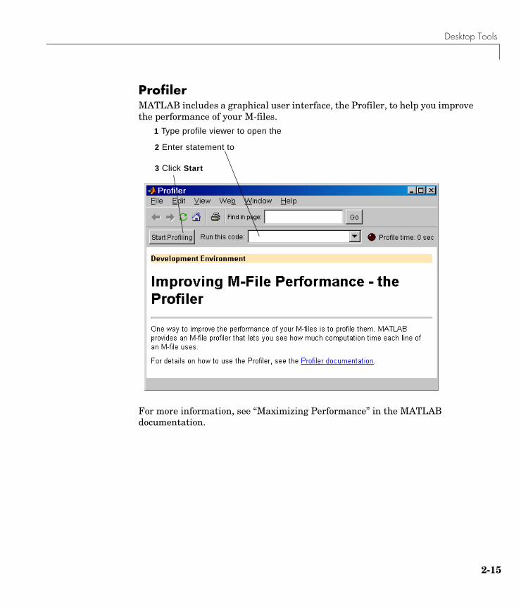
ProfilerMATLAB includes a graphical user interface, the Profiler, to help you improve the performance of your M-files.
For more information, see “Maximizing Performance” in the MATLAB documentation.
2 Enter statement to
3 Click Start
1 Type profile viewer to open the
2-15
2 Development Environment
2-1
Other Development Environment FeaturesAdditional development environment features are
• Importing and Exporting Data—Techniques for bringing data created by other applications into the MATLAB workspace, including the Import Wizard, and packaging MATLAB workspace variables for use by other applications.
• Interfacing with Source Control Systems—Access your source control system from within MATLAB, Simulink®, and Stateflow®.
• Using Notebook—Access MATLAB numeric computation and visualization software from within a word processing environment (Microsoft Word).
6
3
Manipulating Matrices
This section provides an introduction to matrix operations in MATLAB.
Matrices and Magic Squares (p. 3-2) Enter matrices, perform matrix operations, and access matrix elements.
Expressions (p. 3-10) Work with variables, numbers, operators, functions, expressions.
Working with Matrices (p. 3-14) Generating matrices, load matrices, create matrices from M-files and concatentation, and delete matrix rows and columns.
More About Matrices and Arrays (p. 3-18)
Use matrices for linear algebra, work with arrays, multivariate data, scalar expansion, and logical subscripting, and use the find function.
Controlling Command Window Input and Output (p. 3-28)
Change output format, suppress output, enter long lines, and edit at the command line.
3 Manipulating Matrices
3-2
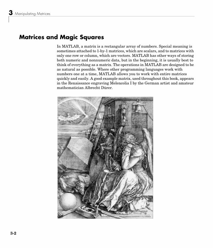
Matrices and Magic SquaresIn MATLAB, a matrix is a rectangular array of numbers. Special meaning is sometimes attached to 1-by-1 matrices, which are scalars, and to matrices with only one row or column, which are vectors. MATLAB has other ways of storing both numeric and nonnumeric data, but in the beginning, it is usually best to think of everything as a matrix. The operations in MATLAB are designed to be as natural as possible. Where other programming languages work with numbers one at a time, MATLAB allows you to work with entire matrices quickly and easily. A good example matrix, used throughout this book, appears in the Renaissance engraving Melencolia I by the German artist and amateur mathematician Albrecht Dürer.
Matrices and Magic Squares
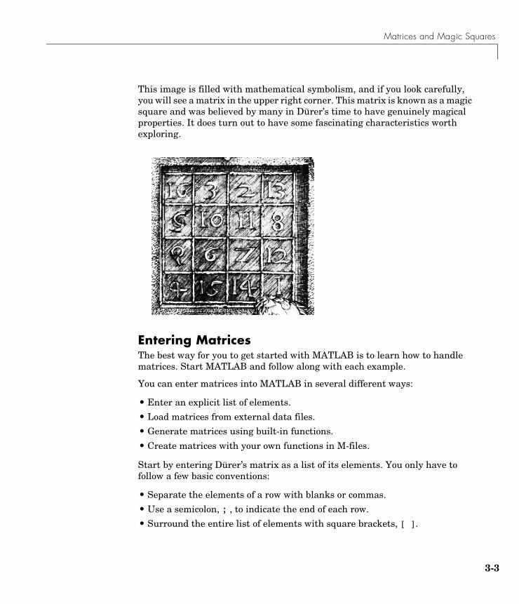
This image is filled with mathematical symbolism, and if you look carefully, you will see a matrix in the upper right corner. This matrix is known as a magic square and was believed by many in Dürer’s time to have genuinely magical properties. It does turn out to have some fascinating characteristics worth exploring.
Entering MatricesThe best way for you to get started with MATLAB is to learn how to handle matrices. Start MATLAB and follow along with each example.
You can enter matrices into MATLAB in several different ways:
• Enter an explicit list of elements.
• Load matrices from external data files.
• Generate matrices using built-in functions.
• Create matrices with your own functions in M-files.
Start by entering Dürer’s matrix as a list of its elements. You only have to follow a few basic conventions:
• Separate the elements of a row with blanks or commas.
• Use a semicolon, ; , to indicate the end of each row.
• Surround the entire list of elements with square brackets, [ ].
3-3
3 Manipulating Matrices
3-4
To enter Dürer’s matrix, simply type in the Command Window
A = [16 3 2 13; 5 10 11 8; 9 6 7 12; 4 15 14 1]
MATLAB displays the matrix you just entered.
A = 16 3 2 13 5 10 11 8 9 6 7 12 4 15 14 1
This exactly matches the numbers in the engraving. Once you have entered the matrix, it is automatically remembered in the MATLAB workspace. You can refer to it simply as A. Now that you have A in the workspace, take a look at what makes it so interesting. Why is it magic?
sum, transpose, and diagYou are probably already aware that the special properties of a magic square have to do with the various ways of summing its elements. If you take the sum along any row or column, or along either of the two main diagonals, you will always get the same number. Let us verify that using MATLAB. The first statement to try is
sum(A)
MATLAB replies with
ans = 34 34 34 34
When you do not specify an output variable, MATLAB uses the variable ans, short for answer, to store the results of a calculation. You have computed a row vector containing the sums of the columns of A. Sure enough, each of the columns has the same sum, the magic sum, 34.
How about the row sums? MATLAB has a preference for working with the columns of a matrix, so the easiest way to get the row sums is to transpose the matrix, compute the column sums of the transpose, and then transpose the result. The transpose operation is denoted by an apostrophe or single quote, '. It flips a matrix about its main diagonal and it turns a row vector into a column vector.
Matrices and Magic Squares
So
A'produces
ans = 16 5 9 4 3 10 6 15 2 11 7 14 13 8 12 1
And
sum(A')'
produces a column vector containing the row sums
ans = 34 34 34 34
The sum of the elements on the main diagonal is obtained with the sum and the diag functions.
diag(A)
produces
ans = 16 10 7 1
and
sum(diag(A))
produces
ans = 34
3-5
3 Manipulating Matrices
3-6
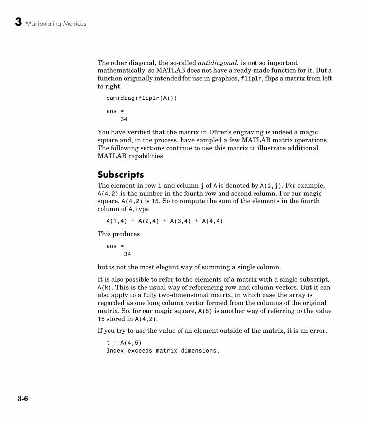
The other diagonal, the so-called antidiagonal, is not so important mathematically, so MATLAB does not have a ready-made function for it. But a function originally intended for use in graphics, fliplr, flips a matrix from left to right.
sum(diag(fliplr(A)))
ans = 34
You have verified that the matrix in Dürer’s engraving is indeed a magic square and, in the process, have sampled a few MATLAB matrix operations. The following sections continue to use this matrix to illustrate additional MATLAB capabilities.
SubscriptsThe element in row i and column j of A is denoted by A(i,j). For example, A(4,2) is the number in the fourth row and second column. For our magic square, A(4,2) is 15. So to compute the sum of the elements in the fourth column of A, type
A(1,4) + A(2,4) + A(3,4) + A(4,4)
This produces
ans = 34
but is not the most elegant way of summing a single column.
It is also possible to refer to the elements of a matrix with a single subscript, A(k). This is the usual way of referencing row and column vectors. But it can also apply to a fully two-dimensional matrix, in which case the array is regarded as one long column vector formed from the columns of the original matrix. So, for our magic square, A(8) is another way of referring to the value 15 stored in A(4,2).
If you try to use the value of an element outside of the matrix, it is an error.
t = A(4,5)Index exceeds matrix dimensions.
Matrices and Magic Squares
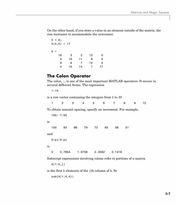
On the other hand, if you store a value in an element outside of the matrix, the size increases to accommodate the newcomer.
X = A;X(4,5) = 17
X = 16 3 2 13 0 5 10 11 8 0 9 6 7 12 0 4 15 14 1 17
The Colon OperatorThe colon, :, is one of the most important MATLAB operators. It occurs in several different forms. The expression
1:10
is a row vector containing the integers from 1 to 10
1 2 3 4 5 6 7 8 9 10
To obtain nonunit spacing, specify an increment. For example,
100:-7:50
is
100 93 86 79 72 65 58 51
and
0:pi/4:pi
is
0 0.7854 1.5708 2.3562 3.1416
Subscript expressions involving colons refer to portions of a matrix.
A(1:k,j)
is the first k elements of the jth column of A. So
sum(A(1:4,4))
3-7
3 Manipulating Matrices
3-8
computes the sum of the fourth column. But there is a better way. The colon by itself refers to all the elements in a row or column of a matrix and the keyword end refers to the last row or column. So
sum(A(:,end))
computes the sum of the elements in the last column of A.
ans = 34
Why is the magic sum for a 4-by-4 square equal to 34? If the integers from 1 to 16 are sorted into four groups with equal sums, that sum must be
sum(1:16)/4
which, of course, is
ans = 34
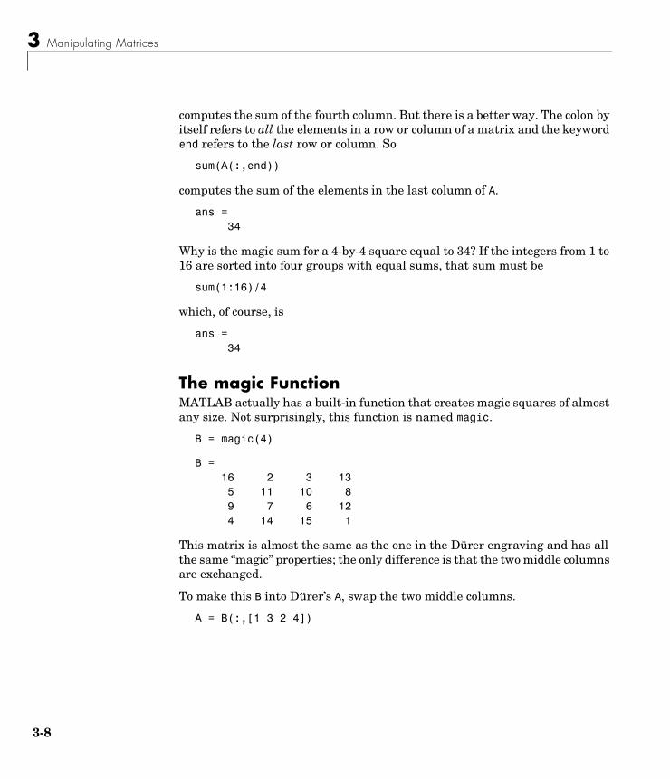
The magic FunctionMATLAB actually has a built-in function that creates magic squares of almost any size. Not surprisingly, this function is named magic.
B = magic(4)
B = 16 2 3 13 5 11 10 8 9 7 6 12 4 14 15 1
This matrix is almost the same as the one in the Dürer engraving and has all the same “magic” properties; the only difference is that the two middle columns are exchanged.
To make this B into Dürer’s A, swap the two middle columns.
A = B(:,[1 3 2 4])
Matrices and Magic Squares
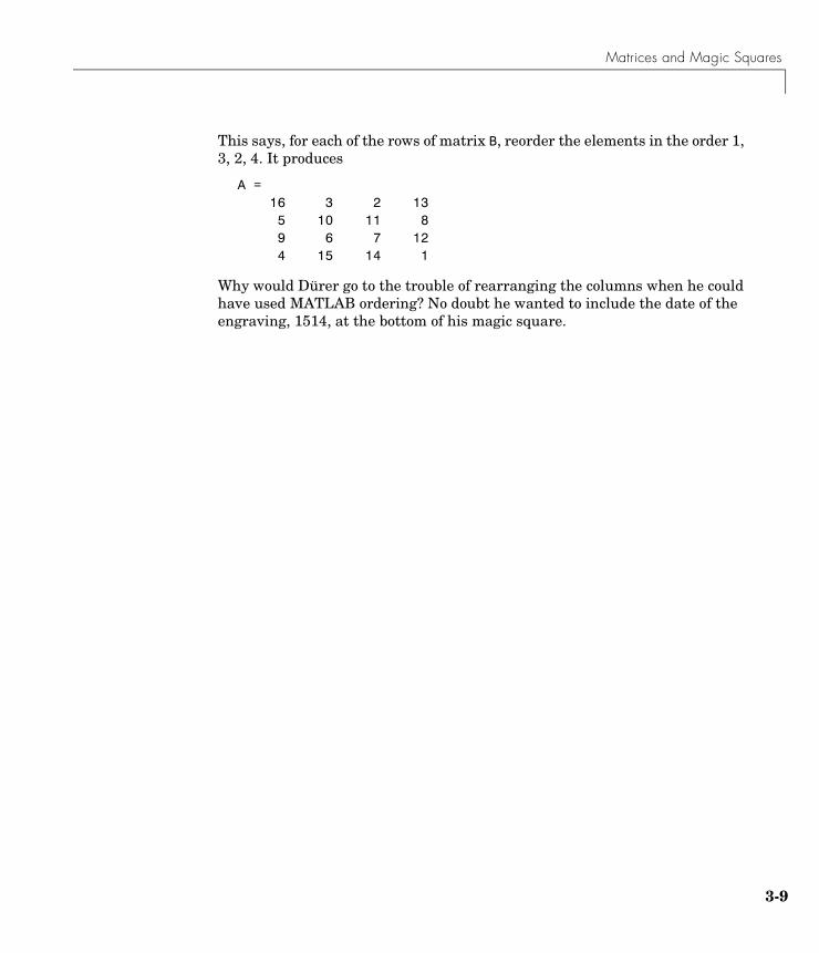
This says, for each of the rows of matrix B, reorder the elements in the order 1, 3, 2, 4. It produces
A = 16 3 2 13 5 10 11 8 9 6 7 12 4 15 14 1
Why would Dürer go to the trouble of rearranging the columns when he could have used MATLAB ordering? No doubt he wanted to include the date of the engraving, 1514, at the bottom of his magic square.
3-9
3 Manipulating Matrices
3-1
ExpressionsLike most other programming languages, MATLAB provides mathematical expressions, but unlike most programming languages, these expressions involve entire matrices. The building blocks of expressions are
• “Variables” on page 3-10
• “Numbers” on page 3-10
• “Operators” on page 3-11Operators
• “Functions” on page 3-11
See also, “Examples of Expressions” on page 3-13.
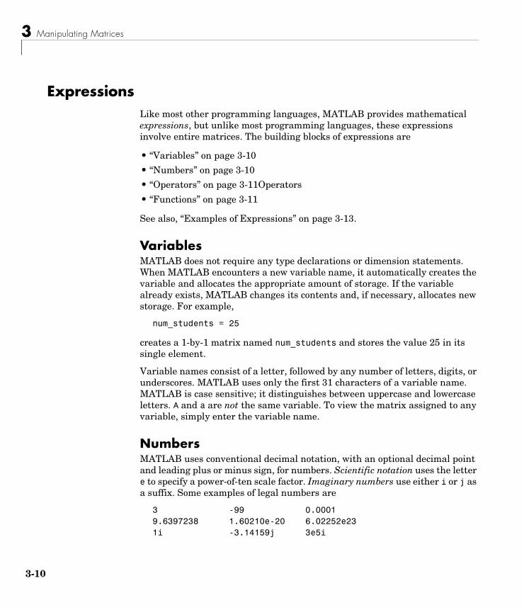
VariablesMATLAB does not require any type declarations or dimension statements. When MATLAB encounters a new variable name, it automatically creates the variable and allocates the appropriate amount of storage. If the variable already exists, MATLAB changes its contents and, if necessary, allocates new storage. For example,
num_students = 25
creates a 1-by-1 matrix named num_students and stores the value 25 in its single element.
Variable names consist of a letter, followed by any number of letters, digits, or underscores. MATLAB uses only the first 31 characters of a variable name. MATLAB is case sensitive; it distinguishes between uppercase and lowercase letters. A and a are not the same variable. To view the matrix assigned to any variable, simply enter the variable name.
NumbersMATLAB uses conventional decimal notation, with an optional decimal point and leading plus or minus sign, for numbers. Scientific notation uses the letter e to specify a power-of-ten scale factor. Imaginary numbers use either i or j as a suffix. Some examples of legal numbers are
3 -99 0.00019.6397238 1.60210e-20 6.02252e231i -3.14159j 3e5i
0
Expressions
All numbers are stored internally using the long format specified by the IEEE floating-point standard. Floating-point numbers have a finite precision of roughly 16 significant decimal digits and a finite range of roughly 10-308 to 10+308.
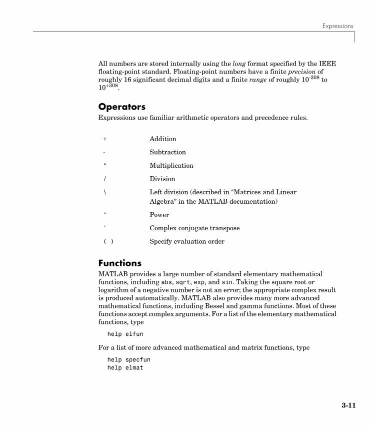
Operators Expressions use familiar arithmetic operators and precedence rules.
FunctionsMATLAB provides a large number of standard elementary mathematical functions, including abs, sqrt, exp, and sin. Taking the square root or logarithm of a negative number is not an error; the appropriate complex result is produced automatically. MATLAB also provides many more advanced mathematical functions, including Bessel and gamma functions. Most of these functions accept complex arguments. For a list of the elementary mathematical functions, type
help elfun
For a list of more advanced mathematical and matrix functions, type
help specfunhelp elmat
+ Addition
- Subtraction
* Multiplication
/ Division
\ Left division (described in “Matrices and Linear Algebra” in the MATLAB documentation)
^ Power
' Complex conjugate transpose
( ) Specify evaluation order
3-11
3 Manipulating Matrices
3-1
Some of the functions, like sqrt and sin, are built in. They are part of the MATLAB core so they are very efficient, but the computational details are not readily accessible. Other functions, like gamma and sinh, are implemented in M-files. You can see the code and even modify it if you want.
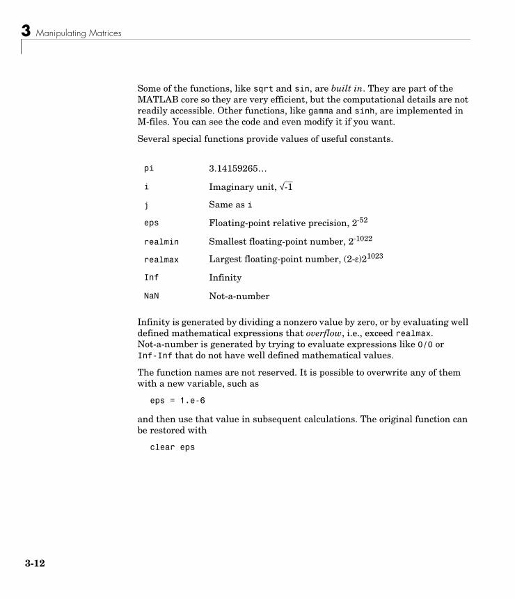
Several special functions provide values of useful constants.
Infinity is generated by dividing a nonzero value by zero, or by evaluating well defined mathematical expressions that overflow, i.e., exceed realmax. Not-a-number is generated by trying to evaluate expressions like 0/0 or Inf-Inf that do not have well defined mathematical values.
The function names are not reserved. It is possible to overwrite any of them with a new variable, such as
eps = 1.e-6
and then use that value in subsequent calculations. The original function can be restored with
clear eps
pi 3.14159265…
i Imaginary unit, √-1
j Same as i
eps Floating-point relative precision, 2-52
realmin Smallest floating-point number, 2-1022
realmax Largest floating-point number, (2-ε)21023
Inf Infinity
NaN Not-a-number
2
Expressions
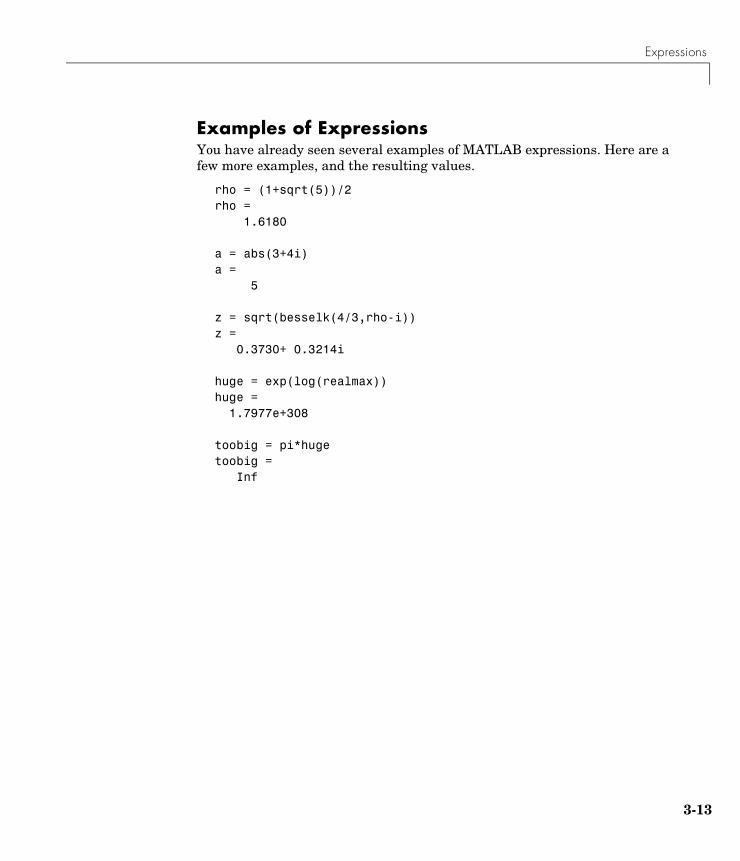
Examples of ExpressionsYou have already seen several examples of MATLAB expressions. Here are a few more examples, and the resulting values.
rho = (1+sqrt(5))/2rho = 1.6180
a = abs(3+4i)a = 5
z = sqrt(besselk(4/3,rho-i))z = 0.3730+ 0.3214i
huge = exp(log(realmax))huge = 1.7977e+308
toobig = pi*hugetoobig = Inf
3-13
3 Manipulating Matrices
3-1
Working with MatricesThis section introduces you to other ways of creating matrices:
• “Generating Matrices” on page 3-14
• “The load Function” on page 3-15
• “M-Files” on page 3-15
• “Concatenation” on page 3-16
• “Deleting Rows and Columns” on page 3-17
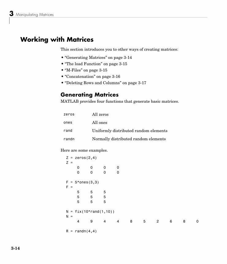
Generating MatricesMATLAB provides four functions that generate basic matrices.
Here are some examples.
Z = zeros(2,4)Z = 0 0 0 0 0 0 0 0
F = 5*ones(3,3)F = 5 5 5 5 5 5 5 5 5
N = fix(10*rand(1,10))N = 4 9 4 4 8 5 2 6 8 0
R = randn(4,4)
zeros All zeros
ones All ones
rand Uniformly distributed random elements
randn Normally distributed random elements
4
Working with Matrices
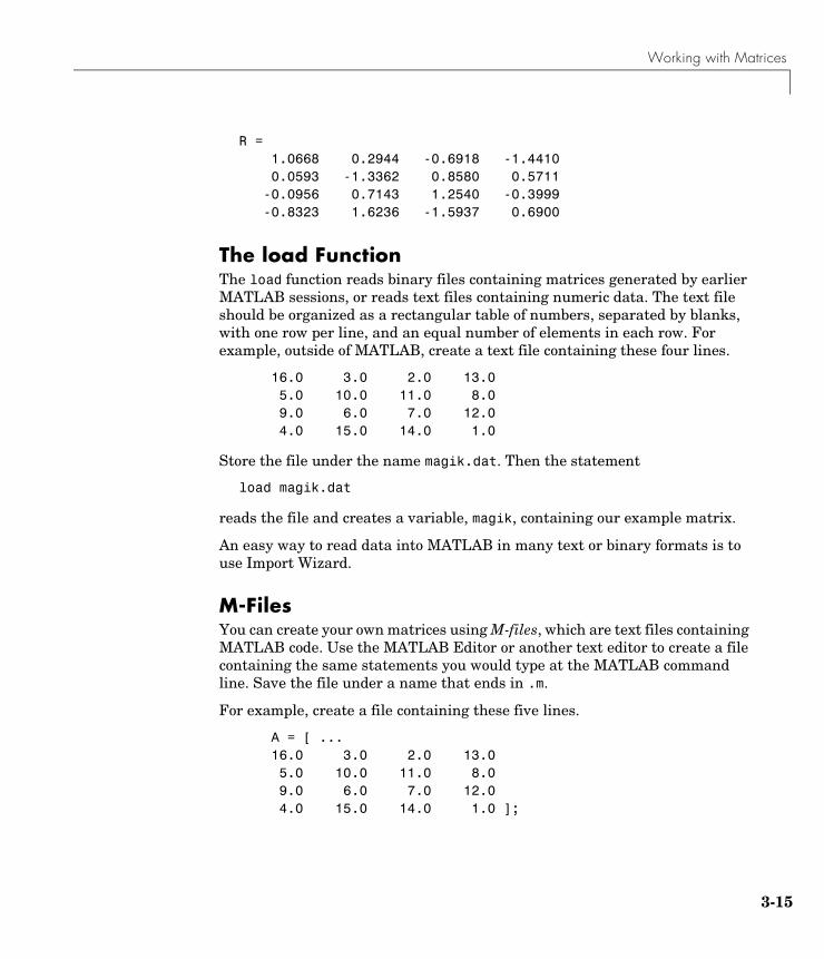
R = 1.0668 0.2944 -0.6918 -1.4410 0.0593 -1.3362 0.8580 0.5711 -0.0956 0.7143 1.2540 -0.3999 -0.8323 1.6236 -1.5937 0.6900
The load FunctionThe load function reads binary files containing matrices generated by earlier MATLAB sessions, or reads text files containing numeric data. The text file should be organized as a rectangular table of numbers, separated by blanks, with one row per line, and an equal number of elements in each row. For example, outside of MATLAB, create a text file containing these four lines.
16.0 3.0 2.0 13.0 5.0 10.0 11.0 8.0 9.0 6.0 7.0 12.0 4.0 15.0 14.0 1.0
Store the file under the name magik.dat. Then the statement
load magik.dat
reads the file and creates a variable, magik, containing our example matrix.
An easy way to read data into MATLAB in many text or binary formats is to use Import Wizard.
M-FilesYou can create your own matrices using M-files, which are text files containing MATLAB code. Use the MATLAB Editor or another text editor to create a file containing the same statements you would type at the MATLAB command line. Save the file under a name that ends in .m.
For example, create a file containing these five lines.
A = [ ... 16.0 3.0 2.0 13.0 5.0 10.0 11.0 8.0 9.0 6.0 7.0 12.0 4.0 15.0 14.0 1.0 ];
3-15
3 Manipulating Matrices
3-1
Store the file under the name magik.m. Then the statement
magik
reads the file and creates a variable, A, containing our example matrix.
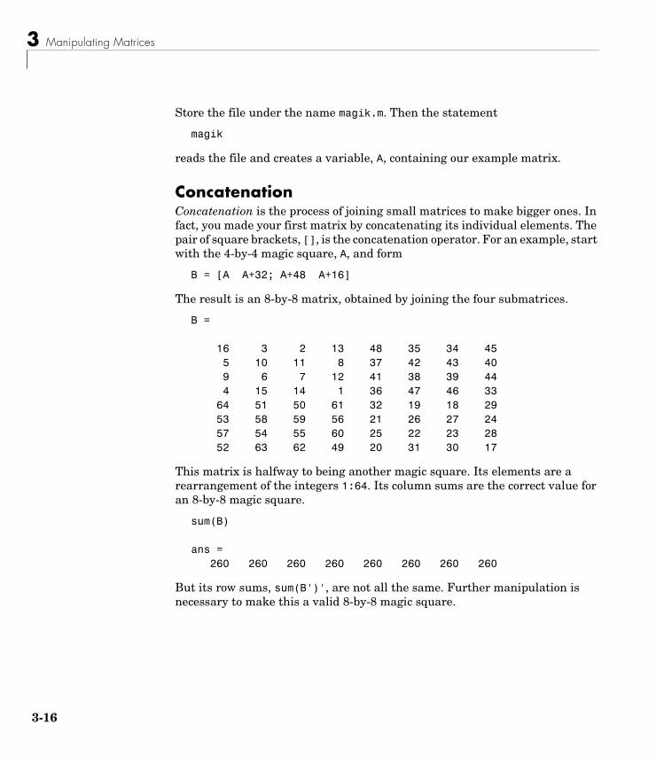
ConcatenationConcatenation is the process of joining small matrices to make bigger ones. In fact, you made your first matrix by concatenating its individual elements. The pair of square brackets, [], is the concatenation operator. For an example, start with the 4-by-4 magic square, A, and form
B = [A A+32; A+48 A+16]
The result is an 8-by-8 matrix, obtained by joining the four submatrices.
B =
16 3 2 13 48 35 34 45 5 10 11 8 37 42 43 40 9 6 7 12 41 38 39 44 4 15 14 1 36 47 46 33 64 51 50 61 32 19 18 29 53 58 59 56 21 26 27 24 57 54 55 60 25 22 23 28 52 63 62 49 20 31 30 17
This matrix is halfway to being another magic square. Its elements are a rearrangement of the integers 1:64. Its column sums are the correct value for an 8-by-8 magic square.
sum(B)
ans = 260 260 260 260 260 260 260 260
But its row sums, sum(B')', are not all the same. Further manipulation is necessary to make this a valid 8-by-8 magic square.
6
Working with Matrices
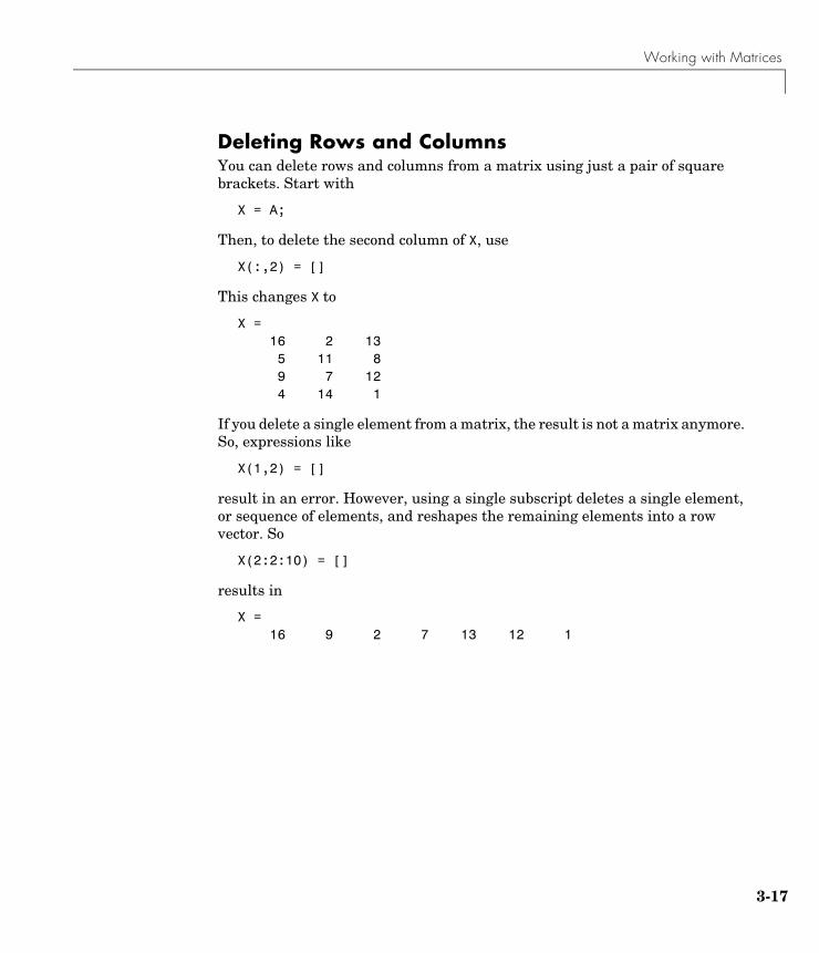
Deleting Rows and ColumnsYou can delete rows and columns from a matrix using just a pair of square brackets. Start with
X = A;
Then, to delete the second column of X, use
X(:,2) = []
This changes X to
X = 16 2 13 5 11 8 9 7 12 4 14 1
If you delete a single element from a matrix, the result is not a matrix anymore. So, expressions like
X(1,2) = []
result in an error. However, using a single subscript deletes a single element, or sequence of elements, and reshapes the remaining elements into a row vector. So
X(2:2:10) = []
results in
X = 16 9 2 7 13 12 1
3-17
3 Manipulating Matrices
3-1
More About Matrices and ArraysThis section shows you more about working with matrices and arrays, focusing on
• “Linear Algebra” on page 3-18
• “Arrays” on page 3-21
• “Multivariate Data” on page 3-24
• “Scalar Expansion” on page 3-25
• “Logical Subscripting” on page 3-26
• “The find Function” on page 3-27
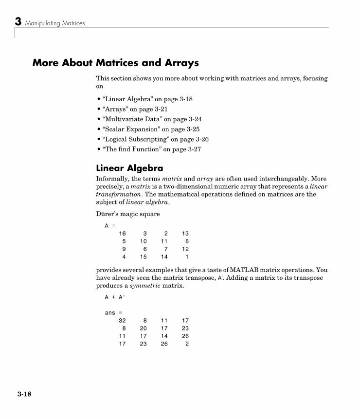
Linear AlgebraInformally, the terms matrix and array are often used interchangeably. More precisely, a matrix is a two-dimensional numeric array that represents a linear transformation. The mathematical operations defined on matrices are the subject of linear algebra.
Dürer’s magic square
A = 16 3 2 13 5 10 11 8 9 6 7 12 4 15 14 1
provides several examples that give a taste of MATLAB matrix operations. You have already seen the matrix transpose, A'. Adding a matrix to its transpose produces a symmetric matrix.
A + A'
ans = 32 8 11 17 8 20 17 23 11 17 14 26 17 23 26 2
8
More About Matrices and Arrays
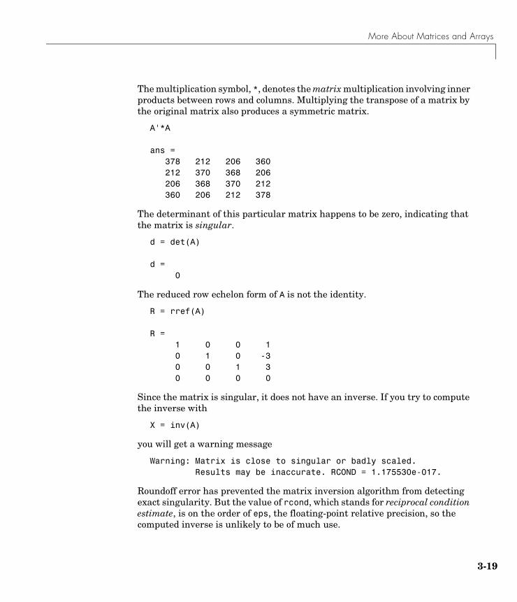
The multiplication symbol, *, denotes the matrix multiplication involving inner products between rows and columns. Multiplying the transpose of a matrix by the original matrix also produces a symmetric matrix.
A'*A
ans = 378 212 206 360 212 370 368 206 206 368 370 212 360 206 212 378
The determinant of this particular matrix happens to be zero, indicating that the matrix is singular.
d = det(A)
d = 0
The reduced row echelon form of A is not the identity.
R = rref(A)
R = 1 0 0 1 0 1 0 -3 0 0 1 3 0 0 0 0
Since the matrix is singular, it does not have an inverse. If you try to compute the inverse with
X = inv(A)
you will get a warning message
Warning: Matrix is close to singular or badly scaled. Results may be inaccurate. RCOND = 1.175530e-017.
Roundoff error has prevented the matrix inversion algorithm from detecting exact singularity. But the value of rcond, which stands for reciprocal condition estimate, is on the order of eps, the floating-point relative precision, so the computed inverse is unlikely to be of much use.
3-19
3 Manipulating Matrices
3-2
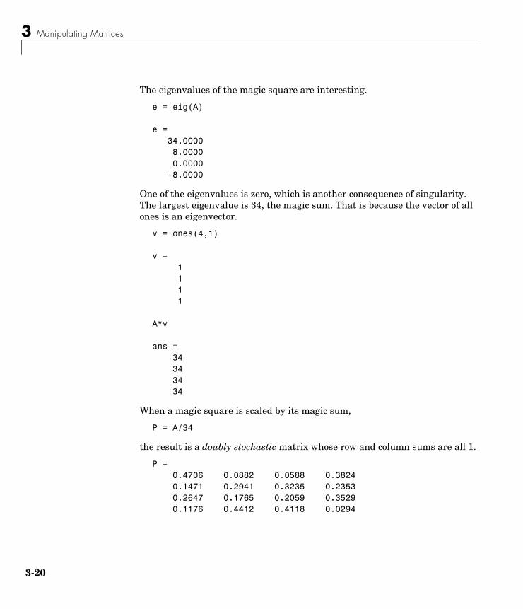
The eigenvalues of the magic square are interesting.
e = eig(A)
e = 34.0000 8.0000 0.0000 -8.0000
One of the eigenvalues is zero, which is another consequence of singularity. The largest eigenvalue is 34, the magic sum. That is because the vector of all ones is an eigenvector.
v = ones(4,1)
v = 1 1 1 1
A*v
ans = 34 34 34 34
When a magic square is scaled by its magic sum,
P = A/34
the result is a doubly stochastic matrix whose row and column sums are all 1.
P = 0.4706 0.0882 0.0588 0.3824 0.1471 0.2941 0.3235 0.2353 0.2647 0.1765 0.2059 0.3529 0.1176 0.4412 0.4118 0.0294
0
More About Matrices and Arrays
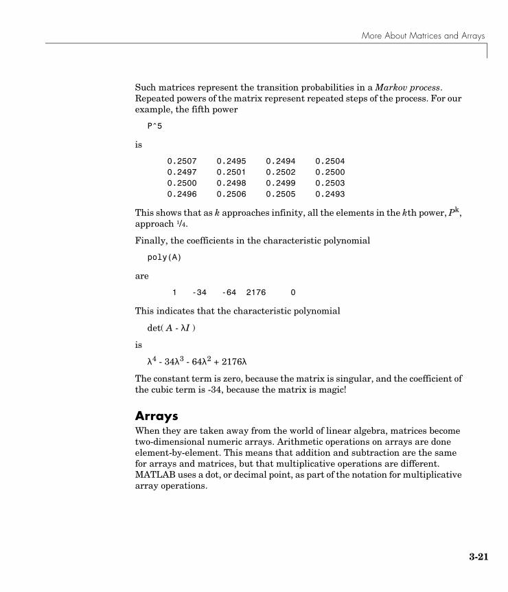
Such matrices represent the transition probabilities in a Markov process. Repeated powers of the matrix represent repeated steps of the process. For our example, the fifth power
P^5
is
0.2507 0.2495 0.2494 0.2504 0.2497 0.2501 0.2502 0.2500 0.2500 0.2498 0.2499 0.2503 0.2496 0.2506 0.2505 0.2493
This shows that as k approaches infinity, all the elements in the kth power, Pk, approach 1/4.
Finally, the coefficients in the characteristic polynomial
poly(A)
are
1 -34 -64 2176 0
This indicates that the characteristic polynomial
det( A - λI )
is
λ4 - 34λ3 - 64λ2 + 2176λ
The constant term is zero, because the matrix is singular, and the coefficient of the cubic term is -34, because the matrix is magic!
ArraysWhen they are taken away from the world of linear algebra, matrices become two-dimensional numeric arrays. Arithmetic operations on arrays are done element-by-element. This means that addition and subtraction are the same for arrays and matrices, but that multiplicative operations are different. MATLAB uses a dot, or decimal point, as part of the notation for multiplicative array operations.
3-21
3 Manipulating Matrices
3-2
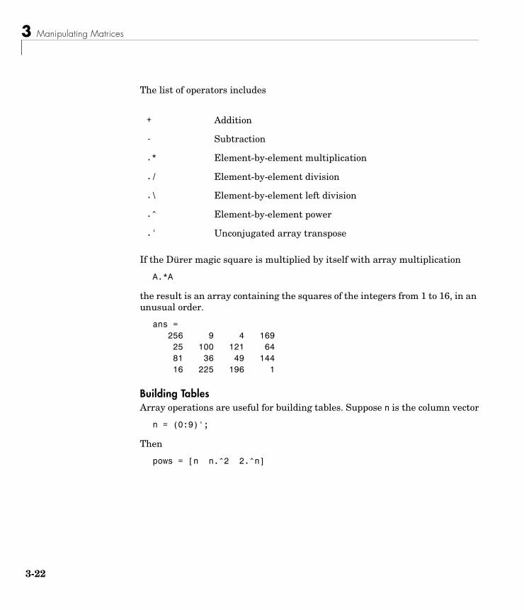
The list of operators includes
If the Dürer magic square is multiplied by itself with array multiplication
A.*A
the result is an array containing the squares of the integers from 1 to 16, in an unusual order.
ans = 256 9 4 169 25 100 121 64 81 36 49 144 16 225 196 1
Building TablesArray operations are useful for building tables. Suppose n is the column vector
n = (0:9)';
Then
pows = [n n.^2 2.^n]
+ Addition
- Subtraction
.* Element-by-element multiplication
./ Element-by-element division
.\ Element-by-element left division
.^ Element-by-element power
.' Unconjugated array transpose
2
More About Matrices and Arrays
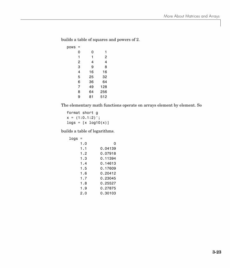
builds a table of squares and powers of 2.
pows = 0 0 1 1 1 2 2 4 4 3 9 8 4 16 16 5 25 32 6 36 64 7 49 128 8 64 256 9 81 512
The elementary math functions operate on arrays element by element. So
format short gx = (1:0.1:2)';logs = [x log10(x)]
builds a table of logarithms.
logs = 1.0 0 1.1 0.04139 1.2 0.07918 1.3 0.11394 1.4 0.14613 1.5 0.17609 1.6 0.20412 1.7 0.23045 1.8 0.25527 1.9 0.27875 2.0 0.30103
3-23
3 Manipulating Matrices
3-2
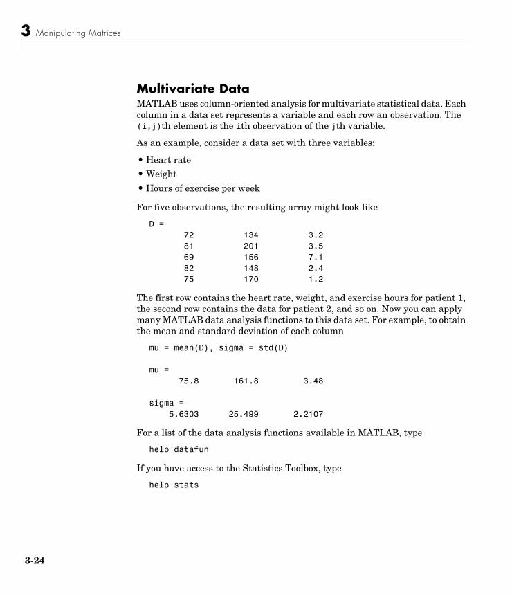
Multivariate DataMATLAB uses column-oriented analysis for multivariate statistical data. Each column in a data set represents a variable and each row an observation. The (i,j)th element is the ith observation of the jth variable.
As an example, consider a data set with three variables:
• Heart rate
• Weight
• Hours of exercise per week
For five observations, the resulting array might look like
D = 72 134 3.2 81 201 3.5 69 156 7.1 82 148 2.4 75 170 1.2
The first row contains the heart rate, weight, and exercise hours for patient 1, the second row contains the data for patient 2, and so on. Now you can apply many MATLAB data analysis functions to this data set. For example, to obtain the mean and standard deviation of each column
mu = mean(D), sigma = std(D)
mu =75.8 161.8 3.48
sigma =5.6303 25.499 2.2107
For a list of the data analysis functions available in MATLAB, type
help datafun
If you have access to the Statistics Toolbox, type
help stats
4
More About Matrices and Arrays
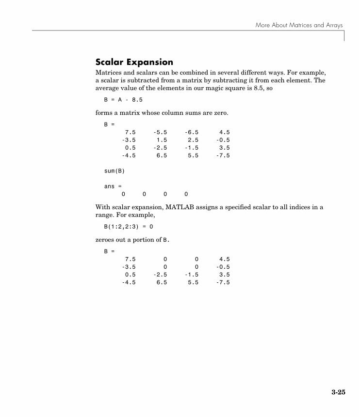
Scalar ExpansionMatrices and scalars can be combined in several different ways. For example, a scalar is subtracted from a matrix by subtracting it from each element. The average value of the elements in our magic square is 8.5, so
B = A - 8.5
forms a matrix whose column sums are zero.
B = 7.5 -5.5 -6.5 4.5 -3.5 1.5 2.5 -0.5 0.5 -2.5 -1.5 3.5 -4.5 6.5 5.5 -7.5
sum(B)
ans = 0 0 0 0
With scalar expansion, MATLAB assigns a specified scalar to all indices in a range. For example,
B(1:2,2:3) = 0
zeroes out a portion of B.
B = 7.5 0 0 4.5 -3.5 0 0 -0.5 0.5 -2.5 -1.5 3.5 -4.5 6.5 5.5 -7.5
3-25
3 Manipulating Matrices
3-2
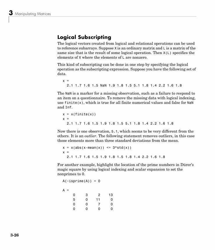
Logical SubscriptingThe logical vectors created from logical and relational operations can be used to reference subarrays. Suppose X is an ordinary matrix and L is a matrix of the same size that is the result of some logical operation. Then X(L) specifies the elements of X where the elements of L are nonzero.
This kind of subscripting can be done in one step by specifying the logical operation as the subscripting expression. Suppose you have the following set of data.
x = 2.1 1.7 1.6 1.5 NaN 1.9 1.8 1.5 5.1 1.8 1.4 2.2 1.6 1.8
The NaN is a marker for a missing observation, such as a failure to respond to an item on a questionnaire. To remove the missing data with logical indexing, use finite(x), which is true for all finite numerical values and false for NaN and Inf.
x = x(finite(x))x = 2.1 1.7 1.6 1.5 1.9 1.8 1.5 5.1 1.8 1.4 2.2 1.6 1.8
Now there is one observation, 5.1, which seems to be very different from the others. It is an outlier. The following statement removes outliers, in this case those elements more than three standard deviations from the mean.
x = x(abs(x-mean(x)) <= 3*std(x))x =2.1 1.7 1.6 1.5 1.9 1.8 1.5 1.8 1.4 2.2 1.6 1.8
For another example, highlight the location of the prime numbers in Dürer’s magic square by using logical indexing and scalar expansion to set the nonprimes to 0.
A(~isprime(A)) = 0
A = 0 3 2 13 5 0 11 0 0 0 7 0 0 0 0 0
6
More About Matrices and Arrays
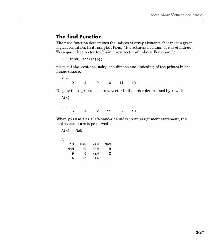
The find FunctionThe find function determines the indices of array elements that meet a given logical condition. In its simplest form, find returns a column vector of indices. Transpose that vector to obtain a row vector of indices. For example,
k = find(isprime(A))'
picks out the locations, using one-dimensional indexing, of the primes in the magic square.
k = 2 5 9 10 11 13
Display those primes, as a row vector in the order determined by k, with
A(k)
ans = 5 3 2 11 7 13
When you use k as a left-hand-side index in an assignment statement, the matrix structure is preserved.
A(k) = NaN
A = 16 NaN NaN NaN NaN 10 NaN 8 9 6 NaN 12 4 15 14 1
3-27
3 Manipulating Matrices
3-2
Controlling Command Window Input and OutputSo far, you have been using the MATLAB command line, typing functions and expressions, and seeing the results printed in the Command Window. This section describes
• “The format Function” on page 3-28, to control the appearance of the output values
• “Suppressing Output” on page 3-30
• “Entering Long Statements” on page 3-30
• “Command Line Editing” on page 3-30
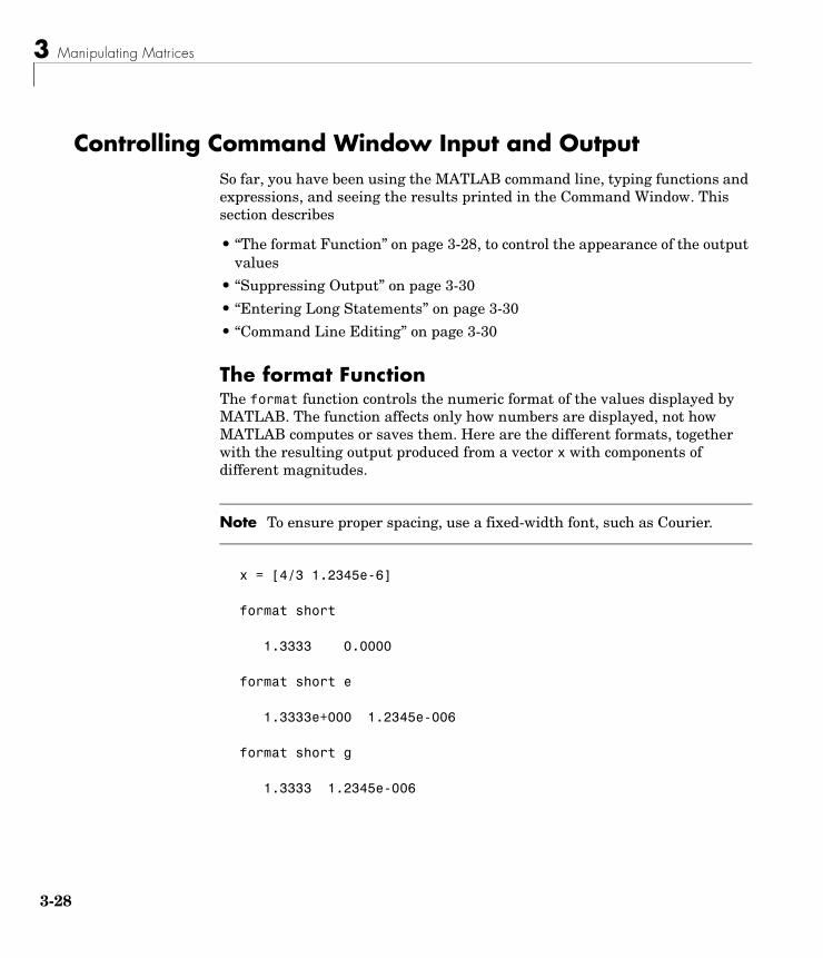
The format FunctionThe format function controls the numeric format of the values displayed by MATLAB. The function affects only how numbers are displayed, not how MATLAB computes or saves them. Here are the different formats, together with the resulting output produced from a vector x with components of different magnitudes.
Note To ensure proper spacing, use a fixed-width font, such as Courier.
x = [4/3 1.2345e-6]
format short
1.3333 0.0000
format short e
1.3333e+000 1.2345e-006
format short g
1.3333 1.2345e-006
8
Controlling Command Window Input and Output
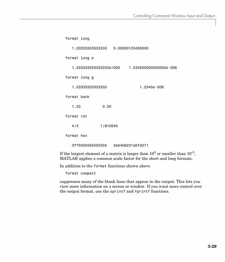
format long
1.33333333333333 0.00000123450000
format long e
1.333333333333333e+000 1.234500000000000e-006
format long g
1.33333333333333 1.2345e-006
format bank
1.33 0.00
format rat
4/3 1/810045
format hex
3ff5555555555555 3eb4b6231abfd271
If the largest element of a matrix is larger than 103 or smaller than 10-3, MATLAB applies a common scale factor for the short and long formats.
In addition to the format functions shown above
format compact
suppresses many of the blank lines that appear in the output. This lets you view more information on a screen or window. If you want more control over the output format, use the sprintf and fprintf functions.
3-29
3 Manipulating Matrices
3-3
Suppressing OutputIf you simply type a statement and press Return or Enter, MATLAB automatically displays the results on screen. However, if you end the line with a semicolon, MATLAB performs the computation but does not display any output. This is particularly useful when you generate large matrices. For example,
A = magic(100);
Entering Long StatementsIf a statement does not fit on one line, use an ellipsis (three periods), ..., followed by Return or Enter to indicate that the statement continues on the next line. For example,
s = 1 -1/2 + 1/3 -1/4 + 1/5 - 1/6 + 1/7 ... - 1/8 + 1/9 - 1/10 + 1/11 - 1/12;
Blank spaces around the =, +, and - signs are optional, but they improve readability.
Command Line EditingVarious arrow and control keys on your keyboard allow you to recall, edit, and reuse statements you have typed earlier. For example, suppose you mistakenly enter
rho = (1 + sqt(5))/2
You have misspelled sqrt. MATLAB responds with
Undefined function or variable 'sqt'.
Instead of retyping the entire line, simply press the ↑ key. The statement you typed is redisplayed. Use the ← key to move the cursor over and insert the missing r. Repeated use of the ↑ key recalls earlier lines. Typing a few characters and then the ↑ key finds a previous line that begins with those characters. You can also copy previously executed statements from the Command History. For more information, see “Command History” on page 2-6.
Following is the list of arrow and control keys you can use in the Command Window. If the preference you select for Command line key bindings is
0
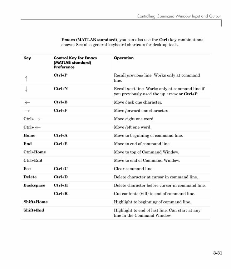
Controlling Command Window Input and Output
Emacs (MATLAB standard), you can also use the Ctrl+key combinations shown. See also general keyboard shortcuts for desktop tools.
Key Control Key for Emacs (MATLAB standard) Preference
Operation
Ctrl+P Recall previous line. Works only at command line.
Ctrl+N Recall next line. Works only at command line if you previously used the up arrow or Ctrl+P.
Ctrl+B Move back one character.
Ctrl+F Move forward one character.
Ctrl+ Move right one word.
Ctrl+ Move left one word.
Home Ctrl+A Move to beginning of command line.
End Ctrl+E Move to end of command line.
Ctrl+Home Move to top of Command Window.
Ctrl+End Move to end of Command Window.
Esc Ctrl+U Clear command line.
Delete Ctrl+D Delete character at cursor in command line.
Backspace Ctrl+H Delete character before cursor in command line.
Ctrl+K Cut contents (kill) to end of command line.
Shift+Home Highlight to beginning of command line.
Shift+End Highlight to end of last line. Can start at any line in the Command Window.
3-31
3 Manipulating Matrices
3-3
2
4
Graphics
Basic Plotting (p. 4-2) Create a plot, include multiple data sets, specify line style, colors, and markers, plot imaginary and complex data, add new plots, work with figure windows and axes, and save figures.
Editing Plots (p. 4-14) Edit plots interactively and using functions, and use the property editor.
Mesh and Surface Plots (p. 4-18) Visualize functions of two variables.
Images (p. 4-22) Work with images.
Printing Graphics (p. 4-24) Print and export figures.
Handle Graphics (p. 4-26) Work with graphics objects and set object properties.
Graphics User Interfaces (p. 4-33) Create graphical user interfaces.
Animations (p. 4-34) Create moving graphics.
4 Graphics
4-2
Basic PlottingMATLAB has extensive facilities for displaying vectors and matrices as graphs, as well as annotating and printing these graphs. This section describes a few of the most important graphics functions and provides examples of some typical applications:
• “Creating a Plot” on page 4-2
• “Multiple Data Sets in One Graph” on page 4-3
• “Specifying Line Styles and Colors” on page 4-4
• “Plotting Lines and Markers” on page 4-5
• “Imaginary and Complex Data” on page 4-6
• “Adding Plots to an Existing Graph” on page 4-7
• “Figure Windows” on page 4-8
• “Multiple Plots in One Figure” on page 4-9
• “Controlling the Axes” on page 4-10
• “Axis Labels and Titles” on page 4-12
• “Saving a Figure” on page 4-13
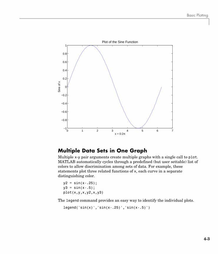
Creating a PlotThe plot function has different forms, depending on the input arguments. If y is a vector, plot(y) produces a piecewise linear graph of the elements of y versus the index of the elements of y. If you specify two vectors as arguments, plot(x,y) produces a graph of y versus x.
For example, these statements use the colon operator to create a vector of x values ranging from zero to 2π, compute the sine of these values, and plot the result.
x = 0:pi/100:2*pi;y = sin(x);plot(x,y)
Now label the axes and add a title. The characters \pi create the symbol π.
xlabel('x = 0:2\pi')ylabel('Sine of x')title('Plot of the Sine Function','FontSize',12)
Basic Plotting
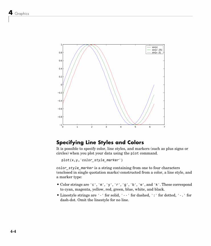
Multiple Data Sets in One GraphMultiple x-y pair arguments create multiple graphs with a single call to plot. MATLAB automatically cycles through a predefined (but user settable) list of colors to allow discrimination among sets of data. For example, these statements plot three related functions of x, each curve in a separate distinguishing color.
y2 = sin(x-.25);y3 = sin(x-.5);plot(x,y,x,y2,x,y3)
The legend command provides an easy way to identify the individual plots.
legend('sin(x)','sin(x-.25)','sin(x-.5)')
0 1 2 3 4 5 6 7−1
−0.8
−0.6
−0.4
−0.2
0
0.2
0.4
0.6
0.8
1
x = 0:2π
Sin
e of
x
Plot of the Sine Function
4-3
4 Graphics
4-4
Specifying Line Styles and ColorsIt is possible to specify color, line styles, and markers (such as plus signs or circles) when you plot your data using the plot command.
plot(x,y,'color_style_marker')
color_style_marker is a string containing from one to four characters (enclosed in single quotation marks) constructed from a color, a line style, and a marker type:
• Color strings are 'c', 'm', 'y', 'r', 'g', 'b', 'w', and 'k'. These correspond to cyan, magenta, yellow, red, green, blue, white, and black.
• Linestyle strings are '-' for solid, '--' for dashed, ':' for dotted, '-.' for dash-dot. Omit the linestyle for no line.
0 1 2 3 4 5 6 7−1
−0.8
−0.6
−0.4
−0.2
0
0.2
0.4
0.6
0.8
1sin(x) sin(x−.25)sin(x−.5)
Basic Plotting
• The marker types are '+', 'o', '*', and 'x' and the filled marker types are 's' for square, 'd' for diamond, '^' for up triangle, 'v' for down triangle, '>' for right triangle, '<' for left triangle, 'p' for pentagram, 'h' for hexagram, and none for no marker.
You can also edit color, line style, and markers interactively. See “Editing Plots” on page 4-14 for more information.
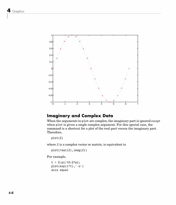
Plotting Lines and MarkersIf you specify a marker type but not a linestyle, MATLAB draws only the marker. For example,
plot(x,y,'ks')
plots black squares at each data point, but does not connect the markers with a line.
The statement
plot(x,y,'r:+')
plots a red dotted line and places plus sign markers at each data point. You may want to use fewer data points to plot the markers than you use to plot the lines. This example plots the data twice using a different number of points for the dotted line and marker plots.
x1 = 0:pi/100:2*pi;x2 = 0:pi/10:2*pi;plot(x1,sin(x1),'r:',x2,sin(x2),'r+')
4-5
4 Graphics
4-6
Imaginary and Complex DataWhen the arguments to plot are complex, the imaginary part is ignored except when plot is given a single complex argument. For this special case, the command is a shortcut for a plot of the real part versus the imaginary part. Therefore,
plot(Z)
where Z is a complex vector or matrix, is equivalent to
plot(real(Z),imag(Z))
For example,
t = 0:pi/10:2*pi;plot(exp(i*t),'-o')axis equal
0 1 2 3 4 5 6 7−1
−0.8
−0.6
−0.4
−0.2
0
0.2
0.4
0.6
0.8
1
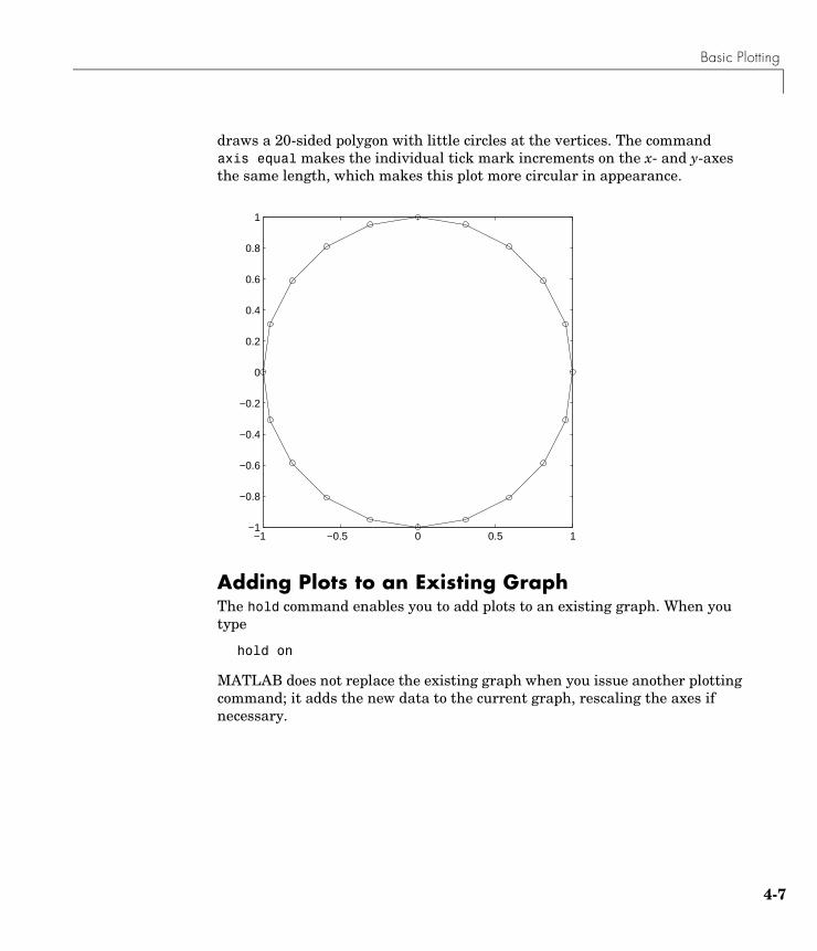
Basic Plotting
draws a 20-sided polygon with little circles at the vertices. The command axis equal makes the individual tick mark increments on the x- and y-axes the same length, which makes this plot more circular in appearance.
Adding Plots to an Existing GraphThe hold command enables you to add plots to an existing graph. When you type
hold on
MATLAB does not replace the existing graph when you issue another plotting command; it adds the new data to the current graph, rescaling the axes if necessary.
−1 −0.5 0 0.5 1−1
−0.8
−0.6
−0.4
−0.2
0
0.2
0.4
0.6
0.8
1
4-7
4 Graphics
4-8
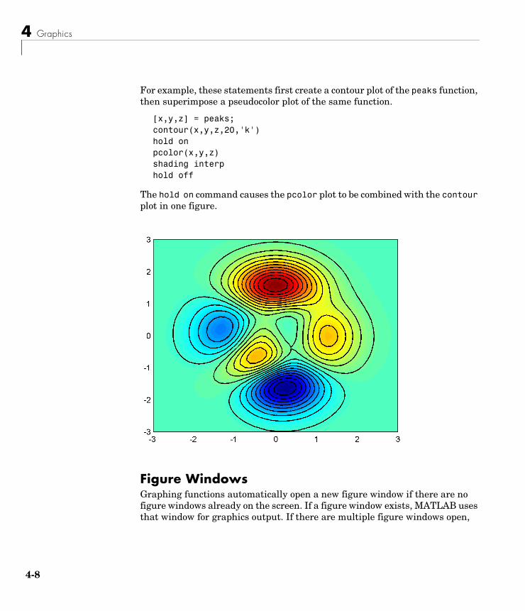
For example, these statements first create a contour plot of the peaks function, then superimpose a pseudocolor plot of the same function.
[x,y,z] = peaks;contour(x,y,z,20,'k')hold onpcolor(x,y,z)shading interphold off
The hold on command causes the pcolor plot to be combined with the contour plot in one figure.
Figure Windows Graphing functions automatically open a new figure window if there are no figure windows already on the screen. If a figure window exists, MATLAB uses that window for graphics output. If there are multiple figure windows open,
Basic Plotting
MATLAB targets the one that is designated the “current figure” (the last figure used or clicked in).
To make an existing figure window the current figure, you can click the mouse while the pointer is in that window or you can type
figure(n)
where n is the number in the figure title bar. The results of subsequent graphics commands are displayed in this window.
To open a new figure window and make it the current figure, type
figure
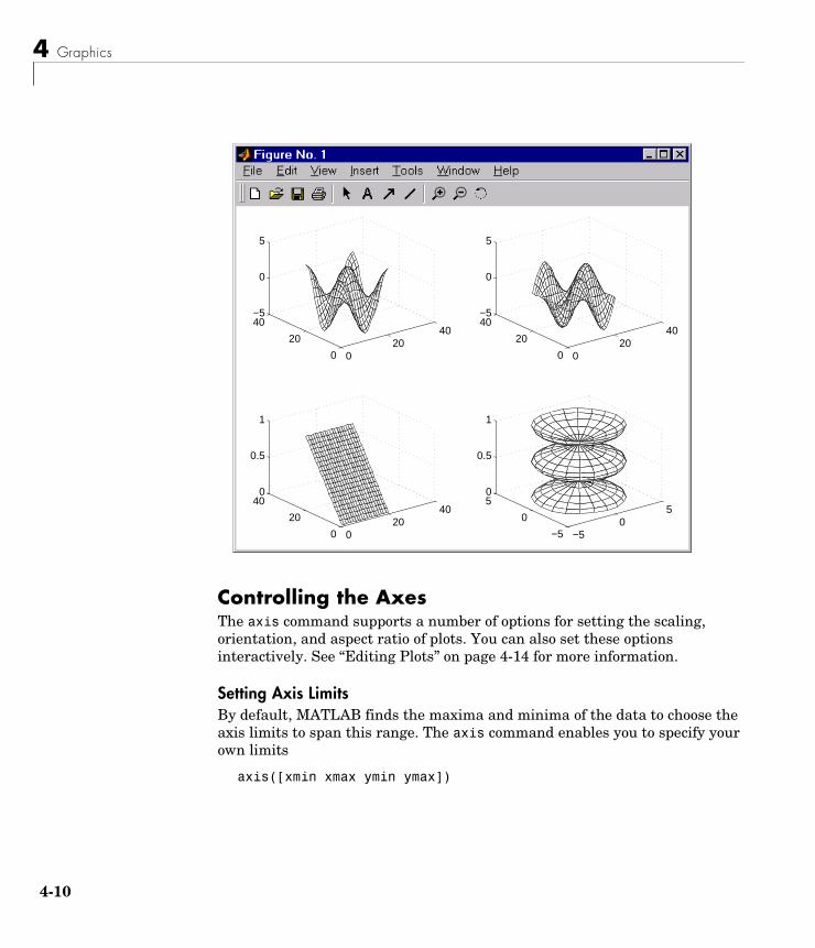
Multiple Plots in One FigureThe subplot command enables you to display multiple plots in the same window or print them on the same piece of paper. Typing
subplot(m,n,p)
partitions the figure window into an m-by-n matrix of small subplots and selects the pth subplot for the current plot. The plots are numbered along first the top row of the figure window, then the second row, and so on. For example, these statements plot data in four different subregions of the figure window.
t = 0:pi/10:2*pi;[X,Y,Z] = cylinder(4*cos(t));subplot(2,2,1); mesh(X)subplot(2,2,2); mesh(Y)subplot(2,2,3); mesh(Z)subplot(2,2,4); mesh(X,Y,Z)
4-9
4 Graphics
4-1
Controlling the AxesThe axis command supports a number of options for setting the scaling, orientation, and aspect ratio of plots. You can also set these options interactively. See “Editing Plots” on page 4-14 for more information.
Setting Axis LimitsBy default, MATLAB finds the maxima and minima of the data to choose the axis limits to span this range. The axis command enables you to specify your own limits
axis([xmin xmax ymin ymax])
020
40
0
20
40−5
0
5
020
40
0
20
40−5
0
5
020
40
0
20
400
0.5
1
−50
5
−5
0
50
0.5
1
0
Basic Plotting
or for three-dimensional graphs,
axis([xmin xmax ymin ymax zmin zmax])
Use the command
axis auto
to reenable MATLAB automatic limit selection.
Setting Axis Aspect Ratioaxis also enables you to specify a number of predefined modes. For example,
axis square
makes the x-axes and y-axes the same length.
axis equal
makes the individual tick mark increments on the x- and y-axes the same length. This means
plot(exp(i*[0:pi/10:2*pi]))
followed by either axis square or axis equal turns the oval into a proper circle.
axis auto normal
returns the axis scaling to its default, automatic mode.
Setting Axis VisibilityYou can use the axis command to make the axis visible or invisible.
axis on
makes the axis visible. This is the default.
axis off
makes the axis invisible.
4-11
4 Graphics
4-1
Setting Grid LinesThe grid command toggles grid lines on and off. The statement
grid on
turns the grid lines on and
grid off
turns them back off again.
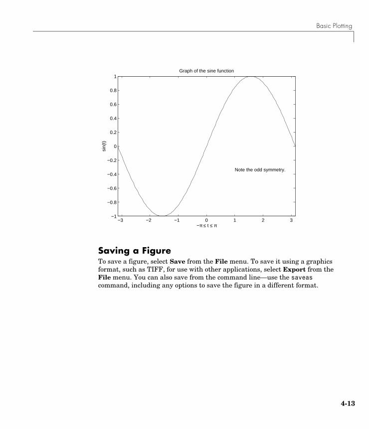
Axis Labels and TitlesThe xlabel, ylabel, and zlabel commands add x-, y-, and z-axis labels. The title command adds a title at the top of the figure and the text function inserts text anywhere in the figure. A subset of TeX notation produces Greek letters. You can also set these options interactively. See “Editing Plots” on page 4-14 for more information.
t = -pi:pi/100:pi;y = sin(t);plot(t,y)axis([-pi pi -1 1])xlabel('-\pi \leq {\itt} \leq \pi')ylabel('sin(t)')title('Graph of the sine function')text(1,-1/3,'{\itNote the odd symmetry.}')
2
Basic Plotting
Saving a FigureTo save a figure, select Save from the File menu. To save it using a graphics format, such as TIFF, for use with other applications, select Export from the File menu. You can also save from the command line—use the saveas command, including any options to save the figure in a different format.
−3 −2 −1 0 1 2 3−1
−0.8
−0.6
−0.4
−0.2
0
0.2
0.4
0.6
0.8
1
−π ≤ t ≤ π
sin(
t)
Graph of the sine function
Note the odd symmetry.
4-13
4 Graphics
4-1
Editing Plots MATLAB formats a graph to provide readability, setting the scale of axes, including tick marks on the axes, and using color and line style to distinguish the plots in the graph. However, if you are creating presentation graphics, you may want to change this default formatting or add descriptive labels, titles, legends and other annotations to help explain your data.
MATLAB supports two ways to edit the plots you create.
• Using the mouse to select and edit objects interactively
• Using MATLAB functions at the command-line or in an M-file
Interactive Plot EditingIf you enable plot editing mode in the MATLAB figure window, you can perform point-and-click editing of the objects in your graph. In this mode, you select the object or objects you want to edit by double-clicking it. This starts the Property Editor, which provides access to properties of the object that control its appearance and behavior.
For more information about interactive editing, see “Using Plot Editing Mode” on page 4-15. For information about editing object properties in plot editing mode, see “Using the Property Editor” on page 4-16.
Note Plot editing mode provides an alternative way to access the properties of MATLAB graphic objects. However, you can only access a subset of object properties through this mechanism. You may need to use a combination of interactive editing and command line editing to achieve the effect you desire.
Using Functions to Edit GraphsIf you prefer to work from the MATLAB command line or if you are creating an M-file, you can use MATLAB commands to edit the graphs you create. Taking advantage of MATLAB Handle Graphics system, you can use the set and get commands to change the properties of the objects in a graph. For more information about using command line, see “Handle Graphics” on page 4-26.
4
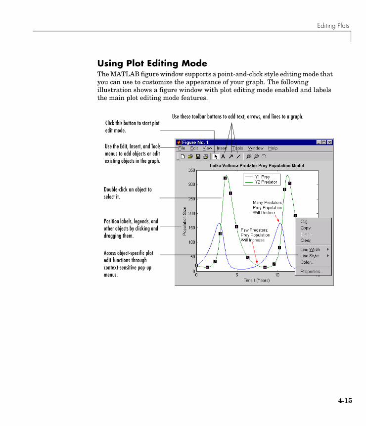
Editing Plots
Using Plot Editing ModeThe MATLAB figure window supports a point-and-click style editing mode that you can use to customize the appearance of your graph. The following illustration shows a figure window with plot editing mode enabled and labels the main plot editing mode features.
Click this button to start plot edit mode.
Use the Edit, Insert, and Tools menus to add objects or edit existing objects in the graph.
Double-click an object to select it.
Position labels, legends, and other objects by clicking and dragging them.
Access object-specific plot edit functions through context-sensitive pop-up menus.
Use these toolbar buttons to add text, arrows, and lines to a graph.
4-15
4 Graphics
4-1
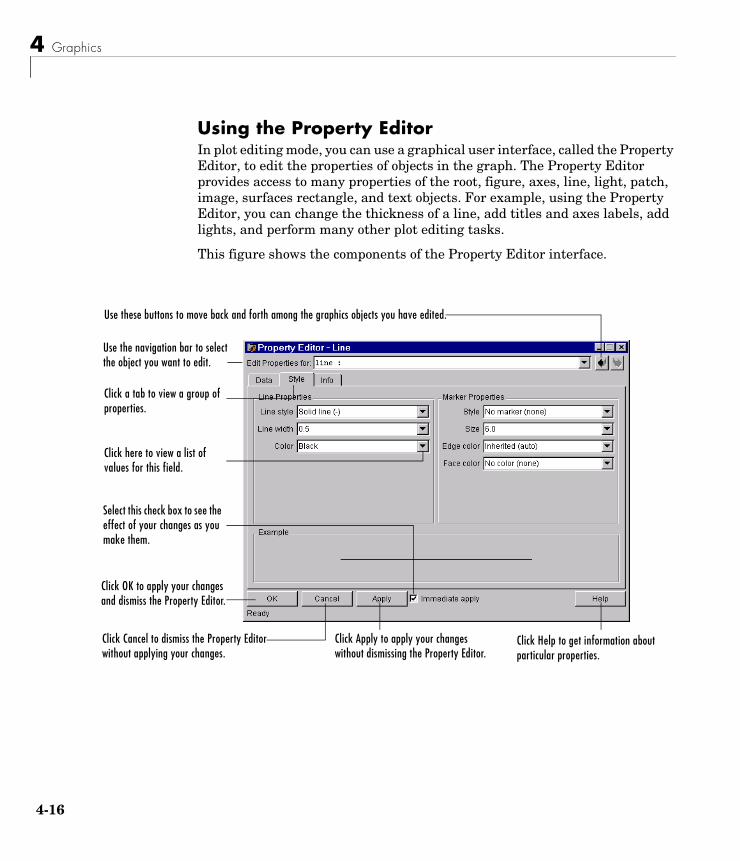
Using the Property EditorIn plot editing mode, you can use a graphical user interface, called the Property Editor, to edit the properties of objects in the graph. The Property Editor provides access to many properties of the root, figure, axes, line, light, patch, image, surfaces rectangle, and text objects. For example, using the Property Editor, you can change the thickness of a line, add titles and axes labels, add lights, and perform many other plot editing tasks.
This figure shows the components of the Property Editor interface.
Use these buttons to move back and forth among the graphics objects you have edited.
Click Help to get information about particular properties.
Use the navigation bar to select the object you want to edit.
Click a tab to view a group of properties.
Click here to view a list of values for this field.
Select this check box to see the effect of your changes as you make them.
Click OK to apply your changes and dismiss the Property Editor.
Click Cancel to dismiss the Property Editor without applying your changes.
Click Apply to apply your changes without dismissing the Property Editor.
6
Editing Plots
Starting the Property EditorYou start the Property Editor by double-clicking an object in a graph, such as a line, or by right-clicking an object and selecting the Properties option from the object’s context menu.
You can also start the Property Editor by selecting either the Figure Properties, Axes Properties, or Current Object Properties from the figure window Edit menu. These options automatically enable plot editing mode, if it is not already enabled.
Once you start the Property Editor, keep it open throughout an editing session. It provides access to all the objects in the graph. If you click another object in the graph, the Property Editor displays the set of panels associated with that object type. You can also use the Property Editor’s navigation bar to select an object in the graph to edit.
4-17
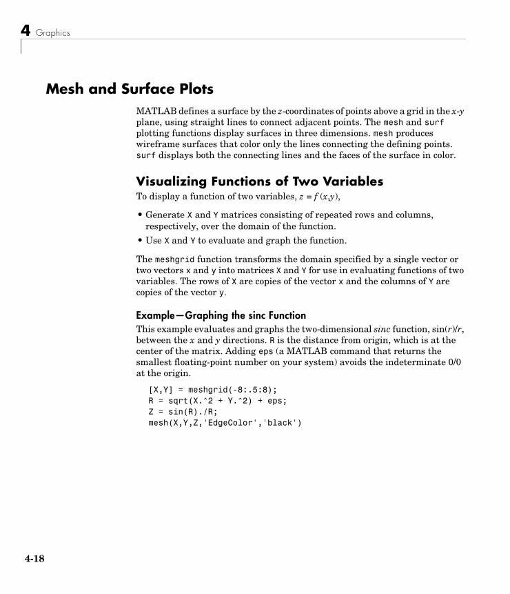
4 Graphics
4-1
Mesh and Surface PlotsMATLAB defines a surface by the z-coordinates of points above a grid in the x-y plane, using straight lines to connect adjacent points. The mesh and surf plotting functions display surfaces in three dimensions. mesh produces wireframe surfaces that color only the lines connecting the defining points. surf displays both the connecting lines and the faces of the surface in color.
Visualizing Functions of Two VariablesTo display a function of two variables, z = f (x,y),
• Generate X and Y matrices consisting of repeated rows and columns, respectively, over the domain of the function.
• Use X and Y to evaluate and graph the function.
The meshgrid function transforms the domain specified by a single vector or two vectors x and y into matrices X and Y for use in evaluating functions of two variables. The rows of X are copies of the vector x and the columns of Y are copies of the vector y.
Example—Graphing the sinc FunctionThis example evaluates and graphs the two-dimensional sinc function, sin(r)/r, between the x and y directions. R is the distance from origin, which is at the center of the matrix. Adding eps (a MATLAB command that returns the smallest floating-point number on your system) avoids the indeterminate 0/0 at the origin.
[X,Y] = meshgrid(-8:.5:8); R = sqrt(X.^2 + Y.^2) + eps;Z = sin(R)./R;mesh(X,Y,Z,'EdgeColor','black')
8
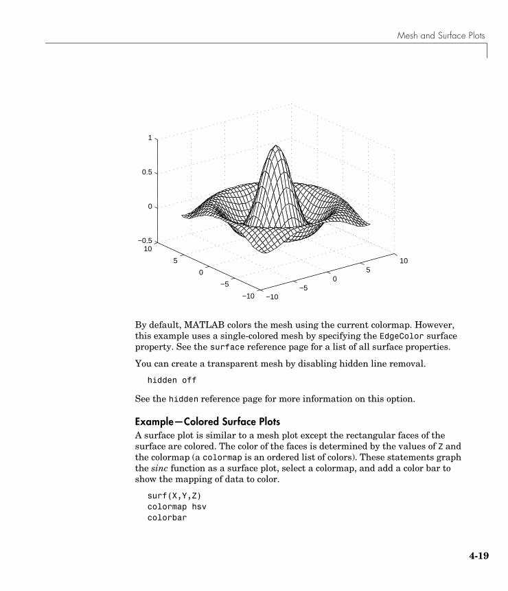
Mesh and Surface Plots
By default, MATLAB colors the mesh using the current colormap. However, this example uses a single-colored mesh by specifying the EdgeColor surface property. See the surface reference page for a list of all surface properties.
You can create a transparent mesh by disabling hidden line removal.
hidden off
See the hidden reference page for more information on this option.
Example—Colored Surface PlotsA surface plot is similar to a mesh plot except the rectangular faces of the surface are colored. The color of the faces is determined by the values of Z and the colormap (a colormap is an ordered list of colors). These statements graph the sinc function as a surface plot, select a colormap, and add a color bar to show the mapping of data to color.
surf(X,Y,Z)colormap hsvcolorbar
−10−5
05
10
−10
−5
0
5
10−0.5
0
0.5
1
4-19
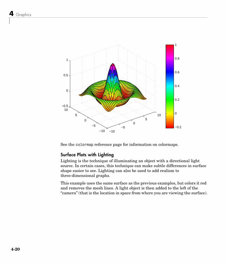
4 Graphics
4-2
See the colormap reference page for information on colormaps.
Surface Plots with LightingLighting is the technique of illuminating an object with a directional light source. In certain cases, this technique can make subtle differences in surface shape easier to see. Lighting can also be used to add realism to three-dimensional graphs.
This example uses the same surface as the previous examples, but colors it red and removes the mesh lines. A light object is then added to the left of the “camera” (that is the location in space from where you are viewing the surface).
−0.2
0
0.2
0.4
0.6
0.8
1
−10−5
05
10
−10
−5
0
5
10−0.5
0
0.5
1
0
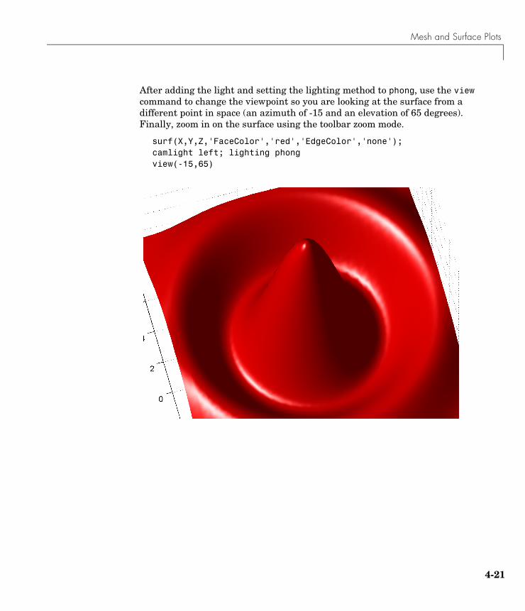
Mesh and Surface Plots
After adding the light and setting the lighting method to phong, use the view command to change the viewpoint so you are looking at the surface from a different point in space (an azimuth of -15 and an elevation of 65 degrees). Finally, zoom in on the surface using the toolbar zoom mode.
surf(X,Y,Z,'FaceColor','red','EdgeColor','none');camlight left; lighting phongview(-15,65)
4-21
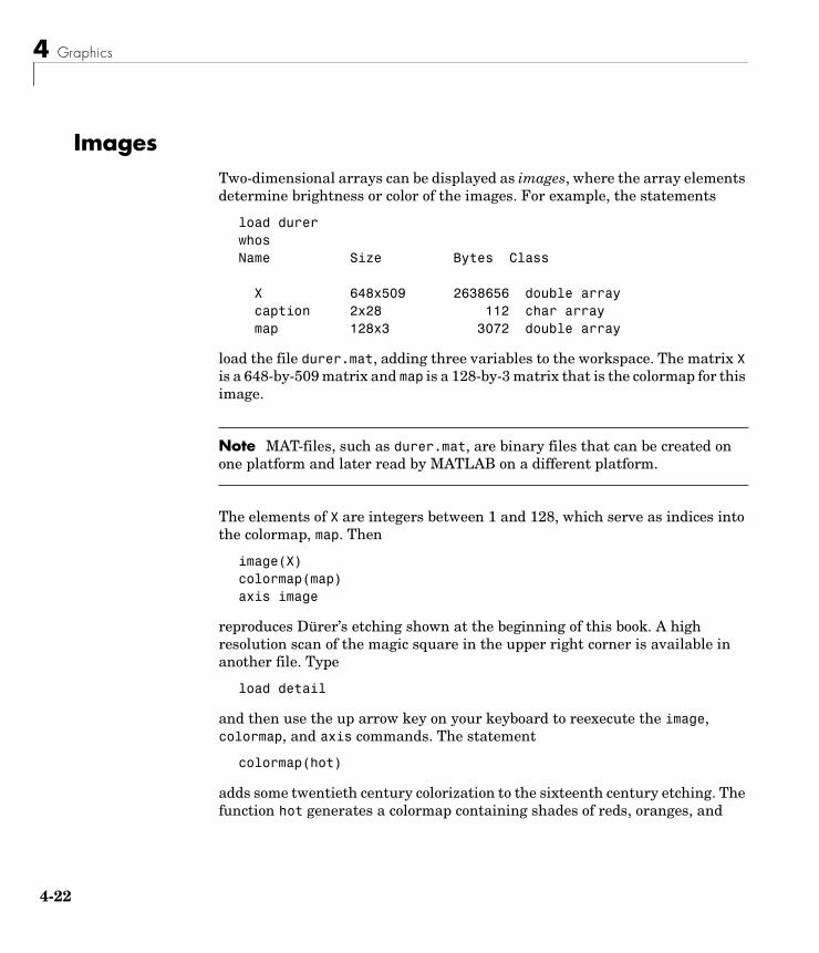
4 Graphics
4-2
ImagesTwo-dimensional arrays can be displayed as images, where the array elements determine brightness or color of the images. For example, the statements
load durerwhosName Size Bytes Class
X 648x509 2638656 double array caption 2x28 112 char array map 128x3 3072 double array
load the file durer.mat, adding three variables to the workspace. The matrix X is a 648-by-509 matrix and map is a 128-by-3 matrix that is the colormap for this image.
Note MAT-files, such as durer.mat, are binary files that can be created on one platform and later read by MATLAB on a different platform.
The elements of X are integers between 1 and 128, which serve as indices into the colormap, map. Then
image(X)colormap(map)axis image
reproduces Dürer’s etching shown at the beginning of this book. A high resolution scan of the magic square in the upper right corner is available in another file. Type
load detail
and then use the up arrow key on your keyboard to reexecute the image, colormap, and axis commands. The statement
colormap(hot)
adds some twentieth century colorization to the sixteenth century etching. The function hot generates a colormap containing shades of reds, oranges, and
2
Images
yellows. Typically a given image matrix has a specific colormap associated with it. See the colormap reference page for a list of other predefined colormaps.
4-23
4 Graphics
4-2
Printing GraphicsYou can print a MATLAB figure directly on a printer connected to your computer or you can export the figure to one of the standard graphic file formats supported by MATLAB. There are two ways to print and export figures:
• Using the Print option under the File menu
• Using the print command
Printing from the MenuThere are four menu options under the File menu that pertain to printing:
• The Page Setup option displays a dialog box that enables you to adjust characteristics of the figure on the printed page.
• The Print Setup option displays a dialog box that sets printing defaults, but does not actually print the figure.
• The Print Preview option enables you to view the figure the way it will look on the printed page.
• The Print option displays a dialog box that lets you select standard printing options and print the figure.
Generally, use Print Preview to determine whether the printed output is what you want. If not, use the Page Setup dialog box to change the output settings. Select the Page Setup dialog box Help button to display information on how to set up the page.
Exporting Figure to Graphics FilesThe Export option under the File menu enables you to export the figure to a variety of standard graphics file formats.
Using the Print CommandThe print command provides more flexibility in the type of output sent to the printer and allows you to control printing from M-files. The result can be sent directly to your default printer or stored in a specified file. A wide variety of output formats, including TIFF, JPEG, and PostScript, is available.
For example, this statement saves the contents of the current figure window as color Encapsulated Level 2 PostScript in the file called magicsquare.eps. It
4
Printing Graphics
also includes a TIFF preview, which enables most word processors to display the picture
print -depsc2 -tiff magicsquare.eps
To save the same figure as a TIFF file with a resolution of 200 dpi, use the command
print -dtiff -r200 magicsquare.tiff
If you type print on the command line,
MATLAB prints the current figure on your default printer.
4-25
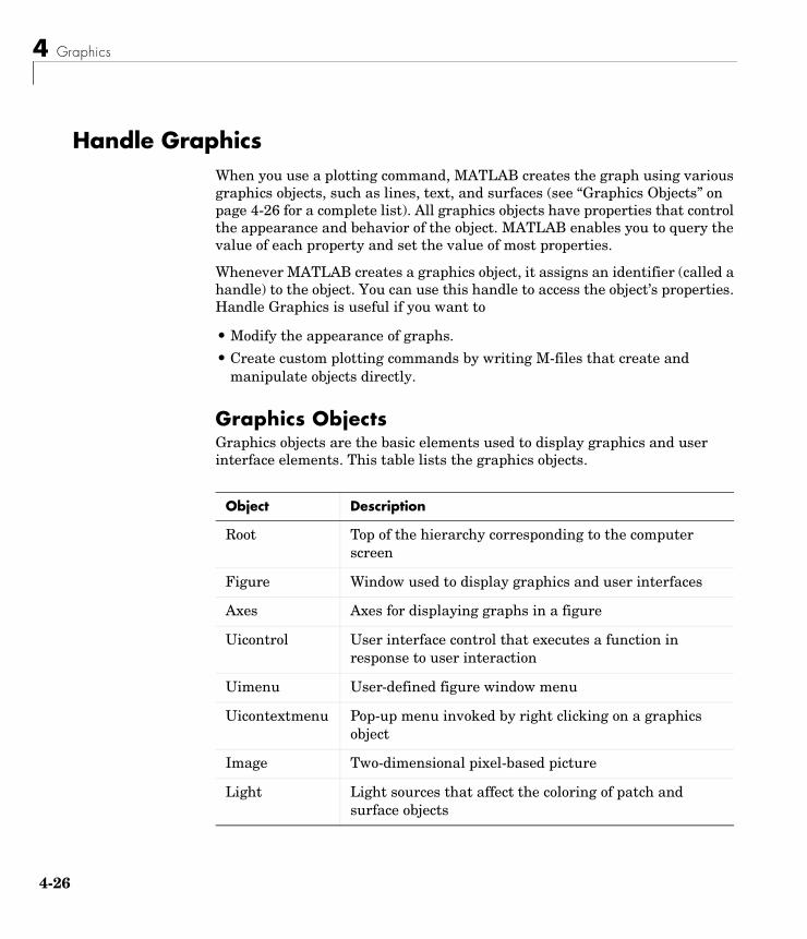
4 Graphics
4-2
Handle GraphicsWhen you use a plotting command, MATLAB creates the graph using various graphics objects, such as lines, text, and surfaces (see “Graphics Objects” on page 4-26 for a complete list). All graphics objects have properties that control the appearance and behavior of the object. MATLAB enables you to query the value of each property and set the value of most properties.
Whenever MATLAB creates a graphics object, it assigns an identifier (called a handle) to the object. You can use this handle to access the object’s properties. Handle Graphics is useful if you want to
• Modify the appearance of graphs.
• Create custom plotting commands by writing M-files that create and manipulate objects directly.
Graphics ObjectsGraphics objects are the basic elements used to display graphics and user interface elements. This table lists the graphics objects.
Object Description
Root Top of the hierarchy corresponding to the computer screen
Figure Window used to display graphics and user interfaces
Axes Axes for displaying graphs in a figure
Uicontrol User interface control that executes a function in response to user interaction
Uimenu User-defined figure window menu
Uicontextmenu Pop-up menu invoked by right clicking on a graphics object
Image Two-dimensional pixel-based picture
Light Light sources that affect the coloring of patch and surface objects
6
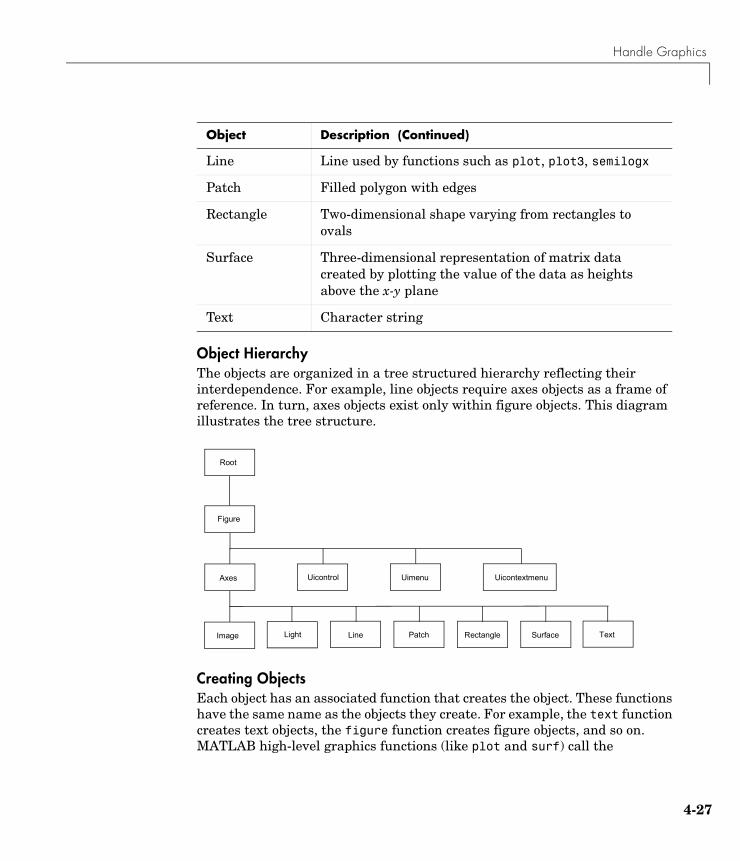
Handle Graphics
Object HierarchyThe objects are organized in a tree structured hierarchy reflecting their interdependence. For example, line objects require axes objects as a frame of reference. In turn, axes objects exist only within figure objects. This diagram illustrates the tree structure.
Creating ObjectsEach object has an associated function that creates the object. These functions have the same name as the objects they create. For example, the text function creates text objects, the figure function creates figure objects, and so on. MATLAB high-level graphics functions (like plot and surf) call the
Line Line used by functions such as plot, plot3, semilogx
Patch Filled polygon with edges
Rectangle Two-dimensional shape varying from rectangles to ovals
Surface Three-dimensional representation of matrix data created by plotting the value of the data as heights above the x-y plane
Text Character string
Object Description (Continued)
Uimenu
Line
Axes Uicontrol
Image
Figure
Uicontextmenu
Light SurfacePatch Text
Root
Rectangle
4-27
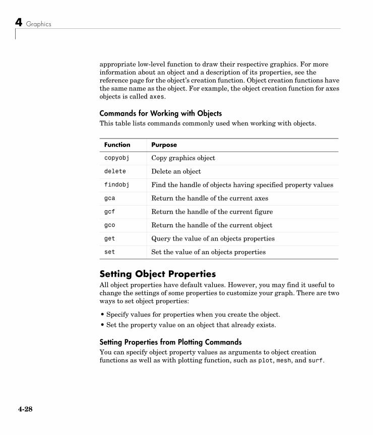
4 Graphics
4-2
appropriate low-level function to draw their respective graphics. For more information about an object and a description of its properties, see the reference page for the object’s creation function. Object creation functions have the same name as the object. For example, the object creation function for axes objects is called axes.
Commands for Working with ObjectsThis table lists commands commonly used when working with objects.
Setting Object PropertiesAll object properties have default values. However, you may find it useful to change the settings of some properties to customize your graph. There are two ways to set object properties:
• Specify values for properties when you create the object.
• Set the property value on an object that already exists.
Setting Properties from Plotting CommandsYou can specify object property values as arguments to object creation functions as well as with plotting function, such as plot, mesh, and surf.
Function Purpose
copyobj Copy graphics object
delete Delete an object
findobj Find the handle of objects having specified property values
gca Return the handle of the current axes
gcf Return the handle of the current figure
gco Return the handle of the current object
get Query the value of an objects properties
set Set the value of an objects properties
8
Handle Graphics
For example, plotting commands that create lines or surfaces enable you to specify property name/property value pairs as arguments. The command
plot(x,y,'LineWidth',1.5)
plots the data in the variables x and y using lines having a LineWidth property set to 1.5 points (one point = 1/72 inch). You can set any line object property this way.
Setting Properties of Existing ObjectsTo modify the property values of existing objects, you can use the set command or, if plot editing mode is enabled, the Property Editor. The Property Editor provides a graphical user interface to many object properties. This section describes how to use the set command. See “Using the Property Editor” on page 4-16 for more information.
Many plotting commands can return the handles of the objects created so you can modify the objects using the set command. For example, these statements plot a five-by-five matrix (creating five lines, one per column) and then set the Marker to a square and the MarkerFaceColor to green.
h = plot(magic(5));set(h,'Marker','s',MarkerFaceColor','g')
In this case, h is a vector containing five handles, one for each of the five lines in the plot. The set statement sets the Marker and MarkerFaceColor properties of all lines to the same values.
Setting Multiple Property ValuesIf you want to set the properties of each line to a different value, you can use cell arrays to store all the data and pass it to the set command. For example, create a plot and save the line handles.
h = plot(magic(5));
Suppose you want to add different markers to each line and color the marker’s face color to the same color as the line. You need to define two cell arrays – one containing the property names and the other containing the desired values of the properties.
4-29
4 Graphics
4-3
The prop_name cell array contains two elements.
prop_name(1) = {'Marker'};prop_name(2) = {'MarkerFaceColor'};
The prop_values cell array contains 10 values; five values for the Marker property and five values for the MarkerFaceColor property. Notice that prop_values is a two-dimensional cell array. The first dimension indicates which handle in h the values apply to and the second dimension indicates which property the value is assigned to.
prop_values(1,1) = {'s'};prop_values(1,2) = {get(h(1),'Color')};prop_values(2,1) = {'d'};prop_values(2,2) = {get(h(2),'Color')};prop_values(3,1) = {'o'};prop_values(3,2) = {get(h(3),'Color')};prop_values(4,1) = {'p'};prop_values(4,2) = {get(h(4),'Color')};prop_values(5,1) = {'h'};prop_values(5,2) = {get(h(5),'Color')};
The MarkerFaceColor is always assigned the value of the corresponding line’s color (obtained by getting the line’s Color property with the get command).
After defining the cell arrays, call set to specify the new property values.
set(h,prop_name,prop_values)
0
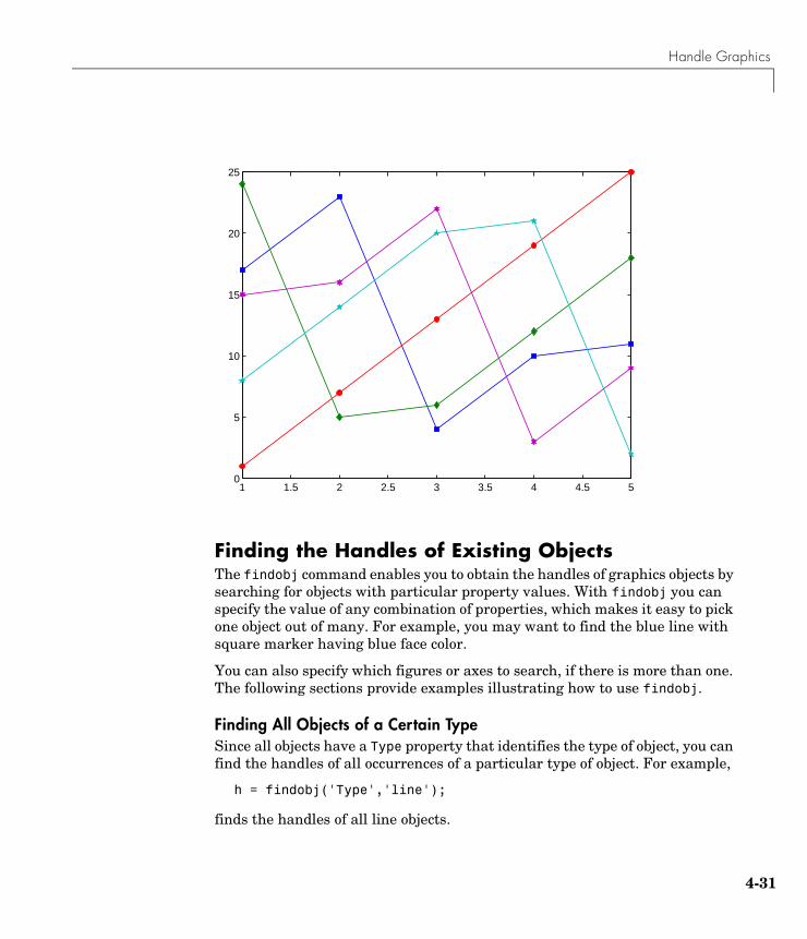
Handle Graphics
Finding the Handles of Existing ObjectsThe findobj command enables you to obtain the handles of graphics objects by searching for objects with particular property values. With findobj you can specify the value of any combination of properties, which makes it easy to pick one object out of many. For example, you may want to find the blue line with square marker having blue face color.
You can also specify which figures or axes to search, if there is more than one. The following sections provide examples illustrating how to use findobj.
Finding All Objects of a Certain TypeSince all objects have a Type property that identifies the type of object, you can find the handles of all occurrences of a particular type of object. For example,
h = findobj('Type','line');
finds the handles of all line objects.
1 1.5 2 2.5 3 3.5 4 4.5 50
5
10
15
20
25
4-31
4 Graphics
4-3
Finding Objects with a Particular PropertyYou can specify multiple properties to narrow the search. For example,
h = findobj('Type','line','Color','r','LineStyle',':');
finds the handles of all red, dotted lines.
Limiting the Scope of the SearchYou can specify the starting point in the object hierarchy by passing the handle of the starting figure or axes as the first argument. For example,
h = findobj(gca,'Type','text','String','\pi/2');
finds the string π/2 only within the current axes.
Using findobj as an ArgumentSince findobj returns the handles it finds, you can use it in place of the handle argument. For example,
set(findobj('Type','line','Color','red'),'LineStyle',':')
finds all red lines and sets their line style to dotted.
2
Graphics User Interfaces
Graphics User InterfacesHere is a simple example illustrating how to use Handle Graphics to build user interfaces. The statement
b = uicontrol('Style','pushbutton', ... 'Units','normalized', ... 'Position',[.5 .5 .2 .1], ... 'String','click here');
creates a push button in the center of a figure window and returns a handle to the new object. But, so far, clicking the button does nothing. The statement
s = 'set(b,''Position'',[.8*rand .9*rand .2 .1])';
creates a string containing a command that alters the push button’s position. Repeated execution of
eval(s)
moves the button to random positions. Finally,
set(b,'Callback',s)
installs s as the button’s callback action, so every time you click the button, it moves to a new position.
Graphical User Interface Design ToolsMATLAB provides GUI Design Environment (GUIDE) tools that simplify the creation of graphical user interfaces. To display the GUIDE Layout Editor, issue the guide command.
4-33
4 Graphics
4-3
AnimationsMATLAB provides two ways of generating moving, animated graphics:
• “Erase Mode Method” on page 4-34—Continually erase and then redraw the objects on the screen, making incremental changes with each redraw.
• “Creating Movies” on page 4-35—Save a number of different pictures and then play them back as a movie.
Erase Mode MethodUsing the EraseMode property is appropriate for long sequences of simple plots where the change from frame to frame is minimal. Here is an example showing simulated Brownian motion. Specify a number of points, such as
n = 20
and a temperature or velocity, such as
s = .02
The best values for these two parameters depend upon the speed of your particular computer. Generate n random points with (x,y) coordinates between -1/2 and +1/2.
x = rand(n,1)-0.5;y = rand(n,1)-0.5;
Plot the points in a square with sides at -1 and +1. Save the handle for the vector of points and set its EraseMode to xor. This tells the MATLAB graphics system not to redraw the entire plot when the coordinates of one point are changed, but to restore the background color in the vicinity of the point using an “exclusive or” operation.
h = plot(x,y,'.');axis([-1 1 -1 1])axis squaregrid offset(h,'EraseMode','xor','MarkerSize',18)
Now begin the animation. Here is an infinite while loop, which you can eventually exit by typing Ctrl+c. Each time through the loop, add a small amount of normally distributed random noise to the coordinates of the points.
4
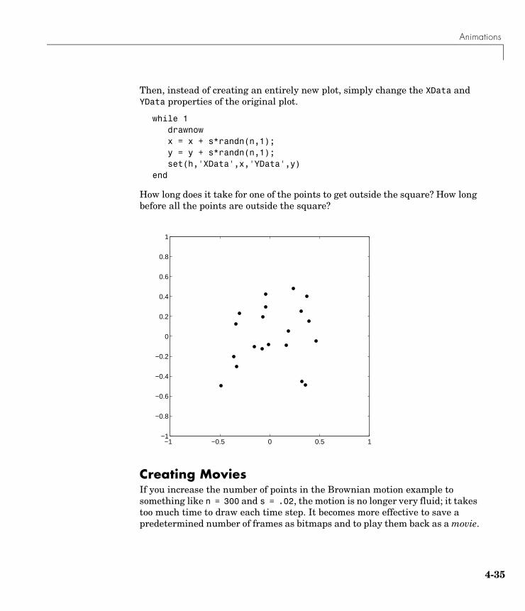
Animations
Then, instead of creating an entirely new plot, simply change the XData and YData properties of the original plot.
while 1 drawnow x = x + s*randn(n,1); y = y + s*randn(n,1); set(h,'XData',x,'YData',y)end
How long does it take for one of the points to get outside the square? How long before all the points are outside the square?
Creating MoviesIf you increase the number of points in the Brownian motion example to something like n = 300 and s = .02, the motion is no longer very fluid; it takes too much time to draw each time step. It becomes more effective to save a predetermined number of frames as bitmaps and to play them back as a movie.
−1 −0.5 0 0.5 1−1
−0.8
−0.6
−0.4
−0.2
0
0.2
0.4
0.6
0.8
1
4-35
4 Graphics
4-3
First, decide on the number of frames, say
nframes = 50;
Next, set up the first plot as before, except using the default EraseMode (normal).
x = rand(n,1)-0.5;y = rand(n,1)-0.5;h = plot(x,y,'.');set(h,'MarkerSize',18);axis([-1 1 -1 1])axis squaregrid off
Generate the movie and use getframe to capture each frame.
for k = 1:nframes x = x + s*randn(n,1); y = y + s*randn(n,1); set(h,'XData',x,'YData',y) M(k) = getframe;end
Finally, play the movie 30 times.
movie(M,30)
6
5
Programming with MATLABFlow Control (p. 5-2) Use flow control constructs including if, switch and case, for, while, continue, and break.
Other Data Structures (p. 5-7) Work with multidimensional arrays, cell arrays, character and text data, and structures.
Scripts and Functions (p. 5-17) Write scripts and functions, use global variables, pass string arguments to functions, use eval to evaluate text expressions, vectorize code, preallocate arrays, reference functions using handles, and use function that operate on functions.
Demonstration Programs Included with MATLAB (p. 5-28)
View and run demos.
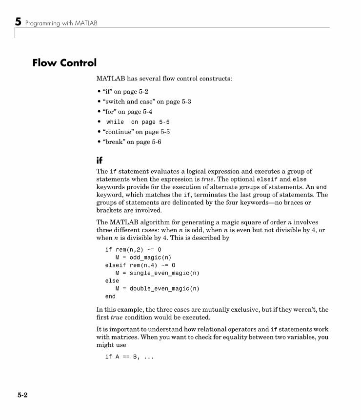
5 Programming with MATLAB
5-2
Flow ControlMATLAB has several flow control constructs:
• “if” on page 5-2
• “switch and case” on page 5-3
• “for” on page 5-4
• while on page 5-5
• “continue” on page 5-5
• “break” on page 5-6
ifThe if statement evaluates a logical expression and executes a group of statements when the expression is true. The optional elseif and else keywords provide for the execution of alternate groups of statements. An end keyword, which matches the if, terminates the last group of statements. The groups of statements are delineated by the four keywords—no braces or brackets are involved.
The MATLAB algorithm for generating a magic square of order n involves three different cases: when n is odd, when n is even but not divisible by 4, or when n is divisible by 4. This is described by
if rem(n,2) ~= 0 M = odd_magic(n)elseif rem(n,4) ~= 0 M = single_even_magic(n)else M = double_even_magic(n)end
In this example, the three cases are mutually exclusive, but if they weren’t, the first true condition would be executed.
It is important to understand how relational operators and if statements work with matrices. When you want to check for equality between two variables, you might use
if A == B, ...
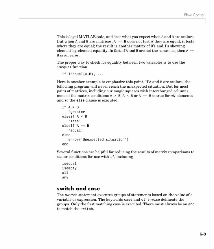
Flow Control
This is legal MATLAB code, and does what you expect when A and B are scalars. But when A and B are matrices, A == B does not test if they are equal, it tests where they are equal; the result is another matrix of 0’s and 1’s showing element-by-element equality. In fact, if A and B are not the same size, then A == B is an error.
The proper way to check for equality between two variables is to use the isequal function,
if isequal(A,B), ...
Here is another example to emphasize this point. If A and B are scalars, the following program will never reach the unexpected situation. But for most pairs of matrices, including our magic squares with interchanged columns, none of the matrix conditions A > B, A < B or A == B is true for all elements and so the else clause is executed.
if A > B 'greater'elseif A < B 'less'elseif A == B 'equal'else error('Unexpected situation')end
Several functions are helpful for reducing the results of matrix comparisons to scalar conditions for use with if, including
isequalisemptyallany
switch and caseThe switch statement executes groups of statements based on the value of a variable or expression. The keywords case and otherwise delineate the groups. Only the first matching case is executed. There must always be an end to match the switch.
5-3
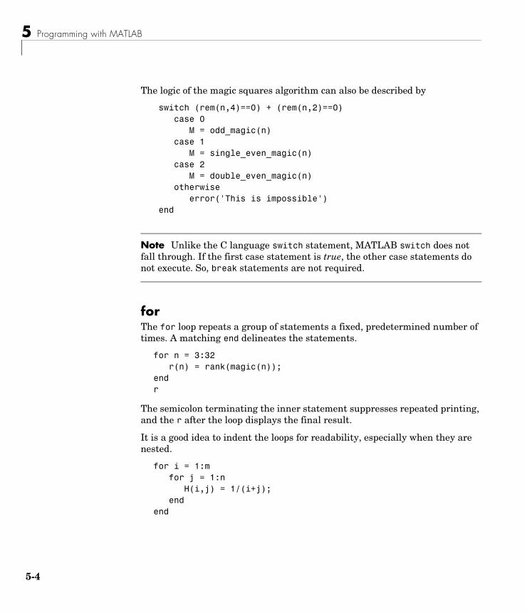
5 Programming with MATLAB
5-4
The logic of the magic squares algorithm can also be described by
switch (rem(n,4)==0) + (rem(n,2)==0) case 0 M = odd_magic(n) case 1 M = single_even_magic(n) case 2 M = double_even_magic(n) otherwise error('This is impossible') end
Note Unlike the C language switch statement, MATLAB switch does not fall through. If the first case statement is true, the other case statements do not execute. So, break statements are not required.
forThe for loop repeats a group of statements a fixed, predetermined number of times. A matching end delineates the statements.
for n = 3:32 r(n) = rank(magic(n));endr
The semicolon terminating the inner statement suppresses repeated printing, and the r after the loop displays the final result.
It is a good idea to indent the loops for readability, especially when they are nested.
for i = 1:m for j = 1:n H(i,j) = 1/(i+j); endend
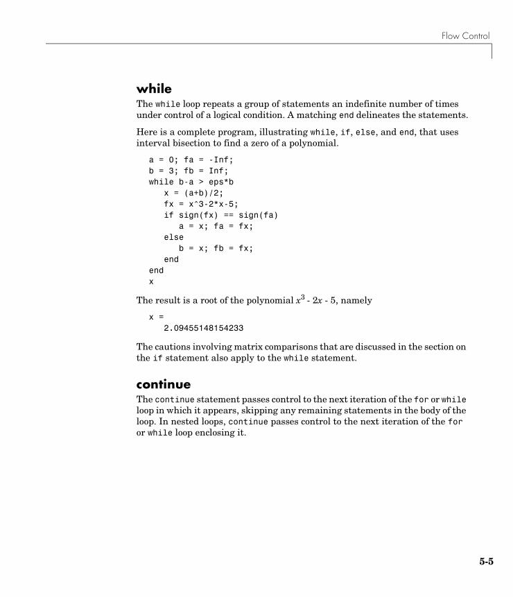
Flow Control
while The while loop repeats a group of statements an indefinite number of times under control of a logical condition. A matching end delineates the statements.
Here is a complete program, illustrating while, if, else, and end, that uses interval bisection to find a zero of a polynomial.
a = 0; fa = -Inf;b = 3; fb = Inf;while b-a > eps*b x = (a+b)/2; fx = x^3-2*x-5; if sign(fx) == sign(fa) a = x; fa = fx; else b = x; fb = fx; endendx
The result is a root of the polynomial x3 - 2x - 5, namely
x = 2.09455148154233
The cautions involving matrix comparisons that are discussed in the section on the if statement also apply to the while statement.
continueThe continue statement passes control to the next iteration of the for or while loop in which it appears, skipping any remaining statements in the body of the loop. In nested loops, continue passes control to the next iteration of the for or while loop enclosing it.
5-5
5 Programming with MATLAB
5-6
The example below shows a continue loop that counts the lines of code in the file, magic.m, skipping all blank lines and comments. A continue statement is used to advance to the next line in magic.m without incrementing the count whenever a blank line or comment line is encountered.
fid = fopen('magic.m','r');count = 0;while ~feof(fid) line = fgetl(fid); if isempty(line) | strncmp(line,'%',1) continue end count = count + 1;enddisp(sprintf('%d lines',count));
breakThe break statement lets you exit early from a for or while loop. In nested loops, break exits from the innermost loop only.
Here is an improvement on the example from the previous section. Why is this use of break a good idea?
a = 0; fa = -Inf;b = 3; fb = Inf;while b-a > eps*b x = (a+b)/2; fx = x^3-2*x-5; if fx == 0 break elseif sign(fx) == sign(fa) a = x; fa = fx; else b = x; fb = fx; endendx
Other Data Structures
Other Data StructuresThis section introduces you to some other data structures in MATLAB, including
• “Multidimensional Arrays” on page 5-7
• “Cell Arrays” on page 5-9
• “Characters and Text” on page 5-11
• “Structures” on page 5-14
Multidimensional ArraysMultidimensional arrays in MATLAB are arrays with more than two subscripts. They can be created by calling zeros, ones, rand, or randn with more than two arguments. For example,
R = randn(3,4,5);
creates a 3-by-4-by-5 array with a total of 3x4x5 = 60 normally distributed random elements.
A three-dimensional array might represent three-dimensional physical data, say the temperature in a room, sampled on a rectangular grid. Or, it might represent a sequence of matrices, A(k), or samples of a time-dependent matrix, A(t). In these latter cases, the (i, j)th element of the kth matrix, or the tkth matrix, is denoted by A(i,j,k).
MATLAB and Dürer’s versions of the magic square of order 4 differ by an interchange of two columns. Many different magic squares can be generated by interchanging columns. The statement
p = perms(1:4);
generates the 4! = 24 permutations of 1:4. The kth permutation is the row vector, p(k,:). Then
A = magic(4);M = zeros(4,4,24);for k = 1:24 M(:,:,k) = A(:,p(k,:));end
5-7
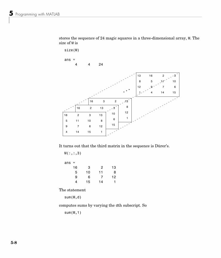
5 Programming with MATLAB
5-8
stores the sequence of 24 magic squares in a three-dimensional array, M. The size of M is
size(M)
ans = 4 4 24
It turns out that the third matrix in the sequence is Dürer’s.
M(:,:,3)
ans = 16 3 2 13 5 10 11 8 9 6 7 12 4 15 14 1
The statement
sum(M,d)
computes sums by varying the dth subscript. So
sum(M,1)
16 3 2 13
8 11 10 8
12 7 6 12
1 14 15 1
16 2 13 3
10 8 11 10
6 12 7 6
15 1 14 15
13 16 2 3
8 5 11 10
12 9 7 6
1 4 14 15
16 2 3 13
5 11 10 8
9 7 6 12
4 14 15 1
...
Other Data Structures
is a 1-by-4-by-24 array containing 24 copies of the row vector
34 34 34 34
and
sum(M,2)
is a 4-by-1-by-24 array containing 24 copies of the column vector
34 34 34 34
Finally,
S = sum(M,3)
adds the 24 matrices in the sequence. The result has size 4-by-4-by-1, so it looks like a 4-by-4 array.
S = 204 204 204 204 204 204 204 204 204 204 204 204 204 204 204 204
Cell ArraysCell arrays in MATLAB are multidimensional arrays whose elements are copies of other arrays. A cell array of empty matrices can be created with the cell function. But, more often, cell arrays are created by enclosing a miscellaneous collection of things in curly braces, {}. The curly braces are also used with subscripts to access the contents of various cells. For example,
C = {A sum(A) prod(prod(A))}
produces a 1-by-3 cell array. The three cells contain the magic square, the row vector of column sums, and the product of all its elements. When C is displayed, you see
C = [4x4 double] [1x4 double] [20922789888000]
5-9
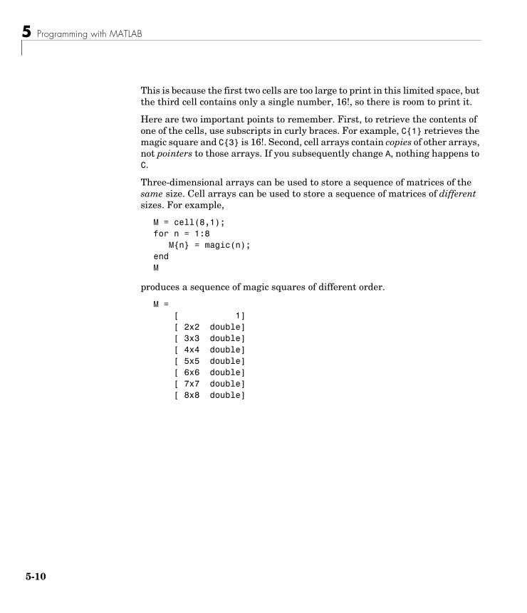
5 Programming with MATLAB
5-1
This is because the first two cells are too large to print in this limited space, but the third cell contains only a single number, 16!, so there is room to print it.
Here are two important points to remember. First, to retrieve the contents of one of the cells, use subscripts in curly braces. For example, C{1} retrieves the magic square and C{3} is 16!. Second, cell arrays contain copies of other arrays, not pointers to those arrays. If you subsequently change A, nothing happens to C.
Three-dimensional arrays can be used to store a sequence of matrices of the same size. Cell arrays can be used to store a sequence of matrices of different sizes. For example,
M = cell(8,1);for n = 1:8 M{n} = magic(n);endM
produces a sequence of magic squares of different order.
M = [ 1] [ 2x2 double] [ 3x3 double] [ 4x4 double] [ 5x5 double] [ 6x6 double] [ 7x7 double] [ 8x8 double]
0
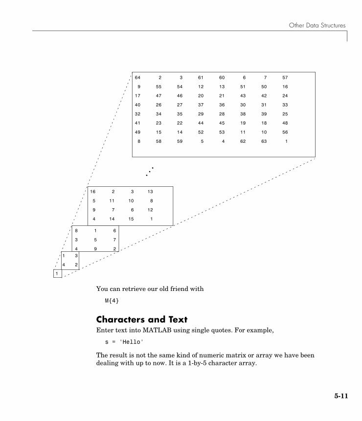
Other Data Structures
You can retrieve our old friend with
M{4}
Characters and TextEnter text into MATLAB using single quotes. For example,
s = 'Hello'
The result is not the same kind of numeric matrix or array we have been dealing with up to now. It is a 1-by-5 character array.
16 2 3 13
5 11 10 8
9 7 6 12
4 14 15 1
...
64 2 3 61 60 6 7 57
9 55 54 12 13 51 50 16
17 47 46 20 21 43 42 24
40 26 27 37 36 30 31 33
32 34 35 29 28 38 39 25
41 23 22 44 45 19 18 48
49 15 14 52 53 11 10 56
8 58 59 5 4 62 63 1
1 3
4 2
8 1 6
3 5 7
4 9 2
1
5-11
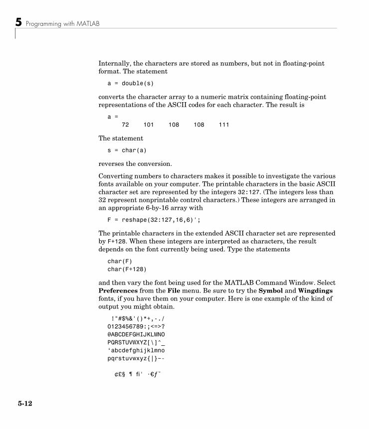
5 Programming with MATLAB
5-1
Internally, the characters are stored as numbers, but not in floating-point format. The statement
a = double(s)
converts the character array to a numeric matrix containing floating-point representations of the ASCII codes for each character. The result is
a = 72 101 108 108 111
The statement
s = char(a)
reverses the conversion.
Converting numbers to characters makes it possible to investigate the various fonts available on your computer. The printable characters in the basic ASCII character set are represented by the integers 32:127. (The integers less than 32 represent nonprintable control characters.) These integers are arranged in an appropriate 6-by-16 array with
F = reshape(32:127,16,6)';
The printable characters in the extended ASCII character set are represented by F+128. When these integers are interpreted as characters, the result depends on the font currently being used. Type the statements
char(F)char(F+128)
and then vary the font being used for the MATLAB Command Window. Select Preferences from the File menu. Be sure to try the Symbol and Wingdings fonts, if you have them on your computer. Here is one example of the kind of output you might obtain.
!"#$%&'()*+,-./0123456789:;<=>?@ABCDEFGHIJKLMNOPQRSTUVWXYZ[\]^_‘abcdefghijklmnopqrstuvwxyz{|}~-
¢£§ ¶ fi' ·¤ƒ˘
2
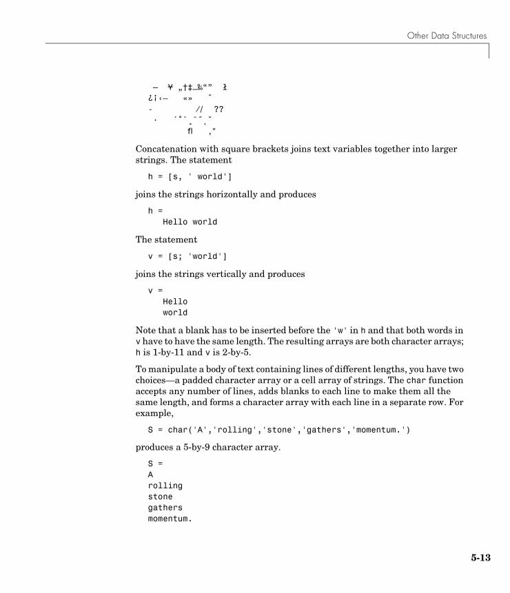
Other Data Structures
– ¥ „†‡…‰“” ł¿¡‹— «» ˆ- ⁄⁄ ??• ´˚`¸¨˝˛ˇ
fl ‚″
Concatenation with square brackets joins text variables together into larger strings. The statement
h = [s, ' world']
joins the strings horizontally and produces
h = Hello world
The statement
v = [s; 'world']
joins the strings vertically and produces
v = Hello world
Note that a blank has to be inserted before the 'w' in h and that both words in v have to have the same length. The resulting arrays are both character arrays; h is 1-by-11 and v is 2-by-5.
To manipulate a body of text containing lines of different lengths, you have two choices—a padded character array or a cell array of strings. The char function accepts any number of lines, adds blanks to each line to make them all the same length, and forms a character array with each line in a separate row. For example,
S = char('A','rolling','stone','gathers','momentum.')
produces a 5-by-9 character array.
S =A rolling stone gathers momentum.
5-13

5 Programming with MATLAB
5-1
There are enough blanks in each of the first four rows of S to make all the rows the same length. Alternatively, you can store the text in a cell array. For example,
C = {'A';'rolling';'stone';'gathers';'momentum.'}
is a 5-by-1 cell array.
C = 'A' 'rolling' 'stone' 'gathers' 'momentum.'
You can convert a padded character array to a cell array of strings with
C = cellstr(S)
and reverse the process with
S = char(C)
StructuresStructures are multidimensional MATLAB arrays with elements accessed by textual field designators. For example,
S.name = 'Ed Plum';S.score = 83;S.grade = 'B+'
creates a scalar structure with three fields.
S = name: 'Ed Plum' score: 83 grade: 'B+'
4
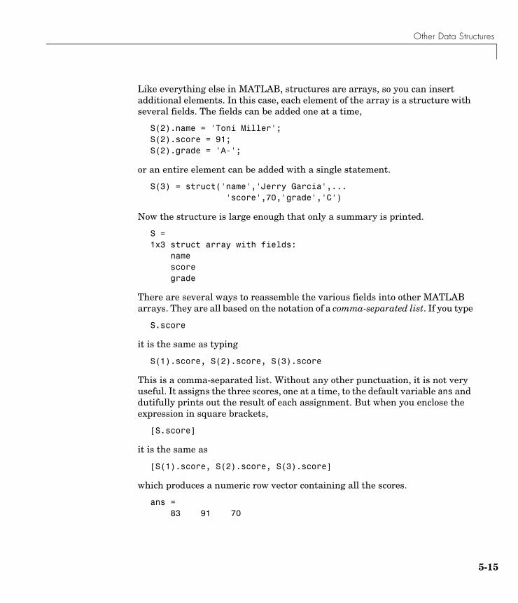
Other Data Structures
Like everything else in MATLAB, structures are arrays, so you can insert additional elements. In this case, each element of the array is a structure with several fields. The fields can be added one at a time,
S(2).name = 'Toni Miller';S(2).score = 91;S(2).grade = 'A-';
or an entire element can be added with a single statement.
S(3) = struct('name','Jerry Garcia',... 'score',70,'grade','C')
Now the structure is large enough that only a summary is printed.
S = 1x3 struct array with fields: name score grade
There are several ways to reassemble the various fields into other MATLAB arrays. They are all based on the notation of a comma-separated list. If you type
S.score
it is the same as typing
S(1).score, S(2).score, S(3).score
This is a comma-separated list. Without any other punctuation, it is not very useful. It assigns the three scores, one at a time, to the default variable ans and dutifully prints out the result of each assignment. But when you enclose the expression in square brackets,
[S.score]
it is the same as
[S(1).score, S(2).score, S(3).score]
which produces a numeric row vector containing all the scores.
ans = 83 91 70
5-15
5 Programming with MATLAB
5-1
Similarly, typing
S.name
just assigns the names, one at a time, to ans. But enclosing the expression in curly braces,
{S.name}
creates a 1-by-3 cell array containing the three names.
ans = 'Ed Plum' 'Toni Miller' 'Jerry Garcia'
And
char(S.name)
calls the char function with three arguments to create a character array from the name fields,
ans =Ed Plum Toni MillerJerry Garcia
6
Scripts and Functions
Scripts and FunctionsTopics covered in this section are
• “Scripts” on page 5-18
• “Functions” on page 5-19
• “Global Variables” on page 5-21
• “Passing String Arguments to Functions” on page 5-21
• “The eval Function” on page 5-23
• “Vectorization” on page 5-23
• “Preallocation” on page 5-24
• “Function Handles” on page 5-24
• “Function Functions” on page 5-25
MATLAB is a powerful programming language as well as an interactive computational environment. Files that contain code in the MATLAB language are called M-files. You create M-files using a text editor, then use them as you would any other MATLAB function or command.
There are two kinds of M-files:
• Scripts, which do not accept input arguments or return output arguments. They operate on data in the workspace.
• Functions, which can accept input arguments and return output arguments. Internal variables are local to the function.
If you’re a new MATLAB programmer, just create the M-files that you want to try out in the current directory. As you develop more of your own M-files, you will want to organize them into other directories and personal toolboxes that you can add to your MATLAB search path.
If you duplicate function names, MATLAB executes the one that occurs first in the search path.
To view the contents of an M-file, for example, myfunction.m, use
type myfunction
5-17
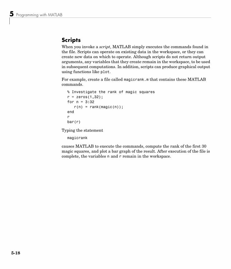
5 Programming with MATLAB
5-1
ScriptsWhen you invoke a script, MATLAB simply executes the commands found in the file. Scripts can operate on existing data in the workspace, or they can create new data on which to operate. Although scripts do not return output arguments, any variables that they create remain in the workspace, to be used in subsequent computations. In addition, scripts can produce graphical output using functions like plot.
For example, create a file called magicrank.m that contains these MATLAB commands.
% Investigate the rank of magic squaresr = zeros(1,32);for n = 3:32 r(n) = rank(magic(n));endrbar(r)
Typing the statement
magicrank
causes MATLAB to execute the commands, compute the rank of the first 30 magic squares, and plot a bar graph of the result. After execution of the file is complete, the variables n and r remain in the workspace.
8
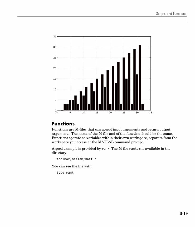
Scripts and Functions
Functions Functions are M-files that can accept input arguments and return output arguments. The name of the M-file and of the function should be the same. Functions operate on variables within their own workspace, separate from the workspace you access at the MATLAB command prompt.
A good example is provided by rank. The M-file rank.m is available in the directory
toolbox/matlab/matfun
You can see the file with
type rank
0 5 10 15 20 25 30 350
5
10
15
20
25
30
35
5-19
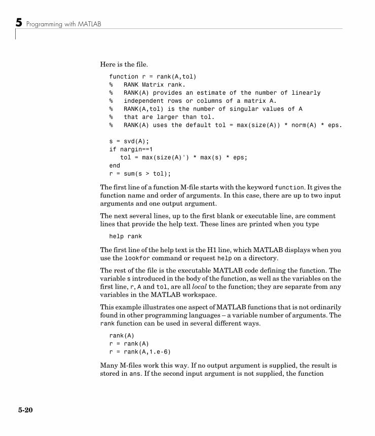
5 Programming with MATLAB
5-2
Here is the file.
function r = rank(A,tol)% RANK Matrix rank.% RANK(A) provides an estimate of the number of linearly% independent rows or columns of a matrix A.% RANK(A,tol) is the number of singular values of A% that are larger than tol.% RANK(A) uses the default tol = max(size(A)) * norm(A) * eps.
s = svd(A);if nargin==1 tol = max(size(A)') * max(s) * eps;endr = sum(s > tol);
The first line of a function M-file starts with the keyword function. It gives the function name and order of arguments. In this case, there are up to two input arguments and one output argument.
The next several lines, up to the first blank or executable line, are comment lines that provide the help text. These lines are printed when you type
help rank
The first line of the help text is the H1 line, which MATLAB displays when you use the lookfor command or request help on a directory.
The rest of the file is the executable MATLAB code defining the function. The variable s introduced in the body of the function, as well as the variables on the first line, r, A and tol, are all local to the function; they are separate from any variables in the MATLAB workspace.
This example illustrates one aspect of MATLAB functions that is not ordinarily found in other programming languages – a variable number of arguments. The rank function can be used in several different ways.
rank(A)r = rank(A)r = rank(A,1.e-6)
Many M-files work this way. If no output argument is supplied, the result is stored in ans. If the second input argument is not supplied, the function
0
Scripts and Functions
computes a default value. Within the body of the function, two quantities named nargin and nargout are available which tell you the number of input and output arguments involved in each particular use of the function. The rank function uses nargin, but does not need to use nargout.
Global VariablesIf you want more than one function to share a single copy of a variable, simply declare the variable as global in all the functions. Do the same thing at the command line if you want the base workspace to access the variable. The global declaration must occur before the variable is actually used in a function. Although it is not required, using capital letters for the names of global variables helps distinguish them from other variables. For example, create an M-file called falling.m.
function h = falling(t)global GRAVITYh = 1/2*GRAVITY*t.^2;
Then interactively enter the statements
global GRAVITYGRAVITY = 32;y = falling((0:.1:5)');
The two global statements make the value assigned to GRAVITY at the command prompt available inside the function. You can then modify GRAVITY interactively and obtain new solutions without editing any files.
Passing String Arguments to FunctionsYou can write MATLAB functions that accept string arguments without the parentheses and quotes. That is, MATLAB interprets
foo a b c
as
foo('a','b','c')
However, when using the unquoted form, MATLAB cannot return output arguments. For example,
legend apples oranges
5-21
5 Programming with MATLAB
5-2
creates a legend on a plot using the strings apples and oranges as labels. If you want the legend command to return its output arguments, then you must use the quoted form.
[legh,objh] = legend('apples','oranges');
In addition, you cannot use the unquoted form if any of the arguments is not a string.
Constructing String Arguments in CodeThe quoted form enables you to construct string arguments within the code. The following example processes multiple data files, August1.dat, August2.dat, and so on. It uses the function int2str, which converts an integer to a character, to build the filename.
for d = 1:31 s = ['August' int2str(d) '.dat']; load(s) % Code to process the contents of the d-th fileend
A Cautionary NoteWhile the unquoted syntax is convenient, it can be used incorrectly without causing MATLAB to generate an error. For example, given a matrix A,
A = 0 -6 -1 6 2 -16
-5 20 -10
The eig command returns the eigenvalues of A.
eig(A)ans =-3.0710 -2.4645+17.6008i-2.4645-17.6008i
2
Scripts and Functions
The following statement is not allowed because A is not a string; however, MATLAB does not generate an error.
eig Aans =
65
MATLAB actually takes the eigenvalues of ASCII numeric equivalent of the letter A (which is the number 65).
The eval FunctionThe eval function works with text variables to implement a powerful text macro facility. The expression or statement
eval(s)
uses the MATLAB interpreter to evaluate the expression or execute the statement contained in the text string s.
The example of the previous section could also be done with the following code, although this would be somewhat less efficient because it involves the full interpreter, not just a function call.
for d = 1:31 s = ['load August' int2str(d) '.dat']; eval(s) % Process the contents of the d-th fileend
VectorizationTo obtain the most speed out of MATLAB, it’s important to vectorize the algorithms in your M-files. Where other programming languages might use for or DO loops, MATLAB can use vector or matrix operations. A simple example involves creating a table of logarithms.
x = .01;for k = 1:1001 y(k) = log10(x); x = x + .01;end
5-23
5 Programming with MATLAB
5-2
A vectorized version of the same code is
x = .01:.01:10;y = log10(x);
For more complicated code, vectorization options are not always so obvious. When speed is important, however, you should always look for ways to vectorize your algorithms.
Preallocation If you can’t vectorize a piece of code, you can make your for loops go faster by preallocating any vectors or arrays in which output results are stored. For example, this code uses the function zeros to preallocate the vector created in the for loop. This makes the for loop execute significantly faster.
r = zeros(32,1);for n = 1:32 r(n) = rank(magic(n));end
Without the preallocation in the previous example, the MATLAB interpreter enlarges the r vector by one element each time through the loop. Vector preallocation eliminates this step and results in faster execution.
Function HandlesYou can create a handle to any MATLAB function and then use that handle as a means of referencing the function. A function handle is typically passed in an argument list to other functions, which can then execute, or evaluate, the function using the handle.
Construct a function handle in MATLAB using the at sign, @, before the function name. The following example creates a function handle for the sin function and assigns it to the variable fhandle.
fhandle = @sin;
Evaluate a function handle using the MATLAB feval function. The function plot_fhandle, shown below, receives a function handle and data, and then performs an evaluation of the function handle on that data using feval.
function x = plot_fhandle(fhandle, data)plot(data, feval(fhandle, data))
4
Scripts and Functions
When you call plot_fhandle with a handle to the sin function and the argument shown below, the resulting evaluation produces a sine wave plot.
plot_fhandle(@sin, -pi:0.01:pi)
Function FunctionsA class of functions called “function functions” works with nonlinear functions of a scalar variable. That is, one function works on another function. The function functions include
• Zero finding
• Optimization
• Quadrature
• Ordinary differential equations
MATLAB represents the nonlinear function by a function M-file. For example, here is a simplified version of the function humps from the matlab/demos directory.
function y = humps(x)y = 1./((x-.3).^2 + .01) + 1./((x-.9).^2 + .04) - 6;
Evaluate this function at a set of points in the interval 0 ≤ x ≤ 1 with
x = 0:.002:1;y = humps(x);
Then plot the function with
plot(x,y)
5-25
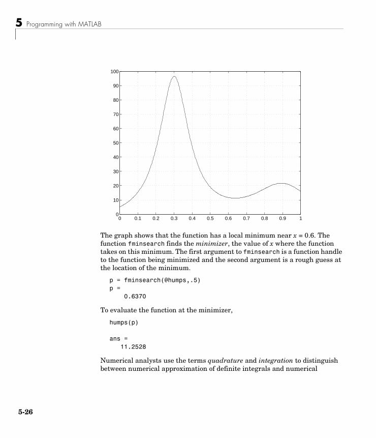
5 Programming with MATLAB
5-2
The graph shows that the function has a local minimum near x = 0.6. The function fminsearch finds the minimizer, the value of x where the function takes on this minimum. The first argument to fminsearch is a function handle to the function being minimized and the second argument is a rough guess at the location of the minimum.
p = fminsearch(@humps,.5)p = 0.6370
To evaluate the function at the minimizer,
humps(p)
ans = 11.2528
Numerical analysts use the terms quadrature and integration to distinguish between numerical approximation of definite integrals and numerical
0 0.1 0.2 0.3 0.4 0.5 0.6 0.7 0.8 0.9 10
10
20
30
40
50
60
70
80
90
100
6
Scripts and Functions
integration of ordinary differential equations. MATLAB quadrature routines are quad and quadl. The statement
Q = quadl(@humps,0,1)
computes the area under the curve in the graph and produces
Q = 29.8583
Finally, the graph shows that the function is never zero on this interval. So, if you search for a zero with
z = fzero(@humps,.5)
you will find one outside the interval
z = -0.1316
5-27
5 Programming with MATLAB
5-2
Demonstration Programs Included with MATLABMATLAB includes many demonstration programs that highlight various features and functions. For a complete list of the demos, type
demo
A list of demos for the products you have installed appears in the Demos tab of the Help browser. Select the product, category, and demo. Information to run the demo and view the source code appears in the display pane.
In addition to the demos listed below, the Demos tab includes playback demos which illustrate how certain graphical user interfaces work.
Some demos listed here are not directly available via the Help browser Demos tab. The description includes “(command line)”. To run these demos, type the demo name at the command line.
Note Many of the demonstrations use multiple windows and require you to press a key in the MATLAB Command Window to continue through the demonstration.
The following tables list the current demonstration programs that are available, organized into these categories:
• “Matrix Demonstration Programs” on page 5-29
• “Numeric Demonstration Programs” on page 5-30
• “Graphics Demonstration Programs” on page 5-31
• “Language Demonstration Programs” on page 5-32
• “Differential Equations Demonstration Programs” on page 5-33
• “Gallery Demonstration Programs” on page 5-34
• “Miscellaneous Demonstration Programs” on page 5-36
8
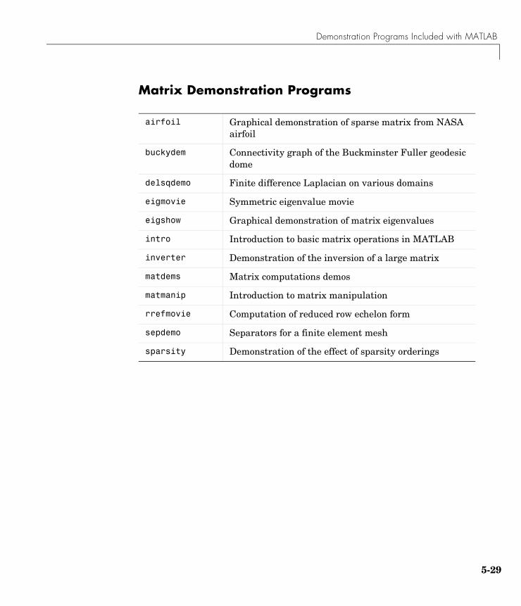
Demonstration Programs Included with MATLAB
Matrix Demonstration Programs
airfoil Graphical demonstration of sparse matrix from NASA airfoil
buckydem Connectivity graph of the Buckminster Fuller geodesic dome
delsqdemo Finite difference Laplacian on various domains
eigmovie Symmetric eigenvalue movie
eigshow Graphical demonstration of matrix eigenvalues
intro Introduction to basic matrix operations in MATLAB
inverter Demonstration of the inversion of a large matrix
matdems Matrix computations demos
matmanip Introduction to matrix manipulation
rrefmovie Computation of reduced row echelon form
sepdemo Separators for a finite element mesh
sparsity Demonstration of the effect of sparsity orderings
5-29
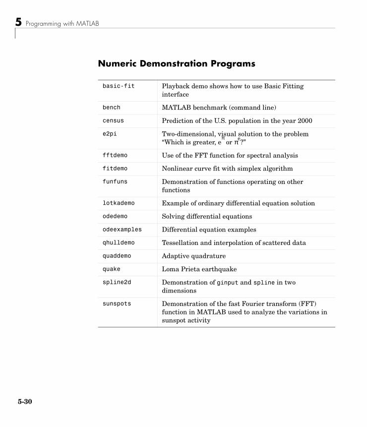
5 Programming with MATLAB
5-3
Numeric Demonstration Programs
basic-fit Playback demo shows how to use Basic Fitting interface
bench MATLAB benchmark (command line)
census Prediction of the U.S. population in the year 2000
e2pi Two-dimensional, visual solution to the problem “Which is greater, e
π or πe
?”
fftdemo Use of the FFT function for spectral analysis
fitdemo Nonlinear curve fit with simplex algorithm
funfuns Demonstration of functions operating on other functions
lotkademo Example of ordinary differential equation solution
odedemo Solving differential equations
odeexamples Differential equation examples
qhulldemo Tessellation and interpolation of scattered data
quaddemo Adaptive quadrature
quake Loma Prieta earthquake
spline2d Demonstration of ginput and spline in two dimensions
sunspots Demonstration of the fast Fourier transform (FFT) function in MATLAB used to analyze the variations in sunspot activity
0
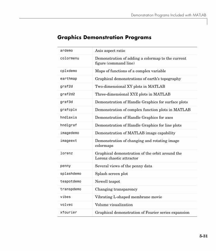
Demonstration Programs Included with MATLAB
Graphics Demonstration Programs
ardemo Axis aspect ratio
colormenu Demonstration of adding a colormap to the current figure (command line)
cplxdemo Maps of functions of a complex variable
earthmap Graphical demonstrations of earth’s topography
graf2d Two-dimensional XY plots in MATLAB
graf2d2 Three-dimensional XYZ plots in MATLAB
graf3d Demonstration of Handle Graphics for surface plots
grafcplx Demonstration of complex function plots in MATLAB
hndlaxis Demonstration of Handle Graphics for axes
hndlgraf Demonstration of Handle Graphics for line plots
imagedemo Demonstration of MATLAB image capability
imageext Demonstration of changing and rotating image colormaps
lorenz Graphical demonstration of the orbit around the Lorenz chaotic attractor
penny Several views of the penny data
splashdemo Splash screen plot
teapotdemo Newell teapot
transpdemo Changing transparency
vibes Vibrating L-shaped membrane movie
volvec Volume visualization
xfourier Graphical demonstration of Fourier series expansion
5-31
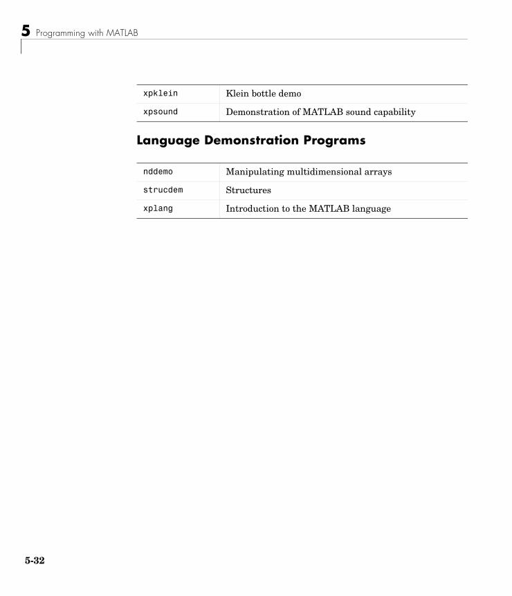
5 Programming with MATLAB
5-3
Language Demonstration Programs
xpklein Klein bottle demo
xpsound Demonstration of MATLAB sound capability
nddemo Manipulating multidimensional arrays
strucdem Structures
xplang Introduction to the MATLAB language
2
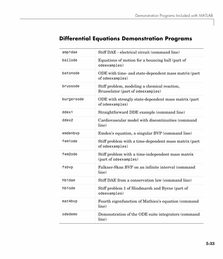
Demonstration Programs Included with MATLAB
Differential Equations Demonstration Programs
amp1dae Stiff DAE - electrical circuit (command line)
ballode Equations of motion for a bouncing ball (part of odeexamples)
batonode ODE with time- and state-dependent mass matrix (part of odeexamples)
brussode Stiff problem, modeling a chemical reaction, Brusselator (part of odeexamples)
burgersode ODE with strongly state-dependent mass matrix (part of odeexamples)
ddex1 Straightforward DDE example (command line)
ddex2 Cardiovascular model with discontinuities (command line)
emdenbvp Emden's equation, a singular BVP (command line)
fem1ode Stiff problem with a time-dependent mass matrix (part of odeexamples)
fem2ode Stiff problem with a time-independent mass matrix (part of odeexamples)
fsbvp Falkner-Skan BVP on an infinite interval (command line)
hb1dae Stiff DAE from a conservation law (command line)
hb1ode Stiff problem 1 of Hindmarsh and Byrne (part of odeexamples)
mat4bvp Fourth eigenfunction of Mathieu's equation (command line)
odedemo Demonstration of the ODE suite integrators (command line)
5-33
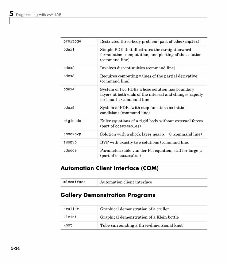
5 Programming with MATLAB
5-3
Automation Client Interface (COM)
Gallery Demonstration Programs
orbitode Restricted three-body problem (part of odeexamples)
pdex1 Simple PDE that illustrates the straightforward formulation, computation, and plotting of the solution (command line)
pdex2 Involves discontinuities (command line)
pdex3 Requires computing values of the partial derivative (command line)
pdex4 System of two PDEs whose solution has boundary layers at both ends of the interval and changes rapidly for small t (command line)
pdex5 System of PDEs with step functions as initial conditions (command line)
rigidode Euler equations of a rigid body without external forces (part of odeexamples)
shockbvp Solution with a shock layer near x = 0 (command line)
twobvp BVP with exactly two solutions (command line)
vdpode Parameterizable van der Pol equation, stiff for large µ (part of odeexamples)
mlcomiface Automation client interface
cruller Graphical demonstration of a cruller
klein1 Graphical demonstration of a Klein bottle
knot Tube surrounding a three-dimensional knot
4
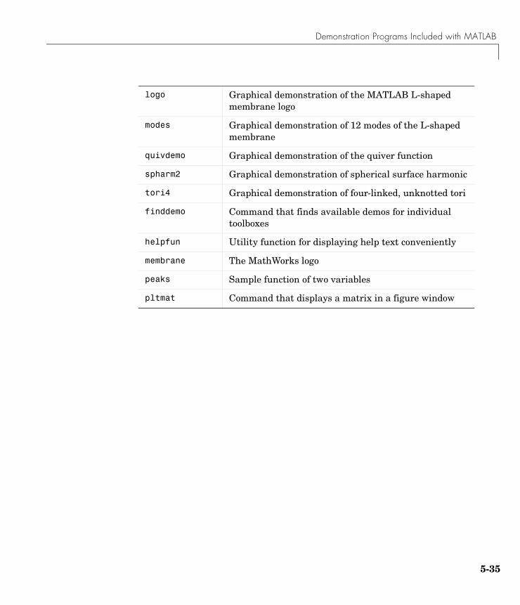
Demonstration Programs Included with MATLAB
logo Graphical demonstration of the MATLAB L-shaped membrane logo
modes Graphical demonstration of 12 modes of the L-shaped membrane
quivdemo Graphical demonstration of the quiver function
spharm2 Graphical demonstration of spherical surface harmonic
tori4 Graphical demonstration of four-linked, unknotted tori
finddemo Command that finds available demos for individual toolboxes
helpfun Utility function for displaying help text conveniently
membrane The MathWorks logo
peaks Sample function of two variables
pltmat Command that displays a matrix in a figure window
5-35
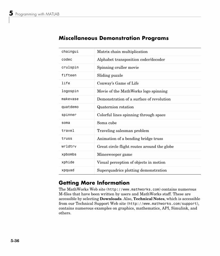
5 Programming with MATLAB
5-3
Miscellaneous Demonstration Programs
Getting More Information The MathWorks Web site (http://www.mathworks.com) contains numerous M-files that have been written by users and MathWorks staff. These are accessible by selecting Downloads. Also, Technical Notes, which is accessible from our Technical Support Web site (http://www.mathworks.com/support), contains numerous examples on graphics, mathematics, API, Simulink, and others.
chaingui Matrix chain multiplication
codec Alphabet transposition coder/decoder
crulspin Spinning cruller movie
fifteen Sliding puzzle
life Conway’s Game of Life
logospin Movie of the MathWorks logo spinning
makevase Demonstration of a surface of revolution
quatdemo Quaternion rotation
spinner Colorful lines spinning through space
soma Soma cube
travel Traveling salesman problem
truss Animation of a bending bridge truss
wrldtrv Great circle flight routes around the globe
xpbombs Minesweeper game
xphide Visual perception of objects in motion
xpquad Superquadrics plotting demonstration
6
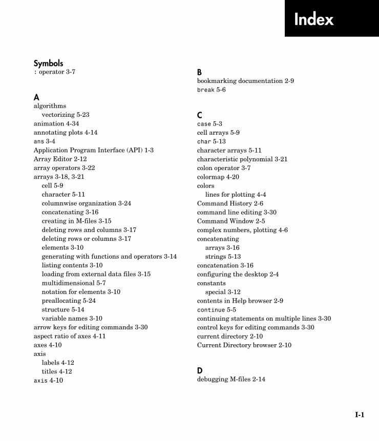
Index
Symbols: operator 3-7
Aalgorithms
vectorizing 5-23animation 4-34annotating plots 4-14ans 3-4Application Program Interface (API) 1-3Array Editor 2-12array operators 3-22arrays 3-18, 3-21
cell 5-9character 5-11columnwise organization 3-24concatenating 3-16creating in M-files 3-15deleting rows and columns 3-17deleting rows or columns 3-17elements 3-10generating with functions and operators 3-14listing contents 3-10loading from external data files 3-15multidimensional 5-7notation for elements 3-10preallocating 5-24structure 5-14variable names 3-10
arrow keys for editing commands 3-30aspect ratio of axes 4-11axes 4-10axis
labels 4-12titles 4-12
axis 4-10
Bbookmarking documentation 2-9break 5-6
Ccase 5-3cell arrays 5-9char 5-13character arrays 5-11characteristic polynomial 3-21colon operator 3-7colormap 4-20colors
lines for plotting 4-4Command History 2-6command line editing 3-30Command Window 2-5complex numbers, plotting 4-6concatenating
arrays 3-16strings 5-13
concatenation 3-16configuring the desktop 2-4constants
special 3-12contents in Help browser 2-9continue 5-5continuing statements on multiple lines 3-30control keys for editing commands 3-30current directory 2-10Current Directory browser 2-10
Ddebugging M-files 2-14
I-1
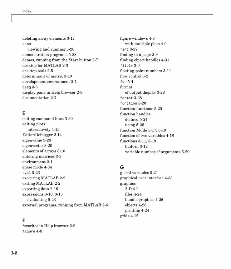
Index
I-2
deleting array elements 3-17demo
viewing and running 5-28demonstration programs 5-28demos, running from the Start button 2-7desktop for MATLAB 2-3desktop tools 2-5determinant of matrix 3-19development environment 2-1diag 3-5display pane in Help browser 2-9documentation 2-7
Eediting command lines 3-30editing plots
interactively 4-15Editor/Debugger 2-14eigenvalue 3-20eigenvector 3-20elements of arrays 3-10entering matrices 3-3environment 2-1erase mode 4-34eval 5-23executing MATLAB 2-2exiting MATLAB 2-2exporting data 2-16expressions 3-10, 3-13
evaluating 5-23external programs, running from MATLAB 2-6
Ffavorites in Help browser 2-9figure 4-8
figure windows 4-8with multiple plots 4-9
find 3-27finding in a page 2-9finding object handles 4-31fliplr 3-6floating-point numbers 3-11flow control 5-2for 5-4format
of output display 3-28format 3-28function 5-20function functions 5-25function handles
defined 5-24using 5-26
function M-file 5-17, 5-19function of two variables 4-18functions 3-11, 5-19
built-in 3-12variable number of arguments 5-20
Gglobal variables 5-21graphical user interface 4-33graphics
2-D 4-2files 4-24handle graphics 4-26objects 4-26printing 4-24
grids 4-12
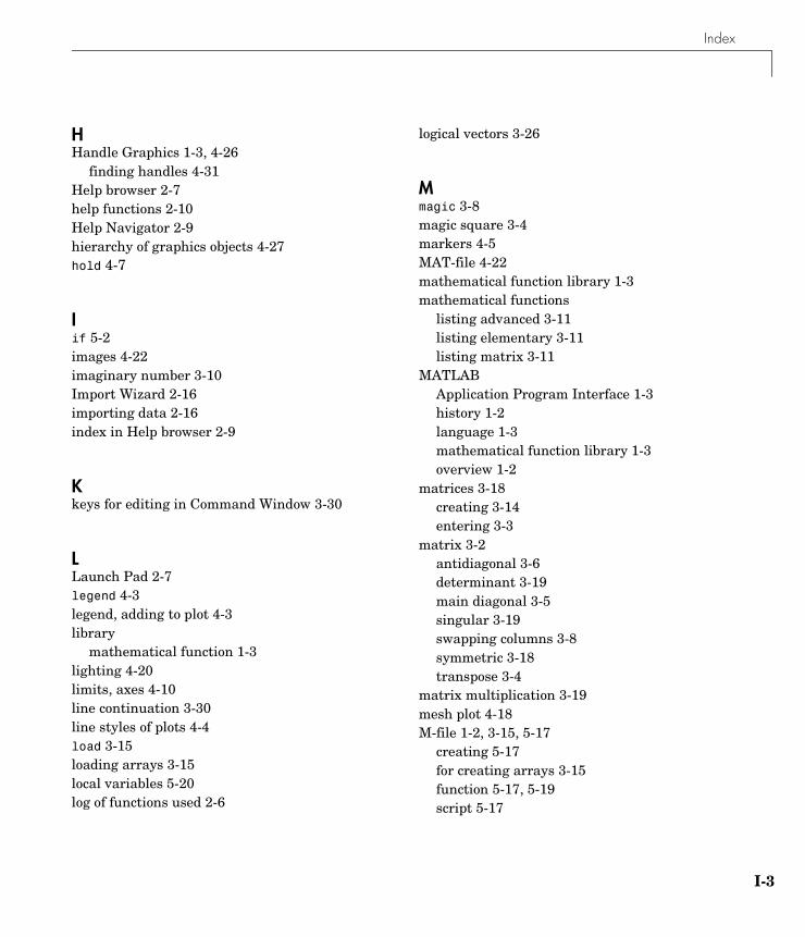
Index
HHandle Graphics 1-3, 4-26
finding handles 4-31Help browser 2-7help functions 2-10Help Navigator 2-9hierarchy of graphics objects 4-27hold 4-7
Iif 5-2images 4-22imaginary number 3-10Import Wizard 2-16importing data 2-16index in Help browser 2-9
Kkeys for editing in Command Window 3-30
LLaunch Pad 2-7legend 4-3legend, adding to plot 4-3library
mathematical function 1-3lighting 4-20limits, axes 4-10line continuation 3-30line styles of plots 4-4load 3-15loading arrays 3-15local variables 5-20log of functions used 2-6
logical vectors 3-26
Mmagic 3-8magic square 3-4markers 4-5MAT-file 4-22mathematical function library 1-3mathematical functions
listing advanced 3-11listing elementary 3-11listing matrix 3-11
MATLABApplication Program Interface 1-3history 1-2language 1-3mathematical function library 1-3overview 1-2
matrices 3-18creating 3-14entering 3-3
matrix 3-2antidiagonal 3-6determinant 3-19main diagonal 3-5singular 3-19swapping columns 3-8symmetric 3-18transpose 3-4
matrix multiplication 3-19mesh plot 4-18M-file 1-2, 3-15, 5-17
creating 5-17for creating arrays 3-15function 5-17, 5-19script 5-17
I-3
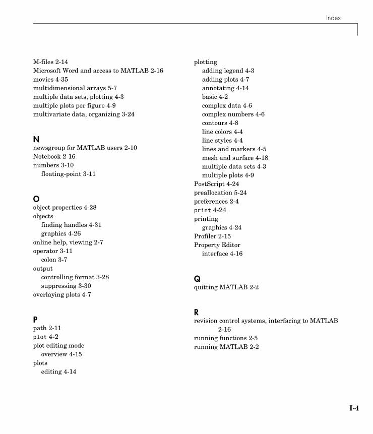
Index
M-files 2-14Microsoft Word and access to MATLAB 2-16movies 4-35multidimensional arrays 5-7multiple data sets, plotting 4-3multiple plots per figure 4-9multivariate data, organizing 3-24
Nnewsgroup for MATLAB users 2-10Notebook 2-16numbers 3-10
floating-point 3-11
Oobject properties 4-28objects
finding handles 4-31graphics 4-26
online help, viewing 2-7operator 3-11
colon 3-7output
controlling format 3-28suppressing 3-30
overlaying plots 4-7
Ppath 2-11plot 4-2plot editing mode
overview 4-15plots
editing 4-14
plottingadding legend 4-3adding plots 4-7annotating 4-14basic 4-2complex data 4-6complex numbers 4-6contours 4-8line colors 4-4line styles 4-4lines and markers 4-5mesh and surface 4-18multiple data sets 4-3multiple plots 4-9
PostScript 4-24preallocation 5-24preferences 2-4print 4-24printing
graphics 4-24Profiler 2-15Property Editor
interface 4-16
Qquitting MATLAB 2-2
Rrevision control systems, interfacing to MATLAB
2-16running functions 2-5running MATLAB 2-2
I-4
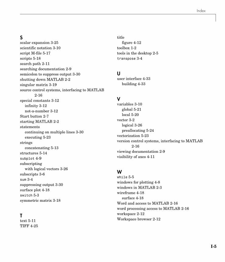
Index
Sscalar expansion 3-25scientific notation 3-10script M-file 5-17scripts 5-18search path 2-11searching documentation 2-9semicolon to suppress output 3-30shutting down MATLAB 2-2singular matrix 3-19source control systems, interfacing to MATLAB
2-16special constants 3-12
infinity 3-12not-a-number 3-12
Start button 2-7starting MATLAB 2-2statements
continuing on multiple lines 3-30executing 5-23
stringsconcatenating 5-13
structures 5-14subplot 4-9subscripting
with logical vectors 3-26subscripts 3-6sum 3-4suppressing output 3-30surface plot 4-18switch 5-3symmetric matrix 3-18
Ttext 5-11TIFF 4-25
titlefigure 4-12
toolbox 1-2tools in the desktop 2-5transpose 3-4
Uuser interface 4-33
building 4-33
Vvariables 3-10
global 5-21local 5-20
vector 3-2logical 3-26preallocating 5-24
vectorization 5-23version control systems, interfacing to MATLAB
2-16viewing documentation 2-9visibility of axes 4-11
Wwhile 5-5windows for plotting 4-8windows in MATLAB 2-3wireframe 4-18
surface 4-18Word and access to MATLAB 2-16word processing access to MATLAB 2-16workspace 2-12Workspace browser 2-12
I-5
Index
Xxor erase mode 4-34
I-6