1

The Lewis Turning Point in China and its Impacts

on the World Economy

Andong Zhu and Wanhuan Cai

Associate Professor and Post-Doc Fellow, School of Marxism, Tsinghua University, Beijing

AUGUR Working Paper, February 2012 (WP #1)

Abstract: On the basis of perusing Lewis’s own writings and his followers’ works on the Lewis

economic growth model, this paper adjusts the meaning of the Lewis turning point (LTP)

according to China’s specific institutional system and economic reality: the Lewis turning point is a

period of time rather than a time point; and undergoing the LTP is considered as a trend or

process of development, during which the supply of labor decreases and the cost of labor

increases. With the passing of the LTP, China will not promote its economic growth with a cheap

and unlimited labor force; the labor-intensive export oriented economy should be altered,

independent technology innovation should be promoted, and industry structure should be

adjusted. Changes and transitions in China’s economy will have great significance to the world

economy, and the impacts are estimated in the paper with Cambridge-Alphametrics Model (CAM)

initially developed by the University of Cambridge. The arrival of the LTP also means China needs

to make serious policy efforts to realize the transformation of its economic development pattern,

and to avoid the so-called “middle-income trap”.

Keywords: Lewis turning point, world economy, Cambridge-Alphametrics Model, transformation

of economic development pattern

1. Introduction

With a 1.3 billion population, China is known as a labor-abundant country. It is argued that the

cheap and unlimited labor supply from the agricultural sector with low productivity to the

industrial sector with high productivity has contributed a lot to China’s rapid economic growth in

the process of its export-oriented industrialization. As Fang Cai and Dewen Wang (2005)

estimate, demographic dividend1 contributed 26.8% to per capita GDP growth during 1982-

2000.2 However, there are some significant phenomena which should be paid close attention to

since the start of the new millennium, especially the waves of labor shortage that hit the country

in 2002, 2004 and 2009; for a time employers in southeastern coastal areas experienced

difficulties in recruiting enough migrant workers.

The phenomenon of the shortage of migrant workers has become a hot topic and inspires

debate among scholars on whether China has reached the Lewis turning point (LTP). Some

1 Demographic dividend means output and other economic gains from having a large proportion of working-age

group in the total population. See Cai and Wang, 2005. 2 Cai, Fang & Wang, Dewen. 2005. China’s demographic transition: Implications for growth. In The China boom

and its discontents, Ross Garnaut and Ligang Song (eds.), pp.34-52. Canberra: Asia Pacific Press.

2

asserted that it’s just a short-term phenomenon which happened occasionally; others argued

that labor shortage is an inevitable result lead by China’s more than 30 years rapid economic

growth, with the surplus labor supply in rural areas all being absorbed by the industrial sector,

which signifies the arrival of the Lewis turning point, and that China will need to make serious

policy efforts to maintain its economic development and social stability. People have conflicting

opinions about the reality, and explain the same phenomenon in different ways, to judge

whether China has reached, is passing, or is close to the Lewis turning point, and to realize

China’s economic reality exactly, we need to understand the Lewis model correctly, including

Lewis’s own writings and those of other researchers’ to clarify the assumptions and predictions of

the Lewis model.

From a general point of view, most of the existing documents treat the Lewis turning point as a

specific point in time; in this paper, as Ryoshin Minami (1968) pointed out, the turning point is a

time of period rather than a time point, which may extend over a number of years1. And if the

Lewis turning point is an inevitable development phase in the course of a country’s economic

development, and if China has not yet passed the turning point,, it will be approaching or passing

it sooner or later; it’s only a matter of time. The coming of the LTP will have a great influence on

China’s economy, such as on the growth rate of the urban resident wage, the income of rural

residents, GDP growth rate, inflation, the economic structure and the mode of economic

development, and so on. As the global manufacturing center, the significance of the changes in

China’s economy will extend far beyond China and have a great impact on the world economy,

the higher wage of labor and the appreciation of RMB making Chinese goods less competitive in

the global market, which may lead to the labor-intensive industry transfer to other economies

with cheap labor. A higher inflation rate in China may promote the inflation rate in other

countries, and the large volume of exchange reserve in China may be reduced. Few scholars pay

attention to the impacts of the Lewis turning point on the world economy, which may be of great

significance to the development trend of world economy and which will be discussed in this

paper.

In this paper, we apply a Cambridge-Alphametrics Model (CAM) to assess world-wide economic

impacts of Lewis turning point in China, which is quite different from Computable General

Equilibrium Model (CGE Model) constructed under the principles of neoclassical economic

theory. The CAM is a derivative of a model originally developed at the Department of Applied

Economics of the University of Cambridge (UK) in the late 1970s. Since the 1970s the model has

been modified various times in significant ways, taking advantage of the improved availability of

statistics and reflecting more recent historical experience.2

This paper is organized as follows. In the next section we summarize Lewis’s theory on the dual

economy and the turning point. The third section introduces debate on whether China has

reached the Lewis turning point and our point of views. The fourth section introduces the CAM

model and explains the results turned out by the model, and the impacts of the LTP on China and

world economy. And the last section concludes the paper by giving some policy implications in

the process of passing the Lewis turning point on how to transfer China’s mode of economic

1 Minami, Ryoshin. 1968. The turning point in the Japanese economy. The Quarterly Journal of Economics, Vol.82,

No. 3, pp. 380-402. 2 Cripps, Francis, & Alex Izurieta & Ajit Singh. Global imbalances, under-consumption and overborrowing: The

state of the world economy and future policies. Centre for Business Research, University of Cambridge. Working Paper No. 419.

3

development and to avoid the “middle-income trap”.

2. Brief review of the Lewis model

The Lewis model, put forward by Arthur Lewis (1954)1 and implemented by Ranis and Fei (1961)2

and Lewis3 himself in 1972, is also known as Lewis-Ranis-Fei model. It provides a significant

contribution to economic development theories for economies with surplus labor and scarce

resources.

According to the Lewis model, an economy at the starting point of economic development is

characterized by a dual economy, which means there are two economic structures in the

economy; one is “subsistence”, “traditional” or agricultural sector and the other “capitalist”,

“modern” or industrial sector. The “traditional” or agricultural sector is assumed to have surplus

labor and the marginal productivity of labor (MPL) is much lower than that of the “modern” or

industrial sector, which can be formalized as MPLT < MPLM ; here the superscript of T denotes

the traditional sector and M denotes the Modern sector. The definition of “surplus labor”, as

Lewis pointed out, is labor with extremely low, even close to zero, marginal productivity, and the

transfer of which has no effect to the total output of this sector while enabling the expansion of

the other sector without any impact on wages.

The wage rate of the traditional sector, wT , is determined by the subsistence level before the

Lewis turning point, known as subsistence wage or institutional wage, and is higher than its

marginal productivity of labor (MPLT), thus wT > MPLT; after the LTP, wage rate in the

traditional sector is determined by the marginal productivity of labor of this sector. And

distribution in the modern sector follows the “marginal product rule” of distribution, so

wM = MPLM , where wM denotes wage rate in modern sector. Wage rate in the modern sector is

higher than that of the traditional sector, i.e. wM > wT, according to Lewis, wage rate in the

modern sector is higher than the traditional sector’s institutional wage by about 30 percent

(Lewis, 1954)4. Due to the higher wage provided by the modern sector, surplus labor can be

drawn out of the traditional sector into the modern sector. The expansion of the modern sector

takes advantage of the infinitely elastic supply of labor from the traditional sector until the

surplus labor is exhausted. This can be concluded as the so-called “Lewis turning point Ⅰ”, during

which the modern or industrial sector expands and workers migrate from rural areas into urban

areas; this can also be depicted as the process of industrialization or urbanization.

Nazrul Islam and Kazuhiko Yokota (2008) point out that the differences between the two

sectors analyzed by Lewis, i.e. MPLT < MPLM , wT > MPLT and wM = MPLM manifest some

departures from neoclassical paradigm. Firstly, the inequality between MPLT and MPLM signifies

a departure from neoclassical paradigm of perfect mobility and equalization of factor returns.

Secondly, the difference in distribution of the two sectors signifies another departure from the

neoclassical model, according to which the same “marginal product rule” of distribution applies

1 Lewis, W. Arthur. 1954. Economic development with unlimited supplies of labour. Manchester School of

Economic and Social Studies. Vol.22, No. 2, pp. 139-191. 2 Ranis, G., & Fei, J. 1961. A theory of economic development. The American Economic Review, Vol. 51, No. 4, pp.

533-565. 3 Lewis, W. Arthur. 1972. Reflections on unlimited labour. In International economics and development, ed. L. Di

Marco, pp.75-96. New York: Academic Press. 4 Lewis, W. Arthur. 1954. Economic development with unlimited supplies of labour. Manchester School of

Economic and Social Studies. Vol.22, No. 2, pp. 139-191.

4

to the entire economy.1

Ranis and Fei (1961), and Lewis (1972) refined the theory by revising Lewis’s two-stage

economic development into three stages, demarcated by when the marginal productivity of labor

of one sector equals the other. After the passing of “Lewis turning point Ⅰ”, though surplus labor

in traditional sector runs out, labor in the sector still transfers into the modern sector because of

its higher marginal productivity of labor thus higher wage rate. However, with the law of

diminishing marginal returns, the outflow of labor from the former sector will lead to the

increase in its marginal productivity of labor until the point when the marginal productivity of

labor in both sectors is equalized. As Lewis depicts, the turning point is attained when the

marginal productivity of labor in the traditional sector is equal to that of the modern sector.

Therefore, this turning point can be called “Lewis turning point Ⅱ”. With the increase of marginal

productivity of labor in the traditional or agricultural sector, wage, i.e. cost of labor rises, and

more capital would be input into agricultural production, the capital-labor ratio goes up, the

imbalance and inequality of development between the two sectors be changed, thus the dual

economic structure disappears, and the economic development enters into its third phase, the

phase of economic integration.

Hitherto, we have already had two turning points, “Lewis turning point Ⅰ” and “Lewis turning

point Ⅱ”. When referring to the Lewis turning point of China’s economic development, it’s Lewis

turning point Ⅰ2. If we confuse “Lewis turning point Ⅰ” with “Lewis turning point Ⅱ”, there will

be some misunderstanding with the Lewis model and may probably lead to errors in explaining

what’s happening in China. Accordingly, except for special illustration, the Lewis turning point

mentioned in this paper is Lewis turning point Ⅰ.

Because the definition of surplus labor defined by Lewis is not explicit enough to some extent

and changes in marginal productivity of labor is difficult to calculate, there are some difficulties in

applying the model to a specific case. For this reason, some scholars make reflections on

amending or revising the Lewis model according to the realities in developing countries. For

example, the standards of identifying the Lewis turning point in the course of a country’s

economic development are concretized as five criteria by Ryoshin Minami (1973) as follows:

comparison between wage and the marginal productivity of labor in the traditional sector, the

correlation ship between wage and the marginal productivity of labor in the traditional sector,

the moving direction of real wage of the traditional sector, changes in wage differentials, and the

traditional sector’s supply elasticity of labor to the modern sector.3 And Minami summarizes the

applicability of the Lewis model in the following ways. First, unlimited supply of labor is

applicable only to the unskilled labor force because skilled workers are limited in supply. Second,

the theory is not applicable to the modern sector because it depends on the existence of a dual

economic structure. Third, the turning point is a period of time rather than a specific point in

time, which may extend over several years. Fourth, the turning point is a long-term and trend-

related economic phenomenon.4

John Knight et al. argue that the Lewis model requires several qualifications and amendments

1 Islam, Nazrul & Kazuhiko Yokota. 2008. Lewis growth model and China’s industrialization. Asian Economic

Journal. Vol.22, No. 4, pp. 359-396. 2 Wang, Dewen. 2008. Lewis turning point and China’s experiences. In Reports on China’s population and labor

No. 9. ed. Fang Cai. p. 90. Beijing: Social Sciences Academic Press (China). 3 Minami, Ryoshin. 1973. The turning point in economic development: Japan’s experience, Economic Research

Series No. 14. The Institute of Economic Research, Hitotsubashi University, Kinokuniya Bookstore, Tokyo. 4 Ibid.

5

as a description of the development process of currently poor economies, such as there is

unlikely to be a clear-cut distinction between the classical and the neoclassical stages, there can

be capital accumulation and technical progress in the rural sector, which raises the average and

marginal product and hence the supply price of rural labor before the labor outflow itself has its

effect on the supply curve, and so on.1

3. Debates on whether China has reached the Lewis turning point

The phenomenon of a shortage of migrant workers in the 2000s become a hot topic and inspires

debate among scholars on whether China has reached Lewis turning point. From a general point

of view, the scholars’ opinions can be classified into two main kinds: one asserts that China has

already reached or has passed the Lewis turning point, surplus labor runs out and the

demographic dividend disappears; while the other argues that it’s too early to mention the LTP in

China’s economic development, and they believe they have mastered some significant evidence

backing their viewpoints. The scholars discuss the topic thoroughly and comprehensively from

the aspects of China’s age structure, structure of labor market, demand and supply of the labor

market, wage growth of ordinary workers, the Hukou system, and rural-urban migration and so

on, and issues at the forefront of discussions are as follows.

First, the volume of surplus labor in China’s rural areas. More and more people have noticed

such an interesting phenomenon: on the one hand, there are reports of migrant labor shortages;

on the other hand, estimates suggest that a considerable volume of relatively unskilled labor is

still available in the agricultural sector, which is called “a China paradox”2 and needs to be paid

more attention to. As the Lewis turning point is defined by the time when surplus labor runs out,

the volume of surplus labor becomes the key to be discussed as it’s the criterion of identifying

the LTP. With migrant workers’ average wage as reference standard, Xianzhou Zhao (2010) argues

that the surplus labor isn’t decreasing but has continued to rise in recent years, and the amount

hit approximately 190 million in 2003-2005. Zhao analyzes the reason why there’s a large amount

of surplus labor on the one hand while there’s a shortage of migrant labor on the other hand; he

attributes it to the increase in mobility costs of labor such as job search costs and the cost of

losing jobs.3 By estimating the agricultural production function using time-series (annual) data

and cross-sectional statistics and comparing marginal productivity of labor with two indices, per

capita net income of rural households and per capita consumption expenditure of rural

households, for the subsistence wage of agricultural sector, Ryoshin Minami and Xinxin Ma

(2010) calculate the surplus labor to be between 159 million and 297 million.4 However, Fang Cai

and other scholars insist that surplus agricultural labor in China is so small that it’s negligible.

Fang Cai (2010) points out that some confusion exists in the Chinese statistics; one is that the

official survey on the utilization of agricultural workforce is unable to reflect the fast-changing

reality of agricultural production - some scholars are unaware of the changed situation, while

others who have tried to understand the statistics are actually trapped in “the tyranny of

1 Knight, J., et al. 2011. The puzzle of migrant labour shortage and rural labour surplus in China, China Economic

Review, doi:10.1016/j.chieco.2011.01.006 2 Kam Wing Chan. 2010. A China paradox: migrant labor shortage amidst rural labor supply abundance. Eurasian

Geography and Economics. Vol. 51, No. 4, pp. 513–530 3 Xianzhou Zhao. 2010. Some theoretical issues on Lewis turning point. Economist, No. 5, pp. 75-80.

4 Minami, Ryoshin & Xinxin Ma. 2010. The Lewis turning point of Chinese economy: Comparison with Japanese

experience. China Economic Journal. Vol. 3, No. 2, pp. 163-179.

6

numbers”. Therefore, the declaration that the marginal productivity of labor in agriculture is still

very low (Minami and Ma 2009), which is based on the aggregated dataset, tends to

overestimate the degree of labor surplus in agriculture and concludes that the Lewis turning

point has not come to China.1 Cai (2007) believes that among the 485 million working-age

population in rural China, 2005, about 200 million have already been transferred into the non-

agricultural sector, thus there remain 2.85 million in the agricultural sector. According to the

current agricultural productivity, the agricultural sector still needs about 170 million labor forces,

so the surplus labor is 115 million, which is not accurate yet. When taking the age structure of

the 120 million labor forces into consideration, of which 50% are over 40 years old, accordingly,

the real surplus labor in rural China is 58 million at most, the percentage is 11.7%. Comparing this

with the rapid development of China’s economy, the volume of surplus labor is negligible.2 The

similar analysis method is also applied by some other scholars. By calculating the gap between

the volume of workers in the agricultural sector and the necessary volume for agricultural

production, Xiaohe Ma and Jianlei Ma (2007) estimate that the surplus labor in rural China is 110

million, of which 50% over 40 years old, 55.37% female and 42.96% below primary education.

Therefore, they conclude that the surplus labor in rural China cannot meet the needs of the rapid

development of the non-agricultural industry.3By means of the classical estimation method, the

neoclassical estimation method and standard structural comparison, Jiangui Wang and Shouhai

(2005) Ding re-estimate, compare and analyze China’s current surplus of agricultural labor and

suggest that the classical estimation method is the best in terms of both credibility and

explanatory power, thus they conclude that China’s surplus agricultural labor amounts to 46

million,4 the result of which is very close to that of Yang Du and Meiyan Wang’s (2010).5

We can have a general view of the volume of agricultural surplus labor estimated by different

studies in the table below.

Table 1. Estimations on the volume of agricultural surplus labor (ASL)

Year Volume of ASL Researcher(s)

2007 100 million Jiadong Tong etc.6 2003 46 million Jiangui Wang etc. 2007 58 million Fang Cai 2007 55 million Xiaohe Ma etc. 2001-2005

159 million-297 million Ryoshin Minami etc.

Second, demand and supply of the labor market and unemployment rate. According to the

Lewis model, when approaching the Lewis turning point labor demand will increase and the labor

market will become tightened by the rapid growth of the industrial sector, which also means that

the unemployment rate will fall after the LTP. Ryoshin Minami et al. (2010) hold the opinion that

1 Cai, Fang. 2010. Demographic transition, demographic dividend, and Lewis turning point in China. China

Economic Journal. Vol. 3, No. 2, pp. 107-119. 2 Cai, Fang. 2007. The myth of surplus labor force in rural China. Chinese Journal of Population Science. No. 2, pp.

27. 3 Ma, Xiaohe & Jianlei Ma. 2007. How much surplus labor in rural China on earth? Chinese Rural Economy. Vol.12,

pp. 4-9,34. 4 Wang, Jiangui & Shouhai Ding. 2005. How much surplus agricultural labor is there in China? Social Sciences in

China, No.5, pp. 27-35. 5 Du, Yang & Meiyan Wang. 2010. New estimate of surplus rural labor force and its implications. Journal of

Guangzhou University (Social Science Edition). Vol.9, No. 4, pp. 17-24. 6 Tong, Jiadong & Zhou Yan. 2011. Dual economy, Lewisian turning point and the foreign trade development

strategy of China. Economic Theory and Management. No. 1, pp. 18-26.

7

there are some problems in the unemployment statistics compiled by the Bureau of Statistics in

China: it does not include the unemployment of migrant workers and laid-off urban workers, who

are in fact in unemployment status. They estimate a said to be more appropriate series of the

unemployment rate, from 2.8% in 1985 to 12% in the first half of 2000s. Thus Ryoshin Minami et

al. argue that the existence of large unemployed labors in urban China should be one of the

counter evidences to the phenomenon of the shortage of migrant workers.1 Fang Cai (2010)

points out that as a result of sectoral changes and the increasing diversification of ownership,

especially after the labor market shock in the late 1990s, multifaceted sectors have appeared to

absorb labor into urban areas, contrary to the pre-reform period when state and collective

sectors dominated employment absorption. And he views the difference between the number of

total employment based on the unit reporting system and the number of employment based on

the household survey as a proxy for urban informal employment, which amounts to 95.1 million

and accounts for 31.5% of total urban employment in 2008.2 Using World Bank cross national

parallel data to estimate the economic development level that corresponds to the Lewis turning

point, Jin Wang and Xiaohan Zhong (2011) find that as GDP per capita increases, the proportion

of rural labor to the total labor force tends to decrease first at an accelerated rate and then, after

passing the Lewis turning point, at a reduced rate. Regression analysis of cross- national parallel

data shows that the Lewis turning point emerges when GDP per capita reaches somewhere

between 3,000 and 4,000 dollars (PPP, constant international US dollars for the year 2000). GDP

per capita in China has exceeded this level, but the proportion of rural labor remains much higher

than the average for countries at the same level of economic development. This strongly implies

great potential for rural labor transfer in China.3

Third, wage increase in both sectors. The Lewis model suggests that the turning point may be

identified by a sharp increase in wages in both the agricultural and industrial sectors. Jane Golley

and Xin Meng (2011) claim that despite some evidence of rising nominal urban unskilled wages

between 2000 and 2009, there is little in the data to suggest that this wage increase has been

caused by unskilled labor shortages. The increase between 2005 and 2006 may be considered as

being close to ‘abnormal’ growth in that it is the first (and only) time that the annual earnings

growth of migrant workers is almost equal to that for urban workers.4 Tianyong Zhou (2011)

argues that the migrant workers’ wage increase definitely exists, but it’s the subsistence wage

increase, which is due to the country’s agricultural policy, the higher inflation rate, and the

strengthening of workers’ bargaining power.5 Fang Cai (2010) believes that the wage rate will

increase when the demand for labor exceeds labor supply. For example, the growth rate of

migrant workers’ wage was 2-3 % in 2002 and 5-6% in 2003, while there’s nearly no growth

before. From the aspect of the growth rate of real wage, the growth rate was always above 7% in

2004-2007 and it reached 19.6% in 2008 when the financial crisis has already broke out. Though

there may be some short-term fluctuation, the law of the Lewis turning point is clear and obvious

1 Minami, Ryoshin & Xinxin Ma. 2010. The Lewis turning point of Chinese economy: Comparison with Japanese

experience. China Economic Journal. Vol. 3, No. 2, pp. 163-179. 2 Cai, Fang. 2010. Demographic transition, demographic dividend, and Lewis turning point in China. China

Economic Journal. Vol. 3, No. 2, pp. 107-119. 3 Wang, Jin & Xiaohan Zhong. 2011. Whether the Lewis turning point has arrived in China: Theoretical studies and

international experiences. Social Sciences in China. Vol. 5, pp. 22-37. 4 Golley, Jane & Xin Meng. 2011. Has China run out of surplus labour? China Economic Review,

doi:10.1016/j.chieco.2011.07.006 5 Zhou Tianyong. 2010. Whether the labor surplus in China. Shanghai Economy. Vol.11, pp. 17-19.

8

in the long run.1 Xiaobo Zhang et al. (2011) take the view that there’s a clear rising trend of the

real wages rate since 2003. The acceleration of real wages even in slack seasons indicates that

the era of surplus labor is over.2

Fourth, income gap and Gini coefficient. When the LTP hits an economy, the surplus labor is

exhausted, the demand for labor increases in industrial sector, marginal productivity of labor

boosts, thus wage rates in both agricultural sector and industrial sector increase, and the income

gap between rural and urban residents is narrowed visibly. Ryoshin Minami (1973) has the

viewpoint that China’s income distribution condition is deteriorating, income gap becomes wider

and wider and the Gini coefficient mounted from 0.382 in 1988 to 0.445 in 2002. The inequality

in income reflects the existence of large amount of surplus labor.3 Besides, in accordance with

Ryoshin’s estimation, wage differentials of agriculture to urban industries were increasing even in

the 2000s.4 By using data from the China Statistical Yearbook and Rural Survey, Anders

Reutersward, Vincent Koen and Richard Herd (2010) discover that for most of the 2000s, migrant

workers’ wages have risen by around 6% per year. This is markedly less than the growth of wages

of all urban workers, whose growth rate of wages were between 10.7%-16.2% from 2002 to

2007, with migrant workers’ earnings dropping from 71% to 49% of salaried urban workers

between 2001 and 2007.5 Fang Cai and Meiyan Wang (2007) argue that the income gap between

rural and urban areas can be expressed by Kuznets curve, the gap is narrow initially and then is

widened, and finally it is narrowed again. Assertions that the income gap between rural and

urban China is wider than that of the beginning of China’s economic reform is unilateral, because

they didn’t take price index differentials between rural and urban areas into consideration. If

adjusted by the price index, the income gap between rural and urban areas in 2006 is on the

same level as in 1978, the ratio is of rural residents income to urban residents income is 1:2.57,

not 1:3.28.6

The precise understanding of Lewis model is the basis of our analysis, but it’s not far enough.

Persuading theoretical analysis requires us to recognize the specific economic reality and

institutional system in China correctly, which may also ask for some necessary modification and

adjustment to the theory according to particular conditions. When talking about the Lewis

turning point, most scholars take it as a specific time point, as Fang Cai (2010), 2004 is the turning

point in China’s economy7. In this paper we agree with Ryoshin Minami (1968), the turning point

is a time of period rather than a time point, which may extend over a number of years8, which

means the economic development including the passing of the LTP is a gradually changing

1 Cai, Fang. 2010. On the challenges of and the path for China’s development of the Lewis turning point of large

country’s economy. Journal of Guangdong University of Business Studies. Vol. 1, pp. 4-12. 2 Zhang Xiaobo, Jin Yang & Shenglin Wang. 2011. China has reached the Lewis turning point. China Economic

Review, doi:10.1016/j.chieco.2011.07.002 3 Minami, Ryoshin. 1973. The turning point in economic development: Japan’s experience, Economic Research

Series No. 14. The Institute of Economic Research, Hitotsubashi University, Kinokuniya Bookstore, Tokyo. 4 Minami, Ryoshin & Xinxin Ma. 2010. The Lewis turning point of Chinese economy: Comparison with Japanese

experience. China Economic Journal. Vol. 3, No. 2, pp. 163-179. 5 Reutersward, Anders, Vincent Koen & Richard Herd. 2010. China's labour market in transition: Job creation,

migration and regulation. OECD Economics Department Working Papers, No. 749, OECD Publishing. doi: 10.1787/5kmlh5010gg7-en 6 Cai, Fang & Meiyan Wang. 2007. Re-assessment of rural surplus labor and some correlated facts. Chinese Rural

Economy. Vol. 10, pp.4-12. 7 Cai, Fang. 2010. The Lewis turning point and the reorientation of public policies: some stylized facts of social

protection in China. Social Science in China. No. 6, pp. 125-137. 8 Minami, Ryoshin. 1968. The turning point in the Japanese economy. The Quarterly Journal of Economics, Vol.82,

No. 3, pp. 380-402.

9

process. As for the criterion or standards identifying the turning point, we tend to believe that

the Lewis turning point – more accurately the Lewis turning period – is such a kind of economic

development tendency or state, during which an economy will be less and less reliant on its

cheap and abundant labor force, the labor-intensive industrial structure should be adjusted,

independent technology innovation should be prompted to develop capital and technology

intensive industry, income polarization should be modified to promote domestic consumption,

and the dependence of China’s economic growth on exports and investment should be altered to

transform China’s economic development mode. And since the industrial structure adjustment

and economic development mode transformation cannot be done in one day, all these should be

accomplished in the process of passing the Lewis turning point or period.

According our viewpoint, the Lewis turning point is a certain phenomenon under a certain

economic system and a certain economic development stage. It is the process of primitive

accumulation of capital as Karl Marx had already pointed out and analyzed in detail in his work of

Das Kapital. And there are some factors or changes which may lead to China experiencing the

Lewis turning point. First, with the development of globalization, the connections between

countries become closer and closer, and the capitalist mode of production has spread all around

the world, as the member of world economy, China has been irresistibly involved into the global

system of capitalism. Second, since the implementation of the Opening up and Reform policy,

diverse forms of ownership as private ownership are developing prosperously in China, taking

more and more share in China’s GDP. Moreover, private ownership has also influenced China’s

rural land tenure system. As the rural land circulation law passed, rural land can be transacted in

China, which will result in a large amount of land deprived peasants. The land deprived peasants

can only live by working as employees or salary earners. This is just what was depicted in Lewis’

dual economy theory. In this sense, and in its appearance, the Lewis turning point can also be

depicted as the process of industrialization and urbanization, during which the peasants are

separated from their land and their home in rural area and have to work in factories in cities. And

since China is such a big country, if East China such as Shanghai or Zhejiang has already passed

the Lewis turning point, West China as Gansu or Guizhou may still have a long way to go. In a

word, because of the existence of factors promoting the capitalist mode of production in China

and China’s specific situation, we can come to the conclusion that China is experiencing the Lewis

turning period.

4. The CAM model and simulation scenarios

From a general view of the current studies on the Lewis turning point, most are concerned with

the time point and impacts of the Lewis turning point on China, which can be summarized as

whether inequality in income gap will be narrowed and industrial structure will be adjusted,

whether growth rate will slow down after the LTP and if it’s a new phase of development for

China’s economy (Ligang Song and Yongsheng Zhang, 2010)1, and China’s transition from an

abnormal economy to a normal economy with somewhat lower growth but higher inflation2.Few

pay attention to the impacts of China’s LTP on the world economy.

1 Song, Ligang & Yongsheng Zhang. 2010. Will Chinese growth slow after the Lewis turning point? China Economic

Journal. Vol. 3, No. 2, pp. 209–219. 2 Huang, Yiping & Tingsong Jiang. 2010. What does the Lewis turning point mean for China? A computable

general equilibrium analysis. China Economic Journal. Vol. 3, No. 2, pp. 191-207.

10

After the rapid development for over three decades since the Reform and Opening-up, China is

now an indispensable member of global economy interactions, and has become the world’s

manufacturing center, called “the world’s factory”. Changes in China’s economy will have seminal

effects to the world economy through the exchange rate of RMB, the price index of exports, and

foreign exchange reserve and so on. For instance, if China has already passed the Lewis turning

point, which means the unlimited supply of surplus labor force in rural China will no longer exist,

the salary of migrant workers will definitely rise, so many labor-intensive industries such as the

textile industry and stationery manufacturing industry will be transferred to other countries with

cheap labor, for example, India or Vietnam. And because of the adjustment of the industrial

structure in China since the approach of the Lewis turning point, technology intensive industry

will be highly developed, and more and more machines will be brought into production, the

demand for petroleum and oil will increase considerably, making the oil price much higher in the

world market and thus affecting the world economy.

Following the above ideas, we will assess these impacts with the CAM model by constructing

several simulation scenarios and comparing them with the baselines in this section.

The Cambridge-Alphametrics Model (CAM) is a derivative of a model originally developed at

the Department of Applied Economics of the University of Cambridge (UK) in the late 1970s

(Cripps et al., 1979)1. Since the 1970s the model has been modified various times in significant

ways taking advantage of the improved availability of statistics and reflecting more recent

historical experience.2 With an integrated databank and modeling framework that can bring

together analysis in different fields, the CAM model is aimed at clarifying the potential impact of

current global trends and evolving public policies on the global economic situation in the medium

to long term.

The model uses official data from over 130 countries plus residuals for each continent (thus

including the entire world economy). And it represents the world economy as a collection of 19

blocs, each of which comprises one or more countries or country group. The hypothesis of

aggregating these blocs or country groups is that each bloc is different from one another in terms

of their economic development level or income level, such as the US, Japan, Central Europe and

North Europe etc. represent developed countries, China and India are taken individually as

developing and emerging economies, Central America and North Africa are another two blocs as

underdeveloped and low-income countries. The 19 blocs are as follows: North Europe, Central

Europe, UK, South Europe, East Europe, USA, Japan, Other Developed Countries (such as Canada,

Australia, New Zealand and so on), East Asia High Income (such as Hong Kong SAR of China,

Singapore, Taiwan and Republic of Korea), CIS, West Asia, South America, Central America, China,

Other East Asia, India, Other South Asia, North Africa, and Other Africa. Different blocs may react

differently to China’s LTP, i.e. transformation of economic development mode. For instance, with

the upgrading of China’s industrial structure, India, Vietnam and Indonesia may benefit a lot from

industry relocation from China, while Japan probably has to face fiercer competition in the global

market with China.

There are more than 190 variables in the model, associated with each other by approximately

1 Cripps, F., G. Gudgin & J. Rhodes. 1979. Technical Manual of the CEPG Model of World Trade’, Cambridge

Economic Policy Review 3 (June). 2 Cripps, Francis, & Alex Izurieta & Ajit Singh. Global imbalances, under-consumption and overborrowing: The

state of the world economy and future policies. Centre for Business Research, University of Cambridge. Working Paper No. 419.

11

40 constant equations and over 150 behavioral equations. As the Lewis turning point in China’s

economy is such an economic transition period, it requires some imperative policies to stabilize

the economy and to realize the transformation of economic development mode, among which

the most significant ones are as follows.

First, fiscal policy of expanding government expenditure. In traditional national income

accounts, the gross domestic product (GDP) is represented asY = C + I + G + NX, where Y =

GDP, C = private consumption, I = gross investment, G = government expenditures, and NX = net

export, and increase in each single part is positively related to Y. After the turning point,

agricultural surplus labor runs out and the wage, i.e. the cost of labor will have a significant rise,

China will not promote its growth by taking advantage of low-cost and unlimited labor force any

longer, labor-intensive industry which contributes a lot to China’s growth rate may be transferred

to other countries with an abundant and cheap labor force. Technology-intensive industry should

be highly encouraged, which requires the country’s investment in developing independent

technologies. Independent technology innovation is a systematic project including government’s

investment in education to improve the quality of human resource, in R&D, and basic science to

strengthen the foundation of the applied technology progress, infrastructure construction and so

on. Furthermore, the government should invest in perfecting China’s social security system to

promote Chinese people’s domestic consumption, which will be discussed below.

Second, monetary policy stimulating increase in domestic private consumption expenditure.

According to the accounting formula of GDP, rising private consumption expenditure also plays a

very important role in GDP. In the past 30 years since China’s economic reform, the export of

labor-intensive products contributes highly to China’s growth rate - in other words, foreign

consumption and demand for Chinese goods is an important factor promoting China’s growth. On

the other hand, domestic consumption has long been neglected. China has the largest population

in the world and the market potential is huge, which may be more reliable to her development.

The key of expanding domestic consumption is to improve people’s income, and the income

distribution gap should also be narrowed to realize social equality. According to Keynesian theory,

the amount of private savings equal to that of private investment, the reduction in interest rate

leads to the decline of private savings and the rise of private investment, which will definitely

result in the increase of income, thus domestic consumption. Therefore, in this paper, instrument

used by the policy maker to improve income is the interest rate.

Third, exchange rate policy of reduction in exports of manufactures and services. Many

scholars focus on the growing role played by exports and investment in China’s rapid economic

growth since 1978. Andong Zhu and David M. Kotz point out that China’s high degree growth

dependence on exports and foreign investment poses a serious problem and is probably not

sustainable for very long,1 which makes China in a disadvantaged position in its international

economic relationship and vulnerable, extremely sensitive and lack of internal support when a

world economic crisis breaks out. In accordance with Chinese statistics, the ratio of total export-

import volume to GDP is 49.17%, 2010.2 In order to cut down export volume to lower China’s

excessively high degree of dependence upon foreign trade, the exchange rate of RMB is

appreciated in this paper.

1 Zhu, Andong & David M. Kotz. 2011. The dependence of China's economic growth on exports and investment.

Review of Radical Political Economics. Vol.43, No.1, pp. 9-32. 2 resource: http://edu.macrochina.com.cn/skins/1/stat/index.shtml?ny=1

12

The policies suggested above also have certain interrelationships to some extent. For instance,

government investment in construction and the perfection of China’s social security system has

the effect of stimulating domestic consumption; the reduction in interest rate used to increase

income has significant impact on reducing foreign capital, which helps to cut down China’s

degree of dependence on foreign trade and investment.

In this section, in order to cope with the arrival of the Lewis turning point and to transform

China’s economic development mode, a package of policies is assumed to be implemented,

including the ratio of government expenditure to GDP to rise from about 22% in 2010 to 30%, the

ratio of private consumption to GDP to rise from approximately 32.3% in 2010 to 40%, and the

ratio of export volume of manufactures and services to GDP to fall from 25.4% to 15%. We will

assess the impacts of these policies on China’s economy and more significantly, the effects or

influences on the world economy with the CAM model.

4.1 Impacts on GDP growth rate

China is considered to be one of the most important engines driving the growth of the world

economy in the last three decades. In 2010, GDP growth rate in China was above 10%, while the

world’s total GDP growth rate is 4.7%, much higher than -1.0% in 2009. After the implementation

of the policy package when passing the Lewis turning point in China, what will happen to the

world GDP growth rate? Graph 1 below is the simulation scenarios produced by the CAM model

which shows us the growth rate of the world total GDP at PPP (Purchasing Power Parity) rate

from 1980-2030. The blue line is the baseline (_0) describing the continuation of existing global

arrangements, and the red line is the scenario (_C), which retains the same basic model and

instruments specified for the baseline, with variations in policies and other behavior specified by

alternative values of add factors and policy rules.

Graph 1. World total GDP at PPP rate

13

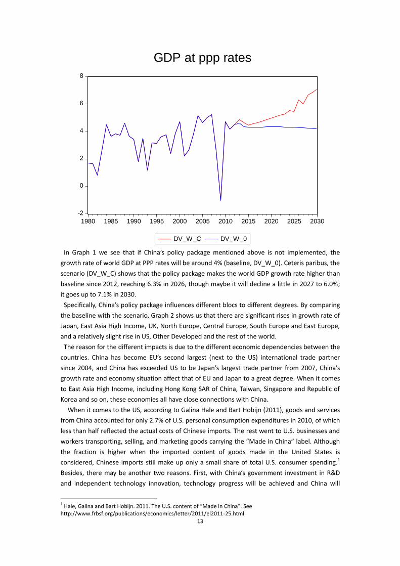
In Graph 1 we see that if China’s policy package mentioned above is not implemented, the

growth rate of world GDP at PPP rates will be around 4% (baseline, DV_W_0). Ceteris paribus, the

scenario (DV_W_C) shows that the policy package makes the world GDP growth rate higher than

baseline since 2012, reaching 6.3% in 2026, though maybe it will decline a little in 2027 to 6.0%;

it goes up to 7.1% in 2030.

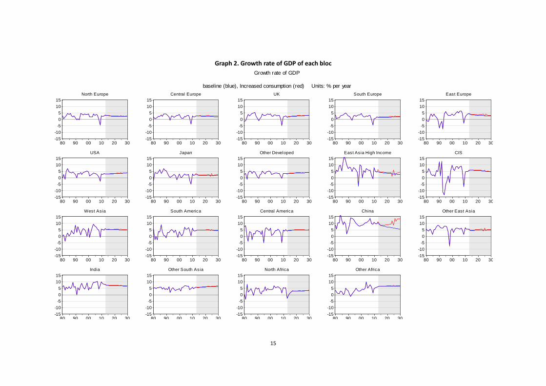
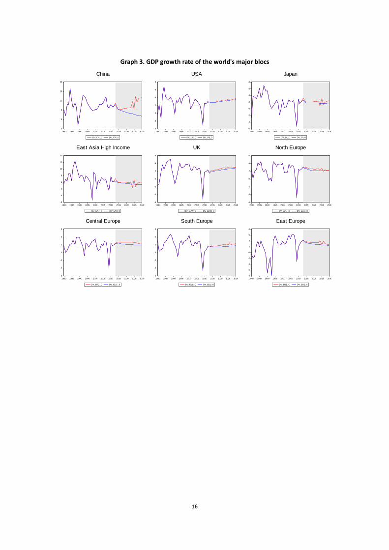
Specifically, China’s policy package influences different blocs to different degrees. By comparing

the baseline with the scenario, Graph 2 shows us that there are significant rises in growth rate of

Japan, East Asia High Income, UK, North Europe, Central Europe, South Europe and East Europe,

and a relatively slight rise in US, Other Developed and the rest of the world.

The reason for the different impacts is due to the different economic dependencies between the

countries. China has become EU’s second largest (next to the US) international trade partner

since 2004, and China has exceeded US to be Japan’s largest trade partner from 2007, China’s

growth rate and economy situation affect that of EU and Japan to a great degree. When it comes

to East Asia High Income, including Hong Kong SAR of China, Taiwan, Singapore and Republic of

Korea and so on, these economies all have close connections with China.

When it comes to the US, according to Galina Hale and Bart Hobijn (2011), goods and services

from China accounted for only 2.7% of U.S. personal consumption expenditures in 2010, of which

less than half reflected the actual costs of Chinese imports. The rest went to U.S. businesses and

workers transporting, selling, and marketing goods carrying the “Made in China” label. Although

the fraction is higher when the imported content of goods made in the United States is

considered, Chinese imports still make up only a small share of total U.S. consumer spending.1

Besides, there may be another two reasons. First, with China’s government investment in R&D

and independent technology innovation, technology progress will be achieved and China will

1 Hale, Galina and Bart Hobijn. 2011. The U.S. content of “Made in China”. See

http://www.frbsf.org/publications/economics/letter/2011/el2011-25.html

-2

0

2

4

6

8

1980 1985 1990 1995 2000 2005 2010 2015 2020 2025 2030

DV_W_C DV_W_0

GDP at ppp rates

14

produce more facilities or equipments by itself and thus cut down on imports from the US and

other developed countries with high and advanced technologies. Second, due to the great

differences in industry structure, the development level of financial market and the composition

of export products, the effect of China’s growth is milder to US GDP growth.

15

Graph 2. Growth rate of GDP of each bloc

-15

-10

-5

0

5

10

15

80 90 00 10 20 30

North Europe

-15

-10

-5

0

5

10

15

80 90 00 10 20 30

Central Europe

-15

-10

-5

0

5

10

15

80 90 00 10 20 30

UK

-15

-10

-5

0

5

10

15

80 90 00 10 20 30

South Europe

-15

-10

-5

0

5

10

15

80 90 00 10 20 30

East Europe

-15

-10

-5

0

5

10

15

80 90 00 10 20 30

USA

-15

-10

-5

0

5

10

15

80 90 00 10 20 30

Japan

-15

-10

-5

0

5

10

15

80 90 00 10 20 30

Other Developed

-15

-10

-5

0

5

10

15

80 90 00 10 20 30

East Asia High Income

-15

-10

-5

0

5

10

15

80 90 00 10 20 30

CIS

-15

-10

-5

0

5

10

15

80 90 00 10 20 30

West Asia

-15

-10

-5

0

5

10

15

80 90 00 10 20 30

South America

-15

-10

-5

0

5

10

15

80 90 00 10 20 30

Central America

-15

-10

-5

0

5

10

15

80 90 00 10 20 30

China

-15

-10

-5

0

5

10

15

80 90 00 10 20 30

Other East Asia

-15

-10

-5

0

5

10

15

80 90 00 10 20 30

India

-15

-10

-5

0

5

10

15

80 90 00 10 20 30

Other South Asia

-15

-10

-5

0

5

10

15

80 90 00 10 20 30

North Africa

-15

-10

-5

0

5

10

15

80 90 00 10 20 30

Other Africa

Growth rate of GDP

baseline (blue), Increased consumption (red) Units: % per year

16

Graph 3. GDP growth rate of the world's major blocs

0

4

8

12

16

20

1980 1985 1990 1995 2000 2005 2010 2015 2020 2025 2030

DV_CN_C DV_CN_0

China

-4

-2

0

2

4

6

8

1980 1985 1990 1995 2000 2005 2010 2015 2020 2025 2030

DV_US_C DV_US_0

USA

-6

-4

-2

0

2

4

6

8

1980 1985 1990 1995 2000 2005 2010 2015 2020 2025 2030

DV_JA_C DV_JA_0

Japan

-8

-4

0

4

8

12

16

20

1980 1985 1990 1995 2000 2005 2010 2015 2020 2025 2030

DV_EAH_C DV_EAH_0

East Asia High Income

-6

-4

-2

0

2

4

6

1980 1985 1990 1995 2000 2005 2010 2015 2020 2025 2030

DV_EUW_C DV_EUW_0

UK

-6

-4

-2

0

2

4

6

1980 1985 1990 1995 2000 2005 2010 2015 2020 2025 2030

DV_EUN_C DV_EUN_0

North Europe

-6

-4

-2

0

2

4

6

1980 1985 1990 1995 2000 2005 2010 2015 2020 2025 2030

DV_EUC_C DV_EUC_0

Central Europe

-6

-4

-2

0

2

4

6

1980 1985 1990 1995 2000 2005 2010 2015 2020 2025 2030

DV_EUS_C DV_EUS_0

South Europe

-8

-6

-4

-2

0

2

4

6

8

1980 1985 1990 1995 2000 2005 2010 2015 2020 2025 2030

DV_EUE_C DV_EUE_0

East Europe

17

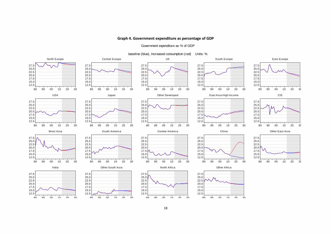
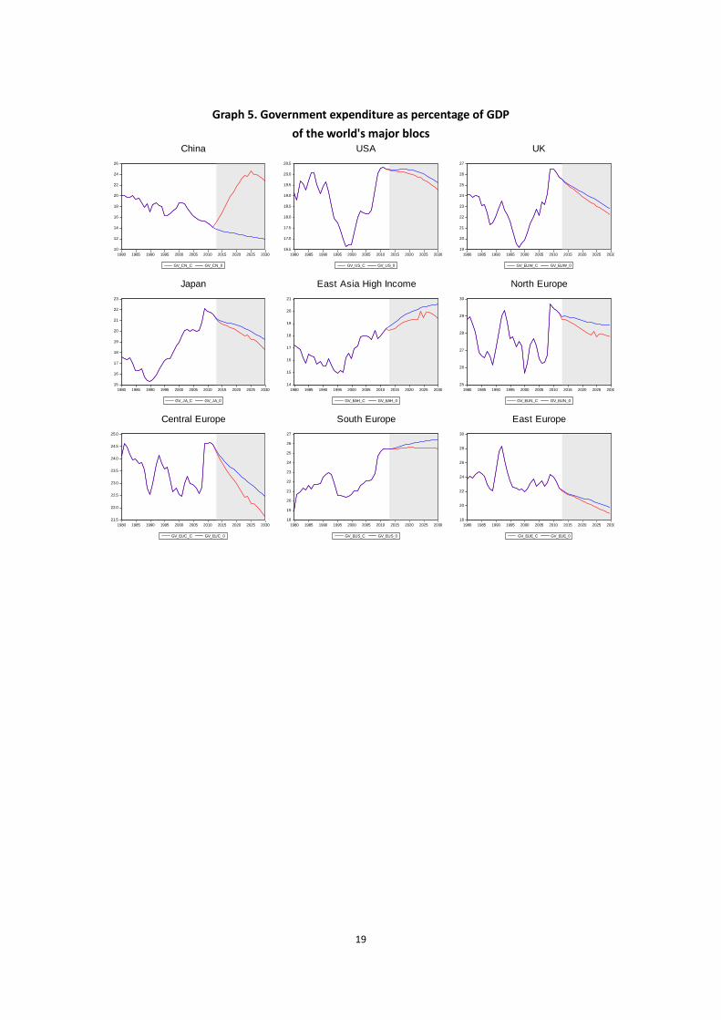
4.2 Impacts on government expenditure

One of the major instruments in the policy package is fiscal policy, specifically the expansion of

government expenditure on R&D, education and the social security system, and so on. The

government expenditure as a percentage of GDP in China is 14.5% in 2010 as manifested in

baseline (the blue line, GV_CN_0) in Graph 4, and it slides slowly from then to 12% in 2030. As

the scenario (the red line, GV_CN_C) depicts, the ratio of government expenditure to GDP soars

drastically from 14.2% in 2012 to over 20% during mid 2020s, with 2025 as its peak, then falls

from 24.5% in 2025 to 22.8% in 2030, which is still a very high proportion. In Graph 4, we may

find that by contrast to rapid government expenditure growth in China, the ratio of government

spending to GDP in USA, UK, Japan and EU all declines by 0.5 to 1.0 percent. For instance, by

comparing the scenario with the baseline of Central Europe and Japan, government expenditure

shares fall by approximately 1%. The reason for this is the rise of income per capita at PPP rates,

which will bring down the government spending on welfare, as poverty relief and other measures

stabilize the society.

18

Graph 4. Government expenditure as percentage of GDP

12.5

15.0

17.5

20.0

22.5

25.0

27.5

80 90 00 10 20 30

North Europe

12.5

15.0

17.5

20.0

22.5

25.0

27.5

80 90 00 10 20 30

Central Europe

12.5

15.0

17.5

20.0

22.5

25.0

27.5

80 90 00 10 20 30

UK

12.5

15.0

17.5

20.0

22.5

25.0

27.5

80 90 00 10 20 30

South Europe

12.5

15.0

17.5

20.0

22.5

25.0

27.5

80 90 00 10 20 30

East Europe

12.5

15.0

17.5

20.0

22.5

25.0

27.5

80 90 00 10 20 30

USA

12.5

15.0

17.5

20.0

22.5

25.0

27.5

80 90 00 10 20 30

Japan

12.5

15.0

17.5

20.0

22.5

25.0

27.5

80 90 00 10 20 30

Other Developed

12.5

15.0

17.5

20.0

22.5

25.0

27.5

80 90 00 10 20 30

East Asia High Income

12.5

15.0

17.5

20.0

22.5

25.0

27.5

80 90 00 10 20 30

CIS

12.5

15.0

17.5

20.0

22.5

25.0

27.5

80 90 00 10 20 30

West Asia

12.5

15.0

17.5

20.0

22.5

25.0

27.5

80 90 00 10 20 30

South America

12.5

15.0

17.5

20.0

22.5

25.0

27.5

80 90 00 10 20 30

Central America

12.5

15.0

17.5

20.0

22.5

25.0

27.5

80 90 00 10 20 30

China

12.5

15.0

17.5

20.0

22.5

25.0

27.5

80 90 00 10 20 30

Other East Asia

12.5

15.0

17.5

20.0

22.5

25.0

27.5

80 90 00 10 20 30

India

12.5

15.0

17.5

20.0

22.5

25.0

27.5

80 90 00 10 20 30

Other South Asia

12.5

15.0

17.5

20.0

22.5

25.0

27.5

80 90 00 10 20 30

North Africa

12.5

15.0

17.5

20.0

22.5

25.0

27.5

80 90 00 10 20 30

Other Africa

Government expenditure as % of GDP

baseline (blue), Increased consumption (red) Units: %

19

Graph 5. Government expenditure as percentage of GDP

of the world's major blocs

10

12

14

16

18

20

22

24

26

1980 1985 1990 1995 2000 2005 2010 2015 2020 2025 2030

GV_CN_C GV_CN_0

China

16.5

17.0

17.5

18.0

18.5

19.0

19.5

20.0

20.5

1980 1985 1990 1995 2000 2005 2010 2015 2020 2025 2030

GV_US_C GV_US_0

USA

19

20

21

22

23

24

25

26

27

1980 1985 1990 1995 2000 2005 2010 2015 2020 2025 2030

GV_EUW_C GV_EUW_0

UK

15

16

17

18

19

20

21

22

23

1980 1985 1990 1995 2000 2005 2010 2015 2020 2025 2030

GV_JA_C GV_JA_0

Japan

14

15

16

17

18

19

20

21

1980 1985 1990 1995 2000 2005 2010 2015 2020 2025 2030

GV_EAH_C GV_EAH_0

East Asia High Income

25

26

27

28

29

30

1980 1985 1990 1995 2000 2005 2010 2015 2020 2025 2030

GV_EUN_C GV_EUN_0

North Europe

21.5

22.0

22.5

23.0

23.5

24.0

24.5

25.0

1980 1985 1990 1995 2000 2005 2010 2015 2020 2025 2030

GV_EUC_C GV_EUC_0

Central Europe

18

19

20

21

22

23

24

25

26

27

1980 1985 1990 1995 2000 2005 2010 2015 2020 2025 2030

GV_EUS_C GV_EUS_0

South Europe

18

20

22

24

26

28

30

1980 1985 1990 1995 2000 2005 2010 2015 2020 2025 2030

GV_EUE_C GV_EUE_0

East Europe

20

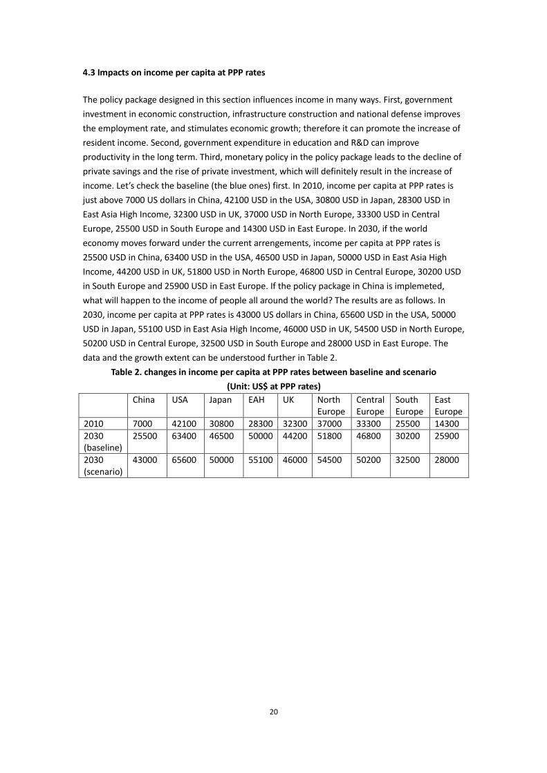
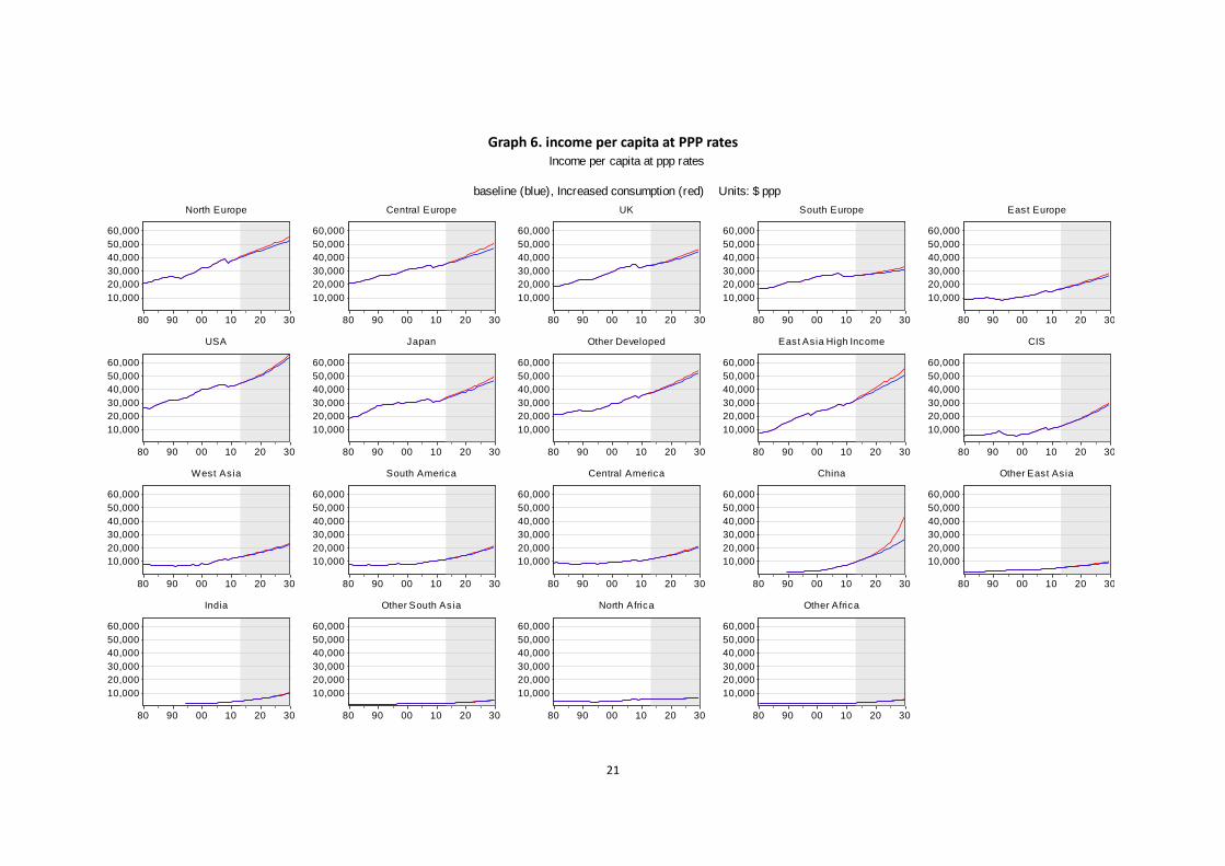
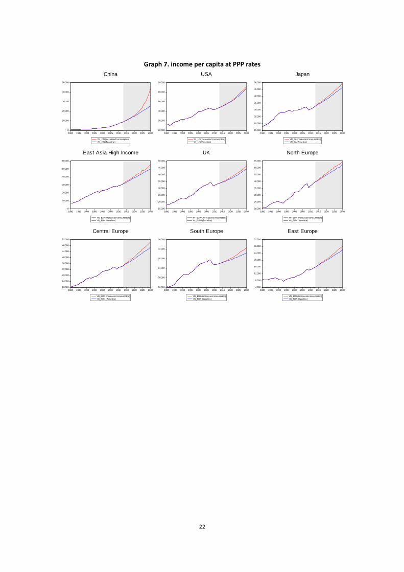
4.3 Impacts on income per capita at PPP rates

The policy package designed in this section influences income in many ways. First, government

investment in economic construction, infrastructure construction and national defense improves

the employment rate, and stimulates economic growth; therefore it can promote the increase of

resident income. Second, government expenditure in education and R&D can improve

productivity in the long term. Third, monetary policy in the policy package leads to the decline of

private savings and the rise of private investment, which will definitely result in the increase of

income. Let’s check the baseline (the blue ones) first. In 2010, income per capita at PPP rates is

just above 7000 US dollars in China, 42100 USD in the USA, 30800 USD in Japan, 28300 USD in

East Asia High Income, 32300 USD in UK, 37000 USD in North Europe, 33300 USD in Central

Europe, 25500 USD in South Europe and 14300 USD in East Europe. In 2030, if the world

economy moves forward under the current arrengements, income per capita at PPP rates is

25500 USD in China, 63400 USD in the USA, 46500 USD in Japan, 50000 USD in East Asia High

Income, 44200 USD in UK, 51800 USD in North Europe, 46800 USD in Central Europe, 30200 USD

in South Europe and 25900 USD in East Europe. If the policy package in China is implemeted,

what will happen to the income of people all around the world? The results are as follows. In

2030, income per capita at PPP rates is 43000 US dollars in China, 65600 USD in the USA, 50000

USD in Japan, 55100 USD in East Asia High Income, 46000 USD in UK, 54500 USD in North Europe,

50200 USD in Central Europe, 32500 USD in South Europe and 28000 USD in East Europe. The

data and the growth extent can be understood further in Table 2.

Table 2. changes in income per capita at PPP rates between baseline and scenario

(Unit: US$ at PPP rates)

China USA Japan EAH UK North Europe

Central Europe

South Europe

East Europe

2010 7000 42100 30800 28300 32300 37000 33300 25500 14300

2030 (baseline)

25500 63400 46500 50000 44200 51800 46800 30200 25900

2030 (scenario)

43000 65600 50000 55100 46000 54500 50200 32500 28000

21

Graph 6. income per capita at PPP rates

10,000

20,000

30,000

40,000

50,000

60,000

80 90 00 10 20 30

North Europe

10,000

20,000

30,000

40,000

50,000

60,000

80 90 00 10 20 30

Central Europe

10,000

20,000

30,000

40,000

50,000

60,000

80 90 00 10 20 30

UK

10,000

20,000

30,000

40,000

50,000

60,000

80 90 00 10 20 30

South Europe

10,000

20,000

30,000

40,000

50,000

60,000

80 90 00 10 20 30

East Europe

10,000

20,000

30,000

40,000

50,000

60,000

80 90 00 10 20 30

USA

10,000

20,000

30,000

40,000

50,000

60,000

80 90 00 10 20 30

Japan

10,000

20,000

30,000

40,000

50,000

60,000

80 90 00 10 20 30

Other Developed

10,000

20,000

30,000

40,000

50,000

60,000

80 90 00 10 20 30

East Asia High Income

10,000

20,000

30,000

40,000

50,000

60,000

80 90 00 10 20 30

CIS

10,000

20,000

30,000

40,000

50,000

60,000

80 90 00 10 20 30

West Asia

10,000

20,000

30,000

40,000

50,000

60,000

80 90 00 10 20 30

South America

10,000

20,000

30,000

40,000

50,000

60,000

80 90 00 10 20 30

Central America

10,000

20,000

30,000

40,000

50,000

60,000

80 90 00 10 20 30

China

10,000

20,000

30,000

40,000

50,000

60,000

80 90 00 10 20 30

Other East Asia

10,000

20,000

30,000

40,000

50,000

60,000

80 90 00 10 20 30

India

10,000

20,000

30,000

40,000

50,000

60,000

80 90 00 10 20 30

Other South Asia

10,000

20,000

30,000

40,000

50,000

60,000

80 90 00 10 20 30

North Africa

10,000

20,000

30,000

40,000

50,000

60,000

80 90 00 10 20 30

Other Africa

Income per capita at ppp rates

baseline (blue), Increased consumption (red) Units: $ ppp

22

Graph 7. income per capita at PPP rates

0

10,000

20,000

30,000

40,000

50,000

1980 1985 1990 1995 2000 2005 2010 2015 2020 2025 2030

YN_CN (Increased consumption)

YN_CN (Baseline)

China

20,000

30,000

40,000

50,000

60,000

70,000

1980 1985 1990 1995 2000 2005 2010 2015 2020 2025 2030

YN_US (Increased consumption)

YN_US (Baseline)

USA

15,000

20,000

25,000

30,000

35,000

40,000

45,000

50,000

1980 1985 1990 1995 2000 2005 2010 2015 2020 2025 2030

YN_JA (Increased consumption)

YN_JA (Baseline)

Japan

0

10,000

20,000

30,000

40,000

50,000

60,000

1980 1985 1990 1995 2000 2005 2010 2015 2020 2025 2030

YN_EAH (Increased consumption)

YN_EAH (Baseline)

East Asia High Income

15,000

20,000

25,000

30,000

35,000

40,000

45,000

50,000

1980 1985 1990 1995 2000 2005 2010 2015 2020 2025 2030

YN_EUW (Increased consumption)

YN_EUW (Baseline)

UK

20,000

25,000

30,000

35,000

40,000

45,000

50,000

55,000

1980 1985 1990 1995 2000 2005 2010 2015 2020 2025 2030

YN_EUN (Increased consumption)

YN_EUN (Baseline)

North Europe

20,000

24,000

28,000

32,000

36,000

40,000

44,000

48,000

52,000

1980 1985 1990 1995 2000 2005 2010 2015 2020 2025 2030

YN_EUC (Increased consumption)

YN_EUC (Baseline)

Central Europe

16,000

20,000

24,000

28,000

32,000

36,000

1980 1985 1990 1995 2000 2005 2010 2015 2020 2025 2030

YN_EUS (Increased consumption)

YN_EUS (Baseline)

South Europe

4,000

8,000

12,000

16,000

20,000

24,000

28,000

32,000

1980 1985 1990 1995 2000 2005 2010 2015 2020 2025 2030

YN_EUE (Increased consumption)

YN_EUE (Baseline)

East Europe

23

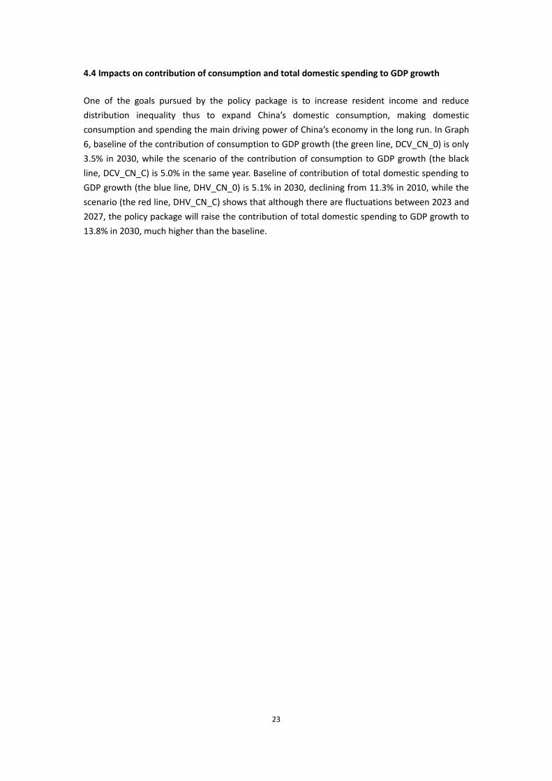
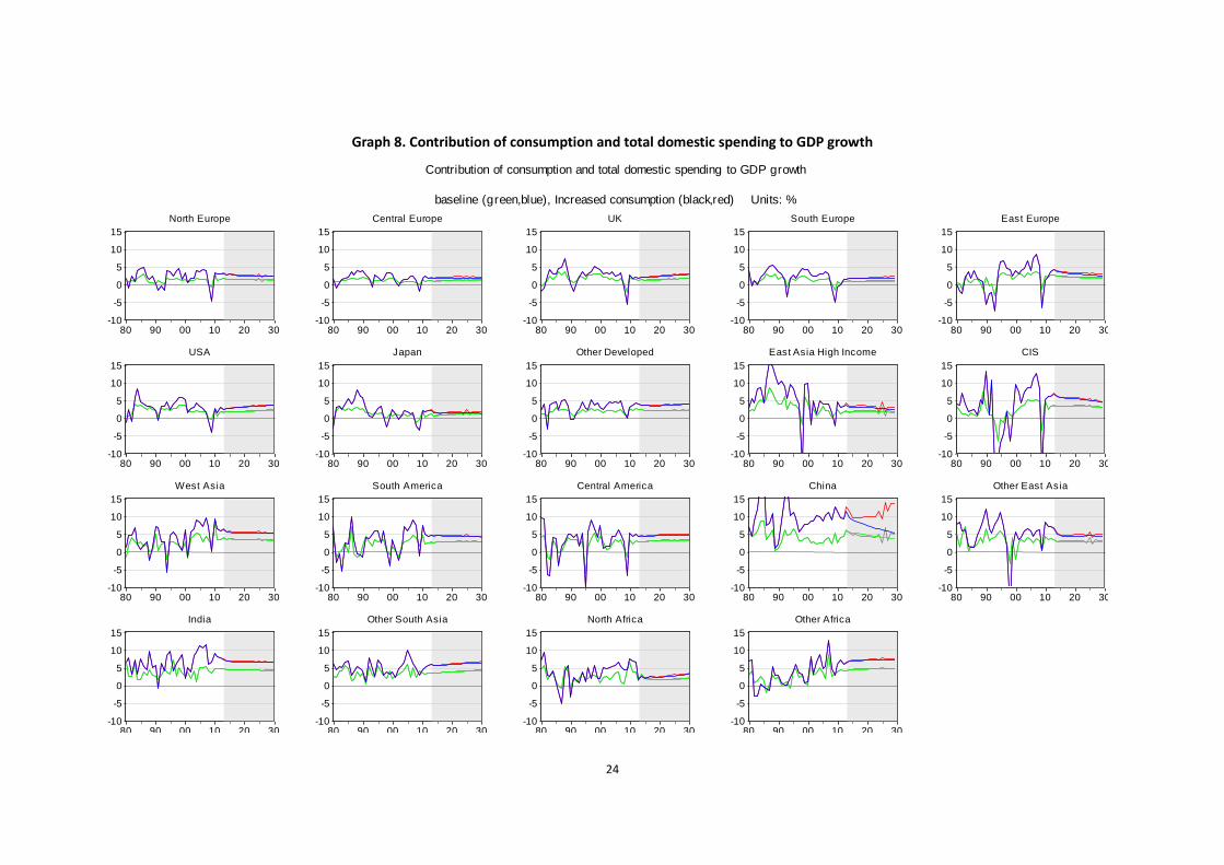
4.4 Impacts on contribution of consumption and total domestic spending to GDP growth

One of the goals pursued by the policy package is to increase resident income and reduce

distribution inequality thus to expand China’s domestic consumption, making domestic

consumption and spending the main driving power of China’s economy in the long run. In Graph

6, baseline of the contribution of consumption to GDP growth (the green line, DCV_CN_0) is only

3.5% in 2030, while the scenario of the contribution of consumption to GDP growth (the black

line, DCV_CN_C) is 5.0% in the same year. Baseline of contribution of total domestic spending to

GDP growth (the blue line, DHV_CN_0) is 5.1% in 2030, declining from 11.3% in 2010, while the

scenario (the red line, DHV_CN_C) shows that although there are fluctuations between 2023 and

2027, the policy package will raise the contribution of total domestic spending to GDP growth to

13.8% in 2030, much higher than the baseline.

24

Graph 8. Contribution of consumption and total domestic spending to GDP growth

-10

-5

0

5

10

15

80 90 00 10 20 30

North Europe

-10

-5

0

5

10

15

80 90 00 10 20 30

Central Europe

-10

-5

0

5

10

15

80 90 00 10 20 30

UK

-10

-5

0

5

10

15

80 90 00 10 20 30

South Europe

-10

-5

0

5

10

15

80 90 00 10 20 30

East Europe

-10

-5

0

5

10

15

80 90 00 10 20 30

USA

-10

-5

0

5

10

15

80 90 00 10 20 30

Japan

-10

-5

0

5

10

15

80 90 00 10 20 30

Other Developed

-10

-5

0

5

10

15

80 90 00 10 20 30

East Asia High Income

-10

-5

0

5

10

15

80 90 00 10 20 30

CIS

-10

-5

0

5

10

15

80 90 00 10 20 30

West Asia

-10

-5

0

5

10

15

80 90 00 10 20 30

South America

-10

-5

0

5

10

15

80 90 00 10 20 30

Central America

-10

-5

0

5

10

15

80 90 00 10 20 30

China

-10

-5

0

5

10

15

80 90 00 10 20 30

Other East Asia

-10

-5

0

5

10

15

80 90 00 10 20 30

India

-10

-5

0

5

10

15

80 90 00 10 20 30

Other South Asia

-10

-5

0

5

10

15

80 90 00 10 20 30

North Africa

-10

-5

0

5

10

15

80 90 00 10 20 30

Other Africa

Contribution of consumption and total domestic spending to GDP growth

baseline (green,blue), Increased consumption (black,red) Units: %

25

Graph 9. Contribution of consumption and total domestic spending to GDP growth

of the world's major blocs

0

4

8

12

16

20

24

1980 1985 1990 1995 2000 2005 2010 2015 2020 2025 2030

DCV_CN_C DCV_CN_0

DHV_CN_C DHV_CN_0

China

-6

-4

-2

0

2

4

6

8

10

1980 1985 1990 1995 2000 2005 2010 2015 2020 2025 2030

DCV_US_C DCV_US_0

DHV_US_C DHV_US_0

USA

-4

-2

0

2

4

6

8

1980 1985 1990 1995 2000 2005 2010 2015 2020 2025 2030

DCV_JA_C DCV_JA_0

DHV_JA_C DHV_JA_0

Japan

-6

-4

-2

0

2

4

6

8

1980 1985 1990 1995 2000 2005 2010 2015 2020 2025 2030

DCV_EUW_C DCV_EUW_0

DHV_EUW_C DHV_EUW_0

UK

-6

-4

-2

0

2

4

6

1980 1985 1990 1995 2000 2005 2010 2015 2020 2025 2030

DCV_EUN_C DCV_EUN_0

DHV_EUN_C DHV_EUN_0

North Europe

-3

-2

-1

0

1

2

3

4

1980 1985 1990 1995 2000 2005 2010 2015 2020 2025 2030

DCV_EUC_C DCV_EUC_0

DHV_EUC_C DHV_EUC_0

Central Europe

-6

-4

-2

0

2

4

6

1980 1985 1990 1995 2000 2005 2010 2015 2020 2025 2030

DCV_EUS_C DCV_EUS_0

DHV_EUS_C DHV_EUS_0

South Europe

-8

-4

0

4

8

12

1980 1985 1990 1995 2000 2005 2010 2015 2020 2025 2030

DCV_EUE_C DCV_EUE_0

DHV_EUE_C DHV_EUE_0

East Europe

-15

-10

-5

0

5

10

15

20

1980 1985 1990 1995 2000 2005 2010 2015 2020 2025 2030

DCV_EAH_C DCV_EAH_0

DHV_EAH_C DHV_EAH_0

East Asia High Income

26

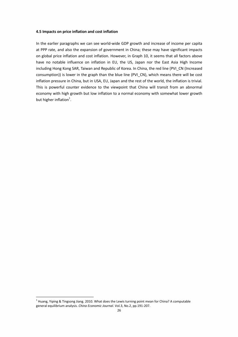
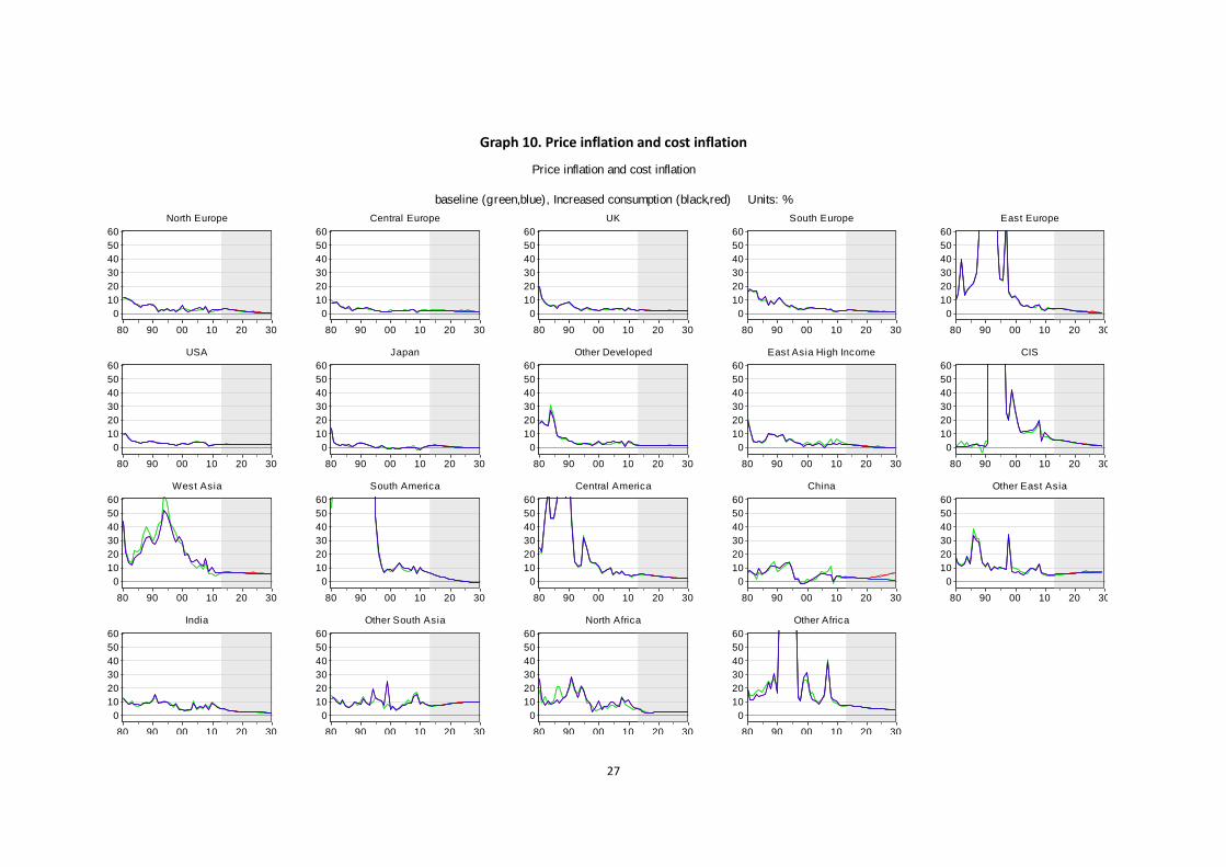
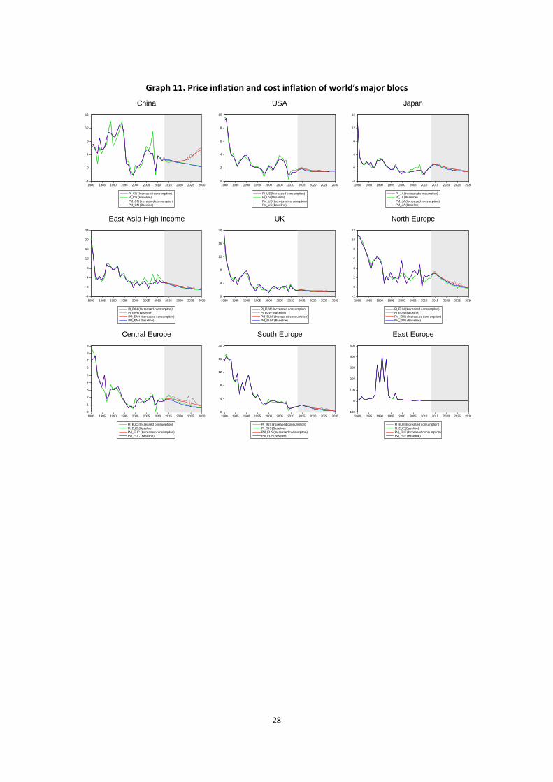
4.5 Impacts on price inflation and cost inflation

In the earlier paragraphs we can see world-wide GDP growth and increase of income per capita

at PPP rate, and also the expansion of government in China; these may have significant impacts

on global price inflation and cost inflation. However, in Graph 10, it seems that all factors above

have no notable influence on inflation in EU, the US, Japan nor the East Asia High Income

including Hong Kong SAR, Taiwan and Republic of Korea. In China, the red line (PVI_CN (Increased

consumption)) is lower in the graph than the blue line (PVI_CN), which means there will be cost

inflation pressure in China, but in USA, EU, Japan and the rest of the world, the inflation is trivial.

This is powerful counter evidence to the viewpoint that China will transit from an abnormal

economy with high growth but low inflation to a normal economy with somewhat lower growth

but higher inflation1.

1 Huang, Yiping & Tingsong Jiang. 2010. What does the Lewis turning point mean for China? A computable

general equilibrium analysis. China Economic Journal. Vol.3, No.2, pp.191-207.

27

Graph 10. Price inflation and cost inflation

0

10

20

30

40

50

60

80 90 00 10 20 30

North Europe

0

10

20

30

40

50

60

80 90 00 10 20 30

Central Europe

0

10

20

30

40

50

60

80 90 00 10 20 30

UK

0

10

20

30

40

50

60

80 90 00 10 20 30

South Europe

0

10

20

30

40

50

60

80 90 00 10 20 30

East Europe

0

10

20

30

40

50

60

80 90 00 10 20 30

USA

0

10

20

30

40

50

60

80 90 00 10 20 30

Japan

0

10

20

30

40

50

60

80 90 00 10 20 30

Other Developed

0

10

20

30

40

50

60

80 90 00 10 20 30

East Asia High Income

0

10

20

30

40

50

60

80 90 00 10 20 30

CIS

0

10

20

30

40

50

60

80 90 00 10 20 30

West Asia

0

10

20

30

40

50

60

80 90 00 10 20 30

South America

0

10

20

30

40

50

60

80 90 00 10 20 30

Central America

0

10

20

30

40

50

60

80 90 00 10 20 30

China

0

10

20

30

40

50

60

80 90 00 10 20 30

Other East Asia

0

10

20

30

40

50

60

80 90 00 10 20 30

India

0

10

20

30

40

50

60

80 90 00 10 20 30

Other South Asia

0

10

20

30

40

50

60

80 90 00 10 20 30

North Africa

0

10

20

30

40

50

60

80 90 00 10 20 30

Other Africa

Price inflation and cost inflation

baseline (green,blue), Increased consumption (black,red) Units: %

28

Graph 11. Price inflation and cost inflation of world’s major blocs

-4

0

4

8

12

16

1980 1985 1990 1995 2000 2005 2010 2015 2020 2025 2030

PI_CN (Increased consumption)

PI_CN (Baseline)

PVI_CN (Increased consumption)

PVI_CN (Baseline)

China

0

2

4

6

8

10

1980 1985 1990 1995 2000 2005 2010 2015 2020 2025 2030

PI_US (Increased consumption)

PI_US (Baseline)

PVI_US (Increased consumption)

PVI_US (Baseline)

USA

-4

0

4

8

12

16

1980 1985 1990 1995 2000 2005 2010 2015 2020 2025 2030

PI_JA (Increased consumption)

PI_JA (Baseline)

PVI_JA (Increased consumption)

PVI_JA (Baseline)

Japan

-4

0

4

8

12

16

20

24

1980 1985 1990 1995 2000 2005 2010 2015 2020 2025 2030

PI_EAH (Increased consumption)

PI_EAH (Baseline)

PVI_EAH (Increased consumption)

PVI_EAH (Baseline)

East Asia High Income

0

4

8

12

16

20

1980 1985 1990 1995 2000 2005 2010 2015 2020 2025 2030

PI_EUW (Increased consumption)

PI_EUW (Baseline)

PVI_EUW (Increased consumption)

PVI_EUW (Baseline)

UK

-2

0

2

4

6

8

10

12

1980 1985 1990 1995 2000 2005 2010 2015 2020 2025 2030

PI_EUN (Increased consumption)

PI_EUN (Baseline)

PVI_EUN (Increased consumption)

PVI_EUN (Baseline)

North Europe

0

1

2

3

4

5

6

7

8

9

1980 1985 1990 1995 2000 2005 2010 2015 2020 2025 2030

PI_EUC (Increased consumption)

PI_EUC (Baseline)

PVI_EUC (Increased consumption)

PVI_EUC (Baseline)

Central Europe

0

4

8

12

16

20

1980 1985 1990 1995 2000 2005 2010 2015 2020 2025 2030

PI_EUS (Increased consumption)

PI_EUS (Baseline)

PVI_EUS (Increased consumption)

PVI_EUS (Baseline)

South Europe

-100

0

100

200

300

400

500

1980 1985 1990 1995 2000 2005 2010 2015 2020 2025 2030

PI_EUE (Increased consumption)

PI_EUE (Baseline)

PVI_EUE (Increased consumption)

PVI_EUE (Baseline)

East Europe

29

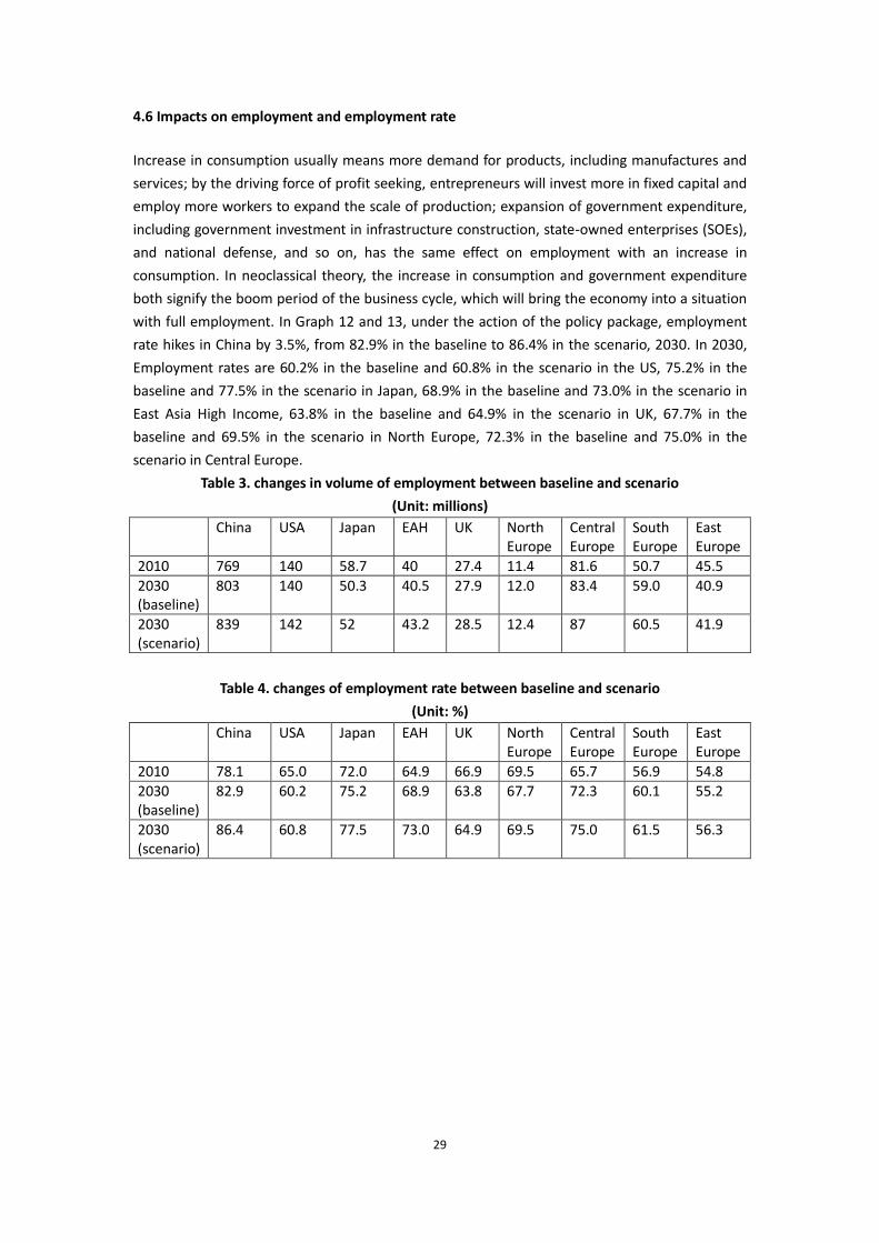
4.6 Impacts on employment and employment rate

Increase in consumption usually means more demand for products, including manufactures and

services; by the driving force of profit seeking, entrepreneurs will invest more in fixed capital and

employ more workers to expand the scale of production; expansion of government expenditure,

including government investment in infrastructure construction, state-owned enterprises (SOEs),

and national defense, and so on, has the same effect on employment with an increase in

consumption. In neoclassical theory, the increase in consumption and government expenditure

both signify the boom period of the business cycle, which will bring the economy into a situation

with full employment. In Graph 12 and 13, under the action of the policy package, employment

rate hikes in China by 3.5%, from 82.9% in the baseline to 86.4% in the scenario, 2030. In 2030,

Employment rates are 60.2% in the baseline and 60.8% in the scenario in the US, 75.2% in the

baseline and 77.5% in the scenario in Japan, 68.9% in the baseline and 73.0% in the scenario in

East Asia High Income, 63.8% in the baseline and 64.9% in the scenario in UK, 67.7% in the

baseline and 69.5% in the scenario in North Europe, 72.3% in the baseline and 75.0% in the

scenario in Central Europe.

Table 3. changes in volume of employment between baseline and scenario

(Unit: millions)

China USA Japan EAH UK North Europe

Central Europe

South Europe

East Europe

2010 769 140 58.7 40 27.4 11.4 81.6 50.7 45.5

2030 (baseline)

803 140 50.3 40.5 27.9 12.0 83.4 59.0 40.9

2030 (scenario)

839 142 52 43.2 28.5 12.4 87 60.5 41.9

Table 4. changes of employment rate between baseline and scenario

(Unit: %)

China USA Japan EAH UK North Europe

Central Europe

South Europe

East Europe

2010 78.1 65.0 72.0 64.9 66.9 69.5 65.7 56.9 54.8

2030 (baseline)

82.9 60.2 75.2 68.9 63.8 67.7 72.3 60.1 55.2

2030 (scenario)

86.4 60.8 77.5 73.0 64.9 69.5 75.0 61.5 56.3

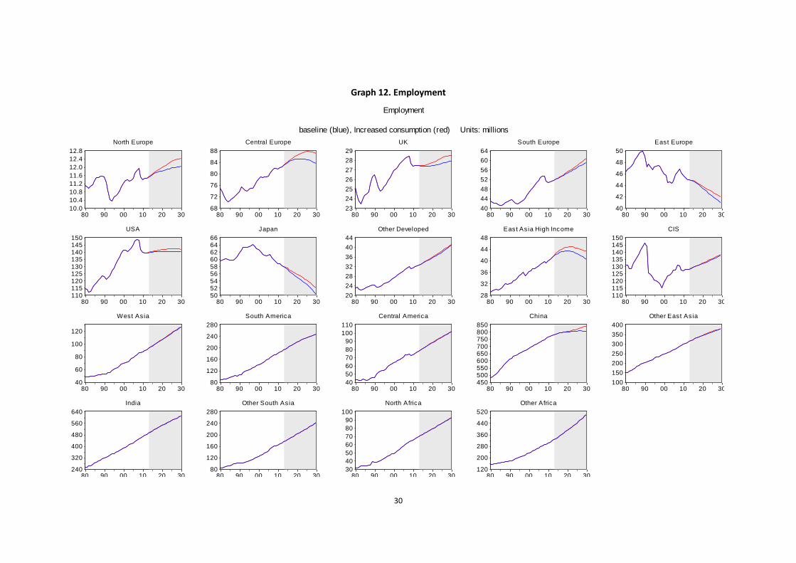
30

Graph 12. Employment

10.0

10.4

10.8

11.2

11.6

12.0

12.4

12.8

80 90 00 10 20 30

North Europe

68

72

76

80

84

88

80 90 00 10 20 30

Central Europe

23

24

25

26

27

28

29

80 90 00 10 20 30

UK

40

44

48

52

56

60

64

80 90 00 10 20 30

South Europe

40

42

44

46

48

50

80 90 00 10 20 30

East Europe

110115120125130135140145150

80 90 00 10 20 30

USA

505254565860626466

80 90 00 10 20 30

Japan

20

24

28

32

36

40

44

80 90 00 10 20 30

Other Developed

28

32

36

40

44

48

80 90 00 10 20 30

East Asia High Income

110115120125130135140145150

80 90 00 10 20 30

CIS

40

60

80

100

120

80 90 00 10 20 30

West Asia

80

120

160

200

240

280

80 90 00 10 20 30

South America

40

50

60

70

80

90

100

110

80 90 00 10 20 30

Central America

450500550600650700750800850

80 90 00 10 20 30

China

100

150

200

250

300

350

400

80 90 00 10 20 30

Other East Asia

240

320

400

480

560

640

80 90 00 10 20 30

India

80

120

160

200

240

280

80 90 00 10 20 30

Other South Asia

30

40

50

60

70

80

90

100

80 90 00 10 20 30

North Africa

120

200

280

360

440

520

80 90 00 10 20 30

Other Africa

Employment

baseline (blue), Increased consumption (red) Units: millions

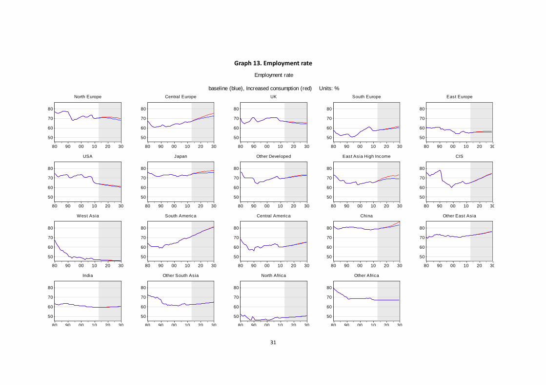
31

Graph 13. Employment rate

50

60

70

80

80 90 00 10 20 30

North Europe

50

60

70

80

80 90 00 10 20 30

Central Europe

50

60

70

80

80 90 00 10 20 30

UK

50

60

70

80

80 90 00 10 20 30

South Europe

50

60

70

80

80 90 00 10 20 30

East Europe

50

60

70

80

80 90 00 10 20 30

USA

50

60

70

80

80 90 00 10 20 30

Japan

50

60

70

80

80 90 00 10 20 30

Other Developed

50

60

70

80

80 90 00 10 20 30

East Asia High Income

50

60

70

80

80 90 00 10 20 30

CIS

50

60

70

80

80 90 00 10 20 30

West Asia

50

60

70

80

80 90 00 10 20 30

South America

50

60

70

80

80 90 00 10 20 30

Central America

50

60

70

80

80 90 00 10 20 30

China

50

60

70

80

80 90 00 10 20 30

Other East Asia

50

60

70

80

80 90 00 10 20 30

India

50

60

70

80

80 90 00 10 20 30

Other South Asia

50

60

70

80

80 90 00 10 20 30

North Africa

50

60

70

80

80 90 00 10 20 30

Other Africa

Employment rate

baseline (blue), Increased consumption (red) Units: %

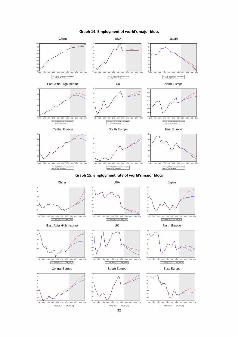
32

Graph 14. Employment of world’s major blocs

Graph 15. employment rate of world’s major blocs

450

500

550

600

650

700

750

800

850

1980 1985 1990 1995 2000 2005 2010 2015 2020 2025 2030

NE_CN (Increased consumption)

NE_CN (Baseline)

China

110

115

120

125

130

135

140

145

150

1980 1985 1990 1995 2000 2005 2010 2015 2020 2025 2030

NE_US (Increased consumption)

NE_US (Baseline)

USA

50

52

54

56

58

60

62

64

66

1980 1985 1990 1995 2000 2005 2010 2015 2020 2025 2030

NE_JA (Increased consumption)

NE_JA (Baseline)

Japan

28

32

36

40

44

48

1980 1985 1990 1995 2000 2005 2010 2015 2020 2025 2030

NE_EAH (Increased consumption)

NE_EAH (Baseline)

East Asia High Income

23

24

25

26

27

28

29

1980 1985 1990 1995 2000 2005 2010 2015 2020 2025 2030

NE_EUW (Increased consumption)

NE_EUW (Baseline)

UK

10.0

10.4

10.8

11.2

11.6

12.0

12.4

12.8

1980 1985 1990 1995 2000 2005 2010 2015 2020 2025 2030

NE_EUN (Increased consumption)

NE_EUN (Baseline)

North Europe

68

72

76

80

84

88

1980 1985 1990 1995 2000 2005 2010 2015 2020 2025 2030

NE_EUC (Increased consumption)

NE_EUC (Baseline)

Central Europe

40

44

48

52

56

60

64

1980 1985 1990 1995 2000 2005 2010 2015 2020 2025 2030

NE_EUS (Increased consumption)

NE_EUS (Baseline)

South Europe

40

42

44

46

48

50

1980 1985 1990 1995 2000 2005 2010 2015 2020 2025 2030

NE_EUE (Increased consumption)

NE_EUE (Baseline)

East Europe

76

78

80

82

84

86

88

1980 1985 1990 1995 2000 2005 2010 2015 2020 2025 2030

NER_CN_C NER_CN_0

China

60

62

64

66

68

70

72

74

76

1980 1985 1990 1995 2000 2005 2010 2015 2020 2025 2030

NER_US_C NER_US_0

USA

70

71

72

73

74

75

76

77

78

1980 1985 1990 1995 2000 2005 2010 2015 2020 2025 2030

NER_JA_C NER_JA_0

Japan

62

64

66

68

70

72

74

1980 1985 1990 1995 2000 2005 2010 2015 2020 2025 2030

NER_EAH_C NER_EAH_0

East Asia High Income

63

64

65

66

67

68

69

70

71

1980 1985 1990 1995 2000 2005 2010 2015 2020 2025 2030

NER_EUW_C NER_EUW_0

UK

66

68

70

72

74

76

78

1980 1985 1990 1995 2000 2005 2010 2015 2020 2025 2030

NER_EUN_C NER_EUN_0

North Europe

60

62

64

66

68

70

72

74

76

1980 1985 1990 1995 2000 2005 2010 2015 2020 2025 2030

NER_EUC_C NER_EUC_0

Central Europe

50

52

54

56

58

60

62

1980 1985 1990 1995 2000 2005 2010 2015 2020 2025 2030

NER_EUS_C NER_EUS_0

South Europe

53

54

55

56

57

58

59

60

61

1980 1985 1990 1995 2000 2005 2010 2015 2020 2025 2030

NER_EUE_C NER_EUE_0

East Europe

33

4.7 Impacts on real exchange rate

It is argued a lot in international society and also in China whether the exchange rate of RMB is

under-appreciated. The US government attributes its large amount of trade deficit to the import

from China; they assert that if the exchange rate of RMB is appreciated, the US will get a trade

balance. In fact, the trade deficit of the US derives from its own industry structure and the

excessive expansion of finance capital. Statistics show that the service sector including the

finance sector takes over 70% of the GDP in the US - the US doesn’t produce commodities or

manufactures, it imports goods from the emerging economies such as China. The growth pattern

of the US has resulted in a disequilibrium world economy system. On the one hand, countries like

China and some other developing countries produce goods and export them to the US and

accumulate a large amount of exchange reserves, with which they buy the US government bond,

lending the money to the US to expand their consumption. On the other hand, the US’s only

production is the US dollars they print; they produce nothing but finance capital to promote GDP

growth. This also leaves China in a disadvantaged position in international economy and

vulnerable when an economic crisis breaks out in the US, just like the subprime crisis.

In this paper, we assume that the RMB exchange rate is appreciated in order to cut down

China’s dependence on export. We can see RMB’s exchange rate significantly rise to 0.66 in 2014

in the scenario comparing with that in the baseline; however, it falls down to 0.48 in 2024 and

goes up to 0.57 in 2025, and then declines again. On the contrary, other blocs witness slight

depreciation first since 2011, but it soars from 2025.

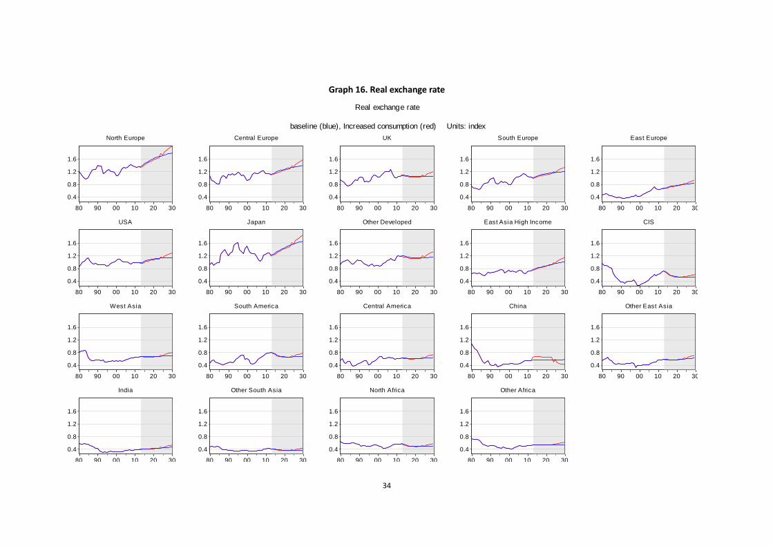
34

Graph 16. Real exchange rate

0.4

0.8

1.2

1.6

80 90 00 10 20 30

North Europe

0.4

0.8

1.2

1.6

80 90 00 10 20 30

Central Europe

0.4

0.8

1.2

1.6

80 90 00 10 20 30

UK

0.4

0.8

1.2

1.6

80 90 00 10 20 30

South Europe

0.4

0.8

1.2

1.6

80 90 00 10 20 30

East Europe

0.4

0.8

1.2

1.6

80 90 00 10 20 30

USA

0.4

0.8

1.2

1.6

80 90 00 10 20 30

Japan

0.4

0.8

1.2

1.6

80 90 00 10 20 30

Other Developed

0.4

0.8

1.2

1.6

80 90 00 10 20 30

East Asia High Income

0.4

0.8

1.2

1.6

80 90 00 10 20 30

CIS

0.4

0.8

1.2

1.6

80 90 00 10 20 30

West Asia

0.4

0.8

1.2

1.6

80 90 00 10 20 30

South America

0.4

0.8

1.2

1.6

80 90 00 10 20 30

Central America

0.4

0.8

1.2

1.6

80 90 00 10 20 30

China

0.4

0.8

1.2

1.6

80 90 00 10 20 30

Other East Asia

0.4

0.8

1.2

1.6

80 90 00 10 20 30

India

0.4

0.8

1.2

1.6

80 90 00 10 20 30

Other South Asia

0.4

0.8

1.2

1.6

80 90 00 10 20 30

North Africa

0.4

0.8

1.2

1.6

80 90 00 10 20 30

Other Africa

Real exchange rate

baseline (blue), Increased consumption (red) Units: index

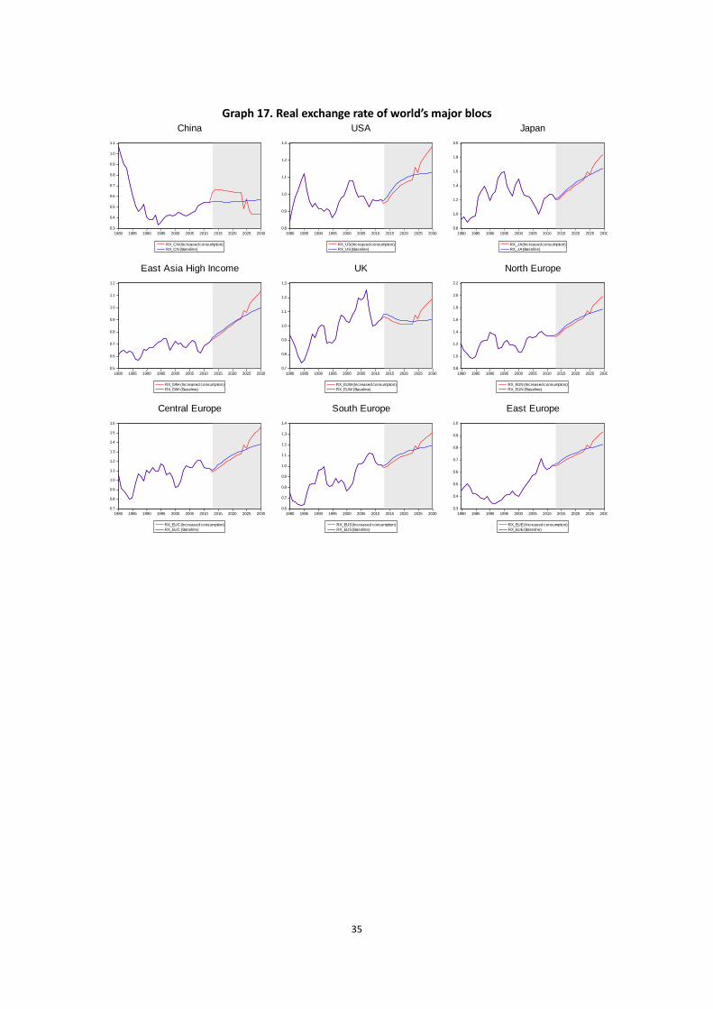
35

Graph 17. Real exchange rate of world’s major blocs

0.3

0.4

0.5

0.6

0.7

0.8

0.9

1.0

1.1

1980 1985 1990 1995 2000 2005 2010 2015 2020 2025 2030

RX_CN (Increased consumption)

RX_CN (Baseline)

China

0.8

0.9

1.0

1.1

1.2

1.3

1980 1985 1990 1995 2000 2005 2010 2015 2020 2025 2030

RX_US (Increased consumption)

RX_US (Baseline)

USA

0.8

1.0

1.2

1.4

1.6

1.8

2.0

1980 1985 1990 1995 2000 2005 2010 2015 2020 2025 2030

RX_JA (Increased consumption)

RX_JA (Baseline)

Japan

0.5

0.6

0.7

0.8

0.9

1.0

1.1

1.2

1980 1985 1990 1995 2000 2005 2010 2015 2020 2025 2030

RX_EAH (Increased consumption)

RX_EAH (Baseline)

East Asia High Income

0.7

0.8

0.9

1.0

1.1

1.2

1.3

1980 1985 1990 1995 2000 2005 2010 2015 2020 2025 2030

RX_EUW (Increased consumption)

RX_EUW (Baseline)

UK

0.8

1.0

1.2

1.4

1.6

1.8

2.0

2.2

1980 1985 1990 1995 2000 2005 2010 2015 2020 2025 2030

RX_EUN (Increased consumption)

RX_EUN (Baseline)

North Europe

0.7

0.8

0.9

1.0

1.1

1.2

1.3

1.4

1.5

1.6

1980 1985 1990 1995 2000 2005 2010 2015 2020 2025 2030

RX_EUC (Increased consumption)

RX_EUC (Baseline)

Central Europe

0.6

0.7

0.8

0.9

1.0

1.1

1.2

1.3

1.4

1980 1985 1990 1995 2000 2005 2010 2015 2020 2025 2030

RX_EUS (Increased consumption)

RX_EUS (Baseline)

South Europe

0.3

0.4

0.5

0.6

0.7

0.8

0.9

1.0

1980 1985 1990 1995 2000 2005 2010 2015 2020 2025 2030

RX_EUE (Increased consumption)

RX_EUE (Baseline)

East Europe

36

4.8 Impacts on exchange reserves as percentage of GDP

Theoretically, appreciation of the currency means a relatively higher price for foreign countries,

which may probably lead to the country’s export diminish and the decrease of exchange reserves.

In 2010, the exchange reserve of China is equivalent to half of GDP of the same year, which is

59%. According to the baseline, the ratio of China’s exchange reserve to GDP will surprisingly rise

to 94%, and after the implementation of the policy package, it will be 86% in the scenario. Graph

18 shows the impacts on exchange reserves as percentage of GDP of the 19 blocs; there are

trivial impacts on the developed countries such as UK, the US, while there are impacts to a

certain degree on developing countries such as CIS, Other East Asia (including Indonesia,

Malaysia and Cambodia and so on), West Asia, India and North Africa. The explanation is that

since costs of commodities made in China are higher than before, the demands of developed

countries have been transferred to other developing countries with a cheap and abundant labor

force, which enables these developing countries to get some exchange reserves.

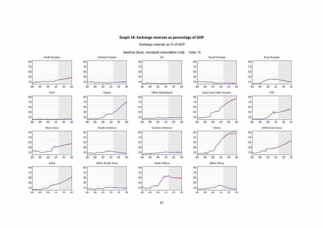
37

Graph 18. Exchange reserves as percentage of GDP

10

30

50

70

90

80 90 00 10 20 30

North Europe

10

30

50

70

90

80 90 00 10 20 30

Central Europe

10

30

50

70

90

80 90 00 10 20 30

UK

10

30

50

70

90

80 90 00 10 20 30

South Europe

10

30

50

70

90

80 90 00 10 20 30

East Europe

10

30

50

70

90

80 90 00 10 20 30

USA

10

30

50

70

90

80 90 00 10 20 30

Japan

10

30

50

70

90

80 90 00 10 20 30

Other Developed

10

30

50

70

90

80 90 00 10 20 30

East Asia High Income

10

30

50

70

90

80 90 00 10 20 30

CIS

10

30

50

70

90

80 90 00 10 20 30

West Asia

10

30

50

70

90

80 90 00 10 20 30

South America

10

30

50

70

90

80 90 00 10 20 30

Central America

10

30

50

70

90

80 90 00 10 20 30

China

10

30

50

70

90

80 90 00 10 20 30

Other East Asia

10

30

50

70

90

80 90 00 10 20 30

India

10

30

50

70

90

80 90 00 10 20 30

Other South Asia

10

30

50

70

90

80 90 00 10 20 30

North Africa

10

30

50

70

90

80 90 00 10 20 30

Other Africa

Exchange reserves as % of GDP

baseline (blue), Increased consumption (red) Units: %

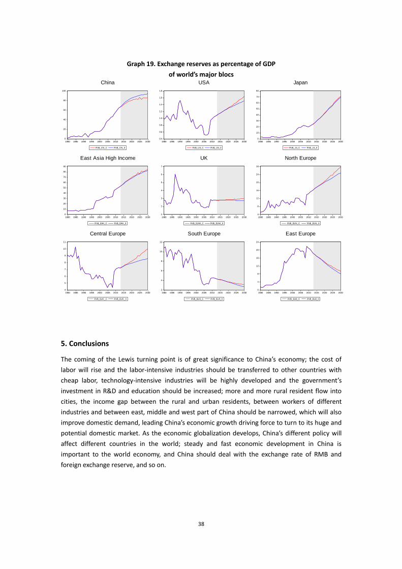
38

Graph 19. Exchange reserves as percentage of GDP

of world’s major blocs

5. Conclusions

The coming of the Lewis turning point is of great significance to China’s economy; the cost of

labor will rise and the labor-intensive industries should be transferred to other countries with

cheap labor, technology-intensive industries will be highly developed and the government’s

investment in R&D and education should be increased; more and more rural resident flow into

cities, the income gap between the rural and urban residents, between workers of different

industries and between east, middle and west part of China should be narrowed, which will also

improve domestic demand, leading China’s economic growth driving force to turn to its huge and

potential domestic market. As the economic globalization develops, China’s different policy will

affect different countries in the world; steady and fast economic development in China is

important to the world economy, and China should deal with the exchange rate of RMB and

foreign exchange reserve, and so on.

0

20

40

60

80

100

1980 1985 1990 1995 2000 2005 2010 2015 2020 2025 2030

RV$_CN_C RV$_CN_0

China

0.4

0.6

0.8

1.0

1.2

1.4

1.6

1.8

1980 1985 1990 1995 2000 2005 2010 2015 2020 2025 2030

RV$_US_C RV$_US_0

USA

0

10

20

30

40

50

60

70

80

1980 1985 1990 1995 2000 2005 2010 2015 2020 2025 2030

RV$_JA_C RV$_JA_0

Japan

0

10

20

30

40

50

60

70

80

90

1980 1985 1990 1995 2000 2005 2010 2015 2020 2025 2030

RV$_EAH_C RV$_EAH_0

East Asia High Income

1

2

3

4

5

6

7

1980 1985 1990 1995 2000 2005 2010 2015 2020 2025 2030

RV$_EUW_C RV$_EUW_0

UK

4

8

12

16

20

24

28

1980 1985 1990 1995 2000 2005 2010 2015 2020 2025 2030

RV$_EUN_C RV$_EUN_0

North Europe

4

5

6

7

8

9

10

11

1980 1985 1990 1995 2000 2005 2010 2015 2020 2025 2030

RV$_EUC_C RV$_EUC_0

Central Europe

2

4

6

8

10

12

1980 1985 1990 1995 2000 2005 2010 2015 2020 2025 2030

RV$_EUS_C RV$_EUS_0

South Europe

0

4

8

12

16

20

24

1980 1985 1990 1995 2000 2005 2010 2015 2020 2025 2030

RV$_EUE_C RV$_EUE_0

East Europe

39

References

Cai, Fang & Dewen Wang. 2005. China’s demographic transition: Implications for growth. In The

China boom and its discontents, eds. Ross Garnaut and Ligang Song, pp. 34-52. Canberra: Asia

Pacific Press.

Cai, Fang & Meiyan Wang. 2007. Re-assessment of rural surplus labor and some correlated facts.

Chinese Rural Economy. Vol. 10, pp.4-12.

Cai, Fang. 2007. The myth of surplus labor force in rural China. Chinese Journal of Population

Science. No. 2, pp. 27.

Cai, Fang. 2010. Demographic transition, demographic dividend, and Lewis turning point in

China. China Economic Journal. Vol. 3, No. 2, pp. 107-119.

Cai, Fang. 2010. Demographic transition, demographic dividend, and Lewis turning point in

China. China Economic Journal. Vol. 3, No. 2, pp. 107-119.

Cai, Fang. 2010. On the challenges of and the path for China’s development of the Lewis turning

point of large country’s economy. Journal of Guangdong University of Business Studies. Vol. 1,

pp. 4-12.

Cai, Fang. 2010. The Lewis turning point and the reorientation of public policies: some stylized

facts of social protection in China. Social Science in China. No. 6, pp. 125-137.

Cripps, F., G. Gudgin & J. Rhodes. 1979. Technical Manual of the CEPG Model of World Trade’,

Cambridge Economic Policy Review 3 (June).

Cripps, Francis, & Alex Izurieta & Ajit Singh. Global imbalances, under-consumption and

overborrowing: The state of the world economy and future policies. Centre for Business

Research, University of Cambridge. Working Paper No. 419.

Du, Yang & Meiyan Wang. 2010. New estimate of surplus rural labor force and its implications.

Journal of Guangzhou University (Social Science Edition). Vol.9, No. 4, pp. 17-24.

Golley, Jane & Xin Meng. 2011. Has China run out of surplus labour? China Economic Review,

doi:10.1016/j.chieco.2011.07.006

Hale, Galina and Bart Hobijn. 2011. The U.S. content of “Made in China”.

http://www.frbsf.org/publications/economics/letter/2011/el2011-25.html

Huang, Yiping & Tingsong Jiang. 2010. What does the Lewis turning point mean for China? A

computable general equilibrium analysis. China Economic Journal. Vol. 3, No. 2, pp. 191-207.

Islam, Nazrul & Kazuhiko Yokota. 2008. Lewis growth model and China’s industrialization. Asian

Economic Journal. Vol.22, No. 4, pp. 359-396.

40

Kam Wing Chan. 2010. A China paradox: migrant labor shortage amidst rural labor supply

abundance. Eurasian Geography and Economics. Vol. 51, No. 4, pp. 513–530

Knight, J., et al. . 2011. The puzzle of migrant labour shortage and rural labour surplus in China,

China Economic Review, doi:10.1016/j.chieco.2011.01.006

Lewis, W. Arthur. 1954. Economic development with unlimited supplies of labour. Manchester

School of Economic and Social Studies. Vol.22, No. 2, pp. 139-191.

Lewis, W. Arthur. 1972. Reflections on unlimited labour. In International economics and

development, ed. L. Di Marco, pp. 75-96. New York: Academic Press.

Ma, Xiaohe & Jianlei Ma. 2007. How much surplus labor in rural China on earth? Chinese Rural

Economy. Vol.12, pp. 4-9,34.

Minami, Ryoshin & Xinxin Ma. 2010. The Lewis turning point of Chinese economy: Comparison

with Japanese experience. China Economic Journal. Vol. 3, No. 2, pp. 163-179.

Minami, Ryoshin. 1968. The turning point in the Japanese economy. The Quarterly Journal of

Economics, Vol.82, No. 3, pp. 380-402.

Minami, Ryoshin. 1973. The turning point in economic development: Japan’s experience,

Economic Research Series No. 14. The Institute of Economic Research, Hitotsubashi University,

Kinokuniya Bookstore, Tokyo.

Ranis, G., & Fei, J. 1961. A theory of economic development. The American Economic Review, Vol.

51, No. 4, pp. 533-565.

Reutersward, Anders, Vincent Koen & Richard Herd. 2010. China's labour market in transition:

Job creation, migration and regulation. OECD Economics Department Working Papers, No. 749,

OECD Publishing. doi: 10.1787/5kmlh5010gg7-en

Song, Ligang & Yongsheng Zhang. 2010. Will Chinese growth slow after the Lewis turning point?

China Economic Journal. Vol. 3, No. 2, pp. 209–219.

Tong, Jiadong & Zhou Yan. 2011. Dual economy, Lewisian turning point and the foreign trade

development strategy of China. Economic Theory and Management. No. 1, pp. 18-26.

Wang, Dewen. 2008. Lewis turning point and China’s experiences. In Reports on China’s

population and labor No. 9. ed. Fang Cai. p. 90. Beijing: Social Sciences Academic Press (China).

Wang, Jiangui & Shouhai Ding. 2005. How much surplus agricultural labor is there in China?

Social Sciences in China, No.5, pp. 27-35.

Wang, Jin & Xiaohan Zhong. 2011. Whether the Lewis turning point has arrived in China:

Theoretical studies and international experiences. Social Sciences in China. Vol. 5, pp. 22-37.

Xianzhou Zhao. 2010. Some theoretical issues on Lewis turning point. Economist, No. 5, pp. 75-

80.

Zhang Xiaobo, Jin Yang & Shenglin Wang. 2011. China has reached the Lewis turning point. China

41

Economic Review, doi:10.1016/j.chieco.2011.07.002

Zhou Tianyong. 2010. Whether the labor surplus in China. Shanghai Economy. Vol.11, pp. 17-19.

Zhu, Andong & David M. Kotz. 2011. The dependence of China's economic growth on exports and

investment. Review of Radical Political Economics. Vol. 43, No.1, pp. 9-32.