The Rise of Working Mothers and the 1975 Earned

Income Tax Credit

By Jacob Bastian∗

The rise of working mothers radically changed the U.S. econ-

omy and the role of women in society. In one of the first stud-

ies of the 1975 introduction of the Earned Income Tax Credit,

I find that this program increased maternal employment by 6

percent, representing one million mothers and an elasticity of

0.49. The EITC may help explain why the U.S. has long had

such a high fraction of working mothers despite few childcare

subsidies or parental-leave policies. I also find evidence that

this influx of working mothers affected social attitudes and led

to higher approval of working women. (JEL: H24, I38, J16,

J38)

∗ University of Chicago, Harris School of Public Policy, 1155 E 60th St, Chicago, IL60637. Email: jbastian@uchicago.edu. I would like to thank Martha Bailey, CharlieBrown, Jim Hines, Luke Shaefer, and Ugo Troiano for advising and support. Thanksalso to Hoyt Bleakley, John Bound, Eric Chyn, Austin Davis, John DiNardo, MorganHenderson, Hilary Hoynes, Sara LaLumia, Day Manoli, Mike Mueller-Smith, JohannesNorling, Paul Rhode, Elyce Rotella, Joel Slemrod, Jeff Smith, Mel Stephens, BryanStuart, Brenden Timpe, Justin Wolfers, and conference and seminar participants at theUniversity of Michigan, New York University, University of Illinois at Urbana-Champaign,U.S. Department of the Treasury, U.S. Bureau of Labor Statistics, the 2016 Society ofLabor Economists Annual Meeting, WEAI, International Institute of Public Finance, andEconomic History Association, and the 2015 MEA, Mannheim Tax Conference, SEA,APPAM, and National Tax Association. I am grateful to Dan Feenberg for his help withthe IRS tax data. This research was supported by the Michigan Institute for Teaching andResearch in Economics. Some of the data used in this analysis are derived from SensitiveData Files of the GSS, obtained under special contractual arrangements designed toprotect the anonymity of respondents, and are not available from the author. Gallup dataobtained from the iPOLL Databank and the Roper Center for Public Opinion Research.

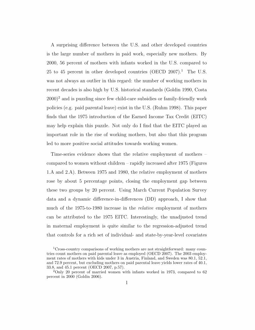
A surprising difference between the U.S. and other developed countries

is the large number of mothers in paid work, especially new mothers. By

2000, 56 percent of mothers with infants worked in the U.S. compared to

25 to 45 percent in other developed countries (OECD 2007).1 The U.S.

was not always an outlier in this regard: the number of working mothers in

recent decades is also high by U.S. historical standards (Goldin 1990, Costa

2000)2 and is puzzling since few child-care subsidies or family-friendly work

policies (e.g. paid parental leave) exist in the U.S. (Ruhm 1998). This paper

finds that the 1975 introduction of the Earned Income Tax Credit (EITC)

may help explain this puzzle. Not only do I find that the EITC played an

important role in the rise of working mothers, but also that this program

led to more positive social attitudes towards working women.

Time-series evidence shows that the relative employment of mothers –

compared to women without children – rapidly increased after 1975 (Figures

1.A and 2.A). Between 1975 and 1980, the relative employment of mothers

rose by about 5 percentage points, closing the employment gap between

these two groups by 20 percent. Using March Current Population Survey

data and a dynamic difference-in-differences (DD) approach, I show that

much of the 1975-to-1980 increase in the relative employment of mothers

can be attributed to the 1975 EITC. Interestingly, the unadjusted trend

in maternal employment is quite similar to the regression-adjusted trend

that controls for a rich set of individual- and state-by-year-level covariates

1Cross-country comparisons of working mothers are not straightforward: many coun-tries count mothers on paid parental leave as employed (OECD 2007). The 2003 employ-ment rates of mothers with kids under 3 in Austria, Finland, and Sweden was 80.1, 52.1,and 72.9 percent, but excluding mothers on paid parental leave yields lower rates of 40.1,33.8, and 45.1 percent (OECD 2007, p.57).

2Only 20 percent of married women with infants worked in 1973, compared to 62percent in 2000 (Goldin 2006).

1

(Figures 1.B and 2.B). The EITC also increased labor-force attachment

and work intensity, raising average annual work hours by 5.7 percent (35

hours) and earnings by 7.3 percent ($750 in 2013 dollars). Results imply a

participation elasticity of 0.41 to 0.49, in line with other estimates of this

period (Blau and Kahn 2005, Heim 2007, Chetty et al. 2012).

Consistent with the 1975 EITC causing this rise in employment, I find

larger responses from mothers more likely to be EITC-eligible and null re-

sponses from placebo groups of women and mothers not eligible for EITC

benefits. Responses varied by marital status, spousal earnings, and edu-

cation in a manner consistent with a simple labor-supply model. I use the

placebo group of EITC-ineligible mothers in a triple differences (DDD) spec-

ification to net out contemporaneous policies and trends (e.g. birth control,

divorce laws, abortion) affecting all mothers: the DDD estimate corrobo-

rates the DD result (2.6 and 3.3 percentage points).

My estimates suggest that the 1975 EITC encouraged about one million

mothers to begin working. Yet, this is unlikely to capture the full impact

of the EITC on society. In section VI, I use General Social Survey data

to examine whether this influx of working mothers affected social attitudes

towards working women (“gender-equality preferences”). This hypothesis is

motivated by recent evidence that such attitudes are malleable and increase

with exposure to working women: Fernandez, Fogli and Olivetti (2004) and

Olivetti, Patacchini and Zenou (2016) find that having a working mother –

and having friends with working mothers – leads to stronger gender-equality

preferences in adulthood. Additionally, Finseraas et al. (2016) shows that

exposure to female colleagues reduces discriminatory attitudes. With these

results in mind, the attitudes of millions of Americans may have been af-2

fected when a million mothers began working after 1975.3

To estimate the impact of the EITC on gender-equality preferences, I

use a two-sample two-step process, in which I characterize and exploit ge-

ographic heterogeneity in the EITC response and test whether states with

larger EITC responses experienced larger attitude changes after 1975. Using

both the actual state EITC response and the predicted response (based on

preexisting state demographic traits, to help alleviate concerns about the

potential endogeneity of gender-equality preferences and EITC response), I

find that states with larger EITC responses had larger increases in prefer-

ences for gender equality after 1975. Preference changes occurred among

both men and women, within and across regions, and do not appear to be

driven by preexisting attitudes, demographics, or general trends in social

norms. Subgroup analysis confirms larger preference changes among people

more likely to know these newly working women: lower-educated adults. I

also use a placebo outcome on racial-equality preferences to test and rule

out the possibility that states with higher EITC responses were simply ex-

periencing changes in various types of social attitudes. Regarding external

validity and whether working women can affect social attitudes towards

women in other contexts, I also find evidence of attitude changes due to the

large increase in working women during World War II.

In one of the first studies of the 1975 EITC,4 I find that the EITC encour-

aged a million mothers to begin working and affected the social attitudes of

millions of Americans.

3Google ngrams (Michel et al. 2011) provide descriptive evidence that the rise ofworking mothers was salient and that references to working mothers became much morecommon after the mid-1970s (Figure 3).

4Subsequent EITC expansions – and their effect on maternal employment – have beenstudied (see section I).

3

I. EITC History and Known Effects of the EITC

The EITC came to exist partly as a response to the 1960s War on Poverty,

which succeeded in improving health (Almond, Hoynes and Schanzenbach

2011, Hoynes, Page and Stevens 2011, Goodman-Bacon 2013, Bailey and

Goodman-Bacon 2015) and decreasing poverty, but also had unintentional

work disincentives (Moffitt 1992, Hoynes 1996, Hoynes and Schanzenbach

2012).5 Welfare dependency came to be seen as a growing social prob-

lem and momentum built for a guaranteed annual income with support

from economists Milton Friedman (Friedman 1962) and James Tobin (Tobin

1969). The U.S. House of Representatives passed such a plan – the Fam-

ily Assistance Plan – in 1970 with the backing of President Nixon that

would have replaced welfare.6 However, the U.S. Senate never passed the

plan because of disagreement about how generous the program should be

and concerns about potential work disincentives. An alternative program

called the Work Bonus Plan – with work requirements – was introduced by

Louisiana Senator Russell Long in 1972. A version of this bill was eventu-

ally passed as the Earned Income Tax Credit (EITC) and signed into law by

President Ford on March 29, 1975. See Liebman (1998) and Ventry (2000)

for a detailed history of the EITC program and legislation.

The 1975 EITC was a refundable tax credit that provided a 10 percent

earnings subsidy to working parents with annual household earnings up

to $18,000 in 2013 dollars ($4,000 nominal dollars).7 The EITC was also

5See Bailey and Danziger (2013) for a detailed analysis of War on Poverty programs.6FAP would have guaranteed $3,100 (2013 dollars) for each parent and $1,800 for each

child – $9,800 for a family of four (the 1970 poverty line was about $23,000 for a family offour). Benefits would phase out at 50 percent when household earned income surpassed$4,400 (Trattner 2007, p.315). See New York Times April 17, 1970. Rhys-Williams (1943)was among the first to outline this type of program.

7To be EITC-eligible, tax filers had to have at least one child living in their home for

4

available to parents with earnings above $18,000, but benefits decreased at a

rate of 10 percent and reached zero for earnings above $36,000 (Figures 4.A

and 4.B).8 At this time, there were no additional EITC benefits for having

more than one child and benefits did not vary by state or marital status.

Since 1975, the EITC has been expanded many times (see Figure 4.B for

details) and has grown into one of the largest anti-poverty program in the

U.S., redistributing $66 billion to 28 million individuals and lifting 6.5 mil-

lion people – including 3.3 million children – out of poverty in 2013 (Center

on Budget and Policy Priorities 2014). The EITC has raised maternal em-

ployment (Dickert, Houser and Scholz 1995, Eissa and Liebman 1996, Meyer

and Rosenbaum 2001, Hotz and Scholz 2006, Eissa, Kleven and Kreiner

2008), increased earnings (Dahl, DeLeire and Schwabish 2009), improved

health (Evans and Garthwaite 2014), decreased poverty (Scholz 1994, Neu-

mark and Wascher 2001, Meyer 2010, Hoynes and Patel 2015, Bitler, Hoynes

and Kuka 2016), and helped children of EITC recipients by improving

health (Hoynes, Miller and Simon 2015, Averett and Wang 2015), test scores

(Chetty, Friedman and Rockoff 2011, Dahl and Lochner 2012), and longer-

run outcomes like educational attainment (Manoli and Turner 2014, Bas-

tian and Michelmore 2018) and employment and earnings (Bastian and

Michelmore 2018). The EITC’s unintended consequences include lower pre-

more than half the year (“residency test”). This child must be under 19, under 24 if afull-time student, or any age if disabled. Before 1987, tax filers did not have to provideSocial Security numbers for dependents. Until 1990, tax filers had to demonstrate theyprovided at least half the costs of maintaining the household (“support test”): cash andin-kind public assistance had to be less than half of the household budget (Holtzblatt1991, Holtzblatt, McCubbin and Gillette 1994). Married couples had to file taxes jointly.Since I do not observe tax filing, I assume all unmarried women file taxes as householdhead, married couples file joint taxes, and family members under 19 (or 24 if a student)are dependent children. I treat subfamilies within a household as separate tax-filers.

8Figure 4.A shows a budget constraint under the EITC and Figure 4.B illustratesthe “phase-in” and “phase-out” portion of the EITC schedule while contrasting the 1975EITC schedule with the 2013 EITC. Benefits phase out with adjusted gross income.

5

tax wages of low-skill workers (Leigh 2010, Rothstein 2010) and possible

effects on fertility and marriage.9 See Nichols and Rothstein (2015) and

Hoynes and Rothstein (2016) for recent EITC literature reviews.

Although much is known about the EITC, almost nothing is known about

the 1975 introduction or how the EITC may affect attitudes towards working

women. I show that the 1975 EITC encouraged one million mothers to begin

working, which subsequently increased approval of working women.

Almost all studies of the EITC ignore the program’s first decade.10 Al-

though there was little policy variation before 1986, the 1975 introduction

was itself a large policy change that has received surprisingly little atten-

tion, in part due to the common misconception that the original EITC was

too small to have had much of an effect.11 However, the 1975 EITC was

large in at least three ways (Figure A.1): first, almost half of all house-

holds had earning below the EITC income limit; second, benefits were quite

high, up to $1,800 (2013 dollars); third, a 10 percent earnings subsidy rep-

resented a substantial year-over-year increase in potential earnings. Other

reasons to expect the 1975 EITC to have had a large impact is that female

labor supply was more elastic during this period than in later decades (Blau

and Kahn 2005, Heim 2007) and the fraction of mothers on the margin

of working declined with subsequent program expansions (Bjorklund and

9Effects on these margins are generally small: For fertility, Baughman and Dickert-Conlin (2009) and Bastian (2018) find positive effects. For marriage, Ellwood (2000),Dickert-Conlin and Houser (2002), Herbst (2011), and Michelmore (2015) find negativeeffects, while Bastian (2018) finds positive effects.

10Bastian and Michelmore (2018) is one exception.11As seen in the following representative quotes: “Between 1975 and [the] Tax Reform

Act of 1986, the EITC was small, and the credit amounts did not keep up with inflation”(Meyer and Rosenbaum 2001). “The [EITC] began in 1975 as a modest program aimedat offsetting the social security payroll tax for low-income families with children. Aftermajor expansions in the tax acts of 1986, 1990, and 1993, the EITC has become a centralpart of the federal government’s antipoverty strategy” (Eissa and Liebman 1996).

6

Moffitt 1987, Heckman and Vytlacil 1999).

II. Conceptual Framework

The EITC was a wage subsidy for low-income parents and should have

increased the employment of mothers.12 Intuition for this can be formalized

in the following framework (where work could be binary or continuous).

(1) U(c(.), L, gst(.)

)=[c(li, wi, ni, hi, ki) + Lαi − gst(li, ki)

]Women, states, and years are denoted by i, s, and t. Women divide one

unit of time between labor li, leisure Li, and home production hi. Consump-

tion c(.) is a function of her labor supply li, wage wi, non-labor income ni,

home production good hi, and kids ki. Accounting for the EITC requires an

interaction between wi and ki since only working parents were eligible for

the EITC. The cost of working gst(li, ki) is a function of labor supply li and

kids ki. The EITC increased wi for EITC-eligible mothers, making work a

relatively more attractive use of time.

To estimate the EITC’s effect on maternal employment, I use difference

in differences (DD) and compare the employment rates of women with and

without kids (first difference), before and after 1975 (second difference). I

approximate equation (1) with the following non-linear model that estimates

the probability that each woman works.

(2) P (Eist) = f(β1Momist + β2Mom× Post1975ist + β3Xist + δst + εist)

12I assume working mothers did not displace non-mothers (Neumark and Wascher2011). However, even if an increase in working mothers led to declines in earnings (Leigh2010, Rothstein 2010), this apparently did not lead to a general-equilibrium effect wherethe employment of non-mothers decreased (see Figures 1.A and 2.A).

7

Eist is binary for whether a woman is employed.13 Mom and Post1975

denote whether a woman is a mother and if the year is after 1975; Mom×

Post1975 is the DD variable of interest. The EITC treatment effect β2

should be positive since the EITC subsidized work. Xist are controls that

vary at the individual, state, and year level. δst contain state and year fixed

effects to control for national trends and state-specific traits associated with

female employment. εist is an error term. Coefficients are measured in per-

centage points. Average marginal effects from a logit model are reported

throughout (unless otherwise stated). Standard errors are robust to het-

eroskedasticity and clustered at the state level.

A. Data and Descriptive Statistics

I estimate equation (2) using 1971 to 1986 March CPS data (Ruggles

et al. 2015) and the sample of all 18- to 50-year-old women. The treatment

group consists of mothers14 and the control group consists of women without

children. Table 1 shows summary statistics for all 571,170 women in column

1, while columns 2 and 3 split the sample into treatment and control groups,

and columns 4 and 5 split the sample by marital status. Women in the

sample average 32 years old with 12.3 years of education, 12 and 6 percent

are Black and Hispanic, 66 percent work, average individual annual earnings

are $14,158 ($21,418 conditional on working), average household earnings

are $45,822 (2013 dollars), and 41 percent have household earnings below

the EITC limit. Mothers are older, less likely to be white, less likely to work,

13I focus on employment since this is where most EITC benefits are and since theparticipation margin generally manifests greater responsiveness to wage variation thanhours of work (Heckman 1993).

14To match the definition of EITC-eligible children, I define mothers as having at leastone child 18 or under, or having a child between 19 and 23 that is in school full time.

8

and have less education and higher household earnings. Married women are

older, have more children, are less likely to work, and have higher household

earnings. See Appendix E for data and sample details.

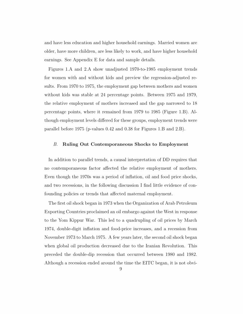
Figures 1.A and 2.A show unadjusted 1970-to-1985 employment trends

for women with and without kids and preview the regression-adjusted re-

sults. From 1970 to 1975, the employment gap between mothers and women

without kids was stable at 24 percentage points. Between 1975 and 1979,

the relative employment of mothers increased and the gap narrowed to 18

percentage points, where it remained from 1979 to 1985 (Figure 1.B). Al-

though employment levels differed for these groups, employment trends were

parallel before 1975 (p-values 0.42 and 0.38 for Figures 1.B and 2.B).

B. Ruling Out Contemporaneous Shocks to Employment

In addition to parallel trends, a causal interpretation of DD requires that

no contemporaneous factor affected the relative employment of mothers.

Even though the 1970s was a period of inflation, oil and food price shocks,

and two recessions, in the following discussion I find little evidence of con-

founding policies or trends that affected maternal employment.

The first oil shock began in 1973 when the Organization of Arab Petroleum

Exporting Countries proclaimed an oil embargo against the West in response

to the Yom Kippur War. This led to a quadrupling of oil prices by March

1974, double-digit inflation and food-price increases, and a recession from

November 1973 to March 1975. A few years later, the second oil shock began

when global oil production decreased due to the Iranian Revolution. This

preceded the double-dip recession that occurred between 1980 and 1982.

Although a recession ended around the time the EITC began, it is not obvi-9

ous why this would have affected the relative employment of mothers since

no such increase occurred after the 1980-1982 recessions (Figures 1.A and

2.A).15 To account for these factors, I control for annual inflation, state-by-

year employment and manufacturing employment, and allow these variables

to vary by family size, marital status, and education.

Two potential identification threats include public-program cuts, which

could increase maternal employment via an income effect, or a sudden

change in demographic traits associated with employment and unrelated

to the EITC. However, public assistance expanded in the 1970s (a period of

“welfare explosion” (Moffitt 2003)): AFDC, Food Stamps, WIC, and pay-

roll taxes all increased or were flat (Figure A.3).16 Also, trends in marriage,

fertility, education, and male earnings were smooth (Figure A.2).17 I control

for the impact of welfare and demographics on employment, and allow them

to vary by state, year, and race.

Perhaps the most serious potential confounder is the 1976 Child and De-

pendent Care Tax Credit (CDCTC), a non-refundable tax credit for child

care expenses. I investigate whether this policy affects my analysis in three

ways: First, I look at the fraction of EITC recipients that received CDCTC

benefits (using IRS Statistics of Income [SOI] data):18 only 1 percent of

EITC-eligible tax filers received any CDCTC benefits, compared to 30 per-

15Theoretically, a permanent price increase could increase labor supply through an in-come effect, but the 1970s price shocks were temporary and should not have differentiallyaffected mothers.

16AFDC denotes Aid to Families with Dependent Children, a cash assistance wel-fare program. WIC denotes Women, Infants, and Children, an in-kind food assistanceprogram. See Figure A.3 notes for brief histories of these public programs.

17I cannot rule out a threshold-crossing model (Schelling 1971) where a continuouslychanging covariate has a discrete impact on an outcome.

18SOI data are de-identified samples of U.S. Federal Individual Income Tax returnswith detailed income information, but little demographic information. SOI samplingweights used. More details in Appendix B.

10

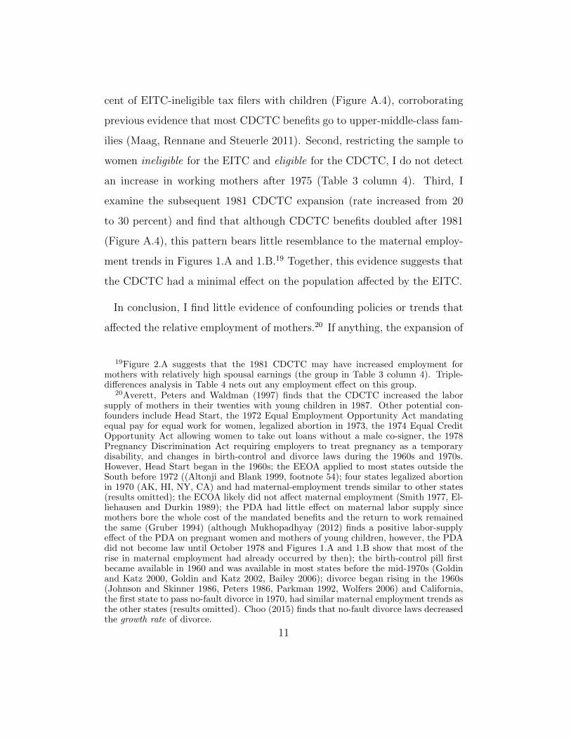
cent of EITC-ineligible tax filers with children (Figure A.4), corroborating

previous evidence that most CDCTC benefits go to upper-middle-class fam-

ilies (Maag, Rennane and Steuerle 2011). Second, restricting the sample to

women ineligible for the EITC and eligible for the CDCTC, I do not detect

an increase in working mothers after 1975 (Table 3 column 4). Third, I

examine the subsequent 1981 CDCTC expansion (rate increased from 20

to 30 percent) and find that although CDCTC benefits doubled after 1981

(Figure A.4), this pattern bears little resemblance to the maternal employ-

ment trends in Figures 1.A and 1.B.19 Together, this evidence suggests that

the CDCTC had a minimal effect on the population affected by the EITC.

In conclusion, I find little evidence of confounding policies or trends that

affected the relative employment of mothers.20 If anything, the expansion of

19Figure 2.A suggests that the 1981 CDCTC may have increased employment formothers with relatively high spousal earnings (the group in Table 3 column 4). Triple-differences analysis in Table 4 nets out any employment effect on this group.

20Averett, Peters and Waldman (1997) finds that the CDCTC increased the laborsupply of mothers in their twenties with young children in 1987. Other potential con-founders include Head Start, the 1972 Equal Employment Opportunity Act mandatingequal pay for equal work for women, legalized abortion in 1973, the 1974 Equal CreditOpportunity Act allowing women to take out loans without a male co-signer, the 1978Pregnancy Discrimination Act requiring employers to treat pregnancy as a temporarydisability, and changes in birth-control and divorce laws during the 1960s and 1970s.However, Head Start began in the 1960s; the EEOA applied to most states outside theSouth before 1972 ((Altonji and Blank 1999, footnote 54); four states legalized abortionin 1970 (AK, HI, NY, CA) and had maternal-employment trends similar to other states(results omitted); the ECOA likely did not affect maternal employment (Smith 1977, El-liehausen and Durkin 1989); the PDA had little effect on maternal labor supply sincemothers bore the whole cost of the mandated benefits and the return to work remainedthe same (Gruber 1994) (although Mukhopadhyay (2012) finds a positive labor-supplyeffect of the PDA on pregnant women and mothers of young children, however, the PDAdid not become law until October 1978 and Figures 1.A and 1.B show that most of therise in maternal employment had already occurred by then); the birth-control pill firstbecame available in 1960 and was available in most states before the mid-1970s (Goldinand Katz 2000, Goldin and Katz 2002, Bailey 2006); divorce began rising in the 1960s(Johnson and Skinner 1986, Peters 1986, Parkman 1992, Wolfers 2006) and California,the first state to pass no-fault divorce in 1970, had similar maternal employment trends asthe other states (results omitted). Choo (2015) finds that no-fault divorce laws decreasedthe growth rate of divorce.

11

public assistance during the 1970s would have led to slight decreases in ma-

ternal employment, implying that results in this paper may underestimate

the employment effects of the 1975 EITC.

III. The EITC and Extensive-Margin Labor Supply

A. Average Treatment Effects

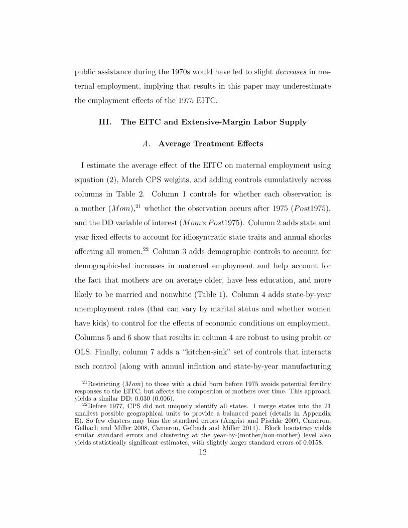
I estimate the average effect of the EITC on maternal employment using

equation (2), March CPS weights, and adding controls cumulatively across

columns in Table 2. Column 1 controls for whether each observation is

a mother (Mom),21 whether the observation occurs after 1975 (Post1975),

and the DD variable of interest (Mom×Post1975). Column 2 adds state and

year fixed effects to account for idiosyncratic state traits and annual shocks

affecting all women.22 Column 3 adds demographic controls to account for

demographic-led increases in maternal employment and help account for

the fact that mothers are on average older, have less education, and more

likely to be married and nonwhite (Table 1). Column 4 adds state-by-year

unemployment rates (that can vary by marital status and whether women

have kids) to control for the effects of economic conditions on employment.

Columns 5 and 6 show that results in column 4 are robust to using probit or

OLS. Finally, column 7 adds a “kitchen-sink” set of controls that interacts

each control (along with annual inflation and state-by-year manufacturing

21Restricting (Mom) to those with a child born before 1975 avoids potential fertilityresponses to the EITC, but affects the composition of mothers over time. This approachyields a similar DD: 0.030 (0.006).

22Before 1977, CPS did not uniquely identify all states. I merge states into the 21smallest possible geographical units to provide a balanced panel (details in AppendixE). So few clusters may bias the standard errors (Angrist and Pischke 2009, Cameron,Gelbach and Miller 2008, Cameron, Gelbach and Miller 2011). Block bootstrap yieldssimilar standard errors and clustering at the year-by-(mother/non-mother) level alsoyields statistically significant estimates, with slightly larger standard errors of 0.0158.

12

employment) with year, state, marital status, having kids, and race. These

interactions flexibly account for the impact of economic conditions, changing

demographics, and general trends in the employment of women.

Across each set of controls the DD estimate is stable between 3.3 and 4.9

percentage points (or 6.2 and 9.2 percent from a baseline of 53 percent)23

and significant at the 99-percent level. Results imply that about one million

mothers began working because of the 1975 EITC.24 The EITC is responsi-

ble for about a quarter of the 12-percentage-point rise in absolute maternal

employment and a fifth of the 10-percentage-point rise in overall female em-

ployment between 1975 and 1985. I use the more conservative logit model

and set of controls in column 4 throughout the rest of the analysis (un-

less otherwise specified). Results are robust to alternate binary definitions

of working based on earnings, weeks worked, or labor-force participation

(Table A.1), using alternate age cutoffs (Table A.2), not using CPS weights

(estimate is 0.030 [0.007]), and additional robustness checks (Appendix B).25

B. Heterogeneous and Subgroup Treatment Effects

Although the average employment effect of the EITC was positive, this

effect should have varied by the likelihood of receiving EITC benefits. In

Table 3, I test whether the treatment effect varied in a way consistent with

2353 percent baseline seen in Figure 2.A. Results are intent-to-treat effects: about 20percent of households are EITC-eligible and do not claim the EITC or are EITC-ineligiblefamilies and do (Scholz 1994). Liebman (1997) and Liebman (2000) find that 89 and 95percent of women allocated to the treatment and control groups filed taxes appropriatelyin the 1980s. Random misallocation implies that the estimates should be scaled up by19 percent (Eissa and Liebman 1996).

2460 percent of the 53.8 million women 18-50 in 1980 are mothers (March CPS). 3.3percentage points of these mothers corresponds to about 1 million mothers.

25Appendix B shows results are robust to model choice, sample period, reweighting toaccount for group composition and CPS data imputations; I also explain how flat EITCbeneficiaries and increases in working mothers are compatible, and why I observe largerresponses from women with more than one child.

13

the EITC causing this rise in maternal employment. Traits associated with

these heterogeneous responses are also used in section VI.F to predict state-

level EITC responses and test whether states with larger EITC responses

had larger post1975 increases in approval of working women.

B. i. Heterogeneous Treatment Effects: Marital Status

There are at least two reasons why married mothers should have responded

less to the EITC than unmarried mothers. First, since EITC eligibility

is determined by household earnings, spousal earnings often pushed the

household out of EITC eligibility (point C in Figure 4.A). Second, spousal

earnings increased the likelihood that the highest feasible indifference curve

is achieved with zero labor supply (point A in Figure 4.A).

I verify this heterogeneity in Table 3 column 1, where I add the variable

Mom×Post1975×Unmarried to equation (2) and interpret its coefficient

(5.3 percentage points) as the treatment effect of the EITC on unmarried

mothers relative to married mothers. I interpret the sum of the two coef-

ficients in column 1 (6.9 percentage points, or 10.7 percent from a base of

64.5 percent) as the overall effect of the EITC on unmarried mothers.26

To estimate the effect of the EITC on married mothers, I carry out two

approaches. In column 1, I pool all women; in column 2, I restrict the sample

to married women. These approaches yield statistically significant estimates

of 1.6 and 2.1 percentage points and align with prior EITC research that

has consistently found a larger response among single mothers.27

26For comparison, the 1986 EITC expansion increased the number of unmarried work-ing mothers by 2.8 percentage points (Eissa and Liebman 1996), the 1990s EITC expan-sion was responsible for a 6.1-percentage-point increase (Hoynes, Miller and Simon 2015),and the combined 1984-1996 EITC expansions increased the employment of unmarriedmothers by 7.2 percentage points (Meyer and Rosenbaum 2001).

27See Eissa and Liebman (1996), Meyer and Rosenbaum (2001), Grogger (2003), and

14

Although I find a small positive average response among married mothers

to the 1975 EITC, there should have been substantial heterogeneity that

varied by spousal earnings. Mothers with very low spousal earnings should

have responded to the EITC much like unmarried mothers. Restricting

the sample to EITC-eligible married women with spouses earning below

the EITC kink point,28 the EITC increased the employment of this group

by 4.5 percentage points.29 I also test for a negative correlation between

spousal earnings and EITC response by adding a variable to equation (2)

that interacts Mom×Post1975 with spousal earnings. Column 5 shows that

the treatment effect on married women with zero spousal earnings was 4.6

percentage points and declined by 0.5 percentage points for every $10,000

(2013 dollars) in spousal earnings.30

Married mothers with spouses earning above the 1975 EITC kink point

were not eligible for the EITC and faced the same work incentives before

and after 1975. If it appears that the EITC increased the employment of

this placebo group of mothers, this could indicate that an omitted factor is

biasing-up the results. However, Table 3 column 4 shows a null effect on

this placebo group and small effects can be statistically ruled out.

Hotz and Scholz (2006) for responses of unmarried mothers, and Ellwood (2000), Eissaand Hoynes (2004), and Bitler, Hoynes and Kuka (2016) for responses of married mothers.

28This sample is restricted to married women with spouses earning below $18,000 in2013 dollars (the 1975 EITC kink point) in each year; the bottom fifth of spousal earnings.

29This result is nested in Figure A.5 which uses the entire spousal-earnings distributionand shows the largest EITC responses came from women with the lowest earning spouses.

30I verify that this pattern is also evident for the 1986 and 1993 EITC expansions (TableA.3). Results are robust to using actual or predicted spousal earnings. Table 3 treatsa married woman’s work decision like a second mover in a two-person sequential game,where the primary earner’s labor supply does not depend on his spouse’s labor supply(Eissa and Hoynes 2004). This assumption may not be completely unrealistic since 1970s-male labor supply was inelastic (Blundell and MaCurdy 1999). Also, the EITC is basedon household earnings and no additional EITC benefits should arise from substitutinglabor supply between spouses. Heterogeneous responses among married women are alsofound by (Eissa and Hoynes 2004, Table 8) and Eissa and Hoynes (2006b).

15

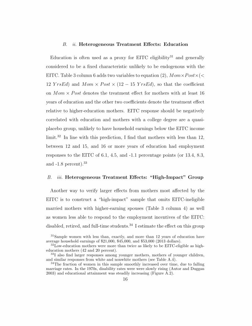
B. ii. Heterogeneous Treatment Effects: Education

Education is often used as a proxy for EITC eligibility31 and generally

considered to be a fixed characteristic unlikely to be endogenous with the

EITC. Table 3 column 6 adds two variables to equation (2), Mom×Post×(<

12 Y rsEd) and Mom × Post × (12 − 15 Y rsEd), so that the coefficient

on Mom × Post denotes the treatment effect for mothers with at least 16

years of education and the other two coefficients denote the treatment effect

relative to higher-education mothers. EITC response should be negatively

correlated with education and mothers with a college degree are a quasi-

placebo group, unlikely to have household earnings below the EITC income

limit.32 In line with this prediction, I find that mothers with less than 12,

between 12 and 15, and 16 or more years of education had employment

responses to the EITC of 6.1, 4.5, and -1.1 percentage points (or 13.4, 8.3,

and -1.8 percent).33

B. iii. Heterogeneous Treatment Effects: “High-Impact” Group

Another way to verify larger effects from mothers most affected by the

EITC is to construct a “high-impact” sample that omits EITC-ineligible

married mothers with higher-earning spouses (Table 3 column 4) as well

as women less able to respond to the employment incentives of the EITC:

disabled, retired, and full-time students.34 I estimate the effect on this group

31Sample women with less than, exactly, and more than 12 years of education haveaverage household earnings of $21,000, $45,000, and $53,000 (2013 dollars).

32Low-education mothers were more than twice as likely to be EITC-eligible as high-education mothers (42 and 20 percent).

33I also find larger responses among younger mothers, mothers of younger children,and similar responses from white and nonwhite mothers (see Table A.4).

34The fraction of women in this sample smoothly increased over time, due to fallingmarriage rates. In the 1970s, disability rates were were slowly rising (Autor and Duggan2003) and educational attainment was steadily increasing (Figure A.2).

16

by adding a variable to equation (2) that interacts Mom × Post1975 with

a binary for being in this “high-impact” group. The two estimates in Table

3 column 7 show that these mothers had an EITC response of about 5.1

percentage points (or 8.1 percent).

B. iv. Heterogeneous Treatment Effects: Men

Since most males were already working in the 1970s (over 90 percent), and

their participation elasticity was near zero (Blundell and MaCurdy 1999), it

should not be surprising that the EITC had no detectable effect on males,

(0.3 percentage points) in Table 3 column 8.

C. Triple Differences Corroborate DD Estimates

Splitting the sample of mothers into EITC-eligible and EITC-ineligible

(Table 3 column 4) creates a third difference for triple differences (DDD).35

(3) P (Eist) = f(β1Mom× Post1975× Treatist + β2Xist + δst + εist)

The estimate of β1 is 2.5 percentage points (Table 4 column 1), similar

to DD, and suggests that factors affecting all mothers (e.g. abortion and

divorce laws, birth control) may not pose a threat to the DD estimates.36

When men from Table 3 column 8 are used as a comparison group, I find a

similar DDD estimate in Table 4 column 2 (2.6 percentage points).

35An omitted factor affecting the employment of all mothers could bias DD (discussedin section II.B), which is why DDD “may generate a more convincing set of results”(Angrist and Pischke 2009, p.182).

36Equation (3) also controls for Treat, Mom × Treat, Post1975 × Treat, Mom ×Post1975, along with interactions of each control with Treat for a more flexible model.

17

D. Extensive Margin Results: Annual DD Estimates

I estimate annual effects of the EITC and test if the DD results are driven

by outliers or general trends by replacing Mom × Post in equation (2)

with Mom × Y eary for y ∈ [1970, 1985]. I omit y = 1975 and estimates

measure the annual effect of being a mother on the probability of working

relative to 1975. Using the “high-impact” sample, Figure 1.B shows that

these estimates closely resemble the unadjusted time-series trend. Relative

to 1975, the estimates on Mom × Y eary are jointly insignificant (p-value

0.42) for y ∈ [1970, 1975], become increasingly positive for y ∈ [1975, 1979],

and remain positive and relatively stable for y ∈ [1979, 1985]. The 1975-to-

1979 increase may suggest it took mothers a few years to learn about the

EITC, similar to the response to the 1986 and 1993 EITC expansions (Eissa

and Liebman 1996; Meyer and Rosenbaum 2001).37

IV. Annual Work Hours and Earnings

A. Average Treatment Effects

Results above show that the EITC increased maternal employment and

imply that earnings and work hours should also have been affected. Results

in Table 4 use equation (2), an OLS specification, and replace the binary

employment outcome with annual work hours and earnings (in 2013 dol-

lars). For each outcome, I show results for three samples of women: the

“high-impact” group (from Table 3 column 7), all women (from Table 2),

37The EITC does not pay until the following tax refund; it could take a year beforeEITC recipients became aware of the EITC (Liebman 1998). To test whether EITCresponse required an understanding of the tax code (Chetty, Friedman and Saez 2013,Bhargava and Manoli 2015), I plot the annual response by education subgroup and donot find quicker responses by higher-education mothers (omitted).

18

and the EITC-ineligible placebo group (from Table 3 column 4). Among

the “high-impact” sample, the EITC led to increases of 63.9 annual work

hours and $1249.1 in annual earnings (Table 4 columns 1 and 4). Among

the sample of all women, the EITC led to smaller increases in work hours

(35.1) and earnings ($750.3) (columns 2 and 5). Results capture both inten-

sive and extensive margins, but primarily reflect participation responses.38

Among the placebo group, columns 3 and 6 show that the EITC had a sta-

tistically insignificant effect on work hours (2.4) and earnings (438), which

corroborates the placebo test in Table 3 column 4.

B. The EITC and the Distribution of Hours and Earnings

Where in the earnings and work-hours distribution did these newly work-

ing mothers enter? To investigate this, I estimate regressions resembling

equation (2) but with a binary outcome variable for having annual earnings

or work hours in a particular range. Figures 5 and A.6 show the DD esti-

mates using the “high-impact” sample to focus on mothers most affected by

the EITC. These figures also serve as robustness checks since it would raise

concerns if these newly working mothers earned above the EITC limit.

For annual earnings (in 2013 dollars), the most common response to the

EITC was to earn between $10,000 and $20,000, which encompassed the

most generous portion of the EITC schedule (Figure 5) and suggests that

many of these newly working mothers received the EITC. The minimum

wage during this period was $7 to $9 per hour, and since Figure A.6 shows

that many mothers began working full time, this maps to about $14,000

38See Figures 5 and A.6 for evidence. As a percent, these four estimates are 8.1, 10.3,5.7, and 7.3. Although some people in or beyond the EITC phase-out region had anincentive to decrease labor supply to receive the EITC, there is little evidence for this(Meyer 2002, Saez 2002, Eissa and Hoynes 2006a); although see Kline and Tartari (2016).

19

to $18,000 per year, consistent with Figure 5. Figure 5 also suggests that

mothers were slightly more likely to earn between $20,000 and $50,000.

Figure A.6 shows that the most common response to the EITC was to

work full-time, full-year (about 2000 annual hours)39 and may also have

increased part-time work, although estimates on annual hours below 2000

are not statistically significant. Consistent with previous results, mothers

were less likely to have zero work hours or earnings (Figures 5 and A.6).40

Using IRS SOI data (see footnote 18), I also find suggestive evidence

that the EITC affected the composition of tax filers. Consistent with Table

3 column 1, the fraction of unmarried tax filers increased after 1975 in a

pattern similar to Figure 1.B (see Appendix B.6 and Figure B.3).

C. Quantile Analysis

I now characterize the effect of the EITC on the distribution of earnings.

I use the regression behind Table 4, but instead of average effects, I estimate

the effect at each centile of the earnings distribution. Instead of minimizing

the sum of squared residuals like OLS, quantile regression uses heteroskedas-

ticity as a feature of the data and minimizes a weighted sum of the absolute

value of the residuals (Koenker 2005). These quantile difference in differ-

ences (QDD) are effects on quantiles, not on individual mothers, since rank

preservation would require strong assumptions or panel data (see Bitler,

Gelbach and Hoynes (2003)). Using the “high-impact” sample, Figure 6

shows that the EITC had the largest effect on the annual earnings of the

39Annual hours combines the categorical weeks worked last year variable (continuousvariable not available until 1976 CPS) and hours worked last week, in an attempt toreduce measurement error (Bound, Brown and Mathiowetz 2001).

40To isolate intensive-margin responses, I re-run the analysis in Figures 5 and A.6conditional on working, and find (noisy) evidence of more mothers working over 1000hours and earning between $10,000 and $20,000.

20

43th centile, with a positive but decreasing effect higher up the earnings dis-

tribution, eventually becoming statistically insignificant for the top centiles.

Work hours yield a similar pattern. The EITC had no effect on the lowest

four centiles as these mothers did not work before or after 1975. Together,

these QDD estimates drive the average effects in Table 4.

V. Implied Elasticities

I follow (Chetty et al. 2012, Appendix B) and calculate the participation

elasticity as the pre1975-post1975 change in log employment rates divided

by the pre1975-post1975 change in the log net-of-tax earnings from work-

ing. I account for various taxes (EITC, income tax, payroll tax, dependent

deduction) and transfers (AFDC, food stamps, WIC). I calculate this elas-

ticity for a representative unmarried mother of one child with the average

pre-tax earnings of such a mother in the sample ($19,000, in 2013 dollars).

I estimate an elasticity between 0.41 (0.11) and 0.49 (0.13). See Table C.1

for complete details. Accounting for public assistance take-up rates yields

a slightly larger elasticity between 0.45 and 0.54. Finally, I estimate the

total intensive plus extensive margin elasticity from the annual work hours

and earnings estimates in Table 4 to be 0.37 (0.10) and 0.47 (0.13). These

elasticity estimates are larger than those for more recent decades, but are

consistent with elasticity estimates for this period.41

41Female labor-supply elasticity has steadily declined since World War II (Goldin1990): Bowen and Finegan (1969) finds 0.67 in 1960; Fields (1976) finds 0.52 in 1970;Blundell and MaCurdy (1999) shows that empirical studies using data from the 1970sand 1980s produce an average estimate of about 0.8; Blau and Kahn (2005) and Heim(2007) find an uncompensated elasticity of about 0.6 in 1980. Mroz (1987) discussesmany of these early studies. The 1968-1982 negative income tax experiments yieldedelasticities of 0.2 to 0.3 (Burtless and Hausman 1978, Robins 1985). Chetty et al. (2012)finds a range of 0.30 to 0.45. Elasticities are a function of the tax code (Saez, Slemrodand Giertz 2012) and vary across populations and time.

21

VI. Effects on Attitudes Towards Working Women

If the 1975 EITC encouraged a million mothers to begin working, this

likely had subsequent effects on the country. Although there is a large

literature showing that the EITC has benefited children of EITC recipients

(see section I), how this program may have affected social attitudes towards

working women has remained understudied.42

Google ngrams (Michel et al. 2011) show that in the mid-1970s, the phrases

working mom and – the previously redundant – stay at home mom began to

be used much more often (Figure 3). This suggests that the rise of working

mothers was a salient phenomenon and reflects changes in language and

attitudes towards the role of women in society. After 1975, people were

more likely to have working-female family members, friends, and coworkers,

while media stories about working mothers also became more common.43

An emerging literature shows that gender-equality preferences can be al-

tered via exposure to working women. Fernandez, Fogli and Olivetti (2004)

and Olivetti, Patacchini and Zenou (2016) show that having a working

mother – and having friends with working mothers – during childhood

leads to stronger gender-equality preferences in adulthood.44 Finseraas et al.

42Exposure to working women could theoretically have increased or decreased approvalof working women. Analysis in section VI fits into an economics literature analyzing therole of attitudes and social norms (Becker 1957, Arrow 1971, Akerlof and Dickens 1982,Akerlof and Kranton 2000, Benabou and Tirole 2006). Gender-role preferences are passedon intergenerationally (Fernandez and Fogli 2009, Alesina, Giuliano and Nunn 2011, Farreand Vella 2013) and affect female labor market outcomes (Fortin 2005, Charles, Guryanand Pan 2009, Bertrand, Kamenica and Pan 2015, Fortin 2015, Pan 2015, Janssen, Sartoreand Backes-Gellner 2016). Unlike these studies, my goal is to characterize a determinant– not consequence – of these attitudes. There is also a long-standing sociology literaturedescribing the time trends and correlates of these attitudes (Thornton and Freedman1979, Thornton, Alwin and Camburn 1983, Plutzer 1988, Lottes and Kuriloff 1992).

43Media has been shown to affect teen pregnancy (Kearney and Levine 2015), divorce(Chong and Ferrara 2009), and fertility (La Ferrara, Chong and Duryea 2012). SeeDellaVigna and Ferrara (2015) for a recent literature review.

44Additional evidence that various attitudes can be altered via exposure has also been

22

(2016) shows that exposure to female colleagues reduces discriminatory at-

titudes.45 With these results in mind, the attitudes of millions of Americans

may have been affected when the EITC led one million mothers to begin

working in the late 1970s.

A. Empirical Strategy

I characterize and exploit geographic heterogeneity in EITC responses

and use a two-sample two-stage approach to test whether states with larger

EITC responses had larger changes in gender-equality preferences. Gender-

equality preferences are defined as approving of working women and are

created from General Social Survey (GSS) data, an appealing source for

measuring these social attitudes since the survey question is consistent over

time and begins in 1972, providing a few baseline years before 1975.46 Ta-

ble A.5 shows GSS sample summary statistics and Table A.6 shows gender-

equality preferences are positively correlated with education, having a work-

ing mother, and being younger, female, unmarried, and white.

I aggregate the gender-equality preferences of 8,713 adults, ages 18-60, ob-

served between 1972 and 1985, to the state-by-year level using GSS weights.

I then construct a state panel on gender-equality preferences before and

shown by Finseraas and Kotsadam (2015) (ethnic minorities), Beaman et al. (2012) (fe-male aspirations), Stouffer et al. (1949) (race), and experimental evidence (Heilman andMartell 1986, Lowery, Hardin and Sinclair 2001, Dasgupta and Asgari 2004). This conceptis related to psychology concept of intergroup contact theory (Allport 1954).

45Attitude changes consist of individual and intergenerational changes (Firebaugh1992). Fernandez, Fogli and Olivetti (2004) and Olivetti, Patacchini and Zenou (2016) fo-cus on intergenerational change, Finseraas et al. (2016) on individual change. Fernandez,Fogli and Olivetti (2004, footnote 1) acknowledges individual change: “as more womenjoined the labor force, attitudes towards these women changed in society at large.” Myapproach captures both channels and tests how individual attitude changes aggregate.

46The GSS question asks, “Do you approve or disapprove of a married woman earningmoney in business or industry if she has a husband capable of supporting her?” Suchapproval rose from 20 to 80 percent between the 1930s and the 1990s (Figure A.7).

23

after 1975 and create the variable ∆GenderEquality(1976−85)−(1972−75)s – the

change in the fraction of a state’s adults that approve of working women – by

subtracting the 1972-1975 state average from the 1976-1985 state average.47

I use March CPS data and the full sample and full set of controls from

Table 2 column 4 to estimate the state-level, EITC-led increase in working

mothers (i.e. state EITC response).

(4) P (Eist) = f(β1Momist+∑s

β2sMom×Post1975is+β3Xist+δst+ εist)

Equation (4) modifies the national-level DD in equation (2) and estimates

β2s, state-level DDs.48 I rename β2s, EITC Responses, and estimate:

(5) ∆GenderEquality(1976−85)−(1972−75)s = γEITC Responses+δ∆Xs+εs.

γ measures the effect of a percentage-point increase in state EITC response

on the change in the fraction of a state’s population with gender-equality

preferences after 1975. Since the treatment variable is a generated regressor,

standard errors are bootstrapped (Pagan 1984, Hardin 2002, Murphy and

Topel 2002). Xs are controls to account for state-level traits. Regressions are

weighted by state population since observations represent grouped data.49

47Results are robust to extending the GSS sample to any year between the early 1980sand the 1990s (Figure A.8). Ideally, I would construct a state-by-year panel, but sinceGSS samples are relatively small I pool years to increase statistical power.

48Results are robust to estimating equation (4) with various sets of controls (includingstate-by-year fixed effects), using OLS, probit, or logit, and ending the CPS sample inany year between 1979 and 1985 (Table A.7).

49Similar results if unweighted or weighted by the standard-error inverse (equation4). Equation (5) is a first-difference estimator, which nets out the problem of omittedvariables and is unbiased and consistent under the condition E[uit−uit−1|xit−xit−1] = 0,which is less restrictive than the assumption of weak exogeneity for unbiasedness whenpre1975 and post1975 components are separated in a fixed effects estimator (Wooldridge2015). This second approach produces similar, but noisier, estimates.

24

B. Results

Using equation (5) and no controls, Figure 7 shows that each percentage-

point increase in state EITC response led to a 2.0-percentage-point increase

in state-level preferences for gender equality (p-value 0.001).50 Results are

similar with region fixed effects, reflecting changes within and across regions,

and are similar by gender (Table 7 columns 2 and 3).51 Appendix D shows

that less parametric approaches yield similar results.

One threat to my hypothesis would be if changes in gender-equality pref-

erences coincided with changes in demographics or other attitudes unrelated

to the EITC or working women, implying that an omitted trend is driving

the results in Figure 7. To test this, I re-estimate equation (5) with controls

for various demographic, political, and social-attitude variables.52 The effect

is stable between 1.6 and 2.3 percentage points, even when all 13 controls are

included together (Table 6). Changes in gender-equality preferences do not

seem to be driven by demographics or general trends in social attitudes.53

50The estimated magnitude appears plausible: the interquartile effect is 5.7 percentagepoints, comparable to having two more years of education or being a decade younger, butless than having a working wife or having racial-equality preferences (Table A.6).

51I test how likely Figure 7 is due to chance with a variant of the permutation test inBuchmueller, DiNardo and Valletta (2011): I randomly reassign a new attitude change toeach state (with replacement) from the set of state attitude changes, re-estimate equation(5), record γ, and iterate 10,000 times. Figure A.9 shows that the actual estimate (0.0177)is in the top 0.07 percent of permutations and unlikely to occur by chance.

52Controls are education, age, marriage, number of mothers, race, employment, earn-ings, whether mother worked and mother’s education, fraction Democrat and religious,and views on public assistance and racial-equality. Table 6 Panels A and B control for thepre1975-post1975 change and the pre1975 level. See Table A.5 for summary statistics.

53Although it is impossible to control for every state trait that may be correlated withincreases in working mothers and with attitudes towards working women, the GSS hasdata on a wide range of topics (e.g. racial attitudes, voting behavior, religion, attitudestowards public assistance, mother’s work and education). Furthermore, state-level re-sponse to the EITC (estimated in equation 4) accounts for changes in demographic traitsand economic conditions and isolates the increase in working mothers due to the EITC.

25

C. Dose Response

If the EITC did affect gender-equality preferences through exposure to

working women, then people more likely to know these newly working

women should have had larger preference changes. Since the EITC had a

larger effect on lower-education mothers (Table 3 column 6), lower-education

adults were more likely to know (or even be) these women. Table 7 columns

4 and 5 re-estimate equation (5), but divide the sample into adults with

more or less than 12 years of education. For lower-education adults, the es-

timate of γ in equation (5) is 0.023 (p-value 0.001) and for higher-education

adults it is 0.005 (p-value 0.63). These estimates are statistically different

at the 99-percent level and confirm that people more likely to know these

newly working women did have larger preference changes.

D. Placebo Outcome: Changes in Racial-Equality Preferences

Since attitudes towards gender and race were correlated with the same

traits (Table A.6), it is conceivable that an omitted factor – other than

the EITC – was driving changes in various types of attitudes. One way

to test for this is to use racial attitudes as a control (Table 6 column 7).

Another approach is to use racial attitudes as a placebo outcome: Table

7 column 6 shows that state EITC responses had no detectable effect (p-

value=0.19) on racial-equality preferences after 1975.54 Changes in gender-

equality preferences do not seem to be driven by general trends in attitudes.

54The relationship between EITC response and changes in racial attitudes is even lesssignificant (p-value 0.79) when education is controlled for (Table 7 Panel B column 7).

26

E. Ruling Out Reverse Causation and Mean Reversion

Perhaps the most obvious threat to the results in Figure 7 is reverse cau-

sation: that is, if higher-responding states already had higher approval of

working women before 1975. In Table 7 columns 7 and 8, I follow the ap-

proach in Acemoglu, Autor and Lyle (2004) and test for a positive relation-

ship between state EITC response and pre1975 gender-equality preferences.

I find an insignificant relationship between state EITC response and the

1972-to-1975 preference trend (p-value 0.70), and interestingly, a negative

relationship between state EITC response and the 1974 preference level.55

This negative estimate suggests that the EITC may have led to an attitude

“catch up” among states with lower gender-equality preferences.56

Since states with the lowest approval of working women before 1975 had

the largest increase in approval of working women after 1975, it is possible

that Figure 7 simply due to mean reversion. In this context, mean reversion

could reflect data limitations and relatively small GSS sample sizes, or real

convergence in social norms across states over time. One way to test for

mean reversion is to see if states with higher EITC responses (and lower

approval of working women) continued to have larger increases in approval

of working women in the 1980s and 1990s. As shown by Charles, Guryan

and Pan (2009), states with the lowest approval of working women in the

1970s also had the lowest approval of working women in later decades.57 If

55Although the relationship between pre1975 attitudes and EITC response becomesstatistically insignificant when education is controlled for (Table 7 Panel B column 7).

56If states that voted for the EITC benefited the most from it, perhaps the EITC wasthe outcome, not the cause, of changing attitudes. To test this, I regress state EITCresponse on the fraction of a state’s Senators and House Representatives that voted forthe 1975 EITC legislation. Figure A.10 shows that, in fact, the opposite is true: statesvoting against the EITC had higher EITC responses and thus preference changes werelarger in places less likely to be in favor of a social program like the EITC.

57I also find a strong positive correlation between state-level gender-equality prefer-

27

mean reversion drove attitude changes after 1975, it should also have driven

attitude changes in later decades. Figure A.11 re-estimates equation (5), but

instead of 1975, measures attitude changes after placebo years in the 1980s

and 1990s. I find that EITC response had no apparent relationship with

changes in gender-equality preferences after these placebo years, suggesting

that mean reversion may not explain post1975 preference changes either.

Another way to investigate whether mean reversion explains Figure 7, is

to see if state EITC response is still associated with changes in attitudes

when controlling for pre1975 attitudes. Table 7 column 9 shows that while

pre1975 attitudes are significantly associated with post1975 attitude changes

(corroborating column 7), EITC response continues to have an independent

effect on attitude changes; although the estimate falls from 0.020 to 0.013,

perhaps suggesting that a third of the estimate in Figure 7 may be due to

mean reversion. Panel B takes this approach one step further and re-runs

each regression in Panel A with controls for pre1975 education, a trait asso-

ciated with EITC response and social attitudes: EITC response continues

to have an independent effect on attitude changes even when attitudes and

education are controlled for (estimate 0.013 [0.006] in column 9).58

F. 2SLS and Predicted State EITC Responses

In this section I exploit pre1975 state traits, Xpre1975s , and the hetero-

geneous EITC responses in Table 3 to predict state EITC response and

test whether predicted EITC response is associated with changes in gender-

equality preferences. This two-stage-least-squares approach helps alleviate

ences in the 1970s, 1980s, and 1990s (not shown).58The estimate of EITC response remains positive (0.017 [0.005]) when pre1975 atti-

tudes and all 13 controls from Table 6 column 9 are used.

28

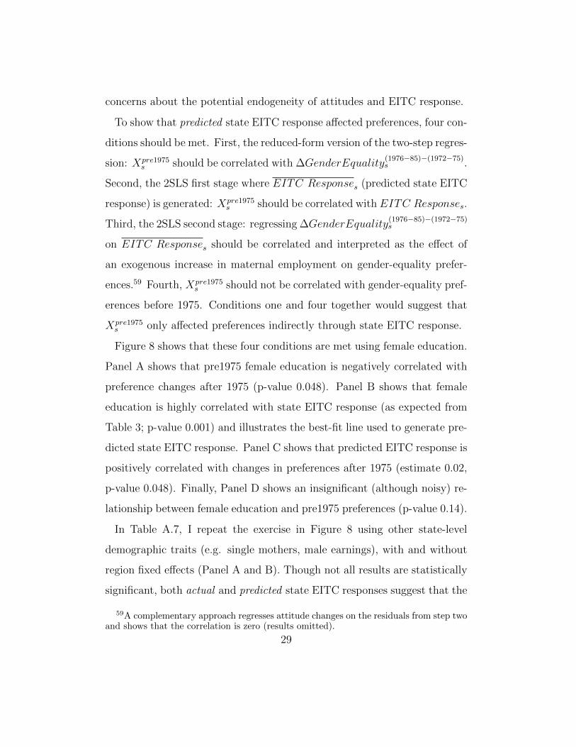
concerns about the potential endogeneity of attitudes and EITC response.

To show that predicted state EITC response affected preferences, four con-

ditions should be met. First, the reduced-form version of the two-step regres-

sion: Xpre1975s should be correlated with ∆GenderEquality

(1976−85)−(1972−75)s .

Second, the 2SLS first stage where EITC Responses (predicted state EITC

response) is generated: Xpre1975s should be correlated with EITC Responses.

Third, the 2SLS second stage: regressing ∆GenderEquality(1976−85)−(1972−75)s

on EITC Responses should be correlated and interpreted as the effect of

an exogenous increase in maternal employment on gender-equality prefer-

ences.59 Fourth, Xpre1975s should not be correlated with gender-equality pref-

erences before 1975. Conditions one and four together would suggest that

Xpre1975s only affected preferences indirectly through state EITC response.

Figure 8 shows that these four conditions are met using female education.

Panel A shows that pre1975 female education is negatively correlated with

preference changes after 1975 (p-value 0.048). Panel B shows that female

education is highly correlated with state EITC response (as expected from

Table 3; p-value 0.001) and illustrates the best-fit line used to generate pre-

dicted state EITC response. Panel C shows that predicted EITC response is

positively correlated with changes in preferences after 1975 (estimate 0.02,

p-value 0.048). Finally, Panel D shows an insignificant (although noisy) re-

lationship between female education and pre1975 preferences (p-value 0.14).

In Table A.7, I repeat the exercise in Figure 8 using other state-level

demographic traits (e.g. single mothers, male earnings), with and without

region fixed effects (Panel A and B). Though not all results are statistically

significant, both actual and predicted state EITC responses suggest that the

59A complementary approach regresses attitude changes on the residuals from step twoand shows that the correlation is zero (results omitted).

29

EITC positively affected gender-equality preferences.

G. External Validity: Attitude Changes After WWII

If the EITC-led increase in working women affected attitudes towards

working women, then the same pattern should exist during other periods

of large increases in female employment. During World War II, more than

7 million women began working – compared to a total of about 14 million

women working in 1940 – to make up for the 14 million men that joined

the military. More women worked in places with higher mobilization rates

(Acemoglu, Autor and Lyle 2004, Goldin and Olivetti 2013).60

I follow the approach in equation (5), and construct a state panel on

gender-equality preferences before and after WWII, using WWII mobiliza-

tion rates as the treatment variable. Testing whether mobilization rates

(and large increases in working women) affected social attitudes is feasible

since Gallup began asking such questions in the 1930s (see Figure A.13 notes

for details) and identifies individuals by state. I find that mobilization rates

are strongly associated with increases in gender-equality preferences after

WWII (p-value 0.003), providing corroborating evidence that increases in

working women may affect attitudes about the role of women in society.

VII. Summary

In one of the first systematic studies of the 1975 introduction of the EITC, I

find that this program led to a 6-percent increase in maternal employment,

60Two-thirds of these rates can be explained by exogenous factors (Goldin and Olivetti2013). I focus on attitudes and mobilization of white adults, since WWII had a largereffect on white women: “black womens [labor force] participation was high before the warand many were in agricultural occupations” (Goldin and Olivetti 2013). Mobilizationrates are not correlated with state responses to the 1975 EITC (p-value 0.38).

30

which represents about one million mothers and a participation elasticity

of 0.49. Regression-adjusted and unadjusted time-series trends show that

the relative employment of mothers began to increase after 1975 (Figures

1.A and 1.B). Consistent with the EITC being responsible for this rise in

employment, I find larger responses from mothers more likely to be EITC

eligible and null responses from placebo groups not eligible for EITC benefits

(Table 3). Using the placebo group of EITC-ineligible mothers in a triple-

differences specification to net out contemporaneous policies (e.g. birth

control, divorce laws, abortion) yields similar estimates.

In hindsight, the employment effect of the 1975 EITC should not be

that surprising: female labor-supply elasticity was larger during this pe-

riod (Blau and Kahn 2005, Heim 2007) and the 10-percent wage subsidy

of the EITC represented a large increase in potential earnings.61 Although

much was already known about the rise of working women (Killingsworth

and Heckman 1986, Goldin 1990, Fernandez, Fogli and Olivetti 2004), this

study helps explain why so many mothers began working in the 1970s.

The 1970s also provide a clean policy environment to evaluate the effects

of the EITC. By the 1980s, policymakers were cutting public benefits and

nudging low-income women into the labor force, and the 1990s EITC expan-

sion coincided with welfare reductions and the Family Medical Leave Act,

which increased maternal employment (Ruhm 1998, Moffitt 1999).

This EITC-led increase in working mothers also appears to have increased

approval of working women. States with larger EITC responses – and larger

predicted responses based on pre1975 demographic traits – had larger in-

61This paper may also help resolve an anomaly observed by Smith and Ward (1985):although real wage growth explains most of the increase in the female labor supplybetween 1950 and 1980, after 1970, the growth rate of female labor supply rose as thereal-wage growth rate fell (Parkman 1992).

31

creases in attitudes approving of women working. Results do not appear to

be driven by changes in demographics or general trends in social attitudes,

and are larger among people more likely to know these newly working moth-

ers. As for external validity, I find similar attitude changes due to the large

increase in working women during World War II. Since social attitudes to-

wards working women and the number of working women are endogenous,

I use two episodes of largely exogenous increases in female employment

to show that increases in working women affect attitudes towards working

women. I conclude that the 1975 EITC played an important role in the rise

of U.S. working mothers and in fostering egalitarian social attitudes.

REFERENCES

Acemoglu, Daron, H Autor, and David Lyle. 2004. “Women, War, and Wages: The Effect of FemaleLabor Supply on the Wage Structure at Midcentury.” Journal of Political Economy, 112(3): 497–551.

Akerlof, George, and Rachel Kranton. 2000. “Economics and Identity.” Quarterly Journal of Eco-nomics, 115(3): 715–753.

Akerlof, George, and William Dickens. 1982. “The Economic Consequences of Cognitive Disso-nance.” American Economic Review, 72(3): 307–319.

Alesina, Alberto, Paola Giuliano, and Nathan Nunn. 2011. “Fertility and the Plough.” AmericanEconomic Review, 101(3): 499–503.

Allport, G. 1954. The Nature of Prejudice. Reading, MA: Addison Wasley.

Almond, Douglas, Hilary Hoynes, and Diane Schanzenbach. 2011. “Inside the War on Poverty:The Impact of Food Stamps on Birth Outcomes.” Review of Economics and Statistics, 93(2): 387–403.

Altonji, Joseph, and Rebecca Blank. 1999. “Race and Gender in the Labor Market.” Handbook ofLabor Economics, 3: 3143–3259.

Angrist, Joshua, and Jorn-Steffen Pischke. 2009. Mostly Harmless Econometrics: an Empiricist’sCompanion. Vol. 1, Princeton University Press.

Arrow, Kenneth. 1971. “Some Models of Racial Discrimination in the Labor Market.”

Autor, David, and Mark Duggan. 2003. “The Rise in the Disability Rolls and the Decline in Unem-ployment.” Quarterly Journal of Economics, 118(1): 157–206.

Averett, Susan, and Yang Wang. 2015. “The Effects of the Earned Income Tax Credit on ChildrensHealth, Quality of Home Environment, and Non-Cognitive Skills.” IZA Working Paper.

Averett, Susan, Elizabeth Peters, and Donald Waldman. 1997. “Tax Credits, Labor Supply, andChild Care.” Review of Economics and Statistics, 79(1): 125–135.

Bailey, Martha. 2006. “More Power to the Pill: The Impact of Contraceptive Freedom on Women’sLife Cycle Labor Supply.” Quarterly Journal of Economics, 121(1): 289–320.

Bailey, Martha, and Andrew Goodman-Bacon. 2015. “The War on Poverty’s Experiment in PublicMedicine: Community Health Centers and the Mortality of Older Americans.” American EconomicReview, 105(3): 1067–1104.

Bailey, Martha, and Sheldon Danziger. 2013. Legacies of the War on Poverty. Russell Sage.

Bastian, Jacob. 2018. “Unintended Consequences? More Marriage, More Children, and the EITC.”University of Chicago, Working Paper.

Bastian, Jacob, and Katherine Michelmore. 2018. “The Long-Term Impact of the Earned In-come Tax Credit on Children’s Education and Employment Outcomes.” Journal of Labor Economics,Forthcoming.

Baughman, Reagan, and Stacy Dickert-Conlin. 2009. “The Earned Income Tax Credit and Fer-tility.” Journal of Population Economics, 22(3): 537–563.

32

Beaman, Lori, Esther Duflo, Rohini Pande, and Petia Topalova. 2012. “Female LeadershipRaises Aspirations and Educational Attainment for Girls: A Policy Experiment in India.” Science,335(6068): 582–586.

Becker, Gary. 1957. “The Economics of Discrimination.”

Benabou, Roland, and Jean Tirole. 2006. “Incentives and Prosocial Behavior.” American EconomicReview, 96(5): 1652–1678.

Berinsky, Adam, and Eric Schickler. 2011. “Gallup Data, 1936-1945: Guide to Coding & Weight-ing.” Roper Center for Public Opinion Research, University of Connecticut.

Bertrand, Marianne, Emir Kamenica, and Jessica Pan. 2015. “Gender Identity and RelativeIncome Within Households.” Quarterly Journal of Economics, 571: 614.

Bhargava, Saurabh, and Dayanand Manoli. 2015. “Psychological Frictions and the IncompleteTake-Up of Social Benefits: Evidence from an IRS Field Experiment.” American Economic Review,105(11): 3489–3529.

Bitler, Marianne, Hilary Hoynes, and Elira Kuka. 2016. “Do In-Work Tax Credits Serve as aSafety Net?” Journal of Human Resources.

Bitler, Marianne, Jonah Gelbach, and Hilary Hoynes. 2003. “What Mean Impacts Miss: Distri-butional Effects of Welfare Reform Experiments.” National Bureau of Economic Research.

Bjorklund, Anders, and Robert Moffitt. 1987. “The Estimation of Wage Gains and Welfare Gainsin Self-Selection Models.” Review of Economics and Statistics, 69(1): 42–49.

Blau, Francine, and Lawrence Kahn. 2005. “Changes in the Labor Supply Behavior of MarriedWomen: 1980-2000.” National Bureau of Economic Research.

Blundell, Richard, and Thomas MaCurdy. 1999. “Labor Supply: A Review of Alternative Ap-proaches.” Handbook of Labor Economics, 3: 1559–1695.

Bound, John, and Richard Freeman. 1992. “What Went Wrong? The Erosion of Relative Earningsand Employment among Young Black Men in the 1980s.” Quarterly Journal of Economics, 107(1): 201–232.

Bound, John, Charles Brown, and Nancy Mathiowetz. 2001. “Measurement Error in SurveyData.” Handbook of Econometrics, 5: 3705–3843.

Bowen, William, and Aldrich Finegan. 1969. “The Economics of Labor Force Participation.”

Buchmueller, Thomas, John DiNardo, and Robert Valletta. 2011. “The Effect of an EmployerHealth Insurance Mandate on Health Insurance Coverage and the Demand for Labor: Evidence fromHawaii.” American Economic Journal: Economic Policy, 3(4): 25–51.

Burtless, Gary, and Jerry Hausman. 1978. “The Effect of Taxation on Labor Supply: Evaluatingthe Gary Negative Income Tax Experiment.” Journal of Political Economy, 86(6): 1103–1130.

Busso, Matias, John DiNardo, and Justin McCrary. 2014. “New Evidence on the Finite SampleProperties of Propensity Score Reweighting and Matching Estimators.” Review of Economics andStatistics, 96(5): 885–897.

Butcher, Kristin, and John DiNardo. 2002. “The Immigrant and Native-Born Wage Distributions:Evidence from United States Censuses.” Industrial & Labor Relations Review, 56(1): 97–121.

Cameron, Colin, Jonah Gelbach, and Douglas Miller. 2008. “Bootstrap-Based Improvements forInference with Clustered Errors.” Review of Economics and Statistics, 90(3): 414–427.

Cameron, Colin, Jonah Gelbach, and Douglas Miller. 2011. “Robust Inference with MultiwayClustering.” Journal of Business & Economic Statistics, 29(2): 238–249.

Center on Budget and Policy Priorities. 2014. “Center on Budget and Policy Priorities Analysisof the Census Bureau’s March 2013 Current Population Survey.”

Charles, Kerwin, Jonathan Guryan, and Jessica Pan. 2009. “Sexism and Womens Labor MarketOutcomes.” Unpublished manuscript, Booth School of Business, University of Chicago.

Chetty, Raj, Adam Guren, Day Manoli, and Andrea Weber. 2012. “Does Indivisible LaborExplain the Difference Between Micro and Macro Elasticities? A Meta-Analysis of Extensive MarginElasticities.” In NBER Macroeconomics Annual 2012, Volume 27. 1–56. University of Chicago Press.

Chetty, Raj, John Friedman, and Emmanuel Saez. 2013. “Using Differences in Knowledgeacross Neighborhoods to Uncover the Impacts of the EITC on Earnings.” American Economic Re-view, 103(7): 2683–2721.

Chetty, Raj, John Friedman, and Jonah Rockoff. 2011. “New Evidence on the Long-Term Impactsof Tax Credits.” IRS Statistics of Income White Paper.

Chong, Alberto, and Eliana La Ferrara. 2009. “Television and Divorce: Evidence from BrazilianNovelas.” Journal of the European Economic Association, 7(2-3): 458–468.

Choo, Yan. 2015. “Two Essays on Divorce and One on Utilitarianism.” PhD diss. Univ of Michigan.

Cleveland, William. 1979. “Robust Locally Weighted Regression and Smoothing Scatterplots.” Journalof the American Statistical Association, 74(368): 829–836.

33

Costa, Dora. 2000. “From Mill Town to Board Room: The Rise of Women’s Paid Labor.” Journal ofEconomic Perspectives, 14(4): 101–122.

Currie, Janet. 2003. “US Food and Nutrition Programs.” In Means-Tested Transfer Programs in theUnited States. 199–290. University of Chicago Press.

Dahl, Gordon, and Lance Lochner. 2012. “The Impact of Family Income on Child Achievement:Evidence from the Earned Income Tax Credit.” American Economic Review, 102(5): 1927–1956.

Dahl, Molly, Thomas DeLeire, and Jonathan Schwabish. 2009. “Stepping Stone or Dead End?The Effect of the EITC on Earnings Growth.” National Tax Journal, 62(2): 329–347.

Dasgupta, Nilanjana, and Shaki Asgari. 2004. “Seeing is Believing: Exposure to CounterstereotypicWomen Leaders and its Effect on the Malleability of Automatic Gender Stereotyping.” Journal ofExperimental Social Psychology, 40(5): 642–658.

DellaVigna, Stefano, and Eliana La Ferrara. 2015. “Economic and Social Impacts of the Media.”National Bureau of Economic Research.

Dickert-Conlin, Stacy, and Scott Houser. 2002. “EITC and Marriage.” National Tax Journal,55(1): 25–40.

Dickert, Stacy, Scott Houser, and John Karl Scholz. 1995. “The Earned Income Tax Creditand Transfer Programs: A Study of Labor Market and Program Participation.” Tax Policy and theEconomy, 9: 1–50.

DiNardo, J, N Fortin, and T Lemieux. 1996. “Labor Market Institutions and the Distribution ofWages, 1973-1992: A Semiparametric Approach.” Econometrica, 64(5): 1001–1044.

DiNardo, John. 2002. “Propensity Score Reweighting and Changes in Wage Distributions.” Universityof Michigan, Mimeograph.

Eissa, Nada, and Hilary Hoynes. 2004. “Taxes and the Labor Market Participation of MarriedCouples: The Earned Income Tax Credit.” Journal of Public Economics, 88(9): 1931–1958.

Eissa, Nada, and Hilary Hoynes. 2006a. “Behavioral Responses to Taxes: Lessons from the EITCand Labor Supply.” In Tax Policy and the Economy, Volume 20. 73–110. The MIT Press.

Eissa, Nada, and Hilary Hoynes. 2006b. “The Hours of Work Response of Married Couples: Taxesand the Earned Income Tax Credit.” Tax Policy and Labor Market Performance, 187–228.

Eissa, Nada, and Jeffrey Liebman. 1996. “Labor Supply Response to the Earned Income Tax Credit.”Quarterly Journal of Economics, 111(2): 605–637.

Eissa, Nada, Henrik Kleven, and Claus Kreiner. 2008. “Evaluation of Four Tax Reforms in theUnited States: Labor Supply and Welfare Effects for Single Mothers.” Journal of Public Economics,92(3): 795–816.

Elliehausen, Gregory, and Thomas Durkin. 1989. “Theory and Evidence of the Impact of EqualCredit Opportunity: An Agnostic Review of the Literature.” Journal of Financial Services Research,2(2): 89–114.

Ellwood, David. 2000. “The Impact of the Earned Income Tax Credit and Social Policy Reforms onWork, Marriage, and Living Arrangements.” National Tax Journal, 53(4): 1063.

Evans, William, and Craig Garthwaite. 2014. “Giving Mom a Break: The Impact of Higher EITCPayments on Maternal Health.” American Economic Journal: Economic Policy, 6(2): 258–290.

Farre, Lıdia, and Francis Vella. 2013. “The Intergenerational Transmission of Gender Role Attitudesand its Implications for Female Labour Force Participation.” Economica, 80(318): 219–247.

Fernandez, Raquel, Alessandra Fogli, and Claudia Olivetti. 2004. “Mothers and Sons: PreferenceFormation and Female Labor Force Dynamics.” Quarterly Journal of Economics, 119(4): 1249–1299.

Fernandez, Raquel, and Alessandra Fogli. 2009. “Culture: An Empirical Investigation of Beliefs,Work, and Fertility.” American Economic Journal: Macroeconomics, 1(1): 146–177.

Fields, Judith. 1976. “A Comparison of Intercity Differences in the Labor Force Participation Rates ofMarried women in 1970 with 1940, 1950, and 1960.” Journal of Human Resources, 11(4): 568–577.

Finseraas, Henning, and Andreas Kotsadam. 2015. “Does Personal Contact with Ethnic MinoritiesAffect Support for Welfare Dualism? Evidence From a Field Experiment.” Mimeo, Oslo University.

Finseraas, Henning, Ashild A Johnsen, Andreas Kotsadam, and Gaute Torsvik. 2016. “Ex-posure to Female Colleagues Breaks the Glass CeilingEvidence from a Combined Vignette and FieldExperiment.” European Economic Review.

Firebaugh, Glenn. 1992. “Where Does Social Change Come From?” Population Research and PolicyReview, 11(1): 1–20.

Fortin, Nicole. 2005. “Gender Role Attitudes and the Labour-Market Outcomes of Women AcrossOECD Countries.” Oxford Review of Economic Policy, 21(3): 416–438.

Fortin, Nicole. 2015. “Gender Role Attitudes and Women’s Labor Market Participation: Opting-Out,AIDS, and the Persistent Appeal of Housewifery.” Annals of Economics and Statistics, 379–401.

Fraker, Thomas, and Robert Moffitt. 1988. “The Effect of Food Stamps on Labor Supply: ABivariate Selection Model.” Journal of Public Economics, 35(1): 25–56.

34

Fraker, Thomas, Robert Moffitt, and Douglas Wolf. 1985. “Effective Tax Rates and Guaranteesin the AFDC Program, 1967-1982.” Journal of Human Resources, 20(2): 251–263.

Friedman, Milton. 1962. Capitalism and Freedom. University of Chicago Press.

Gallup. 1937a. “Gallup Poll # 1937-0064: Finances/General Motors Strike/Spanish Civil War, Jan,1937. USAIPO1937-0064, Version 2. Gallup Organization. Cornell University, Ithaca, NY: Roper Centerfor Public Opinion Research, RoperExpress, accessed Sep-5-2016.”

Gallup. 1937b. “Gallup Poll # 1937-0066: Automobiles/World War I/Trade, Jan, 1937. USAIPO1937-0066, Version 2. Gallup Organization. Cornell University, Ithaca, NY: Roper Center for Public OpinionResearch, RoperExpress, accessed Sep-5-2016.”

Gallup. 1937c. “Gallup Poll # 63, Jan, 1937. USAIPO1937-0063, Version 4. Gallup Organization.Cornell University, Ithaca, NY: Roper Center for Public Opinion Research, RoperExpress, accessedSep-5-2016.”

Gallup. 1938. “Gallup Poll # 136, Oct, 1938. USAIPO1938-0136, Version 2. Gallup Organization.Cornell University, Ithaca, NY: Roper Center for Public Opinion Research, RoperExpress, accessedSep-5-2016.”

Gallup. 1939. “Gallup Poll # 1939-0165: Women and Employment/1940 Presidential Election/NewYork World’s Fair, Jul, 1939. USAIPO1939-0165, Version 2. Gallup Organization. Cornell University,Ithaca, NY: Roper Center for Public Opinion Research, RoperExpress, accessed Sep-5-2016.”

Gallup. 1945. “Gallup Poll # 360, Nov, 1945. USAIPO1945-0360, Version 2. Gallup Organization.Cornell University, Ithaca, NY: Roper Center for Public Opinion Research, RoperExpress, accessedSep-5-2016.”

Goldin, Claudia. 1990. The Gender Gap: An Economic History of American Women. New York:Cambridge University Press.

Goldin, Claudia. 2006. “The Quiet Revolution That Transformed Women’s Employment, Education,and Family.” American Economic Review, 96(2): 1–21.

Goldin, Claudia, and Claudia Olivetti. 2013. “Shocking Labor Supply: A Reassessment of the Roleof World War II on Women’s Labor Supply.” National Bureau of Economic Research.

Goldin, Claudia, and Lawrence Katz. 2000. “Career and Marriage in the Age of the Pill.” AmericanEconomic Review, 90(2): 461–465.

Goldin, Claudia, and Lawrence Katz. 2002. “The Power of the Pill: Oral Contraceptives andWomens Career and Marriage Decisions.” Journal of Political Economy, 110(4).

Goodman-Bacon, Andrew. 2013. “Public Insurance and Mortality: Evidence from Medicaid Imple-mentation.” University of Michigan.

Grogger, Jeffrey. 2003. “The Effects of Time Limits, the EITC, and Other Policy Changes on Wel-fare Use, Work, and Income among Female-Headed Families.” Review of Economics and Statistics,85(2): 394–408.

Gruber, Jonathan. 1994. “State-Mandated Benefits and Employer-Provided Health Insurance.” Jour-nal of Public Economics, 55(3): 433–464.

Hagstrom, Paul. 1996. “The Food Stamp Participation and Labor Supply of Married Couples: AnEmpirical Analysis of Joint Decisions.” Journal of Human Resources, 31(2): 383–403.

Hardin, James. 2002. “The Robust Variance Estimator for Two-Stage Models.” Stata Journal,2(3): 253–266.

Heckman, James. 1993. “What Has Been Learned About Labor Supply in the Past Twenty Years?”American Economic Review, 83(2): 116–121.

Heckman, James, and Edward Vytlacil. 1999. “Local Instrumental Variables and Latent VariableModels for Identifying and Bounding Treatment Effects.” Proceedings of the National Academy ofSciences, 96(8): 4730–4734.

Heilman, Madeline, and Richard Martell. 1986. “Exposure to Successful Women: Antidote toSex Discrimination in Applicant Screening Decisions?” Organizational Behavior and Human DecisionProcesses, 37(3): 376–390.

Heim, Bradley. 2007. “The Incredible Shrinking Elasticities Married Female Labor Supply, 1978–2002.”Journal of Human Resources, 42(4): 881–918.

Herbst, Chris. 2011. “The Impact of the Earned Income Tax Credit on Marriage and Divorce: Evidencefrom Flow Data.” Population Research and Policy Review, 30(1): 101–128.

Holtzblatt, Janet. 1991. “Administering Refundable Tax Credits: Lessons from the EITC Experience.”Vol. 84, 180–186, JSTOR.

Holtzblatt, Janet, Janet McCubbin, and Robert Gillette. 1994. “Promoting Work through theEITC.” National Tax Journal, 47(3): 591–607.

Hotz, Joseph, and John Scholz. 2006. “Examining the Effect of the Earned Income Tax Credit onthe Labor Market Participation of Families on Welfare.” National Bureau of Economic Research.

35

Hoynes, Hilary. 1996. “Welfare Transfers in Two-Parent Families: Labor Supply and Welfare Partici-pation Under AFDC-UP.” Econometrica, 64(2): 295–332.

Hoynes, Hilary, and Ankur Patel. 2015. “Effective Policy for Reducing Inequality? The EarnedIncome Tax Credit and the Distribution of Income.” National Bureau of Economic Research.

Hoynes, Hilary, and Diane Schanzenbach. 2012. “Work Incentives and the Food Stamp Program.”Journal of Public Economics, 96(1): 151–162.

Hoynes, Hilary, and Jesse Rothstein. 2016. “Tax Policy Toward Low-Income Families.” NationalBureau of Economic Research.

Hoynes, Hilary, Doug Miller, and David Simon. 2015. “Income, the Earned Income Tax Credit,and Infant Health.” American Economic Journal: Economic Policy, 7(1): 172–211.

Hoynes, Hilary, Marianne Page, and Ann Huff Stevens. 2011. “Can Targeted Transfers ImproveBirth Outcomes?: Evidence from the Introduction of the WIC Program.” Journal of Public Economics,95(7): 813–827.

Janssen, Simon, Simone Tuor Sartore, and Uschi Backes-Gellner. 2016. “Discriminatory So-cial Attitudes and Varying Gender Pay Gaps within Firms.” Industrial & Labor Relations Review,69(1): 253–279.

Johnson, William, and Jonathan Skinner. 1986. “Labor Supply and Marital Separation.” AmericanEconomic Review, 76(3): 455–469.

Keane, Michael, and Robert Moffitt. 1998. “A Structural Model of Multiple Welfare ProgramParticipation and Labor Supply.” International Economic Review, 39(3): 553–589.

Kearney, Melissa, and Phillip Levine. 2015. “Media Influences on Social Outcomes: The Impact ofMTV’s 16 and Pregnant on Teen Childbearing.” American Economic Review, 105(12): 3597–3632.

Killingsworth, Mark, and James Heckman. 1986. “Female Labor Supply: A Survey.” Handbook ofLabor Economics, 1: 103–204.

Kline, Patrick, and Melissa Tartari. 2016. “Bounding the Labor Supply Responses to a RandomizedWelfare Experiment: A Revealed Preference Approach.” American Economic Review, 106(4): 971–1013.

Koenker, Roger. 2005. Quantile Regression. Cambridge University Press.

Kuka, Elira. 2014. “EITC and the Self-Employed: Real or Reporting Effects?” Public Finance Review,42(6): 691–719.

La Ferrara, Eliana, Alberto Chong, and Suzanne Duryea. 2012. “Soap Operas and Fertility:Evidence from Brazil.” American Economic Journal: Applied Economics, 4(4): 1–31.

LaLumia, Sara. 2009. “The Earned Income Tax Credit and Reported Self-Employment Income.” Na-tional Tax Journal, 62(2): 191–217.

LaLumia, Sara, and James Sallee. 2013. “The Value of Honesty: Empirical Estimates from the Caseof the Missing Children.” International Tax and Public Finance, 20(2): 192–224.

Leigh, Andrew. 2010. “Who Benefits from the Earned Income Tax Credit? Incidence Among Recipi-ents, Coworkers and Firms.” The BE Journal of Economic Analysis & Policy, 10(1): 1–43.

Liebman, Jeffrey. 1997. “Noncompliance and the Earned Income Tax Credit: Taxpayer Error orTaxpayer Fraud?” Harvard University, John F. Kennedy School of Government. Mimeograph, August.

Liebman, Jeffrey. 1998. “The Impact of the Earned Income Tax Credit on Incentives and IncomeDistribution.” In Tax Policy and the Economy, Volume 12. 83–120. MIT Press.

Liebman, Jeffrey. 2000. “Who Are the Ineligible EITC Recipients?” National Tax Journal,53(4): 1165–1185.

Lottes, Ilsa, and Peter Kuriloff. 1992. “The Effects of Gender, Race, Religion, and Political Orien-tation on the Sex Role Attitudes of College Freshmen.” Adolescence, 27(107): 675.

Lowery, Brian, Curtis Hardin, and Stacey Sinclair. 2001. “Social Influence Effects on AutomaticRacial Prejudice.” Journal of Personality and Social Psychology, 81(5): 842.

Maag, Elaine, Stephanie Rennane, and Eugene Steuerle. 2011. “A Reference Manual for ChildTax Benefits.” Washington, DC: The Urban Institute.

Manoli, Dayanand, and Nicholas Turner. 2014. “Cash-on-Hand & College Enrollment: Evidencefrom Population Tax Data and Policy Nonlinearities.” National Bureau of Economic Research.

Manski, Charles. 1990. “Nonparametric Bounds on Treatment Effects.” American Economic Review,80(2): 319–323.

Meyer, Bruce. 2002. “Labor Supply at the Extensive and Intensive Margins: The EITC, Welfare, andHours Worked.” American Economic Review, 92(2): 373–379.

Meyer, Bruce. 2010. “The Effects of the Earned Income Tax Credit and Recent Reforms.” In TaxPolicy and the Economy, Volume 24. 153–180. University of Chicago Press.

Meyer, Bruce, and Dan Rosenbaum. 2001. “Welfare, the Earned Income Tax Credit, and the LaborSupply of Single Mothers.” Quarterly Journal of Economics, 116(3): 1063–1114.

Michel, Jean-Baptiste, Yuan Kui Shen, Aviva Aiden, Adrian Veres, Matthew Gray, Joseph

36

Pickett, Dale Hoiberg, Dan Clancy, Peter Norvig, Jon Orwant, and Steven Pinker. 2011.“Quantitative Analysis of Culture Using Millions of Digitized Books.” Science, 331(6014): 176–182.

Michelmore, Katherine. 2015. “The Earned Income Tax Credit and Union Formation: The Impactof Expected Spouse Earnings.” Available at SSRN 2610682.

Milligan, Kevin, and Mark Stabile. 2007. “The Integration of Child Tax Credits and Welfare: Evi-dence from the Canadian National Child Benefit Program.” Journal of Public Economics, 91(1): 305–326.

Moffitt, Robert. 1992. “Incentive Effects of the US Welfare System: A Review.” Journal of EconomicLiterature, 30(1): 1–61.

Moffitt, Robert. 1999. “Models of Treatment Effects when Responses are Heterogeneous.” Proceedingsof the National Academy of Sciences, 96(12): 6575–6576.

Moffitt, Robert. 2003. Means-Tested Transfer Programs in the US. University of Chicago Press.

Mroz, Thomas. 1987. “The Sensitivity of an Empirical Model of Married Women’s Hours of Work toEconomic and Statistical Assumptions.” Econometrica, 55(4): 765–799.

Mukhopadhyay, Sankar. 2012. “The Effects of the 1978 Pregnancy Discrimination Act on FemaleLabor Supply.” International Economic Review, 53(4): 1133–1153.

Murphy, Kevin, and Robert Topel. 2002. “Estimation and Inference in Two-Step EconometricModels.” Journal of Business & Economic Statistics, 20(1): 88–97.

Neumark, David, and William Wascher. 2001. “Using the EITC to Help Poor Families: NewEvidence and a Comparison with the Minimum Wage.” National Tax Journal, 54(2): 281–281.

Neumark, David, and William Wascher. 2011. “Does a Higher Minimum Wage Enhance the Effec-tiveness of the Earned Income Tax Credit?” Industrial & Labor Relations Review, 64(4): 712–746.

Nichols, Austin, and Jesse Rothstein. 2015. “The Earned Income Tax Credit.” In Economics ofMeans-Tested Transfer Programs in the United States, Volume 1. University of Chicago Press.

OECD. 2007. Society at a Glance: OECD Social Indicators 2006 Edition.

Olivetti, Claudia, Eleonora Patacchini, and Yves Zenou. 2016. “Mothers, Peers and GenderIdentity.” Boston College Department of Economics.

Pagan, Adrian. 1984. “Econometric Issues in the Analysis of Regressions with Generated Regressors.”International Economic Review, 25(1): 221–247.

Pan, Jessica. 2015. “Gender Segregation in Occupations: The Role of Tipping and Social Interactions.”Journal of Labor Economics, 33(2): 365–408.

Parkman, Allen. 1992. “Unilateral Divorce and the Labor-Force Participation Rate of Married Women,Revisited.” American Economic Review, 82(3): 671–678.

Peters, Elizabeth. 1986. “Marriage and Divorce: Informational Constraints and Private Contracting.”American Economic Review, 76(3): 437–454.

Plutzer, Eric. 1988. “Work Life, Family Life, and Women’s Support of Feminism.” American Sociolog-ical Review, 53(4): 640–649.

Rhys-Williams, Juliet. 1943. “Something to Look Forward To. A Suggestion for a New Social Con-tract.” In The Origins of Universal Grants. 161–169. Springer.

Robins, Philip. 1985. “A Comparison of the Labor Supply Findings from the Four Negative IncomeTax Experiments.” Journal of Human Resources, 20(4): 567–582.

Rothstein, Jesse. 2010. “Is the EITC as Good as an NIT? Conditional Cash Transfers and Tax Inci-dence.” American Economic Journal: Economic Policy, 2(1): 177–208.

Ruggles, Steven, Sarah Flood, Miriam King, and Robert Warren. 2015. “Integrated PublicUse Microdata Series, Current Population Survey: Version 4.0.” University of Minnesota.

Ruhm, Christopher. 1998. “The Economic Consequences of Parental Leave Mandates: Lessons fromEurope.” Quarterly Journal of Economics, 113(1): 285–317.

Saez, Emmanuel. 2002. “Optimal Income Transfer Programs: Intensive versus Extensive Labor SupplyResponses.” Quarterly Journal of Economics, 117(3): 1039–1073.

Saez, Emmanuel. 2003. “The Effect of Marginal Tax Rates on Income: A Panel Study of ‘BracketCreep’.” Journal of Public Economics, 87(5): 1231–1258.

Saez, Emmanuel. 2010. “Do Taxpayers Bunch at Kink Points?” American Economic Journal: Eco-nomic Policy, 2(3): 180–212.

Saez, Emmanuel, Joel Slemrod, and Seth Giertz. 2012. “The Elasticity of Taxable Income withRespect to Marginal Tax Rates: A Critical Review.” Journal of Economic Literature, 50(1): 3–50.

Schelling, Thomas. 1971. “Dynamic Models of Segregation.” Journal of Mathematical Sociology,1(2): 143–186.

Scholz, John. 1994. “The Earned Income Tax Credit: Participation, Compliance, and AntipovertyEffectiveness.” National Tax Journal, 47(1): 63–87.

37

Smith, James. 1977. “The Equal Credit Opportunity Act of 1974: A Cost/Benefit Analysis.” Journalof Finance, 32(2): 609–622.

Smith, James, and Michael Ward. 1985. “Time-Series Growth in the Female Labor Force.” Journalof Labor Economics, 3(1): S59–S90.

Stouffer, Samuel, Edward Suchman, Leland DeVinney, Shirley Star, and Robin Williams Jr.1949. The American Soldier: Adjustment During Army Life. Studies in Social Psychology in WorldWar II, Vol. 1. Princeton University Press.

Thornton, Arland, and Deborah Freedman. 1979. “Changes in the Sex Role Attitudes of Women,1962-1977: Evidence from a Panel Study.” American Sociological Review, 44(5): 831–842.

Thornton, Arland, Duane Alwin, and Donald Camburn. 1983. “Causes and Consequences ofSex-Role Attitudes and Attitude Change.” American Sociological Review, 48(2): 211–227.

Tobin, James. 1969. Raising the Incomes of the Poor. Yale University.

Trattner, Walter. 2007. From Poor Law to Welfare State: A History of Social Welfare in America.Simon and Schuster.

Ventry, Dennis. 2000. “The Collision of Tax and Welfare Politics: The Political History of the EarnedIncome Tax Credit, 1969–99.” National Tax Journal, 53(4): 983–1026.

Welch, Finis. 1979. “Effects of Cohort Size on Earnings: The Baby Boom Babies’ Financial Bust.”Journal of Political Economy, 87(5): S65–S97.

Wolfers, Justin. 2006. “Did Unilateral Divorce Laws Raise Divorce Rates? A Reconciliation and NewResults.” American Economic Review, 96(5): 1802–1820.

Wooldridge, Jeffrey. 2015. Introductory Econometrics: A Modern Approach. Nelson Education.

VIII. Tables and Figures

38

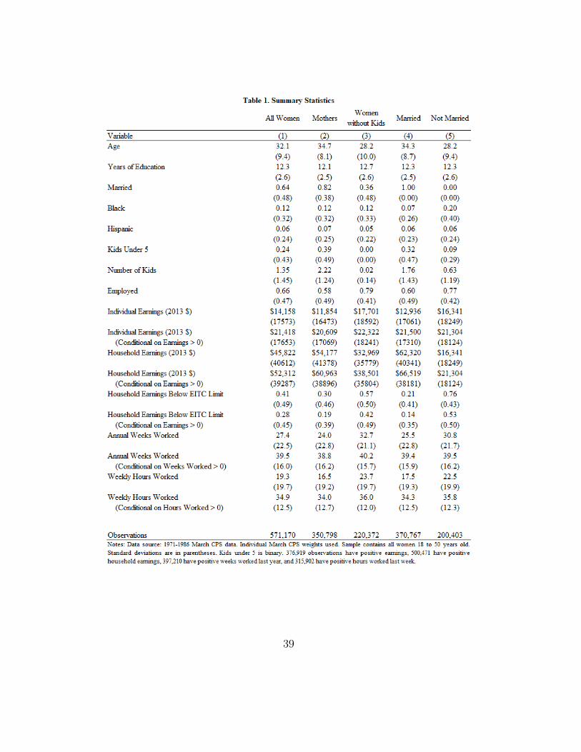
39

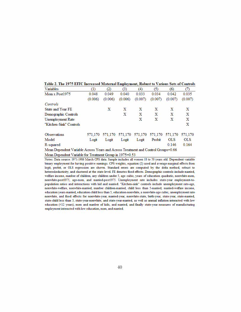
40

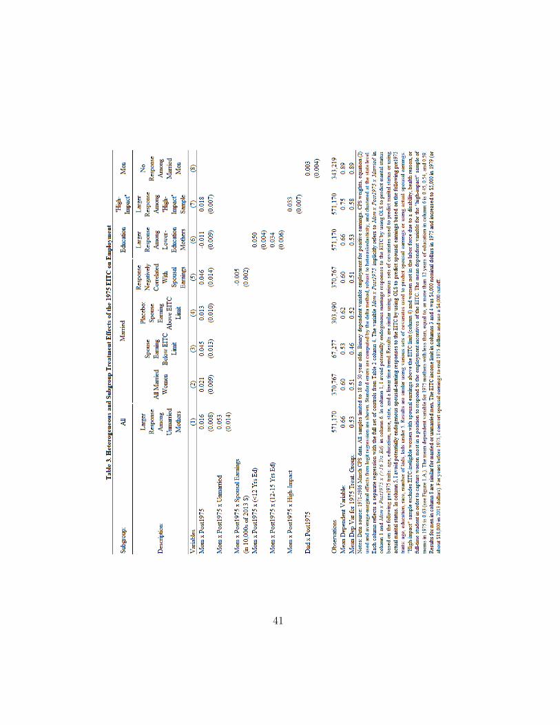
41

42

43

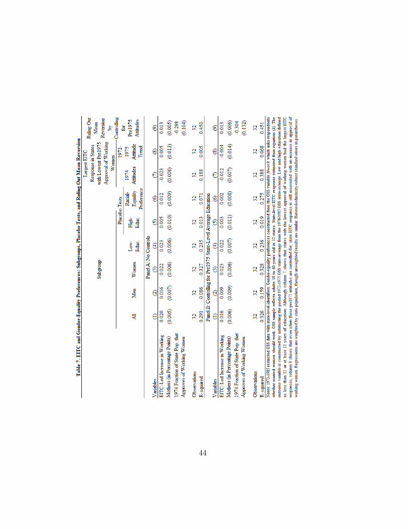
44

Figure 1.A. Unadjusted Employment Trends (High-Impact Sample)

Figure 1.B. Unadjusted and Regression-Adjusted Employment Gap

Notes: 1969-1986 March CPS data. Employment defined as positive income. Best-fit linesshown for 1969-75, 1975-79, 1979-85. Regression adjusted employment gap estimates froma probit and the full set of controls from Table 2 column 4. The estimates are jointlystatistically insignificant for all years before 1975 (p-value 0.42). “High-impact” sampleincludes all women 18-50 and excludes married women with spousal earning above $36,000in 2013 $ (corresponding to the 1975 EITC income limit), full-time students, disabled,and retired. Kids are 0-18 years old, or 19-23 if a student. Standard errors are computedby the delta method, robust to heteroskedasticity, and clustered at the state level.

45

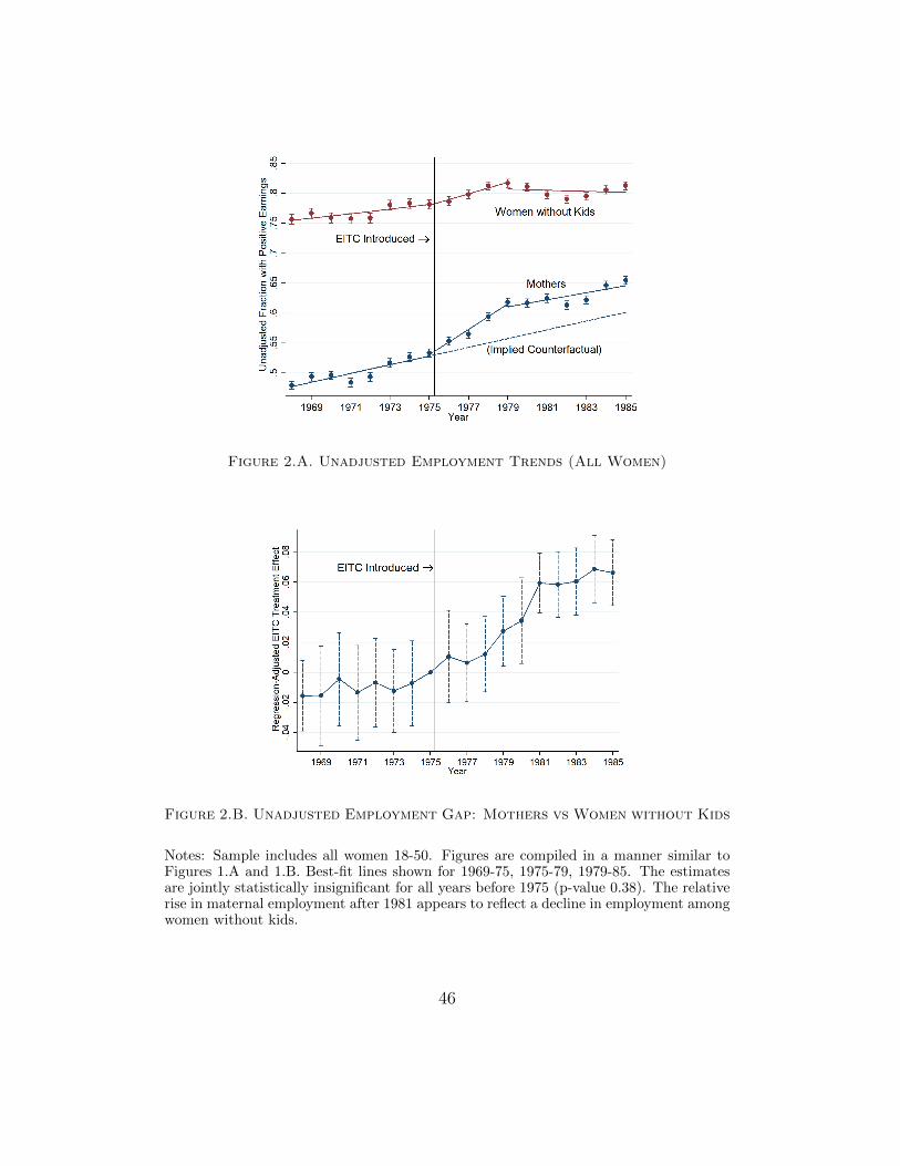
Figure 2.A. Unadjusted Employment Trends (All Women)

Figure 2.B. Unadjusted Employment Gap: Mothers vs Women without Kids

Notes: Sample includes all women 18-50. Figures are compiled in a manner similar toFigures 1.A and 1.B. Best-fit lines shown for 1969-75, 1975-79, 1979-85. The estimatesare jointly statistically insignificant for all years before 1975 (p-value 0.38). The relativerise in maternal employment after 1981 appears to reflect a decline in employment amongwomen without kids.

46

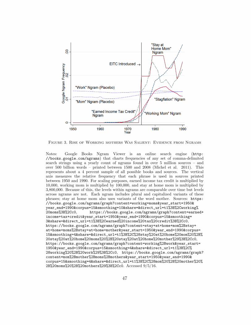
Figure 3. Rise of Working mothers Was Salient: Evidence from Ngrams

Notes: Google Books Ngram Viewer is an online search engine (http://books.google.com/ngrams) that charts frequencies of any set of comma-delimitedsearch strings using a yearly count of ngrams found in over 5 million sources – andover 500 billion words – printed between 1500 and 2008 (Michel et al. 2011). Thisrepresents about a 4 percent sample of all possible books and sources. The verticalaxis measures the relative frequency that each phrase is used in sources printedbetween 1950 and 1990. For scaling purposes, earned income tax credit is multiplied by10,000, working mom is multiplied by 100,000, and stay at home mom is multiplied by3,800,000. Because of this, the levels within ngrams are comparable over time but levelsacross ngrams are not. Each ngram includes plural and capitalized variants of thesephrases; stay at home mom also uses variants of the word mother. Sources: https://books.google.com/ngrams/graph?content=working+moms&year_start=1950&year_end=1990&corpus=15&smoothing=10&share=&direct_url=t1%3B%2Cworking%20moms%3B%2Cc0, https://books.google.com/ngrams/graph?content=earned+income+tax+credit&year_start=1950&year_end=1990&corpus=15&smoothing=3&share=&direct_url=t1%3B%2Cearned%20income%20tax%20credit%3B%2Cc0,https://books.google.com/ngrams/graph?content=stay+at+home+mom%2Bstay+at+home+moms%2Bstay+at+home+mother&year_start=1950&year_end=1990&corpus=15&smoothing=4&share=&direct_url=t1%3B%2C%28stay%20at%20home%20mom%20%2B%20stay%20at%20home%20moms%20%2B%20stay%20at%20home%20mother%29%3B%2Cc0,https://books.google.com/ngrams/graph?content=working%2Bwork&year_start=1950&year_end=1990&corpus=15&smoothing=4&share=&direct_url=t1%3B%2C%28working%20%2B%20work%29%3B%2Cc0, https://books.google.com/ngrams/graph?content=mom%2Bmother%2Bmoms%2Bmothers&year_start=1950&year_end=1990&corpus=15&smoothing=4&share=&direct_url=t1%3B%2C%28mom%20%2B%20mother%20%2B%20moms%20%2B%20mothers%29%3B%2Cc0. Accessed 9/5/16.

47

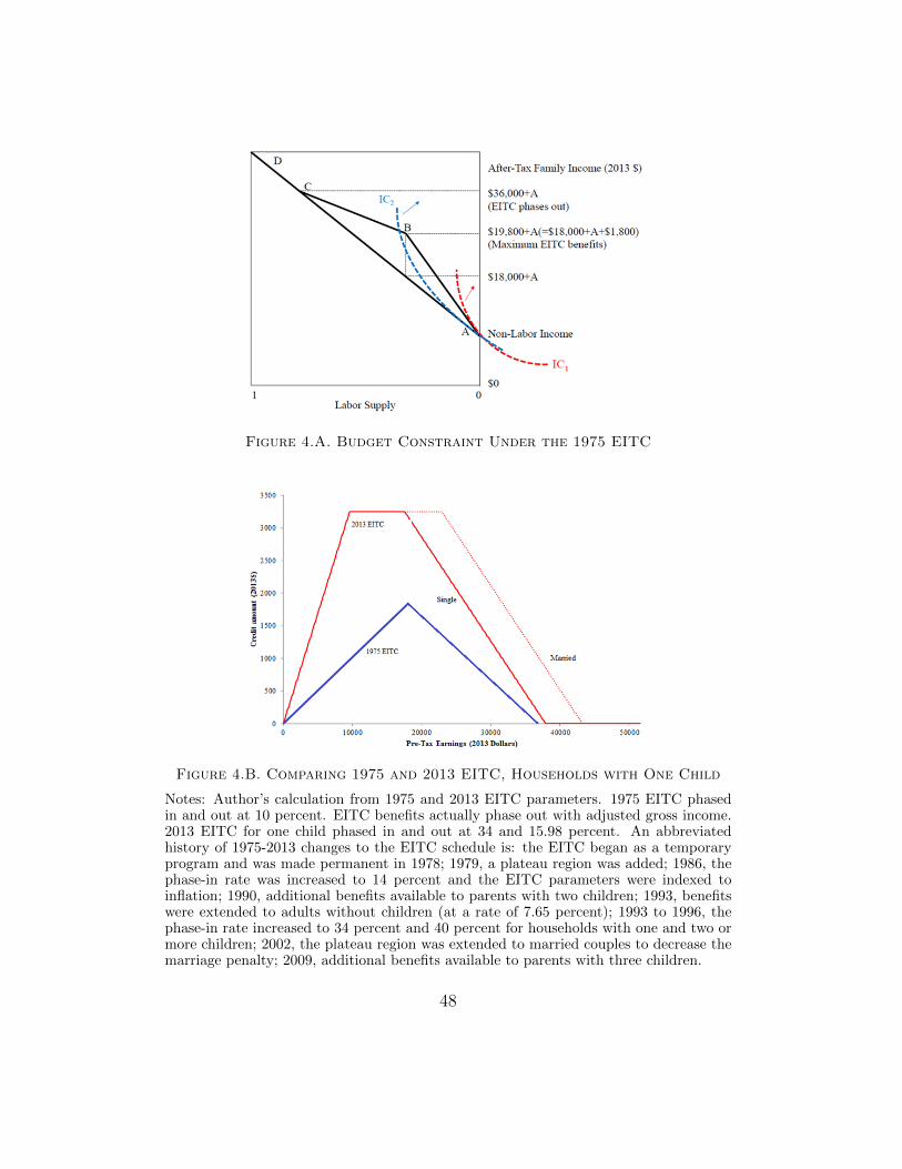
Figure 4.A. Budget Constraint Under the 1975 EITC

Figure 4.B. Comparing 1975 and 2013 EITC, Households with One Child

Notes: Author’s calculation from 1975 and 2013 EITC parameters. 1975 EITC phasedin and out at 10 percent. EITC benefits actually phase out with adjusted gross income.2013 EITC for one child phased in and out at 34 and 15.98 percent. An abbreviatedhistory of 1975-2013 changes to the EITC schedule is: the EITC began as a temporaryprogram and was made permanent in 1978; 1979, a plateau region was added; 1986, thephase-in rate was increased to 14 percent and the EITC parameters were indexed toinflation; 1990, additional benefits available to parents with two children; 1993, benefitswere extended to adults without children (at a rate of 7.65 percent); 1993 to 1996, thephase-in rate increased to 34 percent and 40 percent for households with one and two ormore children; 2002, the plateau region was extended to married couples to decrease themarriage penalty; 2009, additional benefits available to parents with three children.

48

Figure 5. Effect of the EITC on the Distribution of Annual Earnings

Notes: 1971-1986 March CPS data. Full set of controls from Table 2 column 4 and“high-impact” sample used. Each estimate is from a different logit regression of havingannual earnings in the specified range. Not conditional on working, the mean dependentvariables are 0.25, 0.22, 0.16, 0.16, 0.10, 0.06, 0.03, 0.02, 0.01; and conditional on workingare 0.0, 0.29, 0.21, 0.19, 0.14, 0.08, 0.04, 0.02, 0.02. Standard errors are computed by thedelta method, robust to heteroskedasticity, and clustered at the state level.

Figure 6. Effect of the EITC on Annual Earnings (Quantile Dif in Dif)

Notes: Same data, sample, controls, and standard errors as Figure 5. Mimics the re-gression behind Table 4 except instead of average effects, results shown are the effect ofMom× Post at each centile. The mean dependent variable at deciles 1 to 9 for mothersin 1975 are 0, 0, 0, 0, 2066, 8503, 17229, 25895, 36707.

49

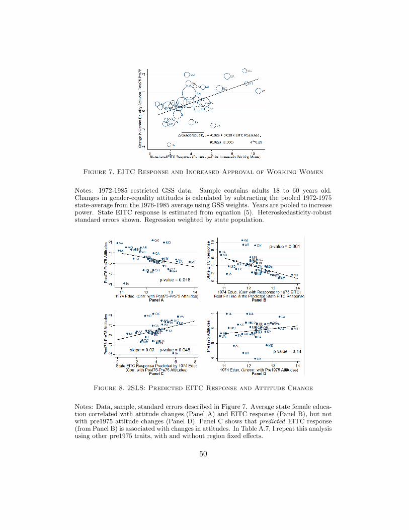
Figure 7. EITC Response and Increased Approval of Working Women

Notes: 1972-1985 restricted GSS data. Sample contains adults 18 to 60 years old.Changes in gender-equality attitudes is calculated by subtracting the pooled 1972-1975state-average from the 1976-1985 average using GSS weights. Years are pooled to increasepower. State EITC response is estimated from equation (5). Heteroskedasticity-robuststandard errors shown. Regression weighted by state population.

Figure 8. 2SLS: Predicted EITC Response and Attitude Change

Notes: Data, sample, standard errors described in Figure 7. Average state female educa-tion correlated with attitude changes (Panel A) and EITC response (Panel B), but notwith pre1975 attitude changes (Panel D). Panel C shows that predicted EITC response(from Panel B) is associated with changes in attitudes. In Table A.7, I repeat this analysisusing other pre1975 traits, with and without region fixed effects.

50

For Online Publication“The Rise of Working Mothers and the 1975 Earned Income Tax Credit”

Jacob Bastian

Appendix A: Additional Tables and Figures

1

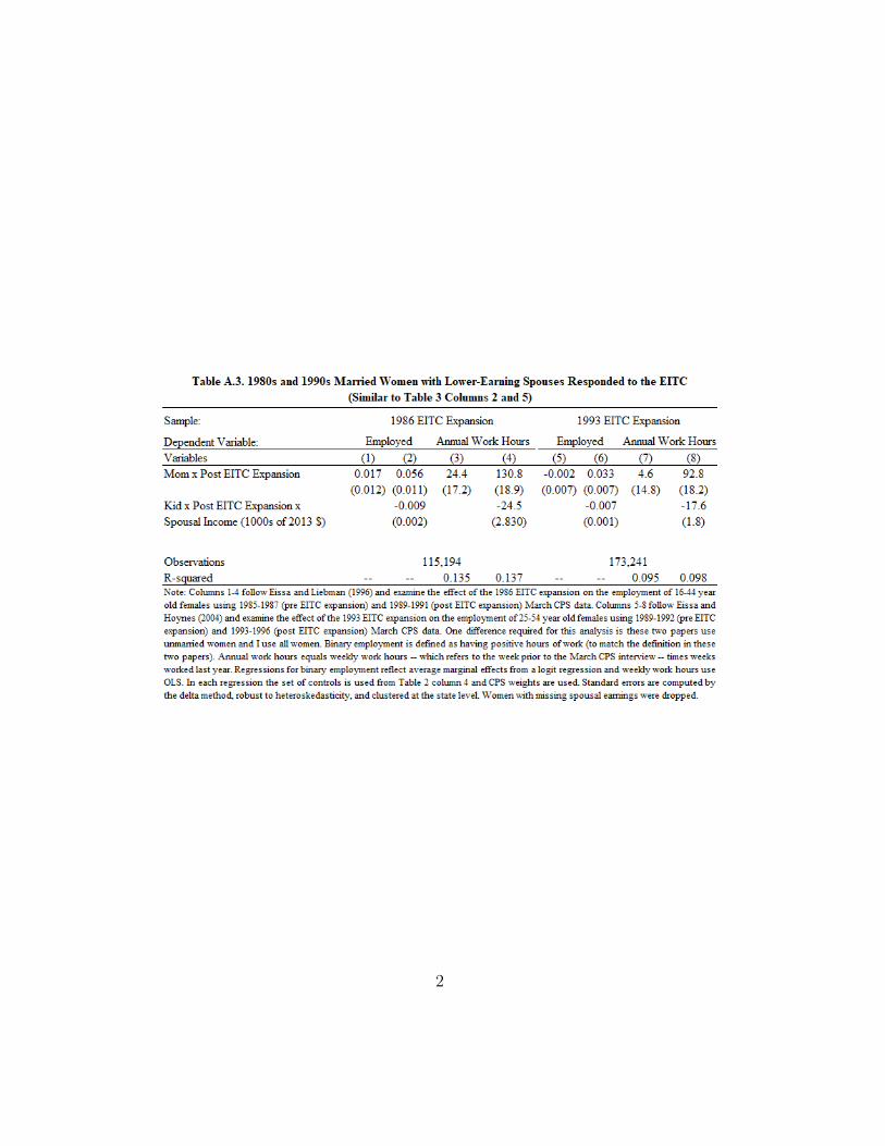
2

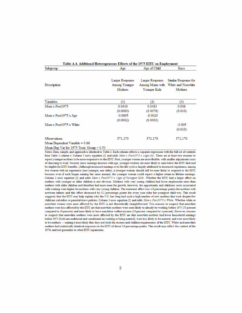
3

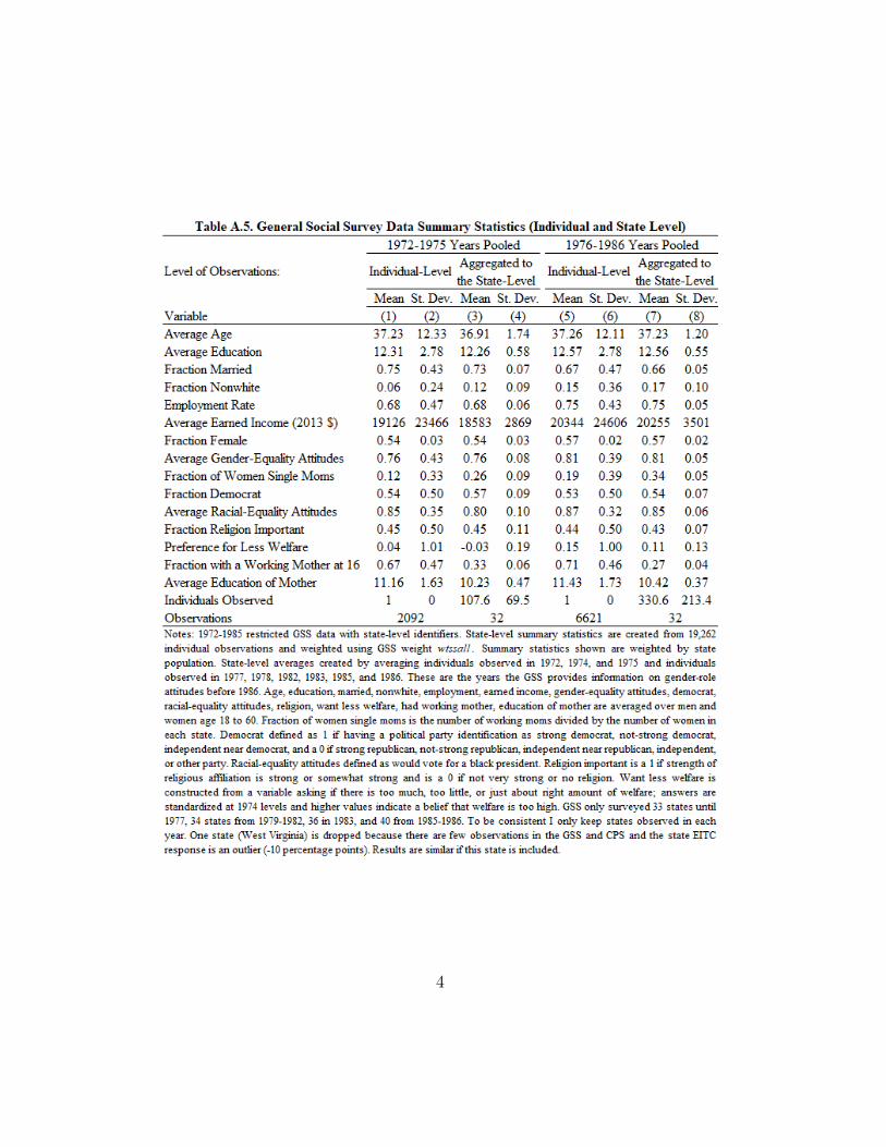
4

5

6

7

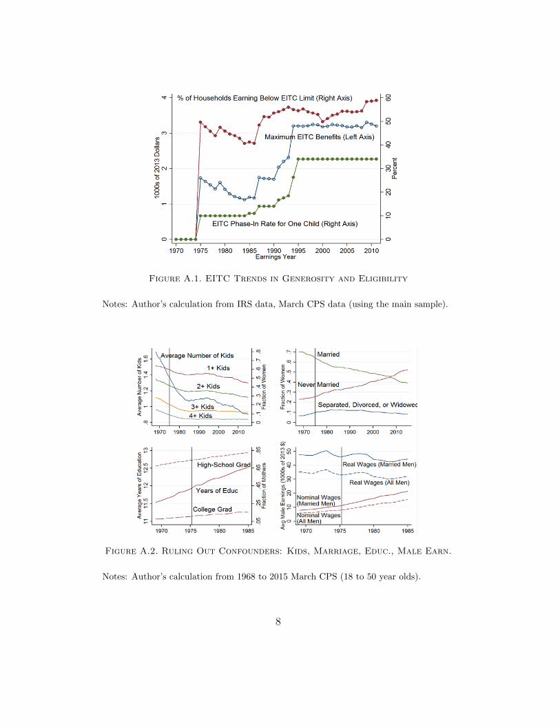
Figure A.1. EITC Trends in Generosity and Eligibility

Notes: Author’s calculation from IRS data, March CPS data (using the main sample).

Figure A.2. Ruling Out Confounders: Kids, Marriage, Educ., Male Earn.

Notes: Author’s calculation from 1968 to 2015 March CPS (18 to 50 year olds).

8

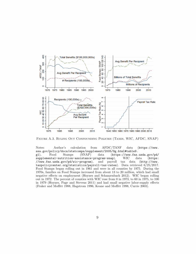
Figure A.3. Ruling Out Confounding Policies (Taxes, WIC, AFDC, SNAP)

Notes: Author’s calculation from AFDC/TANF data (https://www.ssa.gov/policy/docs/statcomps/supplement/2005/9g.html#table9.g1), Food Stamps (SNAP) data (https://www.fns.usda.gov/pd/supplemental-nutrition-assistance-program-snap), WIC data (https://www.fns.usda.gov/pd/wic-program), and payroll tax data (http://www.taxpolicycenter.org/statistics/payroll-tax-rates). Data retrieved 6/25/2017.Food Stamps began rolling out in 1961 and were in all counties by 1975. During the1970s, families on Food Stamps increased from about 13 to 20 million, which had smallnegative effects on employment (Hoynes and Schanzenbach 2012). WIC began rollingout in 1972. The percent of counties with WIC rose from 0 in 1973, to 60 in 1975, to 100in 1979 (Hoynes, Page and Stevens 2011) and had small negative labor-supply effects(Fraker and Moffitt 1988, Hagstrom 1996, Keane and Moffitt 1998, Currie 2003).

9

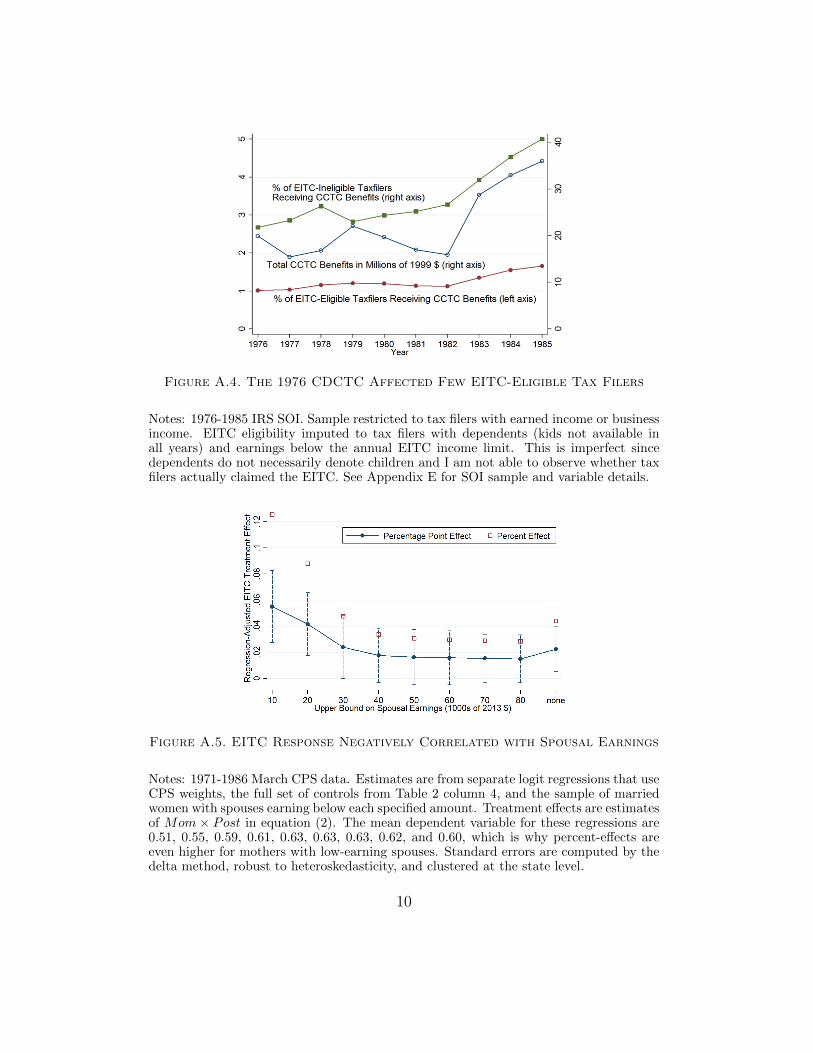
Figure A.4. The 1976 CDCTC Affected Few EITC-Eligible Tax Filers

Notes: 1976-1985 IRS SOI. Sample restricted to tax filers with earned income or businessincome. EITC eligibility imputed to tax filers with dependents (kids not available inall years) and earnings below the annual EITC income limit. This is imperfect sincedependents do not necessarily denote children and I am not able to observe whether taxfilers actually claimed the EITC. See Appendix E for SOI sample and variable details.

Figure A.5. EITC Response Negatively Correlated with Spousal Earnings

Notes: 1971-1986 March CPS data. Estimates are from separate logit regressions that useCPS weights, the full set of controls from Table 2 column 4, and the sample of marriedwomen with spouses earning below each specified amount. Treatment effects are estimatesof Mom × Post in equation (2). The mean dependent variable for these regressions are0.51, 0.55, 0.59, 0.61, 0.63, 0.63, 0.63, 0.62, and 0.60, which is why percent-effects areeven higher for mothers with low-earning spouses. Standard errors are computed by thedelta method, robust to heteroskedasticity, and clustered at the state level.

10

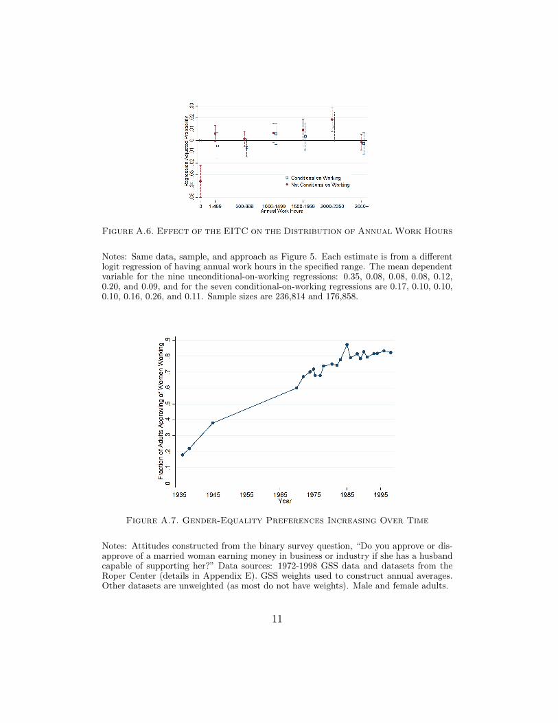
Figure A.6. Effect of the EITC on the Distribution of Annual Work Hours

Notes: Same data, sample, and approach as Figure 5. Each estimate is from a differentlogit regression of having annual work hours in the specified range. The mean dependentvariable for the nine unconditional-on-working regressions: 0.35, 0.08, 0.08, 0.08, 0.12,0.20, and 0.09, and for the seven conditional-on-working regressions are 0.17, 0.10, 0.10,0.10, 0.16, 0.26, and 0.11. Sample sizes are 236,814 and 176,858.

Figure A.7. Gender-Equality Preferences Increasing Over Time

Notes: Attitudes constructed from the binary survey question, “Do you approve or dis-approve of a married woman earning money in business or industry if she has a husbandcapable of supporting her?” Data sources: 1972-1998 GSS data and datasets from theRoper Center (details in Appendix E). GSS weights used to construct annual averages.Other datasets are unweighted (as most do not have weights). Male and female adults.

11

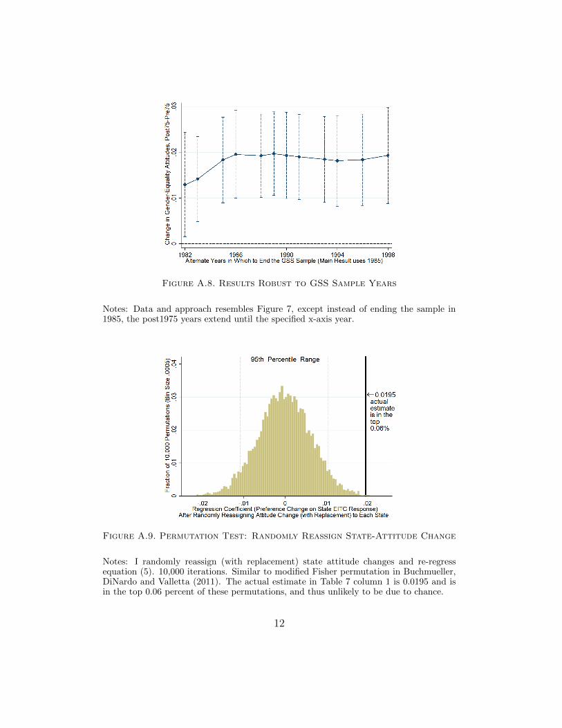
Figure A.8. Results Robust to GSS Sample Years

Notes: Data and approach resembles Figure 7, except instead of ending the sample in1985, the post1975 years extend until the specified x-axis year.

Figure A.9. Permutation Test: Randomly Reassign State-Attitude Change

Notes: I randomly reassign (with replacement) state attitude changes and re-regressequation (5). 10,000 iterations. Similar to modified Fisher permutation in Buchmueller,DiNardo and Valletta (2011). The actual estimate in Table 7 column 1 is 0.0195 and isin the top 0.06 percent of these permutations, and thus unlikely to be due to chance.

12

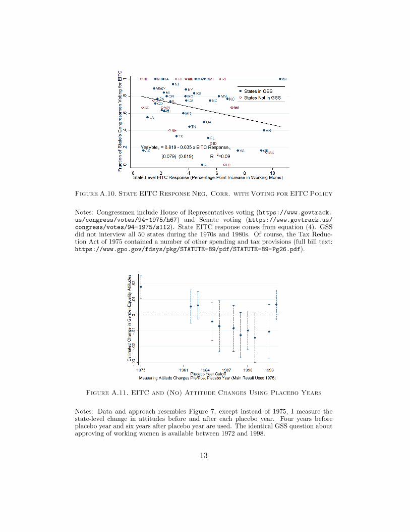
Figure A.10. State EITC Response Neg. Corr. with Voting for EITC Policy

Notes: Congressmen include House of Representatives voting (https://www.govtrack.us/congress/votes/94-1975/h67) and Senate voting (https://www.govtrack.us/congress/votes/94-1975/s112). State EITC response comes from equation (4). GSSdid not interview all 50 states during the 1970s and 1980s. Of course, the Tax Reduc-tion Act of 1975 contained a number of other spending and tax provisions (full bill text:https://www.gpo.gov/fdsys/pkg/STATUTE-89/pdf/STATUTE-89-Pg26.pdf).

Figure A.11. EITC and (No) Attitude Changes Using Placebo Years

Notes: Data and approach resembles Figure 7, except instead of 1975, I measure thestate-level change in attitudes before and after each placebo year. Four years beforeplacebo year and six years after placebo year are used. The identical GSS question aboutapproving of working women is available between 1972 and 1998.

13

Figure A.12. Which Occupations Did Newly Working Mothers Enter Into?

Notes: 1971-1986 March CPS data. Professions are defined by occ1950 codes: professional0-99, manager 200-290, clerical 300-390, sales 400-490, craftsmen 500-595, services 700-790; and occ1990 codes: teacher/librarian 155-165, construction/laborers 558-599, andnone 999. Full set of controls and “high-impact” sample used. Each estimate is from adifferent logit regression of having the specified occupation. Mean dependent variablesare 0.13, 0.05, 0.27, 0.04, 0.05, 0.01, 0.16, 0.01, 0.22. Standard errors are computed bythe delta method, robust to heteroskedasticity, and clustered at the state level.

14

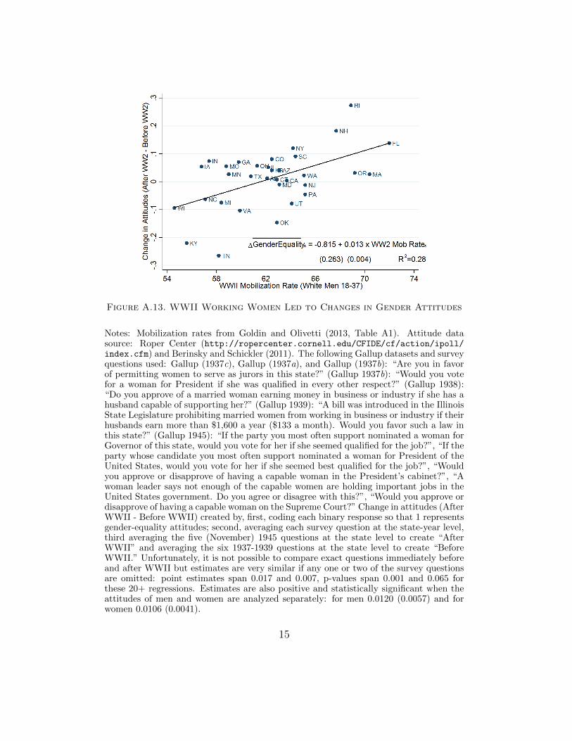
Figure A.13. WWII Working Women Led to Changes in Gender Attitudes

Notes: Mobilization rates from Goldin and Olivetti (2013, Table A1). Attitude datasource: Roper Center (http://ropercenter.cornell.edu/CFIDE/cf/action/ipoll/index.cfm) and Berinsky and Schickler (2011). The following Gallup datasets and surveyquestions used: Gallup (1937c), Gallup (1937a), and Gallup (1937b): “Are you in favorof permitting women to serve as jurors in this state?” (Gallup 1937b): “Would you votefor a woman for President if she was qualified in every other respect?” (Gallup 1938):“Do you approve of a married woman earning money in business or industry if she has ahusband capable of supporting her?” (Gallup 1939): “A bill was introduced in the IllinoisState Legislature prohibiting married women from working in business or industry if theirhusbands earn more than $1,600 a year ($133 a month). Would you favor such a law inthis state?” (Gallup 1945): “If the party you most often support nominated a woman forGovernor of this state, would you vote for her if she seemed qualified for the job?”, “If theparty whose candidate you most often support nominated a woman for President of theUnited States, would you vote for her if she seemed best qualified for the job?”, “Wouldyou approve or disapprove of having a capable woman in the President’s cabinet?”, “Awoman leader says not enough of the capable women are holding important jobs in theUnited States government. Do you agree or disagree with this?”, “Would you approve ordisapprove of having a capable woman on the Supreme Court?” Change in attitudes (AfterWWII - Before WWII) created by, first, coding each binary response so that 1 representsgender-equality attitudes; second, averaging each survey question at the state-year level,third averaging the five (November) 1945 questions at the state level to create “AfterWWII” and averaging the six 1937-1939 questions at the state level to create “BeforeWWII.” Unfortunately, it is not possible to compare exact questions immediately beforeand after WWII but estimates are very similar if any one or two of the survey questionsare omitted: point estimates span 0.017 and 0.007, p-values span 0.001 and 0.065 forthese 20+ regressions. Estimates are also positive and statistically significant when theattitudes of men and women are analyzed separately: for men 0.0120 (0.0057) and forwomen 0.0106 (0.0041).

15

Appendix B: Additional Robustness Checks

1. Model Choice and Sample Period

In Figure B.1, I show that the estimated DD treatment effect is robustto a probit, logit, or OLS model, and when to end the sample after 1975.As would be expected from Figure 1.B, the treatment effect is small if thesample ends soon after 1975, but grows and flattens out as more years after1975 are included. OLS results are consistently larger.

2. Larger Response from Mothers Eligible for More EITC Benefits

Conditional on year and spousal earnings (if any), I calculate maximumpotential EITC benefits in 2013 dollars (MaxEITC) and run a regres-sion identical to equation (2) except with the additional variable Mom ×Post1975×MaxEITC. For mothers with non-earning spouses and unmar-ried mothers, the value of MaxEITC varied by year and ranged between$1,100 and $1,700 since the EITC schedule was not pegged to inflationuntil 1986; for married mothers with a working spouse earning above theEITC kink point (placebo group from Table 3 column 4), MaxEITC waszero; for married women with a spouse earning below the EITC kink point,MaxEITC was equal to 10 percent of the difference between the EITC kinkpoint and her spouse’s earnings. For example, a mother with spousal earn-ings of $10,000 and an EITC kink point of $16,000 would have a MaxEITCvalue of $600. Table B.1 column 1 shows that a $1,000 (2013 dollars) in-crease in MaxEITC is associated with a 3.9-percentage-point increase inmaternal employment1 and carries out the placebo test from Table 3 col-umn 4 in a different way: the estimate of Mom × Post is now statisticallyinsignificant (that is, a mother after 1975 is no more likely to work thanbefore 1975 if she is eligible for zero EITC benefits) and the effect of theEITC is loaded onto Mom× Post×MaxEITC.

3. Potentially Endogenous Fertility and Group Composition

In addition to using controls, another way to account for endogenous fer-tility, marital status, and group composition is by reweighting mothers after1975 to look like mothers before 1975. Although regression controls should

1Similar to Hoynes, Miller and Simon (2015) that $1000 in EITC benefit increasedmaternal employment by 7.3 percentage points, and Milligan and Stabile (2007) that$1,000 increase in public benefits increased maternal employment by 4 percentage points.

16

largely account for the changing composition of mothers over time, reweight-ing acts as an additional robustness check (DiNardo 2002). I use two sets ofweights: one set is constructed from the approach in DiNardo, Fortin andLemieux (1996) (“DFL” weights) and the other set is inverse propensityweights (“IP” weights). To construct these weights, I first use a logit2 anda parsimonious set of traits – six age bins, three education bins, state, anddummies for married, nonwhite, and mother – to estimate the probabilitythan each observation in the sample is from a year before 1975.3

(B1) P (Pre75) = f(β1Age+β2Ed+β3St+β4Marr+β5Race+β6Mom+ε)

Each observation is assigned a probability p of being from a year before1975; I create DFL and IP weights by assigning each observation a weightof p/(1− p) and 1/p.4 Women are weighted less if their observed character-istics are less likely to be from a year before 1975 and weighed more if theircharacteristics are more likely to be from a year before 1975 (e.g. low educa-tion or high fertility). Figure B.2 verifies that the characteristics of womenbefore and after 1975 overlap sufficiently and have common support (Busso,DiNardo and McCrary 2014). Re-estimating equation (2) with these newweights yields estimates of 3.4 and 3.2 percentage points (Table B.1 columns2 and 3), similar to the baseline estimate of 3.3.

4. March CPS Imputations

In 1975 the Census changed its hot deck procedure5 for imputing missingearnings (Welch 1979, Bound and Freeman 1992)6 and could affect the re-

2The logit has the advantage over a probit in that the sum of predicted values equalsthe sum of the empirically observed ones (Butcher and DiNardo 2002). Probit and logitproduce very similar results.

3DiNardo, Fortin and Lemieux (1996) utilize a parsimonious set of controls that con-tains only 32 education-experience-gender cells. Butcher and DiNardo (2002) utilizeseveral covariates which yields many more cells. My choice results in 1512 cells, althoughresults do not change much with alternate decisions.

4Weights are multiplied with the CPS sample weights and normalized to add up to 1(DiNardo 2002).

5Where people with missing information are matched with similar people based on sex,race and ethnicity, household relationship, years of school completed, geographic area,age, disability status, presence of children, veteran status, work experience, occupation,class-of-worker status, earnings, and value of property or monthly rent. Source IPUMS:https://usa.ipums.org/usa/voliii/80editall.shtml#note1.

6Welch (1979): “The imputation procedure used in the first eight surveys differs fromthat of the ninth so that summary statistics for the 1976 survey (i.e., for 1975 earnings)are not comparable to other years” and “individual records for the first eight surveys

17

sults in Tables 2, 3, and B1 since I define employment as having positiveearnings (although Table A.1 shows similar estimates for other binary defi-nitions of working). The percentage of observations with imputed earningsin the sample is zero before 1975, but between 1975 and 1985 is 13.0, 11.1,12.7, 14.0, 12.6, 13.1, 10.1, 10.1, 10.5, 11.8, and 10.8. In Table B.2 Column1 shows the baseline DD estimate using the default CPS imputation andcolumn 2 simply drops all imputed observations. In columns 3 and 4 I useequation (B1) and a logit to predict the probability than an observation hasmissing earnings data (to account for data missing not at random), createDFL and IP weights (in the way described in the previous section), andre-estimate equation (2) with these weights. Columns 5 and 6 reflect esti-mates from a bounding exercise – similar to Manski bounds (Manski 1990)– where I assign all observations with missing earnings data to be workingor not working. Across each regression, the DD estimate is stable between3.2 and 3.9 percentage points, similar to the baseline estimate of 3.3.

5. Additional Response from Women with Multiple Children

Since the EITC did not provide additional benefits for having more thanone child until 1991, mothers with multiple children should not have re-sponded to the EITC more than women with only one child. I test this withthe following logit model that expands equation (2) and accounts for anydifferential impact on employment from having at least J kids.(B2)

P (E) = f(β1Post1975 +J∑k=1

[β2kMomk + β3kMomk ×Post1975] + β4X + ε)

Table B.3 columns 1 to 3 show results of this regression for J = 1, 2, 3.Column 1 replicates the baseline estimate where J = 1, but surprisingly, incolumns 2 and 3 where J = 2 and J = 3, results show that the estimateof β3,k=2 is positive and significant. This means that women with at leasttwo kids were more likely to respond to the EITC than women with exactlyone child. (Column 3 shows that mothers with at least three children do

contain no flag to identify cases when earnings are imputed. Family records do howeveridentify imputation of total family earnings, which presumably means that earnings forat least one family member are imputed. In contrast, the 1976 survey contains flags forindividual amputations but none for families.” This issue does not present a problemfor my analysis since I focus on the extensive margin, and since I show that results arerobust to other definitions of working based on earnings, weeks worked, or labor-forceparticipation (Table A.1).

18

respond less than women with exactly two children.) Interestingly, Eissaand Liebman (1996) also find an additional response from women with atleast two children. They suggest that this may be due to the concurrentincrease in the tax exemption for each dependent, which benefited familieswith multiple children more. During my sample period, the tax exemptionfor each child also increased from $750 to $1,000 in 1979. However, when Irestrict the sample to years before 1979, I still find a positive estimate onβ3,k=2 (Table B.3 column 4) and conclude that increased exemptions is notdriving my results.

Another potential explanation is that mothers with multiple children weremore likely to have completed their fertility. If mothers that had completedtheir fertility were more receptive to working – especially when their chil-dren reached school age – then with cross-sectional CPS data there couldbe a mechanical relationship between having multiple children and EITCresponse. I test this hypothesis in Table B.3 columns 5 to 9 by restrictingthe sample of mothers in the treatment group to those with a youngest childat least 2, 3, 4, 5, and 6 years old. As this youngest-child age restriction in-creases, the EITC response from mothers with at least two children (relativeto mothers with one child) converges to zero, while the estimated response

of mothers with exactly one child (β3,k=2) remains positive and grows from2.3 to 2.8 percentage points. Mothers with multiple children and a youngestchild at least 5 years old are statistically no more likely to respond to theEITC than women with just one child. I find the same pattern for the 1986and 1993 EITC expansion as well (results omitted) and conclude that theadditional employment increase for women with at least two children maybe explained by mothers that had completed their fertility. (This may alsoexplain why Eissa and Liebman (1996) find the same pattern.)

6. Using IRS Tax Data

Since the CPS shows that the 1975 EITC had a large effect on the employ-ment of mothers, this should be evident in the IRS Statistics of Income (SOI)data as well, however, a few features of the IRS SOI data make it unattrac-tive for detecting the effects of the 1975 EITC. First, many non-workingindividuals do not file taxes, so detecting an extensive margin response isnot easy. Second, household income is reported, so it is not possible to de-termine whether one or two spouses worked. Third, IRS SOI data includefew demographic variables so it is not possible to determine the gender, age,race, or education of the tax filer, whether they have children – dependents

19

are not necessarily children – or child’s age.7

Constrained by the IRS SOI data, I find evidence that the EITC affectedthe composition of tax filers. Using 1968 to 1985 IRS SOI data, I showthat the fraction of unmarried EITC-eligible tax filers (Table 3 shows thatsingle mothers were relatively more affected by the EITC) increased in theyears after 1975 (Figure B.3). The pattern closely resembles Figure 1.B:flat before 1975, a quick rise between 1975 and 1980, and relatively flatagain after 1980. Without knowing tax filer gender or whether dependentsdenote children, this is only suggestive evidence that the EITC affected theemployment of single mothers.8

To corroborate the effect of the EITC with administrative tax records,I first compare the annual number of EITC-eligible households and theamount of EITC benefits implied by CPS data with aggregate IRS EITCstatistics. Figure B.4 shows that the number of EITC-eligible householdsand aggregate EITC benefits – that I calculate from reported household chil-dren and earnings – is nearly identical to the published EITC statistics in1975. However, in the years after 1975, the CPS undercounts EITC recipi-ents and benefits. The ratio of the CPS numbers to the official IRS numbersdrops to about 90 percent by 1978, and continues to fall to 70 percent by themid-1980s. One reason to expect EITC benefits calculated from the CPSto be lower than the actual benefits is that 20 to 25 percent of EITC claimsare paid in error9 due to unintentional tax filer error, divorced parents eachclaiming the same child, married couples splitting their qualifying childrenand filing separately as household heads, or lying about having children.Liebman (2000) finds that 11 to 13 percent of EITC recipients had no chil-dren.10 The growing gap between CPS and IRS data in Figure B.4 suggeststhat tax filer error may have increased between 1975 and 1985.

7Marital status is available. Number of children available after 1977, otherwise onlyin 1970 and 1975. See http://users.nber.org/~taxsim/taxsim-ndx.txt for annualavailable IRS SOI variables.

8It is difficult to determine whether the number of tax filers increased, since onemillion working mothers over a four year period (Figures 1.A and 1.B) corresponds toabout 250,000 mothers per year, small in comparison to the 80 million households, 100million adults in the labor force, and 95 million tax filers in the U.S. by 1980 (source:CPS, BLS, IRS SOI). As a result, I am not able to detect an aggregate rise in tax filers orin the number of working households using IRS SOI or CPS data. Time-series analysisof these data would not detect a newly-working mother that was already a part of atax-filing household.

9See https://www.eitc.irs.gov/Tax-Preparer-Toolkit/faqs/fraud.10This is related to the infamous event where millions of children disappeared when

taxpayers had to begin reporting the Social Security number of all dependents in 1987(LaLumia and Sallee 2013).

20

Observing less (imputed) EITC benefits in the CPS than the aggregateIRS numbers suggest that my employment estimates from the CPS are notoverestimates of the actual working response to the EITC. Although FigureC.1 shows evidence of misreporting self-employed income to take advantageof EITC benefits, this represents a relatively small number of the millionmothers that begin working in response to the EITC.

Aggregate IRS data also reveal a puzzle in light of estimates in Table 2:the number of EITC recipients and the aggregate EITC benefits remainedroughly constant between 1975 and 1985 (Figure B.5). One way to reconcilethe positive maternal employment response to the EITC and flat EITCbenefits is by considering that the EITC schedule was not pegged to inflationuntil 1986 and inflation was high in the years after 1975. About 6.3 millionhouseholds received EITC benefits in 1975, but most recipients seem to havealready been working since Figures 1.A and 1.B suggest that the employmentwas not affected until 1976. Due to rising prices and nominal wages, withina few years some of these households would earn above the nominal EITCearnings limit and no longer receive EITC benefits, akin to “bracket creep”(Saez 2003).11 The increase in EITC-eligible working mothers (Table 2) andno-longer-EITC-eligible households may have cancelled out and resulted ina roughly constant number of EITC recipients. The following back of theenvelope calculation examines whether this is plausible. Using the 1974 SOIearnings distribution (before any labor supply response to the EITC), I usethe CPI to inflate the 1974 earnings distribution into 1975, 1976, 1977, and1978 dollars, and calculate the number of tax filers that were EITC-eligiblein 1975 but EITC-ineligible in 1976, 1977, or 1978 due to rising nominalincome.12 Figure B.6 illustrates that by 1976, 1977, and 1978, 0.6, 1.0, and1.6 percent of tax filers eligible for the EITC in 1975 would bracket-creepout of EITC eligibility, corresponding to 700,000, 1,200,000, and 1,800,000tax filers.13 Even though the stock of EITC recipients remained roughlyconstant in the decade after 1975, there was substantial flow in and out ofEITC eligibility. This may explain why the number of EITC recipients wasflat even as a million mothers entered into employment due to the EITC.

11This nominal limit was $8,000 through 1978 and $10,000 through 1984.12Assuming constant real earnings. Rising real wages yields even more bracket creep.13Population growth accounts for at most about half a million of these 1.8 million

additional EITC recipients: IRS SOI data shows that about a quarter of tax filers withdependents had positive earnings below the EITC limit and CPS data shows that thenumber of households with children steadily grew from 34.5 million in 1975 to 35.1 mil-lion in 1978. Depending on where in the income distribution these new households fell,population growth led to between 200,000 and 600,000 additional EITC recipients.

21

Tables and Figures for Appendix B

22

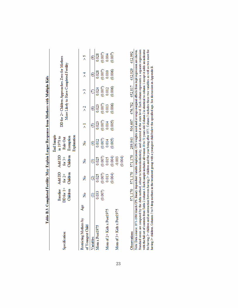
23

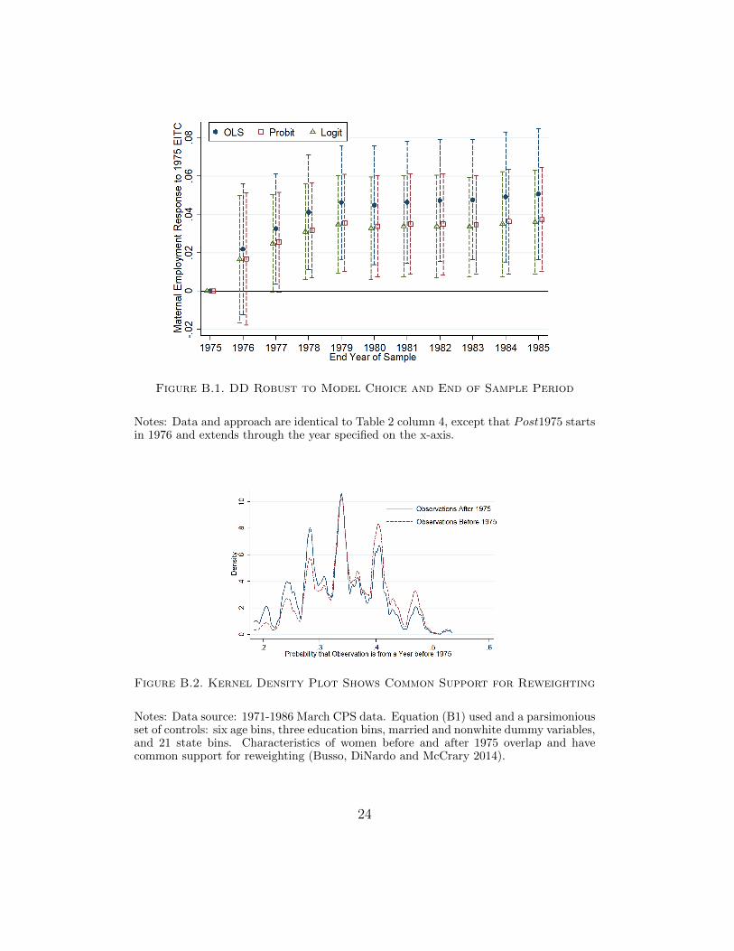
Figure B.1. DD Robust to Model Choice and End of Sample Period

Notes: Data and approach are identical to Table 2 column 4, except that Post1975 startsin 1976 and extends through the year specified on the x-axis.

Figure B.2. Kernel Density Plot Shows Common Support for Reweighting

Notes: Data source: 1971-1986 March CPS data. Equation (B1) used and a parsimoniousset of controls: six age bins, three education bins, married and nonwhite dummy variables,and 21 state bins. Characteristics of women before and after 1975 overlap and havecommon support for reweighting (Busso, DiNardo and McCrary 2014).

24

Figure B.3. The 1975 EITC Affected the Composition of Tax Filers

Notes: Author’s calculations from 1968-1985 IRS Statistics of Income Public Use datafiles. Sample restricted to tax filers with earned income or business income; this elimi-nates tax filers with only dividend, interest, capital gains, pensions, farm, and alimonyincome. Refundable portion of the EITC is also provided in the data, but this does notinclude households who benefit from the EITC through decreased tax liabilities and thusundercounts EITC recipients. Years are grouped into three-year bins to reduce noise.

Figure B.4. Comparing EITC Recipients and Benefits: CPS vs. IRS Data

Notes: Author’s calculation from 1976-1986 March CPS data and published aggre-gate EITC recipients and benefits (http://www.taxpolicycenter.org/statistics/eitc-recipients). EITC recipients and benefits based on household earnings, the an-nual EITC schedule, and whether the household had any children. The growing gapsuggests that tax-filer error may have increased between 1975 and 1985.

25

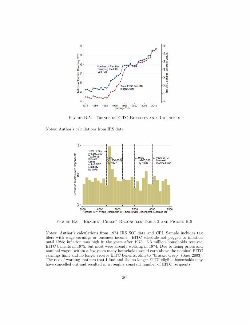
Figure B.5. Trends in EITC Benefits and Recipients

Notes: Author’s calculations from IRS data.

Figure B.6. “Bracket Creep” Reconciles Table 2 and Figure B.5

Notes: Author’s calculations from 1974 IRS SOI data and CPI. Sample includes taxfilers with wage earnings or business income. EITC schedule not pegged to inflationuntil 1986; inflation was high in the years after 1975. 6.3 million households receivedEITC benefits in 1975, but most were already working in 1974. Due to rising prices andnominal wages, within a few years many households would earn above the nominal EITCearnings limit and no longer receive EITC benefits, akin to “bracket creep” (Saez 2003).The rise of working mothers that I find and the no-longer-EITC-eligible households mayhave cancelled out and resulted in a roughly constant number of EITC recipients.

26

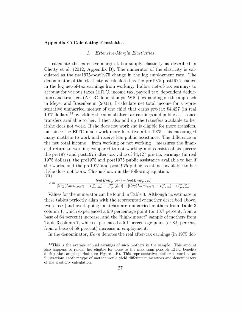
Appendix C: Calculating Elasticities

1. Extensive-Margin Elasticities

I calculate the extensive-margin labor-supply elasticity as described inChetty et al. (2012, Appendix B). The numerator of the elasticity is cal-culated as the pre1975-post1975 change in the log employment rate. Thedenominator of the elasticity is calculated as the pre1975-post1975 changein the log net-of-tax earnings from working. I allow net-of-tax earnings toaccount for various taxes (EITC, income tax, payroll tax, dependent deduc-tion) and transfers (AFDC, food stamps, WIC), expanding on the approachin Meyer and Rosenbaum (2001). I calculate net total income for a repre-sentative unmarried mother of one child that earns pre-tax $4,427 (in real1975 dollars)14 by adding the annual after-tax earnings and public-assistancetransfers available to her. I then also add up the transfers available to herif she does not work. If she does not work she is eligible for more transfers,but since the EITC made work more lucrative after 1975, this encouragedmany mothers to work and receive less public assistance. The difference inthe net total income – from working or not working – measures the finan-cial return to working compared to not working and consists of six pieces:the pre1975 and post1975 after-tax value of $4,427 pre-tax earnings (in real1975 dollars), the pre1975 and post1975 public assistance available to her ifshe works, and the pre1975 and post1975 public assistance available to herif she does not work. This is shown in the following equation.(C1)

ε =log(Emppost75)− log(Emppre75)

[(log(Earnpost75 + Twpost75)− (T∼ w

post75)]− [(log(Earnpre75 + Twpre75)− (T∼ w

pre75)]

Values for the numerator can be found in Table 3. Although no estimate inthese tables perfectly align with the representative mother described above,two close (and overlapping) matches are unmarried mothers from Table 3column 1, which experienced a 6.9 percentage point (or 10.7 percent, from abase of 64 percent) increase, and the “high-impact” sample of mothers fromTable 3 column 7, which experienced a 5.1-percentage-point (or 8.9-percent,from a base of 58 percent) increase in employment.

In the denominator, Earn denotes the real after-tax earnings (in 1975 dol-

14This is the average annual earnings of such mothers in the sample. This amountalso happens to render her eligible for close to the maximum possible EITC benefitsduring the sample period (see Figure 4.B). This representative mother is used as anillustration; another type of mother would yield different numerators and denominatorsof the elasticity calculation.

27

lars) for the representative mother earning $4,437 (in constant 1975 dollars)and accounts for the income tax, payroll tax, and dependent deduction. Tw

and T∼ w denote the public assistance available to her if she works or doesnot work.

I transparently show my elasticity calculation in Table C.1 Panel A, whichshows the 1970-1985 annual values of the EITC, income tax, payroll tax,dependent exemption, as well as AFDC, Food Stamps, and WIC benefitsavailable if she works and if she does not work. However, calculating pub-lic assistance is not straightforward: benefit levels varied by state and didnot phase out linearly with earnings. To overcome this, I first calculateAFDC benefits available to this mother if she does not work, using two dif-ferent sources: one source is the Department of Health and Human Services(DHHS), showing the average benefits for a recipient family; a second sourceis Fraker, Moffitt and Wolf (1985), which also calculates average family ben-efits. These two data sources align quite well, and I assign the average ofthese two values for the case where the mother does not work (Table C.1Panel A column 17). Second, to calculate the AFDC benefits available toher if she does work, I use the average annual effective tax rates estimatedby Fraker, Moffitt and Wolf (1985). This tax rate varies by year, but on av-erage, every dollar of earnings leads to a 25-cent decline in AFDC benefits.15

Annual AFDC benefits available to this working mother is shown in TableC.1 Panel A column 14. Table C.2 shows details on the DHHS and Fraker,Moffitt and Wolf (1985) data, effective tax rates, and my calculations usedto generate the data in Table C.1 Panel A columns 14 and 17.

In Table C.3 I show my calculations for Food Stamps and WIC. It turnsout that this representative mother is not eligible for Food Stamps if sheworks because her earnings are too high. Although the effective tax rate onthese benefits are also approximately 25 percent (see Table C.3 notes), FoodStamp benefits are much lower than AFDC benefits. It also turns out thatshe is eligible for the same amount of WIC whether she works or not, sinceWIC does not phase out with income and is available for mothers earningbelow 185 percent of the poverty line (the 1975 poverty line was $6771, innominal dollars, for a mother with one child). Table C.3 shows completedetails on the Food Stamps and WIC benefits, which are then inputted intoTable C.1 Panel A columns 12, 13, 15, and 16.

In Table C.1 Panel B, I aggregate the annual after-tax earnings and trans-fers (available if she works or not) from Table C.1 Panel A, average themfor 1970-1974 and 1975-1985, and plug them into equation (C1) to calcu-

15EITC benefits do not count against AFDC eligibility limits (Moffitt 2003).

28

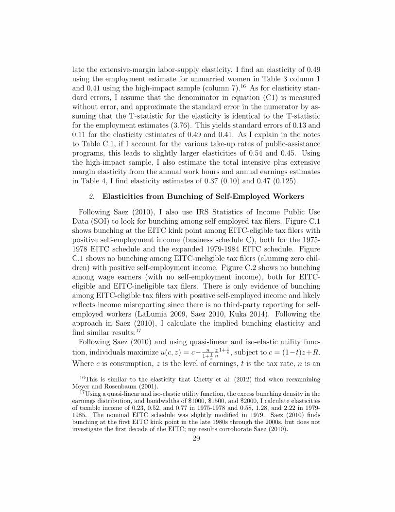
late the extensive-margin labor-supply elasticity. I find an elasticity of 0.49using the employment estimate for unmarried women in Table 3 column 1and 0.41 using the high-impact sample (column 7).16 As for elasticity stan-dard errors, I assume that the denominator in equation (C1) is measuredwithout error, and approximate the standard error in the numerator by as-suming that the T-statistic for the elasticity is identical to the T-statisticfor the employment estimates (3.76). This yields standard errors of 0.13 and0.11 for the elasticity estimates of 0.49 and 0.41. As I explain in the notesto Table C.1, if I account for the various take-up rates of public-assistanceprograms, this leads to slightly larger elasticities of 0.54 and 0.45. Usingthe high-impact sample, I also estimate the total intensive plus extensivemargin elasticity from the annual work hours and annual earnings estimatesin Table 4, I find elasticity estimates of 0.37 (0.10) and 0.47 (0.125).

2. Elasticities from Bunching of Self-Employed Workers

Following Saez (2010), I also use IRS Statistics of Income Public UseData (SOI) to look for bunching among self-employed tax filers. Figure C.1shows bunching at the EITC kink point among EITC-eligible tax filers withpositive self-employment income (business schedule C), both for the 1975-1978 EITC schedule and the expanded 1979-1984 EITC schedule. FigureC.1 shows no bunching among EITC-ineligible tax filers (claiming zero chil-dren) with positive self-employment income. Figure C.2 shows no bunchingamong wage earners (with no self-employment income), both for EITC-eligible and EITC-ineligible tax filers. There is only evidence of bunchingamong EITC-eligible tax filers with positive self-employed income and likelyreflects income misreporting since there is no third-party reporting for self-employed workers (LaLumia 2009, Saez 2010, Kuka 2014). Following theapproach in Saez (2010), I calculate the implied bunching elasticity andfind similar results.17

Following Saez (2010) and using quasi-linear and iso-elastic utility func-

tion, individuals maximize u(c, z) = c− n1+ 1

e

zn

1+ 1e , subject to c = (1−t)z+R.

Where c is consumption, z is the level of earnings, t is the tax rate, n is an

16This is similar to the elasticity that Chetty et al. (2012) find when reexaminingMeyer and Rosenbaum (2001).

17Using a quasi-linear and iso-elastic utility function, the excess bunching density in theearnings distribution, and bandwidths of $1000, $1500, and $2000, I calculate elasticitiesof taxable income of 0.23, 0.52, and 0.77 in 1975-1978 and 0.58, 1.28, and 2.22 in 1979-1985. The nominal EITC schedule was slightly modified in 1979. Saez (2010) findsbunching at the first EITC kink point in the late 1980s through the 2000s, but does notinvestigate the first decade of the EITC; my results corroborate Saez (2010).

29

ability parameter distributed with density f(n), e is the compensated elas-ticity, and R is non-labor income. The first order condition is z = n(1− t)eand the bunching elasticity can be estimated by solving the following for e:

(C2) B =z∗

2

[(1− t01− t1

)e

− 1

][h(z∗)− +

h(z∗)+(1−t01−t1

)e

]

Where z∗ is the kink threshold,

(1−t01−t1

)is the net of tax ratio at the kink,

h(z∗)− and h(z∗)+ is the density of the distribution just below and abovethe kink, and B is the amount of bunching at z∗. For a given empiricaldistribution h(z) and a choice of bandwidth δ, B is equal to the density of taxfilers with income is the range (z∗−δ, z∗+δ)−(z∗−2δ, z∗−δ)−(z∗+δ, z∗+2δ).See Saez (2010) Figure 3 for more details and intuition.

I use this formula, the empirical earnings distribution in the SOI tax filesfor 1975-1978 and 1979-1984 (see Figure C.1 for nominal EITC schedules),and bandwidths of $1000, $1500, and $2000 to calculate the implied bunch-ing elasticity.

For 1975-1978 and δ=$1000: z∗=$4000, 1−t01−t1 = 1.2, B = .0114, h(z∗)− =

0.0000582, and h(z∗)+ = 0.0000788. Yielding e=0.23.

For 1975-1978 and δ=$1500: z∗=$4000, 1−t01−t1 = 1.2, B = .0173, h(z∗)− =

0.0000388, and h(z∗)+ = 0.0000525. Yielding e=0.52.

For 1975-1978 and δ=$2000: z∗=$4000, 1−t01−t1 = 1.2, B = .0191, h(z∗)− =

0.0000291, and h(z∗)+ = 0.0000394. Yielding e=0.77.

For 1979-1984 and δ=$1000: z∗=$5000, 1−t01−t1 = 1.1, B = .0204, h(z∗)− =

0.0000642, and h(z∗)+ = 0.0000838. Yielding e=0.58.

For 1979-1984 and δ=$1500: z∗=$5000, 1−t01−t1 = 1.1, B = .0299, h(z∗)− =

0.0000428, and h(z∗)+ = 0.0000559. Yielding e=1.28.

For 1979-1984 and δ=$2000: z∗=$5000, 1−t01−t1 = 1.1, B = .0388, h(z∗)− =

0.0000321, and h(z∗)+ = 0.0000419. Yielding e=2.22.

Saez (2010) finds elasticities among self-employed workers in the range of0.7 to 1.6, depending on bandwidth choice.

Tables and Figures for Appendix C

30

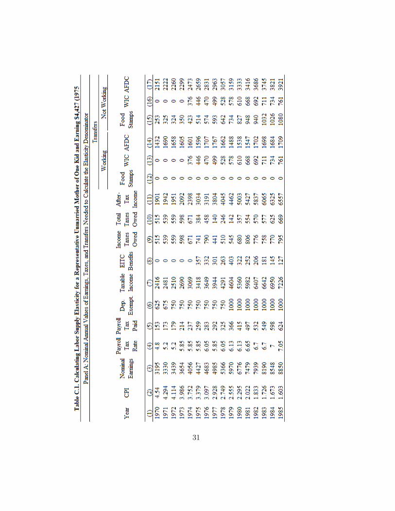
31

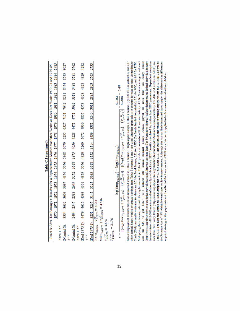
32

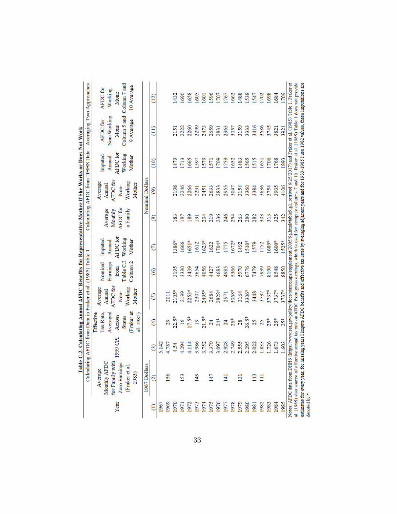
33

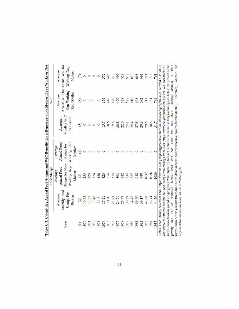
34

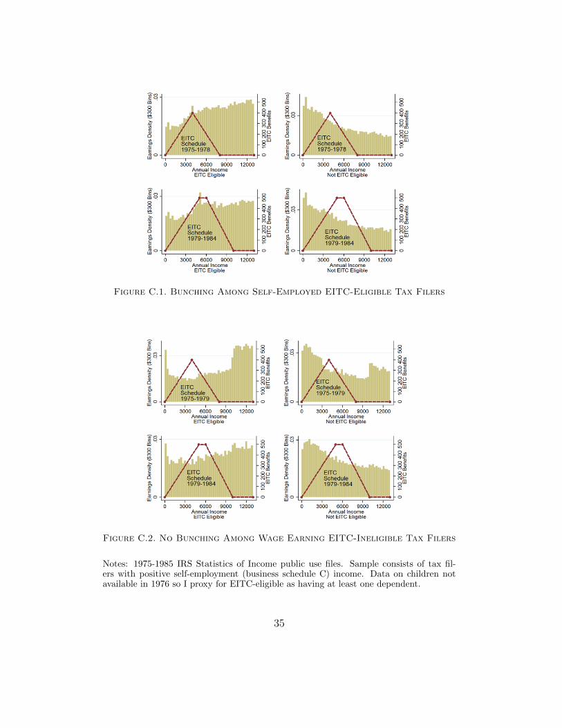
Figure C.1. Bunching Among Self-Employed EITC-Eligible Tax Filers

Figure C.2. No Bunching Among Wage Earning EITC-Ineligible Tax Filers

Notes: 1975-1985 IRS Statistics of Income public use files. Sample consists of tax fil-ers with positive self-employment (business schedule C) income. Data on children notavailable in 1976 so I proxy for EITC-eligible as having at least one dependent.

35

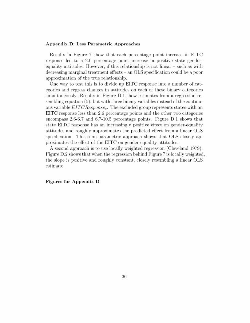
Appendix D: Less Parametric Approaches

Results in Figure 7 show that each percentage point increase in EITCresponse led to a 2.0 percentage point increase in positive state gender-equality attitudes. However, if this relationship is not linear – such as withdecreasing marginal treatment effects – an OLS specification could be a poorapproximation of the true relationship.

One way to test this is to divide up EITC response into a number of cat-egories and regress changes in attitudes on each of these binary categoriessimultaneously. Results in Figure D.1 show estimates from a regression re-sembling equation (5), but with three binary variables instead of the continu-ous variable EITCResponses. The excluded group represents states with anEITC response less than 2.6 percentage points and the other two categoriesencompass 2.6-6.7 and 6.7-10.5 percentage points. Figure D.1 shows thatstate EITC response has an increasingly positive effect on gender-equalityattitudes and roughly approximates the predicted effect from a linear OLSspecification. This semi-parametric approach shows that OLS closely ap-proximates the effect of the EITC on gender-equality attitudes.

A second approach is to use locally weighted regression (Cleveland 1979).Figure D.2 shows that when the regression behind Figure 7 is locally weighted,the slope is positive and roughly constant, closely resembling a linear OLSestimate.

Figures for Appendix D

36

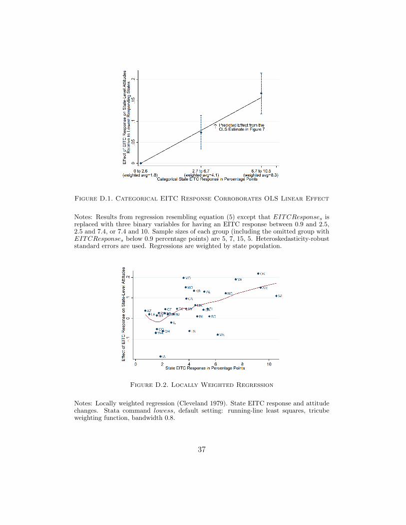
Figure D.1. Categorical EITC Response Corroborates OLS Linear Effect

Notes: Results from regression resembling equation (5) except that EITCResponses isreplaced with three binary variables for having an EITC response between 0.9 and 2.5,2.5 and 7.4, or 7.4 and 10. Sample sizes of each group (including the omitted group withEITCResponses below 0.9 percentage points) are 5, 7, 15, 5. Heteroskedasticity-robuststandard errors are used. Regressions are weighted by state population.

Figure D.2. Locally Weighted Regression

Notes: Locally weighted regression (Cleveland 1979). State EITC response and attitudechanges. Stata command lowess, default setting: running-line least squares, tricubeweighting function, bandwidth 0.8.

37

Appendix E: Data Appendix

The following information is intended to be detailed enough to replicatemy sample.

1. March Current Population Survey Data

I use 1971 to 1986 March CPS (Ruggles et al. 2015) downloaded in De-cember 2014 (2,461,704 observations). I replace year with year-1 to matchthe survey year with the work year. I define EITC-eligible households ashaving at least one child 18 or under, or an adult child between 19 and 23and in school full time. Households are defined as unique combinations ofvariables year and serial. I then drop individuals under 18, observationswith a CPS weight (wtsupp) of 0, missing education, leaving 1,699,783 ob-servations. Husbands defined as married males. 432,054 individuals live ina household with 0 married males, 1,251,017 individuals live with 1 marriedmale, 16,320 live with two, 384 live with three, and 8 live with four. Eachsub-family within a household is assumed to be a separate tax-filing familyunit. Dropping women with missing spousal earnings or state, males, andwomen over 50, yields the 571,170 women used in the main analysis.

The following is a discussion of variables used in employment analy-sis. Missing incwage values of 99999 assigned to be 0 for 574 observa-tions. Weeks worked assigned as the midpoint of the categorical variablewkswork. Post1975 begins in 1976. Welfare comes from incwelfr, mar-ried defined as marstat equals 1 or 2, and nonwhite created from raceand hispan. Age is rounded to bins of two so that birth year, year, andage can all be controlled for; age squared and cubed are based on actualage. Spousal earnings created from incwage and matching a male hus-band to a female wife; single women assigned zero spousal earnings. Statesare not identified individually until (working year) 1976. For consistent“states” over time I define 21 “states”: CA, CT, DC, FL, IL, IN, NY, NJ,OH, PA, TX, and AL-MS, AK-HI-OR-WA, AR-LA-OK, AZ-CO-ID-MT-NE-NM-NV-UT-WY, DE-MD-VA-WV, GA-NC-SC, KY-TN, IA-KS-MN-NE-ND-SD, ME-MA-NH-RI-VT, and MI-WI. National unemployment ratescome from BLS: http://www.bls.gov/cps/cpsaat01.htm. State-year em-ployment to population ratios created from state-year measures of total em-ployment (found here: http://www.bea.gov/regional/downloadzip.cfm

under “Local area personal income accounts” file CA25, row 2 in each statefile) and state-year measures of population (found at same link under “Localarea personal income accounts” file CA25, row 3 in each state file). Whenstate-level measures pertain to these multi-state groups, I weight the vari-

38

able by annual state population. This data source begins in 1969. Dollarsadjusted to real dollars (when specified) using the Consumer Price Index.Occupations detailed in Figure A.12 notes.

2. IRS Statistics of Income Public Use Files

Analysis behind Figures C.1 and C.2 and bunching elasticities calculatedin Appendix C use 1975 to 1984 SOI data. Sample restricted to tax filerswith positive wages and salaries (data11) or positive schedule C business netincome (data17). EITC-eligible children determined by data106, children athome. In 1976 this variable was not available and I instead use data8 fornumber of total dependents. Variable availability in SOI data found here:http://users.nber.org/~taxsim/taxsim-ndx.txt.

Analysis behind Figure A.4 use 1976 to 1985 SOI data. EITC-eligible taxfilers defined those with wage earnings or business schedule C income belowthe EITC income limit with a child dependent. Child and Dependent CareTax Credits given by SOI variable data64.

Section .6 uses 1968 to 1985 SOI data. Marital status given by SOI variabledata2. Number of tax filers in Figure B.3 determined from SOI weight data1.

3. General Social Survey Data

I use restricted GSS data with state-level identifiers. Gender-equalityattitudes defined from GSS variable fework and racial-equality attitudesfrom racpres. Log income from conrinc and is in real 1000s. Democratdefined as partyid values between 0 and 2, religious defined as reliten valuesof 1 or 3, too much welfare defined from natfare, mom worked and momeducation defined from mawk16 and maedyrs.

In each regression, N=32 since I drop one outlier (West Virginia) that hasan EITC response of -10 percentage points and GSS only surveyed 33 statesbefore 1975. Not dropping the outlier has almost no effect on the results.To have a balanced panel and to be consistent over time, I only keep thestates that have observations in all years.

Figure A.7 includes adults of all ages (18+) and pools men and women.All other GSS analysis is restricted to adults ages 18-60. This cutoff doesnot have much of an effect on the results, however when the age cutoff islowered sufficiently, the sample size and power shrinks, and results becomeless statistically significant (e.g. age 30 cutoff).

Results define the post1975 period through 1985 and include years 1977,1978, 1982, 1983, and 1985. The other questions do not have the outcome

39

variable of interest. Results are similar if 1985 (or if 1983 and 1985) isexcluded. As would be expected from the employment trends in Figures1.A and 1.B, the effect on attitudes is larger if 1977 is excluded from thepost-1975 period.

4. Gallup Data

Data obtained from Roper Center (http://ropercenter.cornell.edu/CFIDE/cf/action/ipoll/index.cfm) and Berinsky and Schickler (2011).The following Gallup datasets and survey questions were used for analy-sis in Figure A.13. Gallup (1937c), Gallup (1937a), and Gallup (1937b):“Are you in favor of permitting women to serve as jurors in this state?”Gallup (1937b): “Would you vote for a woman for President if she was qual-ified in every other respect?” Gallup (1938): “Do you approve of a marriedwoman earning money in business or industry if she has a husband capableof supporting her?” Gallup (1939): “A bill was introduced in the IllinoisState Legislature prohibiting married women from working in business orindustry if their husbands earn more than $1,600 a year ($133 a month).Would you favor such a law in this state?” Gallup (1945): “If the party youmost often support nominated a woman for Governor of this state, wouldyou vote for her if she seemed qualified for the job?”, “If the party whosecandidate you most often support nominated a woman for President of theUnited States, would you vote for her if she seemed best qualified for thejob?”, “Would you approve or disapprove of having a capable woman inthe President’s cabinet?”, “A woman leader says not enough of the capablewomen are holding important jobs in the United States government. Do youagree or disagree with this?”, “Would you approve or disapprove of havinga capable woman on the Supreme Court?”

40