NBER WORKING PAPER SERIES

MATH OR SCIENCE? USING LONGITUDINAL EXPECTATIONS DATA TO EXAMINETHE PROCESS OF CHOOSING A COLLEGE MAJOR

Todd R. StinebricknerRalph Stinebrickner

Working Paper 16869http://www.nber.org/papers/w16869

NATIONAL BUREAU OF ECONOMIC RESEARCH1050 Massachusetts Avenue

Cambridge, MA 02138March 2011

This work was made possible by generous funding from The Mellon Foundation, The Spencer Foundation, The National Science Foundation, SSHRC, and Berea College. We are grateful for the helpful commentsthat we received from Peter Arcidiacono, Wilbert van der Klaauw, Basit Zafar, and numerous seminarparticipatns. The views expressed herein are those of the authors and do not necessarily reflect theviews of the National Bureau of Economic Research.

NBER working papers are circulated for discussion and comment purposes. They have not been peer-reviewed or been subject to the review by the NBER Board of Directors that accompanies officialNBER publications.

© 2011 by Todd R. Stinebrickner and Ralph Stinebrickner. All rights reserved. Short sections of text,not to exceed two paragraphs, may be quoted without explicit permission provided that full credit,including © notice, is given to the source.

Math or Science? Using Longitudinal Expectations Data to Examine the Process of Choosinga College MajorTodd R. Stinebrickner and Ralph StinebricknerNBER Working Paper No. 16869March 2011JEL No. I21,J24

ABSTRACT

Due primarily to the difficulty of obtaining ideal data, much remains unknown about how collegemajors are determined. We take advantage of longitudinal expectations data from the Berea PanelStudy to provide new evidence about this issue, paying particular attention to the choice of whetherto major in math and science. The data collection and analysis are based directly on a simple conceptualmodel which takes into account that, from a theoretical perspective, a student’s final major is bestviewed as the end result of a learning process. We find that students enter college as open to a majorin math or science as to any other major group, but that a large number of students move away frommath and science after realizing that their grade performance will be substantially lower than expected.Further, changes in beliefs about grade performance arise because students realize that their abilityin math/science is lower than expected rather than because students realize that they are not willingto put substantial effort into math or science majors. The findings suggest the potential importanceof policies at younger ages which lead students to enter college better prepared to study math or science.

Todd R. StinebricknerDepartment of EconomicsUniversity of Western OntarioLondon, Ontario, N6A 5C2CANADAand NBERtrstineb@uwo.ca

Ralph StinebricknerBerea Collegeralph_stinebrickner@berea.edu

1

Section I. Introduction

There exist important differences in earnings across college majors. In addition, policymakers often

discuss the possibility of increasing the number of students in certain disciplines, such as those in math and

science, which are viewed as being particularly important for the future path of the economy (COSEPUP,

2007). Nonetheless, much remains unknown about how college majors are determined.

The absence of a full understanding about how students choose a college major can be attributed

primarily to the difficulty of obtaining ideal data. A simple, static conceptual model has students choose a

major by comparing the expected benefits and costs across the set of possible alternatives (Montmarquette

et. al, 2002)). This simple theory highlights a primary difficulty faced by researchers studying the choice of

college major using standard data sources - that beliefs about expected benefits and costs (e.g., expected

earnings) are not observed directly for either the major that is chosen by a particular person or for any of

the majors that the person considers but does not choose. Further, data requirements become even more

prohibitive when one enriches the conceptual model to take into account that, from a theoretical

perspective, a student’s final major is best viewed as the end result of a process in which he learns about the

quality of his match with each possible major. Viewing the major decision as a process that begins at the

time of college entrance implies that a researcher needs access to not only beliefs about the expected

benefits and costs associated with each major throughout the entire time a student is in college, but also to

appropriate information describing beliefs about the dependent variable itself, college major, throughout the

entire time a student is in college.

In this paper we provide some of the first evidence about the process by which a student chooses a

college major, with a particular focus on understanding the choice of math/science, by taking advantage of

unique data that we collected specifically to meet the challenges described in the previous paragraph. The

data come from the Berea Panel Study, a longitudinal survey of students at Berea College that was initiated

to allow an in-depth study of a variety of decisions and outcomes in higher education. Generally, the data

from the BPS are well-suited for the type of analysis in this paper because the data collection was guided

closely by theoretical models of learning. More specifically, the data contain two unique features that are of

central importance for this study. First, the survey is unique among surveys of college students in its

frequency of contact with respondents; each student was surveyed approximately twelve times each year

while in school, with the first survey taking place immediately before the beginning of the student’s

freshman year. Second, taking advantage of recent methodological advances in the elicitation of beliefs

(Dominitz, 1998; Dominitz and Manski, 1996, 1997; Manski, 2004), the BPS was perhaps the first

sustained longitudinal survey to have a strong focus on the collection of expectations data. Together, these

two features imply that, at the beginning of each semester starting at the time of entrance, the BPS elicited

2

the individual-specific beliefs that are necessary to understand the process determining a college major.

Our objective of providing evidence about the process by which a person arrives at a college major,

in general, and whether this major is in math/science, in particular, involves two primary components. The

first component, examined in Section III, involves characterizing how an appropriate dependent variable for

college major changes over time. Generally, in contexts where uncertainty exists about a choice that will be

made in the future, it is desirable to allow agents to express beliefs about the future choice in probabilistic

form. In our context, we recognize that the object of interest is one’s final major and our survey questions

are designed to elicit the amount of uncertainty that each person has about this object in each semester.

We find that much uncertainty exists about one’s final major at the time of college entrance. For example,

grouping specific majors into a smaller number of major “groups” (hereafter typically referred to simply as

majors), students assign an average probability of only .43 at the time of entrance to the major group that

they ultimately end up choosing. After entrance, uncertainty decreases at a roughly constant rate over the

first three years.

Examining trends separately by major, we find that students are quite open to the idea of majoring

in math/science at the start of college. Indeed, in our sample at the time of entrance: A) the proportion of

students who believe that math/science is the most likely major is higher than the proportion for any other

major and B) the average perceived probability (across students) of choosing math/science is as high as the

average perceived probability for any other major. However, by the second semester of the third year in

college, the proportion of students who believe that math/science is the most likely major has decreased by

45% and the average perceived probability of choosing math/science has decreased by 38% so that

math/science is ultimately one of the least commonly chosen majors. We find that these changes take place

in a non-linear fashion with much of the decrease having occurred by the beginning of the second year even

though students are not required to formally choose a major by this time. In contrast to the findings for

math/science, for all other majors both the proportion of students who believe the major is most likely and

the average perceived probability of choosing the major either increase or remain roughly unchanged

across semesters. As such, the results in Section III strongly underscore a common theme in the paper - that

the math/science field is unique among the set of majors - and motivate further our specific focus on the

choice of math/science.

The second component of providing evidence about the process by which a person arrives at a

college major, examined in Section IV, involves attempting to understand why the dependent variable

measuring a person’s beliefs about his final major changes over time. In terms of factors that may influence

the expected benefits of the various majors, we focus primarily on a student’s beliefs about his academic

performance/ability in each particular major and the future income he would receive if he had each

3

particular major.

Descriptive statistics suggest strongly that these factors will be important in explaining the patterns

for math/science seen in Section III. For the sample as a whole we find that, while on average students enter

college believing that their academic performance/ability will be lower in math/science than any other

major, this belief is strengthened considerably over time. Perhaps more informative are our findings

obtained after stratifying the sample on the basis of the dependent variable from Section III. For example,

particularly dramatic changes in beliefs about academic performance in math/science are observed for

students who start school thinking that math/science is most likely but subsequently “leave” math/science.

These students start school with beliefs that look very similar to students who begin school thinking that

math/science is most likely and “stay” in math/science, but finish school with beliefs that look very similar

to those who begin school thinking that a major other than math/science is most likely. Further, we find that

these changes occur because students realize that their ability in math/science is lower than expected rather

than because students realize that they are not willing to put the required effort into the math/science major.

In general, the results related to academic performance/ability suggest a situation in which students are

“pushed” rather than “pulled” out of math/science.

The remainder of Section IV involves estimating models which quantify the importance of the

major-specific factors in determining major choice. In the later semesters of college, when uncertainty

about one’s final college major has been resolved, the appropriate models are of the standard discrete

choice variety. However, in early semesters of college these models are not appropriate, and we formulate a

Maximum Likelihood Estimator that explicitly accounts for the reality that much uncertainty about one’s

final college major often exists at this stage of school.

Our results indicate that future grade performance in a major and future income in a major both play

important roles in determining whether a student chooses that major, with the former being of especially

strong importance. These results, when combined with our finding that the likelihood of majoring in the

math/science major declines substantially over time for the sample as a whole and for particular subgroups

of interest, allow this paper to contribute some of the strongest direct evidence to-date to a recent literature

which recognizes the importance of learning in determining schooling outcomes (Manski, 1989; Altonji,

1993; Carneiro et al., 2005; Cunha et al., 2005, Stinebrickner and Stinebrickner, 2009). We find that the

proportion of students predicted to have a final major in math/science would increase by as much as 68%

under the counterfactual in which no learning takes place about academic performance/ability during

school. In the Conclusion (Section V) we briefly discuss the potential policy importance of our primary

findings - that students enter school quite open to a major in math or science, but that a large movement

away from math and science occurs as many students realize that their grade performance will be

1Arcidiacono et al. (2010) uses a single cross-section of 173 students from Duke University across differentstages of college. Zafar (2008, forthcoming) collects information in the sophomore and junior years at NorthwesternUniversity, with 161 students participating in their sophomore year and 117 participating in both years.

The BPS was initiated in 2000. The surveys of Zafar, which took place starting in 2006, and the survey ofArcidiacono et al., which took place in 2009, were designed without the benefit of seeing our earlier BPS surveydesign and its focus on collecting beliefs about the dependent variable, final college major, in probabilistic form.Instead, using the terminology in Blass et al. (2010), these surveys asked respondents to “state” their current major.Blass et al. (2010) provide an in-depth discussion of the methodological concerns of using “stated” choices when theobject of interest is a choice that will be finalized sometime in the future.

2Even with observations at two points in time, Zafar (forthcoming) is not able to examine how uncertaintyis resolved per se because his survey questions do not allow students to express uncertainty about different majors.However, of relevance for thinking about how uncertainty might be resolved, Zafar (forthcoming) does examine howbeliefs about factors that influence the choice of major evolve between his two sample periods.

3Blass et al. (2010) study preferences for electricity reliability by eliciting choice probabilities under avariety of hypothetical scenarios that differ in the duration and frequency of electricity outages and in the price ofelectricity.

4

substantially lower than expected.

In terms of other papers examining the choice of college major, our work is most related to that of

Zafar (2008, forthcoming) and Arcidiacono et al. (2010) in that several years after the initiation of the BPS,

these projects also took the approach of collecting expectations data specifically for the purpose of studying

college major. However, while these projects serve as helpful background by illustrating that expectations

data can allow a useful next step beyond what is possible using traditional data, they are not able to provide

evidence related to the central motivation for this paper - that obtaining a comprehensive understanding

requires viewing the final major as the end result of a learning process which starts at the time of entrance.

This is the case both because these projects do not involve the type of longitudinal aspect that is present in

the BPS and because, although students were often interviewed at relatively early stages of college, the

survey instruments used in these other projects did not allow students to express uncertainty about their

final major.1 Thus, for example, there currently exists no evidence about how much uncertainty is present

about one’s major at the time of college entrance, no evidence about the rate at which uncertainty dissipates

over time, and no evidence about how uncertainty is resolved.2 In addition, due to sample sizes that are

substantially smaller than what is available in the BPS, these projects are also not well-suited to study the

choice of particular majors of interest such as math/science.

From a methodological standpoint, our work received helpful guidance from the study of electricity

demand in Blass et al. (2010) which, to the best of our knowledge, is the only other work using survey

questions that allow agents to express uncertainty about a choice that will be made in the future.3 Our work

complements Blass et al. (2010) by taking the natural next descriptive and modelling steps. From a

descriptive standpoint, because we collected longitudinal data and because we study a real-world situation

5

in which the future decision is actually observed, we are able to further illustrate the potential benefits of

collecting information about a dependent variable of interest in probabilistic form. Of importance from a

policy standpoint we are able to, for example: a) characterize the amount of uncertainty that is present at the

time of entrance; b) examine whether, on average, students have correct beliefs at the time of entrance; and

c) examine the rate at which uncertainty dissipates over time. From a modelling standpoint, because in our

context it is reasonable to take a stand on the underlying factors that may cause uncertainty about a final

decision (e.g., academic performance/ability and future income) and because we can use additional survey

questions to characterize the person-specific distributions representing beliefs about these factors, we are

able to show how desirable realism might be added to a model which incorporates uncertainty about a

future choice. Specifically, we are able to relax the assumption in Blass et al. (2010) that the amount of

uncertainty about underlying factors is unobservable and homogeneous across people.

Section II. The Berea Panel Study and the sample used in this paper

Designed and administered by Todd Stinebrickner and Ralph Stinebrickner, the BPS is a multi-

purpose longitudinal survey that takes place at Berea College and elicits information of relevance for

understanding a wide variety of issues in higher education, including those related to drop-out, college

major, time-use, social networks, peer effects, and transitions to the labor market. The BPS consists of two

cohorts. Baseline surveys were administered to the first cohort (the 2000 cohort) immediately before it

began its freshman year in the fall of 2000 and baseline surveys were administered to the second cohort (the

2001 cohort) immediately before it began its freshman year in the fall of 2001. In addition to collecting

detailed background information, the baseline surveys were designed to take advantage of recent advances

in survey methodology (see, e.g., Barsky et al., 1997; Dominitz, 1998; and Dominitz and Manski, 1996,

1997) in order to collect expectations towards uncertain outcomes and the factors that might influence these

outcomes. Substantial follow-up surveys that were administered at the beginning and end of each

subsequent semester document how expectations towards uncertain outcomes and the factors that might

influence these outcomes have changed. In addition, time-use surveys were administered eight times a year.

Thus, in all, students were surveyed between ten and twelve times a year while in school.

Here we study college major choice using data from the first three years of college. We refer to the

start of semesters 1, 2, 3, 4, 5, and 6 as t=1, t=2, t=3, t=4, t=5, t=6, respectively. Thus, t=1 is the time of

entrance and t=6 is the beginning of the second semester of the third year. Combining the 2000 and 2001

cohorts, 664, 561, 451, 419, 383, and 376 students provided legitimate responses to our primary survey

question (Question 1, Appendix, discussed in detail in Section III) at t=1, t=2, t=3, t=4, t=5, and t=6,

respectively. Approximately 86% of all Berea students in the two cohorts participated in the baseline BPS

4The 371 number differs from the 376 number seen for t=6 above because five people who responded withlegitimate values at t=6 had illegitimate values in t=1.

6

survey and subsequent participation rates remained between .85 and .95 for students who continued to be

enrolled at Berea. Thus, the decrease above in the number of students responding is due primarily to the

overall drop-out rate of approximately .40 at Berea (S&S, 2008a, 2009).

Because we are ultimately interested in how the choice of major evolves over time, it is often most

useful for our purposes to hold the sample composition constant across the six semesters that we examine.

Thus, we focus primarily on the 371 individuals who provided legitimate responses to our primary survey

question on both the baseline survey and the survey at the beginning of the sixth semester.4 We refer to this

as our “composition-constant” sample.

The BPS survey data are linked to administrative data to obtain information about a variety of

observable characteristics, Xi. We focus primarily on a student’s sex and his/her score on the American

College Test (ACT). For the composition-constant sample, the proportion of students that are male is

34.7%, the average (std. deviation) score on the ACT math test is 21.95 (4.08), and the average (std.

deviation) score on the ACT verbal test is 23.202 (4.47). As discussed in Stinebrickner and Stinebrickner

(2008a), college entrance exam scores at Berea are similar to those at the University of Kentucky and the

University of Tennessee.

III. Characterizing an appropriate dependent variable for college major

III.A. An appropriate dependent variable for college major

The first component of providing evidence about the process by which a student arrives at a college

major involves characterizing how an appropriate dependent variable for college major changes across

semesters, starting at the time of college entrance. Our data collection was motivated by the reality that our

object of ultimate interest is a student’s major at graduation, which we refer to as his “final” major. The

final major is known with certainty starting at a time t* when the school requires a student to finalize his

choice. However, if one wishes to understand the process leading to a final major, it is necessary to collect

information about the final major at times before t* (e.g., at the time of entrance) when uncertainty about

the final major may remain. Blass et al. (2010) describe the problems that can arise when a respondent is

forced to “state” a choice in a context in which uncertainty exists about a decision that will take place in the

future. Then, an important feature of our data is that, at the time of entrance, the first column of Survey

Question 1 (Appendix A) allows a respondent to express uncertainty about his final major by asking him to

report the percent chance that he will ultimately end up with a major in each of seven mutually exclusive

and collectively exhaustive major groups: Agriculture and Physical Education (AG), Business (BUS),

5This “percent chance” question was answered after students completed classroom training which, amongother things, discussed this type of question in non-education contexts. For this paper, “illegitimate” responses in thefirst column of Question 1 are responses where the sum of the percent chances was more than 110 or less than 90. For sums that were between 90 and 110, but not equal to 100, we adjusted each percent chance proportionally tomake the sum equal 100.

7

Education (ED), Humanities (HUM), Science including Math (SCI), Professional programs (PRO), and

Social Science (SS).5 Further, we repeated Question 1 at the beginning of every subsequent semester. This

allows us to examine how uncertainty changes over time on the path to a final major. To the best of our

knowledge, our survey approach is unique - nothing is known about how much uncertainty exists about

college major at any stage of college.

We often refer to student i’s reported probability at time t of ending up with a final major of j0{AG,

BUS, ED, HUM, SCI, PRO, SS} as i’s perceived probability at t of choosing j and denote this probability

Prti,j.

Section III.B. Uncertainty about major at different stages of college

Question 1 (Appendix A) was first administered immediately before the start of the first year. Juster

(1966) and Manski (1990) reasoned that, when asked to declare the outcome of a future decision in a case

where uncertainty will be resolved before the final decision is made, survey respondents will tend to state

the alternative with the highest probability as of the time of the survey. Hereafter, we follow this literature

by referring to the most likely major at time t (i.e., arg maxj0{AG, BUS,...,SS}Prti,j) as the “stated” major at time t,

although we note that this is somewhat of a misnomer in our context since we construct the stated major

ourselves from Question 1. Hereafter, we refer to the stated major at the time of entrance (t=1) as the

“starting” major and the stated major in our last observed semester (t=6) as the “final” major. We note that

the former is somewhat of a misnomer because a student is not really forced to start in any particular major,

although, of relevance later, students may disproportionately choose elective courses in the first

semester/year from their stated major area. The latter would be a misnomer if a non-trivial number of

students do not determine their final major until the fourth year of school. We examine whether this is the

case later in this subsection.

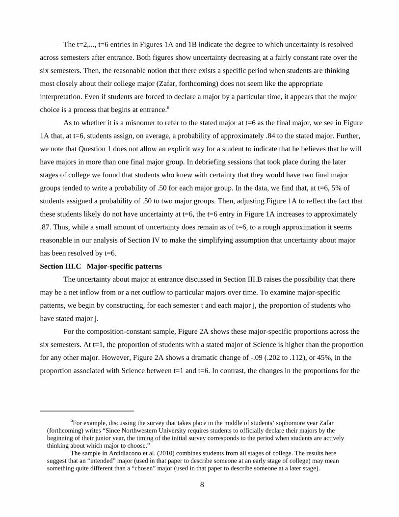
If no uncertainty existed about college major at entrance, each student would assign a probability of

one to the starting major. Instead, for our composition-constant sample, the t=1 entry in Figure 1A shows

that, on average, students assign at t=1 a probability of approximately .60 to the starting major. Further,

many students may ultimately choose a major that is different than the one that they believe is most likely at

entrance. The t=1 entry in Figure 1B shows that, on average, students perceive at t=1 that the probability

associated with their final major is only .44, and we find that at t=1 only 5% of students assign a probability

of one to the final major. Thus, much uncertainty exists about college major at entrance.

6For example, discussing the survey that takes place in the middle of students’ sophomore year Zafar(forthcoming) writes “Since Northwestern University requires students to officially declare their majors by thebeginning of their junior year, the timing of the initial survey corresponds to the period when students are activelythinking about which major to choose.”

The sample in Arcidiacono et al. (2010) combines students from all stages of college. The results heresuggest that an “intended” major (used in that paper to describe someone at an early stage of college) may meansomething quite different than a “chosen” major (used in that paper to describe someone at a later stage).

8

The t=2,..., t=6 entries in Figures 1A and 1B indicate the degree to which uncertainty is resolved

across semesters after entrance. Both figures show uncertainty decreasing at a fairly constant rate over the

six semesters. Then, the reasonable notion that there exists a specific period when students are thinking

most closely about their college major (Zafar, forthcoming) does not seem like the appropriate

interpretation. Even if students are forced to declare a major by a particular time, it appears that the major

choice is a process that begins at entrance.6

As to whether it is a misnomer to refer to the stated major at t=6 as the final major, we see in Figure

1A that, at t=6, students assign, on average, a probability of approximately .84 to the stated major. Further,

we note that Question 1 does not allow an explicit way for a student to indicate that he believes that he will

have majors in more than one final major group. In debriefing sessions that took place during the later

stages of college we found that students who knew with certainty that they would have two final major

groups tended to write a probability of .50 for each major group. In the data, we find that, at t=6, 5% of

students assigned a probability of .50 to two major groups. Then, adjusting Figure 1A to reflect the fact that

these students likely do not have uncertainty at t=6, the t=6 entry in Figure 1A increases to approximately

.87. Thus, while a small amount of uncertainty does remain as of t=6, to a rough approximation it seems

reasonable in our analysis of Section IV to make the simplifying assumption that uncertainty about major

has been resolved by t=6.

Section III.C Major-specific patterns

The uncertainty about major at entrance discussed in Section III.B raises the possibility that there

may be a net inflow from or a net outflow to particular majors over time. To examine major-specific

patterns, we begin by constructing, for each semester t and each major j, the proportion of students who

have stated major j.

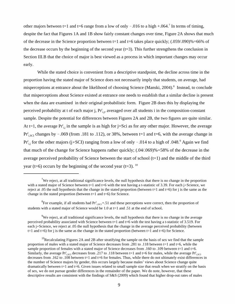
For the composition-constant sample, Figure 2A shows these major-specific proportions across the

six semesters. At t=1, the proportion of students with a stated major of Science is higher than the proportion

for any other major. However, Figure 2A shows a dramatic change of -.09 (.202 to .112), or 45%, in the

proportion associated with Science between t=1 and t=6. In contrast, the changes in the proportions for the

7We reject, at all traditional significance levels, the null hypothesis that there is no change in the proportionwith a stated major of Science between t=1 and t=6 with the test having a t-statistic of 3.39. For each j…Science, wereject at .05 the null hypothesis that the change in the stated proportion (between t=1 and t=6) for j is the same as thechange in the stated proportion (between t=1 and t=6) for Science.

8For example, if all students had Pr1i,SCI =.51 and these perceptions were correct, then the proportion of

students with a stated major of Science would be 1.0 at t=1 and .51 at the end of school.9We reject, at all traditional significance levels, the null hypothesis that there is no change in the average

perceived probability associated with Science between t=1 and t=6 with the test having a t-statistic of 3.519. Foreach j…Science, we reject at .05 the null hypothesis that the change in the average perceived probability (betweent=1 and t=6) for j is the same as the change in the stated proportion (between t=1 and t=6) for Science.

10Recalculating Figures 2A and 2B after stratifying the sample on the basis of sex we find that the sampleproportion of males with a stated major of Science decreases from .281 to .118 between t=1 and t=6, while thesample proportion of females with a stated major of Science decreases from .160 to .109 between t=1 and t=6. Similarly, the average Prt

i,SCI decreases from .217 to .118 between t=1 and t=6 for males, while the average Prti,SCI

decreases from .162 to .108 between t=1 and t=6 for females. Thus, while there do not ultimately exist differences inthe number of Science majors by gender, this occurs largely because males’ views about Science change quitedramatically between t=1 and t=6. Given issues related to small sample size that result when we stratify on the basisof sex, we do not pursue gender differences in the remainder of the paper. We do note, however, that thesedescriptive results are consistent with the findings of S&S (2009) which found that higher drop-out rates of males

9

other majors between t=1 and t=6 range from a low of only !.016 to a high +.064.7 In terms of timing,

despite the fact that Figures 1A and 1B show fairly constant changes over time, Figure 2A shows that much

of the decrease in the Science proportion between t=1 and t=6 takes place quickly; (.059/.090)%=66% of

the decrease occurs by the beginning of the second year (t=3). This further strengthens the conclusion in

Section III.B that the choice of major is best viewed as a process in which important changes may occur

early.

While the stated choice is convenient from a descriptive standpoint, the decline across time in the

proportion having the stated major of Science does not necessarily imply that students, on average, had

misperceptions at entrance about the likelihood of choosing Science (Manski, 2004).8 Instead, to conclude

that misperceptions about Science existed at entrance one needs to establish that a similar decline is present

when the data are examined in their original probabilistic form. Figure 2B does this by displaying the

perceived probability at t of each major j, Prti,j, averaged over all students i in the composition-constant

sample. Despite the potential for differences between Figures 2A and 2B, the two figures are quite similar.

At t=1, the average Prti,j in the sample is as high for j=Sci as for any other major. However, the average

Prti,SCI changes by !.069 (from .181 to .112), or 38%, between t=1 and t=6, with the average change in

Prti,j for the other majors (j…SCI) ranging from a low of only !.014 to a high of .048.9 Again we find

that much of the change for Science happens rather quickly; (.04/.069)%=58% of the decrease in the

average perceived probability of Science between the start of school (t=1) and the middle of the third

year (t=6) occurs by the beginning of the second year (t=3). 10

arise because males are more likely to learn that they started school with overoptimistic beliefs about academicability.

11Figure 3B shows the sample average of Pr1i,j for all students who have j as their starting major. Figure 4B

shows the sample average of Pr1i,j for all students who do not have j as their starting major.

10

Figures 2A and 2B show that, relatively speaking, students tend to start school thinking that a major

in Science is quite likely, but few students ultimately choose a final major of Science. It is worth delving

further into why Science is unique among majors in this respect. The number of students who end up with a

final major of j depends on both: A) the actual probability of having a final major of j conditional on having

a starting major of j (i.e., the probability of “staying” in j) and B) the actual probability of having a final

major of j conditional on having a starting major of k…j (i.e., the probability of “changing” to j). With

respect to A), Figure 3A shows that the proportion in the sample who stay in j is lower when j is Science

than when j is any of the other majors. With respect to B), Figure 4A shows that the proportion in the

sample who change to j is lower when j is Science than when j is any of the other majors. Misperceptions

will exist if beliefs about the probability of staying in j and changing to j do not correspond to the actual

probabilities in Figures 3A and 4A. In contrast to Figure 3A, Figure 3B indicates that, at t=1, students who

start in Science believe they are as likely to stay in their starting major as are students who start in other

majors. In contrast to Figure 4A, Figure 4B shows that, at t =1, students believe they are as likely to change

into Science as they are to change into any other major.11 Thus, Figures 3A and 4A show that starting in

Science is close to necessary but far from sufficient for having a final major of Science, but Figures 3B and

4B show that students do not fully realize that this is the case.

IV. Understanding why the dependent variable changes over time

IV.A. A conceptual model and basic data needs

As mentioned in Section I, the second component of providing evidence about the process by which

a person arrives at a college major involves attempting to understand why the dependent variable measuring

a person’s beliefs about his final major changes over time. A simple conceptual model guided our data

collection and guides our analysis.

A student i enters college (t=1) uncertain about his college major. At a time t* he must finalize his

choice of major by choosing a major from the set {AG, BUS, ED, HUM, SCI, PRO, SS). For the sake of

the discussion of the conceptual model we think of t* as occurring relatively quickly and abstract from

issues related to the utility obtained while in college but before t*. Denote as Uj(Xi,Mi,j,,i,j) the lifetime

utility starting at t* that student i receives from choosing major j. Xi is a vector of observable permanent

characteristics. ,i,j represents the effect on Uj of individual factors that are not observed by the

12If, as in Arcidiacono et al. (2010), one assumes that some major-specific factors only influence utility inschool and other characteristics only influence utility after school, then it is possible to put a stronger interpretationon individual coefficients. This would not be an unreasonable approximation for the types of characteristics usedhere, although, as discussed later, it would not be guaranteed by theory.

11

econometrician. Mi,j is a major-specific schooling or job characteristic/outcome that influences the lifetime

benefits of choosing major j. For example, Mi,j may be a person’s future grade performance or the future

income if he had major j. We stress that Mi,j is a constant representing the true value of some characteristic,

but that this true value may not be known with certainty by the student. Here we assume that Mi,j is one-

dimensional, but we relax this assumption in our empirical work.

Our primary interest is in understanding the importance of the Mi,j’s. Hereafter, we refer to the

elements of Mi,j as major-specific “factors” and define Mi ={Mi,AG,Mi,BUS ,...,Mi,SS}. Mi,j may influence both

the utility received while in school and the utility received after leaving school. Then, if one wanted to

understand why a particular major-specific factor mattered or did not matter at its most basic level, it would

be necessary to identify the impact of the factor on utility in both the schooling and post-schooling periods.

Largely because of the difficulty of this identification task, our objective is more modest - to examine

whether and to what extent factors matter in determining changes in the dependent variable. As such, we

further simplify by assuming a simple reduced form for the utility function.12

(1) Uj(Xi,Mi,j, ,i,j)= "jXi+$Mi,j +,i,j.

In terms of estimation of the parameters in (1), the approach we take differs depending on whether the

dependent variable is measures at t* (when, by assumption, no uncertainty about the final choice remains)

or before t*.

Analysis at t*

At time t* no uncertainty remains about a student’s final major because the student is forced to

make his final choice. Although we relax this assumption somewhat in our empirical work, for the

discussion here we maintain the assumption that ,i ={,i,AG, ,i,BUS,..., ,i,SS} is fully known by the student.

Then, in terms of the sources of uncertainty faced by the student, we focus on the possibility that the

student may be uncertain about Mi at any stage of college. If uncertainty about Mi remains “unresolved” at

t*, the student makes his choice by choosing the option with the highest expected utility. Denoting the

expected utility of option j as Et*Uj(), the person is observed to choose j if

(2) Et*Uj()!Et*Uk()>0 for all k…j.

We let Mti,j be a random variable which represents a student’s beliefs at t about Mi,j so that Mt*

i,j

denotes the unresolvable uncertainty at t*. To compute Et*Uj() for each j, the student integrates Uj(Xi,Mi,j,

,i,j) over the distribution of the random variable Mt*i,j. Given the linear specification in equation (1), this

12

integration results in

(3) Et*Uj(Xi,Mi,j, ,i,j)= "jXi+$ E(Mt*i,j)+,i,j.

The econometric analysis at t* follows the standard discrete choice framework. We assume

throughout that the econometrician knows the student’s beliefs about Mi,j at all times. However, because the

econometrician does not observe ,i, he does not know with certainty which option j has the highest

expected utility. Using his knowledge of the distribution of ,i, the econometrician basis estimation on the

likelihood that ,i falls within an interval such that observed choice j is optimal,

(4) Prob(i chooses j) =Prob (,i :Et*Uj()!Et*Uk()>0 for all k…j )=I1(Et*Uj()!Et*Uk()>0 for all k…j) dF(,i),

where 1(C) is an indicator function that has a value of one if its expression is true. For example, assuming

that ,i,j has an Extreme Value distribution yields the standard logit closed form for the probability in

equation (4).

Analysis before t*

At t=1 and subsequent times before t* a person may be uncertain about his final major. This

uncertainty arises because, in addition to the possibility of uncertainty about Mi that will not be resolved by

t*, there may also exist uncertainty about Mi that will be “resolved” by t*. Let E(Mti)={E(Mt

i,AG),

E(Mti,BUS),...,E(Mt

i,SS)}. The final decision at t* will be made taking into account E(Mt*i). However, at time t

the student does not know exactly what the value of E(Mt*i) will turn out to be, and, therefore does not

know what choice will turn out to be optimal. What he can compute at t given his knowledge of ,i and his

beliefs at t about E(Mt*i) is the perceived probability that each possible final major will turn out to be

optimal. Specifically, the perceived probability at t of having a final major of j, Prti,j, is the probability at t

that the person will arrive at t* with a value of E(Mt*i) such that, given his ,i, j is the optimal choice. Letting

E(Mt*i)t be a random variable that represents a student’s beliefs at time t about E(Mt*

i) and letting G

represent the distribution of E(Mt*i)t, Prt

i,j, is given by

(5) I1(Et*Uj()!Et*Uk()>0 for all k…j) g(E(Mt*i)t) dE(Mt*

i)t.

The econometric analysis is analogous to equation (4) from the standard discrete choice case. Our

earlier assumption that the econometrician knows the student’s beliefs about Mi,j at all times implies here

that the econometrician knows E(Mt*i)t. Then, using his knowledge of the distribution of ,i the

econometrician bases estimation on the likelihood that ,i is such that a person would have the Prti,j that he

reported:

(6) Prob(i reports his perceived probability at time t of having final major of j to be Prti,j)

=Prob{,i: I1(Et*Uj()!Et*Uk()>0 for all k…j) g(E(Mt*i)t) dE(Mt*

i)t = Prti,j}.

Summary of basic data needs

Then, for estimation at t* we require information about the mean E(Mt*i). As will be discussed, this

13See Arcidiacono (2004) and Beffy et al. (forthcoming ), respectively, for work that uses traditional types of data (i.e., non-expectations data) to focus on the role of ability and expected income, respectively, in determiningcollege major.

13

is observed directly in our data. However, for estimation at t=1 or other times t before t* we require the

entire distribution describing a student’s beliefs at t about E(Mt*i). This is not observed directly in our data,

but can be constructed, under certain assumptions, from E(Mti) and other unique information in the BPS.

Our effort to be explicit about the source of uncertainty about a student’s final major and to allow this

uncertainty to be heterogeneous across students represents a natural next step in the very small literature

which allows agents to express uncertainty about a choice that will be made in the future. For example, in

Blass et. al (2010) the source of uncertainty is not explicit and agents are assumed to have homogenous

beliefs about this source.

The next subsection (IV.B) is devoted to describing E(Mti), t=1,...,6. In Section IV.C, when we

discuss details of estimation for the t=1 case, we describe how we use this and other information to

construct the distribution describing beliefs about E(Mt*i) at times before t*.

Section IV.B E(Mti), Beliefs about major-specific factors influencing major choice

IV.B.1 E(Mti): Survey questions and full-sample means

In terms of the major-specific factors in Mi,j that influence the lifetime utility of i, we focus primarily

on student i’s future academic performance/ability if he had major j and student i’s future income if he had

major j.13 The latter is presumably a primary determinant of post-college utility, but could also influence

utility while in school if students are able to smooth consumption between the schooling and working

portions of their lives. The former is likely to play an important role in determining utility while in school -

struggling academically may make studying frustrating, may make it difficult to become interested in

course material, and may make school stressful due to a concern about failing out of school - but may also

influence a student’s post-college utility both by being a determinant of future income and by being related

to the extent to which a person enjoys his/her job.

Elements of Mi,j: beliefs about future academic performance and ability in major j

Assume that i’s grade point average (GPA) in major j in some future semester tN is given by

(7) GPAi,j,tN =AGPAi,j +<i,j,tN,

where AGPAi,j is a constant representing the average semester grade point average (GPA) that a person

would receive in major j and <i,j,tN is a mean-zero random variable representing the transitory portion of

grades in tN.

14Technically speaking, lifetime utility associated with j might depend on not only AGPAi,j but also on <i,j,tN.However, the simplifying focus on the average can be motivated by the reality that knowing AGPAi,j is close tosufficient for knowing one’s cumulative grade point average at the end of college for j since the sum of <i,j,tN will tendtowards zero with the number of semesters.

15A test rejects, at all traditional significance levels, the null that there is no change in E(AGPAti,SCI) over

time. For each major jó{SCI, BUS, HUM}, a test rejects, at all traditional significance levels, the null that thedifference between E(AGPAt

i,SCI) and E(AGPAti,j) is the same at t=6 as at t=1. For each major j0{BUS,HUM} a test

rejects at significance levels greater than .07 the null that the difference between E(AGPAti,SCI) and E(AGPAt

i,j) is thesame at t=6 as at t=1.

14

In terms of academic performance/ability, AGPAi,j is an obvious measure of interest.14 At time t, a

person may be uncertain about GPAi,j,tN both because he is uncertain about his true value of AGPAi,j and

because he does not know the future realization of <i,j,tN. Drawing on the notation from Section IV.A, we let

GPAti,j,tN, AGPAt

i,j, and <ti,j,tN, respectively, be random variables representing a person’s beliefs at time t

about GPAi,j,tN, AGPAi,j, and <i,j,tN , respectively, so that

(8) GPAti,j,tN =AGPAt

i,j +<ti,j,tN.

Then with <ti,j,tN mean-zero, E(AGPAt

i,j) is equal to E(GPAti,j,tN) and is elicited by the second column of

Question 1 (Appendix A) which asks a student about the GPA that he “would expect to receive in a typical

semester in the future” if he had major j.

Figure 5A shows the sample average of E(AGPAti,j) for each j and each t. Most striking is the

pattern related to the Science major. While students do begin school (t=1) with a belief that their grades

will be lowest in Science, this belief is strengthened substantially over time.15 Thus, at first glance, changes

after entrance in beliefs about grade performance in Science have at least the potential to explain the

negative slopes of the Science lines in Figures 2A and 2B.

Theory does not suggest whether beliefs about grade performance or beliefs about academic ability

per se should be more important in determining major choice. Regardless, given the importance of study

effort found in S&S (2004) and S&S (2008b), whether E(AGPAti,j) should be thought of as measuring

beliefs about academic ability per se depends to a large extent on what students believe about their study

effort in different majors. On one hand, if students tend to believe that they would expend little effort if

they were forced to choose certain majors that might not be of particular interest, low values of E(AGPAti,j)

might arise primarily due to low anticipated effort in j rather than due to beliefs that academic ability is low

in j. On the other hand, if students believe that receiving good grades is important regardless of major, they

may tend to believe that they will study (at least) as much when they find courses difficult. In this case

differences in E(AGPAti,j) across majors will tend to reflect differences in academic ability across majors.

Which of the two scenarios is most relevant is an empirical question that can be examined because

at time t we elicited the expected number of hours per day that a person would study in a future semester if

16Consistent with our notation for the GPA variable, ASTUDYi,j is a constant measuring the true averageamount a person would study in the future in major j, ASTUDYt

i,j is a random variable representing a person’sbeliefs about ASTUDYi,j at time t, and E(ASTUDYt

i,j) is the mean of the distribution describing beliefs.

17Informed by S&S (2008b), which takes advantage of variation in study effort created by whether astudent’s roommate brought a video game to school, we assume that studying an extra hour per day increase astudent’s grade point average by .30. Then, E(ABILITYt

i,j)=E(AGPAti,j)!.30*[E(ASTUDYt

i,j)!3.0], t=1,...,6.

15

he had each potential major group j (survey question not shown). Denoting i’s report for major group j at

time t as E(ASTUDYti,j), Figure 5B shows evidence that the second scenario above is more relevant as it

pertains to the Science major; while we found in Figure 5A that for all t the sample average of E(AGPAti,j)

is lowest when j=Sci, Figure 5B shows that for all t the sample average of E(ASTUDYti,j) is highest when

j=Sci.16

We can approach the interpretation of E(AGPAti,j) more formally by considering a measure

ABILITYi,j which represents the average GPA that a person would receive in major j if study effort were

held constant across majors. Here we hold study effort constant at 3.0 hours per day, which is

approximately the sample average at t=1 across all students and all majors. Since the causal relationship

between studying and grade performance in each major j is not observed in our data, it is necessary to make

an assumption in order to construct E(ABILITYti,j), the mean of the distribution describing i’s beliefs at

time t about ABILITYi,j. We assume that the causal effect of studying is homogenous across both i and j

and use the estimate of the causal effect of studying from Stinebrickner and Stinebrickner (2008b).17 Not

surprisingly given Figure 5B, the message from the sample averages for E(ABILITYti,j) shown in Figure 5C

is the same as the message from Figure 5A. Thus, our results support the notion that differences in

E(AGPAti,j) tend to largely represent differences that are not attributable to effort. Given the general

similarities between 5C and 5A and the reality that creating 5C requires assumptions about the causal effect

of studying, in the remainder of the paper we choose to use E(AGPAti,j) rather than E(ABILITYt

i,j) as our

primary measure of beliefs about academic quality.

Elements of Mi,j: beliefs about future income associated with major j

With respect to future income, our measure of interest is AINCOMEi,j, which represents the average

income a person would receive at age 28 if he had major j. The mean of the distribution describing i’s

beliefs about AINCOMEi,j, which we denote E(AINCOMEti,j), comes from the third column of Question 1.

Figure 5D shows large decreases in the sample average of E(AINCOMEti,SCI) over time. However, unlike

what is seen in Figures 5A and 5C, the decreases for the other majors are similar in nature to those observed

for Science.

IV.B.2. E(Mti): Heterogeneity in beliefs about major-specific factors

18It would be desirable to separate the Start_Other group into a Stay_Other and Leave_Other group.However, this is not practical due to the very small number of students who change into Science (Figure 4A).

19For t=1, we reject the null that the average E(AGPAti,SCI) is the same for Stay_Science and Start_Other (t-

statistic 10.071) and reject the null that the average E(AGPAti,SCI) is the same for Leave_Science and Start_Other (t-

statistic 11.379). We cannot reject the null hypothesis that the average E(AGPAti,SCI) is the same for Stay_Science

and Leave_Science (t-statistic .607). For t=6, we reject the null that the average E(AGPAti,SCI) is the same for

Stay_Science and Start_Other (t-statistic 11.387) and reject the null that the average E(AGPAti,SCI) is the same for

Stay_Science and Leave_Science (t-statistic 5.41). A test of the null hypothesis that the average E(AGPAti,SCI) is the

16

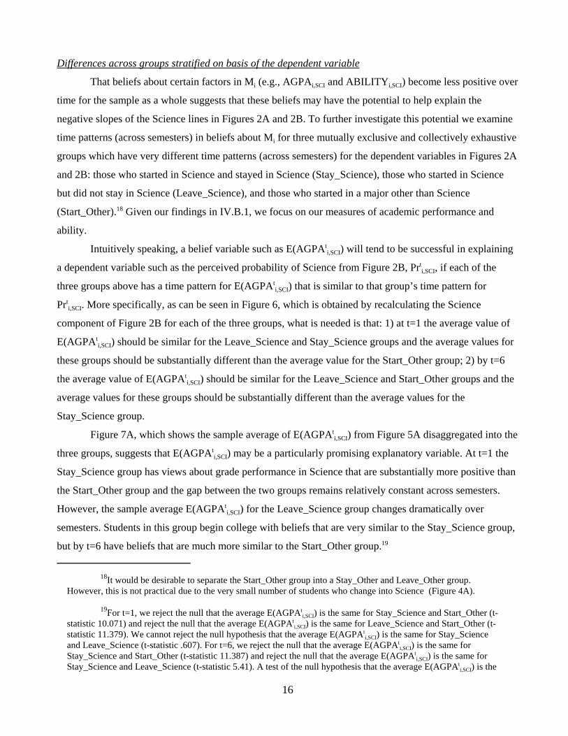
Differences across groups stratified on basis of the dependent variable

That beliefs about certain factors in Mi (e.g., AGPAi,SCI and ABILITYi,SCI) become less positive over

time for the sample as a whole suggests that these beliefs may have the potential to help explain the

negative slopes of the Science lines in Figures 2A and 2B. To further investigate this potential we examine

time patterns (across semesters) in beliefs about Mi for three mutually exclusive and collectively exhaustive

groups which have very different time patterns (across semesters) for the dependent variables in Figures 2A

and 2B: those who started in Science and stayed in Science (Stay_Science), those who started in Science

but did not stay in Science (Leave_Science), and those who started in a major other than Science

(Start_Other).18 Given our findings in IV.B.1, we focus on our measures of academic performance and

ability.

Intuitively speaking, a belief variable such as E(AGPAti,SCI) will tend to be successful in explaining

a dependent variable such as the perceived probability of Science from Figure 2B, Prti,SCI, if each of the

three groups above has a time pattern for E(AGPAti,SCI) that is similar to that group’s time pattern for

Prti,SCI. More specifically, as can be seen in Figure 6, which is obtained by recalculating the Science

component of Figure 2B for each of the three groups, what is needed is that: 1) at t=1 the average value of

E(AGPAti,SCI) should be similar for the Leave_Science and Stay_Science groups and the average values for

these groups should be substantially different than the average value for the Start_Other group; 2) by t=6

the average value of E(AGPAti,SCI) should be similar for the Leave_Science and Start_Other groups and the

average values for these groups should be substantially different than the average values for the

Stay_Science group.

Figure 7A, which shows the sample average of E(AGPAti,SCI) from Figure 5A disaggregated into the

three groups, suggests that E(AGPAti,SCI) may be a particularly promising explanatory variable. At t=1 the

Stay_Science group has views about grade performance in Science that are substantially more positive than

the Start_Other group and the gap between the two groups remains relatively constant across semesters.

However, the sample average E(AGPAti,SCI) for the Leave_Science group changes dramatically over

semesters. Students in this group begin college with beliefs that are very similar to the Stay_Science group,

but by t=6 have beliefs that are much more similar to the Start_Other group.19

same for Leave_Science and Start_Other has a t-statistic of 1.97.

20If the probabilities associated with the alternative majors are all zero for a particular t, we construct theweights using the probabilities from the most recent period in which the probabilities were not all zero. The variablesE(AINCOMEt

i,NON-SCI), E(ABILITYti,NON-SCI), E(ASTUDYt

i,NON-SCI) are constructed in the same way.

17

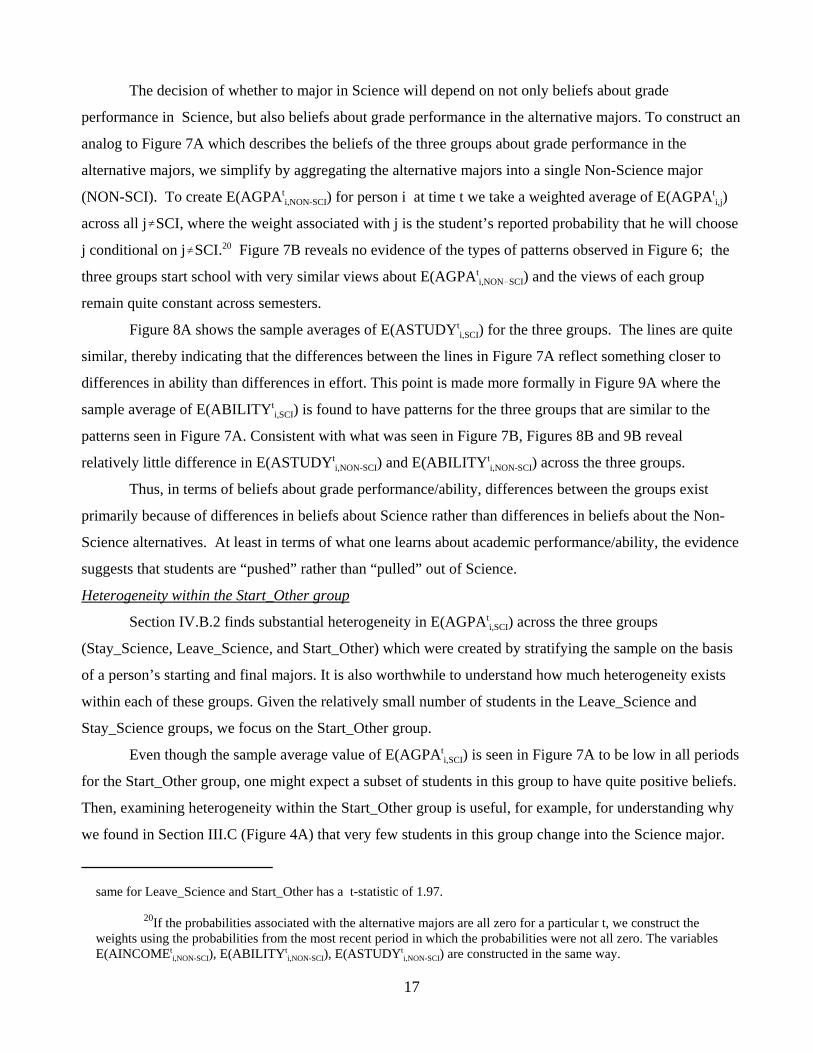
The decision of whether to major in Science will depend on not only beliefs about grade

performance in Science, but also beliefs about grade performance in the alternative majors. To construct an

analog to Figure 7A which describes the beliefs of the three groups about grade performance in the

alternative majors, we simplify by aggregating the alternative majors into a single Non-Science major

(NON-SCI). To create E(AGPAti,NON-SCI) for person i at time t we take a weighted average of E(AGPAt

i,j)

across all j…SCI, where the weight associated with j is the student’s reported probability that he will choose

j conditional on j…SCI.20 Figure 7B reveals no evidence of the types of patterns observed in Figure 6; the

three groups start school with very similar views about E(AGPAti,NON!SCI) and the views of each group

remain quite constant across semesters.

Figure 8A shows the sample averages of E(ASTUDYti,SCI) for the three groups. The lines are quite

similar, thereby indicating that the differences between the lines in Figure 7A reflect something closer to

differences in ability than differences in effort. This point is made more formally in Figure 9A where the

sample average of E(ABILITYti,SCI) is found to have patterns for the three groups that are similar to the

patterns seen in Figure 7A. Consistent with what was seen in Figure 7B, Figures 8B and 9B reveal

relatively little difference in E(ASTUDYti,NON-SCI) and E(ABILITYt

i,NON-SCI) across the three groups.

Thus, in terms of beliefs about grade performance/ability, differences between the groups exist

primarily because of differences in beliefs about Science rather than differences in beliefs about the Non-

Science alternatives. At least in terms of what one learns about academic performance/ability, the evidence

suggests that students are “pushed” rather than “pulled” out of Science.

Heterogeneity within the Start_Other group

Section IV.B.2 finds substantial heterogeneity in E(AGPAti,SCI) across the three groups

(Stay_Science, Leave_Science, and Start_Other) which were created by stratifying the sample on the basis

of a person’s starting and final majors. It is also worthwhile to understand how much heterogeneity exists

within each of these groups. Given the relatively small number of students in the Leave_Science and

Stay_Science groups, we focus on the Start_Other group.

Even though the sample average value of E(AGPAti,SCI) is seen in Figure 7A to be low in all periods

for the Start_Other group, one might expect a subset of students in this group to have quite positive beliefs.

Then, examining heterogeneity within the Start_Other group is useful, for example, for understanding why

we found in Section III.C (Figure 4A) that very few students in this group change into the Science major.

18

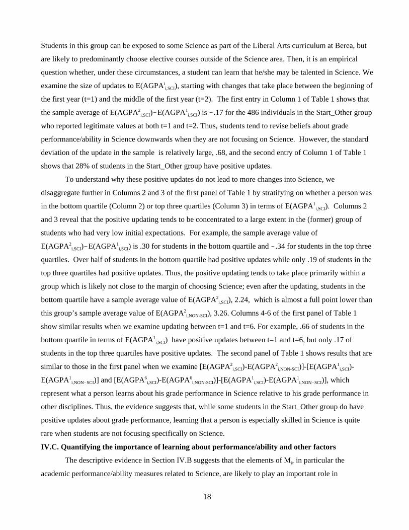
Students in this group can be exposed to some Science as part of the Liberal Arts curriculum at Berea, but

are likely to predominantly choose elective courses outside of the Science area. Then, it is an empirical

question whether, under these circumstances, a student can learn that he/she may be talented in Science. We

examine the size of updates to E(AGPAti,SCI), starting with changes that take place between the beginning of

the first year (t=1) and the middle of the first year (t=2). The first entry in Column 1 of Table 1 shows that

the sample average of E(AGPA2i,SCI)!E(AGPA1

i,SCI) is !.17 for the 486 individuals in the Start_Other group

who reported legitimate values at both t=1 and t=2. Thus, students tend to revise beliefs about grade

performance/ability in Science downwards when they are not focusing on Science. However, the standard

deviation of the update in the sample is relatively large, .68, and the second entry of Column 1 of Table 1

shows that 28% of students in the Start_Other group have positive updates.

To understand why these positive updates do not lead to more changes into Science, we

disaggregate further in Columns 2 and 3 of the first panel of Table 1 by stratifying on whether a person was

in the bottom quartile (Column 2) or top three quartiles (Column 3) in terms of E(AGPA1i,SCI). Columns 2

and 3 reveal that the positive updating tends to be concentrated to a large extent in the (former) group of

students who had very low initial expectations. For example, the sample average value of

E(AGPA2i,SCI)!E(AGPA1

i,SCI) is .30 for students in the bottom quartile and !.34 for students in the top three

quartiles. Over half of students in the bottom quartile had positive updates while only .19 of students in the

top three quartiles had positive updates. Thus, the positive updating tends to take place primarily within a

group which is likely not close to the margin of choosing Science; even after the updating, students in the

bottom quartile have a sample average value of E(AGPA2i,SCI), 2.24, which is almost a full point lower than

this group’s sample average value of E(AGPA2i,NON-SCI), 3.26. Columns 4-6 of the first panel of Table 1

show similar results when we examine updating between t=1 and t=6. For example, .66 of students in the

bottom quartile in terms of E(AGPA1i,SCI) have positive updates between t=1 and t=6, but only .17 of

students in the top three quartiles have positive updates. The second panel of Table 1 shows results that are

similar to those in the first panel when we examine [E(AGPA2i,SCI)-E(AGPA2

i,NON-SCI)]-[E(AGPA1i,SCI)-

E(AGPA1i,NON!SCI)] and [E(AGPA6

i,SCI)-E(AGPA6i,NON-SCI)]-[E(AGPA1

i,SCI)-E(AGPA1i,NON!SCI)], which

represent what a person learns about his grade performance in Science relative to his grade performance in

other disciplines. Thus, the evidence suggests that, while some students in the Start_Other group do have

positive updates about grade performance, learning that a person is especially skilled in Science is quite

rare when students are not focusing specifically on Science.

IV.C. Quantifying the importance of learning about performance/ability and other factors

The descriptive evidence in Section IV.B suggests that the elements of Mi, in particular the

academic performance/ability measures related to Science, are likely to play an important role in

19

determining whether a student chooses Science as his final major. In this Section we estimate models of

college major choice. Our objective is to provide the first direct evidence about the quantitative importance

that learning about major-specific academic performance/ability and other factors play in the decision to

major in Science. Because, as described in Section IV.A our models are reduced form in nature, we leave

aside certain fundamental questions about, for example, the strategy students take after entrance in an effort

to find a major with a good match.

We estimate the parameters of equation (1) by taking advantage of the data in the first (t=1) and last

(t=6) semesters in our data. While it would perhaps be possible to take advantage of data from all six

periods, the simplifying focus on these two periods is natural because changes in beliefs about Mi between

these periods reflect the full degree of learning about Mi during our sample period and because changes in

Prti,j between these periods reflect the full extent to which uncertainty about major is resolved during our

sample period. Unless otherwise stated, we focus on the 323 students in the composition-constant sample

who have no missing information at either t=1 or t=6.

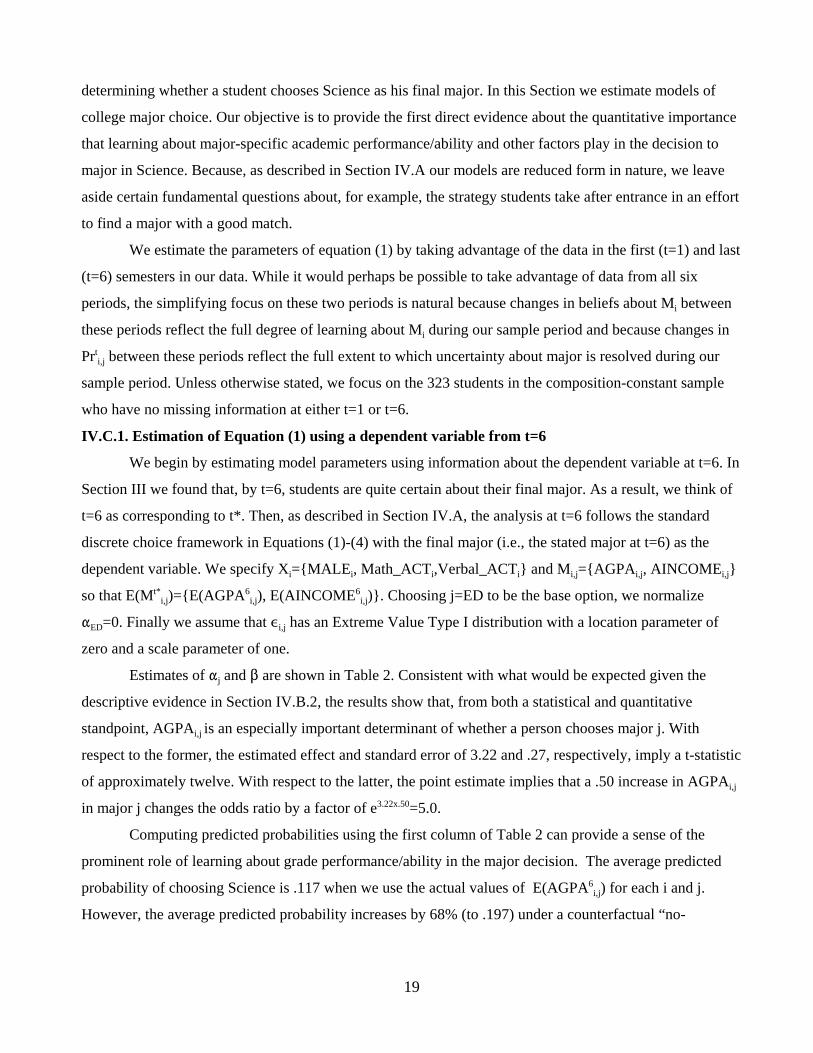
IV.C.1. Estimation of Equation (1) using a dependent variable from t=6

We begin by estimating model parameters using information about the dependent variable at t=6. In

Section III we found that, by t=6, students are quite certain about their final major. As a result, we think of

t=6 as corresponding to t*. Then, as described in Section IV.A, the analysis at t=6 follows the standard

discrete choice framework in Equations (1)-(4) with the final major (i.e., the stated major at t=6) as the

dependent variable. We specify Xi={MALEi, Math_ACTi,Verbal_ACTi} and Mi,j={AGPAi,j, AINCOMEi,j}

so that E(Mt*i,j)={E(AGPA6

i,j), E(AINCOME6i,j)}. Choosing j=ED to be the base option, we normalize

"ED=0. Finally we assume that ,i,j has an Extreme Value Type I distribution with a location parameter of

zero and a scale parameter of one.

Estimates of "j and $ are shown in Table 2. Consistent with what would be expected given the

descriptive evidence in Section IV.B.2, the results show that, from both a statistical and quantitative

standpoint, AGPAi,j is an especially important determinant of whether a person chooses major j. With

respect to the former, the estimated effect and standard error of 3.22 and .27, respectively, imply a t-statistic

of approximately twelve. With respect to the latter, the point estimate implies that a .50 increase in AGPAi,j

in major j changes the odds ratio by a factor of e3.22x.50=5.0.

Computing predicted probabilities using the first column of Table 2 can provide a sense of the

prominent role of learning about grade performance/ability in the major decision. The average predicted

probability of choosing Science is .117 when we use the actual values of E(AGPA6i,j) for each i and j.

However, the average predicted probability increases by 68% (to .197) under a counterfactual “no-

21The use of the term “no-learning” is a misnomer to the extent that the variance of the belief distributionmay also have changed from t=1 to t=6 and our approach does not attempt to hold this constant.

For this sample, the average perceived probability is .118 at t=1 and .182 at t=6.

20

learning” assumption that involves setting E(AGPA6i,j) equal to the initial value E(AGPA1

i,j) for all i and j.21

While the results point to AGPAi,j playing a particularly prominent role, consistent with the results

of Arcidiacono et. al (2010) we also find evidence that, from both a statistical and quantitative standpoint,

AINCOMEi,j is also an important determinant of major choice. With respect to the former, the estimated

effect and standard error of .056 and .008, respectively, imply a t-statistic in excess of six. With respect to

the latter, the point estimate implies that a $5,000 increase in AINCOMEi,j in major j changes the odds ratio

by a factor of e.056x5=1.32. The average predicted probability of choosing Science increases by 21% (from

.117 to .142) under the counterfactual “no-learning” assumption that E(AINCOME6i,j)=E(AINCOME1

i,j) for

all i and j.

Given our particular interest in Science, a desirable simplification for much of the analysis that

follows involves, as in Figures 7B-10B, collapsing the set of alternative majors into a single non-Science

major. In this case, the choice set becomes {SCI, NON-SCI} with NON-SCI as the base case (so that

"NON!SCI is normalized to 0). We find that this binary specification yields results that are very similar to

those in the uncollapsed specification. The first two columns of Table 2 show that the coefficients

associated with AGPAi,j and AINCOMEi,j remain similar in size (2.65 vs. 3.22 and .048 vs. .056) and both

remain statistically significant (t-statistics of 4.85 and 3.31 respectively). Our results quantifying the

importance of learning also produce similar results. The average predicted probability of choosing Science

increases by 58% (from .117 to .185) under the counterfactual “no-learning” assumption that

E(AGPA6i,j)=E(AGPA1

i,j) for all i and both j, and the average predicted probability of choosing Science

increases by 23% (from .117 to .144) under the counterfactual “no-learning” assumption that

E(AINCOME6i,j) =E(AINCOME1

i,j) for all i and both j.

IV.C.2. Estimation of Equation (1) using a dependent variable from t=1

We can also estimate the model parameters using information about the dependent variable from

t=1. In Section III we found that, at t=1, much uncertainty tends to exist about a student’s final major. Then,

as discussed in Section IV.A, the analysis at t=1 follows the framework in equations (5) and (6) with Pr1i,j as

the dependent variable. Given our finding that the model with the binary choice set {SCI, NON-SCI}

provides conclusions about the choice of Science that are similar to those obtained with the full choice set,

we focus on the binary model here.

The key difference between the t=1 analysis and the t=6 analysis is that Equations (5) and (6)

require knowledge of G, the distribution of the random variable E(Mt*i)1 representing i’s beliefs at t=1 about

22In practice, we assign a value of .99 if Pr1i,SCI=1.0 and assign a value of .01 if Pr1

i,SCI=0.0, in essenceassuming that a small amount of measurement error exists at the two extremes. We find that results do not changesubstantially when we use .95 and .05 instead. The non-MLE approach in Blass et al. (2010) does not require thistype of adjustment of reported probabilities.

21

E(Mt*i)={E(AGPAt*

i, SCI), E(AINCOMEt*i, SCI), E(AGPAt*

i, NON-SCI), E(AINCOMEt*i, NON-SCI)}. As a reminder,

E(Mt*i) is observed directly in our data at t*. However, what is needed here is, E(Mt*

i)1, person i’s beliefs at

time t=1 about what E(Mt*i) will turn out to be. Because the distribution describing these beliefs, G, is not

elicited directly by a single survey question, we must construct it from several sources of information in the

BPS. Here we provide an outline of our approach, leaving a detailed description for Appendix B.

For the sake of illustration, we focus here on the construction of beliefs at t=1 about E(AGPAt*i,SCI).

Our construction is built on the notion that the ultimate value of E(AGPAt*i,SCI) is determined by an

updating process that occurs as a person proceeds through school. In the spirit of Bayesian updating we

specify an updating rule in which the updated mean E(AGPAt*i, SCI) depends on the initial mean

E(AGPA1i,SCI) and a noisy signal of the person’s academic performance. Equation (7) suggests that grade

performance between t=1 and t* is an appropriate noisy signal and we refer to this grade performance as

GPA_Earlyi. Since E(AGPAt*i, SCI) and E(AGPA1

i, SCI) are observed in our survey data and GPA_Earlyi is

observed in administrative data, the unknown parameters of the updating rule can be estimated. Given

student i’s starting point E(AGPA1i, SCI), the estimated updating rule tells student i what E(AGPAt*

i, SCI) will

be for each realized value of GPA_Earlyi. Then, the distribution G describing i’s beliefs about

E(AGPAt*i,SCI) can be constructed if the distribution describing i’s beliefs about GPA_Earlyi are known.

Under the assumption (discussed in more detail in Appendix B) that, at the time of entrance, students

believe that they will settle on a college major rather quickly, the belief distribution of GPA_Earlyi is

obtained directly from Question 2 (Appendix) which asks about grade performance in the early portion of

college. As described in Appendix B, we take a similar approach for constructing the distribution

describing beliefs at t=1 about the other elements of E(Mt*i).

With the binary choice set, the second line in equation (6) becomes

(9) Prob{,i: I1("SCIXi+$ [E(Mt*i,SCI)1!E(Mt*

i,NON-SCI)1]+,i,SCI!,i,NON-SCI >0) g(E(Mt*i)1) dE(Mt*

i)1 = Pr1i,j}.

This integral will be strictly increasing in ,i,diff =,i,SCI!,i,NON-SCI over the range (0,1) so that, for any value of

Pr1i,SCI 0(0,1), there will exist a unique value of ,i,diff such that the condition in equation (9) is satisfied. The

likelihood contribution for person i from equation (6) is the density h of ,i,diff evaluated at this unique value.

For example, with ,i,SCI and ,i,NON-SCI having independent Extreme Value distributions, h is a Logit density

function. The model can then be estimated by maximum likelihood.22

In practice, we modify the t=1 model slightly to relax the assumption that the student faces no

23One cannot directly compare the coefficients across columns in Table 2 because the estimated variance ofthe ,i,diff* in column 3 is not the same as the normalized variance (that accompanies the extreme value assumption) inthe other columns.

24That is, in the first scenario the student assumes that E(AGPAt*i,j) will be equal to E(AGPA1

i,j). In thesecond scenario the student assumes that E(AGPAt*

i,j) will be equal to E(AGPA6i,j)

22

uncertainty about factors other than those included explicitly in Mi. We assume at t=1 that ,i,diff=,i,diff*+L,

where ,i,diff* follows the standard assumption of being known to the student but not by the econometrician

and L represents factors which are not known to the student or econometrician at time t but whose value

will be realized by the student by t* (i.e., uncertainty about L will be resolved by the time the final decision

is made at t*). The t=1 model is discussed in more detail in Appendix B. Here we note two things. First,

from an operational standpoint, the presence of the L component introduces an additional integral into the

student computation in equation (9). Second, in this model the variance of ,i,diff* can be identified subject to

a normalization of the variance of L.

Results are shown in the third column of Table 2. As with the t=6 case, we find that a student’s

academic performance AGPAi,j is statistically significant at all traditional levels (t-statistic= 11.97).23 In

Section IV.C.1, the estimates from our t=6 analysis indicated a prominent role of learning about grade

performance/ability in the major decision. Here we reexamine the role of learning using our estimates from

Column 3. Specifically, we first compute predicted reported probabilities at t=1 using the actual values of

E(AGPA1i,j) for each i and j. We then examine how different predicted reported probabilities would have

been at t=1 if students had started school with their final beliefs by setting E(AGPA1i,j) equal to the final

value E(AGPA6i,j) for each i and j. In each case we assume that students do not anticipate resolving any

uncertainty about E(AGPAt*i,j) after t=1.24 We again find that learning about ability is important in

determining a student’s major; the average predicted probability of choosing Science is 27% higher (.178

versus .140) in the former scenario than in the latter scenario.

There are several plausible explanations for why the importance of learning about grade

performance is found to be somewhat different in this section (basing estimation on a dependent variable

from t=1) than in Section IV.C.1 (basing estimation on a dependent variable from t=6). In addition to the

conceptual exercise being somewhat different, it could be the case that students’ views/preferences about

the importance of grade performance change over time during school or it could be the case that the

assumptions needed to construct beliefs at t=1 about E(Mt*i) in this section are somewhat problematic.

Regardless, given that our project should be viewed as an in-depth case study, the consistency (across time

periods and specifications) of the finding that learning about academic performance plays a crucial role in

the final choice of major is more important than quantifying the exact size of the effect.

25We use somewhat different notation for the Interest variable than for the other variables to reflect that theelicited information about Interest at time t reflects a student’s current level of interest at time t while the elicitedinformation about other variables reflects a belief at time t about a constant true value.

23

IV.C.3. A specification with changes in beliefs between t=1 and t=6

Sections IV.C.1 and IV.C.2 identify the importance of learning by estimating models in which it is

a person’s beliefs about Mi,j at a given time t that enters the specification, and then comparing the predicted

probabilities associated with these actual beliefs at t with predicted probabilities associated with beliefs at t

that represent a non-learning counterfactual. Here we examine the robustness of our primary conclusion -

that learning about grade performance/ability plays a prominent role in the choice of Science - to a

specification in which the amount that a person learns about Mi,j during school enters the specification

directly.

From the standpoint of specifying a model in which changes in beliefs about Mi enter directly, the

central conceptual question is whether the change in beliefs is sufficient to push the student into Science (or

push the student out of Science) given how close to the margin of indifference he was at the time of

entrance. Then, focusing on the binary outcome variable that takes a value of one if a person’s final major

is Science, we estimate a logit model including as explanatory variables both measures of how much a

student has learned during school (i.e., [E(AGPA6i,SCI)-E(AGPA6

i,NON-SCI)]-[E(AGPA1i,SCI)-

E(AGPA1i,NON!SCI)] and [E(INCOME6

i,SCI)-E(INCOME6i,NON-SCI)]-[E(AINCOME1

i,SCI)-

E(AINCOME1i,NON!SCI)] ) and measures related to how close to the margin a student was at the time of

entrance ( i.e., E(AGPA1i,SCI)-E(AGPA1

i,NON-SCI), E(AINCOME1i,SCI)-E(AINCOME1

i,NON-SCI), and Pr1i,SCI).

As shown in Table 3, we find that the amount that a person learns has a statistically important effect

on whether he becomes a Science major; the estimate (std. error) for [E(AGPA6i,SCI)!E(AGPA6

i,NON!SCI)] -

[E(AGPA1i,SCI)-E(AGPA1

i,NON-SCI)] is 2.410 (.687). Consistent with our earlier findings, we find that the

effect of learning is quantitatively important; the average predicted probability of choosing Science

increases by 54% (from .117 to .181) under the counterfactual assumption that no learning takes place

about academic performance (i.e., setting [E(AGPA6i,SCI)-E(AGPA6

i,NON-SCI)]-[E(AGPA1i,SCI)-

E(AGPA1i,NON!SCI)]=0 for all students.

IV.C.4 Discussion of Potential Omitted Variables

Given the parsimonious specification for Mi, it is natural to consider the issue of omitted variables

that might be correlated with AGPAi,j. Perhaps most obvious in this respect is a student’s interest level in

major j. Figures 5E, 11A, and 11B show sample average values of INTERESTt,i,j, i’s current interest in

major j at time t as elicited in the last column of Question 1.25 In terms of descriptive statistics of interest,

there are a couple of obvious things to note. First, Figure 5E shows that there is non-trivial interest in

26At all traditional significance levels, we reject the null hypothesis of a zero population correlation in allthree cases.

27The endogeneity concern would also suggest that some portion of the change in INTERESTt,i,j that isobserved across semesters might have been anticipated by a student who realizes that interest will tend to increase ashe receives exposure to j. This would be problematic given our desire to understand the role that learning per seplays in the major decision.

24

Science at entrance, with Science being the median major in terms of sample average interest at t=1.

Second, a comparison of, for example, Figure 11A to Figure 7A suggests that there is a strong relationship

between a student’s current interest in a topic and his beliefs about grade performance. This is confirmed in

more formal tests. For example, the sample correlation between E(AGPAti, SCI) and INTERESTt,i,SCI is .543

at t=1 and .484 at t=6 and the sample correlation between [E(AGPA6i,Sci)-E(AGPA1

i,Sci)] and

[INTEREST6,i,Sci !INTEREST1,i,Sci ] is .340.26

Unfortunately, the fact that the survey questions elicits a student’s current interest in major j creates

a potential endogeneity concern because current interest in a major j is likely to be affected by how many

classes a person has taken in j in the past. This concern would imply that a student’s major decision may

influence his current interest level when what we wish to identify is the reverse.27 As a result, it does not

seem desirable to include INTERESTt,i,j directly in our empirical specifications.

Given that INTERESTt,i,j is not included, whether the estimated effect that AGPAi,j has on major

choice should be viewed as a causal effect depends on the relevance of the various underlying reasons for

the correlation found between E(AGPAti,j)and INTERESTt,i,j. The most obvious potential reason for the

correlation is that AGPA may have a direct influence on INTEREST. For example, it seems likely that

students who have a difficult time understanding course material in a particular major may have difficulty

appreciating the subject matter or find studying unenjoyable/stressful. However, excluding INTEREST

from our specification is not problematic in this scenario given our interest in identifying the total causal

effect of AGPAi,j - the correlation simply identifies one avenue through which the total causal effect of

AGPAi,j may arise.

Problematic scenarios are ones in which the correlation between INTERESTt,i,j and E(AGPAti,j) is

present for other reasons. The most obvious possibility is that a lack of interest in a major such as Science

could cause a person to believe he will perform poorly in the major. However, because it seems reasonable

to believe that study effort is the most likely avenue through which a lower interest in major j would affect

E(AGPAti,j), this possibility can be examined directly. We find no evidence of a relationship between

INTERESTt,i,Sci and E(ASTUDYti,Sci) or a relationship between changes in INTERESTt,i,Sci and changes in

28 For the composition-constant sample, the sample correlation between E(ASTUDYti, SCI) and

INTERESTt,i,SCI is .052 at t=1 and .075 at t=6 and the sample correlation between [E(ASTUDY6i,Sci)-

E(ASTUDY1i,Sci)] and [INTEREST6,i,Sci !INTEREST1,i,Sci ] is .074. The p-values associated with the three estimates

are .346, .176, and .185, respectively.

29Another potentially problematic scenario is one in which the correlation between E(AGPAti,Sci) and

INTERESTt,i,Sci exists because each is influenced by a common third factor. Seemingly the most logical commonfactor of this type is a background factor such as whether a person’s parents work in a Science occupation. However,if such background factors are the primary factor driving the correlation, one would expect students with muchhigher levels of interest in Science at t=1 to continue to have much higher levels of interest in Science at t=6 (thanstudents with lower levels of interest at t=1) even if they learn that their grade performance/ability in Science islower than expected. Figure 11A shows that much of the difference in INTERESTt,i,SCI for the Leave_Science andStart_Other groups disappears after the former group realizes that their grade performance will not be particularlyhigh. Given that some differences in INTERESTt,i,SCI between the two groups would be expected to persist becausethe Leave_Science group has received more exposure to Science than the Start_Other group, Figure 11A does notseem to provide much evidence in support of this common background factor story.

25

E(ASTUDYti,Sci).28 In addition, we can approach this issue more formally by estimating the choice models

using ABILITYi,j instead of APGAi,j. Despite the fact that the ability measure likely suffers from substantial

measurement error (due, in part, from the necessity of making assumptions about the effect of studying), we

continue to find a significant effect. For example, when ABILITYi,j replaces APGAi,j in Column 1 of Table

2, a test of the null hypothesis that ABILITYi,j has no effect is rejected with a t-statistic of 5.80.29

V. Conclusion

We find that students enter college as open to a major in math or science as to any other major, but

that a large number of students move away from math and science after realizing that their grade

performance will be substantially lower than expected. Further, our results indicate that changes in beliefs

about grade performance arise because students realize that their ability in math/science is lower than

expected rather than because students realize that they are not willing to put the required effort into math or

science majors. Our measure of ability likely captures a variety of factors related to a student’s propensity

at the time of college entrance to understand math or science, including not only his innate intelligence but

also his background preparation. As such, the findings suggest the potential importance of policies at

younger ages which lead students to enter college better prepared to study math or science.

26

References

Altonji, Joseph. “The Demand for and Return to Education When Education Outcomes are Uncertain,”Journal of Labor Economics, 1993, vol. 11, no. 1, 48-83.

Arcidiacono, Peter. “Ability Sorting and the Returns to College Major,” Journal of Econometrics, Vol.121, Nos. 1-2 (August, 2004), 343-375.

Arcidiacono, Peter, Hotz, Joseph, and Kang, Songman, “Modeling College Major Choices usingElicited Measures of Expectations and Counterfactuals,” Duke University working paper, 2010.

Barsky, Robert, Kimball, Miles, Juster, F. Thomas, and Shapiro, Matthew. “Preference Parameters andBehavioral Heterogeneity: An Experimental Approach in the Health and Retirement Survey,” TheQuarterly Journal of Economics, May 1997, 537-579.

Beffy, Magali, Fougere, Denis, Maurel, Arnaud, “Choosing the Field of Study in Post-SecondaryEducation: Do Expected Earnings Matter?” The Review of Economics and Statistics, Forthcoming.

Black, Dan and Jeffrey Smith, Evaluating the Returns to College Quality with Multiple Proxies forQuality.” Journal of Labor Economics 24(30: 701-728.

Blass, Asher, Lach, Saul, and Manski, Charles. “Using Elicited Choice Probabilities to EstimateRandom Utility Models: Preferences for Electricity Reliability,” International Economic Review, 2010.

Carneiro, Pedro, Hansen, Karsten, and Heckman, James, “Estimating Distributions of Counterfactualswith an Application to the Returns to Schooling and Measurement of the Effect of Uncertainty onSchooling Choice,” International Economic Review, 2005.

Cunha, Flavio, Heckman, James, and Navarro, Salvador, “Separating Uncertainty from Heterogeneityin Life Cycle Earnings,” Oxford Economic Papers, 2005, 57(2), 191-261.

COSEPUP (Committee on Science, Engineering, and Public Policy), “Rising Above the GatheringStorm: Energizing and Employing America for a Brighter Economic Future.” The National AcademiesPress (2007).

Dominitz, Jeff. “Earnings Expectations, Revisions, and Realizations,” The Review of Economics andStatistics, August 1998, 374-388.

Dominitz, Jeff and Manski, Charles. “Eliciting Student Expectations of the Returns to Schooling,”Winter 1996, 1-26.

Dominitz, Jeff and Manski, Charles. “Using Expectations Data to Study Subjective IncomeExpectations,” Journal of American Statistical Association, September 1997, 855-867.

Dominitz, Jeff and Manski, Charles. “How Should We Measure Consumer Confidence (sentiment)? Evidence form the Michigan Survey of Consumers,” Working paper 9926, National Bureau ofResearch, 2003.

Juster, T., “Consumer Buying Intentions and Purchase Probability: An Experiment in Survey Design,”

27

Journal of the American Statistical Association 61 (1966), 658-96.

Manski, Charles, “Schooling as Experimentation: a reappraisal of the post-secondary drop-outphenomenon,” Economics of Education Review, Volume 8 number 4, 1989, 305-312.

Manski, C., “The Use of Intentions Data to Predict Behavior: A Best Case Analysis,” Journal of theAmerican Statistical Association 85 (1990), 934-940.

Manski, C., “Measuring Expectations,” Econometrica, 72 (5), (2004), 1329-1376.

Montmarquette, C, Cannings, Kathy, and Mahseredjian, Sophie, “How Do Young People ChooseCollege Majors?,” Economics of Education Review, Elsevier, 21(6), (2002) 543-556, December.

Smith, Jeffrey, “Heterogeneity and Higher Education,” in Michael McPherson and Morton OwenSchapiro (eds.) Succeeding in College: What it Means and How to Make it Happen. New York:College Board, 131-144.

Stinebrickner, Todd and Stinebrickner, Ralph, “Time-Use and College Outcomes,” Journal ofEconometrics, 121 (1-2) July-August (2004), 243-269.

Stinebrickner, Todd and Stinebrickner, Ralph, “The Effect of Credit Constraints on the College Drop-Out Decision: A Direct Approach Using a New Panel Study,” American Economic Review. December(2008a)

Stinebrickner, Todd and Stinebrickner, Ralph, “The Causal Effect of Studying on AcademicPerformance,” Frontiers in Economic Policy and Analysis (Frontiers), Berkeley Electronic Press(2008b).

Stinebrickner, Todd and Stinebrickner, Ralph, “Learning about Academic Ability and the CollegeDrop-Out Decision” (2009).

Zafar, Basit, “College Major Choice and the Gender Gap,” working paper (2008)

Zafar, Basit, “How Do College Students Form Expectations?” Journal of Labor Economics,Forthcoming.

28

Table 1 Descriptive statisticsChanges in EGPA - Start_Other group

-1 -2 -3 -4 -5 -6t=2full samplen=486

t=2bottom 25%n=131

t=2top 75%n=355

t=6full sample

n=334

t=6bottom 25%

n=83

t=6top 75%n=251

E(AGPAti,SCI)-E(AGPA1

i,SCI) -.17 (.68) .30 (.71) -.34 (.58) -0.21 .45 (.76) -.43 (.58)

Proportion withE(AGPAt

i,SCI)-E(AGPA1i,SCI)>0

0.28 0.51 0.19 0.29 0.66 0.17

E(AGPA1i,SCI) 2.97 (.76) 1.93 (.56) 3.35 (.36) 2.99 (.75) 1.91 (.59) 3.34 (.37)

E(AGPAti,SCI) 2.80 (.75) 2.24 (.68) 3.01 (.66) 2.77 (.61) 2.37 (.56) 2.91 (.56)

E(AGPA1i,NON_SCI) 3.41 (.33) 3.25 (.35) 3.48 (.31) 3.42 (.32) 3.26 (.34) 3.48 (.30)

E(AGPAti,NON_SCI) 3.36 (.34) 3.26 (.35) 3.40 (.33) 3.36 (.34) 3.27 (.35) 3.39 (.32)

t=2full samplen=486

t=2bottom 25%n=121

t=2top 25%n=365

t=6full sample

n=334

t=6bottom 25%

n=82

t=6top 25%n=252

[E(AGPAti,SCI)-E(AGPAt

i,NON-SCI)]-[E(AGPA1

i,SCI)!E(AGPA1i,NONSCI)]

-.11 (.69) .34 (.80) -.27 (.57) -.145 (.69) .47 (.71) -.34 (.55)

Proportion with[E(AGPAt

i,SCI)-E(AGPAti,NON-SCI)]-

[E(AGPA1i,SCI)!E(AGPA1

i,NONSCI)]>0

0.38 0.66 0.29 0.39 0.75 0.27

E(AGPA1i,SCI)-E(AGPA1

i,NON-SCI) -.44 (.70) -1.43 (.55) -.11 (.57) -.43 (.70) -1.41 (.58) -.11 (.353)E(AGPAt

i,SCI)-E(AGPAti,NON-SCI) -.56 (.69) -1.08 (.71) -.39 (.59) -.58 (.55) -.93 (.50) -.46 (.52)

Notes: The descriptive statistics in the Table show mean (standard deviation).In first panel: Bottom 25% refers to students with E(AGPA1

i,SCI)#2.5 and Top 75% refers to students withE(AGPA1

i,SCI)>2.5. In second panel: Bottom 25% refers to students with E(AGPA1i,SCI)-E(AGPA1

i,NON-

SCI)#!.795 and Top 75% refers to students with E(AGPA1i,SCI)-E(AGPA1

i,NON-SCI)>!.795.

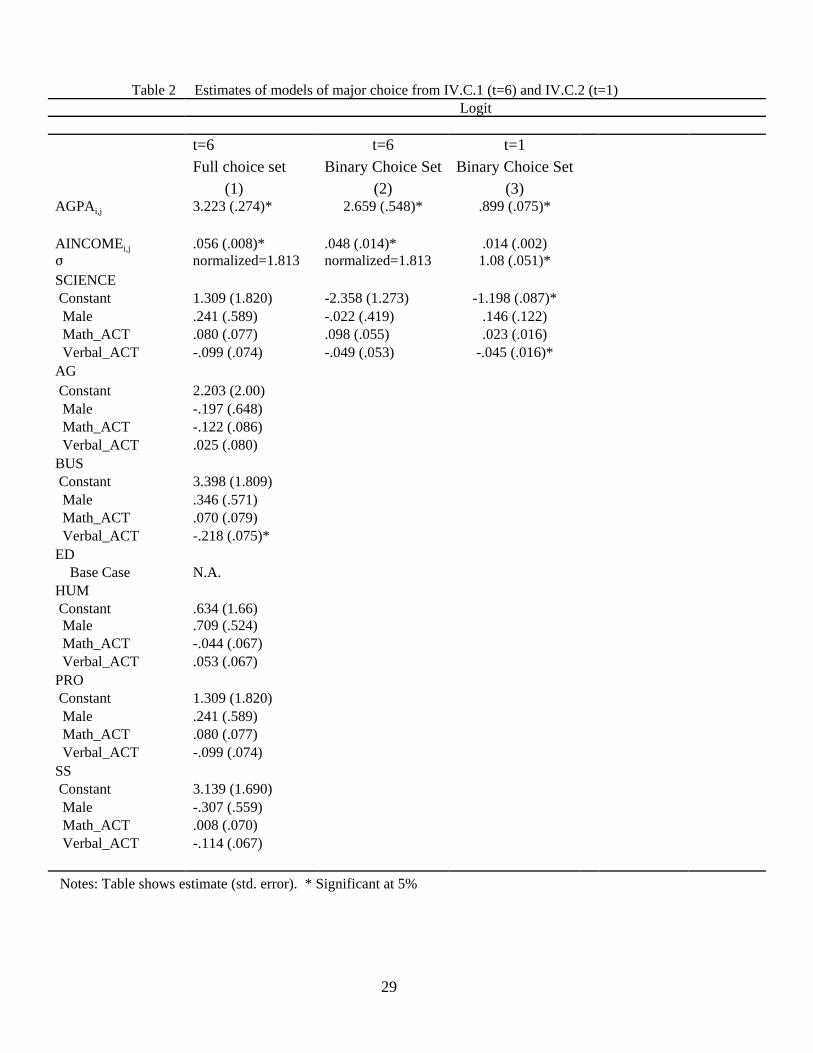
29

Table 2 Estimates of models of major choice from IV.C.1 (t=6) and IV.C.2 (t=1)Logit

t=6 Full choice set (1)

t=6Binary Choice Set

(2)

t=1Binary Choice Set

(3)AGPAi,j 3.223 (.274)* 2.659 (.548)* .899 (.075)*

AINCOMEi,j .056 (.008)* .048 (.014)* .014 (.002)F normalized=1.813 normalized=1.813 1.08 (.051)*SCIENCE Constant 1.309 (1.820) -2.358 (1.273) -1.198 (.087)* Male .241 (.589) -.022 (.419) .146 (.122) Math_ACT .080 (.077) .098 (.055) .023 (.016) Verbal_ACT -.099 (.074) -.049 (.053) -.045 (.016)*AG Constant 2.203 (2.00) Male -.197 (.648) Math_ACT -.122 (.086) Verbal_ACT .025 (.080)BUS Constant 3.398 (1.809) Male .346 (.571) Math_ACT .070 (.079) Verbal_ACT -.218 (.075)*ED Base Case N.A.HUM Constant .634 (1.66) Male .709 (.524) Math_ACT -.044 (.067) Verbal_ACT .053 (.067)PRO Constant 1.309 (1.820) Male .241 (.589) Math_ACT .080 (.077) Verbal_ACT -.099 (.074)SS Constant 3.139 (1.690) Male -.307 (.559) Math_ACT .008 (.070) Verbal_ACT -.114 (.067)

Notes: Table shows estimate (std. error). * Significant at 5%

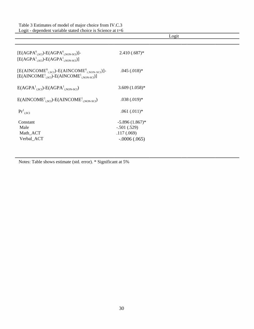
30

Table 3 Estimates of model of major choice from IV.C.3 Logit - dependent variable stated choice is Science at t=6

Logit

[E(AGPA6i,SCI)-E(AGPA6

i,NON-SCI)]-[E(AGPA1

i,SCI)-E(AGPA1i,NON-SCI)]

2.410 (.687)*

[E(AINCOME6i,SCI)-E(AINCOME6

i,NON-SCI)]-[E(AINCOME1

i,SCI)-E(AINCOME1i,NON-SCI)]

.045 (.018)*

E(AGPA1i,SCI)-E(AGPA1

i,NON-SCI) 3.609 (1.058)*

E(AINCOME1i,SCI)-E(AINCOME1

i,NON-SCI) .038 (.019)*

Pr1i,SCI .061 (.011)*

Constant -5.896 (1.867)* Male -.501 (.529) Math_ACT .117 (.069) Verbal_ACT -.0006 (.065)

Notes: Table shows estimate (std. error). * Significant at 5%

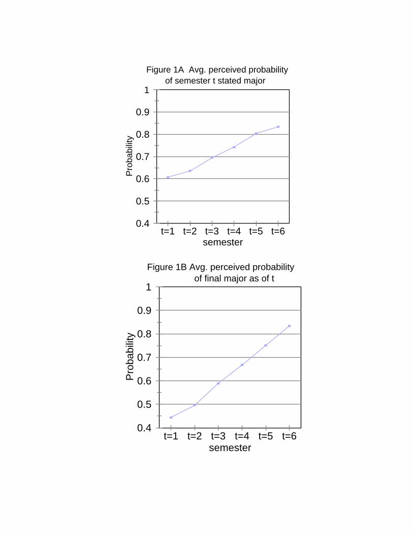
0.4

0.5

0.6

0.7

0.8

0.9

1

Pro

babi

lity

t=1 t=2 t=3 t=4 t=5 t=6semester

Figure 1A Avg. perceived probabilityof semester t stated major

0.4

0.5

0.6

0.7

0.8

0.9

1

Pro

babi

lity

t=1 t=2 t=3 t=4 t=5 t=6semester

Figure 1B Avg. perceived probability of final major as of t

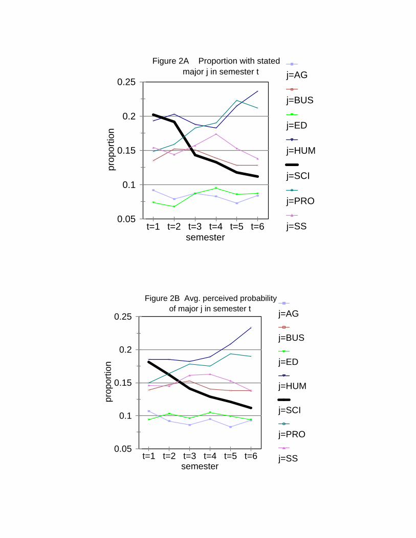
0.05

0.1

0.15

0.2

0.25

prop

ortio

n

t=1 t=2 t=3 t=4 t=5 t=6semester

j=AG

j=BUS

j=ED

j=HUM

j=SCI

j=PRO

j=SS

Figure 2A Proportion with stated major j in semester t

0.05

0.1

0.15

0.2

0.25

prop

ortio

n

t=1 t=2 t=3 t=4 t=5 t=6semester

j=AG

j=BUS

j=ED

j=HUM

j=SCI

j=PRO

j=SS

Figure 2B Avg. perceived probability of major j in semester t

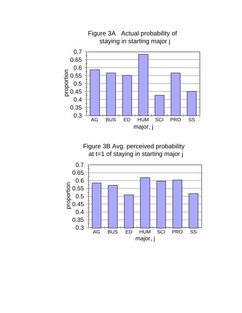
0.3 0.35

0.4 0.45

0.5 0.55

0.6 0.65

0.7

prop

ortio

n

AG BUS ED HUM SCI PRO SSmajor, j

Figure 3A Actual probability of staying in starting major j

0.3 0.35

0.4 0.45

0.5 0.55

0.6 0.65

0.7

prop

ortio

n

AG BUS ED HUM SCI PRO SSmajor, j

Figure 3B Avg. perceived probability at t=1 of staying in starting major j

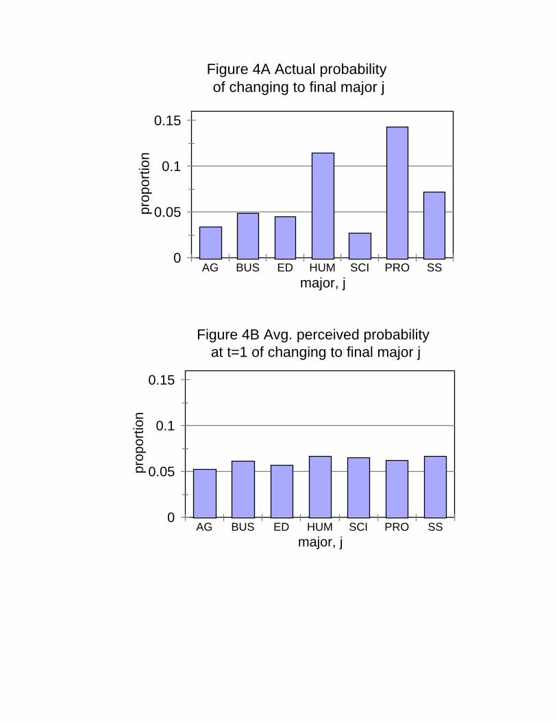
0

0.05

0.1

0.15

prop

ortio

n

AG BUS ED HUM SCI PRO SSmajor, j

Figure 4A Actual probabilityof changing to final major j

0

0.05

0.1

0.15

prop

ortio

n

AG BUS ED HUM SCI PRO SSmajor, j

Figure 4B Avg. perceived probabilityat t=1 of changing to final major j

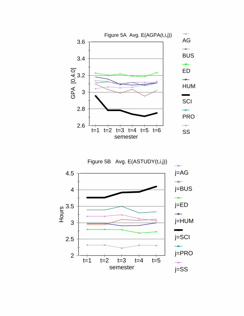
2.6

2.8

3

3.2

3.4

3.6

GP

A [

0,4.

0]

t=1 t=2 t=3 t=4 t=5 t=6semester

AG

BUS

ED

HUM

SCI

PRO

SS

Figure 5A Avg. E(AGPA(t,i,j))

2

2.5

3

3.5

4

4.5

Hou

rs

t=1 t=2 t=3 t=4 t=5semester

j=AG

j=BUS

j=ED

j=HUM

j=SCI

j=PRO

j=SS

Figure 5B Avg. E(ASTUDY(t,i,j))

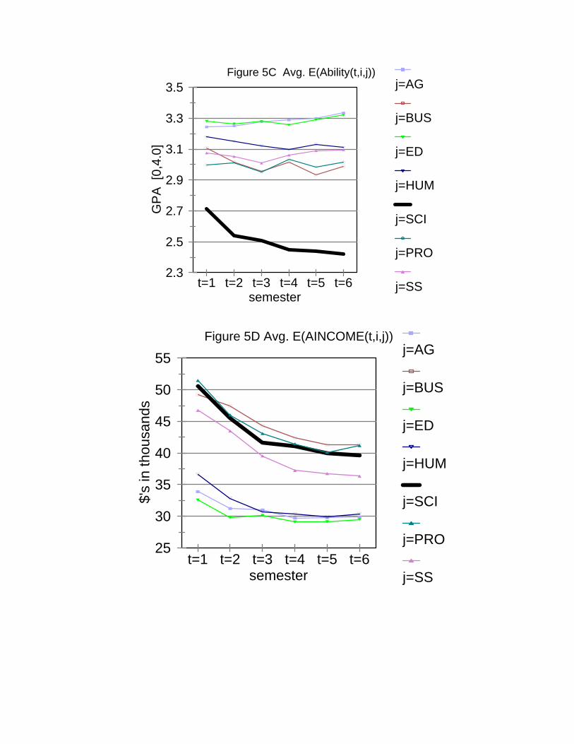
2

2.5

3

3.5

4

4.5

Hou

rs

t=1 t=2 t=3 t=4 t=5semester

j=AG

j=BUS

j=ED

j=HUM

j=SCI

j=PRO

j=SS

Figure 5B Avg. E(ASTUDY(t,i,j))

2.3

2.5

2.7

2.9

3.1

3.3

3.5

GP

A [

0,4.

0]

t=1 t=2 t=3 t=4 t=5 t=6semester

j=AG

j=BUS

j=ED

j=HUM

j=SCI

j=PRO

j=SS

Figure 5C Avg. E(Ability(t,i,j))

25

30

35

40

45

50

55

$'s

in th

ousa

nds

t=1 t=2 t=3 t=4 t=5 t=6semester

j=AG

j=BUS

j=ED

j=HUM

j=SCI

j=PRO

j=SS

Figure 5D Avg. E(AINCOME(t,i,j))

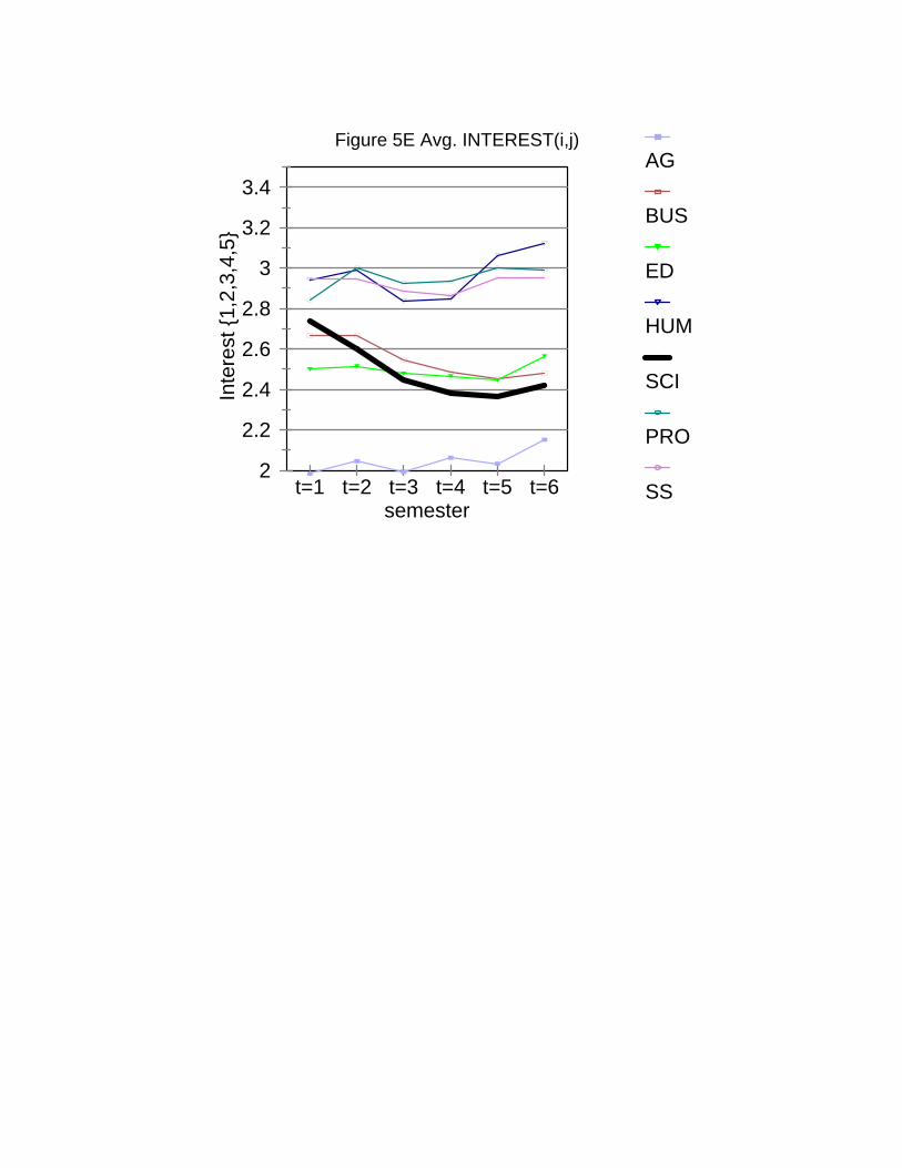
2

2.2

2.4

2.6

2.8

3

3.2

3.4

Inte

rest

{1,2

,3,4

,5}

t=1 t=2 t=3 t=4 t=5 t=6semester

AG

BUS

ED

HUM

SCI

PRO

SS

Figure 5E Avg. INTEREST(i,j)

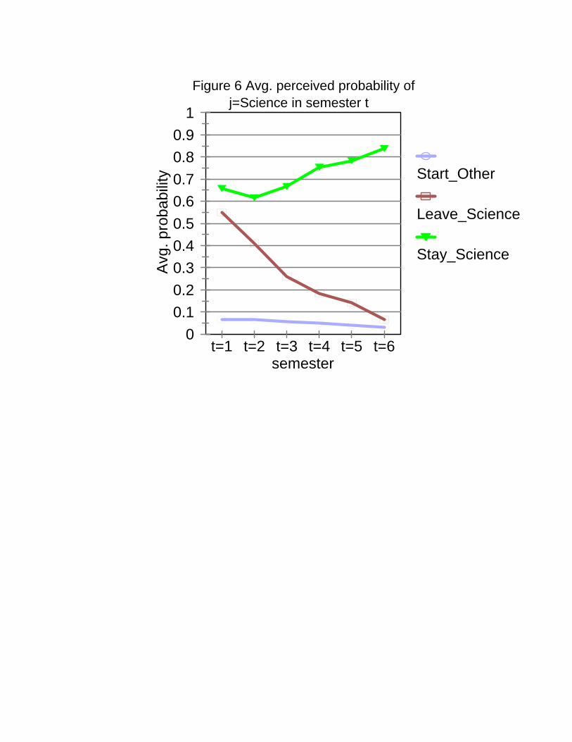
0 0.1 0.2 0.3 0.4 0.5 0.6 0.7 0.8 0.9

1

Avg

. pro

babi

lity

t=1 t=2 t=3 t=4 t=5 t=6semester

Start_Other

Leave_Science

Stay_Science

Figure 6 Avg. perceived probability ofj=Science in semester t

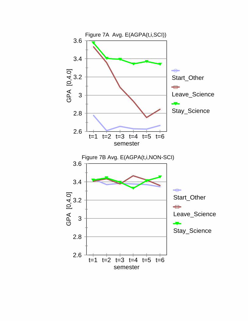
2.6

2.8

3

3.2

3.4

3.6

GP

A [

0,4.

0]

t=1 t=2 t=3 t=4 t=5 t=6semester

Start_Other

Leave_Science

Stay_Science

Figure 7A Avg. E(AGPA(t,i,SCI))

2.6

2.8

3

3.2

3.4

3.6

GP

A [

0,4.

0]

t=1 t=2 t=3 t=4 t=5 t=6semester

Start_Other

Leave_Science

Stay_Science

Figure 7B Avg. E(AGPA(t,i,NON-SCI)

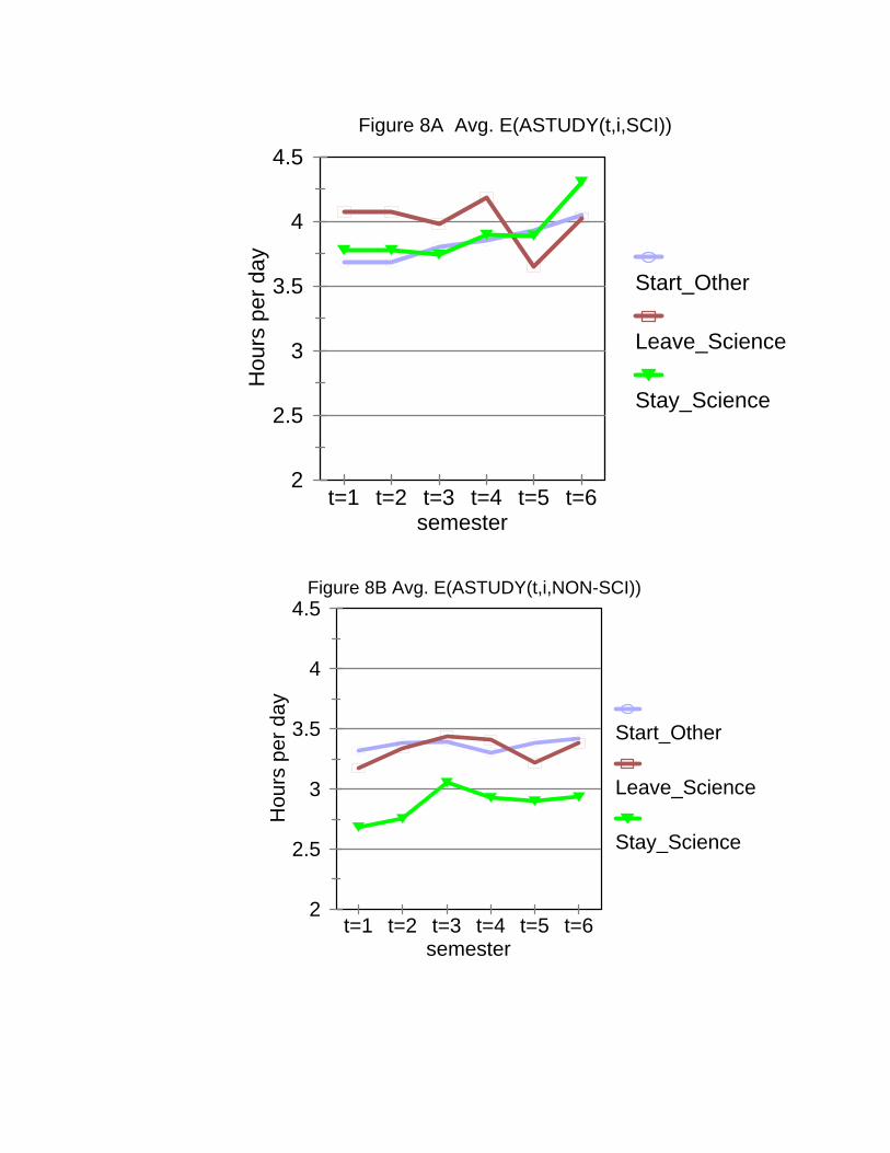
2

2.5

3

3.5

4

4.5

Hou

rs p

er d

ay

t=1 t=2 t=3 t=4 t=5 t=6semester

Start_Other

Leave_Science

Stay_Science

Figure 8A Avg. E(ASTUDY(t,i,SCI))

2

2.5

3

3.5

4

4.5

Hou

rs p

er d

ay

t=1 t=2 t=3 t=4 t=5 t=6semester

Start_Other

Leave_Science

Stay_Science

Figure 8B Avg. E(ASTUDY(t,i,NON-SCI))

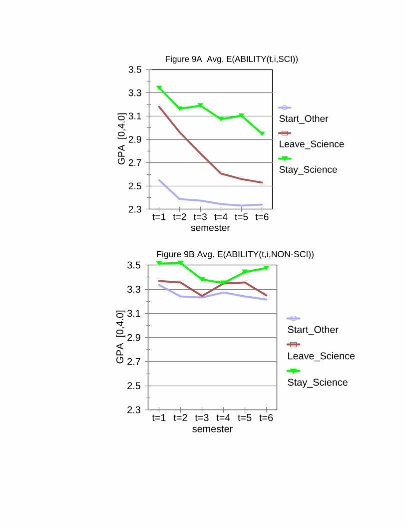
2.3

2.5

2.7

2.9

3.1

3.3

3.5

GP

A [

0,4.

0]

t=1 t=2 t=3 t=4 t=5 t=6semester

Start_Other

Leave_Science

Stay_Science

Figure 9A Avg. E(ABILITY(t,i,SCI))

2.3

2.5

2.7

2.9

3.1

3.3

3.5

GP

A [

0,4.

0]

t=1 t=2 t=3 t=4 t=5 t=6semester

Start_Other

Leave_Science

Stay_Science

Figure 9B Avg. E(ABILITY(t,i,NON-SCI))

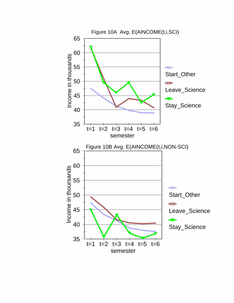
35

40

45

50

55

60

65

Inco

me

in th

ousa

nds

t=1 t=2 t=3 t=4 t=5 t=6semester

Start_Other

Leave_Science

Stay_Science

Figure 10A Avg. E(AINCOME(t,i,SCI)

35

40

45

50

55

60

65

Inco

me

in th

ours

ands

t=1 t=2 t=3 t=4 t=5 t=6semester

Start_Other

Leave_Science

Stay_Science

Figure 10B Avg. E(AINCOME(t,i,NON-SCI)

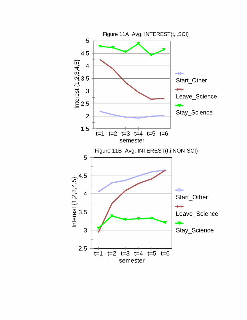
1.5

2

2.5

3

3.5

4

4.5

5

Inte

rest

{1,2

,3,4

,5}

t=1 t=2 t=3 t=4 t=5 t=6semester

Start_Other

Leave_Science

Stay_Science

Figure 11A Avg. INTEREST(t,i,SCI)

2.5

3

3.5

4

4.5

5

Inte

rest

{1,2

,3,4

,5}

t=1 t=2 t=3 t=4 t=5 t=6semester

Start_Other

Leave_Science

Stay_Science

Figure 11B Avg. INTEREST(t,i,NON-SCI)

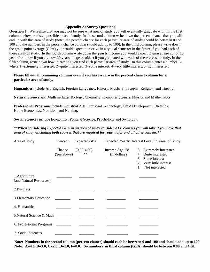
Appendix A: Survey QuestionsQuestion 1. We realize that you may not be sure what area of study you will eventually graduate with. In the firstcolumn below are listed possible areas of study. In the second column write down the percent chance that you willend up with this area of study (note: the percent chance for each particular area of study should be between 0 and100 and the numbers in the percent chance column should add up to 100). In the third column, please write downthe grade point average (GPA) you would expect to receive in a typical semester in the future if you had each ofthese areas of study. In the fourth column write down the yearly income you would expect to earn at age 28 (or 10years from now if you are now 20 years of age or older) if you graduated with each of these areas of study. In thefifth column, write down how interesting you find each particular area of study. In this column enter a number 1-5where 1=extremely interested, 2=quite interested, 3=some interest, 4=very little interest, 5=not interested.

Please fill out all remaining columns even if you have a zero in the percent chance column for aparticular area of study.

Humanities include Art, English, Foreign Languages, History, Music, Philosophy, Religion, and Theatre.

Natural Science and Math includes Biology, Chemistry, Computer Science, Physics and Mathematics.

Professional Programs include Industrial Arts, Industrial Technology, Child Development, Dietetics,Home Economics, Nutrition, and Nursing.

Social Sciences include Economics, Political Science, Psychology and Sociology.

**When considering Expected GPA in an area of study consider ALL courses you will take if you have thatarea of study -including both courses that are required for your major and all other courses.**

Area of study Percent Expected GPA Expected Yearly Interest Level in Area of Study

Chance (0.00-4.00) Income Age 28 5. Extremely interested (See above) ** (in dollars) 4. Quite interested

3. Some interest 2. Very little interest

1. Not interested

1.Agriculture ________ ________ _________ _________(and Natural Resources)

2.Business ________ ________ __________ __________

3.Elementary Education ________ ________ __________ __________

4. Humanities ________ ________ __________ __________

5.Natural Science & Math ________ ________ __________ __________

6. Professional Programs ________ ________ ___________ __________

7. Social Sciences _________ ________ ___________ __________

Note: Numbers in the second column (percent chance) should each be between 0 and 100 and should add up to 100.Note: A=4.0, B=3.0, C=2.0, D=1.0, F=0.0. So numbers in third column (GPA) should be between 0.00 and 4.00.

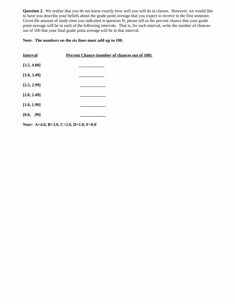
Question 2. We realize that you do not know exactly how well you will do in classes. However, we would liketo have you describe your beliefs about the grade point average that you expect to receive in the first semester.Given the amount of study-time you indicated in question H, please tell us the percent chance that your gradepoint average will be in each of the following intervals. That is, for each interval, write the number of chancesout of 100 that your final grade point average will be in that interval.

Note: The numbers on the six lines must add up to 100.

Interval Percent Chance (number of chances out of 100).

[3.5, 4.00] ____________

[3.0, 3.49] ____________

[2.5, 2.99] ____________

[2.0, 2.49] ____________

[1.0, 1.99] ____________

[0.0, .99] ____________

Note: A=4.0, B=3.0, C=2.0, D=1.0, F=0.0

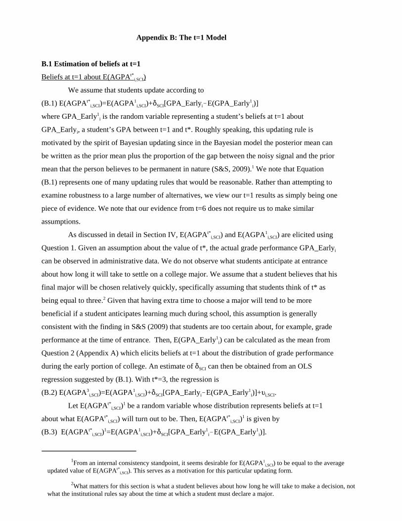
1From an internal consistency standpoint, it seems desirable for E(AGPA1i,SCI) to be equal to the average

updated value of E(AGPAt*i,SCI). This serves as a motivation for this particular updating form.

2What matters for this section is what a student believes about how long he will take to make a decision, notwhat the institutional rules say about the time at which a student must declare a major.

Appendix B: The t=1 Model

B.1 Estimation of beliefs at t=1

Beliefs at t=1 about E(AGPAt*i,SCI)

We assume that students update according to

(B.1) E(AGPAt*i,SCI)=E(AGPA1

i,SCI)+*SCI[GPA_Earlyi!E(GPA_Early1i)]

where GPA_Early1i is the random variable representing a student’s beliefs at t=1 about

GPA_Earlyi, a student’s GPA between t=1 and t*. Roughly speaking, this updating rule is

motivated by the spirit of Bayesian updating since in the Bayesian model the posterior mean can

be written as the prior mean plus the proportion of the gap between the noisy signal and the prior

mean that the person believes to be permanent in nature (S&S, 2009).1 We note that Equation

(B.1) represents one of many updating rules that would be reasonable. Rather than attempting to

examine robustness to a large number of alternatives, we view our t=1 results as simply being one

piece of evidence. We note that our evidence from t=6 does not require us to make similar

assumptions.

As discussed in detail in Section IV, E(AGPAt*i,SCI) and E(AGPA1

i,SCI) are elicited using

Question 1. Given an assumption about the value of t*, the actual grade performance GPA_Earlyi

can be observed in administrative data. We do not observe what students anticipate at entrance

about how long it will take to settle on a college major. We assume that a student believes that his

final major will be chosen relatively quickly, specifically assuming that students think of t* as

being equal to three.2 Given that having extra time to choose a major will tend to be more

beneficial if a student anticipates learning much during school, this assumption is generally

consistent with the finding in S&S (2009) that students are too certain about, for example, grade

performance at the time of entrance. Then, E(GPA_Early1i) can be calculated as the mean from

Question 2 (Appendix A) which elicits beliefs at t=1 about the distribution of grade performance

during the early portion of college. An estimate of *SCI can then be obtained from an OLS

regression suggested by (B.1). With t*=3, the regression is

(B.2) E(AGPA3i,SCI)=E(AGPA1

i,SCI)+*SCI[GPA_Earlyi!E(GPA_Early1i)]+Li,SCI.

Let E(AGPAt*i,SCI)1 be a random variable whose distribution represents beliefs at t=1

about what E(AGPAt*i,SCI) will turn out to be. Then, E(AGPAt*

i,SCI)1 is given by

(B.3) E(AGPAt*i,SCI)1=E(AGPA1

i,SCI)+*SCI[GPA_Early1i!E(GPA_Early1

i)].

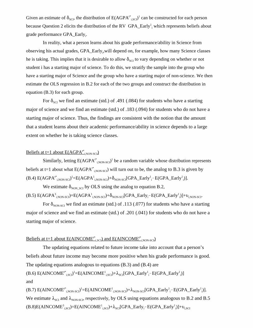
Given an estimate of *SCI, the distribution of E(AGPAt*i,SCI)1 can be constructed for each person

because Question 2 elicits the distribution of the RV GPA_Early1i which represents beliefs about

grade performance GPA_Earlyi.

In reality, what a person learns about his grade performance/ability in Science from

observing his actual grades, GPA_Earlyi,will depend on, for example, how many Science classes

he is taking. This implies that it is desirable to allow *SCI to vary depending on whether or not

student i has a starting major of science. To do this, we stratify the sample into the group who

have a starting major of Science and the group who have a starting major of non-science. We then

estimate the OLS regression in B.2 for each of the two groups and construct the distribution in

equation (B.3) for each group.

For *SCI we find an estimate (std.) of .491 (.084) for students who have a starting

major of science and we find an estimate (std.) of .183 (.094) for students who do not have a

starting major of science. Thus, the findings are consistent with the notion that the amount

that a student learns about their academic performance/ability in science depends to a large

extent on whether he is taking science classes.

Beliefs at t=1 about E(AGPAt*i,NON-SCI)

Similarly, letting E(AGPAt*i,NON-SCI)1 be a random variable whose distribution represents

beliefs at t=1 about what E(AGPAt*i,NON-SCI) will turn out to be, the analog to B.3 is given by

(B.4) E(AGPAt*i,NON-SCI)1=E(AGPA1

i,NON-SCI)+*NON-SCI[GPA_Early1i!E(GPA_Early1

i)].

We estimate *NON_SCI by OLS using the analog to equation B.2,

(B.5) E(AGPA3i,NON-SCI)=E(AGPA1

i,NON-SCI)+*NON-SCI[GPA_Earlyi!E(GPA_Early1i)]+Li,NON-SCI.

For *NON-SCI we find an estimate (std.) of .113 (.077) for students who have a starting

major of science and we find an estimate (std.) of .201 (.041) for students who do not have a

starting major of science.

Beliefs at t=1 about E(AINCOMEt*i,SCI) and E(AINCOMEt*

i,NON-SCI)

The updating equations related to future income take into account that a person’s

beliefs about future income may become more positive when his grade performance is good.

The updating equations analogous to equations (B.3) and (B.4) are

(B.6) E(AINCOMEt*i,SCI)1=E(AINCOME1

i,SCI)+8SCI[GPA_Early1i!E(GPA_Early1

i)]

and

(B.7) E(AINCOMEt*i,NON-SCI)1=E(AINCOME1

i,NON-SCI)+8NON-SCI[GPA_Early1i!E(GPA_Early1

i)].

We estimate 8SCI and 8NON-SCI, respectively, by OLS using equations analogous to B.2 and B.5

(B.8)E(AINCOME3i,SCI)=E(AINCOME1

i,SCI)+8SCI[GPA_Earlyi!E(GPA_Early1i)]+Li,SCI

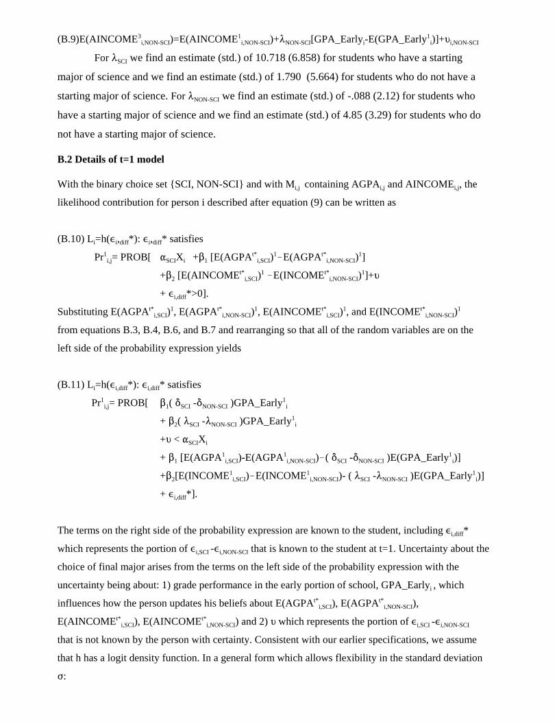
(B.9)E(AINCOME3i,NON-SCI)=E(AINCOME1

i,NON-SCI)+8NON-SCI[GPA_Earlyi-E(GPA_Early1i)]+Li,NON-SCI

For 8SCI we find an estimate (std.) of 10.718 (6.858) for students who have a starting

major of science and we find an estimate (std.) of 1.790 (5.664) for students who do not have a

starting major of science. For 8NON-SCI we find an estimate (std.) of -.088 (2.12) for students who

have a starting major of science and we find an estimate (std.) of 4.85 (3.29) for students who do

not have a starting major of science.

B.2 Details of t=1 model

With the binary choice set {SCI, NON-SCI} and with Mi,j containing AGPAi,j and AINCOMEi,j, the

likelihood contribution for person i described after equation (9) can be written as

(B.10) Li=h(,i,diff*): ,i,diff* satisfies

Pr1i,j= PROB[ "SCIXi +$1 [E(AGPAt*

i,SCI)1!E(AGPAt*i,NON-SCI)1]

+$2 [E(AINCOMEt*i,SCI)1 !E(INCOMEt*

i,NON-SCI)1]+L

+ ,i,diff*>0].

Substituting E(AGPAt*i,SCI)1, E(AGPAt*

i,NON-SCI)1, E(AINCOMEt*i,SCI)1, and E(INCOMEt*

i,NON-SCI)1

from equations B.3, B.4, B.6, and B.7 and rearranging so that all of the random variables are on the

left side of the probability expression yields

(B.11) Li=h(,i,diff*): ,i,diff* satisfies

Pr1i,j= PROB[ $1( *SCI -*NON-SCI )GPA_Early1

i

+ $2( 8SCI -8NON-SCI )GPA_Early1i

+L < "SCIXi

+ $1 [E(AGPA1i,SCI)-E(AGPA1

i,NON-SCI)!( *SCI -*NON-SCI )E(GPA_Early1i)]

+$2[E(INCOME1i,SCI)!E(INCOME1

i,NON-SCI)- ( 8SCI -8NON-SCI )E(GPA_Early1i)]

+ ,i,diff*].

The terms on the right side of the probability expression are known to the student, including ,i,diff*

which represents the portion of ,i,SCI -,i,NON-SCI that is known to the student at t=1. Uncertainty about the

choice of final major arises from the terms on the left side of the probability expression with the

uncertainty being about: 1) grade performance in the early portion of school, GPA_Earlyi , which

influences how the person updates his beliefs about E(AGPAt*i,SCI), E(AGPAt*

i,NON-SCI),

E(AINCOMEt*i,SCI), E(AINCOMEt*

i,NON-SCI) and 2) L which represents the portion of ,i,SCI -,i,NON-SCI

that is not known by the person with certainty. Consistent with our earlier specifications, we assume

that h has a logit density function. In a general form which allows flexibility in the standard deviation

F:

h(,i,diff*)=( (/F) exp[( ,i,diff*/F] / [ (1+exp[( ,i,diff*/F])2] where ( is the constant 1.83799327... .

If we assume that L is normal with a mean of 0 and a standard deviation of v, then we can write L=vZ

where Z is a standard normal random variable.

Given that *SCI, *NON-SCI, 8SCI, and 8NON-SCI are estimated outside the model as described in

Appendix B.1 and the distribution of GPA_Early1i is elicited directly by Question 2, the parameters to

be estimated are "SCI, $1, $2, v, and F. To see that the full set of parameters is not identified, note that

multiplying each of the parameters "SCI, $1, $2, v by some scale factor B causes the value of ,i,diff* that

satisfies the probability condition in equations (B.10) and (B.11) to change by a factor of B for each i.

Then, multiplying F by the same factor B guarantees that the likelihood contribution remains the same

for each i (up to a scaling constant 1/B). Thus, we normalize v=1 and estimate the remaining

parameters.

For estimation, we assume that GPA_Early1i has a multi-level uniform distribution - the

density is uniform within each of the grade categories in Question 2 in which the reported probability

is non-zero, with the reported probability in a particular grade category determining the height of the

uniform density in that grade category relative to the height in the other categories. We estimate the

model by Maximum Likelihood taking advantage of an estimator for the probability expression in B.1

which uses simulation to perform the integration over GPA_Early1i.

(B.12) Li=h(,i,diff*): ,i,diff* satisfies

Pr1i,j= 1/K 3 M[ "SCIXi

+ $1 [E(AGPA1i,SCI)-E(AGPA1

i,NON-SCI)!(*SCI -*NON-SCI )E(GPA_Early1i)]

+ $2 [E(INCOME1i,SCI)-E(INCOME1

i,NON-SCI)!( 8SCI -8NON-SCI )E(GPA_Early1i)]

+ ,i,diff*

! $1( *SCI -*NON_SCI )GPA_Early1i(k)

! $2( 8SCI -8NON-CI )GPA_Early1i(k)]

where GPA_Early1i(k) is the kth of K draws of GPA_Early1

i(k) from the multi-level uniform density

elicited in Survey Question 2, the summation is over the K draws, and M is the cumulative distribution

function of L, which, as described above, is assumed to be normal with a mean of zero and a standard

deviation of v=1.