1

Topic 6: Optimal Monetary Policy and International

Policy Coordination - Now that we understand how to construct a utility-based

intertemporal open macro model, we can use it to study the welfare implications of alternative policies.

- We study three interrelated questions: the choice of exchange rate regime, the choice of monetary policy rule, and the choice of whether to coordinate monetary policy with

other countries.

2

Part 1. Background on International Coordination: There is a long-standing literature studying the benefits of international policy coordination, usually using Mundell and Fleming model. - Analyze cost/benefit of flexible exchange rates. - Benefit: can compensate for price stickiness in promoting

equilibrium adjustment to shocks. - Cost: But exchange rate variability can discourage

international trade.

3

International Policy Coordination: Oudiz and Sachs

(Brookings Papers, 1984) - Spillovers lead to externalities in policy making: - Example 1: global shock that lowers global demand - Could resolve by all countries using expansionary fiscal

policy. - National policy makers may fail to respond alone, fearing

leak away to foreign demand.

4

- Example 2: monetary expansions beggar they neighbor - Tend to cause currency depreciations that shift demand

way from foreign goods. - The temptation might induce national policy makers to

utilize policy too much, thereby generating excessive inflation.

- Coordination could eliminate these externalities.

5

How large? - Oudiz and Sachs argued that the size of the gains from

coordination small because major economies are fairly closed, so spillovers small.

- Estimated gains at only about 0.5 percentage points of

GDP for the U.S. - But given that integration has increased over the last 20

years, will this conclusion change?

6

Part 2: Devereux and Engel (RES 2003) a. Motivation - This paper emphasizes the role of local currency pricing. - main idea: In the cost/benefit analysis of exchange rate

flexibility, under LCP, exchange rate flexibility no longer offers the benefit of promoting equilibrium adjustment.

7

b. Model:

- Two countries, shown here for countries of equal size.

- Prices preset by one period.

- Consider prices set in local currency (LCP) as well as producer’s currency (PCP)

- Firms are monopolistically competitive.

- Households infinitely lived.

- Complete asset markets.

- Are two shocks: technology and money velocity.

8

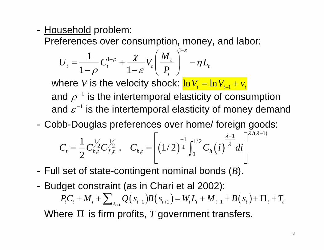
- Household problem: Preferences over consumption, money, and labor:

1

111 1

tt t t t

t

MU C V LP

where V is the velocity shock: 1ln lnt t tV V v and 1 is the intertemporal elasticity of consumption and 1 is the intertemporal elasticity of money demand

- Cobb-Douglas preferences over home/ foreign goods:

1 1

2 2, ,

12t h t f tC C C ,

/( 1)11 1/ 2

, 01/ 2h t hC C i di

- Full set of state-contingent nominal bonds (B).

- Budget constraint (as in Chari et al 2002):

11 1 1

tt t t t t t t t t t ts

PC M Q s B s W L M B s T

Where is firm profits, T government transfers.

9

Household FOCs: - money demand condition:

11 1

(1 )tt t t t

t

M V C i iP

- Labor supply:

t

t t

WPC

- Risk sharing condition:

*

0 *t t t

t t

S P CP C

where S is nominal exchange rate

10

Firms: representative firm, no heterogeneity or entry.

- Production function:

1with shocks: ln ln

t t t

t t t

Y Lu

- Prices set one period ahead to maximize expected profit,

as shown previously.

1 , 1 , 1 1 ,

,1 , 1 ,

1 ,

11 ,

cov

1 1

cov ,

1 1

t t tt c t t t c t t t t c t t

t t th t

t c t t t c t t

tt c t t

ttt

t t c t t

W W WE U C E U C E U CP

E U C E U C

WU CWE

E U C

Price markup includes risk premium that is low if demand for good (function of Ct) is high when marginal cost is low.

11

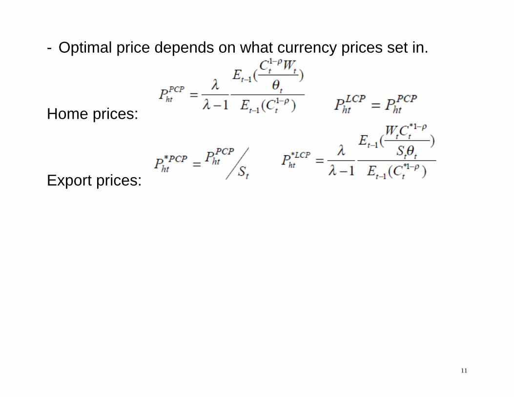
- Optimal price depends on what currency prices set in.

Home prices:

Export prices:

12

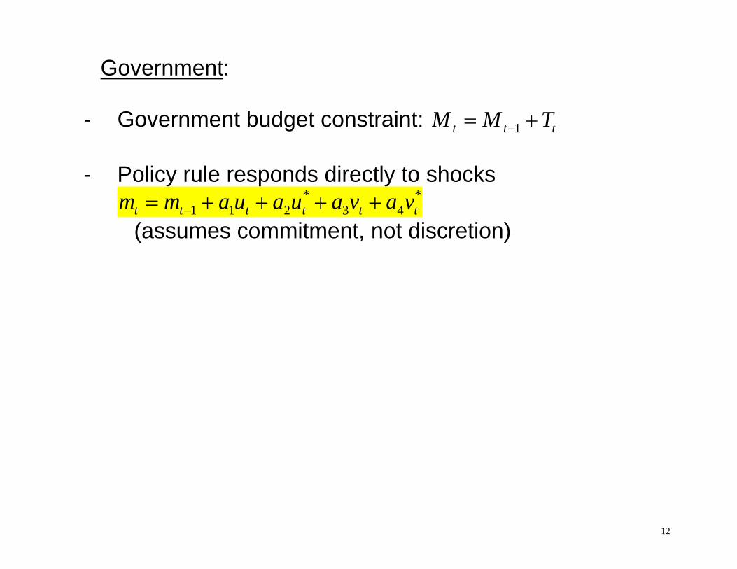
Government:

- Government budget constraint: 1t t tM M T

- Policy rule responds directly to shocks * *

1 1 2 3 4t t t t t tm m a u a u a v a v (assumes commitment, not discretion)

13

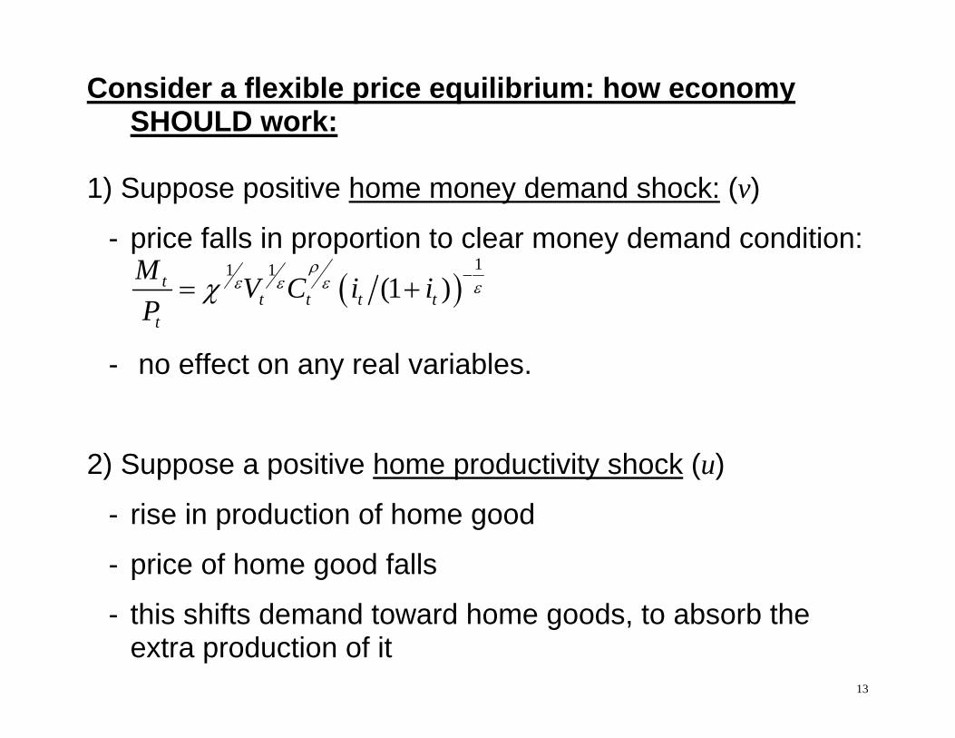
Consider a flexible price equilibrium: how economy SHOULD work:

1) Suppose positive home money demand shock: (v)

- price falls in proportion to clear money demand condition:

11 1

(1 )tt t t t

t

M V C i iP

- no effect on any real variables. 2) Suppose a positive home productivity shock (u)

- rise in production of home good

- price of home good falls

- this shifts demand toward home goods, to absorb the extra production of it

14

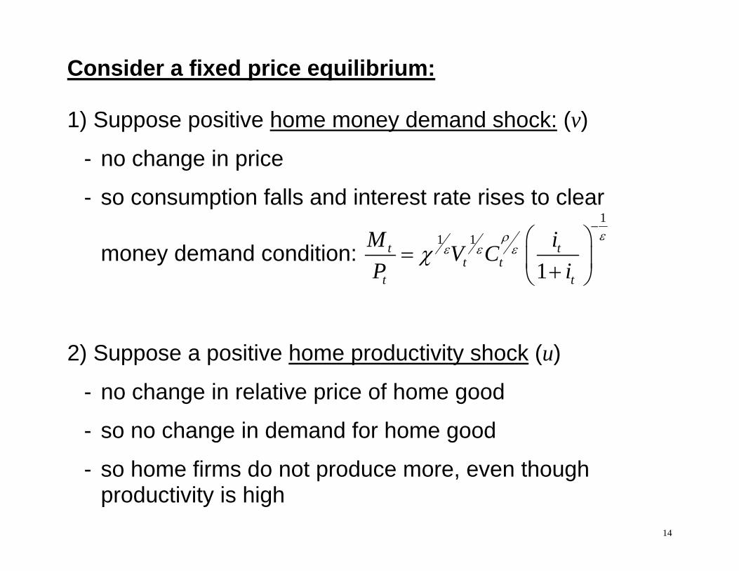
Consider a fixed price equilibrium: 1) Suppose positive home money demand shock: (v)

- no change in price

- so consumption falls and interest rate rises to clear

money demand condition:

1

1 1

1t t

t tt t

M iV CP i

2) Suppose a positive home productivity shock (u)

- no change in relative price of home good

- so no change in demand for home good

- so home firms do not produce more, even though productivity is high

15

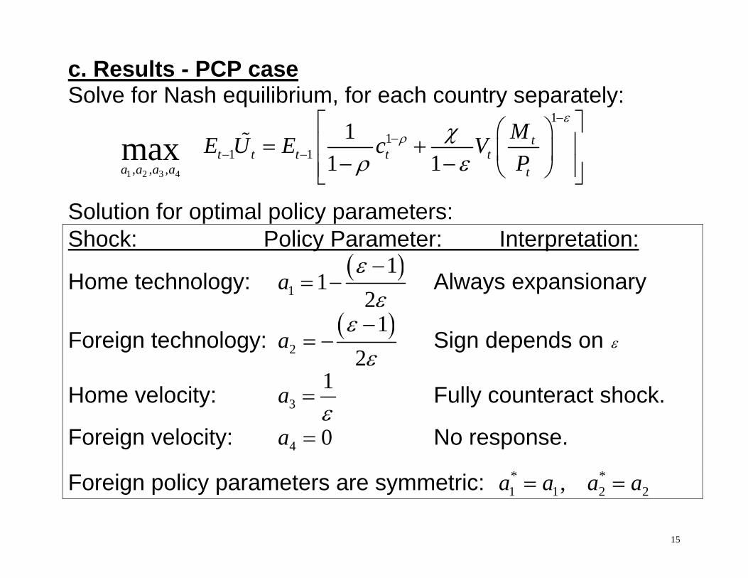
c. Results - PCP case Solve for Nash equilibrium, for each country separately:

1 2 3 4

11

1 1, , ,

11 1max t

t t t t ta a a a t

ME U E c VP

Solution for optimal policy parameters: Shock: Policy Parameter: Interpretation:

Home technology: 1

11

2a

Always expansionary

Foreign technology: 2

12

a

Sign depends on

Home velocity: 31a

Fully counteract shock.

Foreign velocity: 4 0a No response.

Foreign policy parameters are symmetric: * *1 1 2 2,a a a a

16

1) Replicates flexible equilibrium - The sticky price distortion is the only distortion. - Money supply accommodates increased money demand. - When home output rises, need terms of trade shift

demand toward home goods. Can mimic this by increasing the home money supply. (see next point)

2) Flexible exchange rates compensate for sticky prices. - Monetary policy manipulates the exchange rate to shift

the terms of trade to clear the goods market. - So flexible exchange rates are a good thing here. 3) There is no gain from coordinating national policies. Each country can achieve the flexible price equilibrium on

its own, so there is no need to coordinate.

17

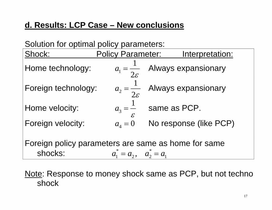
d. Results: LCP Case – New conclusions Solution for optimal policy parameters: Shock: Policy Parameter: Interpretation:

Home technology: 11

2a

Always expansionary

Foreign technology: 21

2a

Always expansionary

Home velocity: 31a

same as PCP.

Foreign velocity: 4 0a No response (like PCP) Foreign policy parameters are same as home for same

shocks: * *1 2 2 1,a a a a

Note: Response to money shock same as PCP, but not techno

shock

18

- Both countries adjust their money supply in exactly the same way to a technology shock.

- This means there is no change in the exchange rate. - This is because the exchange rate no longer affects the

terms of trade. 1) Does not replicate flexible equilibrium The Flexible price equilibrium would involve changes in

the terms of trade, so that demand moves with the increased supply of home goods. This cannot happen here.

2) It is optimal to leave exchange rates fixed. Because exchange rate movements do not serve a

function for shifting demand, there is no reason to manipulate them in the case of technology shocks. (confirmed by examining an explicit exchange rate rule)

19

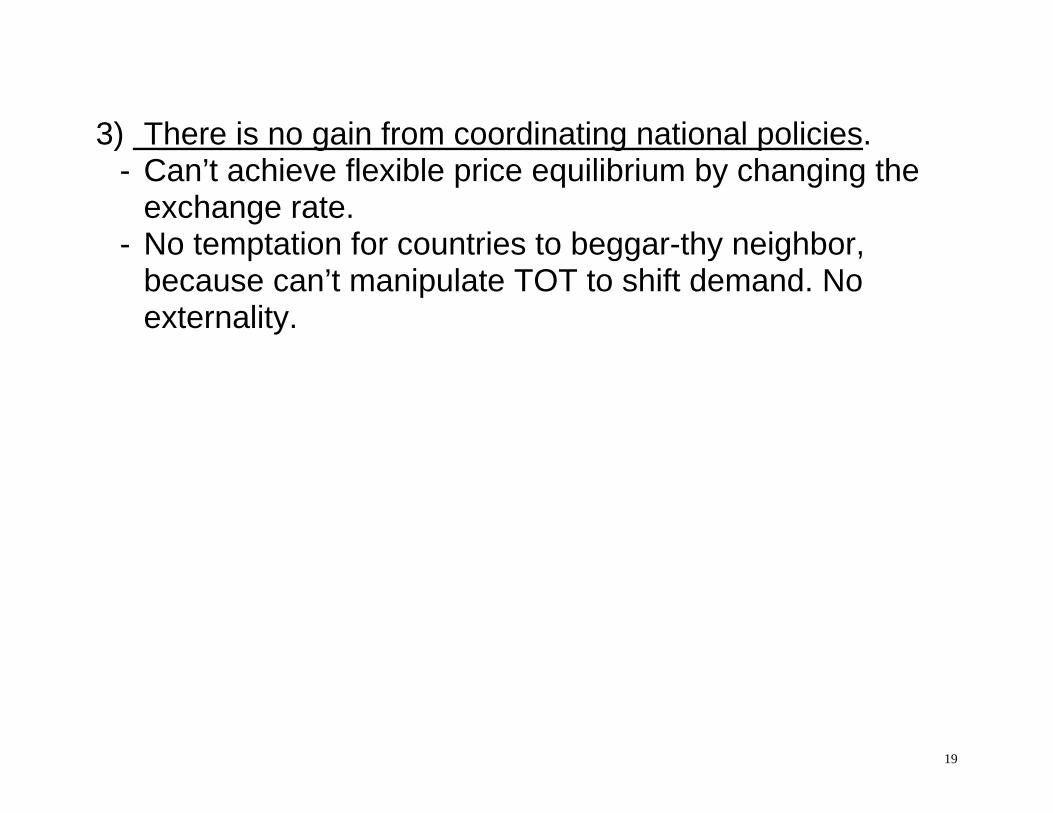
3) There is no gain from coordinating national policies. - Can’t achieve flexible price equilibrium by changing the

exchange rate. - No temptation for countries to beggar-thy neighbor,

because can’t manipulate TOT to shift demand. No externality.

20

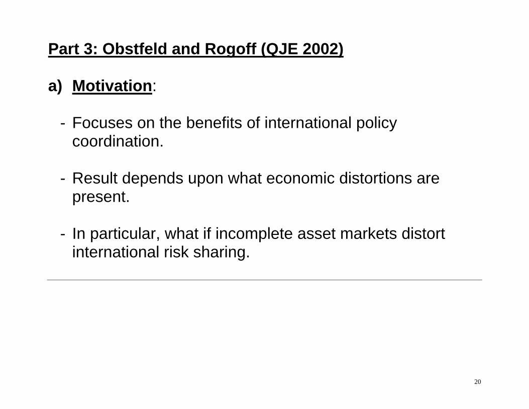
Part 3: Obstfeld and Rogoff (QJE 2002) a) Motivation: - Focuses on the benefits of international policy

coordination. - Result depends upon what economic distortions are

present. - In particular, what if incomplete asset markets distort

international risk sharing.

21

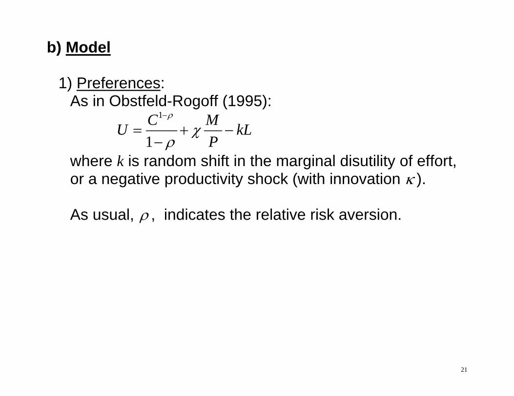
b) Model 1) Preferences: As in Obstfeld-Rogoff (1995):

1

1C MU kL

P

where k is random shift in the marginal disutility of effort, or a negative productivity shock (with innovation ).

As usual, , indicates the relative risk aversion.

22

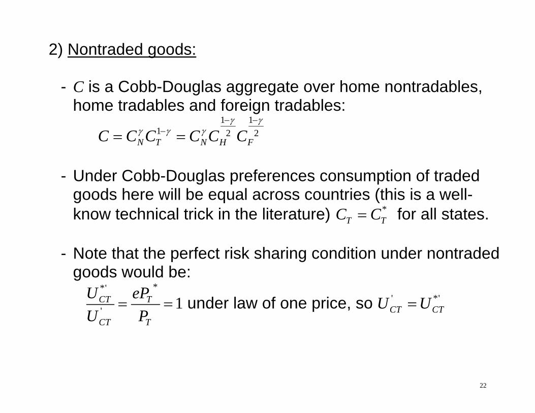
2) Nontraded goods: - C is a Cobb-Douglas aggregate over home nontradables,

home tradables and foreign tradables:

1 1

1 2 2N T N H FC C C C C C

- Under Cobb-Douglas preferences consumption of traded

goods here will be equal across countries (this is a well-know technical trick in the literature) *

T TC C for all states. - Note that the perfect risk sharing condition under nontraded

goods would be:

**'

' 1CT T

CT T

U ePU P

under law of one price, so ' *'CT CTU U

23

- In general we cannot conclude that this is satisfied, because

11' 1 N TCT

T

C CU

C

,

and *T TC C does not ensure that ' *'

CT CTU U , due to nontradeds.

- But in the special case of log utility ( 1 ), we have: ' 11CT TU C , and *

T TC C does ensure that ' *'CT CTU U .

- Main point: risk sharing will fail to hold except in the special

case of 1 . So there will be an additional distortion in the model lowering welfare below the Pareto optimum.

24

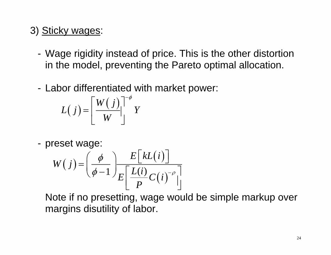
3) Sticky wages: - Wage rigidity instead of price. This is the other distortion

in the model, preventing the Pareto optimal allocation. - Labor differentiated with market power:

W jL j Y

W

- preset wage:

( )1E kL i

W jL iE C iP

Note if no presetting, wage would be simple markup over margins disutility of labor.

25

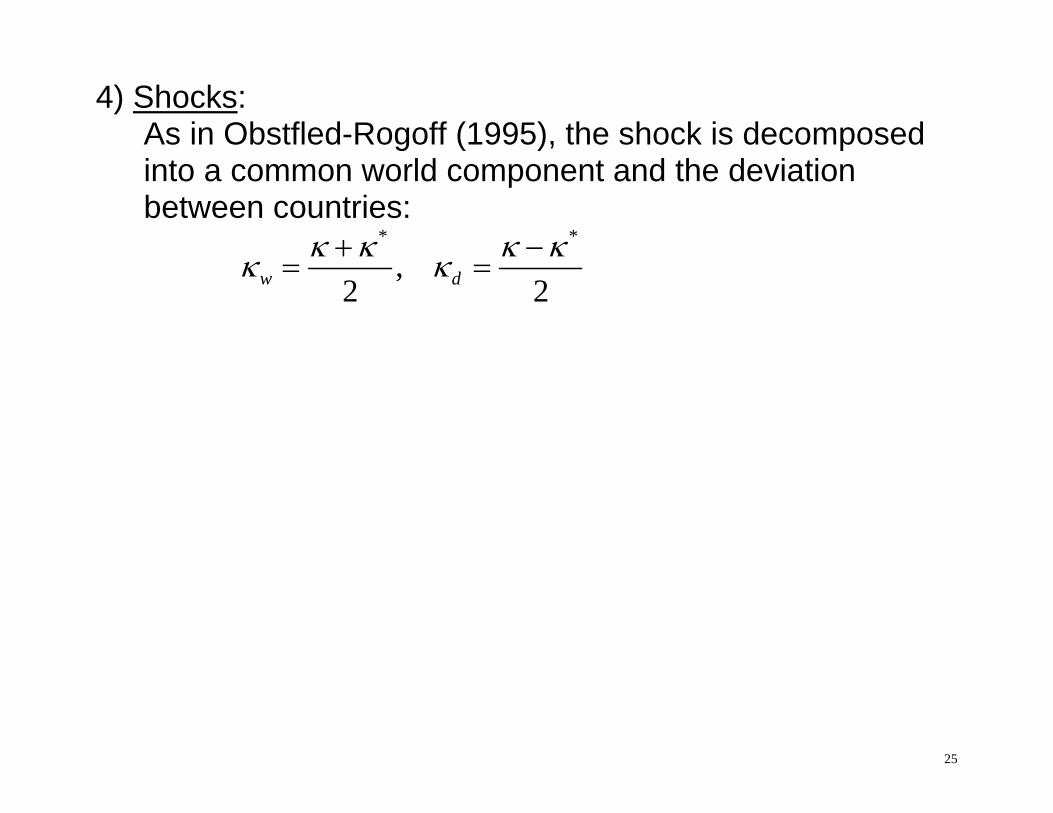
4) Shocks: As in Obstfled-Rogoff (1995), the shock is decomposed

into a common world component and the deviation between countries:

* *

,2 2w d

26

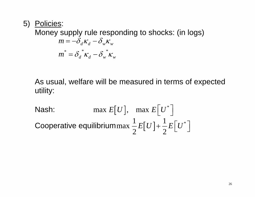
5) Policies: Money supply rule responding to shocks: (in logs)

* **

d d w w

d d w w

m

m

As usual, welfare will be measured in terms of expected

utility: Nash: *max , maxE U E U

Cooperative equilibrium *1 1max2 2

E U E U

27

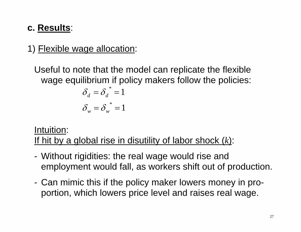
c. Results: 1) Flexible wage allocation: Useful to note that the model can replicate the flexible

wage equilibrium if policy makers follow the policies:

*

*

1

1d d

w w

Intuition: If hit by a global rise in disutility of labor shock (k):

- Without rigidities: the real wage would rise and employment would fall, as workers shift out of production.

- Can mimic this if the policy maker lowers money in pro-portion, which lowers price level and raises real wage.

28

But if only home is hit by the shock:

- Without rigidities: the real wage would rise and employment would fall in only the home country.

- And since output can be produced relatively more easily in the foreign country, the real wage would fall there and induce a rise in employment.

- Can mimic if the home policy maker lowers money supply, and if the foreign country does the opposite.

Conclude:

- It is always possible to eliminate the sticky wage distortion. But Will this lead to a Pareto optimal result?

- Not if there is a second distortion (risk sharing).

29

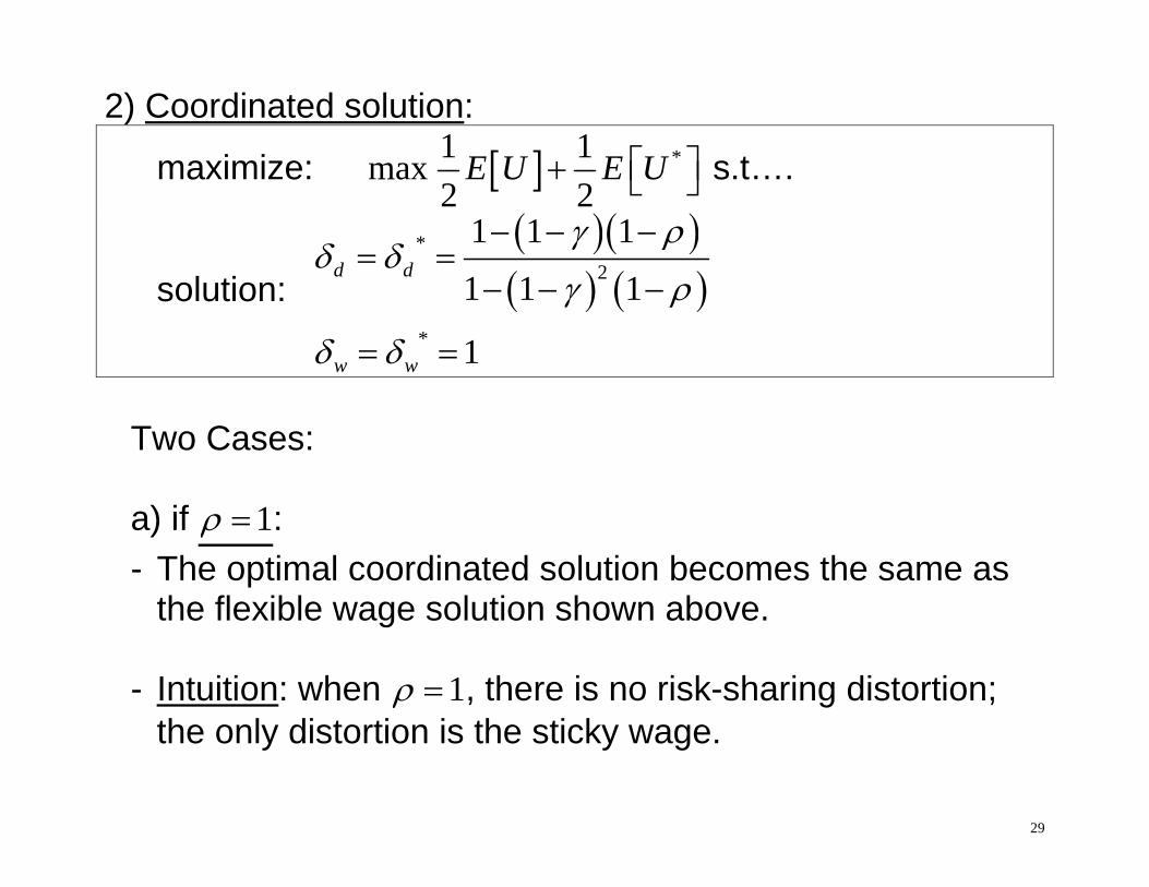
2) Coordinated solution:

maximize: *1 1max2 2

E U E U s.t….

solution:

*2

*

1 1 1

1 1 1

1

d d

w w

Two Cases: a) if 1 : - The optimal coordinated solution becomes the same as

the flexible wage solution shown above. - Intuition: when 1 , there is no risk-sharing distortion;

the only distortion is the sticky wage.

30

b) if 1 : - Now the optimal coordinated policy differs from the flexible

wage solution, for asymmetric shocks d . Intuition: - Policy maker takes advantage of the wage distortion to

help alleviate the lack of risk sharing.

- If shock lowers output in the home country, want to shift some consumption goods from foreign to home country.

- For 1 , do this by lowering home money supply more than otherwise, and raising foreign more. This improves the home terms of trade.

- For 1 , the opposite is true.

31

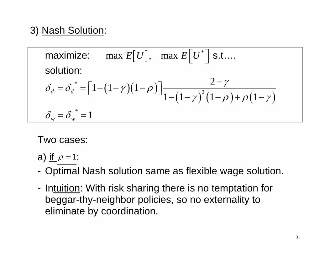
3) Nash Solution: maximize: *max , maxE U E U s.t…. solution:

*

2

*

21 1 11 1 1 1

1

d d

w w

Two cases:

a) if 1 : - Optimal Nash solution same as flexible wage solution.

- Intuition: With risk sharing there is no temptation for beggar-thy-neighbor policies, so no externality to eliminate by coordination.

32

b) if 1 : - Now the Nash response differs from the cooperative

solution. Intuition: - Now there is a lack of international risk sharing, so

temptation for beggar-thy-neighbor policies. - When 1 , this can be accomplished by lowering money

supply less in the home country than in the cooperative solution in response to a home negative productivity shock.

33

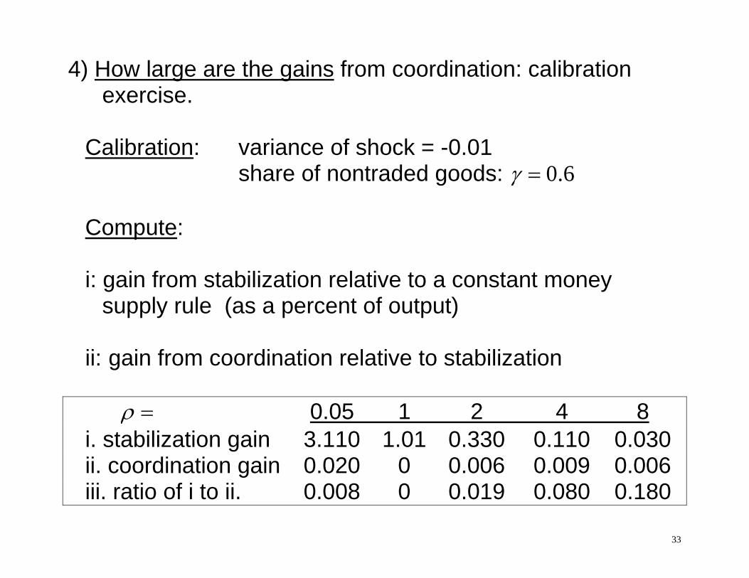
4) How large are the gains from coordination: calibration exercise.

Calibration: variance of shock = -0.01 share of nontraded goods: 0.6 Compute: i: gain from stabilization relative to a constant money

supply rule (as a percent of output) ii: gain from coordination relative to stabilization 0.05 1 2 4 8 i. stabilization gain 3.110 1.01 0.330 0.110 0.030 ii. coordination gain 0.020 0 0.006 0.009 0.006 iii. ratio of i to ii. 0.008 0 0.019 0.080 0.180

34

Conclusions: - Theoretically there may be gains for coordination when

risk sharing is incomplete ( 1 ) - But the experiment indicates that even for rather high and

low values of , the gains from coordination are small relative to the gains from stabilization.

- So there does not appear to be good reason to promote

international monetary policy coordination.

35

Contrast with older literature on coordination:

- Recall that Oudiz and Sachs found the gains from coordi-nation are small because economies are rather closed

- The overall conclusion here is the same as the older literature, but for a different reason.

- Gains are small because when a government pursues optimal policy on its own, this looks very similar to the optimal policy of an international coordinator.

- If integration increases in the future, this will further lower the gains from coordination rather than raise them.

- As the share of traded goods approaches 100%, then risk sharing is complete, and no benefit.

- If asset markets become more integrated, this also im-proves risk sharing and lowers gains from coordination.

36

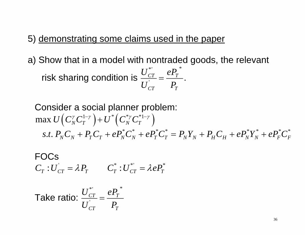
5) demonstrating some claims used in the paper a) Show that in a model with nontraded goods, the relevant

risk sharing condition is **'

'CT T

CT T

U ePU P

.

Consider a social planner problem: 1 * * *1max N T N TU C C U C C

* * * * * * * *. . N N T T N N T T N N H H N N F Fs t P C P C eP C eP C P Y P C eP Y eP C

FOCs

' * *' *: :T CT T T CT TC U P C U eP

Take ratio: **'

'CT T

CT T

U ePU P

37

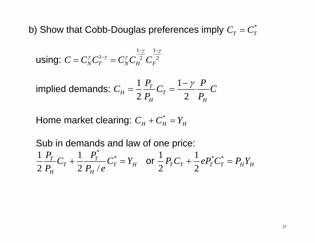
b) Show that Cobb-Douglas preferences imply *T TC C

using: 1 1

1 2 2N T N H FC C C C C C

implied demands: 1 12 2

TH T

H H

P PC C CP P

Home market clearing: *

H H HC C Y Sub in demands and law of one price:

*

*1 12 2 /

T TT T H

H H

P PC C YP P e

or * *1 12 2T T T T H HP C eP C P Y

38

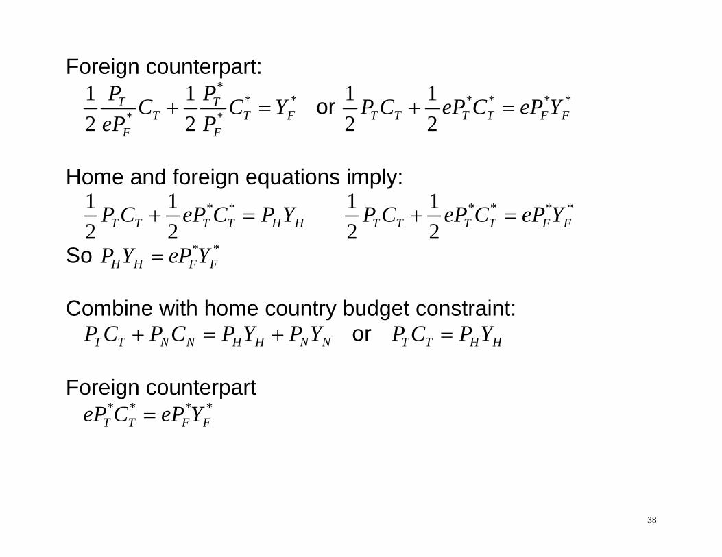
Foreign counterpart:

*

* ** *

1 12 2

T TT T F

F F

P PC C YeP P

or * * * *1 12 2T T T T F FP C eP C eP Y

Home and foreign equations imply:

* *1 12 2T T T T H HP C eP C P Y * * * *1 1

2 2T T T T F FP C eP C eP Y

So * *H H F FP Y eP Y

Combine with home country budget constraint: T T N N H H N NP C P C P Y P Y or T T H HP C P Y Foreign counterpart * * * *

T T F FeP C eP Y

39

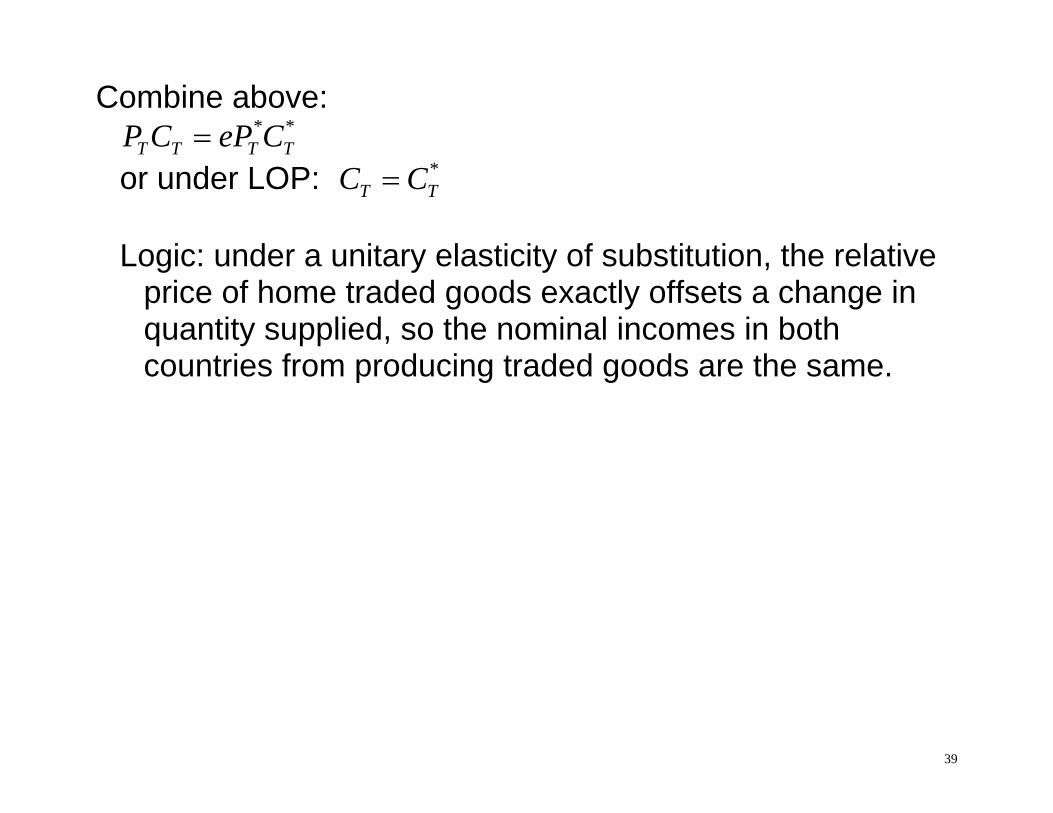
Combine above:

* *T T T TP C eP C

or under LOP: *T TC C

Logic: under a unitary elasticity of substitution, the relative

price of home traded goods exactly offsets a change in quantity supplied, so the nominal incomes in both countries from producing traded goods are the same.