Embed Size (px)
Citation preview

TREND ESTIMATION AND DE-TRENDING
D.S.G. POLLOCKDepartment of Economics, Queen Mary College,University of London,Mile End Road, London E1 4NS, UK
Abstract. An account is given of a variety of linear filters which can be used for extractingtrends from economic time series and for generating de-trended series. A family of rationalsquare-wave filters is described which enable designated frequency ranges to be selectedor rejected. Their use is advocated in preference to other filters which are commonly usedin quantitative economic analysis.
1. Introduction: The Variety of Linear Filters
Whenever we form a linear combination of successive elements of a discrete-time signal y(t) = {yt; t = 0,±1,±2, . . .}, we are performing an operationwhich is described as linear filtering. Such an operation can be representedby the equation
x(t) = !(L)y(t) =!
j
!jy(t ! j), (1)
wherein!(L) = { · · · + !!1L
!1 + !0I + !1L + · · · }, (2)
is described as the filter.The e!ect of the operation it to modify the signal y(t) by altering the
amplitudes of its cyclical components and by advancing or delaying themin time. These modifications are described, respectively, as the gain e!ectand the phase e!ect of the filter. The gain e!ect is familiar through theexample of the frequency-specific amplification of sound recordings whichcan be achieved with ordinary domestic sound systems. A phase e!ect inthe form of a time delay is bound to accompany any signal processing thattakes place in real time.
In quantitative economic analysis, filters are used for smoothing data se-ries, which is a matter of attenuating or even discarding the high-frequencycomponents of the series and preserving the low-frequency components.The converse operation, which is also common, is to extract and discard
bcMS-08.tex; 10/03/2006; 21:02; p.1
2 POLLOCK
the low-frequency trend components so as to leave a stationary sequenceof residuals, from which the dynamics of short-term economic relationshipscan be estimated more easily.
As it stands, the expression under (2) represents a Laurent series com-prising an indefinite number of terms in powers of the lag operator L andits inverse L!1 = F whose e!ects on the sequence y(t) are described by theequations Ly(t) = y(t ! 1) and L!1y(t) = Fy(t) = y(t + 1).
In practice, !(L) often represents a finite polynomial in positive powersof L which is described as a one-sided moving-average operator. Such afilter can only impose delays upon the components of y(t).
Alternatively, the expression !(L), might stand for the series expan-sion of a rational function "(L)/#(L); in which case the series is liable tocomprise an indefinite number of ascending powers of L, beginning withL0 = I. Such a filter is realised via a process of feedback, which may berepresented by the equation
#(L)x(t) = "(L)y(t), (3)
or, more explicitly, by
x(t) = "0y(t) + "1y(t ! 1) + · · · + "dy(t ! d) (4)!#1x(t ! 1) ! · · ·! #gx(t ! g).
Once more, the filter can only impose time delays upon the components ofx(t); and, because the filter takes a rational form, there are bound to bedi!erent delays at the various frequencies.
Occasionally, a two-sided symmetric filter in the form of
!(L) = "(F )"(L) = !0I + !1(F + L) + · · · + !d(F d + Ld) (5)
is employed in smoothing the data or in eliminating its seasonal compo-nents. The advantage of such a filter is the absence of a phase e!ect. Thatis to say, no delay is imposed on any of the components of the signal.The so-called Cramer–Wold factorisation which sets !(L) = "(F )"(L),and which must be available for any properly-designed filter, provides astraightforward way of explaining the absence of a phase e!ect. For thefactorisation enables the transformation of (1) to be broken down into twooperations:
(i) z(t) = "(L)y(t) and (ii) x(t) = "(F )z(t). (6)
The first operation, which runs in real time, imposes time delays on everycomponent of x(t). The second operation, which works in reversed time,imposes an equivalent reverse-time delay on each component. The reverse-time delays, which are advances in other words, serve to eliminate thecorresponding real-time delays.
bcMS-08.tex; 10/03/2006; 21:02; p.2

TREND ESTIMATION AND DE-TRENDING 3
The processed sequence x(t) may be generated via a single applicationof the two-sided filter !(L) to the signal y(t), or it may be generated intwo operations via the successive applications of "(L) to y(t) and "(F ) toz(t) = "(L)y(t). The question of which of these techniques has been usedto generate y(t) in a particular instance should be a matter of indi!erence.
The final species of linear filter that may be used in the processing ofeconomic time series is a symmetric two-sided rational filter of the form
!(L) ="(F )"(L)#(F )#(L)
. (7)
Such a filter must, of necessity, be applied in two separate passes run-ning forwards and backwards in time and described, respectively, by theequations
(i) #(L)z(t) = "(L)y(t) and (ii) #(F )x(t) = "(F )z(t). (8)
Such filters represent a most e!ective way of processing economic data inpursuance of a wide range of objectives.
The essential aspects of linear filtering are recounted in numerous textsdevoted to signal processing. Two that are worthy of mention are by Haykin(1989) and by Oppenheim and Shafer (1989). The text of Pollock (1999)bridges the gap between signal processing and time-series analysis.
In this paper, we shall concentrate on the dual objectives of estimatingeconomic trends and of de-trending data series. However, before we presentthe methods that we wish to advocate, it seems appropriate to provide acritical account of some of the methods that are in common use.
2. Di!erencing Filters
The means of reducing time series to stationarity, which has been employedtraditionally in quantitative economics, has been to take as many di!erencesof the series as are necessary to eliminate the trend and to generate aseries that has a convergent autocovariance function. A sequence of d suchoperations can be represented by the equation
x(t) = (I ! L)dy(t). (9)
This approach to trend-elimination has a number of disadvantages, whichcan prejudice the chances of using the processed data successfully in esti-mating economic relationships.
The first of the deleterious e!ects of the di!erence operator, which iseasily emended, is that it induces a phase lag. Thus, when it is appliedto data observed quarterly, the operator induces a time lag of one-and-a-half months. To compensate for the e!ect, the di!erenced data may be
bcMS-08.tex; 10/03/2006; 21:02; p.3
4 POLLOCK
0
0.25
0.5
0.75
1
0 !/2"!/2 !"!
B
D
S
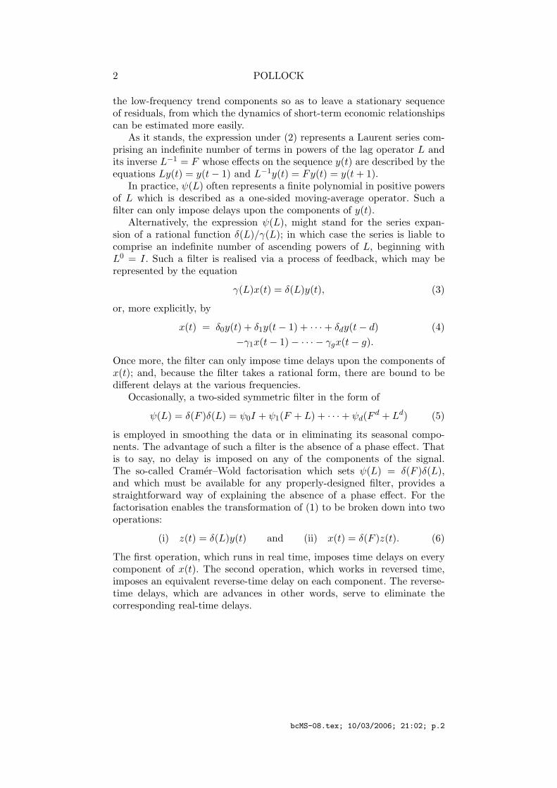
Figure 1. The frequency-response functions of the lowpass filter !S(z) = 14 (z+2+z!1),
the highpass filter !D(z) = 14 (!z + 2 ! z!1) and the binomial filter
!B(z) = 164 (1 + z)3(1 + z!1)3.
shifted forwards in time to the points that lie midway between the obser-vations. When applied twice, the operator induces a lag of three months.In that case, the appropriate recourse in avoiding a phase lag is to applythe operator both in real time and in reversed time. The resulting filter is
(I ! F )(I ! L) = !F + 2I ! L, (10)
which is a symmetric two-sided filter with no phase e!ect.As Figure 1 shows, this filter serves to attenuate the amplitude of the
components of y(t) over a wide range of frequencies. It also serves to increasethe amplitude of the high-frequency components. If the intention is only toremove the trend from the data, then the amplitude of these componentsshould not be altered. In order not to a!ect the high-frequency components,the filter coe"cients must be scaled by a factor of 0.25.
To understand this result, one should consider the transfer-function ofthe resulting filter, which is obtained by replacing the lag operator L bythe complex argument z!1 to give
!D(z) =14( ! z + 2 ! z!1). (11)
The e!ect of the filter upon the component of the highest observable frequency—which is the so-called Nyquist frequency of $ = %—is revealed by settingz = exp{i%}, which creates the filter’s frequency-response function. This is
!D(ei!) =14
"2 ! (ei! + e!i!)
#(12)
bcMS-08.tex; 10/03/2006; 21:02; p.4

TREND ESTIMATION AND DE-TRENDING 5
=14
"2 ! 2 cos(%)
#= 1.
Thus, the gain of the filter, which is the factor by which the amplitude ofa cyclical component is altered, is unity at the frequency $ = %, which iswhat is required.
The condition that has been fulfilled by the filter may be expressedmost succinctly by writing |!D(!1)| = 1, where the vertical lines denotethe operation defined by
|!(z)| =$
!(z)!(z!1), (13)
which, in the case where z = exp{i$}, amounts to taking the complexmodulus. In that case, z is located on the unit circle; and, when it isexpressed as a function of $, |!(exp{i$})| becomes the so-called amplitude-response function, which indicates the absolute value of the filter gain ateach frequency.
In the case of the phase-neutral di!erencing filter of (10), as in the caseof any other phase-free filter, the condition !(z) = !(z!1) is fulfilled. Thiscondition implies that the transfer function !(z) = |!(z)| is a non-negativereal-valued function. Therefore, the operation of finding the modulus isredundant. In general, however, the transfer function is a complex-valuedfunction !(z) = |!(z)| exp{i&($)} whose argument &($), evaluated at aparticular frequency, corresponds to the phase shift at that frequency.
Observe that the di!erencing filter also obeys the condition |!D(1)| = 0.This indicates that the gain of the filter is zero at zero frequency, whichcorresponds to the fact that it annihilates a linear trend, which may beconstrued as a zero-frequency component.
The adjunct of the highpass trend-removing filter !D(z) is a comple-mentary lowpass trend-estimation or smoothing filter defined by
!S(z) = 1 ! !D(z) =14(z + 2 + z!1). (14)
As can be seen from Figure 1, the two filters !S(z) and !D(z) bear a relationof symmetry, with is to say that, when they are considered as functions onthe interval [0,%], they represent reflections of each other about a verticalaxis drawn through the frequency value of $ = %/2. The symmetry con-dition can be expressed succinctly via the equations !S(!z) = !D(z) and!D(!z) = !S(z).
The di!erencing filter !D(z) = 14(1 ! z)(1 ! z!1) and its complement
!S(z) = 14(1 + z)(1 + z!1) can be generalised in a straightforward manner
to generate higher-order filters. Thus, we may define a binomial lowpassfilter via the equation
!B(z) =14n
(1 + z)n(1 + z!1)n. (15)
bcMS-08.tex; 10/03/2006; 21:02; p.5

6 POLLOCK
This represents a symmetric two-sided filter whose coe"cients are equal tothe ordinates of the binomial probability function b(2n; p = 1
2 , q = 12). The
gain or frequency response of this filter is depicted in Figure 1 for the casewhere 2n = 6.
An n increases, the profile of the coe"cients of the binomial filter tendsincreasingly to resemble that of a Gaussian normal probability densityfunction. The same is true of the profile of the frequency-response functiondefined over the interval [!%,%], which is the Fourier transform of thesequence of coe"cients. In this connection, one might recall that the Fourier(integral) transform of a Gaussian distribution is itself a Gaussian distribu-tion. As n increases, the span of the filter coe"cients widens. At the sametime, the dispersion of the frequency-response function diminishes, withthe e!ect that the filter passes an ever-diminishing range of low-frequencycomponents.
It is clear that, for the family of binomial filters, the symmetry of therelationship between the highpass and lowpass filters prevails only in thecase of n = 1. Thus, if !C(z) = 1!!B(z), then, in general, !C(z) "= !B(!z).This is to be expected from the characterisation that we have given above.
It remains to conclude this section by demonstrating the e!ect thatthe simple di!erencing filter of equation (10) is liable to have on a typicaleconomic time series. An example is provided by a series of monthly mea-surements on the U.S. money stock from January 1960 to December 1970.Over the period in question, the stock appears to grow at an acceleratingrate.
Figure 2 shows the e!ect of fitting a polynomial of degree five in thetemporal index t to the logarithms of the data. This constitutes a rough-and-ready means of estimating the trend.
The periodogram of the residuals from the polynomial regression is dis-played in Figure 3. Here, there is evidence of a strong seasonal componentat the frequency of $ = %/6. Components of a lesser amplitude are alsoevident at the harmonic frequencies of $ = %/3, %/2, 2%/3, and there is abarely perceptible component at the frequency of $ = 5%/6.
Apart from these components, which are evidently related to an annualcycle in the money stock, there is a substantial low-frequency component,which spreads over a range of adjacent frequencies and which attains itsmaximum amplitude at a frequency that corresponds to a period of roughlyfour years. This component belongs to the trend; and the fact that it is ev-ident in the periodogram of the residuals is an indication of the inadequacyof the polynomial as a means of estimating the trend.
Figure 4 shows the periodogram of the logarithmic money-stock se-quence after is has been subjected to the di!erencing filter of (10). Asmight be expected, the e!ect of the filter has been to remove the low-
bcMS-08.tex; 10/03/2006; 21:02; p.6

TREND ESTIMATION AND DE-TRENDING 7
4.8
5
5.2
5.4
0 25 50 75 100 125
Figure 2. The logarithms of 132 monthly observations on the U.S. money stock withan interpolated polynomial time trend of degree 5.
0
0.005
0.01
0.015
0 !/4 !/2 3!/4 !
Figure 3. The periodogram of the residuals from fitting a 5th degree polynomial timetrend to the logarithms of the U.S. money stock.
0
0.005
0.01
0.015
0.02
0 !/4 !/2 3!/4 !
Figure 4. The periodogram of a sequence obtained by applying the second-orderdi!erencing filter to the logarithms of the U.S. money stock.
bcMS-08.tex; 10/03/2006; 21:02; p.7

8 POLLOCK
frequency trend components. However, it also has an e!ect which spreadsinto the mid and high-frequency ranges. In summary, we might say that thedi!erencing filter has destroyed or distorted much of the information thatwould be of economic interest. In particular, the pattern of the seasonale!ect has been corrupted. This distortion is liable to prejudice our abilityto build e!ective forecasting models that are designed to take account ofthe seasonal fluctuations.
One might be tempted to use the lowpass binomial filter, defined under(15), as a means of extracting the trend. However, as Figure 1 indicates,even with a filter order of 6, there would be substantial leakage fromthe seasonal components into the estimated trend; and we should needto deseasonalise the data before applying the filter.
In the ensuing sections, we shall describe alternative procedures fortrend extraction and trend estimation. The first of these procedures, whichis the subject of the next section, is greatly superior to the di!erencingprocedure. Nevertheless, it is still subject to a variety of criticisms. Theprocedure of the ultimate section is the one which we shall recommend.
3. Notch Filters
The binomial filter !B(z), which we have described in the previous section,might be proposed as a means of extracting the low-frequency componentsof an economic time series, thereby estimating the trend. The complemen-tary filter, which would then serve to generate the de-trended series, wouldtake the form of !C(z) = 1 ! !B(z).
Such filters, however, would be of limited use. In order to ensure that asu"ciently restricted range of low-frequency components are passed by thebinomial filter, a large value of n would be required. This would entail afilter with numerous coe"cients and a wide time span. When a two-sidedfilter of 2n + 1 coe"cients reaches the end of the data sample, there is aproblem of overhang. Either the final n sample elements must remain un-processed, or else n forecast values must be generated in order to allow themost recent data to be processed. The forecasts, which could be providedby an ARIMA model, for example, might be of doubtful accuracy.
In applied economics, attention is liable to be focussed on the mostrecent values of a data series; and therefore a wide-span symmetric filter,such as the binomial filter, is at a severe disadvantage. It transpires thatmethods are available for constructing lowpass filters which require far fewerparameters.
To describe such methods, let us review the original highpass di!erenc-ing filter of equation (10). Such a filter achieves the e!ect of annihilating atrend component by placing a zero of the function !(z) on the unit circle at
bcMS-08.tex; 10/03/2006; 21:02; p.8

TREND ESTIMATION AND DE-TRENDING 9
" i
i
"1 1Re
Im
" i
i
"1 1Re
Im
Figure 5. The pole–zero diagram of the real-time components of the notch filter !N
(left) and of the Hodrick–Prescott filter !P = 1 ! !N (right) in the case where " = 64.The poles are marked by crosses and, in the case of the notch filter, the double zero atz = 1 is marked by concentric circles.
the point z = 1, which corresponds to a frequency value of $ = 0. Higher-order di!erencing filters are obtained by placing more than one zero at thislocation. However, the e!ect of the zeros is likely to be felt over the entirefrequency range with the deleterious consequences that we have alreadyillustrated with a practical example.
In order to limit the e!ects of a zero of the filter, the natural recourse isto place a pole in the denominator of the filter’s transfer function locatedat a point in the complex plane near to the zero. The pole should havea modulus that is slightly less than unity. The e!ect will be that, at anyfrequencies remote from the target frequency of $ = 0, the pole and thezero will virtually cancel, leaving the frequency response close to unity.However, at frequencies close to $ = 0, the e!ect of the zero, which is onthe unit circle, will greatly outweigh the e!ect of the pole, which is insideit, and a narrow notch will be cut in the frequency response of the transferfunction.
The device that we have described is called a notch filter. It is commonlyused in electrical engineering to eliminate unwanted components, which aresometimes found in the recordings of sensitive electrical transducers andwhich are caused by the inductance of the alternating current of the mainselectrical supply. In that case, the zero of the transfer function is placed, notat z = 1, but at some point on the unit circle whose argument correspondsto the mains frequency Also, the pole and the zero must be accompaniedby their complex conjugates.
The poles in the denominator of the electrical notch filter are commonlyplaced in alignment with the corresponding zeros. However, the notch canbe widened by placing the pole in a slightly di!erent alignment. Such a re-
bcMS-08.tex; 10/03/2006; 21:02; p.9

10 POLLOCK
course is appropriate when the mains frequency is unstable. Considerationsof symmetry may then dictate that there should be a double zero on theunit circle flanked by two poles. If µ denotes a zero and ' denotes a pole,then this prescription would be met by setting
µ1, µ2 = ei" and '1,'2 = (ei"±# with 0 < (< 1, (16)
where $ denotes the target frequency and ) denotes a small o!set. Theaccompanying conjugate values are obtained by reversing the sign of theimaginary number i.
The concept of a notch filter with o!set poles leads directly to the ideaof a rational trend-removal filter of the form
"(z!1)#(z!1)
=(1 ! z!1)2
(1 ! 'z!1)(1 ! '"z!1), (17)
where ' = ( exp{i)} is a pole which may be specified in terms of its modulus( and its argument ), and where '" = ( exp{!i)} is its conjugate. Togenerate a phase-neutral filter, this function must be compounded withthe function "(z)/#(z), which corresponds to the same filter applied inreversed time. Although only two parameters ( and ) are involved, thesearch for an appropriate specification for the filter is liable to be di"cultand time-consuming in the absence of a guiding design formula.
A notch filter, which has acquired considerable popularity amongsteconomists, and which depends on only one parameter, is given by theformula
!N (z) ="(z)"(z!1)#(z)#(z!1)
=(1 ! z)2(1 ! z!1)2
(1 ! z)2(1 ! z!1)2 + *!1. (18)
The placement of its poles and zeros within the complex plane is illustratedin Figure 5. The complement of the filter, which is specified by
!P (z) = 1 ! !N (z) =*!1
(1 ! z)2(1 ! z!1)2 + *!1(19)
is know to economists as the Hodrick–Prescott smoothing filter.The filter was presented originally by Hodrick and Prescott (1980) in a
widely circulated discussion paper. The paper was published as recently as(1997). Examples of the use of this filter have been provided by Kydlandand Prescott (1990), King and Rebelo (1993) and by Cogley and Nason(1995).
The Hodrick–Prescott filter has an interesting heuristic. It transpiresthat it is the optimal estimator of the trajectory of a second-order randomwalk observed with error. Its single adjustable parameter *!1 correspondsto the signal-to-noise ratio, which is the ratio of the variance of the white-noise process that drives the random walk and the variance of the error
bcMS-08.tex; 10/03/2006; 21:02; p.10

TREND ESTIMATION AND DE-TRENDING 11
0.00
0.25
0.50
0.75
1.00
0 !/4 !/2 3!/4 !
116
464
Figure 6. The frequency-response function of the notch filter !N for various values ofthe smoothing parameter ".
0.00
0.25
0.50
0.75
1.00
0 !/4 !/2 3!/4 !
116
464
Figure 7. The frequency-response function of the Hodrick–Prescott smoothing filter !P
for various values of the smoothing parameter ".
0.00
0.10
0.20
0.30
0.00 0.25 0.50 0.75 1.00
#
$
%
Figure 8. The trajectory in the complex plane of a pole of the norch filter !N . The poleapproaches z = 1 as "!1 " 0.
bcMS-08.tex; 10/03/2006; 21:02; p.11

12 POLLOCK
that obscures its observations. It is usual to describe * as the smoothingparameter.
The filter is also closely related to the Reinsch (1976) smoothing spline,which is used extensively in industrial design. With the appropriate choiceof the smoothing parameter, the latter represents the optimal estimator ofthe underlying trajectory of an integrated Wiener process observed witherror.
The e!ect of increasing the value of * in the formula for the smoothingfilter is to reduce the range of the low-frequency components that are passedby the filter. The converse e!ect upon the notch filter is to reduce thewidth of the notch that impedes the passage of these components. Thesetwo e!ects are illustrated in Figures 6 and 7, which depict the frequency-response functions of the two filters. Figure 8 shows the trajectory of thepoles of the filter as a function of the value of *.
In order to implement either the smoothing filter or the notch filter, it isnecessary to factorise their common denominator to obtain an expressionfor #(z). Since z2#(z)#(z!1) is a polynomial of degree four, one can, inprinciple, find analytic expressions for the poles which are in terms of thesmoothing parameter *. Alternatively, one may apply the iterative proce-dures which are used in the obtaining the Cramer–World factorisation of aLaurent polynomial. This is, in fact, how Figure 8 has been constructed.
The Hodrick–Prescott smoothing filter has been subjected to criticismsfrom several sources. In particular, it has been claimed—by Harvey andJaeger (1993) amongst others—that thoughtless de-trending using the filtercan lead investigators to detect spurious cyclical behaviour in economicdata. The claim can only be interpreted to mean that, sometimes, thenotch filter will pass cyclical components which ought to be impeded andattributed to the trend. One might say, in other words, that in such cir-cumstances, the trend has been given a form which is too inflexible. Thisproblem, which cannot be regarded as a general characteristic of the filter,arises from a mismatch of the chosen value of the smoothing parameterwith the characteristics of the data series. However, it must be admittedthat it is often di"cult to find an appropriate value for the parameter.
A more serious shortcoming of the filter concerns the gradation betweenthe stopband, which is the frequency range which is impeded by the filter,and the passband which is the frequency range where the components ofa series are una!ected by the filter. This gradation may be too gentle forsome purposes, in which case there can be no appropriate choice of valuefor the smoothing parameter.
In order to construct a frequency-selective filter which is accuratelyattuned to the characteristics of the data, and which can discriminate ad-equately between the trend and the residue, a more sophisticated method-
bcMS-08.tex; 10/03/2006; 21:02; p.12

TREND ESTIMATION AND DE-TRENDING 13
ology may be called for. We shall attempt to provide this in the ensuingsections of the paper.
4. Rational Square-Wave Filters
In the terminology of digital signal processing, an ideal frequency-selectivefilter is one for which the frequency response is unity over a certain range offrequencies, described as the passband, and zero over the remaining frequen-cies, which constitute the stopband. In a lowpass filter !L, the passbandcovers a frequency interval [0,$c] ranging from zero to a cut-o! point. Inthe complementary highpass filter !H , it is the stopband which stands onthis interval. Thus
|!L(ei")| =%
1, if $ < $c
0, if $ > $c
and |!H(ei")| =%
0, if $ < $c
1, if $ > $c.(20)
In this section, we shall derive a pair of complementary filters thatfulfil this specification approximately for a cut-o! frequency of $c = %/2.Once we have designed these prototype filters, we shall be able to applya transformation that shifts the cut-o! point from $ = %/2 to any otherpoint $c # [0,%].
The idealised conditions of (20), which define a periodic square wave,are impossible to fulfil in practice. In fact, the Fourier transform of thesquare wave is an indefinite sequence of coe"cients defined over the posi-tive and negative integers; and, in constructing a practical moving-averagefilter, only a limited number of central coe"cient can be taken. In such afilter, the sharp disjunction between the passband and the stopband, whichcharacterises the ideal filter, is replaced by a gradual transition. The cost ofa more rapid transition is bound to be an increased number of coe"cients.
A preliminary step in designing a pair of complementary filters is todraw up a list of specifications that can be fulfilled in practice. We shall beguided by the following conditions:
(i) !L(z) + !H(z) = 1, Complementarity (21)
(ii) !L(!z) = !H(z), !H(!z) = !L(z), Symmetry
(iii) !L(z!1) = !L(z), !H(z!1) = !H(z), Phase-Neutrality
(iv) |!L(1)| = 1, |!L(!1)| = 0, Lowpass Conditions
(v) |!H(1)| = 0, |!H(!1)| = 1. Highpass Conditions
bcMS-08.tex; 10/03/2006; 21:02; p.13

14 POLLOCK
There is no reference here to the rate of the transition from the passbandto the stopband. In fact, the condition under (iv) and (v) refer only to theend points of the frequency range [0,%], which are the furthest points fromthe cut-o!.
Observe that the symmetry condition !L(!z) = !H(z) under (ii) ne-cessitates placing the cut-o! frequency at $c = %/2. The condition impliesthat, when it is reflected about the axis of $c = %/2, the frequency responseof the lowpass filter becomes the frequency response of the highpass filter.This feature is illustrated by Figure 10.
It will be found that all of the conditions of (21) are fulfilled by thehighpass di!erencing filter !D defined under (11) in conjunction with thecomplementary lowpass smoothing filter !S = 1 ! !D defined under (14).However, we have already rejected !D and !S on the grounds that theirtransitions between the passband to the stopband are too gradual.
In order to minimise the problem of spectral leakage whilst maintain-ing a transition that is as rapid as possible, we now propose to fulfil theconditions of (21) via a pair of rational functions that take the forms of
!L(z) ="L(z)"L(z!1)#(z)#(z!1)
and !H(z) ="H(z)"H(z!1)#(z)#(z!1)
. (22)
The condition of phase neutrality under (iii) is automatically satisfied bythese forms. We propose to satisfy the lowpass and highpass conditionsunder (iv) and (v) by specifying that
"L(z) = (1 + z)n and "H(z) = (1 ! z)n. (23)
Similar specifications are also to be found in the binomial filter !B of (15)and in the notch filter !N of (18).
Given the specifications under (22), it follows that the symmetry condi-tion of (ii) will be satisfied if and only if every root of #(z) = 0 is a purelyimaginary number. It follows from (i) that the polynomial #(z) must fulfilthe condition that
#(z)#(z!1) = "L(z)"L(z!1) + "H(z)"H(z!1). (24)
On putting the specifications of (23) and (24) into (22), we find that
!L(z) =(1 + z)n(1 + z!1)n
(1 + z)n(1 + z!1)n + (1 ! z)n(1 ! z!1)n(25)
=1
1 +&
i1 ! z
1 + z
'2n
bcMS-08.tex; 10/03/2006; 21:02; p.14

TREND ESTIMATION AND DE-TRENDING 15
and that
!H(z) =(1 ! z)n(1 ! z!1)n
(1 + z)n(1 + z!1)n + (1 ! z)n(1 ! z!1)n(26)
=1
1 +&
i1 + z
1 ! z
'2n .
These will be recognised as instances of the Butterworth filter, which isfamiliar in electrical engineering—see, for example, Roberts and Mullis(1987).
The Butterworth filter, in common with the Hodrick–Prescott filtercan also be derived by applying the Wiener–Kolmogorov theory of signalextraction to an appropriate statistical model. In that context, the filterrepresents a device for obtaining the minimum-mean-square-error estimateof the component in question. See Kolmogorov (1941) and Wiener (1950)for the original expositions of the theory and Whittle (1983) for a modernaccount.
A defining characteristic of the Wiener–Kolmogorov filters is the condi-tion of complementarity of (21) (i). On that basis, we might also regardthe complementary binomial filters !D(z) and !S(z) of (11) and (15),respectively, as Wiener–Kolmogorov filters; but they are unusual in beingrepresented by polynomials of finite degree, whereas filters of this class aremore commonly represented by rational functions.
Since "L(z) and "H(z) are now completely specified, it follows that #(z)can be determined via the Cramer–Wold factorisation of the polynomial ofthe RHS of (24). However, it is relatively straightforward to obtain analyticexpressions for the roots of the equation #(z)#(z!1) = 0. The roots comein reciprocal pairs; and, once they are available, they may be assignedunequivocally to the factors #(z) and #(z!1). Those roots which lie outsidethe unit circle belong to #(z) whilst their reciprocals, which lie inside theunit circle, belong to #(z!1). Therefore, consider the equation
(1 + z)n(1 + z!1)n + (1 ! z)n(1 ! z!1)n = 0, (27)
which is equivalent to the equation
1 +&
i1 ! z
1 + z
'2n
= 0. (28)
Solving the latter for
s = i1 ! z
1 + z(29)
bcMS-08.tex; 10/03/2006; 21:02; p.15

16 POLLOCK
is a matter of finding the 2n roots of !1. These are given by
s = exp" i%j
2n
#, where j = 1, 3, 5, . . . , 4n ! 1, (30)
or j = 2k ! 1; k = 1, . . . , 2n.
The roots correspond to a set of 2n points which are equally spaced aroundthe circumference of the unit circle. The radii, which join the points to thecentre, are separated by angles of %/n; and the first of the radii makes anangle of %/(2n) with the horizontal real axis.
The inverse of the function s = s(z) is the function
z =i ! s
i + s=
i(s + s")2 ! i(s ! s")
. (31)
Here, the final expression comes from multiplying top and bottom of thesecond expression by s" ! i = (i + s)", where s" denotes the conjugate ofthe complex number s, and from noting that ss" = 1. On substituting theexpression for s from (29), it is found that the solutions of (28) are given,in terms of z, by
zk = icos{%(2k ! 1)/2n}
1 + sin{%(2k ! 1)/2n} , where k = 1, . . . , 2n. (32)
The roots of #(z!1) = 0 are generated when k = 1, . . . , n. Those of #(z) = 0are generated when k = n + 1, . . . , 2n.
Figure 9 shows the disposition in the complex plane of the poles andzeros of the prototype lowpass filter !(z)L for the case where n = 6,whilst Figure 10 shows the gain of this filter together with that of thecomplementary filter !(z)H .
5. Frequency Transformations
The object of the filter !L(z) is to remove from a time series a set oftrend components whose frequencies range from $ = 0 to a cut-o! value of$ = $c. The prototype version of the filter has a cut-o! at the frequency$ = %/2. In order to convert the prototype filter to one that will serve thepurpose, a means must be found for mapping the frequency interval [0,%/2]into the interval [0,$c]. This can be achieved by replacing the argument z,wherever it occurs in the filter formula, by the argument
g(z) =z ! +
1 ! +z, (33)
where + = +($c) is an appropriately specified parameter.
bcMS-08.tex; 10/03/2006; 21:02; p.16

TREND ESTIMATION AND DE-TRENDING 17
" i
i
"1 1Re
Im
" i
i
"1 1Re
Im
Figure 9. The pole–zero diagrams of the lowpass square-wave filters for n = 6 when thecut-o! is at # = $/2 (left) and at # = $/8.
0
0.25
0.5
0.75
1
1.25
0 !/4 !/2 3!/4 !
Figure 10. The frequency-responses of the prototype square-wave filters with n = 6 andwith a cut-o! at # = $/2.
0
0.25
0.5
0.75
1
1.25
0 !/4 !/2 3!/4 !
Figure 11. The frequency-responses of the square-wave filters with n = 6 and with acut-o! at # = $/8.
bcMS-08.tex; 10/03/2006; 21:02; p.17

18 POLLOCK
The function g(z) fulfils the following conditions:
(i) g(z)g(z!1) = 1, (34)
(ii) g(z) = z if + = 0,
(iii) g(1) = 1 and g(!1) = !1,
(iv) Arg{g(z)} $ Arg{z} if + > 1,
(v) Arg{g(z)} % Arg{z} if + < 1.
The conditions (i) and (ii) indicate that, if g(z) "= z, then the modulus ofthe function is invariably unity. Thus, as z encircles the origin, g = g(z)travels around the unit circle. The conditions of (iii) indicate that, if z = ei"
travels around the unit circle, then g and z will coincide when $ = 0 andwhen $ = %—which are the values that bound the positive frequency rangeover which the transfer function of the filter is defined. Finally, conditions(iv) and (v) indicate that, if g "= z, then g either leads z uniformly or lagsbehind it as the two travel around the unit circle from z = 1 to z = !1.
The value of + is completely determined by any pair of correspondingvalues for g and z. Thus, from (33), it follows that
+ =z ! g
1 ! gz(35)
=g1/2z!1/2 ! g!1/2z1/2
g1/2z1/2 ! g!1/2z!1/2.
Imagine that the cut-o! of a prototype filter is at $ = & and thatit is desired to shift it to $ = '. Then z = ei$ and g = ei% will becorresponding values; and the appropriate way of shifting the frequencywould be to replace the argument z within the filter formula by the functiong(z) wherein the parameter + is specified by
+ =ei(%!$)/2 ! e!i(%!$)/2
ei(%+$)/2 ! e!i(%+$)/2(36)
=sin{(& ! ')/2}sin{(& + ')/2} .
To find an explicit form for the transformed filter, we may begin byobserving that, when g(z) is defined by equation (33), we have
1 ! g(z)1 + g(z)
=(1 + +
1 ! +
) (1 ! z
1 + z
). (37)
Here there is1 + +
1 ! +=
sin{(& + ')/2} + sin{(& ! ')/2}sin{(& + ')/2}! sin{(& ! ')/2} (38)
bcMS-08.tex; 10/03/2006; 21:02; p.18

TREND ESTIMATION AND DE-TRENDING 19
=sin(&/2) cos('/2)cos(&/2) sin('/2)
.
In the prototype filter, we are setting & = %/2 and, in the transformedfilter, we are setting ' = $c, which is the cut-o! frequency. The result ofthese choices is that
1 + +
1 ! +=
1tan($c/2)
. (39)
It follows that the lowpass filter with a cut-o! at $c takes the form of
!L(z) =1
1 + *&
i1 ! z
1 + z
'2n (40)
=(1 + z)n(1 + z!1)n
(1 + z)n(1 + z!1)n + *(1 ! z)n(1 ! z!1)n,
where * = {1/ tan($c)}2n. The same reasoning shows that the highpassfilter with a cut-o! at $c takes the form of
!H(z) =1
1 +1*
&i1 + z
1 ! z
'2n (41)
=*(1 ! z)n(1 ! z!1)n
(1 + z)n(1 + z!1)n + *(1 ! z)n(1 ! z!1)n.
In applying the frequency transformation to the prototype filter, we arealso concerned with finding revised values for the poles. The conditionsunder (iii) indicate that the locations of the zeros will not be a!ected bythe transformation. Only the poles will be altered. Consider, therefore, thegeneric factor within the denominator of the prototype. This is z!i(, wherei( is one of the poles specified under (30). Replacing z by g(z) and settingthe result to zero gives the following condition:
z ! +
1 ! +z! i( = 0. (42)
This indicates that the pole at z = ( will be replaced by a pole at
z =+ + i(
1 + i(+=
+(1 ! (2) + i((1 ! +2)1 ! (2+2
, (43)
where the final expression comes from multiplying top and bottom of itspredecessor by 1 ! i(+.
Figure 11, displays the pole-zero diagram of the prototype filter andof a filter with a cut-o! frequency of %/8. It also suggests that one of the
bcMS-08.tex; 10/03/2006; 21:02; p.19

20 POLLOCK
e!ects of a frequency transformation may be to bring some of poles closerto the perimeter of the unit circle. This can lead to stability problems inimplementing the filter, and it is liable to prolong the transient e!ects ofill-chosen start-up conditions.
6. Implementing the Filters
The classical signal-extraction filters are intended to be applied to lengthydata sets. The task of adapting them to limited samples often causes di"-culties and perplexity. The problems arise from not knowing how to supplythe initial conditions with which to start a recursive filtering process. Bychoosing inappropriate starting values for the forwards or the backwardspass, one can generate a so-called transient e!ect, which is liable, in fact,to a!ect all of the processed values.
Of course, when the values of interest are remote from either end of along sample, one can trust that they will be barely a!ected by the start-up conditions. However, in many applications, such as in the processing ofeconomic data, the sample is short and the interest is concentrated at theupper end where the most recent observations are to be found.
One approach to the problem of the start-up conditions relies upon theability to extend the sample by forecasting and backcasting. The additionalexta-sample values can be used in a run-up to the filtering process whereinthe filter is stabilised by providing it with a plausible history, if it is workingin the direction of time, of with a plausible future, if it is working in reversedtime. Sometimes, very lengthy extrapolations are called for—see Burman(1980), for example.
The approach that we shall adopt in this paper is to avoid the start-up problem altogether by deriving specialised finite-sample versions of thefilters on the basis of the statistical theory of conditional expectations.
Some of the more successful methods for treating the problem of thestart-up conditions that have been proposed have arisen within the contextof the Kalman filter and the associated smoothing algorithms—see Ansleyand Kohn (1985), De Jong (1991), and Durbin and Koopman (2001), forexample. The context of the Kalman filter is a wide one; and it seems thatthe necessary results can be obtained more easily by restricting the context.
Let us begin, therefore, by considering a specific model for which thesquare-wave filter would represent the optimal device for extracting thesignal, given a sample of infinite length. The model is represented by theequation
y(t) = ,(t) + -(t) (44)
=(1 + L)n
(1 ! L)2.(t) + (1 ! L)n!2/(t),
bcMS-08.tex; 10/03/2006; 21:02; p.20
TREND ESTIMATION AND DE-TRENDING 21
where .(t) and /(t) are statistically independent sequences generated bynormal white-noise processes. This can be rewritten as
(1 ! L)2y(t) = (1 + L)n.(t) + (1 ! L)n/(t) (45)= 0(t) + '(t),
where 0(t) = (1 ! L)2,(t) = (1 + L)n.(t) and '(t) = (1 ! L)2-(t) =(1 ! L)n/(t) both follow noninvertible moving-average processes.
The statistical theory of signal extraction, as expounded by Whittle(1983), for example, indicates that the lowpass filter !L(z) of equation(40) will generate the minimum mean-square-error estimate of the sequence,(t), provided that the smoothing parameter has the value of * = 12
&/12' .
The theory also indicates that the Hodrick–Prescott filter will generate theoptimal estimate in the case where ,(t) is a second-order random walk and-(t) is a white-noise process:
y(t) = ,(t) + -(t) (46)
=1
(1 ! L)2.(t) + -(t).
Now imagine that there are T observations of the process y(t) of equa-tion (44), which run from t = 0, to t = T ! 1. These are gathered in avector
y = , + -. (47)
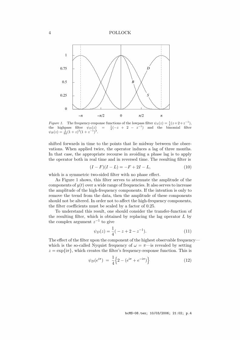
To find the finite-sample the counterpart of equation (45), we need torepresent the second-order di!erence operator (1 ! L)2 in the form of amatrix. The matrix that finds the di!erences d2, . . . , dT!1 of the data pointsy0, y1, y2, . . . , yT!1 is in the form of
Q# =
*
+++++++,
1 !2 1 0 . . . 0 00 1 !2 1 . . . 0 0...
......
... . . . ......
0 0 0 0 . . . 1 00 0 0 0 . . . !2 1
-
......./
. (48)
Premultiplying equation (47) by this matrix gives
d = Q#y = Q#, + Q#- (49)= 0 + ',
where 0 = Q#, and ' = Q#-. The first and second moments of the vector 0may be denoted by
E(0) = 0 and D(0) = 12'M, (50)
bcMS-08.tex; 10/03/2006; 21:02; p.21

22 POLLOCK
and those of ' by
E(') = 0 and D(') = Q#D(-)Q (51)
= 12&Q
##Q,
where both M and Q##Q are symmetric Toeplitz matrices with 2n + 1nonzero diagonal bands. The generating functions for the coe"cients ofthese matrices are, respectively, "L(z)"L(z!1) and "H(z)"H(z!1), where"L(z) and "H(z) are the polynomials defined in (23).
The optimal predictor z of the twice-di!erenced signal vector 0 = Q#,is given by the following conditional expectation:
E(0|d) = E(0) + C(0, d)D!1(d){d ! E(d)} (52)= M(M + *Q##Q)!1d = z,
where * = 12&/1
2' . The optimal predictor k of the twice-di!erenced noise
vector ' = Q#- is given, likewise, by
E('|d) = E(') + C(', d)D!1(d){d ! E(d)} (53)= *Q##Q(M + *Q##Q)!1d = k.
It may be confirmed that z + k = d.The estimates are calculated, first, by solving the equation
(M + *Q##Q)g = d (54)
for the value of g and, thereafter, by finding
z = Mg and k = *Q##Qg. (55)
The solution of equation (54) is found via a Cholesky factorisation whichsets M +*Q##Q = GG#, where G is a lower-triangular matrix. The systemGG#g = d may be cast in the form of Gh = d and solved for h. ThenG#g = h can be solved for g.
There is a straightforward correspondence between the finite-sampleimplementations of the filter and the formulations that assume an infinitesample. In terms of the lag-operator polynomials, equation (54) would berendered as
#(F )#(L)g(t) = d(t), where (56)
#(F )#(L) = "L(F )"L(L) + *"H(F )"H(L).
The process of solving equation (54) via a Cholesky decomposition corre-sponds to the application of the filter in separate passes running forwardsand backwards in time respectively:
(i) #(L)f(t) = d(t) (ii) #(F )g(t) = f(t). (57)
bcMS-08.tex; 10/03/2006; 21:02; p.22

TREND ESTIMATION AND DE-TRENDING 23
The coe"cients of successive rows of the Cholesky factor G converge uponthe values of the coe"cients of #(z); and, at some point, it may becomeappropriate to use the latter instead. This will save computer time andcomputer memory.
The two equations under (55) correspond respectively to
z(t) = "L(F )"L(L)g(t) and k(t) = "H(F )"H(L)q(t). (58)
Our object is to recover from z an estimate x of the trend vector ,.This would be conceived, ordinarily, as a matter of integrating the vectorz twice via a simple recursion which depends upon two initial conditions.The di"culty is in discovering the appropriate initial conditions with whichto begin the recursion.
We can circumvent the problem of the initial conditions by seeking thesolution to the following problem:
Minimise (y ! x)##!1(y ! x) Subject to Q#x = z. (59)
The problem is addressed by evaluating the Lagrangean function
L(x, µ) = (y ! x)##!1(y ! x) + 2µ#(Q#x ! z). (60)
By di!erentiating the function with respect to x and setting the result tozero, we obtain the condition
#!1(y ! x) ! Qµ = 0. (61)
Premultiplying by Q## gives
Q#(y ! x) = Q##Qµ. (62)
But, from (54) and (55), it follows that
Q#(y ! x) = d ! z (63)= *Q##Qg,
whence we get
µ = (Q##Q)!1Q#(y ! x) (64)= *g.
Putting the final expression for µ into (61) gives
x = y ! *#Qg. (65)
This is our solution to the problem of estimating the trend vector ,. Noticethat there is no need to find the value of z explicitly, since the value of xcan be expressed more directly in terms of g = #!1z.
bcMS-08.tex; 10/03/2006; 21:02; p.23

24 POLLOCK
4.8
5
5.2
5.4
0 25 50 75 100 125
Figure 12. The data on the U.S. money stock with an interpolated trend estimated bya lowpass square-wave filter with n = 6 and a cut o! at # = $/8.
0
0.01
0.02
0.03
0
"0.01
"0.02
0 25 50 75 100 125
Figure 13. The residual sequence obtained by detrending the logarithm of the moneystock data with a square-wave filter.
0
0.005
0.01
0.015
0 !/4 !/2 3!/4 !
Figure 14. The periodogram of the residuals from detrending the logarithm of the U.S.money stock data.
bcMS-08.tex; 10/03/2006; 21:02; p.24

TREND ESTIMATION AND DE-TRENDING 25
It is notable that there is a criterion function which will enable us toderive the equation of the trend estimation filter in a single step. Thefunction is
L(x) = (y ! x)##!1(y ! x) + *x#QM!1Q#x, (66)
wherein * = 12&/1
2' as before. This is minimised by the value specified
in (65). The criterion function becomes intelligible when we allude to theassumptions that y & N(,,12
&#) and that Q#, = 0 & N(0,12'M); for then
it plainly resembles a combination of two independent chi-square variates.The e!ect of the square-wave filter is illustrated in Figures 12–14 which
depict the detrending of the logarithmic series of the U.S. money stock. Itis notable that, in contrast to periodogram of Figure 3, which relates to thethe residuals from fitting a polynomial trend, the periodogram of Figure14 shows virtually no power in the range of frequencies below that of theprincipal seasonal frequency.
We should point out that our derivation and the main features of ouralgorithm are equally applicable to the task of implementing the Hodrick–Prescott (H–P) filter and the Reinsch smoothing spline. In the case of theH–P filter, we need only replace the matrices # and M in the equationsabove by the matrices I and Q#Q respectively. Then equation (52) becomes
(I + *Q#Q)!1d = z, (67)
whilst equation (65), which provides the estimate of the signal or trend,becomes
x = y ! *Qz. (68)
References
Ansley, C.F., and R. Kohn, (1985), Estimation, Filtering and Smoothing in State SpaceModels with Incompletely Specified Initial Conditions, The Annals of Statistics, 13,1286–1316.
Burman, J.P., (1980), Seasonal Adjustment by Signal Extraction, Journal of the RoyalStatistical Society, Series A, 143, 321–337.
Cogley, T., and J.M. Nason, (1995), E!ects of the Hodrick–Prescott Filter on Trend andDi!erence Stationary Time Series, Implications for Business Cycle Research, Journalof Economic Dynamics and Control, 19, 253–278.
De Jong, P., (1991), The Di!use Kalman Filter, The Annals of Statistics, 19, 1073–1083.Durbin, J., and S.J. Koopman, (2001), Time Series Analysis by State Space Methods,
Oxford University Press.Harvey, A.C., and A. Jaeger, (1993), Detrending, Stylised Facts and the Business Cycle,
Journal of Applied Econometrics, 8, 231–247.Haykin, S., (1989), Modern Filters, Macmillan Publishing Company, New York.Hodrick, R.J., and E.C Prescott, (1980), Postwar U.S. Business Cycles: An Empirical
Investigation, Working Paper, Carnegie–Mellon University, Pittsburgh, Pennsylvania.
bcMS-08.tex; 10/03/2006; 21:02; p.25

26 POLLOCK
Hodrick R.J., and Prescott, E.C., (1997), Postwar U.S. business bycles: An EmpiricalInvestigation, Journal of Money, Credit and Banking, 29, 1–16.
King, R.G., and S.G. Rebelo, (1993), Low Frequency Filtering and Real Business Cycles,Journal of Economic Dynamics and Control, 17, 207–231.
Kolmogorov, A.N., (1941), Interpolation and Extrapolation. Bulletin de l’academie dessciences de U.S.S.R., Ser. Math., 5, 3–14.
Kydland, F.E., and C. Prescott, (1990), Business Cycles: Real Facts and a MonetaryMyth, Federal Reserve Bank of Minneapolis Quarterly Review, 14, 3–18.
Oppenheim A.V. and R.W. Schafer, (1989), Discrete-Time Signal Processing, Prentice-Hall, Englewood Cli!s, New Jersey.
Pollock, D.S.G., (1999), Time-Series Analysis, Signal Processing and Dynamics, TheAcademic Press, London.
Reinsch, C.H., (1976), Smoothing by Spline Functions, Numerische Mathematik, 10,177–183.
Roberts, R.A., and C.T. Mullis, (1987), Digital Signal Processing, Addison Wesley,Reading, Massachusetts.
Whittle, P., (1983), Prediction and Regulation by Linear Least-Square Methods, SecondRevised Edition, Basil Blackwell, Oxford.
Wiener, N., (1950), Extrapolation, Interpolation and Smoothing of Stationary TimeSeries, MIT Technology Press, John Wiley and Sons, New York.
bcMS-08.tex; 10/03/2006; 21:02; p.26