Embed Size (px)
Citation preview
TRIFT III TOF SIMS
Operator’s Guide Part No 649277 Rev. C
The PHI logo ( ) is a registered trademark of ULVAC-PHI, Inc.
Physical Electronics USA, PHI, WinCadence and Watcher are trademarks of ULVAC-PHI, Inc.
All other trademarks are the property of their respective owners.


Part No. 642151 Rev. A iii
PHI Safety Notices
Physical Electronics’ (PHI’s)products are designed andmanufactured in compliancewith accepted worldwidepractices and standards toprovide protection againstelectrical and mechanicalhazards for the operator andthe area surrounding theproduct. All PHI products aredesigned and intended forprofessional use only, byskilled “operators” for theirintended purpose andaccording to all of theinstructions, safety notices,and warnings provide by PHI.
Those instructions, notices,and warnings assume that an“operator” will not employ anytool when using PHI products.They further assume that alloperators clearly understandthat use of PHI products in anymanner not specified by PHImay impair the protectionprovided by the products andexpose them to hazards.
A “technician” is a qualifiedservicing individual who:
• Has received training towork with voltages above 50 V,
• Has read and understoodthe PHI technician’s manualfor the equipment,
• Observes and under-stands all safety notices onPHI equipment.
The safety symbols that PHIuses are defined on thefollowing page.* To reduce oreliminate hazards, techniciansand operators of thisequipment must fullyunderstand these symbols.
PHI’s products are installedwith international-style orANSI†-style safety notices,according to site requirements.International notices aresymbols within triangles(alerts) or circles (mandatoryactions). PHI’s ANSI-stylesafety notices contain:
• One of three signal words(in all capitals) preceded by thegeneral danger symbol ( );
• One of PHI’s safety symbolsalong with a brief description ofthe hazard and the risk or injurythat could occur;
• Short message thatobserves ANSI’s Hazard AlertTrilogy Rule by identifying thehazard, the possible result ofignoring the notice, and how toavoid the hazard.
The three signal words aredefined as follows:
• DANGER—imminentlyhazardous situation that, if notavoided, will result in death orserious injury;
• WARNING—potentiallyhazardous situation that, if not
avoided, could result in death orserious injury;
• CAUTION—potentiallyhazardous situation or unsafepractice that, if not avoided,may result in minor ormoderate injury or damage toequipment.
SEMI‡ standards requireidentification of type 3, 4, and5 electrical maintenance tasksin equipment manuals:
• Type 3 electricalmaintenance tasks involveenergized equipment, exposedlive circuits, and possibleaccidental contact; potentialexposures are less than 30 VRMS, 42.2 V peak, 240 V-A,and 20 J.
• Type 4 is the same butpotential exposures are greaterthan 30 V RMS, 42.2 V peak,240 V-A, and 20 J or radiofrequency is present.
• Type 5 tasks involveenergized equipment andmeasurements andadjustment require physicalentry into the equipment, orequipment configuration willnot allow the use of clamp-onprobes.
Only experienced, trainedtechnicians should attempt toperform type 3, 4, or 5electrical maintenance tasks.
* Many of PHI’s safety symbols are provided and copyrighted by Hazard Communication Systems, Inc., Milford, PA.* American National Standards Institute, 1430 Broadway, New York, NY 10018.‡ Semiconductor Equipment and Materials International, 805 E. Middlefield Rd., Mountain View, CA 94043-4080.

PHI Safety Notices
Part No. 642151 Rev. A iv
Voltages may be present thatcould cause death or
personal injury.
A risk of death, personal injury,and/or damage to equip-ment exists (and a more
specific label isnot available).
Pulling the plug from its powersource before servicing
is mandatory.
A pinching point is present thatcould cause personal injury.
A risk of explosion or implosionmay be present that could
cause personal injury.
Lifting with assistance orequipment could cause
personal injury.
Visible or invisible radiation maybe present that could cause
personal injury.
Hot surfaces may be presentthat could causepersonal injury.
Turning off the power switchbefore servicing is mandatory.
Refer to the manual(s)before proceeding.
Contents are under pressure.
A harmful or irritant materialmay be present that could
cause personal injury.
Extremely low temperaturesmay be present that could
cause personal injury.
A potentially dangerous
magnetic field may be present.
Wearing protective glovesis mandatory.
Wearing eye protectionis mandatory.
Wearing foot protectionis mandatory.
This is the location of theprotective groundingconductor terminal.
This is the location of the fuse.
This is the location of an earth(ground) terminal.
Contents PHI Safety Notices ................................................................................................... iii Table of Contents..................................................................................................... v Limited Warranty ...................................................................................................... xiii
Section 1: Introduction......................................................................................... 1-1
Operator’s Guide: Purpose and Contents.................................................. 1-2 Introduction to SIMS and TOF-SIMS .......................................................... 1-3
Unique Properties of TOF-SIMS........................................................... 1-5 Brief Introduction to the System.................................................................. 1-7 Data Acquisition Modes .............................................................................. 1-8
Mass Spectra........................................................................................ 1-8 Imaging ................................................................................................. 1-8 Region of Interest (ROI) Analysis......................................................... 1-8 Depth Profiles ....................................................................................... 1-9 Retrospective Analysis: Raw Data Files............................................... 1-9
How To Reach PHI Customer Service........................................................ 1-10
Section 2: Mounting & Introducing Samples ..................................................... 2-1 Cleanliness of the Sample Preparation and Mounting Area....................... 2-1 Cleaning Sample Holders and Accessories................................................ 2-1 Back Mounting for Fixed Z Position ............................................................ 2-2
Quadrant Sample Carrier and Sample Holders.................................... 2-2 Large, Single Window Sample Carrier (50 mm Systems).................... 2-4 300mm 200mm and 150mm Sample Carriers ..................................... 2-4
Load Lock and Sample Carrier Introduction/Removal (All Systems).......... 2-5 Sample Carriers for 50mm Systems .................................................... 2-5 Sample carriers for 300mm and 200mm systems................................ 2-8
Digital Scanner Option ................................................................................ 2-10 Finding the Analysis Position ...................................................................... 2-12 Typical Procedures in Escosy (8” TRIFT Systems) .................................... 2-12
Stage Directions ................................................................................... 2-12 Methods of Moving the Stage............................................................... 2-13 Pre-Alignment....................................................................................... 2-14 Loading a Project.................................................................................. 2-14 Position Lists......................................................................................... 2-15 Wafer Maps .......................................................................................... 2-16 Coordinate Window .............................................................................. 2-16 Adjust Three Points .............................................................................. 2-16 Importing KLA Coordinates and Finding Defects ................................. 2-17 Stage Initialization ................................................................................ 2-17 Align Exchange Position....................................................................... 2-18
TRIFT II TOF-SIMS Operator’s Guide v

Contents
Align the 4-Position Marker .................................................................. 2-19 Find Rotation Center ............................................................................ 2-20
Section 3: Instrument State Files ........................................................................ 3-1
System Setup Prior to Analysis................................................................... 3-1 The Concept of Instrument States: “INS” Files..................................... 3-1 Inspecting the Library of Instrument State Files ................................... 3-1 Creating New Instrument State Files.................................................... 3-2 Filter-Loading Part of the Instrument State Files.................................. 3-3
Section 4: Tuning the Primary Beams ................................................................. 4-1
Liquid Metal Ion Gun (LMIG)....................................................................... 4-1 Firing the Source .................................................................................. 4-2 Tuning of the LMIG............................................................................... 4-7 Optimizing the LMIG for High Spatial Resolution................................. 4-13 Optimizing the LMIG for High Mass Resolution ................................... 4-14 Primary Beam Dose Calculation for LMIG Experiments ...................... 4-17
Cesium Ion Gun .......................................................................................... 4-19 Precautions........................................................................................... 4-19 Ion Gun Overview................................................................................. 4-19 Ion Source Operation ........................................................................... 4-19
Operation .................................................................................................... 4-20 Oven Set Temp Function...................................................................... 4-20 Tuning for Spectroscopy at 10kV Beam Energy .................................. 4-22 D.C. Beam Alignment ........................................................................... 4-24 Pulsing and Bunching Operations Yield Short Primary Pulses ............ 4-25 Tuning the Pulsing and Bunching Operations ...................................... 4-26 Low Energy Cesium Beam Alignment.................................................. 4-28
Dual Source Column Option ....................................................................... 4-29 General Description.............................................................................. 4-29
Duoplasmatron Ion Source ......................................................................... 4-31 General Description.............................................................................. 4-31 Source Operation using the Model 20-740 Source Controller ............. 4-32 Starting Values (First Time Firing)........................................................ 4-33 Normal Source Operating Conditions................................................... 4-35
Electron Neutralization Gun ........................................................................ 4-37 Testing for Filament Current and Filament Continuity.......................... 4-37 Setting the Correct Filament Current.................................................... 4-38 Measuring/Maximizing Pulsed Electron Current .................................. 4-39
Sputter Gas Gun ......................................................................................... 4-42 Gas Gun Overview ............................................................................... 4-42 Gas Gun Operatiion.............................................................................. 4-42 Conditioning the Gas Gun Ionizer and High Voltage ........................... 4-47 Setup and Calibrating the Argon Gas Regulation ................................ 4-47 Creating New or Tuning Existing Gas Gun Parameters....................... 4-49
TRIFT III TOF-SIMS Operator’s Guide vi

Contents
D.C. Beam Alignment ........................................................................... 4-51 SED-based method for tuning the D.C. Gas Gun beam w/ 0v float ..... 4-51 Method for tuning the D.C. Gas Gun beam with a float voltage........... 4-52 Timed Sputter ....................................................................................... 4-54 Gas Gun Ionizer Shutdown .................................................................. 4-54
Section 5: System Alignments ............................................................................ 5-1
Alignment of Primary Beam Analysis Area with SIMS Optics..................... 5-1 Concept of SIMS Acceptance Area...................................................... 5-1 Effect of Sample Height Variations....................................................... 5-1 Use of Primary Beam Steering (Beam Position) .................................. 5-6 Setup, Verification of Primary Beam Alignment to the Spectrometer... 5-7
Alignment of Viewing (Light Optics) to SIMS Optics................................... 5-8 Alignment of Viewing Optics................................................................. 5-8
Alignment of + and - SIMS Fields of View (Polarity Offsets) ...................... 5-9 Primary Beam Steering Effects in Different Polarities.......................... 5-9 Determining the Polarity Offset Values ................................................ 5-9
Section 6: Tuning the Spectrometer ................................................................... 6-1
Theoretical Aspects of Spectrometer Operation......................................... 6-1 Physical Effects Influencing High Mass Resolution TOF Analysis....... 6-2 Secondary Ion Focusing System: Stigmatic Secondary Ion Optics ..... 6-4
Practical Aspects of Spectrometer Operation............................................. 6-8 DEM (Dynamic Emittance Matching) ................................................... 6-8 Secondary Ion Filters............................................................................ 6-10 Practical Method: Tuning the Spectrometer for High Mass Resolution 6-13
Section 7: Data Acquisition.................................................................................. 7-1
System Configuration.................................................................................. 7-1 Mass Spectra .............................................................................................. 7-2
Setting and Varying the Primary Pulse Width of the LMIG .................. 7-2 Imaging ....................................................................................................... 7-3
SIMS Images: Peak Window............................................................... 7-3 Creating Peak Lists .............................................................................. 7-3 SED Images.......................................................................................... 7-5 Mosaic Mapping ................................................................................... 7-6
TOF-SIMS Depth Profiling .......................................................................... 7-11 Definitions and Descriptions ................................................................. 7-11 Near-Surface, TOF-SIMS Profiling with High Current Pulsed Beams.. 7-12 TOF-SIMS at Depth with Aanalysis / Sputter Ssequence .................... 7-12 Phased Depth Profiling......................................................................... 7-13 Interleaved Depth Profiling ................................................................... 7-14 Practical System Set-up ....................................................................... 7-16 Profiling Tools: Enhancing Small Area Imaging of Insulators ............. 7-24 Depth Profiling of Insulators ................................................................. 7-28
TRIFT III TOF-SIMS Operator’s Guide vii

Contents
Retrospective Analysis: ‘Raw’ Data Files................................................... 7-29 Region-of-Interest (ROI) Analysis ............................................................... 7-30
Section 8: Charge Neutralization of Insulators.................................................. 8-1
Sample Charging in SIMS with Positive Ion Beams ................................... 8-1 Recognizing Charging Effects: System Diagnosis ............................... 8-2
Extraction Field Penetration: Techniques for Obtaining Data..................... 8-8 Use of Metallic Grids ................................................................................... 8-8 Practical Guide to Insulating Samples ........................................................ 8-9 General Description of the Electron Neutralization Scheme....................... 8-14 Changing Default Electron Gun Parameters .............................................. 8-14 Techniques for Optimum Charge Dissipation ............................................. 8-15
Section 9: Sample Preparation Techniques....................................................... 9-1
Powder Samples ......................................................................................... 9-1 Loose Powders..................................................................................... 9-1 Preparation from slurries ...................................................................... 9-5
Preparation and Mounting of Cross-Section Samples................................ 9-7 Analysis of Fiber Samples .......................................................................... 9-10
Analysis of single fibers along the axial direction................................. 9-10 Analysis of fiber mats ........................................................................... 9-13 Analysis of fiber cross-sections ............................................................ 9-14
Rough Samples........................................................................................... 9-18 Introduction........................................................................................... 9-18 Recovery of Mass Resolution from Rough Surfaces ........................... 9-18
Difficult Geometry Samples ........................................................................ 9-21 Sample Mounting.................................................................................. 9-27
Cold Stage Option [50mm (2”) Introduction Systems] ................................ 9-27 Operation of the Cold Stage................................................................. 9-28
Section 10: Routine Instrument Evaluation / Maintenance............................... 10-1
Introduction ................................................................................................. 10-1 System Bakeout .......................................................................................... 10-1
Bakeout Prerequisites .......................................................................... 10-1 Bakeout Preparations ........................................................................... 10-2 Starting the Bake .................................................................................. 10-3 After the Bakeout.................................................................................. 10-5
Statistical Process Control (SPC) ............................................................... 10-6 Example of SPC Measurement ............................................................ 10-7
Immersion Lens Conditioning ..................................................................... 10-8 Regular Lens Conditioning as a Routine Practice................................ 10-9 Conditioning Lens Elements After a System Vent................................ 10-10 Remedial Action for an Electron Emitting Lens.................................... 10-11
Logging Operating Values and Performance.............................................. 10-11 Leaving/Inheriting the System in a ‘Standard State’ ................................... 10-11
TRIFT III TOF-SIMS Operator’s Guide viii

Contents
A Typical 'Standard State' ........................................................................... 10-12 Routine System Back-Up on External Media.............................................. 10-13
Section 11: Preventative Maintenance Schedules, Info.................................... 11-1
Introduction ................................................................................................. 11-1 Tools Required............................................................................................ 11-2 Preventative Maintenance (PM) Checklist .................................................. 11-2
PM Checklist......................................................................................... 11-3 PM Schedule ........................................................................................ 11-4 TRIFT PM Parts Checklist .................................................................... 11-5
Routine Maintenance .................................................................................. 11-9 Cesium Ion Gun Source ....................................................................... 11-9 Cesium Ion Gun Column ...................................................................... 11-9 Console Panels .................................................................................... 11-9 Cooling Filters....................................................................................... 11-9 Convectron Gauges.............................................................................. 11-10 Detector (DMCP) .................................................................................. 11-11 Emergency Manual Off (EMO) Box Lamps .......................................... 11-11 Ion Gauges ........................................................................................... 11-12 Light Source.......................................................................................... 11-13 Liquid Metal Ion Gun (LMIG) ................................................................ 11-13 Rough Pump (Alcatel) .......................................................................... 11-13 System Vacuum Control (SVC)............................................................ 11-13 Sample Bias Feedthrough / Connector ................................................ 11-14 Turbo, Rough Pump Maintenance (Wicks) .......................................... 11-14 Vacuum Gauge Controls ...................................................................... 11-15
Appendix A: Service Procedures ........................................................................ A-1
Rigorous Heating to Start the LMIG Source ............................................... A-1 Mechanical Alignment of Cs Column to Analysis Region ........................... A-2
Appendix B: Mass Resolution Tuning Grid........................................................ B-1 Appendix C: Indium Liquid Metal Ion Source (LMIS) ........................................ C-1
LMIS Installation into the TRIFT ................................................................. C-1 Vacuum................................................................................................. C-1
Conditioning the Source.............................................................................. C-1 High Voltage Conditioning.................................................................... C-1 Outgassing the LMIS ............................................................................ C-2
Operation .................................................................................................... C-2 Igniting the Source ...................................................................................... C-2 Day to Day Operation.................................................................................. C-3 Revitalizing the Indium Source (Every 1 -2 Months)................................... C-4 Instrument Parameters Affected by the Indium LMIS ................................. C-5
TRIFT III TOF-SIMS Operator’s Guide ix
Contents
Figures
1-1 An Illustration of the SIMS Process ............................................................ 1-4 1-2 An Example of a TOF-SIMS Mass Spectrum. ............................................ 1-6 2-2 Example of the Stage Control window using Scanned Images. ................. 2-10 4-1 Current versus Voltage Characteristics for a Clean LMI Source. ............... 4-3 4-2 Surface Oxide Thickness versus Time on a Liquid Metal Source. ............. 4-4 4-3 Surface Oxide Thickness as a Function of the Sublimation Process. ........ 4-6 4-4 Schematic Diagram of the LMIG Gun. ........................................................ 4-8 4-5 Principal Effects of Mass Resolution versus Mass in TOF-SIMS. .............. 4-14 4-6 Cutaway View of the Duoplasmatron Source. ............................................ 4-21 4-7 Schematic Diagram of the Cesium Ion Gun. .............................................. 4-23 4-8 Flowchart Diagram of the Cesium Ion Gun Alignment Procedure.............. 4-24 4-9 Long Pulse Produced by Blanker 1 Entering the Buncher Region. ............ 4-25 4-10 Buncher Pulsing Sequence......................................................................... 4-25 4-11 Blanker 2 Operation. ................................................................................... 4-26 4-12 Compressed Buncher Pulse. ...................................................................... 4-26 4-13 Dual Source Ion Column Schematic. .......................................................... 4-30 4-14 Schematic Diagram of the Duoplasmatron Ion Source............................... 4-31 4-15 Illustration of the Sources Tabbed Page..................................................... 4-34 4-16 Correlation between Pressure in the Ion Source and Arc Voltage ............. 4-36 4-17 Illustration of Ion Gun Emission Current vs. Filament Current................... 4-38 4-18 Schematic of the Faraday cup assembly for 50mm TRIFT Systems. ........ 4-40 4-19 Schematic of the Faraday cup assembly for 200mm TRIFT Systems. ...... 4-41 4-20 Schematic Diagram of the Sputter Ion Gun ................................................ 4-50 5-1 Sample at the Optimum Height within the Analysis Chamber. ................... 5-3 5-2 TOF Image of the Acceptance Area as seen by the Spectrometer ............ 5-3 5-3 Sample Height too High within the Analysis Chamber. .............................. 5-4 5-4 TOF Image of the Acceptance Area with the Sample Position too High. ... 5-4 5-5 Sample Height too Low within the Analysis Chamber. ............................... 5-5 5-6 TOF Image of the Acceptance Area with the Sample Position too Low. .... 5-5 6-1 Schematic Diagram of the TOF-SIMS Mass Spectrometer. ....................... 6-4 6-2 Secondary Ion Image Path within the TOF-SIMS Mass Spectrometer. ..... 6-6 6-3 Example of the DEM tabbed page in WinCadence. ................................... 6-9 6-4 The Principal Effects of Mass Resolution vs. Mass in TOF-SIMS.............. 6-13 6-5 Plot of Channel Number of Organic Species CxHy. .................................... 6-15 7-1 Mosaic Map Ion Images. ............................................................................. 7-6 7-2 Mosaic Mapping tab of the Acquisition setup Dialog. ................................. 7-7 7-3 Data Appears in a stepwise fashion during Mosaic Map Acquisition ......... 7-9
TRIFT III TOF-SIMS Operator’s Guide x
Contents
7-4 The Imaging tab of the Tools/Options Dialog. ............................................ 7-10 7-5 Timing Schematic of the Dual-Beam Interleaved Mode. ............................ 7-15 7-6 Change in Sample Surface Potential as a Function of Acquisition Time.... 7-24 7-7 Using Phased Acquisition to Minimize Surface Effects of Insulators.......... 7-26 7-8 Example of the Acquisition Setup window with Profile Settings ................. 7-27 8-1 Recognizing Charging Effects: Positive Mass Spectrum (1). ..................... 8-3 8-2 Recognizing Charging Effects: Positive Mass Spectrum (2). ..................... 8-3 8-3 Recognizing Charging Effects: Positive Mass Spectrum (3). ..................... 8-4 8-4 Recognizing Charging Effects: Positive Mass Spectrum (4). ..................... 8-4 8-5 Recognizing Charging Effects: Negative Mass Spectrum (1)..................... 8-6 8-6 Recognizing Charging Effects: Negative Mass Spectrum (2)..................... 8-6 8-7 Recognizing Charging Effects: Negative Mass Spectrum (3)..................... 8-7 8-8 Recognizing Charging Effects: Negative Mass Spectrum (4)..................... 8-7 9-1 Diagram of Trapping Loose Powders on Double-Sided Adhesive Tape. ... 9-2 9-2 Diagram of Indium Powder “Sandwich”. ..................................................... 9-3 9-3 Diagram of Dry Powder Compacts. ............................................................ 9-4 9-4 Diagram of Settling from Fine Suspension. ................................................ 9-5 9-5 Diagram of Preparation from Slurries. ........................................................ 9-6 9-6 Diagram of Cross Section Samples: Microtoming. ..................................... 9-8 9-7 Diagram of Fracture Cross Section............................................................. 9-9 9-8 Diagram of Analysis of Fibers: Axial Direction............................................ 9-11 9-9 Diagram of Mounting without a Backing Plate or Adhesive Tape............... 9-12 9-10 Diagram of Mounting Fiber Mats................................................................. 9-13 9-11 Diagram of Epoxy Mounting........................................................................ 9-14 9-12a Diagram of Cross-Sectioning of Free-Standing Fibers. .............................. 9-16 9-12b Diagram of Cross-Sectioning of Free-Standing Fibers. .............................. 9-17 9-13 The Effect of Topography on Mass Spectra. .............................................. 9-19 9-14 Sample Geometry for a Woven Fiber Mat with Variable Heights. .............. 9-20 9-15 A Variety of Samples Mounted in the Sample Holders for the TRIFT III. ... 9-21 9-16 Cross Section View of the Various Sample Holders for the TRIFT III. ....... 9-22 9-17 Cross Section View of the Various Sample Holders for the TRIFT III. ....... 9-22 9-18 The Process of Sample Preparation from a Metallic Tube. ........................ 9-25 9-19 The Process of Sample Preparation from a Ceramic Tube. ....................... 9-26 9-20 Cutaway Diagram of the Cold Stage “Gooseneck Assembly”. ................... 9-28 10-1 Diagram of the Bakeout Warning Sign........................................................ 10-4 11-1 Diagram of the Convectron Gauge Pin Layout ........................................... 11-11 11-2 View of the Ion Gauge Filament Assembly ................................................. 11-12 11-3 Location of the Backup Battery within the System Vacuum Control........... 11-14
TRIFT III TOF-SIMS Operator’s Guide xi
Contents
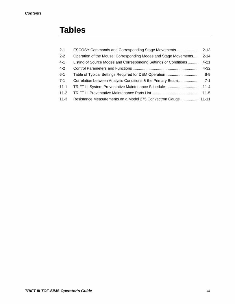
Tables
2-1 ESCOSY Commands and Corresponding Stage Movements.................... 2-13 2-2 Operation of the Mouse: Corresponding Modes and Stage Movements.... 2-14 4-1 Listing of Source Modes and Corresponding Settings or Conditions ......... 4-21 4-2 Control Parameters and Functions ............................................................. 4-32 6-1 Table of Typical Settings Required for DEM Operation.............................. 6-9 7-1 Correlation between Analysis Conditions & the Primary Beam.................. 7-1 11-1 TRIFT III System Preventative Maintenance Schedule .............................. 11-4 11-2 TRIFT III Preventative Maintenance Parts List ........................................... 11-5 11-3 Resistance Measurements on a Model 275 Convectron Gauge ................ 11-11
TRIFT III TOF-SIMS Operator’s Guide xii

Part No. 617281
Limited Warranty
Except as otherwise provided herein, the Sellerwarrants to Buyer that the equipment soldhereunder, whether it is new equipment orremanufactured (reconditioned) equipment, is, atthe time of shipment to Buyer from Seller, freefrom defects in material and workmanship. AsBuyer’s sole exclusive remedy under thiswarranty Seller agrees either to repair or replace,at Seller’s sole option and free of part charge toBuyer, any part or parts of such equipmentwhich, under proper and normal conditions of useprove to be defective within 12 months from thedate of receipt by the Buyer. Warranty period forequipment requiring installation by Seller willcommence on completion of standard installationservices. If customer delays installation beyond45 days after delivery, the warranty period willcommence to run 45 days after delivery. Afterinstallation, any realignment, readjustment,recleaning or recalibration, provided it does notrelate to a proven defect in material orworkmanship, shall be performed only at Seller’sthen current rates for service.
Exclusions and LimitationsIt is recognized that some parts by their nature(expendable items) may not function for one fullyear; therefore, excluded from the foregoingwarranty are filaments, anodes, cathodes,multipliers, retard grids, special ceramics,ionizers, along with other such parts mentionedin the applicable operating manual.
The foregoing warranty excludes certain majoritems or accessories specifically indicated onapplicable price lists or quotations, as to whichSeller passes to Buyer whatever warranty isprovided to Seller by the manufacturer or the
specific warranty indicated by the price list orquotation.
This warranty does not cover loss, damage, ordefects resulting from transportation to theBuyer’s facility, improper or inadequatemaintenance by Buyer, buyer-supplied softwareor interfacing, unauthorized modification ormisuse, operation outside of the environmentalspecifications for the equipment or improper sitepreparation and maintenance.
Product ServiceAll claims must be brought to the attention ofSeller within 30 days of the failure to perform.
Seller at his option may require the product to bereturned to the factory, transportation prepaid, forrepair.
Refund of Purchase PriceIn lieu of the foregoing, Seller may at any timeelect, in its sole discretion, to discharge itswarranty by accepting the return of suchequipment and refunding any portion of thepurchase price paid by Buyer.
Software and Firmware ProductsThe sole exclusive warranty applicable tosoftware and firmware products provided bySeller for use with a processor will be as follows:Seller warrants that such software and firmwarewill conform to Seller’s program manuals currentat the time of shipment to Buyer when properlyinstalled on that processor. Seller does notwarrant that the operation of the processorsoftware or firmware will be uninterrupted orerror free.
No other warranty is expressed or implied. Seller expressly disclaims the impliedwarranties of merchantability and fitness for a particular purpose.
TRIFT III TOF-SIMS Operator’s Guide 1-1
Section 1:Introduction
Physical Electronics, Inc. (PHI) provides three main system manuals whichpertain to the TRIFT III system—this operator’s guide, and the Operator’sWinCadence Version 3.5 Software Reference Manual, several individual OEMand PHI-based components, including the system computer, printer, turbopumps, monitors, gauges, and some electronics units.
This manual should be used in conjunction with the WinCadence SoftwareReference manual and the Hardware manual for the TRIFT III TOF-SIMSsystem. The software manual describes the user interface and details allfunctions within the software. The hardware manual describes the systemhardware, periodic service procedures, and contains a complete set of systemcable diagrams.
This TRIFT III Operator’s Guide takes the system operator through operationsequences, from system startup to data acquisition, to system log off andshutdown. It is intended as a resource for getting familiar with how to operatethe TRIFT III system under routine conditions.
Physical Electronics’ TRIFT III system is operated using one main interactingsoftware application, namely WinCadence. This software operates inconjunction with the Microsoft Windows NT operating system. The operatoruses the WinCadence software to set all instrument parameters, perform dataacquisition, data reduction, and publishing of the results. An additional softwareutility known as Watcher is also used on the TRIFT III system for controllingvarious pneumatic valves on the vacuum console.
This section presents an overview of Time-of-Flight Secondary Ion MassSpectrometry (TOF-SIMS) and data acquisition using the TRIFT III TOF-SIMS:
• Operator’s Guide: Purpose and Contents.• Introduction to SIMS and TOF-SIMS.• Brief Introduction to the System.• Data Acquisition Modes.• How To Reach PHI Customer Service.
Section 1: Introduction
TRIFT III TOF-SIMS Operator’s Guide 1-2
Operator’s Guide: Purpose and ContentsThe TRIFT III, once installed in the analytical laboratory, can be operated in a"push and go" mode, using pre-recorded "instrument states", with littleknowledge of primary gun or spectrometer tuning. However, as the userbecomes more familiar with the operation of the instrument, it is inevitable thathe or she will want to delve deeper into how the instrument functions, so as toexplore the full capabilities of this powerful analysis tool. This guide has beenwritten with that aim in mind. Many of the sections are extremely detailed and itis certainly not necessary to read and understand all that is written for you tomake good use of the instrument initially. Like all users' guides, you willprobably begin to consult it after you have had some "hands on" experience. Theguide is used as a basis for your instrument training, and can be used thereafter asa reference to remind you of certain principles and methods that you learnedduring training.
The layout of the guide follows the logical sequence in which you come acrossvarious aspects of the instrument as you move from loading a sample through todata acquisition. Some of the sections, such as LMIG fine tuning andspectrometer theory and tuning may appear not only daunting, but rather overlydetailed, especially as we have noted that the instrument is designed for routine"push and go" analysis without having to worry about such tuning. While it isintended that most analyses be conducted in this way, we do not wish to withholddetailed descriptions on how to proceed if you have to conduct the tuningyourself, and thus the details in these sections are for those who wish tounderstand why the instrument defaults have been set the way they are.
The operator’s guide attempts to follow the order in which various aspects of theinstrument are encountered when performing a typical analysis:
Section 2—Start your analysis sequence by first mounting and introducing asample. This section details how to mount various size sample carriers for thetwo different types of sample introduction systems (50 mm and 200 mm).
Section 3—Calling up the instrument files from the computer to setup the systemin the required ‘state’ is the next step prior to analysis.
Section 4—Tuning the TRIFT primary beams is the third step in the analysisprocess. This should be set automatically by the instrument file and need noadjustment. However, if necessary, detailed tuning of the LMIG, the Cesium gun,and the low energy electron neutralizer are all covered in this section.
Section 5—The next required step is to perform a simple, software-assistedalignment of the primary beam(s) to the mass spectrometer acceptance area. Thissection details this alignment, as well as adjustment of the light optics, and thepositive and negative fields of view.

Section 1: Introduction
TRIFT III TOF-SIMS Operator’s Guide 1-3
Section 6The next step involves matching the energy of the secondary ions tothe mass spectrometer. The mass spectrometer is normally not adjusted from dayto day, but a detailed explanation is provided in this section should it benecessary to check the spectrometer tuning.
Section 7—This section explores the various types of analysis which can beperformed, including mass spectral acquisition, imaging, depth profiling,retrospective analysis, and ROI (Region-of-Interest) analysis.
Section 8This section covers charge neutralization of insulators.
Section 9—This section is an extensive treatment of sample preparationtechniques including all different types of samples (i.e., powders, slurries,fracture samples, cross sections, fibers etc.)
Section 10This section outlines routine instrument evaluations and generalmaintenance including any procedures of a non-service nature (i.e., those tasksthat do not require a field service engineer or technician).
Introduction to SIMS and TOF-SIMSWhen energetic "primary" ions (typically, several keV) bombard a samplesurface in vacuum, various atoms and molecules are 'sputtered' from that surface.A small percentage of those sputtered species are ionized naturally and may beextracted by an electric field and then transferred into a mass spectrometer,where their mass-to-charge ratios are measured. The "secondary ions" (todistinguish them from the primary bombarding ions) are emitted from only thetop few atom layers, and thus secondary ion mass spectrometry, or "SIMS",belongs to the family of surface analytical techniques which include Augerelectron spectroscopy (AES) and X-ray photoelectron spectroscopy (XPS) forcharacterization of material surfaces.
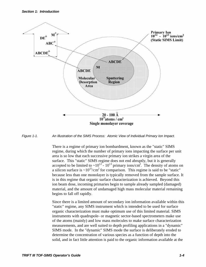
Energy from the primary ion is transferred into the sample surface in such a waythat, in the immediate vicinity of the impact site, considerable fragmentation ofthe original surface occurs, resulting in the release primarily of atomic and lowmass molecular species. Further out from the impact site the energy imparted tothe substrate results in the release of higher mass molecular species. This isillustrated in Figure 1-1 below.
Section 1: Introduction
TRIFT III TOF-SIMS Operator’s Guide 1-4
Figure 1-1. An Illustration of the SIMS Process: Atomic View of Individual Primary Ion Impact.
There is a regime of primary ion bombardment, known as the "static" SIMSregime, during which the number of primary ions impacting the surface per unitarea is so low that each successive primary ion strikes a virgin area of thesurface. This "static" SIMS regime does not end abruptly, but it is generallyaccepted to be limited to ~1012 - 1013 primary ions/cm2. The density of atoms ona silicon surface is ~1015/cm2 for comparison. This regime is said to be "static"because less than one monolayer is typically removed from the sample surface. Itis in this regime that organic surface characterization is achieved. Beyond thision beam dose, incoming primaries begin to sample already sampled (damaged)material, and the amount of undamaged high mass molecular material remainingbegins to fall off rapidly.
Since there is a limited amount of secondary ion information available within this"static" regime, any SIMS instrument which is intended to be used for surfaceorganic characterization must make optimum use of this limited material. SIMSinstruments with quadrupole- or magnetic sector-based spectrometers make useof the atoms (mainly) and low mass molecules to make surface characterizationmeasurements, and are well suited to depth profiling applications in a "dynamic"SIMS mode. In the "dynamic" SIMS mode the surface is deliberately eroded todetermine the concentration of various species as a function of depth into thesolid, and in fact little attention is paid to the organic information available at the

Section 1: Introduction
TRIFT III TOF-SIMS Operator’s Guide 1-5
outer surface. To be fair, quadrupole SIMS instruments have been usedsuccessfully for many years to perform static SIMS measurements, although thequadrupole is a relatively inefficient analyzer considering the limited informationavailable in the static SIMS regime. More recently, instruments based on time-of-flight mass spectrometers have been added to the SIMS family, increasing therange of secondary ion detection out to many thousands of mass units, andmaking optimum use of those molecular secondary ion species released from theouter periphery of the primary ion impact zone.
Unique properties of TOF-SIMS
In a quadrupole or magnetic sector SIMS analyzer, the spectrometer scansthrough the mass range to record a mass spectrum. If the mass spectrometer isanalyzing Fe it is not analyzing Al or Cu or indeed any other secondary species.This is not a serious restriction if only one or two species are being monitored ina depth profile, but it is a problem for surface studies within the static SIMSregime. By contrast, the TOF spectrometer is a parallel detection analyzer whichdoes not scan through the mass range and thus no information is lost whenrecording a mass spectrum. As well as parallel detection, a well-designed TOFspectrometer has extremely high transmission even when operating at high massresolution. In the TRIFT III analyzer, approximately 80-90% of organicmolecular ions entering the mass spectrometer are recorded at the detector.
Since the basis of the TOF-SIMS mass measurement is the accurate measurementof secondary ion flight times from start to finish, it is clear that there must be astart time. This is achieved by pulsing the primary ion beam. This is verydifferent to quadrupole and magnetic sector SIMS instruments in which theprimary beam(s) operate in a continuous (d.c.) mode. As well as pulsing, if theprimary beam is also focused and scanned over the sample surface, the output ofthe secondary ion detector may be synchronized with the primary beam raster toproduce SIMS images (and also secondary electron images). Owing to theefficient use of secondary ion signal via parallel detection and high transmission,mass spectra and SIMS images can be recorded during the static SIMS regime,and thus the technique is unique as a surface organic microprobe.
During each analytical 'cycle', there are relatively long periods when the primarybeam is off and the secondary ions are traveling around to the detector. Forinsulator analysis, it is possible to collapse the extraction field to zero during thistime and inject low energy (20eV) electrons to perform charge neutralization.Thus, unlike continuous primary beam SIMS instruments, insulator analysis inTOF-SIMS is relatively trivial.
Section 1: Introduction
TRIFT III TOF-SIMS Operator’s Guide 1-6
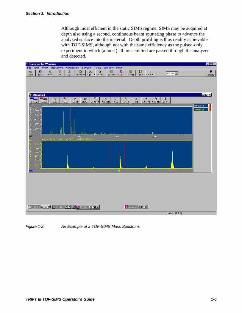
Although most efficient in the static SIMS regime, SIMS may be acquired atdepth also using a second, continuous beam sputtering phase to advance theanalyzed surface into the material. Depth profiling is thus readily achievablewith TOF-SIMS, although not with the same efficiency as the pulsed-onlyexperiment in which (almost) all ions emitted are passed through the analyzerand detected.
Figure 1-2. An Example of a TOF-SIMS Mass Spectrum.

Section 1: Introduction
TRIFT III TOF-SIMS Operator’s Guide 1-7
Brief Introduction to the SystemThe PHI TRIFT III (TRIple Focusing Time-of-Flight) is a high transmission,parallel detection instrument that been designed to make optimum use of all thesecondary ion species leaving the sample surface, and can thus be used for bothorganic surface characterization and elemental analysis. The instrument has aunique and patented time-of-flight analyzer which has the highest angular andenergy acceptance of all commercially available TOF-SIMS instruments. Theanalyzer continually re-focuses the secondary ions within the spectrometer, andthis permits a number of powerful experiments to be performed with thesecondary ion beam. The primary ion beams are also designed with state-of-the-art technology to permit imaging at high lateral resolution and with high massresolution, and are under computer control. A variety of instrumental settings fordifferent analytical needs are simply re-called at the loading of a single file. Thesoftware package, WinCadence, has been developed and evolved with theextensive interaction of TOF-SIMS analysts to make operation of the instrumentsimple and effective.
Considering the sophistication of the TRIFT mass spectrometer's secondary ionoptics, the mass spectrometer is extremely simple to use, and is almost neveradjusted once the instrument has been installed. The mass spectrometer has beenset during installation to operate at high performance when passing secondaryions which have an energy of ~3000eV. Thus, the only parameter which theanalyst may need to adjust (in the case of insulating samples) is the samplepotential, which effectively matches the energy of the secondary ions to the massspectrometer. An angular filter and an energy filter are available, and are easilymoved into place if required. For most analyses, the spectrometer is operated"fully open", i.e. with no filters in place.
With regard to the primary ion beams, the liquid metal ion gun (LMIG) is anextremely powerful and versatile tool, which can operate over 3 orders ofmagnitude of primary beam current, from 20nA down to 20pA. The gun istypically operated either at 15kV for optimization of high mass resolutionspectroscopy (9000 FWHM) simultaneous with a 2µm imaging capability, or at25kV for small probe sizes (0.5µm down to ~100nm) with low to medium massresolution (up to ~5000 FWHM). The high current mode (20nA) is usedprimarily for spectroscopy, while the low current modes (≤ 60pA) are usedexclusively for small probe applications. The broader beam Cs gun is typicallyused either for spectroscopy at 10kV, or as a low energy (≤ 1keV) beam foroptimization of TOF-SIMS depth profiling. The electron gun used for lowenergy (≤ 20eV) electron charge compensation of insulators is focused into astatic probe of ~3mm diameter. Operation is automatic and self stabilizing.
Section 1: Introduction
TRIFT III TOF-SIMS Operator’s Guide 1-8
Data Acquisition ModesMass Spectra
Generation of a mass spectrum (intensity vs. mass-to-charge ratio) from a samplesurface is at the heart of the TOF-SIMS technique. Mass spectral data can beacquired in either positive or negative SIMS (but not both simultaneously), andcan be acquired from all vacuum compatible materials, including insulators.Volatile samples may be analyzed via the cold stage option. Mass spectralfragments from mass 1 (H) to many thousands of mass units (e.g. polymericoligomer distributions) can be recorded at the detector. Mass spectral acquisitionoccurs using either the Cs or LMIG gun to provide the primary ion beam, and avariety of beam energies from ~5-10kV (Cs) and ~5-25kV (LMIG) are available.Mass spectral analysis may or may not involve simultaneous imaging of thesample surface.
Imaging
When lateral distributions of surface species are required, the LMIG is the iongun of choice, since it provides sub-micrometer probes. A variety of primarycurrents from 20nA to 20pA are available, and, as with any charged beamtechnique, there is a trade off between probe size and primary beam current(equivalent to data rate). At the highest available beam energy (25kV), shortprimary beam pulses (high mass resolution) are achieved by reducing theprimary pulse width in software. This preserves the primary beam probe size,but reduces the secondary ion count rates. To obtain high mass resolutionwithout loss of secondary ion count rates, the LMIG is operated at 15kV and theprimary beam is “bunched” (electrodynamically compressed). One consequenceof this method of maintaining a short (sub-nanosecond) pulse without choppingthe beam is that the probe size increases significantly. The TRIFT III LMIGprovides a 2-3µm probe simultaneous with a sub-nanosecond, bunched pulse.
Region of Interest (ROI) Analysis
The primary beam raster is under full computer control, and it is possible toextract mass spectral information from any ‘region(s)-of-interest’ visible in animage. The system can acquire full images and selectively port out mass spectraldata when the ion beam is in the user-defined ‘region-of-interest’. Region-of-interest data can also be acquired retrospectively (see Retrospective Analysis:Raw Data Files below).
Section 1: Introduction
TRIFT III TOF-SIMS Operator’s Guide 1-9
Depth Profiles
In a pulsed-only mode of operation, the ‘duty cycle’ (time on: time off) of theprimary beam is such that the analysis typically occurs in the ‘static’ SIMSregime. If the primary current is increased to ≥20nA, the repetition rate inincreased to >25kHz, and the primary beam raster reduced, it is possible tosample to depths of ~100A in acquisition times of 20-30 minutes with a pulsedbeam. For greater depths, it is necessary to invoke a separate d.c. sputteringphase (with no mass measurement) in order to expose new material at depth.This can be achieved with a single gun system, or with a dual beam system. If ad.c. phase is used, then the sensitivity falls, since most of the material removed isnot analyzed. Such TOF-SIMS profiles are useful, but the inherent sensitivity ofthe technique is sacrificed to make such measurements.
Retrospective Analysis: Raw Data Files
Because of the parallel detection capabilities of the technique, it is possibleduring data acquisition to record (store) the x and y position, the time-of-flight(mass) and appearance time (within the acquisition) of every secondary ionrecorded at the detector. Such files can be extremely large, but this facilitymakes it possible to analyze data retrospectively. This can be invaluable (forinstance) if the analyst is analyzing an unknown sample, conducting failureanalysis or analyzing a unique and limited amount of material. In such cases it isoften difficult at the beginning of the analysis to anticipate what species areimportant to monitor and therefore which images will prove to be mostinformative. In retrospective analysis of ‘raw’ files, mass spectral data can bereconstructed from ‘regions-of-interest’ visible in an image, or images can be re-created from any peak in the mass spectrum. Depth profiles may also beacquired in this mode.

Section 1: Introduction
TRIFT III TOF-SIMS Operator’s Guide 1-10
How to Reach PHI Customer Service
If any PHI manufactured or supported controls or equipment fail or otherproblem-solving is called for, contact PHI Customer Service as follows:
By mail:
Physical Electronics, Inc.
PHI Customer Service, M/S G11
6509 Flying Cloud Drive
Eden Prairie, MN 55344
USA
ULVAC-PHI, Inc.
ULVAC-PHI Customer Service Organization
370, Enzo, Chigasaki
253-0084 Japan
By e-mail:
[email protected] (USA)
[email protected] (Japan - Domestic)
[email protected] (Japan - International)
By telephone or fax:
Region Telephone Fax
U.S. 1-800-922-4744 1-952-828-6325
Outside U.S. 1-952-828-5831 1-952-828-6325
Japan 81-467-85-6522 81-467-85-4411
Europe 49-89-96275-0 49-89-96275-50

TRIFT III TOF-SIMS Operator’s Guide 2-1
Section 2:Mounting & Introducing Samples
This section of the operator's guide discusses the process of mounting samples onthe sample carriers, then steps through the process of introducing the mountedsamples into the analysis chamber using the sample introduction system.
Cleanliness of the Sample Preparation and Mounting AreaWhen mounting samples for TOF-SIMS analysis, always maintain a cleanpreparation area: remember the technique is surface sensitive. The followingsteps will help in maintaining clean preparation surfaces when mountingsamples.
1. Cut a square of aluminum foil and tape the edges to a flat preparation benchor preferably to a small square of thick window glass. The surfaces of mostcommercially available Aluminum foil are extremely clean. Replace the foilsurface based on usage.
2. Obtain a supply of lens tissue paper, such as SPI lens tissue from StructureProbe, Inc., P.O.Box 656, Westchester, Pennsylvania, PA 19381-0656.(www.2spi.com). Use fresh sheets of this lens tissue each and every timenew samples are prepared and mounted. Again, a hard and flat surface suchas a square of thick window glass is ideal as a substrate for this operation.
Cleaning Sample Holders and AccessoriesSample holders and accessories (including tweezers, scissors, hemostats, etc.)should be cleaned regularly. This prevents the spread of organic compoundsfrom one sample to another. The recommended sequence for cleaning is asfollows:
1. Ultrasonic rinse in methylene chloride;
2. Ultrasonic rinse in hexane;
3. Ultrasonic rinse in acetone; and
4. Ultrasonic rinse in methanol.

Section 2: Mounting & Introducing Samples
TRIFT III TOF-SIMS Operator’s Guide 2-2
If holders come into contact with samples having liquid fluorocarbons such as‘Krytox’ or ‘Fomblin’ oils on their surfaces, the holders and accessories shouldbe rinsed thoroughly with trifluoroethylene prior to performing the standardcleaning process outlined above.
After analyzing samples that contain surface silicones, it is advisable to repeatthe hexane rinsing two or three times to insure removal of the silicones that willinevitably have transferred to the sample holders.
Store clean sample holders to minimize the risk of contamination. Most plasticproducts (sample drawers, sample boxes) have been molded with the aid of amold-release agent such as polydimethyl siloxane. Clean storage is assured inclean petri dishes within a drying oven, or in boxes or drawers lined withAluminum foil.
Always remember that TOF-SIMS will detect compounds on sample surfacesthat are only a few monolayers thick. The user should always maintainscrupulously clean preparation methods, so that detection of compounds can, inconfidence, be linked to sample chemistry only.
Back Mounting for Fixed Z PositionThe PHI TRIFT III TOF-SIMS sample stage has extensive x and y movement,but no z movement. This simplifies the subsequent tuning process, for reasonsthat will be discussed later.
The stage’s z position is where the primary ion beams, the electron beam and theaxis of the TOF-SIMS optics all intersect. Ultimately, when mounting samples,the sample surface to be analyzed should be at that optimum z position. This isachieved by “back mounting” samples within a sample carrier (50 mm systemsand small sample holders in 200 and 300mm systems), or by clamping thesample against a 150 mm, 200 mm or 300mm sample diameter holder (200 mmand 300mm systems). The carriers have been designed so that sample surfaces tobe analyzed will be at the correct z position when the sample carrier is within theanalytical chamber.
Quadrant Sample Carrier and Sample Holders
In the 150mm, 200mm and 300mm TRIFT systems, a quadrant sample carrier isused to position small sample holders (up to four) within the TRIFT analyticalchamber. The quadrant carrier is, however, different for each system.

Section 2: Mounting & Introducing Samples
TRIFT III TOF-SIMS Operator’s Guide 2-3
The full sample mounting kit is comprised of:
• Carrier and holders− A sample carrier with four sample holder positions, arranged as quadrants− Sample holders, 25mm diameter, with 13mm circular openings
• Sample holder inserts− Recessed sample ‘pucks’, with a variety of recess depths− Masks with different windows to permit mounting of small samples− Coarse mesh grids− Cross-section holder− Aluminum backing plates− Be-Cu springs− Be-Cu sample clips.
Place the circular sample holder face down on a clean surface, as describedearlier in this section. Assume, for example, that the current sample is a single,thin and flat sample. Place the surface to be analyzed face down over the openwindow in the sample holder. Provided that the preparation surface is flat, thesample surface will not touch it, as it will be separated by the thickness of thewindow in the sample holder. Choose a window size to suit the area over whichanalysis is to be performed. Next, lower one of the aluminum backing disks ontothe rear of the sample. Using tweezers, compress a beryllium-copper sample clipand lower it inside the sample holder until the three legs of the clip lightlycompress the backing disk. Release the compression and leave the clip in placewithin the sample holder.
If mounting more than one sample in a single holder, select one of the multiplewindow masks as appropriate and insert into a sample holder. Load the samplesas before, and place the small Cu-Be springs on each sample. Lower analuminum backing plate into the holder, taking care not to displace any samplesideways. The disk should now be resting on a symmetrical arrangement ofconical springs. Finally, compress a sample clip as before and lower into theholder until the backing disk is under load and each sample is held in place bycompression from its own conical spring. Note that the use of the conical springsis essential if samples of different thickness’ are to be mounted together andretained in place.
With the sample carrier face down on the preparation area, lower each sampleholder into the desired quadrant of the carrier. Using the caphead allen screwsprovided, lightly grip the holder within the carrier. Turn each screw gently untilno further movement is possible, and then turn approximately one sixteenth of aturn at the most. Do not overtighten.
For information on when it may be appropriate to use stainless steel grid meshes,refer to Section 8 “Charge Neutralization of Insulators”.
For information about how to prepare and mount difficult geometry samples,refer to Section 9 “Sample Preparation Techniques”.
Section 2: Mounting & Introducing Samples
TRIFT III TOF-SIMS Operator’s Guide 2-4
Large, Single Window Sample Carrier (50 mm TRIFT Systems)
For large area samples, a separate sample carrier is provided which allows amaximum sample size of 25 mm x 25 mm x 5mm.
This sample mounting kit consists of:− Sample carrier;− A variety of front plates to allow different sample sizes to be mounted;− Four tapered screws for affixing the front plates to the carrier; and− Five beryllium-copper sample clips.
Place the sample carrier (with the front plate removed) onto the clean preparationarea. Place the sample to be analyzed face up within the carrier. Next, select acover plate with the most appropriate window size and place onto the carrier.Using the tapered screws provided, lightly grip the cover plate to the carrier. Donot overtighten. Invert the carrier assembly as carefully as possible. With thecarrier face down, move the sample to the desired position and use as manysample clips as is necessary to hold the sample firmly in position.
300 mm, 200 mm and 150 mm Sample Carriers (300 mm and 200 mmTRIFT Systems)There are different sample carrier types for the 300 mm and 200 mm systems:carriers that hold 150 mm diameter (6 inch) samples; carriers that hold 200 mmdiameter (8 inch) samples; carriers that hold 300 mm (12 inch) samples; and asmall sample holder which has four (quadrant) positions and receives the smallsample holders used in the 50 mm TRIFT III systems. These first three carriertypes have been designed primarily to carry silicon wafers, although the carriershave also been designed to be versatile and can be configured to hold other largesamples such as hard disks, for instance. Sample mounting is relatively simple.300 mm and 200 mm system sample introduction assemblies can be rotated 90degrees so that the large sample carriers are held horizontally while the sample isbeing loaded onto the carrier. Once mounted, the introduction rod is rotated 90degrees back to the vertical position prior to sliding the introduction chamberdoor forward ready for pump down. The quadrant, small sample carrier for the300 mm and 200 mm systems does not require such rotation.

Section 2: Mounting & Introducing Samples
TRIFT III TOF-SIMS Operator’s Guide 2-5
Load Lock and Sample Carrier Introduction/Removal −(All Systems)
To load a sample carrier into the load lock, first check visually that there is nocarrier already within the sample chamber.
Perform the following steps in the System Vacuum Control's (SVC) Watchersoftware.
1. It is good practice (although not strictly necessary) to ensure that thespectrometer gate valve is closed (V5-Spectro Gate).
2. Select the “Backfill Intro” button.
3. There will be a few seconds delay, after which the introduction gate valvewill close, and then a pneumatic valve will open and vent gas will enter theload lock. Always use a ‘dry’ vent gas such as nitrogen or argon. Observethat the convectron gauge reading in the load lock (the central reading on theGranville-Phillips controller display, or “Intro Convectron” in VacuumWatcher) rises until ~760 Torr , signifying that the load lock is now atatmospheric pressure.. Note that if the turbo pump is brought up toatmospheric pressure too quickly, the overall lifetime of the intro turbo pumpmay be reduced. The intro chamber pressure should rise to near atmosphericpressure in a minimum of 30 seconds. If the chamber vents too quickly,please consult PHI customer service.
4. It is not necessary or advisable to turn the introduction turbo pump off at thecontroller prior to venting the load lock.
Sample Carriers for 50mm Systems
1. Screw the sample carrier handle into the sample carrier and transport thecarrier over to the load lock. Lift the lid of the load lock and lower the carrierinside. Using the large circular handle (or the magnet in the case of magneticrod systems) on the external end of the sample introduction rod, rotate theintroduction rod clockwise (CW) and screw the threaded end into the side ofthe sample carrier. Do not overtighten, but rather rotate clockwise (CW)until no further rotation is possible and then ‘back-off’ one quarter of a turncounterclockwise (CCW).
2. Remove the sample carrier handle by unscrewing counterclockwise (CCW).Before closing the load lock lid, insure that the o-ring surface is free of dustand/or particulate. Remove the o-ring and wipe with a methanol-soakedtissue, if necessary. Reinstall the o-ring and close the load lock lid. Select“Pump Intro Chamber” in the Vacuum Watcher control software. Thebacking line (rotary) pump will now begin to evacuate the load lock, and theconvectron gauge reading will begin to fall, until it is offscale low, displaying1.0 x 10-4. No ion gauge exists within the load lock, but the VacuumWatcher software gives feedback to determine the length of time required to

Section 2: Mounting & Introducing Samples
TRIFT III TOF-SIMS Operator’s Guide 2-6
leave samples pumping within the load lock prior to sample introduction.The series of statements is as follows: “waiting for intro turbo to reach speedwith good roughing,” “waiting for good pressure in load lock,” “task pumpintro complete.” To ensure a good vacuum level, the load lock can be leftpumping for another 10 minutes.
Before attempting sample introduction, check that the sample stage is in the“Exchange Position”. If not, manipulate the stage until it is. In WinCadence,under Instrument/Stage Control, select “Exchange Position” (button in thecenter of the window).
3. To open the introduction gate valve, select “Transfer Sample” in the VacuumWatcher. If the analytical chamber pressure, measured by an ion gauge anddisplayed in the upper section of the Granville-Phillips controller (or the“Chamber Ion Gauge” in Vacuum Watcher), rises above 2 x 10⁻⁶ and remainsthere, close the introduction gate valve. The gas load inside the load lock istoo high and more pumping is required. To close the intro gate valve, simplypush the intro rod part of the way in, then retract it all the way out and thegate valve will automatically shut.
When the introduction gate valve can be opened without the chamberpressure rising and remaining in the low 10-6 range, the sample carrier can beintroduced into the chamber.
4. With the introduction gate valve open, push on the introduction rod handleand slide the carrier a few centimeters towards the analytical chamber.Immediately, a switch is activated, and the sample stage voltage (if it is on)will begin to drop. Continue sliding the carrier forward. An internal guidesystem will prevent misalignment, and will guide the carrier onto the samplestage.
5. When the introduction rod is as far forward as possible, it should be possibleto see that the carrier is engaged within the sample stage, by viewing throughone of the external viewports.

Section 2: Mounting & Introducing Samples
TRIFT III TOF-SIMS Operator’s Guide 2-7
6. Now begin turning the sample introduction rod handle counterclockwise(CCW). Eventually the rod will disengage from the thread of the carrier,allowing the sample introduction rod to be retracted without withdrawing thesample carrier. Just before you finally withdraw the introduction rod, use itto push gently on the carrier to ensure that it is as far onto the stage as it cango. There is an Allen screw stop which the carrier should touch. By doingthis, you can ensure a repeatable correlation between stage co-ordinates andposition on the carrier. As the rod is withdrawn, check through a viewport oron the optical viewing screen, to ensure that the carrier is not beingwithdrawn also. Withdraw the introduction rod until the magnetic handlepasses over the magnetic switch. The introduction gate valve willautomatically close.
7. Sample carrier removal:
a. When removing a sample carrier from the analytical chamber, check that thestage is in the “Exchange Position,” and select "transfer sample" in theWatcher software. The load lock gate valve is interlocked to preventaccidental loss of vacuum in the analytical chamber. If for any reason theload lock is not under vacuum when the transfer button is pushed, the gatevalve will not open and no harm will come to the analytical chamber. If theinterlock condition has been met, the load lock gate valve will open when”Transfer Sample” is selected.
b. Slide the introduction rod forward slowly, as before, until the threaded end ofthe rod can be felt pushing up against the threaded hole in the sample carrier.If there is any doubt, gently rotate the introduction rod counterclockwise(CCW) and maintain a slight forward pressure. The user should feel the rod‘click’ once every 360 degrees, as the thread of the rod passes over the threadin the sample carrier.
c. After confirming the alignment of the rod with the sample carrier, rotate theintroduction rod clockwise (CW), maintaining a slight forward pressure toengage the thread. Begin turning the introduction rod handle (or magnet)clockwise (CW). When no more rotation is possible and the rod is fullyengaged, ‘back-off’ at least one quarter of a turn counterclockwise (CCW). Itshould now be possible to withdraw the introduction rod and sample carrierinto the load lock. When the introduction rod is fully retracted, theintroduction gate valve closes automatically. Vent the load lock by selecting“Backfill Intro” in Vacuum Watcher.

Section 2: Mounting & Introducing Samples
TRIFT III TOF-SIMS Operator’s Guide 2-8
Sample carriers for 200mm and 300mm systems
1. Once the load lock is vented to atmospheric pressure, you may slide back theintro lock door on its guide rail. To do this, depress the spring-loaded leverarm located near the guide rail which releases a mechanical lockingmechanism. Slide the assembly back, and depress the lever arm once againto lock the assembly in place at the furthest point of travel.
2. Select the appropriate sample carrier, and insure that the spring loaded“latch” (which holds the carrier in place within the main chamber) isperpendicular (90°) to the plane of the sample carrier. Slide the carrier intoplace on the intro rod, gently matching the holes in the carrier with the prongson the rod. With a gentle but firm action, push forward on the couplingmagnet and twist the magnet 90 degrees counterclockwise (CCW) so that thelatch swings from a horizontal position to a vertical one, now parallel to theplane of the sample carrier. The rationale for this is as follows: when thesample carrier is transferred into the analytical chamber, these steps will bereversed so that the latch will rotate clockwise (CW) and the carrier will be inplace on the sample stage.
3. A “flat” exists on the coupling magnet. It can be used to aid this process tohelp load and unload with confidence. The magnet flat should be upwardswith respect to the instrument when the carrier is locked in place on the rod.The magnet flat should be at a “3 o’clock” position when the carrier isloaded.
4. Once the carrier is in place on the intro rod, raise a second lever, located atthe intro door above the intro rod, and rotate the intro rod and carrier so thatthe face of the sample carrier is horizontal. Note that this only applies to the150mm, 200mm and 300mm sample carriers. Allow the lever to lock intoplace. Load the sample by sliding back the single, extendible sample grip,placing the sample onto the carrier in the correct orientation (flat or notch onthe wafer against flat or notch on the carrier), and allowing the grip to retractgently.
5. Lift the rotary locking lever once again and rotate the whole assemblycounterclockwise (CCW) so that carrier and wafer are now vertical.
6. Depress the guide rail locking lever and slide the intro door assembly forwarduntil the door adjoins the o-ring seal in the opposite face of the intro chamber.
7. Within the watcher software, select “pumpdown”. See previous notes fordetails about pump down.

Section 2: Mounting & Introducing Samples
TRIFT III TOF-SIMS Operator’s Guide 2-9
8. When the intro chamber has pumped sufficiently, open the intro gate valve bypressing selecting the "Transfer Sample" button within the Watcher softwareand then sliding the sample intro rod forward using the coupling magnet.Maintain the rotational position of the magnet. The magnet flat should behorizontal and on top. Until the action of “latching” the sample carrier inplace on the stage becomes a routine task, proceed carefully during the nextstep. Bring the magnet as far forward as it will go with gentle pressure. Themagnet should be ~5-10 mm away from a locking ring around the intro rodtube to prevent pushing too far. If more than ~10 mm away from this ring,stop. Check the carrier position by going around to the other side of theinstrument to look through the viewport before proceeding.
9. With a firm action, push the coupling magnet forward to the locking ring andthen rotate the magnet 90 degrees clockwise (CW). Try to visualize what ishappening inside the system: the vertical latch on the sample carrier isrotating in place onto the stage to grip the carrier in place. If any mechanicalabrasion of any sort is felt during this procedure, do not force the action.With the magnet flat now on its side and at a “3 o’clock” position, use yourfinger tips only and gently slide the coupling magnet back along the intro rodtube. The carrier will remain in place on the stage while the intro rod slidesback into the intro chamber.
10. Once the magnet is fully retracted, the intro gate valve is closedautomatically. The analytical chamber vacuum should improve more rapidly.
11. To remove the sample carrier, reverse the procedure described above. Thecoupling magnet will be sliding forward with its “flat” in a verticalorientation and at a “3 o’clock” position. Gently engage the intro rod ontothe sample carrier, and then firmly but gently first push forward and thenrotate 90 degrees counterclockwise (CCW) to bring the sample carrier latchvertical. This will release the carrier from the stage and allow for sliding themagnet back, pulling the carrier into the intro chamber. Sample introductionand removal will become routinely fast and easy.
Section 2: Mounting & Introducing Samples
TRIFT III TOF-SIMS Operator’s Guide 2-10
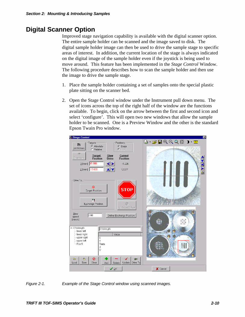
Digital Scanner OptionImproved stage navigation capability is available with the digital scanner option.The entire sample holder can be scanned and the image saved to disk. Thedigital sample holder image can then be used to drive the sample stage to specificareas of interest. In addition, the current location of the stage is always indicatedon the digital image of the sample holder even if the joystick is being used tomove around. This feature has been implemented in the Stage Control Window.The following procedure describes how to scan the sample holder and then usethe image to drive the sample stage.
1. Place the sample holder containing a set of samples onto the special plasticplate sitting on the scanner bed.
2. Open the Stage Control window under the Instrument pull down menu. Theset of icons across the top of the right half of the window are the functionsavailable. To begin, click on the arrow between the first and second icon andselect ‘configure’. This will open two new windows that allow the sampleholder to be scanned. One is a Preview Window and the other is the standardEpson Twain Pro window.
Figure 2-1. Example of the Stage Control window using scanned images.

Section 2: Mounting & Introducing Samples
TRIFT III TOF-SIMS Operator’s Guide 2-11
3. By selecting the preview button, a low-resolution image is scanned for setup.Select an area to be scanned by clicking a dragging a rectangle and select thedesired resolution (e.g. 1200 dpi).
4. Click on the Scan button. A high resolution scan will be done and theresulting image will be automatically placed in the Stage Control Menu asshown in Figure 2-1 above.
5. The image on top is intended to show a magnified view of the area outlinedin the red square in the image on the bottom. The magnification can beadjusted by left click-and-drag with the mouse on the top image. The redsquare on the bottom image will be adjusted immediately. The ‘magnify’ and‘de-magnify’ icons can also be used to change the magnification.
6. Left clicking with the mouse on the red square and dragging it around on thebottom image can be used to explore the sample holder. This will cause themagnified view to change in real-time. The up, down, left, and right arrowsto the right of the top image can be used to fine tune the position of the crosshairs. The Target Position X (mm) and Y(mm) values are continuouslyupdated to reflect the location of the cross-hair in the top image.
7. Once the desired location is centered on the cross hairs in the top image, hitthe Target Position button and the stage will drive to that location.
Section 2: Mounting & Introducing Samples
TRIFT III TOF-SIMS Operator’s Guide 2-12
Finding the Analysis PositionThe analytical chamber may need to be illuminated to view the sample holderinside. If an instrument file (*.ins) is not loaded, the chamber will be dark. Toilluminate the chamber, in WinCadence, go to Hardware Menu/Instrument tab,and fill in a value of 10 for Illuminator Power. Note the sample holder can beviewed at two different magnifications. In the SVC’s Watcher software program,the Camera Field option can be set to small or large.
Moving to the analysis position can be done in several ways. The stage can bemoved directly using the joystick. Or, in WinCadence, go to Instrument/StageControl. A designated position can be entered in the X(mm) and Y(mm) values;then, when “Target Position,” is selected, the stage will automatically drive tothis position. Also, positions from memory can be called up (load file *.plx).Highlight the position desired, then select “Drive To.”
TRIFT systems running the “ESCOSY” wafer navigation software can also movethe stage into the exchange position from within ESCOSY.
Typical Procedures in ESCOSY (200mm, 300mm Systems)The ESCOSY software is a separate software application apart from theWinCadence software application, however, the two applications are heavilyintegrated. ESCOSY allows control of the TRIFT system’s 8 inch sample stage.The following section is an overview of the commonly used features ofESCOSY.
Stage Directions
X,Y, Rotation Orientation
• The point of view is looking at the sample from the SPECTROMETER.
• + X direction is towards the INTRO
• + Y direction is UP
• + Rotation direction is clockwise
• The ROTATION ANGLE is assumed to be 0 at the EXCHANGEPOSITION.
Section 2: Mounting & Introducing Samples
TRIFT III TOF-SIMS Operator’s Guide 2-13
Stage Movements
• + X movement will cause the stage to move AWAY from the INTRO
• + Y movement will cause the stage to move DOWN
• + R movement will cause the stage to move COUNTER CLOCKWISE
Methods of Moving the Stage
Command Window
The Command Window allows the operator to control stage movement bysending single commands to the motor control. Commands are entered in theCommand text box. To repeat the last command, choose the “Repetition” buttonbesides the Command text box.
Table 2-1. Escosy commands and Corresponding Stage Movements.
Commands: Resulting Stage Movement:
-5.5x moves the stage to the ABSOLUTE x coordinate -5.5mm
2.5X moves the stage over 2.5mm in the positive x direction RELATIVE to thecurrent position
e30r does a eucentric rotation to the ABSOLUTE R coordinate 30o
e-30R does a eucentric rotation of -30o RELATIVE to the current R coordinateposition
1b does a backlash correction in the X-axis
2b does a backlash correction in the Y-axis
4b does a backlash correction in the R-axis
x drives the stage to 0.0 in the X-axis
y drives the stage to 0.0 in the Y-axis
r drives the stage to 0.0 in the R-axis
15g moves the stage to position no. 15 in the last opened position list
i15g moves the stage to position ID 15
Automated Drive
At the bottom of the Command Window is a pulldown menu of stage locations,including “Origin”, “Exchange”, “Notch” and “4 POS ALIGN MARK”. Toautomatically drive to any of these locations, choose the desired location fromthe pulldown menu, then press the “Drive” button.
Joy Stick Control
The joystick can be used to move the stage for fine adjustment within a localarea. However, when using the joystick, be careful not to run out of bounds. If itis necessary to move large distances, it is better to use the mouse to define thedesired location on the wafer map.

Section 2: Mounting & Introducing Samples
TRIFT III TOF-SIMS Operator’s Guide 2-14
Addressing Modes on the Wafer Map
There are 6 different addressing modes available in the wafer map window,depending on the lasso status and the usage of the “Shift” key. If the targetposition is within the allowed X-Y travel, point to the target and click the rightmouse key. To reach positions within the forbidden zone, you must use stagerotation. This can be done automatically by using the “Shift” key and clickingthe desired location in the forbidden zone with the right mouse key.
Table 2-2. Operation of the Mouse and Corresponding Modes and Stage Movements.
Operation Lasso Mode Resulting Stage Movement
right mouse Lasso off “X” Move to exactly the mouse pointer position
right mouse Lasso on Move to the coordinate inside the selected chip, whichhas been defined by setting the “Chip Catch Offset”.
right mouse Lasso w/ dot Move to the defined position nearest the mouse pointerposition.
If “Shift” right mouse key is used, the above 3 modes can be performed on aposition within the forbidden zone.
Addressing from the Position List
By highlighting one of the positions in the position list, then clicking with theright mouse key, a menu is displayed. One of the options in the menu is “scan”.By selecting “scan”, the stage will drive to that position.
Pre-Alignment
The purpose of pre-alignment is to calculate the rotation angle and offset vectorbetween the XY and the UV coordinate system. Whenever you change to a newwafer map with a different rotation angle, you must drive to the alignmentposition (e.g. 4-pos alignment) and execute the pre-alignment routine.
Loading a Project
Each of the 200 mm TRIFT III sample holders has an associated “project” whichcan be loaded in Escosy. Project files contain data concerning screenconfiguration, software limits, and associated position lists and wafer maps. Toget the wafer map to align with the actual sample holder, one has to do a pre-alignment after loading the project. For the 3 different sample holders use thefollowing steps:

Section 2: Mounting & Introducing Samples
TRIFT III TOF-SIMS Operator’s Guide 2-15
4-position holder:
1. Load the 4-position project.
2. Drive to the 4-position alignment mark.
3. Click on the wafer map window.
4. Under Edit choose “prealign”.
5. Click on OK.
12-position holder:
1. Load the 12-position project.
2. Drive to the 12-position alignment mark.
3. Click on the wafer map window.
4. Under Edit choose “prealign”.
5. Click on OK.
8” Wafer holder
1. Load the 8-inch wafer project.
2. Drive to the notch position.
3. Click on the wafer map window.
4. Under Edit choose “prealign”.
5. Click on OK.
Position Lists
Each PROJECT file contains a position list of the locations of each of the sampleanalysis areas. A position list is defined and stored as an ASCII data file with anextension “.PLS”. To drive to one of the sample positions using the position list,select the position of interest and choose SCAN ACTUAL. The operator canalso click on a position line in the list with the right mouse key and chose SCAN.
Many different position lists can be saved on disk for different auto-analysisroutines. The number of analysis points and the pattern of analysis points can bevaried and saved as separate position lists. To load a new position list chooseOpen Positionlist under the File menu.

Section 2: Mounting & Introducing Samples
TRIFT III TOF-SIMS Operator’s Guide 2-16
Wafer Maps
A wafer map layout file is used to define a specific sample holder layout. Theseare ASCII files with an extension “.WLO”. Each position list will have acorresponding wafer map associated with it.
Once a position list has been read from disk, the corresponding wafer map can bebrought to the desktop by clicking on the ‘wafer map’ icon in the top toolbar.The defined positions can be identified on the wafer map (red dots) by clickingthe appropriate icon in the toolbar at the top of the Escosy window.
Coordinate Window
This window provides the X,Y,R,U,V values for the current position of the stage.
Adjust Three Points
This routine is performed when the prealign is not accurate enough. When doingdefect analysis, one performs the adjust three point routine on three defects.Some defect review systems (Tencor, KLA) provide alignment mark coordinateswhich will be automatically transferred to the related position list during theimport routine.
Open the Adjust 3 Points window.
1. Enter the UV coordinates of the first position either digitally or by settingflag #1 within the wafer map or the defect map.
2. Choose the GO button referring to label #1. The stage will go to thespecified UV coordinates.
3. Use the joystick to move the stage exactly to the position of label #1 andexecute backlash for the X and Y axes. This position may either be a defector a die corner.
4. Choose the READ button referring to label #1 to display the current stage(XY) coordinates.
5. Repeat the above steps for label #2 and #3.
6. Choose the ADJUST button to calculate and store the parameters.

Section 2: Mounting & Introducing Samples
TRIFT III TOF-SIMS Operator’s Guide 2-17
Importing KLA Coordinates and Finding Defects
The Data Import module allows conversion of defect coordinate lists fromexternal defect inspection systems into standard ESCOSY positionlists. Ifavailable, the import filter also creates the corresponding wafer layout.
Escosy Plus supports the following:
• Tencor SFS-6000 and 7000 series;
• KLA 21xx series;
• INSPEX TPC 8500;
• DefectFinder 2000.
Refer to the unabridged Escosy manual (pp. 8-32 to 8-48) for a description ofhow to import these specific file formats.
After importing a defect position list and corresponding wafer map, use thealignment marks which come with the file to do a 3 point alignment.
Stage Initialization
1. Within WinCadence, select “Instrument” pulldown menu.
2. Select “Stage Drive”.
3. >stage requires init.
4. Press OK.
5. Select INIT MOTORS.
6. >init stage.
7. Select YES.
8. >Turn motors off & on.
9. Go the back of the Motor Chassis and turn power off and back on.
10. Select OK.
11. All three axis will move to preset positions, then search for HOME.
12. Press OK.

Section 2: Mounting & Introducing Samples
TRIFT III TOF-SIMS Operator’s Guide 2-18
Align Exchange Position
ESCOSY assumes that the ROTATION ANGLE at the exchange position is 0.
The actual ROTATION ANGLE will not end up at 0, therefore, ESCOSYprovides an OFFSET ANGLE to account for this difference.
Install the 4 position sample holder in system.
1. Click COMMAND WINDOW to assure all pulldown menus appear.
2. Choose PROJECT.
3. Choose OPEN.
4. Open the 4 POSITION PROJECT.
5. Select MODULE STATUS from the menu bar.
6. Select COMPU MOTOR CONTROL form the list.
7. Click EDIT VARIABLES.
8. Select OFFSET R form the list.
9. Click EDIT.
10. Enter 0 and click OK.
11. Click OK.
12. Click OK.
13. Exit ESCOSY and reenter to assure the change takes effect.
14. Using the COMMAND SHELL manually move the stage to the exchange(load) position making sure to use a ROTATION value between -180 and180 degrees.
15. Multiply the ROTATION value in the COORDINATE WINDOW by 2000to determine the ROTATION OFFSET.
16. Select the MODULE STATUS from the menu bar.
17. Select COMPU MOTOR CONTROL from the list.
18. Click EDIT VARIABLES.
19. Select OFFSET R from the list.
20. Click EDIT.
21. Enter ROTATION OFFSET and click OK.

Section 2: Mounting & Introducing Samples
TRIFT III TOF-SIMS Operator’s Guide 2-19
22. Click OK.
23. Click OK.
24. Exit ESCOSY and Reenter to assure the change takes effect.
25. Make sure the ROTATION VALUE in the COORDINATE WINDOWshould now read 0.00.
26. Select EXCHANGE from the COMMAND WINDOW pull down list.
27. Click EDIT.
28. Manually enter the X,Y,R values or Click READ to read the values from theCOORDINATE WINDOW.
Align the 4-Position Marker
1. Select the 4 POS ALIGN MARK from the COMMAND WINDOW pulldown list.
2. Click DRIVE.
3. Sample will rotate 180 degrees.
4. Sample will move to the ALIGN MARK machined in the sample holder (+)
5. Using the COMMAND SHEL4L BOX move the stage in X and Y to alignthe center of the MARK to the viewing optics
6. Select 4 POS ALIGN MARK from the COMMAND WINDOW pull downlist.
7. Click EDIT.
8. Manually enter the X,Y,R values or Click READ to read values fromCOORDINATE WINDOW.
Note: The location of this alignment mark is also used to set the PREALIGNMENT values that will allow the 4-POS Position List (set up in U,Vcoordinates) to be properly oriented to the stage coordinates.
9. Click MODULE STATUS form the pull down menu.
10. Select ADJUST MODULE from the list.
11. Click EDIT VARIABLES.
12. Scroll down the variable list to PREALIGN CENTER X.
13. Click EDIT.
14. Enter 4 POS ALIGN MARK X value from COORDINATE WINDOW.

Section 2: Mounting & Introducing Samples
TRIFT III TOF-SIMS Operator’s Guide 2-20
15. Click OK.
16. Click PREALIGN CENTER Y.
17. Click EDIT.
18. Enter 4 POS ALIGN MARK Y value from COORDINATE WINDOW.
19. Click OK.
20. Click POSITION LIST WINDOW.
21. Save the 4-POS PROJECT.
22. Exit ESCOSY and reenter to assure values are used.
Note: You should now be able to use the 4-POS POSITION LIST and theWAFER MAP to navigate around the 4-Pos Sample Holder.
Note: If the sample height is adjusted you should recheck the position of theALIGNMENT MARKER and reset it in the 4-POS ALIGN MARK position in theCOMMAND WINDOW and also the PREALIGN CENTER X and Y in theADJUST MODULE in the MODULE STATUSS WINDOW.
Find Rotation Center
The rotation center of the stage is saved as the “origin” in the pulldown menu ofstage locations in the Command Window. It should only be necessary for this tobe set once and it will be used for all projects. To check, perform the followingsteps.
1. Drive to the “origin”.
2. Click FIND ROTATION CENTER icon.
3. Click START ROTATION.
4. Adjust X-Y position of stage to find the CENTER.
5. Click STOP ROTATION.
6. Click SET ROTATION CENTER.
The new coordinates will be written in the coordinate.
TRIFT III TOF-SIMS Operator’s Guide 3-1
Section 3:Instrument State Files
This section discusses the “Instrument State” files. These files reside on thesystem computer and contain all of the software settings, parameters, andinformation required to setup and control the TRIFT system.
System Setup prior to AnalysisThe Concept of Instrument States: “INS” Files
An instrument file, which uses the file extension “.ins”, contains all theinformation required to set-up and control the system in a single file, for bothpositive and negative SIMS. All the information concerning voltages, thesequencer and calibration files are now contained in a single file, along withinformation to control the high mass blanker and post-ESA blanker (pre- andpost-spectrometer blanking).
The only parts of the system not under instrument file control are: the secondaryion apertures (Contrast diaphragm or “angular filter”, and the energy filter); andthe primary beam apertures on the LMIG and Cs gun. The Cs and the LMIGguns are slightly different: the Cs column has both a “slit” and an aperture, whilethe LMIG has a single, mechanically variable aperture (MVA).
NOTE: Computer control of the LMIG MVA is offered as an option on theTRIFT system.
The TRIFT system comes with a set of instrument files prepared at the factory.These files are specific to both the system and to its configuration as well as theanalytical modes that the configuration supports. During on-site installation,these same files may need some adjustments. At the end of the TRIFTinstallation, the system should contain a full set of instrument files. Afterbecoming familiar with routine system operation and tuning, the system user isfree to create more instrument files that are optimized for specific analyses.
Inspecting the Library of Instrument State Files
Certain important parameters from the instrument state file are passed through toa file header and appear when a file is highlighted prior to reading in the file.These parameters include primary beam, beam energy etc. A two-linedescription of the file, entered at the time that the file was created, is alsodisplayed. Thus, the description and the basic properties of the file can bereviewed prior to loading it. For instance, an instrument file may have beensaved that was specifically tuned to analyze a difficult glass sample for a client,

Section 3: Instrument State Files
TRIFT III TOF-SIMS Operator’s Guide 3-2
and now a repeat analysis of the same material is required. Unless the “ins” filehad been saved with an obvious filename such as “GLASS1.INS”, the “ins” filesmay need to be searched for the properties: i.e., charge compensation; 15kVenergy; Ga beam; bunched; post-acceleration. This will greatly reduce thenumber of files to be searched before locating the correct one.
Creating New Instrument State Files
After becoming familiar with the routine operation of the system, creation ofcustomized instrument files will be necessary. If any modifications to an existinginstrument file are made and the new conditions need to be saved as a newinstrument state, simply save the instrument file with an appropriate newfilename. Remember, however, that an instrument state file should contain allthe information required for both SIMS polarities. If the file is saved in onepolarity, but the user neglects to switch to the other polarity to create the otherinformation for the file, the “ins” file will not be complete, although it will loadcorrectly in the polarity where the files were created. When creating a newinstrument file, use the following checklist to verify that the new file has thefollowing parameters set correctly in each polarity:
− Mass calibration, with relevant species;
− Raster size;
− Polarity offset values (- to +);
− Buncher voltage (Mass resolution LMIG or Cs);
− Buncher delay (Mass resolution LMIG or Cs);
− Raster scale factor for correct image calibration (LMIG or Cs);
− High mass blanker calibration (LMIG or Cs);
− Post ESA blanker calibration (LMIG or Cs);
− Tilt (LMIG or Cs)
− Chicane amplitude (LMIG files);
− Pulse width (LMIG files).
Section 3: Instrument State Files
TRIFT III TOF-SIMS Operator’s Guide 3-3
Filter-Loading Part of the Instrument State Files
It is possible to load specific values of interest from a saved instrument state file.For instance, if the charge compensation parameters (Egun steering, lens andfilament bias) were optimized in one INS file, and the operator wants to use thesesame values in another INS file, filter-loading part of the instrument state file isuseful. To do this, first load the INS file with the parameters that you want tomodify. Then in the Hardware Utility, select the INS file with the specific valuesof interest (the INS file with the optimized charge compensation), check the boxfor “Filter-load part of the INS file,” and select Open. In the new window, moveto the page with the values of interest (in this case the Semi-perm/Cal page) andselect the boxes with the values of interest (Egun steering, lens and filamentbias). When OK is selected, these values will replace the values already loadedin the Hardware Utility. The INS file can be resaved with the new values ifapplicable.
Another reason to use the Filter-Load option is during ion gun tuning. Forexample, when all the voltages are optimized in the positive polarity at aparticular current and energy, the voltages required for the negative polarity arequite similar. It is possible to transfer the positive polarity voltages to thenegative polarity mode; then tuning in the negative mode will require minortweaking of these values. To transfer voltages from one polarity to the other,select the “Load voltages into opposite polarity” box located at the bottom of thefilter-load window, and select all the voltages to transfer (for example all thevoltages on the LMIG tab in the positive polarity). When OK is chosen thesevalues replace the ones in the current Hardware Utility.
The Filter-Load option also comes in handy for creating dual beam INS files.For example, in depth profiling one often needs to analyze with the LMIG at15keV and sputter with the Cs at 1 keV. For this mode, the operator would loadthe 15keV LMIG INS file. Next, the Cs voltages could be added using filter-load. Select the “filter-load part of the INS file box” and select the 1 keV Cs INSfile, then choose open. In the filter-load window select all the voltages that areapplicable: in the Cs tab, include all the voltages; in the Sources tab select all therelevant Cs column values (e.g. Cs Beam Energy, Cs Control Electrode, Cs FritPower, Cs Oven Temp, Cs Extractor, Cs Emission and Cs Frit Bias); in theSemiperm/Cal tab, select the relevant Cs column values (e.g. uBeam Rotation, CsRaster Scale Factor, uBeam Tilt, uBeam Quad/Oct Ratio, and Microbeam Vref).When OK is chosen the Hardware Utility will contain voltages for both Ga andCs sources. The new INS file should be saved. Note that for depth profiling, theoperator must ensure that the Cs and Ga guns are aligned for the sample ofinterest (refer to Section 7).
Section 4: Tuning the Primary Beams
This section discusses the tuning process for the LMIG, the Cs ion gun, the O2 ion gun (on the dual source option), and the Gas Gun . Tuning of the low energy electron beam is also covered in this section. The TRIFT III instrument is delivered from the factory with the following LMIG instrument files:
Filename Description
15Ga3.ins 15kV, 600 pA high mass resolution (bunched) file
15Ga2.ins 15kV, 2nA high mass resolution (bunched) file
15Ga1.ins 15kV, 20nA high mass resolution (bunched) file
25Ga4.ins 25kV, 60pA high spatial resolution (unbunched) file
25Ga3.ins 25kV, 600pA high spatial resolution (unbunched) file
25Ga2.ins 25kV, 2nA high spatial resolution (unbunched) file
If the system includes a Cs ion beam, additional files will be included for 10kV Cs spectroscopy and for 1kV dual beam depth profiling. If the system includes the Gas Gun, additional files will be included for “phase depth profiling”. The factory set instrument files can be loaded and used without tuning the ion beams. However, there may be times, such as after replacing any of the ionizer assemblies, that re-tuning of the ion beams will be necessary. The procedures outlined in this section describe how to optimize the LMIG for both the bunched and unbunched mode of operation. It also covers tuning of the Cs gun and O2 gun for both spectroscopy and depth profiling. Tuning of the Gas Gun is covered for optimizing “phased depth profiling” settings.
Liquid Metal Ion Gun (LMIG) The latest generation liquid metal ion gun (LMIG) on the TRIFT features:
• Primary D.C. beam currents that range over three orders of magnitude from 20nA to 20pA;
• A pulsing scheme that minimizes beam aberrations which arise from the pulsing process, producing analytical probes down to 100 nm and 200 nm analytical probes at high mass resolution;
• An optimized electrodynamic buncher which permits high primary pulse compression with two micrometer spatial resolution; and
• High current (20 nA) spectroscopy mode at high mass resolution.
TRIFT III TOF-SIMS Operator’s Guide 4-1

Section 4: Tuning the Primary Beams
The ion gun is computer-controlled, resulting in a whole host of differing analytical conditions which can be recalled at the click of a mouse button. The following sections provide in-depth details to help the user to understand how the gun can be set up and optimized. Standard 'instrument files' will be loaded and used throughout this text as examples. Although the following sections may seem unnecessarily detailed, the more the user understands how the ion gun functions, the more he/she will be able to harness the gun for their own special analytical circumstances.
Firing the Source The first required step is to fire the source as outlined below.
1. Load the desired instrument file. The source may or may not fire, since the 'onset' voltage for emission from a liquid metal ion source is always higher than the 'extinction' voltage.
2. If the source fires at the desired voltage, adjust the suppressor voltage until the emission current registers approximately 1 microamp.
3. If the source does not fire at the desired extraction voltage, lower the suppressor voltage until the source does fire. Again, adjust the suppressor voltage until the correct emission current is obtained.
4. If the source will not fire with the extractor at the desired value and the suppressor voltage at maximum, increase the extractor voltage until the source does fire. Sometimes, the resulting emission current can be instantaneously high (several microamps), and the extraction voltage should be quickly reduced to lower the emission current. If the source cannot be fired as described above, it may be necessary to heat the source. For instructions on how to perform this step, refer to 'Heating the Source' below.
Heating the Source There are different circumstances in which it will be necessary to apply heating to the gallium source.
If the source cannot be fired, or the extraction voltage cannot be reduced to the desired voltage without extinguishing the source, it may be necessary to heat the source until the appropriate emission current can be achieved with the 'usual' extraction and suppressor voltage settings.
In time, as the source reaches the end of its life, it will be necessary to move to higher extraction voltages to extract the last of the gallium. This is expected after several months of steady operation, when heating the source is ineffective in maintaining the extraction voltage.
TRIFT III TOF-SIMS Operator’s Guide 4-2
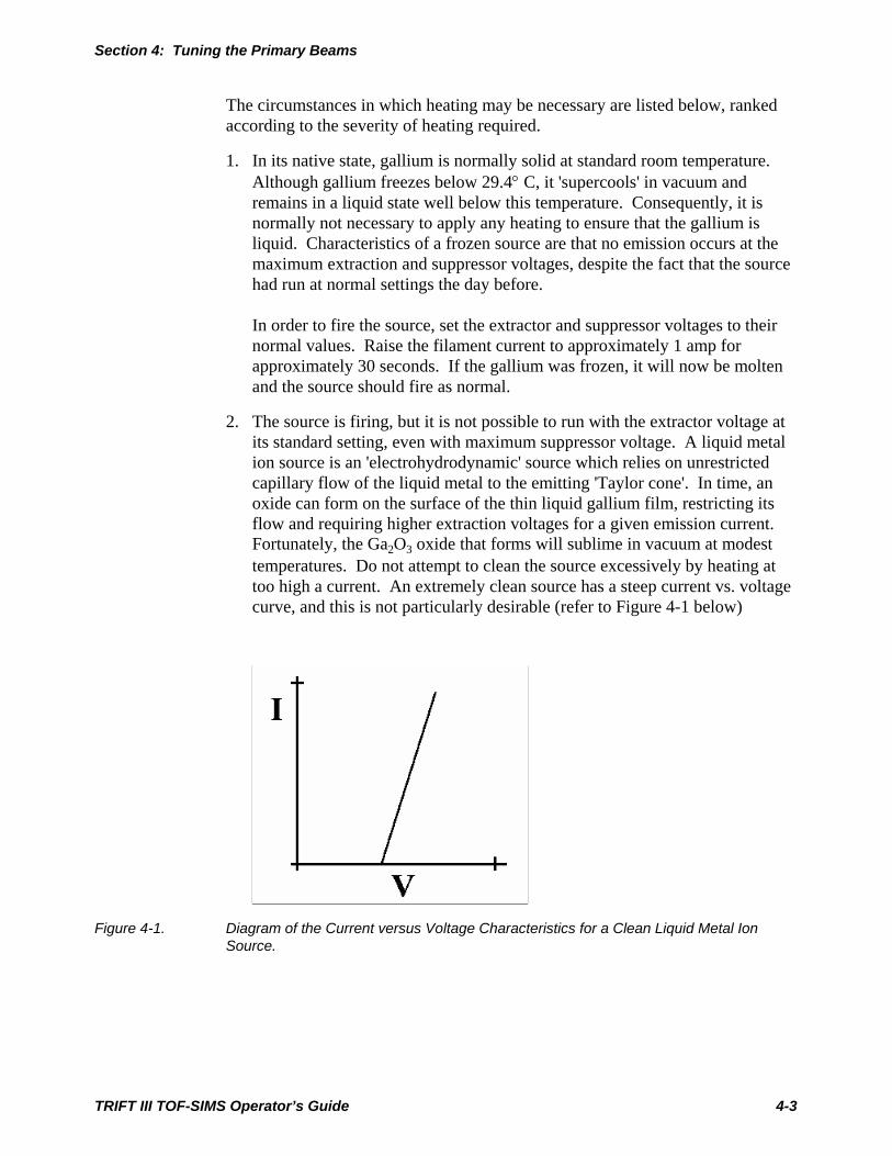
Section 4: Tuning the Primary Beams
The circumstances in which heating may be necessary are listed below, ranked according to the severity of heating required.
1. In its native state, gallium is normally solid at standard room temperature. Although gallium freezes below 29.4° C, it 'supercools' in vacuum and remains in a liquid state well below this temperature. Consequently, it is normally not necessary to apply any heating to ensure that the gallium is liquid. Characteristics of a frozen source are that no emission occurs at the maximum extraction and suppressor voltages, despite the fact that the source had run at normal settings the day before. In order to fire the source, set the extractor and suppressor voltages to their normal values. Raise the filament current to approximately 1 amp for approximately 30 seconds. If the gallium was frozen, it will now be molten and the source should fire as normal.
2. The source is firing, but it is not possible to run with the extractor voltage at its standard setting, even with maximum suppressor voltage. A liquid metal ion source is an 'electrohydrodynamic' source which relies on unrestricted capillary flow of the liquid metal to the emitting 'Taylor cone'. In time, an oxide can form on the surface of the thin liquid gallium film, restricting its flow and requiring higher extraction voltages for a given emission current. Fortunately, the Ga2O3 oxide that forms will sublime in vacuum at modest temperatures. Do not attempt to clean the source excessively by heating at too high a current. An extremely clean source has a steep current vs. voltage curve, and this is not particularly desirable (refer to Figure 4-1 below)
Figure 4-1. Diagram of the Current versus Voltage Characteristics for a Clean Liquid Metal Ion Source.
TRIFT III TOF-SIMS Operator’s Guide 4-3
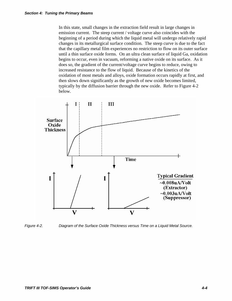
Section 4: Tuning the Primary Beams
In this state, small changes in the extraction field result in large changes in emission current. The steep current / voltage curve also coincides with the beginning of a period during which the liquid metal will undergo relatively rapid changes in its metallurgical surface condition. The steep curve is due to the fact that the capillary metal film experiences no restriction to flow on its outer surface until a thin surface oxide forms. On an ultra clean surface of liquid Ga, oxidation begins to occur, even in vacuum, reforming a native oxide on its surface. As it does so, the gradient of the current/voltage curve begins to reduce, owing to increased resistance to the flow of liquid. Because of the kinetics of the oxidation of most metals and alloys, oxide formation occurs rapidly at first, and then slows down significantly as the growth of new oxide becomes limited, typically by the diffusion barrier through the new oxide. Refer to Figure 4-2 below.
Figure 4-2. Diagram of the Surface Oxide Thickness versus Time on a Liquid Metal Source.
TRIFT III TOF-SIMS Operator’s Guide 4-4
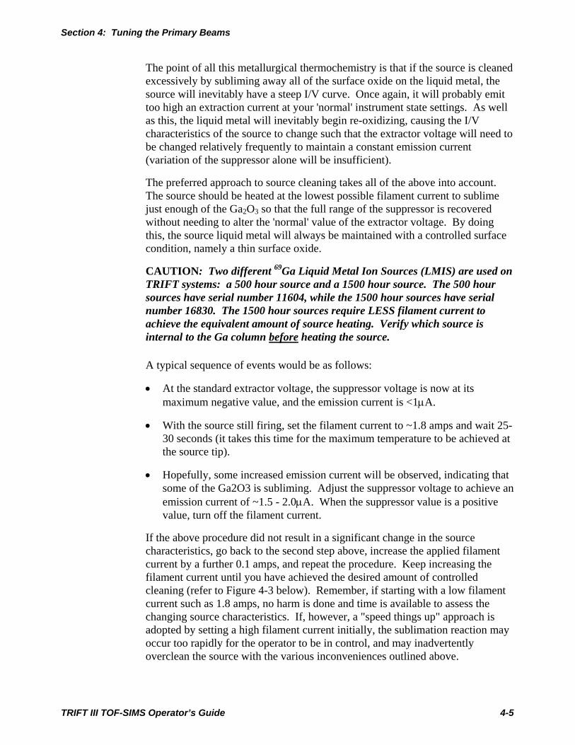
Section 4: Tuning the Primary Beams
The point of all this metallurgical thermochemistry is that if the source is cleaned excessively by subliming away all of the surface oxide on the liquid metal, the source will inevitably have a steep I/V curve. Once again, it will probably emit too high an extraction current at your 'normal' instrument state settings. As well as this, the liquid metal will inevitably begin re-oxidizing, causing the I/V characteristics of the source to change such that the extractor voltage will need to be changed relatively frequently to maintain a constant emission current (variation of the suppressor alone will be insufficient).
The preferred approach to source cleaning takes all of the above into account. The source should be heated at the lowest possible filament current to sublime just enough of the Ga2O3 so that the full range of the suppressor is recovered without needing to alter the 'normal' value of the extractor voltage. By doing this, the source liquid metal will always be maintained with a controlled surface condition, namely a thin surface oxide.
CAUTION: Two different 69Ga Liquid Metal Ion Sources (LMIS) are used on TRIFT systems: a 500 hour source and a 1500 hour source. The 500 hour sources have serial number 11604, while the 1500 hour sources have serial number 16830. The 1500 hour sources require LESS filament current to achieve the equivalent amount of source heating. Verify which source is internal to the Ga column before heating the source.
A typical sequence of events would be as follows:
At the standard extractor voltage, the suppressor voltage is now at its maximum negative value, and the emission current is <1µA.
•
•
•
With the source still firing, set the filament current to ~1.8 amps and wait 25-30 seconds (it takes this time for the maximum temperature to be achieved at the source tip).
Hopefully, some increased emission current will be observed, indicating that some of the Ga2O3 is subliming. Adjust the suppressor voltage to achieve an emission current of ~1.5 - 2.0µA. When the suppressor value is a positive value, turn off the filament current.
If the above procedure did not result in a significant change in the source characteristics, go back to the second step above, increase the applied filament current by a further 0.1 amps, and repeat the procedure. Keep increasing the filament current until you have achieved the desired amount of controlled cleaning (refer to Figure 4-3 below). Remember, if starting with a low filament current such as 1.8 amps, no harm is done and time is available to assess the changing source characteristics. If, however, a "speed things up" approach is adopted by setting a high filament current initially, the sublimation reaction may occur too rapidly for the operator to be in control, and may inadvertently overclean the source with the various inconveniences outlined above.
TRIFT III TOF-SIMS Operator’s Guide 4-5
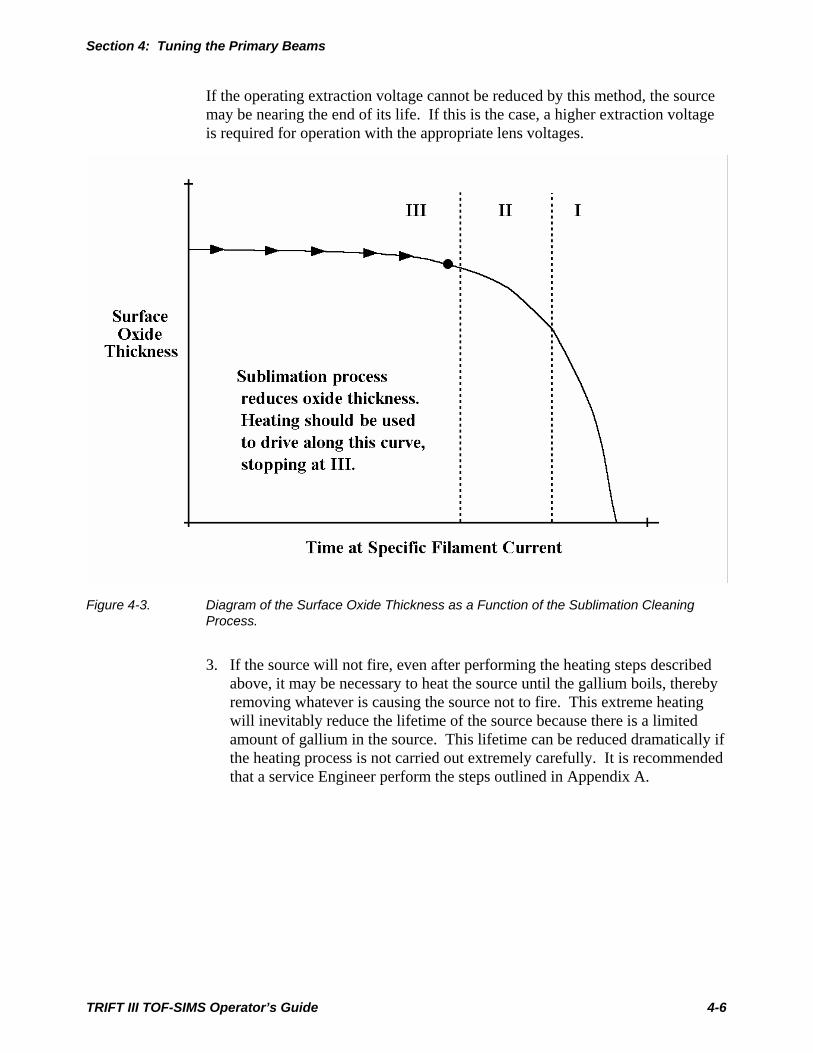
Section 4: Tuning the Primary Beams
If the operating extraction voltage cannot be reduced by this method, the source may be nearing the end of its life. If this is the case, a higher extraction voltage is required for operation with the appropriate lens voltages.
Figure 4-3. Diagram of the Surface Oxide Thickness as a Function of the Sublimation Cleaning Process.
3. If the source will not fire, even after performing the heating steps described above, it may be necessary to heat the source until the gallium boils, thereby removing whatever is causing the source not to fire. This extreme heating will inevitably reduce the lifetime of the source because there is a limited amount of gallium in the source. This lifetime can be reduced dramatically if the heating process is not carried out extremely carefully. It is recommended that a service Engineer perform the steps outlined in Appendix A.
TRIFT III TOF-SIMS Operator’s Guide 4-6

Section 4: Tuning the Primary Beams
Tuning the LMIG For routine system operation, the range of instrument files provided in the 'instrument state' library should meet nearly all analytical needs. However, if different files are desired, the following describes how this procedure may be carried out.
Choose a primary beam aperture a. On the mechanically variable aperture (MVA) at the side of the gun, rotate
the linear motion drive to a new aperture position. The convention for naming these apertures is as follows: The first visible white ring on the manipulator corresponds to the first aperture, the 20 nA beam position; the second ring to the second aperture, the 2 nA beam position; etc. The sequence is: 20 nA; 2 nA; 600 pA; 60 pA and 20 pA, representing apertures 1-5. The manipulator should be set so that the x and y vernier readings are close to 0 when an aperture is in place. The convention for reading these scales on the MVA is as follows: aperture 1 = position 1.0, 0.0 (ideal setting); aperture 2 = position 2.0, 0.0 (ideal setting); and so on. Readings are taken at the white marks provided on the x and y drives.
b. Produce an SEM image by pressing the "DC" button at the bottom of the LMIG page of the Hardware window. Under the "Deliver beam to sample" option, choose "Liquid Metal Ion Gun", then select the OK button. Adjust the SED gain and the Raster Size to obtain a good SEM image.
c. Move to the LMIG control page. Wobble lens 1 using the automatic wobbling tool. This is done by highlighting the Lens1 field and pressing the wobble button at the bottom of the LMIG page.
TRIFT III TOF-SIMS Operator’s Guide 4-7
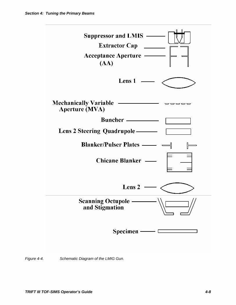
Section 4: Tuning the Primary Beams
Figure 4-4. Schematic Diagram of the LMIG Gun.
TRIFT III TOF-SIMS Operator’s Guide 4-8

Section 4: Tuning the Primary Beams
d. Move the x and y adjusters on the MVA to minimize any observable motion in the D.C. beam image. In order to reduce the effects of ‘backlash’ (mechanical uncertainty) on the accuracy of positioning, approach the aperture position from the same direction each time, for instance, a clockwise (CW) direction. When satisfied that the image is motion-free at a low magnification, zoom in and check at a higher magnification. Write down the final MVA readings as these settings will be keyed into the ‘instrument file’ header in the software when this particular gun tuning is saved as a file.
e. Remove the lens 1 wobble with the Remove Wobble button.
f. Now add a wobble to lens 2 using the software wobble tool detailed above. If the automatic, fixed amplitude wobbler is too much for this lens, try performing the wobble manually with the + and - keys on the keyboard. Adjust the x and y beam steering for lens 2 to reduce the wobble observed in the image. As a general rule, the lower these x and y values the better, although it is not realistic to expect them to be zero. Remove the lens 2 wobble.
g. Now add a wobble to the “blanker” voltage, and adjust the values of lens 1 and lens 2 so as to minimize the motion and yet still maintain a sharp image. This determines the “conjugate pair” that sites the beam crossover in the center of the blanking plates for motionless blanking. This is best done by first adjusting Lens 2 to minimize the wobble, the adjust Lens1 to refocus the image. Repeat this procedure until the image is wobble-free. Remove the wobble when finished.
h. Now comes the setting of the chicane amplitude. Until now, the beam has passed through the chicane and has not been near to the blanking "knife edge" owing to a high chicane amplitude. As a crucial part of achieving motionless blanking, it is now necessary to begin lowering the chicane amplitude so as to bring the beam closer to the knife edge. Try lowering the chicane amplitude in 10 volt steps until a clear reduction of the image intensity is perceived. Now raise the amplitude in 5 volt steps until the brightness reaches a plateau. The correct setting of the chicane amplitude for a given beam energy and beam current (aperture setting) is the one where the beam is just clear of the knife edge, i.e., has just reached the maximum image brightness. From this position, the minimum displacement to completely blank the beam is required. Generally, the blanker voltage required to just blank the beam at 25kV beam energy is as follows: the 2 nA beam requires ~15 volts; the 600 pA beam requires ~10 volts; the 60 pA beam requires ~5 volts; and the 20 pA beam requires ~3-5 volts. If the blanking required to blank the beam is significantly greater than these values, the chicane amplitude may still be a little high.
TRIFT III TOF-SIMS Operator’s Guide 4-9

Section 4: Tuning the Primary Beams
i. As the beam current is changed, the physical size of the beam at the knife edge changes, and so for each beam current there will be a different value of the chicane amplitude that brings the beam as close to the knife edge as possible. Note also that the magnitude of the chicane amplitude is proportional to the beam energy. Therefore, when setting the gun for 25kV operation, a chicane amplitude >360 (260 x 25/15) volts may be needed to allow a 2 nA beam to go well past the knife edge for tuning purposes.
Stigmator balancing and stigmation a. Before stigmation of the beam can take place, make sure that the beam is
centered as best as possible within the octupole stigmator. To do this, add a wobble to each of the two stigmators in turn, adjusting the x and y “balance” for each of them to reduce the wobble in the image, i.e., wobble stigmator 1 first, adjusting balance 1x and balance 1y in the gun menu. Once the beam is centered in the octupole stigmator, adjust each of the stigmators in turn to give the sharpest image possible. It may be helpful to operate at lower raster speeds at this point. To change the raster clock speed press the Raster Specs button in the LMIG page. Select a slower scan speed (i.e., 0.5 or 0.25 MHz). This will allow for easier observation of the fine tuning with the stigmators. Low scan speeds are mandatory when tuning the gun with smaller beam currents. Iterate between the stigmators and Lens 2 to produce the sharpest image.
b. Verify that the image size obtained corresponds to the one requested in the menu. If it does not, adjust the parameter "raster scale factor" in the Semiperm/Cal page. Note that this value will be different for positive SIMS and will need to be determined separately.
c. Beam tuning is now complete in this polarity (-SIMS). Except for the stigmator settings, the beam position and the raster scale factor, the gun parameters are the same for the opposite polarity (+SIMS). Printout the LMIG page in readiness for tuning the other polarity (+SIMS) by pressing the Print Page button.
TRIFT III TOF-SIMS Operator’s Guide 4-10
Section 4: Tuning the Primary Beams
d. During data acquisition, the blanker voltage remains at a constant D.C. voltage. A matching voltage is applied to the opposite blanking plate only when the pulser unit fires resulting in the beam pulsing on. The beam has now just been tuned in D.C. condition with the blanker plate voltages at zero. This means that the best image has been obtained at a specific place with reference to the knife edge in the chicane. When the beam is pulsing during acquisition, the values of the blanker and the pulser (amplitude) will need to be set so that the pulsed beam appears at the same position. This will not happen automatically. The values obtained at PHI, which appear in your master instrument files, should be used.
e. If it is necessary to determine the pulser value yourself, the following method can be used. Start an acquisition, setting the pulser deliberately low and then begin raising the pulser voltage. No counts are obtained until the beam begins to pulse past the knife edge, after which a rapid increase in the count rate is observed as a function of pulser amplitude. Once the beam is pulsing clear of the knife edge, the rise in the count rate will slow down, and any further increase in the count rate will be due to a longer on-time for the beam due to an increased transit time past the knife edge and then back again. Make a graph of the count rate vs. pulser amplitude, and then set the pulser at the point where the rate of change in the count rate just turns over.
Saving “Instrument files” a. Once satisfied that the LMIG menu parameters are correct, save this
instrument state as a file if the primary beam is: -pulsing correctly, with an appropriate pulse width; -steered with beam position x and y to center it to the spectrometer acceptance area; -an appropriate default raster size (>200µm recommended); and -provided that the other system parameters are acceptable. The concept of the “instrument file” is to be able to read and write a single file which contains all the relevant information to return the system to that particular state, e.g. imaging at 15 kV, etc. At the present time, the only parameters not under computer control are: the mechanically variable aperture (MVA) on the LMIG (although a computer control option is available); the contrast diaphragm, and the energy filter. All other parameters are stored in the “instrument file”.
b. Remember that an “instrument state” file needs all relevant parameters for both SIMS polarities. A helpful way to think of an instrument file is to consider that it contains two “pages” of information to control the system: a +SIMS “page” and a -SIMS “page”. For instance, following the preceding tuning instructions above has resulted in only one page (-SIMS) of this instrument file.
TRIFT III TOF-SIMS Operator’s Guide 4-11
Section 4: Tuning the Primary Beams
Changing polarity a. To change polarity, press the Instrument pull-down menu and select the
desired polarity. A check mark ( √ )will be shown next to the current polarity. Changing polarity takes about 10 seconds and is complete once the user hears the click of a relay within the system.
b. The LMIG values for the newly tuned polarity now can be transferred to the opposite polarity. This can be done by selecting the filter-load option from Load Ins File in the Hardware Menu. Then select “Load voltages into the opposite polarity” and select all the parameters that have just been optimized (also refer to Chapter 3). When OK is chosen the values will be transferred to the opposite polarity. Remember that the beam position x and y will be incorrect, since the “polarity offset” parameters have not yet been determined. Also, the exact stigmator settings will need to be determined. The beam position values stored in the master instrument state files for a given beam energy and polarity should be used as a first approximation.
c. Put the LMIG into a D.C. tuning mode, and fine tune the stigmators in +SIMS using a continuous image at the SED detector. Check that the raster scale factor is correct by adjusting it until the requested field of view on a known, patterned sample such as the Cu tuning grid matches the field of view actually obtained in +SIMS. Now save the instrument file again with the same name used initially for the -SIMS page. This completes a full instrument file with all the relevant LMIG parameters set correctly. All the time invested in creating this first, detailed file will pay off as more files are created with different primary currents at the same energy. Effectively, the only difference between these files in a given SIMS polarity will be the Chicane Amplitude setting, and possibly a small change to the stigmators.
Polarity offsets and beam alignment The appropriate offset values have been determined at PHI and are stored with the instrument files. If new instrument files are created at energies for which files already exist by modifying a file, the correct polarity offset values will automatically be copied into the new file. However, if an understanding of how to determine the polarity offsets at any beam energy is necessary, refer to Section 5, “Determining the Polarity Offset Values”.
TRIFT III TOF-SIMS Operator’s Guide 4-12
Section 4: Tuning the Primary Beams
Optimizing the LMIG for High Spatial Resolution The highest spatial resolution is achieved at 25keV with the buncher off. In this mode, the pulse width can be adjusted to trade-off between sensitivity (long pulse width) and mass resolution (short pulse width).
The chicane LMIG allows data to be acquired at high spatial resolution no matter what the primary pulse width. This is because the chicane beam blanking system permits rapid blanking of the beam with the minimum of beam motion. In order to obtain the best spatial resolution while pulsing the ion beam, the chicane amplitude should be set so that the beam just clears the knife edge when the beam is pulsed on. By doing this, the beam has the minimum travel before it is blanked, minimizing aberrations introduced by pulsing. Refer to the previous section for details on how this is achieved.
The minimum analytical beam size (<120nm) is achieved with the smaller of the available D.C. beam currents (20, 60 pA), and at longer pulse lengths where slight residual beam shifts due to pulsing represent only a negligible fraction of the beam ‘on’ time.
High mass resolution simultaneous with probe sizes of ~200 nm is achievable at all primary beam currents, but in practice is performed at the higher beam currents of 600 pA or 2 nA. This is because mass resolution at high spatial resolution (200 nm) is achieved by reducing the primary pulse width, not by electrodynamic bunching. As a consequence of reducing the primary pulse width, the primary beam flux is reduced. This in turn reduces the secondary ion count rate. For this to be high enough for practical data acquisition, begin with a high primary beam current. When reducing the pulse width to increase mass resolution in a 25 kV beam energy instrument file, a point is reached at very short widths where the pulser amplitude begins to also fall. This requires compensation through increasing the value of the pulser (amplitude) for pulsing the beam just past the chicane’s knife edge once again. Remember to be realistic about acquisition times. If 5 minutes in needed with a pulse width of ~10ns to acquire sufficient data at a 1000 m/z range, it will take 25 minutes to acquire the same data using a 2 ns (reduced) pulse width. In such cases, set the maximum mass range as low as possible to increase the repetition rate of the experiment. By doing so, the data rate is increased by a factor of 3 which reduces the acquisition time in the above example to ~8 minutes.
TRIFT III TOF-SIMS Operator’s Guide 4-13
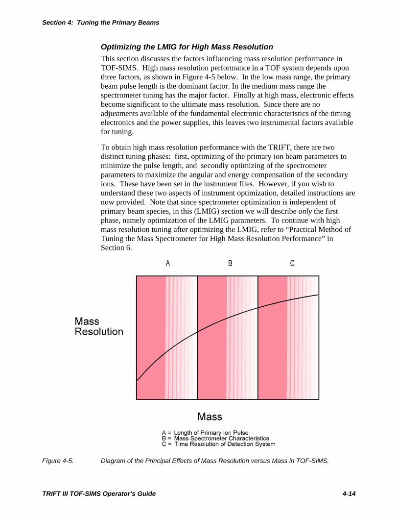
Section 4: Tuning the Primary Beams
Optimizing the LMIG for High Mass Resolution This section discusses the factors influencing mass resolution performance in TOF-SIMS. High mass resolution performance in a TOF system depends upon three factors, as shown in Figure 4-5 below. In the low mass range, the primary beam pulse length is the dominant factor. In the medium mass range the spectrometer tuning has the major factor. Finally at high mass, electronic effects become significant to the ultimate mass resolution. Since there are no adjustments available of the fundamental electronic characteristics of the timing electronics and the power supplies, this leaves two instrumental factors available for tuning.
To obtain high mass resolution performance with the TRIFT, there are two distinct tuning phases: first, optimizing of the primary ion beam parameters to minimize the pulse length, and secondly optimizing of the spectrometer parameters to maximize the angular and energy compensation of the secondary ions. These have been set in the instrument files. However, if you wish to understand these two aspects of instrument optimization, detailed instructions are now provided. Note that since spectrometer optimization is independent of primary beam species, in this (LMIG) section we will describe only the first phase, namely optimization of the LMIG parameters. To continue with high mass resolution tuning after optimizing the LMIG, refer to “Practical Method of Tuning the Mass Spectrometer for High Mass Resolution Performance” in Section 6.
Figure 4-5. Diagram of the Principal Effects of Mass Resolution versus Mass in TOF-SIMS.
TRIFT III TOF-SIMS Operator’s Guide 4-14

Section 4: Tuning the Primary Beams
Preliminary Tuning
a. Tune the LMIG for 15kV operation as described in the LMIG tuning section. Select the 600pA aperture. When attempting to set up files for mass resolution, tune the gun with the buncher voltage on. If you have not yet determined the optimum buncher voltage, set this parameter to ~800 volts. Remember to check all alignments: lens 1 centering; lens 2 centering; a crossover in the center of the blanking plates (wobble blanker and set lens1 and lens2 for minimum motion); set chicane amplitude, and finally the stigmator "balancing" (centering) and stigmation itself. The chicane amplitude should be set so that the minimum voltage is required on the blanker to turn the beam "off" (see LMIG tuning). Set the stigmation after you have determined the correct chicane amplitude for any given beam parameters (energy, current).
b. Note that, even with a perfectly tuned column, if you make the blanker an increasingly negative value, the image will not only become less focused, but it will move as well. Don't worry. This is the expected behavior. You are moving the beam away from the knife edge into a position which results in greater aberrations. The important thing is how the image appears as you take the blanker from zero to positive values. If you do not achieve a motionless blanking at low blanking voltages, consult the LMIG tuning section once again.
c. The gun has just been tuned with the buncher voltage on, in a D.C. condition, i.e. the buncher voltage was constant and not pulsing. During data acquisition however, the buncher is pulsed, and this results in an "overfocusing" of the beam. To compensate, you will need to determine a new lens 2 voltage which, during pulsing, will compensate for this overfocusing effect.
d. The way to determine this lens 2 value is to reduce lens 2 in 50 volt steps, acquiring an image at each lens 2 value from a copper grid in positive SIMS mode. Since the buncher overfocuses the beam, lens 2 will need to be lower to compensate. Each LMIG column is slightly different in its behavior, and the appropriate drop in lens 2 will have to be determined experimentally. Move to the next step when a SIMS image with 2 - 3 um resolution in the image has been obtained.
TRIFT III TOF-SIMS Operator’s Guide 4-15

Section 4: Tuning the Primary Beams
Minimizing the bunched primary pulse length a. In this first phase of tuning the system for high mass resolution, only two
LMIG parameters will be dealt with: the buncher voltage and the buncher delay. The buncher voltage is accessed directly in the Hardware menu; the buncher delay is accessed under Instrument, Set Delay Lines, Buncher. To perform this next task, have a silicon wafer in position, and set the spectrometer to "fully open" (no C.D. or energy filter). For convenience, a blank tuning grid is provided in an appendix to help in note taking. Although this is the full tuning grid including the spectrometer parameters, entries for the relevant LMIG parameters are also discussed below.
b. Before adjusting the bunching parameters, make sure to not attempt to bunch too much primary beam. In general, a 15ns pulse can be compressed efficiently, although in practice a 12ns pulse or less is more forgiving. To check the input pulse going into the buncher, set the buncher voltage to zero, set the time channels to 1ns and acquire data. Count the number of channels at FWHM at hydrogen. Make sure that the input pulse is appropriate. If you want to have the maximum input pulse into the buncher, the buncher timing will need to be set very carefully. If a lower input pulse is chosen, there will be some 'play' in the buncher timing.
c. Turn the buncher voltage back on and arrange the mass spectral display so that hydrogen occupies the full screen. Insure that the minimum time resolution, namely 138ps, is being used. Begin altering the delay until the beam is clearly being compressed, and then, for a given buncher voltage, optimize the buncher delay (2ns steps) so as to minimize the number of channels which define the full width half maximum (FWHM) of the hydrogen peak. When this is minimized, switch to the buncher voltage, and try altering this in 25 volt steps until the FWHM of hydrogen is minimized. With no C.D., a FWHM of 6-8 channels should be achievable. Note that if this experiment is performed with the 1st C.D. (400um) in place, the FWHM will be less because the angular acceptance of hydrogen is being reduced. If tails are observed at either side of the peak, the buncher is attempting to bunch more ions than it can accommodate.
d. Monitoring hydrogen is an excellent way to minimize the primary pulse width. However, for final determination of the correct buncher and delay values, repeat the above experiment on an organic peak (i.e. C3H5 at mass 41), again minimizing the FWHM in terms of the number of channels which constitute the peak. This is because, unless the spectrometer is completely misaligned, the molecular ions are much less sensitive to spectrometer tuning than the atomic ion species. Good mass resolution can be achieved on molecular species as long as the primary pulse length is short, even if the spectrometer tuning is not fully optimized. This is not true of atomic species such as Si.
TRIFT III TOF-SIMS Operator’s Guide 4-16

Section 4: Tuning the Primary Beams
e. If you have achieved 6-8 channels on hydrogen (no C.D.), and if the mass resolution at C3H5 is ~8000-9000, this concludes the LMIG parameter tuning. It is still likely that the atomic species such as Si will not yet be optimized, and so now move to the second phase of instrument optimization, namely spectrometer tuning which is referenced in Section 6.
Primary Beam Dose Calculation for LMIG Experiments A brief explanation below centers on two topics: the first principles on calculating the number of ions delivered (and thereafter the dose calculation); and secondly, how the dose calculation is implemented in the software from a practical approach.
First Principles
a. In a continuous beam system, this is a simple parameter to determine. Only the primary beam current and the experiment time are needed to calculate this. Then: Primary ions = Beam Current (Amps) x 6.25 E18 (ions/Amp.sec) x Experiment Time (seconds). For instance, a beam current of 1 nanoamp on for 100 seconds will give: 1 E-9 (Amps) x 6.25 E18 (ions/Amp.sec) x 100 (seconds) = 6.25 E11 Primary Ions delivered
b. In a TOF system, the beam is not on continuously, and so in addition, the frequency of pulsing and the duration of the beam 'on-time' for each primary pulse is needed. Then: Primary ions = Beam Current (Amps) x 6.25 E18 (ions/Amp.sec) x Experiment Time (seconds) x Frequency (Hz) x Primary Pulse Width (nanoseconds). The frequency is dependent upon the mass range. It can be determined for a specific mass range in the Hardware menu, in the Sequencer. The Load value of Prate 0 must be multiplied by 200 x 10-9 to obtain the 1/frequency. Invert to obtain Hz.
The Primary Pulse Width was determined in the previous section by measuring the FWHM of the H signal. Multiply the number of channels at FWHM by the time resolution of the acquisition (the nanoseconds/channel value found in Acquistion Setup/Advanced Settings).
TRIFT III TOF-SIMS Operator’s Guide 4-17
Section 4: Tuning the Primary Beams
Here is an example, for a beam current of 1 nanoamp, an experiment time of 100 seconds, a repetition rate of 10kHz and a beam 'on-time' of 10 nanoseconds per pulse of primary beam, the yield is: 1 E-9 x 6.25 E18 x 100 x 1 E4 x 10 E-9 = 6.25 E7 primary ion delivered (i.e., down by 10,000 on D.C. case).
c. Dose calculations are simple once the number of primary ions delivered is known. Express the area of analysis in cm2, and divide it into the total number of primary ions delivered, e.g. Number of Primary Ions = 6.25 E7; Area of Analysis 100um x 100um; Dose = 6.25 E7 ions/1 E-4cm2 = 6.25 E11 ions/cm2
WinCadence Dose Calculator
The dose of primary ions for each acquisition will automatically be calculated through the software once the dose standardization is set up. The dose standardization is found on the Instrument Settings page of Acquisition Setup, and can be performed using the simple or automatic options. For the simple method, click on this option and choose Go. You will be prompted to enter the primary ion current (can be measured by choosing the D.C. option in the Hardware Menu and “monitoring beam inside primary column”) and the pulse width (measure the FWHM of H and multiply the number of channels by the time resolution of the acquisition (the nanoseconds/channel value found in Acquisition Setup/Advanced Settings)). Then the ions per pulse will be automatically calculated. For the automatic method of dose standardization, you will be prompted to position the sample and accept an acquire time of 7 sec. The system will then automatically measure the primary beam current in the Faraday cup, acquire a spectrum in the unbunched mode, measure the CH3 (positive polarity) or OH (negative polarity) peak width and intensity, measure the peak intensity in the bunched mode, and finally make a dose estimate. If the estimate sounds reasonable Accept when prompted. After the dose standardization has been performed, subsequent spectra will have their total dose property set. Check the Info Tool in the Spectral Viewer. Remember, the dose rate must be determined each time a different current or pulse width is used for the dose calculation to be accurate.
TRIFT III TOF-SIMS Operator’s Guide 4-18
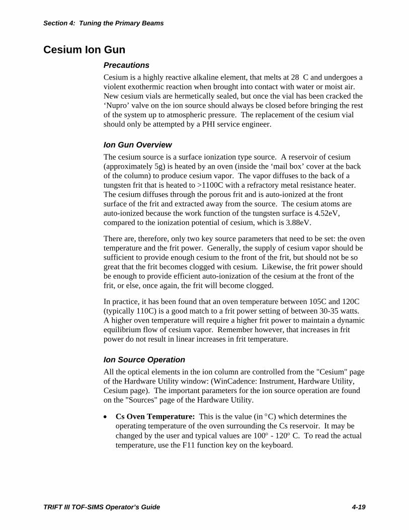
Section 4: Tuning the Primary Beams
Cesium Ion Gun Precautions Cesium is a highly reactive alkaline element, that melts at 28 C and undergoes a violent exothermic reaction when brought into contact with water or moist air. New cesium vials are hermetically sealed, but once the vial has been cracked the ‘Nupro’ valve on the ion source should always be closed before bringing the rest of the system up to atmospheric pressure. The replacement of the cesium vial should only be attempted by a PHI service engineer.
Ion Gun Overview The cesium source is a surface ionization type source. A reservoir of cesium (approximately 5g) is heated by an oven (inside the ‘mail box’ cover at the back of the column) to produce cesium vapor. The vapor diffuses to the back of a tungsten frit that is heated to >1100C with a refractory metal resistance heater. The cesium diffuses through the porous frit and is auto-ionized at the front surface of the frit and extracted away from the source. The cesium atoms are auto-ionized because the work function of the tungsten surface is 4.52eV, compared to the ionization potential of cesium, which is 3.88eV.
There are, therefore, only two key source parameters that need to be set: the oven temperature and the frit power. Generally, the supply of cesium vapor should be sufficient to provide enough cesium to the front of the frit, but should not be so great that the frit becomes clogged with cesium. Likewise, the frit power should be enough to provide efficient auto-ionization of the cesium at the front of the frit, or else, once again, the frit will become clogged.
In practice, it has been found that an oven temperature between 105C and 120C (typically 110C) is a good match to a frit power setting of between 30-35 watts. A higher oven temperature will require a higher frit power to maintain a dynamic equilibrium flow of cesium vapor. Remember however, that increases in frit power do not result in linear increases in frit temperature.
Ion Source Operation All the optical elements in the ion column are controlled from the "Cesium" page of the Hardware Utility window: (WinCadence: Instrument, Hardware Utility, Cesium page). The important parameters for the ion source operation are found on the "Sources" page of the Hardware Utility.
• Cs Oven Temperature: This is the value (in °C) which determines the operating temperature of the oven surrounding the Cs reservoir. It may be changed by the user and typical values are 100° - 120° C. To read the actual temperature, use the F11 function key on the keyboard.
TRIFT III TOF-SIMS Operator’s Guide 4-19

Section 4: Tuning the Primary Beams
• Cs Frit Power: This is the power value in Watts applied to the filament that surrounds the Cesium frit assembly. Cesium ionization occurs when the surface of the tungsten frit is high enough for the Cesium (diffusing up from the reservoir) to auto-ionize. Typical settings are 30 - 35 watts.
• Cs Emission: This is a ‘readable’ value to allow the user to measure the total ion emission from the frit, and is in units of microamperes. It can be read back using the F10 function key on the keyboard.
• Cs Control Electrode: This is a ‘field-shaping’ electrode immediately in front of the frit, for the purpose of optimizing the lens properties of the source region.
• Cs Frit Bias: This negative voltage floats on top of the beam energy. A negative voltage on the frit bias permits the stable operation of the control electrode. The frit bias has no ion optical purpose.
• Cs Extractor: This ‘floating extractor’ supply is downstream from the frit and control electrode, and allows more ion current to be drawn from the source. Its main use is to increase the probe current from low energy beams (typically ≤2,000 volts).
Operation Oven Set Temp Function Older, manual controllers for the Cesium source had “On”, “Off”, and “Revive” settings. This is now controlled by the simple expedient of the oven set temperature in the Sources tabbed page of the Hardware menu within the WinCadence software.
On: When the oven set temp is >40° C, the oven heater is turned on, the frit (ionizer) heater is turned on, as well as a minimum bias voltage on the frit (500V). The fan is set to off.
•
•
•
Off: If the oven set temperature is <20° C (for instance when a zero volt file is loaded), the fan is turned on (until oven temp is sensed to be <40° C), and the oven heater is turned off. The frit heater and frit bias are turned off once the oven temperature has fallen below 60° and 40° C respectively (Cs extracted from source while Cs vapor is inside ionizer tube).
Revive: If the oven temperature is set between 20° and 40° C, the oven is turned off, but the frit heater and frit bias remain on. This is the mode that you use to clear a ‘clogged’ frit. For instance, if the source had been run with too high an oven temperature, it is possible that there could be too much Cs in the tungsten pores, blocking smooth diffusion of Cs vapor (supply rate of Cs > removal of Cs by ionization). By running the frit heater and frit bias at a minimum value with the oven off, excess Cs can be cleared out of the source. This is the mode known as “revive”, for obvious reasons.
TRIFT III TOF-SIMS Operator’s Guide 4-20
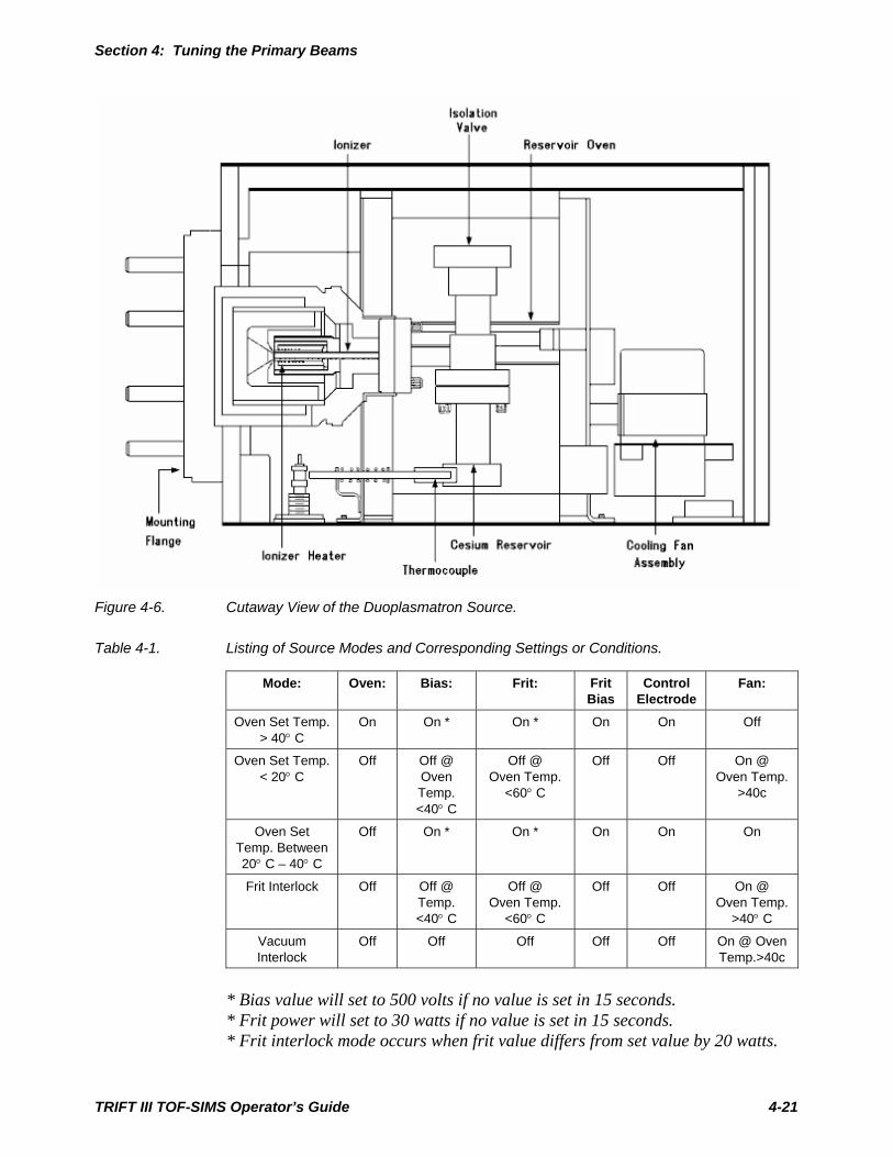
Section 4: Tuning the Primary Beams
Figure 4-6. Cutaway View of the Duoplasmatron Source.
Table 4-1. Listing of Source Modes and Corresponding Settings or Conditions.
Mode: Oven: Bias: Frit: Frit Bias
Control Electrode
Fan:
Oven Set Temp. > 40° C
On On * On * On On Off
Oven Set Temp. < 20° C
Off Off @ Oven Temp. <40° C
Off @ Oven Temp.
<60° C
Off Off On @ Oven Temp.
>40c
Oven Set Temp. Between 20° C – 40° C
Off On * On * On On On
Frit Interlock Off Off @ Temp. <40° C
Off @ Oven Temp.
<60° C
Off Off On @ Oven Temp.
>40° C
Vacuum Interlock
Off Off Off Off Off On @ Oven Temp.>40c
* Bias value will set to 500 volts if no value is set in 15 seconds. * Frit power will set to 30 watts if no value is set in 15 seconds. * Frit interlock mode occurs when frit value differs from set value by 20 watts.
TRIFT III TOF-SIMS Operator’s Guide 4-21

Section 4: Tuning the Primary Beams
Tuning for Spectroscopy at 10kV Beam Energy For spectroscopy performed at a beam energy of 10kV, the Cesium ion gun is first tuned for a D.C. beam current of ~1-2 nA (5ml slit / 5ml aperture) producing a probe diameter of ~50 µm. For spectral acquisition at high mass resolution, the beam is electrodynamically bunched to give a pulse width of ∼1.25-1.5 ns. The following description starts with a discussion of how to tune the ion gun in a D.C mode, followed by a discussion on how pulsing and bunching is achieved within this column. Finally, tuning for a pulsed, bunched and focused beam is described. A schematic of the Cesium ion column with all its optical elements is provided in Figure 4-6 below to assist the operator in becoming familiar with these operations.
Once the reservoir has reached its operating temperature, the total emission current from the source can be monitored by read-back of the emission current in the Source page of the hardware menu. With a beam energy of 10 keV, the emission current should be somewhere between 5-15 µA. The Control Electrode element in the Cesium page floats at the beam energy potential and is given an offset voltage to establish ion emission from the source (typically 0-100V) and provide some control over ion trajectories in the extraction region. This parameter is power supply-dependent and typically does not require any alteration.
TRIFT III TOF-SIMS Operator’s Guide 4-22
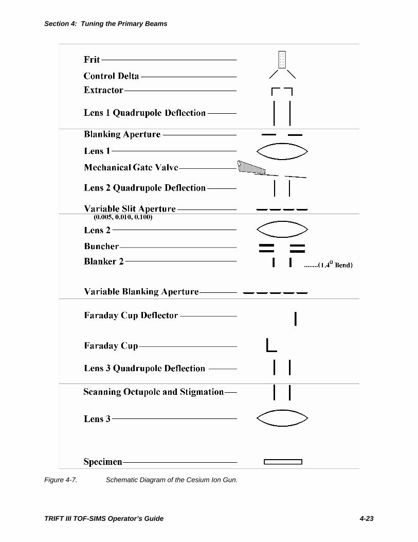
Section 4: Tuning the Primary Beams
Figure 4-7. Schematic Diagram of the Cesium Ion Gun.
TRIFT III TOF-SIMS Operator’s Guide 4-23
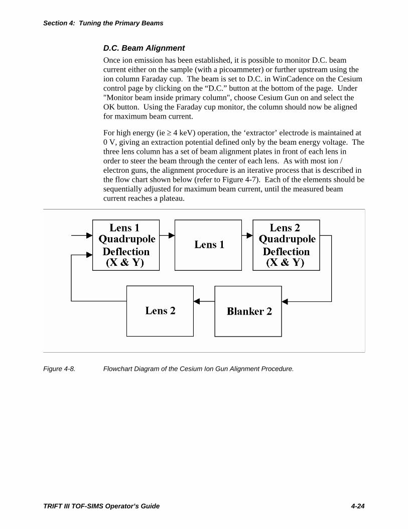
Section 4: Tuning the Primary Beams
D.C. Beam Alignment Once ion emission has been established, it is possible to monitor D.C. beam current either on the sample (with a picoammeter) or further upstream using the ion column Faraday cup. The beam is set to D.C. in WinCadence on the Cesium control page by clicking on the “D.C.” button at the bottom of the page. Under "Monitor beam inside primary column", choose Cesium Gun on and select the OK button. Using the Faraday cup monitor, the column should now be aligned for maximum beam current.
For high energy (ie ≥ 4 keV) operation, the ‘extractor’ electrode is maintained at 0 V, giving an extraction potential defined only by the beam energy voltage. The three lens column has a set of beam alignment plates in front of each lens in order to steer the beam through the center of each lens. As with most ion / electron guns, the alignment procedure is an iterative process that is described in the flow chart shown below (refer to Figure 4-7). Each of the elements should be sequentially adjusted for maximum beam current, until the measured beam current reaches a plateau.
Figure 4-8. Flowchart Diagram of the Cesium Ion Gun Alignment Procedure.
TRIFT III TOF-SIMS Operator’s Guide 4-24
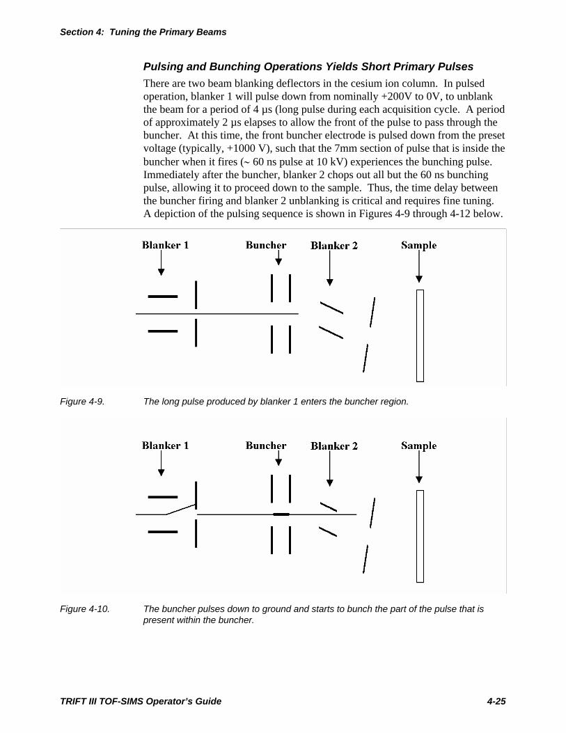
Section 4: Tuning the Primary Beams
Pulsing and Bunching Operations Yields Short Primary Pulses There are two beam blanking deflectors in the cesium ion column. In pulsed operation, blanker 1 will pulse down from nominally +200V to 0V, to unblank the beam for a period of 4 µs (long pulse during each acquisition cycle. A period of approximately 2 µs elapses to allow the front of the pulse to pass through the buncher. At this time, the front buncher electrode is pulsed down from the preset voltage (typically, +1000 V), such that the 7mm section of pulse that is inside the buncher when it fires (∼ 60 ns pulse at 10 kV) experiences the bunching pulse. Immediately after the buncher, blanker 2 chops out all but the 60 ns bunching pulse, allowing it to proceed down to the sample. Thus, the time delay between the buncher firing and blanker 2 unblanking is critical and requires fine tuning. A depiction of the pulsing sequence is shown in Figures 4-9 through 4-12 below.
Figure 4-9. The long pulse produced by blanker 1 enters the buncher region.
Figure 4-10. The buncher pulses down to ground and starts to bunch the part of the pulse that is present within the buncher.
TRIFT III TOF-SIMS Operator’s Guide 4-25
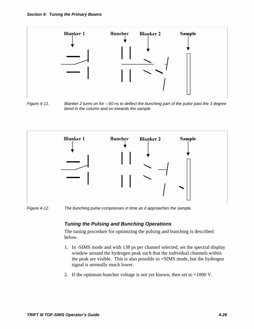
Section 4: Tuning the Primary Beams
Figure 4-11. Blanker 2 turns on for ∼ 60 ns to deflect the bunching part of the pulse past the 3 degree
bend in the column and on towards the sample.
Figure 4-12. The bunching pulse compresses in time as it approaches the sample.
Tuning the Pulsing and Bunching Operations The tuning procedure for optimizing the pulsing and bunching is described below.
1. In -SIMS mode and with 138 ps per channel selected, set the spectral display window around the hydrogen peak such that the individual channels within the peak are visible. This is also possible in +SIMS mode, but the hydrogen signal is normally much lower.
2. If the optimum buncher voltage is not yet known, then set to +1000 V.
TRIFT III TOF-SIMS Operator’s Guide 4-26

Section 4: Tuning the Primary Beams
3. Acquire data from a planar sample, such as a silicon wafer.
4. In the delay line page (WinCadence: ‘Instrument, Set Delay Lines’) the parameter called ‘Buncher’ allows the buncher timing to be adjusted in 1 ns increments. The parameter referred to as ‘Blanker 2’ sets the pulse width of blanker 2 in units of nanoseconds. Set the pulse width to 40-60 ns and the delay to anything between 0 to 255ns.
5. Lower the blanker 2 voltage by about 10 % from the D.C. value, to allow for the reduction in mean beam energy brought about by the bunching operation.
6. Using the image on the DMCP, adjust the bucher delay until some bunching is evident. Bunching is recognized by a defocusing of the beam viewed on the DMCP. Typically, lens 3 will focus ∼300 V lower in the pulsing / bunching operation compared to the D.C. beam condition. Re-focus Lens 3 for the best probe under bunched conditions.
7. Slight adjustment of the lens 2 voltage may now be necessary to obtain the brightest image at the DMCP. This will optimize the position of the beam cross-over in the blanking aperture. This should result in the minimum change in the blanker 2 voltage to turn the beam off (∼20 V reduction in the blanker 2 voltage should blank the beam). Focus the beam again with lens 3.
8. The timing of the buncher and the setting of blanker 2 should now be optimized while acquiring a negative ion spectrum and observing the H- peak width. It is possible to compress a 40-60 ns pulse down to 1.25-1.5 ns FWHM (i.e. 9-11 channels at 138 ps / channel) with optimum buncher voltage and timing.
TRIFT III TOF-SIMS Operator’s Guide 4-27

Section 4: Tuning the Primary Beams
Low Energy Cesium Beam Alignment For dual beam depth profiling, an instrument file containing both the LMIG settings and the Cs beam settings is necessary. New instruments ship with an instrument file for depth profiling with a 1 keV Cs beam and a 15 keV bunched LMIG for acquisition. This section is useful for setting up other low energy Cs beam settings or for re-tuning the 1 keV file. A variety of dual beam depth profiling instrument files can be setup by using the filter load function to match the desired LMIG settings with the desired Cs beam settings.
All three lenses and lens 1 and 2 steering are expressed as a percentage (%) of the beam energy. This makes it easier to generate new Cesium beam files at different energies by simply changing the beam energy value. The three lenses and lens 1 and 2 steering should scale close to the optimum value. Notice that the settings for lens 3 steering will have to be set manually by scaling to the new beam energy.
The D.C. tuning procedure is almost the same as the high energy D.C. beam alignment described above, with the exception of tuning the extractor electrode in order to maintain an approximately 3kV extraction potential. Set the Extractor voltage so that the Cesium beam energy plus the Extractor potential = 3kV. For example, if the Beam Energy is 1,000, set the Extractor to 2,000. Fine tuning of the lens 3 voltage does, however, require a different method to that described for 10keV operation. At beam energies suitable for high depth resolution depth profiling (≤ 3keV), the column needs to be tuned with a sample bias as close to zero as possible.
A method of setting the lens 3 value is described below using SEM imaging.
SED-based method for tuning the low energy D.C. Cs beam 1. Use as a sample one of the coarse metallic grids in a sample holder, with no
backing plate and no true sample. Imaging the coarse grid bars will give good image contrast.
2. Close the spectrometer gate valve as a precaution, since you do not need to use the mass spectrometer for this operation.
3. In -SIMS mode, turn the Cesium beam to DC using the DC button at the bottom of the Cesium page in Hardware Utilities. Select Cesium Beam under "Deliver Beam to Sample" and select the OK button. Now set the following: -The sample bias to approximately -200 V. -The immersion lens to 550. -The high mass blanker to 7.
TRIFT III TOF-SIMS Operator’s Guide 4-28

Section 4: Tuning the Primary Beams
4. Set the cesium raster size to 1,000 µm, and increase the SED gain until you begin to see an image. Fine-tune the immersion lens and the high mass blanker voltages for the most intense and uniform image intensity. It should now be possible to focus lens 3 for the best grid image.
5. Wobble the lens 3 voltage by approximately 50 V and minimize the translation of the image with the lens 3 (quadrupole) deflectors.
6. Switch the video so that the optical view is on the monitor, and position the sample so that a recognizable part of the grid is in the center of the light optic’s field of view (closely corresponding to the center of the spectrometer’s field of view during analysis).
7. Switch the video to display the SED image once again and adjust the Cesium beam x and y position voltages to image the same field of view as the light optics. While this will not necessarily position the cesium beam exactly, it will bring it very close. More accurate alignment of the LMIG and cesium probes is described in the ‘Interleaved Depth Profiling’ section.
8. Once the best focus is obtained, press the DC button again to blank the beam. Set the sample bias and immersion lens to their original values. Resave the instrument file.
Dual Source Column Option General Description Some TRIFT systems are equipped with a dual source ion column for depth profiling. The dual source column consists of the Cs gun as described above, along with the addition of a duoplasmatron ion source for producing an oxygen ion beam. In general, the Cs+ ion beam is used for –SIMS depth profiling while the O2
+ ion beam is used for +SIMS depth profiling. In many cases, the O2+
beam is used together with the oxygen leak valve to ensure full oxidation of the material being depth profiled.
The duoplasmatron source is mounted in-line on the end of the column while the cesium source is mounted at a 45 degree angle to the column. The Cs+ primary ion beam is steered around the 45o bend with an electrostatic sector in order to bring it down the optical center of the column. A schematic of the dual source column is shown in Figure 4-13 below.
The column should be tuned up first with the O2+ beam with the ESA’s set to 0
volts. The column is tuned up in the normal way as described above for the cesium ion beam. Once the column is tuned up for the oxygen beam, Lens 1, Lens 1 steering, and the ESA’s can be set for the Cs+ beam to bring it down the same path through the column. A description of the duoplasmatron source is given below.
TRIFT III TOF-SIMS Operator’s Guide 4-29
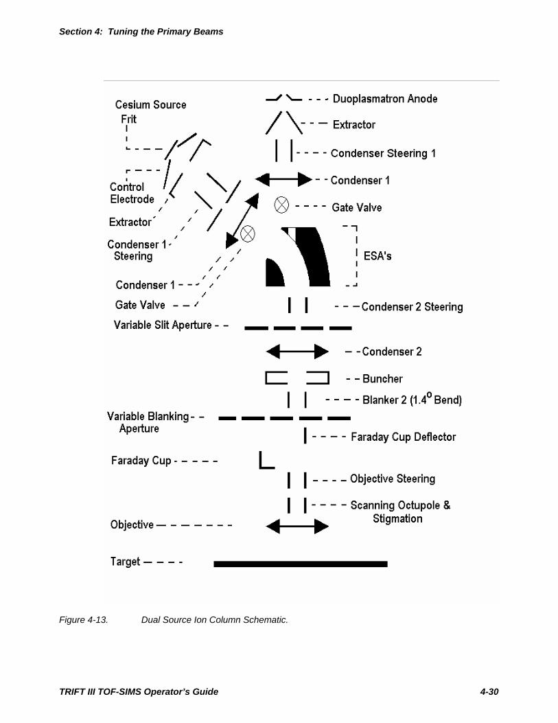
Section 4: Tuning the Primary Beams
Figure 4-13. Dual Source Ion Column Schematic.
TRIFT III TOF-SIMS Operator’s Guide 4-30
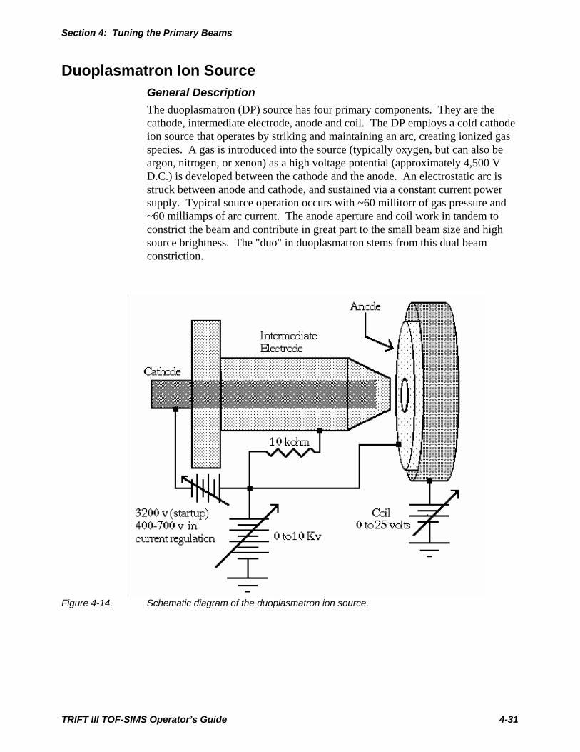
Section 4: Tuning the Primary Beams
Duoplasmatron Ion Source General Description The duoplasmatron (DP) source has four primary components. They are the cathode, intermediate electrode, anode and coil. The DP employs a cold cathode ion source that operates by striking and maintaining an arc, creating ionized gas species. A gas is introduced into the source (typically oxygen, but can also be argon, nitrogen, or xenon) as a high voltage potential (approximately 4,500 V D.C.) is developed between the cathode and the anode. An electrostatic arc is struck between anode and cathode, and sustained via a constant current power supply. Typical source operation occurs with ~60 millitorr of gas pressure and ~60 milliamps of arc current. The anode aperture and coil work in tandem to constrict the beam and contribute in great part to the small beam size and high source brightness. The "duo" in duoplasmatron stems from this dual beam constriction.
Figure 4-14. Schematic diagram of the duoplasmatron ion source.
TRIFT III TOF-SIMS Operator’s Guide 4-31
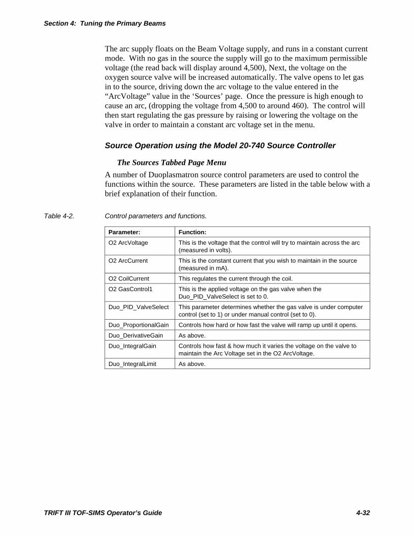
Section 4: Tuning the Primary Beams
The arc supply floats on the Beam Voltage supply, and runs in a constant current mode. With no gas in the source the supply will go to the maximum permissible voltage (the read back will display around 4,500), Next, the voltage on the oxygen source valve will be increased automatically. The valve opens to let gas in to the source, driving down the arc voltage to the value entered in the “ArcVoltage” value in the ‘Sources’ page. Once the pressure is high enough to cause an arc, (dropping the voltage from 4,500 to around 460). The control will then start regulating the gas pressure by raising or lowering the voltage on the valve in order to maintain a constant arc voltage set in the menu.
Source Operation using the Model 20-740 Source Controller
The Sources Tabbed Page Menu A number of Duoplasmatron source control parameters are used to control the functions within the source. These parameters are listed in the table below with a brief explanation of their function.
Table 4-2. Control parameters and functions.
Parameter: Function: O2 ArcVoltage This is the voltage that the control will try to maintain across the arc
(measured in volts).
O2 ArcCurrent This is the constant current that you wish to maintain in the source (measured in mA).
O2 CoilCurrent This regulates the current through the coil.
O2 GasControl1 This is the applied voltage on the gas valve when the Duo_PID_ValveSelect is set to 0.
Duo_PID_ValveSelect This parameter determines whether the gas valve is under computer control (set to 1) or under manual control (set to 0).
Duo_ProportionalGain Controls how hard or how fast the valve will ramp up until it opens.
Duo_DerivativeGain As above.
Duo_IntegralGain Controls how fast & how much it varies the voltage on the valve to maintain the Arc Voltage set in the O2 ArcVoltage.
Duo_IntegralLimit As above.
TRIFT III TOF-SIMS Operator’s Guide 4-32

Section 4: Tuning the Primary Beams
Starting values (first time firing) Note: The values and steps listed below should be used any time after the following conditions to verify that the valve characteristics have not changed: - anytime that a new Piezo valve is installed; or - just after a bake.
1. Start with a zero volt (zerovolt.ins) instrument file.
2. Verify (within Watcher) that gate valve V4 is open and that the Duo Source is being differentially pumped. There is no safety interlock. Also insure that the isolation valve is open on the ion gun column.
3. Before starting to let in gas, measure the O2 ArcVoltage. It should be in a range between 4,000 to 4,500. If it is around 500 – 700, an Intermediate-to-Cathode short exists and the source will require cleaning. This is a very unambiguous diagnostic. Similarly, the O2 ArcCurrent readback should be around 1 – 4 (without oxygen gas flowing), if it reads 60, there is a short (probably caused by a flake of oxide).
TRIFT III TOF-SIMS Operator’s Guide 4-33
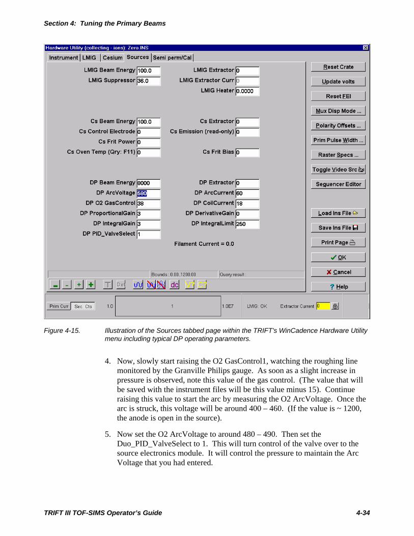
Section 4: Tuning the Primary Beams
Figure 4-15. Illustration of the Sources tabbed page within the TRIFT's WinCadence Hardware Utility menu including typical DP operating parameters.
4. Now, slowly start raising the O2 GasControl1, watching the roughing line monitored by the Granville Philips gauge. As soon as a slight increase in pressure is observed, note this value of the gas control. (The value that will be saved with the instrument files will be this value minus 15). Continue raising this value to start the arc by measuring the O2 ArcVoltage. Once the arc is struck, this voltage will be around 400 – 460. (If the value is ~ 1200, the anode is open in the source).
5. Now set the O2 ArcVoltage to around 480 – 490. Then set the Duo_PID_ValveSelect to 1. This will turn control of the valve over to the source electronics module. It will control the pressure to maintain the Arc Voltage that you had entered.
TRIFT III TOF-SIMS Operator’s Guide 4-34

Section 4: Tuning the Primary Beams
6. Now set the O2 GasControl1 to the value from step 3 (value of just opening minus 15 volts).
7. Record these values. Change polarity and enter them on the other side of the instrument file, (in case polarities are changed accidentally, the arc will not be lost). Now save this Instrument file as ‘StartUpDuo.ins’, or some other clearly named file. This will result in a good file to get the source going. It will still be running a gas load of approx. 100 – 120 millitorr in the source, but should start the arc and go into pressure regulation fairly quickly.
Normal Source Operating Condition
Best Starting Conditions We have just discussed how to create a file with duo parameters that allow the source to start easily. Unfortunately, such a duo condition will result in a poor probe, no matter how hard you try to tune the ion column subsequently. Consequently, the source will start with a lower arc voltage, but then the arc voltage will need to be raised to a higher value, as discussed in the next section.
Best Probe-Forming Conditions For best performance (source brightness), it is well known that a duoplasmatron should be run ‘lean’, i.e. with a lower gas pressure. On a well-conditioned source with a nickel cathode, running a value of around 570 – 600 for the arc voltage should be close. The higher the voltage you set, the less will be the gas pressure. (refer to following chart in Figure 4-16 below). A parameter value is required that is not set too close to a level at which the source will lose its arc.
Invest a few moments and perform the following experiment: on a conditioned source, raise the arc voltage in 10 volt steps, monitoring an ion beam into the column Faraday, or frequently reading back the arc voltage. Raise the arc voltage until the arc is extinguished. A good operating arc voltage will be ~50-75 volts down from that extinction value. Verify that you have a stable source at such a value, and then save an instrument file with a suitable name, such as ‘BestDuo.ins’ or some such name.
TRIFT III TOF-SIMS Operator’s Guide 4-35
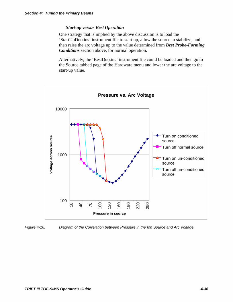
Section 4: Tuning the Primary Beams
Start-up versus Best Operation One strategy that is implied by the above discussion is to load the ‘StartUpDuo.ins’ instrument file to start up, allow the source to stabilize, and then raise the arc voltage up to the value determined from Best Probe-Forming Conditions section above, for normal operation.
Alternatively, the ‘BestDuo.ins’ instrument file could be loaded and then go to the Source tabbed page of the Hardware menu and lower the arc voltage to the start-up value.
Pressure vs. Arc Voltage
100
1000
10000
10 40 70 100
130
160
190
220
250
Pressure in source
Turn on conditionedsourceTurn off normal source
Turn on un-conditionedsourceTurn off un-conditionedsource
Figure 4-16. Diagram of the Correlation between Pressure in the Ion Source and Arc Voltage.
TRIFT III TOF-SIMS Operator’s Guide 4-36

Section 4: Tuning the Primary Beams
The Electron Neutralization Gun Important features of the neutralization scheme employed in the PHI TRIFT III TOF-SIMS system are its simplicity of operation and the infrequency of tuning. There are no front panel tuning knobs, and the parameter variations that are available within the WinCadence software program rarely require any adjustment. The benefits of this scheme are that, under most experimental conditions, the only requirement is to remember to select "Analytical with chg. comp" within Acquisition setup in WinCadence.
There are, however, circumstances in which the tuning of the e-gun will require checking. These occur:
• After replacing the filament;
• If a deterioration in the neutralization performance is detected; or
• If system performance is to be monitored on a routine basis.
Testing for Filament Current and Filament Continuity The filament current to the electron gun is applied either by:
• Setting the value of Egun Filament Power in the Instrument page of the Hardware menu to some value such as 4.5 (0-6 max), or
• Selecting “Analytical with chg. comp” in the acquisition setup menu. In this latter case, a default value stored in the registry is used.
If a sudden deterioration in the neutralization performance is detected, the most likely cause is loss of filament current, probably due to filament failure.
To determine if the filament is intact, check the readback voltage (V) for the E-gun Filament Power on the Instrument page of the WinCadence Hardware menu. Note that the E-gun Filament Power is normally set to 4.5 (for the “On” state of the E-gun) and that this should be the readback value if the filament is intact.
TRIFT III TOF-SIMS Operator’s Guide 4-37

Section 4: Tuning the Primary Beams
Setting the Correct Filament Current The curve of electron emission current versus filament current for a thermionic emission source is 'S-shaped', exhibiting three major regimes:
• No electron emission: temperature of the filament insufficient for thermionic emission.
• Rapid rate of change of electron emission with filament current: temperature for onset of thermionic emission exceeded.
• Decreasing amounts of extra electron emission for incremental changes in filament current: the filament is said to be "saturated", owing to 'space-charge' effects.
The correct filament current setting occurs when the curve of electron emission versus filament current has just "turned over", e.g., just as the filament begins to 'saturate'. If the filament current is higher than this, the filament’s lifetime is significantly reduced for no significant gain in electron emission. If the filament current is less than this, small fluctuations in current result in large variations in the electron emission.
Figure 4-17. Illustration of Ion Gun Emission Current v.s. Filament Current.
The correct filament current for the tungsten filaments used in the electron gun is typically 2.4 amps, or a measured filament voltage of ~1.2 volts. The actual value may vary slightly from this, and should be determined by the saturation curve.
TRIFT III TOF-SIMS Operator’s Guide 4-38

Section 4: Tuning the Primary Beams
Measuring/Maximizing Pulsed Electron Current This section outlines the steps that are necessary both to measure and then maximize the pulsed electron current to the analytical area. If for any reason the factory-set values must be changed, record these factory settings first so they can be returned to the original values if necessary. For this next stage, measurements need to be made with a Faraday cup.
A Faraday cup is provided in the Sample Mounting Kit, but one can also be made. To make a Faraday cup, cut two standard length microscope slides so that both fit horizontally within the single window sample holder. Attach the large window front plate as described in Section 2. Use four Cu-Be sample clips to hold the glass slides in place against the window. Next, cut a strip of aluminum foil with dimensions 4mm x 50mm. Fold the strip to produce a more rigid strip with dimensions 2 mm x 50 mm. Insert the strip in the gap between the two glass slide, and with the aid of tweezers, fold the strip to produce a square with dimensions 2 mm x 2 mm on one of the glass slides. The remainder of the metal strip should now be behind the glass slides. Now connect this tail to the sample carrier by trapping it with a fifth sample clip, in the center of the holder. Refer to the schematic diagram below. For 200mm systems (which has no 50mm single window sample holder), take a 150mm or 200mm wafer and place a clean, adhesive-backed plastic square, approximately 50mm x 50mm, at the center of the wafer. Cut out a 2mm x 2mm square of the plastic in the center of the wafer. This serves very well as a Faraday cup sample for electron gun alignments for the 200mm instrument. Refer to Figure 4-18 below.
To monitor and/or maximize the pulsed electron current to the Faraday cup, proceed as follows:
1. Load the Faraday cup assembly described above and centralize the aluminum square within the optical field of view.
2. Select “Analytical with chg. comp” in Acquisition Setup to ensure the filament is ON.
3. Set the instrument for Negative SIMS.
4. Set the sample voltage to 0 (zero). Lower the LMIG Extractor to turn off the filed emission so that the LMIG extractor current reads 0 (zero).
5. Remove the high voltage cable to the sample stage and connect an electrometer using the PHI-supplied lead which has an MHV connector at one end for the stage and a BNC connector at the other end for the electrometer.
TRIFT III TOF-SIMS Operator’s Guide 4-39
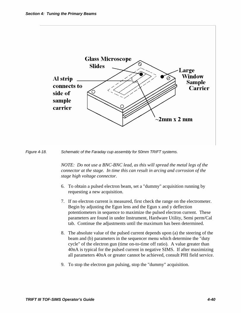
Section 4: Tuning the Primary Beams
Figure 4-18. Schematic of the Faraday cup assembly for 50mm TRIFT systems.
NOTE: Do not use a BNC-BNC lead, as this will spread the metal legs of the connector at the stage. In time this can result in arcing and corrosion of the stage high voltage connector.
6. To obtain a pulsed electron beam, set a "dummy" acquisition running by requesting a new acquisition.
7. If no electron current is measured, first check the range on the electrometer. Begin by adjusting the Egun lens and the Egun x and y deflection potentiometers in sequence to maximize the pulsed electron current. These parameters are found in under Instrument, Hardware Utility, Semi perm/Cal tab. Continue the adjustments until the maximum has been determined.
8. The absolute value of the pulsed current depends upon (a) the steering of the beam and (b) parameters in the sequencer menu which determine the "duty cycle" of the electron gun (time on-to-time off ratio). A value greater than 40nA is typical for the pulsed current in negative SIMS. If after maximizing all parameters 40nA or greater cannot be achieved, consult PHI field service.
9. To stop the electron gun pulsing, stop the "dummy" acquisition.
TRIFT III TOF-SIMS Operator’s Guide 4-40
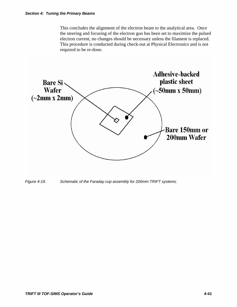
Section 4: Tuning the Primary Beams
This concludes the alignment of the electron beam to the analytical area. Once the steering and focusing of the electron gun has been set to maximize the pulsed electron current, no changes should be necessary unless the filament is replaced. This procedure is conducted during check-out at Physical Electronics and is not required to be re-done.
Figure 4-19. Schematic of the Faraday cup assembly for 200mm TRIFT systems.
TRIFT III TOF-SIMS Operator’s Guide 4-41

Sputter Gas Gun The TRIFT III instrument is delivered from the factory with the following Gas Gun instrument files:
Filename Description
GasGun_5kV_Max.ins 5kV, 3uA max sputter current file
GasGun_5kV_Min.ins 5kV, minimum beam size file
GasGun_5kV_1uA.ins 5kV, 1uA sputter current file
GasGun_2kV_400nA.ins 2kV, 400nA sputter current file
GasGun_1kV_200nA.ins 1.5kV,-500Float, 200nA sputter current file
GasGun_500V_100nA.ins 1kV,-500Float, 100nA sputter current file
These files have been saved as Gas Gun only instrument files and are meant to be filter loaded with a desired primary gun file to customize the desired profiling performance. Please refer to Section7 Dual Gun Profiling.
This section describes the operation of the sputtering ion gun, which can be used to sputter clean samples and to perform “phase depth profiles”. Included will be information needed to tune and operate the ion gun efficiently for best results and to prolong the lifetime of the ionizer/filament. The subsections in this section include:
Gas Gun Overview
Gas Gun Operation
Conditioning the Gas Gun Ionizer and High Voltage
Setup and Calibrating the Argon Gas Regulation
Creating New or Tuning Existing Gas Gun Parameters
Gas Gun Ionizer Shutdown
Gas Gun Overview The 06-360 is a low energy argon sputter gun. The ion gun has been developed for high depth resolution, rapid sputtering and low impact energy. It can be used as an alternative to the micro-focusing (duo/cesium) column in “phased depth profiling” applications. The Gas Gun does not operate in a pulsed/bunched mode and will not be used as the primary spectroscopy gun.
The ion source is a hot filament, electron impact ionizer that is configured for ionizing argon. The argon ionizer uses a tungsten filament to operate the ionizer at 15mA emission, while a pneumatic controller and flow restriction aperture delivers a source pressure of 15mPa. New ionizers should be conditioned prior
TRIFT III TOF-SIMS Operator’s Guide 4-42

Section 4: Tuning the Primary Beams
to operating. An adjustable grid voltage is provided to optimize ionization and extraction of ions from the source into the gun column. The Gas Gun is differentially pumped by the turbo pump mounted to the condenser section of the gun column.
The ion gun has a continuously variable energy range from 0-5keV. At low beam energies (impact energies < 1keV) the ion column is “floated” up to -500V to improve beam transport through the ion column. A condenser lens focuses ions extracted from the source to a position at or before the objective (pressure step) aperture. The objective lens focuses the beam onto the sample. The higher the condenser lens setting, the smaller the spot size and smaller the sputter current. With varying condenser lens settings, a slight adjustment is required of the objective lens for best focus.
To blank the beam and also prevent neutrals from hitting the sample, a set of deflector plates are located just upstream of the objective aperture to deflect the beam around a 5º bend. During sputter operation, the blanking voltage is optimized to steer the beam through the bend and through the center of the objective lens/octupole region. During blank operation, the condenser lens is automatically set to provide a crossover of the beam at the blanking plates and the blanker voltage is automatically set to deflect the beam into a beam trap to minimize column current from reaching the sample.
A set of octupole deflectors are located at the end of the ion column to scan and shift the beam across the sample.
The Gas Gun housing is equipped with a set of X/Y port alignment adjustor. These are used to mechanically align a non-deflected beam to the center of the spectroscopy position of a sample, when the sample is at “zero” potential.
Gas Gun Operation All the optical elements in the ion column are controlled from the "Gas Gun" page of the Hardware Utility window: (WinCadence: Instrument, Hardware Utility, Gas Gun page). Additional parameters for the blanking operation and ionizer usage are found on the "Gas Gun" page of the WinCadence Options window. The sputter raster pattern during external raster operation is found on the Raster Specification window. The following page contains examples of WinCadence menus associated with the Gas Gun.
TRIFT III TOF-SIMS Operator’s Guide 4-43
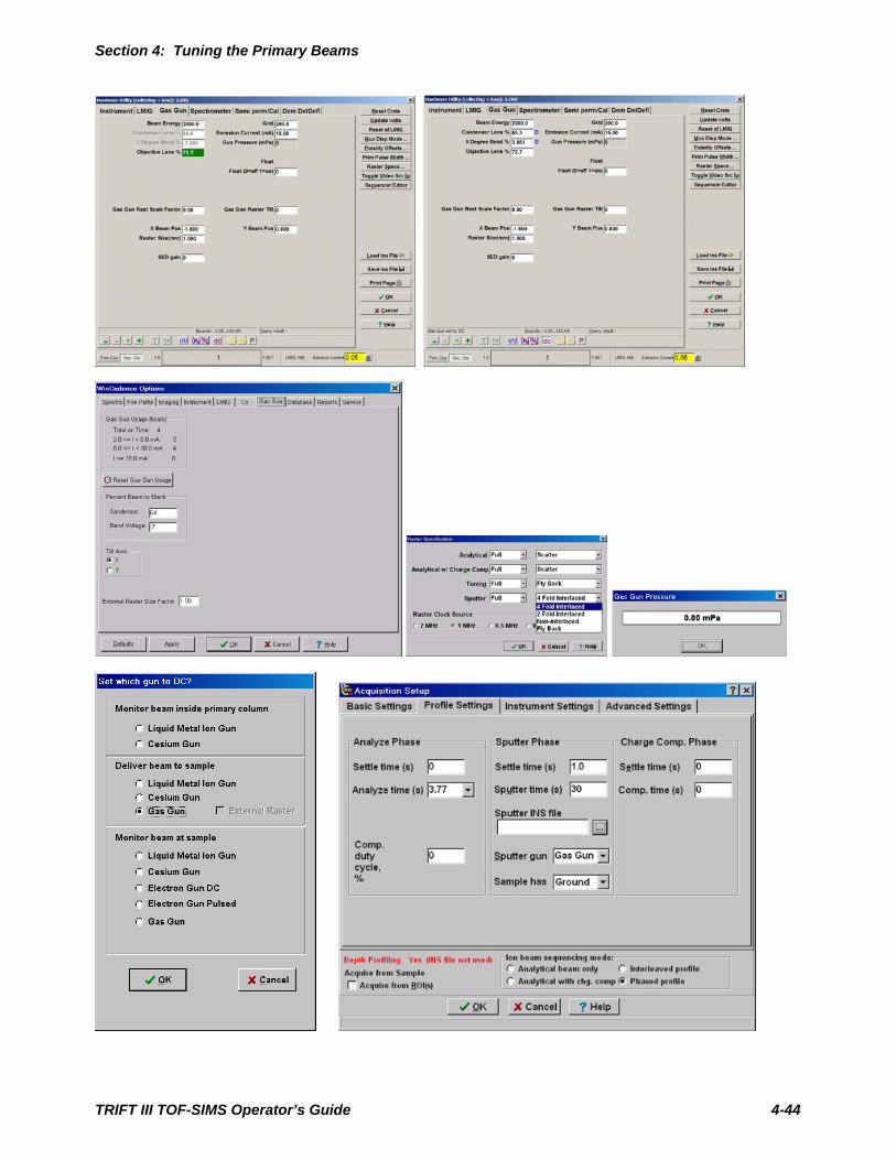
Section 4: Tuning the Primary Beams
TRIFT III TOF-SIMS Operator’s Guide 4-44

Section 4: Tuning the Primary Beams
Emission Current (mA): This value determines the voltage applied to the ionizer filament to maintain this target emission current. The recommended value of 15mA will extend the life of the filament and provide required emission from the source. Higher values may provide additional emission current but will greatly reduce the life of the filament. To read the actual current, use the F10 function key on the keyboard while this field is highlighted. Note: This field is not saved with an instrument file. When an instrument file is loaded, the emission will need to be manually adjusted as well as manual operation of V10 to initiate the flow of Argon into the ionizer. Once this value has been entered, it will be used to regulate the ionizer until a new value or 0mA has been entered. This input will be incremented in 1mA steps by the software when a new value is entered.
• Grid voltage: The grid voltage is set to 200 during calibration of the argon pressure control. In the DC mode, it is adjusted to maximize the sample current. Typical settings are 120-160 volts in the DC mode. To read the actual supply voltage, use the F10 function key on the keyboard while this field is highlighted.
• Gun Pressure (mPa): This field is a readback only display of the pressure measured in the ionizer. This reading is accurate at 0.1kev Beam Energy with a 200v Grid voltage. During DC operation, lower Grid voltages and higher Beam Energies will appear to reduce this value as fewer electrons are available in the ionizing region and more ions are being accelerated from the ionizer. Clicking the “P” icon at the bottom of the Gas Gun window will pop-up an auxiliary window displaying the pressure reading and bar graph of pressure intensity. See section on calibrating gas flow.
• Beam Energy and Float: The beam energy is used in conjunction with the Float to select the impact energy of the sputtering ions. Higher values of Beam Energy will deliver a smaller beam diameter with higher sputter rates. Higher values will also result in increased impact energy and reduced “depth resolution”. Lower Beam Energies are desired to improve “depth resolution”. With desired energies of <1keV, the Float supply can be used in conjunction with the Beam Energy to increase the efficiencies of the transport of the lower energy ions down the ion column. The actual impact energy can be determined by adding the -Float voltage to the +Beam Energy. To read either of the actual supply voltages, use the F10 function key on the keyboard while either of these fields is highlighted. Note: External rastering is not available if a Float Voltage is selected. The default is an internal triangular raster pattern. Note: When choosing a Beam Energy and Float value, keep the final impact energy => the Float value. Choosing a combination resulting in an impact energy < the Float value will alter the operation of the Objective Lens focusing.
TRIFT III TOF-SIMS Operator’s Guide 4-45

Section 4: Tuning the Primary Beams
• Condenser Lens: The condenser lens is adjusted to set the desired sample current for a given Beam Energy. Typically a value of 68-70% of the Beam Energy will maximize the sample current. Increasing this value towards 100% will reduce the beam size and current. To read the actual supply voltage, use the F10 function key on the keyboard while this field is highlighted. Note: Normally this field is dithered and a fixed value 64% of the Beam Energy is applied to optimize the beam blanking state. When the “dc” icon is chosen, this field will display the previously saved Condenser Lens value selected to set the sputter current. In addition, a “D” will be displayed next to the field to indicate the DC operation mode.
• 5º Bend: The 5º Bend is adjusted to steer the beam through the center of the Objective Lens and Octupole; as well as to optimize sample current for a given Beam Energy. Typically a value of 3.5% of the Beam Energy will optimize operation. To read the actual supply voltage, use the F10 function key on the keyboard while this field is highlighted. Note: Normally this field is dithered and a fixed value -7% of the Beam Energy is applied to optimize the beam blanking state. When the “dc” icon is chosen, this field will display the previously saved 5º Bend value. In addition, a “D” will be displayed next to the field to indicate the DC operation mode.
• Gas Gun Rast Scale Factor: This value is used to calibrate the Raster Size in the Y axis. This calibration can be accomplished at 5KeV operation [where it is easier to image] and will be accurate for all selected Beam Energies. Note: a slightly different value may be needed between +SIMS and – SIMS. Note: This parameter will also affect the X axis size, but the Gas Gun Raster Tilt will provide the final calibration of the X axis scanning.
• Gas Gun Raster Tilt: This value is used to calibrate the Raster Size in the X axis [due to the mounting angle of the sputter gun with respect to sample normal]. This should be optimized after the Y axis has been calibrated. This calibration can be accomplished at 5KeV operation and will be accurate for all selected Beam Energies. Note: a slightly different value may be needed between +SIMS and – SIMS.
• X Beam Pos: This value is used to steer the sputter pattern to coincide with the Primary Gun’s analysis area on the sample. This value will need to be optimized for different trajectories in –SIMS vs +SIMS and float vs. non-float operation. A more + value will move the sputter position to the right on the sample as viewed on the optical camera or LMIG SED image.
• Y Beam Pos: This value is used to steer the sputter pattern to coincide with the Y position of the Primary Gun’s Analysis area on the sample. This value will track the Beam Energy supply and will need minimal optimization with varying Beam Energies. A more + value will move the sputter position down on the sample as viewed on the optical camera or LMIG SED image.
TRIFT III TOF-SIMS Operator’s Guide 4-46

Section 4: Tuning the Primary Beams
• Raster Size(mm): This value when calibrated with the Scale and Tilt Factors will track the Beam Energy supply and will determine the size of the sputter crater. This value should typically be set to 4x the analysis area dimension.
Conditioning the Gas Gun Ionizer and High Voltage The ionizer needs to be conditioned (to outgas the filament) whenever the Gas Gun column has been vented. Verify that differential pumping is on and that the chamber pressure is less than 1x10⁻⁹ torr. Verify V10 is closed.
Load the GasGunMaintenance.INS file. Note: if this has not been created yet, perform the following: Create an instrument file filtering in a typical Ga setting. Set the Gas Gun Beam Energy to 100V, the Emission to 0mA, and the Grid to 200V. Save this as GasGunMaintenance.INS.
Select the P icon and monitor the pressure during this procedure. Set the Emission to 1mA. Wait for the pressure to recover to <0.5mPa. Increase the Emission in 1mA steps up to 15mA, keeping the Extractor Pressure reading below 50mPa. Wait for the pressure to recover to <0.5mPa before going to the next emission Current setting. After proper outgassing, the Extractor Pressure should reach a value below 0.5mPa with the Emission set to 15mA. Set the Emission back to 0mA.
Increase the Beam Energy to 500v. Monitor the Extractor Pressure and chamber pressure while increasing the Beam Energy in 500v increments up to 5000v. With the Beam Energy at 5000v, repeat this procedure increasing the Condenser and Objective Lens values to match the Beam Energy value of 5000v. If there is a jump in pressure, reduce the voltages and repeat the procedure.
Setup and Calibrating the Argon Gas Regulation The gas handling system has been designed to provide a constant pressure delivered to the argon ionizer. Once it is manually calibrated, on/off control is provided through Watcher control of V10.
TRIFT III TOF-SIMS Operator’s Guide 4-47
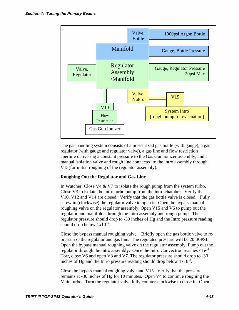
Section 4: Tuning the Primary Beams
Valve, Bottle
1000psi Argon Bottle
Manifold Gauge, Bottle Pressure
Regulator Assembly /Manifold
Gauge, Regulator Pressure 20psi Max
Valve, Regulator
Valve, NuPro
V15
V10 System Intro
[rough pump for evacuation]
The gas handling system consists of a pressurized gas bottle (with gauge), a gas regulator (with gauge and regulator valve), a gas line and flow restriction aperture delivering a constant pressure to the Gas Gun ionizer assembly, and a manual isolation valve and rough line connected to the intro assembly through V15(for initial roughing of the regulator assembly).
Roughing Out the Regulator and Gas Line
In Watcher: Close V4 & V7 to isolate the rough pump from the system turbo. Close V3 to isolate the intro turbo pump from the intro chamber. Verify that V10, V12 and V14 are closed. Verify that the gas bottle valve is closed. Fully screw in (clockwise) the regulator valve to open it. Open the bypass manual roughing valve on the regulator assembly. Open V15 and V6 to pump out the regulator and manifolds through the intro assembly and rough pump. The regulator pressure should drop to -30 inches of Hg and the Intro pressure reading should drop below 1x10⁻³.
Close the bypass manual roughing valve. Briefly open the gas bottle valve to re-pressurize the regulator and gas line. The regulated pressure will be 20-30PSI. Open the bypass manual roughing valve on the regulator assembly. Pump out the regulator through the intro assembly. Once the Intro Convectron reaches <1e-3 Torr, close V6 and open V3 and V7. The regulator pressure should drop to -30 inches of Hg and the Intro pressure reading should drop below 1x10⁻³.
Close the bypass manual roughing valve and V15. Verify that the pressure remains at -30 inches of Hg for 10 minutes. Open V4 to continue roughing the Main turbo. Turn the regulator valve fully counter-clockwise to close it. Open
Flow Restriction
Gas Gun Ionizer
TRIFT III TOF-SIMS Operator’s Guide 4-48

Section 4: Tuning the Primary Beams
V10 to pump out the small volume between the pressure step aperture and the Gas Gun. Close V10. Open the gas bottle valve.
Setting the Regulator Pressure for Ion Gun Operation
Load the GasGunMaintenance.INS file. Note: if this has not been created yet, perform the following: Create an instrument file filtering in a typical Ga setting. Set the Gas Gun Beam Energy to 100V, the Emission to 0mA, and the Grid to 200V. Save this as GasGunMaintenance.INS.
Open V10 in Watcher. Set the Emission to 15mA. [Note: WinCadence will increment the emission in 1maA steps]. Select the P icon to monitor the pressure. (J11 on the back of the 11-066 Gas Control will also provide a 5mPa/V reading). Verify that the pressure is <0.5mPa before continuing. Slowly turn the regulator valve clockwise until the pressure reading is 15mPa or ~3V on J11. Allow the regulator and ionizer to stabilize for 1 hour and then readjust if necessary for a reading of 15mPa or 3V on J11.
Close V10. The pressure reading should drop to <0.5mPa. Open V10 and the pressure reading should stabilize at ~15mPa within 5 minutes. Close V10. Set the emission to 0mA.
Creating New or Tuning Existing Gas Gun Parameters For “phase depth profiling”, an instrument file containing both the LMIG settings and the Gas Gun settings is necessary. New instruments ship with instrument files for the Gas Gun for “phase depth profiling”. This section is useful for setting up new low energy Gas Gun settings or for re-tuning the existing Gas Gun instrument files. A variety of Gas Gun depth profiling instrument files can be setup by using the filter load function to match the desired LMIG settings with the desired Gas Gun settings.
Setting new instrument files or tuning saved files:
To modify an existing “phase depth profile” setting; open an existing instrument file. To generate new Gas Gun files at different energies, filter load the desired LMIG settings to create a new instrument file OR open an existing “phase depth profile” instrument file and modify it.
The Gas Gun Raster Scale Factor and Gas Gun Raster Tilt have been calibrated and should not need adjustment. Notice: if changing to a new Beam Energy, the settings for Condenser Lens, 5º Bend and Objective Lens will have to be set manually by scaling to the new beam energy.
The following description starts with a discussion of how to tune the Gas Gun in a D.C mode. A schematic of the Gas Gun column with all its optical elements is provided in Figure 4-19 below to assist the operator in becoming familiar with these operations.
TRIFT III TOF-SIMS Operator’s Guide 4-49
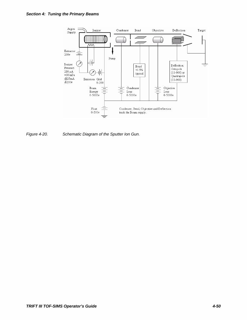
Section 4: Tuning the Primary Beams
Figure 4-20. Schematic Diagram of the Sputter Ion Gun.
TRIFT III TOF-SIMS Operator’s Guide 4-50

Section 4: Tuning the Primary Beams
D.C. Beam Alignment
File Beam Energy
Float Voltage
Impact Energy
Grid Bend3.5%
Current Condenser Objective73%
GasGun_5kV_Max.ins 3uA 68-70% 3400-3500v
GasGun_5kV_1uA.ins
5000v
5000v
175v1uA 80-84%
4000-4200v
3650v
GasGun_2kV_400nA.ins 400nA 80% 1600v
GasGun_2kV_1400nA.ins
2000v
0v
2000v
110v
70v1.4uA 70%
1400v
1460v
GasGun_1kV_200nA.ins 1500v 1000v 52v 200nA 76-83% 1150-1250v
1095v
GasGun_500V_100nA.ins 1000v
-500v500v
130v 35v 100nA 75-85%
750-850v 730v
SED-based method for tuning the D.C. Gas Gun beam with 0v float 1. Use one of the coarse metallic grids in a sample holder, with no backing plate
and no true sample. Imaging the coarse grid bars will give good image contrast.
2. Tuning is best done in –SIMS, which provides the optimum SED image for tuning the Objective Lens. Objective Lens values will then transfer to +SIMS settings later.
3. Close the spectrometer gate valve as a precaution, since you do not need to use the mass spectrometer for this operation.
4. In the Gas Gun page, select the desired Beam Energy and verify that the Float Voltage is set to 0v. Set the Emission to 15mA. [Note: if changing this value from 0mA, incrementally set the value in 5mA steps] Open V10 in Watcher.
5. Once ion emission has been established, it is possible to monitor D.C. beam current on the sample (with a picoammeter) The beam is set to D.C. in WinCadence on the Gas Gun control page by clicking on the “D.C.” button at the bottom of the page. Select the Gas Gun button under “Monitor beam at sample”.
6. Set the 5º Bend to ~+3.5% of the Beam Energy. Adjust the Grid voltage to maximize the current. Adjust the Condenser Lens for the desired sample
TRIFT III TOF-SIMS Operator’s Guide 4-51

Section 4: Tuning the Primary Beams
current at this Beam Energy. Maximum current will occur with a condenser setting of 68-70% of the Beam Energy. Increasing the Condenser between 70% and 100% will provide a smaller beam size and reduced sample current.
7. Turn off the DC operation
8. In -SIMS mode, turn the Gas Gun beam to DC using the DC button at the bottom of the Gas Gun page in Hardware Utilities. Select Gas Gun Beam under "Deliver Beam to Sample" and select the OK button. Now set the following: -The sample bias to approximately -200 V. -The immersion lens to 550. -The high mass blanker to 7.
9. Set the Gas Gun raster size to 2mm, and increase the SED gain until you begin to see an image. Fine-tune the immersion lens and the high mass blanker voltages for the most intense and uniform image intensity. Reduce the sample bias to minimize its deflection affect on the primary beam; but still provide a good SED image. It should now be possible to focus the Objective Lens for the best grid image. Adjust the Bend voltage to center the beam in the Objective Lens and minimizing wobble of the lens in the “Y” axis. This should coincide with maximum current. You may need to return to the picoammeter mode to readjust sample current with the Condenser Lens.
9. Switch the video so that the optical view is on the monitor, and position the sample so that a recognizable part of the grid is in the center of the light optic’s field of view (closely corresponding to the center of the spectrometer’s field of view during analysis).
10. Switch the video to display the SED image once again and adjust the Gas Gun beam x and y position voltages to image the same field of view as the light optics. While this will not necessarily position the Gas Gun beam exactly, it will bring it very close. More accurate alignment of the LMIG and Gas Gun probes is described in the “Phased Depth Profiling: Dual Gun” sub-section of Section7: Data Acquisition. Note: The following alignment section pertaining to low energy “float” setting alignment can also be used to optimize X,Y and Focus for these higher energy files.
11. Adjust the objective lens for best focus. Once the best focus is obtained, press the DC button again to blank the beam. Set the sample bias and immersion lens and high mass blanker to their original values. Resave the instrument file.
Method for tuning the D.C. Gas Gun beam with a float voltage 1. Use a piece of Silicon Oxide or Silicon Nitride.
TRIFT III TOF-SIMS Operator’s Guide 4-52

Section 4: Tuning the Primary Beams
2. Close the spectrometer gate valve as a precaution, since you do not need to use the mass spectrometer for this operation.
3. In the Gas Gun page, select the desired Beam Energy and associated Float Voltage (ie:1500V,-500V or 1000V,-500V). Set the Emission to 15mA. [Note: if changing this value from 0mA, WinCadence will incrementally set the value in 1mA steps] Open V10 in Watcher. Note: When choosing a Beam Energy and Float value, keep the final impact energy => the Float value. Choosing a combination resulting in an impact energy < the Float value will alter the operation of the Objective Lens focusing.
4. Once ion emission has been established, it is possible to monitor D.C. beam current on the sample (with a picoammeter) The beam is set to D.C. in WinCadence on the Gas Gun control page by clicking on the “D.C.” button at the bottom of the page. Select the Gas Gun button under “Monitor beam at sample”.
5. Set the 5º Bend to ~+3.5% of the Beam Energy. Adjust the Grid voltage to maximize the current. Adjust the Condenser Lens for the desired sample current at this Beam Energy. Maximum current will occur with a condenser setting of 68-70% of the Beam Energy. Increasing the Condenser between 70% and 100% will provide a smaller beam size and reduced sample current.
6. Turn off the DC operation.
7. Switch the video so that the optical view is on the monitor, and position the sample so that an un-sputtered part of the sample is in the center of the light optic’s field of view (closely corresponding to the center of the spectrometer’s field of view during analysis).
8. Set the Sample voltage to 0v
9. Set the Gas Gun raster size to 0mm
10. In -SIMS mode, turn the Gas Gun beam to DC using the DC button at the bottom of the Gas Gun page in Hardware Utilities. Select Gas Gun Beam under "Deliver Beam to Sample" and select the OK button.
11. Adjust the Gas Gun beam x and y position voltages to align the sputtered area to the center of the field of view of the light optics. A more + X will move the sputter area to the right. A more +Y will move the sputter area down.
12. Adjust the objective lens for best focus or use table on previous page. Once the best focus is obtained, press the DC button again to blank the beam.
13. Set the sample bias back to its original value.
14. Set the raster size to 2mm or desired size.
15. Resave the instrument file.
TRIFT III TOF-SIMS Operator’s Guide 4-53
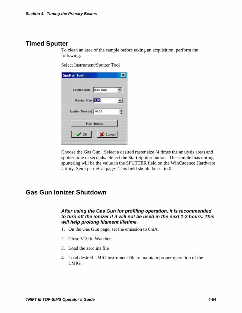
Section 4: Tuning the Primary Beams
Timed Sputter To clean an area of the sample before taking an acquisition, perform the following:
Select Instrument/Sputter Tool
Choose the Gas Gun. Select a desired raster size (4 times the analysis area) and sputter time in seconds. Select the Start Sputter button. The sample bias during sputtering will be the value in the SPUTTER field on the WinCadence Hardware Utility, Semi perm/Cal page. This field should be set to 0.
Gas Gun Ionizer Shutdown
After using the Gas Gun for profiling operation, it is recommended to turn off the ionizer if it will not be used in the next 1-2 hours. This will help prolong filament lifetime. 1. On the Gas Gun page, set the emission to 0mA.
2. Close V10 in Watcher.
3. Load the zero.ins file
4. Load desired LMIG instrument file to maintain proper operation of the LMIG.
TRIFT III TOF-SIMS Operator’s Guide 4-54
TRIFT III TOF-SIMS Operator’s Guide 5-1
Section 5:System Alignments
This section discusses the alignment process of key system components andstresses the importance of having all critical portions of the system in alignmentwith one another (i.e., beam steering, viewing optics, spectrometer, etc.)
Alignment of Primary Beam Analysis Area with SIMS OpticsConcept of SIMS Acceptance Area
In any SIMS instrument, a limited area exists on a sample from which secondaryions can be collected efficiently. In stigmatic imaging SIMS systems, this area iseffectively determined by the de-magnified image of the detector at the surfaceof the sample, as a consequence of the magnification properties of themicroscope. Even though the primary ion beam may be illuminating or scanninga large area, the area from which secondary ions are extracted is thus restricted or'gated'. In the PHI TRIFT III spectrometer, the maximum SIMS acceptance areaat the surface of the sample is ∼600 microns at maximum secondary iontransmission. Larger fields of view can be achieved at the loss of sometransmission, refer to ‘Defocusing the Immersion Lens: Analytical Trade Offs’ inSection 6.
Effect of Sample Height Variations
In the TRIFT system, the SIMS optics are normal to the sample surface, and thusthe position on the sample from which secondary ions are extracted does not varywith z position (sample height changes). What does vary with sample heightvariations are the points of intersection of the primary beams and electron gunwith the sample surface. A sample at the optimum z height is positioned to be atthe intersection of the SIMS optical 'gate', the primary ion beams and the electronneutralization beam. When the sample height changes, however, the primarybeam impact point moves by z.tan (theta), where z is the height variation, andtheta is the primary beam impact angle with respect to normal incidence.

Section 5: System Alignments
TRIFT III TOF-SIMS Operator’s Guide 5-2
The exact primary beam impact angle at the sample surface depends on threeparameters:
• The primary beam column orientation;
• The primary beam energy; and
• The sample potential.
In the TRIFT system, the LMIG and Cesium columns are set at 35° and 42° fromsample normal, respectively. The Ga+ beam voltage can be varied continuouslyfrom +1 to +25 kV, and the Cs+ beam energy is continuously variable fromapproximately +2 kV through to +11 kV. Typically, however, the Cs+ beam isset at +10 kV and the Ga+ beam is usually switched between operation at +15 kVand +25 kV. The sample potential is likewise continuously variable between 0and 5 kV (positive or negative), although it is typically set at 3 kV. If the sampleis at a negative potential, then the primary beam is accelerated towards thesample, reducing the impact angle from the nominal 35° or 42°. The lower theprimary beam energy, the greater is this effect. The converse is true when thesample potential is positive.
As a general rule, each variation of 1 micron in sample height (z) corresponds toa movement of the center of primary beam impact point of approximately 1micron.
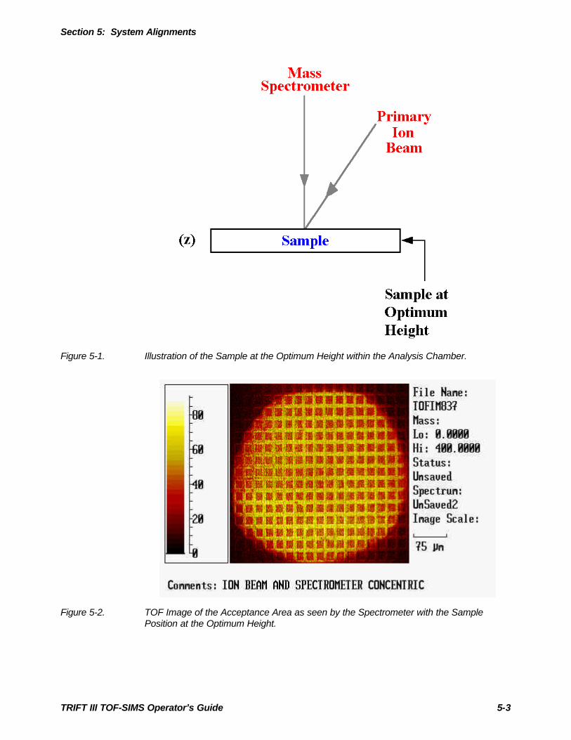
Section 5: System Alignments
TRIFT III TOF-SIMS Operator’s Guide 5-3
Figure 5-1. Illustration of the Sample at the Optimum Height within the Analysis Chamber.
Figure 5-2. TOF Image of the Acceptance Area as seen by the Spectrometer with the SamplePosition at the Optimum Height.
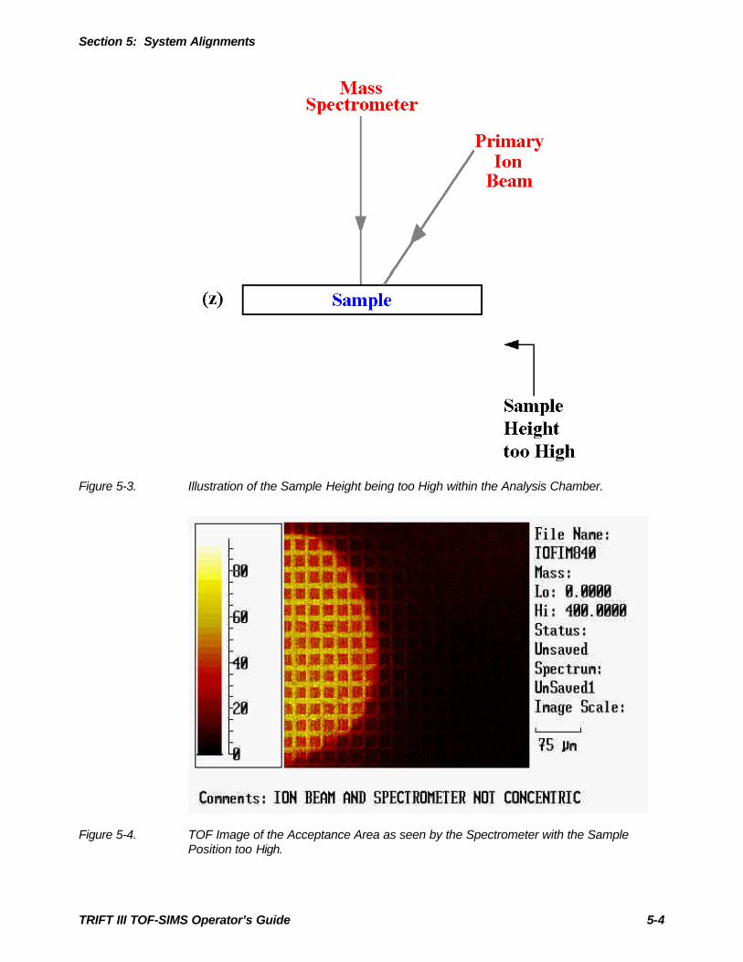
Section 5: System Alignments
TRIFT III TOF-SIMS Operator’s Guide 5-4
Figure 5-3. Illustration of the Sample Height being too High within the Analysis Chamber.
Figure 5-4. TOF Image of the Acceptance Area as seen by the Spectrometer with the SamplePosition too High.
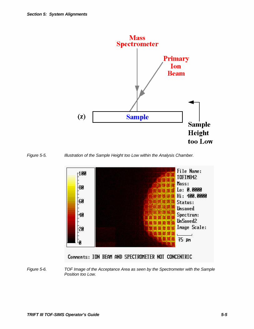
Section 5: System Alignments
TRIFT III TOF-SIMS Operator’s Guide 5-5
Figure 5-5. Illustration of the Sample Height too Low within the Analysis Chamber.
Figure 5-6. TOF Image of the Acceptance Area as seen by the Spectrometer with the SamplePosition too Low.
Section 5: System Alignments
TRIFT III TOF-SIMS Operator’s Guide 5-6
Use of Primary Beam Steering (Beam Position)
The final deflectors in the primary columns of both the Cesium and the LMIGare used not only to raster the primary beams on the sample surface, but also tosteer the position of impact of the primary beams on the sample surface. Theraster signals effectively 'float' on top of D.C. steering voltages. These primarybeam steering voltages are changed by altering the x and y values of "beamposition" in the LMIG control page.
The usefulness of this beam steering should now be evident: it is possible tocompensate for sample height variations by simply steering the primary beamuntil it is concentric with the secondary ion optical gate on the sample surface.
The distance moved by the primary beam per unit of "beam position" x and yvaries linearly with the primary beam energy, since the available steeringvoltages are fixed (a beam of higher energy is less affected by a given steeringvoltage than a beam of lower energy). Typically, a 25 kV Ga+ beam will moveapproximately 50 microns in the x and y directions for every unit of beamposition x and y. Since the beam positions values have ±10 units variation, thisimplies that the maximum height variation away from optimum that the systemcan accommodate electronically is ±500 µm, or a total of 1 millimeter. At lowerbeam energies this value is greater.
It is not difficult to mount samples to this positioning accuracy. If a sample isflat to begin with, then back-mounting against the sample holder window willautomatically position the sample at the correct height. If the sample is not flat,employ one of the techniques outlined in Section "Sample PreparationTechniques", and use a low magnification binocular microscope to assist inaligning the z position by eye. Optical microscopes typically have a short depthof field, and it is quite easy to calibrate your microscope to determine if a sampleis mounted within ±500um of the optimum z. Remember that a little care andattention to sample mounting saves considerable time once the samples are insidethe analytical chamber.

Section 5: System Alignments
TRIFT III TOF-SIMS Operator’s Guide 5-7
Setup, Verification of Primary Beam Alignment to the Spectrometer
It is good practice to steer the primary ion beam so that it is concentric with thesecondary ion acceptance area. This concentricity is vital for scanning a largefield of view and yields good illumination of the entire area.
Verification of this alignment can be performed either in a TOF-SIMS imagingmode or directly on the secondary ion detector.
TOF-SIMS Imaging Mode
A simple way to set the concentricity of the primary beam and the secondary ionacceptance area is as follows:
1. Select a primary beam raster size that is significantly larger than theacceptance area, e.g., ≥1,000µm.
2. Begin an acquisition and acquire a total ion image (automatic inWinCadence)
3. Now examine the total ion image. An image should now be forming of partor all of the secondary ion acceptance area. Once you have acquiredsufficient signal, stop the acquisition.
Right click on the image using the mouse and select “center beam at cursor”.Position the arrow at the center of the acceptance area and left click on themouse.
This will adjust the beam position x and y values so that the primary beam willnow be concentric with the acceptance area. Repeat the procedure, if necessary,and then reset the raster size to the desired analytical value.
Direct imaging on the secondary ion detector
It is even simpler to center the primary beam to the acceptance area using theimage obtained at the secondary ion detector. To do this, set the video screen tomonitor the detector, set a raster size of ~100µm, and begin an acquisition. Steerthe primary beam x and y position so that the secondary ion raster is centered onthe detector.

Section 5: System Alignments
TRIFT III TOF-SIMS Operator’s Guide 5-8
Alignment of Viewing (Light Optics) to SIMS OpticsThe light optical field of view of the TRIFT is designed to provide a maximummagnification of ∼600 at the video screen, with a field of view of ∼450 µm and alateral resolution of ∼2 µm. The TRIFT III system is fitted with a variable fieldof view light optics, permitting ~1 mm field of view. For systems with dual-magnification capabilities of light optics, the alignment of light optics to SIMSoptics should be done for the view of highest magnification (~450 µm). InVacuum Watcher, the Camera Field option should be set to Small.
Alignment of Viewing Optics
The viewing optics, like the primary ion beams, are designed to be set concentricwith the secondary ion acceptance area. This is achieved by small adjustments ofan angled mirror at the base of the microscope assembly mounted on top of theanalytical chamber. The procedure to set and verify this alignment is as follows:
1. Mount and load a sample into the system containing a unique feature that canbe easily located within the optical field of view. The corner of the standard25 micron Cu grid sample is perfect for this procedure.
2. Start an acquisition and using the X and Y beam steering, align the LMIGwith the spectrometer acceptance area.
3. Turn the LMIG to D.C. and view the SEM image.
4. Move the sample stage until the corner of the grid (or some other feature) iscentered in the SIMS field of view. Decrease the image size, adjusting thestage coordinates to keep the feature centered. When finished, blank thebeam once again.
5. Center the feature in the optical field of view by adjusting the two diagonallyopposed knobs which control the tilt of the angled mirror at the base of theoptical microscope assembly. Rotate each knob until the corner of the grid(or other feature) is centered in the optical field of view.
6. The viewing optics are now aligned to the SIMS optics.
The procedure just explained aligns the viewing optics to the SIMS optics formost samples. Once again, however, large displacements of the sample in the zdirection will result in some displacement of the viewing optics with respect tothe SIMS optics. If considerable time is invested in the analysis of a samplewhich is clearly displaced in the z direction, it is often worth setting the viewingoptics for that sample, since the procedure is simple. Remember to exercisecaution if using a DC primary beam depending on the sample type. If a DCprimary beam cannot be used, a standard SIMS image should be used to identifya feature and then set the viewing optics for that sample.
Section 5: System Alignments
TRIFT III TOF-SIMS Operator’s Guide 5-9
Alignment of + and - SIMS Fields of View (Polarity Offsets)Primary Beam Steering Effects in Different Polarities
The sample potential causes the beam to steer away from the nominal impactangles of 35° and 42° for the Ga+ and Cs+ beams, respectively. When thesample potential is negative, the beam is steered towards the sample, and whenthe sample potential is positive, the beam is steered away from the sample. Theexact steering values vary, but for a given primary column (LMIG or Cesium), agiven beam energy and a given sample potential, the beam steering betweennegative and positive SIMS is always constant.
This is an important result, because the system software allows the user to applya fixed polarity offset (delta x, delta y in the beam position) such that uponchanging polarities, the feature in the SIMS field of view is always retained.
In WinCadence, the polarity offset values are determined at a specific energy foreither the LMIG and Cs gun, and are stored with each instrument file. Thesevalues do not vary for a given set of conditions. Thereafter, whenever thepolarity is changed, the polarity offset values will be applied to the current beamposition values.
Determining the Polarity Offset Values
The procedure below determines the polarity offset values for a given primaryspecies and experimental conditions (beam energy, sample potential).
1. Mount and load a sample into the system containing a unique feature easilylocated within the optical field of view. The corner of the standard 25 micronCu grid sample is ideal for this procedure.
2. Locate the grid corner (or other feature) in the optical field of view.
3. Assuming that the viewing optics have been set correctly, switch to negativeSIMS mode.
4. Center the primary beam raster to the secondary ion acceptance area asoutlined in a previous section above entitled “Setup and Verification ofPrimary Beam Alignment to the Spectrometer”.
5. Obtain an image using a DC primary beam, either at the SED detector, ifusing Ga+ beam, or at the DMCP detector if using the Cs+ beam. For detailson how to do this, refer back to “Alignment of the Viewing Optics” withinthis section.
6. Zoom into the corner feature, using stage adjustments only to center thefeature in the image. When the corner is centered within approximately 100x 100 microns field of view, blank the primary beam.
7. Note the x and y beam position values. Obtain a printed hardcopy of theprimary beam control page.

Section 5: System Alignments
TRIFT III TOF-SIMS Operator’s Guide 5-10
8. Change to positive SIMS. Select a large raster size and unblank the beamonce again.
9. The grid corner will now be somewhere in the field of view. Using changesto the beam position x and y only, bring the grid corner into the center of thefield of view. Zoom in until it is centered within approximately 100 x 100microns field of view and blank the beam.
10. Note the new beam position values, and calculate the difference in goingfrom negative to positive SIMS.
Offset value = (+SIMS value) - (-SIMS value)
These are the values that are entered into the polarity offsets in the instrumentfile.
The signs of the values are important, so double-check your calculation. Forinstance, if an x value in negative SIMS was -2, and an x value in positive SIMSwas +3, then the entered value would be +5. [(+3) - (-2) = +5).
It’s good practice to check the result by taking a positive SIMS image of thefeature, changing polarities, and acquiring a SIMS image. Hint: use Cl- or CN-and Cu+ signals for the best contrast. This insures that the offset can be trustedat a later time on a real sample.

TRIFT III TOF-SIMS Operator’s Guide 6-1
Section 6:Tuning the Mass Spectrometer
This section is intended to give an introduction to the stigmatic secondary ionoptics of the PHI TRIFT TOF-SIMS mass spectrometer and familiarize theoperator with the most important ion optical features of the instrument. For amore detailed treatment of this subject, the operator should refer to the paper"Microscope imaging by time-of-flight secondary ion mass spectrometry", by B.W. Schueler in Microscopy Microanalysis Microstructures 3 (1992) p. 119-139.
Theoretical Aspects of Spectrometer OperationThe basic principles of TOF-SIMS are very simple. A pulsed primary ion beambombards the sample surface, causing the emission of atomic and molecularsecondary ions. The secondary ions are then electrostatically accelerated into afield-free drift region with a nominal kinetic energy of:
(1) Ekin = eVo = mv2 /2,
where Vo is the accelerating potential, m the mass of the ion, and e its charge.Since lighter ions will have higher velocities than the heavier ones, they willarrive at the detector at the end of the drift region earlier than the high masses.The mass separation is thus obtained in the flight time t from the sample to thedetector. This is given approximately by:
(2) t = Lo/v = Lo ( m / 2 e Vo ) l/2,
where Lo is the effective length of the mass spectrometer. Since different massions arrive sequentially at the detector, the operating conditions of a TOF-SIMSinstrument can be chosen such that (virtually) all secondary ions of a givenpolarity are detected and recorded in the mass spectrum. This efficient collectionand detection of secondary ions by TOF-SIMS instruments means that significantnumbers of secondary ions can be produced from a sample surface with theminimum primary ion dose and results in a very sensitive technique for organicand inorganic surface analysis. Typical primary ion doses in this "static SIMS"analysis mode are ≤1012 primary ions / cm2 for mass analysis and ≤1013 primaryions / cm2 for imaging.

Section 6: Tuning the Mass Spectrometer
TRIFT III TOF-SIMS Operator’s Guide 6-2
Neighboring masses mo and mo + ∆m = mo (1 + γ) can only be resolved as such iftheir time width and separation ∆t is sufficient. For small mass differences itfollows from equation (2) that the relationship between flight times and massresolution is:
(3) mo / ∆m = γ1 = to / 2∆t.
It is obvious from equation (3) that in order to obtain high mass resolution a shortprimary ion pulse duration, tp, has to be used since the smallest measurable timedifference ∆t is tp. The mass measurement in a TOF-SIMS instrument isachieved by converting the flight time into the exact mass by determining theflight time differences of ions through the spectrometer.
Physical Effects Influencing High Mass Resolution TOF-SIMSAnalysisAlthough TOF-SIMS is conceptually very simple, there are a number of physicalprocesses which require a more sophisticated design for a TOF-SIMSspectrometer than merely having a long flight tube and fast detection electronicsat the end. The two most extenuating phenomena are:
1. Secondary ions can be generated with non-zero initial kinetic energy and willthus acquire total kinetic energies which are larger than those imparted by theaccelerating potential. For sputtered atomic secondary ions, the initial kineticenergy distribution is typically centered around 5 - 10 eV with a tail of thedistribution extending out to greater than 100 eV. Molecular ions are ejectedwith lower mean kinetic energy and are distributed over a much smallerenergy range. The narrower energy distribution is a result of the kinetics ofthe sputtering process: collisions which impart high kinetic energy to amolecule will also result in high internal energy, thereby resulting inmolecular fragmentation. Only those molecules which have sustained"gentle" collisions will survive and be detected. Inorganic molecular ions arethus observed to have kinetic energies in the 1 - 5 eV range with distributionsrapidly falling off towards higher energies. Generally, the more complex thedetected molecule, the lower is its initial kinetic energy. Larger organicmolecular ions, as the extreme, are typically emitted with kinetic energies inthe low or sub-eV region.
2. Secondary ions are emitted from the sample surface with an angulardistribution with respect to the surface normal. Ions extracted by theaccelerating field may enter the mass spectrometer with angular momentum,i.e. kinetic energy, which causes them to diverge from the desired flight paththrough the mass spectrometer.

Section 6: Tuning the Mass Spectrometer
TRIFT III TOF-SIMS Operator’s Guide 6-3
The TOF mass spectrometer must therefore not only separate ions according totheir mass to charge ratio but must also compensate for the initial kinetic andangular distribution of the secondary ions, caused by the sputtering andionization process. This task would be trivial if the influence of the very smallacceleration section at the beginning of the mass spectrometer could be neglected(as this is usually done in the literature). The fact is that the flight time errorscaused in the accelerating section are typically the limiting factor for the highmass resolution performance of any TOF-SIMS mass spectrometer. Thefollowing discussion refers primarily to the analysis of atomic secondary ions.
When ions are created at the sample, their velocity spread will be dominated bythe initial kinetic energy distribution as they are just leaving the solid's surface.Ions with higher kinetic energy will spend less time in the accelerating space thanions that are ejected with near zero initial energy. As mentioned above, thiseffect is most pronounced for atomic/inorganic secondary ions and relativelyunimportant (but not negligible) for higher molecular organic species. The flighttime error caused in the accelerating space alone will be smaller the shorter thetotal acceleration time, e.g., the shorter the acceleration section and the higher themagnitude of the acceleration potential. For the case that the ions are ejectedonly in the direction of the spectrometer axis, the mass spectrometer can typicallybe tuned to provide the proper energy compensation over some range of initialion kinetic energies. The TRIFT spectrometer is capable of compensating for the(axial) kinetic energy distribution ∆E of secondary ions over a range of ∆E/eUo ≥20% (e.g., ≥ 60 eV at 3,000 V acceleration potential).
As well as emission along the spectrometer axis, secondary ions will also have adistribution of emission angles. Again, the dominating flight time errors will beintroduced within the acceleration space. It should be intuitively clear that an ionemitted with 10 eV kinetic energy in the direction of the spectrometer axis willhave a shorter flight time through the acceleration section than an ion emittedparallel to the sample surface with the same initial kinetic energy. The TOFmass spectrometer will, of course, provide the appropriate compensation for thetotal kinetic energy but it cannot distinguish between different emissiondirections. In order to achieve high mass resolution, the angular acceptance of thespectrometer has to be limited (or otherwise corrected) so that the effect of flighttime differences in the accelerating space is minimized. This effect is onlynoticeable in TOF spectrometers of high angular acceptance which provide themaximum ion transmission for atomic secondary ions where ultimate massresolution is not imperative.
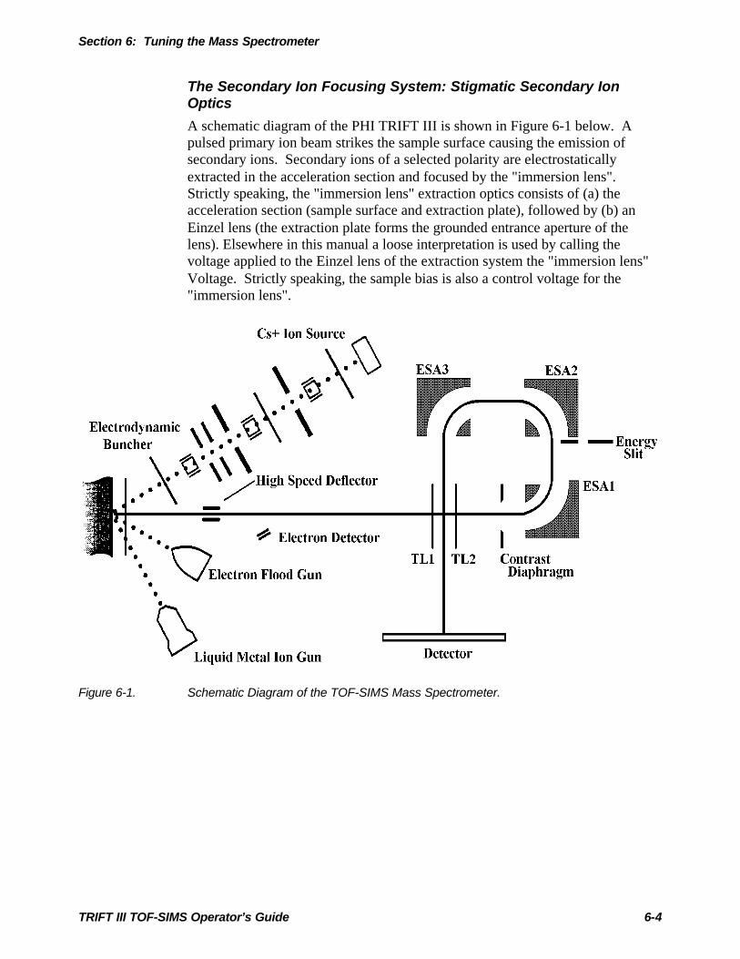
Section 6: Tuning the Mass Spectrometer
TRIFT III TOF-SIMS Operator’s Guide 6-4
The Secondary Ion Focusing System: Stigmatic Secondary IonOptics
A schematic diagram of the PHI TRIFT III is shown in Figure 6-1 below. Apulsed primary ion beam strikes the sample surface causing the emission ofsecondary ions. Secondary ions of a selected polarity are electrostaticallyextracted in the acceleration section and focused by the "immersion lens".Strictly speaking, the "immersion lens" extraction optics consists of (a) theacceleration section (sample surface and extraction plate), followed by (b) anEinzel lens (the extraction plate forms the grounded entrance aperture of thelens). Elsewhere in this manual a loose interpretation is used by calling thevoltage applied to the Einzel lens of the extraction system the "immersion lens"Voltage. Strictly speaking, the sample bias is also a control voltage for the"immersion lens".
Figure 6-1. Schematic Diagram of the TOF-SIMS Mass Spectrometer.
Section 6: Tuning the Mass Spectrometer
TRIFT III TOF-SIMS Operator’s Guide 6-5
The immersion lens in conjunction with the transfer lenses determines the totalimage magnification of the secondary ion optics. A stigmatic imaging system ofthree 90° (quasi) hemispherical electrostatic analyzers (ESA) forms part of thesecondary ion optics and provides "first order" energy focusing for imaging andion flight times with small residual "second order" aberrations. The final,magnified secondary ion image is then projected onto an imaging secondary iondetector. The ESAs are fitted with field termination plates known as "Herzogshunts", and the center ESA is fitted with "Matsuda Plates" above and below forelectrostatic field shaping.
The secondary ion mass spectrometer optics always projects a magnified imageof the ion emission profile from the sample surface to an imaging detector. Theion arrival position at the final secondary ion detector is correlated with theemission point at the sample surface. A schematic diagram of the secondary ionimage transport through the TOF spectrometer is shown in Figure 6-2. Theextraction optics consists of the accelerating section formed by the samplesurface and the extraction plate. The immersion lens projects a magnified imageof the ion emission profile into the first field-free region of the massspectrometer. This image is transported via the transfer lens into the first ESA,where an image is formed close to its exit aperture. Another intermediate imageis formed close to the entrance of the third ESA, which projects the finalmagnified ion image onto the imaging secondary ion detector.
For continuous beam tuning of the LMIG, a set of deflectors (high mass blanker)is located after the extraction lens in order to deflect ion-induced secondary ionsand/or secondary electrons into a channeltron secondary electron detector (SED).The high mass blanker is also used during mass spectral acquisition to blankcertain ranges of high or low mass secondary ions from the mass spectrum bydeflecting them out of the ion optical path. The high mass blanker, as its namesuggests, is used principally to remove high mass ions with masses greater thanthe requested mass range of the experiment. Without this blanking, these highmass ions would “wraparound” and appear as noise at the low mass end of themass spectrum.
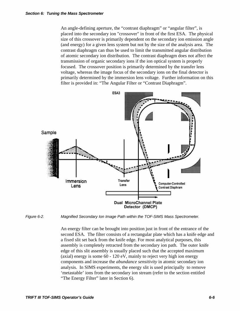
Section 6: Tuning the Mass Spectrometer
TRIFT III TOF-SIMS Operator’s Guide 6-6
An angle-defining aperture, the “contrast diaphragm” or “angular filter”, isplaced into the secondary ion "crossover" in front of the first ESA. The physicalsize of this crossover is primarily dependent on the secondary ion emission angle(and energy) for a given lens system but not by the size of the analysis area. Thecontrast diaphragm can thus be used to limit the transmitted angular distributionof atomic secondary ion distribution. The contrast diaphragm does not affect thetransmission of organic secondary ions if the ion optical system is properlyfocused. The crossover position is primarily determined by the transfer lensvoltage, whereas the image focus of the secondary ions on the final detector isprimarily determined by the immersion lens voltage. Further information on thisfilter is provided in: “The Angular Filter or “Contrast Diaphragm”.
Figure 6-2. Magnified Secondary Ion Image Path within the TOF-SIMS Mass Spectrometer.
An energy filter can be brought into position just in front of the entrance of thesecond ESA. The filter consists of a rectangular plate which has a knife edge anda fixed slit set back from the knife edge. For most analytical purposes, thisassembly is completely retracted from the secondary ion path. The outer knifeedge of this slit assembly is usually placed such that the accepted maximum(axial) energy is some 60 - 120 eV, mainly to reject very high ion energycomponents and increase the abundance sensitivity in atomic secondary ionanalysis. In SIMS experiments, the energy slit is used principally to remove‘metastable’ ions from the secondary ion stream (refer to the section entitled“The Energy Filter” later in Section 6).
Section 6: Tuning the Mass Spectrometer
TRIFT III TOF-SIMS Operator’s Guide 6-7
After the third ESA, there is another focus plane or "cross-over" where a secondset of mass blanking plates is located. This blanker is known therefore as the"post ESA" blanker. At this position in the secondary ion flight path the ions arewell separated in time, and it is possible to use the post ESA blankers, forinstance, to remove mass 28 from the secondary ion stream without removingmasses 27 and 29. The post ESA blanker is used when high primary ion currentsare used at high repetition rates. For more details, refer to Section 7.
Secondary ion images are obtained using a pulsed, micro focused primary ionbeam from a liquid metal ion gun (LMIG). The tuning of the mass spectrometeris (usually) unchanged but an ion image is formed by synchronizing thesecondary ion flight time with the primary beam raster position, ignoring thesecondary ion arrival position on the detector. This imaging mode is referred toas "microprobe" imaging. In this imaging mode, lateral image resolutions of1,000 Αngstroms may be obtained in the TOF-SIMS
Mass spectra are recorded by measuring the time difference between pulsing ofthe primary ion gun and the arrival of secondary ions on a fast dual microchannelplate (DMCP) detector at the end of the spectrometer by means of a multistop(1024) time-to-digital converter (TDC) of 138 ps time resolution. A phosphorscreen may be placed behind the DMCP to observe the secondary ion arrivalposition at the detector, although the (x y) information is not stored in the dataacquisition computer system. The collection of image information is thuscorrelated to, but decoupled from, the time measurement. Ion imaging isachieved by registering the (x y) raster position of the primary ion beam(microprobe).
Section 6: Tuning the Mass Spectrometer
TRIFT III TOF-SIMS Operator’s Guide 6-8
Practical Aspects of Spectrometer OperationDynamic Emittance Matching (DEM)
One of the biggest changes of the TRIFT III compared to previous generationTRIFT’s is the addition of dynamic emittance matching (DEM). The mainmotivation of adding DEM was to improve the mass resolution that could beachieved from large analysis areas. Without DEM, the mass resolution falls asthe raster size is increased. This is because secondary ions that are generatedfrom points off the central ion optical axis take a different path through thespectrometer to the detector. This is illustrated in Figure 6-2. The goal of theDEM optics is send all secondary ions through the TRIFT analyzer along the ionoptical axis. In doing this, the peak broadening which came from large rastersizes is nearly eliminated.
On way to conceptualize DEM is to imagine that the extraction field-of-view israstered perfectly in sync with the LMIG raster. Therefore, from thespectrometer point of view, it appears as if the LMIG is not being rastered.Rather than seeing a square pattern on the detector that is proportional in size tothe LMIG raster size, secondary ions always hit the same spot on the detector,independent of the LMIG raster size. The direct ion image viewed at the detectoralways appears like the raster size is set to zero.
Although this accomplishes the goal of maintaining high mass resolution overraster sizes up to 600 µm, it would result in rapidly producing a “dead spot” onthe detector. Therefore, in addition to DEM, a set of scanning plates has beenadded to scan the secondary ion beam on the detector. These are called the‘detector deflectors’. The size of the scanned area on the detector can be set inthe software and is independent of the LMIG raster size on the sample.
When using the TRIFT III, the DEM and detector deflectors should always beturned on. However, there are times when tuning of the instrument it may benecessary to turn them off. When they are turned off, the TRIFT III operates inthe direct imaging mode just like the TRIFT I and TRIFT II. The instrumentfiles will come with the values for DEM and the detector deflectors properlycalibrated. These values have been determined specifically for your instrument.The DEM tabbed page within the Hardware Utility of the WinCadence softwareis shown in Figure 6-3 below.
To turn the DEM and detector deflectors OFF, use Table 6-1 below. To turnthem back ON, re-enter the values that are in the instrument file.
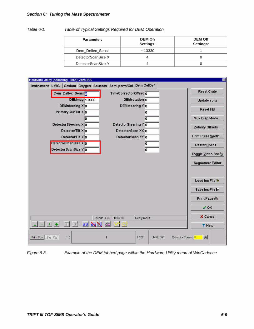
Section 6: Tuning the Mass Spectrometer
TRIFT III TOF-SIMS Operator’s Guide 6-9
Table 6-1. Table of Typical Settings Required for DEM Operation.
Parameter: DEM OnSettings:
DEM OffSettings:
Dem_Deflec_Sensi ~ 13330 1
DetectorScanSize X 4 0
DetectorScanSize Y 4 0
Figure 6-3. Example of the DEM tabbed page within the Hardware Utility menu of WinCadence.
Section 6: Tuning the Mass Spectrometer
TRIFT III TOF-SIMS Operator’s Guide 6-10
Secondary Ion Filters
The TRIFT is unique among TOF mass spectrometers because it continuallyrefocuses the secondary ion beam at various crossovers within the system. Thisallows the system to be run stigmatically, and permits the placement ofsecondary ion filters at appropriate points in the secondary ion flight path. Thesystem’s normal state is “fully open” (no filters), and under these circumstancesthe spectrometer’s energy acceptance is ~240eV, and the angular acceptance is~90mrad. This last number is better understood by stating that, with an angularacceptance of 90mrad, an ion of up to 5eV with an angular emission of 89degrees will be extracted into the mass spectrometer.
The two principle filters, angular and energy, are described in the following twosections. These sections also discuss when it is appropriate to use these filtersand the consequences associated with using each.
The Angular Filter or “Contrast Diaphragm”
Secondary ions are extracted through the immersion lens and are then passed onto the transfer lens. This lens forms a focus plane or “crossover” in front of thefirst ESA, where ions with the same angle of emission are focused. Ions emittednormal to the sample surface (zero angle) pass through the center of this cross-over, while ions with increasing angles of emission are dispersed toward theoutside of the cross-over. By placing a circular aperture at this crossover, highangle ions may be removed from the secondary ion stream. These high angleions contribute significant aberrations to the stigmatic image, and the use of anaperture at this point increases the contrast in the subsequent stigmatic ion image(hence the name “contrast diaphragm”). More importantly for the routineoperation of the TRIFT, it is these high angle ions which limit the achievablehigh mass resolution, particularly on atomic species. In order to achieve highmass resolution (>7000 FWHM) on atomic species, all TOF spectrometers mustlimit the angular acceptance into the system, either in the initial extraction optics,or, as in the TRIFT, by use of an angular filter at a crossover position.

Section 6: Tuning the Mass Spectrometer
TRIFT III TOF-SIMS Operator’s Guide 6-11
Angular Aperture
The angular aperture manipulator is computer controlled and has two positions;in or out. With the aperture “out”, the spectrometer solid angle of acceptance iswide open. For this setting, we use a 2 mm aperture size. This setting is ideal forimaging rough surfaces where the solid angle of collection is more importantthan the ultimate mass resolution.
When the angular aperture is “in”, a 400 µm diameter aperture is used. Thiseliminates the atomic secondary ions which are emitted from the surface at highemission angle from sample normal and at high kinetic energy. The result ofremoving these specific ions from the secondary ion beam is a significantimprovement in both mass resolution and peak shape on atomic species. Thetransmission of atomic species is reduced to approximately 40%, while thetransmission of molecular secondary ions is not effected because of their narrowenergy distribution. The mass resolution of atomic species increases from~5,500 - 6,000 with the angular aperture out to ~ 9,000 with the aperture in.
In general, the angular aperture should only be put in when the maximum massresolution needs to be achieved on atomic species. This could be because theanalysis requires the user to deal with well known mass interferences, such as56Fe /28Si2, 63Cu/28Si35Cl, or 31P/30SiH, where high mass resolution is critical toresolve peaks fully. The mass spectrometer does not need any adjustmentwhether the angular aperture is in or out.

Section 6: Tuning the Mass Spectrometer
TRIFT III TOF-SIMS Operator’s Guide 6-12
The Energy Filter
As well as pupils or “crossovers” in the spectrometer, there are dispersions. Adispersion of energy occurs before the second ESA (in fact it is at a maximum inthe center of this ESA). Just before the entrance to the second ESA is located theplane of the energy filter. When the energy filter is fully retracted, the energyacceptance is defined by the Herzog shunts in front of the electrostatic sectors,and is approximately 240eV. Just in front of the second ESA, ions with highenergies appear on the outside of the secondary ions stream. By bringing in theknife edge of the energy filter, these high energy ions may be progressivelyfiltered. As well as a knife edge, the energy filter has a slit which may be movedin to pick off a particular band of secondary ion energies. The energy band widthis determined by the fixed slit size, and is typically 50eV. Users have exploitedthis energy band width filtering by making customized energy slits to makefundamental studies on organic secondary ions detected in the TOF-SIMSexperiment. For further details, please refer to the work of Delcorte and Betrandin Nucl. Instrum. and Methods B100 (1995) p. 213, ibid. B115 (1996) p. 235, andibid. B117 (1996) p. 246.
The principal use of the energy filter is to place the slit over the secondary ionbeam so as to reject low energy ions which are created by the process ofmetastable decay. In the TOF-SIMS experiment, metastable decay typicallytakes the form of the loss of hydrogen from a neutral molecule. This creates acharged ion with a mass one unit less than the parent (neutral) molecule. Thenewly formed ion begins to accelerate in the acceleration (extraction) space, butdoes not acquire the same energy, and thus velocity, as the other identical ionswhich were created at the sample surface. Because metastable decay occurs at arange of times and thus distances in the acceleration space, most organic peakswill show a metastable “tail” (interestingly, intense metal ions have metastabletails also, due to the metastable decay of the neutral species MHo). Because ofthe way that the energy compensation is performed in the TRIFT, these lowerenergy metastables typically appear on the low mass side of the peak, and not onthe high mass side as one might expect for lower velocity ions. The metastableions contribute significant background noise in the narrow mass region next tothe organic mass, and can mask the appearance of other low level secondary ions.Some transmission losses do of course occur on atomic species when using theenergy filter, since the fully open position is rather large at ~240eV acceptance.Transmission losses on molecular organic ions are associated with the removal ofthe metastable ions as described above, and this loss is normally one of thereasons for employing the energy filter anyway.
The energy filter has only one axis of movement, the x-axis. The energy filter iscorrectly located over the secondary ion dispersion when the maximum countrate is observed on the ratemeter, coinciding with the brightest stigmatic ionimage. Like the angular filter, experimenting with the energy acceptance of themass spectrometer does not involve any re-tuning of the spectrometer settings,and is thus quick and easy to try.
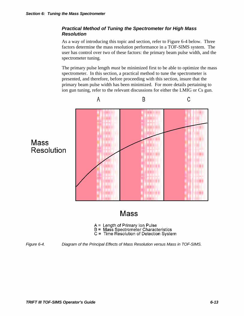
Section 6: Tuning the Mass Spectrometer
TRIFT III TOF-SIMS Operator’s Guide 6-13
Practical Method of Tuning the Spectrometer for High MassResolution
As a way of introducing this topic and section, refer to Figure 6-4 below. Threefactors determine the mass resolution performance in a TOF-SIMS system. Theuser has control over two of these factors: the primary beam pulse width, and thespectrometer tuning.
The primary pulse length must be minimized first to be able to optimize the massspectrometer. In this section, a practical method to tune the spectrometer ispresented, and therefore, before proceeding with this section, insure that theprimary beam pulse width has been minimized. For more details pertaining toion gun tuning, refer to the relevant discussions for either the LMIG or Cs gun.
Figure 6-4. Diagram of the Principal Effects of Mass Resolution versus Mass in TOF-SIMS.
Section 6: Tuning the Mass Spectrometer
TRIFT III TOF-SIMS Operator’s Guide 6-14
Mass Spectrometer Tuning
If the mass spectrometer is already optimized, high mass resolution should beachieved on both molecular and atomic species the moment the primary pulselength is minimized. Typically, high mass resolution will be achieved onmolecular species, but less than optimum performance is achieved on atomicspecies.
If this is the case, the spectrometer should now be optimized for atomics. Oncethe atomic mass resolution has been optimized, the molecular ions are still athigh mass resolution. As a general rule when using the TRIFT, "if you take careof the atomics, the moleculars will look after themselves". This is becausemolecular species have such narrow kinetic energy spreads compared to atomicspecies, and therefore, it is much easier to compensate these species and providehigh mass resolution performance.
Optimizing the spectrometer for mass resolution on atomic species
When using the LMIG, the mass resolution specification is achieved with a600pA beam at 15kV beam energy, with appropriate electrodynamic bunching.Therefore, the spectrometer tuning should be performed with that LMIG beamenergy and current.
Using a clean silicon wafer, arrange the data acquisition screen so that the peak atSi, with the individual 138ps time channels, can be seen clearly. Without theangular aperture out and with a "fully open" spectrometer, the goal is to achieve~5,500 - 6,000 mass resolution with a sub-nanosecond primary pulse width.
Since there are a number of parameters which must be set correctly to achievehigh mass resolution on a species such as Si, it is advisable to make a table,change one parameter at a time and write down the results. A good log of theresults will make it easier for PHI personnel to assist with any difficultiesencountered. An example of a blank mass resolution tuning grid is included inAppendix A at the back of this guide for the user’s convenience. The relevantparameters to note are: Sample potential; Matsuda Voltage; Raster Size;Detector Voltage; Post Acceleration; C.D. Number; Primary Beam BuncherVoltage; Primary Beam Buncher Delay; Primary Beam Pulse Width; LMIGEmission Current; LMIG Blanker Voltage; LMIG Pulser Voltage, and the MassResolution achieved on Atomic and Molecular species.
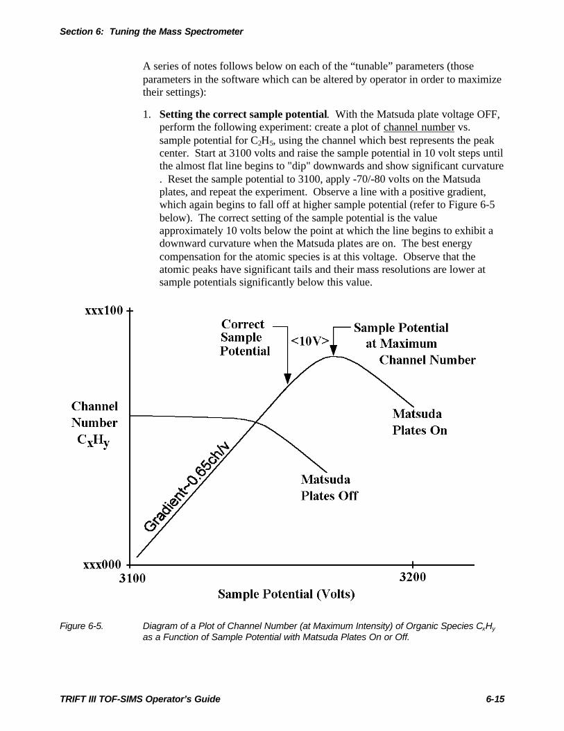
Section 6: Tuning the Mass Spectrometer
TRIFT III TOF-SIMS Operator’s Guide 6-15
A series of notes follows below on each of the “tunable” parameters (thoseparameters in the software which can be altered by operator in order to maximizetheir settings):
1. Setting the correct sample potential. With the Matsuda plate voltage OFF,perform the following experiment: create a plot of channel number vs.sample potential for C2H5, using the channel which best represents the peakcenter. Start at 3100 volts and raise the sample potential in 10 volt steps untilthe almost flat line begins to "dip" downwards and show significant curvature. Reset the sample potential to 3100, apply -70/-80 volts on the Matsudaplates, and repeat the experiment. Observe a line with a positive gradient,which again begins to fall off at higher sample potential (refer to Figure 6-5below). The correct setting of the sample potential is the valueapproximately 10 volts below the point at which the line begins to exhibit adownward curvature when the Matsuda plates are on. The best energycompensation for the atomic species is at this voltage. Observe that theatomic peaks have significant tails and their mass resolutions are lower atsample potentials significantly below this value.
Figure 6-5. Diagram of a Plot of Channel Number (at Maximum Intensity) of Organic Species CxHy
as a Function of Sample Potential with Matsuda Plates On or Off.

Section 6: Tuning the Mass Spectrometer
TRIFT III TOF-SIMS Operator’s Guide 6-16
2. Matsuda Plate Voltage. For PHI TRIFT III systems, the theoretical value ofthe Matsuda plates is approximately 80 volts. However, explore the effect ofvarying the Matsuda plate voltage on the mass resolution of Si, usingwhichever value gives the optimum mass resolution and a sharp rising edgeon the low mass side of the peak.
3. Raster Size. For the purposes of maximizing the mass resolution, the beamshould be set in a probe mode, i.e. zero (0) raster on the beam.
4. Detector Voltage. The correct setting for the detector is when the secondaryion count rate no longer increases significantly with applied voltage on thedetector. To be more thorough, plot the peak integral for a given peak as afunction of detector voltage, and plot the shape of the curve. At somedetector voltage, the peak integral will stop rising dramatically, and begin tolevel out. This is the "knee" of the curve. Note that if this experiment isperformed with zero post-acceleration voltage, the detector will saturate at ahigher value than it does when post-acceleration is on (typically, 5000 voltsor more). Keep this in mind when deciding the appropriate detector voltage.Set the voltage just past the "knee". Over a period of time (i.e., a few weeksor months) with a new detector, the detector voltage will need to be increasedslightly to maintain correct detector efficiency.
Also explore the effect of detector voltage on the achieved mass resolution atSi, looking for a voltage past which there are no significant improvements inmass resolution.
5. Detector position. This really means "the position of the secondary ionbeam on the detector". The best energy compensation of the secondary ionsoccurs when the ions travel down the centerline of the ESAs. Provided thedetector is centered to the exit plane of the last ESA, this will result in thebeam arriving in the center of the detector. However, explore how steeringthe beam on the detector affects the mass resolution (if at all) to maximize theresolution.
6. Post acceleration. In general, the application of post acceleration increasesthe mass resolution slightly. However, changing the post acceleration oftenrequires a slight adjustment of the Matsuda Plate voltage.

Section 6: Tuning the Mass Spectrometer
TRIFT III TOF-SIMS Operator’s Guide 6-17
7. C. D. position. The C.D. is at a fixed position and cannot be adjusted.
8. Primary Beam Buncher Voltage and Buncher Delay. Ideally, theseparameters were optimized earlier when minimizing the primary pulse lengthduring bunching. If the input pulse length is changed significantly, re-examine the buncher delay value because it will probably need to be changedalso.
9. LMIG Emission Current. For obtaining the optimum mass resolution whenusing the LMIG, the emission current from the LMIG should be kept at orbelow 1uA in order to limit the energy spread of the primary beam. For thisreason, tune the gun for mass resolution only when a liquid metal ion sourceis stable and does not have a steep current/voltage (I/V) curve (refer to theLMIG section for more details).
10. LMIG Blanker and Pulser Voltage. These two voltages should beconsidered as a pair, since the blanker voltage shuts the LMIG beam off andthe pulser brings it back on. If the pulser voltage is not matched to theblanker voltage, the best mass resolution may not be achieved when using theLMIG (refer to the LMIG section for more details).
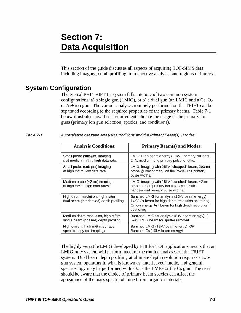
Section 7: Data Acquisition
This section of the guide discusses all aspects of acquiring TOF-SIMS data including imaging, depth profiling, retrospective analysis, and regions of interest.
System Configuration The typical PHI TRIFT III system falls into one of two common system configurations: a) a single gun (LMIG), or b) a dual gun (an LMIG and a Cs, O2 or Ar+ ion gun. The various analyses routinely performed on the TRIFT can be separated according to the required properties of the primary beams. Table 7-1 below illustrates how these requirements dictate the usage of the primary ion guns (primary ion gun selection, species, and conditions).
Table 7-1 A correlation between Analysis Conditions and the Primary Beam(s) \ Modes.
Analysis Conditions: Primary Beam(s) and Modes:
Small probe (sub-µm) imaging, ≤ at medium m/δm, high data rate.
LMIG: High beam energy (25kV); primary currents 2nA; medium-long primary pulse lengths.
Small probe (sub-µm) imaging, at high m/δm, low data rate.
LMIG: imaging with 25kV "chopped" beam, 200nm probe @ low primary ion flux/cycle, 1ns primary pulse widths.
Medium probe (~2µm) imaging, at high m/δm, high data rates.
LMIG: imaging with 15kV "bunched" beam, ~2µm probe at high primary ion flux / cycle; sub-nanosecond primary pulse widths.
High depth resolution, high m/δm dual beam (interleaved) depth profiling.
Bunched LMIG for analysis (15kV beam energy): 1keV Cs beam for high depth resolution sputtering. Or low energy Ar+ beam for high depth resolution sputtering
Medium depth resolution, high m/δm, single beam (phased) depth profiling.
Bunched LMIG for analysis (5kV beam energy): 2-5keV LMIG beam for sputter removal.
High current, high m/δm, surface spectroscopy (no imaging).
Bunched LMIG (15kV beam energy); OR Bunched Cs (10kV beam energy).
The highly versatile LMIG developed by PHI for TOF applications means that an LMIG-only system will perform most of the routine analyses on the TRIFT system. Dual beam depth profiling at ultimate depth resolution requires a two-gun system operating in what is known as "interleaved" mode, and general spectroscopy may be performed with either the LMIG or the Cs gun. The user should be aware that the choice of primary beam species can affect the appearance of the mass spectra obtained from organic materials.
TRIFT III TOF-SIMS Operator’s Guide 7-1
Section 7: Data Acquisition
Mass Spectra The sections below deal with features which the user should become familiar with from an instrumental point of view. These features are important because they represent hardware tools which have a significant impact on the way in which mass spectra are acquired. However, specific details on how to acquire, display, manipulate and store mass spectral data using the system software are discussed in a separate software manual.
Setting and Varying the Primary Pulse Width of the LMIG If the LMIG beam is electrodynamically bunched, there is little point varying the primary pulse width, which has been set to provide an efficiently bunched beam with a pulse length of <1ns at the sample surface. However, if the beam is not being bunched, for instance at 25kV operation, it can be quite useful to vary the primary pulse width, either to achieve a specific mass resolution, or perhaps as a means of adjusting the secondary ion count rate.
The pulse width of the signal originating from the pulser unit for the LMIG can be varied from 100 ns down to approximately 1.5 ns. Below 1.5 ns, the pulse amplitude falls off resulting in an ion beam that no longer pulses back on. When attempting to produce extremely short pulses (<2ns) by chopping back the pulse width, it will be necessary to reduce the magnitude of the blanker voltage to match the reduced amplitude of the pulser signal.
When the pulse length is set at 100 ns, the primary ion flux and the secondary ion signal are maximized. In the absence of bunching, however, the primary pulse length becomes the limiting factor in achieving mass resolution. Below mass 50, atomic and molecular species of the same nominal mass will not be separated when the primary pulse length is set to >20 ns.
In order to achieve a mass resolution which permits peak separation, it is often sufficient to reduce the primary pulse length to 10 ns or less. Naturally, the acquisition time will be increased because the dose rate is reduced. There are many occasions where the increased acquisition time is more than offset by the ability to conduct SIMS imaging with good mass spectral resolution.
When the primary pulse length is reduced, it is important to know what the new pulse length is, for example, to enable the dose calculator to function. A very close estimate of its value can be obtained by measuring the time width of the hydrogen peak at full width half maximum (FWHM) when reducing the pulse length. To do this, simply note the number of time channels defined by the FWHM, and multiply that number by the TDC timing resolution set in the acquisition, acquisition setup menu. For instance, if the hydrogen peak is 8 channels wide at half its height, and the TDC time resolution is 1.25 ns, the primary pulse length is close to 10 nanoseconds (ns).
TRIFT III TOF-SIMS Operator’s Guide 7-2
Section 7: Data Acquisition
Imaging SIMS Images: Peak Window The Peak Window allows the user to view and edit the list of mass-windows which define what images or profiles will be built during data acquisition, as well as the mass range(s) which will be blanked by the post-ESA blanker. The initial list of defined mass-windows is called the master list (in Wincadence it is termed (AllPeaks)). If the imaging option is selected for these mass-windows, an image will be created for each mass-window during acquisition. Secondary lists of mass-windows can also be created. The secondary lists (termed ImagePks#) allow the data from all the mass-windows in the list to be summed into one image. The mass-window defined in the secondary list will automatically be added to the master list, thereby, an individual image of the peak will be generated, as well as its summation with the other peaks in the secondary list. In practice, the summation of signals from several mass-windows into one image allows the fragments from one compound in a sample to be combined; it gives a more realistic view of the compound’s distribution as well as improved signal-to-noise.
Creating Peak Lists A master list can easily be created in the Peak Window. From the toolbar, in the upper left, select New Peak. On the right side of the Peak Window, fill in the information about the mass-window desired (for example type Cu into the Formula box, then select Imaging from the list below it). This results in the mass-window being added to the “(All Peaks)” master list (see lower left of the Peak Window). Additional mass-windows can be added in a similar manner.
If a secondary list of peaks is desired, the Image Pks button should be selected from the toolbar. A new list will be begun, labeled ImagePks#1 (see upper left of the Peak Window). Now select New Peak from the toolbar, fill in the information about the new mass-window desired (right side of Peak Window), and the mass-window will be added to the secondary list and the master list. Subsequent peaks can be generated in a similar manner. Remember that all the peaks in the secondary list will be summed into a single image. In addition, their individual images will be generated because they also reside in the master list.
Note that the peak lists are maintained in a “tree” format in the upper left of the Peak Window. The titles of the master list and the secondary lists are shown. They can be double clicked to show the mass-windows defined within each list. It is possible to drop-and-drag peak windows among different peak lists. A mass-window can be deleted from a secondary list, but it will remain in the master list. If a mass-window is deleted from the master list it will be automatically be deleted from the secondary list.
After the mass-windows of interest have been defined, imaging data acquisition can begin.
TRIFT III TOF-SIMS Operator’s Guide 7-3

Section 7: Data Acquisition
The default primary ion beam raster for SIMS imaging is known as the "scatter" raster. This raster was originally designed to be used only for insulating samples. Although there is no harmful effect on conducting samples, this raster mode is used as a default for all data acquisition. A variety of raster modes are available and can be set in the "hardware" section of the software (Instrument, Hardware Utility, Raster Specs).
Raster Types and Description The five (5) various raster types are listed below followed by a brief description of each type.
Scatter: Each pixel point is located as far from the previous and next pixel point as is possible so as to spread the primary beam charge homogeneously. A frame is finished when all 256 x 256 points have been addressed once, when the sequence begins again.
Flyback: The frame is completed as a series of lines, with the beam "flying back" at the end of each line. In each line scan, the beam position increments by one x value, until that value has reached 255, whereupon the x value is set back to zero and the y value is increased by 1. At the end of the last line, the beam flies back to the starting pixel position.
Non-interlaced: Similar to flyback, except that at the end of the line scan, they value changes by one, moving to the next line, and the x value starts at 255 and decrements until it reaches zero. The non-interlaced raster thus does not fly back at the end of each line, but zig-zags through the frame. At the end of the frame, the beam does then flyback to the starting pixel position.
2-Fold interlaced: Similar to non interlaced, except that at the end of each line the y value increments by two. At the end of the sweep, only half the pixel points have been addressed, and the beam then zig-zags back, covering the pixels that were not addressed in the first sweep. At the end of the frame, all pixels have been addressed, and the beam is close to the starting point for the next frame, and thus does not flyback at any point.
4-Fold interlaced: Similar to 2 Fold interlaced, except that the y value increments by 4 at the end of each line.
"Scatter" is typically used as the default for acquisition, "flyback" for tuning the LMIG in a D.C. beam mode, and the "2 fold" or "4 fold interlacing" are used for depth profiling and other D.C. beam sputtering applications where homogeneous ion beam flux density is required.
Provided that the LMIG has been tuned correctly, the remaining aspects of acquiring secondary ion images that are not covered in the LMIG section are defined by software tools, and are not covered in this manual.
TRIFT III TOF-SIMS Operator’s Guide 7-4

Section 7: Data Acquisition
SED Images The TRIFT system produces secondary electron images when the sample is at negative potential (-SIMS mode). Secondary electrons are extracted from the surface with high efficiency because of the high extraction field. Consequently, it is possible to acquire SED images in a pulsed primary beam (as opposed to D.C. primary beam) mode, under "static" SIMS conditions. These images are acquired simultaneously with negative secondary ion images, provided that the high mass blanker is set accordingly. If the high mass blanker is set for a mass range of 0.5 to (say) 400, during each pulsing cycle the high mass blanker will send electrons to the channeltron detector, but then change state in time to allows secondary ions to pass into the mass spectrometer, where images are produced at the DMCP.
To acquire a pulsed SED image into the computer you must instruct the software to acquire such an image by requesting "SEM image" in the acquisition menu (WinCadence: Acquisition, Setup acquisition menu). Normally, the SED gain is set for tuning of a D.C. primary beam, and so it is necessary to increase the SED gain by approximately 300 volts to compensate for the reduction in secondary electron flux in a pulsed beam mode. Pulsed SED imaging allows SEM images to be acquired from organic samples with ultra low primary ion beam doses ("static" SIMS condition) without destroying the sample. Also, because the instrument is in a pulsed state, it is possible to use low energy electron charge compensation simultaneously with pulsed SED imaging! This allows the user to acquire SEM images from highly insulating surfaces, and under "static" SIMS conditions. For these reasons, the pulsed SED imaging is also known as "static" SEM imaging.
Acquiring an SED image under D.C. primary beam conditions is not commonly done, because the act of bombarding the sample with a D.C. primary ion beam will often damage the sample (organic surfaces) or result in charge build-up (insulators). However, it is simple to acquire a D.C. ion beam-induced SED image. Choose DC in the menu Instrument, Hardware Utility, LMIG tab. If the video monitor is set to show the output of the SED, you will now observe an image. Adjust the SED gain accordingly. The scan speed defaults to T.V. rate, and can be reduced to 0.25 MHz for slower, clearer scans.
TRIFT III TOF-SIMS Operator’s Guide 7-5
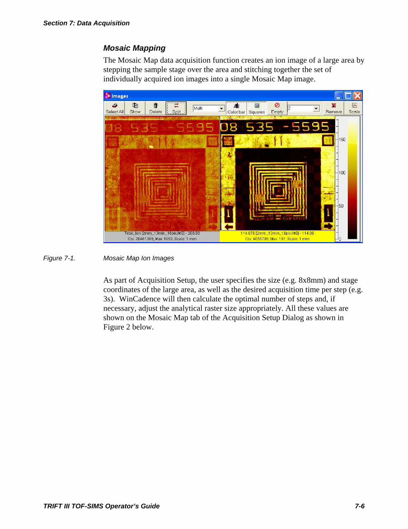
Section 7: Data Acquisition
Mosaic Mapping The Mosaic Map data acquisition function creates an ion image of a large area by stepping the sample stage over the area and stitching together the set of individually acquired ion images into a single Mosaic Map image.
Figure 7-1. Mosaic Map Ion Images
As part of Acquisition Setup, the user specifies the size (e.g. 8x8mm) and stage coordinates of the large area, as well as the desired acquisition time per step (e.g. 3s). WinCadence will then calculate the optimal number of steps and, if necessary, adjust the analytical raster size appropriately. All these values are shown on the Mosaic Map tab of the Acquisition Setup Dialog as shown in Figure 2 below.
TRIFT III TOF-SIMS Operator’s Guide 7-6
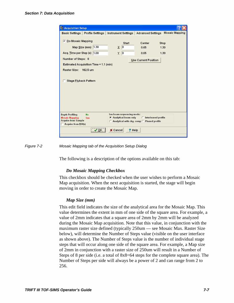
Section 7: Data Acquisition
Figure 7-2 Mosaic Mapping tab of the Acquisition Setup Dialog
The following is a description of the options available on this tab:
Do Mosaic Mapping Checkbox This checkbox should be checked when the user wishes to perform a Mosaic Map acquisition. When the next acquisition is started, the stage will begin moving in order to create the Mosaic Map.
Map Size (mm) This edit field indicates the size of the analytical area for the Mosaic Map. This value determines the extent in mm of one side of the square area. For example, a value of 2mm indicates that a square area of 2mm by 2mm will be analyzed during the Mosaic Map acquisition. Note that this value, in conjunction with the maximum raster size defined (typically 250um — see Mosaic Max. Raster Size below), will determine the Number of Steps value (visible on the user interface as shown above). The Number of Steps value is the number of individual stage steps that will occur along one side of the square area. For example, a Map size of 2mm in conjunction with a raster size of 250um will result in a Number of Steps of 8 per side (i.e. a total of 8x8=64 steps for the complete square area). The Number of Steps per side will always be a power of 2 and can range from 2 to 256.
TRIFT III TOF-SIMS Operator’s Guide 7-7

Section 7: Data Acquisition
Acq. Time per Step (s) This edit field indicates the amount of acquisition time that will be spent at each step of the Mosaic Map (i.e. at each individual stage position). This value, along with the Number Of Steps, determines the Estimated Acquisition Time (visible on the user interface as shown above). Note that the calculation of the Estimated Acquisition Time includes an additional amount of time per step required for stage movement and related timing overhead.
Start X and Start Y Stage Coordinate edit fields These edit fields are used to determine the starting stage position (in mm) of the Mosaic Map. The center and end of travel are also indicated on the user interface as shown above.
Use Current Position Button This button is used to set the current stage position as the starting point for the Mosaic Map. When this button is clicked, the Start X and Start Y values should update appropriately with the current stage position.
Stage Flyback Pattern Checkbox This checkbox is used to ensure that the primary axis of stage travel is followed in the same direction on every row of stage movement. When a row of stage movement is completed, the stage will ‘flyback’ to the other side before beginning the next row. This flyback option lengthens the total time of acquisition, but may improve Mosaic Map alignment in some cases where stage hysteresis is of concern. Note: if this checkbox is not checked, the stage will follow a serpentine pattern, without flybacks.
Mosaic Size 2 4 8 10 16 20 32 50 64
#Steps 8 16 32 64 64 128 128 256 256
RasterSize 250 250 250 156 250 156 250 195 250
Mosaic Pixels 32 16 8 4 4 2 2 1 1
Mosaic Pixel Resolution (µm) 8 16 31 39 63 78 125 195 250
Total # Steps 64 256 1,024 4,096 4,096 16,384 16,384 65,536 65,536
Minutes for each 1sec/acq 1.1 4.3 17.1 68.3 68.3 273.1 273.1 1092.3 1092.3
Hours for each 1sec/acq 0.0 0.1 0.3 1.1 1.1 4.6 4.6 18.2 18.2
TRIFT III TOF-SIMS Operator’s Guide 7-8
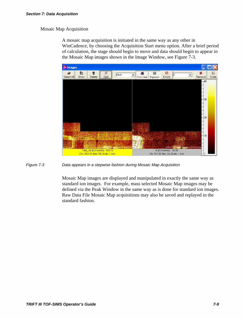
Section 7: Data Acquisition
Mosaic Map Acquisition
A mosaic map acquisition is initiated in the same way as any other in WinCadence, by choosing the Acquisition Start menu option. After a brief period of calculation, the stage should begin to move and data should begin to appear in the Mosaic Map images shown in the Image Window, see Figure 7-3.
Figure 7-3 Data appears in a stepwise fashion during Mosaic Map Acquisition
Mosaic Map images are displayed and manipulated in exactly the same way as standard ion images. For example, mass selected Mosaic Map images may be defined via the Peak Window in the same way as is done for standard ion images. Raw Data File Mosaic Map acquisitions may also be saved and replayed in the standard fashion.
TRIFT III TOF-SIMS Operator’s Guide 7-9
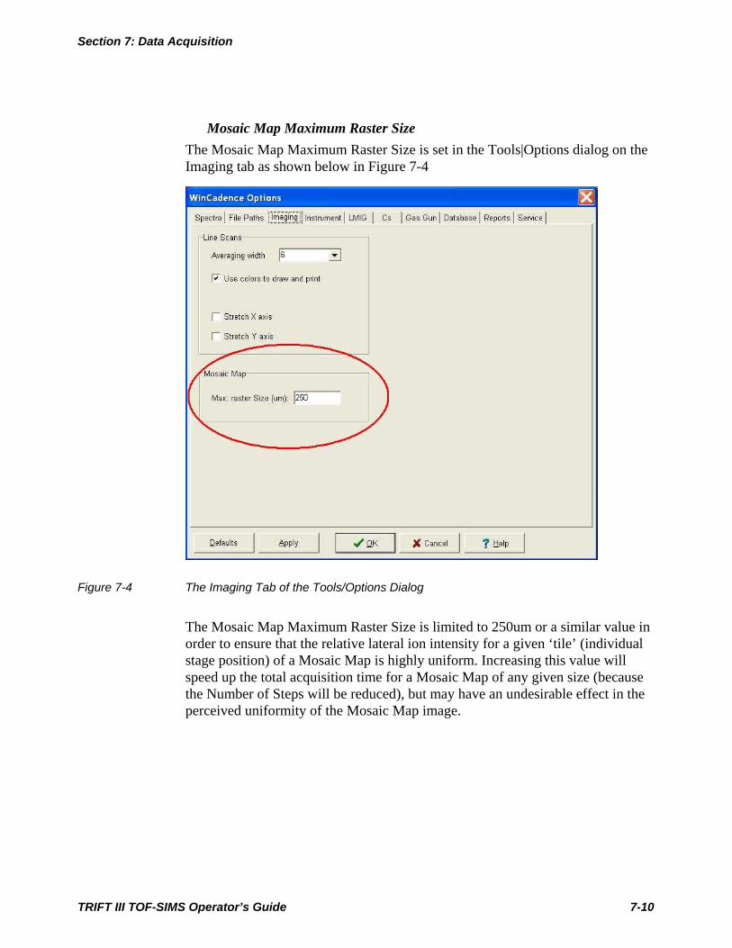
Section 7: Data Acquisition
Mosaic Map Maximum Raster Size The Mosaic Map Maximum Raster Size is set in the Tools|Options dialog on the Imaging tab as shown below in Figure 7-4
Figure 7-4 The Imaging Tab of the Tools/Options Dialog
The Mosaic Map Maximum Raster Size is limited to 250um or a similar value in order to ensure that the relative lateral ion intensity for a given ‘tile’ (individual stage position) of a Mosaic Map is highly uniform. Increasing this value will speed up the total acquisition time for a Mosaic Map of any given size (because the Number of Steps will be reduced), but may have an undesirable effect in the perceived uniformity of the Mosaic Map image.
TRIFT III TOF-SIMS Operator’s Guide 7-10
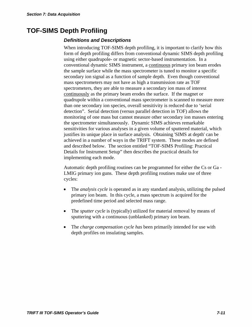
Section 7: Data Acquisition
TOF-SIMS Depth Profiling Definitions and Descriptions When introducing TOF-SIMS depth profiling, it is important to clarify how this form of depth profiling differs from conventional dynamic SIMS depth profiling using either quadrupole- or magnetic sector-based instrumentation. In a conventional dynamic SIMS instrument, a continuous primary ion beam erodes the sample surface while the mass spectrometer is tuned to monitor a specific secondary ion signal as a function of sample depth. Even though conventional mass spectrometers may not have as high a transmission rate as TOF spectrometers, they are able to measure a secondary ion mass of interest continuously as the primary beam erodes the surface. If the magnet or quadrupole within a conventional mass spectrometer is scanned to measure more than one secondary ion species, overall sensitivity is reduced due to ‘serial detection”. Serial detection (versus parallel detection in TOF) allows the monitoring of one mass but cannot measure other secondary ion masses entering the spectrometer simultaneously. Dynamic SIMS achieves remarkable sensitivities for various analyses in a given volume of sputtered material, which justifies its unique place in surface analysis. Obtaining 'SIMS at depth' can be achieved in a number of ways in the TRIFT system. These modes are defined and described below. The section entitled “TOF-SIMS Profiling: Practical Details for Instrument Setup” then describes the practical details for implementing each mode.
Automatic depth profiling routines can be programmed for either the Cs or Ga - LMIG primary ion guns. These depth profiling routines make use of three cycles:
• The analysis cycle is operated as in any standard analysis, utilizing the pulsed primary ion beam. In this cycle, a mass spectrum is acquired for the predefined time period and selected mass range.
• The sputter cycle is (typically) utilized for material removal by means of sputtering with a continuous (unblanked) primary ion beam.
• The charge compensation cycle has been primarily intended for use with depth profiles on insulating samples.
TRIFT III TOF-SIMS Operator’s Guide 7-11
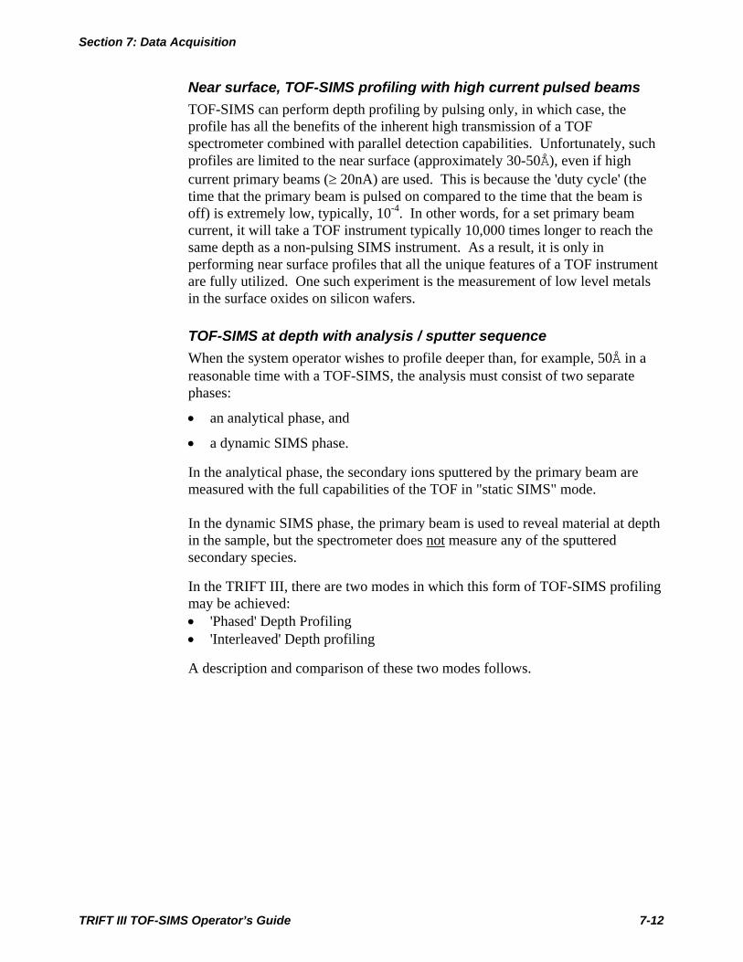
Section 7: Data Acquisition
Near surface, TOF-SIMS profiling with high current pulsed beams TOF-SIMS can perform depth profiling by pulsing only, in which case, the profile has all the benefits of the inherent high transmission of a TOF spectrometer combined with parallel detection capabilities. Unfortunately, such profiles are limited to the near surface (approximately 30-50Å), even if high current primary beams (≥ 20nA) are used. This is because the 'duty cycle' (the time that the primary beam is pulsed on compared to the time that the beam is off) is extremely low, typically, 10-4. In other words, for a set primary beam current, it will take a TOF instrument typically 10,000 times longer to reach the same depth as a non-pulsing SIMS instrument. As a result, it is only in performing near surface profiles that all the unique features of a TOF instrument are fully utilized. One such experiment is the measurement of low level metals in the surface oxides on silicon wafers.
TOF-SIMS at depth with analysis / sputter sequence When the system operator wishes to profile deeper than, for example, 50Å in a reasonable time with a TOF-SIMS, the analysis must consist of two separate phases:
• an analytical phase, and
• a dynamic SIMS phase.
In the analytical phase, the secondary ions sputtered by the primary beam are measured with the full capabilities of the TOF in "static SIMS" mode. In the dynamic SIMS phase, the primary beam is used to reveal material at depth in the sample, but the spectrometer does not measure any of the sputtered secondary species.
In the TRIFT III, there are two modes in which this form of TOF-SIMS profiling may be achieved: • 'Phased' Depth Profiling • 'Interleaved' Depth profiling
A description and comparison of these two modes follows.
TRIFT III TOF-SIMS Operator’s Guide 7-12

Section 7: Data Acquisition
Phased Depth Profiling In 'phased' profiling, the analysis begins with an acquisition phase within the static SIMS regime (typically, 10-30 seconds). Following this, the analytical conditions are stored to temporary memory, and a sputter phase is invoked.
After a set sputter time is defined by the user (typically, 1-30 seconds), the analytical phase is re-loaded from temporary memory. The next analysis is a static SIMS analysis, but it occurs at some depth into the sample. The cycle of analysis/sputter/analysis/sputter... continues until either the countdown timer times out, or to a point where the profile is terminated by the user. This mode of profiling is very similar to that used for Auger or XPS profiling: an ion beam reveals a new surface which is then probed by the analyzing beam.
In addition to an analytical phase and a sputter phase, the user can invoke two other phases: 1. A charge compensation phase; and 2. A 'settling' phase.
The charge compensation phase invoked in profiling is different from the typical pulsed charge compensation which occurs during acquisition. The charge compensation phase pauses the profiling, lowers the extraction field to zero (0), and then turns the electron gun on in a continuous mode to equalize any charge build-up that may have occurred during the sputtering phase. This phase may also be used to assist with imaging of insulators at high magnification, as described in another section.
A settling phase permits optimization of profiling conditions for single gun systems by allowing the system to settle in between phases. It is designed for profiles in which a single gun is switching beam energy between the acquisition phase (higher energy) and the sputter phase (low impact energy). Settling phases can be programmed prior to each of the other phases: acquisition; sputter; and charge compensation.
Phased profiling can involve the use of one primary ion beam only, or can use two beams to optimize the depth resolution of the profile with a second low energy beam.
Phased depth profiles are useful for deep structures in which the concentration changes are either continuous, or where the layer structures are quite thick.
The disadvantage of 'phased' depth profiling is that it is possible to miss shallow, buried layers bypassing through them during a single sputter phase. For such structures, a different profiling mode known as interleaved depth profiling is preferred.
TRIFT III TOF-SIMS Operator’s Guide 7-13
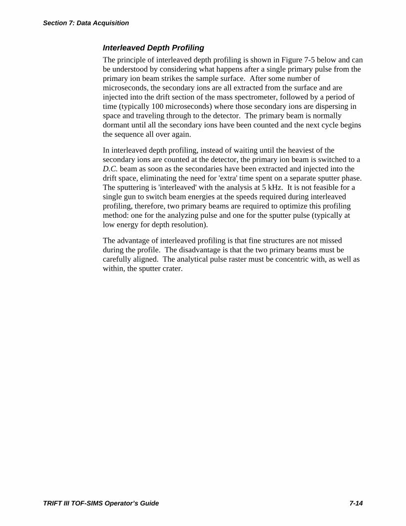
Section 7: Data Acquisition
Interleaved Depth Profiling The principle of interleaved depth profiling is shown in Figure 7-5 below and can be understood by considering what happens after a single primary pulse from the primary ion beam strikes the sample surface. After some number of microseconds, the secondary ions are all extracted from the surface and are injected into the drift section of the mass spectrometer, followed by a period of time (typically 100 microseconds) where those secondary ions are dispersing in space and traveling through to the detector. The primary beam is normally dormant until all the secondary ions have been counted and the next cycle begins the sequence all over again.
In interleaved depth profiling, instead of waiting until the heaviest of the secondary ions are counted at the detector, the primary ion beam is switched to a D.C. beam as soon as the secondaries have been extracted and injected into the drift space, eliminating the need for 'extra' time spent on a separate sputter phase. The sputtering is 'interleaved' with the analysis at 5 kHz. It is not feasible for a single gun to switch beam energies at the speeds required during interleaved profiling, therefore, two primary beams are required to optimize this profiling method: one for the analyzing pulse and one for the sputter pulse (typically at low energy for depth resolution).
The advantage of interleaved profiling is that fine structures are not missed during the profile. The disadvantage is that the two primary beams must be carefully aligned. The analytical pulse raster must be concentric with, as well as within, the sputter crater.
TRIFT III TOF-SIMS Operator’s Guide 7-14
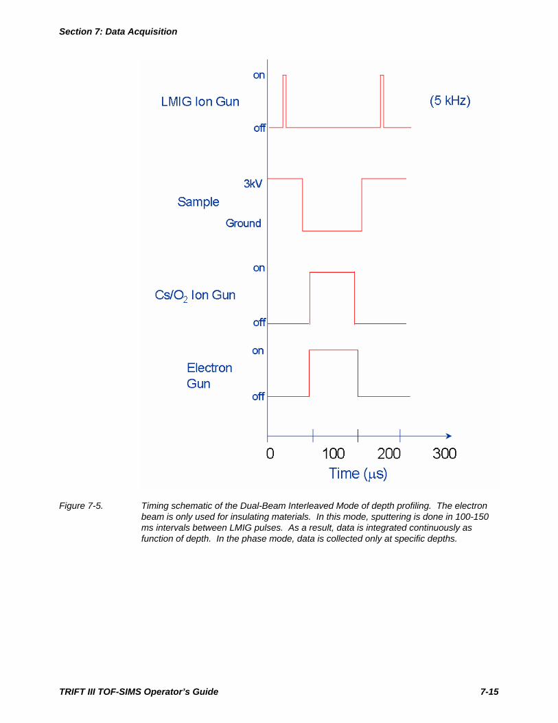
Section 7: Data Acquisition
Figure 7-5. Timing schematic of the Dual-Beam Interleaved Mode of depth profiling. The electron beam is only used for insulating materials. In this mode, sputtering is done in 100-150 ms intervals between LMIG pulses. As a result, data is integrated continuously as function of depth. In the phase mode, data is collected only at specific depths.
TRIFT III TOF-SIMS Operator’s Guide 7-15
Section 7: Data Acquisition
Practical System Set-up The previous section defined the different profiling modes. This section will consider the practical details for implementing profiles in each of the different modes, such as setting a single gun LMIG system for low energy profiling, and how to use the profiling tools in software to finesse other experiments, (e.g., imaging insulators at high magnification, etc.)
Near surface, TOF-SIMS profiling with high current pulsed beams High sensitivity, near surface profiling (typically, 30-50Å) can be achieved in a pulsed-only mode in ‘reasonable’ times (e.g., 15-20 minutes) using primary beam currents of ≥20nA. The beam energy for the Ga beam is typically 15kV, and 10 or 11kV for the Cs beam (for high mass resolution in bunched mode). These beams could be tuned to a lower beam energy, except the probe size increases and the efficiency of the primary beam transport is reduced at these lower beam energies, resulting in lower probe currents. The only drawback to using the higher energy beams is reduced depth resolution.
The principal use for these pulsed-only profiles has been to make quantitative measurements of the surface metal concentrations in thin surface oxides on silicon wafers. The following notes in this section reflect this. In these measurements, it is important to not confine the measurement to the top surface only, but to consume the entire native oxide. In some cases, metal species are segregated to either the outer surface or the oxide/silicon interface. Concentration profiles help to determine such segregations, although it is the final integrated mass spectrum which is used to derive the metal concentrations.
Post-ESA blanking When using the high current probes of either the Ga or the Cs beam, insure that the post-ESA blanker is set to remove intense matrix peaks right from the outset. There are three reasons for doing this:
1. The most intense peaks will often suffer 'dead time effects' which distort their relative peak intensities. Dead time effects are encountered when the secondary ion count rate is significantly higher than the primary beam repetition rate. For example, consider a secondary count rate of 1 x 10⁵, and a primary beam repetition rate of 1 x 10⁴. An average of 10 secondary ions arrive at the detector in every cycle. If these secondary ions are significantly different in mass, spread apart in time, the detector will register all of the ions. If these ions, as is typically the case, represent only one or two masses, then some of the ions will be ignored due to detector dead time effects. Consider the specific example of a Si wafer analysis. Most of the secondary ion signals are due to 28Si, 29Si, 28SiH and 30Si. In the case of 10 secondary ions per cycle, let’s say that four of them are 28Si. When the first of the batch of four arrives at the detector, the detector registers the ion, and there is a charge transfer within the detector. During that period of approximately 10ns
TRIFT III TOF-SIMS Operator’s Guide 7-16

Section 7: Data Acquisition
(or ~70 channels at 138ps/channel), the detector is unable to count any more ions and is experiencing a period of 'dead time'. The second of the 28Si ions arrives at the detector while the detector is dormant, and is not counted. In the case of 29Si, statistically there will be a smaller number per cycle compared to 28Si, and the dead time effect on that peak is not as pronounced (e.g, less ions lost). Therefore, the isotope ratios for Si appear not to be in accordance with the natural abundance of the isotopes.
2. Secondly, high current pulsed probes operating at high repetition rates can, in some cases, result in instantaneous secondary count rates of ~1010/second at the detector. By using the post-ESA blanker to remove these intense matrix peaks (which are often hampered by dead time effects anyway), the detector lifetime is extended.
3. Extremely high count rates tend to slow the computer as it sorts and plots the incoming data. For the case cited above, the 28Si, 29Si and 28SiH peaks often account for >95% of the secondary ion population. By removing these, the secondary ion count rate falls by a factor of 20, making data acquisition much more manageable (and also very beneficial when saving ‘raw’ data to disk!)
Since post-ESA blanking windows can be stored with an instrument file, instrument files can be modified and re-stored according to your particular analytical needs. For instance, a file could be prepared which blanks mass 28 and 29, but leaves mass 30 detected for quantification purposes, and then store this out with a customized name (e.g., SIWAFER.INS, etc.)
Crater Edge Effects: Gating There is no automatic secondary ion ‘gating’ when performing pulsed-only profiles. This can limit the dynamic range of secondary signals due to crater edge effects. Gating may be achieved by taking an acquisition as a ‘region of interest’ from the center of a raster, provided the beam size is much smaller than the total raster size.
Profiling Species The goal of near surface profiling is normally to integrate the counts for various species in the near surface. For a given set of conditions, the beam will profile to a standard depth in a set time on a specified substrate, and the experiment can be run with a spectrum (only) as the final product. Typically, the goal is to produce a concentration profile as well as a total, integrated mass spectrum, or at least, allows for determination of a suitable end point for the experiment. If concentrations of various species are to be monitored as a function of depth (elapsed time), a list of these species needs to be set up in the Peak window and profile selected. If 0 seconds is entered for the sputter time, the profile window will show the intensity of the selected peaks as a function of acquisition time.
TRIFT III TOF-SIMS Operator’s Guide 7-17
Section 7: Data Acquisition
Phased Depth Profiling: Single Gun Instrument Files need to be created for the analytical phase and for the sputter phase. The analytical phase is accomplished by aligning and tuning the pulsing primary beam as per a normal mass spectral acquisition. The instrument state does not need to be saved specifically because it is stored and recalled automatically from a temporary memory during profiling. If the sputter phase is to be accomplished with the same primary beam and energy as the analytical phase, setting up the sputter phase is simple. To prepare the sputter file, increase the raster size of the beam in the control page (typically >4 times the size of the analytical area). If necessary, alter any settings for the beam which affect its focus when in the D.C. mode (for instance, raise Lens 2 in the LMIG back to its focused value for D.C. tuning as opposed to pulsed and bunched focus). Note that the beam blanker does not need to be set to zero. The software automatically sets the beam blanker to zero during the sputter phase of profiling. Now, save the sputter file with a unique identifier (e.g. sputter.ins). Reset all values back to their original settings for the acquisition phase (e.g. raster and Lens 2).
To setup the single gun depth profile, go to Acquisition Setup, Basic Settings tab. Select Phased Profile from the bottom of the page. This automatically opens the Profile Settings tab, which is divided into sections for the Analytical Phase, Sputter Phase and Charge Compensation phase.
Choose the analyze time. Note that the analyze time is dependant upon the mass range chosen (repetition rate), and that the time periods listed are multiples of a complete frame (data acquired at each of the 256x256 pixels). If the species of interest are present at low concentrations, the time for the analytical phase may need to be increased so that a statistically significant number of counts is generated for the species of interest per cycle.
In the Sputter Phase, load the sputter file previously created (sputter.ins), select the sputter gun (i.e, LMIG), choose the sputter time (20 sec. = typically a good intermediate time for an “unknown” sample), and choose the settle time (normally 1 sec.) Specify the sample potential during the Sputter Phase: high voltage, at ground or with charge compensation (implies at ground). Note: if either “at ground” or “charge comp” is chosen, the ion beam will shift in the x-axis. This will have to be accounted for in the x beam position value saved in sputter.ins in order to keep the analysis phase and sputter phase aligned.
For single gun depth profiles, the sample is typically set at high voltage; in this manner the impact energy of the sputter ions will be lower in the positive ion polarity (5 keV Ga sputter file and 3 keV sample potential results in 2 keV impact energy). In the Charge Comp phase, enter a time (typically a few seconds) if charge compensation is desired in a continuous mode between the analytical and sputter phases. This extra phase drops the secondary extraction field to zero and then turn on the electron gun continuously. Note that if charge compensation is desired during the analytical phase, a value should be entered in the charge comp duty cycle box in the Analyze Phase (typically 64%). Also note
TRIFT III TOF-SIMS Operator’s Guide 7-18

Section 7: Data Acquisition
that this value is automatically entered if the operator selects Analytical with Chg. Comp in the Basic Settings tab, before selecting Phased Profile.
The species to be monitored must be designated. A peak table should be created with the peaks of interest and the “Profile?” option selected. It may also be desirable to blank matrix peaks of high intensity and the peak of the sputter source species. This table should be open in the Peak Viewer. The depth profile acquisition can then be started: select Start Acquisition.
Phased Depth Profiling: Dual Gun An Instrument File that contains parameters for both guns must be used (typically LMIG for analysis and Cs, O2 or Gas Gun for sputtering). If an instrument file (*.ins) does not already exist, one can be created by filter loading the values for the sputter gun into the open instrument file for the analytical gun (15 keV LMIG). Refer to Section 3: Filter-Loading Part of the Instrument State Files.
NOTE: If the Gas Gun has not been used recently, it will be necessary to set the emission to 15mA [the software will ramp the emission setting in 1mA steps per second]. Open V10 in Watcher to introduce the flow of Argon gas into the ionizer.
The sputter and analytical ion beams must be aligned. This can be done manually on a sample where sputter craters can be observed visually (for example, a thin Au film on Si). Use the following steps to align the two beams:
1. Start a spectral acquisition, switch to the detector view, and using the LMIG X and Y beam position, center the secondary ions on the detector. The LMIG is now aligned with the spectrometer.
2. Set the LMIG raster to 25µm and turn the beam to D.C. on the sample. Note the location of the sputtered crater.
3. Adjust the optical microscope to center the LMIG sputter crater. Now the optical microscope is aligned with the LMIG and the spectrometer.
4. Set the sample voltage to zero (0). Set the sputter gun raster to zero (0). Turn the sputter gun beam to D.C. on the sample. Then adjust the X and Y beam position to align the sputter gun sputtered spot with the LMIG crater. Once this is done, the sputter gun beam is now aligned with the LMIG, optical microscope and the spectrometer. Return the sample voltage and sputter gun raster size to their previous values and save the file.
Once a file has been created containing parameters for two ion guns, and the guns have been aligned on a particular sample, the beam alignment can be done automatically on subsequent samples. The automatic alignment takes into consideration the z-height shift of the sample and moves the X/Y beam positions of the guns accordingly. Move to the sample of interest. In the Acquisition Setup, in the Instrument Settings tab, choose “Re-align analysis beam on detector
TRIFT III TOF-SIMS Operator’s Guide 7-19

Section 7: Data Acquisition
for z-height shift (non-destructive).” Then select Go. The distance of the resulting LMIG Beam Position shift will be shown. If the value is greater than 5 micron, the auto alignment should be repeated until the resulting X/Y Beam shift is less than 5 micron. Care must be taken to only use this method if the off-set is due to a z-height change. If it is due to some other type of phenomenon, such as extraction field curvature near the sample’s edge, then a propagation error will result.
If the operator wishes to verify the alignment of the beams and has ample sample for a destructive test, this can be done as follows.
For the Cs sputter gun: Implant Cs into the sample in the D.C. mode using a zero raster size and zero sample potential. Image the Cs implant with the LMIG in the analytical mode. If the Cs is not in the center of the analytical area, it can be moved there by right clicking on the image and choosing “Move sputter beam from cursor.” Now move the pointer to the center of the Cesium beam spot and left click on the mouse. The guns are now aligned.
For the O2 sputter gun: If O2 is used as the sputter source, the location of the O2 source can be determined by D.C. sputtering with O2 (zero spot size, zero sample potential) and then imaging some surface species that will be sputtered away so as to make a dark spot (e.g., C2H3). If the O2 beam is not in the center of the analytical area, it can be moved there by right clicking on the image and choosing “move sputter beam from cursor.” Now move the cursor to the center of the sputtered area in the image and click the left mouse button. This test can be done automatically by choosing “Center sputter beam on image field (destructive!)” in Acquisition Setup, Instrument Settings tab. The automatic mode works only in positive SIMS, for Cs as the sputter source and the LMIG as the analytical source.
For the Ar+ sputter gun: If Ar+ is used as the sputter source, the location of the Ar+ source can be determined by D.C. sputtering with Ar+ (zero spot size, zero sample potential) and then imaging some surface species that will be sputtered away so as to make a dark spot (e.g., C2H3). Any correction required will need to be done manually by adjusting the Xpos or YPos on the Gas Gun page to center the dark spot. A more +X will move the spot to the right. A more +Y will move the spot down.
Once the dual beams are aligned, set the raster size for both the Ga and sputter ion beams. The sputter gun should be at least 2mm or 4x larger than the primary gun raster size. Make sure the sample potential has been set back to its original value in the hardware page. The acquisition can now be set up. Go to Acquisition Setup, Basic Settings tab. Select Phased Profile from the bottom of the page. This automatically opens the Profile Settings tab, which is divided into sections for the Analytical Phase, Sputter Phase and Charge Compensation
TRIFT III TOF-SIMS Operator’s Guide 7-20

Section 7: Data Acquisition
phase. Choose the analyze time. Note that the analyze time is dependant upon the mass range chosen (repetition rate), and that the time periods listed are multiples of a complete frame (data acquired at each of the 256x256 pixels). If the species of interest are present at low concentrations, the time for the analytical phase may need to be increased so that a statistically significant number of counts is generated for the species of interest per cycle.
In the Sputter Phase, do not load a sputter file. The software will use the sputter gun settings in the current instrument file. Set the Settling time (s) to 3. Choose the sputter time (20 sec. is typically a good intermediate time to try on an “unknown”sample). Select the desired sputter gun. Specify the potential of the sample during the Sputter Phase: high voltage, at ground or with charge compensation (implies at ground). Note: If a low energy Cs sputter gun energy is being used as the sputter source or if the Ar+ Gas Gun is being used as the sputter source, the sample potential must be at ground during the sputter phase.
In the Charge Comp phase, enter a Settle time (s) of 1, and choose a Comp time (s) (typically a few seconds) if charge compensation is desired in a continuous mode between the analytical and sputter phases. This extra phase drops the secondary extraction field to zero and then turns on the electron gun continuously. Note that if charge compensation is desired during the analytical phase, a value should be entered in the charge comp duty cycle box in the Anayze Phase (typically 64%). Also note that this value is automatically entered if the operator selects Analytical with Charge Comp in the Basic Settings tab, before selecting Phased Profile.
The species to be monitored must be designated. A peak table should be created with the peaks of interest and the “Profile?” option selected. It may also be desirable to blank matrix peaks of high intensity and the peak of the sputter source species. This table should be open in the Peak Viewer.
The depth profile acquisition can be started: select Start Acquisition.
NOTE: Perform the following if the Gas Gun is used for sputtering:
Close the Spectrometer Gate Valve Setup the GasGun Parameters Start with known setting Select desired Beam Energy, Float State, Float Voltage and Grid Voltage Launch the GasGun DC mode in the Hardware Menu Monitor beam at sample—GasGun Adjust GasGun Condenser for desired current Select GasGun Objective Set GasGun Raster Size to 0.001 Align the GasGun to LMIG Move to new area Launch the GasGun DC mode in the Hardware Menu Monitor beam at sampleThis will turn on the GasGun & burn a spot
TRIFT III TOF-SIMS Operator’s Guide 7-21

Section 7: Data Acquisition
Select DC to sample OFF Launch the LMIG DC mode in the Hardware Menu LMIG--DC image with 1000um [this will display image of rastered area by GasGun] Adjust GasGun X&Y to recenter Launch the GasGun DC mode in the Hardware Menu Monitor beam at sample-This will turn on the GasGun & burn a spot DC to sample OFF Launch the LMIG DC mode in the Hardware Menu LMIG--DC image with 1000um [this will display image of rastered area by GasGun] Iterate until centered raster Create the Final settings and SAVE *desired_name*.ins setting Select GasGun Raster Size for crater Select LMIG Raster Size for analysis SAVE GasGun setting with *desired_name*.ins Change GasGun Beam Energy to 100 [this will minimize the ion current at the sample during the analysis phase] Acquisition Setup Open Spectrometer Gate Valve Move to desired analysis area Setup Profile Acquisition Setup Settle time(s) = (BeamEnergyDelta+1) (eg. 5kv > =6) sputter time = desired sputter file = *desired_name*.ins sputter gun = GasGun sample has = Ground Acquire
If the Gas Gun is used during the sputter cycle, turn off the ionizer after the profiling is complete. This is important to prolong ionizer lifetime.
1. On the Gas Gun page, set the emission to 0mA.
2. Close V10 in Watcher.
3. Load the zero.ins file
4. Load desired LMIG instrument file to maintain proper operation of the LMIG.
TRIFT III TOF-SIMS Operator’s Guide 7-22
Section 7: Data Acquisition
Interleaved Depth Profiling: Dual Gun An Instrument File that contains parameters for both guns must be used (typically LMIG for analysis and Cs for sputtering). If an instrument file does not already exist, create one by filter-loading the values for the sputter gun (1 keV Cs) into the open instrument file for the analytical gun (15 keV LMIG). Refer to Section 3: Filter-Loading Part of the Instrument State Files. The sputtter and analytical ion beams must be aligned (see suggestions above in Phased Mode Dual Beam Depth Profiling).
Once the dual beams are aligned, the acquisition can be set up. In Acquisition Setup, in the Basic Settings tab, choose Interleaved Profile at the bottom right. Select the cycle time of the analytical phase. Note that in the interleaved mode, the repetition rate is automatically set to 5 kHz, and that the cycle times are based on multiples of the time it takes to acquire a complete frame at this rate. Enter the duty cycle of the sputter pulse (typically 50%). Enter the duty cycle of charge compensation, if desired (typically 64%). Note that this value is automatically entered if the operator selects Analytical with Charge Comp in the Basic Settings tab, before selecting Interleaved Profile.
The species to be monitored must be designated. A peak table should be created with the peaks of interest and the “Profile?” option selected. It may also be desirable to blank matrix peaks of high intensity and the peak of the sputter source species. The depth profile acquisition can be started. Select Start Acquisition.
Low impact energy, LMIG only depth profiles The material in this section, (depth profiling with an LMIG-only TRIFT system), could have been covered above, but instead is being considered separately in this section.
1. For positive SIMS depth profiling, a 2keV impact energy can be achieved by tuning the LMIG beam energy to 5kV. In +SIMS, a +5kV beam bombards the +3kV sample with a net energy of 2keV, making it quite suitable for depth profiling at high depth resolution. To tune the gun at 5kV beam energy, first make a plot of the lens 1 and lens 2 values against beam energy from the existing instrument files on the system. From this, estimated values for lens 1 and lens 2 can be extrapolated that will be approximately correct at 10kV and 5kV. Typically, for an extractor value of 7.5kV, the values for lens 1 and lens 2 at 10kV are ~2.1kV and ~5.9, and at 5kV, they are ~ 1.6kV and 2.9kV, respectively. Because it is typically easier to tune the LMIG using secondary electrons, consider switching to negative SIMS mode in order to set up the gun. If a focused image cannot be produced at an energy level of 5kV, go up to 10kV. The LMIG should be tuned with the buncher voltage off initially, even if the intention is to bunch at a later stage.
2. Once the beam voltages are in negative SIMS, switch to positive SIMS. Since the LMIG is now tuned, the only new detail left is where the beam is
TRIFT III TOF-SIMS Operator’s Guide 7-23
Section 7: Data Acquisition
striking the sample with respect to the mass spectrometer acceptance area. At 2keV impact energy, the x beam position will require considerable adjustment for the beam to reach the acceptance area of the spectrometer, because the beam is steered significantly by the decelerating sample potential. Note that the x beam position may need to be moved significantly before secondary ions can detected at the DMCP detector.
3. A 5kV beam can be bunched quite effectively to permit high mass resolution mass spectroscopy. The buncher voltage will need to be reduced when compared to the value used for the 15kV beam, and the buncher firing (delay line) will need to change slightly (typically some tens of nanoseconds compared to the 15kV case). Experiment until some narrowing of any mass peak is observed, and then fine tune the values of the buncher and the delay until the highest mass resolution is obtained. Do not be alarmed if the application of the buncher voltage causes the beam to shift slightly on the DMCP. Also, remember that the application of the buncher will cause the beam to be over focused, and lowering the lens 2 value to compensate (as happens at 15kV also) will be required. The lens 2 value for the best bunched imaging at 5kV beam energy is best determined empirically on a copper grid sample.
4. In the case of negative SIMS, the lowest impact energy for a sputter beam that can be realistically achieved is 5keV, using a 5kV LMIG beam onto a sample at zero potential. This is not as low an impact energy as the positive SIMS case, but it is useful.
5. When switching between analytical files and sputtering files tuned for 5kV beam energy, two things can occur: if the beam is being bunched, the value of lens 2 needs changing to keep the beam focused in both phases; and the beam may shift position due to one of two reasons: a) the dynamic steering of the buncher when it is firing (a smaller effect); or b) due to a change in the beam impact energy between the phases in the profile, as is the case for negative SIMS (a larger effect). This is the more likely reason for the shift.
6. The first effect is easily corrected on the computer-controlled LMIG by setting the appropriate lens 2 value in the analytical phase file, and by storing the higher value of lens 2 for the D.C. beam condition in the sputtering phase file. As for the second effect, if the crater is not concentric with the analysis area, appropriate x and y beam positions must be determined for the sputter beam to insure that it is concentric with the analytical beam. When the shift is due to a sputter phase with zero (0) sample potential, proceed as follows. With the sample at zero potential, steer the low energy D.C. beam until the observed crater in the optical view of the sample is concentric with a mark that was made previously with the analytical file in a D.C. condition, with the sample potential on.
TRIFT III TOF-SIMS Operator’s Guide 7-24
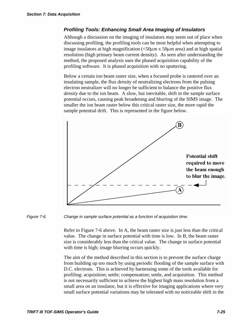
Section 7: Data Acquisition
Profiling Tools: Enhancing Small Area Imaging of Insulators Although a discussion on the imaging of insulators may seem out of place when discussing profiling, the profiling tools can be most helpful when attempting to image insulators at high magnification (<50µm x 50µm area) and at high spatial resolution (high primary beam current density). As seen after understanding the method, the proposed analysis uses the phased acquisition capability of the profiling software. It is phased acquisition with no sputtering.
Below a certain ion beam raster size, when a focused probe is rastered over an insulating sample, the flux density of neutralizing electrons from the pulsing electron neutralizer will no longer be sufficient to balance the positive flux density due to the ion beam. A slow, but inevitable, shift in the sample surface potential occurs, causing peak broadening and blurring of the SIMS image. The smaller the ion beam raster below this critical raster size, the more rapid the sample potential drift. This is represented in the figure below.
Figure 7-6. Change in sample surface potential as a function of acquisition time.
Refer to Figure 7-6 above. In A, the beam raster size is just less than the critical value. The change in surface potential with time is low. In B, the beam raster size is considerably less than the critical value. The change in surface potential with time is high; image blurring occurs quickly.
The aim of the method described in this section is to prevent the surface charge from building up too much by using periodic flooding of the sample surface with D.C. electrons. This is achieved by harnessing some of the tools available for profiling: acquisition; settle; compensation; settle, and acquisition. This method is not necessarily sufficient to achieve the highest high mass resolution from a small area on an insulator, but it is effective for imaging applications where very small surface potential variations may be tolerated with no noticeable shift in the
TRIFT III TOF-SIMS Operator’s Guide 7-25

Section 7: Data Acquisition
primary beam position. The duty cycle between acquisition and charge compensation phases can be adjusted according to requirements. This method is shown schematically in the following diagram.
TRIFT III TOF-SIMS Operator’s Guide 7-26
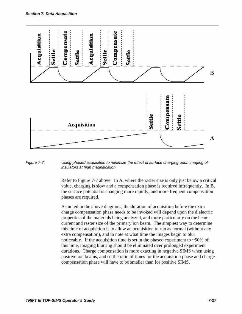
Section 7: Data Acquisition
Figure 7-7. Using phased acquisition to minimize the effect of surface charging upon imaging of insulators at high magnification.
Refer to Figure 7-7 above. In A, where the raster size is only just below a critical value, charging is slow and a compensation phase is required infrequently. In B, the surface potential is changing more rapidly, and more frequent compensation phases are required.
As noted in the above diagrams, the duration of acquisition before the extra charge compensation phase needs to be invoked will depend upon the dielectric properties of the materials being analyzed, and more particularly on the beam current and raster size of the primary ion beam. The simplest way to determine this time of acquisition is to allow an acquisition to run as normal (without any extra compensation), and to note at what time the images begin to blur noticeably. If the acquisition time is set in the phased experiment to ~50% of this time, imaging blurring should be eliminated over prolonged experiment durations. Charge compensation is more exacting in negative SIMS when using positive ion beams, and so the ratio of times for the acquisition phase and charge compensation phase will have to be smaller than for positive SIMS.
TRIFT III TOF-SIMS Operator’s Guide 7-27
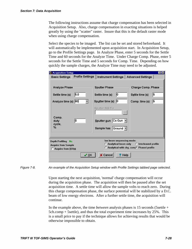
Section 7: Data Acquisition
The following instructions assume that charge compensation has been selected in Acquisition Setup. Also, charge compensation in exacting situations is helped greatly by using the "scatter" raster. Insure that this is the default raster mode when using charge compensation.
Select the species to be imaged. The list can be set and stored beforehand. It will automatically be implemented upon acquisition start. In Acquisition Setup, go to the Profile Settings page. In Analyze Phase, enter 5 seconds for the Settle Time and 60 seconds for the Analyze Time. Under Charge Comp. Phase, enter 5 seconds for the Settle Time and 5 seconds for Comp. Time. Depending on how quickly the sample charges, the Analyze Time may need to be adjusted.
Figure 7-8. An example of the Acquisition Setup window with Profile Settings tabbed page selected.
Upon starting the next acquisition, 'normal' charge compensation will occur during the acquisition phase. The acquisition will then be paused after the set acquisition time. A settle time will allow the sample volts to reach zero. During this charge compensation phase, the surface potential will be stabilized by a D.C. beam of low energy electrons. After a further settle time, the acquisition will continue.
In the example above, the time between analysis phases is 15 seconds (5settle + 5ch.comp + 5settle), and thus the total experiment time increases by 25%. This is a small price to pay if the technique allows for achieving results that would be otherwise impossible to obtain.
TRIFT III TOF-SIMS Operator’s Guide 7-28
Section 7: Data Acquisition
Depth Profiling of Insulators The challenge in performing depth profiles on an insulating material such as a ceramic or a glass sample is to ensure that the sputter crater does not drift away from the analytical beam position during the sputter phase in a depth profile.
There are three different methods for attempting to perform profiles on insulators as follows.
• Coat the sample with a thin (50A) conducting film. This is the simplest, but potentially dirtiest, solution. After the sputter phase has eroded through the coating layer, the sputter crater is pinned in place by the conducting film surrounding it. Any charge that would otherwise build up is immediately drained to the conducting layer. The disadvantage of this method is that unless an extremely clean coating unit exists dedicated to surface analytical techniques, the coating will inevitably contain the usual contaminants such as Na, K, Ca, etc. These species are extremely mobile and will move in advance of the sputter crater. Avoid using this method if any chance exists that the coating could provide a spurious source of the very elements that are being sought in the profile.
• Using a D.C. electron beam and sputter ion beam simultaneously. Another method for assisting with the profiling of insulators involves the use of a D.C. electron beam concurrent with the sputter ion beam. If the extraction field is zero during the sputter phase (sample potential to zero), it is possible to neutralize the effect of the incoming ion beam by simultaneously using a D.C. electron beam. If the sample potential is not zero, then either the electrons will never reach the sample (negative SIMS), or will be accelerated into the sample, causing further charge build-up (positive SIMS). The D.C. electron beam can be set on, concurrent with the sputter beam in the Phased Mode of depth profiling. In Acquisition Setup, in the Profile Settings tab for Phased profile, select “Sample has CComp” in the Sputter Phase. This will result in the D.C. electron beam and the sputter ion beam being on with the sample at ground. If a separate and additional charge compensation phase is desired, a value should be added in the Charge Comp Phase, in the Comp time box. If charge compensation is desired during data acquisition in the Analytical Phase, a value should be entered in the box for Comp. duty cycle% (typically 63%). If the Interleaved Mode of profiling is used, the sample is automatically set to ground between the LMIG pulses. To turn the electron beam on during sputtering, enter a value of up to 71 in the Duty Cycle, % field under Charge Comp. Pulse.
TRIFT III TOF-SIMS Operator’s Guide 7-29
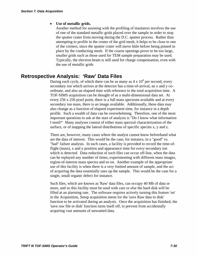
Section 7: Data Acquisition
• Use of metallic grids. Another method for assisting with the profiling of insulators involves the use of one of the standard metallic grids placed over the sample in order to stop the sputter crater from moving during the D.C. sputter process. Rather than attempting to profile in the center of the grid mesh, it helps to be close to one of the corners, since the sputter crater will move little before being pinned in place by the conducting mesh. If the coarse openings prove to be too large, smaller grids such as those used for TEM sample preparation may be used. Typically, the electron beam is still used for charge compensation, even with the use of metallic grids
Retrospective Analysis: ‘Raw’ Data Files During each cycle, of which there can be as many as 4 x 10⁴ per second, every secondary ion which arrives at the detector has a time-of-arrival, an x and y co-ordinate, and also an elapsed time with reference to the total acquisition time. A TOF-SIMS acquisition can be thought of as a multi-dimensional data set. At every 256 x 256 pixel point, there is a full mass spectrum available and at every secondary ion mass, there is an image available. Additionally, these data may also change as a function of elapsed experiment time, for instance in a depth profile. Such a wealth of data can be overwhelming. Therefore, one of the most important questions to ask at the start of analysis is "Do I know what information I need?" Many analyses consist of either mass spectral characterization of the surface, or of mapping the lateral distributions of specific species x, y and z.
There are, however, many cases where the analyst cannot know beforehand what are the data of interest. This would be the case, for instance, in a "good" vs. "bad" failure analysis. In such cases, a facility is provided to record the time-of-flight (mass), x and y position and appearance time for every secondary ion which is detected. Data reduction of such files can occur off-line, when the data can be replayed any number of times, experimenting with different mass images, region-of-interest mass spectra and so on. Another example of the appropriate use of this facility is when there is a very limited amount of sample, and the act of acquiring the data essentially uses up the sample. This would be the case for a single, small organic defect for instance.
Such files, which are known as 'Raw' data files, can occupy 40 Mb of data or more, and so this facility must be used with care or else the hard disk will be filled at an alarming rate. The software requires actively turning this feature 'on' in the Acquisition, Setup acquisition menu for the 'save Raw data to disk' function to be activated during an analysis. Once the acquisition has finished, the 'save raw file to disk' function turns itself off, to prevent from accidentally acquiring vast amounts of unwanted data.
TRIFT III TOF-SIMS Operator’s Guide 7-30
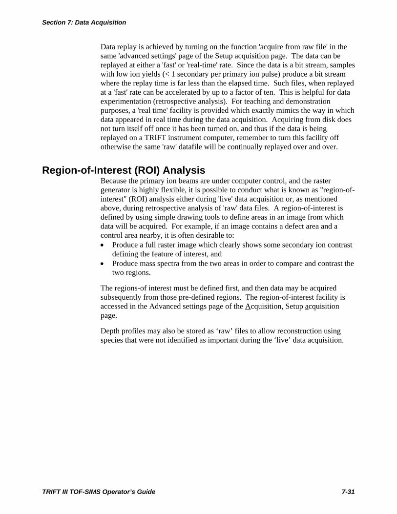
Section 7: Data Acquisition
Data replay is achieved by turning on the function 'acquire from raw file' in the same 'advanced settings' page of the Setup acquisition page. The data can be replayed at either a 'fast' or 'real-time' rate. Since the data is a bit stream, samples with low ion yields (< 1 secondary per primary ion pulse) produce a bit stream where the replay time is far less than the elapsed time. Such files, when replayed at a 'fast' rate can be accelerated by up to a factor of ten. This is helpful for data experimentation (retrospective analysis). For teaching and demonstration purposes, a 'real time' facility is provided which exactly mimics the way in which data appeared in real time during the data acquisition. Acquiring from disk does not turn itself off once it has been turned on, and thus if the data is being replayed on a TRIFT instrument computer, remember to turn this facility off otherwise the same 'raw' datafile will be continually replayed over and over.
Region-of-Interest (ROI) Analysis Because the primary ion beams are under computer control, and the raster generator is highly flexible, it is possible to conduct what is known as "region-of-interest" (ROI) analysis either during 'live' data acquisition or, as mentioned above, during retrospective analysis of 'raw' data files. A region-of-interest is defined by using simple drawing tools to define areas in an image from which data will be acquired. For example, if an image contains a defect area and a control area nearby, it is often desirable to: • Produce a full raster image which clearly shows some secondary ion contrast
defining the feature of interest, and • Produce mass spectra from the two areas in order to compare and contrast the
two regions.
The regions-of interest must be defined first, and then data may be acquired subsequently from those pre-defined regions. The region-of-interest facility is accessed in the Advanced settings page of the Acquisition, Setup acquisition page.
Depth profiles may also be stored as ‘raw’ files to allow reconstruction using species that were not identified as important during the ‘live’ data acquisition.
TRIFT III TOF-SIMS Operator’s Guide 7-31

TRIFT III TOF-SIMS Operator’s Guide 8-1
Section 8:Charge Neutralization of Insulators
Sample Charging in SIMS with Positive Ion BeamsWhether the sample is a crystalline ceramic, a glass, or a polymer, the surface ofthe sample always charges positively when bombarded with a positive primaryion beam (in the absence of any electron neutralization).
In positive SIMS, the rate of arrival of positive charge (from the primary beam)is greater than the loss of positive charge due to positive secondary ion emission,owing to low secondary ion yields from most materials. This results in a netbuild-up of positive charge.
In negative SIMS, the charging occurs more rapidly. As well as gaining positivecharge from the primary beam, negative charge is lost through the emission ofsecondary ions, and, more significantly, through the emission of copious amountsof secondary electrons. The net result is a build-up of positive charge onceagain, although this time it occurs at a higher rate.
When charging occurs, secondary ions continue to be emitted, but their energiescan are shifted to levels which are outside the mass spectrometer acceptance'window'. This 'window' is also referred to as the 'band-pass' of the spectrometer,and represents the energy band which can be successfully transferred through thespectrometer to the detector. The band-pass of the TRIFT spectrometer is large,approximately 240 eV, and this means that for a sample potential of 3,000 V,secondary ions with energies ranging from 3,000 - 3,200 eV can be passedaround the spectrometer. For insulating materials, a compensating beam ofelectrons is required to prevent the analyzed area from charging up to a levelwhere secondary ions are emitted with energies outside the spectrometer energy'window'.
Most molecular ions are emitted with maximum energies of only a few eV abovethe sample potential, but atomic species can have very large kinetic energyspreads, often out to several hundred eV. This fact accounts for the hightransmission of atomic species in the TRIFT spectrometer (often misconstruedfrom the resulting mass spectrum as a low transmission of molecular species).The significance of these observations will become evident in the followingsection "Recognizing charging effects: system diagnosis".

Section 8: Charge Neutralization of Insulators
TRIFT III TOF-SIMS Operator’s Guide 8-2
Recognizing Charging Effects: System Diagnosis
The appearance of the mass spectrum can reveal significant informationconcerning sample charging effects, if the neutralization scheme is undersuspicion.
As stated earlier, under positive primary ion beam bombardment, the sample willalways charge positively, no matter what SIMS mode you have selected.However, this positive charge build-up has a different effect on the appearance ofthe mass spectrum, depending upon the SIMS mode.
Positive SIMS
Refer to the Figures 8-1 through 8-4. Note the following:
1. Correct neutralization: This results in the kinetic energy distributions of allsecondary ions being positioned correctly within the spectrometer energy'window'. The resulting mass spectrum displays intensities of atomic andmolecular species that accurately represents the ratio of emission of thesespecies from the sample surface.
2. Beginnings of positive charge build-up: Now the kinetic energy distributionsof the secondary ions are shifted to a higher value. This results in some'trimming' of the higher energy atomic ions, but the effect is hardlydiscernible in the mass spectrum.
3. Continued positive charge build-up. The kinetic energy distributions areshifted further to higher energies. Since the maximum of the distribution foratomic species occurs at higher values, the 'trimming' of higher energyspecies can result in a mass spectrum which appears to have lower intensitiesof atomic species.
4. Severe positive charge build-up. As the kinetic energy distributions areshifted out of the spectrometer energy 'window', the total secondary ion countrate falls off dramatically. A mass spectrum acquired just before this occurswould have low signal intensities, and would be heavily biased towardsmolecular species.
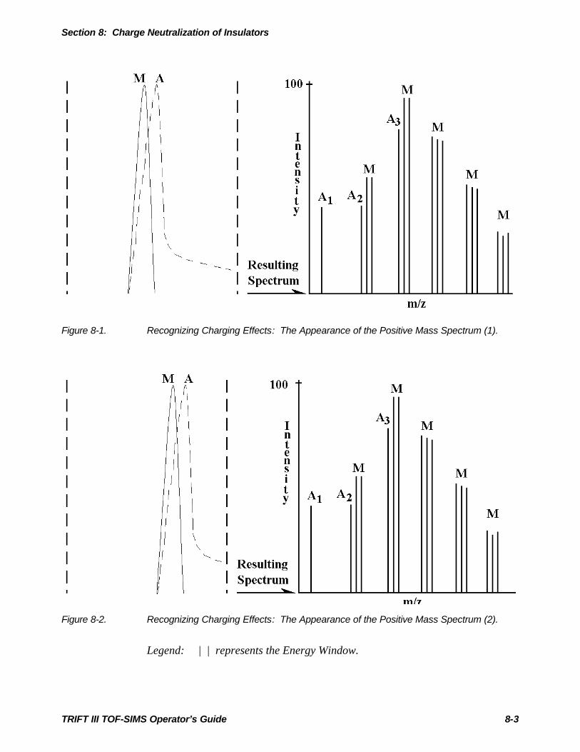
Section 8: Charge Neutralization of Insulators
TRIFT III TOF-SIMS Operator’s Guide 8-3
Figure 8-1. Recognizing Charging Effects: The Appearance of the Positive Mass Spectrum (1).
Figure 8-2. Recognizing Charging Effects: The Appearance of the Positive Mass Spectrum (2).
Legend: | | represents the Energy Window.
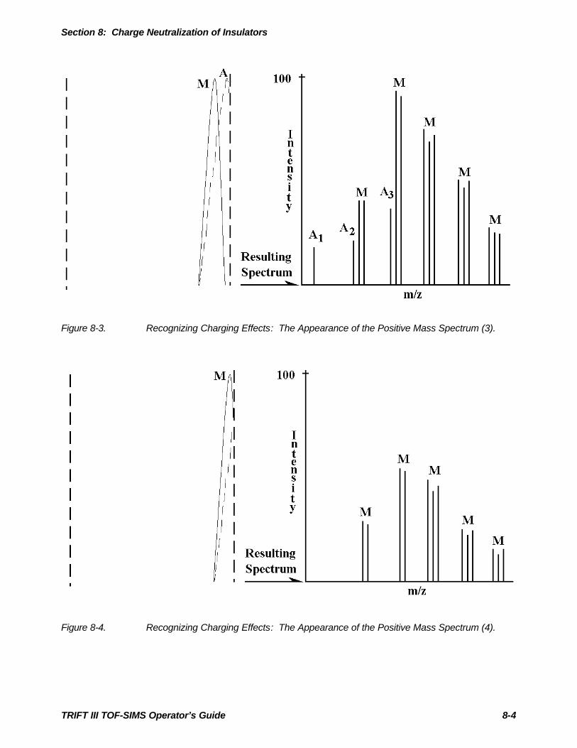
Section 8: Charge Neutralization of Insulators
TRIFT III TOF-SIMS Operator’s Guide 8-4
Figure 8-3. Recognizing Charging Effects: The Appearance of the Positive Mass Spectrum (3).
Figure 8-4. Recognizing Charging Effects: The Appearance of the Positive Mass Spectrum (4).

Section 8: Charge Neutralization of Insulators
TRIFT III TOF-SIMS Operator’s Guide 8-5
Negative SIMS
Refer to the Figures 8-5 through 8-8. Note the following:
1. Correct neutralization: This results in the kinetic energy distributions of allsecondary ions being positioned correctly within the spectrometer energy'window'. The resulting mass spectrum displays intensities of atomic andmolecular species that accurately represents the ratio of emission of thesespecies from the sample surface.
2. Beginnings of positive charge build-up: Now the kinetic energy distributionsof the secondary ions are shifted to a lower value (a positive charge build upon a negative surface potential results in a less negative surface potential).This results in a 'trimming' of the low energy ions, and consequently themolecular ions first of all. The resulting mass spectrum appears to have areduced yield of molecular species.
3. Continued positive charge build-up. The kinetic energy distributions areshifted further to lower potentials. Since the maximum of the distribution formolecular species occurs at lower values, the 'trimming' of low energyspecies can result in a mass spectrum which appears to contain only atomicspecies.
4. Severe positive charge build-up. As the kinetic energy distributions areshifted out of the spectrometer energy 'window', the total secondary ion countrate falls slowly with potential changes, owing to the high energy tail of theatomic species. A mass spectrum acquired just before this occurs would havelow signal intensities, and would be heavily biased towards atomic species.
In the absence of an electron beam, these effects will always be observed withinsulators, at rates that are determined by the dielectric properties of thematerials. It is instructive to turn off the electron gun and take a series of massspectra, sequentially, as this charging process occurs, so that a 'feel' can bedeveloped for the effects of charging, as manifested in a mass spectrum.
These effects are reproduced more controllably by taking TOF-SIMS spectrafrom a conducting sample, altering the sample voltage to simulate the effects ofcharging on the emission energies of the secondary ions (increase the samplevoltage progressively for positive SIMS, and decrease it progressively fornegative SIMS).
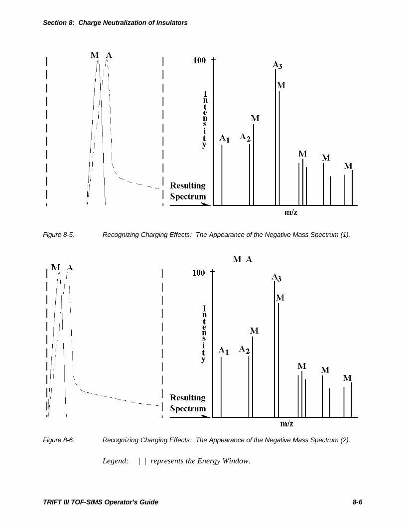
Section 8: Charge Neutralization of Insulators
TRIFT III TOF-SIMS Operator’s Guide 8-6
Figure 8-5. Recognizing Charging Effects: The Appearance of the Negative Mass Spectrum (1).
Figure 8-6. Recognizing Charging Effects: The Appearance of the Negative Mass Spectrum (2).
Legend: | | represents the Energy Window.
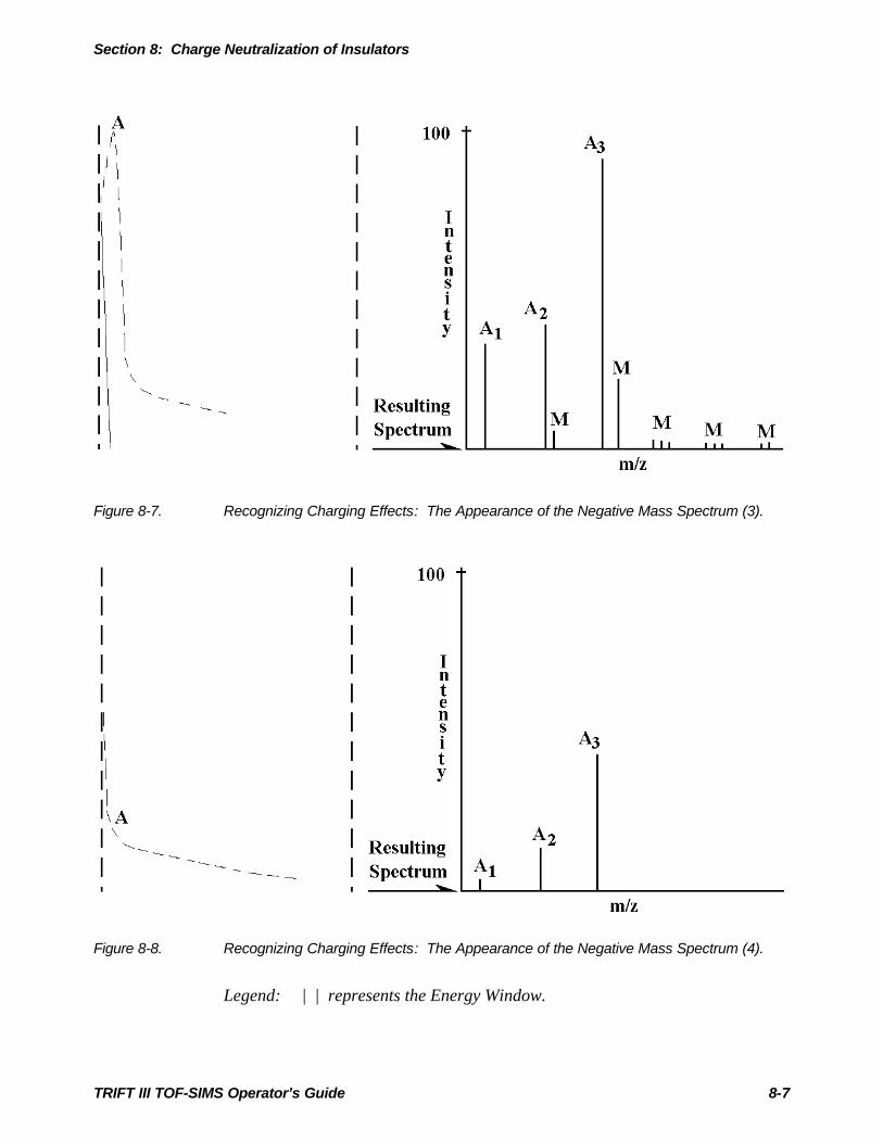
Section 8: Charge Neutralization of Insulators
TRIFT III TOF-SIMS Operator’s Guide 8-7
Figure 8-7. Recognizing Charging Effects: The Appearance of the Negative Mass Spectrum (3).
Figure 8-8. Recognizing Charging Effects: The Appearance of the Negative Mass Spectrum (4).
Legend: | | represents the Energy Window.

Section 8: Charge Neutralization of Insulators
TRIFT III TOF-SIMS Operator’s Guide 8-8
Extraction Field Penetration: Techniques for Obtaining DataIt is possible to have correct electron neutralization and yet still obtain poorresults from large area, thick insulators, because the extraction field is too low inthe area under analysis. This is due to variable field penetration at the insulatorsurface.
One simple technique which can be used to overcome this effect is to increasethe sample potential to a level where, in the area under analysis, the extractionfield attains the correct value of 3,000 V (or whatever). Secondary ions areemitted with energies that are 'matched' to the spectrometer energy 'window'.Adjusting the sample potential for maximum secondary ion yield displayed onthe rate meter is the normal method.
One drawback with this method, however, is that the required setting of thesample potential tends to be area-specific, i.e., moving to another area on thesample, will typically result in the need to re-tune the sample potential. This isbecause the field penetration can vary significantly from one area to another.
Use of Metallic GridsAn alternative method for obtaining even field penetration across the samplesurface is the use of conducting grids. A grid prevents large variations in theextraction field over a large area insulator. This means that increasing thesample potential is virtually never necessary, since the correct extraction field isobtained all over the sample surface. It is possible, therefore, to move from onegrid 'window' to any of the other 'windows' without re-tuning.
It is important to note that placing a grid or mesh over an insulating sample hasnothing to do with electron charge neutralization. The grid merely 'pins' theextraction field on the sample surface and allows the user to use the defaultvoltage settings. If using a grid, but without an electron beam, the sample will(eventually) charge up and resulting in the inability to acquire data. If anelectron beam is present but without a grid, it is still possible to obtain good,neutralized data, provided the sample potential is varied to the optimum valueevery time.
The grids provided with the instrument have a thickness of 125 microns, and arefabricated from a non-magnetic stainless steel. The grids are designed to berigid, and it is possible to re-use them many times, provided reasonable care isexercised.

Section 8: Charge Neutralization of Insulators
TRIFT III TOF-SIMS Operator’s Guide 8-9
When mounting a sample with a grid, simply lay the grid inside the invertedsample holder and then place the sample surface to be analyzed against the grid.When inserting the backing plate and Cu-Be sample clip, use the minimumcompressive force to hold the sample in place to prevent deformation of the grid.If the grid mesh does not lie flat on the sample surface, but is raised up off thesurface, this will cause the sample to be shielded from the field, leading to ionextraction problems. Refer to the portion of Section 9 entitled "DifficultGeometry Samples".
Practical Guide to Insulating SamplesNOTE: When performing analysis on insulating materials, the goal is to passsecondary ions with an optimum energy into the mass spectrometer.
Two simple principles need to be discussed when analyzing insulators: a) themass spectrometer energy 'window'; and b) field penetration of insulatingmaterials. Once these principles are understood, insulator analysis can beapproached much more rationally and viewed much less as a 'black art'.
First, consider the analysis of a 'standard' conductor to introduce the idea of themass spectrometer acceptance window.
1. Why SIMS signals expected without performing a tuning when aconducting sample is loaded and optimized.
One of the procedures carried out during instrument checkout is to tune the massspectrometer for optimum performance. This requires laser-assisted alignment ofthe spectrometer housing to the analytical chamber, as well as setting the correctvalues of the various ion optical elements: the immersion lens; the transfer lens;the ESA's and the Matsuda plates. Once set correctly, the TRIFT massspectrometer can almost be regarded as a 'black box': in other words, noadjustment to any parameters on a regular basis is necessary, nor is anyonerequired to understand how it functions to be able to acquire good data.
The mass spectrometer, when 'fully open' (i.e., no energy filter) has an energyacceptance window of ±120 eV. This indicates that an ion with ±120 eV aboutthe optimum value will be passed around the spectrometer to the detector. Thecloser the ions energies to that optimum value, the better the energy and timefocusing of the spectrometer, resulting in optimum mass resolution. Conversely,as the secondary ions' mean energies approach the outer limits of this energywindow, the energy focusing is not as efficient, and the mass resolution degrades.
An "optimum" value has been mentioned twice, but what is this value? It’sbasically the energy that an ion must have for it to travel down the centerline ofthe mass spectrometer. The mass spectrometer has been set to pass ions with amean energy of -3000 eV around the centerline. Provided that secondary ionsenter the spectrometer with this mean energy, they are transported and optimally

Section 8: Charge Neutralization of Insulators
TRIFT III TOF-SIMS Operator’s Guide 8-10
energy focused at the detector. They acquire such energy by traveling through theextraction (acceleration) space.
The following analogy may help to reinforce what is happening within thesystem. Imagine yourself at the top of a steep slope sitting on a 4-wheel sled.The sled has no pedals or engines to propel you, no steering wheel, and no brakes!An accomplice positions you to the very brink of the slope and gently tips youover its edge. The sled begins to accelerate, and velocity increases until you reachthe end of the slope. The sled begins to glide with a uniform velocity. Aftersome distance, a building with a doorway leading to the inside of a chamber isencountered. The chamber walls are not vertical, but slope so that the top of thechamber is more open than the bottom, like an inverted cone. If your kineticenergy is correct, the sled stays on a centerline of the chamber wall and passesaround 270 degrees to a conveniently located exit door which exits out to safety.If your kinetic energy is severely mismatched to the chamber dimensions, youwill either fall to the bottom of the inverted cone, or be spun out at the top. Ifyour kinetic energy is close to but not at the optimum value, you may escape fromthe chamber provided that the exit door is wide enough. If the chamberdimensions are not to be changed, the height of the initial slope must be adjustedinstead to make sure that you pass safely around the centerline and out throughthe exit door.
The kinetic energy of the secondary ions is determined primarily by the samplepotential (equivalent to the height of the slope in our analogy). On a conductingsample, the default instrument settings apply a sample potential that correctlymatches the secondary ion kinetic energies to the optimum acceptance energy ofthe mass spectrometer. No additional tuning is required for a conductor becausethe sample surface potential is the same as the applied potential. Secondary ionscreated at the sample surface are launched at a potential which results in kineticenergies that are matched to the mass spectrometer.
The method for determining this correct potential for a conductor is described inthe mass spectrometer section within this manual.
2. What happens when thin, insulating samples are loaded?
(a) Let us suppose that we now load a sample which consists of a 2 µm thickpolymer film on a metal substrate. The film's dielectric properties are suchthat it is an insulator, and thus we need to invoke the TRIFT's electroncharge compensation system to balance the incoming positive charges fromthe primary ion beam.
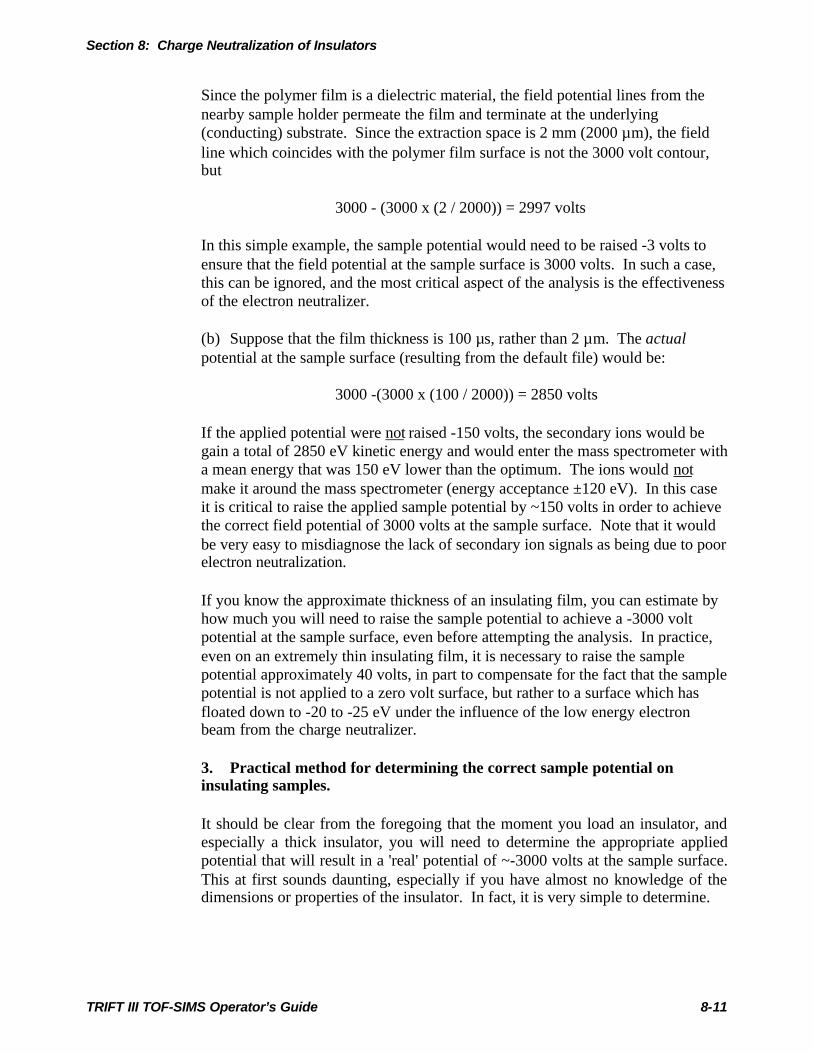
Section 8: Charge Neutralization of Insulators
TRIFT III TOF-SIMS Operator’s Guide 8-11
Since the polymer film is a dielectric material, the field potential lines from thenearby sample holder permeate the film and terminate at the underlying(conducting) substrate. Since the extraction space is 2 mm (2000 µm), the fieldline which coincides with the polymer film surface is not the 3000 volt contour,but
3000 - (3000 x (2 / 2000)) = 2997 volts
In this simple example, the sample potential would need to be raised -3 volts toensure that the field potential at the sample surface is 3000 volts. In such a case,this can be ignored, and the most critical aspect of the analysis is the effectivenessof the electron neutralizer.
(b) Suppose that the film thickness is 100 µs, rather than 2 µm. The actualpotential at the sample surface (resulting from the default file) would be:
3000 -(3000 x (100 / 2000)) = 2850 volts
If the applied potential were not raised -150 volts, the secondary ions would begain a total of 2850 eV kinetic energy and would enter the mass spectrometer witha mean energy that was 150 eV lower than the optimum. The ions would notmake it around the mass spectrometer (energy acceptance ±120 eV). In this caseit is critical to raise the applied sample potential by ~150 volts in order to achievethe correct field potential of 3000 volts at the sample surface. Note that it wouldbe very easy to misdiagnose the lack of secondary ion signals as being due to poorelectron neutralization.
If you know the approximate thickness of an insulating film, you can estimate byhow much you will need to raise the sample potential to achieve a -3000 voltpotential at the sample surface, even before attempting the analysis. In practice,even on an extremely thin insulating film, it is necessary to raise the samplepotential approximately 40 volts, in part to compensate for the fact that the samplepotential is not applied to a zero volt surface, but rather to a surface which hasfloated down to -20 to -25 eV under the influence of the low energy electronbeam from the charge neutralizer.
3. Practical method for determining the correct sample potential oninsulating samples.
It should be clear from the foregoing that the moment you load an insulator, andespecially a thick insulator, you will need to determine the appropriate appliedpotential that will result in a 'real' potential of ~-3000 volts at the sample surface.This at first sounds daunting, especially if you have almost no knowledge of thedimensions or properties of the insulator. In fact, it is very simple to determine.

Section 8: Charge Neutralization of Insulators
TRIFT III TOF-SIMS Operator’s Guide 8-12
Make sure that the electron charge compensation is on (filament on and 'on' in thesoftware), and then begin an analysis, preferably over a large area (~400 µm). Ifno secondary signals are detected, begin raising the sample potential until somecounts are detected. Raise the sample potential until you appear to have passedthrough a-maximum in the count rate, and note that count rate. Now lower thesample potential until the count rate falls off to ~10 to 20% of its maximum value.Note down this sample potential. Now begin raising the sample potential onceagain, go through the maximum count rate, and then note the sample potential onthe high side at which the secondary count rate again falls to ~10 to 20% of themaximum value. The difference in the two sample potentials should be ~240 eV,mapping the energy 'window' of the mass spectrometer. If you set the samplepotential half way between these two values, i.e. ~120 volts up from the lowpotential, you should have a good approximation of the correct applied potentialrequired to match secondary ions to the center of the mass spectrometers energywindow. For optimum performance, you may need to vary the sample potentialby 10 volts either side of this value to determine if the mass resolution can beoptimized further.
Enthusiastic students can perform this experiment on a simple, metallicconductor and see the mapping of the energy 'window' under ideal conditions.Naturally, the correct setting should be at the default potential, but theexperiment is instructive because on the low side of the correct setting youshould observe that the counts fall off more slowly than on the high side. This isdue to the shape of the kinetic energy distribution for atomic species. As youlower the applied potential, the kinetic energy distribution of the secondaries aresliding to the low energy side of the spectrometers energy window. Eventually,only atomic tails appear in the spectrometer energy window, and a massspectrum acquired at this point would be dominated by atomic species.
Conversely, on the high side of the correct applied sample potential, you areeffectively sliding the kinetic energy distribution to the high energy side of thespectrometer's energy window. The count rate remains high (although theenergies are no longer correctly ideally matched to the spectrometer), until overthe course of a few volts the main peaks of the kinetic energy distributions forboth atomic and molecular ions disappear completely from the spectrometer'senergy window. At this point the secondary ion count rate falls dramatically. Amass spectrum acquired just before this occurs may even be dominated bymolecular species, since it is possible to push the peak of atomic energydistributions out of the energy window and yet still keep the molecular ionswithin the energy window (just). The correlation of the observed mass spectrumand the position of the kinetic energy distributions within the mass spectrometer'senergy window are shown in the schematics which are used to demonstrate whathappens when the neutralizer is not functioning correctly and the sample beginsto charge up.

Section 8: Charge Neutralization of Insulators
TRIFT III TOF-SIMS Operator’s Guide 8-13
4. Practical procedure for analysis in 'worst case' scenario: a thickinsulator-mounted at the wrong height.
Having considered points 1, 2, and 3 above, we can now go on to consider aworst case' scenario in which a thick insulator is mounted at the incorrect height.In this case there are now three aspects to consider: a) correct neutralization(taken for granted for the moment); b) finding the correct applied potential; andfinally, c) the steering of the primary beam to the spectrometer acceptance area.Raising the sample potential alone may not have the desired result of finding thesecondary ion beam if the primary beam is not illuminating the acceptance area.If you can estimate the insulator thickness, raise the potential accordingly andthen sweep the x beam position to try to find the secondary beam. If you cannotestimate the change in sample potential, it will be necessary to raise the samplepotential in ~100 volt increments, and then sweep the x beam position at eachsample potential until you find the beam.
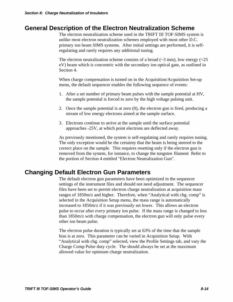
Section 8: Charge Neutralization of Insulators
TRIFT III TOF-SIMS Operator’s Guide 8-14
General Description of the Electron Neutralization SchemeThe electron neutralization scheme used in the TRIFT III TOF-SIMS system isunlike most electron neutralization schemes employed with most other D.C.primary ion beam SIMS systems. After initial settings are performed, it is self-regulating and rarely requires any additional tuning.
The electron neutralization scheme consists of a broad (~3 mm), low energy (<25eV) beam which is concentric with the secondary ion optical gate, as outlined inSection 4.
When charge compensation is turned on in the Acquisition/Acquisition Set-upmenu, the default sequencer enables the following sequence of events:
1. After a set number of primary beam pulses with the sample potential at HV,the sample potential is forced to zero by the high voltage pulsing unit.
2. Once the sample potential is at zero (0), the electron gun is fired, producing astream of low energy electrons aimed at the sample surface.
3. Electrons continue to arrive at the sample until the surface potentialapproaches -25V, at which point electrons are deflected away.
As previously mentioned, the system is self-regulating and rarely requires tuning.The only exception would be the certainty that the beam is being steered to thecorrect place on the sample. This requires resetting only if the electron gun isremoved from the system, for instance, to change the tungsten filament Refer tothe portion of Section 4 entitled "Electron Neutralization Gun".
Changing Default Electron Gun ParametersThe default electron gun parameters have been optimized in the sequencersettings of the instrument files and should not need adjustment. The sequencerfiles have been set to permit electron charge neutralization at acquisition massranges of 1850m/z and higher. Therefore, when “Analytical with chg. comp” isselected in the Acquisition Setup menu, the mass range is automaticallyincreased to 1850m/z if it was previously set lower. This allows an electronpulse to occur after every primary ion pulse. If the mass range is changed to lessthan 1850m/z with charge compensation, the electron gun will only pulse everyother ion beam pulse.
The electron pulse duration is typically set at 63% of the time that the samplebias is at zero. This parameter can be varied in Acquisition Setup. With“Analytical with chg. comp” selected, view the Profile Settings tab, and vary theCharge Comp Pulse duty cycle. The should always be set at the maximumallowed value for optimum charge neutralization.

Section 8: Charge Neutralization of Insulators
TRIFT III TOF-SIMS Operator’s Guide 8-15
Techniques for Optimum Charge DissipationWhen using a standard 'linescan' raster with a focused LMIG probe on a 'high'insulator, it is sometimes possible to see the effect of surface potential changeson the secondary ion image displayed on the DMCP. It may appear that thelinescan width increases and that the line of displayed secondary ions becomesmore diffuse as the frame sweep progresses. This is probably due to changingsurface potentials as the sweep progresses across the insulating surface.
The software is capable of rastering the primary beam in a ‘scatter’ raster toaddress each pixel point such that the next beam pulse is as far away from theprevious one within the analyzed area. Although this raster is referred to as a'scatter raster', it is not truly random in nature, since the separation between eachpixel point is constant, and the sequence of pixel points follows a well-definedgeometrical pattern.
Using this raster, the charge resulting from each frame of acquisition isdistributed evenly across the analyzed area, facilitating charge neutralization.This raster should be used as the default mode for analysis when the chargecompensation is used. A variety of raster modes are available and can be set asdefaults under different analytical conditions in the "hardware" section of thesoftware. For further details, refer to the portion of Section 7 entitled “SIMSImages”.
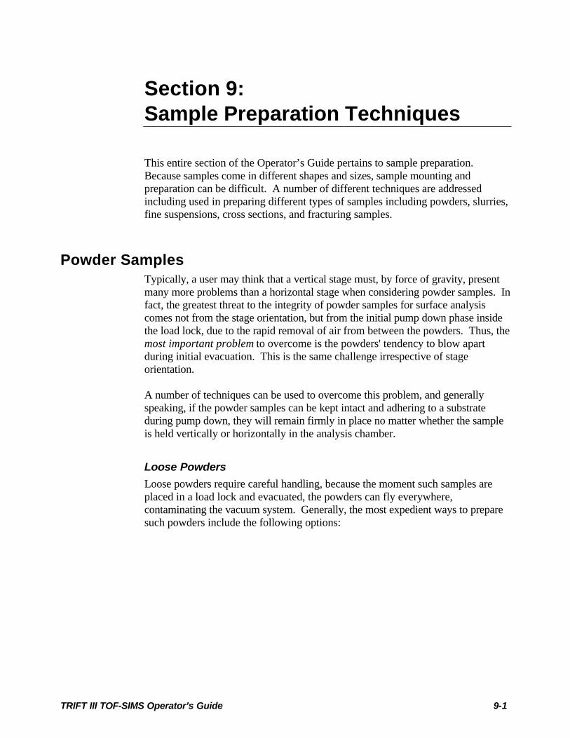
TRIFT III TOF-SIMS Operator’s Guide 9-1
Section 9:Sample Preparation Techniques
This entire section of the Operator’s Guide pertains to sample preparation.Because samples come in different shapes and sizes, sample mounting andpreparation can be difficult. A number of different techniques are addressedincluding used in preparing different types of samples including powders, slurries,fine suspensions, cross sections, and fracturing samples.
Powder SamplesTypically, a user may think that a vertical stage must, by force of gravity, presentmany more problems than a horizontal stage when considering powder samples. Infact, the greatest threat to the integrity of powder samples for surface analysiscomes not from the stage orientation, but from the initial pump down phase insidethe load lock, due to the rapid removal of air from between the powders. Thus, themost important problem to overcome is the powders' tendency to blow apartduring initial evacuation. This is the same challenge irrespective of stageorientation.
A number of techniques can be used to overcome this problem, and generallyspeaking, if the powder samples can be kept intact and adhering to a substrateduring pump down, they will remain firmly in place no matter whether the sampleis held vertically or horizontally in the analysis chamber.
Loose PowdersLoose powders require careful handling, because the moment such samples areplaced in a load lock and evacuated, the powders can fly everywhere,contaminating the vacuum system. Generally, the most expedient ways to preparesuch powders include the following options:
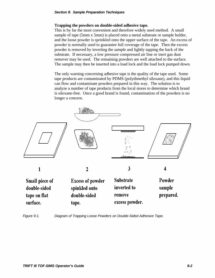
Section 9: Sample Preparation Techniques
TRIFT III TOF-SIMS Operator’s Guide 9-2
Trapping the powders on double-sided adhesive tape.This is by far the most convenient and therefore widely used method. A smallsample of tape (5mm x 5mm) is placed onto a metal substrate or sample holder,and the loose powder is sprinkled onto the upper surface of the tape. An excess ofpowder is normally used to guarantee full coverage of the tape. Then the excesspowder is removed by inverting the sample and lightly tapping the back of thesubstrate. If necessary, a low pressure compressed air line or inert gas dustremover may be used. The remaining powders are well attached to the surface.The sample may then be inserted into a load lock and the load lock pumped down.
The only warning concerning adhesive tape is the quality of the tape used. Sometape products are contaminated by PDMS (polydimethyl siloxane), and this liquidcan flow and contaminate powders prepared in this way. The solution is toanalyze a number of tape products from the local stores to determine which brandis siloxane-free. Once a good brand is found, contamination of the powders is nolonger a concern.
Figure 9-1. Diagram of Trapping Loose Powders on Double-Sided Adhesive Tape.
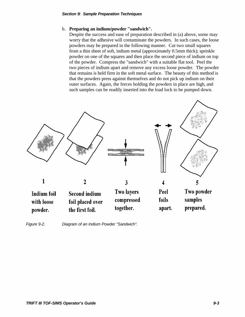
Section 9: Sample Preparation Techniques
TRIFT III TOF-SIMS Operator’s Guide 9-3
b. Preparing an indium/powder "sandwich".Despite the success and ease of preparation described in (a) above, some mayworry that the adhesive will contaminate the powders. In such cases, the loosepowders may be prepared in the following manner. Cut two small squaresfrom a thin sheet of soft, indium metal (approximately 0.5mm thick); sprinklepowder on one of the squares and then place the second piece of indium on topof the powder. Compress the "sandwich" with a suitable flat tool. Peel thetwo pieces of indium apart and remove any excess loose powder. The powderthat remains is held firm in the soft metal surface. The beauty of this method isthat the powders press against themselves and do not pick up indium on theirouter surfaces. Again, the forces holding the powders in place are high, andsuch samples can be readily inserted into the load lock to be pumped down.
Figure 9-2. Diagram of an Indium Powder "Sandwich".
Section 9: Sample Preparation Techniques
TRIFT III TOF-SIMS Operator’s Guide 9-4
c. Preparation of dry powder compacts.In this method, a suitable die and press is used to form a pellet from the drypowder. The compacting of powders is due only to mechanical keying of thematerial to itself, yet the bond is quite strong. The pellet is then fractured toreveal a fresh powder surface which has never been in contact with the diematerials. The user can load the pellet into the load lock and rest assured thatit will not fracture apart into the powder material it.
Figure 9-3. Diagram of Dry Powder Compacts.
(d) Settling from fine suspensions.
Sometimes analysis must be carried out on powders where it was important tohave a very low surface coverage of the powder, so that individual particles canbe studied. In such cases, and where a suitable inert liquid can be identified, it isvery easy to simply pipette a droplet of a suspension onto a suitable substrate(such as a carbon planchet). Powders prepared by this method are remarkablytenacious (i.e., great adhesion to a surface), but powders exhibiting poor adhesionmay be removed by inverting the planchet and tapping the backside. Note that thismethod is not good when the powders become large, namely ~>100um, becausethe bond to the substrate is not as strong as in the above methods. Adhesion can beimproved by lightly abrading the substrate beforehand with an abrasive which hasa similar dimension to the particles under investigation, greatly improving the“mechanical keying” of the particles to the substrate.
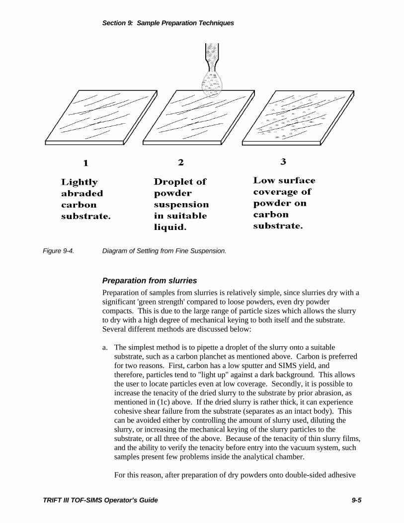
Section 9: Sample Preparation Techniques
TRIFT III TOF-SIMS Operator’s Guide 9-5
Figure 9-4. Diagram of Settling from Fine Suspension.
Preparation from slurriesPreparation of samples from slurries is relatively simple, since slurries dry with asignificant 'green strength' compared to loose powders, even dry powdercompacts. This is due to the large range of particle sizes which allows the slurryto dry with a high degree of mechanical keying to both itself and the substrate.Several different methods are discussed below:
a. The simplest method is to pipette a droplet of the slurry onto a suitablesubstrate, such as a carbon planchet as mentioned above. Carbon is preferredfor two reasons. First, carbon has a low sputter and SIMS yield, andtherefore, particles tend to "light up" against a dark background. This allowsthe user to locate particles even at low coverage. Secondly, it is possible toincrease the tenacity of the dried slurry to the substrate by prior abrasion, asmentioned in (1c) above. If the dried slurry is rather thick, it can experiencecohesive shear failure from the substrate (separates as an intact body). Thiscan be avoided either by controlling the amount of slurry used, diluting theslurry, or increasing the mechanical keying of the slurry particles to thesubstrate, or all three of the above. Because of the tenacity of thin slurry films,and the ability to verify the tenacity before entry into the vacuum system, suchsamples present few problems inside the analytical chamber.
For this reason, after preparation of dry powders onto double-sided adhesive

Section 9: Sample Preparation Techniques
TRIFT III TOF-SIMS Operator’s Guide 9-6
tape, this is the second most convenient way to prepare powder samples foranalysis, provided of course, that it is legitimate to use a liquid for suspensionpurposes.
b. Alternatively, the separation of the dried slurry from the substrate can beexploited by removing the dried layer and placing it onto double-sidedadhesive tape as outlined in (1a). This ensures that the dried layer is heldfirmly in place for subsequent analysis.
c. Slurries may also be allowed to dry in suitable molds to produce thick pelletsor cakes which may be fractured to produce fresh surfaces, and then used asdescribed in (1c) above.
Figure 9-5. Diagram of Preparation from Slurries.

Section 9: Sample Preparation Techniques
TRIFT III TOF-SIMS Operator’s Guide 9-7
Preparation and Mounting of Cross-Section SamplesAlthough TOF-SIMS is unique in its surface analytical capabilities, there are oftentimes when the elemental sensitivity and organic detection capability of TOF-SIMS is invaluable in the analysis of sample cross-sections. In a sense, a cross-section analysis represents the deepest possible SIMS depth profile, providinginformation extending several hundred micrometers into a sample. Whenconsidering analysis of a cross-section, the most critical aspect is the cleanlinessof the preparation. Standards of cleanliness that are acceptable for the preparationof conventional SEM cross-sections are not acceptable for TOF-SIMS. Thefollowing methods of preparation are recommended:
a. Preparation of cross-sectionsMechanically polished cross-sections. It is possible to follow conventionalmetallographic polishing techniques, provided tap water is NOT used as alubricant for the coarse carbide wheels. Use a supply of de-ionized ordistilled water instead. When it is time to move on to fine diamond polishing,do not use oil-based diamond pastes, since the organic component of the pastewill badly contaminate the sample. Instead, use diamond impregnated polymerfilms, and use a distilled water or distilled water-methanol mixture forlubrication. As a final, ultra-fine finish, use a γ-alumina (typically 0.05µm)and distilled water mix on a cloth wheel, or a 0.05µm diameter silicasuspension such as “syton”, also on a cloth wheel. In the latter case, use afinal, liberal distilled water rinse to remove the potassium hydroxide solutionthat is a part of the syton suspension (to prevent aggregation of the silicaparticles). A final ultrasonic clean in methanol or distilled water is thenessential to remove any fine polishing particles. This method workssurprisingly well if strictly using either distilled water and high puritymethanol. This method has even been used successfully to prepare flatpolymer cross-sections.
b. Microtomed and cryo-microtomed cross-section samplesMicrotoming is only useful for relatively soft samples such as polymers. Theblades and sample holder must be cleaned thoroughly beforehand, beginningwith a distilled water wash to remove alkali metals, and also a hexane wash toremove the ubiquitous siloxanes. There are two approaches to preparingsamples for TOF-SIMS by microtoming: one is to make a conventional thinslice from the sample; the other is to remove a thin slice (which is thrownaway) to reveal a fresh face on the sample cross-section (“facing off” thesample).
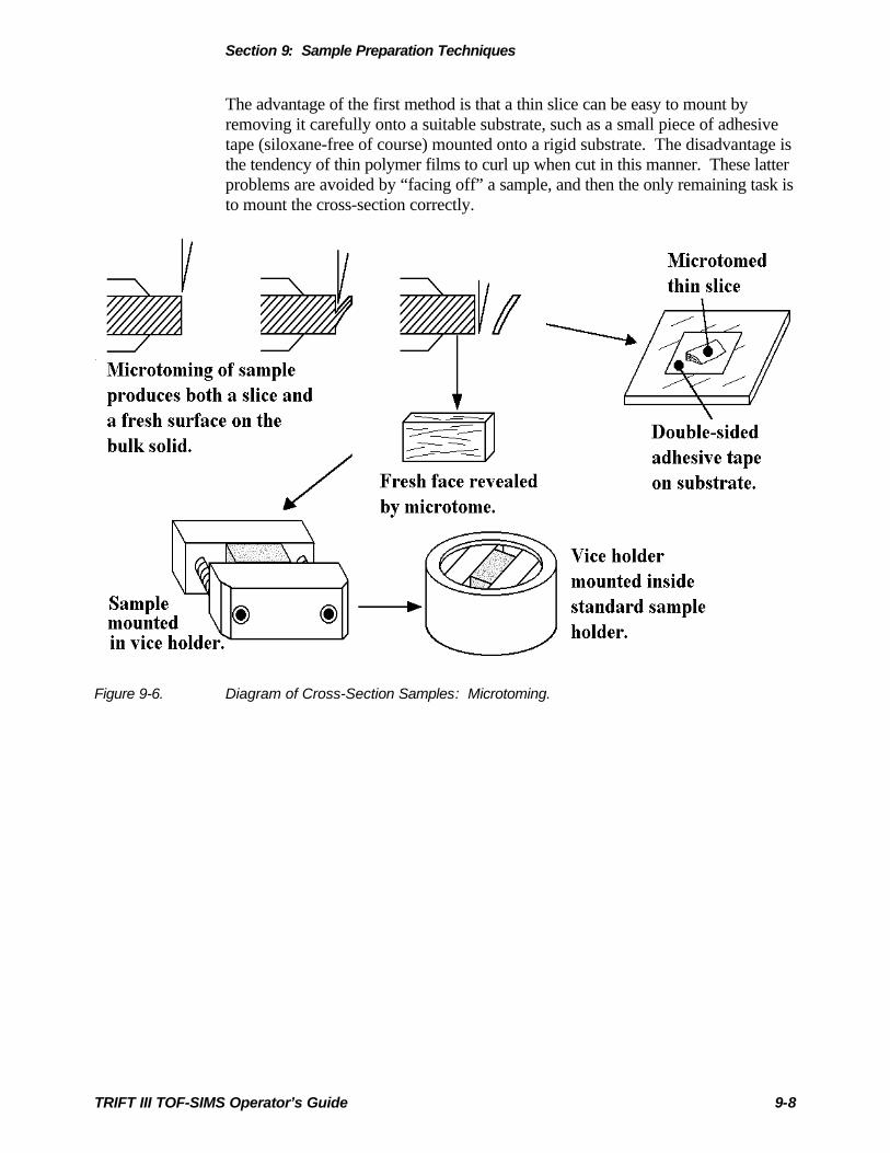
Section 9: Sample Preparation Techniques
TRIFT III TOF-SIMS Operator’s Guide 9-8
The advantage of the first method is that a thin slice can be easy to mount byremoving it carefully onto a suitable substrate, such as a small piece of adhesivetape (siloxane-free of course) mounted onto a rigid substrate. The disadvantage isthe tendency of thin polymer films to curl up when cut in this manner. These latterproblems are avoided by “facing off” a sample, and then the only remaining task isto mount the cross-section correctly.
Figure 9-6. Diagram of Cross-Section Samples: Microtoming.
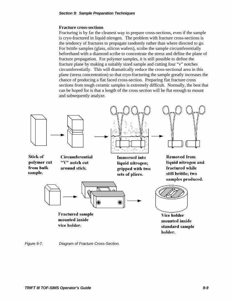
Section 9: Sample Preparation Techniques
TRIFT III TOF-SIMS Operator’s Guide 9-9
Fracture cross-sectionsFracturing is by far the cleanest way to prepare cross-sections, even if the sampleis cryo-fractured in liquid nitrogen. The problem with fracture cross-sections isthe tendency of fractures to propagate randomly rather than where directed to go.For brittle samples (glass, silicon wafers), scribe the sample circumferentiallybeforehand with a diamond scribe to concentrate the stress and define the plane offracture propagation. For polymer samples, it is still possible to define thefracture plane by making a suitably sized sample and cutting four “v” notchescircumferentially. This will dramatically reduce the cross-sectional area in thisplane (stress concentration) so that cryo-fracturing the sample greatly increases thechance of producing a flat faced cross-section. Preparing flat fracture crosssections from tough ceramic samples is extremely difficult. Normally, the best thatcan be hoped for is that a length of the cross section will be flat enough to mountand subsequently analyze.
Figure 9-7. Diagram of Fracture Cross-Section.

Section 9: Sample Preparation Techniques
TRIFT III TOF-SIMS Operator’s Guide 9-10
Mounting of cross-sectioned samplesA simple cross-section sample holder, which fits as an insert into the circular“standard” 25mm sample holders, is provided as part of the sample holder kit.This sample holder restricts the user to samples which have a width that will fit inbetween the two compression screws (~8mm), and has a maximum thickness of~4mm.
When mounting the prepared cross-section, remember that an important aspect ofmounting is to keep the cross-sectioned sample face at the same height (or veryslightly low) as the vice holder. This is particularly important if the cross sectionis very thin, because the metal of the vice can be used to align the primary beam tothe correct height before going to search for an area of interest on the cross-section. When the sample has been fixed in place in the vice holder, invert andlower the holder into the circular “standard” sample holder. If the sample isslightly higher that the vice surface, take care to raise the sample (quadrant) carrieroff the mounting bench, otherwise, the clean and carefully prepared sample surfacemay accidentally be contaminated. Finally, try to align the length of the crosssection with the horizontal axis of the system. If the sample is mounted slightlylow, shadowing effects of the vice holder are avoided by doing so.
Analysis of Fiber Samples
NOTE: A critical reminder to perform the analysis of SHORT,CONDUCTINGFIBERS such as fine carbon fibers with great care. Any fibers which are fineand conducting can leave the sample surface and migrate into the system wherethey can create shorts between high voltage components and ground if notproperly secured to the sample holder. To avoid this problem, use one of themethods outlined below for mounting THESE fibers.
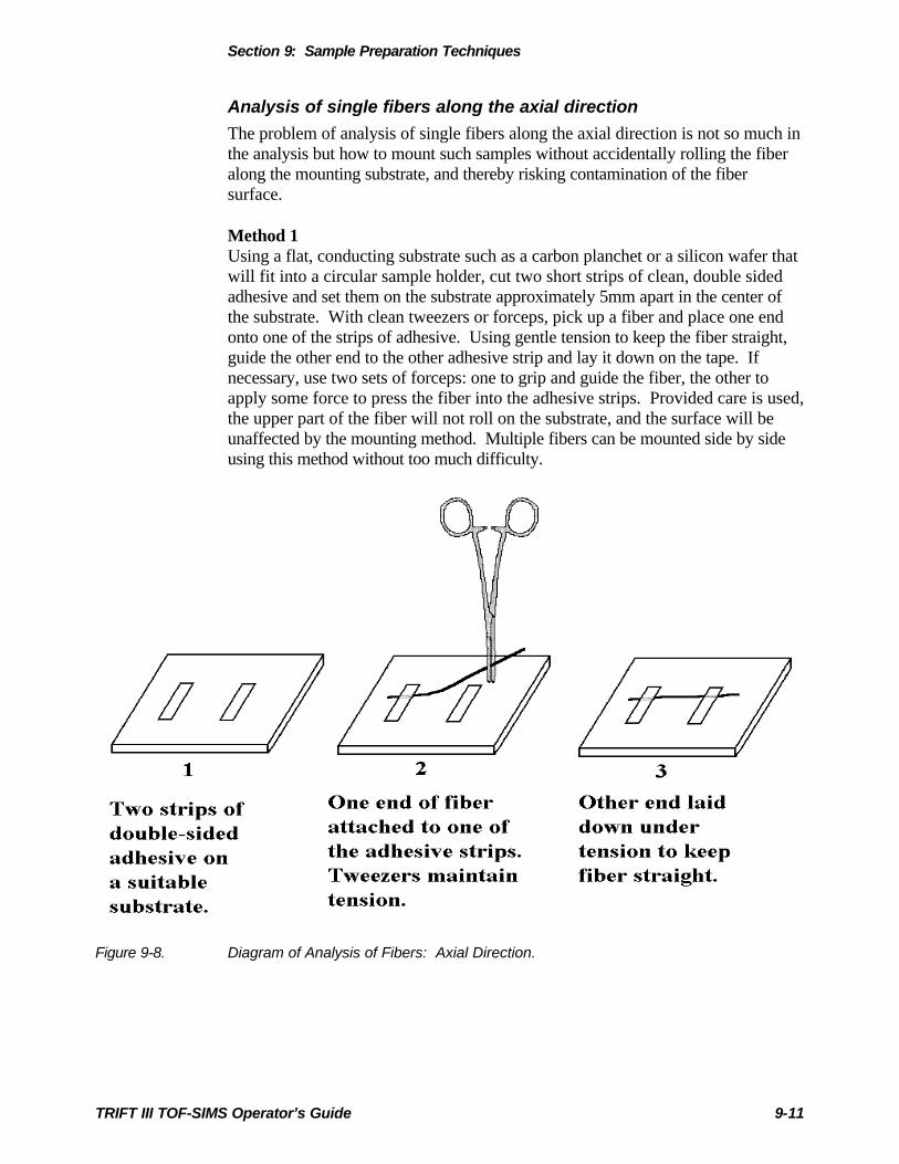
Section 9: Sample Preparation Techniques
TRIFT III TOF-SIMS Operator’s Guide 9-11
Analysis of single fibers along the axial directionThe problem of analysis of single fibers along the axial direction is not so much inthe analysis but how to mount such samples without accidentally rolling the fiberalong the mounting substrate, and thereby risking contamination of the fibersurface.
Method 1Using a flat, conducting substrate such as a carbon planchet or a silicon wafer thatwill fit into a circular sample holder, cut two short strips of clean, double sidedadhesive and set them on the substrate approximately 5mm apart in the center ofthe substrate. With clean tweezers or forceps, pick up a fiber and place one endonto one of the strips of adhesive. Using gentle tension to keep the fiber straight,guide the other end to the other adhesive strip and lay it down on the tape. Ifnecessary, use two sets of forceps: one to grip and guide the fiber, the other toapply some force to press the fiber into the adhesive strips. Provided care is used,the upper part of the fiber will not roll on the substrate, and the surface will beunaffected by the mounting method. Multiple fibers can be mounted side by sideusing this method without too much difficulty.
Figure 9-8. Diagram of Analysis of Fibers: Axial Direction.
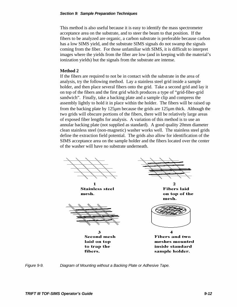
Section 9: Sample Preparation Techniques
TRIFT III TOF-SIMS Operator’s Guide 9-12
This method is also useful because it is easy to identify the mass spectrometeracceptance area on the substrate, and to steer the beam to that position. If thefibers to be analyzed are organic, a carbon substrate is preferable because carbonhas a low SIMS yield, and the substrate SIMS signals do not swamp the signalscoming from the fiber. For those unfamiliar with SIMS, it is difficult to interpretimages where the yields from the fiber are low (and in keeping with the material’sionization yields) but the signals from the substrate are intense.
Method 2If the fibers are required to not be in contact with the substrate in the area ofanalysis, try the following method. Lay a stainless steel grid inside a sampleholder, and then place several fibers onto the grid. Take a second grid and lay iton top of the fibers and the first grid which produces a type of “grid-fiber-gridsandwich”. Finally, take a backing plate and a sample clip and compress theassembly lightly to hold it in place within the holder. The fibers will be raised upfrom the backing plate by 125µm because the grids are 125µm thick. Although thetwo grids will obscure portions of the fibers, there will be relatively large areasof exposed fiber lengths for analysis. A variation of this method is to use anannular backing plate (not supplied as standard). A good quality 20mm diameterclean stainless steel (non-magnetic) washer works well. The stainless steel gridsdefine the extraction field potential. The grids also allow for identification of theSIMS acceptance area on the sample holder and the fibers located over the centerof the washer will have no substrate underneath.
Figure 9-9. Diagram of Mounting without a Backing Plate or Adhesive Tape.

Section 9: Sample Preparation Techniques
TRIFT III TOF-SIMS Operator’s Guide 9-13
Analysis of fiber matsThe mat to be analyzed should first be cut to size and then placed on a stainlesssteel grid within an inverted sample holder. Using a metal backing plate andsample clip, lightly compress the matte so that it is held firmly against the grid. Itis strongly advised to use compressed air (or an inert gas at raised pressure) toremove any loose fibers in the mat prior to loading the sample holder into the loadlock. If the mat to be analyzed has a very low density and is very loose, andespecially if the fibers are conducting, the mat should be pressed into double-sided adhesive tape and then all loose fibers removed using a compressed air line.
Figure 9-10. Diagram of Mounting Fiber Mats.
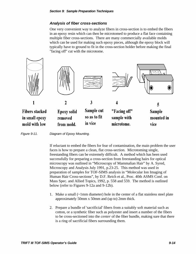
Section 9: Sample Preparation Techniques
TRIFT III TOF-SIMS Operator’s Guide 9-14
Analysis of fiber cross-sectionsOne very convenient way to analyze fibers in cross-section is to embed the fibersin an epoxy resin which can then be microtomed to produce a flat face containingmultiple fiber cross-sections. There are many commercially available moldswhich can be used for making such epoxy pieces, although the epoxy block willtypically have to ground to fit in the cross-section holder before making the final"facing off" cut with the microtome.
Figure 9-11. Diagram of Epoxy Mounting.
If reluctant to embed the fibers for fear of contamination, the main problem the userfaces is how to prepare a clean, flat cross-section. Microtoming single,freestanding fibers can be extremely difficult. A method which has been usedsuccessfully for preparing a cross-section from freestanding hairs for opticalmicroscopy was outlined in “Microscopy of Mammalian Hair” by A. Syred,Microscopy and Analysis July 1991, p.23-25. This method was used inpreparation of samples for TOF-SIMS analysis in “Molecular Ion Imaging ofHuman Hair Cross-sections”, by D.F. Reich et al., Proc. 40th ASMS Conf. onMass Spec. and Allied Topics, 1992, p. 558 and 559. The method is outlinedbelow (refer to Figures 9-12a and 9-12b).
1. Make a small (~1mm diameter) hole in the center of a flat stainless steel plateapproximately 50mm x 50mm and (up to) 2mm thick.
2. Prepare a bundle of 'sacrificial' fibers from a suitably soft material such ascotton, or a synthetic fiber such as polyester and insert a number of the fibersto be cross-sectioned into the center of the fiber bundle, making sure that thereis a ring of sacrificial fibers surrounding them.

Section 9: Sample Preparation Techniques
TRIFT III TOF-SIMS Operator’s Guide 9-15
3. Draw the bundle through the hole in the metal plate, adding additional fibers tomake sure that the bundle fits tightly through the plate. Mount the plate in avice and arrange a collection dish under the vice.
4. Using a new, one-sided, razor blade, carefully sweep the blade at as low anangle as possible across the plate and through the bundle in the center of theplate. As the blade strikes the outer part of the bundle, more force must beapplied to begin cutting the fibers. By the time the blade reaches the bundlecenter, it should be near a constant velocity, and should cut the center fiberssmoothly. Keep both sides of the fiber cuts. This will double the chances offinding a suitable face for analysis.
5. Take the fibers to an optical microscope and inspect the cross-sections for theflattest, least deformed cuts. Note that most razor blades are supplied with alight coating of oil, and blades should be de-greased thoroughly before using it.
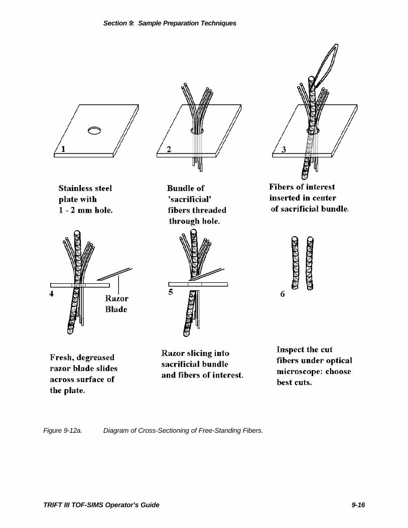
Section 9: Sample Preparation Techniques
TRIFT III TOF-SIMS Operator’s Guide 9-16
Figure 9-12a. Diagram of Cross-Sectioning of Free-Standing Fibers.
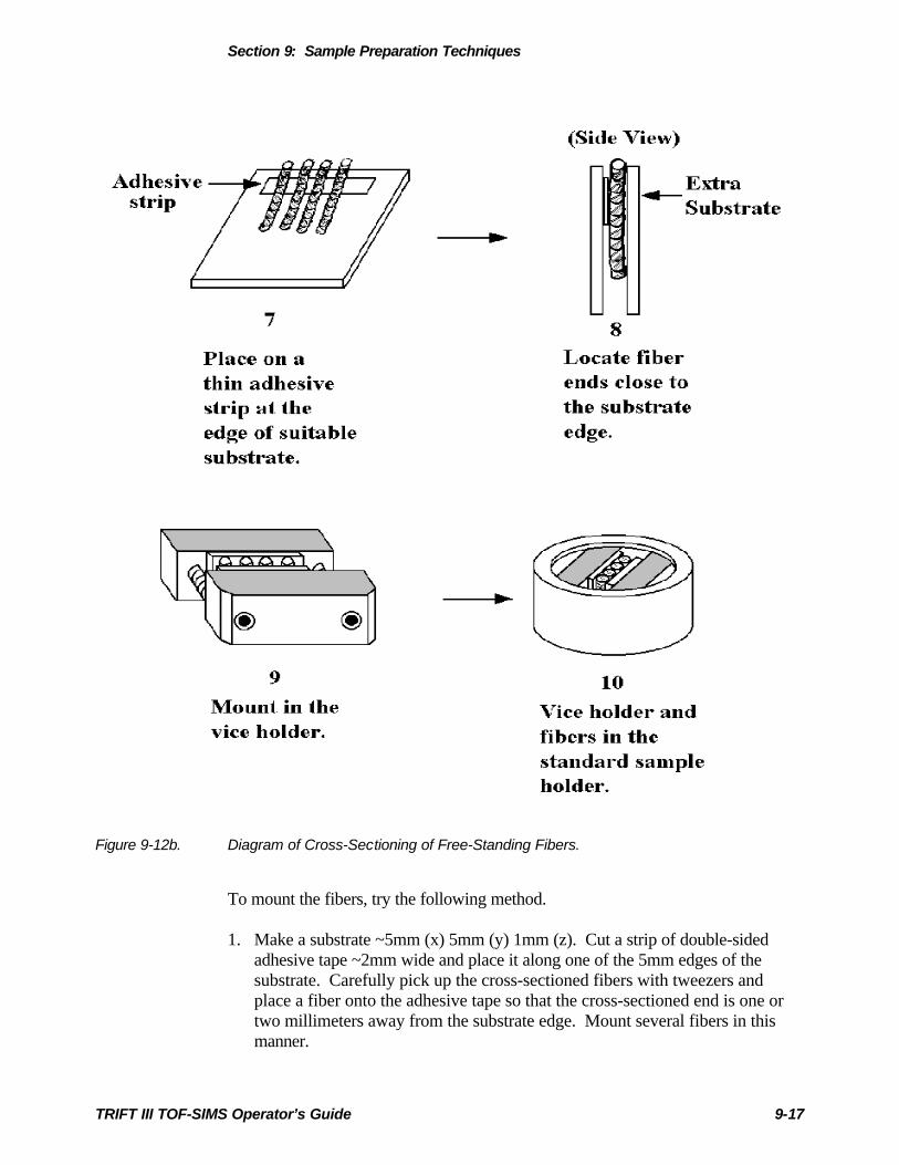
Section 9: Sample Preparation Techniques
TRIFT III TOF-SIMS Operator’s Guide 9-17
Figure 9-12b. Diagram of Cross-Sectioning of Free-Standing Fibers.
To mount the fibers, try the following method.
1. Make a substrate ~5mm (x) 5mm (y) 1mm (z). Cut a strip of double-sidedadhesive tape ~2mm wide and place it along one of the 5mm edges of thesubstrate. Carefully pick up the cross-sectioned fibers with tweezers andplace a fiber onto the adhesive tape so that the cross-sectioned end is one ortwo millimeters away from the substrate edge. Mount several fibers in thismanner.

Section 9: Sample Preparation Techniques
TRIFT III TOF-SIMS Operator’s Guide 9-18
2. Mount the assembly within the standard cross-section holder so that the fiberends are approximately level, or very slightly below, the faces of the cross-section holder.
3. Once within the analysis chamber, use the faces of the cross-section holder tocenter the analyzing beam to the spectrometer axis, and then search for thefibers in the optical image. By placing the fiber ends at or near the same heightas the cross-section holder, locating the fiber ends in the SIMS image shouldnot be difficult. Tests have shown that elaborately-designed holders whichgrip a single fiber and present it at the correct sample height offered littleimprovement on the simple method outlined here.
Rough Samples
IntroductionTime-of-Flight SIMS systems require high extraction fields in order to providesubsequent high mass resolution performance. Variations in the sample toextraction distance result in varying total times-of-flight. Take the case of arecessed sample: a secondary ion ejected from a recessed sample spends moretime in the (now greater) extraction region. It seems that such small changesshould have a minimum effect on the total flight times until one considers that theinitial velocities of the secondary ions are very low, and it is only at the end of theextraction (acceleration) space that they acquire their full velocity. Therefore,small changes in the extraction space distance have a disproportionate effect on thetotal flight times. These shifts are normally detected in practice by the need toadjust the calibration of the mass spectra slightly as one moves from sample tosample. In such cases, and following re-calibration, the mass resolution ispreserved, because every peak in the mass spectrum is shifted by a predictableamount, and can be corrected by the simple act of re-calibration.
Recovery of Mass Resolution from Rough SurfacesFor rough samples however, the time shifts can occur within a sample and within asingle field of view, and the resulting mass spectrum will have broader masspeaks. Since this broadening is due to the summation of mass signals from areas atdifferent heights, it is possible to recover the mass resolution by taking data fromspecific areas within a field of view which are approximately at the same height.This can either be done during a live acquisition, or later in retrospective analysismode.

Section 9: Sample Preparation Techniques
TRIFT III TOF-SIMS Operator’s Guide 9-19
Consider the following simple case. The user is analyzing an area which containsa step (refer to Figure 9-13 below). The left half of the field of view is higher thanthe right half. In such a case, there are only two discrete heights, and the total massspectrum may show peaks which are doublets (“peak splitting”), depending uponthe step height. Using an image in which the step boundary is observable, define a"region of interest" on one side of the step, and proceed to take data from that areawhich is at one height. The peaks in the mass spectrum will now not show peaksplitting, and the mass resolution of the peaks will be as normal.
Figure 9-13. The Effect of Topography on Mass Spectra.

Section 9: Sample Preparation Techniques
TRIFT III TOF-SIMS Operator’s Guide 9-20
Now consider a more complex example, the use of fiber mats (refer to Figure 9-14below). The peaks in the mass spectrum are all broadened, but now, because thesurface heights are changing continuously, there is no obvious peak splitting towarn the user that topographic effects are responsible for the broadening. Sincethere are no discrete heights, it is not obvious how to proceed, unlike the previousexample of the stepped sample. The best that can be done is to acquire data fromareas in the image which appear to have the least variations in height; for instancethe tops of the fibers, as opposed to the sides. The narrower the band from whichmass spectral data is acquired, the better the resulting mass resolution.
Figure 9-14. Sample Geometry for a Woven Fiber Mat with Continuously Variable Heights.
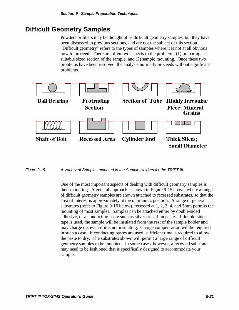
Section 9: Sample Preparation Techniques
TRIFT III TOF-SIMS Operator’s Guide 9-21
Difficult Geometry SamplesPowders or fibers may be thought of as difficult geometry samples, but they havebeen discussed in previous sections, and are not the subject of this section."Difficult geometry" refers to the types of samples where it is not at all obvioushow to proceed. There are often two aspects to the problem: (1) preparing asuitable sized section of the sample, and (2) sample mounting. Once these twoproblems have been resolved, the analysis normally proceeds without significantproblems.
Figure 9-15. A Variety of Samples mounted in the Sample Holders for the TRIFT III.
One of the most important aspects of dealing with difficult geometry samples istheir mounting. A general approach is shown in Figure 9-15 above, where a rangeof difficult geometry samples are shown attached to recessed substrates, so that thearea of interest is approximately at the optimum z position. A range of generalsubstrates (refer to Figure 9-16 below), recessed at 1, 2, 3, 4, and 5mm permits themounting of most samples. Samples can be attached either by double-sidedadhesive, or a conducting paste such as silver or carbon paste. If double-sidedtape is used, the sample will be insulated from the rest of the sample holder andmay charge up, even if it is not insulating. Charge compensation will be requiredin such a case. If conducting pastes are used, sufficient time is required to allowthe paste to dry. The substrates shown will permit a large range of difficultgeometry samples to be mounted. In some cases, however, a recessed substratemay need to be fashioned that is specifically designed to accommodate yoursample.

Section 9: Sample Preparation Techniques
TRIFT III TOF-SIMS Operator’s Guide 9-22
Figure 9-16. Cross Section View of the Various Sample Holders for the TRIFT III.
Having shown the general mounting procedure, consider the requirement toprepare a sample which can be mounted as described above. For most cases, thepreparation is simple; in other cases, more preparation is required. The followinglist of sample types is by no means exhaustive, but should provide a number ofideas as to how to analyze a sample with a specific geometry.
Figure 9-17. Cross Section View of the Various Sample Holders for the TRIFT III.

Section 9: Sample Preparation Techniques
TRIFT III TOF-SIMS Operator’s Guide 9-23
1. Small Diameter (≤5mm), Thick (≥ 1mm) SamplesWhen a sample has a small diameter or width, mounting the sample in a smallhole sample holder may not be possible. Even if the diameter is large enoughto back-mount inside a standard sample holder, perhaps too much of theprecious surface will be obscured in doing so. In such cases, it is best toadopt the approach outlined above, using a recessed substrate.
2. Non-Planar Geological SamplesAlthough many geological samples are prepared as cross-sections, sometimesanalysis is required of mineral grain surfaces. Fine mineral grains may betreated as described in Section 9 on Powders, but as these samples growlarger, consider mounting them on recessed substrates instead. Use theattachment methods suggested in Section 9, but select a recessed substrate thatwill best accommodate the coarser grain sizes.
3. SpheresMost powders are spherical, but as the size increases much past a few hundredmicrons, it may be better to attach larger spheres to recessed substrates. Anobvious extreme case would be ball bearings, where the diameter of the ballwould dictate the choice of recessed substrate.
4. Protruding Pieces on Otherwise Planar SamplesWhen the area to be analyzed is protruding from the rest of the sample bynearly a millimeter or more, it is better to recess the rest of the sample so thatthe area of analysis is close to the optimum z position. Choose a recessedsubstrate that best matches the height of the feature to be analyzed.
5. Recessed Areas on Otherwise Planar SamplesWhen the area to be analyzed is recessed with respect to the surroundingsample, and the area is not large enough to prepare a sample from that area,use a recessed substrate and raise the surrounding sample higher than theoptimum z to bring the recessed area to the correct height. The maximumheight the rest of the sample should protrude is approximately 1.5mm,otherwise risk is involved in striking the extraction plate and damaging thesample as it is inserted into the sample chamber.

Section 9: Sample Preparation Techniques
TRIFT III TOF-SIMS Operator’s Guide 9-24
6. Analysis on the inner surfaces of tubesFirst, a section of the tube must be prepared. For tubes with large innerdiameters, this is no problem, but more care must be taken as the tube’s i.d.(inner diameter) becomes smaller. Aim for a final sample where the distancefrom the inner (concave) face to the highest part of the cut sample is less than2mm (refer to Figure 9-18).
If the tube is metallic, cut the section with a saw. On some samples, it may notmatter if debris from the cutting process touches the area to be analyzed. If thatis the case, cut with a fresh, degreased saw (no cutting fluids, of course), andtry to cut slowly, to keep the sample from becoming hot due to the cuttingprocess. Organic detection may be crucial, and the goal is to not remove theall-important organic in the act of preparation.
After cutting has been completed, remove all debris from the sample by using acompressed air jet. If the cutting debris cannot touch the area of analysis,proceed as follows: cut a strip of fresh Al foil (or some other clean materialthat is siloxane-free) that is larger than the area of analysis. Slide the stripinside the tube, and use adhesive tape to stick all four of the sides of theprotective strip down to the inside of the tube. Leave 2-3mm of sticky tapetouching the tube. Cut through the tube so that the saw blade cuts through thesticky tape, leaving a small strip sealing the protective layer to the tube (referto Figure 9-18).
Once the section has been cut out from the tube, blow away the cutting debrisas mentioned above. Remove the sticky tape and the protective layer, knowingthat the surface to be analyzed has been protected during the preparationprocess. This procedure is equally useful when preparing debris-free sectionsfrom flat samples.

Section 9: Sample Preparation Techniques
TRIFT III TOF-SIMS Operator’s Guide 9-25
Figure 9-18. Illustrations of the Process of Sample Preparation from a Metallic Tube.

Section 9: Sample Preparation Techniques
TRIFT III TOF-SIMS Operator’s Guide 9-26
If the tube to be analyzed is a glass, produce pieces for analysis by the inelegant(but effective) method of crushing the tube in a vice while insuring that a cleancollection tray catches the fractured pieces. Select a suitable sized sample fromamong the pieces. Remember to wear protective glasses and to degrease thecontact surfaces of the vice beforehand to reduce the chance of contaminating theoutside of the tube with unwanted organic material.
If the tube to be analyzed is a tough ceramic, fracture pieces can still be prepared,but a grinding wheel may be necessary to grind cuts into the tube that will confinethe fracture to a particular place and to reduce the amount of forces required tofracture the tube. This is a good way to ensure that a sample can be prepared froma glass sample in a specific area, for instance, when the sample must be taken froma very specific area, such as one containing a defect of interest. (Refer to Figure9-19 below).
Figure 9-19. Illustrations of the Process of Sample Preparation from a Metallic Tube.

Section 9: Sample Preparation Techniques
TRIFT III TOF-SIMS Operator’s Guide 9-27
Sample MountingFor mounting the sample, refer to Figure 9-15. The objective is to locate thesurface of interest at approximately the optimum height for analysis by a simplemounting method.
Be careful to make sure that the sample does not protrude more than ~1.5mm,otherwise the sample will strike the extraction plate as the sample is loaded intothe sample chamber. If the sample is insulating, it does not matter if the tubeprotrudes a little further, as long as it does not exceed 2 mm. The extraction fieldspermeate the insulator, and so it has little effect on the field shape. If the tube ismetallic, it is highly advisable to reduce the amount of the tube that is protruding toa minimum (<1mm), to reduce the distortion of the extraction field, and also tominimize the chance of an arc between the sample and the extraction plate.
Cold Stage Option [For 50mm (2-Inch) Introduction Systems]Many liquids and solids, which are stable at room temperature and pressure, arerapidly pumped away under UHV conditions. In order to analyze such materials, itis necessary to introduce and maintain them at temperatures where theirequilibrium vapor pressures are less than the vacuum inside the chamber. A largenumber of organic compounds, which would normally pump away at roomtemperature, may be stabilized at modest temperatures of -50ºC and lower invacuo. To this end, a cold stage option is available for the TRIFT system.
The cold stage option is comprised of the following components:
1. A customized, gold-coated copper sample holder and carrier;
2. A cold transfer vessel and dewar to allow the sample to be cooled using liquidnitrogen and then transferred into the load lock without being exposed to air;
3. A digital thermocouple probe to monitor the sample carrier temperature duringinitial cooling at atmospheric pressure;
4. A special sample stage which allows delivery of liquid nitrogen to the stage tocool the sample while it is inside the analysis chamber; and
5. A cold stage control unit which controls the rate of delivery of liquid nitrogen;monitors the sample temperature, and permits active heating of the stage tobring it back to room temperature.

Section 9: Sample Preparation Techniques
TRIFT III TOF-SIMS Operator’s Guide 9-28
Operation of the 50mm Cold Stage1. Fill the stage cryo dewar (large stainless steel cylindrical) with liquid nitrogen
and fit the dewar onto the bottom of the collar or “gooseneck” assembly whichprotrudes from the front of the stage. The plastic tube hanging from thegooseneck should go down into the liquid nitrogen (refer to Figure 9-20below). The flask should make a gas-tight seal with the base of the gooseneck.Gently tighten the four screws together finger tight for even compressionaround the collar. Use an Allen wrench to tighten the screws.
Figure 9-20. Cutaway Diagram of the Cold Stage Dewar and “Gooseneck” Assembly.

Section 9: Sample Preparation Techniques
TRIFT III TOF-SIMS Operator’s Guide 9-29
2. Connect all relevant pipes and leads to the stage if they are not already inplace. Thermocouple connectors will allow for monitoring the sampletemperature in-situ, and the heater leads will allow for accelerated warming ofthe stage once analysis has been finished. The small band heater fitted to thegooseneck will prevent ice from forming around it. The nylon gas pipe fromthe cold stage controller should be fitted onto the 0.25 inch o.d. stainless tubingwhich emerges from the gooseneck.
3. The Dewar, the gooseneck, the pipes inside the gooseneck, and the controllerall comprise a sealed system when assembled correctly. A pump inside thecontroller creates a partial vacuum inside the assembly. Liquid nitrogen (LN2)is drawn up from the Dewar and travels down a pipe inside the gooseneck toemerge on the atmosphere side of the stage, just behind where the sample ismounted. The copper-based sample carrier is in good thermal contact with thestage, and heat is conducted away from the sample through the solid wall of thevacuum chamber into the liquid nitrogen. The liquid nitrogen then passes backdown towards the front of the stage, where it boils and is pumped away as agas by the controller pump. Liquid nitrogen should not be seen appearing pastthe emergent stainless pipe on the gooseneck. The unit has been designed sothat the nitrogen will be a gas at this point. Allow the stage to cool wellbefore introducing a sample. This is particularly important if imaging at highmagnification is desired. If the stage is not thermally stable, drift in the initialion images will be observed.
Take precautions against frostbite and liquid nitrogen burns when using LN2.Insulated gloves and goggles should be worn when pouring LN2 from anyinsulated Dewar.
4. Mount the sample to be analyzed in the sample holder.
5. Next, place the L-shaped thermal mass plate so that the short part of the plate isresting on the top of the carrier, and the long part is in front of the samplecarrier.
6. Insert the long sample carrier handle into the top of the transfer vessel throughthe rubber seal. Open the guillotine at the base of the sample transfer vessel,position the sample carrier and thermal mass plate so that the sample carrierhandle can be screwed into the top of the sample carrier, holding the thermalmass plate loosely in place. Pull the sample carrier upwards with the carrierhandle so that the guillotine may be closed.
7. Slide open the guillotine on the sample transfer vessel Dewar and fill it withliquid nitrogen. Slide the guillotine shut until ready for sample cooling.

Section 9: Sample Preparation Techniques
TRIFT III TOF-SIMS Operator’s Guide 9-30
8. Place the sample transfer vessel on top of the sample transfer vessel Dewar,and open both guillotines so that cool nitrogen gas can begin to purge the airfrom the transfer vessel. Allow approximately 5 minutes for full purging.
9. Lower the sample carrier into the liquid nitrogen using the carrier handle, butdo not allow the sample itself to contact the liquid nitrogen. It is sufficient toimmerse only the lower cut away section of the sample carrier into the liquidnitrogen. Heat will be conducted away from the main body of the carrier.
10. Raise the sample carrier periodically back up into the transfer vessel, andinsert the probe from the digital thermocouple probe through the rubber seal atthe back of the transfer vessel. Make contact between the probe and thesample carrier and monitor the temperature. When the sample carrier hasreached approximately -70C, raise the carrier into the transfer vessel and slidethe transfer vessel guillotine shut.
11. Remove the transfer vessel from the Dewar beneath, and place it on top of thesample introduction chamber.
12. Vent the introduction chamber. Slide both the intro chamber guillotine and thetransfer vessel guillotine open. Carefully lower the sample carrier and thermalmass plate so that the thermal mass plate locates on the two pins providedinside the intro chamber. This takes some practice, and may appear to be verydifficult at first. The best approach is to practice this maneuver with an emptycarrier at room temperature. This will help when the time comes to work witha cold sample carrier.
13. When the thermal mass plate is in position, bring the horizontal sampleintroduction rod forward and engage the thread on the end of the sample introrod with the screw thread on the side of the sample carrier. Rotate the sampleintro rod at least three turns (but do not tighten fully). Unscrew the samplecarrier handle from the sample carrier and withdraw upwards into (but not outof) the transfer vessel. Close the intro chamber guillotine and begin pumpingthe intro chamber.

Section 9: Sample Preparation Techniques
TRIFT III TOF-SIMS Operator’s Guide 9-31
14. Inside the intro chamber the sample carrier is not actively cooled, but the massof the carrier plus the thermal mass plate have been designed to maintain thetemperature of the sample for the initial pump down period. Also, sincewarming of the sample carrier occurs mainly by conduction, and since thecarrier is only in contact with the intro rod, the rate of warming is also slowedby being in vacuo. Realistically however, do not allow the sample to remainin the introduction chamber for more than approximately 15 minutes. Once theintroduction turbo pump has reached full speed, allow a further 3-5 minutes ofpumping before opening the intro gate valve to observe if the pressure isacceptable for sample introduction.
15. Once the sample is inside the chamber, the sample and carrier temperature canbe regulated by adjusting the amount of gas flow through the flow controller(determining the rate at which liquid nitrogen is drawn up to keep the samplecool).
16. If initial analysis indicates that the sample surface is covered with ice(characteristic clusters 18 mass units apart), wait a little while for the ice tosublime. Try to exclude this moist air during the next sample preparation.
17. When analysis is complete, remove the sample carrier as normal. Once thesample and carrier are exposed to lab air, they will inevitably ice up quickly.Use a hair dryer to warm the carrier and dry it if further analysis will beperformed at low temperatures.
18. If the sample stage must be warmed up to room temperature as quickly aspossible, a heater is provided inside the stage to allow for this. Turn theheater on at the controller.
TRIFT III TOF-SIMS Operator’s Guide 10-1
Section 10:Routine System Evaluation \Maintenance (Non-Service Issues)
IntroductionThere are a few procedures which the system operator should follow as a matterof good laboratory practice if the TRIFT III system is to be maintained inoptimum condition while possessing full knowledge of that instrument condition.
The following procedures are suggested.
System BakeoutThe following procedure describes baking the TRIFT system. A system bake istypically performed only when:• necessary to remove contaminants within the vacuum chamber(s); or• after the system has been up-to-air for servicing.
A system bakeout should result in returning the level within the chamber(s) toultra-high vacuum. If the system's vacuum level is lower than 5 x 10⁻¹⁰ Torr,system bakeout is not necessary.
The TRIFT III system is essentially "bake-ready" which means there is minimalintervention to set up for a system bake. There are no requirements to removecables or electronics of any type from the system prior to the bakeout sequence.
Bakeout Prerequisites
Several system conditions must be met prior to starting a bake:
• vacuum levels must be greater than 5 x 10⁻⁶ Torr (as displayed on theVacuum Gauge Control labeled MAIN CHAMBER ION GAUGE);
• the introduction rod must be fully retracted; and
• the Introduction Gate Valve (V1) must be in the closed position.

Section 10: Routine Instrument Evaluation / Maintenance
TRIFT III TOF-SIMS Operator’s Guide 10-2
Bakeout Preparations
1. Remove any wafer or samples from the vacuum chamber.
WARNING: Some samples when heated produce highly toxic vapors thatcould contaminate the interior of the chamber and the optics. Remove anywafer/sample from the vacuum chamber before baking.
2. Using a clean cloth and a cleaner such as isopropyl alcohol, remove anyfinger prints or oils on all stainless steel portions of the TRIFT system,especially the spectrometer and analytical chambers.
ATTENTION: Any oils on surfaces subjected to bakeout temperatures canpit and stain the stainless steel. Oils will turn a brown color and willremain after bake.
3. Within the WinCadence software on the system computer, load a zero.insfile. This instrument file will load all zero values into critical voltageparameters to insure all portions of the system are in an idled state (no highvoltage potential applied.)
4. Exit the WinCadence software.
5. On the Electronics Console, press the ELECTRONICS POWER button onceto turn it OFF. In the OFF position, the ELECTRONICS POWER button isnot illuminated and it will stay OFF throughout the bake.
6. On the vacuum console, insure that no cables are resting against any of theexternal heater bands including the main turbo heater.
7. On the System Vacuum Control located in the Electronics Console, theBAKE INTERLOCK key switch must be turned to the ON position.
ATTENTION: Cover the end of the three (3) analytical chamber viewports with aluminum foil prior to starting the bakeout on the analyticalchamber. The internal quartz heater lamps produce an intense light andalso heat the view port glass.

Section 10: Routine Instrument Evaluation / Maintenance
TRIFT III TOF-SIMS Operator’s Guide 10-3
8. Place the large yellow bakeout warning sign on the vacuum console or in aclearly visible location on the vacuum console or on the top of the electronicsconsole.
WARNING: All metal surfaces exposed to bakeout temperatures will bevery hot. To prevent injury, allow sufficient cooling time before attemptingto touch any portion of the vacuum console.
Starting the Bake
When the hardware has been set up for bake, the bake is enabled and started.
REMINDER: Insure that the BAKE INTERLOCK key located on the front panelof the System Vacuum Control is turned to the ON position.
1. The Watcher software is used to start and control the bakeout. All bakeoutentries should be made within the Watcher software from this point on.
2. The Bakeout Timer Control is located within the Watcher software on thesystem computer. Watcher must be in the SERVICE MODE in order toaccess the bakeout settings and to initiate the bake sequence.
3. Insure that the spectrometer gate valve (V5) is in the closed position. This isthe gate valve attached to the transfer coupler located between thespectrometer chamber and the analytical chamber.
4. Within Watcher, insure that the CD (Contrast Diaphragm ) is in the 2mm(Large) position.
5. Remove the Cesium source housing and close the cesium ampoule vavle onthe cesium ion gun, if applicable. Open the cesium isolation valve on the iongun, if applicable.
NOTE: For TRIFT systems with a 200mm (8-inch) sample stage, install the bandheater on the stage bellows assembly prior to starting the bake.
6. With the Watcher user interface open, select the Options pull down. SelectService Mode. When prompted to Enter Password: type in phiphi. This willchange the Watcher software from the User Mode to the Service Mode.
7. Under the "Valve Control and Overrides" section, Sample, HV: change fromEnabled to Disabled.
8. Under the Vacuum Tasks section, select Bakeout.

Section 10: Routine Instrument Evaluation / Maintenance
TRIFT III TOF-SIMS Operator’s Guide 10-4
9. Under the Comments section, select the Execute Tasks button. A TaskMessage window entitled Enter Time will appear which prompts the user toset the length of time for the bakeout in hour and minutes.
10. Enter the desired amount of time for the bakeout by setting the Watcherbakeout timer for number of Hours, Minutes, and Seconds. Then choose theOK button.
11. Watcher will prompt the user with another Task Message:"Install and connect the Bake warning sign".
12. Plug the two-pin connector and cable into the BAKEOUT INTERLOCKconnection on the utility panel located on the back of the vacuum console.Place the large yellow bake warning sign in a conspicuous place - either onthe vacuum console table top or on top of the electronics console.
WARNING: Insure that the non-bakeable interlock cable does not touchthe vacuum chambers or any other area being baked on the system.
Figure 10-1. Installation of the Bakeout Warning Sign is required prior to starting the bake.
13. Once the warning sign is plugged in, click the OK button within Watcher.Watcher will then prompt the user with the following Task Message:"What bakeout zones?"
14. There are three options to select from: Sample, Spectrometer, Both. Selectthe button that represents the portion of the TRIFT system that requiresbaking.
-If Sample is selected, the analytical chamber and heat clamps associatedwith that portion of the system will be baked,
-If Spectrometer is selected, only the quartz heater lamps within thespectrometer chamber and the external heat clamp on the detector flange willbe used for baking that portion of the system;

Section 10: Routine Instrument Evaluation / Maintenance
TRIFT III TOF-SIMS Operator’s Guide 10-5
-If Both is selected, the entire vacuum system will be baked including thespectrometer chamber(internal quartz lamp), analytical chamber (internalquartz heater lamp), and all external heater clamps (ion guns, turbo pump,transfer coupler, and sample stage).
NOTE: A GFI circuit breaker fuse trip error message will occur if the BakeInterlock key switch is not set to the ON position prior to starting thebakeout.
NOTE: Bakeout power is interlocked to the MAIN CHAMBER ION GAUGEusing set point #4, which is set to 5 x 10⁻⁶ Torr. During bake, power will bedisabled if vacuum increases to more than 5 x 10⁻⁶ Torr and will not be re-enabled until the vacuum drops below 5 x 10⁻⁶ Torr.
15. When the appropriate option has been selected in Watcher, the bakeoutprocess begins and power is applied to all of the corresponding heaters.
16. After the bakeout commences, a Timer display and an "Abort Task" buttonboth appear on the right side of the Watcher user interface.
ATTENTION: In the unlikely event that the bakeout must be shut downprematurely, the Abort Task button MUST be selected. This will removepower to all of the heaters immediately.
17. Watcher will control the bake process until the timer counts down to 0 Hours,0 Minutes, 0 Seconds.
After the Bakeout
1. When the bakeout is done, Watcher displays the following Task Message:"Please disconnect and remove the Bake Warning Sign".
NOTE: There are no voltages involved during removal of the bakeout cableand bakeout sign. The cable and sign only provide an interlock to enable thebakeout to begin.
2. Disconnect the two-pin BAKE INTERLOCK connector from the utility panelon the back of the vacuum console. Return the warning sign and cable to asafe location for usage on the next bakeout.
3. Select the OK button on the Watcher prompt.
WARNING: All metal surfaces exposed to bakeout temperatures will bevery hot. To prevent injury, allow sufficient cooling time before attemptingto touch any portion of the system.

Section 10: Routine Instrument Evaluation / Maintenance
TRIFT III TOF-SIMS Operator’s Guide 10-6
4. Turn Off the BAKE INTERLOCK key switch on the front panel of theSystem Vacuum Control (SVC).
5. Remove and discard the aluminum foil that was placed over the three viewports on the analytical chamber.
6. If baking a TRIFT system equipped with a 200mm (8-inch) stage, remove theheater band from the sample stage bellows when it has cooled sufficiently.
7. On the Emergency Off (EMO) panel, push the ELECTRONICS POWERbutton in to apply power for the main electronics console.
In the event that ELECTRONICS POWER was turned Off before exiting theWinCadence software at the start of the bakeout procedure, or ifWinCadence was started without the ELECTRONICS POWER On, the systemcomputer will need to be rebooted.
8. Restart the WinCadence software.
9. The bakeout procedure is complete.
Statistical Process Control (SPC)Purpose: to evaluate the overall performance of the instrument on a regular basisby means of a single analytical measurement which incorporates severalimportant instrumental parameters. The measurement yields a "figure of merit"by which the general instrument condition may be judged. Significant changes inany one of these important instrumental aspects is detected by a figure of meritvalue outside the normal 2σ deviation of those values, and alerts the user to apossible change of instrument performance which may require further attention.
Nature of measurement: a determination of the yield of a specific secondary ionspecies from a standard sample with a standard surface condition, bombarded bya known number of primary ions of a given species and energy. The final figureof merit is expressed as counts per nanocoulomb.
Time required to conduct measurement: the measurement can be reduced to ashort pre-cleaning of the sample surface (to eliminate varying surface adsorptioneffects), followed by a 1 or 2 minute acquisition. From a prior calculation of thenumber of nanocoulombs of primary beam delivered in the standard time for agiven instrument state file, the peak integral of the relevant species can bemultiplied by a pre-determined constant to generate the counts per nanocoulomb"figure of merit". After positioning the sample, the total time required to obtainthe figure of merit is approximately 5 minutes.

Section 10: Routine Instrument Evaluation / Maintenance
TRIFT III TOF-SIMS Operator’s Guide 10-7
Example of SPC Measurements
Figure of merit: counts Al+ / nanocoulomb of Ga+, data acquired from Reynolds(or equivalent) Al foil. This is the standard Al foil product available in mostcommon stores. It is extremely clean and readily available, hence itsapplicability for this measurement.
Method:
1. Sample: mat surface of Al foil
2. Ga LMIG set at 15kV (could be 25kV), 600pA current (third primaryaperture), using standard instrument file
3. LMIG emission current adjusted to 1-1.5µA
4. Positive ion spectroscopy mode selected
5. Buncher set to zero (0)
6. Charge compensation set to off
7. Mass range 0.5-1000 m/z (=10kHz rep.rate)
8. Set TDC time/channel to 0.138ns
9. No angular filtering, no energy filtering
10. Post acceleration 10kV (could be 0-10kV, but should not vary once decided)
11. SIMS acceptance area centered (manually or automatically)
12. Sputter clean sample for 40 seconds at raster size of 120µm x 120µm
13. Reduce raster to 20µm x 20µm
14. Begin a 2 minute (countdown) acquisition, and go to LMIG control page
15. Vary primary pulse width to give a secondary count rate of ~5 x 10³/sec
16. Stop and restart acquisition, allow it to perform full 2 minute acquisition
17. Measure number of time channels in hydrogen peak at full width halfmaximum (FWHM), using the mass spectral data you have just acquired.
Figure of Merit = (Al peak integral) / (H channels) x (9.94 x 10⁻⁵ nC)

Section 10: Routine Instrument Evaluation / Maintenance
TRIFT III TOF-SIMS Operator’s Guide 10-8
In the example described above, Al is measured using readily obtainable Al foil.The operator may decide to conduct the SPC measurement on a material that ismore typical of the materials analyzed in their own laboratory, such as a cleansilicon surface, or whatever. If a different material is chosen, remember to find away to guarantee that the sample surface is always in the same, stable conditionwhen making the measurement.
In the example above, a 40 second pre-sputter at a 120µm x 120µm rasterremoves all surface adsorbed hydrocarbons, and the measurement is made in thenative Al2O3 oxide. This greatly reduces variations in the final value whichwould otherwise occur due to differing amounts of surface contamination on thesample from week to week and from month to month. The amount of pre-sputtering required on an inorganic sample will vary from substrate to substrate,and should be investigated by the user. In contrast, an SPC measurement carriedout on an organic material should have no pre-sputter treatment (of course), andthe operator must then have confidence that the surface condition remains thesame from analysis to analysis.
Immersion Lens ConditioningThere are two situations which can contribute to continuous electron emissionwithin the system:
1. After a system vent. If the immersion lens voltage (in positive SIMS) andthe Cesium gun lens 3 are applied too early, i.e., before a short bake or anovernight pump (or both), it is possible to have voltage breakdown which canresult in electron emission from these elements.
2. After prolonged use of the system with volatile samples. In practice,systems that are used principally to analyze 'wet' or 'dirty' samples, or simplyorganic materials with high vapor pressures, appear to develop carbonaceouslayers on lens elements. This can eventually lead to formation of electronemission sites, especially where field gradients are highest, and where theelement in question is at a negative potential. The elements most prone tothis are the immersion lens and lens 3 in the Cesium ion gun.
In either case, unwanted electron emission can occur. This situation is easilydiagnosed from a positive ion mass spectrum of an insulator. As noted in Section8, charging of a sample in positive SIMS (in the absence of a neutralizingelectron beam) usually occurs to produce a mass spectrum which displays a biastowards molecular ions just before complete loss of the secondary ion signal.

Section 10: Routine Instrument Evaluation / Maintenance
TRIFT III TOF-SIMS Operator’s Guide 10-9
In the case of continuous electron emission, however, the following phenomenonoccurs with insulating samples: electrons are emitted at high negative potential(immersion lens at -7,500V, Cs lens 3 at -12,000V) while the sample potential isat + potential. This can also occur if the electron pulse is not correctly nestedwithin the sample bias 'on' time (refer to Section 8). The net result is thatelectrons impact the sample with extremely high energies (10,500 and 15,000keV), and cause rapid negative charging and almost immediate loss of secondaryion signal.
The mass spectrum produced during this process is heavily biased towardsatomic species, and typically the only species observed will be H+ and C+, withperhaps a few other metallic atomic species.
Thus, if a mass spectrum as described above is observed when acquiring datafrom an insulating sample in positive SIMS, first check the 'nesting' of theelectron gun pulse in the sequencer menu as described in Section 8. If this iscorrect, then continuous electron emission must be occurring from one of the lenselements.
If continuous electron emission is suspected , refer to "Remedial Action forPersistent, Continuous Electron Emission" included later in this section.
Refer to the following two sections entitled “Regular Lens Conditioning” and“Conditioning Lens Elements After a System Vent” below. These sectionsoutline the steps necessary to condition the high voltage lens elements in thecesium ion gun.
Regular Lens Conditioning as a Routine Practice
If the system is regularly used for analysis of volatile or 'wet' samples, it is goodpractice to condition the immersion lens and lens 3 of the Cs column on a routinebasis, as outlined above. Doing so approximately once a month appears toprevent periodic electron emission from these lens elements that would otherwiseoccur. To do this, raise the immersion lens voltage to ~12kV over the course ofseveral minutes (i.e., 0.5kV / minute), and allow the lens to ‘soak’ for a period ofapproximately one hour (the lunch break is very convenient for this!)
Note: If any sharp snaps are heard as the lens voltage is raised, do not continue,but ‘soak’ at a voltage just below the value at which the snapping was heard, andthen proceed slowly to a higher voltage. The same procedure applies to the Csgun lens 3 also.

Section 10: Routine Instrument Evaluation / Maintenance
TRIFT III TOF-SIMS Operator’s Guide 10-10
Conditioning Lens Elements After a System Vent
Always allow sufficient pumpdown time after a system vent before applyingsystem voltages. The recommended procedure after a system bake is as follows:
1. Once the system has been pumping for sufficient time to allow the ion pumpsto be switched on, program a bake of at least one hour to desorb water vaporthat may have entered the system.
2. If possible, leave the system pumping overnight with a bake going through tothe early hours of the morning.
3. Once the system has cooled sufficiently and before the power supplies areswitched back on, enter the TRIFT software program and load the 'zero' or'null' voltage file in positive SIMS mode.
4. Exit the program, turn all the supplies on, and enter the program once again.Defaulting to the 'zero' or 'null' voltage file ensures that no voltages areapplied anywhere within the system.
5. Raise the immersion lens voltage in units of 1000 volts slowly up to 5000volts, and thereafter, in 500 volt increments to 12,000 volts. If possible,connect a picoammeter to the sample bias feedthrough and monitor thecurrent to the sample holder. Leave the lens 'soaking' at each voltage settingfor one minute before advancing on to the next setting.
6. If any sudden increases in negative current are measured on a one nA fullscale range, immediately decrease the lens voltage. Slowly re-approach thatvoltage setting, allowing time for the measured current to fall to its baselinevalue. Note that as the lens voltage increases past 6 or 7kV, it is typical tomeasure some picoamps of 'leakage' current across the insulators. 'Leakage'current is characterized by a linear increase with applied potential, and is nocause for concern. The magnitude of the leakage current decreases withincreasing pumpdown time.
7. Raise the immersion lens voltage to 12kV without measuring any suddenincreases in negative current. Leave the lens ‘soaking’ at this voltage for ~30minutes or so. Upon completion of this operation, the immersion lens isconsidered fully conditioned. Set the immersion lens back to zero (0).
Section 10: Routine Instrument Evaluation / Maintenance
TRIFT III TOF-SIMS Operator’s Guide 10-11
Remedial Action for (Persistent, Continuous Electron Emission) anElectron Emitting Lens
If it has been established beyond all reasonable doubt that the immersion lens isemitting electrons continuously at its normal operating voltage, it will benecessary to vent the system and remove that lens element for cleaning andpolishing. The vent, removal, cleaning, polishing and re-assembly processrequires approximately six hours time.
Before considering undertaking this task, contact one of the PHI serviceengineers for more detailed advice and further information.
Logging Operating Values and PerformanceWhether the system is used by a single operator or shared by many operators, alloperators are encouraged to use a dedicated logbook in which the system, LMIG,Cs, and e-gun operating voltages and the performance values achieved are notedon a regular basis (i.e., daily). For example, the LMIG can be operated in anumber of different ways, according to the following analytical needs:
1. At 25kV for the best lateral resolution in imaging SIMS.
2. At 15kV to obtain a 'bunched' probe for high mass resolution work.
3. At 5 or 10kV to minimize sputter mixing during depth profiling.
If a log is kept of all the relevant parameters for each of the various systemconditions, including primary beam parameters, all users will find it is muchfaster to consult the logbook than it is to 'rediscover' the relevant settings eachtime. A regularly updated logbook is particularly helpful in allowing multipleusers to develop a common 'language' when describing the system state.
Leaving/Inheriting the System in a ‘Standard State’There are two simple reasons why the system should be left in in a 'standardstate' at the end of each day:
1. Ease with which a user can begin analysis on the next day.
2. Ease with which the system can be shared by multiple users.
The system settings which are considered as 'standard' will depend upon whatform of TOF-SIMS analysis is performed most frequently, and varies fromsystem site to system site. At the time of installation and training, PHI personnelwill assist in setting up default files that are tailored to users specific requests.With subsequent experience, users may wish to change these accordingly.
If a user does not require the system to be in the 'standard state', then at least theyknow exactly what to change in order to achieve the desired state as quickly aspossible. There is nothing more frustrating than struggling to obtain 'normal'secondary ion yields, only to find after an hour that the last user forgot to set thecontrast diaphragm, etc. back to its 'standard state'. User protocol should dictate

Section 10: Routine Instrument Evaluation / Maintenance
TRIFT III TOF-SIMS Operator’s Guide 10-12
that the user who changes the system to a 'non-standard state' be responsible forreturning the system back to a specific 'standard state' prior to leaving the systemfor the next user.
A Typical 'Standard State'Sample and sample holders
1. Sample carrier removed from the instrument.
2. Samples removed from holders. Holders in suitable condition for next user(cleaned if samples are likely to have left any organic material or residue onthe sample holders).
3. Load lock placed under vacuum.
Overnight settings of the instrument
1. Load the zero.ins file which will set all instrument voltages to zero.
2. Spectrometer gate valve is closed.
Apertures, electronics and software
1. Exit the Cadence control program.
2. Remove or compress large quantities of data that would otherwise restrict thememory space available to the next user. Remove all 'raw' files to a suitableoff-line storage media.
Daily log
1. Make a brief report in the logbook. Minimum comments include: operatingmode (e.g. 25kV Ga imaging) and relevant lens settings.
2. If you have time, include notes on the SIMS performance in spectral andimaging modes, including examples of data.
Section 10: Routine Instrument Evaluation / Maintenance
TRIFT III TOF-SIMS Operator’s Guide 10-13
Routine System Back-up on External MediaThe reader is gently reminded of the value of routine back-up of both instrument-related files and data files onto an external medium.
General system back-upYou are encouraged to back-up your system routinely. The applications programthat is installed on the computer has a variety of options to make this an easyprocess. It is simple, for instance, to select only certain subdirectories for back-up, such as C:\TFS (instrument-related files), C:\ANALYST1,2,3, etc. TheTRIFT III computer is able to support a variety of devices through a SCSIinterface, and many users have their own preferred medium, such as CD-RWdrives, magneto-optical drives, “Zip” drives, network drives and so on.
Instrument file back-upAlways keep a copy of you master instrument files on a floppy disk(C:\TFS\*.INS). The files are small enough that most instrument file librariesshould fit onto a single 1.4Mb floppy disk. The PHI service engineer or scientistwho visits you laboratory will also take away an updated copy of these files forstorage in your customer file at PHI.
TOF-SIMS data back-upIt is possible to generate vast quantities of data on the TRIFT III, even in a singleday, and you are encouraged to make plans from the outset as to how you plan tomanage the data in your laboratory. The TRIFT III computer is able to support avariety of devices through a SCSI interface, and many users have their ownpreferred medium, such as CD-ROM writers, magneto-optical drives, “Zip”drives, network drives and so on. Whatever the medium of choice, you will findthat it is important to remove data from the instrument computer on a regularbasis, particularly if there are a number of analysts who work on the instrument.
In a multi-user laboratory, analysts should be encouraged to remove their data ona regular basis, so as to keep the instrument computer from becoming full. Ifyour laboratory does not already have a standard procedure for data archiving, itis recommended that you appoint someone who will at least perform a systemback-up onto DAT tape, including all data files, on a regular basis, say at leastonce a month. When there are multiple users, it is recommended that you followthe following simple rules:
• No data in the root directory C:\
• No data in the system directory C:\TFS (where instrument-related files arestored).
• Each analyst has their own, easily recognised, subdirectory.
• Appoint a person whose responsibility is to perform routine system back-upsand to gently remind colleagues (a) to (c) above.
TRIFT III TOF-SIMS Operator’s Guide 11-1
Section 11:Preventative Maintenance Schedule
IntroductionPreventative maintenance (PM) at regular intervals insures that the TRIFT IIITOF-SIMS system will operate at maximum performance and minimizes theneed for down time and unnecessary repairs. All PM procedures are performedby qualified PHI Customer Service personnel. This section of the Operator'sGuide is meant to inform the system operator as what preparations may berequired in anticipation of a PM visit.
By mail:Physical Electronics, Inc.
PHI Customer Service, M/S G11
6509 Flying Cloud Drive
Eden Prairie, MN 55344
USA
By e-mail:[email protected]
By telephone or fax:Region Telephone Fax
U.S. 1-800-922-4744 1-952-828-6325
Outside U.S. 1-952-828-5831 1-952-828-6325
Japan 81-46-785-6522 81-46-785-4411
Europe 49-89-96275-0 49-89-96275-50
WARNING: Performing any service tasks other than those described in thissection without the assistance of PHI Customer Service could result in seriousinjury, could damage equipment, and may nullify applicable equipmentwarranties.
WARNING: Service procedures are for use by qualified and authorizedpersonnel who have experience working with voltages greater than 50 volts.To avoid personal injury, do not perform any installation or serviceprocedures unless qualified to do so.

Section 11: Preventative Maintenance Schedules
TRIFT III TOF-SIMS Operator’s Guide 11-2
Preventative Maintenance (PM)The following maintenance should be performed on a routine basis, if necessary:
• Replace LMIG source
• Turbo and rough pump maintenance
• Replace electron gun filaments*
• Replace ion gauge filaments*
• Replace SEM electron multipliers*
• Replace detector channel plates*
• Cleaning electronic air filters
• MBIG maintenance
• Duoplasmatron maintenance includingReplace cesium source ion gun ionizer*
• Magnetic intro transfer rod maintenance
NOTE: *All parts listed above are considered consumables and are replaced atthe system user's or operator’s expense. It is the operator’s responsibility tohave these parts on hand prior to the start of the PM visit.
NOTE: Major repairs to the system and maintenance that is not considered to beof a preventative nature will not be performed during a scheduled PM visit.Examples include (but not limited to) the following:
- Ion pump rebuilds;- Performance checks on samples that are non-standard;- Major repairs of non-functional electronics or optics components.

Section 11: Preventative Maintenance Schedules
TRIFT III TOF-SIMS Operator’s Guide 11-3
PM Checklist
Preliminary Responsibilities
Review the PM parts checklist on a regular basis.
PM visits are scheduled in advance. The system user should contact CustomerCare Center in Eden Prairie, Minnesota (USA) to schedule a PM visit by acustomer service engineer.
The user is responsible for purchasing consumable parts and should have theparts on hand prior to the start of the PM visit.
Maintenance
Requested parts to be replaced or repaired inside the vacuum chamber should bescheduled early in the PM visit. This will make best use of pump down and baketime to take care of any other issues.
Electrical calibrations and mechanical alignments should be performed asnecessary to optimize the system performance.
The results should be documented and a course of action will be recommended ifperformance concerns are identified.
NOTE: Unless stated otherwise in writing, PHI does not guarantee the systemwill meet or exceed original performance specifications.
The following items should also be addressed during a preventative maintenancevisit:
• Changing oil in all rough pumps;
• Lubrication of all wicks in all turbo pumps;
• Cleaning all electronics console and electronics chassis filters; and
• Alignment of the introduction probe to the stage.

Section 11: Preventative Maintenance Schedules
TRIFT III TOF-SIMS Operator’s Guide 11-4
PM Schedule
A complete PM schedule is listed in Table 11-1 below for the TRIFT III system.The intervals listed are marked from the time of the initial installation.
Table 11-1. TRIFT III System Preventative Maintenance Schedule (based on 8-hour day operation).
Preventive Maintenance Schedule:6
Months12
months18
months24
months
Replace Turbo Wicks X X X X
Replace Rough Pump oil X X X X
Bakeout Vacuum Chamber X X X X
Clean Air filters X X X X
System performance:
Mass resolution X X X X
Imaging X X X X
Blanker calibrations X X X X
Ion Gun currents
O2: All apertures X X X X
LMIG: All apertures X X X X
Cs: All apertures X X X X
Charge compensation performance X X X X
Check Alignment of sample viewing camera X X X X
Check Operation of automated Stage X X X X
Recheck and save Instrument files X X X X
Replace Battery in SVC X
Replace LMIG In emitter X
Clean/rebuild Duoplasmatron O2 source X
Replace LMIG Ga emitter X
Replace Ion Detector Channel Plates andPhosphor screen X
Replace Cs Ionizer X
Replace Cs Column Condenser #1 assembly X
Replace electron gun filament X
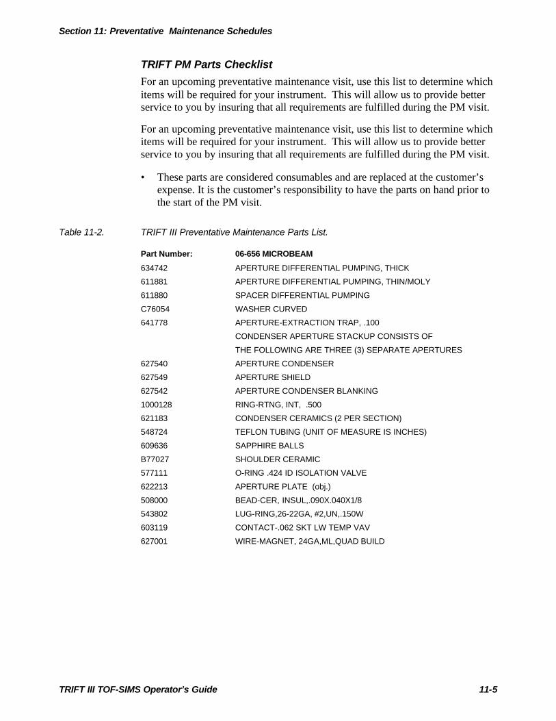
Section 11: Preventative Maintenance Schedules
TRIFT III TOF-SIMS Operator’s Guide 11-5
TRIFT PM Parts Checklist
For an upcoming preventative maintenance visit, use this list to determine whichitems will be required for your instrument. This will allow us to provide betterservice to you by insuring that all requirements are fulfilled during the PM visit.
For an upcoming preventative maintenance visit, use this list to determine whichitems will be required for your instrument. This will allow us to provide betterservice to you by insuring that all requirements are fulfilled during the PM visit.
• These parts are considered consumables and are replaced at the customer’sexpense. It is the customer’s responsibility to have the parts on hand prior tothe start of the PM visit.
Table 11-2. TRIFT III Preventative Maintenance Parts List.
Part Number: 06-656 MICROBEAM
634742 APERTURE DIFFERENTIAL PUMPING, THICK
611881 APERTURE DIFFERENTIAL PUMPING, THIN/MOLY
611880 SPACER DIFFERENTIAL PUMPING
C76054 WASHER CURVED
641778 APERTURE-EXTRACTION TRAP, .100
CONDENSER APERTURE STACKUP CONSISTS OF
THE FOLLOWING ARE THREE (3) SEPARATE APERTURES
627540 APERTURE CONDENSER
627549 APERTURE SHIELD
627542 APERTURE CONDENSER BLANKING
1000128 RING-RTNG, INT, .500
621183 CONDENSER CERAMICS (2 PER SECTION)
548724 TEFLON TUBING (UNIT OF MEASURE IS INCHES)
609636 SAPPHIRE BALLS
B77027 SHOULDER CERAMIC
577111 O-RING .424 ID ISOLATION VALVE
622213 APERTURE PLATE (obj.)
508000 BEAD-CER, INSUL,.090X.040X1/8
543802 LUG-RING,26-22GA, #2,UN,.150W
603119 CONTACT-.062 SKT LW TEMP VAV
627001 WIRE-MAGNET, 24GA,ML,QUAD BUILD

Section 11: Preventative Maintenance Schedules
TRIFT III TOF-SIMS Operator’s Guide 11-6
FILAMENTS
627285 EMITTER-LMI, TOF GA-69, 1500 HR
642819 EMITTER-LMIG, InPUR MONO
633380 E-GUN FILAMENTS
131-00010 FIL-GAUGE,ION ELECT DEGASS,G.P. 274025
LMIG COLUMN
FEI 16387 EXTRACTOR CAP
FEI 18181 SUPPRESSOR
FEI 20037 STEM APERTURE ASSEMBLY; "20 nA COLUMN"
FEI 168484 MVA ASSEMBLY
Cs COLUMN
612458 FRIT ASSEMBLY
639387 CESIUM AMPULE- 1 GRAM
O2 SOURCE
608892
613265
ASSY-GAS CYLINDER, OXYGEN
KIT-REPAIR,INDIRECT GAS, 06-660A
ION DETECTOR
570-00005 MCP, MATCHED SET, 25MM, HOT
636047 PHOSPHOR SCREEN
SPECTROMETER CHAMBER
638298 GATE VALVE (HVA 11220-0150X), SPECTROMETER
639695 KIT-UPDATE, POSITION MANIPULATOR
SAMPLE CHAMBER
123-00002 MULTIPLIER-ELECTRON, SEM DETECTOR
2" INTRO / STAGE SECTION
248-00001 GATE VALVE, 3 " I.D., MDC
639388 ADPTR-SCREW, LOADLOCK, TRIFT, MAG INTRO
02-03145 SHAFT, SAMPLE INTRO, 2" SLIDING SEAL INTRO
352-00011 O-RING, ELASTOMER, 0.239ID; INTRO ROD
02-03140 BSHG-WILSON SEAL; INTRO ROD
352-00013 O-RING-ELASTOMER, 2.975ID; INTRO COVER
8" STAGE SAMPLE CARRIERS
02-05555 ASSY-SAMPLE CARRIER, SM HLDR, 8"
02-05647 ASSY-SAMPLE HOLDER, 8", TFS

Section 11: Preventative Maintenance Schedules
TRIFT III TOF-SIMS Operator’s Guide 11-7
2" STAGE SAMPLE CARRIERS
02-03465 SAMPLE CARRIER, 4-POSITION, 2" STAGE
02-03464 ASSY- SAMPLE CARRIER, LARGE SAMPLES, 3 MASKS
UNIVERSAL SAMPLE HOLDERS / ACCESSORIES
02-03466-03 HOLDER- SAMPLE, .500" ID
02-03467 HOLDER- MULTI SAMPLE
636853 MASK-SMALL HLDR,10MM, TRIFT II
636854 MASK-SMALL HLDR, 5MM, TRIFT II
642207 MASK-SMALL HLDR, 2MM, 4X, TRIFT II
636856 MOUNT-RECESSED BKLD, 1MM, TRIFT II
636857 MOUNT-RECESSED BKLD, 2MM, TRIFT 2
636858 MOUNT-RECESSED BKLD, 3MM, TRIFT 2
636859 MOUNT-RECESSED BKLD, 4MM, TRIFT 2
636860 MOUNT-RECESSED BKLD, 5MM, TRIFT 2
642259 SAMPLE-FARADAY CUP, BOROSILICATE
642260 PLATE-BACKING,FARADAY CUP
02-05695 WAFER MESH, 3/4" DIA, CHARGE COMP GRID
640756 PLATE-BACKING,SAMPLE, .82 OD
640755 ASSY-CLAMP, SAMPLE CROSS SECTION VICE
246-00008 SPRG-CPRSN, CNCL, .225 - .11OD, .01
00-05133 SCR-BUTTON, 4-40X .250"
896-00002 SAMPLE, AL/CU GRID (CAMECA)
02-04677 SPRING- SAMPLE HOLDER, FORMED CU
638031 SAMPLE HOLDER SHIM KIT
TURBO PUMP ACCESSORIES
897-00001 BALZERS, 60 L/S TURBO WICKS
897-00002 BALZERS, 240 L/S TURBO WICKS
619393 OIL, PUMP, ALCATEL, 1 LTR.
MISC ACCESSORIES
A79106 GAUGE TUBE-GRAN PHILLIP 275071, CONVECTRON
638274 LAMP T1.75 28V .04 A (EMO BOX)
131-00002 LAMP, HALOGEN, 250W, 120V
131-00003 LAMP, HALOGEN, 150W, 120V
622301 LAMP LIGHT SOURCE
639187 BATTERY, 3 V LITHIUM SIZE C, FOR SVC
637045 PHOSPHOR SCREEN
636047 TRIFT III STAGE BELLOWS 50 MM

Section 11: Preventative Maintenance Schedules
TRIFT III TOF-SIMS Operator’s Guide 11-8
GASKETS
2680750 KIT-GASKET, 1.33 OD FLG, (10)
633382 GASKET-CU, 2.125 FLG, CLN, LMIG MVA
2681500 KIT-GASKET, 2.75 OD FLG, (10)
2682000 KIT-GASKET, 3.37 OD FLG, (10)
2682500 KIT-GASKET, 4.50 OD FLG, (10)
1001887 KIT-GASKET, 4.62 OD FLG, (10), LMIG SOURCE
2684000 KIT-GASKET, 6.00 OD FLG, (10)
633381 GSKT-SPECIAL,TRIFT,6.0 FLG CLN, LMIG THICK
2688000 KIT-GASKET, 8.00 OD FLG, (10)
633357 GASKET-CU, 14.00 FLG, CLN, 8" STAGE
352-00014 GASKET-W/S, 18.00 FLG, SPECTROMETER LID
632197 GASKET-VATSEAL, 46X236, SEAT SEAL, 8" STAGE
632198 GASKET-VATSEAL, 46X236, BONNET SEAL, 8" STAGE
Section 11: Preventative Maintenance Schedules
TRIFT III TOF-SIMS Operator’s Guide 11-9
Routine MaintenanceTRIFT parts or components that require maintenance on a routine basis aredescribed below. Manuals for components from original equipmentmanufacturers (OEM) other than Physical Electronics are supplied with thesystem for reference.
NOTE: Routine monitoring of certain system performance parameters andmaintenance events, as described later in this section, is recommended to revealtrends in the system performance and help uncover potential or apparentproblems.
Cesium Ion Gun Source
Service or maintenance of the cesium ion gun source should be nominal,however, if the source becomes unstable and does not operate properly, it mayindicate that the reservoir has run out of cesium material or the cesium frit hasbecome plugged.
Cesium Ion Gun Column
Regular service or maintenance of the cesium ion gun column should also beminimal, however, if excessive steering values within the WinCadence softwareare required to operate the column, excessive cesium material may have built upon the column's steering plates.
Console Panels
Service or maintenance of the system often involves opening or removing one ormore panels from the consoles. Most of the panels on the electronics console arehinged for opening and are held closed with captive screws. All of the panels onthe vacuum console are held closed with captive screws.
Panels that are not hinged are replaced by (1) lowing the openings on the insidebottom of the panel into the console’s receiving brackets, (2) pushing the top ofthe panel in until it snaps into position, and (3) tightening the captive panelscrews to hold the panel in place.
Cooling Filters
The TRIFT TOF-SIMS system only has one 10 inch x 24 inch filter locatedinside the right-hand door of the back of the electronics console. No tools arerequired.
To remove the filter, open the door and lift up on the filter frame, which isattached to the console door with L-shaped tabs. Lift the filter out of the frame.The filter should be removed as needed and cleaned with a vacuum cleaner. IFcleaning the filter with a vacuum does not remove the trapped particles, wash thefilter with plain water and dry it completely before replacing it in its holder in theconsole.
Section 11: Preventative Maintenance Schedules
TRIFT III TOF-SIMS Operator’s Guide 11-10
NOTE: Replacement filters may be ordered through PHI Customer Serviceunder P/N 636840.
Several electronics units also contain filters mounted over the cooling fansattached to the back of the chassis. These electronics filters also require periodiccleaning.
The filters contained within the units cannot be easily removed, therefore, thepreferred method of cleaning should be externally with a vacuum cleaner. If thismethod does not work sufficiently, the unit must be removed from the electronicsconsole. Take the unit away from the system and use compressed dry air fromthe inside of the unit to blow the filter clean. The top of the chassis may requireremoval in order to accomplish this task. Reinstall the top of the chassis andreturn the unit to the electronics console.
Convectron Gauges
A complete Installation, Operation and Maintenance Instructions manualpublished by Granville-Phillips is shipped with the TRIFT system and containsall of the necessary service procedures and precautions. The instructions listedbelow contain just a brief overview of the cleaning and maintenance steps.
The TRIFT system contains two different types of Convectron gauges: an analogversion and a digital version. Both types attach to the roughing manifold in thevacuum console.
Analog Convectron Gauges: A gauge may become contaminated with oil orother films over time, but can be cleaned. When the small internal sensor wire iscontaminated, its emissivity or its diameter may be altered and a change ofcalibration will result. Cleaning with trichloroethylene, perchloroethyylene,toluene, or acetone is possible, but it must be done very carefully so as not todamage the sensor. Consult the Granville-Phillips service manual for the propercleaning procedure.
If required, the Convectron gauge may be baked to 150°C non-operating whileunder vacuum with the connector/cable removed.
A small diameter internal sensor wire can be damaged by small voltages. Do notperform electrical continuity tests with instruments applying in excess of 1 voltwhen the gauge is at vacuum or 5 volts when at atmospheric pressure. The gaugeshould show the following resistance measurements (pin numbers are embossedon the gauge base).
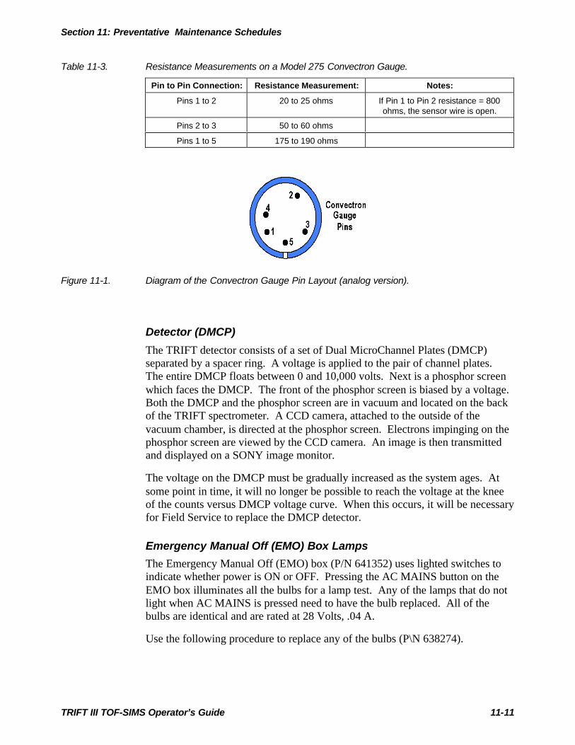
Section 11: Preventative Maintenance Schedules
TRIFT III TOF-SIMS Operator’s Guide 11-11
Table 11-3. Resistance Measurements on a Model 275 Convectron Gauge.
Pin to Pin Connection: Resistance Measurement: Notes:
Pins 1 to 2 20 to 25 ohms If Pin 1 to Pin 2 resistance = 800ohms, the sensor wire is open.
Pins 2 to 3 50 to 60 ohms
Pins 1 to 5 175 to 190 ohms
Figure 11-1. Diagram of the Convectron Gauge Pin Layout (analog version).
Detector (DMCP)
The TRIFT detector consists of a set of Dual MicroChannel Plates (DMCP)separated by a spacer ring. A voltage is applied to the pair of channel plates.The entire DMCP floats between 0 and 10,000 volts. Next is a phosphor screenwhich faces the DMCP. The front of the phosphor screen is biased by a voltage.Both the DMCP and the phosphor screen are in vacuum and located on the backof the TRIFT spectrometer. A CCD camera, attached to the outside of thevacuum chamber, is directed at the phosphor screen. Electrons impinging on thephosphor screen are viewed by the CCD camera. An image is then transmittedand displayed on a SONY image monitor.
The voltage on the DMCP must be gradually increased as the system ages. Atsome point in time, it will no longer be possible to reach the voltage at the kneeof the counts versus DMCP voltage curve. When this occurs, it will be necessaryfor Field Service to replace the DMCP detector.
Emergency Manual Off (EMO) Box Lamps
The Emergency Manual Off (EMO) box (P/N 641352) uses lighted switches toindicate whether power is ON or OFF. Pressing the AC MAINS button on theEMO box illuminates all the bulbs for a lamp test. Any of the lamps that do notlight when AC MAINS is pressed need to have the bulb replaced. All of thebulbs are identical and are rated at 28 Volts, .04 A.
Use the following procedure to replace any of the bulbs (P\N 638274).

Section 11: Preventative Maintenance Schedules
TRIFT III TOF-SIMS Operator’s Guide 11-12
ATTENTION: This bulb replacement procedure involves activating the switchassociated with the burned-out bulb. Prepare the system conditions for theactivation or deactivation of any switch on the EMO box to replace the bulb(s).
1. Prepare the system for activation of the switch that has the bad bulb.
2. Pull the colored button plate off.
3. Pull the bad bulb out of its seating, and push in the new bulb.
4. Push the colored button plate all the way back on to the box, which will alsoactivate its switch. Push the switch a second time to deactivate the switch.
Ions Gauges
The TRIFT system has a single (1) ion gauge and two (2) Convectron gauges.See also “Vacuum Gauge Controls” later in this section. The Convectron gaugesare Granville-Phillips gauges. Refer to the manufacturer’s manual forreplacement procedures.
The MAIN CHAMBER ION GAUGE is nude ion gauge assembly. It ismounted on a vacuum flange containing a twist-lock connector feedthrough thatmates with a corresponding connector on the ion gauge cable. The nude iongauge is equipped with two filaments, as shown in Figure 11-2 below. Only oneion gauge filament is used at a time, depending on which way the cable isinstalled on the ion gauge flange.
Figure 11-2. Side View of the Ion Gauge Filament Assembly.
When one filament burns out, the cable connector may be switched to the secondfilament without breaking vacuum as follows.
NOTE: If both filaments in a nude ion gauge are burned out, the system must bevented to remove the gauge. This is a PHI Customer Service procedure.Filament replacement kits (P/N 2141400) may be ordered from PHI CustomerService. One kit is sufficient for one ion gauge filament change.
Section 11: Preventative Maintenance Schedules
TRIFT III TOF-SIMS Operator’s Guide 11-13
Light Source
The light-source control is typically located within the electronics console andincludes an extended fiber optic cable to direct the high intensity light to thesample. One end of this fiber optic cable is attached to the power supply and theother end is connected to a mount attached to the vacuum chamber. This lightsource is used for illuminating the sample area for viewing by the samplecamera.
The replacement halogen bulb is a type EKE lamp, rated at 150 Watts and can beordered from PHI Customer Service (P/N 622301). Replacement of the lamps isrelatively easy and is done by turning off power to the unit, removing the burnedout lamp, placing the new lamp in the unit and replacing the cover. No tools arerequired for replacement of the bulbs.
Liquid Metal Ion Gun (LMIG)
Maintenance on the LMI gun may involve replacement of the emitter, theMoveable Variable Aperture (MVA), and/or the Liquid Metal Ion Source(LMIS). Repair and replacement of these items is considered extensive.Therefore, procedures covering the major components within the LMIG areincluded later in this section of the manual.
The controller for the LMIG does not require routine maintenance of any type.
Rough Pump (Alcatel)
The rough pump does require normal maintenance at six-month intervalsincluding replacement of the wick and the pump oil. Follow the maintenanceprocedures included in the Alcatel manual shipped with the TRIFT system.
If the rough pump is unusually loud, maintenance may be required sooner thanevery 6 months.
System Vacuum Control (SVC)
Maintenance and service of the SVC is described in the System Vacuum Controlcomponent manual. The SVC does require maintenance on a routine basis.
However, the System Vacuum Control does contain a 3 Volt Lithium backupbattery (P/N 639187) which is used to retain the Watcher software tasks. Thisbattery must be changed every 24 months. The battery is located on the mainSVC printed circuit board. To replace the battery, remove the SVC from theelectronics console and open the chassis. Locate BT1 on the board, cut theplastic tie wrap holding the battery in place and remove the battery. Replace thebattery while observing the correct polarity and install a new tie wrap. Reinstallthe chassis top and reinstall the SVC unit into the electronics console.

Section 11: Preventative Maintenance Schedules
TRIFT III TOF-SIMS Operator’s Guide 11-14
Figure 11-3. Location of the backup battery within the System Vacuum Control chassis.
Sample Bias Feedthrough / Connector
The TRIFT system contains a high voltage bias feedthrough located in the centerof the sample stage on the vacuum console. This sample high voltage biasfeedthrough should be inspected for corrosion.
If corrosion does exist, the high voltage feedthrough must be replaced(P/N C79141) and also the Sample Bias High Voltage cable (P/N 633797).
Turbo, Rough Pump Maintenance (Wicks)
The TRIFT system uses two (2) turbo pumps: a 160 l/s turbo pump is mounted tothe introduction chamber and a 240 l/s turbo pump is mounted to the analyticalchamber. It is recommended that the turbo wicks be replaced annually and thatrough pump oil be changed every 6 months. Refer to the turbo maintenancesection later in this section.

Section 11: Preventative Maintenance Schedules
TRIFT III TOF-SIMS Operator’s Guide 11-15
Vacuum Gauge Controls
The Vacuum Gauge Controls must be calibrated on-site as follows for properoperation of the routines built into the System Vacuum Control software:
• All system Convectron gauges must be calibrated on-site to read 760 torr atatmospheric pressure; and
• Ion gauges must be calibrated to 0 torr at full ultra-high vacuum at the site.
Calibration is adjusted by turning the set screw associated with the gauge to beadjusted. The set screw is accessed by opening the “door” on the front of theVacuum Gauge Control located in the electronics console. Refer also to theOEM manual provided with the TRIFT system.

TRIFT III TOF-SIMS Operator’s Guide A-1
Appendix A:Service Procedures
Appendix A contains a set of three service procedures which address thefollowing topics:• Rigorous heating to start the LMIG Source;• Mechanical alignment of the Cesium column to the analysis region; and• Low energy beam alignment.
ATTENTION: The following instructions and procedures are for use byqualified service personnel only. To avoid personal injury, do not perform anyinstallation or servicing procedures unless qualified to do so and havingreceived training from PHI personnel.
Rigorous Heating to Start the LMIG SourceIf the source will not fire after performing the steps described in Section 4(“Heating the Source”) of this operator’s guide, it may be necessary to heat thesource until the gallium boils, thereby removing whatever is causing the source notto fire. This extreme heating will inevitably reduce the lifetime of the sourcebecause there is a limited amount of gallium in the source. This lifetime can bereduced dramatically IF the heating process is not carried out extremely carefully.It is recommended that a PHI Service Engineer perform the steps outlined below.
CAUTION: Only use a high voltage probe for the following step.
1. Before the final decision is made to heat the source, check that the extractorvoltage supply is functioning properly. First, set the extraction voltage to zero,then remove the extractor lead from the gun. Test the supply by setting it to 1kV, and verify this potential at the end of the lead with a high voltage probe. Ifthe source will not fire after heating as described above with maximumextractor and suppressor voltages applied, and after the extractor supply hasbeen checked, the following additional steps are recommended.
2. Set the extractor voltage to below the typical value, e.g. 5 kV with thesuppressor set to a value of 1 kV.
Appendix A: Attachments
TRIFT III TOF-SIMS Operator’s Guide A-2
3. For 500-hour sources, raise the filament voltage to a value of 3.5 - 3.8 amps(PN 11604), and begin timing. After 30 seconds, turn the filament currentdown to zero (0 Amps) as quickly as possible. For the 1500-hour sources (PN16830), use LESS current than the 500-hour sources, typically use a rangebetween 3.1 - 3.2 amps. [Do NOT apply 3.5 - 3.8 amps to a 1500-hoursource!]
4. Raise the extractor voltage until the source fires. If the source fires at the'normal' voltage, everything is fine. If the source fires, but at a high extractorvoltage, the source tip is probably near the end of its life. Preparations shouldbe made to replace the source when it will be most convenient.
5. If the source fails to fire, even at maximum extractor and suppressor voltages,the source is probably 'dry' and preparations should be made to replace thesource immediately.
6. It is possible to conduct step 2 above with the extractor voltage set above the'normal' operating voltage (e.g., 12 kV). When the source fires, it may do sowith a very high emission current. Both the extraction voltage and the filamentcurrent should be reduced as quickly as possible. When this occurs, somegallium will have boiled away, and a significant volume of gallium willprobably have been extracted in the form of microdroplets, which furtherreduces the gallium remaining for source emission. For this reason, extremeheating without extraction is preferred at least initially.
Mechanical Alignment of Cs Column to Analysis RegionIn the event of not measuring any sample current (given that current can bemeasured at the Faraday cup), a simple, mechanical misalignment of the columnmay be the cause. Mechanical alignment of the column to the sample (and moreprecisely, to the analysis region) can be performed with the ring of knurled knobslocated around the circumference of the column, however, this procedure must bereferred a qualified technician or service engineer.
Lower the sample potential to zero (0) volts and connect a picoammeter to thestage. Maximize the sample current by adjusting the alignment knobs. Once asample current of 1-2 nA for a 10kV beam (using the 5ml slit and 5ml aperture)has been achieved, remove the picoammeter, reconnect the MHV stage cable andproceed to fine tuning of the column with the aid of imaging at the DMCP detector.

TRIFT III TOF-SIMS Operator’s Guide B-1
Appendix B:Mass Resolution Tuning Grid
Appendix B contains a Mass resolution Tuning Grid template for recordingkeeping on the TRIFT III system. The system operator may use this template tomake additional copies to keep with the TRIFT system records.

AP
PE
ND
IX B
:TR
IFT
MA
SS
RE
SO
LUTI
ON
TU
NIN
G G
RID
Sam
ple
Pot
entia
l:R
aste
rS
ize:
Mat
suda
Vol
tage
:D
etec
tor
Vol
tage
:D
etec
tor
Pos
ition
:P
ost
Acc
el.:
C.D
. No.
:
LMIG
Em
issi
on:
Bun
cher
Vol
tage
:B
unch
erD
elay
:B
lank
erV
olta
ge:
Pul
ser
Vol
tage
:M
ass
Ato
mic
:R
esol
.O
rgan
ic:

TRIFT III TOF-SIMS Operator’s Guide C-1
Appendix C:Indium Liquid Metal Ion Source (LMIS)
Appendix C contains a set of procedures which address the following LMIStopics:• Daily operation of the source;• Periodic revitalization of the source; and• Parameters affected by the Indium source.
LMIS Installation into the TRIFTBefore installing the indium LMIS, check the performance of the instrument (i.e., isthe LMIG ’wobble free’) and also log the best mass resolution on 28Si+.
The indium LMIS installs into the FEI LMIG in exactly the same manner as thegallium LMIS. Following the installation of the emitter, the following procedureshould be followed:
VacuumThe LMIS typically requires installation by a field engineer from PhysicalElectronics. Evacuation and bakeout of the LMIG is performed overnight (6 hoursminimum). Once the gun pressure has fallen into the 10-9 torr region (or <2µA ionpump current), it can then be operated.
Conditioning the Source
High Voltage ConditioningBefore attempting to fire the source, the LMIG should go through a high voltageconditioning:
1. Load a ‘zero volts’ instrument file and gradually increase the beam energyfrom 0 to 25 keV in 5 keV steps (up to 15 keV) and then 1 keV steps (up to 25keV).
2. With the filament current still set to 0 Amps, increase the extractor potential in1 kV steps up to 12 kV (or at least 10 kV, if the LMIG is old and has arecognized voltage limitation). There should be zero emission current.
Appendix C: Indium Liquid Metal Ion Source
TRIFT III TOF-SIMS Operator’s Guide C-2
Outgassing the LMIS1. Re-load the ‘zero volt’ instrument file and increase the heater current to 2.0
Amps. Check the ion pump current (i.e. should not rise). Increase the currentin 0.2 Amp steps, up to 2.8 Amps. If the ion pump current rises to greater than5µA, allow the source to sit at 2.8 Amps for approx. 20 minutes while itoutgasses. (Note that it can be fatal to raise the extraction potential to 9 or 10kV while the source is outgassing heavily).
2. Once the ion pump pressure has recovered to less than 5 µA (with the heatercurrent at 2.8 Amps), reduce the heater current to 1.8 Amps and wait 5 minutesfor pressure to recover further.
Operation
Igniting the Source1. Load a 15GA3.INS (gallium file) or a 15IN3.INS (indium file, if one exists)
instrument file. If you load a 15IN3.INS file, quickly set the filament current tozero once the file is loaded.
2. Gradually raise the extraction potential to 10 kV (Note For TRIFT I’s, wherean extractor voltage of 11 kV is required for a gallium LMIS, you should setthe extractor potential to 13-14kV) . Check the ion pump current does not riseabove 2 µA.
3. Set the filament current to 2.0 Amps. Wait.
4. If there is no emission current, then raise the filament current by 0.05 Amps.Continue to raise the filament current in 0.05 Amp steps, waiting 30 secondsbetween each increment. Do not exceed 3.6 Amps.
5. When the source fires, allow the source to emit at > 20 µA for ∼30 secondsand then lower the extraction voltage to give 5 µA of emission current. Let thesource emit at 5 µA for a 3-4 minutes.
6. Once the emission current has stabilized, reduce the filament current andextractor voltage quickly until emission terminates.
7. Wait at least one minute. Raise the extractor to 10 kV and then raise the heatingcurrent from 1.90 Amps in 0.05 Amp steps (wait 20 seconds between steps),until stable emission is obtained. Lower the extractor voltage, until theemission current is <2 µA. Raise the heater current by an extra 0.1 µA - thiswill now be the operating filament current.
8. Typically, a source will ignite for the first time with the following parameters:

Appendix C: Indium Liquid Metal Ion Source
TRIFT III TOF-SIMS Operator’s Guide C-3
Vext = 10 kV (TRIFT II) Vext = 13.5 kV (TRIFT I)Iheater = 2.5-3.0 Amps
And typical operating parameters are :-
Vext = 6.5-7.5 kV (TRIFT II) Vext = 10.0-10.5 kV (TRIFT I)Iheater = 2.1-2.5 Amps
If the source ignites, but requires an excessively large extractor voltage (ie >7.5kV) to maintain emission, then the source will have to be heated at 3.2-3.4 Ampsfor approximately 30 seconds with Vext = 9-10kV.
Note down the ignition and subsequent operating parameters for the source in the‘Emitter Record’ that came attached to the new source.
Day to Day Operation1. Raise the extraction potential by 2000 V from the normal operating voltage.
2. Set the filament current to 0.2 Amps above the usual operating value. It willtake about 30-60 seconds for the tip to reach operating temperature.
3. When the source fires, allow the source to emit at ∼ 20 µA for ∼20 secondsand then lower the heater current to the usual operating value and reduce theextraction voltage to give ∼1 µA of emission current. The extraction voltageshould consistently return to the usual extraction potential and the fine tuning ofthe emission current should now be done with the suppressor voltage.
4. Typical switch on parameters are:Vext 8.5 to 9.5 kVVsup -1.0 kV Iem >20.0 µA for 20 secondsIfil 2.4 Amps
Typical operating parameters are:Vext 6.5 to 7.5 kVVsup -0.00 kV Iem 1.0 µAIfil 2.2 Amps Itarg 10-20 nA (large MVA, +75 V sample bias)
NOTE: Experience has shown that the extractor potential required for anindium LMIS under normal operation can be as low as 6000 V (as opposed to7500 V with the gallium LMIS). Since the tip geometry is the same for bothgallium and indium sources, the lower extract potential is attributed to thelower surface tension and flow impedance of liquid indium.

Appendix C: Indium Liquid Metal Ion Source
TRIFT III TOF-SIMS Operator’s Guide C-4
Revitalizing the Indium Source (every 1-2 months)After intervals of 100-200 µA hrs of operation, the liquid flow impedance to thetip often increases to the point where ion emission can not be sustained withoutraising the extractor potential above the usual value. This is usually accompaniedby a very weak ‘emission current’ v’s ‘extractor voltage’ dependence. In this‘flow restricted’ condition it may take 1000-1500 V increase in extractor potentialin order to increase the emission current from 5µA to 10µA. After re-vitalizingthe source, the emission current should go from 5µA to 10µA with only a 200-500V increase in extractor potential. In order to revitalize the source, such that itwill operate at its usual extractor potential it will be necessary to follow theprocedure below.
1. Set the heater current to it’s usual value and then increase the extractor voltageby 2500 V in 500 V increments (e.g. from 7000 V to 9500 V). If there are nosigns of high voltage break down (e.g. a rapid increase in ion pump current)then you can proceed.
2. Increase the heater current to 2.8 amps and wait 1 minute (or until the emissioncurrent increases above ∼25 µA).
3. If the emission current hasn’t increased significantly (ie by 10 µA or more),then raise the heater current to 3.0 Amps. Wait for 30 seconds. Again, if theemission current hasn’t increased significantly, then raise the heater to 3.2Amps and wait 30 seconds. Usually, an indium source will start to emitstrongly once it has been heated at 3.2 Amps for 30 seconds or so. If this is notthe case, then increase the current to 3.4 Amps for no longer than 30 seconds.
4. If the source fails to emit all together and the source has been operated for>800 µA hours, then the indium reservoir has probably run dry and will needreplacing.

Appendix C: Indium Liquid Metal Ion Source
TRIFT III TOF-SIMS Operator’s Guide C-5
Instrument Parameters Affected by the Indium LMIS
LMIG Alignment
If starting with an old 15 keV gallium *.INS file, the ion source brass knobs shouldbe mechanically aligned, first to measure current on the LMIG Faraday cup andthen finally onto the sample. When current is hitting the sample, try to acquire anSEM image of the copper grid.
Operate the LMIG extractor potential at a lower value than that required by thegallium LMIS. Since the extractor electrode has beam focusing properties, thelens 1 potential will need to be tuned again to keep the first crossover in theblanking plates and the second crossover on the sample. Lens 2 should stay thesame.
Fine tuning of the source position can be done by aligning the brass knobs whilewobbling lens 2, with a view towards minimizing image motion.
Ideally, the new source should be aligned to the existing ion gun deflectorvoltages, but in reality some fine tuning on the beam deflectors may be required inorder to achieve fine alignment of the beam. The procedure for fine tuning thebeam is described elsewhere in the User’s Guide.
Pulse/Buncher Timing
the LMIG buncher delay will need to be re-optimized for indium because thevelocity of 115In is approximately ¾ of 69Ga for a given beam energy. In 15 keVpulse/bunched indium mode, reducing the buncher delay by ∼10 ns from thatrequired for gallium is close to the optimum setting. From here, fine tune the delayby 1 or 2 ns (in both directions) to find the optimum delay for best mass resolution.
It should be noted that the energy spread of ions from an indium LMIS is greaterthan those from a gallium LMIS. The larger energy spread results in a broadeningof the primary bunched pulse width, such that the mass resolution for 28Si+ islimited to 7,500 under typical source operating conditions of 1µA emission and aheater current of 2.2 Amps. A shorter primary pulse width can be obtained byrunning the source at a lower emission current and the lowest possible heatercurrent, but this may result in unstable emission. Mass resolution as a function ofemission current is shown in Figure A-1 below, with heater current as aparameter.
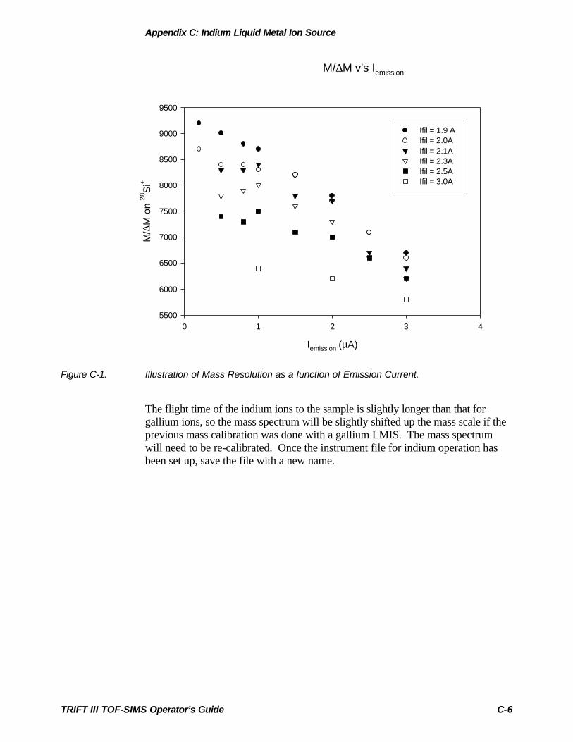
Appendix C: Indium Liquid Metal Ion Source
TRIFT III TOF-SIMS Operator’s Guide C-6
M/∆M v's Iemission
Iemission (µA)
0 1 2 3 4
M/∆
M o
n 28
Si+
5500
6000
6500
7000
7500
8000
8500
9000
9500
Ifil = 1.9 A Ifil = 2.0A Ifil = 2.1A Ifil = 2.3A Ifil = 2.5A Ifil = 3.0A
Figure C-1. Illustration of Mass Resolution as a function of Emission Current.
The flight time of the indium ions to the sample is slightly longer than that forgallium ions, so the mass spectrum will be slightly shifted up the mass scale if theprevious mass calibration was done with a gallium LMIS. The mass spectrumwill need to be re-calibrated. Once the instrument file for indium operation hasbeen set up, save the file with a new name.


![[特集]有機エレクトロニクス (2)GCIB-TOF-SIMSに …...GCIB-TOF-SIMS分析を行った。TOF-SIMS測定には、 ION-TOF社製TOF.SIMS.5を用い、GCIB(エッチング](https://img.pdfslide.net/doc/110x75/5f2c80fe25b37a65f137eca3/ceoeffff-2igcib-tof-sims-gcib-tof-simseoetof-sims.jpg)