Embed Size (px)
Citation preview

Master Thesis in Geosciences
Tunnel Health Monitoring Using
Active Seismics
Mesay Geletu Gebre


Tunnel Health Monitoring Using Active Seismics
Mesay Geletu Gebre
Master Thesis in Geosciences
Discipline: Geophysics
Department of Geosciences
Faculty of Mathematics and Natural Sciences
University of Oslo
June 2013

© Mesay Geletu Gebre, 2013
Tutor(s): Dr. Dominik Lang (NORSAR), Assoc. Prof. Isabelle Lecomte (NORSAR/UiO)
and Prof. Valerie Maupin (UiO)
This work is published digitally through DUO – Digitale Utgivelser ved UiO
http://www.duo.uio.no
It is also catalogued in BIBSYS (http://www.bibsys.no/english)
All rights reserved. No part of this publication may be reproduced or transmitted, in any form or by any means,
without permissio

I
Acknowledgements
First and foremost I offer my sincerest gratitude to my thesis supervisor Dr. Dominik Lang
(NORSAR) and to my co-supervisors Assoc. Prof. Isabelle Lecomte (NORSAR/UiO) and Prof. Valerie
Maupin (UiO). Without their continuous support, guidance, and patience throughout the year this
work would have been impossible. I am grateful to Dr. Ulrich Polom (LIAG) for teaching me
ProMax 2D software, helpful suggestions, advice, and for sharing his excellent knowledge on
vibroseis method.
I want to thank all my friends supported me throughout my thesis with their knowledge. I am
grateful to NORSAR staff, particularly the IT team. I am obliged to Mr. Jan Fredrik Olsen
(Campus Kjeller) and PhD student Guillaume Sauvin (NORSAR/UiO) for their endless efforts
performing seismic measurements at Nittedal site. I am also grateful to Kamran Iranpour (
NORSAR) for his help in writing MATLAB codes.
At last but not least, I would like to thank NORSAR for the financial support through this thesis. I
also like to thank the Norwegian government quota scheme program for providing me a scholarship
to study geophysics at the department of geosciences, University of Oslo.
Mesay Geletu
June 2013
II
Abstract
In this thesis a new approach, called THEAMTM
, is presented. The THEAMTM
methodology is a
non-invasive tunnel health monitoring method using active seismic. The method incorporates
geophysical seismic analysis methods and geotechnical engineering with available wireless
technologies. The fundamental idea of the THEAMTM
procedure is to artificially generate a
controlled seismic signal at the tunnel wall, and to record the response from the tunnel
surrounding system at fixed receivers attached to the tunnel surface. The change in seismic
signatures overtime are used as a precursor about the tunnel rock wall conditions, such as, new
emerging cracks or any structural changes.
The THEAMTM
procedure was applied at Oslofjord tunnel. The results of this study suggest that
the THEAMTM
methodology is a robust and potentially very applicable procedure for long-term
monitoring of the tunnel rock wall conditions before any hazardous collapse. This method is
more powerful compared to conventional method like visual inspection, because it provides fast
and continuous reliable information about the geological rock wall conditions in the tunnel.
Furthermore, the THEAMTM
method is easy to accomplish because once system is instrumented
the data is acquired by remote control from office.

III
Contents Acknowledgements .......................................................................................................................... I
Abstract II
Chapter 1: INTRODUCTION........................................................................................................ 1
Background and Motivation ....................................................................................................... 1
1.1 Seismic Methods during Tunnel Excavation ................................................................... 2
1.2 Shear Wave Technique..................................................................................................... 3
1.3 Tunnel Health Monitoring (THEAMTM
) Method ............................................................ 3
1.4 Objectives of the Study .................................................................................................... 5
1.5 Software .......................................................................................................................... 5
1.6 Outline of the Thesis ........................................................................................................ 5
2.1 THEAMTM
Operation Principle and Main System Components ..................................... 6
2.2 Cross-correlation ............................................................................................................ 7
2.3 Vibroseis Method ............................................................................................................. 8
2.4 Repeatability in Land Seismic Data ............................................................................... 13
2.5 Coverage Distance.......................................................................................................... 15
2.6 Seismic Expression in Propagation through Cracks ...................................................... 16
Chapter 3: SURVEY SITES AND DATA ACQUISITION ........................................................ 17
3.1 Survey Sites .................................................................................................................... 17
3.2 Data Acquisition ............................................................................................................. 18
3.2.1 Oslofjord tunnel acquisition .................................................................................... 20
3.2.2 Feiring Bruk Nittedal site acquisition ..................................................................... 25
Chapter 4: DATA PROCESSING STEPS AND RESULTS ....................................................... 30
4.1 Data Processing Steps .................................................................................................... 30
4.2 Importing Data and Pilot Sweep Cleaning ..................................................................... 31
4.2.1 Processing steps in harmonic noise removal from pilot sweep and results ............ 32
4.3 Cross-correlation of Vibrograms with Cleaned Sweep .................................................. 32
4.4 Stacking Repeated Sweep Each Day and Component Sorting ...................................... 34
4.5 Spectral Analysis ............................................................................................................ 34
4.6 Band-pass Filter.............................................................................................................. 35
4.7 Repeatability Analysis................................................................................................... 39

IV
4.8 Coverage Distance from Oslofjord Data ........................................................................ 42
4.8 Velocity Estimation ........................................................................................................ 45
Chapter 5: DISCUSSION AND CONCLUSION ........................................................................ 59
5.1 Resonance Frequency Monitoring ......................................................................... 59
5.2 Normalized Cross-correlation Monitoring ..................................................................... 60
5.3 Conclusion and Recommendations ................................................................................ 61
5.4 Future Work ................................................................................................................... 63
References ……………………………………………………………………………………..64
Appendix A: Resonance frequency ....................................................................................... 67
A.1: Nittedal site ............................................................................................................. 67
Appendix B: Zero-lag cross correlation ................................................................................ 67
B.1 Nittedal site .................................................................................................................... 67
C: Fourier Transform .......................................................................................................... 68
Appendix D: MATLAB code ............................................................................................... 69
D.1 Computes RMS amplitude of the signal and noise within a given time window .......... 69
D.2 Horizontal distance estimation. .................................................................................... 70
D.3 Evolution of power spectra and resonance frequency ( ). ......................................... 71
D.3 Evolution of normalized cross-correlation ..................................................................... 72
1
Chapter 1: INTRODUCTION
Background and Motivation
The utilization of underground structures, particularly tunnels for storage and transportation
purposes, is a suitable solution for improving life in urban environment, all over the world.
Norway is characterized by hilly topography, with large climatic changes throughout the year.
Hence, road tunnels are in high demand with respect to protecting traffic from harsh winter
climate, and in order to lead traffic through the mountains instead of long and winding climbs. In
addition, subsea tunnels are required in order to provide alternative transportation means at the
fjords. Because of these circumstances, there is a dire need for tunnel construction in Norway.
However, the construction processes of tunnels are risky, often affected by hazards and incidents,
particularly by collapses due to stress changes in the surrounding rock. Subsea tunnels are
particularly challenging (Nilsen and Palmstrøm, 2001), because they pass under bodies of water
such as fjords and straits. Thus there is an inexhaustible possible inflow of water that may cause
severe tunnel rock conditions and also the saline character of leakage water causes great
problems for rock support materials. In addition they often coincide with weak zones or faults of
very poor quality in the bedrock, causing difficult ground conditions. In recent years, incidents at
the tunnel structure due to instability of structural integrity of the surrounding rock caused severe
damages and high economic losses in Norway. One typical example is the Hanekleiv tunnel
(Vestfold, Norway) roof collapse that happened on December 25, 2006. After the initial collapse,
debris continued to fall in the tunnel for up to three hours and blocked a 25 m long stretch of the
road. This resulted in the tunnel’s closure for about 8 months until its repair was finished and it
reopened fully (Nilsen, 2011).
Due to this, systematic checks and monitoring procedures of existing tunnels are required to
guarantee a problem-free and non-interruptive utilization of tunnels during their life time. The
same applies of course to newly constructed tunnels or those being in planning. Until today,
visual inspections of the tunnel roof and its surroundings is the only way to check the tunnel
conditions and the integrity of the rock. However, this procedure is expensive, dangerous as well
2
as time-consuming, and to some extent an unreliable process. In addition, it is difficult to assess a
tunnel’s condition in confined spaces with this method.
Since the year 2008, NORSAR in collaboration with LIAG Hannover (Germany) is developing a
new approach, called THEAMTM
, to continuously monitor the integrity of tunnels. The procedure
could be used for any underground structure as well. The method incorporates geophysical
seismic analysis methods and geotechnical engineering with available wireless technologies
(Lang and Lindholm, 2009). In this thesis, we present the methodology of THEAMTM
seismic
monitoring approach applied to vehicular road tunnels.
1.1 Seismic Methods during Tunnel Excavation
In recent years, a number of different seismic methods were developed to forecast the lithological
and structural heterogeneities ahead of a tunnel excavation and construction (Inazaki et al., 1999).
In seismic prediction methods, seismic waves are generated near the tunnel wall or directly at the
tunnel face, which will then propagate around and ahead of the tunnel. These waves are reflected
or backscattered at geological heterogeneities in the rock and then recorded by receivers at the
tunnel face (ahead of, e.g., the tunnel boring machine (TBM) or around the tunnel. The spatial
locations and distribution of geological heterogeneities are then estimated by reflection
tomography or migration methods. The resolution and the prediction range from seismic methods
depend on the acquisition quality and the heterogeneity of the surrounding rock mass.
The tunnel-seismic while-drilling (TSWD) method is a passive method which utilizes a tunnel
TBM as a seismic source (Brückl et al., 2008, Petronio et al., 2007). Elastic waves generated
during tunnel excavation are recorded and processed to obtain information for predicting the
geology ahead of the drilling machine. The Integrated Seismic Imaging System (ISIS), a new
seismic acquisition and interpretation technique, has been developed at the
GeoForschungsZentrum (GFZ) Potsdam, primarily for topographic investigations (Rechlin et al.,
2009). This system is independent of subsurface and geotechnical conditions, and capable of
collecting data throughout the excavation process. The method employs a pneumatic impact
hammer to generate Rayleigh and S-waves, while three-component (3-C) geophones placed
behind the cutter wheel of the TBM are used as receivers.
3
Once the relevant surrounding rock is characterized (i.e., judged to be suitable), and the tunnel
construction is completed based on pre-excavation, and during excavation geophysical studies,
effective evaluation strategies need to be carried out throughout the tunnel life time. Different
seismic methods have been developed for nondestructive evaluation of artificial or natural
geological structures (Hassani et al., 1999, Savage, 1978).
1.2 Shear Wave Technique
In geotechnical site investigation and for the evaluation of artificial or natural near-surface
geological structures, in most conditions, S-wave data acquisition was found to have advantages
over compressional-wave acquisition (Dasios et al., 1999). S-waves have shorter wavelengths
than P-waves for a given frequency; hence shear waves provide approximately two to four times
the resolution when compared to a similar P-wave survey. In contrast to compressional waves,
shear waves are slightly affected by pore fluid variations and changes in fluid saturation. Thus,
they are much more sensitive towards the detection of mechanical changes in the propagation
medium. In homogeneous isotropic rock, seismic waves travel with the same velocity in different
directions. But the presence of fractures or cracks causes considerable change in elastic
parameters (i.e., modulus of elasticity) and hence the rock mass becomes anisotropic. In
anisotropic media, seismic wave velocity varies in different direction, the difference in P-wave
velocity when measured parallel to and perpendicular to the fracture orientation is not as high as
that of S-waves. Therefore, S-wave data analysis is a more direct and sensitive method for
deducing and evaluating rock fracture properties through remote measurements (Hardage, 2011,
Winterstein, 1992).
1.3 Tunnel Health Monitoring (THEAMTM
) Method
The seismic techniques mentioned in Chapter 1.1 have been developed to predict ground
conditions (lithological and structural heterogeneities) sufficiently far in front of an advancing
tunnel face and around the excavated tunnel structure so that the efficiency of tunnel construction
and safety during construction can be improved. However, due to changes in the stress conditions
caused by natural or artificial processes, structural integrity of tunnels may change over time.
Therefore, tunnels under operation require continuous monitoring systems that work in real-time
mode, and which provide important information immediately for decision making before any

4
hazardous collapse may take place. In order to monitor continually, any procedure that is to be
applied in a tunnel under operation should satisfy two main types of prerequisites:
1. The first type of prerequisites are related with the hardware (this applies to the reliability
and suitability of all system components):
a. Non-destructive (any harm or damage to the existing structure should be avoided);
b. cost-effective and easy to accomplish;
c. quick so that road traffic is not disturbed or interrupted and to get immediate
reliable information for decision;
d. automatic for real-time and continuous data communication system;
e. robust with regard to the hardware’s resistance against humidity and dust
exposure;
f. convenient and capable of being used in difficult and confined spaces.
2. The second type of prerequisites, which will be discussed more in detail later, is related
with the source signal characteristics and data acquisition procedure, i.e.:
a. signal propagation distance,
b. repeatability and sensitivity towards mechanical changes in the rock medium.
Considering the above prerequisites, since 2008, NORSAR in collaboration with LIAG Hannover
(Germany) is developing a new methodology, called THEAMTM
. THEAMTM
can be applied to
continuously monitor the integrity of tunnels, while it could be used for the surveillance of any
type of underground structure as well. This method incorporates geophysical seismic analysis
methods with principles of geotechnical engineering with available wireless technologies. The
fundamental idea of the THEAMTM
procedure is to artificially generate a controlled seismic
signal at the tunnel wall, and to record the response from the tunnel surrounding system at fixed
receivers attached to the tunnel surface to investigate changes in surrounding rock over time. By
retaining an identical processing flow, acquisition setup and parameters for all survey,
comparisons between the various measurements are conducted. A change in the seismic response
over time can then be associated to changes in the structural integrity of the tunnel-bedrock
system.
5
1.4 Objectives of the Study
The main aim of the present thesis is to further develop the THEAMTM
methodology. In doing so,
excitation data is analyzed while additional instrumental tests are conducted in order to get more
information on the wave propagation characteristics. Different signal processing tools (software)
are applied to analyze the seismic data.
To understand the characteristics of the source signal and its propagation, the following three
aspects are studied in more detail:
Propagation distance: it provides information about the distance between the source point
at the tunnel surface and the maximum horizontal distance that the source signal can
propagate before it completely attenuates.
Reproducibility: repeatability of the generated seismic signals over time both in phase and
amplitude. It helps to relate any differences in the measurements to reflect cracks or
fractures in subsurface medium if other conditions are assumed to remain stable.
Sensitivity towards mechanical changes in the rock medium which helps to exploit
different seismic signature of emerging cracks if exits.
To achieve the above objectives, testing of instrumental settings (seismic sensors) and updating
of existing processing code will be carried out.
1.5 Software
The raw seismic data in this study was mainly processed using the ProMax 2D geophysical
seismic data processing software. Mathworks’ MATLAB computing language and Reflexw
seismic processing and interpretation software are also used.
1.6 Outline of the Thesis
Since it is one of the main system components of the THEAMTM
methodology, the basic
theoretical background of the vibroseis seismic method is first reviewed in Chapter 2. Chapter 3
discusses survey sites and data acquisition. Chapter 4 discusses time-lapse data processing steps
that were applied and their individual results. Finally, in Chapter 5 the main results of this study
are discussed; conclusions and further works for improving the THEAMTM
are then presented.
6
Chapter 2: THEAMTM
OPERATION PRINCIPLE AND THEORY
2.1 THEAMTM
Operation Principle and Main System Components
The THEAMTM
methodology uses a vibroseis source emitting S-waves, i.e., so-called
electrodynamical shear-wave generator (Chapter 2.3), and shear wave techniques (Chapter 1.2) to
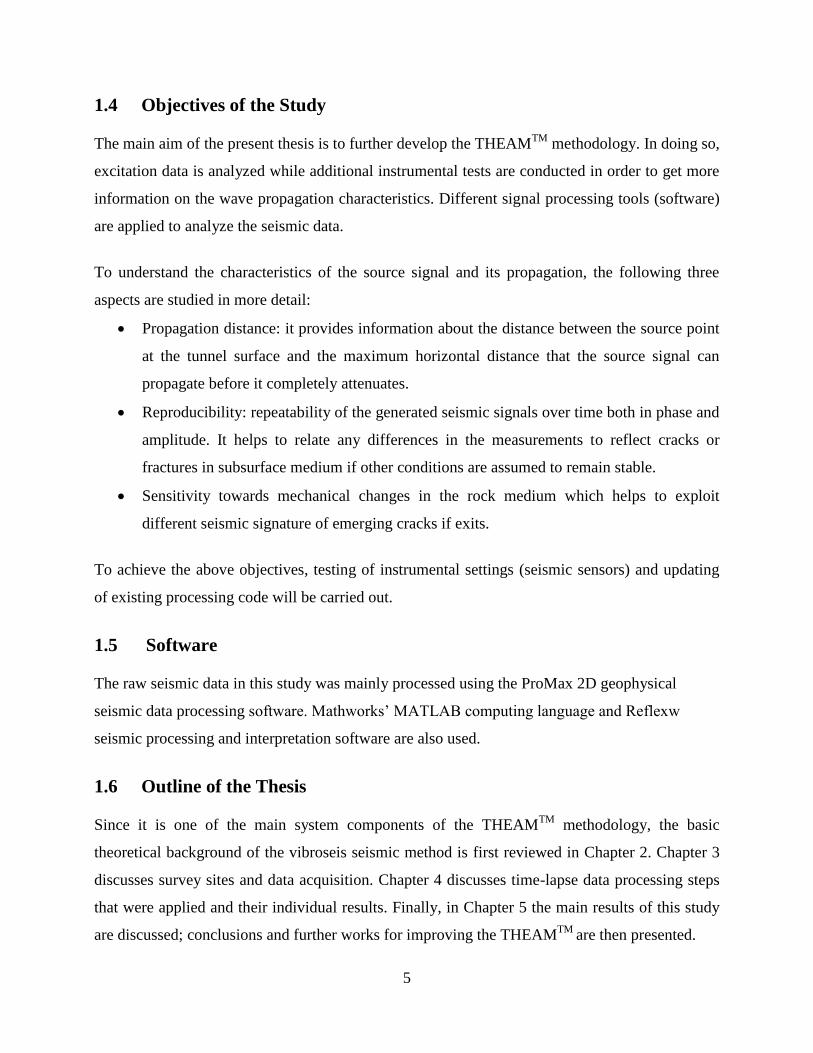
address the two main types of prerequisites (Chapter 1.3). A sketch illustrating the operation
principle and system components of the THEAMTM
approach is shown in Figure 2.1. The
measuring and communication process steps of the THEAM method include:
1. Triggering the shaker, which is attached to the tunnel wall. This is done automatically
each day by NORSAR’s Tunnel Service software that is installed and continuously runs
on the central acquisition PC inside the test tunnel. The shaker emits shear waves
following a predefined sweep signal from the base plate of the shaker. The shaker is kept
in tight contact with the tunnel wall and thereby producing a vibration into the
surrounding rock structure.
2. Seismic responses are recorded by the central acquisition unit (CAU), which consists of a
GEODE field digitizer and laptop PC, through 3-C seismic sensors that are attached to the
wall at various distances to the source.
Figure 2.1: Measuring and communication process steps of the THEAMTM
method.
7
3. Data from each measurement is automatically transferred, using wireless communication
units (WCU), to the SPX Server located at the NORSAR office in Kjeller.
4. Processing and analysis of raw data at NORSAR. Finally, sending out alerts to concerned
authorities if the difference in seismic response is greater than allowable threshold limits.
2.2 Cross-correlation
Cross correlation is used to evaluate the degree of similarity between two time series data sets. It
involves progressively sliding one time series relative to the other; for each time shift
multiplication of the corresponding values of two individual time series and summation of cross
products provide values of cross correlation as a function of shift or lag value. It is
mathematically defined as (Sheriff and Geldart, 1995, Kearey et al., 2009).
∑ (2.1)
Where and are time series data sets, is shift or lag of relative to .
If one time series is correlated with itself then the cross correlation is called autocorrelation
( ). It is a measure of similarity between a signal and time-shifted version of a signal. Most
commonly, the cross correlation function is normalized, using different techniques of
normalization depending on the intended application (Neidell and Taner, 1971). In this study, the
similarity between two traces is measured and the cross correlation coefficient is normalized
following the procedure given by Sheriff (2006):
[ ]
⁄ (2.2)
Where and are zero-lag autocorrelations of and , respectively.
The normalized correlation coefficient ( ) values vary between -1 and 1. The value -1
means the two traces are identical with opposite polarity; zero means they are orthogonal, and
zero similarity; 1 means identical traces with perfect correlation. When similarity is measured by
normalized correlation coefficient the trace amplitude do not influence the results hence
normalized cross-correlation will be insensitive to changes in the scaling of the amplitudes of
either of the input traces (Taner, 1996). Here we measure this similarity between two traces (i.e.,
8
reference trace and monitoring trace) by means normalized cross-correlation to determine how
much the monitoring trace looks like the reference. The reference trace is a trace recorded at the
beginning of the survey and monitoring traces are traces from different day recordings.
2.3 Vibroseis Method
On land seismic investigation methods, as an alternative to explosive or impulsive sources,
vibroseis source is used as seismic energy source to be sent to the ground. Vibroseis is a seismic
method where the energy source is an electrodynamic vibrator that generates a controlled sweep
(Sheriff, 2002). A sweep is continuously oscillating signal of constant amplitude whose
frequency varies linearly or non-linearly with time (Goupillaud, 1976). Very large and small-
scale land vibroseis sources have been developed and used for different geophysical
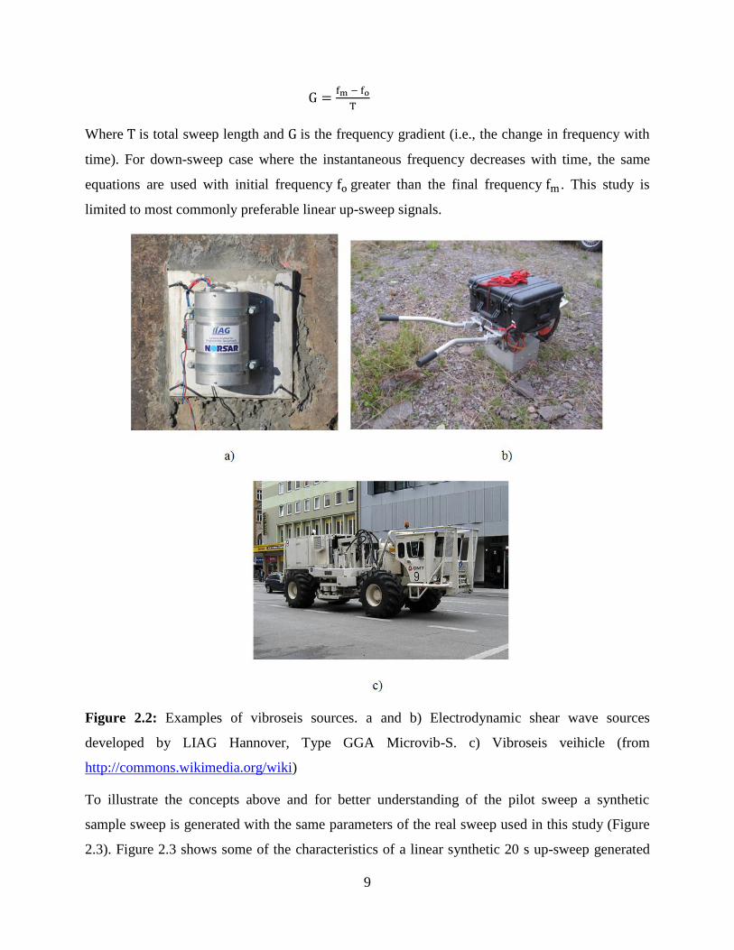
investigations. Some examples of seismic vibroseis sources are shown in Figure 2.2.
Unlike explosives or hammer source the signal emitted by a seismic vibrator has many seconds
duration, which is called a sweep period, typically up to 32 s. Different type of nonlinear sweeps
have been developed and used depending on the intended application (Strong and Hearn, 2009,
Goupillaud, 1976). Particularly, to compensate attenuation of high frequency through the
propagation of the signal where higher frequencies are used for longer time nonlinear sweeps are
preferable.
A linear tapered upsweep where the instantaneous frequency increases linearly from to with
time has a general from (Seriff and Kim, 1970, Baeten, 1989):
(2.3)
Where Q is constant and is special “window” function of time, having a linear or cosine
shape taper at the beginning and at the end, applied to reduce truncation effects (Gibbs
phenomena) that produce side lobes. The instantaneous frequency, , is given by:
[ ] (2.4)
(2.5)
Then constant can be given by:
(2.6)
9
Where is total sweep length and is the frequency gradient (i.e., the change in frequency with
time). For down-sweep case where the instantaneous frequency decreases with time, the same
equations are used with initial frequency greater than the final frequency . This study is
limited to most commonly preferable linear up-sweep signals.
Figure 2.2: Examples of vibroseis sources. a and b) Electrodynamic shear wave sources
developed by LIAG Hannover, Type GGA Microvib-S. c) Vibroseis veihicle (from
http://commons.wikimedia.org/wiki)
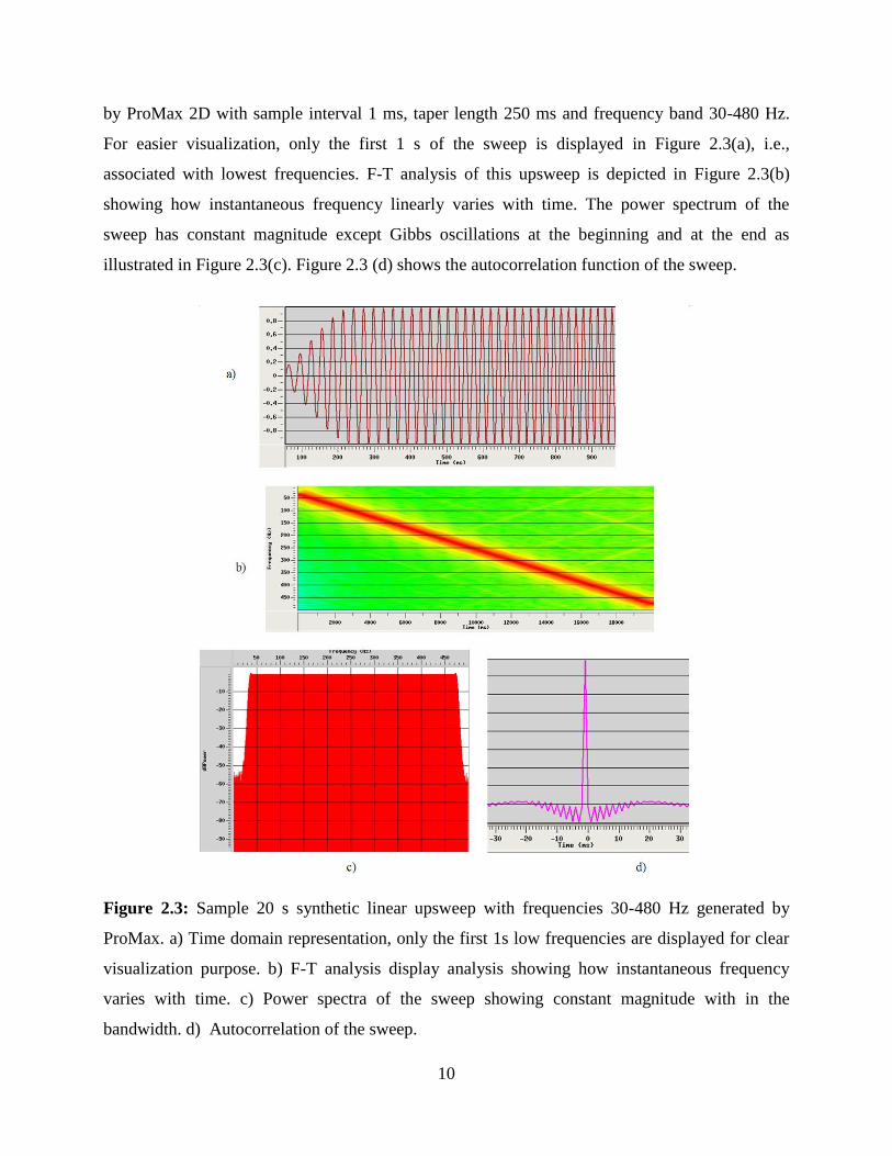
To illustrate the concepts above and for better understanding of the pilot sweep a synthetic
sample sweep is generated with the same parameters of the real sweep used in this study (Figure
2.3). Figure 2.3 shows some of the characteristics of a linear synthetic 20 s up-sweep generated
10
by ProMax 2D with sample interval 1 ms, taper length 250 ms and frequency band 30-480 Hz.
For easier visualization, only the first 1 s of the sweep is displayed in Figure 2.3(a), i.e.,
associated with lowest frequencies. F-T analysis of this upsweep is depicted in Figure 2.3(b)
showing how instantaneous frequency linearly varies with time. The power spectrum of the
sweep has constant magnitude except Gibbs oscillations at the beginning and at the end as
illustrated in Figure 2.3(c). Figure 2.3 (d) shows the autocorrelation function of the sweep.
Figure 2.3: Sample 20 s synthetic linear upsweep with frequencies 30-480 Hz generated by
ProMax. a) Time domain representation, only the first 1s low frequencies are displayed for clear
visualization purpose. b) F-T analysis display analysis showing how instantaneous frequency
varies with time. c) Power spectra of the sweep showing constant magnitude with in the
bandwidth. d) Autocorrelation of the sweep.
11
In vibroseis acquisition, the resulting field record, which is called vibrogram, is the superposition
of wave trains due to the embedded sweep. To obtain a meaningful recording, the vibrogram is
cross-correlated with the pilot sweep and the resulting trace is known as correlogram. If the
sweep source signal is and the response from the ground is then the recorded trace
from the geophones, employing convolution trace model, is given as:
(2.7)
Where * indicates convolution
Since convolution in time domain is equal to multiplication in frequency domain, the above
equation in frequency domain can be written as:
(2.8)
Where indicates multiplication, ω is the angular frequency and the capital letters indicate
Fourier transforms.
Assuming that the source signal and the pilot sweep are identical then cross correlation of
recorded trace with pilot sweep is given as:
(2.9)
Combining equation (2.7) and (2.9) gives:
(2.10)
Since cross correlation in time domain is the same as convolution with time reversed:
(2.11)
Since convolution is commutative:
[ ] (2.12)
(2.13)
Where is autocorrelation of the sweep. Substituting equation (2.13) in (2.12) gives:
(2.14)
Where and is correlated seismogram. In frequency domain:
(2.15)
12
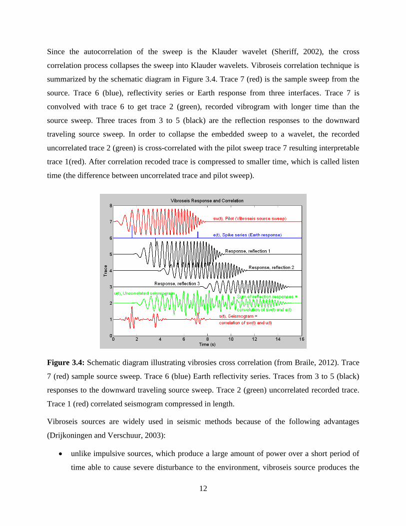
Since the autocorrelation of the sweep is the Klauder wavelet (Sheriff, 2002), the cross
correlation process collapses the sweep into Klauder wavelets. Vibroseis correlation technique is
summarized by the schematic diagram in Figure 3.4. Trace 7 (red) is the sample sweep from the
source. Trace 6 (blue), reflectivity series or Earth response from three interfaces. Trace 7 is
convolved with trace 6 to get trace 2 (green), recorded vibrogram with longer time than the
source sweep. Three traces from 3 to 5 (black) are the reflection responses to the downward
traveling source sweep. In order to collapse the embedded sweep to a wavelet, the recorded
uncorrelated trace 2 (green) is cross-correlated with the pilot sweep trace 7 resulting interpretable
trace 1(red). After correlation recoded trace is compressed to smaller time, which is called listen
time (the difference between uncorrelated trace and pilot sweep).
Figure 3.4: Schematic diagram illustrating vibrosies cross correlation (from Braile, 2012). Trace
7 (red) sample source sweep. Trace 6 (blue) Earth reflectivity series. Traces from 3 to 5 (black)
responses to the downward traveling source sweep. Trace 2 (green) uncorrelated recorded trace.
Trace 1 (red) correlated seismogram compressed in length.
Vibroseis sources are widely used in seismic methods because of the following advantages
(Drijkoningen and Verschuur, 2003):
unlike impulsive sources, which produce a large amount of power over a short period of
time able to cause severe disturbance to the environment, vibroseis source produces the

13
same power over longer period of time resulting in much less destructive effects so that it
can operate in urban environments.
seismic vibrator sources are repeatable and the amplitude, frequency and phase of the
outgoing signal are controllable.
explosive sources are labor intensive due to the need to drill holes in order to bury the
source.
One of the main problems with vibroseis data is harmonic distortion (Seriff and Kim, 1970).
Harmonic distortion is caused by nonlinear processes, mainly from the coupling of the vibrator to
the ground. For this reason, the source signal from the vibrator injected into the ground is not
exactly the same as the pilot sweep. Considering the addition of the harmonic on the pilot
sweep, the harmonically distorted outgoing signal is given by Seriff and Kim (1970):
(2.16)
Then equation 2.7 becomes:
[ ] (2.17)
Then cross correlation with pilot sweep gives:
[ ] (2.18)
Where is cross correlation of and and it is the resulting correlation artifact due
to harmonic distortion.
As clearly explained by Seriff and Kim (1970), the effect of harmonic distortion is to produce a
large correlation artifact, a ‘forerunner’ for up-sweep source and or a ‘tail’ using down-sweep
source during correlation process with the pilot sweep. Different techniques have been developed
in elimination of such artifacts before correlation (Li et al., 1995, Stiller et al., 2012) and after
correlation (Polom, 1997).
2.4 Repeatability in Land Seismic Data
One of the main factors, which determine the success of any time-laps seismic method, is the
repeatability of the seismic experiment. Repeatability helps to remove differences between the
seismic surveys that are not due to new changes in the surrounding rock, and hence helps to relate

14
any significant differences in measured signal to reflect genuine emerging cracks over time. In
general, repeatability of the surface vibrator data is affected by the following factors (Jervis et al.,
2012, Pevzner et al., 2011, Marelli et al., 2010):
i. Inherent fidelity of the source,
ii. Source and receiver geometry or location errors,
iii. Changes in acquisition parameter,
iv. Vibrator interaction with the ground (inconsistent coupling), and
v. Daily/seasonal variations in the surrounding and ambient noise.
Even slight variations in any of these factors will affect the repeatability of the survey. With
respect to the THEAMTM
methodology, the first factor is reduced by the shaker’s ability to
generate seismic signals which are fully reproducible and controllable both in phase and
amplitude. This requires input conditions that must be as similar as possible so that amplitude,
phase and spectral content are constant over time and hence create a stable source signature. The
second and the third factors are addressed by taking all surveys in a consistent fashion, i.e. no
changes in the mounting conditions of the shaker and the receivers, no exchange of cables, and
using the same acquisition setup and parameters for all surveys.
To evaluate repeatability of the THEAMTM
system, which is more related to the reproducibility
of the shaker and its coupling to the wall, a simple test was out. For this purpose, one commonly
used metric, normalized-root-mean-square (NRMS), which is the RMS of the difference of two
traces divided by the average RMS of the inputs and expressed in percentage, will be computed.
NRMS of the two traces and within a given time window - is given by Kragh and
Christie (2002):
{
(
)} (2.19)
Where is the monitoring trace, is the chosen reference trace, and the RMS operator is defined
as:
√∑
(2.20)

15
Where is the RMS amplitude; is the amplitude; N is the number of samples within time
window - . As described by Kragh and Christie (2001) NRMS is extremely sensitive to phase
or amplitude differences in the data. NRMS values ranges from 0, for perfectly similar traces, to
200 for, anti-correlated, out of phase traces; thus, NRMS values should be lower for repeatable
data sets.
2.5 Coverage Distance
Amplitude decay with offset can provide an indication of the signal propagation distance. The
signal amplitude from the source is less than or equal to the energy of background noise after
propagating a certain offset. This will tell the horizontal range of the tunnel that the system can
monitor. In this study, signal propagation maximum horizontal distance limit is defined as a
distance where the source-generated energy ceases to decrease spatially and amplitudes are on the
same level as the incoherent background noise (Yordkayhun et al., 2009). The distance
corresponding to this offset give information on the maximum horizontal distance of effective
signal propagation, since amplitudes after this offset are almost entirely dominated by ambient
noise and hence are not repeatable.
Here computing of this maximum distance is done in three steps which are adopted from
(Wuxiang et al., 2007):
1) Computing the RMS amplitude of the signal and the background noise from real data
within a time window - : using the formula given in equation 2.20, the RMS
amplitude of every trace at different receiver location can be computed. The variation of
can reflects the relationship of the amplitude variation with offset so that an energy
decay equation can be quantitatively fitted. The RMS amplitude of the background noise
is also computed using equation 2.20 within a time window at a later time.
2) Fitting an energy decay equation: depending the character of , a model function is
chosen to fit the relationship of with distance.
3) Determining the maximum horizontal monitoring distance combined with background
noise.

16
2.6 Seismic Expression in Propagation through Cracks
Seismic methods can be used to deduce rock fracture from remote measurements. Works on
effects of cracks on seismic wave propagation suggests that (Pyrak-Nolte, 1996, Boadu and
Long, 1996, Pyrak‐Nolte et al., 1990): cracks decrease seismic wave velocities and increase
velocity dispersion. The wavelet shows amplitude and phase changes as it propagates. These
effects of fractures on wave propagation are seen for fractures at all scales from micro cracks to
crustal faults. Boadu and Long (1996) showed that even single fracture causes frequency
dependent reflections, refractions and group time delays in plane waves. It can also trap energy as
interface waves, and have a profound influence on the propagating seismic waveform. It is these
distinctive seismic signatures that we are going to use to detect newly emerging cracks using
THEAMTM
methodology.
17
Chapter 3: SURVEY SITES AND DATA ACQUISITION
3.1 Survey Sites
In the course of investigating and further developing the THEAMTM
methodology, two data
collection sites were studied. The first survey site was the Oslofjord tunnel. The Oslofjord tunnel
is a subsea road tunnel that is located some 50 km south of Oslo (Norway). It provides an
alternative method of transportation between the east and the west side of the Oslofjord. With its
7,230 m length, deepest part 134 m below sea level, 11.0 m underground width and a maximum
gradient of 7% it represents one of the longest subsea tunnel in Northern Europe. The rocks in the
Oslofjord tunnel mainly consist of granitic augen gneiss. The Oslofjord tunnel is one of the
infrastructures in Norway, which are often in the focus of the media since a number of severe
incidents happened in recent years. That is why it was chosen to conduct continuous monitoring
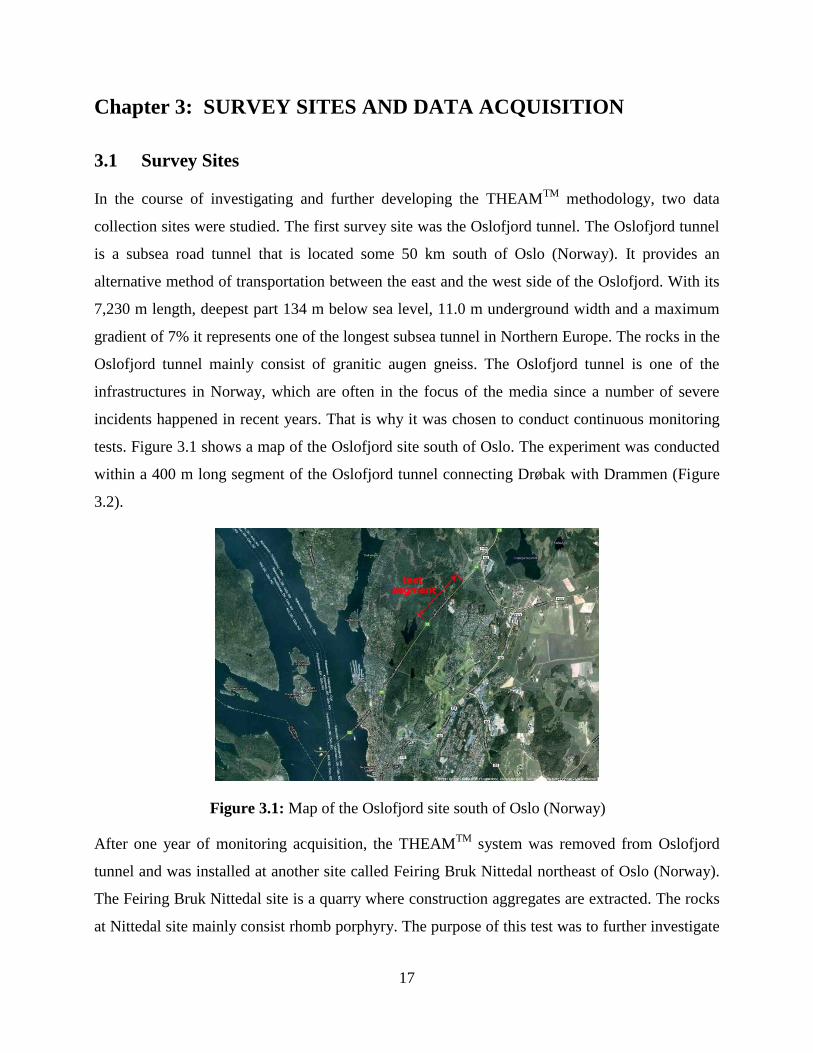
tests. Figure 3.1 shows a map of the Oslofjord site south of Oslo. The experiment was conducted
within a 400 m long segment of the Oslofjord tunnel connecting Drøbak with Drammen (Figure
3.2).
Figure 3.1: Map of the Oslofjord site south of Oslo (Norway)
After one year of monitoring acquisition, the THEAMTM
system was removed from Oslofjord
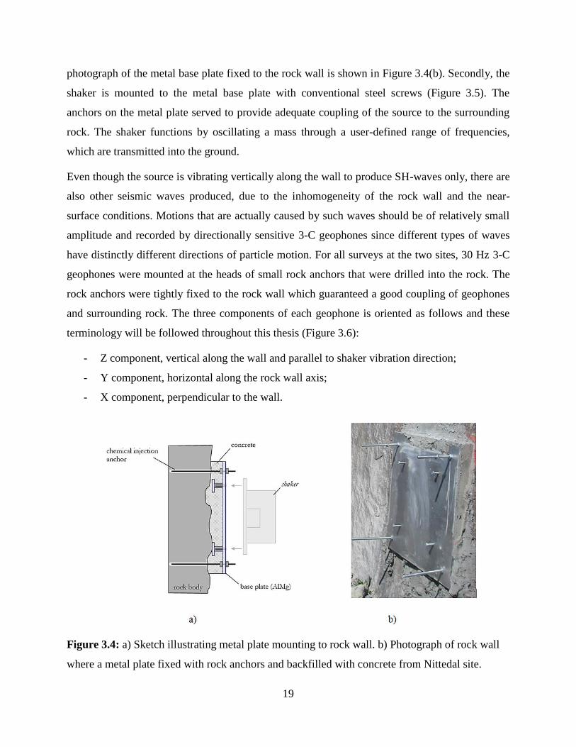
tunnel and was installed at another site called Feiring Bruk Nittedal northeast of Oslo (Norway).
The Feiring Bruk Nittedal site is a quarry where construction aggregates are extracted. The rocks
at Nittedal site mainly consist rhomb porphyry. The purpose of this test was to further investigate
18
source propagation characteristics and sensitivity of the THEAMTM
system. Photographs of the
site are displayed in Figure 3.3.
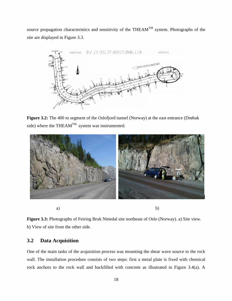
Figure 3.2: The 400 m segment of the Oslofjord tunnel (Norway) at the east entrance (Drøbak
side) where the THEAMTM
system was instrumented.
Figure 3.3: Photographs of Feiring Bruk Nittedal site northeast of Oslo (Norway). a) Site view.
b) View of site from the other side.
3.2 Data Acquisition
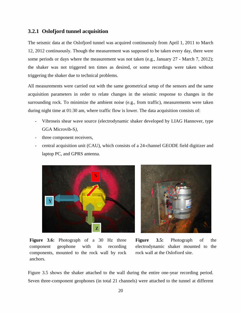
One of the main tasks of the acquisition process was mounting the shear wave source to the rock
wall. The installation procedure consists of two steps: first a metal plate is fixed with chemical
rock anchors to the rock wall and backfilled with concrete as illustrated in Figure 3.4(a). A
19
photograph of the metal base plate fixed to the rock wall is shown in Figure 3.4(b). Secondly, the
shaker is mounted to the metal base plate with conventional steel screws (Figure 3.5). The
anchors on the metal plate served to provide adequate coupling of the source to the surrounding
rock. The shaker functions by oscillating a mass through a user-defined range of frequencies,
which are transmitted into the ground.
Even though the source is vibrating vertically along the wall to produce SH-waves only, there are
also other seismic waves produced, due to the inhomogeneity of the rock wall and the near-
surface conditions. Motions that are actually caused by such waves should be of relatively small
amplitude and recorded by directionally sensitive 3-C geophones since different types of waves
have distinctly different directions of particle motion. For all surveys at the two sites, 30 Hz 3-C
geophones were mounted at the heads of small rock anchors that were drilled into the rock. The
rock anchors were tightly fixed to the rock wall which guaranteed a good coupling of geophones
and surrounding rock. The three components of each geophone is oriented as follows and these
terminology will be followed throughout this thesis (Figure 3.6):
- Z component, vertical along the wall and parallel to shaker vibration direction;
- Y component, horizontal along the rock wall axis;
- X component, perpendicular to the wall.
Figure 3.4: a) Sketch illustrating metal plate mounting to rock wall. b) Photograph of rock wall
where a metal plate fixed with rock anchors and backfilled with concrete from Nittedal site.
20
3.2.1 Oslofjord tunnel acquisition
The seismic data at the Oslofjord tunnel was acquired continuously from April 1, 2011 to March
12, 2012 continuously. Though the measurement was supposed to be taken every day, there were
some periods or days where the measurement was not taken (e.g., January 27 - March 7, 2012);
the shaker was not triggered ten times as desired, or some recordings were taken without
triggering the shaker due to technical problems.
All measurements were carried out with the same geometrical setup of the sensors and the same
acquisition parameters in order to relate changes in the seismic response to changes in the
surrounding rock. To minimize the ambient noise (e.g., from traffic), measurements were taken
during night time at 01:30 am, where traffic flow is lower. The data acquisition consists of:
- Vibroseis shear wave source (electrodynamic shaker developed by LIAG Hannover, type
GGA Microvib-S),
- three component receivers,
- central acquisition unit (CAU), which consists of a 24-channel GEODE field digitizer and
laptop PC, and GPRS antenna.
Figure 3.5 shows the shaker attached to the wall during the entire one-year recording period.
Seven three-component geophones (in total 21 channels) were attached to the tunnel at different
Figure 3.6: Photograph of a 30 Hz three
component geophone with its recording
components, mounted to the rock wall by rock
anchors.
Figure 3.5: Photograph of the
electrodynamic shaker mounted to the
rock wall at the Oslofjord site.
21
distances from 5 m to 90 m to the shaker (Figure 3.7). Due to large irregularities of the tunnel
wall it was difficult to place geophones in equal spacing, so the spacing between the various
geophones were different. Figure 3.9 shows a schematic diagram of the S-wave source and
geophones placement illustrating the geophone spacing and their distance from the source.
Numbers in red color, above each geophone, shows the distance from the source and numbers
with black color below indicate the geophone numbering starting from the first geophone near to
the shaker.
The shaker was triggered automatically each day by the NORSAR Tunnel Service software that
is installed and continuously runs on the central acquisition PC inside the test tunnel. The shaker
then transmits a predefined sweep signal with a frequency band 30−480 Hz (20 s duration) into
the surrounding rock wall by the vibrator plate vibrating in vertical (Z) direction. The response of
the rock wall coming from the 21 channels is then recorded by the central acquisition unit (CAU)
with a recording length of 22 s. The 20 sec long sweep signal is recorded on channel 22.
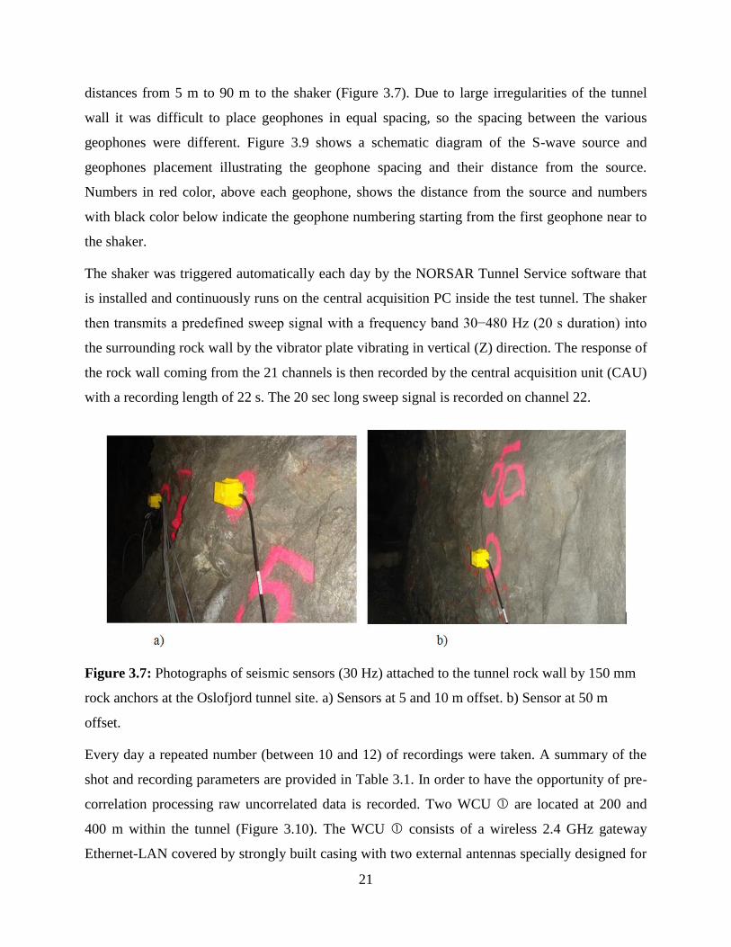
Figure 3.7: Photographs of seismic sensors (30 Hz) attached to the tunnel rock wall by 150 mm
rock anchors at the Oslofjord tunnel site. a) Sensors at 5 and 10 m offset. b) Sensor at 50 m
offset.
Every day a repeated number (between 10 and 12) of recordings were taken. A summary of the
shot and recording parameters are provided in Table 3.1. In order to have the opportunity of pre-
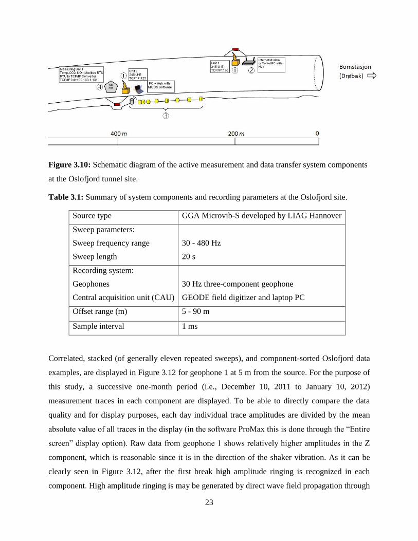
correlation processing raw uncorrelated data is recorded. Two WCU are located at 200 and
400 m within the tunnel (Figure 3.10). The WCU consists of a wireless 2.4 GHz gateway
Ethernet-LAN covered by strongly built casing with two external antennas specially designed for
22
tunnel applications (Figure 3.11). The WCU at 400 m transfers raw uncorrelated data from
CAU to WCU at 200 m. The WCU at 200 m delivers the received data to the Internet
modem placed next to it. Then the data is transferred to the central data processing center at
NORSAR for further processing and analysis.
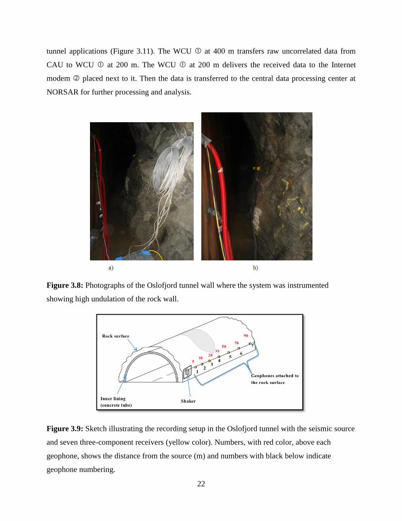
Figure 3.8: Photographs of the Oslofjord tunnel wall where the system was instrumented
showing high undulation of the rock wall.
Figure 3.9: Sketch illustrating the recording setup in the Oslofjord tunnel with the seismic source
and seven three-component receivers (yellow color). Numbers, with red color, above each
geophone, shows the distance from the source (m) and numbers with black below indicate
geophone numbering.
23
Figure 3.10: Schematic diagram of the active measurement and data transfer system components
at the Oslofjord tunnel site.
Table 3.1: Summary of system components and recording parameters at the Oslofjord site.
Source type GGA Microvib-S developed by LIAG Hannover
Sweep parameters:
Sweep frequency range
Sweep length
30 - 480 Hz
20 s
Recording system:
Geophones
Central acquisition unit (CAU)
30 Hz three-component geophone
GEODE field digitizer and laptop PC
Offset range (m) 5 - 90 m
Sample interval 1 ms
Correlated, stacked (of generally eleven repeated sweeps), and component-sorted Oslofjord data
examples, are displayed in Figure 3.12 for geophone 1 at 5 m from the source. For the purpose of
this study, a successive one-month period (i.e., December 10, 2011 to January 10, 2012)
measurement traces in each component are displayed. To be able to directly compare the data
quality and for display purposes, each day individual trace amplitudes are divided by the mean
absolute value of all traces in the display (in the software ProMax this is done through the “Entire
screen” display option). Raw data from geophone 1 shows relatively higher amplitudes in the Z
component, which is reasonable since it is in the direction of the shaker vibration. As it can be
clearly seen in Figure 3.12, after the first break high amplitude ringing is recognized in each
component. High amplitude ringing is may be generated by direct wave field propagation through
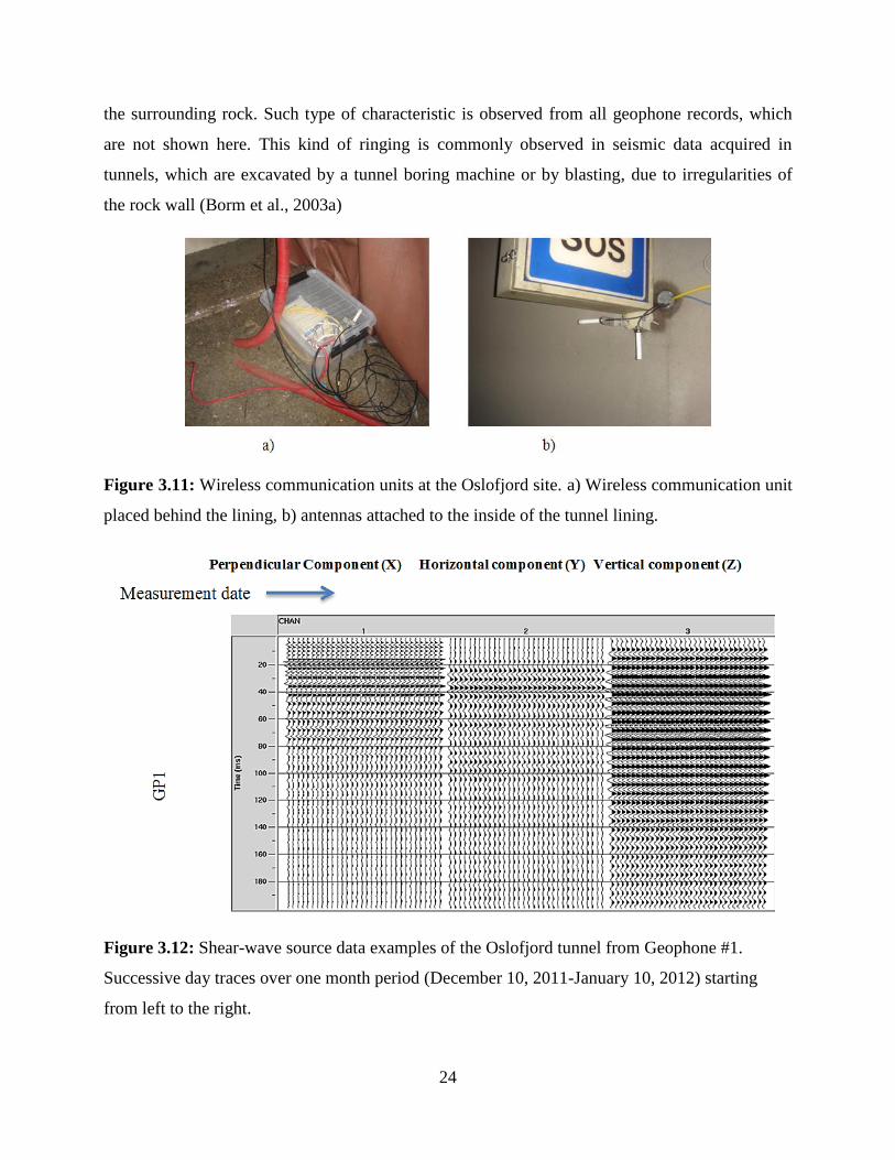
24
the surrounding rock. Such type of characteristic is observed from all geophone records, which
are not shown here. This kind of ringing is commonly observed in seismic data acquired in
tunnels, which are excavated by a tunnel boring machine or by blasting, due to irregularities of
the rock wall (Borm et al., 2003a)
Figure 3.11: Wireless communication units at the Oslofjord site. a) Wireless communication unit
placed behind the lining, b) antennas attached to the inside of the tunnel lining.
Figure 3.12: Shear-wave source data examples of the Oslofjord tunnel from Geophone #1.
Successive day traces over one month period (December 10, 2011-January 10, 2012) starting
from left to the right.
25
3.2.2 Feiring Bruk Nittedal site acquisition
3.2.2.1 Shear wave source
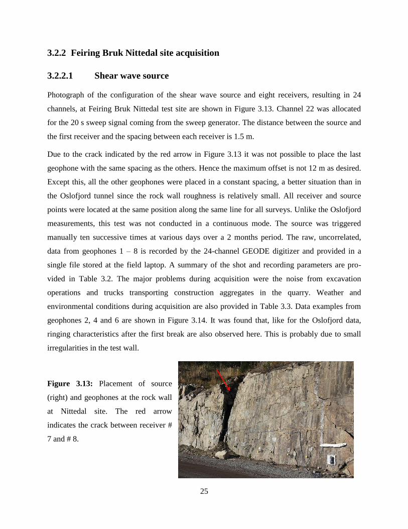
Photograph of the configuration of the shear wave source and eight receivers, resulting in 24
channels, at Feiring Bruk Nittedal test site are shown in Figure 3.13. Channel 22 was allocated
for the 20 s sweep signal coming from the sweep generator. The distance between the source and
the first receiver and the spacing between each receiver is 1.5 m.
Due to the crack indicated by the red arrow in Figure 3.13 it was not possible to place the last
geophone with the same spacing as the others. Hence the maximum offset is not 12 m as desired.
Except this, all the other geophones were placed in a constant spacing, a better situation than in
the Oslofjord tunnel since the rock wall roughness is relatively small. All receiver and source
points were located at the same position along the same line for all surveys. Unlike the Oslofjord
measurements, this test was not conducted in a continuous mode. The source was triggered
manually ten successive times at various days over a 2 months period. The raw, uncorrelated,
data from geophones 1 – 8 is recorded by the 24-channel GEODE digitizer and provided in a
single file stored at the field laptop. A summary of the shot and recording parameters are pro-
vided in Table 3.2. The major problems during acquisition were the noise from excavation
operations and trucks transporting construction aggregates in the quarry. Weather and
environmental conditions during acquisition are also provided in Table 3.3. Data examples from
geophones 2, 4 and 6 are shown in Figure 3.14. It was found that, like for the Oslofjord data,
ringing characteristics after the first break are also observed here. This is probably due to small
irregularities in the test wall.
Figure 3.13: Placement of source
(right) and geophones at the rock wall
at Nittedal site. The red arrow
indicates the crack between receiver #
7 and # 8.
26
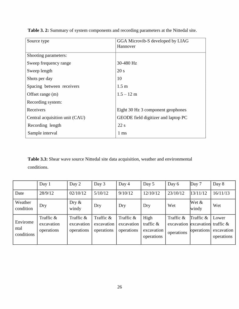
Table 3. 2: Summary of system components and recording parameters at the Nittedal site.
Source type GGA Microvib-S developed by LIAG
Hannover
Shooting parameters:
Sweep frequency range
Sweep length
Shots per day
30-480 Hz
20 s
10
Spacing between receivers 1.5 m
Offset range (m) 1.5 – 12 m
Recording system:
Receivers
Central acquisition unit (CAU)
Eight 30 Hz 3 component geophones
GEODE field digitizer and laptop PC
Recording length 22 s
Sample interval 1 ms
Table 3.3: Shear wave source Nittedal site data acquisition, weather and environmental
conditions.
Day 1 Day 2 Day 3 Day 4 Day 5 Day 6 Day 7 Day 8
Date 28/9/12 02/10/12 5/10/12 9/10/12 12/10/12 23/10/12 13/11/12 16/11/13
Weather
condition Dry
Dry &
windy Dry Dry Dry Wet
Wet &
windy Wet
Envirome
ntal
conditions
Traffic &
excavation
operations
Traffic &
excavation
operations
Traffic &
excavation
operations
Traffic &
excavation
operations
High
traffic &
excavation
operations
Traffic &
excavation
operations
Traffic &
excavation
operations
Lower
traffic &
excavation
operations
27
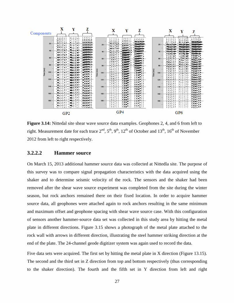
Figure 3.14: Nittedal site shear wave source data examples. Geophones 2, 4, and 6 from left to
right. Measurement date for each trace 2nd
, 5th
, 9th
, 12th
of October and 13th
, 16th
of November
2012 from left to right respectively.
3.2.2.2 Hammer source
On March 15, 2013 additional hammer source data was collected at Nittedla site. The purpose of
this survey was to compare signal propagation characteristics with the data acquired using the
shaker and to determine seismic velocity of the rock. The sensors and the shaker had been
removed after the shear wave source experiment was completed from the site during the winter
season, but rock anchors remained there on their fixed location. In order to acquire hammer
source data, all geophones were attached again to rock anchors resulting in the same minimum
and maximum offset and geophone spacing with shear wave source case. With this configuration
of sensors another hammer-source data set was collected in this study area by hitting the metal
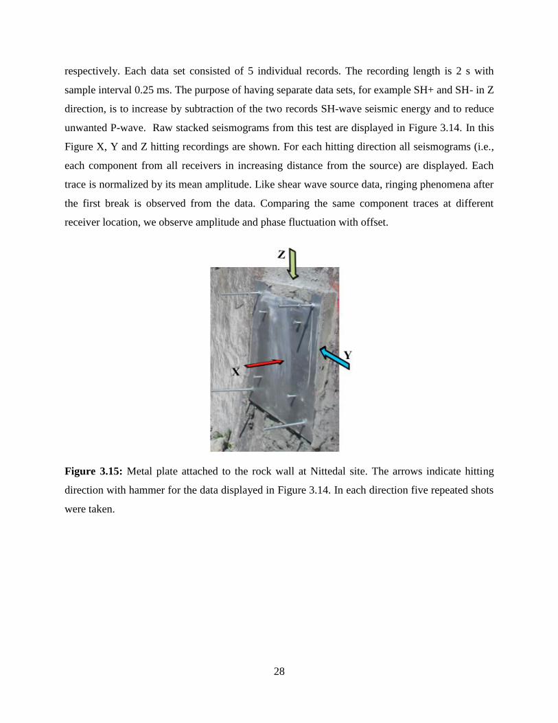
plate in different directions. Figure 3.15 shows a photograph of the metal plate attached to the
rock wall with arrows in different direction, illustrating the steel hammer striking direction at the
end of the plate. The 24-channel geode digitizer system was again used to record the data.
Five data sets were acquired. The first set by hitting the metal plate in X direction (Figure 13.15).
The second and the third set in Z direction from top and bottom respectively (thus corresponding
to the shaker direction). The fourth and the fifth set in Y direction from left and right
28
respectively. Each data set consisted of 5 individual records. The recording length is 2 s with
sample interval 0.25 ms. The purpose of having separate data sets, for example SH+ and SH- in Z
direction, is to increase by subtraction of the two records SH-wave seismic energy and to reduce
unwanted P-wave. Raw stacked seismograms from this test are displayed in Figure 3.14. In this
Figure X, Y and Z hitting recordings are shown. For each hitting direction all seismograms (i.e.,
each component from all receivers in increasing distance from the source) are displayed. Each
trace is normalized by its mean amplitude. Like shear wave source data, ringing phenomena after
the first break is observed from the data. Comparing the same component traces at different
receiver location, we observe amplitude and phase fluctuation with offset.
Figure 3.15: Metal plate attached to the rock wall at Nittedal site. The arrows indicate hitting
direction with hammer for the data displayed in Figure 3.14. In each direction five repeated shots
were taken.
29
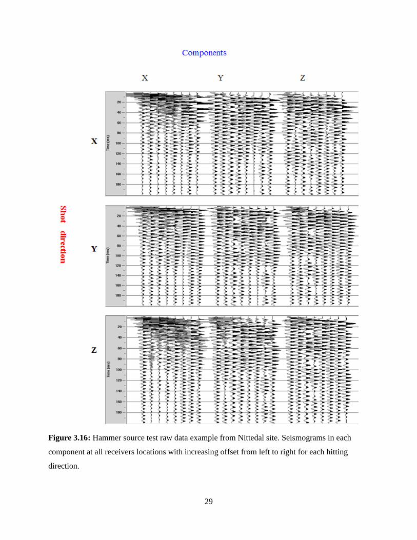
Figure 3.16: Hammer source test raw data example from Nittedal site. Seismograms in each
component at all receivers locations with increasing offset from left to right for each hitting
direction.

30
Chapter 4: DATA PROCESSING STEPS AND RESULTS
4.1 Data Processing Steps
To infer newly emerging geological changes over time by comparing each day recording, the
same processing parameters and steps were used for all data sets. All data processing is done
using the software tools ProMax 2D, MATLAB and Reflexw. The data processing procedure for
the shear wave source at both sites and the hammer source (only at the Nittedal site) consists of:
Shear wave source
1. Importing raw data in SEG2 format and cleaning of the pilot sweep
2. Cross correlation of vibrograms with cleaned sweep
3. Stacking repeated sweeps each day and component sorting
4. Amplitude spectra analysis
5. Band pass filter
6. Repeatability test
1. Coverage distance estimation (only for the Oslofjord site)
2. Velocity estimation
3. Resonance frequency and peak power monitoring analysis
4. Cross correlation monitoring analysis
Hammer source test
1. Importing SEGY data
2. Stacking repeated shots and component sorting
3. Amplitude spectra analysis.
4. Band pass filter
5. Subtraction in of opposite direction shots in Y and Z directions
6. Exporting to Reflexw and velocity computation

31
Each processing step with its corresponding results will be presented in detail in the following
subsections.
4.2 Importing Data and Pilot Sweep Cleaning
Both, data in SEGY and SEG2 format (for the hammer source and the shear-wave source,
respectively) were imported to ProMax 2D. After importing the shear-wave source data it was
found that all pilot sweep (channel 22) recordings were distorted by harmonic noise. An example
of a recorded pilot sweep, only the first 500 ms for clear display purpose, is shown in Figure
4.1(a). As it is shown, the pilot sweep looks like clipped in time domain representation due to the
harmonic distortion. Figure 4.1(b) depicts the frequency-time (f-t) analysis of the pilot sweep
showing more clearly contamination of the pilot sweep with the 3rd
harmonic. This harmonic
distortion is maybe due to electronic crosstalk between the Geode acquisition unit and the sweep
generator, and the high sensitivity of the “high gain” acquisition parameter (U. Polom, 2012,
personal communication). Therefore, before the cross correlation step, the harmonic noise had to
be cleaned from the pilot sweep.
Figure 4.1: a) Raw pilot sweep signal with only the first 500 ms for display purpose. b) f-t
analysis of pilot sweep, clearly showing the harmonic with different frequency range and gradient
32
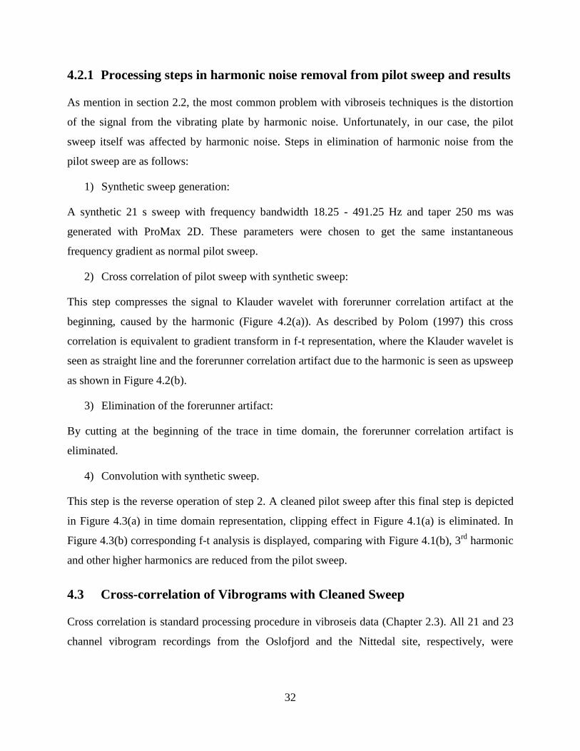
4.2.1 Processing steps in harmonic noise removal from pilot sweep and results
As mention in section 2.2, the most common problem with vibroseis techniques is the distortion
of the signal from the vibrating plate by harmonic noise. Unfortunately, in our case, the pilot
sweep itself was affected by harmonic noise. Steps in elimination of harmonic noise from the
pilot sweep are as follows:
1) Synthetic sweep generation:
A synthetic 21 s sweep with frequency bandwidth 18.25 - 491.25 Hz and taper 250 ms was
generated with ProMax 2D. These parameters were chosen to get the same instantaneous
frequency gradient as normal pilot sweep.
2) Cross correlation of pilot sweep with synthetic sweep:
This step compresses the signal to Klauder wavelet with forerunner correlation artifact at the
beginning, caused by the harmonic (Figure 4.2(a)). As described by Polom (1997) this cross
correlation is equivalent to gradient transform in f-t representation, where the Klauder wavelet is
seen as straight line and the forerunner correlation artifact due to the harmonic is seen as upsweep
as shown in Figure 4.2(b).
3) Elimination of the forerunner artifact:
By cutting at the beginning of the trace in time domain, the forerunner correlation artifact is
eliminated.
4) Convolution with synthetic sweep.
This step is the reverse operation of step 2. A cleaned pilot sweep after this final step is depicted
in Figure 4.3(a) in time domain representation, clipping effect in Figure 4.1(a) is eliminated. In
Figure 4.3(b) corresponding f-t analysis is displayed, comparing with Figure 4.1(b), 3rd
harmonic
and other higher harmonics are reduced from the pilot sweep.
4.3 Cross-correlation of Vibrograms with Cleaned Sweep
Cross correlation is standard processing procedure in vibroseis data (Chapter 2.3). All 21 and 23
channel vibrogram recordings from the Oslofjord and the Nittedal site, respectively, were
33
correlated with the cleaned pilot sweep. By doing this, 22 s long vibrograms were compressed to
2 s correlograms. The embedded sweep is compressed to a Klauder wavelet.
Figure 4.2: a) Cross correlation of pilot sweep with synthetic sweep. b) F-T analysis of cross
correlation.
Figure 4.3: a) Cleaned pilot sweep signal with only the first 500 ms for display purpose.
Clipping due to harmonic distortion is eliminated. b) Corresponding f-t display.
34
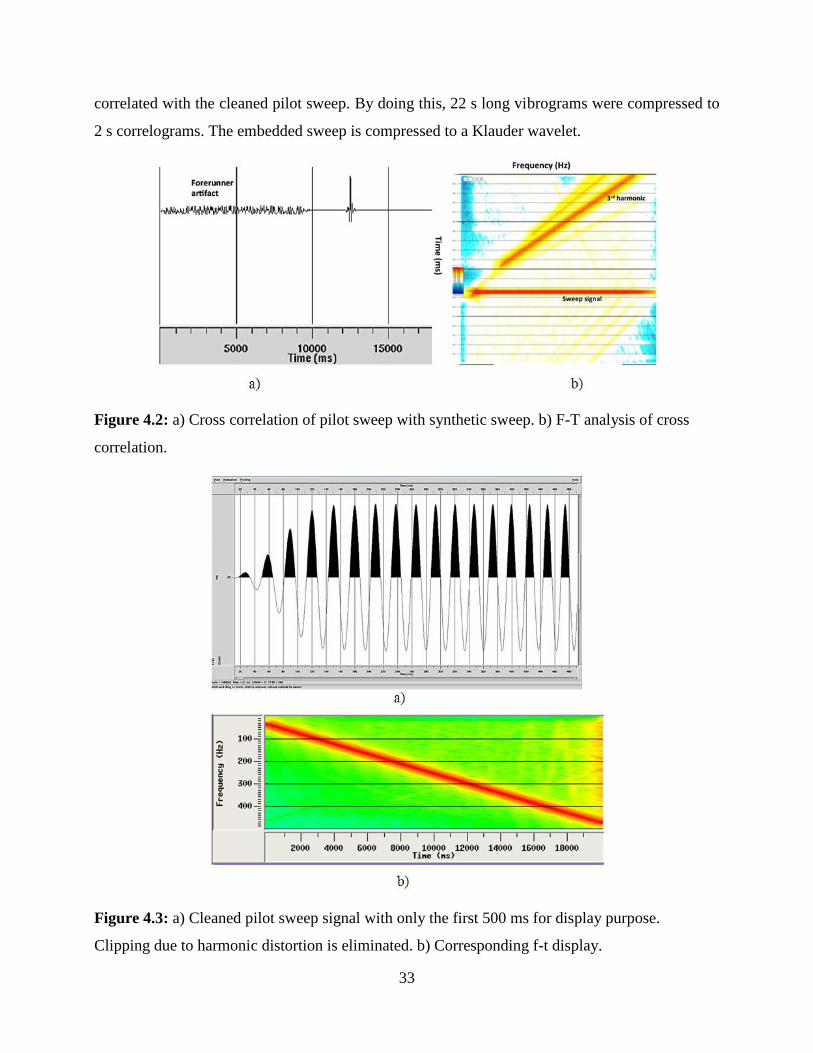
4.4 Stacking Repeated Sweep Each Day and Component Sorting
Stacking is one of the crucial techniques, which plays an important role in improving the signal-
to-noise ratio (S/R) in seismic data processing. A number of repeated correlograms from each day
measurements (11 for the Oslofjord site and 10 for the Nittedal site) were stacked in such a way
that repeatable parts of the signal build up to produce higher resultant amplitudes, while the noise,
being random, has a tendency to cancel itself, or at least to build up much more slowly (Cooper,
2002). For the hammer source case, 5 repeated strokes in the same direction were stacked after
importing the data.
4.5 Spectral Analysis
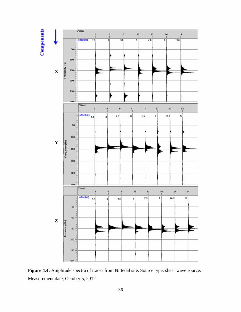
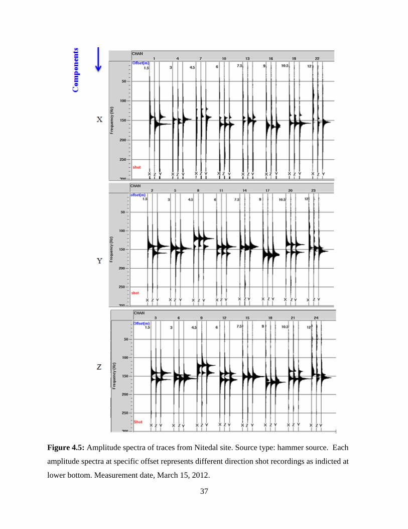
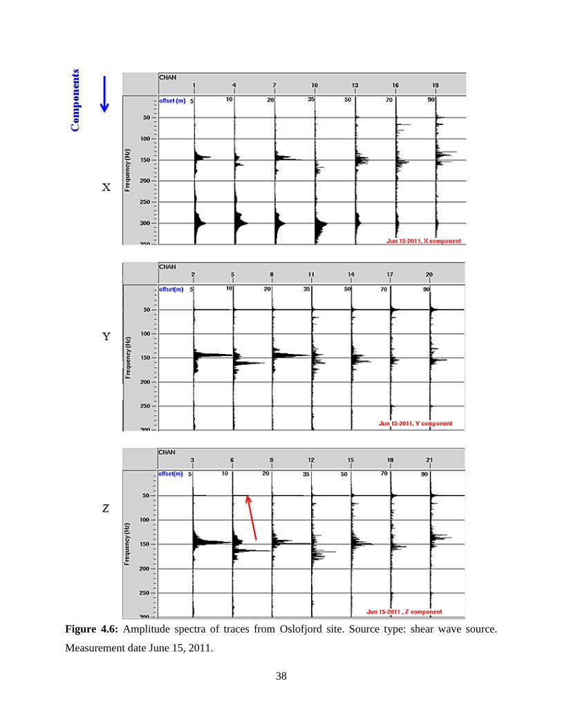
For each site, the amplitude spectra of the traces in each component were computed. The spectra
were computed using 1 s windows. Figure 4.4 shows each component (X, Y and Z) computed
amplitude spectra for the Nittedal site, with the shear wave source. Though the emitted signal has
a constant amplitude within the frequency band 30 - 480 Hz, very high spectral amplitude peaks
at specific frequencies were observed. These spectral peaks are within the frequency bandwidth
of 130 - 170 Hz in both Y and Z components. In X component additional spectral peaks are
observed after 260 Hz. In Figure 4.5 each component (indicated by the blue arrow) amplitude
spectra from the Nittedal site data with the hammer source are displayed. The hitting directions
are shown at the bottom of the traces. The spectral amplitude peaks are also observed with the
hammer source case suggesting a significant connection between this characteristics and the
geology of the rock wall. Moreover the observed resonance frequencies at Nittedal site for shaker
and hammer sources are not that much different this may indicate the effect of the metal plate and
the mounting of the geophones. Figure 4.6 shows amplitude spectra of traces from Oslofjord site,
recordings. The high spectral amplitude peaks can be seen at this site as well. Throughout this
study these peak amplitudes will be called resonance peaks and the corresponding frequencies
resonance peak frequencies. A comparison of the same component at different receiver locations
infers that frequencies of the resonance peaks vary with offset. It can be seen that resonance peak
frequencies also vary from component to component. In the case of the hammer source the
resonance peak frequencies in each component are almost the same for different direction shots
except at the first receiver (Figure 4.5). The exceptional case at the first receiver is probably due
to the vibration of the plate stricken by the hammer since it is only 1.5 m from the plate. For the

35
shear wave source case at both sites, high frequency spectral peaks are observed in the X
component. Finite difference modeling reveals that resonance effects in tunnel seismic tests can
be generated by two types of small-scale strong contrast heterogeneities located in the immediate
vicinity of the receivers (Bohlen, 2004). The first one is small-scale rock wall irregularities due to
the excavation work by the tunnel boring machine (TBM) (Figure 3.8, Chapter 3.2.1). The
resonance effects can be generated by seismic energy trapped in depression of the tunnel wall.
The second type is open or fluid-filled cracks. Seismic energy, trapped between cracks, can
develop a complex resonance pattern. This resonance characteristics are also observed by Borm
et al. (2003a) with data acquired using pneumatic hammer source and 3-C geophone attached at
tips of 2 m rod anchor in boreholes.
Previous research by Borm et al. (2003a) and Bohlen (2003) and the observation here confirm
that resonance frequencies are a unique characteristic at each receiver location. Evaluation of
resonance frequencies over time may indicate changes in rock condition at the vicinity of each
receiver. That is why it is proposed as a monitoring parameter in the THEAMTM
methodology. Its
applicability is evaluated using the two data sets.
4.6 Band-pass Filter
Based on the above arguments to infer the change in surrounding rock over time at each receiver
location it is reasonable to focus on frequency bands where we have these peak amplitude events.
Therefore, after component sorting (step) a band-pass filter with low-cut corner frequencies 70
and 80 Hz, and high-cut corner frequencies 235 and 245 Hz resulting in bandwidth 80-235 Hz
was applied in Y and Z component for all shear wave source data sets. In X component since we
have peaks after 260 Hz, band pass filter with low cut corner frequencies 110 and 120 Hz, and
high cut corner frequencies 330 and 345 Hz was applied. By doing this, 50 Hz (indicated by red
arrow in Figure 4.6) power line noise at Oslofjord site was filtered out. In addition, other noises
(e.g., car) at both sites out of this frequency bandwidth were filtered out. For hammer source case
for all components the same band pass filter with low cut corner frequencies 70 and 80 Hz, and
high cut corner frequencies 235 and 245 Hz was applied since no spectral peaks are observed at
higher frequencies. In Figure 4.7, data from hammer source X, Y and Z direction strokes with
their respective components are displayed after this processing step.
36
Figure 4.4: Amplitude spectra of traces from Nittedal site. Source type: shear wave source.
Measurement date, October 5, 2012.
37
Figure 4.5: Amplitude spectra of traces from Nitedal site. Source type: hammer source. Each
amplitude spectra at specific offset represents different direction shot recordings as indicted at
lower bottom. Measurement date, March 15, 2012.
38
Figure 4.6: Amplitude spectra of traces from Oslofjord site. Source type: shear wave source.
Measurement date June 15, 2011.
39
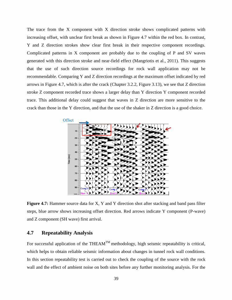
The trace from the X component with X direction stroke shows complicated patterns with
increasing offset, with unclear first break as shown in Figure 4.7 within the red box. In contrast,
Y and Z direction strokes show clear first break in their respective component recordings.
Complicated patterns in X component are probably due to the coupling of P and SV waves
generated with this direction stroke and near-field effect (Mangriotis et al., 2011). This suggests
that the use of such direction source recordings for rock wall application may not be
recommendable. Comparing Y and Z direction recordings at the maximum offset indicated by red
arrows in Figure 4.7, which is after the crack (Chapter 3.2.2, Figure 3.13), we see that Z direction
stroke Z component recorded trace shows a larger delay than Y direction Y component recorded
trace. This additional delay could suggest that waves in Z direction are more sensitive to the
crack than those in the Y direction, and that the use of the shaker in Z direction is a good choice.
Figure 4.7: Hammer source data for X, Y and Y direction shot after stacking and band pass filter
steps, blue arrow shows increasing offset direction. Red arrows indicate Y component (P-wave)
and Z component (SH wave) first arrival.
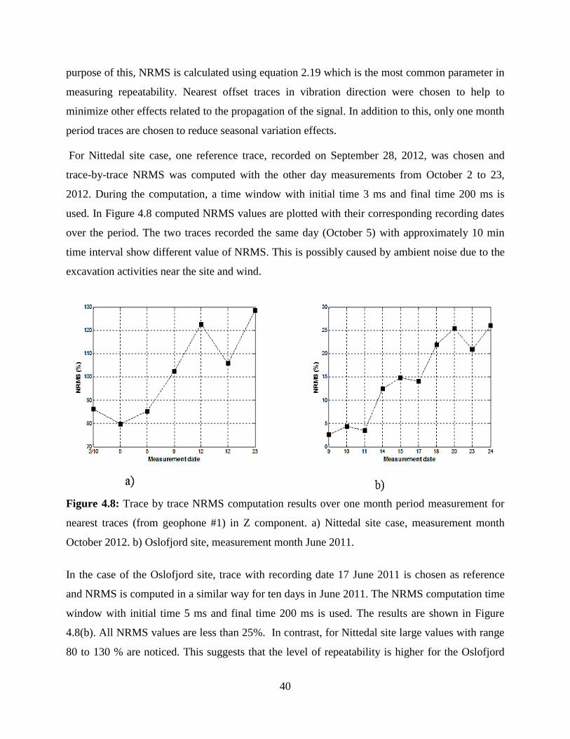
4.7 Repeatability Analysis
For successful application of the THEAMTM
methodology, high seismic repeatability is critical,
which helps to obtain reliable seismic information about changes in tunnel rock wall conditions.
In this section repeatability test is carried out to check the coupling of the source with the rock
wall and the effect of ambient noise on both sites before any further monitoring analysis. For the
40
purpose of this, NRMS is calculated using equation 2.19 which is the most common parameter in
measuring repeatability. Nearest offset traces in vibration direction were chosen to help to
minimize other effects related to the propagation of the signal. In addition to this, only one month
period traces are chosen to reduce seasonal variation effects.
For Nittedal site case, one reference trace, recorded on September 28, 2012, was chosen and
trace-by-trace NRMS was computed with the other day measurements from October 2 to 23,
2012. During the computation, a time window with initial time 3 ms and final time 200 ms is
used. In Figure 4.8 computed NRMS values are plotted with their corresponding recording dates
over the period. The two traces recorded the same day (October 5) with approximately 10 min
time interval show different value of NRMS. This is possibly caused by ambient noise due to the
excavation activities near the site and wind.
Figure 4.8: Trace by trace NRMS computation results over one month period measurement for
nearest traces (from geophone #1) in Z component. a) Nittedal site case, measurement month
October 2012. b) Oslofjord site, measurement month June 2011.
In the case of the Oslofjord site, trace with recording date 17 June 2011 is chosen as reference
and NRMS is computed in a similar way for ten days in June 2011. The NRMS computation time
window with initial time 5 ms and final time 200 ms is used. The results are shown in Figure
4.8(b). All NRMS values are less than 25%. In contrast, for Nittedal site large values with range
80 to 130 % are noticed. This suggests that the level of repeatability is higher for the Oslofjord
41
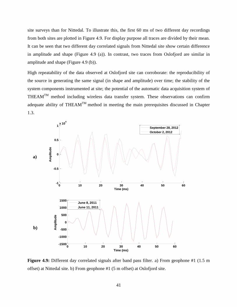
site surveys than for Nittedal. To illustrate this, the first 60 ms of two different day recordings
from both sites are plotted in Figure 4.9. For display purpose all traces are divided by their mean.
It can be seen that two different day correlated signals from Nittedal site show certain difference
in amplitude and shape (Figure 4.9 (a)). In contrast, two traces from Oslofjord are similar in
amplitude and shape (Figure 4.9 (b)).
High repeatability of the data observed at Oslofjord site can corroborate: the reproducibility of
the source in generating the same signal (in shape and amplitude) over time; the stability of the
system components instrumented at site; the potential of the automatic data acquisition system of
THEAMTM
method including wireless data transfer system. These observations can confirm
adequate ability of THEAMTM
method in meeting the main prerequisites discussed in Chapter
1.3.
Figure 4.9: Different day correlated signals after band pass filter. a) From geophone #1 (1.5 m
offset) at Nittedal site. b) From geophone #1 (5 m offset) at Oslofjord site.
0 10 20 30 40 50 60-1
-0.5
0
0.5
1x 10
4
Time (ms)
Am
plitu
de
September 28, 2012
October 2, 2012
0 10 20 30 40 50 60-1500
-1000
-500
0
500
1000
1500
Time (ms)
Am
plitu
de
June 8, 2011
June 11, 2011
a)
b)
42
4.8 Coverage Distance from Oslofjord Data
Signal propagation maximum horizontal distance limit is estimated based on background theory
discussed in Chapter 2.5, only for Oslofjord data set. The distance corresponding to this offset
can be an indication of the maximum horizontal distance of effective signal propagation. And this
will provide information on the extent of the tunnel that the system is able to monitor. In
determining the maximum horizontal distance limit only Z component recordings were
considered, since it is in vibration direction, where higher energy content exists than in the other
components. Steps in determining this distance were as follows:
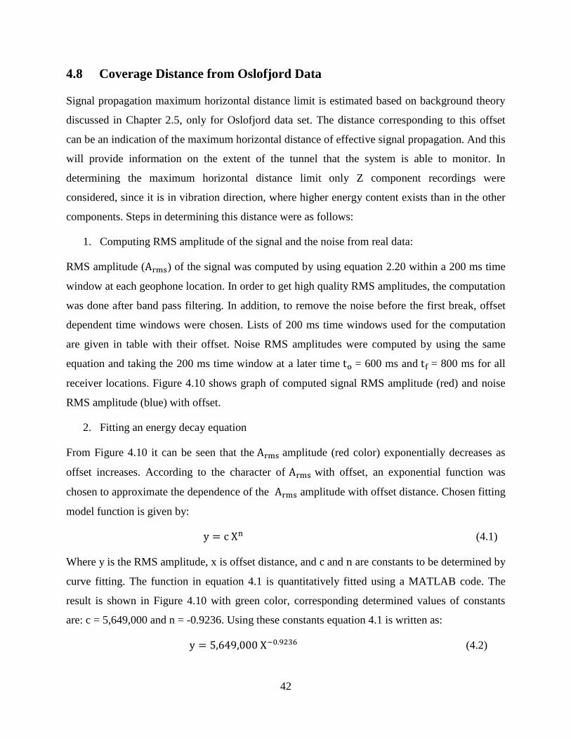
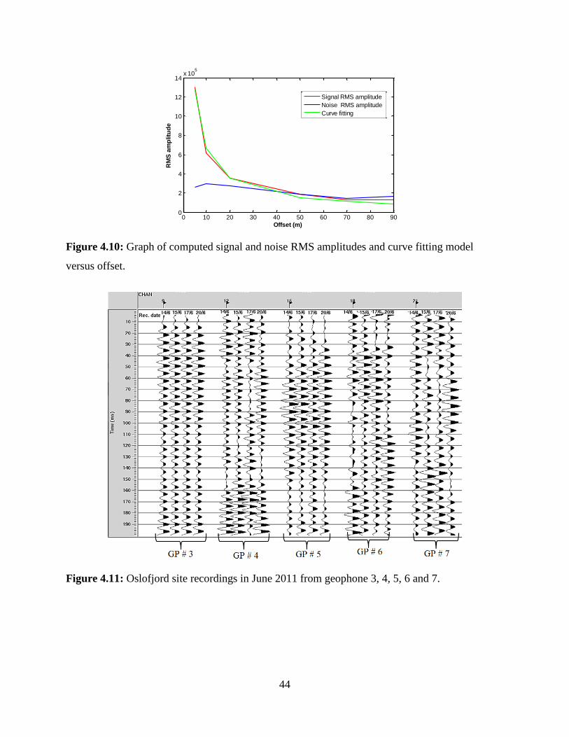
1. Computing RMS amplitude of the signal and the noise from real data:
RMS amplitude ( ) of the signal was computed by using equation 2.20 within a 200 ms time
window at each geophone location. In order to get high quality RMS amplitudes, the computation
was done after band pass filtering. In addition, to remove the noise before the first break, offset
dependent time windows were chosen. Lists of 200 ms time windows used for the computation
are given in table with their offset. Noise RMS amplitudes were computed by using the same
equation and taking the 200 ms time window at a later time = 600 ms and = 800 ms for all
receiver locations. Figure 4.10 shows graph of computed signal RMS amplitude (red) and noise
RMS amplitude (blue) with offset.
2. Fitting an energy decay equation
From Figure 4.10 it can be seen that the amplitude (red color) exponentially decreases as
offset increases. According to the character of with offset, an exponential function was
chosen to approximate the dependence of the amplitude with offset distance. Chosen fitting
model function is given by:
(4.1)
Where y is the RMS amplitude, x is offset distance, and and are constants to be determined by
curve fitting. The function in equation 4.1 is quantitatively fitted using a MATLAB code. The
result is shown in Figure 4.10 with green color, corresponding determined values of constants
are: c = 5,649,000 and n = -0.9236. Using these constants equation 4.1 is written as:
(4.2)
43
3. Determining the maximum horizontal monitoring distance combined with background
noise.
In estimating the maximum horizontal monitoring distance, first average RMS amplitude of
background noise was computed by taking all noise RMS amplitudes at different offsets.
Considering the average RMS amplitude of the background noise as y, the maximum horizontal
distance was estimated by using equation 4.2. Estimated maximum horizontal monitoring
distance ranges from approximately 65 to 75 m.
Table 4.1: Time windows with their offset in determining signal RMS amplitude.
Channel Offset (m) (ms) (ms)
3 5 5 205
6 10 7 207
9 20 10 210
15 50 30 230
18 70 35 235
21 90 40 240
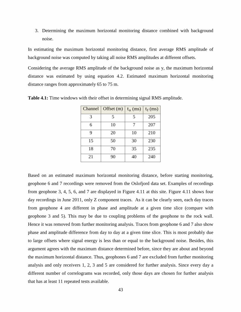
Based on an estimated maximum horizontal monitoring distance, before starting monitoring,
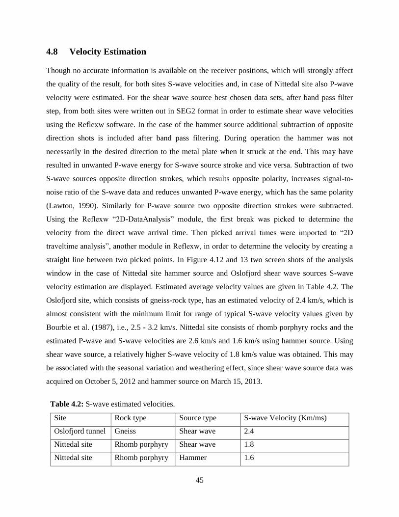
geophone 6 and 7 recordings were removed from the Oslofjord data set. Examples of recordings
from geophone 3, 4, 5, 6, and 7 are displayed in Figure 4.11 at this site. Figure 4.11 shows four
day recordings in June 2011, only Z component traces. As it can be clearly seen, each day traces
from geophone 4 are different in phase and amplitude at a given time slice (compare with
geophone 3 and 5). This may be due to coupling problems of the geophone to the rock wall.
Hence it was removed from further monitoring analysis. Traces from geophone 6 and 7 also show
phase and amplitude difference from day to day at a given time slice. This is most probably due
to large offsets where signal energy is less than or equal to the background noise. Besides, this
argument agrees with the maximum distance determined before, since they are about and beyond
the maximum horizontal distance. Thus, geophones 6 and 7 are excluded from further monitoring
analysis and only receivers 1, 2, 3 and 5 are considered for further analysis. Since every day a
different number of correlograms was recorded, only those days are chosen for further analysis
that has at least 11 repeated tests available.
44
Figure 4.10: Graph of computed signal and noise RMS amplitudes and curve fitting model
versus offset.
Figure 4.11: Oslofjord site recordings in June 2011 from geophone 3, 4, 5, 6 and 7.
0 10 20 30 40 50 60 70 80 900
2
4
6
8
10
12
14x 10
5
Offset (m)
RM
S a
mp
litu
de
Signal RMS amplitude
Noise RMS amplitude
Curve fitting
45
4.8 Velocity Estimation
Though no accurate information is available on the receiver positions, which will strongly affect
the quality of the result, for both sites S-wave velocities and, in case of Nittedal site also P-wave
velocity were estimated. For the shear wave source best chosen data sets, after band pass filter
step, from both sites were written out in SEG2 format in order to estimate shear wave velocities
using the Reflexw software. In the case of the hammer source additional subtraction of opposite
direction shots is included after band pass filtering. During operation the hammer was not
necessarily in the desired direction to the metal plate when it struck at the end. This may have
resulted in unwanted P-wave energy for S-wave source stroke and vice versa. Subtraction of two
S-wave sources opposite direction strokes, which results opposite polarity, increases signal-to-
noise ratio of the S-wave data and reduces unwanted P-wave energy, which has the same polarity
(Lawton, 1990). Similarly for P-wave source two opposite direction strokes were subtracted.
Using the Reflexw “2D-DataAnalysis” module, the first break was picked to determine the
velocity from the direct wave arrival time. Then picked arrival times were imported to “2D
traveltime analysis”, another module in Reflexw, in order to determine the velocity by creating a
straight line between two picked points. In Figure 4.12 and 13 two screen shots of the analysis
window in the case of Nittedal site hammer source and Oslofjord shear wave sources S-wave
velocity estimation are displayed. Estimated average velocity values are given in Table 4.2. The
Oslofjord site, which consists of gneiss-rock type, has an estimated velocity of 2.4 km/s, which is
almost consistent with the minimum limit for range of typical S-wave velocity values given by
Bourbie et al. (1987), i.e., 2.5 - 3.2 km/s. Nittedal site consists of rhomb porphyry rocks and the
estimated P-wave and S-wave velocities are 2.6 km/s and 1.6 km/s using hammer source. Using
shear wave source, a relatively higher S-wave velocity of 1.8 km/s value was obtained. This may
be associated with the seasonal variation and weathering effect, since shear wave source data was
acquired on October 5, 2012 and hammer source on March 15, 2013.
Table 4.2: S-wave estimated velocities.
Site Rock type Source type S-wave Velocity (Km/ms)
Oslofjord tunnel Gneiss Shear wave 2.4
Nittedal site Rhomb porphyry Shear wave 1.8
Nittedal site Rhomb porphyry Hammer 1.6
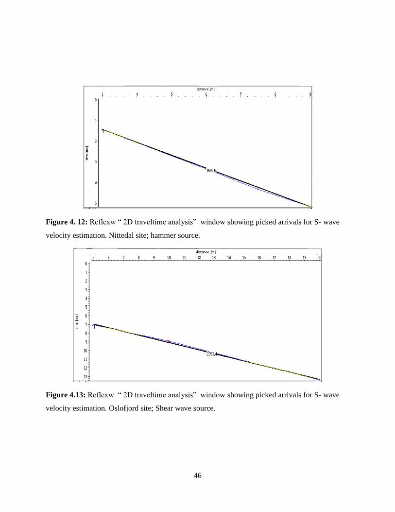
46
Figure 4. 12: Reflexw “ 2D traveltime analysis” window showing picked arrivals for S- wave
velocity estimation. Nittedal site; hammer source.
Figure 4.13: Reflexw “ 2D traveltime analysis” window showing picked arrivals for S- wave
velocity estimation. Oslofjord site; Shear wave source.
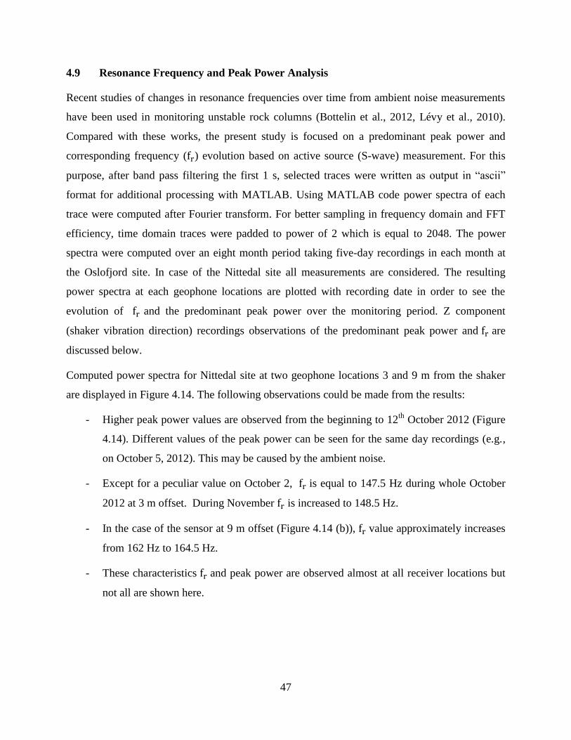
47
4.9 Resonance Frequency and Peak Power Analysis
Recent studies of changes in resonance frequencies over time from ambient noise measurements
have been used in monitoring unstable rock columns (Bottelin et al., 2012, Lévy et al., 2010).
Compared with these works, the present study is focused on a predominant peak power and
corresponding frequency ( ) evolution based on active source (S-wave) measurement. For this
purpose, after band pass filtering the first 1 s, selected traces were written as output in “ascii”
format for additional processing with MATLAB. Using MATLAB code power spectra of each
trace were computed after Fourier transform. For better sampling in frequency domain and FFT
efficiency, time domain traces were padded to power of 2 which is equal to 2048. The power
spectra were computed over an eight month period taking five-day recordings in each month at
the Oslofjord site. In case of the Nittedal site all measurements are considered. The resulting
power spectra at each geophone locations are plotted with recording date in order to see the
evolution of and the predominant peak power over the monitoring period. Z component
(shaker vibration direction) recordings observations of the predominant peak power and are
discussed below.
Computed power spectra for Nittedal site at two geophone locations 3 and 9 m from the shaker
are displayed in Figure 4.14. The following observations could be made from the results:
- Higher peak power values are observed from the beginning to 12th
October 2012 (Figure
4.14). Different values of the peak power can be seen for the same day recordings (e.g.,
on October 5, 2012). This may be caused by the ambient noise.
- Except for a peculiar value on October 2, is equal to 147.5 Hz during whole October
2012 at 3 m offset. During November is increased to 148.5 Hz.
- In the case of the sensor at 9 m offset (Figure 4.14 (b)), value approximately increases
from 162 Hz to 164.5 Hz.
- These characteristics and peak power are observed almost at all receiver locations but
not all are shown here.
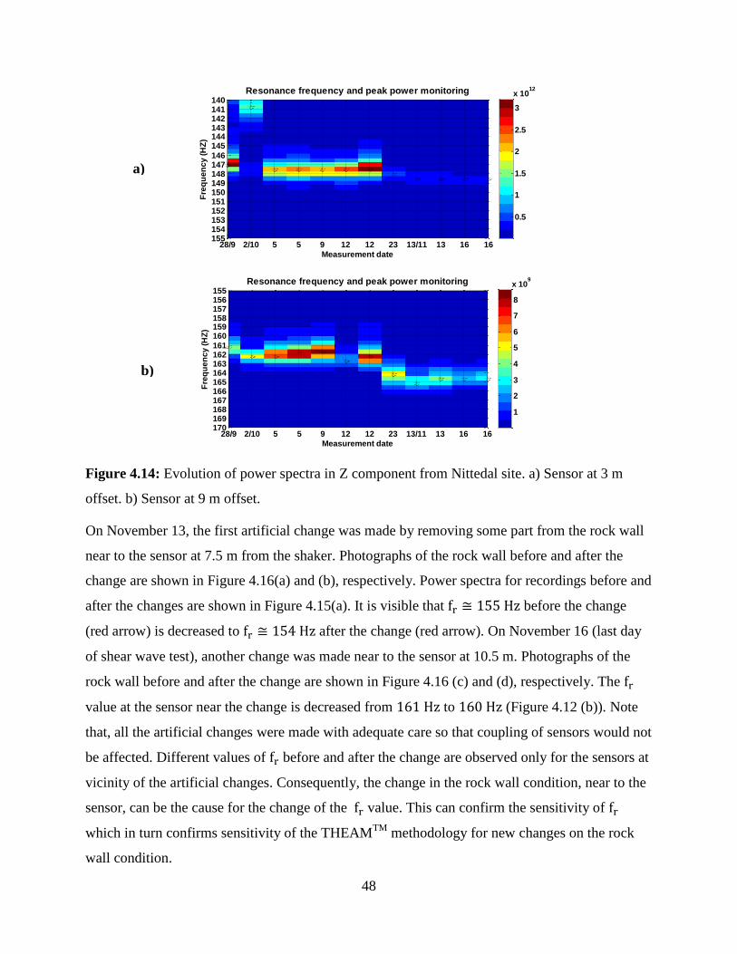
48
Figure 4.14: Evolution of power spectra in Z component from Nittedal site. a) Sensor at 3 m
offset. b) Sensor at 9 m offset.
On November 13, the first artificial change was made by removing some part from the rock wall
near to the sensor at 7.5 m from the shaker. Photographs of the rock wall before and after the
change are shown in Figure 4.16(a) and (b), respectively. Power spectra for recordings before and
after the changes are shown in Figure 4.15(a). It is visible that before the change
(red arrow) is decreased to after the change (red arrow). On November 16 (last day
of shear wave test), another change was made near to the sensor at 10.5 m. Photographs of the
rock wall before and after the change are shown in Figure 4.16 (c) and (d), respectively. The
value at the sensor near the change is decreased from to (Figure 4.12 (b)). Note
that, all the artificial changes were made with adequate care so that coupling of sensors would not
be affected. Different values of before and after the change are observed only for the sensors at
vicinity of the artificial changes. Consequently, the change in the rock wall condition, near to the
sensor, can be the cause for the change of the value. This can confirm the sensitivity of
which in turn confirms sensitivity of the THEAMTM
methodology for new changes on the rock
wall condition.
Measurement date
Fre
qu
en
cy
(H
Z)
Resonance frequency and peak power monitoring
28/9 2/10 5 5 9 12 12 23 13/11 13 16 16
140141142143144145
146147148149150151152153154155
0.5
1
1.5
2
2.5
3
x 1012
Measurement date
Fre
qu
en
cy
(H
Z)
Resonance frequency and peak power monitoring
28/9 2/10 5 5 9 12 12 23 13/11 13 16 16
155156157158159160
161162163164165166167168169170
1
2
3
4
5
6
7
8
x 109
a)
b)
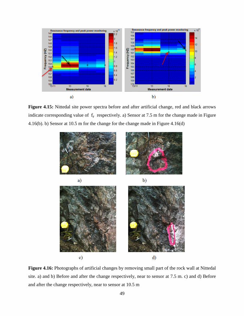
49
Figure 4.15: Nittedal site power spectra before and after artificial change, red and black arrows
indicate corresponding value of respectively. a) Sensor at 7.5 m for the change made in Figure
4.16(b). b) Sensor at 10.5 m for the change for the change made in Figure 4.16(d)
Figure 4.16: Photographs of artificial changes by removing small part of the rock wall at Nittedal
site. a) and b) Before and after the change respectively, near to sensor at 7.5 m. c) and d) Before
and after the change respectively, near to sensor at 10.5 m
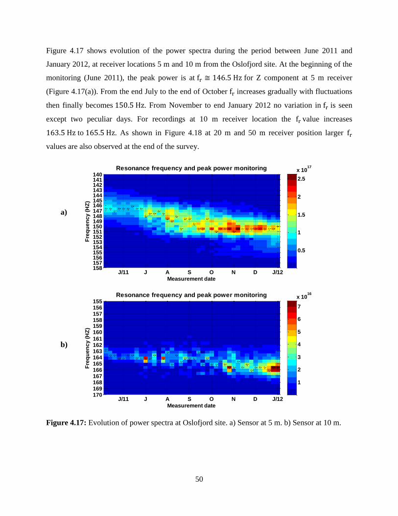
50
Figure 4.17 shows evolution of the power spectra during the period between June 2011 and
January 2012, at receiver locations 5 m and 10 m from the Oslofjord site. At the beginning of the
monitoring (June 2011), the peak power is at for Z component at 5 m receiver
(Figure 4.17(a)). From the end July to the end of October increases gradually with fluctuations
then finally becomes . From November to end January 2012 no variation in is seen
except two peculiar days. For recordings at 10 m receiver location the value increases
to . As shown in Figure 4.18 at 20 m and 50 m receiver position larger
values are also observed at the end of the survey.
Figure 4.17: Evolution of power spectra at Oslofjord site. a) Sensor at 5 m. b) Sensor at 10 m.
Measurement date
Fre
qu
en
cy
(H
Z)
Resonance frequency and peak power monitoring
J/11 J A S O N D J/12
140141142143144145146147148149150151152153154155156157158
0.5
1
1.5
2
2.5
x 1017
Measurement date
Fre
qu
en
cy
(H
Z)
Resonance frequency and peak power monitoring
J/11 J A S O N D J/12
155156157158159160
161162163164165166167168169170
1
2
3
4
5
6
7
x 1016
a)
b)
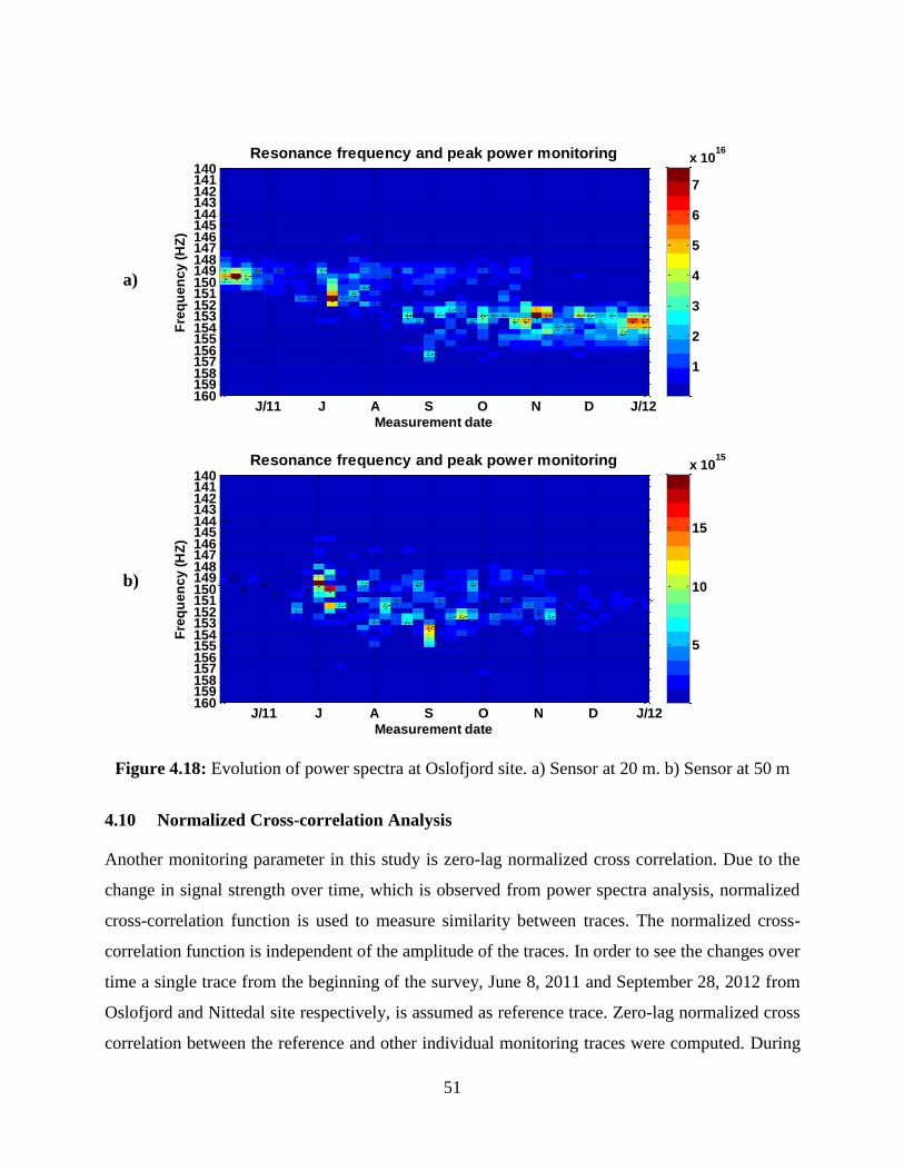
51
Figure 4.18: Evolution of power spectra at Oslofjord site. a) Sensor at 20 m. b) Sensor at 50 m
4.10 Normalized Cross-correlation Analysis
Another monitoring parameter in this study is zero-lag normalized cross correlation. Due to the
change in signal strength over time, which is observed from power spectra analysis, normalized
cross-correlation function is used to measure similarity between traces. The normalized cross-
correlation function is independent of the amplitude of the traces. In order to see the changes over
time a single trace from the beginning of the survey, June 8, 2011 and September 28, 2012 from
Oslofjord and Nittedal site respectively, is assumed as reference trace. Zero-lag normalized cross
correlation between the reference and other individual monitoring traces were computed. During
Measurement date
Fre
qu
en
cy
(H
Z)
Resonance frequency and peak power monitoring
J/11 J A S O N D J/12
140141142143144145146147148149150151152153154155156157158159160
1
2
3
4
5
6
7
x 1016
Measurement date
Fre
qu
en
cy
(H
Z)
Resonance frequency and peak power monitoring
J/11 J A S O N D J/12
140141142143144145146147148149150151152153154155156157158159160
5
10
15
x 1015
b)
a)
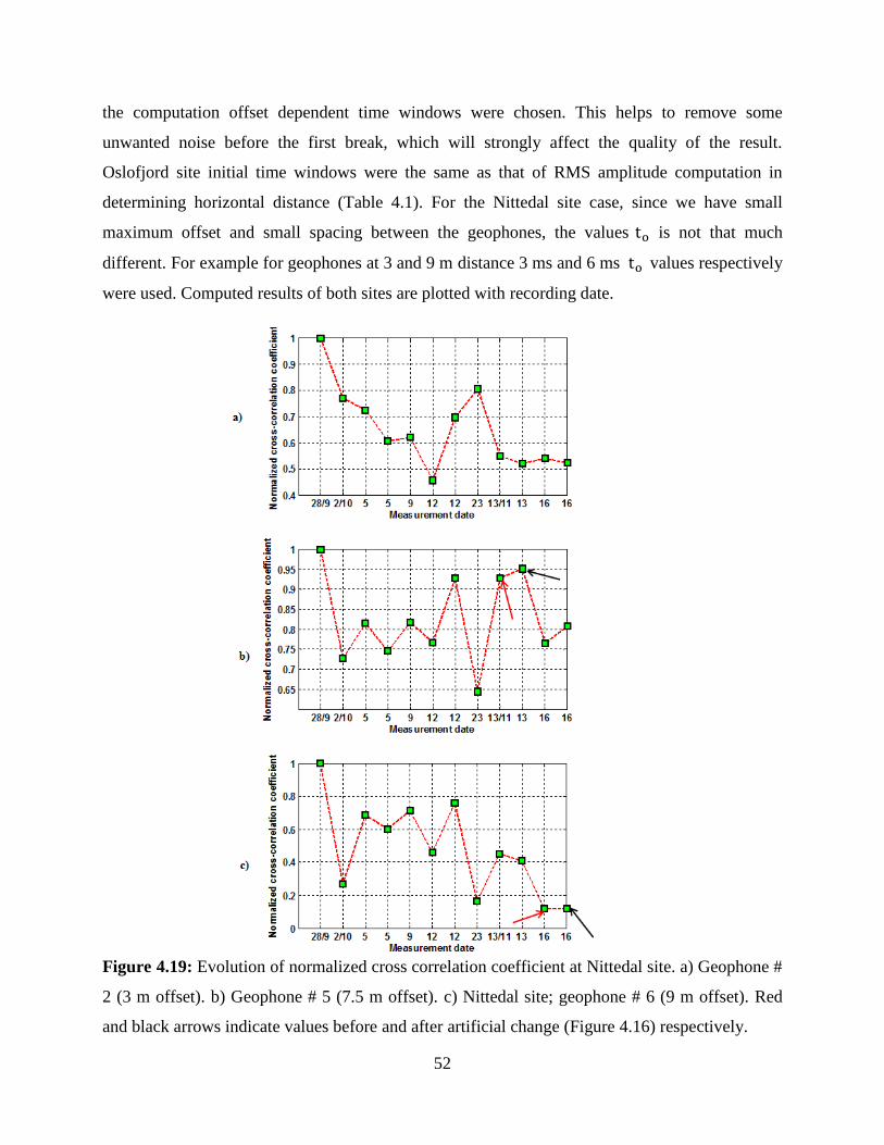
52
the computation offset dependent time windows were chosen. This helps to remove some
unwanted noise before the first break, which will strongly affect the quality of the result.
Oslofjord site initial time windows were the same as that of RMS amplitude computation in
determining horizontal distance (Table 4.1). For the Nittedal site case, since we have small
maximum offset and small spacing between the geophones, the values is not that much
different. For example for geophones at 3 and 9 m distance 3 ms and 6 ms values respectively
were used. Computed results of both sites are plotted with recording date.
Figure 4.19: Evolution of normalized cross correlation coefficient at Nittedal site. a) Geophone #
2 (3 m offset). b) Geophone # 5 (7.5 m offset). c) Nittedal site; geophone # 6 (9 m offset). Red
and black arrows indicate values before and after artificial change (Figure 4.16) respectively.
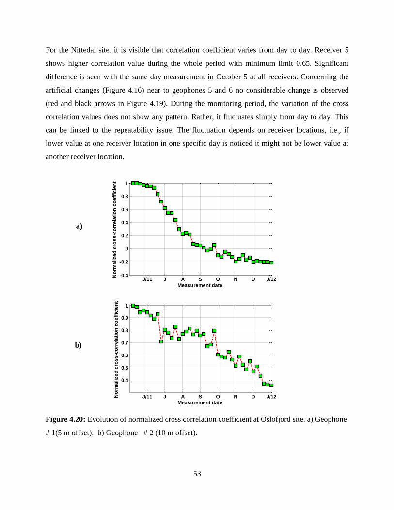
53
For the Nittedal site, it is visible that correlation coefficient varies from day to day. Receiver 5
shows higher correlation value during the whole period with minimum limit 0.65. Significant
difference is seen with the same day measurement in October 5 at all receivers. Concerning the
artificial changes (Figure 4.16) near to geophones 5 and 6 no considerable change is observed
(red and black arrows in Figure 4.19). During the monitoring period, the variation of the cross
correlation values does not show any pattern. Rather, it fluctuates simply from day to day. This
can be linked to the repeatability issue. The fluctuation depends on receiver locations, i.e., if
lower value at one receiver location in one specific day is noticed it might not be lower value at
another receiver location.
Figure 4.20: Evolution of normalized cross correlation coefficient at Oslofjord site. a) Geophone
# 1(5 m offset). b) Geophone # 2 (10 m offset).
J/11 J A S O N D J/12-0.4
-0.2
0
0.2
0.4
0.6
0.8
1
Measurement date
No
rma
lize
d c
ros
s-c
orr
ela
tio
n c
oe
ffic
ien
t
J/11 J A S O N D J/12
0.4
0.5
0.6
0.7
0.8
0.9
1
Measurement date
No
rma
lize
d c
ros
s-c
orr
ela
tio
n c
oe
ffic
ien
t
a)
b)
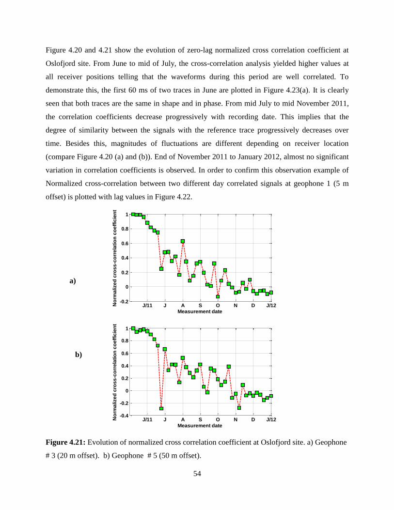
54
Figure 4.20 and 4.21 show the evolution of zero-lag normalized cross correlation coefficient at
Oslofjord site. From June to mid of July, the cross-correlation analysis yielded higher values at
all receiver positions telling that the waveforms during this period are well correlated. To
demonstrate this, the first 60 ms of two traces in June are plotted in Figure 4.23(a). It is clearly
seen that both traces are the same in shape and in phase. From mid July to mid November 2011,
the correlation coefficients decrease progressively with recording date. This implies that the
degree of similarity between the signals with the reference trace progressively decreases over
time. Besides this, magnitudes of fluctuations are different depending on receiver location
(compare Figure 4.20 (a) and (b)). End of November 2011 to January 2012, almost no significant
variation in correlation coefficients is observed. In order to confirm this observation example of
Normalized cross-correlation between two different day correlated signals at geophone 1 (5 m
offset) is plotted with lag values in Figure 4.22.
Figure 4.21: Evolution of normalized cross correlation coefficient at Oslofjord site. a) Geophone
# 3 (20 m offset). b) Geophone # 5 (50 m offset).
J/11 J A S O N D J/12-0.2
0
0.2
0.4
0.6
0.8
1
Measurement date
No
rma
lize
d c
ros
s-c
orr
ela
tio
n c
oe
ffic
ien
t
J/11 J A S O N D J/12-0.4
-0.2
0
0.2
0.4
0.6
0.8
1
Measurement date
No
rma
lize
d c
ros
s-c
orr
ela
tio
n c
oe
ffic
ien
t
a)
b)
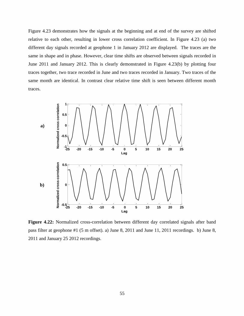
55
Figure 4.23 demonstrates how the signals at the beginning and at end of the survey are shifted
relative to each other, resulting in lower cross correlation coefficient. In Figure 4.23 (a) two
different day signals recorded at geophone 1 in January 2012 are displayed. The traces are the
same in shape and in phase. However, clear time shifts are observed between signals recorded in
June 2011 and January 2012. This is clearly demonstrated in Figure 4.23(b) by plotting four
traces together, two trace recorded in June and two traces recorded in January. Two traces of the
same month are identical. In contrast clear relative time shift is seen between different month
traces.
Figure 4.22: Normalized cross-correlation between different day correlated signals after band
pass filter at geophone #1 (5 m offset). a) June 8, 2011 and June 11, 2011 recordings. b) June 8,
2011 and January 25 2012 recordings.
-25 -20 -15 -10 -5 0 5 10 15 20 25-1
-0.5
0
0.5
1
Lag
No
rma
lize
d c
ros
s c
orr
ela
tio
n
-25 -20 -15 -10 -5 0 5 10 15 20 25-0.5
0
0.5
Lag
No
rma
lize
d c
ros
s-c
orr
ela
tio
n
a)
b)
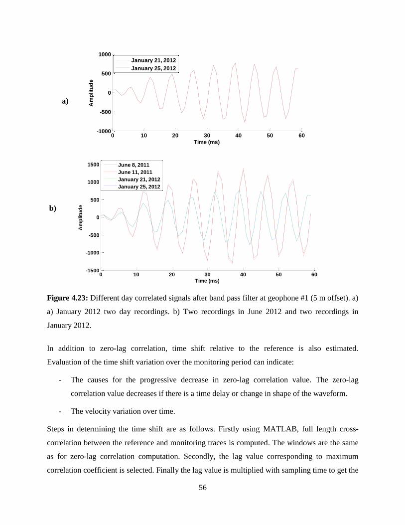
56
Figure 4.23: Different day correlated signals after band pass filter at geophone #1 (5 m offset). a)
a) January 2012 two day recordings. b) Two recordings in June 2012 and two recordings in
January 2012.
In addition to zero-lag correlation, time shift relative to the reference is also estimated.
Evaluation of the time shift variation over the monitoring period can indicate:
- The causes for the progressive decrease in zero-lag correlation value. The zero-lag
correlation value decreases if there is a time delay or change in shape of the waveform.
- The velocity variation over time.
Steps in determining the time shift are as follows. Firstly using MATLAB, full length cross-
correlation between the reference and monitoring traces is computed. The windows are the same
as for zero-lag correlation computation. Secondly, the lag value corresponding to maximum
correlation coefficient is selected. Finally the lag value is multiplied with sampling time to get the
0 10 20 30 40 50 60-1000
-500
0
500
1000
Time (ms)
Am
plitu
de
January 21, 2012
January 25, 2012
0 10 20 30 40 50 60-1500
-1000
-500
0
500
1000
1500
Time (ms)
Am
plitu
de
June 8, 2011
June 11, 2011
January 21, 2012
January 25, 2012
a)
b)
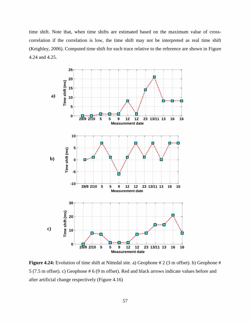
57
time shift. Note that, when time shifts are estimated based on the maximum value of cross-
correlation if the correlation is low, the time shift may not be interpreted as real time shift
(Keighley, 2006). Computed time shift for each trace relative to the reference are shown in Figure
4.24 and 4.25.
Figure 4.24: Evolution of time shift at Nittedal site. a) Geophone # 2 (3 m offset). b) Geophone #
5 (7.5 m offset). c) Geophone # 6 (9 m offset). Red and black arrows indicate values before and
after artificial change respectively (Figure 4.16)
28/9 2/10 5 5 9 12 12 23 13/11 13 16 160
5
10
15
20
25
Measurement date
Tim
e s
hif
t (m
s)
28/9 2/10 5 5 9 12 12 23 13/11 13 16 16-10
-5
0
5
10
Measurement date
Tim
e s
hif
t (m
s)
28/9 2/10 5 5 9 12 12 23 13/11 13 16 160
10
20
30
Measurement date
Tim
e s
hif
t (m
s)
a)
b)
c)
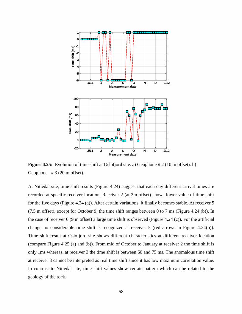
58
Figure 4.25: Evolution of time shift at Oslofjord site. a) Geophone # 2 (10 m offset). b)
Geophone # 3 (20 m offset).
At Nittedal site, time shift results (Figure 4.24) suggest that each day different arrival times are
recorded at specific receiver location. Receiver 2 (at 3m offset) shows lower value of time shift
for the five days (Figure 4.24 (a)). After certain variations, it finally becomes stable. At receiver 5
(7.5 m offset), except for October 9, the time shift ranges between 0 to 7 ms (Figure 4.24 (b)). In
the case of receiver 6 (9 m offset) a large time shift is observed (Figure 4.24 (c)). For the artificial
change no considerable time shift is recognized at receiver 5 (red arrows in Figure 4.24(b)).
Time shift result at Oslofjord site shows different characteristics at different receiver location
(compare Figure 4.25 (a) and (b)). From mid of October to January at receiver 2 the time shift is
only 1ms whereas, at receiver 3 the time shift is between 60 and 75 ms. The anomalous time shift
at receiver 3 cannot be interpreted as real time shift since it has low maximum correlation value.
In contrast to Nittedal site, time shift values show certain pattern which can be related to the
geology of the rock.
J/11 J A S O N D J/12-6
-5
-4
-3
-2
-1
0
1
Measurement date
Tim
e s
hif
t (m
s)
J/11 J A S O N D J/12-20
0
20
40
60
80
100
Measurement date
Tim
e s
hif
t (m
s)

59
Chapter 5: DISCUSSION AND CONCLUSION
5.1 Resonance Frequency Monitoring
From the results of analysis, the following general characteristics are observed for both sites:
Once is increased from the beginning no lower values in were seen at the end for all
receiver recordings.
Magnitude of relative variation, during the monitoring period, is strongly different from
one receiver location to the other.
Gradual increase with some fluctuations in peak power is observed during the whole
monitoring period from June 2011 to January 2012 at the Oslofjord site. In contrast to the
Oslofjord site, progressive decrease and fluctuation in peak power is observed at Nittedal
site.
Due to the fluctuation of the peak power and sensitivity to the ambient noise, it is reasonable to
concentrate more on variation of over time. Thus, from now on, only variation over time is
discussed in order to investigate the applicability of as monitoring parameter.
If is a unique characteristic at each receiver location, so what are the causes for the variation
over time? Besides the causes for resonance effect described in Chapter 4.5 other factors which
may cause the variation include:
(i) Variation of receiver and rock anchor coupling
(ii) Variation of coupling shaker
(iii) Seasonal variation.
The first two are associated with the stability of instrumentation. However, their effect can be
assumed to be the same over time as long as the source-receiver coupling is not loose. In addition,
if the variation was caused by instability of the instrumentation, it cannot show a pattern as
observed from the results. It could be nice to minimize or stabilize those factors that can cause
changes not related to mechanical behavior of the rock.
Regarding the seasonal variation, is lower and somewhat stable during summer season. The
value starts to increase when the season gets relatively colder (autumn) with fluctuations during
60
rainy season. Finally during winter it gets stable with higher values. It is obvious that a change in
temperature either due to diurnal variation or to seasonal variation will cause changes in the
geology of the rocks. Therefore, though no temperature measurement was taken during the
acquisition, probably the change in temperature might cause the change in . This may be the
case for Nittedal site. This behavior is consistent with the observation made on a rock column
made up of strongly fractured heterogeneous layers studied by Bottelin et al. (2012) using
ambient vibrations. However, changes related to seasonal or temperature variations are
reversible. There is no data set taken in the same season to proof whether the change is reversible
or not. For the Oslofjord tunnel case (since it is deep in the ground with its deepest section at 134
m below sea level) a somewhat stable temperature is expected. Thus the seasonal variation might
not affect the results.
In the case of the Oslofjord site, the other factor which may causes changes in is ingress of
water. Before explaining this in more detail, it is good to describe the effect of excavation on the
rock wall first. It is well known that the excavation process creates disturbed and damaged zones
in the rock (Barton, 2007). This zone is named as Excavation Damaged Zone (EDZ). Several
features of EDZ are explained by findings of Borm et al. (2003b) and Klose (2003). Particular
features related to this study are brittle faults, fissured zones, fracture sets and irregularities of the
rock wall. Continuous ingress of water or changes in stress conditions can cause gradual changes
to these features. This in turn can cause progressive variation in , which is observed from the
results. These features are probably the main reasons for resonance effects at the vicinity of each
receiver (Chapter 4.5). This can be demonstrated by artificial changes done in Nittedal (Figure
4.16) and their corresponding results (Figure 4.15). Therefore, combining the main causes for
resonance effect and reasons for variation with the trend, it could be possible to use as a
monitoring parameter.
5.2 Normalized Cross-correlation Monitoring
From zero-lag correlation and time shift result it can be seen that, for small time shifts, the value
of correlation coefficient is large.
However for zero time shifts the correlation values are not equal to 1. This tells that the variation
zero-lag correlation is caused by changes in both waveform shape and time shift. Because of
61
large NRMS and inconsistent zero-lag correlation value at Nittedal site it is possible to say that
the data is not repeatable. For this reason zero-lag correlation value is not interpreted in that case.
Oslofjord site zero-lag cross correlation value (Figure 4.20 and 21) shows a general downward
trend from the beginning to the end of November and becomes somewhat stable at the end. This
tells the decrease in degree of similarity between the reference trace and monitoring. This in turn
suggests the change in the waveform shape or time shift relative to the reference trace. Changes
in the waveform or time shift can be linked to either structural characteristics or composition
property of the rock wall. Before interpreting the specific trends observed from the results, it
should be highlighted that this study focuses on structural characteristics of rock that can cause
waveform changes. The structural characteristics of the rock that could be the reason for changes
in the shape of the waveform are EDZ features (Chapter 5.1; Chapter 2.6). Particularly, cracks or
fractures could be the reason for the change. Cracks can cause interference of the seismic wave
that can change the amplitude and waveform. Therefore the gradual decrease in the degree of
similarity (zero-lag correlation) might be linked to developing cracks and when it finally becomes
stable the correlation result is also stable. Moreover, the same trend observed at all receivers
possibly indicates changes in composition property of the rock over time.
5.3 Conclusion and Recommendations
In this study the applicability of the THEAMTM
methodology was investigated based on two data
sets collected from the Oslofjord and the Nittedal site. Based on this comprehensive study, the
following major conclusions and recommendations could be made:
Based on repeatability analysis Oslofjord site data showed by far better repeatability, with
NRMS value below 25%, than Nittedal. Lower repeatability at Nittedal site may be
caused by excavation activities near the site and wind. The weathering effect might also
be considered. In such noisy areas, it would be nice to use buried geophones. Buried
geophones have better repeatability (Jervis et al., 2012). It can also reduce loose of the
coupling of geophones over time.
High repeatability of the data observed at Oslofjord site can confirm:
a. The potential of the automatic data acquisition system of THEAMTM
method.
62
b. The quality of the data, particularly the traffic noise did not appreciably degrade
the quality of the data. This in turn confirms the independency of the THEAMTM
method on the noise level in the tunnel.
c. Reproducibility of the overall instrumentation system, especially the ability of
the shaker to produce the same signal (in amplitude and phase) over time.
The above findings can verify the potential of THEAMTM
methodology in meeting the
main prerequisites (Chapter 1.3) that any monitoring procedure applied in a tunnel under
operation should satisfy.
Maximum horizontal distance was estimated which can tell how far from the source point
one can monitor with THEAMTM
system. Based on the estimated results about 65 m
(from the source point) of the tunnel rock wall can be monitored using the THEAMTM
methodology. This estimation depends on amplitude variation with offset. Thus factors
that affect amplitude can determine the value of the distance. During instrumentation of
the system, before monitoring measurement, estimation of this distance is recommended.
Amplitude spectrum of the traces showed well-defined spectral energy peaks which have
been interpreted as resonance peaks. The frequency corresponding to the predominant
resonance peak power has been picked and interpreted as resonance frequency ( ).
Based on the results and the observations is proposed as a monitoring parameter for
detection of structural changes at vicinity of the sensors. In addition, it could also be used
to check the coupling of the receivers if there is a loose over time.
Comparing zero-lag correlation and results, is relatively insensitive to ambient noise,
so this could be considered as one of the advantages of monitoring.
Due to several reasons straightforward interpretation of the progressive changes in
monitoring parameters such as and normalized cross-correlation is difficult. One
of the main reasons is that it is not known whether the changes are reversible or
not. However two possible causes may be linked to the variation. First the seasonal
variation may cause the stiffness rock to increase and hence the monitoring
parameters to vary. The results of the zero-lag cross correlation analysis at the Oslofjord
site indicate a gradual decrease in similarity of the waveforms and the same decreasing
63
trend is observed at all receivers recordings. This could be linked to the gradual change in
the stiffness of the rock over time. This can also be supported by the observed positive
time shift values and the progressive increase in values. Secondly small changes in
stress strain condition or ingress of water may result change in EDZ features and
hence the monitoring parameters.
The overall results and their correspond interpretations of this study suggest that the
THEAMTM
methodology is a robust and potentially very applicable procedure for long-
term monitoring of structural changes of the tunnel rock wall conditions before any
hazardous collapse. This method is more powerful compared to conventional method like
visual inspection, because it provides fast and continuous reliable information about the
geological rock wall conditions in the tunnel. Furthermore, the THEAMTM
method is easy
to accomplish because once system is instrumented the data is acquired by remote control
from office.
5.4 Future Work
It would be advantageous to perform synthetic modeling. This can give a better
understanding of the wave propagation characteristics. In addition, it helps for good
processing strategies and solid background in interpreting seismic signatures.
Perform repeated measurement and estimate threshold values for monitoring parameters.
Depending on the site perform measurements over a longer duration (at least for two
years) so that seasonal variation effect can be discriminated. During monitoring
measurements perform temperature measurements as well. This will help to understand
the effect of diurnal variation in setting cut-off values for monitoring parameters.
64
References Baeten, G. J. M. 1989. Theoretical and practical aspects of the Vibroseis method, Technische
Universiteit Delft.
Barton, N. 2007. Rock quality, seismic velocity, attenuation and anisotropy, Taylor & Francis
Group.
Boadu, F. K. & Long, L. T. 1996. Effects of fractures on seismic‐wave velocity and attenuation.
Geophysical Journal International, 127, 86-110.
Bohlen, T. 2004. Analysis of Seismic Waves in the Presence of Small-Scale Strong Material
Discontinuities. Habilitation (professorial dissertation).
Borm, G., Giese, R., Klose, C., Mielitz, S., Otto, P. & Bohlen, T. 2003b. ISIS integrated seismic
imaging system for the geological prediction ahead of underground construction. EAGE
the 65th Conference and Exhibition, Stavanger Norway.
Borm, G., Giese, R. & Otto, P. 2003a. Integrated seismic imaging system for geologic prediction
ahead of a tunnel construction. 10th International congress on rock mechanics.
Bottelin, P., Jongmans, D., Baillet, L., Turpin, J., Levy, C., Lebourg, T., Hantz, D., Leroux, O.,
Cadet, H. & Lorier, L. 2012. Study of the dynamic response of prone-to-fall
compartments using seismic noise. EGU General Assembly Conference Abstracts.
Brückl, E., Chwatal, W., Mertl, S. & Radinger, A. 2008. Exploration Ahead of a Tunnel Face by
TSWD–Tunnel Seismic While Drilling. Geomechanics and Tunnelling, 1, 460-465.
Cooper, N. 2002. Vibroseis–a counter-intuitive tool. Canadian Society of Exploration
Geophysicists Conference Abstracts: Taking Exploration to the Edge.
Dasios, A., Mccann, C., Astin, T., Mccann, D. & Fenning, P. 1999. Seismic imaging of the
shallow subsurface: shear-wave case histories. Geophysical prospecting, 47, 565-592.
Drijkoningen, G. & Verschuur, D. 2003. TA3600 TG001.
Goupillaud, P. L. 1976. SIGNAL DESIGN IN THE “VIBROSEIS”® TECHNIQUE. Geophysics,
41, 1291-1304.
Hardage, B. 2011. GC Fracture Identification and Evaluation Using S-Waves.
Hassani, F. P., Sadri, A. & Momayez, M. 1999. Non-destructive evaluation of geological material
structures. Google Patents.
Inazaki, T., Isahai, H., Kawamura, S., Kurahashi, T. & Hayashi, H. 1999. Stepwise application of
horizontal seismic profiling for tunnel prediction ahead of the face. The Leading Edge, 18,
1429-1431.
Jervis, M., Bakulin, A., Burnstad, R., Berron, C. & Forgues, E. 2012. Suitability of vibrators for
time-lapse monitoring in the Middle East. SEG Technical Program Expanded Abstracts
2012. Society of Exploration Geophysicists.
Kearey, P., Brooks, M. & Hill, I. 2009. An introduction to geophysical exploration, Wiley-
Blackwell.
Keighley, D. 2006. P-wave time-lapse seismic data interpretation at Rulison Field. Piceance
Basin, Colorado: MS thesis, Colorado School of Mines.
Kragh, E. & Christie, P. 2002. Seismic repeatability, normalized rms, and predictability. The
Leading Edge, 21, 640-647.
Lang, D. H. & Lindholm, C., D 2009. THAEMTM
-Tunnel Health Monitoring Using Active
seismics. Oslo, Norway: Norwegian Tunneling Society.
Lawton, D. 1990. A 9-component refraction seismic experiment: Canadian Journal of
Exploration Geophysics.
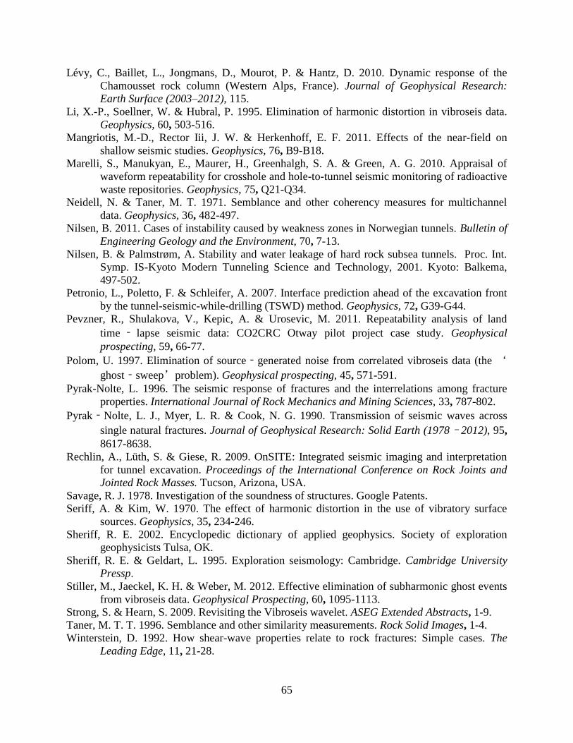
65
Lévy, C., Baillet, L., Jongmans, D., Mourot, P. & Hantz, D. 2010. Dynamic response of the
Chamousset rock column (Western Alps, France). Journal of Geophysical Research:
Earth Surface (2003–2012), 115.
Li, X.-P., Soellner, W. & Hubral, P. 1995. Elimination of harmonic distortion in vibroseis data.
Geophysics, 60, 503-516.
Mangriotis, M.-D., Rector Iii, J. W. & Herkenhoff, E. F. 2011. Effects of the near-field on
shallow seismic studies. Geophysics, 76, B9-B18.
Marelli, S., Manukyan, E., Maurer, H., Greenhalgh, S. A. & Green, A. G. 2010. Appraisal of
waveform repeatability for crosshole and hole-to-tunnel seismic monitoring of radioactive
waste repositories. Geophysics, 75, Q21-Q34.
Neidell, N. & Taner, M. T. 1971. Semblance and other coherency measures for multichannel
data. Geophysics, 36, 482-497.
Nilsen, B. 2011. Cases of instability caused by weakness zones in Norwegian tunnels. Bulletin of
Engineering Geology and the Environment, 70, 7-13.
Nilsen, B. & Palmstrøm, A. Stability and water leakage of hard rock subsea tunnels. Proc. Int.
Symp. IS-Kyoto Modern Tunneling Science and Technology, 2001. Kyoto: Balkema,
497-502.
Petronio, L., Poletto, F. & Schleifer, A. 2007. Interface prediction ahead of the excavation front
by the tunnel-seismic-while-drilling (TSWD) method. Geophysics, 72, G39-G44.
Pevzner, R., Shulakova, V., Kepic, A. & Urosevic, M. 2011. Repeatability analysis of land
time ‐ lapse seismic data: CO2CRC Otway pilot project case study. Geophysical
prospecting, 59, 66-77.
Polom, U. 1997. Elimination of source‐generated noise from correlated vibroseis data (the ‘
ghost‐sweep’problem). Geophysical prospecting, 45, 571-591.
Pyrak-Nolte, L. 1996. The seismic response of fractures and the interrelations among fracture
properties. International Journal of Rock Mechanics and Mining Sciences, 33, 787-802.
Pyrak‐Nolte, L. J., Myer, L. R. & Cook, N. G. 1990. Transmission of seismic waves across
single natural fractures. Journal of Geophysical Research: Solid Earth (1978–2012), 95,
8617-8638.
Rechlin, A., Lüth, S. & Giese, R. 2009. OnSITE: Integrated seismic imaging and interpretation
for tunnel excavation. Proceedings of the International Conference on Rock Joints and
Jointed Rock Masses. Tucson, Arizona, USA.
Savage, R. J. 1978. Investigation of the soundness of structures. Google Patents.
Seriff, A. & Kim, W. 1970. The effect of harmonic distortion in the use of vibratory surface
sources. Geophysics, 35, 234-246.
Sheriff, R. E. 2002. Encyclopedic dictionary of applied geophysics. Society of exploration
geophysicists Tulsa, OK.
Sheriff, R. E. & Geldart, L. 1995. Exploration seismology: Cambridge. Cambridge University
Pressp.
Stiller, M., Jaeckel, K. H. & Weber, M. 2012. Effective elimination of subharmonic ghost events
from vibroseis data. Geophysical Prospecting, 60, 1095-1113.
Strong, S. & Hearn, S. 2009. Revisiting the Vibroseis wavelet. ASEG Extended Abstracts, 1-9.
Taner, M. T. T. 1996. Semblance and other similarity measurements. Rock Solid Images, 1-4.
Winterstein, D. 1992. How shear-wave properties relate to rock fractures: Simple cases. The
Leading Edge, 11, 21-28.

66
Wuxiang, C., Yong, X. & Shidong, Y. Estimation of maximum interference distance. 2007 SEG
Annual Meeting, 2007.
Yordkayhun, S., Ivanova, A., Giese, R., Juhlin, C. & Cosma, C. 2009. Comparison of surface
seismic sources at the CO2SINK site, Ketzin, Germany. Geophysical Prospecting, 57,
125-139.
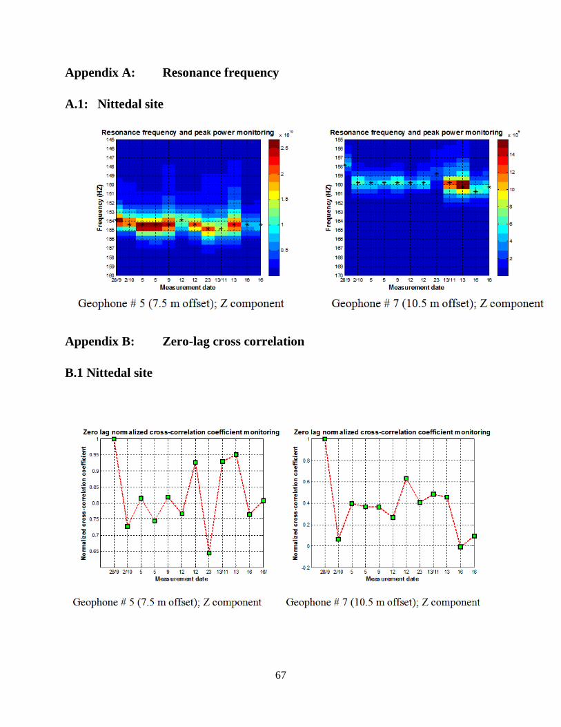
67
Appendix A: Resonance frequency
A.1: Nittedal site
Appendix B: Zero-lag cross correlation
B.1 Nittedal site
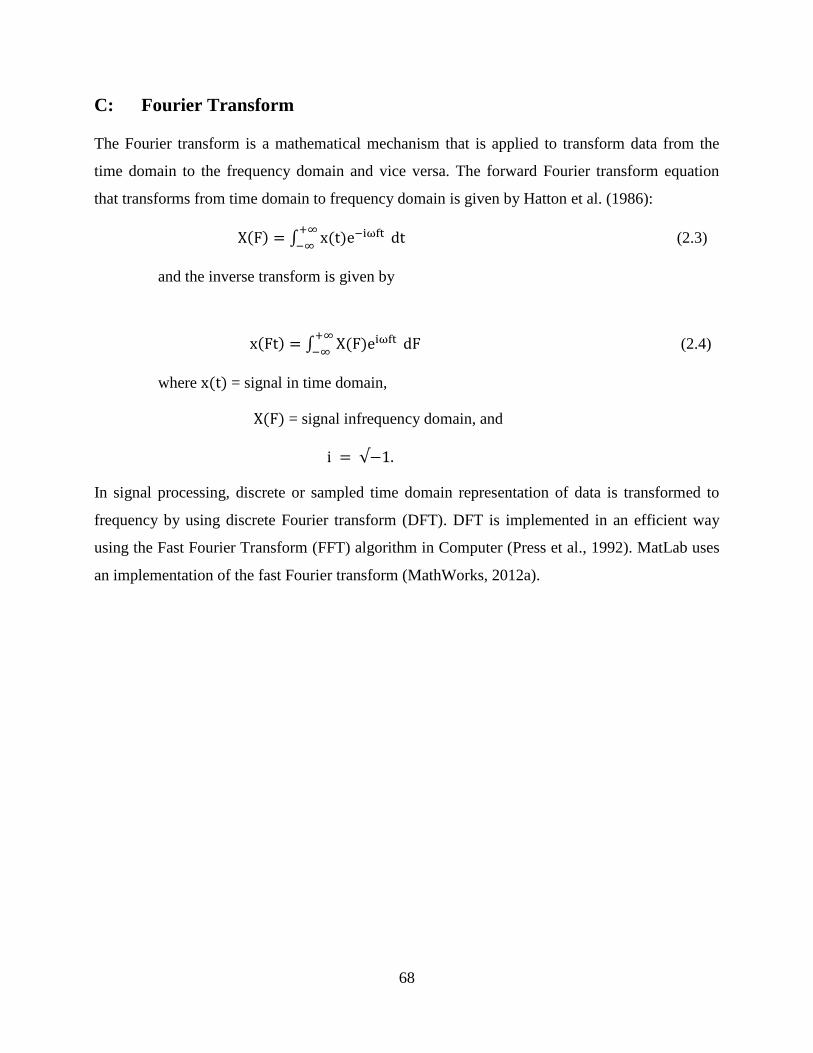
68
C: Fourier Transform
The Fourier transform is a mathematical mechanism that is applied to transform data from the
time domain to the frequency domain and vice versa. The forward Fourier transform equation
that transforms from time domain to frequency domain is given by Hatton et al. (1986):
∫
(2.3)
and the inverse transform is given by
∫
(2.4)
where = signal in time domain,
= signal infrequency domain, and
In signal processing, discrete or sampled time domain representation of data is transformed to
frequency by using discrete Fourier transform (DFT). DFT is implemented in an efficient way
using the Fast Fourier Transform (FFT) algorithm in Computer (Press et al., 1992). MatLab uses
an implementation of the fast Fourier transform (MathWorks, 2012a).
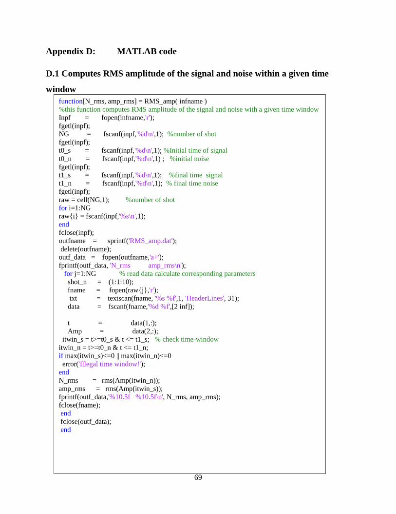
69
Appendix D: MATLAB code
D.1 Computes RMS amplitude of the signal and noise within a given time
window
function[N_rms, amp_rms] = RMS_amp( infname )
%this function computes RMS amplitude of the signal and noise with a given time window
Inpf = fopen(infname,'r');
fgetl(inpf);
NG = fscanf(inpf,'%d\n',1); %number of shot
fgetl(inpf);
t0_s = fscanf(inpf,'%d\n',1); %Initial time of signal
t0_n = fscanf(inpf,'%d\n',1) ; %initial noise
fgetl(inpf);
t1_s = fscanf(inpf,'%d\n',1); %final time signal
t1_n = fscanf(inpf,'%d\n',1); % final time noise
fgetl(inpf);
raw = cell(NG,1); %number of shot
for i=1:NG
raw{i} = fscanf(inpf,'%s\n',1);
end
fclose(inpf);
outfname = sprintf('RMS_amp.dat');
delete(outfname);
outf_data = fopen(outfname,'a+');
fprintf(outf_data, 'N_rms amp_rms\n');
for j=1:NG % read data calculate corresponding parameters
shot_n = (1:1:10);
fname = fopen(raw{j},'r');
txt = textscan(fname, '%s %f',1, 'HeaderLines', 31);
data = fscanf(fname,'%d %f',[2 inf]);
t = data(1,:);
Amp = data(2,:);
itwin_s = t>=t0_s & t <= t1_s; % check time-window
itwin_n = t>=t0_n & t <= t1_n;
if max(itwin_s)<=0 || max(itwin_n)<=0
error('Illegal time window!');
end
N_rms = rms(Amp(itwin_n));
amp_rms = rms(Amp(itwin_s));
fprintf(outf_data,'%10.5f %10.5f\n', N_rms, amp_rms);
fclose(fname);
end
fclose(outf_data);
end
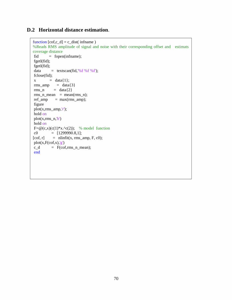
70
D.2 Horizontal distance estimation.
function [cof,c_d] = c_dist( infname )
%Reads RMS amplitude of signal and noise with their corresponding offset and estimats
coverage distance
fid = fopen(infname);
fgetl(fid);
fgetl(fid);
data = textscan(fid,'%f %f %f');
fclose(fid);
x = data{1};
rms_amp = data{3}
rms_n = data{2}
rms_n_mean = mean(rms_n);
ref_amp = max(rms_amp);
figure
plot(x,rms_amp,'r');
hold on
plot(x,rms_n,'b')
hold on
F=@(c,x)(c(1)*x.^c(2)); % model function
c0 = [1299990.8,1];
[cof, r] = nlinfit(x, rms_amp, F, c0);
plot(x,F(cof,x),'g')
c_d = F(cof,rms_n_mean);
end
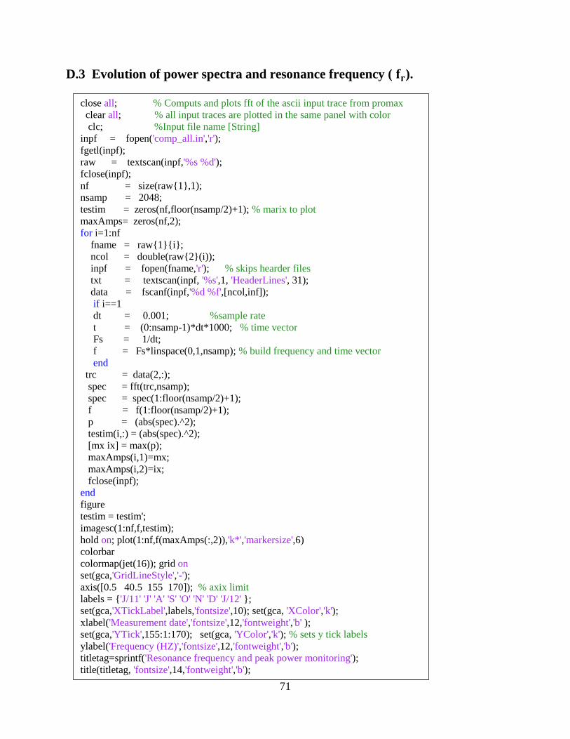
71
D.3 Evolution of power spectra and resonance frequency ( ).
close all; % Computs and plots fft of the ascii input trace from promax
clear all; % all input traces are plotted in the same panel with color
clc; %Input file name [String]
inpf = fopen('comp_all.in','r');
fgetl(inpf);
raw = textscan(inpf,'%s %d');
fclose(inpf);
nf = size(raw{1},1);
nsamp = 2048;
testim = zeros(nf,floor(nsamp/2)+1); % marix to plot
maxAmps= zeros(nf,2);
for i=1:nf
fname = raw{1}{i};
ncol = double(raw{2}(i));
inpf = fopen(fname,'r'); % skips hearder files
txt = textscan(inpf, '%s',1, 'HeaderLines', 31);
data = fscanf(inpf,'%d %f',[ncol,inf]);
if i==1
dt = 0.001; %sample rate
t = (0:nsamp-1)*dt*1000; % time vector
Fs = 1/dt;
f = Fs*linspace(0,1,nsamp); % build frequency and time vector
end
trc = data(2,:);
spec = fft(trc,nsamp);
spec = spec(1:floor(nsamp/2)+1);
f = f(1:floor(nsamp/2)+1);
p = (abs(spec).^2);
testim(i,:) = (abs(spec).^2);
[mx ix] = max(p);
maxAmps(i,1)=mx;
maxAmps(i,2)=ix;
fclose(inpf);
end
figure
testim = testim';
imagesc(1:nf,f,testim);
hold on; plot(1:nf,f(maxAmps(:,2)),'k*','markersize',6)
colorbar
colormap(jet(16)); grid on
set(gca,'GridLineStyle','-');
axis([0.5 40.5 155 170]); % axix limit
labels = {'J/11' 'J' 'A' 'S' 'O' 'N' 'D' 'J/12' };
set(gca,'XTickLabel',labels,'fontsize',10); set(gca, 'XColor','k');
xlabel('Measurement date','fontsize',12,'fontweight','b' );
set(gca,'YTick',155:1:170); set(gca, 'YColor','k'); % sets y tick labels
ylabel('Frequency (HZ)','fontsize',12,'fontweight','b');
titletag=sprintf('Resonance frequency and peak power monitoring');
title(titletag, 'fontsize',14,'fontweight','b');
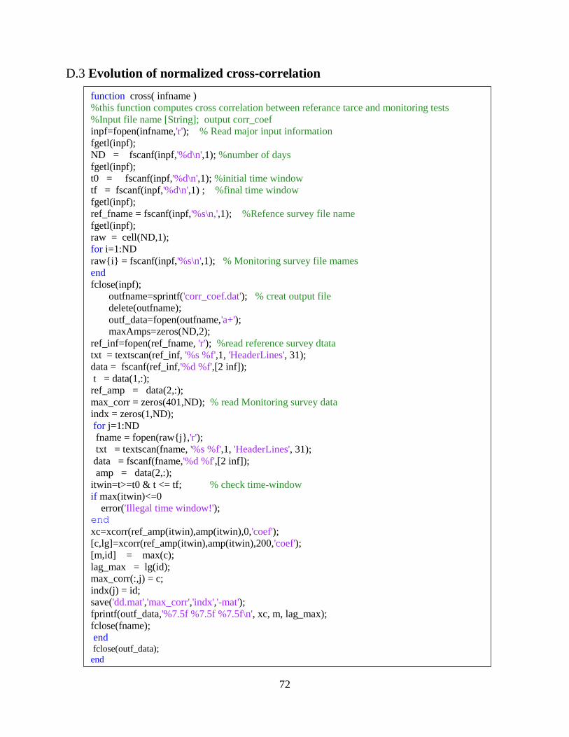
72
D.3 Evolution of normalized cross-correlation
function cross( infname )
%this function computes cross correlation between referance tarce and monitoring tests
%Input file name [String]; output corr_coef
inpf=fopen(infname,'r'); % Read major input information
fgetl(inpf);
ND = fscanf(inpf,'%d\n',1); %number of days
fgetl(inpf);
t0 = fscanf(inpf,'%d\n',1); %initial time window
tf = fscanf(inpf,'%d\n',1) ; %final time window
fgetl(inpf);
ref_fname = fscanf(inpf,'%s\n,',1); %Refence survey file name
fgetl(inpf);
raw = cell(ND,1);
for i=1:ND
raw{i} = fscanf(inpf,'%s\n',1); % Monitoring survey file mames
end
fclose(inpf);
outfname=sprintf('corr_coef.dat'); % creat output file
delete(outfname);
outf_data=fopen(outfname,'a+');
maxAmps=zeros(ND,2);
ref_inf=fopen(ref_fname, 'r'); %read reference survey dtata
txt = textscan(ref_inf, '%s %f',1, 'HeaderLines', 31);
data = fscanf(ref_inf,'%d %f',[2 inf]);
t = data(1,:);
ref_amp = data(2,:);
max_corr = zeros(401,ND); % read Monitoring survey data
indx = zeros(1,ND);
for j=1:ND
fname = fopen(raw{j},'r');
txt = textscan(fname, '%s %f',1, 'HeaderLines', 31);
data = fscanf(fname,'%d %f',[2 inf]);
amp = data(2,:);
itwin=t>=t0 & t <= tf; % check time-window
if max(itwin)<=0
error('Illegal time window!'); end
xc=xcorr(ref_amp(itwin),amp(itwin),0,'coef');
[c,lg]=xcorr(ref_amp(itwin),amp(itwin),200,'coef');
[m,id] = max(c);
lag_max = lg(id);
max_corr(:,j) = c;
indx(j) = id;
save('dd.mat','max_corr','indx','-mat');
fprintf(outf_data,'%7.5f %7.5f %7.5f\n', xc, m, lag_max);
fclose(fname);
end fclose(outf_data); end


![Duo-Scherzo Duo En cours Brahms Musorgskii …shop.kawai.jp/umeda/floor/pdf/concert2017030_alumni.pdfAlumni Concerto Duo-Scherzo primo & 37 Duo-Scherzo] . . (Duo-Scherzo official site:](https://img.pdfslide.net/doc/110x75/5e708faf92f2ea21071ee302/duo-scherzo-duo-en-cours-brahms-musorgskii-shopkawaijpumedafloorpdfconcert2017030.jpg)