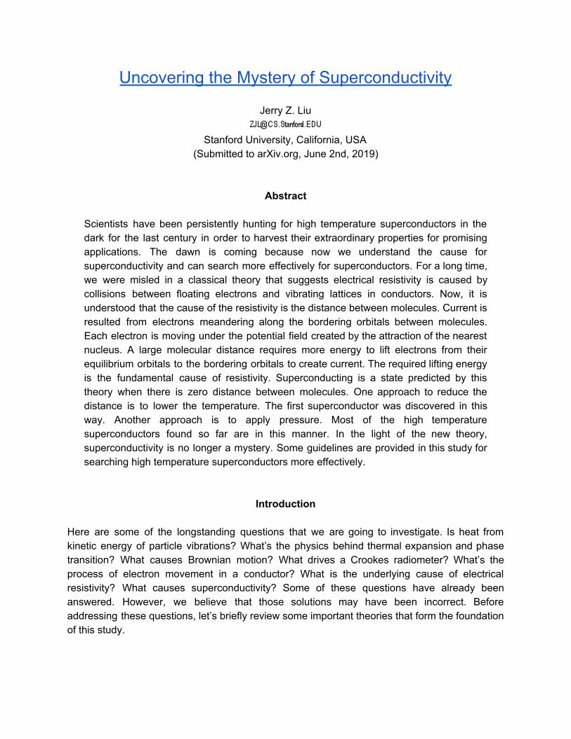
Uncovering the Mystery of Superconductivity

Jerry Z. Liu

Stanford University, California, USA (Submitted to arXiv.org, June 2nd, 2019)

Abstract

Scientists have been persistently hunting for high temperature superconductors in the dark for the last century in order to harvest their extraordinary properties for promising applications. The dawn is coming because now we understand the cause for superconductivity and can search more effectively for superconductors. For a long time, we were misled in a classical theory that suggests electrical resistivity is caused by collisions between floating electrons and vibrating lattices in conductors. Now, it is understood that the cause of the resistivity is the distance between molecules. Current is resulted from electrons meandering along the bordering orbitals between molecules. Each electron is moving under the potential field created by the attraction of the nearest nucleus. A large molecular distance requires more energy to lift electrons from their equilibrium orbitals to the bordering orbitals to create current. The required lifting energy is the fundamental cause of resistivity. Superconducting is a state predicted by this theory when there is zero distance between molecules. One approach to reduce the distance is to lower the temperature. The first superconductor was discovered in this way. Another approach is to apply pressure. Most of the high temperature superconductors found so far are in this manner. In the light of the new theory, superconductivity is no longer a mystery. Some guidelines are provided in this study for searching high temperature superconductors more effectively.

Introduction Here are some of the longstanding questions that we are going to investigate. Is heat from kinetic energy of particle vibrations? What’s the physics behind thermal expansion and phase transition? What causes Brownian motion? What drives a Crookes radiometer? What’s the process of electron movement in a conductor? What is the underlying cause of electrical resistivity? What causes superconductivity? Some of these questions have already been answered. However, we believe that those solutions may have been incorrect. Before addressing these questions, let’s briefly review some important theories that form the foundation of this study.

An analogy to Isaac Newton’s universal gravitation is Charles-Augustin de Coulomb’s law for charged particles, published in 1785.[1-5] The interaction electric force between two charges is:

F = Kq1q2r -2, (1)

where K is Coulomb’s constant, positive F is the repulsive force between signed charges q1 and q2, and r is the distance between the charges.[6-9] While gravity governs the interactions among celestial bodies in classical mechanics, Coulomb’s force is most prominent at the subatomic realm because it is 1036 magnitude stronger than the gravitational force.[10] Coulomb’s law was essential to the development of the theory of electromagnetism and the Bohr atomic model because it was then possible to discuss quantity of electric charge in a meaningful way.[11-17] Unlike classical mechanics, in subatomic interactions, quantum mechanics also play a significant role.[18-20]

By the early 1900s, scientists had established that heat energy travels in electromagnetic waves or photons.[11] While studying blackbody radiation, Max Planck derived a law predicting the spectral density of electromagnetic radiation emitted by a blackbody in thermal equilibrium at a given temperature T, given no net flow of matter or energy between the body and its environment, known as Planck law:

B(f,T) = 2hf3c-2(ehf/kT - 1)-1, (2) where B is the spectral radiance (the power per unit solid angle and per unit of area normal to the propagation) density of frequency f radiation per unit frequency at the thermal equilibrium at the temperature T, h is the Planck constant, c is the speed of light, k is the Boltzmann constant, f is the frequency of electromagnetic radiation, and T is the absolute temperature of the body.[21-37] In order to fit his model with the observed blackbody radiation and to overcome the energy divergence problem at higher frequencies predicted by existing theories, commonly known as the ultraviolet catastrophe, Planck suggested that the energy carried by electromagnetic waves could only be released in discrete “packets”.[38-39] The idea that energy comes in quantized levels was confirmed by Albert Einstein in his research on the photoelectric effect in 1905.[20,40] In his experiments, electrons were dislodged only by the impingement of light that reached or exceeded a threshold frequency (or energy level), but not under the threshold even with high intensity.[20] To make sense of the fact that light can eject electrons even with low intensity, Einstein proposed that a beam of light is a collection of discrete wave packets, named photons later, each with energy hf, where f is the frequency of the light and h is Planck's constant. These works laid the foundation for quantum mechanics. Based on these studies, Niels Bohr derived the first quantized model of the atom in 1913, known as the Bohr model, which overcame a major shortcoming of Rutherford’s model.[15-17] In early models, a charge moving in a circle should radiate electromagnetic waves. Hence, for an orbiting electron, the radiation should cause it to lose energy and spiral down into the nucleus. Bohr solved this paradox with explicit reference to Planck’s work: an electron in an atom could

only have certain defined energy levels, therefore can only stay in discrete orbitals. Thus, An electron can only gain and lose energy by jump from one allowed orbit to another by absorbing or emitting photons with a discrete energy hf. This is also consistent with Einstein’s proposal that electrons must absorb energy at discrete level.[20] One problem with the Bohr model is that all the electrons would pile up at the lowest orbit, which is inconsistent with observations. This problem was resolved 12 years later by Wolfgang Pauli in his exclusion principle.[41-47] It states that two or more identical fermions cannot occupy the same quantum state in a quantum system simultaneously.[42] In other words, two electrons cannot have all four identical quantum numbers. If two electrons reside in the same orbital with the same principal quantum number, azimuthal quantum number and magnetic quantum number, their spin quantum numbers must be different and be the two opposite half-integer spin projections of ½ and -½. Hence, there are at most two electrons in an orbital with the same first three quantum numbers. This sets a limit on the number of electrons in each orbital and shell. For a given atom, there is a fixed orbital structure and the photons absorbed or emitted must be at certain frequencies, producing spectral lines at the corresponding frequencies.[48-49] The phenomena of spectral lines are well studied.[49] There is a specific pattern for each atom, known as its “fingerprint”.[50] Numerous applications have been developed for identifying atomic components for a given sample. This technology makes it possible for us to inspect the components of a remote star or planet just from its radiation. These works did not address the questions raised early, but laid a solid foundation for us to study further for the solutions. To address the questions we need to understand the processes of electron interactions between molecules. There are two categories of electron interactions: interactions with electron exchanges and interactions without electron exchanges. With electron exchanges via transferring or sharing, chemical bonds such as ionic and covalent bonds are formed between molecules, which determine the chemical properties of matters. This is not the subject of this study. What we are going to investigate in the second category is the interactions between molecules without the formation of these chemical bonds. These are the interactions that determine the physical properties or processes of matters, such as thermal expansion, phase transition, electrical resistivity, Brownian motion and so on. By looking into electron dynamics in the second category, we are able to identify and understand some processes, such as orbital expansion, orbital repulsion and orbital crossing, which allow us to address the above questions with some newly developed theories. To simplify the discussion, let’s clarify some terms. An orbital ascension is the process that an electron jumps to a higher orbital after absorbing photons. An orbital descension is the process that an electron steps down to a lower orbital after emission. An orbital jump can be either ascension or descension. A thermal equilibrium is a state of dynamic balance between absorption and emission in a system. This usually occurs when a system reaches the same temperature as its environment. At this time, the energy exchange between the system and the environment is balanced. There is an infinite number of orbitals surrounding the nucleus of an atom. Starting from the lowest energy level, the orbitals are filled one by one with electrons up to the point where the atom becomes electrically neutral. Intrinsic orbitals are defined as all the orbitals filled up by at least one electron. An orbital with the same first three quantum

numbers is at the same energy level and may be occupied by at most two electrons. Hence, the outermost intrinsic orbital may not be fully filled. An extrinsic orbital is not one of the intrinsic orbitals. In a single atom, if all the electrons are in the intrinsic orbitals, it is said to be in its base state, also known as ground state, and has the lowest possible potential energy. Orbital jumps occur constantly in any system with a temperature above absolute zero. Normally, not all electrons are in the intrinsic orbitals. Equilibrium orbitals are the orbitals where there are most electron activities at the equilibrium. The equilibrium radius of an atom is defined as the radius of the outermost equilibrium orbital. When an atom radius is referred in this study, we are loosely referring to the equilibrium radius. Hence, the size of an atom varies with temperatures. After absorbing energy, an electron jumps to an extrinsic orbital, creating an electron hole in the intrinsic or lower orbitals. As a result, the atom has more potential energy than its previous state. Under the attraction of the nucleus, an electron in an extrinsic orbital tends to jump down to fill the intrinsic orbital and releases the stored potential energy. Thus, the overall energy level of the atom tends to return to the base state. This is similar to the process in classical mechanics under gravity where an object tends to move from a high potential location to a low position. Let’s coin a new term electrovity, short for electrostatic gravity, to emphasize the similarity between the electric force and gravitational force. Electrovity governs many phenomena and processes to be discussed later.

Is Heat from Kinetic Energy? Any substance with a temperature above absolute zero radiates heat/thermal energy in the form of photons or electromagnetic waves. Where does the thermal energy come from? The answer can be found in almost every high school textbook. It is usually associated with kinetic energy, more specifically to the vibrations of particles in a system. The higher the level of kinetic energy, the more heat it radiates, therefore, the higher temperature. Then, my question is how the vibrations are converted into heat? The former has kinetic energy, while the latter is in the form of photons. The answer to this question, if it can be found, has much less certainty. If we are not sure how heat is produced, how can we so sure to associate heat with vibrations? It turns out this is a fundamental physics question because the answer to this question had become the proposition for many theories and models that have been used to explain numerous physical phenomena, such as Brownian motion, thermal expansion, electrical resistivity, and so on. Our solution is to abandon this classical theory. Heat is from Potential Energy With the proposition set forth in the introduction, it is more logical for us to postulate that heat is radiated from the potential energy stored by electrons in extrinsic orbitals. Upon absorbing energy, an electron is excited and “jumps” to a higher orbital. The energy is stored by the electron as the potential with respect to the attraction of its nucleus, Figure 1B. The more electrons ascend to high orbitals, the more energy is stored. Due to electrovity, the stored potential energy tends to be released by emitting photons, or electromagnetic waves, which are

the heat that can be detected with thermometers. Hence, temperature is a measurement of radiated energy, indicating the average potential level of a system.

Figure 1, Potential energy stored by electrons in high orbitals.

The absolute zero temperature represents the base state of a system, such as shown in Figure 1A. Because all the electrons are in the “basement”, there is nowhere for the electrons to step down, therefore, no energy release, no radiation, no heat detected, hence zero temperature. Absolute zero temperature is not just a theoretical prediction of the ideal gas law but has a physical meaning: the base state.[51-54] This does not exclude vibrations. Since there are still angular momentum in electrons, there must be some kinetic energy even at absolute zero. Absolute zero is the lowest temperature not because there is no vibration, but because all the electrons are in their lowest possible orbitals. The point is that the heat is not from kinetic energy, but from potential energy stored by electrons. In a few sections, we will show that the kinetic energy of vibrations is just a side effect resulted from orbital jump. It is understood that chemical energy is a type of potential energy. The potential energy that we are consuming everyday is resulted from breaking or making of chemical bonds in batteries, food, gasoline, etc. The energy of chemical bonds is actually stored potential energy with respect to the attraction between electrons and nuclei. For instance, heat is released when two H atoms are combined to form an H2 molecule. In an H atom, the electron is attracted by a single nucleus. In an H2 molecule, each of the electrons is essentially attracted by two nuclei in the covalent bond. Compared with the electron in an H atom, the electrons in an H2 is more tightly bonded by the nuclei, hence are at a lower energy level and have less potential energy. The heat released in the combining process is the reduced potential energy of the electron with respect to the attraction from the single hydrogen nucleus. On the other hand, energy is required in the reverse process to separate an H2 molecule into H atoms. Here is one more example in this line. The potential energy of the hydrogen electron is further released in the process of 2H2 + O2 -> 2H2O. In a water molecule H2O, the oxygen atom is covalently bonded to two hydrogen atoms, or H-O-H, which is actually a variation of covalent bond, named polar bond. Because the nucleus of the oxygen atom is much larger than that of the hydrogen atom, the electrons are more tightly bonded to the oxygen nucleus than the hydrogen nucleus in the covalent bond of H2 molecule.[88] All forms of the energy discussed so far are the potential with

respect to the attraction between electron and nucleus. Each bond is just a named form of the attraction between electron and nucleus. All the potentials are resulted from the electric force between particles. With the potential theory, it becomes clear that the driving mechanism behind the second law of thermodynamics is electrovity.[55-71] Just like how gravity tends to level the surface of the Earth, electrovity encourages potential energy to be redistributed evenly, therefore increasing the entropy in a closed system. The physics behind the third law of thermodynamics is also tangible now.[72-75] The so-called ground state with minimum energy in the third law of thermodynamics is just the base state we discussed here where all the electrons are in their intrinsic orbitals. Wien’s Displacement By considering adiabatic expansion of a cavity containing waves of light at thermal equilibrium in 1893, Wilhelm Wien was able to derive that the peak frequency of the blackbody radiation curve is proportional to the temperature, known as Wien’s law.[76-77] Differentiating Planck’s law in equation (2) for blackbody radiation with respect to frequency and setting the derivative equal to zero, we will reach the same result as Wien’s law:

T = bc-1fpeak, (3) where T is the absolute temperature, fpeak is the peak radiation frequency, c is the speed of light and b is Wien’s displacement constant. Using the law, we are able to calculate the temperature of a system by its radiation. Just as an experienced baker can use the color of a flame to tell the temperature inside an oven, we can use Wien's law to calculate the temperature of a star remotely by analyzing its radiation. With the potential theory, the physics behind Wien’s law becomes clear. Since temperature is the measurement of the potential energy level, a high temperature indicates that most electron activities are in high orbitals. In other words, the equilibrium orbitals are at a high energy level. Orbiting in a high level, an electron may descend across multiple orbitals in a single step, releasing more energy by emitting high energy photons, therefore peaking at high frequency. However, at low temperatures, electrons are in low equilibrium orbitals. There are fewer orbitals to step across, radiating only low energy photons, hence peaking at low frequency.

Is Thermal Expansion Caused by Vibrations? Thermal expansion is a phenomenon observable every day. What is the physics behind the phenomenon? A classical textbook theory is typically attributing it to kinetic energy in a system. The vibrations of molecules increase with temperature. More vibrations require a larger average space to accommodate the particles in the system. I am not convinced by this theory. First, the space seems not an issue. The size of an atom is at 10-12 m level. The size of a nucleus is at 10-15 m level and an electron is even smaller. That means 99.99% of the space between

particles is empty in a solid. Second, let’s do an analogy between the particles in a solid and the trees in a forest. Each particle is anchored to its lattice and each tree is rooted in the ground. The particles vibrate in their frame and the trees swing in a wind. The forest does expand to a larger area in a strong wind because the area of the forest never changes. Disregarding the expansion of the lattice, the vibration theory is not a sufficient solution. In addition, the vibration theory only accounts for monotonic thermal expansion but short for an explanation for water that expands with decreasing temperature below 4 oC. In our believe, it is the force between molecules that determines the thermal expansion. Force between Molecules In challenging the common theory of thermal expansion, we propose further scrutiny of the forces between molecules. Normally, each molecule is electrically neutral. However, it does not mean there is no electric force between molecules. This force is called intermolecular force and modeled next. Consider a model where electrons orbit around their nucleus in a cloud and the charge density is evenly distributed in the shells. The repulsion against a negatively charged particle outside the atom can be computed by integrating the force over the shell. The resulted accumulative repulsion from the shells is canceled exactly by the attraction of their nucleus, producing a zero net repulsion to any particle outside the atom. This is not consistent with observations, because there are attractions holding molecules together in a solid. Then, how can we model the force between molecules? To establish the model, we need an accurate atom model in the first place. Unfortunately, a general solution to the Schrödinger equation is not available other than the hydrogen atom.[78-87] Nevertheless, one thing we can do at least is to find the bounding values for the repulsion or attraction forces using a simplified model. Figure 2 shows two configurations for two helium atoms next to each other. The maximum repulsion force is found in configuration 2A and minimum in 2B. In configuration 2B, the two electrons orbital in the left atom is in a plane perpendicular to the centerline between the atoms.

Figure 2, Configurations for helium atom repulsion model.

Based on Coulomb's law in equation (1), the net repulsion forces between the two helium atoms for configuration 2A and 2B are:

Fa = Kqe2(s-2 + 6(s+2r)-2 + (s+4r)-2 - 4(s+r)-2 - 4(s+3r)-2), (4)

and Fb = Kqe

2(4(s+2r)-2 - 2(s+r)-2 - 2(s+3r)-2 + 2(s+r)(r2+(r+s)2)-1.5 + 2(s+3r)(r2+(s+3r)2)-1.5 - 4(s+2r)(r2+(s+2r)2)-1.5), (5)

where Fa and Fb are the maximum and minimum repulsion forces, K is the Coulomb’s constant, qe is the charge of an electron, r is the radius of the helium atoms and s is the distance between the two atoms. Using the model, we can investigate the repulsion trends in terms of atom sizes and distances between the atoms. For instance, given a helium atom radius 140 pm, Figure 3 shows the repulsion trends as a function of atom distances. The maximum repulsion decreases quickly with increasing distances. The repulsion force is about 5.4 nano N at the distance of one atom radius 140 pm. It is interesting to note that the minimum repulsion is negative, meaning there is an attraction between the two atoms in configuration 2B. The attraction decreases with increasing distance. Both values decrease to zero at infinite distance, which is consistent with observations. It is important to understand that the two configurations are extreme cases. Since electrons are very dynamic particles, the actual configuration at any moment is something in between. So, for a given distance, the actual force must be a value between the two curves. Figure 3 also shows an important trend for the range between maximum and minimum forces, which increases with decreasing distances between atoms. With a small distance, the range is very large and may fluctuate from repulsion all the way to attraction. In other words, the force can be either repulsion or attraction. It all depends on the actual configuration of the electron clouds.

Figure 3, Maximum forces between two helium atoms as a function of distance.

It is also interesting to look into the repulsion trends as a function of atom sizes. The repulsion increases with atom sizes for a fixed atom distance. Three curves, blue, red and yellow, are plotted in Figure 4 for different distances, 20, 30 and 40 pm. In general, the repulsion increases with atom sizes for all the three distances. This is consistent with observations. When atom size increases, the distance between the nucleus and electrons of adjacent atoms increases, which reduces the attractive components in equation (4) of the model.

Figure 4, Repulsion as a function of atom sizes for three different atom distances.

Phase Transition of Matter It is the intermolecular force just discussed above that determines phase transition including thermal expansion. The force was modeled above purely in the context of physical distance between atoms and atom sizes. Now, let’s put it in a context with temperature. The force is affected by temperature via atom radius and distance. At high temperatures, electrons are active in high equilibrium orbitals. Atom sizes are effectively increased, or the r term in the above equation is increased. As atom radius increases, the repulsion between atoms also increases, which pushes the atoms apart further. The overall effect is volume expansion, named orbital expansion. This explains thermal expansion. The force is also affected by temperature though the type of electron configuration as shown in the above model. The repulsion force comes primarily from the two outer electrons between the two atoms like in configuration 2A. The force tends to push the electrons apart, creating an attractive configuration similar to 2B. At low temperatures, there is less orbital jump and the attractive configurations may be sustained, which provides less repulsion, or even attraction force that holds particles together in a solid and provides viscosity and surface tension for liquid. At high temperatures, the electrons are very

dynamic. Configurations similar to 2A may be observable more frequently and the repulsion dominates, causing the phase transition to fluid. Even though the above model is based on simple configurations with two helium atoms, the results are generally applicable to most atoms, especially for large ones. Compared with helium, a hydrogen atom has only one proton and exerts less attraction to its electron. So, its atom size is much larger. The same model for hydrogen atoms is simpler and the general trends are similar, but with larger maximum repulsion/attraction ranges. The force modeled using helium and hydrogen represents the two extreme cases, where helium has fully filled in the outermost shell while hydrogen is minimally filled. For other elements, the force will be in between of the two models. With more electrons in large atoms, the repulsion between electrons causes them to be distributed more evenly in their shells. As mentioned at the beginning of the previous section, the evenly distributed charges cancel the attraction from their nucleus to an outside electron. Only the outermost electrons are significant to the force between atoms. Hence, the force trends are similar to either helium model or hydrogen model depending on the structure of the outermost orbitals. With large nuclei, multiple outermost orbitals may be partially filled. Our model suggests that an increase in temperature leads to a larger atomic radius which produces more repulsion. As such, we would expect repulsivity to be correlated with atomic size and inversely correlated with melting or boiling points. Figure 5 shows the melting and boiling points of elements in the periodic table. The states of the elements in the table are colored with blue for the liquid state. At 1000 K, Figure 5B, most of the elements in column 1, such as hydrogen, melt or boil because of their large radii compared with the elements to their right in the same row. This is consistent with our model that predicts a large radius produces a greater repulsion. There are two other trends. In looking across a particular row, our model would predict increased repulsion with more electrons in the outer shell, leading to lower melting and boiling points. In each column of elements, there are the same number of electrons in the outermost shell. The element in the lower row has one more inner shell compared with the upper element, which makes its outermost electrons less significant than these in the upper row in terms of repulsion. Thus, the lower elements are less repulsive. The combination of these two trends produces an overall trend that is the repulsion decreases from the top right to the bottom left. This trend is clearly shown in the table where the melting points increase from the top right to bottom left, Figure 5A-5D. As a result of all the factors, the least repulsive elements are found at the lower part of the table centered to the left, indicated in Figure 5C and 5D.

Figure 5, States of elements at different temperatures (screenshots from ptable site).

Now that it is understood that thermal expansion and phase transition is generally determined by the interaction force between molecules: repulsion force and attraction force. The repulsion is mostly caused by electrons between adjacent molecules at high temperatures. The attraction is mostly between a nucleus and electrons of adjacent molecules at low temperatures. Attraction may take different forms, such as bonds. Note, the attractions interested here are not resulted from chemical bonds, such as covalent and ionic bonds. To differentiate, let’s name these bonds intramolecular forces. The forces are formed either through electron sharing or transferring. With anchored electrons, the atoms are held so tight in a molecule that they are normally not separable in thermal expansion or phase transition processes. The forces determine primarily chemical properties of the molecules. Some of the attractions are also identified and named as bonds, such as hydrogen bonds and metallic bonds. The key difference is that there is no electron sharing or transferring and electrons are not anchored by the bonds. Hence, they are also belong to intermolecular force. Intermolecular force not only determines thermal expansion and phase transition, but also control the formation of different crystal structures, such as the angles in the crystal lattice that are determined by attraction forces in different directions.

To illustrate intermolecular force in action, let’s look into the crystal formation of ice. A water molecule consists of a single oxygen atom covalently bonded to two hydrogen atoms, or H-O-H.[88] These bonds are so tight that they hold the atoms together even in the gaseous state, therefore not the cause of phase transition. Because the oxygen nucleus is much larger than the hydrogen nucleus, it attracts and holds the two sharing electrons most of the time.[89] The oxygen atom behaves like a negatively charged particle, while hydrogens positive. With the two hydrogen atoms forming an angle of 106.6o, the oxygen atom attracts hydrogen atoms from adjacent water molecules on the opposite side of the two hydrogen atoms, forming a hydrogen bond.[90] Compared with a covalent bond, this is a weak bond. There is no electron sharing or transferring, therefore is an intermolecular force. However, it dominates force between water molecules at low temperatures and becomes critical in controlling the structure of ice, such as hexagonal crystals in snow flakes.[91-95] At standard atmospheric pressure, liquid water is densest at 4 oC. Above this temperature, water undergoes a normal orbital expansion. Below 4 oC, hydrogen bond becomes dominating and water begins to form the hexagonal structure as the freezing point is reached, resulting in a less compacted molecular packing of crystals in ice.

What Causes Brownian Motion? While looking through a microscope at pollen in water, 1827, Robert Brown discovered that the triangular shaped pollen burst at the corners, emitting particles which he noted jiggled around in the water in a random fashion.[96-101] It was later confirmed by Albert Einstein, 1905, that the motion that Brown had observed was a result of the pollen being pushed by individual water molecule.[102-103] In fact, Brownian motion is a common phenomenon observable in daily life. Most people may have noticed dust particles dancing in a ray of light in a dark room. Similar to Einstein’s observation, the dust particles are actually moved by air molecules. The physics behind Brownian motion is not well understood. Because of the positive relationship between temperature and average momentum of particles, it is usually attributed to the kinetic energy in a system. However, there is a missing link as to how exactly the large pollen or dust particles are pushed by much smaller molecules. To comprehend the question, let’s estimate the speed required for an air molecule to push a dust particle. Molecule Speed Estimation Suppose an air molecule moves at a velocity V and a dust particle is initially motionless. After a collision, the dust particle gains a speed of 1 cm/s, or 10-2 m/s, a conservative estimate of the dancing speed of dust particles based on my observations. The least wavelength of visible light is 4x10-7 m, which determines the size of smallest dust particles that can be seen with the naked eye, or equivalent to a volume of 6.4x10-20 m3. The radius of an air molecule is at the magnitude of 10-10 m, or 10-30 m3 in volume. The momentum of the air molecule before the collision is Vda10-30, where da is the density of air molecules. The momentum of the dust particle after the collision is 10-2dd6.4x10-20, or 6.4dd10-22, where dd is the density of the dust particle. Assuming that all the momentum of the air molecule is transferred to the dust particle in the collision,

Vda10-30 = 6.4dd10-22, or reduced to, Vda = 6.4dd108. To be conservative, suppose the density of the air molecule is 10 times that of the dust particle. It gives us an estimate for the speed of the air molecule before the collision, 6.4x107 m/s. Note, because of the random nature, there is a slim chance that multiple air molecules may hit a dust particle at the same time. It is likely that they come from different directions, therefore canceling each other. Hence, it is not the situation that we need to concern. Thus, to push pollen or dust particles requires incredibly high-speed impacts. What processes can create such a high speed? What moves the water or air molecule in the first place? Based on the classical vibration theory, there is no kinetic energy at absolute zero temperature. As temperature increases from 0 K, what kicks off the motionless molecules? Before reading further, I hope these questions cause you to pause and think. Orbital Repulsion Orbital repulsion is a consequence of orbital expansion when an atom/molecule is next to another particle or object. As shown in Figure 6A, an atom is next to an object initially. On absorbing energy, the atom goes through an orbital expansion process, Figure 6B, which actually includes two sub-processes. First, it increases the atom size (term r in equation 4), which increases the repulsion as shown in Figure 4. Second, the atom distance decreases (term s in equation 4), which also increases the repulsion based on equation (4). Both processes contribute to the repulsion force.

Figure 6, Orbital repulsion resulted from orbital expansion.

The process of orbital jump is still under active research. It appears spontaneous as an electron jumps from one energy level to another, typically in nanoseconds or less. Because an orbital expansion is sudden, the orbital repulsion of an atom or molecule may push apart the particles

or objects next to it with significant momentum. An orbital repulsion may also take place where an atom is next to a container wall. This will exert some pressure on the container wall and also push the atom to move in the opposite direction. This seems to be the primary force driving Brownian motion. This force also provides a better solution to the Crookes radiometer in a few sections. This is also the force that breaks molecules apart in solid at the liquefying phase transition to be discussed later. Cause of Particle Vibration There are two side effects in an orbital expansion process: subatomic particle vibrations and the photoelectric effect. Within an atom, an orbital jump also causes vibrations for both the electron and its nucleus. Because the nucleus is 103 magnitudes heavier than the electron, most of the vibrations are observed in the electron. Hence the electron is moving in a cloud orbital partially due to the vibrations/oscillations caused by electron jump. However, this is not the cause of Brownian motion. The momentum created in an orbital expansion for the electron and nucleus are in opposite directions and cancel each other, producing zero net momentum. If the absorbed energy is strong enough, electrons may be ejected from the atom, known as the photoelectric effect. Demonstrated by Albert Einstein, electrons are only kicked out by the incident photons above a certain frequency, or energy level. The maximum kinetic energy of the ejected electrons is proportional to the extra energy of the photons above a threshold. In other words, part of the incident energy is used to lift the electrons out of their orbitals and the rest of the energy is contributed to the momentum of the ejected electrons. In the process, there should be changes in kinetic energy in the original molecule that lost electrons. Again, this is not the process that causes Brownian motion either because most Brownian motions are observed without the photoelectric effect. The photoelectric effect may be considered an extreme case in the orbital jump spectrum. Whenever orbital repulsion occurs between two particles, the momentum for each particle may be changed. The overall kinetic energy in a system increases as orbital repulsion occurs more frequently at high temperatures. However, the momentum created in each individual orbital repulsion for the two particles are in the opposite direction and canceled. Hence, the net momentum of the system is zero. That is why the container is not moving. Imagine that we were able to prevent the orbital repulsion from happening in a system completely, even though there were still orbital jump maintaining the thermal equilibrium. What would happen? The random Brownian motion would eventually settle down even at high temperatures. In other words, thermal radiation exists regardless of vibrations. Hence, vibrations are not the cause of heat radiation, but a result of the radiation from the potential energy stored by the electrons. The absolute zero temperature is the state of having all electrons in their lowest orbitals, not a lack of motion. A side note is that, unlike a planet that travels in a single orbit, an electron moves in a cloud, known as orbital. It is our belief that the cloud is resulted from two mechanisms. First, an electron is repelled by other electrons, causing it to deviate from its theoretical orbit. Second, an

electron also oscillates along its orbit due to orbital jump. It would be an interesting research topic to find out if the electron in a hydrogen atom revolves in a single orbit like a planet at very low temperatures close to absolute zero. The experiment would allow us to investigate the interaction between a hydrogen nucleus and its electron without interference from other factors. This may provide important insight to understand quantum mechanics.

What Drives a Crookes Radiometer? A Crookes radiometer, also known as a light mill, consists of a low pressure glass bulb containing a set of vanes mounted on a low friction spindle inside. Each vane is coated black on one side and white on the other. The vanes rotate when exposed to light, with faster rotation for more intense of light. If a mill is left under sunlight, it can spin all day. The rotation is such that the black sides of the vanes are retreating from the light. When the bulb is cooled quickly by putting it into a freezer, it turns backwards slowly and stops in a minute or so. The mechanism for the rotation has been a scientific debate over a century. However, a convincing explanation has yet to appear. The light mill inventor, Crookes, incorrectly suggested that the force was due to the pressure of photons, predicted by James Clerk Maxwell, well known for his equations of electromagnetism.[104-105] If this is true, a faster rotation should be observed with better vacuum in the bulb. It turned out the best result is observed at a pressure around 1 pascal. The vanes stay motionless in a hard vacuumed bulb. There were numerous theories, trying to establish an unbalanced pressure between black and white sides of the vanes or over the edges.[106-113] One proposal is that gas molecules hitting the warmer side of the vane will pick up some of the heat, bouncing off the vane with increased speed. The problem with the idea is that while the faster-moving molecules produce more force, they also do a better job of colliding and preventing other molecules from reaching the vane, so the net force on the vane should be the same. Albert Einstein showed that the two pressures do not cancel out exactly at the edges of the vanes because of the temperature difference there. The force predicted by Einstein would be barely enough to move the vanes. A more complicated model called thermal creep suggests air creeps cross the edge of vanes from the white side to the black side.[107] This creates a high pressure on the black side that pushes the vanes forwards. A problem that all the theories failed to address is how to create the driving force at the thermal equilibrium. Left under sunlight, a mill will reach a dynamic equilibrium sooner or later, and the temperature will be the same on both sides of the vanes. Focused Light Experiment To investigate the problem, we designed an experiment, in which a small torch was used as the light source, Figure 7. To turn the mill forwards, the torch was pointed and focused on the black side of a vane. The motionless vanes started moving immediately. It completed the first circle in less than 5 seconds. Within a minute, the speed reached a highest/plateau value, about 2 rotations per second. The results are similar to the experiments with none focused light sources. Next, the torch was focused on the white side of a vane so that the light ray was perpendicular

to the surface of the vane to avoid reflecting on to the black side of the adjacent vane. The vanes stayed motionless no matter how long the light was kept on.

Figure 7, Focused light source experiment for the Crookes radiometer. The purpose of the experiment was to test if there is enough driving force in the air pressure to move the vanes. Avoiding any reflection onto the black sides isolates the influences of other factors that the black sides might have. As the light focused on the white side, the air near the white side was doubly heated by both the directed and the reflected photons. Giving it enough time, the air should be heated, creating some kind of aerodynamic force to move the vanes. The fact was that the vanes did not move, indicating there was not enough driving force to overcome the static friction. At a pressure of 1 pascal, which is about 10-5 of the pressures at the sea level, the air is as thin as that on the top of the mesosphere, an altitude of 80 km above the Earth. This is where an airplane is less efficient than a rocket, where the rocket is not driven by the air pressure but the momentum created through ejecting high speed molecules. In the other direction, the torch was pointed to a single black vane and the push force was so strong that the vane was moved spontaneously without waiting time for the air to warm up, indicating the driving force may result from interactions other than air pressure. Not every Crookes radiometer was made equal. Next experiment was more interesting by using a mill with smaller static friction, therefore more sensitive. As expected, in the forward direction, it just spun quicker and faster. When the torch was pointed to a white vane, it started to move immediately but slowly. More interestingly, the rotation was in the forward direction. The white vane was chasing the light source. It stopped in a few seconds. After removing the light source, it rotated backwards and stopped quickly, which was similar to the situation observed in the freezer experiment. Why did the vanes chase the light source, then stopped instead of moving faster?

Solution to Crookes Radiometer The solution again is in the orbital repulsion. Upon absorbing photons, the electrons in the molecules on the surface of the vanes were excited, jumping to higher orbitals, which caused a sudden orbital repulsion. The process kicks away air molecules next to the vanes, creating a momentum to move the vanes. When the torch was pointed to the black side of a vane, the photons were absorbed quickly, producing an orbital repulsion effect to move the vanes immediately. On the white side, the light was mostly reflected. The same repulsion effect applies to the second experiment, however the process is a little more complex. Orbital repulsion takes place on any surface with a temperature above absolute zero. In fluid, this is the driving force causing Brownian motion. The orbital repulsion takes place on both sides of the vanes, creating repulsion forces on both black side Fb and white side Fw. There is also a resistance Fr, which approximates to static friction at a low speed. To move the vanes, the force difference between the two sides must be greater than the resistance:

|Fb - Fw| > Fr. (6) There will be no motion otherwise. When the mill was placed in a freezer, the heat energy inside the mill radiated to the environment and the black side was doing the blackbody radiation that was faster than the white side. Hence, the white side was relatively warmer, creating a greater orbital repulsion Fw that pushed the vanes in the backward direction. It stopped quickly as the mill approached the new equilibrium, and the difference of the forces between the two sides could not overcome the static friction. When the torch was pointed towards the white side in the second experiment, the visible light was mostly reflected and infrared light was bounced around inside of the bulb. The black sides absorbed the infrared radiation faster than the white sides, creating a greater repulsion force Fb that pushed the vanes forwards. The mill stopped quickly when reached the new equilibrium. When the light source was removed, the mill went through a cooling process similar to that occurred in the freezer experiment. What was just explained above is for the situation in which the mill reaches a new equilibrium quickly at the ambient temperature. The uneven speed of the cooling or warming between the two sides creates a short term temperature difference. The vanes stop quickly after reaching the new equilibrium. Now, let’s look into the long term driving force at the equilibrium under sunlight. Both are in the equilibrium state. Why does one move forever, but not the other? The answer is still in orbital repulsion. Recall blackbody radiation. By integrating Planck’s law, equation (2), over the frequency, then over the solid angle, we found that the power P emitted by a blackbody is directly proportional to the fourth power of its absolute temperature T, known as the Stefan-Boltzmann law:

P = pT4, (7)

where P is the power emitted per unit area of the surface of a blackbody, T is the absolute temperature, and p is the Stefan-Boltzmann constant.[114-115] Most systems are not a perfect blackbody. Their radiation power Pn can be approximated using:

Pn = EpT4, (8) where E is the radiation efficiency of a system, which is normally less than 1. For a perfect blackbody, Eperfect = 1. Let Eb and Ew be the radiation efficiencies of the black and white sides of the vanes. After the mill reaches the equilibrium, e.g. at the same ambient temperature T, such as left under sunlight for enough time, the radiation power for the black and white sides are EbpT4 and EwpT4. Remember at the equilibrium, radiation equals to absorption. Hence, EbpT4 and EwpT4 equal to the absorption levels for the black and white sides, too. The orbital repulsion is a result of orbital ascension after energy absorption. So, the repulsion force is proportional to the energy absorption. By introducing an orbital repulsion coefficient r, the repulsion forces can be estimated for the black and white sides using:

Fb = EbrpT4, (9) and

Fw = EbrpT4, (10) respectively. Hence, inequality (6) can be rewritten as:

|Eb - Ew|rpT4 > Fr. (11) The black side is better at absorption and radiation than the white side. In other words, it has a higher radiation efficiency, Eb > Ew. For a given Crookes radiometer, (Eb - Ew)rp has a fixed value. This inequality provides an explanation for both cases of the equilibrium. If the environment radiation (measured by T) is high enough that (Eb - Ew)rpT > Fr, the rotation will be maintained. This occurred when mill was left under the sunlight. The higher the temperature T, the stronger the force, and the faster the mill rotates. At a low temperature T, such as in the case of the freezer experiment and light pointed towards the white vane side in the second experiment, (Eb - Ew)rpT is not large enough to overcome resistance Fr, hence cannot create enough force to move the vanes after the equilibrium. Note, the initial movement in the low temperature experiments is due to the temperature difference between the two sides of the vanes as mentioned earlier. Keep in mind, in the high temperature equilibrium, the resistance term actually includes two components: the static friction and dynamic air drag. The drag is proportional to the square of the angular velocity of the vanes. When the ambient temperature/radiation is large enough, the vanes will start accelerating. As the angular velocity increases, the drag increases. The drag plus the static friction will eventually reach the equilibrium with the driving force. The rotational speed will approach a highest value, which is the plateau speed observed in each experiment with intensive light sources

To be comprehensive, there are actually five forces acting inside a light mill. The general form for Fb in inequality (6) should be Fb = Fa + Frv - Fcv + Fra - Fca. Fa is the air pressure discussed in most of the existing theories. Frv is the repulsion of the surface molecules on the vanes pushing the air molecules next to the vanes. Fcv is the countering effect of the molecules kicked off by the vanes due to Frv term that prevents incoming air molecules from reaching the vanes. This term may cancel part of the air pressure when there is a high density of air molecules, e.g. at high pressures. Similar to the repulsion by the molecules on the vanes, there are also two terms Fra and Fca due to the repulsion of air molecules against the vanes. All these forces are proportional to the density of air molecules inside the mill, e.g. the air pressure. At very low air pressures, there are not enough molecules for all the five terms of the interactions to create enough driving force Fb to overcome the static friction of the vanes. The mill does not move at all. At low pressures, molecules rarely collide. The two countering terms Fcv and Fca are negligible because there are little or no collisions against air molecules to counter the air pressure term. Without the countering terms Fcv and Fca, the air pressure Fa is the same on the two sides of each vane and cancels from the two sides. Similarly, the Fra term is also the same on the two sides of each vane and cancels. Thus, the other four terms can be neglected in inequality (6) and Fb = Frv. Therefore, the explanation above can be simplified. At higher pressures, the chance that molecules bump into each other increases and the air pressure term eventually becomes dominant. The orbital repulsion creates a push to the vanes; and at the same time, the kicked/bounced air molecules by the repulsion collide against the incoming air molecules, which counter and reduce the air pressure. The air pressure is reduced by the same amount of force that the push generated by the repulsion to the vanes. Hence, Frv - Fcv = 0 and Fra - Fca = 0. There is only one term left in the driving force Fb = Fa. Since both Fb and Fw equals to the pressure that is the same on the two sides of each vane. There is no net force to drive the vanes. On a side note, this is a perfect example where orbital repulsion must be considered for precise modeling or measurement for pressure. As discussed earlier, at very low pressure, an identical pressure meter can output different readings at different temperatures of the measuring instrument.

Is Electrical Resistivity Caused by Collisions? A common observation is that the electrical resistivity increases with temperature for most conductors. This relationship is usually attributed to the thermal vibrations of particles in conductors.[116-118] Current is actually the flow of electrons. Vibrations disturb the electrons flow via deflection and scattering. The effect of heat on a conductor is to make the molecules vibrate, increasing the chance of collisions between moving electrons and the lattices in the conductor. Each collision uses up some of the electron’s energy, resulting in electrical resistance.[119-125]

Here is an inconsistency with the collision theory. At room temperature (~200 K), the density of gold (19.30 g/cm3) is more than double the density of iron (7.87 g/cm3). Not only is the nucleus

of a gold atom much larger, but also the number of electrons in a gold atom (79) is more than double that of iron (26). Since there are more particles per unit volume in gold, we should expect more collisions and higher resistances. In fact, gold (4.1x107 S/m) is a much better conductor than iron (1.0x107 S/m). Another problem is that under increasing pressures, a conductor becomes more conductive. Since the particles are packed more densely, collision theory predicts a higher collision rate and a higher resistance. If the collision theory is not true, what is the cause for electrical resistivity? How exactly do electrons flow inside a conductor? The answer to these questions shall also provide clues to understand superconductivity. Orbital Crossing According to Coulomb’s law, a free electron is one infinitely far away from its nucleus. Floating electrons in plasma can be approximately considered as free electrons, which are moving under applied electrical fields. However, in a close range with nuclei, such as in a solid, electrons are unlike moving in the free manner. Each electron is in the potential field created by the attraction of a nearby nucleus, pulling the electron into its orbitals. In a gas, this attraction may be canceled or even overcome by the repulsion of the electron shell of atoms. In a solid, this is unlikely to be the case because the solid state has already proved that the attraction dominates the control. The attraction force is large enough to hold adjacent molecules, and must be strong enough to pull the electron. So, unless there are strong external fields, the electron will be bound to its orbital in a normal conductor. Thus, under the attraction of its nucleus, an electron is normally confined in an orbital corresponding its energy level and cannot move freely. There will be no current. However, when the electron is in an orbital that shares its border with the orbital of an adjacent atom at the same energy/potential level, a slingshot effect may take place. At the border, the attraction created by the two adjacent atoms is the same. A minor advantage from the other side will cause the electron crossing the border from one atom to the next, named orbital crossing. During the process, the electron is moving at the same energy level along a contour formed by the two orbitals, named bordering orbitals. A current created in this manner requires no additional energy. This is an efficient, low energy mode current compared with currents in plasma, or in photoelectric effect.

Figure 8, Electron crossing over atom boundary along bordering orbitals.

Consider two atoms next to each other as shown in Figure 8. Consider a plane cutting through the centers of the nuclei. The contours in the plane indicate the potential levels created by the attractions of the nuclei to electrons. At the border B, the potential is the same with respect to the nuclei. Suppose there is an electron hole in the atom on the right side. The atom becomes a positively charged ion, while the other atom remains neutral. Normally, an electron at location A circulates in its orbital of the left atom. However, missing an electron gives the ion the advantage to pull the electron, causing it to cross the orbital border at B and continue to C along the red contour. This type of potential advantage may also arise when there is an extra electron in one of the atoms, which creates a negatively charged ion. There is no energy gain or loss in the orbital crossing process. The blue curves, in the lower part of Figure 8, show the potential fields created by the nuclei. During the entire orbital crossing process, the electron stays at the same potential/energy level indicated by the light blue horizontal line.

Figure 9, Orbital crossing through contour path over potential terrain. Figure 9 illustrates the potential fields in a 3D terrain created by of the two atoms. A funnel shaped potential field is created by each atom with a minimum centered at the nucleus,

increasing outwards. There is a saddle shaped potential field between the atoms. The entire electron path ABC is on a potential contour where B is the lowest point to cross the potential ridge indicated by the blue curve between the atoms.

Figure 10, Orbital crossing at different levels.

Orbital crossing does not have to be at a particular orbital level. It may occur at any border between two orbitals sharing a common energy level. Since an atom has infinite number of orbitals, there always exist such bordering orbitals at some level between two atoms. Figure 10 shows three different levels of orbital overlaps. With a large distance between the atoms, the common border of orbital overlap will be at a higher energy level. An electron circulating around a nucleus in an orbital lower than the bordering orbital will be confined in the atom. There will be no orbital crossing and no current. Normally, currents will not be created unless there are electrons moving at the bordering orbitals.

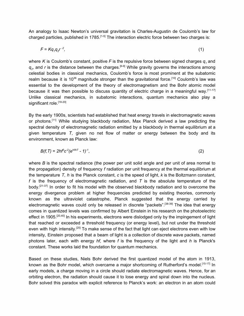
Figure 11, Currents created by orbital crossing.

As a result of orbital crossing, current is created as illustrated in Figure 11. Suppose there is an electron hole in atom C. An electron located at A tends to cross the orbital to C following the red contour ABC. Now the electron hole shifted to atom F. An electron at D tends to move to F through DEF, and so on. The overall effect is electrons flowing to the left indicated by the red arrow. The electron hole shifts to the right, creating a current to the right indicated by the blue arrow. Each electron meanders around atoms along a path at the same energy level, shown as the red contour in the top portion in Figure 11. Currents created in this example assume the existence of electron holes, or positive ions. Similarly, currents can be created with negative ions as well. Equilibrium Distance To produce currents in an orbital crossing, an electron has to be lifted to a bordering orbital sharing the same energy level between two atoms. This requires energy, which comprises the initial cost to create a current. If the current is maintained in the bordering orbital level throughout the entire process, no energy is required further. However, because of electrovity, the electron tends to step down to lower orbitals whenever there are electron holes. To maintain the current, energy has to be constantly supplied to re-lift the electron everytime it drops to a low level, which comprises the majority of the power cost for the current and is the basic cause of electrical resistance in a conductor. Normally, electrons are in their equilibrium orbitals. So, the energy cost is to lift electrons from equilibrium orbitals to bordering orbitals. The bordering orbital is determined by the distance between molecules. To be clear for the distance in this context, let’s define an equilibrium distance as the minimum distance between the outermost equilibrium orbitals of two adjacent atoms of different molecules. Essentially, the energy cost, or electrical resistance, is determined by equilibrium distances. A large equilibrium distance results

in a high level of bordering orbital and high resistivity. Hence, a logical hypothesis is that the equilibrium distance is the key factor to the electrical resistivity of a conductor. In other words, resistivity is a function of equilibrium distances. The resistivity in a conductor increases with equilibrium distances. A large equilibrium distance has several effects on resistivity. It requires more energy to lift an electron to the bordering orbitals. A large equilibrium distance also means more chances and options for orbital ascension. The density of matter is inversely related to equilibrium distance. Hence, a prediction with equilibrium distance theory is that electrical resistivity is inversely related to density. This is more useful because density is much easier to measure than equilibrium distances. The density of a substance is determined by two factors: temperature and pressure. Density increases with pressure and decreases with temperature, so does the electrical conductivity as predicted by the theory. Electrical Resistivity The classical theory for electrical resistivity was based on two misleading concepts: particle vibrations and collisions. As discussed earlier, particle vibrations are not the cause of heat radiation that is the temperature measured for. The collision theory cannot pass the density test with gold described earlier. A more significant problem is that it predicts a result that contradicts observed resistances in terms of pressure. We were forced to abandon the classical theory and developed a new equilibrium distance theory. The new theory predicts that electrical resistivity increases with temperature and decreases with pressure. Unlike equilibrium distance, both temperature and pressure are easier to measure. Hence, the prediction can be easily verified in terms of temperature and pressure. To restate the logic between temperature and resistance in equilibrium distance theory, a high temperature indicates a high level of energy and equilibrium orbitals. High equilibrium orbitals increase equilibrium distance as indicated in the helium model. This is also consistent with observations in thermal expansion and phase transition as temperature increases. A large equilibrium distance requires more energy to lift electrons to bordering orbitals for orbital crossing to create current, resulting in a high energy cost and a high electrical resistance. There is a large body of empirical evidence that supports the positive relationship between resistance and temperature.

Figure 12, Resistance as a function of temperature.

Figure 12 illustrates the general trend of resistance as a function of temperature. Here is an example: the relationship between resistance and temperature in MeB2 compound was recorded in Fig. 8 of a paper by Machado A., et al.[126] As shown in their figures, the overall downward trend is consistent with our prediction. The resistance curves up with increasing temperature. Up next, the state transition from normal conductivity to superconductivity at low temperatures is also predicted by equilibrium distance theory.

Figure 13, Resistance as a function of pressure.

The equilibrium distance theory predicts low electrical resistivity at high pressures. High pressures increase density and reduce equilibrium distance. A small equilibrium distance costs less energy to lift electrons to bordering orbitals, resulting in a low resistance. Figure 13 illustrates the general trend of resistance as a function of pressure. There are many studies on this topic. A research reported by Vaidya R., et al., indicates that the electrical resistance decreases with increasing pressure on single crystals of WSe2, as shown in Fig. 2 of the paper.[127] The electrical resistances were measured at pressures up to 8.5 GPa using Bridgman anvil setup and beyond it using diamond anvil call (DAV) up to 27 GPa. There was no clear indication of any structural transition till 27 GPa, the highest pressure reached in the study. Another research published by Souza E., et al., also shows that electrical resistance decreases under pressure for three different transmission joints, as shown in Fig. 2 of the paper. The study was conducted to search for better materials for transmission joints.[128] All the three types of materials in the comparison display the same negative relationship between electrical resistance and pressure, consistent with the prediction by equilibrium distance theory.

What Causes Superconductivity? Initially discovered in 1911, superconductivity has been the subject of many researches due to its extraordinary properties and applications, such as MRI and Maglev trains.[129-133] Cooper pairs of electrons bound together at low temperatures were proposed to be responsible for the superconductivity in BCS theory.[134-137] Since 1986, more and more superconductive materials have been found at higher temperatures, considerably above the theoretical maximum of 30 K predicted by BCS theory.[138-149] The theory also cannot stand the test of pressure similar to the classical theory for electrical resistivity. The effect of pressure to a substance is to increase the density of particles, which would increase resistivity and were not in favor of electrons flow of Cooper pairs. As shown earlier, resistivity is actually decreasing with increasing pressure. Superconductivity is observed with applied pressures for materials that are not superconductors at lower pressures. A complete theory for superconductivity must also provide explanations for the phenomena of the Meissner effect and quantum levitation. These are addressed in the theory proposed next. Superconductivity Equilibrium distance theory predicts the existence of superconductivity. Based on its postulations, electrical resistivity decreases with equilibrium distance and zero distance means no resistance. As an example, in Figure 10, superconductivity is a theoretical consequence of orbital bordering at or near the intrinsic level for low temperature superconductors. As equilibrium distance decreases from Figure 10A, 10B to 10C, the orbital border occurs at decreasing levels and eventually at the intrinsic level. In 10B, electrons have to be lifted to the bordering orbitals to create current. Energy is required. To create current for the distance in 10A, more energy is required. However, in 10C, since there is zero distance, no lifting energy is required and electrons can move across atom boundary freely.

Figure 14, Theory of resistivity and superconductivity.

A normal equilibrium distance usually creates a potential barrier, preventing electrons from crossing over the border freely, Figure 14A. As discussed in the thermal expansion section earlier, the distance between atoms usually decreases with decreasing temperature, and vise versa. At low temperatures, the distance between atoms may decrease to a point where intrinsic orbitals overlap. The electrons in the outermost orbitals are capable of propagating from one atom to another without the need for lifting energy. As an example in Figure 14B, an electron at location A in the bordering orbital of one atom moves across the boundary along the red potential contour to B in the adjacent atom. The electron stays at the same energy/potential level throughout the entire process. Keep in mind that the only requirement for superconductivity by equilibrium distance theory is zero equilibrium distance. Orbital crossing does not have to be at the intrinsic level. As long as electrons can be lifted to the bordering orbitals, current will flow. At thermal equilibrium, electrons are lifted to high orbitals by the energy from the environment and are dynamically maintained in those orbitals, known as equilibrium orbitals. In other words, if the bordering orbitals are at the same level as the equilibrium orbitals, as shown in Figure 15A, current can be maintained at orbitals higher than the intrinsic orbitals. In this case, the required lifting energy is constantly provided by the environment. As temperature increases, the equilibrium orbital moves higher. However, as discussed in the thermal expansion section, molecular separation increases with temperature which also raises the level of ordering orbitals. As temperature increases, the ascending speed of equilibrium orbitals may not keep up with the rising speed of bordering orbitals. At normal pressure on the Earth, the level of bordering orbitals usually increases with temperature faster than the equilibrium orbitals, as shown in Figure 15. This is why low temperature superconductivity is usually destroyed as temperature increases, typically to a point called the critical temperature. Now it becomes clear that the critical point for a given substance is determined by the temperature at which the bordering orbitals are at the same level as the equilibrium orbitals under normal pressure on the Earth.

Figure 15, Increasing of equilibrium orbitals and bordering orbitals with temperature

However, the situation will be different with applied pressure because pressure subdues the repulsion between molecules and force the molecules packed closely, which effectively reduces the level of bordering orbitals. With applied pressures, the critical temperature can be increased for a given superconductor. Hence, critical temperature is not a single point, but a curve in the space of temperature and pressure, as shown by the deep blue line to the left in Figure 16A. Critical temperature usually increases with pressure. In fact, superconductors are not uncommon and should be considered as a new state, as shown in the phase transition diagram. It has already been evidenced by more and more high temperature superconductors that have been discovered with applied pressures. Equilibrium distance theory shows that the distance between molecules is the key factor not only to electrical resistivity but also to superconductivity. Electrical resistivity and equilibrium distance increase with temperature and decrease with pressure. Superconducting is a state of zero equilibrium distance produced by specific combinations of pressure and temperature. The temperature at which there is zero equilibrium distance, also known as critical point, increases with pressure. The electrical resistance can be more precisely defined as the energy cost to lift electrons from equilibrium orbitals to bordering orbitals. When equilibrium orbitals are at the same levels as bordering orbitals, there is no required lifting energy and no resistance, which is the state of superconducting.

Figure 16, Phase transition and intermolecular force.

State of Matter Now we are ready to revisit phase transition with superconducting state in the picture. State of matter is determined by intermolecular force, orbital repulsion and pressure, where the two former forces are affected by temperature. To understand how the state of a system is affected by the interactions of these forces, let’s look into the phase transition diagram, Figure 16A. The intermolecular force is the accumulative electrtic forces between subatomic particles of the adjacent atoms/molecules, which has been modeled in the thermal expansion section earlier. The force is usually attractive at low temperatures or repulsive at high temperatures as shown by the blue curve in Figure 16B. This is the primary force determines the state of matter. At low temperatures, the attraction holds the molecules together in solid. At high temperatures, the repulsion breaks the molecules apart resulting in gases. Orbital repulsion force also plays an important role in phase transition. In Figure 16B, the solidifying point indicates the temperature where the orbital repulsion breaks even with the molecular attraction. To the left of this point, molecular attraction is greater than orbital

repulsion. The attraction is able to hold molecules together against the repulsion in a fixed frame. Solid is observed. To the right, orbital repulsion overcomes molecular attraction. Molecules are pushed apart and broken into fluid. The temperature at this point becomes the transition point between solid and fluid phases at zero pressure. At a higher pressure, it requires a higher repulsion force to break the solid. So, the solidifying line curves to high temperatures with increasing pressures because orbital repulsion increases with temperature. Note, there is still attraction between molecules to the right of the solidifying point. Even though the force is not enough to hold against the orbital repulsion, but still provides the attraction between molecules to create viscosity in fluid and surface tension on the liquid. The attraction is also responsible for the phenomenon of capillarity, where liquid seems defying gravity. Orbital repulsion occurs only when there is orbital jump. In fluid, orbital repulsion knocks molecules apart which is the cause of Brownian motion. On the surface of liquid or solid, orbital repulsion kicks and ejects molecules into the air in the process known as vaporization or sublimation. Molecular attraction decreases with increasing temperature. At a temperature of supercritical point, Figure 16A, the molecular attraction breaks even with molecular repulsion. Beyond this point, molecular repulsion is greater. There is no viscosity between molecules in fluid and no surface tension on liquid. Because of that, there is no latent heat in phase transition between super liquid and super gas, therefore the transition is not distinctive, a state also known as supercritical fluid.[156-158]

At a temperature beyond the ionizing point, electrons are so energetic that they can escape from the attractions of their atoms. Molecules break apart into electrons and ions, which is a state known as plasma, Figure 16A. Plasma is observable in the outer layers of the Earth and the Sun. Electrons are at such a high energy level in plasma that they can be considered free from the influence from the nuclei of atoms. In a sense, pressure provides additional force to restraint molecules together. Hence, the phase transition lines are generally curve to the high temperatures side at increasing pressures. Liquid is just pressured gas. In fluid, as pressure increases, molecules are forced to stay at a closer range. As pressure increases to a point, the liquefying pressure, Figure 16A, intermolecular attraction is able to glue the molecules together into liquid. The liquefying line curves up with temperature because molecular repulsion increases with temperature. Beyond the supercritical point, the liquefying curve is not solid because there is no distinction between super liquid and gas. Most of low pressure superconductors observed so far are at low temperatures beyond the critical points, Figure 16A. At the critical temperature, the bordering orbitals are at the same level of equilibrium orbitals and the equilibrium distance is zero. As predicted by equilibrium distance theory, with applied pressure, the repulsion between molecules may be overcome and the distance between molecules can be squeezed so that zero equilibrium distance can be established. Superconductivity may be observed for most substances with enough pressure.

Hence, the low temperature end of superconducting phase transition curve may start at a pressure above zero for some materials. Meissner Effect A superconductor is not just a perfect conductor, but more significant because of its Meissner effect. Under an external magnetic field, a moving electron, or current, is affected by the Lorentz force:

F = q(E + v x B), (12)

where F is the force, q is the electrical charge, v is the velocity of the moving charge, B is the magnetic field, E is the electric field (not applicable in this context).[150-152] The force deflects electron’s movement (or current) in superconductors. Looking in the direction of the applied magnetic field, electrons are deflected to circulate in a clockwise direction. The circulating current creates an internal magnetic field that cancels the external field inside the superconductor and superimposes the applied field outside of the superconductor. The net result appears as if the applied field is expulsed from the superconductor, known as the Meissner effect. Unlike magnetic fields created by induction where the current is induced by a change in magnetic flux, in superconductors, electron movements, or currents, are driven under the potential created by the attractions of atom nuclei, which exist naturally regardless of applied fields. This is another challenge to BCS theory, which cannot explain the Meissner effect. Cooper pairs cannot create current without additional electrical fields. Motionless electrons or Cooper pairs cannot be deflected by an applied magnetic field because v = 0 and the Lorentz force is also zero. Critical Field Confined in the orbitals of an atom, the electrons may also be deflected by an applied magnetic field via the Lorentz force, especially for the outermost electrons which have more freedom to change circulating plane due to less tangling effect from other electrons in the same atom. The deflected orbital cloud tends to conform to the plane perpendicular to the applied field, named orbital deflection. As a result, the shape of the electron cloud is flattened in the direction of the applied field. Equilibrium distance is usually increased in the same direction. As an applied field increases to a certain level, known as the critical field, the equilibrium orbitals in a superconductor becomes separated, causing the destruction of superconductivity.

Figure 17, Deformed electron cloud in a magnetic field.

Figure 17A shows a normal electron cloud shape in a superconductor. Deflected in a magnetic field, the electron clouds are flattened in the plane perpendicular to the field, Figure 17B. When the strength of the magnetic field applied passes the critical field, the equilibrium distance will be large enough to separate the equilibrium orbitals. The potential barriers will then be re-established between molecules, and the electrons can no longer propagate freely across the bordering orbitals and the resistivity is restored in the material. In large atoms/molecules, the orbital deflection may occur only in the outermost electrons where the shell is partially filled and those electrons are significant to the orbital crossing for superconductivity. Figure 17 illustrates just one example of possible crystal structures. With a crystal structure made of large and complicated molecules, different deflection/flattening effects may be observed for fields applied from different directions. This explains why certain superconductors have different critical fields for applied magnetic fields from different directions. The complication becomes more interesting for type-II superconductors.[153-155] Due to heterogeneous crystal structures in different directions, the equilibrium distances not only deviate in one direction from the other, but also for different field strengths. At a small applied field Bc1, a small distance between molecules may cause partial superconductivity. With a greater field Bc2, a larger separation between molecules eventually destroys the superconductivity. Between Bc1 and Bc2, there are some non-superconductive islands in the sample, known as vortices or normal cores in some literatures.

Figure 18, Type-II superconductors at different field strengths.

Figure 18 illustrates a type-II superconductor made of alloys. The superconductivity was established in Figure 18A. With a magnetic field strength between Bc1 and Bc2, Figure 18B, the equilibrium distance for the central molecule is large enough to destroy the superconductivity, while other molecules surrounding it are still in superconducting state. The center part forms a vortice, or non-superconducting island. This is the mixed state where flux pinning or quantum locking effect can be observed. At a field greater than Bc2, Figure 18C, the equilibrium distance is so large that the superconductivity is destroyed in the entire sample. The vortices surrounded by superconductors, such as shown in Figure 18B, are responsible for the quantum locking or the quantum levitation phenomenon, which makes type-II superconductors more interesting and valuable for applications.

How to Search for Superconductors? Scientists have been searching for high temperature superconductors blindly, without theoretical guideline, for over a century. With the equilibrium distance theory, we are very optimistic that room or higher temperature superconductors will be discovered soon. As shown in Figure 16, superconducting is just another state of matter and not uncommon. Why then, is superconductivity so hard to observe? This is because we were searching in the wrong space. As shown in Figure 16, superconductivity usually appears at the top left (high pressure/low temperature), whereas room (pressure/temperature) conditions are off to the right. Most of the high temperature superconductors obtained so far require very high pressures. Essentially, pressures are being traded for high temperatures. As modeled in equation (4), the repulsion force could increase significantly as molecules get closer. To overcome the repulsion with pressure may pose a huge engineering challenge. Sometimes, high pressures are more difficult to maintain than low temperatures. With that said, it is not impossible either. Since we are not in the dark any more, we can search much more effectively. Basically, to find high temperature superconductors, we need to search for materials with a phase transition curve that includes room temperature and pressure. Based

on the equilibrium distance theory, this requirement translates to searching for substances with zero equilibrium distance at room conditions. In other words, the equilibrium orbitals at room temperature must be at the same level of bordering orbitals at the room pressure. The challenge we are facing is that equilibrium orbitals cannot keep up with the rising of the bordering orbitals as temperature increases. So, all we need to search for materials whose repulsion forces between molecules increase slower with temperature, or less repulsive materials. Less repulsive materials usually have higher melting or boiling points and should be good candidates for superconductors. This will become the first principle in searching for high temperature superconductors. That is to seek for materials with high melting or boiling points. So, let’s turn to the periodic table to look for elements that are melting and boiling at high temperatures.

Figure 19, Solid or liquid elements at 3500 K (screenshots from ptable site).

Figure 19 shows the states of elements at 3500 K in different colors. It is interesting to note that elements on both sides of the table are in gas states, colored in red, indicating high repulsive. Most of the small atoms are also more repulsive. Some large atoms are still in liquid or solid state at this temperature, indicating these are less repulsive elements. This make sense because the nuclei of these atoms are large and provide greater attractions. Although there are more electrons, they are more evenly distributed in the shells. Overall, their attraction force between molecules becomes more prominent. What we just learned from these observations is that the structure of the outermost orbitals is important. Atoms with less filled outermost orbitals are less repulsive. This is consistent with our model because the repulsion are mostly resulted from the outermost electrons between adjacent molecules. Also note, the atoms in the leftmost

columns are repulsive. This is resulted from their large radii, which is indicated by Figure 4 of our model. Hence, the least repulsive elements are found to the left of the low center portion in the table. Of note is the fact that these elements match the low temperature superconductors discovered so far as shown in Figure 20, indicating that we are on the right track.

Figure 20, Known superconductive elements (Tc from Peter J. Lee’s page).

So, the first practical guideline for searching high temperature superconductors is to seek molecules composed from large atoms. The second guideline is to try materials with high melting/boiling points, such as the insulation used in rocket motors. Some of the superconductors are ceramics similar to those used in rocketry, which is surprising because these materials are not good conductors and even used as insulators. Now it makes sense with our theory. As shown in the helium model, the repulsion is huge when atoms are placed close to each other at high temperatures, indicating that it is unlikely to obtain high temperature superconductors with substances made of uniform element. So, the third guideline is to look into compounds and alloys. And one more guideline is to consider intermolecular force in the crystal formation. Intramolecular forces, such as covalent bonds, hold atoms together for molecule formation, but not help for superconductivity, because the bonds also anchor the pertaining electrons in place, preventing them from creating current with orbital crossing. As an example shown in Figure 20, carbon in diamond has a very high melting point. However, it is not a good candidate for high temperature superconductors because the diamond crystal is formed through covalent bonds.

Conclusions Several processes of electron dynamics, such as orbital jump, orbital repulsion, orbital crossing have been investigated, modeled or estimated in this study. With the understandings, three new theories, the potential energy theory, the orbital repulsion theory and the equilibrium distance theory, are proposed to provide solutions to some of the longstanding mysteries or phenomena, such as superconductivity. Here are some of the major conclusions. The potential energy theory is proposed to explain the origin of heat. Particle vibrations in a system are not the cause of heat radiation, but the result from electron dynamics. Heat is the radiation of the potential energy stored by electrons orbiting around their nuclei. Temperature is a measurement of heat, not the average kinetic energy of vibrations. The orbital repulsion theory is developed to provide solutions for the Crookes radiometer, Brownian motion and phase transition. Vibrations, including Brownian motion, are caused and kicked by the force created in orbital repulsion. The Crookes radiometer is driven by the same type of repulsion force, not air pressure. Orbital repulsion also plays a critical role in the phase transition from solid to liquid by overcoming the molecular attraction and breaking the molecules apart. Intermolecular force is estimated using a helium model, which provides a better understanding of thermal expansion and phase transition. At high temperatures, electron activities are in high equilibrium orbitals, which increase the size of atoms/molecules. High electron activities also increase the distance between molecules. Both processes increase the volume of matter, causing normal thermal expansion. In solid, the intermolecular attraction force holds the molecules in a fixed framework. As temperature increases, the orbital repulsion force increases. When the orbital repulsion is greater than the molecular attraction, the molecules in a solid break apart and melt into a fluid. Liquid is just a special gas under pressure. The intermolecular attraction also provides the force for viscosity in fluid and surface tension on liquid. The attraction force also provides explanation to the anti-gravitational phenomenon of capillarity. The equilibrium distance theory provides a solution to address the problems in existing theories for electrical resistivity and superconductivity. The collision theory for electrical resistivity fails apart on pressure test, so does BCS theory for superconductivity. It is the equilibrium distance that determines resistivity and superconductivity. Equilibrium distances are inversely related to the density of matter, which is in turn determined by pressure and temperature. Hence, the equilibrium distance theory predicts that resistivity increases with temperature and decreases with pressure. The theory also predicts superconductivity at zero equilibrium distance. Currents created by orbital crossing exist naturally regardless of external fields, which explains the Meissner effect for superconductors. Orbital deflection theory provides an explanation to critical fields for both type-I and type-II superconductors. With the equilibrium distance theory, some guidelines are provided for searching high temperature superconductors more effectively.

References

1. Comins, N.F.; Kaufmann, W.J. (2008). “Discovering the Universe: From the Stars to the Planets”. MacMillan. p. 347.

2. Pauli, W.E. (1958). "Part IV. General Theory of Relativity". Theory of Relativity. Courier Dover Publications.

3. Weinberg, S. (1972). “Gravitation and cosmology”. John Wiley & Sons. p. 194. 4. Nemiroff, R.; Bonnell, J. (2014). "The Potsdam Gravity Potato". Astronomy Picture of

the Day. NASA. 5. Haugan, M.P; Lämmerzahl, C. (2011). "Einstein gravity from conformal gravity".

arXiv:1105.5632. 6. Roller, D.; Roller, D.H.D. (1954). “The development of the concept of electric charge:

Electricity from the Greeks to Coulomb”. Cambridge, MA: Harvard University Press. p. 79.

7. Stewart, J. (2001). “Intermediate Electromagnetic Theory”. World Scientific. p. 50. 8. Simpson, B. (2003). “Electrical Stimulation and the Relief of Pain”. Elsevier Health

Sciences. pp. 6–7. 9. Baigrie, B. (2007). “Electricity and Magnetism: A Historical Perspective”. Greenwood

Press. pp. 7–8. 10. Weisstein, E.W. (2007). "Fifth Force". World of Science. Wolfram Research. 11. Maxwell, J.C.; et al. (1967). "Experiments on Electricity: Experimental determination of

the law of electric force.". The Electrical Researches of the Honourable Henry Cavendish.... Cambridge, England: Cambridge University Press. pp. 104–113.

12. Ravaioli, F.T.; et al. (2010). “Fundamentals of applied electromagnetics”. Boston: Prentice Hall. p. 13.

13. Lakhtakia, A.; et al. (1996). "Models and Modelers of Hydrogen". American Journal of Physics. 65 (9): 933.

14. Bohr, N. (1913). "On the Constitution of Atoms and Molecules, Part I". Philosophical Magazine. 26 (151): 1–24.

15. Stachel, J. (2009). "Bohr and the Photon". Quantum Reality, Relativistic Causality, and Closing the Epistemic Circle. Dordrecht: Springer. p. 79.

16. Whitaker, M.A.B. (1999). "The Bohr–Moseley synthesis and a simple model for atomic x-ray energies". European Journal of Physics. 20 (3): 213–220.

17. Svidzinsky, A.A.; et al. (2005). "Bohr's 1913 molecular model revisited". Proceedings of the National Academy of Sciences. 102 (34[1]): 11985–11988.

18. Darrigol, O. (2000). “Electrodynamics from Ampère to Einstein”. New York: Oxford University Press.

19. Whittaker, E.T. (1910). “A History of the Theories of Aether and Electricity from the Age of Descartes to the Close of the Nineteenth Century”. Longmans, Green and Company.

20. Einstein, A. (1993). “The Collected Papers of Albert Einstein. 3”. English translation by Beck, A. Princeton University Press.

21. Hapke, B. (1993). “Theory of Reflectance and Emittance Spectroscopy”. Cambridge University Press, Cambridge UK.

22. Kangro, H. (1976). “Early History of Planck's Radiation Law”. Taylor & Francis. 23. Klein, M.J. (1962). "Max Planck and the beginnings of the quantum theory". Archive for

History of Exact Sciences. 1 (5): 459–479. doi:10.1007/BF00327765. 24. Kragh, H. (December 2000). "Max Planck: The reluctant revolutionary". Physics World. 25. Kramm, G.; Mölders, N. (2009). "Planck's Blackbody Radiation Law: Presentation in

Different Domains and Determination of the Related Dimensional Constant". Journal of the Calcutta Mathematical Society. 5 (1–2): 27–61. arXiv:0901.1863.

26. Lewis, G.N. (1926). "The Conservation of Photons". Nature. 118 (2981): 874. doi:10.1038/118874a0.

27. Loudon, R. (2000). “The Quantum Theory of Light” (3rd ed.). Oxford University Press. 28. Pauli, W.; et al. (1973). “Wave Mechanics. Margulies”, S.; Lewis, H. R. (transl.). MIT

Press. 29. Planck, M. (1914). “The Theory of Heat Radiation”. Masius, M. (transl.) (2nd ed.). P.

Blakiston's Son & Co. OL 7154661M. 30. Planck, M. (1915). “Eight Lectures on Theoretical Physics”. Wills, A. P. (transl.). Dover

Publications. 31. Stehle, P. (1994). “Order, Chaos, Order. The Transition from Classical to Quantum

Physics”. Oxford University Press. 32. Tyndall, J. (1865). “Heat considered as a Mode of Motion”. D. Appleton & Company. 33. Maxwell, J.C. (1873) A Treatise on Electricity and Magnetism, Oxford University Press. 34. Schlamminger, S.; et al. (2014). "Determination of the Planck constant using a watt

balance with a superconducting magnet system at the National Institute of Standards and Technology". Metrologia. 51 (2): S15. arXiv:1401.8160.

35. Planck, M. (1920), “The Genesis and Present State of Development of the Quantum Theory” (Nobel Lecture).

36. Pitre, L; et al. (2017). "New measurement of the Boltzmann constant by acoustic thermometry of helium-4 gas". Metrologia. 54 (6): 856–873. doi:10.1088/1681-7575/aa7bf5.

37. Kalinin, M.; Kononogov, S. (2005), "Boltzmann's Constant, the Energy Meaning of Temperature, and Thermodynamic Irreversibility", Measurement Techniques, 48 (7): 632–36, doi:10.1007/s11018-005-0195-9.

38. Mason, S.F. (1962). “A History of the Sciences”. Collier Books. p. 550. 39. Stone, A.D. (2013). “Einstein and the Quantum”. Princeton University Press. 40. Lamb, W.E.; Scully, M.O. (1968). "Photoelectric effect without photons, discussing

classical field falling on quantized atomic electron". 41. Langmuir, I. (1919). "The Arrangement of Electrons in Atoms and Molecules". Journal

of the American Chemical Society. 41 (6): 868–934. doi:10.1021/ja02227a002. 42. Straumann, N. (2004). "The Role of the Exclusion Principle for Atoms to Stars: A

Historical Account". Invited talk at the 12th Workshop on Nuclear Astrophysics. arXiv:quant-ph/0403199.

43. Pauli, W. (1925). "Über den Zusammenhang des Abschlusses der Elektronengruppen im Atom mit der Komplexstruktur der Spektren". Zeitschrift für Physik. 31: 765–783. doi:10.1007/BF02980631.

44. Griffiths, D.J. (2004), “Introduction to Quantum Mechanics” (2nd ed.), Prentice Hall. 45. Dyson, F. (1967). "Ground-State Energy of a Finite System of Charged Particles". J.

Math. Phys. 8 (8): 1538–1545. doi:10.1063/1.1705389. 46. Lieb, E.H.; et al. (1995). "Stability of Matter in Magnetic Fields". Physical Review

Letters. 75 (6): 985–9. arXiv:cond-mat/9506047. 47. Bojowald, M. (2012). “The Universe: A View from Classical and Quantum Gravity”.

John Wiley & Sons. 48. Rothman, L.S.; et al. (2013). "The HITRAN2012 molecular spectroscopic database".

Journal of Quantitative Spectroscopy and Radiative Transfer. 130: 4–50. doi:10.1016/j.jqsrt.2013.07.002.

49. Peach, G. (1981). "Theory of the pressure broadening and shift of spectral lines". Advances in Physics. 30 (3): 367–474. doi:10.1080/00018738100101467.

50. Sommerfeld, A. (1923). “Atomic Structure and Spectral Lines”. Brose, H. L. (transl.) (from 3rd German ed.). Methuen.

51. Zielinski, S. (2008). "Absolute Zero". Smithsonian Institution. Retrieved 26 January 2012.

52. Masanes, L.; Oppenheim, J. (2017), "A general derivation and quantification of the third law of thermodynamics", Nature Communications, 8 (14538): 14538, doi:10.1038/ncomms14538, PMC 5355879, PMID 28290452.

53. Thomson, W. (1848). "On an Absolute Thermometric Scale founded on Carnot's Theory of the Motive Power of Heat, and calculated from Regnault's observations". Proceedings of the Cambridge Philosophical Society. 1: 66–71.

54. Moran; S. (2000). “Fundamentals of Engineering Thermodynamics” (4th ed.). Wiley. 55. Adkins, C.J. (1968/1983). “Equilibrium Thermodynamics”, (1st edition 1968), third

edition 1983, Cambridge University Press, Cambridge UK. 56. Attard, P. (2012). “Non-equilibrium Thermodynamics and Statistical Mechanics:

Foundations and Applications”, Oxford University Press, Oxford UK. 57. Baierlein, R. (1999). “Thermal Physics”, Cambridge University Press, Cambridge UK. 58. Boltzmann, L. (1896/1964). “Lectures on Gas Theory”, translated by S.G. Brush,

University of California Press, Berkeley. 59. Borgnakke, C.; Sonntag, R.E. (2009). “Fundamentals of Thermodynamics”, seventh

edition, Wiley. 60. Buchdahl, H.A. (1966). “The Concepts of Classical Thermodynamics”, Cambridge

University Press, Cambridge UK. 61. Bridgman, P.W. (1943). “The Nature of Thermodynamics”, Harvard University Press,

Cambridge MA. 62. Callen, H.B. (1960/1985). “Thermodynamics and an Introduction to Thermostatistics”,

(1st edition 1960) 2nd edition 1985, Wiley, New York. 63. Eu, B.C. (2002). “Generalized Thermodynamics. The Thermodynamics of Irreversible

Processes and Generalized Hydrodynamics”, Kluwer Academic Publishers, Dordrecht.

64. Glansdorff, P., Prigogine, I. (1971). “Thermodynamic Theory of Structure, Stability, and Fluctuations”, Wiley-Interscience, London, 1971.

65. Grandy, W.T., Jr (2008). “Entropy and the Time Evolution of Macroscopic Systems”. Oxford University Press.

66. Greven, A.; et al. (2003). “Entropy”, Princeton University Press, Princeton NJ. 67. Kondepudi, D., Prigogine, I. (1998). “Modern Thermodynamics: From Heat Engines to

Dissipative Structures”, John Wiley & Sons, Chichester. 68. Lieb, E. H.; Yngvason, J. (1999). "The Physics and Mathematics of the Second Law of

Thermodynamics". Physics Reports. 310 (1): 1–96. arXiv:cond-mat/9708200. 69. Lieb, E.H., Yngvason, J. (2003). “The Entropy of Classical Thermodynamics”, pp.

147–195, Chapter 8 of Entropy, Greven, A., Keller, G., Warnecke (editors) (2003). 70. Mandl, F. (1988). “Statistical physics” (second ed.). Wiley & Sons. 71. Tisza, L. (1966). “Generalized Thermodynamics”, MIT Press, Cambridge MA. 72. Wilks J. (1961). “The Third Law of Thermodynamics”. Oxford University Press. 73. Heidrich, M. (2016). "Bounded energy exchange as an alternative to the third law of

thermodynamics". Annals of Physics. 373: 665–681. doi:10.1016/j.aop.2016.07.031. 74. Kozliak, E.; Lambert, F.L. (2008). "Residual Entropy, the Third Law and Latent Heat".

Entropy. 10 (3): 274–84. doi:10.3390/e10030274. 75. Guggenheim, E.A. (1967). “Thermodynamics. An Advanced Treatment for Chemists

and Physicists”, fifth revised edition, North-Holland Publishing Company, Amsterdam, page 157.

76. Walker, J. (2008). “Fundamentals of Physics”, 8th ed., John Wiley and Sons, p. 891. 77. Mehra, J.; Rechenberg, H. (1982). “The Historical Development of Quantum Theory”.

New York City: Springer-Verlag. Chapter 1. 78. Schrödinger, E. (1926). "An Undulatory Theory of the Mechanics of Atoms and

Molecules". Physical Review. 28 (6): 1049–1070. doi:10.1103/PhysRev.28.1049. 79. Shankar, R. (1943). “Principles of Quantum Mechanics” (2nd ed.). Kluwer

Academic/Plenum Publishers. 80. Sakurai, J.J. (1995). “Modern Quantum Mechanics”. Reading, Massachusetts:

Addison-Wesley. p. 68. 81. Zettili, N. (2009). “Quantum Mechanics: Concepts and Applications”. John Wiley &

Sons. 82. Ballentine, L. (1998). “Quantum Mechanics: A Modern Development”, World Scientific

Publishing Co. 83. Schrödinger, E. (1995). “The interpretation of quantum mechanics: Dublin seminars

(1949–1955) and other unpublished essays”. Ox Bow Press. 84. Schrödinger, E. (1982). “Collected Papers on Wave Mechanics”: Third Edition.

American Mathematical Soc. 85. Schrödinger, E. (1926). "Quantisierung als Eigenwertproblem; von Erwin Schrödinger".

Annalen der Physik. 384 (4): 361–377. 86. Einstein, A.; et al. "Letters on Wave Mechanics:

Schrodinger–Planck–Einstein–Lorentz".

87. Ajaib, M.A. (2015). "A Fundamental Form of the Schrödinger Equation". Found. Phys. 45 (12): 1586–1598. arXiv:1502.04274.

88. Voitkovskii, K.F., Translation of: "The mechanical properties of ice" ("Mekhanicheskie svoistva l'da"), Academy of Sciences (USSR).

89. Harvey, A.H. (2017). "Properties of Ice and Supercooled Water". In Haynes, W.M.; et al. CRC Handbook of Chemistry and Physics (97th ed.). Boca Raton, FL: CRC Press.

90. Salzmann, C.G.; et al. (2006). "The Preparation and Structures of Hydrogen Ordered Phases of Ice". Science. 311 (5768): 1758–1761. doi:10.1126/science.1123896. PMID 16556840.

91. Tyson, N.; "Water, Water". Haydenplanetarium.org. 92. Militzer, B.; Wilson, H.F. (2010). "New Phases of Water Ice Predicted at Megabar

Pressures". Physical Review Letters. 105 (19): 195701. arXiv:1009.4722. 93. MacMahon, J.M. (1970). "Ground-State Structures of Ice at High-Pressures". Physical

Review B. 84 (22): 220104. arXiv:1106.1941. 94. Murray, B.J. (2008). "The Enhanced formation of cubic ice in aqueous organic acid

droplets". Environmental Research Letters. 3 (2): 025008. doi:10.1088/1748-9326/3/2/025008.

95. Murray, B.J.; et al. (2005). "The formation of cubic ice under conditions relevant to Earth's atmosphere". Nature. 434 (7030): 202–205. doi:10.1038/nature03403. PMID 15758996.

96. Feynman, R. (1964). "The Brownian Movement". The Feynman Lectures of Physics, Volume I. pp. 41&#45, 1.

97. Li, T.; et al. (2010). "Measurement of the instantaneous velocity of a Brownian particle". Science. 328 (5986): 1673–1675. doi:10.1126/science.1189403. PMID 20488989.

98. Weiss, G.H. (1994). “Aspects and applications of the random walk”. North Holland. 99. Ben-Avraham, D.; Havlin, S. (2000). “Diffusion and reaction in disordered systems”.

Cambridge University Press. 100. Morozov, A. N.; Skripkin, A. V. (2011). "Spherical particle Brownian motion in viscous

medium as non-Markovian random process". Physics Letters A. 375 (46): 4113–4115. doi:10.1016/j.physleta.2011.10.001.

101. Krapf, D.; et al. (2018). "Power spectral density of a single Brownian trajectory: what one can and cannot learn from it". New Journal of Physics. 20 (2): 023029. doi:10.1088/1367-2630/aaa67c.

102. Einstein, A. (1956) [1926]. “Investigations on the Theory of the Brownian Movement”. Dover Publications. Retrieved 25 December 2013.

103. Stachel, J., (1989). "Einstein's Dissertation on the Determination of Molecular Dimensions". The Collected Papers of Albert Einstein, Volume 2. Princeton University Press.

104. Crookes, W. (1874). "On Attraction and Repulsion Resulting from Radiation". Philosophical Transactions of the Royal Society of London. 164: 501–527. doi:10.1098/rstl.1874.0015.

105. Maxwell, J.C. (1879). "On stresses in rarefied gases arising from inequalities of temperature". Philosophical Transactions of the Royal Society of London. 170: 231–256. doi:10.1098/rstl.1879.0067.

106. Worrall, J. (1982), "The pressure of light: The strange case of the vacillating 'crucial experiment'”, Studies in History and Philosophy of Science, 13 (2): 133–171, doi:10.1016/0039-3681(82)90023-1.

107. Gibbs, P. (1996). "How does a light-mill work?". math.ucr.edu/home/baez/physics/index.html. Usenet Physics FAQ. Retrieved 8 August 2014.

108. Brush, S.G.; Everitt, C.W.F. (1969). “Maxwell, Osborne Reynolds, and the Radiometer.” Historical Studies in the Physical Sciences, vol. 1, 1969, pp. 105–125.

109. Han, L.H.; et al. (2010). "Light-Powered Micromotor Driven by Geometry-Assisted, Asymmetric Photon-heating and Subsequent Gas Convection". Applied Physics Letters. 96 (21): 213509(1–3). doi:10.1063/1.3431741.

110. Han, L.H.; et al. (2011). "Light-Powered Micromotor: Design, Fabrication, and Mathematical Modeling". Journal of Microelectromechanical Systems. 20 (2): 487–496. doi:10.1109/JMEMS.2011.2105249.

111. Wolfe, D.; et al. (2016). "A Horizontal Vane Radiometer: Experiment, Theory, and Simulation". Journal-ref: Phys. Fluids 28, 037103. Department of Physics, Naval Postgraduate School, Monterey CA 93940, USA. 28 – via arXiv.

112. Yarris, L. (2010). "Nano-sized light mill drives micro-sized disk". Physorg. Retrieved 6. 113. Osborne, R. (1879). “On certain dimensional properties of matter in the gaseous state“,

Royal Society Phil. Trans., Part 2. 114. Narimanov, E.E.; Smolyaninov, I.I. (2012). "Beyond Stefan–Boltzmann Law: Thermal

Hyper-Conductivity". Conference on Lasers and Electro-Optics 2012. OSA Technical Digest. Optical Society of America. pp. QM2E.1. doi:10.1364/QELS.2012.QM2E.1.

115. Knizhnik, K. "Derivation of the Stefan–Boltzmann Law". Johns Hopkins University – Department of Physics & Astronomy.

116. Califano, S. (1976). “Vibrational States”. New York: Wiley. 117. Gans, P. (1971). “Vibrating Molecules”. New York: Chapman and Hall. 118. Steele, D. (1971). “Theory of vibrational spectroscopy”. Philadelphia: Saunders, W.B. 119. Giancoli, D. (2007). “Physics for Scientists and Engineers, with Modern Physics”

(Chapters 1-37), 4th ed. Mastering Physics Series. Upper Saddle River, NJ: Prentice Hall.

120. Gibilisco, S. (2005). “Electricity Demystified”. New York: McGraw-Hill. 121. Tipler, P.A.; Mosca G. (2004). “Physics for Scientists and Engineers”, Volume 2:

Electricity and Magnetism, Light, Modern Physics, 5th ed. New York: W.H. Freeman. 122. Young, H.D.; Freedman, R.A. (2003). “Physics for Scientists and Engineers”, 11th

edition. San Francisco: Pearson. 123. Forbes T. B. (2006). “Engineering System Dynamics”. CRC Press. p. 43. 124. Kaiser, K.L. (2004). “Electromagnetic Compatibility Handbook”. CRC Press. pp. 13–52. 125. McDonald, J.D. (2016). “Electric Power Substations Engineering”, Second Edition.

CRC Press. pp. 363–.

126. Machado, A.; et al. (2012). “Defect Structure Versus Superconductivity in MeB2 Compounds (Me = Refractory Metals) and One-Dimensional Superconductors”, doi:10.5772/48625.

127. Vaidya, R.; et al. (2003), “Effect of pressure on electrical resistance of WSe2 single crystal”, Pramana -- journal of physics, Vol. 61, No. 1 pp. 183-186.

128. Souza E., et al. (2006), “Improvement of metallic joint electrical conductivity using a novel conductive paste produced from recycled residues”, Rev. Esc. Minas Vol. 59, No. 2.

129. Onnes, H. K. (1911). "The resistance of pure mercury at helium temperatures". Commun. Phys. Lab. Univ. Leiden. 12: 120.

130. Dirk van Delft; Peter Kes, P. (2010). "The Discovery of Superconductivity". Physics Today. 63 (9): 38–43. doi:10.1063/1.3490499.

131. Gibney, E. (2018). "Surprise graphene discovery could unlock secrets of superconductivity". News. Nature. 555 (7695): 151–2. doi:10.1038/d41586-018-02773-w. PMID 29517044.

132. Dolecek R.L. (1954). "Adiabatic Magnetization of a Superconducting Sphere". Physical Review. 96 (1): 25–28. doi:10.1103/PhysRev.96.25.

133. Gallop J.C. (1990). “SQUIDS, the Josephson Effects and Superconducting Electronics”. CRC Press. pp. 1, 20.

134. Bardeen, J.; et al. (1957). "Theory of Superconductivity". Physical Review. 108 (5): 1175–1205. doi:10.1103/PhysRev.108.1175.

135. Bardeen, J.; et al. (1957). “Theory of Superconductivity”. Physical Review. 108. p. 1175. doi:10.1103/physrev.108.1175.

136. Ginzburg V.L.; Landau L.D. (1950). "On the theory of superconductivity". Zhurnal Eksperimental'noi i Teoreticheskoi Fiziki. 20: 1064.

137. Combescot M.; et al. (2013). "BCS ansatz for superconductivity in the light of the Bogoliubov approach and the Richardson–Gaudin exact wave function". Physica C: Superconductivity. 485: 47–57. arXiv:1111.4781.

138. Bednorz J.G. & Müller K.A. (1986). "Possible high Tc superconductivity in the Ba−La−Cu−O system". Z. Phys. B. 64 (1): 189–193. doi:10.1007/BF01303701.

139. Wu M.K.; et al. (1987). "Superconductivity at 93 K in a New Mixed-Phase Y-Ba-Cu-O Compound System at Ambient Pressure". Physical Review Letters. 58 (9): 908–910. doi:10.1103/PhysRevLett.58.908. PMID 10035069.

140. Berlincourt, T.G. (1987). "Emergence of Nb-Ti as Supermagnet Material". Cryogenics. 27 (6): 283–289. doi:10.1016/0011-2275(87)90057-9.

141. Drozdov, A; et al. (2015). "Conventional superconductivity at 203 kelvin at high pressures in the sulfur hydride system". Nature. 525 (2–3): 73–76. arXiv:1506.08190.

142. Bogoliubov, N.N. (1958). "A new method in the theory of superconductivity". Zhurnal Eksperimental'noi i Teoreticheskoi Fiziki. 34: 58.

143. Mann, A. (2011). "High-temperature superconductivity at 25: Still in suspense". Nature. 475 (7356): 280–2. doi:10.1038/475280a. PMID 21776057.

144. Pines, D. (2002), "The Spin Fluctuation Model for High Temperature Superconductivity: Progress and Prospects", The Gap Symmetry and Fluctuations in

High-Tc Superconductors, NATO Science Series: B, 371, New York: Kluwer Academic, pp. 111–142, doi:10.1007/0-306-47081-0_7.

145. Monthoux, P.; et al. (1991). "Toward a theory of high-temperature superconductivity in the antiferromagnetically correlated cuprate oxides". Phys. Rev. Lett. 67 (24): 3448–3451. doi:10.1103/PhysRevLett.67.3448. PMID 10044736.

146. Schilling, A.; et al. (1993). "Superconductivity above 130 K in the Hg–Ba–Ca–Cu–O system". Nature. 363 (6424): 56–58. doi:10.1038/363056a0.

147. Takahashi, H.; et al. (2008). "Superconductivity at 43 K in an iron-based layered compound LaO1−xFxFeAs". Nature. 453 (7193): 376–378. doi:10.1038/nature06972. PMID 18432191.

148. Cho, A. (2014-10-30). "Second Family of High-Temperature Superconductors Discovered". ScienceNOW Daily News.

149. Drozdov, A.P.; et al. (2015). "Conventional superconductivity at 203 kelvin at high pressures in the sulfur hydride system". Nature. 525 (7567): 73–6. arXiv:1506.08190.

150. Huray, P.G. (2010). “Maxwell's Equations”. Wiley-IEEE. p. 22. 151. Lorentz, H.A. (1895). “Versuch einer Theorie der electrischen und optischen

Erscheinungen in bewegten Körpern”. 152. Chow, T.L. (2006). “Electromagnetic theory”. Sudbury MA: Jones and Bartlett. p. 395. 153. Hove, J.; et al. (2002). "Vortex interactions and thermally induced crossover from

type-I to type-II superconductivity". Physical Review B. 66 (6): 064524. arXiv:cond-mat/0202215.

154. Callaway, D.J.E. (1990). "On the remarkable structure of the superconducting intermediate state". Nuclear Physics B. 344 (3): 627–645. doi:10.1016/0550-3213(90)90672-Z.

155. Abrikosov, A.A. (2003). "type II Superconductors and the Vortex Lattice". Nobel Lecture.

156. Székely K. (2014). "What is a supercritical fluid?". Budapest University of Technology and Economics.

157. Padrela, L.; et al. (2009). "Formation of indomethacin–saccharin cocrystals using supercritical fluid technology". European Journal of Pharmaceutical Sciences. 38 (1): 9–17. doi:10.1016/j.ejps.2009.05.010.

158. Ye, X.R.; et al. (2003). "Supercritical fluid fabrication of metal nanowires and nanorods templated by multiwalled carbon nanotubes". Advanced Materials. 15 (4): 316–319. doi:10.1002/adma.200390077.