Embed Size (px)
Citation preview

Portland State University Portland State University
PDXScholar PDXScholar
Systems Science Faculty Publications and Presentations Systems Science
7-1-2012
Using System Dynamics to Contribute to Ecological Using System Dynamics to Contribute to Ecological
Economics Economics
Takuro Uehara Portland State University
Yoko Nagase Portland State University
Wayne Wakeland Portland State University, [email protected]
Follow this and additional works at: https://pdxscholar.library.pdx.edu/sysc_fac
Part of the Computer Engineering Commons, and the Economics Commons
Let us know how access to this document benefits you.
Citation Details Citation Details Uehara, T., Y. Nagase and W. Wakeland. “Using system dynamics to contribute to ecological economics” Proc. 30th Int’l Conf. System Dynamics Society, St. Gallen, Switzerland, July 2012.
This Conference Proceeding is brought to you for free and open access. It has been accepted for inclusion in Systems Science Faculty Publications and Presentations by an authorized administrator of PDXScholar. Please contact us if we can make this document more accessible: [email protected].

1
Using System Dynamics to Contribute to Ecological Economics
Takuro Uehara Doctoral Student, Systems Science Graduate Program and Dept. of Economics, Portland State
University, SYSC, P.O. Box 751, Portland, OR 97207, USA Tel: 503-725-3907
Yoko Nagase Senior Lecturer, Department of Accounting, Finance and Economics, Oxford Brookes University,
Wheatley Campus, Wheatley, Oxford, OX33 1HX, U.K. Tel: 44-01865-485-997 [email protected]
Wayne Wakeland
Ph.D., Associate Professor, Systems Science Graduate Program Portland State University, SYSC, P.O. Box 751, Portland, OR 97207, USA
Tel: 503-725-4975 Fax: 503-725-8489 [email protected]
Abstract This paper demonstrates the usefulness of the system dynamics approach to the development of ecological economics, the study of the interactions between economic systems and ecological systems. We build and analyze an ecological economic model: an extension of a population–resource dynamics model developed by Brander and Taylor and published in American Economic Review in 1998. The focus of the present paper is on the model building and analysis to contribute to theory building rather than eliciting policy implications from the model. Hence, this is an example of model-based theory building using system dynamics. Our analysis sheds light on several problems with this type of ecological economics model that can be attributed to three commonly taken approaches to model building and analysis by traditional economics: simplification through the use of exogenous variables, equilibrium thinking, and a focus on the so-called balanced growth path. To solve these problems ecological economic models should adopt approaches that are not prevalent in traditional economics such as taking an endogenous point of view and allowing for out-of-equilibrium (adaptation) which are key principles of the system dynamics method. Keywords: Ecological Economics; Model-Based Theory Building; Endogenous Point of View; Adaptation (out-of-equilibrium); Population-resource dynamics
1. Introduction Real problems in complex systems do not respect academic boundaries.
- Herman Daly and Joshua Farley (Ecological Economics, 2nd ed., (2010), xvii) This article demonstrates the usefulness of the system dynamics approach to ecological economics–the study of the interactions between economic systems and ecological systems (Common and Stagl,

2
2005). We build and analyze an ecological economic model: an extension of a population–resource dynamics developed by Brander and Taylor and published in American Economic Review in 1998 (henceforth the BT model). The model is characterized as a general equilibrium version of the Gordon-Schaefer Model, using a variation of the Lotka-Volterra predator-prey model.
Ecological economics is an interdisciplinary approach to solve problems that stem from the interactions between economic systems and ecological systems. Ecological considerations have often been either neglected or not treated properly in economics. Given the essential dynamic complexity of an ecological economic system, we need an approach that goes beyond the simplified, analytic approaches by standard economics. System dynamics can provide such an alternative.
Although ecological economic systems are ‘undeniably’ complex (Limburg et al., 2002), standard economics has generally taken a strategy of simplification to be able to employ analytic approaches. However, simplification has many drawbacks. There are many examples of this. First, simpler functions such as the Cobb-Douglas type function (e.g., Solow, 1974a; Anderies, 2003), while easy-to-handle analytically, limit the analysis of substitutability between man-made capital and natural resources that is essential for sustainable development under natural resource constraints. Second, the system boundary is set narrowly for the sake of simplicity. In analyzing the role of substitutability in an economy, the law of motion of resources is often ignored (e.g., Bretschger, 1998). However, feedbacks between ecology and economy play an important role (Costanza et al., 1993). Whenever an element is treated as exogenous, the feedback loops are dropped. Third, standard economic theories mostly focus on equilibrium conditions. “Transition dynamics” has largely been neglected (Sargent, 1993), except for the recent development of learning (expectation) theory in modern macroeconomics (e.g., Evans and Honkapohja, 2009; Evans and Honkapohja, 2011; Bullard, 2006). States of disequilibrium and equilibrium-seeking adaptive systems have not been investigated well in economics, but such transition dynamics are important for studying ecological economic systems (Costanza et al., 1993).
This paper strives to bridge economics and system dynamics in order to provide deeper insights into the dynamics of ecological economic systems. While system dynamics has often neglected economic theories because of its unrealistic tendencies (in the views of system dynamicists), economics seems to largely ignore system dynamics (except for the notable reaction against The Limits to Growth) because of its inconsistencies with economic theories. On the one hand, it is true that economic theories provide a solid foundation for modeling economic systems. On the other hand, system dynamics provides tools and a way of thinking for studying complex systems. We particularly focus on the role of system dynamics as model-based theory building (Schwaninger and Grosser, 2008). We propose to employ standard economic theories as a base for ecological economic models and to employ the system dynamics approach to build and validate the models. Since the research employs the system dynamics approach as a primary method, the analysis of model results will look different from how they are typically presented in economic journals.
In addition to technical characteristics of system dynamics as a computer-aided approach to solve a system of coupled, nonlinear, first-order differential equations, system dynamics provides useful tools and approaches to analyze complex systems. What characterizes system dynamics is its emphasis on 1) feedback thinking, 2) loop dominance and nonlinearity, and 3) taking an endogenous point of view. The endogenous point of view is the sine qua non of systems approaches (Richardson, 2011). System dynamics also uses several unique techniques for mapping a model, including causal loop diagrams, system boundary diagrams, and stock and flow diagrams, in order to visualize a complex system. The model developed by Brander and Taylor (1998) is adopted as a baseline ecological economic model. The BT model explains a pattern of economic and population growth, resource

3
degradation, and subsequent economic decline. Since its initial appearance in the American Economic Review, the BT model has generated many descendants (Anderies, 2003; Basener and Ross, 2005; Basener et al., 2008; D'Alessandro, 2007; Dalton and Coats, 2000; Dalton et al., 2005; de la Croix and Dottori, 2008; Erickson and Gowdy, 2000; Good and Reuveny, 2006; Maxwell and Reuveny, 2000; Nagase and Mirza, 2006; Pezzey and Anderies, 2003; Prskawetz et al., 2003; Reuveny and Decker, 2000; Taylor, 2009; Nagase and Uehara, 2011). In addition to its high quality, the BT model is attractive, because of its simplicity and potential extendability. Hence the BT model should serve as a good starting point for investigating the role of such critical factors as substitutability, resource management regimes, population growth, and adaptation in an economy under limited available natural resources, to evaluate the sustainability and resilience of an ecological economic system. This article will extend the BT model following the suggestions for further research by Nagase and Uehara (2011): population growth, substitutability, innovation, capital accumulation, property rights/institutional designs, and modeling approach. The model is also an extension of the model developed by Uehara et al (2010) presented at the ISDC 2010 conference held in South Korea. Although their model resulted in unexpected inflation, the cause of the problem was later identified (an issue related to Euler’s Theorem) and the problem has now been fixed. The model developed here will be most applicable to developing economies where their economies may depend on natural resources and population dynamics in a significant way. Contrasted with the substantial body of work on limits to growth (c.f,, Meadows, et al. 2004), the underlying equations in the present model are much simplified and are tied more directly to traditional economic theory. The purpose of our modeling and analysis is to find directions for the further development of ecological economic models through conducting sensitivity analysis. Hence, this is an example of model-based theory building using system dynamics. Through sensitivity analysis, we found two problems with the BT model that are attributed to three commonly taken approaches to model building and analysis by traditional economics: a simplification by the use of exogenous variables, equilibrium thinking, and a focus on the so-called “balanced growth path.” The BT model relies on exogenous or constant consumer preference, and maintains instantaneous equilibrium (i.e., no adaptive process). These considerations are important in view of the desire to use the model for the sustainability of dynamic and complex ecological economic systems, and indicate that ecological economic models would benefit from the adoption of approaches that are not prevalent in traditional economics such as taking an endogenous point of view and allowing for disequilibrium (adaptation) which are key principles of the system dynamics method. Section 2 presents the model and preliminary model testing, Section 3 provides the primary results from conducting a variety model experiments focused on parameter sensitivity, and discussion follows in Section 4. Model details are provided in an Appendix.
2. Model 2.1. Problem We model a problem of sustainable development in developing economies which face a new economic reality in which natural resource constraints are largely defining the future outlook (UNESCAP, 2010, vii). While major economic growth models such as Solow growth model, neoclassical growth model, Ramsey-Cass-Koopmans, and Overlapping Generations Model1 do not embrace natural resource 1 For a good review of these standard economic growth models, see Romer (2011)
4
constraints as a primary component of their models, a report by UNESCAP (2010) argues that based on real data, in Asia and the Pacific region, natural resource constraints such as food, water and energy supplies, and climate change will play an increasingly important role in defining the sustainability of economies in the region. Natural resource constraints are a real problem for sustainable development. To develop a system dynamics model, we need graphs and other descriptive data showing the behavior of the problem, which is called a reference mode. However, as the report by UNESCAP addresses, this is a new phenomenon so that we do not have a good reference mode based on actual data (either qualitative or quantitative).2 Therefore while the model developed here is to eventually be used to elicit policy implications for developing economies, the model does not intend to seek fitness to any particular historical data because developing economies may go through unprecedented experiences since their situations could be quite different from the currently developed economies (e.g., the availability of many technologies and the increased scarcity of natural resources). Nevertheless, it will be worthwhile to discuss possible dynamic behaviors by considering possible reference modes.
One possible reference pattern could be a collapse. As Diamond (2005) documented, there are many historical cases of collapse. One of them is the boom and bust in Easter Island. As shown in Figure 1 below, Easter Island faced a severe collapse after depleting natural resources.
Figure 1. Easter Island dynamics from archaeological study by Bahn and Flenley (1992)
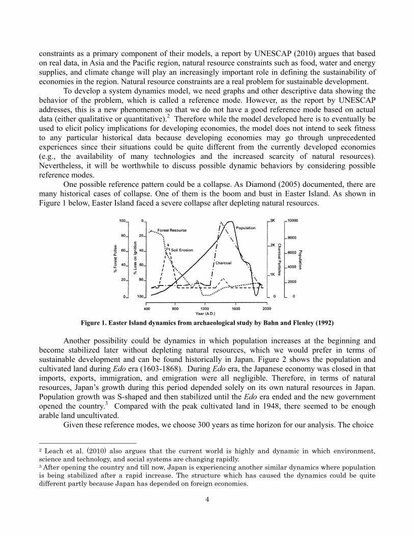
Another possibility could be dynamics in which population increases at the beginning and become stabilized later without depleting natural resources, which we would prefer in terms of sustainable development and can be found historically in Japan. Figure 2 shows the population and cultivated land during Edo era (1603-1868). During Edo era, the Japanese economy was closed in that imports, exports, immigration, and emigration were all negligible. Therefore, in terms of natural resources, Japan’s growth during this period depended solely on its own natural resources in Japan. Population growth was S-shaped and then stabilized until the Edo era ended and the new government opened the country.3 Compared with the peak cultivated land in 1948, there seemed to be enough arable land uncultivated. Given these reference modes, we choose 300 years as time horizon for our analysis. The choice
2 Leach et al. (2010) also argues that the current world is highly and dynamic in which environment, science and technology, and social systems are changing rapidly. 3 After opening the country and till now, Japan is experiencing another similar dynamics where population is being stabilized after a rapid increase. The structure which has caused the dynamics could be quite different partly because Japan has depended on foreign economies.
5
Figure 2. Population and Cultivated Land in Japan during Edo Era (1603-1868). Source: Wikipedia and Kito (1996) of time horizon influences the analysis of the dynamics of a system. Time horizon should be long enough to reflect how problems emerge and how causes and effects impact the dynamics of the system. Since dynamically complex systems involve many feedback loops, some of which might take a long time to manifest, as pointed out by Sterman (2000). The Edo era was 265 years; Easter Island’s boom and bust played out over 1600 years. Since as Leach et al. (2010) argue, we are currently facing dynamic and faster changes in many respects including environmental, economical, and social aspects, 1600 years would be too long on the one hand. On the other hand, since Edo era would be simpler than the situations mankind currently faces, it would be prudent to consider a somewhat longer time horizon.
2.2. Background
2.2.1. Review of the Original BT Model For completeness, we provide a thorough review of the original BT model. The BT model explains a pattern of population growth, resource degradation, and subsequent economic decline. The model is applied to the economy of Easter Island to depict its historical boom and bust. The authors characterize the model as a Ricardo-Malthus model of renewable resources consisting of three central components. The first component is Malthusian population dynamics in which increases in real income per capita cause population growth, depressing the income level back to the subsistence level. The second component is a common renewable resource regime and the absence of proper resource management, such that the negative effect of population growth on the resource stock becomes exacerbated. The third component is a Ricardian production structure at each point in time. Harvesting level of the resource is determined endogenously by economic activities that follow economic theory. This model setting allows us to study the effects of economic policies such as a price control and/or a labor cap.
In structural sense, the model is characterized as a general equilibrium version of the Gordon-Schaefer Model, using a variation of the Lotka-Volterra predator-prey model. Resource (S) dynamics and Population (L) dynamics are given by (dropping the time argument for convenience)
HKSrSHSG
dtdS
−
−=−= 1)( (1)

6
where G(S), r, K, and H are a logistic growth function of S, the intrinsic growth rate, the carrying capacity, and the harvest of S, respectively, and
+−=
LHdbL
dtdL φ (2)
where b−d and φ are the base rate of population increase and a positive constant, respectively. The population dynamics is Malthusian in the sense that the higher per capita consumption of the resource good leads to higher population growth. There are two sectors, the harvested good (H) and manufactured good (M).
At any point in time, the production functions for goods H and M are given by
HP = αSLH (3) MP = LM (4)
where α, LH and LM are a productivity coefficient, labor allocated to producing H and labor allocated to producing M, respectively.
Assuming common access without explicit rental cost for using S, the contribution of additional labor in monetary value (i.e., the marginal revenue product of labor) must equal the price of labor,
w = pαS (5) where w is wage.
A representative consumer who is endowed with one unit of labor maximizes utility:
u = hβm1−β subject to the budget constraint: pHh+pMm = w (6)
where h, m, β, pH, and pM are individual consumption of H and M and preference for consumption of H, price for H, and price for M respectively.
Solving the representative consumer’s maximizing problem and multiply that by the size of population yields the market demand for H and M as
HD = wβL/pH (7) MD = w(1-β)L/pH (8) Plugging (5) into (7) (i.e., quantity demanded = quantity supplied) yields an equilibrium resource harvest, H.
H = αβLS (9) Substituting (9) into (1) and (2), we obtain
LSKSrS
dtdS αβ−
−= 1 (10)
7
( )SdbLdtdL φαβ+−= (11)
Three characteristics of the model are worth highlighting. First, the harvest level H is
determined endogenously as a result of an economic activity explained by a general equilibrium model, in contrast to some other similar studies on the dynamics of population and natural resource (e.g., Shukla et al., 2011). Second, in contrast to standard approach in natural resource economics (e.g., Conrad, 2010), agents in this model face a period-by-period optimization problem, without taking into account any consequences of the future resource availability and population size. It is a reasonable approach for the situation where the resource stock is held in common and agents are atomistic (Taylor, 2009). Third, at the each moment of time, the economy reaches a temporary general equilibrium instantaneously (i.e., quantity demanded equals quantity supplied for both sectors) given a fixed amount of the natural resource stock and population at that point in time. Since the natural resource stock and population will change over time, so do the equilibrium prices and quantities. The economy is always in equilibrium, whereas the population and the natural resource stocks change over time.
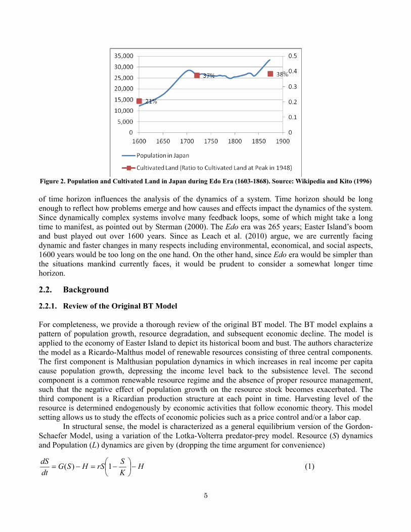
Applying the above model to Easter Island, Brander and Taylor (1998) demonstrate the dynamics of population and natural resource shown in Figure 3.
Figure 3. The Dynamics of Population and Natural Resource in the Original BT model
2.2.2. Six Directions for Further Study Nagase and Uehara (2011) discussed six key attributes of population-resource dynamic models based the BT model and its descendants; they are (1) population growth, (2) substitutability, (3) innovation, (4) capital accumulation, (5) property rights/institutional designs, and (6) modeling approach. Here we discuss these six attributes in terms of economics in general and the BT model and its descendants. The discussion regarding the BT model and its descendants owes a great deal to Nagase and Uehara (2011).
(1) Population growth
8
Since population dynamics interacts with natural resources and economic growth in developing economies, it should be incorporated endogenously into an ecological-economic model. However, as Sir Partha Dasgupta, an economist at University of Cambridge, addressed, “The study of possible feedback loops between poverty, population growth, and the character and performance of both human institutions and natural capital is not yet on the research agenda of modern growth economists” (Dasgupta, 2008, p. 2). There is a field of economic growth which incorporates population dynamics endogenously into economic growth models. It is called the unified growth theory which focuses on the transition to a steadily growing economy (e.g., Strulik, 1997; Galor and Weil, 2000; Hansen and Prescott, 2002; Galor, 2005; Voigtlander and Voth, 2006; Strulik, and Weisdorf, 2008; Madsen et al. 2010).4 While there are many methodological variations to address the transition (e.g., using a one-sector vs. a two-sector model),5 most studies attempt to explain a transition from one equilibrium to another, e.g., from a low income per capita (Malthusian) steady-state to a high income per capita (Modern Growth) steady-state (Galor, 2005), applying endogenously determined technological progress and fertility rates.6 However, these studies share a common feature with regard to stocks and flows of natural resources: natural resources are fixed or ignored in their models.
Regarding the BT model and its descendants, they incorporate both the population and the resources endogenously but in simpler way. Nagase and Uehara (2011) proposed two directions for extending the original BT model to enhance its theoretical basis and empirical relevance in application. First, incorporation of manufactured goods into population dynamics will capture demographic transition more accurately because birth rates and death rates do not solely depend on the availability of food but also the availability of medical technology, for example. Second, population growth will be a function of the natural resource to allow people to respond to its scarcity.
(2) Substitutability (3) Innovation and (4) Capital Accumulation, Taken Together
The degree of substitutability between man-made capital and natural resources plays an important role in determining the sustainability of ecological economic systems in which the economy faces natural resource constraints. Under resource constraints, we want to replace the natural resources as production inputs with man-made capital, which does not have the same constraints. Studies on substitutability have been almost exclusively conducted using either constant elasticity of substitution (CES) or Cobb-Douglas (C-D) production functions (with C-D being one type of CES).7,8 The CES function is expressed as:
4 The unified growth theory is not the only realm from which studies of the transition have emanated. Economic historians have also studied this phenomenon (e.g., Crafts, 1995). 5 Hansen and Prescott (2002), Voigtlander and Voth (2006), and Strulik and Weisdorf (2008) employ a two-sector model, while Strulik (1997), Galor and Weil (2000), Galor (2005), and Madsen et al. (2010) employ a one-sector model. 6 The unified growth theory is basically a variant of the endogenous growth theory in that the source of growth is determined endogenously. However, Hansen and Prescott (2002) provide an exception. They assume that changes in total factor productivity are given exogenously. 7 Here we focus on substitutability in production. Other studies argue with respect to substitutability in consumption (e.g., Gerlagh, Reyer, and B.C.C. van der Zwaan, 2002). 8 Stern (1994) proposes the translog production function because it can effectively model minimum input requirements, any elasticity of substitution, and uneconomic regions, for any number of inputs and outputs.

9
( )1111
1),,(−−−−
−−++=
σσ
σσ
σσ
σσ
βαβα LRKLRKF (12)
α, β > 0, α + β < 1, σ > 0, σ ≠ 0. where K, R, and L are respectively man-made capital, a natural resource, and labor; α, β, and σ are fixed parameters; σ is called the elasticity of substitution. In other words, σ indicates the trade-off between factors of inputs. With σ > 1, inputs are substitutable so that the natural resource (R) is not essential for production. We can produce the good without the natural resource by substituting other inputs. With σ < 1, inputs are complements so that the natural resource (R) is essential for production. We cannot produce the good without the natural resource.9 In relation to sustainability, the key discussion of the substitutability is the trade-off between natural resources and the accumulation of man-made capital. Whereas mainstream economics has supported σ = 1, which is the special case and the production function reduces to the C-D function, ecological economists assert σ < 1 for various reasons (e.g., Cleveland et al., 1984; Cleveland and Ruth, 1997; Daly, 1991; Daly and Farley, 2010). However, according to Nuemayer (2002), the empirical evidence is inconclusive. The original BT model and its descendants do not include man-made capital. In addition to recommending the inclusion of man-made capital in a production function, Nagase and Uehara (2011) suggested two more points to consider. First, to allow σ to evolve over time endogenously has both theoretical and empirical basis through endogenous innovation. Second, other functional forms should be investigated (e.g., a production function proposed by Prskawetz et al., 2003). Thus, substitutability, innovation, and capital accumulation are intimately intertwined.
(5) Property rights/ institutional designs The original BT model assumes a common property resource (CPR). Some controls over CPRs tend to be beneficial in view of sustainability. Although there are many studies of CPRs, three points remain underexplored, particularly in theoretical studies. The first point is the impact of population growth on cooperation. While it is well known from empirical studies that a smaller group size of people who have the right to use resources is preferable for cooperation, dynamic treatment of population size is rare at best. Sethi and Somanathan (1996) point out the importance of population growth for sustainable resource use and provide some “guess” of the impact of population growth on the resource use, but without any formal analysis. One model, by Caputo and Lueck (2003), in which the population size n affects an individual’s optimal decision, highlights this point. The second point is the interaction between human beings and the environment (Agrawal, 2003; Janssen and Anderies, 2011). Most studies do not capture “the relevant complexity of the ecological and social dynamics communities face” (Janssen and Anderies, 2011, pp.1569). Through the incorporation of the institutional design into the model, it will be possible to investigate the impact of the institutional design on the sustainability of the economy in the context where population, economy and natural resources are dynamically interrelated. Third, most models use partial equilibrium and assume players are price takers. However, it will be important to use a general equilibrium model to reflect the endogenous changes in prices that affect, for example, relative attractiveness of cheating (Copeland and Taylor, 2009). 9 For a comprehensive discussion about the relationship between substitutability and sustainability, see Hamilton (1995).
10
(6) Modeling approach
By employing the system dynamics approach, this article models a complex ecological economic system without making undue simplifications. Standard economics has generally taken a strategy of simplification to be able to employ analytic approaches. However, simulation exercises are unlikely avoidable for models of complex systems that are used primarily to increase understanding (Dasgupta, 2000). In addition, while economics generally puts emphasis on the existence of a steady state and its comparative statics, and growth theory employs growth accounting, the system dynamics approach puts its focus on the transition path; that is, how the dynamics of a system change over time.
2.3. Methods
2.3.1. Main Extensions The present model implements four of the six suggestions by Nagase and Uehara (2011) to extend the original BT model: population dynamics, substitutability, capital accumulation, and modeling approach. These extensions are summarized here, with details provided in the Appendix.
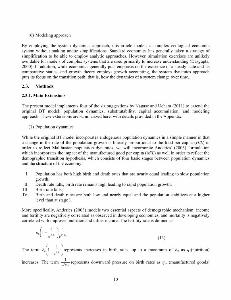
(1) Population dynamics While the original BT model incorporates endogenous population dynamics in a simple manner in that a change in the rate of the population growth is linearly proportional to the food per capita (H/L) in order to reflect Malthusian population dynamics, we will incorporate Anderies’ (2003) formulation which incorporates the impact of the manufactured good per capita (M/L) as well in order to reflect the demographic transition hypothesis, which consists of four basic stages between population dynamics and the structure of the economy:
I. Population has both high birth and death rates that are nearly equal leading to slow population
growth; II. Death rate falls, birth rate remains high leading to rapid population growth;
III. Birth rate falls; IV. Birth and death rates are both low and nearly equal and the population stabilizes at a higher
level than at stage I.
More specifically, Anderies (2003) models two essential aspects of demographic mechanism: income and fertility are negatively correlated as observed in developing economies, and mortality is negatively correlated with improved nutrition and infrastructure. The fertility rate is defined as
mqbqb eeb
211
1110
−
. (13)
The term
−
11
110 qbeb represents increases in birth rates, up to a maximum of b0 as q1(nutrition)
increases. The term mqbe 2
1 represents downward pressure on birth rates as qm (manufactured goods)

11
increases. The death rate is defined as
)(0 211
1mqddqe
d + . (14)
Improved nutrition reduces death rates via the term q1d1, while improved infrastructure reduces death rates via the term q1d2qm.
(2) Capital Accumulation
The original BT model and most of its descendants do not include capital accumulation. However, it is essential to incorporate capital accumulation into the model in order to investigate the role of substitutability between man-made capital and natural resources for sustainability. While there is one important difference in its treatment, capital accumulation is also an essential component in growth literature. To model capital accumulation, standard economic approach is adopted as a base structure. That is:
MdK H Kdt
δ= − (15)
where HM, δ, and K are respectively harvested good for capital formation, capital depreciation rate, and current stock of man-made capital. There are two things worth mentioning about HM. First, this equation indicates that the source of capital formation, HM, is produced using the same technology as producing H good for consumers, as standard economics assumes. Second, in contrast to capital formation in standard economics, capital formulation depends on natural resources for HP = αSLH. Therefore, in our model, natural resources are a so-called “growth-essential” (Groth, 2007).
(3) Substitutability
To investigate the substitutability between man-made capital and natural resources, a CES function is used for manufacturing sector instead of a function of labor alone (MP = LM) used in the original BT model. The manufacturing sector maximizes its profit by solving the following maximization problem.
(1 )M
, ,max ( )
M M MM H M M M MM ML H K
p L H K p H w L Kγ
γ ρ ρ ρπ ν µ−= + − − − (16)
ν: Efficiency parameter
ρ: Substitution parameter (ρ <0) ⇒ elasticity of substitution ≡ σ = γ: Positive parameter (0 < γ < 1)
(4) Modeling Approach
12
Modeling takes two steps. For the first step, a general equilibrium model drawing from economic theory is built. For the second step, the first step model is expanded so as to incorporate adaptation (out-of-equilibrium) using the system dynamics approach. To be more specific, the second step employs an approach suggested by Sterman (1980, 2000). For example, the manufacturing sector seeks to find the optimal amounts of inputs, labor (LM), harvested good (HM), and man-made capital (K) to satisfy the following first order conditions:
( )(1 ) ( )MM MM M
Mp L H K w
L
γγ ρ ρ ρπ γ ν −∂
= − + =∂ (17)
1(1 ) 1( )M
M HM M MM
p L H H K pH
γγ ρ ρ ρ ρπ γ ν
−− −∂
= + =∂ (18)
1(1 ) 1( )M
M M M Mp L K H KK
γγ ρ ρ ρ ρπ γ ν µ
−− −∂
= + =∂
(19)
In a standard equilibrium model used in economics, agents are assumed to be able to find such optimal values instantaneously.
In addition, price for H(pH), price for M (pM), and the return to man-made capital (µ) will be adjusted to clear the market (that is, quantity demanded = quantity supplied). The full description of the model can be found in appendix.
2.3.2. Summary Model Diagrams To help grasp the whole picture of our model, two model descriptions are provided: a causal loop diagram (CLD) and a description of the model boundary. Figure 4 shows CLDs for the original BT model and our extended model, with the differences highlighted. The original BT model has population, natural resource, harvesting, manufacturing, and labor sector. Although the harvesting sector and manufacturing both sectors have demand and supply, they are kept equal by the instantaneous adjustment of prices to clear the market. The extended model allows for disequilibrium and has a man-made capital sector. Thick arrows indicate important newly added connections. Manufacturing and man-made capital are connected to each other. Manufacturing also depends on harvested goods (natural resources). Population dynamics depend not only on harvested goods but also on manufactured goods (e.g., medical technology). Figure 5 documents the boundary of our model and clarifies what is exogenously given and what is excluded, in order to avoid misinterpretation of our model results and to underscore the limitations of our model. Exogenous variables for population dynamics follow Anderies (2003) to capture the basic demographic transition. The carrying capacity and the regeneration rate of natural resources are exogenous (constants) as in the original BT model. However, they could be endogenous. Particularly, the regeneration rate may be modified via innovation. The other exogenous variables except for adjustment times are standard economics treatment. Adjustment times are often exogenously given in system dynamics models, but these could be endogenous as well.10
10 For example, Kostyshyna (forthcoming) suggests an adaptive step-size algorithm to allow a time-varying learning speed (or a time-varying gain parameter) that change endogenously in response to changes in environment.

13
The choice to highlight specific excluded variables is somewhat subjective. They are chosen for their importance in view of ecological economic systems for developing economies. The inclusion of money, for example would likely lead to different results. Nonrenewable resources are also important, as most studies on the economics of sustainability focus on nonrenewable resources (e.g., Hartwick, 1977). As is often discussed in environmental economics textbooks, societies tend to use less expensive nonrenewable resources first, such as oil, and then switch to more expensive renewable

14
Figure 4. Causal Loop Diagrams for the original BT Model and our Extended Model. Red text and thick arrows indicate newly added items.

15
Endogenous Exogenous Excluded Population - Population - Birth Rate - Death Rate
Natural Resource - Renewable resource - Natural Growth Rate of S - Harvesting Rate of S Harvesting - Inventory of H - Supply and demand of H - Price for good H Manufacturing - Inventory of M - Supply and demand of M - Price for good M
Labor - Labor to H industry - Labor to M industry - Wage for H industry - Wage for M industry Man-Made Capital - Man-made capital - Return to man-made capital Household - Total earning - Earning - Spending
Popultion - Impact of H on population - Impact of M on population - Maximum fertility rate - Maximum mortality rate Natural Resource - Regeneration rate of natural
resource - Carrying capacity Harvesting - Efficiency parameter - Adjustment time for pH
Manufacturing - Adjustment time for pM - Efficiency parameter - Substitution parameter - Output elasticity Labor Man-Made Capital - Capital depreciation rate - Adjustment time for the
return to man-made capital Household - Consumer preference for
goods - Savings rate
- Money - Non-renewable resources - Negative externalities of
production (pollution,...) - International relationships
(exports, imports, immigration, emigration)
Figure 5. Model Boundary
resources such as wind and solar when the marginal cost of the nonrenewable resource begins to exceed that of the renewable resources (e.g., Tietenberg, 2011). Negative externalities such as pollution may not be negligible. For example, a study by Asian Development Bank showed that the costs associated with climate change could be equivalent to a loss of 6.7% of their combined gross domestic product (GDP) by 2100 (ADB, 2009). International relationships may be most important factors excluded from our model. When international relationships exist, as is the case for most developing economies, they can use resources and new technologies from abroad and perhaps avoid collapse.
2.4. Model Testing Various model tests are used in the system dynamics method (Sterman, 2000). What is particularly different in this paper compared to other system dynamics models is that structural assessment was

16
made based on economic theory. In other words, we assume that our model passes the structure assessment tests because the basic structure of the model follows standard economic theory.
Of course we tested to verify that the integration step-size was adequate, and we made sure to initialize the model in steady state by forcing population to be constant and setting the initial conditions to the equilibrium values derived from economic theory. These initial values resulted in a near equilibrium result, so minor changes were made to achieve a computational equilibrium.
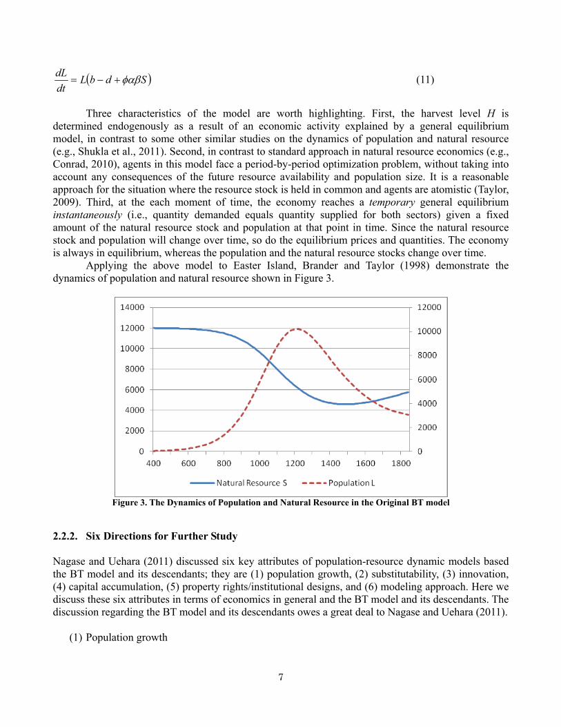
In many cases, a full suite of model tests, including sensitivity tests, extreme condition tests and many others would be performed prior to actually applying the model to find answers to the questions posed at the outset of a modeling project. For the present research, however, which aims to show how the use of the system dynamics method can contribute to economics research, the sensitivity analysis in particular will be presented in Section 3 as a primary result. To complete this lengthy Section 2 which presents the model, we describe a baseline run and compare this to the baseline run from the original BT model. The baseline model run is shown in Figure 6. Population grows rapidly, then declines and reaches a steady state value well above the initial value. The Natural Resource declines to near half the carrying capacity (the value at which the natural regeneration rate becomes zero). Not shown, but inventories of H good and M good both increase significantly, and the prices for H and M both decline significantly, due in part to the decline in Natural Resource and the fact that increasing population is placing increased pressure on production. Labor shifts towards the harvesting sector initially, then partially reverses as the Natural Resource is reduced. Capital increases rapidly, then declines and levels off as population stabilizes. Wealth, as shown in Figure 6 declines somewhat initially, then increases,
and settles at a value somewhat higher than the starting point. The shape of the Natural Resource and Population curves are similar to the baseline BT model results shown in Figure 3, and the extended model could be calibrated to match the BT model, but much of its logic would need to be neutralized. Because the extended model has man-made capital formation, the population decline is buffered somewhat.
3. Results of Sensitivity Analyses For this paper we consider the sensitivity analyses to be a primary result in addition to serving as an important model validation tool. Sensitivity analysis can be used to investigate possible transitional
Figure 6: Extended Model Population and Resources

17
paths for ecological economic systems. Given the complexity of such systems, it is almost impossible to find an optimal solution by taking into account all the necessary information including possible future states.11 Therefore what policy makers need to obtain from modeling and analysis is not an optimal solution that would allow them to control an ecological economic system, but rather they need to know what kinds of transition paths to expect so that society can prepare for these possible changes (Leach et al, 2010). Given past experiences, Folke et al. (2002) suggested “structured scenarios” as a tool to envision multiple alternative futures and the pathways for making policies.
Through the sensitivity analysis we found two critical issues that ecological economics should consider in when developing models of ecological economic systems: 1) endogenous consumer preference, and 2) adaptation (out-of-equilibrium). While they are critical issues in terms of policy implications for a sustained economy, they have been rarely considered in economics. There are at least three reasons inherent in standard economics. First, economics prefers to simplify a model, for example by using exogenous variables, so that it can be solved analytically. However, resulting implicit model boundary may give misleading policy implications. Second, an equilibrium-oriented paradigm continues to prevail, in which there is a belief that society can find an optimal solution to attain a sustained economy. Because ecological economic systems are complex and highly dynamic, optimal management is very difficult (if not impossible) to implement (Folke et al, 2002).12 Third, a focus is put on the balanced-growth path (BGP) which strived to achieve a long-run steady state characterized by constant growth rates. In the growth literature, the discussion of sustainability is about finding conditions for the BGP (e.g., sufficient growth rate of technology which sustains the growth) (e.g., Groth, 2007). Therefore, it is rare at best in the growth literature that sensitivity analysis is done to study how changes in factors affect the transitional paths. In other words, the robustness of a model is not its main focus. However, the steady state (BGP) could occur usually only in the very long run, which may not be what policy makers want to know. What is important for policy makers given our imperfect knowledge of dynamic and complex ecological economic systems may be to understand how factors affect the transitional paths of an economy. Because of the absence of sensitivity analysis in most economic studies, these needs have not received sufficient attention.
3.1. Sensitivity to Consumer Preference In our model, following standard economics, a preference for good H (β) is exogenously given as a constant. Solving the consumer’s utility maximization problem, we obtain an individual consumer’s quantity demanded for H as a function of price for H and income as:
hD = wβ/pH
Hence the quantity of good H depends on the preference for good H (β), wage (w), and price for good H (pH). Since wage depends on pH, hD basically responds only to changes in pH.
Although any preference seems to be acceptable as long as 0 < β < 1, a low β shows unreasonable behavior, as shown in Figure 7, when β is 0.15 (i.e., a lower preference for H good), population becomes extinct at time 100. This does not make sense because the natural resource S –
11 However, Leach et al. (2010) points out that dynamics and complexity have been ignored in conventional policy approaches for development and sustainability. They relate this tendency to prevailing equilibrium thinking as we mention later. 12 Folke et al. (2002) asserts that we should use adaptive management instead given imperfect knowledge about the ecological economics systems.

18
Figure 7. Dynamics of Population and Natural Resources with Different Values for Fixed Consumer Preference, β
which is the source of food – remains abundant. This occurs because the preference for H (i.e., β) is constant (i.e., exogenously given) regardless of the value for food per capita. However, a constant preference for goods is a standard approach for economics. This problem has been rarely investigated in standard economics. David Stern (1997) points out that neoclassical economists are very reticent to discuss the origin of preferences and that preferences are normally assumed to be unchanging over time. However, as our sensitivity analysis shows, exogenous consumer preference is not a robust and realistic formulation.13 The importance of endogenous preferences for sustainability issues has been argued by several heterodox economics such as ecological economics (Common and Stagl, 2005; Georgescu-Roegen, 1950; Stern, 1997), evolutionary economics (Gowdy, 2007), and institutional economics (Hahnel and Albert, 1990; Hahnel, 2001). Gowdy (2007) argues that neoclassical economics assumes that consumers not only respond to price signals as we modeled but also to other incentives such as the individual’s personal history, their interaction with others, and the social context of the individual choice. He called the former the self-regarding preference and the latter the other-regarding preference. If these factors change over time, then preferences should reflect these changes. Gowdy asserts further that modeling the other-regarding behavior would be more realistic for sustainability research. Common and Stagl (2005) argue that to change preference is a normative requirement from a sustainability perspective, including the idea that there could be an ethical basis for
13 It is not impossible to solve this problem using an exogenous preference. For example, a Stone-Geary type utility function (Anderies, 2003) incorporates the minimum amount of the quantity demanded for H into the utility function as ( ) ( ) ββ −−= 1
min, mhhmhU . Then we can derive the demand function
( ) min1h
wh hpββ= − +
Hence, the first part does not depend on the price. It means that people put their effort to harvest at least the minimum level, hmin, irrespective of the price.

19
changing preferences. While there have been several discussions on endogenous preference, there is no standard way of modeling endogenous preference in economics literature.14
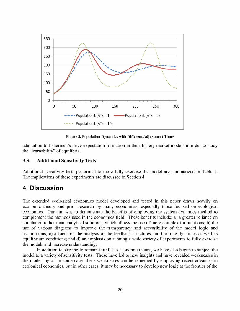
3.2. Sensitivity to Adaptation (out-of-equilibrium responses) The amplitude of oscillations increase with longer adjustment times, and the oscillations dampen out more slowly if at all. The period of the oscillations does not change very much. Figure 8 shows the dynamics of population with different adjustment times for the prices for H and M, the factor demand of H (use of H to produce M), and for adjustments to the return to man-made capital. All of these time constants were varied together from 1 year, to 5 years, to 10 years. Although adaptation and oscillation caused by adaptive process are nothing new to system dynamics, the concept of adaptation (out-of-equilibrium) and its importance have been recognized in ecological economics only relatively recently (e.g., Common and Stagl, 2005; de Vries, 2010; Folke, 2002; Hanley, 1998; Holling, 1999; Leach et al., 2010; Levin et al, 1998; Stagl, 2007). Leach et al. (2010) argue that conventional policy approaches for development and for sustainability have ignored the dynamics and complexity of ecological economic systems in order to be able to use standard equilibrium thinking and its associated policy implications. Essentially, the hope is that ecological economic systems are both predictable and controllable. However, as Leach et al. point out, both ecological systems and economic systems are changing so rapidly that it is difficult if not impossible to find an optimal solution in order to “control” these systems. Given the dynamic and complex nature of ecological economic systems, we face risks, uncertainty, ambiguity, and ignorance (Leach et al., 2010); that is, we have imperfect knowledge. The use of adaptation is more than a philosophical or preference issue. Folke et al. (2002) argues, based on actual examples, that we should adopt a dynamic view that emphasizes far-from-equilibrium conditions. Incorporating adaptation into an ecological economic model enables us “to understand how humans have constructed environmental problems (and opportunities) in particular ways. They depend on the particular contexts of governance structures and cultures and over time shape and are shaped by biophysical environments, technologies and human behavior.” (Stagl, 2007, p.59).15
In terms of modeling adaptation in ecological economic models, it has not been thriving.16, 17 Some studies were done by Hommes and Rosser (2001) and Forini et al. (2003). They applied 14 One example of modeling endogenous preference is proposed by Stern (1997). Using the symmetric characteristics of production and consumption, he proposes the factor augmentation model using an analogy to endogenously augmenting technology in production. 15 Robert Solow, a Nobel Memorial Prize in Economic Sciences, pointed out the importance of disequilibrium in early 1970s. He published two articles about natural resources and economic growth in 1974 (Solow 1974a and 1974b). Whereas one with an orthodox formal growth model employs equilibrium model, the other paper without a formal model discussed importance of disequilibrium for its impact on resource allocation. 16 There seems to be two types of adaptation. One is adaptive management in which natural resource management and policy making in general are adaptive against changing situations. The other is adaptation system where adaptation is incorporated to explain system’s behavior such as market dynamics. We are talking the latter. 17 Learning is not absent at all in economics. Learning plays a key role in modern macroeconomics. Learning in macroeconomics refers to models of expectation formation in which agents revise their forecast rules over time, for example in response to new data (Evans and Honkapohja, 2008). Evans and Honkapohja (2008) pick three roles of learning in macroeconomics: 1) assessing the plausibility (learnability) of an equilibrium, 2) providing a selection criterion when there are multiple equilibria, and 3) addressing macroeconomic fluctuations.
20
Figure 8. Population Dynamics with Different Adjustment Times
adaptation to fishermen’s price expectation formation in their fishery market models in order to study the “learnability” of equilibria.
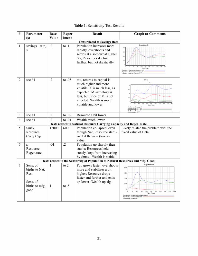
3.3. Additional Sensitivity Tests Additional sensitivity tests performed to more fully exercise the model are summarized in Table 1. The implications of these experiments are discussed in Section 4.
4. Discussion The extended ecological economics model developed and tested in this paper draws heavily on economic theory and prior research by many economists, especially those focused on ecological economics. Our aim was to demonstrate the benefits of employing the system dynamics method to complement the methods used in the economics field. These benefits include: a) a greater reliance on simulation rather than analytical solutions, which allows the use of more complex formulations; b) the use of various diagrams to improve the transparency and accessibility of the model logic and assumptions; c) a focus on the analysis of the feedback structures and the time dynamics as well as equilibrium conditions; and d) an emphasis on running a wide variety of experiments to fully exercise the models and increase understanding.
In addition to striving to remain faithful to economic theory, we have also begun to subject the model to a variety of sensitivity tests. These have led to new insights and have revealed weaknesses in the model logic. In some cases these weaknesses can be remedied by employing recent advances in ecological economics, but in other cases, it may be necessary to develop new logic at the frontier of the
21
Table 1: Sensitivity Test Results # Parameter
(s) Base Value
Experiment
Result Graph or Comments
Tests related to Savings Rate 1 savings rate,
s .2 to .1 Population increases more
rapidly, overshoots and settles at a somewhat higher SS; Resources decline further, but not drastically
2 see #1 .2 to .05 mu, returns to capital is much higher and more volatile; K is much less, as expected, M inventory is less, but Price of M is not affected; Wealth is more volatile and lower
mu
3 see #1 .2 to .02 Resource a bit lower 4 see #1 .2 to .01 Wealth much lower
Tests related to Natural Resource Carrying Capacity and Regen. Rate 5 Smax,
Resource Carry Cap.
12000 6000 Population collapsed, even though Nat, Resource stabil- ized at the new (lower) value.
Likely related the problem with the fixed value of Beta
6 r, Resource Regen.rate
.04 .2 Population up sharply then stable; Resources held steady, kept from increasing by Smax. Wealth is stable.
Tests related to the Sensitivity of Population to Natural Resources and Mfg. Good 7 Sens. of
births to Nat. Res. Sens. of births to mfg. good
1 1
to 2 to .5
Pop grows faster, overshoots more and stabilizes a bit higher; Resource drops faster and further and ends up lower; Wealth up sig.

22
8 Sens. of births to Nat. Resources Sens. of births to mfg’d good
1 1
to .5 to 2
Population rose slowly and stabilized; Resource declined modestly and stabilized; wealth is flat; M production increases and stabilizes; returns to capital decline steadily (but less than baseline) and stabilize
9 Sens. of
deaths to resources Sens. of deaths to mfg’d good
5 1
to 10 to .5
Similar to #7 except the peak in Population (and drop in Resource) occur later, at the same time as in the baseline run; Wealth up significantly
10 see #9
5 1
to 2.5 to 2
Population flat lines, along with everything else
11 Sens. of deaths to resources
5 to 10 Population flat lines
12 Sens. of deaths to mfg’d good
1 to .5 Negligible effect; looks just like baseline
13 Sens. of births to resources
1 to .5 Population is a little higher than #8 (graph to the right shows pop for baseline, #8 and #13); Resource is a bit lower than #8; Wealth is a little higher
Tests related to Adjustment Times (AT) for Prices, Returns, and Demand
14 AT for Price of H good
2 1 to 6 No significant effect
15 AT for Price of M good
2 1 to 6 Minimal effect until near 6: Population is sig. higher with wide swings; Natural Resource is lower
Wealth goes to zero; Man made capital begins to collapse
16 AT for Return to manmade capital, mu
2 1 to 6 Smaller values lowers Wealth; higher values increase Wealth considerably
Nothing else seems to be impacted!
17 AT for Factor Demand, Hm
2 1-6 Little effect Factor demand is the demand for Natural Resources by Manufacturing

23
field, a frontier that will be extended by bringing together the powerful traditions and disciplines from economics and new ways of thinking about and addressing complexity from the system dynamics discipline. Some of the specific questions raised by the results of the present research include: 1) the common practice of assuming fixed consumer preferences rather than endogenously determining the relative preferences for different goods depending on current conditions, 2) the assumption that all important results can be found by finding equilibrium solutions rather than taking into account how complex systems learn and adapt based on disruptions and other changes that drive them out of equilibrium perhaps for long periods of time, 3) the model’s response to very small savings rates indicates a higher degree of volatility and vulnerability, 4) exploration of resource carrying capacity and regeneration rates exhibit both favorable and adverse outcomes and constraints, 5) experiments with the sensitivity parameters in the population model indicate the potential for both population collapse and for trajectories that are more steady and do not lead to collapse, 6) testing the impact of different speeds of adjustment to out-of-equilibrium conditions reveals major differences in system response which reinforces the case for not relying on equilibrium methods. These findings must not yet be taken very seriously, however, since the model on which they are based is subject to many limitations, especially the restrictive model boundary documented in Figure 5, and the need for much more testing, including the application/calibration of the model to represent actual developing economies in a realistic fashion. In conclusion, we have demonstrated that the system dynamics methods appears to have considerable potential to complement economic research, especially ecological economics which strives to address the complex interactions between the economy, ecological systems, and human behavior.

24
References Asia Development Bank (ADB). (2009). The Economics of Climate Change in Southeast Asia: A regional
review. Manila: ADB. Anderies, John M. (2003). Economic development, demographics, and renewable resources: a dynamical
systems approach. Environment and Development Economics, 8, 219-246. Basener, B. and Ross, D.S. (2005). Booming and Crashing Populations and Easter Island. SIAM, Journal on
Applied Mathematics, 65(2), 684-701. Brander, J., and Taylor, M., (1998). The simple economics of Easter Island: a Ricardo–Malthus model of
renewable resource use. American Economic Review, 88 (1), 119–138. Bretschger, Lucas. (1998). How to substitute in order to sustain: knowledge driven growth under environmental
restrictions. Environment and Development Economics, 3, 425-442. Bullard, James B. (2006). The learnability criterion and monetary policy. Federal Reserve Bank of St. Louis
Review, 203-217. Basener, W., Brooks, B., Radin, M., and Wiandt. (2008). Dynamics of a Discrete Population Model for
Extinction and Sustainability in Ancient Civilizations. Nonlinear Dynamics, Psychology, and Life Sciences, 12(1), 29-53.
Cleveland, C.J., Costanza, R., Hall, C.A.S., Kaufmann, R. (1984). Energy and the US economy: a biophysical perspective. Science, 255, 890–897.
Cleveland, C. and M. Ruth (1997). When, Where and by how Much do Biophysical Limits Constrain the Economic Process: a Survey of Nicolas Georgescu-Roegen's Contribution to Ecological Economics. Ecological Economics, 22, 203-223.
Common, Michael., and Sigrid Stagl. (2005) Ecological Economics: An introduction. Cambridge: Cambridge University Press.
Costanza, Robert., Lisa Wainger, Carl Folke, and Karl-Goran Maler. (1993). Modeling Complex Ecological Economic Systems. BioScience, 43(8), 545-555.
D’Alessandro, Simone. (2007). Non-linear Dynamics of Population and Natural Resources: The Emergence of Different Patterns of Development. Ecological Economics, 62, 473-471.
Dalton, Thomas R., and R. Morris Coats. (2000). Could Institutional Reform Have Saved Easter Island? Journal of Evolutionary Economics, 10, 489-505.
Dalton, Thomas R., R. Morris Coats., and Badiollah R. Asrabadi. (2005). Renewable Resources, Property-Rights Regimes and Endogenous Growth. Ecological Economics, 52, 31-41.
Daly, H.E., (1991). Elements of an environmental macroeconomics. In Costanza, R. (Ed.). Ecological Economics (pp. 32–46). New York: Oxford University Press.
Daly Herman E. and Joshua Farley. (2010). Ecological Economics: Principles and Applications (2nd Ed.). Washington: Island Press.
Dasgupta, Partha. (2008). Nature in economics. Environmental Resource Economics, 39, 1-7. de la Croix., and Dottori, D. (2008). Easter Island: A Tale of a Population Race. Journal of Economic Growth,
13, 27-55. de Vries, Bert. (2010). Interacting with complex systems: models and games for a sustainable economy,
Netherlands Environmental Assessment Agency. Erickson, Jon D. and John M. Gowdy (2000). Resource Use, Institutions, and Sustainability: A Tale of Two
Pacific Island Cultures. Land Economics, 76, 345-354. Evans, George W and Seppo Honkapohja (2008). Learning in macroeconomics. The New Palgrave Dictionary
of Economics, Second Edition. Evans, George W and Seppo Honkapohja (2009). Learning and macroeconomics. The Annual Review of
Economics, 1, 421-449. Evans, George W and Seppo Honkapohja (2011). Learning as a rational foundation for macroeconomics and
finance. Working Paper. Folke, Carl, Steve Carpenter, Thomas Elmqvist, Lance Gunderson, C. S. Holling,Brian Walker. (2002).
Resilience and sustainable development: building adaptive capacity in a world of transformations.
25
Ambio, 31(5), 437-440. Galor, Oded. (2005). From stagnation to growth: unified growth theory. In Philippe Aghion and Steven N.
Durlauf (Ed.). Handbook of Economic Growth, Volume 1A (pp.171-293). Galor, O., and Weil, D. (2000). Population, technology, and growth: from Malthusian stagnation to demographic
transition and beyond. The American Economic Review, 90(4), 806–828. Georgescu-Roegen, N., 1950. The theory of choice and the constancy of economic laws. Quarterly Journal of
Economics, 64, 125-138. Gerlagh, Reyer and B.C.C. van der Zwaan. (2002).Long-term substitutability between environmental and man-
made goods. Journal of Environmental Economics and Management, 44, 329-345. Good, David H. and Rafael Reuveny (2006). The Fate of Easter Island: The Limits of Resource Management
Institutions. Ecological Economics, 58, 473-490. Gowdy, John. (2007). Avoiding self-organized extinction: Toward a co-evolutionary economics of sustainability.
International Journal of Sustainable Development & World Ecology, 14, 27-36. Groth, Christian. (2007). A new-growth perspective on non-renewable resources. In L. Bretschger and S.
Smulders (Eds.). Sustainable Resource Use and Economic Dynamics (pp.127-163). Springer. Hahnel, Robin. (2001). Endogenous preferences: The institutionalist connection. Dutt, In Amitava K. and
Kenneth P. Jameson (Eds.). Crossing the Mainstream: Ethical and Methodological Issues in Economics (pp.315-331). Notre Dame: University of Notre Dame Press.
Hahnel, Robin., and Michael Albert. (1990). Quiet Revolution in Welfare Economics. Oxford: Princeton University Press.
Hanley, Nick. (1998). Resilience in social and economic systems: a concept that fails the cost-benefit test? Environment and Economic Development, 3, 244-249.
Hansen, Gary D. and Edward C. Prescott. (2002). Malthus to Solow. American Economic Review, 92(4), 1205-1217.
Hartwick, John M. (1977). Intergenerational equity and investing rents from exhaustible resources. The American Economic Review, 67(5), 972-974.
Holling, C.S. (1999). Introduction to the special feature: Just complex enough for understanding; Just simple enough for communication. Conservation Ecology, 3(2):1. [online] URL: http://www.consecol.org/vol3/iss2/art1/
Hiroshi Kito, (1996). The regional population of Japan before the Meiji period. Jochi Keizai Ronsyu. 41(1–2), 65–79 (in Japanese).
Kostyshyna, Olena. Application of an adaptive step-size algorithm in models of hyperinflation. Macroeconomic Dynamics, (Forthcoming).
Leach, Melissa, Ian Scoones and Andy Stirling. (2010). Dynamic Sustainabilities: Technology, Environment, Social Justice. London: Earthscan.
Levin, Simon A., Scott Barrett, Sara Aniyar, William Baumol, Christopher Bliss, Bert Bolin, Partha Dascupta, Paul Ehrlich, Carl Folke, Ing-Marie Gren, C.S. Holling, Annmari Jansson, Bengt-Owe Jansson, Karl-Goran Maler, Dan Martin, Charles Perrings, and Eytan Sheshinski. (1998). Resilience in natural and socioeconomic systems. Environment and Development Economics, 3, 222-235.
Madsen, Jakob B., James B. Ang, and Rajabrata Banerjee. (2010). Four centuries of British economic growth: the roles of technology and population. Journal of Economic Growth, 15, 263-269.
Maxwell, John W. and Rafael Reuveny. (2000). Resource Scarcity and Conflict in Developing Countries. Journal of Peace Research, 37(3), 301-322.
Meadows, Donella, Jorgen Randers, Dennis Meadows (2004) Limits to Growth: The 30-Year Update, Chelsea Green Publ. Co., White River Junction, VT.
Nagase, Yoko and Tasneem Mirza (2006). Substitutability of Resource Use in Production and Consumption. Conference Proceedings, 3rd World Congress of Environmental and Resource Economics.
Nagase, Yoko and Uehara, Takuro. (2011). Evolution of population-resource dynamics models. Ecological Economics, (72), 9-17.
Neumayer, E. (2000). Scarce or abundant? The economics of natural resource availability. Journal of Economic Surveys, 14(3), 307-335.

26
Pezzey, J., and Anderies, J., (2003). The effect of subsistence on collapse and institutional adaptation in population-resource societies. Journal of Development Economics, 72 (1), 299-320.
Prskawetz, Alexia., Gragnani, Alessandra., and Gustav Feichitnger. (2003). Reconsidering the Dynamic Interaction of Renewable Resources and Population Growth: A Focus on Long-Run Sustainability. Environmental Modeling and Assessment, 8, 35-45.
Reuveny, Rafael., and Christopher S. Decker. (2000). Easter Island: Historical Anecdote or Warning for the Future? Ecological Economics, 35, 271-287.
Richardson, George P. (2011). Reflections on the foundations of system dynamics. System Dynamics Review, 27(3), 219-243.
Sargent, Thomas J. (1993). Bounded Rationality in Macroeconomics. Oxford: Oxford University Press. Schwaninger, Markus and Stefan Grsser. (2008). System dynamics as model-based theory building. Systems
Research and Behavioral Science, 25, 447-465. Solow, Robert M. (1974a). Intergenerational Equity and Exhaustible Resources. The Review of Economic
Studies, 41, 29-45. Solow, Robert M. (1974b). The economics of resource or the resources of economics. American Economic
Review Papers and Proceedings, 64(2), 1-14. Stagl, Sigrid. (2007). Theoretical foundations of learning processes for sustainable development. International
Journal of Sustainable Development & World Ecology, 14, 52-62. Sterman, John. (1980). The use of aggregate production functions in disequilibrium models of energy-economy
interactions. MIT System Dynamics Group Memo D-3234. Cambridge, MA 02142. Sterman, John D. (2000). Business Dynamics: systems thinking and modeling for a complex world. Boston:
McGraw-Hill Higher Education. Stern, David I. (1997). Limits to substitution and irreversibility in production and consumption: A neoclassical
interpretation of ecological economics. Ecological Economics, 21, 197-215. Strulik, Holger. (1997). Learning-by-doing, population pressure, and the theory of demographic transition.
Journal of Population Economics, 10, 285-298. Strulik, Holger and Jacob Weisdorf. (2008). Population, food, and knowledge: a simple unified growth theory.
Journal of Economic Growth, 13, 195-216. Taylor, M. Scott. (2009). Innis Lecture: Environmental crises: past, present, and future. Canadian Journal of
Economics, 42(4), 1240-1275. Tietenberg, Tom., and Lynne Lewis. (2011). Environmental & Natural Resource Economics (9th Ed). NJ:
Prentice Hall. Uehara, Takuro, Yoko Nagase, and Wayne Wakeland. (2010). “System Dynamics Implementation of an
Extended Brander and Taylor-like Easter Island Model”, Proceedings of the 28th International Conference of the System Dynamics Society, Seoul, Korea.
United Nations Economic and Social Commission for Asia and the Pacific (ESCAP). (2010). Green Growth, Resources and Resilience: Environmental Sustainability in Asia and the Pacific.
Voigtlander, Nico., and Hans-Joachim Voth. (2006). Why England? Demographic factors, structural change and physical capital accumulation during the Industrial Revolution. Journal of Economic Growth, 11, 319-361.
27
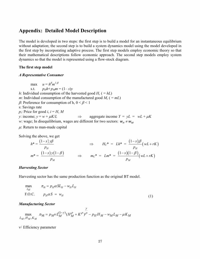
Appendix: Detailed Model Description The model is developed in two steps: the first step is to build a model for an instantaneous equilibrium without adaptation; the second step is to build a system dynamics model using the model developed in the first step by incorporating adaptive process. The first step models employ economic theory so that their mathematical descriptions follow economic approach. The second step models employ system dynamics so that the model is represented using a flow-stock diagram.
The first step model
A Representative Consumer
max u = hβm1-β s.t. pHh+pMm = (1– s)y h: Individual consumption of the harvested good Hc ( = hL) m: Individual consumption of the manufactured good Mc ( = mL) β: Preference for consumption of h, 0 < β < 1 s: Savings rate pi: Price for good i, i = H, M y: income; y = w + µK/L ⇒ aggregate income Y = yL = wL + µK w: wage; In disequilibrium, wages are different for two sectors: H Mw w≠ µ: Return to man-made capital Solving the above, we get
h* = ( )1
H
s yβp
− ⇒ HC* = Lh* = ( ) ( )1
H
swL rK
pβ−
+
m* = ( ) ( )1 1
M
s yp
− − β ⇒ mC* = Lm* = ( )( ) ( )1 1
M
swL rK
pβ− −
+
Harvesting Sector Harvesting sector has the same production function as the original BT model.
Hmax H H H HLHp SL w Lπ α= −
F.O.C. H Hp S wα = (1)
Manufacturing Sector
(1 )M
, ,max ( )
M M MM H M M M MM ML H K
p L H K p H w L Kγ
γ ρ ρ ρπ ν µ−= + − − −
ν: Efficiency parameter
28
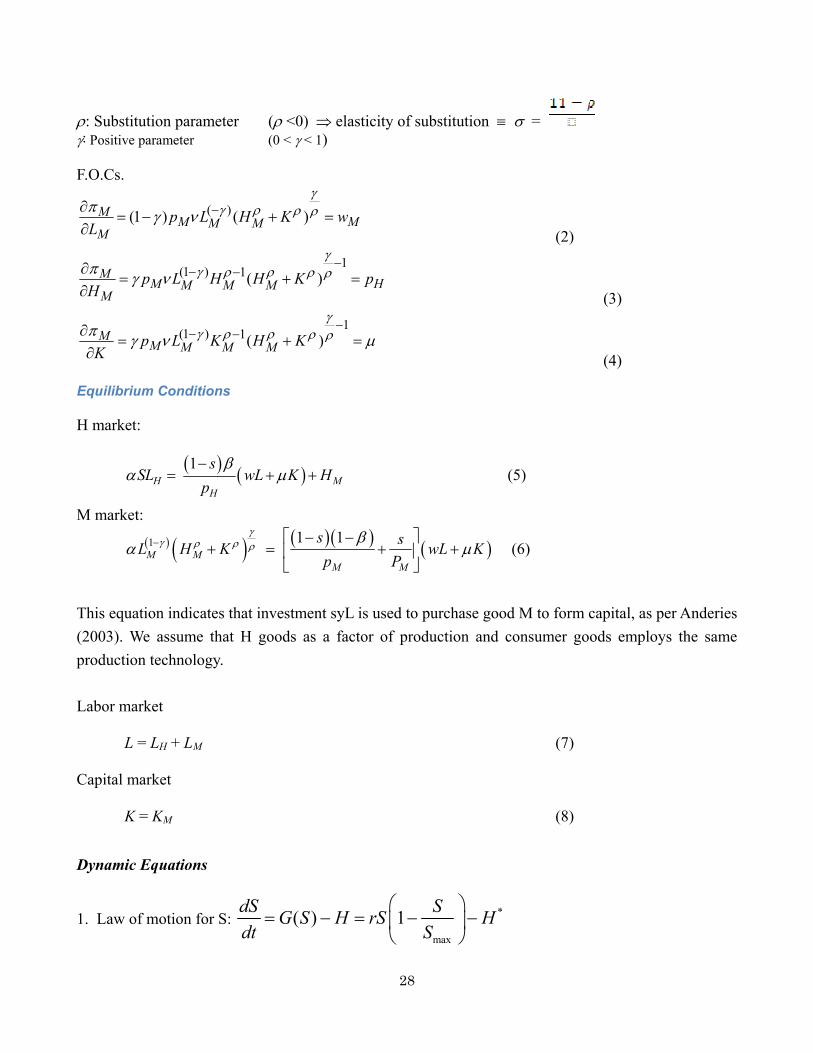
ρ: Substitution parameter (ρ <0) ⇒ elasticity of substitution ≡ σ = γ: Positive parameter (0 < γ < 1) F.O.Cs.
( )(1 ) ( )MM MM M
Mp L H K w
L
γγ ρ ρ ρπ γ ν −∂
= − + =∂ (2)
1(1 ) 1( )M
M HM M MM
p L H H K pH
γγ ρ ρ ρ ρπ γ ν
−− −∂
= + =∂ (3)
1(1 ) 1( )M
M M M Mp L K H KK
γγ ρ ρ ρ ρπ γ ν µ
−− −∂
= + =∂
(4)
Equilibrium Conditions H market:
( ) ( )1H M
H
sSL wL K H
pβ
α µ−
= + +
(5)
M market:
( ) ( ) ( )( ) ( )1 1 1M M
M M
s sL H K wL Kp P
γγ ρ ρ ρ
βα µ− − −
+ = + +
(6)
This equation indicates that investment syL is used to purchase good M to form capital, as per Anderies (2003). We assume that H goods as a factor of production and consumer goods employs the same production technology. Labor market
L = LH + LM (7)
Capital market
K = KM (8)
Dynamic Equations
1. Law of motion for S: *
max
( ) 1dS SG S H rS Hdt S
= − = − −

29
2. Law of motion for L The formulation by Anderies (2003) is used to capture the hypothetical demographic transition.
1 2 1 20 0 ( )
1 1 11 b h b m h d d m
dL b d Ldt e e e +
= − −
The term 10
11 b hbe
−
represents increases in birth rates, up to a maximum of b0 as h(nutrition)
increases. The term 2
1b me
represents downward pressure on birth rates as m (manufactured goods)
increases. The death rate is defined as
1 20 ( )
1h d d md
e +.
Improved nutrition reduces death rates via the term q1h, while improved infrastructure reduces death rates via the term hd2m.
3. Law of motion for K: MM
dK syLH K Kdt p
δ δ= − = −
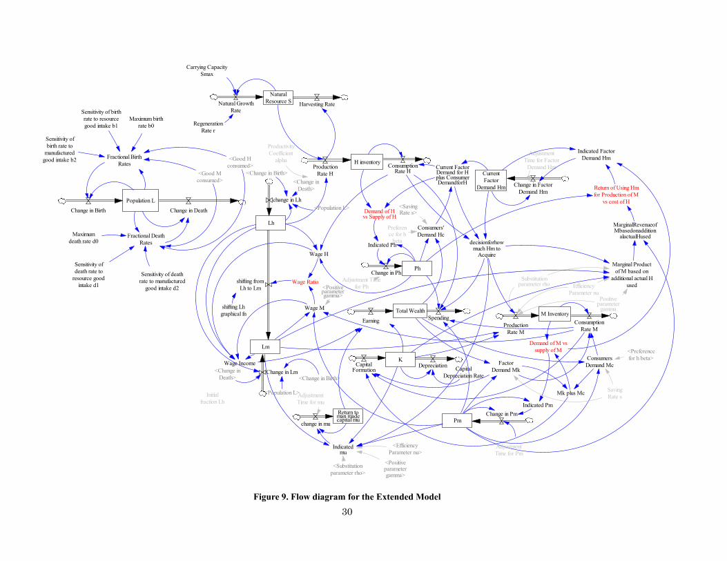
30
Figure 9. Flow diagram for the Extended Model
H inventoryProduction
Rate HConsumption
Rate H
ProductivityCoefficient
alpha
Population L
Lh
Demand of Hvs Supply of H
Indicated FactorDemand Hm
Consumers'Demand Hc
Ph
Wage H
M Inventory
ProductionRate M
ConsumptionRate M
Lm
Marginal Productof M based on
additional actual Hused
ConsumersDemand McFactor
Demand Mk
Demand of M vssupply of M
Pm
Wage M
Wage Ratio
Positiveparameter
gamma
Substitutionparameter rho
MarginalRevenueofMbasedonaddition
alactualHused
EfficiencyParameter nu
Return of Using Hmfor Production of M
vs cost of H
Return toman madecapital mu
Wage Income
Preference for h
beta
SavingRate s
Change in Pm
AdjustmentTime for Pm
Indicated Pm
Change in PhAdjustment Time
for Ph
Indicated Ph
change in mu
Indicatedmu
AdjustmentTime for mu
CurrentFactor
Demand Hm Change in FactorDemand Hm
AdjustmentTime for Factor
Demand Hm
<Positiveparametergamma>
<EfficiencyParameter nu>
<Substitutionparameter rho>
<Preferencefor h beta>
<SavingRate s>
decisionforhowmuch Hm to
Acquire
shifting fromLh to Lm
Initialfraction Lh
shifting Lhgraphical fn
Current FactorDemand for Hplus ConsumerDemandforH
Mk plus Mc
KDepreciation Capital
Depreciation Rate
CapitalFormation
Total Wealth
Earning Spending
<Positiveparametergamma>
NaturalResource SNatural Growth
RateHarvesting Rate
Carrying CapacitySmax
RegenerationRate r
Change in Birth
Fractional BirthRates
<Good Hconsumed>
<Good Mconsumed>
Maximum birthrate b0
Sensitivity of birthrate to resourcegood intake b1
Sensitivity ofbirth rate to
manufacturedgood intake b2
Sensitivity ofdeath rate to
resource goodintake d1
Sensitivity of deathrate to manufactured
good intake d2
Maximumdeath rate d0
Change in Death
Fractional DeathRates
change in Lh
Change in Lm
<Change in Birth><Change in
Death>
<Change inDeath> <Change in Birth>
<Population L>
<Population L>