Vibration analysis of a cantilevered trapezoidal ... · PDF file72 Based on the classical theory of plates, there is a considerable amount of work related to the vibration analysis

* Corresponding author. Tel.: +98 31 55912448; fax: +98 31 55559930. E-mail addresses: [email protected] (K. Torabi) © 2017 Growing Science Ltd. All rights reserved. doi: 10.5267/j.esm.2016.7.001

Engineering Solid Mechanics (2017) 71-92

Contents lists available at GrowingScience

Engineering Solid Mechanics

homepage: www.GrowingScience.com/esm

Vibration analysis of a cantilevered trapezoidal moderately thick plate with variable thickness

Keivan Torabi* and Hassan Afshari

Department of Solid Mechanics, Faculty of Mechanical Engineering, University of Kashan, Kashan, Iran

A R T I C L EI N F O A B S T R A C T

Article history: Received 6 March, 2016 Accepted 3 August 2016 Available online 3 August 2016

This paper presents a numerical solution for vibration analysis of cantilevered non-uniform trapezoidal thick plates. Based on the first shear deformation theory, kinetic and strain energies of the plate are derived and using Hamilton's principle, governing equations and boundary conditions are derived. A transformation of coordinates is used to convert the equations and boundary conditions from the original coordinates into a new computational coordinates. Using Differential quadrature method (DQM), natural frequencies and corresponding modes are derived numerically. Convergence and accuracy of the proposed solution are confirmed using results presented by other authors and also results obtained based on the finite element method using ANSYS software. Finally, as the case studies, two cases for variation of thickness are considered and the effects of angles, aspect ratio and thickness of the plate on the natural frequencies are studied. It is concluded that two angles of the trapezoid have opposite effect on the natural frequencies. Also, it is shown that all frequencies rise as value of thickness increases or value of the aspect ratio of the plate decreases. The most advantage of the proposed solution is its applicability for plates with variable thickness.

© 2017 Growing Science Ltd. All rights reserved.

Keywords: Trapezoidal plate Moderately thick plate Variable thickness Differential quadrature method

1. Introduction

Trapezoidal plates are widely used in aeronautical and civil engineering applications such as aircraft wings and tails, ship hulls, highway bridges, etc. The free vibration analysis of such models is a necessity to design them to have a safe operation under different loading conditions. There are many studies regarding to bending, buckling, thermal and dynamic analyses of thin and thick rectangular and circular plates; but analysis of skew and trapezoidal ones have been poorly studied especially those plates with variable thickness.

72

Based on the classical theory of plates, there is a considerable amount of work related to the vibration analysis of trapezoidal thin plates; e.g. Chopra and Durvasula (1971, 1972) applied Galerkin method and investigated the free vibration of simply supported symmetric and un-symmetric trapezoidal plates. Finite element method was employed by Orris and Petyt (1973) to study the vibration of simply supported and clamped triangular and trapezoidal plates. Using the integral equation method, the vibration analysis of cantilevered quadrilateral and trapezoidal plates was studied by Srinivasan and Babu (1983). Maruyama et al. (1983) presented an experimental study of the free vibration of clamped trapezoidal plates. Bert and Malik (1996a) applied the differential quadrature method and presented a numerical solution for the free vibration of plates with irregular shapes. Using least-square-based on finite difference method, Shu et al. (2007) studied free vibration analysis of plates. Using moving least square Ritz method, Zhou and Zheng (2008) presented a numerical solution for vibration analysis of skew plates. Shufrin et al. (2010) presented a semi-analytical solution for the geometrically nonlinear analysis of skew and trapezoidal plates subjected to out-of-plane loads. Wang et al. (2013) used new version of the differential quadrature method and presented accurate results for free vibration of skew plates. They studied eight combinations of simply supported, clamped and free boundary conditions. Using the element-free Galerkin method, Naghs and Azhari (2015) analyzed large amplitude vibration of point supported laminated composite skew plate. In order to increase the accuracy of solution, thick plate theories were used by some authors; e.g. With considering corner stress singularities, Huang et al. (2005) applied Ritz method and presented a solution for vibration analysis of skewed cantilevered triangular, trapezoidal and parallelogram plates. Zhao et al. (2009) investigated free vibration analysis of functionally graded square and skew plates with different boundary conditions using the element free kp-Ritz method. Xia et al. (2009) hired the meshless local radial point interpolation method to study the static and free vibration analysis of a non-homogeneous moderately thick plate. Based on the first order shear deformation theory, Zamani et al. (2012), investigated free vibration analysis of moderately thick symmetrically laminated general trapezoidal plates with various combinations of boundary conditions. Using a simple mixed Ritz-differential quadrature (DQ) methodology, Eftekhari and Jafari (2013) proposed a solution for free vibration of thick rectangular and skew plates with general boundary conditions. Petrolito (2014) employed hybrid-Trefftz method and presented a numerical solution for vibration and stability analyses of thin and thick orthotropic plates. Using a meshless local natural neighbor interpolation method, Chen et al. (2015) investigated free vibration of moderately thick functionally graded plates. They presented results for triangle and skew plates. Torabi and Afshari (2016) used generalized differential quadrature method and presented a numerical solution for vibration analysis of cantilever trapezoidal thick plates made of functionally graded materials. In most of papers dealing with plate theories, simply supported and clamped boundary conditions are considered (Dehghan et al. 2016, Samaei et al. 2015, Dehghany & Farajpour 2014, Gupta et al. 2016). Unfortunately meanwhile having wide industrial applications, the cantilevered beam or plate problem is one of the most difficult boundary conditions to solve for all presented theories (Torabi et al. 2013). In fact, it is because of the complexities which appear at free edges. In this paper, a numerical solution for vibration analysis of a non-uniform trapezoidal cantilevered plate is presented. Based on the first order shear deformation theory and using Hamilton's principle, the set of governing equations and boundary conditions are derived. A transformation of coordinates is used and equations are mapped to a computational coordinates. Natural frequencies and corresponding modes are derived using differential quadrature method. The accuracy of the proposed solution is confirmed by results presented by other authors and results obtained based on finite element method. Finally the effect of the variation of thickness, angles, aspect ratio and thickness of the plate on the natural frequencies of the plate are investigated. 2. Governing equations

As depicted in Fig. 1, a cantilevered trapezoidal plate clamped at y=0 is considered. Thickness of the plate is considered to vary in the y direction (h=h(y)). According to the Reissner-Mindlin plate theory, the displacement field is considered as follows (Mindlin, 1951):

K. Torabi and H. Afshari / Engineering Solid Mechanics 5 (2017)

73

(1)

, , , ,

, , , ,

, , ,

zx

zy

z

u x y z u x y z x y

v x y z v x y z x y

w x y z w x y

Fig. 1. Geometry and boundary conditions of model

where uz, vz and wz show the components of displacement along x, y and z directions, respectively; u, v and w indicate components of displacement on the middle surface (z=0) along x, y and z directions, respectively. Also ψx and ψy are rotations about y and x axes, respectively. The notation that ψx represents the rotation about the y-axis and vice versa may be confusing and in addition they do not follow the right-hand rule. However, these notations will be used herein because of their extensive use in the open literatures (Liew et al., 1998). For homogenous isotropic plate, in-plane and transverse vibrations happen separately; thus, by neglecting in-plane deformations of plate at the middle surface, Eq. (1) can be summarized as

(2)

, , ,

, , ,

, , ,

zx

zy

z

u x y z z x y

v x y z z x y

w x y z w x y

Now, according to strain-displacement equations, components of strain of the plate can be stated as:

(3)

0

yx xx xy

yy xz x

z yz y

z zx y x

wz

y x

w

y

By neglecting σz in comparison with σx and σy , Using Hook's laws, components of stress of the plate can be obtained as:

(4)

2

2

1

1

0

y yx xx xy

y xy xz x

z yz y

EzGz

x y y x

Ez wkG

y x x

wkG

y

α

β

y

b

74

in which E, G and ν are modulus of elasticity, shear modulus and Poisson's ratio, respectively; meanwhile k is ''shear correction factor" introduced to make up the geometry-dependent distribution of shear stress. For homogeneous materials, this factor depends on the shape of the section and Poisson's ratio of material and in this paper following relation is used for k (Kaneko, 1975):

(5) 5 5

6 5k

Hamilton's principle states that of all the paths of admissible configurations that the body can take as it moves from configuration "1" at time t1 to configuration "2" at time t2, the path that satisfies Newton's second law at each instant during the interval is the path that extremizes the time integral of the Lagrangian (L=U-T) during the interval; this principle can be stated in the mathematical form as:

(6) 2

1

0t

t

T U dt

where U and T are strain and kinetic forms of energy, respectively. The kinetic energy of the plate can

be considered as:

(7)

2 2 21

2

z z z

V

u v wT dV

t t t

in which ρ is density of the plate material and V is the volume of the plate. Strain energy can be stated as:

(8) 1

2 x x y y z z xy xy xz xz yz yz

V

U dV

By substituting Eq. (2), Eq. (4), Eq. (7) and Eq. (8) into the Eq. (6), the set of governing equations

can be derived as:

(9)

2

2

23

2

23

2

0

012

012

yzxz

xyxx xxz

yy xy yyz

QQ wh

x y t

MM hQ

x y t

M M hQ

y x t

in which

(10) 2 2

2 2

h hxx x

xz xz

yy yyz yzh h

xy xy

MQ

M z dz dzQ

M

Using Eq. (4), Eq. (10) can be stated as

(11)

1

1

1

yxxx

xz x

yxyy

yz y

yxxy

M Dx y w

Q k Ax

M Dx y w

Q k Ay

M Dy x


75

in which

(12) 3

12 2

1

1 212 1

Eh EhA A y D D y

Also external boundary conditions can be stated as

(13)

0

0

0

nn n

ns s

n

M

M

Q w

where

(14) 2 2

2 2

2nn xx x yy y xy x y

ns yy xx x y xy x y

n xz x yz y

M M n M n M n n

M M M n n M n n

Q Q n Q n

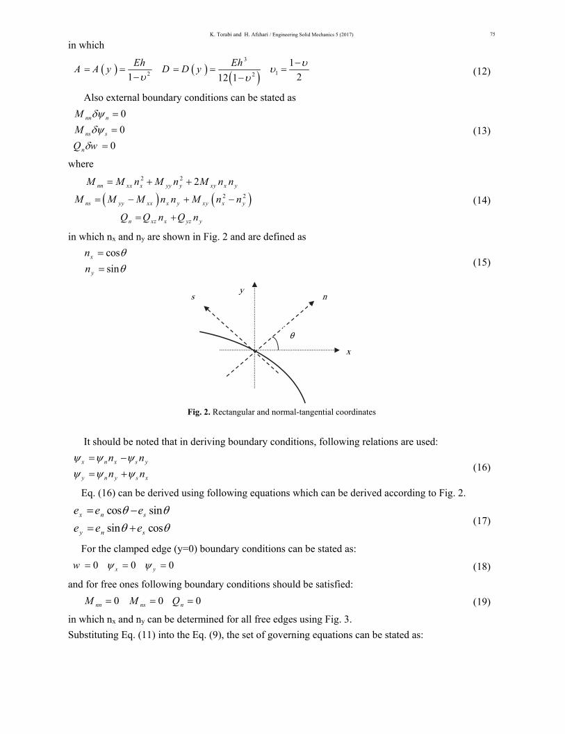
in which nx and ny are shown in Fig. 2 and are defined as

(15) cos

sinx

y

n

n

Fig. 2. Rectangular and normal-tangential coordinates

It should be noted that in deriving boundary conditions, following relations are used:

(16) x n x s y

y n y s x

n n

n n

Eq. (16) can be derived using following equations which can be derived according to Fig. 2.

(17) cos sin

sin cosx n s

y n s

e e e

e e e

For the clamped edge (y=0) boundary conditions can be stated as:

(18) 0 0 0x yw

and for free ones following boundary conditions should be satisfied:

(19) 0 0 0nn ns nM M Q

in which nx and ny can be determined for all free edges using Fig. 3.

Substituting Eq. (11) into the Eq. (9), the set of governing equations can be stated as:

x

y n s

θ

76

(20)

2 2 2

1 12 2 2

22 2

1 2 12 2

23

1 2

2 22

2 1 2 2

0

012

yxy

y yx x x

xx

y yx

w w A w wk A k h

x y x y y y t

DD

x y x y y y x

w hk A

x t

Dx y x y

23

1 20

12

yx

yy

D

y x y

w hk A

y t

in which

(21) 2

1

2

Fig. 3. Angle of normal vector (θ) for free edges of the plate

Also substituting Eq. (11) into the Eq. (14) and (19), boundary conditions at free edges can be

stated as:

(22)

3 4 1

2 2

2 0

2 0

0

y yx xx y

y yx xx y x y

x x y y

n nx y y x

n n n nx y y x

w wn n

x y

where

n

θ=-β

s

x

y

n

s

sθ=π-α

θ=π/2

n


77

(23)

2 23

2 24

x y

y x

n n

n n

The analysis of the non-rectangular plates uses a local parameter coordinate system rather than a Cartesian one. As Fig. 4 shows, the original trapezoidal shape of the plate in the x–y coordinates system is mapped to a square in the ζ-η coordinates, using the following transformation:

(24) tanx a L G

y L

where

(25) tan tanG

Fig. 4. Original and computational coordinates

Inverse form of Eq. (24) can be rewritten as:

(26)

tan0 1

0 1

x y

a Gy

y

L

which leads to the following relations for derivatives:

(27)

2 2 2

2 2 2

2 2 2 22 2 2

2 2 2 2

2 2 22 2

2 2

1

12 2

1

H

x L

H

x L

FHy L

F H FH GFHy L

FH H GHx y L

where

ζ

η

1

1

a

L

α

β

x

y

b

78

(28)

1

sec

tan

H HG

F F G

a

b

Note that in deriving Eq. (27), following relation is used:

(29) 2dH

GHd

By definition of the dimensionless function of variation of thickness as

(30) 0

hr

h

and using the method of separation of variables as

(31)

, , ,

, , ,

, , ,

i tx

y

w t bW

t e

t

the set of Eq. (20) can be rewritten as:

(32)

2 2 21

2 2

1

1 1sec 1 2 2

1 cos0

12

dr drk F H W FHW W GH H FW W

r d r d

drk H FH W

r d

2 2112 2

22 1

1 2 2

2 2 22 2 1

2 2

12 cos1

12 cos3 3 12 2

3 cos0

12

k HW F H

r

kdr drFH GH H F

r d r d r

drFH H GH H

r d

2 2122 2

2

2 2 21

2 2 2 21

2 2

12 cos 1 3

3 32 2

12 cos 1 cos0

12

k drFHW W FH H GH H

r r d

dr drF H FH GH H F

r d r d

k

r

where following dimensionless parameters are defined:

(33) 4 2

2 0 0

0

h b h

D b

in which


79

(34) 30

0 212 1

EhD

Also dimensionless form of boundary conditions at the free edges can be stated as

(35)

3 1 1 4 1 4

2 2 2 2 2 2

2 2 2 0

2 2 2 0

sec 0

x y x y x y

x y x y x y x y x y x y

x y x y y

Fn n H n n F n n H

F n n n n H n n n n Fn n H n n

n n n Fn HW W n

and at the clamped edge one can write:

(36) 0 0 0W

3. Differential Quadrature Method (DQM)

Consider f(ζ,η) as a two dimensional function. Values of this function at N×M pre-selected grid of points can be considered as

(37) , 1,2,..., 1,2,..., .ij i jf f i N j M

The differential quadrature method is based on the idea that all derivatives of a function can be easily approximated by means of weighted linear sum of the function values at the pre-selected grid of points as:

(38)

2

21 1, , , ,

2

21 1, , , ,

2

1 1, ,

,

i j i j

i j i j

i j

N N

in nj in njn n

M M

jm im jm imm m

N M

in jm nmn m

f fA f B f

f fA f B f

fA A f

where A(ζ), B(ζ), A(η) and B(η) are the weighting coefficients associated with the first and second order derivatives in ζ and η directions, respectively. These matrices for the first-order derivatives are given as (Bert and Malik, 1996b)

(39)

1,

1

1

1,

1

1

, , 1,2,3,..., ;

1, 1,2,3,...,

,

, , 1,2,3,..., ;

1, 1,2,3,...,

N

i kkk i n

N

n kin k

k n

N

k i kk i

M

j kkk j m

M

m kjm k

k m

M

k j kk j

i n N i n

A

i n N

j m M j m

A

j m M

80

and of second-order derivatives can be extracted from the following relations:

(40)

.

B A A

B A A

Eq. (38) can be written in the matrix form as

(41)

,T T

T

f A f f B f

f f A f f B

f A f B

in which superscript T shows the transpose operation. For a matrix N Mf

, an equivalent column

vector 1NM

f

can be defined as

(42) 1v ijf f v j N i

In other words, f is made of column of f ; Using this technique, multiple of three matrices as

a f b can be replaced by Tb a f ; in which ⊗ indicates the Kronecker product.

Therefore, Eq. (41) can be converted to

(43)

,

f I A f f I B f

f A I f f B I f

f A A f

in which Iζ and Iη indicate the identity matrix of size N and M, respectively.

Different choices for the sampling point positions can be considered. The simplest choice for these points is one with equal spacing. But it has been shown that some unequally spaced points may lead to faster convergence of the solution, and more accurate results (Bert and Malik, 1996b). A well-accepted set of the grid points is the Gauss–Lobatto–Chebyshev points given for interval [0,1] by

(44)

111 cos

2 ( 1).

111 cos

2 1

i

j

i

N

j

M

4. DQM Analogue

Using DQ rules, the set of governing differential Eq. (32) is transformed to the following form:

(45) 2K u M u

where [K] and [M] are stiffness and mass matrices; definition of these matrices are presented in Appendix A. Also in a similar manner boundary conditions of Eq. (35) and Eq. (36) can be written using DQ rules as

(46) 0T u

in which definition of the matrix [T] is presented in Appendix B.


81

In order to find Eigen frequencies and corresponding Eigen vectors, Eq. (45) and Eq. (46) should be satisfied simultaneously. Let us divide the grid points as two sets: boundary points which are located at the four edges of the plate and domain ones which are other internal points. By neglecting satisfying the Eq. (45) at the boundary points, this equation can be written as

(47) 2K u M u

where bar sign implies the corresponding non-square matrix. Eq. (46) and Eq. (47) may be rearranged and partitioned in order to separate the boundary and domain points as the following:

(48-a) 2

d b d bd b d bK u K u M u M u

(48-b) 0d bd bT u T u

where subscripts ''b'' and ''d'' indicate to the boundary and domain points, respectively. Substituting Eq. (48-b) into Eq. (48-a) leads to the following Eigen value equation:

(49) 2K Md d

F u F u

in which

(50)

1

1

K b dd b

M b dd b

F K K T T

F M M T T

5. Numerical results

Here the numerical results are given for the developed numerical solution in the previous section. It should be noted that in all of the following examples, value of the Poisson's ratio is considered as ν=0.3. In order to check the convergence of the proposed solution, consider a plate with the following parameters:

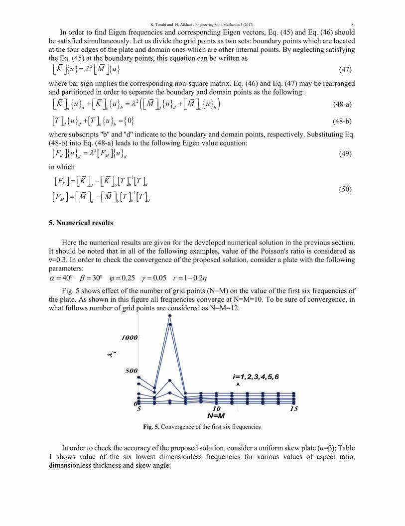
40 30 0.25 0.05 1 0.2r Fig. 5 shows effect of the number of grid points (N=M) on the value of the first six frequencies of the plate. As shown in this figure all frequencies converge at N=M=10. To be sure of convergence, in what follows number of grid points are considered as N=M=12.

Fig. 5. Convergence of the first six frequencies

In order to check the accuracy of the proposed solution, consider a uniform skew plate (α=β); Table 1 shows value of the six lowest dimensionless frequencies for various values of aspect ratio, dimensionless thickness and skew angle.

5 10 150

500

1000

N=M

i

i=1,2,3,4,5,6

82

Table 1. Values of the six lowest dimensionless frequencies of a uniform skew plate for various values of aspect ratio, dimensionless thickness and skew angle

Mode sequence number φ γ α 1 2 3 4 5 6

1

0.1 15

DQM 3.500 8.252 20.90 24.83 31.03 46.39 Liew et al., 1998 3.536 8.228 20.84 24.64 30.77 46.12

30 DQM 3.751 8.818 23.18 24.58 36.98 45.16

Liew et al., 1998 3.858 8.870 23.23 24.27 37.03 45.24

0.2 15

DQM 3.424 7.518 18.20 21.87 26.16 37.67 Liew et al., 1998 3.434 7.489 18.05 21.59 25.96 37.47

30 DQM 3.771 8.090 19.74 21.41 30.76 37.47

Liew et al., 1998 3.719 8.055 19.51 21.34 30.57 37.00

2

0.1 15

DQM 3.621 5.414 10.084 18.33 21.67 24.36 Liew et al., 1998 3.594 5.366 9.949 18.28 21.42 23.24

30 DQM 3.737 5.883 10.45 19.12 22.34 28.21

Liew et al., 1998 3.986 6.050 10.72 19.04 23.48 28.11

0.2 15

DQM 3.260 4.843 8.624 16.71 19.91 22.08 Liew et al., 1998 3.493 5.071 9.178 16.43 18.47 20.80

30 DQM 3.722 5.450 10.057 15.19 19.35 24.51

Liew et al., 1998 3.842 5.692 9.850 17.08 19.66 23.92

Comparing these results with those presented based on Ritz method (Liew et al., 1998), confirms adaptation and accuracy of the proposed solution. Also corresponding mode shapes for a case with φ=1, γ=0.1 and α=30∘ are depicted in Figs. 6.a-6.f.

(a). Mode 1 (b). Mode 2

(c). Mode 3 (d). Mode 4

(e). Mode 5 (f). Mode 6

Fig. 6. First six modes for a skew plate with uniform thickness

00.5

11.5

2

0

0.5

1

-1

-0.5

0

0.5

W

00.5

11.5

2

0

0.5

1

-0.5

0

0.5

W

00.5

11.5

2

0

0.5

1

-0.2

-0.1

0

0.1

0.2

0.3

W

00.511.52

0

0.5

1

-0.2

0

0.2

0.4

0.6

W

00.5

11.5

2

0

0.5

1

-0.4

-0.2

0

0.2

0.4

W

00.5

11.5

2

0

0.5

1

-0.1

0

0.1

0.2

0.3

W


83

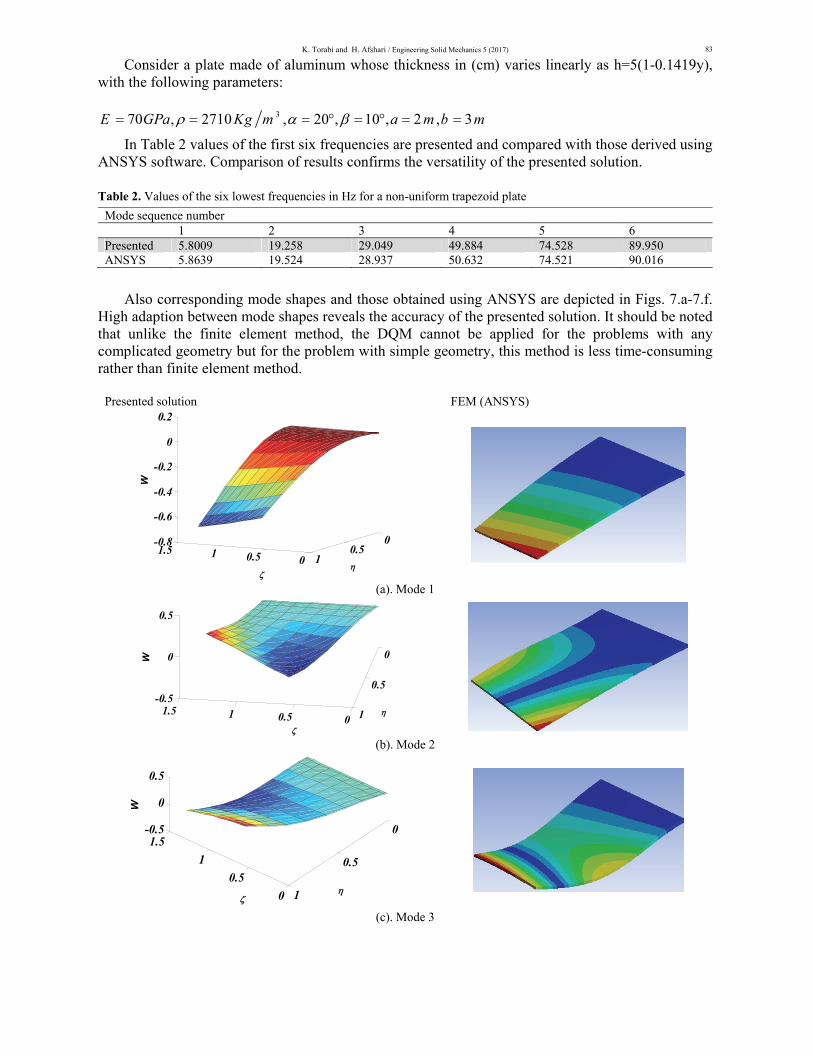
Consider a plate made of aluminum whose thickness in (cm) varies linearly as h=5(1-0.1419y), with the following parameters:

370 , 2710 , 20 , 10 , 2 , 3E GPa Kg m a m b m

In Table 2 values of the first six frequencies are presented and compared with those derived using ANSYS software. Comparison of results confirms the versatility of the presented solution.

Table 2. Values of the six lowest frequencies in Hz for a non-uniform trapezoid plate

Mode sequence number 1 2 3 4 5 6

Presented 5.8009 19.258 29.049 49.884 74.528 89.950 ANSYS 5.8639 19.524 28.937 50.632 74.521 90.016

Also corresponding mode shapes and those obtained using ANSYS are depicted in Figs. 7.a-7.f. High adaption between mode shapes reveals the accuracy of the presented solution. It should be noted that unlike the finite element method, the DQM cannot be applied for the problems with any complicated geometry but for the problem with simple geometry, this method is less time-consuming rather than finite element method.

Presented solution FEM (ANSYS)

(a). Mode 1

(b). Mode 2

(c). Mode 3

00.511.50

0.51

-0.8

-0.6

-0.4

-0.2

0

0.2

W

00.511.5

0

0.5

1

-0.5

0

0.5

W

0

0.5

1

1.50

0.5

1

-0.5

0

0.5

W

84

(d). Mode 4

(e). Mode 5

(f). Mode 6Fig. 7. First six modes for a trapezoidal plate with non-uniform thickness

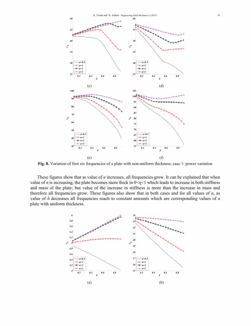
The accuracy and versatility of the proposed solution were confirmed and now the effect of influencing parameters on the frequencies can be investigated. First, consider a plate (α=20∘, β=10∘, φ=0.25, γ=0.1) and two cases for variation of thickness: case 1: power law variation as r=1-δηn

case 2: exponential variation as r=exp(-δηn)

For various amounts of 0.1 δ 0.9 and n values of the first six frequencies are depicted in Figs. 8 and 9 for case 1 and case 2, respectively.

(a) (b)

00.5

11.5

0

0.5

1

-0.5

0

0.5

W

00.5

11.5

0

0.5

1

-0.2

0

0.2

W

00.51

1.50

0.5

1

-0.2

-0.1

0

0.1

W

0.2 0.4 0.6 0.84

4.5

5

5.5

6

6.5

7

1

n=0.5n=1n=2n=3

0.2 0.4 0.6 0.810

15

20

25

2

n=0.5n=1n=2n=3


85

(c) (d)

(e) (f)

Fig. 8. Variation of first six frequencies of a plate with non-uniform thickness; case 1: power variation

These figures show that as value of n increases, all frequencies grow. It can be explained that when value of n is increasing, the plate becomes more thick in 0<η<1 which leads to increase in both stiffness and mass of the plate; but value of the increase in stiffness is more than the increase in mass and therefore all frequencies grow. These figures also show that in both cases and for all values of n, as value of δ decreases all frequencies reach to constant amounts which are corresponding values of a plate with uniform thickness.

(a) (b)

0.2 0.4 0.6 0.825

30

35

40

45

50

3

n=0.5n=1n=2n=3

0.2 0.4 0.6 0.835

40

45

50

55

60

4

n=0.5n=1n=2n=3

0.2 0.4 0.6 0.830

40

50

60

70

80

90

100

5

n=0.5n=1n=2n=3

0.2 0.4 0.6 0.855

60

65

70

75

80

85

90

95

100

105

6

n=0.5n=1n=2n=3

0.2 0.4 0.6 0.84

4.2

4.4

4.6

4.8

5

5.2

5.4

5.6

5.8

6

1

n=0.5n=1n=2n=3

0.2 0.4 0.6 0.815

16

17

18

19

20

21

22

23

24

2

n=0.5n=1n=2n=3

86

(c) (d)

(e) (f)

Fig. 9. Variation of first six frequencies of a plate with non-uniform thickness; case 2: exponential variation

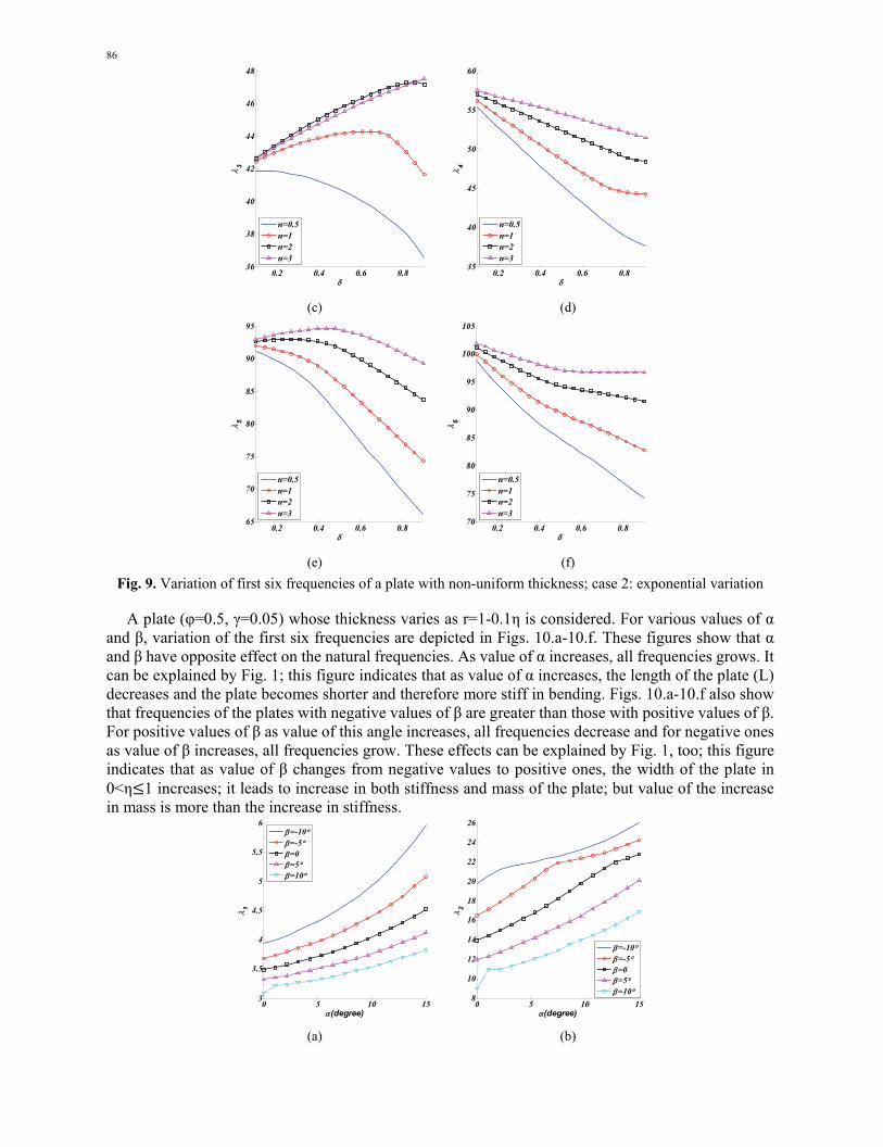
A plate (φ=0.5, γ=0.05) whose thickness varies as r=1-0.1η is considered. For various values of α and β, variation of the first six frequencies are depicted in Figs. 10.a-10.f. These figures show that α and β have opposite effect on the natural frequencies. As value of α increases, all frequencies grows. It can be explained by Fig. 1; this figure indicates that as value of α increases, the length of the plate (L) decreases and the plate becomes shorter and therefore more stiff in bending. Figs. 10.a-10.f also show that frequencies of the plates with negative values of β are greater than those with positive values of β. For positive values of β as value of this angle increases, all frequencies decrease and for negative ones as value of β increases, all frequencies grow. These effects can be explained by Fig. 1, too; this figure indicates that as value of β changes from negative values to positive ones, the width of the plate in 0<η 1 increases; it leads to increase in both stiffness and mass of the plate; but value of the increase in mass is more than the increase in stiffness.

(a) (b)

0.2 0.4 0.6 0.836

38

40

42

44

46

48

3

n=0.5n=1n=2n=3

0.2 0.4 0.6 0.835

40

45

50

55

60

4

n=0.5n=1n=2n=3

0.2 0.4 0.6 0.865

70

75

80

85

90

95

5

n=0.5n=1n=2n=3

0.2 0.4 0.6 0.870

75

80

85

90

95

100

105

6

n=0.5n=1n=2n=3

0 5 10 153

3.5

4

4.5

5

5.5

6

(degree)

1

=-10=-5=0=5=10

0 5 10 158

10

12

14

16

18

20

22

24

26

(degree)

2

=-10=-5=0=5=10


87

(c) (d)

(e) (f)

Fig. 10. Variation of first six frequencies of a plate with non-uniform thickness for various values of angles

According to Eq. (33), thickness of the plate is used in definition of the dimensionless frequency (λ), Before studying the effect of thickness, let us define following new dimensionless frequency:

(51) 2 2 2

2 2 212 1 b

E

which is independent of thickness. Now consider a plate (α=20∘, β=10∘) whose thickness varies as r=exp(-0.1η); Figs. 11.a-11.f shows the effect of dimensionless thickness and aspect ratio on the six lowest dimensionless frequencies (Λ1-Λ6).

(a) (b)

0 5 10 15

20

25

30

35

40

(degree)

3

=-10=-5=0=5=10

0 5 10 15

35

40

45

50

55

60

65

(degree)

4

=-10=-5=0=5=10

0 5 10 1550

55

60

65

70

75

80

85

90

95

(degree)

5

=-10=-5=0=5=10

0 5 10 1550

60

70

80

90

100

110

120

(degree)

6

=-10=-5=0=5=10

0.02 0.04 0.06 0.08 0.10

0.05

0.1

0.15

0.2

0.25

0.3

0.35

0.4

0.45

1

=0.2=0.3=0.4=0.5

0.02 0.04 0.06 0.08 0.10.2

0.4

0.6

0.8

1

1.2

1.4

1.6

1.8

2

2.2

2

=0.2=0.3=0.4=0.5

88

(c) (d)

(e) (f)

Fig. 11. Variation of first six frequencies of a plate with non-uniform thickness for various values of aspect ratio and

dimensionless thickness

These figures show that as value of thickness increases, all frequencies grows; when thickness of the plate is rising, both stiffness and mass of the plate increase; but value of the increase in stiffness is more than the increase in mass. These figures also indicate that as value of the aspect ratio increases, all frequencies decrease. It can be explained that as value of the aspect ratio rises, the width of the plate grows which increase both stiffness and mass of the plate; but value of the increase in mass is more than the increase in stiffness of the plate.

6. Conclusion

Using Differential quadrature method, a numerical solution for vibration analysis of a cantilevered trapezoidal thick plate with variable thickness was presented. The convergence and accuracy of the proposed solution were confirmed using results presented by other authors and also results obtained using ANSYS software. Finally, the effect of the variation of thickness, angles, aspect ratio and thickness of the plate on the natural frequencies were investigated. Two cases for variation of thickness were considered: case 1 as r=1-δηn and case 2 as r=exp(-δηn); following results were obtained: For both cases it was shown that as value of the n increases, all frequencies become more.

As value of α increases, all frequencies becomes more.

Plates with negative values of β have larger frequencies with respect to those plates with positive

ones.

For positive values, as value of β increases, all frequencies are decreased and vice versa.

0.02 0.04 0.06 0.08 0.10

0.5

1

1.5

2

2.5

3

3.5

3

=0.2=0.3=0.4=0.5

0.02 0.04 0.06 0.08 0.10.5

1

1.5

2

2.5

3

3.5

4

4.5

5

5.5

4

=0.2=0.3=0.4=0.5

0.02 0.04 0.06 0.08 0.10

1

2

3

4

5

6

7

8

9

5

=0.2=0.3=0.4=0.5

0.02 0.04 0.06 0.08 0.11

2

3

4

5

6

7

8

9

10

6

=0.2=0.3=0.4=0.5


89

All frequencies rise by increasing the thickness and conversely the frequencies are decreased when

the width of plate becomes more.

Appendix A

Definition of stiffness and mass matrices which are used in Eq. (45) are presented as

(A-1)

0 0

0 0

0 0

WW W W W

W

W

k k k m

K k k k M m

k k k m

where [0] indicates the null matrix of size MN*MN and following matrices are defined:

(A-2)

2 2

2

1

1

1

2

sec 2WW

W

W

b I a B b A a A

k k B I G b a A

b d a A d A I

k k b A

k k b a A A I d I

212

2 2

1

2

1

221

2

2

2

2

2 1

12 cos

2 2

3 3

12 cos

3

W

kk b c A

k b I a B

b A a A B I G b a A

b d a A d A I

kc I

k b a B b A A

G b A b d A

2 212

2

2 2

2

2 2

1

2

1

12 cos

3

2

2 3

12 c3

W

kk b c a A c A I

b a B b A A

kG b A b d A

k b I a B b A a A

B I G b a A b d a A

kd A I

2

2

2

osc I

2

2 2

cos

12

cos

12

Wm I I

m m I I

It should be noted that in Eq. (A-2), following diagonal matrices are defined:

(A-3) 1 1

j

ii i jj j jj jj

j

dra F b H c d

r dr

Appendix B

Definition of matrix [T] appeared in Eq. (46) is considered as follows:

90

(B-1)

11 12 13

21 22 23

31 32 33

41 42 43

51 52 53

61 62 63

71 72 73

81 82 83

91 92 93

101 102 103

111 112 113

121 121 123

T T T

T T T

T T T

T T T

T T T

T T TT

T T T

T T T

T T T

T T T

T T T

T T T

where components of this matrix are related to the boundary conditions at four edges of the plate as:

at edge 0 :

(B-2)

11 22 33 1

12 13 21 23 31 32 *0

j

N NM

T T T I I

T T T T T T

at edge 1 :

(B-3)

41 51 62 *

42

6143 52

53

63

0

1

1sec

1

N NM

Mj

Mj Mj

Mj

Mj

T T T

T H I A

TT T H I a A A I

T H I A

T I I

at edge 0 :

(B-4)

71 81 *

72 3 1 1i 1 1i

73 4 1 1i 4 1i

2 2 2 282 1i 1i

2 283 1i 1i

91

0

2 0 2

0 2

0 2

2 0 2

sec

M NM

x y x y

x y

x y x y x y

x y x y x y

T T

T F n n b A n n A I

T F n n b A A I

T F n n n n b A n n A I

T n n F n n b A n n A I

T

1i 1i

92 1i

93 1i

0x y y

x

y

n F n b A n A I

T n I I

T n I I

where

(B-5) cos sinx yn n


91

and finally at edge 1 :

(B-6)

101 111 *

102 3 1 Ni 1 Ni

103 4 1 Ni 4 Ni

2 2 2 2112 Ni Ni

2 2113 Ni Ni

1

0

2 1 2

1 2

1 2

2 1 2

M NM

x y x y

x y

x y x y x y

x y x y x y

T T

T F n n b A n n A I

T F n n b A A I

T F n n n n b A n n A I

T n n F n n b A n n A I

T

21 Ni Ni

122 Ni

123 Ni

sec 1x y y

x

y

n F n b A n A I

T n I I

T n I I

where

(B-7) cos sinx yn n

It should be noted that in Eqs. (B-2)-(B-6), indices i and j are considered as

(B-8) 1,2,3, , 1,2,3, ,i N j M

and also following obvious relations are considered:

(B-9) 11 0 tan 1 tan

secH F F

G

References Bert, C. W., & Malik, M. (1996a). The differential quadrature method for irregular domains and

application to plate vibration. International Journal of Mechanical Sciences, 38(6), 589-606. Bert, C. W., & Malik, M. (1996b). Differential quadrature method in computational mechanics: a

review. Applied Mechanics Reviews, 49(1), 1-28. Chen, S. S., Xu, C. J., Tong, G. S., & Wei, X. (2015). Free vibration of moderately thick functionally

graded plates by a meshless local natural neighbor interpolation method. Engineering Analysis with Boundary Elements, 61, 114–126.

Chopra, I., & Durvasula, S. (1971). Vibration of simply supported trapezoidal plates. I. symmetric trapezoids. Journal of Sound and Vibration, 19, 379-392.

Chopra, I., & Durvasula, S. (1972). Vibration of simply supported trapezoidal plates. II. un-symmetric trapezoids. Journal of Sound and Vibration, 20, 125-134.

Dehghany, M., & Farajpour, A. (2014). Free vibration of simply supported rectangular plates on Pasternak foundation: An exact and three-dimensional solution. Engineering Solid Mechanics, 2(1), 29-42.

Dehghan, M., Nejad, M., & Moosaie, A. (2016). An effective combination of finite element and differential quadrature method for analyzing of plates partially resting on elastic foundation. Engineering Solid Mechanics, 4(4), 201-218.

Eftekhari, S. A., & Jafari, A. A. (2013). Modified mixed Ritz-DQ formulation for free vibration of thick rectangular and skew plates with general boundary conditions. Applied Mathematical Modelling, 37(12), 7398-7426.

Huang, C. S., Leissa, A. W., & Chang, M. J. (2005). Vibrations of skewed cantilevered triangular, trapezoidal and parallelogram Mindlin plates with considering corner stress singularities. International Journal for Numerical Methods in Engineering, 62(13), 1789-1806.

92

Gupta, U., Sharma, S., & Singhal, P. (2016). DQM modeling of rectangular plate resting on two parameter foundation. Engineering Solid Mechanics, 4(1), 33-44.

Kaneko, T. (1975). On Timoshenko's correction for shear in vibrating beams.Journal of Physics D: Applied Physics, 8(16), 1927.

Liew, K. M., Xiang, Y., Kitipornchai, S., & Wang, C. M. (1998). Vibration of Mindlin plates: programming the p-version Ritz method. Elsevier.

Maruyama, K., Ichinomiya, O., & Narita, Y. (1983). Experimental study of the free vibration of clamped trapezoidal plates. Journal of Sound and Vibration, 88(4), 523-534.

Mindlin, R. D. (1951). Influence of rotary inertia and shear on flexural motions of isotropic elastic plates. Journal of Applied Mechanics-T ASME, 18, 31–38.

Naghsh, A., & Azhari, M. (2015). Non-linear free vibration analysis of points supported laminated composite skew plate. International Journal of Non-linear Mechanics, 76, 64-76.

Orris, R. M., & Petyt, M. (1973). A finite element study of the vibration of trapezoidal plates. Journal of Sound and Vibration, 27, 325-344.

Petrolito, J. (2014). Vibration and stability analysis of thick orthotropic plates using hybrid-Trefftz elements. Applied Mathematical Modelling, 38(24), 5858-5869.

Samaei, A. T., Aliha, M. R. M., & Mirsayar, M. M. (2015). Frequency analysis of a graphene sheet embedded in an elastic medium with consideration of small scale. Materials Physics and Mechanics, 22, 125-135.

Shu, C., Wu, W. X., Ding, H., & Wang, C. M. (2007). Free vibration analysis of plates using least-square-based finite difference method. Computer Methods in Applied Mechanics and Engineering, 196(7), 1330-1343.

Shufrin, I., Rabinovitch, O., & Eisenberger, M. (2010). A semi-analytical approach for the geometrically nonlinear analysis of trapezoidal plates. International Journal of Mechanical Sciences, 52(12), 1588-1596.

Srinivasan, R.S., & Babu, B.J.C. (1983). Free vibration of cantilever quadrilal plates. Journal of the Acoustical Society of America, 73, 851-855.

Torabi, K., Afshari, H., & Heidari-Rarani, M. (2013). Free vibration analysis of a non-uniform cantilever Timoshenko beam with multiple concentrated masses using DQEM. Engineering Solid Mechanics, 1(1), 9-20.

Torabi, K. & Afshari, H. (2016). Generalized differential quadrature method for vibration analysis of cantilever trapezoidal FG thick plate. Journal of Solid Mechanics, 8(1), 184-203.

Wang, X., Wang, Y., & Yuan, Z. (2013). Accurate vibration analysis of skew plates by the new version of the differential quadrature method. Applied Mathematical Modelling, 38(3), 926-937.

Xia, P., Long, S. Y., Cui, H. X., & Li, G. Y. (2009). The static and free vibration analysis of a nonhomogeneous moderately thick plate using the meshless local radial point interpolation method. Engineering Analysis with Boundary Elements, 33(6), 770-777.

Zamani, M., Fallah, A., & Aghdam, M. M. (2012). Free vibration analysis of moderately thick trapezoidal symmetrically laminated plates with various combinations of boundary conditions. European Journal of Mechanics-A/Solid, 36, 204–212.

Zhao, X., Lee, Y. Y., & Liew, K. M. (2009). Free vibration analysis of functionally graded plates using the element-free kp-Ritz method. Journal of sound and Vibration, 319(3), 918-939.

Zhou, L., & Zheng, W. X. (2008). Vibration of skew plates by the MLS-Ritz method. International Journal of Mechanical Sciences, 50(7), 1133-1141.

© 2016 by the authors; licensee Growing Science, Canada. This is an open access article distributed under the terms and conditions of the Creative Commons Attribution (CC-BY) license (http://creativecommons.org/licenses/by/4.0/).

Documents

Vibration analysis of a cantilevered trapezoidal ... · PDF file72 Based on the classical theory of plates, there is a considerable amount of work related to the vibration analysis