\documentclass[a4paper,oneside]{book}\usepackage{tabu,float,hyperref,color,amsmath,amsxtra,amssymb,latexsym,amscd,amsthm,amsfonts,graphicx}\numberwithin{equation}{chapter}\usepackage{fancyhdr}\pagestyle{fancy}\fancyhf{}\fancyhead[RE,LO]{\footnotesize \textsc \leftmark \hfill \thepage}%\cfoot{}\renewcommand{\headrulewidth}{0.5pt}\setcounter{tocdepth}{3}\setcounter{secnumdepth}{3}\usepackage{imakeidx}\makeindex[columns=2, title=Alphabetical Index, options= -s index.ist]\title{\Huge Project on $\star$ Runge Kutta method}\author{\textsc{Nguyen Quan Ba Hong}\footnote{Student ID. 1411103}\\\textsc{Doan Tran Nguyen Tung}\footnote{Student ID. 1411352}\\\textsc{Nguyen An Thinh}\footnote{Student ID. 1411289}\\{\small Students at Faculty of Math and Computer Science}\\ {\small Ho Chi Minh University of Science, Vietnam} \\{\small \texttt{email. nguyenquanbahong@gmail.com}}\\{\small \texttt{email. dtrngtung@live.com}}\\{\small \texttt{blog. \url{http://hongnguyenquanba.wordpress.com}} \footnote{Copyright \copyright\ 2016 by Nguyen Quan Ba Hong, Student at Ho Chi Minh University of Science, Vietnam. This document may be copied freely for the purposes of education and non-commercial research. Visit my site \texttt{\url{http://hongnguyenquanba.wordpress.com}} to get more.}}}\begin{document}\frontmatter\maketitle\tableofcontents\cleardoublepage\phantomsection\addcontentsline{toc}{chapter}{List of Figures}\listoffigures\mainmatter\chapter{Introduction}\section{Initial Value Problems}The Runge Kutta methods\index{Runge Kutta method} are an important family of iterative methods\index{iterative method} for the approximation of solutions of ODE's, that were developed around 1900 by the German mathematicians Carl Runge (1856-1927) and Martin. W. Kutta (1867-1944). Modern developments are mostly due to John Butcher in the 1960s.

We consider initial value problems\index{initial value problems} expressed in autonomous form\index{autonomous form}. Starting with the non-autonomous\index{non-autonomous form}, we assume that $f\left(x,y\right)$ is a continuous function with domain $\left[a,b\right]\times \mathbb{R}^n$ where $t \in \left[a,b\right]$ and $y\in \mathbb{R}^n$.

Consider the initial value problem\begin{align}\label{1}\dfrac{{dy\left( t \right)}}{{dt}} &= f\left( {t,y\left( t \right)} \right)\\

y\left( x_0 \right) &= {y_0}\end{align}where\begin{align}y\left( t \right) = {\left( {{y_1}\left( t \right),{y_2}\left( t \right), \ldots ,{y_n}\left( t \right)} \right)^T}\end{align}\begin{align}f:\left[ {a,b} \right] \times {\mathbb{R}^n} \to {\mathbb{R}^n}\end{align}

We assume that\begin{align}{\left\| {f\left( {t,{y_1}} \right) - f\left( {t,{y_2}} \right)} \right\|_{{L^2}\left( {{\mathbb{R}^n}} \right)}} \le L{\left\| {{y_1} - {y_2}} \right\|_{{L^2}\left( {{\mathbb{R}^n}} \right)}}\end{align}for all $t \in \left[ {a,b} \right],{y_1} \in {\mathbb{R}^n},{y_2} \in {\mathbb{R}^n}$.

Thus the IVP \eqref{1} has a unique solution.

For convenience, we write \eqref{1} briefly as\begin{align}y_t=f\end{align}

Most efforts to increases the order of the Runge Kutta methods have been accomplished by increasing the number of Taylor's series\index{Taylor's series} terms used and thus the number of functional evaluations, e.g. Butcher 1987, Gear 1971. The use of higher order derivative terms has been proposed for stiff problems\index{stiff problems}, e.g. Rosenbrock 1963, Enright 1974. Our method add higher order derivative terms to the Runge Kutta $k_i$ terms ($i>1$) to achieve a higher order of accuracy\index{order of accuracy}.

We are interested in a numerical approximation of the continuously differentiable solution $y\left( t\right)$ of the IVP \eqref{1} over the time interval $t \in \left[ a,b\right]$.\section{Mesh}We subdivide the interval $\left[ {a,b} \right]$ into $M$ equal subintervals and select the mesh points $t_j$\index{mesh}\begin{align}{t_j} = a + jh,j = 0,1, \ldots ,M\end{align}where\begin{align}h = \dfrac{{b - a}}{M}\end{align}is called a step size\index{step size}.\section{General Runge Kutta method}The family of explicit Runge Kutta (RK) methods\index{family of explicit Runge Kutta methods} of the $m$th stage is given by\begin{align}\label{1.8}{y^{\left( {n + 1} \right)}} = {y^{\left( n \right)}} + h\sum\limits_{i = 1}^s {{b_i}{k_i}} \end{align}

where\begin{align}\label{1.9}{k_i} = f\left( {{\tau _i},{\eta _i}} \right),i = 1,2, \ldots ,s\end{align}and\begin{align}{\tau _i} &= {t_n} + {c_i}h\end{align}\begin{align}{\eta _i} &= {y_n} + h\sum\limits_{j = 1}^{i - 1} {{a_{ij}}{k_j}} \\ &= {y_n} + h\sum\limits_{j = 1}^{i - 1} {{a_{ij}}f\left( {{\tau _j},{\eta _j}} \right)} \end{align}

We use the notation\begin{align}{f_n}: = f\left( {{t_n},{y_n}} \right)\end{align}

To specify a particular method, we need to provide the integer $s$ (the number of stages), and the coefficients $c_i,i=2,\ldots,s$, $a_{ij},1\le j<i\le m$ and $b_i,i=1,2,\ldots,s$.

These data are usually arranged in a so-called Butcher tableau\index{Butcher tableau} (after John C. Butcher)\begin{align}\begin{array}{*{20}{c}} 0&\vline & {}&{}&{}&{}&{} \\ {{c_2}}&\vline & {{a_{21}}}&{}&{}&{}&{} \\ {{c_3}}&\vline & {{a_{31}}}&{{a_{32}}}&{}&{}&{} \\ \vdots &\vline & \vdots & \vdots & \ddots &{}&{} \\ {{c_s}}&\vline & {{a_{s1}}}&{{a_{s2}}}& \cdots &{{a_{ss - 1}}}&{} \\ \hline {}&\vline & {{b_1}}&{{b_2}}& \cdots &{{b_{s - 1}}}&{{b_s}} \end{array}\end{align}\section{Runge Kutta Order 1 Method}We consider the Runge Kutta order 1 method\index{Runge Kutta order 1 method} here because it is very short and easy. There is no need to represent this into a separated chapter.

For $s=1$, \eqref{1.9} becomes\begin{align}{k_1} = f\left( {{t_n},{x_n}} \right)\end{align}and \eqref{1.9} becomes\begin{align} {y^{\left( {n + 1} \right)}} &= {y^{\left( n \right)}} + h{b_1}{k_1} \\ &= {y^{\left( n \right)}} + h{b_1}{f_n}\label{1.16}\end{align}

On the other hand, the Taylor expansion yields\begin{align}{y^{\left( {n + 1} \right)}} &= {y^{\left( n \right)}} + h{\left. {{y_t}} \right|_{{t_n}}} + O\left( {{h^2}} \right)\\

&= {y^{\left( n \right)}} + h{f_n} + O\left( {{h^2}} \right) \label{1.18}\end{align}

Comparing \eqref{1.16} and \eqref{1.18}, we obtain easily\begin{align}b_1=1\end{align}Hence, The Butcher table\index{Butcher table} in this case has the following form\begin{align}\begin{array}{*{20}{c}}0&\vline& {}\\\hline{}&\vline& 1\end{array}\end{align}\textbf{Remark 1.1.} The Runge Kutta order 1 method is equivalent to the explicit Euler's method\index{explicit Euler's method}. Note that the Euler's method\index{Euler's method} is of the first order of accuracy. Hence, we get the name Runge Kutta method of the `first order' as above.\chapter{Runge Kutta order 2 method}\section{Derivation of Runge Kutta Order 2 Method}To set up the Runge Kutta order 2 method\index{Runge Kutta order 2 method}, we need to do 4 steps.\begin{enumerate}\item Write down Runge Kutta order 2 formula described by \eqref{1.8} and \eqref{1.9}.\item Write down Taylor series expansion.\item Compare the coefficients of two formulas above to obtain a system of equations. \item Solve the system of equation or find some its solutions.\end{enumerate}\textbf{Remark 2.1.} This process is also applied for Runge Kutta method of higher orders. Therefore, we can regard it as the standard process for derivation of the general Runge Kutta method in this context.\\

After these steps, with some solutions of the derived system of equations, we can simulate some IVPs easily.\subsection{Runge Kutta Order 2 Formula}For $s=2$, \eqref{1.9} becomes\begin{align}{k_1} &= {f_n}\\{k_2} &= f\left( {{t_n} + {c_2}h,{y_n} + h{a_{21}}{f_n}} \right)\end{align}and \eqref{1.8} becomes\begin{align}{y^{\left( {n + 1} \right)}} &= {y^{\left( n \right)}} + h{b_1}{k_1} + h{b_2}{k_2}\\ &= {y^{\left( n \right)}} + h{b_1}{f_n} + h{b_2}f\left( {{t_n} + {c_2}h,{y_n} + h{a_{21}}{f_n}} \right) \label{2.4}\end{align}

Now we write down the Taylor series expansion $O\left(h^2\right)$ for ${k_2} $\begin{align}{k_2} &= f\left( {{t_n} + {c_2}h,{y_n} + h{a_{21}}{f_n}} \right)\\

&= {f_n} + {c_2}h{f_t} + h{a_{21}}{f_n}{f_y} + O\left( {{h^2}} \right)\label{2.6}\end{align}

Inserting \eqref{2.6} into \eqref{2.4}, we obtain\begin{align}{y^{\left( {n + 1} \right)}} &= {y^{\left( n \right)}} + h{b_1}{f_n} + h{b_2}\left[ {{f_n} + {c_2}h{f_t} + h{a_{21}}{f_n}{f_y} + O\left( {{h^2}} \right)} \right]\\ &= {y^{\left( n \right)}} + h\left( {{b_1} + {b_2}} \right){f_n} + {h^2}{b_2}{c_2}{f_t} + {h^2}{b_2}{a_{21}}{f_n}{f_y} + O\left( {{h^3}} \right) \label{2.8}\end{align}\subsection{Taylor Series Expansion Formula}We need to compute $y_{tt}$ for Taylor series expansion below.\begin{align}{y_{tt}} &= \dfrac{{df}}{{dt}}\\ &= \dfrac{{\partial f}}{{\partial t}}\dfrac{{\partial t}}{{\partial t}} + \dfrac{{\partial f}}{{\partial y}}\dfrac{{\partial y}}{{\partial t}}\\ &= {f_t} + f{f_y}\end{align}

Now we write down the Taylor series expansion of $y$ in the neighborhood of $t_n$ with $O\left(h^3\right)$.\begin{align}{y^{\left( {n + 1} \right)}} &= {y^{\left( n \right)}} + h{\left. {{y_t}} \right|_{{t_n}}} + \dfrac{{{h^2}}}{2}{\left. {{y_{tt}}} \right|_{{t_n}}} + O\left( {{h^3}} \right)\\ &= {y^{\left( n \right)}} + h{f_n} + \dfrac{{{h^2}}}{2}{\left. {{y_{tt}}} \right|_{{t_n}}} + O\left( {{h^3}} \right)\\ &= {y^{\left( n \right)}} + h{f_n} + \dfrac{{{h^2}}}{2}{\left. {\left( {{f_t} + f{f_y}} \right)} \right|_{{t_n}}} + O\left( {{h^3}} \right)\\ &= {y^{\left( n \right)}} + h{f_n} + {\left. {\dfrac{{{h^2}}}{2}{f_t}} \right|_{{t_n}}} + \dfrac{{{h^2}}}{2}{f_n}{\left. {{f_y}} \right|_{{t_n}}} + O\left( {{h^3}} \right)\label{2.11}\end{align}\\\\\textbf{Remark 2.2.} (Important) From here to later, if nothing is misundertood, we can abbreviate notation ${f_{{t^\alpha }{y^\beta }}}$ for \begin{align}{\left. {{f_{{t^\alpha }{y^\beta }}}} \right|_{{t_n}}}\end{align}in the Taylor series expansion.

For example, under this abbreviation, \eqref{2.11} can be rewritten briefly as\begin{align}\label{2.13}{y^{\left( {n + 1} \right)}} = {y^{\left( n \right)}} + h{f_n} + \dfrac{{{h^2}}}{2}{f_t} + \dfrac{{{h^2}}}{2}{f_n}{f_y} + O\left( {{h^3}} \right)\end{align}

This abbreviation reduces the complexity of the formulas in this context. As you will see later, this abbreviation is really essential.\subsection{Derivation of System of Equations}

Return to our problem, as usual, comparing \eqref{2.8} and \eqref{2.13}, we obtain\begin{align}h{f_n}:1 &= {b_1} + {b_2}\\{h^2}{f_t}:\dfrac{1}{2} &= {b_2}{c_2}\\{h^2}{f_n}{f_y}:\dfrac{1}{2} &= {b_2}{a_{21}}\end{align}

Hence, we obtain the system of equations\begin{align}{b_1} + {b_2} &= 1\label{2.21}\\{b_2}{c_2} &= \dfrac{1}{2}\label{2.22}\\{b_2}{a_{21}} &= \dfrac{1}{2}\label{2.23}\end{align}\subsection{Solutions of System of Equations}We can solve the above system of equations easily. Here, the authors represent two solutions. The idea behind these two solutions will be use later for higher order Runge Kutta method.\\\\\textsc{Solution 1.} The system involves four unknowns in three equations. Taking $b_2=\alpha$ is free variable. Due to \eqref{2.23} we must have $\alpha \ne 0$. Then we can easily obtain the general solution for \eqref{2.21}-\eqref{2.23} is\begin{align}{b_2} &= \alpha \\{b_1} &= 1 - \alpha \\{c_2} &= {a_{21}} = \dfrac{1}{{2\alpha }}\label{2.26}\end{align}where $\alpha$ is an arbitrary real number.

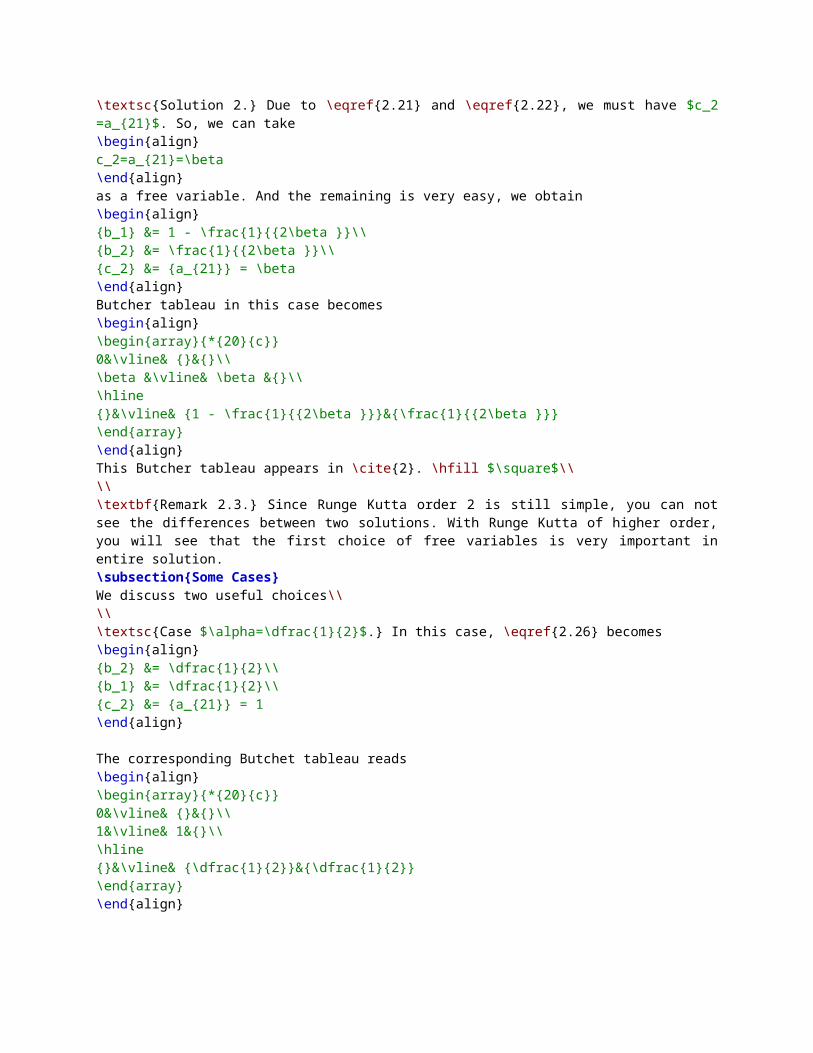
Butcher tableau in this case becomes\begin{align}\begin{array}{*{20}{c}}0&\vline& {}&{}\\{\frac{1}{{2\alpha }}}&\vline& {\frac{1}{{2\alpha }}}&{}\\\hline{}&\vline& {1 - \alpha }&\alpha \end{array}\end{align}\hfill $\square$\\\\\textsc{Solution 2.} Due to \eqref{2.21} and \eqref{2.22}, we must have $c_2 =a_{21}$. So, we can take\begin{align}c_2=a_{21}=\beta\end{align}as a free variable. And the remaining is very easy, we obtain \begin{align}{b_1} &= 1 - \frac{1}{{2\beta }}\\{b_2} &= \frac{1}{{2\beta }}\\{c_2} &= {a_{21}} = \beta \end{align}Butcher tableau in this case becomes\begin{align}\begin{array}{*{20}{c}}0&\vline& {}&{}\\

\beta &\vline& \beta &{}\\\hline{}&\vline& {1 - \frac{1}{{2\beta }}}&{\frac{1}{{2\beta }}}\end{array}\end{align}This Butcher tableau appears in \cite{2}. \hfill $\square$\\\\\textbf{Remark 2.3.} Since Runge Kutta order 2 is still simple, you can not see the differences between two solutions. With Runge Kutta of higher order, you will see that the first choice of free variables is very important in entire solution.\subsection{Some Cases}We discuss two useful choices\\\\\textsc{Case $\alpha=\dfrac{1}{2}$.} In this case, \eqref{2.26} becomes\begin{align}{b_2} &= \dfrac{1}{2}\\{b_1} &= \dfrac{1}{2}\\{c_2} &= {a_{21}} = 1\end{align}

The corresponding Butchet tableau reads\begin{align}\begin{array}{*{20}{c}}0&\vline& {}&{}\\1&\vline& 1&{}\\\hline{}&\vline& {\dfrac{1}{2}}&{\dfrac{1}{2}}\end{array}\end{align}

Thus, in this case the Runge Kutta method of second order\index{Runge Kutta method of second order} takes the form\begin{align}{y^{\left( {n + 1} \right)}} = {y^{\left( n \right)}} + \dfrac{h}{2}\left[ {{f_n} + f\left( {{t_n} + h,{y_n} + h{f_n}} \right)} \right]\end{align}and is equivalent to the Heun's method.\\\\\textsc{Case $\alpha =1$.} In this case, \eqref{2.26} becomes\begin{align}{b_2} &= 1\\{b_1} &= 0\\{c_2} &= {a_{21}} = \dfrac{1}{2}\end{align}

The corresponding Butcher tableau reads\begin{align}\begin{array}{*{20}{c}}0&\vline& {}&{}\\{\dfrac{1}{2}}&\vline& {\dfrac{1}{2}}&{}\\\hline{}&\vline& 0&1\end{array}\end{align}

In this case Runge Kutta method of second order can be written as

\begin{align}{y^{\left( {n + 1} \right)}} = {y^{\left( n \right)}} + hf\left( {{t_n} + \dfrac{h}{2},{y_n} + \dfrac{h}{2}{f_n}} \right)\end{align}and is called the RK2 method.\\\\Remember $\alpha \in \mathbb{R}^*$, so there is infinite many choices of solution for \eqref{2.21}-\eqref{2.23}.\section{\textsc{Matlab} Implementation}See section 4.2 for general code.

\chapter{Runge Kutta order 3 method}\section{Derivation of Runge Kutta Order 3 Method}\subsection{Runge Kutta Order 3 Formula}For $s=3$, \eqref{1.9} becomes\index{Runge Kutta order 3 method}\begin{align}{k_1} &= {f_n}\\{k_2} &= f\left( {{t_n} + {c_2}h,{y_n} + h{a_{21}}{f_n}} \right)\\{k_3} &= f\left( {{t_n} + {c_3}h,{y_n} + h{a_{31}}{k_1} + h{a_{32}}{k_2}} \right)\\ &= f\left( {{t_n} + {c_3}h,{y_n} + h{a_{31}}{f_n} + h{a_{32}}f\left( {{t_n} + {c_2}h,{y_n} + h{a_{31}}{k_1} + h{a_{32}}{k_2}} \right)} \right)\end{align}and \eqref{1.8} becomes\begin{align}\label{3.5}{y^{\left( {n + 1} \right)}} &= {y^{\left( n \right)}} + h{b_1}{k_1} + h{b_2}{k_2} + h{b_3}{k_3}\end{align}

Now we write down the Taylor series expansion $O\left(h^3\right)$ for $k_2$.\begin{align}{k_2} &= f\left( {{t_n} + {c_2}h,{y_n} + h{a_{21}}{f_n}} \right)\\ &= {f_n} + {c_2}h{f_t} + h{a_{21}}{f_n}{f_y} + {h^2}\dfrac{{c_2^2}}{2}{f_{tt}} + {h^2}{c_2}{a_{21}}{f_n}{f_{ty}} + {h^2}\dfrac{{a_{21}^2}}{2}f_n^2{f_{yy}} \\ &+ O\left( {{h^3}} \right) \label{3.7}\end{align}

And we also write down the Taylor series expansion $O\left(h^3\right)$ for $k_3$.\begin{align}{k_3} &= f\left( {{t_n} + {c_3}h,{y_n} + h{a_{31}}{f_n} + h{a_{32}}{k_2}} \right)\\ &= {f_n} + {c_3}h{f_t} + h\left( {{a_{31}}{f_n} + {a_{32}}{k_2}} \right){f_y} \\& + {h^2}\dfrac{{c_3^2}}{2}{f_{tt}} + {c_3}{h^2}\left( {{a_{31}}{f_n} + {a_{32}}{k_2}} \right){f_{ty}} + {h^2}\dfrac{{{{\left( {{a_{31}}{f_n} + {a_{32}}{k_2}} \right)}^2}}}{2}{f_{yy}} \\&+ O\left( {{h^3}} \right) \label{3.10}\end{align}

Inserting \eqref{3.7} into \eqref{3.10}\begin{align}

{k_3} &= f\left( {{t_n} + {c_3}h,{y_n} + h{a_{31}}{f_n} + h{a_{32}}{k_2}} \right)\\ &= {f_n} + {c_3}h{f_t} + h{a_{31}}{f_n}{f_y}\\ &+ h{a_{32}}{f_y}\left( {{f_n} + h{c_2}{f_t} + h{a_{21}}{f_n}{f_y}} \right)\\ &+ {h^2}\dfrac{{c_3^2}}{2}{f_{tt}} + {c_3}{h^2}\left( {{a_{31}}{f_n} + {a_{32}}{f_n}} \right){f_{ty}}\\ &+ {h^2}\dfrac{{\left( {a_{31}^2f_n^2 + a_{32}^2f_n^2 + 2{a_{31}}{a_{32}}f_n^2} \right)}}{2}{f_{yy}}\\ &+ O\left( {{h^3}} \right)\end{align}

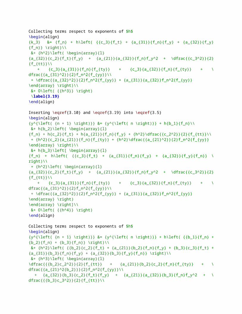
Collecting terms respect to exponents of $h$\begin{align}{k_3} &= {f_n} + h\left( {{c_3}{f_t} + {a_{31}}{f_n}{f_y} + {a_{32}}{f_y}{f_n}} \right)\\ &+ {h^2}\left( \begin{array}{l}{a_{32}}{c_2}{f_t}{f_y} + {a_{21}}{a_{32}}{f_n}f_y^2 + \dfrac{{c_3^2}}{2}{f_{tt}}\\ + {c_3}{a_{31}}{f_n}{f_{ty}} + {c_3}{a_{32}}{f_n}{f_{ty}} + \dfrac{{a_{31}^2}}{2}f_n^2{f_{yy}}\\ + \dfrac{{a_{32}^2}}{2}f_n^2{f_{yy}} + {a_{31}}{a_{32}}f_n^2{f_{yy}}\end{array} \right)\\ &+ O\left( {{h^3}} \right) \label{3.19}\end{align}

Inserting \eqref{3.10} and \eqref{3.19} into \eqref{3.5}\begin{align}{y^{\left( {n + 1} \right)}} &= {y^{\left( n \right)}} + h{b_1}{f_n}\\ &+ h{b_2}\left( \begin{array}{l}{f_n} + h{c_2}{f_t} + h{a_{21}}{f_n}{f_y} + {h^2}\dfrac{{c_2^2}}{2}{f_{tt}}\\ + {h^2}{c_2}{a_{21}}{f_n}{f_{ty}} + {h^2}\dfrac{{a_{21}^2}}{2}f_n^2{f_{yy}}\end{array} \right)\\ &+ h{b_3}\left[ \begin{array}{l}{f_n} + h\left( {{c_3}{f_t} + {a_{31}}{f_n}{f_y} + {a_{32}}{f_y}{f_n}} \right)\\ + {h^2}\left( \begin{array}{l}{a_{32}}{c_2}{f_t}{f_y} + {a_{21}}{a_{32}}{f_n}f_y^2 + \dfrac{{c_3^2}}{2}{f_{tt}}\\ + {c_3}{a_{31}}{f_n}{f_{ty}} + {c_3}{a_{32}}{f_n}{f_{ty}} + \dfrac{{a_{31}^2}}{2}f_n^2{f_{yy}}\\ + \dfrac{{a_{32}^2}}{2}f_n^2{f_{yy}} + {a_{31}}{a_{32}}f_n^2{f_{yy}}\end{array} \right)\end{array} \right]\\ &+ O\left( {{h^4}} \right)\end{align}

Collecting terms respect to exponents of $h$\begin{align}{y^{\left( {n + 1} \right)}} &= {y^{\left( n \right)}} + h\left( {{b_1}{f_n} + {b_2}{f_n} + {b_3}{f_n}} \right)\\ &+ {h^2}\left( {{b_2}{c_2}{f_t} + {a_{21}}{b_2}{f_n}{f_y} + {b_3}{c_3}{f_t} + {a_{31}}{b_3}{f_n}{f_y} + {a_{32}}{b_3}{f_y}{f_n}} \right)\\ &+ {h^3}\left( \begin{array}{l}\dfrac{{{b_2}c_2^2}}{2}{f_{tt}} + {a_{21}}{b_2}{c_2}{f_n}{f_{ty}} + \dfrac{{a_{21}^2{b_2}}}{2}f_n^2{f_{yy}}\\

+ {a_{32}}{b_3}{c_2}{f_t}{f_y} + {a_{21}}{a_{32}}{b_3}{f_n}f_y^2 + \dfrac{{{b_3}c_3^2}}{2}{f_{tt}}\\ + {a_{31}}{b_3}{c_3}{f_n}{f_{ty}} + {a_{32}}{b_3}{c_3}{f_n}{f_{ty}} + \dfrac{{a_{31}^2{b_3}}}{2}f_n^2{f_{yy}}\\ + \dfrac{{a_{32}^2{b_3}}}{2}f_n^2{f_{yy}} + {a_{31}}{a_{32}}{b_3}f_n^2{f_{yy}}\end{array} \right)\\ &+ O\left( {{h^4}} \right) \label{3.27}\end{align}\subsection{Taylor Series Expansion Formula}We need to compute $y_{ttt}$ for Taylor series expansion below.\begin{align}{y_{ttt}} &= \dfrac{d}{{dt}}\left( {{f_t} + f{f_y}} \right)\\ &= {\left( {{f_t} + f{f_y}} \right)_t} + f{\left( {{f_t} + f{f_y}} \right)_y}\\ &= {f_{tt}} + {f_t}{f_y} + f{f_{ty}} + f{f_{ty}} + ff_y^2 + {f^2}{f_{yy}}\\ &= {f_{tt}} + {f_t}{f_y} + 2f{f_{ty}} + ff_y^2 + {f^2}{f_{yy}}\end{align}

Now we write down the Taylor series expansion of $y$ in the neighborhood of $t_n$ with $O\left(h^4\right)$.\begin{align}{y^{\left( {n + 1} \right)}} &= {y^{\left( n \right)}} + h{y_t} + \dfrac{{{h^2}}}{2}{y_{tt}} + \dfrac{{{h^3}}}{6}{y_{ttt}} + O\left( {{h^4}} \right)\\ &= {y^{\left( n \right)}} + h{f_n} + \dfrac{{{h^2}}}{2}\left( {{f_t} + {f_n}{f_y}} \right)\\ &+ \dfrac{{{h^3}}}{6}\left( {{f_{tt}} + {f_t}{f_y} + 2{f_n}{f_{ty}} + {f_n}f_y^2 + f_n^2{f_{yy}}} \right) + O\left( {{h^4}} \right) \label{3.34}\end{align}\subsection{Derivation of System of Equations}Comparing \eqref{3.27} and \eqref{3.34}\begin{align}h{f_n}:1 &= {b_1} + {b_2} + {b_3}\\{h^2}{f_t}:\dfrac{1}{2} &= {b_2}{c_2} + {b_3}{c_3}\\{h^2}{f_n}{f_y}:\dfrac{1}{2} &= {a_{21}}{b_2} + {a_{31}}{b_3} + {a_{32}}{b_3}\\{h^3}{f_{tt}}:\dfrac{1}{6} &= \dfrac{{{b_2}c_2^2}}{2} + \dfrac{{{b_3}c_3^2}}{2}\\{h^3}{f_t}{f_y}:\dfrac{1}{6} &= {a_{32}}{b_3}{c_2}\\{h^3}{f_n}{f_{ty}}:\dfrac{1}{3} &= {a_{21}}{b_2}{c_2} + {a_{31}}{b_3}{c_3} + {a_{32}}{b_3}{c_3}\\{h^3}{f_n}f_y^2:\dfrac{1}{6} &= {a_{21}}{a_{32}}{b_3}\\{h^3}f_n^2{f_{yy}}:\dfrac{1}{6} &= \dfrac{{a_{21}^2{b_2}}}{2} + \dfrac{{a_{31}^2{b_3}}}{2} + \dfrac{{a_{32}^2{b_3}}}{2} + {a_{31}}{a_{32}}{b_3}\end{align}

Hence, we obtain the system of 8 equations with 8 unknowns.\begin{align}{b_1} + {b_2} + {b_3} &= 1\label{3.45}\\{b_2}{c_2} + {b_3}{c_3} &= \dfrac{1}{2}\\{b_2}{a_{21}} + {b_3}\left( {{a_{31}} + {a_{32}}} \right) &= \dfrac{1}{2}\\{b_2}c_2^2 + {b_3}c_3^2 &= \dfrac{1}{3}\\{b_3}{a_{32}}{c_2} &= \dfrac{1}{6}\label{3.49}\\

{b_2}{c_2}{a_{21}} + {b_3}{c_3}\left( {{a_{31}} + {a_{32}}} \right)& = \dfrac{1}{3}\\{b_3}{a_{32}}{a_{21}} &= \dfrac{1}{6}\label{3.51}\\{b_2}a_{21}^2 + {b_3}{\left( {{a_{31}} + {a_{32}}} \right)^2} &= \dfrac{1}{3}\label{3.52}\end{align}\subsection{Solutions of System of Equations}We now solve the above system of equations in two different ways.\\\\\textsc{Solution 1.} We take $b_2=\alpha,b_3=\beta$ as two free variables, then \begin{align}{b_1} = 1 - \alpha - \beta \end{align}our task remains to solve\begin{align}\alpha {c_2} + \beta {c_3} &= \dfrac{1}{2}\\\alpha {a_{21}} + \beta \left( {{a_{31}} + {a_{32}}} \right) &= \dfrac{1}{2}\\\alpha c_2^2 + \beta c_3^2 &= \dfrac{1}{3}\\\beta {a_{32}}{c_2}& = \dfrac{1}{6}\label{3.57}\\\alpha {c_2}{a_{21}} + \beta {c_3}\left( {{a_{31}} + {a_{32}}} \right) &= \dfrac{1}{3}\\\beta {a_{32}}{a_{21}} &= \dfrac{1}{6}\label{3.59}\\\alpha a_{21}^2 + \beta {\left( {{a_{31}} + {a_{32}}} \right)^2} &= \dfrac{1}{3}\end{align}We can solve $c_2$ and $c_3$ by using two equations\begin{align}\alpha {c_2} + \beta {c_3} &= \dfrac{1}{2}\label{3.61}\\\alpha c_2^2 + \beta c_3^2 &= \dfrac{1}{3}\label{3.62}\end{align}Since \eqref{3.59}, we must have $\beta \ne 0$.

Then we can take ${c_3} = \dfrac{1}{{2\beta }} - \dfrac{\alpha }{\beta }{c_2}$ from \eqref{3.61} and insert into \eqref{3.62} to obtain the following equation respect to $c_2$.\begin{align}\label{3.63}12\alpha \left( {\alpha + \beta } \right)c_2^2 - 12\alpha {c_2} + 3 - 4\beta = 0\end{align}Consider two following cases.\begin{enumerate}\item \textbf{Case $\alpha \left( {\alpha + \beta } \right)=0$.} Consider two subcases.\begin{enumerate}\item \textbf{Case $\alpha=0$.} Then we have immediately\begin{align}\beta &= \dfrac{3}{4}\\{c_3} &= \dfrac{2}{3}\\b_1=\dfrac{1}{4}\end{align}and the system of equations remains\begin{align}{a_{31}} + {a_{32}} &= \dfrac{2}{3}\\{a_{32}}{c_2} &= \dfrac{2}{9}\\\dfrac{3}{4}{a_{32}}{a_{21}} &= \dfrac{1}{6}

\end{align}To solve this remaining system of equations, we can take $a_{32}=\gamma \ne 0$ as a free variable. Then\begin{align}{a_{31}} &= \dfrac{2}{3} - \gamma \\{c_2} &= \dfrac{2}{{9\gamma }}\\{a_{21}} &=\dfrac{2}{{9\gamma }}\end{align}Hence, we obtain the solutions\begin{align}{b_1} &= \dfrac{1}{4}\\{b_2} &= 0\\{b_3} &= \dfrac{3}{4}\\{c_2} &= \dfrac{2}{{9\gamma }}\\{c_3} &= \dfrac{2}{3}\\{a_{21}} &= \dfrac{2}{{9\gamma }}\\{a_{31}} &= \dfrac{2}{3} - \gamma \\{a_{32}} &= \gamma \end{align}where $\gamma$ is an arbitrary nonzero real number, in this subcase.

Butcher tableau becomes\begin{align}\begin{array}{*{20}{c}}0&\vline& {}&{}&{}\\{\dfrac{2}{{9\gamma }}}&\vline& {\dfrac{2}{{9\gamma }}}&{}&{}\\{\dfrac{2}{3}}&\vline& {\dfrac{2}{3} - \gamma }&\gamma &{}\\\hline{}&\vline& {\dfrac{1}{4}}&0&{\dfrac{3}{4}}\end{array}\end{align}\item \textbf{Case $\alpha + \beta =0,\alpha \ne 0$.} Then we have immediately\begin{align}{b_1} &= 1\\{b_2} &= \alpha \\{b_3} &= - \alpha \\{c_2} &= \dfrac{1}{3} + \dfrac{1}{{4\alpha }}\end{align}and the system of equations remains\begin{align}{c_2} - {c_3} &= \dfrac{1}{{2\alpha }}\\{a_{21}} - \left( {{a_{31}} + {a_{32}}} \right) &= \dfrac{1}{{2\alpha }}\\c_2^2 - c_3^2 &= \dfrac{1}{{3\alpha }}\\{a_{32}}{c_2} &= - \dfrac{1}{{6\alpha }}\\{c_2}{a_{21}} - {c_3}\left( {{a_{31}} + {a_{32}}} \right) &= \dfrac{1}{{3\alpha }}\\{a_{32}}{a_{21}}& = - \dfrac{1}{{6\alpha }}\\a_{21}^2 - {\left( {{a_{31}} + {a_{32}}} \right)^2} &= \dfrac{1}{{3\alpha }}\end{align}We again have immediately\begin{align}{c_3} &= \dfrac{1}{3} - \dfrac{1}{{4\alpha }}\\{a_{32}} &= - \dfrac{2}{{4\alpha + 3}}\\{a_{21}} &= \dfrac{1}{3} + \dfrac{1}{{4\alpha }}\\{a_{31}} &= \dfrac{{16{\alpha ^2} + 24\alpha - 9}}{{12\alpha \left( {4\alpha + 3} \right)}}\end{align}

Hence, we obtain the solution\begin{align}{b_1} &= 1\\{b_2} &= \alpha \\{b_3} &= - \alpha \\{c_2}& = \dfrac{1}{3} + \dfrac{1}{{4\alpha }}\\{c_3} &= \dfrac{1}{3} - \dfrac{1}{{4\alpha }}\\{a_{21}} &= \dfrac{1}{3} + \dfrac{1}{{4\alpha }}\\{a_{31}} &= \dfrac{{16{\alpha ^2} + 24\alpha - 9}}{{12\alpha \left( {4\alpha + 3} \right)}}\\{a_{32}} &= - \dfrac{2}{{4\alpha + 3}}\end{align}where $\alpha$ is an arbitrary nonzero real number, in this subcase.

Butcher tableau becomes\begin{align}\begin{array}{*{20}{c}}0&\vline& {}&{}&{}\\{\dfrac{1}{3} + \dfrac{1}{{4\alpha }}}&\vline& {\dfrac{1}{3} + \dfrac{1}{{4\alpha }}}&{}&{}\\{\dfrac{1}{3} - \dfrac{1}{{4\alpha }}}&\vline& {\dfrac{{16{\alpha ^2} + 24\alpha - 9}}{{12\alpha \left( {4\alpha + 3} \right)}}}&{ - \dfrac{2}{{4\alpha + 3}}}&{}\\\hline{}&\vline& 1&\alpha &{ - \alpha }\end{array}\end{align}\end{enumerate}\item \textbf{Case $\alpha \left( {\alpha + \beta } \right)\ne 0$.} \eqref{3.63} is a quadratic equation respect to $c_2$.

Computing the determinant of \eqref{3.63}\begin{align}\Delta ' &= 36{\alpha ^2} + 12\alpha \left( {\alpha + \beta } \right)\left( {4\beta - 3} \right)\\ &= 12\alpha \beta \left( {4\alpha + 4\beta - 3} \right)\end{align}Hence, we have to make the assumption \begin{align}\alpha \beta \left( {4\alpha + 4\beta - 3} \right) \ge 0\end{align}so that \eqref{3.63} has roots in this case.

Under this assumption, \eqref{3.63} have two roots\begin{align}{c_2} = \dfrac{{3\alpha \pm \sqrt {3\alpha \beta \left( {4\alpha + 4\beta - 3} \right)} }}{{6\alpha \left( {\alpha + \beta } \right)}}\end{align}Consider two subcases respect to $c_2$.\begin{enumerate}\item \textbf{Case ${c_2} = \dfrac{{3\alpha + \sqrt {3\alpha \beta \left( {4\alpha + 4\beta - 3} \right)} }}{{6\alpha \left( {\alpha + \beta } \right)}}$.}We easily solve the remaining system of equations to get\begin{align}{b_1} &= 1 - \alpha - \beta \\{b_2} &= \alpha \\

{b_3} &= \beta \\{c_2} &= \dfrac{{3\alpha + \sqrt {3\alpha \beta \left( {4\alpha + 4\beta - 3} \right)} }}{{6\alpha \left( {\alpha + \beta } \right)}}\\{c_3} &= \dfrac{{3\beta - \sqrt {3\alpha \beta \left( {4\alpha + 4\beta - 3} \right)} }}{{6\beta \left( {\alpha + \beta } \right)}}\\{a_{21}} &= \dfrac{{3\alpha + \sqrt {3\alpha \beta \left( {4\alpha + 4\beta - 3} \right)} }}{{6\alpha \left( {\alpha + \beta } \right)}}\\{a_{31}} &= \dfrac{1}{{2\beta }} - \dfrac{{3\alpha + \sqrt {3\alpha \beta \left( {4\alpha + 4\beta - 3} \right)} }}{{6\beta \left( {\alpha + \beta } \right)}} \\&- \dfrac{{\alpha \left( {\alpha + \beta } \right)}}{{\beta \left( {3\alpha + \sqrt {3\alpha \beta \left( {4\alpha + 4\beta - 3} \right)} } \right)}}\\{a_{32}} &= \dfrac{{\alpha \left( {\alpha + \beta } \right)}}{{\beta \left( {3\alpha + \sqrt {3\alpha \beta \left( {4\alpha + 4\beta - 3} \right)} } \right)}}\end{align}Butcher tableau reads all obtained coefficients.\item \textbf{Case ${c_2} = \dfrac{{3\alpha - \sqrt {3\alpha \beta \left( {4\alpha + 4\beta - 3} \right)} }}{{6\alpha \left( {\alpha + \beta } \right)}}$.} We also easily solve the remaining system of equations to get\begin{align}{b_1} &= 1 - \alpha - \beta \\{b_2} &= \alpha \\{b_3} &= \beta \\{c_2} &= \dfrac{{3\alpha - \sqrt {3\alpha \beta \left( {4\alpha + 4\beta - 3} \right)} }}{{6\alpha \left( {\alpha + \beta } \right)}}\\{c_3} &= \dfrac{{3\beta + \sqrt {3\alpha \beta \left( {4\alpha + 4\beta - 3} \right)} }}{{6\beta \left( {\alpha + \beta } \right)}}\\{a_{21}} &= \dfrac{{3\alpha - \sqrt {3\alpha \beta \left( {4\alpha + 4\beta - 3} \right)} }}{{6\alpha \left( {\alpha + \beta } \right)}}\\{a_{31}} &= \dfrac{1}{{2\beta }} - \dfrac{{3\alpha - \sqrt {3\alpha \beta \left( {4\alpha + 4\beta - 3} \right)} }}{{6\beta \left( {\alpha + \beta } \right)}}\\ &- \dfrac{{\alpha \left( {\alpha + \beta } \right)}}{{\beta \left( {3\alpha - \sqrt {3\alpha \beta \left( {4\alpha + 4\beta - 3} \right)} } \right)}}\\{a_{32}} &= \dfrac{{\alpha \left( {\alpha + \beta } \right)}}{{\beta \left( {3\alpha - \sqrt {3\alpha \beta \left( {4\alpha + 4\beta - 3} \right)} } \right)}}\end{align}Butcher tableau reads all obtained coefficients.\end{enumerate}\end{enumerate}We have solved the system of equations \eqref{3.45}-\eqref{3.52} completely. \hfill $\square$\\\\\textbf{Remark 3.1.} In the first solution, we have used $b_2$ and $b_3$ as two free variables. This choice makes square roots appear in the solutions. This is quite easy to understand. Because of choice of $b_2,b_3$ as free variables, we have to solve a quadratic equation. This quadratic equation make square roots appear obviously.\\

Now, we solve our system of equation by alternative ways. The idea is very simple. It is just a matter of the first choice. More explicitly, instead of choosing $b_2,b_3$ as two free variables, we will choose $c_2,c_3$ as two free variables. Let us see the differences between two solutions through the following second one.\\

\\\textsc{Solution 2.} We take ${c_2} = \alpha ,{c_3} = \beta $ as two free variables and focus on the following two equations of our system of equations.\begin{align}{b_2}{c_2} + {b_3}{c_3} &= \frac{1}{2}\label{3.128}\\{b_2}c_2^2 + {b_3}c_3^3 &= \frac{1}{3}\label{3.129}\end{align}We consider two cases respect to $c_2$ and $c_3$.\begin{enumerate}\item \textbf{Case $c_2=c_3=\alpha$.} Due to \eqref{3.57}, we must have $\alpha \ne 0$. Then the above sub-system of equations becomes\begin{align}{b_2} + {b_3} &= \frac{1}{{2\alpha }}\\{b_2} + {b_3} &= \frac{1}{{3{\alpha ^2}}}\end{align}Hence\begin{align}c_2=c_3 =\alpha =\dfrac{2}{3}\end{align}The remaining system of equations is\begin{align}{b_1} + {b_2} + {b_3} &= 1\\{b_2} + {b_3} &= \frac{3}{4}\\{b_2}{a_{21}} + {b_3}\left( {{a_{31}} + {a_{32}}} \right) &= \frac{1}{2}\\{b_3}{a_{32}} &= \frac{1}{4}\\{b_3}{a_{32}}{a_{21}} &= \frac{1}{6}\\{b_2}a_{21}^2 + {b_3}{\left( {{a_{31}} + {a_{32}}} \right)^2} &= \frac{1}{3}\end{align}We obtain immediately\begin{align}{b_1} &= \frac{1}{4}\\{a_{21}} &= \frac{2}{3}\end{align}and the remaining system of equations is\begin{align}{b_2} + {b_3} &= \frac{3}{4}\label{3.141}\\\frac{2}{3}{b_2} + {b_3}\left( {{a_{31}} + {a_{32}}} \right) &= \frac{1}{2}\label{3.142}\\{b_3}{a_{32}} &= \frac{1}{4}\\\frac{4}{9}{b_2} + {b_3}{\left( {{a_{31}} + {a_{32}}} \right)^2} &= \frac{1}{3}\label{3.144}\end{align}We now choose $b_3=\gamma$ then\begin{align}{b_2} &= \frac{3}{4} - \gamma \\{a_{31}} &= \frac{2}{3} - \frac{1}{{4\gamma }}\\{a_{32}} &= \frac{1}{{4\gamma }}\end{align}Therefore,\begin{align}{c_2} &= \frac{2}{3}\\{c_3} &= \frac{2}{3}\\{b_1} &= \frac{1}{4}\\{b_2} &= \frac{3}{4} - \gamma \\{b_3} &= \gamma \\{a_{21}} &= \frac{2}{3}\\{a_{31}} &= \frac{2}{3} - \frac{1}{{4\gamma }}\\

{a_{32}} &= \frac{1}{{4\gamma }}\end{align}where $\gamma$ is an arbitrary nonzero real number, is the solution of \eqref{3.45}-\eqref{3.52} in this case.\item \textbf{Case $c_2 \ne c_3$.} Due to \eqref{3.49} and \eqref{3.51}, we have immediately\begin{align}a_{21}=c_2=\alpha\end{align}

Due to \eqref{3.128} and \eqref{3.129}, we obtain\begin{align}{b_2} &= \frac{{3\beta - 2}}{{6\alpha \left( {\beta - \alpha } \right)}}\\{b_3} &= \frac{{3\alpha - 2}}{{6\beta \left( {\alpha - \beta } \right)}}\end{align}Hence, \begin{align}{b_1} = \frac{{6\alpha \beta - 3\alpha - 3\beta + 2}}{{6\alpha \beta }}\end{align}The remaining system of equations is\begin{align}\frac{{3\beta - 2}}{{6\alpha \left( {\beta - \alpha } \right)}}\alpha + \frac{{3\alpha - 2}}{{6\beta \left( {\alpha - \beta } \right)}}\left( {{a_{31}} + {a_{32}}} \right) &= \frac{1}{2}\\\frac{{3\alpha - 2}}{{6\beta \left( {\alpha - \beta } \right)}}{a_{32}}\alpha &= \frac{1}{6}\\\frac{{3\beta - 2}}{{6\left( {\beta - \alpha } \right)}}\alpha + \frac{{3\alpha - 2}}{{6\left( {\alpha - \beta } \right)}}\left( {{a_{31}} + {a_{32}}} \right) &= \frac{1}{3}\\\frac{{3\beta - 2}}{{6\alpha \left( {\beta - \alpha } \right)}}{\alpha ^2} + \frac{{3\alpha - 2}}{{6\beta \left( {\alpha - \beta } \right)}}{\left( {{a_{31}} + {a_{32}}} \right)^2} &= \frac{1}{3}\end{align}We easily solve this and obtain\begin{align}{a_{21}} &= \alpha \\{a_{31}} &= \beta - \frac{{\beta \left( {\alpha - \beta } \right)}}{{\alpha \left( {3\alpha - 2} \right)}}\\{a_{32}} &= \frac{{\beta \left( {\alpha - \beta } \right)}}{{\alpha \left( {3\alpha - 2} \right)}}\end{align}Therefore, \begin{align}{c_2} &= \alpha \\{c_3} &= \beta \\{b_1} &= \frac{{6\alpha \beta - 3\alpha - 3\beta + 2}}{{6\alpha \beta }}\\{b_2} &= \frac{{3\beta - 2}}{{6\alpha \left( {\beta - \alpha } \right)}}\\{b_3} &= \frac{{3\alpha - 2}}{{6\beta \left( {\alpha - \beta } \right)}}\\{a_{21}} &= \alpha \\{a_{31}} &= \beta - \frac{{\beta \left( {\alpha - \beta } \right)}}{{\alpha \left( {3\alpha - 2} \right)}}\\{a_{32}} &= \frac{{\beta \left( {\alpha - \beta } \right)}}{{\alpha \left( {3\alpha - 2} \right)}}\end{align}where $\alpha \ne \beta,\alpha \ne \dfrac{2}{3}$ are two arbitrary nonzero real numbers, is the solution of \eqref{3.45}-\eqref{3.52} in this case.\end{enumerate}

We have solved \eqref{3.45}-\eqref{3.52} completely. \hfill $\square$\\\\\textbf{Remark 3.2.} In the second solution,$n$th roots do not appear in the solution because we does not need to solve any polynomial equations. Since this way is more easy and effective, it will be used for Runge Kutta method of higher orders.\subsection{Some Cases}We consider some cases of Runge Kutta order 3 method respect to some solutions of its associated system of equations.\\\\\textsc{Case $\alpha = \dfrac{2}{3},\beta = \dfrac{1}{6}$.}\\We use case \textbf{2.(b)} above to obtain\begin{align}\begin{array}{*{20}{c}}0&\vline& {}&{}&{}\\{\dfrac{1}{2}}&\vline& {\dfrac{1}{2}}&{}&{}\\1&\vline& { - 1}&2&{}\\\hline{}&\vline& {\dfrac{1}{6}}&{\dfrac{2}{3}}&{\dfrac{1}{6}}\end{array}\end{align}This Butcher tableau appears in \cite{3} - Kutta's third order method\index{Kutta's third order method} and in \cite{butcher}, p.82.\\\\\textsc{Case $\alpha = \dfrac{3}{8},\beta = \dfrac{3}{8}$.}\begin{align}\begin{array}{*{20}{c}}0&\vline& {}&{}&{}\\{\dfrac{2}{3}}&\vline& {\dfrac{2}{3}}&{}&{}\\{\dfrac{2}{3}}&\vline& 0&{\dfrac{2}{3}}&{}\\\hline{}&\vline& {\dfrac{1}{4}}&{\dfrac{3}{8}}&{\dfrac{3}{8}}\end{array}\end{align}This Butcher tableau appears in \cite{butcher}, p.82.\\\\\textsc{Case $\alpha = \dfrac{3}{4},\beta = \dfrac{1}{4}$.}

\begin{align}\begin{array}{*{20}{c}}0&\vline& {}&{}&{}\\{\dfrac{2}{3}}&\vline& {\dfrac{2}{3}}&{}&{}\\0&\vline& { - 1}&1&{}\\\hline{}&\vline& 0&{\dfrac{3}{4}}&{\dfrac{1}{4}}\end{array}\end{align}This Butcher tableau appears in \cite{butcher}, p.82.\\

\section{\textsc{Matlab} Implementation}See section 4.2 for general code.

\chapter{Runge Kutta Order 4 Method}\section{Derivation of Runge Kutta Order 4 Method}\subsection{Runge Kutta Order 4 Formula}For $s=4$, \eqref{1.9} becomes\index{Runge Kutta order 4 method}

\begin{align}{k_1} &= {f_n}\\{k_2} &= f\left( {{t_n} + {c_2}h,{y_n} + h{a_{21}}{f_n}} \right)\\{k_3} &= f\left( {{t_n} + {c_3}h,{y_n} + h{a_{31}}{f_n} + h{a_{32}}{k_2}} \right)\\{k_4} &= f\left( {{t_n} + {c_4}h,{y_n} + h{a_{41}}{f_n} + h{a_{42}}{k_2} + h{a_{43}}{k_3}} \right)\end{align}

and \eqref{1.8} becomes\begin{align}\label{4.5}{y^{\left( {n + 1} \right)}} = {y^{\left( n \right)}} + h{b_1}{k_1} + h{b_2}{k_2} + h{b_3}{k_3} + h{b_4}{k_4} \end{align}

Now we write down the Taylor series expansion $O\left(h^4\right)$ for $k_2$.\begin{align}{k_2} &= f\left( {{t_n} + {c_2}h,{y_n} + h{a_{21}}{f_n}} \right)\\ &= {f_n} + h{c_2}{f_t} + h{a_{21}}{f_n}{f_y} + {h^2}\dfrac{{c_2^2}}{2}{f_{tt}} + {h^2}{a_{21}}{c_2}{f_n}{f_{ty}} + {h^2}\dfrac{{a_{21}^2}}{2}f_n^2\\ &+ {h^3}\dfrac{{c_2^3}}{6}{f_{ttt}} + {h^3}\dfrac{{{a_{21}}c_2^2}}{2}{f_n}{f_{tty}} + {h^3}\dfrac{{a_{21}^2{c_2}}}{2}f_n^2{f_{tyy}} + {h^3}\dfrac{{a_{21}^3}}{6}f_n^3{f_{yyy}} + O\left( {{h^4}} \right)\\ &= {f_n} + h\left( {{c_2}{f_t} + {a_{21}}{f_n}{f_y}} \right) + {h^2}\left( {\dfrac{{c_2^2}}{2}{f_{tt}} + {a_{21}}{c_2}{f_n}{f_{ty}} + \dfrac{{a_{21}^2}}{2}f_n^2} \right)\\ &+ {h^3}\left( {\dfrac{{c_2^3}}{6}{f_{ttt}} + \dfrac{{{a_{21}}c_2^2}}{2}{f_n}{f_{tty}} + \dfrac{{a_{21}^2{c_2}}}{2}f_n^2{f_{tyy}} + \dfrac{{a_{21}^3}}{6}f_n^3{f_{yyy}}} \right) + O\left( {{h^4}} \right) \label{4.10}\end{align}

We write down the Taylor series expansion $O\left(h^4\right)$ for $k_3$.\begin{align}{k_3} &= f\left( {{t_n} + {c_3}h,{y_n} + h{a_{31}}{f_n} + h{a_{32}}{k_2}} \right)\\ &= {f_n} + h{c_3}{f_t} + h\left( {{a_{31}}{f_n} + {a_{32}}{k_2}} \right){f_y}\\ &+ {h^2}\dfrac{{c_3^2}}{2}{f_{tt}} + {h^2}{c_3}\left( {{a_{31}}{f_n} + {a_{32}}{k_2}} \right){f_{ty}} + \dfrac{1}{2}{h^2}{\left( {{a_{31}}{f_n} + {a_{32}}{k_2}} \right)^2}{f_{yy}}\\ &+ \dfrac{{c_3^3{h^3}}}{6}{f_{ttt}} + \dfrac{{{h^3}c_3^2}}{2}\left( {{a_{31}}{f_n} + {a_{32}}{k_2}} \right){f_{tty}} + \dfrac{{{h^3}{c_3}}}{2}{\left( {{a_{31}}{f_n} + {a_{32}}{k_2}} \right)^2}{f_{tyy}}\\ &+ \dfrac{{{h^3}}}{6}{\left( {{a_{31}}{f_n} + {a_{32}}{k_2}} \right)^3}{f_{yyy}} + O\left( {{h^4}} \right) \label{4.15}\end{align}

Inserting \eqref{4.10} into \eqref{4.15}\begin{align}{k_3} &= {f_n} + h{c_3}{f_t} + h{a_{31}}{f_n}{f_y}\\ &+ h{a_{32}}{f_y}\left[ {{f_n} + h\left( {{c_2}{f_t} + {a_{21}}{f_n}{f_y}} \right) + {h^2}\left( {\dfrac{{c_2^2}}{2}{f_{tt}} + {a_{21}}{c_2}{f_n}{f_{ty}} + \dfrac{{a_{21}^2}}{2}f_n^2} \right)} \right]\\

&+ \dfrac{{{h^2}c_3^2}}{2}{f_{tt}} + {h^2}{c_3}{a_{31}}{f_n}{f_{ty}} + {h^2}{c_3}{a_{32}}{f_{ty}}\left[ {{f_n} + h\left( {{c_2}{f_t} + {a_{21}}{f_n}{f_y}} \right)} \right]\\ &+ \dfrac{{{h^2}}}{2}a_{31}^2f_n^2{f_{yy}} + \dfrac{{{h^2}}}{2}2{a_{31}}{a_{32}}{f_n}{f_{yy}}\left[ {{f_n} + h\left( {{c_2}{f_t} + {a_{21}}{f_n}{f_y}} \right)} \right]\\ &+ \dfrac{{{h^2}}}{2}a_{32}^2{f_{yy}}{\left[ {{f_n} + h\left( {{c_2}{f_t} + {a_{21}}{f_n}{f_y}} \right)} \right]^2}\\ &+ \dfrac{{c_3^3{h^3}}}{6}{f_{ttt}} + \dfrac{{{h^3}c_3^2}}{2}\left( {{a_{31}}{f_n} + {a_{32}}{f_n}} \right){f_{tty}}\\ &+ \dfrac{{{h^3}{c_3}}}{2}\left( {a_{31}^2f_n^2 + 2{a_{31}}{a_{32}}f_n^2 + a_{32}^2f_n^2} \right){f_{tyy}}\\ &+ \dfrac{{{h^3}}}{6}\left( {a_{31}^3f_n^3 + 3a_{31}^2{a_{32}}f_n^3 + 3{a_{31}}a_{32}^2f_n^3 + a_{32}^3f_n^3} \right){f_{yyy}} + O\left( {{h^4}} \right)\end{align}

Collecting terms respect to exponents of $h$\begin{align}{k_3} &= {f_n} + h\left( {{c_3}{f_t} + {a_{31}}{f_n}{f_y} + {a_{32}}{f_n}{f_y}} \right)\\ &+ {h^2}\left( \begin{array}{l}{a_{32}}{c_2}{f_t}{f_y} + {a_{21}}{a_{32}}{f_n}f_y^2 + \dfrac{{c_3^2}}{2}{f_{tt}} + {a_{31}}{c_3}{f_n}{f_{ty}}\\ + {c_3}{a_{32}}{f_n}{f_{ty}} + \dfrac{{a_{31}^2}}{2}f_n^2{f_{yy}} + {a_{31}}{a_{32}}f_n^2{f_{yy}} + \dfrac{{a_{32}^2}}{2}f_n^2{f_{yy}}\end{array} \right)\\ &+ {h^3}\left( \begin{array}{l}\dfrac{{{a_{32}}c_2^2}}{2}{f_y}{f_{tt}} + {a_{32}}{a_{21}}{c_2}{f_n}{f_y}{f_{ty}} + \dfrac{{a_{21}^2{a_{32}}}}{2}f_n^2{f_y}\\ + {a_{32}}{c_2}{c_3}{f_t}{f_{ty}} + {a_{21}}{a_{32}}{c_3}{f_n}{f_y}{f_{ty}} + {a_{31}}{a_{32}}{c_2}{f_n}{f_t}{f_{yy}}\\ + {a_{21}}{a_{31}}{a_{32}}f_n^2{f_y}{f_{yy}} + a_{32}^2{c_2}{f_n}f{f_{yy}}_t + {a_{21}}a_{32}^2f_n^2{f_y}{f_{yy}}\\ + \dfrac{{c_3^3}}{6}{f_{ttt}} + \dfrac{{{a_{31}}c_3^2}}{2}{f_n}{f_{tty}} + \dfrac{{{a_{32}}c_3^2}}{2}{f_n}{f_{tty}} + \dfrac{{a_{31}^2{c_3}}}{2}f_n^2{f_{tyy}}\\ + {a_{31}}{a_{32}}{c_3}f_n^2{f_{tyy}} + \dfrac{{a_{32}^2{c_3}}}{2}f_n^2{f_{tyy}} + \dfrac{{a_{31}^3}}{6}f_n^3{f_{yyy}}\\ + \dfrac{{a_{31}^2{a_{32}}}}{2}f_n^3{f_{yyy}} + \dfrac{{{a_{31}}a_{32}^2}}{2}f_n^3{f_{yyy}} + \dfrac{{a_{32}^3}}{6}f_n^3{f_{yyy}}\end{array} \right)\\ &+ O\left( {{h^4}} \right) \label{4.27}\end{align}

We continue to write down the Taylor series expansion $O\left(h^4\right)$ for $k_4$.\begin{align}{k_4} &= f\left( {{t_n} + {c_4}h,{y_n} + h{a_{41}}{f_n} + h{a_{42}}{k_2} + h{a_{43}}{k_3}} \right)\\ &= {f_n} + {c_4}h{f_t} + h\left( {{a_{41}}{f_n} + {a_{42}}{k_2} + {a_{43}}{k_3}} \right){f_y}\\ &+ \dfrac{{c_4^2{h^2}}}{2}{f_{tt}} + {c_4}{h^2}\left( {{a_{41}}{f_n} + {a_{42}}{k_2} + {a_{43}}{k_3}} \right){f_{ty}}\\ &+ \dfrac{1}{2}{h^2}{\left( {{a_{41}}{f_n} + {a_{42}}{k_2} + {a_{43}}{k_3}} \right)^2}{f_{yy}} + \dfrac{{c_4^3{h^3}}}{6}{f_{ttt}}\\

&+ \dfrac{{c_4^2}}{2}{h^3}\left( {{a_{41}}{f_n} + {a_{42}}{k_2} + {a_{43}}{k_3}} \right){f_{tty}}\\ &+ \dfrac{{{c_4}{h^3}}}{2}{\left( {{a_{41}}{f_n} + {a_{42}}{k_2} + {a_{43}}{k_3}} \right)^2}{f_{tyy}}\\ &+ \dfrac{1}{6}{h^2}{\left( {{a_{41}}{f_n} + {a_{42}}{k_2} + {a_{43}}{k_3}} \right)^3}{f_{yyy}} + O\left( {{h^4}} \right) \label{4.34}\end{align}

Inserting \eqref{4.15} and \eqref{4.27} to \eqref{4.34}\begin{align}{k_4} &= {f_n} + h{c_4}{f_t} + h{a_{41}}{f_n}{f_y}\\ & + h{a_{42}}{f_y}\left[ \begin{array}{l}{f_n} + h\left( {{c_2}{f_t} + {a_{21}}{f_n}{f_y}} \right)\\ + {h^2}\left( {\dfrac{{c_2^2}}{2}{f_{tt}} + {a_{21}}{c_2}{f_n}{f_{ty}} + \dfrac{{a_{21}^2}}{2}f_n^2} \right)\end{array} \right]\\ &+ h{a_{43}}{f_y}\left[ \begin{array}{l}{f_n} + h\left( {{c_3}{f_t} + {a_{31}}{f_n}{f_y} + {a_{32}}{f_n}{f_y}} \right)\\ + {h^2}\left( \begin{array}{l}{a_{32}}{c_2}{f_t}{f_y} + {a_{21}}{a_{32}}{f_n}f_y^2 + \dfrac{{c_3^2}}{2}{f_{tt}} \\+ {a_{31}}{c_3}{f_n}{f_{ty}} + {c_3}{a_{32}}{f_n}{f_{ty}} + \dfrac{{a_{31}^2}}{2}f_n^2{f_{yy}}\\ + {a_{31}}{a_{32}}f_n^2{f_{yy}} + \dfrac{{a_{32}^2}}{2}f_n^2{f_{yy}}\end{array} \right)\end{array} \right]\\ &+ {h^2}\dfrac{{c_4^2}}{2}{f_{tt}} + {h^2}{a_{41}}{c_4}{f_n}{f_{ty}} + {h^2}{a_{42}}{c_4}{f_{ty}}\left[ {{f_n} + h\left( {{c_2}{f_t} + {a_{21}}{f_n}{f_y}} \right)} \right]\\ &+ {h^2}{a_{43}}{c_4}{f_{ty}}\left[ {{f_n} + h\left( {{c_3}{f_t} + {a_{31}}{f_n}{f_y} + {a_{32}}{f_n}{f_y}} \right)} \right] \\ &+ {h^2}\dfrac{{a_{41}^2}}{2}f_n^2{f_{yy}} + {h^2}\dfrac{{a_{42}^2}}{2}{f_{yy}}{\left[ {{f_n} + h\left( {{c_2}{f_t} + {a_{21}}{f_n}{f_y}} \right)} \right]^2}\\ &+ {h^2}\dfrac{{a_{43}^2}}{2}{f_{yy}}{\left[ {{f_n} + h\left( {{c_3}{f_t} + {a_{31}}{f_n}{f_y} + {a_{32}}{f_n}{f_y}} \right)} \right]^2}\\&+ {h^2}{a_{41}}{a_{42}}{f_n}{f_{yy}}\left[ {{f_n} + h\left( {{c_2}{f_t} + {a_{21}}{f_n}{f_y}} \right)} \right]\\ &+ {h^2}{a_{42}}{a_{43}}{f_{yy}}\left[ {{f_n} + h\left( {{c_2}{f_t} + {a_{21}}{f_n}{f_y}} \right)} \right] \times \\& \times \left[ {{f_n} + h\left( {{c_3}{f_t} + {a_{31}}{f_n}{f_y} + {a_{32}}{f_n}{f_y}} \right)} \right]\\ &+ {h^2}{a_{41}}{a_{43}}{f_n}{f_{yy}}\left[ {{f_n} + h\left( {{c_3}{f_t} + {a_{31}}{f_n}{f_y} + {a_{32}}{f_n}{f_y}} \right)} \right]\\ &+ {h^3}\dfrac{{c_4^3}}{6}{f_{ttt}} + {h^3}\dfrac{{c_4^2}}{2}\left( {{a_{41}}{f_n} + {a_{42}}{f_n} + {a_{43}}{f_n}} \right){f_{tty}}\\ & + {h^3}\dfrac{{{c_4}}}{2}\left( \begin{array}{l}a_{41}^2f_n^2 + a_{42}^2f_n^2 + a_{43}^2f_n^2 + 2{a_{41}}{a_{42}}f_n^2\\ + 2{a_{42}}{a_{43}}f_n^2 + 2{a_{41}}{a_{43}}f_n^2\end{array} \right){f_{tyy}} \\&+ {h^3}\left( {\begin{array}{*{20}{l}}{\dfrac{{a_{41}^3}}{6}f_n^3 + \dfrac{{a_{42}^3}}{6}f_n^3 + \dfrac{{a_{43}^3}}{6}f_n^3 + \dfrac{{a_{41}^2{a_{42}}}}{2}f_n^3}\\{ + \dfrac{{a_{41}^2{a_{43}}}}{2}f_n^3 + \dfrac{{a_{42}^2{a_{41}}}}{2}f_n^3+ \dfrac{{a_{42}^2{a_{43}}}}{2}f_n^3 + \dfrac{{a_{43}^2{a_{41}}}}{2}f_n^3 } \\

{+ \dfrac{{a_{43}^2{a_{42}}}}{2}f_n^3 + {a_{41}}{a_{42}}{a_{43}}f_n^3}\end{array}} \right){f_{yyy}}\\ &+ O\left( {{h^4}} \right)\end{align}

Collecting terms respect to exponents of $h$\begin{align}{k_4} &= {f_n} + h\left( {{c_4}{f_t} + {a_{41}}{f_n}{f_y} + {a_{42}}{f_n}{f_y} + {a_{43}}{f_n}{f_y}} \right)\\ &+ {h^2}\left( {\begin{array}{*{20}{l}}\begin{array}{l}{a_{42}}{c_2}{f_t}{f_y} + {a_{21}}{a_{42}}{f_n}f_y^2 + {a_{43}}{c_3}{f_t}{f_y} + {a_{31}}{a_{43}}{f_n}f_y^2\\ + {a_{32}}{a_{43}}{f_n}f_y^2 + \dfrac{{c_4^2}}{2}{f_{tt}} + {c_4}{a_{41}}{f_n}{f_{ty}} + {c_4}{a_{42}}{f_n}{f_{ty}}\end{array}\\{ + {c_4}{a_{43}}{f_n}{f_{ty}} + \dfrac{{a_{41}^2}}{2}f_n^2{f_{yy}} + \dfrac{{a_{42}^2}}{2}f_n^2{f_{yy}} + \dfrac{{a_{43}^2}}{2}f_n^2{f_{yy}}}\\{ + {a_{41}}{a_{42}}f_n^2{f_{yy}} + {a_{42}}{a_{43}}f_n^2{f_{yy}} + {a_{41}}{a_{43}}f_n^2{f_{yy}}}\end{array}} \right)\\ &+ {h^3}\left( {\begin{array}{*{20}{l}}\begin{array}{l}\dfrac{{{a_{42}}c_2^2}}{2}{f_y}{f_{tt}} + {a_{21}}{a_{42}}{c_2}{f_n}{f_y}{f_{ty}} + \dfrac{{{a_{42}}a_{21}^2}}{2}f_n^2{f_y}{f_{yy}}\\ + {a_{43}}{a_{32}}{c_2}{f_t}f_y^2 + {a_{21}}{a_{32}}{a_{43}}{f_n}f_y^3 + \dfrac{{{a_{43}}c_3^2}}{2}{f_y}{f_{tt}}\end{array}\\\begin{array}{l} + {a_{31}}{a_{43}}{c_3}{f_n}{f_y}{f_{ty}} + {a_{32}}{a_{43}}{c_3}{f_n}{f_y}{f_{ty}} + \dfrac{{a_{31}^2{a_{43}}}}{2}f_n^2{f_y}{f_{yy}}\\ + {a_{31}}{a_{32}}{a_{43}}f_n^2{f_y}{f_{yy}} + \dfrac{{a_{32}^2{a_{43}}}}{2}f_n^2{f_y}{f_{yy}} + {a_{42}}{c_2}{c_4}{f_t}{f_{ty}}\end{array}\\{ + {a_{21}}{a_{42}}{c_4}{f_n}{f_y}{f_{ty}} + {a_{43}}{c_3}{c_4}{f_t}{f_{ty}} + {a_{31}}{a_{43}}{c_4}{f_n}{f_y}{f_{ty}}}\\\begin{array}{l} + {a_{32}}{a_{43}}{c_4}{f_n}{f_y}{f_{ty}} + a_{42}^2{c_2}{f_n}{f_t}{f_{yy}} + {a_{21}}a_{42}^2f_n^2{f_y}{f_{yy}}\\ + a_{43}^2{c_3}{f_n}{f_t}{f_{yy}} + {a_{31}}a_{43}^2f_n^2{f_y}{f_{yy}} + {a_{32}}a_{43}^2f_n^2{f_y}{f_{yy}}\\ + {a_{41}}{a_{42}}{c_2}{f_n}{f_t}{f_{yy}} + {a_{21}}{a_{41}}{a_{42}}f_n^2{f_y}{f_{yy}} + {a_{42}}{a_{43}}{c_3}{f_n}{f_t}{f_{yy}}\\ + {a_{31}}{a_{42}}{a_{43}}f_n^2{f_y}{f_{yy}} + {a_{32}}{a_{42}}{a_{43}}f_n^2{f_y}{f_{yy}} + {a_{42}}{a_{43}}{c_2}{f_n}{f_t}{f_{yy}}\\ + {a_{21}}{a_{42}}{a_{43}}f_n^2{f_y}{f_{yy}} + {a_{41}}{a_{43}}{c_3}{f_n}{f_t}{f_{yy}} + {a_{31}}{a_{41}}{a_{43}}f_n^2{f_y}{f_{yy}}\\ + {a_{32}}{a_{41}}{a_{43}}f_n^2{f_y}{f_{yy}} + \dfrac{{c_4^3}}{6}{f_{ttt}} + \dfrac{{{a_{41}}c_4^2}}{2}{f_n}{f_{tty}} + \dfrac{{{a_{42}}c_4^2}}{2}{f_n}{f_{tty}}\\ + \dfrac{{{a_{43}}c_4^2}}{2}{f_n}{f_{tty}} + \dfrac{{a_{41}^2{c_4}}}{2}f_n^2{f_{tyy}} + \dfrac{{a_{42}^2{c_4}}}{2}f_n^2{f_{tyy}}\\ + \dfrac{{a_{43}^2{c_4}}}{2}f_n^2{f_{tyy}} + {a_{41}}{a_{42}}{c_4}f_n^2{f_{tyy}} + {a_{42}}{a_{43}}{c_4}f_n^2{f_{tyy}}\\ + {a_{41}}{a_{43}}{c_4}f_n^2{f_{tyy}} + \dfrac{{a_{41}^3}}{6}f_n^3{f_{yyy}} + \dfrac{{a_{42}^3}}{6}f_n^3{f_{yyy}}\\

+ \dfrac{{a_{43}^3}}{6}f_n^3{f_{yyy}} + \dfrac{{a_{41}^2{a_{42}}}}{2}f_n^3{f_{yyy}} + \dfrac{{a_{41}^2{a_{43}}}}{2}f_n^3{f_{yyy}}\\ + \dfrac{{{a_{41}}a_{42}^2}}{2}f_n^3{f_{yyy}} + \dfrac{{a_{42}^2{a_{43}}}}{2}f_n^3{f_{yyy}} + \dfrac{{{a_{41}}a_{43}^2}}{2}f_n^3{f_{yyy}}\\ + \dfrac{{{a_{42}}a_{43}^2}}{2}f_n^3{f_{yyy}} + {a_{41}}{a_{42}}{a_{43}}f_n^3{f_{yyy}}\end{array}\end{array}} \right)\\ &+ O\left( {{h^4}} \right) \label{4.53}\end{align}

Inserting \eqref{4.10}, \eqref{4.27} and \eqref{4.53} into \eqref{4.5}\begin{align}&{y^{\left( {n + 1} \right)}}\\ &= {y^{\left( n \right)}} + h\left( {{b_1}{f_n} + {b_2}{f_n} + {b_3}{f_n} + {b_4}{f_n}} \right)\\ &+ {h^2}\left( {\begin{array}{*{20}{l}}{{b_2}{c_2}{f_t} + {a_{21}}{b_2}{f_n}{f_y} + {b_3}{c_3}{f_t} + {a_{31}}{b_3}{f_n}{f_y} + {a_{32}}{b_3}{f_n}{f_y}}\\{ + {b_4}{c_4}{f_t} + {a_{41}}{b_4}{f_n}{f_y} + {a_{42}}{b_4}{f_n}{f_y} + {a_{43}}{b_4}{f_n}{f_y}}\end{array}} \right)\\& + {h^3}\left( {\begin{array}{*{20}{l}}\begin{array}{l}\dfrac{{{b_2}c_2^2}}{2}{f_{tt}} + {b_2}{c_2}{a_{21}}{f_n}{f_{ty}} + \dfrac{{a_{21}^2{b_2}}}{2}f_n^2{f_{yy}} + {a_{32}}{b_3}{c_2}{f_t}{f_y}\\ + {a_{32}}{b_3}{a_{21}}{f_n}{f_y}{f_y} + \dfrac{{{b_3}c_3^2}}{2}{f_{tt}} + {c_3}{b_3}{a_{31}}{f_n}{f_{ty}} + {c_3}{b_3}{a_{32}}{f_n}{f_{ty}}\end{array}\\{ + \dfrac{{a_{31}^2{b_3}}}{2}f_n^2{f_{yy}} + {a_{31}}{a_{32}}{b_3}{f_n}{f_n}{f_{yy}} + \dfrac{{a_{32}^2{b_3}}}{2}f_n^2{f_{yy}} + {a_{42}}{b_4}{c_2}{f_t}{f_y}}\\\begin{array}{l} + {a_{42}}{b_4}{f_y}{a_{21}}{f_n}{f_y} + {a_{43}}{b_4}{c_3}{f_t}{f_y} + {a_{43}}{a_{31}}{b_4}{f_n}f_y^2 + + {a_{43}}{a_{32}}{b_4}{f_n}f_y^2\\ + \dfrac{{{b_4}c_4^2}}{2}{f_{tt}} + {c_4}{b_4}{a_{41}}{f_n}{f_{ty}} + {c_4}{b_4}{a_{42}}{f_{ty}}{f_n} + {c_4}{b_4}{a_{43}}{f_{ty}}{f_n}\\ + \dfrac{{a_{41}^2{b_4}}}{2}f_n^2{f_{yy}} + \dfrac{{a_{42}^2{b_4}}}{2}f_n^2{f_{yy}} + \dfrac{{a_{43}^2{b_4}}}{2}f_n^2{f_{yy}} + {a_{41}}{a_{42}}{b_4}{f_{yy}}f_n^2\\ + {a_{42}}{a_{43}}{b_4}{f_{yy}}f_n^2 + {a_{41}}{a_{43}}{b_4}{f_{yy}}f_n^2\end{array}\end{array}} \right)\\ &+ {h^4}\left( {\begin{array}{*{20}{l}}\begin{array}{l}\dfrac{{{b_2}c_2^3}}{6}{f_{ttt}} + \dfrac{{{b_2}c_2^2{a_{21}}}}{2}{f_n}{f_{tty}} + \dfrac{{{b_2}{c_2}a_{21}^2}}{2}f_n^2{f_{tyy}} + \dfrac{{a_{21}^3{b_2}}}{6}f_n^3{f_{yyy}}\\ + \dfrac{{{a_{32}}{b_3}c_2^2}}{2}{f_{tt}}{f_y} + {a_{32}}{b_3}{c_2}{a_{21}}{f_n}{f_{ty}}{f_y} + \dfrac{{{a_{32}}a_{21}^2{b_3}}}{2}f_n^2{f_{yy}}{f_y}\end{array}\\{ + {c_3}{a_{32}}{b_3}{c_2}{f_t}{f_{ty}} + {c_3}{a_{32}}{b_3}{a_{21}}{f_n}{f_y}{f_{ty}} + {a_{31}}{a_{32}}{b_3}{c_2}{f_n}{f_t}{f_{yy}}}\\{ + {a_{31}}{a_{32}}{a_{21}}{b_3}{f_n}{f_n}{f_y}{f_{yy}} + a_{32}^2{b_3}{f_n}{c_2}{f_t}{f_{yy}} + a_{32}^2{b_3}{f_n}{a_{21}}{f_n}{f_y}{f_{yy}}}\\\begin{array}{l}

+ \dfrac{{{b_3}c_3^3}}{6}{f_{ttt}} + \dfrac{{{b_3}c_3^2\left( {{a_{31}} + {a_{32}}} \right)}}{2}{f_n}{f_{tty}} + \dfrac{{{b_3}{c_3}a_{31}^2}}{2}f_n^2{f_{tyy}}\\+ {b_3}{c_3}{a_{31}}{a_{32}}{f_n}{f_n}{f_{tyy}} + \dfrac{{{b_3}{c_3}a_{32}^2}}{2}f_n^2{f_{tyy}} + \dfrac{{{b_3}a_{31}^3}}{6}f_n^3{f_{yyy}}\\ + \dfrac{{{b_3}a_{31}^2{a_{32}}}}{2}f_n^3{f_{yyy}} + \dfrac{{{b_3}{a_{31}}a_{32}^2}}{2}f_n^3{f_{yyy}} + \dfrac{{{b_3}a_{32}^3}}{6}f_n^3{f_{yyy}}\\ + \dfrac{{{a_{42}}{b_4}c_2^2}}{2}{f_y}{f_{tt}} + {a_{42}}{b_4}{c_2}{a_{21}}{f_n}{f_y}{f_{ty}} + \dfrac{{{a_{42}}a_{21}^2{b_4}}}{2}f_n^2{f_y}{f_{yy}}\\ + {a_{43}}{a_{32}}{b_4}{c_2}{f_t}f_y^2 + {a_{43}}{a_{32}}{a_{21}}{b_4}{f_n}f_y^3 + \dfrac{{{a_{43}}{b_4}c_3^2}}{2}{f_y}{f_{tt}}\\ + {a_{43}}{b_4}{c_3}{a_{31}}{f_n}{f_y}{f_{ty}} + {a_{43}}{b_4}{c_3}{a_{32}}{f_n}{f_y}{f_{ty}} + \dfrac{{{a_{43}}a_{31}^2{b_4}}}{2}f_n^2{f_y}{f_{yy}}\\ + {a_{43}}{a_{31}}{a_{32}}{b_4}f_n^2{f_y}{f_{yy}} + \dfrac{{{a_{43}}a_{32}^2{b_4}}}{2}f_n^2{f_y}{f_{yy}} + {c_4}{a_{42}}{b_4}{c_2}{f_t}{f_{ty}}\\ + {c_4}{a_{42}}{a_{21}}{b_4}{f_n}{f_y}{f_{ty}} + {c_4}{a_{43}}{c_3}{b_4}{f_t}{f_{ty}} + {c_4}{a_{43}}{a_{31}}{b_4}{f_n}{f_y}{f_{ty}}\\ + {c_4}{a_{43}}{a_{32}}{b_4}{f_n}{f_y}{f_{ty}} + a_{42}^2{b_4}{c_2}{f_n}{f_t}{f_{yy}} + a_{42}^2{a_{21}}{b_4}f_n^2{f_y}{f_{yy}}\\ + a_{43}^2{b_4}{c_3}{f_n}{f_t}{f_{yy}} + a_{43}^2{a_{31}}{b_4}f_n^2{f_y}{f_{yy}} + a_{43}^2{a_{32}}{b_4}f_n^2{f_y}{f_{yy}}\\ + {a_{41}}{a_{42}}{b_4}{c_2}{f_n}{f_t}{f_{yy}} + {a_{41}}{a_{21}}{a_{42}}{b_4}f_n^2{f_y}{f_{yy}} + {a_{42}}{a_{43}}{b_4}{c_3}{f_n}{f_t}{f_{yy}}\\ + {a_{42}}{a_{43}}{a_{31}}{b_4}f_n^2{f_y}{f_{yy}} + {a_{42}}{a_{43}}{a_{32}}{b_4}f_n^2{f_y}{f_{yy}} + {a_{42}}{a_{43}}{b_4}{c_2}{f_n}{f_t}{f_{yy}}\\ + {a_{42}}{a_{43}}{a_{21}}{b_4}f_n^2{f_y}{f_{yy}} + {a_{41}}{a_{43}}{b_4}{c_3}{f_n}{f_t}{f_{yy}} + {a_{41}}{a_{43}}{a_{31}}{b_4}f_n^2{f_y}{f_{yy}}\\ + {a_{41}}{a_{43}}{a_{32}}{b_4}f_n^2{f_y}{f_{yy}} + \dfrac{{{b_4}c_4^3}}{6}{f_{ttt}} + \dfrac{{{b_4}c_4^2{a_{41}}}}{2}{f_n}{f_{tty}} + \dfrac{{{b_4}c_4^2{a_{42}}}}{2}{f_n}{f_{tty}}\\ + \dfrac{{{b_4}c_4^2{a_{43}}}}{2}{f_n}{f_{tty}} + \dfrac{{{c_4}{b_4}a_{41}^2}}{2}f_n^2{f_{tyy}} + \dfrac{{{c_4}{b_4}a_{42}^2}}{2}f_n^2{f_{tyy}} + \dfrac{{{c_4}{b_4}a_{43}^2}}{2}f_n^2{f_{tyy}}\\ + {c_4}{b_4}{a_{41}}{a_{42}}f_n^2{f_{tyy}} + {c_4}{a_{42}}{a_{43}}{b_4}f_n^2{f_{tyy}} + {c_4}{a_{41}}{a_{43}}{b_4}f_n^2{f_{tyy}}\\ + \dfrac{{a_{41}^3{b_4}}}{6}f_n^3{f_{yyy}} + \dfrac{{a_{42}^3{b_4}}}{6}f_n^3{f_{yyy}} + \dfrac{{a_{43}^3{b_4}}}{6}f_n^3{f_{yyy}} + \dfrac{{a_{41}^2{a_{42}}{b_4}}}{2}f_n^3{f_{yyy}}\\ + \dfrac{{a_{41}^2{a_{43}}{b_4}}}{2}f_n^3{f_{yyy}} + \dfrac{{a_{42}^2{a_{41}}{b_4}}}{2}f_n^3{f_{yyy}} + \dfrac{{a_{42}^2{a_{43}}{b_4}}}{2}f_n^3{f_{yyy}}\\ + \dfrac{{a_{43}^2{a_{41}}{b_4}}}{2}f_n^3{f_{yyy}} + \dfrac{{a_{43}^2{a_{42}}{b_4}}}{2}f_n^3{f_{yyy}} + {a_{41}}{a_{42}}{a_{43}}{b_4}f_n^3{f_{yyy}}\end{array}\end{array}} \right)\\& + O\left( {{h^5}} \right)\label{4.59}\end{align}

\subsection{Taylor Series Expansion Formula}We need to compute $y_{tttt}$ for Taylor series expansion below.\begin{align}{y_{tttt}} &= \dfrac{d}{{dt}}\left( {{f_{tt}} + {f_t}{f_y} + 2f{f_{ty}} + ff_y^2 + {f^2}{f_{yy}}} \right)\\ &= {\left( {{f_{tt}} + {f_t}{f_y} + 2f{f_{ty}} + ff_y^2 + {f^2}{f_{yy}}} \right)_t}\\

&+ f{\left( {{f_{tt}} + {f_t}{f_y} + 2f{f_{ty}} + ff_y^2 + {f^2}{f_{yy}}} \right)_y}\\ &= {f_{ttt}} + {f_y}{f_{tt}} + {f_t}{f_{ty}} + 2{f_t}{f_{ty}} + 2f{f_{tty}} + {f_t}f_y^2 + 2f{f_y}{f_{ty}}\\ &+ 2f{f_t}{f_{yy}} + {f^2}{f_{tyy}} + f{f_{tty}} + f{f_y}{f_{ty}} + f{f_t}{f_{yy}} + 2f{f_y}{f_{ty}}\\ &+ 2{f^2}{f_{tyy}} + ff_y^3 + 2{f^2}{f_y}{f_{yy}} + 2{f^2}{f_y}{f_{yy}} + {f^3}{f_{yyy}}\\ &= {f_{ttt}} + {f_y}{f_{tt}} + 3{f_t}{f_{ty}} + 3f{f_{tty}} + {f_t}f_y^2 + 5f{f_y}{f_{ty}} + 3f{f_t}{f_{yy}}\\ &+ 3{f^2}{f_{tyy}} + ff_y^3 + 4{f^2}{f_y}{f_{yy}} + {f^3}{f_{yyy}}\end{align}

Now we write down the Taylor series expansion of $y$ in the neighborhood of $t_n$ with $O\left(h^5\right)$.\begin{align}\label{taylor}{y_{n + 1}} &= {y_n} + h{f_n} + \dfrac{{{h^2}}}{2}\left( {{f_t} + {f_n}{f_y}} \right)\\ &+ \dfrac{{{h^3}}}{6}\left( {{f_{tt}} + {f_t}{f_y} + 2{f_n}{f_{ty}} + {f_n}f_y^2 + f_n^2{f_{yy}}} \right)\\ &+ \dfrac{{{h^4}}}{{24}}\left( \begin{array}{l}{f_{ttt}} + {f_y}{f_{tt}} + 3{f_t}{f_{ty}} + 3{f_n}{f_{tty}} + {f_t}f_y^2 + 5{f_n}{f_y}{f_{ty}}\\ + 3{f_n}{f_t}{f_{yy}} + 3f_n^2{f_{tyy}} + {f_n}f_y^3 + 4f_n^2{f_y}{f_{yy}} + f_n^3{f_{yyy}}\end{array} \right)\\ &+ O\left( {{h^5}} \right)\end{align}\subsection{Derivation of System of Equations}Compare the coefficients of \eqref{taylor} and \eqref{4.59}\newpage\begin{align}h{f_n}:1 &= {b_1} + {b_2} + {b_3} + {b_4}\\{h^2}{f_t}:\dfrac{1}{2} &= {b_2}{c_2} + {b_3}{c_3} + {b_4}{c_4}\\{h^2}{f_n}{f_y}:\dfrac{1}{2} &= {b_2}{a_{21}} + {b_3}{a_{31}} + {b_3}{a_{32}} + {a_{41}}{b_4} + {a_{42}}{b_4} + {a_{43}}{b_4}\\{h^3}{f_{tt}}:\dfrac{1}{6} &= \dfrac{{{b_2}c_2^2}}{2} + \dfrac{{{b_3}c_3^2}}{2} + \dfrac{{{b_4}c_4^2}}{2}\\{h^3}{f_t}{f_y}:\dfrac{1}{6} &= {a_{32}}{b_3}{c_2} + {a_{42}}{b_4}{c_2} + {a_{43}}{b_4}{c_3}\\{h^3}{f_n}{f_{ty}}:\dfrac{1}{3} &= {b_2}{c_2}{a_{21}} + {c_3}{b_3}{a_{31}} + {c_3}{b_3}{a_{32}}\\& + {c_4}{b_4}{a_{41}} + {c_4}{b_4}{a_{42}} + {c_4}{b_4}{a_{43}}\\{h^3}{f_n}f_y^2:\dfrac{1}{6} &= {a_{32}}{b_3}{a_{21}} + {a_{42}}{b_4}{a_{21}} + {a_{43}}{a_{31}}{b_4} + {a_{43}}{a_{32}}{b_4}\\{h^3}f_n^2{f_{yy}}:\dfrac{1}{6} &= \dfrac{{a_{21}^2{b_2}}}{2} + \dfrac{{a_{31}^2{b_3}}}{2} + {a_{31}}{a_{32}}{b_3} + \dfrac{{a_{32}^2{b_3}}}{2} + \dfrac{{a_{41}^2{b_4}}}{2} \\ &+ \dfrac{{a_{42}^2{b_4}}}{2} + \dfrac{{a_{43}^2{b_4}}}{2} + {a_{41}}{a_{42}}{b_4} + {a_{42}}{a_{43}}{b_4} + {a_{41}}{a_{43}}{b_4}\\{h^4}{f_{ttt}}:\dfrac{1}{{24}} &= \dfrac{{{b_2}c_2^3}}{6} + \dfrac{{{b_3}c_3^3}}{6} + \dfrac{{{b_4}c_4^3}}{6}\\{h^4}{f_y}{f_{tt}}:\dfrac{1}{{24}} &= \dfrac{{{a_{32}}{b_3}c_2^2}}{2} + \dfrac{{{a_{42}}{b_4}c_2^2}}{2} + \dfrac{{{a_{43}}{b_4}c_3^2}}{2}\\{h^4}{f_t}{f_{ty}}:\dfrac{1}{8} &= {c_3}{a_{32}}{b_3}{c_2} + {c_4}{a_{42}}{b_4}{c_2} + {c_4}{a_{43}}{c_3}{b_4}\\

{h^4}{f_n}{f_{tty}}:\dfrac{1}{8} &= \dfrac{{{b_2}c_2^2{a_{21}}}}{2} + \dfrac{{{b_3}c_3^2\left( {{a_{31}} + {a_{32}}} \right)}}{2} + \dfrac{{{b_4}c_4^2{a_{41}}}}{2} \\&+ \dfrac{{{b_4}c_4^2{a_{42}}}}{2} + \dfrac{{{b_4}c_4^2{a_{43}}}}{2}\\{h^4}{f_t}f_y^2:\dfrac{1}{{24}} &= {a_{43}}{a_{32}}{b_4}{c_2}\\{h^4}{f_n}{f_y}{f_{ty}}:\dfrac{5}{{24}} &= {a_{32}}{b_3}{c_2}{a_{21}} + {c_3}{a_{32}}{b_3}{a_{21}} + {a_{42}}{b_4}{c_2}{a_{21}}\\ &+ {c_4}{a_{42}}{a_{21}}{b_4} + {c_4}{a_{43}}{a_{31}}{b_4} + {a_{43}}{b_4}{c_3}{a_{31}} \\ &+ {a_{43}}{b_4}{c_3}{a_{32}} + {c_4}{a_{43}}{a_{32}}{b_4}\\{h^4}{f_n}{f_t}{f_{yy}}:\dfrac{1}{8} &= {a_{31}}{a_{32}}{b_3}{c_2} + a_{32}^2{b_3}{c_2} + a_{42}^2{b_4}{c_2} + a_{43}^2{b_4}{c_3}\\ &+ {a_{41}}{a_{42}}{b_4}{c_2} + {a_{42}}{a_{43}}{b_4}{c_3} + {a_{42}}{a_{43}}{b_4}{c_2} + {a_{41}}{a_{43}}{b_4}{c_3}\\{h^4}f_n^2{f_{tyy}}:\dfrac{1}{8} &= \dfrac{{{b_2}{c_2}a_{21}^2}}{2} + \dfrac{{{b_3}{c_3}a_{31}^2}}{2} + {b_3}{c_3}{a_{31}}{a_{32}} + \dfrac{{{b_3}{c_3}a_{32}^2}}{2} \\ &+ \dfrac{{{c_4}{b_4}a_{41}^2}}{2}+ \dfrac{{{c_4}{b_4}a_{42}^2}}{2} + \dfrac{{{c_4}{b_4}a_{43}^2}}{2} + {c_4}{b_4}{a_{41}}{a_{42}} \\ &+ {c_4}{a_{42}}{a_{43}}{b_4} + {c_4}{a_{41}}{a_{43}}{b_4}\\{h^4}{f_n}f_y^3:\dfrac{1}{{24}} &= {a_{43}}{a_{32}}{a_{21}}{b_4}\end{align}\begin{align}{h^4}f_n^2{f_y}{f_{yy}}:\dfrac{1}{6} &= \dfrac{{{a_{32}}a_{21}^2{b_3}}}{2} + {a_{31}}{a_{32}}{a_{21}}{b_3} + a_{32}^2{b_3}{a_{21}} + \dfrac{{{a_{42}}a_{21}^2{b_4}}}{2}\\ &+ \dfrac{{{a_{43}}a_{31}^2{b_4}}}{2} + {a_{43}}{a_{31}}{a_{32}}{b_4}+ \dfrac{{{a_{43}}a_{32}^2{b_4}}}{2} + a_{42}^2{a_{21}}{b_4} \\ & + a_{43}^2{a_{31}}{b_4} + a_{43}^2{a_{32}}{b_4} + {a_{41}}{a_{21}}{a_{42}}{b_4} + {a_{42}}{a_{43}}{a_{31}}{b_4}\\ & + {a_{42}}{a_{43}}{a_{32}}{b_4} + {a_{42}}{a_{43}}{a_{21}}{b_4} + {a_{41}}{a_{43}}{a_{31}}{b_4} \\ &+ {a_{41}}{a_{43}}{a_{32}}{b_4}\\{h^4}f_n^3{f_{yyy}}:\dfrac{1}{{24}} &= \dfrac{{a_{21}^3{b_2}}}{6} + \dfrac{{{b_3}a_{31}^3}}{6} + \dfrac{{{b_3}a_{31}^2{a_{32}}}}{2} + \dfrac{{{b_3}{a_{31}}a_{32}^2}}{2} + \dfrac{{{b_3}a_{32}^3}}{6}\\ &+ \dfrac{{a_{41}^3{b_4}}}{6} + \dfrac{{a_{42}^3{b_4}}}{6} + \dfrac{{a_{43}^3{b_4}}}{6} + \dfrac{{a_{41}^2{a_{42}}{b_4}}}{2} + \dfrac{{a_{41}^2{a_{43}}{b_4}}}{2} \\ &+ \dfrac{{a_{42}^2{a_{41}}{b_4}}}{2}+ \dfrac{{a_{42}^2{a_{43}}{b_4}}}{2}+ \dfrac{{a_{43}^2{a_{41}}{b_4}}}{2} \\ &+ \dfrac{{a_{43}^2{a_{42}}{b_4}}}{2} + {a_{41}}{a_{42}}{a_{43}}{b_4}\end{align}Hence, we obtain the system of equations\begin{align}{b_1} + {b_2} + {b_3} + {b_4} &= 1\label{4.106}\\{b_2}{c_2} + {b_3}{c_3} + {b_4}{c_4} &= \dfrac{1}{2}\\{b_2}{a_{21}} + {b_3}\left( {{a_{31}} + {a_{32}}} \right) + {b_4}\left( {{a_{41}} + {a_{42}} + {a_{43}}} \right)& = \dfrac{1}{2}\\{b_2}c_2^2 + {b_3}c_3^2 + {b_4}c_4^2 &= \dfrac{1}{3}\\{b_3}{a_{32}}{c_2} + {b_4}\left( {{a_{42}}{c_2} + {a_{43}}{c_3}} \right) &= \dfrac{1}{6}\\{b_2}{c_2}{a_{21}} + {b_3}{c_3}\left( {{a_{31}} + {a_{32}}} \right) + {b_4}{c_4}\left( {{a_{41}} + {a_{42}} + {a_{43}}} \right) &= \dfrac{1}{3}\\{b_3}{a_{32}}{a_{21}} + {b_4}\left[ {{a_{42}}{a_{21}} + {a_{43}}\left( {{a_{31}} + {a_{32}}} \right)} \right] &= \dfrac{1}{6}\\

{b_2}a_{21}^2 + {b_3}{\left( {{a_{31}} + {a_{32}}} \right)^2} + {b_4}{\left( {{a_{41}} + {a_{42}} + {a_{43}}} \right)^2} &= \dfrac{1}{3}\\{b_2}c_2^3 + {b_3}c_3^3 + {b_4}c_4^3 &= \dfrac{1}{4}\\{b_3}{a_{32}}c_2^2 + {b_4}\left( {{a_{42}}c_2^2 + {a_{43}}c_3^2} \right) &= \dfrac{1}{{12}}\\{b_3}{c_3}{a_{32}}{c_2} + {b_4}{c_4}\left( {{a_{42}}{c_2} + {a_{43}}{c_3}} \right) &= \dfrac{1}{8}\\ {b_2}c_2^2{a_{21}} + {b_3}c_3^2\left( {{a_{31}} + {a_{32}}} \right) + {b_4}c_4^2\left( {{a_{41}} + {a_{42}} + {a_{43}}} \right) &= \dfrac{1}{4}\\{b_4}{a_{43}}{a_{32}}{c_2} &= \dfrac{1}{{24}}\\\left\{ \begin{array}{l}{b_3}{a_{32}}{a_{21}}\left( {{c_2} + {c_3}} \right)\\ + {b_4}\left[ {{a_{42}}{a_{21}}\left( {{c_2} + {c_4}} \right) + {a_{43}}\left( {{a_{31}} + {a_{32}}} \right)\left( {{c_3} + {c_4}} \right)} \right]\end{array} \right\} &= \dfrac{5}{{24}}\\{b_3}{a_{32}}{c_2}\left( {{a_{31}} + {a_{32}}} \right) + {b_4}\left( {{a_{42}}{c_2} + {a_{43}}{c_3}} \right)\left( {{a_{41}} + {a_{42}} + {a_{43}}} \right) &= \dfrac{1}{8}\\{b_2}{c_2}a_{21}^2 + {b_3}{c_3}{\left( {{a_{31}} + {a_{32}}} \right)^2} + {b_4}{c_4}{\left( {{a_{41}} + {a_{42}} + {a_{43}}} \right)^2} &= \dfrac{1}{4}\\{b_4}{a_{43}}{a_{32}}{a_{21}} &= \dfrac{1}{{24}}\\\left\{ \begin{array}{l}{b_3}{a_{32}}{a_{21}}\left[ {{a_{21}} + 2\left( {{a_{31}} + {a_{32}}} \right)} \right]\\ + {b_4}{a_{42}}{a_{21}}\left[ {{a_{21}} + 2\left( {{a_{41}} + {a_{42}} + {a_{43}}} \right)} \right]\\ + {b_4}{a_{43}}\left( {{a_{31}} + {a_{32}}} \right)\left[ {{a_{31}} + {a_{32}} + 2\left( {{a_{43}} + {a_{42}} + {a_{41}}} \right)} \right]\end{array} \right\} &= \dfrac{1}{3}\\{b_2}a_{21}^3 + {b_3}{\left( {{a_{31}} + {a_{32}}} \right)^3} + {b_4}{\left( {{a_{41}} + {a_{42}} + {a_{43}}} \right)^3} &= \dfrac{1}{4}\label{4.124}\end{align}\subsection{Solutions of System of Equations}We now solve the above system of equations.

We take \begin{align}{c_2} &= \alpha \\{c_3} &= \beta \\{c_4} &= \gamma \end{align}as three free variables.

Then, our system of equations becomes\begin{align}{b_1} + {b_2} + {b_3} + {b_4} &= 1\label{4.128}\\\alpha {b_2} + \beta {b_3} + \gamma {b_4} &= \dfrac{1}{2}\\{b_2}{a_{21}} + {b_3}\left( {{a_{31}} + {a_{32}}} \right) + {b_4}\left( {{a_{41}} + {a_{42}} + {a_{43}}} \right) &= \dfrac{1}{2}\\{\alpha ^2}{b_2} + {\beta ^2}{b_3} + {\gamma ^2}{b_4} &= \dfrac{1}{3}\\\alpha {b_3}{a_{32}} + {b_4}\left( {\alpha {a_{42}} + \beta {a_{43}}} \right) &= \dfrac{1}{6}\\\alpha {b_2}{a_{21}} + \beta {b_3}\left( {{a_{31}} + {a_{32}}} \right) + \gamma {b_4}\left( {{a_{41}} + {a_{42}} + {a_{43}}} \right) &= \dfrac{1}{3}\\

{b_3}{a_{32}}{a_{21}} + {b_4}\left[ {{a_{42}}{a_{21}} + {a_{43}}\left( {{a_{31}} + {a_{32}}} \right)} \right] &= \dfrac{1}{6}\\{b_2}a_{21}^2 + {b_3}{\left( {{a_{31}} + {a_{32}}} \right)^2} + {b_4}{\left( {{a_{41}} + {a_{42}} + {a_{43}}} \right)^2} &= \dfrac{1}{3}\\{\alpha ^3}{b_2} + {\beta ^3}{b_3} + {\gamma ^3}{b_4} &= \dfrac{1}{4}\\{\alpha ^2}{b_3}{a_{32}} + {b_4}\left( {{\alpha ^2}{a_{42}} + {\beta ^2}{a_{43}}} \right) &= \dfrac{1}{{12}}\\\alpha \beta {b_3}{a_{32}} + \gamma {b_4}\left( {\alpha {a_{42}} + \beta {a_{43}}} \right) &= \dfrac{1}{8}\\{\alpha ^2}{b_2}{a_{21}} + {\beta ^2}{b_3}\left( {{a_{31}} + {a_{32}}} \right) + {\gamma ^2}{b_4}\left( {{a_{41}} + {a_{42}} + {a_{43}}} \right) &= \dfrac{1}{4}\\\alpha {b_4}{a_{43}}{a_{32}} &= \dfrac{1}{{24}}\\\left\{ {\begin{array}{*{20}{l}}{{b_3}{a_{32}}{a_{21}}\left( {\alpha + \beta } \right)}\\{ + {b_4}\left[ {{a_{42}}{a_{21}}\left( {\alpha + \gamma } \right) + {a_{43}}\left( {{a_{31}} + {a_{32}}} \right)\left( {\beta + \gamma } \right)} \right]}\end{array}} \right\} &= \dfrac{5}{{24}}\\\alpha {b_3}{a_{32}}\left( {{a_{31}} + {a_{32}}} \right) + {b_4}\left( {\alpha {a_{42}} + \beta {a_{43}}} \right)\left( {{a_{41}} + {a_{42}} + {a_{43}}} \right) &= \dfrac{1}{8}\\\alpha {b_2}a_{21}^2 + \beta {b_3}{\left( {{a_{31}} + {a_{32}}} \right)^2} + \gamma {b_4}{\left( {{a_{41}} + {a_{42}} + {a_{43}}} \right)^2} &= \dfrac{1}{4}\\{b_4}{a_{43}}{a_{32}}{a_{21}} &= \dfrac{1}{{24}}\\\left\{ {\begin{array}{*{20}{l}}{{b_3}{a_{32}}{a_{21}}\left[ {{a_{21}} + 2\left( {{a_{31}} + {a_{32}}} \right)} \right]}\\{ + {b_4}{a_{42}}{a_{21}}\left[ {{a_{21}} + 2\left( {{a_{41}} + {a_{42}} + {a_{43}}} \right)} \right]}\\{ + {b_4}{a_{43}}\left( {{a_{31}} + {a_{32}}} \right)\left[ {{a_{31}} + {a_{32}} + 2\left( {{a_{43}} + {a_{42}} + {a_{41}}} \right)} \right]}\end{array}} \right\} &= \dfrac{1}{3}\\a_{21}^3{b_2} + {b_3}{\left( {{a_{31}} + {a_{32}}} \right)^3} + {b_4}{\left( {{a_{41}} + {a_{42}} + {a_{43}}} \right)^3} &= \dfrac{1}{4}\end{align}We now need to focus on three special equations of the above system.\begin{align}\alpha {b_2} + \beta {b_3} + \gamma {b_4} &= \dfrac{1}{2}\\{\alpha ^2}{b_2} + {\beta ^2}{b_3} + {\gamma ^2}{b_4} &= \dfrac{1}{3}\\{\alpha ^3}{b_2} + {\beta ^3}{b_3} + {\gamma ^3}{b_4} &= \dfrac{1}{4}\end{align}\textsc{Case $\left( {\alpha = \beta } \right) \vee \left( {\beta = \gamma } \right) \vee \left( {\gamma = \alpha } \right)$.}\\Reader do this case as exercises.\\\\\textsc{Case $\alpha,\beta,\gamma$ are pairwise distinct.}\\Solving this system of three equations respect to $b_2,b_3,b_4$, we obtain\begin{align}{b_2} &= - \dfrac{{4\beta + 4\gamma - 6\beta \gamma - 3}}{{12\alpha \left( {\alpha - \beta } \right)\left( {\alpha - \gamma } \right)}}\\{b_3} &= - \dfrac{{4\gamma + 4\alpha - 6\gamma \alpha - 3}}{{12\beta \left( {\beta - \gamma } \right)\left( {\beta - \alpha } \right)}}\\{b_4} &= - \dfrac{{4\alpha + 4\beta - 6\alpha \beta - 3}}{{12\gamma \left( {\gamma - \alpha } \right)\left( {\gamma - \beta } \right)}}\end{align}

Then we use \eqref{4.128} to obtain\begin{align}{b_1} = \dfrac{{4\left( {\alpha + \beta + \gamma } \right) - 6\left( {\alpha \beta + \beta \gamma + \gamma \alpha } \right) + 12\alpha \beta \gamma - 3}}{{12\alpha \beta \gamma }}\end{align}

Now using $b_1,b_2,b_3,b_4$, we need to focus on the following three equations of the remaining system.\begin{align}\alpha {b_3}{a_{32}} + {b_4}\left( {\alpha {a_{42}} + \beta {a_{43}}} \right) &= \dfrac{1}{6}\\{\alpha ^2}{b_3}{a_{32}} + {b_4}\left( {{\alpha ^2}{a_{42}} + {\beta ^2}{a_{43}}} \right) &= \dfrac{1}{{12}}\\\alpha \beta {b_3}{a_{32}} + \gamma {b_4}\left( {\alpha {a_{42}} + \beta {a_{43}}} \right) &= \dfrac{1}{8}\end{align}Solving this system of three equations respect to $a_{32},a_{42},a_{43}$, we obtain\begin{align}{a_{32}} &= \dfrac{{\beta \left( {4\gamma - 3} \right)\left( {\alpha - \beta } \right)}}{{2\alpha \left( {4\alpha + 4\gamma - 6\alpha \gamma - 3} \right)}}\\{a_{42}} &= \dfrac{{\gamma \left( {\alpha - \gamma } \right)\left( {4{\beta ^2} - 5\beta + 3\alpha + 2\gamma - 4\alpha \gamma } \right)}}{{2\alpha \left( {6{\alpha ^2}\beta - 4{\alpha ^2} - 6\alpha {\beta ^2} + 3\alpha + 4{\beta ^2} - 3\beta } \right)}}\\{a_{43}} &= \dfrac{{\gamma \left( {1 - 2\alpha } \right)\left( {\gamma - \alpha } \right)\left( {\gamma - \beta } \right)}}{{\beta \left( {6{\alpha ^2}\beta - 4{\alpha ^2} - 6\alpha {\beta ^2} + 3\alpha + 4{\beta ^2} - 3\beta } \right)}}\end{align}Now, we only need to solve $a_{21},a_{31},a_{41}$. To do this, we need to focus on the following three equations of the remaining system.\begin{align}{b_2}{a_{21}} + {b_3}{a_{31}} + {b_4}{a_{41}} &= \dfrac{1}{2} - {b_3}{a_{32}} - {b_4}{a_{42}} - {b_4}{a_{43}}\\\alpha {b_2}{a_{21}} + \beta {b_3}{a_{31}} + \gamma {b_4}{a_{41}}& = \dfrac{1}{3} - \beta {b_3}{a_{32}} - \gamma {b_4}{a_{42}} - \gamma {b_4}{a_{43}}\\\left( {{b_3}{a_{32}} + {b_4}{a_{42}}} \right){a_{21}} + {b_4}{a_{43}}{a_{31}} &= \dfrac{1}{6} - {b_4}{a_{43}}{a_{32}}\end{align}We solve this system of three equations respect to $a_{21},a_{31},a_{41}$ by the following \textsc{Matlab} routine because the formulas are quite long.\begin{verbatim}format long

syms a b c; % a=alpha, b=beta, c=gammaA = [a b c; a^2 b^2 c^2; a^3 b^3 c^3];v=[1/2;1/3;1/4];B = A^-1*v;b2 = B(1); b3 = B(2);b4 = B(3);A1 = [a*b3 a*b4 b*b4; a^2*b3 a^2*b4 b^2*b4;

a*b*b3 c*b4*a c*b4*b];v1 = [1/6;1/12;1/8];B1 = A1^-1*v1;a32 = B1(1)a42 = B1(2)a43 = B1(3)A2 = [b2 b3 b4;a*b2 b*b3 c*b4;(b3*a32+b4*a42) b4*a43 0];v2 = [1/2-b3*32-b4*a42-b4*a43; 1/3-b*b3*a32-c*b4*a42-c*b4*a43; 1/6-b4*a43*a32];B2 = A2^-1*v2;a21 = B2(1)a31 = B2(2)a41 = B2(3)\end{verbatim}

This \textsc{Matlab} routine returns the formulas of $a_{21},a_{31},a_{41}$ in terms of $\alpha,\beta,\gamma$. Hence, we obtain the solutions of our system of equations in terms of $\alpha,\beta,\gamma$. Checking whether this solutions satisfies the remaining system of equations is just computation matter. Although those computations is quite complicated by hand, checking by \textsc{Matlab} is quite easy and there is no benefit to represent those computations here. You should check yourself.

In practice, we don't need to know the final three formulas of $a_{21},a_{31},a_{41}$ in terms of $\alpha,\beta,\gamma$. For each 3 tuples $\alpha,\beta,\gamma$, we can easily solve the other unknowns by the process described above.

We have solved \eqref{4.106}-\eqref{4.124} completely. \hfill $\square$\subsection{Some Cases}\textsc{Case $\alpha = \dfrac{1}{2},\beta = \dfrac{1}{2},\gamma = 1$.} Using the above process, we obtain\begin{align}\begin{array}{*{20}{c}}0&\vline& {}&{}&{}&{}\\{\dfrac{1}{2}}&\vline& {\dfrac{1}{2}}&{}&{}&{}\\{\dfrac{1}{2}}&\vline& 0&{\dfrac{1}{2}}&{}&{}\\1&\vline& 0&0&1&{}\\\hline{}&\vline& {\dfrac{1}{6}}&{\dfrac{1}{3}}&{\dfrac{1}{3}}&{\dfrac{1}{6}}\end{array}\end{align}This Butcher tableau appears in \cite{butcher}, p.100.\\\\\textsc{Case $\alpha = \dfrac{1}{3},\beta = \dfrac{2}{3},\gamma = 1$.}\begin{align}\begin{array}{*{20}{c}}0&\vline& {}&{}&{}&{}\\{\dfrac{1}{3}}&\vline& {\dfrac{1}{3}}&{}&{}&{}\\{\dfrac{2}{3}}&\vline& { - \dfrac{1}{3}}&1&{}&{}\\1&\vline& 1&{ - 1}&1&{}\\\hline{}&\vline& {\dfrac{1}{8}}&{\dfrac{3}{8}}&{\dfrac{3}{8}}&{\dfrac{1}{8}}\end{array}\end{align}This Butcher tableau appears in \cite{2}.

\section{\textsc{Matlab} Implementation}\subsection{Curtiss-Hirchfelder Equation}In this subsection, we will use Runge Kutta order 4 method\index{Runge Kutta order 4 method} to solve numerically the Curtiss-Hirchfelder equation.\\\\\textbf{Definition 4.1.} The Curtiss-Hirchfelder equation\index{Curtiss-Hirchfelder equation} is an ordinary differential equation (ODE) which has the following form\begin{align}\label{4.164}\dfrac{{dy}}{{dt}} &= - 50\left( {y - \cos t} \right)\\y\left( 0 \right) &= 1\end{align}In general, \begin{align}\dfrac{{dy}}{{dt}} &= f\left( {t,y} \right)\\y\left( {{x_0}} \right) &= {y_0}\end{align}The following \textsc{Matlab} routines aims at\begin{enumerate}\item Approximating solution of \eqref{4.164} by using Runge Kutta order 4 method.\item Compute absolute errors\index{absolute errors} and relative errors\index{relative errors} and plot the obtained numerical solutions and errors.\end{enumerate}\subsubsection{Subroutine s.m}This subroutine provides the exact solution of \eqref{4.164}.\begin{verbatim}function s = s(t)s = 50/2501*(50*cos(t)+sin(t)) + exp(-50*t)/2501;\end{verbatim}\subsubsection{Subroutine f.m}This subroutine provides the function $f$ in RHS of \eqref{4.164}. Users can modify these functions later.\begin{verbatim}function f = f(t,y)f = -50*y + 50*cos(t);\end{verbatim}\subsubsection{Subroutine x.m}This subroutine provides the Runge Kutta order 4 method.\begin{verbatim}function x = x(a,b,c,h,t,y)k1 = f(t,y);k2 = f(t+c(2)*h,y+h*a(2,1)*k1);k3 = f(t+c(3)*h,y+h*(a(3,1)*k1+a(3,2)*k2));k4 = f(t+c(4)*h,y+h*(a(4,1)*k1+a(4,2)*k2+a(4,3)*k3));x = h*(b(1)*k1+b(2)*k2+b(3)*k3+b(4)*k4);\end{verbatim}\subsubsection{Main Routine RK4}\begin{verbatim}close allclear allclcformat long

tic

%% Initial.A1(1) = 1;A2(1) = 1;% A3(1) = 1;

N=1000;h=25/N;t = 0:h:25;

%% Coefficientsa1 = [0 0 0 0 ; 1/2 0 0 0 ; 0 1/2 0 0 ; 0 0 1 0];b1 = [1/6 1/3 1/3 1/6];c1 = [0 1/2 1/2 1];

a2 = [0 0 0 0 ; 1/3 0 0 0 ; -1/3 1 0 0 ; 1 -1 1 0];b2 = [1/8 3/8 3/8 1/8];c2 = [0 1/3 2/3 1];

%% Numerical Solution.for n=1:N A1(n+1) = A1(n) + x(a1,b1,c1,h,t(n),A1(n)); A2(n+1) = A2(n) + x(a2,b2,c2,h,t(n),A2(n));end

%% Plot Numerical Solution

figure(1)hold onplot(t,s(t),'b');plot(t,A1,'r');legend('Exact Solution','Numerical Solution');title('Numerical Solution (Butcher Table 1)');

figure(2)hold onplot(t,s(t),'b');plot(t,A2,'r');legend('Exact Solution','Numerical Solution');title('Numerical Solution (Butcher Table 2)');

%% Absolute Error.

display('Absolute Error 1')ae1 = h*sum(abs(A1-s(t)))

display('Absolute Error 2')ae2 = h*sum(abs(A2-s(t)))

figure(3)hold onplot(t,abs(A1-s(t)),'g');

plot(t,abs(A2-s(t)),'b');legend('a1 b1 c1','a2 b2 c2');title('Absolute Error');

%% Relative Error.display('Relative Error 1')re1 = h*sum(abs((A1-s(t))./s(t)))display('Relative Error 2')re2 = h*sum(abs((A2-s(t))./s(t)))

figure(4)hold onplot(t,abs((A1-s(t))./A1),'g');plot(t,abs((A2-s(t))./A2),'b');legend('a1 b1 c1','a2 b2 c2');title('Relative Error');toc\end{verbatim}\newpage\subsubsection{Results}\begin{figure}[h]\centering\includegraphics[scale=0.1]{ns1}\caption{\textsc{Numerical Solutions.}}\end{figure}\begin{figure}[h]\centering\includegraphics[scale=0.1]{ae}\caption{\textsc{Absolute Errors.}}\end{figure}\begin{figure}[h]\centering\includegraphics[scale=0.1]{re}\caption{\textsc{Relative Errors.}}\end{figure}\newpage\subsection{Brusselator Equation}\textbf{Definition 4.2.} The Brusselator equation\index{Brusselator equation} is the following system of equations\begin{align}\dfrac{{d{y_1}}}{{dt}} &= 1 - 4{y_1} + y_1^2{y_2}\\\dfrac{{d{y_2}}}{{dt}} &= 3{y_1} - y_1^2{y_2}\end{align}In general,\begin{align}\dfrac{{d{y_1}}}{{dt}} &= {f_1}\left( {t,{y_1},{y_2}} \right)\label{4.170}\\\dfrac{{d{y_2}}}{{dt}} &= {f_2}\left( {t,{y_1},{y_2}} \right)\label{4.171}\end{align}In vector form $y=\left(y_1,y_2\right)$,\begin{align}\dfrac{{dy}}{{dt}} = f\left( {t,y} \right)\end{align}\subsubsection{Subroutine f.m}This subroutine provides $f_1$ and $f_2$ in the RHS of \eqref{4.170} and \eqref{4.171}. Users can modify these functions later.\begin{verbatim}function f = f(t,y)

f(1) = 1-4*y(1)+y(1)^2*y(2);f(2) = 3*y(1)-y(1)^2*y(2);\end{verbatim}\subsubsection{Subroutine x.m}This subroutine provides the Runge Kutta order 4 method.\begin{verbatim}function x = x(a,b,c,h,t,y)k1 = f(t,y);k2 = f(t+c(2)*h,y+h*a(2,1)*k1);k3 = f(t+c(3)*h,y+h*(a(3,1)*k1+a(3,2)*k2));k4 = f(t+c(4)*h,y+h*(a(4,1)*k1+a(4,2)*k2+a(4,3)*k3));x = h*(b(1)*k1+b(2)*k2+b(3)*k3+b(4)*k4);\end{verbatim}\subsubsection{Main Routine RK4.m}\begin{verbatim}clear allclose allclcformat long

tic%% Initial for Reference Solutions.N0 = 10^6;h0= 20/N0;t0 = 0:h0:20;

B1 = zeros(N0,2);B1(1,1) = 1.5;B1(1,2) = 3;

B2 = zeros(N0,2);B2(1,1) = 1.5;B2(1,2) = 3;

%% Initial for Numerical Solutions.N = 10^4;h = 20/N;t = 0:h:20;

A1 = zeros(N,2);A1(1,1) = 1.5;A1(1,2) = 3;

A2 = zeros(N,2);A2(1,1) = 1.5;A2(1,2) = 3;

A3 = zeros(N,2);A3(1,1) = 1.5;A3(1,2) = 3;

% Step step = N0/N;

%% Runge Kutta initials.% Coefficientsa1 = [0 0 0 0 ;

1/2 0 0 0 ; 0 1/2 0 0 ; 0 0 1 0];b1 = [1/6 1/3 1/3 1/6];c1 = [0 1/2 1/2 1];

a2 = [0 0 0 0 ; 1/3 0 0 0 ; -1/3 1 0 0 ; 1 -1 1 0];b2 = [1/8 3/8 3/8 1/8];c2 = [0 1/3 2/3 1];

%% Reference Solutions.for n=1:N0 B1(n+1,:) = B1(n,:) + x(a1,b1,c1,h0,t0(n),B1(n,:)); B2(n+1,:) = B2(n,:) + x(a2,b2,c2,h0,t0(n),B2(n,:));end

%% Numerical Solutions, Absolute Errors and Relative Errors.

ae1 = zeros(N+1,2);ae2 = zeros(N+1,2);re1 = zeros(N+1,2);re2 = zeros(N+1,2);

for n=1:N% Numerical Solutions A1(n+1,:) = A1(n,:) + x(a1,b1,c1,h,t(n),A1(n,:)); A2(n+1,:) = A2(n,:) + x(a2,b2,c2,h,t(n),A2(n,:));

% Absolute Errors ae1(n,:) = h.*abs(A1(n,:)-B1(step*(n-1)+1,:)); ae2(n,:) = h.*abs(A2(n,:)-B2(step*(n-1)+1,:));

% ae1(n,1) = abs((A1(n,1)-s(1,t));% ae1(n,2) = abs((A1(n,2)-s(2,t));% ae2(n,1) = abs((A2(n,i)-s(1,t));% ae2(n,2) = abs((A2(n,i)-s(2,t)); % Relative Errors re1(n,:) = h.*abs((A1(n,:) ... -B1(step*(n-1)+1,:))./B1(step*(n-1)+1,:)); re2(n,:) = h.*abs((A2(n,:) ... -B2(step*(n-1)+1,:))./B2(step*(n-1)+1,:));

% re1(n,1) = abs((A1(n,1)-s(1,t))./s(i,t));% re1(n,2) = abs((A1(n,2)-s(2,t))./s(i,t));% re2(n,1) = abs((A2(n,i)-s(1,t))./s(i,t));% re2(n,2) = abs((A2(n,i)-s(2,t))./s(i,t));

end

% Absolute Errorsdisplay('Absolute Error of Table 1')ae1_y1 = h*sum(ae1(:,1))

ae1_y2 = h*sum(ae1(:,2))display('Absolute Error of Table 2')ae2_y1 = h*sum(ae2(:,1))ae2_y2 = h*sum(ae2(:,2))

% Relative Errorsdisplay('Relative Error of Table 1')re1_y1 = h*sum(re1(:,1))re1_y2 = h*sum(re1(:,2))display('Relative Error of Table 2')re2_y1 = h*sum(re2(:,1))re2_y2 = h*sum(re2(:,2))

%% Plot Numerical Solution

figure(1) subplot(2,1,1)hold on% plot(t,s(1,t),'b')plot(t0,B1(:,1),'b')plot(t,A1(:,1),'r')legend('Exact/Reference','Numerical Solution');title('Numerical Solution for Y1 (Butcher Table 1)');

subplot(2,1,2)hold on% plot(t,s(2,t),'b')plot(t0,B1(:,2),'b')plot(t,A1(:,2),'r')legend('Exact/Reference','Numerical Solution');title('Numerical Solution for Y2 (Butcher Table 1)');

figure(2)subplot(2,1,1)hold on% plot(t,s(1,t),'b')plot(t0,B2(:,1),'b')plot(t,A2(:,1),'r')legend('Exact/Reference','Numerical Solution');title('Numerical Solution for Y1 (Butcher Table 2)');

subplot(2,1,2)hold on% plot(t,s(2,t),'b')plot(t0,B2(:,2),'b')plot(t,A2(:,2),'r')legend('Exact/Reference','Numerical Solution');title('Numerical Solution for Y2 (Butcher Table 2)');

%% Plot: Dependency of y2 with respect to y1.figure(3)hold onplot(A1(:,1),A1(:,2),'b');plot(A2(:,1),A2(:,2),'g');% plot(A3(:,1),A3(:,2),'r');legend('a1 b1 c1','a2 b2 c2');

title('Dependency of y2 with respect to y1');

%% Plot Absolute Errors.figure(4)subplot(2,1,1)hold onplot(t,ae1(:,1),'b');plot(t,ae2(:,1),'g');% plot(t,ae3(:,1),'r');legend('a1 b1 c1','a2 b2 c2');title('Absolute Errors Y1');

subplot(2,1,2)hold onplot(t,ae1(:,2),'b');plot(t,ae2(:,2),'g');% plot(t,ae3(:,2),'r');legend('a1 b1 c1','a2 b2 c2');title('Absolute Errors Y2');

%% Plot Relative Errors.figure(5)subplot(2,1,1)hold onplot(t,re1(:,1),'b');plot(t,re2(:,1),'g');% plot(t,re3(:,1),'r');legend('a1 b1 c1','a2 b2 c2');title('Relative Errors Y1');

subplot(2,1,2)hold onplot(t,re1(:,2),'b');plot(t,re2(:,2),'g');% plot(t,re3(:,2),'r');legend('a1 b1 c1','a2 b2 c2');title('Relative Errors Y2');toc\end{verbatim}\newpage\subsubsection{Results}\begin{figure}[h]\centering\includegraphics[scale=0.1]{1ns1}\caption{\textsc{Numerical Solutions.}}\end{figure}\begin{figure}[h]\centering\includegraphics[scale=0.1]{1d}\caption{\textsc{Dependency of $y_2$ with respect to $y_1$.}}\end{figure}\begin{figure}[h]\centering\includegraphics[scale=0.1]{1ae}\caption{\textsc{Absolute Errors.}}\end{figure}\begin{figure}[h]

\centering\includegraphics[scale=0.1]{1re}\caption{\textsc{Relative Errors.}}\end{figure}\newpage\subsection{Examples}\subsubsection{Subroutine s2.m}\begin{verbatim}function s2 = s2(t)s2 = [3*exp(2*t)-2*exp(3*t);-3*exp(2*t)+4*exp(3*t)];\end{verbatim}\subsubsection{Subroutine f2.m}\begin{verbatim}function f2 = f2(t,y)% f2=[y(1)-y(2),2*y(1)+4*y(2)];f2(1) = y(1)-y(2);f2(2) = 2*y(1)+4*y(2);\end{verbatim}\subsubsection{Subroutine x2.m}\begin{verbatim}function x2 = x2(a,b,c,h,t,y)k1 = f2(t,y);k2 = f2(t+c(2)*h,y+h*a(2,1)*k1);k3 = f2(t+c(3)*h,y+h*(a(3,1)*k1+a(3,2)*k2));k4 = f2(t+c(4)*h,y+h*(a(4,1)*k1+a(4,2)*k2+a(4,3)*k3));x2 = h*(b(1)*k1+b(2)*k2+b(3)*k3+b(4)*k4);\end{verbatim}\subsubsection{Main Routine RK4ex2.m}\begin{verbatim}clear allclose allclcformat long

tic% %% Initial for Reference Solutions.% N0 = 10^6;% h0= 20/N0;% t0 = 0:h0:20;% % B1 = zeros(N0,2);% B1(1,1) = 1;% B1(1,2) = 1;% % B2 = zeros(N0,2);% B2(1,1) = 1;% B2(1,2) = 1;

%% Initial for Numerical Solutions.N = 10^4;h = 1/N;t = 0:h:1;

A1 = zeros(N+1,2);A1(1,1) = 1;A1(1,2) = 1;

A2 = zeros(N+1,2);A2(1,1) = 1;A2(1,2) = 1;

A3 = zeros(N+1,2);A3(1,1) = 1;A3(1,2) = 1;

% Step % step = N0/N;

%% Runge Kutta initials.% Coefficientsa1 = [0 0 0 0 ; 1/2 0 0 0 ; 0 1/2 0 0 ; 0 0 1 0];b1 = [1/6 1/3 1/3 1/6];c1 = [0 1/2 1/2 1];

a2 = [0 0 0 0 ; 1/3 0 0 0 ; -1/3 1 0 0 ; 1 -1 1 0];b2 = [1/8 3/8 3/8 1/8];c2 = [0 1/3 2/3 1];

% %% Reference Solutions.% for n=1:N0% B1(n+1,:) = B1(n,:) + x(a1,b1,c1,h0,t0(n),B1(n,:));% B2(n+1,:) = B2(n,:) + x(a2,b2,c2,h0,t0(n),B2(n,:));% ends=s2(t)';%% Numerical Solutions, Absolute Errors and Relative Errors.

ae1 = zeros(N+1,2);ae2 = zeros(N+1,2);re1 = zeros(N+1,2);re2 = zeros(N+1,2);

for n=1:N% Numerical Solutions A1(n+1,:) = A1(n,:) + x2(a1,b1,c1,h,t(n),A1(n,:)); A2(n+1,:) = A2(n,:) + x2(a2,b2,c2,h,t(n),A2(n,:));

% Absolute Errors% ae1(n,:) = h.*abs(A1(n,:)-B1(step*(n-1)+1,:)); ae1 = (abs(A1-s));% ae2(n,:) = h.*abs(A2(n,:)-B2(step*(n-1)+1,:)); ae2 = (abs(A2-s));% ae1(n,1) = abs((A1(n,1)-s(1,t));% ae1(n,2) = abs((A1(n,2)-s(2,t));% ae2(n,1) = abs((A2(n,i)-s(1,t));% ae2(n,2) = abs((A2(n,i)-s(2,t)); % Relative Errors

% re1(n,:) = h.*abs((A1(n,:)-B1(step*(n-1)+1,:))./B1(step*(n-1)+1,:)); re1 = (abs((A1-s)./s));% re2(n,:) = h.*abs((A2(n,:)-B2(step*(n-1)+1,:))./B2(step*(n-1)+1,:)); re2 = (abs((A2-s)./s));

% re1(n,1) = abs((A1(n,1)-s(1,t))./s(i,t));% re1(n,2) = abs((A1(n,2)-s(2,t))./s(i,t));% re2(n,1) = abs((A2(n,i)-s(1,t))./s(i,t));% re2(n,2) = abs((A2(n,i)-s(2,t))./s(i,t));

end

% Absolute Errorsdisplay('Absolute Error of Table 1')ae1_y1 = h*sum(ae1(:,1))ae1_y2 = h*sum(ae1(:,2))display('Absolute Error of Table 2')ae2_y1 = h*sum(ae2(:,1))ae2_y2 = h*sum(ae2(:,2))

% Relative Errorsdisplay('Relative Error of Table 1')re1_y1 = h*sum(re1(:,1))re1_y2 = h*sum(re1(:,2))display('Relative Error of Table 2')re2_y1 = h*sum(re2(:,1))re2_y2 = h*sum(re2(:,2))

%% Plot Numerical Solution

figure(1) subplot(2,1,1)hold on% plot(t,s(1,t),'b')plot(t,s(:,1),'b')plot(t,A1(:,1),'r')legend('Exact/Reference','Numerical Solution');title('Numerical Solution for Y1 (Butcher Table 1)');

subplot(2,1,2)hold on% plot(t,s(2,t),'b')plot(t,s(:,2),'b')plot(t,A1(:,2),'r')legend('Exact/Reference','Numerical Solution');title('Numerical Solution for Y2 (Butcher Table 1)');

figure(2)subplot(2,1,1)hold on% plot(t,s(1,t),'b')plot(t,s(:,1),'b')plot(t,A2(:,1),'r')legend('Exact/Reference','Numerical Solution');title('Numerical Solution for Y1 (Butcher Table 2)');

subplot(2,1,2)hold on% plot(t,s(2,t),'b')plot(t,s(:,2),'b')plot(t,A2(:,2),'r')legend('Exact/Reference','Numerical Solution');title('Numerical Solution for Y2 (Butcher Table 2)');

%% Plot: Dependency of y2 with respect to y1.figure(3)hold onplot(A1(:,1),A1(:,2),'b');plot(A2(:,1),A2(:,2),'g');% plot(A3(:,1),A3(:,2),'r');legend('Butcher Table 1','Butcher Table 2');title('Dependency of y2 with respect to y1');

%% Plot Absolute Errors.figure(4)subplot(2,1,1)hold onplot(t,ae1(:,1),'b');plot(t,ae2(:,1),'g');% plot(t,ae3(:,1),'r');legend('Butcher Table 1','Butcher Table 2');title('Absolute Errors Y1');

subplot(2,1,2)hold onplot(t,ae1(:,2),'b');plot(t,ae2(:,2),'g');% plot(t,ae3(:,2),'r');legend('Butcher Table 1','Butcher Table 2');title('Absolute Errors Y2');

%% Plot Relative Errors.figure(5)subplot(2,1,1)hold onplot(t,re1(:,1),'b');plot(t,re2(:,1),'g');% plot(t,re3(:,1),'r');legend('Butcher Table 1','Butcher Table 2');title('Relative Errors Y1');

subplot(2,1,2)hold onplot(t,re1(:,2),'b');plot(t,re2(:,2),'g');% plot(t,re3(:,2),'r');legend('Butcher Table 1','Butcher Table 2');title('Relative Errors Y2');

toc\end{verbatim}\newpage\subsubsection{Results}

\begin{figure}[h]\centering\includegraphics[scale=0.1]{3ns1}\caption{\textsc{Numerical Solutions.}}\end{figure}\begin{figure}[h]\centering\includegraphics[scale=0.1]{3ns2}\caption{\textsc{Numerical Solutions.}}\end{figure}\begin{figure}[h]\centering\includegraphics[scale=0.1]{3d}\caption{\textsc{Dependency of $y_2$ with respect to $y_1$.}}\end{figure}\begin{figure}[h]\centering\includegraphics[scale=0.1]{3ae}\caption{\textsc{Absolute Errors.}}\end{figure}\begin{figure}[h]\centering\includegraphics[scale=0.1]{3re}\caption{\textsc{Relative Errors.}}\end{figure}

\newpage\printindex\newpage\begin{thebibliography}{999}\bibitem {1} Richard L. Burden, J. Douglas Faires, \textit{Numerical Analysis}, Ninth Edition.\bibitem {4} David Goeken, Olin Johnson, \textit{Fifth-order Runge-Kutta with higher order derivative approximations}, Electronic Journal of Differential Equations, Conference 02, 1999, pp. 1-9.\bibitem {5} J. C. Butcher, \textit{On fifth and sixth order explicit Runge-Kutta methods: Order conditions and Order barriers}, Canadian applied mathematics quarterly, Volume 17, Number 3, Fall 2009.\bibitem {butcher} John Butcher, \textit{Runge-Kutta methods for ordinary differential equations}, The University of Auckland New Zealand, COE Workshop on Numerical Analysis, Kyushu University, May 2005.\bibitem {2} \url{https://en.wikipedia.org/wiki/Runge%E2%80%93Kutta_methods}\bibitem {3} \url{https://en.wikipedia.org/wiki/List_of_Runge%E2%80%93Kutta_methods}\end{thebibliography}\end{document}