Wall shear stress in a subject specific human aorta ...liu.diva-portal.org/smash/get/diva2:453413/FULLTEXT01.pdf · WALL SHEAR STRESS IN A SUBJECT SPECIFIC HUMAN AORTA ... if the

Wall shear stress in a subject specific human

aorta - Influence of fluid-structure interaction

Jonas Lantz, Johan Renner and Matts Karlsson

Linköping University Post Print

N.B.: When citing this work, cite the original article.

Original Publication:

Jonas Lantz, Johan Renner and Matts Karlsson, Wall shear stress in a subject specific human

aorta - Influence of fluid-structure interaction, 2011, International Journal of Applied

Mechanics, (3), 4, 759-778.

http://dx.doi.org/10.1142/S1758825111001226

Copyright: World Scientific Publishing

http://www.worldscinet.com/

Postprint available at: Linköping University Electronic Press

http://urn.kb.se/resolve?urn=urn:nbn:se:liu:diva-71720

http://dx.doi.org/10.1142/S1758825111001226

http://www.worldscinet.com/

http://urn.kb.se/resolve?urn=urn:nbn:se:liu:diva-71720

August 8, 2011 9:43 WSPC/INSTRUCTION FILE manuscript˙LANTZ

International Journal of Applied Mechanicsc© Imperial College Press

WALL SHEAR STRESS IN A SUBJECT SPECIFIC HUMAN

AORTA - INFLUENCE OF FLUID-STRUCTURE INTERACTION

JONAS LANTZ∗, JOHAN RENNER, MATTS KARLSSON

Department of Management and Engineering

Linkoping University

SE-581 83 Linkoping

Sweden

[email protected]

Received dateAccepted date

Vascular wall shear stress (WSS) has been correlated to the development of atheroscle-rosis in arteries. As WSS depends on the blood flow dynamics, it is sensitive to pulsatileeffects and local changes in geometry. The aim of this study is therefore to investigateif the effect of wall motion changes the WSS or if a rigid wall assumption is sufficient.Magnetic resonance imaging (MRI) was used to acquire subject specific geometry andflow rates in a human aorta, which were used as inputs in numerical models. Both rigidwall models and fluid-structure interaction (FSI) models were considered, and used tocalculate the WSS on the aortic wall. A physiological range of different wall stiffnesses inthe FSI simulations was used in order to investigate its effect on the flow dynamics. MRImeasurements of velocity in the descending aorta were used as validation of the numer-ical models, and good agreement was achieved. It was found that the influence of wallmotion was low on time-averaged WSS and oscillating shear index, but when regardinginstantaneous WSS values the effect from the wall motion was clearly visible. Therefore,if instantaneous WSS is to be investigated, a FSI simulation should be considered.

Keywords: computational fluid dynamics; wall deformation; windkessel model; pressurewave; magnetic resonance imaging

1. Introduction

The development of atherosclerosis and its flow-dependence is one of the main rea-

sons for simulating the flow in the aortic system. Atherosclerotic lesions has been

found to develop in the vicinity of branching arteries and strong curvature, where

disturbed flow patterns are present [Ku et al., 1985; Malek et al., 1999]. In these

areas low and/or oscillating wall shear stress (WSS) have been established as pre-

dictors of increased risk for the development atherosclerotic plaques [Moore et al.,

1994; Irace et al., 2004].

In recent years there has been a great emphasis on fluid-structure interaction

(FSI) modelling of arterial blood flow. The topics investigated range from heart

∗Corresponding Author

1


2 J. Lantz et al.

valves [Cheng et al., 2003, 2004; Dahl et al., 2010; Simon et al., 2010], to estimation

of wall stresses and strains in either healthy subjects [Gao et al., 2006b; McGregor

et al., 2007] or in pathological cases such as aneurysms [Isaksen et al., 2008; Li and

Kleinstreuer, 2005a,b; Scotti et al., 2008; Kelly and O’Rourke, 2010; Xenos et al.,

2010; Tan et al., 2009]. There have also been attempts to estimate the WSS on

the arterial surface [Jin et al., 2003; Gao et al., 2006a; Shahcheraghi et al., 2002].

Some advantages with FSI-simulations are that the arterial wall movement due to

the pulsatile blood flow is resolved, and the pressure wave can be computed. The

drawback is that it is very computationally expensive compared to a simulation

where the wall is considered rigid, as the coupling between the fluid and solid

domain increases model complexity.

Also, assumptions of patient specific material parameters must be made, such

as wall elasticity and the tissue surrounding the blood vessel. There is ongoing

research trying to circumvent this by measuring the wall motion and then prescribe

it in the CFD model, see e.g. [Jin et al., 2003] for the case of the ascending aorta

and [Dempere-Marco et al., 2006] for the case of intracranial aneurysms. The time-

resolution of those measurements are on the order of 20 frames per second, and to

get a smooth transition from one time step to another, a transformation from one

image to the next needs to be done. If there are sudden movements between two

images this may not be accounted for. On the other hand, in a FSI simulation the

time resolution is arbitrary and the stress in the wall can be resolved.

WSS is a very sensitive parameter as it is based on the velocity profile at the

wall, and the deformation of the arterial wall might have a large impact on it. It

was therefore decided to investigate if WSS is dependent on the wall movement, or

if rigid-wall simulations, which are cheaper to run, can be considered.

In this article, MRI-acquired geometry and flow rates of a subject specific human

aorta are used as input to different simulation models, in order to determine the

local flow dynamics. Measured velocity in the ascending aorta were used as an inlet

boundary condition while measured velocity in the descending aorta were used to

validate the simulation results. A comparison between FSI and rigid-wall models

was performed in order to investigate the rigid-wall assumption.

2. Method

The workflow of estimating subject specific WSS in this work includes MRI measure-

ments of geometry and blood flow in subjects, segmentation of the MRI geometry

into CAD surfaces, creation of computational meshes, simulation setup (includ-

ing physiological boundary conditions and constraints), solving the simulation, and

post-processing the results. In this section the methodology is presented, with focus

on the simulation part.


Wall Shear Stress in a Subject Specific Human Aorta - Influence of Fluid-Structure Interaction 3

2.1. MRI acquisition and segmentation

Geometric and flow data were acquired using a 1.5 T Philips Achieva MRI scanner.

The complete aorta was obtained within a breath hold and the 3D volume data was

reconstructed to a resolution of 0.78x0.78x1.00 mm3. To retrieve a physiological inlet

velocity profile for the fluid simulation, time-resolved aortic flow rates were obtained

by performing throughplane 2D velocity MRI acquisition placed supracoronary and

perpendicular to the flow direction and was reconstructed to 40 time-frames per

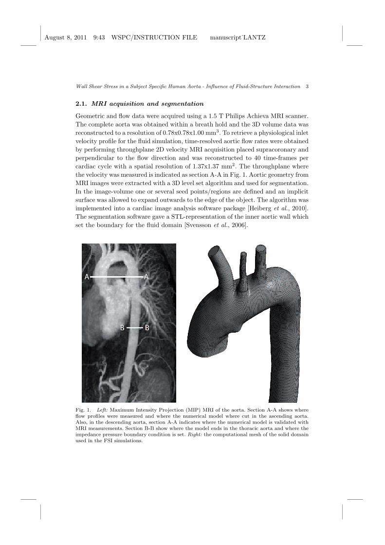
cardiac cycle with a spatial resolution of 1.37x1.37 mm2. The throughplane where

the velocity was measured is indicated as section A-A in Fig. 1. Aortic geometry from

MRI images were extracted with a 3D level set algorithm and used for segmentation.

In the image-volume one or several seed points/regions are defined and an implicit

surface was allowed to expand outwards to the edge of the object. The algorithm was

implemented into a cardiac image analysis software package [Heiberg et al., 2010].

The segmentation software gave a STL-representation of the inner aortic wall which

set the boundary for the fluid domain [Svensson et al., 2006].

Fig. 1. Left: Maximum Intensity Projection (MIP) MRI of the aorta. Section A-A shows whereflow profiles were measured and where the numerical model where cut in the ascending aorta.Also, in the descending aorta, section A-A indicates where the numerical model is validated withMRI measurements. Section B-B show where the model ends in the thoracic aorta and where theimpedance pressure boundary condition is set. Right: the computational mesh of the solid domainused in the FSI simulations.


4 J. Lantz et al.

2.2. Numerical models

In this study, two-way fully coupled FSI simulations were carried out, solving the

solid and fluid problem in a sequential manner and coupled through dynamic and

kinematic interfaces. The dynamic interface meant that the pressure and shear load

on the fluid side balanced the traction of the solid side, whereas the kinematic

interface meant that the velocity of the solid had to match the velocity of the fluid.

2.2.1. Meshes

The segmented geometry obtained from the MRI measurement was cut in the as-

cending aorta at section A-A and in the thoracic aorta at section B-B, see Fig. 1.

The brachiocephalic, left common carotid, and left subclavian arteries (Fig 1, up-

per three branches from left to right) were extended 30 mm to minimize numerical

problems at the outlets. No other arteries leaving the aorta were included in the

model. High quality hexahedral computational meshes were constructed in AN-

SYS ICEM CFD 12.0 (ANSYS Inc. Canonsburg, PA, USA) and used in both the

fluid and the solid geometries. The mesh quality metric in ICEM has a range from

-1 to 1, where -1 is unacceptable, 1 is perfect, and 0.2 is usually considered as an

acceptable threshold value. The quality is a weighted diagnostic between Determi-

nant, Max Orthogls and Max Warpgls, and the minimum of the 3 diagnostics is

presented as the quality of the mesh. The Determinant is the ratio of the smallest

determinant of the Jacobian matrix divided by the largest determinant of the Ja-

cobian matrix, where a value of 1 would indicate a perfectly regular mesh element,

while a negative value would indicate an inverted element. Max Orthogls is the

calculation of the maximum deviation of the internal angles from 90 degrees, and

Max Warpgls is the warp of a quadrilateral faces of a hex element. For more details,

see [ANSYS Inc., 2010b]. The stability and robustness of the simulations proved to

be very sensitive to mesh quality, and therefore a lot of effort was put into mak-

ing the mesh as good as possible. In total, 97% of the mesh elements had a quality

above 0.7 and remaining 3% had a quality above 0.4. To resolve the boundary layer,

the fluid mesh had 10 prism layers adjacent to the wall, which grew exponentially

until the thickness of the last layer matched the core mesh size. The dimensionless

wall distance y+ is important to check, as it is a measure of the near-wall resolution

and also determines how the solver handles the wall (see next section). The y+

values changes during a cardiac cycle due to the fluid motion. For highly accurate

simulations where the boundary layer treatment is important a y+ in the order of

1-2 is needed, and in these simulations it was found to to have a maximum value

of 1.5 during the cardiac cycle.

Mesh independency tests were carried out with 0.5 MC (million cells), 2.8 MC,

and 4.8 MC and it was found that the u, v, and w velocity profiles in the descending

aorta were identical (within 5 %) for all three meshes. To save computational power,

the 0.5 MC mesh was therefore chosen. The solid mesh had roughly 65 000 elements,

and the wall thickness was divided into 3 elements. The element concentration was



higher in areas were large deformations were found to occur. To find these areas

an iterative process was employed: a simulation was run and in areas were large

displacement occured the element concentration was increased. Then the simula-

tion was rerun and the displacement was compared to the smaller mesh. When no

significant difference in deformation could be found, the solid mesh was said to be

mesh independent.

2.2.2. Fluid model

The fluid was set to resemble blood with a constant viscosity of 2.56e-3 Pa s (i.e.

Newtonian fluid) [Wells and Merril, 1962] and a density of 1080 kg/m3 [Kenner,

1989]. From the velocity profiles in the MRI measurements, the Reynolds number

based on inlet diameter, ranged from 200 at late diastole to 7500 at peak systole,

with a mean of 1600. Therefore, the k − ω based Shear Stress Transport (SST)

turbulence model was used, which accounts for the transport of turbulent shear

stress and gives reasonable predictions of the onset and amount of flow separation

under adverse pressure gradients [ANSYS Inc., 2010a]. The SST turbulence model

solves the k−ω model in the near wall region and the k− ǫ model in the bulk flow,

with blending functions to ensure a smooth transition between the two models.

The automatic near-wall treatment method available in CFX was used to model

the flow near the wall. This method switches between wall-functions and a low-

Reynolds number near wall formulation depending on mesh resolution. The wall-

function approach uses empirical correlations near the wall without resolving the

boundary layer. On the other hand, the low-Reynolds number approach resolves the

details of the boundary layer profile, increasing accuracy of the boundary layer. As

the boundary layer mesh is well resolved, the near-wall treatment is used, instead

of wall-functions.

Velocity profiles were measured with MRI in a plane in both the ascending

and descending aorta (see section A-A in Fig. 1), enabling the use of physiological

correct inlet velocity profiles. A sensitivity study showed that the time step needed

to resolve the flow accurately was 0.005 s, but only 40 time frames per cardiac

cycle (about 1 frame every 0.03 s) was measured with the MRI. Therefore, linear

interpolation of the velocity profiles was performed to get a smooth inlet boundary

condition. To represent initial disturbances in the flow, a turbulence intensity of 5%

was specified on the inlet. From the measured flow rates, the flow leaving the arteries

in the aortic arch could be deducted, as the difference between the ascending and

descending flow rates. Mass flow rates were specified on each of the three arteries in

the aortic arch; the difference between ascending and descending flow times a scale

factor were used. The scale factors were based on cross-sectional area and were:

10/16, 1/16, 5/16, for the brachiocephalic, left common carotid, and left subclavian

artery, respectively.

On the lower outlet in the thoracic aorta an impedance boundary condition

was imposed to get a realistic pressure wave profile. A three-element Windkessel


6 J. Lantz et al.

model was used, which describes the relationship between the aortic outflow and

aortic pressure. The Windkessel model is a lumped model, and is capable of defining

physiologically relevant pressure waves [Westerhof et al., 2009; Stergiopulos et al.,

1999]. The model can be viewed analogously to an electrical circuit, where the

current represent the flow rate and the voltage difference the drop in pressure.

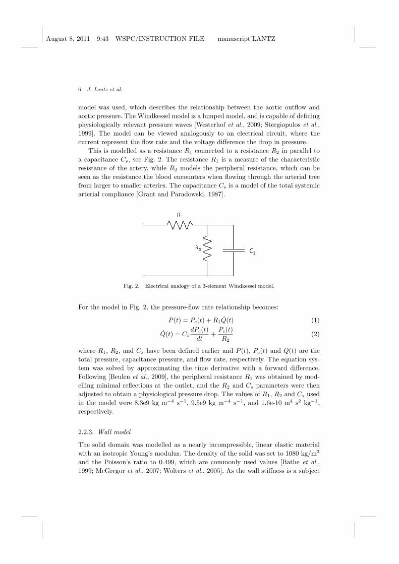
This is modelled as a resistance R1 connected to a resistance R2 in parallel to

a capacitance Cs, see Fig. 2. The resistance R1 is a measure of the characteristic

resistance of the artery, while R2 models the peripheral resistance, which can be

seen as the resistance the blood encounters when flowing through the arterial tree

from larger to smaller arteries. The capacitance Cs is a model of the total systemic

arterial compliance [Grant and Paradowski, 1987].

Fig. 2. Electrical analogy of a 3-element Windkessel model.

For the model in Fig. 2, the pressure-flow rate relationship becomes:

P (t) = Pc(t) +R1Q(t) (1)

Q(t) = Cs

dPc(t)

dt+

Pc(t)

R2

(2)

where R1, R2, and Cs have been defined earlier and P (t), Pc(t) and Q(t) are the

total pressure, capacitance pressure, and flow rate, respectively. The equation sys-

tem was solved by approximating the time derivative with a forward difference.

Following [Beulen et al., 2009], the peripheral resistance R1 was obtained by mod-

elling minimal reflections at the outlet, and the R2 and Cs parameters were then

adjusted to obtain a physiological pressure drop. The values of R1, R2 and Cs used

in the model were 8.3e9 kg m−4 s−1, 9.5e9 kg m−4 s−1, and 1.6e-10 m4 s2 kg−1,

respectively.

2.2.3. Wall model

The solid domain was modelled as a nearly incompressible, linear elastic material

with an isotropic Young’s modulus. The density of the solid was set to 1080 kg/m3

and the Poisson’s ratio to 0.499, which are commonly used values [Bathe et al.,

1999; McGregor et al., 2007; Wolters et al., 2005]. As the wall stiffness is a subject



0 0.2 0.4 0.6 0.8 1−0.05

0

0.05

0.1

0.15

0.2

0.25

0.3

0.35

0.4

0.45

0.5

Time [s]

Mas

s F

low

[kg/

s]

0 0.2 0.4 0.6 0.8 170

75

80

85

90

95

100

105

110

115

120

125

Pre

ssur

e [m

mH

g]

Ascending Mass FlowDescending Mass FlowWindkessel Pressure

PS

MA

MD

EDLD

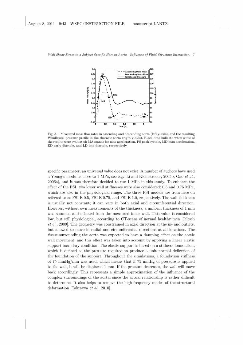
Fig. 3. Measured mass flow rates in ascending and descending aorta (left y-axis), and the resultingWindkessel pressure profile in the thoracic aorta (right y-axis). Black dots indicate when some ofthe results were evaluated; MA stands for max acceleration, PS peak systole, MD max deceleration,ED early diastole, and LD late diastole, respectively.

specific parameter, an universal value does not exist. A number of authors have used

a Young’s modulus close to 1 MPa, see e.g. [Li and Kleinstreuer, 2005b; Gao et al.,

2006a], and it was therefore decided to use 1 MPa in this study. To enhance the

effect of the FSI, two lower wall stiffnesses were also considered: 0.5 and 0.75 MPa,

which are also in the physiological range. The three FSI models are from here on

referred to as FSI E 0.5, FSI E 0.75, and FSI E 1.0, respectively. The wall thickness

is usually not constant; it can vary in both axial and circumferential direction.

However, without own measurements of the thickness, a uniform thickness of 1 mm

was assumed and offseted from the measured inner wall. This value is considered

low, but still physiological, according to CT-scans of normal healthy men [Jeltsch

et al., 2009]. The geometry was constrained in axial direction at the in- and outlets,

but allowed to move in radial and circumferential directions at all locations. The

tissue surrounding the aorta was expected to have a damping effect on the aortic

wall movement, and this effect was taken into account by applying a linear elastic

support boundary condition. The elastic support is based on a stiffness foundation,

which is defined as the pressure required to produce a unit normal deflection of

the foundation of the support. Throughout the simulations, a foundation stiffness

of 75 mmHg/mm was used, which means that if 75 mmHg of pressure is applied

to the wall, it will be displaced 1 mm. If the pressure decreases, the wall will move

back accordingly. This represents a simple approximation of the influence of the

complex surroundings of the aorta, since the actual relationship is rather difficult

to determine. It also helps to remove the high-frequency modes of the structural

deformation [Takizawa et al., 2010].


8 J. Lantz et al.

2.2.4. Simulation

The calculations were performed with ANSYS CFX 12.0 for the fluid simulations

and ANSYS Mechanical for the solid simulations. The FSI-algorithm is iteratively

implicit, meaning that an implicit result is found by iterating the loads transferred

at the interfaces for each time step. The time steps were divided into a number of

coupling iterations called staggers, and for each stagger iteration, CFX passed the

total force on the interface wall to ANSYS Mechanical, which in turn passed the

resulting total mesh deformation back to ANSYS CFX. The stagger iterations were

repeated until all field equations were converged and then an advance in time was

executed. A maximum root-mean-square (RMS) residual of 10−6 was defined for

the fluid simulation, and a maximum RMS residual of 10−3 for the solid simulation

to ensure a well-converged solution. For each time step an upper limit of 30 stagger

iterations was set but the solution always converged before that limit. Domain

imbalances were converged below 0.5 % and for the interface quantities on the FSI-

interface, the convergence criteria was 10−4 while the convergence criteria for mesh

displacement was 10−5. Independence tests were carried out on all of the convergence

criteria to ensure an accurate solution. Temporal discretization was performed with

a second order backward Euler scheme and the spatial discretization used second

order differencing.

Ideally, the MRI measurements would be performed at different times during

the cardiac cycle, yielding a specific geometry for each time point. However, the

measurements are an average of the geometry during several cardiac cycles. As the

systolic phase is only one third of the pulse while the diastolic phase is two thirds,

it is reasonable to assume that the acquired geometry is diastolic-dominant.

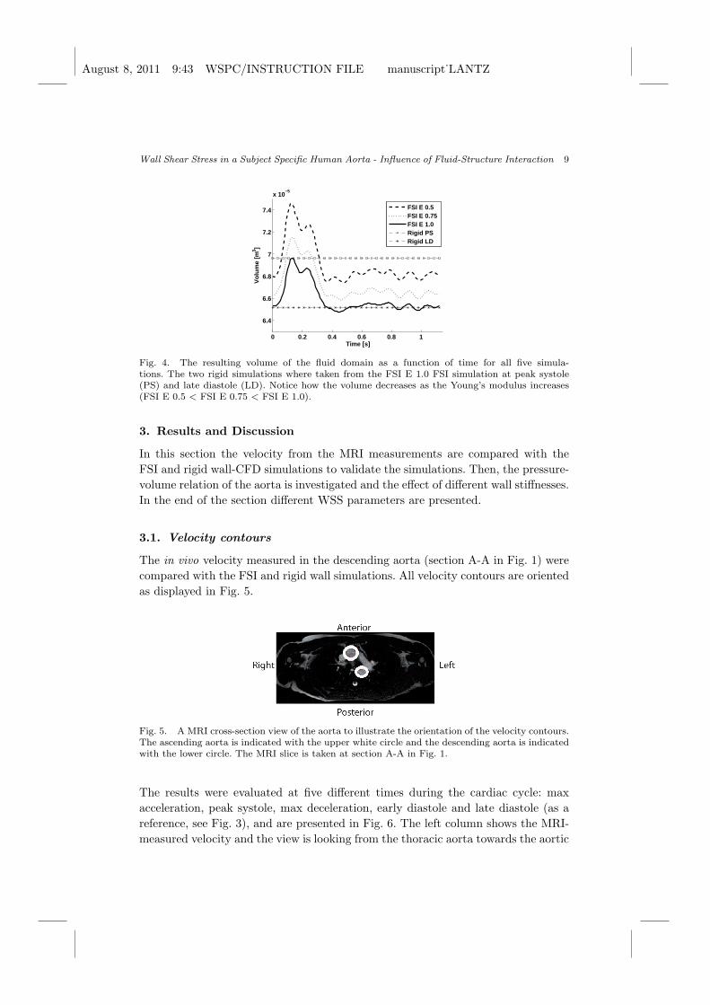
In order to investigate the importance of deforming walls, both FSI and regular

CFD simulations with rigid walls were performed. In total, five simulations were

run, three FSI with different wall stiffnesses (Young’s modulus of 0.5, 0.75, and

1.0 MPa) and two rigid wall simulations. The rigid wall simulations were taken

from the resulting geometry of the 1.0 MPa FSI simulation at peak systole (PS)

and at late diastole (LD). This corresponds to two geometrical approximations of

imaginary snapshot MRI measurements at those two times. The reason peak systole

and late diastole were chosen is because they represents the two extremes in terms

of deformation and domain volume. The three FSI simulations will have different

degrees of deformation, which is shown in Fig. 4.

Seven cardiac cycles were simulated and results are only taken from the last

cycle. The last three cardiac cycles were identical in terms of flow and displacement,

indicating that the results were independent of initial and transient effects. Due

to the strong convergence criteria in the FSI simulations, one cardiac pulse took

about one week to simulate on an eight-core Intel Xeon E5520 machine with 32 GB

of RAM. The simulations were run on the Linux clusters Neolith and Kappa at

National Supercomputer Centre (NSC), Linkoping, Sweden.



0 0.2 0.4 0.6 0.8 1

6.4

6.6

6.8

7

7.2

7.4

x 10−5

Time [s]

Vol

ume

[m3 ]

FSI E 0.5FSI E 0.75FSI E 1.0Rigid PSRigid LD

Fig. 4. The resulting volume of the fluid domain as a function of time for all five simula-tions. The two rigid simulations where taken from the FSI E 1.0 FSI simulation at peak systole(PS) and late diastole (LD). Notice how the volume decreases as the Young’s modulus increases(FSI E 0.5 < FSI E 0.75 < FSI E 1.0).

3. Results and Discussion

In this section the velocity from the MRI measurements are compared with the

FSI and rigid wall-CFD simulations to validate the simulations. Then, the pressure-

volume relation of the aorta is investigated and the effect of different wall stiffnesses.

In the end of the section different WSS parameters are presented.

3.1. Velocity contours

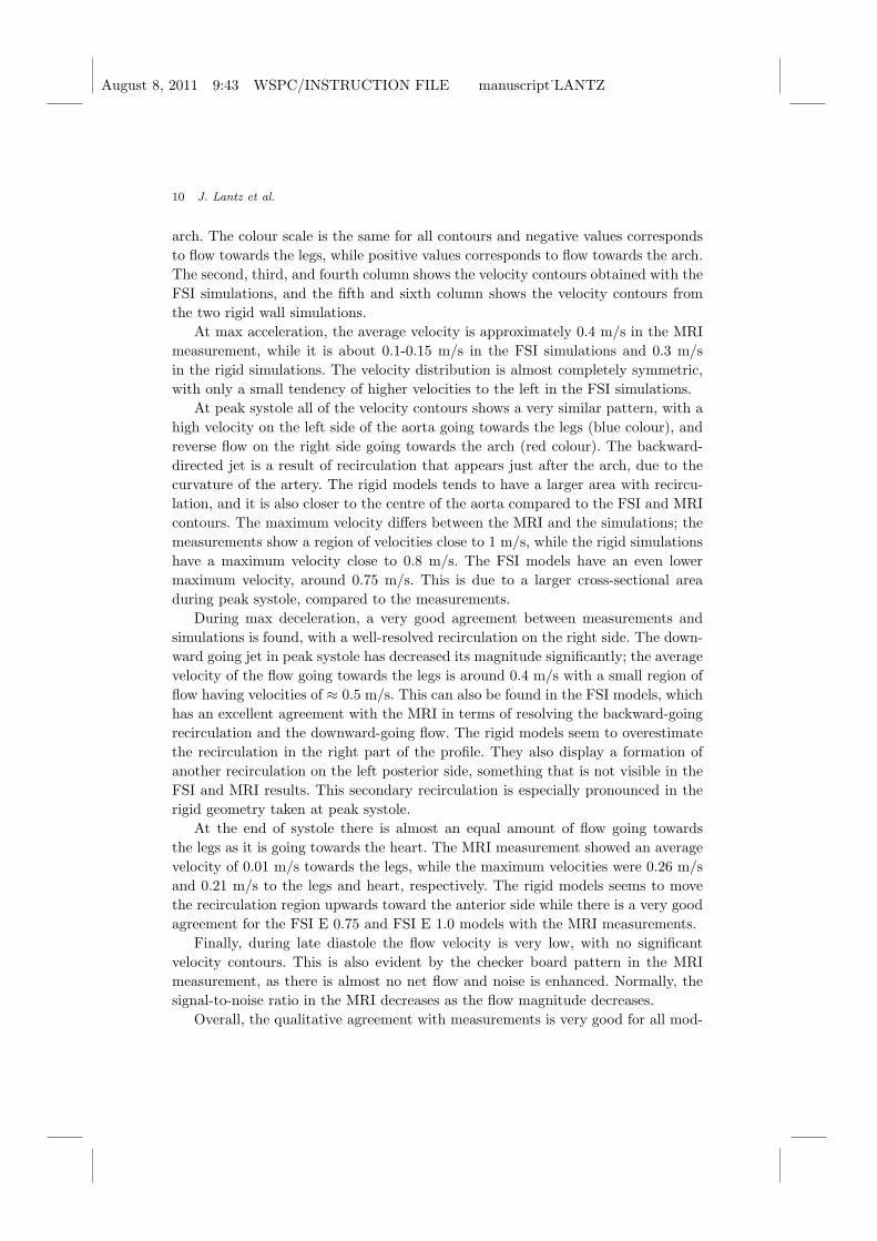
The in vivo velocity measured in the descending aorta (section A-A in Fig. 1) were

compared with the FSI and rigid wall simulations. All velocity contours are oriented

as displayed in Fig. 5.

Fig. 5. A MRI cross-section view of the aorta to illustrate the orientation of the velocity contours.The ascending aorta is indicated with the upper white circle and the descending aorta is indicatedwith the lower circle. The MRI slice is taken at section A-A in Fig. 1.

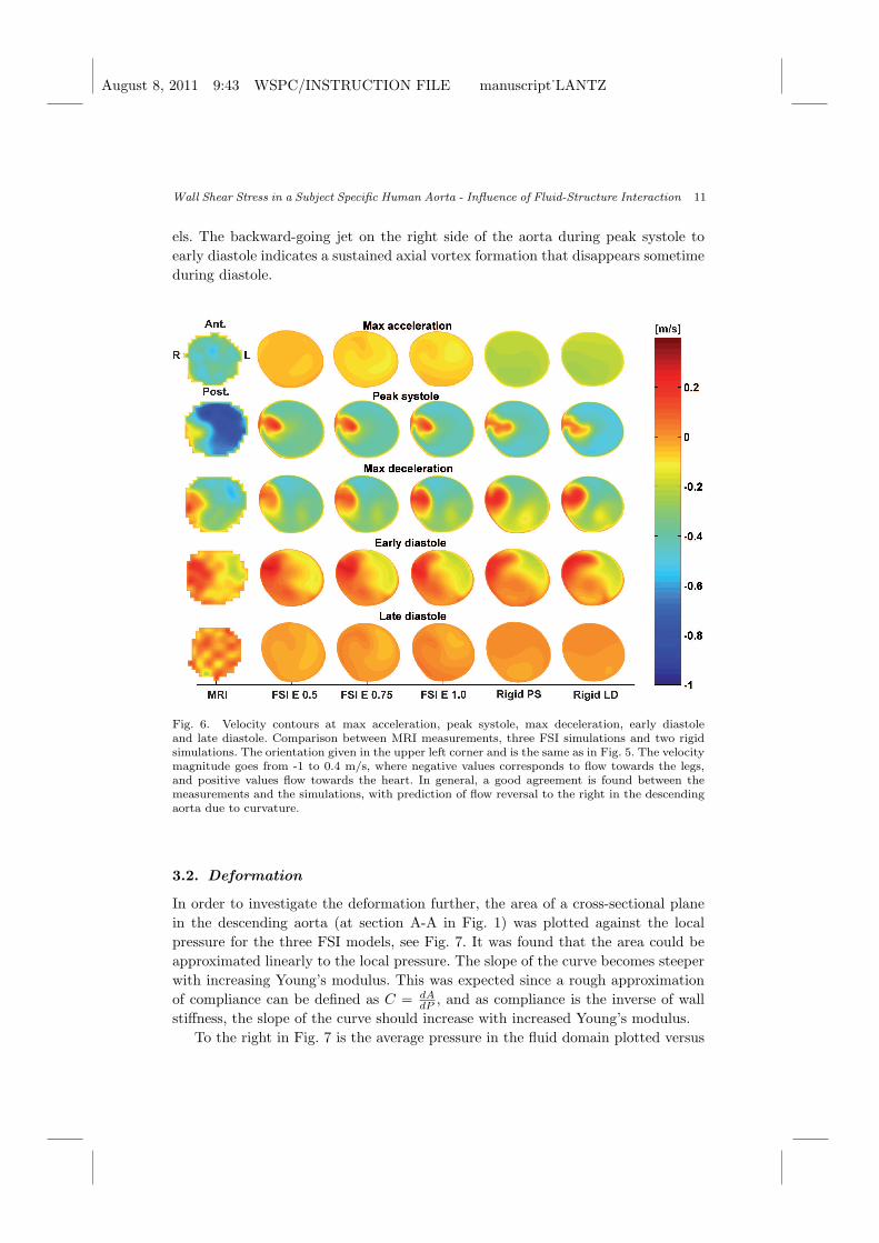
The results were evaluated at five different times during the cardiac cycle: max

acceleration, peak systole, max deceleration, early diastole and late diastole (as a

reference, see Fig. 3), and are presented in Fig. 6. The left column shows the MRI-

measured velocity and the view is looking from the thoracic aorta towards the aortic


10 J. Lantz et al.

arch. The colour scale is the same for all contours and negative values corresponds

to flow towards the legs, while positive values corresponds to flow towards the arch.

The second, third, and fourth column shows the velocity contours obtained with the

FSI simulations, and the fifth and sixth column shows the velocity contours from

the two rigid wall simulations.

At max acceleration, the average velocity is approximately 0.4 m/s in the MRI

measurement, while it is about 0.1-0.15 m/s in the FSI simulations and 0.3 m/s

in the rigid simulations. The velocity distribution is almost completely symmetric,

with only a small tendency of higher velocities to the left in the FSI simulations.

At peak systole all of the velocity contours shows a very similar pattern, with a

high velocity on the left side of the aorta going towards the legs (blue colour), and

reverse flow on the right side going towards the arch (red colour). The backward-

directed jet is a result of recirculation that appears just after the arch, due to the

curvature of the artery. The rigid models tends to have a larger area with recircu-

lation, and it is also closer to the centre of the aorta compared to the FSI and MRI

contours. The maximum velocity differs between the MRI and the simulations; the

measurements show a region of velocities close to 1 m/s, while the rigid simulations

have a maximum velocity close to 0.8 m/s. The FSI models have an even lower

maximum velocity, around 0.75 m/s. This is due to a larger cross-sectional area

during peak systole, compared to the measurements.

During max deceleration, a very good agreement between measurements and

simulations is found, with a well-resolved recirculation on the right side. The down-

ward going jet in peak systole has decreased its magnitude significantly; the average

velocity of the flow going towards the legs is around 0.4 m/s with a small region of

flow having velocities of ≈ 0.5 m/s. This can also be found in the FSI models, which

has an excellent agreement with the MRI in terms of resolving the backward-going

recirculation and the downward-going flow. The rigid models seem to overestimate

the recirculation in the right part of the profile. They also display a formation of

another recirculation on the left posterior side, something that is not visible in the

FSI and MRI results. This secondary recirculation is especially pronounced in the

rigid geometry taken at peak systole.

At the end of systole there is almost an equal amount of flow going towards

the legs as it is going towards the heart. The MRI measurement showed an average

velocity of 0.01 m/s towards the legs, while the maximum velocities were 0.26 m/s

and 0.21 m/s to the legs and heart, respectively. The rigid models seems to move

the recirculation region upwards toward the anterior side while there is a very good

agreement for the FSI E 0.75 and FSI E 1.0 models with the MRI measurements.

Finally, during late diastole the flow velocity is very low, with no significant

velocity contours. This is also evident by the checker board pattern in the MRI

measurement, as there is almost no net flow and noise is enhanced. Normally, the

signal-to-noise ratio in the MRI decreases as the flow magnitude decreases.

Overall, the qualitative agreement with measurements is very good for all mod-



els. The backward-going jet on the right side of the aorta during peak systole to

early diastole indicates a sustained axial vortex formation that disappears sometime

during diastole.

Fig. 6. Velocity contours at max acceleration, peak systole, max deceleration, early diastoleand late diastole. Comparison between MRI measurements, three FSI simulations and two rigidsimulations. The orientation given in the upper left corner and is the same as in Fig. 5. The velocitymagnitude goes from -1 to 0.4 m/s, where negative values corresponds to flow towards the legs,and positive values flow towards the heart. In general, a good agreement is found between themeasurements and the simulations, with prediction of flow reversal to the right in the descendingaorta due to curvature.

3.2. Deformation

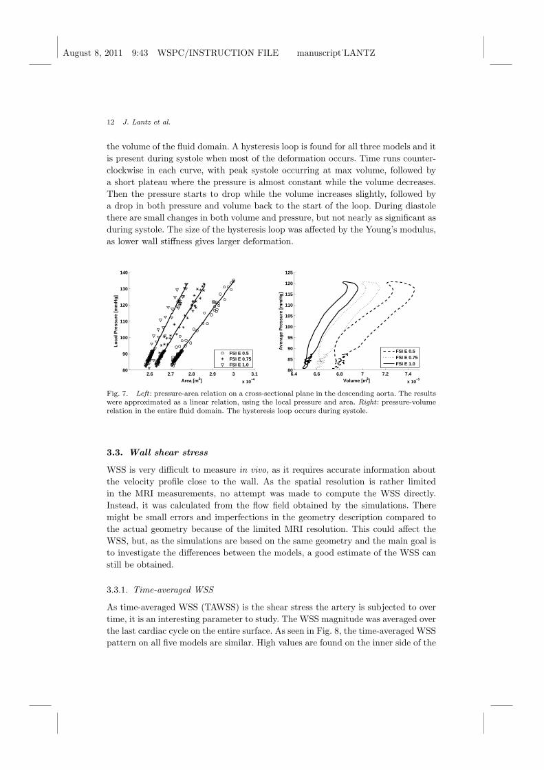
In order to investigate the deformation further, the area of a cross-sectional plane

in the descending aorta (at section A-A in Fig. 1) was plotted against the local

pressure for the three FSI models, see Fig. 7. It was found that the area could be

approximated linearly to the local pressure. The slope of the curve becomes steeper

with increasing Young’s modulus. This was expected since a rough approximation

of compliance can be defined as C = dA

dP, and as compliance is the inverse of wall

stiffness, the slope of the curve should increase with increased Young’s modulus.

To the right in Fig. 7 is the average pressure in the fluid domain plotted versus


12 J. Lantz et al.

the volume of the fluid domain. A hysteresis loop is found for all three models and it

is present during systole when most of the deformation occurs. Time runs counter-

clockwise in each curve, with peak systole occurring at max volume, followed by

a short plateau where the pressure is almost constant while the volume decreases.

Then the pressure starts to drop while the volume increases slightly, followed by

a drop in both pressure and volume back to the start of the loop. During diastole

there are small changes in both volume and pressure, but not nearly as significant as

during systole. The size of the hysteresis loop was affected by the Young’s modulus,

as lower wall stiffness gives larger deformation.

2.6 2.7 2.8 2.9 3 3.1

x 10−4

80

90

100

110

120

130

140

Area [m 2]

Loca

l Pre

ssur

e [m

mH

g]

FSI E 0.5FSI E 0.75FSI E 1.0

6.4 6.6 6.8 7 7.2 7.4

x 10−5

80

85

90

95

100

105

110

115

120

125

Volume [m 3]

Ave

rage

Pre

ssur

e [m

mH

g]

FSI E 0.5FSI E 0.75FSI E 1.0

Fig. 7. Left : pressure-area relation on a cross-sectional plane in the descending aorta. The resultswere approximated as a linear relation, using the local pressure and area. Right : pressure-volumerelation in the entire fluid domain. The hysteresis loop occurs during systole.

3.3. Wall shear stress

WSS is very difficult to measure in vivo, as it requires accurate information about

the velocity profile close to the wall. As the spatial resolution is rather limited

in the MRI measurements, no attempt was made to compute the WSS directly.

Instead, it was calculated from the flow field obtained by the simulations. There

might be small errors and imperfections in the geometry description compared to

the actual geometry because of the limited MRI resolution. This could affect the

WSS, but, as the simulations are based on the same geometry and the main goal is

to investigate the differences between the models, a good estimate of the WSS can

still be obtained.

3.3.1. Time-averaged WSS

As time-averaged WSS (TAWSS) is the shear stress the artery is subjected to over

time, it is an interesting parameter to study. The WSS magnitude was averaged over

the last cardiac cycle on the entire surface. As seen in Fig. 8, the time-averaged WSS

pattern on all five models are similar. High values are found on the inner side of the



(a) (b) (c)

(d) (e)

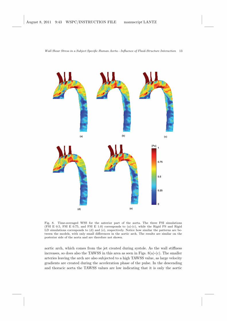
Fig. 8. Time-averaged WSS for the anterior part of the aorta. The three FSI simulations(FSI E 0.5, FSI E 0.75, and FSI E 1.0) corresponds to (a)-(c), while the Rigid PS and RigidLD simulations corresponds to (d) and (e), respectively. Notice how similar the patterns are be-tween the models, with only small differences in the aortic arch. The results are similar on theposterior side of the aorta and are therefore not shown.

aortic arch, which comes from the jet created during systole. As the wall stiffness

increases, so does also the TAWSS in this area as seen in Figs. 8(a)-(c). The smaller

arteries leaving the arch are also subjected to a high TAWSS value, as large velocity

gradients are created during the acceleration phase of the pulse. In the descending

and thoracic aorta the TAWSS values are low indicating that it is only the aortic


14 J. Lantz et al.

arch and the arteries leaving the arch that are subjected to high sustained WSS

values.

The rigid models are almost identical to each other with only minor differences

visible in the aortic arch, indicating that there will be no significant differences in

WSS with different domain volumes if the walls are rigid.

3.3.2. Oscillatory shear index

Another WSS parameter often used in literature is the Oscillatory Shear Index

(OSI), which describes the cyclic departure of the WSS vector from its predominant

axial alignment [Ku et al., 1985; He and Ku, 1996]. It is defined as

OSI = 0.5

(

1−

∣

∣

1

T

∫ T

0τwdt

∣

∣

1

T

∫ T

0|τw|dt

)

. (3)

OSI values vary from zero to 0.5, where zero means that the instantaneous WSS

vector is aligned with the time-averaged WSS vector throughout the cardiac cycle.

A value of 0.5 implies that the instantaneous WSS vector never is aligned with

the time-averaged vector. OSI is insensitive to shear magnitude and must therefore

be used with caution; a large OSI value can indicate a disturbed flow region with

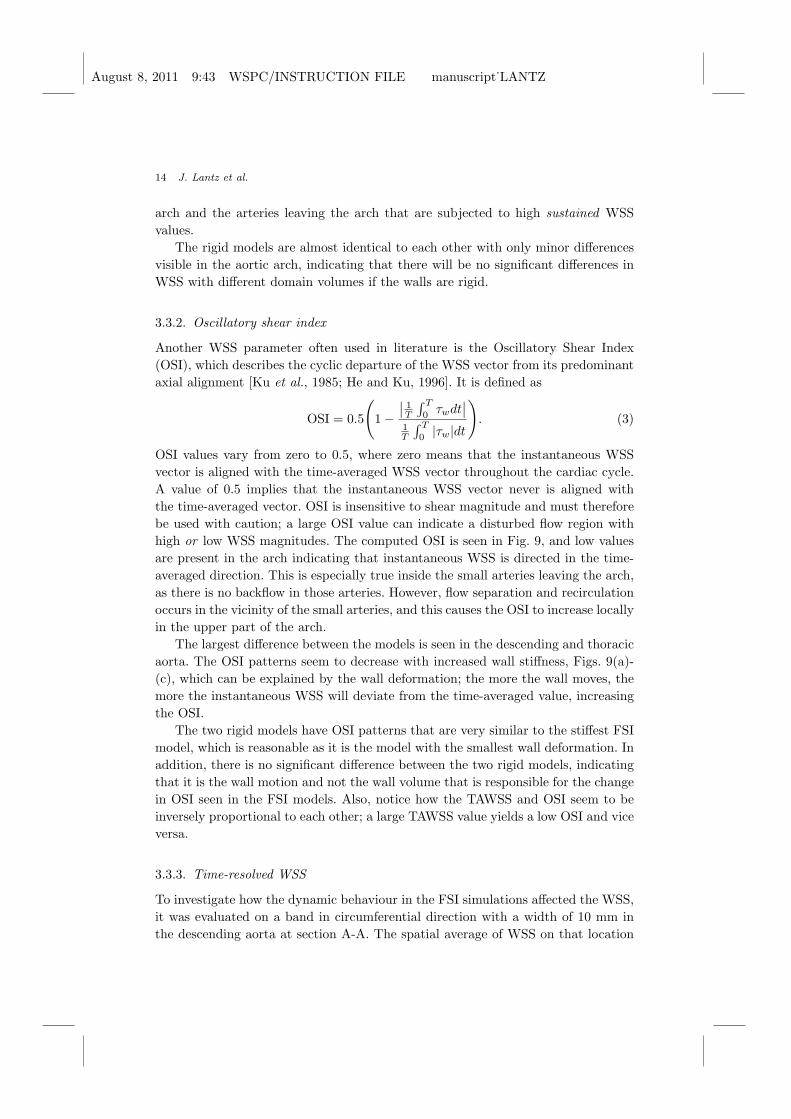
high or low WSS magnitudes. The computed OSI is seen in Fig. 9, and low values

are present in the arch indicating that instantaneous WSS is directed in the time-

averaged direction. This is especially true inside the small arteries leaving the arch,

as there is no backflow in those arteries. However, flow separation and recirculation

occurs in the vicinity of the small arteries, and this causes the OSI to increase locally

in the upper part of the arch.

The largest difference between the models is seen in the descending and thoracic

aorta. The OSI patterns seem to decrease with increased wall stiffness, Figs. 9(a)-

(c), which can be explained by the wall deformation; the more the wall moves, the

more the instantaneous WSS will deviate from the time-averaged value, increasing

the OSI.

The two rigid models have OSI patterns that are very similar to the stiffest FSI

model, which is reasonable as it is the model with the smallest wall deformation. In

addition, there is no significant difference between the two rigid models, indicating

that it is the wall motion and not the wall volume that is responsible for the change

in OSI seen in the FSI models. Also, notice how the TAWSS and OSI seem to be

inversely proportional to each other; a large TAWSS value yields a low OSI and vice

versa.

3.3.3. Time-resolved WSS

To investigate how the dynamic behaviour in the FSI simulations affected the WSS,

it was evaluated on a band in circumferential direction with a width of 10 mm in

the descending aorta at section A-A. The spatial average of WSS on that location



Fig. 9. OSI for the anterior part of the aorta. The three FSI simulations (FSI E 0.5, FSI E 0.75,and FSI E 1.0) correspond to Figs. (a)-(c), while the Rigid PS and Rigid LD simulations correspondto Figs. (d) and (e), respectively. Notice how similar the results are between the models, with onlysmall differences in the descending and thoracic aorta. The OSI patterns are similar on the posteriorside of the aorta and are therefore not shown.

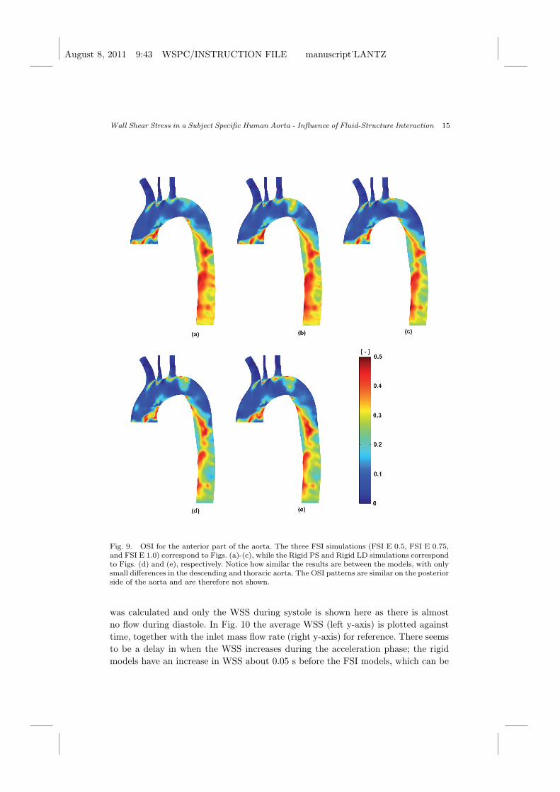
was calculated and only the WSS during systole is shown here as there is almost

no flow during diastole. In Fig. 10 the average WSS (left y-axis) is plotted against

time, together with the inlet mass flow rate (right y-axis) for reference. There seems

to be a delay in when the WSS increases during the acceleration phase; the rigid

models have an increase in WSS about 0.05 s before the FSI models, which can be


16 J. Lantz et al.

0 0.1 0.2 0.3 0.4 0.5

1

2

3

4

5

6

7

8

Time [s]

WS

S [P

a]

0 0.1 0.2 0.3 0.4 0.50

0.1

0.2

0.3

0.4

Inle

t mas

s flo

w [k

g/s]

FSI E 0.5FSI E 0.75FSI E 1.0Rigid PSRigid LDMass Flow

Fig. 10. The WSS during systole in a part of the descending aorta; comparison between FSI(FSI E 0.5, FSI E 0.75, and FSI E 1.0) and rigid wall models (PS and LD). The inlet mass flowis plotted as a reference (right y-axis). Notice how the WSS oscillates during the latter part ofsystole for the FSI models, while the rigid wall models does not show this behaviour.

explained by the dynamics introduced by the wall deformation. With a rigid wall

assumption and an incompressible fluid the pressure and mass wave speeds become

infinite, while with a deforming wall the wave speeds are finite. The shape of the

WSS-curve in the rigid models therefore follows the shape of the mass flow pulse

due to the direct influence of the inflow. On the other hand, the FSI models shows

an oscillatory average WSS during the latter part of systole, which is believed to

be due to the flow dynamics caused by the wall deformation. The peak value seems

to depend on the wall stiffness; the stiffer the wall, the lower the WSS. However,

the rigid models, which in theory has an infinite wall stiffness, has a much lower

peak value. Therefore, the wall motion is believed to be important when considering

instantaneous WSS.

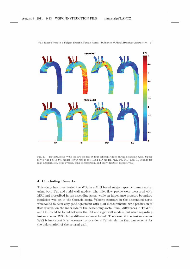
To investigate the time-dependent WSS further, the instantaneous WSS pattern

on the whole aorta was plotted at four times during the cardiac pulse for the least

stiff FSI model and the smallest rigid model, see Fig. 11. The late diastole (LD)

time point was excluded since there is no significant flow at that part of the cardiac

pulse. Clearly, there is a big difference in instantaneous WSS patterns between a

rigid wall model and a FSI model. During the max acceleration phase the WSS is

much higher in the rigid model due to the infinite wave speed. In the FSI model

it takes some time to transmit the inlet pulse through the domain and the WSS is

therefore ”lagging behind”. During peak systole the FSI model show a large area

with elevated WSS values in the descending and thoracic aorta which is not visible

in the rigid model. During max deceleration the patterns are somewhat similar, with

low WSS in the descending aorta in the rigid model while the FSI model predicts a

higher value. This is also true for the early diastolic phase, but here the differences

are smaller.



Fig. 11. Instantaneous WSS for two models at four different times during a cardiac cycle. Upperrow is the FSI E 0.5 model, lower row is the Rigid LD model. MA, PS, MD, and ED stands formax acceleration, peak systole, max deceleration, and early diastole, respectively.

4. Concluding Remarks

This study has investigated the WSS in a MRI based subject specific human aorta,

using both FSI and rigid wall models. The inlet flow profile were measured with

MRI and prescribed in the ascending aorta, while an impedance pressure boundary

condition was set in the thoracic aorta. Velocity contours in the descending aorta

were found to be in very good agreement with MRI measurements, with prediction of

flow reversal on the inner side in the descending aorta. Small differences in TAWSS

and OSI could be found between the FSI and rigid wall models, but when regarding

instantaneous WSS large differences were found. Therefore, if the instantaneous

WSS is important it is necessary to consider a FSI simulation that can account for

the deformation of the arterial wall.


18 J. Lantz et al.

5. Acknowledgements

This work was supported by grants from the Swedish research council, VR 2007-4085

and VR 2010-4282. The Swedish National Infrastructure for Computing (SNIC) is

acknowledged for computational resources provided by the National Supercomputer

Centre (NSC) under grant No. SNIC022/09-11. Dr. Tino Ebbers at the Department

of Medicine and Care at Linkopings University is acknowledged for the MRI mea-

surements. This work has been conducted in collaboration with the Center for Medi-

cal Image Science and Visualization (CMIV, http://www.cmiv.liu.se/) at Linkoping

University, Sweden. CMIV is acknowledged for provision of financial support and

access to leading edge research infrastructure.

References

ANSYS Inc. [2010a] ANSYS CFX-Solver Modeling Guide, 275 Technology Drive, Canons-burg, PA 15317, USA.

ANSYS Inc. [2010b] ANSYS ICEM CFD User Guide, 275 Technology Drive, Canonsburg,PA 15317, USA.

Bathe, M., Kamm, R. D. and Kamm, R. D. [1999] A fluid–structure interaction finiteelement analysis of pulsatile blood flow through a compliant stenotic artery, Journalof Biomechanical Engineering 121, 361–369.

Beulen, B., Rutten, M. and van de Vosse, F. [2009] A time-periodic approach for fluid-structure interaction in distensible vessels, Journal of Fluids and Structures 25(5),954 – 966.

Cheng, R., Lai, Y. G. and Chandran, K. B. [2003] Two-dimensional fluid-structure inter-action simulation of bileaflet mechanical heart valve flow dynamics, Journal of Heart

Valve Disease 12, 772–780.Cheng, R., Lai, Y. G. and Chandran, K. B. [2004] Three-dimensional fluid-structure in-

teraction simulation of bileaflet mechanical heart valve flow dynamics, Annals of

Biomedical Engineering 32, 1471–1483.Dahl, S. K., Vierendeels, J., Degroote, J., Annerel, S., Hellevik, L. R. and Skallerud, B.

[2010] FSI simulation of asymmetric mitral valve dynamics during diastolic filling,Computer Methods in Biomechanics and Biomedical Engineering , 1.

Dempere-Marco, L., Oubel, E., Castro, M., Putman, C., Frangi, A. and Cebral, J. [2006]CFD analysis incorporating the influence of wall motion: application to intracranialaneurysms, Medical Image Computing and Computer-Assisted Intervention 9, 438–445.

Gao, F., Guo, Z., Sakamoto, M. and Matsuzawa, T. [2006a] Fluid-structure interactionwithin a layered aortic arch model, Journal of Biological Physics 32, 435–454.

Gao, F., Watanabe, M. and Matsuzawa, T. [2006b] Stress analysis in a layered aortic archmodel under pulsatile blood flow, BioMedical Engineering OnLine 5, 25.

Grant, B. J. and Paradowski, L. J. [1987] Characterization of pulmonary arterial inputimpedance with lumped parameter models, American Journal of Physiology 252,H585–593.

He, X. and Ku, D. N. [1996] Pulsatile flow in the human left coronary artery bifurcation:average conditions, Journal of Biomechanical Engineering 118, 74–82.

Heiberg, E., Sjogren, J., Ugander, M., Carlsson, M., Engblom, H. and Arheden, H. [2010]Design and validation of Segment–freely available software for cardiovascular imageanalysis, BMC Medical Imaging 10, 1.



Irace, C., Cortese, C., Fiaschi, E., Carallo, C., Farinaro, E. and Gnasso, A. [2004] Wallshear stress is associated with intima-media thickness and carotid atherosclerosis insubjects at low coronary heart disease risk, Stroke 35, 464–468.

Isaksen, J. G., Bazilevs, Y., Kvamsdal, T., Zhang, Y., Kaspersen, J. H., Waterloo, K.,Romner, B. and Ingebrigtsen, T. [2008] Determination of wall tension in cerebralartery aneurysms by numerical simulation, Stroke 39, 3172–3178.

Jeltsch, M., Klass, O., Klein, S., Feuerlein, S., Aschoff, A. J., Brambs, H. J. and Hoffmann,M. H. [2009] Aortic wall thickness assessed by multidetector computed tomographyas a predictor of coronary atherosclerosis, International Journal of CardiovascularImaging 25, 209–217.

Jin, S., Oshinski, J. and Giddens, D. P. [2003] Effects of wall motion and compliance onflow patterns in the ascending aorta, Journal of Biomechanical Engineering 125,347–354.

Kelly, S. C. and O’Rourke, M. J. [2010] A two-system, single-analysis, fluid-structureinteraction technique for modelling abdominal aortic aneurysms, Proceedings of the

Institution of Mechanical Engineers. Part H, Journal of engineering in medicine

224, 955–969.Kenner, T. [1989] The measurement of blood density and its meaning, Basic Research in

Cardiology 84, 111–124.Ku, D. N., Giddens, D. P., Zarins, C. K. and Glagov, S. [1985] Pulsatile flow and atheroscle-

rosis in the human carotid bifurcation. Positive correlation between plaque locationand low oscillating shear stress, Arteriosclerosis 5, 293–302.

Li, Z. and Kleinstreuer, C. [2005a] Blood flow and structure interactions in a stentedabdominal aortic aneurysm model, Medical Engineering & Physics 27, 369–382.

Li, Z. and Kleinstreuer, C. [2005b] Fluid-structure interaction effects on sac-blood pressureand wall stress in a stented aneurysm, Journal of Biomechanical Engineering 127,662–671.

Malek, A. M., Alper, S. L. and Izumo, S. [1999] Hemodynamic shear stress and its role inatherosclerosis, Journal of the American Medical Association 282, 2035–2042.

McGregor, R. H., Szczerba, D. and Szekely, G. [2007] A multiphysics simulation of a healthyand a diseased abdominal aorta, Medical Image Computing and Computer-Assisted

Intervention 10, 227–234.Moore, J. E., Xu, C., Glagov, S., Zarins, C. K. and Ku, D. N. [1994] Fluid wall shear stress

measurements in a model of the human abdominal aorta: oscillatory behavior andrelationship to atherosclerosis, Atherosclerosis 110, 225–240.

Scotti, C. M., Jimenez, J., Muluk, S. C. and Finol, E. A. [2008] Wall stress and flowdynamics in abdominal aortic aneurysms: finite element analysis vs. fluid-structureinteraction, Computer Methods in Biomechanics and Biomedical Engineering 11,301–322.

Shahcheraghi, N., Dwyer, H. A., Cheer, A. Y., Barakat, A. I. and Rutaganira, T. [2002]Unsteady and three-dimensional simulation of blood flow in the human aortic arch,Journal of Biomechanical Engineering 124, 378–387.

Simon, H. A., Ge, L., Borazjani, I., Sotiropoulos, F. and Yoganathan, A. P. [2010] Simu-lation of the three-dimensional hinge flow fields of a bileaflet mechanical heart valveunder aortic conditions, Annals of Biomedical Engineering 38, 841–853.

Stergiopulos, N., Westerhof, B. E. and Westerhof, N. [1999] Total arterial inertance asthe fourth element of the windkessel model, American Journal of Physiology 276,H81–88.

Svensson, J., Gardhagen, R., Heiberg, E., Ebbers, T., Loyd, D., Lanne, T. and Karlsson,M. [2006] Feasibility of patient specific aortic blood flow cfd simulation, in R. Larsen,


20 J. Lantz et al.

M. Nielsen and J. Sporring (eds.), Medical Image Computing and Computer-Assisted

Intervention, Lecture Notes in Computer Science, Vol. 4190, pp. 257–263.Takizawa, K., Moorman, C., Wright, S., Christopher, J. and Tezduyar, T. [2010] Wall shear

stress calculations in spacetime finite element computation of arterial fluidstructureinteractions, Computational Mechanics 46, 31–41.

Tan, F., Torii, R., Borghi, A., Hohiaddin, R., Wood, N. and XU, X. [2009] Fluid-structureinteraction analysis of wall stress and flow patterns in a thoracic aneurysm, Inter-national Journal of Applied Mechanics 1, 179–199.

Wells, R. E. and Merril, E. W. [1962] Influence of flow properties of blood upon viscosity-hematocrit relationships, Journal of Clinical Investigation 41, 1591–1598.

Westerhof, N., Lankhaar, J. W. and Westerhof, B. E. [2009] The arterial Windkessel,Medical & Biological Engineering & Computing 47, 131–141.

Wolters, B. J., Rutten, M. C., Schurink, G. W., Kose, U., de Hart, J. and van de Vosse,F. N. [2005] A patient-specific computational model of fluid-structure interaction inabdominal aortic aneurysms, Medical Engineering & Physics 27, 871–883.

Xenos, M., Rambhia, S. H., Alemu, Y., Einav, S., Labropoulos, N., Tassiopoulos, A., Ri-cotta, J. J. and Bluestein, D. [2010] Patient-based abdominal aortic aneurysm rup-ture risk prediction with fluid structure interaction modeling, Annals of Biomedical

Engineering 38, 3323–3337.

Documents

Wall shear stress in a subject specific human aorta ...liu.diva-portal.org/smash/get/diva2:453413/FULLTEXT01.pdf · WALL SHEAR STRESS IN A SUBJECT SPECIFIC HUMAN AORTA ... if the