WHAT MAKES A GOOD ECONOMY? EVIDENCE FROM PUBLIC OPINION SURVEYS1

Darren GrantDepartment of Economics and International Business

Sam Houston State UniversityBox 2118

Huntsville, TX 77341dgrant@shsu.edu

Abstract: Thirty-five years of previously unstudied survey data are analyzed to determine how the American public evaluates the health of the macroeconomy. Survey responses are multi-dimensional, distinct from indexes of “consumer sentiment,” and based mostly on genuine perceptions of economic conditions, not media reports of economic statistics. As such, they contain unique information about current and future values of these statistics, particularly consumption growth, a longstanding focus of the literature. Both “intangibles” and macroeconomic fundamentals explain substantial variation in the survey data; the public equates two to five percentage points of inflation with one percentage point of unemployment.

Forthcoming, Economic Inquiry

** This paper has several figures that are best viewed in color. **

1 I am grateful to Mishuk Chowdhury, Mitchell Graff, Sohna Jaye, Mohammed Khan, RyanMurphy, Tino Sonora, Mark Tuttle, Charles Vogel, and Jadrian Wooten, all of whom providedassistance for this project, and to Claudia Deane of the Washington Post for providing ABCNews/Washington Post survey data through 2005. Comments from Jae Won Lee, Vance Ginn,Andrew Oswald, anonymous referees (who contributed some phrasing used herein), Co-EditorsNezih Guner and Gian Luca Clementi, and participants at the Western Economic Associationmeetings, the Southern Economic Association meetings, and a seminar at Sam Houston StateUniversity are also appreciated.

Traditional business cycle measurement and theory tends to downplay the role of public

perceptions. The health of the macroeconomy is evaluated, with a lag, through formal measurement

of fundamentals like GDP growth, rather than by the opinion of the public. The objective functions

employed by models of macro policy, derived from theory or prescribed ad-hoc, are similarly

unshaped by public opinion on the attractiveness of various states of the economy.

For a profession that is enamored of consumer sovereignty and cognizant of the value of

idiosyncratic, decentralized information, this is a little surprising. It probably reflects, in part, a lack

of available data. In the U.S., prior research on the macroeconomic perceptions of the public has

almost exclusively employed the widely-available Michigan Index of Consumer Sentiment or its

counterpart from the Conference Board, the Consumer Confidence Index, to predict future

consumption. But these measures are not intended to be, and have not been interpreted as, general

assessments of the national macroeconomy. They combine responses to a variety of questions, about

personal finances and the macroeconomy, about employment, consumption, and profitability, about

current conditions and the change in those conditions. These questions are sufficiently disparate that

it is unclear what, exactly, either index measures or how it should be interpreted (see Merkle, Langer,

and Sussman, 2004). This ambiguity has probably contributed to a decades-long debate over the

usefulness of such indices, which has been compounded by divergent findings on their ability to

forecast future consumption (see Golinelli and Parigi, 2004, and Manski, 2004).

To surmount these data limitations, we assembled thirty-five years of responses from three

reputable, national U.S. polls that ask about the current state of the national economy and/or whether

economic conditions are getting better or worse. All are conceptually and (we show) statistically

distinct from indexes of consumer sentiment, and none has been previously studied.

As we show in this paper, this poll data enriches our understanding of the business cycle in

2

three ways. It contains information about fundamental macroeconomic variables, which are reported

with a lag and (often) subsequently revised. It establishes the role of various macroeconomic

fundamentals (and of intangibles) in determining the public’s satisfaction with the economy, which

informs policy and suggests simple summary measures of economic conditions. And it reveals the

multifaceted nature of consumers’ macroeconomic perceptions, which span four dimensions across

a total of nine survey questions. Section 1 introduces these surveys and shows how they relate to

each other and to the Michigan and Conference Board indices. In Section 2, we examine how

macroeconomic conditions influence the assessments reported therein; their predictive power is

examined in Section 3. Section 4 concludes.

1. Polling on the State of the Economy.

For decades, American news organizations have asked respondents to assess the national

macroeconomy; Table 1 lists the questions, time spans, sample periods, and response options for

each. (We are not aware of any analogous surveys conducted abroad.) These surveys have

developed in three phases.

In the late 1970s and early 1980s, CBS News, (generally) in conjunction with the New York

Times (NYT), and ABC News, in conjunction with the Washington Post, occasionally asked a

national sample of the U.S. public about the change in macroeconomic conditions: “Do you think the

economy (CBS) / nation’s economy (ABC) is getting better, getting worse, or staying about the

same?” Each of these surveys was, in isolation, too episodic to be of use to researchers.

This changed in the mid-1980s, when both organizations introduced a question about the

3

level, rather than the change, in macroeconomic conditions, and began reporting the responses several

times per year. In December, 1985, ABC News began asking: “Would you describe the state of the

nation's economy these days as excellent, good, not so good, or poor?” CBS News soon followed

with a similar, though differently phrased, question: “How would you rate the condition of the

national economy these days–Very Good, Fairly Good, Fairly Bad, or Very Bad?” Unlike ABC

News, it continued to ask the “better/worse” question as well. Later a third poll, by Gallup and

sponsored by USA Today, also asked both types of questions, using somewhat different wording.

The USA Today poll was discontinued in October, 2008, and that by ABC News in February, 2010.

In the third, modern phase, the quantity, quality, and availability of data has expanded further.

In January, 2008, Gallup began daily tracking of both “good economy” and “better/worse” questions,

interviewing five hundred people each day. This continues to be supplemented by the CBS News

polls, now conducted almost every month, and by Bloomberg, which picked up the ABC News

survey after a one year hiatus.

We use data from the first two phases in our analysis. Initially, we analyze the five survey

questions in the second phase: the “good economy” questions from ABC News, CBS News, and USA

Today, along with the “better/worse” questions from CBS News and USA Today. Finding a strong

commonality underlying the responses to each question type, we then integrate the responses, using

a method described below, and incorporate phase one data to create two latent variables, one for the

“good economy” question and one for the “better/worse” question. Further analysis is then

conducted using these latent variables. While each survey begins at a different time, listed in Table

1, our data terminates in February, 2010 (or, for the USA Today surveys, October, 2008). Time is

measured in months. Each survey contains at least one thousand respondents in each month it is

2 Merkle, Langer, and Sussman (2004) detail the differences in timing, sampling, sample sizes,and interview methods across the ABC News, Michigan, and Conference Board surveys.

4

conducted, and each is conducted in more than half of the months in its sample period (see Table 1).

The first two responses to each “good economy” question are considered “positive.” Figure

1a presents the time series of the fraction of each survey’s responses that are positive, while Figure

1b presents the time series of the fraction of “better” responses to the “better/worse” questions (along

with the change in positive responses to the ABC News “good economy” question). The level of

positive responses differs across surveys, consistent with the different phrasing of the questions and

response options, but the temporal variation appears to be similar, a strong cyclical component

punctuated with higher frequency modulations. The large samples in each monthly survey ensure

virtually none of this variance (about 0.1%) comes from sampling error.

The Michigan and Conference Board surveys also present indexes of current conditions, also

represented in Table 1. (These, and a separate expectations index, also represented in the table,

average to form that entity’s consumer sentiment index.) These questions are distinctly different:

neither survey asks explicitly about the overall macroeconomy, but about “business conditions,”

“available jobs,” and durable goods purchases, and most questions concern the respondent or his local

area, instead of the country as a whole. While these indexes also have a strong cyclical component,

the questions themselves do not have the face validity necessary to represent an general assessment

of the national macroeconomy. The ABC News, CBS News, and USA Today poll questions do.2

Despite this face validity, and microfoundations by which macroeconomic fundamentals

generate dynamic responses to opinion surveys (Lux, 2008; Easaw and Ghoshray, 2010), we

recognize that “economists have been deeply skeptical of subjective statements” (p. 1337 of Manski,

5

2004, who argues that such skepticism is unwarranted, as does Bewley, 2002). Given this skepticism

and the aforementioned conflict concerning the consumer sentiment surveys, it is worthwhile to

further support these surveys’ legitimacy by establishing construct validity (Litwin, 1995). This

requires a certain logical consistency across surveys: questions about similar concepts should have

similar responses (convergent validity), while the responses to questions about distinct concepts

should differ (divergent validity).

In our data, convergent construct validity requires that 1) the responses to the “better/worse”

questions are related to differences of the “good economy” responses, and 2) the responses to all

three “good economy” questions have a strong underlying commonality, despite differences in

wording (and similarly for the “better/worse” questions). Divergent construct validity requires, in

turn, that 3) these survey responses are distinguishable from the consumer sentiment indexes, which

are conceptually different.

1) Levels and Differences. To compare the “good economy” and “better/worse” questions,

we begin by regressing the percentage of “better” responses to the CBS/NYT and USA Today/Gallup

“better/worse” questions on leads and lags of the percentage of positive responses to the “good

economy” question asked by ABC News–the only one that is reported each and every month. Six

months of leads and twelve months of lags were included. A condensed version, using two month

intervals, is reported in the first and third columns of Table 2.

In these regressions, positive coefficients near the current date offset negative coefficients for

the recent past, suggesting the expected differencing interpretation. These differences are essentially

backward-looking, with hindsight that extends several months. To pin down the timing more

precisely, we found that two-month combination of the ABC News “good economy” measure that

3 The coefficients on the leads are biased upward if positive assessments of the current changein economic conditions favorably affect the economy’s performance in the future. This reinforces theconclusion that the better/worse series compare the present to the past, not expectations of the futureto the present. Estimations in which the leads were instrumented with lags of the “better/worse”and/or “good economy” variables, though much less precise, also support this conclusion.

6

best explains the responses to each “better/worse” question. The optimal pairs are shown in the

second and fourth columns of Table 2, a (mostly) backward difference of six months for the USA

Today series and eight months for the longer CBS/NYT series. Treating these specifications as the

null, we then tested the alternative that any of the remaining coefficients were nonzero. For neither

series could this null be rejected at conventional levels (in the CBS News survey, F = 0.98, p >.10;

in the USA Today survey, F = 1.53, p > .10).3

In three of the four specifications we cannot reject a strict differencing interpretation, that the

coefficients sum to zero. This interpretation and the R² values, which range from 0.5 to 0.7, both

suggest a reasonable degree of concordance between the level and difference assessments of the

macroeconomy. The fit is not so good, however, that the two measures can be considered

synonymous. Accordingly, each is examined below.

2) Underlying Commonalities. For each survey question, the response frequencies–the

percent of respondents saying the economy is “excellent,” and so forth–can be viewed as governed

by three terms: a latent variable common to all respondents, L, that can be considered a scalar index

of perceived macroeconomic conditions; a random variate, ", that generates cross-section variation

in individual responses at any given point in time; and a set of thresholds, :, that distinguish an

“excellent” response from a “good” response, and so on. If all “good economy” series have a strong

underlying commonality, then the latent variables underlying each series should be highly correlated.

Each latent variable, and the associated thresholds, can be estimated by relating the response

7

(1)

frequencies nonparametrically to time. The most practical way to do this is to express time as a

series of splines, which are used as independent variables in an ordered probit model in which the

response frequencies are the dependent variable. (See Takezawa, 2006 and Wasserman, 2006.

Informally, these splines resemble an overlapping sequence of bell curves. We use many splines, fifty-

two over the sample period, to preserve all but the highest frequency variation.) Applying the

estimated coefficients to the splines yields a smoothed, unrestricted estimate of the latent variable that

extends for the full time span of the survey, filling in any survey-less months.

The formal statement of this model is as follows. For each survey question Z, the individual-

level latent variable, I, underlying any discrete choice model equals the sum of L and ", as follows:

where S is a set of “B-splines,” determined according to the method of deBoor (1978), which sum

to one at each point in time, and the :’s are the thresholds that Ij,t must exceed in order for that

respondent to report that economic conditions are “excellent” instead of “good,” and so on. The

predicted value of L at any time T is simply E $̂ sSs,T.

Figures 2a and 3a present the results for all “good economy” and “better/worse” questions,

with the estimated latent variables and thresholds vertically scaled (additively) so that all latent

variables have the same mean for the periods in which they overlap. (We do not present confidence

8

intervals, as they are so small.) For both questions the latent variables are as similar as the cutoffs,

driven by the various response options, are different. Correlations between the “good economy”

latent variables are each 0.99, and the correlation between the “better/worse” latent variables is 0.96.

3) Comparison with Other Indexes. These latent variables are, in effect, indexes

themselves, and can be statistically compared to the Michigan and Conference Board indexes. We

begin with a simple correlation analysis, presented in Table 3. To incorporate both the “good

economy” and “better/worse” series and address potential stationarity concerns, eight month

backward differences are taken of all variables except the two “better/worse” series, consistent with

our findings above (for the longer CBS News “better/worse” series). The nine series included in this

analysis can be placed into four groups, each clearly demarcated in the table: “good economy” series,

Michigan and Conference Board current conditions indexes, expectations indexes, and “better/worse”

series. This grouping is supported by the correlation matrix, in which intra-group correlations, of

about 0.9, comfortably surpass the cross-group correlations, which never exceed 0.8. (The one

exception, the weak correlation between the Michigan and Conference Board current situation

indexes, proves the rule. These are composed of responses to quite different questions.) These four

groups of variables appear to represent multiple dimensions of macroeconomic perceptions.

To explore further, we employ a principal component analysis. (This has been previously used

for quantifying the state of the macroeconomy in other contexts: see the discussion and references

in Bai, 2003.) This yields a set of nine independent components that linearly reconstruct each of the

original series. Economic significance is restricted to the first four of these, which together explain

95% of the aggregate variance of all nine series. The associated factor loadings, also found in Table

3, are easily interpreted. The first, dominant component, a simple, almost-unweighted average of the

9

nine series, reflects basic business cycle variation. The second component distinguishes measures of

expectations from everything else. The third component distinguishes the “better/worse” series, while

the fourth component represents a difference between the “good economy” series and the

Michigan/Conference Board current conditions indexes. The cyclical component explains 72% of

the joint variance of these series. Of the remaining 28%, almost half is contributed by the

distinctiveness of the expectations indices, and another half by the distinctiveness of the two survey

questions analyzed here, with the remainder noise, or “scree.”

These findings all support construct validity. The economic assessments that underlie

responses to the “good economy” and “better/worse” questions are insensitive to minor differences

in wording, logically consistent with each other, and distinct from surveys of consumer sentiment.

2. Macroeconomic Factors Affecting Assessments of the National Economy.

“Aggregated” Latent Variables. The results in the previous section indicate we can adequately

describe our survey data with two temporal latent variables, one underlying the responses to all “good

economy” questions, the other underlying the responses to all “better/worse” questions. Differences

in response frequencies across surveys are captured by differences in the thresholds separating the

response options in each survey. This “aggregated” latent variable also improves the temporal

coverage for the “better/worse” question, which has occasional temporal gaps in any one survey,

which are now “filled in” by another survey. These gaps were particularly frequent prior to 1988, but

with this technique, we can incorporate the early CBS News and ABC News responses and extend

this latent variable back to 1976, covering a period of high inflation and volatile economic growth.

4 Inflation is calculated using the all-urban Consumer Price Index, and the unemployment rateis seasonally adjusted. Each quarterly observation of the real, chain-weighted, seasonally-adjustedGross Domestic Product is assumed to pertain to the middle month of each quarter; the other monthsare calculated by linear interpolation. The trade-weighted index of exchange rates of the U.S.’s mostimportant trading partners, from the Federal Reserve Bank of St. Louis, has been divided by ten hereso that its variation is comparable to that of the other variables.

Additional regressions, not reported here, “scaled” unemployment, inflation, or both, forexpectations. Unanticipated inflation was calculated using expectations from the well-knownLivingston survey; this variable performs slightly worse than simple inflation does. Unemploymentwas adjusted by calculating its deviation from the Natural Rate of Unemployment, taken fromGordon’s (2006) macroeconomics text, or replaced with personal income growth, also to no effect.

10

For each question type, the specification of the model used to estimate this latent variable is

a slight modification of that in equation (1): LtZ = Lt �Z, ßs

Z = ßs �Z, and :0 = 0 for the first series

only. Figures 3b and 4b show both estimated latent variables, along with the thresholds associated

with each survey. The resemblance to those reported in Figures 3a and 4a is clear. The remaining

analysis is conducted using these latent variables.

Basic Regressions. To determine the macroeconomic underpinnings of these survey responses, we

regress the associated latent variables on a set of economic fundamentals. The set we use includes

and exceeds those employed in political business cycle models and analyses of the macroeconomics

of happiness: inflation, the unemployment rate, output growth, a medium-term interest rate (the

seven-year Treasury bill), an index of the strength of the dollar, and a time trend.4

The first three variables in this list are not instantaneously reported with perfect accuracy.

Preliminary values for unemployment and output growth are reported by the appropriate federal

agency with a lag of one month, then subsequently revised. Also, the CPI, used in calculating

inflation, is reported with a one month delay. Which, then, should be used: the ex post, revised

values, or the “real-time” data available to respondents at the time the survey is taken?

11

Our answer is: both. Initially, we use the ex post, revised values, which best measure the

“true” value of that variable in that month. Then, subsequently, we replace these values with those

constructed using real-time data (distributed by the Federal Reserve Banks of Philadelphia and St.

Louis). If the public’s economic assessments are based mostly on reported statistics, the real-time

data should have superior explanatory power. On the other hand, if these assessments stem from

individuals’ genuine perceptions of macroeconomic conditions, the ex post, revised data should be

superior. Means and detrended standard deviations for the ex post data are listed in Table 4.

The five variables measuring economic fundamentals are often characterized by different

integration orders. GDP growth is typically found to be stationary, while inflation and interest rates

are I(1); there is much less agreement on the integration properties of the unemployment rate and

dollar strength indicator. But, rather than deepen the integration order of our measures, we prefer

to look for robustness. Thus, we estimate both level and difference specifications for the “good

economy” question, and also regress the “better/worse” latent variable on differences of the

independent variables. The levels specification can be viewed as estimating an a priori known

cointegration relationship, with the observed autocorrelation in the residuals representing slow

adjustment of survey responses to their long-run fundamental level. The differences specifications,

which are more appropriate statistically, estimate short run relationships.

These specifications require a total of three different differences: 1) in output and price levels,

to determine output growth and inflation, 2) of all dependent and independent variables in some

“good economy” specifications, and 3) of the independent variables in the “better/worse” regression.

Our earlier findings suggest only the length of this last difference: six to eight months (we use eight,

which maximizes explanatory power). For the other two, we simply take one year (backward)

5 In consecutive months autocorrelation is at least 0.85 in all specifications. Unfortunately,trying to improve estimation efficiency by using generalized least squares is impractical: it generatessubstantial errors in variables bias in the coefficient estimates, because it implicitly differences the dataa second time, reducing the signal and amplifying the noise. For example, the standard deviation ofthe sampling and truncation error in the doubly-differenced unemployment rate is 0.16 percentagepoints (www.bls.gov/cps/eetech.methods.pdf), while the standard deviation of this variable in the datais 0.194 percentage points. Thus, the GLS coefficient estimate should be–and is–attenuated by0.16²/0.194², to one-third of its true value. Similar reductions were observed for other variables.

12

differences. These nearly maximize explanatory power and, in the differenced “good economy”

regressions, also control for seasonality without sacrificing degrees of freedom.

Estimation is conducted using OLS, which yields consistent coefficient estimates in all

specifications. But OLS standard errors are biased in cointegrating regressions and when, as here,

the error term is serially correlated, so these are adjusted using the Newey-West correction.5 Three

sample periods are analyzed: June 1976-February 2010, the full time span of the “better/worse”

question, December 1985-February 2010, the full time span of the “good economy” question, and

December 1985-August 2008, which eliminates the September 2008 credit crunch and its aftermath.

Estimates are presented in Table 4. Each independent variable’s standard deviation is

approximately one, and the thresholds separating different response options are usually a little more

than one unit apart, so, loosely speaking, each coefficient translates a one standard deviation change

in the independent variable into the probability the respondent will choose the next most favorable

response option. By a wide margin, economic assessments are most strongly influenced by

unemployment. Increasing this by two or three percentage points will cause half of all respondents

to choose the next worse response option. Significant but smaller effects, in the expected direction,

are also observed with inflation and GDP growth. In contrast, the exchange rate and interest rate

generally have smaller, variable, and insignificant coefficients, suggesting that they are secondary.

6 The most noticeable difference is a notable reduction in the unemployment coefficient, andexplanatory power, when the September 2008-February 2010 period is added to the sample. Thecredit crunch sharply and immediately reduced optimism about the state of the economy, while thecorresponding increase in unemployment was much more gradual.

13

These estimates are all reasonably consistent across specifications and sample periods.6

The similarity of key coefficients across specifications occurs partly because assessments of

the macroeconomy are adjusted almost instantaneously, as indicated by unreported regressions using

lagged dependent variables. This similarity implies that, to the first order, the deterministic factor in

our regressions is common to both the “good economy” and “better/worse” series. But its relative

importance differs: this factor explains over one-half of the variation in the differenced “good

economy” measure, but only one-third of the variation in the “better/worse” measure. Because

sampling error is so small, almost all of the remaining variation consists of “intangibles”–unmeasured

factors, animal spirits (Akerlof and Shiller, 2009), etc. These intangibles are also, to a considerable

extent, common to the two series–thus the differenced “good economy” measure, in Table 2, explains

far more variation in the “better/worse” latent variable than any of the regressions in Table 4.

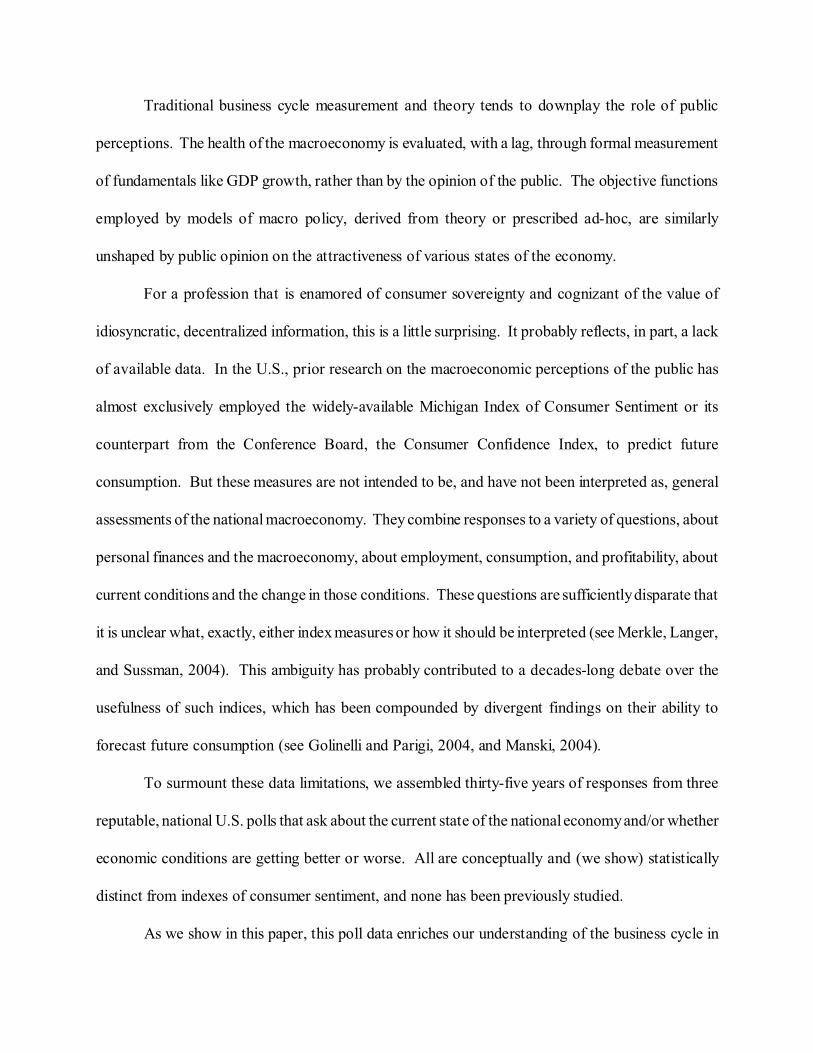
The effects of individual variables are depicted more concretely in Figure 4. This contains a

continuous decomposition of the contributions of inflation, unemployment, GDP growth, and the

residual to the value of the “better/worse” latent variable, using the estimates in the last column of

Table 4. (The effects of the exchange rate and the interest rate, which are insignificant in this

regression, are suppressed for clarity.) These four components are demeaned and stacked: the value

of the unemployment component is ßU)(Ut-U% ), and so on. Thus, at each point in time, extending

upward from the horizontal axis is the cumulative positive contribution of these four factors toward

the deviation of the latent variable from its mean, and similarly for the negative contribution.

14

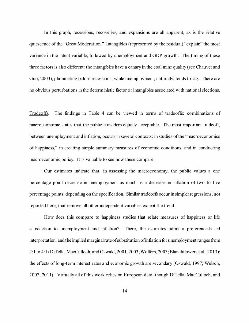
In this graph, recessions, recoveries, and expansions are all apparent, as is the relative

quiescence of the “Great Moderation.” Intangibles (represented by the residual) “explain” the most

variance in the latent variable, followed by unemployment and GDP growth. The timing of these

three factors is also different: the intangibles have a canary in the coal mine quality (see Chauvet and

Guo, 2003), plummeting before recessions, while unemployment, naturally, tends to lag. There are

no obvious perturbations in the deterministic factor or intangibles associated with national elections.

Tradeoffs. The findings in Table 4 can be viewed in terms of tradeoffs: combinations of

macroeconomic states that the public considers equally acceptable. The most important tradeoff,

between unemployment and inflation, occurs in several contexts: in studies of the “macroeconomics

of happiness,” in creating simple summary measures of economic conditions, and in conducting

macroeconomic policy. It is valuable to see how these compare.

Our estimates indicate that, in assessing the macroeconomy, the public values a one

percentage point decrease in unemployment as much as a decrease in inflation of two to five

percentage points, depending on the specification. Similar tradeoffs occur in simpler regressions, not

reported here, that remove all other independent variables except the trend.

How does this compare to happiness studies that relate measures of happiness or life

satisfaction to unemployment and inflation? There, the estimates admit a preference-based

interpretation, and the implied marginal rate of substitution of inflation for unemployment ranges from

2:1 to 4:1 (DiTella, MacCulloch, and Oswald, 2001, 2003; Wolfers, 2003; Blanchflower et al., 2013);

the effects of long-term interest rates and economic growth are secondary (Oswald, 1997; Welsch,

2007, 2011). Virtually all of this work relies on European data, though DiTella, MacCulloch, and

15

Oswald (2001) provide comparable (but less precise) estimates for the United States. The similarity

of these findings to ours suggests we cannot rule out the possibility that members of the public

evaluate the economy according to their preferences over macroeconomic states.

In contrast, these tradeoffs run counter to the simplest common metric of aggregate economic

conditions, Okun’s “Misery Index,” the unweighted sum of unemployment and inflation. In contrast,

equal weights cannot be rejected in explaining the Index of Consumer Sentiment or the Consumer

Confidence Index, according to Lovell and Tien (2000) and Golinelli and Parigi (2004). But we have

shown that the two sets of surveys measure distinct concepts. The Misery Index seemingly serves

better as an indicator of consumer confidence than as a metric of aggregate economic conditions.

Lastly, we compare measurement with theory: the tradeoffs embodied in models of monetary

policy, often derived from an approximation to household utility in an intertemporal maximization

problem. The best known of these, Woodford (2003, Chapter 6), is expressed in terms of output

growth and inflation, which can be translated into an inflation-unemployment tradeoff using Okun’s

law (Abel and Bernanke, 2005; Mitchell and Pearce, 2010). Doing so, we find that this loss function

places far more weight on inflation than unemployment, in contrast with our findings and those of the

macroeconomics of happiness.

3. The Information Content of Economic Assessments.

The deterministic and intangible components of these survey responses could contain novel

information about the current or future values of macroeconomic fundamentals, which, as mentioned,

are measured with a lag and (often) subsequently revised. The deterministic component could contain

7 The smoothing involved in the construction of the latent variables in Section 2 is bothforward and backward in time. This is obviously problematic for these forecasting regressions. Thus,both latent variables were re-constructed by replacing the splines in equation (1) with a set ofyear*month dummy variables. The resulting latent variables are wholly contemporaneous, but arenot available for every month in the sample period, reducing the number of observations for analysis.

16

(2)

such information if it primarily reflects individuals’ perceptions of economic conditions, rather than

the reporting of economic statistics (as in Doms and Morin, 2004 or Starr, 2012). It does. In the

“real-time” row of Table 4 we re-estimated the regressions above using real-time data for

unemployment, output growth, and inflation, on which reported statistics would be based. The R²

values show that this data has much less explanatory power.

Thus, our latent variables should help predict current values of macroeconomic fundamentals

that have yet to be reported, and possibly future revisions of past values that have already been

reported. One candidate fundamental is real GDP, because the surveys ask about the national

economy; another, based on the previous section’s results, is unemployment. In that spirit, we predict

ex-post (superscript EX) revised values of GDP growth, )Y, and unemployment, U, in month t* from

the real-time (superscript RT) macro and survey data available in the middle of month t, as follows:

where )B is inflation, S contains survey data,7 {",(,N,R,2} are coefficient vectors or matrices, q is

time in quarters ()Y) / three-month intervals (U), and > is an error term. The term Xt,0RT is the most

recent reported value of variable X as of time t, Xt,-1RT is the most recent reported value of that

variable three months (or one quarter) previous, and so on.

Three types of regressions are run, each with different timing. Nowcasts relate final, revised

current-period values to current period real-time data: t* = t. Hindcasts relate final, revised,

17

previous-period values to current period real-time data: t* = t-1. These determine whether survey

data can predict revisions of macro variables. We also estimate forecasts that relate final, revised

future values to current-period real-time data: t* > t. Following Bram and Ludvigson (1998) and

others, our metric is the adjusted R² statistic, Rð². Mindful of the multidimensionality revealed in

Section 1, we employ three different combinations of poll data: the “good economy” and

“better/worse” latent variables; a consumer sentiment index, either the Index of Consumer Sentiment

or the Consumer Confidence Index; or both the latent variables and a sentiment index. This makes

it easy to compare the effects of the two types of surveys, and to see whether the information they

contribute is distinct or overlapping.

The results for real GDP growth are found in the top panel of Table 5. The latent variables

and sentiment indexes improve hindcasts and nowcasts, raising Rð² by five to ten percentage points.

The information they contain is overlapping: the Rð² values are no higher when the latent variables and

sentiment indexes are jointly included in the regression. Both also help hindcast or nowcast

unemployment, in the second panel of the table, but the improvement in fit is quite marginal.

Past studies (Matsusaka and Sbordone, 1995, and Golinelli and Parigi, 2004, each conducted

before the advent of real-time data) have found consumer sentiment indexes to be predictive of future

GDP growth, so forecasting equations for GDP and unemployment are also presented. Forecasting

power must come from the intangible component of the data, which could predict future economic

performance in two ways. A belief that the economy is improving could cause increased economic

activity. Or surveys could “anticipate” changes in economic activity that are not predictable from past

values of macro variables. The results show that our latent variables do indeed provide substantial

new information–unlike the sentiment indexes.

8 This slightly overstates and understates the case. A much noisier, preliminary value of theMichigan index is available mid-month, while the final value of the Conference Board index is notavailable until the end of the month following the survey. See Merkle, Langer, and Sussman (2004).

9 Real time data on the personal consumption expenditures deflator is not available on amonthly basis, so stock prices were deflated with the CPI instead.

18

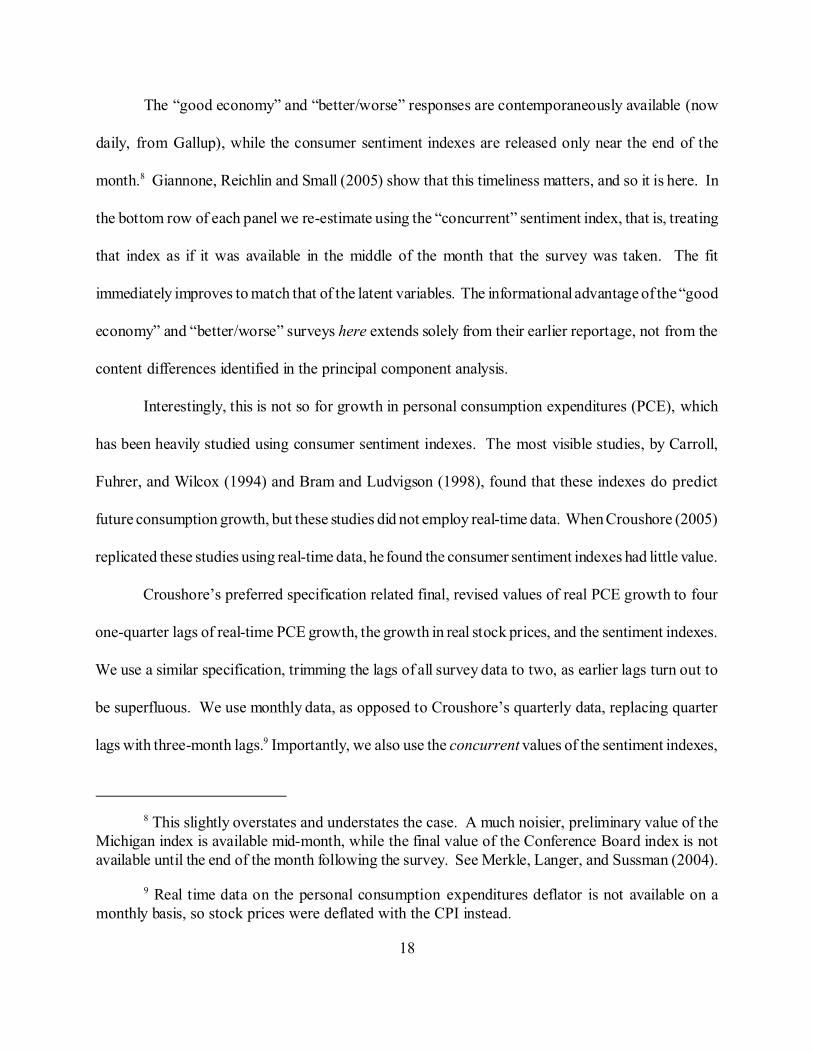
The “good economy” and “better/worse” responses are contemporaneously available (now

daily, from Gallup), while the consumer sentiment indexes are released only near the end of the

month.8 Giannone, Reichlin and Small (2005) show that this timeliness matters, and so it is here. In

the bottom row of each panel we re-estimate using the “concurrent” sentiment index, that is, treating

that index as if it was available in the middle of the month that the survey was taken. The fit

immediately improves to match that of the latent variables. The informational advantage of the “good

economy” and “better/worse” surveys here extends solely from their earlier reportage, not from the

content differences identified in the principal component analysis.

Interestingly, this is not so for growth in personal consumption expenditures (PCE), which

has been heavily studied using consumer sentiment indexes. The most visible studies, by Carroll,

Fuhrer, and Wilcox (1994) and Bram and Ludvigson (1998), found that these indexes do predict

future consumption growth, but these studies did not employ real-time data. When Croushore (2005)

replicated these studies using real-time data, he found the consumer sentiment indexes had little value.

Croushore’s preferred specification related final, revised values of real PCE growth to four

one-quarter lags of real-time PCE growth, the growth in real stock prices, and the sentiment indexes.

We use a similar specification, trimming the lags of all survey data to two, as earlier lags turn out to

be superfluous. We use monthly data, as opposed to Croushore’s quarterly data, replacing quarter

lags with three-month lags.9 Importantly, we also use the concurrent values of the sentiment indexes,

19

setting aside differences in reporting dates and focusing on the difference in informational content.

The results are presented in the final panel of Table 5. In the Hindcast column, the Rð²’s are

all similar: no survey contributes information. For the nowcasts, both do: Rð² increases substantially,

and by a similar amount, whether our latent variables, a consumer sentiment index, or both are

included. For the forecasts, the value of the latent variables waxes while that of consumer sentiment

wanes. The latent variables increase fit by an astonishing thirty percentage points at a four-quarter

horizon, while the contribution of consumer sentiment is far smaller or nil (as in Croushore, 2005).

Thus, ironically, the simple “good economy” and “better/worse” surveys predict consumption

growth far better than the more sophisticated consumer sentiment indexes that have been designed

for this purpose. As these surveys do not ask directly about consumption, their predictive power

probably stems from intangibles: the effect of economic optimism on consumption choices. Because

Section 1 showed that the “better/worse” question–which has by far the most predictive power

here–is not forward-looking, the most plausible mechanism is that optimism causes, rather than

anticipates, future consumption growth (as Matsusaka and Sbordone, 1995, found for GDP growth).

In summary, the “good economy” and “better/worse” surveys contain useful information

about the past, current, and future evolution of fundamental macroeconomic variables. Some of this

information is duplicated by consumer sentiment indexes, with a reporting lag; some is not.

4. Conclusion.

What makes a good economy? A strong labor market, predominantly, though the public also

values lower inflation, more economic growth, and a stronger dollar. Changes in these fundamentals

20

also help explain the whether the public views the economy as getting better or getting worse. Still,

responses to both types of survey questions are strongly influenced by intangibles that have no

obvious economic correlate.

The phrasing of the “good economy” question and response options differs across three

surveys, engendering differences in raw response probabilities; nonetheless, these responses are

governed by the same underlying latent variable. This latent variable is distinct from various

consumer sentiment indices published by the University of Michigan and the Conference Board,

though all of these surveys exhibit cyclicality. The same is true for the “better/worse” question, which

looks backward with hindsight of six to eight months.

Responses to the “good economy” and “better/worse” questions are based primarily on

respondents’ perceptions of economic conditions, not media reports of fundamental economic

variables. Partly because of this, these responses contain new, timely information about the past,

current, and future values of consumption growth, GDP growth, and unemployment. The recently

expanded, daily tracking of these two questions by Gallup therefore promises to be a valuable source

of information about economic fundamentals.

Table 1. Survey Details.

Survey Title and Sponsor

Question(s) Asked ofRespondents

Temporal Span, Survey Frequency, and ResponseReporting (Phone Survey unless Noted)

Observations,Sample Period

ABC News (partof the ConsumerComfort Index):Levels A

“Would you describe the stateof the nation’s economy thesedays as excellent, good, not sogood, or poor?”

Weekly from Dec. 1985-Feb. 2010, nationwide.Percentages in each category are reported for about1,000 respondents over the previous four weeks. Thevalues reported in the last survey of the month are used.

291 obs. in the291 months fromDec. 1985 - Feb.2010

ABC News /Washington Post:Changes B

“Do you think the nationaleconomy is getting better,getting worse, or staying aboutthe same?”

Reported in 49 of the 110 months between Sept. 1981and Oct. 1990, and sporadically afterward, nationwide. Percentages in each category are reported for about1,000 respondents over the previous week.

reporting toosporadic to beindividuallyanalyzed

New York Times /CBS News Poll:Levels C

“How would you rate thecondition of the nationaleconomy these days? Is itvery good, fairly good, fairlybad, or very bad?”

Oct. 1987-present, at irregular intervals, nationwide. Percentages in each category are reported for least1,000 respondents over the previous three or five days. All surveys in taken in any given month are averaged.

161 obs. in the268 months fromOct. 1987 to Feb.2010

New York Times /CBS News Poll:Changes C

“Do you think the economy isgetting better, getting worse,or staying about the same?”

Sept. 1976-present, irregular intervals, nationwide.Percentages in each category are reported for at least1,000 respondents over the previous three to five days. All surveys in each month are averaged.

154 obs. of the235 months fromAug. 1990 to Feb.2010 E

USA Today /Gallup Poll:Levels D

“How would you rateeconomic conditions in thiscountry today–as excellent,good, only fair, or poor?”

Jan. 1997-Oct. 2008, at irregular intervals, nationwide.Percentages in each category are reported for at least1,000 respondents over the previous three to five days. All surveys in each month are averaged.

111 obs. in the142 months fromJan. 1997 to Oct.2008

USA Today /Gallup Poll:Changes D

“Right now, do you think thateconomic conditions in thecountry as a whole are gettingbetter or getting worse?” (thepercent volunteering theresponse “same” also reported)

Feb. 1997-Oct. 2008, at irregular intervals, nationwide.Percentages in each category are reported for at least1,000 respondents over the previous three to five days. All surveys in each month are averaged.

109 obs. in the141 months fromFeb. 1997 to Oct.2008

University ofMichigan Indexof CurrentEconomicConditions E

“Would you say that you arebetter off or worse offfinancially than you were ayear ago?” and “Generallyspeaking, do you think now isa good or bad time for peopleto buy major householditems?”

Monthly, Jan. 1978-present; three or four times yearly,1951-Dec. 1977, continental U.S. At least 500respondents over the course of the month. Percentageresponses (with one decimal place) to each question areavailable online. The fraction of positive minusnegative responses for each question is calculated,averaged, and indexed to 1966:1.

291 obs. in the291 months fromDec. 1985 to Feb.2010

ConferenceBoard PresentSituation Index D

“How would you rate presentgeneral business conditions inyour area–good, normal, orbad?” and “What would yousay about available jobs inyour area right now–plentiful,not so many, or hard to get?”

Monthly, June 1977-present; bi-monthly, Feb. 1967-Apr. 1977, nationwide. Throughout the month about3,500 respond to a mailing of 5,000 surveys, made atthe end of the previous month. The fraction of all non-neutral responses that are positive is calculated andindexed to 1985.

158 of the 158months from Jan.1997 to Feb. 2010

Notes:A Available from 2004 forward from: http://abcnews.go.com/PollingUnit/CCI/ , with earlier values obtained via request to the WashingtonPost in 2005, when they were a partner with ABC News for the Consumer Comfort Survey.B Available from the Interuniversity Consortium for Political and Social Research (ICPSR)C Available from: http://www.cbsnews.com/stories/2007/10/12/politics/main3362530.shtml D Data available, from 1997 forward, from: http://www.pollingreport.com/consumer.htm E Breakdowns of response percentages by demographic group available from: http://www.sca.isr.umich.edu/subset/F Data prior to Aug. 1990 reported too sporadically to be individually analyzed

Table 2. Regressions of “Better / Worse” Measures on Leads/Lags of “Good Economy” PositiveResponses (coefficient estimates, with standard errors in parentheses).

PERCENT SAYING THE ECONOMY IS “GETTING BETTER”

Percent Saying theEconomy Is “Excellent”or “Good” in ABC Survey

CBS /NYT CBS /NYT(Best 2 MonthCombination)

USA Today /Gallup

USA Today(Best 2 MonthCombination)

Six Month Lead -0.01 (0.12)

-0.10 (0.14)

Four Month Lead 0.20 (0.17)

0.12 (0.19)

Two Month Lead 0.18 (0.16)

0.29 (0.18)

One Month Lead 0.61* (0.05)

0.86* (0.09)

Current Month 0.37* (0.15)

0.76* (0.19)

Two Month Lag 0.08 (0.14)

-0.07 (0.19)

Four Month Lag -0.39* (0.16)

-0.53* (0.19)

Five Month Lag -0.76* (0.08)

Six Month Lag -0.15 (0.16)

-0.14 (0.19)

Seven Month Lag -0.58* (0.05)

Eight Month Lag -0.12 (0.14)

-0.19 (0.18)

Ten Month Lag -0.06 (0.15)

-0.25 (0.18)

Twelve Month Lag 0.01 (0.11)

0.20 (0.13)

F-Statistic on Null thatCoefficient Sum Is 0(p value)

6.00 (0.02)

1.04 (0.31)

1.47 (0.23)

3.47 (0.07)

R² / Adjusted R² 0.54 / 0.51 0.49 / 0.48 0.75 / 0.72 0.71 / 0.70

Note: Time trend also included. N = 144 for CBS/NYT survey and N=109 for USA Today/Gallup.* = p < .05.

Table 3. Correlations and Principal Components Factor Loadings. CORRELATIONS (N in parentheses) PRINCIPAL COMPONENT

“Good Economy” “Better/Worse” FACTOR LOADINGS Latent Variables Current Indices Expectations Indices Latent Variables (N = 127)

Variable NYT /CBS

USA /Gallup

Michigan Conf.Board

Michigan Conf.Board

NYT /CBS

USA /Gallup

1st P.C. 2nd P.C 3rd P.C. 4th P.C.

ABC NewsGood Econ.

0.96(205)

0.95(127)

0.73(266)

0.79(128)

0.65(266)

0.57(128)

0.77(252)

0.70(130)

0.37 -0.24 0.15 -0.25

NYT / CBSGood Econ.

0.95(127)

0.72(205)

0.71(128)

0.64(205)

0.59(128)

0.79(205)

0.70(130)

0.37 -0.19 0.09 -0.42

USA/GallupGood Econ.

0.75(127)

0.71(127)

0.61(127)

0.60(127)

0.78(127)

0.68(127)

0.37 -0.18 0.10 -0.43

MichiganCurrent

0.69(131)

0.70(269)

0.68(131)

0.60(252)

0.59(130)

0.34 0.16 0.18 0.40

Conf. BoardCurrent

0.43(131)

0.43(131)

0.55(128)

0.44(128)

0.29 -0.31 0.50 0.56

MichiganExpectations

0.86(131)

0.53(252)

0.53(130)

0.30 0.60 0.06 -0.13

Conf. BoardExpectations

0.57(128)

0.52(128)

0.30 0.59 0.05 0.04

NYT / CBSBetter/Worse

0.96(130)

0.35 -0.15 -0.49 0.18

USA/GallupBetter/Worse

0.31 -0.10 -0.64 0.22

Joint VarianceExplained

72% 11% 8% 4%

Note: All variables are scaled to have the same variance for the principal component analysis, as is standard. Consistent with the findings in Table 2,eight month differences are taken of for all “good economy” latent variables, Michigan indices, and Conference Board indices.

Table 4. Regression Results (coefficient estimates, with robust standard errors in parentheses). “BETTER/WORSE”

“GOOD ECONOMY” LATENT VARIABLE LATENT VARIABLE

Independent Variable

Mean, StandardDeviation (de-trended), Dec.‘85-Feb. ‘10

Levels Dec. ‘85- Dec. ‘85- Aug. ‘08 Feb. ‘10 (N=274) (N=291)

Differences Dec. ‘86- Dec. ‘86- Aug. ‘08 Feb. ‘10 (N=262) (N=279)

(on differences of)Dec. ‘85- Dec. ‘85- June ‘76-Aug. ‘08 Feb. ‘10 Feb. ‘10 (N=274) (N=291) (N=405)

Unemployment(percentage points)

5.74 (1.23)

-0.39* (0.03)

-0.23* (0.05)

-0.36* (0.05)

-0.19* (0.06)

-0.32* (0.08)

-0.17* (0.08)

-0.25*(0.09)

One Year OutputGrowth (percent)

2.63 (1.67)

0.06* (0.02)

0.08* (0.02)

0.03 (0.02)

0.05 (0.03)

0.05 (0.03)

0.08* (0.03)

0.06*(0.02)

Twelve MonthInflation (percent)

2.88 (1.20)

-0.08* (0.02)

-0.11* (0.02)

-0.06* (0.02)

-0.07* (0.01)

-0.09 (0.05)

-0.10* (0.04)

-0.08*(0.04)

Exchange Rate (Fedseries, scaled by 0.1)

9.10 (0.88)

0.13* (0.02)

0.15* (0.03)

0.08* (0.03)

0.06* (0.03)

0.08 (0.06)

0.04 (0.06)

0.05(0.06)

Seven Year T-Bill Rate (percentage pts)

5.85 (0.78)

0.00 (0.02)

0.12* (0.04)

0.02 (0.02)

0.08* (0.03)

-0.03 (0.05)

0.01 (0.05)

-0.10 (0.05)

Trend in Years ---- -0.02* (0.01)

0.02 (0.01)

---- ---- ---- ---- ----

R² ---- 0.91 0.87 0.69 0.54 0.32 0.27 0.36

R² using real-timedata

---- 0.89 0.82 0.68 0.45 0.26 0.14 0.24

Note: Final revised values of each independent variable are used in the regressions reported in the table. The R² values for regressionsusing real-time data, instead, are reported in the last row. Each regression also includes a constant. As discussed in the text, differencesare taken over twelve months for the “good economy” regressions and over eight months for the “better/worse” regressions. * = p < .05.

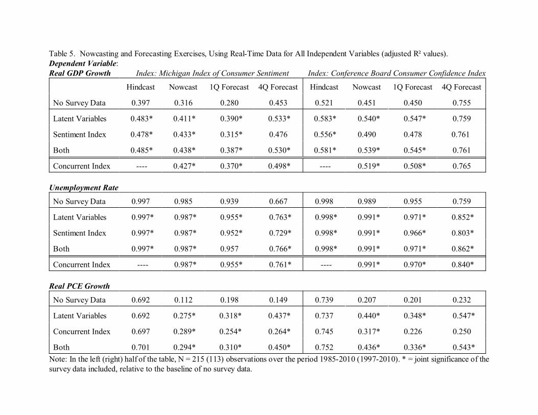
Table 5. Nowcasting and Forecasting Exercises, Using Real-Time Data for All Independent Variables (adjusted R² values).Dependent Variable:Real GDP Growth Index: Michigan Index of Consumer Sentiment Index: Conference Board Consumer Confidence Index

Hindcast Nowcast 1Q Forecast 4Q Forecast Hindcast Nowcast 1Q Forecast 4Q Forecast

No Survey Data 0.397 0.316 0.280 0.453 0.521 0.451 0.450 0.755

Latent Variables 0.483* 0.411* 0.390* 0.533* 0.583* 0.540* 0.547* 0.759

Sentiment Index 0.478* 0.433* 0.315* 0.476 0.556* 0.490 0.478 0.761

Both 0.485* 0.438* 0.387* 0.530* 0.581* 0.539* 0.545* 0.761

Concurrent Index ---- 0.427* 0.370* 0.498* ---- 0.519* 0.508* 0.765

Unemployment Rate

No Survey Data 0.997 0.985 0.939 0.667 0.998 0.989 0.955 0.759

Latent Variables 0.997* 0.987* 0.955* 0.763* 0.998* 0.991* 0.971* 0.852*

Sentiment Index 0.997* 0.987* 0.952* 0.729* 0.998* 0.991* 0.966* 0.803*

Both 0.997* 0.987* 0.957 0.766* 0.998* 0.991* 0.971* 0.862*

Concurrent Index ---- 0.987* 0.955* 0.761* ---- 0.991* 0.970* 0.840*

Real PCE Growth

No Survey Data 0.692 0.112 0.198 0.149 0.739 0.207 0.201 0.232

Latent Variables 0.692 0.275* 0.318* 0.437* 0.737 0.440* 0.348* 0.547*

Concurrent Index 0.697 0.289* 0.254* 0.264* 0.745 0.317* 0.226 0.250

Both 0.701 0.294* 0.310* 0.450* 0.752 0.436* 0.336* 0.543*

Note: In the left (right) half of the table, N = 215 (113) observations over the period 1985-2010 (1997-2010). * = joint significance of thesurvey data included, relative to the baseline of no survey data.

REFERENCES

Abel, Andrew, and Ben Bernanke. Macroeconomics, 5th edition. Upper Saddle River, New Jersey:Pearson (2005).

Akerlof, George, and Robert Shiller. Animal Spirits: How Human Psychology Drives the Economy,and Why It Matters for Global Capitalism. Princeton: Princeton University Press (2009).

Bai, Jushan. “Inferential Theory for Factor Models of Large Dimensions,” Econometrica 71:135-171(2003).

Bewley, Truman. “Interviews as a Valid Empirical Tool in Economics,” Journal of Socio-Economics31:343-353 (2002).

Bram, J., and S. Ludvigson. “Does Consumer Confidence Forecast Household Expenditure? ASentiment Index Horse Race,” Economic Policy Review 4,2:59-78 (1998).

Carroll, C., J. Fuhrer, and D. Wilcox. “Does Consumer Sentiment Forecast Household Spending?If So, Why?” American Economic Review 84,5:1397-1408 (1994).

Chauvet, M., and J.-T. Guo. “Sunspots, Animal Spirits, and Economic Fluctuations,”Macroeconomic Dynamics 7,1:140-169 (2003).

de Boor, C. A Practical Guide to Splines. New York: Springer Verlag (1978).

Blanchflower, David, David Bell, Alberto Montagnoli, and Mirko Miro. “The Effects ofMacroeconomic Shocks on Well-Being,” Manuscript, University of Stirling (2013).

Croushore, Dean. “Do Consumer Confidence Indexes Help Forecast Consumer Spending in RealTime?” North American Journal of Economics and Finance 16:435-450 (2005).

DiTella, Rafael, Robert MacCulloch, and Andrew Oswald. “Preferences over Inflation andUnemployment: Evidence from Surveys of Happiness,” American Economic Review 91:335-341 (2001).

----. “The Macroeconomics of Happiness,” Review of Economics and Statistics 85:809-827 (2003).

DiTella, Rafael, and Robert MacCulloch. “Some Uses of Happiness Data in Economics,” Journalof Economic Perspectives 21,4:25-46 (2007).

Doms, Mark, and Norman Morin. “Consumer Sentiment, the Economy, and the News Media,”Federal Reserve Board Working Paper (2004).

Easaw, Joshy, and Atanu Ghoshray. “News and Households’ Subjective MacroeconomicExpectations,” Journal of Macroeconomics 32,1:469-475 (2010).

Giannonne, Domenico, Lucrezia Reichlin, and David Small. “Nowcasting GDP and Inflation: TheReal-Time Informational Content of Macroeconomic Data Releases,” Federal Reserve Board(2005).

Golinelli, Roberto, and Giuseppe Parigi. “Consumer Sentiment and Economic Activity: A CrossCountry Comparison,” Journal of Business Cycle Measurement and Analysis 1,2:147-170(2004).

Goodfriend, Marvin. “How the World Achieved Consensus on Monetary Policy,” Journal ofEconomic Perspectives 21,4:47-68 (2007).

Gordon, Robert. “The History of the Phillips Curve: Consensus and Bifurcation,” Economica 78,10-50 (2011).

----. Macroeconomics, 10th edition. Upper Saddle River, New Jersey: Pearson (2006).

Leeper, E. “Consumer Attitudes: King for a Day,” Economic Review 77,4:1-15 (1992).

Litwin, Mark. How to Measure Survey Reliability and Validity. New York: Sage (1995).

Lovell, Michael C., and Pao-Lin Tien. “Economic Discomfort and Consumer Sentiment,” EasternEconomic Journal 26,1:1-8 (2000).

Ludvigson, Sydney. “Consumer Confidence and Consumer Spending,” Journal of EconomicPerspectives 18, 2:29-50 (2004).

Lux, Thomas. “Rational Forecasts or Social Opinion Dynamics: Identification of Interaction Effectsin a Business Climate Survey.” Kiel Institute for the World Economy Working Paper (2008).

Manski, Charles. “Measuring Expectations,” Econometrica 72,5:1329-1376 (2004).

Malasevic-Perovic, Lena. “Subjective Well-Being in Transition Countries: Investigating the RelativeImportance of Macroeconomic Variables,” Financial Theory and Practice 32,4:519-537(2008).

Matsusaka, John, and Argia Sbordone. “Consumer Confidence and Economic Fluctuations,”Economic Inquiry 36,2:296-318 (1995).

Merkle, Daniel, Gary Langer, and Dalia Sussman. “Consumer Confidence: Measurement andM e an in g , ” m an u s c r ip t , A B C N e w s ( 2 0 0 4 ) . A v a il ab le a tabcnews.go.com/images/PollingUnit/ConsumerConfidence061804.pdf.

Mitchell, Karlyn, and Douglas Pearce. “Do Wall Street Economists Believe in Okun’s Law and theTaylor Rule?” Journal of Economics and Finance 34,2:196-217 (2010).

Oswald, Andrew. “Happiness and Economic Performance,” Economic Journal 107,5:1815-1831(1997).

Roos, Michael W.M. “The Factors behind Consumer Confidence,” Manuscript, UniversitätDortmund (2006).

Rudebusch, Glenn, and Lars Svensson. “Policy Rules for Inflation Targeting,” in J.B. Taylor, ed.,Monetary Policy Rules. Chicago: University of Chicago Press (1999).

Starr, Martha. “Consumption, Sentiment, and Economic News,” Economic Inquiry 50,4:1097-1111(2012).

Takezawa, Kurio. Introduction to Nonparametric Regression. Hoboken, N.J.: John Wiley (2006).

Wasserman, Larry. All of Nonparametric Statistics. New York: Springer (2006).

Welsch, Heinz. “Macroeconomics and Life Satisfaction: Revisiting the ‘Misery Index’,” Journal ofApplied Economics 10,12:237-251 (2007).

Welsch, Heinz. “The Magic Triangle of Macroeconomics: How Do European Countries Score?”Oxford Economic Papers 63,1:71-93 (2011).

Wolfers, Justin. “Is Business Cycle Volatility Costly? Evidence from Surveys of Subjective Well-Being,” International Finance 6,1:1-31 (2003).

Woodford, Michael. Interest and Prices: Foundations of a Theory of Monetary Policy. Princeton:Princeton University Press (2003).

Figure 1. Time Series of Positive “Good Economy” and “Better/Worse” Survey Responses.

0

10

20

30

40

50

60

70

80

90

100Ja

n-86

Jan-

87

Jan-

88

Jan-

89

Jan-

90

Jan-

91

Jan-

92

Jan-

93

Jan-

94

Jan-

95

Jan-

96

Jan-

97

Jan-

98

Jan-

99

Jan-

00

Jan-

01

Jan-

02

Jan-

03

Jan-

04

Jan-

05

Jan-

06

Jan-

07

Jan-

08

Jan-

09

Jan-

10

Perc

ent R

espo

ndin

g Pos

itive

ly

Three Measures of the Current State of the Economy

ABC News CBS News / NYT USA Today / Gallup

-40

-20

0

20

40

60

80

Jan-

86

Jan-

87

Jan-

88

Jan-

89

Jan-

90

Jan-

91

Jan-

92

Jan-

93

Jan-

94

Jan-

95

Jan-

96

Jan-

97

Jan-

98

Jan-

99

Jan-

00

Jan-

01

Jan-

02

Jan-

03

Jan-

04

Jan-

05

Jan-

06

Jan-

07

Jan-

08

Jan-

09

Jan-

10

Perc

ent S

ayin

g th

e Ec

onom

y Is

Impr

ovin

g /

Diffe

renc

e in

Pos

itive

"Goo

d Ec

onom

y" R

espo

nses

Three Measures of the Change in the State of the Economy

CBS News / NYT USA Today / Gallup ABC News Good Econ 8 Mo. difference

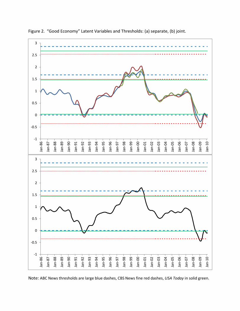
Figure 2. “Good Economy” Latent Variables and Thresholds: (a) separate, (b) joint.

Note: ABC News thresholds are large blue dashes, CBS News fine red dashes, USA Today in solid green.

-1

-0.5

0

0.5

1

1.5

2

2.5

3Ja

n-86

Jan-

87

Jan-

88

Jan-

89

Jan-

90

Jan-

91

Jan-

92

Jan-

93

Jan-

94

Jan-

95

Jan-

96

Jan-

97

Jan-

98

Jan-

99

Jan-

00

Jan-

01

Jan-

02

Jan-

03

Jan-

04

Jan-

05

Jan-

06

Jan-

07

Jan-

08

Jan-

09

Jan-

10

-1

-0.5

0

0.5

1

1.5

2

2.5

3

Jan-

86

Jan-

87

Jan-

88

Jan-

89

Jan-

90

Jan-

91

Jan-

92

Jan-

93

Jan-

94

Jan-

95

Jan-

96

Jan-

97

Jan-

98

Jan-

99

Jan-

00

Jan-

01

Jan-

02

Jan-

03

Jan-

04

Jan-

05

Jan-

06

Jan-

07

Jan-

08

Jan-

09

Jan-

10

Figure 3. “Better/Worse” Latent Variables and Thresholds: (a) separate, (b) joint.

Note: ABC News thresholds are large blue dashes, CBS News fine red dashes, USA Today in solid green.

-1.5

-1

-0.5

0

0.5

1Ja

n-87

Jan-

88

Jan-

89

Jan-

90

Jan-

91

Jan-

92

Jan-

93

Jan-

94

Jan-

95

Jan-

96

Jan-

97

Jan-

98

Jan-

99

Jan-

00

Jan-

01

Jan-

02

Jan-

03

Jan-

04

Jan-

05

Jan-

06

Jan-

07

Jan-

08

Jan-

09

Jan-

10

-1.5

-1

-0.5

0

0.5

1

Jan-

76Ja

n-77

Jan-

78Ja

n-79

Jan-

80Ja

n-81

Jan-

82Ja

n-83

Jan-

84Ja

n-85

Jan-

86Ja

n-87

Jan-

88Ja

n-89

Jan-

90Ja

n-91

Jan-

92Ja

n-93

Jan-

94Ja

n-95

Jan-

96Ja

n-97

Jan-

98Ja

n-99

Jan-

00Ja

n-01

Jan-

02Ja

n-03

Jan-

04Ja

n-05

Jan-

06Ja

n-07

Jan-

08Ja

n-09

Jan-

10

Figure 4. Four Components of the “Better/Worse” Latent Variable.

-1

-0.8

-0.6

-0.4

-0.2

0

0.2

0.4

0.6

0.8

1Ja

n-76

Jan-

77

Jan-

78

Jan-

79

Jan-

80

Jan-

81

Jan-

82

Jan-

83

Jan-

84

Jan-

85

Jan-

86

Jan-

87

Jan-

88

Jan-

89

Jan-

90

Jan-

91

Jan-

92

Jan-

93

Jan-

94

Jan-

95

Jan-

96

Jan-

97

Jan-

98

Jan-

99

Jan-

00

Jan-

01

Jan-

02

Jan-

03

Jan-

04

Jan-

05

Jan-

06

Jan-

07

Jan-

08

Jan-

09

Jan-

10

Unemployment Real GDP Growth Inflation Rate Residual