Working With the Wave Equation in Aeroacoustics- The ... With the Wave Equation in Aeroacoustics- The Pleasures of Generalized Functions F. Farassat NASA Langley Research Center, Hampton,

Working With the Wave Equation in Aeroacoustics- The Pleasures of

Generalized Functions F. Farassat

NASA Langley Research Center, Hampton, VirginiaSenior Theoretical Aeroacoustician, Fellow AIAA,

[email protected]

Kenneth S. BrentnerThe Pennsylvania State University, University Park, Pennsylvania

Associate Professor, Associate Fellow AIAA, [email protected]

Mark H. DunnNational Institute for Aerospace (NIA), Hampton, Virginia

Consultant, Senior Member AIAA, [email protected]

AbstractThe theme of this paper is the applications of generalized function (GF) theory to the wave equation inaeroacoustics. We start with a tutorial on GFs with particular emphasis on viewing functions as continu-ous linear functionals. We next define operations on GFs. The operation of interest to us in this paper isgeneralized differentiation. We give many applications of generalized differentiation, particularly for thewave equation. We discuss the use of GFs in finding Green’s function and some subtleties that only GFtheory can clarify without ambiguities. We show how the knowledge of the Green’s function of anoperator L in a given domain D can allow us to solve a whole range of problems with operator L fordomains situated within D by the imbedding method. We will show how we can use the imbeddingmethod to find the Kirchhoff formulas for stationary and moving surfaces with ease and elegance with-out the use of the four-dimensional Green’s theorem, which is commonly done. Other subjects coveredare why the derivatives in conservation laws should be viewed as generalized derivatives and what arethe consequences of doing this. In particular we show how we can imbed a problem in a larger domainfor the identical differential equation for which the Green’s function is known. The primary purpose ofthis paper is to convince the readers that GF theory is absolutely essential in aeroacoustics because of itspowerful operational properties. Furthermore, learning the subject and using it can be fun.

Nomenclature

C¶ : The space of infinitely differentiable functionsC n : The space of continuously differentiable functions up to the order n

https://ntrs.nasa.gov/search.jsp?R=20070021694 2018-07-12T05:32:06+00:00Z

D : The space of infinitely differentiable functions with compact Hclosed and boundedL supportD£ : The space of continuous linear functionals on the space D, i.e., the space of Schwartz GFsGD : Generalized derivativeGF : Generalized functionOF : Ordinary function, any function that is locally Lebesgue integrablee : Belongs to@0, 1D \ @a, bD : Set subtraction, @0, aD ‹ Hb, 1D

1- IntroductionThe linear wave equation and its counterpart in frequency domain, the Helmholtz equation, are the mostimportant partial differential equations of aeroacoustics. For example, both the Lighthill1 jet noiseequation and the Ffowcs Williams-Hawkings (FW-H) equation2 are linear wave equations. We willprimarily be concerned with the wave equation here. Although this equation in one, two, three andhigher space dimensions has been analyzed since the eighteenth century3, there are still many issues andsubtleties associated with finding the solution, particularly in aeroacoustics, that are in need of furtherattention. It is true to say, and this fact is well-known to mathematicians, that the appropriate mathemati-cal tool for solving PDEs is the theory of distributions or generalized functions (GFs)3-12 . The deriva-tion and finding the solution of the FW-H equation depend heavily on the concept of GFs whichrequires much mathematical maturity from the users. Furthermore, even when we use the Lighthillequation, we may be dealing with flowfields that have discontinuities within them, such as shocks,which can be sources of sound. The natural tool to work with these discontinuities is GF theory. Theprincipal aim of this paper is to give a working knowledge of the multidimensional GF theory to acousti-cians, particularly when using the linear wave equation.

There are many books and papers on the mathematics of the wave equation and the related problemsthat are used by acousticians. Unfortunately, almost all of the commonly referenced books and paperswere written before, or without the use of, the theory of distributions (generalized functions) of LaurentSchwartz4. These books and papers use an intuitive approach to Dirac delta function and its algebra thatis not rigorous and is prone to giving erroneous results. Furthermore, much of the true power of GFtheory is not apparent from the intuitive approach. The available books on mathematics that discussgeneralized functions (GFs) rigorously4- 6 are also beyond the reach of most acousticians because ofthe level of abstraction involved to comprehend the theory. We believe that most of the abstractions arenot necessary for application of the GFs. The situation is much like the use of the real numbers by theman in the street in everyday business without ever knowing about Cauchy convergent sequencesbecause he only needs to know the useful properties of the real numbers. For mathematically mindedpersons the abstractions in the development of the theory can be learned most easily after a workingknowledge of GFs is attained.

We will start by giving the definition of GFs as continuous linear functionals on a given space of func-tions. We will do this in the simplest possible way. We will then discuss how the definition of manyuseful operations on ordinary functions can be extended to GFs. Of particular interest to us here is thedefinition of generalized derivative and its many useful applications. These include the Green’s func-tions of ODEs and PDEs, finite part of divergent integrals, the Kirchhoff formula for moving surfacesand getting the jump condition from conservation laws. We will discuss some questions associated withthe derivation of the FW-H equation. In particular, we answer the question of whether any functionother than the null function can be assumed inside the moving surface in the derivation of the FW-Hequation. We will see that in every aspect of working with the linear wave equation, the natural mathe-matical tool is the GF theory.

FF, KSB, FF-AIAA-CEAS 2007F.nb 2

We will start by giving the definition of GFs as continuous linear functionals on a given space of func-tions. We will do this in the simplest possible way. We will then discuss how the definition of manyuseful operations on ordinary functions can be extended to GFs. Of particular interest to us here is thedefinition of generalized derivative and its many useful applications. These include the Green’s func-tions of ODEs and PDEs, finite part of divergent integrals, the Kirchhoff formula for moving surfacesand getting the jump condition from conservation laws. We will discuss some questions associated withthe derivation of the FW-H equation. In particular, we answer the question of whether any functionother than the null function can be assumed inside the moving surface in the derivation of the FW-Hequation. We will see that in every aspect of working with the linear wave equation, the natural mathe-matical tool is the GF theory.

We wish to convey to the readers our enthusiasm of working with GFs as the most essential, useful andpowerful tool for application in acoustics. We have, therefore, chosen a subtitle for this paper with anapproving nod to the title of the delightful and scholarly book of Thomas Körner13.

2- Generalized Functions (GFs)In this section we will first start by giving the definition of GFs. We then present the most commonoperations on GFs. We will pay a special attention to generalized differentiation which is the fundamen-tal concept for obtaining the Green’s function, finding the finite part of divergent integrals and workingwith jump conditions from conservation laws. We will then give many applications of GFs relevant toacoustics. We will say little about generalized Fourier transformation because that subject by itselfrequires a full paper.

In learning GF theory, you should know that there are several different approaches to the definition ofGFs. The method we present here is the functional approach of Schwartz4-11. The sequentialapproach of Temple and Lighthill14, Jones12 and Mikusinski15. The completeness theorem of GFsrelates the two approaches7. The approach by Bremermann defines GFs as the boundary value of ana-lytic functions16.This subject is valuable in studying generalized Fourier analysis and, in its full general-ity, requires the knowledge of the highly specialized topic of functions of several complex variables.Most of Bremermann’s book16 does not require this topic and for learning about one dimensional GFs,it is easily accessible to readers with a good knowledge of analytic functions of a single complex vari-able. Eventually, when you work on advanced Fourier transform theory, you will have to learnBremermann’s approach because it sheds light on the derivation of many of the results obtained byphysicists and applied mathematicians using ad hoc and mostly intuitive reasoning. The subject can beshown to be also closely related to the functional approach we use here but we will not say any moreabout this connection7.

The Polish mathematician Jan Mikusinski introduced one more method of defining GFs known as theoperational approach which is based on the concepts from abstract algebra17, 18. Mikusinski’s publica-tions are beautifully written and are easy to read and comprehend. Apart from explaining rigorously theHeaviside operational calculus, this approach can also be used to solve an entirely different set of prob-lems than the first three approaches, such as finding the exact solutions to finite difference equations andrecursion relations. The relationship between the Mikusinski’s operational approach and the functionalapproach cannot be established easily and we are not aware of any publications on the subject. Weencourage the readers to study this approach because of its usefulness and power in solving some impor-tant problems of physics and engineering17- 20. We will say no more on this approach here.

And finally, the readers should be aware of the fact that in recent years GF theory has been extended tothe so-called nonlinear GF (NLGF) theory where some of the limitations of Schwartz distribution (GF)theory are removed21- 23 . For example, it can be shown that one cannot extend the operation of multipli-cation to all of Schwartz GFs. This shortcoming of the Schwartz theory does cause some difficulties inapplications that Colombeau21, Rosinger22 and Oberguggenberger23 as well as other mathematicianshave tried to resolve. Currently, the NLGF theory is very abstract and difficult to master. The subject isunder intense development but is badly in need of simplification. However, it appears that the subject ofnonstandard analysis HNSAL24 will eventually be able to clarify and simplify NLGF theory considerablyand bring the theory within the reach of physicists and engineers25. We will not cover this subject here.The readers should know that to understand NLGF theory and NSA, requiring one to have a knowledgeof several esoteric areas of mathematics including topology, abstract algebra and mathematical logic.Fortunately, there are many expository books and articles on these subjects on the internet, particularlyon NSA. We will not cover this theory here.


And finally, the readers should be aware of the fact that in recent years GF theory has been extended tothe so-called nonlinear GF (NLGF) theory where some of the limitations of Schwartz distribution (GF)theory are removed21- 23 . For example, it can be shown that one cannot extend the operation of multipli-cation to all of Schwartz GFs. This shortcoming of the Schwartz theory does cause some difficulties inapplications that Colombeau21, Rosinger22 and Oberguggenberger23 as well as other mathematicianshave tried to resolve. Currently, the NLGF theory is very abstract and difficult to master. The subject isunder intense development but is badly in need of simplification. However, it appears that the subject ofnonstandard analysis HNSAL24 will eventually be able to clarify and simplify NLGF theory considerablyand bring the theory within the reach of physicists and engineers25. We will not cover this subject here.The readers should know that to understand NLGF theory and NSA, requiring one to have a knowledgeof several esoteric areas of mathematics including topology, abstract algebra and mathematical logic.Fortunately, there are many expository books and articles on these subjects on the internet, particularlyon NSA. We will not cover this theory here.

For those interested in the history of GF theory, we recommend the books by Lützen26 and Dieudon-né27 as well as the article by Synowiec28 . In the opinion of Lützen, the Russian mathematician Sobolevinvented the concept of GFs (more exactly, generalized derivatives) and Schwartz developed the theoryof GFs without being aware of Sobolev’s earlier contributions4. As expected, many other mathemati-cians contributed to the field. Without a doubt, the members of the Moscow School of Mathematicsunder I. M. Gelfand have contributed substantially to the development and applications of GF theorymaking the subject accessible to physicists and engineers. The well-known book on GFs by Gelfand andShilov7 is the first of a six volume opus by this School published in the West in the sixties of the lastcentury. This monumental work, which is still read today, has popularized the GF theory enormouslyamong physicists and mathematicians by its breadth and depth as well as by the clarity of the exposition.For learning about more recent advances we suggest the books by Hörmander5 and Taylor6 which areboth written for mathematicians.

Most of this section is based on the first author’s expository NASA publication29. In addition to thispublication, we recommend that you consult the books by Strichartz10, Stakgold8, Gelfand and Shilov7,and Kanwal11. For beginners, we particularly recommend the excellent book by Strichartz for deeperunderstanding of many of the concepts discussed here. This book emphasizes GFs in one dimensionwhich is essential in some applications, e.g., time series analysis. However, there are many problems ofphysics and engineering for which multidimensional GF theory is very important7- 9, 11, 12, 29. This isthe subject that we concentrate in the present paper. The emphasis will be on using the theory to solveproblems rather than stating theorems and giving proofs.

2.1- Definition of Generalized Functions (GFs)What we call a function, say f HxL , in calculus can be thought of as a table of ordered pairs Hx, f HxLL . Wecan visualize this table as a graph of x versus y = f HxL . If we want to generalize the concept of a func-tion, we must change the definition of a function in such a way that our old functions are still consideredfunctions and we have many new useful mathematical objects that are functions by the new definition.Once we introduce a new definition of a function, we must make sure that we can extend all the usefuloperational properties of the old functions, e.g., addition of two functions, to all the new mathematicalobjects which we now collectively (the old functions and the new objects) call generalized functions(GFs). For now, we refer to all the functions that we learned about in calculus as ordinary functions(OFs). We will elaborate further on this below.

Let us start by considering an ordinary function gHxL which is periodic over the interval @0, 2 pD . Weknow that the complex Fourier components of this function are given by the relation

(1)Gn =1

ÅÅÅÅÅÅÅÅÅÅ2 p

‡0

2 p

gHxL e- i n x d x Hn = -¶ to ¶LWe know that gHxL = ⁄ n =-¶

¶ Gn ei n x , that is, the periodic function gHxL can be constructed from theknowledge of the table with infinite entry 8Gn , n = -¶ to ¶< . From another point of view, the set ofcomplex numbers 8Gn< can be considered as the mapping of the space of functions 9ei n x , n = -¶ to ¶=into complex numbers by the rule given in eq. (1). Such a mapping from a given space of functions intoscalars (real or complex numbers) is called a functional. Remember that a functional is always a rulethat describes the mapping from a given space of functions into scalars. The numbers 8Gn< are thefunctional values of this functional. Note that the function gHxL enters the definition of the functional. Asa matter of fact, we should use the symbol Gn@gD to remind us that the number Gn depends on the func-tion gHxL . So far we have shown that the periodic function gHxL can be described (identified, defined) bythe table of its functional values:


We know that gHxL = ⁄ n =-¶¶ Gn ei n x , that is, the periodic function gHxL can be constructed from the

knowledge of the table with infinite entry 8Gn , n = -¶ to ¶< . From another point of view, the set ofcomplex numbers 8Gn< can be considered as the mapping of the space of functions 9ei n x , n = -¶ to ¶=into complex numbers by the rule given in eq. (1). Such a mapping from a given space of functions intoscalars (real or complex numbers) is called a functional. Remember that a functional is always a rulethat describes the mapping from a given space of functions into scalars. The numbers 8Gn< are thefunctional values of this functional. Note that the function gHxL enters the definition of the functional. Asa matter of fact, we should use the symbol Gn@gD to remind us that the number Gn depends on the func-tion gHxL . So far we have shown that the periodic function gHxL can be described (identified, defined) bythe table of its functional values:

(2)lomno

Gn@gD =1

ÅÅÅÅÅÅÅÅÅÅ2 p

‡0

2 p

gHxL e- i n x d x, n = -¶ to ¶|o}~o

on the space 9ei n x , n = -¶ to ¶=

We have assumed here that the function gHxL has a Fourier series (e.g., satisfies the Dirichlet conditions,etc.). Now we have the germ of an idea to extend the definition of a function.

Let us take a space of functions of one variable D with a large number of well-defined functions in thespace. We will say more about the properties of the functions in this space soon. Let us select an ordi-nary function f HxL and for any function f HxL in the space D , define the functional (i.e., the rule):

(3)F@fD = ‡-¶

¶

f HxL f HxL d x H f is fixed in this rule and f varies all over DLNote carefully how the function f HxL enters the definition of the functional. To describe f , this functionis kept fixed in the rule given by eq. (3) and different functions f are taken (conceptually, of course, notliterally) from the space D to form the table 8F@fD, f e D< . Therefore, we must have so many functionsin space D that any two different ordinary functions generate different tables of functional values atleast for some entries. The space D is known as the test function space. The question is how to selectthe space D in such a way that the set of the functional values 8F@fD, f D< represents (i.e., describes orhas as much information content as) any ordinary function f HxL . Before we do this, we must now elabo-rate on what we mean by ordinary functions.

By ordinary functions (OFs), we mean the locally Lebesgue integrable functions. This means that theyare functions that are Lebesgue integrable7- 11, 19 over any finite interval. These functions include anyconceivable functions, no matter how wild, that are needed in applications. If you do not know Leb-esgue integration, you can think of Riemann integration that you learned in calculus courses. Lebesgueintegration is a generalization of the Riemann integration that can be used for the integration of mostfunctions that do not have Riemann integral.

One can show that there is an uncountable number of OFs. Therefore, the space of test functions mustcontain an uncountable number of functions so that any two different OFs can be distinguished fromeach other when viewed as tables of functional values. This means that our tables of functional valuesused to represent OFs are also uncountable. Furthermore, since OFs are as wild as they can be, werequire that the functions in space D to be as well-behaved as they can be so that the integral in eq. (3) isalways defined. This leads us to require that the functions in D to be infinitely differentiable (denotedC¶ functions). Also to ensure the integral in eq. (3) does not become infinite, we assume that all func-tions in space D are identically zero outside of a finite interval. This interval can be different for differ-ent test functions. A function that is identically zero outside some finite interval is said to have boundedsupport. Thus, we have come to the following conclusion regarding the space of test functions D that weneed to use to identify OFs by their tables of functional values:


One can show that there is an uncountable number of OFs. Therefore, the space of test functions mustcontain an uncountable number of functions so that any two different OFs can be distinguished fromeach other when viewed as tables of functional values. This means that our tables of functional valuesused to represent OFs are also uncountable. Furthermore, since OFs are as wild as they can be, werequire that the functions in space D to be as well-behaved as they can be so that the integral in eq. (3) isalways defined. This leads us to require that the functions in D to be infinitely differentiable (denotedC¶ functions). Also to ensure the integral in eq. (3) does not become infinite, we assume that all func-tions in space D are identically zero outside of a finite interval. This interval can be different for differ-ent test functions. A function that is identically zero outside some finite interval is said to have boundedsupport. Thus, we have come to the following conclusion regarding the space of test functions D that weneed to use to identify OFs by their tables of functional values:

The test function space D that one needs to use in defining OFs by their tables of functionalvalues is the space of all C¶ functions with compact Hclosed and boundedL support.

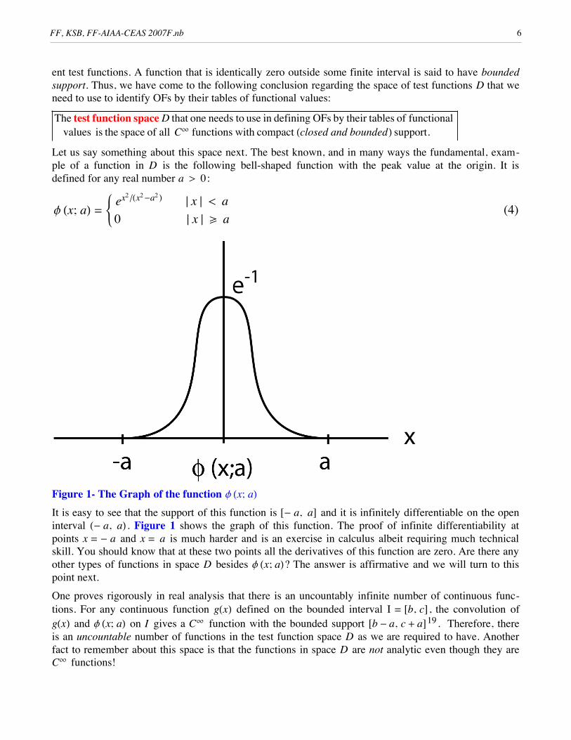
Let us say something about this space next. The best known, and in many ways the fundamental, exam-ple of a function in D is the following bell-shaped function with the peak value at the origin. It isdefined for any real number a > 0:

(4)f Hx; aL =lomno

ex2 êHx2 -a2 L † x § < a0 † x § r a

Figure 1- The Graph of the function f Hx; aLIt is easy to see that the support of this function is @- a, aD and it is infinitely differentiable on the openinterval H- a, aL . Figure 1 shows the graph of this function. The proof of infinite differentiability atpoints x = - a and x = a is much harder and is an exercise in calculus albeit requiring much technicalskill. You should know that at these two points all the derivatives of this function are zero. Are there anyother types of functions in space D besides f Hx; aL? The answer is affirmative and we will turn to thispoint next.

One proves rigorously in real analysis that there is an uncountably infinite number of continuous func-tions. For any continuous function gHxL defined on the bounded interval I = @b, cD , the convolution ofgHxL and f Hx; aL on I gives a C¶ function with the bounded support @b - a, c + aD19 . Therefore, thereis an uncountable number of functions in the test function space D as we are required to have. Anotherfact to remember about this space is that the functions in space D are not analytic even though they areC¶ functions!

At this stage, we have a new way of looking at OFs but our original intention was to extend the defini-tion of a function so that we have new objects that are not OFs but are considered functions. To do thiswe study two important properties of the functionals described by eq. (3). The first one is very easy tosee:


At this stage, we have a new way of looking at OFs but our original intention was to extend the defini-tion of a function so that we have new objects that are not OFs but are considered functions. To do thiswe study two important properties of the functionals described by eq. (3). The first one is very easy tosee:

1 - The functional F@fD is linear.

This simply means that for a and b scalars and f and y functions in D , we have

(5)F@a f + b yD = a F@fD + b F@yDTo show this, replace f HxL on the right of eq. (3) with a f + b y and use the linearity property of inte-grals followed by functional interpretation of the result to get the right side of eq. (4). We remind thereaders that the OF f HxL used in the definition of the functional of eq. (3) is fixed here and the functionalF@fD is, in point of fact, representing f HxL.The second property is much harder to explain and comprehend. It is:

2 - The functional F@fD is continuous.

The first thing you must know is that this property, whatever it means, gives GFs a lot of useful proper-ties that we need in applications. Second, to the beginners the definition of continuity of a functionalappears too complicated and perhaps a futile attempt in abstraction. We admit that the definition of thecontinuity of a functional is complicated but its definition cannot be stated in simpler form than we givehere. The original definition by Schwartz was much more complicated and based on locally convextopological spaces4. Just remember that you will appreciate the full usefulness of this property whenyou learn some more about GFs and their applications. See, for instance, Example 3 below.

We first distinguish some sequences of functions 8f n< in D, which we say they go to zero in D , and

write it as f n ö 0D

. For any such sequence, we require that it satisfies two conditions:

i- There is a bounded interval J such that the support of f n Õ J for all n , and

ii- fn and all its derivatives go to zero uniformly in J .

We make two useful comments here concerning these conditions. First, in general, different sequencesgoing to zero in D have different bounded interval J associated with them. In other words, we requireonly that for a given sequence going to zero in D such a bounded interval to exist. Second, condition iisimply means that if m is the order of the derivative, m = 0, 1, 2, ...., and given > 0, we can find NHmL such that for any x in the interval J , we have °fn

HmL HxL• < for all n > NHmL .Note that the word “uniformly” means that the number NHmL is independent of x but it can depend onthe order of differentiation m . Here we have used the notation f n

HmLHxL for the mth derivative of f nHxL. Example 1- We can show easily that the following sequence goes to zero in D :

(6)f nHxL =1ÅÅÅÅÅn

f Hx; aL HSee eq. H4L for the definition of f Hx; aLLExample 2- The following sequence of functions does not go to zero in D:

(7)f nHxL =1ÅÅÅÅÅn

f J xÅÅÅÅÅn

; aN HSee eq. H4L for the definition of f Hx; aLL


The reason is that for a given function f n , the support is the interval @-n a, n aD and, therefore, thesupport cannot remain bounded for all n. Condition ii is, thus, violated.

Now we can give the definition of continuity of a functional:

A functional F@fD is continuous if for any f n ö 0D

, we have F@f nDö0 .

Note that 8F@f nD < is simply a sequence of real or complex numbers. By using the properties of (Leb-esgue) integrals, we can show the following very important result:

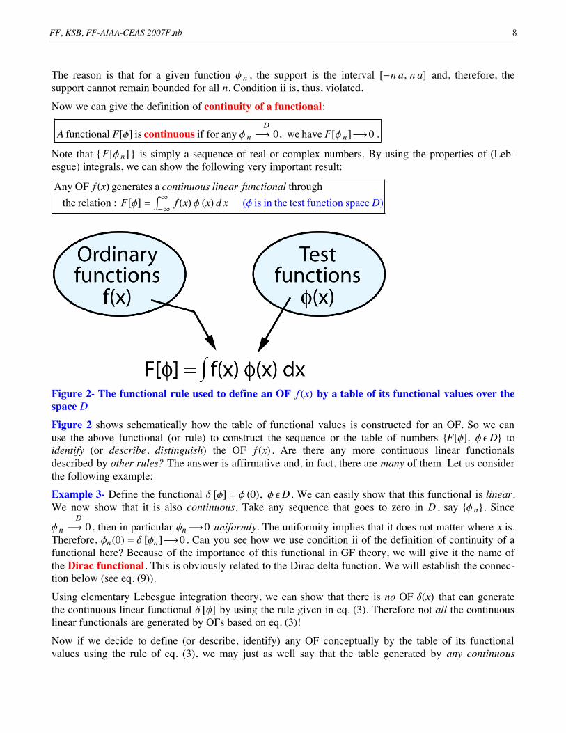
Any OF f HxL generates a continuous linear functional throughthe relation : F@fD = Ÿ-¶

¶ f HxL f HxL d x Hf is in the test function space DL

Figure 2- The functional rule used to define an OF f HxL by a table of its functional values over thespace DFigure 2 shows schematically how the table of functional values is constructed for an OF. So we canuse the above functional (or rule) to construct the sequence or the table of numbers 8F@fD, f e D< toidentify (or describe, distinguish) the OF f HxL . Are there any more continuous linear functionalsdescribed by other rules? The answer is affirmative and, in fact, there are many of them. Let us considerthe following example:

Example 3- Define the functional d @fD = f H0L, f e D . We can easily show that this functional is linear.We now show that it is also continuous. Take any sequence that goes to zero in D , say 8f n< . Since

f n ö 0D

, then in particular fn ö0 uniformly. The uniformity implies that it does not matter where x is.Therefore, fnH0L = d @fnDö0. Can you see how we use condition ii of the definition of continuity of afunctional here? Because of the importance of this functional in GF theory, we will give it the name ofthe Dirac functional. This is obviously related to the Dirac delta function. We will establish the connec-tion below (see eq. (9)).

Using elementary Lebesgue integration theory, we can show that there is no OF dHxL that can generatethe continuous linear functional d @fD by using the rule given in eq. (3). Therefore not all the continuouslinear functionals are generated by OFs based on eq. (3)!

Now if we decide to define (or describe, identify) any OF conceptually by the table of its functionalvalues using the rule of eq. (3), we may just as well say that the table generated by any continuouslinear functional also defines a function. We now have new objects (tables) that cannot be identifiedwith OFs, e.g., the functional in Example 3. We call the entire collection of objects (tables of functionalvalues) generalized functions (GFs). We have achieved our goal of generalizing the definition of OFs.We, thus, state the following:


Now if we decide to define (or describe, identify) any OF conceptually by the table of its functionalvalues using the rule of eq. (3), we may just as well say that the table generated by any continuouslinear functional also defines a function. We now have new objects (tables) that cannot be identifiedwith OFs, e.g., the functional in Example 3. We call the entire collection of objects (tables of functionalvalues) generalized functions (GFs). We have achieved our goal of generalizing the definition of OFs.We, thus, state the following:

Generalized functions are defined by the tables of functional values of continuous linear functionals.

Since we are now going to think of functions in the new way by their functional values, we will use aslight abuse of language and say:

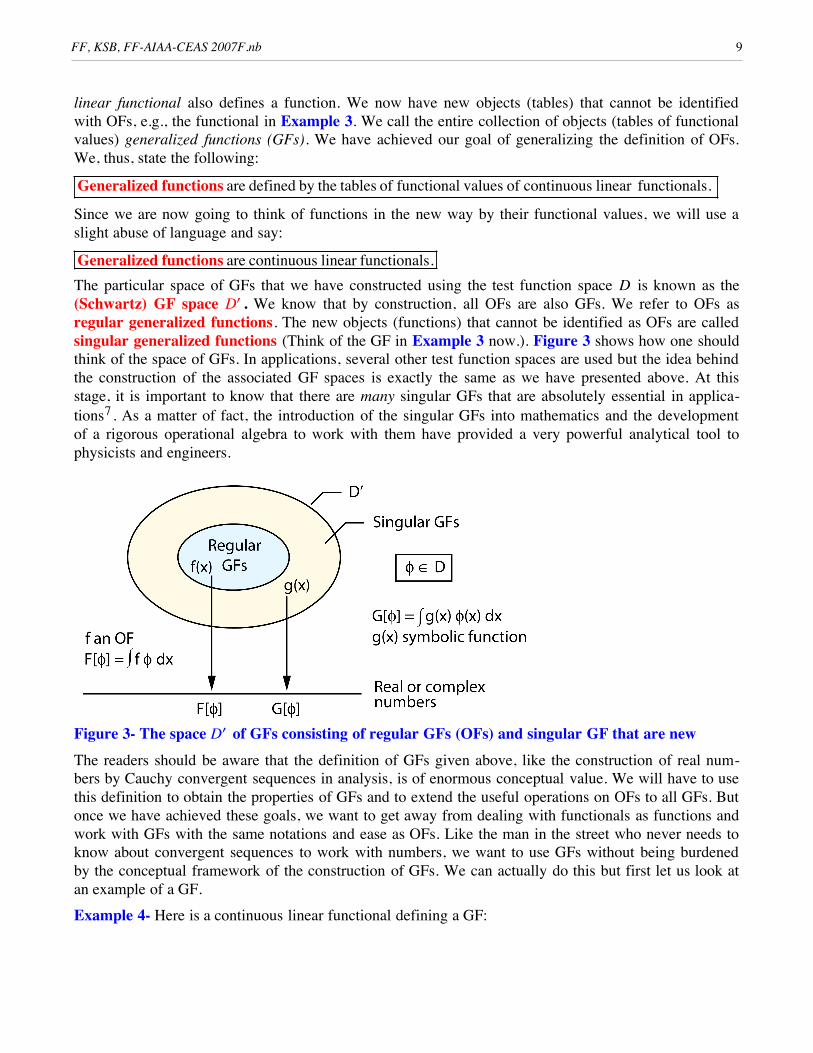
Generalized functions are continuous linear functionals.The particular space of GFs that we have constructed using the test function space D is known as the(Schwartz) GF space D£ . We know that by construction, all OFs are also GFs. We refer to OFs asregular generalized functions. The new objects (functions) that cannot be identified as OFs are calledsingular generalized functions (Think of the GF in Example 3 now.). Figure 3 shows how one shouldthink of the space of GFs. In applications, several other test function spaces are used but the idea behindthe construction of the associated GF spaces is exactly the same as we have presented above. At thisstage, it is important to know that there are many singular GFs that are absolutely essential in applica-tions7. As a matter of fact, the introduction of the singular GFs into mathematics and the developmentof a rigorous operational algebra to work with them have provided a very powerful analytical tool tophysicists and engineers.

Figure 3- The space D£ of GFs consisting of regular GFs (OFs) and singular GF that are newThe readers should be aware that the definition of GFs given above, like the construction of real num-bers by Cauchy convergent sequences in analysis, is of enormous conceptual value. We will have to usethis definition to obtain the properties of GFs and to extend the useful operations on OFs to all GFs. Butonce we have achieved these goals, we want to get away from dealing with functionals as functions andwork with GFs with the same notations and ease as OFs. Like the man in the street who never needs toknow about convergent sequences to work with numbers, we want to use GFs without being burdenedby the conceptual framework of the construction of GFs. We can actually do this but first let us look atan example of a GF.

Example 4- Here is a continuous linear functional defining a GF:


(8)G@fD = ‡-¶

¶

e2 x sin 3 x f HxL d x - 5 f H0L f e D

You should have little problem to prove this fact. Note that, in practice, we always give the rule (thedefinition of the functional) only and we do not attempt to construct the table of the functional valuesbecause it is technically impossible. But we can use the rule to make part of the table if we want to!

We will now dispose of the functional notation by the introduction of symbolic functions. This is abrilliant idea. It will allow us to work with singular generalized functions just like the OFs. We startwith the Dirac functional of Example 3 which is a singular GF. We introduce a symbolic function dHxLwhich is supposed to hold the information (or the memory) about the Dirac functional when we aredoing algebraic manipulations until it appears as an integrand of an integral in a product with a testfunction.We then use the following relation agreed upon by convention:

(9)‡-¶

¶

f HxL dHxL d x ª d@fD = f H0L f e D

It is very important to recognize that ‘the integral’ on the left of this equation is not a Riemann or aLebesgue integral because dHxL is not an OF. You should think of the whole integral symbol like aChinese character standing for d@fD = f H0L which is now completely meaningful. The symbolic functiondHxL , known universally as the Dirac delta function, can be used in algebraic manipulations like an OFuntil it appears under an integral sign like that on the left of eq. (9). You should, however, learn somemore about the properties of singular GFs before you can comfortably or boldly manipulate them algebra-ically. We will give you what you need to know later but first let us look again at Example 4 usingsymbolic function notation.

Example 5- The GF in Example 4 can be written symbolically as gHxL = e2 x sin 3 x - 5 dHxL . This GF isthe sum of a regular and a singular GF.

2.2 - Multidimensional GFsThe above definition of GFs can easily extended to multidimensions. The test function space D is now n-dimensional and consists of all infinitely differentiable functions with bounded support. An example of such a function can be constructed from the function in eq. (4). Let x = Hx1, x2, ...., xnL , and † x§ = Ix1

2 + x22 + ... + xn

2M1ê2 . Then the we can show that for a > 0, the following function is in space D :

(10)f Hx; aL =loomnoo

e† x§2ëI † x§2 -a2 M † x § < a

0 † x § r a

From this function and any continuous function, we can generate another test function by convolutionover a finite region of space. Therefore, the space of test functions D has an uncountably many func-tions in it. We then define the multidimensional (Schwartz) GF space D¢ as the space of continuouslinear functionals on D . This definition is appropriate for discovering the operational properties of GFsthat give us a powerful tool for applications. In practice, however, we will work with symbolic functionswhen we deal with singular generalized functions. Therefore, we will be always working with general-ized functions as if we are working with OFs. Intuitively, this is of great help to people interested inapplications. The situation is similar to the use of identical notations for real and complex numbers asmuch as possible when we are solving a problem in complex plane.


From this function and any continuous function, we can generate another test function by convolutionover a finite region of space. Therefore, the space of test functions D has an uncountably many func-tions in it. We then define the multidimensional (Schwartz) GF space D¢ as the space of continuouslinear functionals on D . This definition is appropriate for discovering the operational properties of GFsthat give us a powerful tool for applications. In practice, however, we will work with symbolic functionswhen we deal with singular generalized functions. Therefore, we will be always working with general-ized functions as if we are working with OFs. Intuitively, this is of great help to people interested inapplications. The situation is similar to the use of identical notations for real and complex numbers asmuch as possible when we are solving a problem in complex plane.

From our point of view, the multidimensional generalized functions are much more important than GFsof one variable in studying partial differential equations and in particular wave propagation problems. Itis important to recognize that to study the multidimensional GFs, one needs to have a working knowl-edge of differential geometry of curves and surfaces30.

As in the case of one variable, the most important singular GFs in multidimensions are the Dirac deltafunction and its derivatives. Of interest to us is the delta function with the support on a surface whichcan be in motion. This function has no one dimensional analogue. We start with a simple example andthen discus the Dirac delta function with the support on a surface.

Example 6- The Dirac delta function dHxL with support at the origin has the following property

(11)‡V

fHxL dHxL d x = f H0L f e D

where V is an arbitrary volume which includes the origin.

Example 7- Referring to Figure 4, let S : f HxL = 0 be a smooth surface defined in such a way that theunit outward normal n = ı f . This can always be done because if n ı f , then define this surface bythe new implicit function f HxL ê † ı f § = 0 which has the desired property.

Figure 4- The description of the surface S defined implicitly by f HxL = 0 with unit outward normaln = ı f .We want to interpret the important GF dH f L often appearing in applications. We define a Gaussiancurvilinear coordinates Iu1, u2M over the surface S and define the third coordinate u3 = f along the localnormal to S to all points in the space in the vicinity of S . Note that we have

(12)d x = "##############gH2L HuL d u u = Iu1, u2, u3Mwhere gH2L HuL is the determinant of the first fundamental form of the surfaceu3 = f HxL = constant 29- 31. We thus have the following very useful result


(13)‡ dH f L f HxL d x = ‡ dIu3M f HxHuLL "##############gH2L HuL d u1 d u2 d u3 =

‡ f IxIu1 , u2, 0MM "###########################gH2L Hu1, u2, 0L d u1 d u2 = ‡f = 0

f HxL d S

You can see the importance of differential geometry here. Note that we have used the definition of theDirac delta function in one variable when we integrate with respect to variable u3 after the secondequality sign. For a more geometric derivation of this result see the papers by Farassat29, 31 .

It is important to remember that one cannot define a GF at a single point but over a finite interval. Thisdoes not cause any difficulties in applications. We can talk about equality of two GFs over an interval.We say that two GFs F@fD and G@fD are equal over an interval I if for all f e D with support fullywithin I , we have F@fD = G@fD . Remember, a functional is a rule that gives us a number for any functionin D . Therefore, we are talking about equality of two numbers obtained from two rules. From this defini-tion we can say that d HxL = 0 (the zero function and not the real number zero) over the intervalH-¶, -D ‹ @, ¶L for any > 0.

To learn more about the multidimensional GFs we recommend the books by Gelfand and Shilov7,Stakgold8, Vladimirov9, Kanwal11, Jones12 , Fenyo and Frey19, and the two NASA papers by Faras-sat29, 31. For more advanced treatment as well some very important recent advances, see the books byHörmander5 and Taylor6.

2.3- Operations on GFsNow that we have extended the definition of ODs to GFs, we must extend the definitions of operationson OFs to GFs. The general approach is as follows. Write the definition of the operation in the languageof linear functionals and then use it for all GFs if it makes any sense (see the definition of generalizedFourier Transform below where we have to change the test function space). In some cases the extensionof the definition of an operation gives us the opportunity to solve new problems or solve old problems inmuch simpler ways. We single out generalized differentiation here as an example of an operation ofconsiderable importance in applied mathematics.

In the following we assume that all test functions are in space D .

2.3.1- Simple Operations1- Addition of two GFs- If f HxL and gHxL are two OFs described by functionals F@fD and G@fD , f e Dthen using the linear property of integrals, we can write

(14)‡ H f + gL f d x = ‡ f f d x + ‡ g f d x = F@fD + G@fDBasically, we know the left side of the first equality is the functional representation of the sum of theOFs f HxL and gHxL and is given by the right side of the last equality sign. The above result now makessense for all GFs, i.e., we define

(15)HF + GL@fD = F@fD + G@fD


Note that HF + GL is a single functional which stands for the sum of the two GFs.

Written in symbolic function notation, there is no difference between the notation for OFs and GFs forthe sum of two functions. For example, for the sum of an OF f HxL and the Dirac delta function we cansimply write f HxL + dHxL . 2- Multiplication of two GFs- This operation cannot be extended to all of Schwartz GFs. In fact it isthe aim of the new nonlinear GF theory to be able to define multiplication for all GFs22, 23. Any twoOFs can be multiplied. We can define multiplication of any GF with any C¶ function. Again let f HxL beany OF and let aHxL e C¶ , then

(16)‡ aHxL f HxL f HxL d x = ‡ f HxL HaHxL fHxLL d x = F@a fDWe know that the left side of the first equality sign is the functional representation of the OF aHxL f HxL .Since the function a f e D , the expression on the right of the third equality sign is a functional on the testfunction space D. The rule of multiplication of a generalized function F@fD and a C¶ function aHxL isgiven by the rule

(17)aF@fD = F@a fDNote that in this equation, the symbol aF stands for a single functional, i.e., a rule described by the rightside of eq. (17). Again in symbolic notation we simply write aHxL f HxL but now we have a rule to inter-pret such products when f HxL is a singular GF. We give an example here.

Example 8- What is aHxL dHxL where a e C¶ ? Let f e D, then

(18)a d@fD = ‡ aHxL dHxL d x = d @a fD = aH0L f H0L = ‡ aH0L dHxL d x

We can write this result in symbolic function notation as

(19)aHxL dHxL = aH0L dHxLThis useful result has been known for many years to physicists.

3- Translation of a GF- Let f HxL be an OF, and let us define Eh f HxL = f Hx - hL , i.e., translating thefunction to the right for h > 0. In functional notation, we have

(20)‡ Eh f HxL fHxL d x = ‡ f Hx - hL fHxL d x = ‡ f HyL f Hy + hL d y = F@E-h fDAgain the left side of the first equality sign is the functional generated by Eh f HxL for which we use thesymbol Eh F@fD . Since for f e D , we have E-h f e D. Therefore, we use the following result for thedefinition of the translation of any GF:

(21)Eh F@fD = F@E-h fDOnce again we have obtained a nontrivial result. In symbolic function notation we use the same notationfor GFs as for OFs but occasionally we have to resort to eq. (21) to interpret the exact meaning of thetranslated GF such as in the following example.


Example 9- What is dHx - aL where a is a real constant? The functional representation of this GF isobviously Ea d@fD. Using the above rule, we have

(22)‡ dHx - aL fHxL d x = Ea d@fD = d@E- a fD = d@fHx + aLD = fHaLAgain this result has been known by physicists for a long time.

We can extend the definition of other simple operations on OFs to GFs such as the expansion and con-traction of the scale of the independent variable. For example, one can rigorously show that for a 0 wehave the following useful result

(23)dHa xL =1

ÅÅÅÅÅÅÅÅÅÅÅ† a § dHxL

2.3.2- More Advanced OperationsWe will extend the definition of two operations on OFs to GFs here. These are Fourier transformationand differentiation operations.

1- Fourier Transform of GFs- We work in one dimension here. Let f HxL be a function defined on !which has Fourier transform define by the relation

(24)f`HyL = ‡

-¶

¶

f HxL e2 p i x y d x

If the functional F@fD is identified with f HxL , then its Fourier transform must be identified with f`HyL as

follows

(25)F` @fD = ‡

-¶

¶

f`HyL f HyL d y = ‡

-¶

¶

f HyL f` HyL d y = F@f` D

where f`

is the Fourier transform of f . We have used Parseval’s theorem after the second equality sign.Now the functional F@f` D is only defined if f

`e D whenever f e D. We can show that, in general, this is

not so and f`

can lie outside the space D . We need to define a test function space S on ! consisting ofC¶ functions which go to zero at infinity faster than † x - n § for any n . This can be done and in fact wecan show that D Õ S . The space of tempered GFs S£ is the space of all continuous linear functionals onS . An important relation to remember is D Õ S Õ S£ Õ D£ . All the GFs in the space S£ have generalizedFourier transform given by the relation F

` @fD = F@f` D where now f e S . We will say no more on thisinteresting subject here. See the references at the end of this paper. We strongly recommend the book byStrichartz10 for this subject.

2- Differentiation of GFs- This is the most important operation on GFs because of its many applica-tions in mathematics. Many of the problems of wave propagation need the use of this concept. Let usstart with a C1 function f HxL which we identify with the functional F@fD . The functional representationof f £HxL can be manipulated as follows


(26)F£@fD = ‡ f £HxL f HxL d x = -‡ f HxL f£HxL d x = -F@f£DNote that we have integrated by parts after the second equality sign and we have used the fact that thesupport of f is compact to drop the terms involving the limits of the integral. Since we know that thefunction f£ is in D , F@f£D is a proper functional on D and we can use the following relation for thedefinition of the generalized derivative (GD) of a GF

(27)F£@fD = -F@f£DFrom this we can define the nth generalized derivative of a GF

(28)FHnL @fD = H-1L n FAf HnLEThis significant result states that GFs have GDs of all orders. When we work with symbolic functionswe often utilize a bar over a derivative operator to designate generalized differentiation if theoperation can be confused with ordinary differentiation. See eqs. (30) and (34) below. It is understoodthat the differentiation of singular GFs can only be GD and in that case we will not use this notation.

Example 10- GD of the Heaviside function hHxL = 0 for x < 0 and hHxL = 1 for x > 0 is found as follows

(29)H £@fD = -H@f£D = -‡0

¶

f£ HxL d x = f H0LNote that we have used the fact that the test function has a bounded support and, thus, we havefH¶L = 0. Therefore, we have

(30)hêê£HxL = dHxL

That is, the GD of the Heaviside function is the Dirac delta function. Note that h£HxL = 0 but hêê£HxL 0.

We will return to this point later. This result shows that the GD of an OF can be a singular GF! Example 11- Generalized derivative of the Dirac delta function is

(31)d£@fD = ‡ d£HxL f HxL d x = -d@f£D = -f£H0LSimilarly, we have

(32)d HnL @fD = ‡ d HnL HxL f HxL d x = H-1L n f HnL H0LNote that in eqs. (31) and (32), the integrals are meaningless and stand for the functional rules to the leftof the first equality sign in the respective equations.

Example 12- Let the OF f HxL be differentiable with a single jump of Û f = f Hx0+L - f Hx0-L at the pointx0 as shown in Figure 5.


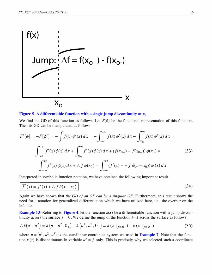
Figure 5- A differentiable function with a single jump discontinuity at x0

We find the GD of this function as follows. Let F@fD be the functional representation of this function.Then its GD can be manipulated as follows

(33)

F£@fD = -F@f£D = -‡ f HxL f£HxL d x = -‡-¶

x0-

f HxL f£HxL d x - ‡x0+

¶

f HxL f£HxL d x =

‡-¶

x0-

f £HxL fHxL d x + ‡x0+

¶

f £HxL fHxL d x + H f Hx0+L - f Hx0-LL fHx0L =

‡-¶

¶

f £HxL fHxL d x + Û f fHx0 L = ‡-¶

¶

H f £HxL + Û f dHx - x0LL f HxL d x

Interpreted in symbolic function notation, we have obtained the following important result

(34)fêê£HxL = f £HxL + Û f dHx - x0L

Again we have shown that the GD of an OF can be a singular GF. Furthermore, this result shows theneed for a notation for generalized differentiation which we have utilized here, i.e., the overbar on theleft side.

Example 13- Referring to Figure 4, let the function kHxL be a differentiable function with a jump discon-tinuity across the surface f = 0. We define the jump of the function kHxL across the surface as follows:

(35)Û kIu1, u2M = k Iu1, u2, 0+M - k Iu1, u2, 0-M ª k Hx » f = 0+L - k Hx » f = 0-Lwhere u = Iu1, u2, u3M is the curvilinear coordinate system we used in Example 7. Note that the func-tion k HxL is discontinuous in variable u3 = f only. This is precisely why we selected such a coordinatesystem in the vicinity of the surface of discontinuity. Now we are going to use eq. (34) to derive thefollowing important result:


where u = Iu1, u2, u3M is the curvilinear coordinate system we used in Example 7. Note that the func-tion k HxL is discontinuous in variable u3 = f only. This is precisely why we selected such a coordinatesystem in the vicinity of the surface of discontinuity. Now we are going to use eq. (34) to derive thefollowing important result:

(36)

êê

k Hx HuLLÅÅÅÅÅÅÅÅÅÅÅÅÅÅÅÅÅÅÅÅÅÅÅÅÅÅÅÅ

xi=

ujÅÅÅÅÅÅÅÅÅÅÅÅ xi

k

ÅÅÅÅÅÅÅÅÅÅÅÅuj + Û k

u3ÅÅÅÅÅÅÅÅÅÅÅÅ xi

d Iu3M =k

ÅÅÅÅÅÅÅÅÅÅÅxi

+ Û k f


d H f L =k


+ Û k ni d H f LWe have used the summation convention on repeated index in the above equation. We can write theabove result in vector notation as follows:

(37)ıêêê k HxL = ı k HxL + Û k n d H f L HNote n = ı f here.LWe give here two more important relations which can be remembered easily. Let k HxL be a vector fieldwith a jump discontinuity across the surface f = 0 with the jump defined similar to eq. (35). Then thefollowing results hold:

(38)ıêêê ÿk HxL = ı ÿk HxL + Û k ÿ n d H f L HNote n = ı f here.L(39)ıêêê µk HxL = ıµ k HxL + nµÛ k d H f L HNote n = ı f here.L

With what we have obtained so far we can solve a lot of interesting problems. Before we give someexamples, let us say a little more about why one should use generalized derivative.

2.4- Why We Use Generalized DerivativesThe most important fact to remember about GDs is that in GF theory generalized differentiation is acontinuous operation. In particular, generalized differentiation and integration are inverse operations.This means that the integration of GD of a GF recovers the function faithfully with all of its jumps.Examine the following

Example 14- Let hHxL be the Heaviside function defined in Example 10. Then we can easily show that

(40)‡-¶

xhêê £

HyL d y = h HxL but ‡-¶

xh £ HyL d y = constant h HxL

Therefore, any problem involving unknowns with discontinuities should be set up in GF space andall derivatives must be treated as GDs from the start. Such discontinuities are either artificiallyintroduced, e.g., as in FW-H equation, or are genuine, e.g., a shock wave in the flow field. The state-ment following eq. (40) has profound implications for applications some of which will mentioned below:

1- All local conservation laws obtained from control volume analysis are valid if all the derivativesare considered GDs. Examples of such conservation laws are the mass continuity and the Navier-Stokes equations.

2- The jump conditions across a natural discontinuity in the flow are inherent in the conservationlaws. These jump conditions are obtained easily by applying the definition of GD to the conservationlaws. See Example 15 below.

3- Any problem involving derivatives in which singular GFs appear must be set up in GF space.One must then carefully distinguish between the GDs and the ordinary derivatives of any functionappearing in the algebra. An example of such a problem is finding the Green’s function of an ODE or aPDE.


3- Any problem involving derivatives in which singular GFs appear must be set up in GF space.One must then carefully distinguish between the GDs and the ordinary derivatives of any functionappearing in the algebra. An example of such a problem is finding the Green’s function of an ODE or aPDE.

4- Generalized differentiation operator commutes with all common limit operations. This is themost pleasant and useful property of generalized differentiation. The following operations are allowedprovided that the limits of the integration is independent of the variable of differentiation:

(41)êê

ÅÅÅÅÅÅÅÅÅÅÅ xi

‡W

q Hx, yL d y = ‡W

êê

q Hx, yLÅÅÅÅÅÅÅÅÅÅÅÅÅÅÅÅÅÅÅÅÅÅÅÅÅÅ

xi d y,

êê


limnØ¶

qn Hx, yL = limnØ¶

êê

qn Hx, yLÅÅÅÅÅÅÅÅÅÅÅÅÅÅÅÅÅÅÅÅÅÅÅÅÅÅÅÅÅxi

See the NASA paper by Farassat31 for more examples.

Example 15- Let us find one of the jump conditions across an unsteady shock wave which is describedby the surface f Hx, tL = 0. We define the jumps in fluid parameters as in eq. (35). The mass continuityequation is

(42) rÅÅÅÅÅÅÅÅÅÅ t

+ ı ÿ Hr uL = 0

Here the fluid density is r and the fluid velocity is u . First we know this conservation law was derivedfrom a control volume analysis. Therefore, it is valid if we treat all ordinary derivatives as GDs, i.e., wehave

(43)êê

rÅÅÅÅÅÅÅÅÅÅ t

+ ıêêê ÿ Hr uL = 0

We now use the definition of GD in this equation as follows

(44)

êê


+ ıêêê ÿ Hr uL =


+ Û r fÅÅÅÅÅÅÅÅÅÅ t

d H f L + ı ÿ Hr uL + Û Hr uL ÿn d H f L = Û@r Hun - vnLD d H f L = 0

where we have used the notations un = u ÿn and vn = - f ê t is the local normal velocity of the shock.We have used eq. (42) in the above result. Therefore, one jump condition across an unsteady shockwave is

(45)Û@r Hun - vnLD = 0 or ÛHr unL - vn Û r = 0Note that we derived this condition without using the pill box analysis employed in the classical deriva-tion of the result.

5- We can use the Green’s function technique to find the discontinuous solutions of an ODE or aPDE provided that we formulate the problem in GF space and use generalized differentiationeverywhere. This is a very powerful result and its impact on applications is enormous. We will not giveany example here but you can see some good examples in the next section.

We conclude this section by stating the fundamental theorem that characterizes GFs in D£ :

6- GFs in D£ are GDs of finite orders of continuous functions7 . This is a very profound resultobtained by Laurent Schwartz. As a simple example we note that the Dirac delta function is the general-ized second derivative of the continuous function that is zero on the negative axis and is equal to x onthe positive axis.


6- GFs in D£ are GDs of finite orders of continuous functions7 . This is a very profound resultobtained by Laurent Schwartz. As a simple example we note that the Dirac delta function is the general-ized second derivative of the continuous function that is zero on the negative axis and is equal to x onthe positive axis.

2.5- A Note on Test Function SpacesWe have developed above the GF theory using the test function space D . Although the GF spaces D£

and S£ are very useful in applications, we often have to use test functions other than the spaces D and Swhich are not C¶ functions. But the construction of GFs in the space D£ can be used as a model toget other kinds of GFs. For example if we take a space of test functions consisting of C n functions,then we can define GFs on this space as continuous linear functionals which only have GDs up to theorder n . We must, of course, modify our definition of the continuity of a linear functional appropriately.To define GFs suitable to treat ODEs and PDEs, say a differential operator L (a differential equationplus linear homogeneous boundary conditions (BCs)), the test functions must have continuous deriva-tives of some order (related to the order of highest derivative of L) and should satisfy the adjoint BCs.Everything we have learned about GFs here, particularly the operations on GFs, apply as they are. Forthis reason we do not specifically identify the test function space unless such identification will shedsome light on the problem at hand.

3- Some Applications of Generalized DifferentiationWe will give two important applications of generalized differentiation which are very useful in solvingwave propagation problems. These are:

1- The Green’s function of a second order ODE, and

2- The imbedding of a problem in another problem whose Green’s function is known.

You should note that in these applications we have to utilize almost everything we presented on GFs inthe previous section.

3.1- The Green’s Function of a Second Order ODE In working with wave propagation problems in time or frequency domains, we often have to obtain theGreen’s function of a second order ODE in intermediate steps. Since we are now able to explain some ofthe subtleties of the derivation of this Green’s function from the point of GF theory, we will present adiscussion of it here. We hope that you will agree with us that GF theory is the right tool to use here.

Consider the following second order ODE with two linear homogeneous boundary conditions (BCs):

(46)l u = aHxL uHxL + bHxL u£HxL + cHxL uHxL = kHxL x e @0, 1D(47)BC1 @uD = 0, BC2 @uD = 0

The Green’s function gHx, yL for this problem is formulated classically as follows8 (see volume 1 of thisreference):


(48)lx gHx, yL ª aHxL 2 gHx, yL

ÅÅÅÅÅÅÅÅÅÅÅÅÅÅÅÅÅÅÅÅÅÅÅÅÅÅÅx2 + bHxL gHx, yL

ÅÅÅÅÅÅÅÅÅÅÅÅÅÅÅÅÅÅÅÅÅÅÅÅ x

+ cHxL gHx, yL = d Hx - yL, x, y e @0, 1D(49)BC1@gHx, yLD = 0, BC2@gHx, yLD = 0 Hin variable x onlyL

Now we see that we have the Dirac delta function on the right of eq. (48) which is a singular GF. So thepartial derivatives in this equation are most likely GDs (we know the answer but we are presenting whatmost books for engineers and physicists give). But how did we suddenly get into the GF space? Well,we did not really set up our problem correctly. First from the theory of ODEs we must know somethingabout the nature of the solution of the BC problem described by eqs.(46) and (47). Let us assume thatwe know that u e C2 . This can be proved a posteriori when the solution is at hand. In that case, in thedomain of the definition of this function, since a C2 function cannot have any jumps or sharp corners,we have

(50)lê

u ª aHxL uêêHxL + bHxL uêêê£ HxL + cHxL uHxL = aHxL uHxL + bHxL u£HxL + cHxL uHxL = l u

The Green’s function is used to find the unknown function from the following relation:

(51)uHxL = ‡0

1kHyL gHx, yL d y

Let us discover further properties of the Green’s function from this relation by applying the linear differ-ential operator (the ODE plus the BCs) to both sides of the equality. First we get

(52)l uHxL = lê

uHxL = lêx ‡

0

1kHyL gHx, yL d y = ‡

0

1kHyL lêx gHx, yL d y = kHxL

Note that we freely took the generalized derivatives in lêx inside the integral sign without concern

because this step is allowed in GF theory. From this we immediately can see that

(53)lêx gHx, yL = aHxL

êê2 gHx, yLÅÅÅÅÅÅÅÅÅÅÅÅÅÅÅÅÅÅÅÅÅÅÅÅÅÅÅ

x2 + bHxL êê

gHx, yLÅÅÅÅÅÅÅÅÅÅÅÅÅÅÅÅÅÅÅÅÅÅÅÅ

x+ cHxL gHx, yL = d Hx - yL

Therefore, we established rigorously that all the derivatives in eq. (48) are GDs. We will get back tothe implications of this fact soon. Next we apply the two BCs to both sides of eq. (51) remembering thatthese are linear and homogeneous:

(54)BCx @uHxLD = BCx ‡0

1kHyL gHx, yL d y = ‡

0

1kHyL BCx@ gHx, yLD d y = 0

where the symbol BCx stands for either of the two BCs but applying to variable x only. From the aboveresult, because the function kHyL is arbitrary, we conclude that the Green’s function in variable xsatisfies both BCs:

(55)BC1, x@ gHx, yLD and BC2, x@ gHx, yLD


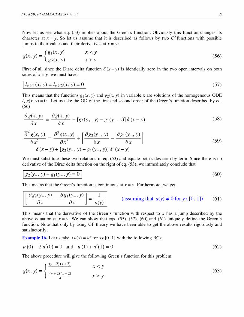
Now let us see what eq. (53) implies about the Green’s function. Obviously this function changes itscharacter at x = y . So let us assume that it is described as follows by two C2 functions with possiblejumps in their values and their derivatives at x = y :

(56)gHx, yL = ; g1Hx, yL x < yg2Hx, yL x > y

First of all since the Dirac delta function d Hx - yL is identically zero in the two open intervals on bothsides of x = y , we must have:

(57)lx g1Hx, yL = lx g2Hx, yL = 0

This means that the functions g1Hx, yL and g2Hx, yL in variable x are solutions of the homogeneous ODElx gHx, yL = 0. Let us take the GD of the first and second order of the Green’s function described by eq.(56)

(58)êê


x=


x+ @g2Hy+ , yL - g1Hy- , yLD d Hx - yL

(59)êê2 gHx, yLÅÅÅÅÅÅÅÅÅÅÅÅÅÅÅÅÅÅÅÅÅÅÅÅÅÅÅ

x2 =2 gHx, yLÅÅÅÅÅÅÅÅÅÅÅÅÅÅÅÅÅÅÅÅÅÅÅÅÅÅÅ

x2 + C g2Hy+ , yLÅÅÅÅÅÅÅÅÅÅÅÅÅÅÅÅÅÅÅÅÅÅÅÅÅÅÅÅÅÅ

x-

g1Hy- , yLÅÅÅÅÅÅÅÅÅÅÅÅÅÅÅÅÅÅÅÅÅÅÅÅÅÅÅÅÅÅ

xG

d Hx - yL + @g2Hy+ , yL - g1Hy- , yLD d£ Hx - yLWe must substitute these two relations in eq. (53) and equate both sides term by term. Since there is noderivative of the Dirac delta function on the right of eq. (53), we immediately conclude that

(60)g2Hy+ , yL - g1Hy- , yL = 0

This means that the Green’s function is continuous at x = y . Furthermore, we get

(61)C g2Hy+ , yLÅÅÅÅÅÅÅÅÅÅÅÅÅÅÅÅÅÅÅÅÅÅÅÅÅÅÅÅÅÅ

x-

g1Hy- , yLÅÅÅÅÅÅÅÅÅÅÅÅÅÅÅÅÅÅÅÅÅÅÅÅÅÅÅÅÅÅ

xG =

1ÅÅÅÅÅÅÅÅÅÅÅÅÅaHyL Hassuming that aHyL 0 for y e @0, 1DL

This means that the derivative of the Green’s function with respect to x has a jump described by theabove equation at x = y . We can show that eqs. (55), (57), (60) and (61) uniquely define the Green’sfunction. Note that only by using GF theory we have been able to get the above results rigorously andsatisfactorily.

Example 16- Let us take l uHxL = u for x e @0, 1D with the following BCs:

(62)u H0L - 2 u£H0L = 0 and u H1L + u£H1L = 0The above procedure will give the following Green’s function for this problem:

(63)gHx, yL =loomnoo

Hy - 2L Hx + 2LÅÅÅÅÅÅÅÅÅÅÅÅÅÅÅÅÅÅÅÅÅÅÅÅÅÅÅÅ4 x < yHy + 2L Hx - 2LÅÅÅÅÅÅÅÅÅÅÅÅÅÅÅÅÅÅÅÅÅÅÅÅÅÅÅÅ4 x > y


This Green’s function satisfies the conditions derived above. Note that the differential operator in thisexample is selfadjoint and, therefore, the symmetry of the Green’s function in variables x and y isexpected8.

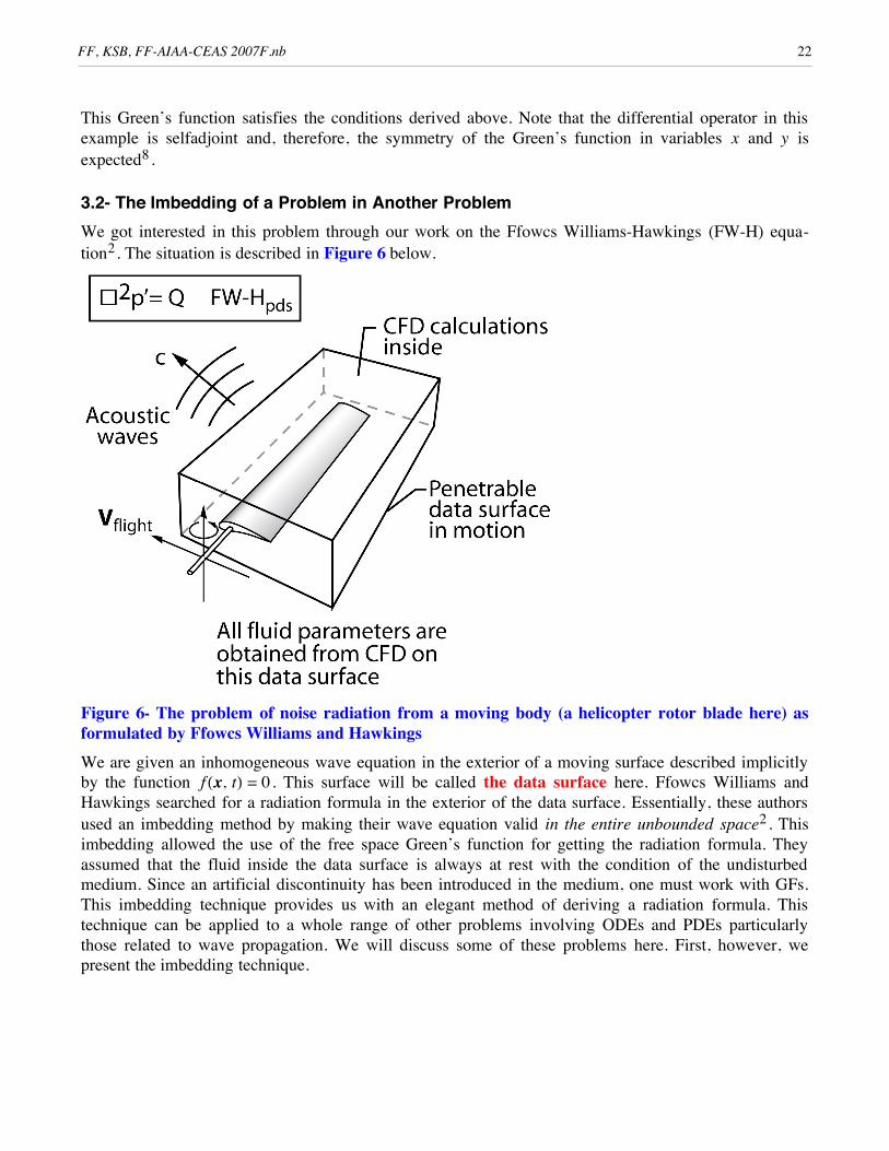
3.2- The Imbedding of a Problem in Another ProblemWe got interested in this problem through our work on the Ffowcs Williams-Hawkings (FW-H) equa-tion2. The situation is described in Figure 6 below.

Figure 6- The problem of noise radiation from a moving body (a helicopter rotor blade here) asformulated by Ffowcs Williams and HawkingsWe are given an inhomogeneous wave equation in the exterior of a moving surface described implicitlyby the function f Hx, tL = 0. This surface will be called the data surface here. Ffowcs Williams andHawkings searched for a radiation formula in the exterior of the data surface. Essentially, these authorsused an imbedding method by making their wave equation valid in the entire unbounded space2. Thisimbedding allowed the use of the free space Green’s function for getting the radiation formula. Theyassumed that the fluid inside the data surface is always at rest with the condition of the undisturbedmedium. Since an artificial discontinuity has been introduced in the medium, one must work with GFs.This imbedding technique provides us with an elegant method of deriving a radiation formula. Thistechnique can be applied to a whole range of other problems involving ODEs and PDEs particularlythose related to wave propagation. We will discuss some of these problems here. First, however, wepresent the imbedding technique.


3.2.1- The Imbedding TechniqueWe will consider the problem of radiation from a moving and deformable surface f Hx, tL = 0, assumingthat ı f = n , where n is the unit outward normal. We have shown the moving surface at two times inspace in Figure 7.

Figure 7- A moving deformable surface described by f Hx, tL = 0 at two different times t1 and t2 inspaceWe want to solve the following exterior acoustic radiation problem:

(64)1

ÅÅÅÅÅÅÅÅc2

2 jÅÅÅÅÅÅÅÅÅÅÅÅÅ t2 - ı2 j =

·2 j = Q Hx, tL Hx in exterior of f = 0, c = constantLWe are assuming that we have all the data about the function j on the moving surface. These data maybe overdetermined but right now we are not concerned about this fact. We want to extend the domain ofthe problem to the interior of the surface so that we can use the simple free space Green’s function ofthe wave equation. In other words, we want to imbed our problem in another problem with largerdomain in space (this can be done also for the dimension of time). This imbedding will require thepowerful machinery of GFs. Here is how we do the imbedding. We start by extending the definition ofthe two functions in eq. (64) as follows:

(65)jè Hx, tL = ;j Hx, tL f > 00 f < 0

, and Qè Hx, tL = ; Q Hx, tL f > 0

0 f < 0The first thing we notice is that with this extension, the new functions satisfy the following wave equa-tion:

(66)·2 jè = Qè Hx, tL


Note that the unknown function jè is discontinuous. To find this function, we must set the problem inGF space. This simply means that we find what the wave operator looks like when all the ordinaryderivatives are written as GDs as follows:

(67)êê

jèÅÅÅÅÅÅÅÅÅÅ t

=jèÅÅÅÅÅÅÅÅÅÅ t

+ j fÅÅÅÅÅÅÅÅÅÅ t

dH f L =jèÅÅÅÅÅÅÅÅÅÅ t

- j vn dH f Lwhere vn = - f ê t is local normal velocity of the surface which is unambiguously defined even for adeformable surface. Also we use the notation j = j H f = 0+L when this function multiplies the Diracdelta function d H f L as in the last term on the right of eq. (67). Next we find the following relations:

(68)êê2

jèÅÅÅÅÅÅÅÅÅÅÅÅÅ t2 =

2 jèÅÅÅÅÅÅÅÅÅÅÅÅÅ t2 -

jÅÅÅÅÅÅÅÅÅÅ t

vn dH f L -

ÅÅÅÅÅÅÅÅ t

@j vn dH f LD

(69)ıêêê2 jè = ı2 jè + n ÿı j dH f L + ı ÿ @j n dH f LDwhere we have again used the notation that any function of jè multiplying the Dirac delta function isevaluated at f = 0+ . Let us define the local normal Mach number of the surface as M n = vn ê c , anddefine additionally the following two symbols j t = j ê t and j n = n ÿı j . Then the above two rela-tion will give us:

(70)·êêê2 jè = ·2 jè -1ÅÅÅÅÅc

j t Mn dH f L -1ÅÅÅÅÅc

ÅÅÅÅÅÅÅÅ t

@j M n dH f LD - j n dH f L - ı ÿ @j n dH f LDOr, after using eq. (66), we obtain

(71)·êêê2 jè = -1ÅÅÅÅÅc

j t Mn dH f L -1ÅÅÅÅÅc

ÅÅÅÅÅÅÅÅ t

@j M n dH f LD - j n dH f L - ı ÿ @j n dH f LDNote that we do need to use a bar over the wave operator on the left side since from the right side it isclear that all derivatives involved are GDs. Now we can use the Green’s function of the wave equationin the unbounded space, the so-called free-space Green’s function, to find the unknown functionjè Hx, tL everywhere in space. The result is the Kirchhoff formula for moving surfaces31, 32 . Theclassical derivation of this formula by Morgans33 is very complicated and in fact until Farassat andMyers rederived it by the modern method presented here, there were some doubts expressed about thecorrectness of Morgans’ result2, 34 .

We will not derive the Kirchhoff formula for moving surfaces here since the two references by Farassatand Myers32 and Farassat31 are quite comprehensive alleviating the need for further elaboration. How-ever, we next derive some classical results for stationary surfaces by the imbedding method which aresurprisingly simpler than the classical methods of their derivation.

Before we end this discussion we want to mention an important question that comes to mind. Answeringthis question may lead to further applications of the Green’s function of the unbounded space. To imbedour exterior radiation problem in !3 we have imposed that inside the surface both jè and Qè be zero.Can the functions jè and Q

è be assumed to take other values and are there advantages in doing so?We will find the answer to this question using an ODE to simplify the analysis.


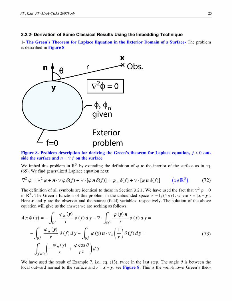
3.2.2- Derivation of Some Classical Results Using the Imbedding Technique1- The Green’s Theorem for Laplace Equation in the Exterior Domain of a Surface- The problemis described in Figure 8.

Figure 8- Problem description for deriving the Green’s theorem for Laplace equation, f > 0 out-side the surface and n = ı f on the surface

We imbed this problem in !3 by extending the definition of j to the interior of the surface as in eq.(65). We find generalized Laplace equation next:

(72)ıêêê2 jè = ı2 jè + n ÿı j dH f L + ı ÿ @j n dH f LD = j n dH f L + ı ÿ @j n dH f LD Ix e !3MThe definition of all symbols are identical to those in Section 3.2.1. We have used the fact that ı2 jè = 0in !3 . The Green’s function of this problem in the unbounded space is -1 ê H4 p rL , where r = † x - y § .Here x and y are the observer and the source (field) variables, respectively. The solution of the aboveequation will give us the answer we are seeking as follows:

(73)

4 p jè HxL = -‡!3

j n HyLÅÅÅÅÅÅÅÅÅÅÅÅÅÅÅÅÅÅÅ

r d H f L d y - ı ÿ‡

!3

j HyL nÅÅÅÅÅÅÅÅÅÅÅÅÅÅÅÅÅÅÅÅ

rd H f L d y =

-‡!3

j n HyLÅÅÅÅÅÅÅÅÅÅÅÅÅÅÅÅÅÅÅ

r d H f L d y - ‡

!3 j HyL n ÿıx K 1

ÅÅÅÅÅrO d H f L d y =

‡f = 0

K-j n HyLÅÅÅÅÅÅÅÅÅÅÅÅÅÅÅÅÅÅÅ

r+

j cos qÅÅÅÅÅÅÅÅÅÅÅÅÅÅÅÅÅÅÅÅ

r 2 O d S

We have used the result of Example 7, i.e., eq. (13), twice in the last step. The angle q is between thelocal outward normal to the surface and r = x - y , see Figure 8. This is the well-known Green’s theo-rem for the Laplace equation. Note that a bonus of the imbedding method is that we know that by con-struction this equation will give jè = 0 inside the surface, a fact not at all obvious in classical derivationand must be established separately.


We have used the result of Example 7, i.e., eq. (13), twice in the last step. The angle q is between thelocal outward normal to the surface and r = x - y , see Figure 8. This is the well-known Green’s theo-rem for the Laplace equation. Note that a bonus of the imbedding method is that we know that by con-struction this equation will give jè = 0 inside the surface, a fact not at all obvious in classical derivationand must be established separately.

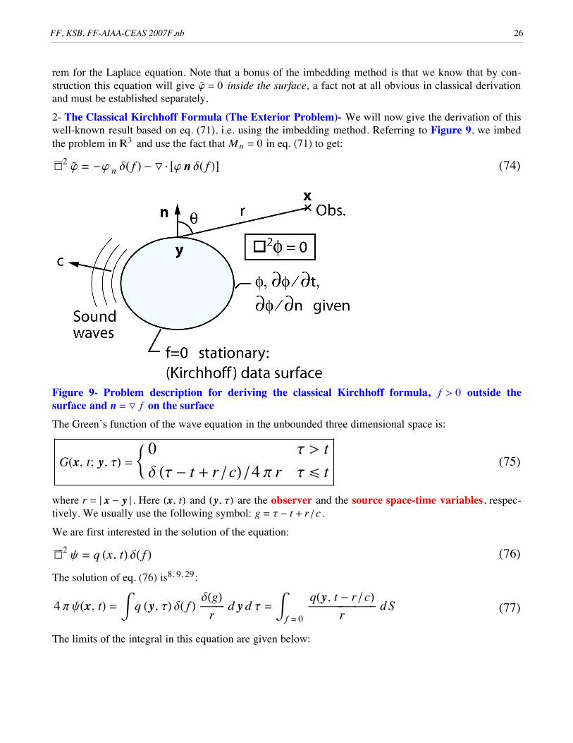
2- The Classical Kirchhoff Formula (The Exterior Problem)- We will now give the derivation of thiswell-known result based on eq. (71), i.e. using the imbedding method. Referring to Figure 9, we imbedthe problem in !3 and use the fact that M n = 0 in eq. (71) to get:

(74)·êêê2 jè = -j n dH f L - ı ÿ @j n dH f LD

Figure 9- Problem description for deriving the classical Kirchhoff formula, f > 0 outside thesurface and n = ı f on the surfaceThe Green’s function of the wave equation in the unbounded three dimensional space is:

(75)GHx, t; y, tL = ; 0 t > td Ht - t + r ê cL ê4 p r t b t

where r = † x - y § . Here Hx, tL and Hy, tL are the observer and the source space-time variables, respec-tively. We usually use the following symbol: g = t - t + r ê c .

We are first interested in the solution of the equation:

(76)·êêê2 y = q Hx, tL dH f LThe solution of eq. (76) is8, 9, 29 :

(77)4 p yHx, tL = ‡ q Hy, tL dH f L dHgLÅÅÅÅÅÅÅÅÅÅÅÅÅ

r d y d t = ‡

f = 0 qHy, t - r ê cLÅÅÅÅÅÅÅÅÅÅÅÅÅÅÅÅÅÅÅÅÅÅÅÅÅÅÅÅÅÅÅÅÅÅÅ

r d S

The limits of the integral in this equation are given below:


(78)‡ ... .. d y d t = ‡-¶

t

‡!3

... .. d y d t = ‡-¶

t

‡-¶

¶

‡-¶

¶

‡-¶

¶

... .. d y1 d y2 d y3 d t

Therefore, the solution of eq. (74) is:

(79)

4 p jè Hx, tL = -‡f = 0

j n Hy, t - r ê cLÅÅÅÅÅÅÅÅÅÅÅÅÅÅÅÅÅÅÅÅÅÅÅÅÅÅÅÅÅÅÅÅÅÅÅÅÅÅÅÅÅ

r d S - ıx ÿ‡

f = 0 n j Hy, t - r ê cLÅÅÅÅÅÅÅÅÅÅÅÅÅÅÅÅÅÅÅÅÅÅÅÅÅÅÅÅÅÅÅÅÅÅÅÅÅÅÅÅÅÅ

r d S =

-‡f = 0

j n Hy, t - r ê cLÅÅÅÅÅÅÅÅÅÅÅÅÅÅÅÅÅÅÅÅÅÅÅÅÅÅÅÅÅÅÅÅÅÅÅÅÅÅÅÅÅ

r d S - ‡

f = 0 n ÿıx K j Hy, t - r ê cL

ÅÅÅÅÅÅÅÅÅÅÅÅÅÅÅÅÅÅÅÅÅÅÅÅÅÅÅÅÅÅÅÅÅÅÅÅÅÅr

O d S

Taking the partial derivatives with respect to the variable x of the integrand of the second integral, weobtain the following result:

(80)4 p jè Hx, tL =

‡f = 0

c-1 cos q j t Hy, t - r ê cL - j n Hy, t - r ê cLÅÅÅÅÅÅÅÅÅÅÅÅÅÅÅÅÅÅÅÅÅÅÅÅÅÅÅÅÅÅÅÅÅÅÅÅÅÅÅÅÅÅÅÅÅÅÅÅÅÅÅÅÅÅÅÅÅÅÅÅÅÅÅÅÅÅÅÅÅÅÅÅÅÅÅÅÅÅÅÅÅÅÅÅÅÅÅÅÅÅÅÅÅÅÅÅÅÅÅÅÅÅÅÅÅÅÅÅÅÅÅÅ

r d S + ‡

f = 0 cos q j Hy, t - r ê cLÅÅÅÅÅÅÅÅÅÅÅÅÅÅÅÅÅÅÅÅÅÅÅÅÅÅÅÅÅÅÅÅÅÅÅÅÅÅÅÅÅÅÅÅÅÅÅÅÅÅÅÅ

r 2 d S

The angle q is between the local outward normal to the surface and r = x - y , see Figure 9. This is thewell-known classical Kirchhoff formula34- 36. Note that we know by construction that jè = 0 insidethe surface. This fact is not obvious in the classical derivation and, as in the case of the classical deriva-tion of the Green’s theorem for the Laplace equation, must be established separately. Notice also that inour derivation we did not have to resort to the four-dimensional Green’s theorem for the wave equation.This is a great advantage of the imbedding method over the classical derivation.

3- Radiation into Half Space- The Rayleigh Integral- We will derive two well-known results forradiation into half space by the imbedding method. Let the half space be defined by x3 > 0. We are,therefore, interested in solving the following problem:

(81)·2 j = Q Hx, tL Hx3 > 0LWe will say nothing about the BC now because two possible BCs emerge from the imbedding method.Let us imbed this problem in !3 in two ways as follows:

(82)jè Hx, tL = ;j Hx, tL x3 > 0

-j Hx, tL x3 < 0,

Qè Hx, tL = ; Q Hx, tL x3 > 0

-Q Hx, tL x3 < 0 HImbedding 1L

and

(83)jè Hx, tL = ;j Hx, tL x3 > 0

j Hx, tL x3 < 0,

Qè Hx, tL = ;Q Hx, tL x3 > 0

Q Hx, tL x3 < 0 HImbedding 2L


Imbedding 1- We can show easily that on the plane x3 = 0 the jumpÛ jè = 2 j Hx1, x2, 0+ , tL ª 2 q Hx1, x2, tL, and also Û Hjè ê x3L = 0. Therefore, the extended functionsatisfies the wave equation:

(84)·êêê2 jè = Qè Hx, tL - 2 q Hx1, x2, tL d£Hx3L Ix e !3M

Using the free space Green’s function of the wave equation, we get

(85)4 p jè Hx, tL = ‡

!3 Qè Hy, t - r ê cL


d y - ‡!3

2 d£Hy3L q Hy1, y2, t - r ê cLÅÅÅÅÅÅÅÅÅÅÅÅÅÅÅÅÅÅÅÅÅÅÅÅÅÅÅÅÅÅÅÅÅÅÅÅÅÅÅÅÅÅÅÅÅÅÅÅÅÅÅÅÅÅÅÅÅÅÅÅÅÅÅÅÅÅÅÅÅÅ

r d y =

‡!3

Qè Hy, t - r ê cL


d y + ‡!2

ÅÅÅÅÅÅÅÅÅÅÅÅ y3

C 2 q Hy1, y2, t - r ê cLÅÅÅÅÅÅÅÅÅÅÅÅÅÅÅÅÅÅÅÅÅÅÅÅÅÅÅÅÅÅÅÅÅÅÅÅÅÅÅÅÅÅÅÅÅÅÅÅÅÅÅÅÅ

rG

y3 =0 d y1 d y2

When we take the derivative in the integrand of the second integral, we obtain the following result:

(86)4 p jè Hx, tL = ‡



d y +

2 ‡!2

ikjjj c-1 cos q qt Hy1, y2, t - r ê cL

ÅÅÅÅÅÅÅÅÅÅÅÅÅÅÅÅÅÅÅÅÅÅÅÅÅÅÅÅÅÅÅÅÅÅÅÅÅÅÅÅÅÅÅÅÅÅÅÅÅÅÅÅÅÅÅÅÅÅÅÅÅÅÅÅÅÅÅÅÅÅÅÅÅÅÅr

+cos q q Hy1, y2, t - r ê cLÅÅÅÅÅÅÅÅÅÅÅÅÅÅÅÅÅÅÅÅÅÅÅÅÅÅÅÅÅÅÅÅÅÅÅÅÅÅÅÅÅÅÅÅÅÅÅÅÅÅÅÅÅÅÅÅÅÅÅÅÅÅÅ

r 2y{zzz d y1 d y2

Here we have used qt = q ê t and the angle q is between the radiation direction x - y and thex3 - axis . Note that the function Qè is defined in eq. (82). This result is the solution of the followingproblem in the half space x3 > 0:

(87)·2 j = Q Hx, tL, j Hx1, x2, 0, tL = q Hx1, x2, tL Hx3 > 0LImbedding 2- We can show that on the plane x3 = 0, the jump Û jè = 0, and alsoÛ Hjè ê x3L = 2 jè Hx1, x2, 0+ , tL ê x3 ª 2 q Hx1, x2, tL . Therefore, the extended function satisfies thewave equation:

(88)·êêê2 jè = Qè Hx, tL - q Hx1, x2, tL dHx3L Ix e !3M

Using the free space Green’s function of the wave equation, we get

(89)4 p jè Hx, tL = ‡



d y - ‡!3

2 dHy3L q Hy1, y2, t - r ê cLÅÅÅÅÅÅÅÅÅÅÅÅÅÅÅÅÅÅÅÅÅÅÅÅÅÅÅÅÅÅÅÅÅÅÅÅÅÅÅÅÅÅÅÅÅÅÅÅÅÅÅÅÅÅÅÅÅÅÅÅÅÅÅÅÅÅÅÅ

r d y =

‡!3

Qè Hy, t - r ê cL


d y - ‡!2

C 2 q Hy1, y2, t - r ê cLÅÅÅÅÅÅÅÅÅÅÅÅÅÅÅÅÅÅÅÅÅÅÅÅÅÅÅÅÅÅÅÅÅÅÅÅÅÅÅÅÅÅÅÅÅÅÅÅÅÅÅÅÅ

rG

y3 =0 d y1 d y2

Since the source in the last integral lies always on the y3 = 0 plane, we can drop this subscript in inte-grand and we obtain:


(90)4 p jè Hx, tL = ‡!3

Qè Hy, t - r ê cL


d y - ‡!2

2 q Hy1, y2, t - r ê cLÅÅÅÅÅÅÅÅÅÅÅÅÅÅÅÅÅÅÅÅÅÅÅÅÅÅÅÅÅÅÅÅÅÅÅÅÅÅÅÅÅÅÅÅÅÅÅÅÅÅÅÅÅ

r d y1 d y2

Note that the function Qè is defined in eq. (83).This is the solution of the following problem in the halfspace x3 > 0:

(91)·2 j = Q Hx, tL, jÅÅÅÅÅÅÅÅÅÅÅÅ x3

Hx1, x2, 0, tL = q Hx1, x2, tL Hx3 > 0L

Equation (90) without the volume term is known as the Rayleigh integral36.

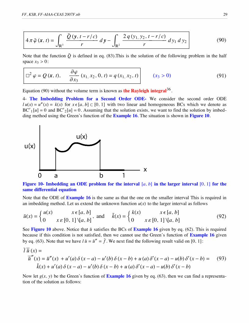
4- The Imbedding Problem for a Second Order ODE- We consider the second order ODEl uHxL = uHxL = kHxL for x e @a, bD Õ @0, 1D with two linear and homogeneous BCs which we denote asBC£

1@uD = 0 and BC£2@uD = 0. Assuming that the solution exists, we want to find the solution by imbed-

ding method using the Green’s function of the Example 16. The situation is shown in Figure 10.

Figure 10- Imbedding an ODE problem for the interval @a, bD in the larger interval @0, 1D for thesame differential equationNote that the ODE of Example 16 is the same as that the one on the smaller interval This is required inan imbedding method. Let us extend the unknown function uHxL to the larger interval as follows

(92)uèHxL = ; uHxL x e @a, bD0 x @0, 1D \@a, bD , and k

èHxL = ; kHxL x e @a, bD0 x @0, 1D \@a, bD

See Figure 10 above. Notice that uè satisfies the BCs of Example 16 given by eq. (62). This is requiredbecause if this condition is not satisfied, then we cannot use the Green’s function of Example 16 givenby eq. (63). Note that we have l uè = uè = f

è. We next find the following result valid on @0, 1D :

(93)lê

uèêê HxL =uèêêHxL = uèHxL + u£HaL d Hx - aL - u£HbL d Hx - bL + u HaL d£Hx - aL - uHbL d£Hx - bL =

kèHxL + u£HaL d Hx - aL - u£HbL d Hx - bL + u HaL d£Hx - aL - uHbL d£Hx - bL

Now let gHx, yL be the Green’s function of Example 16 given by eq. (63), then we can find a representa-tion of the solution as follows:


(94)

uèHxL =

‡0

1kèHyL gHx, yL d y + u£HaL gHx, aL - u£HbL gHx, bL + u HaL gHx, aL

ÅÅÅÅÅÅÅÅÅÅÅÅÅÅÅÅÅÅÅÅÅÅÅÅ y

- uHbL gHx, bLÅÅÅÅÅÅÅÅÅÅÅÅÅÅÅÅÅÅÅÅÅÅÅÅ

y=

‡a

bkHyL gHx, yL d y + u£HaL gHx, aL - u£HbL gHx, bL + u HaL gHx, aL

ÅÅÅÅÅÅÅÅÅÅÅÅÅÅÅÅÅÅÅÅÅÅÅÅ y

- uHbL gHx, bLÅÅÅÅÅÅÅÅÅÅÅÅÅÅÅÅÅÅÅÅÅÅÅÅ

y

We are not finished yet. We can show that using eq. (94), uè Ha-L = 0 and uèHa+L = uHaL give identicalrelations among the boundary values (BVs) of the imbedded problem. Similarly, we can show thatuèHb+L = 0 and uè Hb-L = uHbL also give us another identical relations among the BVs of the imbeddedproblem. We also have two relations supplied by the BCs of the imbedded problem. These four relationswill give us the four unknowns uHaL , uHbL , u£HaL , and u£HbL which we can then substitute in eq. (94) tocompletely solve this problem.

Looking at this procedure we note that all we have required of the behavior of the extended functionuèHxL is that it should satisfy the BCs of the problem whose Green’s function is available in the largerdomain. This means that any solution vHxL of Example 16 can be assumed in the extended region.Assuming that we have l vHxL = jHxL , then eq. (92) must be modified as follows:

(95)uèHxL = ; uHxL x e @a, bDvHxL x @0, 1D \@a, bD , and k

èHxL = ; kHxL x e @a, bDjHxL x @0, 1D \@a, bD

and eq. (93) becomes

(96)

lê

uèêê HxL =

uèêêHxL = uèHxL + @u£HaL - v£HaLD d Hx - aL - @u£HbL - v£HbLD d Hx - bL + @u HaL - vHxLD

d£Hx - aL - @u HbL - vHbLD d£Hx - bL =kèHxL + @u£HaL - v£HaLD d Hx - aL - @u£HbL - v£HbLD d

Hx - bL + @u HaL - vHxLD d£Hx - aL - @u HbL - vHbLD d£Hx - bLAgain using the Green’s function of Example 16, we find the representation of the unknown function as:

(97)uèHxL = ‡

0

1kèHyL gHx, yL d y + @u£HaL - v£HaLD gHx, aL - @u£HbL - v£HbLD

gHx, bL + @u HaL - vHxLD gHx, aLÅÅÅÅÅÅÅÅÅÅÅÅÅÅÅÅÅÅÅÅÅÅÅÅ

y- @u HbL - vHbLD gHx, bL

ÅÅÅÅÅÅÅÅÅÅÅÅÅÅÅÅÅÅÅÅÅÅÅÅy

Two relations are obtained from uè Ha+L = uHaL and uè Hb- L = uHbL among the BVs of the imbedded prob-lem. Together with the two BCs of the imbedded problem, we can then find uHaL , uHbL , u£HaL , and u£HbLand substitute in eq. (97) to find the solution of the imbedded problem.

The implication of this result for wave propagation problems can be substantial. It means that we do nothave to assume that fluid inside the moving body is at rest with the conditions of the undisturbedmedium in the derivation of the FW-H equation. We can take any solution of the wave equation·2 j = q inside the surface and then apply the imbedding technique. This will allow us to use the free-space Green’s function and perhaps not have some of the shortcomings of the FW-H equation such asthe cancellation between the contributions of the surface and volume integrals.


The implication of this result for wave propagation problems can be substantial. It means that we do nothave to assume that fluid inside the moving body is at rest with the conditions of the undisturbedmedium in the derivation of the FW-H equation. We can take any solution of the wave equation·2 j = q inside the surface and then apply the imbedding technique. This will allow us to use the free-space Green’s function and perhaps not have some of the shortcomings of the FW-H equation such asthe cancellation between the contributions of the surface and volume integrals.

4- Concluding RemarksIn this paper we have discussed some applications of GF theory principally to wave propagation prob-lems. We have first given a fairly complete tutorial on GF theory and then have utilized most of theproperties of GFs in the examples and applications presented. We have emphasized generalized differen-tiation here which is a very important operation on GFs with many applications. These are some of ourmain conclusions:

1- GF theory is a very powerful analytic tool in physics and acoustics with a wide range of applications,

2- The derivation of many classical results in physics and acoustics can be enormously simplified byusing GF theory,

3- The power of the Green’s function technique is substantially increased if GF theory is utilized as inthe imbedding technique, and

4- It is possible to use functions other than the null function inside a moving surface in the imbeddingproblem used for obtaining the FW-H equation. Some of these choices may alleviate the shortcomingsof the FW-H equation and still allow us to use the free-space Green’s function.

Generalized function theory is a very powerful tool in mathematics that every physicist and mathemati-cally minded engineer should strive to learn. We have tried to impart to our readers the pleasures oflearning and using GFs in their work.

5- References1- M. J. Lighthill: On sound generated aerodynamically I. General theory, Proceedings of the RoyalSociety of London, A211, 1952, 564-587

2- J. E. Ffowcs Williams and D. L. Hawkings: Sound Generated by Turbulence and Surfaces in Arbi-trary Motion, Philosophical Transactions of the Royal Society, A264, 1969, 321-342

3- Richard Courant and David Hilbert: Methods of Mathematical Physics, Volume 2, Wiley-Inter-science, 1989

4- L. Schwartz: Theorie des Distributions, 2 Volumes, Hermann, Paris, 1957-59

5- L. Hörmander: The Analysis of Linear Partial Differential Operators, 4 volumes, Springer Verlag,2005-2007

6- Michael E. Taylor: Partial Differential Equations, 3 volumes, Springer Verlag, 1997-2004

7- I. M. Gelfand and G. E. Shilov: Generalized Functions, Volume 1: Properties and Operations,Academic Press, 1964

8- Ivar Stackgold: Boundary Value Problems of Mathematical Physics, 2 volumes, The MacMillanCompany, 1968

9- V. S. Vladimirov: Equations of Mathematical Physics, Marcel Dekker, Inc., 1971

10- Robert Strichartz: A Guide to Distribution Theory and Fourier Transforms, CRC Press, 1995


11- Ram P. Kanwal: Generalized Functions- Theory and Applications, 3rd edition, Birkhauser, 2004

12- D. S. Jones: The Theory of Generalized Functions, 2nd edition, Cambridge University Press, 1982

13- Thomas W. Körner: The Pleasures of Counting, Cambridge University Press, 1996

14- M. J. Lighthill: Introduction to Fourier Analysis and Generalized Functions, Cambridge Univer-sity Press, 1964

15- Piotr Antosik, Jan Mikusinski and Roman Sikorski: Theory of Distributions- The SequentialApproach, Elsevier Science Publishing Company, 1973

16- Hans Bremermann: Distributions, Complex Variables, and Fourier Transforms, Addison-Wes-ley Publishing Company, Inc., 1965

17- Jan Mikusinski : Operational Calculus, Volume 1, 2nd edition, Pergamon Press, Inc., 1983

18- Jan Mikusinski and Thomas K. Boehme: Operational Calculus, Volume 2, 2nd edition, PergamonPress, Inc., 1983

19- S. Fenyo and T. Frey: Modern Mathematical Methods in Technology, Volume 1, AmericanElsevier Publishing Company, 1969

20- Arthur Erdélyi: Operational Calculus and Generalized Functions, Holt, Reinhart and Winston,Inc., 1962

21- Jean François Colombeau: New Generalized Functions and Multiplication of Distributions ,Elsevier Science Publishing Company, 1984

22- Elemér E. Rosinger: Non-Linear Partial Differential Equations- An Algebraic View of General-ized Solutions, Elsevier Science Publishing Company, 1990

23- M. Oberguggenberger: Generalized Solutions of nonlinear Partial Differential Equations, JohnWiley and Sons, 1992

24- Robert Goldblatt: Lectures on the Hyperreals: An Introduction to Nonstandard Analysis ,Springer Verlag, 1998

25- Roy S. Baty, F. Farassat and John A. Hargreaves:Nonstandard Analysis and Shock Wave JumpConditions in a One-Dimensional Compressible Gas, Report LA-14334, Los Alamos National Labora-tory, May 2007

26- Jesper Lützen: The Prehistory of the Theory of Distributions, Springer-Verlag, 1982

27- Jean Dieudonné: History of Functional Analysis, Elsevier Science Publishing Company, 1981

28- John Sinowiec: Distributions: The Evolution of a Mathematical Theory, Historia Mathematica, 10,1983, 149-183

29- F. Farassat: Introduction to Generalized Functions With Applications in Aerodynamics and Acous-tics, NASA Technical Paper 3428, 1994, (Corrected Copy April 1996), available from NASA TechnicalReport Server (NTRS) web site, http://ntrs.nasa.gov

30- Alfred Gray, Elsa Abbena and Simon Salamon: Modern Differential Geometry of Curves andSurfaces With MATHEMATICA, Third Edition, Chapman & Hall/ CRC, 2006


31- F. Farassat: The Kirchhoff Formulas for Moving Surfaces in Aeroacoustics - The Subsonic andSupersonic Cases, NASA Technical Memorandum 110285, September 1996, available from NASATechnical Report Server (NTRS) web site, http://ntrs.nasa.gov

32- F. Farassat and M. K. Myers: Extension of Kirchhoff's formula to radiation from moving sources,Journal of Sound and Vibration, 123 (3), 1988, 451-460

33- W. R. Morgans: The Kirchhoff formula extended to a moving surface, Philosophical Magazine, 9,1930, 141-161.

34- D. S. Jones: The Theory of Electromagnetism , Oxford University Press, 1964

35- Philip Morse and Herman Feshbach: Methods of Theoretical Physics, 2 volumes, McGraw-HillScience, 1953

36- Allan D. Pierce: Acoustics- An Introduction to its Physical Principles and Applications, Acousti-cal Society of America, 1989


Documents

Working With the Wave Equation in Aeroacoustics- The ... With the Wave Equation in Aeroacoustics- The Pleasures of Generalized Functions F. Farassat NASA Langley Research Center, Hampton,