Workshop in MagnetochemistryMolecular Magnetism (DFG-SPP 1137)

Kaiserslautern, 29.09. – 02.10.2003Foundations

Heiko Lueken, Institut fur Anorganische Chemie, RWTH Aachen

Contents

1 Magnetic quantities 3

2 Magnetisation and magnetic susceptibility 4

3 Paramagnetism 53.1 Curie law . . . . . . . . . . . . . . . . . . . . . . . . . . . . . . . . . . . . 53.2 Free lanthanide ions and Hund’s rules . . . . . . . . . . . . . . . . . . . . 73.3 Lanthanide ions in octahedral ligand fields . . . . . . . . . . . . . . . . . . 83.4 3d ions in octahedral ligand fields . . . . . . . . . . . . . . . . . . . . . . . 113.5 Curie-Weiss law . . . . . . . . . . . . . . . . . . . . . . . . . . . . . . . 143.6 Exchange interactions in polynuclear compounds . . . . . . . . . . . . . . . 16Problems . . . . . . . . . . . . . . . . . . . . . . . . . . . . . . . . . . . . . . . 16

4 Magnetic ordering 174.1 Ferromagnetism . . . . . . . . . . . . . . . . . . . . . . . . . . . . . . . . . 17

4.1.1 Substances and materials . . . . . . . . . . . . . . . . . . . . . . . . 174.1.2 Hysteresis loop and magnetisation curve . . . . . . . . . . . . . . . 18

4.2 Antiferromagnetism . . . . . . . . . . . . . . . . . . . . . . . . . . . . . . . 194.3 Ferrimagnetism . . . . . . . . . . . . . . . . . . . . . . . . . . . . . . . . . 20

4.3.1 Substances and materials . . . . . . . . . . . . . . . . . . . . . . . . 204.3.2 Magnetic saturation moment . . . . . . . . . . . . . . . . . . . . . . 204.3.3 Paramagnetism above the Curie temperature . . . . . . . . . . . . 22

Problems . . . . . . . . . . . . . . . . . . . . . . . . . . . . . . . . . . . . . . . 24

5 Theory of free ions 255.1 Foundations of quantum-mechanics . . . . . . . . . . . . . . . . . . . . . . 255.2 Perturbation theory . . . . . . . . . . . . . . . . . . . . . . . . . . . . . . . 255.3 One-electron systems . . . . . . . . . . . . . . . . . . . . . . . . . . . . . . 295.4 Angular momentum . . . . . . . . . . . . . . . . . . . . . . . . . . . . . . . 335.5 Spin . . . . . . . . . . . . . . . . . . . . . . . . . . . . . . . . . . . . . . . 355.6 Spin-orbit coupling . . . . . . . . . . . . . . . . . . . . . . . . . . . . . . . 36Problems . . . . . . . . . . . . . . . . . . . . . . . . . . . . . . . . . . . . . . . 44

1

6 Exchange interactions in dinuclear compounds 456.1 Parametrization of exchange interactions . . . . . . . . . . . . . . . . . . . 456.2 Heisenberg operator . . . . . . . . . . . . . . . . . . . . . . . . . . . . . 496.3 Exchange-coupled species in a magnetic field . . . . . . . . . . . . . . . . . 506.4 Mechanisms of cooperative magnetic effects in insulators . . . . . . . . . . 56Problems . . . . . . . . . . . . . . . . . . . . . . . . . . . . . . . . . . . . . . . 57

7 Exchange interactions in chain compounds 59

8 Exchange interactions in layers and 3 D networks 608.1 Molecular-field model . . . . . . . . . . . . . . . . . . . . . . . . . . . . . . 608.2 High-temperature series expansion . . . . . . . . . . . . . . . . . . . . . . . 62

9 Magnetochemical analysis in practice 64

References 65

Appendix 66

2

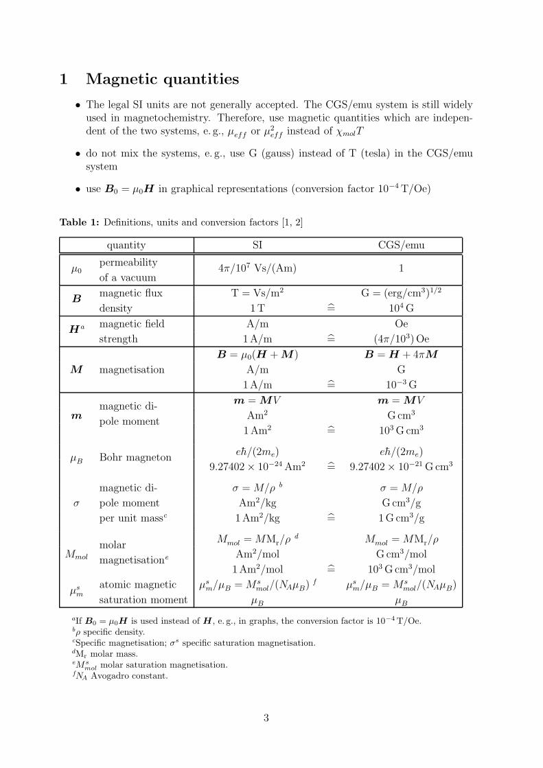
1 Magnetic quantities

• The legal SI units are not generally accepted. The CGS/emu system is still widelyused in magnetochemistry. Therefore, use magnetic quantities which are indepen-dent of the two systems, e. g., µeff or µ2

eff instead of χmolT

• do not mix the systems, e. g., use G (gauss) instead of T (tesla) in the CGS/emusystem

• use B0 = µ0H in graphical representations (conversion factor 10−4 T/Oe)

Table 1: Definitions, units and conversion factors [1, 2]

quantity SI CGS/emu

permeabilityµ0

of a vacuum4π/107 Vs/(Am) 1

magnetic flux T = Vs/m2 G = (erg/cm3)1/2

Bdensity 1T = 104 G

magnetic field A/m OeHa

strength 1A/m = (4π/103)Oe

B = µ0(H + M) B = H + 4πM

M magnetisation A/m G

1A/m = 10−3 G

m = MV m = MV

mmagnetic di-

Am2 Gcm3

pole moment1Am2 = 103 Gcm3

eh/(2me) eh/(2me)µB Bohr magneton9.27402 × 10−24 Am2 = 9.27402 × 10−21 G cm3

magnetic di- σ = M/ρ b σ = M/ρ

σ pole moment Am2/kg G cm3/g

per unit massc 1Am2/kg = 1G cm3/g

Mmol = MMr/ρd Mmol = MMr/ρ

Mmol

molarAm2/mol G cm3/mol

magnetisatione

1Am2/mol = 103 Gcm3/mol

atomic magnetic µsm/µB = M s

mol/(NAµB) f µsm/µB = M s

mol/(NAµB)µs

msaturation moment µB µB

aIf B0 = µ0H is used instead of H , e. g., in graphs, the conversion factor is 10−4 T/Oe.bρ specific density.cSpecific magnetisation; σs specific saturation magnetisation.dMr molar mass.eMs

mol molar saturation magnetisation.fNA Avogadro constant.

3

Table 1: Definitions, units and conversion factors [1, 2] (cont.)

quantity SI CGS/emu

M = χH M = χH

χmagnetic volume

1 1susceptibility

1 = 1/(4π)

χg = χ/ρ χg = χ/ρ

χg

magnetic massm3/kg cm3/g

susceptibility1m3/kg = 103/(4π) cm3/g

χmol = χMr/ρ χmol = χMr/ρ

χmol

magnetic molarm3/mol cm3/mol

susceptibility1m3/mol = 4π/106 cm3/mol

[3kB/(µ0NAµ2B)]1/2[χmolT ]1/2a [3kB/(NAµ

2B)]1/2[χmolT ]1/2

µeff

effective Bohr mag-1 1

neton number [3]1 = 1

akB Boltzmann constant.

2 Magnetisation and magnetic susceptibility

magnetic flux density in vacuo in matter

B = µ0H B = µ0(H + M) (1)

magnetisation M = χH (2)

magnetic susceptibility

magnetic volume susceptibility χ

magnetic mass susceptibility χg = χ/ρ

magnetic molar susceptibility χmol = χgMr (3)

substance class range

diamagnets χ < 0 −10−4 . . .− 10−6 closed shell atoms

vacuum χ = 0

paramagnets χ > 0 10−2 . . . 10−5 open shell atoms

Diamagnetism

(i) χ < 0 and M < 0 owing to small additional currents attributable to the precession ofelectron orbits about the applied magnetic field (shown by all substances);(ii) usually independent of both T and B for purely diamagnetic materials (closed shellsystems);(iii) allowed for as diamagnetic correction in the evaluation of experimental susceptibilitydata of open shell systems.

4

Paramagnetism

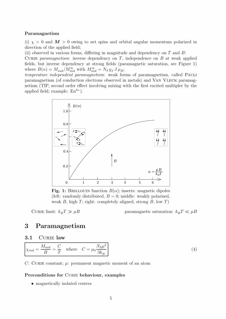
(i) χ > 0 and M > 0 owing to net spins and orbital angular momentum polarized indirection of the applied field;(ii) observed in various forms, differing in magnitude and dependency on T and B:Curie paramagnetism: inverse dependency on T , independence on B at weak appliedfields, but inverse dependency at strong fields (paramagnetic saturation, see Figure 1)where B(α) = Mmol/M

∞

mol with M∞

mol = NA gJ J µB;temperature independent paramagnetism: weak forms of paramagnetism, called Pauli

paramagnetism (of conduction electrons observed in metals) and Van Vleck paramag-netism (TIP, second order effect involving mixing with the first excited multiplet by theapplied field; example: Eu3+).

1.0

0.8

0.4

0.2

1 2 3 4 5 60

B

B a( )

B

kBT

m=a

Fig. 1: Brillouin function B(α); inserts: magnetic dipoles(left: randomly distributed, B = 0; middle: weakly polarised,weak B, high T ; right: completely aligned, strong B, low T )

Curie limit: kBT µB paramagnetic saturation: kBT µB

3 Paramagnetism

3.1 Curie law

χmol =Mmol

H=C

Twhere C = µ0

NAµ2

3kB

(4)

C: Curie constant; µ: permanent magnetic moment of an atom

Preconditions for Curie behaviour, examples

• magnetically isolated centres

5

• thermally isolated ground state −→ temperature independent C

0 Ta

C/c

mol

0 Tb

C/

cm

ol

T

1

0

mef

fef

f/

(0)

m

c

Curie behaviour (in reduced magneticquantities χmol/C and µeff/µeff(0)(C and µeff(0) refer to the free ion)

Fig. 2 a: variation χmol vs. TFig. 2 b: variation χ−1

mol vs. TFig. 2 c: variation µeff vs. T

µ = g√S(S + 1)µB spin-only formula (5)

Gd2(SO4)3 · 8 H2O and (NH4)2Mn(SO4)2 · 6 H2O withGd3+ [4f 7] (ground state 8S7/2, S = 7/2, µ = 7.94µB)Mn2+ [3d5] (ground state 6A1, S = 5/2, µ = 5.91µB)

6

3.2 Free lanthanide ions and Hund’s rules

µ = gJ

√J(J + 1)µB except 4f 4, 4f 5, 4f6 systems (6)

with Lande factor

gJ = 1 +J(J + 1) + S(S + 1) − L(L+ 1)

2J(J + 1)(7)

S, L, J correspond to the total spin angular momentum, the total orbital

angular momentum and the total angular momentum, respectively, of theground state.

The 4f electrons of free Ln ions are influenced by interelectronic repulsionHee (splitting energy 104 cm−1) and spin-orbit coupling HSO (103 cm−1),

i. e., Hee > HSO. To determine the free ion ground state use the followingscheme and apply Hund’s rules:

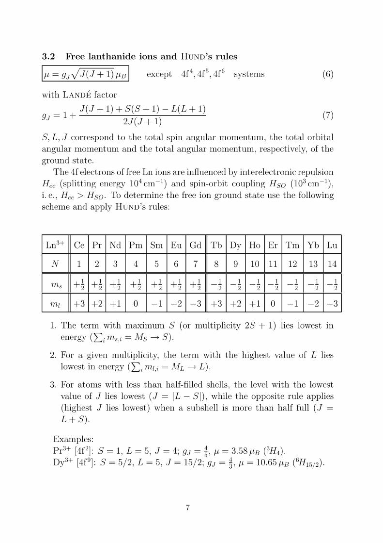
Ln3+ Ce Pr Nd Pm Sm Eu Gd Tb Dy Ho Er Tm Yb Lu

N 1 2 3 4 5 6 7 8 9 10 11 12 13 14

ms +12

+12

+12

+12

+12

+12

+12

−12

−12

−12

−12

−12

−12

−12

ml +3 +2 +1 0 −1 −2 −3 +3 +2 +1 0 −1 −2 −3

1. The term with maximum S (or multiplicity 2S + 1) lies lowest inenergy (

∑ims,i = MS → S).

2. For a given multiplicity, the term with the highest value of L lieslowest in energy (

∑iml,i = ML → L).

3. For atoms with less than half-filled shells, the level with the lowestvalue of J lies lowest (J = |L − S|), while the opposite rule applies

(highest J lies lowest) when a subshell is more than half full (J =L+ S).

Examples:

Pr3+ [4f 2]: S = 1, L = 5, J = 4; gJ = 45, µ = 3.58µB (3H4).

Dy3+ [4f 9]: S = 5/2, L = 5, J = 15/2; gJ = 43, µ = 10.65µB (6H15/2).

7

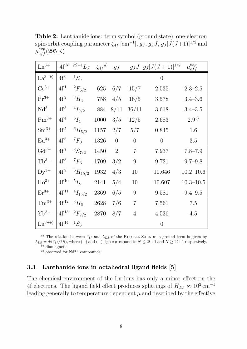
Table 2: Lanthanide ions: term symbol (ground state), one-electronspin-orbit coupling parameter ζ4f [cm−1], gJ , gJJ , gJ [J(J+1)]1/2 andµexp

eff(295 K)

Ln3+ 4f N 2S+1LJ ζ4fa) gJ gJJ gJ [J(J + 1)]1/2 µexp

eff

La3+b) 4f 0 1S0 0

Ce3+ 4f 1 2F5/2 625 6/7 15/7 2.535 2.3–2.5

Pr3+ 4f 2 3H4 758 4/5 16/5 3.578 3.4–3.6

Nd3+ 4f 3 4I9/2 884 8/11 36/11 3.618 3.4–3.5

Pm3+ 4f 4 5I4 1000 3/5 12/5 2.683 2.9c)

Sm3+ 4f 5 6H5/2 1157 2/7 5/7 0.845 1.6

Eu3+ 4f 6 7F0 1326 0 0 0 3.5

Gd3+ 4f 7 8S7/2 1450 2 7 7.937 7.8–7.9

Tb3+ 4f 8 7F6 1709 3/2 9 9.721 9.7–9.8

Dy3+ 4f 9 6H15/2 1932 4/3 10 10.646 10.2–10.6

Ho3+ 4f 10 5I8 2141 5/4 10 10.607 10.3–10.5

Er3+ 4f 11 4I15/2 2369 6/5 9 9.581 9.4–9.5

Tm3+ 4f 12 3H6 2628 7/6 7 7.561 7.5

Yb3+ 4f 13 2F7/2 2870 8/7 4 4.536 4.5

Lu3+b) 4f 14 1S0 0

a) The relation between ζ4f and λLS of the Russell-Saunders ground term is given byλLS = ±(ζ4f/2S), where (+) and (−) sign correspond to N ≤ 2l+1 and N ≥ 2l+1 respectively.

b) diamagneticc) observed for Nd2+ compounds.

3.3 Lanthanide ions in octahedral ligand fields [5]

The chemical environment of the Ln ions has only a minor effect on the

4f electrons. The ligand field effect produces splittings of HLF ≈ 102 cm−1

leading generally to temperature dependent µ and described by the effective

8

Bohr magneton number µeff :

χmol = µ0

NAµ2effµ

2B

3kBTwhere µeff =

(3kBTχmol

µ0NAµ2B

)1/2

= 797.7(Tχmol)1/2(8)

As a rule, µeff approaches the free Ln ion value for T above 200 K (seeTable 2, Figures 3 – 7).

0 100 200 300 4000

100

200

3 00

400

500

T/K

0.0

0.4

0.8

1.2

1.6

2.0

2.4

meff

cm

ol

105

-1m

ol

/m

-3

a

b

c

d

e

f

Fig. 3: Ce3+ in cubic ligand fields; χ−1mol–T - (b,d,f) and µeff–T diagrams

(a,c,e); ∆ = 605 cm−1 (e,f; oct.), ∆ = −605 cm−1 (c,d; tet); straight lines(a,b) refer to the free ion.

9

0

40

80

120

160

200

0 100 200 300 400T/K

U5+

Yb3+

3+Ce

c-1

mol

/10

6m

ol

m-3

()

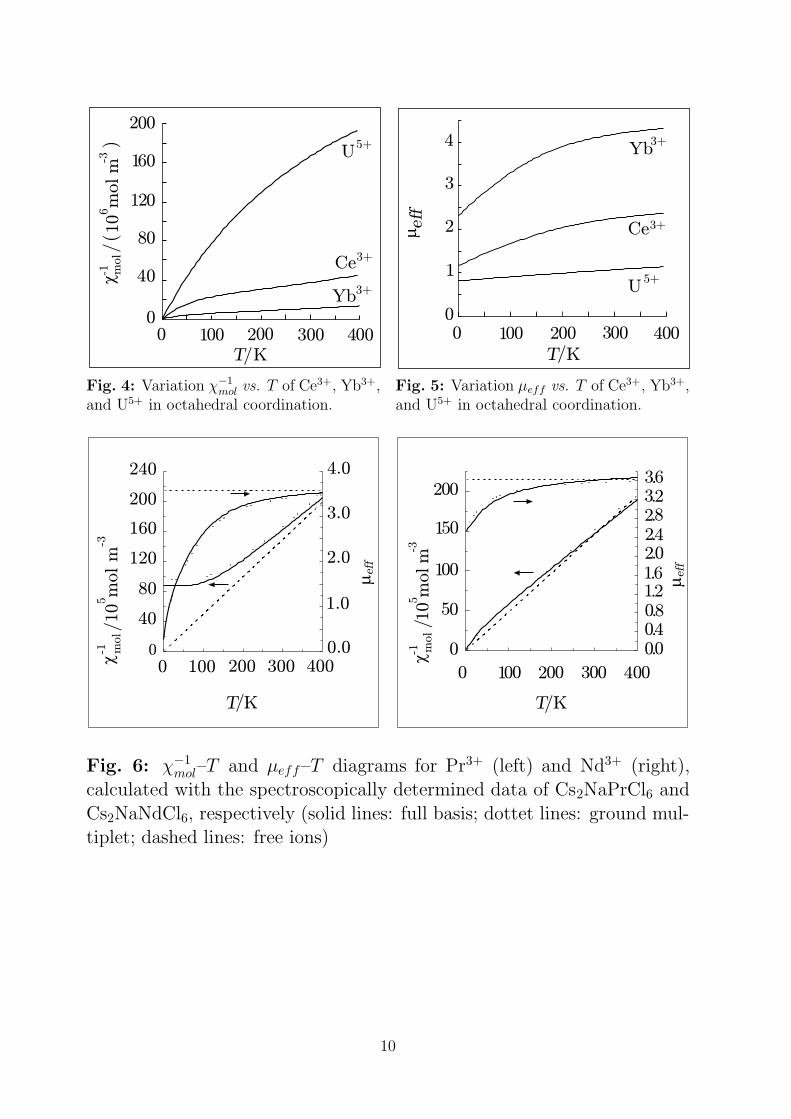
Fig. 4: Variation χ−1

mol vs. T of Ce3+, Yb3+,and U5+ in octahedral coordination.

0

1

2

3

4

0100 200 300 400

T/K

Ce3+

Yb3+

U5+

meff

Fig. 5: Variation µeff vs. T of Ce3+, Yb3+,and U5+ in octahedral coordination.

0

40

80

120

160

200

240

100 200 300 4000.0

1.0

2.0

3.0

4.0

-15

-3/10

mol m

mol

c

meff

/KT

0 0 100 200 300 400

0

50

100

150

200

0.00.40.81.21.62.02.42.83.23.6

meff

mol

c10

/-1

5-3

mm

ol

T/K

Fig. 6: χ−1mol–T and µeff–T diagrams for Pr3+ (left) and Nd3+ (right),

calculated with the spectroscopically determined data of Cs2NaPrCl6 and

Cs2NaNdCl6, respectively (solid lines: full basis; dottet lines: ground mul-tiplet; dashed lines: free ions)

10

0 100 200 300 4000.0

1.0

2.0

3.0

4.0

T/K

mef

f

dc

ba

0 100 200 300 4000

1

2

3

4

5

6

7

8

T/K

cm

ol

-1/10-7

mm

ol

-3

a

b

c

d

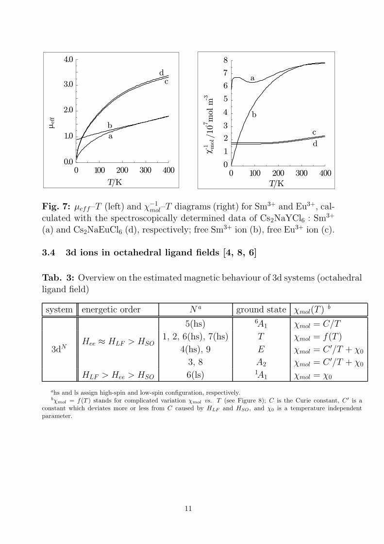
Fig. 7: µeff–T (left) and χ−1mol–T diagrams (right) for Sm3+ and Eu3+, cal-

culated with the spectroscopically determined data of Cs2NaYCl6 : Sm3+

(a) and Cs2NaEuCl6 (d), respectively; free Sm3+ ion (b), free Eu3+ ion (c).

3.4 3d ions in octahedral ligand fields [4, 8, 6]

Tab. 3: Overview on the estimated magnetic behaviour of 3d systems (octahedralligand field)

system energetic order N a ground state χmol(T ) b

5(hs) 6A1 χmol = C/T

1, 2, 6(hs), 7(hs) T χmol = f(T )

3dNHee ≈ HLF > HSO

4(hs), 9 E χmol = C ′/T + χ0

3, 8 A2 χmol = C ′/T + χ0

HLF > Hee > HSO 6(ls) 1A1 χmol = χ0

ahs and ls assign high-spin and low-spin configuration, respectively.bχmol = f(T ) stands for complicated variation χmol vs. T (see Figure 8); C is the Curie constant, C ′ is a

constant which deviates more or less from C caused by HLF and HSO , and χ0 is a temperature independentparameter.

11

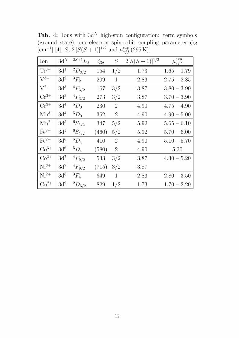
Tab. 4: Ions with 3dN high-spin configuration: term symbols

(ground state), one-electron spin-orbit coupling parameter ζ3d

[cm−1] [4], S, 2 [S(S + 1)]1/2 and µexpeff (295 K).

Ion 3dN 2S+1LJ ζ3d S 2[S(S + 1)]1/2 µexpeff

Ti3+ 3d1 2D3/2 154 1/2 1.73 1.65 – 1.79

V3+ 3d2 3F2 209 1 2,83 2.75 – 2.85

V2+ 3d3 4F3/2 167 3/2 3.87 3.80 – 3.90

Cr3+ 3d3 4F3/2 273 3/2 3.87 3.70 – 3.90

Cr2+ 3d4 5D0 230 2 4.90 4.75 – 4.90

Mn3+ 3d4 5D0 352 2 4.90 4.90 – 5.00

Mn2+ 3d5 6S5/2 347 5/2 5.92 5.65 – 6.10

Fe3+ 3d5 6S5/2 (460) 5/2 5.92 5.70 – 6.00

Fe2+ 3d6 5D4 410 2 4.90 5.10 – 5.70

Co3+ 3d6 5D4 (580) 2 4.90 5.30

Co2+ 3d7 4F9/2 533 3/2 3.87 4.30 – 5.20

Ni3+ 3d7 4F9/2 (715) 3/2 3.87

Ni2+ 3d8 3F4 649 1 2.83 2.80 – 3.50

Cu2+ 3d9 2D5/2 829 1/2 1.73 1.70 – 2.20

12

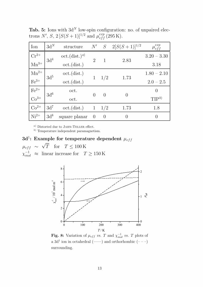
Tab. 5: Ions with 3dN low-spin configuration: no. of unpaired elec-

trons N ′, S, 2 [S(S + 1)]1/2 and µexpeff (295 K).

Ion 3dN structure N ′ S 2[S(S + 1)]1/2 µexpeff

Cr2+ oct.(dist.)a) 3.20 – 3.30

Mn3+3d4

oct.(dist.)2 1 2.83

3.18

Mn2+ oct.(dist.) 1.80 – 2.10

Fe3+3d5

oct.(dist.)1 1/2 1.73

2.0 – 2.5

Fe2+ oct. 0

Co3+3d6

oct.0 0 0

TIPb)

Co2+ 3d7 oct.(dist.) 1 1/2 1.73 1.8

Ni2+ 3d8 square planar 0 0 0 0

a) Distorted due to Jahn-Teller effect.b) Temperature independent paramagnetism.

3d1: Example for temperature dependent µeff

µeff ∼√T for T ≤ 100 K

χ−1mol ≈ linear increase for T ≥ 150 K

Fig. 8: Variation of µeff vs. T and χ−1

mol vs. T plots of

a 3d1 ion in octahedral (——) and orthorhombic (– – –)

surrounding.

13

3.5 Curie-Weiss law

The Curie-Weiss law

χmol =C

T − Θpwith Θp =

2S(S + 1)

3kB

∑

i

ziJi (9)

• is the most overworked formula in paramagnetism [7]

• has only a limited applicability:

– not applicable to magnetic diluted systems

– not applicable to systems like Ti3+ in octahedral surrounding (seeFigure 8) and f systems (except Gd3+, Eu2+)

– only applicable to pure spin paramagnetism with C correspondingwith the permanent magnetic moment µ and Θp measuring the

total exchange interactions of a magnetically active centre withall its magnetic neighbours (nearest, next-nearest, etc.)

300200-100 0 100

T/K

25

75

50

d

c

a

b

mol

10

mol m

c-1

/(

)

-35

100

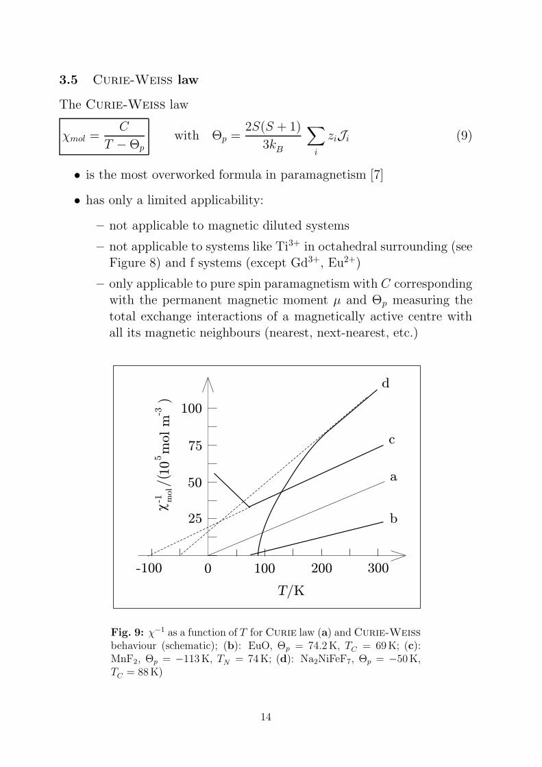
Fig. 9: χ−1 as a function of T for Curie law (a) and Curie-Weiss

behaviour (schematic); (b): EuO, Θp = 74.2K, TC = 69K; (c):MnF2, Θp = −113K, TN = 74K; (d): Na2NiFeF7, Θp = −50K,TC = 88K)

14

0

0

=0

0

0p

0p

0p

Ta

C/c

mol

0

0p

0p

0p

0

0

=0

T

C/

b

cm

ol

0p

0p

0p 0

0

=0

T

1

0

mef

fef

f/

(0)

m

c

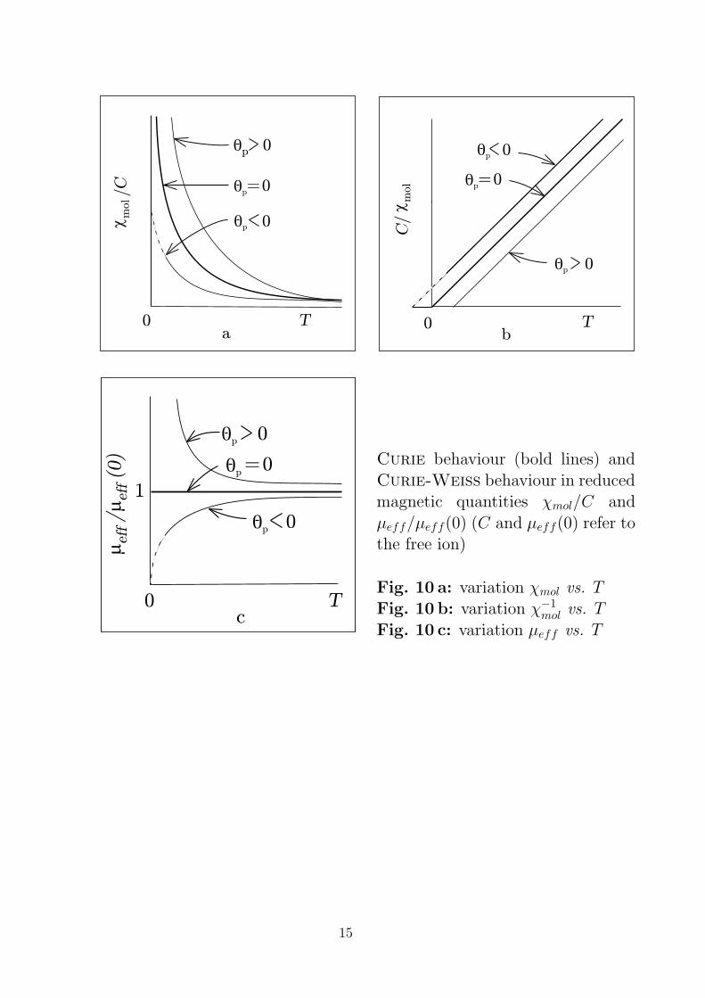
Curie behaviour (bold lines) and

Curie-Weiss behaviour in reducedmagnetic quantities χmol/C and

µeff/µeff(0) (C and µeff(0) refer tothe free ion)

Fig. 10 a: variation χmol vs. TFig. 10 b: variation χ−1

mol vs. T

Fig. 10 c: variation µeff vs. T

15

3.6 Exchange interactions in polynuclear compounds [9]

Example: Dinuclear complex [Cu(CH3COO)2(H2O)]2

oxygen(water)

copper

acetate

S =1/21 S =1/22DE = -2J

S =0

S =1

1,0

0,8

0,6

0,4

0,2

0 100 200 300

T/K

cm

ol/

10

-8m

3m

ol-1

Fig. 11: [Cu(CH3COO)2(H2O)]2; left: molecular structure; right: χmol versus T diagramwith J = −148 cm−1 (Hex = −2J S1 · S2), g = 2.16, χ0 = 76 × 10−11 m3 mol−1. Toexplain J = −148 cm−1 both the direct exchange interactions between the dx2

−y2 orbitalsand the superexchange via the doubly occupied orbitals as well as unoccupied orbitals ofthe bridging ligands have to be accounted for.

χmol = µ0

NAµ2Bg

2

3kBT

[1 +

1

3exp

(−2JkBT

)]−1

+ χ0, see section 6.3, page 54

Problems

1. How are the quantities (i) m, (ii) µeff , (iii) µ, (iv) µsm defined?

2. Calculate the spin contributions to the molar susceptibility of hydrogen atoms at298K (SI units).µ0NAµ

2B/(3kB) = 1.57141 × 10−6m3 K mol−1

3. What are the electronic and structural conditions for a compound to be a param-agnet obeying the Curie law? Give examples!

4. What are the electronic, structural, and thermal conditions for a compound to bea paramagnet obeying the Curie-Weiss law χmol = C/(T − Θp), permitting areasonable interpretation C and Θp? Give examples!

5. Write the ground state term symbols 2S+1LJ of free ions with electronic configuration[Ar] 3dN (N = 0, 1, 2, . . . , 10).

6. What levels (multiplets J) may arise from the terms (a) 1S, (b) 2P , (c) 3P , (d) 3D,(e) 4D? How many states (distinguished by the quantum number MJ) belong toeach level?

16

4 Magnetic ordering

4.1 Ferromagnetism ⇑⇑⇑⇑4.1.1 Substances and materials

Table 6: Ferromagnetic elements and compounds

substance structure TC/K Θp/K µsm/µB

α-Fe bcc 1044(2) 1100 2.216

β-Co hcp 1388(2) 1415 1.715

Ni ccp 627.4(3) 649 0.616

Gd hcp 293.4 317 7.63

EuO NaCl 69 74.2 6.94

La1−xSrxMnO3 perovskite 210−385

CrBr3 BiI3 32.7 54 3.0

Tab. 7: Ferromagnetic materials: properties and application. TC [K], µsm

[µB] per formula unit, (BH)max [kJm−3] (mr: magnetic data recording;sm: softmagnetic material; hm: hardmagnetic material)

material structure TC µsm (BH)max

a) appl.

Fe40Co40B20 amorphous > 800 1.43 sm

supermalloyb) ccp 673 sm

Alnicoc) d) > 800 25 hm

SmCo5 CaCu5 1000 160 hm

Sm2Co17 Th2Zn17 225 hm

Nd2Fe14B Nd2Fe14B 585 37.6 360 hm

CrO2 Rutil 392 2.00 mr

a) (BH)max is the performance of a hardmagnetic material.b) Typical composition (mass %): Ni (79), Fe (15.5), Mo (5.0), Mn (0.5).c) Alnico 2 (mass %): Ni (18–21), Al (8–10), Co (17–20), Cu (2–4), Nb (0–1), Fe (rest).d) Heterogeneous system: ferromagnetic segregations (Fe/Co) in a (Ni/Al) matrix.

17

4.1.2 Hysteresis loop and magnetisation curve

H

,J

Br

Hc

Hc

M

(H+M)=

m0

m0

S

B

M

p

B

B

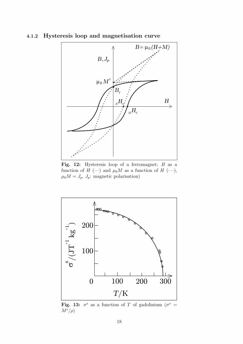
Fig. 12: Hysteresis loop of a ferromagnet; B as afunction of H (—) and µ0M as a function of H (· · ·),µ0M = Jp, Jp: magnetic polarisation)

0

200

100

200100 300

T/K

s

s-

/(J

T1kg

)- 1

Fig. 13: σs as a function of T of gadolinium (σs =M s/ρ)

18

a b c

H H

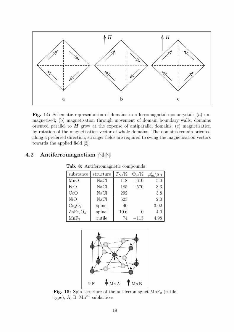
Fig. 14: Schematic representation of domains in a ferromagnetic monocrystal: (a) un-magnetised; (b) magnetisation through movement of domain boundary walls; domainsoriented parallel to H grow at the expense of antiparallel domains; (c) magnetisationby rotation of the magnetisation vector of whole domains. The domains remain orientedalong a preferred direction; stronger fields are required to swing the magnetisation vectorstowards the applied field [2].

4.2 Antiferromagnetism ⇑⇓⇑⇓

Tab. 8: Antiferromagnetic compounds

substance structure TN/K Θp/K µsm/µB

MnO NaCl 118 −610 5.0

FeO NaCl 185 −570 3.3

CoO NaCl 292 3.8

NiO NaCl 523 2.0

Co3O4 spinel 40 3.02

ZnFe2O4 spinel 10.6 0 4.0

MnF2 rutile 74 −113 4.98

F Mn A Mn B

Fig. 15: Spin structure of the antiferromagnet MnF2 (rutiletype); A, B: Mn2+ sublattices

19

4.3 Ferrimagnetism ⇑↓⇑↓4.3.1 Substances and materials

Tab. 9: Ferrimagnetic compounds and materials

substance/material structure TC/K Θp/K µsm/µB

Mn3O4 spinel 42 1.85

Fe3O4 spinel(inverse) 858 4.1

NiFe2O4 spinel(inverse) 858 2.3

Na2NiFeF7 weberite 88 -50 2.2 (Ni)

5.0 (Fe)

4.3.2 Magnetic saturation moment

µsm = M sMr/(ρNA) = M s

mol/NA

Arrangements of magnetic dipoles in ferrimagnets

a b c

+ + += = =

Fig. 16: Three possible arrangements of magnetic dipoles in ferrimagnetic materials: (a)unequal numbers of identical moments on the two sublattices; (b) unequal moments onthe two sublattices; (c) two equal moments and one unequal [2].

Example Fe3O4 = FeIII[FeIIFeIII]O4 (inverse spinel):

µsm = gSµB with g = 2 (pure spin magnetism) of the iron ions occupying

tetrahedral (A) and octahedral holes (B):

Fe3+(A): µsm = 5µB

Fe3+(B): µsm = 5µB

Fe2+(B): µsm = 4µB

20

Resultant moment µsm(Fe3O4):

µsm(B) − µs

m(A) = (5 + 4)µB − 5µB = 4µB per formula unit

(exp.: 4.1µB)

Neel’s suggestion: all interactions in the ferrites are antiferromagnetic,but the A–B interaction is considerably stronger than A–A or B–B. Thus,

in the inverse spinel structure the dominating A–B interaction makes thespins within each sublattice parallel, despite their mutual antiferromagnetic

interaction. This is supported by the fact, that ZnFe2O4, which has thenormal structure, has no net saturation moment.

Examples: Mixed ferrites made of MII[FeIII]O4 and FeIII[MIIFeIII]O4:

Mixing two ferrites, three cases can be distinguished: 1.) Both ferritesare inverse, 2.) one is normal, the other inverse, 3.) both are normal.

While 3.) is practically of no relevance, 1.) and 2.) are of interest.

1. Both base ferrites inverseMII

i (amount x, µsm(Mi)) and MII

j (amount 1 − x, µsm(Mj)) on site B:

µsm = xµs

m(Mi) + (1 − x)µsm(Mj)

Example: Fe[NixMn1−xFe]O4:

Fe[NiFe]O4: µsm ≈ 2.3µB, TC ≈ 900 K

Fe[MnFe]O4: µsm ≈ 4.7µB, TC ≈ 580 K

linear variation µsm vs. x (and also TC vs. x)

2. Normal and inverse base ferrite

Provided MIIi is diamagnetic (µs

m(Mi) = 0), MIIi [FeIII

2 ]O4. SubstitutingMII

j in FeIII[MIIj FeIII]O4 by MII

i , the latter occupies site A. In return

for it, FeIII changes from A to B. The net moment of the mixed ferriteamounts to

µsm = (1 − x)µs

m(Mj) + 2xµsm(FeIII)

Since always µsm(Mj) < µs

m(FeIII), the net moment increases with fur-

ther incorporation of MIIi . For x = 1, however, µs

m must be zero, be-cause MiFe2O4 is a normal ferrite, which is antiferromagnetic. Thus,

µsm passes through a maximum, reflecting the increasing antiferromag-

netic coupling B–B and the decreasing A–B interaction according tothe increasing Mi amount.

21

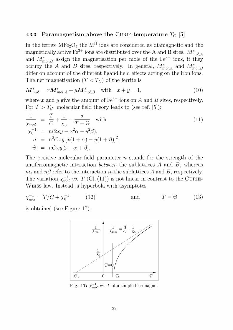
4.3.3 Paramagnetism above the Curie temperature TC [5]

In the ferrite MFe2O4 the MII ions are considered as diamagnetic and the

magnetically active Fe3+ ions are distributed over the A and B sites. M smol,A

and M smol,B assign the magnetisation per mole of the Fe3+ ions, if they

occupy the A and B sites, respectively. In general, M smol,A and M s

mol,B

differ on account of the different ligand field effects acting on the iron ions.The net magnetisation (T < TC) of the ferrite is

M smol = xM s

mol,A + yM smol,B with x+ y = 1, (10)

where x and y give the amount of Fe3+ ions on A and B sites, respectively.For T > TC , molecular field theory leads to (see ref. [5]):

1

χmol=

T

C+

1

χ0

− σ

T − Θwith (11)

χ−10 = n(2xy − x2α − y2β),

σ = n2Cxy [x(1 + α) − y(1 + β)]2 ,

Θ = nCxy[2 + α + β].

The positive molecular field parameter n stands for the strength of the

antiferromagnetic interaction between the sublattices A and B, whereasnα and nβ refer to the interaction in the sublattices A and B, respectively.

The variation χ−1mol vs. T (Gl. (11)) is not linear in contrast to the Curie-

Weiss law. Instead, a hyperbola with asymptotes

χ−1mol = T/C + χ−1

0 (12) and T = Θ (13)

is obtained (see Figure 17).

T T0p C

1 1c

molc

mol c= TC

+ 1

0

Q

0

1c

T Q=

Fig. 17: χ−1

mol vs. T of a simple ferrimagnet

22

Remarks to eq. (11):

• The characteristic feature of a ferrimagnetic material is the hyperbolicvariation χ−1

mol vs. T (in contrast to ferromagnetic materials where the

molecular field approximation gives a straight line).

• A linear dependence is obtained for σ = 0 and x(1 + α) = y(1 + β),

fulfilled for x = y = 1/2 and α = β, which corresponds to antiferro-magnetism.

• The intersection of the asymptote eq. (12) with the T axis at Θp =−C/χ0 is called asymptotic Curie point. It corresponds with the

paramagnetic Curie temperature of an antiferromagnet in the caseof x = y = 1/2 and α = β.

• The intersection of the hyperbola eq. (11) with the T axis is of great

importance:

TC =nC

2

xα+ yβ + [(xα− yβ)2 + 4xy]1/2

TC > 0 means, that at T = TC the susceptibility diverges (χ → ∞),i. e., for T < TC spontaneous magnetisation exists. In the case of TC <

0, the substance behaves paramagnetically in the whole temperaturerange.

• When α > 0 and β > 0 ferrimagnetism exists. If the absolute valuesof α and β exceed those values, which fulfill the condition αβ = 1, the

moment ordering on the sublattices is antiferromagnetic or nonmag-netic. If the absolute values are smaller than the values which fulfill

αβ = 1, the antiferromagnetic interactions within the sublattices arequenched, so that spontaneous magnetisation results.

23

Problems

1. What is a hard magnetic material? Give examples!

2. Fe3O4 adopts the inverse spinel structure type. What type of magneticstructure is expected? How large is the magnetic saturation moment

per formula unit so long as pure spin magnetism is assumed?

3. Co3O4 is a spinel with an antiferromagnetic magnetic structure at T <40 K. Neutron diffraction yields the magnetic saturation moment µs

m =

3µB for the magnetically active centres. What are the magneticallyactive centres? Is the spinel normal or inverse? What are the spin

configurations and total spin quantum numbers of the centres?

4. NiFe2O4 is an inverse spinel. What type of magnetic ordering is ex-

pected? How large is the magnetic saturation moment of each centre,so long as pure spin contributions are considered? What is the µs

m

value per formula unit determined, e. g., by SQUID magnetometry?

5. EuO (NaCl type) is paramagnetic at T > 70 K and obeying theCurie-Weiss law. How large is the expected paramagnetic moment

µ, deduced from the slope of the Curie-Weiss straight line? Whattype of magnetic structure exists at T < 70 K, if neutron diffraction

yields only an increase of reflection intensities, but no extra lines com-pared to those at T > 70 K? Consequently, what sign is expected for

Θp?

6. What law is expected to describe the temperature dependence of the

magnetic susceptibility of magnetically concentrated Mn(II) high-spincompounds above the magnetic ordering temperature TC (Curie tem-perature) and TN (Neel temperature), respectively? What informa-

tion can be gained from a corresponding measurement with regard tothe magnetic centres and the existing interactions?

24

5 Theory of free ions

5.1 Foundations of quantum-mechanics ([10]9–12)

Postulate 1. The state of a system is fully described by the wavefunction

Ψ(r1, r2, . . . , t).Postulate 2. Observables are represented by operators chosen to satisfythe commutation relation

qpq − pqq = [q, pq] = ih (q = x, y, z; i =√−1) (14)

Example 5.1 Application of the commutation relation

x = x · and px =h

i

d

dx

xpxΨ = xh

i

dΨ

dx

pxxΨ =h

i

d(xΨ)

dx=h

i

(Ψ + x

dΨ

dx

)

(xpx − pxx)Ψ = −hiΨ = ihΨ

5.2 Perturbation theory ([5]83–91)

1. Non-degenerate states

H(0)Ψ(0)n = E(0)

n Ψ(0)n unperturbed system (15)

Hamilton operator of the perturbed system:

H = H(0) + λH(1)

Schrodinger equation of the perturbed system:

HΨn = EnΨn; find En,Ψn (16)

Series expansion of Ψn und En:

25

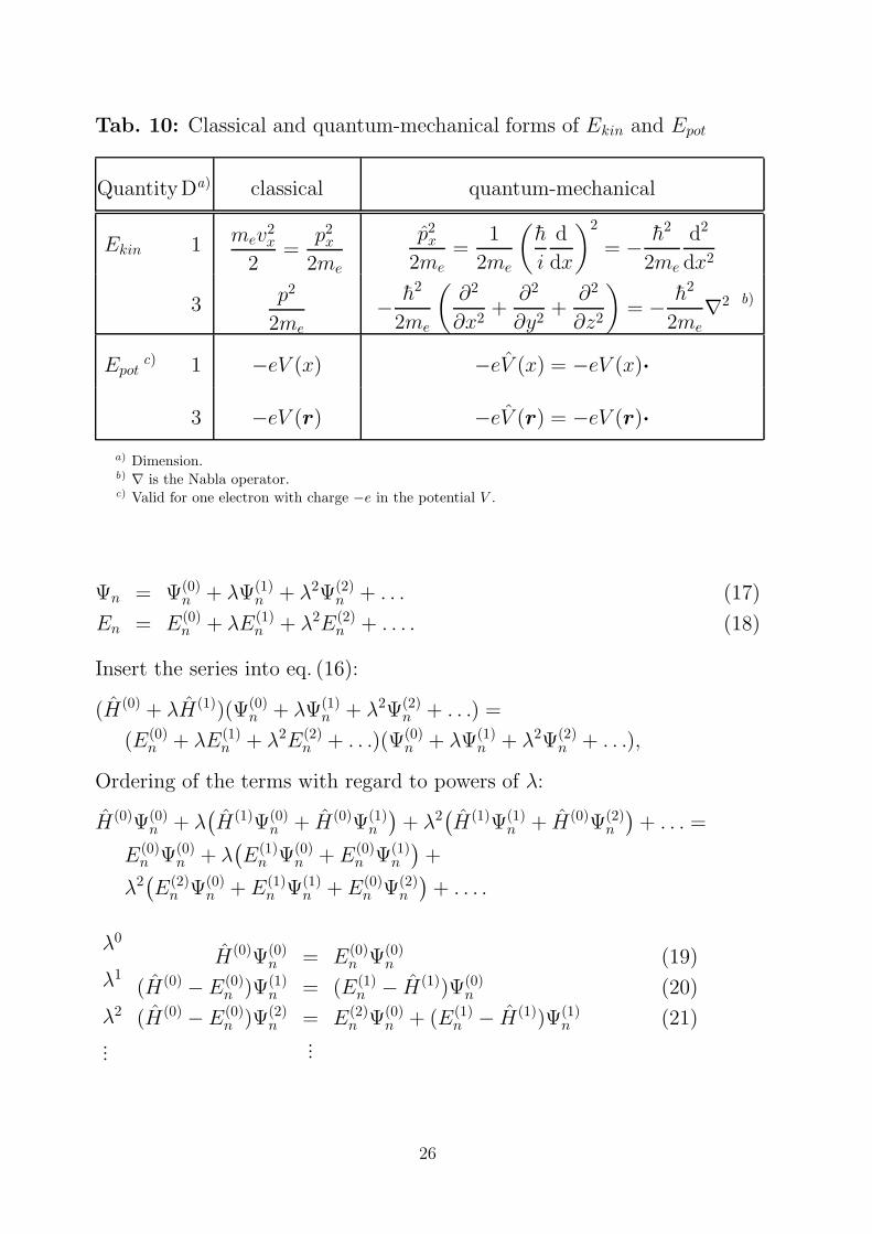
Tab. 10: Classical and quantum-mechanical forms of Ekin and Epot

QuantityDa) classical quantum-mechanical

Ekin 1 mev2x

2=

p2x

2me

p2x

2me=

1

2me

(h

i

d

dx

)2

= − h2

2me

d2

dx2

3 p2

2me

− h2

2me

(∂2

∂x2+

∂2

∂y2+

∂2

∂z2

)= − h2

2me∇2 b)

Epotc) 1 −eV (x) −eV (x) = −eV (x)·

3 −eV (r) −eV (r) = −eV (r)·

a) Dimension.b) ∇ is the Nabla operator.c) Valid for one electron with charge −e in the potential V .

Ψn = Ψ(0)n + λΨ(1)

n + λ2Ψ(2)n + . . . (17)

En = E(0)n + λE(1)

n + λ2E(2)n + . . . . (18)

Insert the series into eq. (16):

(H(0) + λH(1))(Ψ(0)n + λΨ(1)

n + λ2Ψ(2)n + . . .) =

(E(0)n + λE(1)

n + λ2E(2)n + . . .)(Ψ(0)

n + λΨ(1)n + λ2Ψ(2)

n + . . .),

Ordering of the terms with regard to powers of λ:

H(0)Ψ(0)n + λ

(H(1)Ψ(0)

n + H(0)Ψ(1)n

)+ λ2

(H(1)Ψ(1)

n + H(0)Ψ(2)n

)+ . . . =

E(0)n Ψ(0)

n + λ(E(1)

n Ψ(0)n + E(0)

n Ψ(1)n

)+

λ2(E(2)

n Ψ(0)n + E(1)

n Ψ(1)n +E(0)

n Ψ(2)n

)+ . . . .

λ0

λ1

λ2

...

H(0)Ψ(0)n = E(0)

n Ψ(0)n (19)

(H(0) − E(0)n )Ψ(1)

n = (E(1)n − H(1))Ψ(0)

n (20)

(H(0) − E(0)n )Ψ(2)

n = E(2)n Ψ(0)

n + (E(1)n − H(1))Ψ(1)

n (21)...

26

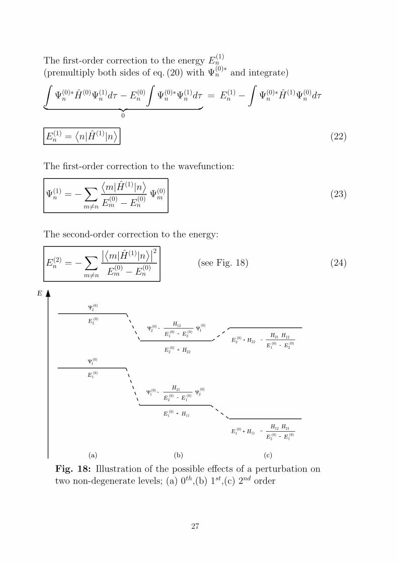
The first-order correction to the energy E(1)n

(premultiply both sides of eq. (20) with Ψ(0)∗n and integrate)

∫Ψ(0)∗

n H(0)Ψ(1)n dτ −E(0)

n

∫Ψ(0)∗

n Ψ(1)n dτ

︸ ︷︷ ︸0

= E(1)n −

∫Ψ(0)∗

n H(1)Ψ(0)n dτ

E(1)n =

⟨n|H(1)|n

⟩(22)

The first-order correction to the wavefunction:

Ψ(1)n = −

∑

m6=n

⟨m|H(1)|n

⟩

E(0)m −E

(0)n

Ψ(0)m (23)

The second-order correction to the energy:

E(2)n = −

∑

m6=n

∣∣⟨m|H(1)|n⟩∣∣2

E(0)m −E

(0)n

(see Fig. 18) (24)

Y2(0)

Y1(0)

2(0)

E

1(0)

E

1(0)

E 11H

Y1(0)

Y2

(0)

1(0)

E2(0)

E

21H

(a) (b) (c)

E

1(0)

E 11H12H

1(0)

E2(0)

E

21H

Y2(0)

Y1

(0)

2(0)

E1(0)

E

12H

2(0)

E 22H

12H21H

2(0)

E 22H

2(0)

E1(0)

E

Fig. 18: Illustration of the possible effects of a perturbation ontwo non-degenerate levels; (a) 0th,(b) 1st,(c) 2nd order

27

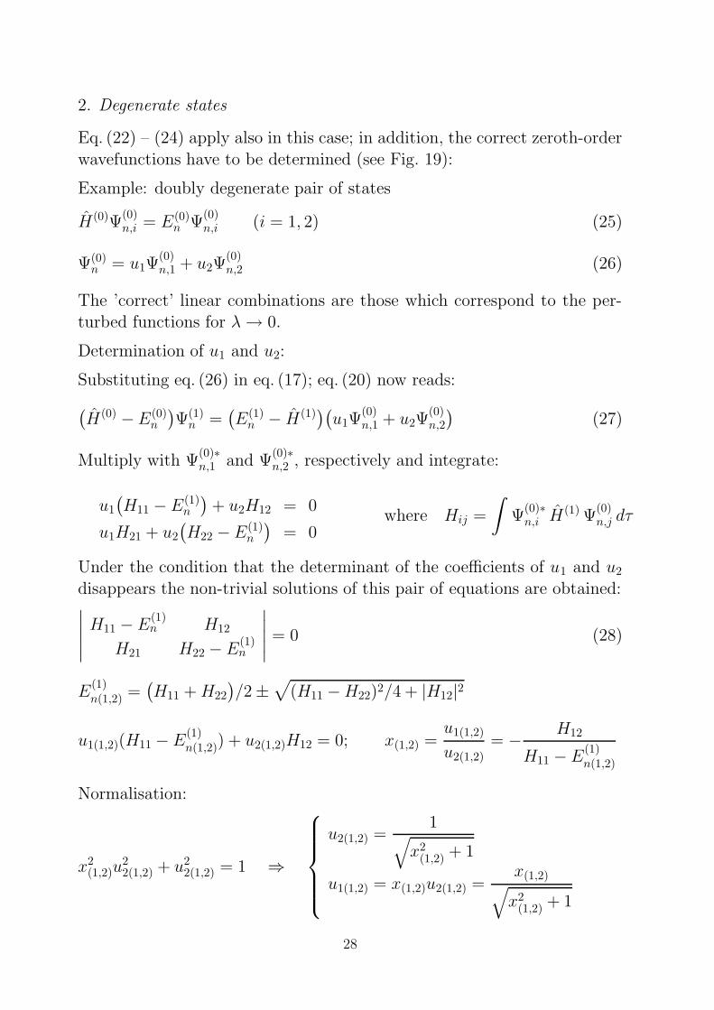
2. Degenerate states

Eq. (22) – (24) apply also in this case; in addition, the correct zeroth-order

wavefunctions have to be determined (see Fig. 19):

Example: doubly degenerate pair of states

H(0)Ψ(0)n,i = E(0)

n Ψ(0)n,i (i = 1, 2) (25)

Ψ(0)n = u1Ψ

(0)n,1 + u2Ψ

(0)n,2 (26)

The ’correct’ linear combinations are those which correspond to the per-turbed functions for λ→ 0.

Determination of u1 and u2:

Substituting eq. (26) in eq. (17); eq. (20) now reads:

(H(0) −E(0)

n

)Ψ(1)

n =(E(1)

n − H(1))(u1Ψ

(0)n,1 + u2Ψ

(0)n,2

)(27)

Multiply with Ψ(0)∗n,1 and Ψ

(0)∗n,2 , respectively and integrate:

u1

(H11 − E(1)

n

)+ u2H12 = 0

u1H21 + u2

(H22 −E(1)

n

)= 0

where Hij =

∫Ψ

(0)∗n,i H

(1) Ψ(0)n,j dτ

Under the condition that the determinant of the coefficients of u1 and u2

disappears the non-trivial solutions of this pair of equations are obtained:∣∣∣∣∣H11 − E

(1)n H12

H21 H22 − E(1)n

∣∣∣∣∣ = 0 (28)

E(1)n(1,2) =

(H11 +H22

)/2 ±

√(H11 −H22)2/4 + |H12|2

u1(1,2)(H11 − E(1)n(1,2)) + u2(1,2)H12 = 0; x(1,2) =

u1(1,2)

u2(1,2)= − H12

H11 − E(1)n(1,2)

Normalisation:

x2(1,2)u

22(1,2) + u2

2(1,2) = 1 ⇒

u2(1,2) =1√

x2(1,2) + 1

u1(1,2) = x(1,2)u2(1,2) =x(1,2)√x2

(1,2) + 1

28

Correct zeroth-order wavefunction for the energy E(1)n(1,2):

Ψ(0)n(1,2) = u1(1,2)Ψ

(0)n,1 + u2(1,2)Ψ

(0)n,2

Y2

2

(0)

(0)E

Y2

2

(0)

(0)E

1(0)

E

E

1(0)

1(2)(1)

EE

2(0)

22HE

1(0)

1(1)(1)

EE

(a) (a )´ (b) (c)

Y(0)

1(2)= Y(0)

Y(0)1,1u1(2) 1,2u2(2)

Y(0)

1(1)= Y(0)1,2Y

(0)1,1u1(1) u2(1)Y

(0)1,2Y

(0)1,1 ,

1(0)

E

2(0)

22HE1(1)2 1(2)2H H21(1) 21(2)H H

2(0)

E1(0)

E

1(0)

1(2)(1)

EE1(2)2H21(2)H

1(0)

E2(0)

E

1(0)

1(1)(1)

EE1(1)2H21(1)H

1(0)

E2(0)

E

Fig. 19: Illustration of the possible effects of a perturbation on

a doubly degenerate ground state and a non-degenerate excitedstate; (a) 0th, (a’) correct 0th, (b) 1st,(c) 2nd order

5.3 One-electron systems ([5]91–96)

Schrodinger equation (spin ignored):

[− h2

2me∇2 − eV (r)

]ψ(r) = Eψ(r). (29)

For convenience the eigenfunctions (atomic orbitals) are given in spherical

polar coordinates:

ψ(r) = ψn,l,ml(r, θ, φ) = Rn,l(r)︸ ︷︷ ︸

radial f.

Y lml

(θ, φ)︸ ︷︷ ︸angular f.

= Rn,l(r) Θlml

(θ)

√1

2πeimlφ

The functions Y lml

(θ, φ) are the (in general, complex) spherical harmon-ics specified by the quantum numbers l and ml (see Table 11). They playa predominant role in magnetism.

29

z

y

x

P( )x,y,z

r cos

r sin

r sin sin

r sin cos

r

q

q

q

q

q

f

ff

.

.

.

..

.

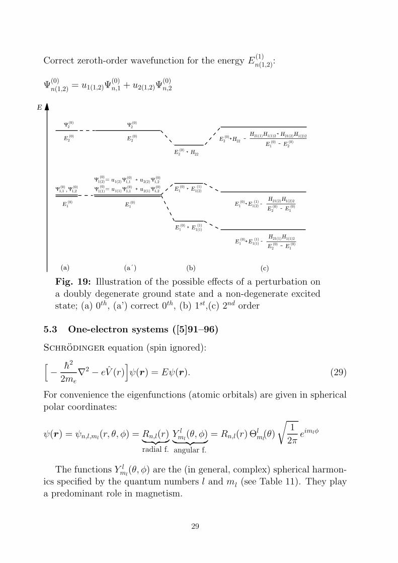
x = r · sin θ · cosφ

y = r · sin θ · sinφz = r · cos θ (30)

r2 = x2 + y2 + z2

cos θ = z/r

tanφ = y/x (31)

Fig. 20: Relation between carte-

sian coordinates and spherical po-lar coordinates

Real functions (see Table 12) are gained by linear combinations

1√2[−ψn,l,ml

+ ψn,l,−ml] = 1√

πRn,l(r)Θ

l−ml

(θ) cosmlφ1

i√

2[−ψn,l,ml

− ψn,l,−ml] = 1√

πRn,l(r)Θ

l−ml

(θ) sinmlφ(32)

1√2[ψn,l,ml

+ ψn,l,−ml] = 1√

πRn,l(r)Θ

lml

(θ) cosmlφ1

i√

2[ψn,l,ml

− ψn,l,−ml] = 1√

πRn,l(r)Θ

lml

(θ) sinmlφ.(33)

For completely describing the wave function, the spin has to be taken

into consideration. If spin-orbit coupling is ignored, the total function (spinorbital) is

ψ(r, θ, φ;σ) = ψ(r, θ, φ)ψ(σ) where σ = ±1

2. (34)

30

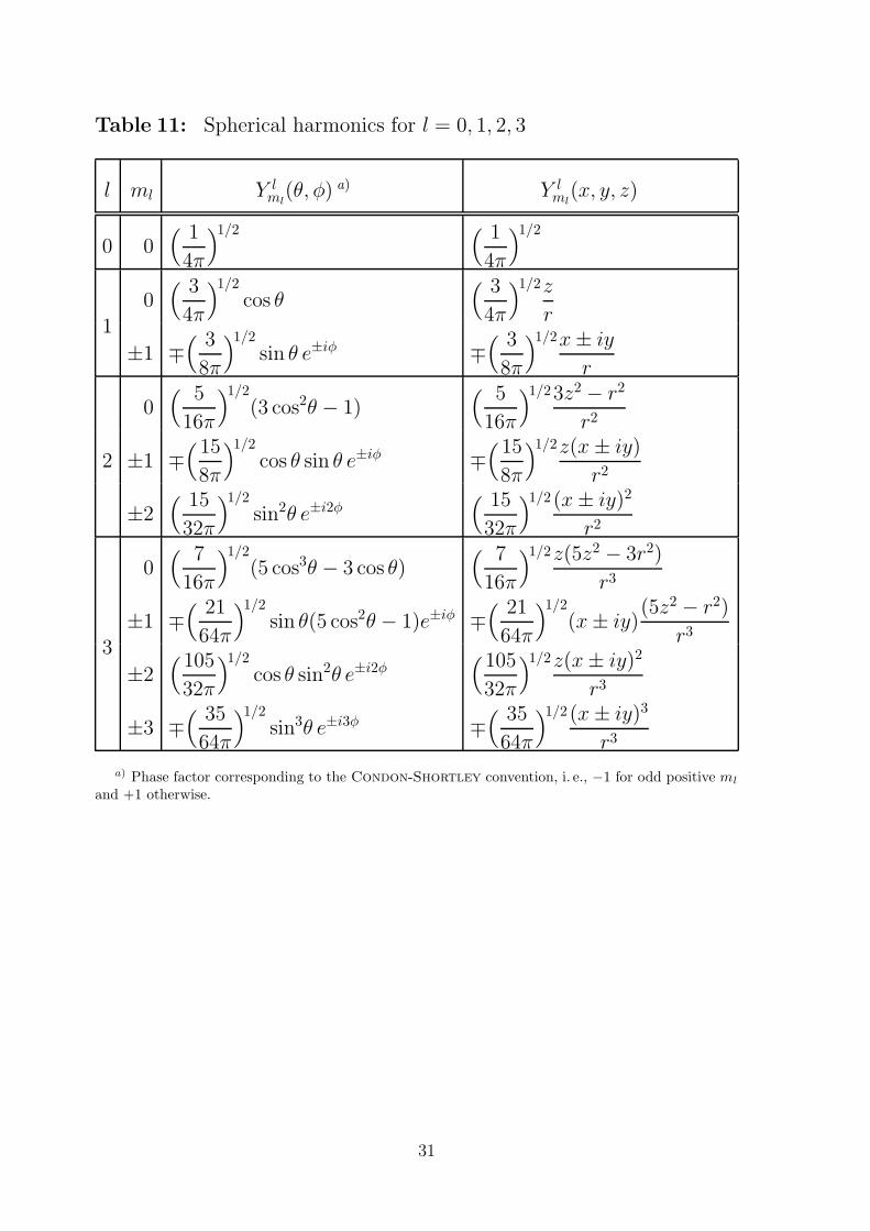
Table 11: Spherical harmonics for l = 0, 1, 2, 3

l ml Y lml

(θ, φ) a) Y lml

(x, y, z)

0 0( 1

4π

)1/2 ( 1

4π

)1/2

0( 3

4π

)1/2

cos θ( 3

4π

)1/2z

r1

±1 ∓( 3

8π

)1/2

sin θ e±iφ ∓( 3

8π

)1/2x± iy

r

0( 5

16π

)1/2

(3 cos2θ − 1)( 5

16π

)1/23z2 − r2

r2

2 ±1 ∓(15

8π

)1/2

cos θ sin θ e±iφ ∓(15

8π

)1/2z(x± iy)

r2

±2( 15

32π

)1/2

sin2θ e±i2φ( 15

32π

)1/2(x± iy)2

r2

0( 7

16π

)1/2

(5 cos3θ − 3 cos θ)( 7

16π

)1/2z(5z2 − 3r2)

r3

±1 ∓( 21

64π

)1/2

sin θ(5 cos2θ − 1)e±iφ ∓( 21

64π

)1/2

(x± iy)(5z2 − r2)

r33

±2(105

32π

)1/2

cos θ sin2θ e±i2φ(105

32π

)1/2z(x± iy)2

r3

±3 ∓( 35

64π

)1/2

sin3θ e±i3φ ∓( 35

64π

)1/2(x± iy)3

r3

a) Phase factor corresponding to the Condon-Shortley convention, i. e., −1 for odd positive ml

and +1 otherwise.

31

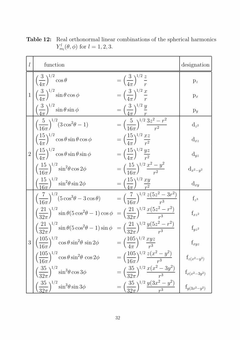
Table 12: Real orthonormal linear combinations of the spherical harmonicsY l

ml(θ, φ) for l = 1, 2, 3.

l function designation

( 3

4π

)1/2

cos θ =( 3

4π

)1/2 z

rpz

1( 3

4π

)1/2

sin θ cosφ =( 3

4π

)1/2 x

rpx

( 3

4π

)1/2

sin θ sinφ =( 3

4π

)1/2 y

rpy

( 5

16π

)1/2

(3 cos2θ − 1) =( 5

16π

)1/2 3z2 − r2

r2dz2

(15

4π

)1/2

cos θ sin θ cosφ =(15

4π

)1/2 xz

r2dxz

2(15

4π

)1/2

cos θ sin θ sinφ =(15

4π

)1/2 yz

r2dyz

( 15

16π

)1/2

sin2θ cos 2φ =( 15

16π

)1/2 x2 − y2

r2dx2−y2

( 15

16π

)1/2

sin2θ sin 2φ =(15

4π

)1/2 xy

r2dxy

( 7

16π

)1/2

(5 cos3θ − 3 cos θ) =( 7

16π

)1/2 z(5z2 − 3r2)

r3fz3

( 21

32π

)1/2

sin θ(5 cos2θ − 1) cosφ =( 21

32π

)1/2 x(5z2 − r2)

r3fxz2

( 21

32π

)1/2

sin θ(5 cos2θ − 1) sinφ =( 21

32π

)1/2 y(5z2 − r2)

r3fyz2

3(105

16π

)1/2

cos θ sin2θ sin 2φ =(105

4π

)1/2 xyz

r3fxyz

(105

16π

)1/2

cos θ sin2θ cos 2φ =(105

16π

)1/2 z(x2 − y2)

r3fz(x2−y2)

( 35

32π

)1/2

sin3θ cos 3φ =( 35

32π

)1/2 x(x2 − 3y2)

r3fx(x2−3y2)

( 35

32π

)1/2

sin3θ sin 3φ =( 35

32π

)1/2 y(3x2 − y2)

r3fy(3x2−y2)

32

5.4 Angular momentum ([5]97–103)

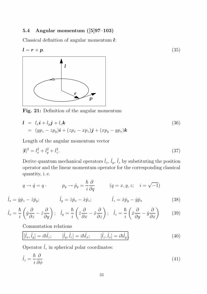
Classical definition of angular momentum l:

l = r × p. (35)

l

rp

Fig. 21: Definition of the angular momentum

l = lxi + lyj + lzk (36)

= (ypz − zpy)i + (zpx − xpz)j + (xpy − ypx)k

Length of the angular momentum vector

|l|2 = l2x + l2y + l2z. (37)

Derive quantum mechanical operators lx, ly, lz by substituting the position

operator and the linear momentum operator for the corresponding classicalquantity, i. e.

q → q = q · pq → pq =h

i

∂

∂q(q = x, y, z; i =

√−1)

lx = ypz − zpy; ly = zpx − xpz; lz = xpy − ypx (38)

lx =h

i

(y∂

∂z− z

∂

∂y

); ly =

h

i

(z∂

∂x− x

∂

∂z

); lz =

h

i

(x∂

∂y− y

∂

∂x

)(39)

Commutation relations

[lx, ly] = ihlz; [ly, lz] = ihlx; [lz, lx] = ihly , (40)

Operator lz in spherical polar coordinates:

lz =h

i

∂

∂φ(41)

33

lz acts on the φ depending part of the atomic orbitals (Table 11):

lz∣∣ l ml

⟩= lz

∣∣ l ml

⟩= mlh

∣∣ l ml

⟩Dirac notation

⟨l ml

∣∣lz∣∣ l ml

⟩= ml h

⟨l ml

∣∣ l ml

⟩︸ ︷︷ ︸

1

generally H Ψ = EΨ, (Ψ normalised eigenfunction of H)∫Ψ∗H Ψ dτ = E

∫Ψ∗ Ψ dτ

︸ ︷︷ ︸1

= E

∫Ψ∗H Ψ dτ ≡ 〈Ψ|H |Ψ〉 matrix element (Dirac notation)

Application of lz:

lz∣∣ 2 2

⟩= Rn,2(r)

h

i

∂Y 22 (θ, φ)

∂φ

= Rn,2(r)h

i

∂

∂φ

[(15

32π

)1/2

sin2θ ei2φ

]

= Rn,2(r)h

i

(15

32π

)1/2

sin2θ∂ei2φ

∂φ

= Rn,2(r)i2h

i

( 15

32π

)1/2

sin2θ ei2φ = 2h∣∣ 2 2

⟩

l2∣∣ l ml

⟩= l(l + 1)h2

∣∣ l ml

⟩(42)

Shift operators:

l+ = lx + ily; l− = lx − ily. (43)

Reverse operations:

lx =1

2(l+ + l−); ly =

1

2i(l+ − l−). (44)

lz∣∣ l ml

⟩= ml h

∣∣ l ml

⟩

l2∣∣ l ml

⟩= l(l + 1) h2

∣∣ l ml

⟩

l±∣∣ l ml

⟩=

√l(l + 1) −ml(ml ± 1) h

∣∣ l ml ± 1⟩.

(45)

34

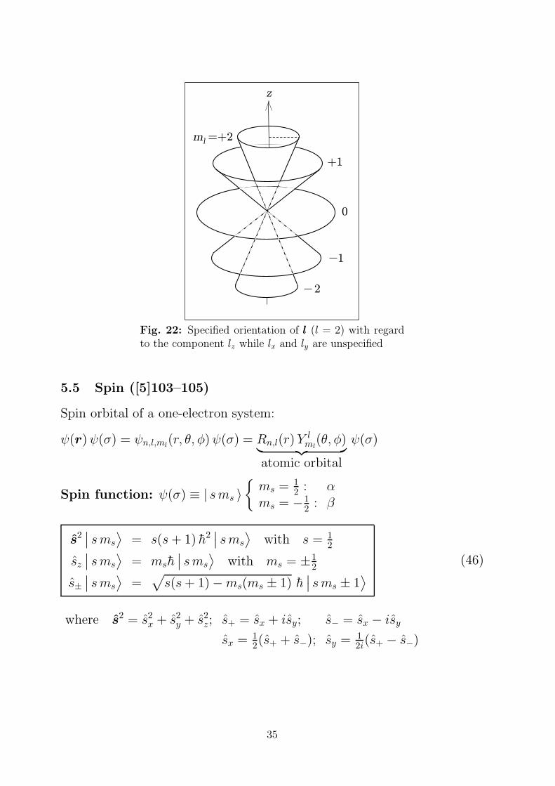
z

ml=+2

+1

0

1

2

Fig. 22: Specified orientation of l (l = 2) with regardto the component lz while lx and ly are unspecified

5.5 Spin ([5]103–105)

Spin orbital of a one-electron system:

ψ(r)ψ(σ) = ψn,l,ml(r, θ, φ)ψ(σ) = Rn,l(r)Y

lml

(θ, φ)︸ ︷︷ ︸atomic orbital

ψ(σ)

Spin function: ψ(σ) ≡ | sms 〉ms = 1

2 : αms = −1

2: β

s2∣∣ sms

⟩= s(s+ 1) h2

∣∣ sms

⟩with s = 1

2

sz

∣∣ sms

⟩= msh

∣∣ sms

⟩with ms = ±1

2

s±∣∣ sms

⟩=

√s(s+ 1) −ms(ms ± 1) h

∣∣ sms ± 1⟩

(46)

where s2 = s2x + s2

y + s2z; s+ = sx + isy; s− = sx − isy

sx = 12(s+ + s−); sy = 1

2i(s+ − s−)

35

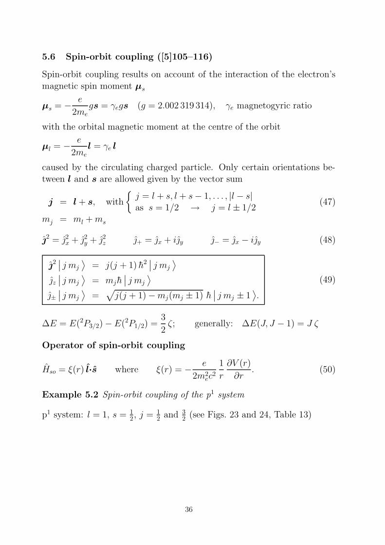
5.6 Spin-orbit coupling ([5]105–116)

Spin-orbit coupling results on account of the interaction of the electron’s

magnetic spin moment µs

µs = − e

2megs = γegs (g = 2.002 319 314), γe magnetogyric ratio

with the orbital magnetic moment at the centre of the orbit

µl = − e

2mel = γe l

caused by the circulating charged particle. Only certain orientations be-

tween l and s are allowed given by the vector sum

j = l + s, with

j = l + s, l + s− 1, . . . , |l − s|as s = 1/2 → j = l ± 1/2

(47)

mj = ml +ms

2 = 2x + 2y + 2z + = x + iy − = x − iy (48)

2∣∣ j mj

⟩= j(j + 1) h2

∣∣ j mj

⟩

z∣∣ j mj

⟩= mjh

∣∣ j mj

⟩

±∣∣ j mj

⟩=

√j(j + 1) −mj(mj ± 1) h

∣∣ j mj ± 1⟩.

(49)

∆E = E(2P3/2) −E(2P1/2) =3

2ζ; generally: ∆E(J, J − 1) = J ζ

Operator of spin-orbit coupling

Hso = ξ(r) l·s where ξ(r) = − e

2m2ec

2

1

r

∂V (r)

∂r. (50)

Example 5.2 Spin-orbit coupling of the p1 system

p1 system: l = 1, s = 12, j = 1

2 and 32 (see Figs. 23 and 24, Table 13)

36

E

E (6)

(4)

(2)

1-2

ohne mit

Spin-Bahn-Wechselwirkung

z

z-

(0)

Fig. 23: Splitting of the p1

levels by spin-orbit interac-tion (ζ: one-electron spin-

orbit coupling constant)

/cm-1

16973

16956

0S

1 2

2P1/

1/

2

2

2P3/2

589.2nml

n

n

17cm1

589.8nm=

2

Fig. 24: Term scheme ofthe sodium atom

Unperturbed sixfold degenerate states:

H(0)ψ(0)i = E(0)ψ

(0)i (i = 1, 2, . . . , 6).

Eq. (27) reads in this case:

(H(0) − E(0))ψ(1) = (E(1) − H(1))(u1ψ

(0)1 + . . .+ u6ψ

(0)6 ). (51)

Multiplication with ψ(0)∗1 from the left and integration gives:∫

ψ(0)∗1

(H(0) − E(0)

)ψ(1)dτ

︸ ︷︷ ︸0

=

∫ψ

(0)∗1

(E(1) − H(1)

)(u1ψ

(0)1 + . . .+ u6ψ

(0)6

)dτ

0 = u1E(1)

∫ψ

(0)∗1 ψ

(0)1 dτ + . . .+ u6E

(1)

∫ψ

(0)∗1 ψ

(0)6 dτ

−u1

∫ψ

(0)∗1 H(1) ψ

(0)1 dτ − . . .− u6

∫ψ

(0)∗1 H(1) ψ

(0)6 dτ.

(52)

Proceeding similarly with ψ(0)∗i (i = 2, . . . , 6) and using the abbreviation∫

ψ(0)∗i H(1)ψ

(0)j dτ ≡ Hij we obtain a system of six equations:

0 = u1

(H11 −E(1)

)+ u2H12 + · · · + u6H16

0 = u1H21 + u2

(H22 −E(1)

)+ · · · + u6H26

......

0 = u1H61 + u2H62 + · · · + u6

(H66 −E(1)

)

(53)

37

Non-trivial solutions for the coefficients of u1, u2, . . . , u6:Calculation of the integrals Hij

∫ (ψn,l,ml

(r, θ, φ)ψms(σ)

)∗HSB ψn,l,m′

l(r, θ, φ)ψm′

s(σ) r2 dr sin θ dθ dφ dσ. (54)

∫ ∞

0

Rn,l(r) ξ(r)Rn,l(r) r2 dr × (55)

∫ π

0

∫ 2π

0

∫ 1/2

−1/2

(Y ml

l (θ, φ)ψms(σ)

)∗l·s

(Y

m′

l

l (θ, φ)ψm′

s(σ)

)sin θ dθ dφ dσ.

hc ζn,l = h2

∫ ∞

0

Rn,l(r) ξ(r)Rn,l(r) r2 dr. (56)

ζn,l: one-electron spin-orbit coupling constantbasis functions in Dirac notation:

∣∣ml ms

⟩

∣∣ 1 12

⟩ ∣∣ 0 12

⟩ ∣∣ −1 12

⟩ ∣∣ 1 − 12

⟩ ∣∣ 0 − 12

⟩ ∣∣ −1 − 12

⟩. (57)

The integral eq. (55) has the short form

hcζn,l

h2

⟨ml ms

∣∣l·s∣∣m′

l m′s

⟩. (58)

Determination of 36 matrix elements of the spin-orbit coupling operator

l·s = lxsx + lysy + lzsz.Replace the x and y components by the step operators (eq. (44,46)):

l·s = lzsz + 12(l+ + l−)1

2(s+ + s−) + 1

2i(l+ − l−) 1

2i(s+ − s−)

= lzsz + 14(l+s+ + l−s+ + l+s− + l−s−

−l+s+ + l−s+ + l+s− − l−s−)

= lzsz + 12(l+s− + l−s+) (59)

The general matrix element (58) is⟨ml ms

∣∣l·s∣∣m′

l m′s

⟩=

⟨ml ms

∣∣lzsz + 12(l+s− + l−s+)

∣∣m′lm

′s

⟩

=⟨ml ms

∣∣lzsz

∣∣m′l m

′s

⟩

+12

⟨mlms

∣∣l+s−∣∣m′

l m′s

⟩

+12

⟨mlms

∣∣l−s+

∣∣m′l m

′s

⟩. (60)

General hints to the evaluation of matrix elements⟨m

∣∣H(1)∣∣n

⟩:

38

(i) Evaluate H(1)∣∣n

⟩. This will result in a constant a multiplied by a wave-

function which may or may not be the same as the original. For the presentlet us assume H(1)

∣∣n⟩

= a∣∣n

⟩.

(ii) The result of (i) is then premultiplied by⟨m

∣∣ giving⟨m

∣∣an⟩.

(iii) Since a is a constant we have⟨m

∣∣an⟩

= a⟨m

∣∣n⟩

and we are thus leftwith the task of evaluating

⟨m

∣∣n⟩. Provided

∣∣m⟩

and∣∣n

⟩are orthonor-

malised,⟨m

∣∣n⟩

= 1 when m = n but is zero otherwise.On account of orthonormalised states⟨ml ms

∣∣m′lm

′s

⟩= δml,m′

lδms,m′

s, (61)

the integral is not zero when ml = m′l and ms = m′

s. The wavefunctions

are eigenfunctions of lz und sz, so that the application of the operatorproducts in eq. (60) on the wavefunction on its right-hand side yields:

lzsz

∣∣ml ms

⟩= ml ms h

2∣∣ml ms

⟩

l+s−∣∣ml ms

⟩=√

l(l + 1) −ml(ml + 1)√s(s+ 1) −ms(ms − 1) h2

∣∣ml + 1ms − 1⟩

l−s+

∣∣ml ms

⟩=√

l(l + 1) −ml(ml − 1)√s(s+ 1) −ms(ms + 1) h2

∣∣ml − 1ms + 1⟩

where s = 12 . For diagonal elements only lzsz may contribute, whereas for

non-diagonal elements only the step operators may account:⟨ml ms

∣∣l+s−∣∣ml − 1ms + 1

⟩ ⟨mlms

∣∣l−s+

∣∣ml + 1ms − 1⟩

Matrix elements (58) which may contribute are restricted to the condition

ml +ms = m′l +m′

s (62)

The non-zero matrix elements are:⟨1 − 1

2

∣∣l+s−∣∣ 0 1

2

⟩ ⟨0 − 1

2

∣∣l+s−∣∣ −1 1

2

⟩⟨0 1

2

∣∣l−s+

∣∣ 1 − 12

⟩ ⟨−1 1

2

∣∣l−s+

∣∣ 0 − 12

⟩.

39

mlms

∣∣ 1 12

⟩ ∣∣ 1 − 12

⟩ ∣∣ 0 12

⟩ ∣∣ 0 − 12

⟩ ∣∣ −1 12

⟩ ∣∣ −1 − 12

⟩

⟨1 1

2

∣∣ 12 ζ⟨

1 − 12

∣∣ −12 ζ

√12 ζ

⟨0 1

2

∣∣√

12 ζ 0

⟨0 − 1

2

∣∣ 0√

12 ζ

⟨−1 1

2

∣∣√

12 ζ −1

2 ζ⟨−1 − 1

2

∣∣ 12 ζ

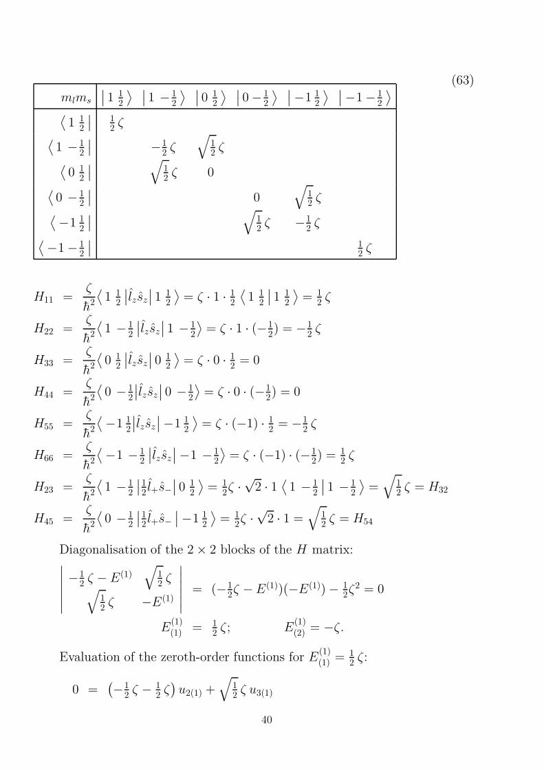
(63)

H11 =ζ

h2

⟨1 1

2

∣∣lzsz

∣∣ 1 12

⟩= ζ · 1 · 1

2

⟨1 1

2

∣∣ 1 12

⟩= 1

2 ζ

H22 =ζ

h2

⟨1 − 1

2

∣∣lzsz

∣∣ 1 − 12

⟩= ζ · 1 · (−1

2) = −1

2ζ

H33 =ζ

h2

⟨0 1

2

∣∣lzsz

∣∣ 0 12

⟩= ζ · 0 · 1

2 = 0

H44 =ζ

h2

⟨0 − 1

2

∣∣lzsz

∣∣ 0 − 12

⟩= ζ · 0 · (−1

2) = 0

H55 =ζ

h2

⟨−1 1

2

∣∣lzsz

∣∣ −1 12

⟩= ζ · (−1) · 1

2 = −12 ζ

H66 =ζ

h2

⟨−1 − 1

2

∣∣lzsz

∣∣ −1 − 12

⟩= ζ · (−1) · (−1

2) = 12 ζ

H23 =ζ

h2

⟨1 − 1

2

∣∣12 l+s−

∣∣ 0 12

⟩= 1

2ζ ·√

2 · 1⟨1 − 1

2

∣∣ 1 − 12

⟩=

√12 ζ = H32

H45 =ζ

h2

⟨0 − 1

2

∣∣12 l+s−

∣∣ −1 12

⟩= 1

2ζ ·√

2 · 1 =√

12 ζ = H54

Diagonalisation of the 2 × 2 blocks of the H matrix:∣∣∣∣∣∣−1

2 ζ − E(1)√

12 ζ√

12 ζ −E(1)

∣∣∣∣∣∣= (−1

2ζ −E(1))(−E(1)) − 12ζ

2 = 0

E(1)(1) = 1

2 ζ; E(1)(2) = −ζ.

Evaluation of the zeroth-order functions for E(1)(1) = 1

2 ζ:

0 =(−1

2 ζ − 12 ζ

)u2(1) +

√12 ζ u3(1)

40

x(1) =u2(1)

u3(1)=

√12; u2(1) =

√13; u3(1) =

√23

ψ2 =√

13

∣∣ 1 − 12

⟩+

√23

∣∣ 0 12

⟩. (64)

For E(1)(2) = −ζ, the result is:

0 =(−1

2 ζ + ζ)u2(2) +

√12 ζ u3(2)

x(2) =u2(2)

u3(2)= −

√2; u2(2) = −

√23; u3(2) =

√13

ψ3 = −√

23

∣∣ 1 − 12

⟩+

√13

∣∣ 0 12

⟩. (65)

Evaluating the second 2 × 2 block the resulting states are

E(1)(1) = 1

2 ζ : ψ4 =√

13

∣∣ −1 12

⟩+

√23

∣∣ 0 − 12

⟩(66)

E(1)(2) = −ζ : ψ5 =

√23

∣∣ −1 12

⟩−

√13

∣∣ 0 − 12

⟩. (67)

The functions are not only eigenfunctions of the operators l·s and s·l but

also of

l 2 + l·s + s·l + s2 =(l + s

)2 = 2. (68)

If 2 acts on a quartet state function ψQ (ψ1, ψ2, ψ4, ψ6) and on a doubletstate function ψD (ψ3, ψ5), respectively the result is

2 ψQ =(l 2 + 2 l·s + s2

)ψQ

= h2(2 + 2 · 1

2 + 34

)ψQ = h2 (15

4 )ψQ = h2 (32)(

52)ψQ

= h2 j1(j1 + 1)ψQ where j1 = 32 (69)

2 ψD =(l 2 + 2 l·s + s2

)ψD

= h2(2 − 2 · 1 + 3

4

)ψD = h2 (3

4)ψD = h2 (12)(

32)ψD

= h2 j2(j2 + 1)ψD where j2 = 12 . (70)

41

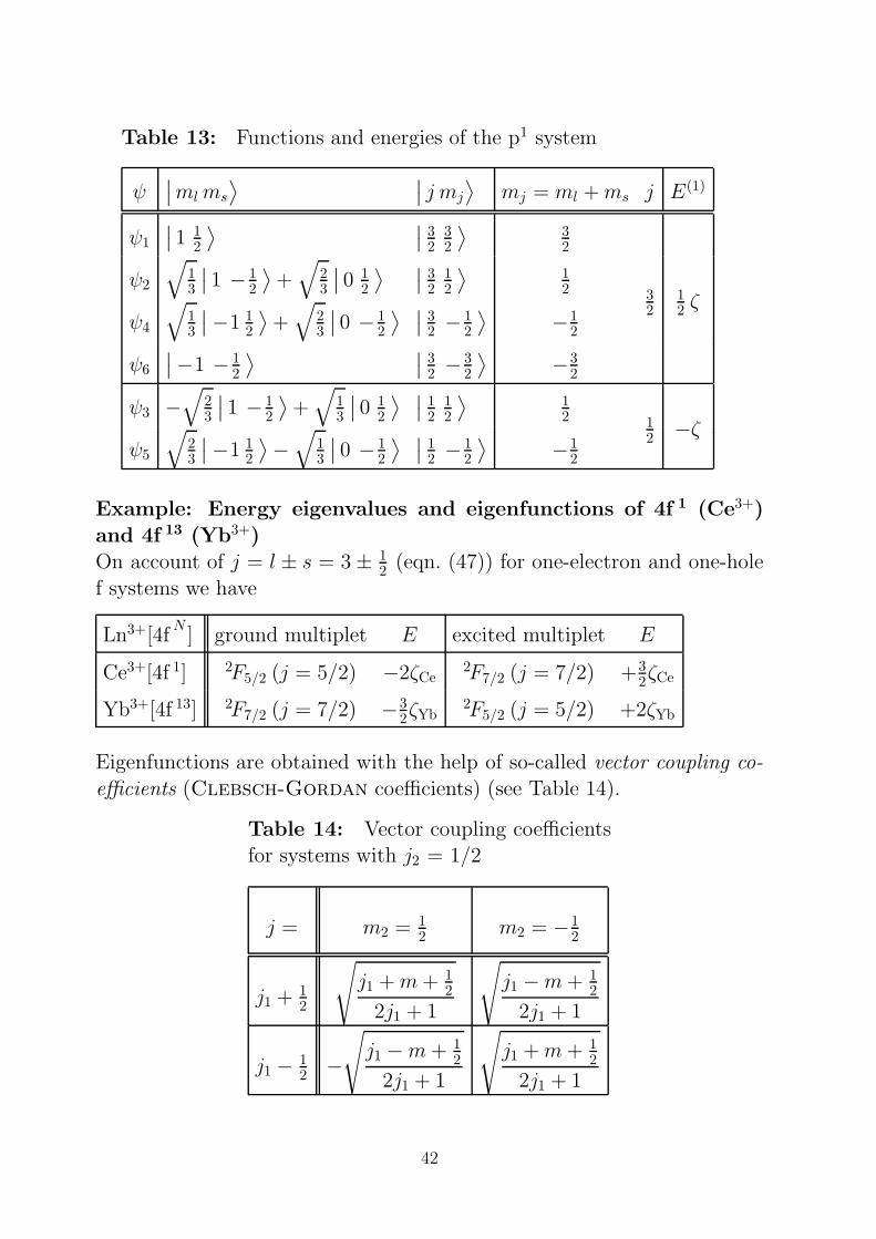
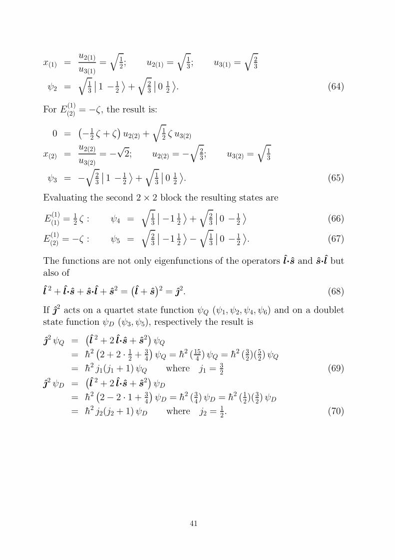
Table 13: Functions and energies of the p1 system

ψ∣∣ml ms

⟩ ∣∣ j mj

⟩mj = ml +ms j E(1)

ψ1

∣∣ 1 12

⟩ ∣∣ 32

32

⟩32

ψ2

√13

∣∣ 1 − 12

⟩+

√23

∣∣ 0 12

⟩ ∣∣ 32

12

⟩12

ψ4

√13

∣∣ −1 12

⟩+

√23

∣∣ 0 − 12

⟩ ∣∣ 32 − 1

2

⟩−1

2

32

12 ζ

ψ6

∣∣ −1 − 12

⟩ ∣∣ 32 − 3

2

⟩−3

2

ψ3 −√

23

∣∣ 1 − 12

⟩+

√13

∣∣ 0 12

⟩ ∣∣ 12

12

⟩12

ψ5

√23

∣∣ −1 12

⟩−

√13

∣∣ 0 − 12

⟩ ∣∣ 12 − 1

2

⟩−1

2

12 −ζ

Example: Energy eigenvalues and eigenfunctions of 4f 1 (Ce3+)

and 4f 13 (Yb3+)On account of j = l ± s = 3 ± 1

2 (eqn. (47)) for one-electron and one-hole

f systems we have

Ln3+[4fN

] ground multiplet E excited multiplet E

Ce3+[4f 1] 2F5/2 (j = 5/2) −2ζCe2F7/2 (j = 7/2) +3

2ζCe

Yb3+[4f 13] 2F7/2 (j = 7/2) −32ζYb

2F5/2 (j = 5/2) +2ζYb

Eigenfunctions are obtained with the help of so-called vector coupling co-

efficients (Clebsch-Gordan coefficients) (see Table 14).

Table 14: Vector coupling coefficientsfor systems with j2 = 1/2

j = m2 = 12

m2 = −12

j1 + 12

√j1 +m+ 1

2

2j1 + 1

√j1 −m+ 1

2

2j1 + 1

j1 − 12 −

√j1 −m+ 1

2

2j1 + 1

√j1 +m+ 1

2

2j1 + 1

42

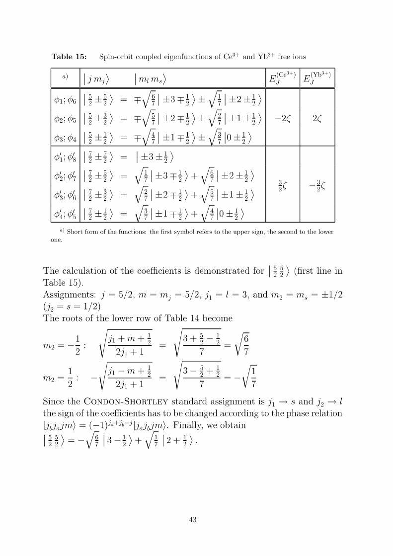
Table 15: Spin-orbit coupled eigenfunctions of Ce3+ and Yb3+ free ions

a)∣∣ j mj

⟩ ∣∣ml ms

⟩E

(Ce3+)J E

(Yb3+)J

φ1;φ6

∣∣ 52 ± 5

2

⟩= ∓

√67

∣∣ ±3 ∓ 12

⟩±

√17

∣∣ ±2 ± 12

⟩

φ2;φ5

∣∣ 52 ± 3

2

⟩= ∓

√57

∣∣ ±2 ∓ 12

⟩±

√27

∣∣ ±1 ± 12

⟩−2ζ 2ζ

φ3;φ4

∣∣ 52 ± 1

2

⟩= ∓

√47

∣∣ ±1 ∓ 12

⟩±

√37

∣∣0 ± 12

⟩

φ′1;φ′8

∣∣ 72 ± 7

2

⟩=

∣∣ ±3 ± 12

⟩

φ′2;φ′7

∣∣ 72± 5

2

⟩=

√17

∣∣ ±3 ∓ 12

⟩+

√67

∣∣ ±2 ± 12

⟩

φ′3;φ′6

∣∣ 72 ± 3

2

⟩=

√27

∣∣ ±2 ∓ 12

⟩+

√57

∣∣ ±1 ± 12

⟩ 32ζ −3

2ζ

φ′4;φ′5

∣∣ 72 ± 1

2

⟩=

√37

∣∣ ±1 ∓ 12

⟩+

√47

∣∣0 ± 12

⟩

a) Short form of the functions: the first symbol refers to the upper sign, the second to the lowerone.

The calculation of the coefficients is demonstrated for∣∣ 5

252

⟩(first line in

Table 15).Assignments: j = 5/2, m = mj = 5/2, j1 = l = 3, and m2 = ms = ±1/2(j2 = s = 1/2)

The roots of the lower row of Table 14 become

m2 = −1

2:

√j1 +m+ 1

2

2j1 + 1=

√3 + 5

2 − 12

7=

√6

7

m2 =1

2: −

√j1 −m+ 1

2

2j1 + 1=

√3 − 5

2 + 12

7= −

√1

7

Since the Condon-Shortley standard assignment is j1 → s and j2 → lthe sign of the coefficients has to be changed according to the phase relation

|jbjajm〉 = (−1)ja+jb−j|jajbjm〉. Finally, we obtain∣∣ 52

52

⟩= −

√67

∣∣ 3 − 12

⟩+

√17

∣∣ 2 + 12

⟩.

43

Problems

1. Calculate the matrix elements 〈l,ml|lq|l,m′l〉 (where q stands for z,+,−)

(a) 〈0, 0|lz|0, 0〉, (b) 〈2, 2|l+|2, 1〉, (c) 〈2, 2|l2+|2, 0〉, (d) 〈2, 0|l+l−|2, 0〉.

2. The 14 microstates |mlms〉 of an f 1 system (l = 3, s = 1/2) yield under

the influence of the spin-orbit coupling operator 14 eigenstates |jmj〉which are linear combinations of the microstates. Use Table 14 to eval-uate the vector coupling coefficients for the coupled states |5/2 1/2〉,|5/2 − 1/2〉, |7/2 3/2〉, and |7/2 − 3/2〉. Control your results withthe entries of Table 15.

44

6 Exchange interactions in dinuclear compounds

6.1 Parametrization of exchange interactions

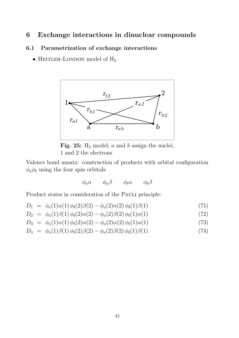
• Heitler-London model of H2

1

2

a br

r

r

r

a

a

b

b

2

2

1

1 rb2

ra1

Fig. 25: H2 model; a and b assign the nuclei,

1 and 2 the electrons

Valence bond ansatz: construction of products with orbital configuration

φaφb using the four spin orbitals

φaα φaβ φbα φbβ

Product states in consideration of the Pauli principle:

D1 = φa(1)α(1)φb(2)β(2)− φa(2)α(2)φb(1)β(1) (71)

D2 = φa(1)β(1)φb(2)α(2)− φa(2)β(2)φb(1)α(1) (72)

D3 = φa(1)α(1)φb(2)α(2)− φa(2)α(2)φb(1)α(1) (73)

D4 = φa(1)β(1)φb(2)β(2)− φa(2)β(2)φb(1)β(1) (74)

45

• Construction of eigenfunctions of the total spin

S′ = S1 + S2 (S1 = S2 = 1/2)

D3 and D4 are eigenfunctions |S ′M ′S 〉 of S′2 = (S1 + S2)

2 and S ′z =

Sz1 + Sz2 with S ′ = 1 and MS′ = 1 and −1 (Spin triplet functions | 1 1 〉and | 1 −1 〉), respectively.

D1 +D2 =⇒ | 1 0 〉 (spin triplet function)D1 −D2 =⇒ | 0 0 〉 (spin singlet function)

Φ1 = D1 −D2 Φ2 = D3 Φ3 = D1 +D2 Φ4 = D4

| 0 0 〉 | 1 1 〉 | 1 0 〉 | 1 −1 〉

φa and φb are normalised:∫φa(1)∗φa(1)dτ1 =

∫φ∗b(2)φb(2)dτ2 = 1,

but not orthogonal:

overlap integral Sab =

∫φa(1)∗φb(1)dτ1 =

∫φa(2)∗φb(2)dτ2 6= 0

Normalised functions of the dinuclear unit:

Φ1 = Ng [φa(1)φb(2) + φa(2)φb(1)]︸ ︷︷ ︸sym

√12[α(1)β(2)− α(2)β(1)]

︸ ︷︷ ︸anti

Φ2

Φ3

Φ4

= Nu [φa(1)φb(2) − φa(2)φb(1)]︸ ︷︷ ︸anti

α(1)α(2)√12[α(1)β(2) + α(2)β(1)]

β(1)β(2)︸ ︷︷ ︸

sym

where Ng = [2 + 2S2ab]

− 12 and Nu = [2 − 2S2

ab]− 1

2 .

46

• Symmetry of the functions with regard to exchange of electrons

total function: anti Φi(1, 2) = −Φi(2, 1)

singlet function: orbital sym (g), spin function anti

triplet functions: orbital anti (u), spin function sym

⇒ Symmetry of the orbital forces a distinct multiplicity of the spin func-tion on account of the Pauli principle

• Evaluation of the energy E(S) and E(T ) of the singlet and triplet

states

H = − h2

2me∇2(1) − e2

ra1− e2

rb1︸ ︷︷ ︸h(1)

− h2

2me∇2(2) − e2

ra2− e2

rb2︸ ︷︷ ︸h(2)

+e2

r12

E(S) = 〈1Φg1|H|1Φg

1〉 =2(h+ habSab) + Jab +Kab

1 + S2ab

(75)

E(T ) = 〈3Φu2|H|3Φu

2〉 =2(h− habSab) + Jab −Kab

1 − S2ab

(76)

where

h =⟨φa(i)

∣∣∣h(i)∣∣∣φa(i)

⟩(one-centre

=⟨φb(i)

∣∣∣h(i)∣∣∣φb(i)

⟩one-electron integral)

hab =⟨φa(i)

∣∣∣h(i)∣∣∣φb(i)

⟩(transfer or hopping integral)

Jab =⟨φa(1)φb(2)

∣∣e2/r12

∣∣φa(1)φb(2)⟩

(Coulomb integral)

Kab =⟨φa(1)φb(2)

∣∣e2/r12

∣∣φa(2)φb(1)⟩

(Exchange integral).

47

Example: Evaluation of E(S) =⟨

1Φg1

∣∣∣H∣∣∣ 1Φg

1

⟩

1. Integration over the spin:

12〈α(1)β(2)− β(1)α(2)|α(1)β(2)− β(1)α(2)〉 =

12

[〈α(1)β(2)|α(1)β(2)〉︸ ︷︷ ︸

1

+ 〈α(2)β(1)|α(2)β(1)〉︸ ︷︷ ︸1

−

〈α(2)β(1)|α(1)β(2)〉︸ ︷︷ ︸0

−〈α(1)β(2)|α(2)β(1)〉︸ ︷︷ ︸0

]= 1.

2. Integration over the space:

E(S) = (77)

N2g

⟨φa(1)φb(2) + φb(1)φa(2)

∣∣∣h(1) + h(2) + e2/r12

∣∣∣φa(1)φb(2)+

φb(1)φa(2)⟩

= 2N2g [2(h+ habSab) + Jab +Kab].

Singlet-triplet splitting:

∆E(T, S) = E(T ) − E(S)

≈ −2Kab − 4habSab + 2S2ab(2h+ Jab)

• Application of the Heitler-London model to dinuclear complexes

having S1 = S2 = 12 centres

Example: L′nCua– L– CubL

′n

As distinguished from the strong covalent bond in H2 the interactions be-

tween both magnetically active electrons is weak.⇒ small ∆E(T, S).

The highest singly occupied antibonding orbitals φa and φb of the fragmentsL′

nCuaL and LCubL′n, respectively take over the role of the 1s orbitals of

the H atoms. φa and φb have mainly d character. They are centered at themetal ions and partially delocalised in the direction of the ligands.

48

6.2 Heisenberg operator

Phenomenological description of the interaction between the unpaired elec-

trons of the centres by an apparent spin-spin coupling, whose magnitudeand sign are given by the spin-spin coupling parameter (exchange param-

eter) J :

Hex = −2J S1·S2 where − 2J = ∆E(T, S) (78)

Hex is an effective operator, describing but not explaining the phenomenon.

Application of Hex to 1Φg1 (S ′ = 0) and 3Φu

i (S ′ = 1, i = 2, 3, 4):

−2J S1·S21Φg

1 =(

32

)J︸ ︷︷ ︸

E(S)

1Φg1, −2J S1·S2

3Φui = −

(12

)J︸ ︷︷ ︸

E(T )

3Φui

⇒ ∆E(T, S) = E(T ) − E(S) = −2J (79)

J < 0: singlet ground state (intramolecular antiferromagnetic interaction)

J > 0: triplet ground state (intramolecular ferromagnetic interaction)

Hints to the evaluation of E(T ) and E(S):

S′2 =(S1 + S2

)2

= S21 + S2

2 + 2S1·S2

2S1·S2 = S′2 − S21 − S2

2

= h2[S ′(S ′ + 1)︸ ︷︷ ︸0 or 2

−S1(S1 + 1)︸ ︷︷ ︸34

−S2(S2 + 1)︸ ︷︷ ︸34

]

Heisenberg operator for more than two centres:

Hex = −2∑

i<j

JijSi·Sj (80) Hex = −2J∑

i<j

Si·Sj (81)

Magnetic susceptibility ([5]138–162)Fundamental magnetisation equation

Mmol = −NA

∑n

(∂En/∂B) exp(−En/kBT )

∑n

exp(−En/kBT )= NA

∑nµn exp(−En/kBT )

∑n

exp(−En/kBT )

49

(82)

Van Vleck equation

Operator: H = H(0) + BzH(1)

En = W (0)n +BzW

(1)n + B2

zW(2)n + . . . .

W(1)n , W

(2)n : First- and second-orderZeeman coefficients

µn = −∂En/∂B = −W (1)n − 2BW (2)

n − . . .

χmol = µ0NA

∑n

[(W(1)n )2/kBT − 2W

(2)n ] exp(−W (0)

n /kBT )

∑n

exp(−W (0)n /kBT )

(83)

Eq. (83) is valid for applied magnetic fields B → 0

6.3 Exchange-coupled species in a magnetic field

Hex = −2J S1·S2 = −2J(Sz1Sz2 + Sx1Sx2 + Sy1Sy2

)

= −2J[Sz1Sz2 + 1

2

(S+1S−2 + S−1S+2

)](84)

Basis: spin functions in the form |MS MS 〉 where the first MS refers toelectron 1 and the second to electron 2

H-Matrix:

MS1MS2

∣∣ 12

12

⟩ ∣∣ − 12

12

⟩ ∣∣ 12 − 1

2

⟩ ∣∣ − 12 − 1

2

⟩

⟨12

12

∣∣ −J /2⟨− 1

212

∣∣ J /2 −J⟨

12 − 1

2

∣∣ −J J /2⟨− 1

2 − 12

∣∣ −J /2

(85)

Evaluation of the diagonal element H11:

−2J⟨

12

12

∣∣ Sz1Sz2

∣∣ 12

12

⟩= −2J

(12

) (12

)= −J /2

50

Evaluation of the off-diagonal element H23:

−2J⟨− 1

212

∣∣ 12S−1S+2

∣∣ 12 − 1

2

⟩= −J (1)(1) = −J

Result:

Tab. 16: Spin functions and exchangeenergies of the S1 = S2 = 1

2system

Spin function MS′ S ′ E

1√2

(∣∣ 12− 1

2

⟩−

∣∣ − 12

12

⟩)0 0 3

2J

∣∣ 12

12

⟩1

1√2

(∣∣ 12 − 1

2

⟩+

∣∣ − 12

12

⟩)0 1 −1

2J∣∣ − 1

2 − 12

⟩−1

51

E

00

1

2

3

4

530J

20J

12J

6J

2J

SS2 1+

1

3

5

7

9

11

Fig. 26: Relative energies and multiplicities of the spin states

of a dinuclear Fe3+ complex (S = 52); for Cu2+ (S = 1

2) only thetwo lowest levels are relevant, while for Gd3+ (S = 7

2) the twolevels with S ′ = 6 (E = |42J |) and S ′ = 7 (E = |56J |) have

to be added.

52

• Magnetic susceptibility of a spin-spin-coupled system with S1 = S2 = 12

0

0

1 2 3 4 5

10

8

6

4

2

0

-2

E/

-1cm

/TB0

M

1

0

-1=S

=S

S

0

1

E(T,S)D

Fig. 27: Correlation diagram of aS1 = S2 = 1

2 system under the in-

fluence of isotropic intramolecularspin-spin coupling (J = −2 cm−1)and applied field

T/K0 5 10 15 20 25

0

2

4

6

8

10

a

b

c

cm

ol

10

-7m

3m

ol-1

/(

)Fig. 28: χmol versus T diagram ofa S1 = S2 = 1

2 exchange-coupled

system with J = −2 cm−1 at ap-plied fields of B0 = 0.01 T (a),3.5 T (b), and 5 T (c)

Application of the Van Vleck equation (83) to a dinuclear system with

S1 = S2 = 12

Zeeman-Operator:

HMz= −γeg(Sz1 + Sz2)︸ ︷︷ ︸

H(1)

Bz = −γe g S′z Bz

S ′MS′

∣∣ 1 1⟩ ∣∣ 1 0

⟩ ∣∣ 1 −1⟩ ∣∣ 0 0

⟩

⟨1 1

∣∣ gµBBz⟨1 0

∣∣ 0⟨1 −1

∣∣ −gµBBz⟨0 0

∣∣ 0

(86)

Matrix elements:

〈11|HMz|11〉 = gµBBz −→W

(1)|11〉 = gµB

〈1 −1|HMz|1 −1〉 = −gµBBz −→W

(1)|1−1〉 = −gµB

53

The remaining matrix elements (Zeeman coefficients) are zero. W(1)|11〉,

W(1)|1−1〉,W

(0)S = E(S), andW

(0)T = E(T ) are substituted into the Van Vleck

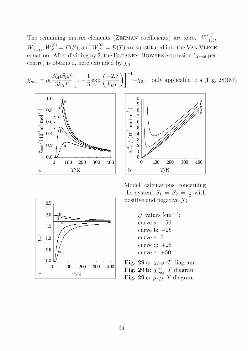
equation. After dividing by 2, the Bleaney-Bowers expression (χmol percentre) is obtained, here extended by χ0

χmol = µ0NAµ

2Bg

2

3kBT

[1 +

1

3exp

(−2JkBT

)]−1

+χ0, only applicable to a (Fig. 28)(87)

1.0

0.8

0.6

0.4

0.2

0.00 100 200 300 400

T/Ka

a

b

d

c

e

cm

ol/

10

mm

ol

3-7

-1(

)

0 100 200 300 4000123456789

10

T/K

ab

b

cde

c10

7m

olm

-3

mol

-1(

)/

meff

1.5

0.5

0 100 200 300 4000.0

1.0

2.0

2.5

T/K

a

b

c

c

de

Model calculations concerning

the system S1 = S2 = 12 with

positive and negative J ;

J values [cm−1]:

curve a: −50curve b: −25

curve c: 0curve d: +25curve e: +50

Fig. 29 a: χmol–T diagram

Fig. 29 b: χ−1mol–T diagram

Fig. 29 c: µeff–T diagram

54

Polynuclear unit of n equivalent centres:

χmol =µ0

n

NAµ2Bg

2

3kBT

∑S′ S ′(S ′ + 1)(2S ′ + 1)Ω(S ′) exp

(−E(S′)

kBT

)

∑S′(2S ′ + 1)Ω(S ′) exp

(−E(S′)

kBT

) (88)

Evaluation of S ′, E(S ′) and Ω(S ′):

S ′ of the coupled states:S ′ = nS, nS − 1, . . . , 0 (nS integer) or 1

2 (nS half integer)

Relative energies E(S ′):

E(S ′) = − zJn− 1

[S ′(S ′ + 1) − nS(S + 1)]

z: number of nearest neighbours of a centre

n: number of interacting centres

Frequency Ω(S ′) of the states S ′:

Ω(S ′) = ω(S ′) − ω(S ′ + 1)

ω(S ′) is the coefficient of XS′

in the expansion

(XS +XS−1 + . . .+X−S)n

• Scope of validity of the Heisenberg model

1. Localised magnetic moments (no band magnetism)

2. good quantum number S of the centres

3. orbital singlet as ground term3d5-High-Spin −→ 6A1

3d3(Oh), 3d7(Td) −→ 4A2

3d8(Oh), 3d2(Td) −→ 3A2

(3d9(Oh) −→ 2E)

55

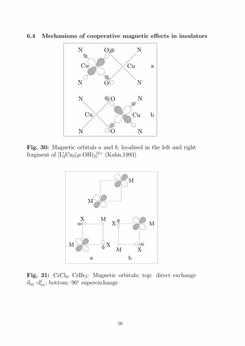
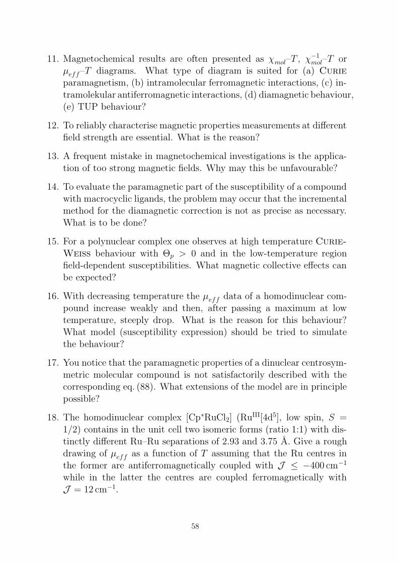
6.4 Mechanisms of cooperative magnetic effects in insulators

N

NN

N

CuCu

O

O

N

N N

N

CuCu

O

O

a

b

Fig. 30: Magnetic orbitals a and b, localised in the left and rightfragment of [L′

2Cu2(µ-OH)2]2+ (Kahn,1993)

M

M

M

M

MX

X

X

a b

XM

Fig. 31: CrCl3, CrBr3: Magnetic orbitals; top: direct exchangedxy–d′

xy; bottom: 90 superexchange

56

Problems

1. Verify the equation S2 = S2z − hSz + S+S−.

2. Show, that the function eq. (74)

Ψ4 = D4 = φa(1)β(1)φb(2)β(2)− φa(2)β(2)φb(1)β(1)

is an eigenfunction of S′2 = (S1 + S2)2 and S ′

z = Sz1 + Sz2! How largeare S ′ and MS′?

3. Corresponding to E(S), eq. (77), evaluate the energy E(T ) of thetriplet state and verify the result given in eq. (76).

4. Reconstruct the steps eq. (86) −→ eq. (87).

5. The Bleaney-Bowers formula, eq. (87), approaches for high tem-perature the Curie-Weiss law, eq. (9). Give the relation between Jand Θp. Is the result in agreement with the right formula in eq. (9)?

6. What magnetic behaviour is obtained, if in the Bleaney-Bowers-

Formel, eq. (87), J is set to 0?

7. Determine on the basis of matrix (85) and perturbation theory the

correct zeroth-order wavefunctions and verify the entries in Table 16.

8. Write the Heisenberg spin operator for a trinuclear unit of equiva-lent centres (equilateral triangle). What spin operator applies for an

isosceles triangle and what operator for a three-membered chain?

9. What general formula evaluates the magnetic susceptibility of an equi-

lateral triangle? The derivation of the susceptibility expression for anisosceles triangle needs more expense. What steps have to be consid-

ered if perturbation theory is consequently applied? Give the basisfunctions (spin functions) for a S1 = S2 = S3 = 1

2 system. What are

the resulting S ′ states? What operator represents the perturbation bythe magnetic field?

10. Give a rough drawing of the χ−1mol–T diagram of a homotrinuclear

cluster with equivalent antiferromagnetically coupled S = 12 centres.

(Hint: Think what magnetic behaviour is expected for high and low

temperature, kBT |J | and kBT |J |, respectively.)

57

11. Magnetochemical results are often presented as χmol–T , χ−1mol–T or

µeff–T diagrams. What type of diagram is suited for (a) Curie

paramagnetism, (b) intramolecular ferromagnetic interactions, (c) in-

tramolekular antiferromagnetic interactions, (d) diamagnetic behaviour,(e) TUP behaviour?

12. To reliably characterise magnetic properties measurements at differentfield strength are essential. What is the reason?

13. A frequent mistake in magnetochemical investigations is the applica-tion of too strong magnetic fields. Why may this be unfavourable?

14. To evaluate the paramagnetic part of the susceptibility of a compoundwith macrocyclic ligands, the problem may occur that the incrementalmethod for the diamagnetic correction is not as precise as necessary.

What is to be done?

15. For a polynuclear complex one observes at high temperature Curie-

Weiss behaviour with Θp > 0 and in the low-temperature regionfield-dependent susceptibilities. What magnetic collective effects can

be expected?

16. With decreasing temperature the µeff data of a homodinuclear com-

pound increase weakly and then, after passing a maximum at lowtemperature, steeply drop. What is the reason for this behaviour?What model (susceptibility expression) should be tried to simulate

the behaviour?

17. You notice that the paramagnetic properties of a dinuclear centrosym-

metric molecular compound is not satisfactorily described with thecorresponding eq. (88). What extensions of the model are in principle

possible?

18. The homodinuclear complex [Cp∗RuCl2] (RuIII[4d5], low spin, S =

1/2) contains in the unit cell two isomeric forms (ratio 1:1) with dis-tinctly different Ru–Ru separations of 2.93 and 3.75 A. Give a roughdrawing of µeff as a function of T assuming that the Ru centres in

the former are antiferromagnetically coupled with J ≤ −400 cm−1

while in the latter the centres are coupled ferromagnetically with

J = 12 cm−1.

58

7 Exchange interactions in chain compounds

Uniform chainJ

−−−− Mi

J−−−− Mi+1

J−−−− Mi+2

J−−−−

H = −2JN−1∑

i=1

Si·Si+1 − γegBz

N∑

i=1

Si,z, (89)

0 0.5 1.0 1.5 2.0 2.50

0.06

0.12.01.0

0

0.02

0.04

0.06

0.08

0.1

3

6810

57

9

11

4

10/9

11/10

cm

ol

J

m0N

g

BA

22

m

J

k TB

S(S+1)

Fig. 32: Temperature dependent magnetic susceptibil-ity (reduced units) of an S = 1/2 antiferromagneticallycoupled 1D system (Heisenberg model)

Simulation of the magnetic susceptibility for infinite chains of Cu(II):

χmol = µ0NAg

2µ2B

kBT

0.25 + 0.074975x+ 0.075235x2

1.0 + 0.9931x+ 0.172135x2 + 0.757825x3(90)

with x = |2J |/(kBT ).Susceptibility equation for classical spins, i. e., spins without space quan-

tization

χmol = µ0NAµ

2Bg

2S(S + 1)

3kBT

1 + u

1 − uwith u = coth

[2JS(S + 1)

kBT

]− kBT

2J S(S + 1).(91)

59

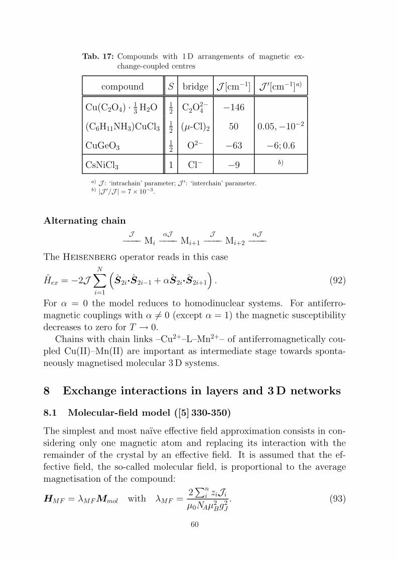
Tab. 17: Compounds with 1D arrangements of magnetic ex-change-coupled centres

compound S bridge J [cm−1] J ′[cm−1]a)

Cu(C2O4) · 13 H2O

12 C2O

2−4 −146

(C6H11NH3)CuCl312

(µ-Cl)2 50 0.05,−10−2

CuGeO312

O2− −63 −6; 0.6

CsNiCl3 1 Cl− −9 b)

a) J : ‘intrachain’ parameter; J ′: ‘interchain’ parameter.b) |J ′/J | = 7 × 10−3.

Alternating chain

J−−−− Mi

αJ−−−− Mi+1

J−−−− Mi+2

αJ−−−−

The Heisenberg operator reads in this case

Hex = −2JN∑

i=1

(S2i·S2i−1 + αS2i·S2i+1

). (92)

For α = 0 the model reduces to homodinuclear systems. For antiferro-magnetic couplings with α 6= 0 (except α = 1) the magnetic susceptibility

decreases to zero for T → 0.Chains with chain links –Cu2+–L–Mn2+– of antiferromagnetically cou-

pled Cu(II)–Mn(II) are important as intermediate stage towards sponta-neously magnetised molecular 3 D systems.

8 Exchange interactions in layers and 3D networks

8.1 Molecular-field model ([5] 330-350)

The simplest and most naıve effective field approximation consists in con-

sidering only one magnetic atom and replacing its interaction with theremainder of the crystal by an effective field. It is assumed that the ef-fective field, the so-called molecular field, is proportional to the average

magnetisation of the compound:

HMF = λMFMmol with λMF =2∑n

i ziJi

µ0NAµ2Bg

2J

. (93)

60

λ is positive for ferromagnetic and negative for antiferromagnetic interac-tions. In the presence of an applied field H, the total field acting on thecentre is

Heff = H +HMF . (94)

Owing to the molecular field, the paramagnetic behaviour (T > TC(TN))

is modified:

Mmol = χ′mol(H +HMF ) = χ′

mol(H + λMmol)

Mmol/H = χmol = χ′mol(1 + λχmol)

χ−1mol = (χ′

mol)−1 − λ. (95)

λ produces a parallel shift of the (χ′mol)

−1–T curve. If the isolated centre

obeys the Curie law, the Curie-Weiss law is obtained:

χ−1mol =

T

C− λ =⇒ χmol =

C

T − Θpwhere Θp = λC. (96)

λ and Θp have the same sign. Positive and negative Θp values refer to

predominating ferro- and antiferromagnetic interactions, respectively. Thelayer-type compound FeCl2 may serve as an example that is magnetically

characterised by dominating ferromagnetic intralayer and weaker antifer-romagnetic interlayer interactions. This does lead to Θp > 0, but an anti-

ferromagnetic spin structure is observed below TN .For pure spin systems Θp and the spin-spin coupling parameters Ji are

related by

Θp =2S(S + 1)

3kB

n∑

i

ziJi, (97)

where zi is the number of ith nearest neighbours of a given magnetic centre,Ji stands for the exchange interaction between the ith neighbours and n is

the number of sets of neighbours for which Ji 6= 0.The molecular field approximation is applicable to ferromagnetic, an-

tiferromagnetic, and ferrimagnetic materials below and above the criticaltemperature TC(TN) [5].

61

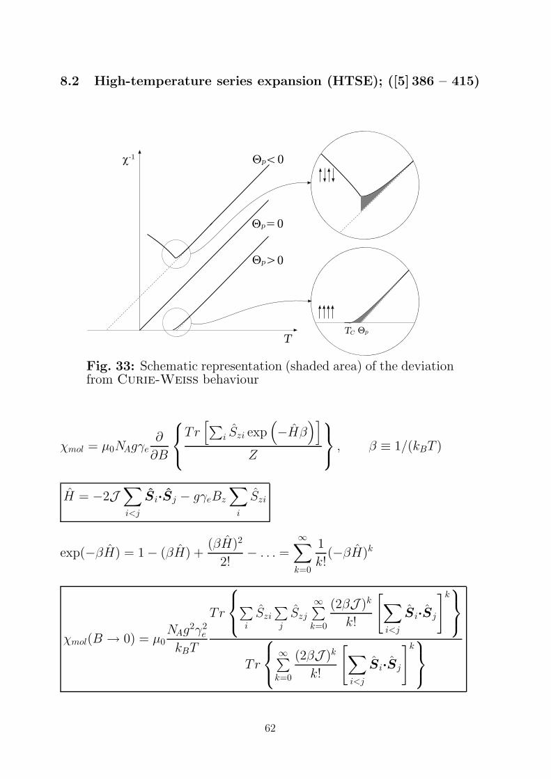
8.2 High-temperature series expansion (HTSE); ([5] 386 – 415)

TpQ

c-1

TC

Qp<0

Qp=0

Qp>0

Fig. 33: Schematic representation (shaded area) of the deviationfrom Curie-Weiss behaviour

χmol = µ0NAgγe∂

∂B

Tr

[∑i Szi exp

(−Hβ

)]

Z

, β ≡ 1/(kBT )

H = −2J∑

i<j

Si·Sj − gγeBz

∑

i

Szi

exp(−βH) = 1 − (βH) +(βH)2

2!− . . . =

∞∑

k=0

1

k!(−βH)k

χmol(B → 0) = µ0NAg

2γ2e

kBT

Tr

∑i

Szi

∑j

Szj

∞∑k=0

(2βJ )k

k!

[∑

i<j

Si·Sj

]k

Tr

∞∑k=0

(2βJ )k

k!

[∑

i<j

Si·Sj

]k

62

Example: CrBr3 (space group R 3), TC = 32.7K

Hex = −2J1

1.n∑

<i,j>

Si·Sj − 2 αJ1︸︷︷︸J2

2.n∑

<k,l>

Sk·Sl − 2 βJ1︸︷︷︸J3

3.n∑

<m,n>

Sm·Sn

χmol =C

T

[1 +

∞∑

t=1

at

( J1

kBT

)t]

with at =∑

r+s≤t

a′t−r−s,r,sαrβs

Results

1 3

2

0 100 200 300 4000

2

4

6

8

10

T / K

cm

ol/10

-6m

3m

ol-1

0

5

10

15

20

c-1

mol /

10

6m

olm

-3

0 50 1000

20

40

60

80

cm

ol/10

-6m

3m

ol-1

T / K

Fig. 34: Cr3+ (S = 3/2) partial structure in CrBr3 and χmol and χ−1

mol

as a function of temperature (applied field: B0 = 0.1T); the solid lines

refer to the HTSE model with g = 1.952, J1 = 6.900 cm−1, J2 = 0

cm−1 (fixed), J3 = −0.080 cm−1 (quality of the fit: SQ = 0.7 %; SQ =

(FQ/n)1/2 × 100%, with FQ =∑n

i=1[χobs(i) − χcal(i)]/χobs(i)1/2)

Parameter g J1 [cm−1] J2 [cm−1] J3 [cm−1]

d(Cr–Cr) [pm] 364 612 631

susceptibility 1.952 6.90 0 → 0.60 −0.08 → −0.19

spin wave analysis 6.85 ≈ 0 −0.115

63

9 Magnetochemical analysis in practice

1. use g as parameter (in addition to J )

2. if necessary use χ0 (TIP) as parameter:

χmol = χ′mol + χ0 (98)

χ′mol: polynuclear unit

3. Intermolecular cooperative interactions, weak compared to the in-

tramolecular interaction:

1

χmol=

1

χ′mol

− λ (99)

λ: molecular field parameter

4. Intermolecular cooperative interactions, competing with the intramolec-

ular exchange interaction:application of higher-dimensional models in the framework of high-

temperature series expansions (CrBr3)

5. Mononuclear impurity:

χmol = (1 − ρ)χ′mol + ρ

C

T − Θp(100)

Use ρ, C, Θp as parameters (in addition to g und J )

6. Spinfrustration: Observed in the case of antiferromagnetic interac-tions, if the topology does not allow a satisfactory antiparallel spin-

spin coupling for all centres (example: tetranuclear rhombic unit withantiferromagnetic interactions in the direction of the edges as well as

in the direction of the short diagonal)

7. Publication of magnetochemical results:

indication of the spin operator (definition of J ),χdia

mol, ∆T , B0, number of magnetic centres

64

References

[1] T. I. Quickenden, R. C. Marshall, J. Chem. Educ. 1972, 49, 114.

[2] B. I. Bleaney, B. Bleaney, Electricity and Magnetism, 3rd ed., OxfordUniversity Press, Oxford, 1994.

[3] J. H. Van Vleck, Electric and Magnetic Susceptibilities, Oxford Uni-versity Press, Oxford, 1932.

[4] J. S. Griffith, The Theory of Transition-Metal Ions, Cambridge Uni-versity Press, Cambridge, 1971.

[5] H. Lueken, Magnetochemie, Teubner, Stuttgart, Leipzig 1999.

[6] F. E. Mabbs, D. J. Machin, Magnetism and Transition Metal Com-

plexes, Chapman and Hall, London 1973.

[7] J. H. Van Vleck, Physica 1973, 69, 177-192.

[8] H. L. Schlafer, G. Gliemann, Einfuhrung in die Ligandenfeldtheorie,

Akad. Verlagsges., Wiesbaden 1980; Engl. Ausgabe: Basic Principles

of Ligand Field Theory, Wiley-Interscience, New York 1969.

[9] O. Kahn, Molecular Magnetism, Wiley-VCH, New York 1993.

[10] P. W. Atkins, R. S. Friedman, Molecular Quantum Mechanics, Oxford

University Press, Oxford 1997.

65

Appendix

Tab. 18: Energy conversion factors

J eV s−1 cm−1 K T kJ/mol

1 J 1 6,24151 1,50919 5,03411 7,24292 1,07828 6,02214

×1018 ×1033 ×1022 ×1022 ×1023 ×1020

1 eV 1,60218 1 2,41799 8,06554 1,16045 1,72760 9,64853

×10−19 ×1014 ×103 ×104 ×104 ×101

1 s−1 6,62607 4,13567 1 3,33564 4,79922 7,14477 3,99031

×10−34 ×10−15 ×10−11 ×10−11 ×10−11 ×10−13

1 cm−1 1,98645 1,23984 2,99792 1 1,43877 2,14195 1,19626

×10−23 ×10−4 ×1010 ×10−2

1K 1,38066 8,61739 2,08367 6,95039 1 1,48874 8,31451

×10−23 ×10−5 ×1010 ×10−1 ×10−3

1T 9,27402 5,78839 1,39963 4,66864 6,71710 1 5,58494

×10−24 ×10−5 ×1010 ×10−1 ×10−1 ×10−3

1 kJ/mol 1,66054 1,03642 2,50607 8,35933 1,20272 1,79053 1

×10−21 ×10−2 ×1012 ×101 ×102 ×102

66